/


Author: Varilly J.C. Figueroa H. Gracia-Bondia J.M.
Tags: mathematics geometry

Text
Birkhauser Advanced Texts
Basler Lehrbucher
Edited by
Herbert Amann, University of Zurich
Jose M. Gracia-Bondia
Joseph С. Vurilly
Hector Figueroa
Elements of
Noncommutative Geometry
Birkhauser
Boston • Basel • Berlin
Contents
Preface xi
I TOPOLOGY 1
1 NoncommutarJve Topology: Spaces 3
1.1 Continuous functions on a locally compact space ... 4
1.2 Characters and the Gelfand Transformation 5
1.3 Trading spaces for algebras 9
1.4 Homotopy In noncommutadve language 16
1.5 Exponentials and cohomology 17
1.6 Identifications and attachments 21
1Л C*-algebra basics 26
13 Hopf algebras and Tannaka-Krem duality 34
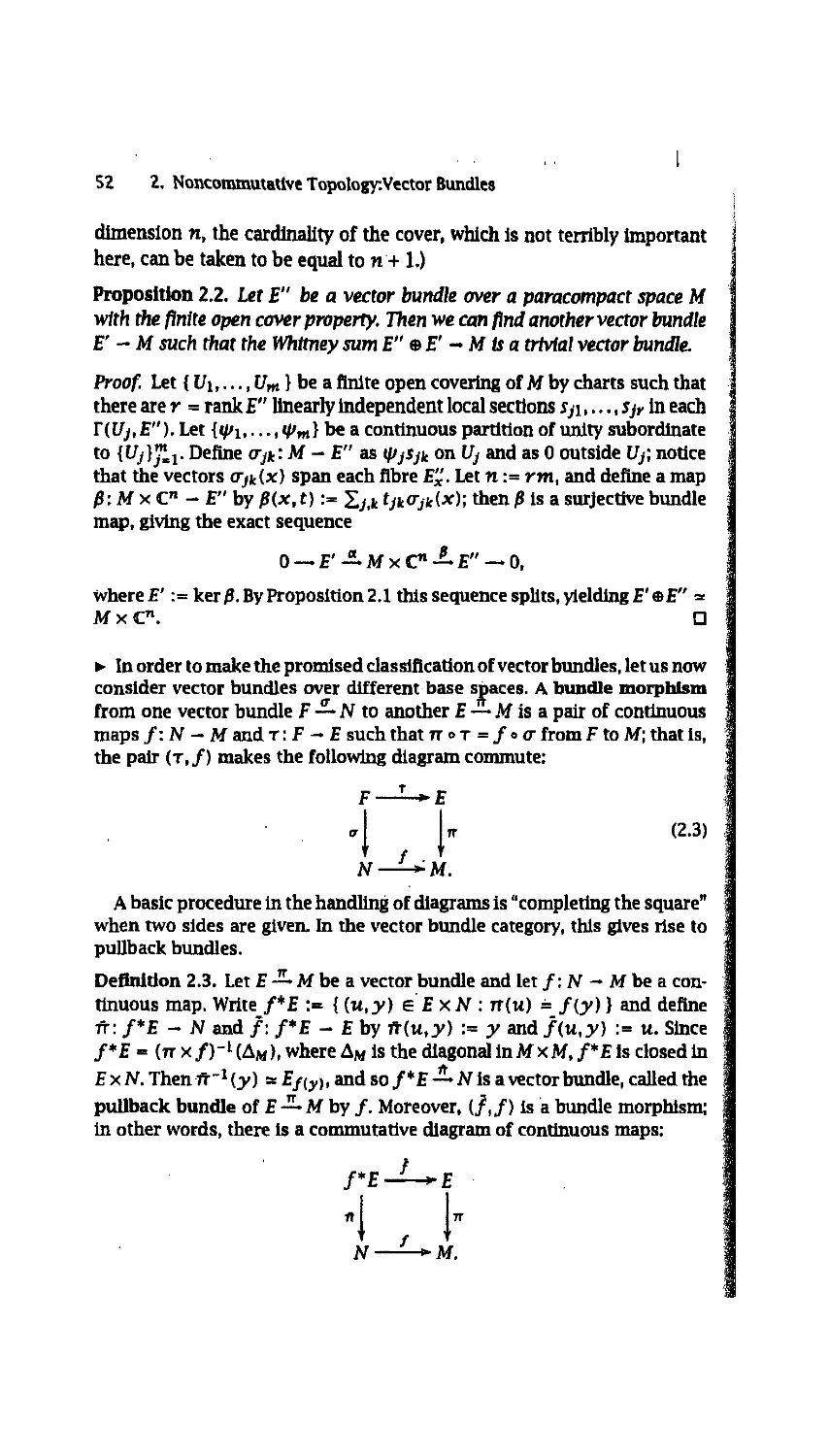
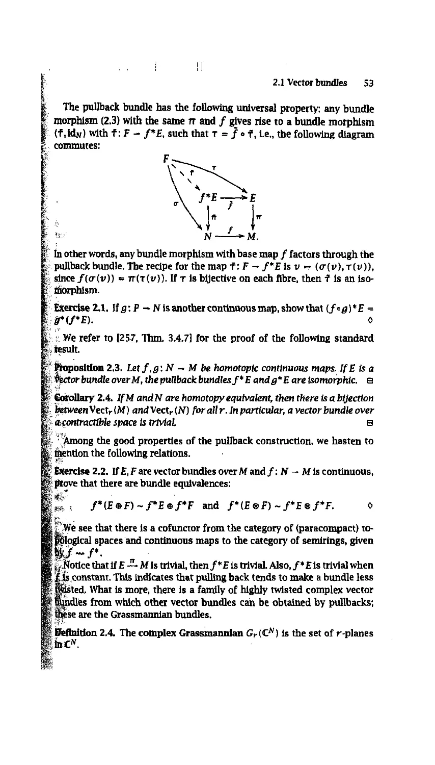
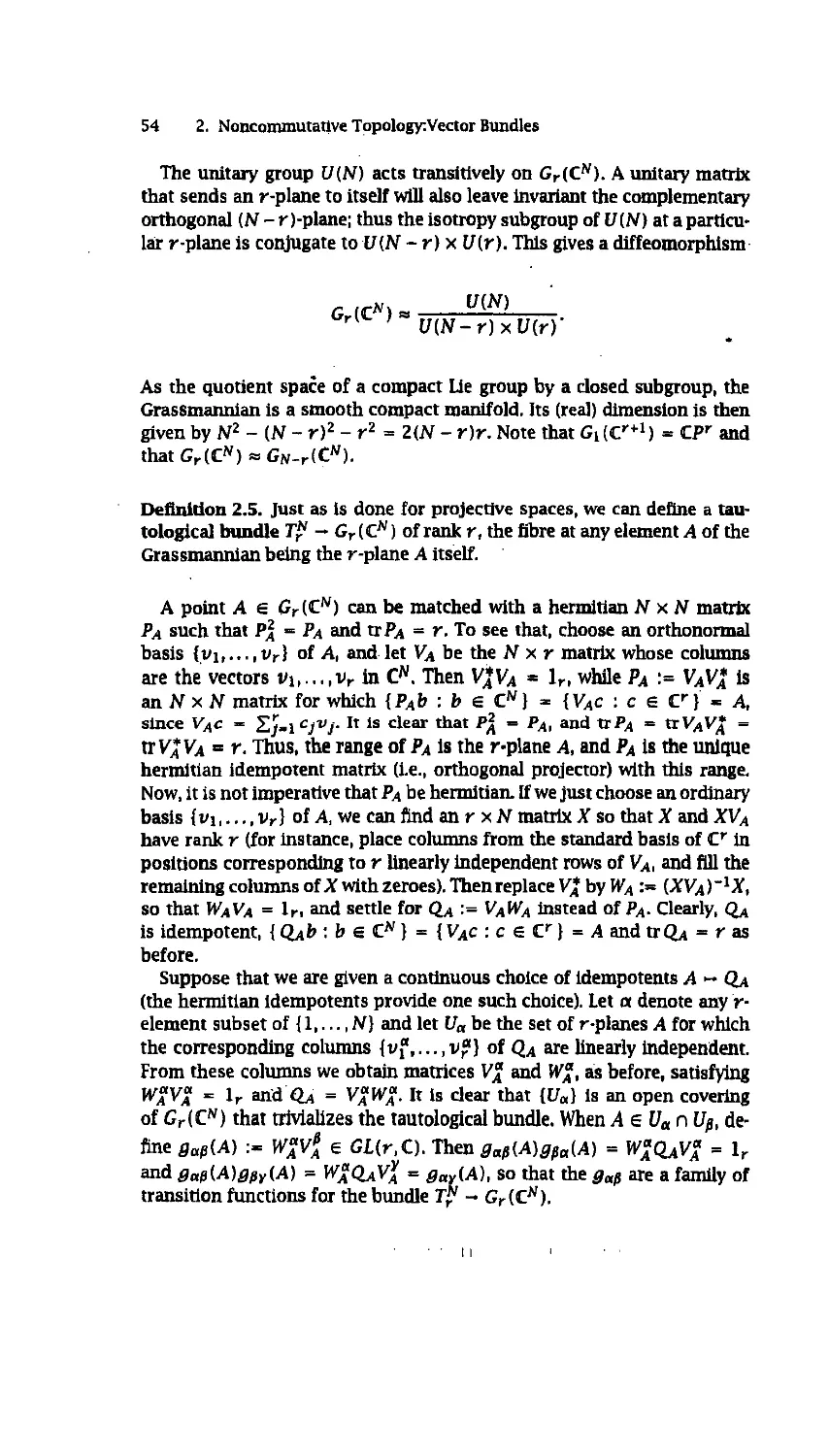
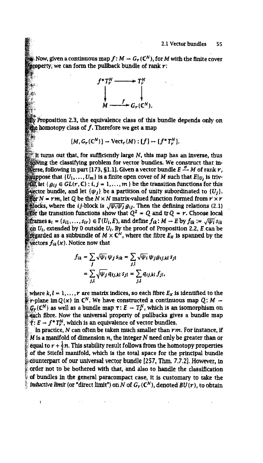
2 Noncommutadve Topology: Vector Bundles 49
2.1 Vector bundles 49
2.2 The functor Г . 56
2.3 The Serre-Swan theorem 59
2.4 Trading bundles for modules 60
2.5 C*-modules 64
2.6 Line bundles and the Bott projector 74
2Л Projective modules over unital rings 79
vill Contents
3 Some Aspects of tf-theory
3.1 Endomorphlsms of C*-modules
3.2 The Ko group
3.3 The importance of being halfexact
3.4 Asymptotic morphisms
3.5 The Moyal asymptotic morphism
3.6 Bott periodicity and the hexagon
3.7 The Kx functor
3.8 Jf-theory of pre-C*-algebras
4 Fredholm Operators on C*-modules
4.1 Fredholm operators and the Atiyah-Janich theorem
4.2 Fredholm operators on C*-modules
4.3 The generalized Fredholm index
4.4 The noncommutative Atiyah-Janich theorem . .
4.5 Morita equivalence of C*-algebras
II CALCULUS AND LINEAR ALGEBRA
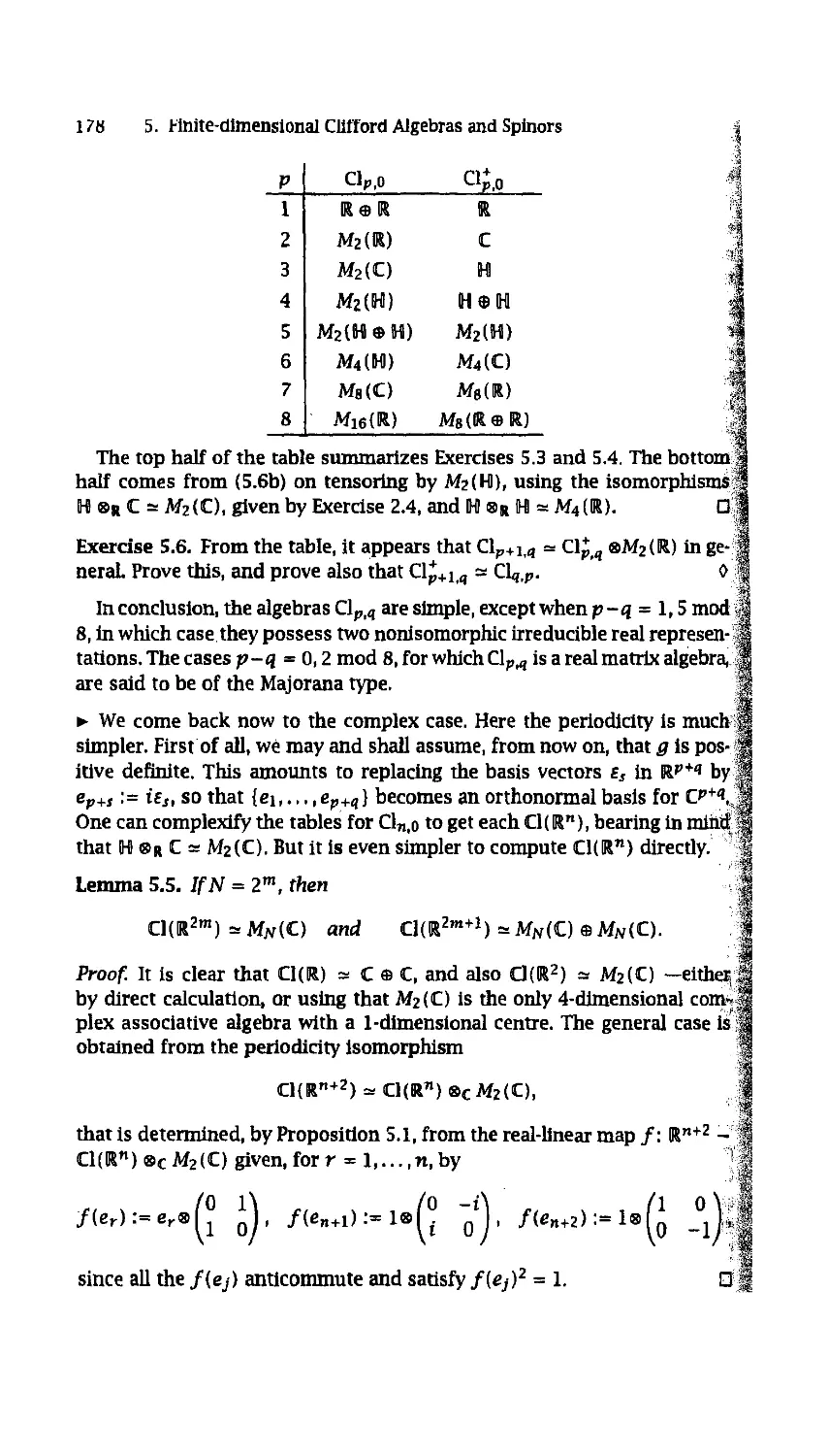
5 Finite-dimensional Clifford Algebras and Spinors
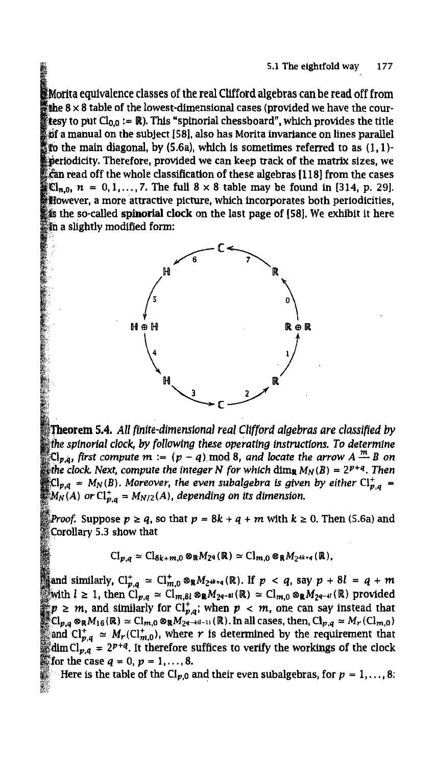
5.1 The eightfold way
5.2 Spin groups
5.3 Fock-space representations
5.4 The exterior algebra viewpoint
5.5 Pfaffians and Gaussians
5.A Superalgebras
6 The Spin Representation
6.1 Infinite-dimensional Clifford algebras
6.2 The infinitesimal spin representation revisited . .
6.3 The Shale-Stinespring theorem
6.4 Charged fields .
7 The Noncommutative Integral
7.1 A rapid course in Riemannian geometry . . . .
7.2 Laplacians
7.3 The Wodzicki residue
7.4 Spectral functions
7.5 The Dixmier trace
7.6 Connes' trace theorem
7.A Pseudodifferential operators ........
7.B Homogeneous distributions
7.C Ideals of compact operators
Co
83
83
92
103
110
113
120
127
133
141
141
145
148
156
159
169
171
171
180
184
195
204
210
213
213
218
224
238
251
251
258
264
272
284
293
298
306
310
8 Noncommutatlve Differential Calculi
8.1 Universal forms .
8.2 Cycles and Fredholm modules
8.3 Connections and the Chern homomorphism . . .
8.4 Hochschild homology and cohomology ....
8.5 The HochschUd-Kostant-Rosenberg-Connes theorem
Ш GEOMETRY
9 Commutative Geometries
9.1 Clifford modules
9.2 Spinc structures: the algebraic way
9.3 Spin connections and Dlrac operators . . . . .
9.4 Analytical aspects of Dtrac operators
9.5 KR-cycles and the eightfold way
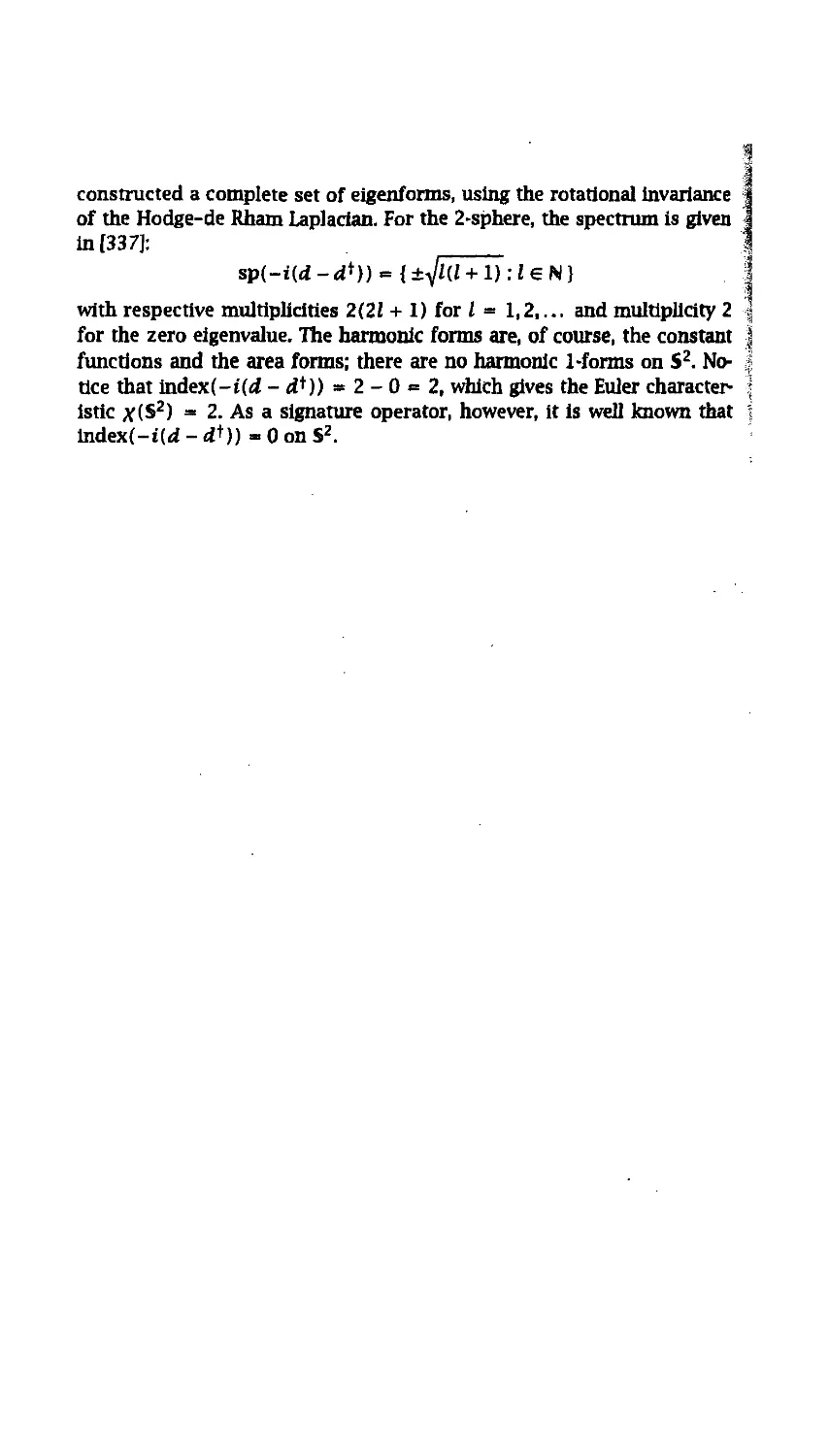
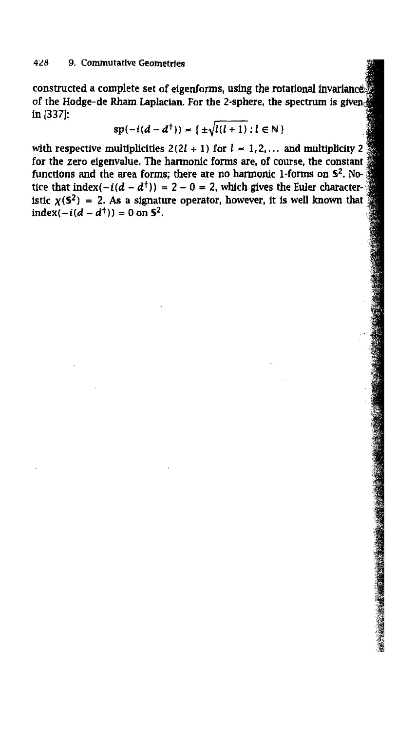
9.A Spin geometry of the Rlemann sphere
9.B The Hodge-Dirac operator
10 Spectral Triples
10.1 Cyclic cohomology
10.2 Chern characters and entire cyclic" сocycles . . .
10.3 Tameness and regularity of spectral triples . . .
10.4 Cormes' character formula
10.5 Terms and conditions for spin geometries . . .
11 Comes' Spin Manifold Theorem
11.1 Commutative spin geometries revisited ....
11.2 The construction of the volume form
11.3 The spin structure and the metric
11.4 The Dirac operator and the action functional . .
11A The Rlemann sphere as a spectral manifold . . .
IV TRENDS
12 Tori
12.1 Crossed products
12.2 Structure of NC tori and the Moyal approach . . .
12.3 Spin geometries on noncommutative tori ....
12.4 Morita equivalence and crossed products ....
13 Quantum Theory
13.1 The Dirac equation and the neutrino paradigm . .
13.2 Propagators
13.3 The classical Dyson expansion in QED
x Contents
13.4 The Rules
13.5 The quantum Dyson expansion
13.A On quantum field theory on noncommutatlve manifolds
14 Krelmer-Cormes-Moscovict Algebras
14.1 The Connes-Kreimer algebra of rooted trees ....
14.2 The Grossman-Larson algebra of rooted trees . . .
14.3 The Mllnor-Мооге theorem
14.4 Duality in Hopf algebras
14.5 Hopf algebras of Feynman diagrams
14.6 Hopf algebras and diffeomorphism groups ....
14.7 Cyclic cohomology of Hopf algebras
References
Symbol Index
Subject Index
Preface
Our purpose and main concern in writing this book is to illuminate classical
concepts from the noncommutative viewpoint, to make the language and
techniques of noncommutative geometry accessible and familiar to practi-
practitioners of classical mathematics, and to benefit physicists interested in the
uses of noncommutative spaces, Some may say that ours is a very "com-
"commutative" way to deal with noncommutative matters; this charge we readily
admit.
Noncommutative geometry amounts to a program of unification of math-
mathematics under the aegis of the quantum apparatus, i.e., the theory of ope-
operators and of C*-algebras. Largely the creation of a single person, Alain
Connes, noncommutative geometry is just coming of age as the new century
opens. The bible of the subject is, and will remain, Connes' Noncommuta-
ttve Geometry A994), itself the .8-fold expansion" of the French Geomi-
I trie поп commutative A990). These are extraordinary books, a "tapestry" of
I physics and mathematics, in the words of Vaughan Jones, and the work of
I a "poet of modern science," according to Daniel Kastler, replete with subtle
I knowledge and insights apt to inspire several generations.
| Despite an explosion of research by some of the world's leading math-
i ematicians, and a bouquet of applications—to the reinterpretation of the
| phenomenological Standard Model of particle physics as a new spacetime
I geometry, the quantum Hall effect, strings, renormalization and more in
I quantum field theory—the six years that have elapsed since the publica-
| tion of Noncommutattve Geometry have seen no sizeable book returning
| to the subject. This volume aspires to fit snugly in that gap, but does not
Parti
TOPOLOGY
The ordinary man wonders
at marvellous things;
the wise man wonders
at the commonplace
— Confucius
1
Noncommutative Topology: Spaces
The geometrical study of quadratic curves or surfaces, i.e., zero sets of
second-degree polynomials, proceeds by examining points of intersection
or tangent lines directly; but already for cubic curves it pays to examine first
the ideal of all polynomials that vanish on the curve: in this way the study
of an algebraic variety (the zero set of a given finite collection of polynomi-
polynomials) is replaced by the study of the corresponding polynomial ideal. Such a
fundamental geometrical object as an elliptic curve is best studied not as a
set of points (a torus) but rather by examining functions on this set, specif-
specifically the doubly periodic meromorphic functions: Weierstrass opened up
a new approach to geometry by studying directly the collection of complex
functions that satisfy an algebraic addition theorem, and derived the point
set as a consequence [51].
In noncommutative geometry, under the influence of quantum physics,
that idea of replacing sets of points by classes of functions is taken fur-
further. In regular cases the set is completely determined by an algebra of
functions, so one can choose to forget about the set and obtain all infor-
information from the algebra alone. When the associated set is too singular or
pathological, a direct examination frequently yields no useful information:
the set of orbits of group actions is generally of this type. In such situa-
situations, when the matter is examined from the algebraic point of view —as is
done in Chapter 12 for the rotation of a circle by multiples of an irrational
angle— we often find an operator algebra holding the information we seek;
however, this algebra is not commutative.
. The 1943 paper [194) containing the results nowadays known as Gel-
fand-Naimark theorems has become a cornerstone of noncommutative geo-
4 1. Noncommutatlve Topology: Spaces
metry, Gelfand and Nalmark characterized the involutive algebras of ope-
operators, nowadays called C*-algebras, from the natural axiomatization for
the algebra of continuous functions, by just dropping commutatlvlty. To
go from there to presuming that C* -algebras held the right generalization
of classical concepts of space still required a leap of faith (in the words of
Effros [152]), but one that has over time paid handsome dividends.
Thus, we proceed by first discovering how function algebras determine
the structure of point sets, and then learning which relevant properties of
those algebras do not depend on commutativity.
1.1 Continuous functions on a locally compact
space
Definition 1.1. A compact Hausdorff topological space X gives rise to a
natural commutative algebra C(X), consisting of all continuous functions
/: X - C. This is a Banach algebra under the sup norm
||/||:=sup|/(*)|. A.1)
xeX
Moreover, C(X) has an isometric involution / « /* by defining /* (x) :=
f{x); and the norm satisfies the C*-property
ll/ll2 = II/*/». A.2)
In other words, С (ДО is a unital C*-algebra —the unit being the constant
function 1.
We shall have to deal with nonunital algebras as well. To any Banach
algebra A we can adjoin a unit, denoted 1 д (or simply 1 when no confusion
is feared), by taking A+ := A x C, with the obvious sum and adjoint and the
multiplication rule (я,Л)(Ь,м) := [аЬ + \Ь + ца,\ц); thenU* = @,1). For
the proof that A+ is indeed a C*-algebra when Л is a nonunital C* -algebra
to start with, and other necessary background on Banach and C*-algebras,
we refer to Section 1Л.
Every topological space considered in this book will be Hausdorff, unless
explicitly indicated otherwise. If У is locally compact but not compact, then
obviously the algebra С (У) is too big to be of any use. A strategy to deal with
this case is to add a "point at infinity" to get a compact space У+ := УИ").
Then the subalgebra of С(У+) whose members satisfy /(») = О may be
identified, by restriction to У, with the algebra C0[Y) of continuous func-
functions "vanishing at infinity". It is clear that C0[Y) is а С *-algebra without
a unit, but then Со(У)+ = C{Y+). Conversely, if one deletes a non-isolated
point x0 from a compact space X, the space Y =X\ {xo} is locally compact
but not compact, У+ * X, and CQ(Y) = {h e C(X): h{x0) = 0}.
1.2 Characters and the Gelfand transformation 5
1.2 Characters and the Gelfand transformation
Definition 1.2. A character of a Banach algebra Л Is a nonzero homomor-
phism fi: A — C, which Is necessarily surjective. The set of all characters
(that may well be empty) will be denoted M(A).
For example, if A - Co(Y), the evaluation map ty: f « f(y) at у e У
clearly defines a character.
Any character ц e M{A) extends to A+ by setting ^(@,1)) := 1 (neces-
(necessarily). The zero functional on A also extends to the character (a, A) - Л
on A+. Thus we identify M(A) и {0} with MM*). We recall -see Sec-
Section 1.A— that the spectrum sp(a) of an element a in A is the set of com-
complex numbers Л such that a - Al is not invertible in A, or in A+ if A is
not unital —in the nonunital case 0 always belongs to the spectrum. Then
/j(a) e sp(a) for Ц € M(A) and a e A: otherwise 0 = fi(a - ц(аI) would
be invertible in C! Therefore \ц(а)\ s ||a||,so ||mII s l.Infact, HmII = 1: since
= /*(l-a) = M(D/'(a)foralla6 A+, it follows that/*A) =MdJ and
Let A* be the Banach space of continuous linear functional ф: A - С
On A* we can consider the so-called weak* topology, that of pointwise
convergence on elements of A For instance, if A = C(X), with X compact,
then A* is the space of complex measures on X with its standard topology.
The Banach-Alaoglu theorem —a corollary of Tikhonov's theorem [383]—
says that the unit ball A* of A* is compact in the weak* topology.
Definition 1.3. If A is commutative, call M(A) the Gelfand spectrum of A.
ThenM(A) >-> A,*: the Gelfand topology is the relative topology determined
on M (A) by this inclusion.
Lemma 1.1. The Gelfand spectrum of a commutative Banach algebra, en-
endowed with the Gelfand topology, is a locally compact space.
Proof. We show that Af (А) и {0} is weak*-dosed in A* and hence is com-
compact. For fixed a, b e A, the map ц « ц(а)ц(Ъ) - ц{аЬ) is weak*-continu-
ous; since it Vanishes on M(A) и {0}, it vanishes on its closure.
The extra point {0}, corresponding to the "evaluation at the point at in-
infinity", is isolated if A is already unital, since the weak*-continuous function
M " /*(U separates it from ЩА). О
Definition 1.4. Let A be a commutative Banach algebra. The Gelfand trans-
transform of я 6 A is the function a: M{A) - С given by
&{»)¦-Via). A.3)
In other words, A is the evaluation at a € A; this is continuous, by definition
of the weak* topology. The Gelfand transformation is the map G: a - a
fromAintoC0(M(A)).
6 1. Noncommutative Topology: Spaces
For general commutative Banach algebras, the Gelfand transformation
is an extremely useful instrument, in spite of being in general neither in-
Jective nor surjective. For instance, the convolution algebra A = iMR) of
Lebesgue-integrable functions on R is a nonunital algebra whose charac-
characters are the integrals / « |R e~itxf{x) dx for any t e R [266, Thm. 3.2.26];
then / is the Fourier transform of /, and the Gelfand transformation is the
Fourier transformation that takes I1 (И) into C0(R): this is the Riemann-
Lebesgue lemma [316, §5.1]. This map is injective, but not isometric nor
surjective (the Fourier transform of an tntegrable function has the extra
property of being absolutely continuous). There are also commutative Ba-
Banach algebras that contain nonzero quasinilpotent elements, whose spec-
spectral radius is zero (an example is the convolution algebra of continuous
functions on [0,1], whose elements are аи quasinilpotent [499, §11.2]); in
such cases the Gelfand transformation Q: A - C(M(A)) is certainly not
injective.
> The situation improves greatly when we limit ourselves to C*-algebras,
as we now hasten to do. The С'-algebras are distinguished among the ge-
general clutter of Banach algebras with involution by the notable properties
of their selfadjoint elements.
Lemma 1.2. Let a be a selfadjoint element ofa C* -algebra A. Then у {а) е R
Proof. Suppose that a = a* and consider the exponential series u :=
exp(ia) := 7л-о(Шк1к\ that converges in A (or in A* if A is nonuni-
nonunital) with the a priori bound ||u|| s em. Then u* = exp(-ia) and so
uu* - 1 = u*u; in particular, u is invertible with u = u*. The C*-
norm condition implies that ||u|j2 = \\u*u\\ - \\l\\ = 1, and likewise
Hu-Ml = 1. Since HmII s 1, we get |/*(u)| < 1 and ImJu)! = \fi{u~l)\ & 1,
so that |fj(u) | = 1. But by continuity and the homomorphism property we
obtain m(m) =X?=o^(ia)>:/k! = e"'(''>,andthus^(a)€lR. a
Exercise 1.1. Prove, along the lines of the previous proof, that in a unital
C*-algebra the spectrum of a unitary element u (satisfying uu* = u*u = 1)
is part of the unit circle, and that the spectrum of a selfadjoint element
a = a* is real. 0
When я € A is not selfadjoint, we write a = a.\ + *яг with a.\ := \ (a* + a),
a2 := j(a*-a) selfadjoint. If A is a C* -algebra and ц е M(A), we then get
ц{а*) = д(Я! - ia2) = M(ai) - ifi(a2) = д(я), A.4)
or equivalenth/, аУ(ц) = й{ц) for \i € M{A); or better yet, a* = (й)*. In
other words, the Gelfand transformation a *• a intertwines the involutions
of A and of C(M(A)).
We need one more lemma.
1.2 Characters and the Gelfand transformation 7
Lemma 1.3. Let Abe a commutative C*-algebra, and let Л belong to the
spectrum ofaeA. If A ts unital, or if A is nonunital and A * 0, there is a
character \x such that\i(a) = Л.
Proof, The kernel of any character ц of a unital commutative C* -algebra
is a (proper) maximal ideal. Indeed, A/ker j/ = C, a field; if J is an ideal
properly containing кегм. and if a e J \ ker/J, then ц[а) has an inverse;
consider then an element b e A such that fi(b)it{a) = 1: both ba and
ba - 1д belong to /, so I a e /, and thus ker/i is maximal.
Reciprocally, if J is a maximal ideal, it must be closed. Indeed, its closure
is also an ideal and, as argued in Section l.A, a proper ideal in a unital
Banach algebra cannot be dense. Therefore A/I is a commutative Banach
algebra without proper ideals, i.e., a field. Moreover, as the spectrum of any
element in this unital Banach algebra is nonempty, this field is A/I = C.
Thus there is a unique character ц, namely the quotient map, such that
ц-Ч0)=1.
The unital case follows, because the nontrivial ideal A(a - Л1) is con-
contained in a maximal ideal, which is an immediate consequence of Zorn's
lemma [3831; for the nonunital case, use the same argument in A+. D
Denote by r{a) the spectral radius of an element a of a Banach algebra.
In Section 1A we remark that r(a) = ||a||, when a is a selfadjoint element
of a C*-algebra.
The last ingredient we need is the Stone-Weierstrass theorem [131,383].
This states that, if X is a locally compact space, and if В is a closed sub-
algebra of Co(X) that (a) separates points, i.e., whenever p * q in X, there
is some у e В withy(p) * y(q.), (b) vanishes Identically at no point of X,
and (c) is closed under complex conjugation; then В is the whole Co{X).
Theorem 1.4 (Gelfand-Naimark). If A is a commutative C* -algebra, the
Gelfand transformation is an isometric ^-isomorphism of A onto Co(M(A)).
Proof. The relation A.4) shows that g: A - C0(M(A)) is a *-homomor-
phism. The isometric property follows from
||d||2 = ||d*d|| = Ik^ll = r(a*a) = \\a*a\\ = ||я||2, A.5)
for as A, where we use Lemma 1.3 to justify the third equality. In partic-
particular, <э is injective. Now <g(A) is a subalgebra of C0{M{A)) that is complete
since A is complete and <j is isometric, and therefore is closed. Clearly the
evaluation maps in Q(A) separate the characters, do not all vanish at any
point, and A.4) again shows that g(A) is closed under complex conjuga-
conjugation; the Stone-Weierstrass theorem then tells us that Q is surjecdve. D
A comment on the proof is in order. We have chosen to underline the
description of the Gelfand spectrum of a commutative C*-algebra in terms
of characters, rather than of maximal ideals, which is perhaps the more
В 1. Noncommutatlve Topology. Spaces
standard procedure. However, we did use the latter to establish the ex-
existence of a character producing any number in the spectrum of a given
element of the algebra. We could have appealed to the Hahn-Banach theo-
theorem instead, but, leaving aside that this does not absolve us of Zomication,
there would remain the work of proving that the linear functional which
it yields is multiplicative. Such an approach is consistently taken in [175]
and [266], where it is shown that characters are just pure states (consult
Section 1 A) for commutative C* -algebras; the subject is then inextricably
tied to representation theory.
To summarize the consequences of the theorem: being a commutative
C*-algebra is at least a necessary condition for an algebra to be isomet-
rically isomorphic to some C{X) or C0(Y). The beauty of the Gelfand-
Nalmark theorem is that this apparently entirely algebraic property is also a
sufficient condition for isomorphism with a space of continuous functions.
Actually, to be a C*-algebra is not wholly a matter of algebraic relations,
since completeness (in the metric determined by the C* -norm) involves lim-
limits. At any rate —as we shall exemplify very soon— all topologlcal informa-
information about X is algebraically stored within C(X). We do gain the insight
to go beyond conventional topology by regarding a noncommutative C*-
algebra as a kind of "function algebra" for a virtual or "noncommutative
topologlcal space". This viewpoint also allows one to study the topology of
non-Hausdorff spaces, such as arise hi probing a continuum where points
are unresolved [20,304].
The second theorem of Gelfand and Naimark [194] says that any C*-
algebra can be embedded as a norm-closed subalgebra of a full algebra of
operators ?(H) for a large enough Hllbert space Я; thus all C*-algebras
are fairly "concrete". For a discussion of this, see Section 1.A; a full discus-
discussion of both theorems and their offshoots is contained in the book [144].
Indeed, C(X) may be embedded in LC{), the algebra of bounded opera-
operators on the Hubert space Jf with a countable orthonormal basis, in many
ways: if X is infinite but separable, take v to be any finite regular Borel
measure onX, and Identify Л" with I2 (X,dv)\ then/ б С{Х) С L°(X,dv)
can be identified with the multiplication operator h « fh on L2{X,dv).
Developing the last remarks, one sees that the first Gelfand-Nalmark theo-
theorem is the basis of the spectral theorem for normal operators on a Hubert
space [132,383].
It is in the spirit of noncommutative geometry to relax closure condi-
conditions as much as possible when defining our algebras; for instance, if Af is
a compact differential manifold, we would like to use the algebra of smooth
functions Л = C°°(M), which is a dense subalgebra of C(M). It is complete
hi its natural topology, that of uniform convergence of functions, together
with their derivatives of all orders; but this yields only a Frechet algebra
(provided M is «r-compact). Even so, it turns out that the characters of this
algebra are simply the evaluations at points of M; that is, every character on
C(M) extends to a character on C{M). Indeed, characters on C°°(M) are
1.3 Trading spaces for algebras 9
automatically continuous, and therefore are distributions on M; moreover,
a positive distribution, as such a character is, is actually a measure C16,
§6.22]. Therefore, the involurJve Frechet algebras of smooth functions on
сг-compact dlfferentiable manifolds do characterize such manifolds. Unfor-
Unfortunately, no one seems to know how, conversely, to characterize algebras
isomorphlc to C{M) among involurJve commutative Frechet algebras. We
shall return to consideration of C°° (M) shortly.
What happens if X is a (topologlcal) group G? Then, at least in the com-
compact case, a dense subalgebra of C(G) is endowed with a much richer alge-
algebraic structure, allowing to recapture G as a group. This is the subject of
Section l.B.
1.3 Trading spaces for algebras
Definition 1.5. If /: X - Y is a continuous mapping between two compact
spaces, denote by Cf the mapping h«h«/ from C{Y) to C(X). Then
Cf is a unital *-homomorphism, since (h * ft) « / = (h о /) + (fc о /),
[hk) of - [h о/)(fco/), and h* of = [h°f)* for h,k e C{Y), and clearly
\t f: X - Y, g\Y -~ Zare continuous mappings between compact
spaces, then C(g of) = Cf°Cg as *-homomorphisms from C{Z) to C{X).
Also, Cidx Is the identity map id еда on C(X). We summarize by saying
that X « C[X), f - Cf is a contravartant functor from the category of
compact spaces and continuous maps to the category of commutative uni-
unital C*-algebras and unital *-homomorphisms. This functor is called con-
travariant since it "reverses the arrows"; we shall use the term cofunctor,
for short.
There is also a cofunctor going the other way. Recall that the Gelfand
topology of M(A) is, by definition, the weakest topology for which all the
functions a: M(A) - C, for a e A, are continuous. Therefore, it has a
universal property, namely, that any function /: X - M(A) is continuous
if and only If each я»/: X - С is continuous.
Definition 1.6. If ф: A — В is a unital *-homomorphism between two com-
commutative unital C* -algebras, denote by Мф the mapping ц - ц о ф from
М(В) to M(A)'. Then Мф is a continuous map, since А о М{ф) = ф{а) is
continuous for each aeA.Ifi//:B-Cis another unital *-homomorphism,
then Af (if/ о ф) - Мф о Мц>.
We can compose these cofunctorsin the obvious manner; if ц е M(C(X))
then ker^i Is a maximal ideal of C{X), so there is at least one point xeX
where all the elements of ker/j vanish. (Were this not the case, by using
the compactness of X, we could construct an invertlble element of ker ц.)
Recall that ex denotes the evaluation map at the point x; then ker \i = ker sx
since both are maximal ideals. If / e C{X), then / - n(f)l e кег/л so
0 = ex{f - v(f)l) = fx(/) - M(/)- Thus the evaluations tx are the only
characters of С (X).
Exercise 1.2. Prove that sx- x « ex is a homeomorphism between the orig-
original compact space X and the compact space M(C(X)) with its Gelfand
topology. 0
hi fine, we have assembled homeomorphic maps ex- X — M{C(X)) for
each compact space X such that ey ° f = MCf о ex whenever f.X-Y
is continuous. In category-theory jargon, f is a natural transformation be-
between the identity functor and the functor MC on the category of compact
(Hausdorff) spaces. In particular, all morphisms in the latter come from
*-homomorphisms of the algebras (i.e., the cpfunctor M is full).
We take this opportunity to shorten the clumsy term " * -homomorphism"
to just "morphism". From now on, a morphism ф: А- В will designate an
involutive homomorphism between the C* -algebras A and B. Also, in this
section, all morphisms between unital algebras are supposed unitaL
> The Gelfand-Nalmark theorem provides another natural transformation
Q between the identity functor and the functor CM on the category of
unital, commutative С *-algebras. Indeed, the theorem states that a *~ a
is an isomorphism of A onto C{M[A)). Moreover, if ф: A - В is a unital -
morphism, then for a e C{M[A)), v e M(B), we get
(С(Мф)а)у = a(W)v) = a(v о ф) = у(ф(а)) = ф{а)(у), A.6)
so (СМф)а = дв(ФЫ)) tortdxha,orequivalently,^ваФ = СМфадА.\п
particular, all unital morphisms from C(Y) to C(X) come from continuous
maps from X to Y.
Therefore, the categories of compact spaces and unital, commutative C*-
algebras are equivalent —or to be more pedantic, one is equivalent to the
opposite category of the other.
> When X and У are only locally compact spaces, the correspondence h ~
h о / will not always map C0(Y) into C0(X).
Exercise 1.3. Show that h~h°f takes functions vanishing at infinity on
Y to functions vanishing at infinity on X iff / is a continuous proper map
(i.e., the preimage under / of any compact set in Y is compact in X). 0
It does not follow that there is an equivalence of categories between
locally compact spaces with continuous proper maps and commutative
C* -algebras with morphisms. For instance, the injective morphism embed-
embedding C0([0,1)) into C([0,a]), for any a ? 1, does not come from any map
(proper or otherwise) from [0, a] into [0,1). To obtain such an equivalence,
one restricts to C*-morphisms which are proper, that is, send approximate
units into approximate units.
At any rate, instead of the former category, we shall use an equivalent one
whose morphisms are easier to deal with, namely, the category of pointed
topologkal spaces. For that, we systematize our previous remarks about
compactlfying locally compact spaces by adding a point at infinity. This
wiH be in tune with later homotopy-theoretlcal considerations.
Definition 1.7. A pointed compact space is a pair {X, *), where X is com-
compact and * € X is a distinguished element, the basepoint. A morphism
from (X, *) to (У, *) is a continuous map /: X - Y such that /(*) = *.
We write /еМар+(Х,У).
Any locally compact space Y determines a pointed space (У+, во); any
continuous proper map/: У - Z is extended to a morphism/+: Y+ - Z?
by setting /+ (со) := a>. Conversely, If (X, *) is a pointed topological space,
then X \ {*} is locally compact, and the restriction of a morphism to X \ {*}
is proper.
We identify У to У+ \ {«} and (X, *).to (X\ {*})*. This allows us to omit
mentioning the basepoint when it is unambiguous.
Let X, Y be compact spaces with Y z X; we call (X, Y) a compact pair.
From them we can always construct a pointed space X/Y ;= (X \ Y)+; one
can think that Y has been smashed to become a base point for the new
space. Let с: X - X/ У be the collapsing map; the restriction of с to X \ У is
ahomeomorphism. Note that XI0 = X* (the basepoint of X+ is an isolated
point since X is already compact).
> We next explore a few consequences of the equivalence of categories.
Proposition 1.5. Two commutative C* -algebras are isomorphic if and only
if their character spaces are homeomorphic.
Proof. Suppose the C*-algebras A and В are both unital. Then morphisms
ф: A - В, ц>: В - A such that tp о ф = id,4, ф° у = Шв yield continuous
maps Мф; М{В) - M(A) and Мц>: М(А) - М{В) such that Af if/ ° Мф =
1йм(в) and Мф о Мф = idbHAY, thus Мф is a homeomorphism.
Conversely, homeomorphisms of compact spaces f:X - Y, g.Y - X
such that g»f = idx and / ° g = idy yield unital morphisms Cf: C{Y) -
C(X) and Cg: C(X) - C{Y) such that Cg*Cf = idC(r) and Cf°Cg =
idcw»; thus Cf is a ^-isomorphism.
If A and В are both nommital, they are isomorphic if and only if A+ =» B+
lfandonlyifM(A+) »M(B+) by a homeomorphism that takes е„ е M(A*)
tOBK€M{B+). a
Corollary 1.6. The group of automorphisms AutA of a commutative C*-
algebra A is isomorphic to the group of homeomorphisms of its character
space. в
Note that there are no nontrivial inner automorphisms in AutA.
12 1. Noncommutative Topology: Spaces
One can make the parallel argument for the Frechet algebra C°°(M). Im-
Implicit In the previous proof is the property that morphisms between C*-
algebras are automatically continuous (consult our remarks in Section 1.A).
But this is also true of C°°(M). Indeed, Klee's theorem [412, Thm V.S.5) as-
asserts that every positive linear form on an ordered Frechet space F such
that F ш F+ - F+ is continuous. This is easily seen to be the case for
C°° (M, R), and then it follows easily [454] that involutive homomorphisms
C°{M) - C°°(N), for cr-compact manifolds M and N, are continuous.
Corollary 1.7. IfM is a compact manifold, then the group of automorphisms
of the algebra Aut C"(M) is isomorphlc to the groupDlft(M) ofdiffeomor-
phtsms of its character space.
Proof. Any real-valued smooth function a e C°{M;R) can be written as
с - \c - a) if с is any positive constant such that -c i a s c; thus
С (M; R) is an ordered Frechet space generated by its positive cone. Thus
each positive linear functional on C°°(M;R), or indeed on C°(M), is con-
continuous. If ф: C°°(M) - C°{M) is an algebra isomorphism and x e M,
then fx о ф: a - ф(а) (x) is a character of C°° (M) and its continuity makes
it a positive distribution on M; it therefore extends to a character гдх) of
C{M). Now/ is a homeomorphism of M onto itself such that C/ extends ф,
and so / preserves the smooth structure of M. D
If /: Y - Z is continuous and injective, then two continuous maps
g: X - Y, h: X - У are equal if and only if/og./eh. Thus two
unital morphisms ф: C(Y) - C{X), Ц/: CiY) - C[X) are equal if and only
if ф о cf = ф в cf, so the range of Cf must be all of С(У). Conversely, if
C/ is surjective, then ф ° Cf = ц> ° Cf implies ф = y, sof°g = f°h
implies g - h and thus / is injective. In particular, if У is a closed (hence
compact) subset of a compact space X, then the inclusion j: Y - 2 is injec-
injective, so the restriction morphism Cj: C(Z) - C{Y) is surjective. In other
words, any continuous function on a closed subset of a compact space can
be extended to a continuous function on the full space.
Exercise 1.4. Show that /: X - У is continuous and surjective if and only
if Cf: C(Y) - C(X) is an injective unital morphism. 0
To a large extent, this chapter constitutes a kind of training course in
Gelfand gymnastics, i.e., the art of rendering topological properties of spa-
spaces in algebraic terms, which is the first step in mastering the language of
noncommutative geometry. As in any language course, we need a dictio-
dictionary. The succeeding paragraphs make new entries in our dictionary.
If 2 is an open subset of a compact space X, then Cq(Z) is an ideal of
C(X).Tosee that, consider X\Z. There is a surjective morphism я: С(Х) -
C[X\Z) given by restriction. Then kerrr is an ideal of C{X) that can be
identified, in an obvious manner, with Cq(Z).
1.i Hading spaces шг aigeuras и
Exercise 1.5. Conversely, If /is an ideal of C{X), then / a= C0{Z) for some
open subset Z с X. 0
An essential ideal I in a C*-algebra A has, by definition, nontrivial inter-
intersection with any other nonzero ideal.
Exercise 1.6. If Z с X, prove that Z is open and dense in X if and only if
C0(Z) is an essential ideal of C(X). 0
Proposition 1.8. J is an essential ideal of A if and only ifaJ*O for any
nonzero а в A.
Proof. Let / be an essential ideal of A and let JL := {я e A : a] = 0};
dearly, Jx is an ideal. Now, if a e / n Jx, then ял* = 0, so 0 = \\aa* || =
||я||2, hence / n Jl - {0}; therefore ]x = {0} since / is essential.
Conversely, assume that J1 = {0}, and let / be another ideal such that
I n / = {0}. If a 6 I and b e J, then ab = 0 since ab 6 J n J. Hence / ?
J1- = {0}. Consequently, a nonzero ideal must have nontrivial intersection
with/. Q
At this point, it is instructive to have another look at compactiflcations.
In general, if У is a locally compact space, a compactiflcation of У is a pair
{X,j), where X is a compact space and j: Y - X is a homeomorphism
from Y into a dense, necessarily open, subset of X. By Exercise 1.6, C(X)
contains C0(Y) as an essential ideal.
Now, if Y is locally compact but noncompact, it is at any rate a "com-
"completely regular" space, that is, any closed set Z с Y and point x e Y \Z
can be separated by a continuous function. An alternative to considering
the algebra of continuous functions vanishing at infinity is to take the alge-
algebra CbiY) of bounded continuous functions. This is a unltal commutative
C*-algebra; let us write 0У := М(СЬ(У)).
Exercise 1.7. Show that the canonical map j: Y - fiY is indeed a homeo-
homeomorphism into its image. 0
Moreover, it.is clear that if / e C(fiY) and /|J(y) = 0, then / = Q for
g € Cb(Y) with g(y) = §{ey) - 0 for each у е У, and so / = 0; there-
therefore Y is dense in 0Y. Consequently, the spate of characters of Cb{Y) is a
compactiflcatton of У: it is the so-called Stone-Cech compactiflcation [30].
The fundamental property of 0 У is that each continuous map from У to a
compact space X extends uniquely to a continuous map from fiY to X.
Exercise 1.8. Prove this extension property using Сь(У) = C(PY) and an
algebraic argument. 0
The Stone-Cech compactification is maximal, in the sense that all pos-
possible compactiflcations are in one-to-one correspondence with closed self-
conjugate subalgebras of C(fiY) that separate points of У. Its construc-
construction, as just presented, is already a fine example of the noncommutative
14 1. Noncommutative Topology: Spaces
viewpoint at work. The noncommutative counterpart of compactifkation
is unitization of a C*-algebra A, by which we mean any embedding of A as
an essential ideal in a unital C* -algebra. (A has a nontrivial unitization in
this sense if and only if it is not already unital.) We require that A, as an
ideal in a larger C* -algebra, be essential, since otherwise we could not find.
a "largest" unitization. The counterpart of the Stone-Cech compactification
is the concept of a multiplier algebra
Definition 1.8. The maximal unitization of a nonunital C*-algebra A is
called M(A), the multiplier algebra of A. In general, if A is a C*-subalgebra
of another C* -algebra B, a multiplier of A in Б is an element b e JS such that
ЬА я A and Ab я A. The set of all such multipliers is called the tdealizer
of A in JS; it is evidently a C*-subalgebra of В containing A as an ideal.
Let us leave aside for now the question of existence of M(A), which is
beautifully solved by means of C*-module theory: see Section 3.1.
Lemma 1.9. Let A be a C*-algebra and let j: A - ?{3{) be an injective
representation of A such that j{A)M is dense in the Htlbert space 3(. Then
j extends to an isomorphism between ЩА) and the tdealizer ofj[A) in
Proof. If T e M(A), then j(.a)if> ~ j(Ta)\p is a linear operator
bounded by ||ГЦ, so it extends by continuity to a bounded linear operator
j(T) 6 L(M); by definition, j(T)j(a) = j(Ta). Its adjoint j(T)* equals
j(T*), since
иШ\ i(Ta)n) = (l\ j{b*(Ta))n)
' ¦ = <? I j(iT*b)*a)n) = ОЧГ*ЬM1 j(a)n) A.7)
for a,b e A, i,n e Я'. Thus j: T - j(T) is a morphism from M(A) to
?(M) that obviously extends j, is injective, and whose image is contained
in the idealizer С of j(A). If S e С satisfies Sj{A) = 0, then5j(A)Jf = {0}
and by continuity SJf = {0}, so S = 0: thus j(A) is an essential ideal in C.
The injective morphism 0: С -~ M{j(A)) = M(A) given by pb(a) := ba,
for b e C, a e A, inverts J, so J: M(A) - С is an isomorphism. D
Proposition 1.10. If Y is a locally compact space, then M(C0{Y)) = Съ(У).
Proof. Let № (Y) be the Hubert space of square-summable functions §: Y -
€ that vanish outside a countable subset of Y. This space carries a rep-
representation J of СЬ(У) by multiplication operators: if / e C0(Y), then
j(f)l := /5 lies va.P(Y) also, with ||/?||2 s ||/|| ||?l|2. It is easily checked
that j(C0(Y))?2(Y) is dense in i2[Y). By Lemma 1.16, M(C0{Y)) is iso-
morphic to the idealizer of j(C0(Y)) hi ?(?2(Y)). Multiplication by any
g e CbiY) gives a bounded operator on ?2(Y) that is clearly a multiplier
ofj(C0(Y)).
1.3 Trading spaces for algebras 15
Conversely, any such multiplier is realized by a bounded function h: Y -
C, as can be seen by considering its effect on any g e 12(Y) supported
by a single point. If К с Y is a compact set, there is an/ € С0(У) that is
Identically 1 on K, so hf e Co (У) coincides with ft ontf; thus the restriction
of h to any compact subset of Y is continuous. Since Y is locally compact,
this implies continuity of h on all of Y, therefore heCb{Y). a
Therefore, the construction of the multiplier algebra is a noncommuta-
tive generalization of the Stone-Cech compactification.
In this context, it is convenient to recall the extended definition of "mor-
phism" in the category of C*-algebras given by Woronowicz [495]: given
C*-algebras A and B, a morphism in this sense is an involutive homomor-
phism n- A. - M(B) such that the subspace rj(A)B is dense in B. Those
are clearly the noncommutative analogues of continuous maps between
noncompact spaces that are not proper.
Exercise 1.9. Prove that, in the commutative case, Woronowicz morphisms
are the Gelfand duals of continuous functions that are not necessarily
proper. о
There are other instances in which modifying the straightforward notion
of morphism of C* -algebras proves useful: see Section 3.4.
> So far, our dictionary has the following entries [481]:
TOPOLOGY ALGEBRA
continuous proper map morphism
homeomorphism automorphism
compact unital
cr-compact a-unital
compactification unitization
Stone-Cech compactification multiplier algebra
open (dense) subset (essential) ideal
closed subset quotient algebra
metrizable separable
Baire measure positive functional
The second-last entry is justified as follows.
Proposition 1.11. A compact topological space X is metrizable if and only
ifC[X) is separable.
Proof. If X is metrizable, there is a countable family of open balls {[/„}
generating its topology. Let /„(x) := d(x, X \ Un); clearly /„ e C(X), and
this sequence of functions separates the points of the Hausdorff space X.
The selfadjoint algebra of functions generated by the constant functions
16 1. Noncommutative Topology. Spaces
and these /„ is therefore dense In C(X) by the Stone-Weierstrass theorem,
and obviously contains a countable dense subset.
Conversely, if C(X) is separable, it contains a dense sequence of con-
continuous functions {/nUeNl we can assume that ||/n|| ? 1 (replace /„ by
/n/d + l/n I) if necessary). This sequence must separate points, since oth-
otherwise it could not approximate a continuous function that separates two
given points of X (such functions exist by Urysohn's lemma). Then the stan-
standard recipe d(x,y) :- ZS-o2-"l/n(x) - fniy)\ defines a metric on X
whose balls are open subsets of X. The identity map idx is thus a contin-
continuous bijection from the compact space X (with its original topology) to a
Hausdorff space {X with the metric topology of d) and so is a homeomor-
phism. О
The last entry corresponds to the Riesz-Markov theorem [406, Thm.
2.14]. We have already mentioned that characters are pure states. The mod-
modern presentations [132] of measure theory use the functional approach;
thus that entry becomes a truism.
1.4 Homotopy in noncominutative language
The translation of concepts of homotopy theory into algebraic language
is a quite trivial endeavour. But an Important one —and excellent Gelfand
gymnastics, too.
Notation. Given a C*-algebra A and a locally compact space Y, we shall
sometimes denote by AY the C*-algebra Co(Y—A) of continuous functions
of Y into A. For instance, If I is the unit interval [0,1], then Al = CG-A).
If a € AY and у е Y, the notations a(y) or ay e A for evaluation of a
at у are clear. For each t e J, let pt: Al - A be the restriction morphism
a-ait).
Definition 1.9. U А, В are two C*-algebras, two morphisms 17: A — В and
ф: A - В are homotopic, written n ~ ф, if there is a morphism Y: A - Bl
such that po » T = n and p\ » Y = ф. A morphism 17: A - В is called a
homotopy equivalence when there is a morphism 5: В - A such that 5 ° 1
and 17 0 5 are homotopic to the respective Identity maps of A and B. Mien
5 о n = Id a and rj о 5 & ids, 1? is called a retraction of A into B. The algebra
A is contractible when [Ад is homotopic to the zero map.
И /, g: X - Z are maps between compact spaces, and if F: X x 7 - Z is
a homotopy between them, then CF: C{Z) - C(X x 7) = C(X)J, given by
PtiCF(h)): x ~ H(F(x,r)) forallh e C(Z), provides a homotopy between
the morphisms C/ and Cg from C(Z) to C(X). If Л - X is a deformation
retract and /: X — R is a retraction, then C/ is a retraction in the C*-
algebra sense.
: 1.5 Exponentials and cohomology 17
|; Warning. If a compact space X is contractible (to a point), however, the
| commutative C*-algebra C{X) is not contractible. This is because idc and 0
I are not homotopic via morphisms of C, since the only available morphisms
I are idc and 0 and they cannot be linked continuously. In fact, no compact
' space possesses a contractible algebra; but some locally compact spaces
¦ do. For instance, Co@,1] is contractible: a homotopy from 0 to id is given
f byY:C0@,l]-Co@,l]/, where, forOsjsl,
f (T/)tE):=/Et), for 0<tsl; (Y/H<5):=0.
| Here pt » Y maps Co@,1] into Co@, r] by rescaling; 4 is continuous since
\ elements of C0@,1] vanish at 0. We yield to the noncommutative world
s and say that @,1] is contractible, whereas R Is not. On the other hand, if
X is contractible to a point, then AX and A are homotopically equivalent.
Exercise 1.10. Prove the last assertion. О
! The following lemma will eventually play an important role.
Lemma 1.12. If (X, Y) is a compact pair and Y is contractible to a point,
> then the collapsing таре: X — X/Y is a homotopy equivalence.
i Proof. Let /: Y - У be a constant map and / ~ idy. We can construct
; g: X - X prolonging / with g ~ id*, and any such g factorlzes as h»c,
г with h:XIY -X. Clearly, с » h:X/Y-X/Y is homotopic to idX/Y. ?
t > In homotopy group theory one deals with morphisms / between pointed
= spaces {X,*) and (У, *); denote by [X, Y]+ the corresponding space of
f homotopy classes.
• Given two C*-algebras A and B, denote by [A,B] the set of homotopy
1 classes of morphisms from Л to В (that need not be unital); if A and В are
I unital C* -algebras, denote by [A,B]+ the set ofhomotopy classes (via unital
homotopies) of unital morphisms. Note that [A,B] = [Д+,В+]+. With A =
i, C0(Y), В = СоB), this becomes [Со(У),С0B)] » [С0(Л+,С0B)+]+ =
i [z+,r+]+. . ¦ •
Г Recall now that the higher homotopy groups of (X, *) are defined as
* nn{X, *) := [Sn,X]+, for n 2 0; therefore
; nn{X,*) = [C(X),C(Sn)]+ = [C0(X\ *),Co(Rn)].
I Connes [91, II.A] suggests a generalization, by replacing C0(Rn) by the al-
l gebraMt(Co(R")).
I 1.5 Exponentials and cohomology
I Definition 1.10. Denote by A* the group of lnvertible elements of any uni-
, tal algebra A. Recall, from Section l.A, that if Л is a unital Banach algebra,
18 1. Noncommutative Topology: Spaces
then A* is open in A. An element a of Л is called logarithmic if it can
be expressed in the form a = expb, for b e A. Logarithmic elements are
invertlble, with (expb) = exp(-b), but the converse does not hold in
general.
For any Banach algebra A, the subgroup H of Ax algebraically generated
by logarithmic elements is the component of the identity in A* (in partic-
particular, if Л is commutative, then exp (A) is the neutral component of Ax). In
order to prove that, note first that H is path-connected, since each element
expb is connected to 1 by the arc t - expcb, 0 s t s 1. Now, if a e A
satisfies \\a - 111 < 1, the power series
b:=
converges to a logarithm for a. Therefore there is a neighbourhood U of 1
in A* such that U с H. For each с e А* л И, the neighbourhood [7c of с
lies in H also. Hence H is open in A*. An open subgroup of a topological
group is always closed (since all its cosets are open too); therefore H must
be the whole neutral component of A*.
Exercise 1.11. Prove that in C(T) the logarithmic functions are precisely
the nowhere-vanishing functions of degree zero. Show also that any invert-
ible function in C(T)* can be expressed in the form
f(z) = zn0(z),
where n is the degree of / and g is logarithmic. 0
Exercise 1.12. Prove that in C([0,1]) all functions that never vanish are
logarithmic. 0
Exercise 1.13. Prove that the neutral component of the unitary group of
а С * -algebra is generated by logarithmic elements of the form exp b, with
b = -b*. 0
> Important topological information about a space M is encoded in its
integral Cech cohomology groups. It is natural —and good training, too—
to try to relate them to the structure and/or the invariants of the algebra
С(М). Familiarity with the basics of Cech cohomology is presupposed from
the reader; a lucid exposition is found in [478]. Also, [41,82] and [447], from
which the "long proof1 of Theorem 1.13 below is taken, are quite useful.
First, let us recall that an idempotent in C{M), where M is compact,
is a continuous function e satisfying e2 = e, and so e{X) ? @,1); thus
M = e-1@) \t) e-1(l)-disconnects M unless e. is constant. So we can add
a new entry to our dictionary: "connected" translates into "without non-
trivial idempotents". More generally, if e is an Idempotent (e2 = e) in any
C*-algebra, then exp(tAe) = 1 + e(exp(iA) - 1) and thus ехрBтпе) =
l + e(exp(-2rri)-l) = l.
1.5 Exponentials and cohomology 19
Theorem 1.13. Let A be a unltal commutative C* -algebra. There are natu-
natural isomorphisms:
) = ker(exp:A-Ax), . A.8a)
ННМ{А),1) "СоЫфхр: A ~AX) = Ax/expA. A.8b)
Forinstance, fromExerdsesl.il and 1.12,Hl{Sl,l) = Z andHl(I,Z) = 0.
Short Proof. Denote by С and Cx the sheaves over the compact character
space M « M{A) such that, for any open set U с M(A), C(U) is the additive
group of continuous maps from U to С and ?*([/) is the multiplicative
group of continuous maps from U to Cx := С \ {0}. There is a short exact
sequence:
where 2rri is the scaled inclusion щ >- 2nim of constant functions. We
thereby get a long exact sequence in cohomology:
0 — H°(M,Z) — Я°(М,?) — Н°(М,СХ)-^Я1(М,2) — •••
Here Э denotes the Bockstein homomorphism [140]. An easily verified prop-
property of Cech cohomology is that Hr (M, C) = 0 for r > 0 (see the discussion
below for the case r = 1). The initial portion of the long exact sequence is
then
0 — H° (M, 2) — H°(M, C) -^ H° (M, C*) — Я1 (М. 2) — 0,
which gives the conclusion of the theorem. From the succeeding terms we
extract, for future use,
HZ{M,1)=H1{M,CX) and H3W,1)-H2{M,C*) A.9)
(and so on, for whatever it is worth). ?
¦vi-
The long proof consists of spelling this out in words, in particular con-
constructing the Bockstein homomorphism explicitly, which is an instructive
exercise; we fashion the proof of A.8b) in a way that can be adapted to
check A.9) by repeating arguments almost verbatim.
long Proof. A function / e C{M) satisfies ехрBпч/) = 1 if and only if it
is integer-valued. On the other hand, any continuous (i.e., locally constant)
integer-valued function g determines an Integral Cech 0-cocycle, say g. It is
clear that g ~ g Is one-to-one and onto. This proves A.8a). Note In passing
that tf °(M, Z) - 0 if and only if A has no nontrivial idempotents.
Let деСШ)*, defining an element g e Z°(M,CX). We choose a finite
open covering U = {Vi,...,Um} such that д{Щ) is contained, for all i,
20 1. Noncommutative Topology: Spaces
in a disk In С not containing the origin. We can find smooth functions
fj-.Uj-C such that expBnifj) - g\ur Define
aij-^fi-fj-.UinVj-C A.10)
whenever Ui л Uj * 0. Then expBTTiay) = 1, so яу is Z-valued. Thus
a = {aij) is an element of С1Щ, 2). Now A.10) says that a = StiaCHll.O,
so (S&)ijk := яу - cijk + я*( = 0 on UtnUjn [/*; these are algebraic relations
among Z-valued functions, and so 5a - 0 in C2 [11, Z); hence a e Zl (li, Z).
If we take a different set of logarithms //: = k{ + ft (we can work with the
same covering 11, by passing to a common refinement of two coverings if
necessary), then ki is Integer-valued and яу := ац + ki - kj. to other words,
we modify a to a + 5k in ZlA1, Z), and the class [a] is unchanged. There-
Therefore we obtain a well-defined homomorphism 3: [g] >» [a] from 2° (M, C*)
to H1{M,2)- Now, if g has a (global) logarithm, clearly the correspond-
corresponding cocycle is zero. Therefore we get a well-defined homomorphism from
C(M)X/ exp(C(M)) to H1 {M, 1).
To see that this is an isomorphism, let {qjj} be a smooth partition of unity
subordinate to 11. That is to say, [tftj] is a family of smooth functions, the
support of each ipj is contained in some open set Uj belonging to 11, the
family is "locally finite" in the sense that each x eM has a neighbourhood
Vx on which all but finitely many of the ipj vanish, and lastly, Xj 4>j = 1;
the local finiteness implies that this is actually a finite sum at each x. Now
suppose a e Zl{M,l) is any Cech 1-cocycle; define f 6 C°(V.,?) by fj :=
r. Then
ft ~ fj B H^r ~ aJrL>r
on using 5a = 0; hence 5f - a. By considering the element g 6 C°CU, Cx)
defined by Qj := ехрB7г</Д we see that Э is onto. On the other hand,
suppose that 3[g] = 0. This means that ft- fj = fc( - kj on Ut n Uj with
fc( integer-valued. Clearly we can then define a global logarithm / for g by
taking /(x) := /j(x) + kj on each I/,. D
We have in effect established that an element of НММ(Л)Д) repre-
represents a homotopy class of maps of M(A) Into Cx. We shall soon deal with
H2iM, Z), in the context of line bundles. The group H3iM, Z) will emerge
when we come to Connes' approach to Rlemarmlan spin geometry in Chap-
Chapter 9.
This discussion of Cech cohomology and commutative C*-algebras Is
almost trivial. Far deeper is the fact that the Gelfand transformation ac-
actually induces the analogous isomorphisms of Theorem 1.13 for arbitrary
commutative Banach algebras; these constitute, respectively, the ShUov and
Arens-Royden theorems [447].
1.6 Identifications and attachments 21
1.6 Identifications and attachments
Let (M,N) be a compact pair, P a third compact space, and /: JV — P a
continuous map. In the disjoint union P w M we identify the points x e N
and fix) e P; the space so obtained is called the attachment ofMtoP
along N by means off and is written P U/ M. It is dear that the quotient
map p:P\aM -Pu/M restricts to a homeomorphlsm of P onto p{P) and
ofM\Nonto(PU/M)\p(P).
Exercise 1.14. Show that PU/M is Hausdorff and compact. Show moreover
that it is connected if M and P are connected. 0
The attachment construction is of foremost Importance in homotopy the-
theory, Morse theory, and related fields in algebraic and differential topology.
A primary task is to find a correlated concept in С *-algebra theory: this is
provided by the puUback or fibred product construction.
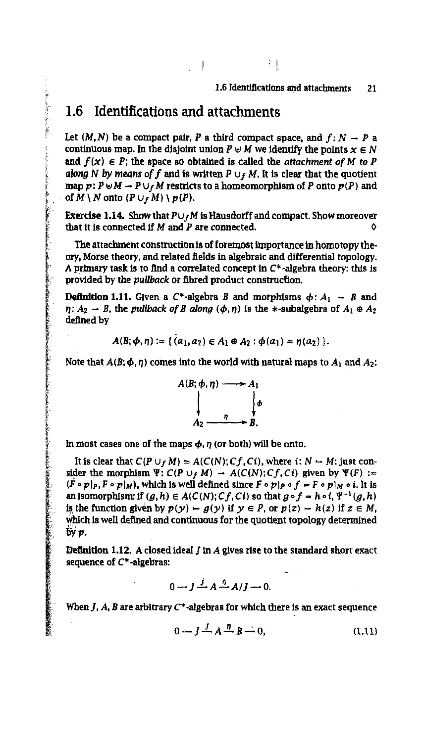
Definition 1.11. Given a C*-algebra В and morphisms ф: A\ — В and
n: Аг - В, the pullback of В along (ф, n) is the *-subalgebra of Ai m Аг
defined by
Note that A(B\ Ф, n) comes into the world with natural maps to Ay and A^.
А{В;ф,п) >-At
I . I'
In most cases one of the maps ф, ц (or both) will be onto.
It is clear that C{P uf M) = A{C{N);Cf,Ci), where UN- M: just con-
consider the morphism 4: C{P u/ M) - A(.C(N);Cf,Ci) given by Y(F) :=
(F о p\p,f о pIm)i which is well defined since F <>p\p o/ = F ep|M ei. It is
an isomorphism: If (g, h) e A(C(N); Cf, Ci) so that g »/ = h ° i, Y (g, h)
is, the function given by p{y) <~ g(y) if у e P, or p (z) - h{z) if z e M,
which is well defined and continuous for the quotient topology determined
Definition 1.12. A closed ideal Jin A gives rise to the standard short exact
sequence of C*-algebras:
When/, А, В are arbitrary C*-algebras for which there is an exact sequence
0 — J-La — B — O, A.11)
then j{J) is an ideal of A (since it equals kerr;) and В is isomorphic to
the quotient of A modulo this ideal. For convenience, we shall sometimes
abbreviate A.11) as J X Л-i B.
The exact sequence of C* -algebras A.11) is split:
a '
if and only if there is a morphism a:B-*A such that t) ° a = idj. (In
the notation, the two maps r? and a are combined on a single arrow.) This
happens if and only if A = j(J) + o-(B), where j(J) and o-(B) sit inside A
as subalgebras with zero overlap. In this case, there is also a C-linear map
тг : A - J with n » j = id;, but rr is not multiplicative in general. Indeed,
it is a morphism if and only if a{B) is also an ideal in A, whereupon we
write A = j(J) ® ar[B); the ideals j(A) and a(B) are said to be mutually
"orthogonal".
As an instructive example, consider the unitization-augmentation se-
sequence
0 — A~A+ ~C—-0, A.12)
and the maps а: С - A* : A - @, A) and тг.' A* - Л : (a, A) - a. The
sequence is split exact, and Л+ is the vector-space direct sum of A and C;
however, С sits as an ideal in A* only when A is already unital, in which
case A* =* А ® С —by means of (я, A) — (a + А1д) в A— is an orthogonal
sum of C* -algebras.
Definition 1.13. Given two C*-algebras/,B, an extension of BbyJisaC*-
algebra A together with morphisms such that there is an exact sequence
0-/-Д-?->0. An extension is called "trivial" when the sequence is
split exact.
Sets of (appropriately defined) equivalence classes of extensions have an
interesting algebraic structure; in particular, when в is a commutative al-
algebra, they yield a functor from locally compact spaces into abelian groups
and the resulting interplay between operator theory and algebraic topology,
when first introduced, solved some outstanding problems. This approach
was pioneered by Brown, Douglas and Filhnore in the seventies: see A46),
for instance.
The commutative example is, in view of Exercise 1.5,
0 — C0(Z) -i- C(X) -^ C(X \ Z) — 0,
for Z an open subset of X, and, in particular,
о—Со(м \ jv) ~ c(M) -L am—o,
uuu auaimucuia
for a compact pair (M,N).
> A very interesting situation arises with a locally compact but noncom-
pact space Y; we take for M some compactification of Y such that N :=M\Y
is its boundary. Then the various solutions of the extension problem of
C(P) by Co(Y) correspond to the different ways to attach MtoP along N.
This happens all the time in practice: for instance, in the construction of a
CW-complex, if P is a suitable subcomplex, M is a closed unit ball and N is
its boundary, one must make an explicit attachment of the eel] M \ N to the
subcomplex. A particular case in point is given by the short exact sequence
0 — Co(K2) — C(B)~ C(T) — 0, A.13)
where U denotes the closed unit disk. Note the difference with the unitiza-
tion (i.e., one-point compactification) extension:
0 — C0(R2) — C($2) -C-0,
where ? denotes evaluation at the point at infinity.
We shall now apply the noncommutative pullback construction with the
morphism ц being onto. Important particular cases are the associated map-
mapping cylinder and mapping cone algebras of a morphism of C* -algebras.
Definition 1.14. The mapping cylinder of a morphism ф: A - В is the
C* -algebra
гФ:= А(В;ф,Р1) := {(a,f) eAmBI:/(l) = ф(а)}.
The cone over a С-algebra В is the contractible C*-algebra CB := 2?@,1].
If p\\ CB - B, for 0 < t s 1, denotes the evaluation morphism f ~ fit),
the mapping cone of the morphism ф is the С * -algebra
Сф := А(В\ф,р'х) := {(aj) sAeCB-.fil) = ф(а)}.
Clearly, Сф is an ideal in Z^ and Z^/Q =* B. Also, if ф = id,» is the
identity morphism on A, then СцА = С А.
Exercise 1.15. Find a homotopy equivalence between 2ф and A. 0
* It is time to bring in the suspension functor. We make the commutative
definition in the context of pointed spaces. The functor Y ~ Y* carries
cartesian products into smash products. This is seen as follows. The bou-
bouquet X v Y and the smash product X л Y of two pointed spaces (X, *),
(Y,*) are defined as
X v У := (A-x {*}) и ({*} x Y) = (X x Y) \ ((X \ *) x (Y \ *));
In this way, X V Y becomes the base point of X л Y. Now, if X, Y are un-
unpointed, (X x Y)+ is the one-point compactification of the complement of
(X+ x {*}) и ({*} x Y+) h\X+x Y\ hence equal to X+ л У+.
24 1. Noncommutanve Topology; Spaces
Exercise 1.16. Check commutatMty and associativity for the smash pro-
product. 0
Exercise 1.17. Check that there is a bjjection
Map+(X,Map+(r-,Z)) -Мар+(Хл Y,Z)
for any triple of pointed spaces. О
In particular, we define the suspension IX of a pointed space X as S1 aX\
alternatively, one can form the one-point compactification of R x (X \ *).
Note that (Rrt)+ = К+л- • -л Runtimes), that Is, Srt = 1"$° = Sja- • -aS1
(n times). Moreover, Zn(X+) = (Rn x X)+.
Definition 1.15. The suspension of a C*-algebra A is the C* -algebra
= {/ e СД : /A) = 0} = АЛ = С0{Л) 9 A. A.14)
The suspension of a morphism ф: A — Bis the morphism 1ф = idco(R) ®Ф:
ТА - IB given by 1ф(/) := ф «> /.
Remark. The tensor product C*-algebra C0(R) ® A Is a completion of the
algebraic tensor product C0(R) о A generated by simple tensors /ea with
/ € C0(R), a e Л. Taking tensor products of C*-algebras Is a surprisingly
delicate matter, the idea is to complete the algebraic tensor product AqB
in a norm that is both a cross-norm, I.e., ||aefr|| = ||a|| ||i>||,andaC*-norm;
there Is always at least one such norm, but there may be several. For details,
see [3S2, Chap. 6]; a fine pedagogical walk-through is given in D81, App. T].
The matter Is also dealt with briefly in Section 1A Happily, if A or В is
either abelian or is the C*-algebra X of compact operators on an Infinite-
dimensional separable Hubert space, the C*-cross-norm is unique and we
can avoid this discussion in those cases.
We probe the С *-algebraic notion of suspension with several exercises.
Exercise 1.18. Show that the suspension 1Л is contractible whenever the
algebra A is contractible. 0
Exercise 1.19. Show that I(AT) = BA)I. Conclude that if the C*-algebras
A and В are homotopy equivalent, then ТА and .IB are also homotopy equi-
equivalent. 0
Exercise L2Q. If /is an Ideal in A, then U is an Ideal in IA and I(A /J) ¦¦
IA/2J. Every exact sequi
sequence of suspensions
IA/IJ. Every exact sequence 0 - J-^-A-^A/J - 0 induces an exact
.,1 . :. I .
1.6 Identifications and attachments 25
Exercise 1.21. Every split exact sequence 0-7 — A ~ A/7-0 induces
a split exact sequence of suspensions:
•0.
Proposition 1.14. For every marphism ofC*-algebras ф: A - B, there is
an exact sequence
A.15)
0 — 1B± Сф~ A — 0.
In particular, the following sequence is exact:
0 — ZA— CA — A — 0.
Proof. The maps in A.15) are y(/) := @,/) and P(a,f) := a. D
We need one more exact sequence related toO — J — А — В — 0.
Proposition 1.15. Given A.11), there is an exact sequence
0 — J — С„ — CB — 0.
Proof. Since r)[j(c)) = 0 for any с 6 /, there is a map «: / - Cn : с ~
ШО. 0); its image is the kernel of the map (a,f) ~ f:Cn ~ CB. ?
> The notions of mapping cylinder, cone, mapping cone and suspension
are algebraic counterparts of well-known topological notions [150]. We Il-
Illustrate them by their roles in the definition of the Puppe sequence, which
we now recall. Let /: M - P be a continuous map between compact spaces;
it is known to be the first arrow of an infinite exact sequence
, In order to make sense of A.16), we consider first the mapping cylinder
W fashioned by attaching M x J to P along M x {1} by means of the map
(x, 1) « f(x) e P. Now, bothM and P are identified to closed subspaces of
the mapping cylinder.Also, M* retracts on P by the homotopy r: M-f x J -
Щ given by .
r(p(x,t),u):=p(x.u
r(p(y),u):=p(y),
for
It is immediately seen that M* is the Gelfand dual of the C* -algebraic map-
mapping cylinder: ZC/ = C(Mf).
i The unreduced cone CM over M is obtained from Af x J by identifying
Mx{0} toapointNote thatCMisa space contractible to a point: Y,(x, t) :=
гь l. Noncommutanve lopojogy: spaces
(x, st), for s e /, provides a homotopy between idcM and the constant map
of CM into its basepoint. The unreduced mapping cone C-f of / is defined
as P uf CM; it is often convenient to see it as the quotient Mf /M. Also,
when M = P and / = idw, then Cf is just the cone CM of M. These are
not quite the Gelfand duals of the cones considered in Definition 1.14. For
instance, ССШ), the cone algebra over C(M), which is not unital, cannot
coincide with C(CM), the continuous function algebra over the (compact)
cone CM. The latter is the unitization of the former: regard the elements
of CC(M) as functions onMx/ that vanish at the points (x, 0).
Exercise 1.22. Show that, if (M,N) is a compact pair, then M/N is homeo-
morphic to С*/СЫ, where i: N - M is the inclusion. 0
Finally, the unreduced suspension IM is obtained from M x J by identify-
identifying bothMx{0} andMx{l} to points: clearly lM « СМ/Мх{1} = CM/M.
It is natural to take the unreduced suspension of the empty set to be the
(two-point) sphere S°. Neither of the two commutative notions of sus-
suspension is quite the Gelfand dual of the suspension considered in Defini-
Definition 1.15. For instance, it Is not true that the suspension IX for a compact
pointed space (X, *) is the character space of 2C(X), since this algebra
is never unital! Instead, 1C(X) = C0(R x X). (In fact, what we did was
equivalent to defining ZX, for X locally compact, simply as R x X, hence
ICoiX) = Co(ZX) in general.) Care needs to be exercised, then, in switching
between these related concepts in spaces and algebras.
Coming back to the Puppe sequence: the map Jf:P~Cfis obtained by
composing the inclusion P - M* and the quotient map Mf - М?/М\ now
P is identified to a subspace of Cf and the next arrow q is the canonical
projection onto the quotient Cf IP =* lM. Finally, If is die suspension of
/, sending the image of (x, t) into the image of (/(*), t). The rest of A.16)
is clear.
By definition, the "Puppe sequence" of algebras, associated to a mor-
phlsm ф: A - B, is of the form
_2 л
¦ I? A
¦ IB
Ф
В. A.17)
The maps ft and у are those given in Proposition 1.14.
The two constructions are quite similar, although not strictly parallel.
We have presented them in the form most suitable for our purposes, to be
revealed in Chapter 3.
1 .A C* -algebra basics
We collect here, for the reader's convenience, several facts and theorems
about С * -algebras as background for the main text. There are many good
ia e--algebra basics П
textbooks on this subject: we recommend [129,137,183,266,352,366,481],
in no particular order.
Definition 1.16. A Banach algebra is an associative algebra over the field
С of complex numbers that is also a complete normed space, and in which
Hafcll s ||a|| ЦЫ1 A.18)
for all elements a, b of the algebra; this condition guarantees continuity of
the product. If a Banach algebra contains a unit 1, we may as well assume
mat II 1|| = 1; for if not, the operator norm of the map b ~ ab yields an
equivalent norm for which the unit has norm 1. Any Banach algebra can be
unitized by defining A* := A x С as in Section 1.1, and extending the norm
in a convenient way, by setting ||(а,Л)|| := sup{ ||аЬ + ЛЬ||: ||b|| si}, for
instance.
f" An involution in a Banach algebra is an isometric antilinear map а — a*
satisfying a** = a and (ab)* = b*a*. When a particular involution is
given, we speak of a Banach * -algebra A C*-algebra is then a Banach *-
algebra that satisfies the crucial equality ||д*я|| .= ||а||2 for each element
a&A.
If A is a C*-algebra, then so is A*, since
||<а,А)*(а,А)|| = sup{ \\a*ab + kab + \a*b + \\b\\: \\b\\ s 1}
: a sup{ \\b*a*ab + \b*ab + \b*a*b + ЛЛЬ*Ь||: ||Ь|| ? 1}
= sup{ \\(ab + №*(ab + Ab)||: IIfoil s 1}
= sup{ ||ab + Ab||2: \\b\\ sl} = ||(a, A)||2,
and the opposite inequality || (а, А)* (а, Л) II s ||(a,A)||2 follows fromd. 18).
If / is a closed (two-sided) ideal in a Banach algebra A, then the quotient
algebra A/J is also a Banach algebra under the obvious norm ||a + J|| :=
inf{ \\a + b\\ : b e J}. If A is unital, then 1 + J is a unit for A/J. If A is a
C*-algebra, so is A/J.
Already in any unital Banach algebra A, the geometric series с :- 2Х=о bk
converges absolutely if ||b|| < 1, since its norm is majorized by Z"»o 11^*11 ^
?"-o W\k = A-ЦЫ1)-1.Clearly, bc = cb = c-l,so (l-b)c = c(l-b) = 1.
Setting a := 1 - b, we find that a is invertible provided || 1 - я|| < 1. More
generally,if xisinvertible and ||x-y|| < \/\\x~x\\, then Ul-x-'yll < 1, so
у is also invertible: the set A* of invertible elements is an open subset of A.
Therefore, a proper ideal in a unital Banach algebra cannot be dense, as then
it would contain an invertible element. Contrast this with the nonunital C*-
algebra X of compact operators on a separable infinite-dimensional Hubert
space, which has many dense ideals (see Section 7.C).
Definition 1.17. Fora e A, the vector-valued function Ra: A - (А-л) is
defined and holomorphic on an open subset of the complex plane C, with
28 L Noncommutative Topology: Spaces
a convergent Laurent series ?"«o Л~к~хак on the annulus |Л| > ||я||. Since
the sum of this series tends to 0 as |A| - «, the function Ra cannot be
extended to an entire function on С (since, by liouvffle's theorem, it would
then have the constant value 0). Therefore, the set of values
sp a := {A 6 С: (A - a) is not invertible}
is a nonvoid, closed (therefore, compact) subset of {z е С: | r | s \\a\\}, and
is called the spectrum of a. The smallest disk (centred at 0) that includes
the spectrum has radius r(a) := limn_« ||an||1/n. Notice that a nilpotent
element satisfies r(a) = 0 and hence spa = {0}.
Any polynomial equation ц - f(z) s (Л - z)g(z) entails \x - /(a) =
(Л - a)g(a) in A, so if / is a complex polynomial, then ц е sp/(a) if and
only if ц = /(A) for some A e spa; in other words, sp/(a) = /(spa).
There are several "functional calculi" that seek to extend this relation to
more general functions, the main problem being to suitably define the el-
element /(a); at any rate, / « f{a) must be an algebra homomorphism
into the (commutative) closed subalgebra generated by a. For general Ba-
nach algebras, the best one can do is to replace polynomials by functions
holomorpblc near sp a: if /(a) is defined by the integral
а)-1^ A.19)
on a rectifiable contour Г that winds once around sp(a), then the spectral
mapping and homomorphism properties hold; this is called the holomor-
phic functional calculus.
When Л is a nonunital Banach algebra, the spectrum of an element а е A
is defined to be its spectrum in A+; it is then automatic that 0 € sp a, since
elements of A are not invertible in A*. The polynomial and holomorphic
functional calculi still make sense in A, provided they are constrained to
functions / satisfying /@) = 0.
> For the rest of this section, we shall suppose that A is a C*-algebra. In a
C*-algebra, the spectrum of a self adjoint element a is real (see Exercise 1.1).
Moreover, its spectral radius r(a) is equal to its norm: this follows from
||а2|| = ||а||2 and r(a) = шп„-„ \\ап\\1'п. From this last equality it also
follows that r(ab) ? r(a)r(b) if a and b commute. A normal element
a e A is one that satisfies aa* = a*a. For instance, any selfadjoint or any
unitary (a*a - 1 = aa*) element is normal. If a is normal:
||a||2 = ||a*a|| = r(a*a) s r(a*)r(a) i ||a*||||a|| = ||a||2,
so r(a) = \\a\\, too. The definition of normality means that the C*-sub-
algebra generated by a is commutative. By applying the Gelfand-Naimark
theorem 1.4 to this subalgebra, we get a continuous functional calculus,
whereby / - f(a) is extended to all functions in C(spa), by matching
1А С* -algebra basics 29
uniform convergence of polynomials to norm convergence of elements of A
(see the remark on the spectral theorem in the main text).
A morphism of C*-algebras is by definition a *-homomorphism. Any
morphism ф: A - В extends uniquely to a unital morphism ф*: A* - B+.
Lemma 1.16. Any morphism ofC* -algebras is norm-decreasing, and so is
continuous.
Proof. It is enough to check this for a unital morphism ф: A - В of unital
C* -algebras. If (Al -a)c = 1 in A then (Al -ф(а))ф(с) = 1 inB; therefore,
sp4>(a) ? spa. In particular, г(ф{а)) s r(a). It follows that
||ф(а)||2 = \\ф{а*а)\\ = г(ф(а*а)) i r(a*a) = ||a||2. D
Definition 1.18. A positive element of A is a selfadjoint element a for
which spa с [0,»). It has a (unique) positive square root; one can define
a112 > f(a) using fix) := -Jx on [0, ||a||]. An element a Is positive if and
only if a = b*b for some b e А Ц37, §1.6], if and only if (? I al) 2 0 for
any vector g in a Hilbert space on which A acts faithfully.
We write с ? d for selfadjoint elements c,d e A whenever d - с is
positive. If A is unital, any positive element satisfies 0 < a < ||a|| 1, since
sp(||a||l - a) С [0, oo); or equivalently, since the function f(x) := x on the
Interval [0, ||a||] satisfies 0 <; / s ||a||. A selfadjoint element is positive if
and only if \\a -11|| <; t for t ? ||a||, again by functional calculus. This
property can be used to show that the sum of two positive elements is
positive, so that the set of positive elements of A is a convex cone, and the
relation с s d is a partial ordering on the set of selfadjoint elements.
Exercise 1.23. Show that HOiaslinA, then Q<,a2 <,a, 0
Definition 1.19. An approximate unit in а С-algebra is an increasingly
ordered net {ua} of positive elements of A such that every ||ua|| ? 1 and
\\bua-b\\ - Ofor eachb e A (and therefore \\uab-b\\ = \\b*ua-b*\\ - 0
too). Such nets certainly exist in nonunital C*-algebras; for instance, one
can take as index set all the positive elements of norm less than one, putting
Ua := a. It turns out that such a net may be chosen from any dense ideal
of A, and can be chosen to be an increasing sequence when A is separa-
separable [137, Prop. 1.7.2]. More generally, a C*-algebra with a countable ap-
approximate unit is called <T-unitaL
A linear functional ф: A - С is called positive if ф (a) a 0 for all а г 0
in A, or equivalently if ф(Ь*Ь) ;> 0 for all b. If A is unital, this implies
that 0 < ф(а) < ||а||фA), so that ф is automatically continuous with
ИФ11 = ФШ- (In the opposite direction, any continuous linear functional
satisfying НфН = фA) must be positive.) In the nonunital case, continuity
is also guaranteed, with ||ф|| = lim,, ф(иа) for any approximate unit [366,
Prop. 3.1.4]; moreover, ф extends to a positive linear functional ф+ on the
unitization A+ just by setting ф+A) :=
30 1. Noncommutative Topology: Spaces
If ф and ф are positive functionals on A such that \\ф\\ = \\ф\\, and if
ф-qi is also positive, then ф = ч>; for we may suppose that A is unital, and
then it is enough to notice that \\ф - i//|| = (ф - i//)(l) = ||ф|| - ||i//|| = 0.
A linear functional т: A - С is called rracia/ if т(яЬ) = т(Ьа) for all
a.beA.
Definition 1.20. A positive linear functional of norm one is called a state
of the C*-algebra. If Л Is unital, any state satisfies фA) - 1. A state ф is
called faithful if a a 0 and ф(а) = 0 imply a - 0.
A (normalized) trace on A is a nontrivial tradal state.
The space of states is a convex set; in the unital case, this follows from
the equality ||A -ПФ + tc/>|| = (d -*)Ф + NJ»)A) = A -1) +t = 1 if ф,ф
are states and 0 ^ t < 1. The extreme points of this convex set are called
the pure states.
Any state ф of a C* -algebra A gives rise to a representation Пф of A,
by what is called the Gelfand-Naimark-Segal construction, or "GNS con-
construction" for short [426]. The starting point of this construction is the
observation that
(a | Ъ)ф := ф(л*Ъ)
demies a positive semidefinite sesquilinear form on the vector space A. As
such, it satisfies the Schwarz inequality, in the form
\ф(а*Ъ)\г s, ф(а*а)ф(Ъ*Ь).
Therefore
Ыф := {b e A : ф(Ъ*Ъ) = 0} = {b e A: ф(а*Ь)=0 for all a e A}
is a closed left ideal in A. We say that ф is a faithful state if Ыф = О. The
quotient vector space А/Ыф, with elements a := а+Ыф, is then a prehilbert
space under the positive definite scalar product (а\Ь)ф := ф(а*Ь). Denote
by 3<ф its completion to a Hilbert space.
If h e A, the map A- A\c -~ b*cb preserves positivity, and so a* as
\\a*a\\ 1 (valid in A+, if A is not unital) entails the inequality
b*a*ab <; ||a*a|| b*b A.20)
among positive elements of A. Applying ф to both sides gives the inequality
ф{Ь*а.*аЬ)и\\а*а\\ф(Ь*Ъ). A.21)
In particular, the maps on А/Ыф defined by
Пф(а):Ь~аЬ A.^2)
extend to bounded operators on Э{ф satisfying ||ттф(я)|| z \\a\\. The map
Пф\ A - ?(Яф) is an algebra homomorphism, and since (k \ Пф(а)с)ф =
1.A С*-algebra basics 31
ф(Ь*ас) = (щ(а*)Ъ | с)ф, the adjoint operator to Пф(а) is
щ(а*). Therefore, щ is an (involutive) representation of A
If A is unltal, write \ф := 1. Otherwise, take an approximate unit {ua}
and define 1ф := lim« и„; indeed, the estimate
for « г р, and the convergence ф(иа) — 1 shows that the net {ua} has
the Cauchy property, so it converges in Мф. (The inequality follows from
Exercise 1.23.) Now щ{Ъ)\ф = bforb e A, so that щ(А)Ъф = А№ф.
This says that Ъф is a cycUc vector for the representation щ, which is to
say that the TT>(A)-invariant subspace generated by \ф is dense in Хф.
furthermore,
(U I Пф(а)ЪФ)ф = Ф(а) for all абА A.23)
When the state ф Is faithful, Лф is the completion of A itself in the new
norm \\а\\ф := ^ф(а*а). In that case, §ф is also a separating vector, that
is, & = rty (ЬMф = 0 in Мф implies b = 0 In A.
The representation Пф is irreducible if and only if the state ф is pure [137,
Prop. 2.5.4].
With the GNS construction m hand, we can state the second Gelfand-
Nabnark theorem.
Theorem 1.17 (Gelfand-Nalmark). Any C*-algebra has an isometric repre-
representation as a closed subalgebra of the algebra ?Cf) of bounded operators
on some Hubert space.
Sketch proof. One uses the Hahn-Banach theorem to show that for any
nonzero positive element b*b e A, there exists a state Ц> = фь such that
ц>(Ъ*Ь) = \\b*b\\ = ||fc||2 [129, Lemma 1.9.10]. Then A.23) shows that
11%(ЬM^||^ = ||i» ||. Therefore, we can find a family Ф of states for which
ф(Ь*Ь) = 0 for all ф е Ф implies b = 0 —if necessary, take Ф to be all
states on A. Now form the direct sum of the corresponding GNS represen-
representations 7Г := ффбфТТф, acting on Л" := ф^еф^Гф; then ||7r(b)|| = l|b|| for
every b e A, so тг is an isometric representation of A on ?{Э{). а
Inparticular,ifi4isaseparaЫeC*-algebгa,wecantakeФ - {фьь) where
{bk} is a countable dense subset of A, so that H is then a separable Hubert
space.
Corollary 1.18. A selfadjoint element ae A is positive Щф(а) г 0 for any
state ф on A.
Proof. For any unit vector »} e Jf, the linear functional a - (»} | n(a)n)
is a state of A, since b*b - Нет(b)/j||2 a 0. Therefore, n(a) is a positive
operator on Я, so it has a positive square root тг(яI/2. Since я is an
isomorphism, this is of the form n[b) for a unique b - b* in A, and n(a) -
n{bJ implies а = Ьг. О
32 1. Noncommutative Topology, Spaces
If AisaC-algebra, then so is Mn(A) = Mn(C)®Aforanyn = 2,3,...;its
elements are matrices [ay] with entries in A. Each representation тг: A -
?Ш) gives rise to a representation, say тг(п): Afn(A) - ?{Cn ® 30, given
by Gr(n)(ft)»j)< := Z"-i TT(ay)n^ for q = (ni,...,nn), and if тт is injective
then so is тг(п).
Lemma 1.19. An element of [ay] € Mn(A) is positive if and only if it is a
sum of matrices of the form [a^aj] with a\ яп е A.
Proof. If a € Mn{A) is the matrix whose first row has entries a\ an
and whose other entries are 0, then a*a = [afaj], so such matrices are
positive in Mn{A). On the other hand, if я = b*b is a positive element of
МпШ, then я = ci + • ¦ ¦ + cn, where с* - [b?,bjy]. D
Proposition 1.20. Аи element of [ay] e Mn{A) Is positive if and only if
^* te positive fti A for af/ci,...,с„ е A.
Proof. If a = b*b is positive in Afn(A), then
n n n
X c,*aycy - ? cfbfabkjcj = J! dfdki
(J-l W,k-1 k-1 >1
Conversely, if ?"j_ t c(* aycj is positive for all C\,.... cn, let ф be any state
of A. The vectors of the form rj * (ттф(С1Mф,...,тгф(сп)§ф) make up a
dense subspace of Cn в Мф, on which
(П I тгфп>(а)п> - t Eф I пф(с;ацс№ф) = ф( f cfaijcj) г О,
so that each ttJ, (a) is a positive operator. If тт = Фф6« ттф is the injec-
injective representation of A given by Theorem 1.17, then тт(п> = ®ф6фПфП) is
also injective, and тт(п) (a) is a positive operator; therefore, a is positive in
Mn{A). . О
> Finally, we briefly address the matter of tensor products of C* -algebras.
The issue in defining such tensor products is to find a suitable norm. Con-
Consider first the tensor product of two Hilbert spaces !tf. and !H'. The alge-
algebraic tensor product JfQJf', namely the vector space consisting of finite
sums of simple tensors X"-i lj ® 1j, is a prebilbert space under the scalar
product (fi e fn I g2 e m) := Ei I b) (Hi I Пг). The Hilbert space M e !H'
is defined as the completion of 3f о 3f in the corresponding norm, which
is a cross-norm, that is, ||g ® n|| = ||g|| ||n\\ in all cases. If 5 e ?E0 and
Г е Х(Л"'), the linear map 5 e rj ~ S? e Tn on 4/" © 5/"' is bounded and
extends to a bounded operator S в Т on 3f e 5f'.
1.A с -aigeDra basics a
For more general Banach spaces E and F, there may be several cross-
norms on E 0 F, each one yielding a different completion. The most impor-
important of these is
y(z) := infjly \\xj\\ \\yj\\: z
where an element zeEeF may be written In many ways as a finite sum of
simple tensors. The completion of jEoF in the norm у is called the projecttve
tensor product, usually written ? ® F. Taking A B) to be the supremum of
I (/ ® 0) U) I, where / and g are continuous linear functionals of norm one
in the dual spaces E* and F* respectively, yields another cross-norm Л, and
In general any cross-norm on E ® F satisfies AB) s ||z|| ? y(z).
For C*-algebras A and B, we consider only crossrnorms having the C*-
property: \\c*c\\ = \\c\\2 for all с 6 A © B. There is a smallest norm at and
& largest norm ц in this family. The former is given by cr(c) := sup{ (ф <s
Ц/)(г*с*сг)/{ф<вц/)(г*г)), where the supremum is over all states ф of A
and i// of В and all z € Л о ? for which (ф ® i//)(z*z) > 0. The latter
is *i(Zj a/ ® b^) := sup||Sj rr(a.j)p{bj)\\, where the supremum is over all
pairs of commuting representations тг: A - ?(^f) and p:B - LC() on
the same Hubert space. It turns out that any C*-norm || -1| on AoS is in fact
a cross-norm [267, Cor. 11.3.10] and it must satisfy A s a s || • || ^ ц z y.
fat the proofs of these inequalities, consult [267, §11.3], [352, Chap. 6]
or .[481, Appendix T].
Definition 1.21. The completion of Л о В in the norm с is a C*-algebra,
called the (spatial) tensor product AeJ.A С *-algebra A is called nuclear
if,, for any C*-algebra B, the algebraic tensor product AoB has only one
C*-cross-norm, namely the spatial one. In that case, А в В is referred to as
the tensor product of A and B.
It is known [352] that finite-dimensional C*-algebras are nuclear, with
A/n(C) в В a Mn(B); and that commutative C*-algebras are nuclear, with
СЬ(У)®В = Со(У-В).ТЬе C*-algebra X is also nuclear. The larger algebra
?(Э{) is an example of a honnuclear C*-algebra.
Example 1.1. An element с € A 0 В can be expressed as a finite sum с =
?, О/ в bj in several ways; let
1/2 } A.24)
Then || • ||h is a cross-norm (although not a C*-norm), and the completion
Ы AoB in this norm is called the "Haagerup tensor product" A «h B. One
. of its useful features is that the multiplication m: AqA - A:a®b ~ ab
extends to a norm-decreasing map from A «h A to A (see Exercise 2.14).
This norm plays an important role in the theory of operator spaces, i.e.,
closed subspaces of ?(M); for background, see the survey [80].
34 1. Noncommutatlve Topology: Spaces
l.B Hopf algebras and Tarmaka-Krein duality
In the unusual situation when the compact space X is not Hausdorff, the
algebra C(X) is still a C*-algebra. Nevertheless, we do not recover X from
the algebra C(X). At the other extreme, when the space X not only is a
compact, Hausdorff space, but has, some extra structure, then the space X
can sometimes be recovered from a smaller algebra. The algebra of smooth
functions on a manifold is a case in point.
If G is a compact topological group, then G can be recovered from the
algebra of real representative functions K(G), which turns out to be a Hopf
algebra. In this appendix section, we outline the basic theory of (real or
complex) Hopf algebras, and give an account of the reconstruction theorem
of Tannaka and Krein. This is a close analogue of the Gelfand-Naimark
theorem, but requires us to work over the real field. What we learn about
Hopf algebras here will be of use in Chapter 14, which is concerned with a
particular, important Hopf algebra.
From a mathematical point of view, we seek the algebraic objects corres-
corresponding to topological groups in the quantization program as described,
for instance, in A52). A satisfactory correspondence for locally compact
groups, including an extension of Pontryagin duality, has only recently been
found [300,301]; it requires a considerable amount of C*-technology. Here
we shall outline the equivalent problem for compact groups, where the al-
algebraic objects m the commutative case turn out to be commutative Hopf
algebras, and we develop an equivalence between the categories of compact
groups and of these Hopf algebras. ^
A Hopf algebra is a vector space over a field F of characteristic 0, taken
here as С, Ш or Q, on'which there is both an algebra and a coalgebra struc-
structure related by some compatibility conditions. To emphasize the duality
between algebras and coalgebras, we shall start by describing the former in
terms of arrows and diagrams. Thus, a unital associative algebra is a triple
(A,m,u), where A is a vector space over F, m: A e A - A and u: F - A
are F-linear maps such that the following diagrams commute:
таЫл
' 1® A
Id,em I \m A-25)
In this Section e always means the algebraic tensor product. Commutativity
of this diagram gives the usual associativity of the algebra product. Also:
! Ha T
A.
l.BHopf algebras and Tannaka-Kreln duality 35
The unnamed arrows denote the natural identifications A ® F = Л = IF в А
pven by о в A - Aa and A ® a - Aa. The diagrams A.26) provide the unit
1л := mAf) for the multiplication m. The commutativity of an algebra can
be expressed by the commutativity of the diagram .
A» A—^-*АвЛ
'/ A.27)
where <r is the flip operator а в b ~ b e a. The commutativity of the
following diagrams:
A»A—?-~A
describes a unital homomorphism ф.
Definition 1.22. The prefix "со" stands for reversing arrows in the dia-
diagrams. A coalgebra, then, is a triple (С, Д, e), where С is a vector space
over F, Д: С — С в С and t: С — F are F-linear maps satisfying the reverse
of A25) and A.26):
A.28)
and
A.29)
It* It*
The maps Л and с are called the coproduct and the counit respectively, and
the property described by diagram A.27) is coassodatMty. Furthermore,
we say the coalgebra is cocommutattve if the opposite diagram to A.27)
commutes:
CzC*-^—C<sC
л\ / A
С
36 l. Noncommmattve Topology: Spaces
The tensor product of two unital algebras is again a unital algebra, where
I At a- = U ® I A' and the product is given on simple tensors by
тл»АЛ(л в а') в (b ® b')) := ab e a'b'.
In terms of arrows, тлел1 and и At a are given by
^аА', A.30)
and IF — F ® F Jifii. Л в Л'. Similarly, the tensor product of two coalgebras
is a coalgebra, where the coproduct Деве is obtained by reversing A.30):
More concretely, if Д(c) - Zt c'i * <' and Д' (d) = Ij d} e dj, then
Деве (с в d) = X c[ в d} в c(" в d}', A.31)
and the counit ec»c- is given by С в С ^- FeF—F; that is to say,
ecec(ced):=f(c)f'(d).
> We now consider the situation where a vector space has both an algebra
and a coalgebra structure, with the obvious compatibility requirement.
Definition 1.23. A bialgebra is a quintet (S,m,u, A, e), where (B,m,u) is
a unital algebra and (B, A, s) is a counital coalgebra, such that the maps Д
and ? are also unital algebra homomorphisms.
Exercise 1.24. Show that the compatibility condition is equivalent to m
and u being counital coalgebra morphisms, where such a morphism is an
F-linear map ?:C - С making the following diagrams commute:
F.
A subbialgebra of ? is a vector subspace D that is both a subalgebra
and a subcoalgebra; in other words, D, together with the restrictions of the
product, Coproduct and so on, is also a bialgebra and the inclusion D - В
is a morphism of bialgebras.
Example 1.2. For q ф 0, consider the algebra of polynomials in two vari-
variables x,y, with the condition xy = qyx. It possesses a bialgebra struc-
structure, setting Ar := x <s x, Ду := у ® 1 + x Q у, e(x) := 1, e(y) := 0. This
is the "quantum plane" [326].
1 .В Hopf algebras and Tannaka-Kreta duality 3 7
Example 1.3. The tensor algebra T(V) of a vector space V is a cocommu-
tative bialgebra, where the coproduct and counlt are defined on v e V by
A(v):=-vel + le v, s(v):=0. A.32)
As given, Д: V - T(V) ® T"(V) is an F-linear map, which, by the universal
property of tensor algebras, extends to an unital algebra homomorphism
Д:Т(У) - T{V)9T(V); in particular, ДA) = lei.Now, (Aeid)oA and
(id ®Д) в д are two unital algebra homomorphisms from T(V) to T(V) 9
f[V) 9 T(V) that agree on V, giving v-velel + level + lelev.
By the uniqueness of extensions, A.28) holds. The counlt property A.29)
likewise follows from
(? 9 id)(A(v)) = «(v) l + t/ = v = i/ + f (v) 1 = (id «f)(A(v)).
The cocommutativity comes from cr(A(v)) = vel+lev = A(v)forv e V.
Since? is an algebra homomorphism, itfollows from A.32) that?(Vie- • -e
vn) = 0 for all n г 1. Similarly, A being an algebra homomorphism, one can
inductively write an explicit formula for A(vi e • ¦ ¦ e vn); see [278, Ш.2.4],
for instance.
Example 1.4. The untversal enveloping algebra l/(g) of a lie algebra g is
the quotient of the tensor algebra T($) by the two sided ideal / generated
by the elements XY-YX- [X, Y], for all X, Y e g. Since Д is an algebra
homomorphism, A.32) yields
MXY)
and thus
MXY -YX- [X, Y]) = {XY - YX - [X, Y]) 9 1 + 1 e (XY -YX- [X, Y]),
so Д(/) sl9H + HeI. Clearly, f (/) = 0, too. These two conditions mean
that I is also a coideal in 7"(g), and the quotient 1i(g) thus becomes a
bialgebra, which is clearly cocommutative. The cornerstone of the theory
of enveloping algebras is the Poincare-Birkhoff-Witt theorem [138, §2.1]
which yields a basis for the vector space 4/(g) in terms of a basis of g: If
Xi,... ,Xn is a basis of g, then the (ordered) products X?X% ...X™, with
П € N, form a basis for 1i(g). Naturally, li(g) becomes a lie algebra under
the commutator bracket, and there is an injective homomorphism of Lie
algebras j: g - t/(g) with the following universal property: if Л is an unital
associative algebra and if ф: g - A is a lie algebra homomorphism, then
there is a unique algebra homomorphism Y: 1/(g) - A such that Y A) = 1
and ip = 4oj. Moreover, if ф: 3 - g' is a lie-algebra homomorphism there is
a unique unital algebra homomorphism 11{ф): ti(g) - f(g') lifting ф. All
this follows trivially from the Poincare-Birkhoff-Witt theorem; in this way,
11 becomes a functor from the category of Lie algebras into the category of
unital associative algebras.
Any vector space V can be regarded as a lie algebra with the trivial lie
bracket, [и, v ]:- 0 for all u, v e V. In this case / is generated by the com-
commutators uv - vu, and the resulting enveloping algebra is commutative: it
is the symmetric algebra S(V) of the vector space V.
Definition 1.24. We point out that there is a lie algebra inside any bialge-
braB. Indeed, be Bis called a primitive element if Д(Ь) = bel + leb.
If с is also primitive, then
&(bc) = be <& 1 + b <з с + с ® b +1 <& be,
and therefore be-cb is also primitive; the set P(B) of all primitive elements
of ? is thus a Lie algebra. In addition, A.29) shows that t (b) = 0 necessarily,
for b primitive.
Lemma 1.21. The set of primitive elements ofU(g) isg itself.
Proof. We claim that P A1 (g)) is just the embedded copy of g. First note that
any element of 1i(g) can be written as a linear combination of powers X",
with X 6 s, n € N. For instance, XY = \ (X+YJ - ?X2 - \ Y2 + \[X, Y\, and
there is an analogous expansion for any element of a PBW basis. If l/n(g)
denotes the subspace generated by {Xn : X € g}, then 11(9) = ф".о 1/п(я)
is a graded bialgebra: since &(Xn) = If,0 (f)Xk»Xn-k, the coproduct is
compatible with this grading. If n a 2 and an element p = Zj сД? € 1in (g)
is primitive, then the terms <jt := Zj cj{i)x'j<*X?~k of bidegree (к, n-k)
in Д(р) must vanish for 0 < к < n; but then (?) p = тп(<ц) - О in ^"(g),
and (j) p * 0 since F has characteristic zero. Thus the primitive elements
are only those in IIх (g) = g- ?
Definition 1.25. Given an algebra A and a coalgebra С over IF, we can define
the convolution of two elements /, g of the vector space of F-linear maps
Hom( С, Л), as the map / *g e Hom(C, Л) given by the composition
Proposition 1.22. If A is an algebra and С a coalgebra, then the triple
(Hom(C,A),*,u of) is a unital algebra.
Proof. By A.25) and A.28), the following diagram commutes:
C»C-
Since (f*g)*h corresponds to the map from С to Л along the top edge of
the diagram, whereas / * {g * h) is the map from С to Л along the bottom
edge, the convolution is associative.
Moreover,if Д(е) = Z,jCjQc'j thenc = [e ° id) (Zj сj в c'j)
by A.29). Then, since с is linear,
(uoe)
= mB,(uoE)(C;
= iKc'j)f(c'J) = fBj,(c'j)c';) = f(c).
j
Similarly one checks that / * (u ¦> e) = /. D
Lemma 1.23. If-В; С — С is a counital coalgebra morphism then t*: g •-
0o^:Hom(C',.A) - Нот(С.Л) is a unital algebra morphism. Similarly, if
ф:А-А' is a unital algebra morphism, then 0*: / ~ ф of: Hom(C, A) -
Hom( C, A') is another unital algebra morphism.
Proof, ttg.he Hom(C,A), then
t*(g * h) = m о (g ® h) о д' о ? = m о (g e h) ° (t в 4) о д
= m»(Г$ в-?*h) = Д
Moreover, ^* (и <> f') = м о г' о f = и о г, so 4* is unital. The proof that ф»
is homomorphic and unital is similar. D
Definition 1.26. A Hopf algebra is a bialgebra H together with a (necessar-
(necessarily unique) convolution inverse S for the identity map id». The map S is
usually called the antipode of H. The property idH *S = S * idH = и ° е
boils down to the commutativity of this diagram:
I t I
hi particular, if Д (a) = Sj a'j e a'j, then
Seld
A.33)
Xja'jS(a.'j), A.34)
andbkewise f(a)lH = IjSia'^a'J.
A morphism of Hopf algebras is a linear map #:H - H' that is both a
unital algebra homomorphism and a counital coalgebra homomorphism,
and satisfies the compatibility condition ?«S = S' о ?. Actually, the com-
compatibility condition is automatic, as the following argument shows [236,
Prop. 37.1.10]; see also [446].
40 1. Noncomamtative Topology: Spaces
Proposition 1.24. LetH andH' be Hopf algebras andt: H - H' a bialge-
bra morphism; then 4oS~S'o?.
Proof. By Lemma 1.23,
u«? = f (id/г *S'} = t*(idH') *4*S' = t*{S'<>i),
* idH) = 4*S * ^*
Associativity of the convolution then gives
Example 1.5. If G is a group, FG denotes the group algebra of G over F,
that is, the vector space over F with G as basis; its product is defined by
extending linearly the group multiplication of G, so the unit in FG is the
identity element of G.
Proposition 1.25. The group algebra FG is a cocommutattve Hopf algebra
where the coproduct, counit and antipode are the respective linear extensions
of the diagonal map A(x) := x ® x, the constant map s(x) := If, and the
inverse map S(x) := x'1 defined on G.
Proof. LetH - FG;byunearity,itisenoughtoverifyA.28),A.29)andA.33)
on elements x € G. Coassociarivity comes from the associativity of the
tensor product:
(Д 9 id) о Д (X) = (X 9 X) 9 X = X 9 (X 8 x) = (id®A) о Д(Х).
Cocommutativity Is obvious. The counit property follows from
(? e id//) о д(х) = е(х)х = x = xe{x) = (idH ее)
For the antipode,
mo(Seid)oA(x) = rn(x~19x) = 1н = m(xex"a) = m°
and moreover, (u о e)(x) = uAf) = 1н. so A.33) holds. D
Conversely, an element a of any Hopf algebra H is called group-like if
Д(а) =ава, The set G{H) of group-like elements is a unital semigroup,
since Д is an algebra homomorphism and ДA) = 1 e 1. If a is group-like,
then а = (?®idH)°A(a) = Е®1с1н(а®а) = e{a)a, so e(a) = 1F; therefore,
by A.34), aS(a) = S(a)a = u e f(a) = 1д, so that a is invertible and
S(a) = a. Since Afa) must be a e a'1, we conclude that G(H) is a
group, indeed a subgroup of Hx, within which S provides the inversion.
Moreover, it can be shown [446] that all the elements of G{H) are linearly
independent in H. In particular, when H = FG, G (H) is the original group G.
1 .В Hopf algebras and Tannaka-Kreln duality 41
Lemma 1.26. The antlpode of a Hopf algebra is a unital algebra antihomo-
morphlsm.
Proof. Consider the maps p, т: H ® Я - H given by
and т(а®&) :=S(b)S(a).
To prove the lemma, it is enough to show that p is a left convolution inverse
and that т is a right convolution inverse for the multiplication m: H в Н —
H. Suppose that Д(а) = ?(aJ e a't and д(ь> = ?/*>} e b'j'< sta" tne
coproduct in H в Н is given by A.31), using A.34) yields
m*T(a®b) - me {тът)(?ца.[ Qb'j ®a" 9b'j)
= Zya5b}5(»y)S(aJ') = I,a;?(b)S(a;')
= f (a)f (b) 1h = f (ab) lH = и о еИвн(а в b).
On the other hand,
p * m[a 9b) = me i
Now, since Д is an algebra homomorphism,
Using once more that с is an algebra homomorphism and A.34), we get
ив*нвя(лв b) =н = f(ab) =me EeidH) о,
r
i
Thus, p + m(a®b)-=uo ЕНвя(а в b), as claimed. а
As maybe anticipated, S is also a counital coalgebra antihomomorphism,
by a similar argument [278]. We note also that S2 = idH when H is commu-
commutative or cpcommutative. Many examples of Hopf algebras which are nei-
neither commutative nor cocommutative, with S2 ф idH to general, are found
in the literature on quantum groups; the books [77], [278] and [324] give
comprehensive accounts of such algebras.
We now return to the tensor algebra example. Consider the F-llnear map
S; V - T(V)° given by S(v) - -v, where T{V)° denotes T(V) with the
reversed product: (wev)e:=vet«/.By the universal property of the tensor
algebras, S extends to a unital algebra homomorphism S: T(V) - T(V)°.
Now, u ° e, m о (s ® id) о Д and m о (id <sS) ° Д are three unital algebra
homomorphlsms from T (V) to itself that agree on V, since
me E®id) в A(v) =m(-v в 1 + le v) = 0
=m(v в 1+ 1 в (-v)) = me (ideS)
42 1. Noncommutative Topology: Spaces
and и о c(v) = u@) = 0. By the uniqueness of the extensions, A.33) holds,
and T(V) is a Hopf algebra. Since S is an algebra antihomomorphism, it
follows that 5(vj ® ¦ • • e vn) = (-l)nvn 8 • • ¦ e v\.
If 9 is a lie algebra, the bialgebra ideal / of T(g) generated by the ele-
elements XY-YX- [X, Y] is 5-invariant, since
S(XY -YX- [X, Y]) = YX-XY + [X, Y] = -(XY -YX- [X, Y]).
It follows that 1i(g) = T(g)/I is also a Hopf algebra.
> We shall now consider commutative Hopf algebras In more detail. We
start with a compact group G, One would like to reconstruct G ftom the
algebra of real-valued continuous functions C(G, R), but this will not work,
since the algebra C(G x G, R) is much larger than C(G, К) в C(G, R). There-
Therefore, we shall use the smaller algebra JUG) of (real-valued) representative
functions, i.e., those functions /: G — R whose right translates Rxf: у -
f(yx) generate a finite-dimensional subspace of C(G, R). If x « [ay (x)]
is a matrix representation of G, then each ay is a representative function.
There is a natural algebra homomorphism я: K(G)®K(G) - K(GxG):
Lemma 1.27. n is an algebra isomorphism.
Proof. Let F = 2"-i fjeejto R(G) e K(G) be such that rr(F) « О. Then
#i #„ generates a finite-dimensional subspace of Я(С); if felt...,fer
is a basis for it, we can find elements y\ yr of G such that ki (yj) =
5f/. Then F - Z.ihi » kt for some hi,...,hr e 3KG), so that h((x) -
?.ihi(x)ki(yj) = тг(Р)(аг,>^) = 0, and consequently F = 0. Thus, тт is
injective.
On the other hand, let F e V.(G x G) and consider the function fy: x -
f^,^). Since (RzFy){x) = Ffxz.y) = (Ru,i)F)(x,y), the subspace ge-
generated by all right translates of Fy is finite-dimensional, so Fy e R(G).
Similarly, the function F*: у - F(x,y) lies in X(G).If ki,...,kr is a basis
for the subspace of R(G) generated by the translates {RZF* : z e G}, we
can write F" = ?/M*)fci for some hi(x) e R. Choosing yi,...,yr ? G
as before, such that ktlyj) = 6y, we obtain ht(x) = F(x,yj) = Fyj(x),
so that hj e R(G). Therefore F = ?f n(hi в к(); we conclude that n is
surjective. D
The lemma allows us to translate the group structure of G into a Hopf
algebra structure on K(G). The counit is evaluation at the identity e(f) :=
/A) and the antipode is given by 5/(x) := /(x). The group product
(x,y) - xy induces the map Cm: R(G) - R(G x G), which yields the
coproduct Д := тг о Cm : R(G) - R(G) в R(G). It is easy to check that
,1,Д,?,У) is a commutative Hopf algebra, whose product ¦ is the*
1.B Hopf algebras and Tannaka-Krein duality 43
usual pointwise product. For a finite group, it is also easy to check that
|, 3R(G) is the dual bialgebra of the group algebra FG.
? - Conversely, if (Я, m, м, Д, e, S) is a real Hopf algebra, the set Q(H) of all
\ algebra homomorphisms ф: H - R is a group, under, the convolution
? Ф1 • Фг ¦= (Ф1 ® Фг) о Д. A.35)
I where we use the identification R в R = OS. The counit ? is the identity of
' this group. The inverse of ф is ф в s, since
ф • (ф о S) = [ф 9 (ф в S)) о д = ф о m о (idff ®S) оД = фоив? = ?,
б. (Я) becomes a topological group when equipped with the weakest topo-
logy that makes the evaluation maps sf. ф - ф(/) continuous.
The compact group G carries a normalized Haar measure. Thus ft(G) has
an extra structure, namely, the linear map /: R(G) - R : / « /c /(*) dx
that is invariant under translations (i.e., J°RX =J for each x), and satisfies
Л/2) > 0 whenever / * 0.
Definition 1.27. A commutative skewgroup is a commutative Hopf alge-
algebra H together with a linear map J: H - R, called a Haar functional, such
that (JeidH)oA = u«J, and J(a?) >0ifa*>0.
^ When Я = K(G), u(J(/)) is the constant function on G with value
jif). Furthermore, if Ryf(x) = f(xy) = J.sBj(x)hj{y), it follows that
i/<«y/) - I.jJ@j)hj{y)aadA(f) - Zjgjahj,therefore (/®id)(A(/)) =
I.jJ@j) hj, whose value at у is J(Ryf). The condition (/ в id) о д = и о J
is thus a reformulation of (right) translation invariance. (The analogous
Jeft-invariance condition would be (id в/) »Д = и»/.)
In this way, to every compact group G we associate the commutative
skewgroup X(G), and, conversely, to each commutative skewgroup H we
associate the topological group CjiH). We shall show that the functors Я
and Q are inverse to each other. For that, we first establish that CjCR(G))
is a compact group.
Lemma 1.28. If(H,m,u,&,E,S,J) is a real commutative skewgroup, then
(a) the formula {b | c) := J(be) defines a scalar product on the real vector
space H;
(b) for each ф e g(H), / = / о (idH в>ф) о Д;
(c) any ф ? @(Н) can be written as ф = е в (id# »ф) а д.
Proof. The assertion (a) follows immediately from the properties of /, but
we should point out that the commutativity of H is used. Property (b)
follows from the translation invariance of /, since if a e H and Д(я) =
44 1. Noncommutative Topology. Spaces
ZjAj9a'J .then
/с (Ыеф) о Д(я) = 1}]{а])ф(а';) = фB,/Ц)я}')
= ф о (/ в id) о Д(д) = ф о и в ]{а) = /(а).
Property (с) follows from
е о (id®<?) о Д(а) = ?j ?(а}) ф(а']) = ф о (? в id) в Д(я) = ф(л),
using the counit relation A.29). О
Proposition 1.29. If (Я, т, и, Д, с, 5 J) tee real commutative sfaewgroiip,
rhen the group Q(H) is compact.
Proof. For each a e H there are я'1,...,а^,я'1',...,я',( such that Д(а) =
S"_i я} в яу; we can assiune that a'u...,a'n are orthonormal wi± respect
to the scalarproduct of Lemma 1.28. Since Aй9ф)Ша)) = 2"-i л'}ф(а']),
the subspace of H generated by {»а®ф)(Д(а)) : ф e g(H)} is finite
dimensional, with basis ai,..., a'n.
Consider the subsets Sa := {Ф(а) : ф в Q(H)} с R for а е Я. By
Lemma 1.28(c), ф(а) - ?еЩ)ф(а'р. Introduce the linear map F; Kn -
R : z " Zjct'1}J'') and observe that 5a is included in the compact set
F{Sa), where 5Я is the sphere of radius -JJia1). Indeed, by Lemma 1.28(b),
Дл2) =J° ^}
= lu <а;Ф«) i о;ф(ву)> = 1,Ф(яуJ.
The Cartesian product Г := Поен^Eя) is compact, by Tikhonov's ±e-
orem [383], and the map j: g(H) - T : ф - {ф(а)}вен is an injective
homeomorphism. To conclude.that Q(H) Is compact, it remains only to
prove that j(g(tf)) is closed in Г. Take anynet{r*} с j($(H)) withtA - t
in T. Then t^(a) - t(a) e F(Sfl) for each a, and Гд(а) = Фл(а) for some
фл € @(Я). Introduce ф: Я - R : a - t(a); it is clear that ф is an algebra
homomorphism, that ф = Шпд фд, and that ^(ф) = t. Therefore, j(§(H))
is closed. ?
Theorem 1.30. Let (H,m,u,A,s,S,J) be a real commutative skewgroup.
Then the mapE: H - JKQ(H)) defined by Еа(ф) := ф(а), foraeH and
ф е б(Я), is an isomorphism of Hopf algebras.
Proof. It is easy to check that ? is an injective algebra homomorphism. If
Еа(ф • I//) = (ф 9 <//) о Д(Я)
у(ф в I//)
[(?®?)оД(я)](фв(//),
. I . :. I
1.B Hopf algebras and Tannaka-Krein duality 45
; so д о ? = (? в Е) о Д. Moreover, since the unit in Cj{H) is the counit e of H,
I then E[Ea) = Eals) = ?(«), so that г « ? = f; thus, ? is also a coalgebra
\ homomorphism.
\ To see that the image E(H) is Щ§(Н)), we notice that the algebra E(H)
; is unital and separates points of the compact group Q{H); by the Stone-
?¦ Weierstrass theorem, ?(Я) is dense in C((J(H), R). More precisely, E(H) is
I dense in 1L(G(H)) in the norm topology of C(G(H), R). Furthermore, E(H)
I is a G(H)-submodule of R(G(H)) under the action
Indeed, if Д(я}) - ?( b'tJ ® b"j, we obtain, using A.35),
Ma)
= E e (id ®(ф] • ф2)) о Д(л) = (ф\ ¦ фг) • Еа.
SJnce all G(#)-submodules of R(S(H)) are closed in the norm topology —
1 see, for instance, [54, Prop. Ш.1.4]— we conclude that?(H) = R(G(H)). D
¦ Theorem 1.31. Let G be a compact Lie group. Then the evaluation map
' e: G - g(R(C)) defined by ex{f) := /(at), forx e G and / e R(G), fa яп
isomorphism of compact groups.
Proof. Let xjeG and / e R(G). If Д(/) = Y.j fj ® /," In
then
= Ijex(fj)ey(f'/) = (e« ® *y) • Д(Л = (в* • ey)(f).
Ulus, e is a group homomorphism. The Peter-Weyl theorem for compact
groups [54, Thm. Ш.3.1] implies that K(G) is dense in C{G, R); therefore e
is injective. The continuity of e foDows from that of each f:x — ex(f).
Let us abbreviate Q := д(Я(С)). The map ?: K(G) - K(G) defined in
theorem 1.30 is a right inverse for e*: К E) - 3t(G): F « F о е. Indeed, if
/ e R(G) and x e G, then
e'ofyU) = ?/(ex) = ex(/) =/U)-
Now ? is an isomorphism, by Theorem 1.30, so ec is also an isomorphism.
Since C(Q, R) and C(G, R) are the respective norm-completions of K(G)
ahd ft(G), we conclude that e': C(Q, R) - C(G,№) is an isomorphism, hi
particular, e:G - G; is surjective. D
46 1. Noncommutatlve Topology: Spaces
Theorems 1.30 and 1.31, taken together, are usually called Tannaka-
Krein duality. In [241 ], one can find an exhaustive discussion that relates the
original works of Tannaka and Krein with more modern treatments. Here
we have followed Hochschild in [248]. Although the result runs in parallel
with (a real version of) the Gelfand-Nalmark theorem, there are interesting
differences. The homomorphisms R(C) - C, for complex representative
functions, do not all extend to * -homomorphisms from C(G, C) to C; in
the Lie group case, they form a complex group, whose Lie algebra is the
complexification of the lie algebra of G.
The requirement that there exist a Haar functional, which is only used to
prove compactness of Q(H), seems suspect, for it might be redundant; after
all, existence of a Haar measure is automatic for compact groups. Certainly
in the Lie group case, it may be dispensed with (see the treatment in [54]).
In the category of "compact quantum groups', which are C*-completions
of certain Hopf algebras, Woronowicz has indeed established the existence
of a normalized Haar functional [495].
Another approach is the theory of HopfC* -algebras developed by Vaes
and Van Daele [463]. In this category, the objects are (not necessarily unital)
C* -algebras, the commutative example being Co (C) for any locally compact
group G. The coproduct is a morphism, in the sense of Woronowicz, from A
to M{A e A); the counit and antipode are only densely defined, in general.
The domain of the multiplication map is taken to be the Haagerup tensor
product A®h A, regarded as a dense subalgebra of A» A, on which continuity
of m is guaranteed.
The C* -algebraic approach can be pushed through to yield a full non-
commutative Pontryagin duality, recently worked out by Kustermans and
Vaes [300,301]. Along the way, it provides a way to relate Haar function-
als Ji and JV which are respectively left and right invariant, whenever their
existence (and faithfulness) can be assured. These are densely denned pos-
positive functionals on a Hopf C* -algebra A, and one can construct a positive
group-like element a affiliated with A such that Jr = /i(cr1/2(-)o-1/2); this
plays the role of the modular function of locally compact groups. Finally,
Connes and Moscovici [116] have extended this notion to that of a modular
pair (S, a) for a Hopf algebra H, where <5 is a character of H and a e H is
a grouplike element such that 5(a) = 1: see Section 14.7.
> Hopf algebras play an important role in the description of symmetry by
algebraic means. To see why this is natural, consider a group G acting on a
space X. This automatically gives a homomorphism G - Aut(FM), where
FIX) is a suitable algebra of (F-valued) functions, such as the Gelfand-
Nalmark algebra. In the presence of symmetry, as pointed out in [237], it is
a very good idea to pass to an algebraic description of X; for instance, if X =
G, the action is indecomposable and so contains essentially no information,
whereas the linear action of G on FIG) is generally decomposable (think of
G = S1, for instance). This is the whole point of harmonic analysis. Now,
1 .В Hopf algebras and Tannaka-Krein duality 47
.more generally, the homomorphism G - Aut(F(JO) can be described by a
piear mapping FG e F(X) - F(JO, with the added property that group-like
^elements in FG give rise to automorphisms.
IPeflnition 1.28. Let Я be a Hopf algebra. A (left) Hopf H-module algebra
pis an algebra which is a (left) module for the algebra Я such that h • 1д =
Zjlh'j • a)(h'j -b) A.36)
I whenever a, b e A and h e Я with Д (h) = ?> h'^,e h'J.
In other words, if A e A is given the natural H-module structure, then m
.and u are module maps. In the case Я = FG, where Д(g) = 5 e g, the defi-
nitlonimplies that 0 ¦ (ab) = (g • a)(g • b), Le., Я acts by endomorphisms.
So any action of G on X gives a Hopf action of FG on the algebra F(X), and
vice versa.
- If h is a primitive element of H, the definition entails that h • 1A = О
¦and that h ¦ (ah) = (ft • a)b + a(h ¦ b)\ primitive elements act by deriva-
: dons. Therefore, A.36) may be regarded as a generalized Leibniz rule. It is
consistent with the algebra structure of Я, since
h ¦ (k • (ab)) = ZtMk' ¦ a) (h'/k" ¦ b) = (hk) • (ab).
definition 1.29. Let Я be a Hopf algebra and A a (left) Hopf Я-module
algebra. The smash product algebra A # Я is the vector space A»H with
file product
(a ® h)(b ® k) := ?, a(h'j ¦ b) e> h'jk.
Usually one writes a # ft for а в Н in this context.
In the case A = F(X) and Я = FG, this can be written as
(a#g1)(b#g2):=a(gi-b)#gi02. A.37)
4s indicated in A20], the smash product is dual to the principal bundle
construction.
This suggests that Hopf algebras provide a natural setting for study-
studying generalized symmetries, and an organizing tool in noncommutative
geometrical contexts. The last chapter of this book turns around a very
Important example of this. Moreover, Hopf algebras of generalized sym-
symmetries of finite noncommutative spaces have been constructed in [477].
There is no shortage of competition, however. For instance, groupoids and
hypergroups have also proved useful in understanding generalized sym-
symmetries [485,486]. There are deep unexplored connections among these
different approaches.
Noncommutative Topology:
Vector Bundles
We continue with our study of the duality between spaces and algebras
by considering modules over these algebras. As we shall shortly see, C*-
algebras have a supply of C* -modules on which they naturally act. In view
of the Gelf and-Nalmark theorem, one should ask whether a compact space
M has topologlcal partners corresponding to modules over C(M)\ under
suitable conditions, these partners turn out to be the vector bundles over M.
The heart of this chapter is thus the Serre-Swan theorem, establishing that
the categories of finitely generated projective modules over C(M) and the
category of vector bundles over M are equivalent.
We do not assume that the reader is thoroughly familiar with the theory
of these bundles, and we begin by surveying it, In a form appropriate for
our purposes. The necessary purely algebraic notions relative to projective
modules over unital rings are given in Section 2.A, as an appendix to the
chapter.
2.1 Vector bundles
Definition 2.1. We recall that a (complex, unless indicated otherwise) vec-
vector bundle ? — M is a fJbratkm on a topologlcal space M such that, for
each x e M, Ex '.= тг^) is a (complex) vector space and there exist an
open neighborhood Wxofx,aa Integer r = rx and r mappings s(: Wx - E
such that n о S{ «id on Wx and such that the map
(y,Ai Ar) ~ Aui(y) + ¦ • • + \rsr(y)
SO 2. Noncommutative Topology:Vector Bundles
is a homeomorphism of Wx x С onto Tr(Wrx).
In other words, a vector bundle over M is a locally trivial continuous
family of vector spaces, indexed by M. The maps sj are called local sections
and the package s := (su.,.,sr) is called a local frame over Wx. Clearly,
x — rx is locally constant; if M is connected, rx is actually constant and
there is a "typical fibre" V such that Ex - V, whose dimension is called the
rank of the vector bundle. When the base space M is fixed, we often write
just E, to refer to a vector bundle E - M.
Partitions of unity are the essential tool in vector bundle theory; there-
therefore we shall assume paracompactness of M at the outset. Any (Haus-
dorff) locally compact and second countable space (for instance, a finite-
dimensional manifold) is paracompact.
Morphisms in the category of vector bundles over a fixed M are continu-
continuous bundle maps т.Е-Е' satisfying я'«т = гг and so defining fibrewlse
maps Tx:Ex -~ E'x for each x e M, which are required to be linear.
Definition 2.2. Let E, E' be two vector bundles over M. A vector bundle
equivalence between them is an invertible vector bundle map, which is
given by a homeomorphism т: E - E' such that each тх:Ех- Е'х is a linear
isomorphism. We shall denote by [?] the equivalence class of the vector
bundle E - M; for the set of equivalence classes with typical fibre V = C,
we write Vectr(M). A vector bundle E - Mis trivialit it is equivalent to the
product bundle MxV^M.W shall write 0 for the trivial vector bundle
M x {0} of rank zero.
Let then E - M be a vector bundle with typical fibre V, and let {Uj}jeJ
be a trivializing open covering of M, so that each Uj carries a local frame
sj = (i/i,..., sjr) of continuous sections over Uj that are pointwise linearly
independent. The family of continuous functions дц: Ut n Uj - GL(V),
defined whenever Vi and Uj overlap, such that s,- = gtj • s7 on Щ n Uj,
satisfies the consistency conditions
0u= id onUit eij9)k = 9ik onUinUjnUk. B.1)
That is to say, the transition functions g = {gtj \ for the vector bundle E - M
determine a Cech 1-cocycle with values in GL(V). The cocycle is trivial if
and only if gtj = fifj1, for some family of functions ft: Ut - GUV).
Therefore, isomorphism classes of vector bundles are determined by the
Cech cohomology classes of the transition functions; see, for instance, B71,
Chap. 1] for more detail. The upshot is that Vectr(Af) = Hl(M,Gl{r,Q)-
In particular,
H1(M,Ci)- B.2)
A more concrete handle on Vectr(M) will be obtained later.
2.1 Vector bundles SI
'- The set of vector bundles over M admits operations such as duality, Whit-
> ney sum and tensor product; the last two make it a semiring. A vector bun-
HJjle ?' - M is a subbundle of a vector bundle ?-Mlf?'??andif
1 = ?' n Ex for each x e M; in particular, the rank function x ~ dimf*
is locally constant, and the inclusion i: ?' — ? is an injective bundle map.
i.% The theory rests on the following two chief propositions.
; feoposition 2.1. IfM is pamcompact, any exact sequence of vector bundles
Splits. In particular, the canonical sequence
0 — ?' — ? — ?/?' — 0,
for a subbundle ?' of E, splits.
Proof. At each point x e M, the short exact sequence E'x ^ ?x— ?? of
sector spaces splits (essentially because dimkerjS* + dimim/J* = dim?*);
moreover, if 5 is the rank of ? and r = rankf", there is an open neigh-
' feourhood Ux of x in which the bundle map P is represented by a matrix
ftinction b: Ux - Hom(CJ,C) with rankb(x) = r. Since the set of maxl-
,, ihalrank operators is open in Hom(C, Cr), there is an open neighbourhood
:• Vj of x with Vj с Ux where rankb(y) = r for all у e Vj, so that over Vj
' The sequence of bundles ?' - ? - E" splits. We may suppose that the sets
Vj form a locally finite covering of M. Denote by yj a right inverse of 0 on
Vj and choose a partition of unity {tpj} subordinate to the covering {Vj}.
Set у:- X.j WjYj\ we remark that rank у = rank fiy = r, that is, у also has
constant rank r. This yields a right inverse for 0 —and thus ? = ?' © ?".
(Note that, by a very similar argument, the bundle map a also splits.) D
Lest the reader be misled, we point out that if т: ? - ?' is a bundle map,
the set t+lxkerTx is nor always a subbundle of ?, the reason being that
x - rank(Tx) is not locally constant in general. If we want to construct
a short exact sequence out of a bundle map, we need to make sure that
the rank is constant; this happens, for instance, if the bundle map is one-
to-one or onto. We shall write кегт := Мхемкегтх only if this disjoint
union forms a subbundle of ?; then, on account of the splitting, imT :=
tyx€MimTx - El кегт is also a subbundle of ?, and vice versa.
Let us agree to call T{U,E) the set of sections over U <= M, i.e., of con-
continuous maps s:U - E such that n ° s Is the inclusion of U in M (already
used in Definition 2.1). For the proof of the next proposition, we need to
assume that, given a vector bundle ? over M, there is a finite open cover
{Vj}f=\ of M such that each E\uj is trivial. This is obviously true for com-
compact spaces, and is also true for manifolds. A proof of the manifold case
is given in [82, Thm. 7.5.16J, using results of [256]. (If the manifold has
52 2. Noncommutative Topology.Vector Bundles
dimension n, the cardinality of the cover, which is not terribly important
here, can be taken to be equal to и +1.)
Proposition 2.2. Let E" be a vector bundle aver a paracompact space M
with the finite open cover property. Then we can find another vector bundle
E' - M such that the Whitney sum ?" ® ?' -Mtsa trivial vector bundle.
Proof. Let {Ui,..., Um} be a finite open covering of M by charts such that
there are r = rank ?" linearly independent local sections sji Sjr in each
T{Uj,E"). Let {iffi,..., 4fm] be a continuous partition of unity subordinate
to {U/}JLi- Define o-jk'.M - E" as Ц/jSjk on Uj and as 0 outside Ify; notice
that the vectors o-jk(x) span each fibre ??. Let и := rm, and define a map
fi: M x Cn - E" by /S(x, t) := ?yik tjto-jk(x); then0 is a surjective bundle
map, giving the exact sequence
wheref' :=ker/?-By Proposition 2.1 this sequence splits, yielding Fe?" =
MxC. D
> In order to make the promised classification of vector bundles, let us now
consider vector bundles over different base spaces. A bundle morphism
from one vector bundle F — N to another E — M is a pair of continuous
maps f:N -M and r:F ~ E such that n о т = / e a from F to M; that is,
the pair (т,/) makes the following diagram commute:
B.3)
Af.
A basic procedure in the handling of diagrams is "completing the square"
when two sides are given. In the vector bundle category, this gives rise to
pullback bundles.
Definition 2.3. Let ? -2- Af be a vector bundle and let /: N - M be a con-
continuous map. Write f*E := {(u, y) e E x N : n(u) = f(y)) and define
fr: f*E - N and /: f*E - E by П(и,у) := у and f(u,y) := u. Since
/*?= (n х/)-ЧДм), where Дм is the diagonal inMxM,f*E Is closed in
ExN. Then ft-1 (y) = E/w, and so /*E~ AMs a vector bundle, called the
pullback bundle of E ~ M by /. Moreover, (/,/) is a bundle morphism;
in other words, there is a commutative diagram of continuous maps:
f*E
N-
f
f
J
i
*?
1-
>M.
2.1 Vector bundles 53
The pullback bundle has the following universal property: any bundle
| morphism B.3) with the same тт and / gives rise to a bundle morphism
I (f ,idw) with f: F ~ /*?, such that т = / о f, i.e., the following diagram
commutes:
N
я In other words, any bundle morphism with base map / factors through the
I pullback bundle. The recipe for the map f.F- /*? is v - (o~(v),t(v)),
since f(o~(v)) = 7T(t(v)). If т is ЬЦеспУе on each fibre, then f is an iso-
fliorphism.
Exercise 2.1. If g: P -N is another continuous map, show that (f*g)*E =
g*(f*E). 0
We refer to [257, Thm. 3.4.7] for the proof of the following standard
result.
' Proposition 2.3. Letf,g: N — M be homotopic continuous maps. IfE is a
factor bundle overM, the pullbackbundlesf*Eandg*Eare isomorphic. в
Corollary 2.4. IfM andN are homotopy equivalent, then there is a bisection
between Vectr(Af) and\ectr(N) for all r. In particular, a vector bundle over
a contracttble space is trivial в
Among the good properties of the pullback construction, we hasten to
mention the following relations.
Exercise 2.2. If E, F are vector bundles over M and /: N - M is continuous,
piove that there are bundle equivalences:
/*(?®F)~/*Ee/*F and /*(?®F) ~/*?®/*F. 0
We see that there is a cofunctor from the category of (paracompact) to-
pSloglcal spaces and continuous maps to the category of semirings, given
:,, Notice that if E -^ Af Is trivial, then/*? is trivial. Also, f*E is trivial when
is constant. This indicates that pulling back tends to make a bundle less
ed. What is more, there is a family of highly twisted complex vector
les from which other vector bundles can be obtained by pullbacks;
these are the Grassmannian bundles.
definition 2.4. The complex Grassmannian Gr{CN) is the set of r-planes
54 2. Noncommutative Topology.Vector Bundles
The unitary group U{N) acts transitively on Gr{CN). A unitary matrix
that sends an r-plane to itself will also leave invariant the complementary
orthogonal (N - r)-plane; thus the isotropy subgroup of U{N) at a particu-
particular r-plane is conjugate to U(N ~r)x U(r). This gives a diffeomorpnism
U{N)
U(N-r)xU(rV
As the quotient space of a compact Lie group by a closed subgroup, the
Grassmannian is a smooth compact manifold. Its (real) dimension is then
given by N2-(N- rJ - r2 = Z(N - r)r. Note that Gi(Cr+1) = €Pr and
thatGr(CN)»GN-r(Cw).
Definition 2.5. Just as is done for projectlve spaces, we can define a tau-
tautological bundle 7^ - Gr (CN) of rank r, the fibre at any element A of the
Grassmannian being the r-plane A itself.
A point A e Gr(CN) can be matched with a hermitian N xN matrix
Pa such that P\ = Pa and xxPa = r. To see that, choose an orthonormal
basis {vi,..., vr) of A, and let Уд be the N x r matrix whose columns
are the vectors Vi,...,vr in CN. Then VJV^ = lr, while PA := VaYX is
an N x N matrix for which {PAb : b e CN} = {VAc : с е С} - A,
since VAc -= ?у„1 cjVj. It Is clear that P\ = PA, and «Рд - trV^V^ =
tr Va Va ¦ r. Thus, the range of Pa Is the r-plane A, and Pa is the unique
hermitian idempotent matrix (i.e., orthogonal projector) with this range.
Now, it is not imperative that Рл be hermitian. If we just choose an ordinary
basis {vi vr) of A, we can find anrxN matrix X so that X and XVA
have rank r (for instance, place columns from the standard basis of С in
positions corresponding to r linearly independent rows of VA, and fill the
remaining columns of X with zeroes). Then replace VJf by WA := (XVA)~lX,
so that WAVA = In and settle for Qa := VAWA instead of PA. Clearly, Qa
is idempotent, {CUb :be€N} = { VAc :ceCr}=AandtrQA = ras
before.
Suppose that we are given a continuous choice of ldempotents A - Qa
(the hermitian ldempotents provide one such choice). Let a denote any r-
element subset of {1 Щ and let Ua be the set of r-planes A for which
the corresponding columns {vf,..., vf] of QA are linearly independent.
From these columns we obtain matrices VA and W?, as before, satisfying
w"va = lr arid Од = V%WX. It is clear that {Ua} Is an open covering
of Gr(Cw) that trivializes the tautological bundle. When A e Ua n ?fy, de-
define gap(A) :- Wa*V*a e Gl(r.C). Then^(A)^aU) = W^Q.AV^ = lr
and дацШвруШ = WXQaVa1 = e«y(A), so that the gafi are a family of
transition functions for the bundle Tf - Gr(CN).
2.1 Vector bundles 55
ft Now, given a continuous map/:M - Gr (С"), for M with the finite cover
property, we can form the pullback bundle of rank r:
?
-г -г
I . J
|у Proposition 2.3, the equivalence class of this bundle depends опту on
ще homotopy class of /. Therefore we get a map
[Af,Gr(Cw)] - Vectr(M): [/] - lf*T?].
It turns out that, for sufficiently large N, this map has an inverse, thus
g the classifying problem for vector bundles. We construct that in-
e, following in part [173, §1.1]. Given a vector bundle E -2- M of rank r,
ipose that {U\ Um} is a finite open cover of M such that E\u, is triv-
t, let {Qij e GL(r, О : i, j = 1,..., ж} be the transition functions for this
¦vector bundle, and let {tf/j} be a partition of unity subordinated to {Uj}.
fejr ЛГ = rm, let Q be the N x N matrix-valued function formed from rxr
flocks, where the ij-block is JWWjgij. Then the defining relations B.1)
'fax the transition functions show that Q? = Q and trQ = r. Choose local
Barnes s< = (sh ,..., sir) e Г(ty,E), and define fik: M - Eby ftk := JipiSik
on Uu extended by 0 outside Uj. By the proof of Proposition 2.2, E can be
Regarded as a subbundle of M x C, where the fibre Ex is spanned by the
^sectors fn (x). Notice now that
/ik = X V"/^ ^ Sifc = ? V"/^ ^ay.kl ^1
j J.l
f 1.1 J.l
t. where k, I - 1,..., r are matrix indices, so each fibre ?* is Identified to the
l-r-plane imQ(x) in CN. We have constructed a continuous map Q: M -
i Cr(CN) as well as a bundle map т: Е - ТД which is an isomorphism on
|-each fibre. Now the universal property of puUbacks gives a bundle map
f t: ? - f*T?, which is an equivalence of vector bundles.
J In practice, N can often be taken much smaller than rm. For instance, if
} M is a manifold of dimension n, the integer N need only be greater than or
» equal to r + \n. This stability result follows from the homotopy properties
| of the Stlefel manifold, which is the total space for the principal bundle
f counterpart of our universal vector bundle [257, Thm. 7.7.2]. However, In
>> order not to be bothered with that, and also to handle the classification
'. of bundles in the general paracompact case, it is customary to take the
" inductive limit (or "direct limit") onN of Gr(CN), denotedBU(r), to obtain
56 2. Nonconunutative Topology:Vector Bundles
a one-to-one correspondence
Vectr(Af)~[M,Bl/(r)]. B.4)
The formal definition of BU{r) is as follows. Denote by C" the space of
complex sequences in which all but finitely many entries are zero; in an
obvious manner, С с С2 с • ¦ ¦ С", topologized by declaring a subset of C"
to be open if and only if its intersection with each Cw is open. Now, BU{r)
is defined as the set of all r-planes of C", also topologized so that a subset
of BU(r) is open if and only if its intersection with each Gr(C"), for N г г,
is open. An important particular case is BU{1) ¦ CP°°, the inductive limit
of CP1 с CP2 с • ¦ •. A canonical bundle over BU(r) is constructed just as
in the finite-dimensional case, and the correspondence B.4) is established
by similar arguments.
We have been working in the "topological" category (where bundle maps
are continuous). The translation of our results to the smooth category is
straightforward. When the base M is a smooth manifold, nothing is won or
lost by working in the smooth category, as every continuous vector bundle
over a smooth manifold has an (essentially unique) compatible differen-
tiable structure (of any differentiability class) [246]. This is a consequence
of the classification theorem itself: the classifying map /: M - Cr(CN)
can be approximated by (and thus is homotopic to) a differentlable map,
and, as the tautological bundle is certainly smooth, the original bundle is
lsomorphic to a smooth one.
Other fundamental properties of vector bundles are similarly worked out
as consequences of the classification theorem; for instance, the construc-
construction of connections from universal connections C54] (see Section 8.3) and
the definition of characteristic classes as inverse images of universal classes
associated to the cohomology of the Grassmannians.
We now begin the long turn to a more algebraic way of life.
2.2 The functor Г
ТГ
The totality of continuous sections of a vector bundle E — M is denoted
by T(M,E), or by T(E) when we need not specify the base space Af. Notice
that T(E) is a module for the commutative algebra of functions C{M); the
action of C(M) is just scalar multiplication in each fibre, which we write on
the right:
sa(x) := s(x) a(x), for s e T(E), a e C(M).
IfT:?-Fisabundlemap,thereisaC(M)-lineatinaprT:r(?) -Ш')
given by Tr(s) :=t«j, The C(M)-linearity of Тт means that Tr(sa) =
Tt{s)cl for S e T{E), a 6 C(M), which follows from linearity of each
rx: Ex - E'x, by ГтEа)(х) = t{s{x)cl{x)) = t(s(x))cl(x) = Tt{s)cl{x).
2.2 The functor Г 57
The equalities Г(Ш?) = 1П?) and Г(т о а) = Гт ° Го1, with an obvious nota-
notation, are clear.
Lemma 2.5. The correspondence E >- Г(?), т « Гт ts a functor Г from the
category of vector bundles overM to the category ofC(M)-modules. в
The Г-functor carries the operations of duality, Whitney sum and ten-
tensor product of bundles to analogous operations on C(M)-modu]es. (Tensor
products of modules over an algebra are defined in the appendix Section
2A.)
I Exercise 2.3. Verify that Г(?) в Г(?') « Г(Е в Е'). Show also that Г(Е*) -
I T{E) *, where E* - M denotes the dual vector bundle to E - Af, and Г(Е)'
I isthedualC(M)-moduleHomcw)(r(?),C(Af)). 0
|j
^ Proposition 2.6. /f E, E' are vector bundles overM and A = C(M), there is
I a canonical Isomorphism of A-modvdes:
|| Г(?)®лГ(Е')=Г(?®?').
j4 ftwf. If i 6 Г(Е), i' б Г(Е'), we provisionally denote by s о j' the section
| * x « j(x) в s' {x) of the tensor product bundle ? в E' - M; let s в j' be the
\l «lement of Г(?) ®дГ(?') given by Definition B.3 (of the tensor product of A-
- Г(? ®?') be the A-linear map determined
б (i ® /): = 5 о i'; the claim Is that 9 Is an isomorphism.
^ ' If U с М is a chart domain over which the bundles ? and ?' are trivial,
f $hen?®?' - Af is also trivial over U. Indeed, any local section s e T(U, E) is
B^ of the form; = 5X.1 Skhk, where (si,...,sr) Is a local frame for ? over U,
**"flnd h\,...,hr 6 C{U); in other words, the sections {^i sr) generate
freely over C{V). If (tv ri) is a local frame for ?' over V, its
generate T(U,E') freely as a C(l/)-module, and It Is clear that
UsjOtk :j = l,...,r; к - 1 1} generate ГA/,Е®?') as a free C(U)-
module, since {sj(x) ®s? (x)} is a basis for each fibre EX®E'X. In summary, 0
fi an isomorphism whenever the bundles ? and ?' (and consequently ? ® ?')
are trivial.
In the general case, by Proposition 2.2 there are vector bundles F and F'
ever Af such that ? Ф F - Af and ?' Ф F' - Af are trivial. Let t: ? - ? e F :
и >* (u, 0) and a: ? e F — E: (u, v) *- u be the extension and restriction
maps, and let t': ?' - ?' 3» F', с': ?' © F' - ?' be similarly defined. Then
<r*i = id?, so Го- о rt = lr<?) and also Го-'«Ti' = Inn; thus, Tt and Ft' are
inject ive, whereas Гст and Го-' are surjective.
* Ex ® E'x is a direct summand of the vector space (Ex ® Fx) ® (E'x ® F'x)
fer each x; this yields bundle maps t": ? ® ?' - (? a> F) ® (?' © F') and
tr": (EeF) ® (?' eF)-?»F satisfying Го-" о п" = lr<?*F). Finally,
define
Г( ® П': Г(?) в>А Т(Е') - Г(? в F) ®л Г(Г т F'),
58 2. Noncommutative Topology:Vector Bundles
by s ® s' ~ ПE) ® Ti'(s'), and r ® r' - Гст(г) ® Гсг'(О, respectively. This
yields a commutative diagram:
г
Г(?вF) 0А Г(?' ФF) -Z-*Г((?«F) в <F ©F})
Го-вГо-' Го-"
t д Т
Г(?) ®л Г(Г) = > Г(? в ?'),
where в is the isomorphism of free A-modules already obtained. The top
half of the diagram shows that в is injective, since Ti в ТС and Tt" are
injective and в is bljective; the bottom half shows analogously that в is
surjective. Thus в is an A-linear isomorphism in the general case. О
Corollary 2.7. Each C(M)-linear map from T(E) to T(E') is of the form Гт
for some bundle map r: E - ?'.
Proof. The bundle maps т form the total space of Hom(?, F) - M, a vector
bundle whose fibres are Hom(Ex,E'x) =* ?¦ в Е'х. Thus т can be identified
with a section of the bundle E* в Г - M. On the other hand, a C(M)-linear
map from T(E) to T(E') belongs to Нопи(Г(Е),Г(?')) = T(E)* eAT(E') *
Г(?*) ®д T(F). It is easily seen that Гт е Нотд(Г(?),Г(?')) corresponds
to e~l (т) е Г(?*) ®л Г(?') under those identifications. Since в is bijective,
these account for all C(M)-llnear maps from Г(?) to T(E'). Q
Corollary 2.8. The functor T is faithful, full and exact.
Proof. "Faithful" means that Гт = Та as module homomorphisms only if
т = a as bundle maps; this is clear from the definition of П "Full" means
precisely what Corollary 2.7 affirms to be true: that т — Гт is a surjective 1
mapping from Hom(?,F) to Honu (Г(?), T(F)). |
"Exact" means that Г preserves short exact sequences. Let then т be a 1
bundle map of constant rank. Note that Г preserves kernels and images: |
Г(кегт) = кег(Гт) and Г(ппт) = пп(Гт). Furthermore, if F ^~E~E" 1
is an exact sequence of vector bundles, then imT = kero-, so ш1(Гт) = J
Г(ипт) =Г(кегсг) = кег(Гст), and thus r(F)-^-r(?) —Г(?") is an exact |
sequence of C(M)-modules. Note that if y: ?" - ? splits a, then Ту splits I
Та, so this sequence of modules is also split exact. О j
When M is locally compact but not compact, we can introduce Го(?) = J
Го(А/,?), the subset of continuous sections that vanish at infinity, which I
is clearly a Co(M)-module (and also а СьШ)-module). For suitable M, the :
previous propositions stand, when Г(?) is replaced by Го(?) and C(Af) by
2.3 The Serre-Swan theorem 59
I). However, in the next result, where we look ahead to modules over
jital rings, we need to assume that Af is compact.
iition 2.9. Let M be a compact space. Then the C{M)-modules T{E)
i 'finitely generated and projecttve.
of. By Proposition 2.2, there is a vector bundle E' - M and a positive
iteger n such that E 9 E' = Af x Cn. Thus, there is a split exact sequence
F - Af x Cn - E - 0, so by Corollary 2.8, 0 - Г(Е') - C(M)n ~
E) - 0 Is also split exact, so that Г(?) is a direct summand of C{M)n. D
e By Proposition 2.22, there is an idempotent ? e Endc(M) (C(Af )n) so that
E) = eC{M)n, arising from the split exact sequence. Since the endomor-
t algebra EndC(M)(C(M)n) can be identified with the matrix algebra
ifn(C(M)), this means that there is a matrix e = e2 e Afn(C(M)j such that
Ш) * e C{M)n as right C(Af)-modules.
13 The Serre-Swan theorem
i theorem appears first in the work by Serre [432], and more or less in
i present form in [445].
orem 2.10 (Serre-Swan). TheT functor from vector bundles over a com-
t space M to finitely generated projecttve modules over C(M) is an equi-
i valence of categories.
Proof. InviewofProposltion2.9,ltonlyremains to prove that everyftmtely
l^generated projective C(M)-module г is of the form T(Af, E) for some bun-
f die E - Af. Now, X = eC(Af)" for some Idempotent e e Afn(C(Af)) and the
gsequence
0 - kere - C(M)n - 1 - 0
| splits (see Proposition 2.21). As Г is fully faithful and exact, the endomor-
§ phism e Induces a bundle map т: М x Cn - Af x Cn, such that the image
"«„.Of т is a subbundle E(e) of Af x C". Then
ГШ,E(e)) = {т о s: s e T{M x C")} = ime = 1. U
(On the matter of the image of т being a subbundle, the doubtful reader
may reason directly that since т2 = т, then id -т is also an idempotent
bundle map; moreover, rank(ln - тх) = n-rank ту since rx is idempotent.
Thus x - гапктх is both lower and upper semicontinuous, hence locally
constant.)
One can understand in retrospect why Proposition 2.6 proved so sticky:
in fact, it incorporates the difficulty of the Serre-Swan theorem. This theo-
rem does for vector bundles what the Gelfand-Naimark theorem does for
60 2. Noncommutative Topology:Vector Bundles
compact spaces, Inviting us to extend the fruitful notions in algebraic topo-
topology to the category of modules over (noncommutative) C* -algebras. And
vice versa. We can summarize what we have learned so far by saying that,
if C* -algebras are the noncommutative generalization of locally compact
spaces, then one should regard the (upcoming) C*-modules as vector bun-
bundles aver noncommutative spaces.
In the smooth category, one defines the Г" functor from manifolds to
smooth sections of a vector bundle, for which the analogue of Proposi-
Proposition 2.6 applies, and one can obtain analogous Serre-Swan equivalence of
smooth vector bundles over a compact manifold M and finitely generated
projective modules over С (Af).
2.4 Trading bundles for modules
With the Serre-Swan theorem In hand, we may look for further algebraic
parallels with vector bundles. Also, in contrast to the proof of the Gelfand-
Naunark theorem, which was at least partly constructive, here we pro-
proceeded by constructing a one-slze-ftts-all algebraic straitjacket We would
Шее to recover the canonlcity of the arguments of Chapter 1, where, given
the algebraic object, the corresponding geometric space was reconstructed
In a fully explicit manner. We shall address these concerns after introducing
an Indispensable algebraic tool.
Let Л and 2 be rings with unit, and let ф: Л - 2 be a unital ring ho-
momorphism. Then any right S-module f becomes a right Л-module by
defining
t ¦ a := t ф(а) for t e J, a e Л.
If Q is another right S-module and ф e Horns(f,Q), then \p(t ¦ a) =
ip(tф(а)) = ф(с) ф(а) = ip{t) ¦ a, so ф can also be regarded as a member
of Нотл(^Г,§). In this way, ф defines a functor йф from the category
of right S-modules to the category of right A-modules. When ф is the
inclusion map of a subring Л into a larger ring % this functor is called
restriction ofscalars.
The homomorphlsm ф demies another functor Еф —called extension of
scalars when Л is a subring of S— from right Д-modules to right S-mod-
ules, as follows.
Definition 2.6. Suppose ф: Л - Ъ is a unital ring homomorphlsm and ?
is a right Д-module. Then Ъ becomes a left .Я-module by a • b := ф{а)Ь;
thus we may construct the tensor product Еф ("?) := I ®л Ъ ofE and Ъ over
Л by means о(ф —one of the key notions in this book. This is the abellan
group whose elements are finite sums ?j Sj ® bj with sj 6 Г and by e 2,
subject only to the relations
sa®b = 5® ф(а)Ь, for each аеЛ.
2.4 Trading bundles for modules 61
There Is a right action of 3 on ?®д 2 defined by {s<g>b)bl := sebb'.ti J
is another right A-module and if т eHonuCE.J), then?$(-r) > T®idB :
<E®д 2 - f ®л 2 is 2-linear. The additive map ф' : j » 5 e 1 from I to
ГвдВ intertwines the module structures: Ф* (sa) = sa в 1 = s в ф(а) =
• ф*(ЯФ(л), and it is "natural" insofar as (т в idB) о ф" = фь в т.
The right 2-module г ®д 2 has a universal property. Let 1, J be right
modules over unital rings А, Ъ respectively. By a module morphism @, ф)
¦ we mean a pair consisting of a unital morphism ф: А - Ъ and an additive
map 0: ? - J that intertwines the module actions: If s e T, then 9(sa) =
lemma 2.11. Given a right A-module I andartght2-modulef,tf9: ? —
J is an additive map satisfying 9(sa) = 9^)ф[а) forseX.ae A, then
"there exists a unique Ъ-Unear map 9:? ®д 2 - J such that 9 = 9°ф°.
Proof. Just put 6{s ® b) := 0(s)b on simple tensors; this is well defined
since 9(sa ® b) = 9{sa)b = 9и)ф(а)Ь - 9{s ® ф(а)Ь), and It Is clearly
2-linear, D
Examples will soon appear; meanwhile, we remark that the previous con-
construction has a nice application In linear algebra: when ф Is the inclusion
: - С and V is a real vector space, then Еф(У) = V ®R С is its complexlfl-
ation Vе. The "quaternionification" Vй can be analogously defined.
: 2.4. Prove that the quaternionification of С as a real algebra is
0
> 2.S. Show that the functors Яф and Еф are mutually adjoint, i.e.,
тя(ЕфA),?) = Нотд(?,Яф(Т)) naturally, for any A-module ? and
' 2-module f. 0
Ise 2.6. Prove the uniqueness: if ?* and ф* satisfy the respective
rtles of ? ®д 2 and ф\ find an isomorphism <r: ? ®д 2 - ?* such
Хоф*. 0
Ise 2.7. Prove that Яф sends projective modules into projective mod-
ties. 0
: 2.8. If ? is a finitely generated projective right A-module, show
at ? ®д 2 is a finitely generated projective right 2-module. 0
! 2.9. We remark that an A-bimodule is a right (A' ® Л)-module,
A' is the opposite algebra of A, that is, A' := {a° : a e A]
, a°b° := [ba)°. Work out the blmodule case of extension of scalars
i ф: A - 2, to conclude that the Eф (?) Is given Ьу2®д?®д2. О
¦«Now we apply all this to the case in which ф: А - 2 is the morphism
Cf between the algebras C(M) and C(N) associated to a continuous map
62 2. Noncommutative Topology:Vector Bundles
Proposition 2.12. There is an isomorphism of С (N) -modules,
TW,f*E) <* Г(М,Е) в>сш) C(N).
Proof. We proceed by interpreting geometrically the right hand side. We can
regard simple tensors like s ® g as functions JV -»E: у » s(f(y })g(y) of
a particular type, to wit, as sections of E - M along die map f.N-M.A
section along a map f: N — M is defined as a continuous map a: N — E
such that tt о cr = /. For instance, a vector field X over JV defines a vector
field along /, namely T/ ¦> X. Now, there is a one-to-one-correspondence,
in fact an isomorphism of C(JV) -modules, between sections cr of E - Af
along the map /: JV — M and sections of the pullback bundle /*? -• N:
N-
given by >> — f~lcr(y); recall that / is an isomorphism on each fibre. D
A couple of comments are In order. The point of the identification made
in the previous proof is that we construct the module of sections of the J
pullback bundle without invoking the commutativity of the algebra: we J
simply apply the functor Ec/ to the C(M)-module T(M,E). Thus we see
that the tensor product construction of Definition 2.6 effectively produces
"noncommutative pullback bundles".
Proposition 2.12 and its proof have obvious analogues in the smooth cat-
category, on replacing continuous functions and sections by smooth functions
and sections; that will be useful later on.
The concept of sections along a map, so natural from the noncommuta-
noncommutative viewpoint, is unfortunately underused as yet in differential geometry.
Until now, it has been employed mainly in theoretical mechanics [70]. For in-
stance, if we pull back the cotangent bundle T*M — Af via the bundle pro-
jection n itself (here E = JV = T*M), we get semibasic differential forms,
i.e., elements of Т(Т*М,тт*Т*М), locally of the form I.jfj(q,p)dqJ on
phase space. The Ltouville form a on T*M is the semibasic form corres-
ponding to the identity section of T*M along тг: T*M - Af. Sections along
a map also play a crucial role in supermechanics, where their geometrical
surrogates prove to be inadequate [69].
Exercise 2.10. Given a continuous map /: N - M and a vector bundle
E - M, prove that Г(ЛГ,/*?*) a T(JV, /*?)', where the latter is the C(N)-
module dual to T(N,f*E). 0
2.4 Trading bundles far modules 63
e is a canonical map C/* from Г(М, Я) to Г(М, E) ®cw> C(N). given
~ (y~ slfiy))), for у eN. Consider the diagram
; is an obvious mapping of sections/*: Г(М,Е) - r(JV,/*?),givenby
r.y « f-4s(f{y))) toise Г(М,Я); on identifying Г(М.Е) ®cw C(N)
U(JV,/*E), it is clear that (С/)' ~ /».
; check that /4s a module morphtsm:
~~Г1ЫПу))а(Пу))]
r instance, the inclusion of a closed subspace, j:N -* M, will Induce the
i map
i j*E m E\N. In that case f4T(M, E) = F(JV,/*?), but in general this
liality need not hold. As an example, in mechanics not every semibasic
titial form is a basic one, i.e., of the form я"ш with w e T(M, T*M),
if ore locally of the form ?j fj(q) dql on phase space.
e can now have a second go at understanding Serre-Swan equivalence.
e m e2 e Mn(C(M)) associated to the projecrtve module 1, the sub-
e ?(e) can be constructed in the following way. Form the tensor pro-
module ? ®c(*o С = eC(M)n ®с(М) С by means of the evaluation
ex: C(M) - С at x: this is a complex vector space Ex of dimen-
s n, namely, the fibre over x! We still have to assemble the vector
e from its pieces: consider the fibration E(e) - M as the disjoint
F(e) := yxeW Ex- To check that this defines a vector bundle, we must
first that it has (locally) constant rank. We extend ex to a morphism
Mn(C(M)) -* Mt,(C) in the obvious way. Then Ex is identified with the
ce ?x(e)Cn, so that dimE* is the rank rx of the matrix ?x(e). Now
rx for all у in a neighbourhood of x, because linearly independent
liumns of Ex(e) remain independent near x. Also, ex(e) is an idempotent
, and ex(l - e) - ln - ?x(e) is the complementary idempotent;
e by 1 - e gives n - ry z n - rx for у near x. Therefore dimE*
constant on M. We may topologize E(e) as a quotient space of
C"; this makes E(e) a topological space for which the obvious projec-
projecs E(e) - M is continuous, and indeed makes E(e) - M a (locally trivial)
tor bundle.
We finally check that ? is isomorphic to T{E(e)): if с e ?, then 4@ <=
С - ?x, so st(x) := fi(t) defines a section jt ? Г(?(е)) and t -
64 2. Noncommutative Topology:Vector Bundles
st is clearly an lnjective C(M)-module homomorphism [198]. To check its
surjectivity, suppose that {ti,...,tm) generates I; any section I e Г(?(е))
is of the form I(x) -S^jt/e/^x), for some// 6 C(M). If ?:=
then
StM - 4(t) = X
> Yet another view comes from the classification theorem. The last discus-
discussion leads us to see the classification theorem and the Serre-Swan theorem
as essentially equivalent. This comes about because an idempotent element
e of Mn(C(M)) can be regarded as a continuous function into the set of
matrix idempotents. We remark, then, that t(e): x - гх(е) gives a map
M - G := Graok<(Cn); identify the ldempotent Ex(e) with its range space
?* (e)Cn = Ex as elements of the Grassmannian tautological bundle T - G.
The vector bundle corresponding to T is just the pullback ?(e) = s(e)*T.
Thusr(W,?(e)) а Г(СГ)®с(С)С(М),and the latter is, by Proposition 2.12,
the C(M)-module of sections along the map ?(e). Now, if a: M - T is such
a section, then <т(х) еЕх с С™, so we can write tr(x) = (/i(x),...,/rt(x)>
with./) e C{M), and a « e(/i,...,/n) gives a C(Af)-Unearisomorphism
from T(G, Г) eC(C) C(M) to e(C(M))n = Г.
Note that the transition functions of a pullback bundle are Just the pull-
backs of the transition functions of the original bundle. This gives a uni-
universal formula foT transition functions:
where A(x) := \xaex(e) is the range of a matrix idempotent. Reciprocally,
given the transition functions, one can construct the matrix idempotent
(and show that its homotopy class depends only on the vector-bundle iso-
isomorphism class), as already done in Section 2.1; see also [173, §1.1].
2.5 C*-modules
i
The formal arguments concerning vector bundles expounded so far prej
serve an "old algebra" flavour. We have refrained from introducing Hilbeftj
space-like structures over the fibres, which indeed would have simplified
some proofs, at the price of obscuring their geometrical roots. In order t^
use the full power of the operator algebra methods, nevertheless, it is higH
time that we bring inner products into our constructs. $
Any complex vector bundle E - M can be endowed, In many ways, wid
a Hermitian metric. For that, we can define a positive definite sesquilineaE
I.
2.5 С*-modules 65
form h on each trivial subbundle E\vJt for Uj belonging to a trivializing
Sipen covering of M; and then splice the metrics together using a partition
sef unity. Or, simpler still, we can restrict the natural scalar product on
lach fibre of M x C" to T(M,E) = еСШ)п. Thereupon, we get a pairing
E) xToiE) - Co(M), given by (r|j) = h{r,s) :x - hx{r{x),s(x)),for
Jf € M and r,s eTo(E), which is Cb(Af bsesquilinear, conjugate-symmetric,
positive definite. With this pairing, Го(?) is called a "pre-C*-module".
pairing does not require or use the commutativity of the C*-algebra
%{M). We now formulate this structure in the noncommutative context.
efinidon 2.7. A (right) pre-C*-module over a C*-algebra A is a complex
ictor space ? that is also a right A-module (not necessarily finitely gene-
ited or projectlve) with a sesquilinear pairing Ixf-A satisfying, for
,i,tel and as A, the following requirements:
[s I s) > 0 for s * 0.
B.5)
i ether words, the pairing is A-linear in the second variable, conjugate-
etric and positive definite. Notice the consequence that [rb | s) =
1 (r | s) if b e A. One can complete ? in the norm
111*111:-
B.6)
here || • || is the C*-norm of A; the resulting Banach space is then a (right)
^•module. When the underlying C*-algebra must be mentioned explicitly,
! call It a right C* A-module.
f A is unital and s 6 2, then
\sl-s\ si -s) - Us 15I - ШIs) - is 15I + {s \s) = 0,
B.7)
[so the relation si = s follows from B.5): there is no need to add this
tion as a postulate.
|>As mentioned in Section l.A, any nonunital C*-algebra has an approx-
approximate unit {ua}, such that \\aua - a\\ - 0 for each a e A. An obvious
ptation of B.7) shows that (sua - s | sua - s) - 0 for each 5 e T,
fore 1A is dense in 1.
: ("E | T) the linear span of the elements {r | s) with r, s e I; it is
ausly an ideal of A. We say that Г is a full C* A-module when the
: of this ideal is all of A. When A is unital, ? is full if and only if
A. In any case, ?(? 11) is dense in ?: use an approximate unit
Ifhe closure of (I | J) in A.
! category of C*-modules —sometimes called "HUbert modules"— en-
sses both Hubert spaces and the kind of Banach spaces that underlie
66 2. Noncommutative Topology:Vector Bundles
C* -algebras. One could say that а С *-module obeys the same set of axioms]
as a Hilbert space, except that the inner product takes its values in a general!
C*-algebra. This seemingly innocent generalization leads to a lot of tech-1
nical trouble: cherished Hilbert space properties, like Pythagoras's formulas
or selfduality, must be relinquished, and, to see our way out of difficultie
in proofs, familiarity with the properties of the cone of positive elements |
in a C*-algebra (see Section 1.A) is essential. But, upon snatching the sur- f
face, we shall find striking similarities with Hilbert spaces in the way the|
corresponding algebras of operators behave. C*-modules were introduced
in the seventies by Rieffel, among others, to deal with the theory of induced
representations [387], and subsequently developed as a fundamental 1
by Kasparov [276]. They bring unity to many apparently unrelated notio
of current use in noncommutative geometry and physics.
The two most obvious examples of C*-modules already hint at their va-|
riety.
Example 2.1. C* C-modules are ordinary Hilbert spaces, where the pa
is just the Hilbert space scalar product (• | • >.
Example 2.2. Any C* -algebra A is a C*-module over itself: if we deflnef
(b | a):- b*a, then B.5) is obvious; and the norm is the same because i
the C* equation, |||a||| := l|a*a||1/2 = ||a||.
Example 2.3. Another obvious example of a C* A-module is An: if a
(a\,.'.., an)' and b = (b\,..., bnI are typical "column vectors" In A", \
(b\a) := b*ai + - • •+bn'an.lU A = Co (M), this is the same as the space off
sections vanishing at » of the trivial vector bundle M x Cn.] We can re
An as the (vector space) tensor product of С with A.
Example 2.4. If we reorganize the direct sum of n copies of A as a set i
"row vectors", denoted by "A from now on, we get a right module ove
the C*-algebra М„Ш- Define the pairing of two such row vectors a
(яь-.-.Яя) and b = (bi,...,bn) as the matrix (a | b) := [efbj] whos
(t, j)-entry is afbj. To see that this pairing is positive definite, it is enough,]
in view of Proposition 1.20, to check that
U-i
(I(«iCi)*(IjajCj) ;>0
for any cj,..., cn e A (strict positivity is obtained by taking c, = яр. Thus
"A is made a right C* Mn(A)-module. '
Example 2.5. The sum of countably many copies of A plays a central rolef
in the theory. Its definition needs a little care.
Notation. In this book, 5/ will denote the Hilbert space with a countabiy-f
infinite orthonormal basis, unless explicitly indicated otherwise; that is,\
shall assume that 5/ is infinite-dimensional and separable. For its scalar!
product, we use the (• J •) notation. It is modelled by the sequence space!
2.5 С*-modules 67
ition 2.8. The algebraic tensor product MeAofrt and а С * -algebra
sting of finite sums of simple tensors XJLj ?y e aj with ?, e Я
\j e A, is clearly a right A-module and it is endowed with an Л-valued
g given on simple tensors by
. B.8)
| pairing can be shown to be positive definite, and the remaining prdp-
i of B.S) are obvious; thus !Hg A is a pre-C* Д-module. Call Л"вЛ
apletion to a C*-module,
! 2.11. Check that the pairing B.8) is indeed positive definite on
JA. 0
! 2.6. Let A be a commutative C*-algebra with Gelfand spectrum M.
btain C*-modules over A, one is not restricted to spaces of sections
f vector bundles over M. One can consider infinite-dimensional vector
atiles, or bundles whose fibres are no longer locally trivial. For instance,
1 quantization may be described with the help of a continuous field
Ifiilbert spaces, over a space related to the set of orbits of the coadjoint
of the Heisenberg group on the dual of its lie algebra; this field
|nns a C*-module. Iniinite-dimensional vector bundles are instrumental
[mathematical formulations of quantum field theory. These generalized
tjpdles are all instances of the following definition [137, Chap. 10].
{ejnition 2.9. Let У be a locally compact space. A continuous field of
over Y is a fibration Я -?¦ Y such that Hy := тг (у) is a
i space for each у e Y, together with a C-linear subspace Д of the
t of general sections Y\yeY Hy, such that
for each у e Y, the subspace {5(y): 5 e A} = Hy;
|) for any I e Д, the function у ~ II g(y) II is continuous;
i
i
с) Д is "locally uniformly closed": if у б ПуегНу and if for each s > 0
! and each yo e Y, there is some ? ? A for which \\y(y) - S(y) II < ?
we* on a neighborhood of yo, then у е Д.
%?*
|[|he condition (b) may be replaced by the requirement that, for any ?, r\ 6
ythe function у - (l(y)\ n(y)) be continuous. We shall use the notation
1? {Hy : у е У} to refer to such a continuous field of Hilbert spaces.
Jjecal uniform closure of the continuous section space Д is needed in
|jer that Д be stable under multiplication by continuous functions on Y.
|eed, if 5 e Д and if /: Y - С is continuous, then given y0 e Y and
le,letV:= {y e Y: \f(y)-f(yo)\ss, 115Ы -5(yo)ll s 1}; then for
Ш
Uiy)l(y) - ПуоШуП s №у)\\
68 2. Noncommutative Topology:Vector Bundles
so that f/is close to f(yo)% e Д over V; by (c), ?/ б Д too.
The condition (a) can be replaced by the apparently less demanding con-
condition that the subspace{%(y): J- e Л} be merely dense in Hy. However,
local uniform closure then guarantees that this dense subspace is all of Hyi
by the following approximation argument [137, Prop. 10.1.10].
Lemma 2.13. For each у eY and n e Hy, there is some ? e Л such that
НУ) - П-
Proof. Approximate ц by the partial sums of an absolutely convergent se-
series rj = ?k I7k, whose members lie in the dense subspace {%(y) : 5 €
Д}. For each k, choose a section & e Д such that &(У) = 1b and de-
define a continuous function fk'.Y^C by /it(x) := 1 if |l5k(*)ll s ||Okll,
/*(x) := ||jjkl|/H5k(x)|| otherwise. Then Ык б Д. and the sum |(x) :-
Z*/k(JfMk(*) converges in Hx for each x e Y; clearly 5(j/) = ^. Now
5 e Д follows from local uniform continuity, since if г > 0, then ;
- f (ьл)(*)|| = III (ВкЛ)(*)||
k.O " "k>m "
k>m k>m
for large enough m and all x e Y. D
Also, for any n e N the subset {у e Y : <HmHy i n} is open: choose
?j,...,fn € Д such that the lj(y) are linearly independent in Hy; then'
they are linearly independent in the neighbourhood of у where the Grant
determinant det[(?((*) I 5j(x')] remains positive.
An isomorphism of two such continuous fields Ц and ? is a family i? =
{фу : у б У) of linear isometries ipy:Hy - F,, that maps Д(Д) onto
ME)- Such a field is trivial if it is isomorphic to a constant field, i.e., one
in which Hy = Я for every у and Д(Я) = Co(Y-!H). We say that H is
locally trivial if each point of Y has an open neighbourhood U such that
the restriction Ц\и is trivial.
The point of Definition 2.9 is that every C*-module over C0(Y) arises
from a continuous field of Hilbert spaces over Y. hi the noneommutative
case, no such spatial picture is available in general. However, it should be
obvious that by making Definition 2.9 we open a Pandora's box of neW>
possibilities, as nothing forbids nbncommutattve C*-algebras to act on the*
spaces of sections of a continuous field of Hilbert spaces. This "quantiza-
"quantization" is one of the themes of this book. *
Definition 2.10. A continuous field of C*-algebras over a locally compact
space У is a fibration A — Y where each fibre Ay is a C* -algebra, together
with an involutive subalgebra Д = A(A) of ПуеуАу that satisfies three
properties listed in Definition 2.9, namely, these sections fill out each fibre
2.5 C*-moduJes 69
I have continuous norms, and Д is locally uniformly closed. An isomor-
l ф_ of two such continuous fields is required to have fibre maps (py
at are C*-algebra isomorphisms.
In particular, if A and В are two С-algebras, a deformation from Л to ?
»a continuous Held of C* -algebras {Ah : 0 i h ? ho}, such that До = А
I Ah - В f or h > 0, the restriction to @, Ho] being trivial.
> With these examples in hand, we make some basic observations about
IC* -modules. First we need to check that B.6) indeed defines a norm!
re is an analogue of the Schwarz inequality.
i2.14. IfTlsarightC* A-module, then \\{r)s)\\ s НИН НИН foratl
f. If a, e e A with с > 0 (i.e., с lies in the positive cone of A), then
i s ||c|| a*a by A.20). In particular. a*(r \ r)a s |||r|||ze*e if r e I.
th this In mind, the usual proof of the Schwarz Inequality goes through.
> tor r,s 6 ?, a e A, consider the inequalities
Os (ra-s\ra-s) = a*(r |r)a+ (s\s) - a*(r \s) - (s\r)a
? \\\r\\\2a*a + ШЛИ2 - a*(r | s) - (s | r)a.
take a := |||г||Гг(г | s) to establish the result. ?
l The triangle inequality follows immediately.
ЕВтЬПагу 2.15. \\\r + s\\\ 4 \\\r\\\ + |||j||| forattr,s e Г.
yif. Since |||r + 5|||2 = Mr I r) + E1 i) + (r 15) + (j | r)||, just apply the
rctinary triangle inequality for the C*-algebra norm II ¦ || and the preceding
jpftchwarz inequality. D
mark. The inner product is separately continuous in each variable:
particular, the pairing of a pre-C* -module extends to an inner product
l its completion.
¦2.12. Check the Banach module condition: |||гя||| <. \\\r\\\ \\a\\ for
А. о
> 2.13. Find counterexamples to Pythagoras's formula, using com-
jitative algebras. о
: 2.14. If ai an, b\ bn are elements of а С *-algebra Л, show
IIIJLi «jbj\f ^ 11X7-1 «Ja*\\ 11X7-1
70 2. Noncommutative Topology:Vector Bundles j
Conclude that the multiplication map m: Ae A- A:a®b ~ ab is norm- j
decreasing if the algebraic tensor product Л о Л is given the Haagerup;:
norm A.24). 0;i
> The morphtsms of C*-modules will obviously be bounded linear maps j
commuting with the module action of the C*-algebra. It turns out that
these properties are not enough; the existence of adjoints must be explicitly |
demanded. On the other hand, this last requirement entails the others; weJ
make it a formal definition. J
Definition 2.11. Let ? and J be C* Л-modules. A map T: ? - J is ad-1
jointable if there is a map Г*: J - ?, called the adjoint of Г, such that , j
(r\Ts) = (T*r\s) forall ref, sef. B.9) j
Proposition 2.16. If T is adjointable, then the adjoint is unique and is ad-)
Jointable:T** = T. Moreover T,T* are bounded module maps and (ST)* =/j
T*S* when S is an adjointable map. -(\
Proof. This is all routine. For instance, I
(r\(Ts)a-T(sa)) = (r\Ts)a-(T*r\s)a = O forall reJ
forces T(sa) = (Ts)a. Notice that T is automatically linear if B.9) holds.
Also, the graph of T is closed, in view of the existence of Г*; hence Г is
bounded, by the closed graph theorem [383, Thm. Ш.12]. О j
The point of Definition 2.11 is that, In contrast to what happens in Huberts-1
spaces, not every bounded Л-linear operator between C*-modules has an 1
adjoint. To see that, consider a C* Л-module ? with a closed submodule J;|
and define its orthogonal submodule J1 in the usual way, as {r e ? :
(r | s) = 0 if s e T}. Then it may happen that J ® Jx ф 1; and ofteo|
J ? J±J-. For instance, take 1 = A := C/ and f := CC; then Jr = 0 and!
J11 = ?. A submodule J of ? Is said to be complementable when there|
is an orthogonal submodule Q such that J ® Q = ?. This does not happen i
in general; but precisely because of that, a bounded Л-linear operator does:
not always have an adjoint. In fact, T: 1 - f is adjointable if and only if •
its graph G(T) satisfies G(T) ® С(Г)Х = ? ® f. Then, as usual, GiT*) Щ
{(r,s) 6 J®?; (s,-r) € C(TI) = {(r',s') e Je?: (s'.-r1) еС(Г)}1!
Moreover, a closed submodule is complementable if and only if it is the;
range of an adjointable operator [481, Cor. 15.3.9].
We write Нотд(?, J) to denote the vector space of all adjointable maps,
T:X - ?. When J = ?, we use the notation EndA(?) for the algebra of
adjointable operators on ?. It is clearly a Banach algebra, with norm given
as usual by ||Г|| := sup{|||rs||| : IIUIII s l}.We shafl see in Chapter 31
that EndA(?), just like the algebra of operators on a Hilbert space, is a<
C* -algebra: this is a cornerstone of the theory.
2.S C*-modules 71
«We can now introduce a very useful concrete presentation of the C*-
dule 3i ® A. Denote by Я a the C* A-module of sequences a - {я*}
t such that ?j°_0 ajajt converges in A, with the obvious pairing (a | b) :=
к- The operators on J/д given by
at flm я„+1, я„+г, ...):= (й1 а„, 0,0,...) B.10)
! dearly adjomtable; indeed, P? = Р„. Moreover, Р„ = Pn. so they are
tors on 5/д.
s 2.15. Prove that |||g - РпШ I 0 as л - » for any 5 e SiA. 0
s 2.16. Compute the norm of ?jli Eji e aj in Л" 0 A when the ?j
> orthonormal vectors in 5Л Then show that 5f ® A may be identified to
$A- 0
i
Consider the "ketbra" operators of the form
r r e J, s e Г. Since r (* I ta) = r E1r) a for a 6 A, these operators are
mear. Clearly, |r>(j| is adjointable, with \r)(s\* = \s)(r\. Composing
> ketbras yields a ketbra:
\Г)(Я\ ¦ \t)(ll\ = \r(S I t))(u\ = |r)(u(t I 5I,
i aU finite sums of ketbras from ? to ? form an algebra.
ise 2.17. Show that this algebra is a selfadjoint two-sided ideal of
0
ticipating a bit, we shall denote this ideal by End°° (Г) and by End" (I)
i norm closure in EndA(?). More generally, when Г and J are two С* А-
iles, the finite sums of ketbras Zk-ilrk)(^kl may be called A-finite
: operators from X to f; they form a vector space Нотд'СЕ', f). The
of its closure Hom°A(l,f) may be called A-compact operators.
¦warn the reader that such an operator is not necessarily compact in the
I sense of the theory of Banach space operators.
Ve illustrate these concepts by examining the commutative case: if A =
I for a compact M and if X = Г(М, E) is the space of sections of a finite-
ensional hermltian vector bundle E — M, then End" (I) = T(M, End?).
j first establish an easy lemma, of independent interest.
[2.17. If A is any C* -algebra, rhenEnd?(A) a A.
¦of. If A is unital, Г - ГA) gives a bijection between bounded module
piaps and elements of A. Obviously any such map a - b*a is adjointable
Ш of A-finite rank: it is just 11 > (b\.
72 2. NoncomnmtativeTopology:Vector Bundles
Assume then that A is nonunital. Consider the map
в: End^U) - A: lj\aj)(bj\ ~ Zjcijbj. B.11)
This is well defined, because if ?, a.jbja = Zj-cjdjO. for all a € A, then
?/ ajbj = ?j qd*. Moreover, б is a *-homomorphism:
9{\a)(b\ \c)(d\) = ab*cd* = 0(\a)(b\) 9(\c)(d\),
9(\a)(b\*) = 9(\b)(a\) - ba* = (afc*)* = 0(|a><b|)*. B.12)
Now, в is anisometry, since ||Ijla/)<b/l(u«)|| - ||?,/«*/b*|| when {ua} is
an approximate unit in A. The range of 9 is the Ideal A2, which is dense in A-
(since аи„ - a); so 9 extends to a «-isomorphism from EndS (A) to A. D
Clearly, EndS (An) = Mn (A) in the same way. Indeed, the following more
general result holds.
Lemma 2.18. If p € Mn{A) is a projector, pAn is a C* A-module and
Proof. We show first that End^(pA) = pAp when pis a projector In A itself.
The argument runs parallel to the proof of Lemma 2.17. If A is unital, then
p is a unit for pAp, and T « pT[p)p gives a mjection between EndJ(pA)
and pAp, any such map pap » pb*pap is of A-flnite rank, since it equals
\p) (pbp\. Assume then that A is nonunital. Then
в : EadJ(pA) ~ pAp : Zj]paj)(pbj\ - Zjpajbjp
is a well-defined *-homomorphism: replace a by pa, bbypb, etc., in B.12).
It is an isometry, since ||Zjlpa/)(pbj|(M<*)|| - llZypa/b/PlI when {ua}
is an approximate unit in A. The range of 9 is pA2p, a dense ideal in pAp,
so 0 extends to a «-isomorphism from End" (pA) to pAp.
The general case follows by an extension of the same argument, defining
9: End™(pAn) - pAfn(A) p as the linear map that takes \pa) (pb\ to the
matrix with (ij)-entry St,i Ptk*kb*pij. Q
The reader who is already familiar with the ^-theory of C*-algebras will ]
know that the K-theory of A is Intimately related to the properties of matrix
algebras over A; here we see that those are operator algebras on natural C*-
modules over A.
When A = C(M), we conclude that End\(T{M,E)) « T(M,indE) when-
whenever ТШ.Е) is of the form pC(M)" for some orthogonal projector p in
М„{С[М)). m order to justify the claim prior to Lemma 2.17, it remains'!
only to prove that in defining projective modules, idempotents can always
be replaced by projectors; in other words, to establish that any finitely genev
rated projective module over a unital C*-algebra can be made a C*-module:.;
This will be proved in Section 3.1.
2.5 C*-modules 73
4 * This Is perhaps a good place to say a few words about duality. For any
I right module T over a C*-algebra A, consider the set Ъ* of bounded A-
I №odule maps 5:1 -> A. This can be regarded as a right A-module, with the
"¦ (not very natural) operations
! ft:s~\Hs), la:s~a*Z(s), B.13)
j for 5 e I*, A б С, л б A and set. Clearly there is an injective module
[ - T* given by r •- (r \ •) —in fact, the existence of this map could
^ to define C*-modules, as Daniel Kastler has suggested. We say
l^hat ? is selfdual if ? = T* under this correspondence. By mimicking the
f Standard argument in Hilbert spaces, one can show that if I is selfdual, then
-iny bounded module map from I to any C* A-module f is adjointable.
It follows that if f is a selfdual submodule of a C* A-module Г, then
f Ф JL - I. It turns out that A is selfdual if and only if it is unital; and
(_ then of course An Is selfdual too.
i> Now we arrive at a key junction. Suppose that a right C* A-module 1
t tod a morphism of C*-algebras ф: A - В are given. We want to import
ptoithe category of C*-modules the functor Еф of Section 2.4, so we need
Poshow that the algebraic ЕфСЕ) becomes naturally a pre-C* Д-module. If
pS 0 b denotes a simple tensor in the algebraic tensor product 1 о В (over С),
|Йа S-valued pairing on I э В is naturally defined by
E©b |r ©b'j :«&*<?((* | r))b'. B,14)
LThls pairing is not definite, and elimination of the nullspace is equivalent to
> condition of good definition of ?4, (I), that is to say, saeb = $оф(а)Ь.
t would be catastrophic if this failed! Let x := sa о b - s о ф(а)Ь. Then,
псе ф(($а | ja)) = ф(а)*ф((*|$))ф(а), we check, with some relief, that
[?The converse is a bit trickier to prove. Suppose that x = ??=i sj о by
^sfies (x | x) = 0. We can regard *? := ? e • • • в ? (n times) as a right
itt5i)-module, where for "row vectors" s = (Ji,...,jn) andt = (ti,...,tn),
1 = t means SHi Jiay = b- Then tne matrix [(Ji | Sj)] satisfies, for all
Wa*
X a(*(J( I J/)a^ = (I?J(a( | ZjSjdj) sO in A,
U-i
У Proposition 1.20, it is a positive element of Mn{A), with a positive
e root a e Mn(A). Now the morphism ф: A — В determines a mor-
1ф(«> fromMn(A) toMn(B),by ф'«'[Л(Л := Шаф].If fl = ф(п'(а),
74 2. Noncommutative Topology:Vector Bundles
implies Zj Pkjbj = 0 in В for each k. Finally, if r e "? is determined by
ra = s, we get
*•
Thus, the pairing B.14) is degenerate only on the vector space spanned by
elements of the form sa о b -jo ф{а)Ь. Therefore it descends to a positive-
definite pairing on the quotient space, which we can rewrite as
where s ® b, t ® b' are simple tensors subject to the condition of good defini-
definition. In this way, the quotient space becomes a right pre-C* -module over Bl
We shall now denote by Еф (Ъ) the completion of this pre-C* -module.
This construction can be generalized to make an "inner tensor product"
of C*-modules and bimodules; we shall need to do that when we come to
the concept of Morita equivalence of C* -algebras in Chapter 4.
Note finally that, if A is unital, then ЯА = Я в А а ЕЛА), where Я is
regarded as a C* C-module and i: С - A is the natural embedding into the
multiples of the unit.
At this stage, the reader may have several unanswered questions. Per-
Perhaps the most pressing one, as to whether any finitely generated projective
module over a unital C*-algebra can be made a C*-module, is implicitly
posed again by our last construction. We shall deal with C* -modules again
at the start of Chapter 3.
2.6 line bundles and the Bott projector
For modules over a commutative unital algebra, we can consider the oper-
operation of (outer) tensor product. The tensor product distributes over direct
sums, so the tensor product of two finitely generated projective modules
is another of the same kind. Let P(A) denote the semiring of finitely ge-
generated projective modules over a commutative unital C*-algebra A, up to
isomorphism: the identity is the ^-module A. By Theorem 2.10, P(A) and;
Vect(M(A)) are isomorphlc semirings. The (isomorphism classes of) mod-
modules in P(A) for which there exists a tensor inverse form a group that we
call the Picard group Pic (A); that is, [?] e Pic(A) if and only if there is an
A-module J such that I »л J a A.
Now if ? =< eA" and J = fAm for appropriate idempotents e, f, then
1 ®a f = eAn в л fAm = (e ® f)Anm,
where ее/is anidempotentinMn(A)exMm(A) = Мят(А).ТЬепГвд/ г
A can happen only if the matrix idempotent ex{e ® /) = ?x(e) ® ex(f) has
2.6 line bundles and the Bott projector 75
Ink 1 for all x e M(A). Thus, a necessary condition for [?] to he in Pic(A)
fthat I have constant rank one; in other words, ? = Г(М(А),?) for some
tomplex) line bundle E - M. .
^Conversely, if I has constant rank one, consider the dual Л-module ?';
jen I* ®д 1 - Г(?*) ®дГ(?) is Identified, as in the proof of Corollary 2.7,
|th the A-moduIe r(M(A),End?). This rank-one module is freely genera-
jetby the nonvanishing global section x » ldb, and so F(M(A),End?) =
i.Thus Is is a tensor inverse for I. In summary, we find that Pic (A) =
«Moreover, in view of B.2), on applying the Bockstein homomorphism of
ection 1.5 we get the following isomorphism.
Imposition 2.19. Я2(М(А),2)=»Ис(А). в
In the nontrivial context of commutative Banach algebras, this is Forster's
fern [448]. Given a discrete abelian group G, an Eilenberg-MacLane
sfor G is a path-connected space K(G,n) such that m(K(G,n), *) = 0
• к 2 1, к ф n, and nn{K(G,n),¦*) = G. We put K(G,0) := G. We know
at TX\(Sl) = Z, as follows already from Theorem 1.13 and Hurewicz's
orem D42, Thm. 7.5.2]: the homotopy classes of maps of the circle to
' are given by the winding number. Higher homotopy groups of the
! are all trivial. Therefore S1, or the homotopy-equivalent space C\ is
Ш, 1). Also, it is well known that Bl/A) = C?" is а Ш, 2). In view of
tieorem 1.13 and the isomorphism B.4) for r = 1, we can state:
f; ИкШ(А),2)-[М1А),Ка,к)) for k = 0,1,2.
t
feeed, these isomorphisms hold for all к e N; see [442, §8.1].
'p The example of line bundles over S2 plays a central role in our story,
be complex projectlve space CP1 is identified with the Riemann sphere
С w {oo}, by identifying [z\:zq] with г = Zi/zo e С if zo * 0, and
with oo. By writing z = x + iy, we can also identify CM with the two-
here S2, regarding the latter as a submanifold of K3, via the (Inverse)
ЩщеодгарЫс projection
2x -2y -1+хг+
[ Л(оо) := @,0,1), the north pole. (Actually, we make a reflection on
> second coordinate axis of R3, in order to get an orientation-preserving
P)
i such, the two-sphere is described by two charts on C, say Usi and Us,
ilch omit respectively the north and south poles, with the respective local
bmplex coordinates
(*f C = ef*tanf, B.16)
76 2. Noncommutatlve Topology:Vector Bundles
related by ? = 1/z on the overlap 1)ц n Us. The formulas
i вШ d<j>)
and those that follow will be useful later. We write
for convenience. The Riemannian metric g and the area form П are given
by
g = dB2 + sin2 0d$2 = 4A + zi)'2dz ¦ di = 4A + CC)'2 dt, ¦ &C, :
B.18a)'
П = sin0d0 лd$ - 2t(l + z2)~2dzsdz = 2t(l + CfГ2d^Adt,
B.18b)
or, in homogeneous coordinates, :
4(Z1d2o-2odZi)<.ZldlO~2Odli) j
9 (Uol2 + |rilM2 ' \
2iBi dz0 - zpdzi) л (it dip - 20dz\) -\
]
* Hermitian line bundles over S2 correspond to projective C*-modules |
over A:= C(S2) of rank one; they are of the form I = pA" where p = p2 = |
p* e Mn(A) is a projector of constant rank 1. We follow the treatment ofj
Mlgnaco et al [337]: such a projector could be conveniently expanded Щ
terms of the identity and the Pauli-Gell-Mann hermitian traceless matrices,;'
i.e., a suitable basis for the lie algebra of the special unitary group SU{n),,\
where a and the ba are real-valued functions on the manifold, here S2,!
When и = 2, these A« are Just the standard Pauli matrices oi, сгг. os,-'|
namely I
For the sphere 521 in view of our remarks on the classification problem for!
vector bundles, it is enough to consider the case и = 2. Then, apart fromj
the trivial solutions p « 1 and p = 0, the general solution is obtained as
I 1 ! .
2.6 Line bundles and the Bott projector 77
where n is a continuous function from S2 to S2. We have thus established,
by algebraic means, the existence of nontrivial line bundles over the two-
Sphere, and, along the way, that the set of rank-one projectors in M2(C)
forms a sphere.
[ Any homotopy between two such functions n yields a homotopy between
^;the corresponding projectors. This amounts to unitary equivalence, as is
'"flmher discussed in Chapter 3. Thus inequivalent finite projective modules
>p№ classified by the homotopy group n2 (S2), which by Hurewicz's theorem
$$ equal to Z —indeed, TTn(Sn) = Z for all n— the corresponding integer m
•%ing the (Brouwer) degree of the map n. If /(z) = (nj - inz)/{l - щ) Is
flie corresponding map on С after stereographic projection B.15), then
fdk is also the degree of /, while
1 /l/(z)|2
^4s a representative degree-m map, one could choose/(z) := zm or/(z) :=
Mzm (notice that these maps are homotopic via a half-turn rotation of the
1 &lemann sphere around the diameter through -1 and 1); the map /(z) :=
"i has degree -m.
Parenthetically, to visualize better the elements of ТГ2($2), one can try
' She following map [ 176]:
Is of course is not smooth at the poles. If one lnsfsts on achieving diffe-
itiability, one can get it at the price of an amount of stretching: substitute
В a suitable function all of whose derivatives vanish at 0 and тт. For
tance,
п(в,ф) - (sinS@)cosm<Mln2(ff)sinтф,cosS@)),
S«?):« ТГ J' e-1'»»-" At j J" e"*"-'' dt.
; to the main subject, let us examine the projector correspond-
Jfte the identity map /(z) = z, of degree 1. We get
B.20)
г celebrated Bott projector, hi general, if m > 0, suitable projectors for
(modules ?(„,}, I(-m) of degrees ±m are given by
78 2. Noncommutative Topology:Vector Bundles
They all have trace 1, as befit rank-one projectors. i.
One can identify 1щ with the space of sections of the tautological line!
bundle I - CPl, the fibre at [v] e CPl being the subspace Cv of C2:
(w\\ (\z\ ._. , zw\+wz
W = (aJ' mth x'~iTzT-
The projector corresponding to the dual of the tautological bundle, usually*
called the hyperplane bundle H - CJ»1, is p.\. Now p-\(z) = рв(г); since!
z and -1/z are homotopic (turn the sphere around the diameter from -ii
toi),andp(-l/2) = l-pBB),it follows thatr(I)er(H) is trivial, and thatf
I ф Я is homotopic to the trivial bundle of rank two. This can also be seen!
by checking that the unitary matrix и = j Л satisfies the intertwining;
relation ыр-iw = 1 - рв, and noting that there is an obvious homotopyl
from 1 to u through-rotation matrices.
Exercise 2.18. Take for n the antipodal map. What is the corresponding'
module?
Example 2.7. Let us show explicitly that Endc($2> I(m) = C(§2) foranypos»;
itive integer m (the case m < 0 is similar). If ы, v e C(§2), then
fu\ _ zmu + v (zm\
Pm[v)~ 1+2»-г«\, 1 )'
so that X(m) is generated, as a C($2)-module, by the single element (*") **\
Pm (z™)- If A e EndC(s2) I(m). there are functions a, be C($2) such that }
zmb + a (zm
we may thus suppose that (*) « (*"), namely b = zma, so that -4(г")
а (г1™). Therefore, A - a is an isomorphism from Endcts^i ?(m> onto C(S2). i
Exercise 2.19. Line bundles over the sphere can be obtained by a general
"clutching" construction. Let Lu L2 be trivial line bundles over the north!
and south hemispheres. Over the equator S1, they are glued together by i
the map
Li|5. «S'xCsU,»)- (z,zmw)eS1xC=I2|5i,
for some m el. Show how the modules l(m) are identified to the spaces
of sections of the resulting bundles. 0 ,
л
For future use, it helps to note that the unitary given by I
ii
2.A Projective modules over unital rings 79
ties the Bott projector with the constant projector ря(оо), that is,
itefc-
u(z)*pB(z)u(z) = L A .
Is of course not a family of unitaries over the sphere (whereupon рв
1 be trivial!), as ы («) is undefined; but is only an element of the unitary
• oftheC*-algebraCi,(E2).
ЩопцЛех vector bundles over the sphere always split into Whitney sums
> bundles. This can be gathered, for instance, from another general
lity result {2 5 7): from any vector bundle of rank r on a compact n-
ehsional manifold, trivial line bundles can be chipped off as long as
;I й 2r. The reason is again homotopy-theoretic: С" \ {0} is Bn - 2)-
ted, so there is enough room to turn and construct a nowhere-van-
section of the bundle. Therefore most relevant information about
ctor bundles over the sphere is contained in the previous presentation.
: bundles on super-spheres have been exploited by Landi {305,306]
r giving unified algebraic descriptions of monopoles and instantons.
| Our definition of the two-sphere is standard; it would be more in charac-
to define it instead as (the space associated to) a C*-algebra generated
|? three commuting elements a, b, с of norm 1, with a and b positive and
4ab. The reader will have no difficulty in recognizing the corres-
onding functions. For this algebra to be isomorphic to C(§2), it is suffi-
at to assume, for instance, that it possesses а С *-norm invariant under
! action of the group 51/B) in a natural sense [364].
[A Projective modules over unital rings
gtfljis section, Л and 2 will denote arbitrary unital rings.
leflnitlon 2.12. A right module T over Я is free if it has an Л-basis, that
S, a set of generators Г such that any relation t\a.\ + • • • + trar = 0, with
i 6 T and я/ е Л, implies that a.\ = • ¦ ¦ = ar = 0. We say that I is
mitety generated if it has a finite generating set. A free module is finitely
enerated if and only if it has a finite basis.
right .Я-module homomorphism ф: ? - f is an additive map such
tiat <t>(sa) - ф(з)а for s 6 T, a 6 A; for brevity, we shall say that ф
s an Я-linear map. The set of all such Д-llnear maps Is commonly called
, J). or Endл(г) when ? = J.
Free Л-modules behave essentially as vector spaces. For instance, if J is
tee, an .Я-linear map ф: J - 1 is determined by its values on a basis, via
$(I.}tjaj) ж Zj<!>(tj)aj- However, one should beware of some pitfalls.
Bar Instance, consider the free Z-module Z. Then 3 t 2Z; nevertheless, 2
and 3 are not "linearly independent" in the sense of Definition 2.12.
80 2. Noncommutatlve Topology.Vector Bundles
The standard free Л-module with n generators is Л" := Л © • • • © Л
(n times); we may think of its elements as "column vectors" with entries j
in Л. The columns uj := @ 0,1,0,...,0)' —with t for transpose, of I
course— with the identity in the jth place, form the standard basis for Л". ¦]
Any finitely generated free Л-module is of the form J = Л" for some I
и 6 N, just by matching bases. 1
As a notational device, we shall denote Л s • •¦ s Л organized as "row \
vectors" by пЛ\ this is a free left Л-module with n generators. In this book, j
we deal mainly with right Л-modules. j
Definition 2.13. We say that a right Л-module T is projective if, given any ]
surjecttve Л-linear map of right Л-modules n: ? - Q and any Л-linear j
map ф\Т ~Q, there is апЛ-Unear map qj:T^l such that пЦ> = ф: j
P . \
'• 1
Any free right Л-module J is projective. Indeed, given n'.'E - g and |
ф: f - §, we may, for each element t of a basis of J, choose st e ? so I
that n(st) = ф(г); this determines ц>: J - Г by if/(t):- Jt and Л-linearity. |
Proposition 2.20. A direct sum ®j V) of right Л-modules is projective tf \
and only if each summand is projective. j
Proof. Assume T = (&j Tj is projective and that Л-linear maps rj: I - g,
Ф1: Ti — Q are given. We define ф : T - Q on finite sums ?j Sj with
s'j e Т]Ьуф{^^]) :=;Z/^i (•*/)• As. 7 is projective, there exists a map ф -
?- I with /ДО = ф. dearly, qtpi = ф<. The converse is obvious. ?
Proposition 2.21. A rights-module 9 is projective if and only if any short
exact sequence of Л-modules O-I-g-^P-O splits; this happens if
and only ifP is a direct summand of a free module.
Proof. Firstly, tf P is projectiVe, there is an Л-Ипеаг map ц>:Т - § such1 ;
that /}<// = It, thereby splitting the exact sequence:
Secondly, if such sequences do split, and if {xj}jej is a generating subset :
of T, let T be the free right Л-module with a basis {tj}jej, and define i
n: J - T by f(t^) := xj and Л-linearity. Let X := ker rj; then fa?e Л, ¦
so that P is a direct summand of a free module. Finally, any direct summand
2.A Projectlve modules over unital rings 81
free module is projectlve, by Proposition 2.20. (Note that X is therefore
projective.) ?
\ple 2.8. Notice that Z2 ®Z3 s Z6 as 26-modules. This shows that there
t projective modules that are not free.
2.9. Let Ъ := М„{Л) be the ring ofnxn matrices over Л, acting
the right on the row vectors "Л. As a right 2-module, 2 = "A © • ¦ • ©"л.
ius nA is projective, but is certainly not a free right 2-module if n > 1.
| proposition 2.22. A right Я -module T is projective if and only if it is of the
-, form T « tT, where f is a free right Л-module and ? is an tdempotent in
fuxUCf).
- Proof. Consider any split short exact sequence
; o—i —y-^-T—o,
I with T free, T projective, and rj split by a: T - J. The Л-linear map
\i := or) 6 End^(jF) satisfies г2 = crjjtrr; - cr»j = г, so ? is idempotent, and
\P « г^. The map lj- - г is also idempotent, and ? * ker rj a A/ - г) J.
i|eciprocafly, if e = г2 б End^(^), the right Л-module t{J) is projective
j--?)j. a
f ? is both a right Л-module and a left 2-module, with compatible ас-
ions, i.e., if b(sa) = (bs)a whenever s e I, a e Я and b e 3, so that
^e can write bsa unambiguously, we say that F is a S-A-bimodule. When
4 S, call it an Л-bimodule.
teflnition 2.14. The notation Г® д J makes sense whenever ? is a right Л-
itodule and J is a left Д-module; it is (at least) an abelian group, generated
fy simple tensors s ® t with s 6 T and t в f, subject only to the relations
4 в t + S2 »t = {si + S2) & t, s e t\ + s 812 = s 8 {h + Гг), and
sa ® t = s e at for each a e Я.
fis dear that 1 вд J is a right 2-module whenever jT is an Д-2-bimodule,
ind that it is a left C-module whenever I is a C-A-bimodule. In particular,
№6th 1 and J are Л-bimodules, then Г вл J is also an Л-bimodule.
.We leave the reader to verify that (I вд J) ®s g and I »л (J ®s 6)
ire isomorphic whenever either of the two expressions makes sense, so we
riay omit parentheses when concatenating tensor products over rings.
2.10. If М„(Д) denotes the ring ofnxn matrices with entries
, then the right Л-module Яп Is also a left М„ (Я )-module, and the left
>dule "A is also a right Mn(.A)-module. There are obvious bimodule
omorphisms,
пвяпЯ = М„(Я) and пЛв
hi this book, the unital rings we use are generally (complex) algebras, that
is, complex vector spaces with a bilinear multiplication. The discussion of
their modules is the same as before, except that the ring homomorphisms
should be considered algebra homomorphisms, and the word "additive"
must be replaced by "C-linear".
щ
Some Aspects of IC-theory
Noncommutative topology brings techniques of operator algebra to alge-
algebraic topology —and vice versa. It is relatively difficult to extend the stan-
standard homotopy and (co)homology functors. On the other hand, Atiyah's
^-functor [12] generalizes very smoothly. We shall continue with that.
The method of rephrasing concepts and results from topology using
Gelfand-Naimark and Serre-Swan equivalence, and extending them to some
category of noncommutative С *-algebras, will recur again and again. How-
«ver, already in this chapter a difference of emphasis appears in our treat-
firent: on several occasions, the commutative case is mainly dealt with after
I Им fact. In other words, we argue that the deeper proofs of some properties
pf objects in the commutative world are to be found in their noncommuta-
noncommutative counterparts. Bott periodicity will provide an outstanding example.
Endomorphisms of C*-modules
jtjfe begin by further sharpening of our main tool, the C*-modules of Sec-
Section 2.5, looking at the structure of their endomorphism algebras.
lU^ Proposition 3.1. Let 1 be a right C* -module over a C* -algebra A. The al-
gsbra of adjointable operators EncUCE) is also a C*-algebra.
' Proof. The norm on ЕЫдСЕ) is given by
||r||:=sup{|||r5|||:
C.1)
In this book, the unital rings we use are generally (complex) algebras, that
is, complex vector spaces with a bilinear multiplication. The discussion of
their modules is the same as before, except that the ring homomorphlsms
should he considered algebra homomorphlsms, and the word "additive"
must be replaced by "C-linear".
\
Some Aspects of IC-theory
Noncommutative topology brings techniques of operator algebra to alge-
algebraic topology —and vice versa. It is relatively difficult to extend the stan-
standard homotopy and (co)homology functors. On the other hand, Atiyah's
^-functor [12] generalizes very smoothly. We shall continue with that.
The method of rephrasing concepts and results from topology using
Gelfand-Naimark and Serre-Swan equivalence, and extending them to some
category of noncommutative C* -algebras, will recur again and again. How-
| «ver, already in this chapter a difference of emphasis appears in our treat-
ftent: on several occasions, the commutative case is mainly dealt with after
t flie fact. In other words, we argue that the deeper proofs of some properties
objects in the commutative world are to be found in their noncommuta-
flve counterparts. Bott periodicity will provide an outstanding example.
.l Endomorphisms of C*-modules
йВГе begin by further sharpening of our main tool, the C*-modules of See-
on 2.5, looking at the structure of their endomorphism algebras.
ffcroposition 3.1. Let 1 be a right C* -module over aC* -algebra A. The al-
ebra ofadjointable operators EmUCE) is also a C*-algebra.
Wroof. The norm on EndACE) is given by
C.1)
84 3. Some Aspects of K-theory
If Г б ЕпсЦСЕ) and s e I, then
IIITslll2 = ||E | T*Ts)\\ < 111*111 |||Г*Г5||| s ||ГГ|||||5|||2, C.2)
in view of Lemma 2.14 (the Schwarz inequality); thus ||T||2 s ||Г*Г|| s
||Г*||||Т||, so ||Г|| s ||Г*||, hence ||Г|| = ||Г*|| as Г** = Т. Then it also
follows that ||T||2 s \\T*T\\ < \\Т\\г, so C.1) is a C*-norm.
To see that EndA (Т) is complete, notice that if {Tn} is a Cauchy sequence
of adjointable operators, then {T*) is likewise Cauchy, and the operator
T:I~T:s- limn Tns is adjointable, with adjoint Г*: г - Шп„Г*г,
since
(r | Ts) = lim(r | Tns) = lim(T*r | 5) = (TV I s).
n n
Then || Tn - T|| - 0, which establishes the completeness. D
Proposition 3.2. The algebra of A-compact operators End°CE) on a right
C* -module 1 is a C*-algebra, which is an essential ideal in EndA(?).
Proof. The only thing to prove is essentiality. Let Г be any nonzero ad-
adjointable operator. Since Г(Т|Т) is dense in T, there are elements r, s, ? e T.
with T(r(s | t)) * 0. But T(r(s | t)) = (Tr){s | t) = \Tr){s\t, and so
T|r) (s | = | Tr) {s | ф 0. We have shown that Г End^ (Г) * 0 whenever Г * 0,
so by Proposition 1.8, End^(T) is essential. D
In particular, the algebra of compact operators JCEf) is an essential
ideal in
> We digress for a moment to illustrate how C*-modules show their use-
usefulness in C*-algebra theory itself: the multiplier algebra can be denned as
an endomorphism algebra.
Theorem 3.3. Let A be a nonunitalC*-algebra. The algebra EndA( A) is an
essential extension of A, maximal in the sense that if В is another C* -algebra
containing A as an essential ideal, there is a unique injecttve morphism from
В to EndA(A) restricting to the standard isomorphism A =« End^A) de-
determined by ac* — |a)<c|. Moreover, EndA(y4) is, up to isomorphism, the
unique maximal essential extension of A. In summary: M{A) = EndA(A).
Proof. The aforesaid isomorphism A * End° (A) is 9'1, where 9 is defined
by B.11). We define /3: В - EndA(A) by Pb(a) := ba, forbeB -as in
Lemma 1.9. Since c*ba = {b*c)*a for а,с е A, we see that fib is ad-
adjointable with adjoint @b)* = j8i>*; and jg is clearly a morphism of C*-
algebras. If b e ker /3, then bA = 0; as A is essential in B, we conclude that
kerjS = 0. It is clear that 0(ac*)(e) = ac*e = |a)(c|e for a,c,e e A; it
follows that /3|A = 9'1. Finally, if В is also a maximal extension, j8 must be
an isomorphism of В with EndA (A). D
Note the following generalization of Lemma 1.9.
3.1 Endomorphisms of C*-modules 85
Corollary 3.4. Let А, В be C*-algebras and J a right C* B-module. Let
/: A - Т-пйв(?) be an injective morphism such that j(A)J is dense in J.
Thenj extends to an isomorphism between M(A) and the idealizer of j(A)
H
PToof. The argument of the proof of Lemma 1.9 goes through in full, on re-
replacing 3i by J and the Hilbert-space scalar product < ¦ | •) by the B-valued
pairing (• | ¦) on J. The analogue of A.7) shows that (j(b)r \ j(Ta)s) =
(j(fb)r | j(a)s) for r,s € J, so that j{T) is an adjolntable map in
ЕпсЫЯ. with adjoint j{T*). ?
The following theorem, due to Green [214, Lemma 16], and rediscovered
by Kasparov [276], ties together even more neatly the multiplier and endo-
morphism algebras.
Theorem 3.5. IfE is a right C* A-module, then EndA(D = M(End°ACE)).
Proof. The idealizer of EndA(T) in EndA(T) is EndA(T) itself. To apply
Corollary 3.4 with j being the inclusion map EndA(T) - EndA(?), it suf-
suffices to check that EndA (T) T. is a dense subspace of ?; but we already know
that End^CEJT = 1A1 T) is dense in T. D
> In particular: EndA(An) * МЩ„{А)) = М„(М{А)). Also, in the case
A = С and 1 = 5f (an infinite-dimensional, separable Hilbert space), we
conclude that ?Ef) = JWEC), where JC := JCEf) denotes fhe compact-
operator algebra (namely, the closure in ?Ш) of the subalgebra of opera-
operators of finite rank). To take the next step, we must introduce an appropriate
C*-algebra of "infinite matrices" over A, that is to say, the tensor product
of X with A; remember that Mn (A) = М„(С) в А.
^Definition 3.1. If A is a C* -algebra, the tensor product X в A is the comple-
f tion of the algebraic tensor product X о A in the (unique) С *-norm that it
;i cairies (see Section LA). We shall write As := X<& A and call this C*-algebra
" the stabilization of A. Note that М„ (X) = X and X e X = X (hence the
4euninology). A C*-algebra В is called stable when Bs = B; the C*-algebras
j В and С are said to be stably equivalent when Bs = Cs-
I'jExercise 3.1. Show that EndACH" в A) = End?Ef) в EndA(A) = As and
^'therefore EndAEf в A) = JW(AS). 0
; Definition 3.2. A unitary operator between two right C* A-modules Ъ and
is an element U e HomA(?, J) such that [/*[/ = 1г and UU* = lj.
^1f such a unitary exists, we say that T and J are unitarily equivalent C*-
modules and we write 1» J.
? To complete the discussion of the questions left over from Section 2.5,
in particular the compact endomorphisms of С (М)-modules, we next look
at projectors on C*-modules. What makes the theory of projectors on a
»t> 5. some Aspects or к-theory
Hubert space comparatively easy is the close link with Hubert subspaces.
Recall that a closed submodule f of a C*-module Г is not (orthogonally)
complemented in general But suppose that J Ф Jl = T does hold. Then,
for any 5 e ?, we can write s = t + и uniquely with t e f, и е fl. Also,
5 — t defines a projector (i.e., a self adjoint idempotent) p e EndA(?) with
range J.
Exercise 3.2. Conversely, assume that p in EndA(^) fulfils pz = p and
p = p*. Then prove that ип(рИ = im(lr - p) = ker p. 0
It follows that im(p) is complemented. Thus the complemented C*-
submodules of X are precisely the ranges of projectors in EndA(I).
Definition 3.3. Let Л be a unital C* -algebra. The A-compact projectors
on Я a. form a subset of the C*-algebra EndA(JfA) = As\ denote it by T(AS).
By Exercise 3.1, this is a norm-closed subset of the unit ball of As, since
p = p*p implies that ||p|| = 1 or 0.
Among the elements of T {As) are found the projectors Pn given by B.10).
As A is unital,'they belong to EndA°EfA) с EndAEfA) = As:
n
Pn = ^\uj)(uj\ with uj:=@ 0,1,0,...), 1 in the jth place,
and they form a countable approximate unit for As, in view of Exercise 2. IS.
Indeed, ifx = \r ){s\ with r,s e MA, then \\x - Pnx\\ = |||r - Pnr)(j||| i
\\\r - Pnr\\\ \\\s\\\ - 0 as n - oo, and it follows that \\x - Pnx\\ - 0 for any
x e As.
Remember the question: can an algebraically finitely generated and pro-
projective right module over a unital C* -algebra A be endowed with the struc-
structure of a C*-module over A? Conversely, do the elements of 'P(As) give rise
only to finitely generated projective modules over A, or do they include in-;
trinsically more complicated objects? We answer the second question first
it turns out that members of T(As) correspond to finitely generated pro-
projective modules only, and that all finitely generated projective A-modules
are described by elements of T(As)\ We need a preliminary lemma, which?
will be useful on other occasions, too. '
Lemma 3.6. Ifp, q are two projectors in a unital C*-algebra В such that
||p - q|| < 1, then there is a unitary и е В such thatq - upu*.
Proof. Consider the symmetries 2p - 1, 2q - 1 in B: these are unitary
self adjoint elements of В with spectra in {-1,1}. Define г е В by 2r :=
l) + l.Thenqr = q.p = rp, and
so p commutes with \r\2 and also with \r\. Now r is invertible in В since
\\r - 1|| - ||2<гр - q - p\\ = ||(q - p)Bp - 1)|| < II4 - p|| < 1.
5.1 tnaomorpnisms 01 i. - -moauies о /
llEfake u := rlrl; this is unitary in В and satisfies upu* = rp\r\~2r* =
К qrr~l =q. a
^Theorem 3.7. Let A be a unital C* -algebra. The right C* -modules ptfA, for
i- p € ?(As), are algebraically finitely generated and projective (equiyalently,
i (hey are isomorphic as right modules to direct summands of An for some
\positive integer n).
Ifroof. First, we prove that for every p e P(As) there is a unitary un in
k1aE/a) such that unpun s Pn\ moreover, un - 1 in norm, as n - oo.
"for that, we first note that for any given г > 0, we can find n such that
'\\P - PnpPnW < e/3. Then the operator а„ := Р„рРп is positive, indeed
< ai s, an in EndA(^A), and
\\an - al\\ s Do* - Pll + \\p(p - On)ll + IKp - an)an\\ < e. C.3)
If ? < 5, then the spectrum of an lies in [0,1] with a gap at |, in fact
spanc[O,2f]te)[l-2e,l].
Let pn be the spectral projector of the upper interval [1 - 2c, 1]; then
n = /(лп) f°r апУ positive continuous function / on [0,1] such that
fit) = 0 for 0 <, t <. 2e and fit) = 1 for 1 - Is. < t < 1. Thus р„ € T{AS),
with||pn-on|| < 2f.Then||pn-p|| < 3f < 3/4. By Lemma 3.6, pn = unpu*
tor some unitary и„ in the unital C*-algebra ЕпAлAЯл).
Finally, pn = f{an) <, ?„: indeed, by approximating / by polynomials
without constant terms, we see that Pnan = л„?п = <*n entails Pnpn =
pnPn = Pn- In consequence, Pn - pn is a projector in Т(А$). Now, as
5fA = An is free and finitely generated, pnttA ® (Pn - РпЖа = Pn3fA,
and 5 « uns is a unitary equivalence of A-modules from р^/д to рп^А',
thus p5fA is isomorphic to a direct summand of A", and so is finitely ge-
1 nerated and projective. D
Clearly, the finitely generated projective modules over A are closed sub-
\ podules of Яд: they can be seen as images of idempotents in EndA(An)
and we identify An to ?nEfA). The converse of Theorem 3.7 hinges on
the question of whether the idempotent is adjointable. For more general
C* -modules, although it happens that the image of any idempotent q is a
complemented submodule, it is not true that q is always adjointable. These
questions are very well discussed in Chapter 3 of [303]. Happily, in our case,
adjointability of the idempotent is guaranteed.
Theorem 3.8. Let 1 be an algebraically finitely generated and projective
right module over a unital C* -algebra A. Then it can be endowed with a
structure of C*-module over A, in such a way that it is isomorphic
for some p
Proof. The argument boils down to little more than linear algebra. First of
all, 1 = eAn, where e is an idempotent in Mn (A). As the range space of an
00 э. аоше Aspects ш л-шеогу
idempotent is closed, the standard C*-module structure on A" restricts to
a C*-module structure on Г. Then, as in linear algebra, e is adjointable: if
{Щ un} is the standard basis of A", so that 1Д(. = ?"=1|Wj)(u/|, we
can write e as 2"=1|еиД(иу|, and then e* = Z^|u,-)(eUj|. Now (ime)-1- =
kere* since e*5 = 0 if and only if (er | 5) = (r | e*s) = 0 for all r e An;
also, (kere*)-1- = ime since s e (kere*)-1- if and only if (r | s - es) =
(r - e*r I 5) = 0 for all r, if and only if s = es. Likewise, (ime*I = kere
and (kere)^ = ime* since e* is idempotent.
Now kere = ker(e*6) since e*e5 = 0 implies (es|es) = E|e*es) = Oand
therefore es = 0. Taking complements, we get ime* = ime*e, so if s e A",
then e*5 = e*et for some t e A", so we can write 5 = et + {s - et) e
ime + kere* =ime + (ime)-1. We have thus shown that A" = j9li,sol'
is complemented. Therefore there exists a projector p € Mn(A) such that
1 = pAn. Since A" = РпШл) and p < Pn under this identification, we can
also write 1 = p!tf\.
There is an explicit formula for p in terms of e, due to Kaplansky [269,
Thm. 26]. Consider r := ее* + A - e*)(l - e) = 1 + (e - e*)(e* - e) =
1-е* -e + ee* + e*e. This is an invertible positive element of Mn(A), since
elements of the form 1 + a*a are always positive and invertible. Moreover,
it commutes both with e and e*: indeed, re = er = ee*e and re* = e*r =
e*ee*. Therefore r also commutes with e and e*. Now take p := ee*r-1;
it is clear that p = p*, and p2 = ee*ee*r = ere*r~2 = p. Furthermore,
ep = p obviously, and pe = e since per = ee*e = er, so p is the range
projector of e. О
We conclude that EndA(r(M,?)) = EndA(r(M,?)) * r(M,End?) for
finite-dimensional (made hermitian) vector bundles E — M.
Notice that the Kaplansky formula for p holds in any C*-algebra, indeed
in any involutive Banach algebra for which elements of the form 1 +x*x are
invertible. (The algebra A need not be unital, since if not, the construction
can be made in A+.) Also, the element 1 + e - p is invertible, with inverse
l-e + p;and(l+e-p)e(l-e+p) = p. Here is a more pictorial version of Ka-
plansky's argument [403], which clarifies the relation between idempotents
and projectors. Assume that the C*-algebra A is faithfully represented on
a Hilbert space Э{; let Jfg be the (closed) range of e. With respect to the
Hilbert space decomposition !Я = 3(t © $(t< we can write
/1 T\ t /1 0\ „, A + TT* 0\ ,. лл
e=[o oj1 e =[t* oj- ee =[ 0 oj- C4)
where Г : Jf/ - Яе is a bounded operator. Now, J{e = e3i = ee*3i
since 1 + Г*Г is invertible on Me, and sp(ee*) с {0} и [1,oo). Thus the
range projector for e is given by p := /(ее*) where / is any continuous
function such that /@) =0 and /(t) = 1 for t a 1; by functional calculus,
it is clear that p belongs to the same C*-subalgebra as e. Moreover, the
3.1 Endomorpnisms ot с-modules «9
fresentation C.4) allows us to write Kaplansky's r and p In the form
П + ТТ* 0 \ (\ 0]
0
from which the invertibility of r and the equality imp
em.
CS)
ime are transpar-
[ 1&cerdse 3.3. If p is obtained from the idempotent e by Kaplansky's for-
&Ula, show that A - t)e + tp is idempotent for 0 <, t s 1. Conclude that
l'\be set of projectors in a C* -algebra is a deformation retract of the set of
\ fts idempotents. 0
; JExerdse 3.4, An obvious equivalence relation on idempotents is similarity:
e ~ e! if and only if e' = xex~l for some invertible x (in A+, if necessary).
tJsing a := 1 + Bc* -1) Bc -1), find a projector q similar both to e and e*.
Inflow also, using a[t) := 1 + tBe* - l)Be - 1) for 0 s t s 1, that c, q
and e* are homotopic via idempotents. 0
r
i Exercise 3.S. If two projectors are homotopic via idempotents, show that
k they are homotopic via projectors. 0
It was noted in the proof of Theorem 3.8 that any finitely generated
|! projective module over a unital C*-algebra A is of the form pA" for some
jlfjSlojector p e Mn(A). An even more beautiful characterization of finitely
generated projective modules can now be revealed.
r ftoposition 3.9. A right C* -module T over a unital C* -algebra A is finitely
v generated and projective if and only if the identity 1г is an A-compact ope-
operator.
Proof In one direction, it is trivial: if 1 = pAn for some n and some pro-
projector p e Mn(A), then 1-е = ?"=ilpwj)(pu,| whereщ,...,un is the stan-
standard basis of An; indeed, if s e pAn, then
I pS) = plA"PS = pS =
Assume, on the other hand, that 1г е End^(?). Then End^(T) is a uni-
unital C*-algebra —and therefore End^CE) = EndA(I"), in view of Proposi-
, Шоп 3.2— and so the dense ideal EndJfCE) cannot be proper. This means
that li e End4°(r), so the identity operator is of the form
with ri,...,rn,si,...,sn
аи о. эише rtspecis 01 л-шеогу
Indeed, the trivial equality lr = 1 jlr allows us to improve this presenta-
presentation to
. with h tnel. C.6)
To see that, write lr = ljlr = Sy>iU«(^\\vj))(sj\ and recall that the ma-
matrix [ (r,-1 rj) ] is a positive element of Mn (A), so it is of the form [ (r, I ri)] =
mm* for some m = [яу] е М„(А). As a result, (n I r,-) = SLi flikfl*k for
each ?, j, so we can take tjt := ?™-i -Sffljk.
Now define right A-module morphisms ф: 2? - A" and i//: An - ?,
by letting <j>(s) be the column b with entries b, := (t,- | i), and setting
ф(а) := Xk_i tfcuk. Clearly, ф and (^ are mutually adjoint and Ц/(ф(з)) =
I.k=i hltt I s) = s by C.6), whereas ф((/у(а)) = ра, where p e Mn(A) is
the matrix p = [(t< 11,)]. Also, ф(^) = pb, so ф(Г) = pAn. Then p* = p,
and C.6) yields p2 = p, so ф(Т) = pAn is a finitely generated projective A-
module. Note also that i//(pA") = T, so that ф and i// are mutually inverse
unitaries between pAn and Г. П
The set of \puj) that give rise to the "reproducing kernel" ?jlpWj) (puj|
clearly do not constitute a basis, since they are not linearly independent in
general. They constitute a (tight, normalized) frame, in the terminology of
wavelet theory. While C*-modules do not in general possess bases, much
of what is known about frames on Hubert spaces extends to frames on
C*-modules [187J.
Corollary 3.10. If p is an A-compact projector in EndjjjB:), then in factp e
End]J0(?). Moreover, any idempotent e 6 End^(?) is actually an A-finite
rank operator.
Proof. The algebra pEnd° (?)p is a unital C*-algebra (whose unit is p it-
itself) that contains p End^0CE)p as a dense ideal. Since this ideal cannot be
proper, we find that p is of the form p = ?"-1 p Ir,) {Sj | p = ?"=i I prj) (pSj \,
so it is of A-finite rank. More generally, if e is an A-compact idempotent,
Kaplansky's formula provides an A-compact projector p such that pe = e,
so that e e End°°(f) also. ?
Notice that for this corollary, A is not required to be unital. Actually, if
A is a nonunital C* -algebra, and if Г is a right C* A-module, the proof
of Proposition 3.9 still shows that ? is of the form pAn for some n and
some projector p e Mn(A) if and only if lr is A-compact; in particular,
? is finitely generated in that case. However, Ъ will not be complemented
in A", since there is no complementary projector 1„ - p, so we cannot
conclude that T is a projective A-module, although it is certainly projective
over A+. Even so, the conclusion justifies the introduction of the following
terminology [171], which will come to be useful later on.
3.1 Endomorphisms of С*-modules 91
f Definition 3.4. Let A be a C*-algebra that is not necessarily unital. We say
¦ Slat a C* A-module Г Is of A-flnlte rank if lj 6 End°(T).
, In particular, if A = Co(M) is a commutative C*-algebra, the spaces of
f sections of vector bundles on M that are trivial near infinity are of C0(M)-
finite rank; this characterization generalizes the Serre-Swan theorem.
> There are several equivalence relations that one may define on the set
of projectors in a C*-algebra A. If A is unital, similarity a >-> zaz'1 pre-
^;' serves idempotents but not projectors, unless the conjugating element z
I» is unitary. Since finitely generated projective A-modules are determined by
projectors in ?(As), we may consider unitary equivalence within the unital
finition 3.5. Call two projectors p,q e T(As) equivalent, p ~ q, if and
q = upu'1 for some unitary и б Вк1д(.?/д). Call two projectors
, q 6 T(As) homotopic, provisionally written p ~ q, if and only if they are
onnected by a norm-continuous path of projections.
Exercise 3.6. Construct a deformation retraction from the set of invertibles
Ux of a unital C-algebra A to its set of unitaries V( A). 0
In view of the proof of Lemma 3.6 and this exercise, homotopy equiva-
equivalence implies unitary equivalence. The converse implication depends on
being able to "border with zeroes" in T(A$).
«lemma 3.11. If p ~ q, then I ? n) ~ @ 0 ' theref°re'there is n0 need
| to distinguish between p~q andp ~ q in T(As).
I "Proof. Say q = upu*, with u unitary. Consider the norm-continuous paths
k of unitaries
/cosfr -sinf
|t cosf
U\ . (u o\ /i о \
|» The latter goes from I ^ M* J to the identity. Then the unitary path t
0\ (p 0\
ojtolo oj-
f Proposition 3.12. The set of equivalence classes Vt0P(A) := ?(As)l~ =
,As] is a commutative unital semigroup.
^pProof. Let p,q e P{As). For convenience, we shall denote by p ® q their
I matrix direct sum:
v@a:
94 3. Some Aspects of K-theory |
and likewise Qn{A) — Qn+j (A): e >- e © 0. However, for invertible matri- j
ces these will not do; Instead we identify
GLn(A)-GLn+i(A):v~
Define
МоЛ-Я) := U М„(Л); Q*(A) := (J QAA); С1»(Л) := (J С1„(Л). j
n=l n=l n=l j
Definition 3.7. Call two idempotents e,/ e <2т(Л) equivalent, e ~ /, if 1
and only if they are conjugate via some v e С1оо(Л); that is, for some щ
n e N there is a v e С1т+п(Л) such that 1
The addition on the quotient Си(Л)/~ is defined by the rule
?)]¦№ ")]¦
which is well defined since e ® / ~ / © e. Therefore Valg(A) := Q»/
is a commutative semigroup, and the algebraic K-theory group Kgg{A) is
its Grothendieck group.
Now we are ready to relate both definitions. #
Theorem 3.14. There is an isomorphism K^{A) = KXO°V{A) for any unital ?
C*-algebra A. |
Proof. It only remains to check that both equivalence conditions coincide. it
Suppose e ~ f inQcaiA). Then, for a suitably large n, the right A-modules
eAn and /A" are isomorphic. By Theorem 3.8, there are projectors p,q 6 ¦$
Р(ЛХ) so that eAn = рЯ"д and /An - <?Я"д, where indeed p,q e Mn(A) *J
by C.5). Thus p~e~f~qin QM(A), and so q = zpz~l for some zs j
GITO(A). In order to show that рМл « 4^4i it is enough that q = ири |
for some unitary endomorphism u of 3fA; in fact, if z = u|z| is the polar |
decomposition of the invertible z in the С *-algebra End4E/), then и is J
unitary and \z\p\z\~1 = u*qu = (u*qu)* = \z\~lp\z\, so p commutes*|
with \z\2 and thus also with \z\, so that indeed q = zpz~l = upu'1. 5
Conversely, if p,q e ?(As) satisfy рЯд я qJ/д, so that q = при*
for some unitary u, then by the proof of Theorem 3.7 we can find n eH
and projectors pn,qn e Mn(A) such that pn ~ p ~ q ~ qn by unitary
conjugations, so that qn = ир„и* with v unitary in EndA(JWA).
If it happens that v e Glm(A) for some m > n, then <?„ and pn are
similar as elements of QM (A), so the modules рЯА and qJ/^ lie in the
same class inKq*(A).
. 3.2 The Ко group 95
', If not, then in any case we can suppose that v e AJ, since v = unuvn
f where pn = и„ри*, qn = v?qvn and un, vn may be constructed via
l Lemma 3.6 to lie in GLn(A) с Ay. Thus, given ? with 0 < e < 1/3, we
can find m г n, some to = PmwPm such that г*/*г*» = u> u> * = Pm and
Some ЛеС with |Л| = 1 so that ||v - (w + ЛA - Pm))\\ < *• Then
qn : = -wpnw* e Мт(Л) is a projector such that
Ып~Чп\\ = \\(v - vj)pn(v - w)* +wpn(v-w)* + (v -w)pnw*\\
< f2 + 2f < 1,
and so there is a unitary ifm e Mm(A) such that qn = wmqnw^, by
lemma 3.6. Now zm := wmw e GIm(A) satisfies qn = zmpnz^, from
ь which we conclude that [qn] = [р„] in Valg(A). О
From now on, we shall write simply V(A), Ko(A) to denote the (algebraic
or topological) V-semigroup and Ko-group of a C*-algebra A. In general,
the unital semigroup V(A) does not admit cancellation; that is, [p] + [q] =
lp'] + № does not imply [p] = [p']. Of course, the canonical map from
V(A) to Ко (A) will be injective only if V( A) is a cancellation semigroup, and,
in principle, to belong to the same element of Ко (A) is a weaker equivalence
than projective module isomorphism. But the eventual loss of information
jjj, Js worth the gain in enhanced algebraic agility. The classic example is given
5jg. by the tangent bundle over the sphere: as a vector bundle, Г§2 — S2 is not
L trivial, but [T§2] is trivial in (real) K-theory. Among the complex bundles,
J» it is known that V(T3) := V(C(T3)) does not admit cancellation [36].
ifl The correspondence A « V(A) is a functor from the category of unital
с - C* -algebras to the category of commutative unital semigroups. Let ф: A —
Б be a unital morphism. Recall that, if ? is a finitely generated projective
,. C* A-module, then ЕфСЕ) is a finitely generated projective C* B-module.
it WE = pAn, then ЕфСЕ) = ф(р)Вп, where ф is extended entrywise to a
&, unital morphism ф: Мп(А) — Mn{B). Notice that if p is a projector, then
С so is ф(р); and if p ~ q, then ф(р) ~ ФЦ). Moreover, to the composi-
ь tion of C*-algebra morphisms corresponds the composition of semigroup
В homomorphisms.
p Any element of Kq(A) is of the form [p] - [<j], with p,q e ?(A5). We
^ write Коф for the map [p] - [q] - [ф(р)] - [ф(<?)]. to other words, КоФ
^ is induced by id вф:Л:в A - 3CeB.
II
!,, ftoposltion 3.15. A « Ко(А) й я (covartant) functor from the category of
}t unital С *-algebras to the category ofabelian groups. в
?„• Exercise 3.8. If A is unital, show that each element of Kq (A) can be written
'\ as [p] - [Pn]; moreover, [p] = [q] in Ko(A) if and only If p в Pn ~ q ® Pn
^ for some n. 0
?r Exercise 3.9. Prove that Jfn(A) is countable if A is seDarable. о
¦ai. з. зшпе/\spects 01 л-meory
The addition in Vt0P(A) is defined by the rule [p] + [q] := [p Ф q]. This is
well defined, since upu~l ®vqv~l = (u© v)(p®q)(u~l ev) if u and
v (and thus also u&v) are unitary in йиЫЛд). Moreover,
(p 0) @ l\(p OWO 1\ (q 0)
[O q)~(l 0Д0 qj(l 0) [o p)'
The unit of V"t0P (Л) is obviously the trivial class [0]. . ?
It is time to introduce .K-theory.
3.2 The Ко group
The K-, KK- and ?-theories of C* -algebras marry the methods of functional
analysis and algebraic topology. They are essential in the formulation of
index theory in noncommutative geometry. Here we examine the first of
these. As pointed out in [481], the very definitions and the proofs of basic
facts in Jf-theory tend to drown in matrix technicalities. We have tried to
avoid that, insofar as possible, partly by full use of the lessons about C*-
modules learned so far, partly by referring the reader in a couple of places
to Chapter 6 of that reference —for outright borrowing of its arguments.
We recommend that book by Wegge-Olsen for the foundations of ^-theory
of C* -algebras. Our purposes are different, however. As stated in the in-
introduction, we want to regard K-theory as yet another meeting ground of
the commutative and noncommutative worlds.
Any commutative unital semigroup S determines an abelian group K,
called its Grothendieck group, together with a unital semigroup homomor-
phism 9: S - К such that the pair (K,9) is universal in the following
sense: whenever G is a group and y: S — G is a unital semigroup homo-
morphism, у factors uniquely through (K,&), i.e., there is a unique group
homomorphism k:K — G with у = к о Э:
By this universal property, К is unique up to isomorphism. It may be con-
constructed as the set of equivalence classes [x,y] e ExS)/~ where (x,y) ~
(x',y') inSxSif andonlyifx+y + z = x' +y + z for some z e S. Define
9(x) := [jc.O]; then [x,y] = &(x) - Ну) in К.
Definition 3.6. The zeroth K-theory group of the unital C* -algebra A, de-
denoted Kx0op(A), is defined as the Grothendieck group of VtoP<A).
i.i ШеЛо group Sd
let Л be a unital ring. The algebraic Ko-group of the ring A, denoted
1{A), is defined as the Grothendieck group of the (direct sum) semi-
roup of isomorphism classes of finitely generated projective right mod-
lies over A. (Working with left modules instead, one ends up with the same
|> Etercise 3.7. Prove that the Grothendieck group of the semigroup of iso-
isomorphism classes of countably generated projective right Л-modules van-
' ishes. (This is known as the "Eilenberg swindle" [403].) 0
There are two definitions, then, for the zeroth K-theory group of a uni-
C*-algebra. The relatively painless, purely C* -theoretic, definition in
f terms of A-compact projectors on 3{д, that is, projectors in As, elegantly
I'Cttiderlines invariance under stabilization, which is one of the trademarks
of К -theory of C*-algebras, or topological ^-theory, as is most often said
vadays. The general algebraic definition (the one usually found in texts)
> also a most elegant one, but it is awkward in operational terms. What is
Ipeeded is an approach based on idempotent matrices, using some equiva-
equivalence relation between idempotent matrices of different sizes. The problem
h solved by the following workhorse lemma.
i3.13. Let e e Mn(A), f e Mm(A) be matrix idempotents aver a
Unital ring A. The corresponding finitely generated projecttve modules e A"
",uttdfAm are isomorphk if and only if, after eventually enlarging the matrix
pizes of e and f by bordering with zeroes at the right and below, one can
ianinvertiblematrixa еМц(А) such thatа(е®0^-п)а~1 = /eOjv-m-
of. The condition is necessary: for suppose ф: еАп - fAm is an iso-
srphism. Construct module maps (//: Д"- Am and 77: Am - A" given
espectively by extending ф by 0 on A - e)An and ф'1 by 0 on A -f)Am.
tien i//(s) = gs and n(t) = ht where g e Mm<n(A) and h e Mn,m(A) are
litable matrices over A. Note the relations gh = /, hg = e, g = ge = fg
tid h = eh = hf. Take now N :=n + m and compute:
/ g l-f\( h 1-eWl 0\
[1-е h ){l-f g )-{0 l)'
( g l-f\(e 0\( h 1-Л/7 0\
[l-e h )\0 0)\l-f g )-\0 О)'
,ihi condition is sufficient: for if aea~x = /, then aeAN = faAN. ?
x Denote by Qn(-&) the set of idempotents in the matrix algebra Mn(A),
tSnd write GLn(A) for the group of invertible elements in М„(А). There are
. canonical identifications
/ж 0\
эо з. some Aspects of K-theory
Exercise 3.10. Let pr t ,pr2 be the projections of the C* -algebra Л1ФЛ2 onto
its summands; show Kq prj ®Ko pr2 is an isomorphism from K0(A\ © Аг)
0
As for the examples, we point out first that the only Invariant of a pro-
jective module over a field F is its dimension, Le., the rank of the corres-
corresponding idempotent, which is given by the trace if the characteristic is zero.
Therefore $*{?) = Z. The only C*-field is С itself, and we see also from
the "topologkal" definition that X0(Q = 1; indeed, V(C) - H, since all
projectors in X are of finite rank (the unit ball of the range space must be
compact, hence finite-dimensional). On the other hand, since two projec-1
tors in L(${) are equivalent if and only if they have the same rank, then
V(?(tf)) = Nu {00}; from that, К0[?Ш)) = О is clear.
Now K0(Mn(O) = K0(C) = 1, since М„Ю в X « X, or simply be-
because all rank-one projectors in Mn (C) are equivalent, so Kq (Mn, (C) © ¦ • • ©
МПг (С)) = 2 © • ¦ ¦ © 1 = lr. The group ?0 (A) provides a complete isomor-
isomorphism invariant for a certain class of C*-algebras, called "almost finite-
dimensional" algebras, or AF-algebras for short. An Af-algebra is, by defi-
definition, a C* -algebra having a dense subalgebra that is an increasing union
of finite-dimensional algebras; for instance, X is the closure of Mx (C). Now
a finite-dimensional C* -algebra is Just a direct sum of full matrix algebras,
A = Мгц(С) в ¦ ¦ ¦ ф Ми, (С); but such algebras may be nested inside larger
ones in very many ways, and many nonisomorphic AF-algebras are thereby
obtained. There is a simple way to describe such nestings, called a Brat-
teli diagram [48], by specifying which matrix blocks of a finite-dimensional
subalgebra fit into which blocks of larger finite-dimensional subalgebras,
and this diagram determines the isomorphism type of the full С *-algebra
—but not conversely. Several interesting examples are worked out in [163].
By Propositions 3.18 and 3.19 below, the Ko-group of any AF-algebra is the
direct limit of such 2r groups, with the corresponding nesting. Such Ко-
groups are ordered groups, whose positive semigroup is generated by the
set of classes of projectors {[p] : p e T(A)} (this set is called a "scale"
for the positive semigroup). The isomorphism invariant for the AF-algebra
A, according to Elliott's theorem [156], is the scaled, ordered group Ko(A).
This is thoroughly discussed and proved in [129, Chap. 4]. i
A particular example of an AF-algebra that models an interesting non- |
commutative space is the classification algebra of the quasiperiodic Pen- щ
rose tilings of the plane. For a beautiful discussion of the tilings them- |
selves, we refer to [225]; the relevant point here is that every finite patch j
of tiles of one tiling occurs also in any other tiling, so that the ordinary *
classifying space has an indiscrete topology. Comes [91, II.3] explains how ?
to describe the set of tilings, up to local isomorphism, by an AF-algebra J
that is the C*-inductive limit of a nested sequence of two-block algebras a
Mr(Q © AMC) *- Mr+J(C) © Mr(C) where r 2s s, starting from the alge- t
bra С ф С; the nth stage is therefore Mfn+l(C) © MFn(C), where Fn is the I
3.2 The Ко group 97
i Fibonacci number. The details of the calculation of Ko(A) are given
|lfe [129, IV.3], [163] and [304, §5.2]; the result is that K0(A) = I2, where
! positive semigroup lies on one side of the line у = -фх in I2, with
= j(l + V5) being the golden ratio. The map (r,s) >- r + t/r1* is an
omorphism of scaled ordered groups from Ko(A) to 1 e ф~11.
Have a look also at the catalogue on page 123 of Wegge-Olsen [481]. Note
at there are cases for which Ко (A) has torsion (and so cannot be ordered).
lltos may also happen with commutative algebras.
We want now to extend the definition of Ко to nonunital C* -algebras,
tfould the same definition as the Grothendieck group of classes of projec-
jktors work? It certainly works for the nonunital algebra X, yielding Ко {X) =
ligain. Some reflection shows that the same definition would work for any
ilgebra whose stabilization enjoys a countable approximate unit consisting
fprojectors [36, §5.5). Sadly, however, we realize that V{C0(X)) = 0, for
' connected, locally compact, but noncompact X, since any continuous
fffunction from X to matrix projectors that vanishes at infinity must vanish
^everywhere.
Therefore, we must take a more "functorial" tack." Whether A is unital
' not, we augment it. Recall the homomorphisms e: A+ — A* IA = С and
};С-Л+:Л- @,Л) and the split exact sequence A.12). Let KoiA+)
I,—read: "reduced Ко of A+"— denote the kernel of K0?. Note that Кое is
|Iarjective, since Koe о koi = K0{e ° i) is the identity. The corresponding
f sequence of Ko-groups
0 — %o(A+) — K0(A+) — JToCC) —0
[Splits, and so К0(Л+) =- K0(A+) © 1. Therefore, if A is already unital, then
' by Exercise 3.10, K0(A) = Ko(A+).
ition 3.8. The group Ко (A) is defined as K0{A+) in all cases.
|,„ Note that the element of [p] - [Pn] of K0[A*) actually lies in KQ(A) if
laid only if the rank of the matrix e(p) is equal to и.
Г Proposition 3.16. A « Ko(A) is a functor from the category of С *-algebras
> to the category of abelian groups.
r. For a morphism ф: A - B, consider the following diagrams:
- u
»-A+
C.9)
K0(B+)
,«jwaere ф+(а + ц) := ф(а) + ц. The left hand diagram commutes, hence so
Г A)es the triangle of the right hand diagram. Therefore, КоФ* ° ja maps
ыв л. ьоте Aspects otx-theory
K0{A) into kerKoffl = imJB, so there is a unique group homomorphism
Коф: КоШ - KoiB) such that Коф* о jA = jB о Коф; in other words,,'
Коф makes the right hand diagram commute. It is now straightforward to ,
check that if (//: В - С is another morphism, then Ко (Ч>»ф) = Ко ц> о Ко ф: *
КоШ-Ко(С). Q.
> One of the most striking features of K-theory is that it lends itself to aa i.
axiomatic treatment: the functor Ко satisfies a short list of characteristic |
properties, that also hold for the other functors of the theory (we shall mee| |
them a little later on).
Definition 3.9. A functor Я from C* -algebras to abelian groups is called
halfexact if, given the short exact sequence of C*-algebras
the corresponding sequence of abelian groups is exact at H(A):
H(J) — ША) -^ H(AIJ). C.10)
Definition 3.10. A functor H from С * -algebras to abelian groups is called' ¦
а К -theory functor if it has the following properties:
(a) It is normalized: either Я(С) = 1 or H(C) = 0; |
(b) It is homotopy-invariant: if A and В are homotopy equivalent, then ц
H(A) » H(B); |
(c) It is stable: H(AS) = H(A)\ 1
(d) It is continuous: it commutes with inductive limits (defined below);
(e) It is halfexact: if / — A— B, then H(J) - H(A) - ЩВ) is exact
at H(A).
> A construction that yields new C* -algebras from old is the inductive limit Ц
of a directed system of С * -algebras {Aj,tl/kj}, indexed by some directed set. J
Here the Aj are C*-algebras and morphisms i//jy: Aj - Аи, for k s j, are |
given, that satisfy ф1к о ipkj = фц whenever Iz. kz. j. jj
Definition 3.11. Given such a directed system, form the Cartesian product j
П, Aj and consider the subset Л с Ц, Aj consisting of families a = {я,} I
such that, for some index j, ak = 4>kj(&j) for all к > j; consequently, %
Д; = 4>ij(aj) = tyik(ak) for ail I > к > j. It is easy to check that Я is J
an involutive algebra. Since the morphisms i//j* are norm-decreasing, the ,
limit lirm ||i//ifc(fljt)|| is finite, but could be zero. The subset N of families ri
for which this limit is zero is an involutive ideal in Л: the limir rfpfm« = ?
3.2 The Ко group 99
i-norm on the quotient Л/N, whose completion Is a C* -algebra, denoted
fA = Щи Д, and called the C*-inductive limit of the system [267, §11.4].
Befine morphisms if/j: Aj — A by ifJj(aj) := a+N, where a* := tpkj (<*./) if
: j and ak := 0 otherwise. The definition of Я guarantees that iff к о qjkj =
(for кг. j.
This construction yields the following universal property.
3.17. Let В be a C*-algebra and suppose that for each j there are
orphisms <i>j: Aj -> B, satisfying фк <> tf/kj = Ф] whenever к г j. Then
Here is a unique morphism ф: А- В such that ф о tpj, = фл for all j. в
I, An important example of а С * -inductive limit is the algebra X of compact
operators. In fact, X = hmMn(C), where the morphisms i//j^: M/(C) —
t(C) are the inclusions aj — a/ © Qk-f, in this case, Я is the algebra of
lite-rank operators on 3f and N = 0. It is easily seen that if A = lim Aj is
$C*-inductive limit, then A+ = junAJ canonically.
There is a purely algebraic, analogous definition of inductive or direct
lit for a directed system of algebraic objects, such as abelian groups.
! continuity property of the Ko-functor may now be stated as follows.
oposition 3.18. If A = limAj is an inductive limit of C* -algebras, then
)f. This is Proposition 6.2.9 in [481], or Theorem 7.3.10 in [352]. в
position 3.19. The functor Ко is halfexact.
boof. We follow the arguments of Theorem 6.3.2 in [481]. If / is a closed
[teal in A with quotient map n: A — A/J and if a e A+, then a e J if and
Billy if n(a) = 0 and a e J+ if and only if n(a) is a scalar. Consider the
C.10):
Го prove that imKoj ? kerKofj, consider an element [p] - [Pn] e
ith p 6 TUs) and г(р -Pn) = 0, where e: A+ - A+/A = С is the natural
projection. Then p-PneX»J, so (Kon <> Koj)([p] - [Р„]) = [f)(p)] -
f," To prove that кетКоП ? im^oj, consider [q] - [Pn] e ker^o»], with
m Mm(A+) and q - Р„ in Mm(A) for some m > n. This means that
lifer some I and к := m + I there is a unitary и е М*((А/У)+) such that
(Ш) Ф Pi)m* = ?n ©^. Suppose that we can find a unitary v in M2k (A+)
iuchthat/7+(v) = и ©u*; then the projector p := v{qePi®0k)v* satisfies
u 0\(n(q)®Pi 0\(u* 0) (Pn+i 0
u*)[ 0 oj(o mJ = ( 0 o
is a scalar matrix, so p belongs to MikU*)- Therefore, [q] - [Р„1 =
DI ГП i г л г • -
D.I ГП
100 3. Some Aspects of K-meory
In order to find such a v, we must lift unitaries in Mk((A/J)+) to uni-.j
taries in M2k(A+). For that purpose only, we may simplify by assuming^
that к = 1 and that A Is unital; thus if u e A/J is unitary, we must lift j
u e u* to a unitary v € Mz(A). But we already know, from the proof ofef
Lemma 3.11, that there is a continuous path of unitaries C.7) from the unit-
1г to u e u*. In view of the discussion in Section 1.5, since u Ф u* is in the j
neutral component of the unitary group of M2 (A/J), it is a finite product of
exponentials:u©u* = [\j(expxj),foiXj eMz(AIJ).l?\bj еМг(А) sue
that ij(bj) = Xj for each j; thenb := Ylj(expbj) is an invertible element in
the neutral component of Мг(А)х such that n(b) = u e u*. A unitary tha
does the same job is v := b{b*b)~112.
Theorem 3.20. The functor Ко is a K-theory functor.
Proof. The normalization Ko(€) = 1 has already been established.
To prove the homotopy invariance, we show that if tf>t: A — B, 0 s t s 1,
is a continuous family of morphisms, then Кофо ~ К0Ф1. The homomor-^
phisms Кофг: [p\ - [q] « №tp] - №ti] *re constant since [p] « [</>t+p}|
is constant, because \№tp - ф}p\\ < 1 for small values of \t - s\. Thus, a<|
homotopy equivalence between A and В induces an isomorphism between^
Ко (A) and Ко (В). For instance, this is true of a retraction. In particular, &|
Ko-group of a contractible algebra is 0. J
Stability is obvious, since (As)s = As. In particular, K0{A) = K0(B) if :1
As « Bs. $
Finally, Propositions 3.18 and 3.19 respectively establish continuity and
hatfexactness of the Ко functor.
Remark. The conditions of Definition 3.10 are essentially the ones Cuntz j3
employed to single out Ко among homology functors, for a large class of J
C*-algebras [124]. 1
> We now interrupt our rush into the noncommutative theory to steal a^
look at the "geometrical" К functor. This yields many examples and is it-j
self a notable example of commutative geometry treated from the noncom-|
mutative point of view. Let Af be a compact space, for the time being. The^
set of isomorphism classes of complex vector bundles of any rank over M|
forms a commutative unital semiring Vect(M), whose addition is the Whit-J
ney sum and whose multiplication is the tensor product of vector bundles, $
We canonically make from this semiring a commutative unital ring by using, X
the Grothendieck construction again. "*
Definition 3.12. The K°-ring of a compact manifold M is the Grothendieck •
ring K(Vect(M)). We write it as K°{M); its elements may be called virtual *
bundles. The notation KU°(M) is sometimes used when dealing simultane» J
ously with the Grothendieck ring K0°(M) of real virtual bundles.
Э.С ПК АО
se 3.11. Fill up the details of the ring aspect of the Grothendieck
struction. What is the unit of the ring? Does the multiplication distribute
er addition? о
et ф: N - M be continuous and consider the pullback bundle map
*: Vect(Af) - Vect(N). This is a semiring homomorphism. Therefore, it
cends to a ring homomorphism К°ф: К°(М) - K°(N). In this way K°
Dines a cofunctor from the category of compact spaces to the category
Ё unital commutative rings. By Proposition 2.3, К°ф depends only on the
ass of ф in [N, MY, if M is a one-point space, or even if M is contractible,
i K°(M) к Z. As a matter of fact, K°(M) contains a canonical copy of
: integers —more generally, of the group H°{M, 1).
There is also a ring structure of Ko(C{M)), since C(M) is commutative.
?fact, for any commutative unital ring Л we can form the (outer) ten-
' product of two Л-modules, and it is not hard to see that the tensor
iuct of two finitely generated projective modules is finitely generated
$& projective; this tensor product clearly drops to a multiplication mak-
$) a commutative unital ring. The Serre-Swan theorem yieids an
aediate consequence.
Dllary 3.21. K°(M) = K0(C(M)) as rings. в
^Denote by Ok — M the trivial vector bundle of rank k. Exercise 3.8 has
! following consequence.
Dsition 3.22. Each element ofK°{M) can be represented as [F] - [Ok]
If some vector bundle F and some k e N. Moreover, two vector bundles
! fti the same class if and only if they become tsomorphic when a suitable
pial bundle is added to both of them. в
We can define a homomorphism called virtual rank from K°{M) to 1 by
| - [F] - rank[?] - rank[F]. The virtual bundle [E © Ok] - [?] is not in
! kernel of this map, but we would like to regard it as essentially trivial
I X-theory, since E and E © Ok are homotopy equivalent by bundle maps.
i deal with this, we return to consideration of pointed spaces.
itiou 3.13. Let M be a compact pointed space, let t be the inclusion
into M at its base point and let с be the collapsing map of M onto *.
be reduced K°-nag R°(M) of M is the kernel of ttie natural projection
k:K°{M) -* K°{*), or the cokemel of the natural injection K°c: K°(*) -
№(M). The following exact sequence splits:
0
¦K°(M)
¦K°{*)
0,
(ice K°i is a left inverse for K°c, and therefore K°(M) = K°(M) © I. It
&'*lear that K° becomes also a cofunctor from the category of compact
Spaces to the category of commutative rings: for ф: М — N a morphism of
compact spaces, К°ф is just the restriction of К°ф to K°(N) whose ima
lies in k°(M). The construction is independent of the chosen base points
and K° is homotopy invariant; J
Definition 3.14. Two vector bundles ? and F over M are called stably equi- \
valent, written ?*« F, if there are trivial bundles Oj and Ok such tha||
E &Oj ~ F Ф Ok. We do not assume that j = k. ij
Proposition 3,23. Stable equivalence classes are elements of the reduceid
K-theoryofM. |
Proof. The map g: Vect(M) - K°(M): E - [E] - [Orank?] is surjective andi
§(?) = g(F) if and only if E and F are stably equivalent. Щ
I
I
As already mentioned in our discussion of vector bundles over S2 to**
Chapter 2, in order to find a Whitney summand that trivializes a given,*
vector bundle, one need not go to very high ranks. There is the following
important result [2 5 7, Thm. 8.1.2], proper to the K-theory of vector bundles,,!
known as the stable range theorem. I
Theorem 3.24. Let Ek - Mbea complex vector bundle of rank k over an n- \
dimensional manifold M, with k > n := f|(n - 1I, i.e., the smallest integer
not less than | (n - 1); then Ek ~ f n ® Ofc-n for some complex vector bundle
Fn~ M ofrankn. В
Such bundles Ek are said to be in the stable range. The stable range the-
theorem has the consequence that, as far as ^-theory is concerned, nothing is-
gained by considering bundles of very high rank, because as soon as the
stable range is reached, no new elements of R°(M) arise. Also, in the stable
range, two bundles are isomorphic if and only if they are equivalent in the <
K-theoretic sense. Thus, one can view ^-theory as a kind of simplification
that occurs in the algebra of high-dimensional bundles. It is worthwhile to ;
note that in real K-theory there is an analogous statement, where the rank
condition is that k > n; and also that results of this kind have been imitated
in algebraic ^-theory. For instance, Bass' stabilization theorem says that if
P and P' are projective modules of rank к on a commutative, noetherian
ring Л of Krull dimension и < fc, and if [P] = [F] in КоН(Я), then P
and P' are isomorphic, Corach and Larotonda [122] have determined the
stable ranges of several Banach algebras. The related concept of "topolo-
gical stable rank" in the ^-theory of C*-algebras has been developed by
Rieffel [393] and applied to the classification of projective modules over
noncommutative tori.
From the stable range theorem, we conclude that, for к > n/2,
K°(M) = [M,BU(k)}, or K°(M) = [M,lxBU(k)]. C.11)
Notice that K°(M) = K°(M+). Just as in the noncommutative case, this
trick is used to define the K-theory of a locally compact space M (more %
i.i The importance or being haJfexact 103
precisely called the ^-theory with compact supports) as the reduced K-
of its one-point compactification. An element of K°{M) can be rep-
sented as a pair of vector bundles over M together with an isomorphism
itween them, defined on the complement of some compact subset of M.
connection with the remark after Definition 3.4, note that Corollary 3.21
;es: K°(M) = K0(C0(M)) as rings.
To close this longish section, we make a few remarks on the meaning
I Theorem 3.20 in the context of K-theory of vector bundles. Homotopy
[variance of the K° cofunctor has already been discussed. Continuity im-
les that the K° group of the intersection of a directed family of compact
isets of a compact space is the direct limit of the corresponding K°-
mps. Stability (in the C*-algebraic sense) is clearly a door opening into
noncommutative world. It will be strengthened and dignified later with
Rename of Morita invariance. we shall eventually understand that classes
^"* Morita equivalent algebras have the same K-theory and that, although
different commutative algebras are never Morita equivalent, a commu-
ative algebra may be Morita equivalent to many noncommutative algebras.
J.3 The importance of being halfexact
Jalfexactness gives a form of excision in ^-theory of vector bundles. Let
f,N) be a compact pair, and consider the open set M \ N. Recall the exact
guence of C*-algebras considered in Section 1.6:
0 — C0(M \ N) — C(M) — C(N) — 0.
sposition 3.19 and Corollary 3.21 then give exactness at K°{M) of
K°(M \ N) — K°(M) — K°(N),
tiich can be rewritten as
-~ K°№.
'? By choosing a base point of N (hence also of M), we immediately see that
*f* K0(M/N)-~K0(M)-~K°(N)
; therefore the above reasoning can be applied to a locally compact
се М with a closed subset N as well. It motivates the following definition
halfexactness adapted to the needs of the commutative context.
tion 3.15. A cofunctor F from the category of compact spaces and
lotopy classes of continuous maps into the category of abelian groups
called halfexact if for any exact sequence N-—M-^M/N, the corres-
tg sequence
piu\ IL c/\n
iu4 5. some Aspects or л-тпеогу
is exact. Note that F(*) = 0 necessarily, if * is a one-point space.
Lemma 3.25. Let F be a half'exact cofunctor. IfX, Y are pointed spaces, then\
the natural homomorphism F(X v Y) — F(X) ®F(Y) is an isomorphism.
Proof. The inclusions t: X - X\/ Y and j:Y - Xv Y define the natural'^
homomorphism. Note that (X v Y)/X = Y and (A' v Y)/Y = X. Therefore ¦
F(Y)~F(XvY)—F{X)
i
is exact. As pr* of = id* and pry oj = idy, the first arrow is injective, the ,
second is surjective, and the sequence splits. d
By no means is K° the only example. For instance, if Я denotes Cech J
cohomology, the reduced cohomology cofunctor #"(•,?) := coker(Z -
H' (•, 1)) is halfexact {154]. Also, if HdR denotes de Rham cohomology on a
manifold, its reduced cohomology cofunctor H^r(-) := coker(R - И^(-})
is also halfexact [199].
> We want to prove that the K-theory of C* -algebras possesses the long
exact sequence, a powerful computational instrument. This is done by us^
ing (a particular case of) the Puppe sequence of algebras A.17), i.e., by
imitating the classical methods by Puppe and Dold [139] to get long exact •
sequences for any "generalized" cohomology theory on topological spaces
—in which the previous definition of half-exactness plays the starring role.
Traditionally, a (co)homology theory for spaces was specified by seven ax- \
ioms, beautifully laid out by Eilenberg and Steenrod in their book [154],
but the ^-theory of spaces is then a generalized cohomology theory since
it does not satisfy the last axiom (the so-called "dimension axiom" that
Hn(*) = 0 for n * 0). Likewise, the ^-theory of C*-algebras is a general- \
ized homology theory in the analogous way. In our context, the Puppe-Dold
method was axiomatized by Schochet [418], whom the expositions in [361.
and [481] follow. By now, it should be folklore, but as we are not sure of
that, we outline it here.
If desired, the domain of the homology theory may be a subcategory of
C*-algebras, which should be closed under the various operations we dis- ',
cuss below, such as suspensions and quotients. It should be noted that in i
most treatments of K-theory, the definition of the functors К\,Кг,... is
given beforehand and the construction of the connecting or "coboundary" j
homomorphisms 6 is hard work. Here we take a different path: namely, to
construct the homology theory using only the Ко and the stated proper-
properties, and then undertake the interpretation of the obtained functors andj
connecting homomorphisms a posteriori. ;
i
Definition 3.16. We consider (covariant) functors from the category of C*- i
algebras to the category of abelian groups that are halfexact and homotopy> j
invariant. A homology theory is a sequence of such functors H. = {Я„} >
з.з ше uiipuriaiict: ш oeing nouexdLL iud
toed by N or I, as the case may be) such that for every short exact
ace 0 - J-^~A~B - 0 of C*-algebras there are group homo-
orphisms 6:Hn(B) - Hn.i(J) connecting the short'exact sequences
%t(J) ~Hn(A) ~"#„(В) into a long exact sequence
¦ ¦ ¦ - Я„(/) -^ Hn (A) -2=1 Я„ (В)
the maps 6 are natural, i.e., to each commutative diagram of short
act sequences
C.12)
0
re corresponds a commutative diagram of long exact sequences
«-i W)
efmition 3.17. The procedure will be to define Х„(А) := KQ(lnA). This
may seem arbitrary, but there is no other choice, as the next result shows.
Jjsoposition 3.26. Let H. be a homology theory. Then Hn+1(A) = Hn(SA)
sfe*
In Proposition 1.14, we proved exactness of 0 — ZA - С A — A — 0.
iince С A is contractible, we obtain ЯП(СА) = 0 for all n (by homotopy
ance). Therefore all the connecting maps corresponding to this short
ict sequence are isomorphisms. D
This short proof shows how to proceed: we use the several exact se-
|Uences of C* -algebras involving cones, suspensions and mapping cones
eady derived in Section 1.6 and apply suitable functors to them to get
roved behaviour of the arrows. A case in point is the next lemma.
13.27. Let 0 - / ~ A -i В - 0 be an exact sequence ofC* -algebras
fbr which В is contractible. IfH is a half exact and homotopy-invariant func-
r, then the mapHj: H(J) — H(A) is an isomorphism.
ui л-шеиху i
Proof. It is clear that Hj is surjective, since Я(В) = 0. To show that it is. ^
injective, we factor the map j: J - A in the form j
in such a way that all the induced maps in homology are injective.
The map pr! occurs in the exact sequence IB-— Cn~ A of AJ5) for \
the mapping cone of /7, and IB is contractible since В is contractible; half- \
exactness then shows that Я prt: H(Cn) - H(A) is injective. Now let |
Dj:={feAI:fa)ej(J)}, |
and for с e J, let i(c) e Dj be the constant function with value j(c) e A. J
To get ф: Dj - Cn such that prx оф о i = j, just take </>(/) := (/@), t)og) '
with #tt) := /A -1) for 0 < t <, 1; notice that ф is onto. NowD, retracts'
on /; indeed, if y(f) := j (/A)) for/ e D,, then yot = id/ and <//,/(t) := -.
f(s + t-st) defines a homotopy between 1 ° у and idp,. Therefore Hi is an'
isomorphism. *
Moreover, the map h — j о h embeds the cone CJ in Dj, and its image ^
is ker ф. This gives another short exact sequence CJ —~ Dj— Cn with a,
contractible first term, so Нф is also injective. D
J
We are almost ready now to build the long exact sequence. |
Theorem 3.28. Let H be a halfexact and homotopy-invariant functor and
let J ^-~ A~B be a short exact sequence of C*-algebras. Then there is a
natural homomorphism 5: HAB) - H(J) that makes the functors {HIn}
into a homology theory.
Proof. The trick is to splice the sequence
HAJ) — H(IA) — H{1B) --* H(J) — H(A) — H(B) C.13)
with an arrow 8 formed from the composition
C.14)
where в and a are the injective maps in the short exact seqifences
SB •—• Cn —• A and J •—¦ Сп -^? CB,
provided by Propositions 1.14 and 1.15, namely, B(h) := @, h) and a{c) :=
(j(c), 0). Since CB is contractible, Ha is an isomorphism by Lemma 3.27.
Exactness of C.13) at H(J) follows from noting that j = prj o«, so that
Hj = Hpry oHa and thus kerHj = (Hoc)'1 kerHprt = (Ha)-1 imHB =
im5.
л.л ine importance ot Deing nail exact m/
-j.Exactness at Щ1В) is harder. Since ker<5 = ker^Ha) о НВ) = kerHjS,
need to show that кегЯ0 = imtflfj. To do that, we decompose В as
\iо в where Нв is an isomorphism and then prove that (H6)~l ker Нц =
HZri. For that, in turn, we find another map к such that кегЯ^ = шНк
l-y half-exactness, and for which (H0)-1 ° Як = H1r\.
LetC:= {(/,h) e CA®CB:h(l) = i?(/(D)}, let *(/) := (/,0) and
h) := @, h) be the obvious embeddings of ZA and IB in C, and let
Xf,h) := / and ц(/,И) := if(l),h) e C4. It is clear that ker^ = iniK
that ц is onto, so We have manufactured two short exact sequences,
ZB^C~CA and 1А^С~С„.
fow Нв is an isomorphism, since С A is contractible. Also, |i@(h)) =
\h) = B(h) for h e ?B, as required. Finally, there is a linear homotopy
to 9 о Хг) given by <//*/ := (A - s)f,sq ° /) for 0 s j s 1 and
/ e ZA. Thus, Нк = Нв° HZn. and it follows that ker 5 = ker HB.
Naturality of 5 is checked as follows. Suppose that a commutative dia-
C.12), with exact rows, is given. From Propositions 1.14 and 1.15, we
?t two more commutative diagrams with exact rows,
Jpy defining ijj (a,f) := (</>д(а),/°Фв). This gives the commutative diagram
НХфв
from which it follows that
HU'),
H(J)
4
HU').
о
,v
> > Therefore, our newly defined ^-functors have the long exact sequence
Кг (A/J) — Ki U) — K\ (A) — ?i (A/J)
~KaU)—Kn(A)~~Kn(Ain «lc
108 3. Some Aspects ot к-theory
As a first application, we give the following result.
Proposition 3.29. Every split exact sequence
0 — J±A~AM — 0
induces a split exact sequence of Ко groups
0 *-*>(/) +K0(A)'*[?*-KoWJ) >0.
Proof. In the exact sequence
— KiU) — *i(A/J) — K0(J) -^ *o(A) —
the last arrow is surjective (and splits), because КоЧ ° Kq(T = id on Ко (A/J).
For the same reason, the second arrow Kin is onto; therefore 5 is the zero |
map and the conclusion follows. D i
Let us now look at the commutative case:
1
K0(ZX)—K0BY)^k0(X/Y)~K0{X)-.K0(Y). C.16)
We notice that this looks very much the result of applying the K° cofunc- 1
tor to the Puppe sequence A.16), corresponding to the inclusion i: Y — X.
That is indeed so^ since it follows from Lemma 1.12 and Exercise 1.22
that K°(X/Y) = К°(С'). The appearance of the unreduced suspensions
in A.16) is unimportant here, in view of the homeomorphism IX ~ tx/1 ;
and Lemma 1.12 again. The exact sequence C.16) can also be rewritten as "
~K°(XxW— K°(YxE.)-^K°{X\Y) — K°(X) —
Exercise 3.12. Prove that the inclusion and quotient maps
MvN^MxN-2-M /\N
induce a split exact sequence of maps in K-theory of vector bundles:
0 — P(MaN)^-K°(MxJV) — ?°(MvN) — 0. 0
> We close with a result by Dold, concerning half exact functors in the com-
commutative context, that will be used decisively in Chapter 8. We follow the I
early treatment by Karoubi [270]. The action takes place in the category of 1
finite CW-complexes.
d.i ine importance 01 Derng nauexact lua
Definition 3.18. A finite CW-complex is a Hausdorff space К equipped
with a finite partition into a family of subsets ?0, ?1 En, where each ?„
is a finite disjoint union of a family of n-cells {ej : j e /„ }; an n-cell is
a homeomorphic copy of OS" (or of the open unit ball of R"). For each cell
there is a continuous map /" of the closed unit ball of IR" into К whose
image is the closure of that cell in K, such that the-restriction of /j1 to the
Open ball is a homeomorphism onto the cell and ff(Sn~l) is contained in
K"'1 := Um<n *m (the (n - D-skeleton of K).
A CW-subcomplex L of a CJV-complex К is the union of a set of cells of
К such that if e" с I, then the closure of e"j is also a subset of I. The space
K/L has a natural structure of CW-complex. The n-skeleton Kn of К is a
CJV-complex and ?n is open in Kn. We shall say that the CW-complex К is
Щ of rank ^ q if it can be constructed by means of at most q attachments of
I cells.
We remark that when M = S" and / = f" is the map in the construc-
construction of a CW-complex, then C* := L U/ CM is just the attaching of the cell
to the previous subcomplex [140, Prop. V.2.9].
Lemma 3.30. LetF and G be halfexact cofunctors on the category of finite
.&W-complexes and let ф: F — С be a morphtsm of cofunctors such that
|fsn): F(S") - G(§") is an isomorphism. Then <p(K):F{K) - G{K) is an
isomorphism for all objects of this category.
SXrdof. We first prove, by induction on the rank of K, that фAК): F(±K) -
j я@(?К) is an isomorphism. The assertion is clear for the empty set К = 0, as
f,lhen tK is S° and F(§°) = G(§°). If К is nonempty, we can choose a base
* е К and consider the reduced suspension IK and the following
commutative diagram:
F(lK)
йп view of Lemma 1.12, the vertical arrows are isomorphisms. To prove that
"¦¦$l><ilK) is an isomorphism, it is enough to prove that фAК) is an isomor-
isomorphism. This follows from the inductive hypothesis, as a careful counting
of attachments shows that ЫС has lower rank than IK. (Observe how the
istence of the two suspensions is essential for the argument!)
At each step in the construction of a CW-complex, the space obtained is
a mapping cone for an attaching map along spheres. We can thus prove the
emma by induction on the rank of K. For rank 1, the statement is trivially
Mrae, as F(*) = 0 and G(*) = 0 for point spaces. For the induction, there
ни з. some Aspects 01 л-теогу
is a commutative diagram with Puppe rows:
F(±L)
ФМ) | Фа)
G(lL)
Here К = С? is obtained from L by attachment of a cell of dimension и by
means of /: §"~l - I. By the hypothesis in the statement of the theorem,
ф(§") and </>(§"~l) are isomorphisms. By the inductive hypothesis, фA)
is an isomorphism. As we have shown that <?(?l) is then also an isomor-,
phism, the result follows from the Five Lemma. ? •
3.4 Asymptotic morphisms -J
\
One of the tricks of the trade, both in topology and operator algebra, is}
to change categories by weakening the conditions on the arrows. This is $
actually done in the definition of ^-theory. It has been argued by Connes |
and Higson that, for applications of C* -algebra theory in topology, the good \
notion of morphism is much weaker than the ordinary one. Jhe ?-theoiy.1
of Connes and Higson [91,104] is a bivariant homology and cohomology*
theory for separable C* -algebras that satisfies the half exactness or excision;
property in both variables (giving rise to a pair of hexagon diagrams [128J;
see the next section). The f-category has separable C*-algebras as objects:
and the ?(•,•) groups as arrows; in order to define these groups, one uses "|
the notion of asymptotic morphism, which in turn generalizes the oldej M
notion of deformation of algebras. While E-theory is not on our agenda, we 1
need asymptotic morphisms to construct important if-theory maps. %
Definition 3.19. Let А, В be two C*-algebras. An asymptotic morphism |
from Л to В is a family of mappings T = { Г/,: A — В : 0 < h ? ho}, for h
some ho > 0, such that h — 7),(a) is norm-continuous on @, ho] for each 1
a e A, and such that, for any a, b e A and A e C: *,
Th{a + \b) - Th(a) - \Th{b) ~ 0
Th(a*)-Th(a)* -0
Th(ab)-Th{a)Th(b)~Q.
as h i 0, C.17)
with convergence in the norm of B. An asymptotic morphism is called urn- J
form if the convergence in C.17) is uniform on compacts subsets of A. |
We say that the asymptotic morphism is unital if A and В are unital and a
Th(lA) = 1b for all h, linear if Th(a + \b) ш Th(a) + АГЛ(Ь) and real if ^
s Th(a)*, for all h. Two asymptotic morphisms T,S from A to В «
3.4 Asymptotic morphisms 111
! equivalent if
lim ||Th (a) -Sh (a) || =0 for all a e A;
hlO
k Jhey are homotopic if there is an asymptotic morphism Y: A - BI such that
P. po ° T = Г and pi о У = 5. We denote by [A,B] the corresponding space of
tr; liomotopy classes.
"¦"t! The choice of the parameter space for h is to a large extent arbitrary. For
h simplicity, we shall take h0 = 1 from now on. Connes and ffigson choose
the interval [1, oo), and so their t is l/h. Our convention accords with the
* usual notation for an important class of examples, the deformations of
? Definition 2.10, in particular with Moyal Quantum Mechanics (where indeed
к can be interpreted as Planck's constant).
If Л is not unital, one can extend Г to a unital asymptotic morphism T+
Г "ftom A+ to (any unitization of) В by setting 7?(я, A) := Th(a) +,
\ Equivalent asymptotic morphisms T and S are homotopic, by s — sTh +
A - s)Sh, for 0 < s s 1. Any point-norm-continuous path {»7h : 0 < /i s 1}
«f morphisms from Л to 5 gives rise to an asymptotic morphism, homo-
to the (constant asymptotic morphism defined by) /71. Clearly, there
is a map from [A,B] to [A,B], which in general is neither surjective nor
ijhnjective.
Each deformation A= {Ah : 0 < h z 1], with Ao = A and Ah = В for
[' "ft > 0, gives rise to a class of asymptotic morphisms from A to B, as follows.
For each a e A, Lemma 2.13 allows us to choose a section sa e A(A) with
»й@) = a;thenletr/,(a):=Ja(H).
lemma 3.31. If T is an asymptotic morphism from A to В and if a eA.then
It suffices to consider the case where A and В are unital. We show
-tiiat limsuphiOrG),(a)) < r(a), where r is the spectral radius. This then
"unplies that
lim sup || 7), (a) ||2 = Umsupr(rh(a)*rfc(a)) = limsuprG),(a*a))
hlO /llO AtO
) = \\a\\2.
'№w if |A| > r(a), then (a - A)c = 1 for some с e Ax, so bh := (Th(a) -
Шн{с) - 1 in В as h f 0. Thus, with a small enough hi, bh is invertible
!-, for 0 < h й h\ and so Л ( sp(Th(a)).
For deformations, the boundedness condition is strengthened to equal-
t it>. limhio \\Th(a)\\ = ||a||, since h - Г/,(Л) is, by definition, a continuous
>¦ section. D
We can manufacture a genuine C* -algebra morphism from an asymptotic
morphism in the followin
112 3. Some Aspects of K-theory
h ~ Thia)-Sh(a) belongs to the cone C*-algebra CB = Q(@,1]-B). From \
the definition and Lemma 3.31, we see that any asymptotic morphismmaps |
A into B-valued bounded continuous functions on @,1], that is, h ~ Ги (я) I
lies in Q,(@,1]-B). Now define Вю as the quotient C*-algebra I
В„:=СЬ{(О,1]-В)/СВ.
Then the equivalence class of h — Th determines a unique mapping •
f: A — Вю; the properties C.17) imply that f is a morphism of C* -algebras.
(Notice that Lemma 3.31 is Just a version of the proof of Lemma 1.16, show-;|
ing that f is contractive.)
It turns out that this process can be reversed, in the sense that a mor-
morphism f: A - B» can be lifted to a (usually not linear) map T:A
Cj,(@,1]-B) that gives an asymptotic morphism; and if f arises from
asymptotic morphism T, then V and T are equivalent. For that, we invokes
a theorem due to Bartle and Graves [21, Thm. 4] that provides a conrtn*
uous lifting in the following situation. Suppose that ? and F are two Ba
nach spaces, and let Hom(E, F) be the space of continuous linear maps
from E to F (with the norm topology). If S is a continuous map from
metric space A into Eom(E,F), there is an associated map a: C(A—E) -
C(A~F) given by a(f):a ~ S(a)[f(a)]. When S(a) is surjective, thi
n{S(a)) := supnj,^! inf {||x|| : S{a)x = у} is finite by the open mapping!
theorem [383, Thm. 111.10]. Now if the range of 5 consists of surjective maps, |
and if supaej4 ||5(я)|| and N := виря6/, n(S(a)) are finite, then Bartle and|
Graves show that a is also surjective by constructing, for each g e C(A—F)J|
a preimage / e C(A-E) such that ||/(a)|| s N\\g{a)\\ for each a € A. For|
the case at hand, let E := Cb(@,1]-B), F := В„ and let S be the constant
function on A whose value is the quotient map q: Q,(@,1]-B) - Ba.)
Then supa \\S(a)\\ = \\q\\ = 1 and N = n(q), so that f e C{A~Bn) lifts td|
T e C(A-Cb(@, l]-B)). Any such lifting is a uniform asymptotic mof-|
phism, and any two liftings are equivalent. ^
> Next we show, following Higson [243], that (classes of) asymptotic mot
phisms give rise to K-theory maps. Suppose that T is a uniform asymptotic
morphism from A to В and that A is unital. First, extend T to the asymp
totic morphism Г ® id from As to Bs, which we continue to call Г.
p e T(As) be nonzero; then the elements {Th(p) : 0 < h < 1} of
satisfy шпмоЦГл(р) - Гй(рJ|| = 0 and Шш,ю11Тл(р)|| = 1. Choose
with 0 < e < \; then we can find hi > 0 such that if 0 < h <. hi
A e sp(Th(p)), then either |A| < f or |A - 1| < e. Let qh be the spec
projector of Th(p) for the disk {A : |A - 1| <; \ }; then \\Th(p) - qh\\ < ?.
Exercise 3.13. Show that if p and p' in 3>(As) are homotopic projectc
then the corresponding projectors qh and q'h are homotopic in T(Bs).
Finally, set KaT([p\) := [qi]. This is a well-defined homomorphism froiffil
Kq(A) to Kq{B). (If A is not unital, use the unital asymptotic morphism P'J
> 3.5 The Moyal asymptotic morphism 113
* -and check that the corresponding ^-theory map restricts to a map from
The lifting theorem has been used to produce uniform asymptotic mor-
pffshisms equivalent to given asymptotic morphisms. It can, and will, also be
•^Exploited in the following way. To define an asymptotic morphism T up
f @ equivalence, it often suffices to determine it on a dense subspace of A
i order to obtain the morphism f: A — BK; the lifting then produces an
tension of the original Г (or an equivalent copy) to all of A.
Tensor products of asymptotic morphisms are important for us. Given
vo asymptotic morphisms {7),: A - B) and {$,: С - D), let B', D' be
tftizations of В and D and let В' e D' be the tensor product defined with
' C*-cross-norm (see Section 1.A). Then { 7), ® 1} and {1 ® Sh } define
lasymptotic morphisms, from Л and С respectively, into B' ®D'', yielding re-
ISpective morphisms from A and С into (B' ® D') M. Their images commute,
nd actually lie in the ideal (B 9 D)», and so define a morphism from the
isor product А 9ц C, with the maximal C*-norm, into (В ® D)K. Hence,
i to equivalence, there is defined an asymptotic morphism 7), ® Sh from
С to В ® D. A similar construction works to produce asymptotic mor-
tisms from А <яц С to В, say, provided that the images of the asymptotic
srphisms from A and С into В commute asymptotically.
5 The Moyal asymptotic morphism
example of asymptotic morphism is given by Moyal quantization; this
iportant on more than one account, so we give a detailed presentation.
ition 3.20. Let X be a phase space (i.e., a finite-dimensional symplec-
manifold), ц a multiple of the Iiouville measure on X, and !H a Hilbert
ice somehow associated to X. A Moyal quantizer for (X, ц, 3f) is a map-
ig Q of X into the space of bounded selfadjoint operators on Я, such
t U(X) is weakly dense in XEf), and verifying
Trfi(u) = 1, C.19a)
Tr[n(u)Q(v)] = 5(u - v), C.19b)
bhe distributional sense. (Here, 5(u - v) denotes the reproducing kernel
M the measure ц.)
lership of a Moyal quantizer solves in principle all quantization prob-
;: quantization of a (sufficiently regular) function or "symbol" a on A:
ected by
a-f a(u)Q(u)d/j(u)=:Q(a), C.20)
114 d. some Aspects ot К-tneory
and dequantization of an operator A € LC<) is achieved by
A~TrACl(-)=:WA(-). C.211
Indeed, from C.21) it follows that 1# ~ 1 by dequantization, and also
TrQ(a)= J a(u)dit(u). C.22
Moreover, using the weak density of П(Х), it is clear that W inverts Q:
=a(u),
so Q and W are inverses. In particular, Wcud = 1 says that 1 >-
quantization, and this amounts to the reproducing property:
Finally, C.19b) and C.20) combine to give
f ^
Tr[Q(a)Q(t>)] = a(u)b(u)dii(u) =: (a,b); C.23)»
note that C.22) and C.23) are together equivalent to C.19).
The concept of Moyal quantizer was introduced in [211,467], where tl
quantizer for spin was worked out. In [467], it was baptized the "StratontK
vich-Weyl quantizer". But that name did not stick, and so, since new appltj
cations for Moyal quantization crop up all the time, we rename it accon
ingly. Most interesting cases occur in an equivariant context [205]; that
to say, there is a (lie) group G for which AT is a symplectic homogeneous
space, with ц then being a G-invariant measure on X, and G acts by a proji
tive unitary irreducible representation U on the Hilbert space J/". A Moy:
quantizer for the combo (X, ц, J/", G, V) is a map ft taking X to bound
selfadjoint operators on Э{ that satisfies both C.19) and the equivarianci
property
U(g)Cl(u)U{gr1 =Q(g-u), for all geG.ueX. C.24
One can think of X as an member of the dual space of G (i.e., the se
of coadjoint orbits). The quantizer then allows Fourier analysis to be ]
formed essentially as in the abelian case [181,467,471]: the "function"
works like the exponential kernel of the Fourier transform. Actually, E(g, -.„
will in general be a distribution on the space of smooth sections of a noni
trivial line bundle over GxX, the nontriviality being related to the nonll
earity of the representation U. Using the properties of the quantizer, t
character x of U may be formally computed by
3.5 The Moyal asymptotic morphism 115
Let X = r*Rn with elements и =: (q, p) and with measure d^h(u) =
яЙ)~п dnqdnp. The (parametrized) Moyal quantizer (for nonrelativistic
f<spinless particles, one would say) is given explicitly on Я = I2(Rn), in the
Ddinger representation, by the Grossmann-Royer reflection operators
?2,405], which are
.p)f)(x) :
- q)) fBq -x). C.25)
properties C.19) are easily checked. We shall work with symbols be-
Llonging to the Schwartz space S(T* Kn). The integral C.20) certainly makes
as a Bochner integral, and
{Qh(a)f)(x):= t*n I a(q,p)(Qh(q,p)f)(x)dnqdnp
C.26)
10 < h й 1, say. This is the basic formula of Moyal pseudodifferential
dculus [252] (a bit different from the standard pseudodifferential calculus
ewed later, in Section 7.A). It is immediate that the operators Qn (a) are
ceclass and
dnxdnp =
moreover,
a(q,p)~-
om which C.23) follows; for that, we compute
BТГЙ)"
1
- z
.Р'У"'
(x-2q+z)/he2ipiq-z)/h
x=z
inp' =a{q,p),
dnp'dnx
^3? the Fourier integral theorem.
S?he group of translations of Г* OS" is represented by the Weyl operators,
(Wn(q,p)f){x) :
: are clearly unitary. With u' = (q',p'),let s(u,u') := qp'-q'p denote
»standard symplectic form on T* Kn. Routine calculations establish that
Us a projective representation of the group of translations,
116 3. Some Aspects of AT-theory
and verify C.24) In the present case:
Wh(u)Qh(v)Wh(-u) = n"(v + u).
By a well-known result of von Neumann [359], this representation is
ducible. It can be proved that C.24) is verified as well for the action of thi
symplectic group SpBn, M.) on T*OS", when U is the metaplectic represen
tation —see [184] for the latter.
Exercise 3.14. Show that
nh(u)nh(v) = 22ne2ts{u'v)lhWhBu - 2v),
in keeping with the geometrical meaning of the operators. Verify also \
I
= 22nexp(-77[i(M,v) + s{v,w) +s(w,u)])Q.h(u.- v + w). 0--
1
Definition 3.21. The Moyal product a xft b of two Schwartz functions а, Щ
is defined in such a way that Q.n(a xn b) = Qh(a)Q.h(b). In view of Exef«
else 3.14, this is achieved by
axhb(u):= [[lh(u,v,w)a(v)b(w)dnh(v)diih(w), C.27a)
where the integral kernel is
Lft(u,v,u/):=Tr[nft(u)n'l(v)n'l(u/)]
Bi \ J
— (s{u,v) + s(v,w) +s(w,u)) 1. C.27b]
n ) ¦
If a,b e S(l2n), then ax^b e S(l2n) and the product operation is coitf
tinuous [210]. I
The Moyal product satisfies an important tracial identity: j
(a,b) = Tr[Qft(a)Qft(b)] = TrQft(a хл b) = (a xh b, 1> = (b xh a, 1). i
C.28J
The cyclicity inherent in this identity allows the extension of the Moyal
product to large classes of distributions via duality: if a,b,c e S(IR2")|
then
(a Xh b,c) = (a,b Xf, c> = (b,c xf,a).
For T e S'(l2n), we can then define T x& a and a x», T in S'(K2")
(Г Xt, a, b) := (T,a хц b) and (я хц Г, b) := (Г, b xft a) respectively. -$
The Moyal product is very regularizing and in fact S'(R2n) x», 5(R2rlfl
and S(R2n) хл S'(R2n) are made of smooth functions. Now Ml:- {T S
3.5 The Moyal asymptotic mqrphism 117
'(R2n) : Г x b e S for b e S} is the left multiplier algebra; the right
tiplier algebra Mr is analogously denned. The Moyal algebra M is
n defined as M := Ml n Mr. It takes no time to see that the functions
,q,p) := q and b(q,p) := p belong to M and of course they are quan-
quanted as the selfadjoint operators of multiplication by x and as -ih д/дх,
ectively.
iere is thus a fascinating interplay between the Moyal product and
stribution theory. We pause to recall the spaces of smooth functions
Rn) с Oc(Rn) с OM(Rn).
ition 3.22. A smooth function </>: Kn - С has derivatives даф for
€ Nn, with the usual multiindex notation. It belongs to Ом(Кп) if each
vative is polynomially bounded:
\даф{х)\ < Ca{l + \x\)N*
some positive integer Na and some C« i 0. Moreover, ф lies in Ос(Шп)
we may take Na = m for some fixed m; and in the space Х(Ш.п) of
mann-Loupias-Stein symbols, which was introduced [223] precisely
6 meet the needs of Moyal quantum mechanics, if we may take Na = m -
. In this last case, we say that ф is a GLS symbol of order m. Note, in
particular, that any polynomial of order m is a GLS symbol of the same
Irder.
'iach of these spaces carries a suitable (locally convex) topology, for which
! inclusions X с Ос с Ом с S' are continuous. For instance, if Xm
lenotes the space of GLS symbols of order m, its topology is generated by
be seminorms
||к,т:=8ир{тахA.|х|к-гп)|а0(ф(х)|:лге1йп, |or| = k}, кеЫ,
I thus Xm - Xm' continuously if m < m'. Notice that даф е Xm-\a\
' e Xm. The space JC(Kn) is then the inductive limit of the spaces Xm
im- oo.
1 0 is either X, 0c, 0M or S', it is true that O(R") n O'(Rn) = S(Kn).
i*ven dimensions, it turns out that <9c(IR2n) and Х(Шгп) are involutive
balgebras of M; moreover, whenever a e 6»м(К2п) and b e <9c(l2n),
rMoyal product a x», b makes sense and belongs to Ом№2п) [178].
¦ We seek now an asymptotic development for the product C.27); this is
I course well known, and can be obtained by several techniques; but we
'&yant to point out that perhaps the quickest [167] uses the characterization
;the dual space Х'(Ш.п) as the space of distributions that satisfy the
ttent asymptotic expansion [170], or that have order -oo at infinity, in
^distributional Cesaro sense. (These matters are treated in more detail in
eetlon 7.4, to which we refer.) In general, the moment asymptotic expansion
for Г е X'№n) can be written as
-г-..
where the ^« are the moments of T, namely,
Ц«:=(Т(х),ха)х.
Since every polynomial lies in Х(Шп), any distribution in Х'{Шп) has mo-}
ments of all orders; this is already an indication that T decays rapidly atj
infinity in some sense.
The Fourier kernel е1хУ, for x,y e OS", belongs to X' (l2n), and its mo-:
ment expansion takes the form
3
. ?'
Let us now define, for a. e H2n,
daa •= t-i)*
d(Xl
¦.. ... ^Па
dun+i ди2п дщ дип
Then, by taking т = 2/й, we immediately obtain that, as ft I 0,
и!
C.29),
for all и s R2" and all smooth functions a, b whose behaviour is not
wild at infinity; for instance, a could belong to <9мШ2п) and b to <9c@S2n)J
or vice versa. *
When one of the factors is a polynomial, the development converges,
particular,
ih da
;
2 H 4!
We shall only need that
(a Xft b)(u) = a(u)b(u) + O(ft),
C.31fl
that could have been obtained as the first term of a stationary phase appro
imation to the integral defining a Xf, b, around the critical point (v, w)
ine MoyaJ asymptotic morphism 119
,0) —like in [476], for instance. At any rate, the task now is to convert the
pntwise estimates into norm estimates. With я still a Schwartz function,
йЙк quantization rule C.26) is given by a well-behaved integral kernel:
a»
kha(x,y)f(y)dny,
:= Bтгй)
, We get a norm bound ||Qft(«)|| s с whenever/Rn \k%(x,y)\dny ? с for
1 x, since then
? f f Mx)kha(x,y)f(y)\2dnydnx
s f c\h(x)\2dnx\ c\f(y)\2dny
Jr" Jr"
f the Schwarz inequality in I2(Kn). Integration by parts N times gives
Where tip := - ?"=1 d2jdp2k. Since a € 5(R2n), this yields the estimates
«ifor all JV e N and some constants cN [243]. It follows that
here fin is the volume of the unit sphere in Rn; since the right hand side
aite for N > n/2 and is independent of h, it provides a uniform norm
ad for the operators <2й(я). In like manner,
ш view of C.31), and on taking N > n/2 again, we find that the norm of
corresponding operator is О (ft) as ft i 0.
After noting that Qt, is linear and real, we want to use the last result
prove the existence of an asymptotic morphism from the C*-algebra
»(T*Kn) to the C*-algebra X{L2(un)). No amount of distribution-theo-
flc wizardry will produce an extension of the Moyal quantization map to
from Со(Г* Rn) to compact, or even bounded, operators; this is be-
luse boundedness on the operator side demands some degree of smooth-
smoothes on the function «iH° ti.»i—^—¦¦ ¦
fand-Nalmark and Serre-Swan theorems, the Shale-Stinespring theorem
¦to be expounded in Chapter 6) and the foundational results by Comes in
jjjHEibapters 7 and 8. The Atiyah-Janich theorem belongs to the theory of Fred-
Jlilm operators on C* -modules, which has a different flavour, and is dealt
in Chapter 4. Bott periodicity is part and parcel of K-theory, as it is
ivalent to the most important property of that theory, namely, the exact
jb^iexagon sequence.
jjjL.. Bott's original version of the periodicity theorem concerned the homo-
Лору groups of the classical lie groups. The fact that nn(U{k)) is inde-
independent of к for large enough к is referred as "stable homotopy". One can
l?Mefme the direct limit group t/(oo) := \jmU(k), via the obvious embed-
gs U{k) *- Щк + 1); the nth stable homotopy group of this group is
efined as 7Tn(l/(«>)) := \jmnn(U(k)), which equals nn(U(k)) for large k.
Bott periodicity result is then written as тгпA7(оо)) = 7т„+г(Щоо)) —
'tsr as TTn(GL(o°)) = nn+2(Gl(oo)),by the usual polar decomposition trick,
f'.the argument rephrasing the classical version of Bott periodicity in terms
4<Jf the /f-theory of the spheres is quite old, but it bears repetition here: let E
be a vector bundle over the sphere Sn in the stable range rank? = к > n/2.
! can cover the sphere with two hemispheres Un, Us, both homeomor-
Ik to Rn; therefore E is determined by a single transition function on
^jv n Us, which is of the same homotopy type as S"; we can assume that
•Jttis transition function takes values in U(k). Therefore,
f' k(Sn)=nn-i(U(k)).
;>%rview of C.11), this (at least for к > n/2) implies that
well-known result in homotopy group theory.
> ,0ne ought to prove, then, that Ko(§n) = K0(Sn+2) for n > 0. The original
of of Bott periodicity used the calculus of variations to establish that
i and the second-order loop space Q2t/(oo) are of the same homotopy
e: we refer to [341] for a complete exposition, or to [135, pp. 498-508]
' a useful summary. In X-theory the scope of Bott periodicity is vastly
ipanded, and we aim to prove that the abelian groups K2(A) := Kq{.I.2A)
I Kq{A) coincide. Nevertheless, the moral of the story so far —especially
discussion in Section 3.3— is that spheres are very important. They
lip their importance in the approach to Bott periodicity employed here
lich is essentially that of Higson [243] as perfected by [460]), one of
ose ingredients is the theory of asymptotic morphisms.
?e need to establish that K0(Q = АГ°(§°) = ?°(S2). No big deal, the
ader may say. Indeed, K°(S2) = 1 Ф 1, in view of our detailed study of
iiebundles over the sphere in Section 2.6, and kerK°i (Definition 3.13) is
derated by [I] - [Oil The reduced К -group ?°(S2) = K0(C0№2)) can
i be identified to the set of multiples of the virtual bundle [I] - [O\],
! I - S2 is the Hopf or tautological line bundle.
Calderon-Vafflancourt type [ 178,184,2 5 5,395]: if a is a differentiable func- J
tion with enough bounded derivatives, then СЫа) is a bounded operator.
See also [466,476].
However, to establish the existence of a Moyal asymptotic morphism i
from C0{T*\&n) to X, it is enough to note that the Moyal quantization*
map C.26) determines a *-homomorphism from S(T*i&n) into X». Tias{
extends (see Corollary 3.42 in Section 3.8) to a morphism Q: Co(T*Rn) - ;
XK. To recover an asymptotic morphism extending Q, one composes this;
with a continuous section of the quotient map from Сь(@,1],Х) to X«
which is given by the Bartle-Graves theorem, hi summary, the following^
lemma holds.
Lemma 3.32. There is a uniform asymptotic morphism T from Со(Г*Шп)<;
to X(L2(Rn)) such that
IID,(a)-Qh(a)||-0 as h I 0,
for alia eS(r*R"). a|
We shall keep the notation Qn instead of Tn for this asymptotic
phism. It may be extended to an asymptotic morphism from Mn (Co (T* R") I
to Mn(X), still denoted Qft, by working elementwise.
The Moyal asymptotic morphism is the first of a large family of i
pies, arising from strict quantizations of Poisson manifolds; several othe
examples in this class are constructed by Landsman in [309].
Before changing the subject, we remark that the very satisfying feat
of Qh give the means in principle to describe (nonrelativistic) quanti
mechanics on the arena of classical phase space; it was introduced witi
this aim by Jose Moyal [351]. The formula C.28) allowed Moyal to compute!
quantum mechanical expectation values as phase space averages. Indeed
a natural step for the rigorous description of quantization processes is i
place the classical and quantum pictures of physical systems on the sa
mathematical footing, with the aim of drawing an unbroken line between
them. Noncommutative geometry, on the other hand, accounts for classic
geometry in the operator language of quantum physics: we could regard Щ
as a gambit, in the opposite direction, for the same purposes of quantize
tion. However, from this standpoint, it has not yet lived up to its pror
3.6 Bott periodicity and the hexagon
Two key results of algebraic topology, relevant for index theory, to wi|
Bott's periodicity theorem and the Atiyah-Janich theorem, are proved i
this book by means of C*-algebra and C*-module techniques. In the pr
cess, the power and reach of the noncommutative methods are reveale
We count these as the sources of noncommutative geometry, alongside i
122 3. Some Aspects of ^-theory
Definition 3.23. This virtual bundle deserves a name, as it plays a cent
role in the theory: we call it the Bon element of Ко (Co (I2)) and write
> No big deal, then, except that the identification of Ко (С) and К (S2) musi
be made in a functorial way. For that, we concentrate on the case n
of the Moyal asymptotic morphism Q, that yields a X-theory map
between C0(IR2) and X. On the other hand, it is also true that Ko(X)
Kq{C) = 1, generated by the class of (any) rank-one projector [p]. Th
fore, KqQ is determined by KoQin) and it is an isomorphism if and
if K0Q(n) = ±lp], i-e-. if and only if KoQ(ri) is represented by a rank-on<
projector in X.
A representative for r\ in Mi (Co (IR2)) is
,, ¦ ¦ '-> 2
/1 0\ 1
where рв is the Bott projector of equation B.20).
Now, the Moyal quantization of z := q + ip is the "annihilation operatoi|
an := x + h(d/dx) of the theory of the harmonic oscillator in quant
mechanics, acting on I2(K). The harmonic oscillator annihilation operato
has closed range since it is in fact surjective: imat, = I2(K); and a\ab is
the number operator, with spectrum {2nh : n e N), so 0 is an isolate
eigenvalue. Indeed, кегац is the one-dimensional subspace spanned by the?|
ground state |0) of the harmonic oscillator, namely, the normalized Gauss
ian function (тгй)-1/4е-*2/2Л. Note also that A + а\ап)-1 is compact.
We consider now the operator
an(l
that is clearly an orthogonal projector. There are several ways to
of р(йй). For any closed operator b on a Hilbert space H, consider th]i
idempotent e(fc) := I _ , I acting on Jf e Jf, whose range {(b§, §):
matches the graph of b.
Exercise 3.15. Show that the orthogonal projector corresponding to е(апЦ
computed by the Kaplansky formula of Section 3.1, is precisely p(ari). ж
Alternatively, like in [243], one can consider the selfadjoint operator ?
f'
/0 -ian\ 4
Bh-[iat П Ь Л
3.6 Bott periodicity and the hexagon 123
ipute the Cayley transform U := {Bt, + i)(Bt, - i)~\ check that S :=
, I U is a symmetry, and form the corresponding projector |A + S).
,e result is again p(an).
In order to compute the ?o-theory class of p(an) - I n n I. we use a
imotopy argument Ц59]. Replace at, by a multiple tan, with til. The
ijector p(ta.h) depends continuously on t (In the norm topology), and
,e can compute the uniform limit limt-oo P{tah) by functional calculus.
:e that/t(A) := At/A + ?2|A|2) - 0 as t - <», uniformly on sets of the
|rm {A : |A| ^ r} with r > 0; therefore tat,(l + t2a\ah)~l - 0, since 0
an isolated point of the spectrum of a\an. Moreover, A + t2a\an)~l -
[0){O|, the projector with one-dimensional range ker(ajaft) = кегял, and
^aja,,)^ = l-(l + t2ahaj) converges to the projector with
:e (кег(айа^))^ = (keraj)x = нпай = Л". Thus p(tan) converges in
to the projector l^ep with range im an ® ker an in Э< ® М. Finally,
- U#- Ф 0] = [0 e |0)@|], which is a generator of KQ(X) = K0(C).
The reader will have noticed the similarity between р(аь) and the Bott
ijector рв. To prove that
KoQin) - № 9 \0){0\],
|%nd so to conclude that KoQ is indeed an isomorphism between KoiCoiU2))
!<|nd.Kb(C), it is enough to check that the dequantization of p(an) tends to
as ft I 0. Because of C.30), that can be rewritten as z x», я = za+hda/dz
z хл a = za - h да/dz, it is enough to show that the dequantization
®f A + а\~аь)-1 tends uniformly to A + zz)'1 as й 1 0.
. Let us call this dequantization An- Note that A + alah) is the quanti-
quantisation of 1 + zz - ft. We contend that At, will be a function of zz. This is
itained from Moyal quantum mechanics: on solving the harmonic oscilla-
>r problem on phase space, one finds a spectral decomposition in which
eigenfunctions depend only on H = zz [22,24,210]. Denote by A'h and
the first two derivatives with respect to zz; then
stag C.29) to second order, this simplifies to
A + zz - h)An - hz(A'h + zzA'n') = 1, C.32)
which it is plain that there is a development for At,,
terms of the series can be obtained recursively: inrlopH n 4?i /•=.« к
124 3. Some Aspects of tf-theory
GLS symbols of order -2 - 2k, hence are square summable; therefore xh
corresponding operators are Hilbert-Schmidt with norms h~ll2\\ck\\2 com*!
puted by C.23), using the measure (ih that contains a factor Й. A fortiori^
the operator norm of the series goes to zero uniformly as h 1 0.
In conclusion, we have established the following result.
Proposition 3.33. The Moyal asymptotic morphism Q yields a K-theory iso-j,
niorphismKoQ between Ко (Со (t2)) andKo(C) that sends the Bott elemenU
toleKo(C). Г
> We develop some relations among K-theory maps, along the lines of [13J*J
Suppose the C* -algebras A and В are unital. There is an obvious map (gett
erally not surjective)
/i:Ko(A) ® Ko(B) -K0(A<sB): [p] ® [q] ~ [p ® q],
where p e T(As), q e T(BS). [The notation А® В is ambiguous, since АоЩ
may be completed in several C*-norms, although if either factor is abeliafti
or X, the norm is unique: see Section LA. To ensure that the multiplication!
map m: A ® A - A is continuous, we can use, say, the maximal C*-norm.f)
If A or В is nonunital, we define the analogous map \i by adjoining a unit.;
and restricting. Replacing both A and В by I2 A = Co(K2) ® A, we denote
also by \i the composed map
K2(A) <s K2(A)-?• Ki(A<&A)-Z^K4(A). C.33)
If we write/(t) := f(-t), the automorphism/ - /of Co(K2) induces ann
involution z ~ z of K2(A) in the obvious way. The transformation (s, t) *-
{t, -s) of R2 x R2 is connected to the identity, since it just a rotation by tt/2,'1 .
and so the automorphism / ® g « g ® / of Co(K4) induces the identity <\
homomorphism on Кц(А). Combining this with C.33) gives an equality
V(y®z) =/i(z®3>), for all y,zeK2(A). (
If we replace either copy of A by С in C.33), we may dispense with the map '
K4V1; we thereby obtain homomorphisms ц: К2{С) ® K2(A) - KA(A)
ц: K2(A)»K2(€) - K4 (A). The argument that gave C.34a) then also yields I
(j(z<sy), for yzKz(A), г&Кг(€). C.34b)
Finally, if x e Kq{A) and z e K2(€), suspension gives the simpler relation :
Щ
> The group homomorphism Q* = KoQ: J^o(Co(K2)) - Ko(X) induced '%
by Moyal quantization extends, via the asymptotic morphism Q^{a ® b) := й
dt,(a) ® b, to a homomorphism Q*: K2(B) := JSTo(Co(IR2) ®B) - K0(X e -4
B) = Kq(B), for any C*-algebra B. We call this the Bott map. Keep in mind I
that Q* is an isomorphism sending 1 e Кг(С) to 1 e Ko(Q. An argument |
based on naturality now yields the full Bott periodicity. *
3.6 Bott periodicity and the hexagon 125
ieorem 334 (Bott periodicity). For any C* -algebra A, the groups K2 (A)
lKo(A) coincide.
f. Given any *-homomorphism (not necessarily unital) ф: В — A, we
ite КгФ := К0ЪгФ- Then the diagram
«
emmutes. Indeed, (idx ®ф) <> (Qft ®idB) = (Qn ® idA) о (idCo(R2) ®Ф) holds
: simple tensors; since the asymptotic morphism Q is linear, this is an
quality between commuting maps from Co (К2) о В to X © A. On comple-
, it yields maps from C0(R2)®BtoJC®A that commute asymptotically;
ad it then passes to Коф ° Qf = Q* ° ХгФ at the ЯГ-theory level.
Because Q?9B = Q* ® ide, the following diagram commutes:
K2(A)@Kq{B)
¦K2{A<SB)
Qt
¦Ko(A®B),
C.35)
the top arrow is ц: К0(С0(Ш2) e A) ® X0(B) - K0(C0(R2) ® А в В),
d so on. The inverse map P? from Kq(A) to ^2 (-4) will be given by
here n = l>fl] - [!J is the Bott element, as in DefinitiQn 3.23. mdeed,
replacing A by С and В by A in the diagram C.35) gives
°P?(x) = Ctf(/;(/7®x)) = (i[Q* oidA)(ne>x) = цA9X) = x e K0(A).
iiefefore, P$ ° Q* is an idempotem endomorphism of Кг(А); for it to be
he identity, it is enough that it be an automorphism. If у € Кг {A), then
У,
SWhere we have used two applications of C.35):
Кг(А)вК2(С)—~ """ - "
>Я)
'I .. 1'
126 3. Some Aspects of ^-theory $
¦3
as well as C.34b) and Q* (rj) = 1 again. Since y~ j> is an automorphism ofrj
Кг (A), it must actually be the identity, and P? is a two-sided inverse of Q^J
In fine, Q$: Кг (A) - Ко (A) is a natural isomorphism. D <|
The proof of invertibility of Q* goes back to Atiyah [13], as adapted by
Trout [460]. There are other proofs of Bott periodicity for C* -algebras. The
original argument of Atiyah [12] for topological K-theory carries over nafc
urally to the C*-algebraic context [481, Chap. 9]. Another standard proof,
given by Cuntz [124] and cited in Connes' book [91, ILB.f] —see also Mur-
Murphy's exposition [352, §7.5]— is based on the Toeplitz operator algebra.
An asymptotic morphism construction has also been used by Higson, Kas-
Kasparov and Trout to extend the topological periodicity theorem to the case1
of an infinite-dimensional Euclidean space [244]. In all proofs, at least one
step needs considerable effort: in our case, it is the construction of the as-
asymptotic morphism Q; the Bott theorem exhibits the irreducible complexity
that marks the deepest results in mathematics.
Corollary 3.35 (The hexagon). Let J be an ideal of A. The following dia-
diagram is exact: ^
ЫА) I
Ko(J) K0(AIJ) {
s s C.36) j
KiUU) KM) ¦
Ki(A) I
Щ
Proof. In the long exact sequence C.15), the Bott map allows us to identify!
Кг (A/J) and the arrow before it with Ko(A/J) and its preceding arrow, and!
so the sequence is short-circuited. Exactness of C.15) at Ki(A/J) yields_f
exactness of the hexagon at Ко (A/J). ? t
1
Actually, the hexagon is equivalent to Bott periodicity: in order to derive "J
periodicity from the six-term exact cyclic sequence C.36), just apply it toЦ
the suspension sequence of A. We remark that the Bott map Kq (A) — Кг (А) >
is unique, up to a sign, since proof of Theorem 3.34 shows that a natural ^
transformation of Ко groups is entirely determined by the specific value 4
taken on the generator [1] of Ko(€) » 1, or equivalently on the generator^
rj of ЛГг(С). For a natural isomorphism from Ко to Кг, there are only two^
options, given by [1] - ±/j. For the same reasons, the connecting maps||
Ki (AU) -?• Ko(J) and Kq(AU) — K\ (J) are unique up to a sign. ,1
3.7 The Ki functor 127
:ise 3.16. Let /, J be ideals in a C* -algebra A, such that I + J = A.
iow that there is an exact "Mayer-Vietoris" sequence:
Ko(DbKqU)
Ko(InJ) Ko(A)
Ki(InJ)
In the commutative case, define K1 (X) := Ki (C(X)) =* K°(X x R). There
Slows the exact cyclic six-term sequence:
K°(X)
K°(X\Y)
K°(Y)
C.37)
KHY)
K4X\Y)
KHX)
3.36. The relationsnn{U(k)) = nn+z(U(k)) = 1 holdforn odd,
1 zn;andnn{U{k)) - nn+2{U{k)) = 0 forn even, 2k - 2 > п. в
Bott periodicity is indisputably the most important property In ^-theory
it holds for Banach algebras as well; in particular, for commutative
ch algebras, this means that the K-groups are invariants of the char-
feter space, rather than of the algebra itself (see the comments in [447]).
Bit periodicity is perhaps the most illustrative example of a whole realm
topological results established by algebraic means. To tell the whole
nth, however, its formulation is rounder in the ^-theory of vector bun-
%dles, where there is a ring structure on the К -functors, and Bott periodicity
fb then beautifully implemented as multiplication by the Bott element [12].
The Ki functor
p is time to examine more explicitly the #i group and the accompanying
ips. The last sections were quite abstract; to make un fnr that ш« rai™
128 3. Some Aspects of К -theory
will easily sharpen most of our remarks into proofs. We first have some
unfinished business to take care of.
Theorem 3.37. K\ is a K-theory functor.
Proof. If A and В are homotopy equivalent C* -algebras, then so are IA and |
IB, by Exercise 1.18, and then Kx (A) = KQ(IA) = KO(.1B) = Ki (B). Clearly* I
(ZA)s = Co(R) <8>A<s>X = Z(As), so Ki{As) = KO({1A)S) = KoOA) * "
Ki(A). Halfexactness of Ki is clear from that of Ко, since 2 is an exact
functor by Exercise 1.19. Continuity of K\ follows form that of Ко and L
For the normalization, we shall soon establish that K\ (C) = 0.
Note that, since I is exact, Proposition 3.29 also goes through for K\. D
Now, in view of what we said about uniqueness of the hexagon in the
Section 3.6, it follows that if we find a functor behaving in every way as Ki
should, it must be the K\, even if at first it does not resemble KqZ. Assume
first that Л is a unital C*-algebra. A promising candidate D02] is
K?P(A) := [Co№),As]. C.38)
It is a definition we favour because it exhibits stability. To make it more
intuitive, notice that [Cb(R), As] * [C(T), А$]+. By Fourier analysis, C(T)
is the C*-algebra freely generated by a single unitary element. Thus, a mor-
phism in KX°P(A) just selects a unitary in AJ = (X ® A)+. Hence we can
regard J^0"(A) as the group щ(U(AJ)) of path components of U(A$).
We would like to give this notion a more algebraic flavour. We recall that
X = VanMn(C). It turns out that
*-t0P//i\ n— УпШ и„ GLn(A)
A) (A)^uro =Um
1 • U(A) —'
uro =Um . д,
—• Un(A)o —' GLn(AH щ
Л
Here Un(A) stands for the group of unitary elements in Мп(Л), with the s
subscript 0 meaning the neutral component in the corresponding group.
This is what the reader will find in the textbooks. Although the statement
seems quite plausible, the detailed manipulations are not so straightfor-
straightforward: after all, Kl°p(A) is abelian, whereas the intermediate groups are,
not. A painstaking treatment along these lines is given in [481, Chap. 7],
and there is little point in repeating it here.
We see immediately that Kjop(C) = 0. Indeed, U(X+) is connected be-
because any unitary in X+ is of the form A(l + k), with A e T and к com-
compact; it has discrete spectrum, and so is logarithmic if A = 1. By multiply-
multiplying an exponential path from 1 to 1 + к with rotations from lc to A, we |
can reach A(l + k) from 1 by a unitary path. As obviously K*°P(A e B) = J
K[op(A)®Kl°p(B), we conclude that Kl°p(A) = ^ор(А+). This is a wonder- §
ful equality, as it allows us to generalize to nonunital algebras at once. f
4
Definition 3.24. For a nonunital C*-algebra A, take Kl°p(A) := KX°P(A+). '""
3.7 The Ki functor
;.ln the case of AF-algebras, the Kygtoup adds no new information, be-
ause it is always trivial. Indeed, by continuity of the K\ -functor, it is enough
f notice that K\ (Afn (C)) = 0, either because K\ (Mn (C)) = K} (C), or sim-
[Jfybecause the unitary groups U(mn), m a 1, are connected. Another C*-
ebra with trivial K\ -group is the full operator algebra ? (M). Any unitary
ator u is logarithmic in ?(${) since one can define log u by Borel func-
l calculus, using the Borel function eie — 9 for -n < в s n; and then
¦ exp(tlogtt) provides a unitary path from 1 to u. Thus K\ (?(Э<)) = О.
l fact, this argument shows that the Ki -group of any von Neumann algebra
It is amusing that C.38) remains valid in the nonunital case, by the fol-
; argument.
: 3.17. Let 0 - A - В - С - 0 be an exact sequence of C*-
ebras. Show that U{A+) is a normal subgroup of V(B+). 0
"in the present case, we need to show that Яо(ЩА?)) = щ(и((А+)$)).
* i there is a split exact sequence
~- X — 0,
C.39)
can consider the quotient U((A+)$)/U(A$) that is identified with an
subgroup of the connected group U+(X) of unitaries of the form
-I- k, with к compact, and so with all of U+ (X). This yields a fibration
I the corresponding long exact sequence of homotopy groups is
t) — щ(и+(Х)) —;
lice C.39) splits, the second arrow is surjective, so the fourth arrow is an
phism.
ise 3.18. Expand the previous remarks into a proper proof that C.38)
is valid in the nonunital case. 0
, To work in Kl°p (A) in practice is quite easy. The multiplication is defined
[u][v]:=[uv] =
second equality and commutativity of the product follow from the
homotopies
(uv 0\ „ /u 0\ „ (v o\ H fvu o\ -
До l) ~ \Q v) " \0 u) ~ \ 0 I)'
130 3. Some Aspects of ^-theory
which are easily checked by using the tricks developed in proving Lemma j
3.11. In particular, we may write the product of [w] and [v] as [uv] or as «
[u © v], according to convenience. J
Let a e К1°Р(А/Л, where / is an ideal in a C*-algebra A. We can write J
a = [u], with u ? Un(AIJ), since any unitary in Ua,(A/J) is of the form,!
u® 1 for some n. Then ueu* belongs to Um(A/J)o since u фu* ~ l2n- We |
lift it to an element w of Uin (A)oi as done in the proof of Proposition 3.18/1
Then we define j
o
o
which is a nontrivial element of Ko(J) ш general. (We have implicitly as-,"-jj
sumed A to be unital, but it should be clear how to proceed in the nonunital ^
case.) As argued in [128], 5 is actually an index map. <%
Stealing a look at [481, §8.1], one checks that the recipe C.40) for S gen**g
erates a well-defined group homomorphism. It is then clear that K\op enjoys J
the long exact sequence property. Hence, there is a twin for the connecting Щ
homomorphism C.13) from Ki {A/J) to KoU)- In view of Proposition 326, щ
we are through: our Kl°p is indeed KqI (allowing us to drop our clumsy |
notation in favour of simply K\). To verify directly the claim essentially -',
amounts to arguing that a unitary and a loop of projectors are the same S
thing. Let м е Un(A). There are unitaries Vt, given by C.7), that form a&
homotopy between umu* and \гп\ define a map from К*°р to Ki by |
Indeed t - [ Vt A n ® 0n) V * ] is a loop, but it is not unitarily equivalent to the g
constant loop, as Vb * Vi in general. It is clear that this construction closely ^
resembles the previous one of 8. The direct check that the map C.41) Is well %
defined and is an isomorphism is given In [481, §7.2], although the author |
recommends it "only for K-masochists".
We still have to develop a feeling for the other index map 6: Ko(A/I) - ^
Кi (I), but this is easier. Given a projector p eMn(A/l), lift it to an element^
x = x* mMn(>l).Then /^
This is trivial if p lifts to a projector x, since then exp(-27rix) = 1, as»a
already remarked in Section 1.5, '¦$
Asymptotic morphisms give rise to K\ -theory maps as well. The argu- f|
ment is even easier that for Ко: if Г is a unital asymptotic morphism from |
A to В and я ? A*, then 7), (a) e B* for small enough h, and its path^J
component in 5* depends only on the path component of a in Л*. *3
When A = С or Co(K), the natural map from [A,B] to [A,E\ is-bijective.4
Therefore {CoW^Asi = K\(A) and, by Bott periodicity, [C0(R),IAjJ =p
). This is the beginning of wisdom in ?-theorv Г361. ^
3.7 The Ki functor 131
; We may ask if a similar formulation could be given for a general ring A.
• far, the only topological ingredient in K\ theory is precisely the role of
: connected component of the identity. We look then for an algebraic sub-
substitute for the notion of neutral connected component. We recall that the
nultiplicattve commutator of two elements a, b of a group G is aba~lb'1.
ponsider the normal subgroup G' generated by such commutators; the quo-
Sent group Gab := GIG' is of course abelian. The algebraic Krgroup of A
! an abelianization in that sense:
P
sercise 3.19. Show that a ring homomorphism ф: А — Ъ induces a group
(ipmomorphism GIoo(A) - GIM(B) that restricts to a map K^S{A) -
Й*). о
Computing Кг * is a difficult business, but when A is a commutative
[ there is a trick that is sometimes helpful [53]. The usual concept of de-
it then makes sense in GLX (A): the inclusion maps commute with
; determinants, as det ln = landdet(u®v) = det u det v. Thus, there
\a homomorphism det: GLM(A) - Ax := GIi(A). Denote by 51»(A)
be kernel of this map:
00
SU(A) :^ ker(det) = (J SLn(A),
n=l
i an obvious notation. Now GIoo(A)' я SLX(A), and therefore det de-
ids to a group homomorphism Kf*{A) - A*, also called det. Writing
(A) := SL*(A)/GL*{A)', the short exact sequence
1 — SKX (A) — K?*(A) — Ax — 1
;>hts, since det has a right inverse given by the map Ax — GLX(A) —
g(A). Thus Kfg(A) = A * ф SKt (A), and so, in the commutative case,
: computation of K?g (A) reduces to that of SKi (A). There are fortunate
.stances in which SKi(A) is trivial. This happens, for instance, when A
ra local ring or an Euclidean ring [403]. In particular, #ilg(Z) = Жг and
1{F) = F* for a field F.
Since any unital C* -algebra Л is a ring, it makes sense to define its alge-
raic K\-group. There is a comparison map Kt г(А) - К\ (A). It is induced
ithe identity map GLM(A)diic - GLK(A)top on the group GLa(A), en-
respectively with the discrete and the usual topologies (one topol-
lzes GLM(A) by the usual method of taking the finest topology that
<es the inclusion maps continuous; this topology is paracompact but not
;trizable). At any rate, since the commutator subgroup lies in GLX (A)o,
comparison map is surjective. Clearly it is not an isomorphism in ge-
132 3. Some Aspects of A'-theory J
in |404], it is now known that the comparison map is an isomorphism for. 4
stable C*-algebras, as conjectured long ago by Karoubi. Therefore the al-
algebraic theory (in particular the Ji^-group, related to central extensions of
groups), which could have tantalizing applications in quantum field theory |
(see [105] in relation with our Chapter 13), keeps a normative character in
the K-theory of C*-algebras. 1
> We close with a direct construction of an important —although quite ^
commutative— example of the index map, that is very instructive. We see 1
that#i(C(T)) = 2, since
¦ Кг(€)=г. C.42>
By the way, we also get
J
K0(C(J)) = Ko((ZC)+) = IbK0(ZC) = 1<bKi(C) = 2.
However, we would rather have a more explicit presentation of Ki(C(J)).
Coming back to det, we note that it maps GIn(A)o into (Ax)o = expAwhen \
A is commutative and unital, as discussed already in Section 1.5. Therefore,
there is the induced map det: Ki (A) - Ax/ exp A, with the obvious right
inverse given by the injection
Ax/expA = GLi(A)/GLi(A)o - K\{A).
By Theorem 1.13, ЯЧМ(А), 2) is a direct summandof K\(A). In our case,
C(T)*/exp(C(T)) =* HHJ,2) - I: as there is nothing else, the classes of
theunitaries е1ф - ein* constituteKi(C(D).
Now remember the short exact sequence A.13):
0 — C0(R2) — C(D) — C(T) — 0.
Here we identify R2 or С with the open unit disk D by z = e-'*cot | «
A - 0/тт)е~'*; that is, we regard Ш2 as the range of the L/Jv chart for the
sphere S2 = D/T, as in Section 2.6, using the complex coordinate z given
by B.16). For any integer m, we choose am - [um] in?i(C(T)) where um
is the unitary e~l* >- е~1тф, and compute 8(am) as in C.40). For that, we
lift um © U& to the following unitary element in t/2(C(D)):
Since zm/Vl + zmzm - е~1тф as \z\ - oo, this formula extends con- Щ
tinuously to the boundary and coincides with um © u^ there. Note that j
3.8 AMheory of pre-C*-algebras 133
^m @) = I j 0 I. We then compute
у z
1 С
«that is to say, we get the К -theory elements of each and every line bundle
¦over the sphere! In particular, as already seen in Section 2.6, we get the Bott
isdement when m = 1. The point is that, since Bott periodicityis used only,
% C.42), to guarantee that Ki(C{J)) contains no more than the unitaries
ifc<n*, we could have obtained the Bott element from the connecting homo-
jimorphism even if we had never heard of it before! We remark that, from the
I9ng exact sequence too, 6 must be an isomorphism, and its image must
^lonsist of nontrivial elements of K°(§2).
Ixercise 3.20. Prove that K0{C(T-A)) = Ki{C{T-A)) = K0(A) © Ki(A),
and then, as C(In) = CCir-CfP1)), show by induction that
? Exercise 3.21. The quotient C*-algebra О.(Я') := XEf)/JCEf) is called
$. the Calkin algebra. Establish that Ki (Q (ЛГ)) = 1, 0
;3,8 if-theory of pre-C*-algebras
It stands to reason that, as soon we get into the differential aspects of non-
commutative geometry, many of the algebras used will not be C* -algebras
at all, just as the algebra С" (М) of smooth functions on a compact manifold
Is only a dense subalgebra of the C*-algebra C(M). That is to say, they will
be represented faithfully as algebras of operators, but need not be complete
to the uniform norm. We would prefer that topological properties, such as
iHheory, remain unaffected by passage to such dense subalgebras. In this
prophylactic section we identify a class of algebras, called pre-C* -algebras,
^ose K-theory is the same as that of their C*-algebraic completions. They
include the algebras C°°(M).
Suppose that Л is a dense *-subalgebra of a C* -algebra A, with inclu-
inclusion i: Л - A. We wish to determine whether Koi: Ko(A) — Kq(A) is an
| Isomorphism of abelian groups. First of all, К0(Л) has to be defined as
the algebraic ?o-group of Section 3.2, since the analogue of T(As) is not
available; but Theorem 3.14 shows that nothing is lost by doing so.
|s Recall from Section 1.A that the holomorphic functional calculus is avail-
!* able for unital Banach algebras. If a e A has spectrum sp a, a compact sub-
%, set of C, and if / is holomorphic on an open neighbourhood of spa with
idi 5. bome Aspects 01 a -meory i
smooth positively oriented boundary Г, then the Dunford integral A.19) |
defines an element f(a) e A (which in fact depends only on the germ of /1
on spa); also, / — /(д) is an algebra homomorphism. (If A is a nonunb Jj
tal Banach algebra, we take the spectrum in A+ and use only functions / ?
satisfying/@) =0.) i
%
Definition 3.25. We say that a subalgebra В of a unital Banach algebra A |
is stable under the holomorphic functional calculus of Л if (i) В is comvi
plete under some locally convex topology finer than the topology of A; and '$
(ii) whenever b e В and f(b) is manufactured by the integral A.19) using
the spectrum of b in A, then f(b) actually lies in B. (When A is nonumtal,
this is required only when /@) = 0.)
The completeness condition is only needed to guarantee that the vector
valued integral in A.19) makes sense in В whenever the integrand consists^
of elements of B; see, for instance, [407, Thm. 3.27]. Given this completed
ness requirement, it is clear that В is stable under the holomorphic fune-^
tional calculus if and only if whenever b e В is invertible in A, then b e В
(briefly: BnA* = Bx). %
Example 3.1 .To see that some completeness condition is necessary, con-
consider the C* -algebra A = С (I) and the dense subalgebra В consisting of 1
(restrictions to / of) rational functions on С with no pole on the interval I. Щ
The set В л A* = B* consists of rational functions with neither poles nor*i|
zeroes on /. However, the Dunford integral, applied to the identity func-'*3
tion z — z in B, reduces to the ordinary Cauchy integral formula, so it can \
produce any function holomorphic in a neighbourhood of /; thus, В is not j
stable under holomorphic functional calculus.
Lemma 3.38. Let A be a unital Banach algebra and let В be a dense subal- 4
gebra with 1A e B. In order that В л А* = Bx, it suffices that В n V я В* for Щ
some open set V in A. 4*
Proof. If b e В has an inverse я e A, then aV n Va is an open set in A ?
and so contains an element с ? В. Then be and cb lie in V, so there exisf^
y,z e В with bey = zeb = 1; thus cy{= zc) is an inverse for b that hes-1^
in B. ' U'r\
i
Definition 3.26. A pre-C*-algebra is a subalgebra of a C*-algebra that U,t?
stable under holomorphic functional calculus. "
Proposition 3.39. If Л is a pre-C* -algebra, then Mn (-Я) is a pre-C* -algebra *
for all n.
Proof. Let A be the C*-algebra completion of Я. We show that Mn(A) is 3
stable under holomorphic functional calculus in Mn(A). The original ш«.'|
pology on Л yields a topology on М„(Л) for which it is complete, so it
remains to show that matrices over Я having inverses in Mn(A) are at
ready invertible in МИ(Л). By the previous lemma, it is enough to showi
3.8 X-toeoryotpre-c-algebras иъ
г я е М„(Л) is invertible whenever it lies in some fixed neighbourhood
tie unit 1„ in Mn(A).
Slow if a matrix я = [яу] is close enough to 1И, its inverse can be com-
ped by Gaussian elimination. The standard "pivoting" procedure, famil-
: when A = C, provides a factorization a = Idu where d is an invertible
Ifagonal matrix and I and u are respectively lower and upper triangular
Ices with l's on the diagonal; e.g., in the case n = 2,
W 1 0\/яц О Wl all
{ли
[й21 «22;
иге generally, I and u are products of elementary matrices (that differ
0Ш ln in only one off-diagonal entry) and the diagonal entries of A are
i "pivots" an, Ъгг '•= Q-гг - Яг\О-\\&\г, сзз .:= Ьзз - ЬггЬ^г^гъ, and so on,
aduced by the elimination. Take a e Mn (A) with each || 1 - akk II < &, and
< 6 for i * j; then for small enough 6, the pivots яц, i?22, C33.... are
|ose enough to 1 that they are indeed invertible in A; by hypothesis, their
rses lie in 5. Therefore, a'1 = u~ld~ll~l where u, l~l are products
I elementary matrices and d~l = diagiali.b^.c^,...), so that я е
?
: 3.2. Consider 5(Rm), the algebra of smooth rapidly decreasing
actions on Rm, whose topology is defined by the norms
||/||k:=sup{(l + |x|2)'t|aa/(Jc)|:|«|sJk} for к е N.
is aFrechet algebra whose C* -completion is C0(Rm); notice that || • ||0
jts the usual sup norm. If / e S(Rm) and 1 + / is invertible in C0(Rm)+ =
У), then A+/) = 1+g where g e Co(Rm). Since g is smooth and all
fits derivatives are bounded, because one can regard 1 + g as an element of
(S2), it follows that fg e 5(Rm), and the equation / + g + fg = 0 then
Shows that g e S(Rm). Therefore, 5(Rm) is a pre-C*-algebra.
To deal sensibly with locally convex algebras whose topology is not given
a single norm, it is crucial to assume the following, which guarantees
Nampactness of the spectra of their elements.
[definition 3.27. We say that a unital locally convex algebra A is good if the
№t of invertible elements Ax is an open subset of A. In particular, every
Banach algebra is good. (Kaplansky coined the name "Q-algebra" for these,
ЩХ the term seems to have fallen into disuse, and in any case nowadays
should be misunderstood by q-theorists.)
',' Outside the realm of Banach algebras, good behaviour is the exception
- father than the rule. For instance, the algebra of continuous functions C(Y)
щ an open domain Y с С, with the topology of uniform convergence on
rnmnarta ic a Cridiot olrreV>»^ U,,» it <- 1 ; «
136 3. Some Aspects of tf-theory
converging to a boundary point zM, then the invertible function z - z» is;
approximated by the noninvertible functions z - Zk.
Exercise 3.22. Show that if Л is a good locally convex algebra, then Mn (
is a good locally convex algebra for all n.
Lemma 3.40. If a pre-C* -algebra A has a locally convex topology stronger*^
than that of its C*-algebraic completion A, then A is a good locally conv
algebra.
Proof. The hypothesis means that the dense inclusion i: A - A is contin-^i
uous, so A* = A n A* = i (Ax) is open in A. a.
Definition 3.28. If Л is a unital pre-C*-algebra and A is its C*-algebraic
completion, the spectrum of an element a e A is sp a := {A e С: (A - a) is
not invertible in A }. Since A* = A n A*, this coincides with the spectrum
of a as an element of the C*-algebra A.
The spectrum of an element in a nonunital pre-C*-algebra A is declared
to be its spectrum in A+, which coincides with its spectrum in A+.
Lemma 3.41. Any *-homomorphism from a pre-C*-algebra A into aC*-
algebraB extends to a morphism from the C* -algebraic completion A intoB. %
Proof. By adjoining units to A and В if necessary, we can assume that я
we are given a unital *-homomorphism х- Л — В. Just as in the proof \
of Lemma 1.16, it follows that x shrinks spectra and is norm-decreasing:*
Ilx(«)l! s ||a|| for all я e A. Therefore, x extends by continuity to its com1'!!
pletion A in the C*-nonn, and this extension is a morphism x'A~ В
is likewise norm-decreasing. D
We record an important special (commutative) case.
Corollary 3.42. Any *-homomorphism from 5(Rm) into a C*-algebra В is ь
automatically continuous in the sup norm, and so extends to a morphism
fromCo№m)toB. 3
> In practice, the examples we shall meet are usually Frechet algebras; we jj
shall always assume that the Frechet topology on A is stronger that the C*-
norm topology on A. For instance, if M is a compact manifold, /k — / in
C°°Ш) if and only if Dfk - Df uniformly on M, for all differential opera-
operators D; by differential operators we mean sums of products of smooth vec-
vector fields on M. The smooth vector fields form a finitely generated (projec- ^
tive) module X(M) over C" (M); by taking finite products of generators, we <;
obtain a countable basis for the unital algebra of differential operators. The I
topology of C°°(M) is generated by the seminorms / - sup^eW |D/(x)|» I
as D runs over this basis; thus, С" (М) is a Frechet space.
3.8 K-theory of pre-C*-algebras 137
& rBemma 3.43. If Л is a Frechet pre-C* -algebra, there is an open neighbour-
[ U ofO such that the set of idempotents СЦЯ) = {e e Я:е2 = e} is a
formation retract of the open set Qv(A) = {v e Л: v2 - v e U}.
Each element x e Я has compact spectrum, and if r(x) < 1/4,
: element v := f(x) provided by functional calculus from /(Л) ¦= \ -
Jl+lX satisfies v2 - v = x. (Here /(A) is holomorphic for |A| < 1/4,
I we take the branch of the square root for which vT = +1; note that
3) = 0.)
Since Я is good, there is a convex open neighbourhood U of 0 such that
4x 6J^lxandr(x(l+4x)) < 1/4whenever* € U.Hv e СМЛ), then
= l-Mxisinvertibleandy := -хЦ-йх) = (v-v2)(l-2v)~2
atisiies r(y) < 1/4. Thus we may define, for each such v and 0 <, s < 1,
ys(v) := v + A - 2v)/(s(v - v2)(l - 2v)).
learly, i^o(v) = u, and
\ps(v) = v2 - v + A - 2vJ (f{syJ -f(sy)) = A - s)(v2 - v),
|*o that q>s(v) G 0и(Я) for all 0 < s ? 1 and </Mv) с (ЦЯ). а
, Therefore, in a Frechet pre-C*-algebra, one can replace the set of idem-
S^fotents СЦЯ) by a suitable open neighbourhood О.и(Я) to which it is ho-
f'lnotopy equivalent; we may use the latter Instead of the Idempotents alone
Ц)\Ъ construct Ко(Я). Now, a quite different argument shows that an open
jjtySet V in the C*-completion A is homotopy equivalent to the intersection
' n Я. Namely, a theorem of Minor [339] shows that an open subset of a
tiet space has the homotopy type of a CW-complex. Therefore, to show
: inclusion j: V n Я - V is a homotopy equivalence, it is enough to show
aD of their higher homotopy groups are thereby isomorphic, i.e., for
jXanypoint vQ € УпЛ, we need to know that TTtj: Пк(УпЯ,ь0) — щ(У, vQ)
ф&яп isomorphism for each k.
y-' The argument for к = 0 is easy; recall that the functor тг0 just counts
J*3he path components of a space. Each connected component of V is open,
1 so meets V n Я since Я is dense in A. On the other hand, if x and у
n Я lie in the same component of V in A, we can connect them via
ipolygonal path, i.e., a chain of segments [x,Vi], [уъуг] [vm,y],
i each vt e V. Then we can find nearby points щ e. V n Я so that each
?f[*. «i 1, [Щ,Щ] Ыт.у] is a polygonal path in Vn Я linking x and у.
i shows that noj: tto(V n Я) - no(V) is bijective.
The general case is then handled by a standard homotopy trick [40]. If *
'ls a basepoint of the sphere §*, we replace A by A{k) '¦= {/ e C(Sk->A) :
= v0}, and also A by Я&) and V by V(k, where these are the subsets
) satisfying f(Sk) с Я and/(Sk) с V, respectively. Take as basepoint
?JbT these sets the constant map with value vo. Then TTk(V,vo) = [Sk,V]+ =
1 ffo (V\k). vq ); the bijectivity of nkj is established by perturbing paths in V(k).
With these preparations, we come to the main result of this section. :*
Theorem 3.44. If A is a Frichex pre-C* -algebra with C* -completion A, thei
inclusion i: A — A induces an isomorphism Koi' K0(A) - K0(A). j
•i
Proof. We may assume that A is unital, since the nonunital case follows
the familiar argument. Choose a convex open neighbourhood U of 0 in A
so that 1 + 4x € A* and r(x(\ + 4X)) < 1/4 whenever x e U. If у е A,
the spectra of у for the algebras A and A coincide, since A n Л* = Л*. so
that U n A has the analogous properties in the algebra A.
The inclusions Q(A) - Qu(A) and Q{A) ^ О.ипя(А) are homotopy
equivalences and so is the inclusion О.иг\я(А) — Qu(A), since
Qu(A)nA = {veA:v2~veU} = QUnA(A),
Thus the inclusion Q(A) — Q{A) is yet another homotopy equivalence. <
By Proposition 3.39, for each fe = 2,3 Mk(A) is again a Frechet рге-
C*-algebra that is dense in the C*-algebra Mk(A), so the inclusion of their
idempotent sets Q* (A) — Qk (A) is the final homotopy equivalence that we
need. It remains only to show that two homotopic idempotents in Q_^(A)
are equivalent in the sense of Definition 3.7; this we leave for the next
exercise. Thus the induced map Koi: K0(A) - K0(A) is bijective. D
Exercise 3.23. Show that if Л is a unital locally convex algebra and
idempotents e,f e Q.m(A) are homotopic, then they are conjugate via|j
some v e GLK(A). Ф ц
It may happen that Koi'- Ko(B) — Ko(A) is an isomorphism for a dense A
subalgebra В of A that is not stable under holomorphic functional calculus.
Bost [40], whose treatment we have followed here, gives the following ex-
ample. Consider the Banach *-algebra В consisting of functions continuous
on X := {z € С : | s \z\ < 2} and holomorphic on \ < \z\ < 2, with the'
involution f*{z) := /A/2). Restriction to the unit circle T yields a homo-
morphism j: В - C(J) that is injective (by analytic continuation) and has-
dense image by the Stone-Weierstrass theorem, since / — /* yields com-;
plex conjugation in C(T). Thus j(B) is a dense subalgebra of C(TT) (with a«
stronger topology: the sup norm in C(X) majorizes that of C(T)). However,"
if z0 e X \ T, then j(z - z0) is invertible in C(T) but not in j(B), so j(B) is'
not a pre-C*-algebra. Even so, Koj is an isomorphism, by [40, Thm. 1.1.1].
This example shows the importance of criteria to decide when a given
dense subalgebra of a C*-algebra is or is not a pre-C*-algebra. The most,
useful criterion is the following.
Proposition 3.45. Let A be a C* -algebra, G a Lie group and a: G - Aut(A)
a strongly continuous action. The dense subalgebra A°° of smooth elements
of A under this action is a Frichet pre-C* -algebra. ¦,
The continuity condition is that, for each a e A, the map G -~ A:t —
ia) is continuous; A" consists of those a for which this map is smooth,
lie algebra g of G and its universal enveloping algebra 1i(g) act on Л00
the obvious way, and the seminorms a - ||Z>(t — at(a)) |t=e||, for D e
pt(g), define a Frechet-space topology on A°°. Since f(at{a)) = at{f(a))
|pr any function holomorphic in the neighbourhood of spa = spat(a),itis
0%lear that A" is closed under the holomorphic functional calculus in A. D
Finally, we note that the Frechet algebra C°° (M), for M a smooth compact
'old, is a рге-C*-algebra. Indeed, any function/ e C°° (M) is invertible
C(M) if and only if it does not vanish on M, and then its reciprocal 1//
also a smooth function. In particular, Ko(C°°(M)) = K°(M)\
Г
Fredholm Operators on C*-modules
r.l Fredholm operators and the Atiyah-Janich
theorem
I definition, two operators 5, Г 6 ? (#") have the same image in the Calkin
gebra ?ЦЯ) := ?(Я)/Х(Я) if and only if S is a compact perturbation
tt, i.e., S = T + К for some compact operator K. As we shall see later
, the compact operators can be regarded as "infinitesimal elements" of
), and it is of interest to know what properties of an operator are
fa&hanged by compact perturbations. For instance, an invertible operator
buot remain invertible (think of 1 -1?> (<=|, where ? e 3{ is any nonzero
or), but we may recall the following well-known result, called Atkinson's
feorem [367, Prop. 3.3.11].
sition 4.1. A bounded linear operator F e LC{) has an invertible
ge in Q.(!hC) if and only if there is another operator G e L(!M) such that
|* FG and l-GF are compact, if and only if both the kernel and cokernel
' are finite-dimensional and F has closed range.
of.Un: ?{Я) - Q.(J{) is the quotient map, then /f(F) and r?(G) are
rse if and only if r; A - FG) = n A - GF) = 0, so the first two conditions
i equivalent.
^e recall that cokerf = 3i\ imF, where the notation means the ordinary
etor-space quotient, and that kerF* = (imFI is isomorphic to the quo-
fit of 3i by the closure of imF. Therefore, we can say cokerF » ker F+ if
' range of F is closed. Assume that the first two conditions hold. Then
142 4. Fredholm Operators on C*-modules
the closed unit ball of ker F is invariant under the compact operator 1 - GF, |
so it is compact; therefore, kerf is a locally compact Hubert space, which J
entails that it is finite-dimensional. i
To see that the subspace imF is closed, choose a finite-rank operator R ¦*
such that ||A - GF) - R\\ <. \. Then, for I e kerK, |
?11511 * II5II -115 - GF5H * HGF5II * ||G|| HF5II, I
and the inequality ||Fg|| > BЦСЦ)-1 ||g|| implies that the restriction of F ?
to kerK has closed range; on the other hand, (kerK)-1- = imK* is finite- J
dimensional since R* also has finite rank, thus imF = F(kerK) + F{imR*}&
is closed. Now kerF* is invariant under A - FG)^ = 1 - G*F*, so it is I
finite-dimensional; since cokerF a kerF*, it has the same finite dimension, ч]
Conversely, if ker F and coker F are finite-dimensional and im F is closed^''
we can construct a suitable G by defining G(F(%)) := § for § e (kerFI^
and G(O := 0 for ? e (imF)-1 = kerFT; this is well defined because^
F: (kerF)x - imF is bijective. Щ
Definition 4.1. A bounded linear operator between Hubert spaces, F: Jf -. 1
S{', is a Fredholm operator if kerF and cokerF are finite-dimensional and ^
F has closed range. Its index is then defined as the integer
indexF := dimkerF - dim cokerF.
With the obvious modifications, Proposition 4.1 shows that F is Fredholm if <-
and only if there is another bounded operator G: M' - !H such that 1#- - jf
FG and \ц - GF are compact. When 3f = M, we shall write Fred (.#"), or'!
simply Fred, for the space of Fredholm operators on M, with the topology «|
induced by the norm topology of L(M). Note that Fred is a multiplicative *]
semigroup. й
Remark. It is worth mentioning that the dosedness of the range of F is *{
actually a redundant condition, in view of the following argument. If coker F'
is finite-dimensional, then we represent each coset by elements of a finite
dimensional supplement to imF; for example, kerF* will do. If С <=
then С + irnF = p + imF for a unique p e kerF*, so that ? = p + F? for J
some §. Therefore the continuous linear map P: M Ф kerF+ — Э{ given,
by F(§, p) := p + F? is surjective. Now the open mapping theorem [383, \
Thm. III.10J tells us that imF = ?Ш Ф 0) is a closed subspace of Я. Even'f
so, the condition is usually kept, as it is hard to tell beforehand whether \*
cokerF is finite-dimensional. In fact, the most useful way to see that an -M
operator is Fredholm is to determine that both kerF and kerF+ are finite- J
dimensional and (no longer redundantly) that F has closed range. ?J
The formal difference (kerF - cokerF) can be thought of as a finite-di- J
mensional "virtual Hilbert space". Its "virtual dimension" is the index D.1). J
The theory of this index is developed in many good books (for instance, ^
[3521 or [367]); here we shall only recall the main properties: . i
4.1 Fredholm operators and the Atiyah-JSnich theorem 143
index: Fred - 2 is a continuous map;
it is also a semigroup homomorphism, i.e., index(FiF2) = indexFi +
index F2;
¦ •A ¦ the index is insensible to compact perturbations: index(F + K) =
index F if Ke X;
¦ index F = 0 if and only if F is a compact perturbation of an invertible
operator.
|trt • the standard (unilateral) shift operator [229] is Fredholm and it has
index-1.
$ote thatindex(F) = dimkerF - dimkerFt = dimkerF+F - dimker FF*.
It is clear that index(Ft) = -index(F); to sum up, the index splits the
ipace of Fredholm operators into a countable number of connected compo-
components, one for each integer value. This follows only because the zero-index
fcisperators form a connected set, which happens because the group of all
\ lavertible operators GUM) is connected, which in turn is true because the
IsMgreup of all unitary operators U(M) is connected (in the norm topology).
Sphis last statement holds because every unitary operator U is logarithmic,
7l*-, U = exp(iD, for some Г = Г*, by the spectral theorem, as was re-
^marked in Section 3.7. Actually, a famous theorem of Kuiper [299] asserts
sShax 11Ш) and GL(?f) are even contractible, in marked contrast to the
finite-dimensional case, where щ(Щп)) = ni(GL(n,C)) = 2.
4
^Exercise 4.1. Develop these hints into a proof that the set of Fredholm
* operators of index zero is connected. (Use the polar decomposition T =
,JI\T\ of bounded operators to reduce from GL (M) toUW).) 0
' > A formula for the index will be handy later. The last part of the proof
jef Proposition 4.1 shows that the operator G can be chosen so that 1 - GF
1 - FG are not merely compact but of finite rank; indeed, with the
ove choice of G they are the finite-rank projectors on kerF and kerF+
Respectively. It follows that
Ф
indexF = Trd*- - GF) - Tr(b/> - FG). D.2)
SNo, there are other possibilities for G; for instance, when F is a Fredholm
|@perator of index zero, one may choose G invertible. But formula D.2) still
s, provided 1 - GF and 1 - FG remain traceclass. Let G' be one such
^1 alternative. Then
ТгAл- - G'F) - Tr(ltf- - FG') = Trdtf - GF) - Tr(bf. - FG)
+ Tr((G-G')F)-Tr(F(G-G')),
ad the last two terms cancel. More eenerallv. the next result holds ffi21.
144 4. Fredholm Operators on C*-modules '
Proposition 4.2. Suppose that A - GF)N and {I- FG)N are traceclass for J
some positive integer N. Then the index of the Fredholm operator F is giveA J1
by
indexF = Tr(l^ - GF)N - Trdtf' -FG)S. D.3)
Proof. Let us remark, before proceeding, that if the formula indeed holds
for a given N, it holds for all integers greater than N. We have already \
dealt with the case N = 1, so assume that N > 1. We replace G by G' :=
G + G(l - FG) + ¦ ¦ ¦ + G{1 - FG)"-1. Using the equality
weseethatl-G'F = A-GF)N and 1-FG' = A-FG)N, and the conclusions I
follows from D.2). D j
Proposition 4.2 is well known; we have more or less reproduced the argu- I
ment by Hormander [253]. See also [86, Appendix 1], for a spectral theory .J
proof of the last two results.
> This chapter is motivatedby the following remarkable theorem of AtiyaK?J
[12] and janich [261]. Let X be a compact space; then
'•1
tf° (*) = [*, Fred], 'j
This result is striking. One would naturally expect the classifying spaces for'-?
K°-theory to be objects of a geometrical rather than an operatorial nature; |
after all, vector bundles are classified by Grassmannians, which are very щ
geometrical objects —recall C.11). Instead, a hidden gate appears, lead'^f
ing to the world of operator algebras, and eventually to noncommutative Щ
geometry. 4
Theorem 4.3. For any compact Hausdorff space X, there is an isomorphism *
of groups "I
index: [X,Fred] -K°(X), |
which is natural i.e., for any continuous шарф: Z - X, *
index о ф* = к°ф о index.
If X is a point, then TTo(Fred) a 1, the isomorphism being the ordinary ШеЩ
map. в
Here ф* arises from the Gelfand mapping h ~ h о ф from C{X- Fred^ii
to C(Z- Fred), by descending to homotopy classes. We do not prove this
theorem yet, as our plan is precisely to supersede it by a noncommu-
noncommutative version. However, it is instructive to look at what is involved. Let $
F: X — Fred : x — Fx be continuous. The field of virtual Hilbert spaces <•'
x - kerf* - cokerFx ought to be a virtual vector bundle. Unfortunately,'"'
4.2 Fredholm operators on С* -modules 14 5
Й
$*he dimensions of kerF* and cokerF* are not locally constant, so this map
sjjloes not define an element of K®(X) in general. Compactness of X aDows
Jto overcome this objection by the following device. Replace {kerFx}xex
ra trivial bundle with fibre Й/V, where V is a dosed subspace of !K
lite codimension such that V n kerFx = {0} for all x; we can take
:= f|(kerFX()x for suitably chosen points xi xm. Write W/V) for
' class of the trivial bundle X x (Я/ V) - X. It can also be arranged that
j§iCh.Fx,(V) fs closed and that E\ := W*e*#7Fx(V) is the total space of
lly trivial vector bundle over X; this bundle replaces {cokerFx}xex.
s index of the map F is now defined by
indexF := [Я/V] - [F.?] e K°(X). D.4)
Kercise 4.2. If V is another subspace with the same properties, and if
V ? V (as we may suppose, because VnV has again the same properties),
owthat
[5/7 V] - [tf/V] = [V/V] = [fJT] - [??].
ondude that the right hand side of D.4) is independent of V. 0
se 4.3. If G: X x I — Fred is a continuous map defining a homo-
between Go and G\, the inclusions jt: x — (x, t) e X x I induce
estriction isomorphisms jt*: K°(X x I) - K°(X). Show that jt* (index G) =
dexGt. Conclude that D.4) yields a well-defined map (also called index)
om[X,Fred]toX°(X). 0
The next steps in the proof, for details of which we refer to the Appendix
[12], establish that (a) the map index: [X.Fred] - K°(X) is a group
emomorphism, (b) there is an exact sequence
— [X.Fred] -252L K°(X) — 0,
(c) an appeal to Kuiper's theorem shows that [X,GLC{)] = 0, since
(Э{) is contractible, so the index map is an isomorphism. In fact, the
strength of Kuiper's theorem is not needed to prove (c); it is enough to
jow that the unitary group of the C*-algebra C(X) ® ?{Я) is connected,
ISnce any homotopy of continuous maps from X to U{3{) can be regarded
&a continuous path in that unitary group.
""Janich [261] finishes the proof in a different manner: after embedding
ШАC<) in Fred(#" © Я) via F - F e 1, he shows that the index of F in
X) depends bijectively on the class of F ffi 1 in [X.FredCtf e 3<)] and
s Kuiper's theorem to pull this back to the dass of F in [X, Fred].
1.2 Fredholm operators on C*-mddules
lie previous characterization of K°(X) =Ko(C(X)) strongly suggests tak-
I a Fredholm-operator approach to K-theory of C*-algebras by forming
146 4. Fredholm Operators on C*-modules '
homotopy classes of Fredholm operators on C* -modules over C* -algebrasu
such as C(X), or indeed over nonconunutative C*-algebras. We can hardly?]
expect that all properties of the usual Fredholm operators, such as closed
ness of the range, hold more generally. However, "invertibility modulo con
pact operators" clearly makes sense in a more general context, so we adop
it as a definition.
Definition 4.2, Let ?, J be right C* -modules over a C* -algebra A, and le
F e HonuCE1, J). We say that F is an A-Fredholm operator if 1/ - FG <
EndA(J) and lj-GF e EndA(?) forsomeG e HomA(.f ,?). Anequivale
definition, when ? = J, is to ask for invertibility in EndA CE)i EndA (?). Щ
write F e FredACE\ J), or F e FredA(?) when ? = J. Note that we do notj
suppose A to be unital.
Exercise 4.4. If F 6 HomA(?,.f) is A-Fredholm, it is also A+-Fredholi
when regarded as an element of HomA+ (X, J).
> The range imF of an A-Fredholm operator will not be closed in genera
A nice example, still in the realm of commutative algebras, is the follov
Take A = C{I) and 1 = A. Define F:A - A by Fa{t) := ta(t) for 0
t < 1. Since A has a unit, EndA(A) = EndA(A) = A, so any operator is Щ
compact, and any operator, F in particular, is also A-Fredholm. But imF i
not closed: the function g(t):- V? is clearly not in the range of F.altho
it can be uniformly approximated by polynomials with constant term
using the Weierstrass approximation theorem. (For instance, the Bernste
polynomials ?J?=1 G)-Д7п t*(l - t)n~k will do.)
Exercise 4.5. Explain how F e C(X- Fred) determines an operator on thf
С * -module Mem and show by an example that this operator need not havj
closed range. ^
It turns out that this difficulty can be overcome by extracting the alg§|
braic essence of the closed-range conditioa Consider again the construgg
tion in Proposition 4.1, which for a given F e Fred determines G so thai
1 - FG and 1 - GF are the respective projectors on kerFf arid kerF. Then
FGF = F and,GFG = G. (
Definition 4.3. Given T e UomA{T,f), a pseudoinverse for T is an ope
rator S e HomA(.f ,?) such that TST = T and STS = S. In that case, Ц
and ST are continuous idempotents, and therefore have closed range. Als
ker ST = ker Г, as Tu = TSTu = 0 for и e kerST. Moreover, the range j
lr - ST is ker T, and the range of TS is im Г, as TSTv = Tv for Tv e:
By the same token, ker TS = kerS, iraST = imS and imdj - TS) = ker;!
Operators endowed with a pseudoinverse are called regular.
The usual Fredholm operators in Fred(J/) are regular, since for eacb|
we have constructed a pseudoinverse G. The point is that, in the prese
context, regularity ensures closed range.
4.2 Fredholm operators on C*-modules 147
fes^Let F be a regular A-Fredholm operator, let G be as in Definition 4.2, and
^tSbeapseudoinverseforf.Note that (lr-GF)(lr-5F) = (lj-5F),so
: Aг - SF) lies in End^CE); and similarly for (lj - FS). Therefore any
§gisjeudoinverse S is itself a suitable G. Let e := It - SF and let p e End° (T)
iits range projector, given by Kaplansky's formula; then p e End^(^) by
Brollary 3.10, and e 6 End^) also, since pe - e. Similarly, (\y - FS) e
ФП
An important technical point is that the A-compact operators appearing
Definition 4.2 can always be taken to have A-finite rank, whether or not
Is regular.
Шетта4.4. Let A be a unitalBanach algebra andj an ideal of A, whose
^•^OSure is 7- Then, if an element a & A is invertible modulo J, it is also
erttble modulo J.
$xoof. Let b be such that 1 - ab e J. Then there exists с e J such that
- ab - c\\ < 1, and so ab + с is invertible. Let b' := b(ab + c)-1. Then
1 - ab' = 1 - ab{ab + c) = c(ab + c),
which lies in J. A similar argument shows that there exists b" such that
jS- b"a e /. This implies that a + J has both a left and a right inverse in
&e quotient A/J, so it is invertible. D
To relate A-Fredholm operators to ЛГ-theory, we need, as an intermediate
ep, to relate them to operators on the particular C* A-module !Ha. The
step is the next theorem, due to Kasparov 1276), by which any finitely,
countably, generated Л-module may be "absorbed" in Э(л- We follow
treatment of Mingo and Phillips C43), simpler than the original proof.
.-je4.6. Let T e HonuCF, J) such that both T and T* have dense
:. Show that imCTT) is dense in I, and conclude that |Г| := (Г*ГI/2
|iemma 4.5. Let T, J be C* A-modules and suppose that there is some T e
for which T and T* have dense range. Then ? and J are
щпИагйу equivalent.
if. Consider |Г| := VT*T, which has dense range by the previous ex-
:ise. Define the A-linear map V: iml - йп|Г| by V(Ts) := \T\s. This
erator is isometric, since (VTs | VTs) = (s | Г*Г*) = (Ts I Ts). Because
T and im | Г| are dense, V can then be extended to a unitary operator
). ?
orem 4,6 (Kasparov absorption theorem). IfTis any countabty gene-
C* A-module. then Tmtft^vf.nt j.m/)..i™
.»..« -i. iicujjumi uperators on C*-modules
Proof. The idea is to find an intertwining operator T between Ma and T e
J/д with Г and T* having dense range. Assume first that A is unital. Le6?
{щ} be a countable set of unit vectors generating 1, and let (s«) be 4
sequence formed by repeating these generators in such a way that everjf
Mt appears infinitely often; let (?„) be the canonical sequence of generator^
of MA. Define the A-compact operator Г: MA - X m MA by
T:= 2 2-иипХ5«1®4-п|?п><?п1.
Each time that sn = ut, it happens that 7"Bngn) = (ut,2-ngn). Because
this occurs for infinitely many n, we see that each (ut,0), and then alsfflf
each @, ?„), lies in the closure of the range of Г. Since Г* @, ?„) = 4~ni=rt,|
we get also that im Г* is dense in Ma. Lemma 4.5 now yields the result foBi
unital algebras.
When A is nonunital, we augment it. We can regard T as an A+-module^
and we obtain a unitary isomorphism of A+-modules W: 1 © Ma* —
Now, the closure of Я a* A is MA, that is, (J{ ® A*) A is dense in J{ ® Ai
since (? ® l)a = ? ® a. Also, the closure of T.A is T, so W extends to aft
Л-module isomorphism from 2 ffi 5Гд to J/д. d
The absorption theorem shows that any A-finite rank C*-module T catt!
be regarded as a submodule of Ma, of the form рМл with p e P{As) antl
p < Pn for some n (compare with Theorem 3.8 in the unital case). We may,
regard p as a projector in T{(As)*) with f (p) = 0, where f comes from the4
augmentation map A+ - C; thus [p] is a class in KoiA), which we denote';
also by [?].
There is a subtlety that should not be overlooked: if A is not unital, 5d
may not itself be countably generated as a C* A-module. In fact, even A
itself may not be singly generated: what is required is that A contain <r
positive element h such that the right ideal hA be dense in A. It turns»,
out [366, Prop. 3.10.5] that this is the case if and only if A is <r-unital,,,
that is, has a countable approximate unit. In particular, Ma ® Ma
whenever A is cr-unital.
4.3 The generalized Fredholm index
hi this section we shall show that Fredholm operators on C*-modules over
a C* -algebra A have an index that takes its values in Ко (A) as expected, and 1
has the homomorphism property. Our treatment follows the outstanding Л
article by Exel [171], for the most part. The goal is to obtain an isomorphism d
result that can be regarded as the noncommutattve Atiyah-Jdnich theorem 'Щ
Definition 4.4. If F e Fred^IE, f) is regular, then kerF and kerF* are A- rf
finite rank C*-modules and determine elements of Kq(A). The index ofF i
4.3 The generalized Fredholm index 149
j defined as
indexF := [kerf] - [kerf*] e K0(A).
D.5)
! 4.7. If F in FredA CE,f) is regular and has a pseudoinverse S,
ow that F* and S are also A-Fredholm and regular, and that index F* =
iexF. Prove that kerS and kerF* are isomorphic as A-modules, and
include that index S = - index F. 0
Ise4.8. If Fi ? FredACFi,Ji) and F2 e FredACft, f2) are regular,
How that Fi ®F2 is regular in FredytCFi 9T2.fi ®7г) with index(Fi ®F2) =
ex Fi + index F2. О
14.7. IfF in VredA(.X,J) is regular, and ifUe EndA(T) and V e
1a(J) are invertible, then bothFU andVF are regular A-Fredholm ope-
itors such that index FU = index VF = index F.
of. The regularity of FU is clear: if 5 is a pseudoinverse for F, then t/-1S
-a pseudoinverse for FU. Also, ker(FU) = t7kerF) is isomorphic to
rF as an A-module, while ker(t/*F*) = kerF*, so index(F[/) = indexF.
: case of VF is similar. D
When T e HonuCEi ® ?2, Jx ® J2). we write it as
(Tn
T=:
7*12^
Г22;1
Where Tfj e Нотд(^, J,) for j = 1,2. We next need a criterion to decide
l two A-finite rank modules have the same X-theory class; this is met
' the next definition.
ition 4.5. Two right C* A-modules T and J of A-fmite rank are called
(bty quasiisomorphic if there is an operator T e Homu (I9^,J« Яд)
it is invertible —call S its inverse— such that \цА - Тгг and \хл- S22
;e A-compact.
ptercise 4.9, Prove that this is an equivalence relation.
position 4,8. ifE and J are. stably quasiisomorphic A-finite-rank C*-
uks, then [Z] = [J] tnK0(A).
tProof. Suppose that operators T and S = Г are given satisfying the con-
Staions of Definition 4.5. Consider the following operators in EndAd®^):
s22
)-
fhey satisfy FGF = F, GFG = G, and also
J
1-GF
C-
S22T21 I-S22T22J'
l-FG:
D.6)
i du н. ггеццияп operators on с " -moauies
The relation ST = 1 implies that
(SuTn SuTi2\ _ (Sn Sn\(l? 0\(Tn Tl2)
[SzT S2lTl2) \S2l S22) \Q 0) \T21 T22)
Since 1 - GF and 1 у s 0 are projectors, taking adjoints yields 1 - GF
(S*)~l(lf © 0M*. so lj e 0 commutes with S*S. Thus, 1 - GF and lj ®
are equivalent via the unitary U = S(S*S)~112 in HomA(J © ЯА, 1Е@Я
By fixing an isomorphism from Т. © Э(а to 9(A, we may regard F and
as operators on Ma- Since ,|
1 - 522T22 = A - S22HI - Г22) + 522A - T22) + A - 522)Г22,
•Si2 = Ii5i2 e Нотд(^д,?) and Тц = T-nlj e HomA(?, J/д), we coflg
elude that 1 - FG and 1 - GF lie in Ьк$СН"л) = As. Thus F and G are
regular A-Fredholm operators in FredA (МА) ¦ '
K-theory now enters the picture through the long exact sequence C.15|
corresponding to the quotient map r\\ ВиЦСНд) - Ви^Яд)/^. Tti|
connecting homomorphism ч
5 :К1(ЪаАл(МАIА5) - KO(AS) = K0{A),
given by C.40), maps the class of the invertible element fj(F) to the class4*
[V(l ©0Ж-1] - [1] inК0Щ), where V e EndA(^A © Ла) drops to i
). For that purpose, we may take
3a
Then 5(r)(F)) is represented by the matrix
4,
( F 1-FGWl 0W G 1-GF\ /1 0\
\1-GF G J 1^0 0){l-FG F ) [o 0) 4
/FG-1 0 \ Z
\ 0 l-GF)' -,
Clearly [1-FG] = [1г©0] = [I], and [1 -GF] = [lj©0] = [J] inli:o(A),j
sothat<5(f)(F)) = [f]-[T].
However, since T2\ is A-compact, F itself differs from 0 © ljfA by ait
A-compact operator, so that q(F) = 1 (the unit in A|), whose Ki-class Ц!
trivial. Thus, finally, [ J] - [?] = 5([1]) = 0 in K0(A). 6
The next thing to notice is that the index Is unchanged by A-co:
perturbations.
Proposition 4.9. IfFuF2 e Fred^(?, J) are regular operators and ifF\ •
F2 e НотдСЕ, f), fhenindexFi = indexF2.
4.d 1 ne generauzea t-reanoun maex i ы
vf. Let S\ be a pseudoinverse for Fi. Define .4-linear operators U and R
ejby
- зд
fl
Si
)¦ МГо1)-
i R is regular and A-Fredholm while U is invertible; indeed, U2 = 1. It
ear that index R = index F2 + index Si = index F2 - index Fi. Therefore
5'f *
index F2 - index Fi = index UR = index f..
HI -
; last matrix is a compact perturbation of the unit, since 1 - S1F2 =
I*- S1F1 +'Si(Fi - F2), and it is regular since R is regular.
|t remains to show that a regular operator F: Ъ — ? of the form lr + К
compact must have zero index. For that, let 5 denote a pseudoin-
! for F and let Q := imS = imSF, a complemented submodule of T.
ke also that 5 is a compact perturbation of the unit, since F = FSF en-
\S=1 + K-KS-SK- KSK. Consider the operator from ker F © Q to
tS © <g given by the matrix
Г:=
/l-FS 1-F5\
( S S )
Has is an invertible operator, with inverse
1-5F A-SF)F\
SF SF2 )'
$ is easily checked, taking into consideration the spaces where the maps
j№ defined and the idempotence of SF. Now, Г Ф \хл takes kerf ф Q ф ЛГа
jjjto kerS e § ф ^/д- Since \q - S and lg - SF2 are A-compact, as soon
щ we identify Q ® !Ha with !tfA we get an invertible operator satisfying
№ conditions of Definition 4.5, so that ker F and kerS are stably quasiiso-
norphic. Since kerS a kerF* as A-modules, Proposition 4.8 implies that
nfoexF = 0. D
. ft is time to look at irregular Fredholm operators. The following result
ves as a preparation.
4.10. Let T and J be C*-modules over a unital C*-algebra A, and
F G FredAd1, f). Then there is an integer и G N and a regular operator
FredA(? eAn, J e An) such thatFn = F.
f. Choose an Л-linear operator G: J - I such that 1г - GF =: R
lj - FG are of A-finite rank. Write R = 1?ж1|г,Ж-| with n.Si e
. If {ui,...,Mn} denotes the standard basis for A", the notation Lr :=
152 4. Fredholm Operators on C*-modules
Z"=i In) (M(I: a - Z".i пя. determines а тар Lr e Hon$(A", I1) with &Щ
joint given by I* := j"sl |u,) (r,|. Now we can define F:T ®An -~ f <s> An,^
as well as an operator S going the other way, by 1
Since IrI* = R = lx - GF, we find that fSf = ?, 5^5 = 5, and
Since jhese are clearly A-compact operators, P is regular and A-Fi
with S as a pseudoinverse. 0]
If F e FredA(?, f) is not regular, we may regard F as an A+-Fredholm "J
operator in the space Нотд+(?. f), and then amplify F to a regular ope
rator P as in D.7). It remains to show that indexP does not depend on th
particular choices made in its construction, and that it lies always in Ko(A)i
once we have accomplished that, we may then extend the index D.5) to alri
A-Fredholm operators by setting index F := index P.
There is indeed considerable arbitrariness in the choice of G and thus of
the integer n and the elements Yu $i e 1 in the construction of Lemma 4.1
so the construction of a regular A-Fredholm operator is by no means canon-
canonical. However, any other G' for which lr - G'F and 1 j -FG' are of Л-finiti
rank will lead to an operator P' that differs from P by a finite-rank ope
rator (as usual, we identify A" with A" © 0„_т с Am if m > n). Thus,
index F' = index F by Proposition 4.9.
Exercise 4.10. By suitably amplifying each A-Fredholm operator F to a reg^J
ular operator P, establish the algebraic properties of the index in general'-1
namely, that indexF* = -indexF, index(Fi © F2) = indexFi + indexF;
and that indexFU = index VF = indexF if U, V are invertible. 0^'i
Exercise 4.11. Prove that two A-Fredholm operators that differ by an
compact operator have the same index, without assuming regularity. О'Щ
Exercise 4.12. Let F e FredA(?, f). If G is such that 1г - GF and 1 j - FcM
are A-compact, show that index G = - index F. ol
I
In the nonunital case, index F, as defined, lies in Kq (A+). Happily, we cart «j
improve this by showing that it actually lies in the subgroup Ko(A). ;|
Proposition 4.11. Let T, J be C* -modules over a nonunital C* -algebra ЛЦ
and let F e FredA(I', JF). Consider a regular A+-Fredholm operator F ьЩ
HomA* (? © A+n, f в A+n) with Pn = F. Then indexf lies in K0(A). «&
4.3 The generalized Fredholm Index 153
of. We reconsider the construction of F in Lemma 4.10, where A+ is
r used instead of A. Let f: A+ - С be the augmentation; we must show
of(indexF) = 0.
Hfirstof all, it follows fromD.7) that [ker?] = [1-Sp] = [1„] inK0(A+),
J." lich implies Kos [kerf] = и.
Ш Next, let P := 1 - PS. This is an A-finite rank idempotent acting on JF ®
so P = Zjlilx/ + Uj)(yj + vj\ with xj.yj e J and u/,v, e A+".
ce P2 = P, we may assume that P{Xj + Uj) = xj + uj for each j; this
l implies that the matrix q G Mm(A+) given by qtj := (yj+v,-|xj + Uj)is
lempotent. Moreover, imP and qA+m are isomorphic as right A+-modules
derthemap ф: J"©A+n — A+m given by <frj(x + u) := (j^ + Vj \x + u).
bese considerations allow us to compute
K0?[kerF*] = K0?[l - PS] = K0?[q] = rank of the matrix B(q)
1jj P22 = In - Ls*Ir where r,5 e ?n, and L*Lr is the
ffltrix in Mn{A) with entries (Si \rj) in kere. Therefore, Ko?[kerF*] =
ЦНР22)) = tr(ln) = n. Finally, Kof[indexf] = n - n = 0, as expected. D
The essential property of the ordinary Fredhohn index is, of course, the
lomorphism property. We show that this holds also for our more gene-
l index map. First, we establish the important continuity property of the
4.12. The setFredACE, f) is an open subset of HomACE,f), and
he index map from FredA(?, J) toK^A) is locally constant
of. First consider the case ? = J. If ц: ЬиЦ(?)
he quotient map, then FredA(I") is the preimage of the invertible ele-
flents in the target C*-algebra, so it is open in EndA(?). A similar result
fields when 1 * f, since a small enough perturbation of an invertible ele-
ntinHom^(I',J)/Hom^(Il,J) is also invertible.
In view of the definition of the index, it is enough to show that the in-
: map is locally constant in the neighbourhood of a regular operator
№edholm operator F. Let 5 be a pseudoinverse for F and let F be an-
er A-Fredholm operator with \\F - F'\\ < 1/Ц5Ц. Then \\SF - SF'W < 1,
> that 1 - SF + SF' is invertible in EndA(?). Since
FSF' =FA-SF
:findthatindex(FSF') = Index F by Lemma 4.7. But FSF' =F'-A-FS)F'
Га compact perturbation of F', so index(FSF') = indexF' also. D
и-* ч. ncuiiuiui upertuuis ил i_ -дмцшеъ
Proposition 4.13. IfF g FredA(?,J) amfF' G FredA(J,g), then F'F
IredA(T,Q) andindex(FF) = indexF + indexF.
Proof. We use the absorption theorem to embed ?, J and Q irrЛд, so I
may consider F, F' and F'F as A-Fredholm operators on 2fA. We can i
replace F by F © 1 in FredA(-#"A © J&) —the index remains the same, t
course. Then we may use the well-worn homotopy argument to show 1
there is a continuous path in FredA(^fA © ${A) from F'F © 1 to F © F. 1
instance, we can take vt as in C.7) and
F' 0\ (F 0
0
for 0 < t < 1. The only thing to notice is that if fj is the quotient
that kills EndA(JfA © J&), then ^(Ft) is invertible for every t, so
remains within the set of A-Fredholm operators. Now
index(F'F) = indexF0 = indexF] = index(F © F) = indexF + indexF,
in view of the previous Lemma.
We would like to establish that the index map from FredAША)
which we now know to be a semigroup homomorphism, in fact yields
isomorphism between a suitable quotient group of these A-Fredholm ope*
rators and the group Kq(A). First, we check surjectivity.
Lemma 4.14. The map index; FredA(JfA) - КоШ is onto.
Proof. If ? and J are finitely generated C* A-modules,anyF e FredACE,j
can be amplified to F © 1 e FredA(? e Лд, J $ Лл) and then, by the
absorption theorem, F can be identified to an operator F' e
with the same index.
Now if A is unital, any element of K0(A) is of the form [?] - [J] wh
1 and J are finitely generated and projective A-modules. Consider thj
zero operator 0 e Homes',JF); both 1-е and If are A-compact, so 0 is,
Fredholm; and clearly, index(O) ¦ [1] - [f]. Therefore, the correspond
operator in ?redAC{A) has the prescribed index.
Next, suppose that A is not unital; then any element of KQ(A) is of the
form [p] - [q] where p,q e ТЩ) and Ko?[p] = K0?[q]. This condition^
means that tip) and e{q) are unitarily equivalent projectors in X; in fact "
for some n, e(p) and e[q) lie in Mn(C) and ?(p) = uf(q)M-1 for some*
unitary u e l/(n). Regarding и as a unitary element of М„(A*) allows us|j
to write ut{<i)u~l = с (щи'1). We may replace q by щи'1, so that now®
f(p) = ?(<?); therefore, p - q lies in Mn(A). й
With 1 = pAn, f = qA", define F € НотА(?, J) and G e HomA(f,W
by F(i) := qs, G(t) := pt. If pj, for j = 1 и are the columns of p (thesH
4.3 me generalized t-reanoun index 1эа
if in A+"), then pjUa e A" If {w«} is an approximate unit for A, If s e T,
len
ad since p(p-q)pjUapjs = lp(p-q)Pj)<p^Ma|5, lj-GF is A-compact.
imilarly, \y - FG is A-compact. This shows that F e Fred^(?, f).
, To compute index F, we amplify F to a suitable operator F from fsA+"
|s J Ф A+" by bordering it with A+-finite rank operators, and we amplify
Щ to an operator 5 going the other way. For instance, we can take
fi
' IP . Чп-Р) \ s.= ( pq p(\-q) \
\{l-p)q (l-p)d-q))'
ie§e operators satisfy SP = p Ф A - p) = li Ф A - p), PS = 1/ ф A - q),
jd so SFS = S, PSP = F, and 1 - SF, 1 - FS are of A+-finite rank; thus f is
egular A+-Fredholm operator, with Pn = F, Also, kerF' = im(l - SP) =
\+n, kerS = im(l -f'S) a qA+", and so indexF = indexP = [p]-[q], as
lesired. D
emma 4.15. IfF inFredA(?, J) WthindexF = 0, then there is an integer n
fuch that F ф 1a» is an A-compact perturbation of an invertible element.
->f. First, suppose that A is unital. Then we can construct F and S as in
1.7), using A-flnite rank operators Lr; An - T and Ц: ? - A" to border
and its partner G. By D.7), 1 - SF - 0 ф 1„, so that [im(l - 5^)] =JA"]
Kq{A). Since indexP = indexF = 0, we conclude that [im(l - PS)] -
I"], so that the A-modules im( 1 - ^5) and A" are stably equivalent. This
:ans that there is some m > n such that im(l - PS) = Am as C* A-
idules. By taking sn+i = ¦ ¦ • = sm = 0 if necessary, we can regard L* as
ing values in Ara; thus we may as well suppose that m = n.
An explicit isomorphism fromim(l -FS) to An is ?"=i |м;> (ti+v(| = It ф
|v, where tj e J, vf e A" and {fi + vj,..., tn + vn} is a set of n generators
for im(l - FS). The operator
i an isomorphism from I1 ф A" to J ф A", and it is an A-compact pertur-
When A is nonunltal, the same argument works with A replaced by A+.
le only difference is that, in order that U- (F® lAn) be A-compact, Lv - 1A»
Ssmust He in Vf- (A) or mnr» n™rio«iu tr> а» ьл—.-i -* -
о. ju «*. ггеапояп uperaiors on i_ "-modules
Now, it does no harm to suppose that the generators {t, + vt} are orthonoifti
mal with respect to the Hermitian structure of f e A+" (after applying the
Gram-Schmidt algorithm); so we can assume that (Г; 1tj) + (v; I v,) =
This implies that c(vj | v,) = Stj, so the matrix v with columns ?(vj)
unitary. Replacing each t< + v,- by v * t{ + v * v,- allows to assume that v = lrt;-
which in turn implies that Lv - 1A» e Mn (A).
We finally have a criterion for two A-Fredholm operators to have the sa
index.
СогоПагу 4.16. IfFj e ?k&aCEj, Jj) forj = 1,2, then indexFi =
if and only if there is some n e N such that F\ © F2* ® 1a» й яп А-со
perturbation of an invertible element.
4.4 The noncommutative Atiyah-Janich theorem
We could have stopped already, by declaring two A-Fredholm operators»!
equivalent if they satisfy the criterion of Corollary 4.16; then the index ma]
identifies the totality of such equivalence classes with Ko(A), and the rel
tion between A-Fredholm operators and X-theory classes is fully spe
However, this is not quite enough to recover the Atiyah-Janich theoi
which speaks of homotopy classes of operators. For that, we must invofo
an important generalization of Kuiper's theorem, proved by Troitskii [45
in the unital case and by Mingo [342] in the cr-unital case; the latter proo:
was somewhat simplified by Cuntz and Higson [125]. We shall not prove ii
here; a good exposition can be found in [481, Chap. 16]. The precise stati
ment is as follows.
Theorem 4.17 (Kuiper-Mingo). If A is a cr-unital C* -algebra, the unitar
group о^пАаШа) is contractible.
Actually, all the proofs show that the group of invertible elements
Э^а) is a contractjble space. Using the polar decomposition Г =
and the homotopy 5 « Ts := U\T\S, this may be retracted to the unitary'\
subgroup. By using the theorem by Milnor mentioned in Section 3.8, thaf|
this open set has the homotopy type of a CW4omplex, this theorem is
reduced to the next proposition.
Proposition 4.18. If A is a cr-unttal C* -algebra and ifX is a compact spac
the unitary group ofC(X) ® EndA(9(a) is connected.
Indeed, Mingo [342] proved a more general theorem: if В is any unita
C*-aIgebra and A is tr-unital, then the unitary group of В ® EndA(.?/A) Щ
connected.
We come finally to the main result of this section. To lighten the notatio
we abbreviate FredA := ТтедлC^А)\ and note that Fredc = Fred.
4.4 The noncommutative Atiyah-janich theorem 157
rem 4.19 (Noncommutative Atiyah-janich theorem). If A is any
bunital C*-algebra, the index map induces a group isomorphism from
ontoKa(A).
By Lemma 4.12, Index: FredA - K0{A) is locally constant. This gives
11-defined semigroup homomorphism [F] ~ index F from TTo(FredA)
i K0(A); its surjectivity is due to Lemma 4.14. If F e FredA and if G e
ed^ is such that 1 - GF and 1 -FG are A-compact, then [F][G] := [FG] =
IJ since t - A - t)l + tFG provides a continuous Fredholm path from 1
\fG; thus TTo(FredA) is actually a group. (A topologist would say that
Ф is an Я-space.)
it remains to show that this homomorphism is injective, i.e., that F lies in
; neutral component of FredA whenever index F = 0. From Lemma 4.15
11 = f = iCb we can suppose that F = U + К where U is invertible
L К is ^-compact. Since the segment t ~ U + tK, 0 < t ? 1, consists of
Fredholm operators, it is enough to show that any invertible U is path-
lected to 1 in ЕЫа(#а). But this follows at once from Theorem 4.17,
ce we have assumed that A is сг-unital. D
! 4.13. Prove that this isomorphism index: 7To(Fred>i) - Kq(A) is
ral, that is, if ф: A — В is a morphism, there is a group homomorphism
щ(FredA) - По (Freda) such that index о ф„, = Коф» index. 0
hen A = C{X) for a compact space X, Theorem 4.3 does not follow
aediately. But the situation is easily sorted out. We recall the notation
C(X-A) if A is a C*-algebra; likewise, we may abbreviate Fred A" :=
f-Fred).
se 4.14. Given a compact space X, show that Fred-Y Is a subsemi-
I
; The semigroup Fredc<x) of Fredholm elements in the (huge) multiplier
gebra EndC(A)(-^c(X)) is much bigger than FredX = Fredcm n?{3f)X.
vever, their respective path components can be matched.
lieorem 4.20. IfX is a compact space, there is an isomorphism of groups
of. First of all, a homotopy class of maps from X to Fred is Just a
Qtinuous path in FredX, so [X.Fred] = TTo(FredX). Now the inclusion
: TredX *- Fredc(A) induces a group homomorphism ttqj: [X.Fred] —
The main point is that if F e Fred-Y is connected to the identity in
, then it can be connected to the identity in FredX. Assume that
ean indeed be connected to 1 in Fredc<xi; then Lemma 4.12 shows that
xF = 0 in Ko(C(X)) = K°(X), and by Lemma 4.15 there exists К е
® C(X)) = X ® C(X) = XX (recall Exercise 3.1) such that
V := F + К g L(ti)X is invertible. Clearly the segment t~F + tK connect!
F to V within FredX. On the other hand, Proposition 4.18 (with A = Cj
shows that the group of invertible elements of C(X) ® 1E/) = ЦМЩ
is connected; so there is a path from V to 1 in FredX In conclusion,
homomorphism ttoj is injective.
To see that it is surjecttve, in the light of Theorem 4.19, we need onl|
show that for any class [p] - [q] in Ko {C(X))t there is some F e Fred* witl
indexF = [p]-[q].NowifindexFi = [p]andindexF2 = [<j],thenF =
will do, so we can suppose q = 0. Using Theorem 3.8, we can also supp
that p is a projector in Mn(C{X)) for some n. Regard p as a projecto
valued map from X to Mn(C). If v e X is an unilateral shift operator
denned on an orthonormal basis {uk\kzo for 5/ by v(Uk) '¦= Uk+
v*v - 1 and dimkerv* = 1, because v*(ito) = 0 and v*(ujt) := щ-i
к a 1. We can then define an operator F on C{X)n ® 5/" by
Fix) := A„ - p(x)) ® v* + p(x) в 1л-.
If § = 2kao §it • et e С" в Jf, then
The equation F(x)? = r\ is solved by §o = pMno + (In - p(x))C for an]?
С e C", and Ik = pMnk + dn - P(x))Oit-i for Ы. Thus, F(x) fsj
surjective, while kerF(x) a im(ln - p(x)) = kerp(x); thus F e FredfJ
and indexF = [kerF] = [p], as required.
Putting the last two theorems together, we obtain that [X, Fred] =*
via the index map, which indeed is Theorem 4.3! Thus Theorem 4.19 mep
its the name we have given it. The more general result that [X, FredA] я
Kq(AX), for X compact and A um'tal, is proved in [342].
All is well, the reader may conclude, concerning the formal beauty oj
the theory of Fredholm operators on C*-modules; but, where are the соп*Ц
crete examples? As a matter of fact, there are plenty of them. Vector
bundles over a space M are defined as ordinary vector bundles but m
fibres that are finite-rank C*-modules over a given C*-algebra A. EDip
pseudodifferential operators and their symbols are defined just as in
classical case (consult Chapter 7); they are seen to be A-Fredholm and theif-
indices in K0(A) can be computed by a generalized Atiyah-Singer theorei
the Mishchenko-Fomenko index theorem [346] —see also the older refi
ence [345], and [460], where the methods of [243] are generalized for app]
cation to this index theorem. This is obviously related, in the commutati'
case, to the family index theorem [33]. Another index theorem for famffiai
of Fredholm operators was given some time ago by Dan Freed [188]; in thaj|
case, the algebra is of the form C°°(G), where G can be any Banach-U$jj
group.
Morita equivalence of C* -algebras
! previous work helps with a different circle of ideas, extremely impor-
[jt in noncommutative geometry. Let us generalize first the construction
Hjpthe tensor product Еф СЕ) at the end of Section 2.5, when a C* Л-module
I a morphism ф: A — В were given. We shall now start from two
gebras A and B, a right pre-C* Д-module T, a right pre-C* B-module
a representation of A by operators on J, i.e., a given morphism
). We can form the algebraic tensor product T © f, which
aturally again a right B-module, together with a positive sesquilinear
ig(- t ¦) satisfying
• h I 52 ® h) := (?X
t2). D.9)
clearly includes the construction of ?</,(?), when J = B, as a parti-
lar case. As before, one can pass to the quotient by the B-submodule of
ients z eT of such that (z\z) = 0. We denote by t ®p f, or more
ly T ®д J, the quotient pre-C* B-module. If Ъ and J are C* -modules,
shall also use the notation ? ®a f, usually without further comment,
denote the C* 2-module obtained by completing that quotient.
4.15. Prove, along the lines of the discussion in Section 2.5, that
(z\z) = 0} is spanned by the elements sa®t -s »p(a)t. О
jSuch tensor products naturally arise when considering C*-bimodules,
} pre-C* bimodules, under commuting left and right actions of two C*-
ebras. Of course, a representation p: A - End^d") is a left action of A
}% by any other name, so we have entered that context already. However,
netrical notation for bimodules is very convenient, so we now bring
: notation for left (pre)-C*-modules; these are obvious analogues of
fenght (pre)-C*-modules treated so far.
Ion 4.6. A left pre-C*-module over a C*-algebra 5 is a complex vec-
f space J that is also a left i?-module equipped with a sesquilinear pairing
с J - B, the obvious analogue of B.5):
{r\s}-ls\r}*,
{s I s] > 0 for s * 0,
! r, s, t g J and b e B. Notice that these requirements demand that
(is pairing be linear (indeed, 5-linear) in the first variable and antilinear
he second variable, in contrast to our standard convention of linearity
be second variable. (This trick of switching conventions, which greatly
plifies subsequent formulas, is due to Daniel Kastler [387].) A left pre-
c B-module f is full if{f\f} is dense in B. A left C*-module over В is
JStained by completing jF in the norm * .- 11/ * 1 и и 1/2
160 4. Fredhohn Operators on C* -modules -
If 1 is any right A-module, its conjugate space J is a left A-module: uslnpjj
the obvious notation ТЕ = {1:5 e X}, we can define
aS:={sa*r.
For instance, if X = pAm, we get T = mAp. If X is a right pre-C*-module!
over A, there is an obvious pairing that makes 1 a left pre-C* A-module
namely, {f 1*}_> (r 15).
In this case, X is isomorphic to the subspace of compact elements of the
dual X'- := HomA(?, A) of X. This is a left A-module, with the operatic]"
cCE, : 5 «¦ аE(Я), for ? e ?*, я е А, 5 e ? —which is more natural th
the right module operation B.13). Recall that there is an injective mod
map X - X'- given by f ~ (r | •): its Image lies_inHomA(X,A). Indeed, if
f = as, then EЯ* I •) = a(s | ¦) = |я)E|, so AX maps onto Hom^i
Now
= sup II(r 15a*)||= sup \\(r\s)a*\\
IIIMttsl
sup
and in the same way, the Т-norm of a finite sum X j a/ Sj equals the operate
norm of Zj I a/) Ej I. Since the closure of ТА is all of ?, the closure of >л
is Т., so that T. maps isometrically onto HomA (I, A). In particular, we hav5
established a sort of "Riesz theorem" for C*-modules, namely that eve
element of НотлBГ, A) is of the form 5 - (r | 5) for some r eT.
Definition 4.7. A pre-C* Б-A-bimodule is a complex vector space X thati
both a left pre-C* B-module and a right pre-C* A-module and, moreove
satisfies
r(s 11) - {r \s}t for all r,s,teX. D.1S
We say that X is right-full if(? | IE) is dense in A, or left-full if {X |
dense in B. We call it simply full if both conditions hold.
Lemma 4.21. The two norms naturally defined on a pre-C* B-A-bimodut
coincide. *s
Proof. We must show that if 5 e X, then ||{s | 5}||s = \\(s \ s)\\A. This 1
lows from the algebraic properties of both pairings, and from the Schwa
inequality of Lemma 2.14, by the following calculation [389]:
{j|*}5)||is||(i|*)|U||({j|*}5 I E |5}5)|tA
IK* I S)\\\\\t - {S I 5}t||2
||2 |
I 5}||2.
Thus ||E I 5)|U ? II{s I s}\\b\ the opposite inequality is obtained by inte
changing A and В and the two pairings as well.
Щ 4.5 Morlta equivalence ot С"-algebras 1Ы
If-
is called a C* B-A-bimodule if it is complete In the norm |||s||r :=
|5I1-Ц{*1Л1|.
' Although C* S-A-bimodules have a formidably rich structure, there is a
entiful supply of them. The simplest examples are afforded by the C*-
gebras themselves, with the pairings (a | b) := a*b and [a | b} := ah*.
iindeed c(a \ b) = ca*b = {с | a}b. Note that they are full: the ideal
is dense in A, since A has an approximate unit.
[Now, take any full right C*-module T. over A, and consider the C*-
gebra В := End° (?); it acts on 1 on the Je/t. Moreover, we claim that
becomes a C* B-A-bimodule, the B-valued pairing being given simply by
) see this, we recall that T\r) (s\ = \Tr) (s\ for T e End^D, and in par-
ocular for Г € В. Since {? 11} = End^CF) is by definition dense in B, ? is
"it-full. The compatibility D.10) of the pairings comes from the definition
ftheketbra operators: r{s \t) = \r)(s\t.
I In general, even if A is commutative, the algebra-End^(r) will not be.
bus we glimpse the main role that C*-modules play in noncommutative
etry, as mediating structures to allow the emergence of new algebras
itated, but not isomorphic, to A. That role is hidden in commutative geo-
etry.
The relation between A and End^CE) has the following key feature of
Etiprocity.
disposition 4.22. Let 1 be a full right C* A-module. If В = End^(J), then
¦ A.
Щ-oof. The algebra EndS,°(?) has a right action on ?, namely
« s{r 11) is bounded by |||r||| ||U||| = |||r>E||| from the Schwarz
quality; by continuity, this map extends to a right action of В on 1. The
(t | ft) := |t)(u| makes 1 a right C* B-module, since if b = \r) (s\,
(t I п)Ъ = \t)(u\ \r){s\ ш \t)(s(r | u)\ = (t | s(r | u)) = (t | ub).
rly, T is left-full since (T | T) = EndS°(?) is dense in B.
IpDefine a morphism cr: A - Endj(I) by <j(a) : i - Та*. Each <r{a) is
adeed B-linear since
cr(a)(i\r){s\) = s(r\t)a* =s{r\ta*) = ta*\r)(s\.
ipthe other hand,
СГ((Г I S))(t) = t(S I Г) = f |5>(t| = f E | t) = \f)(S\
162 4. Fredholm Operators on C*-modules
so u((r | 5)) = |f )<!| e Endg°<Z)._Since ? is right-full, we conclude
a maps Л into, indeed onto, Endjj(IE). Now a is injective, since a (a)
implies (s I t)a* = (s |ta*) = 0 for s, t e ?, so ca* = 0 for all с € Л, thu
a = 0. Hence cr is a C*-algebra isomorphism.
Exercise 4.16. Show in detail, exhibiting all pairings, that the correspoE
ence r ® i - \r) (sI extends to a C* B-module isomorphism ?®д!Ё = В, i
that f ® s ~ (r 15) extends to a C* A-module isomorphism T»в % - A.
Definition 4.8. If f is a C* A-B bimodule and Q is а С* В-С bimodule,
tensor product J ®B Q becomes a C* Л-C-bimodule, with the pairings (
simple tensors given by D.9):
:= ((Г2
52)c
D.11
The compatibility D.10) of the left and right pairings is an easy calculatie
that should by now be routine.
Exercise 4.17. Check the compatibility of the pairings D.11).
Exercise 4.18. If the C* A-B-bimodule J and the C* B-C-bimodule § an
full, show that J ®s Q Is a full A-C-bimodule. „j
Exercise 4.19. Check the associativity of C*-bimodule tensor products, i
> With these C* -bimodule techniques in hand, we can now introduce j
most important equivalence relation between C* -algebras, weaker thanisa
morphism but stronger than equality of X-theory groups.
Definition 4.9. We say that two C*-algebras А, В are (strongly) Moi
equivalent, and we write A~ B, when there is a C* B-A-bimodule T.
C* A-B-bimodule J such that
T®aJ = В and
as B- and A-bimodules, respectively. We refer to T. and J as
bimodules.
For instance, by taking ? = Am and J = mA, we see that any fuD mai
algebra Mm (A) is Morita-equivalent to A.
To say that J ®в ? = A means in particular that the vector space ge
rated by the pairings {(r2 | n)Bsi | s2)A, with rur2 e f and sus2 e :
matched via an A-bimodule isomorphism to the dense subspace A2 of i
generated by products af a2. In particular, A2 e (? | T), sol is right-f
The same argument, applied to 1 в a J - В and the second set of pa
in D.11), shows that 1 is left-full. In synthesis, the C*-bimodules T and i
that implement a strong Morita equivalence are automatically full.
Proposition 4.23. Morita eautvalence is an eauivalpnre relntinn
4.5 Morita equivalence of C*-algebras 163
?-
f&reof. Reflexivity is trivial (if В = A, take Г = f = A, too) and synune-
r is obvious. If we are given a C*-bimodules ?, I', J and J' (over the
ppropriate algebras), such that D.12) holds and also ?' »в У - С and
F ®c ?' - B, then the tensor products 2Г' ®b "?, a C* C-A-bimodule, and
i ®в J'. a C* A-C-bimodule, satisfy
?'®в
pd similarly J <
ociative.
J' ®c ?'
' ®s в ®в т -%' ®*T -C
- A, since bimodule tensor products are
П
fa many cases, one can construct pre-C *-bimodules T and f satisfying
analogue of D.12) where A and В are replaced by pre-C*-algebras Л
2. With the obvious changes, D.12) then defines the relation of Morita
lence between pre-C*-algebras.
Morita equivalence is important for the following reason: if A ~ B, there
a natural way to match right C* A-modules with right C* B-modules,
left C* A-modules with left C* B-modules, or C* A-bimodules with C*
limodules. To be more precise, suppose that equivalence bimodules I
J, satisfying D.12), are given. Then g' - g' вд J takes any right
f;4>module to a right B-module, the inverse map is g «¦ Q ®B I, and this
Correspondence is clearly functorial. Likewise, 2? ®a (•) takes left A-modules
B-modules and is inverted by J ®s (•); finally, 2Г®д (•) ®A J takes
modules to B-bimodules and is inverted by f ®в (¦) в»в ?•
t us look more closely at the transformation of endomorphisms under
first of these correspondences. If Q is a right B-module and 2f is a B-
nmodule, then we can form the right A-module Q ®в ?• Any adjointable
lerator T e Ends (^) can be amplified to an operator Г® lr :r®5 - Tr®s
EndA(g ®д ?). It turns out [171] that if Г is B-compact, then Г ® It is
ompact, provided only that T is left-full, by the following argument.
14.24. If Q is a C* B-module and lisa left-full C* B-A-bimodule,
i Г - Г ® li mapsEndj@) info End^(^ ®д X).
of. First take Г e EndB°(g) of the form Г = \ub)(v\ where u, v e Q
bd b - {r | s] eB with r,s e "E. Since I is left-full, these cases span a
ase subspace of Endg{Q). lfweQ.t&T, then
Г® \t(w ® t) = ub[v |w)et = ue b(v | w )t
= и ® {r | s}(v | ui)t » и e (r | (w | v)s)t
= и ® r({w I v)j 11) = и ® r(u e s I w ® t),
^that|u{r|5})(v|®lj = |u®r)(v®5|.ItisclearthatT « Г® If is norm-
easing on these examples, so it extends continuously to a morphism
veen their closed linear spans, Le., from EndgE) to End" (g ®B I). D
164 4. Fredholm Operators on C*-modules
Corollary 4.25. IfF e HomB(<j, §') is a B-Fredholm operator, and if! ist
left-full C* B-A-bimodule, then F ® lj is an A-Fredholm operator.
Proof. It is clear that lg ® lj is the identity operator on Q ®s ?• If G 4
Нотв(<?'| G) is such that lg - GF and lg- - FG are B-compact, then 1 4
(G ® lr) (F ® lj) and 1 - (F ® lr)(G ® lj) are A-compact, by the previous
lemma.
> It is useful to have a characterization of Morita equivalence of C*-algi
bras that involves only one bimodule, not two. The next theorem „
such a criterion; it amounts to an alternative definition of (strong) Morftl
equivalence, which is in fact the original version introduced by Rieffel |38?f
This is also the approach taken by Lance [303] and Skandalis D40], and maf
be preferred once its symmetry is established.
Theorem 4.26. Two C* -algebras A and В are Morita-equtvalent if and on§
if there is a full right A-module T such that End^CF) = B.
Proof. If В » End^d), then T, with the structure described in Pro
tion 4.22, is actually a C* B-A module. Then, by Exercise 4.16, A ~ B,
Conversely, suppose A ~ В via appropriate C*-bimodules 1 and J. Sine*
В = Endg(B) ^ EndgCF ®д J), it follows from Lemma 4.24 that the mol
phismS ~ S ®1/takes Endj,(:?) into В and is inverted by T -Teli.whid
takes В = Endg(B) into Endl(B ®B 1) = End?(?). Notice that Lemma 4.Щ
can be applied since both T. and f are left-full. й
Exercise 4.20. Prove that any C* B-A bimodule I implementing a Morita
equivalence between unital C* -algebras A and В is finitely generated
prajective as an A-module.
Proposition 4.27. Jfp is a projector in a C* -algebra A such that the ideal
ApA is dense in A, let В denote the C*-algebra pAp; then A ~ B.
Proof. Take 1 := pA, which is clearly a pre-C* B-A-bimodule under the
compatible pairings (pa \ pc) := a*pc e A and [pa \ pc} := pac*p €
B. Since HlpalU = \\pa\\A and ? is a closed right ideal in A, it is in fad
a C*-bimodule. Right-fullness of I follows from the assumed density^!
(? | ?) = ApA in A. (Left-fullness is clear since {? | ?} = pA2p is dens'l
in pAp.) Since \pa)(pc\ is just the operator pe «¦ pac*pe, it is dear thai
End^°(?) = pA2p, and by completing we get End^(IE) = pAp = B. *
The Morita equivalence A ~ В follows from Theorem 4.26. In this case
У = Ар, since pA ®л Ар a pAp, while Ap ®pap pA is the completion ol
ApA, which is A.
An algebra like pAp is sometimes called a corner of the algebra A. If|i
is, say, a matrix algebra and p is a projector of the form 1* о 0n-*, the|
pAp consists of matrices whose only nonzero entries occur in the top lei
4.5 Morlta equivalence of C*-algebras 165
в.
jj&rner. Any (two-sided) Ideal of A that Includes pAp also includes ApAp
pt pApA, so if ApA is dense in A, then any closed ideal of A that includes
ljp also includes Ap and pA and their product ApA, and so is all of A.
the only closed ideal including the subalgebra pAp is A itself: pAp
en called a fall corner of A. It can be shown [57] that A ~ В if and
|my if there is a C* -algebra С in which A and В may be embedded as
irnplementary full corners.
4.28. Any C*-algebra A is Morita-equivalent to its stabilization
Xe>A.
re
fbof. If A is unital and p is a rank-one projector in X, then Pi := p ® 1 д е
|As) is a projector in As such that AsPi As = XpX ® A2 = JC ® A2 = Af,
Inichis dense in As, while Pi AsPi = pJCp ® A = €p ® A = A. Thus As~A
iposition 4.27, via the C*-bimodules ? = Pi As = pX ® A =* Л" ® А =
and J = AsPi * Xp в>А = !Кв>А= Sip,. In the nonunital case, one
directly choose TL and f to be Ha with the algebras As and A acting
the right and left in the obvious manner, with A acting "diagonally". ?
Iforollary 4.29. If А, В are stably equivalent C* -algebras, then A~ В. в
g^Ehis corollary strongly suggests that Morita-equivalent C* -algebras have
iesame ^-theory. Indeed, if its converse were true, that Is, if A ~ В were
j&tonply As^Bs, then Ko (A) = Ko (B) would follow, since Ko (As) =K0(A).
|bw, it happens that Morita-equivalent and «r-unital C* -algebras are in fact
stably equivalent as well [57]. It turns out, however, that there are pairs of
jjp^algebras, not both a -unital, which are Morita-equivalent but not stably
iisemorphic; an example is also given in [S 7].
у The Morita invariance of the Ko-functor can, however, be shown directly,
^building on the theory of Fredholm operators for C* -modules. The proof
i&duetoExel[171].
eorem 4.30 (Exel). If A ~ B, then Ko (A) =* Ko (B).
>f. Let I be a left-full C* B-A-bimodule. By Corollary 4.25, we know
at the correspondence F — F ® Lr takes a B-Fredholm operator F e
3,Q') to an A-Fredholm operator in НотдF »в ?. S' ®в ^)- This
ggests that we can define a map pCE) from K0(B) to K0(A) by
: indexF « index(F ® lr).
Г
fe see that this is well defined, suppose there are two operators Fi, F2 in
jiedB (§,§') with the same index. By Corollary 4.16, we can find n 6 N, I/
fid К such that Fi m F? ® LA« = U + К in FredB(<? ® Q' ® Bn, Q' ® Q ® Bn),
fee U is invertible and К is B-compact. But then
t
11 {F\ ® ix) © (iv ® ^-^^ ® Aли ® ^r) e (^ ® if) "^ (-^ ® lf)«
166 4. Fredholm Operators on C*-modules
Now U» lt is invertible and К ® lj is Л-compact; therefore, index(F) ® li)|
indexes e li). !
The map pCE) is clearly a group homomorphism, on account of Propog
tion 4.13. Also, if J is a left-full C* C-B-bimodule, then 1 j ® lr is the ide|
city operator on theC-A-bimodule j®B:E,sothatp(:E)°p(J) = p(jeff||
Finally, if A ~ B, we can find left-fuU equivalence bimodules ?«nd J s|
isfying D.12). The corresponding homomorphisms pCE): Kq{B) - КоЩ
and p (J): Ко (A) - JCo E) invert each other, so they are isomorphisms, j
> Morita equivalence makes sense for arbitrary unital rings [348]: just 4
move the prefix "C*" from the objects of Definition 4.9. At the purely а]щ
braic level, it establishes an equivalence between the categories of (rign
B-modules and (right) Л-modules, given by the functors g ~ g ®s 1 ajf
Q' ~ Q' G>A J\ see the discussion prior to Lemma 4.24. Similar corresp||
dences hold for left modules and bimodules. For unital С *-algebras, И
relations of "strong" and "ordinary" Morita equivalence coincide [27,391
so we choose to omit the adjective "strong". An intermediate notion!
"formal" Morita equivalence of *-algebras, where the equivalence bimgl
ules carry positive semidennite pairings, has been developed by Вищш
and Waldmarm [59], who show that two C*-algebras are strongly Мог»
equivalent iff their minimal dense ideals are formally Morita equivalent,!
For nonunital C*-algebras, there is also a way to implement (stronj
Morita equivalence by functors, but it is necessary to replace the category»^
С *-modules by that of "operator modules". A (left) operator module ovejs
С * -algebra Л is a closed subspace X of ?(H) such that n(A )X ? X, whei
тт is a nondegenerate representation of A on 3f. Any C*-module is an 0$
rator module, and the (inner) tensor product of C*-modules corresponds!'
the Haagerup tensor product of operator modules. The morphisms in thj
category are the completely bounded module maps ф: X - Y, i.e., tho^
for which the norms of the corresponding maps фм: Mn {X) - М„ (У) as
uniformly bounded. Blecher [37] has shown that A ~ В if and only if the|
are functorial equivalences between the categories of left operator moduli
over A and В respectively. j
Much of the importance of Morita equivalence stems from the
pondence between the representation theories of A and В that is
mented by an equivalence bimodule. Let тг be a nondegenerate *-repres^j
tation of A (that is: the only vector 5 e 9fn for which ет(АJ- = О is the гед
vector), and let ? be a right C* A-module. We shall show how тт induces at
other representation tr of the C*-algebra EndA(?). Before doing so, we as]
the reader to check the following improved version of the inequality C,^
Exercise 4.21. Prove that if s e 1 and T e EndACF), then й
O?(Ts\Ts)<\\T*T\\(s\s)
in tbf> r*.^noUra Л
4.5 Morita equivalence of C* -algebras 167
i the algebraic tensor product 1 о 3^n there is a semidefinite scalar
jfeduct, given on elementary tensors by
build a representation of EndA(?) with the GNS construction of Sec-
1A Namely, if N = {Ф € 1 о Mn : (Ф | Ф) = 0}, then (T о tfn)/N
prehilbert space; its completion is a Hubert space that we denote by
-If T еЬкЦСЕ), then the linear map $®§ - Ts ® g preserves N on
mnt of D.13), so it passes to the quotient as a linear map fr(Г). Again
;4.13), we obtain ||тг(Г)|| < ||T||,sothat ft is a representation of End^CE)
®a J{tj. By restriction, we also get a representation of End^(r). One
come back with I.
conclusion, if A ~ Й via the equivalence bimodule 2f, then n — ft
btjective correspondence between nondegeherate representations of
C*-algebras A and B. Moreover, ft is irreducible if and only if n is ir-
icible. Even more, it turns out that if we denote by A the dual space
A, i.e., the set of equivalence classes of its involutive irreducible repre-
tatlons, this procedure implements a homeomorphism between A and
p/ixh the Jacobson topology).
In particular, if a C*-algebra is Morita-equivalent to a commutative C*-
ebra, then its dual space is locally compact and Hausdorff. A class of
algebras Morita-equivalent to commutative C*-algebras are some con-
iuous trace C*-algebras [137,151]. If A is a C*-algebra in this class, then
anticipated in general terms in Section 2.5), it is isomorphic to the sec-
m algebra of a continuous field of elementary C* -algebras over A, where
lentary" means that each fibre is isomorphic to X or to М„(С) for
me n. In particular, two commutative C*-algebras are Morita-equivalent
and only if they have homeomorphic spectra, if and only if they are iso-
lorphic.
Hta many other instances, Morita invariance mediates between the com-
ptative and the noncommutative worlds. If С is a locally compact group,
HSing on a locally compact space M, and the space of orbits M/Glsa "good"
mace (that will happen if the action is proper and free), then Co (M/G) and
jfte crossed product C*-algebra Co (M) x G (defined precisely In Chapter 12)
Morita-equivalent, and they store essentially the same information. The
r cannot open on all noncommutative algebras, by far: for instance, a
or can be Morita-equivalent to a commutative algebra if and only if it
f type I. Usually M/G is a "bad" space, and its quotient topology is too
for Co (M/G) to be of any use. Nevertheless, Co(M) x G will still
the geometrical information. Similar statements can be made for fo-
ations [91]. This method for dealing with quotient spaces by means of
yactional analysis is one of the grand themes of Alain Connes' thinking.
JRegrettably, we cannot go into all these applications of Morita invariance.
jfileast, in this book, it will be decisively used to obtain a noncommutative
Partn
CALCULUS AND LINEAR
ALGEBRA
Alles sollte so einfach
wie moglich gemacht sein,
aber nicht einfacher
— Albert Einstein
Si
pinite-dimensional Clifford Algebras
idSpinors
From the noncommutative geometric standpoint of Part HI, commutative
geometry and Clifford geometry are one and the same thing. So here we deal
f with their linear-algebraic and lie-theoretic underpinnings, namely Clifford
[ algebra. We chose not to dispense with it in this book, despite the existence
of many excellent treatments, mainly for ease of reference. In particular,
: the infinitesimal spin representation is needed to deal with the spin con-
\ nection, which in turn serves the construction of "unbounded K-cycles" in
s Chapter 9. For the present, we limit ourselves to the case of finite dimen-
•• sions, so as to illuminate more clearly the algebraic nature of many of our
I tools. However, we introduce that representation in a way that affords an
easy transition to the infinite-dimensional case, to be developed in Chap-
Chapter 6. In contrast with the previous (and succeeding) chapters, here there
are no "big theorems" and we trust that the reader will find the going easier.
Familiarity with basic properties of the classical orthogonal and unitary
groups and their representations, as presented for instance in [54] or [439],
is assumed. Also, the reader should be conversant with the terminology of
superalgebras, which is reviewed in Section 5.A, serving as an appendix.
5.1 The eightfold way
A Clifford algebra is an associative algebra generated by a vector subspace
equipped with a symmetric bilinear form g, in such a way that the square of
any vector is a scalar. For the zero bilinear form, the corresponding Clifford
172 S. Finite-dimensional Clifford Algebras and Spinors -
algebra is just the exterior algebra on the given vector space; otherwise, it ^
has the same underlying vector space as the exterior algebra, but with a -4
modified product operation. й
In the infinite-dimensional case, taken up in the next chapter, the Clif-
Clifford algebra will be completed to a C*-algebra, and continuity arguments
must then be handled carefully. When the generating vector space is finite-
dimensional, we need only concern ourselves with the (fairly intricate) al-
algebra that arises from the defining anticommutation relations.
We begin, then, with a finite-dimensional real vector space V. Form its
exterior algebra A'V, whose elements are finite sums of wedge products
Ui л ¦ • ¦ л itk with u\,...,uic 6 V and к < dimm V, subject only to the
anticommutation relation щ л Uj + Uj л щ = 0. For each v in V, there is
an obvious linear map t (v) on A* V given by exterior multiplication: ?
s(v)(ui л ¦ • ¦ л и*) := v л Ui л • • • л Ufc. E.1)
Clearly s(vJ - 0.
A Clifford algebra over V is manufactured by "quantizing" A" V by means
of g so as to get nontrivial commutation relations. For that, we add to e(v) |
a contraction i(v) given by
I
lj) U\ A • • • A Uj A • • • Л Ufc.
E.2)
s
(The circumflex on Uj means, as usual, that this term is omitted.) To fore-*
stall trivial cases, we shall always assume that the symmetric bilinear form t
g is nondegenerate. Now i(vJ = 0 and ?(v)i(v) + i{v)e(v) is the operator}
of multiplication by g(v, v); indeed, i
1
[f (Uo)l(Uo) + l(U0)f (Uo)](Ul Л • ¦ • Л ttfc) I
? i 1 ~ 1
= 2^ (~1)}~ g(UQ,Uj)Uo Л • • • A Uj A ¦ • • Л ttfc *
'-' \
+ ^(-l)jg[Uo,Uj)U0 A • ¦ • AUj A- • ¦ AUfc. |
Hi
It follows that the sum of these operators c(v) := ${v) + t(v) satisfies.^
c{vJ = g(v,v) toxv e V. More generally, f(v)i(u) + i(u)f(v) = g(u,v),
so that
c(v)c{u) + c(m)c(v) = 2g(u,v) for w.veV.
This anticommutation relationis often written {c(u),c(v)} = 2g(u,v);m
conformity with physics tradition, the curly brackets are used to denote гщ
anticommutator. Ordinary brackets [-, •] denote a commutator; but sinceti
5.1 The eightfold way 173
" most algebras considered in this chapter are actually super algebras, i.e.,
I they are 22-graded, the ordinary bracket will occasionally also denote a
!'eupercommutator; we shall usually say so explicitly. For convenience, we
[shall call g a "quadratic form" even though this term usually refers to the
• function v « g (v, v) rather than its polarized version g (u, v).
Definition 5.1. Let V be a real vector space on which is given a nonde-
generate quadratic form g. The (real) Clifford algebra Cl(V,g) is the sub-
algebra of Endn(A'V) generated by the Clifford multiplication operators
[c(v): v 6 V}. This algebra has the same dimension as Л* V itself, namely
2n if dime V = n. To see that, choose a basis {ex en\ for (V,^) such
;thata(eit,ei) = Oforfc * landg(ek,ek) = ±1 for each fc; then the operators
c(eic) anticommute, so Cl(V,a)is linearly generated by the ordered prod-
products c(ekl)c(ek2)... с (ekr), for К = {fci < • • • < kr) s {l,...,n}, including
the operator of multiplication by 1 for the case К = 0.
We shall more often be concerned with complex Clifford algebras. One
? can complexify the exterior algebra to get Л*V ®r С = Л'Vе, where Vе
j denotes the complexification V ®r С = V © tV of V, real-linear operators on
> V being amplified to complex-linear ones on Vе (with no change of names)
Iby the rule A(u + iv) := Аи + iAv, and similarly for forms. Regard the
; щ in (S.I) and E.2), then, as elements of Vе, so each f (v), i(v) and c(v),
Щ with the same defining formulae, on using the amplified quadratic form g,
% are C-linear operators on Л'Vе. The complex Clifford algebra Cl( V) is the
, subalgebra of End(A*Vc) generated by all the operators c(v). (The cute
^notation G is borrowed from the book by Lawson and Michelsohn [314],
JAyhere much information on Clifford algebras may be found.)
To lighten the notational burden, we shall describe the basic properties
!" mainly within the complex case, and ask the reader to check the analogous
f statements for real Clifford algebras.
The Clifford algebra C1(V) can be thought of as the exterior algebra Л* Vе
!' with a new product. In this way, the scalars С and the vectors in V lie in
> C1(V), on identifying v e V with c(v)l. We write simply v\ vz... v^ for the
¦ element corresponding to the operator c(v\)c(v2) ...c(vk). Concretely, the
^vector space isomorphism a: C1(V) - A*VC (the symbol map) is given by
\u(a):=c(a)l. The product in C1(V) satisfies the fundamental relation
uv + vu = 2g(u,v) for u.veV, (S.3)
I.
g,equivalent to v2 = g(v,v).
Ш The inverse isomorphism Q: A'Vе - Cl(V) is a quantization map for
jjjjf the exterior algebra [33]. In particular, since a(uv) = u л v + g{u,v), we
к get Q(u л v) = uv -g(u,v) = j(uv - vu). The general formula is
% X (l)TV E.4)
174 5. Finite-dimensional Clifford Algebras and Spinors
where the sum ranges over the set Sk of permutations of к indices.
Exercise 5.1. If u, v, w are three vectors in V, show that
uvw = Q(u a v aw) + g(v,w)u -g(u, w)v + g(u,v)w.
Then check that cr indeed inverts Q.
Proposition 5.1. The algebra C1(V) satisfies the following universal prop
erty: if Л is a unital complex algebra and f:V~Aisa real-linear Щ
satisfying f(vJ = g(v,v)\s\ forallv eV, then there is a unique algebra^
homomorphism f: C1(V) — A such that/ = f\v.
Proof. The uniqueness is dear, since }(v\ ...Vk) := f(V\) ...f(Vk) musfl
hold in all cases, and then / can be extended by linearity to all of €l(V)i
The question is whether it is thereby well denned. For that, it is enough.]
that/(uv + vvl -2g(u,v)) = 0 for allu.v ? V; but this is clear, since
f(uv + vu) = f((u + vJ - u2 - v2)
:= f(u + vJ - /(uJ -/(vJ = 2g(u, v) 1Я. Q,
The analogous statement for real Clifford algebras is proved similarly.
Example 5.1. Suppose that g,g' are two nondegenerate quadratic forms I
on V that are congruent, i.e., there is an invertible real-linear map h: V — V 4
such that g (u, v) = g'(hu, hv) for all u, v; then h extends to a real alge* ;i
bra homomorphism from C\(V,g) onto CHV.g') that is actually an iso»
morphism, since h'1 extends to its inverse. Thus Cl(V,g) depends, up w \
isomorphism, only on the signature of g. In the complex case, all nonde-
nondegenerate quadratic forms are congruent; this is why we omit mention of g i
in the notation Cl (V). Л
Example 5.2. If h:V - V is a (pseudo)orthogonal linear map, that is, if *
g(hu,hv) = g(u,v) for all u,v, then by taking Л = C1(V,#) we can ex-
extend h to an automorphism 0/, of C\(V,g): this is the Bogoliubov auto*
morphism determined by h. The uniqueness implies that 9hk = &h
whenever h, к are orthogonal. If we take Л = Q(V) instead, we likewis
obtain a Bogoliubov automorphism of C1(V), also denoted by
Example 5.3. In particular, if h = -1, then x '¦= 6-1 Is an automorphism
whose square is the identity, so it gives a Z2-grading of the Clifford alge-
algebra into an even subalgebra and an odd subspace: Cl(V,g) = Cl+(V,g) в
СГ(У,0), or else Cl(V) = Cl+(V) Ф CT(V), as the case may be, where
Cl^V,^) [respectively, С1*(У)] denotes the (±l)-eigenspace of х-
clear that V с СГ(У,#) с C1"(V); more generally, since x(fiV2...
(-1 )k v\V2 ¦ ¦. Vk, the even subalgebra consists of linear combinations of
products of an even number of elements of V.
It is clear that a, Q are even maps and that C\k(V) :=
defines a filtration of C1(V).
5.1 The eightfold way 1 / s
Exercise 5.2. Prove that [C1(V),C1(V)] = СГ'Чу), where the bracket de-
hotes the supercommutator. 0
[Example 5.4. Next, let Л be the opposite algebra C1(V)°, and f(v) := v°;
-then/: C1(V) - Cl(V)° can be regarded as an antiautomorphism! of Cl( V)
Igivenby (vi...Vk)!:= Vk...v\.
^Example 5.5. Even the standard complex conjugation on Cl( V) fits into this
flbntext: we let Л be the conjugate algebra of C1(V) and let / be the iden-
identity map on V; the linear homomorphlsm / can then be regarded as an
ftaitilinear conjugation a « a of Cl(V). Composing this with the product
'reversal gives an involution a - a* := (d)! of the Clifford algebra; notice,
in particular, that (vi ...Vk)* '¦= Vk-..v\.
'•Example 5.6. If we combine complex conjugation on Cl( V) with the grad-
grading x. we get an important antilinear isomorphism к(а) := x(d), called the
charge conjugation.
> We examine the real Clifford algebras more closely now. Since the iso-
isomorphism class of the algebra depends only on the signature of the qua-
quadratic form, we need only consider the standard quadratic form of signa-
signature (p,q) опКР+Ч:
(x,y) — xiyi + ¦¦¦+ ХрУр - Xp+iyp+\ Xp+qyp+q. E.5)
The corresponding Clifford algebra is denoted ClPi4. (Some sources, such
as [314] and the seminal paper 115], where the classification is worked out
, in full, use the opposite sign convention to E.3), by taking uv + vu =
-2g(u,v), so that our Clp,q would be their Clq,p.)
' Exercise 5.3. Work out the low-dimensional cases: Ch,o = IK e R, Clo.i = C,
a M2(R), CU.o = M2(C), Cli.i = МгAК) and Clo,2 - H, constructing
Explicit isomorphisms; e.g., R e R э (a,b) - i(a + b) + \(a - b)ei e
0
^ 5.4. Determine the even subalgebras in low-dimensional cases:
Clii0 =* R, С1г0 = С, CI30 =s H and Cl^.o - H ® H, constructing explicit
' isomorphisms. 0
I lemma 5.2. For each pair of integers p,q e N, there are isomorphisms:
E.6a)
Clp+4,,, - С1РЛ ®RM2(M) = ClPl4+4. E.6b)
fjProof. We denote by {e\ ePifi,...,fq} an orthogonal basis for Kp+"
i with respect to the quadratic form E.5), where each g(er,er) = +1 and
I each 3(?j, ?j) = -l! these vectors anticommute in C\PA. For the first iso-
176 S. Finlte-dlmenslonal Clifford Algebras and Splnors -
morphism, define a linear map /: 1?+ч+2 - С1Р,„ ®цМгA) by
>я
These elements anticommute and their squares are ±1 with the expected <
signs, so / extends by Proposition 5.1 to an algebra homomorphism. A ,
dimension count reveals that this homomorphism is brjective.
Both algebras appearing in E.6b) have dimension 2p+q+A. Thus we need
only define real-linear maps g,h: W+«+4 - арл ЛцМгМ), which take a I
suitable orthogonal basis into anticommuting elements whose squares are
±1 with the correct signs. Let i,j,k be the standard unit quaternions of
square -1 such that ij » к = —ji. Then we can try
g(er) = h(er):=er® (fc ~0 J , g(ss) = h(ss) := ?s ® L ~0 J ,
for r = l,...,p and s = 1 q. On the remaining four generators, we
define respectively
J),
J).
h(eq+4) := 1
Once more, Proposition 5.1 yields the desired isomorphisms. D
Exercise 5.5. Refine E.6b) by finding isomorphisms by which Clp+2,4 - l
Clq,p ®RM2(K) and С\РА+г =« С1„,р ®RH. 0
Note that H ®r H » M4(R) = EndR(C2). Indeed, by Exercises 5.3 and 5.5,
CI2.2 =* Clo.2 ®rH = H®rH; while, from Lemma 5.2,02.2 = Cli.i вцМ2(К) =
M2(K) ®r M2(K) = M4(R). It is then also true that M2(H)'®ii M2{U) *
Mi6(K)- Finally, we take note of the following consequence of Lemma 5.2.
Corollary 5.3. For each pair of integers p, q ? N, there are isomorphisms:
Clp+M - ClPi4 ®RMi6(R) s C1p,4+8 . В \
Now any real algebra JA is Morita equivalent, in the purely algebraic sense, \
to М„(Л) = Л ®R М„(К) —via the bimodules Л" and "Л— so that the
5.1 The eightfold way 177
Morita equivalence classes of the real Clifford algebras can be read off from
tiie 8x8 table of the lowest-dimensional cases (provided we have the cour-
courtesy to put Clo,o := R). This "spinorial chessboard", which provides the title
of a manual on the subject [58], also has Morita invariance on lines parallel
to the main diagonal, by E.6a), which is sometimes referred to as A,1)-
jperiodicity. Therefore, provided we can keep track of the matrix sizes, we
can read off the whole classification of these algebras [118] from the cases
Cln,o, n = 0,1,...,7. The full 8 x 8 table may be found in [314, p. 29].
(However, a more attractive picture, which incorporates both periodicities,
:4s the so-called spinorial clock on the last page of [58]. We exhibit it here
in a slightly modified form:
нем
|Theorem 5.4. A// finite-dimensional real Clifford algebras are classified by
jihe spinorial dock, by following these operating instructions. To determine
first compute m := (p - q) mod 8, and locate the arrow А —В on
he clock. Next, compute the integer N for which dimn Mn(B) = 2P+<!. Then
|ClpL = Мц{В). Moreover, the even subalgebra is given by either Cl^ =
I * , depending on its dimension.
or С1*ч
\Proof. Suppose p ? q, so that p = 8k + q + m with fc
I Corollary 5.3 show that
0. Then E.6a) and
Clm,0®RM2WR),
and similarly, Cl^ = Cl?,0 e&M2*+4{R). Up < q, say p + 81 = q + m
th I a 1, then Clp,4 » Clm,8j ®nM2<i-8i(IR) » Clra,0 ®bM2<i-4i(IR) provided
p > m, and similarly for Clp,,; when p < m, one can say instead that
c1p,4®rMi6(IR) = Clm,o вцМ2«-411-п (К). In all cases, then, Q\rA = Mr(Clm,0)
Clp4 a Mr(Cl^,0), where r is determined by the requirement that
MimClpi4 = 2Р+ч. It therefore suffices to verify the workings of the clock
for the case q = 0, p = 1 8.
Here is the table of the С1р,о and their even subalgebras, for p = 1 8:
17В 5. Finite-dimensional Clifford Algebras and Spinors
p
1
2
3
4
5
6
7
8
Clp,o
leR
M2(R)
M2(C)
М2(И)
М2(НФН)
М4(Н)
М8 (С)
MW{R)
С1Р.О
№
С
Н
НфМ
М2(Н)
М4(С)
Me(R)
Ms(ReR)
The top half of the table summarizes Exercises 5.3 and 5.4. The bottom
half comes from E.6b) on tensoring by M2(H), using the isomorphisms'
H ®r С = M2(C), given by Exercise 2.4, and M ®r M « M4(R). D}
Exercise 5.6. From the table, it appears that Clp+li4 =* Cip
neraL Prove this, and prove also that Clp+lf4 = Clq,p. 0
In conclusion, the algebras ClPi4 are simple, except when p -q = 1,5 mod.
8, in which case they possess two nonisomorphic irreducible real represen-
representations. The cases p-q = 0,2 mod 8, for which С1РЛ is a real matrix algebra,
are said to be of the Majorana type.
> We come back now to the complex case. Here the periodicity is much;
simpler. First of all, we may and shall assume, from now on, that g is pos-
positive definite. This amounts to replacing the basis vectors es in W+<i by
ep+s := ies, so that {e\,..., ep+q} becomes an orthonormal basis for i
One can complexify the tables for Cln,o to get each Cl(Rn), bearing in mind;
that H ®r С в М2(С). But it is even simpler to compute Cl(Kn) directly.
Lemma 5.5. If N = 2m, then
and
Proof. It is clear that C1(R) = CeC, and also d(R2) и Мг(С) —either,
by direct calculation, or using that Af2(C) is the only 4-dimensional conw|
plex associative algebra with a 1-dimensional centre. The general case is
obtained from the periodicity isomorphism
that is determined, by Proposition 5.1, from the real-linear map /: Rn+2 -
С1(КП)®СМ2(С) given,forr = 1 n.by
i о ;
о -ir;
since all the f{ej) anticommute and satisfy /(e,J = 1.
5.1 The eightfold way 1/9
^Proposition 5.6. There is a unique trace т on Cl(V) such that r A) = 1 and
? т(я) = О whenever a is odd.
f
f,Proof. Choose an orthonormal basis {e\,...,en} of (V,g), and let eg :=
екг...еьг for К = {fci < • • • < kr) s {l,...,n}, and e0 := 1. The
I'Several ex form a basis for Cl( V). Suppose that т is a trace satisfying the
| stated conditions, and let К have an odd number of indices; then т (eg) =0.
t Moreover, if I $ K, then since the vectors eit anticommute in Cl( V), we find
j that ejejc = —ej^ei and so T(eiejc) = 0; but of course ejcui = ±eiex, so that
jUjcui) = 0. Thus я = ?кй*ек implies т(я) = я0; this establishes the
'uniqueness of т. (The scalar component Яе> is the same for all bases.) It
Jalso establishes existence, since a — а<г is clearly even and normalized,
\ and it is tracial since (ab)e> = Zjc(-D''<r)/2«jrbjc = (baH. n
The CUfford algebra C1(V) becomes a Hilbert algebra under the positive
definite scalar product:
{а\Ь):=т[а*Ь)ш'?&кЪк, E.7)
V
the expression on the right being independent of the chosen basis.
Exercise 5.7. Show that any real Clifford algebra C1(V,#) also carries a
unique normalized even trace, but that the scal'ar product defined as in E.7)
• is positive definite if and only if д is itself positive definite. 0
> Now suppose that an orientation on the real Hilbert space (V, д) is given.
From now on, let {e j,;..., en} be an orthonormal basis that is compatible
with the given orientation.
Definition 5.2. Write n = 2m or n = 2m +1 according as n is even or odd.
The chiranty element of Cl(V) is
y:=(-i)meie2...en. E.8)
p!jf {e[ e'n) is another oriented orthonormal basis, then e'j = ?k
й where h is an orthogonal matrix of determinant +1, so (~i)me'1e'2...e'n =
jf det(fr)у = у; therefore, у is independent of the chosen basis.
4
i'< Since y* = (-l)m(-l)"<n-»/2y = у (because n(n-l)/2 = mBm + l)),
J > and y*y - en...e\e\ ...en- 1, the chirality element satisfies y2 = 1. Also,
"\- у either anticommutes or commutes with each ej and therefore with each
у v e V, according as n is even or odd. Therefore, if n is even, yvy = -v
? for v ? V, so by Proposition 5.1 y{)y equals x. the grading operator,
p which is then an inner automorphism; whereas if и is odd, yvy - v for
| v e V, and therefore у (¦) у is the identity. It should be clear in general that,
fr when n is odd, inner automorphisms give rise only to special orthogonal
s transformations of V.
leu э. rinue-aimensionai «.unura Aigeoras anu apinors ^
Suppose that n is even. Then the centre of Cl( V) is just the scalars C, This
follows from Lemma 5.5, but let us show it directly. Indeed, if a is a central
element, then x(a) = у ay = ауг = a, so a is even. If a = ZjfevenflJf ек,
then a = eiaei - Siceven aK Wn^i and eiejcei - +ек according as I e К or
not. Therefore, aK = 0 unless К is empty; this means that a - т(я) 1.
On the other hand, if n is odd, then the centre of Cl(V) contains 1 and y.
In fact, the centre is exactly two-dimensional, by Lemma 5.5.
5.2 Spin groups
The group of invertible elements of a complex Clifford algebra contains'
several interesting subgroups that are of crucial importance in this book.
Definition 5.3. Let v be a unit vector in the real Hilbert space (V, g), that is,
g(v,v) = 1. Then v*v = v2 = 1 and therefore {va | vb) = r(a*v*vb) =
т(а*Ь) = (a | b) for all a, b e C1(V), so that left multiplication by v is a
unitary operator on Cl(V). More generally, if u e Cl(V) satisfies u*u = 1,
then a — ua is unitary; conversely, if a — ua is a unitary operator, then
т(а*A - u*u)a) = 0 for all a, which implies u*u - 1. We therefore
call u e C1(V) a unitary element of the Clifford algebra if u*u = 1 (or
equivalently, if uu* = 1).
If a e C1(V)X is an invertible element, we can conjugate other elements ,
by a; this operation Ad(a): b « aba'1 is not particularly useful per se.
An interesting variant uses the grading automorphism x to form "twisted
conjugates" ф(а): b - xi^ba'1. For instance, if v e Visa unit vector
and if x e V is any vector, then
ф(р)х = {-v)xv~1 = (-v)xv = (xv -2g(v,x))v =x-2g(v,x)v,
so that ф(у) preserves the subspace V of C1(V) and its action on V is just
the reflection in the hyperplane orthogonal to v.
Any unitary vector in Vе is of the form w - Xv where v is a unit vector
in V and |Л| = 1; then ф{ги) - ф(у) also. These reflections generate the
orthogonal group O(V,g) of (V,g); when no ambiguity is likely, we shall
just write O(V). The orthogonal group has two connected components;
the products of an even number of reflections form the rotation subgroup
SO (V), which is the connected component of the identity.
Definition 5.4. If u>i,u>2 e Vе are unitary vectors, then w\wi is a unitary
element of Cl+ (V). The group generated by all such even unitaries (i.e., all
products W1W2. ..W2k of an even number of unitary vectors) is denoted Щ
Spinc(V), the so-called spinc group of V. For each u e Spinc(V), the map
ф(и): x - uxu~l (no x is needed since u is even) is a rotation of V, so we
may regard ф as a homomorphism from Spinc (V) to 50 (V). Any u e ker ф
commutes with all x e V, so it is an even element in the centre of O(V) and
5.2 Spin groups 181
(thus is a scalar. Therefore, ker ф a T, the circle group of unitary scalars.
f'This gives a short exact sequence of groups
l, E.9)
I which says that Spinc(V) is a central extension of SO(V) by T.
Note that if и e Spinc(V), then a - uar1, for a e C1(V), is just the
Bogoliubov automorphism 9фЫ); indeed, it is clearly an automorphism of
' C1(V) that preserves V, so it is the unique automorphism that extends the
I orthogonal transformation ф(и) of V.
i > There is another important homomorphism v: Spinc(V) - T given by
* v(u) :- u'u. Concretely, if u = Wiu>2...w2k, where the Wj are unitary
• vectors, then
V(U) = W2k ¦ ¦ ¦ W2U>iU>2 . ¦.U>2k = Al W2k ... w| • ¦ • U>2k = ¦ • • = Л1Л2 ... A2fc,
where Aj := wj e T. Notice that v restricts to the squaring map Л « A2 on
the scalar subgroup T of Spinc(V). Thus (ф, v): Spinc(V) - SO(V) x 1 has
kernel ;{±1}.
f Exercise 5.8. Prove by a direct argument that the sequence E.9) is not split.
' 0
\ Definition 5.5. The spin group Spin(V) is defined as the kernel of v in
l?Spinc(V). By the previous remark, this yields a short exact sequence of
groups:
1 — {±1} ¦— Spin(V) ±SO(V) — 1,
which says that Spin(V) is a double cover of SO(V). Now u e Spin(V) if
and only if u*u = 1 and also u]u - 1, if and only if u is even, unitary and
"real", i.e., и = п. It is important to realize that Spin(V) is contained in
Cl{V,g). Since complex conjugation equals charge conjugation on C1+(V),
> we conclude that Spin(V) is the charge conjugation invariant subgroup of
;Spmc(V).
We summarize the properties of these groups in the following diagram,
I taken from [190]:
For dimV > 1, we exclude the possibility that Spin(V) have two con-
connected components, since exp(teie2) = cost + ?162sint, for e\, ez ortho-
orthogonal unit vectors, is a continuous arc in Spin(V) connecting 1 and -l.,,J
Moreover, for dim V > 2, Spin(V) is the universal covering group of SO(V),
as щ (SO(V)) - 22 —which can be derived from the well-known fact that
щ E0C)) = 12 and the long exact sequence in homotopy.
It is interesting to note that there are parallel constructions for covering*
groups of the symplectic groups. If (V, B) is a symplectic vector space, thatj, 1
is, a real finite-dimensional vector space with a nondegenerate alternating, 1
bilinear form B, its symmetry group is the symplectic group Sp(V, B). Th^
is a central extension of Sp(V,B) by ?, analogous to E.9), denoted Mpc(V},(;'
that unfortunately does not have finite-dimensional irreducible representa*-]
tions. There is also a distinguished homomorphism v: Mpc (V) - T that re-4 j
stricts to the squaring map on the scalar subgroup T, and its kernel Mp(V),?
called the "metaplectic group", provides a double covering of Sp(V, B). This
approach to the metaplectic representation of Sp(V, B) is worked out in full, j
in the monograph by Robinson and Rawnsley [400], which we recommend I
for studying the bosonic analogue to the theory of spin groups.
> The lie algebras of Spin(V) andSO(V) areisomorphic; we describe themf^
more explicitly. The Lie algebra of the rotation group SO(V) consists of th^
skewsymmetric operators
so(V) := {A eEndR V :g(y,Ax) = -g(Ay,x)}.
On the other hand, recall that the space A2V of bivectors is included to
C1+(V) via the quantization map Q: и л v - \(uv - vu).
Lemma 5.7. If ada denotes the operator x - [a,x], then b « adb is able
algebra isomorphism from Q(A2V) onfoso(V).
Proof. First notice that commutators of (quantized) bivectors and vectors
are vectors: on using the famous relation
:] = A{B,C)-{A,C}B, E.101
we obtain
[\(uv -vu),x] = [uv,x] = 2g{v,x)u-2g(u,x)v. E.11)
A similar calculation shows that a commutator of two bivectors is a linear
combination of bivectors, so that Q(A2V) is indeed a Lie algebra. If b e
Q(A2V) and adfo(x) = [b,x] = 0 for all x e V, then b is central and even J
(so it is a scalar) and moreover т(Ь) = 0; therefore, b = 0. This means
that b ~ ad b is an injective lie algebra homomorphism from Q(A2V) into'
; V. In the case b - \(uv - vu), adb is skewsymmetric, since
|so the image of this homomorphlsm lies in so(V). It is also bljectlve since
N ± 2 ?
We need a formula for the inverse isomorphism. For A e so(V), the
I'unique element AeQ(A2V) such that ad A - A is given by
E.12)
fwhere {ei,...,en} is any orthonormal basis of (V,g). By E.11), [ekei,es] =
\26uek - 2 6ksei. Now, if b denotes the right hand side of E.12), then
1
lb,es] =
-g(es,Aer)er =
ег = Aes,
• by skewsymmetry of A.
• Proposition 5.8. The Lie algebra of the spin group Spin(V) is Q(A2V).
Proof. Since Q(A2V) is a subspace of C1(V), it generates a Lie subgroup
of C1(V)X by exponentiation. This lie group consists of the logarithmic
elements exp b := 1 + Y.kzi bk/k\ and their products (actually, the logarith-
logarithmic elements alone are enough, since the resulting lie group is compact).
If u = expb with b e Q(A2V) and if x e V, then
uxu~
E.13)
ггО
and v(w) = exp(-b)expb = 1 since b- = -b for b e Q(A2V); thus
u 6 Spin(V). The equation E.13) can thus be abbreviated as ф(ехр b) =
exp(adb). Since any rotation in 50 (V) is of the form exp Л for some A e
so(V), as is seen, for instance, by expressing its matrix in canonical form,
Lemma 5.7 shows that {ф(ехрЬ) :be Q(A2V)} = SO(V).
[ Infact,oneseesthat{expb:beQ(A2V)} =Spin(V), since the logarith-
jrmlc elements doubly cover the rotation group: if b - A for a skewsymmetric
t operator A, take for е\,ег the leading vectors of an orthonormal basis for
| whichg(ek,Ae\) =0unless I- k± l.Thus,byE.12),
? b = \д(г\,Аег)е\гг + ¦• • + \g(eir-\,Aeir)e2r-\eir with 2r < n.
i? It is now clear that b commutes with тте\ег, so - exp b = exp(TTeie2 + b),
I as claimed. ?
184 5. Finite-dimensional Clifford Algebras and Spinors
5.3 Fock-space representations
The representation theory of finite-dimensional complex Clifford algebras
C1(V) is fairly straightforward. It follows already from Lemma 5.5 that if
dim V is even, then all irreducible representations of O(V) are equivalent,
whereas if dim V is odd, there are exactly two inequivalent irreducible rep-
representations of the same dimension.
Let us concentrate for a while on the even-dimensional case dim V = n =
2m: Fix a positive definite quadratic form g on V. All irreducible represen-
representations of Cl( V) are equivalent and are 2m-dimensional; this uniqueness is
evident from Lemma 5.5, since Cl(V) is a simple algebra.
By definition, the exterior algebra A'VC is a left module for C1(V), with
the action c(v) = e(v) + i(v). However, this module is not irreducible since
its dimension is 22tn. In fact, if F is any finite-dimensional representation
space for CKVJ.thenf = Si®- • -@Sr, where C1(V) acts irreducibly on each
Sk\ in particular, dimF = Zmr. Another way to express this is to say that
F = Fo ® S, where 5 is an irreducible module and C1(V) acts trivially onFo,
that is, c(a)(w ® s) = w ® c(a)s. (Notice that in the case F = A'VC, the,
vector space Fo is also 2m-dimensional.) Now 2m is exactly the dimension
of the exterior algebra over an m-dimensional complex vector space. Since
dimR V = 2m, an obvious stratagem to get an irreducible module is to take
this vector space to be V itself, after imposing a suitable complexin'cation.
However, it is a most important circumstance that there is no canonical
way to do so.
Definition 5.6. The 2m-dimensional real vector space V can be made into
a complex Hilbert space by choosing an orthogonal complex structure, that
is, a real-linear operator J e Enda V satisfying
/2 = -l and g(Ju.Jv) = g(u,v) foru.veV. E.14)
We regard V as a complex vector space via the rule iv := Jv. It carries a
positive definite hermitian scalar product,
(u\v)j:=g(u,v) + ig(Ju,v). E.15)
Note that (Ju\v)j = -i(u\v)}, as it should be. The m-dimensional complex
Hilbert space thereby obtained will be denoted by Vj.
The defining relations E.14) can be rephrased as/2 = -l.J'J = 1,where
the transpose is taken with respect to g. Thus J is also skewsymmetric.
P = -J. In other words, the operator J lies both in the orthogonal group
and in its lie algebra. If {ui,..., um] is an orthonormal basis for Vj, then
{ui,Jui,...,um,Jum} is an orthonormal basis for (V,g). We say that/
is compatible with a given orientation on V if the latter is an oriented or-
orthonormal basis.
S.3 Fock-space representations 185
Example 5.7. Consider V = R4 with the standard Euclidean quadratic form.
<Fhe general orthogonal skewsymmetric matrix is of the form
0, - cos a - sin a cos /5 - sin a sin P\
cosa 0 -sinasin/5 sinacos/}
sinacos/? sin a sin Д 0 -cosa
Vsinasin/5 -sinacos/5 cosa 0
or
-i
0 -cosa -sinacos^ -sinasln^N
cosa 0 sin a sin 0 -sinacos0|
| sinacos/? -sinasin0 0 cosa
I - Г Г
\sinasin/J sinacos^ -cosa
0
У
One of these is compatible with the usual orientation on R4 while the other
is compatible with the opposite orientation.
Exercise 5.9. Which is which? 0
It is clear that, if J is an orthogonal complex structure and h e O(V,g),
then hjh~l is also an orthogonal complex structure on V. This action is
transitive: let J, К be two orthogonal complex structures. There is a unitary
map h between Vj and Vk , which are complex Hilbert spaces of the same
dimension; from
(hu | hv)K = (u | v)j,
we obtain that h is orthogonal and that К = hjh~l. If dim» V = 2m, the
manifold of orthogonal complex structures is a submanifold of the Grass-
mannian Gm(Vе), of complex dimension \m(m-1), that can be identified
with OBm)/l/(m). In general we shall denote by Uj{V) the isotropy sub-
subgroup of J, i.e., the unitary group of Vj.
Exercise S.10. Prove that the manifold of all J compatible with a given
orientation on R4 is homeomorphic to S2. 0
We can construct a Hilbert space equivalence of Vj with a complex sub-
space Wj of Vе, namely, the subspace Wj ;- {v - ijv e Vе : v e V].
Notice first that Wj is isotropic for the amplified bilinear form ^ on Vе,
since g(u - iju,v - ijv) = 0 for u,v 6 V. The conjugate subspace
Wj := {v + ijv e Vе : v e V) is the orthogonal complement of Wj
under the scalar product on Vе given by
({w\z)):=2g(w,z).
E.16)
the projector in End Vе with range Wj, namely Pj :- i(l - ij), is then a
unitary isomorphism between Vj and Wj. The projector with range Wj is
just P-j = 1 - Pj = \ A + ij). The subspaces Wj and Wj are the eigenspaces
for the respective eigenvalues +i and -i of/ on Vе. In general, an isotropic
complex subspace W < Vе, satisfying W n W = {0} and W © W - Vе, is
called a complex polarization for Vе; notice that WnV = WniV= {0}.
There is in fact a one-to-one correspondence between polarizations and
orthogonal complex structures. If w e W, then w - и - iv for unique
elements u,v eV, and Jw ¦ и « v is real-linear; thus W = {u- ijwu: u e
V}. Now R0(wi,u/2) = 0 for wi,u>2 e W shows that Jw is orthogonal,
and Dgivti.wz) = 0 gives Jw = -I. The orthogonal group acts on the
set of polarizations simply by W — hW. The maps W <- Jw and J >- Wj
are mutually inverse, and it is moreover clear that these correspondences
intertwine the adjoint action Jw « hjwh~l of O(V) with the action W -
hW; therefore the latter action is also transitive.
Exercise 5.11. Explain how orthogonal transformations in O(V,g) can be
identified with unitary operators on Vе —for the scalar product E.16)—
that commute with the operator of complex conjugation. 0
Definition 5.7. Fix an orthogonal complex structure J on (V,g). The Fock
space fj(V) is defined as the (complex) exterior algebra A'Vj over Vj. This
is a complex Hubert space, whose scalar product is determined by
(щ л ¦ ¦ ¦ л Uk I vi л • • ¦ л vi)j := 6ki det[<«j | vj)j]. E.17a$
We choose a unit vector п (unique up to a phase factor) in the one-dimen-
one-dimensional subspace A°Vj =* C, and call it the vacuum vector of fj(V).
The maps Pj'.Vj - Wj extend to unitary isomorphisms from A'Vj onto
Л' Wj, where the latter carries the scalar product
((zi л ¦ • ¦ л z/t I u>i л • • • л wi)) := Ski det[(Ui | wj))]. E.17b)
We shall refer to Л* Wj with this scalar product as the polarized Fock space
associated to J. (We identify A°V> with A°Wj, so that П is also a vacuum
vector for the polarized Fock space.) The elements of both spaces are called
spinors, in the present context.
Warning. If we consider, naturally enough, the scalar product on Vfk given
by
(ui e • • • e «k | Vi e • • • e vk) := (щ \ v\), ¦••(uk\ vk)j,
then we must define
щ л • • • л Uk := -j= Y (D^ ® e
in order to have E.17a). In other words, the l/VnT normalization factor is
required so that, if U\,...,щ are orthonormal, then щ л • • • л щ be of
norm one. Similarly for E.17b).
The Fock space fj (V) is more standard in quantum field theory, and so
will be generally preferred in this book. The polarized presentation also has
an illustrious pedigree; we shall use it soon, in the proofs of some lemmata.
Definition 5.8. Each w e Wj determines two operators on A'Wy. exterior
^product e(w) : a — w л a and contraction i(ti») : w\ л • • • л Wk —
5 ли/} л- • ¦ a Wk. Notice that this contraction
I depends antlltnearfy on w, hence the notation. The Clifford action of V on
: the polarized Fock space is then defined by
i(P-jV). E.18)
it is easily checked that nj(vJ = {v\v)j = g (v,v), therefore the real-linear
jnap nj: V.- L(A'Wj) extends to a representation of C1(V) onA'Wj.
Exercise 5.12. Check that ? (PjV) is the adjoint operator to i(P-jv), so that
ttj{v) is self adjoint for each v e V. о
It follows that nj is an invoJutfve representation, i.e., nj(a*) = тг^(а) +
foraUaeCKV).
The representation ttj on the (unpolarized) Fock space is defined simi-
similarly, using the "creation" operators a} (v) and the "annihilation" operators
o/(v) of quantum field theory, defined on A'Vj by
a)(v)(u\ л ¦ • ¦ л «к):- v л «i л • • • л «к,
and
к
aj(v){ui л • • • л tit) := ? (-l)-'(v t Uj)tui л ¦ • • л it} л ¦ • • л Ufc.
Thus {aj(u),aj(v)} = {и | vb = «P/u I P/v)), while {a}(u),aj(v)} =
{a/(u),a/(v)} = 0. It follows that
Exercise 5.13. The Clifford action тг/ extends in particular to the complex-
iftcation_Vc. Show that nj{w) = e{w) for w e Wj and that nj(z) = i{z)
for zeWj. 0
'' Lemma 5.9. The Clifford action E.18) on Fock space is irreducible.
Proof. This follows from Schur's lemma: we show that any operator Г on
Л*И^ commuting with all { ttj(v) : v e Vе } is a scalar. Indeed, Г must
commute with each ?(w) and each i(z), for w,z e Wj. Then i(z)TQ =
TU{2)Cl) = 0 for all z e Wj, so ГП e A°W/, i.e., ГП = гП for some t e С
Thus, T(u>i a ¦¦¦ AWr) = T{e(wi)...e(wr)Q.) = e(w\) ...E(wr)(tu) =
t w\ a ¦ ¦ • л wr, so Г = t /. П
Any Fock space is therefore a carrier of the irreducible representation of
C1(V), i.e., it is an irreducible Clifford module.
i»s ь. unite-dimensional Clifford Algebras and spinors
Lemma 5.10. The operator nj(y) is the grading operator on the exterior
algebra A" Wj.
Proof. The claim is that the (±l)-eigenspacesof nj(y) are the even and odd
subspaces A±Wy, in other words, that nj(y)a - (-l)k« for all a e AkWj.
Given an oriented orthonormal basis {ei,...,e2m} of {V,g) where e2j =
i&2j~\, the vectors z, := Pje2j-i and 2j :- P-jeij-i (j = 1 wt) form
orthonormal bases for W and W respectively. Now ZjZj -ZjZj =
so that
-ZiZi)B2Z2 -Z2Z2)...(ZmZm -ZmZm).
Moreover, ttj(ZjZj - ZjZj) = [ttj(Zj),ttj(zj)] - [i(z/),e(z/)]. A direct cal-
calculation now shows that U(Zj), e(zj)] a = ±a for a = zn л • • • л zn, with
a negative sign if and only if j e {ri,...,nY, thus, ff/(y)ot = (-l)*a. П
> We resume consideration of the odd-dimensional case, dim V = 2m +1.
If V has an oriented orthonormal basis {e\,...,e2m+i}, let U be the sub-
space spanned by {e\ e2m} and let Jj(U) be a Fock space for Cl(l/).
Now Cl(l/) = C1+(V), via the algebra isomorphism that extends the linear
map v i- ive2m+i from U into G+(V); this makes fj(U) an (irreducible)
representation space for C1+(V) also. The algebra Cl(V) is generated by
C1+(V) together with the central element у (which is odd), so we can ex-
extend the action of Cl+ (V) on fj (U) to all of CI( V) in just two ways, namely,
by letting у act on fj(U) as either +1 or -1. We have thus constructed
two irreducible representations for ClG), both of dimension 2m, which
are inequivalent (no nonzero operator can intertwine +1 and -1), whose **
restrictions to the even subalgebra C1+(V) coincide.
Since €\(V) is Z2-graded, we may also consider "superrepresentations"
that respect the gradings; see Definition 5.21 in Section 5.A. It is convenient
to introduce the terminology of graded modules [282].
Definition 5.9. A (left) graded module for the Clifford algebra C1(V) is a
complex Hilbert superspace F*= F+ © F~ with an algebra homomorphism
c: Cl(V) - EndF that respects the Z2'grading; that is, c(a)F* я F± if
a e G+(V) and c{b)F± ? F* if be CT(V). In other words, c(a) e End+F
andc(b) eEnd'F. |
Each superrepresentation of O(V) determines an (ungraded) represen- I
tation of Cl+(V) by restriction; conversely, each representation of Cl+ (V) л
on F+ can be amplified to a graded representation of Cl(V) on F by se- I
lecting, say, a unit vector v and a unitary isomorphism p: F+ - F~, and I
о „ J e End~F. (It is easily checked that, up to $
equivalence, the amplified representation is independent of these choices.) •?
Symbolically, we can write jj
S.3 Fock-space representations 189
In particular, there is a unique 22-paded representation if dim V is odd,
>and there are two inequivalent 22-graded representations if dim V is even,
l the even case, the Fock representation is 1г -graded in the obvious way, by
f parity of the degree of elements of the exterior algebra; each ttj (v) in (S. 18)
! clearly an odd operator. The unitary isomorphism Py. A'Vj - A'Wj is
|<even, and we may take F+ := A+Vj, F~ := A'Vj. The other superrepre-
isentation is given by taking F+ := Л"Vj and F~ :- A+VJt i.e., by using the
lipposite grading. For instance, if v is a fixed unit vector, the operator nj (v)
rintertwines these two superrepresentatlons, takes П e A+Vj to v e A~Vj,
and anticommutes with nj(y).
These superrepresentations are related to Bott periodicity, in the follow-
tlng way [15]. Denote by M? the free abellan group of finite-dimensional
" (possibly reducible) graded modules for Cl(Rn); then Af? = 2 if n is odd,
=* 1 © 1 if n is even. To deal with the relations between modules for
consecutive dimensions, let t: C1(R") - Cl(Rn+1) be the standard inclu-
inclusion and i*: М„+1 - Af? the corresponding homomorphism. The cokernel
A% := M%H* Wn+i) is 0 if n is odd, or 2 if и is even: this is the basic peri-
periodicity. Now Cl(Rn) e Cl(Rk) = Cl(Rn+k), where e denotes the 22-graded
tensor product (see Section 5.A); this gives rise to ring structures on direct
s M,c = 0nMS and its quotient A^ = Фи^п- ft can then be shown
that A$ a 2(^], the polynomial ring generated by the image t] e Аг of the
irreducible representation of Cl(R2).
The relation between this result and Bott periodicity is found in [15] by
using a topological apparatus to construct a natural ring isomorphism from
Af onto 0n ?(§"), where the generator of the latter ring is then identified
as [I] - [Oi] e #(S2), namely, the Bott element of Definition 3.23,
The representations of C1(V) also give rise to left C* C1(V j-modules. To
define the Cl( V)-valued pairing, we can use the recipe
n}
It is easily verified that this definition does not depend on the chosen or-
thonormal basis of V, and that b{g | n) := {c(b)§ I n) for b e Q(V).
> Since the C1(V) are complexfflcations of real algebras C\(V,g), the un-
underlying real structure shines through in its representations.
Definition 5.10. Suppose that с is an irreducible representation of the Clif-
Clifford algebra Cl( V) on a finite-dimensional Hilbert space J/", and that there
is an antiunitary operator C: M - M, i.e., an antilinear bijection such
that (Cg | Crj) = (i? I 5) for all ?,17 e Ht and also that C2 = ±1. Then
c(a) := Cc(a)C~l for a e C1(V) is also a representation. Moreover, с is
said to be of complex type if the representation с is inequivalent to c; oth-
otherwise, it said to be of real type or ofquatemionic type according as C2 = +1
orC2 = -l.
This classification into types is usually associated with group represen-
representations. If dim V = n, we shall also use the notation с for the restriction
of this representation to a certain finite subgroup CL(n) of its inveruble1!
elements. Choose any orthonormal basis {e\,..., en} for (V, g), with g posi-<i
tive definite. Because of the basic commutation relations E.3), these vectorstj
satisfy
+ e/e< = 2 Sij, 1 й i, j <, n,
E.19)h
when regarded as elements of O(V); moreover, the algebra is generatedb^j
these vectors and, up to an automorphism of the algebra, it is immaterial 1
which orthonormal basis is chosen. If c: Q(V) — End(W) is a represent**!
tion of C1(V) on a complex vector space W, then the operators yj : "
satisfy
YiYj + YjYi
E.20) |
Moreover, the algebra generated by the yj is precisely c(O{V)). In finej
each representation of the Clifford algebra is determined by a representa-»;
tion E.20) of the commutation relations E.19). If К = {h < ¦ ¦ ¦ < kr]
{1 n} and I = {h < ¦ ¦ ¦ < ls} s {1 n}, then
eKei = ±eKi.L, where K + L := (KuL) \ {KnL),
E.21)
and the sign is that of the shuffle permutation that puts fci,..., kr, h,. ¦ ¦, ls
in increasing order. Therefore, the 2"+1 elements
CT(n):= {±
Kz{i n}\
form a group, called the Clifford group of order 2n+1. Notice that e^1
(_1)г(г-1)/2ек ?acjj orthonormal basis of (V,g) generates an isomorphic
copy of CL(n) inside C1(V). The finite Clifford groups CI(n) already mark \
a distinction between the even- and odd-dimensional cases, since their
centres differ according to parity; indeed, Z(CI(n)) - {±1} if n is even?'
whereas Z(CI(n)) = {±1, ±ei...n}, a four-element group, if n is odd.
Since exeiej^el1 = ±1 by E.21), the commutator subgroup of CI(n) is ,
just {±1}, and the abelian quotient Cl(n)/{±1} = Щ. yields 2" inequiv-
alent irreducible one-dimensional representations of CL(n). Now the di-
dimension dp of any Irreducible representation p of a finite group divides*
the order of the group, and the counting formula Sp^p = 2n+1, where
the sum runs over all classes of inequivalent irreducible representations,
easily leads precisely to 2m for the dimension of the unique representa-
representation of dimension greater than one (for n = 2m), or of the only two of
dimension greater than one (for n = 2m + 1). Boya and Byrd have pointed
out [46] that the types of the irreducible representations of C1(V) can also
be determined from the types of their irreducible restrictions to CI(n).
rtodeed, the Frobenius-Schur theorem E4, II.6] or [439, Ш.5) says that, for
L any irreducible representation p of a finite group G,
+1 if pis real,
0 if p is complex,
-1 if p is quaternionic.
i For the case G = CL(n), p = c, using that e\ = ±1 for each K, one can
\ compute that
1 ^ 2 fcosBTrn/8) + sinBffn/8) if n is even,
2"+1 к tC вк ~[2-1/2(cosBTrn/8)+sinBTTn/8)) if n is odd,
E.22)
for each of the irreducible representations of CL{n) of dimension greater
than one. (For odd n, the computation is the same for both such represen-
representations.) This reduces to +1 for n я 0,1,2 mod 8; 0 for n s 3,7 mod 8; and
* -1 for n s 4,5,6 mod 8. (A glance at the spinorial clock confirms the re-
result.) The eightfold periodicity of the real Clifford algebras is also manifest
from E.22).
The question left unanswered by this application of the Frobenius-Schur
flieorem is where the antiunitary operator С comes from. Of course, the
representation theory of finite groups guarantees the existence of such a C,
but in a nonconstructive way.
It turns out that С is simply an implementor, on the representation space,
of the charge conjugation к on C1(V); this is an antilinear isomorphism of
the algebra. When V has dimension 2m + 1, we may regard the corres-
corresponding space as the carrier of the (unique) irreducible 2m-dimensional
| representation of Cl+ (V), which we extend to Cl(V) by setting c{y):= +1.
Let us write A := C1(V) or C1+(V), according as n = 2m or n = 2m + 1.
By Lemma 5.5, A is a simple algebra, so that the isomorphism с (a) —
/c(c(a)) := c(x(a)), for a e A, is implemented by an antilinear operator C,
that is,
Сс(а)С"' = к(с(о)). E.23)
ft
$. We can describe the intertwining by choosing an oriented orthonormal
§• basis {ei,...,en] for V and writing yJ :- c(e;). For n even, E.23) reduces
К to
for / = l,...,n. E.24)
\
jt However, if n is odd, then e, ^A.andwecanonlysaythatCy'y'C = yV
I for ij = 1 n.
fc,' Definition 5.11. We shall say that a pair {c,C), consisting of a representa-
J> tion of Cl(V) or Cl+ (V) and an antiunitary operator satisfying E.23), is a
', representation of the pair (Q(+) (V), к).
192 S. Finite-dimensional Clifford Algebras and Spinors ,,,
It is therefore of interest to classify such representations. Atiyah pointed I
out [11] that this is equivalent to classifying the representations of the real
Clifford algebras C\PA with p + q = n. Indeed, since к is determined by its
restriction to the subspace OS" ®r С of 0@5") and is antilinear, it is enough i
to represent a real subspace 0Sp ® iW. Notice that if {e\,... ,ep, ei,..., e4} jj
is an orthonormal basis for W © Ш4, then K(er) = -er and k{es) = +es l
for each r,s. The representation theory of such "Clifford algebras with
involution" can thus be obtained, in principle, from the spinorial clock of
Section 5.1.
As before, one may also catalogue superrepresentations of the real Clif-
Clifford algebras Cln,o, obtained by amplifying ordinary representations of
Cl* 0. Their equivalence classes generate abelian groups Mn and А„ :=
Mn/i* (Mn+i) satisfying Mn = Mn+e, An = An+B, and the ring structure of *
A. is much more complicated than in the complex case (there are three gen-
generators, satisfying four relations) [15]. The topological construction identi-
identifies An to the reduced KO-group of S", thereby yielding an eightfold Bott s
periodicity in the real case. * *&
Ы
> Any representation с of the Clifford algebra C1(V) gives, by restriction, Щ
a representation of the group of invertible elements G(V)* and its sub- dj
groups Spinc(V) and Spin(V). Consider the even-dimensional case again. *M
If the algebra representation is irreducible, then so is the group represen- ц
tation of C1(V)X, since Schur's lemma implies that any intertwining ope- 'jf
rator is a scalar multiple of the identity. The subgroup Spinc(V), on the
other hand, lies in the even subalgebra C1+(V), so c(y) commutes with
c(Spinc(V)); since V is even-dimensional, this implies that c(y) reduces
this representation of Spinc(V). Let S generally denote the Hilbert space
carrying the irreducible 2m-dimensional representation с of C1(V). Since
c(v) is selfadjoint for each v 6 V (Exercise 5.12), the Clifford action is
involutive. In particular, dw1) = c(u*) = c(u)* if u is an even unitary
element, i.e., w 6 Spinc(V).
Definition 5.12. The restriction of the algebra homomorphism с: C1(V) - |
EndS to Spinc(V) is a unitary representation of this group, called the spin g
representation of Spinc( V) on S. We shall denote it by p. when we wish to Ц
distinguish it from the algebra representation с. а
The chirality element у lies in the centre of Spinc(V); let S+ and S~ be j
the (±l)-eigenspaces for the operator c(y) on S. Then the spin represen- ^
tation ц is the direct sum of its two subrepresentations on S+ and S~. i
By Lemma 5.10, when S is realized as the polarized Fock space Л'И^, ^
then S+ = Л+ Wj and S~ = Л" Wj. Thus S+ and S~ have the same dimension, J
2»n-i |i
Lemma 5.11. The two spin subrepresentations onS+ and S~ are irreducible *
and inequivalent. ~>
5.3 Fock-space representations 193
Proof. If w\ u>2k are unit vectors in Wj (with 2k z m), then by Exer-
Eise 5.13,
so the Spinc(V)-invariant subspace of S containing П is all of S+. On the
«ther hand, if v>i, w2 e Wj are unit vectors, then w2 H>i lies in Spinc (V) and
#(W21*'i)'u'i = f(u'2)<(u'i)u'i = m/2i so the cyclic subspace of S~ generated
by any nonzero vector in Wj contains all of Wj and therefore equals all
of S~. Thus both spin subrepresentations are irreducible.
Moreover, if R: S+ — S~ is any operator that intertwines the two sub-
representations, then R commutes with all operators of the form c{uv) =
c{u)c{v), when u and v are unit vectors in V. Therefore, R must commute
with c(y), and hence Ra = Rc{y)a = c(y)Ra = -Ra for all a 6 S+, so
that R = 0. Schur's lemma implies that the subrepresentations are inequiv-
alent. D
By restricting further to the subgroup Spin(V), we again get a spin rep-
representation of this group that is the direct sum of two inequivalent irre-
irreducible subrepresentations on S+ and S~. This happens because Spinc(V)
is generated by Spin(V) and the scalar subgroup T; indeed, as we saw,
Spinc(V) = (Spin(V) x T)/{±1}. The two inequivalent irreducible subrep-
subrepresentations of Spin(V) are usually denoted by Д+ and Д".
> When V is odd-dimensional, the situation of the representations of the
Clifford algebra C1(V) and the group Spinc(V) is reversed: there are two
inequivalent irreducible representations of the algebra, but only one irre-
irreducible representation of the group. Indeed, as already pointed out, the
restrictions of these two representations to the even subalgebra Cl+ (V) co-
coincide. In particular, they coincide on the group Spinc(V), since Spinc(V) с
C1+(V). Therefore, the spin representation ц —usually denoted by Д on
Spin(V)— is obtained by restriction from either irreducible representation
of the algebra C1(V).
Example 5.8. Consider Q(R3) = M2(C) e M2(C). A representation of it is
given by the map ei — a^i = 1,2,3, for {?1,22,63} an orthonormal basis
of R3. Here у is represented by -го^Огоз = +1. Then еге^,е^е\,г\ег е
§pinC) correspond respectively to ia\, io and газ. These are elements of
the Lie algebra suB) of the group 51/B) of unitary matrices of determi-
determinant 1,
eSUB) if
As in Section 2.6, we write n • d := ni<Xi + пгсгг + И3О3 where n =
(п1,П2,пз) denotes a point in S2; then any и е SUB) may be expressed
in the form
u(n,\p) = exp(-|i//n- a) = cos^i//- isin\if>n ¦ &, E.25)
with n e §2 and Osi|/i 2n, with the understanding that u{n, 2n) = -1 \
for all n. This is called the angle-axis parametrization of SU{2). It follows %
that SpinC) a SU{2). By direct computation we find that |
f
и(п,\р)(ха)и*(п,Ц)) = (й^дх)-о-, E.26a)
where the matrix R^a, given by Euler's formula
Rvax := cos^x + sini^n лх+ A ~costp)(n ¦ x)n, E.26b)
is indeed a rotation of axis n and angle ф. Moreover, if
/ 0 -n3 n2 \
JV = n3 0 -Гц =: n • /, E.27) \
\-n2 щ 0 ) \
then JV3 = -JV and, on one hand,
while on the other, $ —in the notation of E.12)— is identified with - {n • <?,
as it should be.
Concerning the topology of the groups involved, we note that the pa-
parameters (n, ф), with 0 s if/ <, n, cover SOC) once, except that n and j
-и correspond to the same rotation when ф = n. That is to say, SOC)
is topologically a ball with antipodal points on the surface identified. This
makes it easy to understand why it is doubly connected. On the other hand!
the underlying manifold of 51/B) is clearly S3. To R^a there correspond
) and u(-n,27r- ф) =
Exercise 5.14. Identify SpincC). Prove that SpinD) = 517B) x 51/B) and
that SpinF) = 51/D). 0
> Since Spinc(V) and Spin(V) are central extensions of the rotation group
SO (V), their spin representations may also be regarded as projectlve repre-
representations of SO (V). The latter viewpoint comes to the fore in the infinite-
dimensional context. We adjourn the matter of a concrete exhibition of the
spin representation until Section 6.2, where, after we have learned about
Pfafflans and Gaussians, it is done for the case of infinite dimensions. Nev-
Nevertheless, in the next section, when we understand better the workings
of Fock space, we describe it for a distinguished subgroup of Spin^V). Of
course, Spin(V) has other irreducible representations, besides Д+, Д" or Д.
Merely at the level of the fundamental representations, it is known that the
ones associated with fundamental weights coi,..., Wj for j = 1 m - 1
if dimV = 2m + 1, respectively for j = l,...,m - 2 if dimV = 2m, lift
from representations of SO(V): the "natural" representation and its exte-
exterior powers.
We do address now, however, the matter of the concrete form for the
responding infinitesimal representations. We make use of the isomor-
isomorphism between the lie algebra so(V) of the special orthogonal group and
that of Spin(V), and therefore regard the infinitesimal version of pj as a
trepresentation of so(V).
Definition 5.13. The infinitesimal spin representation is the real-linear
I inap /i: 5o(V) - Ends obtained by composing the isomorphism of Lemma
5.7 from eo(V) to Q(A2V) with the restriction of the irreducible represen-
representation of C1(V) to Q(A2V); namely,
fi{B):=c{8) for Beso(V). E.28)
'According to Proposition 5.8, ii(expS) = ехр(/>E)). Each ц(В) is skewad-
• Joint. For that, it is enough to note that c(uv - vu)+ = [c{u),c(v)]* =
[c(v),c(u)] = c(vu - uv) for u, v e V.
The basic property of the infinitesimal spin representation is the follow-
following commutation identity.
"Proposition 5.12. ForallB e 8o(V) and v e V,
E.29)
Proof. It is enough to show that [S, v] = Bv as elements of the Clifford
algebra C1(V). By choosing an orthonormal basis {e\ en) for (V,g), we
3 can write
1
[B,v] = - X g{ej,Bek)[ejek,v)
1 ?
= 2 Z 3(ej<Bek)(g(ek,v)ej-g(ej,v)ek)
1 " 1 n
= ^ У.g(ek,v)Bek + - Y.3(ej,v)Bej = Bv,
2 k-i 2 Г=1
on using E.11) and the skewsymmetry of B. ?
5.4 The exterior algebra viewpoint
The moral of the story, so far, is that when the dimension of V is even,
-the Clifford algebra Cl(V) is identified to the algebra of operators on the
complex exterior algebra over Vj, for some orthogonal complex structure J.
" This presentation of End(A"Vj) is not the more natural one in many con-
¦ texts. We now want to learn to use naturally occurring operators on A'Vj,
196 5. Finite-dimensional Clifford Algebras and Spinors
i
and to express them in terms of "creation" and "annihilation" operators: j
this is a kind of toy model for quantum field theory. Given any (complex
linear) operator A on Vj, we can define the lifted (or second-quantized)-1
operators ЛГА and dArA on ArVj by 1
ArA(ui л ¦ • ¦ л ur) := Au\ л ¦ • ¦ л Aur, E.30a)'
r '
dArA(u\ л • ¦ ¦ л ur) := ^ ui л • • • л uj-i л Auj л u,+i л • ¦ • л ur,
j-i *
E.3ОЬ]Н
and A°A := 1 and dA°A := 0 on A°V> = C. Note that AmA - det A. We write
ЛА and dA(A) for the corresponding graded operators on A'Vj. Clearly ;
A(exp tA) = exp(tdAA). If A is unitary, then A A is unitary; if A is selfad- '
joint or skewadjoint, then dA(A) is respectively selfadjoint or skewadjoint. ;
In these cases, the definitions E.30) are especially important.
The traces of the operators ArA appear in an important formula:
m
det(l±A)= ?(±l)rtr(ArA). E.31)
r=o
Before verifying it, we introduce a notation for bases of A'Vj. Given an ori-
oriented basis {mi, ..., un} for Vj (not necessarily orthonormal, except when
indicated), for each increasingly ordered subset К = {fci < • ¦ • < kr} ?
{1,..., m}, we write йк := u^ л ut2 л • • • л Ukr in ArV (the circumflex is
used to distinguish it from the product uk in Clifford algebra introduced'
in the proof of Proposition 5.6). We set йи := П. If A has a triangular
matrix with respect to the basis {uj}, then the matrix of ЛГА for the basis
{йк : \K\ = r} is also triangular. Now let Ai,..., Am be the eigenvalues of A.
The left hand side of E.31) —with the plus sign, say— is then ПГ=1 d + Ar),
while
tr(ArA) = X <«к \ArAuK)j = X Aki...Afcr.
\K\=r lski<--<krsm
Summing over r gives E.31).
Note that A(AJS) = ЛАЛВ. It follows that ||Ar(AB)|| <, \\ArA\\ \\ArB\\. If
A = U\A\ is the polar decomposition of A, the same equality gives ЛА -
AUA\A\, from which |ЛА| = Л|А|. In particular, ArA and Ar|A| have the
same norm. Since the largest eigenvalue of Ar|A| is f]j=i f/(A), where Sj(A)
is the jth singular value of A (see Section 7.C for this notation), we conclude
that
YIsj{AB)zY\sM)sjW- E.32)|
Recall from the previous section that the Clifford action of V on Fock |
space is written as nj (v) := aj (v) + a] (v), using annihilation and creation ^
5.4 The exterior algebra viewpoint 197
Operators. Note that nj(Jv) = i(a](v) - aj(v)). Since we can then solve
|for the a* and a operators:
v), a}(v)=TTj(Pjv), E.33)
^any operator on A'Vj can be decomposed as follows. To reduce notational
clutter, we shall often suppress the dependence on the chosen complex
structure,/, writing a{v), аЦу) and so on.
; Proposition 5.13. Let {ui,...,um} be an orthonormal basis for the Hilbert
space Vj. Any elements ofEad(A'Vj) can be written in the form
K,L
i where К,L ? (l,...,m) анЛа^ := Пкекя+(мк)>яа) := ГЪе1.я(м1) 'игЛе
I natural order, with a}0)a(a, := 1.
в
i It Is particularly easy to express in this way the operators dA( A) of E.30).
| From now on, we shall abbreviate a\ := а*(мк), сц := а(щ), with respect
to a given orthonormal basis of Vj.
Proposition 5.14. Write Ащ =: Х5Г=1 Akiuk. Then
д
dA{A) = ?
k.Ul
g, Proof. First of all,
? lt X jj ? jfl = Aur.
k,l=l k,l=l fe.J-1
Moreover, If b e APVj, с е A'V), the following properties hold:
i\ai(c).
so in particular a\ is an antiderivation, and thus a\ax is an (even) derivation:
lib л с) = aja((fc) л с + b л aj[aj(c).
| The identity E.35) follows by linearity.
Perhaps it is simpler to observe that dA(\uk)(ui\) :» я[а, and A =
'Z>UllMk>(«j|. О
i' Note that S^i atak ~ ^ЛA) = r overArVj; this is the number operator.
Exercise 5.15. If A is invertible, prove the intertwining properties
\~l=ar(Av), AAa(v)AA = a((At)v). 0
From the relation
aHetAv) =A(exptA)at(v)A(expM)-1,
one gets the Heisenberg equation:
d
dt
aHetAv) = [dAA,aHetAv)),
and the fundamental commutation relations
which are to be compared to E.29).
Exercise 5.16. Work out the commutation relation
[dA{A),a(v)] = -a(A+v).
Notice that, on using E.10), one obtains the identities
[ajaj,aj,] = a] Sjk, [ща,,а^\ = —ajSik,
which go perfectly with these commutation relations.
> We can now present the spin representation in a particular case. We
shall show that Uj(V) lifts to Spinc(V), i.e., that there is a map I: Uj(V) -
Spinc(V) so that the following triangle commutes:
Spinc(V)
Uj{V)
1 SO{V).
Moreover, there is also another commutative triangle:
Spinc(V)
UjiV)
End(J;(V)).
For a given U e U;{V), let {u\,...,um} be an orthonormal basis for V}
with respect to which U has the diagonal matrix
1
U =
^ Consider the corresponding basis {e\,... ,егт\ of (V,g) where ezj-i := u.j
[for./ = l,...,m ande2y = Je2j-i. Note that 7^F2^1)^F2/) = i(a}a] -
), and that
= A - 2а^а})йк ~йкИ j $ К, whereas
(a^ - a]aj)UK = Bяуа] - 1)йк - -iijr if j e X, as in the proof of
llemma 5.10. Then
lies in Spinc(V), and 4>A{U)) is the corresponding rotation:
/ cos ti sin h
- sin ti cos ti
cos (^2 sin B
- sin tz cos ?2
costm
sintm
COS tmj
Moreover,
IJ{l{U))uK
е-и>йк
jtK
It is clear that elements in SUj(V) lift to real elements in Spinc(V), i.e., to
Spin(V). Also, as remarked by Plymen [375], these formulas allow an easy
computation of the character of the spin representation.
Let <l>~l(Uj(V)) be the preimage of the unitary group in Spinc(V). It is
dear that the short exact sequence
_?_ ф-Hujm)
splits. Indeed, ф~1(Цт(^)) is isomorphic to the direct product of T and
Vj(V). Compare Exercise 5.8 and the diagram
Uj{V)
SO(V)xl.
> Next, we are interested in the lifting of an element of the lie algebra
|f of the orthogonal group, i.e., in expressing /i in the present language. For
that, we must handle real-linear operators. Any real-linear operator 5 on V
that commutes with / defines a (complex-)linear operator on Vj. On the
200 S. Finite-dimensional Clifford Algebras and Splnors
other hand, if T is a real-linear operator such that TJ = -JT, then T
an antilinear operator on Vj. Evidently, any real-linear operator R can
written uniquely as a sum R = Й+ + Я_, where R+ = ^(R - JRJ) is linea
and R. = \ (R + JRJ) is antilinear. Transposes of operators are taken witbjj!
respect to the real bilinear form g. The transpose of a linear operator
satisfies (u | Slv)j = <5u | v)}, for all u, v e V; indeed,
Ы \Slv)j = g(u,Slv) + igUu.S^) = g(Su,v) + ig(JSu,v)
= <5u|v);. E.36a)
By contrast, (u | Pv)j = (v \ Tu)}, for an antilinear operator Г:
(u\Pv)j = g(u,Pv) + ig(Ju.Pv) = g(Tu,v)-ig(JTu.v)
= g(Tu,v) + ig(TuJv) = g(v,Tu) + igUvJu)
= (i/ | Tu);. E.36b) *ji
Definition 5.14. Denote by Sk(V) the vector space of all operators on
that are antilinear and skewsymmetric (i.e., antiskew in the terminology^
of [378]). This is a complex Hilbert space under the usual rale (« + ifi)T :=*
«T + BJT for ex, в e R, with the Hilbert-Schmidt norm.
Any element В of the De algebra of the orthogonal group is a real-lineat [
operator skewsymmetric with respect to g, so its linear part B+ is skew-"^
adjoint and its antilinear part B- is antiskew with respect to the hermitian J
scalar product on Vj. зд
After these preliminaries, we finally bring ourselves to do the computa- Ц
tion. From the expression E.12) for B, the operator (i(B) can be rewritten %
+ gUuk,Bui)nj(Juk)nj(ui)
k,l
ak)(a\ + at) + igUuk,Bui)(a\-ak)(a\
+ igUuk,JBJui)(al + ак)(а1 - я() +д(щ, JBJui)(al - ak)(a\ - сц) Щ
1 ^ „ t t , , „ , t ,o t
• — 2_,^uk I B-UiijCL^al + (uk | B+ui)j a [a i + (B+uj | uk)j aka[
k.l
(В-Щ\ик),ака1
The last equality follows from
(В-Щ |
- -Trfi+.
/ = (ui\B+uk)jajak-Ski (uk\B+uk)j, ?
5.4 The exterior algebra viewpoint 201
Since B+ is skewadjoint and the commutation relation {a^, a\} = 5\.\ holds,
otice that the trace of B+ is a purely imaginary number. To abbreviate
se rather unwieldy formulae, we adopt a convenient shorthand notation,
en from [213].
| Definition 5.1S. Given two orthonormal bases {Uk} and {vj} of Vj, we in-
! troduce, for each linear operator S and each antiskew operator T on Vj, the
I following quadratic expressions in the creation and annihilation operators:
aid :
k.l
E.37)
k.l
f Notice that a*Sa is just dAS, by Proposition 5.14, and that а*Та* and aTa
are mutually adjoint.
Exercise S.17. If Q and R are linear operators on V>, and if T e Sk(V),
" show that the following identities hold:
[asRa,a^Tas] =af[R,T]af. 0
^ Exercise 5.18. Check that the right hand sides of E.37) are independent
, pf the orthonormal bases used; in particular, there is no loss of generality
: jn taking v* = щ. О
We have arrived at a practical formula for p(B).
Lemma 5.15. If V has finite even dimension, then
= dA(B+) + \(a?B-a* -aB.a) - \ltB+ E.38)
for any В eso(V). в
Observe that, even if В is linear, this does not quite coincide with dAB:
that is the difference between the latter Clifford-algebra and an exterior-
algebra calculation. The summand - j Tr?+ is necessary for ц to be a ho-
momorphism of Lie algebras. This represents also a "fermionic" parallel to
i the difference between Moyal and Berezin quantizations on the "bosonic
Fock space" i.e., the symmetric algebra. Nevertheless, E.38) does not ob-
obstruct the lifting of special unitary elements in SUj(V) to Spin(V), as then-
lie algebra generators are traceless.
> If b e Л2Vj is a finite sum of bivectors, the map
(u,v) —
\b)}
202 5. Finite-dimensional Clifford Algebras and Spinors „
1
defines a skewsymmetric bilinear form on V); thus there is a bounded геаИ
linear operator Ть on V satisfying |
i 'i
{u\ TbV)j = |(ил v \b)} for u.veV. ($.Щ\
It follows that (u | TbV)j = -(v | Гьи); for all u, v e V; in other wordsf|
#(и, TbV) = -5(v, Гьи) so that Ть is skewsymmetric. Also, g{Ju, \
¦¦ 0, i.e., Ть is antiUnear.
Lemma S.I6. b ~ Ть is an isometry.
Proof. Choose an orthonormal basis {uk} for Vj, so that {uk,Juk} is an,
orthonormal basis for (V,g).The square of the HUbert-Schmidt norm of Tj,'.
is computed as
g(TbJuk,ThJuk) = 2^
к
Qj
The inverse isometry between Sk( V) and A2Vj is Г « Яг, where
Ят := - У <Ufc | Tui); Ufc л ui, E.4Q):
since it is obvious that
(HT \ Uk л uj) = Uuk | Tuib - i{ui | Tuk)} ~ (Ufc |
Incidentally, the relation b = Hjb shows that the right hand side of (Б.-Ю
is independent of the chosen orthonormal basis.
Exercise S.19. If A is a linear operator on Vj and R e Sk( V), then ARA*
Sk(V) also. Prove that HarAi = \ 1.и{щ | Ruj) Aut л Auj.
Consider now the grading operator on the exterior algebra, given by
(-l)r on ArVj. By Lemma 5.10 and its proof, this grading equals тг/(у),
and we can write it as
Trj(y) = Y\(akal-a\ak)= \\a-2a\ak). E.4»
k-l k=l
Define a natural supertrace on End (Л" Vj) by " *
StrS:=ttTT;(y)S.
5.4 The exterior algebra viewpoint ZVi
i patently vanishes on odd operators. Let 5 = sonj(y) + other terms,
rom the proof of Proposition 5.6, it is clear that Str 5 = 2mso (since the
ace on C1(V) induced by the spin representation is proportional to т by
he factor trTTyd) = 2m). In the expansion E.34), clearly Str(a\K)aa)) = 0
Jess К = L = {1,..., m], while E.41) shows that
nj(y) = (_i)»"('n+i)/22'naj тЯ1 m + lower-order terms.
|So we conclude that Straf ma1 m = (—l)m(m+1)/2, and then
StrS=(-l)m(m+1)/25i m;i m.
S this is a painless derivation of the so-called Berezin-Patodi formula A27].
% The supertrace Str on the Clifford algebra is unique up to a constant multi-
Uple —in view of Proposition 5.21 and Exercise 5.2.
щ > An exterior algebra over an n-dimensional vector space can be thought
P of as the algebra generated by n anticommuting variables (often called
|f "Grassmann variables"). Grassmann variables are used by physicists par-
iiticularly in super symmetric theories, for which the superspace techniques
^mentioned in Section 5.A are especially relevant. In fact, as explained by
/Wmnberg [487] long ago, superfields are just spinor fields. Berezin C2]
^'proposed a calculus of derivatives and integrals over the Grassmann vari-
variables, which turned out to be a fruitful idea, since many aspects of ordinary
Qtegrarion with commuting variables have interesting analogues. In fact,
ssmann derivatives and integrals with respect to a given variable coin-
ide, and they can be interpreted as the contractions with respect to that
[variable in the polarized Fock space representation. In that context, the
* lerezin integral —defined directly below— is naturally seen as a multidi-
multidimensional integral; and the Pfaffian of a skewsymmetric matrix —which is
fa square root of the determinant, computable by a certain polynomial in
fkfhe matrix elements— turns out to be the analogue of a Gaussian integral
l Berezin's theory.
ition 5.16. The top tier AnV of the exterior algebra is one-dimensio-
so we can define a linear form on the full exterior algebra by selecting
coefficient of li...n. This linear form is called the Berezin integral /л,
iefmed by
{1 n},
< n.
Since Л"Т = detT, the "change-of-variables formula" for this integral
amounts to
ЛГ(«) = det Г Г a for a e A'V, T e End(V).
" Therefore the Berezin integral is invariant under special orthogonal trans-
transformations.
, Note that /л is essentially Str о Q.
Г. fl. UK
J ек:=[о. if |*
204 5. Finite-dlmensiona] Clifford Algebras and Splnors
5.5 Pfaffians and Gaussians
Definition 5.17. The even subalgebra A+V is a commutative algebra, s© I
we may define functions of its elements In the usual way. For instance,
if b e A2V, the exponential exp b is just the finite series
expb:= ? fcjfoA<:-
0s2ksn
whose top-degree term is {т\)~1Ьлт. (The right hand side makes sense for
odd n also, but in that case the top-degree term is zero.) The Pfaffian of b
is defined as the Berezin integral of this expansion:
Pffc
:=J expb.
We remark that a change of orientation on V also changes the sign of the
Pfaffian. Notice also that Pf(-b) = (-l)mPf b.
Exercise 5.20. If b
[bki], check that
kj bki «k a ej for a skewsymmetric matrix В
E-42)
where n runs over all permutations of {1,..., 2m}.
The right hand side of E.42) conveys the usual definition of the Pfaffian
of the skewsymmetric matrix В and is denoted by Pf B. It makes sense if
the entries of В lie in any commutative algebra. Thus the Pfaffian is the
evaluation, at the entries of B, of a certain universal polynomial of degree m
in mBm - 1) variables.
Proposition 5.17. Let b = \ Y.lj=i Ьы *к л ei e A2V. For each subset К ?
{1,..., n}, denote by Bk the skewsymmetric submatrix of В formed by delet-
deleting all rows and all columns whose indices are not in K. Then the exponential
exp b may be expanded in the given basis ofA'V as
expfo= ? VfBKiKl
|K|even
E.43)
using the convention thatPfB@ := 1.
Proof. Let U be the subspace of V spanned by the ek for k e K, and let
P: V — U be the projection for which P(ek) '¦=¦ ek or 0 according as k e К
or not. Then the expansion of AP(expb) has only one term in its top de-
degree \K\, namely the ёк-term of exp b. Its coefficient is obtained by replacing
bwithA2P(b) = 5 7Lk,leKbkiek л ej and computing/л ехр(Л2Р(Ь)) inAU;
the result is Pf Вк- О
5.5 Pfaffians and Gaussians 205
¦Remark. Since each ?{Вк is given by the algebraic expression E.42), we
see that the equality E.43) is in fact obtained by plugging the entries of the
[ matrix В and the blvectors ejt л ex into a certain polynomial identity. Since a
polynomial is determined by its values, this identity holds universally. What
this means is that the relation E.43) will still hold if we replace the Ьц and
the ek a ei by corresponding elements of another commutative algebra.
> We need, for later use, an identity that relates these "subpfaffians" Pf BK
of the skewsymmetric matrix В to complementary subpfaffians of B'1 (as-
(assuming that B~l exists). For a short while, we shall suppose that В is in-
vertible and abbreviate С := В'1. Then С is the matrix of coefficients
of an element с = \ Srl?=i cn e'r л e's e A2V, where V is another 2m-
dimensional vector space with an oriented basis {e'i е'гт}- By "com-
"completing the square", we find the following relation in the space A2 (V © V):
b + X e'r л er = j ]? bki ek л e\ + ]Г е'г л er
r k,l r
\ ? bki(ek + Zr CrkK) л (ei + Y.s csie's) + I X CrsK л e's
5
\
where we have used the skewsymmetry of с and put /* := ek + ?r crk&'r in
V Ф V. After exponentiating in Л+ (V Ф V), we obtain
| ф(Ь 2^J;и*Лехр E.44)
r since the previous remark allows us to replace е* by /к in E.43).
Notation. Before stating the basic combinatorial identity E.45), which is a
version of Cramer's rule for Pfaffians, we need a little more notation. For
each subset K = {h <¦¦¦ < kr] s {l,...,n},let?' := {k\ <¦¦¦ <k'2m.r}
be the complementary set of indices not in К, and let г\кк = ± 1 be the sign
of the shuffle permutation A 2m) - (kb..., kr, к'ъ..., к'гт-г). Then
Lemma 5.18. If В is an invertible skewsymmetric 2m x 2m matrix, then for
subset X s {1,..., n} of even cardinality, the following identity holds:
PfB PfUrMr = (-l)iri/2ijrr PfBjc- E.45)
TheBerezinintegralonA'VextendstoalinearmapfromA#(V"eV)
-toA'V, which we may denote by f?.v, given by j^.v а' л f$ := (/л f$) a' for
л' e A*V, ^ e A'V. For С := В, write fk := ek + Ir crke^ as before; since
the /; above satisfy fj = ej + lower-order terms, it follows that j^.v /у = О
if/ * {1 n}, whereas j^vfi...n = JAei...n = 1- Applying this map to
206 5. Finite-dimensional Clifford Algebras and Spinors
both sides of E.44) gives
Г ехр(Ь + Хге'глег) = Pf b expc = PfB^Pf Qei- E.46)
JA'V ^
On the other hand, it is easy to see that
2m 2m
e* лек) = П ехр[е'к л ек)
I
When \K\ is even, ||K|(IKI +1) s \\K\ mod 2, so the sign is just (-l)l*1'2. j
Thus I
Г
X |Г|2г. E-47)
Comparing the coefficients of e'K, on the right hand sides of E.46) and E.47)
yields the desired identity E.45). D
For the case К = 0, E.45) specializes to Pf В ШВ) = (-l)m or, equiv-
alently,
PfBPf(-B~1) = l. E.48)
Let A be any 2m x 2m matrix. If in Proposition 5.17 we replace et by
Zr <*rfcer, then b becomes b' := 2 arkbu^si^r a e^ with matrix ABA1, and
ei...n becomes (detA) e\...n. Therefore
И {ABA1) = f expfc' = (det.4) PfB.
Takings = B-1 gives the corollary Pf(-B~1) = (detB) PfB; by combining
this with E.48), we arrive at the fundamental relation
(Pf BJ = detB. E.49)
To be more precise: both sides of E.49) are polynomials of degree 2m ia
the entries of B, which coincide when В is Invertible, and therefore coincide
for every skewsymmetric matrix B. We remark now that, by squaring both l|
sides of E.45), we obtain detS detfB )& = detBj?, which is just the usual
Cramer's rule for subdeterminants of B.
S.S PfaffiansandGaussians 207
Exercise 5.21. The relation (Pf BJ = detB can be proved by a more con-
; ventional algebraic method involving polynomial rings [310, Thm. XV.9.1].
Assuming this property, give an alternative derivation of E.45) by proving
that detB detCB)*- = detifo (using, say, the Laplace expansion of deter-
| minants) and then paying due regard to the signs in the square root of both
. sides. 0
> We come now to the main point. Our aim is to show that if A and В
are two skewsymmetric 2m x 2m matrices, then det(l - BA) has a distin-
distinguished square root, which we shall denote by det1/2(l -BA), depending
polynomially on the entries of A and B, that is positive when A = B. As
f E.49) strongly hints, the definition of this square root uses Pfafflans.
Lemma 5.19. If A and В are skewsymmetric 2m x 2m matrices with В in-
vertible, then
Vt{-B)Vf{B'l-A) = ? Pf AKVIBK. E.50)
|K|even
Proof. Let а, с е Л2V have coefficient matrices A and С := В'1; then
<-Л ГЛ
?f(B~1-A)=\ ехр(с-я)= ехрслехр(-д)
= 2 ИСкИ(-А)г ГеКАек-= X (-1)|Г|/2Чтг PfCK Pf AK
IKIeven IXIeven
X Pf Ак' =PfC ?
IK'I even IKIeven
on using E.43) and E.45), and replacing K' by К in the final sum. Since
Pf(-?)Pf С = 1 by E.48), the result follows. ?
Squaring both sides of E.50) yields the important identity
, ,2
det(l-BA) = ( X VlAKVtBK\ , E.51)
IKIeven
valid for invertible В in the first instance. But, once again, this is a polyno-
polynomial identity in the entries of the matrices A and B, so it is generally valid
for all skewsymmetric A and B.
Definition 5.18. Let A and В be skewsymmetric 2m x 2m matrices. Then
we define the preferred square root of det(l - В A) to be
det1/2(l-B^):= ? PMjcPf%. E.52)
Notice that the right hand side does not depend on any orientation. Note
also that det1/2(l - B2) 2 1. with eaualitv nnlv if я = n
го& 5. Finite-dimensional Clifford Algebras and Spinors
> Let us now choose an orthonormal basis {ui,..., um} for the Hilbe
space Vj.
Definition 5.19. For each Г б Sk(V), the corresponding Gaussian is
quadratic exponential in exterior algebra:
2m ,
fr := expHr := ? —Hf E.53|
r=0
= S 577?^(Mfci \Tuk2)...(Uk2r-i \Tuklr)ukl л--- лмк,г,
|ЛС|=2г- ? Г-
where /7* is the sign of the permutation putting the indices k\ k2r Щ
increasing order, and we adopt the convention that the r = 0 term is thi
vacuum vector fi.
The name "Gaussian" refers to the analogous construction on the bosonM
Fock space, where the corresponding elements are exponentials of quas|
dratic functions.
Example 5.9. Here are a few simple Gaussians. First, Q itself is /o. Ne
if 7fc e Sk(V) is determined by Tk(Uzk-i) •= -игк, Тк(игк)
TkiUj) := 0 for other j, then Hjk - Щк-\ л u2k, so fyk = П + Uik-\ л ug*
Furthermore, if Г = T\ + • • ¦ + Tk, then Нт = Sj=i U2j-i л u2j, and fy
Cl + Mi л • • • л игк + lower-order terms.
The linear span of {/г : Г e Sk(V)} is clearly all of J/ (V).
Expanding the Gaussian /r with respect to the orthonormal basis
yields
К \К\even
Here we have denoted by Tk the skewsymmetric matrix with entries (и*
Тщ) for k, I e K. By convention, we take Pf Г0 := 1 and Pf TK := 0 whene
I A: | is odd.
When dealing with subpfaffians of antilinear operators, there is a soi
what subtle point that deserves attention. If С denotes the complex conj
gation operator on Vе —that is, C(u + iv) := и - iv for v e V— and if Г
an antiskew operator on V, then TC becomes a skewsymmetric linear O]
rator on Vе, and all the previous formulae about Pfaffians are applicable
matrix elements of TC. Now, if Г 6 Sk( V) is invertible with inverse R, i
(TC)-1 = CR = C(RC)C, so the matrix elements of RC are complex
jugates of the matrix elements of (TC)'1. Consider the matrix Ti,
L s {l,...,n}; the combinatorial formula E.45) applied to this matrix с
be rewritten in the current notation as
5.5 Pfaffians and Gaussians 209
enever К я L; here the asterisk denotes the complex conjugate. In the
' of Lemma 5.19, the term Pf B% Is likewise conjugated. From that, it
Feasy to see that the analogue of E.51) is
det(l-rS) = ( X WSK)*PfTK\ . E.55)
Vleven
Stotice also that, if det(l - TS) is computed by a straightforward Laplace
pansion, the matrix elements of 5 are conjugated by the action of the
atilinear operator Г, while the matrix elements of Г are not conjugated.
jlcorollary 5.20. For each T e Sk(V), the expansion E.53) defines an ele-
%mentfr of the even Fock subspace Jj (V), whose norm is given by
Il/rll2= Z |Pfrjd2 = det1/2(/-r2). E.56a)
\K\ even
^Polarization of this squared norm yields
(fs I /r) = det1/2(/ - TS) := ? (Pf SK)* Pf TK E.56b)
|X|even
br the scalar product of two Gaussians. в
Since Pf Tk is a polynomial in the matrix entries of Г, the right hand
$Side of E.56b) is a holomorphic function of Г; and, by the same token, it
^"Js an antiholomorphic function of S. Thus, we can regard det1/2(/ - TS)
p as a sesquiholomorphic function of two variables S,T e Sk(V), satisfying
|flet1/2(/ - ST) = (det1/2(/ - TS))*. Its values are therefore determined,
fusing analytic continuation, by its restriction E.56a) to the diagonal.
I A most transparent expression for the spin representation is given by
|lts action on Gaussian elements (a fermionic analogue of "coherent states"
||n ordinary quantum mechanics). We need to deal with it in the context
|itf infinite-dimensional Clifford algebras and Fock spaces, and so, to avoid
Iliseless repetition, we leave the matter for the next chapter.
Л For more about Pfaffians, we recommend the excellent tutorial in [331,
||1], and its continuation in [263], whose treatments we have followed here.
^ We close with an instructive exercise extracted from [33].
:ise S.22. Let V be a vector space. Consider the function
sinh(X/2)
MX).= det
?'"©n so(V), by a theorem of Chevalley, its square root [with $2A) = +1]
f can be extended to an analytic function. Now consider, for an element a of
|Q(A2V), the Clifford exponential expa. Prove that
5.A Superalgebras
The prefix super is used when an object is !2-graded. Thus, a (real or
plex) vector space V is called a superspace if it has a ^-grading:
Elements of V+ are called even, and elements of V~ are called odd. Thi
parity of such an element v is denoted by #v := 0 or 1 according as v
V+ or v e V~. In subsequent formulae, whenever we write #v, it is to 1
understood that v is either even or odd.
Definition 5.20. A superalgebra is a superspace A = A+ © A~, with a
ear product that preserves the grading:
When an algebra A is Z-graded, that is, A = ®kez M with AjAy я
for j, к el, it can also be regarded as a superalgebra by setting
The tensor algebra ^T(V), the symmetric algebra S(V), the exterior algebra
A'(V), and the Clifford algebras C\(V,g) and Cl(V) of a vector space V are
all examples of that.
A typical feature of superstructures is that certain plus or minus signs ч
appear in formulae, obtained from a "rule" that can be schematically ex- 'J
pressed by
In other words, whenever there is an interchange of the order of two el-
elements in a formula across any product operations, one should
the extra factor (-l)#u#v. This rule is sometimes credited [319] to Koszj
or [227] toQuillen. %
If A and В are superalgebras and A ® В is a suitably defined tensor pro*,;
duct, we can define a Z2-grading on it by
For elements of definite parity, we set
d) := (~l)#b#c(acs>bd).
The resulting superalgebra, denoted by A ® B, is called the graded tenso^,
product of A and B. -pt
ii
When V and W are superspaces, Hom(V,W) is also a superspace, by
tting
Hom+(V, И^) := Hom(V+, И^+) © Hom(V-, И^-),
Hom-(V,W):=nom(V+lW-)®Hom(V-,W+).
|The grading is defined so that # (L (v)) = #L+#v whenever v and L (v) have
rdefinite parity. In the case V = W, End( V) = Hom(V, V) is a superalgebra.
ition 5.21. A superrepresentation of a superalgebra Л is an algebra
omomorphism p: A — EndV, for some superspace V, that respects the
ading; that is, p(A+) s End+(V) and p(A~) s End"(V).
|0efinitIon 5.22. A Lie superalgebra is a superspace with a bilinear bracket,
[denoted [•,•], that satisfies the graded versions of anticommutativity and
j^the Jacobi identity:
,Y] = -(-lfx#Y[Y,X],
],Z] + (-l)*x*Y[Y,[X,Z]],
whenever X, Y, Z have definite parities. In particular, End( V) is a lie super-
superalgebra, where its bracket is the supercommutator
[S,T):=ST-(-l)*s*TTS.
If A is a superalgebra, an (even or odd) endomorphism D e End Л is
¦> called a derivation of parity #D if
D(ab) = D(a) b + (-\)*D*aaD(b),
> whenever a € A has a definite parity. Odd derivations are also called an-
anil tiderivations. Inner derivations are those of the form b — [a, b] for some
¦6 A. The supercommutator [D, A] of two derivations is again a deriva-
ftion, with #[D, A] = #D + #A. Indeed,
[D,A](ab)=DA(ab)-(-l
= D(A(a) b + (-lf**aaA(b))
- (-l)*D**A(D(a) b + (-l)*D*aaD(b))
= DA(a)b + (-l){#D+m#aaDA(b)
- {-l)*D*b(AD{a)b + (-l){*D+*AmaAD(b))
= [D,A](a)b + (-l){*D+m*aa[D,A)(b).
; For instance, on the superalgebra Л' (M) of differential forms on a mani-
manifold M, the lie derivative by a vector field is an even derivation, while the
* exterior derivative is an odd derivation.
5. Finite-dimensional Clifford Algebras and Spinors
Definition 5.23. The grading operator on a superspace V is the linear map
X e End+ V defined by x(v) := (-l)*vv when v is either even or odd. \
Tr denotes the usual trace of an operator on V, the supertrace is the 1
functional on End(V) defined by
E.57H
It follows that Str T = 0 if Г is odd. When V is a Z2-graded Hubert spaced
this formula for the supertrace makes sense provided xT is traceclass.
It is convenient to write elements of End(V) in block matrix form:
[T-+ Т..)'
For instance
/1 0\
>x~{o -\y
E.38} I
and hence Str T = Tr Г++ - TrT—. Notice that*
even endomorpbisms are diagonal and odd endomorphisms are antidiag-1
onal.
Proposition S.21. Supertraces vanish on supercommutators.
Proof. Indeed, if S and T are both even, then StrfS.T] = Тг[5++,Г++] -I
Tr[S__, Г__] = 0, whereas if S and Г are both odd, then
Str[S, T] = ТгE+-Г_+ + T+S-+) - Tr(S-+TV- + T^+S+-) = 0.
,i
6
'The Spin Representation
We benefit from the treatment of the spin representation in the previous
I chapter to introduce the infinite-dimensional case as well. As it turns out,
[ it provides a kind of abstract version of quantum field theory, which will
surface in Part IV. The main result, a famous theorem by Shale and Stine-
| spring, is of foremost importance in physics. Furthermore, it points to the
theory of Fredholm modules of Chapter 8, and thus deserves to be counted
I as a source of noncommutative geometry.
6.1 Infinite-dimensional Clifford algebras
[Much of what has already been said about finite-dimensional Clifford al-
Igebras carries over with only minor changes. Suppose, then, that we are
given an infinite-dimensional separable real vector space V with a positive
definite symmetric bilinear form g. We lose nothing by supposing V to be
Complete in the metric induced by g, so that (V,g) is a real Hubert space.
j Then the scalar product E.16) makes Vе a (separable, infinite-dimensional)
'complex Hubert space. On the exterior algebra Л'Vе, the exterior null-
nulls' tiplication, contraction, and the Clifford operators c(v) are well-defined
l. by the same formulas as in the finite dimensional case. The operators
¦ t{v) generate an algebra Clfln(V) that can be regarded as the union of all
the finite-dimensional Clifford ateebras ntv. \ »*— "
212 5. Finite-dimensional Clifford Algebras and Spinors
Definition 5.23. The grading operator on a superspace V is the linear maj
X e End+ V defined by x(v) := (-l)*vv when v is either even or odd. If
Tr denotes the usual trace of an operator on V, the supertrace is the line
functional on End(V) defined by
Strr:=Tr(xr).
(S.57H
It follows that StrT = 0 if Г is odd. When V is a Z2-graded Hubert space
this formula for the supertrace makes sense provided xT is traceclass.
It is convenient to write elements of End( V) in block matrix form:
T =
T+
E.58I
For instance,
(I 0\
and hence Str T = Tr Г++ - Tr Г—. Notice that
even endomorphisms are diagonal and odd endomorphisms are antidiag-
onal.
Proposition 5.21. Supertraces vanish on supercommutators.
Proof. Indeed, if S and T are both even, then StrfS.T] = Тг[5++,Г++] -i
Тг[5—, Г—] = 0, whereas if S and T are both odd, then
Str[5, T] = Tr(S+_r_+ + T+S-+) - Tr(S_+T+_ + 7V+SV-) = 0.
The Spin Representation
| We benefit from the treatment of the spin representation in the previous
[ chapter to introduce the infinite-dimensional case as well. As it turns out,
| it provides a kind of abstract version of quantum field theory, which will
I surface in Part IV. The main result, a famous theorem by Shale and Stine-
| spring, is of foremost importance in physics. Furthermore, it points to the
? theory of Fredholm modules of Chapter 8, and thus deserves to be counted
*< as a source of noncommutative geometry.
16.1 Infinite-dimensional Clifford algebras
»,Much of what has already been said about finite-dimensional Clifford al-
|&ebras carries over with only minor changes. Suppose, then, that we are
I given an infinite-dimensional separable real vector space V with a positive
I definite symmetric bilinear form g. We lose nothing by supposing V to be
I complete in the metric induced by g, so that (V,g) is a real Hilbert space.
I Then the scalar product E.16) makes Vе a (separable, infinite-dimensional)
(* complex Hilbert space. On the exterior algebra Л 'Vе, the exterior mul-
tiplication, contraction, and the Clifford operators c(v) are well-defined
by the same formulas as in the finite dimensional case. The operators
I t{v) generate an algebra Clfln(V) that can be regarded as the union of all
i the finite-dimensional Clifford algebras Cl(Vi), where Vi runs through all
I finite-dimensional subspaces of V.
Exercise 6.1. If Vi < V2 <, V with dim V2 < °°, show that there is an injec-
tive algebra isomorphism CKVi) - CUV2) and that such algebra inclusions
compose in the natural way. 0
If Vi s, V2 < V with V2 finite-dimensional, the (normalized, even) trace т
on Cl(V2) restricts, by the uniqueness in Proposition 5.6, to the correspond-
corresponding trace on Cl(Vi). In this way, we can define a unique trace on CWV^
satisfying т A) = 1 and vanishing on odd elements. The scalar product E.7)
makes CWV) a prehilbert space; call its completion Л"т. The GNS con-
construction (see Section 1.A) now allows us to identify a € Clfin(V) with the
operator b — ab on J{r.
Exercise 6.2. Show that each such operator nr(a): b — ab is bounded,
and is zero if and only if a = 0 in Clen (V). 0
Definition 6.1. In this way, Qfin(VO is represented faithfully as an algebra;
of bounded operators on JfT. Its closure is a C*-algebra, which we define №
be the (complex) Clifford algebra C1(V). The C*-algebra Q(V) is separable
if and only if V is separable.
This construction nails down the intuitive idea that C1(V) should be
the "C*-completion" of €hn(V), since each finite-dimensional subalgebra
Cl(Vi) carries a unique C*-norm. For all the details, and a comprehensive
treatment of the infinite-dimensional algebra, its norm closure C1(V) and
also its weak closure (a von Neumann factor of type П1) the reader shouM
consult [378].
We remark that if v e V, then
||ttt(v)||2 := sup{T((vb)*vb): b e €lua{V), r(b*b) < 1}
= sup{ r(b*v2b): b e CWVO, r(b*b) < 1} = g(v, v),
since v2b = g(v,v)b in Cl(Vi) whenever v e V\ and b e Cl(Vi). Thus
the natural inclusion of V (or of Vе) in €l(V) is an isometry. The Clifford
algebra C1(V) is in fact a simple C*-algebra. This happens because we can
define С1яп(У) as the nested increasing union of the CHV2), where V2 runs
over the even-dimensional subspaces of V. Thus, any nonzero C*-algebi-a
morphism rr: C\(V) — A restricts to a nonzero morphism CHV2) - A
(since тгA) * 0). But each С1(Уг) is a, simple matrix algebra, by Lemma 5.5,,
so these restricted morphisms are isometries; thus тт itself is isometric,
and so kern = 0. Therefore, any closed ideal of G(V) is trivial (since we
can take тг to be the quotient morphism.)
Exercise 6.3. Prove the C* version of Proposition 5.1: that any real-linear
map / from V into а С *-algebra A satisfying /(vJ = #(v, v) 1д extends
uniquely to a morphism /: Q(V) - A. Conclude that the Bogoliubov au1
tomorphisms 8h are C*-algebra automorphisms of €\(V). <У
The operator x = 0-i yields the grading C1(V) « a+(V) e Q~{V) as
before. It is easy to see that €\+(V) is the C*-algebra completion of the
JUrion of all finite-dimensional even subalgebras G+(Vi), so in fact C1(V)
;and Cl+ (V) are isomorphic now. However, in the infinite-dimensional case,
Jthe chirallty element у is no longer available, so we cannot claim that x
Us an inner automorphism. In fact, x is "of inner: for a proof, see [378,
Й 1.2.14].
-> An important class of irreducible representations of this Clifford C*-
!ialgebra are carried by Fock spaces.
Definition 6.2. Let J be any orthogonal complex structure on (V,g). The
Fock space fj(V) is defined to be the Hilbert space completion of the ex-
exterior algebra A'Vj under the scalar product E.17a). Note that TjW) is
1 separable if and only if V is separable. Analogously, the polarized Fock
space is defined to be the Hilbert space completion of the exterior algebra
, A'Wj under the scalar product E.17b). Then'the customary definition of a
Clifford action on Л*Vj, say, extends to a representation of Cl( V) on fj(V)
—necessarily isometric, from the simplicity of Cl( V), This is the Fock rep-
representation 7T/ corresponding to J.
The proof of Lemma 5.9 carries over and shows that each nj is an irre-
\ ducible representation. As a consequence, every nonzero element of fj (V)
"is cyclic. In particular, consider the Fock state 07 on Cl(V) given by the va-
,tuum vector Q, namely
f- сг/(я):= <П|7Г/(а)П);.
Шив Vе, the vector П is killed by nj(u) if and only if u e Wj (recall
Exercise 5.13). In particular,
I crj{u*u) = ||TT,(u)fi||2 = ||i(u)n||2 = O for all ueWj.
; It turns out that this property characterizes the Fock state.
Hemma 6.1. If a is a state of the C*-algebra C1(V) such that a(u*u) = 0
Jorall и e Wj, then a = 07.
\Froof. The relation \cr(a*b)\2 < cr(a*a)a(b*b), which is the Schwarz in-
inequality for states A.A), shows that cr(a*b) = 0 whenever either a or b
3ies in Wj. Now any element in Clnn(V) can be written as a finite sum
& = \1+^гсгwhere\ e Candeachcrisoftheformu'i...u'fcit....zi,with
\Wi € Wj and zj e Wj. Taking a = w\ or b = z\ shows that each a(cr) = 0;
?thus, a(c) = Л. This establishes the uniqueness of or on Clfin(VO, and by
'. continuity on the whole €\(V). D
korollary 6.2. Let n be a representation of C1(V) on a Hilbert space M,
vkaving a cyclic (unit) vector Ф, and suppose that n(v + iJvW = 0 for any
tv e V. Then n is unitarify equivalent to the Fock representation nj.
Proof. The vector state a(a) := (Ф | тг(я)Ф) complies with the hypothe
sis of Lemma 6.1, so it coincides with 07. Now, the linear correspondene
nj{b)D, - п(Ь)Ф is isometric, since
\\nj(b)n\\2 = aj(b*b) = a(b*b) = ||тг(Ь)Ф||2.
Since П and Ф are cyclic vectors, this extends by continuity to a unita
operator U: fj(V) -X.lfa.be CUV), then
n(a)Unj(b)n = тг(яЬ)Ф = Unj(ab)Cl = Unj(a)nj(b)n,
so that n(a)U = Unj(a) for all a e C1(V).
In particular, if we start from the Fock state Oj and build a representatidfi
of €\(V) with the GNS construction, we recover the Fock representation nfi
(There are, in fact, many other irreducible representations of C1(V), arisii
from pure states that do not satisfy the hypothesis of Lemma 6.1; they dfl
not concern us here.)
In the injEinite-dimensional case, the various Fock representations are поЦ
all equivalent. Indeed, from the discussion after Definition 5.6, which als?
carries over, any other orthogonal complex structure is of the form \
with h e O(V); giving a unitary equivalence тг/ ~ Tr^jh-i amounts toimple
menting the Bogoliubov automorphism 0», by unitary operators on
The theorem of Shale and Stinespring {434, Thm. 2.5], to which we con
in Section 6.3, gives a necessary and sufficient condition: namely, that
7-antilinear part of h be a Hilbert-Schmidt operator. j
> There is the matter of adapting the calculation methods of Section 5.4 Щ
the injEinite-dimensional context. For the most part, this is routine. The de?-|
inition E.30a) goes through, and when U is unitary it gives another unita™
operator. The definition E.30b) is trickier, because in general dA(A) is unTl
bounded, even if A is bounded, the number operator providing a simple and§
notable example; and because we may want to use it for unbounded opesa
tors. When A is selfadjoint or skewadjoint, we can use the property that the
exterior algebra A'Vj is a set of analytic vectors for dA(A), together witi
Nelson's analytic vector theorem [384], to establish selfadjointness or
wadjointness of dA(A)\ and the Heisenberg relations are valid at least ia%
analytic vectors. Following [68], [213] and [380], we try to dodge technica
complications, for now, by making heavy use of the presence of Gaussian
elements in the infinite dimensional Fock space.
Definition 5.14 carries over, provided that in computations we ask thai
the operators in Sk(V) be of Hilbert-Schmidt class. Definition 5.15 (and ]
ercises 5.17 and 5.18) will shortly be seen to work, and Lemma 5.16 clea
carries over, establishing an isometry between the closure of A2Vj in Foe
srjace and Sk(V). For each T e Sk(VO. the corresponding Gaussian is
luadratic exponential in exterior algebra:
Л:=?^Я?г. F.1)
r=0
ince this sum is convergent (as we shall soon verify), fj lies in the even
Ubspace ff (V) of the Fock space. As before, we expand the Gaussian fy
respect to the orthonormal basis {йк}. So, again,
Тикг)... (ufc2r_, | Tuk2r) ukl л • ¦ • л ufc
,r.
|The coefficient of uK on the right hand side is just the Pf affian Pf TK, where
|we keep the notation of the finite-dimensional case. Then F.1) can be rewrit-
rewritten as :
\ /r= X ЖТк)йх, F.2)
| IKIeven
phere the sum runs over all finite even subsets К of N. The linear span of
$f/г : Г € Sk( V)} will be dense in J/ (V).
I' We need a well-known property of (Fredholm) determinants in infinite
^dimensions: if R e ?(!tf) is a bounded linear operator on a Hilbert space
f, then detfl is definable if and only if R -1 is traceclass. Let us interrupt
: line of reasoning to discuss this; we follow [437]. Formula E.31) is now
sed to define the determinant:
:= X Тт(АгА),
r=o
traceclass. The operator ArA is traceclass in ArJ{: if sj (A) denote the
iingular values of A, the eigenvalues of |ЛГЛ| = ЛГ(Л| are Sjt (A) ¦ ¦ • Sjk (A),
l < • ¦ • < jk- Therefore
^ SjAA)zh
h<-<h
land so |det(l + A)\ s exp||A|h. Also,
Jl expected properties of determinants flow from these estimates. There
several good treatments of infinite determinants, besides [437]; for a
llean alternative development using spectral theory, see the appendix to
¦ artirlo \nr AmW fOl
Proposition 6.3. For each T e Sk(V), the expansion F.1) defines an element
fr of the even Fock subspace Jj{V), whose norm is given by
Il/rll2=
2=
= det1/2(J-r2).
F.3)
IK I even
Proof. Suppose first that T has finite rank. Then we can choose the or-
orthonormal basis so that F.2) is a finite sum; the result follows from E.56?
and the definition of det1/2.
More generally, T is Hilbert-Schmidt, so T2 is a traceclass linear operator^
on Vj, the determinant det(I - T2) is defined. Moreover, if ГA)РГB),...
a sequence of finite-rank antiskew operators such that Т(П> - T in Sk(V),
then det(/ - Г2) = limn_(edet(/ - TBn)). Thus the series Eleven I РЖ
converges to the limit det1/2(/ - T2); by Parseval's identity, the series F.2i
converges absolutely to the Gaussian /r, showing that fr 6 Jj(V) and
incidentally that F.3) is valid. Q
Corollary 6.4. The scalar product of two Gaussians is given by E.56b).
Proof. This follows by polarization, since the Schwarz inequality shows,
that the series on the right of E.56b) converges absolutely for S, T e Sk( V).
О
Exercise 6.4. Let exp(fc) := X?=0(l/r!) Ьлг, with b 6 A2Vj. Verify directly, 'j
by use of a spectral decomposition for Тъ, that ||2>лг||2 i r!||fc||2r and thus
6.2 The infinitesimal spin representation revisited |
The reason we gave for introducing Gaussian elements was to prepare for
a suitable treatment of the spin representation in the infinite-dimensional
case. It is time to justify this expectation. We deal first with the infinitesimal
spin representation it; it needs an important modification, as we shall see.'
The "global" spin representation ц will be exhibited in next section, in the i
course of proving Shale and Stinespring's theorem. We need the following
lemma, which is just the basic differential equation for Gaussian functions
translated into the language of Grassmann variables.
Lemma 6.5. Ifv € V andS e Sk(V), then
a(v)fs + aH
0.
F.4)
Proof. We may assume that v is a unit vector and construct an orthonormal \
basis {uo,ui,u2,...} for V; with uo = v. We expand /s = ?
with respect to the corresponding orthonormal basis in Fock space.
On account of the development E.42), the Pfafftan of a skewsymmetric
2m x 2m matrix В has a Laplace expansion in complementary minors; for
instance, the expansion along the kth row (and column!) is given by
l*k
where Bk-i- is the principal minor obtained by deleting from В the kth row
and column, and also the {th row and column; and (±)и is the sign of the
permutation that reorders A,..., 2m) as (k, 1,1 к Г,.... 2m). In the
present context, this leads to the formula
Pf(Sjc) = ?(±)w (uk | Sui)j Pf Skuju).
provided that к e К and (±)ki is the sign of the shuffle К - (к, l, К \ {к, 1}).
Consequently, we obtain, for any к е К,
leK\k
(Notice that itk л ui л Mjt\{k,i} = (±)w йк, on reinserting the indices k, t in
their proper places.) Now we get
a(v)fs = а(щ) Х^Ыйк = аЫо) X PfEouz) u0 л uL,
К Ш
because the summands for which йк contains no Uq give zero contribution.
Therefore
a(v)fs = a(u0) X Z <u° I Sukb Pf(SL\k)u0 л uk л uL\k F.5)
I^Ofcel
= - X Z
Next,^we remark that
(a(v) + aHSv)) fs = X PfGN) Su0 л uN,
N30
as a direct consequence of F.5). Thus
(a(v) + a4Sv))fs = XPf(u)u
X Z ^Mo I Suk)j Pf (Sb\k) SuQ л uo л uk л
LiOksL
лиол%
л Sua л uo л йк = 0.
The several interchanges of summations are justified since S is Hilbert-
Schmidt, so all these series converge in the norm of J} (V). D
Lemma 6.6. Provided that T e Sk(V) and thatR is linear and skewadjaint,
every Gaussian fs lies in the domain of each of the operators at Tat, aTa,
a*Ra, which are therefore densely defined, and their evaluations are m
follows:
aTa(fs) = 2HSTs л fs - Tr(ST)fs,
Proof. The first identity is easy; indeed, the creation operators at (v) act эк
exterior multiplications on the exterior algebra A'Vj, so that а+Га*(§) =
2Нт л § for any § 6 A'Vj and consequently for any g in fj(V).
Next, if R is skewadjoint and S is antiskew, then for u, v e V,
{Rv | Su)j - (Ru | Sv)j = -<u | SRv), + <u | RSv)j = (u | [
An application of Lemma 6.5 shows that a^Ra(fs) equals
Uy Л/5
fc.l k.l.r
- ^ (i?uk | uj);(ui | Sur)jUk л ur л fs
k,l,r
Sur)j щ л ur л /s
^| \Sur)j)Uk/SUrAfS
k,r
Л/5.
If both T and S lie in Sk(V), then aTa(fs) equals
fc,2 . k.l
k | ui),a}{Suk)aj(Ui)fs + Х(^ик | ui);<ui | Suk)jfs
mh a](Suk)a}(Sui)fs + X^uk I Suk),fs
k,l к
= - X (.Up\Suk)]auk\Suq)]upr,uli^fs-'Z(Uk\STuk)jfs
к,рл к
= - X (TSuq\Uk)j(uk\Sup)}up*ull*fs-TT(ST)fs
= У (uB I STSue); up л uq л /5 - Tr(ST) /5 = 2Я5Г5 л /5 - Tr(SD fs.
Since both S and T are antilinear and Hilbert-Schmidt, their product ST
is a linear traceclass operator on Vj, so that TrET) is well defined and
finite. D
We now try to combine the constituent parts of F.6) to get the desired
formula expressing the infinitesimal spin representation on Gaussians. But
here a difficulty arises, due to the last term in the expansion E.38) for ft(B),
namely the trace of the linear part of B. If Vj is an infinite-dimensional
Hilbert space, it may very well happen that B+ is not a traceclass opera-
operator. Indeed, while the antiskew operator T in the previous lemma must be
Hilbert-Schmidt in order that Яг exist, no such handicap applies to the
skewadjoint linear operator R, because Нщ^] makes sense if only the in-
index S of the Gaussian fs is Hilbert-Schmidt. We do not want then to assume
that R be traceclass. The only way out is to discard the trace term in E.38)
and redefine (t without it.
Definition 6.3. Let (V,g) be an infinite-dimensional real Hilbert space, on
Which an orthogonal complex structure J has been chosen. The restricted
orthogonal lie algebra o/(V) consists of those skewsymmetric bounded
real-linear operators В on V for which [J,B] is Hilbert-Schmidt, or equiv-
alently, the antilinear part B_ = \(B + JBJ) is Hilbert-Schmidt. (We shall
make acquaintance in Section 6.3 with the Banach-Lie group corresponding
to this Banach-Lie algebra.) The infinitesimal spin representation of oj(V)
is the correspondence В - /i(B), given by E.38) with the trace of B+ sup-
suppressed:
fi(B) := 5(alB-a* + 2a+B+a - aB-a). F.7)
It follows from Lemma 6.6 that (t(B)fs makes sense for any В e oj(V)
and S 6 Sk(V). Indeed, if we put ф(В, S) := B- - SBS + [B+, S], then
(i(B)fs = HmB,S) *fs + \ Tx(SB.)fs. F.8)
Notice also that the "vacuum expectation functional" {u\ii(B)Q)j vanishes.
The following important exercise is now straightforward, and shows how
the basic commutation relations extend to the infinite-dimensional case
(of course, if V is finite-dimensional, the commutator [ц(В), nj(v)] is un-
unaffected by the suppression of the constant -1 TrB+).
Exercise 6.5. Prove that
fi(B)(nj(v)fs) = nj{v)(iJ(B)fs)+nj{Bv)fs,
and also that
(i(B)nj(v)(nj(u)fs) = nj(v)ii(B){nj(u)fs) + nj(Bv)nj(u)fs,
for В e o(V), 5 e Sk(V) and u,v e V. Deduce that the commutation
relation
holds on the dense domain in Fock space spanned by all Gaussians /5 and j
lldO/ «
Informally speaking, the redefinition of fi(B) as F.7) rather than E.38) Щ
is accomplished by "subtracting an infinite constant" | Tr B+. The price we щ
pay for this manoeuvre is that В — /i(B) is no longer a homomorphism of *
Lie algebras; there now appears an anomalous commutator or Schwinger
term.
4
Exercise 6.6. Show that
Try to do the same computation for bosons, instead of fermions.
Theorem 6.7. IfA.B e oj(V), then
]) = -±Тг[Л-,В_].
Proof. RecaU that [A,B]+ = [Л+.В+] + [A-,B.] and [A,B]. = [Л+.В-] +
[A-,B+]. The simplest way to see the result is to reconsider the finite-
dimensional case, with the new definition of />; the redefinition does not
affect [/}(Л),/НВ)]( so the difference is -|Тг([Д,В]+) = -|Тг([А_,В,Ц(
We remark that although [A-, B_] is a traceclass commutator, its trace need)
not vanish, because it is the commutator of antilimar operators.
For a direct proof, we may recall Exercise 5.17, that yielded the identities
[а*А+а,а*В+а] = а*[А+,В+]а and [а*А+а,^В-а*] - а*[А+,В-]а*. By
taking adjoints, the second equality yields the formula [aA-a, a*B+a] =
a[A-,B+]a also. Thus the only contributions to the left hand side of F.7)
come from terms involving both A- and B-. Explicitly, we compute
ИЧАШВ)]-Щ[А,В])
= -
S «Uk\A-Ul)j{B-Uq
M.p.4
l [A-,B-]us),alas.
^ ((uk\A-Ui),{B-U<l\up)j-(uk\B-ui)j(.A-uli\Up)j) ,
M.P.4
Using Exercise 6.6 and the antiskewness of A- and B_, so that, for example,
(Uk I A-Ui)j = -<uj I A-Uk)Jt the quadratic terms in the at and as cancel
out and we are left with
\ X<B_uk I A-uk)j - (A-uk I B.uk)j = -} Tr[A_,B_],
C к
a purely imaginary number; this is an absolutely convergent sum since A-
and B- are Hilbert-Schmidt, but need not cancel to zero. o"
> The simplest interpretation of this result is in terms of Lie algebra coho-
mology [250]. We can construct a 1-dimensional central extension of o/(V)
by tR, with commutator
([A,B], a(A,B))
where
a(A,B) := -±Tr[A_,B-]. F.10)
To see that indeed this defines a lie algebra, we need to verify its Ja-
cobi identity, i.e., that a is a 2-cocycle for the real Lie algebra cohomology
of o/( V). The coboundary operator for this cohomology is
6а(ЛВ,С):=а([ДВ],С) + а([В,С],Л) + а([С,Л],В)= ? а([А,В],С),
cyclic
where ZcycUc denotes a sum over the three cyclic permutations of (А, В, С).
That da = 0 is easily checked:
-2Sa(A,B,C)
= Tr( ? [[A.BL.C-]) =Tr( X [[A-,B+],C-]-[[B-,A+],C
Vcydic ' VcycUc
= Tr( X 11А-.ВЛС-] + [[A+,C-],B-])
Vcydic У
= О.
= Tr(
cyclic
Thus, a acts as a generator for the cohomology space H2(o/(V), R) = R.
When V is finite-dimensional, it simplifies to
which is a trivial 2-cocycle. In other words, the Lie algebra formed from a
is then isomorphic to the trivial extension. In the infinite-dimensional case,
this is no longer true, since [A+, B+ ] is in general not traceclass. In sum-
summary, the Schwinger term comes directly from the obstruction to linearity
of the infinitesimal spin representation.
Proposition 6.8. I7ie Schwinger terms can also be rewritten as
l]), F.11)
where the trace is taken on the Hilbert space Vе (andj, А, В are the amplified
operators on Vе).
Proof. Note that Tr(/[/,A][/,B]) = Tr([J,B)J[J,A]) = -
and also that [J,A] = 2JA-. Therefore, the right hand side of F.11) is
unchanged under skewsymmetrization: -jTt(A-JB-) = {Tt(J[A-,B-]$
It remains only to observe that
ТгША-.В-]) = Tr(iPj[A-,B-]Pj)+TT(-iP4[A-,B-]P-j)
= 2ilx{PjA-P-jB-Pj -PjB-P-jA-Pj) = -4ia(A,B).
For the final equality, we have used the unitary isomorphism Pj: Vj — Wj
to compute the trace of [A_, B_] over Vj. D
The form F.11) of the Schwinger term will become pertinent when we
first deal with cyclic cocycles, in Section 8.4.
6.3 The Shale-Stinespring theorem
Two problems concerning Fock representations turn out to be closely re-
related, so much so, in fact, that the solution to one gives a solution to the
other. Consider, on one hand, the equivalence problem: let /, К be two
different complex structures; we wonder what are the conditions for the
Fock representations nj, n* to be unitarily equivalent, i.e., that a unitary
T: fj(V) - Jjf(V) exist such that nK (a) = Tnj(a)T* fora 6 Cl(V).Then,
there is the implementation problem: for a fixed choice of/, find conditions
on h e О (V) such that there exists a unitary operator U on Jj (V) satisfying
j
Let К := hjh'1. Clearly h: V) - VK is unitary, and then a unitary isomor-
isomorphism between Jj (V) and fK (V) is given by Ah. Let v e V and С 6 Jj (V).
Then
Ah{a){v%) =Ah{v A?) = hv *Ahi: = aUhv)(Ah(Q). ']
Therefore,
4(Jiv) =Aha}(v)(Ah)*.
By the same token, a/cCiv) = Ahaj{v) {Ah)*, so
rrK(hv) = Ahnj(v) (Ah)*. F.12)
From the C* version of Proposition 5.1 (namely, Exercise 6.3) we conclude
that
nK(eha)=Ahnj(a)(Ah)*,
for any a e C1(V). It is immediate that сгк ° 0h = cry, for the Fock states of
the algebra.
Moreover.if Г: Jj(V) - Jk(V) is a unitary map, intertwining пк and nj,
then we consider the unitary operator U := T* (Ah) on fj (V), for which
6.3 The Shale-Stinespring theorem 225
Therefore, a solution to the equivalence problem gives a solution to the im-
implementation problem. Reciprocally, if U solves the implementation prob-
problem, then T := {Ah)U* is a solution to the equivalence problem.
We concentrate now on the implementation problem. It is relatively easy
to find sufficient conditions for h e O(V) to be implementable. Note, to
begin with, that if h e Uj(V) с O(V), then it is certainly implementable,
as К := hjh-1 = /, and so, in view of F.12), Ah will do.
Consider now a general element h e O(V). We decompose it into its
linear and antilinear parts: h - ри + 4h where ph, qh are given by
We find that ph-i = l(h"» - Jh~lJ) - \{h* -JhlJ) = pi and likewise
ФН = dh-
Taking linear and antilinear parts of hh.~l = h~xh - 1, we get the rela-
relations
h - -4hPh< PUh - ~<lhPh- F.13)
Definition 6.4. The restricted orthogonal group Oj(V) is the subgroup of
O(V) consisting of those h for which [J, h] is a Hilbert-Schmidt operator,
or equivalently, for which qh is Hilbert-Schmidt.
The group Oj(V) includes the union O(oo) of finite-dimensional ortho-
orthogonal subgroups, defined just like U(oo) in Chapter 3. Similarly, LT(oo) с
Uj(V)', in fact, the seminal paper by Jordan and Wigner [265] on the canon-
canonical anticommutation relations was framed in terms of UB°°).
The rest of this section involves the structure of Oj(V). This is a topo-
logical group, when provided with one of several natural topologies: for
instance, we may decree that hj - h if and only if qhj - Ом. in the Hilbert-
Schmidt norm and pa, - ри in the strong operator topology, or alterna-
alternatively in the operator norm. The first option is natural if one considers
unbounded generators for curves on Oj(V); the second alternative makes
Oj(V) aBanach-Lie group, whose Banach-Lie algebra o/( V) we have already
met. Verification of the continuity of the operations is routine, on using the
formulae
-i = PhPk + 4h4. Ihk-i - Phik + ЯнРк
Already in the finite-dimensional case, when Oj(V) = O(V), the short exact
sequences of Section 5.2 do not tell the whole story. We already mentioned
that О (V) has two connected pieces, that can be distinguished, for instance,
by the value of the determinant; SO(V) is the connected component of the
identity, and, by looking back at Section 5.2 and not excluding now the
product of odd numbers of unitaries, we obtain the covering group Pin( V)
of O(V) and the short exact sequence
It turns out that (in either of the topologies considered) Oj (V) also has two
connected components! In order to show this, in the spirit of Chapter 4>
all we need is to define a two-valued index map on Oj(V), i.e., a homo-
morphism i of Oj(V) onto It such that two elements h, к of Oj(V) can be
continuously connected if and only if i{h) = i(k). This we shall do later.
Definition 6.5. When h e Oj(V) and ph is invertible, we put I), := йнРЙ1.
This is antilinear and Hilbert-Schmidt, and is skewsymmetric on account
of F.13); thus Th e Sk(V). It also follows from F.13) that p?(l - T?)ph =
1. This indicates that the pair of operators (ph,Th) parametrizes the set
SO'j(V) := {h e Oj(V): p^1 exists}. (This is not a subgroup of Oj{V), but
neighbours of the identity in Oj (V) do belong to SO) (V).)
Proposition 6.9. Let h e SO'}(V). Then Oh is implementable.
Proof. According to Corollary 6.2, it is enough to find a unit vector Ф e
fj(V) such that njFh(v + ijv))$ = 0 for all v e V —that is, a vacuum
vector for nj о Qh, From E.33) we obtain
\iT]{6h(v + ijv)) = \irj(hv) + {irj(hjv) = a(phv) + aHqhV). F.14)
It is then clear that the element we are looking for is a multiple of Д,, as
the equation
a(phv)fTh+aHqhv)fTh=O F.15)
follows from Lemma 6.5, on replacing v by ph v and S by Th. We can normal-
normalize it by taking Ф : = det~1 /4 A - 7^) /rh, on account of Proposition 6.3. Q
We now consider the case in which ри is not invertible. This demands a
deeper study of the orthogonal groups. If К = hjh'1 is the new complex
structure, then J - К has operator norm at most 2; but if \\J - K\\ < 2,
then the operator ^A - JK) = 1 + \j(J - K) would be invertible, since
\\\JU -K)\\ < 1, and hence ph = ^A - JK)h would be invertible. Ob
the other hand, it is clear that noninvertibiUty of ри will occur even in the
finite-dimensional cases. We restrict the set J(V) of complex structures
by introducing Jj(V) := {К 6 J(V) : J - К is Hilbert-Schmidt}. Also, w<*
call "restricted polarizations" those W for which / - Jw is Hilbert-Schmidt;
these form the respective orbits of J and of Wj under Oj{V). Clearly Uj(Vj
is again the isotropy subgroup of J or Wj under the respective actions
ofO/(V).
Let W = hWj be a restricted polarization, and consider G := \ A - JwJ)»
This is a Fredholm operator on the complex Hubert space Vе, since G^G-
1 = GG* - 1 = \(Jw - JJ is compact, indeed traceclass (recall Proposi-
Proposition 4.1). Moreover,
ker G = ker G* = {z e Vе : Jz = -Jwz}.
In particular, its index is dim(ker G) - dim(ker G+) = 0. Since G = hph, it
follows that kerpj, = kerG and dimc(ker ph) = dimlkerGt), so that ph is
also a Fredholm operator of index zero.
The argument establishes, inter alia, that p^1 exists if and only if / + Jw
is invertible.
Exercise 6.7. Prove that, if W = hWj and ph is invertible, then
Th = (J-Jw)(J + Jwrl. О
A few remarks on the structure of ph and qn are in order. We find that
(phv I a.hv)j = (v | piqhv), - {v \ -qlhphv)j = -{phv 11hv)j,
in view of E.36). It follows that
Reciprocally, if F.16) is an orthogonal decomposition, then F.13) holds,
and thus h is orthogonal. We can decompose Vj as ker ри © (ker рьI and
as kerpf, © (kerp^I, where ± can be understood with respect to either g
or (• I ¦)/, as кегрь is a complex subspace. Moreover, imph = (ker pthI< so
ph can be written in the form
<6Л7>
as an operator from ker ph © (ker рь)х to ker p\ s (ker ph)x. We recall that
dim ker ph = dim ker pj, is finite. On the other hand, on again using p^Hh =
-<lhPh, we obtain qh(kerph) ? kerph. Likewise, <jh(kerph) s kerph. It
follows that Ji(kerph) ^ kerph, and then М(кегрнI) я (kerpj,I by
orthogonality. We conclude that ^h(kerphI s (kerpj,I, i.e., a.h also has
the block form
О С)'
Moreover, this В is a (finite-dimensional) antiisometry, since qhq\yV = v
for v 6 ker ph, and qh<lhu = u for u e ker p^; С is obviously still Hilbert-
Schmidt.
Now consider h 6 Oj{V) with dim(kerph) = dim(kerp^) = n > 0. Let
{щ un} be an orthonormal basis (in V/) for the subspace ker ph. Let r*
be the reflection of (V,#) for whichrk(uk) = -Juk, n(Juk) = -Uk while
Yk(v) = v if g(v.Uk) = g(v,Juk) = 0. This operator has the identity
restricted to the subspace orthogonal to u\. as its linear part, and it is
antilinear on the span of и* and Ju*. Let r:=n...rn. The operator r is also
in block form, its lower right corner being just the identity on (ker p},I,
and rh e SO'j(V). We claim that ? л Д.К1 where С is a nonzero element of
Л"(ker plh), is proportional to the vacuum vector for njoQhl i.e.,
O. F.18)
One can take ? = щ л • • • л ип, for the sake of the argument. It is enough
to verify F.18) for v e kerp/, and v e (kerpj,I, respectively. In the first
case qhv e kerpj,, therefore aji,qhV)t, = 0, and F.18) holds. Next let
v e (ker ри)l. As in the proof of Proposition 5.14,
aj(phv)[?, a fTrh] = aj(phv)? л fTrh + (-l)n? л aj(phv)fTrh.
But aj(phV)?, = 0, since p>,v e (kerpf,I. On the other hand,
} л/rrJ = (-1)»? л }
Now, if v e (kerpj,)-1, then prhv = р»,и and qrhv = (ihV. This reduces^
F.18) to F.15) with h replaced by rh, and our claim is proved. We have
arrived at the following result.
Proposition 6.10. Let h e Oj(V). Then ви is implementable. a
Note that in this case the operator A in F.17) is an isomorphism. Also,,
we see that the "out-vacuum" vector u\ л • • ¦ л ип л fjrh lies in Jj(V) or
fj (V) according as n is even or odd.
> The foregoing discussion makes it highly plausible that h e Oj(V) is
also a necessary condition for 9h to be implementable. Before proving this
second (harder) half of the Shale-Stinespring theorem, however, we want
to exhibit the implementors —by describing their action on Gaussians in a
fully explicit form. It is clear that the implementor U(h) of a given Bogoliu-
bov transformation is uniquely denned up to a phase factor. It is also clear
that it generalizes to the infinite-dimensional case the (global) spin repre-
representation, when the latter is thought of as of a prbjective representation of
the orthogonal group; thus we shall write fj(h) for it. We concentrate on
the case h e SOj(V), which is the more pertinent one for the applications
in Part IV.
Let us abbreviate % := 7),-i. The antilinear part of the equation 1 =
hh-1 = A + Th)Phd + Тн)рЪ gives 0 = ThPh + Phfh, so that
fh = -p-hlThPh. F.19)
It is convenient to write p^1 := (pj,) = (Рн1^ ^ог tne contragredient
operator to ph when h e SO'j(V). Then ph + ntJh = (phpj, +
Рь1. Whenever h~l,k, hk 6 SO'jiV), this gives the product formula
PhTk)(Ph + 4hTk)'x = (<ih + PhTk)(l -
= <ihPhl + Dh + PhTk - flhd - ?*Tk))(l - ВДкГ V
*-ihTkrlPZl.
6.3 The Shale-Stinespring theorem 229
The first step toward the construction of the spin representation is to
note that there is a local action of SO'j(V) on Sk(V), given by
(If ph is invertible, so is ри + <lhS, for S small enough in the Hilbert-Schmidt
norm.) The relation
(Ph + 4hSL<lh + PhS) = -Dh + PhS)l(ph + (ihS)
follows from F.13) since Sf = -5. It follows that h • S is also skew, and it
is clearly antilinear and Hilbert-Schmidt; thus h • S e Sk(V). It is readily
checked that hk • S = h • (k • S) whenever к • 5 and hk ¦ S are defined; the
group action is local since they may be undefined in particular cases, this
being of course a signal that \x is not equivalent to a true representation.
From F.20a) with Tk = S, we obtain the useful alternative form
h-S^Th+p^Sa-fhS^Pb1. F.20b)
For a given h e SO'j(V), different from the identity, those S for which
Ph + 4hS is invertible form an open neighbourhood of zero in Sk(V), so
{fs :h- S exists} spans a dense subset of Jj(V). Thus we may define a
unitary operator on Jj (V) by the prescription
where Ch is a positive number and фь($) is a complex number, chosen so
as to make n(h) unitary. More precisely: first let 5 = 0. Then the definition
becomes
so unitarity is met by ch := \\fTh Ц = def1/4(l - Т?), фк@) = 1. Notice
that
ск. F.21)
Lemma 6.11. A suitable choice for the scalar factor is
0hE):=det1/2(l-sfh). F.22)
Proof. To establish unitarity, we require that
c\ D>k(S)/k.5 I Фь(Г)Л.г) = (fs I It). F.23)
The right hand side is det1/2(l - TS), by E.56b). The left hand side, also
from E.56b), equals
since cl = der1/2(l-rh2) =det1/2(php?). Using F.19) and F.20b), we find
that
pth(l-{h-T){h-S))ph
= via - Tl)Ph - та - fhTrlp-hlThPh - p?
- r(i - fhTr^^p^sa
fhsa -
= (\-Tfh)-1(l-TS){l-fhS)-\
and therefore the left hand side of F.23) reduces to
фЩ) фн(Т) der1/2(l - Tfh) det1/2(l - rS)der1/2(l - fhS).
The formula F.22) simplifies this expression to (fs I h). D
Finally, on the odd subspace fj (V) the spin representation is given by
the prescription
U(h)(nj(v)fs) \=TT){hv)»{h)fs,
for S e Sk(V) such that h • S is defined. For the general case, when pj, is
not invertible, we refer to [213].
> We seek to factorize ц in a convenient manner. For h e SO'j{V), we
introduce the following operators Si, S2, S3:
S2{h) = :еь
^f F.24)
The colons in the second operator denote a Wick-ordered or normally or-
ordered product: each monomial a\x aXl... a\ralr obtained by exponentiating
a+ (p?f - 1 )a is replaced by а\х...a{ralr •¦•cl1i, with all creation operator^
on the left. It will be enough to compute the effect of these operators oft
Gaussians.
Lemma 6.12. Si (h) is a bounded operator on fj(V), with Si (H)/r = /rh+«
for any KeSk(V).
Proof. We already noted, in the proof of Lemma 6.6, that (а+7),а+)т§ =*
2mHfhw л 5 for any 5 e fj(V). Moreover, E.40) gives the norm estimat|
||Я^"л§|| < ||Яг»1Г11§11 s2-|rh||f||5ll,with||.||2denotingtheHilbettS
Schmidt norm. The series ехр(|а+Т;,а+) := 1?иоB
converges in the bounded operator norm on fj(V) and satisfies the es-
estimate ||exp(Ja+That)|| < ехрф|7У2).
We now see that Si(h)| = frh л f for any ? e fj(V). In particular, for
I = /к, we obtain Si (h)fR = fTh л /я = /Гц+К. ?
Lemma 6.13. Jf R e Sk(V) and A - ЯГЙ) is invertible, then
S*(h)fR = detW2(l -nfh)/R(i_ftW-..
Proof. Notice that S3(h) restricts to the even subspace J/(V), which is
generated by the Gaussians fs. In view of the previous lemma, it is enough
to compute
{fs \S3(h)fR) = {S3{h)*fs\fR) = (S1(h~1)fs\fR)
= {fs+th I /*> = det1/2(l -R(S + fh))
= det1/2(l -R7),) det1/2(l - A -
because det1/2(l - A - Rfh^RS) = det1/2(l - R(l - Г^Л)-^), which
equals (fs | /л,1_вд-.). ?
Lemma 6.14. IfR e Sk(V), fhen S2(h)fR = /p-'rp-i-
Proof. First, let us note that if A is any bounded linear operator on Vj, then
ARA* G Sk(V), and Har* = ?и(щ \ RutfAm л Auj'by Exercise 5.19.
Therefore,
fARA<= Z PWk) Aukl л ¦ ¦ ¦ л Аик2т; К = {ki k2m}. F.25)
IKIeven
Secondly, we must check that, if Km := {1, - ¦ • • 2m}, then
:exp(a+Ca):uKm = A + C)ui л ¦ • • л A + C)u2m. F.26)
For then, :ехр(а*Са):йк = A + C)Uk, л • • • л A + С)иъ2т by a change of
orthonormal basis. Together with F.25), the substitution С = p^ -1 gives
the desired result.
To verify F.26), note that the left hand side is a finite series, since the
terms aij with lj > 2m give no contribution. Thus
2m , n
:ехр(а+Са):мКт = ? — X
n-o n- k,...fcn j
/l л ¦ • • л /2m,
where fj = Cuj if j e L, /y = u; otherwise. But the latter sum is just an
expansion of the right hand side of F.26). D
It is worth noting that since
\K\ even |X| even
and \det((p^)K)\ = det1/2((p^t)*:(Ph1)*:) * &*m(PhPhl) = ch2
5г extends to Jj (V) as a bounded operator with norm at most c? .
Now we see that, on applying Si, S2, S3 in turn to /к, the index of the
Gaussian transforms as. Я — 7), + p?fK(l - fhK)"/^1 = h • K, and so <|
chdetll2(l-Rfh)fh-R = /J(H)/n, F.27)j
whenever p^1 and h ¦ R exist. Thus /ДН) = ChS\S2S3 holds on J/(V) when-
whenever h e 50} (V). For the factorization in the general case, when ph is not
invertible, we refer again to [213].
> Now for the necessity result. We begin with a lemma about creation ope-
operators.
Lemma 6.15, Let Y be a closed complex subspace ofVj. Then, ifY is infinite'
dimensional, f]veY^^^(v) = {0}; however, ifY is finite-dimensional, ..
П keraHv) =
veY
Proof. Since Y is closed, we can assume that an orthonormal basis {u#
for Vj has been chosen so that some subset {щ : k e M} is an orthonormal
basis for Y.
Let 5 e fiver kera+Cv). Suppose first that dim У = oo; then for each
finite subset К с N, we can find I e M \ K, so that
(«к I §b = (a(ui)m л % I 5); = (uj л и* | а+(иг)?); = О,
and thus 5 = 0. On the other hand, if dim Y is finite, this calculation goes
through unless К 2 M, in which case we can write ug = ±ui л им, with i,
disjoint from M. Therefore, § * 0 only if 5 = n л пм with ^ej^1; and it
is clear that every such n л им lies in ker аЦик) for each k&M. ?
Theorem 6.16 (Shale-Stinespring). Let h be an orthogonal operator on V.
The corresponding Bogoliubov automorphism 6f, of Cl(V) is unitarily imple-
mentable in the Fock representation щ if and only ifqh is Hilbert-Schmidt.
Proof. We have already seen that 9h is implementable if q.h is Hilbert-
Schmidt; only the necessity of this condition remains to be proven. This
requires a more thorough study of the full orthogonal group O(V). We
follow [378] closely here. Our remarks on the structure of ph and qh for
h G Oj{V) remain valid for h e 0 (V), except that now ker ph need not be
finite-dimensional, and im ph is no longer necessarily closed, although its
6.3 The Shale-Stinespring theorem 233
When ph is self adjoint, so that ker ph = kerp?, then Ph, 4h and h pre-
preserve the decomposition kerpj, ® (ker phI. In the polar decomposition
f>M = Wh I Ph I of a general ph, the partial isometry Wh maps (ker ph)l onto
{kerphI itself, and we can construct a unitary operator и by adding to it
a partial isometry w' mapping ker p? onto kerp;,. The relation ph = u\ph\
holds, so that h = u\ph\+qh with и unitary. Now it will be enough to exam-
examine the implementability condition for orthogonal operators whose linear
part is selfadjoint. For suppose h e O(V). Then 0h = 6hu*6u, and 9U is
automatically implementable, while the operator hu* has selfadjoint lin-
linear part u\ph\u* and antilinear part <ihU*, which will be Hubert-Schmidt
if and only if qh is Hilbert-Schmidt.
Let us then assume that ph is selfadjoint. Let U be a unitary operator
on Fj(V) implementing 9h, and let Ф := UC1 be the out-vacuum vector.
Because of F.14), the vacuum condition on Ф implies that at(qhv)$ - 0
for all v 6 ker phi and then, since qh is antiunitary on кегрь, it follows
that a* (v )Ф = 0 for all v e ker Ph. Now, ker ph must be finite-dimensional,
since otherwise Lemma 6.15 would imply Ф = 0.
Let m = dim ker p;, and write Ф = 5 л ? with С G Лткегрь and ? e
5j(ker PhI- For v e (ker phI the vacuum condition can be written as
0= (a(phv) + a4qhv))(Z/\Q = (a(phv) + a4<ihv))l л ?•
Denote by h' the restriction of h to (ker phI', we conclude that 5 is a cyclic
vacuum vector for the representation tcj ° Ow of О ((ker phI)- The range
of ph is a dense subspace of (кетриI.
The Fock space f j(ker phI is the Hilbert-space direct sum of the sub-
spaces Лк (ker phI, so we can write § =: ?fc & with respect to this decom-
decomposition. The odd components vanish, since the vacuum condition partic-
particularizes to a(phfMi = 0 for all v e (кегрь)\ implying ?i = 0, and then
again to
a(phv)§n+2 + a+DhvMn = 0, F.28)
for n = 1,3,..., forcing $3 = $3 = • • • = 0 in turn. Of course, the same
argument would prove that Ф = 0 if ?0 were zero; thus go * 0. We can even
suppose that §o is the vacuum vector of (кегрьI, after dividing 5 and
multiplying С by a suitable constant, if necessary. The case n = 0 of F.28)
then gives
= 0.
This can be restated as saying that (phv л и | &) + Ы I 4hV)j = 0 for
all и e (kerphI; therefore on (kerphI the relation qh = Щ2Рь holds,
where Tg, e Sk((ker ph )x) is associated to the bivector g2 by E.39). Now T*g2
is Hilbert-Schmidt, therefore so is the restriction of qh to (ker phI- Also, its
restriction to the finite-dimensional ker ph is trivially Hilbert-Schmidt. ?
Proof. Choose h e O(V) so that К = hjh~l. Both Fock representations
will be equivalent if and only if JhJ + h is Hilbert-Schmidt, by the previous,
theorem. Equivalently, (JhJ + h)Jh-1 =K-J must be Hilbert-Schmidt. D
We have actually proved that Oj(V) acts transitively on the set Jj(V) of
restricted complex structures that differ from J by a Hilbert-Schmidt ope-:
rator. We can remark here that Oj(V) — Jj(V) is then a principal bundle,:
with contractible fibre Uj(V). Therefore, statements about the topology of
the base translate into statements about the topology of the bundle, and:,
reciprocally.
> We shall now produce the promised index map on Oj(V). Denote by xj
the grading operator on fj(V). It is clear that if n(h) implements вн on
Tj(V), then so does Xjl*(h)xj. Therefore, since x} = 1. either XjV(h)Xj -
/j(h) or xjH(h)xj = -n(h). То decide whether y(h) is even or odd in this,
sense, it Is enough to look at the transformed Fock vacuum, which Is known"
to be of the form щ л • ¦ ¦ л ип л /г, where n is the dimension of kerp^:
the parity of n(h) must be the parity of n. But this parity is a property of
the (restricted) orthogonal transformation itself! The argument, moreover,
shows that the sign map i: Oj(V) — Z2 giveh by XjLt(h)xj =• i(h)ii(h)
is a homomorphism of groups in the abstract sense. We shall denote by
SO/(V) the preimage of +1 by i, justifying some previous notation.
Exercise 6.8. If К = hjfr1, with h e Oj(V), then i(h) = +1 or i(h) = -1
if and only if | dimker(J + К) is respectively even or odd. 0
Theorem 6.18. The sign homomorphism i: Oj(V) — TLi is an index map.
Proof. The only remaining issue Is the continuity of the sign map t. Con-
Consider an element h 6 Oj (V). We must prove that if dim ker ph jumps, then
it does so in steps of even complex dimensions. We argue, for simplic-
simplicity, in the Banach-Iie topology of Oj(V). Because the restriction of ph to
(ker phI is an isomorphism, the spectrum of phPh excludes an interval
@, a) for some e > 0. Choose 6 with 0 < 5 < \a; and then choose a neigh-
neighbourhood N of h such that, for all к e N, sp(p?pk) excludes E, ? - 5) an4
moreover \\p[pk - р{,р^II < <5. Let P be the orthogonal projector of Vj withi
range ker ph, and let П be the spectral projector of plkpk for the interval!
[0,5].
Under those conditions, P maps ЩV) bijectively onto ker ph- Indeed, any
unit vector v e кегрь n П(УI would satisfy (v | (p{pk - pthph)v)J > 5>
violating the norm bound for elements of N; thus P: П(У) - kexph is
surjective. On the other hand, any unit vector и e (ker phI n Щ V) wouldi
satisfy (u I (phPh ~ PkPk)vh ^?-S> 6, overshooting the norm bound,
again; thus P: Tl(V) - кегри is one-to-one.
Clearlyll(V) э ker pk', if this is an equality, then dimkerpk = dim ker p^
Otherwise, consider the antiskewoperator q[pk on (kerpkI nll(V). Since
q[pk commutes with p[pk by F.13), it preserves this spectral subspace for
p[pk and, in particular, has trivial kernel there. If its polar decomposition
is K\q[pk\, then К is nonsingular, isometric and antiskew (with respect
to J), so it is a complex structure anticommuting with J. Together, J and
К generate a representation of the real Clifford algebra Clo,2 = H acting on
(ker pk)x п П (V), which must therefore have even complex dimension. D
Carey and O'Brien, whose treatment [67] we have followed on this matter,
point out that the Atiyah-Singer mod 2 index theorem for real skewadjoint
Fredholm operators [17] can be derived from Theorem 6.18.
> Let us denote the group of the implementors by Curry (V); the notation
stands for "current group": see [8]. An outcome of the discussion in this
section is the existence of nonsplit short exact sequences:
1 — T — Curr/(V) — 0}(V) — 1
and
1 — T — Curr^V) — SOj (V) —1, F.29)
where Curr^ (V) denotes the component of the even implementors sit-
sitting over SOj(V). The group Curr;(V) is the strict analogue of the Spinc
group in the infinite-dimensional case. But there is in infinite dimensions
no twofold covering of SOj(V), i.e., no spin group. Were it to exist, the
sequence would be trivial, since SOj(V), just like Uj{V), is known to be
simply connected [8]. One can manage an exact sequence of the form
1—{±1} —Spill! (V) — SOi(V) — l
by further restricting to the group SOi (V) of special orthogonal transfor-
transformations h for which h -1 is traceclass and ker (H +1) is even-dimensional.
These are "universally implementable", i.e., SOi (V) с SOj (V) for all J. We
shall not dwell on this question any further.
> In the rest of this section, we reconsider the relation between the global
and infinitesimal spin representations, that is not so straightforward since
neither \x nor ц is a representation strictu sensu. It follows from F.22),
using F.19) and F.20), that
4>hk(S) = det1/2(l - S(fk + pi ^
= det1/2(p^(l -Strfpl - p^Sp^fhd - Tkfhr1))
= der1/2(l-Tkfh) det1/^
* = der1/2(l - Tfcffc) фк15) det1/2(l - Tufh -
= der1/2(l - rkffc) фИ5) <Ык • S),
whenever h,k,hk e SO'j (V), provided k- S and hk- S both exist.
the (group) cocycle equation
= c(h,k)n(hk), F.30)
where the cocycle c(h, k) is given by -
c(h,k) := chckCbl det1/2(l - Tkfh) = exp(iargdet1/2(l - Tkfh))
^^1)- F.31^
The second equality follows from F.23) on taking S = T = Tk and noting
det1/2(l - Tkfh) = Фн(Тк); the third one is clear from phk = PhPk + cihUi
and F.19). This confirms that h — n(h) is a projective representation of
the restricted orthogonal group Oj(V). The last expression in F.31) makes-
clear that if the determinants of the ph operators were individually defined,
the cocycle would be trivial. (For the nonregular cases, which are actually
easier, we refer to [213].)
Exercise 6.9. Check the cocycle properties of c:
cd.fc) = c(h, 1) = 1; c(h,k)c(hk,g)=c(h,kg)c(k,g). 0
Definition 6.6. The extended orthogonal group Oj(V) is the one-dimen-
one-dimensional central extension of Oj(V) by T whose elements can be written as
(h. A), where h e Oj(V), Л е Т, with group law
so that (h,\) — Ap(h) is a linear unitary representation of the extended
group. Its lie algebra oj(V) is a one-dimensional central extension of oj(V)
by iR, with commutator
where a(A,B) is defined as
d2
dtds
c(expsA,exptB) -
d2
dtds
c(expt.4,expsB). F.32)
Next we produce the promised relation between /i and ц. One considers
one-parameter groups with values in Oj(V). Let t — exptB be one such;
then pexptB is invertible for small enough t, and
dt
t=o
TexptB = B-.
In particular, J?_ is Hilbert-Schmidt; this is why the antilinear part of oj[v)
6.3 The Shale-Stinespring theorem 237
c(exp tB, expsB). There is an old trick [230] to redefine \x for a one-parame-
one-parameter group so that it becomes a homomorphism. On the dense set of analytic
Vectors in A'Vj given by states of finitely many particles, we may differen-
differentiate the relation
tiBit)liB(s) = CB(t,s) fiB(t + S)
with respect to t. Writing hs(t) := exp tB for small t, we obtain
d_
dt t-o ' яг t=o
_
dt
t=0
PH(hB(t) ¦ S)K)
л fs
according to F.8). We have used the invertibility of (pexptB + <?exp«S). for
small t and any 5 e Sk(V). Therefore
ii(B)Ut(s) = ifs(s)UB(s) + ~~,
where fB(s) := (d/dt)|t=o§B(t,^). By redefining
/в(т)
we obtain
(i(B) ii'B{s) = -?&—. F.33)
In conclusion, \i'B(t) = exp(t/i(B)), and thus
Note that 0Д(О) = 0 by Exercise 6.9. Hence Jp | ы0Цви) =
The vacuum expectation value (fi | exp(t/>(B))n)/ is the so-called vacuum
functional.
Exercise 6.10. Using the Campbell-Baker-Hausdorff formula, check that
the lie algebra cocycle defined by F.32) satisfies
a(A,B) = ША),ц(В)} - fi([A.B]),
forallA,B?0/(V),jUstasinF.9). 0
> As well as the anomalous commutators, there are anomalous transfor-
transformation laws. The group Oj(V) acts on 5/(V) by the adjoint action of the
central extension; this action is of the form
(B,ir) - (Ad(h)B.ir + y(h,B)),
where the anomaly y(h,B) e Ш depends linearly on B. In fact.
Exercise 6.11. Prove that y(h, [A,B]) = <x(Ad(h)A,Ad(h)B) - a(A,B). О
Exercise 6.12. Prove that the anomaly is given by
Y(h,B) = -±Tr[2?_ - fh2?+,fh(l - fir1] F.3#
whenever h 6 SO'j(V) and В e oj(V). 0
6.4 Charged fields
Both in physics and in noncommutative geometry, most pertinent exam-
examples of the spin representation correspond to charged fields. In that case,
there exist two relevant complex structures, and one of them commutes
with all relevant operators, including the other. We may as well baptize the
former as i and regard V as the realification of a complex Hubert space 3{.
The second complex structure is necessarily of the form/ = i(?+ -?_) for
suitable projectors ?± with ?++?_ = ly{. The original complex structure
Q := i is precisely the charge, the generator of "global" gauge transforma-
transformations, in physicists' parlance, which are simply multiplications by a phase
factor.
To repeat: 5f and V denote the same space, regarded as complex or
real, respectively. The complex structure defining the Fock space structure
on V is not Q but J; it should be clear that both i and J are orthogonal
with respect to g, the real part of the "natural" or original inner product
(• | • )Q of 5f (denoted simply by (• | •) from now on). In what follows, the ^
structures Я and Vj on V should be carefully distinguished. The complex
space 5f is graded by ?+-?_, and we shall write J/"* := E±J{. Operator*
on 5f = 5f+ Ф Э{~ can be presented in block form,
A
A=[ *-+ A
all corners being linear for the original complex Hubert space structure,
the diagonal terms represent the linear part with respect to J and the oft-
diagonal terms the antilinear part. Note the simple formula
ф) = Aр+\ф+) + (ф-\1Р-), F.35»
where, for instance, <//± := ?+ (p. The overall trace on Vj (rather than on 3f 1
is therefore given by
For instance, since (A+-)f = -A_+ when A e 0/(V), the Schwinger terms ',
reduce to
a(A,B) = -\
Ц In charged field theory, only orthogonal transformations on V commut-
U ing with Q, i.e., unitary with respect to the original complex structure, are
fr considered. They define a subgroup U(J{) с O(V). In particular, we can
I' write S e U(M) = U(W+ e tf~) in block form:
C S-) ' thUS Ps = ( о s__ j . Ф = (s_+ J J -
Similarly,
5 mS ~\sl. si.)' Ps=U si.)- % = U_ oj1
where, in our notation, s}_ means E+-)*, not E+)+_ = sl+, and so on.
The formulae F.13), with S instead of h, give the identities
Set i. с ct _ ct с . rt с _ г
с c^ _l с ct ^ ct с _l ct с с
S—St- + S-+SU = Sl_S_+ + S\-S++ = 0. F.37)
It is clear that p$1 exists if and only if S++ and 5— are invertible (as ope-
operators on 5f+ and on 3{~, respectively). It is immediate that
@ S S~^\ л / 0 —S~lS \
s-+s;l o"J' Ts = [s-J_S-+ +o )¦ F-
We pause a moment to ponder what "antiskew" means in the present con-
context, namely,
% From F.37), we verify again that Ts,fs are antiskew. It is also clear that
e Oj{V) if and only if S+_ and S_+ are Hilbert-Schmidt.
lExample 6.1. Although it is by now well known that the Schwinger term
allows one to compute "from first principles" the anomalous term of the
Virasoro lie algebra, this example keeps all its instructive value. Let V be
(the realification of) the complex Hilbert space 5f = I2(S1)/C of square-
integrable functions of zero mean on the circle with the standard measure
i-one may consider instead the real Hilbert space of real square integrable
fanctions in I2(S1, K)/R, but we choose the charged field context. Explic-
Explicitly, the scalar product is given by
</1 л = I i/(n)i2 = T- fn \fm2de,
where f(n) denotes the nth Fourier coefficient of /. The group Diff+ (S1)
of orientation-preserving diffeomorphisms is represented on if by I
)'(в) for ф6Diff+(S1). (
Plainly, the representation is unitary. The complex structure J on the real-
iflcation V of 9( is given by
J(eike):=isignkeike.
(This makes a lot of sense in the real context, as J restricted to real func-
functions is the unique rotation-invariant complex structure compatible with
the inner product.)
Lemma 6.19. Each 5ф is implementable in fj{V).
Proof. Since Zk>o eike - Ifc>o e'ike = i cot \&, J is given by the principal-
value integral
Jf(9) = 2^
We compute the integral kernel К{в\, в2) of [S<t>,J], setting ip :
\(вг - 0)
^( i)(ф( 2ф{} dQ
= cot (^ @))/@) 0@)
which is continuous except perhaps when 0j = ф@г)- Since cotx - i
vanishes at x = 0 and is smooth, we need only observe that
as 0i — ф@2), to conclude that [5ф, J] has a continuous (indeed smooth)
—hence square-integrable— kernel, and thus is Hilbert-Schmidt. D
(This proof is found in [336, §7.2] and is a bit different from that by
G. Segal in 1425], for the boson case).
> Denote by UJ(J{) the group of J-restricted unitary operators UC{) n
Oj (V); whereas Oj(V) has two connected pieces, it will soon become clear
that the group UJ C<) has an infinite number of connected pieces, naturally
indexed by 2. But let us look first at the quantization rale that corresponds
to (ij in the present context. We veer closer to physics notation, where one
wants the second-quantized operators to be selfadjoint, rather than skew-
adioint: in fart а с ™.i» <-«.¦--—-• ••
6.4 Charged fields 241
commuting with Q (i.e., skewadjoint with respect to the original complex
structure) are considered, we can construe the infinitesimal spin represen-
representation as a map from (restricted) selfadjoint operators on !H to selfadjoint
operators on FjV; this is accomplished by the rule A > i(ij(iA), for A
selfadjoint.
Note that -i/>Q(iA) would be simply dA(A) on JqV, but -ifoUA) is not
dA(A) on fjV. Recall that
fij(B) = aJB+aj + \{а)В-а) -ajB.aj), F.40)
for any В 6 oj(V). In our present context, when В е иСЮ n oj(V),
M
+ 0
where B++ = -S|+, B— = -Sl_, S+_ = -5l+, and S+_, S_+ are Hilbert-
Schmidt.
Notation. In what follows, we distinguish the "particle" and "antiparticle"
sectors by writing Ь(ф) := а.](ф) and Ь*(ф) := а)(ф) when ф е Л"+,
and d(tp) := а}(ф), сЩц/) := а}(ф) when (// 6 M~. Let {фк} and {(//fc}
denote arbitrary orthonormal bases for 5f+ and 3f~, respectively; we shall
abbreviate bk := Ь(ф^), dt := d(if)k), and so on.
We now compute in turn each term in F.40); from E.37) we find that
\(a)B-a)) = \ Хя}
JJk
+ a)(фJ){^l/J\B-+фk)Ja)(фk)
= \
JJt
F.41a)
using the canonical anticommutation relations {&),<ф =0 and F.35). By
the same token,
j) = -^^
Finally,
J.k
XbU<t>k I B++4>j)jbj - d{(B.-n I tlijh
j.k
j.k
Ь + :dB—<*f:. F.41c)
Recall that for the two first operators to make sense (in that the vacuum is
in their domain of definition), the Shale-Stinesprlng criterion must be met.
But, taking that into account, nothing prevents us from making the result
of the calculation a rule for general operators:
dA(A) := b+A++b + b*A+-d\ + dA-+b + :dA_-d+:.
We just showed that dA{A) = -i(tj{iA) whenever A is selfadjolnt.
Definition 6.7. We can now construct a few "currents", namely, the (quan-
(quantized) charge
and the number operator
N := dX(E+ - E-) = 2>ГЧ + d\dt).
i
Vectors of the form b^ ... Ь^а%х... d\mCl form a basis of Fock space;
they are immediately seen to be eigenvectors both of N and Q with respec-
respective eigenvalues l + m and I -m.lt follows that sp(Q) = 1. We shall call
charge sectors, and denote by Jk {V), the eigenspaces corresponding to the
eigenvalues к 6 2 of Q. The matter of charge sectors is intimately related
to the topology of IJ} Ш). Relabel the vacuum vector ft as |0) or |0ta) and,
for 5 ? UJC{), write |0out) := ju(S)|O> ("out-vacuum") for the new vacuum
vector. From the theory of Section 6.3, we know that if dim(ker ps) = n > 0,
the out-vacuum is written
|0out> oc mi л • • • лм„ AfTrS = aHui)...aHun)exp(\afTrSa^) |0>,
F.42)
where {U\,..., un] is an orthonormal basis of ker p\ and prs is invertible.
It should be clear from F.41a) that all states of the form /r are charge zero
states (for a higher-brow argument, consult [213]). Since ps is a Fredholm
operator of order 0, it follows that index S++ = - index S__.
Exercise 6.13. Check that S(kerS±±)
Thus, indexS±± = dimkersl* - dimkerS++. For out-vacua of the form
F.42), we can choose orthonormal bases {<?i,...,<?i} and {ф1,...,фт}
for kerS++ and kerSl- respectively, so that I + m = n. We get, for the
expectation value of the charge in the out-vacuum 10out> = /i(S)|0>,
(Oom I QOout) ~l-m = dimkerSj+ - dimkersL
= index S-- = - index S++,
and then
which can be rewritten as
[/i(S),Q] =mdexS++. F.43)
> Formula F.43) is an anomalous identity, since 5 commutes with Q; we
will see in a minute that the charge anomaly is "topological" in nature. By
using the Calderon formula D.3), it is possible to give an interesting formula
for [n(S),Q] in terms of J and S. Taking into account F.37), we obtain
indexS++ = Tr(Sl+S_+)m -Tr(S+si-)m for m > 1.
Since
DS+-SI- 0
U.^lU,*1 J = I
it follows that
indexS++ = ^Tr(y(t/,S][/,St])m). F.44a)
Since J[J, S][J, S*] = -S[J, S+ ] + JS[J, S+]/, this can alternatively be writ-
written as
index5++ = -^jj-TrE[/,5t](L/l5][/,5t])m-1). F.44b)
Similarly,
indexS— =indexSj+ = -^rTr(J (U,Sf][J,S])m),
Л rrl
from which the relation index S++ = - index S— follows at once.
For a superficially different proof of F.44), see [293]. The expression
exhibits a truly interesting periodicity. It is actually an important index
formula in noncommutative geometry. It gives an index map Ki (A) — Ж
for suitable algebras [91, IV. 1].
Exercise 6.14. Check formula F.44) for the simple unitaries {ein0} of the
Virasoro example. 0
Let us write i(S) := index5++. The outcome of the discussion preced-
preceding F.43) is that v(S) in general sends the original vacuum into a charged-
vacuum, with charge -i(S). Two unitaries Si, $¦ can be continuously path*
connected in UJ(J{) if and only if i(Si) = i№), with i being constant on
the curve connecting S\ and S2. The connected components u( of UJ(J{),
interchanging the charged vacua, are the sets i~*(k) for IcsZ, and the
connected component of the identity is kert, the map UJ(^[)/]ieri — 2
induced by i being an isomorphism. (Concerning the topology of UJC{),
we know that the connected component of the identity in the norm topo-
topology is algebraically generated by logarithmic elements, by Exercise 1.13"!
But the same is true in the topology induced by the Hilbert-Schmidt norm
on the 7-antilinear parts of elements of UJ Ef), introduced in this chapter,
because the same Banach algebra arguments of Chapter 1 will work. Note
also that the distance between elements of different connected pieces of
иЦ^С) is the generic 2.) All this follows at once from the noncommutative
Atiyah-Janich theorem 4.19; for a bare-hands proof, we refer to [65]. (We
can even use the strong topology for convergence on the /-linear parts, as
established in [66].)
Note that u[ belongs to the neutral component of Oj(V) for к even and
to the other for к odd. The distinction between "neutral" fields (called Ma-
jorana fields by physicists, and most naturally described by the original
formalism of Section 6.3) and charged fields (where we distinguish between
a particle and an antiparticle sector) may largely be ascribed to the topolo-
gical differences between the pertinent groups. When a Majorana particle
undergoes electromagnetic interactions (a possibility still not ruled out in
neutrino physics) charge is therefore not conserved; but It is conserved
modulo 2.
Be that as it may, it has conclusively been shown by Matsui [332,333L
for nonchiral fermions and quite general gauge fields, that the "classical"
scattering matrix S always belongs to the neutral component Uq of the.
group; the contrary is generally true for chiral fermion fields. Our dabbling
in physics in this book is limited to the external field problem of quantum
electrodynamics (discussed in Chapter 13), where Q is conserved, and va-
vacuum polarization in that sense does not occur —only pair creation arises,,
Of course, is always possible that kerS++ * 0, dubbed the "spontaneous
pair creation" case in the literature. The name seems inapt, as pair creation
occurs in essentially the same way whether ps is invertible or not —see be-
below and Chapter 13. (We remark that charged vacua in principle do occur
in QED of strong static fields; but that is not a scattering situation. Consult
the definitive discussion in [414].)
p- We turn to the task of giving the explicit form of n(S) for the charged
fermion field. In view of the previous remarks, we consider only the case iris
which index S++ -0, looking in turn at the "regular" case in which ker ps ==
П ЯПЯ then tho «е^тП....» <- ...l-j-l- 1 - • "
is little that is singular about the latter. We think of any S e иЦЯ) as
a classical scattering matrix, and of ц(Б) as the corresponding quantum
scattering matrix.
In the light of F.21), we can regard cs as the (absolute value of) the
vacuum persistence amplitude (Ощ I 0out). Namely,
cs = 1@ш | <W)I = det/4(l - T$) = det~1/2(l + (S+Szl^S+Szl)
= def1'2^!-)-1*:!) = det1/2(S__sL),
using Sl-S— + St-S+- = E-. On the other hand, since p?(l - Г|)р5 = 1,
1@щ I 0out)| = de\ll4(PsPS) = det1/4(S++Sj+) det1/4(S_-?L), F.45a)
and therefore both factors on the right hand side of F.45a) are equal. We
thus arrive at
| 0out)| = det1/2(S-SL) =
= det1/2(l-S+_sJ_) =det1/2d-S_+Sl+). F.45b)
Exercise 6.15. Check that the operators S+st. and S-+sl+ have the same
spectrum up to multiplicity. 0
Recall now the factorization of the quantum scattering matrix in Sec-
Section 6.3. Combining F.38) and F.41), we see that, in the notation of F.24),
Si = ехр(Ь^+-5Г;Ы*), S3 = exp(dS:iS-+b).
(We abbreviate 5i(S) to Si and so on, to avoid a clash of notations.) Now
write /+_ := S+Sil = (Г5)+_ and /_+ := SrIS_+ = -(ts)-+. These expo-
exponentials are explicitly developed thus:
¦Si = S ^ I (фк1\и-Фь)..ЛФьп\и-Ч>]п)Ъ1/к...ъ1*)п
n=o "• л jn
П=0 "¦ J! jn
*i kn
and
h I DJjl\U<i>kl)...(iiJjn\U4>kJdu...di.M ...b...
i jn
i kn
No ordering prescription is necessary for Si and S3. For the S2 factor, Щ
Wick-ordered product :exp(a+(pjf ~I)a): can be written as SzbSid by sepa
rating the b and d terms. Since (фк I (pj( - 1)Ф./Ь = (Фк I ((S++ Г1 -
we obtain
The remaining factor is
= :exp(dj[(((Sl_) - l)ipj | ц
A -Sll)(//ik)dj): = :exp(d(l - Sll)d^):.
~l-\ and J— := 1 -Sll. The fully developed exponentia
PutI++:=
are
Z- ni Z-
n=o "¦ j, a
... blubjn:
i S
»-оп|Л а
к, к
and
n=0
n=0 "¦ h A
ki kn
Putting everything together, we arrive at the exact regular S-matrix for
the charged fermion field:
S = eiev(S) = @ta I <W)
x l
4
F.46) Щ
: exp(rfS:IS.+bK -Щ
It is customary in mathematical treatments to take the phase factor equal' **
to zero, but in Part IV, by methods generalizing the discussion after Def- '*
inition 6.6, we shall determine it; this is necessary in view of the physical |
interpretation.
By construction,
STr;(v)Sf = nj(Sv) forany veV.
FA7®
i other words,
So/(v)S* =
SaJ(v)Sf =a)(psv) + aj(qsv), F.47b)
Iding on one hand
= МE++ф)+?*E_+ф). F.47c)
[and on the other
i//). F.47d)
[ However, these "global" formulae are not very useful in practice. This is be-
$ cause, as we shall find in Chapter 13, different physical processes are asso-
\ elated to the various factors of the quantum scattering matrix. To compute
' them, we need instead the following commutation relations:
F.48а)
and their adjoints,
= <1(Аф)ещ>(ЛАЬ),
[exp(dAb),dH4J)] = -
:ехр(Ь+(Л - I)b): Ь(ф)
:exp(d(/ - A)d+):d(i//) = d(A~V) :exp(d(J - A)d<):. F.48b)
Other combinations commute. For instance, {ехр(Ь*А^),Ь*(ф)] = 0, and
soon.
Exercise 6.16. Prove formulae F.48) and then verify equations F.47) the
haFd way, by slogging through F.46) with F.48). Then verify that SQ = QS
by the same method. 0
We summarize our results: the regular quantum scattering matrix is of
the form
S=(Ota|0out):exprfX(J).\
248 6. The Spin Representation
where (Ощ | :expdAtf): 0^) = 1. For reference:
F.49)
This operator is the soul of the quantum field theory of external fields; for
it we use, except for an unimportant imaginary unit factor, the notation of
Bellissard [28], who was the first to recognize its importance (in the boson
case). Notice that / satisfies the following equation:
I = S-\-{S-l)E.L F.50)
Exercise 6.17. Verify that / is the only solution of F.S0). 0
> The preceding computations are valid in arbitrary orthonormal bases.
Now, following the excellent paper [431], we introduce "canonical" ortho-
normal bases on the Hilbert space Э{. In effect, as recalled in Section 7.C,
the Hubert-Schmidt operator S+- has the following canonical expansion:
where {фк}, {фк) are respective orthonormal bases in J/"+ and jW~, and
the singular values Sk are such that ?t s\ < oo and 0 s Sk s 1, taking into
account the unitarity of S. It follows that
from which we infer that
for a suitable orthonormal basis {iff'k} for 3f~. By working a bit more
with F.37), we find one more orthonormal basis [ф'к] for J/"+, so that
and 5_+
к к
The canonical bases are uniquely determined if there are no degenerate
eigenvalues. From F.45b), we find that the vacuum persistence amplitude
equals |<Ojn | 0out)l = Пк yjl - Sl- F°r the quantum scattering matrix we
then get >
(-г=-1)ъЧфк)Иф'к)
Kyjl-sl i
where we have used the freedom to sandwich operators between different
orthonormal bases in E.37). It should be clear that the exponential cor-
corresponding to each mode has only two nonvanishing terms and that this
equation can be rewritten as
j= (ЪЧфк)Ь{ф'к)+с1(фк)<1Чфк))):
1 - Sk '
Now it is clear what the trouble may be with invertibility of S± ±: the operator
ps is noninvertible if and only if the eigenvalue 1 occurs in ?+_ and 5_+1
say no times. But nothing really singular happens then, as the apparent
singularities cancel neatly with the zero value of the determinant, yielding
for the contribution of such modes the simpler formula
no
k-l
and moreover, that situation is clearly nongeneric.
> Finally, we introduce what is usually called the fermion field (and its
conjugate), to wit, the pair of charge-conserving operators
Ь(ф+)
. F.51)
The commutation relations are simply
(?(Ф),тAС)} = о, тф),*Чч/)} = (Ф i ф),
and of course ^(ф) = Ч(ф) + ?*(<//) always holds. Clearly,
f F.52)
directly from F.4 7).
In some treatments (see [453], for instance), people try to work the quan-
quantization formulas rigorously from T, forgetting the delicate foundation of
the theory. This is equivalent to the usual rule of thumb: quantize naively
using dA and the standard scalar product, then exchange the roles of d
and d*. That still requires a tricky subtraction of infinity for "normal or-
ordering" (reflecting the fact that the Fock representations corresponding to
Q and J are inequivalent!). Our approach (which goes back to I. E. Segal),
profiting fully from Clifford algebra, has maiw ^'™ "
the field W; but it is a bridge to the formal version of the theory that appea
in all physics texts. We make contact with that in Chapter 13.
Let us finish by pointing out that a bosonic quantization theory i
running parallel to the fermionic one developed in this chapter; espec
the analogue of Theorem 6.16, due to Shale [433], applies. Consult,
instance, [400] for the finite-dimensional theory and [212] for the infiniti
dimensional one. See also [91, V.I 1.0] for a delightful application of bosc
quantization, that in turn introduces Connes' approach to Riemann's cc
jecture on the zeta function 1100].
Irhe Noncommutative Integral
|The road to integral calculus on noncommutative manifolds passes through
pectral analysis. In fact, inasmuch as it tries to discover the geometry of
folds from the analysis of operators strategically associated to them,
^spectral analysis is noncommutative geometry avant la lettre.
* It stands to reason that the noncommutative integral be an operator trace
jjef some sort. Since the sixties, thanks to the work of Dixmier, certain non-
Lnormai, abstract traces on the space of operators on a Hilbert space have
|been known to exist. In the early eighties, Wodzicki uncovered the only ex-
: taut trace on the algebra of (complete symbols of classical) pseudodiffer-
entlal operators; it also became clear that the residues of the zeta functions
, associated to those operators had tracial properties. Later on, Connes real-
\ j,zed that, for an important class of operators, the Dixmier trace(s) and the
'Wodzicki (and zeta-theoretic) residues were one and the same thing; this
* automatically yielded a Dixmier-type formula for ordinary integrals. The
ietails form an interesting story, though by no means a short one.
7.1 A rapid course in Riemannian geometry
I
f We consider a connected manifold M without boundary, of dimension n, on
I which we impose a Riemannian metric. (For convenience, we take M to be
f compact, although the reader will notice that much of what follows applies
\ to noncompact manifolds with minor modifications; we reserve the right
\ to specialize to M = Kn without further apology.)
сзи t>. Ifle Spin Representation
the fldd T, but it is a bridge to the forma] version of the theory that appears
in all physics texts. We make contact with that in Chapter 13.
Let us finish by pointing out that a bosonic quantization theory exists?
running parallel to the fermionic one developed in this chapter; especially,/ \
the analogue of Theorem 6.16, due to Shale [433], applies. Consult, for
instance, [400] for the finite-dimensional theory and [212] for the infinite-
dimensional one. See also [91, V.I 1 .B) for a delightful application of bosonic
quantization, that in turn introduces Connes' approach to Riemann's con-
conjecture on the zeta function [100].
7
The Noncommutative Integral
The road to integral calculus on noncommutative manifolds passes through
spectral analysis. In fact, inasmuch as it tries to discover the geometry of
manifolds from the analysis of operators strategically associated to them,
spectral analysis /5 noncommutative geometry avant la lettre.
It stands to reason that the noncommutative integral be an operator trace
of some sort. Since the sixties, thanks to the work of Dixmier, certain non-
: normal, abstract traces on the space of operators on a Hubert space have
been known to exist. In the early eighties, Wodzicld uncovered the only ex-
extant trace on the algebra of (complete symbols of classical) pseudodiffer-
ential operators; it also became clear that the residues of the zeta functions
associated to those operators had tracial properties. Later on, Connes real-
realized that, for an important class of operators, the Dixmier trace(s) and the
Wodzicld (and zeta-theoretic) residues were one and the same thing; this
automatically yielded a Dixmier-type formula for ordinary integrals. The
details form an interesting story, though by no means a short one.
7.1 A rapid course in Riemannian geometry
We consider a connected manifold M without boundary, of dimension n, on
which we impose a Riemannian metric. (For convenience, we take M to be
compact, although the reader will notice that much of what follows applies
to noncompact manifolds with minor modifications; we reserve the right
to specialize to M = Rn without further apology.)
the fldd T, but it is a bridge to the formal version of the theory that appears
in all physics texts. We make contact with that in Chapter 13.
Let us finish by pointing out that a bosonic quantization theory existsy
running parallel to the fermionic one developed in this chapter; especially,-
the analogue of Theorem 6.16, due to Shale [433], applies. Consult, for \
instance, [400] for the finite-dimensional theory and [212] for the infinite- *
dimensional one. See also [91, V.I 1.0] for a delightful application of bosonic
quantization, that in turn introduces Connes' approach to Riemann's con-
conjecture on the zeta function [100].
7
The Noncommutative Integral
The road to integral calculus on noncommutative manifolds passes through
spectral analysis. In fact, inasmuch as it tries to discover the geometry of
manifolds from the analysis of operators strategically associated to them,
spectral analysis /5 noncommutative geometry avant la lettre.
It stands to reason that the noncommutative integral be an operator trace
of some sort. Since the sixties, thanks to the work of Dixmier, certain non-
normal, abstract traces on the space of operators on a Hilbert space have
been known to exist. In the early eighties, Wodzicld uncovered the only ex-
extant trace on the algebra of (complete symbols of classical) pseudodiffer-
ential operators; it also became clear that the residues of the zeta functions
associated to those operators had tracial properties. Later on, Connes real-
realized that, for an important class of operators, the Dixmier trace(s) and the
Wodzicld (and zeta-theoretic) residues were one and the same thing; this
automatically yielded a Dixmier-type formula for ordinary integrals. The
details form an interesting story, though by no means a short one.
7.1 A rapid course in Riemannian geometry
We consider a connected manifold M without boundary, of dimension n, on
which we impose a Riemannian metric. (For convenience, we take M to be
compact, although the reader will notice that much of what follows applies
to noncompact manifolds with minor modifications; we reserve the right
to specialize to M = Rn without further apology.)
<::><? i. me iNoncommuiauve integral
Definition 7.1. A Riemannian metric on M is a positive definite pairing on
smooth real vector fields, i.e.,
g: MM, R) x MM, R) - C(M, R),
which is C°°(M, R)-bilinear and satisfies g(X,X) > 0 for any nonzero X in
X(M, R). We also denote by g the obvious extension to a symmetric C°°(M)-
bilinear form on the complex-valued vector fields X(M). The pair (M,g) is
a Riemannian manifold. If g is only assumed to be nondegenerate instead
of positive definite, (M,g) is then a pseudo-Riemannian manifold. This is
clearly the globalization of the bilinear form g in Chapter 5.
The metric g induces two bijective C°° (M)-module maps, the so-called
"musical isomorphisms" X « X> from MM) to Л1(М), and its inverse
a- a1 from Al(M) to MM), by the reciprocal recipes
X''(Y):=g(X,Y), g(a',Y):= a{Y). G.1)
There is then an associated pairing of 1-forms, given by
g-4a,fi):-g(a*,fi*),
to which we shall also refer as the metric.
On a chart domain U of M with local coordinate system {x1 xn], we
write the basic vector fields as Э/ = d/dxJ.
Exercise 7.1. In local coordinates, the metric g is described by the matrix
Igtj]. where дц := giSudj); let [grs] be the inverse matrix. Show that
(dxr)} = XjgrJdj and that g~l(dxr,dxs) = grs, thereby justifying the
notation^.
When using local coordinates, we shall write X = XJdj, a = ardxr,
using the Einstein summation convention of summing over each index that
appears twice, as both an upper and a lower index; thus
g(X, Y) = gijXlYJ and g~l(a,P)=g
The metric also yields obvious hennitian pairings on MM) and Л'(М),
which we shall denote, in both cases, with the (• I •) notation; namely,
(X | Y) := g(X, Y) = дцХ'У*, G.2a*
(«I P) :=g~l(a,fi) =grs&rPs- G.2b)
The isomorphism X - Xk is of the form Vg, for a certain bundle iso-
isomorphism g:TM - T*M, in view of Theorem 2.10 (Serre-Swan). Namely,
gx: TXM - Г?М is the linear isomorphism gx(v) := (w - gx(v,w) «
The gradient grad / of a scalar / e С00 (М) is the vector field defined by \
0(grad/,y) =
i.e., grad/ := (d/)f; locally, (grad/)'
IЛ A rapiQ course ш tueuiaumaii geuineu у t j j
Definition 7.2. If E — M is any vector bundle, we use the handy nota-
notation [33]
Ak(M,E) := T°°(M,E) ®с-<м) Ak(M) а Г°°(М,ЛкГ*М в ?).
Then Л*(М,Е) is a graded C~(M)-module of "E-valued differential forms
onM".
A connection V on E is a linear mapping
Ч:Г°(М,Е)-аНМ,Е),
which satisfies the Leibniz rule
Visa) = {Vs)a + s<»da, s eY°°(M,E), a eC°°{M). G.3)
It extends uniquely as a C-linear operator of degree 1 on A'(M,E) by re-
requiring that
V(jeco) = Vs® cu + j® dtu, seT°°(M,E), w eA'{M). G.4)
This can be rewritten as a graded Leibniz rule:
V(o" л w) = Vo" л ш+ (-1)*о" л dia, G.5)
for o- € Ak(M,E), w € A'(M).
Definition 7.3. Any smooth vector field X onM gives rise to an operator
on A'(M,E), of degree -1, namely the contraction ix, defined on simple
tensors 5 ® со by i*(j ® со) := s ® txco, where i*co is the usual contracted
form
i*to(Yi Yk-i) := ia(X,Yx Yk-i),
UweAk(M),Yi yfc_i 6 X(M). In particular, ixs = Qtors el°°{M,E).
Any two contraction operators ix, ir anticommute.
Exercise 7.2. Show that ix is an odd derivation on A' (M, E). 0
Recall that the lie derivative Lx with respect to the vector field X satisfies
the Cartan identity Lx = ix ° d + d о ix on the algebra A' (M) [1]. Given a
connection V on ?, we use the analogous composition
which is a zero-degree operator on A'(M,E) for X € X(M).
Exercise 7.3. Show that V* satisfies the (ungraded) Leibniz rule
V\(<t mo) = Vx& л10+<гл Lxw, а еЛ*(М,Е), шеЛ'{М). G.6)
In the particular case of V = d, ?x is an even derivation on Л' Ш). 0
254 7. The Noncommutatlve Integral
Exercise 7.4. Using the known identity [?x,iy] = 4x,y] on forms, show
that
Exercise 7.5. Check that Vfx = fVx, for / smooth. <
The last exercise tells us that V* depends only on the value of X at a given '
point of a manifold (and not on its derivative); that allows us to consider J
operators of the form Vv, for v e TM.
> Any affine connection V (that is, a connection on TM) has a torsion tensor
V0, where веЛ1 (M, TM) is the fundamental 1-fornt, satisfying i*0 := X
for all X. Now Exercise 7.4 yields the familiar expression for the torsion:
, Y)
VXY - VYX- [X,Y]. G.7)
Definition 7.4. Given a Riemannian manifold (M,g), the Levi-Civita con-
connection VS on TM is the unique affine connection that is torsion-free and
satisfies the metric compatibility relation
g(V0X,Y) + g(X,V0Y)=d(g(X,Y)), for Х.У е X(M,R). G.8a)
This condition can also be stated with complex-valued vector fields X, Y e
ЩМ), provided we also demand that Vf X be a real vector field whenever
X and Z are real. Substituting X - X, G.8a) can then be rewritten as
(V<>X \Y) + (X\ VDY) = d(X | Y). G.8b)
Alternatively, after contracting with another vector field, metric compati-
compatibility means
)) for all X,Y,Z, G.8c) tJ
The lack of torsion of ve can be expressed, using G.7), by the identity
VXY- VfX = [X,Y].
The relation G.8c) may be written in several equivalent ways:
0(VezX,Y) +g(X,VeYZ) = Z@(X,Y))+g(X,[Y,Z}),
~X(MY,Z))+0(Y,[Z.X]).
Adding and subtracting gives
2g(VexY,Z) = X(g(Y,Z)) + Y{g(Z,X)) - Z{g(X,Y))
+ g(Y,[Z,X))+g(Z,[X,Y])-g{X,[Y,Z]). G.9)'
7.1A rapid course In Riemannian geometry 255
It Is easily checked that the right hand side is C"(M)-linear in 1 and X;
therefore, G.9) uniquely determines an element VgY e Л1{М,ТМ) that
satisBes Vex (fY) -fVxY = X(f) Y, and thus VHfY) - / WY = Y • df
for / e C°°(M). This shows that G.9), taken now as a definition of V»,
determines a unique affine connection, as claimed. The same argument
holds for pseudo-Riemannian manifolds as well.
We can now extend the Levi-Civita connection to the whole tensor bundle,
using recursively the tensor product recipe for connections:
V*(s ® t) := Ves ® t + s ® Vat.
We can define on Al(M) = Homc-(W)CC(M),C™(M)) an associated con-
connection, also denoted by Vе and referred to as the Levi-CMta connection
on l-forms. For scalar fields, we settle for V*/ := df. When / = a{X), a
formal application of the Leibniz rule provides the definition
V*«W:=d(«W)-«(V0X) for аеЛНМ), ХеЩМ), G.10)
or Vaza(X) = Z(a(X)) - «(Vf X) after contracting with Z. The tensor pro-
product prescription G.4), followed by skewsymmetrization, allows us to ex-
extend this to a Levi-CMta connection on all of Я'(М), satisfying the graded
Leibniz rale G.5) —with a e Лк(М) in the present case.
Exercise 7.6. Show that (V*J: A' (M, TM) - Л'+г (М, TM) is an Л" (М)-
module map:
(Vg)z(<r л со) = ((V*Jcr) л аз
{от<Г€А'(М,ТМ),шеЯ'(М). о
The Riemannian curvature is the element R e A2 (M, End TM) given by
R(X, Y)Z := iYix(VeJZ = iy(??(V«Z) - V'iVexZ))
for Z e ЩМ) = Г" {TM), on using Exercise 7.4. If g(Z, Z) =: h, it follows
that 2g(Z, V9XZ) = X(g{Z,Z)) = X(h) by the metric compatibility G.8c),
and then
g(Z,R(X,Y)Z) = g(Z,VexV?Z) -g(Z, VaYVxZ) -g(Z, VfXY]Z)
= X(g(Z, VeYZ)) - Y(g(Z, VXZ)) -g{Z,VfXY]Z)
= \X{Y(h))-\Y(X[h))-\[X,Y](h)=0, G.11)
so that g{W,R(X,Y)Z) is skewsymmetric in W and Z (and also has the
obvious skewsymmetry in X and У). Thus Д(Х, Y) can be regarded as a
section of the bundle so(TM) of ^-skewsymmetric endomorphisms of TM.
?ьъ i. ine iNoncommutanve integral
Exercise 7.7. Verify the first Btanchi identity,
by assuming (as you may, since R is a tensor) that the lie brackets of X, Y
and Z all vanish at a given point of M. Then show that
g(W,R(X,Y)Z)=g{Y,R(Z,W)X) for X,Y,Z,W e X(M). 0
> Most calculations involving Vе and R can be done efficiently in local
coordinates. Locally, V* = d + a, where a e Яг(и,ЕаАТМ) is the connec-
connection 1-form on the chart domain U с M. The Christoffel symbols Г* of the
Levi-CMta connection are the functions in C°(U) defined by
Thus Г.* give the matrix components a* of a. From the torsion-freedom
and [dit dj] = 0, one easily derives T'j = Tj{. Since VfC/ = Г/у Эк, the metric
compatibility equation G.8c) becomes
and G.9) reads digji + djgu - Ъ\вц - 2gimVjj, which yields the fundamental
formula
Г* =^,^ + 3,^,-9,^). G.12)
The Levi-Civita connection on the cotangent bundle is determined locally
by G.10):
V» dxk = -I* dx* e dxJ. G.13)
Equivalent^, Vf( dxk - -Г? dx>. Also, Г^ - dxk(Vs3i dj) = -(Vf( dxfcKj.
The symmetries of the Riemannian curvature tensor are also easily ex-
expressible in local coordinates. Writing
R]kl a, := R(dk,di) э, = vft vf, ai - vf,vft э^,
we obtain
Two other important quantities may be obtained by contraction of indices, ¦
namely the Ricci tensor
Rji := R%i, G.14)
and the scalar curvature
G.15) |
7.1 A rapid course in Riemannian geometry 257
We also use other forms of the Riemannian curvature tensor, obtained
by raising or lowering indices, in particular
Rijkl = -Rjikl = -Rijlk'. Rijkl + Riljk + Riklj - 0; Rijkl = Rklij-
\ G.16)
Exercise 7.8. Deduce that the Rlcci tensor is symmetric: Rji = Rij. 0
Finally, we shall assume the following result [401, Prop. 1.14] obtained
from the Taylor expansion of the metric in (geodesic) normal coordinates
at a point of M.
Lemma 7.1. On a suitable neighbourhood of any point xo of a Riemannian
manifold it is possible to define normal coordinates so that
5ij; Г/,(хо) = О; ^f^, Ш - -|
> Integration of functions over orientable Riemannian manifolds is facil-
facilitated by the presence of a distinguished volume form. However, integra-
bility does not in principle require this: the element of integration is the
canonical density determined by the metric. The subject of densities is of
the utmost importance in this chapter, so we start from scratch.
Definition 7.5. Let V be a real vector space of dimension n and let «el
A continuous mapping d: Vn - IR is an «-density if it verifies
for all vi,..., vn in V and all A e End V. The vector space of «-densities is
denoted |Л|"(У); 1-densities are called just densities, and we write
for
The space |ДГ(У) is one-dimensional; for let dud2 e |Л|«(У), and let
{ui,..., un} be a basis for V. Let a = d2(щ,..., un)/di (ui un) —we
assume that d\ is nontrivial. Now, if v\,..., vn e V, let A be defined by
i for i = 1,..., n. Then
vn) = |detA|ad2(ui un) = a|detA|"di(ui un).
It follows that d.2 = ad\.
Densities can be constructed from volume elements: if ш е Лп(У),Шеп
|co|™ is defined by |a)|"(vi,...,vn) := |a)(vb...,vn)|™. This correspond-
correspondence matches positive volume forms in An(V) with positive densities in
|Л|"(У), for any a. Suppose now that g is a nondegenerate symmetric bi-
bilinear form on V, and that an orientation on V is given. Then there is a
unique volume element vg such that vg(wi u/n) = 1 for all positively
258 7. The Noncommutative Integral
oriented g-orthonormal bases {w\ wn] of V;if {щ un) is an arbi-
arbitrary positively oriented basis with dual basis {«i,...,iinli then
vg = |det[5(Ui,u^)]|!/2ui л • ¦ • л и„
Indeed, if uj = Sj-arjWr = Awj, then g(ui,Uj) = ?r(±l)rar(arj, so
det[g(v.t,Uj)] = ±(detAJ,whereasщ л- ¦ -лип = (detA)u/i л- • • ли>щ
so that vg = | det A| oj л ¦ • • л un,
The corresponding a-densities |ve|™ are denned by
|v,|e(v, vn):= |det[*(vi,v,)]|
a/2
We have followed [1] for the algebra. The picture can be easily globalized*
in Riemannian manifolds (or pseudo-Riemannian ones, for that matter).
Definition 7.6. For any « e R, on any Riemannian manifold (M,g) there I
exists a unique Riemannian a-density \vg\a that takes the value 1 on all {
orthonormal bases of the tangent spaces TXM. If V\x vnx e TXM, thett '
Indeed, for any manifold M there is a real line bundle \Л\а(М) of *>*•
densities (whose transition functions are expressed by ath powers of alF*,
solute values of Jacobians). These bundles are trivial, as there is no ol
struction to the construction of nowhere-vanishing sections (whereas till
bundle of volume elements is trivial if and only if M is orientable). In
Riemannian case, the Riemannian a-density provides a canonical basis el
ment, and so a canonical identification of \Л |«(M) with M x R. The density
bundle (for « = 1) is most important, as the classical change of variables!
formula for integrals tells us that there is a unique linear form fM on the •
space of sections of \Л\ (М), which is invariant under diffeomorphisms anet
agrees with the Lebesgue integral on local charts. We shall write, in local;
coordinates (xi,...,xn),
л ¦ • ¦ л dxn\ =: p \dxl л • ¦ • л dxn\ =: p \dnx\
for this distinguished Riemannian density.
Densities allow for more intrinsic definitions of scalar products on spaces
of sections in some contexts; for instance, the Hubert space used in Sec-
Section 6.4 to represent the Virasoro group could be replaced by a Hubert
space of half-densities.
7.2 Laplacians
We want to consider the various Laplacians associated to the Riemannian
manifold (M,g). For simplicity, we consider for the time being only scalar,
Laplacians, i.e., operators acting on sections of the trivial bundle MxC — VL.
7.2 Laplacians 259
A natural generalization to (M,g) for the Lapladan - Xj Щ on an Eu-
Euclidean vector space (the minus sign makes it a positive operator) would be
•simply" given by -д^Ш - -0<МЛ
We may understand this formula thus: on the trivial line bundle L :=
M x С - M, the Levi-Civita connection reduces to d: Г"A) - Я1(М,Ь) =
r<B(r*MeL);thenV«mapsr"(r*M) sT"(T*MeL)ХоЛ1(М,Т*М<&1) =
Г"(Г*М ® Т*М ® I), so it can be composed with d. Contraction with the
metric g~l on T*M gives a CM (M)-linear map Tr^: Г(Г*М ® T*M ® L) -
ГA). The composition of these three maps yields the following operator
on the space of sections T(L):
Д:= -TigoV* °d,
called the connection Laplactan associated tod.
On a chart domain, using G.13) to compute V# df, we get immediately
the local expression for the Lapladan:
Д/ - -0iJ(Wj - Tfjdk)/. G.17)
Before continuing, we make the trivial remark that, just as the metric de-
determines the Lapladan, reciprocally the Laplacian determines the metric:
just apply it to a function of the form x*xJ on some local chart. It is only
to be expected, then, that the analysis of A and the geometry of (M, g) are
intimately related.
Another natural (and time-honoured) generalization to (M,g) for the
Laplacian on an Euclidean vector space is the Laplace-Beltranti operator,
which we consider next.
Definition 7.7. The divergence of a vector field X on an oriented mani-
manifold M, relative to the volume form v, is the scalar field divvX e C"(M)
determined by
(divvX)v:=?xv.
Now, Lxv = d(ixv) by Cartan's identity ?x = ixd + dix- Hence, for M
without boundary, the divergence theorem
f (divvX)v = 0
is an immediate consequence of Stokes1 theorem. If / e С" (М) never van-
vanishes, then /v is another volume form, with (div/vX)/v = Lxifv) =
(Xf)v + flxv = (Xf + f divv X)v, so that
If X = X1 di then div(teiA...ftdxn X = djXJ, since Lxidx1 л • ¦ • л dxn) =
Y.} dxl a • ¦ ¦ a ?x(dxJ) A---Adxn = ZJdx1A---A d(XJ) a ¦ ¦ ¦ л dxn.
We deduce a local formula for the Riemannian divergence (denoted by divJf j
without subscript):
divX := djX* + XJ' 9,(logp) = -
Another local formula for the Riemannian divergence is
divX - dxHvfjX) = djXj + TJkXk. G.W
The second equality follows from the Leibniz rule for V0, the first
follows if we can show that
ljk = dk(logp).
Now, if [G'J] denotes the matrix of cofactors of [дц], then by Cramer^,
rule giJ = G^l det#. Also, g^Hfygki - 3j^y) = 0 since the matrix [ду] Щ4
symmetric, and so, from G,12),
Эк (log p), G.19
on using the Cramer expansion det# = XjgjiGJl (n° summation over I). ''
Definition 7.8. On an Euclidean vector space, (grad/)> = djf and divX
K This leads us to define the Laplace-Beltrami operator Alb by
G.20)
To see that this leads back to the formula G,17) for the Lapladan, we
need the local formula
For this, we compute, from G.12),
Also, from 0 = dk(glm9mj) we obtaingJkglm dkgmj = -gJk(dkglm)gmj = J
-dkglk. On the other hand, |
' 3m?/* - \gXm дтр, з
P 4
because of G.19); and G.21) follows. We conclude that, on scalars, thf ¦
Laplace-Beltrami operator Alb and the connection Lapladan A coindde. ^
7.2 Laplacians 261
> In Section 9.B, we shall consider the Hodge-de Rham Laplacian Ah -
id+ + d* d on forms. Its restriction to scalars can be envisaged here: de-
fine d*\Al(M) - C"(M) bydtfj := -divij* (and d4c°°(M)) := 0); then
I The complex vector space Л1 (M) becomes a prehilbert space under the
I positive definite Hermitian form v -
j <a|0>>JM(«l0)lv,|. G.22)
\ (When M is noncompact, we define this scalar product on the space A\ (M)
\ of 1-forms with compact support.) Its completion is a Hilbert space that
* may be denoted by Lg (M). Notice that the complex conjugation of forms
\ is an antiunitary operator on this Hilbert space. The inner product is ex-
l tended to A°(M) e Al(M) by declaring that forms of different degree be
\ orthogonal; the completion l|'°(M) eLg(M) is a Hilbert space direct sum.
¦ In fact, in Chapter 9, by globalizing the Clifford algebra construction of
: Chapter 5, the whole space of forms Я'(М), or A'C(M) in the noncompact
,. case, is made into a prehilbert space, and in the completed Hilbert space
the operators d, d* and dd* + d* d are densely defined.
If M is compact with two Riemannian metrics g, h, the corresponding
Hilbert spaces are naturally isomorphic (the identity operator from one
to the other being bounded). In the compact case we can thus omit the
subscript g; also, if Mis compact, we normalize the density so that <1|1> =
1. (However, if M is not compact, there are always metrics g, h such that
Lg'°, say, contains smooth elements not contained in h]f.) Of course, one
can decide that the Hilbert spaces are made of sections of a bundle of half-
forms (i.e., forms tensored with half-densities), rather than forms; that is a
more natural viewpoint for some applications.
The notation d* is well justified, in view of the relation
-(&\X\f) = №\df), for Xe*(M), /еЛ°(М), G.23)
which implies <d+r/1 /) = <rj | df) for ^еД1 (М), i.e., df is the (at least
formal) adjoint of d, and moreover (df I df) = (/ I Д/>, so Д is a for-
formally positive selfadjoint operator. It is enough to check G.23) when / is
supported in a chart domain U and X is real, and this is accomplished by
computing
)m iu
= j дцХ* dkfgikp \dnx\ = J^pXi djf \dnx\
f f
= - p~1dj{pXJ)fp\dnx\ = -\ (divX\f)\vg\.
JU JM
In fact, the Laplacian Д on a compact manifold is a bona fide selfadjoint
operator, but in this book we shall be content with proving selfadjointness
of its close relative, the Dirac operator, in Chapter 9.
262 7. The Noncommutative Integral
Proposition 7.2. The adjoint of the operator Vx is-Vx-
Proof. If / e C°(M), then
f (Xf + f<ttVX)Vg = f ?X{fVg)= f dlX(fVg)=0.
•'ДЧ i»i4 •'дЧ
Taking / = (a 10) for any 1-forms «, 0, the metric compatibility of Vе gives'
I [{Via | P) + (or | Vi/3) + (a | P) div.Y)] v» - 0,
JM
so that (Vf« | ^> = -<or | Vxp)-{a\ (divXH>. D
Exercise 7.9. Prove that
r"-1 or V or/ rz
r
> The connection Lapladan generalizes more easily to the nonscalar case.'
Consider again the line bundle I - M (which we no longer assume to be*
trivial). On I one can define a more general connection v = d + a, where^
the connection 1-form a = iA = iAj dxi has only one matrix component. Ц^
we ask that the connection be hermitian, then A is real; this corresponds,
the language of physics, to a LTA) gauge field. Let ^L be the tensor produ
of V1 with the Levi-Civita connection Vs on T*M. Then, as before, ^L ma]
Г(Г*Мв1IоЛ1(М,Г*Мв1) =r(r*Mer*MeI),soitcanbecomposi
with V1. Contraction with the metric again yields the following operator <
the space of sections Г (I):
AL := - Tig °VL° VL. G.24
This is called the Laplacian associated to the connection v*1, which in 1
literature, such as [197], is often (and confusingly) written Д1 = -giJVi, ^
where both the Levi-Civita connection and the line bundle connection i
understood. Proceeding as before, we obtain its local expression:
In a completely explicit way, we can write
j + 2AiDj) + (AiAj + iT^Ak + DtAj)), G.26
where we have taken the opportunity to introduce the customary notati6f
Dj := -idj, familiar from the theory of distributions, in order to absorb tBj|
negative signs.
Just as before, this is synthetically written as
U G.26
7.2 Laplacians 263
which can be obtained from G.20) by application of the "minimal coupling
recipe" D, <- Dj+Aj. In conclusion, connection Laplacians on line bundles
have a physical-geometrical interpretation, corresponding to the presence
of a gravitational field and an Abelian gauge field.
Now, as done in [33], we can decide that a (generalized) Laplacian is any
differential operator with principal symbol gij(x)b%j; then the most ge-
general scalar Laplacian is locally written as
h
I where the bl, с are smooth. In contrast to [33], we shall demand formal
I sdfadjotntness from the outset:
(Hf\h). G.27)
Exercise 7.10. Check that the condition G.27) is equivalent to
G.28)
3c^t
I p
i using integration by parts. 0
| Note that % bJ and % с are left undetermined by the formal selfadjoint-
| ness condition. The diligent reader will immediately see that the first equal-
jj ity of G.28) for the connection Laplacian is precisely G.21) and, writing
* Дк := ±gkj % bJ, will check in earnest the second equality of G.28) in the
jj- expression G.26a). Now let V :=%c - gJkAjAu. We arrive at
I H = AL+V.
fVfe have thus verified, by local computations as in [193], that any gener-
h alized Laplacian Я is made from three ingredients: (a) the metric g on M;
I (b) a (hermltian) connection on a line bundle I; (c) a section V of the bundle
I of endomorphisms of L, determining the zeroth-order piece.
I'Exercise 7.11. Check that the definition of V is not affected by local coor-
; dinate changes. 0
\k Our Я is elliptic because the principal symbol аг(Н)(х, ?) = 0~Ч5,5) =
^j > 0 for all 5 ф 0 —we refer to Section 7.A for the definition
| of elliptlcity and all nomenclature and background on (pseudo)differential
^operators used in this book. The utility of the form G.26b) for the Laplacian
|ls that we immediately find
(/1 Hf) = ?((D + A)f I (D + A)f) |v,| + (/ I Vf).
Therefore, it is enough that V be bounded below for Я to be semibounded
then, according to general theory, to have selfadjoint extensions. We
spell out in geometric language the complete symbol associated to G.26afc
¦V{x).
In the pure Levi-Civita case, we get simply рн(х,§) = 0*JEi§j + fly?k)-
At this point, we realize that the formula for the Laplacian on a general j
vector bundle ? is exactly the same, provided that we reinterpret each Aj (x)
as a matrix acting on Ex —that is, Aj e r°°(l/,End?). Note that the terms
3ub%j + ia'Jru5fc will act diagonally. Given a connection Vе on E, the
connection Laplacian tf is obtained directly from G.24) or G.25).
7.3 The Wodzicki residue
i
Integration on ordinary manifolds may be recast into a noncommutative
mold due to the existence of an important functional on pseudodifferential
operators, called the residue of Wodzicki. In the one-dimensional case, this
was discovered previously by Adler [3] andManin [325], and studied closely
by Guillemln [226]. The higher-dimensional case was developed by Wodz-
Wodzicki [490,491], who realized its role as the unique trace (up to multiples) on \
the algebra of classical pseudodifferential operators. We also recommend'
the notes by Kassel [277], a nice summary of the whole Wresidue matter.
Our discussion is restricted to the case of compact boundaryless mani-
manifolds; for an excellent introduction to noncommutative residues on mani-
manifolds with boundary, see the paper by Schrohe [420].
Symplectic cones constitute the proper geometrical ground for the defi-
definition of the Wodzicki residue.
Definition 7.9. A symplectic cone is a symplectic manifold (Y.fi) that is
a principal bundle with fibre R+ over a compact base X. Let p denote the
action of R+. We also require that
p?P = tfi for all r>0. G.30)
The most pertinent example is Y = T*M minus the zero section, for M
compact, with the standard symplectic form and the dilations pt (x, ?) :=
(x, rg). We can take the cosphere bundle $*Af as the base. If t =: es, the Lie
algebra generator on 1+ is t d/dt = d/ds. The corresponding fundamental
vector field (td/dt)y is the so-called Euler vector field 31, given by
From the definition, or by direct computation, ?лР = p. Indeed, s - pes Is
the flow of 2t, so L%p = {d/ds) \s.oesp = p in view of G.30). The symplectic
7.3 The Wodzicki residue 265
1 form may be expressed in Darboux coordinates as /? = dgy л dxJ where
{x1,...,xn) are local coordinates on a chart domain in M; we abbreviate,
as before, dnx := dx1 л • • • л dxn. Let to := рлп be the volume form on У;
note that L-roj = пш. Consider the Bn - l)-form
ШШ = (-Dn(n-1)/2iR(d§i л ¦ • • л din л dnx) =: (-l)""-1»2^ л dnx,
where
¦ ¦ ¦ лЛ|,- л • • • л<*§„. G.31)
Of course, ctj restricts to the volume form on the unit sphere {§ : |?| = 1}
in each T*M. (The notation |§| means the Euclidean norm of the coordinate
vector (§i,...,5n) in Rn.) Clearly d(i%<o) = (-l)n(n-1)/2A»fc лйпх = пш
(which, in view of Cartan's identity, follows also from ?rcu = n u>).
We restrict to a single cotangent space T*M for a short while, in order to
examine <7g more closely. We regard it as an (n-1 )-form on Rn \ {0}; that is,
0? = i»rfn5 vvith Л = ?>i ?j d/d%j. We need to rely on the connectedness
of the sphere S", so we shall suppose until further notice that n a 2.
Definition 7.10. A smooth function / defined on Rn \ {0} is homogeneous
of degree A if f(tQ = tA/E) for all t > 0 —or, equivalently, if %f = A/.
A derivative of a function homogeneous of degree Л is homogeneous of
degree A -1.
Proposition 7.3. For any function a_n(?) homogeneous of degree -n, the
form а-по~1 on Rn \ {0} is closed.
Proof. Since <r is a graded derivation,
da-n л o-jj = da-n л ix dn§ = tjt da.n л dng = -na.-n л dn§,
so d(a_nfj) = da_n л o-| + a_n do-j = -na_nAdng + na_nAdnf = 0. D
We shall consider integrals of the form /sn-i a_n(§)|trj|. From Propo-
Proposition 7.3 it follows that they can be calculated using any section of the
R+-principal bundle Rn \ {0}. In particular (remember that n ь 2), we can
"blow up" the sphere Sn-1 into a cylinder Sn~2 x R, which is a homologous
cycle in К" \ {0}, and obtain the same value for the integral.
NoW, homogeneous functions are generically sums of derivatives, on ac-
account of Euler's theorem: if / is homogeneous of degree A,
This argument fails, however, for A = -n. Instead, we get a more restricted
result.
266 7. The Noncommutatlve Integral
Lemma 7.4. /s«-i a.n (§) IcrgJ = 0 if and only ifa~n is a sum of derivatives.
Proof. Since Д/ = 0 if and only if df = 0, the kernel of the Laplacian on. \
functions on a compact space consists of the constants only. Assume that
the integral is zero. Given a function h on S™, the equation
Ajn-i/i = a_n|jn-i
must therefore have a solution. We may extend h to ln \ {0} by defining
йE) := 15|-(п-2)М5/|?|), applying the result of Exercise 7.9 to this func-
function, we get
Conversely, take a_n := 3bi_n/3§i, say, with b\-n homogeneous of order
1 - n. Replacing the cycle S™ by Sn~2 x R and writing rj = (& Sn)*
we compute
f a.nE)k?| = ±f f
since bj-n vanishes at infinity, due to its homogeneity. Щ
Before proceeding, we make a few remarks on the general symplectic
case —see [226] or [491]. Nothing really changes: using the Euler vector
field ft = {tdldt)Y, and introducing « := iR0, we see that p*a = ta,
we get P = da, in view of ?.%$ = 0. Then we consider ц:= а л /J", a
clearly р*ц = rn^/. It also follows that ?%<* = a and ?%ц = nj/. A smooth/i
function / defined on a symplectic cone У — X is homogeneous of degree \
A when Xr/ = Л/. Let / be homogeneous of degree -n on Y. Then f\i &
invariant under the action of R+; moreover, it is "horizontal" with respect'
to the flbration, since ir(/m) = / irA* = °; hence it is of the form 7T*fj/ for;
some form ц/ (of top degree) on the base space X. The symplectic residu&l
of / is then defined as the integral jx\fif\.
> It is now time to consider spaces of pseudodifferential operators. Fo
the reader's convenience, we give in Section 7.A a brief overview of thes
operators and outline the symbol calculus. The (scalar, for now) pseudoc
ferential operators of order at most d on a manifold M form a vector space
Yd(M). These spaces are increasingly nested, as d — oo, the intersectio
being the space of smoothing operators Y"~(M). The symbol a dete
the operator A = Op (a) up to a smoothing operator. Properly supp
pseudodifferential operators form an algebra under composition; unde
our standing hypothesis that M is compact, proper support is automati
and Y~(Af) is an algebra. It contains an important subalgebra ?
"classical pseudodifferential operators". The smoothing operators form <
ideal in both these algebras.
7.3 The Wodzickl residue 267
Definition 7.11. The quotient algebra T(M) := Yc" (M)/ЧГ00 (М) is called
the algebra of classical symbols on the compact manifold M. Elements of
?{M), restricted to a local chart of M, can be identified to asymptotic ex-
expansions of the form
), G.32)
where each ar [x, 5) is r-homogeneous in the variable 5 (this is the "dassi-
cality" condition); moreover, any such formal series gives rise to a symbol
a(x, ?) that is uniquely determined modulo smoothing operators. In other
words, we get a short exact sequence
5-0, G.33)
where a denotes the symbol map.
The term of order -n of the expansion G.32) has a special significance. It
is coordinate-dependent, but we can always fix a coordinate domain U с М
over which.the cotangent bundle is trivial, and consider a_n(x,g) as a
smooth function on T* U \ U.
We come now to the key results. We shall follow rather closely the beau-
beautiful elementary proofs by Fedosov et al [174].
Theorem 7.S (Wodzicki). Given a classical pseudodifferential operator A,
ihere exists (independently of local representation) a 1 -density on M, denoted
wres A, whose local expression on any coordinate chart is
„(,5)|$|)|| G.34)
This is the Wodzicki residue density. By integrating this l-density over M,
we get the Wodzicki residue or noncommutative residue functional
WresA:= wres* A G.35)
¦ jm
(in the literature, this residue is commonly written res A; we adjoin the W
—and the w— to help to distinguish the density from the functional.)
Proof, hi order to prove independence of local representation, we need to
know the behaviour of symbols under diffeomorphic changes of coordi-
coordinates. This is dealt with in Section 7.A, where it is shown that under a dif-
feomorphism ф : U - V between open subsets U and V of ln, with inverse
ф : V - U, any operator A e 4d(U) with symbol a(x, n) can be pushed
forward to an operator ф*А е 4"*(V) by setting ф*А{/) := А{ф*/) о ф~1
when / is a test function on V. The complete symbol has, by taking f =
Ч1'(х)*п in Theorem 7.29, the following transformation rule:
where co(x, n) = 1 and the other c« are polynomials in n. This means that
d-n(x, Ц)'(х)*п) differs from а-п(Ц>(х), п) by sums of derivatives in thsf
rj-variable.
Let us now examine the behaviour of /|^ш1 а_„(х, g) Icr^l, for x fixed,
under a nonsingular linear transformation h in the g variable. First of all, j
fe*o = (det/i) (Thi from G.31). Also, if S is the sphere |g| = 1, then i
1
f a_n(x,g)|o{|-±f <!_„<*,
JS Jh(S)
by Proposition 7.3, since the ellipsoid h(S) is homologous to S if h pre-
serves orientation; the minus sign applies if h reverses orientation. Thus,
J
_i«(,5)|^|J
J n(,
Finally, by writing у = ц>(х), 5 =f (//'(x)'^, we obtain
f
n(,?)|5||| |/()|f п(,ф(Уп)\п\№
|f|«l . Jill"!
= f ^-„(x.^'CxJ^lo-^lldVl
Jlijl-i
- Г a-n{y,n)\<Tn\\dny\, G.36) 1
Jl(jl«i ч
as the cycles |1EI = 1 and I/7I = 1 are homologous for fixed x, and the de- ¦¦
rivative terms do not contribute to the last Integral. Therefore, the density 1
G.34) is well defined and independent of local coordinates. О |
i
Theorem 7.6 (Wodzicki). The noncommutattve residue G.35) is a trace on j
T(M). IfdteaM > 1, it is the only such trace, up to multiplication by a con- j
I
Proof. Assume that the symbols a, b are supported on a compact subset of f
a chart domain U (since, in view of Theorem 7.5, we can later patch together |
with a partition of unity). The commutator [А, В] = С of pseudodiff erential Щ
operators corresponds to the composition of the respective symbols a, b,c 4
given by the expansion G.88) \
Each term in this expansion is a finite sum of derivatives, either of the form
dp/dxj or of the form dq/dfy. For instance, the leading term is
? da_db__db_da_ ? Э /. db \ д (. bb \
_,t; Ъ 3xJ ъь dXj = ? dxJ \lad?j J' Wj \iadxl)'
In particular, c_n(x,f) = ?>i dpj/dxJ + dqj/d^j, where pj and qj are
bilinear combinations of the symbols a and b and their derivatives. Thus,
/ljl=1 dpj/dxJ (crgl = dPj/dx-i, where P,- is a smooth function of compact
support within U; therefore the integral over [/of dPjldxj vanishes. At the
same time,/|j|,i dqj/Щ |oj| = 0 by Lemma 7.4. Therefore, Wres[i4,5] = 0.
• To verify the uniqueness property, let Г be any trace on T(M). The sym-
symbol calculus shows that derivatives are commutators in T(M), since the
composition formula particularizes to
Hence T must vanish on derivatives, and thus T(a) depends only on the
(-n)-homogeneous term fl-n(*, ?)• To apply Lemma 7.4, we first average
this term over spheres:
а_„(х)
:=—[
Lin J|3
where fln is the standard volume of the sphere Sn~l. Therefore the centered
(-n)-homogeneous terma_n(x, 5) -e_n(x) |§ГП is a finite sum of deriva-
derivatives. Thus, T(a) = Т(й_„(х) |§Г"). This means that h ~ T(h |g|-«) is a
linear functional on CK(U) that kills derivatives (with respect to the local
coordinates x1,..., xn), so it must be proportional to the Lebesgue integral.
In summary,
T(a) = c[ Д_„(лг) \dnx\ = С Wres/4
JU
for some constant C. D
The hypothesis that n > 1 was used in appealing to Lemma 7.4; in the
case n = 1, the cotangent bundle T*M is disconnected, so there are actually
two residues, which may be Linearly combined [491, 2.14].
> We now look at some examples.
Proposition 7.7. Let A be the scalar Laplacian on an n-dimensional compact
manifold. Then
is the standard volume of the sphere S".
Proof. Note first that the inverse powers of Д are defined, modulo smooth-
smoothing operators. Since Д is second-order, the operator A~n/2 has order -n and
its principal symbol is @y(x)&?./)~n/2, from G.29). Since g(x) is positive
definite, we can make a local coordinate change у = tf/(x), ? = ifj'{x)'t]
270 7. The Noncommutative Integral 1
with the property that \p'(x) := g(xI'2; in the new coordinates, the prin- .
cipal symbol is \n\~n, and G.36) shows that |
wresx.A = Cln\dny\ = Hndet(//'(x) |dnx| = Clnp(x) \dnx\ =Qn \vg\.
Thus Wres A~nl2 := jM П„р(х) |dnx| = Пп, because we have assumed the \
Riemannian density on M to be normalized. D
hi particular, for the n-dimensional sphere with the standard volume,
on using the LegendreduplicationformularCfjrt2^1) = у/тт(п-\)\12п-1.
Naturally, things start to get interesting when we compute the Wresidues
of powers of the Laplacians for which the ст_„ symbol term is no longer
principal, hi this context there appears a very important quantity in non-
commutative geometry, the residue of (the subprincipal symbol in) Д"?+1,
that we may call the action functional; its role in a variational principle will
emerge in Chapter 11.
Theorem 7.8 (Kastler-Kalau-Walze). In dimension n > 3, the action func-
functional on a Riemannian manifold is proportional to the integral of the scalar
curvature by a constant depending on n:
WresA~?+i = 2 " f s \vg\. G.38)
" J fit
This is obviously a Riemannian analogue of the Einstein-Hilbert action
functional of general relativity for Lorentzian 4-manif olds. A proof is given
in the next section, where we introduce different incarnations of the action
functional. The relation G.38) was first announced by Connes in the early
nineties; the result was proved independently by Kastler [281] and by Kalau
and Walze [268]. We recommend a look at the original papers.
For more general classical YDOs operating on spaces of sections of vector
bundles over M, i.e., with matrix-valued symbols, the same arguments are
applicable, except that wres* A is now a matrix-valued density. Its matrix
trace is a scalar-valued density whose integral
WresA:= [ [ tra_n(x,§) |tr5| \dxl л ¦ • ¦ Adxn\
defines a trace, unique up to multiples, on the algebra of classical symbols
of pseudodifferential operators whose coefficients are endomorphisms of
a given vector bundle ? over M.
> The Wresidue of a classical pseudodifferential operator A can alterna-
alternatively be obtained from the asymptotics of its distributional kernel near the
7.3 The Wodzickl residue 271
diagonal. This kernel kA (in local coordinates) is defined in Section 7.A:
kA(x,y) := Bff)"n f e'(jf-^5a(x,f)d. G.39)
where a(x,§) is again the symbol of A It is of the formic (x,x - у) for у
near x, where l(x, •) is the inverse Fourier transform of a(x, ¦) —see the
notation for that in Section 7.B— and кд is smooth off the diagonal у = x.
The coincidence limit of the kernel on the diagonal incorporates the follow-
following logarithmic divergence (if the order is -n or greater), whose coefficient,
as Connes has remarked [92,97], is precisely the noncommutative residue.
Theorem 7.9. The kernel of a classical pseudodtfferential operator A of in-
integer order d has the following local form near the diagonal:
d+n
кл(х,у)= ? w-kix,x-y)-u0(x)\og\x-y\+O(l) asy~x,
k-l
G.40)
where each w-k(x,z) is homogeneous of degree -k in z and щ(х) \dnx\
is the local expression of a l-denstty on M. In fact, uo(x) \dnx\ = wres* A.
Proof. The asymptotic expansion G.32) of the symbol of A may be rewritten
as a finite sum
G.41)
for x e U с Rn and § e Rn, where the remainder term гц belongs to
the symbol class Sd~N(U) of Definition 7.17. By G.85a), this is integrable
in § whenever N > d + n. Applying the inverse Fourier transform in the
5 variable to both sides of G.41), we obtain
N
lA(X,Z) = ? Wj-d-n(X,z)+tN{x,Z),
j-0
where ts(x,z) remains bounded as z — 0.
Each term a.d-j(x, 5) in G.41) is homogeneous of degree d - j for 5 * 0.
Homogeneous distributions on in are discussed in detail in Section 7.B.
Before taking the inverse Fourier transform, we may regularize aa-j(x, 5)
at 5 = 0 if necessary, and the consequent behaviour of Wj-d-n (x, z)dXz =
0 is as follows. For j < d+n, the term wj-d-n (x, z) is homogeneous in z of
negative degree j - d - n, as required. For j > d+n, write k:= j-d-n> 0;
then, by G.100), Wk(x, z) is of the form
wk(x,z) = vk(x,z) - pk(x,z/\z\) \z\klog \z\,
сiс i. nut iNuiitummuiauve integral
where vk and pk are continuous and are Jfc-homogeneous in the second vari-
variable; in fact, z - pk(x,z) is a k-homogeneous polynomial. Consequently,
Wk{x,z) - Oasz - 0.
Finally, for j = d + n, G.99) shows that wo(x,z) = -Uq(x)log \z\ where
Mo(x) is independent of z. Since kA(x,y) = lA(x,x- y), equation G,40)
follows.
On changing coordinates by a local diffeomorphism x — Ц>(х), kA(x,y)
is replaced by кА(у(х),ф(у))Ь(х,у), where L(x,y) - |detv/'(*)l as
у - x. Furthermore, log \Ц)(х) - ф(у)\ ~ log \x -y\ as у - x, so that the
logarithmically divergent term -uo(x) log \x - у | of G.40) is replaced by
-uo(tff(x)) | detф'(х)\ log |x - у|. Thus, the local 1-density uo(x) \dnx\
is invariant.
To compute this 1-density, it is enough to observe that the regulariza-
tion of 15Г™ at ? = 0 contributes -Bn)~n П„ log \z\ to the inverse Fourier
transform, on account of G.99), and that a function of § whose average over
the unit sphere is zero contributes nothing, since the principal-value distri-
distribution is homogeneous. In particular, a_n(x, g) -a-n(x) |?ГП contributes
nothing of this form. It follows that ио(лг) = a-n(x) and that the corres-
corresponding 1-density is just wresx A. The proof of Theorem 7.S confirms its
invariance under local coordinate changes.
Finally, notice that the argument \x - y\ of the logarithm is the local
expression of a Riemannian distance on M; we are free to change this dis-
distance to another (equivalent) one d(x,y), since logd(x,y) -log|x ^y\ is
bounded as у — x, so it may be absorbed in the O(l) term of G.40). D
7.4 Spectral functions
Wodzicki residues are directly related to the asymptotic expansions of
spectral functions. The most venerable of these is the counting function
of the Laplacian,
where the symbol # denotes cardinality. Spectral analysis was probably
born in 1911, when the young Hermann Weyl, under the instigation of
Hilbert, endeavoured to prove the famous estimate:
(Actually, Weyl considered the Dlrichlet Laplacian for bounded domains
in K", but the result is of course the same for compact manifolds.) A source
of frustration for spectral analysts was the subsequent difficulty in mak-
making higher-order expansions, due to heavy oscillations of the remainder.
In fact, for manifolds without boundary, the only thing that can be said in
general, in order to improve on this estimate, is that the remainder term
7.4 Spectral functions 273
is of order Л(п~1)/2. Carleman proposed to "average out" АГд by using the
Laplace transform, i.e., the partition function
/•о
Jo
Tr(e
"tA)
where 0 ? Ai ? A2 ? .. ¦ is the sequence of eigenvalues of A, counted with
their multiplicity. This was found to possess an asymptotic expansion at
all orders as 11 0. Another popular spectra] function is the zeta function
Taking things at their root, the spectral theorem tells us that any (Borel)
function of a selfadjoint operator H can in principle be calculated from the
spectra] family of projectors Eh (A) associated to it; more precisely, what
is used is the derivative, which exists in the distributional sense:
To be concrete, let M be the space of square-integrable sections of an Eu-
Euclidean vector bundle over a compact Riemannian manifold M, and let Я
be a positive elliptic pseudodifferential operator of positive order on !tf,
with domain Dom#. Then H has compact resolvent. We pause to discuss
this matter. Let Г be an operator on a Hilbert space that is either bounded
or unbounded selfadjoint (or normal), so that the spectral theorem applies
to T. The operators R\{T) := (A - Г), for Л $ sp(T), are bounded, and
they are linked by the resolvent equation
Ял(П -R^T) = (Я-Л)ЯА(Г)Я„(Г). G.42)
In particular, R\(T) and R»(T) commute, and if one is compact then so is
the other. To prove G.42), just write ЯА (Г) - Км (Г) = Ял (Г) {» - Г)КМ (Г) -
Ял(Г)(Л - T)Rfi(T) and simplify. For more information on resolvents, see,
for instance, [383]. We say that the operator H has compact resolvent if
one, and therefore any, R\ (H) is compact. When H is a positive operator,
it suffices to show that A + H)~l is compact.
In the present context, A + H)'1 is an elliptic pseudodifferential ope-
operator of negative order, whose compactness is guaranteed (see the end of
Section 7.A). To avoid annoying trivial exceptions, we shall assume that
0 isnot an eigenvalue of H. Therefore, Я has discrete spectrum of finite
multiplicity; if 0 < Ai ? A2 ? • ¦ • is the complete set of its eigenvalues,
with the corresponding orthonormal basis of smooth elgenfunctions Uj,
the spectral family is given [253] by
? |и,Ии/|,
274 7. The Noncommutative Integral
and its derivative is
X\j). G.43)
This spectral density is a distribution with values in ?(DomH,.W). The
defining properties of ?я(А) are
1=Г«), Н=Г \dEH(\). G.44)
J-00 J-M
These are integrals in the weak operator sense, that is,
(y\x)= Г d(y\EH(\)x), {y\Hx)= Г \d(y\EHMx),
J-K J-oo
for x e DomH, у е .W. Then G.44) becomes, in distributional notation,
l = (dH(\),lh, tf=(<*H(A),A>A.
The spectral density may be used to construct the functional calculus
for H. Indeed, we can define ф(Н), whenever ф is a distribution, by
where x e Оотф(Н) means that the evaluation {(y I ^н(А)х),ф(Л))л is
defined for all у e №. As important special cases, we mention the "zeta
operator"
Jh, G.45a)
the "heat operator"
e~tH := (dH(\),e-ah for t > 0, G.45b?
and the 1 -parameter unitary group generated by Я, which is just the Fourier
transform of the spectral density,
UH(t) = e-itH :
The symbolic formula
dH(\)=:5(\-H)
recommends itself, and we shall employ it from now on.
> In an ideal world, one would study the asymptotic behaviour of the spec'J"
tral density, and from there derive the asymptotic expansions for the othet
spectral functions. This seems a bit desperate, as 6(\ - Я) is a quite И
gular object (in the Л-variable). However, it has lately been realized, thankH
mainly to the work of Ricardo Estrada [164,166,168] that local asymptotic;
7.4 Spectral functions 275
expansions at all orders do exist for the spectral density and the kernels
associated to it, in a certain generalized Cesaro sense; indeed, these as-
asymptotic expansions give rise to more or less benevolent expansions for
functions of H, according to the smoothness of each such function. In the
case of the counting function, however, we have to compose Я with the
Heaviside function, which is not smooth.
Definition 7.12. A distribution / s V(OS), is of order 0 at infinity in the
Cesaro sense, for /? e R \ {-1, -2,...}, written as
f(t) = Ott") (C) as t - oo,
if for some N еЫ, there exist an Nth order primitive fa of / and a polyno-
polynomial p of degree at most N -1, such that /w is locally integrable for large t
and the relation
l>) ast-eo
holds in the ordinary sense.
By an Nth order primitive we mean an /n whose Nth distributional de-
derivative equals /. When P is a negative integer, the Cesaro theory becomes
much more complicated, but we do not need that case for our purposes.
An evaluation in the Cesaro sense
(/(t).$(t)>f-I (C) G.46)
means that the distribution g = f<f> has a primitive G such that G(t) -L =
o(l) (C) as t - oo. It turns out [168] that the evaluation
(lZ=1anS(t-n),<Ht))t=L (C)
holds if and only if ?n=i а„ ф(п) = I in the Cesaro sense of the theory of
summabillty of series. Likewise, if / is locally integrable and supported in
anintervalfa.oo), then G.46) is validif and onlyif J~/(t)<?(t)dt =Iinthe
Cesaro sense of the theory of summability of integrals: a merit of Estrada's
Cesaro theory is that it works equally well for operators with discrete or
continuous spectrum.
The main space of symbols for Cesaro theory is the space X@S) of
Grossmann-Loupias-Stein symbols, already considered in Definition 3.23
in connection with the Moyal asymptotic morphism.
Periodic distributions with zero mean belong to the dual space Х'(Щ-Л1
f is such a distribution, then, for n suitably large, the periodic nth-order
primitive with zero mean /„ of / is a continuous function and defines the
evaluation of / at ф s X by a convergent integral:
In this case all the moments are zero. Distributions that have a moment
asymptotic expansion are characterized by the following crucial result [164,
168].
Theorem 7.10 (Estrada). Let f e D'(OS) be a distribution. Then f e JC'(K)
if and only iff satisfies
f{x) = o(\x\"°) (С) л$х-.±оо,
if and only if there are constants Цк forkeN such that
in the weak sense. Moreover, iff e X'(W) and ф е JC(R), the evaluation
(f(x),<f>(x))x is Cesaro summable. в
We want to study the asymptotic behaviour of 5(A - H). Consider the
smooth domain
00
Dom"(H):= f]Dom{Hk);
fc-i
when Я is selfadjoint, Dom°°(H) is dense in M [384, X.6]. The density of
Dom" (Я) has momentous consequences. The relation
Яп = <<5(Л-Я),Л")д
holds in the space of continuous linear maps ?CDom°°(H), .70. Therefore,
5(\ -H) belongs to the space X'№-?(Dom°°(H), 50), the following mo-
moment asymptotic expansion holds:
?^?г asr-co,
n»0
and so 5(A - H) vanishes to infinite order at ±oo in the Cesaro sense:
<5(Л-Н)=о(|ЛГ") (С) as|A|-«. G.47)
(Of course, G.47) is trivial when Я is bounded.)
> Our task is to figure out the symbol for a spectral density. We first ex-
examine a simple case: an elliptic operator with constant coefficients on Eu-
Euclidean space that is essentially selfadjoint. Let Я be the selfadjoint exten-
extension of such an operator. The assumption of constant coefficients implies
that cr{Hn) = <r(H)n; we may therefore define
о-E(А-Я)):=5(А-(Г(Я)).
Indeed, by regarding <5(Л - Я) as a distribution with values in the space
of operators mapping Dom°° (Я) into 3f, the functional calculus gives the
identities
к ( keN,
/Л Spectral functions 277
while
|л*<5(А-<г(Я))<М = сг(Я)к = сг(Я*), keN.
In the general case of nonconstant coefficients, we define <r{6{\ - Я))
as a distributional symbol that satisfies the relations
0-(Я*) = (о-E(Л-Я)),Л*)А, keN. G.48)
In the light of Theorem 7.10 and G.47), we make the following Ansatz for
the symbol:
trE(A -H)) ~ 5(A - <j{H)) - qi 5'(A - cr(H)) + 42 <*"(A -
~q3S'"(\-cr(H)) + --- (C), G.49)
where the coefficients qu depend on H, but not on A; to determine what
they must be, we recompute G.48) for each к е N. What happens is that
any power of A will pair nontrivially with only a finite number of terms in
the development G.49), since
r
for any polynomial p. Thus, for к = 1,2,3,... we get
<тШ3)
etcetera. This is easily solved for each <j* in torn: obviously q\ - 0, and
q2 » \{(T(H2) - <r(HJ), q3 = ?(ог(Я3) - Зог(Я2)сг(Я) + 2сг(ЯK),
and so on.
Exercise 7.12. Work out q4. 0
> To compute traces of pseudodifferential operators, one needs the coin-
coincidence limit for their kernels. If Л is a pseudodifferential operator, we can
rewrite its kernel G.39) as
kA(x,y) := Bтг)-п(в«*-^,0-(А)(х,5))г.
In general, the coincidence limits are not small fii the Cesaro sense. How-
However, in our case, ellipticity actually implies that d«(x, y; A), the kernel of
<J(A - H), is smooth in {x,y), on account of G.43). Letting у - x, we get
the coincidence limit on the diagonal:
kH{x,x) := Bя)-яA,сг(Н)(х,g))f. G.50)
278 7. The Noncommutative Integral
Let us try, then, to compute the first terms of the Cesaro asymptotic ex-
expansion, as A - eo, of the coincidence limit for the kernel &н(х,у;\)
of 5(A - H), where Я is a positive elliptic operator. We shall use nota-
notation appropriate to the scalar case, and abbreviate с := a(H). From G.49)
and G.50), we get
dH(x,x;\)
In polar coordinates on the cotangent fibres, ? = \%\w with |co| = 1, the
right hand side becomes
Bтт)-" f (ISr-'.afA-ctx.lglw))
+ <?2(x, Iglo») 5"(A - c{x, ISM) >,ei dta.
To evaluate this, it is helpful to recall the change-of-variables formula
where the sum is taken over the (simple) roots of the equation /(t) =0.
In the present case, С = |?| is taken positive, and we shall assume that the
equation c(x, Щш) = A has a unique positive solution 151 = I5l(x, w;A).
We therefore need to compute
B7r)-
d2 (<l2(Xm(XW\)w№n-y(XW\\)\ .
"-dt°. G.52)
where c' denotes the derivative of с with respect to the 151 variable.
The asymptotic expansion G.32) of a(H) may be written as
c(x, jg|co) ~ cd(x, w)\t\d + cd-x(x,ш)\Ъ\*-1 + cd-2(x, d
Solving the equation c{x, \%\w) = A amounts to a series reversion. Let us
assume for a short while that the order d of H is 1. We then expect
The integration over |w| = 1 will give an expansion:
dH(x,x;\) ~ Bnrn{a0(X)\n-1 + ai(x)\n-z + a2(x)\n-3 + ¦¦¦) (С)!
The calculation of a\(x), а.г(.х), and so on, is quite involved. However,
at the first order q2 and subsequent terms do not contribute, and then
7.4 Spectral functions 279
ao —which depends on the principal symbol only— equals the coefficient
of A" in the expansion of /M=1 \%\n-4x,w;\)/ci{x,w)dw, which is
Siw^ic1(x,wyndw,so\h&ta0(x)\dnx\ =wresxH"n.
Returning to the general case, where Я is a positive pseudodifferential
operator of order d, observe that A := H1/d is a positive pseudodifferential
operator of first order. Setting \x := A1/d gives
and thus
dH(x,x;\) ~
+ a2U)A(n-d-2)/d+---) (C), G.53)
the leading term in this expansion now being
ao(x) \dnx\ = ^
a
It turns out that the development G.49) gives ever lower powers of A in
the asymptotic expansion of dH{x,x;\).
Exercise 7.13. Show that the order in A of цг(х, |?|(x, w,\)w) is at most
Id -1, so that its higher-order contribution to the development G.53) is in
principle to a\\ that the order in A of q3 is at most 3d - 2, so it contributes
to аг at the earliest, and so on. 0
Note that Weyl's estimate follows from our calculation, at least in the
weak sense: since wresx A~n/2 = fin \vg\,
^^-K^ (C) as A-».
G.54)
Actually, the first term of the expansion is valid in the ordinary sense, not
merely in the Cesaro sense, as the following estimate shows.
Proposition 7.11. Keeping the hypotheses on H, the asymptotic behaviour
of its eigenvalues is
NH(A) = cAn/d + o(An/d) as A - «. G.55)
Proof. Choose and fix в > 0. Иск smooth functions g,h such that 0 s
g(\) s 1, 0 < h(A) < 1 and also #(A) = 1 on [0,1 - г], #(A) = 0 for A > 1,
and h(\) = 1 on [0,1], h(\) = 0 for A > 1 + в. The indicator function of the
interval [0,1] is then sandwiched between the positive smooth functions
g and h; therefore
s; NH(\) s;
By pairing G.53) with g and h, we can find constants с and ц = ц(в) such
that If A>j/(e), then
cAn/d(l - e) s Afa(A) s cAn/d(l + e),
and G.5 5) follows Immediately. D
For higher-order terms this control of the Indicator function no longer
works, so N(\) possesses no ordinary asymptotic expansion. On the other
hand, because e"tA is a very weD behaved function, G.45b) yields the bom
fide asymptotic expansion for the kernel Ки of the heat operator e~tH. For
the coincidence limit we get
KH(t,x,x) - ? ak(x) (<-«+«/* as t\ 0, G.56a)
with . -
^ G.56b)
We shun here the case in which negative integer powers of A appear in the
Cesaro expansion, leading to logarithmic terras in the development (with
coefficients always given in terms of the aic), for the reasons indicated in
Section 7.B. For that, consult [168]. When necessary for clarity, we shall
write аи (x; H) for the coefficients. A bit more generally, if P is pseudodif-
ferential of order 0, the coincidence limit of the kernel Khj> of the operator
Pe'tH is
,x) - X ak(x;H,P) t<-n+k)ld. G.56c)
k=0
> One of the deepest of Wodzicki's discoveries can be rephrased as follows:
ak{x) \dnx\ = ^ wresxH(k-n)/d, G.57)
a
not just the first, but all the coefficients of the Cesaro development for the
spectral density are Wodzicki residue densities! This particularly means, in
view of G.56), that one can read off the result of the Kastler-Kalau-Walze
theorem from the known value of аг, a remark probably made first by
Ackermarm [2].
To sustain G.57) by a direct proof would take us too far afield. However,
we can provide an indirect argument. The result of Wodzicki (and thus
Ackermann's remark) was actually framed in the context of zeta functions.
Let us now address them. The classic paper on zeta-function theory is that
of Seeley [423]. He considers an elliptic (determined system of) pseudo-
differential operator(s) of positive order; no selfadjointness condition is
required. The idea is to define Hs, for s complex, as a Dunford integral
'(Л-ЯГЧЛ, G.58)
where the contour Г must wind around the spectrum of H while avoiding
the branch point of the function X1 at A = 0. For this to work, H must
possess a ray argA = в of minimal growth, i.e., a ray on which there lies
no (eigenvalue of the principal symbol a.d(x,%). One makes Г start at oo,
coming toward the origin along the ray arg Л = 9 of minimal growth, turn-
turning clockwise in a small circle around the origin, and going back to oo along
the ray. Naturally, the results depend somewhat on the ray chosen; it was
the study of the resulting "spectral asymmetry" that led Wodzicki to the
discovery of the noncommutative residue.
For positive operators, however, these elaborate precautions in the def-
definition are unnecessary, since Г may wind around the positive real axis
with any angle of aperture, there is no spectral asymmetry and Seeley's
definition coincides with G.45a), of course. We should remark that H°, as
given by G.58), does not equal 1, but rather 1 - Po, where Po is the (finite-
dimensional) projector on ker#. This happens since the contour Г does
not enclose the possible eigenvalue A = 0 of H. All the complex powers Hs,
in particular H~l, also vanish on кегЯ, though they do satisfy the usual
semigroup law H1+t = Н*Н* on (kerH)x. We shall understand inverses,
such as Д~1, in this sense.
For d > 0, and when % s is negative enough (smaller than -n/d), H* has
a very well behaved kernel, whose trace gives the numerical zeta function
СиE). Seeley was able to prove that кн> (x, у) extends to a entire function
of 5 for x * y, whereas кн> (x,x) extends to a meromorphic function. To
describe this, Seeley used the pseudodifferential calculus to construct a
good approximation to (A - Я). Let
be defined by
о-(Вл)°о-(Л-Н) = 1;
then he was able to prove that Hs is a pseudodifferential operator with
symbol
* I 5=7 f A'fe-rf-teA d\. G.59)
Each pole of kw (x, x) Is simple and is related to a particular term in this
expansion; the poles are located at
k-n
282 7. The Noncotnmutative Integral
as we thoroughly expect from G.53), at least for positive operators. Be-
Beyond the first or second term, the expressions of the b-d-k\\ become very
complicated; the associated residues are given by
G.60)
We know now that, in fact [490],
and the (ordinary) residues at the poles of the zeta function are essentially
our Як. Seeley states that there is never a pole at 5 = 0 (rather obvious for
us, as the noncommutative residue must vanish), nor at 1,2 This asser-
assertion is true for differential operators, whose positive powers have vanishing
Wodzicki densities, but false for pseudodifferential operators in general.
The values of кн< (x, x) at s = 0 can also be computed by similar local for-
formulae —which are instrumental in the proof of the Atiyah-Singer theorem
by zeta functions.
For the first pole of the zeta function X\n at s = -n/d, the equality of the
right hand sides of G.60) and G.61) is immediate: the leading term of the
expansion G.59) of a(H-n'd) is
- а^Г1 dA =
and the associated residue is
-d-l{2ir)-n\ ad(x, ?)-""* lo*|. G.62)
Jl5l=l
But, if H is a positive elliptic operator of order d, the power H'nld is
an elliptic pseudodifferential operator of order -n, and wresxH~n/d =
e
It is time to clinch the main result of this section.
Theorem 7.12. Let H be a positive elliptic pseudodifferential operator of
order -n over an n-dimensional compact manifold M without boundary.
Then the zeta residue ofH, defined as
Rs
is proportional to the Wodzicki residue
ResH= ,} . WresH.
Proof. The inverse operator H~1 is of positive order, so the previous theory
applies to it. Now, Resi=i t;H(s) = -Res,—i Ся-'С*) = n-42TT)-nWresH,
in view of G.62). . ?
7.4 Spectral functions 283
Wodzicki's formula G.61) can be rewritten as
s=Res)/dkH-,(X,X) \dnx\ = —~WKsxH{k-n»d. G.63)
The relation between the residues at poles of the zeta function and the
coeffldents of the heat kernel expansion is derived in many books by a
routine Mellin transform. We review this briefly.
Definition 7.13. Let / e C" @, oo) be a smooth function satisfying \f(t) | ?
Ce~a for some A > 0 and t large enough, and suppose that
fit)- ? htW + clogt
ks-n
for some nastiO. Its Mellin transform Mf is the meromorphic function
Mf(s) = -jy ?° t"lf(t) dt. G.64)
Examples are
i_ 1 rt'^dt -,._ 1 f" t'-1 dt
l~TiI)H~^~l "E)~f(J)Jo T^T'
The first formula has already been used, and ?r denotes the Rlemann zeta
function.
From the transform formula
Г t*'1*-* dt шШ G.65)
Jo л*
it is clear that M[Pe~tH] = PH~S, for P bounded. Using the asymptotic
development G.56c) and formula G.64), by splitting the integration Into
the Intervals [0,1] and [1, oo), it follows that
, ak(x;H,P)
Res kpH-i{x,x) = _., ;w-Ji-
Putting this together with G.56b) and G.63), we obtain G.57). Moreover,
from the well-known [197] result аг(л:;Д) = 5(x)/6Dn)n/2, where s(x)
denotes the scalar curvature of M, there ensues the Kastler-Kalau-Walze
formula:
WresA-n/2+i= f 2a2(x)\dnx\,
m
where, using normal coordinates,
2
2Bтг)" «г 2Bя) _ 2я"/»($ -l)s .
nf-1) бDтг)"/2Г(|-1)~ 6Г(й) "в"»* z
ioi /. ineiNoncommutanve integral
The perceptive reader will have noticed an apparent contradiction, in
that for even-dimensional manifolds WresA"M/2+k can be different from
zero only as long as - \n + fe < 0, whereas the asymptotic development
for the heat kernel has an infinite number of terms. But then, as explained
also in [164,168], the residues are replaced by "moments". For n = 2, the
coefficient од is already a moment and cannot be computed by a Cesaro
development. This strikingly different behaviour of the odd-dimensional
and the even-dimensional cases is concealed in the uniformity of the heat
kernel method, but is reflected in the behaviour of the corresponding zeta
functions: there are infinitely many poles in the odd-dimensional case, and
only a finite number in the even-dimensional case.
Exercise 7.14. Prove the Kastler-Kalau-Walze formula G.38) from a direct
calculation of the Cesaro development coefficient аг (х) of G.53), using the
formula G.52). 0
7.5 The Dixmier trace
An "infinitesimal" operator T on an infinite-dimensional Hilbert space Я
with a countable orthonormal basis is one for which, roughly speaking,
||Г|| < 5 for any e > 0. Of course, the only operator satisfying this condi-
condition, as stated, is T = Q. If, however, we first shave off a finite-dimensional
subspace of !H before computing the norm of Г, then there is an ample
supply of infinitesimals, namely, the space X of compact operators on $t.
To be more precise, an operator T e ?(M) could be called "infinitesimal"
if, for each f > 0, there is a finite-dimensional subspace E с Э< such that
1|ГЫ1<5. G.66)
If Pe is the orthogonal projector with range ?, then PeT and TPe are ope-
operators of finite rank, and
nri?i и = nru - pe)\\ = иг - mil <«,
so Г is a norm-limit of a family of finite-rank operators, and thus is compact.
If Sk(T) denotes the k-th singular value of T (see Section 7,C), occurring in
the canonical expansion |Г| = Zfcao^ft 1м*)(и*|, then the condition G.66)
is satisfied by ? := span{ м* : Sk (Г) г 5} for any f > 0, so the infinitesimals
of LC{) are precisely the compact operators.
On the ideal L1 = ?l(!tf) of traceclass operators (see Definition 7.26),
the rrace ТгГ := ?ь.о(и* I Тик) is absolutely convergent (and indepen-
independent of the orthonormal basis {щ} of !H). It is a positive linear functional
on L1 that satisfies Тг(Г5) = ТгEГ) whenever TS and ST lie in L1. This
"trace property" makes Tr look like a good candidate for a "noncommuta-
tive integral", and indeed, an analogue of Lebesgue integration theory using
/.ь me uixmier trace гвъ
this trace was developed in the fifties by I. E Segal [427]; for instance, the
Schatten ideal Lv is the analogue of the usual V space. However, this the-
theory turns out to be unsatisfactory for our purposes, since the infinitesimals
in ?} are "too small": we want infinitesimals of order 1, i.e., those whose
eigenvalues go to zero like 1/n, to be integrable. Later, Dixmier [136] dis-
discovered another kind of trace functional with a larger domain of compact
operators, which turns out to be just right for noncommutativfe geometry.
To construct it, we begin with the partial sums of the singular values:
<Tn(T):- soiV + sAT) + ¦¦¦ + sn-i{T).
Clearly, T is traceclass if and only if the increasing sequence [crn(T)} is
bounded, and ||7"||i = limn-«i стп{Т). Each crn is a norm, by Corollary 7.33,
and can be characterized as
an{T) = mf{ IIXIl! + nllSH: R,S e X, R + S = T].
This is proved in Proposition 7.34. A useful trick 194,113] is to extend the
sequence of norms {<rn} to a family of norms on X indexed by A 6 [0, <»),
by defining
aK{T) :=M{№h+№\\:R,S eX, R + S = T].
Since \\R\h ;> ||Л|| in general, it follows that о-дСГ) = А||Г|| in the case
0 ? A ? 1.
Exercise 7.15. If n - IAJ is the integer part of A, so that A = n + t with
0 s t < 1, show that
о-А(Г) = A - t)an(T) + to-n+i(D, G.67)
so A - 0д(Г) is piecewise linear. Conclude that each a> satisfies the trian-
triangle inequality. 0
Indeed, the piecewise linear function A — о-д(Г) is concave, since the
increments an+i(T) - сг„(Г) = sn(T) decrease as n - oo.and so any chord
of its graph lies below the graph. If Г is traceclass, the function is bounded
above by HTIIi. We shall be interested in the case that the function A —
a\(T) grows logarithmically.
Lemma 7.13. If A, BeXare positive, then am+n (A + В) г am (A) + an (B)
forallm,n.
Proof. By Lemma 7.32 and the positivity of A and B, we can find subspaces
F andE withdimF = m anddimf = n such that am{A) = sup{ Tt{PfAPf) :
dimf - m} and an(B) = sup{Tt(PeBPe) : dimf = n}. The subspace E+F
has dimension r s m + n, so that if E + FsG with dimC = m + n, then
lr{PFAPF) + Tt(PEBPE) ? Tt(PgAPg) + Tt(PgBPc) = Tr(Pc(A + B)Pr.).
286 7. The Noncommutatlve Integral
Conversely, if G is an (m+n)-dimensional subspace and If F, ? are any sub-:
spaces of respective dimensions m and n with?+F ? G, thenTr(Pf APf) +
Tr(P?BP?) <; Tr(PG(A + B)PC). Taking supreme over all possible E, F, G
yields the desired inequality. О
Exercise 7.16. Extend Lemma 7.13 to nonintegral values of the norm pa-
parameter: if A and В are compact positive operators and if fi, A > 0, then
In particular, we conclude that, for А, В e X positive and А г 0,
o-A(A + В) s о* (А) + а-л(В) s o-2a(A + B). G.68)
These inequalities suggest that for large A, (logA)^ is almost, though
not quite, an additive functional on the cone of positive compact operators.
If it were actually additive, it would be a trace, since o-A(VAV+)/logA =
стд (A) I log A for V unitary, and it could be extended by linearity to a trace
functional on operators that are not necessarily positive. We shall now iden-
identify the domain of this putative trace, and obtain the trace itself by suitably
averaging the norms T -
Definition 7.14. The Dixmier ideal of compact operators is defined by
?1+ := \t e X: ||Г||ц.:- sup ^Ц^ < «}. G.69)
Clearly || ¦ Hi + is a norm, satisfying сгА(Г) < ||T|li+logA for A > 0. Since
A - о-дСП is bounded for T e X1, it is clear that X1 с ?1+, It turns out
(see Section 7.C) that ?l+ с ?J> for any p > 1, whence the notation for the
Dixmier ideal.
Consider the following Cesaro mean of the function <T\(T)I log A:
Тл(Г): 1 [?иШ^ for A,3. G.70)
logAh logu u
ThenTA(S+r) s тлE)+тд(Г) forS, T e ?1+ (see Exercise 7.15). This is still
not an additive functional, but it has an "asymptotic additivity" property:
the following lemma is due to Connes and Moscovici [113].
Lemma 7.14. If А, В е X1+ are positive operators, then
та (A + B) - тл(А) - ЩВ) = оA°1р1вЭдЛ) я*А-°°- G-71)
7.5 The Dlxmler trace 287
Proof. From G.68) and G.69), <ru(A+B) & (||A||i+ + ||B||i+) logu for use.
Using G.68) again with A > 3,
logAJe \ logjM
du
logu / и
1 /fA B*\<Tu(A + B)du
logAUa J6 ) logu и" G'72)
Using the estimates
e Vlogiu / u Mlogu У u J3 ulogu B B B
e
and
6 f2Л
|/fA Г2А\сГи(Д + Д) du = I / f6 _ f2Л\
1U3 Je / logu u IU3 Ja /
logu u
the right hand side of G.72) is majorized by
/11 ^11 . поп ч i— ч 2 + logIogA
AIAII1+ + I1BII1+) Iog2 —— ,
and G.71) follows. П
Of course, the constant 3 in G.70) could be replaced by any number
greater than e, the point being that on the interval [3,oo), the function
log log A/log A is bounded and falls to zero at infinity. Thus A « Тд(А)
hes in Сь([3,»)), and the left hand side of G.71) lies in the C*-subalgebra
C0([3,oe)).
Definition 7.15. In the quotient C*-algebra В„ :- О,([3, оо))/С0([3,»)),
let т{А) e Bx be the class of A — т\(А), for A a positive element of ?1+.
Then т is additive and positive-homogeneous, i.e., r(A + B) = r(A) + т(В)
and т{сА) = ct(A) for с > 0.
By Lemma 7.35 of Section 7.C, the ideal ?1+ is linearly generated by its
positive elements: if Г = Г+ in ?1+, there are spectral projectors P± so
that P+ + P- = 1 and T = P+\T\P+ - Р_|Г|Р_ is a difference of positive
elements of ?1+. Therefore, т extends to a linear map from ?1+ to Bx by
defining т(Г) := т(Р+|Г|Р+) - т(Р_|Г|Р_) if Г is selfadjoint, and then
т(Г) := \т{Т + Г+) + |т(гГ+ - гГ) for a general T.
Exercise 7.17. Show that t{VAV*) = т(Л) for any positive A e ?1+ and
unitary V, conclude that t(ST) = t(TS) for Г e X1+ and S e ?{H). 0
To define a trace functional with domain ?l+, all we have to do is t#,
follow the map т: ?1+ - BM with a state w. Bn - C, given, say, by 3F
positive linear form on Q,([3, oo)) that vanishes on Cb([3, oo)), normalized
by шA) = 1. (The commutative C*-algebra BM has plenty of states; the
Gelfand-Nalmark theorem guarantees that, since each character is a state.
The states of Б» correspond to generalized limits, as A — <», of bounded
but not necessarily convergent functions.)
Definition 7.16. To each state w of the commutative C* -algebra BM there
corresponds a Dixmier trace Тгш T := со(т(Г)) whose domain is ?1+.
We say that Г 6 ?1+ is measurable if the function A - тл(Г) converges
as A - oo. Since in that case —and only in that case— Тгш T = шпа-« тд(Г);
independently of со, we define the Dixmier trace of a measurable compact
operator by
Тг+Г:=11тТА(Г).
Any traceclass operator Г is measurable, since A — стл(Г) is bounded by
||rid, so that o-A(D/logA - 0 and thus also тл(Г) — 0, as A - oo. This
implies that Тгш Г = 0 for any traceclass operator T (so the Dixmier traces
are quite different from the usual trace!).
Actually, the Dixmier traces vanish on an operator ideal somewhat larger
than ?}. Since тд(Т) <, ||r||i+ for all A a 3 by construction, it follows that
! ТГо) T\ ? || ГЦ i+ for any со. That is to say, the Dixmier traces define contin-
continuous linear functionate on the Banach space ?1+, that vanish (in particular)
on finite-rank operators. Therefore, they also vanish on the ideal ?j+, which
is the closure for the ||.||i+ norm of the ideal of finite rank operators.
The norm of ?1+ is a symmetric norm, i.e., ||ATB|li+ 5 ||A|| ЦЩц. ||S||
if Г e ?1+ and А, В are any bounded operators. Any such "symmetrically
normed operator ideal" is known to be separable if and only if the finite-
rank operators are dense [200, Thru. 3.6.2]. We shall shortly exhibit exam-
examples of measurable operators on which the Dixmier traces do nor vanish;
from that we conclude that the Dixmier ideal ?l+ fa not separable, even
though it is sandwiched between Schatten classes which are themselves
separable operator Ideals. Symmetric norms and their operator ideals are
discussed at greater length in Section 7.C.
Proposition 7.15. The measurable compact operators form a closed sub-
space of?1+ that contains ?},* and is invariant under conjugation by boun-
bounded invertible operators on ЛГ (and thus independent of the choice of scalar
product).
Proof. The condition of measurability persists under linear combinations
and norm limits, because each Тгш is linear and continuous on ?1+. Ele-
Elements of IJ+ are clearly measurable since Тгш Г = 0 there. If S is invertible
in ?Ш), then Tr^STS-1) = Тгш(Г) by Exercise 7.17, so that STS'1 is
measurable if Г is measurable. О
Forfeiture use, we prove the Holder inequality for the Dixmier trace. Let
us recall the ordinary Holder inequality: if {як} and [bk] are finite or infinite
sequences of positive numbers, p > 1 and q = p/(p - 1), then
G-73)
The case p - 1, q = e» can be included by interpreting the last term as
Proposition 7.16. Let T,S e X be such that Tf.S* e ?1+, with p > 1 and
Я = P/(P -1); or T e ?1+ andS is bounded. The following inequality holds:
Тгш |Г5| ? (Тгш ГГ|')г/"(Тгм 151"I'", G.74)
where the right hand side, forp = 1, йТгш \Т\ \\S\\,
Proof. First of all, we establish Horn's inequality [254]:
n-l
<rn(TS) ? X sk(T)sk(S). G.75)
This follows from E.32):
n-i n-i
Y\sk(TS)<Y\sk(T)sk(S).
k-0 Ы0
Taking logarithms gives
Xlogsk(TS) <XlogEk(rMk(S)),
Ik к
and the convexity of the exponential function then yields G.75). In more
detail, let xk := log^dS), yk := \og{sk{T)sk{S)); one can check, case by
case, that Z"-i(*it - t)+ 5 Sk-i^fc - t)+ for all t e R; then the integral
representation e* = /Гсс(*-О+ег ^t allows to conclude that Zt^iexpxt s
X?»i expyfc, which is G.75). (For a longer but more elementary argument,
see [34, П.З].)
In particular, for the case p = 1, <rn(TS) < сг„(Г) ||5||.
Using now the ordinary Hdlder inequality for p > 1, it follows that
an(TS)
If n s A < n + 1, the interpolation G.67) allows us to replace n by A:
о-д(Г5) ? A
s (A -t)an(\T\P) +
290 7. The Noncommutatlve Integral
where we have used the ordinary H61der inequality again.
Dividing by log A and averaging, the ordinary Holder inequality for inte-
grab [316] yields
n(TS) *nl\T\')llrTbl\S\*)m for \>3, G.76)
and soT(irs|) ? т(|Г|"I'»'т(|5:|<'I in the commutative C*-algebraS«.
Since any state со of BM is given by an integral, it yields one more Holder
inequality that we can apply:
Тгш |TS| s (o(t(\T\p)Upt(\S\'1I1*)
1/ (Тгш
Of course, since we only needed the H6lder inequality for measurable ope-
operators, we could have omitted the last step by just taking the limit as A - »
in G.76). d
No explicit general formula for Тгш (TS) can be given without specifying
the state w, but we can at least rewrite it as a generalized limit of a se-
sequence. If {fln} is a bounded sequence, we can extend it piecewise-linearly
to a function in on С(,([3,оо)), as in G.67), and let я„ be the its image
in Bm; we write Шпп_ш «n := tv{an). Clearly, 11тп-ш is a positive linear
functional on the space ?°° of bounded sequences, coinciding with the or-
ordinary limit on the subspace of convergent sequences. If T e Lu, then
Тгш Г = lim
о-п(Л
n-ш logn
Lemma 7.17. Let A e ?1+ be a positive operator, and let S e ?(Ю- Let
En := SkJdlUfcXufcl be the spectral projector of A = ?*а0** lu*H«*l for
its first n eigenvalues. Then
Тгш(А5) = lim 7-^— Тг(?„Л5). G.77)
n-w logn
Proof. Since \Ti(EnAS)\ 5 ||S|| Тг(?„Л), it follows that
is a bounded sequence, so the right hand side of G.77) makes sense: call
it ip(S). This defines a positive linear functional ф on ?(Jf), such that
\\ф\\ = ф(\) = Тгш(у4). Now S - TiuiAS) = TtaiA^SA112) is another
positive linear functional on LC{) with the same norm; as remarked in
Section 1.A, to establish their equality it is enough to show that their dif-
difference is also positive. Therefore, we need only show that
lim r-^— Tt(EnAllzBA112) *Тгш(АВ) = lim r-i-On(A1/2BA1/2)
n-<ologn n-a>logn
when В is a positive operator. This follows from Lemma 7.32, which shows
that Tr(EnC) 5 o-n(C) for С positive, since ?„ has rank n. D
7.5 The Dixmier trace 291
> We want to compute Dixmier traces for some examples, before going fur-
further. Clearly, if T e X is such that the sequence {<тп (Г)/ log n} converges,
then Г e ?u, T is measurable, and
Тг+Г= 11ттл(Г) = Ьш^Ш = lim
A-ce Л-ю log A n-«
An important class of examples is provided by the (scalar, for simplicity's
sake) Lapladans on compact Rlemannlan manifolds.
Example 7.1. Take, for instance, the n-dimensional torus Tn := Rn/Zn. For
I e Zn, define ф| е C"(Tn)by(?i(x) := expB7ri(Ii,x1 + - • - + Inxn)). These
are the eigenfunctions of Д; indeed, Аф1 = 4Tr2|I|2^>i,andspA = {47Г21?|2:
I 6 ln}. The multiplicity m\ of any A = 4тг2|1|2 is the number of lattice
points in Zn of length |I|. The only harmonic functions are the constants.
For any 5*> 0, the compact operator Д~* has spectrum {\~s : A e sp Д},
with the same finite multiplicities жд.
To compute the Dixmier trace of Д"', we need to estimate an (Д"*) / log n
for n large. In fact, we shall use the subsequence {Ojvr (A~s) / log Nr}, where
Nr is the total number of lattice points in a ball of radius r centred at
the origin. (If Nq and Nr are two successive values of those numbers, and
N4?n< Nr, then aNq(A-s)/logNr s сг„(Д-*)/'logn s o-jv^A-^/logN,,
so the full sequence tends to the same limit, since log AW log Nq - 1.) Since
a large ball may be approximated by a union of nonoverlapping unit cubes,
we get Nr ~ vol{*r: \x\ sr), and so the shell of radius r and thickness
dr has the volume
Nr+dr -Nr - vol{x: r ? |x| 5 r + dr} ~ П„г" dr.
We estimate
{22rs (Nr+dr -Nr) G.78a)
l
~ПП| Dтг2г2)^гп-Чг = Bп-)-^О„| rn-2s-
The unit ball has volume fo ?1пГп~х dr = Qn/n, and therefore
~ nlogR as R - oo. Thus,
c«rn_2s_ldr
logJVjj nlogR
If 5 < n/2, the integral diverges and thus A~s $ ?1+; we write Tr+ Д"^ =
+oo. If s > n/2, then Rn-2sllogR - 0, so Д~* is measurable and Tr+ A's =
0. Finally, if 5 = n/2, the right hand side of G.78b) is independent of R, so
again A~s Is measurable and
Example 7.2. Consider now the Rlemann sphere S2 (with the standard area-,:
form), where spA = {l(l + l):IeN}, with respective multiplicities пц =e
21 + l. Let JVr := ?[,0BJ + 1) = (r + IJ; then log(Nr+i)/log(JVr) - 1 afc
r — oo, so that limn_aio"n(A~i)/logncanbe computed as the limit of the
subsequence o>/r (Д ~s) I log Nr. We estimate
I
<rNr(A-s) = ?BJ + l)(l + [([+ I))-*
1-0 1-0
?<p+i+J>' a 2
and thus
1 ^„ м-?, as r_oo.
logNr logr ^
If j < 1, the right hand side diverges, so A~s $ ?u. U s > 1, the series
converges, so A~s is traceclass and Tr+ A~s = 0. Lastly, if s = 1, then '
T 2r+1
г»о 1=0 ^l + 1 *=i K i-i"
where Hr is the r th partial sum of the harmonic series. Since Hr ~ log r+у
where у is Eider's constant, 2Hzr+i - Hr ~ log r + у + 2 log 2; therefore
„_ OX (A'1) ,.._. 2Я2^1-ЯГ
lim ,r ¦ •— = lim ; = 1.
I—» lOgJVr r-oe logr
Thus Д 6 ?1+ is measurable and Tr+ Д = 1.
Exercise 7.18. The Laplacian on the n-dimenslonal sphere Srt (with the
standard volume form) has eigenvalues 1A + n - 1) for I e N, with cor-
corresponding multiplicities mi = ('*") - (l+?~2). Show that A~s $ ?l+ for
0 < 5 < n/2, that Tr+ A~s = 0 for 5 > n/2, and that
Тг+д-»/2 * 0
n!
> Before concluding, we add a few words about the problem of choos-
choosing the state со to define a particular Dixmier trace. On the (nonseparable)
C*-algebra B», exhibiting even one such state involves using the axiom
of choice. This problem can be finessed in various ways; what we did in
Definition 7.16 was to notice that a function / € Cf,([3, oo)) has a limit
Шпл-я, /(Л) if and only if ш (/) does not actually depend on со: the states of
В a, separate the points of accumulation at infinity of elements of Q, ([ 3, oo j).
No "naturally occurring" operator has come to our attention that lies
in ?1+ but is not measurable, although it is easy to construct artificial
examples of nonmeasuiable operators (without recourse to the axiom of
choice). For pseudodifferential operators, we are assured of measurabil-
ity by Connes' trace theorem below, and the noncommutative geometrical
conditions discussed in Chapter 11 also allow us to work with measurable
operators only.
In a similar way that Solovay's axiomatic model [441], forbidding the exis-
existence of nonmeasurable Lebesgue subsets of the real line (and, in a stronger
sense, of non-Baire subsets of a complete separable metric space), provides
an alternative framework for ordinary functional analysis, sturdier than the
Zermelo-Fraenkel model of set theory plus the axiom of choice, one can
speculate that a natural framework tailored to the needs of noncommuta-
noncommutative geometry would banish nonmeasurable operators from the outset.
7.6 Connes1 trace theorem
From the examples at the end of Section 7.5, we see that the ratio between
Wres Д""/2 and Тг+ Д-"'2 is the same for tori as for spheres! It appears to
depend only on the dimension:
WresA""'2 .. ,_
Тг+д-и/2 -пBЮ«.
This is much more than a mere coincidence.
Theorem 7.18 (Connes). Let H be an elliptic pseudodifferential operator of
order -n on a complex vector bundle E on a compact Rlemarmian mani-
manifold M. Then H e?u, indeed H is measurable, and
Res Я = Tr+ H = —r~- Wres H. G.80)
пBтг)"
We consider first the case of positive H. The equality of the first and
the third terms is Theorem 7.12. To complete the proof, it is enough to
establish either the first or the second equality. We do both.
Short Proof. The second equality follows from G.53): we get
dH-i {x, x;A)~ ¦ na0(x) + ¦ • • (C),
where ao (x) | dnx | = n wresx H. Then, arguing as in Proposition 7.11, we
obtain
Nh-> (A) ~ jo jw dg-i (x.x-.ii) \dnx\ d» ~ —^ A as A - oo,
and, since JVy-i(A) = к when Л = лСЯ), we conclude that sniH) ~ elk
as к - oo, where с = n~lBn)~nWresH. (For this reason, Weyl's estimate
G.54) can be regarded as a particular case of Connes1 trace theorem —and
as such, a harbinger of the theory of noncommutative integration.)
294 7. The Noncommutative Integral
Long Proof. The first equality (without the restriction to pseudodiff erential
operators) is a consequence of the next two lemmas.
Lemma 7.19. Let {д*} be a decreasing sequence of positive numbers with
limit at = 0, such that T.k=iak ~ log(l/an) asn - oo. Tfcenlog(l/an) ~
log и (and then, of course, Xk~i ak ~ logn).
Proof. Denote I := limlnfnloga^1/logn, I := limsupnloga^1/logn. We
prove first that 1 = 1.
Suppose for a moment that I < 1. Then there is some a < 1 such that
r log(l/an)
E:=\n: , ' " z
i logn
is infinite. For each n e E,
а1 + --- + ап ^ nan n1'"
log(l/an) alogn'
and then lim supn(ai + • • ¦ +an)/loga^1 = °°, contrary to hypothesis.
Suppose instead that I > 1. Then there is some /J > 1 such that log a? * ь
^logk for large enough k. Therefore ak s c/k^ for some с and all fe e N.
It would follow that
fli + ¦ • • + an cd + 1/2* + • • •
logd/Дп) 01ogn piogn'
and so liminfn {ai + ¦ • ¦ +an)/log a^1 = 0, which is also excluded.
To finish the proof, it remains to show that I > 1 is forbidden. For
1 > 1, there is some /? > 1 such that
logn
is infinite; since I = 1 < 0, we can find a, with 1 < a < fj, such that
is infinite. Choose rti € ?i, n2 e ?2 with n2 < m but к $ ?j и ?2 for
n2 <k <щ (and so 1/k* < Дк < 1/k"). Given c> 0, choose no such that
+an
— 1
с for n г no;
log(l/an)
suppose also, as we may, that n2 a n0, so Я1 + ¦ • • + а„2 s A + с) loga^J s
c)alogn2.Then
. at + • • • + ani _ ai + • • • + дп,
log(l/eni) ~ log(l/ani)
?)«l0gn2
7.6 Connes' trace theorem 295
so that limsupn(ai + • • • + an)/log(l/an) s a/0 < 1. We have reached a
contradiction. D
Lemma 7.20. Suppose thatak I 0, that?"=i a[ is convergent fors > 1, and
that?Z=1ask~l/{s-l)ass J i. ТИеп^ых ак ~log(l/an) asn - «..
Proof. We can assume that 0 < ak < 1, for all k. We define, for each x > 0,
apositivemeasureцх on [0,1] by цхИ) := Xk=i al+x№ ~ afc)-so tnat
We claim that &\ix(t) ~ dt/x, as x 1 0. For this, it is enough to check that
limx g(t)dvx(t)=\ g(t)dt G.81)
XlO Jo J0
for all polynomials g, or even for all monomials g{t) = tr. But
Ctr
Jo
asxiO,
by hypothesis. Now consider the function h given by
Jilt. tellMStsl,
10, for 0 ? t < 1/e.
Then /o h{t) dt = 1, and ??=1 at can be written as Д} h{t) dfjx{t) for any
x satisfying a? a 1/e and a?+1 < 1/e, or equivalently log(l/an) ^ 1/x <
log(l/an+i). Thus n - oo and x - 0 together, and G.81) applied to h{t)
implies that
X«klog
as и — oo.
long proo^ of Theorem 7.18, continued. The Lemmata 7.19 and 7.20, taken
together, establish that whenever H Is a positive operator such that ?л U)
is defined for %s > 1 and has a simple pole at s = 1, then Я е ?i+, and,
moreover, that when ResH = 1 then limn_e <rn(H)/logn = 1, too. It fol-
follows at once that limn_« crn(H)/ log и = Res H. Therefore H is measurable
and Тг+ Я = ResH. This establishes G.80) for positive elliptic pseudodif-
pseudodifferential operators of order -n.
Now, to conclude both the long and short proofs, any elliptic pseudodif-
pseudodifferential operator Я of order - и is of the form Я = Hi - Яг + Шз - 1Щ
where each Hj is a positive elliptic operator of order -n. Indeed, the ad-
adjoint Я+ is also pseudodifferential of the same order, so by taking real
and imaginary parts we may suppose that H is selfadjoint; but then Я =
?эо /. ineiNoncommutatlve Integral
|(|Я|+Я)-?(|Я| -Я), so it remains only to observe that |Я| = (Я)-1'2,
as defined by G.58), is a pseudodifferential operator and in fact is elliptic.
Thus Я lies in ?u and is measurable, Тг+ Я is defined, and G.80) holds by
linearity. Q
Exercise 7.19. Prove the following converse of Lemmata 7.19 and 7.20: if
Sk=i як ~ logn, then E - l)XF-i a'k - 1 as s 1 1. 0
> The story of the proofs of Theorem 7.18 is interesting. Connes origi-
originally [88) put forward Theorem 7.18 by proving the second equality di-
directly. That proof was somewhat telegraphic, and we expounded it in [469],
to which the interested reader is referred. Also in [469], relying on the Ike-
hara Tauberian theorem, we gave a proof of Theorem 7.18 by checking the
first equality for pseudodifferential operators. For detailed expositions of
this second approach, see [4] and [228].
Example 7.3. Let us note, however, that the conditions loga^1 ~ logn and
а„ ~ I In are not equivalent: the second does not follow from the first. A
simple counterexample is obtained by taking the sequence defined by ao :=
41og2/3, a, := 21og2/3 and ak := 41og2/3 • 4", for 22n~l n к < 22n+1,
with к a 2 and n ? 1. Then
_3f41og2y 1 1 ,
~2\ 3 j 1-4»-' *-l S h
Whereas nan oscillates between \ and 2. (An even more spectacular ex-
example of ?"=1 ak ~ logn not implying an ~ 1/n is found in Lemma 7.37
in Section 7.C.) Connes later mentions [91, Prop. IV.2.4] that the Taube-
Tauberian theorem of Hardy and Iittlewood [232] guarantees the first equal-
equality of G.80). We have just given an elementary version, due to Rlcardo
Estrada, with the advantage of showing clearly when and why the property
(logn) X?=i аи - 1 is to be expected —so larger classes of measurable
operators are glimpsed.
It is fair to say again that the funny behaviour in the counterexample
cannot take place when the an are the eigenvalues of a pseudodifferential
operator —it is excluded by the argument of our short proof. The coun-
counterexample does not fulfil the hypothesis of the Qcehara-Wiener theorem,
as there are other poles on the line % s = 1, and then the Ikehara-type proof
of Res A = Tr+ A is correct, provided one cares to restrict it to elliptic pseu-
pseudodifferential operators.
Let us add, as a final comment to Theorem 7.18, and also in view of The-
Theorem 7.9, that the selection of a kind of "principal value" for operators that
are "logarithmically divergent", epitomized by the Dixmier trace, has been
in heuristic use for many years by the pioneers of quantum field theory.
7.6 Connes' trace theorem 297
> At last, we can bring all the strands together. Connes' trace theorem
allows us to compute the integral of any function on a Riemarmian manifold
by an operatorial formula. Thus, it is the starting point of a generalization
of the notion of integral.
Corollary 7.21. For any function я e C°° (M),
'2 G.82)
Proof. Think of a as a bounded multiplication operator on Я = L2g°\ then
aA~n/Z is a pseudodifferentJal operator of order -n. Its principal sym-
symbol is just я_„(х,§) = a{x){giJ?i%j)~n/2, and therefore wresx(aA~n/2) =
Clna(x)p{x) \dnx\, by the proof of Proposition 7.7. Thus, the left hand side
of G.82) is just Q Wres(aA-n'2). Then apply Theorem 7.18. ?
Madore [323, pp. 213-214] remarks that the left hand side of this equa-
equation is essentially the integral of a(x; Д, a) over M.
Compactness of M is not decisive; we can make a more general statement.
Corollary 7.22. Let a be an integrable function on a Riemannian mani-
manifold M. Then G.82) again holds.
Proof. This follows from the previous corollary if a is a smooth function
with compact support. For a positive and integrable, use monotone con-
convergence; the general case then follows at once. D
Corollary 7.21 suggests that we define a noncommutative integral as the
functional given by
a ~ { ЯД""'2 := п{*")П Тг+(яД-»'2).
J Hn
G.83)
This is normalized so that, for elements of a pertinent algebra Л (a non-
commutative description of a manifold), the identity 1л has integral 1. It
is to be expected, from the examples we have seen, that the exponent и be
uniquely determined by the requirement that the right hand side be non-
trivial —neither zero nor infinite— when я is a positive element. However,
we cannot at present say in all generality what is the Laplacian on a non-
commutative manifold —because neither can we say in all generality what
is a Riemannian noncommutative manifold. This problem is addressed, and
solved, in Part Ш by using a first-order operator instead of a second-order
one. What we then obtain is the noncommutative analogue of spin mani-
manifolds.
> To close, we point out that the Wodzicki residue has found many appli-
applications in quantum field theory: for instance, in calculations of the multi-
multiplicative anomaly for zeta-function regularized determinants (see, for in-
instance, [155] and references therein! and nf Srhurinmii.»»«— *
298 7. The Noncommutative Integral
algebras, as In [73], in terms of a twisted version of the Kravchenko-Khesm-
Radulcocycle[295,382].
7.A Pseudodifferential operators
Pseudodifferentlal operators are a generalization of differential operators
bom out of the construction of parametrices (approximate inverses) for
elliptic differential operators D58). Nowadays, they belong in every ana-
analyst's toolkit. They can be considered at several levels of generality, de-
depending on one's purpose. In this book, it will be enough to consider only
the simplest case: the standard pseudodifferential operators, also known
as pseudodifferentlal operators of type A,0) in the more technical termi-
terminology [253,449,450].
Let V denote an open subset of ln and C"(t/) the space of smooth
(complex-valued) functions with compact support in U. The space of dis-
distributions on U, i.e., the dual space of Cc"(t/), is denoted by T>'(U), while
?'([/) denotes the space of distributions with compact support, which
is the dual of C(U). When U = R", we let S'(Rn) denote the space of
tempered distributions on Rn. We shall write Dj := -гЭ/Зх-', and Da =
D...D"n for any multiindex a 6 Nn. LetP(x,??) = Z)«isd я«(x)D"be а
differential operator of order d, where aa e C°° (U) for each « б Ып. Using
the Fourier transform and its inverse, we can write
P{x,D)f{x) = —^
G.84)
where p(x,g) = ZMida«(x)la and / € C?(V). A pseudodifferentlal
operator is an operator of the general form G.84), where the function
p{x, i) in the second integral belongs to a suitable class of functions on Ux
1"; it may even be replaced by a function a(x, y, 5) defined on U x IT x R™.
We shall also use, when convenient, the notation D| to denote derivatives
with respect to the variables f j.
Definition 7.17. Afunctionp e C" (I/xRn) is a symbol of order d, written
p e Sd(U), if for any compact subset К cU and any a,fi e Nn, there is a
constant Скор such that
|D?D?p(x.?)l s СкацП + |5|2)W-l-l)/2t G.8Sa)
for all x e К and f € Rn. Similarly, a function я e C(U x U x Rn) is an
amplitude of order d, written a e Ad(U), if for any compact К с U and
any a, /5, у е Nn, there is a constant Ск«ру such that
G;85b)
7.A Pseudodtfferential operators 299
for all (x,y) e К x К and ? e Rn.
The set Ad(U) is a Frechet space with the topology defined by the semi-
norms ркару, whose value at a is the infimum of the constants CKapY
in G.85b). As we shall shortly see, the class of amplitudes does not pro-
produce more general pseudodifferential operators than the class of symbols,
but it does offer more freedom to construct such operators. However, the
symbolic calculus of amplitudes is somewhat involved.
Definition 7.18. A pseudodifferential operator of order d is an operator P
defined by G.84), with p e Sd (U) or a e Ad (U) In the integrand. We write
Р = Ор(р)огОр(а)цгЧ"*Ш).
The integrals in G.84) are to be understood as iterated integrals and it
is, therefore, easy to check that Ор(я): С"([/) - C°°(U) is continuous.
By transposition, Op(a) extends continuously to а тар Ор(я): I*(U) —
2?'(tZ). When U = Rn, the relation x<V*S = D%(eix*) and integration
by parts shows that Op (a) maps S(Rn) into itself continuously and, by
transposition, maps S'(Rn) into itself also.
The (Schwartz) kernel of Op(a) is the distribution ka eV{Ux U) given
by
\,Ъ)а.Ъ, G.86)
where the integral is to be regarded as an "oscillatory integral", that is, in
the distributional sense [450]. When U = R", the kernel lies in S'(R2n).
Since (x - y)aei[x'y)^ = Dj(e((*~^M), integration by parts shows that
(x-y)aka(x,y) = Bтг)-"/е(«х-У>5огя(х,7,5)й5 and, by G.85b), this
integral converges absolutely for | <x\ >d+n. Differentiating r times under
the integral sign is allowed and shows that {x-y)aka (x, у) is C, provided
that \a\ > d + n + r. Therefore, ka is smooth off the diagonal in U x U.
This implies that pseudodifferential operators are pseudolocal: for each / e
T (V), Pf is smooth on every open subset of U where / is smooth. We recall
that differential operators P(x,D) are characterized as local operators: if
/ vanishes on an open subset of U then also P(x,D)f vanishes on this
subset.
Definition 7.19. An operator K: C?{U) - V{U) is smoothing (or "regu-
"regularizing") if its kernel fe lies in CM(U x U) or, equivalently, if it extends as
a continuous linear map from T{U) into С ([/).
A smoothing operator К is actually a pseudodifferential operator whose
amplitude is in Ad(U) for all d e R, in which case we write a e A-°°{U) and
К = Ор(я) e 4-°°(U), and we say that К is a "pseudodifferential operator
of order -oo". Indeed, on account of G.86), we can take
where <p e C"(Rn) is such that /<p(§)dg = Bтг)п. The converse is also
true: all pseudodifferential operators in Y~°°(U) are smoothing operators.
This is related to Sobolev-space continuity of pseudodifferential operators,
as we shall see in a moment.
Definition 7.20. For each s e R, the Sobolev space Hs{Rn) is the space of
tempered distributions u e S'(Rn) whose Fourier transform и is a square
lntegrable function for the measure A + |?|2)Jd?. This is a Hilbert space
whose norm is given by
When s = к is a positive integer, this norm is equivalent to
Illullll» X №«u\\l,
I «Is*
and, in particular, #°(Rn) = I2(Rn). Moreover, the inclusions Hs{un) ->
H'(Rn), for s > t, are norm-decreasing, therefore continuous.
More generally, if К с Rn is compact, НЧК) denotes the subspace of
#*(Rn) whose elements have support in K. We then denote by ЩШ) the
union of all the spaces HS(K) over compact subsets К с U (with the induc-
inductive limit topology). We also consider the space H{0C{U) of distributions
и e T>'{U) such that <pw 6 tf*(Rn) for all «p e C?(U). For pseudodiffer-
pseudodifferential operators, the following continuity property holds [458].
Proposition 7.23. Let P efd(U) and s 6 R. Then P can be extended to a
continuous linear map from Hj.{U) intoH^iU). в
If the symbol ofP also satisfies A + |g|)~d sup^* \p{x, 5I - 0 as 151 -+
oo for any compact К cU, then P Is not only bounded but compact [458].
As a corollary, when p{x, §) s 1, we obtain Rellich's theorem, which says
that the natural inclusions Щ(Щ ~ Я? (?/) are compact operators. Rellich's
theorem and Sobolev's lemma [407, Thm. 7.25], which says that ЩШ) с
Ck(U) if s > jn + k, imply that the operators in f-°°{U) are smoothing
operators, as advertised.
It is not always possible to compose two pseudodifferential operators,
since they are defined on compactly supported distributions, but their
range consists of distributions that need not have compact support. The
following condition offers a way out.
Definition 7.21. A pseudodifferential operator P is property supported if
both P and its adjoint P* map ?' (U) Into itself.
There are several equivalent ways to rephrase this condition [253,449,
458); for instance, using the pseudolocality of pseudodifferential operators,
one finds that P is properly supported if and only if P and P* map Q°(U)
7 A Pseuaoaitterentiai operators aui
into itself. Moreover, since the kernel is smooth off the diagonal, one can
write any pseudodifferential operator as the sum of a properly supported
one and a smoothing operator [253,458].
> The symbol calculus is developed by using asymptotic expansions of
symbols. If pj e Sd'(U) where {dj} is a decreasing sequence of real num-
numbers with dj —oo, then one can find p e S*" (U), which is unique modulo
S~M(U), such that
к
p-^pdjeSdl<(U) for all keN,
j'0
and we write p ~ ?J>0 pdr Such a symbol may be constructed [449] with
an auxiliary function «p 6 C°°(Rn) that vanishes for If | < 1 and equals 1
for |§| > 2, by taking p := 2^<p(§/r/)pd,(jr,5) with a suitable sequence
rj — oo.
Definition 7.22. The most important examples are the classical symbols,
which correspond to the case where the pdj (x, Jj) are homogeneous m ? of
degree dj (i.e., Pd,(x,A5) = \dipj(x, g) for every A > 0) and the degrees
differ by integers: dj -dj+i e N. In that case, it is customary to redefine
d/ > d - j and to write the expansion as
p(x,l)~^Pd-j(x,l), G.87)
./го
where pd-j(.x, ?) Is homogeneous in § of degree (d - j). The leading term
(that of highest homogeneity) pd(x, 5) is called the principal symbol for p.
The key observation to obtain a tractable symbol calculus is the associ-
association of an explicit symbol to each amplitude. Formally,
Pf{x) = BлГп Jp(eix-*)/(?) dl =: BлГп Jе***р(х,§)/(§) df,
where p(x,5) := e-lx*P(eixZ); one should write P(e'(M)(x) instead, but
we shall let that pass. Often one writes cr(P) for the symbol p correspond-
corresponding to P. For instance, if P = Op (я) is given by
Pf(x) = BяГп jj ei{x~y)r>a(x,y,rj)f(y)dydn,
then
p(x,g) = BтгГи
Using a formal expansion eiDfDy = l + iDfDy- \(Di • DyJ + • ¦ ¦, we
arrive at the following formula, proved in Г4501.
302 7. The Noncommutative Integral
Proposition 7.24. Let P = Op(a) eVdbea property supported pseudodif-
ferential operator. ThenP = Op(p) where the symbol p e Sd(U) is given
by p{x, 5) = е~1х*Р{еи*), and the following asymptotic expansion holds,
in the sense of G.87):
„ , .'.S)|y=x- B
ягО ai
Corollary 7.25. LetOp(p) e Yd be a property supported operator. Then its
adjoint is also in Td. Moreover, Op(p)+ = Op(p*)f where
«гО
The symbol for the product of two pseudodifferentlal operators is com-
computed In the same way, based on the following formula for an amplitude
for the product:
Proposition 7.26. Let Op (p) € Tdl and Op (a) e Y1*2 be property supported
operators. Then Op(p) Op(q) й a property supported operator in Yd+d
whose symbol p °q. has the following asymptotic expansion:
(P « «)(x.5) ~ I ^Г^{
G.88)
a>0
/m particular, the principal symbols of classical pseudodtfferential operators
compose as pointwise products:
(P ° q)d1+d2 ix, 1) = pdl (x, l)q.d2 (x, |). G.89)
Proof. The formal expression is easily derived from G.89). For the proof of
the validity of the asymptotic expansion, we refer to [4 50,4 5 8]. ?
Thus, the set of properly supported pseudodif ferential operators is anin-
volutive algebra. Moreover, it is clear that the commutator [Op(p), Op(*j)]
of two pseudodifferential operators, of orders di and dz, is also a pseu-
dodifferential operator of order di + dz - 1 whose leading term in the
asymptotic expansion is -i times the Poisson bracket of p and q:
7 A Pseudodifferentlal operators 303
> The formula p(x, §) := e-'*'5P(e'*S) yields an expression for the prin-
principal symbol of a classical pseudodifferentlal operator. Substituting t§ for
? with t > 0, and dividing by td, we obtain
so that, formally, rde~itx^P(eitx?) = Pd{x,Q + О(Г*). For differential
operators, the series terminates and this growth estimate is certainly valid.
Also, we can replace x ¦ ? in the exponent by h(x), where h e C°° (U) is any
function such that dh(x) = g, keeping the estimate t-de-ith[x)P(eitMx)) =
pdix, I) + O(fl). This yields the following useful formula [33, Prop. 2.1].
Proposition 7.27. Let P be a differential operator of order d > 0 on U. Its
principal symbol is given by
Vd(x,l) = limHe-it't(*'P(e"'t(*)) G.90)
whenever h e C*(U) satisfies dh(x) = g. в
Definition 7.23. We say a pseudodifferential operator Op(p) e Yd([/) is
elliptic if there exist strictly positive continuous functions с and С on U
such that
d for |E|
Elliptic pseudodifferential operators are characterized by possessing a
parametrix, that is, an inverse modulo smoothing operators. The symbol
of a left inverse Q of an elliptic pseudodifferentlal operator P is constructed
by successive approximation based on the product formula. One can define
recursively {q-d-j)j>o by the relations q-d{x, f )p(x, f) = 1, and
^fLtiwDp* G.91)
ls\a\<j и
for j a 1. We refer to [458, Cor. 1.4.3] for the full proof of the following
proposition.
Proposition 7.28. /f Op(p) e Yd([/), then Op(p) is elliptic if and only if
there is some q e S~d(U) such that qep = 1, or such that p»q = l,or else
such that
Op(p) Op{q) = Op(<j) Op(p) = 1 mod Y0 {U).
In particular, such an Op(q) is elliptic of order -d. в
Moreover, by Corollary 7.25 and G.91), the adjoint of an elliptic pseudo-
differential operator is also elliptic.
> To define pseudodifferential operators on manifolds, we need first to
study the behavior of Op(p) e fd(U) under the action of a diffeomor-
phism. Let ф: U - V be a diffeomorphism between open subsets of Rn. It
P = Op(p) e Vd(U), then
Ф*Р(Л := /»(**/) • Ф'1
defines an operator фтР: Q° (V) - C" (V) that is actually pseudodifferen-
tial. To see that, write y> := ф and Jy{x) := dettp'(x) for its Jacobian
determinant, and define Y(x,y) for x * у by the equation
Setting 7(x, x) := ц>' (х), we get a matrix-valued function ? that is smooth
and invertible in a neighbourhood N of the diagonal in V x V. Let Y(x, y)~l
be the contragredient matrix. Then
= Bтт)-
= BттГ
Letp: VxV- [0,1] be supported on JV with p s 1 in a smaller neighbour-
neighbourhood of the diagonal. If we insert the cutoff p(x,y) in the integrand, we
change ф*Р by a smoothing operator (since 1 - p{x,y) vanishes near the i
diagonal), and thereby obtain the following amplitude of order d:
b(x,y,l) := p{x,y)
Therefore, ф*Р s Op(b) mod 4~'(U), which proves that ф*Р е
Now we can apply Proposition 7.24 to compute a symbol q(x, §) for ф*Р
from the amplitude b. We remark that b(x,x,%) = р(Ц/(х),ф'(х)-1%),ап<1
that Т(х,у)"г5 - (//'(х)~г5 vanishes to first order as у - x. We arrive at
the following result.
Theorem 7.29. IfP is a property supported operator inYd{U), and ф-.U -
V a diffeomorphism, then ф*Р е Td(V) is properly supported. Moreover,
*), where
l«l*o
G.92)
where <\a(x, §) = 1 and, in general, q«(x, I) is a polynomial in I of degree
в
A more explicit description of the terms qa{x,^), and a proof of the
estimate on the degree in §, can be found in [253, Thm. 18.1.17]. Ob-
Observe that if p is a classical pseudodifferential operator, then the «-term
of the sum G.92) is also polynomial in 5 of degree at most d, so that, after
some rearrangement, one finds that рф is also a classical symbol. Using
(p'(x)-1 = ф'(ф(х)), equation G.92) also shows that
) eS'-HV), G.93)
so the principal symbol transforms as p*(x,?) = pa{ip{x), ф'(ф(х)У%),
that is,
р$(ф(х)Л) = Р*(х,ф'(х)Ч), for xeU. G.94)
> Now we can describe pseudodifferential operators on manifolds; we shall
consider only compact manifolds, on which the condition of proper support
is automatic —such operators form an involutive algebra.
Definition 7.24. Let M be a compact manifold. An operator P: C™(M) -
С" (M) is called a pseudodifferential operator of order d, if the kernel of?
is smooth off the diagonal in M x M and, for every coordinate chart (U, ф)
on M, the operator / ~ Р{ф*/) « ф~г from С?(фA1)) into СЧфШ))
belongs to Ч*(фA])). We say that P is classical if this local expression
is a classical pseudodifferential operator, for each coordinate chart. More
generally, given vector bundles E and F over M, a linear map P: Гс°° (M, E) -
ГЯ(МГР) is a pseudodifferential operator of order d, if the kernel of P
is smooth off the diagonal in M x M and the local expressions of P are
pseudodifferential operators with matrix-valued symbols, in the obvious
way.
Formula G.94) shows that the principal symbol of a classical pseudodif-
pseudodifferential operator is invariantly defined as a function on the cotangent bun-
bundle T*M -^» M (more generally, as a bundle morphism from the pullback
bundle n*E to the pullback bundle n*F). By G.87) and the multiplicative
property G.89), the mapping sending a classical pseudodifferential opera-
operator to its principal symbol is a homomorphism from Vя (M) to C°° (Г*М). hi
particular, if P is a differential operator of order d on M, the formula G.90)
for the principal symbol remains valid; we need only take h e С (М) such
that dh{x) = ? for (x, g) 6 TfM. In fact, one can define a principal symbol
for any pseudodifferential operator on M by exploiting G.93) on overlap-
overlapping charts and patching with a partition of unity; the result [450] is a
well-defined class in the quotient space Sd(T*M)/Sd~l(T*M).
и^ф: U ~ V is a diffeomorphism between open subsets of Rn, and
P 6 Yd (U) is elliptic, then, by G.93) фщР is also elliptic of order d, Thus, we
say that an operator P 6 Yd(M) is elliptic if its local expression in each co-
coordinate chart is elliptic. Using a partition of unity, one can patch together
local parametrices in each chart to construct a parametrix for P [458].
306 7. The Noncommutative Integral
Sobolev spaces ЩЩ) and ЩК{М) can be defined for any manifold M:
a distribution it on M lies in H{X(M) if (ф-г)*(Х«) е HJ(Rn) for every
local chart (И,ф) and every x e О°(Ф(^)).' the subspace of compactly
supported elements is Щ(М). When M is compact, these two spaces agree
and will be denoted by Hs (M). Proposition 7.23 implies that any P e Tld (M>
extends to a continuous linear map P: HS(M) - Hs~d(M), and Rellich's.
theorem can be restated as follows.
Theorem 7.30 (Rellich). If Mis a compact manifold and ifS>0, then the
natural inclusion HS(M) *- Hs~s (M) is a compact operator. в
In particular, if P is a pseudodifferential operator of negative order -d
on a compact manifold M, the extended operator P: L2(M) - Hd(M) is
continuous; composing it with the inclusion Hd{M) *- LZ{M) yields a com-
compact operator P: L2(M) - I2(M). «
7.B Homogeneous distributions
A basic problem in analysis and quantum field theory is that of regulariza-
tion of divergences at a point. Thus, if V is a neighbourhood of a point xq e
Rn and u is a (locally integrable, say) function on V \ {xq}, one wishes to
extend u to a distribution on V. This is not always possible, if the diver-
divergence of и at xo is too wild; indeed, it is known 1165] that u is regularizable
at x0 if and only if u(x) = O(|x - х0Га) as x - xo, in the Cesaro sense
of Section 7.4, for some « 6 R \ {n - 2, n - 3,...}.
Here we consider the following special case, where the existence of a reg-
ularization is guaranteed. Suppose that и is a smooth function on №n \{0},
that is homogeneous of degree A: how can it be extended to a distribution
in S'(Rn), and does the extended distribution remain homogeneous? (We
shall first define, by duality, what a homogeneous distribution is; it turns
out that homogeneity is equivalent to the Euler formula of Definition 7.10
—but in the distributional sense.) Since и and its derivatives have polyno-
polynomial growth at infinity by homogeneity, the regularized distribution will
be tempered, and it remains to determine the nature of the singularity, if
any, at the origin. This matter is a fairly standard aspect of distribution
theory: we follow A42], D50, §3.8] and [170, Chap. 21, for the most part
See also [25, §15] for a variant which is suitable for the analysis of some
hypoelliptic operators.
If we denote dilations of test functions by ф{ (?) := 4>{t%) for t > 0, the
identity
f u(tg)^(f)d»g = rnf и(п)ф(птс1пп
shows that elements of S' (Rn) may be dilated by denning
{щ,ф);=Гп{и,фш).
7.B Homogeneous distributions 307
In particular, the Dirac delta 5 is homogeneous of degree -n. Since 5 ex-
extends the zero function on R" \ {0}, we see that the required extension
need not be unique if Л < -и. Indeed, for A = -n-iwithj e W, any linear
combination Zi«i-> caDa5 extends the zero function.
In what follows, we assume n i. 2; the one-dimensional case is somewhat
different, since R \ {0} has two connected components. Write \ = гш, with
r = 151 and |a»| = 1; then a A-homogeneous smooth function on Rn \ {0}
may be written as
u(l) = rAv(w), where v e C^S"'1).
If Л > 0, this is trivially extended by setting u@) := 0. If 0 > A > -n,
then u is still a locally integrable function on Rn, and the integral (u, ф) :=
/u(g)</>(?) dn2= defines the desired distribution.
Suppose, then, that Л = -n and assume also that
v(w)(T(w) = 0. G.95)
We may extend u to a principal value distribution Vu, as follows. Choose
a function /: [0, ~) - R such that f(t) - 1 for 0 s t s \, f decreases
smoothly from 1 to 0 on the interval \ <, t <, I, and f(t) = 0 for t > 1.
With the cutoff 5 -/(Ig|), we now define
(Ри,ф):=[ и(ЫФ(Ъ)-фШШ)АпЪ- G.96)
If /. 9 yield any two cutoffs, the corresponding expressions differ by
ф@)Г(/{г)-д(г))— f vtco)<r(w)-0,
on account of G.95), and thus Pu is well defined by G.96).
Let u(§) = ISI"n vE/|J=|); assuming that G.95) holds, then
and thus the principal value distribution is also given by the familiar for-
formula
<Ри.ф)=11тГ u(gHE)dn§.
e'O J|J|>e
Therefore, in this case, Pu is homogeneous of degree -и.
*¦ Next consider u(?) := |grn. The right hand side of G.96) now depends
on the cutoff/(| ?|), but still defines an extension or regularization of u, call
itfl/u,inS'(Rn). (Several alternative ways to regularize |5=ГП are discussed
and compared in [169].) However, Rfu is not a homogeneous distribution.
Indeed, for cMS(Rn),
((RfU)t - Гнк/и,ф) = Гп (Rfu, фш - ф).
Since R/u is clearly rotation-invariant, we can evaluate the right hand side
by first integrating over If | = 1, and thus we can as well assume that ф is
radial: 0(?) = <//(|?|) for a suitable ip. In that case,
(К/и,ф) = а„
for any t > 0; therefore,
- t-nRfut<t>) = П„ф@)Гп jo(/(r/t) -/(r)) ^
= П„ф@)Гп1о8г.
In other words,
(RfU)t - rnRfu = П„ Гп log Г S. G.97)
The regularization of uy(g) := |?|"n"'/, for j = 1,2,..., proceeds along
similar lines. We use a cutoff to replace the test function ф by another
which vanishes to order j at ? = 0:
Note that two different cutoffs yield regularizations which differ by a finite
. sum of delta derivatives:
where ca := Ha{f-g)(\W \%\~n~'Лп\. This procedure is associated with
the names of Epstein and Glaser [162] in quantum field theory computa-
computations.
Exercise 7.20. Show that the dilations of R/jUj are given by
\<x\<j
+ 2] C«rn-J log tDa6,
la\-j
It is convenient to adjust the regularization by absorbing the terms of
homogeneity higher than -n-j:
/ .о nuuiugeueuus aisuiDUUons И)Ч
The inhomogeneity of R/jUj then has the simpler form:
J J? caDaS. G.98)
> Let у denote the Fourier transformation, defined on test functions ф е
S(Rn) by
f
f
One defines the Fourier transform of a tempered distribution by duality;
homogenous distributions are always tempered. The Fourier transform of
а Л-homogeneous distribution on Rn is homogeneous of degree -n - Л
since, for test functions, J4>(tx) = t"n"A ?ф{х) by the obvious change of
variables, and this formula extends to S'(Rn) by duality. Indeed,
t'n (u,
= Г»-А (ut. fW)t> = ГП~А Ы,1Ф) = t~n-A (fu, ф).
Now, if u e S'(Rn) is both Л-homogeneous and smooth off the origin,
we can write JFu = J{gu) + J((l - g)u) where g(\%\) is any standard
cutoff. The first summand is analytic since gu has compact support. Also,
v := A - g)u is a smooth function that vanishes near 0, such that if \p\ >
A + n + \a\, then Da(xfifv) = J(%aDfiv) is continuous since %<*D0v is
integrable. It follows that Jv is smooth except possibly at x = 0, and so
also is fu.
The same argument yields smoothness off 0 of fu, when u is an inho-
mogeneous distribution satisfying either G.97) or G.98), since those condi-
conditions ensure that such distributions (and their derivatives) have polynomial
growth at infinity.
By Fourier-transforming G.97), we find that Wo(x) := J{Rf\%\~n) is a
rotation-invariant function, smooth except at the origin, which satisfies
t~n(b>o(.x/t)-ufoM) =fln?~nlogt, so that
wq(x) =wo(x/t) -Qnlogt for t > 0.
Since wo is radial, С := wo(x/\x\) is constant. It may be suppressed by sub-
subtracting С8 from the regularization K/|Jj|-n, so we may and shall assume
that С = 0. By taking t = \x\, we thereby arrive at
u>o(x) = -finlog|x| for x*0. G.99)
In the same way, Wj{x) := f(R/jl^\~n~J) Is radial, smooth off 0, and
satisfies
rnu/j(x/t) = rn-j(wj(x) + hgt X c'axa),
310 7. The Noncommutative Integral
or, more simply,
wjix/t) = r'wjix) + pjlx) r'logt,
where pj(x) is a homogeneous polynomial of degree j. Again taking t = |x|,
we get
Wj(x) = vj(x) -p.,-(x)log|x|, G.100)
where Vj(x) := \x\JWj{xl\x\) is also homogeneous of degree j. Therefore,
for j = 1,2,..., Wj (x) remains bounded as x — 0.
7.C Ideals of compact operators
We assemble here, for ease of reference, the definitions and properties of
operator ideals that we refer to at several places in this book. Two excel-
excellent general references are the books by Gohberg and Krein [200] and Si-
Simon [438]. The particular ideals needed for the Dtxmier trace are treated
in [91, rV.C], [469] and [475].
We consider compact operators on a Hubert space Jf; we remind the
reader that we assume this space to be separable and infinite-dimensional,
so its orthonormal bases are countably infinite.
Let A be a positive compact operator on Л*. The spectrum of A consists
of the number 0 and countably many (positive) eigenvalues of finite mul-
multiplicity (that may be arranged in decreasing order). We can then assemble
an orthonormal basis {ui<} for !H by choosing a finite orthonormal basis
for each eigenspace, concatenating these, and appending, if necessary, an
orthonormal basis for the kernel of A. This gives us an expansion
A= 2>|иь)<ик|, G.101)
Jt>Q
where the coefficients Sk ='¦ sic(A) are the eigenvalues of A (with multi-
multiple eigenvalues repeated), so that so s ii a i2 s ... and Sk I 0. It is
convergent in the norm of ?{Ю- indeed, for each e > 0 there is an inte-
integer N{e) such that s0 sn-i are the coefficients greater than s, and so
Definition 7.25. If Г 6 X is any compact operator, its "absolute value"
| Л := (Г* TI/z is a compact positive operator satisfying ker | T\ - кег Т, so
it admits an expansion G.101) where the Uk are eigenvectors of |T|, forming
an orthonormal basis for the closure of Г(Л"). The polar decomposition
T = U\T\ is obtained by defining U(\T\x) := Txand Uy := Ofor^ б кегГ;
thus U is a partial isometry uniquely determined by Г. Now let v* := ищ;
then Г has the norm-convergent expansion
G.102)
7.C Ideals of compact operators 311
where {Vk} can also be completed to an orthonormal basis of Э{ by ap-
appending a basis for ker Г, if necessary. We refer to G.102) as a "canonical
expansion" of Г; it is unique if and only if all positive eigenvalues of |Г|
are nondegenerate.
The coefficients Sk =: SkiT), namely, the eigenvalues of |Г|, are called
singular values of Г; we always list them in decreasing order, repeated
according to multiplicity. Since P = ?kSk |u*)(vkl. the basis {Vk} consists
of eigenvectors of GТ*I/г. Also, if t/i, t/2 are unitary operators on Э{, then
and therefore М^П/г) = -МЛ-
Compact operators are those that can be uniformly approximated by
operators of finite rank. Any finite-rank operator R on Jf may be written
as Л = 2,jZo\Vj)(Wj\, where {vo,...,Vk-i} is an orthonormal basis of the
range space Я (Л").
Exercise 7.21. Show that the adjoint operator R* has the same rank as R,
and that Я* (Л") с E implies R|?i =0. 0
Lemma 7.31. If T is a compact operator, then
sk(T) = inf {||Г - R\\ : гапкЯ i к} = inf {ЦГЫ1: dim? = к}.
Proof. If ? is a finite-dimensional subspace of Jf, let Pe denote the orthogo-
orthogonal projector with range E. Note that ||Г|е± || - ||T - TPeW and гапк(Г??) s
dim?; this, together with Exercise 7.21, implies that these infima are equal.
If {Uk} is an orthonormal basis of !K for which G.102) holds, taking R :=
!jl\sj(T)Uj or E := span{tto,.-.,Mk-i} shows that the inflma are at-
attained. If F is a k-dimensional subspace other than E = span{ u0,..., Uk-1},
then ||Гх|| а 5к(Г)||х|| for some nonzero x e E n Fx, and so ^(Г) s
. ?
Definition 7.26. Several subclasses of compact operators may be deter-
determined by imposing suitable conditions on the singular values. If 1 < p < »,
we may define the Schatten p-class ?P by
DO
Ге?р if and only if ? sk(T)p < °°. G.103)
k=0
This is an ideal in X and hence also in ? СЮ. In particular, ?2 is the Hilbert-
Schmidt class, and ?l is the trace class, whose norm is the trace of |Г|,
ИЛЬ := Tr |Г| = X (uk | ITIttk) = X
t=0 k-0
For p > 1, ?f is a Banach space [415], whose norm is the ^p-norm of the
sequence {su(T)}:
\\T\\P := (? sk(T)P)
4-0 '
(
4-0
It is immediate that Г e ?? if and only if | Лр e X1.
The trace ТгГ := 2Г-о(«* I Гик) is absolutely convergent if and only
if Г € ?l, and it demies a linear functional on this Banach space (that is
independent of the orthononnal basis used). If Л is a compact positive ope-
operator not in f1, we write ТгЛ := +oo, and thus regard Tr as a positive linear
functional on all of X, whose domain of finiteness is just ?l. The trace
satisfies Тг(Г5) - ТгEГ) whenever TS and ST lie In ?l, or equivalently,
Tt(UAU^) = Tr A whenever A is positive and U is unitary.
If so(T) = ||Г|| «» 1, the sum G.103) decreases as p increases, so that
?f с Lr if p < r (the singular value sequence Sk := fc"/p produces an
operator in Lr but nor in ?p). It is also easy to see that if ||Г|| = 1, then
II Л|р - 1 as p - oo; for this reason, the convention ?°° := X is sometimes
used, since it allows certain propositions to be stated for 1 s p s oo.
Recall the Holder inequality G.73) for sequences; by taking ot := ^(Г)
and bk := Sk(S) for compact operators T.S, we obtain
TrlTSI <, liriU l|S||q whenever - + - = 1.
P 4
In particular, TS Is traceclass whenever Г e ?f and Se/'. The case p -1,
namely ||rs[li s ЦГЦ11|5||, remains valid for Г e X1 and S e
Exercise 7.22. Generalize the previous Inequality to the case of compact
operators To,...,Tn, with T/ 6 2?^ and pgl + pjfJ + • • • +¦ p = 1:
Тг|ГоГ1...Г„| =?||Го||Ро||Г1||Р1...||Г„||р„, G.104)
provided that each 7) e ?p' and po1 + pf * + • ¦ • + p^1 = 1. 0
*¦ It is often useful to work not with the singular values individually, but
with their partial sums:
an(T) := so(T) + Si(T) + ¦¦¦ + Jn-i(I). G.105)
Lemma 7.32. IfT is compact, then о-„(Г) = sup{ \\TPe\\x : dim? = n}. If T
is also positive, then an(T) = sup{ Tt(P?2Te) : dlm? = n}.
Proof. If Г and S are compact operators such that T*T i. S*S > 0, then
(l - PE)PT(\ - PB) г (l -PS)S*S{1 - PE) г 0, so that \\T\E4 г \\S\E4
for any finite-dimensional subspace ? of H; from Lemma 7,31 it follows
that Sk(T) > Sk(S) for each к ss 0. In particular, if dim? = n, then Sk{T) ss
sic(TPe) for к = 0, l,...,n - 1, and thus
n-l n-l
Thus, сг„(Г) ь sup{ IITftlli : dim? = n}. On the other hand, taking
F := span{ uOl..., un-i} shows that ЦПУ Hi = о-„(Т), so the supremum is
attained.
If Г is also positive, then Ti{PETPE) = Тг(ГРя) <; \\TPE\\X <, an(T);
moreover, <rn(T) = }|TiVIIi = Тг(ПУ) = Tt(PfTPf), because now PF =
Ik=o ЫкНщ\ commutes with Г and hence TPF = PFTPF is positive. ?
Corollary 7.33. Each an obeys the triangle inequality: ay, (S + Г) & o-n E) +
о-п(Г), and fhus defines a norm on X. This norm satisfies o-n(D s n\\T\\.
Proof. It is enough to note that \\(S + T)PEh i \\SPE\h + \\TPEh for each
subspace E with dim? = n. Since ^(Г) & so(T) fork = 0 n-l, it
follows that an(T) & nso(T) = п||Г||. D
The following characterization of ?Г„(Г) is useful; see [34, Prop. IV.2.3]
or {91, IV.2.«].
Proposition 7.34. (Гп(Г) - inf{\\R\h + n\\S\\ :R,S eX, R + S = Г}.
Proof. Both sides of this equation are invariant under the replacement of
Г by VT with V unitary, so, by polar decomposition, we can assume that T
is a positive operator.
If Г = R + S, then an(T) i crH(R) + an(S) <. \\R\h + n\\S\\ by Corol-
Corollary 7.33. To see that the infimumis attained, take F := span{u0,.... un-\]
where uOl.,., un~i are the leading eigenvectors of the positive operator T,
antUplit T as Rn + Sn where Rn := (Г - sn{T)l)PF and Sn := sn(T)PF +
TA-Pf); clearly, ||5n|| = *П(Г) and Rn = Ii?ota(n - ^(Г))|ик){ик|,
so that \\Rnh = 2ЙИ(Г) -Jnd)) = arn(T)-nsn(T), and thus о-„(Г) =
> Many other ideals of compact operators can be defined using the follow-
following device. (We need not concern ourselves with noncompact operators: a
theorem of Calkin guarantees that an ideal of X(Jf) containing even one
noncompact operator must be all of?{^f) [438, Prop. 2.1].)
Definition 7.27. A norm III • Щ on an ideal J я X is called symmetric if
. \\R\\ 1ЦГЦ1 \\S\\ for all Ге J; R,S e
We say that J is a symmetrically normed ideal if J is complete In the
norm III • HI; it is then a Banach space.
314 7. The Noncommutatlve Integral
Exercise 7.23. Show that SkiST) ? l\S\\sk(T) and sk(ST) z UT\\sk(S) for
5, Г e X. Conclude that all the norms <rn and II • ||p are symmetric. О
A symmetric norm is unitarily invariant, that is, |||[7ГУ||| = |||Т||| when-
whenever U and V are unitary. It follows from the canonical expansion G.102)
that a unitarily invariant norm depends only on the singular values of T,
and the previous exercise then shows that It is a symmetric norm. Thus, an
arbitrary symmetric norm is given by
=ФE0(Т),51{Т),52(Т),...), G.106)
for a suitable function Ф.
Definition 7.28. Let coo be the space of complex sequences with only finite-
finitely many nonzero terms. A symmetric gauge function is a function Ф: с<ю —
[О,») such that
(a) Ф is a norm on Coo,
(b) Ф(х) = Ф(а) if ak = |xk| for each k,
(c) Ф(х) = Ф(у) if yk = Хтг(к) for some finite permutation rr, and
(d)
Symmetric gauge functions have the following monotonicity property
[438, Thm. 1.9]: if ?{?o xk s ?"Jo Ук for all и, then Ф(х) ? Ф(у). Prop-
Property (с) means that if x is a positive sequence, we may rearrange the en-
entries of x in decreasing order when computing Ф(х). We can then ex-
extend Ф to infinite sequences (converging to zero) provided that Ф(х) :=
supn Ф(xi,..., xn, 0,0,...) remains finite.
Before going to the examples, we take note of the following algebraic
property of symmetric normed ideals.
Lemma 7.35. Any symmetric normed ideal 3 on3{ is linearly generated by
its positive elements.
Proof. UT eJ.thenT = ±(T+Ti) + j(iT*-iT), so Jis linearly generated
by its selfadjoint elements.
Suppose, then, that T 6 J is selfadjoint. On account of G.106), \T\ lies
in 3 also. If Г = I/|Г| is the polar decomposition of Г, we can define a
symmetry F commuting with |Г| by setting F := 1 on ker Г and F := U
on (ker ГI. The projectors P± := \(l ±F) also commute with |Г|; indeed,
P+ is the spectral projector of T for the interval [0, <»), so that P±|T| =
Р±|Г|Р± are positive operators lying in J, and Г = (P+-P_)|T| =Р+|Г|Р+-
Р-\т\Р-. а
Definition 7.29. The operator ideal
7.C Ideals of compact operators 315
is a symmetrically normed ideal, with the norm given by G.106). Examples
are X with the norms an or the usual operator norm (by taking Ф(х) :=
max* jxfcl) and the Schatten ideals ?p.
If Y is another symmetric gauge function, then ?* - ?T if and only if Ф
and Y are equivalent in the sense that C\ Y < Ф <. C2 Y, for some constants
satisfying 0 < Ci s C2 < oo.
Exercise 7.24. Show that max* |x*| s Ф(х) s ?t |xfc| for any symmetric
gauge function Ф and any x e coo. Conclude that ?l e ?* e x. О
There are symmetrically normed ideals that are not separable, because
the finite-rank operators are not dense. Given Г 6 ?* with canonical ex-
expansion G.102), write Tm := 1Г-о**<Г) Ш(ик\; then Tm e ?* also. The
finite-rank operators are dense if and only if HIT - Гт||| - 0 as m - oo.
Thus, ?* is separable if and only if
lim Ф(хт+1,хт+2,...) = 0 whenever Ф(х) < oo. G.107)
When this condition is not fulfilled, we denote by ?§ the closure of the
finite rank operators.
Any Ф has a dual symmetric gauge function, given by the dual norm
on Coo, which is easily verified to satisfy the requirements of Definition 7.28:
*'iy):-wpi\{x\y)\:*ix)~l),
where (x | у) := ?к ХкУк- То examine the Banach-space duality of the sym-
symmetric ideals, we first consider the sequence spaces c* = {x : Ф(х) < oo},
normed by Ф itself, and its subspace c§, defined as the closure of Coo. A
standard sequence-space argument [438, Thm. 1.17] shows that the dual
space to cf is isometrically isomorphic to c*'. This has the following con-
consequence.
Proposition 7.36. If ?* ф ?x, the dual Banach space to ?* is isometrically
isomorphic to ?*', and the duality is given by functionals of the form T ~
Tr(ST), for Se?*'. в
The duality of the Schatten ideals ?p and f when p > l,q = pl(p-l),
is a special case of that. The case p = 1 is exceptional since the dual space
of I1 is ?{Ю rather than X.
There is a device that produces many interesting examples of nonsepara-
bleideals [200,475].For any sequence x, write crn(x) := хо+х^ + - • -+xn_i;
for instance, if x is the sequence of singular values of a compact operator Г,
then an(x) = сг„(Т) by G.105). Now suppose z is a decreasing sequence
of positive numbers with zo = 1. It yields two symmetric gauge functions,
Ф2(х):=вир
316 7, The Noncommutatlve Integral
that are dual to each other. By [200, Ш.14], ?*' = ?l if the sequence z
is summable; ?*г = X if llm/2/ > 0; and in the intermediate case that
Iimj Zj = 0 but the series ?j Zj diverges, G.107) does not hold, so ?*' is
not separable. The dual ideal ?*'*, however, is always separable.
Example 7.4. The Dixmier ideal ?1+ falls under this heading, by taking z* :=
l/(fc + 1); the gauge function Y(x) := supncrn(x)/logn that defines the
Dixmier ideal by G.69) is equivalent to Фг. The subspace ?j+ is in fact the
common kernel of all the Dixmier traces. Its dual space X~ := [T e X :,
I.kiOSk(T)/(k + l) < oo} is called the Macaev ideal of X(Jf) [322]. Hdlder's
inequality shows that X~ includes every Schatten ideal ?*, and by duality
?1+ с f for each p > 1.
Example. 7.5. If 1 < p < ~, let zk := (k + I)-1", q := p/(p - 1). The1
notations ?p+ := ?** and ?i~ ;= ?*>'• denote the corresponding operator
ideals, with the respective norms
fa G'108)
Then ?4~ is separable with dual space ?p+; the latter is not separable, but
the dual of ?%+ is ?4~. The notation comes from the following inclusions.
Exercise 7.25. Show that ?r с ?«" с ?" if 1 s r < q. Conclude that
D> C?P+ C?*ifs>p. 0
Exercise 7.26. If 1 < p < oo, a compact operator Г lies in ?p+ when
о-„(Г) = O(n(p-1)/P) as и - «. Show that T e fp+ if and only if ЛГт(Л) =
О(ЛР) as Л - oo, where N\f\ is the counting function of |7*|. о
Lemma 7.37. Ifl<p<«> and A e ?p+ is positive, then A? 6 ?1+. How-
However, the converse need not hold.
Proof. Suppose that A 6 D>+ with ||A||P+ = C; then an(A) ? Cn^-^lv for
n г 1. Since t^-D/P = (p - l)/p fts-Wds, we can find С г С(р - Dip
so that **(/!) s C'(k + 1)-j/p for each k. Then ^W) s C'p/(k + 1), and
so <rn (A) <, C" log n for all n, with С"гС.
To give a counterexample [479] of a positive operator В е X1+ for which
A = B1/p does not lie in ?p+, it suffices to constract a sequence x of positive
numbers such that crn (x) / log n is bounded, but к x* is not. (Then take A :=
ХкХ^/р|ик)(Н|(|.) Let xo := 1, and define Xk := (logm)/m! for (m - 1)! s
к < m!. It is easily checked by induction that crm\ (x) s log ml and therefore
o~n(x) ? logn for all n; however, limsup^,» fcx* = limm_«, m\xm\ = oo.
' D
We mention another instructive example, also taken from [479].
Exercise 7.27. Define a sequence x by logd/x^) := log к - VlogT. Show
that the positive operator ?* Xklufc) (u&| belongs to each ?p for p > 1, but
nottoX1+. 0
7.C Ideals of compact operators 317
For other examples of symmetrically normed ideals, we refer to [91,
IV.2.a].Theseexamplesfonnatwo-parameterfaniilyX(p'4),withl < p < oo
and 1 <. q <. oo, constructed by Banach-space interpolation starting from
the pair of spaces ?l and X. They can be matched to points (p~l, q~l) of
the unit square (except for the left and right edges). Some of these interpo-
interpolation spaces are examples we have already seen: each ?(p<°°> on the lower
edge of the square is our ?P+, each ?(Pil) on the upper edge is our ?p',
and on the diagonal lie the Schatten classes ?<»м>> = ?Р. The corners are
X, ?}, the Dixmier ideal ?1+ and its dual, the Macaev ideal X~.
> A feature of Banach-space interpolation theory is that the norms for
intermediate spaces may be estimated precisely in terms of the norms of
the extremes. We shall need later one such estimate [91, IV.2.<5]: if 1 < p <
oo, there is a constant PP > 0 such that for any traceclass operator Г, the
following inequality holds:
^1/'. G.109)
8
Noncommutative Differential Calculi
Until now, our noncommutative callisthenics have involved generalizations
of topology and linear algebra, and a new integral. We are now ready to cross
the Rubicon into differential calculus. The first, and crucial, step is to intro-
introduce first-order differential forms on a noncommutative space defined by
a (complex) pre-C*-algebra Л. We say crucial because, in most developed
differential calculi (e.g., the usual de Rham complex of differential forms
on a manifold), specification of what is to be understood by a space of 1-
forms is effectively enough to introduce the full calculus. We shall start by
indicating the simplest thing that one can do barehanded with just the alge-
algebra, that is, introduce the module of universal 1-forms. The construction is
actually simpler if Л is assumed to be noncommutative. It has a rather ab-
abstract appearance, but, as we shall eventually see, has something to do with
noncommutative geometry proper. Along this road, near the end, we arrive
at the Hochschild-Kostant-Rosenberg-Connes theorem, which amounts to
a homological construction of differential forms. This is one of the key re-
results in this book, and in the whole of noncommutative geometry. Along
the way; we prove the Chem isomorphism theorem.
There are several differential algebras in this chapter, and we trust that
the reader will not get too confused by the many differentials: d, d, d, 5
and so on. Then there is the question of the topological setting of the cal-
calculi we use. It has no general answer, so we are often explicit only on the
abstract algebraic aspects. At any rate, we tacitly assume that the maps be-
between topological algebras are continuous; and, of course, the homological
constructions will require topological versions of the tensor product.
8.1 Universal forms
Let ? be a bimodule over a (complex) algebra A that we shall suppose unital,
Definition 8.1. By a derivation D: Я - I, we understand a linear map that
satisfies the Leibniz rule
D{ab)=Dab+aDb.
Note that D kills the constants: D(l) - 2DA), so D(l) = 0. We shall let
Der(^, ?) denote the complex vector space of all Л-bimodule derivations
with values in 1. Any element m of I defines a derivation:
ad(m)a ;= ma - ят,
called an inner derivation; a bimodule is called symmetric if all inner deriva-
derivations are trivial. We shall denote by Der' (Я, I) the subspace of inner deriva-
derivations.
We remark that the module Der (Я,Я) has a complex lie algebra struc-
structure, since the commutator of two derivations is a derivation.
We ponder the following "universal" problem: find a derivation d from Я
into a bimodule П1Я, such that, given any derivation D of the unital algebra
Я into a bimodule 1, there is a unique bimodule morphism ip: П!Л — ?
with D = tD о d,
\«о
Я
The assignment ф — ф° d defines a linear map
!1 Я,1Е) -
the universal property is the assertion that this arrow is an isomorphism. It
is clear that such an universal derivation (Q1 Я, d) is uniquely determined,
up to isomorphism.
The linear map d: Я ~ Я ® Я given by da := 1 ® a - я ® 1 obeys
d(ab) =
= adb + dab, (8.1)
so d is a derivation. Let П1 Я be the subbimodule of Я ® Я generated by
elements of the form я db. Then
пхЯ = ker(m: Я в А - Л),
where m: a ® b «• ab is the multiplication map. Indeed, If XjO/ ® fc/ e
kerm, then ?j a;-fc^ = 0, so we can write
Zjajdebj-bj ® 1)
(Here and from now on, a simple ?j denotes a finite sum.)
The left and right module structures on CllA are respectively given by
a'(adb) = a'adb, (adb)a" = ad{ba")-abda". (8.2)
Thus, our construct yields what may be called a first-order differential cal-
calculus for A.
Note also that Q1JZlis generally not symmetric even if Л is commutative.
We shall call CllA the bimodule of universal 1-forms over A. Suppose now
that ? is any Л-bimodule and let D: A - 1 be a derivation. We define
id : CllA - 1 by its action on simple tensors:
iD(aeb):=aDb, (8.3)
restricted to CllA. Then t0 is a bimodule morphism, because of (8.2) and
the derivation property of D; also, to(da) = Da.
> Assume now that A is commutative, and consider derivations of A-
modules that verify the Leibniz rule
D(ab) = bDa + aDb.
(We shall write the module action on the left, as is usual in homological
algebra books.)
Exercise 8.1. Show that in the commutative case Dai A, A) possesses, in
addition to its lie algebra structure, an Л-module structure. 0
The construction of a module of universal 1-forms looks paradoxically
more complicated in the commutative case [319], for which it makes sense
not to distinguish between the "universal 1-forms" a db and db a. Thus we
ponder again a universal problem: find a derivation d of the commutative
unital A into an A-module П^Л, such that, given any derivation D of A
into a module 1, there is a unique module map (//?>: Cl^A — 1 such that
D = if>D e d. In this case, the isomorphism
Нотл(П>ьЛ,г)— Оег(Л.Г) (8.4)
will be a module map.
As any module on a commutative algebra is trivially a symmetric bimod-
bimodule, it stands to reason that П^Л will be a quotient of SI1 A. We shall show
that QlbA = п1А1(п1ЛJ. Here (Q.lAJ is a subbimodule of A ® A, ob-
obviously included in (I1 A, and
adb-dba = aeb-abel-leba+b®a = -{l®a-ael){leb-b®l),
since A is commutative. Thus, the quotient Q.lAI(Q.xAJ is a symmetric
Л-bimodule, and therefore can be regarded as an Л-module by Identifying
the left and right actions of A. The differential is defined to be
da := A ® a - a ® 1) mod (C11AJ.
322 8. Noncommutative Differential Calculi
The computation in (8.1) shows again that d is a derivation. To verify the
universal property, consider a derivation D: A - I, and define t//D by
(//?>(a ® b mod (О1 ДJ) := aDb. This is well defined: whenever 2j aj ® bj
belongs to O*.ft, then
Zj(aj®bj)(l®c-c®l) ~ Z.jajDibjtf-XjO.jcDlbj) = J.jajbjDc = 0,
and it follows that ур{(П1АJ) - 0. Clearly, (//?> od = D, and ipp is unique
since О1Л and С11АЦС11А)г are generated respectively by the images of
d andd.
The elements of Cl^A are sometimes called Kdhler differentials. Note
that the presentation of П&А, under the form
П*ЬЛ := CllAI {1jajdbj - dbjaj:aj,bj e A},
makes sense also for noncommutative algebras, but it no longer equals
>
> Returning to the general case where Л is a unital but not necessary
commutative algebra, we can now construct a universal graded differential
algebra over A.
Definition 8.2. A graded differential algebra (R',8) is a (complex) asso-
associative algebra R' = (&k=oRk whose product is graded (in other words,
RkRl s Rk+l), together with a differential S, namely, a linear map of de-
degree +1 such that S2 = 0 is an odd derivation:
5(ШкП) = Eшк)ц + (-1)кШк5п when а^ей*. (8.5)
We shall use the notan'onal convention, when dealing with graded differen-
differential algebras, that co& denotes a homogeneous element of degree k.
What we want, then, is a graded differential algebra П'Л = Фк'=опк-Л
with C1°A = A and a1 A as already defined, endowed with a differential d
that extends the derivation from A into П'Л. Moreover, if (R',6) is an-
another graded differential algebra, any algebra homomorphism \p of A into
the degree-zero subalgebra R° should be lifted to an algebra homomor-
homomorphism of degree zero (//: O'A — R' intertwining the differentials d and S.
The algebra product in A and the derivation d must determine the product
in O'A- _ _
Denote A := Л/С; for brevity, we write d e A for the image of a e
A under the quotient map. Then we remark that A ® ~A * П'Л by the
identification a0 ® di >- aoda.i, which is well defined since dl = 0. If
с e A, then c(a0 ® d\) ~ caoda\, while
(a0 edi)c := ao ® ajc-aoai ® с — aod(«ic) -aoaidc = aoda\c,
so this correspondence is a bimodule isomorphism. The reader will have
also noted the direct decomposition of Л-bimodules:
{А®1). (8.6)
8.1 Universal forms 323
д (Л®Л) =Л®Л®ХМоге
generally, define ClnA := 0}Л ®д С11Я ®д • • • ®д О.1 Я (и times), so that
ППЛ = Л ® Лви; in other words, we take the tensor algebra over A, but
we quotient out the scalar terms except in degree zero. The differential
d: Я ® ~Ж*п - Я ® л*(и+1) is given simply by the shift
d{a0 ® a.\ ® • • • ® dn) := 1 ® do ® &\ ® • • • ® an.
Since i = 0, we get d2 = 0 at once. Starting from an in degree zero, multi-
multiplying on the left and applying d repeatedly gives
¦ ¦ • ® dn = Oo da.\... dan.
We make П*Л an Д-bimodule. The left module property is immediate:
,..dan) = (a'ao)dai ...dan.
To get the right module property, we use the postulated derivation property
dab = d(ab) - adb to pull the elements of A through to the left:
{aoda\...dan)a"
...dan-i d(ana") — aoda\ ...dan-i
= (-l)naoai da.2... dan da"
n-l
...dan-id(ana").
Lastly, we define
(яоda\...dan)(bodbi...dbm) := ((aoda\...dan)b0)dbi...dbm,
so that Cl'A becomes a graded algebra; we shall call it the universal graded
differential algebra over Л.
Notice that d(a0 da\...dan) = daa da\,.. dan. There is also the useful
formula
ао Ы, a\]... [d, an]l = aodai... dan,
where the a,- on the left hand side are regarded as left multiplication ope-
operators. This is easily verified by induction: [d, an)V= dan - an d\ = dan,
and{d,an_i]dan = d(an-\dan) -an-\d(dan) = dan-\dan.
Now, suppose we are given the differential graded algebra (R',5), and an
algebra homomorphism ф: Л — R°. The universality of Cl'A is now clear,
since we can extend this map to the homomorphism tp: Cl'A — R' given
by
). (8.7)
Exercise 8.2. Check that this <p is a graded algebra homomorphism. 0
Note the following generalization of (8.6): for each n z 0, the bimodule
sequence
0 — Пп+1Л -ЬППЛ «Л-ППЛ — 0,
where i{w da) := со в а - ша в 1, is exact.
Dubois-Violette [148] has pointed that the action on A of the Lie algebra
of derivations Вет(Л.Л) can be extended to an action on С1'Я, in the
following way.
Exercise 8.3. Given D e Deri A, A), show that the bimodule morphism
id : п1Я - Я extends to an odd derivation of П'Я of degree -1 (which
we also denote by to). Check that ?p :«= id ° d + d о iD is an even derivation
of П'Я and establish the supercommutator relations:
[io,ib] = 0, [Хв,1д] = 1[дд], [.Cd.-Сд] = -?[D,a]i
forallD.AeDerW.Jl). 0
Before continuing, let us note that, for a nonunital algebra Л, the preced-
preceding constructions can be performed on the unitization Л+. Many authors,
including Connes [86,91], construct the universal differential algebra on
A+, whether Я is unital or not to begin with. In that case, the degree-
zero term is declared to be A rather than A+. Also, Kastler [280] has dealt
at length with the case in which Я is a superalgebra. The "purely alge-
algebraic" construction of п'Я given here is a simplification of the "tangent
algebra" construction of Arveson [10], which lifts bounded derivations to
morphisms of C""-algebras,
> Here is an important example. For A = C(M), with M compact, we can
identify Aen withC(Mx • - ¦ xM).Indeed, C(M)9C(N) = C{MxN) under
the obvious identification {g в h)(x,y) := g{x)h(y), since the subalgebra
of C(MxN) generated by such simple tensors is dense (Stone-Weierstrass
again). Also, for Я = С" (M), we can identify A*n with C{M x • ¦ • x M),
as we shall see in Section 8.5. The multiplication maps m(g в h)(x) :=
(gh)(x) = g(x)h(x) come from restriction to the diagonal in M x M. If
he A, then dh(xo,xi) = A в h - h в l)(xo,xi) = h(x\) - h(x0). Thus
П1 A (or QlA, as the case may be) is identified with the set of functions of
two variables vanishing on the diagonal. It is instructive to check the left
and right actions of A on fi1 A given by
(gf)(xo,xi) :=g(xo)f(xo,xi),
(fg)(xo,xi);=f(xo,xi)g(xi).
More generally, fi" A is identified with the set of functions of n +1 variables
vanishing on contiguous diagonals. The differential is given by
n
df(x0 *„):= ?(-l)*/(*o xk-i,xk+l х„),
8.1 Universal forms 325
and d2/ = 0 is immediate. The left and right actions of A on ClnA are given
by
(gf)(x0 xn):=0(xo)f(xo,...,xn),
(fg)(xo xn) := f(x0
The product of an m-fonn / and an n-form h is
fh{xo,- .-i^mtn) '•— /{Xq,... ,Xm
Even after restricting to the smooth subalgebra Л = С°°(М), this is obvi-
obviously much larger than the space of differential forms in one "variable".
(There is an obvious surjective map from Q'A onto the de Rham complex
A'{M) of differential forms on M, resulting from universality.)
In fact, the universal complex (Q* (M), d) has a cohomology that is trivial
except in dimension 0. To get a nontrivial cohomology, one can restrict to
neighbourhoods of the diagonal, as follows. Call / e ClnA "locally zero"
if there is an open cover {17/} of M such that f{xo,...,xn) = 0 when-
whenever xq, ..., xn € Uj for some j\ it is clear that d/ is also locally zero.
After factoring out the subcomplex of locally zero elements, the quotient
(П* (M), d) is known as the Alexander-Spanier complex of M, and its coho-
cohomology is no longer trivial: it is the Alexander-Spanier cohomology of M
(with complex coefficients). This is known to be isomorphic to the Cech
cohomology of M [442, Chap. 6], and hence to the de Rham cohomology if
M is a smooth manifold [41]. See [111] and also [350], which treats the dual
homology theories.
In the commutative case, it is usual to form simply the exterior algebra
Адй^Л of П^Л over A, denoted С1'ЛА; this is "supercommutative", that
is to say, ajfcojj = {-l)kltoiWk if cu*. W| have respective degrees к and L
The graded differential algebra П*ЬЛ is a cochain complex, where d acts
as the coboundary operator.
Exercise 8.4. Formulate and prove a universal property of П'ЛА for mor-
phisms of A into the degree-0 subalgebra of a supercommutative graded
algebra. О
Proposition 8.1. The exterior algebra CllbC°°{M) may be identified to the
de Rham complex A'(M) of differential forms on M.
Proof. The lie algebra of derivations of Л = С" (М) is just the space X(M)
of vector fields on M (with complex coefficients). Therefore, on account
of (8.4), а\ьЛ is indeed identified to the Л-module Л1(М) of first-order
differential forms on M; and then, on account of Proposition 2.6, п'лЯ is
identified to the Л-module A' (M) of all differential forms on M. D
The equality АНМ) = П1СМ(М)/(П1СМ(М)J conveys nontrivial infor-
information; it has already the flavour of the locality of continuous Hochschild
326 8. Noncommutative Differential Calculi
homology of C°° (M) that will be Instrumental In understanding the Hoch-
schild-Kostant-Rosenberg-Connes theorem.
The approach to "noncommutative differential calculus", based on uni-
universal differential forms, looks at first sight unsatisfactory. Sometimes
П'Л is so huge that an integral may not be defined on it. We now turn
to an apparently more demanding approach, trying to sener de plus pres
the spirit of the de Rham complex, in the noncommutative geometric con-
context; we shall return to П'Л afterwards.
8.2 Cycles and Fredholm modules
Definition 8.3. An n-dimensional cycle is a (complex) graded differential
algebra П* = ф"=0^к. i-e-. Пк = 0 for к > n, together with an integral j,
i.e., a linear map /: il' - C, such that J Шк = 0 for к < n,
ajfcWi = (-l)w I Wj(o* and dwn-x = 0
for homogeneous elements of the indicated degrees. Given an algebra Л, а
cycle over Л is a cycle (fi\ d, f) together with a homomorphism from Л
to fi°.
The simplest examples are afforded by de Rham complexes. Let 0° be
an algebra of smooth functions on Rn, with values in Mm (C) and appropri-
appropriate growth conditions. Then the usual exterior differentiation constructs a
cycle of dimension n, with integral
>„:= I trajn.
JB"
Or take a compact smooth manifold M of dimension n without boundary,
and consider again the space of smooth differential forms. Then, more
generally, any closed de Rham current С on M defines a cycle, with di-
dimension <, n and integral w ~ Jc w, since /c dw = /эс w = 0 by Stokes1
theorem.
> A very interesting class of examples comes from Fredholm modules over
a given algebra.
Definition 8.4. Let Л be an algebra (often a C*-algebra). An odd Fredholm
module over Л is given by an involutive representation cr of Л and a sym-
symmetry F (i.e., an operator satisfying F = ft and Fz = 1) on a (usually sepa-
separable) Hubert space Jf, such that
[F,<r(a)]eXC{) for all аеЛ. (8.8)
An even Fredholm module involves an (even) representation a = <7° © a1 of
the algebra Л on a 22-graded Hubert space !K° Ф Э{х, and F is now an odd
8.2 Cycles and Fredholm modules 327
symmetry on Jf satisfying (8.8) —in other words, F essentially intertwines
Grander1.
We have already met this structure in Section 6.4, in a slightly different
guise: if J and Q are commuting orthogonal complex structures on a real
Hilbert space (V,g), and Jf = Vq, then F := -ij is a symmetry on M.
An algebra satisfying (8.8) is, for example, the algebra generated by the
restricted orthogonal group Oj(V).
A pre-Fredholm module is defined similarly to a Fredholm module, except
that, Instead of demanding that F be a symmetry, we ask only that each
a(a)(F - F+) and <r(a)(F2 - 1) be compact. A Fredholm module can be
associated to each pre-Fredholm module, as follows; we consider only the
(unital) even case, as the odd case can be recovered by using the trivial
grading. Suppose, then, that F is an operator on 3-f° Ф ЛГ1 of the form
¦ \р о)'
(8.9)
where P e FredCH, Я1), Q e FredUtf1, Я0), and 1 - PQ and 1 - QP are
compact. We double the graded Hilbert space by setting St° := 3f° ffl 3V-,
Si1 := Hl © M°, put &°{a) := cr°(a) s 0 and &Ца) := а1 (а) © 0, and
define P := I * jr I, where
, p
:= I * jr I,
PQ.-2Q.I
(
-dP QPQ.-2Q.I ^--yi-PQ -P
Exercise 8.5. Check that Q = P~l, sojthat F2 = 1, and that [P,a(a)] is
compact for each a e Я. Explain why F is selfadjoint. 0
Let M be a smooth compact manifold, Я = C*(M) and let H°, tfl be
the respective Hilbert spaces of sections of Hermitian vector bundles E°,
El over M; let P be an elliptic pseudodifferential operator of order 0 from
E° to f1 that will lie in Fredl^,^1). and consider F given by (8.9) with
Q a parametrix for P. This setup clearly defines a pre-Fredholm module.
This classical example comes from Atiyah's work on index theory [14] and
justifies thinking of Fredholm modules as "abstract" or "noncommutative"
elliptic operators.
The main point for us here is that a Fredholm module (Л, 5i,F) gives
rise to a cycle with П° = Л. Observe first that F in fact defines a grading
on ?{Я): for any operator Г, we can write
T = j(T + FTF) + {(T-FTF) =: T+ + Г- .
Also, (Г5)+ = Г+5+ + TS- and (TS). = Г+S- + T.S+. Here Г = T+ if
T = FTF and Г = Г+ if Г = -FTF; this ^-grading of operators should
be distinguished from the one coming from tf. = JP @ 3i1, in the case of
even Fredholm modules.
To eventually define an integral, we need to impose (relatively weak)
summability conditions on the algebra. We assume again that the reader
is familiar with the main properties of Schatten classes, as expounded, for
instance, in [383] or [438]; a summary treatment is given in Section 7.C, to
which we refer for notation. For all a e Л and for some chosen nonnega-
tive integer n, we shall assume [F,cr(a)] e Ln+1(!H)- Moreover, we shall
suppose that n is odd when dealing with odd Fredholm modules, and that
n is even in the case of even Fredholm modules. Of course, this can always
be arranged by adding 1 to n if necessary, since Zn+1 с ?n+2; but in in-
interesting examples, the parity of the minimal summability degree and that
of the Fredholm module do indeed coincide, for reasons that will emerge
later.
For instance, if [F, сг(л)] is required to be Hilbert-Schmidt, we obtain a
1-summable Fredholm module —a charged field by any other name. His-
Historically, the Shale-Stlnespring version of quantum field theory acted as a
springboard for noncommutative geometry.
From now on, we shall suppress the representation a in the notation,
writing [F,a] rather than [F,tr(«)J, say. The graded differential algebra
structure is introduced by defining, for any operator a in Л,
da:=i[F,a] = 2iFa.. (8.10)
There is a certain inevitability in the definition of the operator differential
as a commutator. After all, as mentioned in Section 1.A, any normal opera-
operator on a Hilbert space is unitarily equivalent to a multiplication operator. If
M/ is the multiplication operator by a function / on the space of square in-
tegrable functions on a manifold, then, as noted in [428], the multiplication
operator associated to djf is given by [dj.M/].
The factor of i is introduced in (8.10) in order that d commute with the
involution, i.e.,
d(a*) = (da)*,
where the right hand side denotes the operator adjoint to da. Some authors
prefer to define da as [F, a], but this would lead to (da)* = -d(a*), which
clashes with the more natural involution on ordinary differential forms.
The differential (8.10) in fact selects the F-odd part of a and the sum-
summability condition can be rewritten as da e ?n+l. Consider the vector sub-
space of -forms" in ?( Jf), spanned by operators of the form ao dab with
ao, a.\ e A. We can define the second-order differential by the rule
d{aodai) := i[F,aodai] = i[F,ao]i[F,ai] = daodai.
The bracket here denotes a supercommutator, for instance, [F.aodai] is
an anticommutator. Since d(a0 dai) = 2iF(ao dai)+, the differential now
8.2 Cycles and Fredholm modules 429
selects the even part of the 1-forms, belonging to /(«+D/Z| whereas the
odd part still belongs to ?n+1. Proceeding in the same vein, we consider
the space of 2-forms, spanned by elements of the type ao dai da2 with
ao,ai,a2 e Л. Then the differential selects the odd part, which now be-
belongs to ?(»+ШЗ( whereas the even part still belongs in x*n+1>/2; and so
on. It is natural then to define Qk as the space of operators spanned by
forms a0 dai... dak with a0 ak e A. If a e Q2r, then a+ e /<n+D/2r
and o_ e ?(n+i)/Br+i)| whereas if a e П21"-1, then a+ e L^^mr and
a- e ?ln+i)№r-i)t j^e algebra multiplication is just the operator product.
The basic identity d2 = 0 follows from
[F, [F, T]] = F2T + FTF ± FTF - TFZ = 0,
for Г either even or odd.
From the identity
[F.ai] ¦ ¦ ¦ [F,ak]F = {-l)kF[F,ai} ¦ ¦ • [F,ak].
we check the equivalence of both ways to define differentiation:
d(«0d«i...d«fc) := i [F,ao[iF,a.\] ¦ • • [iF,ak]] = da0dai... da*. (8.11)
This yields the simple rule: dco = t [F, to] for any ш eCl'.
Exercise 8.6. Verify that if wk e Qk and coj e ill, then wkwi e Пк+|. О
To summarize, the algebra of the cycle can be considered as the direct
sum of operators of different degrees on и + 1 copies of the Hubert space
M. The usual argument for the ordinary exterior differential shows that d
is an odd derivation.
We adopt the block matrix notation of Section 6.4 for the Fredholm
module, denoting by 3i± the ±l-eigenspace of F. (Note, please, that for
even Fredholm modules, this is generally a very different grading from
3f = Jf° © 3{1). Then we may write
(•-О --fc -)•
whereby
and
Now for the integral part. Given an operator T on Я, we introduce its
conditional trace
Тг'Г:=ТгГ+. (8.12)
«u o. Nonconunuianve uuierentlal Calculi
Note that Tr' T = Tr T if T e ?}, by cycllcity of the (usual) trace.
Assume first that n is odd. Then (wn) + e ?l, so it makes sense to define
the integral by
Ju>n:=Tr'<un = -fTr(Fdwn), (8.13)
and /wit := 0 for к ф n. Since /dto = -|Tr(Fd2aj) = 0, closedness
is automatic, and it remains to check the graded trace property. For that,
consider со*, сщ with к +1 = n and, say, к odd and I even, Then
-|Tr(Fd(WfcOJi)) = -jTr(FdajfcWi -Faj*da>i)
+ cuiFdtt!*) = -jTrtFdcoiWfc +FtoidtOk)
J (8.14)
as it should be. The commutation under the trace in the third equality is
allowed since k/(n + l) + (I + l)/(n + l) = 1; here we are using the relation
Tr(AB) = Tr(BA), valid whenever A e С, В e X" and Up + 1/4 = 1.
Assume now that n = к + I is even and let x denote the original grad-
grading operator on Jf, whose (±l)-eigenspaces are Нй and Ji1. In this case,
(ш„) - e I1. We define the integral by
n :=Тг'(хш„) =Тг(х(со„)_) = -|Tr(xFdcon), (8.1S)
and / (Ok = 0 for к < п. We may also write
n = Tr(x(wn)-)=:Str(wn)_,
where Str Is the supertrace E.57), i.e., Str A := Tr(xA), which —always— in-
involves the original grading X- Closedness is again automatic and / WkWi =
(-l)kl [ wiwk is worked out just as before, because our conventions imply
that the parity of elements of П* with respect to x coincide with the parity
induced by the degree, that is, x«Jk = (~1)кШкХ-
Exercise 8.7. Check this graded trace property by reworking (8.14) for the
other parities of к and I. 0
The important matter of groups of transformations of Fredholm mod-
modules [91, TVA.p] —also without the restriction of compatibility with a given
orthogonal or symplectic structure— was taken up in [391.
> A distinguished Fredholm module is given by the Hilbert transform.
Definition 8.5. Given a function h on SI, its Hilbert transform Fh is the
Cauchy principal-value integral
FMx):=i-limf
П eH Jl
lt|>e t Я J t
8.2 Cycles and Fredholm modules 531
Exercise 8.8, If Q(t) is a harmonic polynomial on Rn, homogeneous of
degree к > 0, and if J denotes the Fourier transformation, show that
in the tempered distribution sense. In other words, show that
(8-16Ь)
foraU4>eS(Rn). 0
By taking к = n = 1, Q(t) := t, so that Q(u)/|u| = signu, it follows that
(signu) ф(и) (8.17)
for ф € S(R), and therefore also for ф еЬг{Щ. Thus the eigenfunctlons
for the Hilbert transform have Fourier transforms that vanish on the nega-
negative or positive halfline; such functions satisfy dispersion relations. Notice
also that this formula shows that the Hilbert transform is in fact a pseudo-
differential operator of order 0.
Here is a quicker and not very dirty argument for (8.17). Denote gt(t) :=
1/tfor |r| г eandgt{t) := 0 otherwise. This is a square summable function
for г > 0, and thus
(JFcjWu) = -\хтдс(и)Ф(и).
But
f usinc(tu)dr, where
f
Jt
since Jq sine t dt = rr/2, the formula (8.17) follows.
It appears that F defines a Fredholm module. The (commutative) algebra
could be defined as the set of multiplication operators by / e LM (R) such
that [F, f] e X. What this means is not entirely known, but there is at least
the classical result by Kronecker [379], which says that d/ is of finite rank
if and only if / is almost everywhere a rational function (with poles outside
the real line).
> Also, one can ponder anew the "Virasoro" example in Section 6.4, to
wit, the space of periodic square-integrable functions on the unit interval
0 <, в «г 1 of zero mean, with F given by
F(e2Tr"ie) = (signk)e2rrtke. (8.18)
(Actually, in Section 6.4, we kept to the usual convention that the angle в
run from 0 to 2tt. However, in computations with tori it is handier to nor-
normalize the measure on the torus and write 2nd for the angle. We trust the
reader will have no difficulty in sorting out the factors of 2тг.)
The operator (8.18). was shown to be representable by a Hilbert trans-
transform:
Fh@) = P ih{9-9') cotn9'd9'.
Jo
More precise conditions are known in this case for [F, h] to be compact, or
p-summable, as indicated in [91].
Exercise 8.9. Verify that Fzh = h - \l h@) ЛВ when h is not of zero mean.
0
Exercise 8.10. Using a fractional linear transformation from Ж to T, such as
t <~ (r-T)/(t + i),e8tablisharelationbetweenbothFredhohnmodules. 0
The Hilbert transform is distinguished by its invariance properties: it is
the only symmetry on IZ(K) that commutes both with translations and
homotheties. We recall the argument here: any operator T on I2(K) com-
commuting with translations is of the form
for cr e I°°(K). Then cr(Au) = cr(u) for all A > 0 forces a(u) oe signu, if
we leave aside the trivial constant solution. It is also clear that F anticom-
mutes with reflections.
Definition 8.6. The Hilbert transform can be generalized to the higher-di-
higher-dimensional case in several ways. The most interesting one, from our point
of view, is given by the Riesz operators Rj on I2(Kn), defined by
RMx) := —— lim J... ..— dt.
We recall that 2i/nn+i = trc2^-)/^1-1. It follows from the same dis-
distributional formula (8.16) that
from which it is immediate that the Rj are selfadjoint operators of norm 1
that commute with translations and homotheties. Moreover, ?"=i Rj = 1.
Exercise 8.11. Work out the properties of the Riesz operators with respect
to rotations. 0
Therefore, one method to make a Fredhohn module out of the Riesz
operators is to find N x N matrices yi,..., у„, where N depends on the
dimension n, such that
and to define
8.2 Cycles and Fredholm modules 333
on Iz(!n) ® CN. A Fredholm module can be defined on tori by the same
trick. Such matrices can certainly be found: they are simply the generators
of a representation of the Clifford algebra Cl(Rn). We may as well use an
irreducible representation of this complex Clifford algebra, by taking N :=
2t"/2J, por deflniteness, we use the following convention: for n = 1, take
y\ := 1; for all odd n, define inductively
,„>._ (i о
п -\o -l
(8.20)
y<n>._ ( о y)n)N| y(n> ._ (o -i)
J " \yjn~2) о )' y"-1~Vi о)'
hi particular, for и = 3, we get the Paul! matrices B.19). For all even n,
define yjn) := yjn+1) for j = 1,..., и. The matrix y™lt implicitly defined
by this procedure, is simply the grading operator X of the representation
in the even case.
>¦Now consider matrix functions a in MmiC" (Tn)). They can be regarded
as multiplication operators on H := I2 (Tn) в CN в Cm, say. We may extend
F of (8.18) to Я in the obvious way, using (8.19).
Exercise 8.12. Prove by a Fourier series calculation that [F,a] 6 Lp for
p>n, and that there are no nonconstant functions a such that [F, a] e ?p
for some p sn, 0
The calculus that we have constructed on Fredholm modules has several
analogies to the usual de Rham calculus. Those are more than formal simi-
similarities. Exercise 8.12 indicates that it makes sense to think of the elements
a as belonging both to the cycle defined by integration of differential forms
and to the cycle defined by the Fredholm module operator F. Surprisingly,
both integrals coincide! We now state a theorem by Connes and Langmann
in that respect, which lif ts the hem of the curtain on one of the basic results
of noncommutative geometry,
Theorem 8.2. IfCln ts the volume of the sphere S", and
(8'21a)
then, for any a0 an e Mm(C°°(Tn)),
I aodai...dan = cn \ vc(aQda\ л ¦ • • лЛя„), (8.21b)
J Jt"
where the integral on the left is the abstract integral (8.13) or (8.15) associ-
associated to the Fredholm module. в
The theorem is proved (actually, for Rn rather than I") by Langmann
[312J by a direct Fourier-led assault. We do not prove it here, as it will
be superseded by a foundational result of noncommutative geometry (see
334 8. Noncommutative Differential Calculi
Chapter 10). However, to check the case n = 1 is something that every
analyst (and theoretical physicist) should do at least once. Here we do it
for the case of the circle.
We can assume, without loss of generality, that m = 1 and that a0 and
ai are complex conjugates of each other, so (8.21) boils down to
{ Tr (F[F, a] [F, я]) = i |т d da, (8.22)
for a e CM(T), where a and a on the left hand side are to be regarded as
multiplication operators on I2(T). (We extend the operator F of (8.18) to
I2(T) by declaring that F = 1 on the constant functions.) The right hand
side of (8.22) is equal to
li X n\an\2,
neZ
where an is the nth Fourier coefficient of aF) = Sn—«. «n e2lTin8. Also,
ilF,a]h)k= ^
where we temporarily adopt the convention signO := 1, to simplify the
calculation. Therefore,
(F[F,d][F,a]h)k = ?signk(sign fc _Sign p) (sign p-
and (8.22) is established by computing
±Tr(F[F,a][F,a]) = -| XsiSnk(siSnJk -signpJ|op_k|2
= -i X signk(signk - sign(n + k)J\an\2
k,n
= 11 I 4|an|2-| X I 4|an|2 = 2iX
n>o-nsk<o n<ooik<-n пег
> A similar result for the 2-torus T2 was first obtained by Connes [86,
pp. 274-275], by a different method. The Fredholm module used there
was obtained by considering T2 as the complex manifold C/BttZ + Znil),
where
F=4(9 + *) 0
with ? ( Z + iZ (ensuring that Э + ? is invertible). In order that such an F
be a bounded operator, the graded Hilbert space 5f is chosen by setting
Ml := I2(T2) and then 5f° := {5 6 I2(T2) : 3g 6 I2(T2)}, a Sobolev
space. It is then enough to establish (8.21) for multiplication operators of
8.3 Connections and the Chern homomorphism 335
theforma@i,02) = expBTd(mi<?i+ni202))withme I2. The left hand
side of (8.21) gives
When this is explicitly computed on the vectors of an orthononnal basis
of ?H, a family of Eisenstein series is obtained; these can be summed to
yield (i/2TT)JT2aodfli л da2. Notice that c2 = 2iQ2/8TT2 = i/2n. We refer
to the original paper for the details.
8.3 Connections and the Chern homomorphism
In commutative geometry, Linear connections send tensor fields (spaces of
sections of certain vector bundles) to 1-form-valued tensor fields: see Defi-
Definition 7.2. Innoncommutative geometry, we need not change the definition
at all!
Definition 8.7. Let I be a right Л-module. Consider the right Л-module
? ®д ПХЛ, where, despite our use of the universal form notation, in this
section Q1 Л now denotes a suitable module of 1-forms, like any of those
examined in this chapter. A connection on ? is a linear mapping
that satisfies the Leibniz rule, generalizing G.3):
s®da (8.23)
for s 6 1, a e Л. There is often a graded algebra 1 ®л П'Л of "^-valued
forms", to which V extends uniquely as an operator Of depee 1 by requiring
V(ieco) = V5 в ш + s в du>, for all s el, we п'Л.
Here we are identifying (?®д Q1 Л) вдПпЛ to ?®л ПП+1Л. We still write
V: "E вд Q*Л — T ®л SI'*1 Л for the extension thus defined.
Regarding 1 ®д Q'Л as a right п'Л module, we find that
V(<tco) = (V<r)cu + (-l)k<7da> (8.24)
for a e I ®д пкЛ, со е п'Л, as is readily checked —compare G.5)— by
considering a = 5 ® rj with г)?пкЛ:
V(E ®/))w) = V5 ® r)W + se d(r\io) = V(s ® r))w + (-l)ks ® rjdw.
> It is gratifying that only projective modules admit (universal) connec-
connections Ц26].
Proposition 8.3. A right module admits a universal connection only if it is
projecttve.
Proof. Let пхЛ be the universal Л-bimodule of Section 8.1, with differen-
differential da := I ® a + a ® 1. Define right Л-module homomorphisms
by j(s в da) := s в a - sa в 1 and m(s в а) := sa. This yields a short
exact sequence of right Д-modules (think of ? вс A as a free A-module
generated by a vector-space basis of ?). Any linear map V: ? - ? ® л П1.?!
gives a linear section of m by f{s) := s в 1 + j{ Vs). Then f(sa) - f(s)a =
j(V {sa) -Vsa-s® da), so / is an Л-module homomorphisms precisely
when V satisfies the Leibniz rule (8.23). If that happens, / splits the exact
sequence and embeds г as a direct summand of the free Л-module ?®c A,
so ? is projective. ?
Cuntz and Quillen point out that this theorem can be viewed as a noncom-
mutative analogue of the Narasimhan-Ramanan theorem on (commutative)
universal connections C54].
One should realize that the universal 1-formbimodule is not projective in
general. Cuntz and Quillen called quaslfree, or formally smooth, an algebra
such that this bimodule is projective. A criterion for formal smoothness has
been found by Kontsevich and Rosenberg [289].
When the algebra Л is commutative, we can form the tensor product
"? ®л J of two A-modules ? and f. If these carry respective connections
Vr and V-f, the tensor product connection on ? 9л f is given by
:= у* в 17 + lj в V^, (8.25)
since the Leibniz rule (8.23) is easily checked.
> Let us look at examples. The simplest one is d itself on the free module
Л". We identify An ®л Q1^ to (nJ^)n and write
for this connection. If V is another connection on Л", then V - d is an
Л-linear map from A" to (Г^Л)", i.e., we can write
V = d + a,
where a is an n x n matrix with entries in П'Л. If {uj} is the standard
basis in An, then duj = 0, so Vu/ = ?f=1 щац. If b = [by] is the matrix
of a change of basis uj = ?"=i щЬц, the new 1-form matrix is given by
a = b-1«b + b-ldb. (8.26)
Exercise 8.13. Check that the formula Vs = ds + as still applies for s 6
(ГГЛ)". 0
On a finitely generated projective module 1 with associated idempo-
tent e, the connection given by ed plays an important role.
Definition 8.8. If ? = еЯп is a finitely generated projective Л-module, let
t: I - A" denote the inclusion, and let V be the composition
Regarding I1 as a submodule of Л", we simply write Vs = e ds. The connec-
connection thus defined is called the Levi-Civita connection or the "Grassmannian
connection" on ?.
This terminology incorporates the usual Levi-Civita connection on the
tangent bundle of a Riemannian manifold M, given in Definition 7.4, which
can be described algebraically as follows, the manifold can be smoothly em-
embedded in Rw for a suitably large N. Let /: M - Rw be such an embedding.
Any tangent vector at fix) is of the form ak (х)Л (x), where /* := df/dxk,
slo we may identify TXM with span{/1(x) /„(*)} с RN; the vector field
X = ak dk is identified with akfk 6 C°[M, RN). The standard scalar pro-
product (• | •) on RN induces a metric on M by g\j = g(du dj) := (/< | /,). In
fact, the embedding / can always be chosen so that this restricted met-
metric coincides with an intrinsically given metric on M —this is the Nash
embedding theorem [450, Thm 14.5.1]. If p(x) now denotes the orthogo-
orthogonal projector on Rn with range TXM, then pfk = fk for each ft, so that
the space ЩМ, R) of smooth real vector fields on M is identified with
{u 6 C°°{M, RN) : pu = и}. In short, the embedding / determines the
projector-valued function p (and vice versa, provided p is orthogonal).
Since we work with complex vector fields, we like to complexify this pic-
picture. One can regard / as embedding M in €N, so that the vectors fk(x)
span the complexified tangent space T%M and take (- | •) to be the usual
Hermitian scalar product on CN; the relation gy = (fi \ fj) is unaffected
since each/it (x) is real. We redefine p (x) as the orthogonal projector on CN
with range T%M and identify the (complex) smooth vector fields X{M) with
{u e C(M,€N) :pu = u}; it is a module over the algebra C°°{M).
Recall from Section 7.1 that the torsion of a connection V on X(M) is
V9 e Лг(М, TM), where в is the fundamental 1-fonn in ЯНМ, TM), de-
determined uniquely by the requirement that ix0 = X for each X 6 X(M).
The above identification says that в = df. For V = pd the torsion van-
vanishes, because V0 = pd(df) = 0. Metric compatibility of V = pd follows
easily:
i | fj) + {fi\p dfj)
Pfj) + (Pfi I dfj) = [dft | fj) + (^ | dfj)
338 8. Noncommutative Differential Calculi
using the orthogonality of p and the relations pfk = Л- Thus the Levi-CMta
connection Induced by the embedding Is precisely V = pd.
Definition 8.9. When working in the pre-C*-module framework, we shall
consider only Hermitian connections, i.e., those that are compatible with
the inner product structure:
(Vr\s) + (r\Vs) = d[r\s), for all r.ssl. (8.27)
The summands on the left hand side are obtained by extending the Her-
Hermitian pairing on ?, in the obvious way, to sesquilinear pairings of X with
1 вдО'Л, taking values In Q}A\ e.g., (r \s®adb) := (r \s)adb.
In the case of the Levl-Civita connection, this is equivalent to selfadjoint-
ness of the idempotent p. If Vi, V2 are two Hermitian connections on T,
then Vi - V2 =: /? e Нотд (?, ? ®д Q1^) is skewadjolnt in the sense that
(fir I 5) + (r I ps) = 0.
Exercise 8.14. If X is a finitely generated projective module over A, show
that there is a bijecbve linear map between Нотл (?, ? ®л CllA) and 1 ® д
Q1 А в л T, where Т. is the left A-module conjugate to Т. О
If we identify 1 = pAm, where p is a projector in Mm( A), we can then
write pAm 9л п1А вд mAp = pMm(Q.lA)p. The involution on A leads
to an involution on fil A by setting
(adb)* := d[b*)a* = d(b*a*) -b*da*. (8.28)
Thus a skewadjoint element a of Нотд A, X вд Q1 A) is the same thing
as a matrix of 1-forms a e Mm(ulA) such that
a = pa = ap = pap and «* = -a. (8.29)
Therefore, any Hermitian connection is of the form V := pd + a where a
satisfies (8.29).
We remark that the involution as defined in (8.28) is consistent with our
convention that the Fredholm-module differential be da := i [F, a] so that
(da)* = i[F,a*] = d(a*), using the operator adjoint.
Definition 8.10. Consider the map V2: 1вдП'Л - ?®дП'+2Л. A priori,
it is only complex linear; but a calculation reveals it to be a module map:
V(Vsw+sdw) = (V2s)w-Vsdw+Vsda>+sd2w
Therefore V2 is a homomorphism of Л-modules, entirely determined by
its restriction to 2Г, called the curvature K? of the connection.
It is easy to compute the curvature of a connection d+a on a free module:
Kvs = V(ds + as) = d2s + d(as) + ads + a2s
= das - ads + ads + a2s = [da + a2)s,
as thoroughly expected from ordinary geometry.
8.3 Connections and the Chern homomorpnism ээо
Lemma 8.4. If 2° and I1 are projective modules over a commutative alge-
algebra Л with respective connections Vo, Vi and curvatures Ко, К\, there is
an associated connection V on Нотл(?°, г1) gtven by
(Vt)u:= Vi(tu)-t{Vou), (8.30)
whose curvature is
(8.31)
Proof. On rewriting (8.30) as Vi(tu) = (Vt) u + t( Vou), the Leibniz rule
for V is easily checked. Replacing т by Vt e Нот* (?°, г1) ®л ПХЛ, the
Leibniz rule in degree one yields Vi((Vt)h) = (V2T)u-VT(Vou),sothat
(V2t) u = Vi((Vt)u) + Vt(Vou)
= Vi(Vi(tu) - t(Vou)) +
In particular, any connection V on г over a commutative algebra Л in-
induces a connection on &«1Л ?, also denoted by V, given by Vt := V о т -
т о V. The Bianchi identity then is
V°Kv-KvoV = V3- V3 = 0, (8.32)
since Kv 6 End* 1 вд Q?A.
> Let M be a smooth compact manifold, without boundary. The classical
Chern character ch is a ring homomorphism from K°(M) to the even part
of the rational tech cohomology of M. The kernel of ch is a torsion group,
i.e., a group whose elements all have finite order; thus ch is an isomorphism
when seen as amap from K°(M)®zQtoHeven(M,Q)— and from K°(M)ezC
to Hwen(M, €). The original formulation was in terms of curvature of gauge
fields on the bundles. Here we plunge directly into an analogous treatment
with a noncommutative flavour. It follows the lines of Fedosov's algebraic
treatment of the Chern characters of vector bundles [172].
Recapitulating: in the smooth, as in the continuous, category, vector bun-
bundles over M are described as finitely generated projective modules, over the
algebra C°° (M) of smooth functions on M. Recall that the module of smooth
sections of a vector bundle ? - M is denoted by P° (M, E) or by Г* (?), for
short. Any vector bundle E can be embedded as a direct summand of a
trivial vector bundle of rank AT, say; the results will be independent of the
choice of embedding. As in Chapter 7, we denote the Riemannian curva-
curvature by K, rather than Kve. Acting on a smooth section seT (?) such that
ps -s,R is given simply by
Rs := (VeJs = (pd)(pd)s = pdpds. (8.33)
The procedure serves to detect nontrivial elements of Ko(C(M)). Before
defining the classical Chern character, we learn to compute using the for-
formula (8.33). Differentiating p2 = p, we obtain pdp + dpp = dp, so that
pdp-dp(\-p) and dpp = (l-p)dp, thus pdpp = 0. (8.34)
If s = ps, then ds = dp s + p ds, or dp s = A - p) ds. We arrive at
Rs = pdpds = dp(\-p)ds = dpdps = dpdpps.
Therefore, we can write R = dp dp p = dp A - p) dp = p dp dp.
Exercise 8.15. On identifying 1 a pAm, every Hermitian connection on ?
is given by
V(ps) = pds + as,
with a e рМт(ПхЛ)р skewadjoint. Prove that
Ky =pdpdp + pd<xp + a2. 0
Definition 8.11. The Chern character is defined on projectors p еМт(Л)
as
1
chp :- tr(expfl) = ? ch2fcp := ? ^trp(dpJ*. (8.35)
For the algebra A = С (M), we can regard each dp as a matrix of 1-forms,
i.e., dp e Mm(Al{M)), so that ch2k p € Л2к(М) for each fc, and the sum
is actually finite.
Proposition 8.5. When A = СШ), the Chern character defines de Rham
cohomology classes.
Proof. We need to check that сЬг* р is closed for all ft. We compute
dCap (dpJk) = xi{dpJk+1 = xxip (dpJk+1) + tr((l - p) (dpJk+1).
(8.36)
Both terms on the right vanish; for example,
tr(p (dpJk+1) = tr(p2 (dpJk+1) = tr(p {dpJk+l p)
-tr(p(l-p)(dpJk+1)=0,
where the trick (8.34) of moving p across each dp is repeatedly used. D
A superficially different proof consists of remarking that, as we can write
V = d+«locally (the Leibniz rule shows that a connection is determined by
its restrictions to chart domains), then by (8.30), У t = dx + [«, т] locally
for т 6 EndjaCE). The trace operator tr: ЕпсЫГ) вл Л'{М) -
vanishes on commutators, giving (globally) the useful identity
Thend(trJ?k) = Xt(VRk) = kti{Rk-1VR) = 0, by the Bianchi identity (8.32).
Many authors, e.g. [197], define the Chern character as tr(exp(ii?/2TT))
rather than tr(expK) in (8.3S). This has the advantage that the associated
cohomology classes are integral, i.e., lie in Heven(JVf,Z). However, since we
only need to deal with de Rham cohomology —with complex coefficients—
we may use the simpler normalization (8.35), provided we remember to
keep track of the various 2тг factors when integrating ordinary differential
forms. This normalization fits better with the algebraic approach [403] to
the Chem character.
It is known that the curvature of the Levi-GMta connection measures the
noncommutatMty of parallel transport in two dimensions. In [451], Tele-
man explains how ch* measures the noncommutativity of parallel transport
in 2fe dimensions.
Proposition 8.6. The Chem character classes [сЬгк p\ depend only on the
K-theory class [p] e Kq(A).
Proof. It is enough to prove that each p — di2fe p is a homotopy invariant.
Let {pt: 0. s t ? 1} be a smooth one-parameter family of projectors, and
write pt := dptldt. We need to prove that
j-t tr{pt (dptJk) = tr(pt (dptJk) + tr(pt ^
is an exact form. The first summand vanishes, because, just as in (8.34),
PtPt - Ptd - Pt) and PtptPt = 0. Then, like (8.36),
tr(pt (dptJk) = tr(ptpt (dptJk) +tr((l - pt)pt (dptJk),
and both terms on the right are zero; for instance,
tr(ptpt (dptJk) = tr(ptpt (dptJkPt) = tr(ptptPr (dptJk) = 0.
On the other hand,
: S'
Jeven
- к tr(idptJk-l?t{dPt)) = \ft
and the last expression is an exact 2 Worm.
342 8. Noncommutatlve Differential Calculi
Proposition 8.7. The Chem character da is a ring homomorphism from
KoiC-W) =K°(M)
Proof. Recall, from Definition 3.12, that K°{M) is a commutative ring; the
ring Щ^Ш) of even-degree de Rham cohomology classes (with the mul-
multiplication Induced by the wedge product of forms) is also commutative.
The homomorphism properties may be stated as
ch(?©F) = ch? + chF, ch(?®F) = (ch?)(chF),
for (Hermitian) vector bundles ? and F over M; here ch? means ch p when-
whenever Г™ (?) s pAm, of course. The first equality is immediate from the def-
definition, sincech2fc(p©4) = A/Jk!) tr(p(dpJkeq(dqJk) =ch2kp+ch2kfl.
For the second, after writing T°°(F) = q.An, we use the representation
Гм(? ® F) в {р ® q)Amn, discussed in Section 2.6. We also note some-
something that shall be quite useful later on: given any two connections V on
Гм(?) and V on rM(F), the operator Vel + leV'isa connection on
Г°°(? ® F) whose curvature is given by K? ® 1 + 1 ® Ky. Thus ch(p ® q) =
tr(exp(pdpdp® 1 + 1 zqdqdq)) = (chp)(chq). О
> In order to see what is going on, we apply the map ch to our old friend,
the Bott projector on the sphere S2 « {(x,y,z) :хг 2 г
l/l + z x-iy\ . 1 / dz dx-idy\
) dpB -dz )¦
Then рв dpB dpB = \ A, where A is a matrix with diagonal elements
an = i(l + z)dxdy - (x - iy)dz(dx + idy),
«22 = -id - z) dxdy + (x + iy)dz(dx -idy), (8.37)
and therefore
1 + \(.xdydz - у dxdz + zdxdy) = 1 + |vol(S2),
where vol denotes the volume form on the sphere; the nontrivial part of ch
detects the nontriviality of the line bundle.
Exercise 8.16. More generally, for S2m = {(x\ X2m+i) : *f + • • • +
X2m+i = 1 >. consider the projector p := \(\ + yiXi + ¦ ¦ • + y2m+i*2m+i).
Prove that
It is well known [134] that the only nontrivial element of ^
is vol(S2m). Thus, Exercise 8.16 is all we need to tackle some unfinished
business in Chapter 3, strongly reinforcing Proposition 8.7. The following
result, despite the name, is due to Atiyah and Hirzebruch.
8.4 Hochschild homology and cohomology 343
Corollary 8.8 (Chern isomorphism theorem). The Chern character ch /5 a
ring isomorphism from K0(C"(M)) ®z Q = K°(M) ez Q onroHeven(M,Q)
and from K°(M) ®z С onto H$
Proof. First; H'{M,2) ®z Q = H'(M.Q) for all finite CW-complexes. In
effect, let ф be the natural homomorphism H' (M, 2) ez Q - H* (M, Q). It
is clear that ф(М) is an isomorphism when M is a sphere. Then, according
to Lemma 3.30, it is an isomorphism for all finite CW-complexes. Now,
putting together Proposition 8.7, Exercise 8.16 and Lemma 3.30 again, we
obtain the conclusion for the case of finite CW-complexes.
The general result follows from continuity of both functors; or one may
invoke Morse theory, to the effect that every compact manifold has the ho-
motopy type of a finite CJf-complex. Indeed, if / is a Morse function on M,
its critical points are isolated, by the Morse lemma, hence finite in number.
Let pi pm be the critical points of index 0. By the main theorems of
Morse theory [41], M is constructed, up to homotopy, from p\,..., pm by
attaching cells of dimension n for each critical point of index n. D
Exercise 8.17. Prove that K1 (M) ez Q = НШ{М, Q). 0
There is, then, a hexagon exact sequence Шее C.37), but with K°, K1
replaced by Heven, Hodd. The tensoring with Q is needed since the ^-groups
of a compact space may have torsion, so that ch: K' (M) - H' (M, Q) may
not always be injective; it is, however, injective if M is a finite CW-complex
[447, p. 174].
The moral of the story is that, in the commutative case, K-theory recov-
recovers the essentials of ordinary cohomology via the Chern character. In the
noncommutative case, we need a replacement for the de Rham complex.
8.4 Hochschild homology and cohomology
In this section and the next, we shall deal with unital algebras only.
We anticipate that the map that plays the role of the Chern character
will be a homomorphism from the Ко of an algebra into a suitable homol-
homology class of the same algebra. In preparation for that, we first introduce
the simplest homology theory for associative algebras, namely Hochschild
homology, and the corresponding cohomology.
An ancestor of the Chern character is the trace map in algebraic .K-theory.
If e 6 QnW is anidempotent, let tre := Zk=i en', this gives a well-defined
map from Q*W to Л that is additive under block direct sums. If v 6
), write w = ev; then
trvev -tre =
which belongs to the commutator ideal [Л,Л]. Thus, tr drops to a well-
defined homomorphism from K$*(A) to Л/[Л,Л). The latter turns out
to be the lowest-level module in the Hochschild homology of Л.
On account of the contravariant nature of the Gelfand cofunctor, we
should expect that the cohomology of spaces becomes homology of al-
algebras, and the homology of spaces becomes cohomology of algebras; and
that is indeed what happens. The obvious clash between the degree-raising
coboundary homomorphisms of a cohomology theory and the degree-low-
degree-lowering boundary homomorphisms of a homology theory is resolved by find-
finding another natural map in Hochschild cohomology that lowers degree and
matches the de Rham boundary map: see Proposition 8.18.
Later on, in Chapter 10, we construct the noncommutative Chern charac-
character taking values in the (periodic) cyclic cohomology of the algebra, a variant
of Hochschild cohomology in which both the Hochschild coboundary map
and the degree-lowering map play complementary roles. The domain of this
Chern character, dually to if-theory, will consist of Fredholm modules.
> Before starting the formal proceedings, we recall a few concepts from
homological algebra. We write (C,,d) for an arbitrary chain complex whose
homology modules are denoted #„(C).
Definition 8.12. A chain map f: (C.,d) - (C',,d') is a sequence of maps
fn'Cn — C'n making the following diagrams commute:
'¦
¦I , I'"
Thus / takes cycles to cycles and boundaries to boundaries, and induces
homomorphisms Hnf: Hn(C) - Hn(C) for each n.
Definition 8.13. A chain homotopy between two chain maps f,g: (C.,d) ~
[C',,d') is a sequence of morphisms hn: Cn - C^+1 satisfying the relations
d'hn + hn-id = /n - вп,
usually abbreviated to d'h + hd - f - g. Clearly Hnf = Hng whenever
/ and g are chain homo topic, since f(x) = g(x) + d'(h{x)) whenever
dx = 0. If the Identity map on C, is chain-homotopic to the zero map, the
chain complex (С, d) is called contractible, and the graded map h satisfying
dh + hd = 1 is called a "contracting homotopy".
A chain complex (C.,d) is called acyclic if Н„Ю = 0 for и > 0. Any
contractible complex is acyclic. Some authors use the word "acyclic" to
mean that Ho(C) = 0 also; we shall not.
Similar definitions apply for cochain complexes.
Consider now the chain complex of algebras (С.(Л), b), where Cn(A) :=
Л"п+1), with the boundary map b defined on Cn{A) by
И-1
b(a.o ® a.\ ® ¦ ¦ • ® аи) := X ("D^o e • • • e a.jtij+1 e • • ¦ e an
ai e • ¦-ваи-1. (8.38)
Also, b = 0 on Со(Л) = Л. For example, b(ao ® ai) := aoai - aia0, while
b(ao ® а\ ® аг) := floaj в яг - Яо в Л\лг + агао в Я1.
It is easy to check that b2 = 0, by cancellation of terms with opposite signs.
Definition 8.14. The Hochschild homology of A is the homology of the
complex (C.{A),b). It is denoted by H.(A,A) or, more simply, HH.(A).
Lemma 8.9. ЯЯ0(С) = С, andHHn{C) = 0 forn > 0.
Proof. For Л = С, we get Cn(C) = Сви+1 = С, where a0 в ^ в • ¦ • в а„ =
аоа!...а„ is the ordinary product. The formula (8.38) reduces to b(l) =
X"=o(-1)-' = 0 or 1 according as и is even or odd, so the Hochschild chain
complex is Just
which has trivial homology except at n = 0. D
There is a more general definition of Hochschild homology, obtained
by replacing the first copy of Л in лв(п+1) by any Л-bimodule I. Put
Cn(A, I) := ТвА9п. Notice that the products а„ао and aoai that appear
in the definition (8.38) of b(a0 в а\ в • • ¦ в а„) make sense when a0 e 1.
The homology of this complex is then denoted Я. (Л, "Е). We use the stan-
standard notations г.(Л.'Е) for the Hochschild cycles, and B.{A,T) for the
Hochschild boundaries, so that Я. (Л, 2) = г.(Л,г)/В.(Л,г).
Any homomorphism of algebras /: A — A' (which need not be unital)
induces a chain map in the obvious way, and then a degree zero homomor-
homomorphism HH.f: HH.(A) - HH.(A'). Thus each ЯЯ„ is a functor from the
category of (complex) algebras to the category of (complex) vector spaces.
Exercise 8.18. Formulate and prove functoriality of Hochschild homology
in the bimodule case. 0
Exercise 8.19. Prove that HHn(A © A') = HHn(A) ® HHn(A'). 0
The chains of the form a = а<> в • • • в 1 в • • • в an, with ац = 1 for some
к > 0, generate a subcomplex D.A since a e DnA entails ba e Dn-\A.
Introduce the family V of boundary maps given by
И-1
b'[a0 в ai в • • • в я„) := X (-1)уяо в • ¦ • в я^ау+i в • ¦ • в а„, (8.39)
J-0
J4b 8. Noncommutative Differential Calculi
that is, by dropping the last term in the sum (8.38). When V is combined
with the degree-one map s: оо®--'®ап>-1®ао®-- • в а„, the result is
® an)
n-l
• • ® an + X (-DJ+11 ® ao ® • • • ® ajuj+i ® • • ¦ ® an
= (l-sb')(aos>---ean). (8.40)
We conclude in particular that [bs + sb)a = a for a e DnA with д„ = 1.
By composing s, if necessary, with a cyclic permutation of the factors, we
obtain a chain homotopy (between the identity and the zero map) 5' satis-
satisfying s'ba + bs'a = a for all a e DnA, n > 0. Therefore this subcomplex
is acyclic, i.e., Hn (D.-Я, b) = 0 for n > 0. We can form a reduced complex,
the bimodule С.Л/О.Л, which is none other than our old friend Cl'A.
The boundary operator on the quotient Cl'A, still called b, is written as
b(aoda\ ...dan):- aoaida2...dan (8.41)
n-l
ijJ,i) ...dan + (-l)nanaodai...dan_1.
Exercise 8.20. Show that (8.41)can be rewritten as b(wda) = (-l)k[co,a]
for ы) б пкЯ, а е Л, and check again the boundary property of b using
this formula. 0
We refer to [53] for further treatment of the Hochschild complex along
this line.
> We look at the lower-degree homology spaces. First of all, Но(Л,:Е) =
T/[1.Л], with an obvious notation. If Л is commutative and 1 is a sym-
symmetric bimodule, then Я0(ЛД) = 1. to particular, НЩ(А) = Л/[Л,Л];
and И Но {Л) = Я if Л is commutative.
Suppose that Л is commutative and Г is a symmetric bimodule. Then
Hi (Я, 1) = ?вл П1ъл- bv particular, HH\ (Я) = П1ЬЛ when Л is com-
commutative! This is easily seen [319]: by definition, Hi (Л, ?) is the quotient
of I в Л by the relation sa e b + sb ® a = jeab. Therefore the map
ф: [s ® a) ~ sda is well defined, and its inverse is sadb ~ [sa ® b].
Exercise 8.21. Check carefully the homomorphism properties of ф. о
More generally, there is the following result about the full Hochschild
homology of modules over (complex, unital) commutative algebras.
Proposition 8.10. For any commutative unital algebra Я and any symmet-
symmetric A-bimodule 1, there is a natural map from T ®л П"ЬЛ to Н„ (Л, Т). In
particular, there is a natural map from П"ЪЛ to ННп{Я).
8.4 Hochschild homology and cohomology 347
Proof. This canonical map comes from the skewsymmetrization operator
An: ? ® А"Л - Cn (Л, 2) given by
1 v
А„E®а1Л---ла„):=— 2, (-l)nseana) ® • • • вапМ. (8.42)
И! тгб5л
On applying the Hochschild boundary (8.38) to the right hand side, we ob-
obtain \n\ terms of the form
for each J = 1,..., и -1, which cancel since Л is commutative; the remain-
remaining terms make up the sum
X (-1)"
which cancels since the bimodule I is symmetric. Notice that (-1)" is the
sign of the cyclic permutation (X\,X2,...,xn) — (xn,xi,...,xn-i)- There-
Therefore, the image of the map An consists of Hochschild cycles. When n = 1,
Ai is the identity on 1 в Л; notice that
sao в ai + jai в ao - s в aoai = b(s в ао в ai), (8.43)
so that Ai: г® Л - Zi№,2) drops to the isomorphism (already described)
!E ®д Ogb-^ s ЬГ1(Л,!Е) after factoring out terms of the form (8.43) on
each side. In general, О"ЬЛ = Л^П^Л, so there is a natural Л-module
morphism from 1 в АпЛ to 1 вд й&Л, and it turns out that А„ maps its
kernel into Hochschild boundaries. That can be verified by a tedious check;
for instance,
вaj в а.г + sa\ 9 ao ваг - s
Therefere, An: 2 в ЛПЛ - Znt^.f) drops to an Л-module map from
1 влП5,Д1оЯ„(Л,Г). D
Proposition 8.11. If 1 is a symmetric bttnoduk over a commutative unital
algebra A, then T <8Л П"ЬЛ is a direct summand ofHn (Д, 2).
Л-oof. Let tt : С. (Л, ?) - ? ®л П;ЬЛ be the Л-module map of degree zero
defined by
n(s<sах в ¦ • ¦ вап) := jdai...daM. (8.44)
Then vc{b(s ® a\ ® • • ¦ ® an)) equals
n-l
? (
j-i
Since diajaj+i) = daja7+l + a/da,+i, this telescopes to
(-l)n(ansdai...dan-i -sdai...dan-ian)
= (-l)n(ans-san)dai...djin-\ =0,
since X is symmetric and the identity adb = dba allows us to pass the
rightmost an to the left. We conclude that nob -0, and so the restriction
of я to Z. (Я, T) factors through Н„ (Я, X) and yields a module map тг„
from H. (Л, X) to X ®д Я;ЬЛ.
Consider now the map nn о An from X ®д Я"ь-Я. to itself. It is clear that
rTn(An{sdai...dan)) = — У (-1)
since П"ЬЛ is the exterior product, over Л, of n copies of Й^,Д. Thus А„
is an injectlve module map, with left Inverse тт„. D
hi particular, п'^Л is a direct summand of HH. {Я) when Л is commuta-
commutative; in fact, there is a multiplication on HH. (Л), the "shuffle product" [319,
§4,2], making it a differential algebra, such that A.: П*ЬЛ - HH. (Л) is a
morphism of graded differential algebras. We shall not go into that.
Example 8.1. In the case Л = C°°(M), we can replace С„(Л) by the Л-
module C°(Afn); this corresponds to passing to continuous Hochschild
homology, as will be explained in the next section. The Hochschild bound-
boundary b: C°°(M"+1) - C(Mn) is given by
n-l
(bF)(x0 xn-i) = ?(-1)JF{xOi...,Xj,Xj xn-i)
+ {-l)nF(x0 Xn-uxo). (8.45)
To see that, it suffices to consider the case where F is a simple tensor
F = a0 ® ¦ • • в ап, since these generate a dense subalgebra of C"(Mn+1).
In that case, (8.45) is just obtained by evaluating both sides of (8.38) at an
arbitrary point (xo,... ,xn-i) of Mn.
Example 8.2. Wodzicki's discovery that the noncommutative residue is a
unique trace on the algebra T{M) of classical symbols (Theorem 7.6) can
be understood as an assertion about the Oth Hochschild homology module
of that algebra. To the sequence G.33) there corresponds a short exact
sequence in Hochschild homology of differential and pseudodifferential
operators, studied in [492,493]. (The algebra of smoothing operators on a
compact manifold has the same Hochschild homology as C.) The proof of
Theorem 7.6 actually shows a little more: when n > 1,
ЯЯ0(Р(М)) =* Т(М)![?{М),ПМ)] =* H2n(T*M \M) = C,
where T*M \ M is the cotangent bundle with the zero section removed.
In the case n = 1, T*M \ M is disconnected, there are two such residues,
and ЯЯо(?E1)) =* C2. More generally, Wodzicki was able to prove that
HHk{T(M)) » Н2п~кп*М \ М).
> We pass to cohomology by introducing the dual complex to (C.(A), b).
Definition 8.15. A Hochschild n -cochain on A is an (n+1 )-linear functional
on A. This is the same thing as a linear form опЛв(п+1), or an n-linear form
on A with values in the (algebraic) dual space A*. We mention that A* is
an Д-bimodule, where for q> e A* we put (a'qpa")(ai) := cp(a"a\a').
The coboundary operator, also called b, is the transpose of the boundary
operator of homology:
n
bqp(ao an+i) ."= 2i(-l)}<p(ao л/Яу+ь...i«*n+i)
+ {—l)n+ ф(яп+хЛо,... ,dn). (8.46)
The cohomology of this complex is the Hochschild cohomology of A, de-
denoted by HH-(A).
In particular, a Hochschild 0-cocycle т on the algebra Л is a trace, since
т e A* = Нот(Л.С) and T(aoai) - T(aiao) = bT(ao.ai) = 0.
When the algebra A is ^-graded, one can define a graded version of
Hochschild cohomology [280]: it is enough to modify the coboundary ope-
operator b by introducing a "Koszul sign" in the formula whenever two argu-
arguments are permuted. (The same remark applies to the cyclic pennuter Л of
(8.48) below, and the other cochain operators that appear in Section 10.1.)
The graded Hochschild (and cyclic) cohomologies of the exterior algebra
Л" R" have been computed by Coquereaux and Ragoucy [121].
The Hochschild cohomology of A is often written as Я* (A, A*), as it is
clear from the formula (8.46) that in general one can define the Hochschild
cohomology of A with values in an A-bimodule X. Let Cn (A, T) denote the
vector space of n-linear maps q>: An - ?, regarded as a bimodule under
350 8. Noncommutative Differential Calculi
(a'<pa")(ah...,an) := a'<p(a\ а„) a". The coboundary map is
an+1)
а„)я„+1. (8.47)
Exercise 8.22. Verify that Н°{Л, ?) = {s e I: as = sa for all a e Л}.
Verify that НЦЛ,2) = Вег(Л,'Е)/Вег'(Я,'Е), Le., НЦЛ.Т) is the space
of "outer derivations". 0
The cohomology space H2 (Л, I") classifies the extensions of Л by 2. We
shall not go into that (but see the discussion at the beginning of Section 8.5).
The interested reader may consult [482].
Definition 8.16. To extend the trace property of 0-cocydes to higher or-
orders, we say that an n-cochain <p on Л is cyclic if \qp = <p, where
А(р(ао,а1,...,а„) := (-1)и<р(а„,ао,...,ап-1). (8.48)
The (-l)n is again the sign of the cyclic permutation. A cyclic cocycle is
a cyclic cochain <p for which bqp = 0.
For instance, a cyclic 1-cocycle satisfies qp(ao,a\) = -qp(ai,a0) and
<р(д0Д1.й2) - (р(я0)а1а2) + q>(a.2ao,a.\) = 0.
Clearly, a cyclic 1-coboundary is a linear function of the commutator:
> There is an important relation between cycles over an algebra and cyclic
cocycles on that algebra.
Definition 8.17. Suppose we are given a n-dlmensional cycle over Л. The
Chern character of that cycle is defined to be the (n + 1)-linear functional
on Л given by
т(ао,...,а„) := J aoda1da2...dan.
The whole business of cohomology is to extract information about the
underlying structure —for instance, a Fredholm module (Л, Jf,F)~ from
the character alone. It is amazing how much mileage can be obtained from
this approach. To begin with, Ьт = О, since
f n f
]T(-l)-/aoda1...d(a/a/+1)...dan+1 + (-l)'I+1 an+ia0doi...dan
J=o J -¦¦ . ¦
= (-1)" f(aodai...dan)an+i + (-l)n+1 J an+iaodai...daM = 0.
8.4 Hochschild homology and cohomology 351
The last equality Is just the trace property fau) = f wa for a e fl°, ш е
Cln. Thus т is an n-cocycle. Moreover, т is cyclic: by permuting dan and
до da}... dan_i, we obtain
,d\,.,.,fln) = (—l)n~ I dundodai ...dan_i
= (-1)" | andaodai...dan-i = (-1)ит(а„,ао,...,а„-1),
where we have used that dan a0 + а„ da0 = d(ana0) and the closedness
of /. Also, T(l,ai,...,an) = /dai...dan = 0 since/is closed.
In particular, the character of the de Rham complex of a closed manifold
enjoys these formal properties. Theorem 8.2 can be thought of as giving a
cohomological equivalence of two characters, for suitable manifolds.
Example 8.3. An outstanding example of a cyclic l-cocyde [8] Is the Schwin-
ger term a of Section 6.2. If Л Is, say, the complex algebra generated by
the elements of o/(V), it follows from Proposition 6.8 that
ba(A,B,C) - ±T4JU.AB]U.C]-JU,A]U.BC]+JU.CA][J.B])
= 0. (8.49)
In fact, the Schwinger term is the character of a 1-summable cycle on this
algebra, since, by taking F:= -IJ and using (8.13), we can rewrite the result
of Proposition 6.8 as
The index formula F.44) can now be seen in a new light. Taking F :
E + - E. in the notation of Chapter 6, so that / = if, the operator
can be regarded as belonging to the summand n2m-1 of top degree in a
cycle determined by an odd Fredholm module with operator F. Its integral
gives, according to (8.13),
= index S++.
Thus, as already noted in Chapter 6, a finitely summable odd Fredholm
module over Л couples integrally with Ki(A) via the Chern character.
On the other hand, even Fredholm modules couple integrally with K0(A)
through the Chern character [91, Prop. IV. 1.4].
Proposition 8.12. An (n + 1) -linear functional т: Ли+1 - С that vanishes
олСвЛ" is a cyclic n<ocycle if and only if it is the character of a cycle
over A.
Proof. We have already observed that the character of a cycle is indeed a
cyclic cocycle satisfying т A, a.\,..., an) = 0. Conversely, if т is a cyclic n-
cocyde on Я that vanishes on С $ Яп, we may construct a suitable cycle
out of the universal graded differential algebra П'Л, as follows.
Let Q' := ф?=0П*-Д, take d to be the universal differential from П*Д
to С1к+1Я for к < n and redefine d := 0 on ПпЯ. Define /: ппЯ - С by
J aodai...dan := TUio.ai an), (8.50)
so that т is automatically the character provided that (Cl',d, J) is indeed a
cycle. Recall that ппЯ = Я в Ж*п, so that яо da\... dan is unchanged if,
for any У г 1, aj is replaced by a/ + Ay with A/ e C. In order that (8.50) be
well defined, it is enough that т(а0,..., an) = 0 whenever any a,- = 1; but
this is implied by cydldty of т and the relation T(l,ai,...,an) = 0. The
same relation shows that jdai... dan - 0, so that / is closed.
To see that / has the graded trace property, first consider the case where
wn e О.пЛ and a e Я. Now cona - acon = [wn,a] = {-l)nb(u)nda),
by Exercise 8.20. Since br = 0, it follows that {wna = /acon. Next, if
сои-i e ПП~!Л and da e П'Л, then
a>n-ida- (-l)n-ldawn-x =[wn-i,da]
(-\)n-ld[ujn-i,a] + bidoon-! da),
also by Exercise 8.20; since / is closed, \>r = 0 implies that / con-i
(_l)n-i j ^д con-i. Repeated use of these two cases gives
J wn-k «оda\...dak = (-1)" J dak wn-k «oda\...
.. .dak(on.k. D
The condition т A, a\,..., an) = 0 is linked to the use of the universal
graded differential algebra in the form С1кЯ = Л в I*k. Had we followed
the alternative convention пкЯ := Л+ в Л9к (suitable for nonunital alge-
algebras also), as is done in [91], this condition could have been avoided.
Some ambiguity can be detected in the definition of the character asso-
dated to a Fredholm module, as the precise value of n Is only subject to a
lower bound. If т„ is a cyclic cocycle, we get a sequence of cyclic cocycles
with the same parity тп+2*, for к б N, where n is the smallest integer com-
compatible with summabiUty. We shall remove this ambiguity in Chapter 10,
after introducing a periodicity operator that links this sequence of cocy-
cles.
> It is often possible to compute the Hochschild homology of an algebra
or module by using the following device.
Definition 8.18. Let 2? be an algebra and J a left S-module. A resolution
of f (over 2?) Is an acyclic complex of left 2?-modules of the form
Pnl.l>n_ll....±Tll.T0-Lf — 0. (8.51)
We say the resolution is projective if each Tj is a projective left 3-module.
If Я is any unital algebra with opposite algebra Д", we can form the
algebra 2? := Я ® Я' (tensor product over C), with product (a\ 9 а\)(аъ ®
a\) := aiu3 9 @40.2)°, Any Л-bimodule can be regarded as a left S-module
by setting (ax 9 a°2)s := а\$аг. In particular, the Л-bimodule я91п+2) can
be identified with 2вЛм through
по 9 Й1 9 ¦ ¦ • ® an ® дп+1 — (по 9 a°n+1) в ai в ¦ ¦ ¦ в an.
Also, Я itself is a left 2-module via (a\ 9 a\)c := Л\саг- The modules
Ри := Яe<n+2> provide a standard projective resolution of Я over B, called
the bar resolution [319]:
л*(п+2> ?. л.(п+1) ±1...±1ЛвЛ^л_о, (8.52)
where m is the multiplication map m(ai в a2) := Я!й2, and the maps b'
are given by (8.39). Now, (8.40) says that b's + sb' = 1, so s is a contracting
homotopy and the complex (8.52) is acyclic; moreover, m is onto because
Я is unital, so (8.52) is indeed a resolution. Its modules are all of the form
2? в Vn for some vector spaces Vn, so they are free S-modules.
We can now tensor the bar resolution with any Д-bimodule X, which
we may regard as a right 3-module. Indeed, 1 ®я я9{п*г) » 2Г в Я9П =
Cni-A.T) via the map Ф: s 9 (ao в ¦ ¦ • ®«n+i) ~ Яи+15я0ва1 в • • • ®а„.
Then Ф о (If в V) = i? 0 ф, so we get the Hochschild complex; therefore,
Я. (Л, г) is the homology of the tensored complex.
That would be a fairly trivial remark, were it not that the bar resolution
can be replaced by any other projecttve resolution, so that the Hochschild
homology can be computed as the homology of the complex T ®я Т.. This
follows from the next proposition.
Proposition 8.13. Any two projective resolutions of the same Ъ-moduIe f
are chain-homotopy equivalent.
354 8. Nonconunutative Differential Calculi
Proof. Suppose J has two resolutions, the upper one being projective:
(8-53)
Since To is projective and /7 is onto, there is a map /0: To - ?0 so that
nfo = ? (see Definition 2.13). Now nfoP = 0, so /o0 maps Pi into kerr; =
imfc ? ?0; since ?i is projective, we get a map /i: ?i - 2i such that
b/i = /o/*- It is clear how this process may be continued inductively, to
obtain a chain map /.: P. - g. satisfying nfo = ?•
If the lower resolution is also projective, we obtain another chain map
g.: g. — P. satisfying ego = P- It remains to show that f.g. and g.f. are
chain-homotopic to the identity. For that, we may simplify by supposing
that Q.. = T. (after replacing each /n by gnfn, say), and we must then
show that /. is chain-homotopic to the identity. We need to find maps
sn:Tn-~ P«+i such that f}sn+Sn-iP = /«-!?„ «as in the following diagram:
Now e(/o - ly0) = e/o - ? = 0, so /0 - ly0 maps To into kers = im/3 s ?o,
and then we can find 5o: To - T\ so that /?50 = /0 - Ijv Next, ^(/1 - \?x -
fo/J) = 0(/1-1р,)-(/о-1:РоH = Pfi-foP = 0, so/i-ly, -f0^ maps into
ker(^: Pi - To) = im@: P2 - T\). We can now find a map л: Pi - T2
such that ^51 - /1 - lp, - 5o0, and so /1 - lp, = 0$i + 5O0. On repeating
this argument inductively, the chain homotopy s. emerges. D
In the next section, we use this machinery to examine the Hochschild
homology of the commutative algebra C°°(M).
Hochschild cohomology may also be computed using projective resolu-
resolutions. Indeed, if S = Я о Я°, there is an isomorphism of cochain com-
complexes Нотг(Лв(#+2),1') =* С'(Л.ЗГ) under the correspondence Г - <p
determined by <p(<u,..., я„) := ГA,а\,..., an, 1); notice that
an) = {ao9a'n+l)T{\,ai an,l)
i an,an+i).
Exercise 8.23. Compute the тар Нотг(Лв(п+2),1') - Нотв(Лв(п+3),1')
got by transposing b': лв(п+3) - лв1п+2), and show that it corresponds
to the Hochschild coboundary b given by (8.47). 0
8.5 The Hochschild-Kostant-Rosenberg-Connes theorem 355
8.5 The Hochschild-Kostant-Rosenberg-Connes
theorem
We have already proved that HH\{C*(M)) = ЛЧМ) if M is a compact
manifold, and that Л*(M) is a direct summand of HH.(C°°(M)) (as conse-
consequences of Propositions 8.1 and 8.11, and the remarks preceding Proposi-
Proposition 8.10). This raises the possibility that
НН.(Св0(М))=Л*(М). (8.54)
That would be tantamount to a homological construction of the de Rham
complex. It turns out that (8.54) is true! This is a theorem by Connes (86);
we call it the Hochschild-Kostant-Rosenberg-Connes theorem, as it ex-
extends a well-known algebraic result by Hochschild, Kostant and Rosen-
Rosenberg [249] that computes the Hochschild homology of certain finitely ge-
generated Noetherian rings.
Actually, Connes does not prove the direct analogue of the HKR theorem,
but formulates his result in a dual way. Let С denote a de Rham current of
degree к —by definition, a continuous linear form on Лк(М); its value on
the k-form j? is denoted ]c r\. The boundary of С is the current dC defined
by
f u>:= [ dw for шёЛы(Щ
the notation d here means simply the ordinary exterior derivation of forms,
and we hope that the reader will not confuse it with the universal d, which
in the .commutative case is the finite difference operator. The skewsym-
metrization of a Hochschild k-cocycle ф on Л with respect to all arguments
but the first yields a fc-current Сф:
:= r; ^ (-1OТф(ао,атгA) Ятг(к))- (8.55)
K
Over a commutative algebra, skewsymmetrizing takes cocycles to cocy-
cles and kills coboundaries. Indeed, if ip is a (fc - l)-cochain, then
а) X (l)
anik))
a<r(k))=0, (8.56)
where oranges over the permutations of {1 J-1.J + 1 k}.The other
terms arising from by, of the form i^(a0 anlJ), атто+i) «tum ), can-
cancel on summing over n. Therefore, (8.55) yields a map from Hochschild
cohomology classes to de Rham currents. The claim is that this map is an
isomorphism of differential algebras (we shall later exhibit the differential
on H* (Я) with which the operator д gets intertwined),
We first discuss why this result is reasonable (see [258]). We have al-
already mentioned that, when Я is commutative, HH. (Я) is a commutative
superalgebra with the shuffle product. The Hochschild-Kostant-Rosenberg
theorem asserts that, for a suitable class of commutative algebras, called
smooth algebras, In particular for coordinate rings of affine varieties, the
natural map of Proposition 8.10 is an isomorphism. A commutative algebra
Я is "essentially of finite type" if it is a localization of a finitely generated
algebra. We say that an algebra Л, essentially of finite type, is smooth [4821
if Я,2 (Л, ?) = 0 for all Л-modules f, where H] (Я, T) denotes the submod-
ule of H2 (Я, ?) consisting of equivalence classes of symmetric factor sets
(г:ДхЛ-1. This means that there are no commutative algebras that
can be extensions of Л by any module. The algebra C°°(M) has no commu-
commutative extensions; so the Hochschiid-Kostant-Rosenberg-Connes theorem
is plausible.
The Hochschild cohomology Н'{Я,Я) plays a central role in the theory
of deformation of algebras. An important tool of this theory is the Ger-
stenhaber bracket on Hochschild cochains (that becomes the Schouten-
Nijenhuis bracket in the commutative differentiable case); consult [64,195,
288]. The book [64] describes a wealth of "geometric models" for non-
commutative spaces. It should, however, be clarified that the "differential
Hochschild cohomology" H'm(C° (M)) alluded to In [64, §19.3] is a variant
of Н'(Л,Я) for Л = С°°(М), as opposed to the much subtler cohomol-
cohomology Н'(Я,Я*), here designated by НН'(Я); thus, the algebraic corres-
correspondence between that cohomology and multlvector fields on M, obtained
in [61], while suggestive, is not a cohomological partner of the HKR theo-
theorem.
> Since C°° (M) is far from being finitely generated, its topology must play
a role in going beyond the HKR theorem. We must first review the bidding
to see how Hochschild (co)homology works for algebras that carry natural
locally convex topologies. (This is already indicated by our discussion of the
^-theory of pre-C*-algebras in Section 3.8.) We then speak of continuous
Hochschild (co)homology. We also need to adapt the machinery of projective
resolutions to the case of topological Л-bimodules.
Suppose, then, that Я is a locally convex algebra whose product opera-
operation (я, a') - aa! is a (Jointly) continuous bilinear map from Я х Я to Л.
This is a fairly restrictive assumption in general, but it does hold for Frechet
algebras, as a consequence of the uniform boundedness principle [383]. A
topological right Я-module is a right Л-module I for which the module op-
operation E, a) ~ sa is a jointly continuous bilinear map; again, it is enough
that ? and Я be Frechet spaces. We shall always assume that both Я and
1 are complete; an ordinary tensor product like f в Л must then be re-
placed by the completed tensor product 1 » Л. This is the completion of
the algebraic tensor product of T and Я in the projective tensor product
topology, determined by all the seminorms of the form s ® а « p(s)q(a),
where p and q are seminorms on X and Я respectively. (This extends the
definition given for Banach spaces in Section 1.А.) For instance, the Frechet
algebra C°°(M), whose topology was described in Section 3.8, is also what
is called a nuclear space, which implies that there is an isomorphism of
topological vector spaces [224, Thm. 11.13):
C(M) ® C(M) » C°°(M x M).
Free right Л-modules, of the form V ® Я with V a complex vector space,
are now replaced by V ® Я, where V is a complete locally convex space;
examples are the multiple tensor products Я'п := Я ® Я S ¦ • • S Я
(n times). We say that a right Л-module ? is topologically projecttve if it is
a direct summand of some such V ® Я. We leave to the reader the task of
stating the analogous definitions for left modules and bimodules.
In particular, if Я = C(M), then Я := Я 9 Я° is just Я § Я =*
С" (МхМ), and Я is a topological left 2-module via (Л1®аг)с := а\саг =
агпгс, whose value atxeM equals (a\ ® аг)(х,х)с(х); more generally,
(bc)(x) :=b(x,x)c(x)ilb e Ъ. In other words, the action of Son Я is ob-
obtained by transposing the diagonal embedding l^.: x ^~ (x,x) :M - MxM.
The "bar resolution" of Я over S has fcth component л*(*+2) = C°°(M x
MxMk), where Mk denotes the cartesian product of к copies of M.
> We now show, following Teleman 1452], that the continuous HochschUd
homology of C°° (M) is local in that it depends only on the values near the
diagonal of functions on Cartesian powers of M. Let
Д*(М):= {(х,х x) eMk:xeM)
denote the diagonal submanifold of Mk. Choose a function if: [0, oo) -
[0,1] satisfying ip(t) = Ifor Osrsj, which decreases smoothly from 1
to 0 for \ s t < 1, and such that i//(r) = 0 for t & 1. Write i/MO ¦"= V(f/^)
for 5 > 0, so that supp yjs = [0, s]. Let p be a distance function on M (in-
(induced, say, by some Riemannian metric); then a system of neighbourhoods
of the diagonal Ak+1 (M) is given by Vk+1 (e) := {x e Mk+1: n+i
for * > 0, where
0J. (8.57)
Notice that, for fc г 1,
2 xk) - p{xk,xxJ + p{xk,x0J
358 8. Noncommutatlve Differential Calculi
for a certain angle 0*. Also, p(xk-i,x0J does not exceed 2p(xk-i,xk)z +
2p(Xk,XoJ. These considerations, together with (8.57), yield the estimates
..,Xk), (8.58a)
rk+i(x0 xk-i,xo)&2rk+i(xo xk). (8.58b)
Write also Xk+u := Vt ° П+i : M*+1 - [0,1]; then supp(x*+i,*) с
Vk+i U). Using formula (8.45) for the Hochschild boundary Ь: СШ**1) -
C°°(Mk), one sees that b(Xk+i,tF) = xk,ibF to C(Mk). Therefore, if F e
C°°(M|?+1) satisfies bF = 0, then it can actually be written as the sum of
two Hochschild cycles:
F = Xk+uF + A - Xk+i,i)F,
with the first supported in Vk+iU) and the second vanishing on Vt+i(?/2).
We wish to show that the second type make only a minor contribution to
the Hochschild homology of C°° (M).
Let Ц := {F e C°°{Mk+l): F s 0 on Vk+1(?)}. These S-modules form a
subcomplex Xе. of C.{C°°(M)); each t\ is a closed subspace of C°°(Mk+1)
—so it is complete— and T{ с T* for 0 < 5 < e. Let 2fj? denote the inductive
limit \\mtl0Tl. (As a topological vector space, 1°is m general not metriza-
ble, but is complete, being a strict inductive limit of Frechet spaces [412,
II.6].)
Proposition 8.14. The complex ?? is acyclic.
Proof. Define continuous linear maps o>: C°°(Mk+1) - С(Мк+г) by
If F e Ц andrb+2(x0 xk+i) < f/3, thenrk+i(xi xk+i) < ? from
(8.58a), so that F(xi,...,Xk+i) = 0 and also a€F(xo,...,Xk+i) = 0. hi other
words, &[ maps Щ into T^.
The map cr? does not yield a chain homotopy between the identity and
the zero map, but it comes fairly close to doing so:
+ acb)F](x0 xk)-F{xo,...,xk)
к
Xt-lHWfXo Xj.X, Xk
+ ipc{p{x0,xiJ)bF{xi xk)
8.5 The Hochschild-Kostant-Rosenberg-Connes theorem 359
This equals <Mp(*o,xiJ) times
] xk,xi),
i-\
on using <ре(р{хо,хо)г) = i//?@) = 1. That is, bat + atb = 1 - v?l where
vcF(x0,...,Xk)
V2i xk,x0) -F(xi xk,xi)). (8.59)
It follows from (8.58b) that v? maps ?j[ into Ij/2.
On iterating (8.59), we find that v}F(x0, ...,Xk) equals
Xk,X0,Xi)
~F{X2 Xk,X0,X2)-F{X2,...,Xk,Xi,Xi) +F{X2,...,Xk,Xi,X2)).
After к iterations, we arrive at
k-l
vkF(x0 xk) - n2
.7=0
where G(xo,..., x&) is a signed sum of values F(yo,... ,>»*) with each>»( in
{xo,...,Xk). This vanishes unless p(xj,Xj+i) < Js for j = 0,...,k - 1,
and so also pixk.xo) < k^/s, by the triangle Inequality. In that region,
Гк+\{хо,.:.,хк) < k{k + 1)e; we conclude that v«=F = 0for F 6 г?(к+1)г.
Exercise 8.24. Show that bvcF = vcbF for F eC"(JM*+1). 0
To finish the proof, consider the operators se := <ггA + v? + • • • + v*).
They satisfy bsc + scb = (bat + atb) ZjZo v? = 1 - v*. so (bst + scb)F = F
whenever F e ?kk(k+1)?, and therefore sc: ?fck(k+1)t - j*Wl*-*-x is a
chain homotopy between the conesponding inclusion and the zero map.
In the limit e J 0, the complex T° is acyclic. D
Corollary 8.15. НН.(С"(М)) depends only on the germs of functions F e
C"(Afk+1) on the diagonals Ak+i(M). в
This construction is important because it shows the local character of
(continuous) Hochschild homology and, by duality, of Hochschild coho-
mology, The precise formulation of this locality may now be given, namely
that the Hochschild class of any cycle F e C°°(Mk+1) is determined by
the restriction of F to any diagonal neighbourhood V^+1E). A Hochschild
k-cocycle is then a continuous к + 1-linear functional on C°° (M), or equiva-
lently a continuous linear functional on C°°(Mk+1), depending only on the
restriction of its argument to any neighbourhood of Ait+i (M): that is to say,
it is given by a distribution on the compact manifold M*+1 whose support
lies in the diagonal Дк+i (M).
It is possible to compute the continuous Hochschild homology groups
of С (M) by continuing the previous line of argument, using not just the
germs of smooth functions along the diagonals but also their higher-order
Jets. Thereby one arrives at a differential-geometric proof of the direct ana-
analogue of the HKR theorem; we refer to [452] and [47] for that proof.
> Connes' extension of the (dual) HKR theorem proceeds by finding a pro-
jective resolution of C°°(M) over 2 = C(MxM) that consists of finitely
generated projective modules. These are, of course, by the Serre-Swan the-
theorem, modules of (smooth) sections of vector bundles over M x M. hi fact,
one can take Г* := T°°(M x M,Ek) where Ek comes from pulling back the
fcth exterior power of the (complexified) cotangent bundle
MxM
via the map pr2 (x,y) := y. With these modules, we form a complex
0 — Г„ -? • • • ¦& Тг ~ %\ — C(M x M) — С00 (М) — 0 (8.60)
that looks Шее the de Rham complex over M, pulled back to MxM, but with
maps ix:"Ek- ?*-i "going the wrong way". This can be achieved if these
maps are contractions with a certain vector field X e X(MxM), since ix = 0
automatically, provided we can construct a chain homotopy consisting of
continuous linear maps $jt: 2* - Гк+ь making (8.60) acyclic.
The sequence (8.60) is exact at Го = С" (M x M) if and only if the vector
field X satisfies X(XlX) = 0 and X(Xly) * 0 for x * y. To achieve that
near the diagonal, we can choose a Rlemannian metric on M and use the
corresponding exponential map exp^: TyM - M (see [238], for example),
which is one-to-one near the origin of TyM, to define
X(x,y) '¦= expp (at) 6 TyM
whenever x is close enough to y. If e > 0 is small enough, V2 (e) is a tubular
neighbourhood of Д2 (M) с M x M, over which Л" is a smooth section of the
bundle pr2 M, satisfying *<x,.>o = 0 for x = у only.
To proceed, we can either restrict everything to V2 (e), or extend ЛГ to all
olMxM, keeping the property that Xu,y) * 0 for x * y. By construction,
Jf is a real vector field, but a complex one would do just as well. Suppose,
then, that M carries a real vector field У" that never vanishes; then we can
set Y[Xty) := У^,, and replace X by Хг,Д+1р(х, у)У. Suchanonvanishmg Y'
exists if and only if the Euler characteristic x(M) := ?ыо(
is zero; that is automatic if n = dimM is odd, by Poincare duality on the
compact manifold M. If dimM is even, #(M) can be nonzero, but in that
case хШ x T) = 0. For the time being, then, we assume that x(M) = 0, so
that X can be taken as globally defined and vanishing only on Дг (М).
Lemma 8.16. IfxW) = 0, then (8.60) is a projecttve resolution ofC(M)
overC(MxM).
Proof. The idea of the proof is to establish a sort of "wrong-way Poincare
Lemma" near the diagonal, in order to construct a contracting homotopy.
Choose any 1-form ij 6 fi such that t)(X) = 1 on Vz{e). Define фг
on Vz(t) by ф{{х,у) := expx(tX{yiX)). Then, for со е Ть we can define
s(w) 6 ifc+i by
fl * ,dt
Sk(W) '.= X2,2« I Ф*(dy(XZ,e(O)) — + A — X2,e) П Л СО.
JO ' t
Here dy denotes the exterior derivative in the second variable. If / s
С"(М), then (f(o)(x,y) := f{x)co(x,y) makes each ?* a left C°°{M)-
module, for which sifm) = f s(w).
hi a neighbourhood of x e M, we can use Riemannian normal coordinates
such that the exponential map is given by <f>t(x,y) = ty for 0 i t i 1, and
X(X,y) = -У- Thus, H w e Tk vanishes outside Vzit) and if co(x.x) = 0,
then
t
Г 4>t(dyixaj) — + ix\ <t>?(dyW) — = I <t>?
JO I J0 * J0
= f ф
Jo
where we have used the Cartan formula dix + ixd = ?x. The last equality
comes from the following identity, which we express in the notation of
Section 7.3: if R is the Euler vector field on Rn, generating the dilations
{Pt)t>o, and if a e Лк(К") with a0 = 0, then
Now we compute
f1 dt
(SlX + 1XS)(W) = X2,2* <t>t(dy(X2.tlXW)) -Г + A - X2,i) Ч
Jo г
+ A *) (( Л to)
= X2,2( (X2,fW) + A " X2,() t](X) CO
= (Х2,е + 1-Х2,е)ш = Ш,
since ^2,2f = 1 when xz,i > 0. Thus, six + ixs = 1 on each It. n
362 8. Noncommutative Differential Calculi
Proposition 8.13 now assures us that both the bar resolution (8.52) and
the resolution (8.60) compute the Hochschlld coflomology of Я = СЯ(М),
through the isomorphisms of cochain complexes
Нотв(Г.,Л*) = Нотв(Л*('+2\Л*) *С(Я,А*),
where S = C°(M x M). Indeed, the first isomorphism is obtained from
a chain map of 2-modules /.: 1. - Л*('+2), which is worth describing
explicitly. The boundary map V on л*(к+2) = C"(MxMxMk)is given by
b'F(x,y;xi xk-i)=F(x,y;x,Xi xk-i)
k-l
+ Xf-D-^FU.y;*! xj.xj Xk-i), (8.61)
for fc a 1. The case fc = 0 is m(a ® b) = ab e C°°{M). that is, mF{x) =
F(x,x) = A*F(x); in particular, the rightmost link in the desired chain
map is /o = ids, the identity on C°(MxM).
The other links are given by the recipe
;xi xk)
:= X (-l)nw(x,y)(X{Xnauy) XiXnlk),y)), (8.62)
where ше^.То see that, we check directly that it intertwines the bound-
boundary maps:
\xo,xi xk-i)
Only the first term on the right of (8.61) contributes, since the skewsym-
metry in x\ Xk_i kills the terms with a repeated xj. The case к = 1 also
fits the pattern:
b'fiw(x.y) =fi<v(x,y;x) =
so b'fi w = t^to =
> Denote by Т>кШ) the space of de Rham k-currents on M. Given any
С e 2?k(Af), we define a Hochschild k-cocycle qpc by
Jc
(8.63)
8.5 The Hochschlld-Kostant-Rosenberg-Connes theorem 363
The cocyde property follows at once from the proof of Proposition 8.11;
moreover, it is clear that A* <pc = (PCi where A* here denotes the skewsym-
metrization map on cochains,
i ak) := rj ? (-D^teo^u) «п(ц). (8.64)
It follows from Proposition 8.10 that Ацр is a Hochsehlld cocycle.
The.equatlons (8.63) and (8.55) yield two maps 0: Vk(M) - HHk(A) :
С - [<Pc] and а: HHk(A,A*) - Vk(M) : [Akq>] ~ С„, which satisfy
я о 0 = id. The map a is well-defined on account of (8.56). Therefore, p is
an injectlve Л-module map, identifying T)k(M) with a direct summand of
HHk(A).
We wish to show that /? is onto, i.e., that fi о а = id on ННк{Я); or,
equivalently, that a is injectlve. Suppose for a moment that this is true
when хШ) = 0. If M is even-dimensional, let С := C°° (M x T) and define
г:С-ЛЪуг(с)(х):=с(х,1).
Exercise 8.25. Show that Hkr (the map in cohomology induced by r) em-
embeds HHk(A) as a direct summand of HHk(C). Ф
Thus it is enough to show that 0 о« = id on HHk(C). Better yet, we may
assume that x(M) = 0, replacing M by M x T if necessary. Thus, we may
use the projective resolution (8.60).
Theorem 8.17 (Connes). If M Is a compact manifold, there is a canonical
Isomorphism, given by (8.55), between the continuous Hochschild cohomol-
cohomology module HHk(C°°{M)) and the space T>k(M) of de Rham k-currents
onM.
Proof. Suppose, as we may, that x(Af) = 0. Since (8.60) is a projective res-
resolution of Л, it follows that the continuous Hochschild cohomology of Л
is the cohomology of the complex HomsCEk, A*); our task is to identify
the latter concretely. The diagonal embedding Д: M - M x M satisfies
pr2 оД = idM, so A*Ek = Д* рг|ЛкГс*М = ЛкГс*М. Now Proposition 2.12
(or rather, its analogue in the smooth category) shows that
?fc ®вЛ = ГЮ(М x M,Ek) Ъс-wxM) C°°(M) » Г°°(М, Д*?к) = JAk(M).
The (topological) dual space is then
*) « CEk ®s A)* =» Ak(M)* = Vk(M). (8.65)
The boundary map t*: "Ey. - Tk-i induces a map Dk(M) - Т)к-у(М) that is
the transpose of to — Д* (txco); but this last map is zero, since X vanishes
on the diagonal. Therefore, the complex Нотв(Г.,Л*) has zero maps,
and its cohomology consists of the component modules themselves; that
is, HHk(C"(M)) =» T>k(M).
364 8. Noncommutattve Differential Calculi
To any Hochschild k-cocycle q> corresponds Тф e Нотв(-Я*<к+2),Л*)
given by
Tv(a<s foeai e • • • eoit): ao~ qp{baoa,ai,...,ak). (8.66)
Now Tq, о fk e Еот<вСЕк,Л*У, let C'v be the associated current, given
by (8.65); then [<p] - C^ is an isomorphism from ННк(Л) to Vk(M).
It remains only to compute C'v explicitly.
Take to G Ak (M) and let vb := рг? со, so that Д* 6b = to. The current C^,
is given by Jcj to := Tq,{fkU)){l). If, say, со = «о &л\ л • • • л daj., then
к
fku>{x,y,xi,....xk) = ? (-D'eoty) П daj(yHX{Xn{J),y])
neSk j'l
к
Xn №.67)
The skewsymmetry of this expression shows that Tv ° /k remains un-
unchanged if g? is replaced by Ajccp; thus we can as well suppose that Atcp =
q>. By the construction of X, da{y){X(X,y)) = Х(хо»)(л(у)) - я(х) as
у - x; combining that with (8.66) and (8.67), we obtain
cres»
In other words, a[q>] = Cg, = (l/kDC^. Thus, ex is indeed injective. As а
result, P is an isomorphism when xW) = 0, and so also in general. О
To finish, we want to express the de Rham boundary map С *- ВС in
terms of a functorial degree-lowering operation in Hochschild cohomology.
If С e Dic(M), then Stokes1 theorem gives
I ao day л ¦ • • л dak-i = dao л da.\ л • • • л da^-i
Jac Jc
0,...,Oit_i). (8.68)
Moreover,<pc(«o1 • • ¦.<4-u 1.«j+b• • • .«*-i) = fc*odaiл- • -лйA)л¦ ¦ -л
dafc-i = 0 if the 1 occurs in the jth position and j > 0. We can therefore
add or subtract such terms to the right hand side of (8.68). In particular,
/эс «o da.\ л • ¦ ¦ л dak-i equals
Bo<Pc(&o cuc-i) ¦•
(8.69)
m view of the skewsymmetry of qpc (in all variables but the first), we may
also introduce some permutations of these arguments.
8.5 The Hochschild-Kostant-Rosenberg-Connes theorem 365
Definition 8.19. If Л denotes the operation (8.48) of cyclic permutation, let
N := 1 + A + • • • + \k on fc-cochains; since A*+1 = 1 on fc-cochains, it is
dear that N(\ - A) = A - \)N = 0 and that any cochain of the form Nip is
cyclic. In particular, the operator Б := JV?0 maps Hochschild fc-cochains to
cyclic (k - l)-cochains. Writing I for the inclusion of cyclic cochains into
all Hochschild cochains, we obtain maps IB: Ck(Л, Л*) - С* (Л, Л*):
k-l
3{ки} ak-i,ao.-..,e/-i) (8-70)
Proposition 8.18. The de Rham boundary 3: 2?k(M) - Dk-i(M) corre-
corresponds to the operation {IIk) IB: HHk(Л) - НН*-1 (Л).
Proof. Since фс(ао,...,«к-1,1) = Ofor С е Т>кШ), we get
k-l
IBqpc(ao,...,ak-i) = Х(-1))(к)(РсA,^,...,ак-1,ао,...,я^_1)
j-o
k-i .
= ^ (-II'4*' daj л • ¦ ¦ л daic-\ л dao л • • • л daj-i
j-0 JC
k-i f .
= ? dao л • • • л dak_i = к aodai л • • ¦ л dflk-ь
by using (8.68); thus lBq>c = kq>ic- Since С ~ [q>c] is an isomorphism,
the operations 3 and (l/k)IB are matched at the level of cohomology. О
РаПШ
GEOMETRY
And don't speak too soon,
for the wheel's still in spin
— Bob Dylan
9
Commutative Geometries
In this chapter, our goal is to construct geometries on commutative spaces.
That is to say, given a noncommutative space admitting a differential cal-
calculus that is in fact commutative —in other words, an algebra Л = C°°(M)
for some differential manifold M— we shall find the extra structures that
give rise to geometries.
We must maneuver within two constraints. First of all, our construction
must yield classical differential geometry on M as its output. Secondly, it
must be framed in algebraic (or rather, operatorial) terms so that it extends
to a general recipe for geometries on noncommutative pre-C*-algebras.
The bridge between classical differential geometry and modern noncom-
noncommutative geometry is the Dirac operator. This leads us to limit our study
to those manifolds on which a Dirac operator may exist (the spinc mani-
manifolds, described below). On the other hand, within that restriction, all the
geometric information we need can be teased out of the Dirac operator: a
famous example [88] is how this operator determines the geodesic distance
between points of M.
The main part of the chapter develops the general theory of Dirac opera-
operators. It is followed by two appendix sections that develop detailed examples
of particular Dirac operators; these are placed at the end only ш order not
to interrupt the general line of argument.
370 9. Commutative Geometries
9.1 Clifford modules
Throughout this chapter, M will denote a connected smooth manifold of
dimension n, without boundary. As in Chapter 7, we take M to be com-
compact, mainly for convenience of notation. Unless the contrary is explicitly
indicated, Л will denote the pre-C*-algebra C°°(M) of (complex) smooth
functions on M, and A := C(M) its C*-completion.
Definition 9.1. A Euclidean vector bundle of M is a real vector bundle E -
M, of rank r, say, endowed with a positive definite pairing
д:Тт[Е)хТт{М)-Ст[М,Л).
that is C" (M, R)-bilinear, and extends to a C(M, R)-bilinear form g: Г(?) x
Г(?) - C(M, R). We also denote by g the obvious complexincations to
bilinear forms on the complexified T°°(E) and T(E), with values in C°°(M)
and C(M), respectively. By the Serre-Swan theorem, g is the image, under
the Г functor, of a bundle map E x ? - M; it thereby induces a quadratic
form gx on each fibre Ex. Therefore, we can form the complex Clifford
algebras Cl(?x) for each x e M. Since €\{EX) = A*?? as vector spaces,
these Clifford algebras are the fibres of a complex vector bundle Q? - Af
of rank 2r (which is just the exterior bundle Л'?с - M under another
name).
The A-module of continuous sections В := Г(С1?) is thus an involu-
tive algebra under the pointwise Clifford product (vA)(x) := v(x)A(x),
uniquely determined by the relation v2 = g(v,v) for v e T{E), where
(v*)(x) := v(x)* comes from the involution in each C\(EX). The normal-
normalized trace in each fibre endows Г(С1?) with a Hermitian pairing E.7):
(v| A)(x):=t(v(x)*A(x)), for each xeM,
making it a right C* A-module. In fact, В is a C* -algebra in its own right,
under the norm ||v|| := sup{ ||vj|: x e M}, where ||vx|| is the C*-norm in
the finite-dimensional algebra Cl(Ex).
The prime examples of Euclidean vector bundles are the tangent and
cotangent bundles over a Riemannian manifold: see Definition 7.1. The
corresponding pairings are the metric g on vector fields X(M) and g~l
onl-formsAMM).
Exercise 9.1. Show that the bundle isomorphism g: TM - T*M induced
by the metric on a Riemannian manifold extends to an isomorphism of the
Cufford bundles Cl TM and Cl Г* М. 0
Definition 9.2. The Clifford bundle over a Riemannian manifold (M,g) is
the bundle of complex Clifford algebras C1(M) — M generated by the cotan-
cotangent bundle T*M — M with g~l as its Euclidean structure. In other Words,
CUM) := Cl T*M. When convenient, we shall identify C1(M) with Cl TM via
the isomorphism of the previous Exercise.
9.1 Clifford modules 371
If h is another metric on M, then т := Я'1" g is an automorphism of the
tangent bundle and h(T(X),X) = ХЪ{Х) = g(X,X) > 0 for any nonzero
vector field X; therefore, т is positive definite with respect to the metric h
and thus has a positive definite square root, Le., a bundle automorphism
a of TM satisfying h(a(X),<r(X)) = к(т(Х),Х) = g(X,X). If C1'(M) pro-
provisionally denotes the Clifford bundle formed from the Rlemannian space
(M,h), then a(XJ = g(X,X) in Cl'(M); on applying Proposition S.I to
each fibre, <r extends to a bundle isomorphism &'. €\{M) - Cl'(M). We
conclude that the isomorphism class of C1(M) depends only on the mani-
manifold M and not on the chosen metric.
Definition 9.3. A (left) Clifford module over a compact Riemannian mani-
manifold (M,g) is a finitely generated projective right C(M)-module I = Г(?),
corresponding to a complex vector bundle ? - M, together with a C(M)-
linear homomorphism с: Г(С1(М)) - T(End?). In other words, Г is a B-A-
bimodule for A = C(M) and В = Г(С1(М)).
If E — M is endowed with a Hermitkm pairing, so that T is a pre-C*-
module over A, we say that the Clifford action is selfadjotnt if с (к)+ = с(к*)
for к е В, or equivalently, if c(a)f = c(a) for any real-valued «ел1 (М);
that is, E|c(K)t) = (c(k*)s \t) for s.teZ.
The obvious example of a Clifford module is the de Rham algebra of
differential forms A' (Af), with the Clifford action given by
c(a)w.= ялш + |(я*)ш for ae ЛЧМ), ш е А'Ш), (9.1)
or, more briefly, c{a) := ?(«) + t(a*) where e denotes exterior multipli-
multiplication on the left and t denotes contraction by vector fields. Clearly each
c(a) interchanges differential forms of even and odd degrees, and
{c(oc),c@)} = {1(ог),?@)} + {КГ),г(«)} = Р(а'') + а@'') = 2g-l(«,p),
so that с extends to a Clifford action of Г(С1(М)). This is a natural global-
globalization of formulae E.1), E.2) and E.3).
On each fibre (AT?M)C, the Clifford action of Cl(T*M) is reducible,
by what was remarked in Section 5.3, and one might hope that the global
Clifford module should also decompose into a direct sum of several sub-
modules. Therefore we seek irreducible Clifford modules, where each fibre
be linearly isomorphic to a Fock space of dimension 2m, if dimM = 2m
or 2m + 1. There is, however, a topological obstruction to the existence of
stich an irreducible module, which we shall discuss in detail in the next
section.
There is a natural Z2-grading of Clifford modules over an orientable ma-
manifold M, induced by the chiraHty elements of the fibres Clx(M). Indeed,
each (J$M,gxl) is an oriented Euclidean vector space. The chirality ele-
element у inr(CKM)) is locally given by y{x) := (-i)m 9i (x)... 9n{x), when
dimM = n = 2m or 2m + 1, where {&i 9n) Is any local oriented or-
thonormal basis of 1-forms. (By the way, since we can suppose this local
basis to be smooth, it follows that у е F°(C1(M)).) Recall from Section 5.1
that у = у* and y2 = 1.
Definition 9.4. On any selfadjolnt Clifford module ? over an even-dimen-
even-dimensional manifold, the operator c(y) is thus a grading operator (i.e., it is
formally selfadjoint and involutive). Thus I = ?+ « 1' where Г* is the
(±l)-eigenspace of c{y). The algebra A = C(M) acts evenly on I, so that
?* = Г(?*) where ? = E+ © ?~ (Whitney sum) is a 22-graded vector bundle;
on the other hand, since ay = -ya for ex e Al(M), each c{a) anticom-
mutes with с (у) and so it interchanges T+ and Г". Therefore с(к)Г* ?f*
for к е Г(С1+(М)), while сШХ* ? г* for Л е Г(СГ(М)); that is to say,
the Clifford action is a graded action.
However, if the dimension of M is odd, it is natural to consider modules
under the Clifford action of the even subalgebra Г(С1+(М)) only, whereas
у is a section of СГ(М). We can extend any such action of even sections
to the whole of Г(С1(М)) by the following device (already hinted at, in the
algebraic setting, in Section 5.3): for Л е Г(СГ(М)), the section Ay is even,
so we can define
(9.2)
Since у2 = 1, this is consistent provided с(у)ф = с(уг)ф = ф always;
therefore, c(y) must act trivially on 1. To sum up: in odd dimensions, the
grading is effectively lost, and we shall always consider ungraded Clifford
modules when dimM is odd.
9.2 Spinc structures: the algebraic way
Let us first suppose that M has even dimension n = 2m. A Clifford module
% for В := Г(С1(М)) is at the same time a (right) module for A = C(M),
therefore a 5-A-bimodule. It is natural to ask whether a suitable bimodule
S can be found that can implement a Morita equivalence between the C*-
algebras A and B.
We thus need a full right C* A-module S = T{S) such that End^(S) =
Г(С1(М)). This means that there is a vector bundle isomorphism EndS «
C1(M). Now, by Lemma 5.5, C1(M) is a bundle of simple matrix algebras
whose rank is 2n. If S is a vector bundle of rank N over M, then EndS
has rank N2, so that JV2 = 2" and consequently N = 2m. We then re-
require that the action of QX(M) = Cl T*M on the fibre Sx be given by its
2m-dimensional representation, which is irreducible; we say that 5 is an
irreducible Clifford module.
It is now useful to recall the concept of a continuous field of Hilbert spaces
over M: this a family of Hilbert spaces ? := {Ex : x e M} together with a
given set Д(?) of continuous sections, satisfying conditions (a-c) of Defini-
Definition 2.9.
Lemma 9.1. The set S := {Sx : x e M} is a locally trivial continuous field of
Hubert spaces, whose space of continuous sections is S itself.
Proof. Each fibre Sx of the vector bundle S — M carries a scalar product
coming from the Hermitian pairing on the C* -module S, namely, (rx | sx):=
(r | s)(x). Indeed, if x e M, the set is {sx : s e S} the vector space Sx. If
r,s G S.thenx ~ {rx\sx) is just the continuous function (r|s) in C(M). The
local triviality of the vector bundle means that each point г е Af has a neigh-
neighbourhood U such that the restriction of S to U is trivial, i.e., there is a bundle
isomorphism т: S\u — Sz x U; the corresponding map x « {тх : x e U}
trivializes S over U, since it carries S\u = T{U,S) into C[U-SZ). Finally, if
a general section {ух)хем lies in the local uniform closure of S, it can be
approximately uniformly on compact subsets of such neighbourhoods U
by elements of C(U~SZ), so that it lies in S also. In summary, S fulfils the
three requirements to be a continuous field of Hilbert spaces. D
Definition 9.5. An elementary C* -algebra A is one that is isomorphic to an
algebra of all compact operators over some Hilbert space that may be either
finite-dimensional or infinite dimensional and separable; thus Л = MN(€)
for some NeNor else A = X. If we do not wish to discriminate on grounds
of dimension, we may say that an elementary C*-algebra is simple, that
it contains projectors of rank one, and that any two rank-one projectors
p,q e A are related by q = vpv* for some v e A.
Since C1X(M) = EndSx for each x e M, the fibres of the Clifford bundle
form a (locally trivial) continuous field of elementary C* -algebras over M,
which we denote by C1(M). The space of continuous sections of this field
is just the C* -algebra Г(С1(М)).
Next, consider the alternative case that Af has odd dimension n = 2m+l.
The fibres of C1(M) are no longer simple algebras, since Clx M = Mjv(C) &
Mn(C) where N = 2m. Thus, to get a field of elementary C*-algebras we
shall take the subbundle of even Clifford subalgebras Cl+ (M), whose fibres
are C1XM := Cl+ T*M = AMQ; the corresponding field of elementary
C-algebras is written Cl+ (Af). In this case, we seek a Morita equivalence
between A := C(M) and В := Г(Cl+ (M)), via a bimodule S on whose fibres
a+(M)actsirreducibly.
To unify the two cases as far as possible, we shall use the notation
O.^](M) to mean СЦМ) or Cl+(M) according as dimM is even or odd.
Thus Ci(+)(M) is always a continuous field of elementary C*-algebras.
> Locally trivial continuous fields of elementary C*-algebras over M are
classified, up to isomorphism, by a cohomological invariant called the Dix-
mier-Douady class [137, Chap. 10]. (An isomorphism of two such fields A
and В is a family of C*-algebra isomorphisms ф = {фх: Ax ~BX] that
374 9. Commutative Geometries
matches their algebras of continuous sections.) The construction of this
invariant by tech cohomoiogy follows the procedures set forth in the proof
of Theorem 1.13. We shall now go through it in some detail.
Proposition 9.2. LetB = {Bx:xeM}bea locally trivial continuous field
of elementary C*-algebras over M. Then B_ determines a cohomoiogy class
8(B) eH3(Af,Z), and another such field B' is isomorphic to В if and only if
5A') - 6(B).
Proof. Let Г denote the space of continuous sections of B. If x e M, there
is a neighbourhood U of x for which B\u is trivial; therefore, if px is a
projector of rank one in Bx, there is a family of projectors of rank one
{py : у g U} in Пи that contains px. Now let Hy := Bypy for у б U.
These left ideals become Hilbert spaces under the scalar product
{aypy | bypy) := Тт(руа*Ьуру),
which is easily seen to be well defined. The ketbra \aypy){bypy\ takes
cypy to aypybyCypy. Now since By is elementary, it is generated by its
operators ofrank one, which are all of the form ЯуруЬ?; thus Х(Яу) = By.
If we write Я for this continuous field of Hilbert spaces and X(H_) for
the continuous field of elementary C*-algebras determined by H, we have
shown that B\u <* X(H).
Now we can cover the locally compact manifold Af with an open cov-
covering {Uj), where in each Uj we can find a continuous field of Hilbert
spaces Ej satisfying B|y, = Х{Щ). The question is whether we can patch
them together to a global field of Hilbert spaces with the same property.
Suppose we choose a particular isomorphism 0j: X(Kj) — filt/j for each j;
then &^l§.j- X(iij) - Х{1?{) is an isomorphism over each nonempty
Ui n Uj. By refining the covering if necessary, we can find continuous fam-
families of unitary isomorphisms u^: Kj — Щ, defined over Ui n Uj, so that
Ad(Uy) « ИуСОНу1 equals SJl9j in its domain.
Clearly, Ad(tty) Ad(tt,-fc) = Ad(ujfc) over each UinUjD Uk- Therefore
HiJ Щк ~ Лук Mifc (9-3)
for some continuous maps Ayk: Ui n Uj n Uk — T. Finally, the relation
А/ы ДГы hiji = (Mjj1 Hjk Mki) (Mii1 UJk Ш) («ii1 Hij Hji >
= u'ji uJk urf Ш] U.ji - U.Ji IL
holds, over each Ui n Uj n Uk n Ui. This says that A = {A_ofc} is a Cech
2-cocyde with values in T. Several choices have been made to obtain A,
namely the covering {Uj}, the isomorphisms {0j} and the unitary maps
{«у }• If we begin again with alternative choices, we reach a new 2-cocycle
A'; we leave the reader to check (see Exercise 9.2 below) that A and A' differ
9.2 Splnc structures: the algebraic way 375
by a Cech 2-coboundary. Thus [Л] е H2(M,I) is well-defined and depends
only on the original datum B.
Just as in the proof of Theorem 1.13, from the short exact sequence of
sheaves:
^iR-^I — 0,
we extract the Isomorphism H2(M, I) « Н3(М,1) —compare A.9). We de-
denote by S (B) the image of [ A ] in H3 (M, Z); this is the Dixmier-Douady class
ofB.
If Ф} B. — B.' Is an Isomorphism of continuous fields of C* -algebras, we
can construct this invariant for B_' by replacing {?^} with {?<>?,¦}; thus, the
family 8ul§Ljte unchanged and we conclude that5(B_') = 5(B). We leave the
reader to establish the converse, after we investigate the case 5(B) =0. a
Exercise 9.2. Show that the class [A] 6 H2(M,T) is independent of the
choices of {Uj}, {9_j} and {Uy} made in the previous proof. 0
Theorem 9.3 (Plymen). Let M be a compact Riemannian manifold. Then
the C* -algebras C(M) and Г(С1(+) (M)) are Morita-equtvalent if and only if
() = 0JnH3(M,Z).
Proof. If C(M) ~ Г(С1(+) (M)), then the equivalence bimodule S determines
a locally trivial continuous field of Hubert spaces S = {Sx : x e M} for
which X(S) ¦ O(+) ШУ, hence the {?y} of the previous proof maybe taken
to be restrictions of a single isomorphism 0: X(S) - Q{+) (M). Thus we
may take each {u^} to be the identity map and each {AiJfc} to be the con-
constant function 1, so that 5{Ql+) (M)) = 0.
Conversely, if S(Q{+) (M)) = 0, we can find an open cover {Uj} of M and
maps {?j}, {Uij} and {Ду*} as above, so that [A] = 0 inH2(M,T).Therefore
A is a 2-coboundary, i.e., there are continuous functions v^: Ut n Uj — ?
such that Аул = iUj У-jk 15k on eacn UinUjnUk- Now v.^ := vj^1 u{j defines
unitary maps j/^: H.j — H< over Ui n Uj, which satisfy v.^ Vjfc = y_ik.
This means that these щ are transition functions that allow to patch
together the local fields of Hilbert spaces over each Uj into a global field
?={Sx:xeM};in other words, by redefining the Sx we may assume that
Uij - 1Й over each Uif\Uj. But then, the families of isomorphisms 0< and
9_j coincide on each Щ n Uj, so they are all restrictions of a global isomor-
isomorphism 0: X(S) - Cl(+) (M). Passing to the spaces of continuous sections,
we obtain an isomorphism End^(S) - Г(С1(+) (М)), and Theorem 4.26 now
gives the desired Morita equivalence. D
Exercise 9.3. Now show that if 5(B') - 5(B) inH3(M,Z), then the locally
trivial continuous fields of elementary C* -algebras В and B' are isomorphic.
0
Definition 9.6. Let A and В be two Morita-equivalent C* -algebras. Consider
the set of isomorphism classes of the C* S-A-bimodules T that implement
a Morita equivalence A ~ B; we denote this set by Mrt(B, A).
When A = B, the isomorphism classes of Morita selfequivalences of A
form a group, under the operation ["?] • ["?'] := [T ®д ?']. We shall call this
the Heard group Plc(A) := Mrt(A, A).
The identity element of Pic(A) is [A], where A carries the obvious A-
bimodule structure; recall from Section 2.5 that End^(A) - A. Moreover,
if A is unital, then any class in Pic(A) is represented by an A-bimodule T.
such that A » End^CE) via an isomorphism that takes 1д to It; in view of
Proposition 3.9, ? is finitely generated and projective as a right A-module.
In particular, if A = C(M) for a compact space M, then Plc(A) coincides
with the Picard group of line bundle classes discussed in Section 2.6. We
recall from Proposition 2.19 that Pic(C(M)) * Нг(М, 1) in that case.
The case A - C{M), В := Г(С1(+)(М)) possesses an important simplifi-
simplification. The equivalence bimodules S constructed from locally trivial fields
of Hilbert spaces are finitely generated and projective A-modules; this can
be seen directly, by patching finitely many local sections of trivial bun-
bundles with a finite partition of unity, or indirectly, by invoking the Serre-
Swan theorem, since the construction also produces a vector bundle 5
for which S = T(S). Because the C*-algebra A is unital (by compactness
of M), Proposition 3.9 tells us that the identity operator Is is A-compact,
so that the algebras Erid5°(S), End^ (S) and End^E) all coincide. More gen-
generally, if ? and J are two finitely generated and projective A-modules,
then Hom^CE.jF) = Нот<|<г,я - НотА(г, f) since each adjointable
A-module map is A-compact. We therefore may and shall omit the super-
superscript 0 from all such spaces of A-module maps.
Proposition 9.4. LetM be a compactRiemannian manifold, A := C(M) and
В := Г(С1(+)(М)). Then the Picard group Pic(A) acts (on the right) transi-
transitively and freely on Mrt(B, A).
Proof. As we have seen, each class in Mrt (B, A) is represented by a bimodule
of the form S = T(S) for some vector bundle 5 - M of rank 2m, where
dimM = 2m or 2m +1. These bimodules may be permuted by twisting by
an A-module ? of rank one, via the recipe of Section 4.5
Such an X is a finitely generated projective A-module with a partner ?
satisfying ? @A ? » A; recall, from Section 2.6, that we may take ? to
be the dual A-module ?* = HomA(?,A). Then ? and ?* may be fitted
with compatible pairings to make them C* A-modules, so they become
selfequivalence A-bimodules, with [?*] = [X] in Plc(/1). By Lemma 4.24,
T ~ r®l/mapsEndA(S)mtoEndA(S®Ai:)andisinvertedbyr' - T'ei?t,
9.2 Spin1-structures, me aigeoraic way
so that by Theorem 4.26,
and thus [S ®A ?] 6 Mrt(B.A) also. From any A-module isomorphism
? ~ 1 we obtain a B-A-bimodule isomorphism S eA ? — S ®д X. Thus,
[S] ¦ [X]:- [S ®A ?] (9.4)
is a well-defined right action of Ис(А) on Mrt(B. A).
Suppose that S' is another equivalence bimodule yielding A ~ B. Then it
defines a locally trivial continuous field of Hilbert spaces 5' over M, together
with an isomorphism ?': JC(S') - C1(M), as in the proof of Theorem 9.3.
We can then choose local isomorphisms between the fields 5 and S' that
intertwine the actions of Q(+)(Af). Since the Clifford algebras~a],.+) (M) act
irreducibly on the Hubert-space fibres, these local isomorphisms patch to-
together to yield a line bundle whose sections form HomB (S, S'), the space of
adjointable maps of left B-modules T: S - 5'. This space is an A-bimodule
yia(aiTa2)(.4f):- T(.4Jai)a2, for ai,a2 e A. Now if R e Homes', S), then
RT e EndB(S), and (а'й)(Гя")((//) = R{TD>)a'a"), for a',a" e A. There-
Therefore the map Tв J? >- RT and the fact that [S] 6 Mrt(B, A) give A-bimodule
isomorphisms
HomB(S,S') <8AHomB(S',S) =EndB(S) = A, (9.5)
which shows that Homfi(S, S') is a rank-one A-module. Moreover, the map
S 9A HomB(S, S') - S': ip в Т - Tiy)
is aБ-A-bimodule homomorphism,because ipsaT evaluates to T(yja) and
Ь{Т(ц/)) = Г(Ь<//) for b e B. Indeed, it is an isomorphism: by considering
the analogous homomorphism from S' ®д Horns (S\ S) to S and using (9.5),
it is easily seen to be bijective.
By taking ? = HomB(S',S) in (9.4), we find that the action of Pic(A)
onMrt(B.A) is transitive. Similarly, if [?] e Pic(A), there is a canonical
isomorphism ф: ? - HomB(S, S »A ?) given by <?(t): ф - <// в t. Thus, if
Se>A? = Sqa?' as B-A-bimodules,thenHomB(S,SeAI) = HomB(S,SeA?')
and consequently ? = ?' as A-modules. This means that the action of
Pic(A) on Mrt(B, A) is free. D
The result of the Proposition can be summarized by saying that Mrt(B, A)
is a principal homogeneous space for the group Pic(C(M)) = H2 (M, 2), that
is to say, it is a copy of this group but with no distinguished basepoint.
> It often happens that when a cohomology class of some structure is
guaranteed to be zero, a new class of lower degree appears that is an in-
invariant for that structure. In the present situation, the Morita equivalence
j'o в. Commutative Geometries
of certain algebras is signalled by the vanishing of a third-degree class, so
we may expect to find a second-degree characteristic class of this pair of
algebras. Such a class has been identified by Plymen [377], whose lead we
follow.
Let В = ?l(+)(M) and suppose that 5(B) = 0. Given any B-A-bimodule
S with [S] 6 Mrt(B, A), let S* := Honu(S, A) be its dual A-module. Since
Нотл (S, A) := Horn" (S, A), any element of S* is a "bra operator" <ц/|: ф —
(<// (ф). There is a natural Clifford action of В on S", given by
Ъ{ф\:-{ф\оХ(#). (9.6)
where b - x(b!) is the canonical A-linear antiautoraorphism of Г(С1(М))
that extends the sign reversal a « -a of ЛЧМ); here x ¦ 0-i is the Bo-
goliubov automorphism that supplies the Z2-grading of C1(M) —see Sec-
Section 5.1. [Notice that the presence of \ in (9.6) is moot when Af is odd-
dimensional, since x - 1 опГ(СГ(М)).]
With this protocol, S* becomes a B-A-bimodule. Therefore it is of the
form S* = T(S'), where S' -* M is again a bundle of rank 2m\ consequently,
[S* ] e Mrt(B, A). Let f:- Home (S", S); then T is a rank-one A-module for
which 5»влГ = S. If [?] e Ис(А), we find that
(S 9A ?)* «a Kt «a ?*a?)* {S* «a L*)9A (?¦ ®a ? ®a ?¦)
where the commutativity of the group H2(M,2) has been used. Thus the
action [S] - [S ®a ?] induces the transformation [T] ~[T8a? ®a -C] on
Я2 (Af, Z). Let U: Нг (М, 2) - Яг (М, Z2) be the homomorphism of "mod-2
reduction" that is obtained from the exact sequence of abelian groups
0 —i-Lzizj—O
(where '2' denotes multiplication by two) and the corresponding long exact
sequence in Cech cohomology:
— H1 (M, Z2) — Нг (M, Z) — Я2 (M, Z) ¦?• H2 (Af, Z2) -^ H3 (M, 2) ¦—
where 2*[?] := [? ®a ?]. Therefore, the action [S] - [S] • [?] passes to
the sum [Г]'« [T] + 2«[?] in H2(M,Z), so the class кA) := j*eT) e
Я2 (M, Z2) is independent of S, and depends only on the C*-algebra field g.
Definition 9.7. Let Af be an orientable compact manifold satisfying the con-
condition 5(Cl<+)(Af)) = 0. Apair (v,S), where vis a specific orientation on Af
and S is a Morita equivalence bimodule for A = C(Af) and В = Г(С1(+) (Af)),
is called a spin0 structure on M. If such a pair is given, we refer to M as a
spinc manifold.
If the orientation v of M is fixed, we refer to S alone as the spinc struc-
structure; two such, S and S', are called equivalent if they are isomorphic as
9.2 Spinc structures: the algebraic way 379
equivalence S-A-bimodules; by Proposition 9.4, these equivalence classes
of spinc structures are parametrized by Нг(М, 2).
This definition of a spinc structure is due to Karrer [273,274] and in-
independently to Connes; Plymen [377] was the first to put in print Connes1
ideas in this respect. The idea of supplementing the orientation in this way
goes back to Atiyah, Bott and Shapiro [15], who defined a K-orientation on a
manifold M as an orientation plus a suitable extra ingredient, which turns
Out to be a spin0 structure as usually described in books on differential
geometry (see [314, App. D], for instance). One may also refer to the pair
(v, S) as a K-orientation, as is done by Connes in [91, II.6.y].
Negation in the abelian group H2(M,T) corresponds to reversing the
orientation: -[(v,S)] = [(-v,S)]. The effect of reversing the orientation is
to change the chirality element у to -y. Thus, if dimM is even, the grading
ofthe spinor module is changed toits opposite: (-v,S+®S") ~ (v,S"©S+);
while if dimM is odd, the Clifford action of A e Г(СГ (М)) is changed from
c(A) to -c(A), on account of (9,2).
Fix a spin0 structure (v, S) on a compact spin0 manifold M. The relation
S = T(S) defines the corresponding spinor bundle S -» M. By Proposi-
Proposition 9.4, any other spin0 structure is of the form (v, S ®л ¦?) where ? = ГA)
is a rank-one A-module and L — Af is a complex line bundle. By Proposi-
Proposition 2.6, S ®д L = I{S ® L), so that the twisting of A-modules S ~ S»A?
corresponds to the twisting ofvector bundles 5 « S»L. More generally, one
can twist by any vector bundle f7; iff = T(F), one forms S®a T = T{S9F).
This is still a left Я-module under the obvious Clifford action:
r, (9.7)
if v e B, <// e S, t e f. In fact, any Clifford module over M is of this form.
Proposition 9.5. Any selfacUoint Clifford module over a compact spirf ma-
manifold with prescribed spin0 structure (v, S) is of the form T = S ®A f for
some finitely generated projectfve A-module f.
Proof. Let f := Hom^S.I). Since S and I are A-modules, so also is f,
under the action (at){ift) := tbfja) for t e f, a e A, ifj e S. Now \p ® t -
tD>) is a well-defined and brjectivemap from S<aAf to "E, carrying c(v)(//®?
to r(c(v)<//) = c(v)(r(i//)) if v e B. The action (9.7) on S ®д f makes this
correspondence a B-A-bimodule map. D
Exercise 9.4. Show that EndB(S ®д f) и EadAif), by suitably adapting
Lemma 4.24 to the present case. 0
> Our goal is to construct Dirac operators on spin0 manifolds; we take up
this task in the next section. However, in order to construct a globally well
defined operator, having a spin0 structure does not suffice. It turns out
that the obstruction to such a global construction is precisely the invariant
aeu a. commutative Geometries
к (В). When it vanishes, we find another ingredient for our toolkit, namely,
a conjugation operator on the spinor module.
Theorem 9.6. LetM be a spin0 manifold, A := C{M), В := Г(С1(+)(М)). The
class к (В) 1пЯ2(М,2г) vanishes if and only if at least one Morita equivalence
B-A-bimodule S admits a bijective antilinear map C: S ~ S satisfying the
following conditions:
С(фа)
{Сф)й
X(b)Ctp
(ф\ф)
for
i for
for
aeA,
beB,
ф,ф?5.
(9.8a)
(9.8b)
(9.8c)
(Сф | Сф)
Proof. The condition к (B_) - 0 means that if S is any equivalence B-A-
bimodule and T" := Homes'1, S), then .MO"] - 0, so that [T] + 2*[?] - 0
for some [?] e Pic(A). In that case, S s S* ®д 7* « S" вд ?" ®д Xs, so
that S в a ? s S" 9 a ?*. Replacing (if necessary) the original module S by
S вд ?, we see that к (В) - 0 if and only if S я S* for a suitable equivalence
B-A-bimodule 5, where the action (9.6) on 5" is understood.
_ The "Riesz theorem" of Section 4.5 identifies the conjugate A-module
S with Hom°(S,A) = S", where ф e S corresponds to (i//| e S*. As a
C* A-module, 5 carries the hermitian pairing (ф | ф) := (Ф I (//), so any
B-A-bimodule isomorphism Г: S* - S can be composed with the maps
у ~ ф ~ (ф\ \o yield an antilinear bijection C: S- S-.ф ~ Т{ф\.
The commutativity of the algebra A yields
(фа t ф) = a (^ (ф) - (Ф | ф) а = {ф | фа),
that is to say, (i//a| =• (^ | a (no surprise there), and since Г is an A-module
map, (9.8a) follows. Moreover, if b e B, then (bi//1 ф) ~ (<//1 Ь*ф) —recall
that В = EndA(S)— and so
where we invoke (9.6) for the second equality. Since Г is a left B-module
map, this is equivalent to (9.8b).
Conversely, if С is a given antilinear bijection satisfying (9.8a) and (9.8b),
then Т{ф\ := С(ф) defines a B-A-bimodule isomorphism from S onto S*,
showing that к (BJ = 0.
It remains to show that such a С can be made an isometry by a suit-
suitable normalization. Let C+ be the (antilinear) adjoint of C, defined, as in
Section 5.4, by (ф | С*ф) := {ф | Сф). Then, if b e В and ф, ф е S,
(Ф | tfcbc-Hc-1)^)" (сьс-Нс1)^ i сф) - (xF)ic-l)*ip i сф)
- ((C)^ I Х(Ь!)Сф) - (С-1х(Ъ')Сф I ф)
- (Ь*ф I ф) - (ф I
9.2 Spinc structures: the algebraic way Ш
so that (С+С)Ь = b(C*C) for all b e B. Thus ОС e EndB(S) = A, and
therefore C*C = a\$ where a is a positive Invertible element of A. (This
uses the irreducibility of S as a Clifford module, since EndB(S) = A is
a version of Schur's lemma). If we now replace С by я~1/2С, we thereby
normalize so that Cf С = Is. In that case, (Сф\Сц>) = (ц>\С*Сф) =* (ф\ф),
as claimed. ?
Lemma 9.7. Any conjugation С satisfying (9.8) has square C2 = ±1.
Proof. Since *(&) = CbC'1 for all 2» e B, and b - x(&) is involutive,
it Mows that CzbC~2 - b, so that C2 e EndB(S) = A = C(M). Write
C2 - ulj with и е C(M); then (СП2 = п Is, so that |u|2 = (C*JC2 =
(C*CJ = 1 in C(M).
Moreover, uC = C3 = Cu = uC, so that u = и and therefore u2 = 1 in
СШ). Since we are assuming that M is connected, this implies that и =
D
Even so, the choice of С is still not canonical, since we can replace it by
AC for any scalar function A e C(M-T); indeed, by antilinearity, (ACJ =
ACAC = AAC2 = C2 and (AC)t(AC) = XAC'C = C*C = Is, for any such A.
We shall regard AC and С as equivalent conjugations on 5.
Definition 9.8. A spin structure on an orientable compact manifold M is a
triple (v, S, C) where (v, S) is a spinc structure on Af and С is an antilinear
conjugation on S satisfying (9.8). If M carries such spin structure, we refer
to Af as a spin manifold.
Exercise 9.5. If к(?) = 0, show that the various spin structures on M are
classified by НММДг). О
What we have done in this section, following Plymen C77], is to introduce
spinc and spin structures directly from the noncommutative point of view,
based on the notion of Morita equivalence. There is, to be sure, a standard
"commutative" treatment of these structures in books on differential geo-
geometry —that of [314] is quite comprehensive— starting from the theory of
principal bundles. The paper [377] also contains a comparison of these ap-
approaches, showing that a manifold M carries a spinc structure, in the sense
described here, if and only if the structure group SO(n) of the tangent
bundle can be lifted to the group Spinc(n) s Spinc(Rn). The obstruction
to doing that is a cohomoiogy class 1Уз(М) in H3(M,2), which turns out
to be equal to 5(C1(+)(M)). For spin structures, the lifted structure group
is Spin(n) s Spin(ln), and the obstruction to achieving that is the second
Stiefel-Whitney class лиг (М) е Нг (М, Z2), which is the mod-2 reduction of
W3(M) and can be identified with к(?1(+)(М)).
We are happy to report that the program of relating integral Cech co-
cohomoiogy groups of a manifold M to C* -algebraic invariants, begun with
Theorem 1.13 and Proposition 2.19, has arrived so far.
». v-ommutative Geometries
We remark also that a parallel "bosonlc" theory exists for Mpc and Mp
(metaplectic) structures on symplectic vector bundles [400], with the Clif-
foid bundle replaced by the "Weyl bvmdle" [376].
9.3 Spin connections and Dirac operators
We return to the smooth category In order to address the subject of con-
connections. We have seen in Section 7.1 that the Levi-Civita connection is the
unique torsion-free metric connection V* on X(M), and it determines by
duality G.10) a Levi-Civita connection, also denoted by Vе, on Л1(М).
The algebra Г"(С1(М)) is generated by Л1Ш). The connection V* on
Л1 (Af) now extends to all of Г°°(С1(М)) via a recursive application of the
Leibniz rule:
Vfl(vA):= (V«v)A + v(V*A) for v.A еГ°(С1(М)). (9.9)
This yields a connection V«: Г"(С1(М)) - A^M.CKMM.onceagaln called
a Levi-Civita connection. The Clifford product in Г"(С1(М)) extends in an
obvious way to allow us to multiply elements of ГМ(С1(М)) and elements
of ЛЧМ,С1(М)), so that the right hand side of (9.9) makes sense. After
contracting with any vector field X e X(M), this equation implies that the
operator V* := i^ » V« + V««ix is a derivation of the algebra Г" (C1(M)).
We may express the skewsymmetry G.11) of the Riemannian curvature
by saying that R {X, Y), for any pair of vector fields X, Y, is a section of the
bundle so(TM) — M of 5-skewsymmetric endomorphisms of TM. We also
write so(T*M) to denote the ^-skewsymmetrlc elements of End(r*M).
If U is the domain of a chart that trivializes T*M, we can choose a local
orthonormal basis of 1-forms (S1 9n) over U and express the Levi-
Civita connection on Л1 (М) by the following analogue of G.13):
where ffa are the corresponding Christoffel symbols. (We use Latin letters
for coordinate basis indices and Greek letters for orthonormal basis in-
indices.) The metric compatibility of V* is expressed by the relations
that is, f^ + f/^ = 0. Thus T?a are components of a skewsymmetric matrix.
We summarize this by writing
f e лНи,ао{Т*М)) a Al(U) ®5o(Rn),
so that V* = d - f over the chart domain U.
9.3 Spin connections and Dirac operators 383
By transposing with respect to the metric, the curvature tensor R also
acts on sections of T*M, with components Rrsu := grigSJRijki = 0siRjku
with this understanding, we write R e Л2(М,бо(Г*М)).
The local expression V* = d - f implies that V* = X - ?{X) for any
XeX(M); therefore,
R(X, Y) - [Vex, V$] - VfXY] - [X - f (X), Г - f (У)] - [X, Y]
= -х(?(п) + y(f w)+fax, y]) + [Fm.Fm]
= (-dF + F лГ)(Х,У). (9.10)
thus J? = -df + f л ? in Л2(и,8о(Г*М)).
It is also worthwhile to recall that the metric compatibility property G.8)
of V* holds because the Christoffel symbols are real-valued. Therefore, Vfl
& a Hermitian connection in the sense of Definition 8.9.
> Now let us assume that M is orientable and gifted with a spin struc-
structure {v, S, C), where S is an irreducible Clifford module of the form T(S).
We shall commit a slight abuse of language and refer to the Л-module of
smooth sections S := Г" (S) as the carrier of the spin structure, instead of
the module of all continuous sections. The algebra S := T°°(Cl(M)) acts
ш 5 —bearing (9.2) in mind if dim M is odd— so that S is a S^-bimodule.
As such, it carries a particularly important connection, called Its spin con-
connection, whose existence is given by the following theorem.
Theorem 9.8. Let M be a spin manifold with spin structure (v,S,C). There
is a unique Hermitian connection Vs: S — Л1^!^^) that commutes with С
and satisfies the following Leibniz rule:
V5(c(v)i//) =c(Vsv)i// + c(v)VV, for veS, <//e S, (9.11a)
that can be written more succtnctly as a commutation relation:
[Vs,c(v)] = c(V«v) for veS. (9.11b)
Woof. We first establish existence of Vs locally. By restricting to a chart do-
Siaint/, we may replace Л.2 and SbyC?(U),Co(U,cmn)) and C?(.U,F)
respectively, where F is an irreducible representation space for Cl(Rn).
ЛЪепУЯ = d-? ont/,withf 6 .A1(tf)®so(IRn).Nowfacts by derivations on
СдЧС/.СЩГ1)): that is, the obvious map а- ?аопЛ1(М) extends to Clif-
Clifford products of 1-forms by setting f (ai... ak):- ?jf=i ai... Fa/... a*.
Now apply the infinitesimal spin representation /u:*so(Rn) - EndF to Г,
to obtain
V5:=d-/)(F)e ^(
that is, V5i// := dtp - (i{T)tp for ip е T°°(U,S). If v e Г°A/,а(М)), then
the commutation property E.29) entails that
V5(c(v)(//) = d(c{vL» - (i(T) c(v)qj
= c{dv)ip + c(v)dip -
- c(Tv))<p + c(v)(d<p-(i{T)v)
Next, observe that V$ e r™(l/,End5) commutes with C, for any real
vector field #. Indeed, In view of E.12), the /i(f) part yields a sum of terms
of the form - \ ?«,? X'f? c(9a) c(9fi), and it is enough to note that С com-
commutes with c(&*) c(&P) by (9.8b) and that the Christoffel symbols ffa are
real.
Suppose that V is another C-invariant Hermitian connection on T°° (U, S)
satisfying (9.11). If X e X(M, Я), each Vj-V^ commutes with each c(v), so
it Is a multiplication by a scalar. Herinlticity (8.27) implies that this scalar is
purely imaginary, while C-invariance implies that it is purely real; therefore,
it must be zero. This argument establishes the uniqueness of Vs locally.
But it also means that the locally defined connections must coincide on
spinors supported on the overlap of two charts, so that V5 can be globally
defined while maintaining uniqueness. а
Proposition 9.9. The curvature of the spin connection Vs is(t(R), where R is
the Riemann curvature tensor, regarded as an element ofA* (M,so(T*M)).
Proof. The calculation (9.10) showed that Я = -df+ТлТ on any local chart
where V« = d - f. The curvature of Vs is given by (X, Y) ~ [V$x, V$Y] -
V[X,Y]- The same calculation (9.10), with f replaced by /i(f), shows that this
curvature equals -d(t(T) + /i(f) л /i(f) = (i(R). D
> To write the spin connection in local coordinates, we must first express
the Clifford action locally. Fix a local chart with coordinates x1 xn e
C(U), and let {ya = ya : a = 1 n} be a fixed set of gamma matrices
—for instance, those provided by (8.20)— that are self adjoint unitary ope-
operators on the Fock space for Cl(Rn), satisfying уау* + yfiya = 26"*. The
metric is given by a real matrix-valued function G = [ду] on U that is pos-
positive definite, so we can find another real matrix-valued function Я - [hj]
such that H'H = G. Let Я = [hrp] be the inverse matrix; then
Then the Clifford action of 1-forms is locally given by
:=hrpy^. (9.12)
\).i ьрш connections ana uirac operators зйь
Ibis corresponds to choosing local orthonormal bases of 1-forms {&<*} and
vector fields {?/j}by
9a := hjdxj, Ц := Цдг, (9.13)
so that д-х(9а,9*) = 5°* and д{Е„,Ер) = 5Л^; it is clear that (9a)'- = Ea
and (E/jI" = 9&. The ambiguity of such choices comes from that of the
matrix Я; if G1/2 is the positive definite square root of G, we may take
H = AG112 where A: U -SO (n) is any smooth function (we need deM = 1
so that the orthonormal bases (9.13) be oriented). This can be thought of as
expressing a smooth choice of complex structure on each T?M, in order to
specify the Fock space at each point of U on which (9.12) yields the Clifford
action. We illustrate this "gauge freedom" in Section 9.A.
The spin connection is now expressed locally, using the formulas E.28)
and E.12) for the infinitesimal spin representation /i, by
Vs = d - \tfa dxl 9 YaYp, (
or alternatively,
v?( = 9i-cu,, where w, = \ffa уаУц. (9.14b)
Exercise 9.6. Show that hffia = -dt (fi^) + r/jh?. Deduce the formula
f c(dxl),
that expresses the spin connection in a coordinate basis. 0
Definition 9.9. The Leibniz rule (9.11) can be stated for any selfadjoint Clif-
Clifford module. We say that a HermiU'an connection Vr on a selfadjoint Clif-
Clifford module г is a Clifford connection if it satisfies the Leibniz rule
j, for vessel, (9.15a)
that can also be written as a commutation relation:
[Vr,c(v)]-c(V*v) for veS. (9.15b)
Notice that if ? = S 9Л У, for a given spin structure (v,S,C), and if
V* is an arbitrary Hennitian connection on f, then the tensor product
connection Vs 9 lj + ls 9 V? —recall (8.25)— is a Clifford connection. In
fact, any Clifford connection on a spin manifold is of this form.
Proposition 9.10, Let I = S вд J be a selfadjoint Clifford module over
a compact spin manifold with a given sptn structure [v,S,C). If Vr is a
Clifford connection on 1, then there is a unique Hermitian connection V^
on f such that V1 = Vs ® 1 j + lj ® V*.
386 9. Commutative Geometries
Proof. Choose any Hermltian connection v" on J\ then Vr - (Vs ® lj +
Is ® v") lies in End^CE) ®л ЛЧЛО. and it commutes with the Clifford
action of 2 on ?, on account of (9.11) and (9.15). Since Г - ls 9 T is an
isomorphism from End/UJ") onto Ends(?), by Exercise 9.4, we can find
a(X) e EndA(f) = T(EndF) such that
Vf - (V? elf + lseV'x) = ls9i <x(X), for X e X(M),
and the hermiticity of the left hand side implies that the function a(X) is
real-valued. Since the left hand side ls tensorial in X, we end up with a real
l-form a e A1{M,BndF) such that Vх = V5 9 If + 1$ 9 (V + ia). Now
V/ := v' + ia is the desired Hermitian connection on f. О
We may summarize this result as follows: all Clifford connections on
finitely generated projective Л-modules are obtained by twisting the spin
connection of the given spin structure.
In particular, if (v, S') is another spinc structure on the spin manifoldM,
then S' = S 9л ? for some line bundle ?, so that any Clifford connection
on S is given by V = Vs + ia where a e Л1{М, R). By writing ot
this Clifford connection on S' is then expressed locally as
so that a is a gauge potential. We remark that 5'' » S* 9Л L* = S e^ L* a
S' 9л ?* 9л ¦?'• so that L* is a "square root" of the rank one module
r '*')
Cliff ord connections may also be constructed on Sf when it does not nec-
necessarily arise by twisting a spin structure. For that, choose any Hermitian
connection V3" on the associated rank one module T = ГМ(Г). Locally,
we can write Vr = d + ia with a e AMI/, R). In such a local chart, we
can find a suitable spin structure S = T°°(U,S) and a rank one module
? = T°°(U,L) so that S' - S ®c-w) ? and T = ? вс-(и) ?• Moreover, the
connection V := d + \ia. on ? provides a square root for V1". Therefore
V := Vs 9 It + ls 9 v", given by d - /)(f) + \ia, is a connection defined
on Г* (U, S'), and it is not hard to show that these local definitions are con-
consistent. Notice that there is a matching Clifford connection on 5'", given
locally by d - pr(f) - jia. In brief, the set of Clifford connections on S' is
an affine space, parametrized by Al(M, T).
This local construction of "spinc connections" dependent on scalar gauge
potentials is sometimes described by saying that "while we cannot con-
construct the spinor bundle and we cannot construct [a square root of the
associated line bundle], we can construct their product" [314, p. 397]. This1
viewpoint has been exploited by Seiberg and Witten [429,488] in their work;
on partial differential equations for monopoles-
> We now come to the main object of spin geometry: the Dirac operator.
As we shall see in subsequent chapters, this operator carries the whole
9.3 Spin connections and Dirac operators 387
weight of the geometrical structure when the theory is examined from the
noncommutative point of view.
I Definition 9.10. Let ? be a selfadjoint Clifford module over a compact Rie-
jpannian manifold M. We can rewrite the Clifford action с: Г(С1(М)) -
End,i(?) as the operator с: Г(С1(М)) вдГ-f given by
c(v»s):=c{v)s. (9.16)
let V be a Clifford connection on X. The generalized Dirac operator as-
associated to the connection У and the Clifford action с is the composed
даар
D :=-i(? о v). (9.17)
The factor -i is introduced to make D formally selfadjoint rather than
skewadjoint (see Proposition 9.12 below). It is a C-linear endomorphism of
X; if j: Л1(М) - Г(С1(М)) is the inclusion map, D can be written as the
'composition
l ?-^л1(М)влг^^г(скл1))вдг—г.
t
I Proposition 9.11. IfD is a generalized Dirac operator on a selfadjoint Clif-
i ford module ?, and if а в С°°(М) is regarded as a multiplication operator
'•> on X, then
ft
[D,a] = ~ic{da). (9.18)
t Proof. Scalar multiplication by a commutes with the Clifford action on X,
f so for any 5 e X we obtain
f i[D,a]s = 6(V(as)) -ac(Vs) = ?(V{oj) - aVs) = c(daes) = c(da)s.
I
The generalized Dirac operator is easily expressed in local coordinates:
, choose a local basis of 1-forms to express the Clifford action, and contract
V with the dual local basis of vector fields; for instance,
Ds = -ic(dxi) V3js = -i ya VEas.
Here у" = c(9a) for some local orthonormal basis {91 &n} of 1-forms,
[ .and Ea = (»")« is the dual local orthonormal basis of vector fields.
When a spin structure is given, the (generalized) Dirac operator on the
spinor module is usually referred to as the Dirac operator.
» Definition 9.11. Let M be a compact spin manifold, with prescribed spinor
i «dodule structure S, and let Vs be the spin connection on S. Then the Dirac
| operator on 5 is the operator IP defined by
IP := -i(c о Vs). * (9.19)
эоо у. commutative Geometries
Locally, we may express it by
-iya V|eV. (9.20)
Since any other selfadjoint Clifford module and connection on M is given
by twisting, we see that the generalized Dirac operator on "E = S 9Л J is
of the form D = ф 9 \j - ic 9 V^.
> The Dirac operator ДО on a spin manifold is constructed from the met-
metric g, via the Levi-Civita connection underlying Vs and the Clifford action
determined by (T*M,g~x), in the presence of the topological condition
k(B) = 0. Connes astutely noticed that, conversely, the Dirac operator de-
determines the metric [90]. Although this is to some extent a tautological
observation, it allows us to change our viewpoint by establishing jP as the
main object of study.
Definition 9.12. Given two points p,q of a Riemannian manifold (M,g),
there exists a piecewise smooth curve connecting them. The distance be-
between them is defined as the infimum of the lengths of piecewise smooth
curves running from ptoq (the infimum being attained by a shortest curve
if and only if M is complete). The length 4( y) of such a curve у: [0,1 ] - M
is given by
f \№\dt:= fjg(y(t),nt))dt.
Jo Jo
Then the distance d{p,q) = dg(p,q) is defined as
dg(p.q) := inf{^(y): у piecewise smooth, у@) = p, yd) = q}. (9.21)
Among the required properties of a distance, it is perhaps not entirely
clear that p * q implies dg(p,q) > 0. However, on a local chart around
p e M of Euclidean radius s, not containing q, the relation
holds for some 5 > 0. Therefore the distance from p to q is at least eV5.
The topology on M determined by dg is the same as the original manifold
topology. The argument is basically the same: in each chart, there is an
Euclidean-distance ball containing a ^-distance ball, and conversely.
It is a basic fact of Riemannian geometry that the distance function dg
determines the metric g. Since a smooth manifold can always be provided
with a metric, a precise way of formulating that statement is the Myers-
Steenrod theorem [353]. This says that if ф: (M,g) - (N,h) isa bijective
distance-preserving map, i.e., dhi<t>(p),ft>(q)) =dg(p,q)foip,q e M, then
ф is smooth and an isometry, that is, ф * h = g. For a proof, see, for instance,
[372, Thm. 5.9.1].
Thus, It suffices to show that the Dirac operator determines the distance
function. In fact, what we do is to appeal to the Gelfand cofunctor once more
9.3 Spin connections and Dirac operators 389
in order to redefine the distance d(p, q) in terms of (a dense subalgebra of)
the algebra C{M).
Definition 9.13. The spinor module 5 = Г°°E) is a prehilbert space under
jthe positive definite Hermitian form:
I
:= [ (
(9.22)
nhere |vfl| is the Riemannian density on M —compare G.22). The com-
completed Hilbert space I* (M, S) is called the space of I? spinors determined by
the spinor bundle S - M. Elements of C(M) will be regarded as (bounded)
multiplication operators on L2(M,S).
Given a distance function d, a d-Lipschitz function a satisfies by definition
an inequality
\a(x)-a(y)\<.Cd(x,y)
for x,y e M and some positive constant C; the least possible С is the
d-Iipschitz seminorm of a. Any Iipschitz function is continuous. Sup-
Suppose now that a e C°°(M) and consider the Riemannian distance dg. If
y: [0,1] - M is a piecewise smooth curve with y@) = p, yd) = q, then
a(q) - a{p) = a(y(l)) - a[y@)) = ? ^
)(grady(t) a,y(t))dt.
I Applying the Schwarz inequality to the integrand yields the estimate
I \a(q) - a(p)\ <, { \gnt)(gndyMa,y{t))\dt? f IgradYlt)a\\yit)\dt
I Jo Jo
I/ r1
t s||grada|L ly(t)|dt = ||grada|U-?(y). (9.23)
t Jo
I Thus ||grada||n & 1 implies |a(q) - a(p)\ & H(y) for any y, and hence
I \a(q) - a(p)\ <; de(p,q). Therefore
sup{|a(p)-a(q)| :a6C°°(M), ||grada|U si}
is almost de(p,q).
The estimate (9.23) holds not only for smooth functions a but for any
(continuous) function a whose gradient is denned, almost everywhere, as
an essentially bounded measurable vector field. If we write the length of
a vector Zx e {TXM)C as \ZX\ := gx{2x,ZxI12, this means that the func-
function x - | gradx a | should be measurable, with finite essential supremum
I ||grada||co. To see that the supremum taken over all such functions sat-
I isfying llgradalU s 1 actually equals dg(p,q), we can use the function
390 9. Commutative Geometries
ap (x) := dg (p,x). This is not smooth at p and will become generally sin-
singular on the boundary of the segment domain of p (the "cut locus" of the
point p, or "caustic", in physicists1 parlance); but in any case, ap is dg-
Iipschitz with С = 1, due to the triangle inequality for the distance func-
function (9.21), that is, \dg(p,x) - dg(p,y)\ s dg(x,y). We conclude that
dg(p,q)'S\ip{\a(p)-a(q)\:aeC(M), llgradafl. s 1}. (9.24)
Now, the point is that the Iipschitz subalgebra of C{M), and thus the
distance function itself, can be characterized in terms of the Dirac ope-,
rator, by the condition that [D,a] be a bounded operator on I2(M,5) —
opening the way for defining Iipschitz subalgebras of noncommutative C*-
algebras [480], after Definition 9.16.
Proposition 9.12. Letp andq be two points of a compact spin manifold M.
Then-
, \\W,a]\\ < 1}. (9.25)
Proof. The commutationrelation(9.18) shows that ||[ДО,а]|| is the operator
norm of the Clifford action с (da) on the spinor space L2 (M,S). This is given
by
\\c(da)\\2 = sup \\c(da)(x)\\2 = supg;4da{x),da(x))
xeM xeM
= sup#x(gradxd,gradxa) = ||grada||i. (9.26)
xeM
and the result follows from (9.24). D
Exercise 9.7. Show directly that the formula (9.25), regarded as a definition
of d(p,q), has the formal properties of a distance function: it is symmetric,
vanishes only when p = q, and satisfies the triangle inequality. 0
Example 9.1. The unit circle S1 is a 1-dimensional compact Riemannian
manifold. Elements of C"(S1) can be regarded as periodic functions f{6),
of period 1. The spinor module has rank one and IP = -id/d0, and so
W,f] = -if as multiplication operators on, say, L2[0,1]. Now
s|0-«| if || Л. si,
when a,p e [0,1]; thus, d(a,0) = IP - a|. The supremum is attained
by ha{6) := |0 - a\ for 0 e [a - ±,a + $], which is obviously Lipschitz
with С = 1. The cut locus for a is the antipodal point of the circle with
coordinate a ± \, and (9.25) gives the arc length on the circle (of course) as
the distance function.
9.4 Analytical aspects of Dirac operators 591
The only property of the operator JP used to prove Proposition 9.12 was
the commutation relation (9.18) that is valid for generalized Dirac operators
too. Thus (9.25) remains valid when Ц) is replaced by any D satisfying (9.18).
In particular, on non-spin manifolds with a suitable D, we can still measure
distance between points in the noncommutative way.
¦The distance formula (9.25) suggests an important reformulation that
may be generalized to noncommutative algebras. Write \a(p) - a(q)\ =
\Sp(a) - c4(a)|; the characters iv and ?4 are pure states (i.e., states that
are not convex combinations of other states) on the C*-algebra A = C(M).
Thus we could try to extend it to a distance function on the full state space.
A generalized Dirac operator may be used, as in the following exercise.
Exercise 9.8. Let D be a generalized Dirac operator on a Clifford module
over a compact Riemannian manifold M. Show that the following recipe
defines a distance function on the state space of C{M):
The full state space of a unital С *-algebra A is the closed convex hull of
the set of pure states, and is contained in the unit ball of the dual Banach
space of A. As such, it is compact in the weak* topology (see Section 1.2).
A very important question is whether the topology determined by the dis-
distance function of Exercise 9.8 will coincide with the weak* topology. Rieff el
has found [397] that this is the case for important examples, including the
noncommutative tori discussed in Chapter 12. He has also shown by simple
examples [398] that, even in the commutative case, the distance function
on the state space induced by (further suitably) generalized Dirac operators
is not determined in general by its restriction to the set of pure states.
9.4 Analytical aspects of Dirac operators
i We want to show now that the Dirac operator Щ, defined initially on S, ex-
extends to a selfadjoint (unbounded) operator on the Hubert space L2(M,S),
[ (;&s hinted earlier, we could replace the spinors by "half-densitized spinors",
be., decide to work on the Hubert space completion of Г" (S) ® \Л\1/2, with-
without using the metric. This makes sense in noncommutative geometry when
one wants to separate the "kinematical variables" —the algebra С (M) and
the spinors— from the "dynamical variables" —the Dirac operator— as in
prequantization of gravity. In this book, even so, we stick to the Hilbert
space of Definition 9.13. A fine study of the dependence of the Dirac ope-
operator on the metric is found in [43].)
1" The first step is to establish that D is a formally selfadjoint operator on
; Its original domain.
j»i у. commutative oeometrles
Proposition 9.13. The Dtrac operator Ц> is formally sell"adjoint, that is,
фф\ф)^{ф\Ц>ф) for all 4>,weS. (9.27)
Proof. By using a partition of unity, it suffices to verify (9.27) for the case
that ф,ф е T°°(S) are a pair of sections that vanish outside some chart
domain; thus we use the local expression Jj> = -ic(dxJ) V^. Now
Цф |Щф) - Цфф | ф) = (ф | c(dx')Vf,<//) + Шх^Ч^ф | ф)
= (ф | VjcdtoO^) - (ф
J - (ФI
where we have used the selfadjointness of c(dxJ), the hermitidty of the
spin connection, and the relation lVs,c(dxJ)] = с(У« dxJ). Let Z be the
vector field determined by
аB):={ф\с{а)ф), for а
Then
Эу(ф | c(dxi)q>) - (ф |
^Z) = divZ,
using the duality relation G.10) for the Levi-Civita connection, as well as
the divergence formula G.18). The divergence theorem now yields
(Уф \ф)-{ф\ Ц>Ф) = -i f (divZ) \vg\ =0. ?
Corollary 9.14. Any generalized Dirac operator on a selfadjolnt Clifford
module is formally selfadjolnt.
Proof. On replacing the Leibniz rule (9.11) for Vs by the more general ver-
version (9.15), the proof of Proposition 9.13 applies, mutatis mutandis, to the
generalized case. О
Next, we observe that the Dirac operator JP is an elliptic differential ope-
operator of order one. For that, we need merely look at the local formula
V> = -ic(dx>) Vsdj = c(dx') (Dj + iwj)
to realize that Щ Is Indeed a differential operator, of first order, with some
zeroth-order terms depending linearly on the Christoffel symbols f^ via
(9.14). The principal symbol ai(jp)(x, g) is invariantly defined on T*M, so
to compute it we may use normal coordinates centred at Xq e M, whereby
9.4 Analytical aspects ol uirac operators
c(dx-l) - yJ at x = x0; thus oi@)(xo,g) = fyyJ = c(g). Therefore the
principal symbol of Ц) is given by
o-i@)U,S) = c(?). (9.28)
In particular, CTi(jPJ = c(?J = ^"Ч?,?) is a nonzero scalar and thus
<т\ (jp) is invertible, off the zero section of T*M. This establishes ellipticity
of ф. The theory of pseudodifferential operators (see Section 7Л) shows
that jP has a parametrix, i.e., a pseudodifferential operator Q of order -1 on
the spinor bundle 5 such that R :« / - JpQ and T := / - Q,p are smoothing
operators. Ellipticity is the key to the improvement of the formal selfad-
jointness of Jfi: we can now show that IP has a unique selfadjoint extension.
Definition 9.14. Let Л be an unbounded operator on a Hubert space 5f
whose domain DomA is a dense subspace of 3i. Its adjoint is the operator
j4+ given by (A*? I n) '¦= E I A*l) for П e DomA, whose domain is the
subspace of all § for which the functional t] — (? I A/j) is continuous (and
can thus be represented by a vector A*?).
If Л is formally selfadjoint, that is, (A? | rj) = <g | Л^> for g, /? e DomA,
then DomA s Domi4t, with Afg = A% for ? e DomA; that is, A* is an
extension of A. Since DomAf is therefore also dense, the second adjoint
A := (A*)* is an extension of A that is^ closed operator, i.e., its graph is a
dosed subspace of tf e Jf. In fact, G(A) is the closure of the graph G(A),
and so A is called the closure of A The adjoint of A is again A\ so that A+
is also a closed operator.
Definition 9.15. A densely defined unbounded operator A is selfadjoint if
/1+ = A; in other words, .A is formally selfadjoint and DomA* = DomA
A formally selfadjoint operator A is called essentially selfadjoint if its
closure A is selfadjoint.
In general, if A is formally selfadjoint, it is to expected that the domain
of A* Is larger; while if A Is extended to a larger domain, the domain of Af
will shrink. The goal is then to extend A to a domain just large enough so
that it coincides with the domain of its adjoint. Now a formally selfadjoint
operator might have no selfadjoint extensions at all, or it may have infin-
infinitely many; for examples, see [383, VIII.2]. On the other hand, an essentially
selfadjoint operator has a unique selfadjoint extension, namely its closure.
Theorem 9.IS. The Dirac operator on a compact spin manifold M with
spinor module S = T°° (S) is an essentially selfadjoint operator on the spinor
space !K = L2(M,S).
Proof. Since Щ is formally selfadjoint on the domain S, its closure J> exists
and its graph is the closure of the graph of ip. This means that ip € DomF
if and only if there is a sequence of spinors ij/ne5 such that ipn - 4> and
the limit ф := Шп» Dd/- also pvietc ы ir- -* - ~
зин ». Lommuiauve lieometries
U rj e S and ф е DomF. then
{ф1 iPn) = Urn (фп | ^> = Urn <#(//„ | fj) = <ф | n),
so that /j - (i//1 ДО»)) is continuous for the I2-norm on 5; that is to say,
ф e DomjPf. Thus we need only establish that Domj0>+ ? DomF.
Now since ДО is a pseudodifferential operator, the formula (ДО<//1 n) :=
(ф\фп) may be interpreted as denning Ц)ф, for a general ф е Л\ in the
distributional sense; and the condition <// e Dom#>f means that this distri-
distributional image lies also in 5f. Notice that there is no problem in defining
Тф if Г is a smoothing operator on 5; since T has a smooth Schwartz kernel,
Г</> will belong to S.
In order to use pseudodifferential calculus, it is useful to suppose that
the I2-section ф has support in a chart domain; this can always be arranged
by using a finite partition of unity {/,} (remember that M is compact) and
applying the argument to each 'fj4> separately. Now let Q be a parametrix
for ДО, such that R:=I- J0>Q and T := I- QW are smoothing operators over
this chart domain, and notice that ДОГ = Rip. Since it is a pseudodifferential
operator of order -1, Q extends to a bounded operator on tf.
Choose a sequence {ф„} с S with фп — Ц>Ф in 5/", and introduce ф„ >i
С1ф„ + Тф. This new sequence also lies in 5, and it converges in 5f td
ОД)ф + Тф = ф, while
lim ДОфп = Urn WQ.<t>n + Ч>Тф = Urn (Фп - Яфп)
П ее п 00 П —00
П— ее
This shows that ф е DomW, as claimed. Therefore, F is selfadjoint. О ]
The compactness of M is not a necessary condition for a (generalized) ¦
Dirac operator to be essentially selfadjoint; what is needed, rather, is that ,
the Riemannian manifold be complete. For this more general result, we refer .;
to [494] or [190, §4.1]. J
From now on, we shall suppress the closure bar and denote also by Д01
the unique selfadjoint extension of the Dirac operator originally defined •
on S. Its domain is given in the proof of Theorem 9.15, and consists of all ;
ф e 5f for which фф e M also, where ДО ф is to be understood in the '
distributional sense. \
> Since Ц) locally has the principal symbol cE), its square —a positive self- ;
adjoint operator— has principal symbol <гг(ДО2) = cEJ = 5-1Ei5) I2» = .
gij%i%j 1гт- Now the scalar Laplacian on M has principal symbol gV&j <
given by G.29), and the analogous connection Laplacian on the spinor bun- ;
die has, in view of the remark at the end of Section 7.2, the matrix-valued '
principal symbol gij%i%j Ь-" ¦ We shall call it the spinor Laplacian As; it is '
given by the direct analogue of G.24):
Д* := - Tlg = V* = Vs = -дЧ(V* Vsh -1* V*(). (9.29)
9.4 Analytical aspects of Dirac operators 395
pie difference ЦJ - Д* is thus a differential operator on S of order less
2. It turns out to be of order zero; in fact, as lichnerowicz discov-
d{315] and the following theorem shows, it is proportional to the scalar
jeurvature of (M,g).
Шеогет 9.16 (lichnerowlcz). On a compact spin manifold, the Dirac ope-
wator Ц), the spinor Lapladan Д9 and the scalar curvature s are related by
the equality
Ц>2 = Д5 + \s. (9.30)
0oof. It is enough to prove this on any local chart, so we may use local
«expressions for Щ, Д5 and s = gilRj\ = eik0JlRijH-
Using the symmetry г? = rji and the relation {c(dje'),c(dx')} = 2gij, this
simplifies to
-Buiyi^lt-T^sbk)-\c{d^)c{dxi)[V\i,V5h-\. (9.31)
The first term is the spinor Lapladan, while the second involves the cur-
curvature of Vs, which equals (i{R), by Proposition 9.9. Thus, [Vfk, Vf(] =
U>2 - As = -lRmc{dxk) c{dxl) c(dxl)c(dxJ)
= \Rjat c(dxk)c(dxl)c(dxl)c(dxJ).
We can replace the term c(dxk)c(dxl) c(dx{) by its skewsymmetriza-
ffltln Q\dxk л dxl л dx') plus extra terms, given by Exercise S.I. Since Rjm
i is skewsymmetric in t, k, I by G.16), the last expression simplifies to
lgilc{dxk)c(dxl) -gikc(dxl)c(dxi)).
Pi &m-e RJiklgkl = о by skewsymmetry of Rjm in k, I, the first term vanishes,
e the second and third give equal contributions. Therefore,
y - Д5 = \Rijki9lkc{dxl) c(dxJ) = \Rjic{dxl)c(dxi) = \gllRn = \s,
Where we have used the symmetry Rji = Rij of the Ricci tensor. D
\ The Lichnerowicz formula (9.30) has an Important generalization, appli-
1 table to generalized Dirac operators.
Corollary 9.17 (Bochner-Weitzenbock formula). Let D = -ic о v? be a
generalized Dirac operator on a Clifford module "E = S »д J over a compact
spin manifold. Write v*? =» Vs ® lr © Is ® Vf and /ef Kf be the curvature
F Then
?, (9.32I
Q: Л'(М) - Г(С1(М)) Ье/ид the quantization map given fibrewiseby(SAh I
Proof. In the proof of Theorem 9.16, replace IP by D and Д9 by Д5. Then
(9.31) becomes Д6 - |c(dx<) c(dx')K?C<, fy), where KE is the curvature of
V?. Squaring V? leads to the decompositionKE = ji(R) в lr ® Is ® Jff- Now
recall that the Г(С1(М)) acts effectively on the first factor only of 5 вл f,
so that to the original (9.31) we just add the extra term
The factor \ on the right hand side comes from the relation
\ (c(a) c(fi) - c(jff) c(«)) = Q(« л 0) = \Q(a л fi - 0 л а)
for any a, fie Я1{М). D
The lichnerowicz formula has several useful consequences. First of all,
if the scalar curvature of M is strictly positive, say s(x) a sq for x e M,
then WiPipf ? 550IMI2. so that ker# = {0}. (Actually, it is enough that
s(x) > 0 at one point of M [247].)
Secondly, the positive selfadjoint operator Ц)г is a bounded perturbation
of the spinor Laplacian and has the same asymptotic spectral behaviour for
large eigenvalues. Clearly Ц) also has compact resolvent.
Example 9.2. Consider the circle S1 again. Неге Ц)г = -d2/d02 = Д, since
the metric is flat; indeed, Я1E1) is the free Cn (S1 )-module with the single
generator d&, and Vя = d. Also, 5 a C°°(SJ). The eigenspinors for Jj) =
-id/dd are VA0) := e2nire for r el, since ЩГ = -Wr - 2nripr, so
sp@) = 2nl with multiplicity one.
> When the spin manifold M is even-dimensional, so that 5 = S+ ф S~ is
a Z2-graded Clifford module, the grading operator c(y) commutes with
the spin connection operator Vsx, as is clear from (9.14), and therefore
anticommutes with 1J>:
с(у)Л> = 'В>с(у). ¦ (9.33a)
Recall that с (у) exchanges S+ and 5", c(yJ = lonS,and(c{y)<plc(yLJ) s
(ф I ip) because y*y = 1. Therefore, c(y) extends to a selfadjoint unitary
operator on the splnor space M = L2 (M, S) that we shall denote by x- [This
grading operator is often denoted ЬуГ, but we have too many uses for that
9.4 Analytical aspects 01 uirac operators за/
i |etter already.] Thus Я = Я+ $ Я~, where Я± = tfiM.S*) are the com-
^letlons of the "half-spinor" modules 5*. whose elements are usually called
i Weyl spinors, whereas elements of the full space Jf are sometimes called
I ptrac spinors. Clearly, (9.33a) extends to
XH> = -JJ>X, (9.33b)
an anticommutation relation between self adjoint operators on Я. In
ticular, U> maps a dense subspace of 5f+ into 5f ~ and conversely. With
: respect to the decomposition M = Л"+ ® Jf~, we write
Here, U>+ and ДО" are mutually adjoint operators.
The anticommutation (9.33b) means that the spectrum of the selfadjoint
operator U> is symmetric about 0. Indeed, if Ц>ц> = Aip, then Ц){хф) =
-XWV) " -МХФ)> so that x exchanges the eigenspaces for Л and -Л; in
particular, these eigenvalues have the same multiplicity. More pictorially,
if (// = (//+ ф ip- is an eigenspinor for ф2 with eigenvalue Л2, then
и>-ч>- ±ли/Л / о ^-N /zz>-v- ±\ц>+
) )
f; This exhibits the (±A)-eigenspacesfor^>intennsof the eigenspaces for/Z>2.
I > The kernel of the Dirac operator acting on a Z2-graded Clifford module
f can be written as ker#+ © кегДО", bearing in mind that ДО* takes 5* into
? S'; this is sometimes called the "index space" of ]J). The index of the odd
I operator ф is defined as
| mdex#:=dim(ker0+)-dim(ker0-). (9.36)
In other words, the index of Ц) is defined as the Fredholm index of ip+ —of
course, the Fredholm index of the selfadjoint operator Ц>, in the sense of
Chapter 4, would vanish. (Apart from that, the difference with the frame-
framework of Chapter 4 is superficial: conventionally, Fredholm operators are
taken to be bounded, whereas Ц) is not. But one can remedy this by redefin-
redefining ф as an operator between different Sobolev spaces. Or instead, one
can use the alternative definition [132, §15.12] of a Fredholm operator as
a closed, possibly unbounded, operator between Hilbert spaces which has
dense domain, finite-dimensional kernel and finite-codimensional, there-
therefore closed, range. In this sense, the operator closures of Ц) and A are un-
unbounded Fredholm operators.)
зав a. (.ommutanve Geometries
Example 9.3. On the torus T2, again with its usual flat metric, A = C°(lzl
and Ъ = Г~(С](ТГ2)) а М2(Л); there are two possible spin structures [247}
(apart from change of orientation), and we choose the one whose spinor
module is free of rank two: 5 * Лг. We identify the generators of thel
Clifford action y1, y2 with the Paul! matrices a\, ai. If К denotes complex
conjugation on Л2, then the operator С satisfying (9.8) is given by
If a1, a2 are angular variables parametrizing T2, and if dj = д/daJ, then
(9.38)
can be thought of as a "Cauchy-Riemann operator" on the elliptic curve
T2 = C/Z2. The spin connection is Vs = d, acting on A2, and the spinor,
Laplacian is Д5 = Д ® 12 (two copies of the scalar Laplacian Д = -Э2 - d\).
From (9.38) it is immediate that Ц>2 = Д5 (of course, s = 0). For each j
r = (п.ъ) e I2, there are two eigenspinors for ф2, namely <//J. = <p$ Ф0 |
and tp'r = 0 Ф </^ where (//^(a1,»2) := expB7rt(ria1 + r2a2)). The cor- \
responding eigenvalues of IP2 are 4n2\r\2 = 4тг2(г2 + r2), and the eigen- \
spinors for Ц) can be read off from (9.35).
>¦ Finally, the Dirac operator on a spin manifold can be used to give an easy j
but important simplification of the nonconunutative Integral G.83). From
(9.28), the principal symbol of Ц>2 is
as is also clear from the lichnerowicz formula. It follows that
<r-n(W-n) = о-_„((Д*)-">2) I
After multiplying by any a e A, taking the matrix trace (that contributes !
a factor of 2m, the rank of the spinor bundle) and integrating over the !
cosphere bundle S*M, we arrive at
WresteW") = 2mWres(aA-n/2).
Alternatively, Corollary 7.21 allows us to rewrite this in operator form:
Тг+(а|0Гп) = 2тТг+(аД-"/2).
Of course, \Ц)\~п belongs to the Dixmier trace class ?l+{${); this maybe
seen directly from the Lichnerowicz formula, since
\Л)Гп = (Д5 + \syn'2 ^'2
9.5 ЛК-cycies ала ше eigiinuiu .,<¦,
1Ййсе (^)"п/2 6 Ll+ and the second factor on the right is a bounded ope-
Ktor.
Шо sum up, the usual integral of functions in С (М), with respect to the
fefemannian density, may, when M is a spin manifold, be rewritten as
p.
fpr n = 2m or 2m +1; compare G.82). It is worth stating both cases sepa-
separately [465]:
If а\Ъ
Ум
т!Bтг)'
jaH)-2m if dimM = 2m is even,
Bm + DIItt"*-1 l а ДОГ2™-1 if dimM = 2m + 1 is odd.
J
ЯИе noncommutative integral G.83) can also be rewritten as
). (9.39)
inhere the salient property of # is that it is a self adjoint operator for which
РГ" lies in the Dixmier trace class. This is the form of the noncommuta-
ive integral that we shall use from now on; it generalizes directly to the
IttOncommutative case.
Ш.5 KR-cycles and the eightfold way
lh Chapter 5 we considered the charge conjugation к of the Clifford algebra
»- X(b)i implemented by the antilinear operator С —see equation E.23).
that is globalized by the conjugation operator С of this chapter, defining a
4pin structure. This operator С can be regarded as a partner of the Cliff ord
ifflon of the algebra В on 5, subject to the intertwining rule (9.8b), namely,
CbC'1 =x(&) for beB. (9.40)
Since С a C~l = й for a e С (M) by (9.8a), С acts by an antilinear operator
in each fibre Sx of the spinor bundle, and (9.8c) says that this operator is in
Рях antiunitary. Thus С can be thought of as a smooth assignment x ~ Cx
0 antiunitary operators on a Fock space carrying an irreducible represen-
representation of the algebra Cl<+) (Rn), each satisfying the analogue of (9.40). From
pemma 9.7, we know that C2 = ±1. Recall that, if {e\,..., en) is an oriented
"irthonormal basis for R™ and yi := c(ej) on the Fock space, then (9.40)
ieduces to Cy^C~l = ~yi for j = 1,..., n when n is even; when n is odd,
|We can only say that Cy'y^C'1 = ylyi for t, j - 1,..., n.
¦? One way to talk about this structure is to say that the fibres of the
Spinor bundle carry representations of the pair (Q(+) (Rn), к) —see Defini-
Sbn 5.11. We already mentioned in Chapter 5 that this is equivalent to clas-
llfying the representations of the real Clifford algebras Clp,,, with p+q = n.
4i»u a. commutative Geometries |
In any case, this led Atiyah [11] to define a "Real K-theory" for topologies
cal spaces X with an involution (a homeomorphism whose square is iixh
leading to a family of abelian groups KRPA (X) with the same periodicities
as the algebras QPA. These can be rewritten as "КД-cohomology groups|l
KRp,q(C{X)) and can then be generalized to the case of C*-algebras with,
antilinear involutions. (The use of the terms homology or cohomology inj
these contexts is mainly determined by convention; also, the word "Real",!
with a capital R, was introduced by Atiyah as shorthand for "complex witE|
a given involution".) '
For the spin structure classification, we actually need a dual theory called
KR-homology, which was introduced —for involutive Banach algebras— by
Kasparov [275]. Earlier, the K-homology of topological spaces had been
developed as a functorial theory whose cycles pair with vector bundles In
the same way that currents pair with differential forms in the de Rhanr
theory. Such cycles are given, interestingly enough, by spin0 structures:
see [23] for a clear exposition. However, the index theorem shows that the
right partners for vector bundles are elliptic pseudodifferential operators
(with the pairing given by the index map), and Atiyah [14] sketched how K-
cycles should be recast in terms of elliptic operators. Kasparov found the
right equivalence relation for such cycles and, more importantly, showed
that the correct abstraction of "elliptic operator" is the notion of a Fredholm
module over an algebra.
A K-cyde over a рге-C* -algebra A is nothing other than a pre-Fredholm
module (A,!K,F): see Definition 8.4. Homotopic pre-Fredholm modules
are declared equivalent, and degenerate Fredholm modules (those for which
[F, a] - 0 for all « e A, as well as F - F+ and F2 = 1) are factored out,
i.e., the direct sum of a given pre-Fredholm module and a degenerate Fred-
holm module is declared equivalent to the former. The equivalence class
[А, ЭС, F] is then a K-homology class for the algebra A. With the obvious
notion of direct sum and an application of Grothendieck's trick, they gene-
generate two abelian groups: the classes of even (pre)-Fredholm modules make
up the group K?(A), and those of odd (pre)-Fredholm modules constitute
the group KHA).
Unfortunately, as we have already seen in Section 8.2, computations with |
commutators [F, a] coming from Fredholm modules can be quite cumber- J
some. An important simplification was introduced by Baaj and Julg [18], |
who observed that if D is an unbounded selfadjoint operator, with com- |
pact resolvent, and if each [D, a] is at least a bounded operator, then |
F' := D(l + D2)'1'2 determines a pre-Fredholm module (A,2{,F'). They 1
also showed that all K-homology classes of A arise in this way. This moti- J
vates the following definition. |
Definition 9.16. A spectral triple —also called an "unbounded X-cycleV |
for an algebra Л is a triple (A, M,D), where Я is a Hilbert space carrying |
a representation of A by bounded operators (that we shall write simply j
9.5 KK-cydes and the eightfold way 401
•- a? for the operator representing a e A), and D is a selfadjoint ope-
operator on A, with compact resolvent, such that the commutator [D, a] is а
bounded operator on 5f, for each a&A.
When the algebra A comes equipped with an involution т (which need
\ hot be the standard involution a ~ a*), we can combine this notion with
| an explicit action by a real Clifford algebra.
Theorem 5.4 tells us that the real Clifford algebra С\рл is determined,
I up to tensoring by a real full matrix algebra, by
j:= (p-4) mod 8.
| This can be regarded as an element of 1&. We shall adopt this notational
! convention in what follows.
X
| definition 9.17. An unreduced Кй-'-cycle for an algebra with involution
\{A, t) consists of a package (А, Я, D, C, x), where:
(a) (A, 5f ,D) is an unbounded K-cycle for A;
(b) С is an antilinear isometry on 5f that commutes with D, satisfies
C2 = 1, and implements т, i.e., CaC~l = т(a) for aeA\
' (c) x is a grading operator on Я commuting with С and anticommuting
withD;
(d) together with a representation p of Clp>4 by bounded operators on !tf,
where p-q= j mod 8, which commutes with A and С and anticom-
mutes with the operators D and x-
The representation of ClPilJ is generated by unitary operators yk, for к =
I,..., p + q, satisfying the following relations:
(yk)z = +1 for fc= 1 p,
(ykJ = -l for k = p + l,...,p +q,
yJyk = -ykyJ, if j Фк. (9.41)
The supercommutation relations with the other operators are
ayk = yka for a e A, Dyk = -ykD,
/ Cyk = ykC, XYk = ~YkX- (942)
If desired, the grading operator x can be incorporated into the Clifford
Г algebra representation as an extra generator; now x2 = +1 and Cx = xC
f&X = ~XD, so that x and p together give a representation of Clp+iD super-
'ц commuting with Я, С and D. This was essentially the convention originally
| adopted by Kasparov [275].
402 9. Commutative Geometries
We wish to show that Dirac operators on spin manifolds give rise ti
examples of O-cydes; but it should already be clear that the prese
of the supercommuting representation of ClPl? is incompatible with
irredudbiltty of the spinor modules. So our first order of business is ti
reduce this structure by eliminating the operators y\ passing to a subspadi
of the original Hubert space 5f. We shall see that they leave behind a telW
tale footprint.
The goal of this reduction is to find a set of operators D', С and (where
possible) x' defined on a closed subspace 5Г of Л" that keep the properties
of their namesakes on M. Namely, D' should be a selfadjoint operator
on Jf, С should be an antilinear isometry on 5f implementing т, and x',
if it exists, should be a grading operator on Jf' that anticommutes with D.
Lemma 9.18. Given (Я,У{,О,С,х) and a supercommuting representation
o/'Clp+i.q+i on tf, there is a subspace W of Я that reduces Л, D, С andx
and carries a supercommuting action of ClPA.
Proof. Consider the operator P := yp+1 yp+2. It is involutive:
(yp+1yp+2J = -(yp+1J(yp+2J = +1,
and it commutes with each a G Л, with D, C, x. and also with y1,..., y?
and yp+3,...,yp+"+2. Therefore, the (±l)-eigenspaces M' := {? 6 3{ :
P§ = §} and Jf" := {§ e Jf : P? = -§} reduce all the operators in ques-
question except yp41 and yp+2. The result is obtained by restricting to 5f' all
operators except these two, since the algebraic properties listed in Defini-
Definition 9.17 survive the restriction. Q
Notice that yp+1 and yp+2 generate a real subalgebra of operators iso-
morphic to Clu = ЩКЩ, and that the two complementary minimal pro-
projectors in this algebra reduce all the other operators in question simultane-
simultaneously; we require M2 (R) rather than Мг (С) in order to reduce the antilinear
operator С Thus, we have in effect used the A,1 )-periodicity E.6a) of real
Clifford algebras.
This procedure can be repeated p or a. times (whichever is fewer); at
each stage, eliminating one yr with (yrJ = +1 and one y* with (yJJ =
-1, by reducing the remaining operators to the (+l)-eigenspace of yrys-
We thereby reduce to the case that p = 0 or q = 0 (and p - a. remains
unchanged).
Remark. In the same way, if p > 8, the operators y1 y8 generate a
real subalgebra isomorphic to С1в,о = MiedR), whose minimal projectors
reduce Л, D, С, х and the remaining yfc, on account of the isomorphism
Clp+8,4 - Afi6(K) eClp,,, given by Corollary 5.3. A similar argument applies
if q a 8. In summary, the A,1)-periodicity and the 8-periodicity of real
Clifford algebras shows that there are at most 8 cases left to consider,
labelled by j = (p - q) mod 8.
9.5 О-cycles and the eightfold way 403
'em 9.19. Any unreduced КЮ-cycle for an algebra with involution
, т> may be reduced to a representation of Л on a closed subspace ЭГ с
', together with:
(a) a self'adjoint operator D' опЭС making (A,!tf',D') an unbounded
K-cycle;
и (b) an antllinear tsometry C" on W implementing т; and
t-
; (c) when j is even, a grading operator x' on Я', anttcommuting withD'.
i
The conjugation operator С obeys the following algebraic relations:
C'2 = ±l, C'D' = ±D'C, C'X' = ±X'C (9-43)
where the signs depend only on j mod 8.
Proof. Let (A,2{,D,C,x), together with operators yk on Я obeying (9.41)
and (9.42), constitute the given unreduced KR^-cycle. By applying the re-
reductions described in Lemma 9.18 and in the subsequent remark, which
change neither the algebraic relations among the operators nor the quan-
quantity J= (p-a.) mod 8, we may assume that either a. = Oandp = 0,1,2,3,4,
or p = 0 and q - 0,1,2,3,4.
We must now make some further reductions to eliminate the remain-
tog yk, on a case-by-case basis. There are several possible ways to do that;
we shall choose a procedure that in every case defines D' as the restriction
of D to H', and also defines x' as the restriction of x to !H' when j is even.
(Only the conjugation operator С needs to be modified,) We consider the
even cases first.
Case j = 0: Here p = q = 0 and no yk remains; we take 5f' := 3i and
С := С. For a reduced KK°-cycle, all signs in (9.43) are plus signs.
Cases j = 2,6: When (p,q) = B,0) or @,2), there are two anticom-
muting operators yl, y2, with (y1J = (y2J = ±1, to be eliminated. Note
that (y1y2J = -(у1J(У2J = -1; to get an involutive operator on !tf, we
choose P:=iy1y2. Now each a e Л and also D and x commute with P, so
the (+l)-eigenspace !tf' := {? e Jf: P? = 5} reduces them.
However, P and С anticommute, since С is antilinear; but
- (XY2C)(iyly2) = ~iXY2YlY2C = (iylY2)(XY2O, (9.44)
So we can take С to be the restriction of XY2C to Jf''. This is still an anti-
linear isometry. Since (xY2CJ =. (xY2J = ~(у2J<we obtain the following
Signs in (9.43):
Case j
Casej
= 2:
= 6:
C'2
C'2
= -1,
= +1,
CD'
CD'
= +D'C,
= +D'C,
c'x'
C'x'
= -x'
--X'
C;
С
Case j = 4: When (p,q) = D,0) or @,4), there are four anticommut-
ing operators yk, with equal squares ±1. (The sign of the common square
will not matter, because of «-periodicity.) Their products yield two com-
commuting involutlve operators Pi := iylY2 and ft := iY3Y* that also com-
mute.with Я, D and X- Therefore we reduce to the joint (+l)-eigenspace
H' := {? e Jf: Pi§ = Рг? = §}. Again, С antlcommutes with Pi and Рг,
but the operator y2y3C commutes with them, similarly to (9.44). The pre-
previous choice XY2C will not do, since it anticommutes with Рг. We therefore
take С to be the restriction of y2y3C to Jf'. The signs are now seen to be
'Case./-4: C'2 =-1, C'D' = +D'C, C'x' = +x'C.
Cases j = 1,7: When(p,<?) = A,0) or @,1), only one y1 is available, so
to make a reduction It must be multiplied by the grading operator x, which
Is thereby "lost": there will be no grading operator on the reduced space. We
take P:- ixy1 if j = 1, or P := XYl tf j = 7, in order that P2 = +1 in each
case. Once more P commutes with A and D, and in the case j = 7 It also
commutes with C. In the case j = 1, we find that PyxC = -ylPC = ylCP;
note, however, that yxC anticommutes with D. Thus we may define С as
the restriction to Я' of С when j •» 7, but of ylC when j = 1. The signs
are
Case J = 1: C'2 = +1, CD' = -D'C;
Case j = 7: C'2 = +1, CD' - +?>'C.
Case5 ,/ = 3,5: When (p,q) = C,0) or @,3), there are three yk with
equal squares ±1. We can make two commuting involutive operators by
again pressing the grading operator X into service. We take Pi := ixy1
if j = 3, or P :~ XYl if J = 5, and in both cases we set Рг := iyzy3',
then $1' := {g€if:Pi| = P25 = S},as before. An antuinear operator
commuting with Pi and Рг is easily found. We take С to be the restriction
to 3€' of x У2 С when j = 3, but of у2 С when j = 5; again it should be noted
that y2C anticommutes with D. This gives the signs:
Case j = 3 : C'2 - -1, CD' = +D'C;
Casej = 5: C'2 =-1, C'?>' = -D'C,
Finally, we remark that since the original representation of Я on Jf com-
commutes with x and each yk, the relation CaC'1 => r(a) is unaffected by
multiplying С by any of these operators; thus C'aC'1 = т(а) holds in all
cases for the reduced representation of Я on $1'. Q ?
The reduction process is, of course, not unique. For instance, in the case
j = 1 we could have made the simpler choice P := y1; since Cy1 = ylC, 1
the conjugation С now restricts to Jf' without modification. However, D I
9.5 О-cycles and the eightfold way 405
no longer commutes with P, so we "spend" the grading operator anyway
by defining D' as the restriction to Jf' of ixD. Notice that С anticommutes
with ixD because of the i factor that is needed to make D' self adjoint, so
\ the signs for the case j = 1 are unchanged by this equivalent reduction.
Similarly, in the case j = 6, we could have taken P := xy1, which com-
| mutes with D, С and y2; so D', С are the restrictions of D and С Having
'i thereby "lost" x, we recover a new grading x' from iyz, and this yields the
I minus sign in the relation C'x' = -x'C.
> We summarize the conclusions of Theorem 9.19 by restating what a KRj-
: cycle is in the reduced case, where the Clifford algebra action has been
factored out.
Definition 9.18. Let J € Z8; a (reduced) ОJ-cycle for an algebra with
^involution (-Я.Т), consists of a package {A, M,D,C,x) if j is even, or
{А, Я, D, C) if j is odd, where:
(a) (Л, 3f,D) is an unbounded K-cyde for Л;
(b) С is an antilinear isometry on !H that implements т;
(c) if j Is even, x is a grading operator on H that anticommutes with D\
(d) the operators D, С, х satisfy the commutation rules (9.43), where the
signs are given by the following tables:
j mod 8
C2 = ±l
CD = ±DC
Cx = ±xc
0 2 4 6
* + I *
j mod 8
C2 = ±l
CD = ±DC
13 5 7
+ +
I I
I +
+ i
(9.45)
A moment's thought shows that the process of reduction is reversible.
That is to say, if a reduced OJ-cycle is given, one can enlarge the Hilbert
space H by making a direct sum of extra copies of it, Intertwined by ope-
operators yk forming a representation of some С1РЛ with p-q=j mod 8, and
one can extend the operators to the new copies of d{ in order to satisfy
{9.42), thereby manufacturing an unreduced ?-cycle.
We exemplify this extension with the circle, where A = C°° (S1) acts by
|multiplication operators onJf = I2(§x); we take D := -id/d.0 and С
as complex conjugation on Я. Here the antiautomorphism т is complex
I conjugation опЛ, since CaC~l is the multiplication operator d. Since C2 =
| Ш and CD = -DC and no grading has been mentioned, these Ingredients
form a (reduced) KR1 -cycle. Let Я := Jf e Jf, regarding A, D and С as
406 9. Commutative Geometries
operators on the first copy of M only. With respect to this decomposition*
set
0 1\ . /О -Л , .. , /1 0\
1 oj- x:=[i oj- sothat l*y =(o -ij-
Now define
D:={ 0 idldej' e:=(C oj' я:=(о a) tfeeA,j
The top left corners of a, D and yl? are a, D and С respectively, and it
is clear that б and X anticommute, that C2 = +1 and that С commutes;
with both В and x- Therefore (Л,Я,б,д,х), together with y1, forms att
unreduced КЯ1-сус1е.
Exercise 9.9. Reconstruct unreduced KRJ'-cycles from the reduced ones o?
Definition 9.18, in the remaining cases j = 2,..., 7. 0! i
Theorem 9.20. Let M be a compact spin manifold of dimension n with a
given spin structure (v, S, C) and corresponding Dtrac operator IP on the
spinor space Я = L2(M,S); and let j := nmod8. If Л = C"{M), and
X = c{y) is the grading operator when и is even, then (Л,Э{,Ц),С>х) for
even п,ог(Л,Я,Ц),С) for odd n, is a reduced KRJ<ycle over A.
Proof. Recall from (9.20) that H> is locally of the form V> = -i ya Vfa, where
y<* = c{9") gives the action of a local orthonormal basis of (complex) 1-
forms. The spin connection operators Vsx are C-invariant when we contract
with real vector fields X, so we may suppose also that the 9" are real 1-
forms; at each point of M, {y1 yn] generates a representation of the
real Clifford algebra Cln,o, while the operators {-iyl,...,-iyn} generate
a representation of Clo.n- To find the commutation relations between IP, С
and x, it is enough to examine them at any point of M (using, say, normal
coordinates at that point to suppress the Christoffel symbols).
When n = 2m is even, С satisfies E.24), from which the commutation
CIp = ДОС follows immediately. The chirality element of Cl(R2m) is repre-
represented by x = (-i)myl...y2m, so (S.24) also implies that Cx = {-DmxC,
in accordance with the first table in (9.45). 'i
When n = 2m + 1 is odd, E.24) is not directly applicable. To compute 'I
d-iy*)^1, we use the extended action (9.2) of СГ(Ш2т+1) that replaces "
-iyk by (-i)m+lyfcy1 ...y2m+1. Since С commutes with even products.^
yV. its antilinearity shows that C(-iyk) = (-l)m+l(-iyk)C, and there- I
fore СЩ = (-1)т+1ДОС, In accordance with the second table in (9.45). j
It remains to check the sign of C2 to all cases. This depends on the type *;
of the spin representation [46,54,439] of the Clifford algebra Clo.n- For i
и = 2m, that is the unique 2m-dimensional representation of the algebra; \
for и = 2m + 1, it is the direct sum of the two irreducible representations ;
ЭЛ Spin geometry of the Rlemann sphere 407
|ldimension 2m. As outlined in Section 5.3, the type of the spin repre-
representation of Clq.p depends on -J s q - p mod 8: it is real for j = 6,7,0;
Complex for j ¦ 1 or 5; and quaternionic for j = 2,3,4.
» The classification into types involves the effect of conjugating the spin
Representation by an antiunitary operator on the representation space; in
pe present case, this is precisely the operator С (restricted to the selected
bre of $). Composing with C^C-1 yields the conjugate representation of
lo,n, equivalent to the original one if n is even, but possibly inequivalent
!||t is odd. In the real cases, C2 - +1 and the spin representation and its
ate are equivalent. In the quaternionic cases, both representations
|le also equivalent, but C2 = -1. In the complex cases, the two represen-
representations are inequivalent. This forces C2 = +1 for j = 6,7,0, and C2 = -1
| = 2,3,4.
b-For j = 1, the algebra Clo,i is just С (with -iyl being -i in a one-
I dimensional representation). Here С can only be complex conjugation, and
leo C2 = +1. For j = 5, it happens that Clo,5 * С ®R M2(H) = M4(C) by
' Lemma 5.2; and an explicit calculation (which we leave to the reader, Exer-
!<dse 9.10) shows that there is a unique conjugation that anticommutes with
It given set of generators, and it satisfies C2 = -1. D
f Exercise 9.10. Find 5 matrices e1 ,..., ?5 in M4 (C) generating a faithful rep-
representation of Clo,s and an antlunitary operator Con C4 such that C?kC~1 =
* -«* for fc - 1,..., 5. Show that such а С is unique up to multiplication by
^complex numbers of absolute value 1, and that C2 = -1 in all cases. 0
\x It is possible to give a more constructive proof of Theorem 9.20 by writing
4own a set of matrix generators for Clo,n and a charge conjugation opera-
or С that commutes or anticommutes with them (according to the sign in
= ±DC), in the remaining cases n = 2,3,4,6,7 also. While straightfor-
" ward, this involves considerable bookkeeping: for instance, [58] and [439]
jive lists of generators for the algebras Cln,0, and the proof of Lemma 5.2
tfiay be used to assemble another one. We leave the diligent reader to amuse
himself with this task.
A spinor Ц/ for which Сф = (// is called a Majorana spinor. Notice that,
in view of (9.45), in some dimensions there can be Weyl-Majorana spinors.
9.A Spin geometry of the Riemann sphere
^ln this section, we explore a simple but fundamental example: the Dirac ope-
ь later on the irreducible spinor module over the sphere S2. While the sphere
4s undoubtedly the simplest possible even-dimensional compact spin ma-
, ftlfold, its Dirac operator exemplifies the complexity of the general case
while remaining directly accessible by elementary computations; the study
of eigenspinors of Dirac operators on spheres, begun by Schrodinger [419J;
has always been useful to understand spinors.
We give an account of the action of the Dirac operator on spinors, show its
equivariance under the lie group SUB) of symmetries of the spinor mod-
module, compute its spectrum and exhibit a full set of eigenspinors. Our treat-
treatment is mainly based on the old article of Newman and Penrose [361], who
introduced several families of functions on the 2-sphere that they called
"spinor harmonics", which generalize the ordinary spherical harmonics and
constitute the eigenspinors. See also Section 2 of [465]; however, in that ref- }
erence some signs are not the same as those used here, owing to different
Clifford-algebra conventions.
We shall use the notation of Section 2.6 for complex coordinates on the
Riemann sphere. Recall that S2 = Un и Us is the union of two chart do-
domains omitting respectively the north and south poles, with local complex
coordinates B.16):
on Un and Us respectively, and ? = 1/* on Un n Us.
Any spinc structure on S2 has a spinor module S = re(S2,^) where
S — S2 is a vector bundle of rank 2. Vector bundles over the sphere al-
always split into Whitney sums of line bundles, as we remarked near the
end of Section 2.6. Thus 5 = S+ m S~ where S+, S~ are rank-one projec-
tive modules over S2, and so are of the form Г(Л) for some integer m.
If 5 a ?<„) © ?(„), then Ss =» ?(_OT) @ ?(_„) * ?(_„) Ф Г(_т). Therefore; |
S belongs to a spin structure only if 5 » ?(от) $ ?(_„»>, where the con- |
jugation С interchanges the two summands. Moreover, there are C°°{S2)- J
module isomorphisms S <ья S' = EndAE) = Г"(С1E2)) = Л'{$г); the J
second one comes from the Morita equivalence C(S2) ~ Г(С1(Б2)). Now I
Л'E2) a ?@) ф ?B) ® r,_2) ф r@) -see, for Instance, [197, §2.3]— which |
forces m = ±1. We fix the spin structure on S2 by taking the standard ori- |
entation and putting S+ := Гц), S~ := f (-». In vector-bundle terminology, |
we are taking 5+ := L,S~ :=H, these being respectively the tautological line |
bundle and the hyperplane bundle over S2 = CP1. Recall, from Section 2.6, f
that the bundle S = IФ Я is trivial. !
We can give a more concrete description of these line bundles by their I
transition functions. Writing z:- zi/zo with (Zo, z\) e C2, the fibre over z 1
of the tautological line bundle is Lz := {(Az0, Azi) e C2 : A e С}. We may |
define local sections crN e T(Un,L) and as e T{Us,L) by j
where we have abbreviated q := 1 + zz as in B.17), and q' := 1 +Xt- These i
normalizations are arranged so that (as | as) = 1 on Un and {as I <rs) = j
1 on Us, using the standard hermitian pairing on T(L), namely, the one I
induced by the inclusion L с С2. Clearly, <rsU~l) - ]
ifflzcrN(z) on UN n Us- In a dual fashion, the hyperplane bundle has local
sections Ojv, a^ related by a$(z'x) = ^/zjlar^(z).
Any (global) section <//+ e ГA) is determined by a pair of functions
(//?,(//?) such that ^(z,z)aN(z) = <*?(?, C)<r.s(C) on l/w n l/5. Since
this is equivalent to the relation tp^iz.z) = ,Д7г^(г,*), we may
: dispense with the local sections and define spinor components as such
pairs of functions.
Definition 9.19. The spinor module for the 2-sphere is 5 = S+ e S~, where
S* := Гц) = Г"A), S~ := Г(-и = Г°°(Я). Any spinor q/ has two compo-
components n>±\ these can be regarded as pairs of functions on C, with values
г) and i//y (C, O, satisfying the transformation rules:
(9-46)
> The Levi-Civita connection V* is determined by the metric B.18a), as
follows. Let us use local real coordinates (xl, x2) determined by x' + ix2 :=
z on UN but x1 + ix2 := ? on Us; write q := 1 + (x1J + (x2J in both
cases. Tb&ag = Aq~2{(dx1J + (<ix2J) on either chart, so дц = 4<j5,j
and gkl = \q25u. Also, digy = -I6xlq-38tj. The Christoffel symbols are
given by G.12):
To prepare for the spin connection, it is better to use local orthonormal
L bases of vector fields and 1-forms. In other words, we may take the op-
opportunity to make a "gauge fixing" according to the general prescription
of (9.13). Over the chart domain Ujv, we shall use the vector fields
that clearly satisfy g(Ea,Ep) = 5afi. The corresponding 1-forms are 9a :=
El = 2q~l dx", for я = 1,2, In the notation of Section 9.3, we have chosen
H := 2q~l 1г as a particular square root of G = 4q~21г —namely, the
positive definite square root— over Uu. (We defer fixing the gauge over Us
until the Dirac operator is introduced.) Now
Vg3lEa = х*Э„ + \q Vf(9a - -xadi + Sicxtdp - 2q~l (
and so
tfi', (9A7)
whose skewsymmetry is transparent. The spin connection components are
then given by (9.14b) as wt = \tfa уаур.
410 9. Commutative Geometries
The sphere S2 = GP1 is a complex manifold. We can take advantage
of that by switching to isotropic bases of vector fields and l-forms [46SJ;
over Un, these are
qdz*Ei-iE2, f'dZl
qdz=Ei+iE2, <Cl di = \(9X - i92).
The abbreviations dz := д/dz and Ъг := д/dz will be frequently used.
Exercise 9.11. Show that the relations V§(9* = -??a9a, with (9.47), yield |
the formulae:
Vaq3i (q~ldz) = iq'1 dz, V*3j (q~xdi) = -iq~x di,
Veqh(q~ldz) = -zcC1 dz, Vjf (q'ld2) - 2q~x dl. (9.48)
Find the corresponding relations for v**(q'df) and VB(q'~xd^) con-
contracted with the vector fields q'Z^ and q'3^ over [/д. О
Remark. The relations (9.48) may be thought of as defining isotropic Chris-
toffel symbols [462] for the bases ?+ = qdit E. - qa2, 9+ = q~xdz
and 9" = q~xdz. Thus, У^*** = -?^,9V, with M.v.p e {+,-}. and the
skewsymmetry of the symbols (9.47) implies that f^v « 0 when v and p are
opposite signs. The equations (9.48) are therefore equivalent to the relations
Any 1-form я e ^.X(S2) may be written locally as a = fn(z,z)q~x dz +
^w(«,i)q-l4i or ae a--/stt.fte'^dC-pstC.ftq^. On 17дгп%,
the relations q'**? = -{zz/q)z-2dz = -(z/z)q~ldz and q d? =
-(zzlq)z~2dz = -B/z)q-xdz show that
1,z-1). (9.49) j
By comparing these gauge transformation rules with (9.46), one sees that \
-ЯЧ$2) » ?B) e I(_2). Now Л°E2) - C»(S2) = ?(o, and Лг(Ъ2) = J@) :
since the area form П = liar1 dz л di - 2iq' dC a df of B.18b) pro- 1
vides a nonvanishing global section. This proves our previous claim that |
JV($Z) * ^@) ® ?B) ® ^(-2) ® ?@) and therefore justifies the identifica- |
tions S* и !F(±i). I
> The gamma matrices in dimension two may be taken as the Paul! ma- |
trices y1 := a\, у2 := егг, and the grading operator is x '•= -»У1У2 = <Ъ- 1
We write yi = y1 and У2 = Yz, to take full advantage of the summation ;
convention. It is convenient to introduce y* := j(y* ± ty2), noting that i
[У+> У~] " X as well. Notice also that x"ya = xxyl + x2y2 = iy+ + zy I
9A Spin geometry of the Riemann sphere 411
s (and xaya = ?y+ + Cy~ for the other chart). The components of the
spin connection are then given, according to (9.14b), by
Since v*| = 3( - O)(, this gives
qdz - \[y~,2y+ + zy~] = qd2 + \ix.
qdz - 5[y+,iy+ + zy'] = q9z - \zx-
(9.50)
(Since Cx = -XC in dimension two, these relations illustrate the charge-
conjugation invariance of the spin connection.)
Exercise 9.12. Show that the spinor Laplacian (9.29) has the local form
on the chart 11ц. О
Definition 9.20. The Dirac operator $ = -t(c ° Vs) on Sz acts on spinors
-iya v-fa(// = -i(y+ V^ + y~V^)i//
/. (9.52)
The last equality follows from y*x = ?y*t which is seen from the explicit
representation
0 l\
o oj-
0 0
The particular form of Ц) on the local chart Un depends, of course, on
I the choice of the local orthonormal basis of vector fields Ea := \q da. On
the other chart, the basic vector fields cannot be chosen arbitrarily. Con-
[ sistency requires that we choose Ea := - \q' da on Us, where q' := 1 + f?.
? This accords with the matching of the basic 1-forms q~l dz and q~x dz
on Us with -q'~l dt, and -q'~l d? on Us, hi order to get the transforma-
transformation rules (9,49) for the coefficients. The next lemma shows that the use of
spinors forces us to adopt this particular gauge fixing.
Lemma 9.21. The operator defined on r^i/jv.S) by the formula (9.52) ex-
extends to T°°Ws, S) as follows:
[/. (9.53)
Proof. For a given spinor (// e S, write ф := iptp. The component ф+ e S+ I
is obtained from (9.52) and (9.46):
On the other hand, since ? = z on t/jv n t/s,
,2) = А((г/гI/2^и-1,г-»))
so the operator <j9r - ?z transforms as follows:
= (C/O1/2(-(l + Cft^CCft + KW (Cft)
We conclude that фу = iD'3f - |^)<^5. If we now replace ififi by
i//J by (//^, and apply complex conjugation, we obtain
and it follows that t?j = i(q'3f 1
j
The previous lemma is an Instance of a more general principle of spin |
geometry [93]. Given a local first-order differential operator that imple- |
ments the Dirac operator on one chart of M, the transition functions for |
the spinors produce other local first-order operators that implement IP on I
overlaps with neighbouring charts and may be extended to the whole of \
each such chart; by repeating this process as often as necessary, we get f
local formulas that implement IP over the whole manifold. In this way, IP I
is determined by its restriction to an arbitrarily small open subset of M. j
In the particular case of 52, we can write (9.53) too in the form of (9.52), 1
i.e., as 1Рф = -i y" Vf^ on the chart Us, where now Ea = -\q' Э„. Thus, |
01// = i{y+V\liK + y~V?,5 )ф. Using y*x = ту*, the expression (9.53) J
yields i
to other words, the spin connection over 17s may be obtained from (9.50)
just by replacing z - ?, z ~ ? and Ч ~ Ч'-
> We shall use a convenient shorthand notation, introduced by Newman
and Penrose [361]:
S^^-iz^-a,-*-1'2 (9.54)
: and its complex conjugate Ez:=qd2-jZ. Likewise, we put 65 := q' Э5 - |C
andI5f := q' 9f - |C- Then
?)•
Exercise 9.13. Check directly that the operators appearing in (9.54) are for-
I inally selfadjoint, e.g., by showing that {ф+ 152ip~) = -<<3*ф+ | (//"), where
ф* I (^±>:- /c ф*^* П, using the area form О of B.18b). 0
I The charge conjugation operator С is determined, up to a multiplicative
I constant of absolute value 1, by the requirement that CyaC~l = -y". If К
I is the ordinary complex conjugation on the spinor components, such а С
| is given by
I C:=-iy*K, so that c(*+) := f"*").
I It is immediate that C2 = -1 and Cx = -^C The commutation relation
I C& - +1PC may be exhibited directly:
lemma 9.22. The Lichnerawicz formula for the sphere S2 with the chosen
| spin structure is
]JJ~AS + \. (9.56)
I; Proof. The spinor Lapladan As, given by (9.29), can be expressed in the
| isotropic basis: see Exercise 9.12. From (9.50) it follows that
t Д* = -\{qd2 + \zx.<idz- \zx) + \z(qdz + \zx) + \z(qd2 -
f =-q2d2dz +
414 9. Commutative Geometries
On the other hand, the square of the Dirac operator may be computed \
directly from (9.55):
-Й2 3zd2 + \ + \z2 + \q(z dz - 2h) X.
so that ЩJ = Д5 + \ over the chart Щ. On the other chart, we find the
analogous formulae (replacing z - ? and q « q'), and so U>2 = Д5 + \
over 1/5 also. D
Corollary 9.2 3. Tfte sphere (S2, g) has constant scalar curvature 5 s 2. щ
> The Dirac operator has discrete spectrum, consisting of real eigenvalues
of finite multiplicity; that much we know from the general theory of self-
adjoint operators with compact resolvent. Also, since the Ц> is an elliptic
differential operator, we expect that its eigenspinors are smooth, that is,
they belong to the dense subspace S of the spinor space 3f = I2 (S2, S). In
the present case, we shall exhibit a family of eigenspinors, called spinor har-
harmonics by Newman and Penrose 1202,361] and identified with "monopole
harmonics" by Dray [147].
Exercise 9.14. Prove the following identities for the 3 operators, where
r.sehl:
s+1
i - r)q-lzr{-z)
To construct the components (//* of an eigenspinor for Ц), we may take
certain linear combinations of the terms q~lzr(-z)s, with I and {r-s) held
fixed, and check that these linear combinations obey the gauge transforma-
transformation rules (9.46).
Lemma 9.24. Let ф be a smooth function on C* of the form
for some coefficients a(r,s) e C. Then ф represents a section of S* if and
only ifl + \ is a positive integer, and a{r,s) = 0forr>l *\ or s >
l±\. Moreover, the coefficients must satisfy the symmetry relations a(r,s) =
9A Spin geometry of the Riemann sphere 415
I Proof. Suppose that ф represents a section in Г°° ( Un, S+). Then
a(r,s)z-r(-z)-s
r.seN
where the exponents in the sum on the right hand side must also be non-
negative integers. Thus !-|eN, and the nonnegativity of the exponents
on the right guarantees that r e {0,1 1 - |} whiles e {0, l,...,l + \).
The argument for sections in Г00 ( Un , S~) is similar. D
The structure of the symmetry relations among the coefficients, and the
allowed ranges of the exponents, suggests the introduction of the following
spinor components.
Definition 9.21. For each I e {\, §, f,...} and m e {-I, -l + l 1-1,1}.
define
(9.57a)
(9.57b)
where the normalization constants Qm are defined-as
/2Г
4n \\ r[+i)!(I-i)! "
With these components, we form the following spinors:
(9.57c)
It is clear that the various Y*m are linearly independent; in fact, as we shall
soon see, the coefficients have been chosen to make them an orthonormal
family. The same is true of the Yfm functions.
The notation Y^ quite deliberately brings to mind the everyday spheri-
spherical harmonics Yim that form an orthonormal basis for I2 (S2). Indeed, the
spinor harmonics, as originally introduced in C61] and further studied
in 1202], were denoted sYim withse {-1,-1+1 1 - 1,1}; the case s = 0
are the ordinary spherical harmonics, and the cases s = ± \ are our spinor
component functions.
Lemma 9.25. With I, mas in Definition 9.21, the relationdzY^ = (l+j)Y^ <>
holds.
Proof. From Exercise 9.14, it follows that dzY{~m(z,2) equals
I (?+*V?~*W + i-r)zr(-J)f+1+r2I'-1(-*)'J
The right hand side equals (I + \)Yfm, as the term in brackets simplifies to
Exercise 9.1S. Show likewise that dzY^ = -(I + \)Y{n. 0
Corollary 9.26. The spinors Y(m and Y[^ are eigenspinors for the Dirac ope-
operator.
and a similar calculation shows that Щ\т = -A+ \)Y{^. For each eigen-
eigenvalue ±A + 5), the B1 + 1) possible values of m yield linearly independent
eigenspinors. О
To finish the job, we must establish that this family of eigenspinors is
complete. This is best achieved by appealing to the representation theory
of the compact Lie group SUB); see [54,287,439] for generalities on rep-
representation theory and [35] for a useful bestiary of formulas about 517B).
The properties of the spinor harmonics derive in large part from the cir-
circumstance that the sphere S2 is the homogeneous space SU{2)/J; but we
shall not bother to develop this viewpoint here, beyond what we need for
the spectrum of the Dirac operator.
and each nonzero integer eigenvalue ±(l+%)has multiplicity at least B1+1). ,
Proof. The explicit form (9.55) for Щ shows that
эл эуш gcuiucu у ui шс luciuoiiu spueie 411
(i ?)
The group S[/B) acts on the Riemann sphere S2 = C« by Mobius trans-
transformations:
b\ _ az + b
<V Z'= -&z + a'
where ad + bb = 1 in order that g e SC/B). These are the rotations of
the sphere, since they preserve orientation and take any antipodal pair of
points {z, -1/z} to another antipodal pair: just check that g • {-1/z) =
-ifg^Z. Note, in passing, that since g ¦ z s z if and only if g = ±1, this
provides a quick proof of the double covering SUB} — SOC). The group
517B) acts on spinors as follows:
Elements of Sf/B) are parametrized by three ?«/er angles {a, 0, y), with
a == expE(«+y)) cos f 0,fo = exp( j(a-y)) sin |^; in this way, any element
of SUB) is of the form k(a)h(&)k(y), where
0 e-
Proposition 9.27. The Dirac operator Щ is equtvariant under the action of
SU{2), that is, т(дIр = Ц)т(д) on S for any g.
Proof. It Is enough to check the cases g = k{a) and g = h(P). In view
of (9.55), we need only show that the even operators т(д) on S are in-
intertwined by 3Z: S" - 5+, since т(#)Эг = Эгт(#) entails Ъгт@~1) =
Tte'McSz. For that, notice that both т(к(я)) and T(h(/?)) are of the ge-
general form
It is readily checked that such a transformation is intertwined by 32 if and
only if / and 5 satisfy the following differential equations:
+ 0{z)g(z)),
). (9.58)
In the case of r(k(a)), the functions /(z,2) * e~ia and ^(z) = e~iaz
satisfy these equations. For the transformation r(h(fi)), we get
^
z sin f/3 + cos j^' zsinj/3 + cosj/?'
that also provide solutions to (9.58). D
418 9. Commutative Geometries
The normalized Haar measure on the compact group 51/B) is given by
dg = A67Г2)-1 stiifidadfidy. The irreducible unitary representations oft
this group are labelled by nonnegative half-integers j e {0, \, 1, §, 2,.,.}; J
for each j, the matrix elements of the corresponding representation are the
functions vim, indexed by m, n e {-j, -j + 1 j - l,j), defined by
!(-!)>•-'(' ;m) (r >;™ „)(со
The Parseval-Plancherel formula [287] shows that the functions vinn form J
an orthogonal basis for I2(Sl/B)):
f
JSUB)
m.n—J
If we compare the definition (9.5 7) of the functions Yfm with that of 2^,n,
and use z = e~ta cot j0, we find the equalities [202]:
I e N, m = -I,...,I} form J
- I e
Proposition 9.28. The jm ,^
an orthonormal basis for the spinor space L2 {^,
Proof. We associate to each spinor (// e 5 a pair of functions h* on 51/B)
ьу
^{«,0,y) :
keeping the identifications z = e"ia cot \$, t, = e'" tan 5^. By integration
ovct the у variable, we see that h+ is orthogonal to TPmn unless m = -\,
and h~ is orthogonal to T>3mn unless m = + \. Notice that |h*|2 is indepen-
independent of y, so that jSU{2) \h*ig)\zd0 = D7T) У |^|2Q. The Parseval-
Plancherel formula then shows that
J + \h-(g)\2)dg
9.A Spin geometry of the Rlemann sphere 419
.Slis is a Parseval identity, showing that the family of spinors {Y'lm, Y[^} is
jerthonormal and also establishes its completeness. D
U Therefore, there are no other eigenspinors for IP than those we have
'|lready found, so we now know the full spectrum with its multiplicities.
Corollary 9.29. The spectrum of the Dirac operator on the sphere S2 is given
by
<±(?+$):leN + ?}-l\{O}. (9.59)
Each eigenvalue ±(I + 5) has multiplicity 21 + 1. в
The Iichnerowicz formula (9.56) gives at once the spectrum of the spinor
Laplacian:
^ithrespective multiplicities 2B1 + 1).
A good deal is known about the spectra of Dirac operators on other
particular manifolds. For the sphere Sn with the usual metric, the spec-
spectrum [19,457] is given by sp#> = {(\n + к) : к 6 N}. The respective
multiplicities are 2ln'2J (n+?~'); these may be found by constructing eigen-
I spinors for Ц> by induction on the dimension of the sphere [63].
J The eigenvalue 0 is missing from the spectrum (9.59); that is to say,
I the Dirac operator on 52 has no "harmonic spinors". This is a particular
|- case of the general phenomenon remarked after Corollary 9.17. Concretely,
I (#+J = _gzgz and (Ц>~J = -cjz9z both have spectrum {A + |J : I e
I N + 5} = {1,2,3,...}, since Proposition 9.28 implies that the Y^ yield or-
|, thogonal bases for the Hilbert spaces H- = I2(S2,5*). The index equals
I Zero.
f One can easily obtain generalized Dirac operators on the" two-sphere with
: nontrivialkernels by twisting S with a rank-one module over C°°(S2); forin-
L stance, this procedure is developed in C38], where elements of the twisted
I spinor module are called "Pensov spinors". That is to say, to get a nonzero
| kernel, it suffices to replace the spin structure by some other spin0 struc-
j. toe, The following series of exercises explores the details.
Exercise 9.16. Identify elements of r(m) with pairs of functions
/s(C.C) satisfying fN(z,i) = (zlz)mizfs(z-l,z-1). Show that, for each
mel, there is a connection V(m) on 2f(m) determined by
Compute the curvature of this connection. 0
Exercise 9.17. If V := Vs ® lr,Ml + ls ® V<m) on S ®c-($2) ?<m), and if
Фт '¦= -Uc ° v") is the corresponding generalized Dirac operator, show
that it can be expressed over Un as
kmz
Show also that #?, = -t<|<m+3>« • Эг • <r<m+1>/2 and ^ = _i(|-<m-3)/2
<i>2
Exercise 9.18. If m < 0, show that any element of ker^ is of the form
a{z) <j<m+1>/2 where a{z) is a holomorphic polynomial of degree < |m|;
whereas, if m i 0, then кегДО^ = 0. If m > 0, show that any element
of каЦ)„ is of the form b{z) q-^-Dn where b{2) is an antiholomorphic
polynomial of degree < |w|; whereas, if m sO, then кег$„ = 0. Conclude
that the index of Ц)т equals -m in all cases. 0
> We have derived some properties of the Dirac operator on the sphere S2
from the representation theory of the group 51/B). But this game can be
turned around. The previous exercises are not a mere divertimento: they
indicate that the bundle actions of SU[2) over the ?(m)l at the level of
sections, restrict on the index space of Ц)т to the finite-dimensional, unitary'
irreducible representations of the group. This is clearly a spin variant of the
Borel-Weil construction.
The same principle works for any compact, connected, semisimple lie
group. (The remainder of this section presupposes some knowledge of the
structure theory of lie groups, as found in [54], for instance.) Let G be
such a group, with lie algebra g, on which the group acts by the adjoint
action Ad(-); the Lie algebra is endowed with an Ad(G)-invariant Killing
form, given by (X,Y) := -tr(ad(JO ad(K)) -that can be used to identify 0
with g*. Let T denote a maximal torus of dimension I (the rank of G), and
let t be its Lie algebra (a Cartan subalgebra of g). There is an orthogonal
decomposition g=:tetn, where m Is the space of root vectors. The Weyl
group is the finite group W := NIT, where N is the normalizer of Г in G.
The flag manifold G/T is the typical orbit of maximal dimension of the
adjoint representation; its dimension is always even, and it is always simply
connected. (Its decomposition as a cell complex can be described purely in
terms of the compact group G, i.e., without invoking complex manifold and,
complex group theory, at the price of a little Morse theory [385].) On GIT
we can define several vector bundles by means of the associated bundle
construction. Denote by p the restriction of the adjoint action to the maxi-
maximal torus. Consider the principal Г-bundle G - GIT and then the bundles
GXpS.C xpt and G xp m, which are respectively the spaces of orbits of
Gxg, CxtandCxm under the action p\t) {g, X) := [gt, Ad(f Г1 X) of T,
There are bundle isomorphisms
GXpg~G/rxg~rg|c/r and G xpt ~ G/Txt ~N(G/T),
I where these trivializaaons are given respectively by [g,X] ~ {gT.Ad(g)X)
iforXe$anu[g,H] « igT.H) foiH e t. It is not hard to see that Gxpm ~
I T(G/T). Therefore, T(GjT) ~ (GIT x g) e (G/T x t) is stably trivial. This
I has an important consequence.
I Proposition 9.30. Flag manifolds are spin manifolds In a unique way.
Proof. This generalizes a weD-known property of spheres. The Whitney
product formula [341, §4] gives, for the total StJefel-Whitney classes w e
E-{G/T,12),
w(G/T xt)w(G/T) = w{G/T xg).
I But w(G/T x t) = 1 and w{G/T x g) = 1 since these bundles are triv-
trivial. Therefore w(G/T) = 1, that is, wo{G/T) = 1 and Wj(G/T) = 0 in
^HG/T,22) tor J = 1,2,.... (The same argument gives triviality of the
Pontrjagin classes of the flag manifold.) Now wQ = w\ = 0 shows that G/T
carries a spin structure; moreover, НЧС/ГДг) = О since GIT is simply
connected, so this spin structure is unique (except for reversal of orienta-
orientation). . ?
From here, one can proceed to the construction of the irreducible uni-
unitary representations of G on the index spaces of Dirac operators. There is
in fact a simple relationship between the spinor-based and the Borel-Weil
constructions: one passes from one to the other by twisting or untwisting
with a fixed line bundle that can be obtained directly from the spin struc-
i toe of the maximal (co)adjoint orbit G/T; in fact, it is a square root of the
so-called canonical line bundle An-0(G/r) [7]. Now, the Borel-Weil theorem
yields the archetypical geometric quantization construction. Let us digress
further to point out why and how the Kostant-Kirillov-Souriau "geometric
| quantization" scheme can be replaced by a Dirac operator mechanism. The
;, new approach is a natural variant of the old one, wherein attention was
' concentrated on spaces of (cohomology classes of) holomorphic sections
t of line bundles. But "holomorphic" means only belonging to the kernel of
5 a particular differential operator, and one can replace it profitably by the
| Birac operator; the variants of Borel-Weil-Bott theory for compact groups
i that use the Dirac operator are actually cleaner than the holomorphic treat-
ment.
| hi [472), Vergne noted the "formal analogy" between Kirillov's univer-
| sal formula for characters (of representations associated to orbits of the
\ eoadjoint representation) and the index formula for twisted Dirac opera-
f tors. To quote exactly:"... at least for orbits of maximal dimension with
J eempact stabilizers and spin structures, all these indications would lead
'k us to discover (as Christopher Columbus 'discovered* America) the impor-
I tance of the twisted Dirac operator on orbits to construct the quantized
' representation..." As a logical outcome, she was led to propose the re-
replacement of polarizations in geometric quantization with operators of the
Dirac type [473].
422 9. Commutative Geometries
Let I be a prequantum line bundle over a splnc manifold M and let D&¦{
be a twisted Dirac operator for I. A quantization of M is the virtual Hubert,-i
space
The index theorem gives precisely the dimension of such a space. If M is
already symplectic, it can be made spinc by use of a compatible almost
complex structure; the principal symbol of the associated Dirac operator
is the orientation class in K-theory, and the index does not depend on the
choice of almost complex structure —see [189]. Experience suggests that
the quantization process can be given a richer and more informative for-
formulation for systems with a high degree of symmetry. Let p: G x M - M
be a group action. A vector bundle ? — M is called a G-bundle if there is
a left action т: G x E - E such that each (т{д),р(д)) is a vector bundle
morphlsm on ? — M, i.e., if the diagram
commutes, and each т(д)х is linear on the fibre Ex. In the hermitian case, I
each T(.g)x is unitary. If ? is a superbundle, we suppose that the bun* I
die action of G is even (so both the even and the odd subbundle are G- |
homogeneous). From G-bundles, proceeding in the usual way, one can fab- 1
ricate the ring KgW) of G-equivalence classes of vector bundles over M. |
If p is trivial, then KG(M) * K(M) ® K(G) » K(M) ® R(G), where R{G}. I
is the ring of virtual representations of G. Typically, however, Kg(G/T) Ф J
K(GIT) ® R(G), and as is weU known [424], R(G) = R{T)W. <
The bundle action gives rise to action on the spaces of sections in an j
obvious way. A pseudodifferential operator P: Г(?) - T(F) is a G-operator
if P (g • f) = в ¦ Pf, for all / e Г(?) and all g e G. The basic observation is
that, if P is a G-operator, then kerP and coker P are representation spaces
for G. This is precisely the case for the Dirac operator in the equivariarif
context. A finite-dimensional representation is completely determined by
its character 1286]. Given P and g e G, define
An equivariant Atiyah-Singer formula gives an explicit way for computing
indexp(^), usually in terms of an equivariant Chern character. Vergne's
"universal formula" in [473] is supposed to accomplish precisely that. In
summary, quantization could be construed as a map in K-theory:
Q.:KG(M)~K(G)*R(G),
: 9.B The Hodge-Dlrac operator idi
ad eventually, in a noncommutative context:
Q.:KG(A)~R(G),
Ног Л a pre-C*-algebra, belonging to a suitable spectral triple (Л,5/,О)
f On which the lie group G acts.
i
I9.B The Hodge-Dirac operator
¦ \M,g) is an orientable Riemannian manifold that is not necessarily spin
| or spinc, we can still construct reducible Clifford modules and define gen-
genet eralized Dirac operators on them. The simplest and best-known example
I is the whole de Rham complex Л'(М) of differential forms on M, already
I mentioned in the first section. Once an orientation is chosen, the Riemann-
; Ian volume form vg makes this a prehilbert space, as already mentioned in
Section 7.2; the scalar product of forms is given by
(a|/J):=f (a\P)vg if
JM
(9.60)
Compare G.22): here we replace the Riemannian density | vg | by the volume
5 form, using the orientation. The integrand is a C°° (M)-valued (sesquilinear)
pairing of forms; for 0-forms, I.e., smooth functions, it is just а/J, and for
1-forms it is (a I 0) := g~l (a,/?), as in G.2b). More generally, we define
(а1 л • • • л ak | p1 л • • • л /?') := <5fcldet[(«' | рЬ] = 6к1йе1[д-Ча1,Р)}
for a1,..., a*,/?1,...,/?' e Л1(М); this recipe extends sesquilinearly to a
gositive definite pairing опЛ*(М), whereby forms of different degrees
Ы orthogonal. The completion of A'(M) in the scalar product (9.60) is a
ifllbert space I2-' (M), which is a direct sum of subspaces ©?=0 L2-k (M) of
"sguare-integrable forms" of each degree.
We keep our working assumption that M is compact; in the noncompact
case, it is clear that a Hilbert space can be similarly defined by completing
the space A'C(M) of compactly supported differential forms.
The Clifford action on A'(M) was given in formula (9.1), for 1-forms.
Obviously the Levi-Civita connection is a Clifford connection for this ac-
action. The Hodge star operator on A'(M) is * := c(y), the representative
of the chirality element of Г°(С1(М)). If S1,...,^" is an oriented local or-
thonormal basis of 1-forms with dual vector fields Ej := {&)", then the
star operator may be locally expressed as
Our conventions differ slightly from those of most differential geometry
books, in that we have included some powers of t in the definition of the
star operator in order that * * = 1 in all cases, instead of the usual degree- ¦
dependent sign (-1)*<"-*) for the square of • on fc-forms. The reader can §
rest assured that this is the only deviation from custom, by doing the fol- 1
lowing exercise. sj
Exercise 9.19. If К = {ji < ¦•• < jk) and K' - {h < ¦ ¦ • < in_*} are |
complementary subsets of {1 n}, if пкк' is the sign of the shuffle per- |]
mutation and 9K := $¦» л • ¦ • л 91*, show that |
* 9K = ЫГ(-1)пк-к«+1»2пкк' »к>. О I
Example 9.4. If M = S2 with the usual metric # = d02 +sin2 в d<$>2 and area
form v = sinddd л d<p, we can use 91:- de, 92 := sin9d<t>, so that
*l =-iv =-is\&ede/^d$, *d9 = isia9d<j>,
and therefore *v = i and *(sin0d</>) = -id9. Alternatively, if we use the ;
local basis 9l := q-1 dz, 92 := q~l dz, with v = 2iq~2 dz л dz, then
(*« | */?> = iW(-i)(»-*)(n+*-D/2 Г
| л di, * («i dz) = iq~l dz.
Exercise 9.20. For a, /3 e Л* W), show that
& л */3 = (-f)m(-l)«*-((<*+1>/2(« | /J) v (9.61)
by using local bases as in Exercise 9.19. 0
Both sides of (9.61) are n-forms; by integrating over M, we obtain a
(a | /J> = р(_1)п»-«*+1)Я Г ял*;. (9.62)
JM
The isometric property of the Hodge star operator is easily deduced from
(9.62). Note that, with our conventions, Tof = (-1)ж*й; thus,
(_1)k(n-k) ( aA*«
m
= (-l)M(-l)n(rt-1)'z(^ | «) = (/j I «) = (a IP),
since jn(n - 1) = mBm + 1) s m mod 2. Therefore * extends to the
Hilbert space I2-*(Af) as a unitary operator. Since * • = 1, it is also self ad-
adjoint; that is, the Hodge star is a grading operator on this Hilbert space. It
exchanges the subspaces L2'k{M) and Lz'n~k{M).
> The adjoint d* of the exterior derivative, with respect to the scalar pro-
product (9.60), maps L2-k{M) into L2'k-l(M), and maps L2<°(M) - L2(M, vg) to
zero. It is usually called the codifferential on the de Rham complex, since
it also maps Лk (M) into Лк (М), in view of the following identity.
bemma9.31. cfi = (-l)n*d* onL2'(M).
Proof. If a e Як(М) and /3 e Лк~1(М), then d@ л *«) = dji л *« +
(^•l)*/? л d(*a) is an exact n-fonn, whose integral vanishes, by Stokes1
dieorem. Therefore,
f ^л
JM
f
J M
(/ i )
J M
= (-l)n(p\*d*a),
on using (9.62) and the case (k - 1) of (9.61). ?
The operator did maps C°°(M) into itself; G.23) shows that d^(df) =
-div(grad/) = Ащ/, where Alb denotes the Laplace-Beltrami operator.
We can now extend this operator to forms of any degree. Notice that d*f =
0 for any 0-form /, so that Alb/ = d(d^f) + dHdf) also.
. Definition 9.22. The Hodge-de Rham Laplacian is the operator Дя on the
Hilbert space L2-'(M), with domain Л'(М), defined as
AH := {d + dfJ = (-i(d - d*)J = dd* + d*d. (9.63)
Notice that Дд takes Ak(M) to Лк(М), since d raises and d+ lowers de-
degrees by one. A fc-form n is called harmonic if Ann = 0. It is obvious from
the definition that Ah is formally selfadjoint. It is in fact essentially selfad-
selfadjoint 1197]; we denote also by Дд its selfadjoint closure. The kernel of AH
is just kerd n kerd*; indeed,
| Днсо) = (w | dd*w) + (ш | d*dio) = (d^to \ dfct)) + (dco | dco) a 0,
(9.64)
so that Ауш = 0 implies dto = d+aj = 0.
The inequality (9.64) also shows that Дд is a positive selfadjoint operator.
It commutes with *, d and df. Indeed, *dd* = (-l)n*d*d* = d*d*
and *d'td = (-l)nd*d = dd**, from which *Дд = Ан* follows. Also,
dAn - dd*d = днй since d2 = 0, and likewise d*Au = d+dd* = Дд^+.
We shall see soon that Ah is an elliptic second-order differential operator,
so that the space of harmonic forms is finite-dimensional and contained in
A'{M), and that for each к = 0,1,..., n, there is an orthogonal direct-sum
decomposition
Лк{М) = dAk-l№ чРАмШ) • (кегДя
426 9. Commutative Geometries
In particular, any closed fc-form со can be written as со = da+df0+n with!
n harmonic, and then dd*(! » du) = 0, so that {d+01 df0) = @1 ddt0) =
0 and thus d*(S = 0. Therefore [w] - [ij] in W^(M), so the (complertf!
de Rham class of to is represented by its harmonic component n; indeed,'
[w] ~ n is a byective correspondence. The finite dimensionality (over C) of|
the de Rham cohomology groups Н^(М) « кегДн п Лк(М) follows from
the ellipticity of Дн.
Definition 9.23. The isomorphism [r?] ~ [*r?] from Я^(М) to Н&"к(М)
is the Poincare duality for compact oriented manifolds. (If one prefers ;
to match cohomology groups with real coefficients, one can use instead i
[rj] ~ [im+n] опН^(М,R).) I
Definition 9.24. The Hodge-Dlrac operator on the compact oriented ma- |
nifold M is the operator D := -i(d - d*), whose square is Дн- i
In fact, •;
с о Vе =s d - d*;
that is to say, the Hodge-Dlrac operator is simply the Dirac operator cor-,
responding to the Clifford action denned by (9.1). To prove that, we need ,
a couple of lemmata. By analogy with (9.16), we introduce the operators
i: AHM) <&a АЧМ) - A'(M) and I: MM) ®л А'(М) - A'{M) by
f(« ® rj) := f(«)f? = « aij and l(X& n) := ixtf-
Lemma 9.32. Let V be a torsionless connection on the cotangent bundle
T*M-*M. Then for any to eA'(M),
e(Vto) = dto. (9.65)
Proof. In view of the Leibniz rule, it is enough to establish this for 0-forms.
(where it is evident) and for 1-forms. Write V to = /3)'®r?fc e A1[M)9A'(M)\
then Vx<o = 0k(X) пк by contraction. Therefore, if X, Y 6 X(M) and to 6
), then
l(Vto)(*. Y) = (/Зк л nk){X,Y) = pk{X)nk(Y) - ,
= X(w(Y))-Y(w(X))-<
= dw(X, Y) - w(V'xY - VyX - [X, Y]) = d(a(X, Y),
where V* is the dual connection to V, defined like in G.10), and in the
last line we have used the torsionless condition. This establishes (9.65) for
1-forms. D
The next lemma needs more structure.
Lemma 9.33. If V0 denotes the Levt-CMta connection on the cotangent bun-,
die of an oriented Riemannian manifold M, and dl: A" (M) - A' (M) is the
codifferential, then t о v* = -df.
9.B The Hodge-Dlrac operator 427
&oof. By the previous Lemma,
©n a chart domain U with local coordinates x1 xn,
[Vf(,i(dxk)](a) = Vf((dxk л «) -dxk л Vf((«) = Vf((dxk) л a
л а = -
On the other hand, by Proposition 72 and G.18),
Thus,
d = f(dx') о Vf( = Vf( о l(dx') + г/<? (dx<) = -(Vf()+ ¦
Since ZOi) = Kdx')*, it follows, using a partition of unity, that ioV»
Using the notation ajto := dxj л to, the previous two lemmata can
be written in the language of creation and annihilation operators, as in
Chapters 5 and 6. They translate, respectively, to d = Z,ajvf and df =
i
? The operators d and d+ are not elliptic, although they can be regarded
* as operators in elliptic complexes [197]. However, it is clear from the last
two results that the Hodge-Dirac operator has principal symbol c(g) and
so is elliptic, and the Hodge Laplaclan Лн, with principal symbol c(gJ =
"Ч?, 5), is also elliptic.
If dimM is even, we can change the rules of the game by redefining the
„ grading of differential forms: one splits A'(M) into the (±l)-eigenspaces
? for the Hodge star operator: thus A+ (M) := {w : ¦* ш - to} is the space of
selfdual forms, and A~(M) := {r\: *ц = -t)} is the space of cmtiselfdual
forms. Now d+ * = -*d implies that D* = -*D, so the same operator D =
< -i(d - dh interchanges selfdual and antiselfdual forms. In this context,
the operator D is called the signature operator.
If M is a spin manifold, the operator D is obtained from Щ as a twisted
, Dirac operator. The twisting isomorphism is S ®aS* a A'(M) (one can
' use 5 itself as twisting bundle, since S and S* are antilinearly isomorphic);
twisting the spin connection on S yields precisely the pure Levi-CMta con-
i nection V* on A'{M). If we treat 5s as a superbundle, we recover the
de Rham complex, whereas if we treat it as an ungraded bundle we obtain
the signature complex: see in this connection Lemma 3.3.5 of [197], which
in turn globalizes a classical construction by Brauer and Weyl [50].
The Hodge-Dirac operator has been much studied from the differential
geometry viewpoint. As for examples, for the n-sphere S", Folland [185]
constructed a complete set of eigenforms, using the rotational invariance
of the Hodge-de Rham Laplacian. For the 2-sphere, the spectrum is given
in [337]:
sp(-i(d -rft)) = {±Jl(l +1): I e N}
with respective multiplicities 2B1 + 1) for I = 1,2,... and multiplicity 2
for the zero eigenvalue. The harmonic forms are, of course, the constant
functions and the area forms; there are no harmonic 1-forms on S2. No-
Notice that index(-i(d - d)) = 2-0 = 2, which gives the Euler character-
characteristic x(S2) = 2. As a signature operator, however, it is well known that
index(-i(d - df)) = 0 on S2.
10
Spectral Triples
The central role of the Dirac operator in the geometry of spin manifolds,
illustrated in the previous chapter, reveals the central thesis of noncom-
mutative geometry: that the structures we call geometrical are at the same
time, and perhaps more fundamentally, operator-theoretic in nature. The
transition to the noncommutative world entails putting the metric-genera-
metric-generating operator front and centre. This modern approach to geometry is played
out on a stage which is a Hilbert space Я, on which act both an algebra Л
and an operator D; together, they form a spectral triple (A, 3{,D). Guided
in part by index theory, we develop in this chapter the cohomological struc-
structure of spectral triples; from that structure there emerge several operatorial
properties that allow us to assemble the necessary data for noncommuta-
noncommutative geometries.
10.1 Cyclic cohomology
In this section, Л is a unital algebra over С Our immediate concerns are
purely algebraic, so we shall not mention any topology on Л until the need
arises.
There are two main avenues to cyclic cohomology. The direct cohomo-
cohomological route was pioneered by Connes [86] and is explained at length in
Chapter 3 of his book [91]. The homological approach, introduced by Tsy-
gan [461] and by Loday and Quillen [320], which is set forth in [53,272,319],
first defines cyclic homology and passes by duality to cohomology; it is
428 9. Commutative Geometries
constructed a complete set of eigenforms, using the rotational invariance \
of the Hodge-de Rham Laplacian. For the 2-sphere, the spectrum is given;!
in [337):
sp(-i{d - <*f)) = {±yjl{l + 1): I e N}
with respective multiplicities 2B1 + 1) for I = 1,2,... and multiplicity 2
for the zero eigenvalue. The harmonic forms are, of course, the constant
functions and the area forms; there are no harmonic 1-forms on S2. No-
Notice that index(-i(d - df)) = 2-0 = 2, which gives the Euler character-
characteristic xE2) = 2. As a signature operator, however, it is well known that
index(-i(d - df)) = 0 on S2.
:0
)ectral Triples
The central role of the Dirac operator in the geometry of spin manifolds,
illustrated in the previous chapter, reveals the central thesis of noncom-
mutatlve geometry: that the structures we call geometrical are at the same
time, and perhaps more fundamentally, operator-theoretic in nature. The
transition to the noncommutative world entails putting the metric-genera-
metric-generating operator front and centre. This modem approach to geometry is played
out on a stage which is a Hubert space 5f, on which act both an algebra Л
and an operator D; together, they form a spectral triple [A, !tf, D). Guided
in part by index theory, we develop in this chapter the cohomological struc-
structure of spectral triples; from that structure there emerge several operatorial
properties that allow us to assemble the necessary data for noncommuta-
noncommutative geometries.
10.1 Cyclic cohomology
In this section, Л is a unttal algebra over C. Our immediate concerns are
purely algebraic, so we shall not mention any topology oh Л until the need
arises.
There are two main avenues to cyclic cohomology. The direct cohomo-
cohomological route was pioneered by Connes [86] and is explained at length in
Chapter 3 of his book [91]. The homological approach, introduced by Tsy-
gan[461]andbyLodayandQuillen[320],whichissetforthin[53,272,319],
first defines cyclic homology and passes by duality to cohomology; it is
428 9. Commutative Geometries
constructed a complete set of eigenforms, using the rotational invariance:
of the Hodge-de Rham Lapiacian. For the 2-sphere, the spectrum is given i
in [337): :
with respective multiplicities 2B1 + 1) for I = 1,2,... and multiplicity 2
for the zero eigenvalue. The harmonic forms are, of course, the constant
functions and the area forms; there are no harmonic 1-forms on S2. No-
Notice that index(-i(d - df)) = 2 - 0 = 2, which gives the Euler character-
characteristic x(S2) = 2. As a signature operator, however, it is well known that
index(-x(d-<*+)) =0onS2.
:0
Jpectral Triples
The central role of the Dirac operator in the geometry of spin manifolds,
illustrated in the previous chapter, reveals the central thesis of noncom-
mutative geometry: that the structures we call geometrical are at the same
time, and perhaps more fundamentally, operator-theoretic in nature. The
transition to the noncommutative world entails putting the metric-genera-
metric-generating operator front and centre. This modem approach to geometry is played
out on a stage which is a Hilbert space 5f, on which act both an algebra Л
and an operator D; together, they form a spectral triple (Л, !tf,D). Guided
in part by index theory, we develop in this chapter the cohomological struc-
structure of spectral triples; from that structure there emerge several operatorial
properties that allow us to assemble the necessary data for noncommuta-
noncommutative geometries.
10.1 Cyclic cohomology
In this section, Л is a unital algebra over С Our immediate concerns are
purely algebraic, so we shall not mention any topology on Л until the need
arises.
There are two main avenues to cyclic cohomology. The direct cohomo-
cohomological route was pioneered by Connes 186] and is explained at length in
Chapter 3 of his book [91]. The homological approach, introduced by Tsy-
gan [461] and by Loday and Quillen [320], which is set forth in [53,272,319],
first defines cyclic homology and passes by duality to cohomology; it is
better adapted to studying cyclic theories over general commutative rings.
Since we shall deal only with complex algebras and modules, we shall leave
the homology theory in the background.
We have seen already, in Section 8.4, the Hochschild cochaln complex
(C'(A,A*),b), where Cn := Cn(A,A*) = Нот(Лв(п+1),С) is the set of
(n + l)-linear functional on A. We shall work with several operators be-
between these sets of cochains. We have already met the Hochschild cobound-
aryoperatorfc: Cn - Cn+1, given by (8.46), and the cyclic permuter A: C" -
Cn, given by (8.48). Let us abbreviate Zn := ker(b: С - Cn+1) and Bn :=
im(b: C1 - Cn), so that HHn(A) := ZnlBn is the nth Hochschild co-
homology module of A. An n-cochain qp e Cn is cyclic if A<p = <p. Defini-
Definition 8.19 introduced the cyclic skewsymmetrizer N:=> 1 + A + A2 + - ¦ - + An:
Cn - C"; notice that N(l - A) = A - \)N = 0, since An+1 = 1 on Cn.
Dropping the last term in (8.46) gives the truncated Hochschild cobound-
ary V: Cn - Cn+1, namely
n
b'qpiao,...,an+i) ¦= X(-
that satisfies b'2 = 0. The difference r := b - V is also useful [461]:
r<p(ao,ai,...,an+i) := (-I)n+1(p(an+iao,ai,...,an).
We recall the definition (8.48) of Л on n-cochains:
Аф(яо,й1 an) := (-1)п<р(а„,д0 ап-\)-
One can then observe [53,258] that
for j = 0 n, and so
n n+1
? fe = b' + r = X
since An+1 = 1 on Cn and A"" = 1 on Cn+1.
There are two "degeneracy operators" s, s': Cn+1 — C™, given by
5<р(ао,...,яп) := <рA,йо яп),
o ап):=(-1)>(а0 а„,1).
(Here is where we make essential use of the unit of the algebra A.) Of
course, s' = -sA, but it is handy to have both available. Their sum Bo :=
s+s' = s' A - A) is an auxiliary operator (8.69) much used by Connes [86,91].
Definition 10.1. The Connes boundary map B: C+1 - Cn is given by
Ns'(l-A). A0.2)
This was introduced already in Definition 8.19, in the context of Hochschild
eohomology.
1 lemma 10.1. The following identities hold on each Cn:
b'(l-A) = (l-A)b, bN = Nb'.
b's + SV = b's' + s'b' = 1,
b'B0 + Bob = 1 - A, bB+Bb = 0.
Proof. From A0,1) we obtain
j=o
n
n+1
'(l - A).
Next,
n+l
A0.3a)
A0.3b)
A0.3c)
(A + • • ¦ + A'71 + DrJV = JVrJV
= Nr{l + A + • ¦ • + A") = N
Nb',
since AN = NA = JV.
The chain homotopy identity b'5 + sb' = 1 comes from dualizing the
calculation (8.40); let us check the second equality of A0.3b) explicitly:
lb's' + s'b')<p(a0 an) = (-l)nb'(p(oo,...,an>l) + bV(p(oo an)
n-l
V...,an, 1) + <P(ao,...,«„)
n-l
so b's' + s'b' = 1 by cancellation.
The identities A0.3a) and A0.3b) conspire to yield A0.3c):
[f b'B0 +Bob = b's'(I - A) + /A - X)b = (b's + s'b')(\ - A) = A - A),
bB + Bb = bNs'd - A) + Ns'{l - A)b = N(b's' + s'b')(l - A)
= JVA-A)=O. ' D
432 10. Spectral Triples
Definition 10.2. The sets of cyclic n-cochalns C? := C%(A,A*) are pi
served by the Hochschild boundary operator, since A - A)<p = 0 implie
A -\)bqp = b'(l - A)<p = 0. Therefore, (С{(Я,Я*),b) is a subcomplexo|
{С'(Я,Я*),Ь). The cyclic cohomology НС'{Я) of the algebra Я is
cohomology of this subcomplex. In other words, НСп(Я) is the quotient
of the cyclic n-cocycles Z? := Zn n C% by Bjf := b(C^1).
In Hochschild cohomology, by contrast, one quotients all cocycles Z'
by all «boundaries Bn := i^C™)- So the modules НОЧЛ) are not the
same as the Hochschild modules ННп(Я). If (p e Z?, we denote by [<p]
ННп(Я) its Hochschild class and by [<p]A e НСп(Я) its cyclic class. We;
shall soon see the precise relationship between the two theories.
The letters HC stand for "homologie cydique" [272].
Definition 10.3. The identities A0.3a) show that there is a bicomplex CC",^
introduced by Tsygan [461, Prop. 1] and developed in detail by Loday and>1j
Qufflen [321]:
ь
c1
ь
-v
-V
-b'
A0.4)
The row and column numbers start at 0, so ССРЧ := С (Я, Я*) for p, q e
N. In a bicomplex, all rows and all columns are complexes, and each square
anticommutes: A - \)b + (-fc')d - A) = 0, bN + N(-b') = 0. Therefore,
we can form a total complex Tot* CC by lumping together the diagonals of
the bicomplex:
Totn CC:= 0 CC"= 0 C.
p+q=n Ospsn
All arrows from one diagonal to the next constitute the boundary operator
of the total complex.
Actually, the bicomplex defined in [461] is the homological analogue
of A0.4), with я*1?+1) at each entry of the pth row, and with the arrows
running the other way. The bicomplex A0.4) has two special properties.
Firstly, every row is an acyclic complex. Indeed, on n-cochains, ker A - A) =
C" = im JV and also im( 1 - A) = ker N. In order to see that Nip = 0 implies
10.1 Cyclic cohomology
rim(l - A), we solve the equation (// = <p - \q? by putting
433
®fhis allows us to define a contracting homotopy [349] with the pair of ope-
operors h, h':Cn~ Cn defined by
n + 1
2A2
n\n)ip, h'q> :
n + 1
A0.S)
!k(l-A)+Nh' = 1, which can be rewritten as h'N + {1- A)h= 1.
adly, the odd-numbered columns cC*Br+1), with the coboundary
aps -V, are contractible complexes, in the terminology of Definition 8.13.
lldeed, A0.3b) says that the maps -s provide one contracting homotopy,
the -s' maps yield another. (By defining s and s' on C° as the zero
p, A0.3b) becomes sb' - s'b' = 1 on C°.) The homological dual of any
|S ,"SUch odd column is just the bar resolution (8.52) for Hochschild homology.
Ef Given those properties, a standard procedure of homological algebra
¦"- Shows that HC'(A) equals the cohomology of the bicomplex; the latter
* is, by definition, the cohomology of the associated total complex. We aug-
* Ihent the rows with the sets CjJ1 = ker(l - А), Шее this:
-b'
A0.6)
-V
¦cj-
¦c°
1-Л
l-A
I f Where i:C™ - Cn is the inclusion map. This yields an inclusion that we
also denote by i, of Сд into the total complex Tot* CC, by Insertion of cyclic
cochains into the top component of each diagonal:
Ucp) := (<p,0,...,0)
-' ©C°,
which intertwines the coboundary maps (since A - \)qp = 0 by cyclicity),
and thereby we get homomorphisms i*: Hn (Tot CC) - НСп(Л).
Exercise 10.1. Show that the maps t*: Hn(Tot CC) - HCn{A) are in fact
isomorphisms. 0
434 10. Spectral Triples
> In Connes1 treatment —see [86] and [91, Ш.1]— cyclic cohomology is
computed from another bicomplex, whose differentials are the Hochschild
coboimdary operator b and Connes' operator B. We regard the latter as the
composite В = Ns'{l - A), operating between even columns (only) of the
Tsygan bicomplex:
The operator В thus appears as a bridge between the even columns, that'
remains after the contractible odd columns are removed. The role of the
chain homotopy s' is to provide an isomorphism, at the level of cohomol-
cohomology, between the old bicomplex and the new one that remains.
The identity Вг = 0 is immediately seen, since A -\)N = 0. On account of
A0.3c), В and b are horizontal and vertical boundary maps for a bicomplex.
However, since В takes CC'2r to CC"Ur*2, it is better to adjust the even
columns of the old bicomplex upward to make the map В horizontal.
Definition 10.4. Define ВС" := CC"''2" = С-Ч(Л,Л*) for p z. q i. 0,
BCP* := 0 otherwise. With the arrows B: BO* - BC™+1 and b:
BC+l-i, this yields the Connes bfcomplex:
i . -i . ¦!
4 4
A07)
1
The cochains of its total complex are direct sums of Hochschild cochains
of the same parity;
Tot" ВС := Cn © Cn~2 © С"'4 е • ¦ ¦ © C*n,
where #n = 0 or 1 according as и is even or odd.
We indicate briefly the argument that the complexes Tot* CC and Tot' ВС
yield the same cohomology; for a more complete argument in homological
10.1 Cyclic cohomology 43b
Notation, see [319, Lemma 2.1.6]. Take an element ф = (i//n, Ц>п-г, ¦ ¦ ¦, Ф#п)
'; lin Totn CC (supported in even columns only), and consider
¦ regarded as an element of Tot" ВС в Tot" ВС. Since BN = 0, we get
(b + B)(lBNs') = (b + B)9bNs' = (b+ B)
= (b + Ns'(l - А)) 9Ш- Ns'b') = P L ^ д
; The matrix on the right is recognizable as the coboundary operator for
two terms of the total Tsygan complex, Tot" CC e Tot" CC. Thus, p ex-
extends additively to an operator from Tot* CC to Tof ВС that intertwines
• the coboundary operators and therefore induces a homomorphism in co-
cohomology.
Exercise 10.2. Show that there is an exact sequences of complexes
0 — (C, -V) -^ Tot* CC -?• Tof ВС — 0,
j being the inclusion of the first (odd) column in the Tsygan bicompleK 0
I» Since the complex (С, - b') is contractlble, via the chain homotopy (-s'),
|* its cohomology is trivial, and p*: H'(TotBC) - H'(TotCC) is an isomor-
f,_ phlsm.
| Corollary 10.2. H' (Tot ВС) ^НС'(Л). в
ч
| Example 10.1. We compute HC'(C) using the Comes bicomplex. Multi-
f linearity gives the relation <p(ao,...,an) = aQ...anqp(l,l 1), so that
Cn =* C, with basis element <pn determined by taking <pn(l, 1,..., 1) := 1.
h Clearly, bqpn = Z>o(~l)J<Pn+1 = 0 or <pn+1, according as n is even or
f odd. Also, A - A)(pn = 0 (n even) or 2<pn [n odd]; s'qpn = (-1)п-1срп;
? andWcp"'1 = Zj?o(-l)r|n~1Vn'1 = 0 [neven] or nq?"-1 [nodd].Insum-
й тагу, B<pn = 0 or 2n<pn~l, according as n is even or odd. A glance at the
If bicomplex A0.7), where all entries are C, shows that the total complex is
Г of the form
к ? °, ? dl, c2 °, C2 d2' C3 °- C3 dl-
I where each dj is injective with one-dimensional cokernel; for instance,
| *1 = ((p4,7(p2,2(p0). We conclude that
Exercise 10.3. Compute НС* (С) from the Tsygan bicomplex A0.4).
436 10. Spectral Triples
> One very obvious feature of the bicomplex A0.4) is that its colu
repeat in pairs, and the map that shifts everything two columns to the righ*
is an isomorphism of complexes. The cokernel of such a map is identified to
the subcomplex consisting of the first two columns alone; since the first odd
column is contractible, this two-column complex has the same cohomologyj
as the zeroth column alone, that is to say, the Hochschild cohomology of Л.!
We then get an exact sequence of bicomplexes:
0 — CC" — CC" — CC'° e CC'1 — 0,
and a corresponding exact sequence of their total complexes, with the mapsi
S(<pn-2, Фп-г <Po) := @,0, <pn.2, <р„-з,.. ¦, <Po) € Totn CC,
A standard procedure of homological algebra then yields the following long
exact sequence in cohomology, originally described by Cormes in [86]:
— HCn(A) -L ННп(Я) ~ HCn~l(Л) -^HCn+l(Я) ~ HHn+l(Л) —
A0.8)
where / is the canonical homomorphism from cyclic to Hochschild coho-
cohomology defined by I([q?]\) :- [<p] for q? e Z", S is the "periodicity ho-
homomorphism" given by the two-step shift, and В is the connecting homo-
homomorphism. Since the complex (CC1, -V) is contractible, the cohomology
of the first two columns is that of (CC'°, b), namely, the Hochschild coho-
cohomology of Я.
To describe the connecting homomorphism В more explicitly, and to
justify its name, we only have to apply the "snake lemma" [310, П1.9] to the „
following diagram with exact rows:
0 *• Tot" CC —^-* Totn+1 CC *¦ CCn+l-° © CCnl
Tot" CC *¦ Tot" CC —'—*- CCn0 9 CO1'1-1 *¦ 0,
where 5" 1dnl~1: kerd'n - cokerdn_2 induces В: ННп(Л) ~НСп~1(А).
Explicitly, we pull back (Ц)п,Ц>п-\) to its preimage (i/Zn.t/'n-i.0 0) in
Tot" CC, whose coboundary is (b(//n, A - А)ф„ - Ь>я-ьNipn-i,0,...,0).
For this to lie in the image of S, we need that
bt//n = O, A-Л)Ф„-Ь>„-ь (Ю.9)
1
which is just the condition that d'n(tpn, 4>n-\) = @,0). We end up with the Ц
element (JVi//n-i, 0,.... 0) e Tot" CC. To this result we are free to add a *
coboundary term without changing the induced map in cohomology. 4
10.1 Cyclic cohomology 437
We can use that freedom to obtain the connecting homomorphism from
tcochain map B: Cn — C". Suppose we start afresh with i//n e Zn, so
Ьфп = 0. Now b'(l - A)i//n = A - A)bi//n = 0, and it follows that
А)ф„ = (bV + 5'b')(l - А)ф„ = bV(l - А)ф„, so we may introduce
Уп-i :« 5'A — A)t//n in order to satisfy A0.9). Now Nyn-i - Ns'(l-\)tpn
ets our needs; this is precisely Btpn as defined in A0.2). On the other
if we had chosen i//n-i arbitrarily, subject only to A0.9), we would
nd instead that №//n-i = Ns'b'tyn-i + Nb's't//n_i = Вф„ + bNs'ipn-\,
) that Nipn-i s Bipn mod B" in any case. In summary: the Connes map
bS of A0.2) implements the connecting homomorphism to A0.8), which is
fivhy we call it B, too.
Similar manipulations of chain homotopies enable us to determine a map
J: zr1 - Z?+1 which implements 5: НСп~Цл) - HCn+lW.Givenqp e
| i?" , it suffices to add a coboundary of the form dn(i/>, n, 0,...,0) to its
"'image @,0, <p, 0 0) in Totn+1 CC, so that in the sum
0)
f inly the leading term is nonzero. Using the homotopies A0.5), we obtain
r = Nh'qp + h(l - A)q? = Nh'cp, since <p is cyclic; we may then take
J) := -h'qp = -{l/n)qp. Next, we must select a cochain i// e Cn so that
l-A)«f = b'rj = -b'h'qp. Since i// = ATh'i// + h(l-A)i/y,ltis enough to take
1 := -hb'h'cp, because then Nip = -hNb'h'qp - -hbNh'qp = -hbqp = 0,
for <p is a cocycle. We finally arrive at btp = -bhb'h'qp € Zn+1. Applying
1 - Л, we get
(l - \)ЬЦ) = -b'(l - A)hb'k'(p = b'h'Nb'h'v
- A)<p) = 0,
b'h'bNh'q>
so that -bhb'h'qp lies in Z?+\ as desired.
We remain free to add to it a coboundary term in B"+1, in order to identify
a.preferred cochain Sqp. Before doing so, however, we pause to examine one
more way to set up cyclic cohomology.
> One can introduce Hochschild and cyclic cohomology in a more "cate-
"categorical" way, to allow for extensions of these theories beyond the realm of
United algebras. The general idea is to characterize abstractly the b and В
operators of the Connes bicomplex, as follows. The operator b: Cn~l - Cn
maybe written as b = ХГ=о(~1)'^ь where
= 0,1 n-1,
б[(р(йо,...,я„) := qp{a0 й(Я1+1 лп),
5пф(ао,...,а„) := <p(anao,...,an_i).
We also introduce maps <Xj: cn+1 — Cn, for j = 0,1,..., n, given by
an) := qp(ao,...,aj, l,aj+i,...,an).
For convenience, we redefine the cyclic permuter on C" as
о an) := q>(an,ao,...,an-i),
or, more simply, т := (-l)n\. Notice that Tn+1 = An+1 = 1 on Cn. Also,
N = ?"«0Лк = Sk.o(-DnfcTk, while s' = (-1)псг„ and s = тоът-1 as
operators on Cn, so that
В = N(s + s') = (-D'WtcroT-1 + crn): C"+1 - Cn,
where we have used the relation Nt = (-l)nN.
We can now give a "generators and relations" presentation of cyclic co-
cohomology by identifying the necessary relations satisfied by the various
5j, cTj and т maps. Leaving т aside for a moment, we first check that
the relations among the 5; and a,- arise from the so-called simplicial cate-
category. This is a small category, called Д, whose objects are the ordered sets
[и] := {0,1,..., n}, one for each n e N, and in which the morphisms from
[n] to [m] are the nondecreasing maps /: [n] — [m]. For instance, let
6c [n - 1] - [n] be the injective map that misses i, and let ay. [n + 1] -
[n ] be the surjective map that identifies j and j + 1, for t, j = 0,1,..., n.
Any injective increasing map is a product of such Si, and any surjective
increasing map is a product of such ay, thus, these maps generate all mor-
morphisms of Д. They are subject to the following relations (only): '.
SjSi^dtfj-i if i<j, A0.10a)
¦4о>1 if izj, A0.10b)
'Sio-j-i ili<j,
id if t = j or j + 1, A0.10c)
Exercise 10.4. Verify the relations A0.10) in the category Д. Check that
they also hold for the homonymous maps between Hochschild cochains. 0
It is customary to call a cofunctor Д — С a "simplicial object" in a given
category C; a (covariant) functor Д — С is called a "cosimplicial object" in С
The latter amounts to finding a family of objects {Cn : n e N } together
with morphisms 5t: C" - Cn and 07: Cft+1 - Cn for ij = 0,1 n,
satisfying A0.10). The relations A0.10a) show that b := S"=o(-1)'5( satis-
satisfies b2 - 0, so (C, b) is a cochain complex, whose cohomology generalizes
the Hochschild cohomology of algebras; indeed, for any unital algebra Л,
the complex С (Л, Л*) constitutes a particular cosimplicial object.
Another example is given by the family of standard n-simplices
An := {t 6 Rn : 0 s ^ z ¦ ¦ ¦ z tn s 1}
= (se Rn+1 : Sj 2: 0, s0 + • ¦ • +sn = 1}, A0,11)
where the "face map" $,: Дп-1 - Дп is the injective affine map whose
image is the ith face of Д„, and the "degeneracy map" crj: Д„+1 - Дп
is the surjective affine map which collapses the edge Joining the jth and
(j + l)st vertices to a point. These structures are discussed in many books
on homological algebra, for instance [482, Chap. 8].
To incorporate cyclic cohomology in this framework, Connes [85] intro-
introduces a "cyclic category" Л with the same objects as Д, but which also allows
as morphisms the cyclic permutations т: [n] - [n] given by т@) := n
and T(k) :- к - 1 if к = 1 n. This category is described in detail
in [91, П1А), [319, §6.1] and [482, §9.6]. Suffice it here to say, following [319,
Thm. 6.1.3], that the morphisms of Л are generated by the various 5j, cr,
and т, subject only to A0.10) and the following extra relations:
5i_iT:[n-l] - [n]fori = l n, and 0 П|
o-j-it: [n+ 1] - [n] for j = 1 n, and т<г0 = сг„т2
Tn+1=idtn]. A0.12)
Exercise 10.5. Verify the relations A0.12) in the category Л. Check that
they also hold for the homonymous maps between Hochschild cochains. 0
The map a.\ := сгот : [n + 1] - [n], satisfying cr_i(fc) = к for к =
0 n and cr_i(n + 1) = 0, is sometimes called the "extra degeneracy"
(it is a morphism in Л but not in Д); it satisfies тем := OnT. A "cocyclic
object" is a category С is a functor Л — С; that is to say, a cosimplicial
object {Cn} together with morphisms т: С - Cn satisfying A0.12). We
may define N := IL0(-l)nltTk on Cn, and then B: Cn+l - Cn by
B;=(-l)nN((T-i + (rn). A0.13)
With b and В in hand, we proceed as before: write ВС* := С"* for p > q,
ВС* := 0 otherwise. Then (Tot* ВС, b + B) is a cochain complex, whose
cohomology is, by definition, the cyclic cohomology of the object {Cn}. For
the particular case Cn = СП(Л,Д*), this repeats the previous construction
of НС'(Л). Later on, in Chapter 14, we shall show how this categorical
viewpoint enables to define the cyclic cohomology of Hopf algebras [114,
116) with minimal extra effort.
> We now return to the identification of the cochain Sq> e Z"+1 corres-
corresponding to ф е Z" under the periodicity map. We define an auxiliary
cochain map y: Cn~l - Cn by
Lemma 10.3. Ifqp e Zjf, then yq> = -(n + Dhb'qp.
440 10. Spectral Triples
Proof. From A0.12), we see that A5; = -5i-iA for i = l,...,n. Thereto
since b'q> = (-1)п~15„ср because bq> = 0, we conclude that
-(n + Dhb'cp = (-I)""
k\k 6nq> =
fc=i r=o
= -nbqp + yep = yep,
using both Aq? = <p and bqp = 0.
It follows that n(n + l)Sq> = -n(n + l)bhb'h'q> = byep, since h' =
onC".
The following recipe [86] gives the periodicity operator S as a map of
degree +2 between cyclic cocycles.
Lemma 10.4. The periodicity homomorphism S: HC1-1^) - HCn+l(A\\
is implemented by the operators: Z" - Z"+1 given by
Sq?(a.o,...,an+i):- -
1 v
n(n+ 1)
n(n + l)?x
(-l)i+Jq>(a0 «(_!«(,...,
lsi<jsn
Proof. By definition, fcy = S(.j(-D'+J j 5E^; on C", the sum ranges ove
j = 0,...,n and i = 0,..., n + 1. By splitting that sum into 0 < i s j s
and Osjsi-lsn and applying A0.10a), we obtain
Osisjsn
and the analogous computation for yb leads to
yfc= X (-1)'+Л*-./
Osisjsn
The terms with j = n in both sums add up to
i-0 (=0
Replacing byep by {by + yb + {-l)nSn+ib)(p since bqp = 0, we arrive at
A0.Ш
10.1 Cyclic cohomology 441
^formula A0.14) is then obtained by separating out the terms withi = j.
ace the terms with t = 0 in the sums for by + yb add up to -6ob, we
talso take the first sum in A0.15) over the range 1 < i s j < n. Thus,
lsisjsn
2 (-l
lsisjsn
1) я Z?+1.
fich shows that
D
npk 10.2. Consider the cyclic cocyde of Definition 8.17, namely, the
racter of an n-dimensional cycle (П*, d, J) over A:
т(ао,...,а„):= \ aodaida2...dan.
2)ST(ao,...,an+2) equals
A0.16)
1 * П+1
)... dan+2
Di+J'
n+l
s \
n+1 -
...da/_i
i) + x
i)) daJ+2• • • dan+z,
0 and, for j = 2 n + 1,
Xj = (-I)!'1 a.aa.xda.2.. .dcij-i
J-i
i=2
I. which telescopes to zero. This yields the very handy formula [86]:
St{oq,••¦,0-п+г)
1
A0.17)
n+l
2)
J-i
We can rephrase the exactness of the long sequence A0.8) as the state-
statement that there is an exact triangle of complexes:
HC'(A)
A0.18)
HH'(A)
442 10. Spectral Triples
where S, I and В have respective degrees +2, 0 and -1. There is a standard
machinery in homological algebra for dealing with such exact couples: see,
for instance, [258, Chap. 1] or [245]. The diagram leads to a "spectral se-
sequence" that enables one to compute effectively the cyclic cohomology of
many algebras. The first step is to define a "derived" exact couple, whose
lower complex is the cohomology of the original lower complex —in our
case, HH' (A)— under the differential given by the composition IB; notice
that BI = 0 entails (IBJ = 0. In other words, in the derived triangle, the
lower vertex is ker(JB)/im(Jfl). Now, we have already met the homomor-
phisms IB: ННп{Л) - HHn~l(A) in Chapter 8, in connection with the
HKRC theorem: Proposition 8.18 says that when A = C°°W), IB = nd
equals (a multiple of) the de Rham boundary operator on currents. There-
Therefore, the derived exact couple for С (М) has as lower vertex the homolog-
homological de Rham complex of M.
The exact couple A0.18) allows us to compute the cyclic cohomology of
the algebra C°°(M), for a compact manifold M. The following result [86]
moves the HKRC theorem (Hochschild classes correspond to de Rham cur-
currents) into the terrain of (co)homology proper.
Theorem 10.5. For each к е N, there is a canonical isomorphism
HCk(C°° (M)) = Zf-(M) © HJ??2(Af) в HJ*,(M) © • • ¦ © H$(M), A0.19)
where Zj^fM) is the set of closed k-currents on the compact manifold M,
Ну^Ш) is the de Rham homology group of degree r, and#k = 0 or 1
according as к is even or odd.
Proof. Recall from Theorem 8.17 that the isomorphism ННк(С°°(М)) а
T>k(M) is implemented by [qp] >- C<p, where
-¦ ¦ лЛак-.=-г- ? (-1)пф{ао,апш,..-,ап{к))- A0.20)
K
I
We start with [(р]д е НСк(С°°(М)), represented by a cyclic cocyde cp ? z?;
then (l/k)Bq> = 0, so dCq, = 0; in other words, Cv is a closed current.
Let Afccp denote the skewsymmetrization of qp given by (8.64) —so that
АкФ(а0, ai Як) equals the right hand side of A0.20)— which is also a
Hochschild fc-cocycle. It is in fact a cyclic cocyde, since
= (-1)" f
Jcv
¦¦ Яо da.\ л • ¦ • л da\t
k-l
kr f
- 2l (-1)j «Ло л • • ¦ л ^(fljuj+i) л • • • л dafc,
10.1 i_ycuc conomoiogy ч<*з
so that ЛАкр = Ak(p since Cv is closed. It follows from the proof of Theo-
Theorem 8.17 that <p and Akq? are Hochschild-cohomologous, and their common
Hochschild class corresponds to Cv. We can now express this by saying that
I[qj-Ak<p]A =0.
However, qp and Afccp need not be cydic-cohomologous. Connes period-
periodicity tells us that [cp - Afc<p]\ e imS, so we can find ip e Zk~2 such that
[5(//]a = [<p - Afccph. Such a ip is not unique, but is determined modulo
kerS = imfl, so the corresponding current Сц, е 2?к_г(М) is determined
modulo the de Rhamboundaries B%*2{M); that is to say, [Cw] e H$:%(M)
depends uniquely on [q>]\.
Next, Ак-гф e Zk~2 and /[(// - Ак_2ф]д = О, and we may repeat this
process to find a cyclic cocycle \ e Zk~* with [Sxh = [ф - Ак_2ф]л; and
so on. Let us write qpk := A^cp, фк-2 :¦= Ак-гф, and <Pk-2j for the skewsym-
metrized cocycle produced by the algorithm at degree к - 2 j; also, let Tk-2j
be the (closed) current corresponding to the Hochschild class [q>k-2j]- The
algorithm terminates when к - 2 j = 0 or 1, according to the parity of k.
Therefore,
<p = Jl SJ(Pk-2j mod Bj. A0.21)
The skewsymmetric cocycles opk-ij are recovered from the currents Тк-г
by A0.20) in reverse:
<Pk
-2j{a.o,<*i,---,ak-2j) '¦= aodai л • • ¦ Adak-2j-
Therefore, the map taking [q>]\ = [cpkh + [5<Рк-г]л + [S2<pk-4h + • ¦ • +
[Slfc'2V#k]A to Tk + [Тк-2] + [Гк-4] + • • • + [Г#к], where Гк = Cv, is a well-
defined bijective homomorphism. D
Under the isomorphism A0.19), the periodicity map S: HCk{C°°(M)) -
HCk+2(C(M)) corresponds to
Гк + [Гк_2] + • ¦ • + [Г«] — 0 + [Гк] + [Гк_2] + • ¦ • + [Г«].
In other words, S takes the closed current Cv = Гк to its de Rham class, and
reproduces the lower-degree classes. The Z^W) component of S[q>]\ is
zero, since imS = ker J, so the Hochschild class [Sqp] is zero.
For к > dimM, the right hand side of A0.19) is just the full (even or
odd) de Rham homology complex of M, with S: HCk - HCk+2 yielding
the identity map In homology. This stabilization property motivates the
following definition.
Definition 10.5. The periodicity maps S: HCn - HCn+2 define two di-
directed systems of abelian groups; their inductive limits
НР°(Л):=ШНС2к(Л), НР1(Я):=ЩНС2к+1(Л),
444 10. Spectral Triples *
form a Z2-gradedgroup HP' (Д) := НР°(Л)фНР1 (Л), called the periodft|
cyclic cohomology of the algebra Л. (We follow the notation of [53] fi
these groups).
Exercise 10.6. Show directly that HP°(C) = С and that НР!(С) = 0.
An alternative definition is to say that HP' (Л) is the quotient of НС \
under the equivalence relation [<р]д - [Sq>]\. Although НС'(Я) is I;.
graded, the quotient has only a ^-grading. (However, it conserves а папш
filtration that comes from dropping the leftmost columns of the Connes
complex one by one.) We can now finish the rewriting of de Rham homolc
in noncommutative language.
Theorem 10.6. The periodic cyclic cohomology of the algebra C°° (M)
canonically isomorphic to the Ъг -graded de Rham homology ofM:
HP°(C°°(M)) = Н**П(М), HPy(C(M)) = H$d(M).
Another important example of periodicity [86] concerns the Chem cha> 1
acter of a finitely summable Fredhohn module.
Proposition 10.7. Let (Л, H,F) be a Fredholm module of parity #n,
that [F, a] e ?n+1 (Jf) for еясй я е Я, with character
т"(я0 я„):= JflOdfl1...dan = iinTr(xF[FPa0]...[F,fln]I
/n the notation of Section 8.2, and let тп+2 be the analogous cyclic (n + 2)-
cocyde. ThenS[Tn]A = -Bn + 2)-Чтп+г]д (пНСп+2(Д).
Proof. Consider the following (n + l)-cochain [91, IV.1.0]:
o an+l) := in^T
where Tr' Г := | Тг(Г + FTF), as in (8.12). Then Nqj e C^1, so fcN(// fif
By+2. We shall show that .STn+Bn+2)Tn+2 is amultiple of ЬЫф, thereby ?;|
establishing that St" and - Bn + 2)-1Tn+2 are cohomologous. Щ
Using da := i[F,a], we may write Ni// = I"+o(-l)(n+1)J>j, where Ц
...dan+i dao...daj_i.
If j = 1,..., n + 1, the coboundary btyj (яо,..., an+2) is given by
f
(-Dk
П+2
10.1 Cyclic cohomology 445
i telescopes to
Fclj+\ dcij+2.• .dan+2 (йо)dci\...dcij
+ (-I)-*" I Fa.j+ida.j+2...dan+2dao...da.j-ia.j
+ (-l)nhajdaj+l...dan+2(a0)dai...daj-1. A0.22)
i j = 0, the sum over к < j is void, so the telescoping gives only
о яп+2) = (-1)" j [F, an+2]a0 dax... dan+J
= i I яо dai... dan+i dan+2.
|?or j > 0, we abbreviate
11= dcij+2.• .dan+2 (ao)dfli...da^-i, .
So that dRj ь (-l)n-J+1daj+2 ... dan+2 da0... da,-_i; then A0.22) becomes
I Faj+iRj daj + (-l)nFaj daj+i Rj + (-l)nFa]+i dRj aj
= (-1)" I FdOj aj+iRj +Fa.jda.j+\Rj + i(ajFai+\
-2i(-l)ln+1)Jjaoda1...daj-l(a]aj+i)daj+2...dan+2
+ t(-l)<"+1»Jaodai...daM+2.
berefore, bNqj = 2"=c[(-l)(n+1)-/b(//J- = i(n + 2)(Bn + 2)Srn + тп+2),
Y invoking A0.17) (to which Ьфо does not contribute) and summing over
Ц ?
lion 10.6. To banish the factor -Bn + 2) in the periodicity rela-
m, it is enough to normalize the character by setting
т?(ао,...,а„) :
n!
Hf+ 1)
2n!
1)тп(я0 я„)
Tr(xF[F,ao]...tF,an]).
A0.23)
IBien the result of Proposition 10.7 simplifies to S[t?]a = [t?+2]a- There-
fere, {T$+2k}ki0 determines a well-defined class [tf] in НР*п{Л). This
dass Is the Chern character of (A,M,F) In periodic cyclic cohomology.
> The cyclic cohomology of C*-algebras—as opposed to pre-C*-algebras-*
is regrettably trivial in many cases, because cyclic (or Hochschild) cocydes*
on a рге-C*-algebra often do not extend continuously to its C*-algebraic;
completion. As evidence for that, we mention that an everywhere defined
derivation on a unital C* -algebra A is bounded [366, §8.6] and in many
cases is inner (for instance, if A is abelian or simple or a von Neumann,
algebra), and so Hl (A, A) = 0 by Exercise 8.22. Several variants of periodic
cyclic cohomology have appeared in the literature, which seek to avoid that
limitation. To get a nontrivial theory for C*-algebras, Puschnigg [381] har
constructed a theory of "asymptotic cyclic cohomology". In another diree*
tion, the "analytic cyclic cohomology" of Meyer [335] is developed in the
setting of bornological spaces. Both these theories satisfy the excision ax-
axiom and can then be used to show that excision also holds in entire cyclic
cohomology, which we consider next.
10.2 Chern characters and entire cyclic cocycles f
Щ
The initial development of cyclic cohomology by Connes was geared to 1
solve a problem In index theory. Fredholm modules, or more general К- \
cycles, provide the ingredients for a theory dual to X-theory (that has come |
to be called K-hqmology), and there is an index pairing that gives the du- |
ality. In the even case, the pairing between Kp(A) and the K-homology \
group K°{A) is given as follows. One matches [p] e Ко{Я), represented Ц
by a projector p in МГ[Л), with the homotopy class in K°(A) of a Fred- ;|
holm module (Я, tf, F), by assigning them the integer index(p(F ® lk)p). Щ
If F := D\D\~X is the phase operator for a spectral triple (A,3i,D), we J
may write the result as index(p(D ® U)p); these indices are equal since I
D and F are connected by a homotopy r « Dt := D\D\~f for 0 s r s 1, f
and each p(Dt ® ljjp is a Fredholm operator on the Hubert space pMk. In "i
the context of commutative geometry, when Я = С* (М), this pairing gives ^
the index of a generalized Dirac operator on the vector bundle represented 1
by p. i
The notation F := DIDT1 is apt when kerD = 0. Otherwise, we can work
instead with the pre-Fredholm module determined by F' := D(l + D2)/z;
or we can redefine F := 1 on the (finite-dimensional) kernel of D and, to
conserve the index, we supplement Jf with a second copy of kerD and let
F act as a partial isometry that exchanges the two copies [91, IV.2.y], We
shall adopt the latter convention in all that follows, and continue to write
|DI in the general case, by declaring \D\~l := 0 on kerD; then F is a
canonical symmetry satisfying F := Z7IDI.
The practical problem of how to compute this index is solved, in the
case Л = C°°(M), by passing from K-theory to de Rham cohomology [16]
by the Chern isomorphism of Corollary 8.8, and the index pairing is given j
10.2 Chern characters and entire cyclic cocydes 447
(D,p) H- fMchpI(D), where I(D) is a characteristic class depending
on D. The de Rham homology class of the current w <- fMwI(D)
i then given by a periodic cyclic cohomology class on C{M), in view of
orem 10.6, which is none other than the Chern character chF := [Tf ].
! pairing of К0(Я) with HP0 (Л) -and a similar pairing of Ki (Л) with
01 (Я)— is the main achievement of the seminal paper [86] of Comes.
One can reformulate this result by defining a Chern homomorphism di-
' from the K-theory of Я to the dual theory of periodic cyclic homo-
y, and write the index in the form of a pairing <chp, chF). We shall not
i into that, except to say that there are obvious duals to the Tsygan and
ties bicomplexes, with reversed arrows, whose columns are complexes
br Hochschild homology; these are fully treated in [319] and [321].
Recall that the Hochschild homology of Я may be computed from the re-
l Sliced complex with modules Я ® Л " = С1пЯ and the boundary operator
\b given by (8.41). Define В: ПпЯ ~ ПП+1Л by
B(aQdai ...dan) :
...dan
' Then В2 = 0 and one checks easily that bB+Bb = 0. If p e Я is a projector,
i then for n even,
b(p {dp)n) = p (dp)", fc((dp)") = Bp - 1) (dp)n-\
B(p (dp)n) = (n + 1) (dp)n+1, B((dp)n) = 0,
A0.24)
[andfornodd,b(p(dp)n) = b((dp)n) = Oandfi(p(dp)n) = B((dp)n) = 0.
More generally, if p ? Mr (Л) is a projector, we form tr p := 2k Pick e Я
l#ai likewise define tr p (dp )n and tr(dp )n in ПпЛ. It is easily checked that
the relations A0.24) continue to hold, with p (dp)n and (dp)n replaced by
tip (dp)" and tr(dp)n respectively. Partly guided by Definition 8.11, we
I introduce
A0.25a)
;Jhe formal sum of chains chp := ХГ-о^гк V satisfies [b + B)(chp) = 0.
Apart from the normalization —which can be altered by adjusting the maps
: k and В by convenient factors [91, p. 204]— this differs from the ordinary
era character component(8.35)by the factor p-\ replacing p inA0.25a).
nuance was introduced by Getzler and Szenes [196], for compatibility
A0.24). It can be shown that p - chp leads to a well-defined map
ijfrom К0(Л) to periodic cyclic homology of A: see [319, §8.3].
In the odd case, where a class in Ki (Л) is represented by a unitary и ?
; МАЯ), we may construct
-l)k^p tr((p - i) (dpJk) ? П2кЛ.
A0.25b)
448 10. Spectral Triples
Notice that ch2k+i u = fc! trfu duJk+l. Since
B(ch2k-iu) = (-I)fe-1
the formal series chu := Z"=och2fc+iM satisfies (b + B)(chu) = Oj
pairing chu with a suitable cyclic cocyde, Perrot [369] has shown thati
cal anomaly formulas can be computed in the noncommutative ge
framework.
There is an obvious bilinear pairing between Сп(Л,Я*), the space!
Hochschild n-cochains, and the space лв(п+1) of Hochschild n-chainsj
fined by
(Ф,Оо в Oi e ¦ ¦ • вя„) :=
A0.26
With respect to this pairing, the Hochschild coboundary is the transj
of the Hochschild boundary: (fccp.c) = (cp.bc). Consequently, there is j
induced pairing between cohomology and homology classes. To pair 1
elements A0.25) with cocycles that vanish on degenerate Hochschild (
(as do all the examples we consider), we may replace them by correspond
elements of J4.e(n+1). This leads to
¦} p), A0.26
гг\и), A0.2
whencp ? С2к[Л,Л*) and ф ? С2к+1(Л,Л*).
> In several applications, there appear Fredholm modules which are i
finitely summable, and the question arises as to how the basic setup of J
riodic cyclic cohomology should be modified to accommodate their i
acters.
One possibility is to extend the Connes bicomplex downward to
left, that is, ВС*"* := CP-*(A,A*) for all p a q, without the restrict;
q 2: 0. Cochains of the modified total complex are now infinite sequ
of Hochschild cochains of a definite parity. There are two cases: even!
quences ф := ((po.<P2.<P4.---) and odd sequences ф := (Vi,(Д/з
the coboundary operator b + B maps each kind to the other. Unfortunate*
unless some growth conditions are placed on these sequences, the ]
ing cohomology is trivial [91, IV. 7]. In [8 7], Connes introduced the folio
growth condition in order to accommodate pah-ings with series of cfc
such as A0.25), and he showed that it yields a nontrivial cohomology i
ever Л is a unital Banach algebra.
Definition 10.7. Let Л be a unital Banach algebra. Any д?„ е Сп(Я,Я*
is normed, as a multilinear function on Л, by
WcpnW := sup{ \qpn(a0 я„)|: each ||o,|| si}.
10.2 Chern characters and entire cyclic cocycles 449
i sequence of cochains ф, and an odd sequence of cochains ф, are
Ы entire cochains if each of the series
fj- and
k-0
fc=0
;complex variable z, has infinite radius of convergence. Denote the set of
ten, respectively odd, entire cochains by СЕ°(Я), respectively СЕ1 (Л).
ithe coboundary operator b + В in both directions, these form a two-
complex whose cohomology HE°(A) & HE1 (Я) is called the entire
cohomology of Я.
10.7. If ф and ф are respectively even and odd entire cochains
i Д, show that the functions
k-0
k=0
k\
a)
i entire analytic functions on the Banach space Л. 0
ample 10.3. We compute HE' (C), in order to compare it with the periodic
lie cohomology of С (see Exercise 10.6). Denoting once more by <pn the
sts element of С" = С normalized by qpn A 1) = 1, it is clear that
= l.Thusanevenentirecochainisgivenbyaseriescp = 2Г=оя2кФ2к
i-coefficients a2k б С such that *г1|а2|?|1/к - 0 as к ~ те, and an odd
ecochainis aseries ф = Тк=ос2к+\Фгк+1 such that k |c2fc+il1/fc - 0.
>teiow that for each к б Ы, bqp2k = 0 and Bqplk = 0, whereas bcpzk+1 =
H2 and B<p2k+l = Dk + 2)(p2k. Thus, (b + В)ф = 2aqp° +1"=1 (c2k-i +
2)C2k+i)(p2k, so that (Ь + В)ф = 0 only if ф = 0. On the other hand,
' even entire cochain cp is a cocyde, and it is a coboundary if and only
ad we can solve the equations 2c\ = йо and сгк-i + Dfc + 2)c2k+i =
ffifor к г 1, subject to the growth conditions. It is easy to check, using
se 10.7, that /^A) = 0 if and only if qp = (b + В)ф for some Ц/, so
it<p — /<p(l) provides a isomorphism fromH?°(C) to С Therefore,
H?°(C) = C, H?1(C) = 0.
10.8. Make this check by showing 2г/(ь+в),р (z) = 2A-z2)/V(z)
; We now consider a spectral triple {A,!H,D), as introduced in Defini-
L 9.16: Л is an algebra represented by bounded operators on the Hilbert
ace 3{, D is a selfadjoint operator on 3-C, with compact inverse, such
at [D, a] is bounded for every a ? Л. We shall assume also that there is
a grading operator x °d M\ commuting with Л and anticommuting wit]
(i.e., the spectral triple is even). Odd spectral triples can be treated In ]
allel by taking x = 1 and dropping the anticommutation condition. We j
use the following norm oh Л:
i]l|. A0.27
Since \\ab\\D s ||ab|| + UD,a]b\\ + \\a[D,b]\\ ? ИЬИЫЬ. this
Л а normed algebra. Now, entire cyclic cohomology is a theory for '.
nach algebras, so we shall assume in this section that Л is complete
the norm || • ||д. It should be noted, however, that the theory can also b|
developed for Frechet algebras [91,285].
Definition 10.8. A spectral triple {Л,Я,О) is called:
(a) p-summable if A + D2)'2 e ??{H)\
(b) p'-summable if A + 02)-1'2 € ?"+(Яу,
(c) 0-summable if e~tDl is traceclass for all t > 0.
Since D is invertible, (Л, tt,D) is p-summable if and only if D e ?", I
or p+-summable if and only if D e ?f+.
Lemma 10.8. If (A,J{,D) is p-swnmable for any finite p, then it is also \
9-summable, andlre-tD2 = O(t'P'2) ast 10.
Proof. We can write e~tD2 = (l+D2)Pize-tD7[l+Dz)'pl2 where (l+D2)"»"*-
is traceclass by hypothesis, and A + D2)p/2e-tD2 is bounded. This follows j
from functional calculus, since the function A - A+A2 )p/2e"tA2 hi
mum (р/2е)Р/2Г"/2е(. Qt
There are genuinely infinite-dimensional spectral triples where the sum» J
inability condition must be replaced by "e~tI}2 is traceclass for some (not all} [
t > 0": see the discussion on p. 395 of [91]. The definition of 0-summability \
is modified accordingly. Here we adopt the original definition [90].
> The Chern character for d-summable spectral triples was introduced,,
in [87]; the original version, also discussed in [91, IV.8.yl, was technically*
rather involved. A simpler variant was then proposed by Jaffe, Lesniewski ]
and Osterwalder [262] —now called the JLO cocycle— and later streamlined t
by Getzler and Szenes [196], and is based on ideas from the quantum theory ,
of systems with infinitely many degrees of freedom. Think of D as a super-
supercharge and of D2 as a Hamiltonlan (the Uchnerowicz formula is also sug?
gestive in this regard); for any operator A e ?.(№, let Ait) := e~tD2AetDi.
Then an operator product AoA\{ti)...An(tn) can be averaged over the
simplex 0 < t\ <. • • • s tn & 1 to yield the following correlations.
,10.9. ?atAo,Ai,...,An 6
Mo, Ai An)D := f
¦>Дц
, write
.Ane-s»Dt)dns A0.28)
ere the integral extends over the n-simplex A0.11). The even JLO cocy-
! is the even entire cochain Ch'(D), whose components Ch2k(D) are
Ch"(D)(a0 я„):=(яоЛО,й1] [D,an])D
I = I" Tr(xaoe-'°Dl[Dla1]e-siD2...[D,an)e-*'D2)dns. A0.29)
i
jjffhe odd JLO cocycle has components Ch2l+1 (D) given by the same formula,
|iswth the understanding that x = 1.
To show that Ch"(D) is indeed an entire cocycle, we need a preliminary
"lemma.
I Lemma 10.9. Ifj e {1,... ,n - 1} and Aj 6 Dom(adD2), then
I
(Ao Aj-i,[D2,^],AJ+1,...1An>D A0.30)
- {AOl...,Aj-iAj,Aj+i An)o - (Ao Aj-i,AjAj+i Ап)в-
Proof. There is a standard commutator identity
[e-°2,A]+ I* e-sDl[D2,A]e-(l-!)Dlds = Q,
jo
A0.31)
I; since the integrand is the derivative of -e'sI}2Ae-{l-s)D2. This is easily mod-
modified to give
dtj = -[
.Substituting this in (Ao,...,A/-i, [D2,Aj],Aj+i,...,An)D gives a differ-
| ence of two integrals over (n - l)-simplices that coincide with the right
I hand side of A0.30). ?
Proposition 10.10. The cochain Ch*(D) satisfies (b + B) Ch'(D) = 0.
Proof. According to (8.69), B0Chn+1(D) is given by
A0.32а)
an)
:=Chn+1(D)(l,a0 an) - (-
=A,[Дя0] [D,an])D.
4
f
452 10. Spectral Triples
4
Since В = NBq, cyclic skewsymmetrization of the right hand side yields f,
n
BCbn+l(D)(a0 an)= ^([Да0] UAo,] [D,an])D
A0.32b|
= ({D,a0] [D,an])D.
The second equality follows from the general identity
{Ao,Ai,...,An)D =
/ An)D,
(Ю.З
where {A0,Ai Au)d = /J(Ao,Ai An)odu by introducing a triv
extra integration; the polyhedron Д„ x [0,1] can then be subdivided by I
inequalities tj ? u ? tj+\ into n + 1 simplices, each of which is a copy ol
Дп+ь integration over these simplices yield the terms on the right'
side of A0.33).
Next, when nal.b Ch" (D) (До an) equals
n-l
i,..., [D,an])D + У\(~1)Нао [D, a tAj+\ ],..., [D,an])o
(-!)" (ana0,[D,ai],...,[D,an.1])D
[D,an])D
] [D2,uj] [D,an])D.
The last equality follows from the previous lemma.
The supercommutator [D,aoe-SaD2[D,ai]e~SlD2 ...[D,an]e-s»D2] isafl
nulled by the supertrace Tr(x-). Integration over Дп gives
A0.3S
Since [D, [D.dj]] = [D2, aj], A0.34) simplifies to
bChn-1{D){a0 яя) = -([Б,я0],[Дй1] [D,an])D
= -BChn+1(D)Uo on).
Also, for n = 0, we get BCh1 (D)(a0) = ([D,ao])D = Tr(x[De-D2,a0])
since D is odd.
10.2 Chem characters and entire cyclic cocycles 453
^!he ДО cochains thus have the right algebraic properties to be cocycles.
г growth condition which ensures that they are indeed entire cocycles is
dded by the following estimate of Getzler and Szenes [ 196, Lemma 2.1].
110.11. ifAj, Bj, j = 0,1,...,и, are bounded operators and if at
istk oftheAj are nonzero, then for 0 < f < l/2e,
~f)Ij2 ПA14/И + И*/")-
A0.36)
<of. The generalized Holder inequality (Exercise 7.22) shows that
\7г{ХА0...Ап)\ ? IIAolli/JO---Mn|li/Jn
is0 + ¦ ¦ ¦ + sn = 1. Therefore,
\(A0D+B0 AnD + Bn)D\ s f П \\(AjD+Bj)e-s'D2h,Sjdn
; factors in this product can be estimated thus:
\\AjDe-'JD2\\llSj ? \\Aj\\ ||D
; function A - Ле-";дг, for A a 0, attains its maximum {2eESj)~112 at
^=Btsj)-1'2, and thus
UAjD + Bj)e~'J'
; this into the previous integral, we obtain
W< \(A0D + B0 AnD + Bn>D\
j'O
Г (^...<)
e s'j = 1 or Sj according as Aj = 0 or not. Since
(" (s'0...s'nr1'2dns'=\ (so...skr1'2dksdn-ks"
< 2k \ dn~ks" = 7-^rr,
JA,_k (n-fc)!1
estimate A0.36) follows.
Taking So * До, Bj = [D.aj] for j = 1 n gives
|Chn(D)(ao,...,art)| sij2
so that || Chn(D)|| s Tr<rA-?>D2/n! and thus СЬ'ф) is a cocycle for the?
entire cyclic cohomology of the Banach algebra (Л, || ¦ Ib).
> The essential property of the JLO cocycle is that its entire cohomology «
class is unchanged on applying a differentiable homotopy to the opera*11
tor D. Just as with the invariance of the ?-theory Chem character in Sec-
Section 8.3, this property is established by means of a transgression formula»;
which expresses the difference of two JLO cocydes as a coboundary.
To pave the way for this formula, we introduce an auxiliary entire cochain
ithn{D,V)(a0 an) A0.38)
n
:= ]T {-l)k*v{ao, [D.,a\],...,[D,ak], V, [D,ak+i] [D,an])o, i
\
where V is an operator on Э{ that is either even or odd, with parity #V = 0 '
or 1. More generally, if each Aj is either even or odd, we may write
l(V)(A0 An)D
о Ak,V,Ak+i An)D, (Ю.39)
so that^U?, V) := i(V)Chn(D).
If V is a bounded operator on 3{, or else if V = D, the sequence fli' (D, V)
whose components are <Л12к (D, V), is an entire even cochain, and similarly
in the odd case. This can be checked directly using the estimates A0.36).
We can now determine the coboundary of f!h'(D, V). The argument lead-
leading to A0.35) shows more generally that
Applying this to the right hand side of A0.38) yields a sum of several terms,
adding up to zero. The terms containing [D, До] are
X(-l)k*v([Dla0],...,[D,ak},Vl[D,ak+1} [D,an])D
= (-l)*vt(V)({D,a0],...,[D,an])D = (-l)*vB&n+1(D,V)(a0 а„),
Where the last equality is found by adapting A0.32). The terms containing
?, V] add up to fHin(D, [D, V])(ao я„). The remaining terms are
[D2aj] [D,ak],V [D,an])D
(ao [D,ak],V [D2,aj] [D,an])D
[D,<*i] [V,ak] [D,an])D,
k-l
i applying Lemma 10.9. Denoting the last sum by <xn (D, V) (до,..., an),
; end up with
(-l)*v(bfhn-l(D,V) +Bdhn+1{D,V)) +thn(D,[D,V]) + ««(D.V) - 0.
A0.40)
We come now to the key transgression formula.
| Proposition 10.12. 1ft - Dt is a continuously differentiable one-parameter
\ family of odd self adjoint operators on !H such that either all Dt are bo unded,
lorDt в tD with (Л,М,В) в-summable, then
l(Dt,bt)-B{til+l(Dt,Dt). A0.41)
Proof. We can write Chn(Dt) = (Ао,...,Ап)о, where Ao = «o and Aj =
[Dt,aj] for j = 1 n. We replace D by Dt on the right hand side of
A0.29), and differentiate with respect to t. That gives a sum of terms com-
coming from the derivatives of the [Dt, яД plus other terms arising from the
derivatives of the exponentials. The first sum is
n
X^a0i [Dt, Л\ ],..., [Dt,ak] [Dt,an])ot = ~~an(Dt,Dt){CLo,...,an).
? For the second sum, we need the Duhamel equation
4-e~D> + { e-sD'[Dt,Dt]e-ll-s)D' ds = 0, A0.42)
at Jo
that leads to
dt Jt, f> t
il
Replacing e~(tJ+1~^'D' by this expression in A0.29) gives an integral over
an (n + 1 )-simplex that simplifies to
-I Wo Aj,[Dt,t}t],Aj+i An)D,=-fhn(Dt,[Dt,Dt)).
456 10. Spectral Triples
To see why equation A0.42) holds, consider the operator function
A(t,u) := ^re-uD< + f e-iu's)DhDt,Dt]e-sD' ds.
Clearly A(t, 0) s 0 for all t; to get A{t, 1) s 0, it is enough to check that
A(t,u) satisfies the heat equation {d/du+D?)A(t,u) = 0. Since 3/3u+D|
vanishes on e~uD*, it follows that S
=[k+пг4
= 0.
To justify these operator derivatives, it is enough that the function t
Tre~D? be uniformly bounded on compact intervals. In the case Dt = ti
this is guaranteed by the 0-summabllity assumption. The other case, whe
t — Dt is a continuous path in ?(Л"), requires some finer estimates, fo
which we refer to [196, Thm. C]. Collecting now the derivative terms i
using A0.40) with V = Dt, we end up with
= -<xn(Dt,Dt) - thn(Dt,[Dt,Dt])
HDt.tft) -Bthn+l{Dt,Dt).
Corollary 10.13. If {Я, Jf,D) is a в-summable spectral triple, the entfn
cyclic cohomology class ofCh'(tD) Is independent oft > 0.
Proof. If 0 < s < t, then
ChnUD)-Chrt(tD) = b f ?til-1(uD,D)du + B [ {hn+1(u.D,D)du, '
Js Js
and the right hand side is the nth component of a coboundary. Q..s
> We now restrict our attention to the p-summable case, with p finite»p
Replacing D by tD in A0.37) gives the estimate
Since
||Chn(tD)|| s^
= O(.rp) by Lemma 10.8, it follows that
limChn(tD) = 0, for n > p.
A0.43
Lemma 10.11 shows likewise that || flin(tD,D)\\ = O(tn-f) as t J 0, so thafgj
&лп (tD,D) is integrable on any interval [0, to], if n > p.
This integrability and the limit A0.43b) also hold when (Л, Jf,D) is Щ
p+-summable spectral triple, whereby |D|-1 e ??* с fforanyr > p.Fof^
10.2 Chern characters and entire cyclic cocycles 457
'integer rt > p, of the same parity as the spectral triple, and any t > 0,
: is then a Hochschild n-cochain [112] given by
an) :
an)du.
A0.44)
|?e can now step back from entire to periodic cyclic cohoinology, by replac-
[ the tail of the sequence Ch* (D) by this cochain.
Dsition 10.14. If{A,!>{,D) is a p+-summable spectral triple, then for
integer „n t. p that is even or odd according as the spectral triple is
i)Mded or not, and any t > 0, there is a cocycle ch"(D) in Tot" ВС (Л)
en by
ch?(D):=
A0.45)
0s2ksn
' < s < t, then ch"(D) and ch" (?>) are cohomologous, and determine the
tteclass [chn(D)]A 1пНСп(Л). Moreover, S(ch?(D)) andch?+2(D) are
otnologous, so that there is a well-defined class ch(D) e НР*п{Л).
of. First of all, the top term in the sum A0.45) is a Hochschild cocycle.
eed, the transgression formula of Corollary 10.13 and Proposition 10.10
rthat
b(chn(tD) +B I flin+i(uD,D)du\ = bChn(sD) = -BChn+2(sD),
nd the right hand side vanishes as 5 1 0; taking this limit, we arrive at
b{Chn(tD)+BTth?+1(D)) =0.
' Applying Proposition 10.10 again, we get the cocycle property (in the total
es complex):
B)ch?(D)=
bCb
n'2k(
(tD) + ? BCh
0<2ksn-2
bChn~2J(tD)+BChn'2J+2(tD)
"-2k
(?D)
i < s < t, Corollary 10.13 again gives
ln/2J
f
t(D)-ch?(D)= У Chnk(jD)-Chnk(rD)-B ftin+1(uD,D)du
is
A0.46)
> that ch?(D) and ch?(D) differ by a coboundary in Tot" ВС(Я).
Lastly, S(ch{"(D)) is represented by the same Hochscmld cochains
h?(D), in Totn+2 ВС(Л). Since
- ch?(D) = Chn+2(tD) + BTjdh?+3(D) -
- f b(ftin+1(uD,D)du-BTK!h?+1(D)
Jo
^*i
which is a coboundary, 5(ch"(D)) and ch, (D) are cohomologous. "O
Fix an integer n > p, even or odd according as (&,3{,D) is a graded
or ungraded spectral triple. We claim that ch"(D) converges as t - oo.
and that the limit defines a cyclic n-cocyde over Л. However, when thf <
(finite-dimensional) kernel of D is nontrivial, this limit is rather invol'
the full computation is laid out in [112]. To avoid this complication, we shall
adopt the simplifying assumption, in the rest of this section and whenever:
convenient from now on, that D is invertible.
We may use Holder's inequality, in the form Tr(H2) s \\H\\ TrH for i
positive traceclass operator H, to refine the estimate A0.43a) to
||Ch"(tD)||
It follows that Chn{tD) - 0 in norm as t - »; indeed, the right hand;
side of A0.47) is dominated by tne-u-')t2y'>2, where A2 is the first positive*'
eigenvalue of D2. Notice that no restriction is placed on n for this limit to
hold; therefore, the terms Ch"k (W) on the right hand side of A0.45) all
vanish as t — oo, and there remains only
тЗ := IlmcbfU?) = S
f — oo t—oo
= В Г fSin(uD,D)du. A0.48),
JO
The integral on the right hand side exists, provided n > p to ensure conver-
convergence at the lower boundary; convergence at the upper boundary is guar-
guaranteed by the exponential falloff of the integrand that follows from the.
estimate A0.36), since D has no zero eigenvalues by assumption. The right;
hand side of A0.48) is now a Hochschild n-cocycle, by the proof of Propo- j
sition 10.14, and it is cyclic since it lies in fi(Cjf+1 (Л)).
By letting t - oo in A0.46), we find that
0s2k<n
A0.49)
iKJ.i. сяегп cnaraners шш emiie cyuu. члучс» из
§M> that the periodic class of Тд is still cohomologous to ch"(D) for any
P< s < oo. Explicitly, Tp is given by the formula
«D)Chn(rD)(a0 an)dt
o
^vhere we have used A0.32); here N is again the cyclic skewsymmetrizer in
:*the arguments a,. The right hand side can be written more explicitly as
= N f " KD) A, [tD, a0],..., [tD, an])tD dt
Jo
Jo n+1
# Г!!!!!. Г Tr{xDe-Sat2D2[D,aQ]e-*t2D2...[D,an]e-s»tiD2)dnsdt.
' Jo n + l Jun
A0.50)
We can simplify this expression, up to cohomology at any rate, by apply-
! another differentiable homotopy [110]. This time, we shall use
DU:=D\D\-U, for Osusl.
homotopy starts at D and ends at F = DID I. Even though Du is
led for 0 < u < 1, we may apply the method of Proposition 10.12
"to compute the derivative (d/du)(T?j. Replace D by Du in A0.50); to
leisure that the integrand is differentiable in u, we can estimate it by the
| generalized Holder inequality G.104). The term Due-SotlD« is uniformly
pounded by {2esot2 )~1/2 and the other e~sJt2°« are traceclass, and we shall
Uoon verify (Exercise 10.9 below) that each [Du,aj] belongs to, say, the
j^Schatten class ?r/u for any r > p.
One can then show that (d/du)Tou is a coboundary in the total Connes
i complex. In view of A0.49), it is enough that (d/du) ch?(Du) be a cobound-
* ary. Making use of identities similar to A0.40) —see Proposition 3 of [112]—
this proceeds as in the proof of Proposition 10.12, with the result that
?<nJodu
; Adding d/du of A0.49) or, equivalently, letting t - oo, we get at once
I This establishes the coboundary property in the total Connes complex. It
can in fact be expressed as a Hochschild coboundary; some further manip-
manipulation along the lines of [1121 eliminates the lower-degree terms on the
right hand side, leading to
i(sDu)flin(sDu,Du)ds,
460 10. Spectral Triples
which lies in B%(A). Therefore, rg and т? are cohomologous in Z%(A). \
This last transgression formula allows us to replace the character A0, SQ
by a much simpler cocycle. Namely, since F2 = 1, all the exponential term!
in A0.50) are scalars, and factor out to give
Therefore, taking into account that JV = (n + 1) on n-cocydes that аи
already cyclic, we arrive at
M
т${а0 an) = |n, Tr(xF[F,ao]...[F,aw]).
This is precisely the cyclic cocyde A0.23) representing the Chem charactel
of {Л, 3t, F) in periodic cyclic cohomology, obtained in Section 10.1! .{
10.3 Tameness and regularity of spectral triples
Before tackling the main result of this chapter (computing the image
Hochschild cohomology of the Chem character), we must sharpen our to
by making a closer inspection of the operator-theoretic properties of sp
tral triples. We collect in this section several such tools: estimates for о
mutators between elements of Л and nice functions of D, the permutabffl)
of operators under Dixmier traces, and the stability of some bounded о
rators on Я under certain unbounded derivations. The end product will'
a concept of regularity for spectral triples which provides an operai
formulation of the calculus of smooth functions.
The crucial algebraic feature of the (generalized) Dirac operators, ini
duced in Section 9.3, is the formula (9.18), whereby the commutators [D, a
for a any smooth function, are given by bounded operators on the s
space. It forms part of the general definition of a spectral triple (Dei
tion 9.16). To proceed further, we require several estimates on such со:
mutators, which may be derived by a Fourier-transform technique,
nally due to Helton and Howe [239].
I
Lemma 10.15. Let a be a bounded operator and D a selfadjoint operatoi
such that [D,a] is also bounded; and letg e X>(R). Then [g(D),a] satisfle,
the estimate
\№D),a]\\ <; ±\\[D,a]\\j"jtg(t)\dt. A0.51
Proof. Using functional calculus, we can write
10.3 Tameness and regularity of spectral triples 461
v, it is clear that
[eitD,a]=[ ^-{eistDaei{l-s)tD)ds = it{ eistD[D,a)eHi-s)tDds.
Jo ds Jo
A0.52)
ne space of vectors in J{ that have compact support with respect to the
[ measure of D is a core for D and also for g(D). If §, n e Jf lie in
i common core, then
A0.53)
i 4~ \"'tg(t)dt C
2тг J-oe Jo
fore, the form {g{D)n | ag> - (ц \ ag{D)%) is bounded on this core;
kt is to say, a lies In the domain of the derivation Г « [g(D), T], and the
vertised bound applies. D
' 10.16. LetD be a selfadjoint operator, and suppose that a, [D, a]
I [D, [D, a]] are bounded. Ifg e 2?(R), then
D),a] -g'(D)[D,a]\\ s -±~\\iD,[D,a)))\ Г t2\g[t)\dt. A0.54)
TM J-oo
oof. From A0.52), it follows that ||[e'tD,o]|| ? t \\[D,a}\\ for any t > 0,
I thus
[eitD,a] - iteitD[D,a]\\ = ||? ?{eiltDaei{l-s)tD) ds - it
1 ^D [D,a] ei{1-s)m) ds - iteitD[D,a]\\
jo{l-
<tjo{l-s)tds\\[D,[D,a]]\\ = \
!inces'(D) = B-n)-1 pa,itg(t)[eitD,a]dt, the argument of Lemmal0.15
bow yields A0.54). D
s' We shall need the following variant [81] of Lemma 10.15.
jfemma 10.17. Let a be a bounded operator and D a selfadjoint invertible
Operator such that IDl and [D,a] are bounded. Then, for any 0 < r < 1,
Ж operator [\D\r,a] is bounded; moreover,
Г ||[|Dr,a]||sCr||[D,o]||, A0.55)
I With Cr independent of a.
Proof. By continuity, the equality A0.53) holds when g is smooth enough
that tg(t) is integrable. Choose 5 > 0 so that sp \D\ ? [5, oo), let g(x) :=
\x\r for |x| г 5, and extends smoothly to [—6,5]. Va.&a.g(D) = \D\r.
Since g' is smooth and tg(t) cc g'it), this function decays rapidly at
infinity, so the only issue is whether it is locally integrable (at the origin). As
was noted in Section 7.B, the Fourier transform of a homogeneous function. \
of degree r -1 is homogeneous of degree -r; therefore, as g{x) - \x\r has, (
compact support, д* is the sum of a homogeneous function of degree -r \
and an analytic function. The integrability of tg{t) now follows from the
integrability of \t\~r on any compact interval, for 0 < r < 1.
The proof of Lemma 10.15 then shows that a lies in the domain of Г «
[\D\r, Г], and A0.55) follows, with Cr = BTT)-1 b\tg{t)\dt. a]
> Another class of commutator estimates allows us to compare the sum- „
inability properties of a spectral triple (Л, Jf,D) and of its associated Fred-3
holm module {A,!H,?), where F:=D\D\'1.
Lemma 10.18. If№,tf,D) is a p-summable spectral triple, ktF := D\D\-K
Then the relation [F,a] e D>C{) holds for all a e Л.
Proof. Using the spectral formula for the inverse square root of a positive
selfadjoint operator:
н
тг Jo
we compute
[F,a] = [DID!,a] = [Да] \D\~l +D[\D\-\a]
= -r([D,a]{A + D2r1+D[{\ + D2r1.a])~
it Jo vA
= - Г([Д,а] (A + D2) -Di\ + D2) [D2,a] (A + D2)) ^ 1
0 I
= ^|o°0(A(A+D2)-1[D.a](A+D2)-1 |
- D(A + D2)-1 [D,a] (A +D2)~1D) ^, A0.56J 1
vA li
since [D2, a] = D [D, a] + [D, a] D. The compactness of [F, a] follows fromff
that of both terms of the last integrand: [D, a] is bounded by hypothesis, f
(A + D2)~x is compact for each A —see the discussion of resolvents 1ц j
Section 7.4- and D(A + D2) = Г(А + D2)'2 where Г := D^A + D2)'1'2 I
is bounded. I
To determine the Schatten class of [F, a], we may assume that a* = -a, I
and consequently that [D, a] and [F, a] are selfadjoint. (More generally/'
P'a) ± [D,aV = [D,a] т [D,a*] = [D,a* a*].) Replacing [D,a] by its
form in the last integral of A0.56) gives
[h + D2)-l^ = \\[D,a]\\\Drl,
so the obvious estimate -1| [D, a] || ? [D, a] ? || [D, a] || yields
H-^lF.alsHtD.aUIIDr1. (Ю.57)
Since ЮГ1 6 & and [D, o] is bounded, each [F, a] lies in ?v too. ?
The previous proof is taken from [421], which deals with the converse
problem of reconstructing a spectral triple from a given Fredholm mod-
jjle. There are examples [90] of Fredholm modules with every [F,a] e Lp
ftiat do not arise from any finitely summable spectral triple. However, in
the case where Л is the group algebra of. a discrete group of polynomial
growth r and all [F,a] lie in ?p, a construction by Schrohe, Walze and
WaTzecha [421], based on [91, Thm. IV.8.4], produces a spectral triple sat-
satisfying DIDI = F that is q-summable for all q > p + r + 1.
f The development A0.56) may be generalized by replacing F by D\D\~U
for any 0 < u s 1: since |D|"U = Cu fo°°(A + Dz)~l\-Ul2dh with C;1 :=
Jo"(t+1) t"M'2 dt, we change я dh/VXto СмЛ~и'2 d\ throughout. When
|.a* = -a, A0.57) generalizes to
| -\\[D,a]\\\D\-u<z[D\D\-u,a)*\\[D,a]\\\D\-u. A0.58)
"Exercise 10.9. If D e ?p+, 0 < u < 1, and r > p, show that
¦•. l|[D|Dr",a]||r/u ^ ||[D,a]|| A + UIDTMlr),
:t and conclude that [D\D\~u,a] e ?r'u for each r > p. 0
I¦> When D is a selfadjoint operator with compact resolvent and g e D(R)
\ is a smooth function with compact support, then the operator g{D) has
finite rank, and so also does any commutator [g(D),a]. Indeed, if g(D)
has rank m, then since
for any rank-one operator \ф) W, the rank of [g(D),a] is at most 2m. In
particular, the size of [g(D), a] can be measured with any of the symmet-
symmetric norms discussed in Section 7.C. A particularly useful estimate is the
< following one, due to Connes [89] —see also [91, FV.2.6]— which uses the
norm G.108) of the separable operator ideal ?p~.
lemma 10.19. Let D be a selfadjoint invertible operator such that D'1 e
?p+ with 1 < p < oo, and letg e D(R). Then there is a constantCp(g) such
that
\\[g(tD),a)\\p- s Cp(g) \\[D,a}\\ \\D~%+,
whenever t > 0 and a is a bounded operator with [D,a] bounded too.
464 10. Spectral Triples
Proof. Suppose that supp^s [-fl,fl].Theoperator0(tD)hasafinitera
that cannot exceed the number of indices к for which the correspc
singular value satisfies $кAИ) * tIR. The definition G.108) of the nor
in ??+ gives the estimate
m-l
fc-o
for ж = 1,2,...; it follows that
where ap := I1JD~1HP+. If we choose ж to be the rank of g{tD), so
t/sm s R, then ж s {ap/sm)P <. (apR/t)P. Since the rank of [g{tD),a}i
at most 2m, we get an estimate for the trace norm:
\\[g{tD),a]\\li2m\\ig(tD),al\\i2(apR/t)pUg(tD),a]l
The interpolation inequality G.109) now shows that the norm of this!
commutator in ??~ may be estimated by
ipRr1 ||[0(tDba]||.
Combining this inequality with A0.51) —with D replaced by W— yields^ &
\\[gUD),a]\\p. s BТГГ121"«p0Р1ЩО,а]И Г \u§(u)\du. A0.60р|
The right hand side is no longer t-dependent. Since ap = ||D||P+, this
gives the desired bound, with Cp(g) .= Brr)-i21l"PpR J \ug(u)\ du. O}
hi the previous proof, the bound A0.59) shows that ^
i
sm{\D\'p) = sm{D-l)p aavplm I
for all m, and so the singular value sums obey an estimate of the fo
o-jv(|Drp) ? (ap + 5)P\ogN for any 6 > 0, if JV is large enough. In i
estimate A0.60) for \\[g{tD),a]\\p-, we can thus replace the term ap ^|
IID ||p+ by the pth root of any generalized limit of the bounded sequencli
(log N) ~x <tn (ID I ~p). Each such generalized limit is given by a Dixmier trace!
Тгш \D\~p, as explained in Section 7.5. Letting t 1 0 also, we arrive at the|
estimate 1
where the constant C'p(g) does not depend on D.
10.3 Tameness and regularity of spectral triples 465
P$t one stage in the development of the theory of spectral triples, the
tlthors introduced the word "tameness" in order to develop Hennitian
ctures from such triples [469]. A p+-summable spectral triple is called
! if each functional
a « Тгш a\D\~v
! a trace on the involutive algebra Ad generated by Л and the commuta-
{[D,a]: a e A}. It was then known that the standard commutative
ctral triple is tame, but there was some contention on whether every p+-
ble spectral triple is tame (it is not). The issue was resolved in [81],
rein it was shown that a weak form of regularity is enough to establish
neness.
110.20. Let {A,^C,D) be a p+-summable spectral triple and let
, be anyDkmter trace. Then the functional
if a hypertrace on A; that is,
br any bounded operator T on Э{.
'roof. The Holder inequality G.74) for the Dixmier traces shows that
Ггш([а,Г]|?>|-Р)| = |Тгш(Г[|ОГр,а])| ? ||Г|| Ттш\[Ш\-",а]\.
lierefore, we simply need to check that
Тгш|[|ЯГр,а]| =0 foraU а е A.
Choose r with 0 < r < 1 such that к := p/r is an integer. The identity
l\D\-rk,a]m У |D|-rl
A0.62)
i-i
te apply the Holder inequality of Proposition 7.16 to each term of this
Choose pi > 1 and put оц := piKpi - 1); then the right hand side
If A0.62) is bounded by
A0.63)
4ьь J.u. spectral inpies
Notice finally that we can choose pi so that both exponents -rlpi
-r[k -1 + l)qi are less than -p. For instance,
2p 2p
P':=2Il)' qi~ r{2k-2l + l)'
will do; thus, the expression A0.63) vanishes.
Corollary 10.21. Let {A.tf.D) be a p+-summable spectral triple. Ifbot№s
A and [D,A] := {[D,a]: a e A} lie within the domain of the derivation*
6 : Г - [|D|, Г], then T ~ ТГшЛЯ!"'' is a hypertrace on the algebrd
generated by A and [D,A].
Proof. Let Ad denote the algebra generated Ъу Аи [D, A]. The result isj>
an immediate consequence of Theorem 10.20, provided we can show that/
(Ad, Mi ID I) is also a p+-summable spectral triple. Since 8 is a derivation,'!
it is enough that every [|D|,a] and every [|D|, [D, a]] be bounded, which'
is what the extra hypothesis guarantees. D ]
Remark. We stated that not every p+-summable spectral triple is tame. A&-]
instructive counterexample is given in [81], showing that some smoothness;
condition, to prevent A from becoming too big, is indispensable.
*¦ The boundedness of [ |D|, a] is not assured by the hypotheses of Lemma 1
10.17. Indeed, by writing |D| = FD, one sees that [|D|,a] = F[D,a] +
[F,a]D, so that boundedness of [|D|, д] is a nontrivial requirement, even ,
when [D,a] is already bounded. From now on, the following regularity,;
property of spectral triples will be crucial.
Definition 10.10. A spectral triple (A,3<,D) is called regular if, for each I
a e A and keN, both a and [D, a] belong to Dom6k, where 1
8{T) := [\D\,T]. I
^ 1
We again denote by Ad the algebra (of bounded operators) generated by I
Д and [D, A]:- {[D,a]: a 6 A}. The regularity condition means that |
Ар я Dom" 8, the smooth domain of the derivation 5. *
The prime example of a regular spectral triple is the case where D is t
a (generalized) Dirac operator and A = C°°(M) is the space of smooth I
functions on a manifold M. To understand why that should be so, first \
recall that in pseudodifferential calculus, the smooth functions are those ^
which belong to Sobolev spaces of arbitrarily high order. We shall now lift
the curtain on an abstract pseudodifferential calculus developed by Connes
and Moscovici in [92,113].
Definition 10.11. Let (A, 2f, D) be a regular spectral triple. A scale of Ш- |
bert spaces {Hs '• s e R} is defined by setting
3fs:=Dom\D\s for each s 6 R.
-г ¦—,
ier the norm Hgll? := ||?||2 + II|D|*5II2. each Я"* is a Hilbert space, and
• 5 > t, the inclusion Ш* ^ ЭР is continuous. Notice that 5f° = Э<. The
atersection
Я" := П М1 = П Мк = Dom" |D| A0.64)
|s a Frechet space under the norms || • Ik, for к е N.
For each r e Z, we introduce the vector space Op? of operators Г: Э{°° —
' for which there are constants Cs satisfying
rsClgll,, for all gejf". A0.65)
i that Г extends to a bounded operator from 5fJ to Э('~г for every s e R.
nark. It is enough to know that A0.65) holds for integer values of s,
ce the interpolation theory of Banach spaces yields corresponding in-
lities for the intermediate values. This works as follows: if Г is an ope-
ator satisfying A0.65) for s = к and s = к + 1, then since 5fk+l с Jfk
yfk+i-r c tfk-r^ for eacn s e [k,k + 1] we can find a constant
max(Q, Ck+i) that is an operator bound for the norms \\.\\s-r and || • ||5.
- a useful summary of these matters, see [91, IV.B].
10.22. If {Л.Я.О) is a regular spectral triple, then AD ? Opg.
b - \P\ b IDI б ОрЗ1 for each b e AD.
I Proof Regularity says that any b e Ло lies in Dom5k for each к б N.
fClearly \D\ b IDI = b + 5{b) ЮГ1 is well defined since 5{b) and \D\~l
| are bounded operators. Also,
||PI2 b\D\-2 = |D | ЬЮГ1 + \D\ 6{b) \D\~2 -Ь + гбММ-^ + Згф)^-2.
Idn the other hand, ID! fo |X?| = b - 1ДГ1 <5(b),andby pulUng |D| to the
I left twice we get \D \ ~2b\D \2 = b-lW^1 5(Ь) + ШГ252(Ь). By induction,
1 we arrive at
j*0
\D\-kb\D\k = X
for к = 0,1,2,.... It follows that ]D\kb \D]'k is a bounded operator, for
each к е 2. If j; e Hf», then
468 10. Spectral Triples
where Q s max(||b||, \\\D\k b Ц?Гк||). This shows that b e _
Regularity also Implies that 5(b) e Dom" S whenever b e 3TD, soi
may conclude that 6(b) e Op?, too. It is clear from Definition 10.11 tha
T\D\k e Op?+k whenever T б Opfc; It then follows that b - \D\ b \D\-*
We shall also need to consider the unbounded derivation adD2: Г
[D2, T]. Following [113], we shall abbreviate
T<1) := (adD2)k(D.
This derivation generally does not preserve boundedness, but it mayi
happen, for a given operator T, that Tir)\D\~r remains bounded for <
r = 1,2,3,...; we claim that the operators [D, a] have this property v
the spectral triple is regular. For that, it is enough to show that each T i
Dom°°<5 satisfies T{r) e Op? for every r. Notice that b(r))D\~r = Rr{l
and \D\-rb{r) = Lr(b), where the transformations L,R are defined by
Kb) := IDI [D2,b]. Rib) := [D2,b] Ц7Г1.
.4
Indeed,R2ib) = [D2,[D2,b]\D\-1] IDI = [D2,[D2,b])|D|-2 = b<2>|D|-^
since D2 and ЮГ1 commute, and I2(b) = |D|2)B) similarly, inductioi|
gives their higher powers. J
Exercise 10.10. Using the identity [D2, b] = \D\ Sib) + Sib) \D\, show Щ
Rr(b)=fd(l)\D\k6rib)\D\-k, v-
and conclude that Rrib) is a bounded operator whenever b e Dom°° S. Oj.
In fact, the proof of Lemma 10.22 shows that if b e DomM S, then each|
summand of Rr (b) lies in Op{,; therefore, b(r) e Op? for any r e N. «"J
The transformations I and Л commute, andLkRlib) = |D|-fc b(k+1) |D|
for k, I e M. The common domain of all LkRl certainly includes Dom°° Щ
and in fact coincides with this smooth domain, by the following calculation.,
Lemma 10.23. IfL,R are defined by A0.66) and 5 = ad|?>|, the соттой
smooth domain fl^i-o Dom(Ikfl') equals Dom°° 5. ;
Proof. Assume that b e Domfl n DomI2. We can express commutators
[\D\,b] in terms of [D2,b], as in A0.56):
[\D\,b] = [D2\D\-\b] = [D2,b] ЮГ1 + D2[\D\-\b) ]
- ["(А + О^-Ч^.ЬКА + О2)-1^^. A0.67)
TT JO
10.3 Tameness and regularity of spectral triples 469
hve move [D2, b] to the left of the last integrand, this becomes
^! - f[D2,b] (A + D2) J\d\ = -Д (&) f" |D| (Л + D2T2 VAdA.
* 7Г Jo Я Jo
i
if
tace IT AT t (A + t2)-2&d\ = л-1/0и2A + u2r2du = ?, this ex-
ression reduces to ^R(b), which is bounded. To recover [|D|, b], we must
teal with the commutator
[(A + D2)~\ [D2, b}} = -(A + D2) [D2, [D2, b]] (A + D2)
= -(A +D2)-1D2L2{b) (A +1?2).
bee ||(A +D2)'1D21| <; 1 for all A ? 0 and since I2(fc) is bounded, we get
le estimate
\\[\D\,b) - ±R(b)\\ < ±\\L2(b)\)[ Ш + D2)~2\\y/\d\.
re integral is majorlzedby /J ||D-4|| y/Kd\ + f?\-3/2d\ = |||D-4|| + i;
conclude that [ |D |, b] is also bounded.
WehaveshownthatDomRnDoml2 ? Dom5.Ifwereplacebby<5(b),the
" calculation yields Domfl2 n Doml2i? n DomI4 s Dom52; repeating
5 argument shows that flEi-o Dom(I*iJ') ? Dom5r for any r. D
-Another property of regular spectral triples that we briefly consider is
tether or not Л is a pre-C*-algebra. Since Л s Dora" 5, we may confer
Л the locally convex topology generated by the seminorms о « || 6k (o) ||,
:01кеЫ.Л need not be complete in this topology, but we may complete it
P necessary and represent the completion it by bounded operators on J{,
the new topology is stronger than the norm topology of Л. However,
is not obvious that the commutators [D, a] will remain bounded for el-
ts of the completion^Provided that this last condition is fulfilled, we
ijbtain a spectral triple (Л, Э{, D) where .A~is a Frechet algebra.
Suppose, then, that Л is complete in the aforementioned topology; then
|A = С\Яп, where Яп is the Banach algebra obtained by completing Я
|n the norm a « S*=o Il5k(a)||. It can then be shown, by suitable norm
|stimates 1327], that the invertible elements of the C*-completion А = Я0
pat lie in Яп are already invertible in Я„; in other words, Яп n A*- = Я%.
paking the intersection over all n gives Я л А* = Ях, so that Л is a good
locally convex algebra.
p The upshot is that completeness of Я guarantees that Я Is a Frechet
J)re-C* -algebra. We therefore do not hesitate to include this as a desirable
property of spectral triples.
10.4 Connes' character formula
The Chern character of a finitely summable Fredhohn module (A,2(,
has been identified, in Section 10.1, as the periodic cyclic cohomology class
of the cyclic n-cocycle A0.23):
4
where n is any integer of the same parity as (A,H,F), large enough tha|
the trace converges, and А„ := T(f + l)/2n!. For instance, if {A.tf.
is an n+-summable spectral triple and F = D\D\'1, then Lemma 10.1&
shows that [F, a] e ?p for all p > и, in particular for p = n + 1, so that
[F, йо]... [F, an ] is traceclass. i
However, as the examples in Section 8.2 should indicate, the direct calcu?
lation of the Chem character from this formula may be fraught with diff|
culties. Even in the commutative case, when Л = O0 (M), its evaluation a&
volves integrals like JM»/i{xx,x{)h(*2. *з) • • ¦ /n(xn,xi)dnx, where the
fj may be singular integral kernels. Contrast this with the Dixmier trace,
which in the commutative case leads to ordinary integrals in one variable:
It is therefore very desirable to be find a way to compute the Chern charac;
ter by a "local formula", in which ordinary traces are replaced by Dixmier
traces or suitable generalizations thereof. n
Such a local formula was indeed found by Connes and Moscovici in [113J,
after considerable effort and under extra technical assumptions on the
spectral triple. We shall comment further on that at the end of this sec-
tion. For our purposes in this book, however, we need only to determine
the Hochschild class of т?; that is to say, we must find a Hochschild —not
necessarily cyclic— n-cocycle which agrees with Tj? on Hochschild n-cyclesH
and which is "local" in the sense that it is given by a Dixmier trace. SucS
a Hochschild cocycle was constructed by Connes in 1987, and announced
in [89]; for further discussion, see [91, Tom. IV.2.8]. The detailed construc-
construction, however, has not appeared in print before now. In this section we
develop that constniction, based on the original notes [102] which Alain 1
Connes kindly made available to us. i
We start with an n+-summable spectral triple (Л, H,D), graded or uri- 1
graded according as n is even or odd, and let F := D\D\~l. We further |
assume ajveak regularity property of the spectral triple, namely that the >.
algebra Жц lie in the domain of 62, where S(T) := [|D|, Г]. (This is enough ]
to ensure the tameness property of Corollary 10.21). \
Now let Тгц) be any Dixmier trace, associated to a state w of Д» as in \
Section 7.5.
Lemma 10.24. The (n + 1)-linear functional <pp on Л defined by
<P#(«o яп):=ЛпТгш(хя0[Я,а1].,.[Дя„]|ЯГп) A0.6&) '
is a Hochschild n-cocycle on A.
1U.4 V-Ulliles v.ii<u<u.ici luiuiuia
Since Ц7Г1 e ?n+ and each [D,aj] is bounded, then \D\~n e ?u
I the operator uq [D, a\]...[D, а„] \D\~n lies in the Dixmier trace class,
v qpfi is finite-valued on Лв(п+1). То see that b<p# = О, notice that since
« [D,a] is a derivation, the expression (8.46) for bqpo(a0,...,on+i)
plescopes to
i is of the form Ттю{[Т,ап+1] \D\~n) with Г e ?(Я), and therefore
dshes by Theorem 10.20. Q
Recall that the pairing A0.26a) between Hochschild cochains and chains
atisfies <b<p,c) - <<p, be). It follows that, if <pi and <pi are cohomologous
ycles, with q>\ - q>2 '= Ъф, say, their pairings with any Hochschild
г-cycle yield the same values, since
<<Pi.c) - (<P2iC) = (&t//,c) = (ф,Ьс) = 0 whenever be = 0.
lie converse —equality of pairings with cycles implying that the cocycles
i cohomologous— holds whenever ЯЯ* (Л) and HH. (A) are dual spaces
|:via the induced pairing between cohomology and homology classes; but we
1 shall not need this converse result explicitly. Our goal in this section is to
f establish that <т",с) = <<P0-C> for ^У Hochschild n-cycle c; this is the
'f precise meaning of our claim that "<рд represents the Hochschild class of
% the Chera character т^".
| *¦ The first step is to approximate the expression A0.23) for т? by the trace
| of a finite-rank operator. For that, we use a cutoff of the type described in
| Section 7.B: choose a function g: [0, oo) - Ш. with g(t) = 1 for Q s r i j,
I g decreases smoothly from 1 to 0 for \ i t i 1, and g{t) = 0 for t > 1;
x andlet^(t) :=^(-t)fort < 0. Theng e D(R) withsupps ? [—1,1]. Let
I At := g(t\D\) for t > 0; this is a positive, finite-rank operator satisfying
* Рци гй At ? P\/t, where Ps denotes the spectral projector of \D\ on the
I interval [0,N].
I Lemma 10.25. lfao,...,ane Л, then
' Tr{xF[F,ao]...[F,an}) =UmTr(xAtao[F,a1]...[F,an]).
|
|; Proof. The left hand side may be rewritten as Tr'(x«o [F.ai]... [F,an]),
I where Тг': Г - \(T + FTF) is the conditional trace (8.12). The spectral
| projectors Рщ are finite-rank operators, and Put t 1 weakly as t J 0. If
f- S e L(H), then
Tr'S = UmTr'(Pi/t^) * limTr(Pi/tS),
472 10. Spectral Triples
since Tr' and Tr coincide on traceclass operators. The inequality P^t
At s Рщ shows that JimtioTr(Pi/tS) = limtioTr(AtS) when S is positive
the same is true for any 5 by polarization. For 5 = x«o [F,a\]... [F, an]j
Tr'(x*o[F,ai]...[F,an]) =limTr(Atxao[F,a,]...[F,an]). ,
Since |D| commutes with x> so does At, and the result follows. [
Nowletc ш XjdojQaije- • •®an>beaHochschildn-cycle.Theconditi<ril
be = 0 may be reformulated, using (8.41), as Xj b(aoj day... danj) = 0 it
П"-ХЛ. By Exercise 8.20, this simplifies to
?j[aoj day... dan~ij, anj] = 0.
The universal property of the graded differential algebra (П'Л, d) shows
that the analogous relation holds whenever d is replaced by any otheij
derivation from Л to an Л-bimodule, and in particular by a - [F, а).Щ
conclude that
Zj<*oj[F,aij]... [F,an-i.j]anj - T.janjdojIF,ay]...[F,an-ij].
If we abbreviate 5y := aOj [F, ay]... [F, fln-ijL we may rewrite this equab
ity as Z.j[Sj,anj] = 0. It follows that Л^1 (tj?,c) is approximated by
ljTr{xSjFanJAt -
which leads to the following approximation formula. J
Lemma 10.26. Define vt e Сп(Л,Л*) by J
<M«o an):=-\nTr{xa0[F,ai]...[F,an-i]F[At,an]). j
Then <t",c) = Umtio<(^tiC) whenever с Is a Hochschild n-cycle. a t
Lemma 10.27. The operator ao[F,a\]... [F,an-i]F\D\n~l is bounded, foA
Proof. Since D = F\D\ = \D\F, we may write, for any аеЛ, s
[D,a] = [F,a]\D\ +F[\D\,a] = [F,a]\D\ +F5a,
and sinnlarly [D,a] = \D\[F,a] + SaF. Therefore, [|D|,[F,a]] = [F,Sa]'
is bounded and in fact lies in ?p for p > n. Indeed, on replacing a by 5a !
in A0.57) and using [D,5a] = [D,[\D\,a]] = [\D\,[D,a]) = 5([D,a]), we-
see that IF, 6a] is dominated by ||5([D, a])\\ ID)-1 when a* - ±a. Thus, it
is enough to show that ao[F, a\ ]\D\... [F, an-\ ] \D\F is bounded; and this
follows at once from the relation [F,a]\D\ = [D,a] - F 5a. D
10.4 Connes' character formula 473
„For convenience, let R := -\nxa0[F,ai]...[F,an-i]F\D\n-1 e ?(Я),
> that
Wtiao an)-TxlR\D\-lH-l)[At.an]). A0.69)
; now use the norm estimate of Lemma 10.19 on [At ,an] = [g{t\D\),an],
acing D by |D| in the statement of the lemma. This yields
I*
ll[At1an]lln-sCnE)||[|D|,fln]||||D-1|ln+ foraU t > 0.
fiet q = n/{n - 1), so that ?-<"-»> e ?"+. Since ?"+ is the Banach-space
I of the operator ideal ?n~, as explained in Section 7.C, A0.69) may be
stimated by
l<M«o an)\ s. \\R\\ «^-"•-"ll
s. C»(g) \\R\\ \\San\\ ||D-(n-1)IU+IIDlln+, A0.70)
|o the continuous function t - ipt(«o &n) is bounded for 1/t > 3,
y. Evaluation of the state ш on the corresponding element of B« gives a
Qber which we shall denote by
llm yjtiao,...,an).
j > Computation of this generalized limit is achieved by the following propo-
| slflon of Connes [102]. For any continuous function /: [0, м) - К and any
t integer k, write
mt(/) := sup{/(u): к < logu s к + 1}.
j {Proposition 10.28. Iff: [0,c») - [0, °o) is continuous, p > 1, and if the
*?series 2» Wk(/)epk converges, thenMp := p ? f{u)up-1 du is finite, and
* lim tpTr(/(tH>|M) = MpTra,(S|Drp) A0.71)
f wheneverS e ?(Jf) andD~l e ?"+{Я).
, Pfoof. The hypothesis on / and the estimate
/(uJuP-^u»^
¦'О L J
lc+l
k
|establish the finiteness of Mp. If we subdivide each [к, к + 1] into r equal
F subintervals, and write mvj(f) := sup{/(e^): k+j/r ? s sk
* for j = 0 r - 1, we can likewise estimate
Mp <Ym1ij(f)er>^lr)(e1>lr - 1) ^ffli(/)epl(^ - 1).
kj к
4/4 io. Spectral triples
By choosing r large enough, we can sandwich/ between two functions
Ъ.г of the general form
h(u):=Atu-P for pslogus^-i, A0.72)'
where each Л* а О and ?t At < oo; such that J0M \h\(u) - hz(u)\ ир-1 d&
is as small as we please. It is enough to replace / by a function of the form
A0.72) and to verify A0.71) for such functions! In that case,
h{es)pepsds = —
к J*'r r к
! m
Now let Pk be the spectral projector of \D\ on the interval [eklr, ecfe+D/rj
and let N|D| be the counting function of | D |. By Exercise 7.26, the hypothesis
ЮГ1 e ?*+ is equivalent to JV|D| (u) s Cup for some С > 0. Thus,
Тг(?к|Г>|-Р) = f и"
Since this bound is independent of k, the sequence
ak:=Tr(PklD|-),
is also bounded, by A + p/r)C\\S)\. We may therefore consider the genera-
generalized limit
= lim ak,
as defined in Section 7.5, applied to {*hao
If we replace {ак}кго bythe sequence of Cesaro means ai := I Zfclo |
this generalized limit yields the desired Dixmier trace. For that, notice that ^
Po + ¦ ¦ • + Pi-i is the spectral projector for \D\ on [1, el/r], which contains !
AT|0| (el/r) = О (epllr) eigenvalues; in the notation of Lemma 7.17, P0+• • ¦ + ]
Pi-i = En where logN ~ pl/r. By invoking that lemma for the operator ^
\D\~f e ?1+, we conclude that ]
1 i
^^S) = 7Tw(\D\-pS).
i
On the other hand, if m := -rlogr so that rl = emlr, then tPfitu) щ \
when k/r s log(tu) s (k + l)/r, that is, when {k + tn)/r s logu s j
(k + m + l)/r. Choosing t such that m e N, we obtain 1
10.4 Connes1 character formula 475
(Define a new bounded sequence by
Then
; -MPI«>({0
: p r
To finish the proof, we need only ensure that
= lim t'Tr{f{t\D\)S).
t-'-OJ
for that, it is enough to check that a* - «i and a* ~ Pm are regu-
regular sequence transformations. A linear transformation of sequences bj :=
ikLo cjkak is called regular if whenever {a*} converges, then {bj] also con-
converges to the same limit. The Toeplitz-Schur theorem [231, §3.2] states that
ssuch a transformation preserves convergence if and only if (a) yj := Xk \cjk\
ф bounded independently of j; (b) for each fc, <5* := Mm,-» сд exists; and (c)
•ft Cj := ?t cjk, then 5 := limy-*, cj exists; furthermore, the transformation
is regular if and only if 5k = 0 for each к and 6 = 1.
All those conditions are easily checked for the Cesaro case ak ~ щ,
where сд := 1 / {j + 1) for к - 0,1,..., j and сд := О otherwise. The other
transformation may be obtained by first setting cjk := \k-j for к & j and
Cjk := 0 for к < j. In that case cj = Yj = 2k Afc for each j, and 5^ = 0. The
normalization A0.73) then implies that a* - 0W is regular, too. D
> We return now to the functional ipt of A0.69). The next step is to replace
lAtidn] = [g(.t\D\),an] by a more tractable substitute.
I
I Lemma 10.29. Ifg(t) = h(t)z where h e D(R) to a/so a сиго# and if
I аеЯ, then
Ug(t\D\),a]-±{g'{t\D\),t5a}\\n-=o{t) as t 10, A0.74)
, Proof. Write «t := h(t\D\) = a\12 and 5t := h'(t\D\)\ since ^ = 2hh', the
argument of the norm || ¦ ||n- in A0.74) is -
[Rla]-tRtSt[\D\,a]-t[\D\,a]StRt .
I , -Rt([Rt.a]-tSt[\D\,a))+{[Rt,a}-t[\D\,a]St)Rt.
Г Now Corollary 10.16, with D replaced by \D\, shows that
j \\[Rt,a}-tSt[\DUa}\\*C't2\\52(a)l
where С = Dтг) /_°°„ 52 |KU)| ds. The same estimate holds for [Rt,a] -
) tflDI.ttlSf.too.
476 10. Spectral Triples
On the other hand,
n_ s ? (* +1)'» ~Nt(n-1)/n,
ksNt
where Nt := Npid/t) = Ofr1'") astlO since ?n" с ?n+, using Exer-i
else 7.26. We conclude that ||flt||n_ = Ofr1"-1)/), and the left hand sid«!
of A0.74) is then of order O(t2-(n-1)/n2) as t t 0. fl
Let /(t) := g'MIt*-1 for t * 0 and/@) := 0; then/ e D(R). Now,
+ ltnTr(«|D|-(n-1Mfln/(t|D|)|D|n-1) + o(t) 4j
Since [IDI-^-^.^an] = -Si?Ji |D|-k<S2(an)|D|-n+k, the second termo^
the right is гпТг(/(г|Г>|)Г) with Г = -\ I^1 IDl'-^IDI-'fi^ttn) e ?^
therefore, \D\~"T is traceclass, so this term vanishes in the generalizes
limit as t~l - со.
Lemma 10.29 shows that [At, an] maybe replaced by \{g'{t\D\), t San)
while keeping the estimate A0.70) that justifies taking the limit Г1 - u>,
and therefore
lim 4Jt{a0 an) = \ lim tnTr{f{t\D\) {R,5an})
= ±АГ„Тгш({Я,5а„} IDГп) = МпЪ
The last equality follows from the tameness property of Corollary 10.21.
Since Mn - n Jo°° /(и)и"du = n/0№^'(«) du = -n, we conclude that, <
Шп (//((а0,...,а„)
= n\nTTw{xao[F,a1)...[F,an.l)F\D\n-l[\D\,an]\Drn)
= n\nTr<u(xaQ[F,al]...[F,a»-i]D-1[\D\,an]). A0.7S)
The second equality comes from exchanging [\D\,an] and \D\'n under the
Dixmier trace. This does not alter the result, because [|D|-n,[|D|,an]]
- Sk=o H>l~k62(an)|D|-n+': is of the order of IDI'", so that the two
arguments of Тгш in A0.75) differ by a traceclass operator.
> Denote the right hand side of A0.75) by Cnteo, • • • <an)- The final step Is |
to show that ?n is a Hochschlld n-cocycle which is cohomologous to <p#. i
Since \
Cn(«o an) =nArtTraj(x«o[F,ai]...[F,an-i][|D|,an]D~1) ,м
10.4 Connes' character formula 477
Jecause [D~\ [\D\,an]] = -?>-I5([D,an])D-1 is of the order of D, the
imputation of b%n (a0,..., an+i) gives
= (-l)n*1n\n1ia](xaolF,a1]...[F,an-i][\D\,an][D-l,an+i]),
^hlch vanishes because the last argument of Тгш is traceclass.
We introduce more cochains & ?n-i by defining C*(<*o,..., an) as
n\nTru,(xao[F,ail...lF,ak-l]D-l[\D\,ak][F,ak-1]...[F,an]).
lemma 10.30. The cochains %i,-.-Xnare Hochschild n<ocycles which are
mutually cohomologous.
\$toof. We already know that b?n = 0, so it is enough to produce (n - 1)-
«ochains ^i.-M^n-i such that щ - i^t+i = fen* for к = l,...,n- 1.
In the formula which defines Cfc. we may move D~l to the right under
gieDixmier trace. Indeed, [D^.UDLdk]] = -D-'StfD.afc])!?-1 lies in
/2)+ anjj eacjj [f(aj], for j * k, lies in ?p for p > n, so their product
is traceclass; thus, we can replace D~l[\D\,ak} by [IDI.akJD. To move
O'1 = F\D\~l past [F, a,] for j > k, we likewise note that
which yields a traceclass expression when it replaces [F,aj]; and finally,
F[F,a.j] *= -[F,aj]F. In summary, moving D~l to the extreme right only
Changes ?fc by a sign factor (-l)n"fc:
о an)-(-l)n-knAnTra,Uao[F,a1]...[|D|,ak]...[F,an]D-1).
/;t -i//fc-i)(ao, ...,«n) may be written as
{-l)n-kn\nTral(xao[F,ai]...[F,ak-1]Rk[F,aM)...[F,an]D-1),
Inhere i?t =»= 5йк tF,«k+i 1 + [F,ak] 5ak+i. Define nt(a0 an-i) as
(-l)nn\»TTai{xa0[F,a1]...lF,ak-i][F,5ak][F,ak+l]...[F,an-1]D-1).
Since
= ak [F,Sak+i] +Rk + [F,5ak] ak+b
it follows easily that brjk = Щ - Wk+\-
To establish that [?„] = [<р$]\я.ННп(Л), it is therefore enough tos
that [Ci ] + ••• + [?n] = n[<pj> ]. This is the content of the next proposing
Proposition 10.31. The cochain <p% - n'^Ci + • • • + Cn) is a Ho
n-coboundary.
Proof. In the expression A0.68) for ф%(ао,...,ап), we may exchange i
operators [D, aj] and \D \ ~l under the Dixmler trace, by the same:
we have used several times already. Therefore,
)Г1). (Ю.7
Moreover,
-1 = [F\D\,aj]\D\-1 = [F.aj] +F[\D\,aj]\D\-1
Invoking A0.5 7) with a replaced by Saj, and using [D, Suj ]
we see that [F, fti/flUI is of the order of \\5{[D, aj]) II D~2, so those terai&J
vanish under the Dixmier trace, and we may replace each
in A0.76) by [F, aj] + Saj D~l.
Under this replacement, A0.76) becomes a sum of 2" terms, the first'
of which is An Тгш (X«o [F, at ]... [F, а„]). Since a0 = F[F, a0] + Fa0F an<| ]
XF[F, йо]... [F, an] is traceclass, this term becomes
AnTr«,(xFa0F[F,aiJ...[F,an]) = (-l)nAnTra,(xFa0[F,a1]...[F,anJF)
--AnTru,(xaotF,aj]...[F,an]),
and therefore it vanishes.
The terms having a single SajD'1 factor add up to n-1(Ci + • • ¦ + Cn). I
It only remains to check that terms with two or more Saj D~l factors aje .
coboundaries. For instance, since
it follows that
AnTraj(Xflo[F,ei]...[F,uj-\]Saj5uj+i [F,aj+z]...[F,an)D ) 1
equals bif>j(ao,.,.,an), where 1
Wj(aQ an_i) = ](-l)J\nTia](xao[F,a1]...S2(aj)...[F,an-1]D-2), j
so two consecutive Saj D~x factors yield a coboundary. D \
Exercise 10.11. Check that the remaining terms in the expansion of cp# ;|
are Hochschild coboundaries, too. 0 i
iu.1 v-ишгсэ uuuciiixi ivnuuua
Inputting it all together, we arrive at the main result of this chapter.
10.32 (Connes' character formula). If (A,H,D) is an n+-sum-
able spectral triple, and if the algebra Ad generated by Л and[D,A] lies
jft/i/n the domain ofS2 = (ad |D|J, then, for any Dixmier trace Тгш, the
child n-cocycle <pjj and the cyclic n-cocycle rj- yield the same value
I every Hochschild n-cycle c:
) = <т?,с>, for all
are explicitly: with А„ = Г(? + D/2 и!,
Zy aoj daij л • • • л danj,
JM
[F,anJ]) A0.77)
^whenever с = 5j aoj ® ay ® • • • e an^ satisfies be = 0. ?
Theorem 8.2, which gives a local expression of the Chern character for
1, is a direct consequence of this formula. First replace the constant An
xboth sides of A0.77) by \in, for compatibility with (8.21b). Then, for the
С-cycle over any compact spin manifold M, Connes' trace theorem
> us to compute the left hand side of A0.77) as
—rz—-rWres(xS<«ojc(daij)...c(danj) \W\~n)
TlycTT)"
_ Ш)тП„
nBrr)n
tyhere m = ln/2J, as before. In calculating this Wresidue, tr(x-). with the
trace coming from the spin representation, acts as a Berezin integral and
only the top exterior form survives. The constant before the integral is
the one given by (8.21), and Theorem 8.2 is thereby established for any
compact spin manifold. Indeed, arguing as in Corollary 7.22, Langmann's
noncompact flat case [312] can be proved, too.
> One can go much further than the character formula A0.77). It is indeed
possible, by imposing some extra conditions on the spectral triple, to write
down a local formula for the full Chern character, rather than merely its
Hochschild class. This is the celebrated local index formula of Connes and
Moscovici [113]. Before stating it, we indicate briefly how it comes about.
The road to the local index formula for finitely summable spectral triples
begins with the observation, made at the end of Section 10.2, that the char-
character [tf] may be obtained by performing the-limit t - oo on the family
,Jchfd?) : 0 < t < oo} of entire cyclic cocycles, defined by A0.45), which
are all mutually cohomologous. It is natural to enquire also about the limit
as t J 0. Indeed, the heat-kernel proof of the Atiyah-Singer index theorem
starts from the observation by McKean and Singer that a supertrace of the
form Tr(xe"t02) is independent of r for 0 < t < oo; the limit t — oo, if it
480 10. Spectral Triples
exists, gives the Fredholm index of D, while the limit 11 0 gives a local fofl
mula for the index. However, that requires some work, because the latte
limit is singular: when D is a pseudodiff erentlal operator, the local foi
is extracted from an asymptotic development of the heat kernel.
After a lengthy analysis, Connes and Moscovid have shown [113)
in favourable circumstances, one can compute a finite part of the limit
ch"(D) as t \ 0, and that this finite part is cohomologous to any chf(
with г > 0. The circumstances that allow to control the divergences an
extract the finite part as a certain zeta residue are: (a) finite summability oi
the spectral triple {A, Of, D); (b) regularity, in the sense of Definition 10.
and (c) the property that, as P runs over the algebra generated by all Sk(
and all Sk{[D, a]), for a e A and к e N, the functions &>(z) := Tr(P|D|
extend holomorphically to С \ Sd, where Sd is a discrete subset of
complex plane, depending only on D, where the functions ?j> may have aj
most simple poles. The set Sd is then called the "dimension spectrum'
(A,3f,D)', for the Dirac spectral triple with A = C°°{M), Sd consists of
the integers {0,1 dimM}.
With these provisos, the local index theorem reads as follows [97,98],
the odd case.
Theorem 10.33. Let (A,M,D) be a finitely summable, ungraded,
spectral triple with discrete and simple dimension spectrum. Then the equaU
ity
f
P:=ResTr(P|?>r*)
x-0
defines a trace on the algebra generated by Л, [D,A] and {\D\Z : г е С]
The following formula contains only a finite number of nonzero terms аЩ
defines the odd components {qpn : n = 1,3,5,...} of a cocycle q> in th
complexion ВС (Л):
cpn(ao a*)- 2
keZ" J
A0.78«|
denoting T'r) := {adD2)rm and \k\ := ki + • ¦ • + к„. The coefficients!
The pairing of the cyclic cohomology class of q> inHC'(A) wlthKi(A).
the Fredholm index ofD with coefficients in KiiA).
The last assertion of the theorem deserves some further explanatid
When u e Mr (A) is a unitary representing a class [u] eKx (A) andM> &
cyclic cocycle of odd degree 2k + 1, the pairing
10.5 Terms and conditions for spin geometries 481
410.26c) depends only on [u] and on [ф] e HC2k+l{A) and yields a
j between K\ (A) and HC°dd(A), wliich in fact induces a pairing be-
i Ki{A) and НРЦА): see [91, EOJ. When ф = Л1т}к+1, the result
Pan integer, namely the index of the Fredholm operator Q.rUQr, where
is the projector |A + F) ® lr on Я ® C; and [u] « index(QruQr)
i well-defined homomorphism from Ki (A) to-Z. The theorem therefore
i a local formula that computes the Chern character [tf] in the odd
In the even case, there is a similar result, where one replaces ao by
10.78a) and omits the factor -/21 in A0.78b). However, the lowest-degree
i is given instead by фо(«о) - ResJ»oiTr(x<*0 \D\~S). We refer to
li-3, Thm. 4] for the details. Indeed, the development in [113] deals with
: more general case wherein the dimension spectrum need not be simple
lit may have multiplicities; some extra terms then appear in A0.78).
10.5 Terms and conditions for spin geometries
ij№e now bring together several strands and lay out a structure deserving
the name of noncommutative geometry. Briefly, this is a finitely summable,
tegular spectral triple, with an "orientation class" and a "real structure"
fnat generalize the orientation and spin structure of a spin manifold. The
formal definitions follow.
itlon 10.12. A real spectral triple is a spectral triple (A,3{,D), to-
Ether with an antiunitary operator С on Jf, such that b ~ Cb*C~x deter-
nes an action of the opposite algebra A° on Я that commutes with the
tion of A, that is,
\ [a,Cb*C-l] = 0, for all a,beA. A0.79)
i?'
fi To avoid ambiguity, we shall occasionally denote by n the given repre-
representation of A by bounded operators; in other words, 7т(а)? = а?, for
p € A and \ e Я. Then
g n'(b) := Cn{b*)C-1, A0.80)
pa representation of Д' on 3f, and A0.79) may be interpreted as the
statement that the operator algebras n(A) and it' [A') commute.
&^Ve now list the conditions that we shall impose on a real spectral triple
ifimrder to constitute a noncommutative geometry.
pondition 1 (Classical dimension). There is a nonnegative integer n that
Ж shall call the classical dimension of the ensuing geometry, for which
Ф-1 е ?п+(Я) but D $ ?%+(Я). This n is even if and only if the spec-
jEral triple is even. If the algebra A and the Hubert space !K are finite-
dimensional, the classical dimension of the geometry is zero.
4»<i xu. ареииш
These conditions imply that the operator \D\~n lies in the Dixmier t
class ?1+ and that Тгш |D|~n > 0 for any Dixmier trace Trw. In partii
the spectral triple is n+-summable.
It is important to note that n is uniquely specified by Condition 1. Inde
if Г is an operator in the Schatten class ??(Э{) for p & n, then |Г|П
traceclass, and so Tr+ |Г|П = 0: thus D> ? ??+ for p i n. In pi
if D~l e ?r+ (M) for r (not necessarily an integer) less than n, we
choose p := \(r + n), so that D 6 ??, and a fortiori D~l e ?#+(:
contrary to hypothesis.
Here we part company with the 0-summable spectral triples that are
finitely summable. Indeed, the main point of the dimension condition is th|
finite summability; the integrality is needed only for consistency with th|
orientation and reality conditions below.
Condition 2 (Regularity). The spectral triple №,J{,D) is regular; as we
have already seen, this means that all operators [D, a] are bounded,
Я и [й,Я] s Dom°°E) where <5(Г) := [\D\,T].
The regularity implies that Я с Орд, in view of Lemma 10.22. In partie- i
ular, J{°° is a left Л-module. We shall demand a much stricter finitenessj
condition on this module. й
Condition 3 (Finiteness). The algebra Л is a pre-C*-algebra, and the spaqe
of smooth vectors H°° := П& Dom(Dk) is a finitely generated projecttve left
л-module.
и
The hypothesis on Jf" says that one can find m e Ы, an idempotent
e in Мт(Я) and a left Л-module isomorphism from Jf" onto тЯе.
would like to replace this idempotent by a projector in the involutive algfe \
bra Мт(Я); such a p is indeed given, using Theorem 3.8, by Kaplansky's
formulafore* (since we are dealing with leftmodules), namely, p := e*er~l
where r = e*e + (l-e)(l-e*) = l + {e* -e)(e-e*). The only issue here is
the invertibility of r in Мт(Я), since Theorem 3.8 has been proved for C*-
modules by using functional calculus to invert r (or equivalently, by using
the block-matrix formulas C.4) and C.5) after showing complementability 1
of the module). Thus we can certainly say that r is invertible in Mm (A), I
where A is the C* -completion of Я. This is where the condition that Д |
be a рге-C*-algebra comes in: for, by Proposition 3.39, Мт{Я) is also a I
pre-C*-algebra, and we conclude that r~l e Мт(Я), too. J
That said, we can give a simpler presentation of the status of the alge-1
bra Я. Write M°° = тЯр, and consider the dual right Л-module рЯт, 3
Then we can identify 2 := рМт{Я) p = рЯт ®д тЯр with the endo* !
morphism algebra End^ Я°°, acting on 3f°° on the right. This (algebraic) 1
Morita equivalence shows also that j
Я я тЯр в» рЯт. A0.81) ]
! the example at the end of Section 2.A). Now suppose that Г е ?(Я)
i an operator in the weak closure of the algebra я (A), such that T e
' 8. then the proof of Lemma 10.22 shows that T maps 34k to Mk for
i k, and in particular Г maps Л"" into 3i№. Moreover, by von Neumann's
autant theorem {366, Thm. 2.2.2], the weak closure of тг(А) is just
; bicommutant n(A)" =: A". Recall that the commutant A' = n{A)'
eans the Involutive algebra of all 5 e ?( Jf) such that [S, a] = 0 whenever
6 A, and that А" := (A')'. The identification M" = mAp matches
aents of 2 = Еайя ЭС to members of A', and therefore Г е A" is an
rator that commutes with the right action of 2. From A0.81) we now
tide that
A = {Г б Л": Г е Dom" 8}. A0.82)
We can now conclude that A is a Frichet pre-C*-algebra. Indeed, the
i Neumann algebra A" is in particular a C*-algebra, and A0.82) says
at A is the algebra of its smooth elements under the action of the one-
eter subgroup of automorphisms generated by the derivation 5; the
lit follows from Proposition 3.45. From Theorem 3.44, we therefore
' that the K-theory of A is the same as that of its C*-completion.
|> The previous three items maybe called the analytic conditions for a spin
f geometry. Before stating the algebraic conditions, we recall that x denotes
j the grading operator for an even spectral triple (A,J{,D), and that we
i, Write x '•= 1 when dealing with an odd spectral triple; and that if the conju-
, gation operator С satisfies suitable commutation relations with A, D and x>
|феп the whole package (Л, Л", D, C, x) forms a cycle in O-homology of a
I certain involutive algebra.
Since H carries two commuting representations тг and тт° of the respec-
respective algebras A and A", we may regard a ® b° - aCb*C~l as a represen-
representation of the (algebraic) tensor product АвЛ°. The natural involution on
A ® A° is given by
T{a<g>b°):=b*&(a*y. A0.83)
The right hand side is represented on Jf by the operator b*CaC~l =
€aC~lb* = C(aC-lb*C)C-K If C2 = ±1 also holds, so that C~xb*C =
Cb*C~l, then т is implemented on 3< by СИС.
Condition 4 (Reality). The conjugation С satisfies C2 = ±1, CD = ±DC,
| and Cx = ±xC, where the signs are so chosen that (A,J{,D,C,X) is a
| Reduced) O^-cycle over the algebra with involution (A ® А", т), where
t j&nmod8.
; We call the operator С a real structure on (Л, М, D); the commutation
- relations of С with A, D and x a" set out in the table (9.45).
484 10. Spectral Triples
Condition 5 (First order). The representation of A' commutes not only
with that of A but also with [D, A}; in other words,
[[D,a],Cb*C-l] = 0 for all a.beA. A0.84)
This definition is symmetric in A and A'. Indeed, the Jacobi identity and i
A0.79) show that
{[D,a),[Cb*C-1] + [a,[D,Cb*C^]} = [D,[a,Cb*C-1]] = 0,
and thus
Note also that [D,Cb*C~l] = ±C[D,b*]C-1 = *C[D,b]* C according
as CD = ±27 C.
We shall see in the next chapter that A0.84) expresses the defining prop-
property of first order differential operators. However, its present formulation'.
imposes no obligation that the algebra A be commutative; it is enough that
the Hilbert space be large enough to support commuting representations 1
of A and A'.
The property A0.84) has an Important consequence, namely, it allows us j
to construct a representation of Hochschild chains over A with values in J
А ® A'. The latter is an Л-btaodule in the obvious way: t
Definition 10.13. Given a spectral triple (A,tf,D,C,X) satisfying the re- }
ality and first-order conditions, any Hochschild k-chain in Q (Л, А ® A°} fc
is represented on H by
тгв((а® b°) eai e ¦ • • eat) :=aCb*C-1 [D,ai]...[D,ak]. A0.85) |
We can now formulate the third algebraic condition. It is an abstract ^
version of a volume form on a manifold. i
Condition 6 (Orientation). There is a Hochschild cycle с e Zn (A, A ® A0) }
such that (j
г
тгр(с) = x- A0.86) \
i
The degree n of this cycle is, of course, the classical dimension of Condi- ^
tion 1. We elucidate this condition in the commutative case in Chapter 11,
but we may already connect it with the HKRC theorem of Section 8.5. In- j
deed, that theorem tells us that the Hochschild cohomology classes of i
C°°{M) are given by de Rham currents on M; the dual statement is thai J
Hochschild homology classes of C°° (M) come from differential forms on M, "J
graded by degree. An n-cycle corresponds to a form of top degree; the claim ,
is that the nondegeneracy of the volume form is reflected in the algebraic "
10.5 Terms and conditions for spin geometries 485
condition ttd(c) = x- We repeat, for emphasis, that in odd-dimensional
peases this means тгр(с) = 1.
t
fe The last condition, of a topological nature, is the K-theoretic version of
ilbincare duality [94]. As one may anticipate from the case of (compact) ma-
. nifolds, this involves a homomorphism from the ^-theory group К„-Г(Л)
to the tf-homology group Kr{A°) := K*r{A°), introduced in Section 9.5.
This may be defined directly as the "cap product" Qf elements of Кп-ЛЯ)
by a fixed class In Kn (Л ® Я'), which Is none other than the class of the
unbounded K-cycle (Л в Я', tf.D). In the even case, one can by dual-
duality consider the homomorphism from Ко(Я) х Kq{A°) to Ко(Я 9 Я')
given by ([p], [q°]) -* [p ® q°], and contract it with the index map de-
defined by D. Thus, If p 6 Afk(-A) and q б М/(Л) are projectors, then
Я := p ® (C ® WqiC1 ® lj) is a projector acting on Я в С*', and the
compression P(D в 1м)Р is an odd Fredhohn operator on Р(Э( ® €kl),
; whose index is defined as in (9.36). Replacing [q'] by [q], we end up with
'-- an additive pairing on К0{Я), given by
dpi, Ш) — index(P(D ® I*,)/') € Z. A0.87a)
№ the odd case, given unitaries и е 11к(Л), v € ЩЛ) defining classes in
#i(A), the operator U := и ® (C ® ljJvtC ® It) is unitary on Jf ® C*';
If Q := jd + ОЮГ1) ® lw, Qt/Q is aFredholm operator on Q_C< ® Ck'),
?/0 U*\
t\U О /
^s tne svmmetry °f an even Fredholm module over Я ® Д", and
compression with Q ф Q yields an additive pairing on K\ (Л) by
index (Q2Q QotQ). «0.87b)
1 that is, the Fredholm index of QUQ,
' The duality condition can now be stated as follows.
i Condition 7 (Poincare duality). The additive pairing A0.87) on К. (Л), de-
, termined by the index map of D, is nondegenerate.
» This condition is satisfied by ordinary (compact) manifolds, since it is a
' restatement, via the Chern isomorphism, of the ordinary Poincare duality
between de Rham homology and cohomology: see Section 11.1.
* To finish, we summarize these terms and conditions under the name of
j, geometry.
I Definition 10.14. A noncommutadve spin geometry is a real spectral tri-
' pie Q := {Л, J{,D, C, x) fulfilling Conditions 1-7 of the above catalogue.
I The name will be justified in the next chapter, wherein spin geometries
I over the algebra C°°{M) are classified.
f There is a natural notion of unitary equivalence of geometries over a
I given algebra Л. A geometry is unltarily equivalent to Q if it is of the form
(Л,Э{', UDU^.UCU-1, UxU~l) for some unitary isomorphism U:.
M'\ the corresponding action of Л on M' is a >- Un(a)U~x.
The O-dimensional spin geometries, in which Л is a finite-c
semisimple matrix algebra, have been studied in detail by Paschke
Sitarz [365] and by KrajewsM [292,293], to which we refer. The operator!
is then a Hermitian matrix satisfying the geometrical conditions.
It is not hard to describe the product of two given spin geometries. If (
and & are spin geometries of respective classical dimensions щ and Щ
the data of the product geometry g = gj x g-i come from the product <
the underlying O^<ycles. In other words, Л := Л\ 9 Лг, Э
and the other terms may be defined as follows. If Hi is even, we may I
Since Di and Xi anticommute, it follows that D2 := D\ e 1 + 1 ® D\. Th#
Holder inequality for Dixmier traces then shows that the classical dim<
sion of g is n\ + пг. If пг is even, we may take instead D := D\ в хг +1 ® Щ
when both geometries axe even, these two versions of the product geomefrf';
are equivalent [207]. We also take x := Xi ® Хг. unless both geometries ard
odd; in that case, the product geometry is even, and Q is defined by dovtf
bling the Hilbert space Э<\ ® Яг [91, IV.A] and setting |
/ 0 Di®l-i® Dz\ * i
\ / ¦ j
The conjugation operator on Q may be determined systematically by am* I
plifying each ${ to an unreduced KRn> -cycle, forming the product of theses i
together with a graded tensor product of their supercommuting Clifford! i
actions (which yields a supercommuting action of Clni+n2i0 on the product
cycle), and reducing according to the procedures of Theorem 9.19. We leave*
this task to the reader, pointing out that the resulting С may be simply ex-
expressed in terms of Ci and C2. If m or n2 is even, then in most cases.!
С = Ci ® Сг [941; but, as noted by Vanhecke [464], this rule has some ex-
exceptions. One should take С := Ci ® С2Хг if «i - 6 and пг з 2 mod 8; or ,
Сг if ni is even and щ + Пг = 1 or 5 mod 8.
1
tonnes' Spin Manifold Theorem
i-Let M be a compact oriented n-dimensional manifold without boundary.
I The theorem asserts that an n+-summable real geometry over the algebra
|C(M) determines a unique spin structure on M; and that, among all ab-
abstract spin geometries in the sense of Section 10.5, compatible with that
I structure, the one determined by the Dirac operator is singled out by a
f variational principle.
11.1. Commutative spin geometries revisited
I Iq begin with, we show that Dirac operators do indeed determine abstract
, spin geometries. Suppose that a spin structure is already given on a com-
' pact bojjttidaryless manifold. We now recall the ingredients for a spin geo-
geometry, already assembled in Chapter 9.
Definition 11.1. Let (v, 5, C) be a spin structure on a compact Riemannian
manifold M without boundary. The Dirac geometry determined by this
spin structure is the real spectral triple Q = (Л, J{,Ц), C,x), where
(l)A
B) H
C-(M).
= I2 (M, S) is the spinor space obtained by completing the spinor
module S =: T°°(M,S) with respect to the scalar product (9.22),
C) Ц) = -i(d о Vs) Is the Dirac operator given by (9.19),
(Л, Я', UDU-1, [/CI/-1, UxU'1) for some unitary isomorphism U:
3{'\ the corresponding action of Л on Jf' is a <- I/n^a)!/1.
The O-dimensional spin geometries, in which Л is a finite-dimensic
semisimple matrix algebra, have been studied In detail by Paschke
Sitarz [365] and by Krajewski [292,293], to which we refer. The operator]
is then a Hermitian matrix satisfying the geometrical conditions.
It is not hard to describe the product of two given spin geometries. If (
and Qz are spin geometries of respective classical dimensions m and;
the data of the product geometry § = Qi x Qz come from the product <
the underlying O-'-cycles, In other words, Л := Л\ 9 Лг. $( '•- M\
and the other terms may be defined as follows. If n\ is even, we may I
Since Di and Xi anticommute, it follows that Dz :=» D\ ® 1 + 1 ® D\. 1Ш%
Holder inequality for Dixmier traces then shows that the classical dimeof i
sionof gisni + n2.If щ is even, we may take instead D := Di®X2+l®B
when both geometries are even, these two versions of the product geometrf;
are equivalent [207]. We also take x '•= Xi ® Xz. unless both geometries are !
odd; in that case, the product geometry is even, and Q is defined by dotif ч
bling the Hubert space 5tx ® Я2 [91, IV.A] and setting f Щ
\Di®l + i®D2 0 )' *'
The conjugation operator on Q may be determined systematically by am*,
plifying each C?, to an unreduced KR -cycle, forming the product of these^,
together with a graded tensor product of their supercommuting Clifford
actions (which yields a supercommuting action of Cln,+n,|0 on the product
cycle), and reducing according to the procedures of Theorem 9.19. We leave4
this task to the reader, pointing out that the resulting С may be simply ex-,
pressed in terms of Ci and C2. If m or m is even, then in most cases,'
С = Ci ® Сг 194]; but, as noted by Vanhecke [464], this rule has some ex- \
ceptions. One should take С := C\ ® СгХг if ni н 6 and n2 = 2 mod 8; oi;
c := Qxi ® C2 if ni is even and щ + n2 s 1 or 5 mod 8.
1
tonnes' Spin Manifold Theorem
| Let M be a compact oriented n-dimensional manifold without boundary.
| the theorem asserts that an n+-summable real geometry over the algebra
\C°°(M) determines a unique spin structure on M; and that, among all ab-
abstract spin geometries in the sense of Section 10.5, compatible with that
I structure, the one determined by the Dirac operator is singled out by a
\ variational principle.
! 11.1. Commutative spin geometries revisited
\ To begin with, we show that Dirac operators do indeed determine abstract
spin geometries. Suppose that a spin structure is already given on a com-
compact bo^ndaryless manifold. We now recall the ingredients for a spin geo-
geometry, already assembled in Chapter 9.
' Definition 11.1. Let (v, 5, C) be a spin structure on a compact Rlemannian
manifold M without boundary. The Dirac geometry determined by this
spin structure is the real spectral triple Q = (A,J{,Ip,C,x)< where
A) Л = С°(М),
B) Jf = I2 (M, S) is the spinor space obtained by completing the spinor
module S =: r°°(M,S) with respect to the scalar product (9.22),
C) Ц) = -Цё о Vs) is the Dirac operator given by (9.19),
D) С is the conjugation operator for the spin structure, and
488 11. Connes'Spin Manifold Theorem
E) x = c{y), where у is the chlrality element of P°(C1(M)), is either i
identity operator or the standard grading operator on !H, accor
as dim M is odd or even.
When the algebra A is commutative, the conditions for a spin geomet
admit a few simplifications. First of all, the opposite algebra A° equals.
itself, and the mapping тг° of A0.80) can be regarded as a representat
of the original algebra A on If. Although, in general, one may use
different representations of this algebra, in the case of the Dirac geomet
tt° coincides with the given action тг of Л on St. Indeed, Cb* C = 0-i (I
from (9.8b), when b e Г°(С1(М))—in this chapter we reserve the letter}
for the grading operator and use the notation 0_i of Section 5.hfor 1
Bogoliubov automorphism—and 0-\(b) = b for b e C°°(M), so that
commutation relation A0.79) just expresses the commutativity of the i
bra A = C°°{M). Therefore, тг°(Ь) = тт(Ь) denotes the action of b e A\
a multiplication operator on the spinor space.
A second simplification is that when тт° = тг, we may regard the
entation cycle as an element с е Zn{A). For in that case, the repres
tation ttd: СИЛ,Л ® A) - ?(tf) of A0.85) factors through the
Ck(A,A ® A) - Ck(A) induced by the multiplication A ® A - A;
denote the other factor also by no, from Ck(A) to ?(.W). In other wordj
since aCb*C~l = ab for a,b e A, nothing is lost by replacing a®b°
the left hand side of A0.85) by the product ab in A. (This factorizatio
cannot work unless A is commutative, since then a ® b" - ab is no Ion
a homomorphism.) To summarize, when A is commutative and тг° =
the module Ck(A) is represented on !tf by
ao[D,ai]...[D,a.k],
(ll.ll
and the orientation cycle is an element с е Zn(A).
Notice that the kernel of ттр contains the subcomplex Dk(A) generate
by chains of the form а = ао®-1-®1®---®аь with a, = 1 for sof
i = 1 k, already introduced in Section 8.4. We may then pass to '
quotient пкА = CkA/DkA, and regard ttd as an Л-module map
to?(Jf),givenby
nD(,aodai...dak) = ao[D,ai]...[D,ak].
A1
Theorem 11.1. The Dirac geometry is a noncommutative spin geometry. \
Proof. We must show that G complies with the seven conditions laid outi
Section 10.5, subject to the aforementioned modifications.
A) The classical dimension of Q equals the dimension n = dimM of I
manifold M. This happens because # is an elliptic differential operati
so that \Щ and its powers are pseudodifferential operators. As alread
11.1 Lommuiauve syui gcuincuic
|teserved in Section 9.4, \Ц>\~п is a bounded measurable operator in the
^bonier trace class, and by (9.39),
A1.2)
fence more, we assume in the notation that IP is invertible, by dropping
jfs finite-dimensional kernel from !tf if necessary.) Now |^|-1 is an elliptic
peudodifferential operator of order -1, belonging to Xn+ but not to ?|J+.
I B) Since, by Proposition 9.11,
I []p,d] = -ic(da), A1.3)
I is immediate that ||[0,a]|| = ||c(rfa)|| = || grada||ni so [$>,a] is certainly
jBunded for each a e Л.
To establish regularity of the spectral triple (A.^f.JP), it is enough,
i,view of Lemma 10.23, to show that both a and [IP, a] lie in the com-
ion smooth domain of the commuting operators I and R of A0.66). Since
к principal symbol of Ц)г is a scalar matrix, it follows that W2,a] is a
seudodifferential operator of order one at most; repeated commutation
" shows that alk+l) is of order fc + I at most, and thus LkRl(a) =
||-ke(Jc+O |до|-1 ^8 a bounded pseudodifferential operator, for all a e
"(M). On replacing a by -ic(da), every LkRl{W,a]) is bounded, too.
C) We know that C°°(M) is a pre-C*-algebra, as remarked at the end of
ion 3.8. Also, the smooth domain of ф = -icidxhvfj is the mod-
of smooth spinors: tf* = T°°(M,S) = S, which is a finitely generated
orojective module over C°°{M).
D) The reality condition for the Dirac geometry is precisely Theorem 9.20,
ШпсЬ shows that this geometry forms a reduced KRJ-cycle over C°°{M),
Mi j := dimM mod 8. (Notice that the required involution on CM (M) is
1st complex conjugation, since CaC'1 = a for functions.)
E) The first order condition holds for the Dirac geometry, since
jr functions a,b e CM{M), acting by multiplication operators on the
pinor space.
F) The required Hochschild n-cyde с is given by the volume form vg
efining the given orientation on M. (This is not surprising, since there is a
latural pairing of Hochschild n-cycles with Hochschild n-cocycles, and the
liter are given, in view of Theorem 8.17, by de Rham currents of degree n.)
To compute тгда(с), we need a local expression for с First of all, choose
•(finite) open covering of M by local charts {(Uj,cj)} and take a smooth
partition of unity [fj) subordinate to it. Each Cj-.Uf Rn has components
|,..., c" that may be regarded as elements of C°° (M) supported in Uj. If
{в) 0?} is a local orthonormal basis of 1-forms, where 0J = aris dc
the Riemannian volume form may be written over Uj as
vg = 0j л • • • л в? =» hj dc) л ¦ • • л dc",
where hj = det[a^J. Now put c° := in~mfjhj, which is another smootfif
function supported in Uj (with m = [n/2J, as usual); this notation allowj
us to write in~mvg globally as a finite sum
in~mvg = Ij Cj° dc) л • • • л dc?. A1.4
The corresponding Hochschild n-chain is defined as
Alternatively, с = ?y An (c° e cj л • • • л с"), which lies in the image of a^
skewsymmetrization map An: Л ® ЛПЛ - Cn (Л) introduced in Propqsjr'
tion 8.10; by the proof of that proposition, с is a Hochschild n-q/cle. ""?.
Using A1.1), the commutation relation A1.3), and the fact that the СЩ
ford product of an orthonormal basis of vectors is unchanged by an even
permutation of that basis, we then find that
j 1 l-l)nc[Ojm)...c{0jln))
G) As mentioned already in Section 10.5, the Poincare duality condition
given there is a version of the usual Poincare duality (see [134], for instance)
between the de Rham homology Н&Ш) and the de Rham cohomology
H^W) of the compact oriented manifold M. The latter duality can be re-
restated as the existence of a nondegenerate pairing on H^(M), given by |
where, say, a e Ak(M) and i] e An~k(M) are closed forms; the integral 3
depends only on the cohomology classes [a] and [ц], since it vanishes if j
either a or q is exact. The nondegeneracy is due to the orientation class i
i.^ ine construction ot me volume iorm 4Уl
|vfl]. Indeed, the formula (9.61) can be rewritten as fta л *0 = (a | 0) v
with sk := im(_i)nfc-*«f+i)/2>
sk\ пл*п= I {n\n)vg>0
pi any form r\ representing a nontrivial class in de Rham cohomology. D
Poincare duality can be developed in a purely KK-theoretic setting; this
Is outlined in [91, Vl.4.0], and a version of it was sketched in Section 10.5.
On specializing to the case of manifolds, Kasparov's theory allows one to
establish an isomorphism between the Jf-homology K'(C(M)) and the K-
Iheory К.(Г(С1(+)(М))) for any compact manifold M. The spinc structure
|v, S), which establishes a Morita equivalence between the two C* -algebras,
permits us to replace the latter module by K. (C(M)). One can then transfer
the duality to the de Rham setting via the Chern isomorphism theorem.
tin fact, since taking Chern characters eliminates torsion, this If-theoretic
formulation of Poincare duality is somewhat sharper than the differential
geometric version.)
If p is a nontrivial projector in the centre of A and if D, С and x commute
With тг(р), then g can be written as the direct sum of two geometries over
the algebras pA and A - p)A. This happens, for example, in the case of
the Dirac geometry over a compact spin manifold that is not connected, by
taking p to be the indicator function of one component.
**¦ Definition 11.2. We shall call a spin geometry irreducible if no nontrivial
projector on Jf commutes with тг(Л), D, С and x-
Suppose that Qx = (A,tf\,D\tC\.X\) and Q2 = (А,М2,Ог,Сг>Хг) are
two spin geometries over the same algebra A, having the same classical
dimension n. Their Whitney sum ?:= (A,JfieJ/2.^i«^2.Ci®C2,xi«X2)
then makes sense; the representations of A and A° on Э(\ © 5(г are direct
sums of their given representations on 5/j and 5fz- The classical dimension
of Q is also n, since D = D[1 © DJ1 e ?n+(.#i © M2)-
m$the case of a Whitney sum, the projector ?! with range Л\ © О reduces
die geometry. Any Dirac geometry on a spin manifold is not a Whitney sum
of two subgeometries, because of the irreducibility of the spin representa-
representations of Cl(l2m) and Cl+(l2nt+1) on the fibres of the spinor bundles. If M
is connected, then the Dirac geometry is irreducible.
111.2 The construction of the volume form
| We come, finally, to the classification of abstract noncommutative spin geo-
I metries on manifolds. We suppose that we are given a connected compact
I manifold, and a geometry which is not a Whitney sum of subgeometries.
492 11. Connes' Spin Manifold Theorem
Theorem 11.2. Let<g = (A,!H,D, C,x) be an irreducible noncommutattve [
spin geometry, of classical dimension n = dimAf, over the algebra Л =,•'
С" (Af) of smooth functions on a compact orientable connected manifold M I
without boundary. Then:
(a) There is a unique Riemannian metricg = g(D) onM, whose distance^
function is given by 1
dg(x,y) = sup{\aM-a(y)\:aeC(M), \\[D,a)\\ s 1}. J
(b) Mis a spin manifold, and the possible operators D' for which g (Ц') щ
g(D) form a finite union ofafjlne spaces labelled by the spin sfraciuraH
onM. i
(c) The action functional S(D) := } |D|"n+2 yields a quadratic form onS
each of these affine spaces, attaining an absolute minimum atD = Щ^
the Dirac operator for the corresponding spin structure; this minimum 1
is proportional to the Einstein-Hilbert action, namely, the integral ojf J
the scalar curvature: ;
Before entering on the proof, the expression j \D\~n+2 requires a word t
of explanation. Up to now, the notation j has been used for a certain multi-1
pie G.83) of (any) Dixmier trace of a measurable operator. Yet the operate*"!
\D\'n+2 does not lie in the Dlxmier trace class; indeed, |D|"n+z € ??+ foij
p = n/{n - 2) > 1. However, in the course of the proof, we shall showj
that it is actually a pseudodlfferential operator. Following Connes [96], we|
define the action functional using Wodzidd residues, as follows: Л
S(D) = I |D|-"+2 := „,„* Wres|D|-"+2.
Our normalization, chosen for compatibility with A1.2), differs from thai
of [96], where f is implicitly taken to be synonymous with n Bтг)"п
the Wodzicki residue.
Our approach to the proof consists of three steps:
A) establish the nondegeneracy of the volume form on M,
B) build the spinor bundle over M, together with the corresponding Oifi«
ford action and Riemannian metric, and
C) compute S(D) by pseudodifferential calculus, showing that D
with S(]J)+p) being a positive definite quadratic functional of a cei
remainder term p.
11.2 The construction of the volume form 493
i Let Тгш be any Dixmier trace; then the geometric data for Q provide the
iHochscbild n-cochain A0.68):
r <p%(a0,...,an):=KTTa,(xao[D,a1]...[D,a.n]\Drn).
ithe operator x«o [D,ai]...[D,an] \D\~n lies in the Dixmier trace class
^because x, <*o and each [D, a*] are bounded, and |D|~n e ?u. Recall, from
||emma 10.24, that <p% is a Hochschild n-cocycle.
| We would like now to use these cocydes to define the noncommutative
Integral of a function in A, along the lines of the formulae G.83) and (9.39).
|$ince we do not have the Wodzickl residue at our disposal—at this stage, we
) not yet know whether D is a pseudodifferential operator—we must use
; Dixmier traces directly to integrate functions. The first issue that must
; settled is measurability, that is, the result of the integration must be in-
independent of which of the several Dixmier traces we use to compute it. It is
there that Connes' character formula, Theorem 10.32, decisively intervenes.
't
-Proposition 11.3. IfQ is a spin geometry of dimension n aver Л = C°°(M)
*and if a e Л, then a\D\~" is a measurable operator.
t'
"Vroof. Let с e Zn(A) be the orientation cycle for Q. Then ac is also a
'Hochschild n-cyde. Indeed, if с = ?,• с? в с] в • • • » cf, then
} «^«•••ecj1 + (-l)nac? в с) в • • • в cf^cj
+ (-1)п+1с?ас? в с] в • • • в с?)
= а(Ъс) + (-1)" Xj(ac? - cja)c] в с) в • ¦ • в с? = О,
[
fsince Л is commutative.
Т Consider now the Fredholm module (Л, H, F), where F := DIDI is the
jjj|hase of the Dirac operator, and let
а„) := А„ Tx(xF[F, a0]... [F, an])
ote its Chem character. Then Theorem 10.32 assures us that т? and
Po take the same values on any Hochschild n-cyde, and in particular,
\D\~n) = Тгш(ХвХ \D\~n)
= Trtt)(a|D|-n).
ore a IDT" is measurable, and the noncommutative integral
A1.6)
well defined and independent of со. а
> Our immediate goal is to tease out of this noncommutative integral on
C^iM) a volume form v on M. The difficulty is to show that the inter
gral A1.6) is nondegenerate, that is, f a \D\'n > 0 whenever a is anon гею
positive element of С°°(М).-ТЫа condition is clearly necessary is order to
be able to rewrite this integral as jM a v for a suitable volume form v, yet
to be constructed.
Any local chart on M is given by n coordinate functions c1,...,cn"'e
C°°(M), supported on an open set U с М. These coordinate functions dt^
termine a diffeomorphism from U onto a bounded open subset V с R"
so that any a e C(M) with support in U can be written in the form
a = f(cl cn) for some smooth function / on V. The usual volume
form on V, namely, the restriction of the Lebesgue measure on Rn to Щ
may then be pulled back via the chart с = (с1,..., cn) to give an integral
on functions supported in U:
щ
h
Using a partition of unity subordinate to an atlas of local charts, we can jj
add several such local integrals to define an integral over all of M. Now;
although this elementary construction of an n-density is highly coordinate-
dependent, it does serve to define uniquely the Lebesgue measure class
on M, because two integrals built in this manner are absolutely continuous
with respect to each other [133, 16.22.2]. Furthermore, if the charts are
compatibly oriented, this n-density is in fact a volume form. i
From the operatorial point of vle^v, the local coordinates c1,,.., cn on U jj
are represented on H by и commuting (bounded) selfadjoint operators, |
whose joint spectrum is a subset of V. Before proceeding further, it is
worth recalling what the spectral theorem tells us about such a system
of commuting selfadjoint operators, say S\ 5n, on a separable Hilbert }
space H. These operators generate a unital С * -algebra A, whose character
space Af (A) is compact. Evaluation of polynomials p — p (Si,..., Sn) yields
a surjective morphism from С(П2=1 sp(St)) onto A, which corresponds,
under the Gelfand cofunctor, to an injective continuous map j: M{A) -r
П"=1 sp(Sfc) с Rn; we call the compact set V := j(M(A)) the joint spec-
trumafSx Sn. |
If У{ contains a cyclic vector f for the algebra A, the positive linear t
functional/ - (§ | /(Si SnM) =: \vfd^ defines a positive measure |
on V, or equivalently, a positive measure on I" with support in V. More- |
over, g (Si Sn) f — g defines a unitary isomorphism between Hi and J
I2(V, d^j); under this isomorphism, each Sk corresponds to the /(A) - 1
Afc/(A) on V. In general, just as in [383, Thm.Vn.3], 3f is a direct sum of 1
cyclic subspaces, yielding measures цг',Ц2,---, on In with support in V, |
such that Sk acts as multiplication by \k on the direct sum of die spaces |
I2 (V, fij). We may lump together these measures to get \x := ^ © цг ® ¦ • ¦ i
with support in V, called the spectral measure of the commuting family
3k,...,Sn-
•' Ibis spectral measure can be decomposed into three parts: an atomic
от "pure point" part and two parts that are respectively singular and ab-
absolutely continuous (AC) with respect to Lebesgue measure on In, and the
fflbert space H splits correspondingly into a direct sum of subspaces:
see [284, X.1] or [383, VH.2] for the case of a single operator. We are mainly
concerned here with the AC part, since the operators arising from coordi-
coordinate functions on a manifold will only have absolutely continuous spec-
spectrum. The AC part of the spectral measure is of the form mix) dnx for a
Certain multiplicity function m: V - [0, oo)—the Radon-Nikodym deriva-
derivative—so that
=j f(x)m{x)dnx A1.7)
gives the AC part of the spectral measure of (S\ Sn).
Coming back now to the noncommutative spin geometry Q, consider the
• operators c],..., с" еЛ, obtained from one summand of the orientation
l^de c; if V = Vj с In denotes the AC part of their joint spectrum, we
jean form the integral A1.7), which cannot vanish if / is a positive-valued
continuous function. To get the desired nondegeneracy, we shall argue that,
in this case, the noncommutative integral
I f~ff(c) cp\D\-n A1.8)
I cannot vanish either.
, > Already for a single selfadjoint operator S, the absolutely continuous
| part of the spectrum is a delicate flower that can wither until small per-
peril turbations of S. We refer to [284, Chap. X] for a full discussion of these
J matters; here we recall briefly what we need. The basic result is the Weyl-
; von Neumann theorem [360], which says that any selfadjoint operator 5 on
! a separable Hubert space can be perturbed by a selfadjoint Hilbert-Schmidt
I operator A, with IUH2 as small as we please, in such a way that S + A has
? pure point spectrum. In fact, an improvement by Kuroda [284, Thm. X.2.3]
I shows that one can find such an A making sp(S + Л) discrete, even if the
r Hilbert-Schmidt class is replaced by any symmetric operator ideal other
j: than the trace class (for instance, X1+ would do).
I On the other hand, the Kato-Rosenblum theorem [284, Thm. X.4.4] states
, that if S is selfadjoint and if A is selfadjoint and traceclass, then the abso-
s lutely continuous spectra of 5 and of S + A coincide.
* The comparison of integrals like A1,7) and A1.8) depends crucially on a
"result that widens the scope of the Kato-Rosenblum theorem, in the case
'- where S is replaced by и > 1 commuting selfadjoint operators (Si,...,Sn).
Suppose that these operators are perturbed to another set of commuting
496 11. Connes'Spin Manifold Theorem
self adjoint operators (S\+A\ Sn + А„)\ we need to know the ]
conditions on (A\ An) in order that the AC part of the spectral i
of {Si Sn) be unchanged.
The answer to that question was provided by Voiculescu in a splendid ]
per [474, Thm. 4.9]. He found that, for n > 1, the AC spectrum is pre
for certain perturbations that need not be traceclass. The exact resulty
that (Ai,...,An) should be commuting self adjoint compact operator
the symmetrically normed operator ideal ?"", introduced in Section Щ
which includes the Schatten ideal Lv whenever \ <. p < n. Rather '
prove Voiculescu's theorem here, we refer the interested reader to the <
inal paper; the proof is based on the computation of the following i
quantity, which measures the strength of the perturbation.
Definition 11.3. Let J be a symmetrically normed ideal of compact op
rators on a Hubert space H. Call K.J" the partially ordered set of positii
finite-rank operators on Jf of norm at most 1. Let Ei,..., 5n) be an n-tupl
of commuting self adjoint operators on 5Г. Then Voiculescu's modulus f$
(Si,...,Sn) with respect to J is denned as
Щ
In the case / = ?n~, we write fc" instead of kj.
To see the point of this definition, consider first the easy
all Sj have pure point spectra. Since they commute, they can be simult
neously diagonalized. Then, by taking A to be a projector on some finit
dimensional subspace generated by the largest eigenvalues of the S<, Щ
see that II [A Si ] II; will depend only on the trailing eigenvalues and can 1$
made as small as desired, no matter which symmetric norm is used. Thus
as A t 1 through a sequence of such projectors, the limit inferior vanish*!
and thus kj(Si,...,Sn) = 0. Therefore, the nonvanishing of fcy(Si,...,Щ
signals that the spectral measure of (Si,..., Sn) has a nonzero сопШшоч
part.
It turns out [474, Prop. 4.1] that fc"(Si,...,Sn) also vanishes for opeia
tors that have purely singular continuous spectral measure; thus, if the
modulus is nonzero, the absolutely continuous part of the spectral mi
is nontrivial.
On the other hand, if we use the uniform norm by taking J = X,
can choose an increasingly ordered family A« € Щ that form a quasi
tral approximate unit for ?(${), that is, an approximate unit as in
nition 1.19 that satisfies limn \\А„Т - ТАа\\ = 0 for any T e ?(Jf)
known [9, Thm. 1] that any approximate unit for an ideal of a C-algebj
can be modified to yield another that is quasicentral. Taking the limii
ferior in A1.9) through such a family shows that kx(Si,,..,Sn\ = 0
cases. This indicates that kj(Si,...,Sn) can only be nontrivial if the id]
/ is small enough. In fact, if n > 1, it happens that kj (Si Sn) = 0
11.2 The construction of the volume form 497
is= ?" [474, Thm. 4.2], so that J - ?n" is the borderline case for nonvan-
; of the modulus A1.9).
rThe key result of Voiculescu is the following relation [474, Thm. 4.5].
ose that the absolutely continuous part of the spectral measure of
%...,Sn) is supported onVsR", with multiplicity function m. Then
! is a positive constant Cn, independent of (Si,..., Sn), for which
Cn(k"Ei Sn))n. A1.10)
icular, notice that when Я = L2(M,S) and c1,... ,cn 6 C°° (M) are
I coordinates on a chart for M, then k^ic1,... ,cn) > 0.
Го link Voiculescu's modulus for ?"" to Dixmier traces, we must relate
to continuous functionals on the larger operator ideal ?™+. (The dual
: of ?"" is ?*+, where q = n/(n - 1), rather than Ln+, according to
17.C, so this is not simply a matter of duality.) The link is achieved by
• commutator estimate of Lemma 10.19 and the inequality A0.61) which
llows from that estimate.
isidon 11.4. Let Eb ...,Sn)bean n-tuple of commuting bounded self-
it operators on 9f and let D be a self adjointoperator on !H such that
апд гас\х [DtSj] is bounded. Then there is a constant C'n,
indent of'(Si,..., Sn) andD, such that the following estimate holds for
i Dixmier trace Тгш:
c; max ||[D,5i]|| (Тг<„ \D\~n)m. A1.11)
Isisn
of. We apply the estimate A0.61) with p = и, а = Si and a suitably
sen function 9 e D(I). By construction, g{tD) has finite rank for any
|> 0; to ensure that it lies in K-J", it is enough to require that 0 s g < 1.
demand that 0@) = 1 too, then^tfD) = Bп)-1>г ]хд(и)ешо du
averges weakly to Bтг)-1/2 j^gi^du = ljf as t I 0. Finally, we may
: that g be an even function, smoothly decreasing from 1 to 0 on the
iterval [O.jR]; in fine, g should be a cutoff like those of Section 7.B. Then,
it 1 0, the positive operators g(W) increase monotonically to \ц.
These properties show that, to majorize the Voiculescu modulus A1.9),
! may replace the limit inferior over all A e %\ by using only A - g(tD)
:t I 0. Thus,
max Wlg(tD),Si]\\n.,
t JO Izisn
the Proposition follows from A0.61) by taking C'n := C'n{g), since g
|s constructed without regard to D. ?
I We now return to the system of n commuting selfadjoint operators Su
'hose joint spectral measure has an absolutely continuous part цас sup-
orted on V, given by A1.7). The relation A1.10) of this measure with Voicu-
fescu's modulus allows us to replace the estimate A1.11) with the following
498 11.
inequality:
f m(x) dnx ? Cn(C'n)n max P.iiirue \D\~n. A1.1
Now let Аш (/) := Тгш {/(Si.. - -, Sn) |D | ~n), for / e 2?( V), be the mea
determined by an operator D satisfying the hypotheses of the pr
proposition.If/ a Oandif Pac(/) = lvf(x)m(x)dnx > O,thenA<u(/)
also, so that цас is absolutely continuous with respect to Лш.
Remark. In consequence, if Si,..., Sn have only absolutely continuous j
spectrum and if a = /(Si Sn) г 0 in C"(M), ДепТгша|С|~п
implies that fiK(f) = 0 and hence that / = 0 and then a = 0. We may,"!
example, take the S> to be the operators of multiplication by the coordinaC
on some local chart of M, and a to be a positive function supported?
the chart domain; then Тгш a \D\~n > 0. By writing a general nonnegatf
a e С (АО as a sum а = 2j /jo, with a suitable partition of unity {fj},}
conclude that а — Тгш а ID I ~n is a positive measure on M vanishing <
when а = 0, and any measure in the Lebesgue class is absolutely continue
with respect to this one.
> At this stage, we jump ahead a little to mention an important ргорефщ!
of the geometry that is a consequence of the first-order and finiteness сещ^
ditions (we shall deal with those later), namely that the Hochschild cocydM
<Pp is cyclic. From Connes' character formula, we already that know tbajri
the class [epp ]\ in cyclic cohomology is the Chern character, and therefore!.!
that <pd differs from a cychc n-cocycle by a Hochschild n-coboundary. 03»^
lower-degree terms in the Chern character, which are matched by ТЬеой
rem 10.5 with de Rham classes of degree at most n - 2, contribute Ш*
Hochschild n-cochains here.) However, we claim a little more, namely that 1
B<pg = 0, where В is the Connes boundary map A0.2). Recall that В |
the cochain Bo<p™ is given by
o Яп-i.D \
= AnTrU)(x[Dla0]...[D,an-i]|Drn). AL13»2
j
Now this is already a cyclic (n - l)-cochain, since Afio<pjj « Bo<Pd- Inr.
deed, the term [D, an-i ] may be brought to the front and reinserted before ¦>
[D,ao] since, by Theorem 10.20, Tr<o(-|Drn) is a hypertrace; moreovertj
[D.an_i]x = (-l)n-1x[D,on_l] since [D,an_i] is an odd operator wheij
n is even. It follows that Btpp = nBo<Pp, so our claim is that Bq<Pd " °m
namely that the right hand side of A1.13) vanishes, for all ao,..., an-i € Xf'
Finally, Bo<Pd = 0 if and only if the cocycle Фо is cyclic, since, from A0.3c)t j
For the Dirac geometry, this condition amounts to Stokes' theorem; Щ
should au-eady be dear mat the noncommutative integral A1.13) will r%1
tuce to an ordinary integral of dosed n-forms like dao л- • <Adan-i overM,
yhich will vanish since M has no boundary.
., The HKRC Theorem 8.17 allows us to make the link to Stokes' theorem
flthout going into the particulars of the Dirac geometry. Indeed, even if cpfj
s only cyclic modulo a Hochschild coboundary, it is still true that Bcpfi is a
Qboundary, sinceВ(Ьф) = -Ъ(Вф) for ф e О^Ч-Я), and so IB[q>%] = 0
вНН"(Л). If Cq, is the de Rham n-current determined by [фд], Proposi-
fon 8.18 shows that IB[<Pp ] - n dCv = 0, so that Cv is a closed n-current.
Ъе space Z$p{M) of dosed currents is one-dimensional, the dosed cur-
ents being just multiples of the fundamental class [M]. (Here we use the
ssumption that M is orientable.) In other words: since M is a connected
irientable manifold without boundary, the only available n-dimensional cy-
le for integration is the whole manifold, although we may give the integral
в arbitrary normalization.
r Let us write C<p =: Ш, where t is the appropriate normalization constant.
Ms current is canonically obtained from cpg by skewsymmetrization, ac-
¦ording to (8.55):
an):=— ? <-!)*<?#(ao,ami),...,aTTln))
П
Jm
7Г65„
••¦Adan. A1.14)
IVe now evaluate this identity on the Hochschild n-cyde ас that is provided
by Proposition 11.3, for any а е Л. The proof of Theorem 8.17 shows that
jlhe Hochschild cocydes cp? and Ап<Ро are cohomologous, and so give the
same value when paired with the cycle ас. Therefore,
* Tr+ a\D\-n = ТГа>а \D\~n = Л^
-Now the remark after the inequality A1.12) shows that when а > 0 in
pC*(M), the left hand side of A1.15) is nonzero.and thus the possibility
'&thatt = O is ruled out.
[
[ |мо1 ;Фв
|example, if 0 s oo s 1, with a0slona neighbourhood of some point y,
and if x1,..., xn are local coordinates near y, then by applying the Holder
500 11. Connes' Spin Manifold Theorem
inequality of Proposition 7.14 for the case p = 1, we obtain
ao dx1 л • • ¦ л dxn
\t\nl
,xnW]...[D.
7T65»
1 n
17ТП
(ll.lfi
Consider now the n-form
v :=
The map a ~ Tr+(a|D|~n) = /Mav is a positive linear functic
C°° (M), which kills no nonnegative function other than zero. The estimaf
A1.16) shows that v does not vanish at any point у e M, and therefc
a volume form on Af.
11.3 The spin structure and the metric
We now examine the role of the finiteness and fiist-order conditions
the geometry: these show that the operator D is not too far from 1
Dirac operator on M. To support that claim, we must first produce a i
structure on M.
, A candidate for the spinor module is already available, namely the spa
M" of smooth vectors for the action of D on 3i, which by the finite
hypothesis is a finitely generated projective -A-module; the algebra Лл
on the left by (the restriction to Ma of) multiplication operators on НЛ
Serre-Swan theorem allows us to write 5f °° as a module of smooth se
Г°° (M, 5) for a certain vector bundle S - M.
Proposition 11.5. There is a unique Л-valued pairing {•
that
•} on 3i"
f'
| ф] \D\~n = (ф |
for all ф,уеЯ~
(Ш
Proof. As already discussed in Section 10.5, we may identify 5f °° with
for some positive integer m and some projector p € Мт(Л); the st
positive definite Hermittan pairing on mAp is given by {ap\cp}' := ape*
Zjk ajPjkC% for a,c € mA. The notation indicates that the pairing i
linear in the first variable, as discussed in Section 4.5. We may provision
define a new scalar product on 3i °° by setting
11.3 The spin structure and the metric 501
Pie calculation of this scalar product depends on the identification of 5f°°
iwlth mAp, so it will be equivalent, though perhaps not equal, to the original
scalar product (• | •>. Let Г denote the positive invertible operator on Jf
ssuchthat
jt- (ФI 4>Y = <Ф I Ту) forall ф,ц>еЯ«.
the tameness of the noncommutative integral shows that, for each аеЛ,
I (ф | Tatff) = (ф |aq>)' = [{ац>\ ф}' |D|"n . -f а {ц> | ф}' \D\'n
Si»
I ф}1 я |ЛГП
ф,ф € Jf°°. We conclude that Г commutes with the action of Л, so
at {Ц) | ф} := {r~V IФ}' defines another positive definite pairing on the
jjeft) Л-module Э{°°. The new pairing clearly satisfies A1.17).
To see that the pairing that verifies A1.17) is unique, it is enough to notice
at the difference of two such pairings would be an Л-valued bilinear map
I by all functionals of the form с •- f ac \D\'n, for a e Л; then, since
i* \D\~n - 0 only if ал* = 0 in Л, this difference must be zero. ?
; It is now time to bring in the first-order condition. The identification
¦at Г°°(М,5), whereby elements of Л act as multiplication operators
! left and equivalently on the right, shows that Hm can be regarded
i symmetric Л-bimodule (or more simply, an Л-module); that is, я ° = тг.
!¦ first-order condition A0.84) simplifies to »
[[?>,a],b] = 0 forall a,beC°°(M).
|We may extend this formula by continuity to all b e C(M)\ then it states
atfpreacha € C°°(M) the operator [I>,a] belongs toEndc(w)(r(M,5)) =
f.EndS). hi fact, the regularity condition shows, through the agency of
110.22, that [D, a] preserves Jf" and so it belongs to Г" (M, EndS).
: words, when a e C°°(Af), [D, a] is a matrix-valued multiplication
ator on 3i °°.
ore, if a,b € Л and iff ? 5f°°, then
[D,ab]ip = a[D,b](// + [D,a]btp = a[D,b]tp + b[D,a]fp,
[D,ab] = a[D,b] + b[D,a] in r°°(M,EndS). Thus,
Dafai^ - aDb(// - bDatff = abDtp
t each Ц); that is to say, D itself is a (matrix-valued) first-order differential
itor acting on smooth sections of the bundle 5. (This can also be seen
502 ll. Connes'Spin Manifold THeorem л
f 4
"fi
by noting that each X(a) := \[D,a]ip\<t>} satisfies the Leibniz rule X(afolg
a(Xb) + b(Xa) and so defines a vector field on M.)
> The principal symbol of this differential operator is a function ai (D)
the cotangent bundle T*M. We refer again to Section 7Л for the
calculus; we need mainly the formula G.90):
)
t —00
for any a e C°° (M) such that da(x) = ?. Note that o-j (D)(x, 5) € End(S*|
furthermore, if a e Л1 (Af), the assignment x ~ cri(D)(x, a*) is a smooa
section in Гш (M,EndS) which we shall denote byc(a), namely,
c(aHx):=<Ti(D)(x,ax). A1.1
In particular, when a = da and § = da(x), this symbol can be compute
with lHopital's rule:
c(da)(x) = o-i(D)(x,5) = lim le-De = iim?
t-oo t t-» dt
= i am e-"a(JC) [D, a) eUaM = i [D, a]\x), %*
t~'° - 3*j
where the last equality holds because [D,a] is a multiplication operator^
We conclude that
[D,a] = -ic(da).
The reader may have wondered at the absence here of "quantum diffe
entials" (images of universal forms in п'Л under the representation'
that played so prominent a role in earlier treatments: see [91, VI.l] or [46
for instance. In that scheme, the de Rham algebra of differential forms i
recovered from the Clifford action of тсо(п'Л) by factoring out the diffe
ential ideal / = ker тгд + d ker no, lovingly called "junk" by the practrdoii
ers [259,422]. A lucid exposition of how this works, when О is the 1
operator, has been given by Frank [186]. But the contrast with our prese
situation should now be clear: we possess the differential forms
and it is the Clifford action that had to be painstakingly built.
> To obtain the promised spin structure, we now construct an algebra
is Morita equivalent to Л; the equivalence bimodule will be 3i", of cours
The first step is to note that the action of 1-forms given by A1.18) satisfii
a crucial commutation relation.
Lemma 11.6. If ot,0 e Al(M), then [c@J,c(ot)] = 0.
Proof. Since we can always write a = da locally, it is enough to show u
[c(PJ,c(da)] = 0 for each a. Moreover, c(/3J(x) = (o-i(D)(x,ftc)J
a-2{D2)(x,px), using the multiplicative property G.89) of principal
bols. By the same multiplicative property,
[c(PJ,c(da)] = [a2(D2),ao(i[D,a])] = ia2([D2,[D,a]]),
11.3 The spin structure and the metric 503
»we must show that the expected principal symbol of [D2, [D,a]] —of
cond order—vanishes. (One may except such a commutator to yield a
st-order operator, with principal symbol given by the Poisson bracket as
plained in Section 7Л, only if the commutands are scalar pseudodifferen-
jEal operators; for matrix-valued symbols, as in the present case, the order
tif the commutator could be the sum of the orders of the commutands.)
We have already met, in Section 10.3, the relation
[D2,[D,a]]~ \D\5{[D,a])+6([D,a])\D\,
ieS(T) := [|D|ir]asbefore.Lemmal0.22showsthat5([D,a])
regularity, and it follows that [D2, [D,a]] = [D,a]{1) e Op},. In the
flotation of the norm estimate A0.65), this means that ||[D,a]A)e"b(j/|| s,
:"Vlli = 0{t) for b e A, since
\\еиьф\\\ = (ф\ф) + (ф\ e-itbD2eitb4>) = O(t2).
refore.if %>=db(x),
oi([D,a]a))(x,g) - umr2e-itb(x)[D.a]A1e"b(;t) = 0. D
t-eo
Fix a point x € M and consider the effect at this point of the operators
Ha) obtained from real 1-forms a e Л1(,М,Л). From A1.18), the matrix
C(«)(x) € End(Sx) depends only on ? = ax e T*M; we denote it by
). The finite-dimensional (complex) vector space Sx carries a positive
definite scalar product, namely, the restriction to this fibre of the pairing
|ll.17) on r°°(Af,S). The matrix c(§) is Henoitian, since it is the value at a
seal cotangent vector of the principal symbol of the selfadjoint operator D.
therefore, the algebra generated by all such с E) is an involutive sub algebra
[the matrix algebra End Sx. As such, it is a finite direct sum of full matrix
gebras:
alg<cE): 5 e T*M) * Afkl(C) a • • • e Mkr(Q. A1.19)
Г
Kj-It follows from Lemma 11.6 that each cEJ lies in the centre of this
ilgebrarvLet p\ be the orthogonal projector in EdASx whose range is the
fsummand Mk, (C); it is a minimal projector in the centre. Then
Where gx is a scalar-valued quadratic form on T?M.
| More generally, 5 - cEJ may yield a direct sum of several quadratic
iorms. If all of these are nondegenerate at each point x, then by the continu-
continuity of the principal symbol a\ (D), the number and size of the component
in A1.19) is independent of x, the module 4Г00 breaks up into a
rect sum of submodules, and the geometry Q decomposes as a corres-
snding Whitney sum of subgeometries. By the irreducibility assumption,
ere is only one such submodule.
504 11. Connes'Spin Manifold Theorem i
Therefore, it can happen that r > 1 and p\ * lsx in A1.19) only if the>«
quadratic form A1.20) is degenerate at the point x; if that is so, we ca%|
choose abasis5i,...,5n for ГХМ such that cEnJ = 0andherice c(§n) =%;
Consequently,
сEяA))-"СEя(п>) = о A1.21),;
for each permutation тг € 5n, since one factor of the product vanishes. **
In fact, A1.21) holds for any basis of T*M, since a change of basis
multiplies the left hand side by a determinant. Therefore,
X (—1)'ТО'^(ХхС(§тгA)) ¦••C(§ir(n))) = 0.
However, on account of the equality A1.15), this entails that the voli
form v vanishes at the point x, contrary to what we have established in i
previous section. Therefore, degeneracy ofgx is ruled out, and consequent]
P\ = 1. Note the immediate consequence that the differential operator tf%
is elliptic.
We have shown that, at each x e M, the operators c(?) generate an ir-1
reducible representation of an n-dimensional Clifford algebra (TxM,0xh
with a nondegenerate quadratic form. Furthermore, the irreducibility as
sumption shows that the bundle S - M has rank 2ln/2J.
Taking stock, we have manufactured a Clifford action of Л1 (M) on 3f*
whose square yields a nondegenerate metric on M:
c(axJ = gx(ax,ax) =:g~1(.cx,a)(x).
This metric is Riemannian since c(aJ(x) = сгг(D2)(x, ax) is the prinapa
symbol of a positive differential operator. Along the way, we have :
that the fibres of the vector bundle S form a continuous field of ]
spaces Sx, whose endomorphism algebras EndSx carry an irreducible;
tion of a Clifford bundle. When n = dimAf is odd, the central elements <
these Clifford algebras act trivially on each fibre, by Schur's lemma, so 1
we need only consider the action of their even subalgebras. The CliffoE
action generates the following C*-subalgebra of ?Ш):
1Лщ{с((х):аеЛНМ)) if n is even,
" [alg<c(a)c(j3):a,j3€J4.4M)) if n is odd,
and we have shown that the C*-completion T(M,S) of 3i°° implements
Morita equivalence between A := C(M) and B. Thus (v,Jf°°) constitute
spin0 structure on the Riemannian manifold (M,g).
The distance formula follows at once from the relation [D, a] = -i C(d
and the formula (9.26) which says that \\c{da)\\ = HgradalL, where, 1
gradient is taken with respect to the metric g Just constructed. Inde
I 11.3 The spin structure and the metric 505
i
parting from (9.24), we see that
! dg(x,y) = sup{|a(x) - a(y)\: a e C(M), HgradalU s 1}
У - sup{ \a(x) - a{y)\: a 6 C(M), \\c(da)\\ i 1}
I: = sup{ \a{x) - a(y)\ :a e C(M), ||[D,a]|| < 1}.
A- ¦¦
pfne first part of the proof of Theorem 11.2 is now complete.
-In order to get the spin structure, we now bring in the conjugation opera-
rC that specifies the reality condition on the geometry Q. We may write
C = a in view of the identification of it'(a) with тг(а); in partic-
г, С determines an antilinear bundle isomorphism of 5, that is, it acts
brewise on each Sx as an antilinear isomorphism.
l4-;If a € Л1(М, R) is a real 1-form, the operator С intertwines c(a) with
i negative. Indeed, locally we can write а = da, where a is a real-valued
oth function, so that
c(<x)(x) Hm
t-co
Ы is even, so that CDC-1 = D by the reality condition, then
Cc(<x)C~l =Hmt~1eitaDe-ita = c(-a) = -c(ot) =: 0_
t-oo
n is odd, CDC = ±D only, but this is enough to establish that
'c(a)c(P)C-1 = c(a)c(fi) for a,b € ЛЧМ.Й). m either case, we may
include that
re b lies in the algebra В of A1.22).
|Thus С satisfies (9.8a) and (9.8b). It remains to show that С is antiunitary
lie pairing {• | •} on Я°° (which corresponds to (9.8c) in our case, where
le roles of A and Л are reversed). Since С is by hypothesis an antilinear
||ometry on 3i, then, for each а € Л,
¦ а {Сф | Сф} \D\~n = <OJ/1 аСф) =
= (а*ф I <//) = (ф | ai//> = 4- a {ip | ф} \D\~n.
: uniqueness argument of Proposition 11.5 allows us to conclude that
?ф | Сф} = {ф | ф} for ф,1// € 5f". Therefore, С fulfils the require-
its (9.8) for a conjugation operator on J{°°, and so (v, 3i°°, C) defines
pin structure on the manifold M.
fWObserve that the data of the given geometry Q now form a reduced KRJ-
^cle over'the involutive algebra Л, in accordance with Definition 9.18. The
lity condition supplies, by hypothesis, the correct signs for j = n mod 8.
506 11. Connes' Spin Manifold Theorem j
'3
11.4 The Dirac operator and the action functional ^
Now that we have built a spin structure on M from the data of the given;
noncommutative spin geometry g over C°°(M), we can proceed to define
the spin connection and the Dirac operator Щ uniquely associated to the;!
spin structure (v, 3f°°, C); this construction has already been explored ш
Section 9.3. However, the Dirac operator will generally not coincide witte
the original operator D. i
The operators D and ДО have two properties in common. Firstly, they <
both first-order differential operators on M, acting on the spinor bundle i
(or equivalently, on the module 5f°°). Secondly, they share the scone j
cipal symbol namely, the Clifford action A1.18):
Therefore, D and Щ) differ only by a zeroth-order term, that is, a matrix^
valued multiplication operator on Л"": \
D=:lj> + p, where p en°(M,EndS). A1.23);;
Three important algebraic properties verified by D and Ц) are also shared ,
by p; these are selfadjointness, (anti)commutation withx and (anti)commu-r
tation with C:
P1=P, XP = (-DnPX. CpC-1 = ±p, A1.24):
where the sign of the third equality is negative if and only if n = 1 or?
5 mod 8. •
The affine space referred to in part (b) ofTheorem 11.2 is the translate by
Ц) of the real vector subspace of r°°(M,End5) satisfying A1.24). By fixing
a metric g in advance, one can regard the problem of classifying geomet- ;*
ries over CiM) from the viewpoint of the topology of the Riemanniarr|
manifold (M.^).NowMhas only finitely many spin structures, since these'
are classified by the finite set H2 (M, Z2); fixing the spin structure specifies^
the Dirac operator, and the remaining freedom in the geometry is just the'
choice of p, subject to A1.24). The second part of Theorem 11.2 is now*
established.
> Since the differential operators D and P are elliptic, their powers are "
elliptic pseudodifferential operators, and noncommutative integrals such „•
as f a \D\ ~n can be computed by means of Wodzicki residues. Connes1 trace ,
theorem yields
alDl~n -
which generalizes (9.39). For я e C°°(M), the operator a \D\~n is pseudo^
differential of order -n, with principal symbol \
a(x)o-_n(|Drn) = а(х)сг_„(Д-п/2) 1, , j
11.4 The Dirac operator and the action functional 507
where the factor 1 is an identity matrix of rank 2ln/2J. The proof of Corol-
Corollary 7.21 then shows that
wresx(a |D|-n) = 2ln/2JCln a{x)yjdttgx \dnx\,
where the trace has been taken over the fibres of the spinor bundle, and
\vg\(x) = Vdet^x \dnx\ is the Riemannian density of the metric that we
have constructed. Thus the integral}a\D\~n = fMavg is independent of
the zeroth-order term p in A1.23).
Other powers of \D\ may also have nontrivial Wresidues. Kastler, and in-
independently Kalau and Walze, computed Wres | j> Гп+2 and showed its rela-
relation to the Einstein-HObert action [268,281]. It turns out that Wres |D|-n+2
indeed depends on p. Recall that the action functional S(D) of A1.5) is
defined to be a multiple of this Wresidue; our next task is to compute it
explicitly.
We shall work with local coordinates (x, g) on T*M, and write с E) =
yk%k for the Clifford action of a local 1-form. It will be handy to abbreviate
Ш\2 '•= 3'1 E.5)i so that, for instance, the principal symbol of any power
\D\k is o*(|I>|k) = ||?||fc. Recall from Section 9.3 that the Dirac operator Щ
has complete symbol
where the coj are the coefficients of the spin connection. The complete
symbol of D is therefore <r(D) = o\(D) + <Tq(D) = c(§) + сгоФ), where
(To(D) = a-0(P) + p = г yju}j + p.
The second-order differential operator O2 has symbol cr(D2) = &г +
ai+ffo, easily found from (ДО + рJ - Р2 + Ш,р}+рг and the composition
formula G.88):
1 do:=o-0(D2) = <то(Щг) + i{yJC0j,p} - iyj djp + p2.
We abbreviate o-o(D2) = ao@2)+i2(p)+P2.wherel2(p) is linear inporits
derivatives djp. In what follows we shall generally find that ofc_2(|D|fc) =
0*-гAДО1к) + Lk(p) + Qk(p). where Qk is quadratic in p and Lk(p) is a
linear term. We do not write Lk explicitly, since it is always traceless and
does not contribute to the Wresidue density. We shall, however, compute
the quadratic part in full.
We now elaborate the complete symbol of D~2. Write <t(D~2) =: cr_2 +
(Г-3+О--4+- • •, and apply the composition formula G.88) to D2D~Z = l;the
principal symbols obey a2a-2 = l,andsocr-2 = &{* = II5II. In particular,
d(T-2ldx-i = 0 for each j, which greatly simplifies the composition formula.
50S 11. Connes' Spin Manifold Theorem
For the next two orders we find:
дгс-з + &\<т-г = О,
+ &о<Г-2 - i
A1.25
Solving order by order, we get
<r-3(D-2) = -б-2-2о-! = о
- И51
Г4
Г6
И51
The same technique gives the leading terms in the symbol of jDI'
analyzing the product IDTMDI = D~2. It, say, crCIDr1) = &-\ + &-z-
&-3 + • • •, then &lx = o-_2(D), so o-_i = HgH. The next two order
satisfy
б-_22 - i
_22
which entails
Next, we consider the product D~2m+2 = (D),whose principals
bol is cr^l = ||5Иж+2. The two succeeding terms are
a.2m+1(D-2m+2) = (m -
- (m - 1)И51Г2ж
and
-3_2
'-г
- (m -
11.4 The Dlrac operator and the action functional 509
', using \D\~2m+1 = D-2m+z\D\-1, we find that o-_2m+1(|D|-2"t+1) =
Щ||-2"t+i and
m(|D|-2m+1) = o-_2m(IZZ>r2m+1) - (m- i)H5ir2'"
Ц CT-2m-l(\D\-2m+1) = tr-bn-llW-*"*1) +I-2m+l(P)
When n = 2m or 2m + 1, we can combine these two cases in one:
-n(|D|-n+2) = о-.„
О
-^HSirV- A1-26)
.¦ To compute its wresidue density, we take the trace of this (matrix-valued)
symbol over each EndS* and integrate over |§| = 1—where |g|2 = ?
to contrast to H5II2 = g~l (g, ?). First of all,
2||§||2trp2
the integral /)?(=1 §fc?i l<7g| vanishes if к * I and gives equal results, by
symmetry, when к = I; it follows that J"|g|el §fc?i |ст§I = Skiln. Therefore,
J HgH"""ztr{c($),p}z|ojf
Inhere the integration is performed just as in the proof of Proposition 7.7.
When n = 2m is even, the terms in parentheses equal D/n) tr(p N{p)),
I where we introduce
| We observe that, if r is odd:
|yjl... Yir + \ Ik Yk Yh ¦ ¦ ¦ YJr
..yj\ A1.27)
fsincethe fcth summand equals уЛ ...y> if к e {ji,...,>} and -у-*1 ...у-'1'
lotherwise. Since xp = -PX by A1-24), p (x) is an odd element of End Sx and
|so A1.27) determines N(p). Notice that N is none other than the "number
operator11 on О"(Г*М) = Л-(Г?М).
ыи 11. connes spin малыош ineorem
When n = 2m +1 is odd, N(p) can be computed by replacing each yk Щ
yky, for к = 1,..., 2m, since the Clifford action is specified by (9.2). Sinqn
the chirality element у is central, A1.27) holds also for r odd, whereas-
N(yjl...yir) = (n -r)yh ...уЬ if r is even.
In either case,
q(p):=tr(pUV(p)-p)) A1.28^
defines a positive (semidefinite) quadratic form. ,,
Lemma 11.7. The quadratic form A1.28) is positive definite.
Proof. Wemaywriteitasq(p) = tr(p(N-l)p). The domain of q is specified!
by the conditions A1.24) on p: if n is even, it is the selfadjoint part off
End' 5, whereas if n is odd, it is the selfadjoint part of End 5. Now,
n even, N has eigenvalues 1,3,5,.... n -1 on each End" Sx; and for n
N has eigenvalues 1,3,5,..., n on each Ends*. Thus N a 1 on the domaifi
of q in both cases.
It is clear that q(p) =0 if and only if (N - Dp = 0, i.e., if and only if
Nip) = p. Now suppose that n is even, and restrict to a local chart. Then^
since N is the number operator, the condition Nip) = p means that p(x)
ykAk(x) for some complex functions A\ An, and the selfadjointness
of p implies that each Ak is real. We also know that CpC'1 = p and that
Cc(<x)C~l = r-c(a) for any real 1-fonn a; this implies that CykC~x = -)
The conclusion is that CAkC'1 = -Ak\ in other words, the function Ak
purely imaginary. This forces Ak - 0 for each k.
There is a parallel argument when n is odd. Again we work locally; noW
Nip) = p and p^ = p means that p(x) = ykyAk(x) for some real func-
functions Ak. Since у = (-i){nt2lyl... yn, we find that CykyC~l = ±yky, with
the positive sign if and only if n s l or 5 mod 8. By A1.24), CpC~x
holds with the opposite sign, and again CAkC'1 = -Ak and Ak is purely
imaginary, so it vanishes.
Therefore, on any local chart, and thus globally too, we find that p =&^
whenever N(p) = p, which shows that the form q is positive definite. 131
I
> We are ready to compute the Wresidue of |D|~n+2. The quadratic terms %
in p yield i
i
(n(n-2) 4
I 8
times П„ V3it^|dnx| = Qn v^ in wresx |D|"n+2. On integration over AfT |
the linear term in A1.26) vanishes, as already noted, and we end up with* 1
I
-n+2 + (f-1)П„ tr(p(N-l)p) vg. *
JM щ
11.4 The Diiac operator and the action functional 511
ore,
S(D) =| |D|-n+2 = | |0ГП+2 + (f - lJ"^2J |Mtr(p(N - l)p) vg.
lemma 11.7 now shows that S{D) has a unique minimiim when p{x) з 0.
Jts value is given by Б{Ц>) = j \Щ~п+2, and it only remains to compute this
quantity.
A closely related quantity is Wres (Д*) ~ ?+', where Д9 is the spinor Lapla-
dan. In Chapter 7, we computed the analogous Wresidue for the scalar
ilacian (associated to the Levi-Civita connection). The spinor Lapladan
obtained from the scalar one by replacing V* = d - P by Vs = d - /i (f) in
local orthonormal basis, as explained in Section 9.3. The Kastler-Kalau-
'alze formula expresses WresA+1 in terms of the coefficient аг(х)
if the spectral density kernel of Д~5+1, that is computed from the sym-
1G.29) of Д; on replacing f by /i(f) and taking the trace over Ends* to
«ompute the wresidue density, a2 (x) is simply multiplied by the numerical
2ln/2j xherefore, in view of G.38), the KKW formula for the spinor
iplacian is
sv
g,
' where s is the scalar curvature of M.
\ Recall now the Iichnerowicz formula (9.30): ЦJ = Д5 + 55 (where s acts
\ as a multiplication operator on M"). We can use it to express the symbol
itr[l}>'n+2) in terms of ст((Д5)~?+1) and s\ we just replace the relation D =
\ JP+p by Iichnerowicz' formula and run the algorithm again, to compute the
L first three terms in the symbol of <г(\Щк), fork = -2,-1, -2m+2,-2m+l
in turn.
For instance, setting &t := ?Г,(ДО2) and cr,- := o-j(J0T2), we again find that
r-2»^ = Illll and that A1.25) holds. In the present case, d"i = ai{As)
and сто = сто(Д5) + \s —where each o-j{As) can be read off from G.29) on
; replacing the terms Aj by the components u)j of the spinor connection.
Therefore,
| Notice that the only contribution of 5 comes from the term -а2~1&о<т-г =
? -Н51Г4 *o- In all cases, on comparing (т{\Ц>\к) with cr({As)kl2), both the
I principal and subprincipal symbols coincide, while <Тк_2(|ф|к) contains a
I term linear in s. As a shortcut, we may determine it from the previous cal-
calif dilation by setting {c{Q,p} and all linear tenns In p to zero, and replacing
I p2 by \s. We end up with
512 11. Connes'Spin Manifold Theorem
Integration over |g| = 1 and M then gives the required Wresidue:
Wres(|0|-w+2) =
24
Finally, the minimum of the action functional is
n-2
S(V» = --
24
the required multiple of the Einstein-Hilbert action. The proof of Thed
rem 11.2 is finished.
> Suppose now that the reality condition is omitted from the definition^
a noncommutative spin geometry, so that only the data (С™ (М), #", D,;
satisfying Conditions 1-3 and 5-7 of Section 10.5, are given. Then the i
struction of volume form, Clifford action and metric go through wit
change, and they produce a spinc structure (v,^/"). However, since '
conjugation С is not now available, this need not underlie a spin st
That leaves open the possibility that u/2 Ш) * 0.
Moreover, a Dirac operator may not be available either, since therei
be no global spin connection. Even so, the spinc manifold M carries ;
erali^ed Dirac operators, obtained from Clifford connections on
explained in Section 9.3: each of these is of the form V@) + iA,
V@) is an arbitrary but fixed Clifford connection and the gauge potent!
A lies in Л1 (M, T) = А1 Ш) ®л T, where T = Г" (M, Г) is the гапкч
module associated to the.spinc structure. Let 1P(A) := -ic° (V@) + 1AI
the corresponding generalized Dirac operator. The principal symbols of"|
and ipi0) coincide, so we may write D = 0<o) + p, as before. However, i
proof of Lemma 11.7 fails in the absence of the conjugation operator C, <
now q(p) is merely positive semidefinite. When q{p) = 0, all that we i
now conclude is that p{x) is locally of the form ykAk(x) [or ykYAie{x):
the odd-dimensional case] where the functions Аь are real; the local fo
Akdxk combine to yield a 1/A) gauge potential in A1{M,T). Thus
minimum of the action functional S(D) Is no longer unique, and instead, i
attained precisely on the set of generalized Dirac operators H>iA).
In other words, by suppressing torsion terms, the minimization of 1
action picks out exactly those operators that determine the commutati
geometry of the spinc manifold.
> Theorem 11.2, which we have named Connes' "spin manifold th
provides a purely noncommutative foundation for spin geometry, in i
ПА The Riemann sphere as a spectral manifold 513
Immutativity only enters through the assumption that the underlying al-
1$га is C°°{M). With its proof, we have achieved the goal of showing pre-
feely how the realm of classical spin geometry foreshadows the noncom-
ftrtative world. It therefore shows what are the essential features of a spin
Sbmetry over a noncommutative algebra: we shall see some examples of
rat in the next chapter. Each of the first six of the conditions laid out in
iapter 10 plays an important role in the recovery of the spin structure
id the Dirac operator from the noncommutative geometric data.
The theorem was announced in the paper [96]; the proof in this chapter
jffrows the one outlined by Alain Connes in his 1996 winter course at the
Siege de France [95]. In keeping with the general approach of this book,
e have limited ourselves to that version of the theorem that takes the
|ebra С-ЧМ) as given.
;One can make the stranger statement [96,97] that a data set <? over a
Mnmutative algebra Я, complying with all terms and conditions laid out
^Section 10.5, will yield the same spin geometry, by identifying along the
ay a manifold M whose algebra of smooth functions Is lsomorphic to Л.
Ms requires a ^-theoretic formulation of the nature of a differentiable
anifold, beyond being the Gelfand spectrum of a commutative pre-C*-
|ebra. Key issues are Poincare duality in its Я-theoretic form, and how the
anifold coordinates maybe extracted from the geometric terms, provided
lit duality holds. This stronger version of the spin theorem has been taken
p-by Rennie [386]. An important feature of his paper is the argument
at the natural map from ОД,Д to ЯЯ„(Л)—see Proposition 8.10—is an
Imorphism, which then allows the reconstruction of a de Rham complex
Шва. the Hochschild homology, in order to build up .the desired manifold.
Connes' spin manifold theorem gives, then, a spectral reformulation of
ю classical geometry of spin manifolds. It is by now well known that in or-
Багу Riemannian geometry, the spectrum of the Laplacian does not fully
Itermine the metric, even if its conformal class is given [55], so the shape
la drum cannot be heard. For spin manifolds, the situation is better: the
jectrum of the Dirac operator together with the volume form, or more pre-
sely the unitary equivalence class of its noncommutative spin geometry,
Sly determines the metric and the spin structure. In that sense, one can
Seed hear the shape of a spinorial drum.
ir
'LA The Riemann sphere as a spectral manifold
rthe course of this chapter, we have seen that the orientation condition
j) (c) = x is a defining equation for spin geometries. If D is fixed, one may
igard it as a (highly nonlinear) equation for the coefficients cj of c; we shall
ow see, by an example, that it can determine the algebra Л which these
^efficients generate. On the other hand, if this algebra and consequently
S14 11. Connes'Spin Manifold Theorem
4
the cycle с are known beforehand, one may ask which operators D oh
the relation тгд(с) = x. In the commutative case, this amounts to findiiM
all Rlemannian metrics having a prescribed volume form; the orienta
condition then becomes a fixed-volume constraint while allowing variatj
of the metric, and thus is important for a noncommutative treatment^
gravity [96].
It is pointed out in [101] that if one replaces с by components of i
cyclic-homology Chern character A0.25), these same equations hold a {
deal of geometrical information, provided one replaces the commutauv
algebra A by the mildly noncommutative matrix algebras Mr {A). We 1
the opportunity here to explain how the 2-sphere S2, with its st
volume form, emerges from such equations.
If a (not necessarily commutative) Involutive algebra Л is given, we сщ|
consider a projector p 6 Mz(A), say, which leads to the chain сЬгк р :«
tr((p -1) ®p*2k) e Azk+1, where in this section we define the partial trass
tr. М2{Л) - A as "*i
so that tr(l2) = 1. We have omitted the normalization factor of A0.25aj|
Recall, from Section 10.2, that the various <±2k P appear as components^
a cycle ch p in the total complex, with boundary operator b + B, defining
cyclic homology. It follows that chzk p is a Hochschild 2k-cyde whenever
the lower components vanish: city p - 0 for j = 0,1,.... к - 1. ц
For simplicity, we shall consider only the case fc = 1. Writing [D,p] aa
a shorthand for [D ® 12, p], and plugging с = ch2 p into the orientation
condition, we arrive at a pair of equations
tr(p-±)=O,
tr<(p-i)[D,p][D,p])=x.
Now, however, we may regard this pair of equations form a different!
standpoint, by taking them to be simply a pair of equations for unknowfili
p and D: we then look for X-cycles which solve this equatioa That is to saj
suppose we are given (only) a Z2-graded Hilbert space 3f, and tr denote!
the normalized partial trace A1.29), taking ?Ef © 50 to ?{${). Then\$i
seek a family of projectors p on Jf e Jf and a selfadjoint operator D will
compact resolvent satisfying A1.30), where it is implicit that the operate*
[D, p] be bounded. If A denotes the algebra of bounded operators onJfj
generated by the components py of such projectors p, then (A, M,D) &
a spectral triple for which A1.30b) provides an orientation condition. -
The defining conditions p* = p and tr(p - |) = 0 allow us to write tbfi
projector p in the form *
1-2 )
1/1 + 2
2\x + iy
HA Hie КЛеШШШ spucie аэ а apcv.u<u luouuuAu л-.
here х, у, z are bounded self adjoint operators on tf, with -lizslby
iitivity of p. The idempotence p2 = p implies
A ± zJ + x2 + y2 ± i[x,y] = 2A ± z),
A + z)(x±iy) + (x±iy)(l±z) = 2(x±i;y),
simplify to [x,y] = [y,z] = [z,x] = 0 and x2 + y2 + z2 = 1. Thus,
y, z generate a commutative algebra Л, and their joint spectrum in R3
a closed subset V of the sphere S2, on account of x2 + y2 + z2 = 1.
Simply put; the equation A1.30a) alone, applied to a projector p, shows
ady that p is the restriction to V E S2 of the Bott projector! Our hap-
will be complete if we can show that V is all of S2. For that, the
equation A1.30b) is needed. If we abbreviate da := [D,a] here, it
enough to compute tr((p - j) dp dp); in fact, we have essentially done
already in Section 8.3. The result is |(вц + агг) where an and агг are
ar to (8.37), except that 1 ± z must be replaced by ±z, and dx by dx
so on in that formula, without forgetting that here dx and dy need
>t anticommute. We find that
= tr((p-|)dpdp)
= j(x{dydz~dzdy) +y(dzdx-dxdz) + zidxdy - dydx)).
Bos is just the equation яс (с) = x. where с is the Hochschild 2-cycle
i
lc:= Hx 9 {y 9 Z - Z 9 y) + у 9 {z 9 X - X 9 Z) + Z 9 {X » у - у 9х)).
fhe corresponding volume form is given by A1.4), with n = 2 and in~m = i
jjn the present case. It is none other than
a -xdy л dz-ydx Adz + zdx Ady,
pamely, the standard volume form on S2! Since this vanishes nowhere on
Ithe sphere, we conclude that V = S2. Therefore, the pre-C*-algebra gene-
generated by x, y, z is isomorphic to C" (S2). We have recovered the Riemann
sphere from the equations A1.30).
r On the other hand, Connes' spin manifold theorem shows that, if g is any
nettle on S2 —not just the round metric— whose volume form Vdetad2x
equals a, then the corresponding Dirac operator D = S>g satisfies A1.30b).
therefore, A1.30) provides a geometrical framework within which one may
rary the metric while keeping the volume form fixed.
At the next stage, we may consider the system of equations
tr(p-i) = O, tr((p-i)[D,p]2)=0, tr((p-i)[D,p]4)=x,
tr is now the normalized partial trace on 4 x 4 matrices. We re-
to [101] for the detailed calculation. One finds solutions p e M4(J4)
ere Л = C°°(S4), the sphere being obtained as the quatemionic projec-
space; and D is any Dirac operator whose metric gives the standard
.volume form on the 4-sphere.
Й2
I This last part of the book sets out to explore several interfaces between
J noncommutative geometry (NCG) and physics. We have chosen to report
on the avenues that look more promising, as the century draws to a close,
rather than on the more established "applications".
The noncommutative geometry reconstruction of the Standard Model of
particle physics, originated in [109], has been exhaustively explored. This
is a purely classical model, whose quantum counterpart still eludes us [5].
' This book is not the appropriate place to review it, and we must refer to
our own survey [329] and to the pathbreaking papers by Chamseddine and
; Comes [75,76].
However, the pivotal role played by the noncommutative view of the
Higgs particle as a vector boson in the rapprochement between noncom-
noncommutative geometry and physics cannot be ignored altogether. We there-
| fore quickly review the relevant facts. The elementary particles discovered
so far in Nature fall into two categories only: spin-1 bosons called gauge
particles, and (three generations of) spin-^ fermions. These two kinds are
: very different from both the physical and geometrical standpoints. Phys-
* icaUy, spin-1 bosons are the carriers of fundamental interactions that go
hand in hand with a gauge symmetry: local 527C) for the strong force, and
SU{Z)l x 27(l)y for the electroweak interactions. The physics of spin-|
fermions is obtained by applying Dirac's minimal coupling recipe to the
fermionic free action: fermions interact by exchanging the gauge particles
that their quantum numbers allow.
The dynamics of the spin-1 gauge bosons are governed by the Yang-
Mills action, which is the square of the curvature of the gauge connection.
520 12. Tori
Geometrically, fermions are sections of the spinor bundle. The
coupled Dirac operator, that is, the Dirac operator twisted with a
connection, yields the gauge-covariant derivative of these sections.
Fermionic matter splits into left-handed and right-handed sectors. С
rality or handedness, and the fact that SUB)l x tT(l)y quantum numb
of the left-handed fermions differ from the corresponding quantum num|
bers of their right-handed partners, must be incorporated as ingredients of
any noncommutative geometry treatment.
In nature, the5f/B)xt/(l)y symmetry has been broken down to t/(lW
The standard way of inducing such a symmetry breaking implies include
ing in the spectrum of the theory a scalar particle, called the Higgs bo-
boson, by adding to the sum of Yang-Mills and fermionic Lagrangians the
so-called Higgs Lagrangian. The latter has three parts: the gauge-covariant
kinetic term for the Higgs field, the symmetry-breaking Higgs potential,
and the Yukawa terms. Three of the original 5GB) x U(l)y gauge bosons
become massive via the Higgs mechanism. The Yukawa terms, in turn, ren-
render massive the appropriate fermions. Although the Higgs particle has nol
yet been detected —so there is no definitive evidence that nature behave»
in accordance with the symmetry-breaking pattern provided by the Higgs
Lagrangian— it looks increasingly likely that it will be detected in the com- i
ing years. <*J
The Higgs sector of the Standard Model Lagrangian is undeniably an «f f
hoc addition to the original Lagrangian, its main virtue being that it рин J
vides a perturbatively renormalizable and unitary way to implement ОД1
breaking of the SUB)i x U{l)y symmetry. It lacks the geometrical inter-1
pretations of the Yang-Mills and Dirac actions. Moreover, the Higgs рагпсЦ I
is undeniably a very odd particle in the Standard Model: it belongs to nonef 1
of the particle categories discovered so far, being the only scalar elementary |
particle in the minimal Standard Model. ;
If we examine the structure of interaction terms in the Standard Models I
we may notice something peculiar: the point-like couplings between fer-J
mions and the Higgs particle look very like those between fermions andf I
gauge bosons. Noncommutative geometry has the capacity to substantial
ate this remark, by reinterpreting the Higgs field as a gauge potential: one j
would then expect Dirac's minimal coupling recipe to yield at once the. 1
Yukawa terms and the Dirac terms. This is possible because in noncom* I
mutative geometry external and internal degrees of freedom of elementary 1
particles are, of course, on the same footing.
A particular spectral triple, able to reproduce the whole gamut of the ,
Standard Model particle interactions, is defined as follows. Consider the '
"Eigenschaften algebra", "
J2lf:=CelHIeM3(C), " ;
with HI denoting the quaternions. Let #> be a finite-dimensional Hilbert
space with a basis labelled by the list of elementary particles. A Dirac ope-
12. Tori S21
rator Df, defining a O-dlmensional spin geometry, is appropriately chosen
according to the Kobayashi-Maskawa generation-mixing matrices. Then the
product of this geometry, in the sense of Section 10.5, with the ordinary
¦spin geometry over (Euclideanized) spacetime gives (a Euclidean version of)
the Standard Model.
The Higgs particle (a quaternionic field) now lies at the output end of the
model, and the properties of the symmetry-breaking sector are determined.
By means of an extra condition, the so-called unimodularity condition (equi-
(equivalent to cancellation of anomalies in the noncommutative framework [6]),
tie model gives also the correct hypercharge assignments. It has been ar-
argued that "most" models of the Yang-Mills-Higgs type cannot be obtained
from noncommutative geometry [259,317,422]; it is all the more remark-
remarkable that the Standard Model can.
The Connes-Lott approach which is reviewed in [329] and the Chamsed-
dine-Connes approach differ mainly in that, in order to obtain the "world
Lagrangian", the former makes heavy use of the "quantum differentials"
briefly mentioned in Section 11.3, whereas the latter relies on the gener-
generalization of the action functional calculation of Section 11.4 to the pro-
product spectral triple (see also [180] in that regard). The calculations are
rather formidable in both cases. For a recent painstaking summary of those,
see [160]. The first method seems to suggest that the mass of the Higgs
particle (after allowing for some quantum corrections) should be of the
order of 1.3 top masses, at least. The second points to lower values, but
still higher than present estimates. Other vexing issues remain, such as the
(incompatibility of Poincare duality and massive neutrinos [417], and there
seems to be no clear way forward at the time of writing.
It is fair to say that some attempts to interpret the Higgs field as a gen-
generalized Yang-Mills model predate noncommutative geometry proper. A
pioneer paper in that respect was [149]. A particularly appealing effort is
the su( 211) model of electroweak interactions, due to Coquereaux, Esposito-
Farese, and Vaillant [119] and to Hau&Iing, Papadopoulos and Scheck [235],
building on an idea that goes back at least to [356]. Generation mixing is
very naturally described in this model. A good review of it is [234].
> Chapter 12 belongs to the category of examples; but these are models
that crop up in different areas and enjoy a tremendous popularity. Besides,
maybe (two-dimensional) noncommutative tori are only the first of a class
of examples describing noncommutative Riemann surfaces; in this sense
the paper [355] looks promising. The most impressively beautiful applica-
application of the noncommutative tori is undoubtedly that they provide a geomet-
geometric model for the integer quantum Hall effect: see [29,334,497], or [91, IV.6]
itself, for lucid surveys of the physical theory of this effect and the role of
noncommutative 2-tori in explaining how and why the Hall conductance is
quantized. We are unable to improve on those.
Noncommutative tori have been used, for instance, as compactfficationsj
In superstring theories [103] and as first-quantized spaces underlying feftjj
mion geld theories [470]; see [430] for a comprehensive discussion of thesjj
issues. The full geometrical structure is needed to obtain the physical ini
pretation of the models. For other approaches which use tori to deal
spacetime geometry, consult the review [318].
At a deep and perhaps fundamental level, quantum field theory (QFT) an<!
noncommutative geometry are made of the same stuff. To examine thei|
interconnection, it helps to have an algebraic version of QFT. This is onei
reason why we unearth the Shale-Stinespring second quantization apparaji
tus (which, in the charged case, is tantamount to the simplest Connes' Fred|
holm module): the transition from the commutative to the noncommutativej
manifold case is almost unnoticeable in that framework. And indeed, quan*
turn theory on noncommutative backgrounds, starring with [182] and [4ЭД
has known an explosive development. Doubtless, not everything in thatprofe
duction is quite correct, and a lot of work needs to be done to clarify the4
issues of principle. Beyond that, Chapter 13 is an unabashed excursion in!
physics; the matter of the phase of the quantum scattering matrix is solved
within the Shale-Stinespring formalism, thereby brushing with the diver-
divergence troubles and renormalization procedures of quantum field theory*\,
In Chapter 14, we encounter them again; some melodies insinuated in i
the very first chapter in relation with the understanding of noncommutag\
tive symmetries, are woven with new themes in renormalization theory» i
substantiating the claim that QFT and noncommutative geometry are cat]
from the same doth. We have tried to dissipate the aroma of mystery that j
still surrounds the simultaneous appearance of the algebra of rooted tree» %
in both theories; but, perhaps fortunately, some of it still lingers. <
12.1 Crossed products
The simplest examples of highly noncommutative spaces that can carry tar
teresting spin geometries are the noncommutative tori. They arose from
problems in ergodic theory, namely, the study of the rotation of the dr-
cle by an irrational angle and the related issue of the Kronecker flow on
the 2-torus with an irrational slope. These dynamical systems generate cer-
tain "transformation group C*-algebras" [153] that are highly noncommn-
tative. On considering rotations of the circle by rational angles too, one ob-
obtains a family of C*-algebras that include the commutative algebra C(T*f
as "case zero"; these are the noncommutative 2-tori. About 1980, their К-
theory groups and Morita equivalence classes were computed by Pimsner,
Voiculescu and Rieffel [374,390], while Connes [83] analyzed their differ-
differential structure. The 2-tori were, indeed, forerunners of the noncomnmta-
tive differential geometries introduced by Connes in his 1985 paper [86].
12.1 Crossed products S23
Higher-dimensional tori also exist and provide interesting examples of non-
tommutative spaces in any dimension.
; Let it be said that, although this chapter is not very short, we barely
scratch the surface of what is known on noncommutative tori. The most
glaring omission is the lack of direct consideration and use of the Chern
character. A treatment rendering full justice to the subject, sorely needed,
would already be of book size.
> The term "noncommutative torus" refers to two species of algebras: the
C*-algebras originally called "irrational rotation algebras", as well as the
pre-C* -algebras that consist of the smooth elements of these C*-algebras
under the action of certain Lie groups of automorphisms. We begin with the
C*-algebras, and turn later to the pre-C*-algebras when we need to focus
on the differential structure.
Definition 12.1. A continuous action of a locally compact group GonaC*-
algebra A is a group homomorphism a: G — Aut(A) such that t — at(a)
is a continuous map from G to A, for any a 6 A. The triple (A, G, a) is
often referred to as а С*-dynamical system [366,456]. The systems of most
interest to us are the cases G = R, involving one-parameter groups of auto-
automorphisms of A, and G = 1, obtained by iteration of a single automorphism
a\. We limit our scope—and lighten the notation—by dealing with abelian
groups only.
Several involutive algebras can be associated to а С * •dynamical system.
The first is CC{G—A), consisting of continuous functions a: G — A with
compact support. (For a discrete group bke Z, this means finite support.)
The algebra operations are the convolution and involution given by
(a*b)(t):= f a(s)*s(b(t-s))ds, a*(t) := oct(a(-t)*). A2.1)
JG
This product is continuous for the I1-norm
IHi:- f \W)\\dt,
JG
and the completion of CC(.G—A) in this norm is an involutive Banach al-
algebra I4G-A). This is a C*-algebra only in trivial cases; even if A = С
and G = I, this algebra is ^(Z), not a C*-algebra. However, we can also
associate a C* -algebra to the dynamical system, as follows.
Definition 12.2. If В is an involutive Banach algebra with norm II • II ь any
involutive representation p of B—that is, a * -homomorphism from В to
?(ЯР) for some Hubert space Jfp—satisfies ||p(b)|| s \\b\h. Indeed, p is
norm-decreasing (since it shrinks spectra and ?(Э(р) is a C*-algebra). The
supremum over all such involutive representations p is bounded:
A2.2)
524 12. Tori
and thus defines a seminorm on B. (In many cases, it is already a:
otherwise, we quotient В by its kernel to get a normed algebra.)
\\p(b*b)\\ = ||p(b)||2 for each p, this is a C*-norm, and the compli
of В in this norm is a C*-algebra, called the enveloping C*-algebra ofBH
Given a C*-dynamical system (A,G,a), the enveloping C*-algebra1
^(G^A) is denoted by A xa G, and is called the crossed product of,,
by the action a of G.
Even if the C*-algebra A is itself commutative, say A = C0(Y),
G is abelian, the crossed product C* -algebra is in general not со
tive. These are the so-called transformation-group C*-algebras C* (G, Y):
C0(Y)xaG [153]. Many of the examples we consider are of this type.
When G is a discrete group, A is embedded inI1(G-»A) and thus .
in A xa G as the functions supported by the identity element of G.'
group G is also represented inside A xe G by the delta-functions 8t (t) :-
8t(s) := 0 for s * t; it follows that 8ta8f = at(a) for a e A, t e G.]
construction, each involutive representation p of I4G—A) extends to"!
representation of A xia G (also called p). Given such a p, let n :=
set ut := p (St )• We thereby obtain an instance of the following definMorj
Definition 12.3. A covariant representation of a system [A, G, a) is a ^
(тг, u), where я is a representation of A and и is a unitary representation.'!
of the group G on the same Hubert space, satisfying •' % j
utn(a)uf = n(ctt{a)), for all a e A, t e G.
Given a covariant representation (тг, u) of (Л, G, a), the recipe - ,.>'
f
р(я):= f n(a(t))utdt A2.3) ;
determines a nondegenerate * -representation of Ll{G-A). The converse '
is also true [366, Prop. 7.6.4]: using approximate units for A and I1 (G), one ;
can construct a covariant representation of {A, G,«) from any nondegen-
nondegenerate representation of Ll{G~A) and recover the latter from A2.3). Thus,
there is a bijective correspondence between covariant representations of
(A, G, «) and nondegenerate «-representations of A xa G.
> The following alternative construction avoids the need to take the supre»
mum A2.2) over all possible involutive representations. If A acts faithfully,
on a Hubert space 3i, let 3T := l}{G-3i) = I2(G) ® X be the ffllbertf
space of functions ?: G - 3f for which ||§||2 := /G ||§(t)||2 it is finite, and
define a covariant representation (тг, Л) of (A, G, a) on St by
[rt(*)g](j>:-a-f(aME>. [AtflW := ?(J -1). L
The closure of the range of the corresponding "regular" representation
p: LHG-A) - X(I2(G-5f)) is a C*-subalgebra of X(I2(G-Jf)) called
12.1 Crossed products 525
he reduced crossed product. Indeed, this C*-algebra is generated by the
operators fc(a) and At.
The representation p extends to a morphism of C* -algebras from A *« G
mto the reduced crossed product. It turns out that, when G is an amenable
p—a class that includes all abelian groups and compact groups, but not
misimple noncompact groups Шее 51B, R)—this is an isomorphism [366,
7.7.7]. Since we shall deal with abelian groups only, all our crossed
cts will be reduced.
Consider the particular case where A = C(X), G = Z; the automorphism
s«i of C(X) is determined, using the Gelfand cofunctor, by a homeomor-
jjphism ф: X - X via сц(/(х)) =: /(ф"Чх)). Suppose that X is endowed
swath a regular Borel measure ц which is invariant under ф. In this case, the
grossed product C(X) »„ Z acts on the Hilbert space BA) ® L2(X,dn) by
4:
Exercise 12.1. Show that, if ц is a ф-invariant measure on X with full sup-
support, then the C* -algebra of operators on I? (X, dp) generated by the mul-
multiplication operators §(x) >- /(x) §(x) and the shift operator V?(x) :=
f (ф(х)) is a faithful representation of C(X) xa Z. 0
We shall take the representation of this exercise as a working definition
of C(X) xa I.
> Another special case is A = С with trivial action a. Then A2.1) is the
ordinary group convolution, and the crossed product, now written C*(G),
is just the enveloping C*-algebra of LX{G) [137]; it is usually called the
group C* -algebra of G.
A useful variant of the group C*-algebra construction arises in the the-
theory of projective group representations, where one needs another datum,
namely a 2-cocycle or "multiplier" determining a central extension of the
group (a concept that appeared already in Chapter 6, in multiplicative no-
notation).
Definition 12.4. If G is a locally compact abelian group, a 2-cocyde on G is
a function ir:CxC-T such that o-@,0) = 1 and
o-(r,s)a{r + s,t) = a(r,s + t)(r{s,t) for all r,s,teG.
It follows easily that <r(t,0) = o-@,r) = 1 and a(t, -t) = a-(-t.t) for all
16 G. Two cocycles «r and т are called cohomologous if <r(s, t)r{s, t) =
чи)П@пE + f)~l f°r some »?: G — I. The Banach algebra l}(G,cr) is
denned by introducing a twisted convolution and involution
{a*b){t):= \ a{s)b{t-s)a{s,t-s)ds,
Jc
a*(t) := <r(t,-t)a{-t). A2.5)
The cocyde property ensures that this convolution is associative. The <
veloping C*-algebra of I1 (G,cr) is denoted C* (G, cr); it is called the i
group C* -algebra of G by the cocyde tr. We shall usually denote pn
in the completed algebra C*(G, cr) simply by ab rather than a * b.
Exerdse 12.2. Show that C* (G, cr) = С (G, т) if and only if the
cr and т of G are cohomologous.
12.2 Structure of NC tori and the Moyal approach"
The two-dimensional noncommutative tori are transformation group <
algebras obtained from the action of Z on the circle X = T by iterates oft
rigid rotation by an angle 2n0. An obvious invariant measure \i is then, i
course, the Lebesgue measure on the circle.
Definition 12.5. Let 9 be any real number. For convenience, we idenj
functions F e C(T) to continuous periodic functions on /: R — С
period 1 by f{t) =F(e27T"). The rigid rotation of the drde by the angled
yields the automorphism a{f)(t) := f(t + 9) of C(T). The torus alt
Ag is defined as
A|:=C(T)xie2.
This can be regarded as the algebra of operators on I2 (T) generated by t
multiplication operators and,the unitary shift operator V%(t) := g(t + &l
We can expand elements of C(T) as Fourier series:
ne
The unitary multiplication operator
generates the representation of C(T) on I2(T). Therefore, the algebras
is generated by the two unitaries U and V. Since (VU%)(t) = (U?)(t + fff
e2TTi(t+e)g(t + 0) _ е2тв (yvg)(t), these unitaries obey the commutat
relation VU = eZni0UV.
Proposition 12.1. Let A be the universal C*-algebra generated by twot
taries u, v such that - J
vu=e2lTieuv. A2.Щ
The map и - U, v - V determines an isomorphism of A onto Ад. \
Proof. The linear map that takes finite sums 2m,n amnumvn to the rasj
spective sums Xm>n amnUmVn is multiplicative, on account of A2.6), and!
12.2 Structure of NC tori and the Moyal approach S27
«ends to a unital morphism ф: A - A\. To define an inverse morphism,
tsuffices to obtain a covariant representation of (C(T), Z, a) whose image
somorphic to A. We can suppose that A is faithfully represented on a
t.space Jf and define (тг, A) on Э{ as follows: set Am := vm, and if
Ш = SnCne27"nt is a finite Fourier series, let n{f) := ?„с„мп. Clearly
F)AJ, = ?.пспе2тт'тпвип = ff(am(/)), therefore n extends to C(T)
) give the desired covariant representation. The associated representation
tA\ is an isomorphism p: A\ - A satisfying p(U) = и and p(V) = v,
l is inverse to ф. D
In consequence, any C*-algebra generated by two unitaries satisfying
12.6) is a quotient of A2e. In fact, since A\ is simple for irrational 9, as we
1 see, any such algebra is isomorphic to A2,.
It is clear from A2.6) that A2, is abelian if and only if 9 is an integer. We
- identify Ao with the C*-algebra C(T2), Le., functions on the familiar
Horus with angular coordinates (ф\, фг), by taking u := eZ7T'*> and v :=
The "generators and relations" presentation of the C*-algebra afforded
' Proposition 12.1 immediately gives certain isomorphisms between the
is A2,. Firstly, there is the isomorphism A2, = A^+e for any и е Z, since
Ц.2.6) is unchanged by 9 « n + 0. Therefore we can, whenever convenient,
strict the range of the parameter в to the interval 0 s 9 < 1. On the
¦ hand, since uv = e2itiil~9) vu, the correspondence и — v, v -* и
is to an isomorphism A| = A\_9. We shall see shortly that these
|re the only isomorphisms between the torus algebras; so that the interval
|0, \] parametrizes a family of nonisomorphic C*-algebras.
? For nontntegral values of 9, the rational and irrational cases are very
iifferent. We are chiefly interested in the algebras A2, for irrational 9, but,
to gain some perspective, we first examine the structure of the rational
rotation algebras, following [251].
f;
Proposition12.2. Suppose that 9 = p/q where p,q are relatively prime
Integers, with q > 0. The torus algebra A\{<1 is the algebra of continuous
sections of a vector bundle over T2, whose fibres are fullq.xq. matrix alge-
algebras.
Let R, S be the unitary qxq matrices
A2
S:=
@
1
ко
0
1
•. о
1
o)
A2.7)
Xi.. 1U11
where we abbreviate Л := e27Ti"/<J. It is clear that R« = 14, S* = 14 ,
RS = \SR.
Define an action of the finite abelian group H = Z4 s Z4 on the;
Mq(c(J2)) = cor2) а м<,(С)Ьу
w) ® A) := /(z.A»
«01(f(z,w)e>A):=f{\z,v»e>SAS-1'.
Г2л
The fixed-point subalgebra of M4(C(T2)) under this action is generated)!
the elements u:=waSand v :- ze>R. Since
this subalgebra is isomorphic to Aj,/q. Any element of Д2/4 is of the ?
b :
Let E - T2 be the trivial bundle with fibre M4(C), and let tOi,
the bundle isomorphisms defined by Tio(z,u/;A)
toi(z,w,A) := (Az,-U/I5AS). These maps commute and generate
patible free actions of the group H on E and its base space I2. Now T2/
T2 via the wrapping map {z,w) - (z4, w*), so the quotient E/H isi
tal space of a vector bundle F - T2, whose typical fibre is Af4(O,
twisting indexed by p. It is then easy to see that T(F) is isomorphic, i
C(T2)-module, to the fixed-point subalgebra of Г(?) under the action dl
which is just A2 lq.
Corollary 12.3. If в is rational, the centre ofAj is isomorphk to C(T2).;
Proof. Central elements are those of the form g(z*, м/") ® 14.
For irrational 9, the algebra A2, is in fact an inductive limit of finite i
sums of matrix algebras over С (I) [158].
*¦ When 9 = 0, any element a eAjj = C(T2) can be developed as a <
series:
а(ФиФг) ~ 5
where the series converges uniformly to the function a only under cert
conditions (say, if a is piecewise C1); to avoid the severe representa%
problems that arise even in the classical case, it is convenient to restrict!
the series developments to the pre-C*-algebra of smooth functions on I*'
(whereby the Fourier series converges to a both uniformly and in I2-nom]fei
Now а е С" (Т2) if and only if the coefficients ars belong to the space ${Z2)
of rapidly decreasing double sequences, i.e., those that satisfy .
+ r2 + 52)fe|arj|2<oo for all к е N.
12.2 Structure of NC tori and the Moyal approach 529
Ion 12.6. The noncommutative torus T2, is the dense subalgebra of
I given by
Je ¦= { a = S я« «rf * '• <a«J e s(z2) (¦ A2-8>
^particular, the unit 1 of A| lies in T|. The lie group T2 acts on the algebra
] by (z, u>) ¦ urvs := zrws urvs, and l| is just the subalgebra of smooth
nts for this action. It follows from Proposition 3.45 that T| is a united
*-algebra.
C*-algebra A\ comes equipped with a distinguished fractal state,
i on the dense subalgebra l\ by т(а) := aoo- Clearly, тA) = 1 and
easy to check that r(a*a) = Xr^ I «г* I2 a 0, with equality only if
= 0. We shall check later—in Proposition 12.10—that т is continuous for
: C*-norm, so it extends to a faithful state on A\. Bearing in mind that
! C(T) -Adi with unitary generators и = e2rri* and v, we write elements
|j| as a =: Xj fsV* where /, = ?r arsur is a Fourier expansion, so that
т(а)
Jo
: turns out that, when 9 is irrational, A\ is a simple C*-algebra, and
rtradal state т is unique. We postpone the proofs for a short while (see
pposition 12.11 and Corollary 12.12 at the end of this section).
: now possess an isomorphism invariant that will allow us to classify
: C*-algebras A|, namely, the range of the trace т on the set of all projec-
i in Ag. Since these C*-algebras are separable, these ranges are count-
: subsets of the interval [0,1]. It turns out that they give a complete
ssification in the irrational case.
|M course, it is not obvious that A2, contains nontrivial projectors. When
0, there are none; since A2, » C(J2), its only projectors are the constant
10 and 1, because T2 is connected. On the other hand, for rational
itegral p/q, die algebra A2,, does have nontrivial projectors.
12.3. Exhibit a nontrivial projector in the algebra A2
172-
,. For irrational в, nontrivial projectors in a\ were first constructed by Rief-
|el [390], building on a suggestion by Powers that a\ contains self adjoint el-
dements with disconnected spectra. These are now called the Powers-Rieffel
projectors. To construct such a projector, first consider any crossed pro-
fhict of the form A = В *a Z; we can regard В as a subalgebra of A and ex
m its outer automorphism b.— vbv, where v e A is unitary and B, v
generate A. Rieffel's idea is to look for a projector of the form
p=hv~l +f + gv, where f,g,heB. A2.9)
530 12. Tori
Now p* = vh*+f* + v~lg* = c((h*)v +/* + erlig*)v'\ and
p2 = ha~Hh)v-2 + {ha-Hfi+ftyv-1 + (hocHg) + f2
+ (fg + gaif))v+gotig)v2,
so that p2 = p = p* implies that / is self adjoint, g = «(h)*, and
g, gg* + a~lig*g) = /A-/).
Any solution (/,5) of A2.10) yields a projector in the crossed
В L« 2, though such solutions may not be easy to find. Note, in pa
that the last relation implies that 0 s f s 1 in B.
Proposition 12.4. If в $ I, the algebra A\ contains a nontrtvtalprojecto
lying in l\.
Proof. We need to solve A2.9) in the case where В = C(T), regarding:
members as periodic functions on 01 with period 1, where a Is given ]
a(g)(t) :=g(t- в). We can assume that 0 < в s j, because A\ 2e+
any integer n and A\ = A\_e. Then A2.10) simplifies to a system of 1
functional equations:
g(t)g(t-e)=O,
]git)J + )git + в)\2 = fit) (l -fit)). A2.11|
We claim that this admits smooth solutions / and g, whereby A2.9) defines
a projector p 6 T§. From A2.1 lb), fit - в) = 1 - fit) on the support of ft
and 0 s fit) s 1 follows from A2.11c).
Suppose that we can arrange matters so that git) > 0 on @,0) whfll
git) = 0 on [в, 1]. Then A2.11a) is automatic and A2.11c) implies mil
fit) = 0 or 1 for 0 s t s 1 - 0. Also, A2.11b) shows that / is detenniBeii
on the interval [1 - 0,1] by its values on [0, в], since
0) = 1-/@ for Ostse. A2.Г
After these preliminaries, we can solve A2.11). Let / decrease smoot
from 1 to 0 on the interval [0, в], with all derivatives zero at both end&j
the interval; let fit) := 0 on [в, 1 - в]; and let / be defined on the inte
[1 - в, 1] by A2.12), having thus a smooth increase from 0 to 1 that matches!
its decrease on [0, в]. Then define git) := ^f(t)(l -fit)) on [0,0] anil
git) := 0 on [в, 1] (a smooth bump function). The function hit) := git+6) i
satisfies hit) = ^jfit) A - fit)) on [1 - 9,1] and vanishes on [0, l-&t\
Therefore, p := hv1 + / + gv is the desired projector in T|. Ct\
Since there is considerable freedom in drawing the graph of / on the I
interval [0,9], this projector p is of course not unique. But all such p are
homotopic, so they define a unique class [p] € KoiA2e).
12.2 Structure of NC tori and the Moyal approach 531
corollary 12.5. IfO<0< 1, any Powers-Rieffel projector in Al has trace
Up) = в.
'hvof. It is dear from the construction of p that
т(р)= f /(r)dt= f f(t)dt+ f (l-f(t))dt = 0,
Jo Jo Jo
ri the case that 0 <9 <. j.ThenT(l-p) = 1-d.andwecanregardl-pas
Powers-Rieffel projector in Ai_e, via the isomorphism A^ = A\_g induced
gy v *• v; this effectively exchanges g with h and / with 1 - / in the
construction of Proposition 12.4. D
rheorem 12.6. If 0 is an irrational real number, the fractal state on Al
naps the set of all projectors in A\ onto B + 02) n [0,1].
hoof. Let и and v be unitary generators of A§ satisfying A2.6). For any
lonzero m e 1, consider the dosed subalgebra of A| generated by um
md v. Since vum = e27T<OTettOTv, this subalgebra is isomorphic to A^,e, and
he restriction of т to this subalgebra is the (unique) tradal state on А2тв.
Hue Powers-Rieffel projector in A?,e is then a projector pm ш А2д such that
T(Pm) - m.0 - Lm0J, the fractional part of m.0. (Recall that p.\ = 1 - pi,
|Whose trace is 1 - 0.) Now the numbers 0 - т@), 1 = тA) and {т(рт) :
pft * 0} fill out B + 01) n [0,1], so the range of t on projectors includes
Ёcountable dense subset of [0,1].
) see that no other numbers lie in this range, we use an embedding
It due to Pimsner and Voiculescu [374]: there is another C*-algebra Be
a trace т', where т' maps projectors in Bg into (Z + 01) n [0,1], and
[jthere is a unital embedding A\ — Be. That being the case, the restriction
§Bf t' to A2e equals т by uniqueness, so the range of т on projectors is no
Isnore than (Z + 02) n [0,1].
• The embedding is found by constructing two elements it, v e Be satis-
• lying A2.6). This induces a morphism Al - Bg whose kernel is zero, since
A2e is simple.
The algebra Be is constructed from the continued fraction expansion of
me irrational number 0. We assume, as we may, that 0 > 0. Then 0 =
limm-« pm/qm, where
': 0 =: Го + :—, — := Vq
у 1 flm
П + г
with all r, e N, r/ > 0 for j a 1, and рш, qm 6 N. (Take r0 := L0J, n :=
l(^ - гъ).!. etc.) The convergents pm/4m obey ±e recurrence relations
pm = TmVm-l + Pm-2i Чга = УупЯт-Х + 4m-2. A2.13)
ъзг гг. Tori
and start with po = тъ, «Jo = I, Pi = Г\го + 1, Hi = n- These relat
can then be used to define an inductive system of finite-dimensional <
algebras {(Вт,Фт) :теЫ, фт:Вт-1 - Sm) by
5т:=МЧи(С)©М4и.1(С),
фт(а©Ъ) := ц/т(аф---фд Фb)wmфл,
Гт summands
where wm е МЧт (С) are suitable unitary matrices.
In each M4m (C) there are matrices Rm, Sm as in A2.7), for which
RmSm = \mSmRm with Am = expBTripm/qm);
let vm '¦= Rm ® JRm-i and um := 5m e Sm-i- Pimsner and Voiculescu {37
showed how to choose the unitary matrices wm so as to make the :
Sm IIФ™ (ttm-i)-и„|| and 2m ||фт(vm_i)-vm || converge; see also [
VI.5]. Now define Be as the C*-inductive limit hm m (Bm, фт) —recall I
tion 3.11— so that there are morphisms jm\Bm~ Bg satisfying jm о фп
jm-i. The sequences jm (um) and jm (vm) converge in norm to res
unitaries u, v in Be satisfying vu = \uv where Л = limm_« Am = егЩ
they generate a subalgebra of Bg isomorphic to A2g.
The C*-algebra Bg is an AF-algebra, being the inductive limit of fimt<
dimensional C*-algebras. Moreover, since фтA) = 1 in all cases, Be
unital and jm A) - 1 holds in every case. A tracial state t ' of Be is i
mined by its restriction trm := т' о jm to each Bm, which must be
form
/?mtrfc' for a' eМЧи(С), Ъ' 6M^.,(С). %
The relations A2.13) show that -f,
trm(jm(aeb)) = (rmam + 0m) tr a+
so that rm«m +0m = «m-i and am = Bm-i for m г 2. Since Si = Mr, (CH
C, the normalization t'A) = 1 implies r\«\ + &\ = 1. In summary, т' L
determined by a sequence of nonnegative numbers {<xm} determined Щ?
the recurrence formula i
«m+l = «m-l ~»m«m (Wl a 2), «2 = 1-Гг«1.
The starting value a\ = 9 serves to define such a sequence and thereby?
a tracial state r' on Be. Then every «m lies in Z + 0Z by induction. Now;,
any projector in Be is unitarily equivalent to a projector in some Bm, b%,
Lemma 3.6, so the range of r' on projectors is the union of the ranges qJ^
the various trm. Any projector p in Bm is the sum of a projector in Мвп1 (?Щ
of rank sm s qm and another in M^., (C) of rank sm-i s <jm_i, for whicbr-
that of т, is contained in 2 + 92. Q
12.2 Structure of NC tori and the Moyal approach 533
ixerdse 12.4. Show that the initial condition «i = 9 is necessary and suf-
?cient to guarantee that am i 0 for all т. о
Corollary 12.7. The C*-algebras A2e, for irrational 9 with 0 < 9 < j, are
mutually nonisomorphic
hoof. If ф: A\ - A2ff is a surjective isomorphism, and if т and т' are the
respective tradal states on Ae and A2g,, then т' » ф = т by uniqueness,
therefore Z + 0Z = Z + 0'Z. If k, I, m, л are integers such that 0 = к + Iff
jna& 9' = т. + пв, then fc + Im + Infl = в, so In = 1 and I = n = ±1; since
j§,?» 0' т 9 and 0 < 0' + 9 < 1, we get m = 0* - 9 e (-|, ?), which forces
"p. = 0 and 9' = 9. П
Of course, if 0 is irrational and 0' is rational, then A\ and A2,, cannot be
isomorphic since only A| has a trivial centre. The previous proof does not
ipply directly to the case where both 0 and 0' are rational, but from the
presentation A\lq = Г(Т2,?) where ? is a matrix bundle of rank q2, it is
Jear that A2/4 = Лр./ч- only if q' = q. A more extensive analysis of such
|undles shows that isomorphism demands p' = p, too [251]. To sum up:
lie 2-tori А2в, for 0 s 9 s |, are mutually nonisomorphic.
Having determined the isomorphisms among the various 2-torus alge-
algebras, we may inquire about automorphisms of a given A\. There are, of
course, the inner automorphisms; and there are also the hyperbolic auto-
automorphisms, given on generators by
u - uavb, v - ucvd,
wttha,b,c,d e Z; since №vd){uavb) = e2-"mad-bc4uavbHucvd), this
map extends to an automorphism of A2g if and only it ad-be = 1. The
hyperbolic automorphisms can be thought of as a right action of the group
51B, Z) on A\. This action preserves the smooth subalgebra l\.
> Noncommutative 3-tori are pre-C*-algebras with three unitary genera-
generators; before introducing them, we adopt a few notational conventions. First,
we rewrite the basic commutation relation for 2-tori by setting u\ := u,
U-2 := v, 0i2 :- 0 and вг\ := -9. Then A2.6) becomes, for j, к = 1,2:
A2.14)
The exponents determine a skewsymmetric matrix I a n ]. This prompts
\-v 0)
us to change notation, writing в to denote this matrix.
к
Exercise 12.S. Let 9 be a real skewsymmetric nxn matrix with entries &,-&.
Define a: Z" x 2n - T by
n
<r(r,s):=e-nmr's\ where S(r,s):= J r,^fc5fc. A2.15)
534 12. Toil
Show that (г is a 2-cocycIe for the group Zn, such that o{r,s) . _
and a(r, -r) = l for r,s e Z". Щ
Any such skewsymmetric matrix в еМп(Л),п г 2, determines м ,_
group С*-algebra A|J := С*(Z", a). To simplify the notation, we shalM
n = 3 In what follows, since the general case can be obtained by obviri
adaptations. '-$
The algebra a\ is generated by three unitary elements U\, иг, щ, i
the delta functions in I1 (Z3, cr) corresponding to the standard i
ei, e2. ез of Z3. Replacing the integral in A2.5) by summation over Z*,!
find that UjUfc = o~(ej,ekMej+tk, so that UkUj = a(ej,ekJUjUkl inol
words, the generators obey the commutation relations A2.14).
To prepare for Fourier expansions in such algebras, it is convenient^
470] to introduce a set of Weyl elements {ur : r e Z3 } of A\. Thg
the images of {Sr : r e Z3} under the inclusion iMZ3,^) c
Using A2.5), one can check that 5nei * 5^«2 * 5n*3 - Uj<
for any r e Z3, and thus
These unitary elements obey the product rule
urus = cr(r,s)ur+s. *'
In particular, (ur)* = (ur)~l = u~r for eachr. \
More generally, the Weyl elements of A" are indexed by r 6 Z", with i
scalar factor in A2:16) replaced by ехр{ттч \
Proposition 12.8. The algebra A\ is isomorphic to an iterated crossed Щ
duct . ' |
с *Я1 z Х1Я2 г *аз z.
Proof. We need only show that A\ = В яа Z, where В =» A\l2 is the 3
subalgebra of A\ generated by щ and иг, and a is the automorphisms]
given by conjugation with U3. Since U3UJU31 = e2rriei*Uj for j = 1,2,-d
conjugation normalizes B. It is clear that В and щ together generate I
On the other hand, В ия Z is generated by В and an extra unitary v sit
that vbv~x = a(b) for & e B. The obvious recipe rj(b) := b, rj(v) := ?
determines a surjective morphism n: В xa Z - A\. §
The circle group T acts on both algebras by z • b := b, z ¦ v := гздв
z • из := 2U3 for b e B, z 6 T. The fixed-point subalgebra of the action.fi
in both cases, and ц is T-equivariant. Thus ker n is T-invariant. If с е 1
is nonzero, then x := JT z • (с* с) dz is a nonzero positive element of
that is fixed by the action of T, so x e S; but then x = rf(x) = 0. Thereft
ker 77 = 0, so 77 is injective and provides the desired isomorphism. Щ
12.2 Structure of NC tori and the Moyal approach 535
n-ollary 12.9. The algebra A\ is isomorphic to the universal C*-algebra
mented by three unitartes ui, u2, u3, subject only to the relations A2.14)
rj.k = 1,2,3. a
srdse 12.6. If в is a skewsymmetric 3x3 matrix with rational entries,
owthat A| is generated from С (I3) by iterated crossed products by finite
clic groups. Conclude that л| = Г(?) for a suitable matrix bundle E - T3,
к that the centre of A\ is isomorphic to C(T3). 0
The C*-algebra Ag may be written as an n-fold iterated crossed product
Z; it should be clear how to adapt the proof of Proposition 12.8 by in-
Ktinn on n. The cases n = 1 and n - 2 yield, respectively, C^Z» C(T)
С »a, Z xa, Z = C(T) xi„2 Z = Лф for a suitable ф.
Weyl elements form the bases for Fourier expansions that give a
le description of the elements of 3-tori.
definition 12.7. The Schwartz space 5B3) is the vector space of rapidly
_ sequences indexed by Z3, i.e., sequences {ar : r = (n, Тг, Гз)}
ir which A + |r|2)k \ar\2 is bounded for all к е N.
noncommutative torus T| is the unital dense subalgebra of A\ con-
of (norm-convergent) sums a = Xreparur with {ar} e 5(Z3),
igously to A2.8). The lie group T3 acts on A\ by z • ur := zrur, where
:= zpz^zlj5 e 1. The subalgebra of smooth elements for this action is
it T|, which is thus a pre-C*-algebra.
112.7. Show that {ar} e S(Z3) if and only if the sequences {b{k) \
ed by brk) := A + \r\2)kl2ar are square-summable for each к е N.
:«nchide that 5(Z3) carries the topology of a Frechet space. 0
4 Each 3-torus comes equipped with a canonical normalized trace. The
Mowing construction—which works for any n—shows, along the way, that
ie trace on l\ extends continuously to Ag, as claimed earlier.
foposition 12.10. On each C*-algebra A\ there exists a faithful tradal
late.
%>of. Elements of T| or, for that matter, of I1 (Z3, cr), can be written as
onvergent series a = ?rep arur\ on such elements we can define r(a):=
|. Clearly tA) = 1 and
s
r(a*a) = т( X usarcr(-s,r)ur-s) = X
V ce73 ' Г
ince cr(-r,r) = 1; thus т is a normalized positive linear functional on
НЖЪ, (г), so it extends by continuity to a state on A3,. Since r(a*a) > 0
)r nonzero a e I1 (Z3, a), this state is faithful.
536 12. Tori
If v = ZrcrUr 6 Tg, then v* = 2
v*v = Sm/ff(m,r) crcr+m uOT, so v is unitary if and only if $\
and
A2.1
If a eTj.thenvav* = ?r_jtcra,c-tcr(r,j)o-(r+s,t)itl'+f+t,soumta^
of v implies |
T(vav*)
IV
т{а). . Т-,
•4 9
By continuity, T(vav*) = т(а) for any unitary и e A| and any a e Af,
т is tracial.
Exercise 12.8. The last step in the previous proof assumes that the \
elements in T| are dense in the unitary group of A\. Prove this.
> The trace т arises by averaging images of the lie group action, t
introduced, on the twisted group C*-algebra. For that, it is immate
whether л = 2 or 3 (or more), so we consider the general case where'
acts on Ag by z • ur := zr ur and the Weyl elements are given by the i
mentioned generalization of A2.16).
Recall that T™ is just the dual group of Zn, consisting of all (c
ous) homomorphisms from Z" to T, since each such homomorphism-з
of the form r >- zr for some z. More generally, on any twisted group C*«
algebra C*(G,(T), any homomorphism ц: G — T operates by multiplicat
on L1 (G, a) and this operator extends continuously to C* (G, a).
Averaging the IP-action over Ag gives a linear operator ?: Ag -
namely,
?(a):= f (z-a)dz
using the normalized Lebesgue measure on In. ? is called the condtt
expectation onto the fixed-point subalgebra of the torus actioa It is
idempotent, it satisfies ?A) = 1 and ?(a*) = E(a)* for all a e АЦ, am&ifj
preserves positivity: ]
E(a*a)
Г (z
a)* (z ¦ a) dz a 0.
The term "conditional expectation" refers to the foDowing property, shared '
by projections that arise in probability theory: '
E(E(a)bE(c))
b)(zz2 ¦ c)dzxdz2dz
Yi..i. ыгасшге 01 in\_ ion aiiu uic muyai aypiuaui j j i
or a, b, с e Ag. This identity implies the "generalized Schwarz inequality"
U)*EW s E(a*a), since
0 <; ?((й - ?(л))*(а - ?(а))) = ?(а*й) - ?(а)*?(а).
Continuity of ? is then easy: if ||a|] s 1, so that 1 - a*a г 0 in Ag, then
'"-E(a)*E(a.) > 1 -?(а*а) = ?A -a*a) > 0, and therefore \\E(a)\\ < 1;
re conclude that ||?(л)|| s \\a\\ for all a. When a = Z.rarur lies in Tg,
у continuity, ?(a) = т (a) 1 for all a ? Ag, and the range of ? is С1. This
hows, by the way, that the action of F1 on Ag is ergodic.
> An important question is whether т is the only tracial state on Ag. For
ational 0, the answer is no. Consider, for instance, the 2-torus algebra
vitb. the rational parameter p/q. To see that there are many tracial states
D Ap/4, we use the isomorphism A\j(i = Г(?) of Proposition 12.2. Consider
map P: А2/ч - C(T2) given by taking the matrix trace on the fibres of ?
zed by the factor 1/q). This is a tracial operator: P(ab) = P(ba).
follow P by integration with respect to any positive Borel measure
T2 of total mass 1; the composition is a tracial state.
On the other hand, we can expect less flexibility if the parameter matrix
is irrational enough that the centre of the torus algebra is just С1. How
:h irrationality is enough?
lition 12.8. We say that the skewsymmetric real matrix в is quit» ir-
jational if the lattice Ag generated by its columns is such that Ag + Z" is
dense in R".
- To put it another way, the representatives in the unit cell /" of vectors
in Ag (after suitable integral translations) form a countable dense subset
'Ш F1. If 6k is the fcth column of the matrix 0, any vector in Ле is of the
form 6\S\ + • • • + 6nsn for some seZ", Exponentiation yields an element
z(s) e T", where z(s)j := ехрBтпХк OjkSk); thus 0 is quite irrational if
and only if {z{s): s e Z"} is dense in I".
Exercise 12.9. Show that a 2 x 2 skewsymmetric real matrix в is quite ir-
irrational if and only if 9n $ Q. 0
Proposition 12.11. If 9 is quite irrational, the tracial stater onAg is unique.
Proof. Let т'be any tracial state on Ag. Then T'(uJuru-J) = T'(ur)forall
r,s € Z". Since
usuru~s = ar{s,rJur = ехрBя1в(г,5))иг = z{s)rur = z(s) • ur
for each r e Z", It follows that usau~s » z(s) ¦ a for all a. Hence т' (z(s) ¦
a) = т'(а) for every s € Z71. For each fixed a 6 Ag, the set {z e F1 :
538 12. Tori
t'(z ¦ я) ~ т'(я)} is dosed in F1 since z « t'(z • a) is continuous,
dense since it contains every z(s) and 0 is quite irrational. Therefore;
Since a is arbitrary, we conclude that т' =• т.
Corollary 12.12. If 9 is quite irrational the C* -algebra Ад is simple.
4
4
Proof. Let / be a closed ideal of A", and suppose that л е /is nonzero; Щ
a*a € J is positive and nonzero. From the previous proof, z(s) • a*a
usa*au~s e 7 for 5 e Zn, so that {z e T™ : z ¦ {a*a) e J} is dense in 1
since 0 is quite irrational; this set is closed in T" since J is a closed id«
of A. Hence z • (a*a) ej for all z, and so
т(а*а) 1 = E(a*a)
f
Jt"
z • (a*a) dz
lies in J, too. But т(а*л) > 0 since т is faithful; therefore, 1 e / andi
In particular, if в e R is an irrational number, then the C* -algebras-i
are simple and carry a unique tracial state, as previously claimed.
> The trace т can be regarded as an integral on the noncommutatlve to
that reduces to the ordinary Lebesgue integral when в = 0. In fact, to i"
a = Xr лгиг G Tg, we can associate the periodic function
••¦+ГпФп)Ь
This lies in CM(Tn), since {ar} g S(Zn). Then
[0,l]n
&(ф)<Гф.
The element a e TJJ may be regarded as a quantization [130,161] oi
function a, where the Fourier-series exponentials e2nir* are repli
the Weyl elements ur. In this context, A2.18) says that the expected
of a in the tracial state т equals its classical expectatioa In this way,
noncommutatlve torus emerges as a leading example of a quantizatioi
the Moyal type: these and other quantizations are exhaustively
Landsman in [308].
Indeed, in the even-dimensional (symplectic) case, the formula
|f/(u +
plainly says that the Moyal product of two periodic functions is perioeitS
with the same period. The matter is a bit less straightforward than it seem?
12.3 Spin geometries on noncommutative tori 539
one must first ascertain that the Moyal product is defined. This is
1 for the product of exponentials, these being elements of the Moyal
l M. With an adequate reinterpretation of the parameter ft [484], one
ately gets a correspondence between the product of elements a, b
¦ and the Moyal product of a, b. Moreover,
T(ab)=\ й(ф)Ь(ф)с1пф.
Mil"
t Moyal product can be lifted to the C* -algebra level by means of tech-
i that hark back to the classical paper [2 79]; that is to say, the torus al-
i is regarded as a subalgebra of the algebra generated by the Weyl ope-
i of Section 3.5. Some subtle points of this identification are discussed
И161}. For the odd-dimensional (presymplectic) case, the sequel [283]
r [279] is probably relevant.
Spin geometries on noncommutative tori
1th the algebraic structure of the noncommutative tori now in place, we
to the construction of spin geometries on tori. For toral geometries,
algebra will be one of the TJ, and we must now find the other terms.
Since the noncommutative torus may be thought of as a quantization of
lie commutative torus, we seek to identify a "Dirac IsT-cycle" over each T|J
^suitably reinterpreting the formula Щ = -iyJ2j that holds for в = 0
jmen the ordinary torus carries the Sat metric).
start with, we need to exhibit the topological and differential struc-
ttres of T{J as explicitly as possible. In principle, we already know how
to reconstruct any torus as a "noncommutative cell complex". Indeed, the
lie Rham currents on an ordinary torus are given, via the HKRC theorem, by
pie Hochschild cohomology classes of its algebra; moreover, Theorem 10.5
Illows us to recover the de Rham homology of the space from the cyclic
lOlogy of the algebra.
For example, the ordinary 2-torus Tz may be built up as a cell complex by
with a 0-cell (a point), attaching two 1-cells to form a pair of circles,
then gluing a 2-cell (a plane sheet) to the two circles. These cells are
ted by four independent homology classes: one in Ho(Tz), two in
(T2) and one in Яг(Т2). The Euler characteristic of the torus is then
ited asl-2 + l = 0. The 3-torus T3 requires a 0-cell, three 1-cells,
2-cells attached independently to pairs of the 1-cells, and one 3-cell
to top it off.
I The Hochschild cohomology of the 2-tori l\ was computed by Connes
[86]; it depends strongly on the number-theoretic properties of the param-
parameter в. The cyclic and periodic cyclic cohomology modules are easier to
describe: It turns out that ЯР°<Т|) = С2 and НРЧТ2,) - С2, indepen-
independently of 0. The cyclic cohomology of tori for higher n was worked out by
Ь40
12. Tort
Nest 1357], who found that ЯР°(Т|) » с4 and HP^Tj) * C4, i
of the skewsymmetric matrix в (so mat the result may be read off i
de Rham homology of the space T3). More generally, НРЦТ$) = СгТ|<
j = 0 and 1.
For our purposes, it is enough to exhibit a cyclic cocyde in each (
ogy dass. Since a cyclic 0-cocyde is a trace, unique up to multiplesi
is quite irrational, HC°(Jg) is one-dimensional, with generator [т]д.
Cyclic 1-cocydes can be manufactured by using т and certain derivaO
that are just the first-order partial derivatives acting on Fourier se
Definition 12.9. The basic derivations 6\,...,6n of the n-torus Vt
fined by
6j (?r arur):= 2ni ?r rj arur. A2.1
The property 5j(ab) = E,a) b + a Ejb) is easily checked It is dear i
t{5jo) =0 for all a.
These basic derivations commute; in fact, they span the abelian lie г
bra of infinitesimal generators of the action of Tn on the C* -algebra,
and their common smooth domain is the pre-C*-algebra TJ}.
If 5 is any derivation of an involutive algebra into itself, then 6*: <
E (a*))* is also a derivation. Thus, S is symmetric, i.e., S* - S, if and (
if Ea)* = S(a*) for all a. Notice that the basic derivations A2.19b
symmetric.
Definition 12.10. There are cyclic 1-cocydes (//I,..., фп on Tj, definedt
i//j(a0,ai) := т(а0<5,ai).
These are Hochschild cocydes because the 5j are derivations:
biftj(ao,ai,a.2) = т(aoai 6ja.2 - ao Sjiaw) +аоEла.\)аг)
A2.Й
0.
and cydidty also follows from the derivation property, since
TEj(aiao) -Sj(ai)ao) = -if»j{ao,ai). They are not cohomologous,:
1-coboundaries depend linearly on commutators.
Exercise 12.10. Show that the cocydes c//y are invariant under the act
of Tn, that is, ipj(z- Oo.z-ai) = ipj(ao,ai) forzeTP1.
Note that A2.20) is a character of a one-dimensional cyde (Tg ©TJ, 5j, i
We can write down many other cyclic cocydes on ?g that are characters
higher-dimensional cycles over TJ. For К = {fci < • • • < kr) ? U,....'
we define
where the sum ranges over all permutations of K. As in the previous
dse, one checks that each ipK is IP-invariant.
12.3 Spin geometries on noncommutatlve tori 541
Other cocycles arise by promoting lower-degree cyclic cocydes with the
Ity operator S. For example,
: do not contribute to the periodic cyclic cohomology ЯР'(Тд), which
I fully described by the classes [tp*]. When в = 0, we recover the de Rham
aology of T", in view of Theorem 10.6.
To each noncommutative torus there is a naturally associated Hilbert
pace, given by the GNS construction associated with its state т.
Jtion 12.11. Denote by Э{т the Hilbert space carrying the GNS repre-
atation A.22) associated to the tradal state т on Ag. Since т is faithful,
i is the completion of the vector space Ag in the Hilbert norm
, i in Section 1Л, we shall write a 6 Ag as a when regarded as a vector
In 3{r. The GNS representation of Ag on 3fT can then be expressed as
nv(a): b - ab.
The vector §T = 1 is a cyclic vector for the representation nT (i.e., nT (Ag) 5т
is dense in Э{т) and, since т is faithful, it is also a separating vector, that
is, а = ттт (а)?т = 0 in Э{т implies a'= 0 in Ag.
Lemma 12.13. The mapping Sji a*~ 5ja, fora e Tg, extends to a closed
(unbounded) skewadjoint operator on jiT.
Proof. The derivation property, the symmetry and the vanishing of т о 6j
combine to show that
тЩа)*Ъ) = т(«5,(я*) b) = -т(я* E}b))
sfor я, fceTg. In other words, (Д,(я)|Ь) = -(я \5j(b)) in ^V- Writing the
Closure of the operator as Ду also, this means that Д} - -Д|. а
In the theory of von Neumann algebras (operator algebras that are closed
^n the strong operator topology), algebras with a cyclic and separating vec-
vector have a special place. Suppose A is a C*-algebra of operators acting on
a Hilbert space tf, and that 5 б Я" is cyclic and separating. By von Neu-
Neumann's density theorem, the strong operator closure of A is just its bicom-
mutant A". The functional R « (g | R%) defines a faithful state on A and
also on A". A fundamental theorem of Tomita [267, Thm. 9.2.9] states that
Ithe commutant A' is isomorphic to the bicommutant via a certain antiuni-
Itary intertwining operator Jo- This works in the following way: the densely
542 12. Tori
defined antilinear operator a{- - a*? turns out to be dosable, its <
has the polar decomposition JoA1/2 where A is a positive selfadjointt
tor and Jo is antiunitary with Jl = 1. The (antilinear) Tomita i
R - JoRJo exchanges A' and A".
Consequently, the linear map a' - Joa*Jo is an isomorphisms
opposite algebra A' with a strongly dense subalgebra of the commut
The positive operator A is the identity whenever a| - a*§ is j
and in this case, Jo is just the obvious extension (by continuity)¦¦«#I
map to an antilinear isometry of Я. This happens whenever the stati
(? | R?) is tracial; in the case at hand, where the von Neumann alge
7Гт(А$)". it follows from
l|agT||| = T(a*a) = т(аа*) = \\а*Ы22.
Definition 12.12. The Tomita conjugation associated to the nonce
tative torus T? is the antiunitary map Jo: MT - Э{т given by щ
Jo(a):=a*_.
The representation n-;: (Ag)° - ?(ЯГ) : a' - JoTTT(a*)Jo acts
right multiplication by elements of Ag on 3{T, that is,
= JonT(a*)Job = Jna*b* . ba.
Exercise 12.11. Explain why (Tg)* is isomorphic to 1%.
The Tomita conjugation implements the involution A0.83) on T$ ® (
but does not determine a ?Яп-сус1е over this Involutive algebra, beca
/o = +1 irrespective of nmod 8. To get a conjugation with the
sign according to the table (9.45), we enlarge the Hubert space &CT so
support a Cuff or d action of Rn.
Definition 12.13. Let 3i := Э{твCN, whereJV = 2m (for и = 2m or 2n0.
is the dimension of the irreducible spinor representation of Cl(+) (Rn). У
X ¦= 1® c(y), where у is the chirality element of а(йп)—acting triviaf
when n is odd—and let С := Jo ® Co where Co is the antiunitary operate
on CN implementing the charge conjugation. In particular, for n = 2, ffl
Hilbert space is Л" = 3{T e 3{r and |
-at),
i
For n = 3, we use the same № and C, but x = !• j
The representation of the algebra on tf is just the direct sum n := щщ
of N copies of the GNS representation. In matrix form, for n = 2 or 3,* j
тг(а) :=
12.3 Spin geometries on noncommutadve tori 543
Ight multiplication by this matrix yields the corresponding representation
of the opposite algebra Vlg, since C7r(b*)C = J0nT(b*)Jo ® 1 =
We now seek to Identify an operator Dontf that can combine with the
ata (T?, 3f, С, x) to yield a spin geometry on the torus. We first examine
ю case n = 2. The selfadjoint operator D must commute with С and
ittcommute with x of A2.21). Therefore, it must be of the form
V)-
' suitable closed operators 312, fkn on 3{T, satisfying d|1 = -312 and
hxJa - Ъ\г> ^е first-order condition [[0,7г(а)],С7г(Ь*)С~1] = 0 for
,be l\, implies that the off-diagonal blocks of [D, n(a)] are operators
Ш tfr that lie in the commutator п^A2_в)' which, by Tomita's theorem,
|quals луСф".Therefore, [D,n(a)] 6 tt(J\)".
I The regularity and finiteness conditions now conspire to force [D, тг(а)]
^ lie in тг(Т|) itself. In this example, we find it useful to write the represen-
representation n explicitly, even though it was omitted in A0.82). In consequence,
where Э12, Э21 are linear endomorphisms of T§; indeed, they are derivations
If T|, since тг(а) - [?>, тг(а)] is a derivation.
F We shall also assume that the cyclic vector I is killed by each operator d_Jk,
k. hid) = Said) = 0. It follows that Э12(а) = [Э12,а]Ш - З^а for aU
i € T|, and similarly for Э21. The selfadjointness of D now implies that
I т№2а)*Ъ) = (Э^ | b) = -<a|^ib) = -T(a*O2ib)).
fy setting a = 1 or b = 1, we find that т о Э12 = т ° 32i = 0, and thus
?. т(Ь{диа)*) = -T(C2ib)a*) =т(Ь(В2ха*)),
Ihich implies that Ona)* = Э21 (a*) for all a. In other words, Э21 = 3f2 as
lerivations.
fislt remains to classify the possible derivations 821 that can give rise to
eometries. An inner derivation a — [x, a] will not do, since D must be
inbounded in order that \D\~l be compact. It is known [49] that, if в is
[rational, any derivation of T| can be written uniquely as a5i + р5г + д
or some or, 0 e C, where 9 is approximately inner (i.e., can be uniformly
pproximated by inner derivations). Moreover, if the irrational number в
Itisfies the Diophantine condition that |1 _e2Trintf|-i _ o(nk) for some к
iose which do not form a nullser on the real line), then approximately
544 12. Tori
inner derivations are actually inner [49,84]. Thus, we are left with i
aSi + (I82.
This decomposition of derivations depends on the invariance of the t
derivations $i, 8г under the ergodic action of T2 on the torus T2,.:
by A2.19), they are clearly unbounded for the uniform norm,
outer derivations.
> A similar analysis can be used to find spin geometries on 3-tori. St
from the algebra T|, with the same Hubert space and conjugation asi
2-dimensional case, but with x = 1 (no grading), we can write
\221 222/
In dimension 3, D commutes with C, so that
CDC-1 = -i Hf"?0 hhlhr ) = D.
and thus Згг = -JohiJo and Э12 =
The first-order property again shows that each [djk, a] lies in тттA
and A0.82) then implies that [Bjk,a] e ттт(?|), for each a. We i
as before, that
where the djk are derivations of T| into itself.
Again we assume that the cyclic vector 1 lies in the kernel of each j
follows that djk{b) = [d_Jk, b](l) = djkb. Selfadjointness of D yields
j \Ю = -<a\hjb) = -T(a*(SkJb)).
Setting a = 1 gives т °dkj = 0, so the condition
) = T(b(dkja*)).
implies that {djka)* = dkj(a*) for all a, that is, dkj = B*k. In particular,
and 922 are symmetric derivations.
Moreover, since
[/0l/fc/o,a*]к = MBjk(b*a)) - a*Jo(Bjkb*) = Jo{djk{b*a) -
= Mb* dJka) = {djka)*b = CJka)* h
weseethat[Jo9jk7oii*] = (Э^а)*. Thus, the reality condition]
5|i (redundantly) and also Эц = -Sfo consequently, Э22 = -Эц.
Again, we use the decomposition D9] of any derivation of l\ intoi
a.8\ + $82 + у5з + Ь, where Э is an inner derivation for generic
12.3 Spin geometries on noncommutatlve tori 545
Ы, fi, у е С. Leaving Э aside, we end up with the following class of operators:
I^J='s^i+s2 62+3383, A2.23)
where si, 82, S3 e suB), i.e., they are traceless matrices satisfying Sj ¦= -s*.
> In higher dimensions, one can proceed in the same way. For the alge-
algebra Tfl, one obtains D = Z^S/Sj, for certain skewhermMan matrices
Ц''е MtilC). This operator is invariant under the action of Tn on ?(Э{),
Йпсе z • (Sja) = 6j(z- a) inTJ}. The following special case suggests itself
immediately and, as we shall see, demies a noncommutatlve spin geometry
i>n T{} that deserves the name of Dirac geometry.
|eflnidon 12.14. Let у1 у" be the gamma matrices (8.20), implement-
log an irreducible representation of Cl<+) (Rn) on CN. We shall also write
yJ rather than leyj for the corresponding operators on 5f = 3{T e CN.
Pie Dirac operator on Jf is then defined as
D := -Uy1^ + У2§2 + •¦¦ + уп«„). A2.24)
|he right hand side is essentially self adjoint on the domain Tg e CK and D
I its closure, a selfadjoint operator on M.
[, In particular, for и = 2,
I for n = 3,
l the commutative case 0 = 0, A2.24) corresponds to the Dirac operator
a the spinor bundle (dictated by the choice of Hubert space 3-C) for the
ntwlsted spin structure.
proposition 12.14. If D is the Dirac operator A2.24), then \D\~n liesin?1+
той is a measurable operator.
foof. The square of the Dirac operator D = -i Sj Y*Sj is the positive
perator D2 = -(?/ Sj) ® Ik, with JV = 2m. To diagonalize Dz, choose an
rthonormal basis {4« : a = 1,..., N} of CN, which yields an orthonormal
bisof 5f by setting i^r« := u[*4a. From the definitionA2.19) of the5j,it
^immediate that D2ipra = 4n2\r\2ipra- The subspace 3{r of M spanned
I {Фга : a = 1 JV} is invariant under D. The operators D, \D\ and
Ы DIDI have the following restrictions to J/"r:
|D|-2ir|r|,
54G 12. TOtl
(We define F := 1, by convention, on Э{0, the JV-dimensional kernel of
We can estimate the growth of the eigenvalues of \D\~S, for any s
just as in the first example of Section 7.5. From G.78), mutatis
we obtain
l*|rt*R nl0gR
which vanishes for s > n, diverges for i < n, and is positive and finftej
s = n. Thus \D\'n lies in ?1+ and is measurable, with
By adopting the normalization { T := nBn)n/BтП„) Тг+ Т for the nl
commutative integral, as in (9.39), we get ЛDI'" = 1. ; J
Exercise 12.12. If D is the operator given by A2.22) with d2i = a5i +№
show that D~2 e X1+ if and only if the ratio fi/a is not a real number. |
Exercise 12.13. Show likewise that the operator |D|~3 coming from A2.1
lies in I1"" if and only if si, S2, sj are linearly independent In suB).
To define a spin geometry on a torus ТЦ, we need a Hochschild n-i
to define the orientation class. On an ordinary torus Tn with angular t
dinates фь..., фп. the normalized volume form is
&ф\ л Лфг л • • • л с1ф„ = (inD^Un1... и^и^
where uj := e2ni*i are the unitary generators of T? = C" (TP). The i
ponding Hochschild n-chain in Cn(Tg) is obtained by applying the skes
symmetrization operator (8.42): . ^
C'= n!B7rt)n fl J M" '¦¦"* "^
with the same phase factor in~m as in Section 11.1. Using the commutat
of ТГя, this can be rewritten as
A2
which also makes sense as an n-chain in Cn(T?).
If Л is a unital algebra and Л в Л ° is regarded as an -A-bimoduTeJ
a! (a e fe°)a" := a'aa" e fe°, then any n-chain oo ® «i ® • • • ® <*n € Cn|
can be identified with (a0 ® 1°) ® ai e • • • ® а„ and thereby rega
an n-chain in С„(А,Л® Л°). Thus, we may think of A2.26) as de
Hochschild n-chain over TJ with coefficients in Tg ® Vlg.
12.3 Spin geometries on noncommutative tori 547
112.15. The n-chain A2.26) Is a Hochschild cycle.
if. Write c' > n\Bn)nim c; we must show that fee' - 0. Now be' is a
i of two kinds of terms. First, there are
\n) ...U\2) ® UffB) • • • • в Uo.(n)
i from the first and last terms of the boundary of each summand
N12.26). These two tensors can be matched by replacing a by Act in
r second tensor, where Л is a cyclic permutation of {1,..., n} with sign
-I)"; the second term in braces then gets a minus sign, and cancels
! first upon slimming over all a. Next, the other summands in be' yield
: of the form
••¦®Uo.(M).
: commutation relations A2.14) imply that
> these cancel in pairs upon skewsymmetrization. D
|-We can now represent this Hochschild cycle on Л", according to A0.85):
nD(c):»
|emma 12.16. IfD is the Dlrac operator on Tg, then np[c) = х-
4
rpof. From the definition A2.24), [D,Uj] = -f^(uj) ® yJ = 27гиу® у-',
"'1 thus
We have not computed the K-tbeory of the noncommutative tori, so we
not prove the Poincare duality property for these geometries. Never-
ss, a proof for 2-tori is given in [96], on the following basis. First of
since T| is a pre-C*-algebra, its K-theory coincides with that of the C*-
ira A$. It is known {390] that Ко (Л|) « Z2, the two generators being [ 1 ]
: Ш [p], where p is any Powers-Rieffel projector. Moreover, -Ki(A|) » z2
i tso, with generators [u] and [ v ] coming from the generating unitarles. The
i Mrings A0.87) on Ko(A2e) and K\ (Д|) are skewsymmetric integer-valued
brms that can be shown to satisfy ([p], [1]) = 1 and ([v], [u]) - 1, re-
pectlvely. The pairing on K. (A|) is the direct sum of these two and thus
f&nondegenerate.
548 12. Tori
Putting it all together, we have constructed a Dtrac geometry, of (
dimension n, on each noncommutative n-torus T?. When в = 0, we ]
the Dirac geometry on the ordinary torus with its untwisted spin struc
> Exercises 12.12 and 12.13 suggest that the operators D of A2.22);
A2.23) also give rise to geometries on 2- and 3-tori, for generic values*
their parameters. Since these operators are matrix combinations of
basic derivations Sj, it can be expected that the same Hochschild
с of A2.26) will provide the orientation class for a corresponding:
metry, except perhaps for a normalization constant that we interpret^
the total volume of the geometry in question. We shall verify this expU
for the case n = 2. . ,|
Suppose, then that D is given by A2.22) with 32i = aSy + fi52. For п-*щ
A2.26) becomes »Ц
¦*?«
c:=--—j (uj'ui1 eui виг-uf1^1 виг eui). 4
8tt ¦ ч
The chain Bтп')М2 '"Г1 ® "i ® is represented on !K by
Л ( 0 $u2\
Д0и2 0}
Щги\х 0 WO аиЛ ( 0 $u2\ _(afi 0
0 игЧ/^"! 0 Д0и2 0} \0 «$
and the representative of Bm)uJ" 'uj 1eu2«ui is obtained by swappfiig
of and 0. Therefore,
This vanishes if and only if afi is real, which is the case excluded by Ещ
rise 12.12. Notice that ttd(c) = 4п2(а$-а0)/8пЧ = 3(a^).Inparticu|y|,
C(<x/}))~lc serves as orientation cycle for the spin geometry determine!
by D. In other words, this spin geometry has total volume 1 /13(а/j) |.
Exercise 12.14. If sbS2,S3 of A2.23) are linearly independent insuB), and!
if с is given by A2.26) with n = 3, find the total volume of the corresponding'
spin geometry as the constant \K\ such that ttd(Kc) - 1. 4\
The total volume may also be found with the Doncommutative intefggjg
recall that our convention gives f \D\~n = 1 for the Dirac operators.
sider now the case n = 2, and for convenience take Э21 = 6г + т5г
Dt > 0. In order to compute fD = 2^Tr+D,weneedtoknowthesB
trumof?>-2.Now,D2 = -E1 + T52)E1 + f52)el2 onJf = 5/V
eigenvalues 4тт2 \m + пт\г on the two-dimensional subspace with'
Vra with r = (m, n) e Z2 emd « - 1,2. Thus, D~2 has a discrete sped
of eigenvalues Dn2)~l\m + пт|, each with multiplicity two.
The Dixmier trace Tr+D~2 is the coefficient of logarithmic dive _
of the series ?m n \m + пт|, where the primed summation ranges oval
12.4 Morita equivalence and crossed products 549
integer pairs (m, n) * @,0); we again ignore the kernel of D. Note that the
lisenstein series
l
converges absolutely for fc > 1 but only conditionally for к = 1 [443], so the
Series of absolute values certainly diverges. The following calculation [465]
Shows that it diverges logarithmically, thereby confirming the two-dimen-
two-dimensionality of the geometry. By setting т =: s + it and pe'* := m + in and
partially summing over lattice points for m2 + n2 <R2, we get
27T J-тг
2n\ t ) = Зт'
The last integral may be found by contour integration.
The result is inversely proportional to the area of the period parallel-
parallelogram of the elliptic curve ET with periods {1,т}, an analogy remarked
in [96]. For the case Э21 = a5\ + $82, take т := 0/a; the volume is
112A Morita equivalence and crossed products
(!¦
v
Щ have seen that no two C*-algebras л| are isomorphic if 0 s в s \. How-
wer, those with rational parameter в = p/q are well-behaved subalgebras
if matrix algebras Mq(C(J2)), and one may immediately guess that they are
ta-equivalent to C(T2), just like the full matrix algebras. This is indeed
the case, as we shall see, so all rational 2-torus algebras are lumped into
Morita equivalence class. We may then ask what Morita equivalences
d when в is irrational.
To begin this enquiry, we need to construct C*-modules over the toral
-algebras. These algebras are crossed products, and much is known
it C*-modules over crossed products, due to the work of Rieffel. We
begin with an interesting result in harmonic analysis [388] that has direct
application to classifying the noncommutadve tori.
iMon 12.15. Let G be anabelianlie group. There are nonnegative inte-
ip,q,randa finite abelian group F such that G » W x Z4 x V xF [439].
: Schwartz space S(G) consists of all the smooth functions g: G - С
at, together with all their derivatives, are rapidly decreasing in the vari-
fables corresponding to the factor Rp x 2q.
»SU IZ, 1ОП
Suppose now that H and К are cocompact subgroups of G, that is,,I
quotient spaces G/H and G/K are compact. Then Я acts on С(&/Щ
translation, and likewise К acts on C(G/H), We use the coset notatm
x:=x+Kandj> :=э>+Я, and write x-t := (x-t)+K,y-p := (y-p)
for the translates, where x,y e G, г € Я and p <= K. The actions
by at(/)(x) := f{x - t) and Вр(д)(у) :- ?(:? - P)- This setup
introduce two transformation-group C* -algebras,
A := C(G/in x« Я, В \ш C(G/H) Хд K. A2J$
Actually, commutativity of G is not essential; one can use any locally сой
pact group. In that case, К acts by left translations on the left coset spat!
GjH, while H acts by right translations on the right coset space K\G, an'
one must take account of certain modular factors that convert left Hal
measures into right Haar measures. See [388] for the general case. ;
Proposition 12.17. The C*-algebras C{G/K) xa H and C(G/H) XpKd
Morita-equtvalent. ._ *&
•1*1
Proof. We shall indicate how 1 := S(G) carries the structure of a fuHpH
C* B-A-bimodule that implements a Morita equivalence between the (^
algebras A and В of A2.2 7). '-I
The algebraic operations on A and В may be described in a less abstrac
form than A2.1). A compactly supported function in CC(H, C(G/K)) is df
same thing as a continuous function /: Я x (G/K) -> С with compact suf
port; the operations A2.1) become
Ms,x)f2(t-s,x~s)ds, '{
f*(t,x):=f(-t,x-t),
where ds is a suitably normalized Haar measure on H. The correspond!^
I1-norm on this algebra is
И/lli:- f sup \f(t,x)\dt,
JH xtzGIK
and A is its enveloping C*-algebra. The algebra В is analogously
the completion of CC(K x (G/H)) with variables (p,y). ,.
On the bimodule T, the left action of В and the right action of JO
given by
:=\K9(p,y)l(y-p)dp.
'•= 5(x
JH
12.4 Morlta equivalence and crossed products 551
Indeed, by interchanging the order of integration, we get
(S\ • C2 -ШУ) := Jk jK0i(P>Яй(Ч,j>-РШУ-Р-<l)dqdp
=f I 9i(p,5')92(r-p,$-p)l{.y-r)dpdr,
JK JK
jj ((? • /l) • ЛИ*) - (§ • (Л * /z))(x) by a similar calculation.
i Thus, ? is a B-A-bimodule. We introduce pairings on ? by
- p) ds.
Since x, у occur In the integrals only in the combinations (x-q) and (y+s),
the first integral depends only on t and x, while the second depends only
In p and j>. The module properties (f | n) */ = E1 n •/) and 5 ¦ {g | n) =
are easily checked. The compatibility of the pairings follows from
= f
f Г
U JK
-f
гее.
PosltMty of the pairing (• I •) depends on the following fact, proved
\ [392]: the C*-algebra В contains an approximate unit ga of the form
« = Zfc{§«* I ?«*}• For any § e г, this impUes that
g) I 5) = limXE«fc I 5)* (g«fc I 5).
jjto (g I g) is positive in A Moreover, 5 = lim« g*ga~ lim« Ik {g ¦ gak | ?ak}
|hows that T. is left-full. A similar argument, with A and 5 Interchanged,
|hows that {• I •} is positive and that ? is right-full.
[I It follows that the ideal of В corresponding to Endjf (?) is dense, so that
I = End" (Г). Theorem 4.26 now allows us to conclude that A ~ B. D
> Before applying this proposition directly, consider the closely related
fease where К - {0} and G is not compact (so К is not cocompact). Then
|12.27) reduces to A = C0{G) xa H and В := C(G/H); the proposition
remains valid and asserts that the Gelfand algebra of the coset space G/H
552 12. 10П
is Morita equivalent to the crossed product of Co (G) by the action of H. Thiaf
foreshadows the more general result that the appropriate noncommutativef
algebra of an orbit space is a crossed product by a group action [91, И.7Щ
An important special case is the action of the group Z on R by translah
tions, whose orbit space is the circle S1. This fits into our framework ЬЩ
taking G = R,H = ZandK = {0}. We claim, then, that Cq(R) xZ~ С{ЬЩ
Rather than adapt Proposition 12.17 to this case, we give a direct construct
tlon of the equivalence B-A-bimodule.
Let A := C(SM and В := C0(R) и Z, where Z acts by <х„{х) .:= х-п. Й
1 be the Hilbert space of sequences, indexed by Z, of periodic functions :
s = {sn} on [0,1], with norm i
:= S f ^п(Ф)\2с1ф. A2.28J*
1 is a right A-module under the obvious action [5#]„ (ф) := зп(ф)д(ф). А.
commuting left action of Co (R) on 1 is given by '
ф), /eC0(R),
and Z acts on г by "shifting the stack":
According to A2.4), this is a covariant representation of (R,Z, ex), and s
yields a left action of В on 1.
To see this more clearly, we may write any element of the crossed product
as a sum / = Zm fmUm where /m e Co (R). The product in Я is then
f*h = ?[/ * h]nUn = X fmUm hkUk = ? fm(Umhn-mUm)un, ^
n m,k fititt
or, alternatively, jj
m
The left action of В on X is given by
m m
The B-module property follows from
* + П)
m
/ *
!?.* inuuui equivaieuu: сши uuaacu pluuuils j j j
As a right A-module, there is an obvious pairing on ?:
[and it is obvious that (s\tg) - E10# in A A glance at A2.28) shows that
III(*I s) || = ||U III2. Moreover, г is right-full. The left Б-module pairing is less
revident:
{r|j}n(x):=rm(x-m)jOT-n(x-m), where m := LxJ.
With ф := x - m, the relation {/r | j} = / * {r | s) is seen from
- fc)
The compatibility relation D.10) for the pairings follows at once:
[{r I j} t]m(<l>) - 2> I 5}„(Ф + m) Гт_„(ф)
n
Exercise 12.15. Show that ? is left-full, add conclude that it is a Morita
equivalence bimodule for A and В. О
f,^ Proposition 12.17 also allows us to make the link to another important
class of C*-algebras that codify the Kronecker Sows on the 2-torus.
:. Definition 12.16. The Kronecker flow of angle 2nd on the 2-torus is the
following action of Ron?2:
If 0 is rational, this is effectively an action of T on T2. If 9 is irrational, the
\ orbits of this group action are homeomorphic to Rand are dense in T2; they
; are leaves of a foUation. The crossed product F\ := C(TZ) щ R is called the
\ Kronecker foliation algebra of the 2-torus.
I Proposition 12.18. The Kronecker foliation algebra Fj and the toral alge-
I braAll/9 are Morita-equtvalent.
Proof. Consider the cylinder group G :=TxR, with two lie subgroups, Я :=
41} x Z and the helix К := {(е2тг", 9s): s e К}. Clearly G/H » T2, so that
C(G/H) »pK => Fj. On the other hand, G/K is identified to the circle Tx {0}
thatis transversal toK;itlsclearthat(e2rrit,n) s (eZ7Tltt-n/e>,0)mod
the subgroup H acts on T by translating by powers of e~2Tr'/fl, and
C(G/K) мв Я « C(T) *я 2 = /4i1/e.
Proposition 12.19. The roral a/gebras A\ and A2U9 are Morita-eq
Proof. In this case we take G - R, Я - Z and К - Z0; then both G/Bt
G/K are circles, so the crossed products A2.27) are torus algebras. 1
case of A = C(G/K) ая Я, we may regard elements of C{GIK) as ]
functions on R with period 9, and Я acts by (anf)(t) := /(t - n). Us
coordinates z := e2ir"'e, we identify /<t) with g(z) where a e C(Tjg?
that (ctng)(z) = g(e-2niniez); we see that A » ^4f/fl. On the other ]
for В = C(G/H) Ир К, elements of C(G/H) are periodic functions
with period 1 and {pmh){s) = h(s - тв), so that В » A\. The i
follows from Proposition 12.17.
Corollary 12.20. The C* -algebras A\ and Fg are Morita-equivaknt. 1
Proof. We have established that A\ " A?,g = Аг_11в ~ Jj.
More Morita equivalences between the 2-torus algebras can be j
combining Proposition 12.19 with the isomorphisms A\ = A%+n for n 6 2
Let GLB,1) denote the group of integral 2x2 matrices with determinant)
±1; it acts on R by linear fractional transformations, 1
Exercise 12.16. Show that the two elements I. n) and I _ .1 general
, V1 °/ V° V 1
GL{2,1). Conclude that A\ ~ A\, whenever в and 0' belong to the san»
orbit under GIB,Z). "-J
These are in fact the only Morita equivalences between 2-torL To se
that, we need two observations. The first is that any С* В-А bimodule^
implementing a Morita equivalence between unital C* -algebras A and flfi
a finitely generated projecttve A-module. For, since В = End°(!) by Tfce
orem 4.26, unitality of В is the same as saying that h is A-compact (Щ
Lemma 4.24, with T = 1в). But now Proposition 3.9 implies that T is finitj
generated and projective as a right A-module.
The second remark is that a Morita equivalence between unital C*-
bras gives a correspondence [390, Prop. 2.2) between their finite traces*!
positive multiples of tracial states. <
Proposition 12.21. If the unital C* -algebras A and В are Morita eqvavaM
via a B-A bimodule "E, there is а Щесйоп т — f between finite traces от
and on В given by :|
f({s\r})=T((r\s)). A2.3§
12.4 Morita equivalence and crossed products 555
hoof. Suppose that т is a finite trace on A. Since the bimodule ? is full,
he formula A2.30) defines a unique positive linear functional on B. Since
= End?(?) is unital, and the isomorphism takes {s I r} to \s)(r\, then
in C.6), we can find tlt...,tneT such that 1Я = ??ml{tk | tk]. Then
fUfl) = Z*=i T((tk I tk)), so f is a bounded linear functional on B.
The "row vector" t := (ti tn) is an element of "? = ? »A nA, a 2?-
$n(A)-bimodule that implements a Morita equivalence Mn(A) ~ B; also,
= {t|t}.Nowp := (t|t)is aproJectorinMn(A), sincep2 = (t | t(t\t)) =
\ {t \ t}t) = (t \ t) = p; it is clear that p* = p. Define a morphism
|; В - Mn(A) by ф(Ь) := (t 1 bt); notice that its multipllcativity comes
from ф{ЬЬ') = (t | bb't) - (t | b{t | t}b't) = (t | bt(t | b't)) - ф(Ь)ф(Ь').
%ls injectlve since Гф(Ь) = {t\ t} bt = bt and so (гф(Ь) 11} = b. Also, if
у б "?, then
О | y(t 10) - ({x 11} t | {y 11} t) = ф({( |x} {y 11}),
so that ф is an isomorphism from В onto pMn(A)p. In consequence, we
can use the trace т в tr on Mn(A), i.e., т в tr([ay]) := 2?-i T(atk), to
define a trace т' on В by т'(Ь) := т в П"(ф(Ь)). We embed Z in "I by
(i,0 0).Then
T'({*)r»-T*tr(t | {j|r}t)=T®tr(t U(r|t))
= т e tr((t 14) (r 11)) = т в tr((r 11) (t | ,?))
{t\t}s)
Sso that t' = f, making f a trace on B. By reading A2.30) from left to right,
tevery finite trace on В gives a unique finite trace on A in the same way. D
C.
•Corollary 12.22. The 2-torus algebras A\ and A% are Morita-equtvalent if
fand only if в and в' lie in the same orbit ofthe action A2.29) ofGLB,l)
The "if" part is Exercise 12.16. Notice that the orbit of 0 is precisely
: rational numbers Q, since if p, q are nonzero integers with greatest
l divisor 1, then we can find k,l e Z such that kq - Ip = 1, and
i shows that p/q lies in the orbit of 0.
For the "only if" part; let us suppose that A\ ~ A\ with 9, Q' both irra-
tional. By Proposition 12.11, their tracial states are unique. If т is the tradal
state on A\, the formula A2.30) defines a finite trace f on A%, which must
be a positive multiple of the tracial state т' on A\,, say, f = At' with
A > 0. Now, [p] - т в tr(p), for p e Mn(A), defines an additive map
T.Kq(A%) " R; by Theorem 12.6, its range is the real subgroup 1 + 10. The
Isomorphism ф of the previous proof preserves projectors and defines a
concrete isomorphism ф fromК0(Агв,)х.о Ко(A\), which satisfies т о ф = т
S56 12. Tori
by construction. Therefore,
A(Z +16') = ±{K0(A%)) - l(Ko(A|)) = Z + 19.
Thus, there are integers.fc, I, p,q such that fc +19 = A and A(p + <J0'} <=g
Therefore, (k + I9){p + q0') = 1; solving this equation for 9' shows i
9'<ZGL{2,1).
Another characterization of Morita equivalence for 2-tori has been
ted out by Landi, lizzi and Szabo [307]. This is that Ag~ A% if wad
if the AF-algebras Be and Be-, described in Section 12.2, are
Indeed, two irrational numbers в and 9' are in the same GLB,l)
under linear fractional transformations A2.29) if and only if their
tinued fraction expansions have a common tail [233, Thm. 175], thai
гт(в) = rm+k@') for some offset к and m large enough. The definition
the AF-algebras as C*-Inductive limits shows that this condition is in
equivalent to Bg « Be-.
For higher-dimensional tori, the classification up to Morita equivali
is more involved. There is a generalization of the action A2.29) that
serves Morita equivalence among noncommutative n-toii Interpret k, t,
in A2.29) as integral nxn matrices, and let SO(n,n\l) be the di
group of such matrices with determinant +1, satisfying кЧ + l*k = f
plq + q*p and klq + l*p = 1. Then if в € Mn(R) is skewsymmetric,
is 9' := (ltd + p)(l9 + q)~l. Rieffel and Schwarz [399] have shown that,
A9 + q) is inverttble for all elements of SO (n, n\l), then A% "
»¦ A closely related enterprise is the construction of vector bundles <
tori, in other words, finitely generated projecn've modules for the alge
Tg or their C* -algebra completions; they all give rise to new spin geome
ries. By systematically examining the possible actions of Tg on Sc'
spaces of abelian groups, Rieffel constructed and classified such vecti
bundles [394]; they are instrumental in finding Morita equivalences. We*
fer to [91,117,465) for examples over 2-tori.
Morita-equivalent algebras have the same K-tbeory, by Theorem 4.||
so we may ask how the lf-groups of the tori TJJ differ as 0 varies,
it turns out that their ^-groups are all the same! A basic theorem i
crossed products by I, established by Pimsner and Voiculescu [373], is J
existence of a hexagonal exaa sequence linking the ^-groups of A and <
A xa I; see [36] for this theorem and its proof. Since all tori are itera
crossed products by Z, from the obvious generalization of Proposition Ш
Elliott [157] was able to compute the if-groups by induction on n. The l
shot is that the ?-groups do not depend on the parameter 9 and are i
phic to the corresponding groups for commutative tori (see Exercise 3J
K°(T«) - Z2"", z,<T?) - KhT») - Z2.
Thus, tori provide a splendid illustration for the statement that Morita ec$$
valence, while weaker than isomorphism, is stronger than K-equivalence
13
?
Quantum Theory
In Part П, we expounded Sbale-Stinespring theory and exhibited the ab-
abstract charged field as the simplest example of a summable Fredholm mod-
module, and thus a source of noncommutative geometry. Having come so far,
it would be a pity not to develop fermion quantum dynamics in external
fields, which comes straight from the spin representation. As on many oc-
occasions in this book, we set to work here on an enterprise of translation: in
this case, to render in algebraic terms the quantization of wave equations
of the Dlrac type. Most of the footwork has already been laid in Section 6.4.
The algebraic method has been around for a long while, since the pi-
pioneering work of I. ? Segal at least, and always seemed a luxury for the
usual applications. In the path-breaking papers on noncommutative gauge
theory [103,430], availability of the Moyal product has perhaps obscured
the need for this method; but the algebraic trend is unmistakable. The ta-
tables will be turned as quantum field theory becomes applied in a deeper
noncommutative manifold context. The algebraic reconstruction of spaces
able to sustain fermions, effected by Connes' spin theorem (Theorem 11.2),
provides an ideal ground for going further. This is why we chose to frame
our own study of the ultraviolet properties of quantum fields on noncom-
noncommutative geometries [470] fully within the Shale-Stinespring and Connes
theories. The unavailability, at present, of a noncommutative geometry de-
description of Larentzian spin manifolds will not hamper us,
The present excursion in physics includes a dabbling in «normalization
procedures, and thus serves as an extra motivation for the last chapter of
the book, wherein the Hopf algebra of rooted trees, related to renormaliza-
SS6 12. Tori
by construction. Therefore,
Thus, there are integers k, I, p, q such that fc +19 = A and A(p + qff\ щ
Therefore, (k + I9)(p + q9') = 1; solving this equation for 9' shows t]
9'eGLB,Z). . *
Another characterization of Morita equivalence for 2-tori has been i
ted out by Landi, Iizzi and Szabo [307]. This is that a\ ~ A% if and <
if the AF-algebras Be and Be-, described in Section 12.2, are isomorpb
Indeed, two irrational numbers 9 and 9' are in the same GLB,Zb
under linear fractional transformations A2.29) if and only if their
tinued fraction expansions have a common tail [233, Thm. 175], that
rm @) = rm+k (9') for some offset к and m large enough. The definition*
the AF-algebras as С *-inductive limits shows that this condition is in I
equivalent to Be * Be-.
For higher-dimensional tori, the classification up to Morita equivale
is more involved. There is a generalization of the action A2.29) that ]
serves Morita equivalence among noncommutative n-tori. Interpret k, I, j
in A2.29) as integral nxn matrices, and let SO(n,n|Z) be the
group of such matrices with determinant +1, satisfying кЧ + I*fc = 0*4:
p'q + q}p and klq + Iхp = 1. Then if 9 e Mn(R) is skewsymmetric, Щ
is в' := (кв + р)A9 + q)'1. Rieffel and Schwarz [399] have shown that, i
A9 + q) is invertible for аи elements of SO (n, и |Z), then Ag ~ у
*¦ A closely related enterprise is the construction of vector bundles <
tori, in other words, finitely generated projecn've modules for the alge
Jg or their C*-algebra completions; they all give rise to new spin geomet
ries. By systematically examining the possible actions of Tg on Schv
spaces of abelian groups, Rieffel constructed and classified such vectoi|
bundles [394]; they are instrumental in finding Morita equivalences. We Щ
fer to [91,117,465] for examples over 2-tori. ,Jj
Morita-equivalent algebras have the same ^-theory, by Theorem 4.3Щ
so we may ask how the K-groups of the tori Tg differ as 9 varies. Bu|
it turns out that their K-groups are all the same! A basic theorem aboujg
crossed products by 1, established by Pimsner and Voiculescu [373], is tip
existence of a hexagonal exact sequence linking the A-groups of A and щ
A »a 1; see [36] for this theorem and its proof. Since all tori are iterate^
crossed products by Z, from the obvious generalization of Proposition 12j8|
EUiott [157] was able to compute the ^-groups by induction on n. The l
shot is that the X-groups do not depend on the parameter 9 and are is
phic to the corresponding groups for commutative tori (see Exercise 3J
Thus, tori provide a splendid Illustration for the statement that Morita equft
valence, while weaker than isomorphism, is stronger than K-equivalence,~
Quantum Theory
In Part П, we expounded Shale-Stinespring theory and exhibited the ab-
abstract charged field as the simplest example of a summable Fredholm mod-
module, and thus a source of noncommutative geometry. Having come so far,
it would be a pity not to develop fermion quantum dynamics in external
fields, which comes straight from the spin representation. As on many oc-
occasions in this book, we set to work here on an enterprise of translation; in
this case, to render in algebraic terms the quantization of wave equations
of the Dlrac type. Most of the footwork has already been laid in Section 6.4.
The algebraic method has been around for a long while, since the pi-
pioneering work of I. E. Segal at least, and always seemed a luxury for the
usual applications. In the path-breaking papers on noncommutative gauge
theory [103,430], availability of the Moyal product has perhaps obscured
the need for this method; but the algebraic trend is unmistakable. The ta-
tables will be turned as quantum field theory becomes applied in a deeper
noncommutative manifold context. The algebraic reconstruction of spaces
able to sustain fermions, effected by Connes' spin theorem (Theorem 11.2),
provides an ideal ground for going further. This is why we chose to frame
our own study of the ultraviolet properties of quantum fields on noncom-
noncommutative geometries [470] fully within the Shale-Stinespring and Connes
theories. The unavailability, at present, of a noncommutative geometry de-
description of Lorentzian spin manifolds will not hamper us.
The present excursion in physics includes a dabbling in renormalization
procedures, and thus serves as an extra motivation for the last chapter of
the book, wherein the Hopf algebra of rooted trees, related to renormaliza-
558 13. Quantum Theory
tlon in quantum field theory, will be examined in the context of попсов
imitative geometry.
We switch, in this chapter, to a style similar to that of physics books: i
formally stated "theorems" are to be found. We are concerned with ]
ous results, nevertheless. Things are done from scratch; readers cc
with Poincare invariance and the Dirac equation will be able to skip the 1
sections, although they may be scanned anyway, for the notation. Fa
ity with distribution theory, as explained, for instance, in [170], is i
from the reader. Also, we shall continually refer back to Chapter 6, sc
times tacitly.
13.1 The Dirac equation and the neutrino paradij
Let us denote by M4 the Minkowski space, Le., {&4,g) with g the Lorenti
bilinear form: if x = (x°,x), у = (y°,y) are vectors in M4, their \
product is denoted by
(xy) :
x°y° -x
y>" g(x.y).
Here x° = ct, where с is the speed of light in the vacuum, and t is a
coordinate. Henceforth, units are taken so that с = ft * 1.
The Poincare group T is by definition the group of transformatio:
M4 leaving g invariant; it is then the semidirect product Г4 x О A,3),
Г4 denotes the subgroup of spacetime translations and О A,3) is called
(full) Lorentz group; we write
(а,Л) • (а',Л') = (а + Ла',ЛЛ') for а,а'6 Г4, Л,Л'е 0A,3).
The Lorentz group has four connected components. To begin with, the
terminant of an element of О A,3) can be +1 or -1. Examples of
transformations with negative determinant are >?
П \ /-1
1
1
1 1
-1
T:=
the space-reflection and time-reversal transformations. Now, although
has determinant +1, it cannot be continuously Joined to the identity.
effect, ifA= (Л{!),ггот^(Лх,Лх) =^(x,x)forx=; A,0) eAT4we
implying that the sign of Л° must be constant on any component. There ares
then three noteworthy subgroups of ОA,3): the proper Lorentz transfer-1
mations generated by SOo A,3) and Г; the orthochronous Lorentz transformv
mations generated by 500A,3) and P; and 50A,3), the subgroup оГоЦ
thochorous Lorentz transformations, generated by SOod, 3) and PT.'
13.1 The Dlrac equation and the neutrino paradigm 5S9
Intersection of any two of these is the group of restricted Lorentz trans-
transformations SO0(l,3). That SOo(l,3) - {Л : detA - signAg = 1} is a
consequence of its maximal compact subgroup being 50C). For the same
treason, tti(S0qA, 3)) - Z2. Therefore each of the mentioned groups has a
simply connected two-sheeted covering.
The noninvariance of particle physics under space-reflection and time-
reversal teaches us that the relevant group is 5O0(l,3) —or more pre-
precisely, its double cover Spinal, 3). Before continuing, note that although
Spin(l, 3) = SpmC,1), the respective double covers Pin(l, 3) and PinC,1)
of 0A,3) and О C,1) are nonisomorphic. This can be seen as follows: let
±A(P) and ±A'(P) cover P in ИпA,3) and PinC,l), respectively. Then
{±1, ±A(P)} = Z2 x Z2, whereas {±1, ±A'(P)} = Z4. Much was made of
this curiosity in [71]. Typical elements of 500A,3) are rotations E.26b):
>¦ (t',x') = {t.cosii/x + A - со&ф){п • x)n + sinyn л x) =:
and boosts 1Ся, given by
\t',x') ш (t coshC + (n • x)smhC.x + (cosh? - D(n-x)n + t sin?n).
We have adopted for both the "active" viewpoint. Any restricted Lorentz
transformation is the product of a rotation and a boost [416].
> To deal with fermions, we naturally invoke Clifford algebra and Dirac
operator theory. Indeed, most of what was said in Chapters 5 and 9 applies
to spaces with Lorentz forms. The complex Clifford algebra Q{R*,g) =
Ma(Q of course coincides with the Clifford algebra associated to an Eu-
Euclidean form. There is no particularly natural complex structure on M4,
and so we omit the details of the Fock space construction and choose to
think of the spinor space S in abstract terms, just as C4. The spin connec-
connection is almost trivial in this flat-space context, as the Levi-Qvita connection
adapted to 3 has null Christoffel symbols, and the Dirac operator, defined
as in (9.20) —except for a customary change of sign— is written in cartesian
coordinates:
where у" = с(<*х"), as usual, fulfil
+ yyy" = 25"v, A3.1)
and we have introduced Feynman's "slash" notation for general vectors:
)t := (yk). Of course, there is no longer any question of D being selfadjoint.
The (free) Dirac wave equation is then:
i$tp = 0, or,'more generally, i$tp = тф. A3.2)
Exactly as in Section 5.2 for the positive definite case, one defines the
spin group Spin(l, 3) с O(R4). As advertised, we are mainly interested in
зии хэ. uuanium ineory
its neutral component Spinal, 3). Equation A3.2) is not so natural
the standpoint of the spin representation. For then 5 is no longer
ducible, rather it splits into two irreducible spaces 5+, 5~ (again we fo:
an explicit construction and think of them just as copies of C2). We
see that the representations of Spino(l,3) on 5+, 5~ both give
phisms of Spino(l,3) with 51B, C), generalizing the well known
phism SpinC) = 51/B) that we reviewed in Chapter S. For that, let
introduce . щ
(Given any 4-vector x, we write x for the image of x under spatial reflect
Hon.) Then -
form the known properties of the Pauli matrices. Define
X := x° 1 + x ¦ <f = [ax) ?
for x e M4; this X is a general selfadjoint matrix, with x = \ tr crX, and
det X = (xx). Consider now AXA*. for A e 51B, C). It is immediate that
AXA* is still selfadjoint and detAYAf = (xx), therefore there is an ele-
element Л (A) in the (restricted) Lorentz group such that AX A* - (ff[A(A)xi
Infact,
It is also dear that A — Л(А) is a homomorphism; its surjectivity is proved
with the explicit formulae: *
• - sR
<т)х
the first of which is E.26a), which can be obtained also by direct computa-
computation, using '*
{<ry)(az) = (aw), where w = {y°z° + y • z,y°z + z°y + iy az)v t
To the decomposition of Lorentz transformations into products of rota-
rotations and boosts, there corresponds simply the polar decomposition 4»
51B, C). Finally, if Л(АХ) =A(A2),thenAi = ±A2. Г
The group 51B, C) has two inequivalent representations on С2, патф
the self-representation, and also A — (A*). The latter equivalent to the
conjugate representation, since . "
-«(A*)* with e:=
-hi
The two representations are respectively called Di|0 and D°'J, as tbep
belong to a family of irreducible representations D?1?, with dimension^
13.1 The Dlrac equation and the neutrino paradigm 561
{n + l)(m + 1). It is not difficult to check that
-1 = (&[MA)x)).
> Fields occurring in quantum field theory are thought to be (quantized
versions of) spinor fields transforming according to the representations
D7'f —or direct sums of those. The simplest type is the scalar field, which
transforms according to the trivial representation D°-° of 51B, C):
But there are no scalar differential operators of the first order. Nature,
moreover, does not seem to like second-order equations for the description
of matter. Instead, matter particles are fermions, described at the classical
level by first-order equations. The simplest possibilities will transform ac-
according to D5'° and D0>2; they correspond to the description of (massless)
neutrino fields. The (Weyl) neutrino wave equations are respectively given
by
и<гд)цц = (t^ - id ~) cj/L = 0, A33a)
and
(i^ + i& .^)ij/R = 0, A3.3b)
where the unit 2x2 matrix multiplying the time derivative is understood.
They are indeed elegant. The subscripts I, R are explained as follows. The
Fourier-transformed equations are
(? ± a ¦ р)<кд = О,
and the projection of the spin along the direction of motion ("helicity")
is negative for the equation originally with the minus sign, and positive
for the other. The neutrinos found so far in nature have negative helicity
(and the antineutrinos positive helicity). In contradistinction to A3.2), no
mass term is possible —it would break the invariance of the equations. This
could be seen as a shortcoming, all the more so since nowadays neutrinos
are believed to possess a (small) mass. However, mass should perhaps be
regarded as the result of an interaction, rather than an intrinsic property
of the particles. Indeed, as mentioned at the beginning of this Part IV, in
the Standard Model of particle physics, the fundamental objects are chlral
fermions, described in first approximation by equations such as A3.3), with
very different gauge couplings for the fields i//r and i//l, so that one can
conclude that "the left and right-handed fermion fields are fundamentally
independent entities, mixed to form massive fermions by some subsidiary
562 13. Quantum Theory
process" [3 71]. In other words, all particles are born massless, and fields are;
seen to propagate inside the null cone as a result of repeated scattering —as.
explained in [368, §5.12]. This is what Marshak [328] termed the "neutriufls
paradigm" of modern particle physics. -t
On the other hand, in this book we only consider the mathematical de#
scription and problems of a more venerable, nonchiral model quantum»
theory, namely quantum electrodynamics (QED), for which the mass
fermions is a given parameter; thus the Шас operator is sufficient for
purposes. We can get an explicit representation for it on S+9S~ * C4, com*j
patible with tbe foregoing treatment, by supposing that ф%, ipi interact via
a mass term. This yields the system of equations
--{I '.'). <*{l, 1').
We see that A3.1) and A3.2) are satisfied. In this way, the operator.
realized as
0
or
0 iOr - (Г ¦ ds)\ = '?>
where ф := I , I • That leads us to introduce the Weyl-Dirac gamma i
trices:
УМ:=(Д ^J, ^ = 0,1,2,3,
that is,
where ф*: Г"(М4,5*) - ViMt.S7). It will came as no surprise that
chirality element c(y) := iy°yly2y3 (here customarily denoted by;
represented by I i . j.
It remains to check that there exist implementors S(A) such that
SiA) {yd)S(A)-1 - AМА)у]Э). A3
Take
then
13.1 The Dlrac equation and the neutrino paradigm 563
and(l3.S) follows; the proof that Spmo(l,3) = SIB,C) is thereby achieved.
> It is always handy to have formulae for the solutions of the Dirac equa-
equation. Let p be a 4-vector satisfying {pp) = m2 > 0 and p° > 0, in which
case p is called forward timelike, and let ?(p) := yj\p\2 +m2, so that
p:- (?(p), p). Npte the identities
(ap)(&p) = (crp)(o-p) = (pp) = ж2,
where again the unit 2x2 matrix is understood. In order to solve the equa-
equation A3.4), we write
м^я, or qj{x) =:
Then
whose solution is
where § denotes an arbitrary normalized 2-spinor. Then
The normalization is fixed by u^{p)u(p) = 2?(p)|C(p)|2. We thus adopt
C(p) = Bf (p))-1/2. Less tachygraphically,
л/31 \WE + m- -JE-md -p/|p|)fy '
We now turn our attention to the v(p). Notice that
((<xp)
whose solution is
with rj denoting another arbitrary normalized 2-spinor. More explicitly,
„,„* JLf (VF+m + VF^md--p/|p|)g>\
IP) = V4? V-(VF+m + VF^a • p/|p|MJ'
|liote also that
564 13. Quantum Theory
Introduce Щр) := u^(p)y° = (tf-Jap fy/^p), and define v{p)
ogously. Then
i?()v(p)
-у, u(p)v(p) = O. •*]
There are closure relations also:
where {и1 (p),иг{р)} is an orthonormal basis of 2-spinors, and
J-1.2 **
Other imponant closure relations, involving the uHp) and vf(p) are: r!
if
_ ((crp) m\ 'A
A3.6aJ
where Si-1,2 5* Si+ = @ i I nas *}een use<*; and similarly,
A general solution of the Dirac wave equation is written: -,
) = Bя)/2
A3.7)
where summation over the spin index is understood.
13.2 Propagators
If we are given a differential operator I, acting on functions on spacetime, ¦
and if we know the solution К (x, x') of the inhomogeneous problem ,
LK(x,x') = 84(x-x'),
{КЫ,х')\& called the "propagator" for I), then the solution of the ШЬов
geneous problem with source p, namely,
a.l Propagators ььь
is in principle afforded by
ф{х) = фНх)
where фъ is a solution of the homogeneous equation 1ф(х) = О, perhaps
further determined by boundary conditions. We propose to solve by the
propagator method the free Dirac equation with a "source",
- m)qj = p.
Denote by S(x,x') the generic solution of the equation
(i? - m)S(x,x') = 5*(x - x').
Assuming the boundary conditions are translation invariant, as is the equa-
equation itself, then S(x,x') - Six - x'). We now use the Fourier method.
Writing
Six - x')
the equation becomes
that is,
p1- - пи
in relativistlc notation. This expression, however, is ill-defined over the
"mass hyperboloid" p2 -m2 = 0. That is to say, there is a choice of many
different distributions under that cryptic formula. Their inverse Fourier
transforms differ by solutions of the homogeneous equation. The propa-
propagator is given formally by
eip{x-x')
-x')
?(p-J_(p0J
A3.8)
One is then led to work out Л, which actually has a physical significance of
his owa* it is the propagator for a Klein-Gordon particle, that is, the generic
solution of
566 13. Quantum Theory
where to2 denotes the positive operator -{S/SxJ + m2. Note the l_
poles at p° = +?(p) of the integral on p°. There is thus a choice of rant
that will give rise to a zoo of different propagators. The contribut
the residues at the poles are respectively given by
We try to dictate the contours from physical considerations. To
with, we think of the retarded propagator Ащ. Its contour must run <
the poles, as then the "lemma of the big circle" in the residue
ensures that the integral vanishes for t < t'. We obtain:
J«*¦«-
where 9 is the Heaviside function. Analogously, one can define the
vanced propagator Aadv, by prescribing that the contour goes below i
poles. It is clear that
Aadv(* - x') = 6m(x' - X).
Plowing right through the poles, we get the half-advanced, half-r
propagator:
- x') := |
- x') + |
- x').
These real functions are more than sufficient for the needs of classical t
ries, like classical (retarded) electrodynamics, Wheeler-Feynman elec
namics, and linearised gravity, in the massless case. They canbe rewrit
a la Feynman as
That is, instead of playing with the contour, we imagine that the poles i
moved below or above the real line by an amount ?, and then take
limit ? 1 0. For quantum fields, however, we need propagators obta
by making different runs around the poles: they now carry the names i
founders of quantum field theory. The single most important one is
Feynman propagator, which is obtained by going below the first pole a
above the second, hi relatMstic notation,
Indeed, the pole corresponding to positive frequencies
E = +4\p\2 + m2-ie = E(p) - is
13.2 Propagators 567
s below the real ?-axis, while the pole corresponding to negative frequen-
E - -yl\p\2 + m*-i? = -?(p) + if
ated above It.
difference between two propagators, loosely called a propagator
, is a distributional solution of the homogeneous wave equation. A very
at "propagator" of this type is the Jordan-Pautt function
Дгр(х -x') := Дт(х-x') - Aadv(x - x')
rrK J
BrrK J E(p)
ilch Is then the integral kernel of sin to (t -1') / to, a solution of the Klein-
on equation characterized by Д/р(О,х) = 0 and dt&jP(t,x)\tm0 =
r(x). At this point, we pause to reflect that all propagators can in fact
; obtained from circuits turning (clockwise) separately around the two
, giving rise, by definition, to the distributions Д+, Д~, called Wight-
i functions. Solutions of the homogeneous wave equation, like the Д+,
- themselves, correspond to bounded closed contours around the poles,
rly, Д/р = Д+ + Д" with
1**- A39)
also single out the Schwmger function, corresponding to a figure-eight
Circuit around the poles: ,
- x') = 2(Af - Д)(х - x') = (Д+ - Д-)(х - x').
is i times the integral kernel of cos cot/to, certainly also a solution of
Klein-Gordon equation. Coming back to the "true" propagators, we find
. Aret,adv = ±e(±t)Ajp = ±0(±Г)(Д+ + Д").
the same token.
I
Mso,
& AF=0(t)&+-e(-t)A-. A3,10)
©ne can define as well the Dyson propagator.
568 13. Quantum Theory
corresponding to a contour that runs over the first pole and below the i
ond. A prodigious aspect of Feynman and Dyson propagators is the:
dom to rotate the contour ("Wick rotation") that allows computing the
an integral on Euclidean space.
In fact, we need only compute one integral, as obviously Д~ and Д+11
complex conjugates. Let us do it, for training, for the massless easel!
which Д is customarily replaced by D in the notation. We shall use s
well-known distributional identities. First of all,
л -rlldAl A3'lia
and, by derivation,
6(u) = e'(u) = ^- Г i
ITT J-m
that amounts to a trivial residue calculation. Next,
1 ¦¦P-±in6(a),
. P
a +1? a
where P denotes, as usual, the principal part distribution; and finally,
tionG.51).
Now, abbreviating r := \x - x'\, we compute
D <*-*>-2BTTKje e \p
'^lo
Jo
С 5^*
_ * f°° ^ f" e-i|pl(A+t-f-r) _ e-i|p|(A+t-t'
A
ГГ г
87r2rL t'-t + r t'-t-r
In summary, on using G.S1), we find that
•Л
-P^-7-rl \
4тг 4пЦх-х'J'
13.2 Propagators 569
{t follows that
' 4я 4п2(х-х')г 47г2 (x-x'P-W
Also,
«)-g(tf)-g(tf)
2тг 4тгг
on using G.S1) again, and
|-The half-advanced, half-retarded propagator
is the real part of the Feynman propagator; historically, here is the link be-
between the Wheeler-Feynman formulation of classical electrodynamics and
Feynman's formulation of quantum electrodynamics. For the Jordan-Pauli
propagator, we get
All propagators considered are invariant under (restricted) Lorentz trans-
transformations. One can actually write them in terms of Lorentz scalars only.
| On using A3.8), one obtains explicit expressions for 5, in the massless
icase, in terms of the normal derivative of S(x - x') with respect to the
! light cone. We shall not bother to write them. Nor shall we attempt to give
I more explicit formulas here for the Д or massive S in x-space, since one
| nearly always works in momentum space. The most important thing, in
J this context, are the support properties: the leading singularities of the Д
|:pn the lightcone are the same than that of the D, independently of mass.
[Note that the behaviour of 5 on the lightcone will be even worse than that
I of Д. We do recommend [384] for a thorough study of the distribution Д+,
^regarded as an oscillatory integral.
1 The propagators &f, As,&d, Д+ and Д" have in common that their imagi-
; nary parts do not vanish, even outside the lightcone; whereas Aret. Aadv. Д. А
; vanish at spacelike separations. It is plain that, for propagation in more ge-
: neral manifolds than Minkowski space, the definition of the former will be
. troublesome. We cannotrefrain from quoting Steve Fulling [192] at length:
! "Am, Aadv and hence Л, Д can be characterized by their support properties
in spacetime. The spectral representation plays no essential role in its def-
] inition. Ail that is needed is the basic theorem about existence of solutions
of hyperbolic differential equations: the solutions are uniquely defined by
570 13. Quantum Theory
their Cauchy data and finite propagation speed. In contrast, A*, ЩЩ
definitions that hinge on the decomposition of solutions into positl
negative frequency parts [... ] there is no obvious, natural definite
functions of the second type if the dynamics is not independent of 1
This is a fundamental problem for the quantum theory of such:
[... ] we realize that God made Aret, A«dv, A, A, but all the otl
been the work of man". Wise words, to be heeded even in "safe" ]
space.
As we shall see, the "the decomposition of solutions into positive |
negative frequency parts" is equivalent to the choice of the complex!
ture J for quantizing (the space of solutions of) the wave equation.
13.3 The classical Dyson expansion in QED 1
To deal with external field problems in quantum theory, two main stra
recommend themselves. For fields that satisfy the Shale-Stinespring
rion, one approach is to compute the classical scattering matrix S<
then to obtain the quantum scattering matrix as its rigorous quani
H(Sa). It is difficult to see how divergences could arise in this
The other is to apply to the linear problem the formal methods ,
used in the nonlinear problem (which, after the development of the rerj
mahzation program, have had enormous practical success). This gives Й
to "bubble" divergences related to vacuum polarization effects. By с
ing methods, one can reach a better comprehension of the meaning of
Feynman diagrams and their associated divergences, and one can
guess what their proper definition in the noncommutative contexi
be.
In both methods, the Dyson perturbative expansion plays a central
There is an intermediate strategy: to quantize first rigorously at
itesimal level, using the infinitesimal spin representation, and then Ш
to perform the Dyson expansion in Fock space. This turns out to lie
valent to a refinement of the first strategy, in which a precise d<
of the phase of the quantum scattering matrix is sought. Such is the
followed in the next sections.
Consider a wave equation in Hilbert space
We solve it, following more or less the treatment of [384]. Let us, for then:
ment, assume boundedness of H(t), as well as differentiability or at lea
strong continuity in t. Then A3.12) is equivalent to the integral equatiol
13.3 The classical Dyson expansion in Q?D 571
id thus has the solution ф(г) « t/(r, s)q/, where the operators U(t, s) are
Intly strongly continuous in (r, s) and satisfy
ration of this equation yields the Dyson expansion:
t rt\
H{h)l
к series converges absolutely in norm and can be regarded as a product
tegral[141]:
-iJ
mt,s) = 1 -iJ H(u)U(u,5) du. A3.13)
A3.14)
tat would become an ordinary exponential exp( jj -iH{u) du) if the ope-
tors Щи) at different times were to commute). The inverse U(s, t) =
^(t,s) satisfies the integral equation
U(s,u)H(u)du.
the H(t) are selfadjoint, then the U(t,s) are unitary. We shall assume
iis henceforth. The two-parameter family U(t,s) satisfies
U(t,t) ~i, U(t,s)U(s,r) = U(t,r). A3.15)
definition, U is then called & unitary propagator.
sereise 13.1. Check the unitary propagator properties A3.15) from the
yson expansion A3.14). 0
In quantum practice, H(t) is not bounded; instead,
H(r)=Do
fehere Do is typically a time independent, "free" Hamiltonian Dirac operator
(defined precisely below); in particular, Do is unbounded selfadjoint, and
he interaction V(t) is typically a gauge potential, fulfilling the previous
hypothesis of boundedness and strong continuity in t. Following Dyson,
itiepass to the "interactionrepresentation" by defining
p eU)otV(t)e-"Jot.
Let 0 be the propagator that solves the problem
f V(u)G(u,s)du. A3.16)
572 13. Quantum Theory
Then
U(t,s):=e-iD'ti}{t,s)eiD<>s
solves weakly the original problem:
We say "weakly", because it is unclear that U(t,s)ip will be in the domain 1
of Dq even if ф is, and so Doll(t,s) may not make sense. However, if f
V(t)Dom(I>o) с Dom(I>e) and \\[D0, V(t)]\\ is a bounded function of t, 1>
there is a strong solution. Those conditions are often met in practice. 1
> Before going on, we rewrite the iteration solution in a form more suited
to the needs of quantum field theory. The time-ordered product of several
time-dependent operators is denoted by the prefix T, which rearranges the
factors with arguments decreasing from left to right. For instance,
T[V(?i)P(tz)] := 9(h - t2)V(ti)P(t2)
we can analogously use Heaviside functions to enforce this instruction in j
more complicated cases. Since T[^(ti)V(t2)... V(tn)] is necessarily sym- ^
metric in die time variables, we render the iteration solution of A3.16) as ?
G(t,s)= ?bipfff...\tT[V(tl)V(t2)...V(tn)}dtn...dt2dtl .
??Q nl is is Js ¦ '
. A3.171
i
1. .
J
The doubtful reader might be convinced by the following calculation:
Js Js
= f {lV(ti)V{t2)dt2dti+[ f
Js Js Js Jti
The second term, by relabelling ti — t2l can be rewritten as
I v(t2)v(h)d2t= f V
JS<,tli.t2<.t Js Js
For our scattering problem, by the standard argument of "in" and "оцЦ
states [483], the classical (or "first-quantized") scattering matrix 5d equal»
0{oo, -oo). Often V(t) will be a multiplication operator with compact sup*
port in time, so then Sa = VIT, -S) for large enough Г and S. For convex
gence of the series, we need then to assume that /Г» IIV(t)|| dt < oo. f*|
> The next question is whether 5d will be implementable, in the sense of i
Chapter 6. We must now declare what the complex structure defining the ;
meun&au.<uиумшелршшицшчри ma
vacuum state is. We naturally choose / := iF, with F = D0\Dq\~1 -: P+ -
?-, where P± project, respectively onto the states of positive and negative
frequency (we "fill up the Dirac sea"). In Chapter 6, we used the notation / =
t(?+ - ?_), but the present notation for the projectors is more convenient
here.
It is relatively easy to see that, were we to assume that ||[F, V(t)]||2 < »
for all t and /Г» \\[F,V(t)]\\2dt < «, then the propagator would be im-
plementable at all times. This rarely happens in practice, but we need not
worry. The paper [177] established that the vacua associated to the values
of the propagator at different times have no relativlstically invariant mean-
meaning. Hence the "retreat" into scattering theory makes perfect sense. The only
thing we need care about at this moment is that [F, 5d] be Hilbert-Schmidt,
so that Sd will be quantizable. There have been many papers giving suffi-
sufficient conditions for that, in particular by Ruijsenaars in the late seventies.
Strong results in that respect are however quite recent [313]. The tech-
technique by Langmann and Mickelsson consists in modifying the propagator
by conjugation with a time-dependent unitary family of operators T(t), de-
depending on the interaction locally in time, i.e., T(t) - 1 when V(t) = 0, so
that the scattering matrix is not altered. They show that, with the proper
choice of T(t), and provided there is an integer p for which V(t) and all its
temporal derivatives V(k)(r) up to order p fulfil the suggestive condition
that |Dol"pV(fc) be Hilbert-Schmidt, then the new propagator
ntH(t,s)T4s)
can be quantized. The V(*>(t) are required to be bounded and to have
bounded commutators with Do, plus suitable falloff conditions when the
space is not compact, the V{k) being multiplication operators defined on 1".
We shall assume, then, that our external field is such that Sc\ is quantiz-
quantizable. One can submit that external fields not complying with this condition
are unphysical, in that they would be quickly destroyed by the backreaction
of the quantum field. We turn to our main concern, which is to quantize
or implement Sd according to the precepts of Chapter 6, and to examine
the resulting quantum expansion in different scattering situations, with an
eye to the Feynman rules. For that, however, we need to make precise the
nature of V(t). Quantum electrodynamics describes the coupling of Dirac
field to the electromagnetic field; we next review the basic setting.
Introduce the hennirJan matrices
so that the Dirac equation Is rewritten as
i—Ф = Втпф — la—=w —:
574 13. Quantum Theory
in "Hamiltonian" form. In view of the comment after Theorem 9.11
plied to R3, the operator Do is selfadjoint. We consider "minimal couplJ
Hamiltonians of the form
Hit) = Do + e(A°(t) - a • A~(t)) =: Do + V(t),
where e denotes the electromagnetic coupling constant and A°{t), АШ <
real c-number functions. Note the form
V(t) ~
with the usual notation A := (A0, A) for the electromagnetic vector pote
rial and 4 :- у"А„, so that, in covarlant form,
тф
In momentum (Le, Fourier-transformed) space, Do is just given by 1
matrix multiplication operator
and V becomes a convolution operator:
[V(t)/](k) = Bn)-3i2jV(t,k-k')f(k')d3k'.
Let us also introduce V(fc°, k) by
V(t,k) =: Bл-)-1/2
A3.11
The matrix operator D0(k) is already diagonalized, since
D0(k)u(k) = ?(k)u(fc), and D0(k)v(k) = -E(k)v(k).
These equalities can be checked by direct computation, but it is
simpler to note that
and
-m
-m (ck
and then (?(k) + D0(k))u(k) = 2?(k)u(k) and (?(k) - D0(k))v(k
2?{k)v (k), by A3.6), which also implies
p (
?UO±Dpjk)
2?(k)
13.4 The Rules 575
Now write Sci =: I"«0$n for the iteration formula corresponding to
! QED scattering problem. Explicitly, in view of A3.17) and A3.18), SM is
i as an integral kernel in momentum space by
-idtn... dt\.
We are not entirely happy with this expression, however, because it does
exhibit the Pomcare invariance of the classical scattering matrix. So we
ewrite S:n in covariant form. Using the formula
ikf>tdk0, A3.21)
fod integrating with respect to the time variables, with the help of A3.19)
pe obtain
$ SM(k,k') = -iB7T)n+1eny° f••• \Mk-k1)Sm(kiL.(ki-k2)...
,...d4n-u A3.22)
: k° ~ +?(fc) and k'° - ±E(k') are understood.
That the retarded propagator appears in the explicit expression for the
1 scattering matrix is no surprise. It remains to prove A3.21). Recall
S«t(k) := #~z
e invoke the formulae A3.11a) and A3.20) to compute:
i = — I + + dk°
I 2я J-.k°-? + tf k° + E + ie
pVe used the old trick of Section l.S, to exponentiate the projectors. Substi-
Substituting backP± - (?±Du(k))l2E, this gives
I < p "
f «'-
prhich is precisely A3.21).
I
|3.4 The Rules
To quantize the Dtrac field now, one has only to apply the general theory
developed in Chapter 6, in the most direct way, the quantization machinery
576 13. Quantum Theory
and the "first quantized" input are largely independent of one another
this is, of course, the beauty of the Shale-Stinespring theory. The Dirac
is an instance of a charged field: there exists a given complex structure,
charge Q:= i, that commutes with all relevant operators. Thus we
of V as the Hilbert space Л" of solutions of the free Dirac equation, regard^
as a real vector space with the symmetric bilinear form
. Фг):- | (J 0*4>г d?x + J <^<//i d3x).
We identified the complex structure denning the Fock vacuum as t
the sign of the free Hamiltonian Dirac operator. Let {фи} and {ip
orthonormal bases for Я* and Jf~, respectively. Among the quantize
currents, we shall need the quantum free Hamiltonian
Ho := dA(Do) = ?.v\ \*vt i "ovjtvj - ^"j wj i ^ovi/^ji ^
iJ iJ
which is a positive operator, and the quantum interaction Hamiltonian
V(t) := I
j
iJ U
The outcome of the discussion in Section 6.4 is recalled here for %
of reference'. In QjED the quantum charge is conserved, i.e., charged vacua
do not occur in our external field problem. The regular quantum scattering
matrix is of the form
fj(Sd) =: S - <0ta I Оом) :ехр2л(/):,
where @ta | :exp2X(/):0ta) = 1 and
is the unique operator solving the equation J=»S-1-(S- 1)P.I.
To ascertain the pertinence of /, we show, following [213], that natural'
physical quantities are expressed immediately in terms of this operator/;
The simplest of these are the one-pair amplitudes. There are four of themfi
1. For "electron" (i.e., particle) scattering from initial state Ф* to йпЩ
state <bf. -
S/t := (Ь+(Ф/Hй, I Sb+t^XJta) = @ta
A3.2
13.4 The Rules 577
2. For "positron" (i.e., antipartlcle) scattering from initial state цц to final
state ipf.
Sfi := (dt((^/)Oin I Sd'd^jJOta) = (Ощ | Oout) D*i I A -I-
A3.24b)
I 3. For creation of an electron-positron pair in respective states ф, qr.
i>\h-ip). A3.24c)
| 4. For annihilation of an electron-positron pair in respective states ф,Цг.
|; Sfi:- (Ota \Stf(\i))d*D>Hta) = (Ota I Oout) (Ф \1-+ф). A3.24d)
I In each case, the first scalar product is in Fock space, whereas the last is
к the original product in 5/. We verify them carefully in turn. For the first,
[ = (Ota I Oou.) (Ota I bWf)ebiI+-df:ebfI»b-dI~df:edI-+
| = (Ota I Oout) (Ota I e
\ + (Ota I Oou,) (Ota I d4lt^f)ebtI+-dt:ebi^b-"--df:ed>-+bb4<l>i)Oin),
|on using F.48a); the term containing d+ vanishes simply by taking it to the
left. Using now F.48b), the r"Tpafti>ng nontrivial commutation gives
n
= @ta 10out) (A +/|+)ф/ I ф() = (Ota I Oout) (Ф/ I A + I++)<t>i).
¦ For the second,
¦
(Ota I Oom) (Om I di4if)t*>tl~*-Jll+*b-*1-*-Ja-*bd44n)<hn)
(Om I Oout) (Ой, | ebfI*-did(ipf):ebtI«b-dI-df:edI-*bdt(^()Oln)
+ vanishing term.
!
The remaining nontrivial commutation gives
(Ota i Sd((J- - lW/)rf*(Vi>'0ta> = (От I Oout) (Фг I (/- - D4>f)-
for the third,
S<W = (Ota I Oout> (Ota I ь"*^
\
(Ota I Oout) (Ota I e^^UwdUlt^Ota) + vanishing term,
578 13. Quantum Theory
by means of tricks already learned. We are left with
(Oto I 0out) dt-ф | ф) = (Ojn | Oout) (Ф 11+-Ф).
Finally,
(Oin | Sd(I-^)dHiff)Ota) + vanishing term = <0in I Oout) (Ф11-
So A3.24) has been completely verified. The conclusion is that an |
expression for / is of foremost importance. Such an expression is necesj
ily perturbative, and yields the Feymnan rules (the Rules, for short) ft
in external fields. To see what is involved here, let us rewrite the expansi
for Sc\ in the form
,~, J-eo J-eo J—
+ Г Г I"" O(t1)9(t1-t2)O(t2)9(t2-t3)O(t3)dt3dt2dti + -*-
J—ca J—ca J-ee „
Here, precisely,
0{t)
but the form of О will not matter for a while. Now, we contend thatA
°° та
° г
I:n=
-1 J
It is enough to check order by order. Firstly, S:\ - I-i
At the next order,
5:2 " 1:2 =
At the third order, the integrand of S:3 - J:3 is found to be 'I
4
- t3)O{tl)P.O(t2)P-Oit3)
- 9{t2 - h)9(t3 - t2)O(h)P-O{t2)P-O(ti),
на текшее э/а
hereas the integrand of ((Sd - DP-/):3 is
O(tiH(ti-t2)O(t2)P.O(t3)
E! +O(ti)P-O(t2)[P+e(t2-t3)-P-e(t3-t2)]O(t3), A3.25b)
using the old trick that
0(ti - t2)9(t2 - tz) - 0{t2 - h)9(ti - ta) = 0tfi - h) ~ 6(h - h),
в., +1 for the tj in decreasing order, -1 for increasing order, 0 otherwise),
к expressions A3.25a) and A3.25b) coincide. At all orders, equality fol-
m from the identity [408]:
o(tl)e(ti-t2)O(t2)...e(tn-i-tn)O(tn)
n-1
' n-l
'i- =11
i,, (-1 lJ=±J*i
t X
Й8 enough now to pull together A3.10), which of course is equally valid
ft Dirac propagators, and the covariant expansion A3.22) of 5"ci In terms
Pfhe retarded propagator, to conclude that
xSf(fcn-i)A(fcn-i-k')d4ki...d4kn-i, A3.26)
irhere again, fc° = ±?(k) and k'° = ±?(fc') are understood). Presto! The
lynman propagators have materialized in the quantum expansion!
lit will not have escaped the reader's attention that A3.26) can be thought
I as an iteration solution for an equation that we symbolically write as
, 1 = A + ASFI, or I = A + ISfA.
irthermore, the successive terms of the expansion carry the correspond-
g powers of the coupling constant e. As shown by Ruijsenaars some
me ago [409], from A3.26) one can rederive the Rules universally used
> compute transition amplitudes in quantum field theory. This will ac-
implish the translation process we referred to at the beginning of this
tapter. We anticipate, however, that there.is no line-by-line translation,
due to the quirks of the formal theory. Before tackling that, there:
unfinished business of giving an explicit expression for the preexpon _
factor (Oin | Оош) of the quantum scattering matrix. We would also like;
express (the absolute value of) the vacuum persistence amplitude in
form
n=0
Recall that | @ta I (W) I2 = det(J - S+st-). We can use the formula
det(l -A) - exp(Trlog(l -A)) = exp(- ? ^^) =: exp(-
for A selfadjoint of norm less than 1. Let Am be the eigenvalues of.
counted with multiplicity; then the second equality is spelled out as foJ-|
lows:
det(l - A) = Y\ 1 - Am{A) = exp(?log(l - Am)J;
ftl Ttt
therefore, interchanging the order of summation: ;
00 1 ?
m fc=i k m ,j
yields A3.27). It is worth recalling that for nonselfadjoint A, these manip*-
ulations pass muster, too: this is proved in [437], for instance, essen
by use of Hadamard's factorization theorem for entire functions. Note
Udskn's theorem ?m Am (A) = Tr A, a far from trivial identity in that
is an infinitesimal version of A3.27).
In order to reorganize the series on the right of A3.27), consider the \
expansion \
n=0
where the right hand side is found by substituting zA for A in A3.27).
clear that b0 = 1. Differentiation of both sides gives
n=0 4-0 ' -0
which is a recurrence relation for the bn terms:
1 "
bn = ~nIf1?7lbn-1'
so, for example,
12 1 4
! recurrence relation is solved by
n-1 0 ... 0\
o\ п-г ... о
O"n-1
Notice that we have actually found that
A3.28)
r
n!
/TrA n-1
TrA2 TrA
VTrAn TrA"
о \
о
ТгА/
: 13.2. Suppose A is a 3 x 3 matrix. Give a formula for TrA4 in
I of the traces of its three first powers. 0
This process is redolent of Fredholm theory, and in fact :expdX(I): is
ssentially (though not quite) a Fredholm resolvent [291], as pointed out by
|Neuman [358] and Salam and Matthews [411] long ago, in the framework
I of the standard formal theory.
Recall that, in our case, о-„ = Tr(S+_s!_)n. This can be «expressed in
i of the / matrix, as \@ь | 0OUt)l2 = det(J + I+.ll-)-1. Note that 04 is
; total probability for the production of an electron-positron pair. Similar
armulae obtain for | (Оь, 10ош>1 ='¦ Z"=o ^n. just replacing an by \an- We
l to rewrite
n=0
n-0
: it is clear that
d!=0,
A3.29)
In fact, d2n+i = 0 for all n ;> 0. This is the famous theorem of Furry,
which comes straight from the existence of a real structure. In effect, this
'unbounded Lorentz K-cycle" has all the algebraic underpinnings of KRj-
cycle theory, and so, as is well known to physicists, there exists a con-
conjugation operator С on the space of solutions of the Dirac equation. Be-
Because of the Lorentz signature, the properties of С correspond to the entry
6s-2 = 1-3 of the table in Section 9.5. Therefore,
СЦ>С~1 = 0>, implying CP±C~l
and
и. lUCUiy
In fine,
= -Ж-е),
from which follows
CSd{e)C~l - Sd(-e).
Using F.45), we then get
KOin I Oout)l(-e) = det1/2(S._sL)(-e)
- det1/2(C5++s|+C)(e) - |@ta | Oout)l(e^ >*
Exercise 13.3. Work out the recurrence relation for the dn in terms <
*¦ We turn to the formal theory. The everyday method of calc
quantum field theory was introduced by Feynman on an intuitive '
Shortly afterwards, Dyson gave a derivation, which consisted in ~
applying the expansion to a formally denned quantum scattering
The place of the operator H(t) is thereby taken by a quantum int
Hamiltonian —usually obtained from formally quantizing some ]
ian expression of Lagrangian field theory. The nontrivial part of :
quantum Hamiltonian is usually of the form
where the Hamiltonian density Л" is a scalar under Poincare group 1
formations. Therefore,
n=O
This is manifestly Poincare-invariant, except for the time-ordering. A
dent condition for Poincare invariance is
for spacelike separations, (x-x'J > 0, a famous causality conditioa
in generalformal field theory, when evaluating T[5f(xiMf(x2). ..
we can separate the terms with, say, m vertices whose field operators Щ5
fully contracted among each other; these are the "vacuum fluctuation" dja
grams. Denote them by Tvac. and by Т«л the ones that have "connection^
the outside" [215]. We can write
И «О » ' ;.,, *
...d*Xi
13.4 The Rules 583
id so the two factors decouple:
S > —¦—¦
fc-o *•
J=O "
mially, the first sum starts at к * 2.
j obtain an explicit expression for 3f(x), we introduce the formal (free)
bnion fields Y(x, t), prospectively related to their "rigorous" cousins of
iapter 6 by
г an element / in the spinor Hilbert space. It is then said that 7 is an
jperator-valued distribution". Explicitly,
Bтг)-3'2
Sere
/(x) - QiD-w
>mpare A3.7). Then
(P) := Z) b(fj)fJS(p), d\(p) := Ik bHgk)gus(p),
lor any orthonormal systems [fj], {#*} on Л"+ and Л1, respectively. By
same token, the adjoint field is
Bя)/г Г(Ь)(р)и^(р)в;"ж + ds(p)vs4p)e-ipx)d*p.
I
fhe analogue of the commutation relations is clearly
{4{x,t),v4x'.t)}=6(x-x').
imponant is the Dirac adjoint ?{x) := Yf(x)y°.
13.4. Verify that
[T(x),T(x')]+ = -iSjpix - x'). 0
I In our case, in view of V(t) = еу°Д, the Hamiltonian density is given by
f
A3.31)
эоч 13. Ljuanium ineory
On integrating with respect to the space variables, one straightfo
obtains A3.23). All fermion interactions of the Standard Model of ]
physics are of this type, with the classical gauge field A replaced by a f
boson field. (Remember that in noncommutative geometry, the Higgs j
is also regarded as a gauge field.) This expression is potentially i
some, because in interacting field theories normal ordering sits
with spacetime locality; but it is rigorously defined for the external:
problem.
We do not soldier on with the derivation of the Rules for calculat
5-matrix elements from A3.30) and A3.31). There is a wealth of texts \
cover this. The reader may consult [260,371,410,436,483,498], among!
relatively recent ones; also, reference [455] is original in deriving the 1
for chiral fermions on their own. The Rules involve a graphical
tion of the factors, in terms of vertices and lines; they give the gist of I
so-called Wick theorem, by which the time-ordered product of a set of с
rators is decomposed into the sum of the corresponding contracted l
products. In particular, pairing of a field with a Dirac adjoint field in i
ferent interactions gives the Feynman propagator—pairings of fields i
adjoint fields in the same interaction are excluded by normal ordering;:
Ruijsenaars' strategy to compare the "formal" Rules with the :
expansion obtained in this chapter is now plain: the (externally) conne
diagrams should correspond to the second factor in the expression S
<Ojn |0Out) :exp dA(I): and the vacuum diagrams should yield the first fa
The first identification succeeds completely. In fact, one checks that
2л(/:п) - (-iJ
,_i-xnL(xn)Y(xn>d4nx,
coinciding with the expression associated with Text- It is also straightfo
ward^though a bit laborious, to verify combinatorially that the expres
:exp dA{I): coincides with
i-o '•
when the Hamiltonian density is given by A3.31). So far, so good: for con- i
nected diagrams the rales extracted from the rigorous procedure are thf |
ordinary Rules.
13.5 The quantum Dyson expansion
On the other hand, the following expression associated to Tvac immediately- i
spells trouble: 1
1
1 f
шс цишшш иуwu ыуаишии
Hverges at least for к = 2, whatever the configuration of A may be. (This
lorresponds to the bubble diagram
eadlng to vacuum polarization.) But we know that there are fields Д for
fhich | @to | Oout)I• and in particular o~z, is perfectly finite!
Dyson's procedure, in the light of the present framework, can be inter-
ireted as a (not one hundred percent successful) direct attempt to obtain
he spin representation operator S from the infinitesimal spin representa-
ion for V. In fact, Tvac [¦#(*i).. - ¦#(**) ] formally corresponds to det S.-
S.It order fc, as Ruijsenaars [409] was able to show. While КО*, | 0out>|2 =
jetS~Si_, we cannot write (OtnKW) = detS— and <0in|0out>* = detsl_,
;ay, because both expressions are divergent; if we could, the spin represen-
representation would be (redefined so as to become) a homomorphism, which we
mow it is not.
' However, let us take a closer look. The Feynman integral above, for к = 2,
representing the first nontrivial contribution to log@in I Oout), is certainly
Uvergent. But the usual unitarity argument (see [371, §7.3], for instance)
connecting the real part of @щ I (W) at second order to the probability of
pair creation holds in the formal theory. Therefore, despite appearances,
jhe real part of this integral must be finite! And so it is, as Feynman fully
inew back in the forties. The complete (residue) computation can be found
In [31, p. 508], and leads back to our previous result. The crux of the matter
is that the integration actually takes place only on the intersection of two
[mass hypersurfaces.
[ The imaginary part, contributing to the phase of the scattering matrix,
[diverges in the Feynman procedure. One could say, so what? The phase
[does not intervene in the computation of the transition amplitudes. But,
although we avoided the issue for a long while, the phase of the quantum
scattering matrix does matter: the (quantum) current density is modified
with respect to the free field situation by the vacuum polarization effect
(that bears on the photon propagator in the nonlinear theory), and the in-
\ teracting current density is found by functional derivation of S with respect
to the gauge potential, in which the phase intervenes. Thus, it is imperative
1 to find a convergent expression for the phase.
Since we possess up to a phase factor the quantized scattering opera-
operator, rigorously derived by means of the spin representation, it should be
: possible for us to obtain the Dyson expansion in Fock space by integrating
carefully the cocyde associated to that projective representation. This we
proceed to do now, following our article [206]; the validity of the treatment
is not restricted to the charged field case, but applies to Shale-Stinespring
theory in full generality.
Assume, for the moment, that/Г» l|[F,V(t)]||2dt < «,sothet_ _,
0(s, t) is Implementable at all times; if need be, we shall assume *
support of V(t) is compact in spacetime. Let Veven> Vodd denote i
the parts of V that commute and anticommute with the complex st
defining the Fock space (they were called V+, V_ in Chapter 6).
&s, t)). We recall here F.30),
where the cocycle с is (near the identity of the implementable or
group) given by
c{U, U') = exp(iargdetl/2(l - Tv.fv)) = exp(iargdet1/2(p^Puv
In the present case,
H(O(s,t))n(Q(t,r)) = c(s,t,r)v(Q(s,r)),
with an obvious notation, and c(t,t,r) = c{s,t,t) = c(s,t,s) = 1.
On the other hand, arguing exactly as with F.33), we see that
l2s \s~t
We seek to redefine (i{G{s, t)) by multtplying it by a phase factory
so that the new quantum propagator V(s, t) := е*в{*-пA@E, t})
If we manage that, then 0(+<», -oo) will have every right to be ca
phase of the quantum scattering operators. Let с (s,t,r) »: expfiJJfa,1^
Differentiation of A3.32) gives
i=t
Just as in Section 6.3, we redefine
U<5,t):=exp(xf jr
verifying
Equation A3.34) is the quantized version of A3.13) and spons the.
kind of solution, the quantum Dyson expansion:
13.5 The quantum Dyson expansion 587
i us pause a moment to argue this. The claim may look dubious, because
! V(r) are now unbounded operators. They are, however, fairly tame ones.
'?m denote the projector on the states containing at most m particles.
Ш, in view of A3.23), V(t)Em = EmV{t) is a bounded operator from Em
&1m+2. Introduce the norm, mentioned in Section 6.3,
IHV(t)||J := HVevenCt)!! + ||Vodd(t)ll2-
continuity and uniform boundedness, |||Vtt)lll ? a(s,r) holds for some
ite function a{s, r), when r zt ss.lx.is not difficult to check that there
constants Cm such that
s
II I «/»- \ I \n*-\ I л"'г
(s-t)na(s,t)n
nsult [218,362] for precise analysis of these bounds, encompassing both
boson and fermion cases. On the other hand, from the integral equa-
n A3.16),
\\\fj(s,r)\\\sl + (s-r)a(s,r).
ttjng both inequalities together, we get the estimate
Г\(Г1>|%E2)---?""ЧE;
CmCm+2--.Cm+2n-2 | >
Ith the result that the series in A3.35) indeed converges to a unitary ope-
tor for 5 - r small enough. Equation A3.33) then follows from A3.35)
id allow us to extend the validity of the last conclusion—and, in turn,
if own domain of validity. More detail on this is found in the important
iper[311J.
. Notionally, U(+oo, -so) is the same object as A3.30). In view of F.31), we
In compute the missing phase, with the result that
dr.
0(s, t) = -I |Vr[^
о see this, use the standard identities
) ^g) and ^
bich imply
А=т
a-t
ie commutator form appears because det1/2(l - Ти(Т,о^(л,т>) has com-
ex conjugate det1/2(l - Тиа,т)Тщт.п), as explained in Section 5.5. The
i
q
trace of this commutator is not zero because it is taken in Fock space*» 5
recall F.36), for the charged field case. - -W
Note, before continuing, that Й
д_
ds
S't
A-i'
La other words, there is no contribution from the coincidence points Щ
tu(A.T) and T[/(Tit). This will prove to be a crucial remark.
In the charged field case, ^ |A-t^W,t) = &ш(т)- Thus, we arrive af
9{s,t) = |^Тг(^+_(Л)Г_+(Л,Г)-Г+-(Л,О^-+(Л))<*Л, <13.3?§|
which is our basic formula. This expression has a nice interpretation idji
noncommutative geometry, as it is rewritten J
9{s. t) = i
, Г(Л, t)) d\,
where т is Connes' Chem character of Section 8.4.
Note that A3.37) differs from zero only at second order in peiturbatioig
theory. At that order,
with an obvious notation. Since t/:1(T,t) = -i/tT #(A)dA, we set outi
compute
The total phase 9:2 := 6-2@0, -00) at this approximation is then
9a = -i Г Г 5(
? J-00 J-00
It should be clear that, at the same order of approximation, this is pr
where T denotes the time-ordered product. The technical condition 1
Р„ \\[F, V(t)]||2 dt < 00 can be dropped here, as I-angmann and Micke
son's trick, mentioned in Section 13.3, applies.
Next, in order to compare with the bread-and-butter of quantum:
theorists, we calculate the phase in QED. Working like in the
of A3.31), the surviving integral is recast as
-xi)]d4xid*>
Ihe first thing to remark is that, since
Jr(x)yvS+(-x)-S*(x)yvS-(-x) = SjP(x)yvS+(~x)-S+(x)yvSjp{-x),
and 5/p has support inside the lightcone, then the integrand has support
'inside the lightcone. That allows one to substitute for 9(t\-t2) the more
fovariant expression 0((v(Xi-X2))) =: X(*i -хг), where v is an arbitrary
jtimelike vector, which can thus be varied at will. Let
:= tr[y»S-MyvSU-x) - y"S+(x)yv5-(-x)],
[; fv(x):=x(x)f"v(x).
jThen 2
9 - уBтгJ3 Jfv'i(k)A^(k)Av(k)<i4k.
where we take into account that A(-fc) = A(k), because A(x) is real. For-
pally, F"v = Bтг)~1/2х * P"v in momentum space, with * denoting ordi-
nary convolution; then, in view of A3.11a),
«when choosing a frame in which к = (fc°, 0). As mentioned in Section 8.2,
this gives a dispersion relation for F"v.
I: We said "formally" because it is time to declare that x?"v does not ex-
exist: because of the singularities on the lightcone mentioned at the end of
Section 13.2, multiplication of the Heaviside function by the product of
iitwo ^-distributions is undefined. Instead, since x(x)F"v(x) makes sense
lor x ф 0, one defines x^ as some extension or regularization [165] of
the latter distribution. Distinct regularizations of this quantity will be seen
to differ by linear combinations of the delta function at the origin and its
^derivatives up to order two, Le., by polynomials in к of degree at most two
In momentum space. Regularization of distributions takes the place here
«f the standard renormalization prescriptions.
f Let us see what Р"у{к) is, first. We look at the Fourier transform of
|rty+(x)yv5-(x)]. Using G.S1), A3.8), and A3.9), this is expressed by
$
^ I «I/ \fr ' ¦•¦/f \n "-/j"'\f /-¦ \-i /**\f "- ^ \*Л»ЛУ/
x5(qz-m2)S4(k-p-q)d4
loreover,
i tr[(^ + m)yli(i - m)yv] = 4(p"qv + q"pv - ((pq) - m2)gliV).
t
With that, one integral in A3.39) is immediately disposed of with the help
»f the 54-function. The other integral is easily done, with the help of the
590 13. Quantum Theory
remaining 5-functions, again by choosing a frame in which к = (k°v?,
that ?"v can be regarded as a function of only one variable; this is fei
in many books [260,413):
x [k2(l + y(k2))(l - 2y(k2)I/20(l - 2y(k2)H(*
where у(кг) := 2wt2/fc2.
We have been led formally to compute x * #*v. where F»v(k)
that indeed behaves as a polynomial of degree two at high mon
transfer. It is clear from A3.11c) and A3.38) that
The correct (unique) recipe to regularize the imaginary part of x *'
selected by prescribing that the result F"v vanishes, together with <
tives up to order two, at zero momentum. This kills the delta 1
the origin and its derivatives in configuration space, which otherwise \
give a nonzero contribution to 3/351 Smt9(s, t), contradicting A3.36).
The prescription that F"v have a zero of the third (indeed, fourth) с
к = 0 is also natural on physical grounds, from the following strong he
tic argument. On invoking the Maxwell equations (in the Lorentz
A" (k) = j" (k)/k2 to conjure up the source j of the classical field, onej
^BttJK fF"v(fc)AM(k)Av(k)d4fc = -r|-
where
G(k) := ЛA + y(fc2))(l - 2y(fc2)I/20(l - 2y(fc2)) sign(fc°). .:;
The continuity equation {j(k)k) = 0 has also been employed to simp
result. This simple expression exhibits only gauge-invariant variables, l!
(classical) gauge transformations are notimplementablein 1 +3 dime
(see the discussion in the next section); and in the linear theory, this 1
only source of divergence difficulties. We expect, then, to be able to <
the phase in a similar way:
e = -^j(M)j(k))H(k)d4k,
where H(k) is regular. On using the subtracted dispersion relation (a
origin) between the Teal and imaginary parts of F"v:
- 3F"v@) + 3F"v@)k° + i3F"*@)(fc0J
n
13.5 The quantum Dyson expansion S91
Has the advertised prescription, and taking into account that G is odd, we
finally led to a relation between G and H of the simple form
be restriction to timelike к is removed by analytical continuation.
ierdse 13.5. Express в in terms of other gauge-invariant variables, to wit,
lie Fourier transformed) electric and magnetic fields. 0
above integral for H(k) can also be easily carried out. Making the
hange of variable A =: 4m2/(l - v2), we get
f1 v2 - w/4
I ,\ л \,ъ1dv-
Jo 2l42/k2
тгк2 Jo v2-l+4m2/k2
Sne then considers integrals of the form
vndv
с n = 2,4,.... Clearly, Jn = l/(n - 1) + а!п-г- Therefore, they are all
Ferred to
o v2 -
ifa>l,
| ifO<a<l,
(_а)-1/гагсгаПA/л/Га)> if « < 0.
the second case, the integral acquires an imaginary part, which corre-
ponds to the function G we already know. Here « = 1 - Am2Ik2, and the
bree regions correspond respectively to k2 < 0, k2 > 4m2 and 0 < k2 <
|4m2. The final result is immediate and again found in many books on
pantum fields, under the guise of the "renormalized vacuum polarization"
iinctional; we omit it, noting only that there are two possible singularities
в investigate. At k2 = 0, the function H is perfectly smooth. At к2 = 4ж2,
he onset of the absorptive part, H has a cusp.
We have finally obtained a closed expression for
to QJED at the first significant order. Recall that we had, at second order in
|ie coupling constant:
I l@to|0out)|«l-ip*exp(-.P/2),
t ¦ •
Where P, the probability of pair creation from the vacuum at that order, is
given from A3.29)—glancing back at the computations already made—by
12tt
j(j(k)j(k))G(k)d4k.
592 13. Quantum Theory
In summary,
<0m I 0out) a «Ц-^ j (j(k)J(k))(G(k) + Ш(Ю) d*k) =:
Here TV is the effective action at order e2.
Strangely enough, the computation Just performed does not appear \
have been pushed to the finish line before [206], although the tools ]
been there since the seventies at least [28,409]. The authors [213,468] i
also Тящлпяпп and Mickelsson [311,313] came quite close in the i
Now, the "bubble" diagram is essentially the same as the one-loop '
cuum polarization or "photon self-energy" diagram in full QED (see, in 1
respect, [264, pp. 195-196]). The reader will have noticed that, in order i
avoid pitfalls, we reorganized the calculation in the same way as Is i
for vacuum polarization in the Epstein-Glaser renonnalization proce
in [413]. This last reference is a remarkable book which goes a long i
in popularizing that procedure. Here, of course, we knew all along '
the phase is finite. Thus, the contention by Scharf and followers, that 1
Epstein-Glaser renonnalization procedure is the more fundamental one, i
vindicated to some extent. Щ
To summarize: in addition to the standard renonnalization procedure*,;
there are in principle three (of course equivalent) methods to compute the|
phase of the quantum scattering matrix in the linear theory. The first is the^
use of (subtracted) dispersion relations. The second consists of imp
to the linear theory procedures of nonlinear quantum field theory thai:
port to show 3 log (Oin | Oout) and related quantities as explicitly finite; that i
is to say, the Epstein-Glaser procedure. The quantum scattering matrix \
found long ago with this method by Bellissard [28] in the boson case i
by Dosch and Muller [145] for QED of static fields; but they stopped:
of computing the phase. The third treatment is the one developed'.
whereby one proceeds to the Dyson expansion in Fock space, integrating*
the cocycle associated to the spin representation. -*s
¦Щ
13. A On quantum field theory on noncommutative"A
manifolds %
The need for renonnalization is partly tied to the failure of local fo
lae to capture all the nonlocal aspects of quantization. Contrary to i
expectations long held [79], it is not true that the presence of <
or finiteness of quantum theories is primarily associated to commutativie
or noncommutativity of geometry. Yang-Mills theories on noncommut
tive manifolds with physical dimension of the kind studied in this book*
ultraviolet divergent. That was pointed out first by Filk [182] in the i
work of the Moyal product and by the authors in a general, nonperturbat
1ЗЛ On quantum field theory on noncommutative manifolds S93
context in [470] —written when we were unaware of the elegant work by
Ffflc Other early investigations, by Chaichian, Demichev and Presnajder [74]
about the "quantum plane", by Perez-Martin and Sanchez-Ruiz [330] on the
U(l) gauge theory on "noncommutative R4" and by KrajewsM and Wulken-
haar [294] on the same theory on the noncommutative torus, reached the
same conclusion.
By December 1999, the number of papers dealing with quantum field
theory on noncommutative manifolds was still about a dozen (consult the
reference list in [344]); since then, it has had almost exponential growth.
A main reason is that noncommutative Yang-Mills theories of the Moyal
type (i.e., gauge theories on noncommutative manifolds whose algebra law
can be expressed as a Moyal product on a commutative manifold) crop up
naturally in string theory, as was discovered in [103]. Although neither an
experimentally established theory nor a fully rigorous branch of mathe-
mathematics, string theory enjoys great popularity. The first to discuss the non-
noncommutative geometry of strings were Frohlich and Gawedski [191]. The
article [430] surveyed the subject of noncommutative Yang-Mills theories
and gave a great impulse to it. Let us just say here that there is a limit in
which the quantum string dynamics on a flat background with a Neveu-
Schwarz B-fleld and with D-branes becomes effectively a field theory that
can be regularized in two different ways, and the transformation from ordi-
ordinary (in general, nonabelian!) to "noncommutative" Yang-Mills theory cor-
corresponds perturbatively to the relation between these regularizations. The
point is made in [430] that only U(N) gauge groups are obtained. Further-
Furthermore, in the region of "large noncommutativity", tachyon condensation in
«pen strings gets a particularly simple description [489].
7 Thus most papers on the subject matter of this section employ the Moyal
product. Note that the Moyal product rule corresponds locally to the com-
commutation rules
for the coordinates. A model, with a different physical rationale, which
leads to Moyal rules, with 0'J interpreted as a Lorentz tensor, is the "quan-
"quantum spacetime" of [143]. Of course, the ordinary Moyal product is not co-
variant, but this can be fixed by a slight modification of the latter [396]. At
any rate, the covariant case is of little interest in string theory.
Filk's argument for the prevalence of ultraviolet divergences in theories
of the Moyal type proceeds by looking at Feynman diagrams in momentum
space. The standard integrands appear there to be multiplied by trigono-
petrical functions of the momenta, due to the modification of the interac-
interaction vertices. A distinction is made between "planar diagrams", i.e., the ones
Ibat get multiplied by phase factors dependent only on external momenta
(and thus, as Filk recognized, have the same degree of divergence as their
commutative counterparts), and nonplanar diagrams. The dependence of
phase factors on internal momenta "softens" the integrals, so the latter are
jm хл. ццапгат meory
in principle better behaved than their commutative counterparts. Now,,»
explained in [217], some nonplanar diagrams may have phases that vanis!
when the external momenta satisfy particular relations; that gives risegjj
nasty clashes of ultraviolet and infrared problems that tend to spoil rei
malizability. Other pathologies of (at least some) theories of the Moyal t
are pointed out in [203,209]. (We hasten to mention that the distinction
tween planar and nonplanar diagrams is of course very old; for I
one can see it in action, in a context not entirely unrelated to the ]
one, in [204].)
The dust has not settled enough for finer distinctions to be
we shall say no more here; except that apparently nothing is known;
theories not (or not explicitly) of the Moyal type —although they are in ]
dple approachable by a combination of the external field method of [4
and functional integration over noncommutative gauge fields.
We turn, then, to our own argument for the prevalence of ultraviolet i
vergences. (To dispel any possible confusion, we want to emphasize <
we deal with theories on noncommutative manifolds of well-defined ]
tive (classical) dimension, not with 0-dimensional proxies for them,i
are automatically finite; see [216] and references therein for that
work.) The argument is first couched, for simplicity, in terms of tori (a
thus related to the Moyal product as well); but then we show that the i
conclusion is unavoidable in the framework of any noncommutative;
merry in the sense of Part Ш. To make it watertight, we call on the theo|
of Chapters 6 and 10 and this present chapter.
As an indicator of the ferocity of the ultraviolet divergences of a <
turn theory on an (in general, noncommutative) spin manifold, we take i
degree of summability of the corresponding Fredholm module. This'
defined, in Section 8.2, as the least integer n for which all [F,a] e ?"*
let us call it the quantum dimension of the theory. (To leave aside j
metrical complications extraneous to the analytical problem at hand, 1
of a simple 1/A) model.) If the quantum dimension is greater than i
gauge transformations will not be unitarily implementable in the sense <
Shale-Stinespring. Now, Lemma 10.18 tells us at once that the
dimension cannot be larger than the classical dimension.
So far, so good. However, is not difficult to check by direct calcula
that the quantum dimension of tori in fact equals their classical с
Let us choose n = 3, for deflniteness. Let v = ?r arur e T| be a i
tary element; recall that the unitarity can be expressed in terms of
relation A2.17) among the coefficients ar. Choose an orthonormal 1
{фр : r e Z3} for the Hilbert space Jf = ЛГТ а Ят, which diagonals
with respect to this basis, F is given by \f \~*r • 6 on the two
subspace spanned by ф$ SD^ 4>r (according to A2.25), where the
are just the Pauli matrices). Therefore, the matrix entries of the operati
13Л On quantum field theory on noncommutative manifolds 595
A = [F, v] are given by
»?«.
To obtain the Schatten class of A, we must determine the finiteness of
thep-norm||A||p := (Tt(A*A)p/2I/p, which isingeneral hard to compute.
A simpler alternative is to calculate Ц|А|||Р := (I, ||A(p+|lp + ЫЧ>?\\рI/р.
However, these are not equivalent norms unless p = 2. It is known [201]
that ЦАЦ, ? IIIAIHp if 1 s p & 2, whereas |||A|||P s ||A||P if p a 2. Thus,
in general, for p > 2 the divergence of |||A|||P implies that A t D>, but not
conversely.
For the particular case A = [F, us], with us being any Weyl element, this
does not matter, since A*A is diagonal in the chosen basis. Indeed,
sbKe<rtf+s,s)a-(s,r) = \a(r,s)\2 = 1 by A2.15) and the skewsymmetry
|t)f 0. Thus,
2
conchide that [F, us] e ?P it and only if ?r»0 |гГ" converges, if and
if li рг~р dp converges, if and only if p > 3. In other words, the
nmm dimension of T| is 3.
This property is not peculiar to tori. Assume that the classical dimension
' a spin geometry is n. If the quantum dimension were lower, it would still
> an integer of the same parity, being the summability degree of an even
r odd Fredholm module. Suppose it is n-2. By Proposition 10.7, the Chern
racter Tp is cohomologous to 5т", in the notation of Definition 10.6.
r, the cochain map S, as constructed in Section 10.1, takes the cyclic
ycle t" into aHochschild coboundary 5т". If с denotes the n-cycle
d(c) = Xt then Connes' Hauptsatz (Theorem 10.32) shows that
\: Tr+ \D\~n ш Tr+xnD(c) \D\~n = St?'4c) = 0,
which is not possible in classical dimension n. In summary, the quantum
dimension is not lower than n. To avoid this conclusion, one must relax the
596 13. Quantum Theory
conditions for noncommutative (spin) geometries; but then one faces the
task of showing in what sense the new geometries would be able to sustain ^
fermions.
The validity of our argument is not restricted to the case in which the i
gauge field is treated as an external classical source; for the nonlinear the»
ory can be quantized by the dual way of treating the fermions with Focky
space techniques, and with the gauge bosons by functional integration oiu
the space of classical configurations. So there is nowhere to hide. This doe#;
not detract from the interest of quantum field theory on noncommutative
manifolds, which has revealed other fascinating ways in which the попсош*
mutative world begs to differ from the commutative one.
Returning to the difficulties with local formulae, we realize that the mate
problem of quantum field theory is extraordinarily akin to the fundamen-
fundamental and formidable problem of computing the full nonlocal Connes' Chern Л
character (and nor merely the Hochschild class, as in Chapter 10) by local 1
formulae, involving the Dirac operator. Then it is not at all surprising that |
Connes and Moscovld's methods for doing so have the flavour of renor- |
malization A13]. This also makes less than surprising, in retrospect, that \t
essentially the same regulating Hopf algebra has emerged, in recent times, ]
in both fields. Such is the theme of the last chapter of this book. ]
• J
i
•о
i
14
Kreimer-Connes-Moscovici Algebras
The main purpose of this chapter is to discuss the Hopf algebras intro-
introduced by Connes and Moscovici in connection with the index problem for
X-cycles on foliations [114], and the ones introduced by Kreimer in connec-
connection with perturbative renonnalization theory [296]. Both types of Hopf al-
algebras were originally found as organizing principles to simplify some com-
computations. This is not unexpected, in view of our discussion at the end of
Chapter 1. They coalesce in the concept of the "(extended, Connes-Kreimer)
Hopf algebra of rooted trees" Hr, which is the subject of Section 14.1; we
examine it in some depth from several angles, and identify an important
subalgebra Нем-
A very important theme, running throughout the chapter, is duality. We
take the leisure to prove the most important preliminary result for dual-
duality in Hopf algebra theory, to wit, the Milnor-Moore theorem C40], in Sec-
Section 14.2. Before doing so, we introduce the Grossman-Larson Hopf algebra
of rooted trees, and we prove in Section 14.4 that It pairs with HR.
The link between Hopf algebras and renonnalization in quantum field
theory, which was the original insight by Kreimer, has now been made more
functional and precise by the introduction of Hopf algebras of Feynman
diagrams [107,108,208]. Insufficient perspective at the time of writing pre-
prevents a full-blooded treatment of this matter here; however, we give a brief
introduction to it in Section 14.5. The "prehistoric" version of that link, in
terms of the Connes-Kreimer algebra of rooted trees, apart from its role
in noncommutative geometry proper, bears close relations with topics in
applied mathematics, and keeps its normative character in quantum field
theorv F2Q71; this is whv W» ктиЬс л« т-н« „,,u.~~»
aw j.3. Quantum Theory
conditions for noncommutative (spin) geometries; but then one faces
task of showing in what sense the new geometries would be able to
fermions.
The validity of our argument is not restricted to the case in which
gauge field is treated as an external classical source; for the nonlinear
ory can be quantized by the dual way of treating the fermions with
space techniques, and with the gauge bosons by functional integration
the space of classical configurations. So there is nowhere to hide. This
not detract from the interest of quantum field theory on noncommul
manifolds, which has revealed other fascinating ways in which the
imitative world begs to differ from the commutative one.
Returning to the difficulties with local formulae, we realize that the main*
problem of quantum field theory is extraordinarily aldn to the fundamett^
tal and formidable problem of computing the full nonlocal Connes' Chera*
character (and nor merely the Hochschild class, as in Chapter 10) by locdt
formulae, involving the Dlrac operator. Then it is not at all surprising that
Connes and Moscovici's methods for doing so have the flavour of renol-
malization [113]. This also makes less than surprising, in retrospect, that
essentially the same regulating Hopf algebra has emerged, in recent times,
in both fields. Such is the theme of the last chapter of this book. -
14
Kreimer-Connes-Moscovici Algebras
The main purpose of this chapter is to discuss the Hopf algebras intro-
introduced by Connes and Moscovici in connection with the index problem for
К-cycles on foliations [114], and the ones introduced by Kreimer in connec-
connection with perturbative renormalization theory [296]. Both types of Hopf al-
algebras were originally found as organizing principles to simplify some com-
computations. This is not unexpected, in Mew of our discussion at the end of
Chapter 1. They coalesce in the concept of the "(extended, Connes-Kreimer)
Hopf algebra of rooted trees" Hr, which is the subject of Section 14.1; we
examine It In some depth from several angles, and identify an important
subalgebra Нем-
A very important theme, running throughout the chapter, is duality. We
take the leisure to prove the most important preliminary result for dual-
duality in Hopf algebra theory, to wit, the Milnor-Moore theorem [340], in Sec-
Section 14.2. Before doing so, we introduce the Grossman-Larson Hopf algebra
of rooted trees, and we prove in Section 14.4 that it pairs with Яд.
The link between Hopf algebras and renormalization in quantum field
theory, which was the original insight by Kreimer, has now been made more
functional and precise by the Introduction of Hopf algebras of Feynman
diagrams [107,108,208]. Insufficient perspective at the time of writing pre-
prevents a full-blooded treatment of this matter here; however, we give a brief
introduction to it in Section 14.5. The "prehistoric" version of that link, in
terms of the Connes-Kreimer algebra of rooted trees, apart from its role
in noncommutative geometry proper, bears close relations with topics in
applied mathematics, and keeps its normative character in quantum field
theory [297]; this is why Яд remains the main subject.
это и. чиашшп raeory
conditions for noncommutative (spin) geometries; but then one faces. |
task of showing in what sense the new geometries would be able to!
fermions.
The validity of our argument is not restricted to the case in which I
gauge field is treated as an external classical source; for the nonlinear 1
ory can be quantized by the dual way of treating the fermions with Fti
space techniques, and with the gauge bosons by functional integration <
the space of classical configurations. So there is nowhere to hide. This de
not detract from the interest of quantum field theory on none
manifolds, which has revealed other fascinating ways in which the noncoE
mutadve world begs to differ from the commutative one.
Returning to the difficulties with local formulae, we realize that the maltf-|
problem of quantum field theory is extraordinarily akin to the fundameiu- <
tal and formidable problem of computing the full nonlocal Connes' '
character (and nor merely the Hochschild class, as in Chapter 10) by local:
formulae, involving the Dlrac operator. Then it is not at all surprising that
Connes and Moscovici's methods for doing so have the flavour of renoi*
malizadon [113]. This also makes less than surprising, in retrospect, mat
essentially the same regulating Hopf algebra has emerged, in recent times*
in both fields. Such is the theme of the last chapter of this book.
V
14
Kreimer-Connes-Moscovici Algebras
The main purpose of this chapter Is to discuss the Hopf algebras intro-
introduced by Connes and MoscovM In connection with the index problem for
К-cycles on foliations [114], and the ones introduced by Kreimer in connec-
connection with perturbative renormalizadon theory [296]. Both types of Hopf al-
algebras were originally found as organizing principles to simplify some com-
computations. This is not unexpected, in view of our discussion at the end of
Chapter 1. They coalesce in the concept of the "(extended, Connes-Kreimer)
Hopf algebra of rooted trees" #r, which is the subject of Section 14.1; we
examine it in some depth from several angles, and identify an important
subalgebra Яс«.
A very important theme, running throughout the chapter, is duality. We
take the leisure to prove the most important preliminary result for dual-
duality in Hopf algebra theory, to wit, the Milnor-Moore theorem [340], in Sec-
Section 14.2. Before doing so, we introduce the Grossman-Larson Hopf algebra
of rooted trees, and we prove in Section 14.4 that it pairs with HR.
The link between Hopf algebras and renormallzation in quantum field
theory, which was the original insight by Kreimer, has now been made more
functional and precise by the introduction of Hopf algebras of Feynman
diagrams [107,108,208]. Insufficient perspective at the time of writing pre-
prevents a full-blooded treatment of this matter here; however, we give a brief
introduction to it In Section 14.5. The "prehistoric" version of that link, in
terms of the Connes-Kreimer algebra of rooted trees, apart from its role
in noncommutative geometry proper, bears dose relations with topics in
applied mathematics, and keeps its normative character in quantum field
theory [297]; this Is why Яд remains the main subject.
S98 14. Kreimer-Connes-Moscovici Algebras
: Section 14.6 explains how the Hopf algebra Нем arises as the natural
infinitesimal Hopf action on the crossed produa Л of a smooth function?
algebra by a group of diffeomorphisms. In Section 14.7, we briefly explore
the cyclic cohomology of Hopf algebras, opening the way for computing
characteristic classes on Л by transfer from cyclic cohomology classes of
the Hopf algebra.
14.1 The Connes-Kreimer algebra of rooted trees
In Section 1Л we have given an introduction to Hopf algebras, where our
notation for this chapter is established. We now need to add some basic
remarks about duality that did not find their place there.
From Definition 1.22, it is obvious that a coalgebra is obtained by Just
reversing arrows in the definition of an algebra. Taking the dual space of
a vector space is a process that reverses arrows, so one might expect that
algebras and coalgebras are the duals of one another. Unfortunately, this
works smoothly only in one direction. If V is a vector space over F and
V* := Hom( V, F) denotes its (algebraic) linear dual space, the transpose of
a linear map ф: V — W is the linear map ф1: W* — V* given by/ — /«Ф,.
Comparing the diagrams A.25) and A.26) with A.28) and A.29), it is clear
that if (С, Д, c) is a coalgebra, then C* is an algebra with multiplication
Д* (actually, the restriction of Д' to C* 9 C*) and unit ?l. But, if (A,m,u)
is an arbitrary algebra, Л* в A* is in general a proper subalgebra of (A 9*
A)*, so the image of ml: A* -? (А в A)* need not be included in A* ®!
A*, and therefore need not define a coproduct. Nevertheless, if A is finite
dimensional, then A* is a coalgebra with coproduct m( and counit u*.
Therefore, the linear dual of a bialgebra need not itself be a bialgebra,
nor need the dual Я* of a Hopf algebra Я be a Hopf algebra. Even so,
given an arbitrary Hopf algebra (H, m, и, Д, c, S), one can find the largest
subspace H* of H* for which тЧН*) с H* в Н*. This subspace is calleid
the finite dual (or Sweedler dual) of Я, and consists of those / e Я* that'
vanish on a left ideal of Я of finite codimension —see [347] for other equi-
equivalent definitions. One can prove that (H*, Д', ?(,тп',и(,5() is also a Hopf
algebra [347,446].
(The desire to go beyond the finite dual is a powerful motivation to
replace the category of Hopf algebras by some other category allowing
stronger duality properties; in particular, a theorem that the bidual alge-
algebra coincides with the original one under favourable circumstances. For in-
instance, one may wish to extend the Pontryagin duality theorem for compact
abelian groups. The category of Hopf C*-algebras [463] has a subcategory
fulfilling this requirement: these are the "reduced C*-algebraic quantum
groups" of Kustermans and Vaes. See [301], where an isomorphism witfi
14.1 The Connes-Kreimer algebra of rooted trees 599
the bidual is constructed, which generalizes Pontryagin duality to locally
compact nonabelian groups and beyond)
We approach the Connes-Kreimer algebra of rooted trees by considering
a universal cohomological problem [106]. Let В be a bialgebra. We define an
u-cochain as a linear map I: В — Bw, and its coboundary as the (n + 1)-
cochain
bL(.x) := (idel) о д(х) + Х(-1)*Д< о Цх) + (-l)n+1I(x) e 1, A4.1)
i-l
where Д< means that the coproduct Д is applied on the tth factor of Цх).
Denoting a map of the form x — N(x) в 1 by N в 1, we find that
n
b2L = (id*2 el) о (id®A) о Д + ?(-1)*Д(+1 о (idel) о Д
t=i
n+l
+ (-l)n+1(idel в 1) о д + ? (-1)^ о (idв!) о д
n+i n n+l
+ ? ?(-1)'+'д,од4оi + ?(-1)п^+1д,о(iв i)
j-i t-i >i
и
+ (-l)n(idel в 1) о д + J] (-1)П+4(Д( о I) в 1 -1 в 1 в 1
i=i
= (id*2 в!) о (д в id) о Д - Дх о (id в!) о д
п
о Д^ о I - Aj+1 о Д7- с I) + Дп+1
In this calculation, the nontrivial cancellations arise from ДA) = 1 в 1 and
Д| о д, = Ду+1 о д, by coassociativity. We conclude that b2 = 0, so we
Indeed get a cohomology.
To see what is involved here, let us pretend in the notation that B* equals
the finite dual bialgebra B* under the transposed operations. We may take
advantage of its counit c' = uc to regard B* as an ?*-bimodule in a non-
trivial way:
a' -a-a":=a'ae'(a") for all a,a',a"eB*.
Nowl*: (B*)*n - B* determines aHochschildcochain<pi e C71*!»*,]»*)
by q>L(ai,..., an) := Ll(ai»- • •eon). Since e' is the transpose of the unit
map of B, A4.1) yields (oo®- • -вОп.ЬКх)) = (focpi(ao,...,an),x), where
600 14. Kretaer-Connes-Moscovlcl Algebras
which is none other than the Hochschlld coboundary for the given B%
bimodule. The calculation of b2L = 0 is just the transpose of the familiar
calculation that the square of the Hochschild coboundary vanishes! -
On that basis, one can denote by Z\ (B*) the set of l-cocydes for A4.1|
and by H\ (B*) the corresponding cohomology group.
Example 14.1. Perhaps the simplest example of a pair (B,L) where I e
H}(B*) is given by the algebra of polynomials Я1 on one generator, say
8, with the counit defined as the constant term of the polynomial, and the
coproduct given by
Д<5 = <5®1 + 1®5,
extended as an algebra morphism. An easy induction shows that
i=0
Now, if Io: Я1 - F is a 0-cochain, then
bLo(Sk) = (idelo) о ДEк) -LoFk) = ? (*) S^'LoiS*) -Lo(Sk)
Thus, the 1-coboundaries are those linear maps L\\Hl - H1 such that
the degree of the polynomial L\P is at most the degree of P, for every
polynomial P. On the other hand, let I: Я1 ~ Я1 be defined by Ц8к) =
(к +1)"J Sk+l, extended by linearity (so I corresponds to integration of the
polynomial). Since
hUSk) = (idel) о дFк) - Д о Ц6к) + LFk) e 1 = 0.
It follows that I e Z\ (Я1*).
> It turns out that among all the pairs (B, L), consisting of a commutative
bialgebra В and a l-cocyde Le.Z\ (B*), there is one (unique up to isompr-
phism) so that, given another such pair (?',?.'), there is a unique bialgebra
14.1 The Connes-Kreimer algebra of rooted trees 601
morphism p:B->B' making the following diagram commute:
в—=-*-в
РЛ \р A4.2)
т v у
В'-^-*В'.
The solution happens to be a Hopf algebra; by Proposition 1.24, if B' is also
a Hopf algebra, then p is a Hopf algebra morphism. To prove this claim, we
introduce a Hopf algebra of rooted trees.
Definition 14.1. A rooted tree is a finite, connected, simply connected, one-
dimensional simplicial complex with a distinguished vertex called the root
of the tree.
It is easier to handle a more pictorial version, so we can think of a rooted
tree as a finite set of n points, called vertices, joined by oriented lines;
the other adjectives mean that all the vertices have exactly one incoming
line, except the root which has only outgoing lines, so that there is a unique
path of lines and vertices (a branch) that join the root with any other vertex.
Moreover, we assume that the lines do not Intersect.
A vertex with no outgoing line is a leaf. To avoid unnecessary repetition,
we shall actually be working with isomorphism classes of trees. To explain
how this goes, we need some more terminology: the fertility of a vertex is
the number of its outgoing lines or children, and its length (with respect
to the root) is the number of lines that make up the unique positive path
joining it to the root Two rooted trees are tsomorphic if the number of
vertices with given length and fertility is the same for all possible choices
of lengths and fertilities. For a given rooted tree T, we denote by V(D the
set of its vertices and by E(T) the set of outgoing lines from its root.
In particular, there is only one rooted tree ri with a single vertex, and also
only one with two vertices —call it tz. With three vertices, there are two Iso-
Isomorphism classes distinguished by the number of outgoing lines from the
root, we call them t^\ and ?32. For n = 4, there are 4 isomorphism classes,
but the criterion used for three vertices does not tell them apart; even so,
we shall denote by t4i the rooted tree where all vertices have fertility 1 (a
stick), by Цг and Г43 the four-vertex trees with 2 or 3 outgoing lines from
the root respectively (a hook and a claw), and by ?44 the tree whose root
has fertility 1 and whose only vertex with length 1 has fertility 2 (a biped):
* A" /K 1 *
1 /\
602 14. Kreimer-Connes-Moscovici Algebras
All four 4-vertex trees are shown in the diagram; in each case the root is,
marked with а о symbol. We follow the custom of making such hanging
gardens, with the root always at the top of each tree.
A simple cur с of a tree T is a subset of its lines (selected for deletion)
such that the path from the root to any other vertex includes at most one
line of c; the cardinality \c\ of this simple cut is the number of such lines.
Deleting the cut lines produces \c\ + 1 subtrees; the component containing
the original root is denoted RC(T): let us call it the trunk. The remaining
branches also form rooted trees, where in each case the new root is the
vertex immediately below the deleted line; PC(T) denotes the set of these
pruned branches. Here, for instance, are the possible simple cuts of t42: ''
The set of nontrivial simple cuts of a tree Г will be denoted by C(TY;
we exclude as trivial the "empty cut" с = 0, for which Ra(T) - Г and'
Р<г(Т) = 0. There is one more trivial cut / (not a subset of lines of T^
called the "full cut", defined by declaring that R/[T) = 0 and Pf(T) - T*
It is sometimes handy to allow trivial cuts; we write C(T) := C(T) и f0jf-
andC"(T):=C'(Du{/}.
We denote by #T the number of vertices of Г.
Definition 14.2. The algebra of rooted trees Hr is the commutative alge^
bra generated by symbols T, one for each Isomorphism class of rooted
trees, plus a unit 1 corresponding to the empty tree; the product of trees
is written as the juxtaposition of their symbols. f
The counit e : Hr — f is the linear map defined by c(l) := If
e(TiT2...Tn) = 0 if Ti Tn are trees. We also define a map Д: Hr~
Hr e HR on the generators, and extend it as an algebra homomorphlsm, as
follows:
' ¦ it
Д1:=1®1; ДГ:=Гв1 + 1вГ+ ? Рс(Г)вЯс(Г). A43?
сеС(Г) 1
•w
Notice that Яс(Г) is a single tree, whereas PC(T) is the product of the he4
subtrees pruned by the cut c. It is clear that we can shorten A4.3) to ; -
' ДГ = Г®1+ X Pe(J)»Rc(T)t
сбС'(Г)
since the term 1 в Г corresponds to the empty cut; or even
ДТ= X Pc(T)9Rc(T),
14.1 The Connes-Kreimer algebra of rooted trees 603
by regarding Г ® 1 as being produced by the full cut.
For instance, Д(*42) is given by
в* +О /\.+ l®l+O® ^ + \0S,O + OO9l
or, in symbols,
A4.4a)
The other examples of generators with at most 4 vertices are
t32 в 1 + 1 ® t32 + 2tx ® t2 + t\ в-tb
t4i ® 1 + 1 ® t« + t3i ® ti + tz e t2 + ti ® t31,
t44 в 1 + 1 ® t44 + t32 ® tl + 2tl ® t3i + tj в t2- A4.4b)
The sprouting of a new root is precisely the morphism L we are looking
for.
Lemma 14.1. Let L: HR - Hg be the linear map gtfen by
I(Ti...Tk):=r. A4.5)
where T is the rooted tree obtained by conjuring up a new vertex as its root
and extending lines from this vertex to each root ofTi,...,Tk. Then
A. A4.6)
For instance,
Proof. If J is a subset of {1,..., к}, we denote its complement by /'. Let
a = 7i... Tk, then
where each Si is a product of к terms, one from each j. For a fixed i, let
J ¦ {Ji i • • • i jr) be the set of subindices for which the corresponding term
604 14. Kreimer-Connes-Moscovici Algebras
is of the fonn Tj ®1, then for j e J' the factor in the product is of the torn;
Pcj(Tj)9RCj(Tj). "'j
Let -tj be the line that joins the root of Г with the tree Tj, and let c' the
simple cut of Г given by
It is clear that 5, « c' establishes a bijective correspondence between the ;
summands in Л (a) and the simple cuts of Г; moreover, for each i,
and so
ДA(а))-1(а)®1= ? Pei(T)<aRCi(T)"(id(aL)oMa).
Lemma 14.1 is our main workhorse; once we prove that the set of rooted
trees is indeed a Hopf algebra, the Hochschlld equation A4.6) means that
I is a 1-cocycle, so that [I] e НЦЩ); and [I] * 0 is dear since 1A) = ti,
whereas, for any 0-cochain I0,
bolod) = (idelo) о ДA) -Io(l) 1 = (id®Io)U ® 1) -Io(D 1-0.
Corollary 14.2. The map A is a coproduct.
Proof. Let Я" be the polynomial subalgebra of Hr generated by the symbols
of rooted trees with at most n vertices. It is enough to prove that (id ®Д) о
Д = (Д ® id) о Д on each Hn. Since Д is defined recursively, we do this by
induction.
Since 1A) = tlt then, by Lemma 14.1,
A{t\) = ti 8 1 + 1 ® t\, A4.7)
so Д is coassociative on Hl. Assume that Д is coassodative on Hn and let |
Г be a rooted tree with n + 1 vertices. Then Г = L(a) where a = Ту... Tk
and T\ Tk are the branches obtained by removing all the outgoing lines
from the root (this operation is a left inverse for I with a one-dimensional
kernel). Using Lemma 14.1 repeatedly and coassodativity on Hn, .
= L(a) ® 1 ® 1 + (id ®L) о Д(а) ® 1 + (id ® id ®L) « (id®Д) « Д(а)
= L(a) e 1 ® 1 + (id el) о Д(а) ® 1 + (id ® id ®L) о (Д ® id) ° A(a)
= L(a) ® 1 ® 1 + (id ®L) > Д(а) ® 1 + (Д ® id) о (id el) <> Д(а)
14.1 The Connes-Kreimer algebra of rooted trees 60S
Definition 14.3. The factorial Л of a tree Г is recursively defined by t\! := 1
and (L(Ti...Tk))l := #I(Ti...rk)Iil...rk!. For instance, t41! = 24 (the
relation Г! = (#Г)! always holds for sticks), t42! - 8, t43! = 4 and tM\ = 12.
> Now we solve the universal problem.
Theorem 14.3. The pair (Hr,L), with L defined in Lemma 14.1, is the solu-
solution of the universal problem A4.2).
Proof. Let B' be a bialgebra and Г a 1-cocyde in Z\ (S1*). If Г is a rooted
tree, let с the simple cut that contains all the outgoing lines from the root.
Then T = L(PC(T)). We define p: Hr - B' on the generators by
p(T) := L'(p(PAT))),
and extend it as an algebra homomorphism. By definition, p satisfies A4.2).
Since p is defined recursively, we prove by induction that it is a coalgebra
homomorphism. Since V e Z}(B'*), then
Д'A'A)) = I'd) ® 1 + (idB- el')«Д'A) = I'd) ® 1 + 1 ® I'd),
which yields
= (pep)(ti el + leti) = (p ® p) о
so Д' e p =» (p ® p) а д on H1. Assume this equation holds on Я" and let
Г be a rooted tree with (n +1) vertices; then Pc (Г) е Я". Thus, using that
both I' and I are 1-cocycles, the inductive hypothesis and A4.2), •
= L'(P(PC(T)) ® 1 + (id* ®L') о А'(р(Рс(Т)))
= p(L(Pc(T))) ® 1 + (id* •!') » (p ® p) о Д(РС(Г)))
= рA(Рс(Г))) ® 1 + (p ® p -1) о д(Ре(Г)))
= (P ® p)(L(Pc(D) e 1 + (idg| el) о А(РС(Т)))
On the other hand, if a e B', using A.28) and i»I' = 0,
I'(a) = (c' ® idi') » Д'A'(а)) = (г' ® idB')(L'{a) ® 1 + (idi- ®L') » Д'(а))
= (г' ®idB-)(!'(«) el) + (idFel') = (c' ® id^) « Д'(а)
= (г' eidi')a'(a) ® 1) + (idF®I')(l ® a)
so that г'ЦДа)) = 0. Thus, e'»р(Г) = e'»1'(р(Рс(Л)) = с(Г) for all Г,
so p is counital. П
606 14. Krelmer-Connes-Moscovici Algebras
> So far, we have described Яд as a bialgebra. We introduce the antipodq
S: Hr — Як by exploiting its very definition as the convolution inverse q|
the identity—see Definition 1.26—via a geometric series: f
S^id* = (uoE-(uof-id))*-1
By the inductive hypothesis, the third term is zero; the first and second
terms vanish because ц A) = 0. О
As an immediate corollary, we obtain that S, extended as an algebra fao-
momorphism (since Як is a commutative algebra), is indeed an antipode.
Moreover, if a e H", A(a) = ?,, a'h e a"x, Д«,) = Ifa a;if2 ® aj'^ and
in general A(aj; ^) = Sw a;if_>ilt+1 ® a", ^, then, for k г 1,
where
bL...ij ¦-
ej, {j otherwise,
For convenience, we abbreviate n := u о с - id. Note that a(r) = -IifTis
any rooted tree.
Lemma 14.4. If T is a rooted tree with n vertices, the geometric series ex-
expansion of S(T) has at mostn+1 terms.
Proof. We claim that n*m(T) = 0 if mis greater than the number of vertices
of Г. This is certainly true for tx, using A4.7) and rj(l) = 0. Assume that it "\
holds for all trees with n vertices. Let T be a rooted tree with n +1 vertices;
using A4.3), we find that i
rj*<"+2> (T) = n * rj*ln+1) (Г) = m о (>7 ® n*(n+1)) о Д(Г)
a;; ^ otherwise.
Thus, we can compute S directly from the coproduct. For instance, us- 1
ing A4.4), we get i
-tlt S(t2) = -t2 + tj, A4.9a)
14.1 The Connes-Kreimer algebra of rooted trees 607
and
\tz) - Etft2 + 2tJ) + 3tf
. A4.9b)
Similarly, we obtain
S(t4i) = -t4l + 2tlt31 + t\ - $
S(t43) = "t43 + 3tit32 " 3tft2 + tf.
S(t44) - "t44 + tlt32 + 2t!t3l - 3tft2
The definition A4.8) for the antipode is due to the authors [179]. We
briefly turn to the definitions given by the discoverers. The equation m о
E e id) о A(T) - 0 and A4.3) suggest that one may define the antipode
recursively, by
X A4.10)
For instance,
SB(U2) = -ti2-l
which gives A4.9b) again, assuming that A4.9a) also holds for SB.
Proposition 14.S. IfT is any rooted tree, then S(T) = Sb(T).
Proof. The statement holds, by a direct check, if T has 1, 2 or 3 vertices. If
it holds for all rooted trees with at most n vertices and if Г is a rooted tree
with n + 1 vertices, then
S(T) = rj(T) + X n*j * П(Т) = -Г + m » ( X n*J ® n) - Д(Л
ceC(T)
= -Г- X
= -Г- X
ceC(T)
where the penultimate equality uses the inductive hypothesis. D
608 14. Kretaner-Connes-Moscovici Algebras
The subscript В in the previous version of the antipode is to remind ш
of the similarity with Bogoliubov's recursive formula [38J for the renormalfr
ization of Feynman diagrams with subdivergences; a nonrecursive f ormulatl
for the same purpose is the famous forest formula [500] of Zimmermann
(see Section 14.5). To the forest formula corresponds the following nonre-
nonrecursive version of the antipode:
t У (mi + fl 1\- (mr + tr1\ A41
+ tr~1\
deD(T) ' i
i
where D (Г) is the set of all cuts, not necessarily simple, including the empty i
cut. j
Exercise 14.1. Prove that, for an arbitrary rooted tree Г, J
X S(Pc(T))L(Rc(T)). A4.11) 1
Conclude that S(T) = Sz(T) by showing that Sz also satisfies A4.11). .0 j
Exercise 14.2. Prove by a direct calculation that S2 = id/*,. 6 "'
Exercise 14.3. Let pi,P2,P3,--- be the list of prime numbers in ascending
order. If Ti..... Tr are rooted trees, prove that the map / defined recur-
recursively by
r
l and n
is a bljection between the set of rooted trees and the positive integers.
> How many elements does Hr contain, up to a given order in the vertices*
say n - 1? There are as many of these as there are trees of order n, so it is
enough to count trees. This is a venerable subject. The following recurrence
relation for the number tn of rooted trees with n vertices was apparently
first given by Cayley [72] in 1857: J
In particular, t$ = 9, te = 20, t7 = 48, ts = 115, and so on. In the next'
section, following Grossman and Larson [219], we give a derivation of this.
Cayiey's formula has never been summed in closed form. Much easier to
count are heap-ordered trees, which are rooted trees with a total ordering*
of the vertices, increasing along the way from the root to any vertex. There j
are (n - 1)! heap-ordered trees with n vertices.
We can now introduce a natural operator that allows us to find an impor-
important subalgebra of Hr.
14.1 The Connes-Kreimer algebra of rooted trees 609
Definition 14.4. The natural growth operator N: HR - HR Is the unique
derivation denned, for each tree Г with vertices vb..., vn, by
ЩТ) :=* Ti + T2 + • • • + Гп,
where each Tj is obtained from Г by adding a leaf to vj.
In particular,
N(h) - t2,
N3(h) = N(tn + t32) = tii + ЗГ42
For example, die last equality is computed like this:
by sprouting new leaves from each vertex of tn and oih2-
From A4.4),
N(h) ® 1 +
e 1 + 1 ®JV2(ti) + t\ 9ti + t2
el + le JV3(ti) +N2(ti) e fi
7t\
The number of times that the tree T appears in N*r~1(t1) is designated
CM(Г) by Kreimer in [298], who called it the "Connes-Moscovici weight"
of Г. For instance, CM (t42) = 3. It is found, in [52], that
where ar(T), the symmetry factor of a tree T, is the number of isomorphic
trees that can be generated by permutation of the branches. For instance,
ar(Ui) = 3!, so CMCte) = 4!/4 • 3! = 1. By construction, CM(T) is the
number of heap-ordered trees with shape T. The number of summands in
W-^ti) is therefore
' ? СМ(Г) = (п-1)!. A4.13)
> We now extend the Hopf algebra HR into a new Hopf algebra Er by
adding two extra generators X and Y. The first one implements the natural
growth derivation: '
610 14. Kreimer-Connes-Moscovlci Algebras
It is clear that #( Гх T2) = #Ti + #72, so # introduces a Z-grading on HR, and
we can add a second generator satisfying
[У,Г]:=(#Г)Г.
The Jacobi identity forces [Y,X] = X (the affine lie algebra relation), as
follows:
UY.X], T] = [[У,Г],Х] + [У, [Л",Г]] = (#Г) [Г,*] + [Y,N(TI
- -(#T)N(T) + (#T+1)N(T)=N(T) = [Х.Г].
We must declare the coproduct of X and Y. The following exercise shows
that Y must be primitive. On the other hand, X is not primitive; the defini-
definition of A(X) anticipates the result of Proposition 14.6 below:
MY) := Y ® 1 + 1 ® Y,
where we write Si := t\. For later convenience, wa also abbreviate 5n+i :=
Af"(ti) for n = 1,2,3,...; notice that 5n+i = [X,5n].
Exercise 14.4. Show that Д( [У, Г]) = [Y в 1 +1 в У, Д(Г)] for any rooted
tree Г. 0
То motivate the next proposition, note that if A is to be a morphism of
algebras and ДE„) = Zj *'j ® «}'. then
ДEп+1) = [Д(Х),ДE„)]
}] в a; + X «i в t*. аЛ + [
вУ,Д5„]
= (N в id)AEn) + (id®N)AEn) + [Sx в У,Д5„].
We shall verify this relation for every rooted tree, and thus, by the derivation
property, for any element of Hr.
Proposition 14.6. For each rooted tree T, the following relation holds:
AN(T) = (N в id)A(T) + (id вЛГ)Д(Г) + [$i в У, AT].
Proof. By A4.3),
Х X Tj). A4.14a)
Let vi,.... vn be the vertices of Г and ?i 2n the outgoing lines that are
attached by N to each Vj. Then we write C{Tj) = Aj \t> Bj \t) Dj v Ej, where
14.1 The Connes-Kreimer algebra of rooted trees 611
Cj 6 Ajlf ^isnotmcj and vj isinthetrunkflCyGj), cj eBjif ^ is not
in Cj but vj is in a pruned branch of Tj, Dj consists of the cut {?j}, and
cj e Ej if ?j e с/ and cj \ {f/} is not empty. The rightmost term in A4.14a)
becomes
HS+S+S+S )^(Г,)вДс,<Г,). A4.14b)
j A j cyeDj E
For each с е С(Г), we define cj e A/ by Cj :=cn ?(Tj) where ?(Tj) is the
set of lines in 7). Qearly, ?: — (?:!,...,?:„) matches the indices of the first
sum in A4.14b) with those on the right hand side of
Pc(T)e>N(Rc(T)).
Moreover, Pc(T)e>N(Rc(T)) = ?j Ре,(Г;) в Ле,(Г;); so the two sums'agree.
Similarly, since
C6C(T)
the same argument shows that the sum on the right hand side agrees with
the second sum of A4.14b).
On the other hand, since Dj consists of the cut {Sj},
[$1вУ.Г®1 + 1вГ] = [$1,Г]®У* + $1в[У,Г]
= n$i®T = ? X ft, (Г, >• Re, (Г,-).
Finally, since Hr is commutative,
X A4.15)
]
сеС(Г) сеС(Т)
- X
сеС<Г)
Now let X с {1 n} be the integers for which vk e RC(T). To each
с € C(T) we associate #(RC(T)) cuts, namely Cfc := (с и {^к}) n ?(Tfc).
Notice thatPc^Tk) ®ЯСк(Гк) = 5iPc(D ®ЯС(Г) for each к е К, so the last
sum of A4.14b) equals the right hand side of A4.15). ?
In particular, Д extends as an algebra morphism.
Corollary 14.7. The algebra generated by X,Y and all Sn is a Hopf sub-
algebra ofHR. The algebra generated by all 5n only is a Hopf subalgebra
В
> The larger of these Hopf subalgebras coincides with the simplest of the
real Hopf algebras introduced by Connes and Moscovici in [114] in another
context (about which we shall have more to say in Section 14.6). It is worth
a stand-alone definition.
612 14. Krelmer-Connes-Moscovici Algebras
Definition 14.5. Let Нем be the universal enveloping algebra of the;
algebra scm linearly generated by elements X, Y, and {An: n = 1,2,3, .^
subject only to the relations
and
The Jacobi identity shows that [Y, X] = X,as before.
As a universal enveloping algebra, Нем has already a Hopf algebra:
ture; in particular, we let s: Нем - I be the usual counit of 1/(зсм). ]
ever, we consider instead a new coproduct Д: Нем — Нем ® Нем
identifies HCM with the aforementioned Hopf subalgebra of UR. Na
we define Д on the generators by
Д(У):=У®1
1 + le Ai
A4.11
and extend it as an algebra homomorphism.
Exercise 14.S. Showthat(A®id)»Aand(id®A)<>Aagreeonthelie:
Scm; conclude that the algebra map A is coassociative, and hence that J
is a bialgebra.
Exercise 14.6. Show by direct calculation that
Д(Лг)
Д(Аз)
Аг »1 + 1 в Аг
Аз ® 1 + 1 ® A3 + \\
) з 3 \ i г 3Ai
and compute A(A4>.
Exerdse 14.7. Explain why the amipode S of Нем must satisfy
and S(An+i) = [S(An),5(X)]. Prove that the linear operator S anscui
termined by these relations extends to an algebra antihomoc
Нем into itself, satisfying id *S = S*id = u« r, thus, Нем is a Hopf alg
with antipodes.
In summary: three algebra generators,' X, Y and Ai and the relat
A4.16) and A4.17) uniquely specify a Hopf algebra. It follows from 1
sition 14.6 that this Hopf algebra Нем maybe identified with the паш
growth subalgebra of Ur, Even so, it remains a healthy exercise to <
check the compatibility of simple cuts with natural growth.
More trivial subalgebras of Hr are known: the algebra of trees
vertices have fertility not exceeding a given n is a subalgebra of
n = 1, this produces a cocommutative subalgebra.
14.2 The Grossman-Larson algebra of rooted trees 613
14.2 The Grossman-Larson algebra of rooted trees
There Is another Hopf algebra structure on the set of rooted trees, quite
different from the one considered by Connes and Kreimer. It was intro-
introduced in the late eighties by Grossman and Larson [219,220]. We shall now
describe it, postponing until the next section the matter of how these two
Hopf algebras are related.
As before, we shall be dealing with isomorphism classes of rooted trees.
Given two rooted trees S and Г, we call M(S, T) the set of maps from ?(S)
to V(D; for each <r e M(S, T), we form a new tree Ta from Г by hanging
the line e (and the attached subtree of S) from the vertex <r(e), for each
e e E(S). The product m(S, Г) = S ¦ T is then defined as the formal sum
of the T,r as a runs over MIS, T).
Clearly, h is the unit for this product: if S - tu E(S) is empty and Г
remains unchanged, whereas if Г = h, hanging the subtrees of S from the
new root ti Just produces another copy of S. Moreover, tz • tz = *3i + hi,
and
h • t3i = til + Г42 + t44. fcl • fc = Ui + t42,
In particular, this product is not commutative. Note that if #?E) = it and
#V-(D = n, then 5 ¦ T is a sum of nk terms.
For each subset I = {eb..., er} of ?(T), let Ti,.... TV be the subtrees
of T that are pruned by deleting the linesinJ, and write Г/ :=¦= L(TiTz...Tr),
using the notation of the previous section. In other words, 7> is the subtree
of Г obtained by cutting the lines of E(T) that are not in /. Write also
Те :=t\.A coproduct Д is now defined by
Д(Г):- X Г/вГг,
where I' := ?G) \ /. In other words, the coproduct is given by all possible
splittings of the outgoing lines from the root into two groups. Notice that
A(fi) = ti в t^ U T * ti, men by displaying separately the terms where J
is empty or full, we can write
_ i Тг. A4.18)
e>*icE{T)
In particular,
' t2 ® t\ + t\ в ti, Д(^зх) = tyi ® t\ + t\ в Г31,
614 14. Kreimer-Connes-Moscovlcl Algebras i
while • .f.:;j
A(t43) = Г43 в tl + tl ® t43 + 3 t2 в t32 + 3132 8 t2.
A counit s is defined by ё(tj.) := 1 and ЦТ) := 0 for any rooted tree T*№
and extended by linearity. ..
Proposition 14.8. The vector space Hgl generated by alt rooted trees, wiiti
the product m and the coproduct X, is a cocommutattve bialgebra.
Proof. To check associativity of the product, first we observe that
(K-s)-r= ? Sa-T= X I tp< A4-19a>
X Л-Г„- S S Tv. A4.19h)s
lieMiSJ)
Let v denote the root of S. Given (u,p) as in A4.19a), we define fi as the
restriction of p to ?(S), and let v(e) := p(e) if o-(e) - v, or v(e) := сгЦ
otherwise. Conversely, given (p,v) as in A4.19b), we define a(e) := v if
v(e) € V(D, and if not, a(e) := v(e) € VE) by regarding 5 as a subtree
of Г„. Since f (S<r) = E (S) и {ее E(R) :<r(e) = v}, we may define p(e\ vn
ц(е) if e e ?E), and p(e) := v(e) otherwise. In this way we establish a
one-to-one.correspondence between the summands of A4.19a) and these
of A4.19b), showing that the product is associative.
Next, Д is coassodative, since
(id вД) в Д(Г) = IГ/ 8 I) 8 TK = (Д 8 id) о Д(Г), J
where the sum runs over all possible disjoint splittings ?(T) = I w J w K. It
is dearly cocommutative, too. The counit property follows from
0*/с?(Г) iv/
for T * ti, and similarly (i в id) о Д(Г) = Г. ^
It remains to show that Д is an algebra homomorphism. For this, note
that
X X X % A4.20aj
<reM\S,T)
whereas
U peMiSiJj) retiiSf ,Tr)
A4.20b)
14.2 The Grossman-Larson algebra of rooted trees 615
Now, to each pair (a,la) as in A4.20a) we associate the sets I := E(S) n
la and J = E(T) n l<r, and also the maps p, т defined as the respective
restrictions of tr to / and J'. Conversely, given J, /, p, and т, as in A4.20b),
we define a e M(S, T) by cr(e) := p(e) or r(e) according as e e J or e e Г.
We also assign the set
l<r •= J и {e e J: p(e) is the root of Tj).
In this way we establish a one-to-one correspondence between the sum-
mands of A4.20a) and those of A4.20b), so that Л is a homomorphism of
algebras. D
We shall shortly see that Hgl is in fact a Hopf algebra. Note that a rooted
tree whose root has only one child is a primitive element of the bialgebra
Hgl\ thus, I (Г) is primitive for each rooted tree Г. Indeed, P (HGL) is exactly
the range of the linear map I. To see that, one can define a linear map
fx: Hgl ® Hgl - Hgl such that, if S, T are two rooted trees, then ц (S ® T) is
the rooted tree formed by identifying theirroots. Clearly, м(Д (Л) = 2r Г
wheneverE(T) hasr elements;whereas /i(A(A)> > y{A®ti + tx ®A) = 2A
for all Л e P {Hgl ) • Since all trees are linearly independent in Hgl • it follows
that P(Hgl) is spanned by the trees S whose root has one child only.
This remark, with the help of the Milnor-Moore theorem (Theorem 14.14
below), provides us with a proof [219] of Cayley's counting formula A4.12).
Proposition 14.9. Let tn denote (in this proposition) the number of rooted
trees with n vertices; then
(mi + fi ~ Л (™-r+ tr - l\
V ml J \ mr J
Proof. The identification of P(Hci) as the range of I shows that tn is also
the number of primitive trees with n + 1 vertices, counting the root.
Such trees span a subspace Pn of P(HGl)\ indeed, P(Hgl) is the di-
direct sum of these subspaces Pn, for n = 1,2 In the next section, we
shall see that the Milnor-Moore theorem provides an isomorphism Hgl -
U(P(Hgl)).
Thus tn+i is the dimension of the subspace of V(P(Hgl)) spanned by
products of primitive trees up to a certain degree. The Poincare-Birkhoff-
Witt basis of U (P (Hgl )) consists of monomials I^1 • • • 7^", where the prim-
primitive trees 7\ Tp are selected from an ordered basis of P (Hgl) obtained
by concatenating bases of P\, ft, Рз,... (in that order). If 5 is a tree in Pk and
Г is a tree with I+1 vertices, then S • T is a sum of trees with к+1+1 vertices.
If the monomial I^1 • • • т?* contains m* terms from P\c for к = 1,... ,r,
then the number of vertices in each tree appearing in the product is n + 1,
where mi + 2тг + • • • + гшг = п.
Therefore, tn+i is the sum, over all such partitions of the integer n, of
the amount of monomials composed by concatenating monomials of de-
degree nifc from each P*. Since the latter may be selected independently, their
«»o 1.4. vreimer-^onnes-Moscovlci Algebras
total is the product over each к of the number of monomials т{1 • • ¦ Г* й$
degree ji + • • • + ji = m*, with the Ti chosen from a basis of Рь. Bu|
dimPk = tk, so that number is (тк^~1); the recursion formula A4.12Ш
established. tf
With the help of the concept of "k-primitive element", beautiful gener-
generating functions (and asymptotic formulae) for this tn sequence are given
by Broadhurst and Krelmer In [52]. It is easy to see that if the vertices of
the trees (root excepted) are "decorated" by к symbols, then the number of
trees is given by я
nti+2nt2+-"+rmr»n > *
+ ktr-i\
T '
> The reader may be curious to know more about trees and their applied
tions. Let us mention that Cayley [72] found a combinatorial expression for
differentials In terms of rooted trees, by considering a system of ordinary
differential equations, in Rn, say: "';
In components, this is
*k(t) = /k
or we may consider the equivalent Integral system,
ft
x(t) = xo+ \ f(x(s))ds. A4.2J)
Repeated derivatives of x are computed by using the chain rule; for in-
instance,
where S]x...ir := дг/{/дх^ ...dx^{x(t)). To each summand on the right
hand side, we associate a rooted tree whose vertices are labelled by the
indices which appear, with к representing the root. For each term /],...jr,
the subindices ji label vertices growing out of the tth vertex. For example,
- t
/V
14.2 The Grossman-Larson algebra of rooted trees 617
In particular, we see that
xk - JV(tj) = t2, we write x = Nf,
xk •* N2(ti) = t3i +132, we write x = N2f,
"x'k ~ N3 (t!) = t41 + 3t42 + t43 + ?«, we write "x = N3/-
(Since both d/dt and N satisfy the Leibniz rule, it is clear that d/dt corre-
corresponds to the natural growth operator N.)
Thus, the solution of A4.21) is, at least formally, given by the develop-
development
x{t) = x0 + X (*(#г)Г СМ(Г) r/(to)> A42)
where CM(Г) is the Connes-Moscoviciweight of T. To see A4.22) in action,
consider the example corresponding to / = exp, to = 0, x0 = 0, that is,
x(t) = f
Jo
JO
The solution of this nonlinear equation is obviously x(t) = -log(l - t)
?n tn/n, so it is given, in terms of A4.22), by
using (or proving, according to point of view) the equation A4.13).
In general, it can be said that "trees allow simple and systematic manage-
management of calculations involving higher derivations, a fact which was known
to Cayley in the middle of the nineteenth century" [220]. An interesting ap-.
plication to nonlinear differential equations with polynomial coefficients is
indeed made in [221].
Now, Як is a commutative algebra, so in principle it falls within the
precinct of Tannaka-Krem duality. Indeed, the set of characters ф: HR — Ш.
is a group Gr, with the convolution product given by A.35). Keep in mind
that ф'1 = ф о S. Reciprocally, one can think of HR as the algebra of co-
coordinate functions on Gr. We shall see in the next section that a notion of
Lie algebra for GR can be given, so that HR and the Hopf enveloping alge-
algebra of that lie algebra are in duality. It is shown in detail in a most useful
paper by Brouder [56], reinterpreting previous work by Butcher [60], that
any character ф € G* corresponds to the formula
that in turn represents a Runge-Kutta approximation method for solving
the original flow equation (we are making a long story short). We agree then
to call GR the Butcher group.
ык 14. Kielmer-Connes-Moscovid Algebras
14.3 The Milnor-Moore theorem .•>*
Our main goal now is to describe the dual Hopf algebra of Hr. Since this
algebra is commutative, its dual would be a cocommutattve Hopf algebra;
we therefore start with a description of such algebras.
Definition 14.6. We say a bialgebra В is connected if it has a filtration com-
compatible with its bialgebra structure having only scalars in degree 0; that щ
if there is a family {BnJneN of increasingly nested vector subspaces of В
such that
(a) Bo = F
(b) BnBm с Bn+m for all n, m;
(c) Д(В„) с Ik_0Bfc ® Sn-fe for all n.
The name harks back to the topological origins of the theory: the coho-
mology Hopf algebra H' (G, R) of a compact Lie group G has this property
when G is connected. Indeed, it is known that this cohomology is that of a
product of odd-dimensional spheres. A "topological" argument for that is
beautifully made in [44,45]. It is not difficult to see that a connected finite-
dimensional algebra with only one generator must be A'[x], where x is of
odd degree fc; this is nothing but H{Sk, R) with к odd. Therefore, H' (G, R)
is an exterior algebra with generators in odd dimensions [435].
In some treatments, for instance in [347], a bialgebra is called connected
if its "coradical", namely the sum of all simple subcoalgebras (those that
have no proper subcoalgebras), is one-dimensional. The coradical turns out
to be the bottom piece of a filtration (called the coradical filtration), which
is compatible with the coproduct of any coalgebra, and with the algebra
structure too in the case of a bialgebra.
Example 14.2. The Grossman-Larson bialgebra Hgl is connected: for let
Bn be the vector space generated by the rooted trees with at most n + 1
vertices. Since the product of two rooted trees, with m +1 and n+1 vertices
respectively, is a sum of trees with n + m + 1 vertices, the fibration is
compatible with wi. Furthermore, as the coproduct Д is given by all possible
splittings of the outgoing lines from the root into two groups, the filtration
is also compatible with the coproduct.
Example 14.3. For any lie algebra g, the Hopf algebra 12(g) is connected. Its
canonical filtration is given by the subspaces 11n generated by the products
of at most n elements of g; this is compatible with the coproduct since '
n
k-OtreS(k)
14.3 The Milnor-Moore theorem bia
where S(k) denotes the set of "shuffle" permutations of {1 n} such
that a(l) < • • • < <r(fc) and cr(k + 1) < • • ¦ < <r(n).
The Mllnor-Mpore theorem [340] asserts that any cocommutative and
connected bialgebra is an enveloping algebra of a lie algebra. For Its proof,
we follow the argument of [42, П.1.6]. We first establish a few properties of
primitive elements.
Lemma 14.10. Let В be a connected bialgebra. If л е Bn, then
Д(а) = а®1 + 1®а + х> where x e Bn-\ ® Bn-\. A4.23)
Moreover.Bi = ?l®P(B),whereP(B) is the Lie algebra of primitive elements
ofB.
Proof. Since the filtration is compatible with the coproduct, we can write
Д(а) = b»l + \9c + yiox some b, с e Bn and у e Bn-i ® Вп-ь By the
counit property A.29), а = (id®E)(A(a)) = b + e(c)l + (idee)(y), so that
a-b eBn-i.Similarly,a-c eBn-i.Thus,x:= (л-Ь)в1 + 1»(а-с) + ;у
liesinBn_i®Bn-i.
Notice now that Fl nP(B) = 0, since A.29) implies e (a) = Ofora eP(B).
Thus, if a e Bj, we can write Д (a) = а® 1 + 1®а + ЛA®1) for some Л € F;
in consequence, a + Л1 is primitive, and thus a = -Л1 + (о + Л1) lies in
aeFi©P(B). < а
In view of the previous lemma, it will be very convenient to consider the
map Д' defined on В by
Д' (а) := Д(а) - a ® 1 - 1 ® a.
In other words, Д' is the restriction of A as a map ker f — ker ? ® ker ?. We
write B' := ker e and B'n := Bn n ker ?. Note that a is primitive if and only if
it lies in the kernel of Д'. Primitivity is a dual concept to indecomposability:
an element of В is indecomposable if it belongs to the cokernel of ker г ®
kerf - kerf. The set of indecomposable elements is algebraically of the
form ker ? ®s F, where В acts on the right through ?.
It should be clear that when В is a connected bialgebra, then В = Во ®
ker ? = Fl s ker e. Indeed, if л е В„, then by Lemma 14.10 and the counit
property, a = a + f(a)l + (id®f)(x), and the last term lies in Bn-i ®
e(Bn_i) 1; we conclude by induction that s(a) = 0. Now one can use the
equation m о (ideS) о д = u e e to define S recursively by S(a) := -a +
m«(Id ®S) в Д'(а), just as we have already done in A4.10).
Exercise 14.8. Show that if P(B) n B'2 = {0}, then the connected bialgebra
5 is commutative. ' 0
Exercise 14.9. Show that the шар Д' is coassodative, and that it is cocom-
cocommutative when Л is cocommutative. 0
620 14. Kielmer-Comes-Moscovid Algebras
Proposition 14.11. Letrr: В - В' be the projection defined byn{a) := a -»
e(o) 1; then (тг ® тг) о д = Д' а л-. -¦¦/?
|
Proof. If Д (a) = Zj a'j 9 a'j, then X, a'jt(a'j) = a = Zj ttytfj, and thv|
GГ в X 1J
since Д'A) = -1®1. О
Since тг(а) = a when a e B' and since тг(В„) = В'п, Lemma 14.10 and
Proposition 14.11 entail that ,,
&'1ЫеЬ_1»В'я_1. A4.241
Given any connected bialgebra B, the universal property of enveloping
algebras gives an algebra morphism J: 11(P(B)) — В which extends the
canonical injection j :P(B) — B. The following lemma shows that it is ac-
actually a bialgebra morphism.
«si
Lemma 14.12. If В is a bialgebra andg is any Lie algebra, and if ф: $ г- Р(Щ
is a Lie algebra homomorphism, thin the unique extension Hoftyto tf(g)
is a morphism of bialgebras. ¦ "
Proof. By definition, Y is an algebra homomorphism; we must show that it
is also a coalgebra morphism. Since ip(X) is primitive for each X
OF ® Y)(At/(S)iX)) = 4>(X) ® 1 + 1 в Ц/(Х) =
Thus, (Y 9 W) о Д-иC) and Дв <> Y are two algebra homomorphisms from
l/(g) to В ® В that agree on g, so by the universal property of ti(g), they,
are equal. Similarly, fs ° Y = ?11@) since both are algebra homomorphisms
that agree (indeed, vanish) on 3. ?
Recall the symmetric algebra S{V) of a vector space V; it maybe consid-
considered as the universal enveloping algebra 11(V) where V is given the trivial
lie bracket —see Section 1 J. As such, it is a graded bialgebra: S(V) *
ф?=05п(У), where S°(V) = F, 5r(V) = V, and Sn(V) is the vector spacl
generated by homogeneous monomials of degree n. In fact, ?n(V) is the
vector space spanned by the powers {vn : v s V}. When g is a lie al-
algebra, there is an isomorphism of graded vector spaces (not of algebras)
P- S(g) — 1i(g), given by the symmetrization map:
р(Х\Хг...Хп) '¦= —-. 2
n
14.3 The MUnor-Moore theorem 621
Notice that for powers of vectors, this reduces to p(Xn) = Xn. The relation
fc-o
shows that p Is a coalgebra isomorphism.
Lemma 14.13. If С is a coalgebra, and if-6: S(V) - С is a coalgebra mar-
phism whose restriction toFeV is injecttve, then $ is injecttve.
Proof. Let Sn := ©i.05l(V); with this filtration, S(V) is a connected bial-
gebra. We shall prove inductively that i\sn is injective. By hypothesis, this
is true for n = 1. Assume, then, that t is injective on 5n. and consider
x e Sn+i such that ?{x) = 0. Then
=0.
Since Ai(V)(*) € Sn ® Sn, in view of A4.24), it follows that Д^(К)(«) = О,
so that x is primitive. Because S(V) is in particular an enveloping algebra,
Lemma 1.21 implies that x ? S!(V) = V; consequently x = 0, and we
conclude that I is injective on Sn+i • ?
Theorem 14.14 (Mimor-Мооге). If В is a connected cocommutattve bialge-
bra,then'U(P(B))=iB.
Proof. We must show that the bialgebra morphism J:11(P(B)) - В is an
isomorphism. By Lemma 14.13, the coalgebramorphism./°p:?(P(.5)) — В
is injective, and therefore / is injective, too.
It remains to prove that / is surjective. Let {a<}ie/ be a basis of the Lie
algebra P(B); then the ordered products ar = a\\... a?, with each r/ € N,
form the corresponding Poincare-Blrkhoff-Witt basis of 41(P(B)), and so
the elements Ar := A/r!) J(ar) form a basis for the image of /.
We know that В = Fl + Un-i Bn since B is connected. Thus it is enough
to prove that B'n с imj for all n € N. We do so by induction on n.
By Lemma 14.10, this claim is true for n = 1. Assume now that B'nz\mJ
for some n and let a € B'n+l. Then, as remarked after Proposition 14.11,
Aj (a) 6 B'n ® J??. By the induction hypothesis,
r,s*0
for some Л (r, 5) e F; the sum runs over nonzero multilndicesr.j s N7 with
finitely many nonzero entries. Since A-u(i»(B))(aJl) = S"-o (t)fl? • лГ~к> so
that
622 14. Kreimer-Connes-Moseovici Algebras
it follows that Дв(Аг) = Zp+4-r A" e A", and therefore
X Mr.s +
The coassociativity of Дв entails
) = A(r,* + t). A4.25a)
whereas the cocommutativity gives
) = AU,r). A4.25b)
It follows from the relations A4.2 5) that \{r,s) depends only on the sum
r+s. Indeed, if r +s = t+u, we canfindmultiindicesk, I, m.nwithr = k+l,
s = m + n,t = k + m and u = I + n; for this "Riesz decomposition" can
be performed in each coordinate separately, since it is clearly feasible with
nonnegative integers. This means that, if к * 0, then
\(r,s) = A(fc + l,m + n) = A(M + m + n) = Mk + m,l + n) = A(r,it),
as claimed; while \(r,s) = A(i,m + n) = Ml + n,m) = A(«, t) = A(t,«j if
к = 0. Therefore, we can write \(r,s) =: f*{r + s). In particular,
r,J*0 |t|22
hence b:= a- Z|t|a2 P(f) -A'is primitive, and on that account b = j(b) =
J(b). Therefore, a = b + ?|t)a2 M(t) A* lies into/. D
Thus, a connected cocommutative bialgebra is automatically a Hopf al-
algebra. In particular, the Grossman-Larson bialgebra Hcl is a Hopf algebra.
Naturally, when one drops the connectedness, the Hopf algebra will no
longer be an enveloping algebra; but, strikingly, Kostant [290] generalized
this theorem by proving that any cocommutative Hopf algebra is the smash
product —see Definition 1.29— of a group algebra and an enveloping alge-
algebra [446]. For a modern treatment, see [347, §5.6].
14.4 Duality in Hopf algebras
For our present purposes, it is convenient to fonnulate duality in a rather
weak fashion, as a bilinear pairing between two Hopf algebras.
14.4 Duality in Hopf algebras 623
Definition 14.7. We say that two bialgebras В and С are in duality if there
isanF-bUinearform (•,•> on В х С such that, for allb.b' e В and c,c' e C,
(bb'.c) = (b ® b\ Ac(c)>, (lB.c) = ?C(c),
A4.26a)
If В and С are Hopf algebras, we also require compatibility with the an-
antipodes:
(Sa(b).c) = <b,Sc(c)>. A4.26b)
The duality is called separating if (b,c) = 0 for all с е С implies b = 0,
and <b,c> = 0 for all b e В implies с = 0.
The conditions A4.26a) mean that the maps ф: В - C* and tp: С ~~ В*
defined by ф(Ъ): с ~ {b,c} and Ц>.(с)\ b » (b,c) are algebra homomor-
phisms. The duality is separating when the homomorphisms ф and tp are
injective. When B* and C* are actually bialgebras —as happens, for in-
instance, In finite-dimensional cases— A4.26a) implies that ф and (p are coal-
gebra morphisms, too.
Exercise 14.10. Verify all the statements of the previous paragraph. 0
Example 14.4. Let G be a compact Lie group with neutral element 1 and let
9 be its lie algebra. By regarding the elements of <j as left-invariant vector
fields on G, the Hopf algebras 11 (9) and V. (G) are in duality via the following
bilinear pairing:
4;\ /(Ф). for Xes.f
at |t=o
and more generally, by (Xi...XnJ) := *i(- • ¦ (Xn/))(D; also, <l,/> :=
/A). We shall check the conditions A4.26) only on the generators of t/(g).
SinceX eg acts as a derivation.
(XJh) = Xf(l)h(l) + fWXh(l) = (X 91 + 1 ® X)(/ ® h)(l e 1)
• h).
Since 1 e R(G) is a constant-function, (X, 1) = 0 = s(X). Moreover,
d
<Х®У,Д/> = -?;
dt
d
s=0
t=0
(У/)(ехр«)
кил 14. Kietaer-Cormes-Moscovici Algebras
Since <l,/) = /(l) « ?(/} also,1i(g} andOl(G) are ш duality as bialgebtaS,
FinaUy, since S{X) - -X, a»
<S(X),f) = ft
ДехрЫХ)) = 4;
t«o at
t-0
5(/)(exp«)
so they are in duality as Hopf algebras. Since representative functions are
real analytic [287], {D,f) - 0 for all D e U(g) implies that/has a vanishing
Taylor series at 1 and thus / = 0. On the other hand, if (?>,/) ¦ 0 for all
/, the left-invariant differential operator determined by D is null and thus
D = 0 in life). Therefore, the duality is separating. Moreover, it follows
from Lemma 1.27 that representative functions belong to the Sweedler dual
of 11($). m fart, R(G) « Щду if s is semisimple.
If Я is a real skewgroup, then, by the Tannaka-Krern theorem, H *
%.{§(H)).Indeed,if ф е д{Н),±епт'(Ф){а9Ь) - ф(л*) - ф(а)ф(ЬЯ*.<
(ф в ф)(ав Ъ), so 0 belongs to the Sweedler dual H* and is group-like.,
The same calculation shows that group-like elements are algebra homo:
morphisms, and thus Q{H) = G(Hf), the group of group-like elements
ofHs!
Definition 14.8. A linear functional 5: H - IF on a Hopf algebra Я is caUei
a derivation if 6{ab) = 6(a)s(b) + ?(aM(b) for all a,b 6 H. (The te?
minology is justified, in the light of Definition 8.1, by regarding F as an
Я-bimodule via h ¦ A • fe := e[h)\e(k).) Notice that 8A) = 0 necessarily.
Also,
(S.ab) = S(a)e (b) + e(a)S(b) = E ® 1 +1» 5, a e b),
so that m* E) = 5 e 1 •+1 ® S. Thus, S belongs to Hs and is primitive there;
These derivations form a vector subspace Derc(H) of P(H').
Exercise 14.11. Show that the commutator [<5, y] := (<5 ® у - у ® <5) ° Д of
two derivations is a derivation. Conclude that Der? (Я) is a Lie subalgebra |
of Р(Нг). 0s
Proposition 14.15. LetH be a connected Hopf algebra with filtration {Hnlr
and let S e Der* (Я). Then En+1 (a) = 0 for allaeHn.
Proof. Write Д2 := <Д в id) о Д = (ideA) о д and, more generally, denote
by Дп: H - He(n+1) the n-fold Iteration of the coproduct. The convolution
power 5n+1 is defined as (<5 ® • • • ® <5) о Дп. This is immediate when n = 1,
and inductively
5n+2 := E ® 5n+1) о Д = 5e(n+2) о (ideA") о Д = s*lti+2) « Дп+1.
Since Ho - Fl by connectedness, 8(a) - 0 for a e Hq. Suppose a e Ну,
then, by Lemma 14.10, Д(а) = a®l + l®a + Alelfor some scalar Л,
and thus 52(a) = E ® 5) (а ®1 + 1®а + Л1®1) = 0 since S(l) = 0.
Inductively, if a € Н„ and A4.23) holds, then <5n+1(a) = E в 5й)(x) = 0
since x e Hn-i ® Яп-i. О
14.4 Duality JnHopf algebras 625
In view also of Example 14.4, one should think of derivations as Infini-
Infinitesimal characters*. Therefore, when И is connected and 5 e Derf (#). we
define ф :=¦ expS in H* by the usual exponential series: for each a e H,
the series exp 6 (a) has only a finite number of terms. Moreover, since 6 is
primitive,
so that ф is a group-like element of Hs, that is, a character of H. As a
consequence, a type of Campbell-Baker-Hausdorff formula can be written
for the product of characters. In particular, the simplest cases of the CBH
formula for Hr suggest that Gr is nilpotent; the proof of that, however, is
beyond the scope of this book.
> By now, there is a strong motivation to look for the dual of the Connes-
Kreimer Hopf algebra of rooted trees as a suitable enveloping algebra. It is
easy to construct a Hopf algebra in duality with Яд, since we have a canon-
canonical system of generators for HR: we associate to each rooted tree Г the
derivation Zt: Hr - F defined by Zt( T\... Гк) := О unless the monomial
Г1... Tk is Г itself, in which case Zt(Г) > 1. We denote by fj s Derf (H) the
linear span of the elements Zt.
The commutator, in Derf (H), of two such derivations can be computed
explicitly as follows. Let Q(T) denote the set of simple one-line cuts of
the tree Г and let C2{T) be all its other simple cuts. Notice that PC(T) is a
single tree if and only if с е С\ (Г). Now,
X X Pc(T)*Rc(T).
Since Zt kills constants and monomials which are products of two or more
trees, the product of two such derivations satisfies
{ZKZs,T):=(ZR»Zs,b(T))= X ZR(Pc(T))Zs(Rc(T)).
ceCiiT)
Each summand on the right hand side vanishes unless both Pe (T) = R and
RC{T) = S. Therefore,
(ZRZs,T)=n(R,S,T),
where n(R, S, T) is the number of (one-line) cuts с of Г such that Pc (T) - R
and RC(T) = S. Thus, ([ZR,ZS],T) = n(R,S,T) - n(S,R,T). Evaluation of
the derivation [Zr,Zs] on a product T\ ...Tk of two or more trees gives
zero, since each ?{Tj) = 0. Therefore,
[Zr,Zs] = Z(n(R,S,T) -n(S,R,T)) ZT, A4.27)
626 14. Krelmer-Connes-Moscovici Algebras
where the sum runs over all trees Г that can be obtained by grafting <&
onto 5 or vice versa. This is the lie bracket introduced by Connes arM
Kreimerin[106]. <>
It is immediate from A4.27) that 6 is a lie subalgebra of Dert (Я). Mo№
over, as derivations, the elements Zj are primitive in Hjj. This shows that
the coproduct on 1/F) induced by its inclusion in Hr coincides with the
universal algebra coproduct. In this way, 1/F) is in (separating) duality
with HR. 'i
> The promised lie algebra of the group Gr", then, is f). However, envelop
ing algebras are somewhat awkward to work with. Now, it has been pointed
out by Panaite [363] that the duality between 1J((j) and Hr can be gives a
nice and concrete description as a matching of trees; 1/A}) is predsefythe
Grossman-Larson Hopf algebra of rooted trees! У
Theorem 14.16 (Panaite). The Hopf algebras Hgl andtlflj) areisomorphic.
Proof. As a connected, cocommutative bialgebra, Hgl is, by the Mtinor?
Moore theorem, isomorphic to the enveloping algebra of its lie algebra
of primitive elements, P(Hgl)- Consider the linear map ф: 6 — Р(Нсц)
defined by i//(Zt) := ЦТ). It is bijective, since the trees of the form I(?f
span the primitive elements of H«.
The map ф is actually a lie algebra homomorphism. First of all,
[(|/(Zr),(//(Zs)] = [HR),HS)]:=UR) -1E)-1E) ¦ L(R).
*
The root of I (R) has only one outgoing line, and cutting this line leaves the
subtree R, so L(R) ¦ 1E) is the sum of trees formed by attaching R to a
vertex of 1E). If that vertex is the root of 1E), the resulting tree is L(RS).
Otherwise, we obtain a tree of the form 1(Г), where Г itself is formed by
attaching R to some vertex of 5; if с is the cut of Г that severs this joining
line, thenPc(D = R sniiRc(T) = 5. Therefore,
It follows that
L{RS) -L{SR) + Jt(n{R,S,T) -n(S,R.T))Lm
i
,S,T) - MS,R,T)) ip(ZT)
In summary, ф is a lie algebra isomorphism. By the universal property
of enveloping algebras, the canonical extension ? : 1/A5) - IHP(Hgl)) is
an isomorphism of algebras. Lemma 14.12 then shows that Y is a bialgebra
isomorphism, and Proposition 1.24 ensures that it is indeed a Hopf algebra
isomorphism. ?
14.5 Hopf algebras of Feynman diagrams 627
At this point, the reader should try his hand at defining and establishing
the main properties of a dual algebra for Нем, in particular the existence
of a surjective Lie. algebra morphism from fj to such a dual algebra [106].
14.5 Hopf algebras of Feynman diagrams
This section tries to take account of developments still taking place while
this book was essentially written within the framework of the previous
sections. For more detail, we refer to the original papers [107,108,208].
Readers unfamiliar with Feynman diagrams may wish to skip this section,
anyway.
Consider the integrand formally corresponding to any given Feynman
graph Г appearing in a perturbative quantum field theory. If we dilate all
loop momenta in the integrand by a common factor Л, the integral will be-
behave, as A - oo, like some integer power ю(Г) of Л, called the superficial
degree of divergence of the diagram. To each graph we associate the family
of its proper connected subdiagrams (precise definitions are given below).
A theorem in renormalization theory asserts that (the Feynman integral cor-
corresponding to) Г is convergent if ш (у) < 0 for all elements у of that family;
note that Г can be divergent even though ш(Г) < 0, when it contains super-
superficially divergent subdiagrams. The main idea of renormalization theory is
to associate a "counterterm" to each superficially divergent (sub)diagram,
in order to obtain a finite result by subtraction.
We begin by explaining some graph terminology which we need. A graph,
or diagram, of the theory is specified by a set of vertices and a set of lines
among these vertices; external lines are attached to only one vertex each,
internal lines to two. Diagrams with no external lines are not taken into
account.
A diagram is connected when any two of its vertices are joined by lines,
of course. Given a graph Г, a subdiagram у of Г is specified by selecting
two or more vertices of Г, as well as a subset of the lines in Г that join
those vertices. Clearly, the external lines for у include not only some of
the original incident lines but also some internal lines of Г which are not
internal to y. The empty subset 0 will be admitted, exceptionally, as a
subdiagram of Г; and the whole graph Г is considered to be a subdiagram
of itself, too. The connected components of Г are its maximal connected
subdiagrams. A diagram, is proper when the removal of a single internal
line would not increase the number of its connected pieces; otherwise, it is
called improper. An improper graph is the union of its proper components
plus subdiagrams containing a single line.
When working in configuration space [208], it suffices to consider sub-
subgraphs, instead of the more general subdiagrams just defined. A subgraph
of a proper graph is a subdiagram containing all the propagators that join
w..u .i-r. nacuuci-v-uuucs-iyioscavia Aigeoras
its vertices in the whole graph (i.e., a "full" subdiagram); as such, it is>el
termined solely by the vertices. A subgraph of an improper graph Г, i
than 0 and Г itself, is a proper subdiagram each of whose compor
a subgraph with respect to the proper components of Г: in other words, <
product of subgraphs. We write у ? Г if and only if у is a subgraph of гТ
here defined: this will be the important concept for us.
Given у г Г, the quotient graph or cograph Г/у is denned by st
у in Г to a vertex, that is to say, у (bereft of Its external Uses) is consld
as a vertex of Г, and all lines in Г not belonging to this amputated у 1
to Г/у. The graphs Г and Г/у have the same external structure.
Let /(Г) denote the distribution or "unrenormalized integral" t
ponding to a diagram Г. We shall assume that Г is connected, since
whenever yi,.... yn are disjoint graphs. If Г is superficially divergent, ss0
Г is not primitive (that is to say, it does have subdivergences), we let -1"~"
where S denotes here the subtraction procedure and the operation Rr ksJ
fleets the renonnalization of the subdivergences present in/(Г). Now, ]
goliubov's recursive formula [38] for Жт is known to be
where the sum is taken over all proper, superficially divergent, not i
sariry connected subgraphs, -Sz = 1 and /(Г/у) is just denned by
splitting /(у)/(Г/у) := /(Г). ThenEy and also C(y) := -SYTiYf(y)
recursively defined. '
A graph without subdiagrams of the kind just denned is called prin
This recursive formula for renonnalization gives rise, for a proper <
nected diagram Г, to the following nonrecursive formula:
?(Г)уб?«Г)
where ?(Г) runs over all nonempty sets whose elements у are proper, i
vergent, not necessarily connected subdiagrams made of subgraphs i
(possibly including Г itself), and уьУг € ?(Г) implies that either yt
Уг 5 yi, When y\ 9 уз, the order of the subtractions is ; ¦ • Sn • • •
When the counterterm map С verifies
C(yiW---wyn)-C(yi)...C(yn),
the previous formula can be rewritten as
14.5 Hopf algebras of Feynman diagrams 629
with F(T) now denoting nonempty sets whose elements у are proper, di-
divergent, and connected subgraphs of Г, possibly including Г itself, and
УъП 6 Ffl") Implies that y\ ? П or Уг S Y\ or else that y\ and Уг are
disjoint; the order of subtractions is as before. In other words, we then
sum over forests in the sense of Zimmermann [500].
I We are now ready to prove the compatibility of the formulae a la Bogo-
I liubov with the Hopf algebra picture. First, we observe that if у s y' s Г,
r then y'ly is naturally Interpreted as a subdiagram of Г/у; moreover, It is
\ obvious that
(Г/у)/(у'/у)=Г/у'. A4.30)
, The algebra Я is defined as the polynomial (hence commutative) algebra
• generated by the empty set 0 and the connected Feynman graphs that are
'¦¦ (superficially) divergent and/or have (superficially) divergent subdiagrams,
with set union as the product operation; thus, 0 is its unit element
We only need to define the coproduct on connected diagrams. The co-
product of a graph Г is defined to be
AT:= X у ally. A4.31)
The sum extends over all divergent, proper, not necessarily connected sub-
diagrams of Г which are either subgraphs or products of subgraphs, such
that each piece is divergent, Including the empty set and Г itself (exception-
(exceptionally, since Г need be neither divergent nor proper). If у = 0, we write that
term instead as 1 ® Г; when у = Г, we write its term as Г ® 1.
If Г has no nontrlvial subdiagrams, then this graph will be primitive in
both senses, that of quantum field theory and the Hopf algebra sense.
For explicit, pictorial calculations of coproducts, we refer to [208] for ф\
theory; the appendix of [108] exhibits other examples in ф\ theory.
Thecounite :H - С is given by е(Г) := 0 for all graphs and e@) := 1. All
the Hopf algebra properties are easily verified, except for coassodativity,
which is of course the sine qua non\ but that is quite straightforward.
Proposition 14.17. The algebra of graphs His a Hopf algebra.
Proof. We deal only with coassodativity, leaving the rest to the reader. We
need to show that
for every connected graph Г. Using A4.31), this putative equality may be
rewritten as
X уву"в(Г/у)/у".
0СУЕГ, Zsy"sS/y
630 14. Kreimer-Connes-Moscovlcl Algebras
We must then show that, for each subgraph у of Г,
S y'/y ® Г/у'= S у"в(Г/у)/у".
Choose y' so that у s y' s Г; then 0 s y'/y s Г/у. Reciprocally, to evejy
y" ? г/у corresponds a y' such that у ? y' s f and y'/y = y". Thej
relation A4.30) now provides the required matching. CT
It follows directly from Definition 1.25 and A4.31) that characters of IP
are convolved by
Assuming that the linear map С is multiplicative, the renormalization for?
mula ' ,
ЯГ/(Г)=:К(Г) X
is simply recast, on dropping the variable tag Г, as
R = C*f.
Bogoliubov's renormalization maps R are characters of the Hopf algebra of
graphs #. They are the Hopf convolution of the (unrenormalized) Feynman
graph homomorphism and a counterterm homomorphism. This opens the
door to the application of the lie-theoretical methods of (co)commutauve
Hopf algebra theory, developed in the earlier sections, to the renormalized
theory [108]. In particular, Л-maps differing in the choice of subtractions
are related by elements of a huge Renormalization group" sitting inside
the group of characters of H.
Multiplicativity of С was proved in the context of dimensional regular-
ization by Connes and Kreimer in [107] and for Epstein-Glaser renonnal-
ization [162] by Lazzarini and one of the authors in [208].
In principle, by systematizing the methods of [78] in the Hopf algebra
framework, one could extend this construction to field theories on non-
commutative spaces, in the sense of Section 13.A.
14.6 Hopf algebras and diffeomorphism groups
The natural growth operator N on trees, discussed in Section 14.1, gives
rise to a Hopf subalgebra of the extended Hopf algebra Йя of rooted trees.
At the end of that section, we indicated how this subalgebra may be char-
characterized abstractly, as a Hopf algebra, by commutator and coproduct rela-
relations on three algebra generators. The latter, here denoted Hen, originally
14.6 Hopf algebras and diffeomorphism groups 631
appeared in connection with a local index computation in the noncommu-
tative geometry of foliations [114]. Although the theory of foliations lies
outside the scope of this book, we shall now briefly indicate how they give
rise to the Hopf algebra in question.
One wishes to study the geometrical invariants of the action of a group
of diff eomorphisms (or, more generally, a pseudogroup of local diffeomor-
phisms) on an oriented manifold M. This is conceptually an important
first step in dealing with gravity in a noncommutative geometric frame-
framework [97,98]. We confine the discussion to the one-dimensional case, where
the Hopf algebra structure already emerges quite clearly.
Consider the problem of trying to build a noncommutative geometry on
an orbit space M/G, where the homomorphism «: G - Diff+(M) gives
the group action by orientation-preserving diff eomorphisms. The difficulty
that M/G may have a poor topology is solved by replacing the C*-algebra
C0(M/G) with the crossed product C(M) »„С (As discussed in Sections 4.5
and 12.4, in favourable cases these algebras are Morita-equivalent.) In the
smooth category, we may use the algebra Ло := СШ) *a G—see below.
A more serious difficulty is how to construct a suitable representation for
this algebra; this would require a covariant representation of (С (M), G,«)
on some Hubert space L2 (M, ji), but if G is large M might not cany any G-
invariant measure.
The second problem is surmounted by the following procedure [99,114].
One can replace M by its oriented frame bundle F+ — M, lift the action
of G to the frame bundle, find an invariant measure v on F+ for the lifted
action a, and represent on!2(F+,v) the crossed product
A:»qr(F+)x*G, A4.32)
where C?(F+) denotes the compactly supported smooth functions onf+.
(When dimM > 1, one should actually use the bundle of Riemannian met-
metrics over M, which is the quotient of the frame bundle under a natural n-
brewise action of the group 50 (n); but it is handier to deal with the frame
bundle first and restrict to SO(n)-invariant quantities afterwards.) It then
becomes possible to build a noncommutative spin geometry in this frame-
framework [99]. The Hopf algebra we seek describes the effect of the symmetries
of the frame bundle on the algebra Л.
The one-dimensional example consists In taking M to be the line R or the
circle S1 (our longstanding assumption of compactness does not matter
much here), with linear or angular coordinate x, say. The oriented frame
bundle is the (trivial) principal bundle F+ = R x R+ or S1 x R+, with vertical
coordinate^ = e~s. The whole group G = Diff+(R) orDiff+(S1) actsonF+
by
Ф(х,у) := (фМ.ф'Му) s (*,у),
or, alternatively, (p(x,s) := (i//(x),5-log(//'(x)}.Itisclearthatthe2-fonn
y~2
is invariant under each ф, so it defines a (Mnvariant measure \x onf+. л<*
The vertical vector field Y := Э/Э* - y3/3y in X(F+), which generated
the fibrewise action of the group R+ on the frame bundle, is invariant undeP
the lifted action of Ц>. Indeed, ф+Y - ч/'(х)уЗ/ду - уд/ду - У. The*
canonical 1-form «:= у * dx is also invarianr.
On the other hand, the 1-form co:= у 'dy is not invariant, since
:;i
This transformation rule is characteristic of a principal connection 1-form,''
vector fields satisfying w(X) = 0 are called horizontal. ::i'
The vector field X :=- уд/дх is horizontal and also fulfils a(X) = 1. if
is not G-invariant; indeed, а(ф~1Х) > м(ДГ) = 1 by invariance of a, while*
ф*и>(ф-*Х) = w{X) = 0, implying -"
3 ;Jf_ ^
By V '
;
The crossed product algebra A4.32) can be described by using a faithful1
covariant representation—on L2(F+,y~2dydx), say. Therefore, we хсщ
regard Л as the linear span of elements /1$, where / e C?(F+) antf
{Uv: ^ € G} is a group of unitary operators; we use the adjoint operator^
for computational convenience. The covariance property *
UvfU*,*/*, where /•Cx,y):-/@-1<x,y)),
'shows that the product of two such elements is given by
that is, by the smash product A.37). This rule also makes sense if G consists
only of local diffeomorphisms, provided that '"
supp(/E о ф)) с Domt/; n ^(Dom^) с Т)от(фф). ?
To each vector field Z € X(F+) we can associate a linear operator on A,
also denoted by Z, by setting .,
Z(fUl) := (Z/) Uj. A4.34F
Proposition 14.18. The operatorY corresponding to theverttcalvector field?
is a derivation; whereas X, corresponding to the horizontal vector field, satr
isfies
for all a,beA, A4.35);
where \i is also a derivation on A.
14.6 Hopf algebras and diffeomorpbism groups 633
Proof. For any vector field Z, we find that
Z(f(g « ф))и^ - (Z/)<* о 0I/^ + fZ(g о ф)
Since (?» У = У, the operator У is a derivation on Л:
On the other hand,
Using again the invariance of У and A4.33),
ф*Х -Х = фЛХ- Ф11Х) = ф* [h
and thus
/l/Ji [ф*Х(д) - Xg)Ul ж ful (кф о ф^
Therefore,
where 4
Ai(/Oj):-fv/?^. A4.36)
To find the behavior of Ai on products, we first note that
The invariance of <x then implies that
кффа = ф*(ф*ш -ш) + ф*ш - (о -
which establishes that Ai is a derivation:
+ h
We examine the commutators of X, Y and Ль First,
and Yhy - hv, thus [У, Ai] = Ab Similarly, [X, Ai](/t/?) = /(Xh^U^, so
A2 := [X, Л1 ] is the operator of left multiplication by Xh^. In general, there
Is a family of operators Лп inductively defined by An+i := [Х,ЛЯ], where
one multiplies by hj := Х* (hv), so that [AOT, An] = 0. From X = y bjbx
and ф"(хIф'(х) « 3/3x(log(^'(x)), we get at once
Ь^-У1'^ tag *'(*). A4.37)
It follows that Yh\p = nh$ and thus [Y, An] = nAn. Moreover, from die
relation [у В/ду,у д/дх] = у Э/Эх and A4.34), it follows that [Y,X] = X
as operators on A.
> At this point, we have constructed an action on Л of the algebra gene-
generated by the operators X, Y and Ab which complies with the commutator
relations A4.16). It is therefore a representation of Нем, as an algebra, by
operators on A. ,,t
Proposition 14.18 says that this is actually also a Hopf action: die primi-
primitive elements У and Ai of Нем act by derivations, and the Leibniz rule for
the action of X Is precisely A4.35). The remark after Definition 1.28 shows
that it suffices to verify the Leibniz rules on these algebra generators.
Exercise 14.12. In any case, check directly, from A2 = [X, Ai], that
for all a.beA. ¦ 0
It remains to characterize the antipode in this context. Thinking of dif-
feomorphisms ф of R (modulo afflne diffeomorphisms, if one wishes) as
flows at the origin recasts them as elements of the character group. Then,
in view of A4.36) and A4.37), there is a functional of the generators Л„ on
Diff+(R) given by
Then (pi\n) - Ф~1 E(ЛП)) yields the antipode In Нем- Therefore, yet an-
another method for computing antipodes In Нем consists in expressing ip(x)
as a series with coefficients given by die An, using A3.28), making a series
reversion [240,302] to obtain the series corresponding to Ф~1(х), and dif-
differentiating again to get die new coefficients.
> Over higher-dimensional manifolds, this Hopf algebra construction may
also be carried out [114,496]. If dimM = n, the frame bundle will carry
n2 independent vertical vector fields Yj, generating the fibrewise action of
GL+(n, R); and there will be n horizontal vector fields Xk, determined by
SJk and со^(Хк) = 0, where die «J := (y~l)i dx? are components
of a canonical 1-fonn, and toj := (y~l)i(dy^+l^yf dxfi) are components
of a connection 1-form. (There is some trouble due to the nonflatness of
this connection in general: the matter is discussed in [99].) The coproduct
relations for the Xk, acting on the algebra Л of A4.32), take die form
The operators Xit Y^ and A*- generate a Hopf algebra H?$ with a tauto-
tautological Hopf action on A. In [496], Wulkenhaar explains how these higher-
dimensional Connes-Moscovici algebras can also be described in terms of
rooted trees, by decorating the vertices with labels corresponding to the
indices of Ay. We refer to that paper for the details.
14.7 Cyclic cohomology of Hopf algebras
The Hopf algebra Нем and its higher-dimensional counterparts arose, as
described in die previous section, in the course of dealing with certain natu-
natural endomorphisms of the crossed product algebras of foliations. The (gen-
(generalized) Leibniz rales obtained on lifting vector fields to endomorphisms
of those algebras indicate clearly that Hopf actions are involved, and the
coproduct is in fact dictated by those Leibniz rules.
The next step in the Connes-Moscovici program was to use these Hopf ac-
actions to efficiently compute local index formulae. There is a spectral triple
(A,tf,D) naturally associated with a homomorphism «: G — Dlff(Af),
where A is the algebra A4.32) and D\D\ = FD2 is a second-order hypoel-
liptic differential operator on the frame bundle over M; for its description,
we refer to [113]. One can then set up the corresponding local index for-
formula, as stated in Theorem 10.33; to compute die cocycle components <pn
of A0.78), one must first replace D by Q = D\D\, taking advantage of die
homotopy t — D\D\l which leaves the result unchanged, and then evalu-
evaluate die nonzero terms in die resulting formula. It turns out that the num-
number of terms involved is very large: several thousand for even the simplest
cases [114]! hi an (ultimately successful) effort to shrink the calculation
to manageable proportions, Connes and Moscovici proved that die desired
class [<р]л in HC'(A) could be identified as a canonical image of a cyclic
cohomology class over die Hopf algebra.
Here we describe briefly how the cyclic cohomology of a Hopf algebra H
is constructed, and how an action on a Hopf Я-module algebra Л allows
us to build a "characteristic map" from HC'(H) to НС'(Л). For a more
complete account, one may consult [116].
We ought to start with the "unimodular" situation wherein the algebra Л
comes equipped with a distinguished trace q> (we reserve the letter т for
-Moscovici Algebras
rhe upcoming cyclic operator), which is invariant under the Hopf асйщ
that is, <p(h • a) = e(h) <p(o) for all h e H, a e Л. Our chief example^
however, does not comply with these requirements. It does indeed ]
a distinguished trace, given by
<p(fUl) :=0 if Ф* id, q>(f):=lFJdv,
where ц is the invariant measure on F+. However, it turns out that
q>{h-a)=8(h)qp(a), A4Щ
m •
where 5: Нем — Cisthe character of Нем denned on generators byS(Y):»
1, 5(X) = S{\\) := 0. (Note that A" and Ai are commutators.) We shall sa^
that the linear functional qp is S-tnvariant if A4.38) holds.
The character 5 on НСм (which, after all, is the algebra 11(дсм) with a.
new coproduct) plays a role analogous to that of the modular function of
a locally compact group. On the other hand, when Я is a locally compact
quantum group in the sense of Kustermans and Vaes [300], there is another
candidate for that role, namely the "modular element" a e H, a group-lilce
element which satisfies a relation of the form - -t-
n
<p(ab) = qp(b(o- • a)), for all a.beA, A4.J9)
where <p is now no longer a trace, but only an Я-invariant positive linear;
functional on Л (the Haar integral). We shall call qp a tr-trace if A439)
holds. (These are closely related to the KMS-functionals of von Neumann
algebra theory [267,366].) Consistency with A4.38) requires that 6{cJ »-l,
as is seen by taking b = 1. - *
We thereby arrive at the following definition [115], which codifies the
concept of modulus for Hopf algebras.
Definition 14.9. A modular pair (&, a) for a Hopf algebra H consists of a
character S: H — F and a group-Шее element a- e G(H), such that 5(cr) = 1,
On convolving u о S with the antlpode 5 of H, we obtain an algebra att<
tihomomorphism Sg.H-H given by *
called a "twisted antipode" [114,123]. ' 1
Exercise 14.13. Verify that 5«* id = u«5, and that г «5г = SsadSoSt = t. j
Show also the coproduct relation {
where A(h) = J,j h'j ® h'j, as usual.
14.7 Cyclic cohomology of Hopf algebras 637
The mapping Ss behaves in many ways like an anttpode, although neither
S nor Ss need be invohrtive. For instance,
Ssiha)
If qp is a ^-invariant functional, then
' • b)) = <p(h • (ab)) - S(h) <p(ab)
j jh'j • b)),
where die last equality conies from Ss * id = u о 5. Replacing hj • fc by b
and hj by h leads to an alternative formulation of «5-invariance, equivalent
to A4.38) if A is unital, which uses the twisted anrJpode:
a Hopf-algebra formulation of "integration by parts".
> Cyclic cohomology on the Hopf algebra H is defined by building a suit-
suitable double complex ВС", with cochain maps b and B, as in Section 10.1.
The formal definitions run exactly parallel to what was done there for al-
algebras. First, we define C(H) := H9n for n = 1,2,... and C°(H) :- F.
Then we take BCM := СР-ЦН) forp г q a 0 and BCM := 0 other-
otherwise. On C'(H) * ©".оГЧЯ) we introduce maps b of degree +1 and
В of degree -1, defined so that b2, B2 and bB + Bb all vanish; the desired
cyclic cohomology HC'(H) is then just the cohomology of die total com-
complex (Tot* ВС, b + B).
To produce maps b and В with these properties, all we need to do is to
"gift С (Н) with xbe structure of a Л-module, where Л is the cyclic category.
That is to say, we must find maps
Si:Cn-1(H)-Cn(H), oj:Cll+l{H)-Cn(H), т:
A4.40)
for i, j = 0,1,..., n, satisfying the relations A0.10) and A0.12) which spec-
specify a functorial image of Л. Then we define b: С-ЧЯ) - С (Я) and
В: Cn+1 (Я) - (^{H) by the same formulae as in Section 10.1:
b := 5(-l)'&, В := (-l)nN(ar0T~l + <rn),
i-0
where N := 1?.0(-1)п*т* is the cyclic antisymmetrizer on СЧН). The
task, then, is to find a good set of maps A4.40); these will depend on a
modular pair (S,cr).
It,is easy enough to make C'(H) a cosimplicial object by introducing
the maps 5, and <Tj, using the coalgebra structure of H and the modular
638 14. Kreimer-Connes-Moscovici Algebras
element a only. If n a 1, we define
Soih1 e • • • e h"):- 1 e h1 e • • ¦ ® h",
) := h1 ® • • • e A(h') ® • • • ® H", i = 1,...,n -
^„(h1 в • • • e h") := h1 » ¦ • ¦ » h" в о".
For n = 0, with С°(Я) = F, it suffices to define
The relation A0.10a), namely, SjSi = A??-i for i < j, is trivial unless
j - i + 1, whereupon it expresses the coassociatMty of Д and the group-
Шее nature of 1 and a. The operators ctj are defined using the counit If
n = 0, we define cro(fi) := e(h) for heH; otherwise,
ajih1 e • • • ® hn+1) := h1 ® • • • ® h/«(hJ+1) e • • • ® hn+1
= f (hJ+1) h1 e ¦ • • ® hJ »hi+2 e • • • e hn+1.
Exercise 14.14. Verify die remaining relations in A0.10) among die A and
<г/, using the coalgebra properties of H. 0
One might think that die obvious cyclic permutation of die tensor factors
in H*n would yield maps т making С* (Я) into a Л-module; and so indeed it
does, provided that one replaces H*n by He<n+1J. But this is dearly not what
we need, since the algebra structure of H, the antipode S and the character &
are never used. Detailed consideration of Hopf actions in [114] led instead
to the following proposal for the cyclic endomorphism of С (Я):
' T(h1e--.efen):=An-1El5{h1))[fe2»--i»hn»o-]> A4.4!)
where Д": Я ~ H'n is die (n - l)-fold iterated coproduct. If we write
An-i(fc) = Jr k'r ® k" ® • • ¦ ® ki-n), taking account of the coassodattvity,
then
An-l{Ss(k)) = IrS{k|.n>) ® • ¦ • ®S(fc'r') e>Ss{k'r),
with S. applied to all factors but the last.
The cyclicity property тп+1 = idc* is not obvious, to say the least. In fact,
even when n = 1, it imposes a requirement on the modular pair (8, a):
h = t2 (h) = T(Ss(h) a) = Ss(Ss{h) ar) a
Following [115,116], we say diat a modular pair «r, 5) is in involution if
(a-1SsJ=idH. A4.42)
14.7 Cyclic cohomology of Hopf algebras 639
This is a necessary condition for die maps т, defined by A4.41) for n =
1,2 to satisfy the relations A0.12) and thus to determine a cyclic struc-
structure. Remarkably, it turns out that it is also a sufficient condition [115].
To see how the full structure of the Hopf algebra and its involutive mod-
modular pair are needed to establish the cyclic structure, we give the calculation
for n = 2. We require a couple of auxiliary identities. First, for any heH,
'j) S(?{h'J) 1) = Zj Щ ?(h'j)) 1 = 5(h) 1.
A4.43)
Secondly, linearity of Ss implies that
Sj(h) = 2jSs(S(h'j) Sih'j)) = Zj6(h'j)SsS(h'j). A4.44)
Lemma 14.19. The endomorphism т опН в Я satisfies т3 = 1.
Proof. Let h.keH; we must show that т3(h ® k) = h ® k. First of all,
T(h ek) = MSs{h))[k e cr] = Ij5(h;') к в SstfiJ) <r.
Since A(S(l)k) = lijSd'j) k[ в S(l}) k", a second application of т gives
T2{h в k) = Ii.r S(k'/M2(h'r')S5(h;) о- в Ss(k[)SsS{h';') a
'{') а- в 5(h}
where we have used A4.43), A4.44) and the Involution property A4.42), in
turn. A third application of т then yields
T3(h в k) = Ir S(S{k';) a-) Ss(k'r) crh в Ss(S(k';') <r) a
= Zr o-^dk?) Se(k^) o-h в o-
= Ij h 9 o--lSsE(k'j) S(k'j)) cr
Here we have used A4.43) again and the involution property, to finish. D
> We can now establish the correspondence between the cyclic cohomolo-
gies of Я and its Hopf module algebra Л which arises from any <5-invariant
очгасе <p. For each n = 1,2,..., we define a linear map y<p'- Cn(H) -
СП(Л,Л*) as follows:
в ¦ ¦ ¦ ehn](a0 an) := <p(ao(h1 • fli)...(hn • an)). A4.45)
It Is easy to check that yv Intertwines the maps 5t and <rs defined on the
two cochain complexes. For Instance,
«<P(*o (h1 • fli),..(hn • an) (с
= <p(fln+i«o (h1 • аг)...(hn • an))
- «„(y^th1 e «• • e hn])(oo,...,fln+i).
The matching of the cyclic actions is accomplished by noting that
yvlT(k ® h2 e • • ¦ в hn)] = у^[Дп-хEл(к))(Н2 в • • • в hn в о-)]
• • • eh")
We apply this to (ao,...,<*n),abbreviating i? := (h2 • a\)... (hn ¦ an-i); the*
6-invarlance and a-tracial property of <p conspire to give
?j<p(k'j-(a0S(k'j) • Ь)о--я„)
'r. a0) (К SW)-b))
«P(an (k} • a0) ?{kej)b) = <р(а„ (к • я0) b)
(к ¦ ao) (h2 • fli)... (h" • яя-i)).
and thus уФ[т(к ® h2 ® • • • ® hn)] = т(у<р[к ® й2 ® • • • ® hn]).
In retrospect, the origin of A4.41) becomes clear, by reading the last
calculation backwards, we see that т is predetermined by the condition
that yv о т = т ° yv for any <p.
Definition 14.10. The map у„: HC'(H)~ RC'(k) induced by A4.45) Is
called the characteristic map associated to the ^-invariant cr-trace <p.
The result which ties all these threads together asserts that the cyclic
cohdmology classes entering in the statement of the local index theorem
lie, in fact, in the range of a particular characteristic map. This is Propo-
Proposition K.3 of Ц14). This opens a new road toward index theory, through
Hopf algebra territory. Apart from the founders, a few adventurous souls
have already travelled that road. To mention one instance, Perrot C70] has
used these methods to compute explicitly the Chern character of the K-
cycle corresponding to the local confonnal action of a discrete group onTa?
Riemann surface.
The cyclic cohomology has been computed for several known Hopf alge-
algebras; some early results are surveyed in [116]. For the motivating case of
algebras obtained by the actions of diffeomorphism groups, with a = 1, it
is known [114] that the periodic cyclic cohomology of Нем can be identi-
identified with the Gelf and-Fuchs cohomology of the lie algebra of formal vector
fields on Rn. Much more remains to be learned in the years to come.
Inferences
[1] R. Abraham, J. E Marsden and T. Rattu, Manifolds, Tensor Analysts, and Ap-
Applications, Springer, Berlin, 1988.
[2] T. Ackermann, "A note on the Wodzldd residue", J. Geom. Phys. 20 A996),
404-406.
[3] M. Adler, "On a trace functional for formal pseudo-differential operators and
the symplectic structure of the Korteweg-de Vries type equations", Invent.
Math. 50 A979), 219-248.
[4] P. M. Albert! and R. Matthes, "Connes" trace formula and Dlrac realization of
Maxwell and Yang-Mills action", math*ph/9910011 (v2), Leipzig, 1999.
[5] E Alvarez, J. M. Gracia-Bondf a and С P. Martin, "Parameter constraints in a
noncommutative geometry model do not survive standard quantum correc-
corrections", Phys. Lett. В 306 A993), S5-S8.
[6] E Alvarez, J. M. Grada-Bondia and С P. Martin, "Anomaly cancellation and
the gauge group of the Standard Model In NCG", Phys. Lett. В 364 A995),
33-40.
[7] О. Alvarez, L M. Singer and P. Windey, "Quantum mechanics and the geo-
geometry of the Weyl character formula", NucL Phys. В 337 A990), 467^486.
[8] H. AraJd, "Bogoliubov automorphisms and Fock representations of canonical
anticommutation relations", in Operator Algebras and Mathematical Physics,
P. E T. Jorgensen and P. S. Muhly, eds., Contemp. Math. 62 A987), 23-141.
[9] W. B. Arveson, "Notes on extensions of C*-algebras", Duke Math. J. 44 A977),
329-356.
10] W. B. Arveson, "The harmonic analysis of automorphism groups", Proc.
Symp. Pure Math. 38 A982), 199-269.
It Is easy to check that y<p intertwines the maps 5{ and a-j defined on the
two cochain complexes. For instance,
y<p[hl ® ¦ ¦ • ehn eо-](яо,...,яп+1)
<p(oo (&1 • «i)...(Hn • я«)(cr ¦
<р(яп+гя0 (fe1 • fli)... (fen • я„))
The matching of the cyclic actions is accomplished by noting that
у<р[т(к ® h2 ® • ¦ • ® hn)] = y^/^-HSsikMh2 ® • • ¦ ® h" ® cr)]
2в • • ¦ eh")
We apply this to (я0, •... я„), abbreviating b := (h2 ¦ ai)... (hn • an-i); the
<5-invariance and cr-tradal property of <p conspire to give
(S(k'j) • bM«(k}) • (o- • я„)) = ?j q>(k'j • (яо5(кр • b)a ¦ an)
= Z.j «Р(я„ (к} • я0) в(к';)Ъ) = <р(а„ (к • я0) Ь)
= Ф(а„(к ¦ яо) (h2 • Я!)... (hn • ttn.i)),
and thus у,Лт(к в Я2 ® • • • ® Hn)] = T(yv[k ® h2 ® • ¦ • e
In retrospect, the origin of A4.41) becomes dear: by reading the last
calculation backwards, we see that т is predetermined by the condition
that yv в т = т о yv for any ср.
Definition 14.10. The map yp: НС'Ш) '- НС (A) induced by A4.45) is
called the characteristic map associated to the 5-invarlant cr-trace <p.
The result which ties all these threads together asserts that the cyclic
cohomology classes entering in the statement of the local index theorem
lie, in fact, in the range of a particular characteristic map. This is Propo-
Proposition K.3 of Ц14]. This opens a new road toward index theory, through
Hopf algebra territory. Apart from the founders, a few adventurous souls
have already travelled that road. To mention one instance, Perrot C70] has
used these methods to compute explicitly the Chern character of the K-
cycle corresponding to the local confonnal action of a discrete group on*
Riemann surface.
The cyclic cohomology has been computed for several known Hopf alge-
algebras; some early results are surveyed in [116]. For the motivating case of
algebras obtained by the actions of diffeomorphism groups, with cr = 1, it
is known [114] that the periodic cyclic cohomology of Нзд can be identi-
identified with the Gelf and-Fuchs cohomology of the lie algebra of formal vector
fields on Rn. Much more remains to be learned in the years to come.
Inferences
[1] R. Abraham, J. E Marsden and T. Ratlu, Manifolds, Tensor Analysis, and Ap-
Applications, Springer, Berlin, 1988.
[2] T. Ackermann, "A note on the Wodzlckl residue", J. Geom. Phys. 20 A996),
404-406.
[3] M. Adler, "On a trace functional for formal pseudo-differential operators and
the symplectic structure of the Korteweg-de Vries type equations", Invent.
Math. 50 A979), 219-248.
[4] P. M. Alberti and R. Matthes, "Connes1 trace formula and Dirac realization of
Maxwell and Yang-Mills action", math-ph/9910011 (v2), Leipzig, 1999.
[5] E Alvarez, J. M. Grada-Bondfa and С P. Martin, "Parameter constraints in a
noncommutative geometry model do not survive standard quantum correc-
corrections", Phys. Lett. В 306 A993), S5-S8.
[6] E Alvarez, J. M. Gracia-Bondia and С P. Martin, "Anomaly cancellation and
the gauge group of the Standard Model in NCG", Phys. Lett. В 364 A995),
33-40.
[7] О. Alvarez, L M. Singer and P. Windey, "Quantum mechanics and the geo-
geometry of the Weyi character formula", Nud. Phys. В 337 A990), 467^486.
[8] H. AraJd, "Bogoliubov automorphisms and Fock representations of canonical
anticommutation relations", in Operator Algebras and Mathematical Physics,
P. E T. Jargensen and P. S. Muhly, eds., Contemp. Math. 62 A987), 23-141.
[9] W. B. Arveson, "Notes on extensions of C*-algebrasu, Duke Math. J. 44 A977),
329-3S6.
10] W. B. Arveson, "The harmonic analysis of automorphism groups", Proc.
Svmp. Pure Math. 38 A982), 199-269.
642 References
[11] M. F. Atiyah, "K-theory and reality". Quart. J. Math. 17 A966), 367-386.
[12] M. F. Atiyah, K-theory, Benjamin, New York, 1967.
[13] M. F. Atiyah, "Bott periodicity and the index of elliptic operators". Quart. J.
Math. 19 A968), 113-140.
[14] M. F. Atiyah, "Global theory of elliptic operators", in Proceedings of the In-
International Symposium on Functional Analysis, Univ. of Tokyo Press, Tokyo,
1969; pp. 21-30.
[15] M. F. Atiyah, R. Bott and A. Shapiro, "Clifford modules", Topology 3 A964),
3-38.
[16] M. F. Atiyah and I. M. Singer, "The index of elliptic operators. Ш", Ann. Math.
87 A968), 546-604.
[17] M. F. Atiyah and I. M. Singer, "Index theory for skewadjoint Fredholm ope-
operators", Publ. Math. QpS 37 A969), 305-326.
[18] S. Baaj and P. Julg, Theorie bivariante de Kasparov et operateurs non
bornees dans les C*-modules hllbertiens", C. R. Acad. Sci. Paris 296 A983),
875-878.
[19] C. Bar, "The Dirac operator on space forms of positive curvature", J. Math.
Soc. Japan 48 A996), 69-83.
[20] A. P. Balachandran, G. Bimonte, G. Landi, F. lizzi and P. Teotonio-Sobrinho,
"Lattice gauge fields and noncommutative geometry", J. Geom. Phys. 24
A998), 353-385.
[21] R. G. Bartle and L M. Graves, "Mappings between function spaces", Trans.
Amer. Math. Soc. 72 A952), 400-413.
[22] M. S. Bartlett and J. E. Moyal, "The exact transition probabilities of quantum-
mechanical oscillators calculated by the phase-space method", Proc. Cam-
Cambridge Philos. Soc. 45 A949), 545-553.
[23] P. Baum and R. G. Douglas, "Index theory, bordism and ?-homology", in Ope-
Operator Algebras and K-Theory, R. G. Douglas and С Schochet, eds., Contemp.
Math. 10 A982), 1-31.
[24] F. Bayen, M. Flato, С Fronsdal, A. Iichnerowicz and D. Sternheimer, "Defor-
"Deformation theory and quantization. It Physical applications", Ann. Phys. (NY)
111 A978), 111-151.
[25] R. W. Beals and P. 0. Grelner, Calculus on Heisenberg Manifolds, Princeton
Univ. Press, Princeton, NJ, 1988.
[26] E. Bedos, "An introduction to 3D discrete magnetic Lapladans and noncom-
noncommutative 3-tori", J. Geom. Phys. 30 A999), 204-232.
[27] W. Beer, "On Morita equivalence of nuclear C*-algebras", J. Pure AppL Alge-
Algebra 26 A982), 249-267.
[28] J. Bellissard, "Quantized fields in interaction with external fields L Exact
solutions and perturbative expansions", Commun. Math, Phys. 41 A975),
235-266.
[29] J. Bellissard, A. van Elst and H. Schulz-Baldes, The noncommutative geo-
geometry of the quantum Hall effect", J. Math. Phys. 35 A994), 5373-5451.
References wa
[30] S. К. Berberian, Lectures in Functional Analysis and Operator Theory, Spring-
Springer, Berlin, 1974.
[31] V. B. Berestetsktt, E M. Llfshitz and L P. Pitaevskii, Qyumtam Electrodynamics
(volume 4 of the Landau and Llfshitz Course of Theoretical Physics), Perga-
mon Press, Oxford, 1980.
[32] F.A.Berezin, The Method of Second Quantization, Academic Press, New York,
1966.
[33] N. Berline, E Getzler and M. Vergne, Beat Kernels and Dtrac Operators,
Springer, Berlin, 1992.
[34] R. Bhatla, Matrix Analysis, Springer, Berlin, 1997.
[35] L С Biedenharn and J. D. Louck, Angular Momentum in Quantum Physics:
Theory and Applications, Addison-Wesley, Reading, MA, 1981.
[36] B. Blackadar, К-theory for Operator Algebras, 2nd edition, Cambridge Univ.
Press, Cambridge, 1998.
[37] D. P. Blecher, "On Morita's fundamental theorem for C*-algebras", math/
9906082, Houston, 1999; to appear in Math. Scand.
[38] N. N. Bogoliubov and D. V. Shirkov, Introduction to the Theory of Quantized
Fields, Wiley, New York, 1980.
[39] P. J. M. Bongaarts and J. Brodzki, "Mobius transformations hi noncom-
mutative conformal geometry", Commun. Math. Phys. 201 A999), 35-60;
physics/9710005.
[40] J.-B. Bost, "Principe d'Oka, K-thiorie et systemes dynamiques non commu-
tatifs", Invent Math. 101 A990), 261-333.
[41] R. Bott and L W. Tu, Differential Forms in Algebraic Topology, Springer,
Berlin, 1982.
[42] N. Bourbaki, Groupes et Algibres de Lie, Hermann, Paris, 1972.
[43] J.-P. Bourguignon and P. Gauduchon, "Spineurs, operateurs de Dtrac et vari-
variations de metriques", Commun. Math. Phys. 144 A992), 581-599.
[44] L J. Boya, "The geometry of compact lie groups", Rep. Math. Phys. 30 A991),
149-162.
[45] L J. Boya, "Representations of simple Lie groups", Rep. Math. Phys. 32 A993),
351-354.
[46] L J. Boya and M. Byrd, "Clifford periodicity from finite groups", J. Phys. A
32 A999), L201-L205; math-ph/9902013.
[47] J.-P. Brasselet, A. Legrand and N. Teleman, "Hochschild homology of algebras
of controlled functions", preprint, Ancona, 1998.
[48] O. Bratteli, "Inductive limits of finite dimensional C*-algebras". Trans. Amer.
Math. Soc. 171 A972), 195-234. ,
[49] O. Bratteli, G. A. Elliott and P. E T. Jorgensen, "Decomposition of unbounded
derivations into invariant and approximately inner parts", J. reine angew.
Math. 346 A984), 166-193.
[50] R. Brauer and H. Weyl, "Splnors to n dimensions", Amer. J. Math. 57 A935),
425-449.
[51] A. Brill and M. Noether, Die Entwlcklung der Theode der algebralschen Fune-
tionen In aiterer und neuerer Zeit", Bericht der DMV 3 A894), 107-566.
[52] D. J. Broadhurst and D. Kreimer, "Towards cohomology of renormalizatlon:
bigradmg the combinatorial Hopf algebra of rooted trees", hep-th/0001202,
Milton Keynes and Mainz, 2000.
[53] J. Brodzkl, An Introduction to K-theory and Cyclic Cohomology, Polish Scien-
Scientific Publishers (PWN), Warszawa. 1998.
[54] T. Brdcker and T. torn Dieck, Representations of Compact Lie Groups,
Springer, Berlin, 1985.
[55] R. Brooks and С S. Gordon, "Isospectral families of conformally equivalent
Riemannian metrics", Bull. Amer. Math. Soc. 23 A990), 433-436.
[56] С Brouder, "Runge-Kutta methods and renormallzation", Eur. Phys. J. С 12
B000), 521-534; hep-th/9904014.
[57] L G. Brown, P. Green and M. A. Rieffel, "Stable Isomorphism and strong
Morita equivalence of C'-algebras", Рас J. Math. 71 A977), 349-363.
[58] P. Budinich and A. Trautman, The Spinorial Chessboard, Springer, Berlin,
1988.
[59] H. Bursztyn and S. Waldmann, "'-Ideals and formal Morita equivalence of
¦-algebras", math/0005227, Berkeley, CA, 2000.
[60] J. С Butcher, "An algebraic theory of integration methods". Math. Сотр. 26
A972), 79-106.
[61] M. Cahen, S. Gutt and M. de Wilde, "Local cohomology of the algebra of С
functions on a connected manifold", Lett. Math. Phys. 4 A980), 157-167.
[62]'A. P. Calder6n, "The analytic calculation of the index of elliptic equations",
Proc. Natl. Acad. Set USA 57 A967), 1193-1194.
[63] R. Camporesi and A. Higuchi, "On the eigenfunctions of the Dirac operator
on spheres and real hyperbolic spaces", J. Geom. Phys. 20 A996), 1-18.
[64] A. Cannas da Sllva and A. Weinstem, Geometric Models for Noncommutattve
Algebras, Berkeley Math. Lecture Notes 10, Amer. Math. Soc. Providence, RI,
1999.
[65] A. L Carey, С A. Hurst and D. M. O'Brien, "Automorphisms of the canonical
antlcommutation relations and index theory", J. Funct. AnaL 48 A982), 360-
393.
[66] A. L Carey and D. M. O'Brien, "Abscence of vacuum polarization in Fock
space", Lett. Math. Phys. 6 A982), 335-340.
167] A. L Carey and Di M. O'Brien, "Automorphisms of the infinite dimensional
Clifford algebra and the Atiyah-Singer mod 2 index", Topology 22 A983),
437-448.
[68] A. L Carey and J. Palmer, "Infinite complex spin groups", J. Funct. AnaL 83
A9Й9), 1-43.
References 645
[69} J. F. Carinena and H. Figueroa, "Geometric formulation of higher-order La-
grangian systems in supennechanics", Acta AppL Math. 51 A998), 25-58.
[70] J. F. Carinena, С Lopez and E Martinez, "Sections along a map applied to
higher-order Lagranglan mechanics", Acta Appl. Math. 25 A991), 127-151.
[71] S. Carlip and С DeWltt-Morette, "Where the sign of the metric makes a dif-
difference", Phys. Rev. Lett. 60 A988). 1599-1601.
[72] A. Cayley, "On the theory of the analytical forms called trees", Phfl. Magazine
13 A857), 172-176. Also in Collected Mathematical Papers of Arthur Cayley,
VoL 3, Cambridge Univ. Press, Cambridge, 1889; pp. 242-246.
173] M. Cederwall, G. Ferret», B. L W. Nilsson and A. Westerberg, "Schwinger
terms and cohomology of pseudodifferential operators", Commun. Math.
Phys. 175 A996), 203-220.
[74] M. Chaichian, A. Demichev and P. PreSnajder, "Quantum field theory on non-
commutative spacetimes and the persistence of ultraviolet divergences",
Nud. Phys. В 567 B000), 360-390; hep-th/9812180.
[75] A. H. Chamseddine and A. Connes, "Universal formula for noncommutative
geometry actions: Unification of gravity and the Standard Model", Phys. Rev.
Lett. 77 A996), 4868-4871.
[76] A. H. Chamseddine and A. Connes, "The spectral action principle", Commun.
Math. Phys. 186 A997), 731-750.
[77] V. Chart and A. Pressley, A Guide to Quantum Groups, Cambridge Univ. Press,
Cambridge, 1994.
[78] L Chepelev and R. Roiban, "Renonnalization of quantum field theories on
noncommutative №', I: Scalars", J. High Energy Phys. 0005 B000), 037; hep-
th/9911098.
[79] S. Cho, R. Hinterding, J. Madore and H. Steinacker, "Finite field theory on
noncommutative geometries", hep-th/9903239, Chechon, Korea, 1999; to
appear in Int. J. Mod. Phys. D.
[80] ?. Christensen and A. M. Sinclair, "A survey of completely bounded opera-
operators", Bull. London Math. Soc. 21 A989), 417-488.
[81] F. Cipriani, D. Guido and S. Scarlatti, "A remark on trace properties of K-
cycles", J. Oper. Theory 35 A996), 179-189.
[82] L Cordon, DifferenttableManifolds:A Ftrst Course, BirkMuser, Boston, 1993.
[83] A. Connes, "C'-algebres et geometrie differentielle", С R. Acad. Sci. Paris
290A A980), 599-604.
[84] A. Connes, "Spectral sequence and homology of currents for operator al-
algebras", Tagungsbericht 42/81, Mathematisches Forschungszentrum Ober-
wolfach, 1981.
[85] A. Connes, "Cohomologie cydique et foncteurs Ext1", С R. Acad. Sci. Paris
296 A983), 953-958.
[86] A. Connes, "Noncommutative differential geometry", Publ. Math. IHES 39
A985), 257-360.
646 References
[87] A. Connes, "Entire cyclic cohomology of Banach algebras and characters of
0-summable Fredholm modules", K-Theory 1 A988), 519-548.
[88] A. Connes, "The action functional in non-commutative geometry", Commun.
Math. Phys. 117A988), 673-683.
[89] A. Connes, "Trace de Dixmler, modules de Fredholm et geometrie Rieman-
nlenne", NucL Phys. В (Eroc. SuppL) 5B A988), 65-70. ,
[90] A. Connes, "Compact metric spaces, Fredholm modules, and hyperfinite-
ness", Ergod. Thy. & Dynam. Sys. 9 A989), 207-220.
[91] A. Connes, Noncommutattve Geometry, Academic Press, London and San
Diego, 1994.
[92] A. Connes, "Geometry from the spectral point of view", Lett. Math. Phys. 34
A995), 203-238.
[93] A. Connes, private communication, 1995.
[94] A. Connes, "Noncommutative geometry and reality", J. Math. Phys. 36 A995),
6194-6231.
[95] A. Connes, С ours au College de France, Paris, January - March 1996.
[96] A. Connes, "Gravity coupled with matter and foundation of noncommutative
geometry', Commun. Math. Phys. 182 A996), 155-176.
[97] A. Connes, "Brtsure de symetrie spontanee et geometrie du point de vue
spectral", Seminaire Bourbald, 48eme annee, Expose 816, 1996; J. Geom.
Phys. 23 A997), 206-234.
[98] A. Connes, "Noncommutative differential geometry and the structure of
spacetime", in Cyclic Cohomology and Noncommutattve Geometry, J. J. R.
Cuntz and M. Khalkali, eds., Fields Institute Communications 17, Amer.
Math. Soc, Providence, RL. 1997; pp. 17-42.
[99] A. Connes, "HypoeHiptic operators, Hopf algebras and cyclic cohomology",
in Algebraic K-theory and its Applications, H. Bass, A. O. Kuku and С Pedrini,
eds., World Scientific, Singapore, 1999; pp. 164-205.
[100] A. Connes, "Trace formula in noncommutative geometry and the zeroes of
the Riemann zeta function", Selecta Math. 5 A999), 29-106; math/9811068.
[101] A. Connes, "A short survey of noncommutative geometry", J. Math. Phys. 41
B000), 3832-3866; hep-th/0003006.
[102] A. Connes, private communication, 2000.
[103] A. Connes, M. R. Douglas and A. Schwartz, "Noncommutative geometry
and Matrix theory: compactfficatlon on tori", JHEP 2 A998), 003; hep-
th/9711162.
[104] A. Connes and N. Higson, "Deformations, morphismes asymptotiques et K-
theorie bivariante", C. R. Acad. Sci. Paris 311 A990), 101-106.
[105] A. Connes and M. Karoubl, "Caractere multiplicatif d'xm module de Fred-
Fredholm", С R. Acad. Sci. Paris 299 A984), 963-968.
[106] A. Connes and 0. Kreimer, "Hopf algebras, renormaUzanon and non-
noncommutative geometry", Commun. Math. Phys. 199 A998), 203-242; hep-
th/9808042.
References 647
[107] A. Connes and D. Kreimer, "Renormattzation In quantum field theory
and the Riemann-Hilbert problem I: the Hopf algebra structure of graphs
and the main theorem", Common. Math. Phys. 210 B000), 249-273; hep-
th/9912092.
[108] A. Connes and D. Kreimer, "RenormaUzation In quantum field theory and
the Riemann-Hilbert problem It the ^-function, diffeomorphisms and the
renormalization group", hep-th/0003188, IHES, Bures-sur-Yvette, 2000.
[109] A. Connes and J. Lott, "Particle models and noncommutaUve geometry",
NucL Phys. В (Proc. SuppL) 18 A990), 29-47.
[110] A. Connes and H. Moscovlci, "Transgression du caractere de Cherh et coho-
mologie cyclique", С R. Acad. Sd Paris 303 A986), 913-918.
[Ill] A. Connes and H. Moscovici, "Cyclic cohomology, the Novikov conjecture
and hyperbolic groups", Topology 29 A990), 345-388.
[112] A. Connes and H. Moscovici, "Transgression of the Chern character of finite-
dimensional K-cydes", Commun. Math. Phys. 155 A993), 103-122.
[113] A. Connes and H. Moscovici, The local index formula in noncommutative
geometry", Geota Func. Anal. 5 A995), 174-243.
[114] A. Connes and H. Moscovici, "Hopf algebras, cyclic cohomology and the
transverse Index theorem", Commun. Math. Phys. 198 A998), 198-246;
math/9806109.
[115] A. Connes and H. Moscovici, "Cyclic cohomology, Hopf algebras and the
modular theory", math/9905013, IHES, Bures-sur-Yvette, 1999.
[116] A. Connes and H. Moscovici, "Cyclic cohomology and Hopf symmetry",
math/0002125, IHES, Bures-sur-Yvette. 2000.
[117] A. Connes and M. A. Rieffel, "Yang-Mills for noncommutative two-tori", In
Operator Algebras and Mathematical Physics, P. E. T. Jergensen and P. S.
Muhly, eds., Contemp. Math. 62 A987), 237-266.
[118] R. Coquereaux, "Modulo 8 periodicity of real Clifford algebras and particle
physics", Phys. Lett. В 115 A982), 389-395.
[119] R. Coquereaux, G. Esposito-Farese and G. Vaillant, "Higgs fields as Yang-Mills
fields and discrete symmetries", Nud. Phys. В 3S3 A991), 689-706.
[120] R. Coquereaux, A. 0. Garcia and R. Trinchero, "Associated quantum vector
bundles and symplectic structure on a quantum plane", math-ph/9908007,
CPT, Lummy, 1999.
[121] R. Coquereaux and E. Ragoucy, "Currents on Grassmann algebras", J. Geom.
Phys. 15 A995), 333-352.
[122] G. Corach and A. R. Larotonda, "Stable range in Banach algebras", J. Pure
Appl. Algebra 32 A984), 289-300.
[123] M. N. Cralnic, "Cyclic cohomology of Hopf algebras and a noncommutative
• Chem-Weil theory", math/9812113, Utrecht, 1998.
[124] J. J. R. Cuntz, "K-theory and C*-algebras", in Algebraic K-theory, Number
Theory, Geometry and Analysis, A. Bak, ed., Lecture Notes in Mathematics
1046, Springer, Berlin, 1984; pp. 55-79.
648 References
[125] J. J. R. Cuntz and N. Higson, "Kulper's theorem for Hilbert modules", In
Operator Algebras and Mathematical Physics, P. E T. Jergensen and P. S.
Muhly, eds., Contemn. Math. 62 A987), 429-434.
[126] J. J. R. Cuntz and D. Qufflen, "Algebra extensions and nonsmgulaiity", J.
Amer. Math. Soc. 8 A995), 251-289.
[127] H. L. Cycon, R. G. Froese, W. Klrsch and B. Simon, Schrddtnger operators with
applications to quantum mechanics and global geometry, Springer, Berlin,
1987.
[128] M. Dadarlat, "C*-algebras and applications", In Representation Theory of
Groups and Algebras, J. Adams etal, eds., Contemp. Math. 145 A993), 393-
421.
[129] K. R. Davidson, C*-algebras by Example, American Mathematical Society,
Providence, RI, 1996.
[130] S. De Bievre, "Qiaos, quantization and the classical limit on the torus", in Pro-
Proceedings oftheXJVth Workshop on Geometrical Methods tn Physics, Bialowieza
1995, Polish Scientific Publishers (FWN), Warszawa, 1998.
[131] J. A. Dieudonne, Foundations of Modern Analysis, Academic Press, New York,
1969.
[132] J. A. Dieudonne, Treatise on Analysts, Vol. 2, Academic Press, New York,
1970.
[133] J. A. Dieudonne, Treatise on Analysis, Vol. 3, Academic Press, New York;
1972.
[134] J. A. Dieudonne, Elements d'Anafyse, Vol. 9, Gautbier-Villars, Paris, 1982.
[135] J. A. Dieudonne, A History of Algebraic and Differential Topology 1900-1960,
Blrkhauser, Boston, 1989.
[136] J. Dixmier, "Existence de traces non normales", С R. Acad. ScL Paris 262A
A966), 1107-1108.
[137] J. Dixmier, Les C* -algibres et lews Representations, Gauthier-Villars, Paris,
1969.
[138] J. Dixmier, Algebres Enveloppantes, Gautbier-Villars, Paris, 1974.
[139] A. Dold, Halbexakte Homotoptefunktoren, Lecture Notes in Mathematics 12,
Springer, Berlin, 1966.
[140] A. Dold, Lectures on Algebraic Topology, Springer, Berlin, 1980.
[141] J. D. Dollard and C. N. Friedman, Product Integration with Applications to
Differential Equations, Addlson-Wesley, Reading, MA, 1979. '
[142] W. F. Donoghue, Distributions and Fourier Transforms, Academic Press, New
York, 1969.
[143] S. Doplicher, K. Fredenhagen and J. E. Roberts, "The quantum structure of
spacetime at the Planck scale and quantum fields", Commun. Math. Phys.
172A995), 187-220.
[144] R. S. Doran and V. A. Belfi, Characterizations of C*-Algebras: the Gelfand-
Naimark Theorems, Marcel Dekker, New York, 1986.
References 649
[145] H. G. Dosch and V. F. Mullet, "Renonnalization of quantum electrodynamics
in an arbitrarily strong time independent external field", Fortschr. Phys. 23
A975), 661-689.
[146] R. G. Douglas, C*-algebra Extensions and К-homology, Princeton Univ. Press,
Princeton, NJ. 1980.
[147] T. Dray, "The relationship between monopole harmonics and spin-weighted
spherical harmonics", J. Math. Phys. 26 A985), 1030-1033.
[148] M. Dubois-VIolette, "Derivations et calcul differentiel non commutattf", С R.
Acad. Sci. Paris 307 A988), 403-408.
[149] M. Dubois-Violette, R. Kerner and J. Madore, "Gauge bosons in a noncommu-
tative geometry", Phys. Lett. В 217 A989), 485-488.
[150] J. Dugundji, Topology, Allyn and Bacon, Boston, 1966.
[151] S. Echterhoff, Crossed Products wtth Continuous Trace, American Mathemat-
Mathematical Society, Providence, RI, 1996.
[152] E. G. Effros, "Some quantizations and reflections inspired by the Gelfand-
Nabnark theorem", in С -Algebras: 1943-1993: A Fifty Year Celebration, R.
S. Doran, ed., Contemp. Math 167,99-113; Amer. Mam. Soc., Providence, RI,
1994.
[153] E. G. Efftos and F. Hahn, Locally Compact Transformation Groups and C*-
algebras, Amer. Math. Soc, Providence, RI, 1967.
[154] S. Ellenberg and N. Steenrod, Foundations of Algebraic Topology, Princeton
Univ. Press, Princeton, NJ, 1952.
[155] E. EUzalde, G. Cognola and S. Zerbmi, "Applications in physics of the mul-
multiplicative anomaly formula involving some basic differential operators",
Nucl. Phys. В 532 A998), 407-428; hep-th/9804118.
[156] G. A. Elliott, "On the classification of inductive limits of sequences of
semisimple finite dimensional algebras", J. Algebra 38 A976), 29-44.
[157] G. A. Elliott, "On the АГ-theory of the С-algebra generated by a projective
representation of a torsion-free discrete abelian group", in Operator Alge-
Algebras and Group Representations 1, G. Arsene, ed., (Pitman, London, 1984),
pp. 157-184.
[158] G. A. Elliott and D. E. Evans, "The structure of the Irrational rotation C*-
algebra", Ann. Math. 138 A993), 477-501.
[159] G. A. Elliott, T. Natsume and R. Nest, "The Atiyah-Singer index theorem as
passage to the classical limit in quantum mechanics", Commua Math. Phys.
182 A996), 505-533.
[160] K. Eisner, "Elektroschwaches Mode]] und Standardmodell in der nichtkom-
mutatlven Geometrie", Diplomarbeit, Universftat Marburg, 1999.
[161] G. G. Emch, "Chaotic dynamics in noncommutative geometry", in Quantiza-
Quantization, Coherent States and Poisson Structures, A, Strasburger etal, eds., Polish
Scientific Publishers (PWN), Warszawa, 1997.
[162] H. Epstein and V. Glaser, The role of locality in perturbation theory", Ann.
tost. Henri Poincare A 19 A973), 211-295.
650 References
[163] E. Ercolessi, G. Land! and P. Teotonio-Sobrinho, "JC-theory of noncommuta-
tive lattices", K-Theory 18 A999), 339-362.
[164] R. Estrada, The Cesaro behaviour of distributions'', Proc. Roy. Soc. London
A 454 A998), 2425-2443.
[16S] R. Estrada, "Regularization of distributions'', Int. J. Math. & Math. Sd. 21
A998), 625-636.
[166] R. Estrada and S. A. Fulling, "Distributional asymptotic expansions of spec-
spectral functions and of the associated Green kernels", Electron. J. Diff. Eqns.
1999:7 A999), 1-37; funct-an/9710003.
[167] R. Estrada, J. M. Gracia-Bondia and J. C. VarJlly, "On asymptotic expansions
of twisted products", J. Math. Phys. 30 A989), 2789-2796.
[168] R. Estrada, J. M. Gracia-Bondia and J. С Varilly, "On summability of distri-
distributions and spectral geometry", Commun. Math. Phys. 191 A998), 219-248;
funct-an/9702001.
[169] R. Estrada and R. P. Kanwal, "Regularizadon, pseudofunction and Hadamard
finite part", J. Math. AnaL Appl. 141 A989), 195-207.
[170] R. Estrada, and R. P. Kanwal, Asymptotic Analysis: a Distributional Approach,
Birkhauser, Boston, 1994.
[171] R. Exel, "A Fredholm operator approach to Morita equivalence", K-Theory 7
A993), 285-308.
[172] B. V. Fedosov, "Index of an elliptic system on a manifold", Funct AnaL AppL
4 A970), 312-320.
[173] B. V. Fedosov, Deformation Quantization and Index Theory, Akademie Verlag,
Berlin, 1996.
[174] B. V. Fedosov, F. Golse, E. Leichtman and E. Schrohe, "The noncommutative
residue for manifolds with boundary", J. Funct. AnaL 142 A996), 1-31.
[175] J. M. G. Fell and R. S. Doran, Representations of'*¦Algebras. Locally Compact
Groups and Banach *-Algebraic Bundles, Vol. 1, Academic Press, New York,
1988.
[176] B. Felsager, Geometry, Particles and Fields, Springer, Berlin, 1998.
[177] H. Fierz and G. Scharf, "Particle interpretation for external field problems In
QED", Helv. Phys. Acta 52 A979), 437-453.
[178] H. Figueroa, "Function algebras under the twisted product", BoL Soc. Paran.
Mat. 11 A990), 115-129.
[179] H. Figueroa and J. M. Gracia-Bondia, "On the antipode of Krelmer's Hopf
algebra", hep-th/9912170, San Jose, 1999.
[180] H. Figueroa, J. M. Gracia-Bondia, F. lizzi and J. С Varilly, "A nonperturbatlve
form of the spectral action principle in noncommutative geometry", J. Geom.
Phys. 26 A998), 329-339; hep-th/9701l'79.
[181] H. Figueroa, J. M. Gracia-Bondia and J. С Varilly, "Moyal quantization with
compact symmetry groups and noncommutative harmonic analysis", J.
Math. Phys. 31 A990), 2664-2671.
References 651
[182] Т. Filk, "Divergences in a field theory on quantum space", Phys. Lett. В 376
A996), 53-58.
[183] P. A. Ffflmore, A User's Guide to Operator Algebras, Wiley, New York, 1996.
[184] G. B. Folland, Harmonic Analysts tn Phase Space, Princeton Univ. Press,
Princeton, 1989.
[185] G. B. Folland, "Harmonic analysis of the de Rham complex on the sphere", J.
relne angew. Math. 398 A989), 130-143.
[186] M. Frank, "The Standard Model—the commutative case: spinors, Dirac ope-
operator and de Rham algebra", math-pb/OOO2O45, Leipzig, 2000.
[187] M. Frank and D. R. Larson, "A module frame concept for Hilbert C*-
modules", Contemp. Math. 247 B000). 207-233.
[188] D. S. Freed, "An index theorem for families of Fredholm operators parame-
parametrized by a group", Topology 27 A988), 279-300.
[189] D. S. Freed, "Review of The heat kernel Lefschetz fixed point formula for the
Spinc Dirac operator' by J. J. Duistermaat", Bull. Amer. Math. Soc. 34 A997),
73-78.
[190] T. Friedrich, Dtrac-Operatoren in der Riemannschen Geometric Vieweg,
Braunschweig/Wiesbaden, 1997.
[191] J. Frdhlich and K. Gawedzki, "Conformal field theory and geometry of
strings", CRM Proceedings and Lecture Notes 7, CRM, Montreal, 1994; pp. 5 7-
97.
[192] S. A. Fulling, Aspects of Quantum Field Theory in Curved Space-Time, Cam-
Cambridge Univ. Press, Cambridge, 1989.
[193] S. A. Fulling and R. A. Gustafson, "Some properties of Riesz means and
spectral expansions", Electron. J. Diff. Eqns. 1999:6 A999), 1-39; physics/
9710006.
[194] I. M. Gelfand and M. A. Nalmark, "On the embedding of nonned rings into
the ring of operators in Hilbert space", Mat. Sbornik 12 A943), 197-213.
[195] M. Gerstenhaber and S. D. Schack, "Algebras, bialgebras, quantum groups
and algebraic deformations", in Deformation Theory and Quantum Groups
with Application to Mathematical Physics, J. Stasheff and M. Gerstenhaber,
eds., Contemp. Math. 134, A992), 51-92.
[196] E Getzler and A. Szenes, "On the Chern character of a theta-summable Fred-
holm module", J. Func. Anal. 84 A989), 343-357. '
[197] P. B. Gllkey, Invartance Theory, the Heat Equation, and the Attyah-Singer
Index Theorem, 2nd edition, CRC Press, Boca Raton, FL, 1995.
[198] H. Gfflet, "Comparing algebraic and topological K-theory", in Higher Alge-
Algebraic K-theory. an Overview, Lecture Notes in Mathematics 1491, Springer,
Berlin, 1992; pp. 55-99.
[199] С Godbillon, Elements de Topobgie Algebrique, Hermann, Paris, 1971.
[200] L С Gohberg and M. G. Krein, Introduction to the Theory of Linear Nonselfad-
joint Operators, Amer. Math. Soc, Providence, RI, 1969.
652 References
[201] I С. Gohberg and A. S. Markus, "Some relations between eigenvalues and
matrix elements of linear operators". Mat. Sbomlk 64 A964), 481-496.
[202J J. N. Goldberg, A. J. Macfarlane, E. T. Newman, F. Rohrllch and E. С a Sudar-
shan, "Spin-* spherical harmonics and Э", J. Math. Phys. 8 A967), 2155-2161.
[203] J. Gomis and T. Mehen, "Space-time noncommutatlve field theories and unl-
tarity", hep-th/OOO5129, CalTech, Pasadena, CA. 2000.
[204] A. Gonzalez-Arroyo and M. Okawa, "Twisted Eguchi-Kawal model: a reduced
model for laige-N lattice gauge theory", Phys. Rev. D 27 A983), 2397-2411.
[205] J. M. Grada-Bondfa, "Generalized Moyal quantization on homogeneous sym-
plectic spaces", in Deformation Theory and Quantum Groups with Applica-
Application to Mathematical Physics,]. Stasheff and M. Gerstenhaber, eds., Contemp.
Math. 134 A992), 93-114.
[206] J. M. Grada-Bondfa, "The phase of the scattering matrix", Phys. Lett. В 482
B000), 315-322; hep-th/0003141.
[207] J. M. Gracia-Bondia, B. Iochum and T. Schucker, The Standard Model in non-
commutative geometry and fermion doubling", Phys. Lett. В 416 A998), 123-
128; hep-th/9709145.
[208] J. M. Gracia-Bondia and S. Lazzartnl, "Connes-Kreimer-Epstein-Glaser renor-
malization", hep-th/0006106, Marseille and Mainz, 2000.
[209] J. M. Grada-Bondfa and C. P. Martin, "Chlral gauge anomalies on noncom-
mutative R4", Phys. Lett. В 479 B000), 321-328; hep-th/0OO2171.
[210] J. M. Gracia-Bondia and J. С Varffly, "Algebras of distributions suitable for
phase-space quantum mechanics. Г, J. Math. Phys. 29 A988), 869-879.
[211] J. M. Gracia-Bondia and J. C. VariUy, "Phase-space representation for Galilean
quantum particles of arbitrary spin", J. Phys. A: Math. Gen. 21 A988), L879-
L893.
[212] J. M. Gracia-Bondia and J. С VariDy, The metaplectic representation and
boson fields", preprint CPP/91/21, Austin, Texas, 1991.
[213] J. M. Gracia-Bondia and J. С Varffly. "QED in external fields from the spin
representation", J. Math. Phys. 3S A994), 3340-3367.
[214] P. Green, The local structure of twisted covariance algebras", Aeta Math.
140 A978), 191-250.
[215] W. Greiner and J. Reinhardt, Field Quantization, Springer, Berlin, 1996.
[216] H. Grosse, С. Kllmcik and P. Presnajder, "On finite 4D quantum field theory
in noncommutative geometry", Commun. Math. Phys. 180 A996), 429-438.
[217] H. Grosse, T. Krajewsld and R. Wulkenhaar, "Renbrmalizatton of noncommu-
noncommutative Yang-Mills theories: a simple example", hep-th/OOO1182, Wien, 2000.
[218] H. Grosse and ?. Langmann, "A super-version of quasi-free second quanti-
quantization: I. Charged particles", J. Math. Phys. 33 A992), 1032-1046.
[219] R. Grossman andR. G. Larson, "Hopf-algebraic structure of families of trees",
J. Algebra 126 A989), 184-210.
[2201 R- Grossman and R. G. Larson, "Hopf-algebraic structure of combinatorial
objects and differential operators", Israel J. Math. 72 A990), 109-117.
References 653
[221] R. Grossman and R. G. Larson, "Solving nonlinear equations from higher-
order derivations In linear stages", Adv. Math. 82 A990), 180-202.
[222] A. Grossmann, "Parity operators and quantization of ^-functions", Commun.
Math. Phys. 48 A976), 191-193.
[223] A. Grossmann, G. Louplas and E M. Stein, "An algebra of pseudodifferen-
nal operators and quantum mechanics In phase space", Ann. tost. Fourier
(Grenoble) 18 A968), 343-368.
[224] A. Grothendieck, Produits Tensoriels Topologiques et Espaces Nudiatres,
Memoirs of the Amer. Math. Soc. 16, Providence, RI, 1966.
[225] B. Grunbaum and G. С Shephard, Tilings and Patterns, W. H. Freeman, New
York, 1987.
[226] V. W. Guillemin, "A new proof of Weyl's formula on the asymptotic distribu-
distribution of eigenvalues", Adv. Math. 55 A985), 131-160.
[227] V. W. Guillemin and S. Sternberg, Supersymmetry and Equtvariant de Rham
Theory, Springer, Berlin, 1999.
[228] A. A. Hallack, traco de Dixmier e о teorema do traco de Connes", M. Sc.
thesis, Universidade Federal do Rio de Janeiro, 1998.
[229] P. R. Halmos, A Hubert Space Problem Book, Springer, Berlin, 1982.
[230] M. Hamermesh, Group Theory, Addison-Wesley, Reading, MA, 1962.
[231] G. H. Hardy, Divergent Series, Clarendon Press, Oxford, 1949.
[232] G. H. Hardy and J. E Littlewood, "The Riemann zeta function and the theory
of the distribution of primes", Acta Math. 41 A918), 119-196.
[233] G. H. Hardy and E M. Wright, An Introduction to the Theory of Numbers,
Clarendon Press, Oxford, 1960.
[234] R. Hau&ling, "The euB|l) model of electroweak interactions and its connec-
connection to noncommutative geometry". Notes of a talk given at the workshop
"The Standard Model of elementary particle physics from a mathematical-
geometrical viewpoint", Hesselberg, March 1999.
[235] R.rau&ling,N.A.PapadopoulosandF.Scheck,"8UB|l) symmetry,algebraic
supercormections and a generalized theory of electroweak Interactions",
Phys. Lett. В 260 A991), 125-130.
[236] M. HazewtokeL Formal Groups and Applications, Academic Press, New York,
1978.
[237] M. HazewtokeL "Introductory recommendations for the study of Hppf alge-
algebras in mathematics and physics", CWI Quarterly 4 A991), 3-26.
[238] S. Helgason, Differential Geometry, Lie Groups, and Symmetric Spaces, Aca-
Academic Press, New York, 1978.
[239] J. W. Helton and R. E Howe, "Integral operators: traces, index, and homol-
ogy", in Proceedings of a Conference on Operator Theory, P. A. Fillmore, ed.,
Lecture Notes in Mathematics 345, Springer, Berlin, 1973; pp. 141-209.
[240] P. Henrid, "An algebraic proof of the Lagrange-Burmann formula", J. Math.
Anal. Appl. 8 A964). 218-224.
654 References
[241] E. Hewitt and K. A. Ross, Abstract Harmonic Analysis П, Springer, Berlin,
1970.
[242] N. Higson, "Algebraic X-theory of stable C*-algebras". Adv. Math. 67 A988),
1-140.
[243] N. Higson, "On the X-theory proof of the index theorem", in Index. Theory and
Operator Algebras, J. Fox and P. Haskell. eds., Contemp. Math. 148 A993),
67-86.
[244] N. Higson, G. G. Kasparov and J. D. Trout, "A Bott periodicity theorem for
Infinite dimensional Euclidean space", Adv. Math. 135 A998), 1-40.
B45] P. J. Hilton and U. Stammbach, A Course in Homological Algebra, Springer,
Berlin, 1971.
[246] M. W. Hirsch, Differential Topology, Springer, Berlin, 1976:
[247] N. Hitcbin, "Harmonic Spinors", Adv. Matii. 14 A974), 1-S5.
[248] G. Hochschild, La Structure des Groupes de Lie, Dunod, Paris, 1968.
[249] G. Hochschild, B. Kostant and A. Rosenberg, 'Differential forms on regular
affine algebras", Trans. Amer. Math. Soc. 102 A962), 383-408.
[250] G. Hochschild and J.-P. Serre, "Cohomology of lie algebras", Ann. Math. 57
A953), 591-603.
[251] R. Hoegh-Krohn and T. Skjelbred, "Classification of C*-algebras admitting
ergodic actions of the two-dimensional torus", J. reine angew. Math. 328
A981), 1-8.
[252] L Hormander, "The Weyl calculus of pseudodifferential operators", Com-
t mun. Pure AppL Math. 32 A979), 359-443.
[253] L Hormander, The Analysis of Linear Partial Differential Operators Ш,
Springer, Berlin, 1986.
[254] A. Horn, "On the singular values of a product of completely continuous ope-
operators", Proc. Natl. Acad. Sd. USA 36 A950), 374-375.
[255] R. Howe, "Quantum mechanics and partial differential equations", J. Fund.
Anal. 38 A980), 188-254.
[256] W. Hurewicz and H. Wallman, Dimension Theory, Princeton Univ. Press,
Princeton, NJ, 1948.
[257] D. Husemoller, Fibre Bundles, Springer, Berlin, 1975.
[258] D. Husemoller, Lectures on Cyclic Homology, Tata Institute/Springer, Mum-
bai, 1991.
[259] B. Iochum and T. Schiicker, Tang-Mills-Higgs versus Connes-Lott", Com-
mun. Math. Phys. 178 A996), 1-26.
[260] С Itzykson and J.-B. Zuber, Quantum Field Theory, McGraw-Hill, New York,
1980.
[261] 1С Janich, "Vektorraumbundel und der Raum der Frednolm-Operatoren",
Math. Ann. 161 A965), 129-142.
[262] A. Jaffe, A. Lesniewski and K. Osterwalder, "Quantum JC-theory: L The Chern
character", Commun. Math. Phys. 118 A988), 1-14.
References 655
[263] A. Jaffe, A. Lesniewsld and J. Weitsman, "Pfafflans on HUbert space", J. Funct.
Anal. 83 A989), 348-363.
[264] J. M. Jauch and F. Robrlich, The Theory of Photons and Electrons, Springer,
Berlin, 1976.
[265] P. Jordan and E P. Wlgner, "Ober das Paulische Aquivalenzverbot", Z. Phys.
47 A928), 631-651.
[266] R. V. Kadlson and J. R. Ringrose, Fundamentals of the Theory of Operator
Algebras I, Academic Press, Orlando, FL, 1983.
[267] R. V. Kadlson and J. R. Ringrose, Fundamentals of the Theory of Operator
Algebras П, Academic Press, Orlando, FL, 1986.
[268] W. Kalau and M. Walze, "Gravity, noncommutative geometry and die Wodz-
icki residue", J. Geom. Phys. 16 A99S), 327-344.
[269] L Kaplansky, Rings of Operators, W. A. Benjamin, New York, 1968.
[270] M. Karoubi, "Les isomorphismes de Chem et de Thom-Gysin en ЛГ-theorie",
Seminaire Henri Cartan, Fascicule 2, numero 16 A965).
[271] M. Karoubi, K'Theory: An Introduction, Springer, Berlin, 1978.
[272] M. Karoubi, "Homologie Cycllque et JMheorle", Asterisque 149 A987), 1-
147.
[2 73] G. Karrer, "FJnfuhrung von Spinoren auf Riemannschen Marmlgfaltigkeiten",
Ana Acad. ScL Feimlcae Ser. AI Math. 336/S A963), 3-16.
[274] G. Karrer, "Darstellung von Cliffordbtindeln", Ann. Acad. ScL Fennicae Ser.
AI Math. 521 A973), 3-34.
[2 75] G. G. Kasparov, "Topological invariants of efiiptlc operators. I: K-homology",
Math. USSR Izv. 9 A975), 751-792.
[276] G. G. Kasparov, "Hubert C-moduIes: theorems of Stinesprmg and Voicul-
escu", J. Oper. Theory 4 A980), 133-150.
[277] С Kassel, "Le residu nonconunutatiT. Seminaire Bourbakt 708 A989).
[278] С Kassel, Quantum Groups, Springer, Berlin, 1995.
[279] 0. Kastler, The C*-algebras of a free boson field", Commun. Math. Phys. 1
A965), 175-214.
[280] D. Kastler, Cyclic cohomology within the differential envelope, Hermann,
Paris, 1988\
[281] D. Kastler, "The Dirac operator and gravitation", Commun. Math. Phys. 166
A995), 633-643.
[282] D. Kastler, "Lectures on Clifford bundles and generalized Dirac operators".
Lecture notes, Universidade de Madeira, Funchal, 1995.
[283] D. Kastler and M. Mebkhout, "Revisiting the Mackey-Stone-von Neumann
theorem: the C*-algebra of a presymplectic space", CPT-90/P.2450, CPT,
Luminy, 1990.
[284] T. Kato, Perturbation Theory for Linear Operators, Springer, ВегЙп. 1976.
128S] M. Khalkali, "A survey of entire cyclic cohomology", in Cycbc Cohomology
and Noncommutattve Geometry, J. J. R. Cuntz and M. Khalkali, eds., Fields
Institute Communications I7,Amer. Math. Soc., Providence, RL1997; pp. 79-
89.
[286] А. ХКШоу, Elements de la Theorie des Representations,Mir,Moscaw, 1974.
[287] A. W. Knapp, Representation Theory ofSemtsimple Groups, Princeton Univ.
Press, Princeton, NJ, 1986.
[288] M. Kontsevich, "Deformation quantization of Poisson manifolds Г, q-alg/
9709040. IHES, Bures-sur-Yvette, 1997.
[289] M. Kontsevich and A. L Rosenberg, "Noncommutattve smooth spaces", in
The Gelfand Mathematical Seminars. 1997-1999,1. M. Gelfand and V. S. Re-
takh, eds., Birkhauser. Boston, 1999; math/9812158.
[290] B. Kostant, unpublished. (But see R. A. J. Matthews, Eur. J. Phys. 16 A995),
172-176.)
[291] G. Kowalewski, Etnfllhrung in die Determlnantentheorie einschltefrltch der
Fredholmschen Determtnanten, Chelsea, New York, 1948.
[292] T. Krajewski, "Classification of finite spectral triples", J. Geom. Phys. 28
A998), 1-30; hep-th/9701081.
[293] T. Krajewski, "Geometric non commutative et Interactions fondamentales",
these de doctorat, Universite de Provence, 1999; math-ph/9903047.
[294] T. Krajewski and R. Wulkenhaar, "Perturbattve quantum gauge fields on the
noncommutattve torus", Int. J. Mod. Phys. A IS B000), 1011-1030; hep-
th/9903187.
[295] 0. S. Kravchenko and B. A. Khesin, "Central extension of the lie algebra of
(pseudo)differentlal symbols", Func. AnaL AppL 25 A991), 83-85.
[296] D. Kreimer, "On the Hopf algebra structure of perturbative quantum field
theories?, Adv. Theor, Math. Phys. 2 A998), 303-334; q-alg/9707029.
[297] D. Kreimer, "On overlapping divergences", Commun. Math. Phys. 204 A999),
669-689; hep-th/9810022.
[298] D. Kreimer, "Chen's iterated integral represents the operator product expan-
expansion", Adv. Theor. Math. Phys. 3 A999), 3; hep-th/9901099.
[299] N. H. Kuiper, "The homotopy type of the unitary group of Hilbert space",
Topology 3 A965), 19-30.
[300] J. Kustermans and S. Vaes, "A simple definition for locally compact quantum
groups", С R. Acad. Sci. Paris 328 A999), 871-876.
[301] J. Kustermans and S. Vaes, "Locally compact quantum groups", preprint,
Cork and Leuven, 1999; to appear in Ann. Sci. Ёс. Norm. Sup.
[302] J.-L Lagrange, "Nouvelle methode pour resoudre les equations litterales par
la moyen des series1', Mem. Acad. Royale des Sciences et Belles-lettres de
Berlin 24 A770), 251-326.
[303] E. С Lance, Hilbert C* -modules, Cambridge Univ. Press, Cambridge, 1995.
[304] G. Landi, An Introduction to Noncommutattve Spaces and their Geometries,
Lecture Notes In Physics: Monographs mSl, Springer, Berlin, 1997.
[305] G. Landi, "Deconstructing monopoles and lnstantons", math-ph/9812004,
Univ. of Trieste, 1998; to appear in Rev. Math. Pfays.
[306] G. Landi, "Projective modules of finite type and monopoles over S2", math-
ph/9905014, Univ. of Trieste, 1999; to appear in J. Geom. Phys.
[307] G. Landi, F. Iizzi and R. J. Szabo, "From large N matrices to the noncommu-
tative torus", hep-th/9912130, Copenhagen, 1999.
[308] N. P. Landsman, Mathematical Topics between Classical and Quantum Me-
Mechanics, Springer, Berlin, 1998.
[309] N. P. ТятИмпят], "Lie groupoid C*-algebras and Weyl quantization", Com-
mun. Math. Phys. 206 A999), 367-381; math-ph/9903039.
[310] S. Lang, Algebra, 3rd edition, Addison-Wesley, Reading, MA. 1993.
[311] L Langmann, "Cocydes for boson and fermlon Bogollubov transformations",
J. Math. Phys. 3S A994), 96-112.
[312] E. Tangmann, "Noncommutative integration calculus", J. Math. Phys. 36
A995), 3822-3835.
[313] E. Langmann and J. Mickelsson, "Scattering matrix in external fleld prob-
problems", J. Math. Phys. 37 A996), 3933-3953.
[314] H. B. Lawson and M. L Michelsohn, Spin Geometry, Princeton Univ. Press,
Princeton, NJ, 1989.
1315] A. Ltchnerowicz, "Splneurs harmoniques", С R. Acad. Sci. Paris 257A A963),
7-9.
[316] L H. Iieb and M. Loss, Analysis, Graduate Studies in Mathematics 14, Amer-
American Mathematical Society, Providence, RI, 1997.
[317] F. Iizzi, G. Mangano, G. Mlele and G. Sparano, "Constraints on unified gauge
theories from noncommutative geometry", Mod. Phys. Lett.. A 11 A996),
2561-2572.
[318] F. Iizzi and R. J. Szabo, "Duality symmetries and noncommutative geo-
geometry of string spacetimes", Commun. Math. Phys. 197 A998), 667-712;
hep-th/9707202.
[319] J.-L Loday, Cyctic Homology, Springer, Berlin, 1992.
[320] J.-L Loday and D. Quillen, "Homologle cyclique et homologie de l'algebre
des matrices", С R. Acad. Sci. Paris 296 A983), 295-297.
[321] J.-L Loday and D. Quillen, "Cyclic homology and the lie algebra homology
of matrices". Comment. Math. Helv. S9 A984), 565-591.
[322] V. L Macaev, "A class of completely continuous operators", Sov. Math. DokL
2 A961), 972-975. ,
[323] J. Madore, Art Introduction to Noncommutattve Differential Geometry and its
Physical Applications, Cambridge Univ. Press, Cambridge, 1999.
[324] S. Majid, Foundations of Quantum Group Theory, Cambridge Univ. Press,
Cambridge, 1995.
[325] Yu. L Manln, "Algebraic aspects of nonlinear differential equations", J. Sov.
Math. 11 A979), 1-22. . '
658 References
[326] Yu. L Manin, Quantum Groups and Noncommutattve Geometry, PubL Centre
de Recherches Mathematiques 1561 Universite de Montreal, Montreal, 1988.
[327] J. Marion and K. Valavane, "Good spectral triples, associated lie groups
of Campbell-Baker-Hausdorff type and unimodularity", math-ph/9903037,
CPT, Luminy, 1999.
[328] R. L Marshak, Conceptual Foundations of Modem Particle Physics, World Sci-
Scientific, Singapore, 1993.
[329] С P. Martin, J. M. Grada-Bondia and J. С Varilly, The Standard Model as
a noncommutatlve geometry: the low energy regime", Phys. Reports 294
A998), 363-406.
[330] С P. Martin and D. Sanchez-Ruiz, "The one-loop UV divergent structure of
C/(l) Yang-Mills theory on Noncommutatlve K4", Phys. Rev. Lett. 83 A999),
476-479; hep-th/9903077.
[331] V. Mathai and D. Quillen, "Superconnections, Thom classes and equivariant
differential forms", Topology 25 A986), S5-110.
[332] T. Matsui, The index of scattering operators of Dirac equations", Commun.
Math. Phys. 110 A987), 553-571.
[333] T. Matsui, "The index of scattering operators of Dirac equations. IT, J. Funct.
Anal. 94 A990), 93-109.
[334] P. J. McCann, "Geometry and the integer quantum Hall effect", in Geometric
Analysis and Lie Theory in Mathematics and Physics, A. L Carey and M. K.
Murray, eds., Cambridge Univ. Press, Cambridge, 1997.
[335] R. Meyer, "Analytic cyclic cohomology", Ph. D. thesis, Universitat Mttnster,
1999; math/9906205.
[336] J. Mickelsson, Current Algebras and Groups, Plenum, New York, 1989.
[337] J. A. Mignaco, C. Sigaud, A. R. da Suva and F. J. Vanhecke, The Connes-Lott
program on the sphere", Rev. Math. Phys. 9 A997), 689-718.
[338] J. A. Mignaco, С Sigaud, A. R. da Suva and F. J. Vanhecke, "Connes-Lott model
building on the two-sphere", hep-th/9904171, UFRJ, Rio de Janeiro, 1999, to
appear in Rev. Math. Phys.
[339] J. W. Milnor, "On spaces having the homotopy type of a CW-complex", Trans.
Amer. Math. Soc. 90 A959), 272-280.
[340] J. W. Mimor and J. C. Moore, "On the structure of Hopf algebras". Arm. Math.
81 A965), 211-264.
[341] J. W. Mimor and J. D. Stasheff, Characteristic Classes, Princeton Univ. Press,
Princeton, NJ, 1974.
[342] J. A. Mingo, "K-theory and multipliers of stable C*-algebras", Trans. Amer.
Math. Soc. 299 A987), 397-411.
[343] J. A. Mingo and W. J. Phillips, "Equivariant triviality theorems for Hubert
C*-modules", Proc. Amer. Math. Soc. 91 A984), 225-230.
[344] S. Minwalla, M. V. Raamsdonk and N. Seiberg, "Noncommutatlve perturbatlve
dynamics", hep-th/9912 072, Princeton, NJ, 1999.
References 659
[345] A. S. Mishchenko, "Banach algebras, pseudodifferentlal operators, and their
application in JC-theory", Russ. Math. Surveys 34 A979), 77-91.
[346] A. S. Mischenko and A. T. Fomenko, The Index of elliptic operators over
C*-algebras", Math. USSR Izv. 15 A980), 87-112.
[347] S. Montgomery, Hopf Algebras and their Actions on Rings, CBMS Regional
Conference Series in Mathematics 82, American Mathematical Society, Prov-
Providence, RI, 1993.
[348] K. Morita, "Duality for modules and its applications to the theory of rings
with minimum condition", Set Rep. Tokyo Kyoiku Daigaku A 6 A958), 83-
142.
[349] H. Moscovid, "Cyclic cohomology and local index computations", in the Pro-
Proceedings of the EMS Summer School on Noncommutattve Geometry and Ap-
Applications, Monsaraz and Iisboa, September 1997; P. Almeida, ed., to appear.
[350] H. Moscovld and F. Wu, "Index theory without symbols", in C*-Algebras:
1943-1993: A Fifty Year Celebration, R. S. Doran, ed., Contemp. Math. 167
A994), 305-351.
[351] J. E Moyal, "Quantum mechanics as a statistical theory", Proc. Cambridge
Philos. Soc. 45 A949), 99-124.
[352] G. J. Murphy, C* -algebras and Operator Theory, Academic Press, San Diego,
CA, 1990.
[353] S. B. Myers and N. Steenrod, "The group of isometries of a Riemannian ma-
manifold", Ann. Math. 40 A939), 400-416.
[354] M. S. Narasimhan and S. Ramanan, "Existence of universal connections",
, Amer. J. Math. 83 A961), 563-572.
[355] T. Natsume and R. Nest, "Topological approach to quantum surfaces", Com-
mun. Math. Phys. 202 A999), 65-87.
[356] Y. Ne'eman, "Irreducible gauge theory of a consolidated Salam-Weinberg
model", Phys. Lett. В 81 A979), 190-194.
[357] R. Nest, "Cyclic cohomology of crossed products with Z", J. Funct. Anal. 80
A9S8), 235-283.
[358] M. Neuman, "Fredholm structures in positron theory", Phys. Rev. 83 A951),
1258.
[359] J. von Neumann, "Die Elndeudgkeit der Schrddingerschen Operatoren",
Math. Ann. 104 A931), 570-578.
[360] J. von Neumann, "Charakterisierung des Spektrums ernes mtegralopera-
tors", Actualites Set Ind. 229 A935), 38-55.
[361] E. T. Newman and R. Penrose, "Note on the Bondi-Metzner-Sachs group", J.
Math. Phys. 7 A966), 863-S70.
[362] J. T. Ottesen, Infinite Dimensional Groups and Algebras in Quantum Physics,
Lecture Notes in Physics: Monographs m27, Springer, Berlin, 1995.
[363] F. Panaite, "Relating the Connes-Kreimer and Grossman-Larson Hopf alge-
algebras built on rooted trees", math/0003074, IMRA, Bucharest, 2000.
[364] M. Paschke, "Oder nicfatkoimmitatlve Geometrien, lhre Symmetrien und et-
was Hochenergiephyslk", Ph. D. thesis, UniversitSt Mainz, 2000.
[365] M. Paschke and A. Sitarz, "Discrete spectral triples and thdr symmetries", J>
Math. Phys. 39 A998), 6191-6205.
[366] G. K. Pedersen, C* -algebras and their automorphism groups, Academic Press,
London, 1979.
[367] G. K. Pedersen, Analysis New, Springer, Berlin, 1989.
[368] R. Penrose and W. Rlndler, Sptnors and Spacetime I: Two-spinor Calculus,
Reiattvistic Fields, Cambridge Univ. Press, Cambridge, 1987.
[369] O. Perrot, "BRS cohomology and the Chern character in noncommutatlve
geometry", Lett. Math. Phys. 50 A999), 135-144; math-ph/9910044.
[370] D. Perrot, "A Riemann-Roch theorem for one-dimensional complex group-
oids", math-ph/0001040, CPT, Luminy, 2000.
[371] M. E Pesldn and D. V. Schroeder, An Introduction to Quantum Field Theory,
Addison-Wesley, Reading, MA, 1995.
[372] P. Petersen, Rtemannlan Geometry, Springer, Berlin, 1998.
[373] M. V. Pimsner and D. Voiculescu, "Exact sequences for K-groups and Ext-
groups of certain cross-product C*-algebras", J. Oper. Theory 4 A980), 93-
118.
[374] M. V. Pimsner and D. Voiculescu, "Imbedding the irrational rotation C*-
algebra into an AF-algebra", J. Oper. Theory 4 A980), 201-210.
[375] R. J. Plymen, "Spinors in Hilbert space", Math. Proc. Camb. Phil. Soc. 80
A976), 337-347.
[376] R. J. Hymen, "The Weyl bundle", J. Funct. Anal. 49 A982), 186-197.
[377] R. J. Plymen, "Strong Morita equivalence,.spinors and symplectic spinors", J,
Oper. Theory 16 A986), 305-324.
[378] R. J. Flymen and P. L Robinson, Spinors in Htibert Space, Cambridge Univ.
Press, Cambridge, 1994.
[3 79] S. С Power, Hankel operators on HUbert space, Longman Scientific & Techni-
Technical, Harlow, Essex, UK, 1982.
[380] A. Pressley and G. B. Segal, Loop Groups, Clarendon Press, Oxford, 1986.
[381] M. Puschnigg, "A survey of asymptotic cyclic cohomology", in Cyclic Coho-
Cohomology and Noncommutattve Geometry, J. J. R. Cuntz and M. Khalkali, eds.,
Fields Institute Communications 17, Amer. Math. Soc., Providence, RL 1997;
pp. 155-168. t
[382] A. O. Radul, "lie algebras of differential operators, their central extensions
and JV-algebras", Func. Anal. Appl. 25 A991), 25-39.
[383] M. Reed and B. Simon, Methods of Modem Mathematical Physics, I: Functional
Analysts, Academic Press, New York, 1972.
[384] M. Reed and B. Simon, Methods of Modern Mathematical Physics, П: Fourier
Analysis, Self Adjointness, Academic Press, New York, 1975.
References 661
[385] M. Reeder, "On the cohomology of compact lie groups", Enseign. Math. 41
A995), 181-200.
[386] A. Rennie, "Commutative geometries are spin manifolds", math/9903021
(v2), Adelaide, 1999.
[387] M.A.Rleffel, "Induced representations of C*-algebras", Adv. Math. 13A974),
176-257.
[388] M. A. Rieffel, "Strong Morita equivalence of certain transformation group
C*-algebras", Math. Ann. 222 A976), 7-22.
[389] M. A. Rleffel, "Unitary representations of group extensions: an algebraic ap-
approach to the theory of Mackey and Blattner", Adv. Math. Suppl. Studies 4
A979), 43-82.
[390] M. A. Rleffel, "C* -algebras associated with irrational rotations", Рас. J. Math.
93 A981), 41S-429.
[391] M. A. Rieffel, "Morita equivalence for operator algebras", Proc. Symp. Pure
Math. 38 A982), 285-298.
[392] M. A. Rleffel, "Applications of strong Morita equivalence to transformation
group C*-algebras", Proc. Symp. Pure Math. 38 A982), 299-310.
[393] M. A. Rleffel, "Dimension and stable rank in the X-theory of C*-algebras",
Proc. London Math. Soc. 46 A983), 301-333.
[394] M. A. Rieffel, "Projective modules over higher-dimensional noncommutative
tori", Can. J. Math. 40 A988), 257-338.
[395] M. A. Rieffel, Deformation Quantization far Actions ofVLd, Memoirs of the
Amer. Math. Soc. 506, Providence, RL 1993.
[396] M. A. Rieffel, "On the operator algebra for the spacetlme uncertainty re-
relations", in Operator Algebras and Quantum Field Theory, S. Doplicher, R.
Longo, J. E. Roberts and L Zsido, eds., International Press, Cambridge, MA,
1997; pp. 374-382; funct-an/9701011.
[397] M. A. Rieffel, "Metrics on states from actions of compact groups", Doc. Math.
3 A998), 215-229; math/9807084.
[398] M. A. Rieffel, "Metrics on state spaces", Doc. Math. 4 A999), 559-600;
math/9906151.
[399] M. A. Rieffel and A. Schwarz, "Morita equivalence of multidimensional non-
commutative tori", hit. J. Math. 10 A999), 289-299; math/9803057.
[400] P. L Robinson and J. H. Rawnsley, The metaplecttc representation, Mpc struc-
structures and geometric quantization, Amer. Math. Soc, Providence, RI, 1989.
[401] J. Roe, Elliptic operators, topology and asymptotic methods. Pitman Research
Notes in Mathematics 179, Longman Scientific & Technical, Harlow, Essex,
UK, 1988.
[402] J. Rosenberg, "The role of K-theory In noncommutative algebraic topology",
In Operator Algebras and K-Theory, R. G. Douglas and С Schochet, eds.,
Contemp. Math. 10 A982), 155-182.
[403] J. Rosenberg, Algebraic K-theory and its Applications, Springer, Berlin, 1994.
662 References
[404] J. Rosenberg, "The algebraic X-tfaieory of operator algebras", K-Theory 12
A997), 75-99.
[405] A. Royer, "Wlgner function as the expectation value of a parity operator",
Phys. Rev. A 15 A977), 449-450.
[406] W. Rudin, Real and Complex Analysis, McGraw-Hill, New York, 1966.
[407] W. Rudin, Functional Analysis, McGraw-Hill, New York. 1973.
[408] S. N. M. Ruijsenaars, "Charged particles in external fields. L Classical theory",
J. Math. Phys. 18 A977), 720-737.
[409] S. N. M. Ruijsenaars, "Charged particles in external fields. П. The quantized
Dirac and Klein-Gordon theories", Commun. Math. Phys. 52 A977), 267-294.
[410] L. H. Ryder, Quantum Field Theory, 2nd edition, Cambridge Univ. Press, Cam-
Cambridge, 1996.
[411] A. Salam and P. T. Matthews, "Fredholm theory of scattering in a given time
dependent field", Phys. Rev. 90 A953), 690-695.
[412] H. H. Schaefer, Topological Vector Spaces, Macmillan, New York, 1966.
[413] G. Scharf, Finite Quantum Electrodynamics: The Causal Approach, 2nd edi-
edition, Springer, Berlin, 1995.
[414] G. Scharf and H. P. Seipp, "Charged vacuum, spontaneous positron produc-
production and all that", Phys. Lett. В 108 A982), 196-198.
[415] R. Schatten, Norm Ideals of Completely Continuous Operators, Springer,
Berlin, 1960.
[416] F. Scheck, Mechanics, Springer, Berlin, 1994.
[417] R. Schelp, "Fennion masses in noncommutative geometry", hep-th/9905047,
Austin, TX, 1999.
[418] С Schochet, "Topological methods for C*-algebras, Ш: Axiomatic homol-
ogy", Рас. J. Math. 114 A984), 399-445.
[419] E. Schrodinger, "Elgenschwingungen des spharischen Raumes", Commenta-
Qones Pontfflcla Academia Scientiarum 2 A938), 321-364.
[420] E. Schrohe, "Noncommutative residues, Dixmler's trace, and heat trace ex-
expansions on manifolds with boundary", in Geometric Aspects of Partial Dif-
Differential Equations, B. Booss-Bavnbek and K. Wojciechowski, eds., Contemp.
Math. 242 A999), 161-186; math/9911053.
[421] E. Schrohe, M. Walze and J.-M. Warzecba, "Construction de triplets spectraux
a partir de modules de Fredholm", С R. Acad. Sd. Paris 326 A998), 1195-
1199; math/9805063.
[422] T. Schucker and J.-M. Zylinski, "Connes' model building kit", J. Geom. Phys.
16 A995), 207-236.
[423] R. T. Seeley, "Complex powers of an elliptic operator", Proc. Symp. Pure Math.
10 A967), 288-307.
[424] G. B. Segal, "Equlvariant K-theory", PubL Math. IHES 34 A968), 129-151.
[425] G. B. Segal, "Unitary representation of some infinite dimensional groups",
Commun. Math. Phys. 80 A981), 301-342.
References ЬЫ
[426] L E. Segal, "Irreducible representations of operator algebras", BulL Amer.
Math. Soc 53 A947), 73-88.
[427] I. E. Segal, "A noncommutative extension of abstract integration", Ann. Math.
57 A953), 401-457.
[428] L E. Segal, Review of "Noncommutative Geometry", Bull. Amer. Math. Soc. 33
A996), 459-466.
[429] N. Seiberg and E Wltten, "Electromagnetic duality, monopole condensation,
and confinement in N = 2 supersymmetrlc QCD", Nud. Phys. В 426 A994),
19-52.
[430] N. Seiberg and E, Witten, "String theory and noncommutative geometry", J.
High Energy Phys. 9 A999), 032; heprth/9908142.
[431] H. P. Seipp, "On the 5-operator for the external field problem In QED", Helv.
Phys. Acta 55 A982), 1-28.
[432] J.-P. Serre, "Modules projectif s et espaces fibres a fibre vectorielle", Seminaire
Dubreil 23,1957-58.
[433] D. Shale, "linear symmetries of free Boson fields", Trans. Amer. Math. Soc.
103 A962), 149-167.
[434] D. Shale and W. F. Stinespring, "Spinor representations of infinite orthogonal
groups", J. Math. Mech. 14 A965), 315-322.
D35] S. Shnider and S. Sternberg, Quantum Groups: from Coalgebras to Drinfeld
Algebras, a Guided Tour, International Press, Boston, 1993.
[436] W. Slegel, Fields, hep-th/9912205, Stony Brook. 1999.
[437] B. Simon, "Notes on infinite determinants of Hilbert space operators", Ad-
Advances in Mathematics 24 A977), 244-273.
[438] B. Simon, Trace Ideals and their Applications, Cambridge Univ. Press, Cam-
Cambridge, 1979.
[439] B. Simon, Representations of Finite and Compact Croups, Graduate Studies
In Mathematics 10, American Mathematical Society, Providence, RI, 1996.
[440] G. Skandalis, "Kasparov's bivariant K-theory and applications". Expo. Math.
9 A991), 193-250.
[441] R, M. Solovay, "A model of set theory in which every set of the reals is
Lebesgue measurable", Ann. Math. 92 A970), 1-56.
[442] E. H. Spanier, Algebraic Topology, Springer, Berlin, 1966.
[443] J. Stalker, Complex Analysis, Birkhauser, Boston, 1998.
[444] A. A. Suslin and M. WodzicW, "Excision in algebraic K-theory", Ann. Math.
136A992), 51-122.
[445] R. G. Swan, "Vector bundles and projectlve modules", Trans. Amer. Math,
SOc. 105 A962), 264-277.
[446] M. E Sweedler, Hopf algebras, Benjamin, New York, 1969.
[447] J. L Taylor, "Banach algebras and topology", in Algebras in Analysis, J. H.
Williamson, ed., Springer, Berlin, 1975.
[448] J. L Taylor, "Topological invariants of the maximal ideal space of a Banach
algebra", Adv. Math. 19 A976), 149-206.
[449] M. E Taylor, Pseudodtfferential Operators, Princeton Univ. Press, Princeton,
NJ, 1981.
[450] M. E Taylor, Partial Differential Equations, 3 volumes, Springer, Berlin, 1996.
[451] N. Teleman, "From index theory to noncommutatlve geometry", in Quan-
Quantum Symmetries: Lectures of the LXTVEcole d'tti de Physique Theorique, Les
Houches 1995, A. Cannes, K. Gawedzkl and J. Zlnn-Justin, eds. (Elsevler, Am-
Amsterdam, 1998), pp. 787-843.
[452] N. Teleman, "Microlocalisation de rhomologie de Hochschild", С R. Acad.
Sci. Paris 326 A998), 1261-1264.
[453] B. Thaller, The Dirac Equation, Springer, Berlin, 1992.
[454] E G. F. Thomas, "Characterization of a manifold by the «-algebra of its
C"-functions", Mathematics Institute, University of Grontngen, unpublished,
1997.
[455] R. Ticdati, Quantum field theory for mathematicians, Cambridge Univ. Press,
Cambridge, 1999.
[456] J. Tomlyama, Invitation to C* -algebras and Topological Dynamics, World Sci-
Scientific, Singapore, 1987.
[457] A. Trautman, "Spin structures on hypersurfaces and the spectrum of the
Dirac operator on spheres", in Spinors, Twistors, Clifford Algebras and Quan-
Quantum Deformations, 2. Ozlewlcz et al, eds., (Kluwer, Dordrecht, 1993), p. 25.
[458] F. Treves, Introduction to Pseudodifferentlal and Fourier Integral Operators
I, Plenum Press, New York, 1980.
[459] L V. Troitskii, "Contractibility of the full general linear group of the C-
Hilbert module 4>(A)", Func. Anal Appl. 20 A986), 301-307.
[460] J. D. Trout, "Asymptotic morphlsms and elliptic operators over C*-algebras",
K-Theory 18 A999), 277-315; math/9906098.
[461] B. L Tsygan, "The homology of matrix lie algebras over rings and the
Hochschild homology", Russ. Math. Surveys 38 A983), 198-199.
[462] W. J. Ugalde, "Operadores de Dirac en fibrados de base esferica", M. Sc. thesis,
University of Costa Rica, 1996.
[463] S. Vaes and A. Van Daele, "Hopf C*-algebras", math/9907030, Leuven, 1999;
to appear in Proc. London Math. Soc
[464] F. J. Vanhecke, "On the product of real spectral triples", Lett. Math, Phys. 50
A999), 157-162; math-ph/9902029.
[465] J. C. Varilly, "An introduction to noncommutative geometry", in the Pro-
Proceedings of the EMS Summer School on Noncommutative Geometry and Ap-
plications, Monsaraz and Lisboa, September 1997; P. Almeida, ed., to appear;
physics/9709045.
[466] J. С Varilly and J. M. Gracia-Bondia, "Algebras of distributions suitable for
phase-space quantum mechanics. П. Topologies on the Moyal algebra", J.
Math. Phys. 29 A988), 880-887.
[467] J. С. Varilly and J. M. Grada-Bondia, "The Moyal representation for spin",
Am. №ys. (NY) 190 A989), 107-148. -
[468] J. С Varffly and J. M. Gracla-Bondfa, ".S-matrJx from the metaplectic repre-
representation", Mod. Phys. Lett A 7 A992), 659-667.
{469] J. С Varffly and J. M. Grada-Bondla, Tonnes' noncommutative differential
geometry and the Standard Model", J. Geom. Phys. 12 A993), 223-301.
[470] J. С Varilly and J.M. Grada-Bondia, "On the ultraviolet behaviour of quantum
fields over noncommutative manifolds", Int. J. Mod. Phys. A14 A999), 1305-
1323; hep-th/9804001.
[471] J. С Varilly, J. M. Grada-Bondla and W. Schempp, The Moyal representation
of quantum mechanics and spedal function theory", Adv. Appl. Math. 11
A990), 225-250.
[472] M. Vergne, "Representations of lie groups and the orbit method", In Emmy
NoetherlnBrynMawr, B. Srinivasan and J. Sally, eds., Springer, Berlin, 1983;
pp. 59-101.
[473] M. Vergne, "Geometric quantization and equivarlant cohomology", in ECM:
Proceedings of the First European Congress of Mathematics, A. Joseph et al,
eds., Progress in Mathematics 119, Blrkhauser, Boston, 1994; pp. 249-295.
[474] D. Voiculescu, "Some results on norm-ideal perturbations of Hilbert-space
operators", J. Oper. Theory 2 A979), 3-37.
[475] D. Voiculescu, "On the existence of quasicentral approximate units relative
to normed ideals Г, J. Funct. Anal. 91 A990), 1-36.
[476] A. Voros, "An algebra of pseudodifferentlal operators and the asymptotics
of quantum mechanics", J. Funct. Anal. 29 A978), 104-132.
[477] S. Wang, "Quantum symmetry groups of finite spaces", Commun. Math. Phys.
195 A998), 195-211.
[478] F. Warner, Foundations of Dtfferenttable Manifolds and Lie Groups, Scott,
Foresman, Glenvlew, П, 1971.
[479] J.M. Warzecha, "Von Fredholmmoduln zu Spektralen Trlpeln in Nicht-
kommutativer Geometrie", Ph. D. thesis, Unlversitat Mainz, 1997; Shaker,
Aachen, 1998.
[480] N. Weaver, "lipschitz algebras and derivations of von Neumann algebras",
J. Funct. AnaL 139 A996), 261-300.
[481] N. E Wegge-Olsen, K-theory and C* -algebras —a friendly approach, Oxford
Univ. Press, Oxford, 1993.
[482] С A. Welbel, An Introduction to Homological Algebra, Cambridge Univ. Press,
Cambridge, 1994.
[483] S. Weinberg, The Quantum Theory of Fields I, Cambridge Univ. Press, Cam-
Cambridge, 1996.
[484] A. Weinstein, "Symplecdc groupoids, geometric quantization and irrational
rotation algebras", in Semtnatre sud-rhodanien a Berkeley A989), P. Dazord
and A. Weinstein, eds.. Springer, Berlin, 1991; pp. 281-290.
666 References
[485] A. Weinsteln, "Groupoids: unifying Internal and external symmetry", Notices
Amer. Math. Soc. 43 A996), 744-752.
[486] N. J. Wildberger, "Finite commutative bypergroups and applications from
group theory to conformal field theory", Contemp. Math. 183 A995), 413-
434.
[487] J. 0. Winnberg, "Superfields as an extension of the spin representation of
the orthogonal group", J. Math. Phys. 18 A977), 625-628.
[488] E Witten, "Monopoles and four-manifolds", Math. Res. Lett. 1 A994), 769-
796.
[489] E. Witten, "Noncommutative tachyons and string field theory", hep-th/
0006071, CalTech, Pasadena, CA, 2000.
[490] M. Wodzicki, "Local invariants of spectral asymmetry", Invent. Math. 75
A984), 143-178.
[491] M. Wodzicki, "Noncommutative residue. Chapter Ъ Fundamentals", in K-
theory, Arithmetic and Geometry, Yu. L Manln, ed., Lecture Notes in Mathe-
Mathematics 1289 (Springer, Berlin, 1987), pp. 320-399.
[492] M. Wodzicki, "Cyclic homology of differential operators", Duke Math. J. 54
A987), 641-647.
[493] M. Wodzicki, "Cyclic homology of pseudodifferentlal operators and noncom-
noncommutative Euler class", С R. Acad. Sci. Paris 306 A989), 321-325.
[494] J. Wolf, "Essential selfadjointness for the Dirac operator and its square",
Indiana Univ. Math. J. 22 A972), 611-640.
[495] S. L Woronowlcz, "Compact quantum groups", in Quantum Symmetries, A.
Cdnnes, K. GawedsW and J. Zinn-Justin, eds. (Les Houches, Session LYJV,
1995), Elsevier Science, Amsterdam, 1998; pp. 845-884.
[496] R. Wulkenhaar, "On the Connes-Moscovici Hopf algebra associated to the
diffeomorphisms of a manifold", math-ph/9904009, CPT, Luminy, 1999.
[497] J. Xia, "Geometric invariants of the quantum Hall effect", Commun. Math.
Phys. 119 A988), 29-50.
[498] F. J. Yndurain, RelatMstic Quantum Mechanics and Introduction to Field The-
Theory, Springer, Berlin, 1996.
[499] K. Yosida, Functional Analysis, Springer, Berlin, 1971.
[500] W. Zimmermann, "Convergence of Bogoliubov's method of renormaUzation
In momentum space", Commun. Math. Phys. IS A969), 208-234.
Symbol Index
f, 258, 326
Г, 203
f, 297, 492, 546
*,423
#, 210, 272,602
|| • ||p, 312, S9S
111-111,65,161,313
(• |-), 65,159,252,423,551,553
(• | •>, 66, 423, 500
{¦I-}, 159,189,500, 551,553
((•I-)). 185
|0), 122, 242
(Ощ 10out), 245, 580, 585
A+, 4,136
A11,18, 27. 91,134, 469
A*, 393
Att, 238, 246
Д, 574
(Ao.Ai А„Ь, 451
Л', Л", 483, 542
Ж 322
Л', 61, 353,481,488
?.541
а(А,В),223
|A|«(V), 257
А ©В, 33
Л® Б, 33
АЯъВ, 33, 46
Ав„В, 33,113
А®В, 189, 210
axhb, 116
IA.BU, 17
[А,В], 111, 130
Ло, 466
(A, G, а), 523
А »а G, 524
А#Н,47
(A,J/,D,C,x), 401,405,483, 485
(A,J/,F),327
Af, 16
)(v), 187
), 253,325, 371,423
Лк(М,?), 253
A*(M),427
A", "A, 66
An, 347, 363,442
A?, 189 <
Ag, 526, 533
As, 85,112
, aTa, а+Га+, 201, 220
666 References
[485] A. Weinsteln, "Groupoids: unifying internal and external symmetry*, Notices
Amer. Math. Soc. 43 A996), 744-752.
[486] N. J. Wildberger, "Finite commutative hypergroups and applications from
group theory to conformal field theory", Contemp. Math. 183 A995), 413-
434.
[4871 J- 0. Wmnberg, "Superfields as an extension of the spin representation of
the orthogonal group", J. Math. Phys. 18 A977), 625-628.
[488] E Witten, "Monopoles and four-manifolds", Math. Res. Lett. 1 A994), 769-
796.
[489] E. Witten, "Noncommutative tachyons and string field theory", hep-th/
0006071, CalTech, Pasadena, CA, 2000.
[490] M. Wodzlckl, "Local invariants of spectral asymmetry*, Invent. Math. 75
A984), 143-178.
[491] M. Wodzicki, "Noncommutative residue. Chapter Ь Fundamentals", in K-
theory. Arithmetic and Geometry, Yu. L Manln, ed., Lecture Notes in Mathe-
Mathematics 1289 (Springer, Berlin. 1987), pp. 320-399.
[492] M. Wodzida, "Cyclic homology of differential operators", Duke Math. J. 54
A987), 641-647.
[493] M. Wodzicki, "Cyclic homology of pseudodifferential operators and noncom-
noncommutative Euler class", С R. Acad. Sci. Paris 306 A989), 321-325.
[494] J. Wolf, "Essential selfadjointness for the Dirac operator and its square",
Indiana Univ. Math. J. 22 A972), 611-640.
[495] S. L Woronowlcz, "Compact quantum groups", in Quantum Symmetries, A.
Cdimes, K. GawedsW and J. Zmn-Justin, eds. (Les Houches, Session LXIV,
1995), Qsevier Science, Amsterdam, 1998; pp. 845-884.
[496] R. Wulkenhaar, "On the Connes-Moscovici Hopf algebra associated to the
diffeomorphisms of a manifold", math-ph/9904009, CPT, Luminy, 1999.
[497] J. Xia, "Geometric invariants of the quantum Hall effect", Commun. Math.
Phys. 119A988), 29-50.
[498] F. J. Yndurain, Relativistic Quantum Mechanics and Introduction to Field The-
Theory, Springer, Berlin, 1996.
[499] K. Yosida, Functional Analysis, Springer, Berlin, 1971.
[500] W. Zimmermann, "Convergence of Bogoliubov's method of renormaHzation
in momentum space", Commun. Math. Phys. IS A969), 208-234.
Symbol Index
|, 258, 326
Г. 203
f, 297,492, 546
*,423
#, 210, 272,602
II ¦ Up, 312. 595
HI-HI. 65, 161,313
{¦ | -), 65,159, 252, 423, 551. 553
<-|-). 66, 423, 500
{¦I-}, 159,189, 500,551,553
((• I •». 185
|0), 122, 242
<0щ I Oout). 245, 580, 585
A+,4.136
A11,18. 27. 91, 134,469
A\ 393
At±, 238, 246
Д.574
(AoiAi,...,An)D, 451
A', A", 483, 542
A, 322
A', 61,353,481,488
Й. 541
a(A,B),223
|A|«(V), 257
ДоВ.ЗЗ
A ® В, 33
A eh В, 33,46
АвцВ. 33.113
ATS В, 189, 210
axhb,ll6
[A,B}+, 17
[A.B], 111, 130
AD, 466
(A, G, a), 523
A »„G, 524
A#H,47
(A,J/,D),401,450,481
(A.J/,D,C,x), 401, 405, 483, 485
(A,X,F), 327
Af. 16
aj(v),a}(v), 187
A*(M), 253,325, 371,423
Л*(М,?),253
An, "A, 66
А„, 347, 363,442
A$, 189 f
Ag, 526, 533
As, 85,112
a>Sa, aTa, tfTat, 201, 220
668 Symbol Index
В, 365, 431, 436, 439, 447, 637
Bq, 364,430, 498
b, 348. 349. 430, 637
Ь\ 345.430
Bx, 200
В.,112
ВС", 434, 637
Ъ{ф),ЬЧф), 241,576
Вк, 204
Вдя, 432
Be, 531, 556
/ЗУ. 13
С, 189, 380, 399, 481, 487, 505, 581
с, 387
С(-),172, 371, 502, 503
С, 4
С., 75
Ь?М8
с, 488, 490, 493, 546
соо. 314
СВ, 23
С, (У), 13
СС", 432
Сс(С-А), 523
С/, 9
Ср, 355, 499
с(у), 372
C*(G), S25 '
С*(Со-), 526, 533
ch, 339, 340, 447, 514
X, 174, 212, 330, 378, 397, 488
с(М), 236
Х(М), 361. 428
Ch"(D),451
th.n(D,V),4S4
ch?(D),4S7
C1(M), 370
fi(+)(M).373
Cl(n), 190
С1Р,„ 175, 192.399
C1(V), 173, 214
a*(V). 174
C1(V,0), 173
C*(M). 9,12,136,324', 357,370,442
CM(T), 609, 617
СИЛ), 345
Сп(Л,Л*),430
Сп(Л,?),350
CAn,432
СЛ"(Л,Л*),432
СР1, 75
СР", 56, 75
C?(U), 298
Curry(V), 235
С(Х), 4
Со (У), 4
D, 387. 545
Ц>, 387, 406, 411,487, 506, 562
0*. 397
d\ 424
d, 321
Л, 35,193, 259, 438, 599, 602
Д\ Л", 193, 567
6, 130, 150, 322, 466, 482, 636
Д, 613
Э.19
1 559
da, 320
0М|, 512
ДD), 69
Э"а,118
A,dv, Дт< 566
ЭС, 355, 364
До. Дг. Д/f, As, 566-567
Der(A,I), 320,350
Der, (Я), 624
dfl, 388,492, 505
Дн, 261, 425
dH(A). 273
dH(^^;A),278
S,, 437, 637
Difr(S1).240,631
dlvJt, 260
Dj, 262, 298
«j, iJt 540-541
2?)к(М),362
Д*(М), 357
dMA), 196
Ди, 260,425
Sa-H), 274
Z5i.n,418
Ди. 438
DomH, 273, 393
Dom"(H), 276
2J'{K), 275
tf. 394.411.413. 511
Symbol Index 669
Z?f. 298
dMd
, 241,577
e, 574
Г, 65,83
1,160,338
S*. 73, 75
e,3S
«(•), 172,371,423
?«, 385, 409
IA.65
ГвЛ.357
?*(?). 60, 73, 95
, 81,159
?я(Л), 273
?(M)| 77.419
End^(I), 70, 83
rf), 71, 84, 89, 147, 161, 164
), 71, 89
), 91
?(Г), 601, 613
T{U),298
BX, 5,10, 63
, 360
F, 326,446, 545, 595
f+,631
f, 309,331
F, 34, 96
Ф.Ф', 314-315
ф',61
<Pc. 362
<pg,470,493
f*E, 52
FG, 40
Jj(V), 186, 215
t<p}A,432,442
FredA, 156
Fred^Cr.J), 146,149
FredE0.142
FredX 157
/T, 208, 217
f|.S53
^, 172,252, 503
Q, 5,10,485,487
a 47
У, 179,192.215
Г(?),Г(М,?), 56, 370
Го(?), 59
Г-(?),ГМ(М,?), 60,339, 370
У<р. 639
С(Н), 40, 624
ff (H), 43
Г&.382
вц.0",2$2
Vfr, 256, 409
yi, yj, 191, 333, 384,401, 507, 545
СЦЯ). 143
С1.(Л), 94, 131, 343
у", 562
Си, 617
grad, 252, 505
Gr(Cw), 53, 64
TIU.E), 52, 57
Н, 67, 374
Я*, 598, 624
Л"*, 238, 397
Л"-, 467, 482, 489, 500
Но, 576
П, 122, 606
ft, 115
JC4, 71,147
Л"» А, 67 »
Нем, 612, 634
ЯС"(Л), 432, 436, 444
(,
Я,1 (В*), 600
На, 614
ЯЯ„ (Л), 345
ННп{Л), 349, 430, 436
flf (M), 442
HSzW, 342. 426
Пюг.205,424
). 19
Я2(М,22), 378, 506
Я3(М,2), 20, 375
ЯП(Л,Л*), 350
Яп(Л,г),345
Нотл(Г, J), 70, 79
ЯР°(Л), ЯР1 (Л), 444. 540
670 Symbol Index
W, 274,281
Ят, 214, 541
Я(х), 582
/, 365,436
/t41 245, 248, 576-578
i(-), 172, 371,423,454
tD, 320
i<U, 11
index f, 142,145
tx, 253. 360
J, 43, 184, 573
Jo. 542
Jj(V),226, 234
Jw,186
X, 24, 27, 33, 84. 85, 99, 310
Я!-, 316, 317
к, 191, 399
it. If. 4, 559
Ko(A), 95, 138,152, 157, 485, 556
Ki(A), 128,480,485, 556
K2(A), 125
Л^(Л),*1(Л), 400, 485
<м- ^ А ОС
лвД85
КЗ*(Л), 94,101,344
KjN/l), 131
Коф, 95, 97
Kc(Af), 422
Х(Ю, 374
fcJp 496
/i^(M), %°Ш), 100-101
К. 496
Kv, 338
JC(Rn), JC'(Rn), 117, 275
JfJop(A), 92
*Г[011(А), 128
L, 599, 603
Г1, 285, 311
?1*, 286, 316,317, 398
?\+, 288, 316
Л, 439, 637
A. 350, 365, 430
ЛА, 196
?(y), 388
LHG-A), 523
Lz(G~0i), 525
Z(Jf), 8, 33, 310
l"(Xi.V,W),116
limn_u>. 290
I2-*(Af),423
ЛС, 558
I2(Af,S), 389
?", 285, 311,328,482
?'*, 316, 481
?»-, 316, 464, 496
?<"•<!>, 317
ЛГА, 196
ArV, 172,196
?x. 253. 361
m, 34. 320
Mi, 558
ЛГ, JKl,.JKj,, 117
Ц, 192, 235
Ai, 195, 235, 383
M(A), 5
MA), 14, 84
Map+Ut.r), 11
Мф, 9
(Л/,д), 252
М„(А), 66, 81,93,162
Л/«(Л),94
Mj, 189
Mpc(V), 182
MrtE,A), 376
M(S,T), 613
AT, 365, 430, 609
N,242
7,253,335,387,419
7s, 426
v, 490, 500
[n], 438
7*. 385
7*. 254, 262, 382
va, 258,423, 507
Iva 1,258
NH(A), 272
N(p), 509
(v.S), 378,504
(v,S,C), 381, 505
V*. 253, 382
П, 76,186,208,215,242
fl\ 326
Symbol Index 671
П'Л, 320,335
П'Л, 322
С11ЛЯ, 321
а'лЛ, 325, 346
Ос(Лп). Олг(Ии). 117
ш(Г), 627
O/(V), 225, 236, 327
О,(У), 236
o,(V), 221, 223
Ок, 101
П„, 119,269
Ор&, 467
Ор(р). 299
О(И), ИЗ
}, 180
Р, 558
По, 137,157
тт", 481
T(As), 86, 91
Р(В), 38,619
Рв, 77,122
РС(Г),6О2
7TD, 484, 547
Щ, 31, 541
PfB, 204
PufM, 21 ,
Ph. 4л. 225
Pi'. 228
Ис(А), 74, 376
Pln(V), 225
Pj, 185
п>, 187, 215
P(M), 267, 349
тг„(Х,*),17,137
Р » 4, 91
Q, 173, 238, 396
Q.242
Qh. 115
fi(Jf). 133,141
Q.W, 94, 343
Я, 339, 384
Я, 264, 266, 361
RJ.496
Л 506
г{а>, 7, Ш, 137
Яс(Л,602
, 267
Restf, 282
Я*, 60
й/u, 307
i?(G), 422
Х(С), 34. 42, 623
Яг, 628
2ГГ, 628
Rj, 332
Я>|. 256
), 273
194
5, 436,440, 541, 606
5,256,270,395,414,511
s, s', 430
S±±, 239, 576
S, 372, 487
Ss," 378
S*. 397
5, 246,247, 576
51, 240, 390, 631
52, 75, 292, 408, 515
<r, 35,173, 267, 636
6, 560
ZA, Хф, 24
5B, Sz, 607
5d, 572
5ф), 492
Ss, 636
), 502
), 298
SF, 579
S(G), 549
<rj, 215
«г,, 437. 637
5к(Г),248,284, 311, 464
Sk(V), 200, 217
^A(T). 285
1M, Ш, 24, 26,108
S-.n, 575
Sn, 109,121, 270, 292
<г„(Г),285,312,464
SOjiV), 234
SO(V). 180
»(V), 182.195
<r(P), 301
Spin(n), Spinc(n), 381
Spm(V), 181
672 Symbol Index
Spine(V), 181,192,198
Sjtt, 575
S(R"), 116,135
S^R"). 116, 298, 306
a(r,s), 525, 533
5 • Г, 613
Str, 202. 212, 330
51/B), 193,416
SUj(V), 199
S(V), 38, 620
5(Zn), 528, 535
1Г1. 310
Л.605
T[...],572
T2, 334, 398, 527
T, 179,438,483, 529, S3S, 637, 638
Tjftif (Z7)i 457
TettL* • • it *vacl* ¦ • J» 582
Tf. 445,460,470,493
в, 254, 337, 526, 533
0„, 174, 214,232
{91 S"), 382,423
ff«, 385
0(t), 366
T(W,468
TA(T), 286
T", 291, 536
Tg. 529, 535
TofBC.435,637
Tof CC, 432,435
Tr, 285, 312, 329
Tr', 329, 471
Tr+. 288, 546
Тгш, 288, 464, 465,470, 493
T4V),37
U(»), 121. 225
1i(A), 91
{Ua}, 29,65,155
11C), 37,42,139,618,623
WM), 143
U'itf), 240, 244
Ur(V),185,198, 226.234
ujc, 196
mp), 564
ur, 534
Vis, 0.586
V*, 598
V(A). 91,95
Vе, 61
Vectr(M), 50, 56
V/,184
V(D, 601,613
V(t), 576, 586 ¦
Wj, 185
w(M),421
u»2(W), 381
WresA, 267, 282, 506
ите8хА.267,507
(*,*), 17
X(M), 136. 325, 337
X(M, R), 337
[ХУ1+.17
(дсу), 558
XvY.X л У, 23
K+, 4. 23
Ш, 378
Td(Jlf). 266,299
У,^,, 415
<Vl, Vr< 561
У" (М), I'J (M), 266
Т-(М), 266
VN. Vs. 409
Y(x), У(лг), 583
Y((p),?+((//), 249
2*. 23
?н(;}, 281
Zj*(M), 442
2г,'б25 ,
Subject Index
U,l)-periodicity, 177,402
4-vector, SS8
Л-bimodule, 81, 320
absolute value of an operator, 310
A-compact operator, 71,84, 89,146
A-compact projector, 86
action functional, 270,492, S07
acydic complex, 344, 3S3, 3S8, 433
adjoint, 14, 70,393
adjointahle operator, 70,84
AF-algebra, 96,129, 532. 556
afflne connection, 254
A-flnite rank module, 91
A-flnite Tank operator, 71
A-Fredholm operator, 146,164
Alexander-Spaniercobomology, 325
algebra of classical symbols, 267.349
algebra of rooted trees, 602,614
algebraic if-theory, 94,131
algebraic tensor product, 32
Л-linear map, 79
' amplitude, 298
annihilation operator, 122,187,427
anomalous commutator, 222
anticommutation relation, 173
canonical, 241
anticommutator, 173, 328
anUderivation, 211
antipode, 39,606,634
twisted, 636
antiskew operator, 200, 217, 239
antlunitary operator, 189, 399, 481,
SOS
approximate unit, 29, 65,497
arc length, 390
asymptotic expansion, 118, 275
asymptotic morphism, 110,130
Moyal, 120,122
attachment, 21,109
augmentation, 153
augmented algebra, 136
automatic continuity, 12
automorphism, 15, 523
Bogoliubov, 174.181, 214
automorphism group, 11
Banach algebra, 4, 27,135,448,469
involudve, 6, 27,138. 523
Banach-Lie group, 221,225
Banach module, 69
Banach space, 312
Banach-space interpolation, 317,467
bar resolution, 353, 362,433
Berezin Integral, 203, 479
Berezin quantization, 201
Bereztn-Patodi formula, 203
bialgebra, 36, 399
Biandii identity, 256, 339
bicommutant, 483, S42
blmodule, 81, 599
blvector, 182
Bochner-Weltzenbdck formula, 396
Bockstein homomorphism, 19
Bogoliubov automorphism, 174,161,
214, 232, 378, 488
Bore] functional calculus, 129
Borel-Weil construction, 420
Bott element. 122,133,189
Bott map, 124
Bott periodicity, 189. 192
Bott projector, 77,122. 342, 514
bra operator, 378
branch of a rooted tree, 601
Bratteli diagram, 96
Brouwer degree', 77
bubble diagram, S8S, 592
bundle equivalence, 50, 53, 55
bundle map, 50, 370
bundle morphlsm, 52, 505
Butcher group, 617
Calderon's formula, 144,243
C*-algebra, 4, 27, 523
contractible, 16, 23
elementary, 167
nonunital, 14, 97,128
nuclear, 33
simple, 214, 529, 538
stable, 85
cr-unital, 15,29,148, 157
transformation group, 524,550
Calkin algebra, 133,141
cancellation semigroup, 95
canonical anticommutatlon relations,
241
Cartan identity, 253, 265, 361
С art an subalgebra, 420
cartesian product, 23 •
Cauchy Integral formula, 134
Cauchy principal-value integral, 330
Cayley's counting formula, 608, 615
C'-bimodule, 160
C* -bundle, 158
С-cross-norm, 24
C*-dynamical system, 523
Cech cocyde, 19, 50, 374
Cech cohomology, 18, 50, 325, 378
cell complex, 108,420, 539
central extension, 181,194,223,236
Cesaro mean, 286,474
Cesaro order at infinity, 275
chain homotopy, 344,431
chain map, 344,362
character, 5, 617, 630, 636
of a cycle, 350, 352
characteristic map, 639
charge, 238
quantized, 242
charge anomaly, 243
charge conjugation, 175,181,191,399
charged field, 238, 328, 576
charged vacuum, 244
Chern character, 339, 340, 350,441,
445,447,450,470,493,514,
595
Chern isomorphism, 343,485
children of a tree vertex, 601
chlral fermions, 562
chirallty element, 179, 562
Christoffel symbol, 256,382,409
lsotropic, 410
C'-inductive limit, 96,99, 532
classical dimension, 481, 488
. classical symbol, 301
Clifford algebra, 172, 214,333, 504,
559 *
Clifford bundle, 370, 504
Clifford connection, 385, 512
. Clifford group, 190
Clifford module, 371
irreducible, 372
closed operator, 393
closed range, 141,146
C* -module, 65,83,159,189
full, 65,159
selfdual, 73
С-norm, 4, 24, 65,84, 524
< coadjoint orbit, 114,421
coalgebra, 35, 598
coassociativtty, 35
coboundary, 223, 599
cocomimitativity, 35
cocompact subgroup, 550
cocyde, 236, 525
«differential, 424
cofunctor, 9, 53
full, 10
halfexact, 103,109
cograph, 628
cohomology of a bicomplex, 433
coincidence limit of a kernel, 277
collapsing map, 11,17
column vectors, 80
commutant, 483, 542
commutation relation, 198,221,249,
383, 526. 533
commutative superalgebra, 356
commutator, 173,269, 625
commutator Ideal 344
compact group, 44, 54,623
compact Hausdorff space, 4
compact lie group, 416,420
compact operator, 85, 310, 373
compact pair, 11.21,103
compact perturbation, 141,150,155
compact resolvent, 273
compact space, 4,15
compactificatlon, 13,15
one-point, 4,11
Stone-Cech, 13,15
complemented submodule, 70,86
complete symbol, 507
complex projecttve space, 75
complex structure, 184,226,238,240,
327,570, 573
complexfflcation, 61,173
conditional-expectation, 536
conditional trace, 329
cone algebra, 23, 26
cone of a morphism, 25
conjugate space, 160, 380
corrugation operator, 381,403,413,
487, 505, 581
connected bialgebra, 618
connecting homomorphism, 105,126,
130,150, 436
connection, 56,253,335
affine, 254
Clifford, 385, 512
dual, 426
Hermittan, 338, 383
Levt-Civita, 254,337,382
spin, 383
tensor product, 336,385
torsion-free, 254,426
universal, 336
connection 1-fonn, 262, 632, 635
connection Lapladan, 259,262,394
Connes bicompkx, 434, 637
Connes boundary map, 431,452,498
Connes' character formula, 479,493,
498
Connes' distance formula, 390,505
Connes-Moscavid algebra, 612
Connes-Moscovld weight, 609,617
continued fraction expansion, 531,556
continuous field
locally trivial, 68
of С-algebras, 69,167
of elementary C*-algebras, 373
of Hilbert spaces, 67, 373
continuous linear functional, 29
contractible C*-algebra, 23
contractible chain complex, 344,433
contractible space, 17, 53,143,156
contracting homotopy, 344,361,433
contraction, 172, 253, 371
contragredlent operator, 228
convolution, 38, 523, 630
coordinate functions, 494
coproduct, 35, 599,604, 612, 613
comer of a C*-algebra, 165
correlation of operators, 450
cotangent bundle, 264, 305, 349
counlt, 35, 599,602
counterterm map, 628
counting function, 272, 316
со variant representation, 524,527,632
Cramer's rule, 205, 206, 260
creation operator, 187, 427
cross-norm, 24, 32
crossed product, 167, 524, 529, 550,
631
iterated, 534, 556
current, 242
current group, 235
curvature, 338
Rlemannian, 255,339
scalar, 256, 270, 395,414, 511
676 Subject Index
cutoff, 307,471
CW-complex, 23,108,137,343
cycle over an algebra, 326, 3S0
cyclic category, 439, 637
cyclic cocycle, 3S0,3S2,432,498,540
cyclic cohomology, 344,432
analytic, 446
asymptotic, 446
entire, 449
of Hopf algebras, 637
periodic, 444
cyclic pennuter, 350, 365, 430, 438,
638
cyclic skewsymmetrizer, 365,430
cyclic vector, 31, 216, 541
de Rham boundary, 355, 364, 365,
442
de Rham cohomology, 325,340,426,
490
de Rham complex, 32S, 355,423,442
de Rham current, 355, 362
closed, 499
de Rham homology, 442,444
deformation of C*-algebras, 69, 111
deformation retract, 89, 91,137
degeneracy operators, 430
dense ideal, 27
density, 257
dequantization, 114,123
derivation, 211, 320, 325, 382, 446,
543. 624
inner, 320. 544
symmetric, 540
determinant, 131, 217, 580
diagonal submanifold, 357
diagram, 627,
dictionary of spaces and algebras, 15
diffeomorphism group, 12,240, 631
differential, 322
differential form, 325, 371
differential operator, 136,298
elliptic, 427, S04
first-order, 502
dimension spectrum, 480
5-invariant functional, 636,637
Dirac K-cycle, 479
Dirac adjoint, 583
Dirac equation, S59, S73
Dirac geometry, 487, 545,548
Dirac operator, 261, 387, 406, 411,
487, 506, 545, 559
equivariant, 417
generalized, 387, 512
spectrum, 419
Dirac sptnors, 397
dispersion relation, 589
distance, 272, 390, 391,492
geodesic, 388
distribution, 9, 275, 298, 360
operator-valued, 583
periodic, 275
divergence formula, 392
divergence of a vector field, 259
Dlxmier ideal, 286, 316, 317
Dixmier trace, 251,288,464,465,470,
549
Dlxmier trace class, 398
Dixmier-Douady class, 373
domain of an operator, 393
dual A-module, 57, 73, 75.482
dual Banach space, 315
dual of a Hopf algebra, 598,623
Duhamel equation, 455
Dunford integral, 28,134, 281
, Dyson expansion, 571
quantum, 586
effective action, 592
Eigenschaften algebra, 520
eigenspinor, 396,414
Eilenberg-MacLane space, 75
Hnstem-HUbert action, 270,492,507,
512
Eisenstein series, 335, 549
elementary C* -algebra, 167,373
elementary particles, 519
elliptic curve, 398, 549
elliptic operator, 263, 276, 327,400
differential, 392,425,488
pseudodlfferential, 158,293,303
endomorphism algebra, 83
entire cochain, 449, 454
entire cyclic cohomology, 449
enveloping C*-algebra, 524
Epstem-Glaserrenormalization, 592,
630
equivalence btmodule, 162,375,377
Subject Index 677
equivalence of categories, 11
equivalent projectors, 91
essential extension, 84
essential ideal, 13-15,84
essentially selfadjolnt operator, 393
E-theory, 110,130
Euler angles, 417
Euler characteristic, 361,428
Euler vector field, 264, 266, 361
evaluation map, 5,10,43,45,63
exact couple, 441
exact sequence
augmentation, 22
of vector bundles, 51
split, 25, 51, 58
excision. 103,446
extended orthogonal group, 236
extension of C*-algebras, 22
extension of scalars, 60
exterior algebra, 172,184
exterior bundle, 370
external lines, 627
faithful state, 30,529,535
fermion field, 249
Feynman graph, 627
Feynman rules, 578
Feynman slash notation, 559
filtration, 618
finite-rank operator, 142, 284. 463,
471, 496
finite-rank projector, 143
finitely generated module, 79
finitely generated projectlve module,
59, 74.101,164.482,489,
500, 554, 556
first order condition, 489
first-order differential calculus, 321
flag manifold, 420
Fock representation, 187,21S
Fock space, 186, 215, 399
bosonic, 201
polarized, 186
Fock state, 215
forest, 628
formal quantum field theory, 582
formally selfadjoint operator, 391
Fourier kernel, 114,118
Fourier series, S26, 528
Fourier transform, 6, 271, 309, 331
frame, 90
frame bundle, 631
Frechet algebra, 9,135,357,469,483
Frechet space, 12,467, 535
Fredholm index, 142, 397
Fredholmmodule, 326,400,444,446,
462,493
Fredholm operator, 142,226,446,480
485
free Hamiltonian, 576
free module, 79
fun C* -module, 65
full corner, 165
functional calculus, 28, 29, 274, 450
functor, 9, 95
continuous, 98
contravariant, 9
exact, 58
faithful, 58
full, 58
halfexact, 98,105
homotopy-invariant, 98,105
K-theory, 98,128
normalized, 98
stable, 98
fundamental 1-form, 254, 337
fundamental class, 499
gamma matrices, 545, S62
gauge fixing, 385, 409, 411
gauge potential, 386
Gaussian, 208, 217
Gaussian elimination, 135
Gelf and spectrum, 5
Gelfand topology, 5, 9
Gelfand transformation, 5,10
Gelfand-Fuchs cohomology, 640
generalized Dirac operator, 420
generalized limit, 288,290,464,473,
474
geometric quantization, 421
Г functor, 57, 59, 370
GLS symbol, 117,275
GNS construction, 30,167, 214, 541
good locally convex algebra, 135,469
graded bialgebra, 38, 620
graded differential algebra, 322,348
universal, 323
678 Subject Index
graded module, 188
graded tensor product, 210
gradient, 252, 505
grading operator, 188,212,330,372,
424,488
graph, 627
Grassmann variables, 203
Grassmannian, S3,185
Grossman-Larson Hopf algebra, 614,
618, 626
Grossmann-Royer reflection operators,
115
Grothendieck group, 92
ground state, 122
group action, 138, S23, 631
ergodlc, S37
group algebra, 40
group C* -algebra, 525
twisted, S26. 533
group-like element, 40,46, 624, 636
Haagerup tensor product, 33,46,166
Haar functional, 43, 46
Haar measure, 43,418
halfexact cofunctor, 103,109
halfexact functor, 98,105
Hamiltonian density, 582
harmonic form, 425, 428
harmonic oscillator, 122
heat kernel. 280. 284
expansion, 283
Heaviside function, 275, 566
Heisenberg equation, 198
Heisenberg group, 67
Hermitlan connection, 338, 383
Hermitian metric, 65
Hermitian pairing, 6S. 1S9, 370, 371
hexagon, 126, 343
Hubert algebra, 179
Hilbert module, 65
Hubert space, 30,65
virtual, 422
Hilbert transform, 330
Hilbert-Schmidt operator, 217, 225,
240,248,311,328,495,573
Hochschild boundary, 348
Hochschild coboundary, 349,430,599
truncated, 430
Hochschild cocycie, 349, 470, 476
Hochschild cohomology, 349,430,438
continuous, 356
Hochschild cycle, 484,489,493, 514,
515, S47
Hochschild homotogy, 345,447,513
Hodge star operator, 423
Hodge-de Rham Lapladan, 261,425
Hodge-Dirac operator, 426
Holder inequaUty. 289.312,316.453,
458,465, 500
holomoiphic functional calculus, 28,
134
stability under, 134
homeomorphism, 10,15
homogeneous distribution, 271, 306
homogeneous function, 265,266,306
homology module, 105, 344
homology theory, 105
ft-homomorphlsm, 10,12,136
homotopic morphisms, 16
homotopic projectors, 91
homotopy class, 17, 20, 111
homotopy equivalence, 16,17,53,137
homotopy group, 77,121
homotopy invariance, 341
Hopf algebra, 34, 39, 601
Hopf C*-algebra, 46
Hopf module algebra, 47
Horn's inequaUty, 289
hyperbolic automorphism, 533
hyperplane bundle, 78, 408
hypertrace, 465, 498
ideallzer, 14
idempotent, 18,81,87, 93.137, 343
Implementation problem, 224, 573,
594
implementor, 191, 562
index, 142,145,149,227, 397
of an odd operator, 397
index formula, 243
index map, 130,144,154, 234
index pairing. 446.480,485, 547
inductive limit, 56,117, 358
infinitesimal element, 141
infinitesimal operator, 284
infinitesimal spin representation, 195,
221, 383
inner automorphism, 215
Subject Index 679
Integral, 326,333
of a function, 297
Interaction Hamiltonian, 576
Interaction representation, S71
Internal lines, 627
Interpolation inequality, 317,464
Invartance under Hopf action, 636
tnvertible element, 18,93,134,135,
147,482
involution, 27,175, 338,483
irrational rotation algebra, 523
irreducible complexity, 126
irreducible representation, 31, 184,
215,418
isotropic subspace, IBS
Jacobi identity. 211, 223,484
JLO cocycle, 451
joint spectrum, 494
Jordan-Paull function, 567
K° cofunctor, 101
Ко functor, 16S
Kahler differentials, 322
Kaplansk/s formula, 88,122,147,482
K-cycle, 400
unbounded, 401
kernel of a pseudodlf f erential opera-
operator, 271,277. 299
ketbra, 71. 374
Jf-homology, 400, 446,485
Killing form, 420
^-orientation, 379
КЯ-hpmology, 400,483
KRJ-cyde, 483.489
reduced, 403,405, SOS
unreduced, 401
Kronecker flow, 523, 553
Kronecker foliation algebra, 553
K-theory functor, 98,128
K-theoryof tori, 133, SS6
L2-splnors, 389
Laplace expansion, 219
Laplace transform, 273
Laplace-Beltraml operator, 259,260,
425
Lapladan, 259, 272, 291
generalized, 263
scalar, 398,511
splnor, 398, 511
leaf of a rooted tree, 601
Lebesgue measure class, 494
Leibniz rule, 47, 253, 320, 321, 335,
382, 383. 385, 502, 632
length of a curve, 388
length of a tree vertex, 601
Levi-CMta connection, 254,337,382,
409,427
Uchnerowlcz formula, 395,398,413,
419, 511
lie algebra, 38,139,182
restricted orthogonal, 221
Lie algebra cohomology, 223
lie derivative, 253
lie group, 121,138,420
Lie superalgebra, 211
line bundle, 20,75
canonical, 421
Hopf, 121
tautological, 78.121,408
Liouville measure, 113
Upschltz function, 389
local frame, 50, 55,631
local orthonotmal basis of 1-forms,
382,406,423
local section, 50
local uniform closure, 67
locality of Hochscbildhomology, 357
locally compact space, 4
locally convex topology, 134,356,469
logarithmic element. 18,128,183
long exact sequence, 19,104,378,436
Lorentz product, 558
Lorentz transformations, 558
Majorana field, 244
Majorana splnor, 407
manifold, 251. 370,487
mapping cone, 23
unreduced, 26
mapping cylinder, 23, 25
matrix algebra, 32,93,503
mavimal C* CTOSS-ПОПП, 33, 113
maximal ideal, 7
Mayer-Vletoris sequence, 127 :
Macaev ideal, 316,317
680 Subject Index
measurable operator, 288, 293,489,
493, 545
Mellln transform, 283
metaplectk representation, 116,182
metaplectlc structure, 382
metrizable space, 15
minimal coupling, 263
Mlnkowski space, 558
mod-2 reduction, 378
modular pair, 46, 636, 638
module morphism, 61
Mdbius transformation, 417
moment asymptotic expansion, 118,
275
moment of a distribution, 118, 284
Mortta equivalence, 162,164,166,177,
375,482.491,502,504,549,
553
Mortta Invariance. 103,165, 556
morphism, 10,15
bialgebra, 40
bundle, 52
module, 61
of C* -algebras, 10,29,112,136
of C*-modules, 70
of Hopf algebras, 39
restriction, 12, 63
unital, 29
Woronowicz, IS, 46
Moyal algebra, 117, 539
Moyal asymptotic morphism, 120,122
Moyal product, 116, 539, 593
Moyal pseudodifferentlal calculus, 115
Moyal quantization, 67,113,120,201
Moyal quantizer, 113,115
Moyal quantum mechanics, 111, 123
Mpc structure, 382
multiplication map, 34, 46,124, 320
multiplication operator, 14,328,495
matrix-valued, 501
multiplicity function, 495
multiplier algebra, 14, 15, 84,117
musical isomorphisms, 252
i
natural growth operator, 609
natural transformation, 10,10S
neutrino field, 561
neutrino paradigm, 562
noncommutaUve integral, 285, 297,
398, 399,493, 546, 548
noncommutadve pullback bundle, 62
noncommutative residue, 267
noncommutative space, 8
noncommutative spin geometry, 485,
492,545 ¦
noncommutative torus, 102,529,535
noncommutative Yang-Mills theories,
593
nonunital C'-algebra, 14, 97,128
normal coordinates, 257, 361
normally ordered product 230
n-simplex, 438
n-skeleton, 109
nuclear C*-algebra, 33
number operator, 122,197, 509
quantized, 242
one-point compactification, 4,11
operator ideal, 311,313
operator module, 166
opposite algebra, 61, 175, 353, 481,
488, 542
ordered group, 96
oiientable manifold, 371,499
orientation class, 422
orientation cycle, 488,493
orthogonal complex structure, 184
orthogonal group, 180
orthogonal projector, 54
orthononnal basis, 54
oriented, 179,188
out-vacuum vector, 228, 233, 242
pairing, 65,159,423, 448,471, 500,
551, 553, 622
paracompact space, 50
parametrix, 303, 327, 393
parity, 210
Parseval-Plancherel formula, 418
partial trace, 514
partition of unity, 20, 50
path component, 128,137
Pauli matrices, 76,333,411,560,595
PBW basis for 1i(g), 37,621
Penrose tiling, 96
periodic cyclic cohomology, 444,540
periodicity operator, 353,440, 541
Pfaffian, 204,217
phase of the scattering matrix, 585,
586
phase operator, 446, 545
phase space, 113
Plcard group, 74, 376
Ptmsner-Vo tculescu embedding, 531
Pimsner-Volculescu hexagon, 556
Planck's constant. 111
Poincare duality, 361,426,485, 490,
547
Poincare group, 558
point at Infinity, 4
pointed space, 11,17, 23,101
Poisson bracket, 302
polar decomposition, 143,233, 310,
314
polarization, 185,421
restricted, 226
polarized Fock space, 186
Pontryagin duality, 46, 599
positive element of a C*-algebra, 29
positive linear functional, 15,29,290
positive square root, 29, 73
pre-C'-algebra, 134, 469, 482, 489,
529
pre-C--module, 65,159
pre-Fredholm module, 327, 400
primitive element, 38, 610,615, 619
primitive graph, 628
primitive of a distribution, 275
principal bundle, 234, 264,631
principal homogeneous space, 377
principal symbol, 301,393,422,502,
506
principal value distribution, 307
product of spin geometries, 486
projecrive module, 80, 336, 353
protective representation, 114, 115,
194, 236
projective resolution, 353, 360
projectlve tensor product, 33, 357
projector, S4, 71, 76, 86, 112, 185,
529
minimal, 503
of rank one, 373
Powers-Rleffel, 529,547
propagator, 564
advanced, 566
Dyson, 567
Feynman, 566, 579
quantum, 586
retarded, 566,575
unitary, 571
proper ideal, 27 '
proper map, 10,15
pseudo-Riemannian manifold, 252
pseudodlfferential operator, 266,298,
327, 331
classical, 266
elliptic, 506
on a manifold, 304
order of, 299
properly supported, 300
pseudoinverse, 146,149
pullback, 21, 64
pullback bundle, 52
Puppe sequence, 25
of C*-algebras, 104
of spaces, 108
pure state, 8, 30, 391
Q-algebra, 135
quadratic form, 173, 503
positive definite, 179, 510
quantization, 113, 250,422, 538
quantization map, 173, 396
quantum dimension, 594
quantum electrodynamics, 573
quantum field theory, 522
quantum Hall effect, 521
quantum plane, 36
quite irrational matrix, 537
quotient space, 11, 167
range of a projector, 86, 88
rank of a CW-complex, 109
rank of a vector bundle, 50
rank-one projector, 122
rapidly decreasing sequence, 528,535
real structure, 483
realisation, 238
reduced K°-ring, 101
reduced suspension, 109
reflection, 180'
regular operator, 146,151
regularization of distributions, 306,
589
«normalization, 592,627
representation
irreducible, 31,184,191, 21S
of 51B,C), 560
of a C*-algebra. 31.159.167
type of, 189,407
representative function, 34, 42, 623
reproducing kernel, 113
reproducing property, 114
residue calculus, 566
resolvent equation, 273
restricted orthogonal group, 225,236
restricted orthogonal lie algebra, 221
restriction of scalars, 60
Ricd tensor, 256
Riemann curvature tensor, 384
Riemann sphere, 75, 292. 408, 515
Riemann zeta function, 250, 283
Riemanniancurvature, 255, 256,339
Riemannian density, 258, 389, 399,
507
Riemannian manifold. 252
Riemannian metric, 76,2 52,388,492,
304
Riesz operator, 332
Riesz theorem, 160, 380
rooted tree, 601, 613
rotation, 194, 559
rotation group, 180
row vectors, 66, 80
Rules, 578
Runge-Kutta method, 617
scalar curvature, 256, 270, 283, 395,
414, 511
scalar Laplacian, 398, 511
scalar product, 66,179,184,186,423,
500
scattering matrix
classical, 245, 572
quantum, 245, 247, 576, 582
Schattenp-dass, 285, 311, 317, 328,
462, 482
Schur's lemma, 187,193
Schwartz space, 115,135, 535, 549
Schwarz inequality, 30, 69, 84, 119,
389
generalized, 537
Schwlnger function, 567
Schwlnger term, 222,223,298, 351
G-compact space, 15
second-quantized operators, 196
section, 50
along a map, 62
of a continuous field, 67, 111,
373
of a vector bundle, 56
smooth. 60.339
selfadjomt element, 6, 28
selfadjoint operator, 273
separating duality, 623
separating vector, 31, 541
series reversion, 278, 634
sesquilinear form, 65
shift operator, 525
short exact sequence, 19,131, 235
of C*-algebras. 21, 98,105
of groups, 181
of modules, SO
of sheaves, 375
split, 22, 25, 80.108
shuffle permutation. 190, 205,424
shuffle product, 348, 356
signature of a quadratic form, 174
signature operator, 427
similarity of ldempotents, 89, 91
simple cut, 602
simplicial category, 438
singular value, 217, 248, 284, 311,
464
skewadjoint operator, 195, 541
skewgroup, 43
skewsymmetric matrix, 204
skewsymmetrizatlon, 347, 355, 363,
490, 499
smash product, 23,47,622,632
smooth domain, 276,468
smooth element, 138
smooth rapidly decreasing functions,
135 .
smoothing operator, 266, 299
Sobolev space, 300, 306. 335,466
Sobolev's lemma, 300
spectral asymmetry, 281
spectral density, 274
spectral function, 272
spectral measure, 495
spectral projector, 112,471
auojecr шаех ooa
spectral radius, 6, 7,28, 111
spectral sequence, 441
spectral triple, 401,446,487
p+-summable, 450,457,465,482
real, 481
regular, 466,482, 489
tame, 465
0-summable, 450
spectrum, 5, 28,134,136,167, 310
absolutely continuous, 495
spherical harmonics, 415
spin connection, 383,411
twisted, 427
spin curvature, 384
spin geometry, 485, 488
0-dimenslonal, 486
irreducible, 491
spin group, 181
spin manifold, 381,421
spin representation, 192, 235, 585
spin structure, 381, 408, 421, 487,
492, 505
spin' group, 181
splnc manifold, 378
splnc structure, 378, 504, 512
spinor, 186,409
spinor bundle, 379, 500
spinor harmonics, 408,415
spinor laplacian. 394,398,411,413,
419, 511
spinor module, 409,487
spinor space, 389, 487
splnorial dock, 177 *
stable C'-algebra, 85
stable homptopy, 121
stable range, 121
stably equivalent C*-algebras, 85,165
stably equivalent vector bundles, 102
stably quaslisomorphlc C* -modules,
149
Standard Model, 519
state, 30, 215, 391 .
stereographic projection, 75
Stiefel-Whitney class, 381, 421
Stone-?ech compactification, 13,15
ff-trace, 636
Stratonovtch-Weyl quantizer, 114
subbundle, 51
subdlagram, 627
subgraph, 628
subpfafflan, 205,208
superalgebra, 210
supercommutator, 173,175,211,328
superficial degree of divergence, 627
supermechanics, 62
superrepresentaUon, 188, 211
superspace, 188, 210
supertrace, 202,212, 330
suspension, 24,108, 109
unreduced, 26
symbol, 298
Grossmann-Loupias-Stem, 117,
275
of spectral density, 276
symbol calculus, 269, 301
symbol map, 173, 267
symmetric algebra, 38,620
symmetric bilinear form, 172, 576
symmetric bimodule, 320
symmetric gauge function, 314
symmetric norm, 288, 313,463
symmetric operator, 391
symmetrically normed ideal, 2 88,313,
496
symmetry, 86, 314, 326
via Hopf algebras, 47
symplectic cone, 264
symplectic form, 115
symplectic group, 116,182
symplectic homogeneous space, 114
symplectic manifold, 264
tangent algebra, 324
Tannaka-Kreih duality, 46,617
tempered distribution, 298, 300
tensor algebra, 37
tensor product, 85
algebraic, 24, 32, 67, 73
Haagerup, 33, 46
of C* -algebras, 24
ofC*-bimodules, 162
of C*-modules, 159.166
of asymptotic morphisms, 113
of connections, 255, 336, 385
of Hilbert spaces, 32, 33
of modules, 57
of vector bundles, 100
projective, 33,357
spatial, 33
22-graded, 189
theorem
Arens-Royden, 20
Ativah-Janich, 121,144, 244
Atkinson, 141
Banach-Alaoglu, 5
Bartle-Graves, 112,120
Bass, 102
Borel-Wefl, 421
Bon periodicity, 121,125
СаШп, 313
Chem Isomorphism, 343,491
classification, 64
Connes character, 479,595
Connes spin manifold, 4921,513
Connes trace, 293, 479, 506
Connes-Langmann, 333,479
divergence, 259, 392
Bllott, 96
Euler, 265
family index, 158
Forster, 75
Fourier Integral, 115
Frobenius-Schur, 191
Furry. 581
Gelfand-Nabnark, 7,29,31,288
Hahn-Banach, 8, 31
Hardy-Uttlewood, 296
Hochschild-Kost ant-Rosenberg,
356
Hochscbild-Kostant-Rosenberg-
Connes,355,363,442,485,
499
Hurewlcz, 75
Qcehara-Wlener, 296
Kasparov absorption, 147
Kasder-Kalau-Walze, 270, 280,
283, 511
Kato-Rosenblum, 495
Klee, 12
Kuiper, 143,145
Kuiper-Mingo, 156
Kuroda, 495
lichnerowicz, 395
Udskli, 580
Uouvffle, 28
local index, 480,635
Milnor, 137,156
Milnor-Moore, 615, 621, 626
Mishchenko-Fomenko, 158
Mvers-Steenrod, 388
Nash embedding, 337
Nelson, 216
open mapping, 112,142
Panaite, 626
Peter-Weyl, 45 '
Piymen. 375
Poincare-Birkhoff-Wltt. 37
Rellich, 300, 306
Riesz, 160, 380
Riesz-Markov, 16
Serre-Swan, 59,91,101,360,370,
500
Shale-SHnespring, 216, 232
Shilov, 20
spectral, 8, 273
stable range, 102
Stokes, 259, 326,364.499
Stone-Weierstrass, 7,16,45,138,
324
Tannaka-Krein, 624
Tikhonov, 5, 44
Toeplitz-Schur, 475
Tomita, 542
Voiculescu, 496
von Neumann, 483, 542
Weierstrass, 146
Weyl-von Neumann, 495
time-ordered product, 572
Tomita conjugation, 542
topological Л-module, 357
topological group, 9
topological K-theory, 93
topological stable rank, 102
topologically projective module, 357
torsion group, 339
torsion tensor, 2 54, 3 3 7 '
torus, 291, 398, 527
total complex of a bicomplex, 432
total volume of a geometry, 548
trace, 30,179,268,269,285,312,343,
349,479,529,538,554,636
tracedass operator, 115,285,311,495
tracial state, 30, 529, 535, 537
transgression formula, 455,459
transition function, 50, 55,408
transpose, 200,598
tree factorial, 605
triangle inequality, 69, 390
trunk of a simple cut, 602
Tsygan bicomplex, 432
twisting, 376
of vector bundles, 379
type Si factor, 214
type of the spin representation, 407
gauge field, 262
ultraviolet divergences, 593
unbounded X-cyde, 401
unilateral shift, 158
unitalring,60, 79,92,166
unitary element, 6, 28,180,536
unitary equivalence, 86,216,224,233
of C*-modules, 85, 87, 147
of geometries, 486
unitary group, 54,156, 185
unitary operator, 143, 239
on a C*-module, 85
restricted, 240
uniUzation, 14,15
universal 1-form, 321
universal connection, 336
universal enveloping algebra, 37,42,
139, 618, 623
unreduced cone, 26
unreduced suspension, 108,109
vacuum functional, 237
vacuum persistence amplitude, 245,
248, 576, 580
vacuum polarization, 585
vacuum vector, 186, 208, 215, 226,
228,242
vector bundle, 49
dual, 57
equivalence, 50, 55
Euclidean, 370
tautological, 54, 64
trivial, 50, S2,101
vector field, 136,325
horizontal, 632 '
vertical, 632
Virasoro group, 258
virtual bundle, 100,121
virtual Hubert space, 142
virtual rank, 101
Voiculescu's modulus, 496
volume element, 258
volume form, 342,423,489, S00,515,
546
volume of a sphere, 269
von Neumann algebra, 129,483, 542
von Neumann factor, 214
weak* topology, 5, 391
Weyl elements, 534, 535
Weyl neutrino equations, 561
Weyl operators, 115, 539
Weyl spinors, 397
. Weyl's estimate, 272, 279, 293
Whitney product formula, 421
Whitney sum, 52
of spin geometries, 491, 503
Wick rotation, 568
Wick-ordered product, 230
Wightman functions, 567
winding number, 75
Wodzicki residue, 251,267,282,479,
492, 506
density, 267, 280
Zrgrading, 174, 210, 371
zeta function, 273, 281
zeta operator, 274
zeta residue, 251,282
Zimmermann forest formula, 608,628