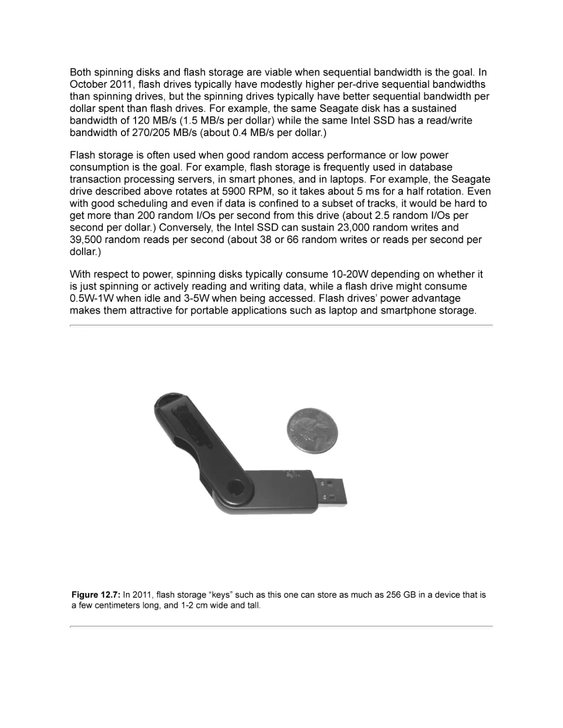
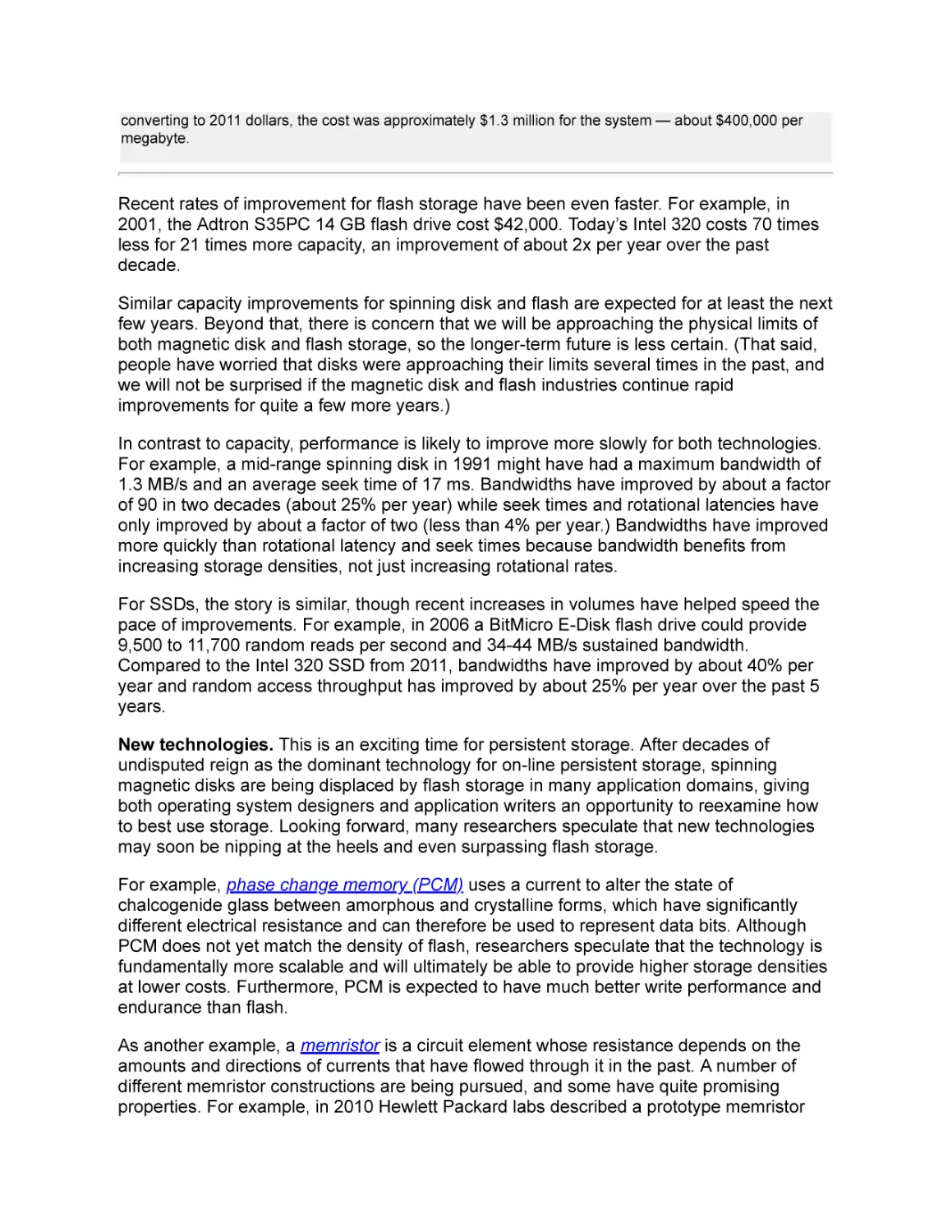
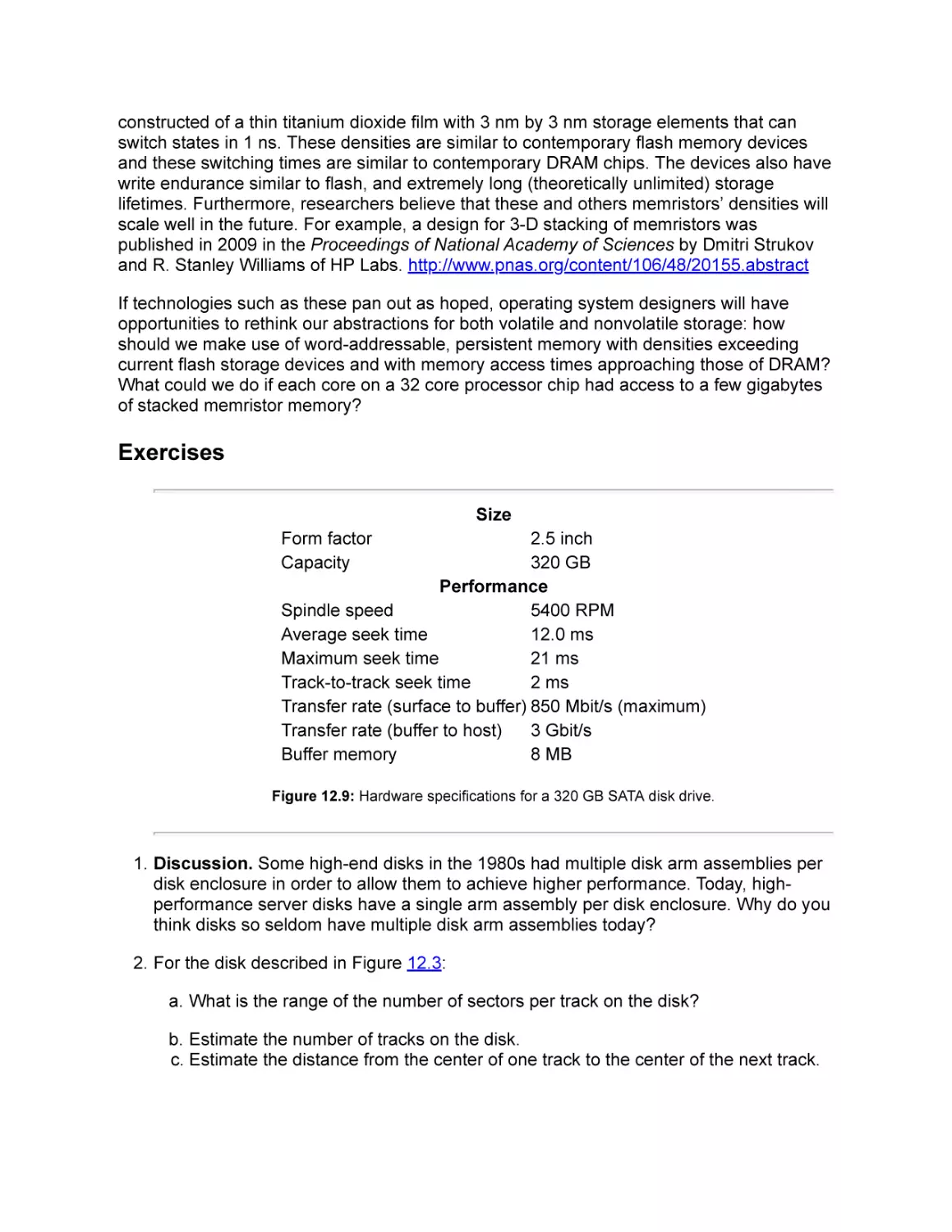
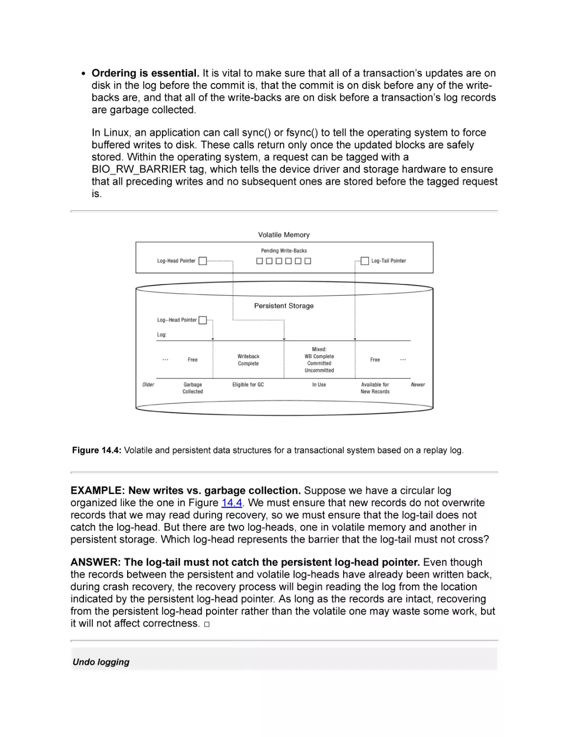
/


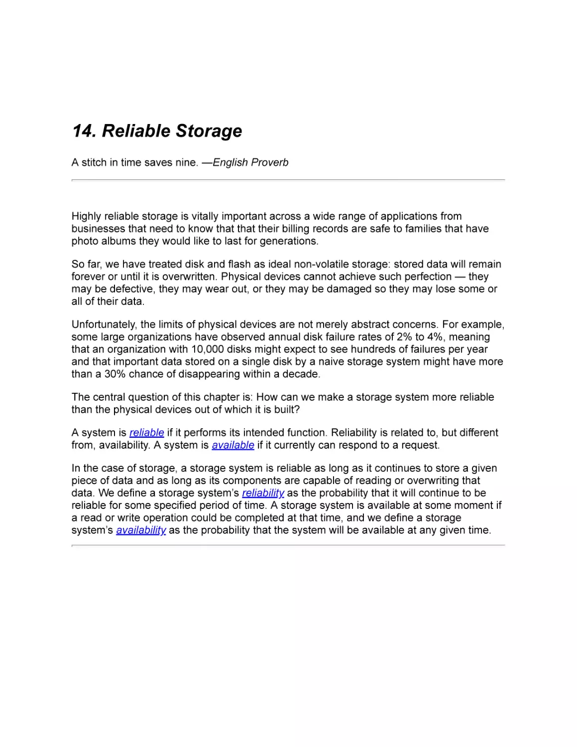


Text
Operating Systems
Principles & Practice
Volume IV: Persistent Storage
Second Edition
Thomas Anderson
University of Washington
Mike Dahlin
University of Texas and Google
Recursive Books
recursivebooks.com
Operating Systems: Principles and Practice (Second Edition) Volume IV: Persistent
Storage by Thomas Anderson and Michael Dahlin
Copyright ©Thomas Anderson and Michael Dahlin, 2011-2015.
ISBN 978-0-9856735-6-7
Publisher: Recursive Books, Ltd., http://recursivebooks.com/
Cover: Reflection Lake, Mt. Rainier
Cover design: Cameron Neat
Illustrations: Cameron Neat
Copy editors: Sandy Kaplan, Whitney Schmidt
Ebook design: Robin Briggs
Web design: Adam Anderson
SUGGESTIONS, COMMENTS, and ERRORS. We welcome suggestions, comments and
error reports, by email to suggestions@recursivebooks.com
Notice of rights. All rights reserved. No part of this book may be reproduced, stored in a
retrieval system, or transmitted in any form by any means — electronic, mechanical,
photocopying, recording, or otherwise — without the prior written permission of the
publisher. For information on getting permissions for reprints and excerpts, contact
permissions@recursivebooks.com
Notice of liability. The information in this book is distributed on an “As Is" basis, without
warranty. Neither the authors nor Recursive Books shall have any liability to any person or
entity with respect to any loss or damage caused or alleged to be caused directly or
indirectly by the information or instructions contained in this book or by the computer
software and hardware products described in it.
Trademarks: Throughout this book trademarked names are used. Rather than put a
trademark symbol in every occurrence of a trademarked name, we state we are using the
names only in an editorial fashion and to the benefit of the trademark owner with no
intention of infringement of the trademark. All trademarks or service marks are the property
of their respective owners.
To Robin, Sandra, Katya, and Adam
Tom Anderson
To Marla, Kelly, and Keith
Mike Dahlin
Contents
Preface
I: Kernels and Processes
1. Introduction
2. The Kernel Abstraction
3. The Programming Interface
II: Concurrency
4. Concurrency and Threads
5. Synchronizing Access to Shared Objects
6. Multi-Object Synchronization
7. Scheduling
III: Memory Management
8. Address Translation
9. Caching and Virtual Memory
10. Advanced Memory Management
IV Persistent Storage
11 File Systems: Introduction and Overview
11.1 The File System Abstraction
11.2 API
11.3 Software Layers
11.3.1 API and Performance
11.3.2 Device Drivers: Common Abstractions
11.3.3 Device Access
11.3.4 Putting It All Together: A Simple Disk Request
11.4 Summary and Future Directions
Exercises
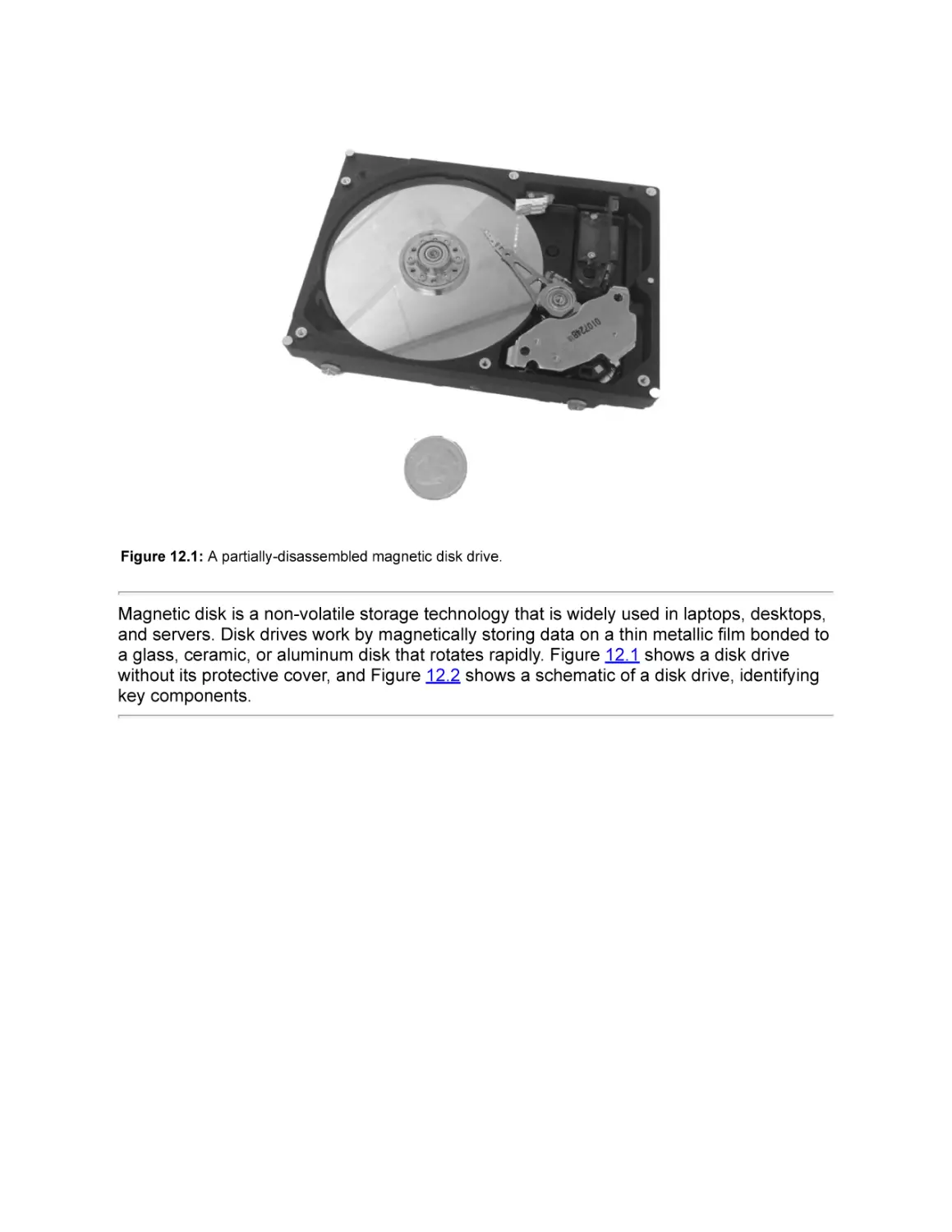
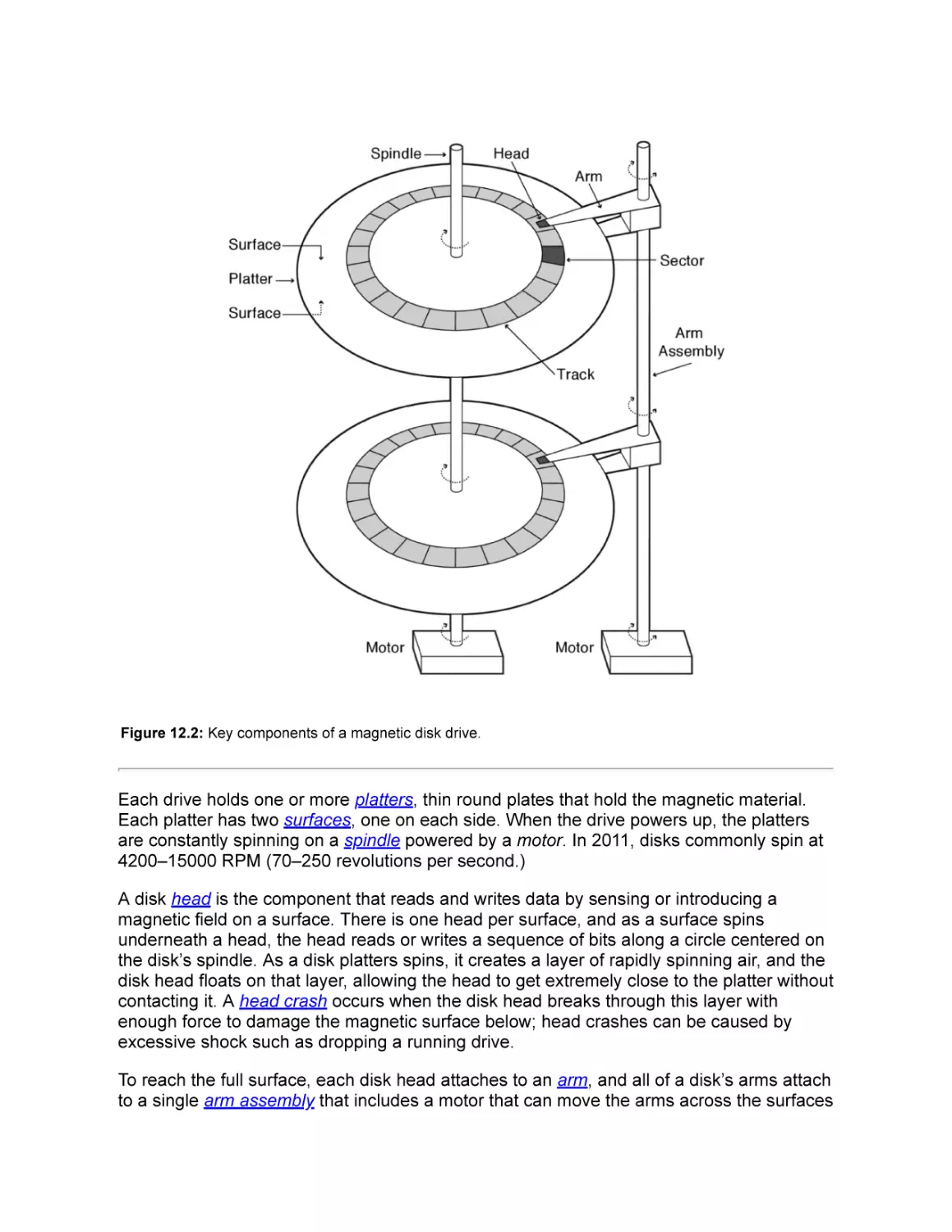
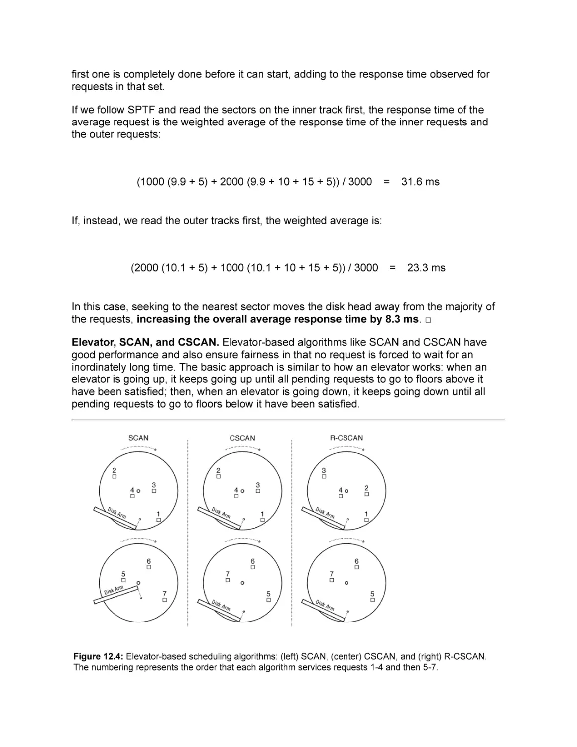
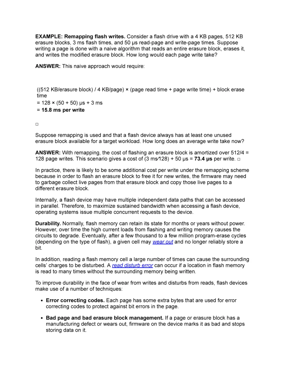
12 Storage Devices
12.1 Magnetic Disk
12.1.1 Disk Access and Performance
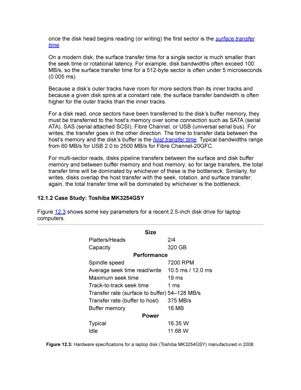
12.1.2 Case Study: Toshiba MK3254GSY
12.1.3 Disk Scheduling
12.2 Flash Storage
12.3 Summary and Future Directions
Exercises
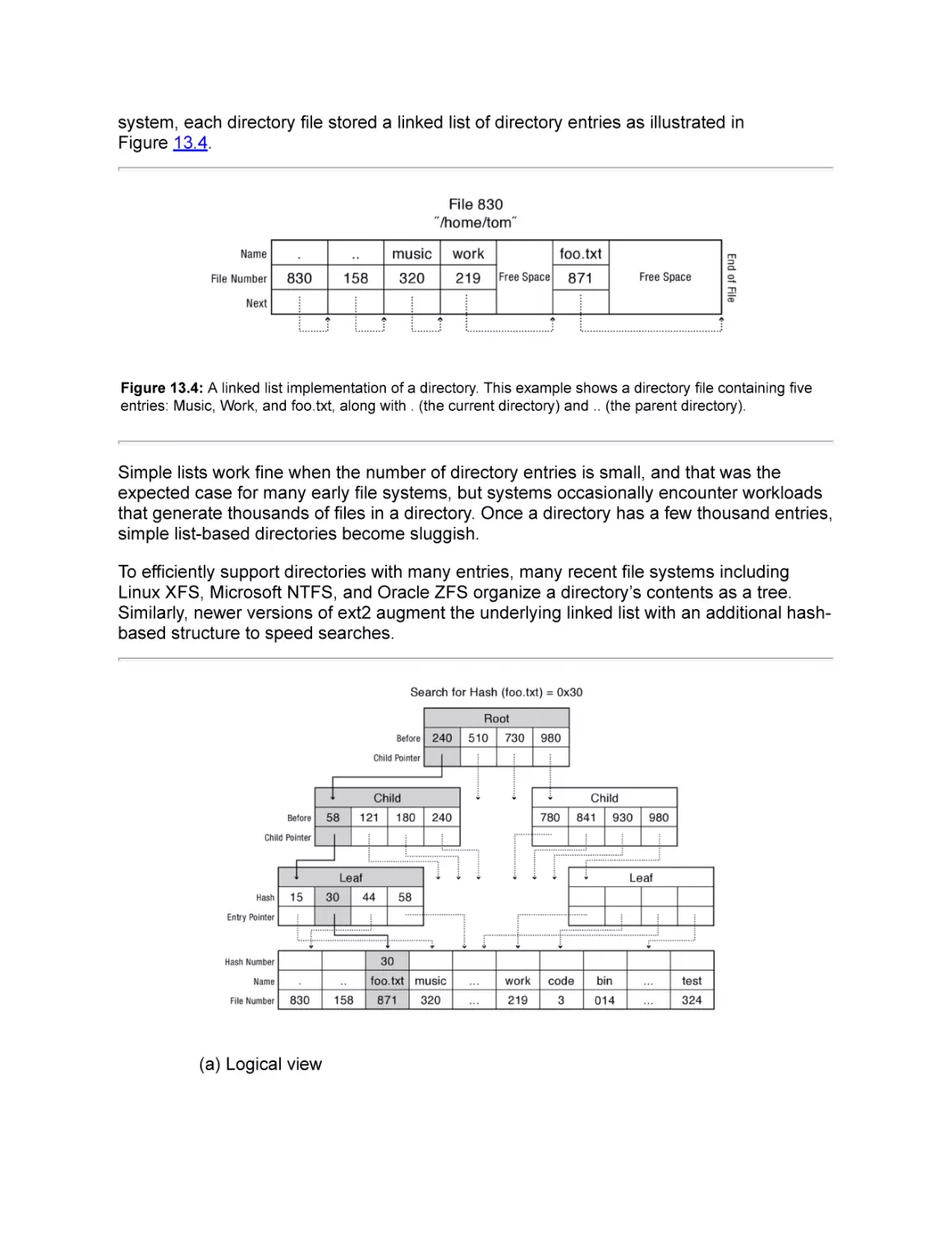
13 Files and Directories
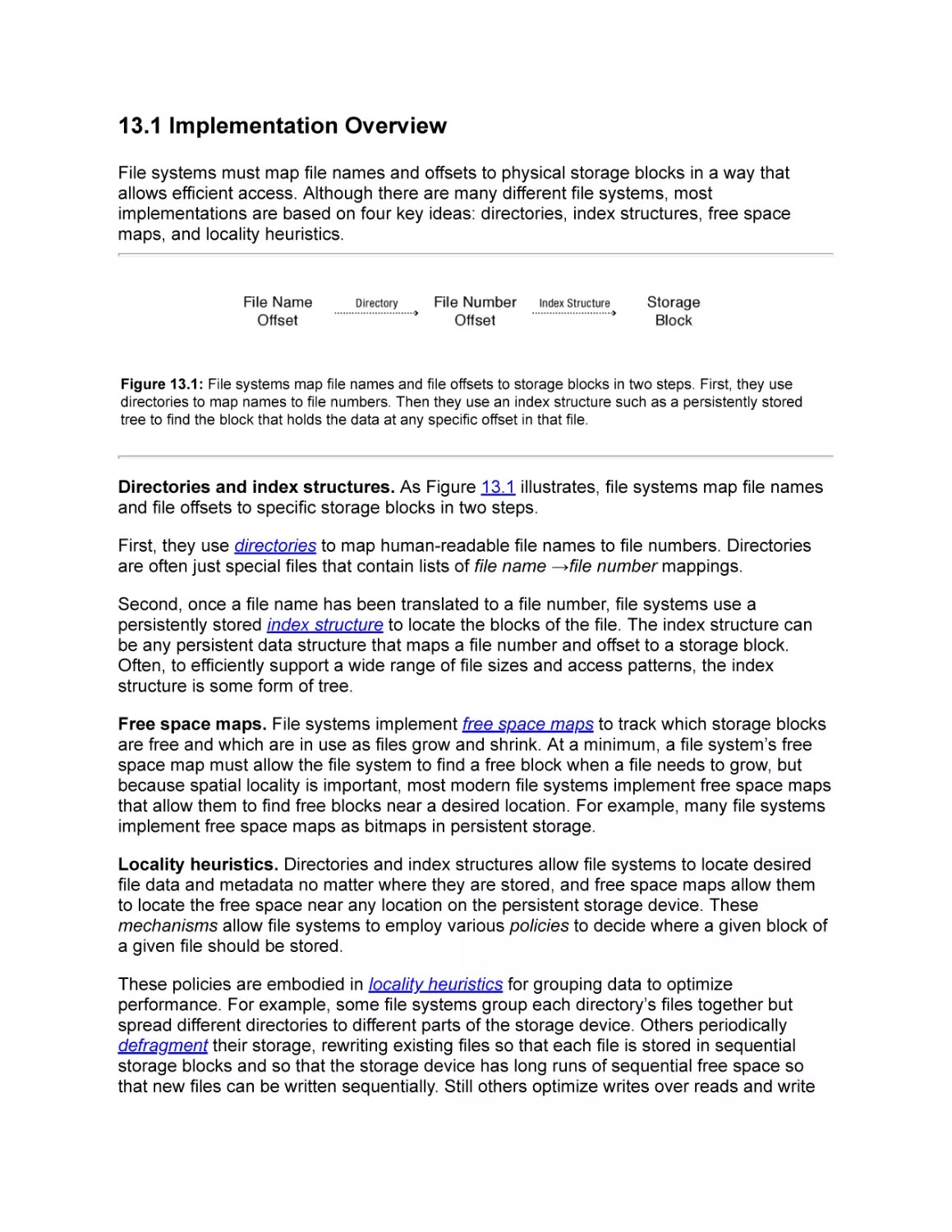
13.1 Implementation Overview
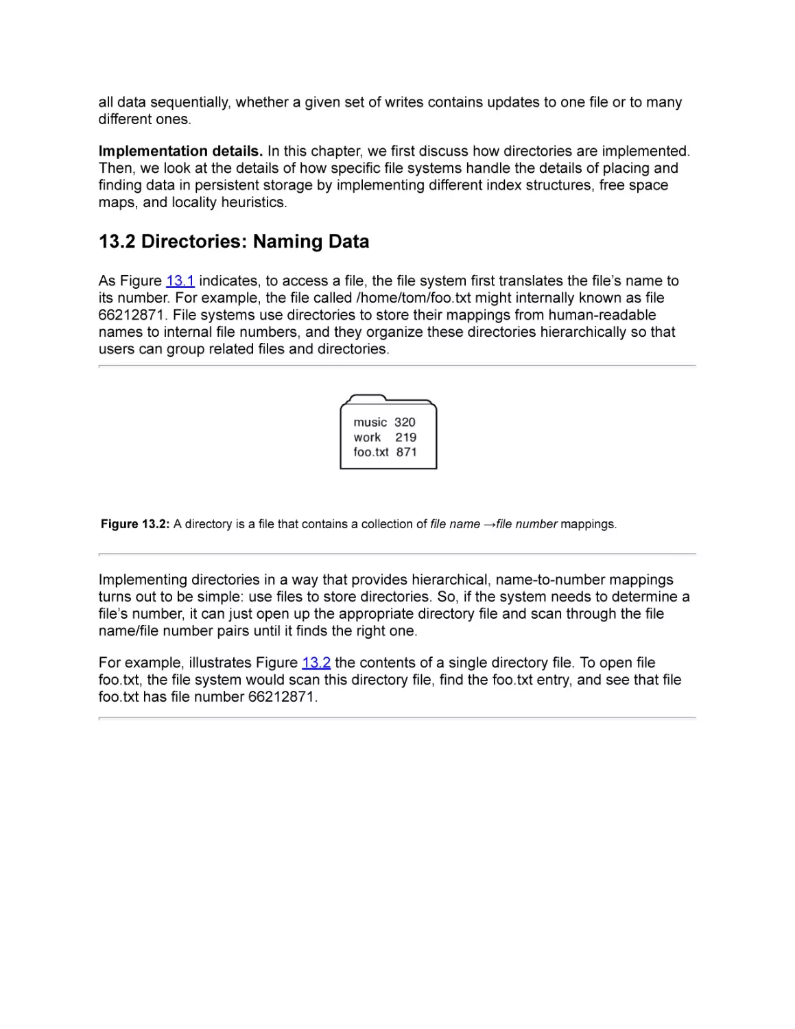
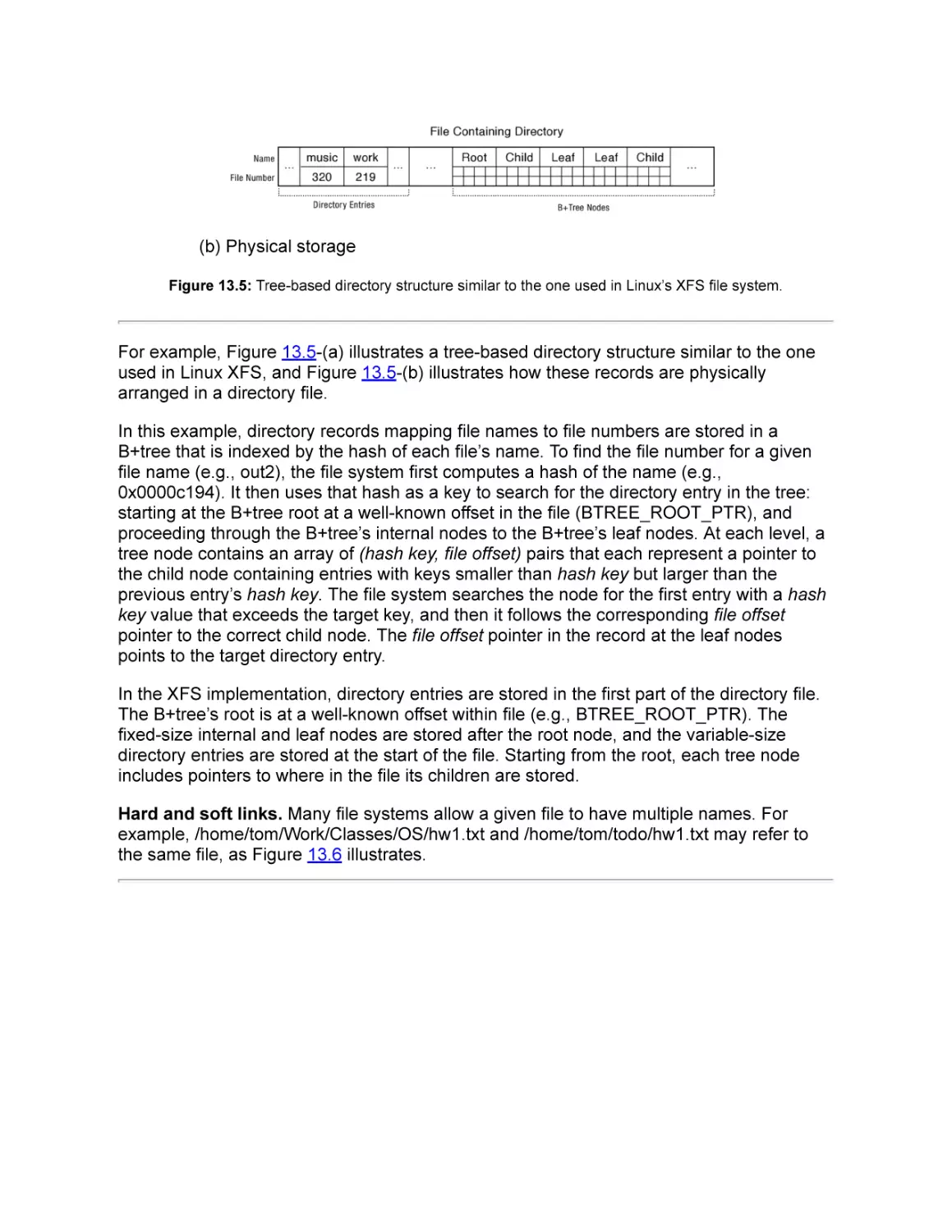
13.2 Directories: Naming Data
13.3 Files: Finding Data
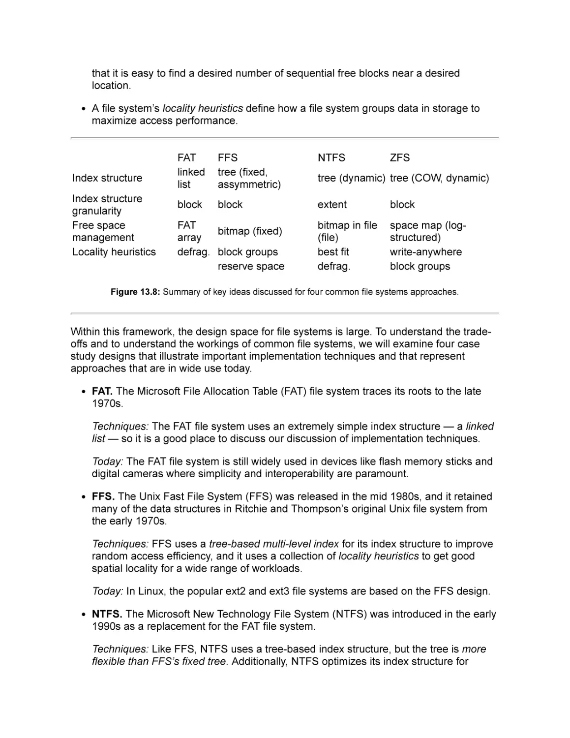
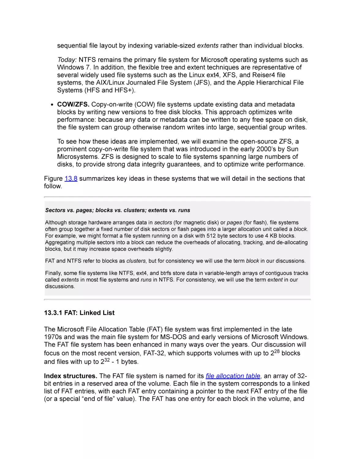
13.3.1 FAT: Linked List
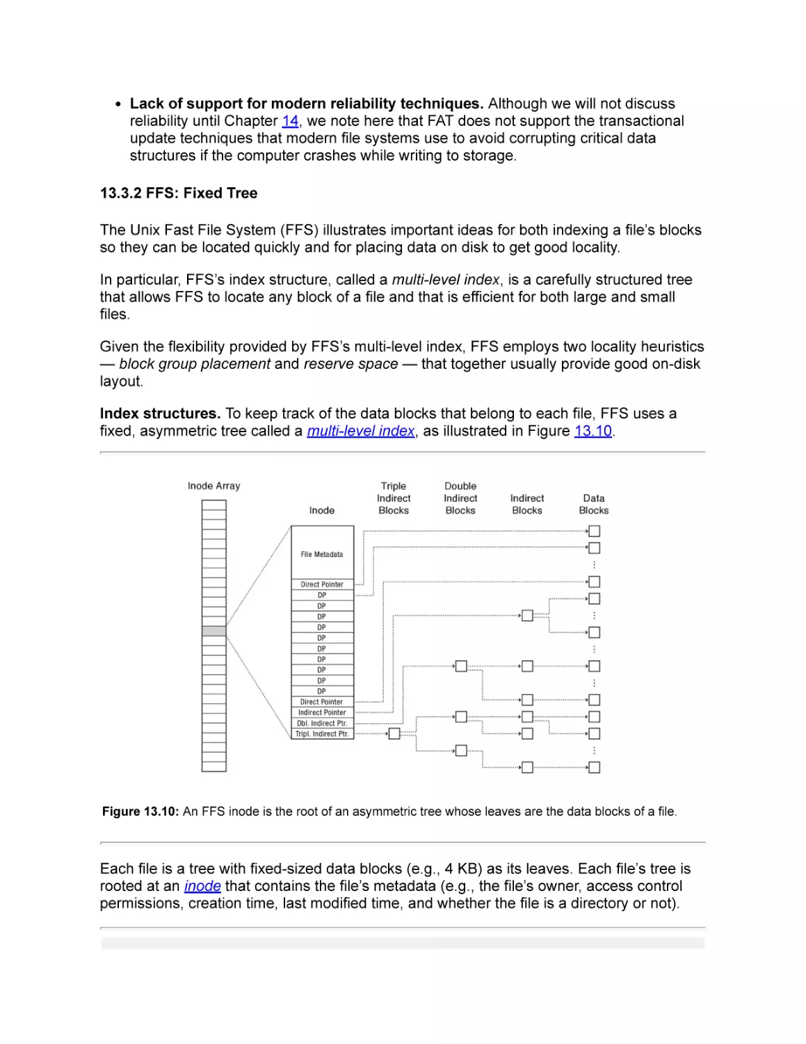
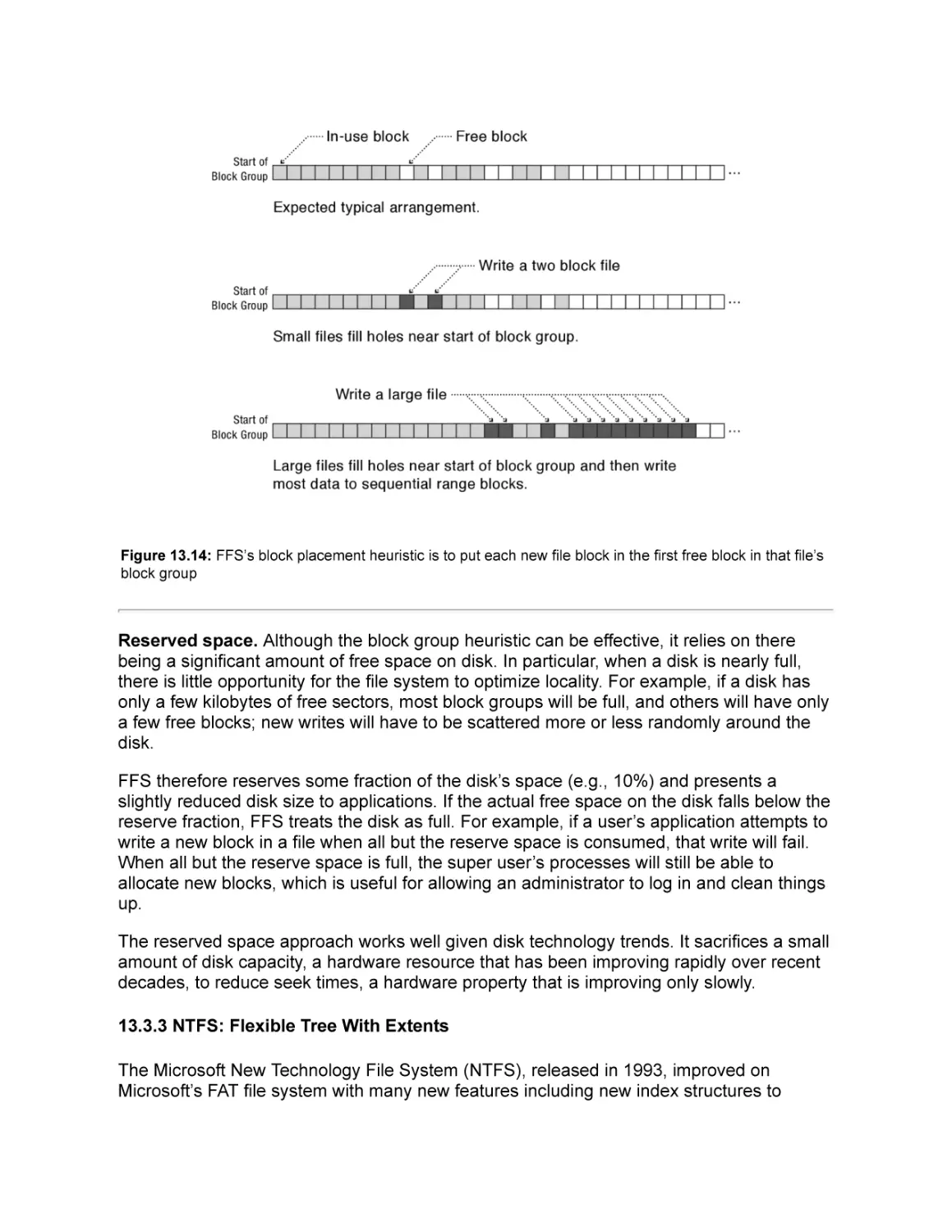
13.3.2 FFS: Fixed Tree
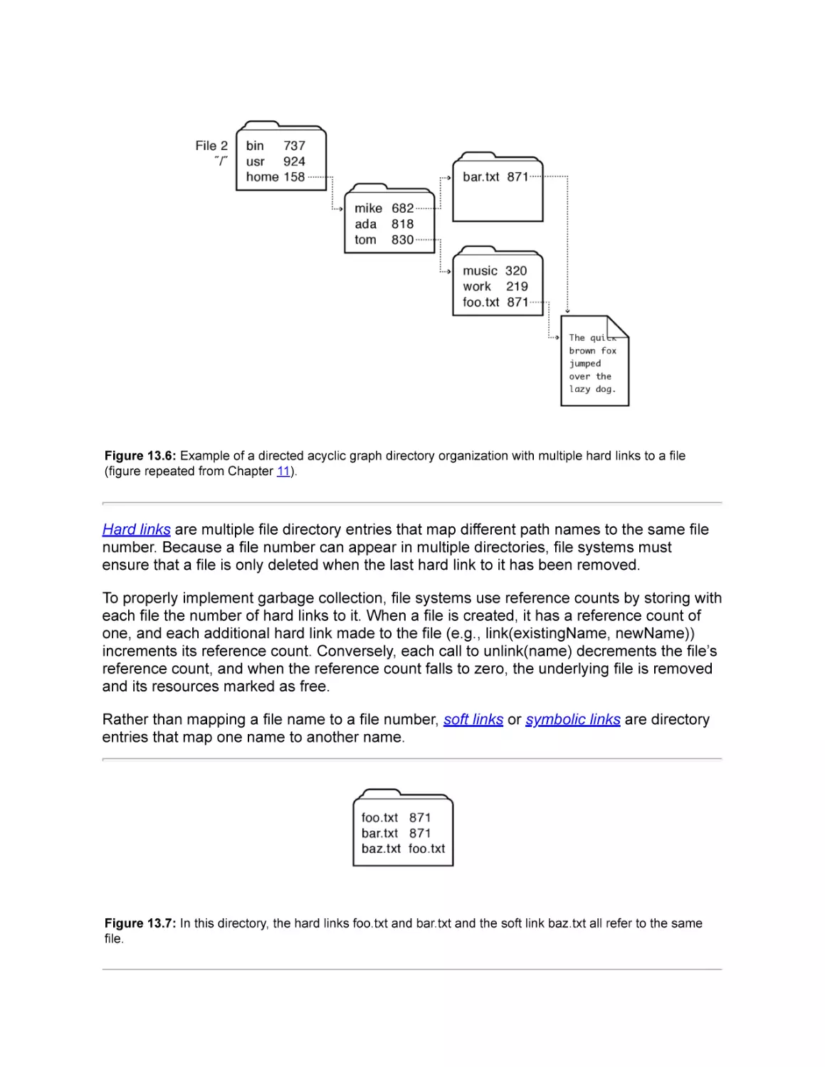
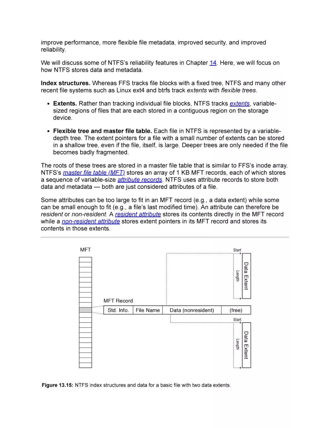
13.3.3 NTFS: Flexible Tree With Extents
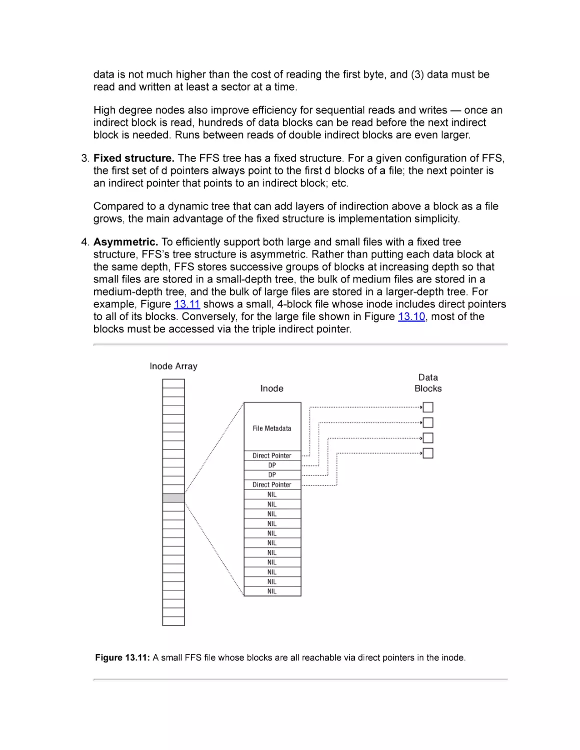
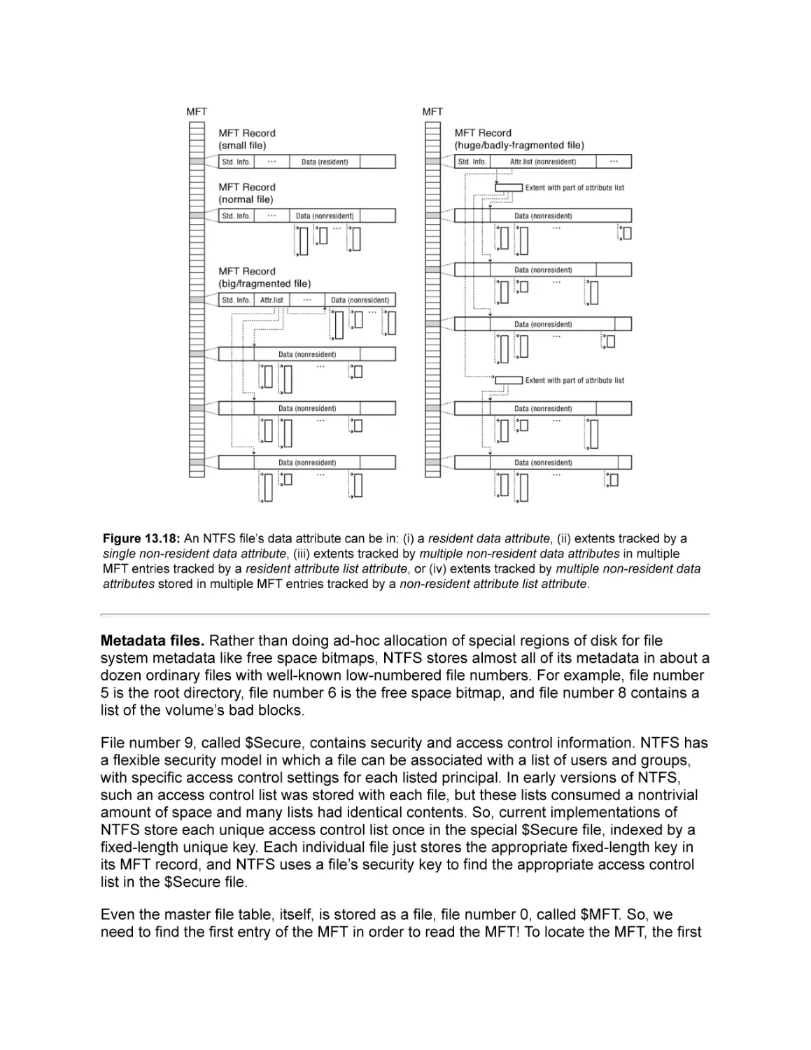
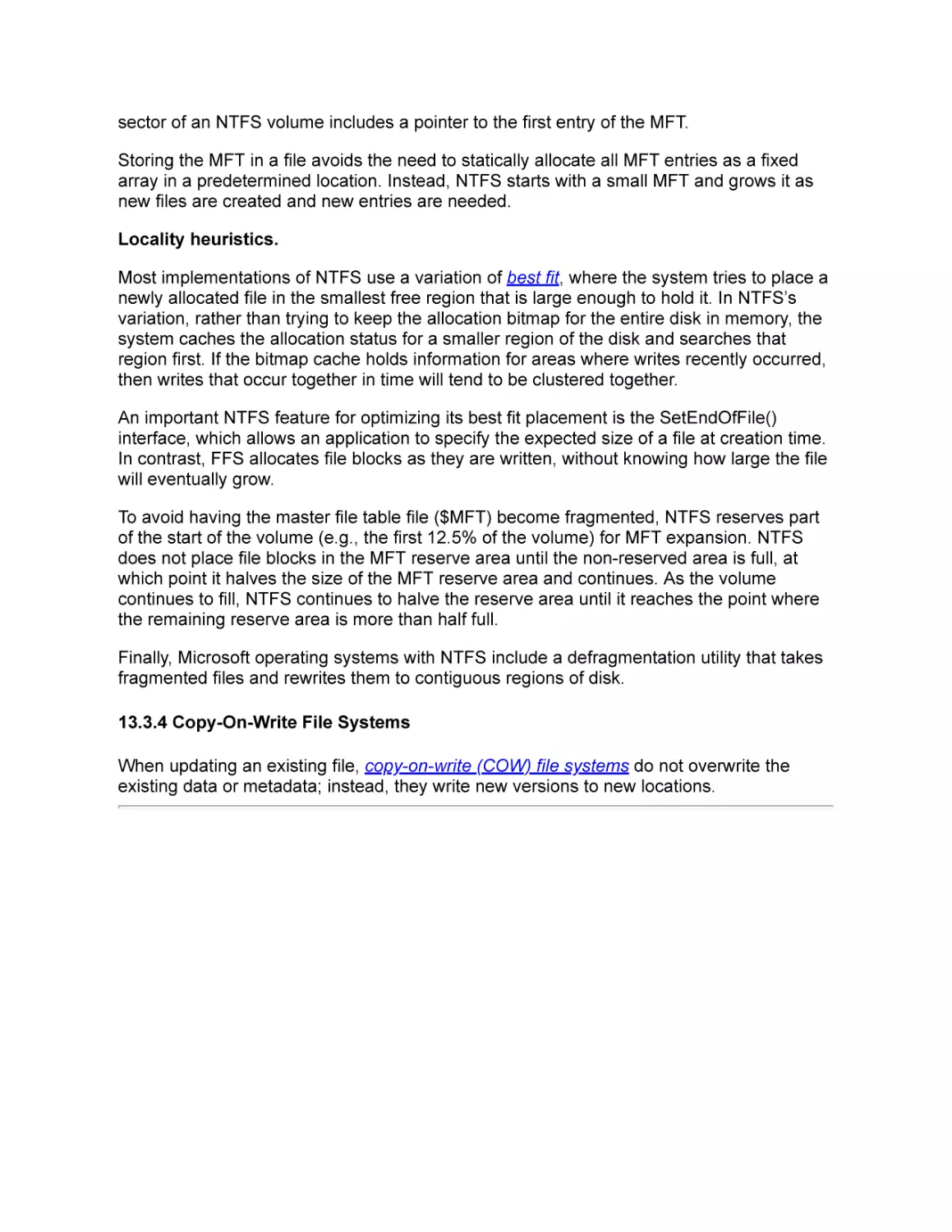
13.3.4 Copy-On-Write File Systems
13.4 Putting It All Together: File and Directory Access
13.5 Summary and Future Directions
Exercises
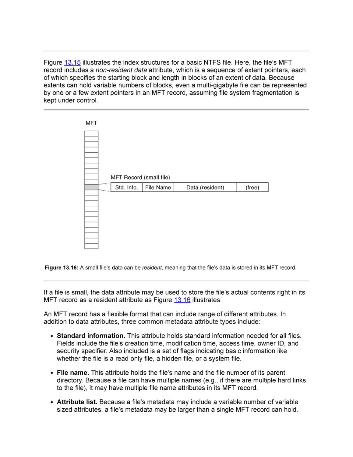
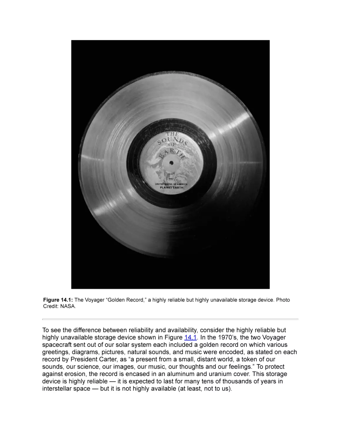
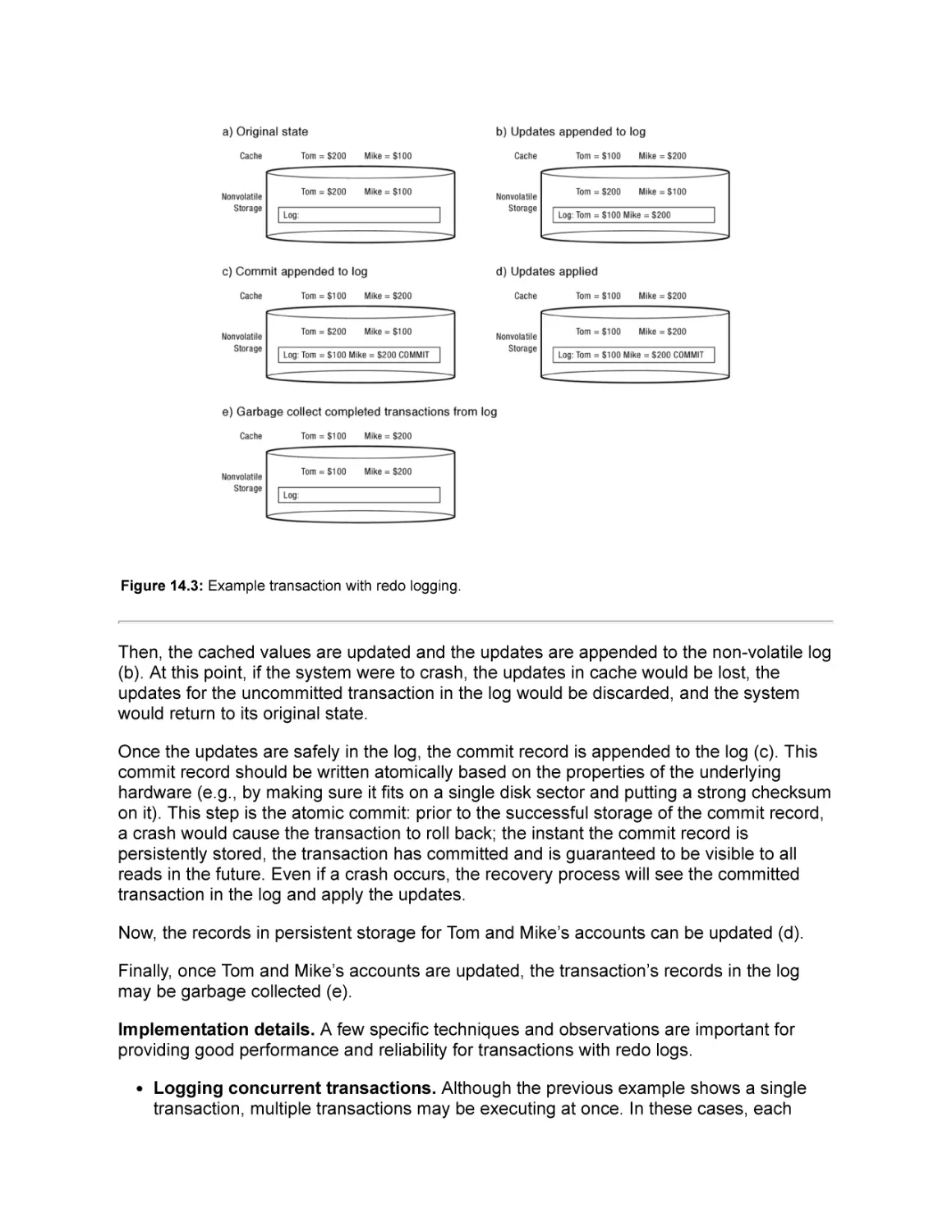
14 Reliable Storage
14.1 Transactions: Atomic Updates
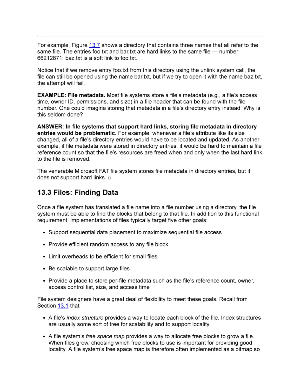
14.1.1 Ad Hoc Approaches
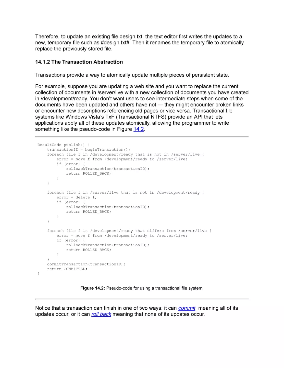
14.1.2 The Transaction Abstraction
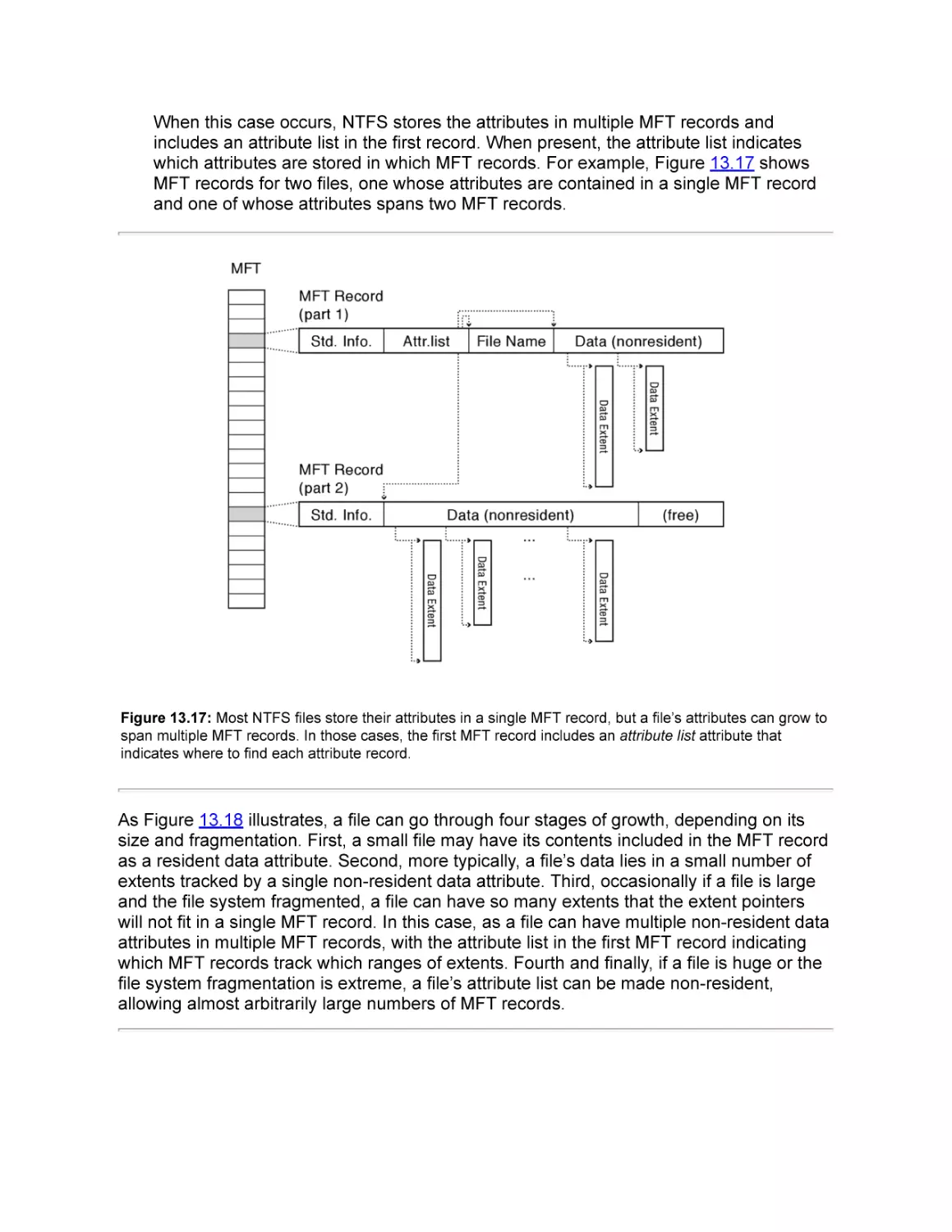
14.1.3 Implementing Transactions
14.1.4 Transactions and File Systems
14.2 Error Detection and Correction
14.2.1 Storage Device Failures and Mitigation
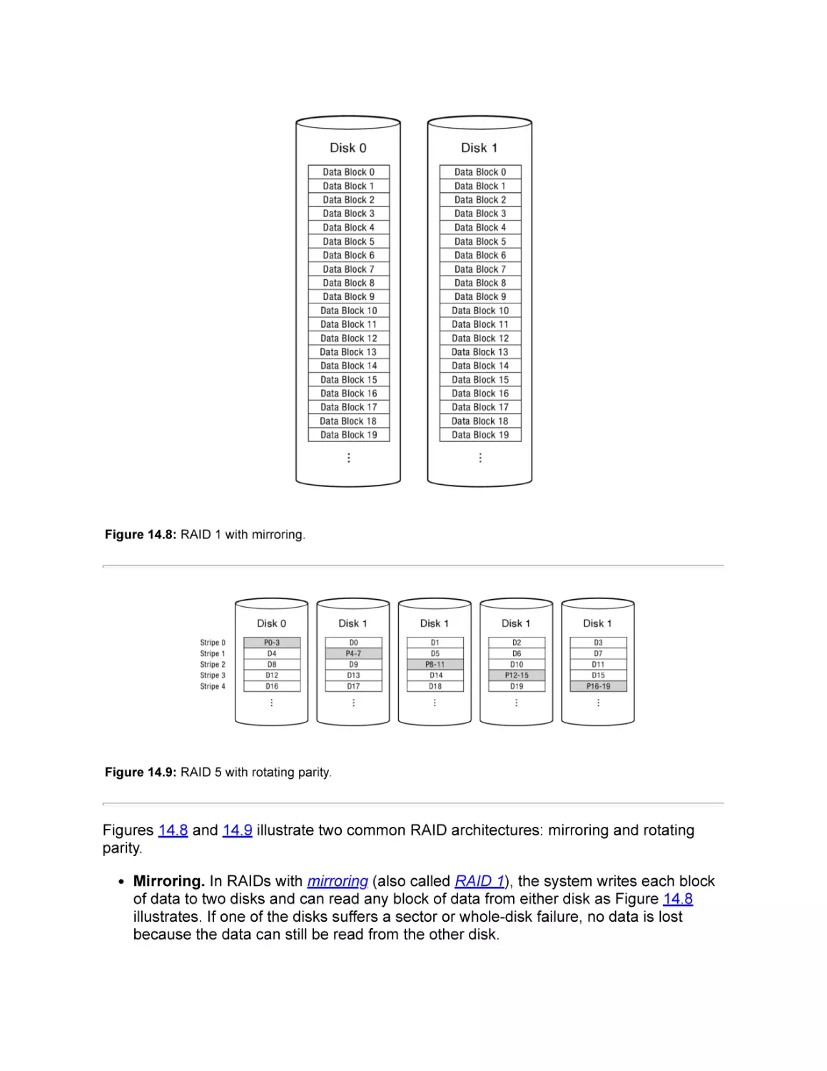
14.2.2 RAID: Multi-Disk Redundancy for Error Correction
14.2.3 Software Integrity Checks
14.3 Summary and Future Directions
Exercises
References
Glossary
About the Authors
Preface
Preface to the eBook Edition
Operating Systems: Principles and Practice is a textbook for a first course in
undergraduate operating systems. In use at over 50 colleges and universities worldwide,
this textbook provides:
A path for students to understand high level concepts all the way down to working
code.
Extensive worked examples integrated throughout the text provide students concrete
guidance for completing homework assignments.
A focus on up-to-date industry technologies and practice
The eBook edition is split into four volumes that together contain exactly the same material
as the (2nd) print edition of Operating Systems: Principles and Practice, reformatted for
various screen sizes. Each volume is self-contained and can be used as a standalone text,
e.g., at schools that teach operating systems topics across multiple courses.
Volume 1: Kernels and Processes. This volume contains Chapters 1-3 of the print
edition. We describe the essential steps needed to isolate programs to prevent buggy
applications and computer viruses from crashing or taking control of your system.
Volume 2: Concurrency. This volume contains Chapters 4-7 of the print edition. We
provide a concrete methodology for writing correct concurrent programs that is in
widespread use in industry, and we explain the mechanisms for context switching and
synchronization from fundamental concepts down to assembly code.
Volume 3: Memory Management. This volume contains Chapters 8-10 of the print
edition. We explain both the theory and mechanisms behind 64-bit address space
translation, demand paging, and virtual machines.
Volume 4: Persistent Storage. This volume contains Chapters 11-14 of the print
edition. We explain the technologies underlying modern extent-based, journaling, and
versioning file systems.
A more detailed description of each chapter is given in the preface to the print edition.
Preface to the Print Edition
Why We Wrote This Book
Many of our students tell us that operating systems was the best course they took as an
undergraduate and also the most important for their careers. We are not alone — many of
our colleagues report receiving similar feedback from their students.
Part of the excitement is that the core ideas in a modern operating system — protection,
concurrency, virtualization, resource allocation, and reliable storage — have become
widely applied throughout computer science, not just operating system kernels. Whether
you get a job at Facebook, Google, Microsoft, or any other leading-edge technology
company, it is impossible to build resilient, secure, and flexible computer systems without
the ability to apply operating systems concepts in a variety of settings. In a modern world,
nearly everything a user does is distributed, nearly every computer is multi-core, security
threats abound, and many applications such as web browsers have become mini-operating
systems in their own right.
It should be no surprise that for many computer science students, an undergraduate
operating systems class has become a de facto requirement: a ticket to an internship and
eventually to a full-time position.
Unfortunately, many operating systems textbooks are still stuck in the past, failing to keep
pace with rapid technological change. Several widely-used books were initially written in
the mid-1980’s, and they often act as if technology stopped at that point. Even when new
topics are added, they are treated as an afterthought, without pruning material that has
become less important. The result are textbooks that are very long, very expensive, and
yet fail to provide students more than a superficial understanding of the material.
Our view is that operating systems have changed dramatically over the past twenty years,
and that justifies a fresh look at both how the material is taught and what is taught. The
pace of innovation in operating systems has, if anything, increased over the past few
years, with the introduction of the iOS and Android operating systems for smartphones, the
shift to multicore computers, and the advent of cloud computing.
To prepare students for this new world, we believe students need three things to succeed
at understanding operating systems at a deep level:
Concepts and code. We believe it is important to teach students both principles and
practice, concepts and implementation, rather than either alone. This textbook takes
concepts all the way down to the level of working code, e.g., how a context switch
works in assembly code. In our experience, this is the only way students will really
understand and master the material. All of the code in this book is available from the
author’s web site, ospp.washington.edu.
Extensive worked examples. In our view, students need to be able to apply concepts
in practice. To that end, we have integrated a large number of example exercises,
along with solutions, throughout the text. We uses these exercises extensively in our
own lectures, and we have found them essential to challenging students to go beyond
a superficial understanding.
Industry practice. To show students how to apply operating systems concepts in a
variety of settings, we use detailed, concrete examples from Facebook, Google,
Microsoft, Apple, and other leading-edge technology companies throughout the
textbook. Because operating systems concepts are important in a wide range of
computer systems, we take these examples not only from traditional operating
systems like Linux, Windows, and OS X but also from other systems that need to
solve problems of protection, concurrency, virtualization, resource allocation, and
reliable storage like databases, web browsers, web servers, mobile applications, and
search engines.
Taking a fresh perspective on what students need to know to apply operating systems
concepts in practice has led us to innovate in every major topic covered in an
undergraduate-level course:
Kernels and Processes. The safe execution of untrusted code has become central to
many types of computer systems, from web browsers to virtual machines to operating
systems. Yet existing textbooks treat protection as a side effect of UNIX processes, as
if they are synonyms. Instead, we start from first principles: what are the minimum
requirements for process isolation, how can systems implement process isolation
efficiently, and what do students need to know to implement functions correctly when
the caller is potentially malicious?
Concurrency. With the advent of multi-core architectures, most students today will
spend much of their careers writing concurrent code. Existing textbooks provide a
blizzard of concurrency alternatives, most of which were abandoned decades ago as
impractical. Instead, we focus on providing students a single methodology based on
Mesa monitors that will enable students to write correct concurrent programs — a
methodology that is by far the dominant approach used in industry.
Memory Management. Even as demand-paging has become less important,
virtualization has become even more important to modern computer systems. We
provide a deep treatment of address translation hardware, sparse address spaces,
TLBs, and on-chip caches. We then use those concepts as a springboard for
describing virtual machines and related concepts such as checkpointing and copy-onwrite.
Persistent Storage. Reliable storage in the presence of failures is central to the
design of most computer systems. Existing textbooks survey the history of file
systems, spending most of their time ad hoc approaches to failure recovery and defragmentation. Yet no modern file systems still use those ad hoc approaches. Instead,
our focus is on how file systems use extents, journaling, copy-on-write, and RAID to
achieve both high performance and high reliability.
Intended Audience
Operating Systems: Principles and Practice is a textbook for a first course in
undergraduate operating systems. We believe operating systems should be taken as early
as possible in an undergraduate’s course of study; many students use the course as a
springboard to an internship and a career. To that end, we have designed the textbook to
assume minimal pre-requisites: specifically, students should have taken a data structures
course and one on computer organization. The code examples are written in a combination
of x86 assembly, C, and C++. In particular, we have designed the book to interface well
with the Bryant and O’Halloran textbook. We review and cover in much more depth the
material from the second half of that book.
We should note what this textbook is not: it is not intended to teach the API or internals of
any specific operating system, such as Linux, Android, Windows 8, OS X, or iOS. We use
many concrete examples from these systems, but our focus is on the shared problems
these systems face and the technologies these systems use to solve those problems.
A Guide to Instructors
One of our goals is enable instructors to choose an appropriate level of depth for each
course topic. Each chapter begins at a conceptual level, with implementation details and
the more advanced material towards the end. The more advanced material can be omitted
without compromising the ability of students to follow later material. No single-quarter or
single-semester course is likely to be able to cover every topic we have included, but we
think it is a good thing for students to come away from an operating systems course with
an appreciation that there is always more to learn.
For each topic, we attempt to convey it at three levels:
How to reason about systems. We describe core systems concepts, such as
protection, concurrency, resource scheduling, virtualization, and storage, and we
provide practice applying these concepts in various situations. In our view, this
provides the biggest long-term payoff to students, as they are likely to need to apply
these concepts in their work throughout their career, almost regardless of what project
they end up working on.
Power tools. We introduce students to a number of abstractions that they can apply in
their work in industry immediately after graduation, and that we expect will continue to
be useful for decades such as sandboxing, protected procedure calls, threads, locks,
condition variables, caching, checkpointing, and transactions.
Details of specific operating systems. We include numerous examples of how
different operating systems work in practice. However, this material changes rapidly,
and there is an order of magnitude more material than can be covered in a single
semester-length course. The purpose of these examples is to illustrate how to use the
operating systems principles and power tools to solve concrete problems. We do not
attempt to provide a comprehensive description of Linux, OS X, or any other particular
operating system.
The book is divided into five parts: an introduction (Chapter 1), kernels and processes
(Chapters 2-3), concurrency, synchronization, and scheduling (Chapters 4-7), memory
management (Chapters 8-10), and persistent storage (Chapters 11-14).
Introduction. The goal of Chapter 1 is to introduce the recurring themes found in the
later chapters. We define some common terms, and we provide a bit of the history of
the development of operating systems.
The Kernel Abstraction. Chapter 2 covers kernel-based process protection — the
concept and implementation of executing a user program with restricted privileges.
Given the increasing importance of computer security issues, we believe protected
execution and safe transfer across privilege levels are worth treating in depth. We
have broken the description into sections, to allow instructors to choose either a quick
introduction to the concepts (up through Section 2.3), or a full treatment of the kernel
implementation details down to the level of interrupt handlers. Some instructors start
with concurrency, and cover kernels and kernel protection afterwards. While our
textbook can be used that way, we have found that students benefit from a basic
understanding of the role of operating systems in executing user programs, before
introducing concurrency.
The Programming Interface. Chapter 3 is intended as an impedance match for
students of differing backgrounds. Depending on student background, it can be
skipped or covered in depth. The chapter covers the operating system from a
programmer’s perspective: process creation and management, device-independent
input/output, interprocess communication, and network sockets. Our goal is that
students should understand at a detailed level what happens when a user clicks a link
in a web browser, as the request is transferred through operating system kernels and
user space processes at the client, server, and back again. This chapter also covers
the organization of the operating system itself: how device drivers and the hardware
abstraction layer work in a modern operating system; the difference between a
monolithic and a microkernel operating system; and how policy and mechanism are
separated in modern operating systems.
Concurrency and Threads. Chapter 4 motivates and explains the concept of threads.
Because of the increasing importance of concurrent programming, and its integration
with modern programming languages like Java, many students have been introduced
to multi-threaded programming in an earlier class. This is a bit dangerous, as students
at this stage are prone to writing programs with race conditions, problems that may or
may not be discovered with testing. Thus, the goal of this chapter is to provide a solid
conceptual framework for understanding the semantics of concurrency, as well as how
concurrent threads are implemented in both the operating system kernel and in userlevel libraries. Instructors needing to go more quickly can omit these implementation
details.
Synchronization. Chapter 5 discusses the synchronization of multi-threaded
programs, a central part of all operating systems and increasingly important in many
other contexts. Our approach is to describe one effective method for structuring
concurrent programs (based on Mesa monitors), rather than to attempt to cover
several different approaches. In our view, it is more important for students to master
one methodology. Monitors are a particularly robust and simple one, capable of
implementing most concurrent programs efficiently. The implementation of
synchronization primitives should be included if there is time, so students see that
there is no magic.
Multi-Object Synchronization. Chapter 6 discusses advanced topics in concurrency
— specifically, the twin challenges of multiprocessor lock contention and deadlock.
This material is increasingly important for students working on multicore systems, but
some courses may not have time to cover it in detail.
Scheduling. This chapter covers the concepts of resource allocation in the specific
context of processor scheduling. With the advent of data center computing and
multicore architectures, the principles and practice of resource allocation have
renewed importance. After a quick tour through the tradeoffs between response time
and throughput for uniprocessor scheduling, the chapter covers a set of more
advanced topics in affinity and multiprocessor scheduling, power-aware and deadline
scheduling, as well as basic queueing theory and overload management. We conclude
these topics by walking students through a case study of server-side load
management.
Address Translation. Chapter 8 explains mechanisms for hardware and software
address translation. The first part of the chapter covers how hardware and operating
systems cooperate to provide flexible, sparse address spaces through multi-level
segmentation and paging. We then describe how to make memory management
efficient with translation lookaside buffers (TLBs) and virtually addressed caches. We
consider how to keep TLBs consistent when the operating system makes changes to
its page tables. We conclude with a discussion of modern software-based protection
mechanisms such as those found in the Microsoft Common Language Runtime and
Google’s Native Client.
Caching and Virtual Memory. Caches are central to many different types of computer
systems. Most students will have seen the concept of a cache in an earlier class on
machine structures. Thus, our goal is to cover the theory and implementation of
caches: when they work and when they do not, as well as how they are implemented
in hardware and software. We then show how these ideas are applied in the context of
memory-mapped files and demand-paged virtual memory.
Advanced Memory Management. Address translation is a powerful tool in system
design, and we show how it can be used for zero copy I/O, virtual machines, process
checkpointing, and recoverable virtual memory. As this is more advanced material, it
can be skipped by those classes pressed for time.
File Systems: Introduction and Overview. Chapter 11 frames the file system portion
of the book, starting top down with the challenges of providing a useful file abstraction
to users. We then discuss the UNIX file system interface, the major internal elements
inside a file system, and how disk device drivers are structured.
Storage Devices. Chapter 12 surveys block storage hardware, specifically magnetic
disks and flash memory. The last two decades have seen rapid change in storage
technology affecting both application programmers and operating systems designers;
this chapter provides a snapshot for students, as a building block for the next two
chapters. If students have previously seen this material, this chapter can be skipped.
Files and Directories. Chapter 13 discusses file system layout on disk. Rather than
survey all possible file layouts — something that changes rapidly over time — we use
file systems as a concrete example of mapping complex data structures onto block
storage devices.
Reliable Storage. Chapter 14 explains the concept and implementation of reliable
storage, using file systems as a concrete example. Starting with the ad hoc techniques
used in early file systems, the chapter explains checkpointing and write ahead logging
as alternate implementation strategies for building reliable storage, and it discusses
how redundancy such as checksums and replication are used to improve reliability
and availability.
We welcome and encourage suggestions for how to improve the presentation of the
material; please send any comments to the publisher’s website,
suggestions@recursivebooks.com.
Acknowledgements
We have been incredibly fortunate to have the help of a large number of people in the
conception, writing, editing, and production of this book.
We started on the journey of writing this book over dinner at the USENIX NSDI conference
in 2010. At the time, we thought perhaps it would take us the summer to complete the first
version and perhaps a year before we could declare ourselves done. We were very wrong!
It is no exaggeration to say that it would have taken us a lot longer without the help we
have received from the people we mention below.
Perhaps most important have been our early adopters, who have given us enormously
useful feedback as we have put together this edition:
Carnegie-Mellon
David Eckhardt and Garth Gibson
Clarkson
Jeanna Matthews
Cornell
Gun Sirer
ETH Zurich
Mothy Roscoe
New York University
Laskshmi Subramanian
Princeton University
Kai Li
Saarland University
Peter Druschel
Stanford University
John Ousterhout
University of California Riverside
Harsha Madhyastha
University of California Santa Barbara Ben Zhao
University of Maryland
Neil Spring
University of Michigan
Pete Chen
University of Southern California
Ramesh Govindan
University of Texas-Austin
Lorenzo Alvisi
Universtiy of Toronto
Ding Yuan
University of Washington
Gary Kimura and Ed Lazowska
In developing our approach to teaching operating systems, both before we started writing
and afterwards as we tried to put our thoughts to paper, we made extensive use of lecture
notes and slides developed by other faculty. Of particular help were the materials created
by Pete Chen, Peter Druschel, Steve Gribble, Eddie Kohler, John Ousterhout, Mothy
Roscoe, and Geoff Voelker. We thank them all.
Our illustrator for the second edition, Cameron Neat, has been a joy to work with. We
would also like to thank Simon Peter for running the multiprocessor experiments
introducing Chapter 6.
We are also grateful to Lorenzo Alvisi, Adam Anderson, Pete Chen, Steve Gribble, Sam
Hopkins, Ed Lazowska, Harsha Madhyastha, John Ousterhout, Mark Rich, Mothy Roscoe,
Will Scott, Gun Sirer, Ion Stoica, Lakshmi Subramanian, and John Zahorjan for their helpful
comments and suggestions as to how to improve the book.
We thank Josh Berlin, Marla Dahlin, Rasit Eskicioglu, Sandy Kaplan, John Ousterhout,
Whitney Schmidt, and Mike Walfish for helping us identify and correct grammatical or
technical bugs in the text.
We thank Jeff Dean, Garth Gibson, Mark Oskin, Simon Peter, Dave Probert, Amin Vahdat,
and Mark Zbikowski for their help in explaining the internal workings of some of the
commercial systems mentioned in this book.
We would like to thank Dave Wetherall, Dan Weld, Mike Walfish, Dave Patterson, Olav
Kvern, Dan Halperin, Armando Fox, Robin Briggs, Katya Anderson, Sandra Anderson,
Lorenzo Alvisi, and William Adams for their help and advice on textbook economics and
production.
The Helen Riaboff Whiteley Center as well as Don and Jeanne Dahlin were kind enough to
lend us a place to escape when we needed to get chapters written.
Finally, we thank our families, our colleagues, and our students for supporting us in this
larger-than-expected effort.
IV
Persistent Storage
11. File Systems: Introduction and Overview
Memory is the treasury and guardian of all things. —Marcus Tullius Cicero
Computers must be able to reliably store data. Individuals store family photos, music files,
and email folders; programmers store design documents and source files; office workers
store spreadsheets, text documents, and presentation slides; and businesses store
inventory, orders, and billing records. In fact, for a computer to work at all, it needs to be
able to store programs to run and the operating system, itself.
For all of these cases, users demand a lot from their storage systems:
Reliability. A user’s data should be safely stored even if a machine’s power is turned
off or its operating system crashes. In fact, much of this data is so important that users
expect and need the data to survive even if the devices used to store it are damaged.
For example, many modern storage systems continue to work even if one of the
magnetic disks storing the data malfunctions or even if a data center housing some of
the system’s servers burns down!
Large capacity and low cost. Users and companies store enormous amount of data,
so they want to be able to buy high capacity storage for a low cost. For example, it
takes about 350 MB to store an hour of CD-quality losslessly encoded music, 4 GB to
store an hour-long high-definition home video, and about 1 GB to store 300 digital
photos. As a result of these needs, many individuals own 1 TB or more of storage for
their personal files. This is an enormous amount: if you printed 1 TB of data as text on
paper, you would produce a stack about 20 miles high. In contrast, for less than $100
you can buy 1 TB of storage that fits in a shoebox.
High performance. For programs to use data, they must be able to access it, and for
programs to use large amounts of data, this access must be fast. For example, users
want program start-up to be nearly instantaneous, a business may need to process
hundreds or thousands of orders per second, or a server may need to stream a large
number of video files to different users.
Named data. Because users store a large amount of data, because some data must
last longer than the process that creates it, and because data must be shared across
programs, storage systems must provide ways to easily identify data of interest. For
example, if you can name a file (e.g., /home/alice/assignments/hw1.txt) you can find
the data you want out of the millions of blocks on your disk, you can still find it after
you shut down your text editor, and you can use your email program to send the data
produced by the text editor to another user.
Controlled sharing. Users need to be able to share stored data, but this sharing
needs to be controlled. As one example, you may want to create a design document
that everyone in your group can read and write, that people in your department can
read but not write, and that people outside of your department cannot access at all. As
another example, it is useful for a system to be able to allow anyone to execute a
program while only allowing the system administrator to change the program.
Nonvolatile storage and file systems. The contents of a system’s main DRAM memory
can be lost if there is an operating system crash or power failure. In contrast, non-volatile
storage is durable and retains its state across crashes and power outages; non-volatile
storage is also called or persistent storage or stable storage. Nonvolatile storage can also
have much higher capacity and lower cost than the volatile DRAM that forms the bulk of
most system’s “main memory.”
However, non-volatile storage technologies have their own limitations. For example,
current non-volatile storage technologies such as magnetic disks and high-density flash
storage do not allow random access to individual words of storage; instead, access must
be done in more coarse-grained units — 512, 2048, or more bytes at a time.
Furthermore, these accesses can be much slower than access to DRAM; for example,
reading a sector from a magnetic disk may require activating a motor to move a disk arm to
a desired track on disk and then waiting for the spinning disk to bring the desired data
under the disk head. Because disk accesses involve motors and physical motion, the time
to access a random sector on a disk can be around 10 milliseconds. In contrast, DRAM
latencies are typically under 100 nanoseconds. This large difference — about five orders of
magnitude in the case of spinning disks — drives the operating system to organize and use
persistent storage devices differently than main memory.
File systems are a common operating system abstraction to allow applications to access
non-volatile storage. File systems use a number of techniques to cope with the physical
limitations of non-volatile storage devices and to provide better abstractions to users. For
example, Figure 11.1 summarizes how physical characteristics motivate several key
aspects of file system design.
Goal
Physical Characteristic Design Implication
Organize data placement with files, directories,
High
Large cost to initiate IO
free space bitmap, and placement heuristics so
performance access
that storage is accessed in large sequential units
Caching to avoid accessing persistent storage
Storage has large
capacity, survives
Named data
crashes, and is shared
across programs
Support files and directories with meaningful
names
Controlled
sharing
Device stores many users’
Include access-control metadata with files
data
Reliable
storage
Crash can occur during
update
Use transactions to make a set of updates atomic
Storage devices can fail
Flash memory cells can
wear out
Use redundancy to detect and correct failures
Move data to different storage locations to even
the wear
Figure 11.1: Characteristics of persistent storage devices affect the design of an operating system’s storage
abstractions.
Performance. File systems amortize the cost of initiating expensive operations —
such as moving a disk arm or erasing a block of solid state memory — by grouping
where its placement of data so that such operations access large, sequential ranges of
storage.
Naming. File systems group related data together into directories and files and
provide human-readable names for them (e.g., /home/alice/Pictures/summervacation/hiking.jpg.) These names for data remain meaningful even after the program
that creates the data exits, they help users organize large amounts of storage, and
they make it easy for users to use different programs to create, read, and edit, their
data.
Controlled sharing. File systems include metadata about who owns which files and
which other users are allowed to read, write, or execute data and program files.
Reliability. File systems use transactions to atomically update multiple blocks of
persistent storage, similar to how the operating system uses critical sections to
atomically update different data structures in memory.
To further improve reliability, file systems store checksums with data to detect
corrupted blocks, and they replicate data across multiple storage devices to recover
from hardware failures.
Impact on application writers. Understanding the reliability and performance properties
of storage hardware and file systems is important even if you are not designing a file
system from scratch. Because of the fundamental limitations of existing storage devices,
the higher-level illusions of reliability and performance provided by the file system are
imperfect. An application programmer needs to understand these limitations to avoid
having inconsistent data stored on disk or having a program run orders of magnitude
slower than expected.
For example, suppose you edit a large document with many embedded images and that
your word processor periodically auto-saves the document so that you would not lose too
many edits if the machine crashes. If the application uses the file system in a
straightforward way, several of unexpected things may happen.
Poor performance. First, although file systems allow existing bytes in a file to be
overwritten with new values, they do not allow new bytes to be inserted into the middle
of existing bytes. So, even a small update to the file may require rewriting the entire
file either from beginning to end or at least from the point of the first insertion to the
end. For a multi-megabyte file, each auto-save may end up taking as much as a
second.
Corrupt file. Second, if the application simply overwrites the existing file with updated
data, an untimely crash can leave the file in an inconsistent state, containing a
mishmash of the old and new versions. For example, if a section is cut from one
location and pasted in another, after a crash the saved document may end up with
copies of the section in both locations, one location, or neither location; or it may end
up with a region that is a mix of the old and new text.
Lost file. Third, if instead of overwriting the document file, the application writes
updates to a new file, then deletes the original file, and finally moves the new file to the
original file’s location, an untimely crash can leave the system with no copies of the
document at all.
Programs use a range of techniques to deal with these types of issues. For example, some
structure their code to take advantage of the detailed semantics of specific operating
systems. Some operating systems guarantee that when a file is renamed and a file with the
target name already exists, the target name will always refer to either the old or new file,
even after a crash in the middle of the rename operation. In such a case, an
implementation can create a new file with the new version of the data and use the rename
command to atomically replace the old version with the new one.
Other programs essentially build a miniature file system over the top of the underlying one,
structuring their data so that the underlying file system can better meet their performance
and reliability requirements.
For example, a word processor might use a sophisticated document format, allowing it to,
for example, add and remove embedded images and to always update a document by
appending updates to the end of the file.
As another example, a data analysis program might improve its performance by organizing
its accesses to input files in a way that ensures that each input file is read only once and
that it is read sequentially from its start to its end.
Or, a browser with a 1 GB on-disk cache might create 100 files, each containing 10 MB of
data, and group a given web site’s objects in a sequential region of a randomly selected
file. To do this, the browser would need to keep metadata that maps each cached web site
to a region of a file, it would need to keep track of what regions of each file are used and
which are free, it would need to decide where to place a new web site’s objects, and it
would need to have a strategy for growing or moving a web site’s objects as additional
objects are fetched.
Roadmap. To get good performance and acceptable reliability, both application writers and
operating systems designers must understand how storage devices and file systems work.
This chapter and the next three discuss the key issues:
API and abstractions. The rest of this chapter introduces file systems by describing a
typical API and set of abstractions, and it provides an overview of the software layers
that provide these abstractions.
Storage devices. The characteristics of persistent storage devices strongly influence
the design of storage system abstractions and higher level applications. Chapter 12
therefore explores the physical characteristics of common storage devices.
Implementing files and directories. Chapter 13 describes how file systems keep
track of data by describing several widely used approaches to implementing files and
directories.
Reliable storage. Although we would like storage to be perfectly reliable, physical
devices fall short of that ideal. Chapter 14 describes how storage systems use
transactional updates and redundancy to improve reliability.
11.1 The File System Abstraction
Today, almost anyone who uses a computer is familiar with the high-level file system
abstraction. File systems provide a way for users to organize their data and to store it for
long periods of time. For example, Bob’s computer might store a collection of applications
such as /Applications/Calculator and /Program Files/Text Edit and a collection of data files
such as /home/Bob/correspondence/letter-to-mom.txt, and /home/Bob/Classes/OS/hw1.txt.
More precisely, a file system is an operating system abstraction that provides persistent,
named data. Persistent data is stored until it is explicitly deleted, even if the computer
storing it crashes or loses power. Named data can be accessed via a human-readable
identifier that the file system associates with the file. Having a name allows a file to be
accessed even after the program that created it has exited, and allows it to be shared by
multiple applications.
There are two key parts to the file system abstraction: files, which define sets of data, and
directories, which define names for files.
File. A file is a named collection of data in a file system. For example, the programs
/Applications/Calculator or /Program Files/Text Edit are each files, as are the data
/home/Bob/correspondence/letter-to-mom.txt or /home/Bob/Classes/OS/hw1.txt.
Files provide a higher-level abstraction than the underlying storage device: they let a
single, meaningful name refer to an (almost) arbitrarily-sized amount of data. For example
/home/Bob/Classes/OS/hw1.txt might be stored on disk in blocks 0x0A713F28,
0xB3CA349A, and 0x33A229B8, but it is much more convenient to refer to the data by its
name than by this list of disk addresses.
A file’s information has two parts, metadata and data. A file’s metadata is information about
the file that is understood and managed by the operating system. For example, a file’s
metadata typically includes the file’s size, its modification time, its owner, and its security
information such as whether it may be read, written, or executed by the owner or by other
users.
A file’s data can be whatever information a user or application puts in it. From the point of
view of the file system, a file’s data is just an array of untyped bytes. Applications can use
these bytes to store whatever information they want in whatever format they choose. Some
data have a simple structure. For example, an ASCII text file contains a sequence of bytes
that are interpreted as letters in the English alphabet. Conversely, data structures stored by
applications can be arbitrarily complex. For example, a .doc files can contain text,
formatting information, and embedded objects and images, an ELF (Executable and
Linkable File) files can contain compiled objects and executable code, or a database file
can contain the information and indices managed by a relational database.
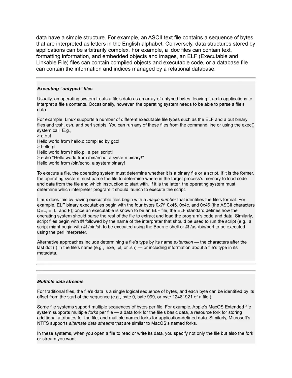
Executing “untyped” files
Usually, an operating system treats a file’s data as an array of untyped bytes, leaving it up to applications to
interpret a file’s contents. Occasionally, however, the operating system needs to be able to parse a file’s
data.
For example, Linux supports a number of different executable file types such as the ELF and a.out binary
files and tcsh, csh, and perl scripts. You can run any of these files from the command line or using the exec()
system call. E.g.,
> a.out
Hello world from hello.c compiled by gcc!
> hello.pl
Hello world from hello.pl, a perl script!
> echo ‘‘Hello world from /bin/echo, a system binary!’’
Hello world from /bin/echo, a system binary!
To execute a file, the operating system must determine whether it is a binary file or a script. If it is the former,
the operating system must parse the file to determine where in the target process’s memory to load code
and data from the file and which instruction to start with. If it is the latter, the operating system must
determine which interpreter program it should launch to execute the script.
Linux does this by having executable files begin with a magic number that identifies the file’s format. For
example, ELF binary executables begin with the four bytes 0x7f, 0x45, 0x4c, and 0x46 (the ASCII characters
DEL, E, L, and F); once an executable is known to be an ELF file, the ELF standard defines how the
operating system should parse the rest of the file to extract and load the program’s code and data. Similarly,
script files begin with #! followed by the name of the interpreter that should be used to run the script (e.g., a
script might begin with #! /bin/sh to be executed using the Bourne shell or #! /usr/bin/perl to be executed
using the perl interpreter.
Alternative approaches include determining a file’s type by its name extension — the characters after the
last dot (.) in the file’s name (e.g., .exe, .pl, or .sh) — or including information about a file’s type in its
metadata.
Multiple data streams
For traditional files, the file’s data is a single logical sequence of bytes, and each byte can be identified by its
offset from the start of the sequence (e.g., byte 0, byte 999, or byte 12481921 of a file.)
Some file systems support multiple sequences of bytes per file. For example, Apple’s MacOS Extended file
system supports multiple forks per file — a data fork for the file’s basic data, a resource fork for storing
additional attributes for the file, and multiple named forks for application-defined data. Similarly, Microsoft’s
NTFS supports alternate data streams that are similar to MacOS’s named forks.
In these systems, when you open a file to read or write its data, you specify not only the file but also the fork
or stream you want.
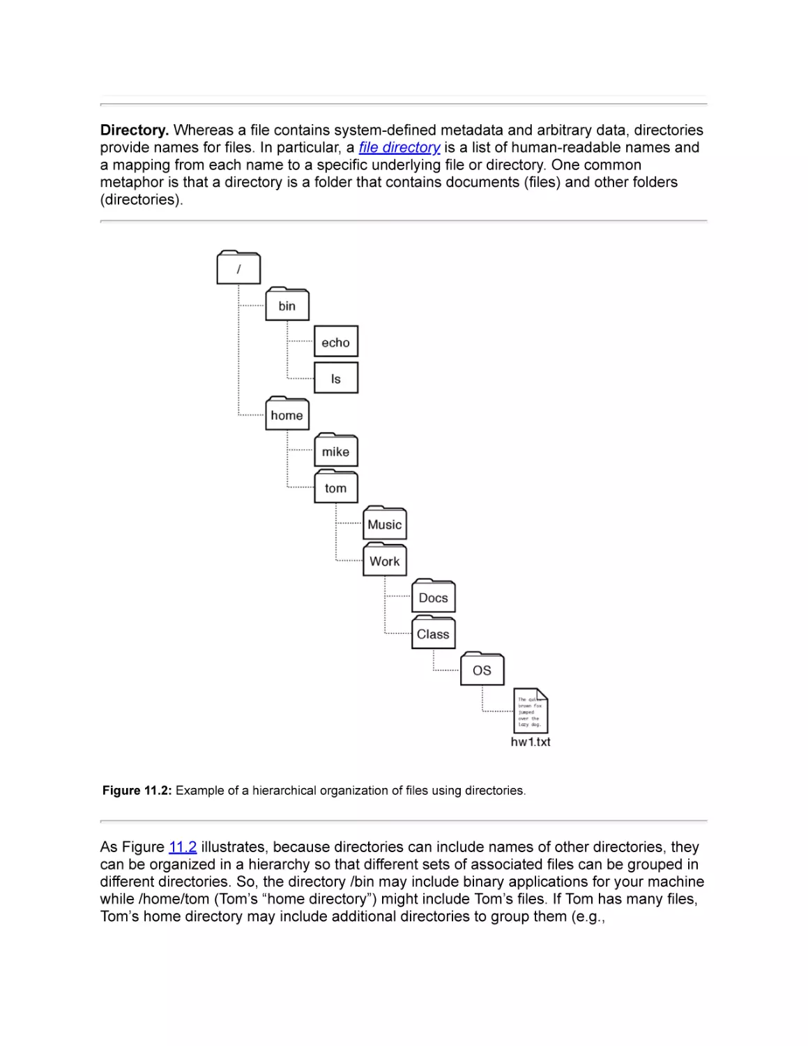
Directory. Whereas a file contains system-defined metadata and arbitrary data, directories
provide names for files. In particular, a file directory is a list of human-readable names and
a mapping from each name to a specific underlying file or directory. One common
metaphor is that a directory is a folder that contains documents (files) and other folders
(directories).
Figure 11.2: Example of a hierarchical organization of files using directories.
As Figure 11.2 illustrates, because directories can include names of other directories, they
can be organized in a hierarchy so that different sets of associated files can be grouped in
different directories. So, the directory /bin may include binary applications for your machine
while /home/tom (Tom’s “home directory”) might include Tom’s files. If Tom has many files,
Tom’s home directory may include additional directories to group them (e.g.,
/home/tom/Music and /home/tom/Work.) Each of these directories may have subdirectories
(e.g.,/home/tom/Work/Class and /home/tom/ Work/Docs) and so on.
The string that identifies a file or directory (e.g., /home/tom/Work/Class/OS/hw1.txt or
/home/tom) is called a path. Here, the symbol / (pronounced slash) separates components
of the path, and each component represents an entry in a directory. So, hw1.txt is a file in
the directory OS; OS is a directory in the directory Work; and so on.
If you think of the directory as a tree, then the root of the tree is a directory called, naturally
enough, the root directory. Path names such as /bin/ls that begin with / define absolute
paths that are interpreted relative to the root directory. So, /home refers to the directory
called home in the root directory.
Path names such as Work/Class/OS that do not begin with / define relative paths that are
interpreted by the operating system relative to a process’s current working directory. So, if
a process’s current working directory is /home/tom, then the relative path Work/Class/OS is
equivalent to the absolute path /home/tom/Work/Class/OS.
When you log in, your shell’s current working directory is set to your home directory.
Processes can change their current working directory with the chdir(path) system call. So,
for example, if you log in and then type cd Work/Class/OS, your current working directory is
changed from your home directory to the subdirectory Work/Class/OS in your home
directory.
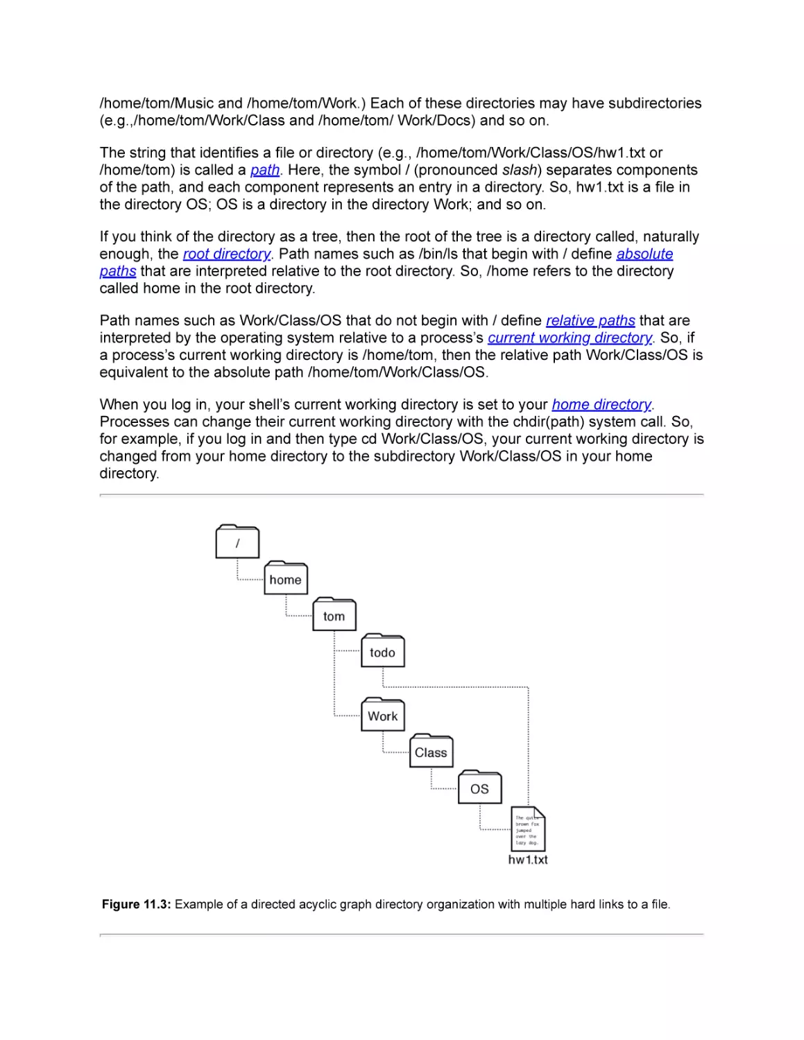
Figure 11.3: Example of a directed acyclic graph directory organization with multiple hard links to a file.
. and .. and ~
You may sometimes see path names in which directories are named ., .., or ~. For example,
> cd ~/Work/Class/OS
> cd ..
> ./a.out
., .., and ~ are special directory names in Unix. . refers to the current directory, .. refers to the parent
directory, ~ refers to the current user’s home directory, and ~name refers to the home directory of user
name.
So, the first shell command changes the current working directory to be the Work/ Class/OS directory in the
user’s home directory (e.g., /home/tom/Work/Class/OS). The second command changes the current working
directory to be the Work/ Class directory in the user’s home directory (e.g., ~/Work/Class or /home/
tom/Work/Class.) The third command executes the program a.out from the current working directory (e.g.,
~/Work/Class/a.out or /home/tom/Work/Class/ a.out.)
If each file or directory is identified by exactly one path, then the directory hierarchy forms a
tree. Occasionally, it is useful to have several different names for the same file or directory.
For example, if you are actively working on a project, you might find it convenient to have
the project appear in both your “todo” directory and a more permanent location (e.g.,
/home/tom/todo/hw1.txt and /home/tom/Work/Class/OS/hw1.txt as illustrated in
Figure 11.3.)
The mapping between a name and the underlying file is called a hard link. If a system
system allows multiple hard links to the same file, then the directory hierarchy may no
longer be a tree. Most file systems that allow multiple hard links to a file restrict these links
to avoid cycles, ensuring that their directory structures form a directed acyclic graph
(DAG.) Avoiding cycles can simplify management by, for example, ensuring that recursive
traversals of a directory structure terminate or by making it straightforward to use reference
counting to garbage collect a file when the last link to it is removed.
In addition to hard links, many systems provide other ways to use multiple names to refer
to the same file. See the sidebar for a comparison of hard links, soft links, symbolic links,
shortcuts, and aliases.
Hard links, soft links, symbolic links, shortcuts, and aliases
A hard link is a directory mapping from a file name directly to an underlying file. As we will see in Chapter 13,
directories will be implemented by storing mappings from file names to file numbers that uniquely identify
each file. When you first create a file (e.g., /a/b), the directory entry you create is a hard link the the new file.
If you then use link() to add another hard link to the file (e.g., link(“/a/b”, “/c/d”),) then both names are equally
valid, independent names for the same underlying file. You could, for example, unlink(“/a/b”), and /c/d would
remain a valid name for the file.
Many systems also support symbolic links also known as soft links. A symbolic link is a directory mappings
from a file name to another file name. If a file is opened via a symbolic link, the file system first translates the
name in the symbolic link to the target name and then uses the target name to open the file. So, if you
create /a/b , create a symbolic link from /c/d/ to /a/b, and then unlink /a/b, the file is no longer accessible and
open(“/c/d”) will fail.
Although the potential for such dangling links is a disadvantage, symbolic links have a number of
advantages over hard links. First, systems usually allow symbolic links to directories, not just regular files.
Second, a symbolic link can refer to a file stored in a different file system or volume.
Some operating systems such as Microsoft Windows also support shortcuts, which appear similar to
symbolic links but which are interpreted by the windowing system rather than by the file system. From the
file system’s point of view, a shortcut is just a regular file. The windowing system, however, treats shortcut
files specially: when the shortcut file is selected via the windowing system, the windowing system opens that
file, identifies the target file referenced by the shortcut, and acts as if the target file had been selected.
A MacOS file alias is similar to a symbolic link but with an added feature: if the target file is moved to have a
new path name, the alias can still be used to reference the file.
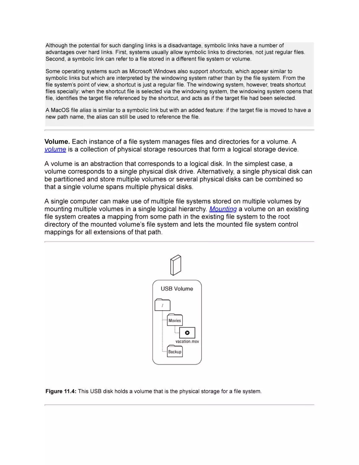
Volume. Each instance of a file system manages files and directories for a volume. A
volume is a collection of physical storage resources that form a logical storage device.
A volume is an abstraction that corresponds to a logical disk. In the simplest case, a
volume corresponds to a single physical disk drive. Alternatively, a single physical disk can
be partitioned and store multiple volumes or several physical disks can be combined so
that a single volume spans multiple physical disks.
A single computer can make use of multiple file systems stored on multiple volumes by
mounting multiple volumes in a single logical hierarchy. Mounting a volume on an existing
file system creates a mapping from some path in the existing file system to the root
directory of the mounted volume’s file system and lets the mounted file system control
mappings for all extensions of that path.
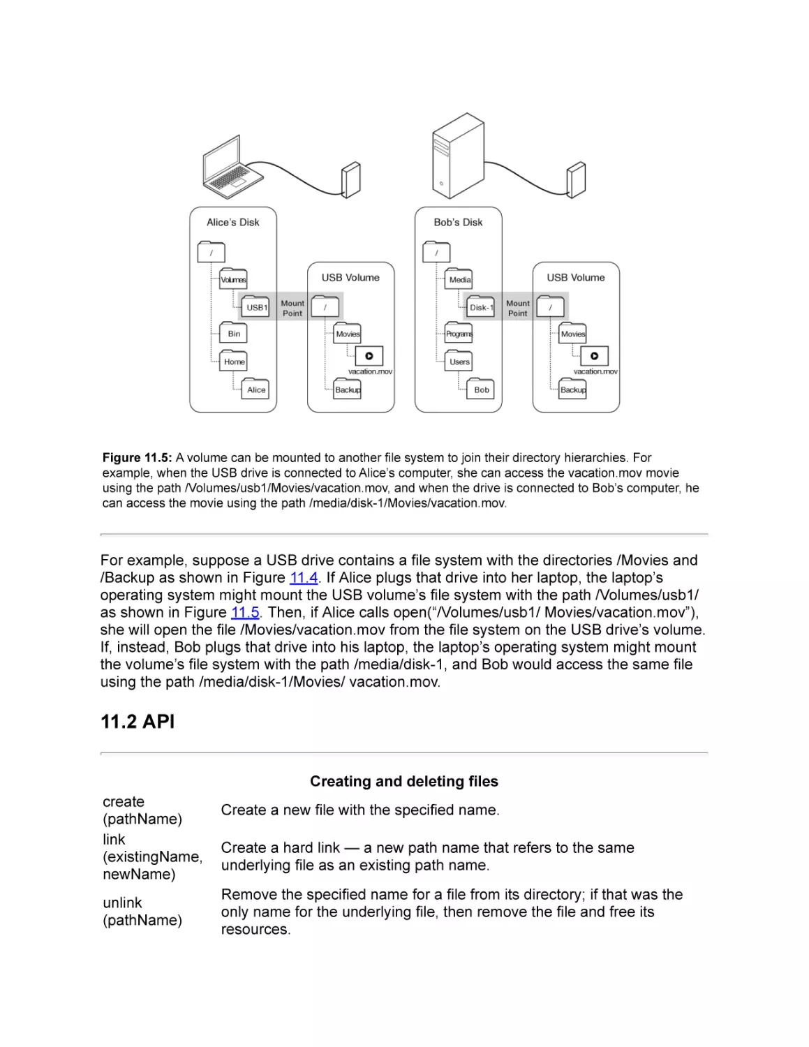
Figure 11.4: This USB disk holds a volume that is the physical storage for a file system.
Figure 11.5: A volume can be mounted to another file system to join their directory hierarchies. For
example, when the USB drive is connected to Alice’s computer, she can access the vacation.mov movie
using the path /Volumes/usb1/Movies/vacation.mov, and when the drive is connected to Bob’s computer, he
can access the movie using the path /media/disk-1/Movies/vacation.mov.
For example, suppose a USB drive contains a file system with the directories /Movies and
/Backup as shown in Figure 11.4. If Alice plugs that drive into her laptop, the laptop’s
operating system might mount the USB volume’s file system with the path /Volumes/usb1/
as shown in Figure 11.5. Then, if Alice calls open(“/Volumes/usb1/ Movies/vacation.mov”),
she will open the file /Movies/vacation.mov from the file system on the USB drive’s volume.
If, instead, Bob plugs that drive into his laptop, the laptop’s operating system might mount
the volume’s file system with the path /media/disk-1, and Bob would access the same file
using the path /media/disk-1/Movies/ vacation.mov.
11.2 API
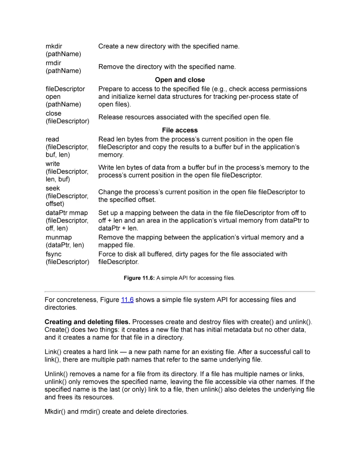
Creating and deleting files
create
(pathName)
link
(existingName,
newName)
unlink
(pathName)
Create a new file with the specified name.
Create a hard link — a new path name that refers to the same
underlying file as an existing path name.
Remove the specified name for a file from its directory; if that was the
only name for the underlying file, then remove the file and free its
resources.
mkdir
(pathName)
rmdir
(pathName)
fileDescriptor
open
(pathName)
close
(fileDescriptor)
read
(fileDescriptor,
buf, len)
write
(fileDescriptor,
len, buf)
seek
(fileDescriptor,
offset)
dataPtr mmap
(fileDescriptor,
off, len)
munmap
(dataPtr, len)
fsync
(fileDescriptor)
Create a new directory with the specified name.
Remove the directory with the specified name.
Open and close
Prepare to access to the specified file (e.g., check access permissions
and initialize kernel data structures for tracking per-process state of
open files).
Release resources associated with the specified open file.
File access
Read len bytes from the process’s current position in the open file
fileDescriptor and copy the results to a buffer buf in the application’s
memory.
Write len bytes of data from a buffer buf in the process’s memory to the
process’s current position in the open file fileDescriptor.
Change the process’s current position in the open file fileDescriptor to
the specified offset.
Set up a mapping between the data in the file fileDescriptor from off to
off + len and an area in the application’s virtual memory from dataPtr to
dataPtr + len.
Remove the mapping between the application’s virtual memory and a
mapped file.
Force to disk all buffered, dirty pages for the file associated with
fileDescriptor.
Figure 11.6: A simple API for accessing files.
For concreteness, Figure 11.6 shows a simple file system API for accessing files and
directories.
Creating and deleting files. Processes create and destroy files with create() and unlink().
Create() does two things: it creates a new file that has initial metadata but no other data,
and it creates a name for that file in a directory.
Link() creates a hard link — a new path name for an existing file. After a successful call to
link(), there are multiple path names that refer to the same underlying file.
Unlink() removes a name for a file from its directory. If a file has multiple names or links,
unlink() only removes the specified name, leaving the file accessible via other names. If the
specified name is the last (or only) link to a file, then unlink() also deletes the underlying file
and frees its resources.
Mkdir() and rmdir() create and delete directories.
EXAMPLE: Linking to files vs. linking to directories. Systems such as Linux support a
link() system call, but they do not allow new hard links to be created to a directory. E.g.,
existingPath must not be a directory. Why does Linux mandate this restriction?
ANSWER: Preventing multiple hard links to a directory prevents cycles, ensuring that the
directory structure is always a directed acyclic graph (DAG).
Additionally, allowing hard links to a directory would muddle a directory’s parent directory
entry (e.g., “..” as discussed in the sidebar). □
Open and close. To start accessing a file, a process calls open() to get a file descriptor it
can use to refer to the open file. File descriptor is Unix terminology; in other systems the
descriptor may be called a file handle or a file stream.
Operating systems require processes to explicitly open() files and access them via file
descriptors rather than simply passing the path name to read() and write() calls for two
reasons. First, path parsing and permission checking can be done just when a file is
opened and need not be repeated on each read or write. Second, when a process opens a
file, the operating system creates a data structure that stores information about the
process’s open file such as the file’s ID, whether the process can write or just read the file,
and a pointer to the process’s current position within the file. The file descriptor can thus be
thought of as a reference to the operating system’s per-open-file data structure that the
operating system will use for managing the process’s access to the file.
When an application is done using a file, it calls close(), which releases the open file record
in the operating system.
File access. While a file is open, an application can access the file’s data in two ways.
First, it can use the traditional procedural interface, making system calls to read() and
write() on an open file. Calls to read() and write() start from the process’s current file
position, and they advance the current file position by the number of bytes successfully
read or written. So, a sequence of read() or write() calls moves sequentially through a file.
To support random access within a file, the seek() call changes a process’s current position
for a specified open file.
Rather than using read() and write() to access a file’s data, an application can use mmap()
to establish a mapping between a region of the process’s virtual memory and some region
of the file. Once a file has been mapped, memory loads and stores to that virtual memory
region will read and write the file’s data either by accessing a shared page from the
kernel’s file cache, or by triggering a page fault exception that causes the kernel to fetch
the desired page of data from the file system into memory. When an application is done
with a file, it can call munmap() to remove the mappings.
Finally, the fsync() call is important for reliability. When an application updates a file via a
write() or a memory store to a mapped file, the updates are buffered in memory and written
back to stable storage at some future time. Fsync() ensures that all pending updates for a
file are written to persistent storage before the call returns. Applications use this function
for two purposes. First, calling fsync() ensures that updates are durable and will not be lost
if there is a crash or power failure. Second, calling fsync() between two updates ensures
that the first is written to persistent storage before the second. Note that calling fsync() is
not always necessary; the operating system ensures that all updates are made durable by
periodically flushing all dirty file blocks to stable storage.
Modern file access APIs
The API shown in Figure 11.6 is similar to most widely used file access APIs, but it is somewhat simplified.
For example, each of the listed calls is similar to a call provided by the POSIX interface, but the API shown
in Figure 11.6 omits some arguments and options found in POSIX. The POSIX open() call, for example,
includes two additional arguments one to specify various flags such as whether the file should be opened in
read-only or read-write mode and the other to specify the access control permissions that should be used if
the open() call creates a new file.
In addition, real-world file access APIs are likely to have a number of additional calls. For example, the
Microsoft Windows file access API includes dozens of calls including calls to lock and unlock a file, to
encrypt and decrypt a file, or to find a file in a directory whose name matches a specific pattern.
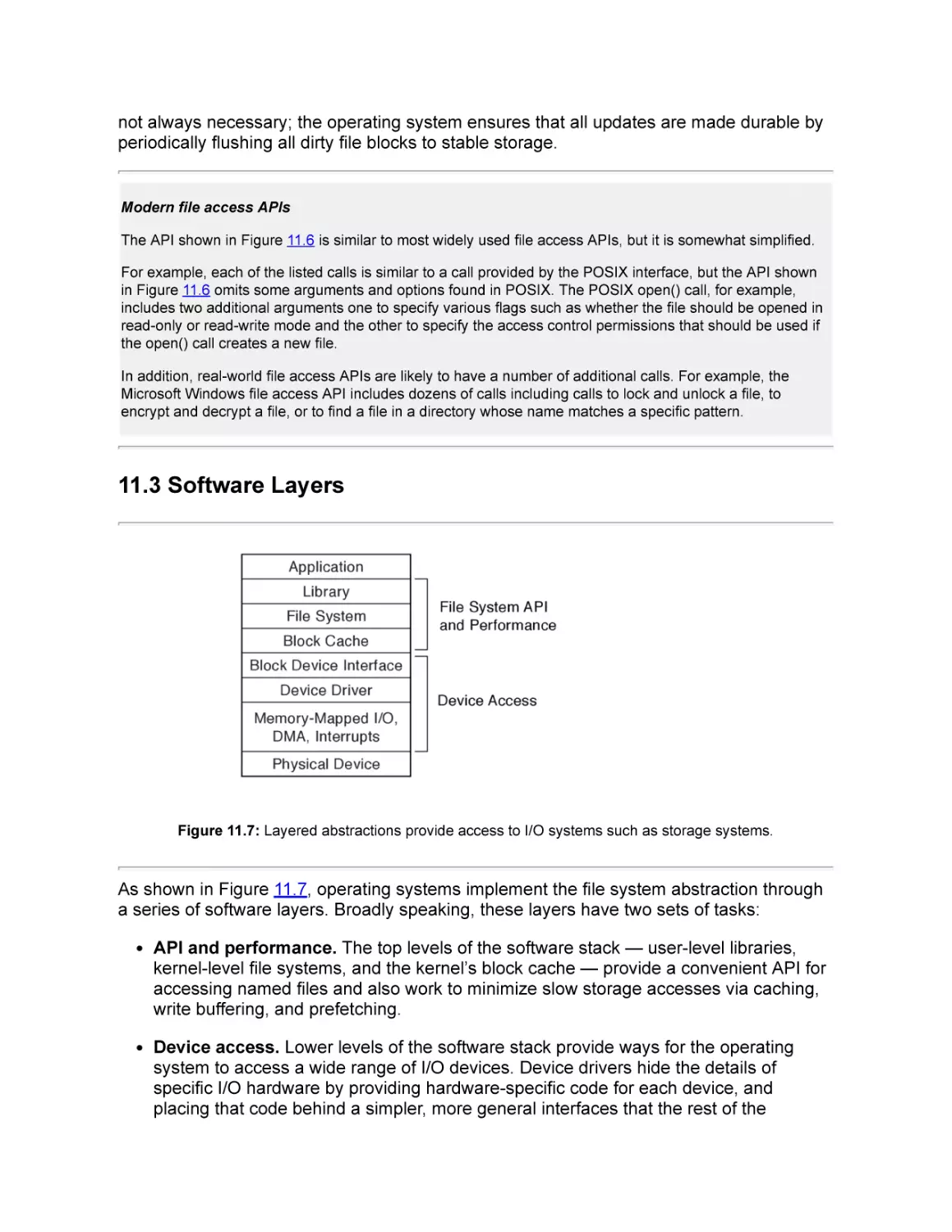
11.3 Software Layers
Figure 11.7: Layered abstractions provide access to I/O systems such as storage systems.
As shown in Figure 11.7, operating systems implement the file system abstraction through
a series of software layers. Broadly speaking, these layers have two sets of tasks:
API and performance. The top levels of the software stack — user-level libraries,
kernel-level file systems, and the kernel’s block cache — provide a convenient API for
accessing named files and also work to minimize slow storage accesses via caching,
write buffering, and prefetching.
Device access. Lower levels of the software stack provide ways for the operating
system to access a wide range of I/O devices. Device drivers hide the details of
specific I/O hardware by providing hardware-specific code for each device, and
placing that code behind a simpler, more general interfaces that the rest of the
operating system can use such as a block device interface. The device drivers
execute as normal kernel-level code, using the systems’ main processors and
memory, but they must interact with the I/O devices. A system’s processors and
memory communicate with its I/O devices using Memory-Mapped I/O, DMA, and
Interrupts.
In the rest of this section, we first talk about the file system API and performance layers.
We then discuss device access.
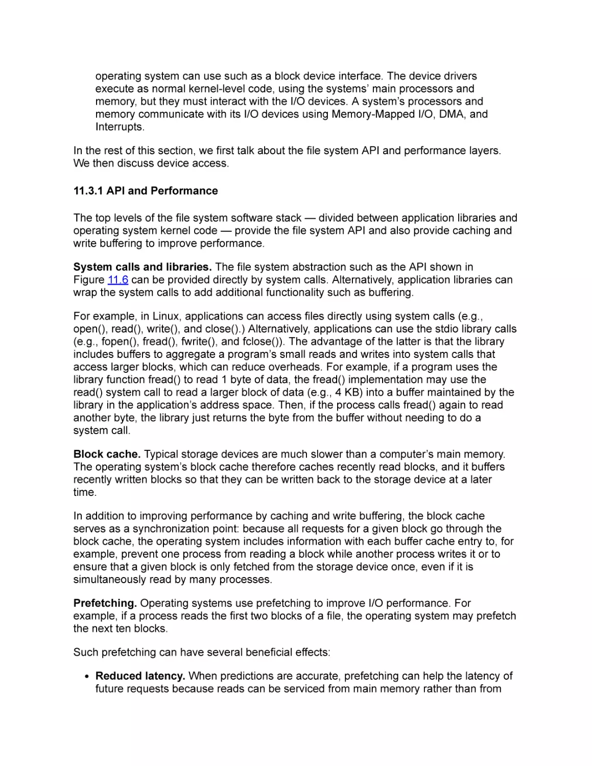
11.3.1 API and Performance
The top levels of the file system software stack — divided between application libraries and
operating system kernel code — provide the file system API and also provide caching and
write buffering to improve performance.
System calls and libraries. The file system abstraction such as the API shown in
Figure 11.6 can be provided directly by system calls. Alternatively, application libraries can
wrap the system calls to add additional functionality such as buffering.
For example, in Linux, applications can access files directly using system calls (e.g.,
open(), read(), write(), and close().) Alternatively, applications can use the stdio library calls
(e.g., fopen(), fread(), fwrite(), and fclose()). The advantage of the latter is that the library
includes buffers to aggregate a program’s small reads and writes into system calls that
access larger blocks, which can reduce overheads. For example, if a program uses the
library function fread() to read 1 byte of data, the fread() implementation may use the
read() system call to read a larger block of data (e.g., 4 KB) into a buffer maintained by the
library in the application’s address space. Then, if the process calls fread() again to read
another byte, the library just returns the byte from the buffer without needing to do a
system call.
Block cache. Typical storage devices are much slower than a computer’s main memory.
The operating system’s block cache therefore caches recently read blocks, and it buffers
recently written blocks so that they can be written back to the storage device at a later
time.
In addition to improving performance by caching and write buffering, the block cache
serves as a synchronization point: because all requests for a given block go through the
block cache, the operating system includes information with each buffer cache entry to, for
example, prevent one process from reading a block while another process writes it or to
ensure that a given block is only fetched from the storage device once, even if it is
simultaneously read by many processes.
Prefetching. Operating systems use prefetching to improve I/O performance. For
example, if a process reads the first two blocks of a file, the operating system may prefetch
the next ten blocks.
Such prefetching can have several beneficial effects:
Reduced latency. When predictions are accurate, prefetching can help the latency of
future requests because reads can be serviced from main memory rather than from
slower storage devices.
Reduced device overhead. Prefetching can help reduce storage device overheads
by replacing a large number of small requests with one large one.
Improved parallelism. Some storage devices such as Redundant Arrays of
Inexpensive Disks (RAIDs) and Flash drives are able to process multiple requests at
once, in parallel. Prefetching provides a way for operating systems to take advantage
of available hardware parallelism.
Prefetching, however, must be used with care. Too-aggressive prefetching can cause
problems:
Cache pressure. Each prefetched block is stored in the block cache, and it may
displace another block from the cache. If the evicted block is needed before the
prefetched one is used, prefetching is likely to hurt overall performance.
I/O contention. Prefetch requests consume I/O resources. If other requests have to
wait behind prefetch requests, prefetching may hurt overall performance.
Wasted effort. Prefetching is speculative. If the prefetched blocks end up being
needed, then prefetching can help performance; otherwise, prefetching may hurt
overall performance by wasting memory space, I/O device bandwidth, and CPU
cycles.
11.3.2 Device Drivers: Common Abstractions
Device drivers translate between the high level abstractions implemented by the operating
system and the hardware-specific details of I/O devices.
An operating system may have to deal with many different I/O devices. For example, a
laptop on a desk might be connected to two keyboards (one internal and one external), a
trackpad, a mouse, a wired ethernet, a wireless 802.11 network, a wireless bluetooth
network, two disk drives (one internal and one external), a microphone, a speaker, a
camera, a printer, a scanner, and a USB thumb drive. And that is just a handful of the
literally thousands of devices that could be attached to a computer today. Building an
operating system that treats each case separately would be impossibly complex.
Layering helps simplify operating systems by providing common ways to access various
classes of devices. For example, for any given operating system, storage device drivers
typically implement a standard block device interface that allows data to be read or written
in fixed-sized blocks (e.g., 512, 2048, or 4096 bytes).
Such a standard interface lets an operating system easily use a wide range of similar
devices. A file system implemented to run on top of the standard block device interface can
store files on any storage device whose driver implements that interface, be it a Seagate
spinning disk drive, an Intel solid state drive, a Western Digital RAID, or an Amazon Elastic
Block Store volume. These devices all have different internal organizations and control
registers, but if each manufacturer provides a device driver that exports the standard
interface, the rest of the operating system does not need to be concerned with these perdevice details.
Challenge: device driver reliability
Because device drivers are hardware-specific, they are often written and updated by the hardware
manufacturer rather than the operating system’s main authors. Furthermore, because there are large
numbers of devices — some operating systems support tens of thousands of devices — device driver code
may represent a large fraction of an operating system’s code.
Unfortunately, bugs in device drivers have the potential to affect more than the device. A device driver
usually runs as part of the operating system kernel since kernel routines depend on it and because it needs
to access the hardware of its device. However, if the device driver is part of the kernel, then a device driver’s
bugs have the potential to affect the overall reliability of a system. For example, in 2003 it was reported that
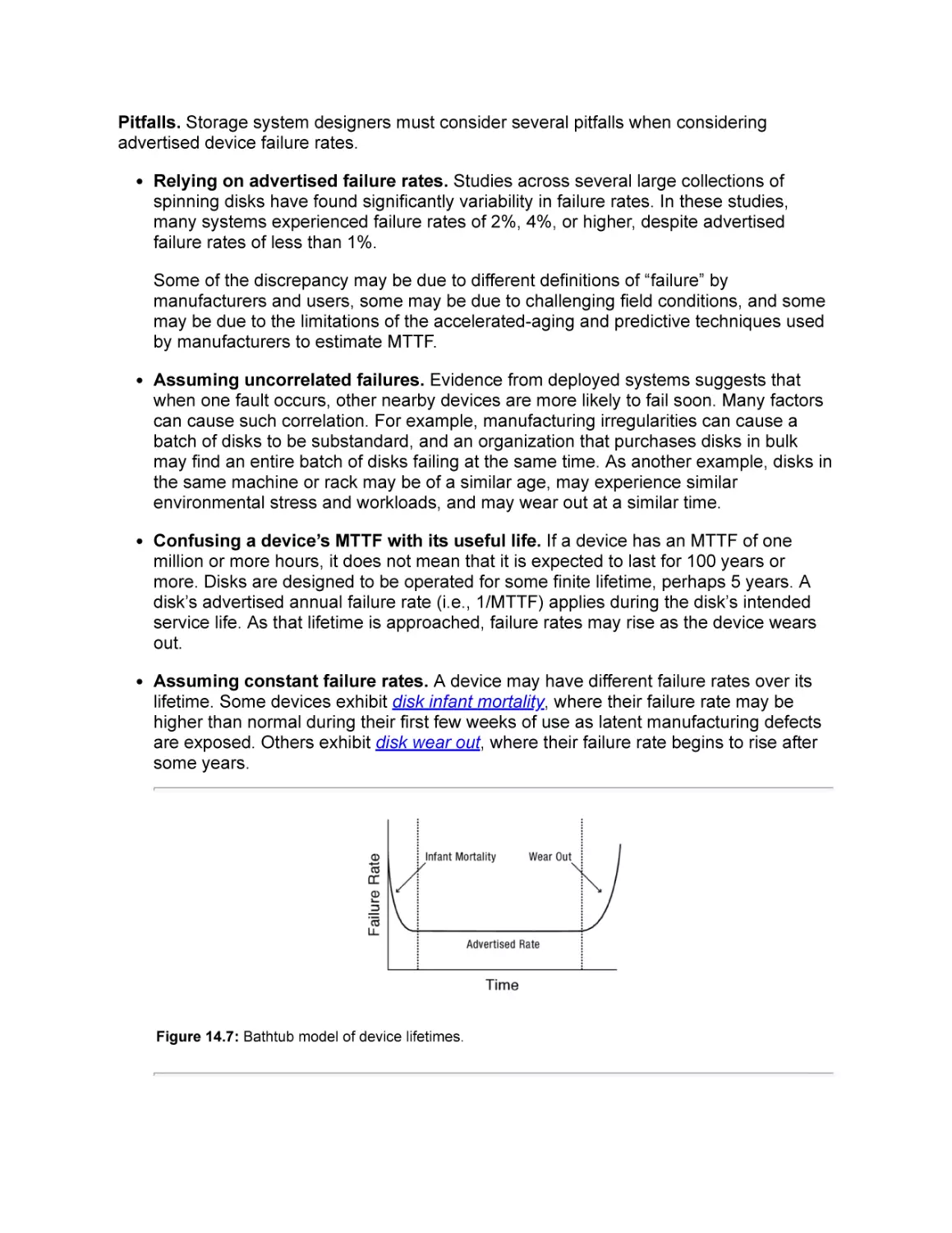
drivers caused about 85% of failures in the Windows XP operating system.
To improve reliability, operating systems are increasingly using protection techniques similar to those used to
isolate user-level programs to isolate device drivers from the kernel and from each other.
11.3.3 Device Access
How should an operating system’s device drivers communicate with and control a storage
device? At first blush, a storage device seems very different from the memory and CPU
resources we have discussed so far. For example, a disk drive includes several motors, a
sensor for reading data, and an electromagnet for writing data.
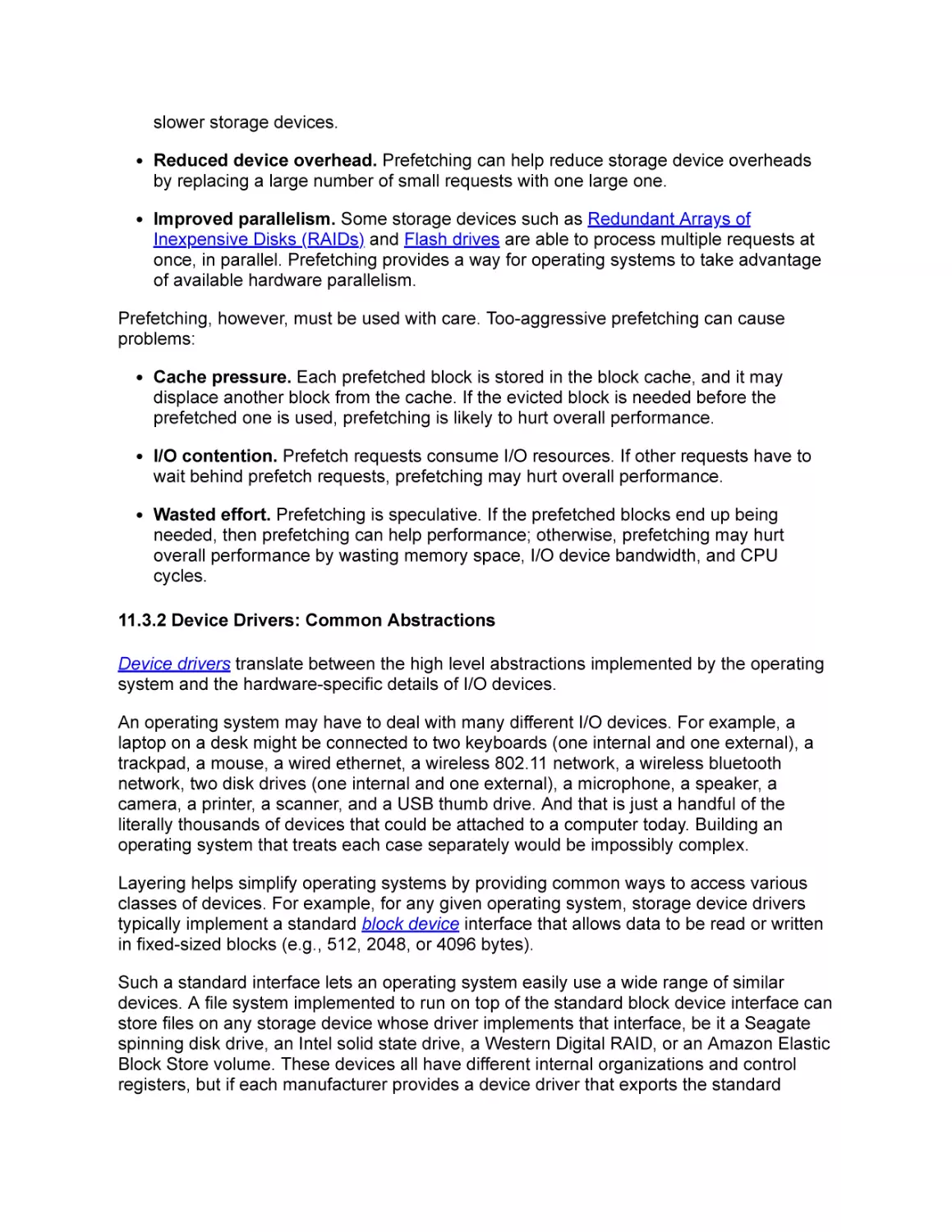
Memory-mapped I/O. As Figure 11.8 illustrates, I/O devices are typically connected to an
I/O bus that is connected to the system’s memory bus. Each I/O device has controller with
a set of registers that can be written and read to transmit commands and data to and from
the device. For example, a simple keyboard controller might have one register that can be
read to learn the most recent key pressed and another register than can be written to turn
the caps-lock light on or off.
Figure 11.8: I/O devices are attached to the I/O bus, which is attached to the memory bus.
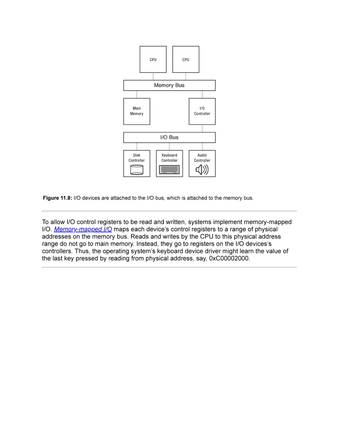
To allow I/O control registers to be read and written, systems implement memory-mapped
I/O. Memory-mapped I/O maps each device’s control registers to a range of physical
addresses on the memory bus. Reads and writes by the CPU to this physical address
range do not go to main memory. Instead, they go to registers on the I/O devices’s
controllers. Thus, the operating system’s keyboard device driver might learn the value of
the last key pressed by reading from physical address, say, 0xC00002000.
Figure 11.9: Physical address map for a system with 2 GB of DRAM and 3 memory-mapped I/O devices.
The hardware maps different devices to different physical address ranges. Figure 11.9
shows the physical address map for a hypothetical system with a 32 bit physical address
space capable of addressing 4 GB of physical memory. This system has 2 GB of DRAM in
it, consuming physical addresses 0x00000000 (0) to 0x7FFFFFFF (231 - 1). Controllers for
each of its three I/O devices are mapped to ranges of addresses in the first few kilobytes
above 3 GB. For example, physical addresses from 0xC0001000 to 0xC0001FFF access
registers in the disk controller.
Port mapped I/O
Today, memory-mapped I/O is the dominant paradigm for accessing I/O device’s control registers. However
an older style, port mapped I/O, is still sometimes used. Notably, the x86 architecture supports both
memory-mapped I/O and port mapped I/O.
Port mapped I/O is similar to memory-mapped I/O in that instructions read from and write to specified
addresses to control I/O devices. There are two differences. First, where memory-mapped I/O uses standard
memory-access instructions (e.g., load and store) to communicate with devices, port mapped I/O uses
distinct I/O instructions. For example, the x86 architecture uses the in and out instructions for port mapped
I/O. Second, whereas memory-mapped I/O uses the same physical address space as is used for the
system’s main memory, the address space for port mapped I/O is distinct from the main memory address
space.
For example, in x86 I/O can be done using either memory-mapped or port mapped I/O, and the low-level
assembly code is similar for both cases:
Memory mapped I/O
MOV register, memAddr // To read
MOV memAddr, register // To write
Port mapped I/O
IN register, portAddr // To read
OUT portAddr, register // To write
Port mapped I/O can be useful in architectures with constrained physical memory addresses since I/O
devices do not need to consume ranges of physical memory addresses. On the other hand, for systems with
sufficiently large physical address spaces, memory-mapped I/O can be simpler since no new instructions or
address ranges need to be defined and since device drivers can use any standard memory access
instructions to access devices. Also, memory-mapped I/O provides a more unified model for supporting DMA
— direct transfers between I/O devices and main memory.
DMA. Many I/O devices, including most storage devices, transfer data in bulk. For
example, operating systems don’t read a word or two from disk, they usually do transfers of
at least a few kilobytes at a time. Rather than requiring the CPU to read or write each word
of a large transfer, I/O devices can use direct memory access. When using direct memory
access (DMA), the I/O device copies a block of data between its own internal memory and
the system’s main memory.
To set up a DMA transfer, a simple operating system could use memory-mapped I/O to
provide a target physical address, transfer length, and operation code to the device. Then,
the device copies data to or from the target address without requiring additional processor
involvement.
After setting up a DMA transfer, the operating system must not use the target physical
pages for any other purpose until the DMA transfer is done. The operating system
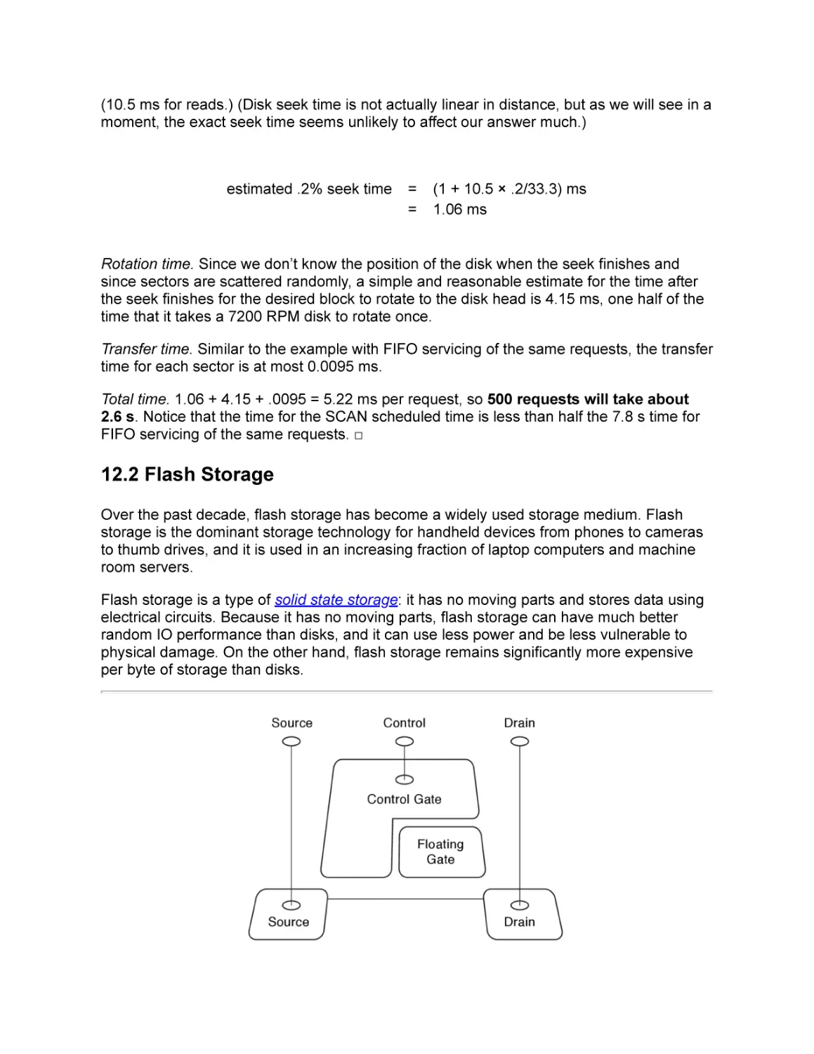
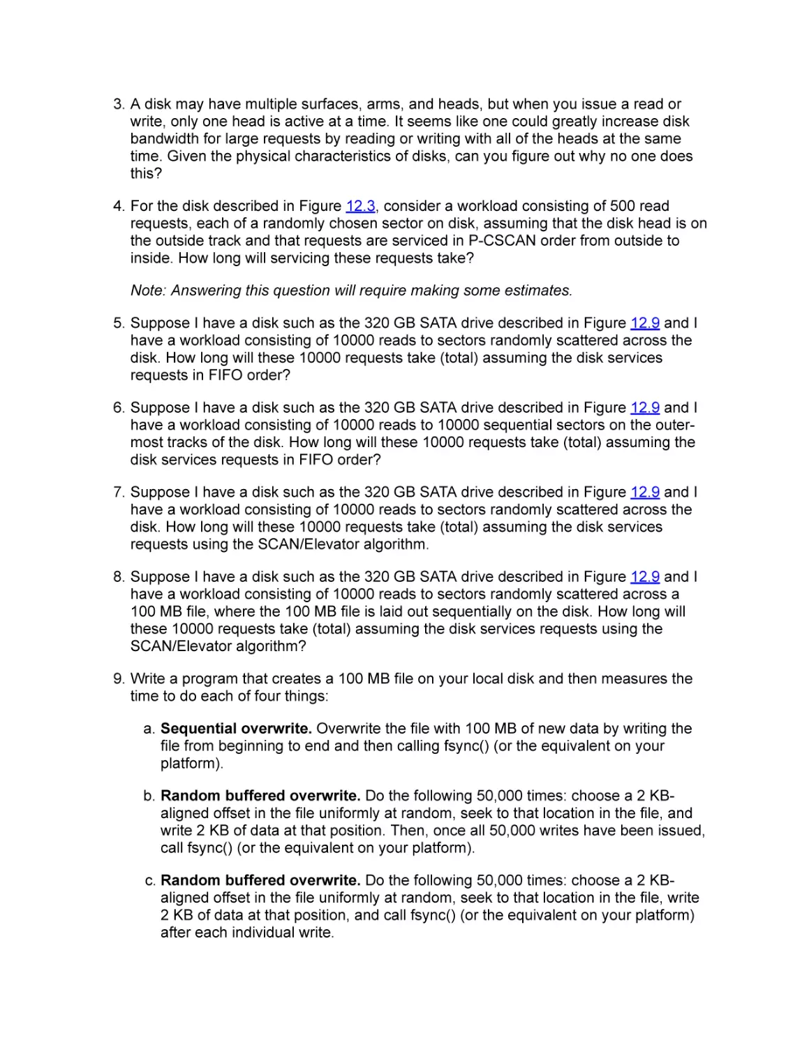
therefore “pins” the target pages in memory so that they cannot be reused until they are
unpinned. For example, a pinned physical page cannot be swapped out to disk and then
remapped to some other virtual address.
Advanced DMA
Although a setting up a device’s DMA can be as simple as providing a target physical address and length
and then saying “go!”, more sophisticated interfaces are increasingly used.
For example rather than giving devices direct access to the machine’s physical address space, some
systems include an I/O memory management unit (IOMMU) that translates device virtual addresses to main
memory physical addresses similar to how a processor’s TLB translates processor virtual addresses to main
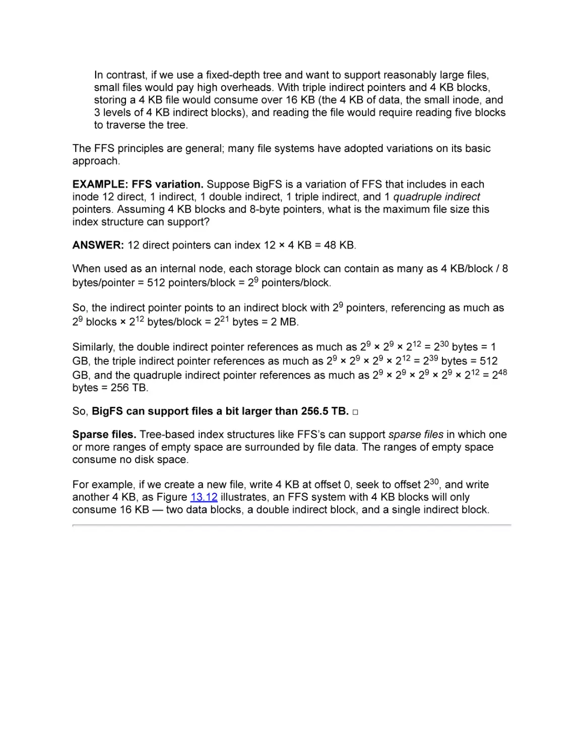
memory physical addresses. An IOMMU can provide both protection (e.g., preventing a buggy IO device
from overwriting arbitrary memory) and simpler abstractions (e.g., allowing devices to use virtual addresses
so that, for example, a long transfer can be made to a range of consecutive virtual pages rather than a
collection of physical pages scattered across memory.)
Also, some devices add a level of indirection so that they can interrupt the CPU less often. For example,
rather than using memory mapped I/O to set up each DMA request, the CPU and I/O device could share two
lists in memory: one list of pending I/O requests and another of completed I/O requests. Then, the CPU
could set up dozens of disk requests and only be interrupted when all of them are done.
Sophisticated I/O devices can even be configured to take different actions depending the data they receive.
For example, some high performance network interfaces parse incoming packets and direct interrupts to
different processors based on the network connection to which a received packet belongs.
Interrupts. The operating system needs to know when I/O devices have completed
handling a request or when new external input arrives. One option is polling, repeatedly
using memory-mapped I/O to read a status register on the device. Because I/O devices are
often much slower than CPUs and because inputs received by I/O devices may arrive at
irregular rates, it us usually better for I/O devices to use an interrupt to notify the operating
system of important events.
11.3.4 Putting It All Together: A Simple Disk Request
When a process issues a system call like read() to read data from disk into the process’s
memory, the operating system moves the calling thread to a wait queue. Then, the
operating system uses memory-mapped I/O both to tell the disk to read the requested data
and to set up DMA so that the disk can place that data in the kernel’s memory. The disk
then reads the data and DMAs it into main memory; once that is done, the disk triggers an
interrupt. The operating system’s interrupt handler then copies the data from the kernel’s
buffer into the process’s address space. Finally, the operating system moves the thread the
ready list. When the thread next runs, it will returns from the system call with the data now
present in the specified buffer.
11.4 Summary and Future Directions
The file system interface is a stable one, and small variations of interface described here
can be found in many operating systems and for many storage devices.
Yet, the file system abstraction is imperfect, and application writers need to use it carefully
to get acceptable performance and reliability. For example, if an application write()s a file,
the update may not be durable when the write() call returns; application writers often call
fsync() to ensure durability of data.
Could better file system APIs simplify programming? For example, if file systems allowed
users to update multiple objects atomically, that might simplify many applications that
currently must carefully constrain the order that their updates are stored using crude
techniques such as using fsync as a barrier between one set of updates and the next.
Could better file system APIs improve performance? For example, one proposed interface
allows an application to direct the operating system to transfer a range of bytes from a file
to a network connection. Such an interface might, for example, reduce overheads for a
movie server that streams movies across a network to clients.
Exercises
1. Discussion Suppose a process successfully opens an existing file that has a single
hard link to it, but while the process is reading that file, another process unlinks that
file. What should happen to subsequent reads by the first process? Should they
succeed? Should they fail? Why?
2. In Linux, suppose a process successfully opens an existing file that has a single hard
link to it, but while the process is reading that file, another process unlinks that file?
What happens to subsequent reads by the first process? Do they succeed? Do they
fail? (Answer this problem by consulting documentation or by writing a program to test
the behavior of the system in this case.)
3. Write a program that creates a new file, writes 100KB to it, flushes the writes, and
deletes it. Time how long each of these steps takes.
Hint You may find the POSIX system calls creat(), write(), fflush(), close(), and
gettimeofday() useful. See the manual pages for details on how to use these.
4. Consider a text editor that saves a file whenever you click a save button. Suppose that
when you press the button, the editor simply (1) animates the button “down” event
(e.g., by coloring the button grey), (2) uses the write() system call to write your text to
your file, and then (3) animates the button “up” event (e.g., by coloring the button
white). What bad thing could happen if a user edits a file, saves it, and then turns off
her machine by flipping the power switch (rather than shutting the machine down
cleanly)?
5. Write a program that times how long it takes to issue 100,000 one-byte writes in each
of two ways. First, time how long it takes to use the POSIX system calls creat(),
write(), and close() directly. Then see how long these writes take if the program uses
the stdio library calls (e.g., fopen(), fwrite(), and fclose()) instead. Explain your results.
12. Storage Devices
Treat disks like tape. —John Ousterhout
Although today’s persistent storage devices have large capacity and low cost, they have
drastically worse performance than volatile DRAM memory.
Not only that, but the characteristics are different and are peculiar to specific persistent
storage devices. For example, although programs can access random individual words of
DRAM with good performance, programs can only access today’s disk and flash storage
devices hundreds or thousands of bytes at a time. Furthermore, even if an application
restricts itself to supported access sizes (e.g., 2 KB per read or write), if the application
access pattern is random, the application may be slower by a factor of several hundred
than if the application accessed the same amount of data sequentially.
To cope with the limitations and to maximize the performance of storage devices, both file
system designers and application writers need to understand the physical characteristics of
persistent storage devices.
Chapter roadmap. This chapter discusses two types of persistent storage: magnetic disks
and flash memory. Both are widely used. Magnetic disks provide persistent storage for
most servers, workstations, and laptops. Flash memory provides persistent storage for
most smart phones, tablets, and cameras and for an increasing fraction of laptops.
12.1 Magnetic Disk
Figure 12.1: A partially-disassembled magnetic disk drive.
Magnetic disk is a non-volatile storage technology that is widely used in laptops, desktops,
and servers. Disk drives work by magnetically storing data on a thin metallic film bonded to
a glass, ceramic, or aluminum disk that rotates rapidly. Figure 12.1 shows a disk drive
without its protective cover, and Figure 12.2 shows a schematic of a disk drive, identifying
key components.
Figure 12.2: Key components of a magnetic disk drive.
Each drive holds one or more platters, thin round plates that hold the magnetic material.
Each platter has two surfaces, one on each side. When the drive powers up, the platters
are constantly spinning on a spindle powered by a motor. In 2011, disks commonly spin at
4200–15000 RPM (70–250 revolutions per second.)
A disk head is the component that reads and writes data by sensing or introducing a
magnetic field on a surface. There is one head per surface, and as a surface spins
underneath a head, the head reads or writes a sequence of bits along a circle centered on
the disk’s spindle. As a disk platters spins, it creates a layer of rapidly spinning air, and the
disk head floats on that layer, allowing the head to get extremely close to the platter without
contacting it. A head crash occurs when the disk head breaks through this layer with
enough force to damage the magnetic surface below; head crashes can be caused by
excessive shock such as dropping a running drive.
To reach the full surface, each disk head attaches to an arm, and all of a disk’s arms attach
to a single arm assembly that includes a motor that can move the arms across the surfaces
of the platters. Note that an assembly has just one motor, and all of its arms move together.
Data bits are stored in fixed-size sectors; typically, sectors are 512 bytes. The disk
hardware cannot read or write individual bytes or words; instead, it must always read or
write at least an entire sector. This means that to change one byte in a sector, the
operating system must read the old sector, update the byte in memory, and rewrite the
entire sector to disk. One reason for this restriction is that the disk encodes each sector
with additional error correction code data, allowing it to fix (or at least detect) imperfectly
read or written data, which, in turn allows higher density storage and higher bandwidth
operation.
A circle of sectors on a surface is called a track. The disk can read or write all of the data
on a track without having to move the disk arm, so reading or writing a sequence of sectors
on the same track is much faster than reading or writing sectors on different tracks.
To maximize sequential access speed, logical sector zero on each track is staggered from
sector zero on the previous track by an amount corresponding to time it takes the disk to
move the head from one track to another or to switch from the head on one surface to the
head on another one. This staggering is called track skewing.
To increase storage density and disk capacity, disk manufacturers make tracks and sectors
as thin and small as possible. If there are imperfections in a sector, then that sector may be
unable to reliably store data. Manufacturers therefore include spare sectors distributed
across each surface. The disk firmware or the file system’s low-level formatting can then
use sector sparing to remap sectors to use spare sectors instead of faulty sectors. Slip
sparing helps retain good sequential access performance by remapping all sectors from
the bad sector to the next spare, advancing each logical sector in that range by one
physical sector on disk.
Disk drives often include a few MB of buffer memory, memory that the disk’s controller
uses to buffer data being read from or written to the disk, for track buffering, and for write
acceleration.
Track buffering improves performance by storing sectors that have been read by the disk
head but have not yet been requested by the operating system. In particular, when a disk
head moves to a track, it may have to wait for the sector it needs to access to rotate under
the disk head. While the disk is waiting, it reads unrequested sectors to its rack buffer so
that if the operating system requests those sectors later, they can be returned immediately.
Write acceleration stores data to be written to disk in the disk’s buffer memory and
acknowledges the writes to the operating system before the data is actually written to the
platter; the disk firmware flushes the writes from the track buffer to the platter at some later
time. This technique can significantly increase the apparent speed of the disk, but it carries
risks — if power is lost before buffered data is safely stored, then data might be lost.
Server drives implementing the SCSI or Fibre Channel interfaces and increasing numbers
of commodity drives with the Serial ATA (SATA) interface implement a safer form of write
acceleration with tagged command queueing (TCQ) (also called native command queueing
(NCQ) for SATA drives.) TCQ allows an operating system to issue multiple concurrent
requests to the disk and for the disk to process those requests out of order to optimize
scheduling, and it can be configured to only acknowledge write requests when the blocks
are safely on the platter.
12.1.1 Disk Access and Performance
Operating systems send commands to a disk to read or write one or more consecutive
sectors. A disk’s sectors are identified with logical block addresses (LBAs) that specify the
surface, track, and sector to be accessed.
To service a request for a sequence of blocks starting at some sector, the disk must first
seek to the right track, wait for the first desired sector to rotate to the head, and then
transfer the blocks. Therefore, the time for a disk access is:
disk access time
=
seek time + rotation time + transfer time
Seek. The disk must first seek — move its arm over the desired track. To seek, the
disk first activates a motor that moves the arm assembly to approximately the right
place on disk. Then, as arm stops vibrating from the motion of the seek, the disk
begins reading positioning information embedded in the sectors to determine exactly
where it is and to make fine-grained positioning corrections to settle on the desired
track. Once the head has settled on the right track, the disk uses signal strength and
positioning information to make minute corrections in the arm position to keep the
head over the desired track.
A request’s seek time depends on how far the disk arm has to move.
A disk’s minimum seek time is the time it takes for the head to move from one track to
an adjacent one. For short seeks, disks typically just “resettle” the head on the new
track by updating the target track number in the track-following circuitry. Minimum seek
times of 0.3–1.5 ms are typical.
If a disk is reading the tth track on one surface, its head switch time is the time it would
take to begin reading the tth track on a different surface. Tracks can be less than a
micron wide and tracks on different surfaces are not perfectly aligned. So, a head
switch between the same tracks on different surfaces has a cost similar to a minimum
seek: the disk begins using the sensor on a different head and then resettles the disk
on the desired track for that surface.
A disk’s maximum seek time is the time it takes the head to move from the innermost
track to the outermost one or vice versa. Maximum seek times are typically over 10 ms
and can be over 20 ms.
A disk’s average seek time is the average across seeks between each possible pair of
tracks on a disk. This value is often approximated as the time to seek one third of the
way across the disk.
Beware of “average seek time”
Although the name average seek time makes it tempting to use this metric when estimating the time it
will take a disk to complete a particular workload, it is often the wrong metric to use. Average seek time
— the average across seeks between each possible pair of tracks on disk — was defined this way to
make it a well-defined, standard metric, not because it is representative of common workloads.
The definition of average seek time essentially assumes no locality in a workload, so it is very nearly a
worst-case scenario. Many workloads access sectors that are likely to be near one another; for
example, most operating systems attempt to place files sequentially on disk and to place different files
in a directory on the same track or on tracks near one another. For these (common) workloads, the
seek times observed may be closer to the disk’s minimum seek time than its “average” seek time.
The demise of the cylinder
A cylinder on a disk is a set of tracks on different surfaces with the same track index. For example, on
a 2-platter drive, the 8th tracks on surfaces 0, 1, 2, and 3 would form the 8th cylinder of the drive.
Some early file systems put related data on different surfaces but in the same cylinder. The idea was
that data from the different tracks in the cylinder could be read without a requiring a seek. Once a
cylinder was full, the file system would start placing data in one of the adjacent cylinders.
As disk densities have increased, the importance of the cylinder has declined. Today, a disk’s tracks
can be less than a micron wide. To follow a track at these densities, a controller monitors the signals
from a disk’s head to control the disk arm assembly’s motor to keep the head centered on a track.
Furthermore, at these densities, the tracks of a cylinder may not be perfectly aligned. As a result, when
a disk switches disk heads, the new head must center itself over the desired track. So, switching heads
within a cylinder ends up being similar to a short 1-track seek: the controller chooses the new
cylinder/track and the disk head settles over the target track. Today, accessing different tracks within
the same cylinder costs about the same as accessing adjoining tracks on the same platter.
Rotate. Once the disk head has settled on the right track, it must wait for the target
sector to rotate under it. This waiting time is called the rotational latency. Today, most
disks rotate at 4200 RPM to 15,000 RPM (15 ms to 4 ms per rotation), and for many
workloads a reasonable estimate of rotational latency is one-half the time for a full
rotation — 7.5 ms–2 ms.
Once a disk head has settled on a new track, most disks immediately begin reading
sectors into their buffer memory, regardless of which sectors have been requested.
This way, if there is a request for one of the sectors that have already passed under
the disk head, the data can be transferred immediately, rather than having to delay the
request for nearly a full rotation to reread the data.
Transfer. Once the disk head reaches a desired sector, the disk must transfer the data
from the sector to its buffer memory (for reads) or vice versa (for writes) as the sectors
rotate underneath the head. Then, for reads, it must transfer the data from its buffer
memory to the host’s main memory. For writes, the order of the transfers is reversed.
To amortize seek and rotation time, disk requests are often for multiple sequential
sectors. The time to transfer one or more sequential sectors from (or to) a surface
once the disk head begins reading (or writing) the first sector is the surface transfer
time.
On a modern disk, the surface transfer time for a single sector is much smaller than
the seek time or rotational latency. For example, disk bandwidths often exceed 100
MB/s, so the surface transfer time for a 512-byte sector is often under 5 microseconds
(0.005 ms).
Because a disk’s outer tracks have room for more sectors than its inner tracks and
because a given disk spins at a constant rate, the surface transfer bandwidth is often
higher for the outer tracks than the inner tracks.
For a disk read, once sectors have been transferred to the disk’s buffer memory, they
must be transferred to the host’s memory over some connection such as SATA (serial
ATA), SAS (serial attached SCSI), Fibre Channel, or USB (universal serial bus). For
writes, the transfer goes in the other direction. The time to transfer data between the
host’s memory and the disk’s buffer is the host transfer time. Typical bandwidths range
from 60 MB/s for USB 2.0 to 2500 MB/s for Fibre Channel-20GFC.
For multi-sector reads, disks pipeline transfers between the surface and disk buffer
memory and between buffer memory and host memory; so for large transfers, the total
transfer time will be dominated by whichever of these is the bottleneck. Similarly, for
writes, disks overlap the host transfer with the seek, rotation, and surface transfer;
again, the total transfer time will be dominated by whichever is the bottleneck.
12.1.2 Case Study: Toshiba MK3254GSY
Figure 12.3 shows some key parameters for a recent 2.5-inch disk drive for laptop
computers.
Size
Platters/Heads
Capacity
2/4
320 GB
Performance
Spindle speed
7200 RPM
Average seek time read/write 10.5 ms / 12.0 ms
Maximum seek time
19 ms
Track-to-track seek time
1 ms
Transfer rate (surface to buffer) 54–128 MB/s
Transfer rate (buffer to host)
375 MB/s
Buffer memory
16 MB
Power
Typical
16.35 W
Idle
11.68 W
Figure 12.3: Hardware specifications for a laptop disk (Toshiba MK3254GSY) manufactured in 2008.
This disk stores 320 GB of data on two platters, so it stores 80 GB per surface. The
platters spin at 7200 revolutions per minute, which is 8.3 ms per revolution; since each
platter’s diameter is about 6.3 cm, the outer edge of each platter is moving at about 85
km/hour!
The disk’s data sheet indicates an average seek time for the drive of 10.5 ms for reads and
12.0 ms for writes. The seek time for reads and writes differs because the disk starts
attempting to read data before the disk arm has completely settled, but it must wait a bit
longer before it is safe to write.
When transferring long runs of contiguous sectors, the disk’s bandwidth is 54-128 MB/s.
The bandwidth is expressed as a range because the disk’s outer tracks have more sectors
than its inner tracks, so when the disk is accessing data on its outer tracks, sectors sweep
past the disk head at a higher rate.
Once the data is transferred off the platter, the disk can send it to the main memory of the
computer at up to 375 MB/s via a SATA (Serial ATA) interface.
Random vs. sequential performance. Given seek and rotational times measured in
milliseconds, small accesses to random sectors on disk are much slower than large,
sequential accesses.
EXAMPLE: Random access workload. For the disk described in Figure 12.3, consider a
workload consisting of 500 read requests, each of a randomly chosen sector on disk,
assuming requests are serviced in FIFO order. How long will servicing these requests
take?
ANSWER: Disk access time is seek time + rotation time + transfer time.
Seek time. Each request requires a seek from a random starting track to a random ending
track, so the disk’s average seek time of 10.5 ms is a good estimate of the cost of each
seek.
Rotation time. Once the disk head settles on the right track, it must wait for the desired
sector to rotate under it. Since there is no reason to expect the desired sector to be
particularly near or far from the disk head when it settles, a reasonable estimate for rotation
time is 4.15 ms, one half of the time that it takes a 7200 RPM disk to rotate once.
Transfer time. The disk’s surface bandwidth is at least 54 MB/s, so transferring 512 bytes
takes at most 9.5 μS (0.0095 ms).
Total time. 10.5 + 4.15 + .0095 = 14.66 ms per request, so 500 requests will take about
7.33 seconds. □
EXAMPLE: Sequential access workload. For the disk described in Figure 12.3, consider
a workload consisting of a read request for 500 sequential sectors on the same track. How
long will servicing these requests take?
ANSWER: Disk access time is seek time + rotation time + transfer time.
Seek time. Since we do not know which track we are starting with or which track we are
reading from, we use the average seek time, 10.5 ms, as an estimate for the seek time.
Rotation time. Since we don’t know the position of the disk when the request is issued, a
simple and reasonable estimate for the time for the first desired block to rotate to the disk
head is 4.15 ms, one half of the time that it takes a 7200 RPM disk to rotate once.
Transfer time. A simple estimate is that 500 sectors can be transferred in 4.8 to 2.0 ms,
depending on whether they are on the inner or outer tracks.
500 sectors × 512 bytes/sector
× 1 / (54 ×106 bytes/second)
=
4.8 ms
=
2 ms
500 sectors × 512 bytes/sector
× 1 / (128 ×106 bytes/second)
(Too) simple answer. These three estimates give us a range from
10.5 + 4.15 + 2
=
16.7 ms
10.5 + 4.15 + 4.8
=
19.5 ms
More precise answer. However, this simple answer ignores the track buffer. Since the
transfer time is a large fraction of the rotation time (about 1/4 to 1/2 of the time for a full
rotation), we know that the request covers a significant fraction of a track. This means that
there is a good chance that after the seek and settle time, the disk head will be in the
middle of the region to be read. In this case, the disk will immediately read some of the
track into the track buffer; then it will wait for the first track to rotate around; then it will read
the remainder of the desired data.
We can estimate that for the outer track, there is a one in four chance that the initial seek
and settle will finish while the head is within the desired range of sectors, and that when
that happens, we read an average of 1∕8th of the desired data before we arrive at the first
desired sector. So, for the outer track, this overlap will save us 1∕4 × 1∕8 = 1∕32 of a rotation
for the average transfer. This effect slightly reduces the average access time: 16.7 ms (1∕32) × 8.3 ms = 16.4 ms.
Similarly, for the inner tracks, there is about a one in two chance that the initial seek will
settle in the middle of the desired data, saving on average 1∕2 × 1∕4 = 1∕8. This reduces the
average access time: 19.5 ms - (1∕8) × 8.3 ms = 18.5 ms.
So, we estimate that such an access would take between 16.4 ms and 18.5 ms. □
Notice that the sequential workload takes vastly less time than the random workload (less
than 20 milliseconds vs. 5.5 seconds). This orders of magnitude disparity between
sequential and random access performance influences many aspects of file system design
and use.
Still, even for a 500 sector request, a non-trivial amount of the access time is spent seeking
and rotating rather than transferring.
EXAMPLE: Effective bandwidth. For the transfer of 500 sequential sectors examined in
the previous example, what fraction of the disk’s surface bandwidth is realized?
ANSWER: The effective bandwidth ranges from
500 sectors × 512 bytes/sector × (1/18.5 ms)
=
13.8 MB/s
500 sectors × 512 bytes/sector × (1/16.4 ms)
=
15.6 MB/s
This gives us a range of 13.8 MB/s / 54 MB/s = 26% to 15.6 MB/s / 128 MB/s = 12% of the
maximum bandwidth from the inner to the outer tracks. □
So, even a fairly large request (500 sectors or 250 KB in this case) can incur significant
overheads from seek and rotational latency.
EXAMPLE: Efficient access. For the disk described in Figure 12.3, how large must a
request that begins on a random disk sector be to ensure that the disk gets at least 80% of
its advertised maximum surface transfer bandwidth?
ANSWER: When reading a long sequence of logically sequential blocks, the disk will read
an entire track, then do a 1 track seek (or a head switch and resettle, which amounts to the
same thing) and then read the next track. Notice that track buffering allows the disk to read
an entire track in one rotation regardless of which sector the head is over when it settles on
the track and starts successfully reading. So, for the outer tracks, it reads for one rotation
(8.4 ms) and then does a minimum seek (1 ms).
Thus, to achieve 80% of peak bandwidth after a random seek (10.5 ms), we need to read
enough rotations worth of data to ensure that we spend 80% of the total time reading. If x
is the number of rotations we will read, then we have:
0.8 totalTime
0.8(10.5 ms + (1 + 8.4) x ms)
x
=
=
=
x rotationTime
8.4 x ms
9.09
We therefore need to read at least 9.09 rotations worth of data to reach an efficiency of
80%. Since each rotation takes 8.4 ms and transfers data at 128 MB/s, 9.09 rotations
transfers 9.77 MB of data, or about 19,089 sectors. □
12.1.3 Disk Scheduling
Because moving the disk arm and waiting for the platter to rotate is so expensive,
performance can be significantly improved by optimizing the order in which pending
requests are serviced. Disk scheduling can be done by the operating system, by the disk’s
firmware, or both.
FIFO. The simplest thing to do is to process requests in first-in-first-out (FIFO) order.
Unfortunately, a FIFO scheduler can yield poor performance. For example, a sequence of
requests that alternate between the outer and inner tracks of a disk will result in many long
seeks.
SPTF/SSTF. An initially appealing option is to use a greedy scheduler that, given the
current position of the disk head and platter, always services the pending request that can
be handled in the minimum amount of time. This approach is called shortest positioning
time first (SPTF) (or shortest seek time first (SSTF) if rotational positioning is not
considered.)
SPTF and SSTF have two significant limitations. First, because moving the disk arm and
waiting for some rotation time affects the cost of serving subsequent requests, these
greedy approaches are not guaranteed to optimize disk performance. Second, these
greedy approaches can cause starvation when, for example, a continuous stream of
requests to inner tracks prevents requests to outer tracks from ever being serviced.
EXAMPLE: SPTF is not optimal. Suppose a disk’s head is just inside the middle track of
a disk so that seeking to the inside track would cost 9.9 ms while seeking to the outside
track would cost 10.1 ms. Assume that for the disk in question, seeking between the outer
and inner track costs 15 ms and that a rotation takes 10 ms.
Also suppose that the disk has two sets of pending requests. The first set is 1000 requests
to read each of the 1000 sectors on the inner track of the disk; the second set is 2000
requests to read each of the 2000 sectors on the outer track of the disk.
Compare the average response time per request for the SPTF schedule (first read the
“nearby” inner track and then read the outer track) and the alternative of reading the outer
track first and then the inner track.
ANSWER: The total amount of time taken to complete all requests is slightly shorter by
seeking first to the inside track and then to the outside. However, the average response
time per request is less in the opposite order.
To service either set of requests, the disk must seek to the appropriate track and then wait
for one full rotation while all of the track’s data sweeps under the arm. For either set, the
average response time for a request in that set will be the delay until the seek completes
plus one half the disk’s rotation time. Notice that the set handled second must wait until the
first one is completely done before it can start, adding to the response time observed for
requests in that set.
If we follow SPTF and read the sectors on the inner track first, the response time of the
average request is the weighted average of the response time of the inner requests and
the outer requests:
(1000 (9.9 + 5) + 2000 (9.9 + 10 + 15 + 5)) / 3000
=
31.6 ms
If, instead, we read the outer tracks first, the weighted average is:
(2000 (10.1 + 5) + 1000 (10.1 + 10 + 15 + 5)) / 3000
=
23.3 ms
In this case, seeking to the nearest sector moves the disk head away from the majority of
the requests, increasing the overall average response time by 8.3 ms. □
Elevator, SCAN, and CSCAN. Elevator-based algorithms like SCAN and CSCAN have
good performance and also ensure fairness in that no request is forced to wait for an
inordinately long time. The basic approach is similar to how an elevator works: when an
elevator is going up, it keeps going up until all pending requests to go to floors above it
have been satisfied; then, when an elevator is going down, it keeps going down until all
pending requests to go to floors below it have been satisfied.
Figure 12.4: Elevator-based scheduling algorithms: (left) SCAN, (center) CSCAN, and (right) R-CSCAN.
The numbering represents the order that each algorithm services requests 1-4 and then 5-7.
The SCAN scheduler works in the same way. The disk arm first sweeps from the inner to
the outer tracks, servicing all requests that are between the arm’s current position and the
outer edge of the disk. Then, the arm sweeps from the outer to the inner tracks. Then the
process is repeated. Figure 12.4-(left) illustrates the SCAN algorithm travelling from outerto-inner tracks to service four pending requests and then travelling from inner-to-outer
tracks to service three additional requests.
The CSCAN (circular SCAN) scheduler is a slight variation on SCAN in which the disk only
services requests when the head is traveling in one direction (e.g., from inner tracks to
outer ones). When the last request in the direction of travel is reached, the disk
immediately seeks to where it started (e.g., the most inner track or the most inner track
with a pending request) and services pending requests by moving the head in the same
direction as the original pass (e.g., from inner tracks to outer ones again.) Figure 12.4(center) illustrates the CSCAN algorithm travelling from outer-to-inner tracks to service four
pending requests and then skipping to the outer track and travelling from outer-to-inner
tracks to service three additional requests.
The advantage of CSCAN over SCAN is that if after a pass in one direction, the disk head
were to just switch directions (as in SCAN), it will encounter a region of the disk where
pending requests are sparse (since this region of the disk was just serviced). Seeking to
the opposite side of the disk (as in CSCAN) moves the disk head to an area where pending
requests are likely to be denser. In addition, CSCAN is more fair than SCAN in that seeking
to the opposite side of the disk allows it to begin servicing the requests that likely been
waiting longer than requests near but “just behind” the head.
Rather than pure seek-minimizing SCAN or CSCAN, schedulers also take into account
rotation time and allow small seeks “in the wrong direction” to avoid extra rotational delays
using the rotationally-aware R-SCAN or R-CSCAN variations. For example, if the disk head
is currently over sector 0 of track 0 and there are pending requests at sector 1000 of track
0, sector 500 of track 1, and sector 0 of track 10,000, a R-CSCAN scheduler might service
the second request, then the first, and then the third. Figure 12.4-(right) illustrates the RCSCAN algorithm handling a request on the outer track, then one a few tracks in, then
another request on the outer track, and a request near the center on the arm’s first sweep.
The arm’s second sweep is the same as for CSCAN.
EXAMPLE: Effect of disk scheduling. For the disk described in Figure 12.3, consider a
workload consisting of 500 read requests, each to a randomly chosen sector on disk,
assuming that the disk head is on the outside track and that requests are serviced in
CSCAN order from outside to inside. How long will servicing these requests take?
ANSWER: Answering a question like this requires making some educated guesses;
different people may come up with different reasonable estimates here.
Seek time. We first note that with 500 pending requests spread randomly across the disk,
the average seek from one request to the next will seek 0.2% of the way across the disk.
With four surfaces, most of these seeks will also require a head switch. We don’t know the
exact time for a seek 0.2% of the way across the disk, but we can estimate it by
interpolating between the time for a 1 track seek (1 ms) and the time for a 33.3% seek
(10.5 ms for reads.) (Disk seek time is not actually linear in distance, but as we will see in a
moment, the exact seek time seems unlikely to affect our answer much.)
estimated .2% seek time
=
=
(1 + 10.5 × .2/33.3) ms
1.06 ms
Rotation time. Since we don’t know the position of the disk when the seek finishes and
since sectors are scattered randomly, a simple and reasonable estimate for the time after
the seek finishes for the desired block to rotate to the disk head is 4.15 ms, one half of the
time that it takes a 7200 RPM disk to rotate once.
Transfer time. Similar to the example with FIFO servicing of the same requests, the transfer
time for each sector is at most 0.0095 ms.
Total time. 1.06 + 4.15 + .0095 = 5.22 ms per request, so 500 requests will take about
2.6 s. Notice that the time for the SCAN scheduled time is less than half the 7.8 s time for
FIFO servicing of the same requests. □
12.2 Flash Storage
Over the past decade, flash storage has become a widely used storage medium. Flash
storage is the dominant storage technology for handheld devices from phones to cameras
to thumb drives, and it is used in an increasing fraction of laptop computers and machine
room servers.
Flash storage is a type of solid state storage: it has no moving parts and stores data using
electrical circuits. Because it has no moving parts, flash storage can have much better
random IO performance than disks, and it can use less power and be less vulnerable to
physical damage. On the other hand, flash storage remains significantly more expensive
per byte of storage than disks.
Figure 12.5: A floating gate transistor.
Each flash storage element is a floating gate transistor. As Figure 12.5 illustrates, an extra
gate in such a transistor “floats” — it is not connected to any circuit. Since the floating gate
is entirely surrounded by an insulator, it will hold an electrical charge for months or years
without requiring any power. Even though the floating gate is not electrically connected to
anything, it can be charged or discharged via electron tunneling by running a sufficiently
high-voltage current near it. The floating gate’s state of charge affects the transistor’s
threshold voltage for activation. Thus, the floating gate’s state can be detected by applying
an intermediate voltage to the transistor’s control gate that will only be sufficient to activate
the transistor if the floating gate is changed.
In single-level flash storage, the floating gate stores one bit (charge or not charged); in
multi-level flash storage, the floating gate stores multiple bits by storing one of several
different charge levels.
NOR flash storage is wired to allow individual words to be written and read. NOR flash
storage is useful for storing device firmware since it can be executed in place. NAND flash
storage is wired to allow reads and writes of a page at a time, where a page is typically 2
KB to 4 KB. NAND flash is denser than NOR flash, so NAND is used in the storage
systems we will consider.
Flash storage access and performance. Flash storage is accessed using three
operations.
Erase erasure block. Before flash memory can be written, it must be erased by
setting each cell to a logical “1”. Flash memory can only be erased in large units called
erasure blocks. Today, erasure blocks are often 128 KB to 512 KB. Erasure is a slow
operation, usually taking several milliseconds.
Erasing an erasure block is what gives flash memory its name for its resemblance to
the flash of a camera.
Write page. Once erased, NAND flash memory can be written on a page-by-page
basis, where each page is typically 2048-4096 bytes. Writing a page typically takes
tens of microseconds.
Read page. NAND flash memory can be read on a page by page basis. Reading a
page typically takes tens of microseconds.
Notice that to write a page, its entire erasure block must first be erased. This is a challenge
both because erasure is slow and because erasure affects a large number of pages. Flash
drives implement a flash translation layer (FTL) that maps logical flash pages to different
physical pages on the flash device. Then, when a single logical page is overwritten, the
FTL writes the new version to some free, already-erased physical page and remaps the
logical page to that physical page.
Write remapping significantly improves flash performance.
EXAMPLE: Remapping flash writes. Consider a flash drive with a 4 KB pages, 512 KB
erasure blocks, 3 ms flash times, and 50 μs read-page and write-page times. Suppose
writing a page is done with a naive algorithm that reads an entire erasure block, erases it,
and writes the modified erasure block. How long would each page write take?
ANSWER: This naive approach would require:
((512 KB/erasure block) / 4 KB/page) × (page read time + page write time) + block erase
time
= 128 × (50 + 50) μs + 3 ms
= 15.8 ms per write
□
Suppose remapping is used and that a flash device always has at least one unused
erasure block available for a target workload. How long does an average write take now?
ANSWER: With remapping, the cost of flashing an erasure block is amortized over 512/4 =
128 page writes. This scenario gives a cost of (3 ms∕128) + 50 μs = 73.4 μs per write. □
In practice, there is likely to be some additional cost per write under the remapping scheme
because in order to flash an erasure block to free it for new writes, the firmware may need
to garbage collect live pages from that erasure block and copy those live pages to a
different erasure block.
Internally, a flash device may have multiple independent data paths that can be accessed
in parallel. Therefore, to maximize sustained bandwidth when accessing a flash device,
operating systems issue multiple concurrent requests to the device.
Durability. Normally, flash memory can retain its state for months or years without power.
However, over time the high current loads from flashing and writing memory causes the
circuits to degrade. Eventually, after a few thousand to a few million program-erase cycles
(depending on the type of flash), a given cell may wear out and no longer reliably store a
bit.
In addition, reading a flash memory cell a large number of times can cause the surrounding
cells’ charges to be disturbed. A read disturb error can occur if a location in flash memory
is read to many times without the surrounding memory being written.
To improve durability in the face of wear from writes and disturbs from reads, flash devices
make use of a number of techniques:
Error correcting codes. Each page has some extra bytes that are used for error
correcting codes to protect against bit errors in the page.
Bad page and bad erasure block management. If a page or erasure block has a
manufacturing defect or wears out, firmware on the device marks it as bad and stops
storing data on it.
Wear leveling. As noted above, rather than overwrite a page in place, the flash
translation layer remaps the logical page to a new physical page that has already been
erased. This remapping ensures that a hot page that is overwritten repeatedly does
not prematurely wear out a particular physical page on the flash device.
Wear leveling moves a flash device’s logical pages to different physical pages to
ensure that no physical page gets an inordinate number of writes and wears out
prematurely. Some wear leveling algorithms also migrate unmodified pages to protect
against read disturb errors.
Spare pages and erasure blocks. Flash devices can be manufactured with spare
pages and spare erasure blocks in the device. This spare capacity serves two
purposes.
First, it provides extra space for wear leveling: even if the device is logically “full” the
wear leveling firmware can copy live pages out of some existing erasure blocks into a
spare erasure block, allowing it to flash those existing erasure blocks.
Second, it allows bad page and bad erasure block management to function without
causing the logical size of the device to shrink.
In addition to affecting reliability, wear out affects a flash device’s performance over time.
First, as a device wears out, accesses may require additional retries, slowing them.
Second, as spare pages and erasure blocks are consumed by bad ones, the wear leveling
algorithms have less spare space and have to garbage collect live pages — copying them
out of their existing erasure blocks — more frequently.
Size
Capacity
300 GB
Page Size
4 KB
Performance
Bandwidth (Sequential Reads) 270 MB/s
Bandwidth (Sequential Writes) 210 MB/s
Read/Write Latency
75 μs
Random Reads Per Second
38,500
Random Writes Per Second
2,000
2,400 with 20% space reserve
Interface
SATA 3 Gb/s
Endurance
Endurance
1.1 PB
1.5 PB with 20% space reserve
Power
Power Consumption Active/Idle 3.7 W / 0.7 W
Figure 12.6: Key parameters for an Intel 710 Series Solid State Drive manufactured in 2011.
Example: Intel 710 Series Solid-State Drive. Figure 12.6 shows some key parameters
for an Intel 710 Series solid state drive manufactured in 2011. This drive uses multi-level
NAND flash to get high storage densities. Normally, multi-level flash is less durable than
single-level, but this Intel drive uses sophisticated wear leveling algorithms and a large
amount of spare space to provide high durability.
The sequential performance of this drive is very good, with peak sustained read and write
bandwidths of 270 MB/s and 210 MB/s respectively. In comparison, a high-end Seagate
Cheetah 15K.7 drive manufactured in 2010 spins at 15,000 revolutions per minute and
provides 122 MB/s to 204 MB/s of sustained bandwidth.
Random read performance is excellent. The latency for a single random 4 KB read is just
75 μs, and when multiple concurrent requests are in flight, the drive can process 38,500
random reads per second — one every 26 μs. This is orders of magnitude better than the
random read performance of a spinning disk drive.
Random write performance is also very good, but not as good as random read
performance. The latency for a single random 4 KB write is 75 μs; the drive reduces write
latency by buffering writes in volatile memory, and it has capacitors that store enough
charge to write all buffered updates to flash storage if a power loss occurs.
When multiple concurrent writes are in flight, the drive can process 2,000 random writes
per second when it is full; if it is less than 80% full, that number rises to 2,400. Random
write throughput increases when the drive has more free space because the drive has to
garbage collect live pages from erasure blocks less often and because when the drive
eventually does do that garbage collection, the erasure blocks are less full.
The drive’s is rated for 1.1 PB (1.1 × 1015 bytes) of endurance (1.5 PB if it is less than 80%
full.) For many workloads, this endurance suffices for years or decades of use. However,
solid state drives may not always be a good match for high-bandwidth write streaming. In
the extreme, an application constantly streaming writes at 200 MB/s could wear this drive
out in 64 days.
Technology affects interfaces — the TRIM command
Historically, when a file system deleted a file stored on a spinning disk, all it needed to do was to update the
file’s metadata and the file system’s free space bitmap. It did not need to erase or overwrite the file’s data
blocks on disk — once the metadata was updated, these blocks could never be referenced, so there was no
need to do anything with them.
When such file systems were used with flash drives, users observed that their drives got slower over time.
As the amount of free space fell, the drives’ flash translation layer was forced to garbage collect erasure
blocks more frequently; additionally, each garbage collection pass became more expensive because there
were more live pages to copy from old erasure blocks to the new ones.
Notice that this slowing could occur even if the file system appeared to have a large amount of free space.
For example, if a file system moves a large file from one range of blocks to another, the storage hardware
has no way to know that the pages in the old range are no longer needed unless the file system can tell it
so.
The TRIM command was introduced into many popular operating systems between 2009 and 2011 to allow
file systems to inform the underlying storage when the file system has stopped using a page of storage. The
TRIM command makes the free space known to the file system visible to the underlying storage layer, which
can significantly reduce garbage collection overheads and help flash drives retain good performance as they
age.
EXAMPLE: Random read workload. For the solid state disk described in Figure 12.6,
consider a workload consisting of 500 read requests, each of a randomly chosen page.
How long will servicing these requests take?
ANSWER: The disk can service random read requests at a rate of 38,500 per second, so
500 requests will take 500/38500 = 13 ms. In contrast, for the spinning disk example, the
same 500 requests would take 7.33 seconds. □
EXAMPLE: Random vs. sequential reads. How does this drive’s random read
performance compare to its sequential read performance?
ANSWER: The effective bandwidth in this case is 500 requests × (4 KB/request) / 13
milliseconds = 158 MB/s. The random read bandwidth is thus 158/270 = 59% of the
sequential read bandwidth. □
EXAMPLE: Random write workload. For the solid state disk described in Figure 12.6,
consider a workload consisting of 500 write requests, each of a randomly chosen page.
How long will servicing these requests take?
ANSWER: The disk can service random write requests at a rate of 2000 per second
(assuming the disk is nearly full), so 500 requests will take 500/2000 = 250 ms. □
EXAMPLE: Random vs. sequential writes. How does this random write performance
compare to the drive’s sequential write performance?
ANSWER: The effective bandwidth in this case is 500 requests × (4 KB/request) / 250 ms
= 8.2 MB/s. The random write bandwidth is thus 8.2/210 = 3.9% of the sequential write
bandwidth. □
12.3 Summary and Future Directions
Today, spinning disk and flash memory dominate storage technologies, and each has
sufficient advantages to beat the other for some workloads and environments.
Spinning disk vs. flash storage. Spinning disks are often used when capacity is the
primary goal. For example, spinning disk is often used for storing media files and home
directories. For workloads limited by storage capacity, spinning disks can often provide
much better capacity per dollar than flash storage. For example, in October 2011, a 2 TB
Seagate Barracuda disk targeted at workstations cost about $80 and a 300 GB Intel 320
Series solid state drive targeted at laptops cost about $600, giving the spinning disk about
a 50:1 advantage in GB per dollar.
Both spinning disks and flash storage are viable when sequential bandwidth is the goal. In
October 2011, flash drives typically have modestly higher per-drive sequential bandwidths
than spinning drives, but the spinning drives typically have better sequential bandwidth per
dollar spent than flash drives. For example, the same Seagate disk has a sustained
bandwidth of 120 MB/s (1.5 MB/s per dollar) while the same Intel SSD has a read/write
bandwidth of 270/205 MB/s (about 0.4 MB/s per dollar.)
Flash storage is often used when good random access performance or low power
consumption is the goal. For example, flash storage is frequently used in database
transaction processing servers, in smart phones, and in laptops. For example, the Seagate
drive described above rotates at 5900 RPM, so it takes about 5 ms for a half rotation. Even
with good scheduling and even if data is confined to a subset of tracks, it would be hard to
get more than 200 random I/Os per second from this drive (about 2.5 random I/Os per
second per dollar.) Conversely, the Intel SSD can sustain 23,000 random writes and
39,500 random reads per second (about 38 or 66 random writes or reads per second per
dollar.)
With respect to power, spinning disks typically consume 10-20W depending on whether it
is just spinning or actively reading and writing data, while a flash drive might consume
0.5W-1W when idle and 3-5W when being accessed. Flash drives’ power advantage
makes them attractive for portable applications such as laptop and smartphone storage.
Figure 12.7: In 2011, flash storage “keys” such as this one can store as much as 256 GB in a device that is
a few centimeters long, and 1-2 cm wide and tall.
Flash memory can also have a significant form factor advantage with respect to physical
size and weight. Although some flash drives are designed as drop-in replacements for
spinning disks and so are similar in size, flash storage can be much smaller than a typical
spinning disk. For example, in 2011, a USB flash storage “key” such as the one in
Figure 12.7 can store as much as 256 GB in a device that is not much larger than a house
key.
Metric
Spinning Disk Flash
Capacity / Cost
Excellent
Good
Sequential BW / Cost
Good
Good
Random I/O per Second / Cost Poor
Good
Power Consumption
Fair
Good
Physical Size
Good
Excellent
Figure 12.8: Relative advantages and disadvantages of spinning disk and flash storage.
Figure 12.8 summarizes these advantages and disadvantages; of course, many systems
need to do well on multiple metrics, so system designers may need to compromise on
some metrics or use combinations of technologies.
Technology trends. Over the past decades, the cost of storage capacity has fallen rapidly
for both spinning disks and solid state storage. Compare the 2 TB disk drive for $80 in
2011 to a 15 MB drive costing $113 in 1984 (or about $246 in 2011 dollars): the cost per
byte has improved by a factor of about 400,000 over 27 years — over 50% per year for
nearly 3 decades.
The first disk drive
Prior to the invention of magnetic disks, magnetic cylinders, called drums, were used for on-line storage.
These drums spun on their axes and typically had one head per track. So, there was no seek time to access
a block of data; one merely waited for a block to rotate underneath its head.
By using spinning disks instead of drums, the magnetic surface area, and hence the storage capacity, could
be increased.
The first disk drive, the IBM 350 Disk System (two are shown in the foreground of this photograph), was
introduced in 1956 as part of the IBM RAMAC (“Random Access Method of Accounting and Control”) 305
computer system. The 350 Disk system stored about 3.3 MB on 50 platters, rotated its platters at 1200
RPM, had an average seek time of 600 ms, and weighed about a ton. The RAMAC 305 computer system
with its 350 disk system could be leased for $3,200 per month. Assuming a useful life of 5 years and
converting to 2011 dollars, the cost was approximately $1.3 million for the system — about $400,000 per
megabyte.
Recent rates of improvement for flash storage have been even faster. For example, in
2001, the Adtron S35PC 14 GB flash drive cost $42,000. Today’s Intel 320 costs 70 times
less for 21 times more capacity, an improvement of about 2x per year over the past
decade.
Similar capacity improvements for spinning disk and flash are expected for at least the next
few years. Beyond that, there is concern that we will be approaching the physical limits of
both magnetic disk and flash storage, so the longer-term future is less certain. (That said,
people have worried that disks were approaching their limits several times in the past, and
we will not be surprised if the magnetic disk and flash industries continue rapid
improvements for quite a few more years.)
In contrast to capacity, performance is likely to improve more slowly for both technologies.
For example, a mid-range spinning disk in 1991 might have had a maximum bandwidth of
1.3 MB/s and an average seek time of 17 ms. Bandwidths have improved by about a factor
of 90 in two decades (about 25% per year) while seek times and rotational latencies have
only improved by about a factor of two (less than 4% per year.) Bandwidths have improved
more quickly than rotational latency and seek times because bandwidth benefits from
increasing storage densities, not just increasing rotational rates.
For SSDs, the story is similar, though recent increases in volumes have helped speed the
pace of improvements. For example, in 2006 a BitMicro E-Disk flash drive could provide
9,500 to 11,700 random reads per second and 34-44 MB/s sustained bandwidth.
Compared to the Intel 320 SSD from 2011, bandwidths have improved by about 40% per
year and random access throughput has improved by about 25% per year over the past 5
years.
New technologies. This is an exciting time for persistent storage. After decades of
undisputed reign as the dominant technology for on-line persistent storage, spinning
magnetic disks are being displaced by flash storage in many application domains, giving
both operating system designers and application writers an opportunity to reexamine how
to best use storage. Looking forward, many researchers speculate that new technologies
may soon be nipping at the heels and even surpassing flash storage.
For example, phase change memory (PCM) uses a current to alter the state of
chalcogenide glass between amorphous and crystalline forms, which have significantly
different electrical resistance and can therefore be used to represent data bits. Although
PCM does not yet match the density of flash, researchers speculate that the technology is
fundamentally more scalable and will ultimately be able to provide higher storage densities
at lower costs. Furthermore, PCM is expected to have much better write performance and
endurance than flash.
As another example, a memristor is a circuit element whose resistance depends on the
amounts and directions of currents that have flowed through it in the past. A number of
different memristor constructions are being pursued, and some have quite promising
properties. For example, in 2010 Hewlett Packard labs described a prototype memristor
constructed of a thin titanium dioxide film with 3 nm by 3 nm storage elements that can
switch states in 1 ns. These densities are similar to contemporary flash memory devices
and these switching times are similar to contemporary DRAM chips. The devices also have
write endurance similar to flash, and extremely long (theoretically unlimited) storage
lifetimes. Furthermore, researchers believe that these and others memristors’ densities will
scale well in the future. For example, a design for 3-D stacking of memristors was
published in 2009 in the Proceedings of National Academy of Sciences by Dmitri Strukov
and R. Stanley Williams of HP Labs. http://www.pnas.org/content/106/48/20155.abstract
If technologies such as these pan out as hoped, operating system designers will have
opportunities to rethink our abstractions for both volatile and nonvolatile storage: how
should we make use of word-addressable, persistent memory with densities exceeding
current flash storage devices and with memory access times approaching those of DRAM?
What could we do if each core on a 32 core processor chip had access to a few gigabytes
of stacked memristor memory?
Exercises
Size
Form factor
Capacity
2.5 inch
320 GB
Performance
Spindle speed
5400 RPM
Average seek time
12.0 ms
Maximum seek time
21 ms
Track-to-track seek time
2 ms
Transfer rate (surface to buffer) 850 Mbit/s (maximum)
Transfer rate (buffer to host)
3 Gbit/s
Buffer memory
8 MB
Figure 12.9: Hardware specifications for a 320 GB SATA disk drive.
1. Discussion. Some high-end disks in the 1980s had multiple disk arm assemblies per
disk enclosure in order to allow them to achieve higher performance. Today, highperformance server disks have a single arm assembly per disk enclosure. Why do you
think disks so seldom have multiple disk arm assemblies today?
2. For the disk described in Figure 12.3:
a. What is the range of the number of sectors per track on the disk?
b. Estimate the number of tracks on the disk.
c. Estimate the distance from the center of one track to the center of the next track.
3. A disk may have multiple surfaces, arms, and heads, but when you issue a read or
write, only one head is active at a time. It seems like one could greatly increase disk
bandwidth for large requests by reading or writing with all of the heads at the same
time. Given the physical characteristics of disks, can you figure out why no one does
this?
4. For the disk described in Figure 12.3, consider a workload consisting of 500 read
requests, each of a randomly chosen sector on disk, assuming that the disk head is on
the outside track and that requests are serviced in P-CSCAN order from outside to
inside. How long will servicing these requests take?
Note: Answering this question will require making some estimates.
5. Suppose I have a disk such as the 320 GB SATA drive described in Figure 12.9 and I
have a workload consisting of 10000 reads to sectors randomly scattered across the
disk. How long will these 10000 requests take (total) assuming the disk services
requests in FIFO order?
6. Suppose I have a disk such as the 320 GB SATA drive described in Figure 12.9 and I
have a workload consisting of 10000 reads to 10000 sequential sectors on the outermost tracks of the disk. How long will these 10000 requests take (total) assuming the
disk services requests in FIFO order?
7. Suppose I have a disk such as the 320 GB SATA drive described in Figure 12.9 and I
have a workload consisting of 10000 reads to sectors randomly scattered across the
disk. How long will these 10000 requests take (total) assuming the disk services
requests using the SCAN/Elevator algorithm.
8. Suppose I have a disk such as the 320 GB SATA drive described in Figure 12.9 and I
have a workload consisting of 10000 reads to sectors randomly scattered across a
100 MB file, where the 100 MB file is laid out sequentially on the disk. How long will
these 10000 requests take (total) assuming the disk services requests using the
SCAN/Elevator algorithm?
9. Write a program that creates a 100 MB file on your local disk and then measures the
time to do each of four things:
a. Sequential overwrite. Overwrite the file with 100 MB of new data by writing the
file from beginning to end and then calling fsync() (or the equivalent on your
platform).
b. Random buffered overwrite. Do the following 50,000 times: choose a 2 KBaligned offset in the file uniformly at random, seek to that location in the file, and
write 2 KB of data at that position. Then, once all 50,000 writes have been issued,
call fsync() (or the equivalent on your platform).
c. Random buffered overwrite. Do the following 50,000 times: choose a 2 KBaligned offset in the file uniformly at random, seek to that location in the file, write
2 KB of data at that position, and call fsync() (or the equivalent on your platform)
after each individual write.
d. Random read. Do the following 50,000 times: choose a 2 KB-aligned offset in the
file uniformly at random, seek to that location in the file, and read 2 KB of data at
that position.
Explain your results.
10. Write a program that creates three files, each of 100 MB, and then measures the time
to do each of three things:
a. fopen()/fwrite(). Open the first file using fopen() and issue 256,000 sequential
four-byte writes using fwrite().
b. open()/write(). Open the second file using open() and issue 256,000 sequential
four-byte writes using write().
c. mmap()/store. Map the third file into your program’s memory using mmap() and
issue 256,000 sequential four-byte writes by iterating through memory and writing
to each successive word of the mapped file.
Explain your results.
Size
Usable capacity
2 TB (SLC flash)
Cache Size
64 GB (Battery-backed RAM)
Page Size
4 KB
Performance
Bandwidth (Sequential Reads from flash) 2048 MB/s
Bandwidth (Sequential Writes to flash) 2048 MB/s
Read Latency (cache hit)
15 μs
Read Latency (cache miss)
200 μs
Write Latency
15 μs
Random Reads (sustained from flash)
100,000 per second
Random Writes (sustained to flash)
100,000 per second
Interface
8 Fibre Channel ports with 4 Gbit/s per port
Power
Power Consumption
300 W
Figure 12.10: Key parameters for a hypothetical high-end flash drive in 2011.
11. Suppose that you have a 256 GB solid state drive that the operating system and drive
both support the TRIM command. To evaluate the drive, you do an experiment where
you time the system’s write performance for random page-sized when the file system
is empty compared to its performance when the file system holds 255 GB of data, and
you find that write performance is significantly worse in the latter case.
What is the likely reason for this worse performance as the disk fills despite its support
for TRIM?
What can be done to mitigate this slowdown?
12. Suppose you have a flash drive such as the one described in Figure 12.10 and you
have a workload consisting of 10000 4 KB reads to pages randomly scattered across
the drive. Assuming that you wait for request i to finish before you issue request i + 1,
how long will these 10000 requests take (total)?
13. Suppose you have a flash drive such as the one described in Figure 12.10 and you
have a workload consisting of 10000 4 KB reads to pages randomly scattered across
the drive. Assuming that you issue requests concurrently, using many threads, how
long will these 10000 requests take (total)?
14. Suppose you have a flash drive such as the one described in Figure 12.10 and you
have a workload consisting of 10000 4 KB writes to pages randomly scattered across
the drive. Assuming that you wait for request i to finish before you issue request i + 1,
how long will these 10000 requests take (total)?
15. Suppose you have a flash drive such as the one described in Figure 12.10 and you
have a workload consisting of 10000 4 KB writes to pages randomly scattered across
the drive. Assuming there are a large number of threads to issue writes concurrently,
how long will these 10000 requests take (total)?
16. Suppose you have a flash drive such as the one described in Figure 12.10 and you
have a workload consisting of 10000 4 KB reads to 10000 sequential pages. How long
will these 10000 request take (total)?
13. Files and Directories
What’s in a name? That which we call a rose
By any other name would smell as sweet. —Juliet
Romeo and Juliet (II, ii, 1-2)
(Shakespeare)
Recall from Chapter 11 that file systems use directories to provide hierarchically named
files, and that each file contains metadata and a sequence of data bytes. However, as
Chapter 12 discussed, storage devices provide a much lower-level abstraction — large
arrays of data blocks. Thus, to implement a file system, we must solve a translation
problem: How do we go from a file name and offset to a block number?
A simple answer is that file systems implement a dictionary that maps keys (file name and
offset) to values (block number on a device). We already have many data structures for
implementing dictionaries, including hash tables, trees, and skip lists, so perhaps we can
just use one of them?
Unfortunately, the answer is not so simple. File system designers face four major
challenges:
Performance. File systems need to provide good performance while coping with the
limitations of the underlying storage devices. In practice, this means that file systems
strive to ensure good spatial locality, where blocks that are accessed together are
stored near one another, ideally in sequential storage blocks.
Flexibility. One major purpose of file systems is allowing applications to share data,
so file systems must be jacks-of-all-trades. They would be less useful if we had to use
one file system for large sequentially-read files, another for small seldom-written files,
another for large random-access files, another for short-lived files, and so on.
Persistence. File systems must maintain and update both user data and their internal
data structures on persistent storage devices so that everything survives operating
system crashes and power failures.
Reliability. File systems must be able to store important data for long periods of time,
even if machines crash during updates or some of the system’s storage hardware
malfunctions.
This chapter discusses how file systems are organized to meet the first three challenges.
Chapter 14 addresses reliability.
13.1 Implementation Overview
File systems must map file names and offsets to physical storage blocks in a way that
allows efficient access. Although there are many different file systems, most
implementations are based on four key ideas: directories, index structures, free space
maps, and locality heuristics.
Figure 13.1: File systems map file names and file offsets to storage blocks in two steps. First, they use
directories to map names to file numbers. Then they use an index structure such as a persistently stored
tree to find the block that holds the data at any specific offset in that file.
Directories and index structures. As Figure 13.1 illustrates, file systems map file names
and file offsets to specific storage blocks in two steps.
First, they use directories to map human-readable file names to file numbers. Directories
are often just special files that contain lists of file name →file number mappings.
Second, once a file name has been translated to a file number, file systems use a
persistently stored index structure to locate the blocks of the file. The index structure can
be any persistent data structure that maps a file number and offset to a storage block.
Often, to efficiently support a wide range of file sizes and access patterns, the index
structure is some form of tree.
Free space maps. File systems implement free space maps to track which storage blocks
are free and which are in use as files grow and shrink. At a minimum, a file system’s free
space map must allow the file system to find a free block when a file needs to grow, but
because spatial locality is important, most modern file systems implement free space maps
that allow them to find free blocks near a desired location. For example, many file systems
implement free space maps as bitmaps in persistent storage.
Locality heuristics. Directories and index structures allow file systems to locate desired
file data and metadata no matter where they are stored, and free space maps allow them
to locate the free space near any location on the persistent storage device. These
mechanisms allow file systems to employ various policies to decide where a given block of
a given file should be stored.
These policies are embodied in locality heuristics for grouping data to optimize
performance. For example, some file systems group each directory’s files together but
spread different directories to different parts of the storage device. Others periodically
defragment their storage, rewriting existing files so that each file is stored in sequential
storage blocks and so that the storage device has long runs of sequential free space so
that new files can be written sequentially. Still others optimize writes over reads and write
all data sequentially, whether a given set of writes contains updates to one file or to many
different ones.
Implementation details. In this chapter, we first discuss how directories are implemented.
Then, we look at the details of how specific file systems handle the details of placing and
finding data in persistent storage by implementing different index structures, free space
maps, and locality heuristics.
13.2 Directories: Naming Data
As Figure 13.1 indicates, to access a file, the file system first translates the file’s name to
its number. For example, the file called /home/tom/foo.txt might internally known as file
66212871. File systems use directories to store their mappings from human-readable
names to internal file numbers, and they organize these directories hierarchically so that
users can group related files and directories.
Figure 13.2: A directory is a file that contains a collection of file name →file number mappings.
Implementing directories in a way that provides hierarchical, name-to-number mappings
turns out to be simple: use files to store directories. So, if the system needs to determine a
file’s number, it can just open up the appropriate directory file and scan through the file
name/file number pairs until it finds the right one.
For example, illustrates Figure 13.2 the contents of a single directory file. To open file
foo.txt, the file system would scan this directory file, find the foo.txt entry, and see that file
foo.txt has file number 66212871.
Figure 13.3: Directories can be arranged hierarchically by having one directory contain the file name →file
number mapping for another directory.
Of course, if we use files to store the contents of directories such as /home/tom, we still
have the problem of finding the directory files, themselves. As Figure 13.3 illustrates, the
file number for directory /home/tom can be found by looking up the name tom in the
directory /home, and the file number for directory /home can be found by looking up the
name home in the root directory /.
Recursive algorithms need a base case — we cannot discover the root directories file
number by looking in some other directory. The solution is to agree on the root directory’s
file number ahead of time. For example, the Unix Fast File System (FFS) and many other
Unix and Linux file systems use two as the predefined file number for the root directory of a
file system.
So, to read file /home/tom/foo.txt in Figure 13.3, we first read the root directory by reading
the file with the well-known root number two. In that file, we search for the name home and
find that directory /home is stored in file 88026158. By reading file 88026158 and searching
for the name tom, we learn that directory /home/tom is stored in file 5268830. Finally, by
reading file 5268830 and searching for the name foo.txt, we learn that /home/tom/foo.txt is
file number 66212871.
Although looking up a file’s number can take several steps, we expect there to be locality
(e.g., when one file in a directory is accessed, other files in the directory are often likely to
be accessed soon), so we expect that caching will reduce the number of disk accesses
needed for most lookups.
Directory API. If file systems use files to store directory information, can we just use the
standard open/close/read/write API to access them?
No. Directories use a specialized API because they must control the contents of these files.
For example, file systems must prevent applications from corrupting the list of name →file
number mappings, which could prevent the operating system from performing lookups or
updates. As another example, the file system should enforce the invariant that each file
number in a valid directory entry refers to a file that actually exists.
File systems therefore provide special system calls for modifying directory files. For
example, rather than using the standard write system call to add a new file’s entry to a
directory, applications use the create call. By restricting updates, these calls ensure that
directory files can always be parsed by the operating system. These calls also bind
together the creation or removal of a file and the file’s directory entry, so that directory
entries always refer to actual files and that all files have at least one directory entry.
In the API described in Chapter 11, the other calls that modify directory files are mkdir, link,
unlink, and rmdir.
So, for example, for the file system illustrated in Figure 13.3, Tom could rename foo.txt to
hw1.txt in his home directory by running a process that makes the following two system
calls
link(‘‘foo.txt’’, ‘‘hw1.txt’’);
unlink(‘‘foo.txt’’);
Processes can simply read directory files with the standard read call.
EXAMPLE: Reading directories. It is useful for programs to be able to get a list of all file
names in a directory to, for example, recursively traverse a hierarchy from some point.
However, the file system API described in Chapter 11 does not have call specifically for
reading directories.
Given just the system call API in that figure, how could a process learn the names of files
in the process’s current working directory?
ANSWER: Processes can read the contents of directory files using the standard file
read system call used to read the contents of “normal” files.
Although operating systems must restrict writes to directory files to ensure invariants on
directory structure, they need not restrict applications from reading the contents of directory
files (that they have permission to read). For simplicity, applications would access this
function via a standard library that also includes routines for parsing directory files. □
Although it is not fundamentally necessary to have dedicated system calls for reading
directories, it can be convenient. For example, Linux includes a getdents (“get directory
entries”) system call that reads a specified number of directory entries from an open file.
Directory internals. Many early implementations simply stored linear lists of file name, file
number pairs in directory files. For example, in the original version of the Linux ext2 file
system, each directory file stored a linked list of directory entries as illustrated in
Figure 13.4.
Figure 13.4: A linked list implementation of a directory. This example shows a directory file containing five
entries: Music, Work, and foo.txt, along with . (the current directory) and .. (the parent directory).
Simple lists work fine when the number of directory entries is small, and that was the
expected case for many early file systems, but systems occasionally encounter workloads
that generate thousands of files in a directory. Once a directory has a few thousand entries,
simple list-based directories become sluggish.
To efficiently support directories with many entries, many recent file systems including
Linux XFS, Microsoft NTFS, and Oracle ZFS organize a directory’s contents as a tree.
Similarly, newer versions of ext2 augment the underlying linked list with an additional hashbased structure to speed searches.
(a) Logical view
(b) Physical storage
Figure 13.5: Tree-based directory structure similar to the one used in Linux’s XFS file system.
For example, Figure 13.5-(a) illustrates a tree-based directory structure similar to the one
used in Linux XFS, and Figure 13.5-(b) illustrates how these records are physically
arranged in a directory file.
In this example, directory records mapping file names to file numbers are stored in a
B+tree that is indexed by the hash of each file’s name. To find the file number for a given
file name (e.g., out2), the file system first computes a hash of the name (e.g.,
0x0000c194). It then uses that hash as a key to search for the directory entry in the tree:
starting at the B+tree root at a well-known offset in the file (BTREE_ROOT_PTR), and
proceeding through the B+tree’s internal nodes to the B+tree’s leaf nodes. At each level, a
tree node contains an array of (hash key, file offset) pairs that each represent a pointer to
the child node containing entries with keys smaller than hash key but larger than the
previous entry’s hash key. The file system searches the node for the first entry with a hash
key value that exceeds the target key, and then it follows the corresponding file offset
pointer to the correct child node. The file offset pointer in the record at the leaf nodes
points to the target directory entry.
In the XFS implementation, directory entries are stored in the first part of the directory file.
The B+tree’s root is at a well-known offset within file (e.g., BTREE_ROOT_PTR). The
fixed-size internal and leaf nodes are stored after the root node, and the variable-size
directory entries are stored at the start of the file. Starting from the root, each tree node
includes pointers to where in the file its children are stored.
Hard and soft links. Many file systems allow a given file to have multiple names. For
example, /home/tom/Work/Classes/OS/hw1.txt and /home/tom/todo/hw1.txt may refer to
the same file, as Figure 13.6 illustrates.
Figure 13.6: Example of a directed acyclic graph directory organization with multiple hard links to a file
(figure repeated from Chapter 11).
Hard links are multiple file directory entries that map different path names to the same file
number. Because a file number can appear in multiple directories, file systems must
ensure that a file is only deleted when the last hard link to it has been removed.
To properly implement garbage collection, file systems use reference counts by storing with
each file the number of hard links to it. When a file is created, it has a reference count of
one, and each additional hard link made to the file (e.g., link(existingName, newName))
increments its reference count. Conversely, each call to unlink(name) decrements the file’s
reference count, and when the reference count falls to zero, the underlying file is removed
and its resources marked as free.
Rather than mapping a file name to a file number, soft links or symbolic links are directory
entries that map one name to another name.
Figure 13.7: In this directory, the hard links foo.txt and bar.txt and the soft link baz.txt all refer to the same
file.
For example, Figure 13.7 shows a directory that contains three names that all refer to the
same file. The entries foo.txt and bar.txt are hard links to the same file — number
66212871; baz.txt is a soft link to foo.txt.
Notice that if we remove entry foo.txt from this directory using the unlink system call, the
file can still be opened using the name bar.txt, but if we try to open it with the name baz.txt,
the attempt will fail.
EXAMPLE: File metadata. Most file systems store a file’s metadata (e.g., a file’s access
time, owner ID, permissions, and size) in a file header that can be found with the file
number. One could imagine storing that metadata in a file’s directory entry instead. Why is
this seldom done?
ANSWER: In file systems that support hard links, storing file metadata in directory
entries would be problematic. For example, whenever a file’s attribute like its size
changed, all of a file’s directory entries would have to be located and updated. As another
example, if file metadata were stored in directory entries, it would be hard to maintain a file
reference count so that the file’s resources are freed when and only when the last hard link
to the file is removed.
The venerable Microsoft FAT file system stores file metadata in directory entries, but it
does not support hard links. □
13.3 Files: Finding Data
Once a file system has translated a file name into a file number using a directory, the file
system must be able to find the blocks that belong to that file. In addition to this functional
requirement, implementations of files typically target five other goals:
Support sequential data placement to maximize sequential file access
Provide efficient random access to any file block
Limit overheads to be efficient for small files
Be scalable to support large files
Provide a place to store per-file metadata such as the file’s reference count, owner,
access control list, size, and access time
File system designers have a great deal of flexibility to meet these goals. Recall from
Section 13.1 that
A file’s index structure provides a way to locate each block of the file. Index structures
are usually some sort of tree for scalability and to support locality.
A file system’s free space map provides a way to allocate free blocks to grow a file.
When files grow, choosing which free blocks to use is important for providing good
locality. A file system’s free space map is therefore often implemented as a bitmap so
that it is easy to find a desired number of sequential free blocks near a desired
location.
A file system’s locality heuristics define how a file system groups data in storage to
maximize access performance.
Index structure
Index structure
granularity
Free space
management
Locality heuristics
FAT
linked
list
FFS
tree (fixed,
assymmetric)
NTFS
block
block
extent
block
bitmap in file
(file)
best fit
defrag.
space map (logstructured)
write-anywhere
block groups
FAT
bitmap (fixed)
array
defrag. block groups
reserve space
ZFS
tree (dynamic) tree (COW, dynamic)
Figure 13.8: Summary of key ideas discussed for four common file systems approaches.
Within this framework, the design space for file systems is large. To understand the tradeoffs and to understand the workings of common file systems, we will examine four case
study designs that illustrate important implementation techniques and that represent
approaches that are in wide use today.
FAT. The Microsoft File Allocation Table (FAT) file system traces its roots to the late
1970s.
Techniques: The FAT file system uses an extremely simple index structure — a linked
list — so it is a good place to discuss our discussion of implementation techniques.
Today: The FAT file system is still widely used in devices like flash memory sticks and
digital cameras where simplicity and interoperability are paramount.
FFS. The Unix Fast File System (FFS) was released in the mid 1980s, and it retained
many of the data structures in Ritchie and Thompson’s original Unix file system from
the early 1970s.
Techniques: FFS uses a tree-based multi-level index for its index structure to improve
random access efficiency, and it uses a collection of locality heuristics to get good
spatial locality for a wide range of workloads.
Today: In Linux, the popular ext2 and ext3 file systems are based on the FFS design.
NTFS. The Microsoft New Technology File System (NTFS) was introduced in the early
1990s as a replacement for the FAT file system.
Techniques: Like FFS, NTFS uses a tree-based index structure, but the tree is more
flexible than FFS’s fixed tree. Additionally, NTFS optimizes its index structure for
sequential file layout by indexing variable-sized extents rather than individual blocks.
Today: NTFS remains the primary file system for Microsoft operating systems such as
Windows 7. In addition, the flexible tree and extent techniques are representative of
several widely used file systems such as the Linux ext4, XFS, and Reiser4 file
systems, the AIX/Linux Journaled File System (JFS), and the Apple Hierarchical File
Systems (HFS and HFS+).
COW/ZFS. Copy-on-write (COW) file systems update existing data and metadata
blocks by writing new versions to free disk blocks. This approach optimizes write
performance: because any data or metadata can be written to any free space on disk,
the file system can group otherwise random writes into large, sequential group writes.
To see how these ideas are implemented, we will examine the open-source ZFS, a
prominent copy-on-write file system that was introduced in the early 2000’s by Sun
Microsystems. ZFS is designed to scale to file systems spanning large numbers of
disks, to provide strong data integrity guarantees, and to optimize write performance.
Figure 13.8 summarizes key ideas in these systems that we will detail in the sections that
follow.
Sectors vs. pages; blocks vs. clusters; extents vs. runs
Although storage hardware arranges data in sectors (for magnetic disk) or pages (for flash), file systems
often group together a fixed number of disk sectors or flash pages into a larger allocation unit called a block.
For example, we might format a file system running on a disk with 512 byte sectors to use 4 KB blocks.
Aggregating multiple sectors into a block can reduce the overheads of allocating, tracking, and de-allocating
blocks, but it may increase space overheads slightly.
FAT and NTFS refer to blocks as clusters, but for consistency we will use the term block in our discussions.
Finally, some file systems like NTFS, ext4, and btrfs store data in variable-length arrays of contiguous tracks
called extents in most file systems and runs in NTFS. For consistency, we will use the term extent in our
discussions.
13.3.1 FAT: Linked List
The Microsoft File Allocation Table (FAT) file system was first implemented in the late
1970s and was the main file system for MS-DOS and early versions of Microsoft Windows.
The FAT file system has been enhanced in many ways over the years. Our discussion will
focus on the most recent version, FAT-32, which supports volumes with up to 228 blocks
and files with up to 232 - 1 bytes.
Index structures. The FAT file system is named for its file allocation table, an array of 32bit entries in a reserved area of the volume. Each file in the system corresponds to a linked
list of FAT entries, with each FAT entry containing a pointer to the next FAT entry of the file
(or a special “end of file” value). The FAT has one entry for each block in the volume, and
the file’s blocks are the blocks that correspond to the file’s FAT entries: if FAT entry i is the
jth FAT entry of a file, then storage block i is the jth data block of the file.
Figure 13.9: A FAT file system with one 5-block file and one 2-block file.
Figure 13.9 illustrates a FAT file system with two files. The first begins at block 9 and
contains five blocks. The second begins at block 12 and contains two blocks.
Directories map file names to file numbers, and in the FAT file system, a file’s number is
the index of the file’s first entry in the FAT. Thus, given a file’s number, we can find the first
FAT entry and block of a file, and given the first FAT entry, we can find the rest of the file’s
FAT entries and blocks.
Free space tracking. The FAT is also used for free space tracking. If data block i is free,
then FAT[i] contains 0. Thus, the file system can find a free block by scanning through the
FAT to find a zeroed entry.
Locality heuristics. Different implementations of FAT may use different allocation
strategies, but FAT implementations’ allocation strategies are usually simple. For example,
some implementations use a next fit algorithm that scans sequentially through the FAT
starting from the last entry that was allocated and that returns the next free entry found.
Simple allocation strategies like this may fragment a file, spreading the file’s blocks across
the volume rather than achieving the desired sequential layout. To improve performance,
users can run a defragmentation tool that reads files from their existing locations and
rewrites them to new locations with better spatial locality. The FAT defragmenter in
Windows XP, for example, attempts to copy the blocks of each file that is spread across
multiple extents to a single, sequential extent that holds all the blocks of a file.
Discussion The FAT file system is widely used because it is simple and supported by
many operating systems. For example, many flash storage USB keys and camera storage
cards use the FAT file system, allowing them to be read and written by almost any
computer running almost any modern operating system.
Variations of the FAT file system are even used by applications for organizing data within
individual files. For example, Microsoft .doc files produced by versions of Microsoft Word
from 1997 to 2007 are actually compound documents with many internal pieces. The .doc
format creates a FAT-like file system within the .doc file to manage the objects in the .doc
file.
The FAT file system, however, is limited in many ways. For example,
Poor locality. FAT implementations typically use simple allocation strategies such as
next fit. These can lead to badly fragmented files.
Poor random access. Random access within a file requires sequentially traversing
the file’s FAT entries until the desired block is reached.
Limited file metadata and access control. The metadata for each file includes
information like the file’s name, size, and creation time, but it does not include access
control information like the file’s owner or group ID, so any user can read or write any
file stored in a FAT file system.
No support for hard links. FAT represents each file as a linked list of 32-bit entries in
the file allocation table. This representation does not include room for any other file
metadata. Instead, file metadata in stored with directory entries with the file’s name.
This approach demands that each file be accessed via exactly one directory entry,
ruling out multiple hard links to a file.
Limitations on volume and file size. FAT table entries are 32 bits, but the top four
bits are reserved. Thus, a FAT volume can have at most 228 blocks. With 4 KB blocks,
the maximum volume size is limited (e.g., 228 blocks/volume × 212 bytes/block = 240
bytes/volume = 1 TB). Block sizes up to 256 KB are supported, but they risk wasting
large amounts of disk space due to internal fragmentation.
Similarly, file sizes are encoded in 32 bits, so no file can be larger than 232 - 1 bytes
(just under 4 GB).
Lack of support for modern reliability techniques. Although we will not discuss
reliability until Chapter 14, we note here that FAT does not support the transactional
update techniques that modern file systems use to avoid corrupting critical data
structures if the computer crashes while writing to storage.
13.3.2 FFS: Fixed Tree
The Unix Fast File System (FFS) illustrates important ideas for both indexing a file’s blocks
so they can be located quickly and for placing data on disk to get good locality.
In particular, FFS’s index structure, called a multi-level index, is a carefully structured tree
that allows FFS to locate any block of a file and that is efficient for both large and small
files.
Given the flexibility provided by FFS’s multi-level index, FFS employs two locality heuristics
— block group placement and reserve space — that together usually provide good on-disk
layout.
Index structures. To keep track of the data blocks that belong to each file, FFS uses a
fixed, asymmetric tree called a multi-level index, as illustrated in Figure 13.10.
Figure 13.10: An FFS inode is the root of an asymmetric tree whose leaves are the data blocks of a file.
Each file is a tree with fixed-sized data blocks (e.g., 4 KB) as its leaves. Each file’s tree is
rooted at an inode that contains the file’s metadata (e.g., the file’s owner, access control
permissions, creation time, last modified time, and whether the file is a directory or not).
FFS access control
The FFS inode contains information for controlling access to a file. Access control can be specified for three
sets of people:
User (owner). The user that owns the file.
Group. The set of people belonging to a specified Unix group. Each Unix group is specified elsewhere
as a group name and list of users in that group.
Other. All other users.
Access control is specified in terms of three types of activities:
Read. Read the regular file or directory.
Write. Modify the regular file or directory.
Execute. Execute the regular file or traverse the directory to access files or subdirectories in it.
Each file’s inode stores the identities of the file’s user (owner) and group as well as 9 basic access control
bits to specify read/write/execute permission for the file’s user (owner)/group/other. For example, the
command ls -ld / shows the access control information for the root directory:
> ls -ld /
drwxr-xr-x 40 root wheel 1428 Feb 2 13:39 /
This means that the file is a directory (d), owned by the user root the group wheel. The root directory can be
read, written, and executed (traversed) by the owner (rwx), and it can be read and executed (traversed) but
not written by members of group wheel (r-x) and all other users (r-x).
Setuid and setgid programs
In addition to the 9 basic access control bits, the FFS inode stores two important additional bits:
Setuid. When this file is executed by any user (with execute permission) it will be executed with the file
owner’s (rather than the user’s) permission. For example, the lprm program allows a user to remove a
job from a printer queue. The print queue is implemented as a directory containing files to be printed,
and because we do not want users to be able to remove other users’ jobs, this directory is owned by
and may only be modified by the root user. So, the lprm program is owned by the root user with the
setuid bit set. It can be executed by anyone, but when it runs, it executes with root permissions,
allowing it to modify the print queue directory. E.g.,
-rwsr-xr-x 1 root root 507674 2010-07-05 12:39 /lusr/bin/lprm*
Of course, making a program setuid is potentially dangerous. Here, for example, we rely on the lprm
program to verify that actual user is deleting his own print jobs, not someone else’s. A bug in the lprm
program could let one user remove another’s printer jobs. Worse, if the bug allows the attacker to
execute malicious code (e.g., via a buffer overflow attack), a bug in lprm could give an attacker total
control of the machine. http://www.linuxjournal.com/article/6701
Setgid. The setguid bit is similar to the setuid bit, execept that the file is executed with the file’s group
permission. For example, on some machines, sendmail executes as a member of group smmsp so that
it can access a mail queue file accessible to group smmsp. E.g.,
-r-xr-sr-x 1 root smmsp 2264923 2011-06-23 14:51 /lusr/opt/sendmail-8.14.4/lib/mail/sendmail*
A file’s inode (root) also contains array of pointers for locating the file’s data blocks
(leaves). Some of these pointers point directly to the tree’s data leaves and some of them
point to internal nodes in the tree. Typically, an inode contains 15 pointers. The first 12
pointers are direct pointers that point directly to the first 12 data blocks of a file.
The 13th pointer is an indirect pointer, which points to an internal node of the tree called an
indirect block; an indirect block is a regular block of storage that contains an array of direct
pointers. To read the 13th block of a file, you first read the inode to get the indirect pointer,
then the indirect block to get the direct pointer, then the data block. With 4 KB blocks and
4-byte block pointers, an indirect block can contain as many as 1024 direct pointers, which
allows for files up to a little over 4 MB.
The 14th pointer is a double indirect pointer, which points to an internal node of the tree
called a double indirect block; a double indirect block is an array of indirect pointers, each
of which points to an indirect block. With 4 KB blocks and 4-byte block pointers, a double
indirect block can contain as many as 1024 indirect pointers. Thus, a double indirect
pointer can index as many as (1024)2 data blocks.
Finally, the 15th pointer is a triple indirect pointer that points to a triple indirect block that
contains an array of double indirect pointers. With 4 KB blocks and 4-byte block pointers, a
triple indirect pointer can index as many as (1024)3 data blocks containing 4 KB × 10243 =
212 × 230 = 242 bytes (4 TB).
All of a file system’s inodes are located in an inode array that is stored in a fixed location
on disk. A file’s file number, called an inumber in FFS, is an index into the inode array: to
open a file (e.g., foo.txt), we look in the file’s directory to find its inumber (e.g., 91854), and
then look in the appropriate entry of the inode array (e.g., entry 91854) to find its metadata.
FFS’s multi-level index has four important characteristics:
1. Tree structure. Each file is represented as a tree, which allows the file system to
efficiently find any block of a file.
2. High degree. The FFS tree uses internal nodes with many children compared to the
binary trees often used for in-memory data structures (i.e., internal nodes have high
degree or fan out). For example, if a file block is 4 KB and a blockID is 4 bytes, then
each indirect block can contain pointers to 1024 blocks.
High degree nodes make sense for on-disk data structures where (1) we want to
minimize the number of seeks, (2) the cost of reading several kilobytes of sequential
data is not much higher than the cost of reading the first byte, and (3) data must be
read and written at least a sector at a time.
High degree nodes also improve efficiency for sequential reads and writes — once an
indirect block is read, hundreds of data blocks can be read before the next indirect
block is needed. Runs between reads of double indirect blocks are even larger.
3. Fixed structure. The FFS tree has a fixed structure. For a given configuration of FFS,
the first set of d pointers always point to the first d blocks of a file; the next pointer is
an indirect pointer that points to an indirect block; etc.
Compared to a dynamic tree that can add layers of indirection above a block as a file
grows, the main advantage of the fixed structure is implementation simplicity.
4. Asymmetric. To efficiently support both large and small files with a fixed tree
structure, FFS’s tree structure is asymmetric. Rather than putting each data block at
the same depth, FFS stores successive groups of blocks at increasing depth so that
small files are stored in a small-depth tree, the bulk of medium files are stored in a
medium-depth tree, and the bulk of large files are stored in a larger-depth tree. For
example, Figure 13.11 shows a small, 4-block file whose inode includes direct pointers
to all of its blocks. Conversely, for the large file shown in Figure 13.10, most of the
blocks must be accessed via the triple indirect pointer.
Figure 13.11: A small FFS file whose blocks are all reachable via direct pointers in the inode.
In contrast, if we use a fixed-depth tree and want to support reasonably large files,
small files would pay high overheads. With triple indirect pointers and 4 KB blocks,
storing a 4 KB file would consume over 16 KB (the 4 KB of data, the small inode, and
3 levels of 4 KB indirect blocks), and reading the file would require reading five blocks
to traverse the tree.
The FFS principles are general; many file systems have adopted variations on its basic
approach.
EXAMPLE: FFS variation. Suppose BigFS is a variation of FFS that includes in each
inode 12 direct, 1 indirect, 1 double indirect, 1 triple indirect, and 1 quadruple indirect
pointers. Assuming 4 KB blocks and 8-byte pointers, what is the maximum file size this
index structure can support?
ANSWER: 12 direct pointers can index 12 × 4 KB = 48 KB.
When used as an internal node, each storage block can contain as many as 4 KB/block / 8
bytes/pointer = 512 pointers/block = 29 pointers/block.
So, the indirect pointer points to an indirect block with 29 pointers, referencing as much as
29 blocks × 212 bytes/block = 221 bytes = 2 MB.
Similarly, the double indirect pointer references as much as 29 × 29 × 212 = 230 bytes = 1
GB, the triple indirect pointer references as much as 29 × 29 × 29 × 212 = 239 bytes = 512
GB, and the quadruple indirect pointer references as much as 29 × 29 × 29 × 29 × 212 = 248
bytes = 256 TB.
So, BigFS can support files a bit larger than 256.5 TB. □
Sparse files. Tree-based index structures like FFS’s can support sparse files in which one
or more ranges of empty space are surrounded by file data. The ranges of empty space
consume no disk space.
For example, if we create a new file, write 4 KB at offset 0, seek to offset 230, and write
another 4 KB, as Figure 13.12 illustrates, an FFS system with 4 KB blocks will only
consume 16 KB — two data blocks, a double indirect block, and a single indirect block.
Figure 13.12: A sparse FFS file with two 4 KB bocks, one at offset 0 and one at offset 230.
In this case, if we list the size of the file using the ls command, we see that the file’s size is
1.1 GB. But, if we check the space consumed by the file, using the du command, we see
that it consumes just 16 KB of storage space.
>ls -lgGh sparse.dat
-rwx------ 1 1.1G 2012-01-31 08:45 sparse.dat*
>du -hs sparse.dat
16K sparse.dat
If we read from a hole, the file system produces a zero-filled buffer. If we write to a hole, the
file system allocates storage blocks for the data and any required indirect blocks.
Similar to efficient support for sparse virtual memory address spaces, efficient support of
sparse files is useful for giving applications maximum flexibility in placing data in a file. For
example, a database could store its tables at the start of its file, its indices at 1 GB into the
file, its log at 2 GB, and additional metadata at 4 GB.
Sparse files have two important limitations. First, not all file systems support them, so an
application that relies on sparse file support may not be portable. Second, not all utilities
correctly handle sparse files, which can lead to unexpected consequences. For example, if
I read a sparse file from beginning to end and write each byte to a different file, I will
observe runs of zero-filled buffers corresponding to holes and write those zero-filled
regions to the new file. The result is a new non-sparse file whose space consumption
matches its size.
>cat sparse.dat > /tmp/notSparse.dat
>ls -lgGh /tmp/notSparse.dat
-rw-r--r-- 1 1.1G 2012-01-31 08:54 /tmp/notSparse.dat
>
>du -hs /tmp/notSparse.dat
1.1G /tmp/notSparse.dat
Free space management. FFS’s free space management is simple. FFS allocates a
bitmap with one bit per storage block. The ith bit in the bitmap indicates whether the ith
block is free or in use. The position of FFS’s bitmap is fixed when the file system is
formatted, so it is easy to find the part of the bitmap that identifies free blocks near any
location of interest.
Locality heuristics. FFS uses two important locality heuristics to get good performance
for many workloads: block group placement and reserved space.
Block group placement. FFS places data to optimize for the common case where a file’s
data blocks, a file’s data and metadata, and different files from the same directory are
accessed together.
Conversely, because everything cannot be near everything, FFS lets different directories’
files be far from each other.
Figure 13.13: FFS divides a disk into block groups, splits free space and inode metadata across block
groups, and puts data blocks for the files in a directory in the same block group.
This placement heuristic has four parts:
Divide disk into block groups. As Figure 13.13 illustrates, FFS divides a disk in to
sets of nearby tracks called block groups. The seek time between any blocks in a
block group will be small.
Distribute metadata. Earlier multi-level index file systems put the inode array and free
space bitmap in a contiguous region of the disk. In such a centralized metadata
arrangement, the disk head must often make seeks between a file’s data and its
metadata.
In FFS, the inode array and free space bitmap are still conceptually arrays of records,
and FFS still stores each array entry at a well-known, easily calculable location, but
the array is now split into pieces distributed across the disk. In particular, each block
group holds a portion of these metadata structures as Figure 13.13 illustrates.
For example, if a disk has 100 block groups, each block group would store 1% of the
file system’s inodes and the 1% portion of the bitmap that tracks the status of the data
blocks in the block group.
Place file in block group. FFS puts a directory and its files in the same block group:
when a new file is created, FFS knows the inumber of the new file’s directory, and from
that it can determine the range of inumbers in the same block group. FFS chooses an
inode from that group if one is free; otherwise, FFS gives up locality and selects an
inumber from a different block group.
In contrast with regular files, when FFS creates a new directory, it chooses an inumber
from a different block group. Even though we might expect a subdirectory to have
some locality with its parent, putting all subdirectories in the same block group would
quickly fill it, thwarting our efforts to get locality within a directory.
Figure 13.13 illustrates how FFS might groups files from different directories into
different block groups.
Place data blocks. Within a block group, FFS uses a first-free heuristic. When a new
block of a file is written, FFS writes the block to the first free block in the file’s block
group.
Although this heuristic may give up locality in the short term, it does so to improve
locality in the long term. In the short term, this heuristic might spread a sequence of
writes into small holes near the start of a block group rather than concentrating them
to a sequence of contiguous free blocks somewhere else. This short term sacrifice
brings long term benefits, however: fragmentation is reduced, the block will tend to
have a long run of free space at its end, subsequent writes are more likely to be
sequential.
The intuition is that a given block group will usually have a handful of holes scattered
through blocks near the start of the group and a long run of free space at the end of
the group. Then, if a new, small file is created, its blocks will likely go to a few of the
small holes, which is not ideal, but which is acceptable for a small file. Conversely, if a
large file is created and written from beginning to end, it will tend to have the first few
blocks scattered through the holes in the early part of the block, but then have the bulk
of its data written sequentially at the end of the block group.
If a block group runs out of free blocks, FFS selects another block group and allocates
blocks there using the same heuristic.
Figure 13.14: FFS’s block placement heuristic is to put each new file block in the first free block in that file’s
block group
Reserved space. Although the block group heuristic can be effective, it relies on there
being a significant amount of free space on disk. In particular, when a disk is nearly full,
there is little opportunity for the file system to optimize locality. For example, if a disk has
only a few kilobytes of free sectors, most block groups will be full, and others will have only
a few free blocks; new writes will have to be scattered more or less randomly around the
disk.
FFS therefore reserves some fraction of the disk’s space (e.g., 10%) and presents a
slightly reduced disk size to applications. If the actual free space on the disk falls below the
reserve fraction, FFS treats the disk as full. For example, if a user’s application attempts to
write a new block in a file when all but the reserve space is consumed, that write will fail.
When all but the reserve space is full, the super user’s processes will still be able to
allocate new blocks, which is useful for allowing an administrator to log in and clean things
up.
The reserved space approach works well given disk technology trends. It sacrifices a small
amount of disk capacity, a hardware resource that has been improving rapidly over recent
decades, to reduce seek times, a hardware property that is improving only slowly.
13.3.3 NTFS: Flexible Tree With Extents
The Microsoft New Technology File System (NTFS), released in 1993, improved on
Microsoft’s FAT file system with many new features including new index structures to
improve performance, more flexible file metadata, improved security, and improved
reliability.
We will discuss some of NTFS’s reliability features in Chapter 14. Here, we will focus on
how NTFS stores data and metadata.
Index structures. Whereas FFS tracks file blocks with a fixed tree, NTFS and many other
recent file systems such as Linux ext4 and btrfs track extents with flexible trees.
Extents. Rather than tracking individual file blocks, NTFS tracks extents, variablesized regions of files that are each stored in a contiguous region on the storage
device.
Flexible tree and master file table. Each file in NTFS is represented by a variabledepth tree. The extent pointers for a file with a small number of extents can be stored
in a shallow tree, even if the file, itself, is large. Deeper trees are only needed if the file
becomes badly fragmented.
The roots of these trees are stored in a master file table that is similar to FFS’s inode array.
NTFS’s master file table (MFT) stores an array of 1 KB MFT records, each of which stores
a sequence of variable-size attribute records. NTFS uses attribute records to store both
data and metadata — both are just considered attributes of a file.
Some attributes can be too large to fit in an MFT record (e.g., a data extent) while some
can be small enough to fit (e.g., a file’s last modified time). An attribute can therefore be
resident or non-resident. A resident attribute stores its contents directly in the MFT record
while a non-resident attribute stores extent pointers in its MFT record and stores its
contents in those extents.
Figure 13.15: NTFS index structures and data for a basic file with two data extents.
Figure 13.15 illustrates the index structures for a basic NTFS file. Here, the file’s MFT
record includes a non-resident data attribute, which is a sequence of extent pointers, each
of which specifies the starting block and length in blocks of an extent of data. Because
extents can hold variable numbers of blocks, even a multi-gigabyte file can be represented
by one or a few extent pointers in an MFT record, assuming file system fragmentation is
kept under control.
Figure 13.16: A small file’s data can be resident, meaning that the file’s data is stored in its MFT record.
If a file is small, the data attribute may be used to store the file’s actual contents right in its
MFT record as a resident attribute as Figure 13.16 illustrates.
An MFT record has a flexible format that can include range of different attributes. In
addition to data attributes, three common metadata attribute types include:
Standard information. This attribute holds standard information needed for all files.
Fields include the file’s creation time, modification time, access time, owner ID, and
security specifier. Also included is a set of flags indicating basic information like
whether the file is a read only file, a hidden file, or a system file.
File name. This attribute holds the file’s name and the file number of its parent
directory. Because a file can have multiple names (e.g., if there are multiple hard links
to the file), it may have multiple file name attributes in its MFT record.
Attribute list. Because a file’s metadata may include a variable number of variable
sized attributes, a file’s metadata may be larger than a single MFT record can hold.
When this case occurs, NTFS stores the attributes in multiple MFT records and
includes an attribute list in the first record. When present, the attribute list indicates
which attributes are stored in which MFT records. For example, Figure 13.17 shows
MFT records for two files, one whose attributes are contained in a single MFT record
and one of whose attributes spans two MFT records.
Figure 13.17: Most NTFS files store their attributes in a single MFT record, but a file’s attributes can grow to
span multiple MFT records. In those cases, the first MFT record includes an attribute list attribute that
indicates where to find each attribute record.
As Figure 13.18 illustrates, a file can go through four stages of growth, depending on its
size and fragmentation. First, a small file may have its contents included in the MFT record
as a resident data attribute. Second, more typically, a file’s data lies in a small number of
extents tracked by a single non-resident data attribute. Third, occasionally if a file is large
and the file system fragmented, a file can have so many extents that the extent pointers
will not fit in a single MFT record. In this case, as a file can have multiple non-resident data
attributes in multiple MFT records, with the attribute list in the first MFT record indicating
which MFT records track which ranges of extents. Fourth and finally, if a file is huge or the
file system fragmentation is extreme, a file’s attribute list can be made non-resident,
allowing almost arbitrarily large numbers of MFT records.
Figure 13.18: An NTFS file’s data attribute can be in: (i) a resident data attribute, (ii) extents tracked by a
single non-resident data attribute, (iii) extents tracked by multiple non-resident data attributes in multiple
MFT entries tracked by a resident attribute list attribute, or (iv) extents tracked by multiple non-resident data
attributes stored in multiple MFT entries tracked by a non-resident attribute list attribute.
Metadata files. Rather than doing ad-hoc allocation of special regions of disk for file
system metadata like free space bitmaps, NTFS stores almost all of its metadata in about a
dozen ordinary files with well-known low-numbered file numbers. For example, file number
5 is the root directory, file number 6 is the free space bitmap, and file number 8 contains a
list of the volume’s bad blocks.
File number 9, called $Secure, contains security and access control information. NTFS has
a flexible security model in which a file can be associated with a list of users and groups,
with specific access control settings for each listed principal. In early versions of NTFS,
such an access control list was stored with each file, but these lists consumed a nontrivial
amount of space and many lists had identical contents. So, current implementations of
NTFS store each unique access control list once in the special $Secure file, indexed by a
fixed-length unique key. Each individual file just stores the appropriate fixed-length key in
its MFT record, and NTFS uses a file’s security key to find the appropriate access control
list in the $Secure file.
Even the master file table, itself, is stored as a file, file number 0, called $MFT. So, we
need to find the first entry of the MFT in order to read the MFT! To locate the MFT, the first
sector of an NTFS volume includes a pointer to the first entry of the MFT.
Storing the MFT in a file avoids the need to statically allocate all MFT entries as a fixed
array in a predetermined location. Instead, NTFS starts with a small MFT and grows it as
new files are created and new entries are needed.
Locality heuristics.
Most implementations of NTFS use a variation of best fit, where the system tries to place a
newly allocated file in the smallest free region that is large enough to hold it. In NTFS’s
variation, rather than trying to keep the allocation bitmap for the entire disk in memory, the
system caches the allocation status for a smaller region of the disk and searches that
region first. If the bitmap cache holds information for areas where writes recently occurred,
then writes that occur together in time will tend to be clustered together.
An important NTFS feature for optimizing its best fit placement is the SetEndOfFile()
interface, which allows an application to specify the expected size of a file at creation time.
In contrast, FFS allocates file blocks as they are written, without knowing how large the file
will eventually grow.
To avoid having the master file table file ($MFT) become fragmented, NTFS reserves part
of the start of the volume (e.g., the first 12.5% of the volume) for MFT expansion. NTFS
does not place file blocks in the MFT reserve area until the non-reserved area is full, at
which point it halves the size of the MFT reserve area and continues. As the volume
continues to fill, NTFS continues to halve the reserve area until it reaches the point where
the remaining reserve area is more than half full.
Finally, Microsoft operating systems with NTFS include a defragmentation utility that takes
fragmented files and rewrites them to contiguous regions of disk.
13.3.4 Copy-On-Write File Systems
When updating an existing file, copy-on-write (COW) file systems do not overwrite the
existing data or metadata; instead, they write new versions to new locations.
Figure 13.19: An update-in-place file system (left) updates data and metadata in their existing locations,
while a copy-on-write file system (right) makes new copies of data and metadata whenever they are
updated.
COW file systems do this to optimize writes by transforming random I/O updates to
sequential ones. For example, when appending a block to a file, a traditional, update-inplace file system might seek to and update its free space bitmap, the file’s inode in the
inode array, the file’s indirect block, and the file’s data block. In contrast, a COW file system
might just find a sequential run of free space and write the new bitmap, inode, indirect
block, and data block there as illustrated in Figure 13.19.
Several technology trends are driving widespread adoption of COW file systems:
Small writes are expensive. Disk performance for large sequential writes is much
better than for small random writes. This gap is likely to continue to grow because
bandwidth generally improves faster than seek time or rotational latency: increasing
storage density can increase bandwidth even if the rotational speed does not increase.
As a result the benefits of converting small random writes to large sequential ones is
large and getting larger.
Small writes are especially expensive on RAID. Redundant arrays of inexpensive
disks (RAIDs) are often used to improve storage reliability. However, as we will discuss
in the next chapter, updating a single block stored with parity on a RAID requires four
disk I/Os: we must read the old data, read the old parity, write the new data, and write
the new parity. In contrast, RAIDs are efficient when an entire stripe — all of the blocks
sharing the same parity block — are updated at once. In that case, no reads are
needed, each new data block is written, and the parity update is amortized across the
data blocks in the stripe.
Widespread use of RAIDs magnifies the benefits of converting random writes to
sequential ones.
Caches filter reads. For many workloads, large DRAM caches can handle essentially
all file system reads. But our ability to use DRAM to buffer writes is limited by the need
to durably store data soon after it is written.
Thus, the cost of writes often dominates performance, so techniques that optimize
write performance are appealing.
Widespread adoption of flash storage. Flash storage has two properties that make
the COW techniques important. First, in order to write a small (e.g., 4 KB) flash page,
one must first clear the large (e.g., 512 KB) erasure block on which it resides. Second,
each flash storage element can handle a limited number of write-erase cycles before
wearing out, so wear leveling — spreading writes evenly across all cells — is
important for maximizing flash endurance.
A flash drive’s flash translation layer uses COW techniques to virtualize block
addresses, allowing it to present a standard interface to read and write specific logical
pages while internally redirecting writes to pages on already-cleared erasure blocks
and while moving existing data to new physical pages so that their current erasure
blocks can be cleared for future writes.
Note that a flash drive’s flash translation layer operates below the file system —
standard update in place or COW file systems are still used over that layer. But, flash
translation layers are constructed using the same basic principles as the COW file
systems discussed here.
Growing capacity enables versioning. Large storage capacities make it attractive
for file systems to provide interfaces by which users can access old versions of their
files.
Since updates in COW systems do not overwrite old data with new, supporting
versioning is relatively straightforward, as we discuss below.
Figure 13.20: A traditional, update-in-place file system, such as FFS.
Figure 13.21: A simple copy-on-write (COW) file system.
Implementation principles. Figures 13.20 and 13.21 illustrate the core idea of COW file
systems by comparing a traditional file system (FFS in this case) with a COW
implementation that uses the same basic index structures.
In the traditional system (Figure 13.20), a file’s indirect nodes and data blocks can be
located anywhere on disk, and given a file’s inumber, we can find its inode in a fixed
location on disk.
In the COW version (Figure 13.21), we do not want to overwrite inodes in place, so we
must make them mobile. A simple way to do that is to store them in a file rather than in a
fixed array. Of course, that is not quite the end of the story — we still need to be able to
find the inode file’s inode, called the root inode.
The simplest thing to do would be to store the root inode in a fixed location. If we did that,
then we could find any file’s inode by using the root inode to read from a computed offset in
the inode file, and from that we could find its blocks.
However, it is useful to make even the root inode copy-on-write. For example, we do not
want to risk losing the root inode if there is a crash while it is being written. A solution is to
include a monotonically increasing version number and a checksum in the root inode and
to keep a small array of slots for the current and recent root inodes, updating the oldest
one when a write occurs. After a crash, we scan all of the slots to identify the newest root
inode that has a correct checksum.
Figure 13.22: In a COW file system, writing a data block causes the system to allocate new blocks for and
to write the data block and all nodes on the path from that data block to the root inode.
In this design, all the file system’s contents are stored in a tree rooted in the root inode,
when we update a block, we write it — and all of the blocks on the path from it to the root
— to new locations. For example, Figure 13.22 shows what happens when one block of a
file is updated in our simple COW system.
ZFS index structures. To better understand how copy-on-write file systems are
implemented, we will look at the open source ZFS file system.
Figure 13.23: ZFS index structures. Note that this diagram is slightly simplified. In reality, there are a few
more levels of indirection between the uberblock and a file system’s root dnode.
As Figure 13.23 illustrates, the root of a ZFS storage system is called the uberblock. ZFS
keeps an array of 256 uberblocks in a fixed storage location and rotates successive
versions among them. When restarting, ZFS scans the uberblock array and uses the one
with a valid checksum that has the highest sequence number.
The current uberblock conceptually includes a pointer to the current root dnode, which
holds the dnode array for a ZFS file system. (We say “conceptually” because we are
simplifying things a bit here. Once you have read this description, see the sidebar if you
want the gory details.)
The basic metadata object in ZFS is called a dnode, and it plays a role similar to an inode
in FFS or an MFT entry in NTFS: a file is represented by variable-depth tree whose root is
a dnode and whose leaves are its data blocks. A dnode has space for three block pointers,
and it has a field that specifies the tree’s depth: zero indicates that the dnode stores the
file’s data; one means that the pointers are direct pointers to data blocks; two means that
the dnode’s pointers point to indirect blocks, which point to data blocks; three means that
the dnode’s pointers point to double indirect blocks; and so on, up to six levels of
indirection.
Data block and indirect block sizes are variable from 512 bytes to 128KB and specified in a
file’s dnode. Note, however, that even a 128 KB indirect node holds fewer block pointers
than you might expect because each block pointer is a 128 byte structure.
ZFS’s block pointers are relatively large structures because they include fields to support
advanced features like large storage devices, block compression, placing copies of the
same block on different storage devices, file system snapshots, and block checksums.
Fortunately, we can ignore these details and just treat each block pointer structure as a
(rather large) pointer.
Figure 13.24: Updating a block of a ZFS file
Figure 13.24 shows what happens when we update the last block in a 2-level ZFS file. We
allocate a new data block and store the new data in it, but that means that we need to
update the indirect block that points to it. So, we allocate a new indirect block and store the
version with the updated pointer there, but that means we need to update the indirect
pointer that points to it. And so on, up through the file’s dnode, the indirect blocks that track
the dnode array, the root dnode, and the uberblock.
ZFS uberblock, meta-root dnode, and root dnodes
For simplicity, the body of the text describes the uberblock as pointing directly to the file system’s root
dnode.
In reality, there are a few additional levels of indirection to allow multiple file systems and snapshots to share
a ZFS storage pool under a single uberblock. The uberblock has a pointer to a meta-root dnode (called the
Meta Object Store dnode in ZFS terminology). The meta-root dnode tracks the meta-root dnode array. The
meta-root dnode array is used by what is essentially a little file system with hierarchical directories that
provide mappings from the names of file systems to “files” that store the metadata for each file system,
including a pointer to the block where the file system’s root dnode is (currently) stored.
So, a more complete picture looks like this:
ZFS space map. ZFS’s space maps track free space in a way designed to scale to
extremely large storage systems.
One concern the ZFS designers had with bitmaps was that the size of a bitmap grows
linearly with storage capacity and can become quite large for large-scale systems. For
example, with 4 KB block size, a file server with 1 PB of disk space would have 32 GB of
bitmaps.
Large bitmaps affect both a server’s memory requirements and the time needed to read
the bitmaps on startup. Although one might attempt to cache a subset of the bitmap in
memory and only allocate from the currently cached subset, we cannot control when
blocks are freed. For workloads in which frees have poor locality, caching will be
ineffective.
ZFS’s space maps use three key ideas to scale to large storage systems:
Per block group space maps. ZFS maintains a space map for each block group, it
restricts allocation of new blocks to a subset of block groups at any given time, and it
keeps those block groups’ space maps in memory.
Tree of extents. Each block group’s free space is represented as an AVL tree of
extents. The tree allows ZFS to efficiently find a free extent of a desired size, and its
search performance does not degrade as the block group becomes full.
Log-structured updates. As noted above, caching a portion of a space map works
for allocations but it may not help frees. Therefore, rather than directly updating the
on-disk spacemap, ZFS simply appends spacemap updates to a log. When a block
group is activated for allocation, ZFS reads in the most recently stored spacemap and
then it reads all subsequently logged updates to bring the space map up to date. After
applying updates to the in-memory spacemap, ZFS can store the new spacemap to
limit the length of its update log.
ZFS locality heuristics. We started the discussion of COW file systems by saying that
they are designed to optimize write performance, but the example in Figure 13.24 make it
sound like ZFS does a lot of work just to update a block. ZFS does two important things to
optimize write behavior:
Sequential writes. Because almost everything in ZFS is mobile, almost all of these
updates can be grouped into a single write to a free range of sequential blocks on
disk. Only the uberblock needs to go elsewhere. Because sequential writes are much
faster than random ones, ZFS and other COW file systems can have excellent write
performance even though they write more metadata than update-in-place file systems.
Batched updates. Figure 13.24 shows what happens when we update a single block
of a single file, but ZFS does not typically write one update at a time. Instead, ZFS
updates several seconds of updates and writes them to disk as a batch. So, updates
to a file’s dnode and indirect nodes may be amortized over many writes to the file, and
updates to the uberblock, root dnode, and the dnode array’s indirect blocks may be
amortized over writes to many files.
When it is time to write a batch of writes, ZFS needs to decide where to write the new block
versions. It proceeds in three steps:
Choose a device. A ZFS storage pool may span multiple devices, so the first step is
to choose which device to use. To maximize throughput by spreading load across
devices, ZFS uses a variation of round robin with two tweaks. First, to even out space
utilization, ZFS biases selection towards devices with large amounts of free space.
Second, to maintain good locality for future reads, ZFS places about 512 KB on one
device before moving on to the next one.
Choose a block group. ZFS divides each device into several hundred groups of
sequential blocks. ZFS’s first choice for is to continue to use the block group it used
most recently. However, if that group is so full or fragmented that its largest free region
is smaller than 128 KB, ZFS selects a new block group.
New block group selection is biased towards groups that have more free space, that
are nearer the outer edge of a disk (to improve bandwidth), and that have recently
been used to store some data (to limit the range of tracks across which the disk head
must seek).
Choose a block within the group. To maximize opportunities to group writes
together, ZFS uses first fit allocation within a block group until the group is nearly full.
At that point, it falls back on best fit to maximize space utilization.
Partitioning, Formatting, and Superblocks
How does an operating system know where to find FFS’s inode array, NTFS’s MFT, or ZFS’s uberblock?
How does it know how large these structures are? How does it even know what type of file system is on a
disk?
A disk device’s space can be divided into multiple partitions, each of which appears a separate (smaller)
virtual storage device that can be formatted as a separate file system. To partition a disk, an operating
system writes a special record (e.g., a master boot record (MBR) or GUID partition table (GPT)) in the first
blocks of the disk. This record includes the disk’s unique ID, size, and the list of the disk’s partitions. Each
partition record stores the partition’s type (e.g., general file system partition, swap partition, RAID partition,
bootable partition), partition ID, partition name, and the partition’s starting and ending blocks.
To improve reliability, operating systems store multiple copies of a disk’s partition table — often in the first
few and last few of a disk’s blocks.
Once a disk has been partitioned, the operating system can format some or all of the partitions by initializing
the partition’s blocks according to the requirements of the type of file system being created.
Formatting a file system includes writing a superblock that identifies the file system’s type and its key
parameters such as its type, block size, and inode array or MBR location and size. Again, for reliability, a file
system typically stores multiple copies of its superblock at several predefined locations.
Then, when an operating system boots, it can examine a disk to find its partitions, and it can examine each
partition to identify and configure its file systems.
13.4 Putting It All Together: File and Directory Access
In Section 13.2 we saw that directories are implemented as files, containing file name to
file number mappings, and in Section 13.3 we saw that files are implemented using an
index structure — typically a tree of some sort — to track the file’s blocks.
In this section, we walk through the steps FFS takes to read a file, given that file’s name.
The steps for the other file systems we have discussed are similar.
Figure 13.25: The circled numbers identify the steps required to read /foo/bar/baz in the FFS file system.
Suppose we want to read the file /foo/bar/baz.
First, we must read the root directory / to determine /foo’s inumber. Since we already know
the root directory’s inumber (it is a pre-agreed number compiled into the kernel, e.g., 2), we
open and read file 2’s inode in step 1 in Figure 13.25. Recall that FFS stores pieces of the
inode array at fixed locations on disk, so given a file’s inumber it is easy to find and read
the file’s inode.
From the root directory’s inode, we extract the direct and indirect block pointers to
determine which block stores the contents of the root directory (e.g., block 48912 in this
example). We can then read that block of data to get the list of name to inumber mappings
in the root directory and discover that directory file /foo has inumber 231 (step 2).
Now that we know /foo’s inumber, in step 3 we can read inode 231 to find where /foo’s data
blocks are stored — block 1094 in the example. We can then read those blocks of data to
get the list of name to inumber mappings in the /foo directory and discover that directory
file /foo/bar has inumber 731 (step 4).
We follow similar steps to read /foo/bar’s inode (step 5) and data block 30991 (step 6) to
determine /foo/bar/baz inumber 402.
Finally, in step 7, we read /foo/bar/baz’s inode (402), and in step 8, we read its data blocks
(89310, 14919, and 23301): “I hear and I forget. I see and I remember. I do and I
understand.”
This may seem like a lot of steps just to read a file. Most of the time, we expect much of
this information to be cached so that some steps can be avoided. For example, if the
inodes and blocks for / and /foo are cached, then we would skip steps 1 to 4. Also, once
file /foo/bar/baz has been opened, the open file data structure in the operating system will
include the file’s inumber so that individual reads and writes of the file can skip steps 1 to 6
(and step 7 while the inode is cached).
EXAMPLE: Reading a file. What would you get if you read the file /foo/fie in the FFS file
system illustrated in Figure 13.25?
ANSWER: First we read the root inode (inode 2) and file (block 48912), then /foo’s inode
(inode 231) and file (block 1094), and then /foo/fie’s inode (inode 402 again) and file
(blocks 89310, 14919, and 23301 again) — /foo/bar/baz and /foo/fie are hard links to the
same file. □
13.5 Summary and Future Directions
We are seeing significant shifts in the technologies and workloads that drive file system
design.
Practical solid state storage technologies like flash memory change the constraints around
which file systems can be designed. Random access performance that is good both in
relative terms compared to sequential access performance and in absolute terms provide
opportunities to reconsider many aspects of file system design — directories, file metadata
structures, block placement — that have been shaped by the limitations of magnetic disks.
Promising future solid state storage technologies like phase change memory or memristors
may allow even more dramatic restructuring of file systems to take advantage of their even
better performance and their support for fine-grained writes of a few bytes or words.
On the other hand, the limited lifetime and capacity of many solid state technologies may
impose new constraints on file system designs. Perhaps we should consider hybrid file
systems that, for example, store metadata and the content of small files in solid state
storage and the contents of large files on magnetic disks.
Even the venerable spinning disk continues to evolve rapidly, with capacity increases
continuing to significantly outpace performance improvements, making it more and more
essential to organize file systems to maximize sequential transfers to and from disk.
Workloads are also evolving rapidly, which changes demands on file systems. In servers,
the rising popularity of virtual machines and cloud computing pressure operating systems
designers to provide better ways to share storage devices with fair and predictable
performance despite variable and mixed workloads. At clients, the increasing popularity of
apps and specialized compute appliances are providing new ways for organizing storage:
rather than having users organize files into directories, apps and appliances often manage
their own storage, providing users with a perhaps very different way of identifying stored
objects. For example, rather than requiring users to create different directories for different,
related sets of photos into different directories, many photo organizing applications provide
an interface that groups related photos into events that may or may not reflect where in the
file system the events are stored. Perhaps our reliance on directories for naming and
locality will need to be rethought in the coming years.
Exercises
1. Why do many file systems have separate system calls for removing a regular file (e.g.,
unlink) and removing a directory (e.g., rmdir)?
2. In Figure 13.4, suppose we create a new file z.txt and then unlink work, removing that
entry. Draw a figure similar to Figure 13.4 that shows the new contents of the directory.
3. What effect will doubling the block size in the UNIX Fast File System have on the
maximum file size?
4. Is there a limit on the maximum size of a file in an extent-based file system? Why or
why not?
5. Suppose a variation of FFS includes in each inode 12 direct, 1 indirect, 1 double
indirect, 2 triple indirect, and 1 quadruple indirect pointers. Assuming 6 KB blocks and
6-byte pointers
a. What is the largest file that can be accessed via direct pointers only?
b. To within 1%, what is the maximum file size this index structure can support?
6. On a Unix or Linux system, use the ls -l command to examine various directories. After
the first ten characters that define each file’s access permissions, there is a field that
indicates the number of hard links to the file. For example, here we have two files, bar
with two links and foo with just one.
drwxr-sr-x 2 dahlin prof 4096 2012-02-03 08:37 bar/
-rw-r--r-- 1 dahlin prof 0 2012-02-03 08:36 foo
For directories, what is the smallest number of links you can observe? Why?
For directories, even though regular users cannot make hard links to directories, you
may observe some directories with high link counts. Why?
7. In NTFS, a master file table entry maximizes the number of extent pointers it can store
by storing extent pointers as a sequence of variable-length records: the first four bits
encode the size used to store pointer to the start of the extent and the next four bits
encode the size used to store the extent length. To further reduce record size, the
extent-start pointer is stored as an offset from the previous extent’s pointer. Thus, if we
have a 10 block extent starting at block 0x20000 and then a 5 block extent starting at
block 0x20050, then the first (absolute) starting address (0x200000) will be stored in
three bytes while the second (relative) starting address will be stored in one byte
(0x20050 - 0x20000 = 0x50).
An apparent disadvantage of this approach is that seeking to a random offset in a file
requires sequentially scanning all of the extent pointers. Given your understanding of
NTFS and disk technology trends, explain why this apparent disadvantage may not be
a problem in practice.
8. When user tries to write a file, the file system needs to detect if that file is a directory
so that it can restrict writes to maintain the directory’s internal consistency.
Given a file’s name, how would you design each file system listed below to keep track
of whether each file is a regular file or a directory?
a. The FAT file system
b. FFS
c. NTFS
9. Why would it be difficult to add hard links to the FAT file system?
10. For the FFS file system illustrated in Figure 13.25, what reads and writes of inodes
and blocks would occur to create a new file /foo/sparse and write blocks 1 and
2,000,000 of that file. Assume that inodes have pointers for 11 direct blocks, 1 indirect
block, 1 double-indirect block, and 1 triple indirect block, and assume 4KB blocks with
4-byte block pointers.
11. Give a formula for the minimum and maximum number of disk blocks that must be
read in the UNIX Fast File System to fetch the first block of a file, as a function of the
number of “/” characters in the file name (in other words, the depth of the file in the
directory tree). Assume that nothing is in the file cache.
12. A web client and web server are running on the same uniprocessor computer. They
have an open connection and are ready to send/receive web requests. List a possible
sequence of user-mode/kernel-mode boundary crossings (counting one for each
direction, and including interrupts) needed for the client to issue a simple web request,
the server to receive the request and fetch the data from the file system, and for the
server to send the data to the client.
Assume that there is a low priority background task running on the processor, the
current directory is cached, but the requested file is not in the server cache or the file
system cache. Also assume that both the request and the requested file data are small
(e.g., they fit inside a single disk block). You may assume any of the file systems
described in this chapter, provided you label which one you are assuming.
14. Reliable Storage
A stitch in time saves nine. —English Proverb
Highly reliable storage is vitally important across a wide range of applications from
businesses that need to know that that their billing records are safe to families that have
photo albums they would like to last for generations.
So far, we have treated disk and flash as ideal non-volatile storage: stored data will remain
forever or until it is overwritten. Physical devices cannot achieve such perfection — they
may be defective, they may wear out, or they may be damaged so they may lose some or
all of their data.
Unfortunately, the limits of physical devices are not merely abstract concerns. For example,
some large organizations have observed annual disk failure rates of 2% to 4%, meaning
that an organization with 10,000 disks might expect to see hundreds of failures per year
and that important data stored on a single disk by a naive storage system might have more
than a 30% chance of disappearing within a decade.
The central question of this chapter is: How can we make a storage system more reliable
than the physical devices out of which it is built?
A system is reliable if it performs its intended function. Reliability is related to, but different
from, availability. A system is available if it currently can respond to a request.
In the case of storage, a storage system is reliable as long as it continues to store a given
piece of data and as long as its components are capable of reading or overwriting that
data. We define a storage system’s reliability as the probability that it will continue to be
reliable for some specified period of time. A storage system is available at some moment if
a read or write operation could be completed at that time, and we define a storage
system’s availability as the probability that the system will be available at any given time.
Figure 14.1: The Voyager “Golden Record,” a highly reliable but highly unavailable storage device. Photo
Credit: NASA.
To see the difference between reliability and availability, consider the highly reliable but
highly unavailable storage device shown in Figure 14.1. In the 1970’s, the two Voyager
spacecraft sent out of our solar system each included a golden record on which various
greetings, diagrams, pictures, natural sounds, and music were encoded, as stated on each
record by President Carter, as “a present from a small, distant world, a token of our
sounds, our science, our images, our music, our thoughts and our feelings.” To protect
against erosion, the record is encased in an aluminum and uranium cover. This storage
device is highly reliable — it is expected to last for many tens of thousands of years in
interstellar space — but it is not highly available (at least, not to us).
To take a more pedestrian example, suppose a storage system required each data block to
be written to a disk on each of 100 different machines physically distributed across 100
different machine rooms spread across the world. Such a system would be highly reliable,
since it would take a spectacular catastrophe to wipe out all of the copies of any data that
is stored. It would be highly available for reads, since there are 100 different locations to
read from. But it would not be highly available for writes, since new writes cannot complete
if any one of 100 machines is unavailable.
Two problems. Broadly speaking, storage systems must deal with two threats to reliability.
Operation interruption. A crash or power failure in the middle of a series of related
updates may leave the stored data in an inconsistent state.
For example, suppose that a user has asked an operating system to move a file from
one directory to another:
> mv drafts/really-important.doc final/really-important.doc
As we discussed in Chapter 13, such a move may entail many low-level operations:
writing the drafts directory file to remove really-important.doc, updating the lastmodified time of the drafts directory, growing the final directory’s file to include another
block of storage to accommodate a new directory entry for really-important.doc, writing
the new directory entry to the directory file, updating the file system’s free space
bitmap to note that the newly allocated block is now in use, and updating the size and
last-modified time of the final directory.
Suppose that the system’s power fails when the updates to the drafts directory are
stored in non-volatile storage but when the updates to the final directory are not; in
that case, the file really-important.doc may be lost. Or, suppose that the operating
system crashes after updating the drafts and final directories but before updating the
file system’s free space bitmap; in that case, the file system will still regard the new
block in the final directory as free, and it may allocate that block to be part of some
other file. The storage device then ends up with a block that belongs to two files, and
updates intended for one file may corrupt the contents of the other file.
Loss of stored data. Failures of non-volatile storage media can cause previously
stored data to disappear or be corrupted. Such failures can affect individual blocks,
entire storage devices, or even groups of storage devices.
For example, a disk sector may be lost if it is scratched by a particle contaminating the
drive enclosure; a flash memory cell might lose its contents when large numbers of
reads of nearby cells disturb its charge; a disk drive can fail completely because
bearing wear causes the platters to vibrate too much to be successfully read or
written; or a set of drives might be lost when a fire in a data center destroys a rack of
storage servers.
Two solutions. Fortunately, system designers have developed two sets of powerful
solutions to these problems, and the rest of the chapter discusses them.
Transactions for atomic updates. When a system needs to make several related
updates to non-volatile storage, it may want to ensure that the state is modified
atomically: even if a crash occurs the state reflects either all of the updates or none of
them. Transactions are a fundamental technique to provide atomic updates of nonvolatile storage
Transactions are simple to implement and to use, and they often have as good or
better performance than ad-hoc approaches. The vast majority of widely used file
systems developed over the past two decades have used transactions internally, and
many applications implement transactions of their own to keep their persistent state
consistent.
Redundancy for media failures. To cope with data loss and corruption, storage
systems use several forms of redundancy such as checksums to detect corrupted
storage and replicated storage to recover from lost or corrupted sectors or disks.
Implementing sufficient redundancy at acceptably low cost can be complex. For
example, a widely used, simple model of RAID (Redundant Array of Inexpensive
Disks) paints an optimistic picture of reliability that can be off by orders of magnitude.
Modern storage systems often make use of multiple levels of checksums (e.g., both in
storage device hardware and file system software), include sufficient redundancy to
survive two or more hardware failures (e.g., keeping three copies of a file or two parity
disks with a RAID), and rely on software that to detect failures soon after they occur
and to repair failures quickly (e.g., background processes that regularly attempt to
read all stored data and algorithms that parallelize recovery when a device fails).
Systems that fail to properly use these techniques may be significantly less reliable
than expected.
14.1 Transactions: Atomic Updates
When a system makes several updates to non-volatile storage and a crash occurs, some
of those updates may be stored and survive the crash and others may not. Because a
crash may occur without warning, storage systems and applications need to be
constructed so that no matter when the crash occurs, the system’s non-volatile storage is
left in some sensible state.
This problem occurs in many contexts. For example, if a crash occurs while you are
installing an update for a suite of applications, upon recovery you would like to be able to
use either the old version or the new version, not be confronted with a mishmash of
incompatible programs. For example, if you are moving a subdirectory from one location to
another when a crash occurs, when you recover you want to see the data in one location
or the other; if the subdirectory disappears because of an untimely crash, you will be
(justifiably) upset with the operating system designer. Finally, if a bank is moving $100 from
Alice’s account to Bob’s account when a crash occurs, it wants to be certain that upon
recovery either the funds are in Alice’s account and records show that the transfer is still to
be done or that the funds are in Bob’s account and the records show that the transfer has
occurred.
This problem is quite similar to the critical section problem in concurrency. In both cases,
we have several updates to make and we want to avoid having anyone observe the state
in an intermediate, inconsistent state. In addition, we have no control when other threads
might try to access the state in the first case or when a crash might occur in the second —
we must develop a structured solution that works for any possible execution. The solution
is similar, too; we want to make the set of updates atomic. However, because we are
dealing with non-volatile storage rather than main memory, the techniques for achieving
atomicity differ in significant ways.
Transactions extend the concept of atomic updates from memory to stable storage,
allowing systems to atomically update multiple persistent data structures.
14.1.1 Ad Hoc Approaches
Until the mid-1990’s, many file systems used ad hoc approaches to solving the problem of
consistently updating multiple on-disk data structures.
For example, the Unix fast file system (FFS) would carefully control the order that its
updates were sent to disk so that if a crash occurred in the middle of a group of updates, a
scan of the disk during recovery could identify and repair inconsistent data structures.
When creating a new file, for example, FFS would first update the free-inode bitmap to
indicate that the previously free inode was now in use. After making sure this update was
on disk, it would initialize the new file’s inode, clear all of the direct, indirect, doubleindirect, and other pointers, set the file length to 0, and set the file’s ownership and access
control list. Finally, once the inode update was safely on disk, the file system would update
the directory to contain an entry for the newly created file, mapping the file’s name to its
inode.
If a system running FFS crashed, then when it rebooted it would use a program called fsck
(file system check) to scan all of the file system’s metadata (e.g., all inodes, all directories,
and all free space bitmaps) to make sure that all metadata items were consistent. If, for
example, fsck discovered an inode that was marked as allocated in the free-inode bitmap
but that did not appear in any directory entry, it could infer that the inode was part of a file
in the process of being created (or deleted) when the crash occurred. Since the create had
not finished or the delete had started, fsck could mark the inode as free, undoing the
partially completed create (or completing the partially completed delete).
Similar logic was used for other file system operations.
This approach of careful ordering of operations with scanning and repair of on-disk data
structures was widespread until the 1990’s, when it was largely abandoned. In particular,
this approach has three significant problems:
1. Complex reasoning. Similar to trying to solve the multi-threaded synchronization
problem with just atomic loads and stores, this approach requires reasoning carefully
about all possible operations and all possible failure scenarios to make sure that it is
always possible to recover the system to a consistent state.
2. Slow updates. To ensure that updates are stored in an order that allowed the
system’s state to be analyzed, file systems are forced to insert sync operations or
barriers between dependent operations, reducing the amount of pipelining or
parallelism in the stream of requests to storage devices.
For example, in the file creation example above to ensure that the individual updates
hit disk in the required order, the system might suffer three full rotations of the disk to
update three on-disk data structures even though those data structures may be quite
near each other.
3. Extremely slow recovery. When a machine reboots after a crash, it has to scan all of
its disks for inconsistent metadata structures.
In the 1970’s and 1980s, it was possible to scan the data structures on most servers’
disks in a few seconds or minutes. However, by the 1990’s this scanning could take
tens of minutes to a few hours for large servers with many disks, and technology
trends indicated that scan times would rapidly grow worse.
Although the first two were significant disadvantages of the approach, it was the third that
finally made depending on careful ordering and fsck untenable for most file systems. New
file systems created since the late 1980’s almost invariably use other techniques —
primarily various forms of transactions that we discuss in the rest of this section.
fsck lives
Although few file systems today rely on scanning disks when recovering from a crash, fsck and other similar
programs are often still used as an “emergency fix” when on-disk data structures are corrupted for other
reasons (e.g., due to software bug or storage device failure).
Application-level approaches. Although modern file systems often use transactions
internally, some standard file system APIs such as the POSIX API provide only weaker
abstractions, forcing applications to take their own measures if they want to atomically
apply a set of updates. Many use application-level transactions, but some continue to use
ad hoc approaches.
For example, suppose that a user has edited several parts of a text file and then wants to
save the updated document. The edits may have inserted text at various points in the
document, removed text at others, and shifted the remaining text forwards or backwards —
even a small insertion or deletion early in the document could ripple through the rest of the
file.
If the text editor application were simply to use the updated file in its memory to overwrite
the existing file, an untimely crash could leave the file in an incomprehensible state. The
operating system and disk schedulers may choose any order to send the updated blocks to
non-volatile storage, so after the crash the file may be an arbitrary mix of old and new
blocks, sometimes repeating sections of text, sometimes omitting them entirely.
To avoid this problem, the text editor may take advantage of the semantics of the POSIX
rename operation, which renames the file called sourceName to be called targetName
instead. POSIX promises that if a file named targetName already exists, rename’s shift
from having targetName refer to the old file to having it refer to the new one will be atomic.
(This atomicity guarantee may be provided by transactions within the file system or by ad
hoc means.)
Therefore, to update an existing file design.txt, the text editor first writes the updates to a
new, temporary file such as #design.txt#. Then it renames the temporary file to atomically
replace the previously stored file.
14.1.2 The Transaction Abstraction
Transactions provide a way to atomically update multiple pieces of persistent state.
For example, suppose you are updating a web site and you want to replace the current
collection of documents in /server/live with a new collection of documents you have created
in /development/ready. You don’t want users to see intermediate steps when some of the
documents have been updated and others have not — they might encounter broken links
or encounter new descriptions referencing old pages or vice versa. Transactional file
systems like Windows Vista’s TxF (Transactional NTFS) provide an API that lets
applications apply all of these updates atomically, allowing the programmer to write
something like the pseudo-code in Figure 14.2.
ResultCode publish() {
transactionID = beginTransaction();
foreach file f in /development/ready that is not in /server/live {
error = move f from /development/ready to /server/live;
if (error) {
rollbackTransaction(transactionID);
return ROLLED_BACK;
}
}
foreach file f in /server/live that is not in /development/ready {
error = delete f;
if (error) {
rollbackTransaction(transactionID);
return ROLLED_BACK;
}
}
foreach file f in /development/ready that differs from /server/live {
error = move f from /development/ready to /server/live;
if (error) {
rollbackTransaction(transactionID);
return ROLLED_BACK;
}
}
commitTransaction(transactionID);
return COMMITTED;
}
Figure 14.2: Pseudo-code for using a transactional file system.
Notice that a transaction can finish in one of two ways: it can commit, meaning all of its
updates occur, or it can roll back meaning that none of its updates occur.
Here, if the transaction commits, we are guaranteed that all of the updates will be seen by
all subsequent reads, but if it encounters and error and rolls back or crashes without
committing or rolling back, no reads outside of the transaction will see any of the updates.
More precisely, a transaction is a way to perform a set of updates while providing the
following ACID properties:
Atomicity. Updates are “all or nothing.” If the transaction commits, all updates in the
transaction take effect. If the transaction rolls back, then none of the updates in the
transaction have any effect.
In the website update example above, doing the updates within a transaction
guarantees that each of the update is only stored or readable if all of the updates are
stored and readable.
Consistency. The transaction moves the system from one legal state to another. A
system’s invariants on its state can be assumed to hold at the start of a transaction
and must hold when the transaction commits.
In the example above, by using a transaction we can maintain the invariant that every
link from one document to another on the server references a valid file.
Isolation. Each transaction appears to execute on its own, and is not affected by other
in-progress transactions. Even if multiple transactions execute concurrently, for each
pair of transactions T and T′, it either appears that T executed entirely before T′ or vice
versa.
By executing the web site update in a transaction, we guarantee that each transaction
to read from the web site occurs against either the old set of web pages or the new
set, not some mix of the two.
Of course, if each individual read of an object is in its own transaction, then a series of
reads to assemble a web page and its included elements could see the old web page
and a mix of old and new elements. If web protocols were changed to allow a browser
to fetch a page and its elements in a single transaction, then we could guarantee that
the user would see either the old page and elements or the new ones.
Durability. A committed transaction’s changes to state must survive crashes. Once a
transaction is committed, the only way to change the state it produces is with another
transaction.
In our web update example, the system must not return from the commitTransaction()
call until all of the transaction’s updates have been safely stored in persistent storage.
Transactions vs. Critical Sections. The ACID properties are closely related to the
properties of critical sections. Critical sections provide a way to update state that is atomic,
consistent, and isolated but not durable. Adding the durability requirement significantly
changes how we implement atomic updates.
Battling terminology
In operating systems, we use the term consistency in two ways. In the context of critical sections and
transactions, we use “consistency” to refer to the idea of a system’s invariants being maintained (e.g., “are
my data structures consistent?”) In the context of distributed memory machines and distributed systems, we
use “consistency” to refer to the memory model — the order in which updates can become visible to reads
(e.g., “are my system’s reads at different caches sequentially consistent?”).
Where there is potential confusion, we will use the terms transaction consistency or memory model
consistency.
14.1.3 Implementing Transactions
The challenge with implementing transaction is that we want a group of related writes to be
atomic, but for persistent storage hardware like disks and flash, the atomic operation is a
single-sector or single-page write. Therefore, we must devise a way for a group of related
writes to take effect when a single-sector write occurs.
If a system simply starts updating data structures in place, then it is vulnerable to a crash in
the middle of a set of updates: the system has neither the complete set of old items (to roll
back) nor a complete set of new items (to commit), so an untimely crash can force the
system to violate atomicity.
Instead, a transactional system can persistently store all of a transaction’s intentions, the
updates that will be made if the transaction commits, in some separate location of
persistent storage. Only when all intentions are stored and the transaction commits should
the system begin overwriting the target data structures; if the overwrites are interrupted in
the middle, then on recovery the system can complete the transaction’s updates using the
persistently stored intentions.
Redo Logging
A common and very general way to implement transactions is redo logging. Redo logging
uses a persistent log for recording intentions and executes a transaction in four stages:
1. Prepare. Append all planned updates to the log.
This step can happen all at once, when the transaction begins to commit, or it can
happen over time, appending new updates to the log as the transaction executes.
What is essential is that all updates are safely stored in the log before proceeding to
the next step.
2. Commit. Append a commit record to the log, indicating that the transaction has
committed.
Of course, a transaction may roll back rather than commit. In this case, a roll-back
record may be placed in the log to indicate that the transaction was abandoned.
Writing a roll-back record is optional, however, because a transaction will only be
regarded as committed if a commit record appears in the log.
3. Write-back. Once the commit record is persistent in the log, all of a transaction’s
updates may be written to their target locations, replacing old values with new ones.
4. Garbage collect. Once a transaction’s write-back completes, its records in the log
may be garbage collected.
The moment in step 2 when the sector containing the commit record is successfully stored
is the atomic commit: before that moment, the transaction may safely be rolled back; after
that moment, the transaction must take effect.
Recovery. If a system crashes in the middle of a transaction, it must execute a recovery
routine before processing new requests. For redo logging, the recovery routine is simple:
scan sequentially through the log, taking the following actions for each type of record:
1. Update record for a transaction. Add this record to a list of updates planned for the
specified transaction.
2. Commit record for a transaction. Write-back all of the transaction’s logged updates
to their target locations.
3. Roll-back record for a transaction. Discard the list of updates planned for the
specified transaction.
When the end of the log is reached, the recovery process discards any update records for
transactions that do not have commit records in the log.
Example. Consider, for example, a transaction that transfers $100 from Tom’s account to
Mike’s account. Initially, as Figure 14.3-(a) shows, data stored on disk and in the volatile
memory cache indicates that Tom’s account has $200 and Mike’s account has $100.
Figure 14.3: Example transaction with redo logging.
Then, the cached values are updated and the updates are appended to the non-volatile log
(b). At this point, if the system were to crash, the updates in cache would be lost, the
updates for the uncommitted transaction in the log would be discarded, and the system
would return to its original state.
Once the updates are safely in the log, the commit record is appended to the log (c). This
commit record should be written atomically based on the properties of the underlying
hardware (e.g., by making sure it fits on a single disk sector and putting a strong checksum
on it). This step is the atomic commit: prior to the successful storage of the commit record,
a crash would cause the transaction to roll back; the instant the commit record is
persistently stored, the transaction has committed and is guaranteed to be visible to all
reads in the future. Even if a crash occurs, the recovery process will see the committed
transaction in the log and apply the updates.
Now, the records in persistent storage for Tom and Mike’s accounts can be updated (d).
Finally, once Tom and Mike’s accounts are updated, the transaction’s records in the log
may be garbage collected (e).
Implementation details. A few specific techniques and observations are important for
providing good performance and reliability for transactions with redo logs.
Logging concurrent transactions. Although the previous example shows a single
transaction, multiple transactions may be executing at once. In these cases, each
record in the log must identify the transaction to which it belongs.
Asynchronous write-back. Step 3 of a transaction (write-back) can be asynchronous
— once the updates and commit are in the log, the write-back can be delayed until it is
convenient or efficient to perform it.
This flexibility yields two advantages. First, it minimizes the latency from when a
transaction calls commit to when the call returns. As soon as the commit is appended
to the sequential log, the call can return. Second, the throughput for write-back is
higher because the disk scheduler can operate on large batches of updates.
Two things limit the maximum write-back delay, but both are relatively loose
constraints. First, larger write-back delays mean that crash recovery may take longer
because there may be more updates to read and apply from the log. Second, the log
takes space in persistent storage, which may in some cases be constrained.
Repeated write-backs are OK. Some of the updates written back during recovery
may already have been written back before the crash occurred. For example, in
Figure 14.4 all of the records from the persistent log-head pointer to the volatile one
have already been written back, and some of the records between the volatile loghead pointer may have been written back.
It is OK to reapply an update from a redo log multiple times because these updates
are (and must be) idempotent — they have the same effect whether executed once or
multiple times. For example, if a log record says “write 42 to each byte of sector 74”
then it doesn’t matter whether that value is written once, twice, or a hundred times to
sector 74.
Conversely, redo log systems cannot permit non-idempotent records such as “add 42
to each byte in sector 74.”
Restarting recovery is OK. What happens if another crash occurs during recovery?
When the system restarts, it simply begins recovery again. The same sequence of
updates to committed transactions will be discovered in the log, and the same writebacks will be issued. Some of the write-backs may already have finished before the
first crash or during some previous, but repeating them causes no problems.
Garbage collection constraints. Once write-back completes and is persistently
stored for a committed transaction, its space in the log can be reclaimed.
For concreteness, Figure 14.4 illustrates a transaction log with an area of the log that
is in use, an area that is no longer needed because it contains only records for
transactions whose write-backs have completed, and an area that is free.
In this example, the system’s volatile memory maintains pointers to the head and tail
of the log; new transaction records are appended to the log’s tail and cached in volatile
memory; a write-back process asynchronously writes pending write-backs for
committed transactions to their final locations in persistent storage; and a garbage
collection process periodically advances a persistent log-head pointer so that recovery
can skip at least some of the transactions whose write-backs are complete.
Ordering is essential. It is vital to make sure that all of a transaction’s updates are on
disk in the log before the commit is, that the commit is on disk before any of the writebacks are, and that all of the write-backs are on disk before a transaction’s log records
are garbage collected.
In Linux, an application can call sync() or fsync() to tell the operating system to force
buffered writes to disk. These calls return only once the updated blocks are safely
stored. Within the operating system, a request can be tagged with a
BIO_RW_BARRIER tag, which tells the device driver and storage hardware to ensure
that all preceding writes and no subsequent ones are stored before the tagged request
is.
Figure 14.4: Volatile and persistent data structures for a transactional system based on a replay log.
EXAMPLE: New writes vs. garbage collection. Suppose we have a circular log
organized like the one in Figure 14.4. We must ensure that new records do not overwrite
records that we may read during recovery, so we must ensure that the log-tail does not
catch the log-head. But there are two log-heads, one in volatile memory and another in
persistent storage. Which log-head represents the barrier that the log-tail must not cross?
ANSWER: The log-tail must not catch the persistent log-head pointer. Even though
the records between the persistent and volatile log-heads have already been written back,
during crash recovery, the recovery process will begin reading the log from the location
indicated by the persistent log-head pointer. As long as the records are intact, recovering
from the persistent log-head pointer rather than the volatile one may waste some work, but
it will not affect correctness. □
Undo logging
Although transactions are often implemented with redo logging in which updates and the commit are written
to the log and then the updates are copied to their final locations, transactions can also be implemented with
undo logging.
To update an object, a transaction first writes the old version of the object to the log. It then writes the new
version to its final storage location. When the transaction completes, it simply appends commit to the log.
Conversely, if the transaction rolls back, the updates are undone by writing the old object versions to their
storage locations.
The recovery process takes no action for committed transactions it finds in the log, but it undoes
uncommitted transactions by rewriting the original object versions stored in the log.
Undo logging allows writes to objects to be sent to their final storage locations when they are generated and
requires them to be persistently stored before a transaction is committed. This pattern is similar to update-inplace approaches, so in some cases it may be easier to add undo logging than redo logging to legacy
systems. On the other hand, for storage systems like disks whose sequential bandwidth dominates their
random I/O performance, undo logging may require more random I/Os before a transaction is committed
(hurting latency) and by writing each transaction’s updates immediately, it gives up chances to improve diskhead scheduling by writing large numbers of transaction updates as a batch.
Undo/redo logging stores both the old and new versions of an object in the log. This combination allows
updated objects to be written to their final storage locations whenever convenient, whether before or after
the transaction is committed. If the transaction rolls back, any modified objects can be restored to the proper
state, and if the system crashes, any committed transactions can have their updates redone and any
uncommitted transactions can have their updates undone.
Isolation and concurrency revisited. Redo logging provides a mechanism for atomically
making multiple updates durable, but if there are concurrent transactions operating on
shared state, we must also ensure isolation — each transaction must appear to execute
alone, without interference from other transactions.
A common way to enforce isolation among transactions is two-phase locking, which divides
a transaction into two phases. During the expanding phase, locks may be acquired but not
released. Then, in the contracting phase, locks may be released but not acquired. In the
case of transactions, because we want isolation and durability, the second phase must wait
until after the transaction commits or rolls back so that no other transaction sees updates
that later disappear.
As we discussed in Chapter 6, two phase locking ensures a strong form of isolation called
serializability. Serializability across transactions ensures that the result of any execution of
the program is equivalent to an execution in which transactions are processed one at a
time in some sequential order. So, even if multiple transactions are executed concurrently,
they can only produce results that they could have produced had they been executed one
at a time in some order.
Although acquiring multiple locks in arbitrary orders normally risks deadlock, transactions
provide a simple solution. If a set of transactions deadlocks, one or more of the
transactions can be forced to roll back, release their locks, and restart at some later time.
Multiversion concurrency control
An alternative to enforcing transaction isolation with locks is to enforce it with multiversion concurrency
control. In multiversion concurrency control each write of an object x creates new version of x, the system
keeps multiple versions of x and directs each read to a specific version of x. By keeping multiple versions of
objects, the system can allow transaction A to read a version of x that has been overwritten by transaction B
even if B needs to be serialized after A.
Several multiversion concurrency control algorithms ensure serializability. A simple one is multiversion
timestamp ordering (MVTO). MVTO processes concurrent transactions, enforces serializability, never blocks
a transaction’s reads or writes, but may cause a transaction to roll back if it detects that a read of a later
transaction (based on the serializable schedule MVTO is enforcing) was executed before — and therefore
did not observe — the write of an earlier transaction (in serialization order).
MVTO assigns each transaction T a logical timestamp. Then, when T writes an object x, MVTO creates a
new version of x labeled with T ’s timestamp tT, and when T reads an object y, MVTO returns the version of
y, yv with the highest timestamp that is at most T ’s timestamp; MVTO also makes note that yv was read by
transaction tT. Finally, when T attempts to commit, MVTO blocks the commit until all transactions with
smaller timestamps have committed or aborted.
MVTO rolls back a transaction rather than allowing it to commit in three situations. First, if MVTO aborts any
transaction, it removes the object versions written by that transaction and rolls back any transactions that
read those versions. Notice that a transaction that reads a version must have a higher timestamp than the
one that wrote it, so no committed transactions need to be rolled back.
Second, if a transaction T writes an object that has already been read by a later transaction T′ that observed
the version immediately prior to T ’s write, T MVTO rolls back T . It does this because if T were to commit,
T′’s read must return T ’s write, but that did not occur.
Third, if MVTO garbage collects old versions and transaction T reads an object for which the last write by an
earlier transaction has been garbage collected, then MVTO rolls back T .
Relaxing isolation
In this book we focus on the strong and relatively simple isolation requirement of serializability: no matter
how much concurrency there is, the system must ensure that the results of any execution of the program is
equivalent to an execution in which transactions are processed one at a time in some sequence. However,
strong isolation requirements sometimes force transactions to block (e.g., when waiting to acquire locks) or
roll back (e.g., when fixing a deadlock or encountering a “late write” under multiversion concurrency control).
Relaxing the isolation requirement can allow effectively higher levels of concurrency by reducing the number
of cases in which transactions must block or roll back. The cost, of course, is potentially increased
complexity in reasoning about concurrent programs, but several relaxed isolation semantics have proven to
be sufficiently strong to be widely used.
For example, snapshot isolation requires each transaction’s reads appear to come from a snapshot of the
system’s committed data taken when the transaction starts. Each transaction is buffered until the transaction
commits, at which point the system checks all of the transaction’s updates for write-write conflicts. A writewrite conflict occurs if transaction T reads an object o from a snapshot at time tstart and tries to commit at
time tcommit but some other transaction T′ commits an update to o between T ’s read at tstart and T ’s
attempted commit at tcommit. If a write-write conflict is detected for any object being committed by T , T is
rolled back.
Snapshot isolation is weaker than serializability because each transaction’s reads logically happen at one
time and its writes logically happen at another time. This split allows, for example, write skew anomalies
where one transaction reads object x and updates object y and a concurrent transaction reads object y and
updates object x. If there is some constraint between x and y, it may now be violated. For example, if x and y
represent the number of hours two managers have assigned you to work on each of two tasks with a
constraint that x + y ≤ 40. Manager 1 could read x = 15 and y = 15, attempt to assign 10 more hours of work
on task x, and verify that x + y = 25 + 15 ≤ 40. In the mean time manager 2 could read x = 15 and y = 15,
attempt to assign 10 more hours of work on task y, verify that that x + y = 15 + 25 ≤ 40, and successfully
commit the update, setting y = 25. Finally, manager 1 could successfully commit its update, set x = 25, and
ruin your weekend.
Performance of redo logging. It might sound like redo logging will impose a significant
performance penalty compared to simply updating data in place: redo logging writes each
update twice — first to the log and then to its final storage location.
Things are not as bad as they initially seem. Redo logging can have excellent performance
— often better than update in place — especially for small writes. Four factors allow
efficient implementations of redo logging:
Log updates are sequential. Because log updates are sequential, appending to the
log is fast. With spinning disks, large numbers of updates can be written as a
sequential stream without seeks or rotational delay once the write begins. Many highperformance systems dedicate a separate disk for logging so that log appends never
require seeks. For flash storage, sequential updates are often significantly faster than
random updates, though the advantage is not as pronounced.
Write-back is asynchronous. Because write-back can be delayed until some time
after a transaction has been committed, transactions using redo logs can have good
response time (because the transaction commit only requires appending a commit
record to the log) and can have good throughput (because batched write-backs can be
scheduled more efficiently than individual or small groups of writes that must occur
immediately).
Fewer barriers or synchronous writes are required. Some systems avoid using
transactions by carefully ordering updates to data structures so that they can ensure
that if a crash occurs, a recovery process will be able to scan, identify, and repair
inconsistent data structures. However, these techniques often require large number of
barrier or synchronous write operations, which reduce opportunities to pipeline or
efficiently schedule updates.
In contrast, transactions need a relatively small number of barriers: one after the
updates are logged and before the commit is logged, another after the commit is
logged but before the transaction is reported as successful (and before write-backs
begin), and one after a transaction’s write-backs complete but before the transaction’s
log entries are garbage collected.
Group commit. Group commit can further improve transaction performance. Group
commit combines a set of transaction commits into one log write to amortize the cost
of initiating the write (e.g., seek and rotational delays). Group commit techniques can
also be used to reduce the number of barrier or sync operations needed to perform a
group of transactions.
EXAMPLE: Performance of small-write transactions. Suppose you have a 1 TB disk
that rotates once every 10 ms, that has a maximum sustained platter transfer rate of 50
MB/s for inner tracks and 100 MB/s for outer tracks, and that has a 5 ms average seek
time, a 0.5 ms minimum seek time, and a 10 ms maximum seek time.
Consider updating 100 randomly selected 512-byte sectors; assume that the updates must
be ordered for safety (e.g., update i must be on disk before update i + 1 is applied).
Compare the total time to complete these updates using a simple update in place approach
with the cost when using transactions implemented with a redo log.
ANSWER: Using a simple update in place approach, we need to use FIFO scheduling to
ensure updates hit the disk in order, so the time for each update is approximately:
time per update
=
=
average seek time + 0.5 rotation time + transfer time
5 ms + 5 ms + transfer time
Transfer time will be at most 512 / (50 × 106) seconds, which will be negligible compared to
the other terms. Thus, we have 10 ms per request or 1 s for 100 requests for update in
place.
For transactions, we first append the 100 writes to the log. We will conservatively assume
that each update consumes 2 sectors (one for the data and the other for metadata
indicating the transaction number and the target sector on disk). So, assuming that the disk
head is at a random location when the request arrives, our time to log the requests is:
time to write log
=
=
=
=
average seek time + 0.5 rotation time + transfer time
5 ms + 5 ms + transfer time
5 ms + 5 ms + (200 × 512) / (100 × 106) s
11.0 ms
Next, we need to append the commit record to the transaction. If the disk hardware
supports a barrier instruction to enforce ordering of multiple in-progress requests, the
operating system can issue this request along with the 100 writes. Here, we will be
conservative and assume that the system does not issue the commit’s write until after the
100 writes in the body of the transaction are in the log. Thus, we will likely have to wait one
full revolution of the disk to finish the commit: 10 ms.
Finally, we need to write the 100 writes to their target locations on disk. Unlike the case for
update in place, ordering does not matter here, so we can schedule them and write them
more efficiently. Estimating this time takes engineering judgment, and different people are
likely to make different estimates. For this example, we will assume that the disk uses a
variant of shortest service time first (SSTF) scheduling in which the scheduler looks at the
four requests on the next nearest tracks and picks the one with the shortest predicted seek
time + rotational latency from the disk head’s current position. Because the scheduler gets
to choose from four requests, we will estimate that the average rotational latency will be
one fourth of a rotation, 2.5 ms. This may be conservative since it ignores the fact that
request i will always remove from the four requests being considered the one that would
have been rotationally farthest away if it were an option for request i + 1. Because we
initially have 100 requests and because we are considering the four requests on the
nearest tracks, the farthest seek should be around 4% of the way across the disk, and the
average one to a member of the group being considered should be around 2%. We will
estimate that seeking 2-4% of the way across disk costs twice the minimum seek time: 1
ms.
Putting these estimates for write-back time together, the write-backs of the 100 sectors
should take about:
per-request write-back time
=
=
=
seek time + rotational latency
1.0 ms + 2.5 ms
3.5 ms
giving us a total of 350 ms for 100 requests.
Adding the logging, commit, and write-back times, we have:
total write time
=
=
=
log time + commit time + write-back time
11.0 ms + 10 ms + 350 ms
371 ms
The transactional approach is almost three times faster even though it writes the data twice
and even though it provides the stronger atomic-update semantics. □
EXAMPLE: For the same two approaches, compare the response time latency from when
a call issuing these requests is issued until that call can safely return because all of the
updates are durable.
ANSWER: The time for update in place is the same as above: 1 s. The time for the
transactional approach is the time for the first two steps: logging the updates and then
logging the commit: 10.24 ms + 10 ms = 20.24 ms. □
Although small writes using redo logging may actually see performance benefits compared
to update in place approaches, large writes may see significant penalties.
EXAMPLE: Performance of large-write transactions. Considering the same disk and
approaches as in the example above, compare the total time to for 100 writes, but now
assume that each of the 100 writes updates a randomly selected 1 MB range of sequential
sectors.
ANSWER: For the update in place approach, the time for each update is approximately
average seek time + 0.5 rotation time + transfer time = 5 ms + 5 ms + transfer time. We will
assume that the bandwidth for an average transfer is 75 MB/s — between the 50 MB/s and
100 MB/s inner and out tracks’ transfer rates. Thus, we estimate the average transfer time
to be 100 MB/75 MB/s = 1.333 s, giving a total time of .005 s + .005 s + 1.333 s = 1.343 s
per request and 134.3 s for 100 requests.
For the transactional approach, our time will be time to log updates + time to commit + time
to write back.
For logging the updates, we assume a reasonably efficient encoding of metadata that
makes the size of the metadata for a 100 MB sequential update negligible compared to the
data. Thus, logging the data will take seek time + rotational latency + transfer time = 5 ms
+ 5 ms + 100 × 100 MB/100 MB/s = .005 s + .005 s + 100 s ≈ 100 s.
Writing the commit adds another 10 ms as in the above example.
Finally, as above, doing the write-backs estimated scheduled seek time + estimated
scheduled latency + transfer time = 1.0 ms + 2.5 ms + 100 MB/75 MB/s, giving a total of
1.337 s per request and 133.7 s for 100 requests.
Adding the data logging, commit, and write-back times together, the transactional
approach takes about 233 s while the update in place approach takes about 134 s. In
this case, transactions do impose a significant cost, nearly doubling the total time to
process these updates. □
EXAMPLE: Now compare the latency from when the call making the 100 writes is issued
until it may safely return.
ANSWER: Under the update in place approach, we can only return when everything is
written, while under the transactional approach, we can return once the commit is
complete. Thus, we have comparable times: 134 s for update in place and 100 s for
transactions. □
One way to reduce transaction overheads for large writes is to add a level of indirection:
write the large data objects to a free area of the disk, but not in the circular log. Then, the
update in the log just needs to be a reference to that data rather than the data itself.
Finally, after the transaction commits, perform the write-back by updating a pointer in the
original data structure to point to the new data.
14.1.4 Transactions and File Systems
File systems must maintain internal consistency when updating multiple data structures.
For example, when a file system like FFS creates a new file, it may need to update the
file’s inode, the free inode bitmap, the parent directory, the parent directory’s inode, and the
free space bitmap. If a crash occurs in the middle of such a group of updates, the file
system could be left in an inconsistent state with, say, the new file’s inode allocated and
initialized but without an entry in the parent directory.
As discussed in Section 14.1.1, some early file systems used ad-hoc solutions such as
carefully ordering sequences of writes and scanning the disk to detect and repair
inconsistencies when restarting after a crash. However, these approaches suffered from
complexity, slow updates, and — as disk capacity grew — unacceptably slow crash
recovery.
To address these problems, most modern file systems use transactions.
Traditional file systems. Transactions are added to traditional, update-in-place file
systems like FFS and NTFS using either journaling or logging .
Journaling. Journaling file systems apply updates to the system’s metadata via
transactions, but they update the contents of users’ files in place.
By protecting metadata updates, these systems ensure consistency of their persistent
data structures (e.g., updates to inodes, bitmaps, directories, and indirect blocks).
Journaling file systems first write metadata updates to a redo log, then commit them,
and finally write them back to their final storage locations.
Updates to the contents of regular (non-directory) files are not logged, they are applied
in place. This avoids writing file updates twice, which can be expensive for large
updates. On the other hand, updating file contents in place means that journaling file
systems provide few guarantees when a program updates a file: if a crash occurs in
the middle of the update, the file may end up in an inconsistent state with some blocks
but not others updated. If a program using a journaling file system requires atomic
multi-block updates, it needs to provide them itself.
Logging. Logging file systems simply include all updates to disk — both metadata and
data — in transactions.
Today, journaling file systems are common: Microsoft’s NTFS, Apple’s HFS+, and Linux’s
XFS, JFS, and ReiserFS all use journaling; and Linux’s ext3 and ext4 use journaling in
their default configurations.
Logging file systems are also widely available, at least for Linux. In particular, Linux’s ext3
and ext4 file systems can be configured to use either journaling or logging.
Copy-on-write file systems. Copy-on-write file systems like the open source ZFS are
designed from the ground up to be transactional. They do not overwrite data in place;
updating the root inode or ZFS uberblock is an atomic action that commits a set of
updates.
Figure 14.5: In a copy-on-write file system, intermediate states of an update such as (top) and (center) are
not observable; they atomically take effect when the root inode is updated (bottom).
For example, suppose we update just a file’s data block or just its indirect blocks, its inode,
and the indirect blocks for the inode file, leaving the state as shown in Figure 14.5(a) or (b).
If the system were to crash in such an intermediate state, before the root inode is updated,
none of these changes would be included in the file system’s tree, and they would have no
effect. Only when the root inode is updated as in Figure 14.5(c) do all of these changes
take effect at once.
The implementations of ZFS and other copy-on-write file systems often add two
performance optimizations.
Batch updates. Rather than applying each update individually, ZFS buffers several
seconds worth of updates before writing them to stable storage as a single atomic
group.
Batching yields two advantages.
First, it allows the system to transform many small, random writes into a few large,
sequential writes, which improves performance for most storage devices including
individual magnetic disks, RAIDs (Redundant Arrays of Inexpensive Disks), and even
some flash storage devices.
Figure 14.6: With batch updates in a COW file system, updates of inodes and indirect blocks are
amortized across updates of multiple data blocks.
Second, not only does batching make writing each block more efficient, it actually
reduces how many blocks must be written by coalescing multiple updates of the same
indirect blocks and inodes. For example, Figure 14.6 illustrates how updates of inodes
and indirect blocks are amortized across updates of multiple data blocks.
Intent log. ZFS typically accumulates several seconds of writes before performing a
large batch update, but some applications need immediate assurance that their
updates are safely stored on non-volatile media. For example, when a word
processor’s user saves a file, the program might call fsync() to tell the file system to
make sure the updates are stored on disk. Forcing the user to wait several seconds to
save a file is not acceptable.
ZFS’s solution is the ZFS Intent Log (ZIL), which is essentially a redo log. The ZIL is a
linked list of ZFS blocks that contain updates that have been forced to disk but whose
batch update may not yet have been stored. The ZIL is replayed when the file system
is mounted.
ZFS includes several optimizations in the ZIL implementation. First, by default writes
are buffered and committed in their batch update without being written to the ZIL; only
writes that are explicitly forced to disk are written to the ZIL. Second, the ZIL may
reside on a separate, dedicated logging device; this allows us to use a fast device
(e.g., flash) for the ZIL and slower, high-capacity devices (e.g., disks) for the main
pool; if no separate ZIL device is provided, ZFS uses the main block pool for the ZIL.
Finally, the contents of small data writes are included in the ZIL’s blocks directly, but
the contents of larger writes are written to separate blocks that are referenced by the
ZIL; then, the subsequent batch commit can avoid rewriting those large blocks by
updating metadata to point to the copies already on disk.
14.2 Error Detection and Correction
Because data storage hardware is imperfect, storage systems must be designed to detect
and correct errors. Storage systems take a layered approach:
Storage hardware detects many failures with checksums and device-level checks, and
it corrects small corruptions with error correcting codes
Storage systems include redundancy using RAID architectures to reconstruct data lost
by individual devices
Many recent file systems include additional end-to-end correctness checks
These techniques are essential. Essentially all persistent storage devices include internal
redundancy to achieve high storage densities with acceptable error rates. This internal
redundancy is insufficient on its own. Storage systems for important data add additional
redundancy for error correction, and it is hard to think of a significant file system developed
in the last decade that does not include higher-level checksums.
Though essential and widespread, there are significant pitfalls in designing and using these
techniques. In our discussions, we will point out issues that, if not handled carefully, can
drastically reduce reliability.
The rest of this section examines error detection and correction for persistent storage,
starting with the individual storage devices, then examining how RAID replication helps
tolerate failures by individual storage devices, and finally looking at the end-to-end error
detection in many recent file systems.
14.2.1 Storage Device Failures and Mitigation
Storage hardware pushes the limits of physics, material sciences, and manufacturing
processes to maximize storage capacity and performance. These aggressive designs
leave little margin for error, so manufacturing defects, contamination, or wear can cause
stored bits to be lost.
Individual spinning disks and flash storage devices exhibit two types of failure. First,
isolated disk sectors or flash pages can lose existing data or degrade to the point where
they cannot store new data. Second, an entire device can fail, preventing access to all of
its sectors or pages. We discuss each of these in turn to understand the problems higherlevel techniques need to deal with.
Sector and Page Failures
Disk sector failures occur when data on one or more individual sectors of a disk are lost,
but the rest of the disk continues to operate correctly. Flash page failures are the
equivalent for flash pages.
Storage devices use two techniques to mitigate sector or page failures: error correcting
codes and remapping.
What causes sector or page failures?
For spinning disks, permanent sector failures can be caused by a range of faults such as pits in the
magnetic coating where a contaminant flaked off the surface, scratches in the coating where a contaminant
was dragged across the surface by the head, or smears of machine oil across some sectors of a disk
surface.
Transient sector faults occur when a sector’s stored data is corrupted but new data can still be successfully
written to and read from the sector. These can be caused by factors such as write interference where writes
to one track disturb bits stored on nearby tracks and “high fly writes” where the disk head gets too far from
the surface, producing magnetic fields too weak to be accurately read.
For flash storage, permanent page failures can be caused by manufacturing defects or by wear-out when a
page experience a large number of write/erase cycles.
Transient flash storage failures can be caused by: (i) write disturb errors where charging one bit also causes
a nearby bit to be charged; (ii) read disturb errors where repeatedly reading one page changes values
stored on a nearby page; (iii) over-programming errors where too high a voltage is used to write a cell, which
may cause incorrect reads or writes; and (iv) data retention errors where charge may leak out of or into a
flash cell over time, changing its value. Wear-out from repeated write/erase cycles can make devices more
susceptible to data retention errors.
Mitigation: Error correcting codes. Error correcting codes deal with failures when some
of the bits in a sector or page are corrupted. When the device stores data, it encodes the
data with additional redundancy. Then, if a small number of bits are corrupted in a sector or
page being read, the hardware automatically corrects the error, and the read successfully
completes. If the damage is more extensive, then with high likelihood the read fails and
returns an error code. Being told that the device has lost data is not a perfect solution, but
it is better than having the device silently return the wrong data.
Manufacturers balance storage space overheads against error correction capabilities to
achieve acceptable advertised sector or page failure rate, typically expressed as the
expected number of bits that can be read before encountering an unreadable sector or
page. In 2011, advertised disk and flash non-recoverable read error rates typically range
between one sector/page per 1014 to 1016 bits read. The non-recoverable read error rate is
sometimes called the bit error rate.
Mitigation: Remapping. Disks and flash are manufactured with some number of spare
sectors or pages so that they can continue to function despite some number of permanent
sector or page failures by remapping failed sectors or pages to good ones. Before shipping
hardware to users, manufacturers scan devices to remap bad sectors or pages caused by
manufacturing defects. Later, if additional permanent failures are detected, the operating
system or device firmware can remap the failed sectors or pages to good ones.
Pitfalls. Although devices’ non-recoverable read rate specifications are helpful, designers
must avoid a number of common pitfalls:
Assuming that non-recoverable read error rates are negligible. Storage devices’
advertised error rates sound impressive, but with the large capacities of today’s
storage, these error rates are non-negligible. For example, if you completely read a 2
TB disk with a bit error rate of one sector per 1014 bits, there may be more than a 10%
chance of encountering at least one error.
Assuming non-recoverable read error rates are constant. Although a device may
specify a single number as its unrecoverable read error rate, many factors can affect
the rate at which such errors manifest. A given device’s actual bit error rate may
depend on its load (e.g., some faults may be caused by device activity), its age (e.g.,
some faults may become more likely as a device ages), or even its specific workload
(e.g., faults in some sectors or pages may be caused by reads or writes to nearby
sectors or pages).
Assuming independent failures. Errors may be correlated in time or space: finding
an error in one sector may make it more likely that you will find one in a nearby sector
or that you will to find a fault in another sector soon.
Assuming uniform error rates. The relative contributions of different causes of nonrecoverable read errors can vary across models and different generations or
production runs of the same model. For example, one model of disk drive might have
many of its sector read errors caused by contaminants damaging its recording
surfaces while another model might have most of its errors caused by write
interference where writes to one track perturb data stored on nearby tracks. The first
might see its error rate rise over time, while the second might have an error rate that
increases as its write/read ratio increases.
Failure rates can even vary across different individual devices. If you deploy several
outwardly identical disks, some may exhibit tens of non-recoverable read errors in a
year, while others operate flawlessly.
EXAMPLE: Unrecoverable read errors. Suppose that the nearly-full 500 GB disk on your
laptop has just stopped working. Fortunately, you have a recent, full backup on a 500 GB
USB drive with an unrecoverable read error rate of one sector per 1014 bits read. Estimate
the probability of successfully reading the entire USB backup disk when restoring your data
to a replacement laptop disk.
ANSWER: We need to read 500 GB, so the expected number of failures is 500 GB × 8 ×
(109 bits/GB) × (10-14 errors/bit) = 0.04. The probability of encountering at least one failure
might be a bit lower than that (since we may encounter multiple failures as we scan the
entire disk), but there appears to be a chance of at least a few percent that the restoration
will not be fully successful.
We can approach the problem in a slightly different way by interpreting the unrecoverable
read rate as meaning that each bit has a 10-14 chance of being wrong and that failures are
independent (both somewhat dubious assumptions, but probably OK for a ballpark
estimate). Then each bit has a 1 - 10-14 chance of being correct, and the chance of reading
9
all bits successfully is PS = (1 - 10-14)8×500×10 = 0.9608. Under this calculation, we estimate
that there is slightly less than a 4% chance of encountering a failure during the full-disk
read of the backup disk.
As noted in the sidebar, these calculations ignore some important factors, so the results
may not be precise. But, even if they are off by as much as an order of magnitude, then it
is still reasonable to conclude that the rate of non-recoverable read errors is likely to be
non-negligible. □
Note that the impact of a small number of lost sectors may be modest (e.g., the backup
software succeeds in restoring all but a file or two) or it may be severe (e.g., no data is
restored). For example, if the sector failure corrupts the root directory, a significant fraction
of the data may be lost.
Device Failures
A full disk failure occurs when a device stops being able to service reads or writes to all
disk sectors; a full flash drive failure is the equivalent for a flash device.
What causes whole-device failures?
Disk failures can be caused by a range of faults such as a disk head being damaged, a capacitor failure or
power surge that damages the electronics, or mechanical wear-out that makes it difficult for the head to stay
centered over a track.
Common causes of flash device failures include wear-out, when enough individual pages fail that the device
runs out of spare pages to use for remapping, and failures of the device’s electronics such as having a
capacitor fail.
When a whole device fails, the host computer’s device driver will detect the failure, and
reads and writes to the device will return error codes rather than, for example, returning
incorrect data. This explicit failure notification is important because it reduces the amount
of cross-device redundancy needed to correct failures.
Full device failure rates are typically characterized by an annual failure rate, the fraction of
disks expected to fail each year, or its inverse, the mean time to failure (MTTF). In 2011,
specified annual failure rates (or MTTFs) for spinning disks typically range from 0.5% (1.7
× 106 hours) to 0.9% (1 × 10⁶ hours); specified failure rates for flash solid state drives are
similar.
Pitfalls. Storage system designers must consider several pitfalls when considering
advertised device failure rates.
Relying on advertised failure rates. Studies across several large collections of
spinning disks have found significantly variability in failure rates. In these studies,
many systems experienced failure rates of 2%, 4%, or higher, despite advertised
failure rates of less than 1%.
Some of the discrepancy may be due to different definitions of “failure” by
manufacturers and users, some may be due to challenging field conditions, and some
may be due to the limitations of the accelerated-aging and predictive techniques used
by manufacturers to estimate MTTF.
Assuming uncorrelated failures. Evidence from deployed systems suggests that
when one fault occurs, other nearby devices are more likely to fail soon. Many factors
can cause such correlation. For example, manufacturing irregularities can cause a
batch of disks to be substandard, and an organization that purchases disks in bulk
may find an entire batch of disks failing at the same time. As another example, disks in
the same machine or rack may be of a similar age, may experience similar
environmental stress and workloads, and may wear out at a similar time.
Confusing a device’s MTTF with its useful life. If a device has an MTTF of one
million or more hours, it does not mean that it is expected to last for 100 years or
more. Disks are designed to be operated for some finite lifetime, perhaps 5 years. A
disk’s advertised annual failure rate (i.e., 1/MTTF) applies during the disk’s intended
service life. As that lifetime is approached, failure rates may rise as the device wears
out.
Assuming constant failure rates. A device may have different failure rates over its
lifetime. Some devices exhibit disk infant mortality, where their failure rate may be
higher than normal during their first few weeks of use as latent manufacturing defects
are exposed. Others exhibit disk wear out, where their failure rate begins to rise after
some years.
Figure 14.7: Bathtub model of device lifetimes.
A simple model for understanding infant mortality and wear out is the bathtub model
illustrated in Figure 14.7.
Ignoring warning signs. Some device failures happen without warning, but others
are preceded by increasing rates of non-fatal anomalies. Many storage devices
implement the SMART (Self-Monitoring, Analysis, and Reporting Technology)
interface, which provides a way for the operating system to monitor events that may
be useful in predicting failures such as read errors, sector remappings, inaccurate
seek attempts, or failures to spin up to the target speed.
Assuming devices behave identically. Different device models or even different
generations of the same model may have significantly different failure behaviors. One
generation might exhibit significantly higher failure rates than expected and the next
might exhibit significantly lower rates.
EXAMPLE: Disk failures in large systems. Suppose you have a departmental file server
with 100 disks, each with an estimated MTTF of 1.5 × 10⁶ hours. Estimate the expected
time until one of those disks fails. For simplicity, assume that each disk has a constant
failure rate and that disks fail independently.
ANSWER: If each disk has a MTTF of 1.5 × 10⁶ hours, then 100 disks fail at a 100 times
greater rate, giving us a MTTF of 1.5 × 10⁴ hours. So, although the annual failure rate of a
single disk is (1 failure / 1.5 × 10⁶ hours) × 24 hours/day × 365 days/year = 0.00585
failures/year, the annual failure rate of the 100 disk system is 0.585 = 58.5%. □
EXAMPLE: Pitfalls. Given the pitfalls discussed above, is this calculation above likely to
overestimate or underestimate the failure rate of the system?
ANSWER: Of the factors listed above, the pitfall of relying on advertised failure rates
seems most significant, and it could lead us to significantly underestimate the failure rate of
the system.
This solution does assume constant failure rates. If the disks are very new or very old, they
may suffer higher failure rates than expected, which might cause us to underestimate the
failure rate of the system.
Because we are only interested in the average rate, the correlation pitfall is probably not
particularly relevant to our analysis. □
The exponential distribution
When — as in the example — device failures occur at a constant rate, the number of failure events in a fixed
time period can be mathematically modeled as a Poisson process, and the interarrival time between failure
events follows an exponential distribution.
The exponential distribution is memoryless — since the rate of failure events is constant across time, then
the expected time to the next failure event is the same — no matter what the current time and no matter how
long it has been since the last failure. Thus, if a device has an annual failure rate of 0.5 and thus a mean
time to failure of 2 years, and we have been operating the device without a failure for a year, the expected
time from the current time to the next failure is still 2 years.
If random variable T represents the time between failures and has an exponential distribution with λ
representing the average number of failure events per unit of time, then the probability density function fTt is:
fT(t)
= λe-λt
=0
if t ≥ 0
if t < 0
The mean time to failure is MTTF = 1 / λ.
Exponential distributions have a number of convenient mathematical properties. For example, because the
failure rate is constant, the mean time to failure is the inverse of the failure rate; this is why it is easy to
convert between MTTF and annual failure rates in storage specifications. Also, if the expected number of
failures is given for one duration (e.g., 0.1 failures per year), it can easily be converted to the expected
number for a different duration (e.g., 0.0003 failures per day). Finally, if we have k independent failure
processes with rates of λ1, λ2, . . . , λk, then the aggregate failure function — the rate at which failures of any
of the k kinds occurs — is
λtot
=
λ1 + λ2 + ... + λk
and the mean time to the next failure of any kind is MTTFtot = 1 / λtot. For example, if we have 100 disks,
each with a MTTFdisk = 1.5 × 10⁶ hours or, equivalently, each failing at a rate of 0.00585 failures per year,
then the overall 100-disk system suffers failures at a rate of 100 × 0.00585 = 0.585 failures per year or,
equivalently, the 100-disk system has MTTF100disks = 1.5 × 10⁴ hours.
Warning. Because the exponential distribution is so mathematically convenient, is tempting to use it even
when it is not appropriate. Remember that failures in real systems may be correlated (i.e., they are not
independent) and may vary over time (i.e., they are not constant).
14.2.2 RAID: Multi-Disk Redundancy for Error Correction
Given the limits of physical storage devices, storage systems use additional techniques to
get acceptable end-to-end reliability. In particular, rather than trying to engineer perfectly
reliable (and extremely expensive) storage devices, storage systems use Redundant
Arrays of Inexpensive Disks (RAIDs) so that a partial or total failure of one device will not
cause data to be lost.
Basic RAIDs
A Redundant Array of Inexpensive Disks (RAID) is a system that spreads data redundantly
across multiple disks in order to tolerate individual disk failures. Note that the term RAID
traditionally refers to redundant disks, and for simplicity, we will discuss RAID in the context
of disks. The principles, however, apply equally well to other storage devices like flash
drives.
Figure 14.8: RAID 1 with mirroring.
Figure 14.9: RAID 5 with rotating parity.
Figures 14.8 and 14.9 illustrate two common RAID architectures: mirroring and rotating
parity.
Mirroring. In RAIDs with mirroring (also called RAID 1), the system writes each block
of data to two disks and can read any block of data from either disk as Figure 14.8
illustrates. If one of the disks suffers a sector or whole-disk failure, no data is lost
because the data can still be read from the other disk.
Rotating parity. In RAIDs with rotating parity (also called RAID 5), the system reduces
replication overheads by storing several blocks of data on several disks and protecting
those blocks with one redundant block stored on yet another disk as Figure 14.9
illustrates.
In particular, this approach uses groups of G disks, and writes each of G - 1 blocks of
data to a different disk and 1 block of parity to the remaining disk. Each bit of the parity
block is produced by computing the exclusive-or of the corresponding bits of the data
blocks:
parity
=
data0 ⊕ data1 ⊕ ... ⊕ dataG-1
If one of the disks suffers a sector or whole-disk failure, lost data blocks can be
reconstructed using the corresponding data and parity blocks from the other disks.
Note that because the system already knows which disk has failed, parity is sufficient
for error correction, not just error detection. For example, if the disk containing block
data0 fails, the block can be reconstructed by computing the exclusive-or of the parity
block and the remaining data blocks:
data0
=
parity ⊕ data1 ⊕ ... ⊕ dataG-1
To maximize performance, rotating parity RAIDs carefully organize their data layout by
rotating parity and striping data to balance parallelism and sequential access:
Rotating parity. Because the parity for a given set of blocks must be updated
each time any of the data blocks are updated, the average parity block tends to
be accessed more often than the average data block. To balance load, rather than
having G-1 disks store only data blocks and 1 disk store only parity blocks, each
disk dedicates 1 / Gth of its space to parity and is responsible for storing 1 / Gth of
the parity blocks and (G - 1) / G of the data blocks.
Striping data. To balance parallelism versus sequential-access efficiency, a strip
of several sequential blocks is placed on one disk before shifting to another disk
for the next strip. A set of G - 1 data strips and their parity strip is called a stripe.
By striping data, requests larger than a block but smaller than a strip require just
one disk to seek and then read or write the full sequential run of data rather than
requiring multiple disks to seek and then read smaller sequential runs.
Conversely, the RAID can service more widely spaced requests in parallel.
Combining rotating parity and striping, we have the arrangement shown in Figure 14.9.
EXAMPLE: Updating a RAID with rotating parity. For the rotating parity RAID in
Figure 14.9, suppose you update data block 21. What disk I/O operations must occur?
ANSWER: The challenge is that we must not only update data block 21, we must also
update the corresponding parity block. Since data block 21 is block 1 of its strip and the
strip is part of stripe 1, we need to update parity block 1 of the parity strip for stripe 1
(Parity (1,1,1) in the figure).
It takes 4 I/O operations to update both the data and parity. First we read the old data
D21 and parity P1,1,1 and “remove” the old data from the parity calculation Ptmp = P1,1,1 ⊕
D21. Then we can compute the new parity from the new data P′1,1,1 = Ptmp ⊕D′21. Finally,
we can write the new data D′21 and parity P′1,1,1 to disks 2 and 1, respectively. □
Atomic update of data and parity
A challenge in implementing RAID is atomically updating both the data and the parity (or both data blocks in
a RAID with mirroring).
Consider what would happen if the RAID system in Figure 14.9 crashes in the middle updating block 21,
after updating the data block on disk 2 but before updating the parity block on disk 1. Now, if disk 2 fails, the
system will reconstruct the wrong (old) data for block 21.
The situation may be even worse if a write to a mirrored RAID is interrupted. Because reads can be serviced
by either disk, reads of the inconsistent block may sometimes return the new value and sometimes return
the old one.
Solutions. Three solutions and one non-solution are commonly used to solve (or not) the atomic update
problem.
Non-volatile write buffer. Hardware RAID systems often include a battery-backed write buffer. An
update is removed from the write buffer only once it is safely on disk. The RAID’s startup procedures
ensure that any data in the write buffer is written to disk after a crash or power outage.
Transactional update. RAID systems can use transactions to atomically update both the data block
and the parity block. For example, Oracle’s RAID-Z integrates RAID striping with the ZFS file system to
avoid overwriting data in place and to atomically update data and parity.
Recovery scan. After a crash, the system can scan all of the blocks in the system and update any
inconsistent parity blocks. Note that until that scan is complete, some parity blocks may be
inconsistent, and incorrect data may be reconstructed if a disk fails. The Linux md (multiple device)
software RAID driver uses this approach.
Cross your fingers. Some software and hardware RAID implementations do not ensure that the data
and parity blocks are in sync after a crash. Caveat emptor.
RAIDs with rotating parity have high overheads for small writes. Their overheads are far
smaller for reads and for full-stripe writes.
RAID levels
An early paper on RAIDs, “A Case for Redundant Arrays of Inexpensive Disks (RAID)” by David Patterson,
Garth Gibson, and Randy Katz http://dl.acm.org/citation.cfm?id=50214 described a range of possible RAID
organizations and named them RAID 0, RAID 1, RAID 2, RAID 3, RAID 4, and RAID 5. Several of these
RAID levels were intended to illustrate key concepts rather than for real-world deployment.
Today, three of these variants are in wide use:
RAID 0: JBOD. RAID level 0 spreads data across multiple disks without redundancy. Any disk failure
results in data loss. For this reason, the term RAID is somewhat misleading, and this organization is
often referred to as JBOD (Just a Bunch Of Disks).
RAID 1: Mirroring. RAID level 1 mirrors identical data to two disks.
RAID 5: Rotating Parity. RAID level 5 stripes data across G disks. G - 1 of the disks in a stripe store
G-1 different blocks of data and the remaining disk stores a parity block. The role of storing the parity
block for different data blocks is rotated among the disks to balance load.
Subsequent to the “Case for RAID” paper, new organizations emerged, and many of them were named in
the same spirit. Some of these names have become standard.
RAID 6: Dual Redundancy. RAID level 6 is similar to RAID level 5, but instead of one parity block per
group, two redundant blocks are stored. These blocks are generated using erasure codes such as
Reed-Solomon codes that allow reconstruction of all of the original data as long as at most two disks
fail.
RAID 10 and RAID 50: Nested RAID. RAID 10 and RAID 50 were originally called RAID 1+0 and
RAID 5+0. They simply combine RAID 0 with RAID 1 or RAID 5. For example, a RAID 10 system
mirrors pairs of disks for redundancy (RAID 1), treats each pair of mirrored disks as a single reliable
logical disk, and then stripes data non-redundantly across these logical disks (RAID 0).
Many other RAID levels have been proposed. In some cases, these new “levels” have more to do with
marketing than technology. (“Our company’s RAID 99+ is much better than your company’s puny RAID 14.”)
In any event, we regard the particular nomenclature used to describe exotic RAID organizations as relatively
unimportant; our discussion focuses on mirroring (RAID 1), rotating parity (RAID 5), and dual redundancy
(RAID 6). Other organizations can be analyzed using principles from these approaches.
Recovery. In either RAID arrangement, if a disk suffers a sector failure, the disk reports an
error when there is an attempt to read the sector and, if necessary, remaps the damaged
sector to a spare one. Then, the RAID system reconstructs the lost sector from the other
disk(s) and rewrites it to the original disk.
If a disk suffers a whole-disk failure, an operator replaces the failed disk, and the RAID
system reconstructs all of the disk’s data from the other disk(s) and rewrites the data to the
replacement disk. The average time from when a disk fails until it has been replaced and
rewritten is called the mean time to repair (MTTR).
RAID Reliability
A RAID with one redundant disk per group (e.g., mirroring or rotating parity RAIDs) can
lose data in three ways: two full disk failures, a full disk failure and one or more sector
failures on other disks, and overlapping sector failures on multiple disks. The expected
time until one of these events occurs is called the mean time to data loss (MTTDL).
Two full-disk failures. If two disks fail, the system will be unable to reconstruct the missing
data.
To get a sense of how serious a problem this might be, suppose that a system has N disks
with one parity block per G blocks, and suppose that disks fail independently with a mean
time to failure of MTTF and a mean time to replace a failed disk and recover its data of
MTTR.
Then, when the system is operating properly, the expected time until the first failure is
MTTF / N. Assuming MTTR << MTTF , there is essentially a race to replace the disk and
reconstruct its data before a second disk fails. We lose this race and hit the second failure
before the repair is done with probability MTTF / ((G - 1) × MTTR), giving us a mean time
to data loss from multiple full-disk failures of
MTTDLtwo-full-disk
=
MTTF2 / (N × (G - 1) × MTTR)
EXAMPLE: Mean time to double-disk failure. Suppose you have 100 disks organized
into groups of 10, with one disk storing a parity block per nine disks storing data blocks.
Assuming that disk failures are independent and the per-disk mean time to failure is 106
hours and assuming that the mean time to repair a failed disk is 10 hours, estimate the
expected mean time to data loss due to a double-disk failure.
ANSWER: Because failures are assumed to occur independently and at a constant rate,
we can use the equation above:
MTTDLtwo-full-disk
=
MTTF2 / (N × (G - 1) × MTTR)
=
(106 hours)2 / (102 × 9 × 10 hours)
≈
108 hours
Thus, assuming independent failures at the expected rate and assuming no other sources
of data loss, this organization appears to have raised the mean time to data loss from
about 100 years (for a single disk) to about 10,000 years (for 90 disks worth of data and 10
disks worth of parity). □
One full-disk failure and a sector failure. If one or more disks suffer sector failures and
another disk suffers a full-disk failure, the RAID system cannot recover all of its data.
Assuming independent failures that arrive at a constant rate, we can estimate probability of
data loss over some interval as the probability of suffering a disk failure times the
probability that we will fail to read all data needed to reconstruct the lost disk’s data:
PlostDataFromDiskAndSector
=
PDiskFailure × PRecoveryError
=
(N / MTTF) × Pfail_recovery_read
If this gives us the probability of losing data over some period of time or equivalently the
rate of data-loss failures, then inverting this equation gives us the mean time to data loss
(MTTDL). Thus, we can estimate the mean time to data loss from this failure mode based
on the expected time between full disk failures divided by the odds of failing to read all data
needed to reconstruct the lost disk’s data.
MTTDLdisk+sector
=
(MTTF / N) × (1 / Pfail_recovery_read)
EXAMPLE: Mean time to failed disk and failed sector. Assuming that during recovery,
latent sector errors are discovered at a rate of 1 per 1015 bits read and assuming that the
mean time to failure for each of 100 1 TB disks organized into groups of 10 is 106 hours,
what is the expected mean time to data loss due to full-disk failure combined with a sector
failure?
ANSWER:
MTTDLdisk+sector
=
(MTTF / N) × (1 / Pfail_recovery_read)
=
(106 / 100) × (1 / Pfail_recovery_read)
To estimate Pfail_recovery_read we will assume that each bit fails independently and is
successfully read with probability (1/(1 - 10-15)). Then the probability of reading 1 TB from
each of 9 disks is:
So, there is roughly a 93% chance that recovery will succeed and a 7% chance that
recovery will fail. We then have
MTTDLdisk+sector
=
(106 / 100) × (1 / .07)
=
1.4 ×10⁵ hours
Notice that this rate of data loss is much higher than the rate from double disk failures
calculated above. Of course, the relative contributions of each failure mode will depend on
disks’ MTTF, size, and bit error rates as well as the system’s MTTR. □
Failure of two sectors sharing a redundant sector. In principle, it is also possible to lose
data because the corresponding sectors fail on different disks. However, with billions of
distinct sectors on each disk and small numbers of latent failures per disk, this failure mode
is likely to be a negligible risk for most systems.
Overall data loss rate. If we assume independent failures and constant failure rates, then
we can add the failure rates from the two significant failure modes to estimate the
combined failure rate:
The total failure rate is thus the rate that the first disk fails times the rate that either a
second disk in the group fails before the repair is completed or a sector error is
encountered when the disks are being read to rebuild the lost disk.
We label the above FailureRateindep+const to emphasize the strong assumptions of
independent failures and constant failure rates. As noted above, failures are likely to be
correlated in many environments and failure rates of some devices may increase over
time. Both of these factors may result significantly higher failure rates than expected.
EXAMPLE: Combined failure rate. For the system described in the previous examples
(100 disks, rotating parity with a group size of 10, mean time to failure of 106 hours, mean
time to repair of 10 hours, and non-recoverable read error rate of one sector per 1015 bits)
assuming that all failures are independent, estimate the MTTDL when both double-disk
and single-disk-and-sector failures are considered.
ANSWER:
Inverting the failure rate gives the mean time to data loss:
MTTDLconst+indep
=
1 / FailureRateindep+const
=
=
1.44 × 10⁵ hours/failure
16.4 years/failure
□
Two things in the example above are worth special note. First, for these parameters, the
dominant cause of data loss is likely to be a single disk failure combined with a nonrecoverable read error during recovery. Second, for these parameters and this
configuration, the resulting 6% chance of losing data per year may be unacceptable for
many environments. As a result, systems use various techniques to improve the MTTDL in
RAID systems.
Improving RAID Reliability
What can be done to further improve reliability? Broadly speaking, we can do three things:
(1) increase redundancy, (2) reduce non-recoverable read error rates, and (3) reduce mean
time to repair. All of these approaches, in various combinations, are used in practice.
Here are some common approaches:
Increasing redundancy with more redundant disks. Rather than having a single
redundant block per group (e.g., using two mirrored disks or using one parity disk for each
stripe) systems can use double redundancy (e.g., three disk replicas or two error correction
disks for each stripe). In some cases, systems may use even more redundancy. For
example, the Google File System (GFS) is designed to provide highly reliable and available
storage across thousands of disks; by default, GFS stores each data block on three
different disks.
A dual redundancy array ensures that data can be reconstructed despite any two failures in
a stripe by generating two redundant blocks using erasure codes such as Reed-Solomon
codes. This approach is sometimes called RAID 6.
A system with dual redundancy can be much more reliable than a simple single
redundancy RAID. With dual redundancy, the most likely data loss scenarios are (a) three
full-disk failures or (b) a double-disk failure combined with one or more non-recoverable
read errors.
If we optimistically assume that failures are independent and occur at a constant rate, a
system with two redundant disks per stripe has a potentially low combined data loss rate:
This data loss rate is nearly MTTF / (MTTR × (G - 1)) times better than the single-parity
data loss rate; for disks with MTTFs of over one million hours, MTTRs of less than 10
hours, and group sizes of ten or fewer disks, double parity improves the estimated rate by
about a factor of 10,000.
We emphasize, however, that the above equation almost certainly underestimates the
likely data loss rate for real systems, which may suffer correlated failures, varying failure
rates, higher failure rates than advertised, and so on.
Reducing non-recoverable read errors with scrubbing. A storage device’s sector-level
error rate is typically expressed as a single non-recoverable read rate, suggesting that the
rate is constant. The reality is more complex. Depending on the device, errors may
accumulate over time and heavier workloads may increase the rate at which errors
accumulate.
An important technique for reducing a disk’s non-recoverable read rate is scrubbing:
periodically reading the entire contents of a disk, detecting sectors with unrecoverable read
errors, reconstructing the lost data from the remaining disks in the RAID array, and
attempting to write and read the reconstructed data to and from the suspect sector. If writes
and reads succeed, then the error was caused by a transient fault, and the disk continues
to use the sector, but if the sector cannot be successfully accessed, the error is permanent,
and the system remaps that sector to a spare and writes the reconstructed data there.
Reducing non-recoverable read error rates with more reliable disks. Different disk
models promise significantly different non-recoverable read error rates. In particular, in
2011, many disks aimed at laptops and personal computers claim unrecoverable read error
rates of one per 1014 bits read, while disks aimed at enterprise servers often have lower
storage densities but can promise unrecoverable read error rates of one per 1016 bits read.
This two order of magnitude improvement greatly reduces the probability that a RAID
system loses data from a combination of a full disk failure and a non-recoverable read error
during recovery.
Reducing mean time to repair with hot spares. Some systems include “hot spare” disk
drives that are idle, but plugged into a server so that if one of the server’s disks fails, the
hot spare can be automatically activated to replace the lost disk.
Note that even with hot spares, the mean time to repair a disk is limited by the time it takes
to write the reconstructed data to it, and this time is often measured in hours. For example,
if we have a 1 TB disk and can write at 100 MB/s, the mean time to repair for the disk will
be at least 104 seconds — about 3 hours. In practice, repair time may be even larger if the
bandwidth achieved is less than assumed here.
Reducing mean time to repair with declustering. Disks with hundreds of gigabytes to a
few terabytes can take hours to fully write with reconstructed data. Declustering splits
reconstruction of a failed disk across multiple disks. Declustering thus allows parallel
reconstruction, thus speeding up reconstruction and reducing MTTR.
For example, the Hadoop File System (HDFS) is a cluster file system that writes each data
block to three out of potentially hundreds or thousands of disks. It chooses the three disks
for each block more or less randomly. If one disk fails, it re-replicates the lost blocks
approximately randomly across the remaining disks. If we have N disks each with a
bandwidth of B, total reconstruction bandwidth can approach (N / 2) × B; for example, if
there are 1000 disks with 100 MB/s bandwidths, reconstruction bandwidth can theoretically
approach 500 GB/s, allowing re-replication of a 1 TB disk’s data in a few seconds.
In practice, re-replication will be slower than this for at least three reasons. First, resources
other than the disk (e.g., the network) may bottleneck recovery. Second, the system may
throttle recovery speed to avoid starving user requests. Third, if a server crashes and its
disks become inaccessible, the system may delay starting recovery — hoping that the
server will soon recover — to avoid imposing extra load on the system.
Pitfalls
When constructing a reliable storage system, it is not enough to plug provide enough
redundancy to tolerate a target number of failures. We also need to consider how failures
are likely to occur (e.g., they may be correlated) and what it takes to correct them (e.g.,
successfully reading a lot of other data). More specifically, be aware of the following pitfalls:
Assuming uncorrelated failures.. It is easy to get gaudy MTTDL numbers by adding
a redundant device or two and multiplying the devices’ MTTFs. But the simple
equation for MTTDL we derived above only applies when failures are uncorrelated.
Even a 1% chance of correlated failures dramatically changes the estimate.
Unfortunately, it is often difficult to estimate correlation rates a priori, so designers
must sometimes just add a significant safety margin and hope that it is enough.
Ignoring the risk from latent errors.. It is not uncommon to see analyses of RAID
reliability that considers full device failures but not non-recoverable read failures. As
we have seen above, non-recoverable read errors can dramatically reduce the
probability of successfully recovering data after a disk failure.
Not implementing scrubbing.. Periodically scrubbing disks to detect and correct
latent errors can significantly reduce the risk of data loss. Although it can be difficult to
predict the appropriate scrubbing frequency a priori, a system that uses scrubbing can
monitor the rate at which non-correctable read errors are found and corrected and use
the measured rate to adjust the scrubbing frequency.
Not having a backup.. The techniques discussed in this section can protect a system
against many, but not all, faults. For example, a widespread correlated failure (e.g., a
building burning down), an operator error (e.g., “rm -r *”), or a software bug could
corrupt or delete data stored across any number of redundant devices.
A backup system provides storage that is separate from a system’s main storage.
Ideally, the separation is both physical and logical.
Physical separation means that backup storage devices are in different locations than
the primary storage devices. For example, some systems achieve physical separation
by copying data to tape and storing the tapes in a different building than the main
storage servers. Other systems achieve physical separation by storing data to remote
disk arrays such as those provided by cloud backup and disaster recovery services.
Logical separation means that the interface to the backup system is restricted to
prevent premature deletion of data. For example, some backup systems provide an
interface that allows a user to read but not write old versions of a file (e.g., the file as it
existed one hour, two hours, four hours, one day, one week, one month, and one year
ago).
Modeling real systems
The equations in the main text for estimating a system’s mean time to data loss are only applicable if failure
rates are constant and if failures are uncorrelated. Unfortunately, empirical studies often observe correlation
among full-disk failures, among sector-level failures, and between sector-level and full-disk failures, and they
frequently find failure rates that vary significantly with disks’ ages. Unfortunately, if failure rates vary over
time or failures are correlated, the failure arrival distribution is no longer described by an exponential
distribution, and the math quickly gets difficult.
One solution is to use randomized simulation to estimate the probability of data loss over some duration of
interest. For example, we might want to estimate the probability of losing data over 10 years for a 1000-disk
system organized in groups of 10 disks with rotating parity.
To do this, our simulation would track which disks are functioning normally, which have latent sector errors,
and which have suffered full disk failures. The transitions between states could be based on measurement
studies or field data on key factors: (a) the rate that disks suffer full disk failures (possibly dependent on the
disks’ ages, the number of recent full disk failures, or the number of individual sector failures a disk has
had); (b) the rate at which sector failures arise (possibly dependent on the age of the disk, workload of the
disk, and recent frequency of sector failures); (c) the repair time when a disk fails; and (d) the expected time
for scrubbing to detect and repair a sector error.
To estimate the probability of data loss, we would repeatedly simulate the system for a decade and count the
number of times the system enters a state in which data is lost (i.e., a group has two full disk failures or has
both a full disk failure and a sector failure on another disk).
14.2.3 Software Integrity Checks
Although storage devices include sector- or page-level checksums to detect data
corruption, many recent file systems have included additional, higher-level, checksums and
other integrity checks on their data.
These checks can catch a range of errors that hardware-level checksums can miss. For
example, they can detect wild writes or lost writes where a bug in the operating system
software, device driver software, or device firmware misdirects a write to the wrong block
or page or fails to complete an intended write. They can also detect rare ECC false
negatives when the hardware-level error correcting codes fail to detect a multi-bit
corruption.
When a software integrity check fails on a block read or during latent-error scrubbing, the
system reconstructs the lost or corrupted block using the redundant storage in the RAID.
Two examples of software integrity checks used today are block integrity metadata and file
system fingerprints.
Block integrity metadata. Some file systems, like Network Appliance’s WAFL file system,
include block integrity metadata that allows the software to validate the results of each
block it reads.
Figure 14.10: To improve reliability Network Appliance’s WAFL file system stores a 64 byte data integrity
segment (DIS) with each 4 KB data block.
As Figure 14.10 illustrates, WAFL stores a 64 byte data integrity segment (DIS) with each 4
KB data block. The DIS contains a checksum of the data block, the identity of the data
block (e.g., the ID of the file to which it belongs and the block’s offset in that file), and a
checksum of the DIS, itself.
Then, when a block is read, the system performs three checks. First, it checks the DIS’s
checksum. Second, it verifies that the data in the block corresponds to the checksum in the
block’s data integrity segment. Third, it verifies that the identity in the block’s DIS
corresponds to the file block it was intending to read. If all of these checks pass, the file
system can be confident it is returning the correct data; if not, the file system can
reconstruct the necessary data from redundant disks in the RAID.
File system fingerprints. Some file systems, like Oracle’s ZFS, include file system
fingerprints that provide a checksum across the entire file system in a way that allows
efficient checks and updates when individual blocks are read and written.
Figure 14.11: ZFS stores all data in a Merkle tree so that each node of the tree includes both a pointer to
and a checksum of each of its children (Chk and Ptr in the figure). On an update, all nodes from the updated
block (I’) to the root (u’) are changed to reflect the new pointer and checksum values.
As illustrated in Figure 14.11, all of ZFS’s data structures are arranged in a tree of blocks
with a root node called the uberblock. At each internal node of the tree, each reference to a
child node includes both a pointer to and a checksum of the child. Thus, the reference to
any subtree includes a checksum that covers all of that subtree’s contents, and the
uberblock holds a checksum that covers the entire file system.
When ZFS reads data (i.e., leaves of the tree) or metadata (i.e., internal nodes of the tree),
it follows the pointers down the tree to find the right block to read, computing a checksum
of each internal or leaf block and comparing it to the checksum stored with the block
reference. Similarly, as Figure 14.11 illustrates, when ZFS writes a block, it updates the
references from the updated block to the uberblock so that each includes both the new
checksum and (since ZFS never updates data structures in place) new block pointer.
Layers upon layers upon layers In this chapter we focus on error detection and correction at three levels:
the individual storage devices (e.g., disks and flash), storage architectures (e.g., RAID), and file systems.
Today, storage systems with important data often include not just these layers, but additional ones.
Enterprise and cloud storage systems distribute data across several geographically distributed sites and
may include high-level checksums on that geographically replicated data. Within a site, they may replicate
data across multiple servers using what is effectively a distributed file system. At each server, the distributed
file system may store data using a local file system that includes file-system-level checksums on the locally
stored data. And, invariably, the local server will use storage devices that detect and sometimes correct lowlevel errors.
Although we do not discuss cross-machine and geographic replication in any detail, the principles described
in this chapter also apply to these systems.
14.3 Summary and Future Directions
Although individual storage devices include internal error correcting codes, additional
redundancy for error detection and correction is often needed to provide acceptably
reliable storage. In fact, today, it is seldom acceptable to store valuable data on a single
device without some form of RAID-style redundancy. By the same token, many if not most
file systems designed over the past decade have included software error checking to catch
data corruption and loss occurrences that are not detectable by device-level hardware
checks.
Increasingly now and in the future, systems go beyond just replicating data across multiple
disks on a single server to distributed replication across multiple servers. Sometimes these
replicas are configured to protect data even if significant physical disasters occur.
For example, Amazon’s Simple Storage Service (S3) allows customers to pay a monthly
fee to store data on servers run by Amazon. Amazon states that the system is “designed to
provide 99.999999999% durability of objects over a given year." To provide such high
reliability, S3 stores data at multiple data centers, quickly detects and repairs lost
redundancy, and validates checksums of stored data.
Exercises
1. Suppose that a text editor application uses the rename technique for safely saving
updates by saving the updated file to a new filed (e.g., #doc.txt# and then calling
rename(“#doc.txt#”, “doc.txt”) to change the name of the updated file from #doc.txt# to
doc.txt. POSIX rename promises that the update to doc.txt will be atomic — even if a
crash occurs, doc.txt will refer to either the old file or the new one. However, POSIX
does not guarantee that the entire rename operation will be atomic. In particular,
POSIX allows implementations in which there is a window in which a crash could
result in a state where both doc.txt and #doc.txt# refer to the same, new document.
a. How should a text-editing application react if, on startup, it sees both doc.txt and
doc.txt and (i) both refer the same file or (ii) each refers to a file with different
contents?
b. Why might POSIX permit this corner case (where we may end up with two names
that refer to the same file) to exist?
c. Explain how an FFS-based file system without transactions could use the “ad hoc”
approach discussed in Section 14.1.1 to ensure that (i) doc.txt always refers to
either the old or new file, (ii) the new file is never lost – it is always available as at
least one of doc.txt or #doc.txt#, and (iii) there is some window where the new file
may be accessed as both doc.txt and #doc.txt#.
d. Section 14.1.1 discusses three reasons that few modern file systems use the “adhoc” approach. However, many text editors still do something like this. Why have
the three issues had less effect on applications like text editors than on file
systems?
2. Above, we defined two-phase locking for basic mutual exclusion locks. Extend the
definition of two-phase locking for systems that use readers-writers locks.
3. Suppose that x and y represent the number of hours two managers have assigned you
to work on each of two tasks with a constraint that x + y ≤ 40. Earlier, we showed that
snapshot isolation could allow one transaction to update x and another concurrent
transaction to update y in a way that would violate the constraint x + y ≤ 40. Is such an
anomaly possible under serializability? Why or why not?
4. Suppose you have transactional storage system tStore that allows you to read and
write fixed-sized 2048-byte blocks of data within transactions, and you run the code in
Figure 14.12.
...
byte b1[2048];
byte b3[2048];
TransID
TransID
TransID
TransID
t1
t2
t3
t4
=
=
=
=
byte b2[2048];
byte b4[2048];
tStore.beginTransaction();
tStore.beginTransaction();
tStore.beginTransaction();
tStore.beginTransaction();
// Interface is
//
writeBlock(TransID tid, int blockNum, byte buffer[]);
tStore.writeBlock(t1, 1, ALL_ONES);
tStore.writeBlock(t1, 2,
tStore.writeBlock(t2, 3,
tStore.writeBlock(t1, 3,
tStore.writeBlock(t1, 2,
tStore.writeBlock(t3, 2,
tStore.writeBlock(t4, 4,
tStore.readBlock(t2, 1,
tStore.commit(t3);
tStore.readBlock(t2, 3,
tStore.commit(t2);
tStore.readBlock(t1, 3,
tStore.readBlock(t4, 3,
tStore.commit(t1);
ALL_TWOS);
ALL_THREES);
ALL_FOURS);
ALL_FIVES);
ALL_SIXES);
ALL_SEVENS);
b1);
b2);
b3);
b4);
// At this point, the system crashes
Figure 14.12: Sample code for a transactional storage system.
The system crashes at the point indicated above.
a. Assume that ALL_ONES, ALL_TWOS, etc. are each arrays of 2048 bytes with the
indicated value. Assume that when the program is started, all blocks in the tStore
have the value ALL_ZEROS.
Just before the system crashes, what is the value of b1 and what is the value of
b2?
b. In the program above, just before the system crashes, what is the value of b3 and
what is the value of b4?
c. Suppose that after the program above runs and crashes at the indicated point.
After the system restarts and completes recovery and all write-backs, what are
the values stored in each of blocks 1, 2, 3, 4, and 5 of the tStore?
5. Go to an on-line site that sells hard disk drives, and find the largest capacity disk you
can buy for less than $200. Now, track down the spec sheet for the disk and, given the
disk’s specified bit error rate (or unrecoverable read rate), estimate the probability of
encountering an error if you read every sector on the disk once.
6. Suppose we define a RAID’s access cost as the number disk accesses divided by the
number of data blocks read or written. For each of following configurations and
workloads, what is the access cost?
a. Workload: a series of random 1-block writes
Configuration: mirroring
b. Workload: a series of random 1-block writes
Configuration: distributed parity
c. Workload: a series of random 1-block reads
Configuration: mirroring
d. Workload: a series of random 1-block reads
Configuration: distributed parity
e. Workload: a series of random 1-block reads
Configuration: distributed parity with group size G and one failed disk
f. Workload: a long sequential write
Configuration: mirroring
g. Workload: a long sequential write
Configuration: distributed parity with a group size of G
Figure 14.13: Example of a poor design choice for the content of redundant blocks.
7. Suppose that an engineer who has not taken this class tries to create a disk array with
dual-redundancy but instead of using an appropriate error correcting code such as
Reed-Solomon, the engineer simply stores a copy of each parity block on two disks,
as in Figure 14.13.
Give an example of how a two-disk failure can cause a stripe to lose data in such a
system. Explain why data cannot be reconstructed in that case.
8. Some RAID systems improve reliability with intra-disk redundancy to protect against
non-recoverable read failures. For example, each individual disk on such a system
might reserve one 4KB parity block in every 32 KB extent and then store 28KB (7 4KB
blocks) of data and 4 KB (1 4KB block) of parity in each extent.
In this arrangement, each data block is protected by two parity blocks: one interdisk
parity block on a different disk and one intradisk parity block on the same disk.
This approach may reduce a disk’s effective non-recoverable read error rate because
if one block in an extent is lost, it can be recovered from the remaining sectors and
parity on the disk. Of course, if multiple blocks in the same extent are lost, the system
must rely on redundancy from other disks.
a. Assuming that a disk’s non-recoverable read errors are independent and occur at
a rate of one lost 512 byte sector per 1015 bits read, what is the effective nonrecoverable read error rate if the operating system stores one parity block per
seven data blocks on the disk?
Hint: You may find the bc or dc arbitrary-precision calculators useful. These
programs are standard in many Unix, Linux, and OSX distributions. See the man
pages for instructions.
b. Why is the above likely to significantly overstate the impact of intra-disk
redundancy?
9. Many RAID implementations allow on-line repair in which the system continues to
operate after a disk failure, while a new empty disk is inserted to replace the failed
disk, and while regenerating and copying data to the new disk.
Sketch a design for a 2-disk, mirrored RAID that allows the system to remain on-line
during reconstruction, while still ensuring that when the data copying is done, the new
disk is properly reconstructed (i.e., it is an exact copy of other disk.)
In particular, specify (1) what is done by a recovery thread, (2) what is done on a read
during recovery, and (3) what is done on a write during recovery. Also explain why
your system will operate correctly even if a crash occurs in the middle of
reconstruction.
10. Suppose you are willing to sacrifice no more than 1% of a disk’s bandwidth to
scrubbing. What is maximum frequency at which you could scrub a 1 TB disk with
100 MB/s bandwidth?
11. Suppose a 3 TB disk in a mirrored RAID system crashes. Assuming the disks used in
the system can sustain 100MB/s sequential bandwidth, what is the minimum mean
time to repair that can be achieved? Why might a system be configured to perform
recovery slower than this?
Size
Platters/Heads
Capacity
2/4
320 GB
Performance
Spindle speed
7200 RPM
Average seek time read/write
10.5 ms/ 12.0 ms
Maximum seek time
19 ms
Track-to-track seek time
1 ms
Transfer rate (surface to buffer)
54–128 MB/s
Transfer rate (buffer to host)
375 MB/s
Buffer memory
16 MB
Reliability
Nonrecoverable read errors per sectors read 1 sector per 1014
MTBF
600,000 hours
Product life
5 years or 20,000 power-on hours
Power
Typical
16.35 W
Idle
11.68 W
Figure 14.14: Disk specification
12. Suppose I have a disk such as the one described in Figure 14.14 and a workload
consisting of a continuous stream of updates to random blocks of the disk.
Assume that the disk scheduler uses the SCAN/Elevator algorithm.
a. What is the throughput in number of requests per second if the application issues
one request at a time and waits until the block is safely stored on disk before
issuing the next request?
b. What is the throughput in number of requests per second if the application buffers
100 MB of writes, issues those 100 MB worth of writes to disk as a batch, and
waits until those writes are safely on disk before issuing the next 100 MB batch of
requests?
Suppose that we must ensure that – even in the event of a crash – the ith update
can be observed by a read after crash recovery only if all updates that preceded
the ith update can be read after the crash. That is, we have a FIFO property for
updates – the i+1’st update cannot “finish” until the ith update finishes. (1) Design
an approach to get good performance for this workload. (2) Explain why your
design ensures FIFO even if crashes occur. (3) Estimate your approach’s
throughput in number of requests per second. (For comparison with the previous
part of the problem, your solution should not require significantly more than
100MB of main-memory buffer space.)
c. Design an approach to get good performance for this workload. (Be sure to
explain how writes, reads, and crash recovery work.)
d. Explain why your design ensures FIFO even if crashes occur.
e. Estimate your approach’s throughput in number of requests per second.
References
[1]
[2]
[3]
[4]
[5]
[6]
[7]
[8]
[9]
[10]
[11]
[12]
Keith Adams and Ole Agesen. A comparison of software and hardware techniques
for x86 virtualization. In Proceedings of the 12th International conference on
Architectural Support for Programming Languages and Operating Systems,
ASPLOS-XII, pages 2–13, 2006.
Thomas E. Anderson, Brian N. Bershad, Edward D. Lazowska, and Henry M. Levy.
Scheduler activations: effective kernel support for the user-level management of
parallelism. ACM Trans. Comput. Syst., 10(1):53–79, February 1992.
Thomas E. Anderson, Henry M. Levy, Brian N. Bershad, and Edward D. Lazowska.
The interaction of architecture and operating system design. In Proceedings of the
fourth International conference on Architectural Support for Programming Languages
and Operating Systems, ASPLOS-IV, pages 108–120, 1991.
Andrew W. Appel and Kai Li. Virtual memory primitives for user programs. In
Proceedings of the fourth International conference on Architectural Support for
Programming Languages and Operating Systems, ASPLOS-IV, pages 96–107,
1991.
Amittai Aviram, Shu-Chun Weng, Sen Hu, and Bryan Ford. Efficient system-enforced
deterministic parallelism. In Proceedings of the 9th USENIX conference on
Operating Systems Design and Implementation, OSDI’10, pages 1–16, 2010.
Özalp Babaoglu and William Joy. Converting a swap-based system to do paging in
an architecture lacking page-referenced bits. In Proceedings of the eighth ACM
Symposium on Operating Systems Principles, SOSP ’81, pages 78–86, 1981.
David Bacon, Joshua Bloch, Jeff Bogda, Cliff Click, Paul Haahr, Doug Lea, Tom May,
Jan-Willem Maessen, Jeremy Manson, John D. Mitchell, Kelvin Nilsen, Bill Pugh,
and Emin Gun Sirer. The “double-checked locking is broken" declaration.
http://www.cs.umd. edu/~pugh/java/memoryModel/DoubleCheckedLocking.html.
Gaurav Banga, Peter Druschel, and Jeffrey C. Mogul. Resource containers: a new
facility for resource management in server systems. In Proceedings of the third
USENIX symposium on Operating Systems Design and Implementation, OSDI ’99,
pages 45–58, 1999.
Paul Barham, Boris Dragovic, Keir Fraser, Steven Hand, Tim Harris, Alex Ho, Rolf
Neugebauer, Ian Pratt, and Andrew Warfield. Xen and the art of virtualization. In
Proceedings of the nineteenth ACM Symposium on Operating Systems Principles,
SOSP ’03, pages 164–177, 2003.
Blaise Barney. POSIX threads programming.
http://computing.llnl.gov/tutorials/pthreads/, 2013.
Joel F. Bartlett. A nonstop kernel. In Proceedings of the eighth ACM Symposium on
Operating Systems Principles, SOSP ’81, pages 22–29, 1981.
Andrew Baumann, Paul Barham, Pierre-Evariste Dagand, Tim Harris, Rebecca
Isaacs, Simon Peter, Timothy Roscoe, Adrian Schüpbach, and Akhilesh Singhania.
The multikernel: a new OS architecture for scalable multicore systems. In
[13]
[14]
[15]
[16]
[17]
[18]
[19]
[20]
[21]
[22]
[23]
[24]
[25]
[26]
[27]
[28]
Proceedings of the 22nd ACM Symposium on Operating Systems Principles, SOSP
’09, pages 29–44, 2009.
A. Bensoussan, C. T. Clingen, and R. C. Daley. The multics virtual memory: concepts
and design. Commun. ACM, 15(5):308–318, May 1972.
Tom Bergan, Nicholas Hunt, Luis Ceze, and Steven D. Gribble. Deterministic
process groups in dOS. In Proceedings of the 9th USENIX conference on Operating
Systems Design and Implementation, OSDI’10, pages 1–16, 2010.
B. N. Bershad, S. Savage, P. Pardyak, E. G. Sirer, M. E. Fiuczynski, D. Becker,
C. Chambers, and S. Eggers. Extensibility safety and performance in the SPIN
operating system. In Proceedings of the fifteenth ACM Symposium on Operating
Systems Principles, SOSP ’95, pages 267–283, 1995.
Brian N. Bershad, Thomas E. Anderson, Edward D. Lazowska, and Henry M. Levy.
Lightweight remote procedure call. ACM Trans. Comput. Syst., 8(1):37–55, February
1990.
Brian N. Bershad, Thomas E. Anderson, Edward D. Lazowska, and Henry M. Levy.
User-level interprocess communication for shared memory multiprocessors. ACM
Trans. Comput. Syst., 9(2):175–198, May 1991.
Andrew Birrell. An introduction to programming with threads. Technical Report 35,
Digital Equipment Corporation Systems Research Center, 1991.
Andrew D. Birrell and Bruce Jay Nelson. Implementing remote procedure calls. ACM
Trans. Comput. Syst., 2(1):39–59, February 1984.
Silas Boyd-Wickizer, Austin T. Clements, Yandong Mao, Aleksey Pesterev, M. Frans
Kaashoek, Robert Morris, and Nickolai Zeldovich. An analysis of Linux scalability to
many cores. In Proceedings of the 9th USENIX conference on Operating Systems
Design and Implementation, OSDI’10, pages 1–8, 2010.
Lee Breslau, Pei Cao, Li Fan, Graham Phillips, and Scott Shenker. Web caching and
Zipf-like distributions: evidence and implications. In INFOCOM, pages 126–134,
1999.
Thomas C. Bressoud and Fred B. Schneider. Hypervisor-based fault tolerance. ACM
Trans. Comput. Syst., 14(1):80–107, February 1996.
Sergey Brin and Lawrence Page. The anatomy of a large-scale hypertextual web
search engine. In Proceedings of the seventh International conference on the World
Wide Web, WWW7, pages 107–117, 1998.
Max Bruning. ZFS on-disk data walk (or: Where’s my data?). In OpenSolaris
Developer Conference, 2008.
Edouard Bugnion, Scott Devine, Kinshuk Govil, and Mendel Rosenblum. Disco:
running commodity operating systems on scalable multiprocessors. ACM Trans.
Comput. Syst., 15(4):412–447, November 1997.
Brian Carrier. File System Forensic Analysis. Addison Wesley Professional, 2005.
Miguel Castro, Manuel Costa, Jean-Philippe Martin, Marcus Peinado, Periklis
Akritidis, Austin Donnelly, Paul Barham, and Richard Black. Fast byte-granularity
software fault isolation. In Proceedings of the 22nd ACM Symposium on Operating
Systems Principles, SOSP ’09, pages 45–58, 2009.
J. Chapin, M. Rosenblum, S. Devine, T. Lahiri, D. Teodosiu, and A. Gupta. Hive: fault
containment for shared-memory multiprocessors. In Proceedings of the fifteenth
ACM Symposium on Operating Systems Principles, SOSP ’95, pages 12–25, 1995.
[29]
[30]
[31]
[32]
[33]
[34]
[35]
[36]
[37]
[38]
[39]
[40]
[41]
[42]
[43]
[44]
[45]
[46]
Jeffrey S. Chase, Henry M. Levy, Michael J. Feeley, and Edward D. Lazowska.
Sharing and protection in a single-address-space operating system. ACM Trans.
Comput. Syst., 12(4):271–307, November 1994.
J. Bradley Chen and Brian N. Bershad. The impact of operating system structure on
memory system performance. In Proceedings of the fourteenth ACM Symposium on
Operating Systems Principles, SOSP ’93, pages 120–133, 1993.
Peter M. Chen and Brian D. Noble. When virtual is better than real. In Proceedings
of the Eighth Workshop on Hot Topics in Operating Systems, HOTOS ’01, 2001.
David Cheriton. The V distributed system. Commun. ACM, 31(3):314–333, March
1988.
David R. Cheriton and Kenneth J. Duda. A caching model of operating system kernel
functionality. In Proceedings of the 1st USENIX conference on Operating Systems
Design and Implementation, OSDI ’94, 1994.
David D. Clark. The structuring of systems using upcalls. In Proceedings of the tenth
ACM Symposium on Operating Systems Principles, SOSP ’85, pages 171–180,
1985.
Jeremy Condit, Edmund B. Nightingale, Christopher Frost, Engin Ipek, Benjamin
Lee, Doug Burger, and Derrick Coetzee. Better I/O through byte-addressable,
persistent memory. In Proceedings of the 22nd ACM Symposium on Operating
Systems Principles, SOSP ’09, pages 133–146, 2009.
Fernando J. Corbató. On building systems that will fail. Commun. ACM, 34(9):72–81,
September 1991.
Fernando J. Corbató and Victor A. Vyssotsky. Introduction and overview of the
Multics system. AFIPS Fall Joint Computer Conference, 27(1):185–196, 1965.
R. J. Creasy. The origin of the VM/370 time-sharing system. IBM J. Res. Dev.,
25(5):483–490, September 1981.
Michael D. Dahlin, Randolph Y. Wang, Thomas E. Anderson, and David A.
Patterson. Cooperative caching: using remote client memory to improve file system
performance. In Proceedings of the 1st USENIX conference on Operating Systems
Design and Implementation, OSDI ’94, 1994.
Robert C. Daley and Jack B. Dennis. Virtual memory, processes, and sharing in
Multics. Commun. ACM, 11(5):306–312, May 1968.
Wiebren de Jonge, M. Frans Kaashoek, and Wilson C. Hsieh. The logical disk: a
new approach to improving file systems. In Proceedings of the fourteenth ACM
Symposium on Operating Systems Principles, SOSP ’93, pages 15–28, 1993.
Jeffrey Dean and Sanjay Ghemawat. MapReduce: simplified data processing on
large clusters. In Proceedings of the 6th USENIX Symposium on Operating Systems
Design & Implementation, OSDI’04, 2004.
Peter J. Denning. The working set model for program behavior. Commun. ACM,
11(5):323–333, May 1968.
P.J. Denning. Working sets past and present. Software Engineering, IEEE
Transactions on, SE-6(1):64 – 84, jan. 1980.
Jack B. Dennis. Segmentation and the design of multiprogrammed computer
systems. J. ACM, 12(4):589–602, October 1965.
Jack B. Dennis and Earl C. Van Horn. Programming semantics for multiprogrammed
computations. Commun. ACM, 9(3):143–155, March 1966.
[47]
[48]
[49]
[50]
[51]
[52]
[53]
[54]
[55]
[56]
[57]
[58]
[59]
[60]
[61]
E. W. Dijkstra. Solution of a problem in concurrent programming control. Commun.
ACM, 8(9):569–, September 1965.
Edsger W. Dijkstra. The structure of the “THE”-multiprogramming system. Commun.
ACM, 11(5):341–346, May 1968.
Mihai Dobrescu, Norbert Egi, Katerina Argyraki, Byung-Gon Chun, Kevin Fall,
Gianluca Iannaccone, Allan Knies, Maziar Manesh, and Sylvia Ratnasamy.
Routebricks: exploiting parallelism to scale software routers. In Proceedings of the
22nd ACM Symposium on Operating Systems Principles, SOSP ’09, pages 15–28,
2009.
Alan Donovan, Robert Muth, Brad Chen, and David Sehr. Portable Native Client
executables. Technical report, Google, 2012.
Fred Douglis and John Ousterhout. Transparent process migration: design
alternatives and the Sprite implementation. Softw. Pract. Exper., 21(8):757–785, July
1991.
Richard P. Draves, Brian N. Bershad, Richard F. Rashid, and Randall W. Dean.
Using continuations to implement thread management and communication in
operating systems. In Proceedings of the thirteenth ACM Symposium on Operating
Systems Principles, SOSP ’91, pages 122–136, 1991.
Peter Druschel and Larry L. Peterson. Fbufs: a high-bandwidth cross-domain
transfer facility. SIGOPS Oper. Syst. Rev., 27(5):189–202, December 1993.
George W. Dunlap, Samuel T. King, Sukru Cinar, Murtaza A. Basrai, and Peter M.
Chen. ReVirt: enabling intrusion analysis through virtual-machine logging and replay.
SIGOPS Oper. Syst. Rev., 36(SI):211–224, December 2002.
Petros Efstathopoulos, Maxwell Krohn, Steve VanDeBogart, Cliff Frey, David Ziegler,
Eddie Kohler, David Mazières, Frans Kaashoek, and Robert Morris. Labels and
event processes in the Asbestos operating system. In Proceedings of the twentieth
ACM Symposium on Operating Systems Principles, SOSP ’05, pages 17–30, 2005.
D. R. Engler, M. F. Kaashoek, and J. O’Toole, Jr. Exokernel: an operating system
architecture for application-level resource management. In Proceedings of the
fifteenth ACM Symposium on Operating Systems Principles, SOSP ’95, pages 251–
266, 1995.
Dawson Engler, David Yu Chen, Seth Hallem, Andy Chou, and Benjamin Chelf. Bugs
as deviant behavior: a general approach to inferring errors in systems code. In
Proceedings of the eighteenth ACM Symposium on Operating Systems Principles,
SOSP ’01, pages 57–72, 2001.
R. S. Fabry. Capability-based addressing. Commun. ACM, 17(7):403–412, July
1974.
Jason Flinn and M. Satyanarayanan. Energy-aware adaptation for mobile
applications. In Proceedings of the seventeenth ACM Symposium on Operating
Systems Principles, SOSP ’99, pages 48–63, 1999.
Christopher Frost, Mike Mammarella, Eddie Kohler, Andrew de los Reyes, Shant
Hovsepian, Andrew Matsuoka, and Lei Zhang. Generalized file system
dependencies. In Proceedings of twenty-first ACM Symposium on Operating
Systems Principles, SOSP ’07, pages 307–320, 2007.
Gregory R. Ganger, Marshall Kirk McKusick, Craig A. N. Soules, and Yale N. Patt.
Soft updates: a solution to the metadata update problem in file systems. ACM Trans.
[62]
[63]
[64]
[65]
[66]
[67]
[68]
[69]
[70]
[71]
[72]
[73]
[74]
[75]
[76]
[77]
Comput. Syst., 18(2):127–153, May 2000.
Simson Garfinkel and Gene Spafford. Practical Unix and Internet security (2nd ed.).
O’Reilly & Associates, Inc., 1996.
Tal Garfinkel, Ben Pfaff, Jim Chow, Mendel Rosenblum, and Dan Boneh. Terra: a
virtual machine-based platform for trusted computing. In Proceedings of the
nineteenth ACM Symposium on Operating Systems Principles, SOSP ’03, pages
193–206, 2003.
Kirk Glerum, Kinshuman Kinshumann, Steve Greenberg, Gabriel Aul, Vince
Orgovan, Greg Nichols, David Grant, Gretchen Loihle, and Galen Hunt. Debugging
in the (very) large: ten years of implementation and experience. In Proceedings of
the 22nd ACM Symposium on Operating Systems Principles, SOSP ’09, pages 103–
116, 2009.
R.P. Goldberg. Survey of virtual machine research. IEEE Computer, 7(6):34–45,
June 1974.
Kinshuk Govil, Dan Teodosiu, Yongqiang Huang, and Mendel Rosenblum. Cellular
Disco: resource management using virtual clusters on shared-memory
multiprocessors. In Proceedings of the seventeenth ACM Symposium on Operating
Systems Principles, SOSP ’99, pages 154–169, 1999.
Jim Gray. The transaction concept: virtues and limitations (invited paper). In
Proceedings of the seventh International conference on Very Large Data Bases,
VLDB ’81, pages 144–154, 1981.
Jim Gray. Why do computers stop and what can be done about it? Technical Report
TR-85.7, HP Labs, 1985.
Jim Gray, Paul McJones, Mike Blasgen, Bruce Lindsay, Raymond Lorie, Tom Price,
Franco Putzolu, and Irving Traiger. The recovery manager of the System R database
manager. ACM Comput. Surv., 13(2):223–242, June 1981.
Jim Gray and Andreas Reuter. Transaction Processing: Concepts and Techniques.
Morgan Kaufmann, 1993.
Jim Gray and Daniel P. Siewiorek. High-availability computer systems. Computer,
24(9):39–48, September 1991.
Diwaker Gupta, Sangmin Lee, Michael Vrable, Stefan Savage, Alex C. Snoeren,
George Varghese, Geoffrey M. Voelker, and Amin Vahdat. Difference engine:
harnessing memory redundancy in virtual machines. In Proceedings of the 8th
USENIX conference on Operating Systems Design and Implementation, OSDI’08,
pages 309–322, 2008.
Hadoop. http://hadoop.apache.org.
Steven M. Hand. Self-paging in the Nemesis operating system. In Proceedings of the
third USENIX Symposium on Operating Systems Design and Implementation, OSDI
’99, pages 73–86, 1999.
Per Brinch Hansen. The nucleus of a multiprogramming system. Commun. ACM,
13(4):238–241, April 1970.
Mor Harchol-Balter and Allen B. Downey. Exploiting process lifetime distributions for
dynamic load balancing. In Proceedings of the fifteenth ACM Symposium on
Operating Systems Principles, SOSP ’95, pages 236–, 1995.
Kieran Harty and David R. Cheriton. Application-controlled physical memory using
external page-cache management. In Proceedings of the fifth International
[78]
[79]
[80]
[81]
[82]
[83]
[84]
[85]
[86]
[87]
[88]
[89]
[90]
[91]
[92]
[93]
[94]
[95]
conference on Architectural Support for Programming Languages and Operating
Systems, ASPLOS-V, pages 187–197, 1992.
Rober Haskin, Yoni Malachi, and Gregory Chan. Recovery management in
QuickSilver. ACM Trans. Comput. Syst., 6(1):82–108, February 1988.
John L. Hennessy and David A. Patterson. Computer Architecture - A Quantitative
Approach (5. ed.). Morgan Kaufmann, 2012.
Maurice Herlihy. Wait-free synchronization. ACM Trans. Program. Lang. Syst.,
13(1):124–149, January 1991.
Maurice Herlihy and Nir Shavit. The Art of Multiprocessor Programming. Morgan
Kaufmann, 2008.
Dave Hitz, James Lau, and Michael Malcolm. File system design for an NFS file
server appliance. Technical Report 3002, Network Appliance, 1995.
C. A. R. Hoare. Monitors: An operating system structuring concept. Communications
of the ACM, 17:549–557, 1974.
C. A. R. Hoare. Communicating sequential processes. Commun. ACM, 21(8):666–
677, August 1978.
C. A. R. Hoare. The emperor’s old clothes. Commun. ACM, 24(2):75–83, February
1981.
Thomas R. Horsley and William C. Lynch. Pilot: A software engineering case study.
In Proceedings of the 4th International conference on Software engineering, ICSE
’79, pages 94–99, 1979.
Raj Jain. The Art of Computer Systems Performance Analysis. John Wiley & Sons,
1991.
Asim Kadav and Michael M. Swift. Understanding modern device drivers. In
Proceedings of the seventeenth international conference on Architectural Support for
Programming Languages and Operating Systems, ASPLOS ’12, pages 87–98, New
York, NY, USA, 2012. ACM.
Paul A. Karger, Mary Ellen Zurko, Douglas W. Bonin, Andrew H. Mason, and
Clifford E. Kahn. A retrospective on the VAX VMM security kernel. IEEE Trans.
Softw. Eng., 17(11):1147–1165, November 1991.
Yousef A. Khalidi and Michael N. Nelson. Extensible file systems in Spring. In
Proceedings of the fourteenth ACM Symposium on Operating Systems Principles,
SOSP ’93, pages 1–14, 1993.
Gerwin Klein, Kevin Elphinstone, Gernot Heiser, June Andronick, David Cock, Philip
Derrin, Dhammika Elkaduwe, Kai Engelhardt, Rafal Kolanski, Michael Norrish,
Thomas Sewell, Harvey Tuch, and Simon Winwood. sel4: formal verification of an
OS kernel. In Proceedings of the ACM SIGOPS 22nd Symposium on Operating
Systems Principles, SOSP ’09, pages 207–220, 2009.
L. Kleinrock and R. R. Muntz. Processor sharing queueing models of mixed
scheduling disciplines for time shared system. J. ACM, 19(3):464–482, July 1972.
Leonard Kleinrock. Queueing Systems, Volume II: Computer Applications. Wiley
Interscience, 1976.
H. T. Kung and John T. Robinson. On optimistic methods for concurrency control.
ACM Trans. Database Syst., 6(2):213–226, June 1981.
Leslie Lamport. A fast mutual exclusion algorithm. ACM Trans. Comput. Syst.,
5(1):1–11, January 1987.
[96]
[97]
[98]
[99]
[100]
[101]
[102]
[103]
[104]
[105]
[106]
[107]
[108]
[109]
[110]
[111]
[112]
[113]
[114]
[115]
B. W. Lampson. Hints for computer system design. IEEE Softw., 1(1):11–28, January
1984.
Butler Lampson and Howard Sturgis. Crash recovery in a distributed data storage
system. Technical report, Xerox Palo Alto Research Center, 1979.
Butler W. Lampson and David D. Redell. Experience with processes and monitors in
Mesa. Commun. ACM, 23(2):105–117, February 1980.
Butler W. Lampson and Howard E. Sturgis. Reflections on an operating system
design. Commun. ACM, 19(5):251–265, May 1976.
James Larus and Galen Hunt. The Singularity system. Commun. ACM, 53(8):72–79,
August 2010.
Hugh C. Lauer and Roger M. Needham. On the duality of operating system
structures. In Operating Systems Review, pages 3–19, 1979.
Edward D. Lazowska, John Zahorjan, G. Scott Graham, and Kenneth C. Sevcik.
Quantitative system performance: computer system analysis using queueing network
models. Prentice-Hall, Inc., 1984.
Will E. Leland, Murad S. Taqqu, Walter Willinger, and Daniel V. Wilson. On the selfsimilar nature of Ethernet traffic (extended version). IEEE/ACM Trans. Netw., 2(1):1–
15, February 1994.
N. G. Leveson and C. S. Turner. An investigation of the Therac-25 accidents.
Computer, 26(7):18–41, July 1993.
H. M. Levy and P. H. Lipman. Virtual memory management in the VAX/VMS
operating system. Computer, 15(3):35–41, March 1982.
J. Liedtke. On micro-kernel construction. In Proceedings of the fifteenth ACM
Symposium on Operating Systems Principles, SOSP ’95, pages 237–250, 1995.
John Lions. Lions’ Commentary on UNIX 6th Edition, with Source Code. Peer-toPeer Communications, 1996.
J. S. Liptay. Structural aspects of the System/360 model 85: ii the cache. IBM Syst.
J., 7(1):15–21, March 1968.
David E. Lowell, Subhachandra Chandra, and Peter M. Chen. Exploring failure
transparency and the limits of generic recovery. In Proceedings of the 4th conference
on Symposium on Operating Systems Design and Implementation, OSDI’00, pages
20–20, 2000.
David E. Lowell and Peter M. Chen. Free transactions with Rio Vista. In Proceedings
of the sixteenth ACM Symposium on Operating Systems Principles, SOSP ’97,
pages 92–101, 1997.
P. McKenney. Is parallel programming hard, and, if so, what can be done about it?
http://kernel.org/pub/linux/kernel/people/paulmck/perfbook/perfbook.2011.05.30a.pdf.
Paul E. McKenney, Dipankar Sarma, Andrea Arcangeli, Andi Kleen, Orran Krieger,
and Rusty Russell. Read-copy update. In Ottawa Linux Symposium, pages 338–367,
June 2002.
Marshall K. McKusick, William N. Joy, Samuel J. Leffler, and Robert S. Fabry. A fast
file system for UNIX. ACM Trans. Comput. Syst., 2(3):181–197, August 1984.
Marshall Kirk McKusick, Keith Bostic, Michael J. Karels, and John S. Quarterman.
The design and implementation of the 4.4BSD operating system. Addison Wesley
Longman Publishing Co., Inc., 1996.
John M. Mellor-Crummey and Michael L. Scott. Algorithms for scalable
[116]
[117]
[118]
[119]
[120]
[121]
[122]
[123]
[124]
[125]
[126]
[127]
[128]
[129]
[130]
[131]
[132]
synchronization on shared-memory multiprocessors. ACM Trans. Comput. Syst.,
9(1):21–65, February 1991.
Scott Meyers and Andrei Alexandrescu. C++ and the perils of double-checked
locking. Dr. Dobbs Journal, 2004.
Jeffrey C. Mogul and K. K. Ramakrishnan. Eliminating receive livelock in an
interrupt-driven kernel. ACM Trans. Comput. Syst., 15(3):217–252, August 1997.
Jeffrey C. Mogul, Richard F. Rashid, and Michael J. Accetta. The packet filter: An
efficient mechanism for user-level network code. In In the Proceedings of the
eleventh ACM Symposium on Operating Systems Principles, pages 39–51, 1987.
C. Mohan, Don Haderle, Bruce Lindsay, Hamid Pirahesh, and Peter Schwarz.
ARIES: a transaction recovery method supporting fine-granularity locking and partial
rollbacks using write-ahead logging. ACM Trans. Database Syst., 17(1):94–162,
March 1992.
Gordon E. Moore. Cramming more components onto integrated circuits. Electronics,
38(8):114–117, 1965.
Madanlal Musuvathi, Shaz Qadeer, Thomas Ball, Gerard Basler,
Piramanayagam Arumuga Nainar, and Iulian Neamtiu. Finding and reproducing
Heisenbugs in concurrent programs. In Proceedings of the 8th USENIX conference
on Operating Systems Design and Implementation, OSDI’08, pages 267–280, 2008.
Kai Nagel and Michael Schreckenberg. A cellular automaton model for freeway
traffic. J. Phys. I France, 1992.
George C. Necula and Peter Lee. Safe kernel extensions without run-time checking.
In Proceedings of the second USENIX Symposium on Operating Systems Design
and Implementation, OSDI ’96, pages 229–243, 1996.
Edmund B. Nightingale, Kaushik Veeraraghavan, Peter M. Chen, and Jason Flinn.
Rethink the sync. ACM Trans. Comput. Syst., 26(3):6:1–6:26, September 2008.
Elliott I. Organick. The Multics system: an examination of its structure. MIT Press,
1972.
Steven Osman, Dinesh Subhraveti, Gong Su, and Jason Nieh. The design and
implementation of Zap: a system for migrating computing environments. In
Proceedings of the fifth USENIX Symposium on Operating Systems Design and
Implementation, OSDI ’02, pages 361–376, 2002.
John Ousterhout. Scheduling techniques for concurrent systems. In Proceedings of
Third International Conference on Distributed Computing Systems, pages 22–30,
1982.
John Ousterhout. Why aren’t operating systems getting faster as fast as hardware?
In Proceedings USENIX Conference, pages 247–256, 1990.
John Ousterhout. Why threads are a bad idea (for most purposes). In USENIX
Winter Technical Conference, 1996.
Vivek S. Pai, Peter Druschel, and Willy Zwaenepoel. Flash: an efficient and portable
web server. In Proceedings of the annual conference on USENIX Annual Technical
Conference, ATEC ’99, 1999.
Vivek S. Pai, Peter Druschel, and Willy Zwaenepoel. IO-lite: a unified I/O buffering
and caching system. In Proceedings of the third USENIX Symposium on Operating
Systems Design and Implementation, OSDI ’99, pages 15–28, 1999.
David A. Patterson, Garth Gibson, and Randy H. Katz. A case for redundant arrays
[133]
[134]
[135]
[136]
[137]
[138]
[139]
[140]
[141]
[142]
[143]
[144]
[145]
[146]
[147]
[148]
of inexpensive disks (RAID). In Proceedings of the 1988 ACM SIGMOD International
conference on Management of Data, SIGMOD ’88, pages 109–116, 1988.
L. Peterson, N. Hutchinson, S. O’Malley, and M. Abbott. RPC in the x-Kernel:
evaluating new design techniques. In Proceedings of the twelfth ACM Symposium on
Operating Systems Principles, SOSP ’89, pages 91–101, 1989.
Jonathan Pincus and Brandon Baker. Beyond stack smashing: recent advances in
exploiting buffer overruns. IEEE Security and Privacy, 2(4):20–27, July 2004.
Eduardo Pinheiro, Wolf-Dietrich Weber, and Luiz André Barroso. Failure trends in a
large disk drive population. In Proceedings of the 5th USENIX conference on File
and Storage Technologies, FAST ’07, pages 2–2, 2007.
Vijayan Prabhakaran, Lakshmi N. Bairavasundaram, Nitin Agrawal, Haryadi S.
Gunawi, Andrea C. Arpaci-Dusseau, and Remzi H. Arpaci-Dusseau. IRON file
systems. In Proceedings of the twentieth ACM Symposium on Operating Systems
Principles, SOSP ’05, pages 206–220, 2005.
Richard Rashid, Robert Baron, Alessandro Forin, David Golub, Michael Jones,
Daniel Julin, Douglas Orr, and Richard Sanzi. Mach: A foundation for open systems.
In Proceedings of the Second Workshop on Workstation Operating
Systems(WWOS2), 1989.
Richard F. Rashid, Avadis Tevanian, Michael Young, David B. Golub, Robert V.
Baron, David L. Black, William J. Bolosky, and Jonathan Chew. Machineindependent virtual memory management for paged uniprocessor and
multiprocessor architectures. IEEE Trans. Computers, 37(8):896–907, 1988.
E.S. Raymond. The Cathedral and the Bazaar: Musings On Linux And Open Source
By An Accidental Revolutionary. O’Reilly Series. O’Reilly, 2001.
David D. Redell, Yogen K. Dalal, Thomas R. Horsley, Hugh C. Lauer, William C.
Lynch, Paul R. McJones, Hal G. Murray, and Stephen C. Purcell. Pilot: an operating
system for a personal computer. Commun. ACM, 23(2):81–92, February 1980.
Dennis M. Ritchie and Ken Thompson. The UNIX time-sharing system. Commun.
ACM, 17(7):365–375, July 1974.
Mendel Rosenblum and John K. Ousterhout. The design and implementation of a
log-structured file system. ACM Trans. Comput. Syst., 10(1):26–52, February 1992.
Chris Ruemmler and John Wilkes. An introduction to disk drive modeling. Computer,
27(3):17–28, March 1994.
J. H. Saltzer, D. P. Reed, and D. D. Clark. End-to-end arguments in system design.
ACM Trans. Comput. Syst., 2(4):277–288, November 1984.
Jerome H. Saltzer. Protection and the control of information sharing in Multics.
Commun. ACM, 17(7):388–402, July 1974.
M. Satyanarayanan, Henry H. Mashburn, Puneet Kumar, David C. Steere, and
James J. Kistler. Lightweight recoverable virtual memory. ACM Trans. Comput. Syst.,
12(1):33–57, February 1994.
Stefan Savage, Michael Burrows, Greg Nelson, Patrick Sobalvarro, and Thomas
Anderson. Eraser: a dynamic data race detector for multithreaded programs. ACM
Trans. Comput. Syst., 15(4):391–411, November 1997.
Bianca Schroeder and Garth A. Gibson. Disk failures in the real world: what does an
MTTF of 1,000,000 hours mean to you? In Proceedings of the 5th USENIX
conference on File and Storage Technologies, FAST ’07, 2007.
[149] Bianca Schroeder and Mor Harchol-Balter. Web servers under overload: How
scheduling can help. ACM Trans. Internet Technol., 6(1):20–52, February 2006.
Michael D. Schroeder, David D. Clark, and Jerome H. Saltzer. The Multics kernel
[150] design project. In Proceedings of the sixth ACM Symposium on Operating Systems
Principles, SOSP ’77, pages 43–56, 1977.
Michael D. Schroeder and Jerome H. Saltzer. A hardware architecture for
[151]
implementing protection rings. Commun. ACM, 15(3):157–170, March 1972.
D. P. Siewiorek. Architecture of fault-tolerant computers. Computer, 17(8):9–18,
[152]
August 1984.
[153] E. H. Spafford. Crisis and aftermath. Commun. ACM, 32(6):678–687, June 1989.
[154] Structured Query Language (SQL). http://en.wikipedia.org/wiki/SQL.
Michael Stonebraker. Operating system support for database management.
[155]
Commun. ACM, 24(7):412–418, July 1981.
Michael M. Swift, Muthukaruppan Annamalai, Brian N. Bershad, and Henry M. Levy.
[156] Recovering device drivers. ACM Trans. Comput. Syst., 24(4):333–360, November
2006.
K. Thompson. Unix implementation. Bell System Technical Journal, 57:1931–1946,
[157]
1978.
Ken Thompson. Reflections on trusting trust. Commun. ACM, 27(8):761–763, August
[158]
1984.
Paul Tyma. Thousands of threads and blocking i/o.
[159]
http://www.mailinator.com/tymaPaulMultithreaded.pdf, 2008.
Robbert van Renesse. Goal-oriented programming, or composition using events, or
[160] threads considered harmful. In ACM SIGOPS European Workshop on Support for
Composing Distributed Applications, pages 82–87, 1998.
Joost S. M. Verhofstad. Recovery techniques for database systems. ACM Comput.
[161]
Surv., 10(2):167–195, June 1978.
Michael Vrable, Justin Ma, Jay Chen, David Moore, Erik Vandekieft, Alex C.
Snoeren, Geoffrey M. Voelker, and Stefan Savage. Scalability, fidelity, and
[162]
containment in the Potemkin virtual honeyfarm. In Proceedings of the twentieth ACM
Symposium on Operating Systems Principles, SOSP ’05, pages 148–162, 2005.
Robert Wahbe, Steven Lucco, Thomas E. Anderson, and Susan L. Graham. Efficient
[163] software-based fault isolation. In Proceedings of the fourteenth ACM Symposium on
Operating Systems Principles, SOSP ’93, pages 203–216, 1993.
Carl A. Waldspurger. Memory resource management in VMware ESX server.
[164]
SIGOPS Oper. Syst. Rev., 36(SI):181–194, December 2002.
Andrew Whitaker, Marianne Shaw, and Steven D. Gribble. Scale and performance in
[165] the Denali isolation kernel. In Proceedings of the fifth USENIX Symposium on
Operating Systems Design and Implementation, OSDI ’02, pages 195–209, 2002.
J. Wilkes, R. Golding, C. Staelin, and T. Sullivan. The HP AutoRAID hierarchical
[166] storage system. In Proceedings of the fifteenth ACM Symposium on Operating
Systems Principles, SOSP ’95, pages 96–108, 1995.
Alec Wolman, M. Voelker, Nitin Sharma, Neal Cardwell, Anna Karlin, and Henry M.
Levy. On the scale and performance of cooperative web proxy caching. In
[167]
Proceedings of the seventeenth ACM Symposium on Operating Systems Principles,
SOSP ’99, pages 16–31, 1999.
[168] W. Wulf, E. Cohen, W. Corwin, A. Jones, R. Levin, C. Pierson, and F. Pollack. Hydra:
the kernel of a multiprocessor operating system. Commun. ACM, 17(6):337–345,
June 1974.
Bennet Yee, David Sehr, Gregory Dardyk, J. Bradley Chen, Robert Muth, Tavis
Ormandy, Shiki Okasaka, Neha Narula, and Nicholas Fullagar. Native Client: a
[169]
sandbox for portable, untrusted x86 native code. In Proceedings of the 2009 30th
IEEE Symposium on Security and Privacy, SP ’09, pages 79–93, 2009.
Nickolai Zeldovich, Silas Boyd-Wickizer, Eddie Kohler, and David Mazières. Making
[170]
information flow explicit in HiStar. Commun. ACM, 54(11):93–101, November 2011.
Glossary
absolute path
A file path name interpreted relative to the root directory.
abstract virtual machine
The interface provided by an operating system to its applications, including the system
call interface, the memory abstraction, exceptions, and signals.
ACID properties
A mnemonic for the properties of a transaction: atomicity, consistency, isolation, and
durability.
acquire-all/release-all
A design pattern to provide atomicity of a request consisting of multiple operations. A
thread acquires all of the locks it might need before starting to process a request; it
releases the locks once the request is done.
address translation
The conversion from the memory address the program thinks it is referencing to the
physical location of the memory.
affinity scheduling
A scheduling policy where tasks are preferentially scheduled onto the same processor
they had previously been assigned, to improve cache reuse.
annual disk failure rate
The fraction of disks expected to failure each year.
API
See: application programming interface.
application programming interface
The system call interface provided by an operating system to applications.
arm
An attachment allowing the motion of the disk head across a disk surface.
arm assembly
A motor plus the set of disk arms needed to position a disk head to read or write each
surface of the disk.
arrival rate
The rate at which tasks arrive for service.
asynchronous I/O
A design pattern for system calls to allow a single-threaded process to make multiple
concurrent I/O requests. When the process issues an I/O request, the system call
returns immediately. The process later on receives a notification when the I/O
completes.
asynchronous procedure call
A procedure call where the caller starts the function, continues execution concurrently
with the called function, and later waits for the function to complete.
atomic commit
The moment when a transaction commits to apply all of its updates.
atomic memory
The value stored in memory is the last value stored by one of the processors, not a
mixture of the updates of different processors.
atomic operations
Indivisible operations that cannot be interleaved with or split by other operations.
atomic read-modify-write instruction
A processor-specific instruction that lets one thread temporarily have exclusive and
atomic access to a memory location while the instruction executes. Typically, the
instruction (atomically) reads a memory location, does some simple arithmetic
operation to the value, and stores the result.
attribute record
In NTFS, a variable-size data structure containing either file data or file metadata.
availability
The percentage of time that a system is usable.
average seek time
The average time across seeks between each possible pair of tracks on a disk.
AVM
See: abstract virtual machine.
backup
A logically or physically separate copy of a system’s main storage.
base and bound memory protection
An early system for memory protection where each process is limited to a specific
range of physical memory.
batch operating system
An early type of operating system that efficiently ran a queue of tasks. While one
program was running, another was being loaded into memory.
bathtub model
A model of disk device failure combining device infant mortality and wear out.
Belady’s anomaly
For some cache replacement policies and some reference patterns, adding space to a
cache can hurt the cache hit rate.
best fit
A storage allocation policy that attempts to place a newly allocated file in the smallest
free region that is large enough to hold it.
BIOS
The initial code run when an Intel x86 computer boots; acronym for Basic Input/Output
System. See also: Boot ROM.
bit error rate
The non-recoverable read error rate.
bitmap
A data structure for block allocation where each block is represented by one bit.
block device
An I/O device that allows data to be read or written in fixed-sized blocks.
block group
A set of nearby disk tracks.
block integrity metadata
Additional data stored with a block to allow the software to validate that the block has
not been corrupted.
blocking bounded queue
A bounded queue where a thread trying to remove an item from an empty queue will
wait until an item is available, and a thread trying to put an item into a full queue will
wait until there is room.
Bohrbugs
Bugs that are deterministic and reproducible, given the same program input. See also:
Heisenbugs.
Boot ROM
Special read-only memory containing the initial instructions for booting a computer.
bootloader
Program stored at a fixed position on disk (or flash RAM) to load the operating system
into memory and start it executing.
bounded queue
A queue with a fixed size limit on the number of items stored in the queue.
bounded resources
A necessary condition for deadlock: there are a finite number of resources that threads
can simultaneously use.
buffer overflow attack
An attack that exploits a bug where input can overflow the buffer allocated to hold it,
overwriting other important program data structures with data provided by the attacker.
One common variation overflows a buffer allocated on the stack (e.g., a local,
automatic variable) and replaces the function’s return address with a return address
specified by the attacker, possibly to code “pushed” onto the stack with the overflowing
input.
bulk synchronous
A type of parallel application where work is split into independent tasks and where
each task completes before the results of any of the tasks can be used.
bulk synchronous parallel programming
See: data parallel programming.
bursty distribution
A probability distribution that is less evenly distributed around the mean value than an
exponential distribution. See: exponential distribution. Compare: heavy-tailed
distribution.
busy-waiting
A thread spins in a loop waiting for a concurrent event to occur, consuming CPU
cycles while it is waiting.
cache
A copy of data that can be accessed more quickly than the original.
cache hit
The cache contains the requested item.
cache miss
The cache does not contain the requested item.
checkpoint
A consistent snapshot of the entire state of a process, including the contents of
memory and processor registers.
child process
A process created by another process. See also: parent process.
Circular SCAN
See: CSCAN.
circular waiting
A necessary condition for deadlock to occur: there is a set of threads such that each
thread is waiting for a resource held by another.
client-server communication
Two-way communication between processes, where the client sends a request to the
server to do some task, and when the operation is complete, the server replies back to
the client.
clock algorithm
A method for identifying a not recently used page to evict. The algorithm sweeps
through each page frame: if the page use bit is set, it is cleared; if the use bit is not
set, the page is reclaimed.
cloud computing
A model of computing where large-scale applications run on shared computing and
storage infrastructure in data centers instead of on the user’s own computer.
commit
The outcome of a transaction where all of its updates occur.
compare-and-swap
An atomic read-modify-write instruction that first tests the value of a memory location,
and if the value has not been changed, sets it to a new value.
compute-bound task
A task that primarily uses the processor and does little I/O.
computer virus
A computer program that modifies an operating system or application to copy itself
from computer to computer without the computer owner’s permission or knowledge.
Once installed on a computer, a virus often provides the attacker control over the
system’s resources or data.
concurrency
Multiple activities that can happen at the same time.
condition variable
A synchronization variable that enables a thread to efficiently wait for a change to
shared state protected by a lock.
continuation
A data structure used in event-driven programming that keeps track of a task’s current
state and its next step.
cooperating threads
Threads that read and write shared state.
cooperative caching
Using the memory of nearby nodes over a network as a cache to avoid the latency of
going to disk.
cooperative multi-threading
Each thread runs without interruption until it explicitly relinquishes control of the
processor, e.g., by exiting or calling thread_yield.
copy-on-write
A method of sharing physical memory between two logically distinct copies (e.g., in
different processes). Each shared page is marked as read-only so that the operating
system kernel is invoked and can make a copy of the page if either process tries to
write it. The process can then modify the copy and resume normal execution.
copy-on-write file system
A file system where an update to the file system is made by writing new versions of
modified data and metadata blocks to free disk blocks. The new blocks can point to
unchanged blocks in the previous version of the file system. See also: COW file
system.
core map
A data structure used by the memory management system to keep track of the state of
physical page frames, such as which processes reference the page frame.
COW file system
See: copy-on-write file system.
critical path
The minimum sequence of steps for a parallel application to compute its result, even
with infinite resources.
critical section
A sequence of code that operates on shared state.
cross-site scripting
An attack against a client computer that works by compromising a server visited by the
client. The compromised server then provides scripting code to the client that
accesses and downloads the client’s sensitive data.
cryptographic signature
A specially designed function of a data block and a private cryptographic key that
allows someone with the corresponding public key to verify that an authorized entity
produced the data block. It is computationally intractable for an attacker without the
private key to create a different data block with a valid signature.
CSCAN
A variation of the SCAN disk scheduling policy in which the disk only services requests
when the head is traveling in one direction. See also: Circular SCAN.
current working directory
The current directory of the process, used for interpreting relative path names.
data breakpoint
A request to stop the execution of a program when it references or modifies a
particular memory location.
data parallel programming
A programming model where the computation is performed in parallel across all items
in a data set.
deadlock
A cycle of waiting among a set of threads, where each thread waits for some other
thread in the cycle to take some action.
deadlocked state
The system has at least one deadlock.
declustering
A technique for reducing the recovery time after a disk failure in a RAID system by
spreading redundant disk blocks across many disks.
defense in depth
Improving security through multiple layers of protection.
defragment
Coalesce scattered disk blocks to improve spatial locality, by reading data from its
present storage location and rewriting it to a new, more compact, location.
demand paging
Using address translation hardware to run a process without all of its memory
physically present. When the process references a missing page, the hardware traps
to the kernel, which brings the page into memory from disk.
deterministic debugging
The ability to re-execute a concurrent process with the same schedule and sequence
of internal and external events.
device driver
Operating system code to initialize and manage a particular I/O device.
direct mapped cache
Only one entry in the cache can hold a specific memory location, so on a lookup, the
system must check the address against only that entry to determine if there is a cache
hit.
direct memory access
Hardware I/O devices transfer data directly into/out of main memory at a location
specified by the operating system. See also: DMA.
dirty bit
A status bit in a page table entry recording whether the contents of the page have
been modified relative to what is stored on disk.
disk buffer memory
Memory in the disk controller to buffer data being read or written to the disk.
disk infant mortality
The device failure rate is higher than normal during the first few weeks of use.
disk wear out
The device failure rate rises after the device has been in operation for several years.
DMA
See: direct memory access.
dnode
In ZFS, a file is represented by variable-depth tree whose root is a dnode and whose
leaves are its data blocks.
double indirect block
A storage block containing pointers to indirect blocks.
double-checked locking
A pitfall in concurrent code where a data structure is lazily initialized by first, checking
without a lock if it has been set, and if not, acquiring a lock and checking again, before
calling the initialization function. With instruction re-ordering, double-checked locking
can fail unexpectedly.
dual redundancy array
A RAID storage algorithm using two redundant disk blocks per array to tolerate two
disk failures. See also: RAID 6.
dual-mode operation
Hardware processor that has (at least) two privilege levels: one for executing the
kernel with complete access to the capabilities of the hardware and a second for
executing user code with restricted rights. See also: kernel-mode operation. See also:
user-mode operation.
dynamically loadable device driver
Software to manage a specific device, interface, or chipset, added to the operating
system kernel after the kernel starts running.
earliest deadline first
A scheduling policy that performs the task that needs to be completed first, but only if
it can be finished in time.
EDF
See: earliest deadline first.
efficiency
The lack of overhead in implementing an abstraction.
erasure block
The unit of erasure in a flash memory device. Before any portion of an erasure block
can be over-written, every cell in the entire erasure block must be set to a logical “1.”
error correcting code
A technique for storing data redundantly to allow for the original data to be recovered
even though some bits in a disk sector or flash memory page are corrupted.
event-driven programming
A coding design pattern where a thread spins in a loop; each iteration gets and
processes the next I/O event.
exception
See: processor exception.
executable image
File containing a sequence of machine instructions and initial data values for a
program.
execution stack
Space to store the state of local variables during procedure calls.
exponential distribution
A convenient probability distribution for use in queueing theory because it has the
property of being memoryless. For a continuous random variable with a mean of 1∕λ,
the probability density function is f(x) = λ times e raised to the -λx.
extent
A variable-sized region of a file that is stored in a contiguous region on the storage
device.
external fragmentation
In a system that allocates memory in contiguous regions, the unusable memory
between valid contiguous allocations. A new request for memory may find no single
free region that is both contiguous and large enough, even though there is enough
free memory in aggregate.
fairness
Partitioning of shared resources between users or applications either equally or
balanced according to some desired priorities.
false sharing
Extra inter-processor communication required because a single cache entry contains
portions of two different data structures with different sharing patterns.
fate sharing
When a crash in one module implies a crash in another. For example, a library shares
fate with the application it is linked with; if either crashes, the process exits.
fault isolation
An error in one application should not disrupt other applications, or even the operating
system itself.
file
A named collection of data in a file system.
file allocation table
An array of entries in the FAT file system stored in a reserved area of the volume,
where each entry corresponds to one file data block, and points to the next block in
the file.
file data
Contents of a file.
file descriptor
A handle to an open file, device, or channel. See also: file handle. See also: file
stream.
file directory
A list of human-readable names plus a mapping from each name to a specific file or
sub-directory.
file handle
See: file descriptor.
file index structure
A persistently stored data structure used to locate the blocks of the file.
file metadata
Information about a file that is managed by the operating system, but not including the
file contents.
file stream
See: file descriptor.
file system
An operating system abstraction that provides persistent, named data.
file system fingerprint
A checksum across the entire file system.
fill-on-demand
A method for starting a process before all of its memory is brought in from disk. If the
first access to the missing memory triggers a trap to the kernel, the kernel can fill the
memory and then resume.
fine-grained locking
A way to increase concurrency by partitioning an object’s state into different subsets
each protected by a different lock.
finished list
The set of threads that are complete but not yet de-allocated, e.g., because a join may
read the return value from the thread control block.
first-in-first-out
A scheduling policy that performs each task in the order in which it arrives.
flash page failure
A flash memory device failure where the data stored on one or more individual pages
of flash are lost, but the rest of the flash continues to operate correctly.
flash translation layer
A layer that maps logical flash pages to different physical pages on the flash device.
See also: FTL.
flash wear out
After some number of program-erase cycles, a given flash storage cell may no longer
be able to reliably store information.
fork-join parallelism
A type of parallel programming where threads can be created (forked) to do work in
parallel with a parent thread; a parent may asynchronously wait for a child thread to
finish (join).
free space map
A file system data structure used to track which storage blocks are free and which are
in use.
FTL
See: flash translation layer.
full disk failure
When a disk device stops being able to service reads or writes to all sectors.
full flash drive failure
When a flash device stops being able to service reads or writes to all memory pages.
fully associative cache
Any entry in the cache can hold any memory location, so on a lookup, the system
must check the address against all of the entries in the cache to determine if there is a
cache hit.
gang scheduling
A scheduling policy for multiprocessors that performs all of the runnable tasks for a
particular process at the same time.
Global Descriptor Table
The x86 terminology for a segment table for shared segments. A Local Descriptor
Table is used for segments that are private to the process.
grace period
For a shared object protected by a read-copy-update lock, the time from when a new
version of a shared object is published until the last reader of the old version is
guaranteed to be finished.
green threads
A thread system implemented entirely at user-level without any reliance on operating
system kernel services, other than those designed for single-threaded processes.
group commit
A technique that batches multiple transaction commits into a single disk operation.
guest operating system
An operating system running in a virtual machine.
hard link
The mapping between a file name and the underlying file, typically when there are
multiple path names for the same underlying file.
hardware abstraction layer
A module in the operating system that hides the specifics of different hardware
implementations. Above this layer, the operating system is portable.
hardware timer
A hardware device that can cause a processor interrupt after some delay, either in
time or in instructions executed.
head
The component that writes the data to or reads the data from a spinning disk surface.
head crash
An error where the disk head physically scrapes the magnetic surface of a spinning
disk surface.
head switch time
The time it takes to re-position the disk arm over the corresponding track on a different
surface, before a read or write can begin.
heap
Space to store dynamically allocated data structures.
heavy-tailed distribution
A probability distribution such that events far from the mean value (in aggregate) occur
with significant probability. When used for the distribution of time between events, the
remaining time to the next event is positively related to the time already spent waiting
— you expect to wait longer the longer you have already waited.
Heisenbugs
Bugs in concurrent programs that disappear or change behavior when you try to
examine them. See also: Bohrbugs.
hint
A result of some computation whose results may no longer be valid, but where using
an invalid hint will trigger an exception.
home directory
The sub-directory containing a user’s files.
host operating system
An operating system that provides the abstraction of a virtual machine, to run another
operating system as an application.
host transfer time
The time to transfer data between the host’s memory and the disk’s buffer.
hyperthreading
See: simultaneous multi-threading.
I/O-bound task
A task that primarily does I/O, and does little processing.
idempotent
An operation that has the same effect whether executed once or many times.
incremental checkpoint
A consistent snapshot of the portion of process memory that has been modified since
the previous checkpoint.
independent threads
Threads that operate on completely separate subsets of process memory.
indirect block
A storage block containing pointers to file data blocks.
inode
In the Unix Fast File System (FFS) and related file systems, an inode stores a file’s
metadata, including an array of pointers that can be used to find all of the file’s blocks.
The term inode is sometimes used more generally to refer to any file system’s per-file
metadata data structure.
inode array
The fixed location on disk containing all of the file system’s inodes. See also: inumber.
intentions
The set of writes that a transaction will perform if the transaction commits.
internal fragmentation
With paged allocation of memory, the unusable memory at the end of a page because
a process can only be allocated memory in page-sized chunks.
interrupt
An asynchronous signal to the processor that some external event has occurred that
may require its attention.
interrupt disable
A privileged hardware instruction to temporarily defer any hardware interrupts, to allow
the kernel to complete a critical task.
interrupt enable
A privileged hardware instruction to resume hardware interrupts, after a noninterruptible task is completed.
interrupt handler
A kernel procedure invoked when an interrupt occurs.
interrupt stack
A region of memory for holding the stack of the kernel’s interrupt handler. When an
interrupt, processor exception, or system call trap causes a context switch into the
kernel, the hardware changes the stack pointer to point to the base of the kernel’s
interrupt stack.
interrupt vector table
A table of pointers in the operating system kernel, indexed by the type of interrupt, with
each entry pointing to the first instruction of a handler procedure for that interrupt.
inumber
The index into the inode array for a particular file.
inverted page table
A hash table used for translation between virtual page numbers and physical page
frames.
kernel thread
A thread that is implemented inside the operating system kernel.
kernel-mode operation
The processor executes in an unrestricted mode that gives the operating system full
control over the hardware. Compare: user-mode operation.
LBA
See: logical block address.
least frequently used
A cache replacement policy that evicts whichever block has been used the least often,
over some period of time. See also: LFU.
least recently used
A cache replacement policy that evicts whichever block has not been used for the
longest period of time. See also: LRU.
LFU
See: least frequently used.
Little’s Law
In a stable system where the arrival rate matches the departure rate, the number of
tasks in the system equals the system’s throughput multiplied by the average time a
task spends in the system: N = XR.
liveness property
A constraint on program behavior such that it always produces a result. Compare:
safety property.
locality heuristic
A file system block allocation policy that places files in nearby disk sectors if they are
likely to be read or written at the same time.
lock
A type of synchronization variable used for enforcing atomic, mutually exclusive
access to shared data.
lock ordering
A widely used approach to prevent deadlock, where locks are acquired in a predetermined order.
lock-free data structures
Concurrent data structure that guarantees progress for some thread: some method will
finish in a finite number of steps, regardless of the state of other threads executing in
the data structure.
log
An ordered sequence of steps saved to persistent storage.
logical block address
A unique identifier for each disk sector or flash memory block, typically numbered from
1 to the size of the disk/flash device. The disk interface converts this identifier to the
physical location of the sector/block. See also: LBA.
logical separation
A backup storage policy where the backup is stored at the same location as the
primary storage, but with restricted access, e.g., to prevent updates.
LRU
See: least recently used.
master file table
In NTFS, an array of records storing metadata about each file. See also: MFT.
maximum seek time
The time it takes to move the disk arm from the innermost track to the outermost one
or vice versa.
max-min fairness
A scheduling objective to maximize the minimum resource allocation given to each
task.
MCS lock
An efficient spinlock implementation where each waiting thread spins on a separate
memory location.
mean time to data loss
The expected time until a RAID system suffers an unrecoverable error. See also:
MTTDL.
mean time to failure
The average time that a system runs without failing. See also: MTTF.
mean time to repair
The average time that it takes to repair a system once it has failed. See also: MTTR.
memory address alias
Two or more virtual addresses that refer to the same physical memory location.
memory barrier
An instruction that prevents the compiler and hardware from reordering memory
accesses across the barrier — no accesses before the barrier are moved after the
barrier and no accesses after the barrier are moved before the barrier.
memory protection
Hardware or software-enforced limits so that each application process can read and
write only its own memory and not the memory of the operating system or any other
process.
memoryless property
For a probability distribution for the time between events, the remaining time to the
next event does not depend on the amount of time already spent waiting. See also:
exponential distribution.
memory-mapped file
A file whose contents appear to be a memory segment in a process’s virtual address
space.
memory-mapped I/O
Each I/O device’s control registers are mapped to a range of physical addresses on
the memory bus.
memristor
A type of solid-state persistent storage using a circuit element whose resistance
depends on the amounts and directions of currents that have flowed through it in the
past.
MFQ
See: multi-level feedback queue.
MFT
See: master file table.
microkernel
An operating system design where the kernel itself is kept small, and instead most of
the functionality of a traditional operating system kernel is put into a set of user-level
processes, or servers, accessed from user applications via interprocess
communication.
MIN cache replacement
See: optimal cache replacement.
minimum seek time
The time to move the disk arm to the next adjacent track.
MIPS
An early measure of processor performance: millions of instructions per second.
mirroring
A system for redundantly storing data on disk where each block of data is stored on
two disks and can be read from either. See also: RAID 1.
model
A simplification that tries to capture the most important aspects of a more complex
system’s behavior.
monolithic kernel
An operating system design where most of the operating system functionality is linked
together inside the kernel.
Moore’s Law
Transistor density increases exponentially over time. Similar exponential
improvements have occurred in many other component technologies; in the popular
press, these often go by the same term.
mount
A mapping of a path in the existing file system to the root directory of another file
system volume.
MTTDL
See: mean time to data loss.
MTTF
See: mean time to failure.
MTTR
See: mean time to repair.
multi-level feedback queue
A scheduling algorithm with multiple priority levels managed using round robin queues,
where a task is moved between priority levels based on how much processing time it
has used. See also: MFQ.
multi-level index
A tree data structure to keep track of the disk location of each data block in a file.
multi-level paged segmentation
A virtual memory mechanism where physical memory is allocated in page frames,
virtual addresses are segmented, and each segment is translated to physical
addresses through multiple levels of page tables.
multi-level paging
A virtual memory mechanism where physical memory is allocated in page frames, and
virtual addresses are translated to physical addresses through multiple levels of page
tables.
multiple independent requests
A necessary condition for deadlock to occur: a thread first acquires one resource and
then tries to acquire another.
multiprocessor scheduling policy
A policy to determine how many processors to assign each process.
multiprogramming
See: multitasking.
multitasking
The ability of an operating system to run multiple applications at the same time, also
called multiprogramming.
multi-threaded process
A process with multiple threads.
multi-threaded program
A generalization of a single-threaded program. Instead of only one logical sequence of
steps, the program has multiple sequences, or threads, executing at the same time.
mutual exclusion
When one thread uses a lock to prevent concurrent access to a shared data structure.
mutually recursive locking
A deadlock condition where two shared objects call into each other while still holding
their locks. Deadlock occurs if one thread holds the lock on the first object and calls
into the second, while the other thread holds the lock on the second object and calls
into the first.
named data
Data that can be accessed by a human-readable identifier, such as a file name.
native command queueing
See: tagged command queueing.
NCQ
See: native command queueing.
nested waiting
A deadlock condition where one shared object calls into another shared object while
holding the first object’s lock, and then waits on a condition variable. Deadlock results
if the thread that can signal the condition variable needs the first lock to make
progress.
network effect
The increase in value of a product or service based on the number of other people
who have adopted that technology and not just its intrinsic capabilities.
no preemption
A necessary condition for deadlock to occur: once a thread acquires a resource, its
ownership cannot be revoked until the thread acts to release it.
non-blocking data structure
Concurrent data structure where a thread is never required to wait for another thread
to complete its operation.
non-recoverable read error
When sufficient bit errors occur within a disk sector or flash memory page, such that
the original data cannot be recovered even after error correction.
non-resident attribute
In NTFS, an attribute record whose contents are addressed indirectly, through extent
pointers in the master file table that point to the contents in those extents.
non-volatile storage
Unlike DRAM, memory that is durable and retains its state across crashes and power
outages. See also: persistent storage. See also: stable storage.
not recently used
A cache replacement policy that evicts some block that has not been referenced
recently, rather than the least recently used block.
oblivious scheduling
A scheduling policy where the operating system assigns threads to processors without
knowledge of the intent of the parallel application.
open system
A system whose source code is available to the public for modification and reuse, or a
system whose interfaces are defined by a public standards process.
operating system
A layer of software that manages a computer’s resources for its users and their
applications.
operating system kernel
The kernel is the lowest level of software running on the system, with full access to all
of the capabilities of the hardware.
optimal cache replacement
Replace whichever block is used farthest in the future.
overhead
The added resource cost of implementing an abstraction versus using the underlying
hardware resources directly.
ownership design pattern
A technique for managing concurrent access to shared objects in which at most one
thread owns an object at any time, and therefore the thread can access the shared
data without a lock.
page coloring
The assignment of physical page frames to virtual addresses by partitioning frames
based on which portions of the cache they will use.
page fault
A hardware trap to the operating system kernel when a process references a virtual
address with an invalid page table entry.
page frame
An aligned, fixed-size chunk of physical memory that can hold a virtual page.
paged memory
A hardware address translation mechanism where memory is allocated in aligned,
fixed-sized chunks, called pages. Any virtual page can be assigned to any physical
page frame.
paged segmentation
A hardware mechanism where physical memory is allocated in page frames, but
virtual addresses are segmented.
pair of stubs
A pair of short procedures that mediate between two execution contexts.
paravirtualization
A virtual machine abstraction that allows the guest operating system to make system
calls into the host operating system to perform hardware-specific operations, such as
changing a page table entry.
parent process
A process that creates another process. See also: child process.
path
The string that identifies a file or directory.
PCB
See: process control block.
PCM
See: phase change memory.
performance predictability
Whether a system’s response time or other performance metric is consistent over
time.
persistent data
Data that is stored until it is explicitly deleted, even if the computer storing it crashes or
loses power.
persistent storage
See: non-volatile storage.
phase change behavior
Abrupt changes in a program’s working set, causing bursty cache miss rates: periods
of low cache misses interspersed with periods of high cache misses.
phase change memory
A type of non-volatile memory that uses the phase of a material to represent a data bit.
See also: PCM.
physical address
An address in physical memory.
physical separation
A backup storage policy where the backup is stored at a different location than the
primary storage.
physically addressed cache
A processor cache that is accessed using physical memory addresses.
pin
To bind a virtual resource to a physical resource, such as a thread to a processor or a
virtual page to a physical page.
platter
A single thin round plate that stores information in a magnetic disk, often on both
surfaces.
policy-mechanism separation
A system design principle where the implementation of an abstraction is independent
of the resource allocation policy of how the abstraction is used.
polling
An alternative to hardware interrupts, where the processor waits for an asynchronous
event to occur, by looping, or busy-waiting, until the event occurs.
portability
The ability of software to work across multiple hardware platforms.
precise interrupts
All instructions that occur before the interrupt or exception, according to the program
execution, are completed by the hardware before the interrupt handler is invoked.
preemption
When a scheduler takes the processor away from one task and gives it to another.
preemptive multi-threading
The operating system scheduler may switch out a running thread, e.g., on a timer
interrupt, without any explicit action by the thread to relinquish control at that point.
prefetch
To bring data into a cache before it is needed.
principle of least privilege
System security and reliability are enhanced if each part of the system has exactly the
privileges it needs to do its job and no more.
priority donation
A solution to priority inversion: when a thread waits for a lock held by a lower priority
thread, the lock holder is temporarily increased to the waiter’s priority until the lock is
released.
priority inversion
A scheduling anomaly that occurs when a high priority task waits indefinitely for a
resource (such as a lock) held by a low priority task, because the low priority task is
waiting in turn for a resource (such as the processor) held by a medium priority task.
privacy
Data stored on a computer is only accessible to authorized users.
privileged instruction
Instruction available in kernel mode but not in user mode.
process
The execution of an application program with restricted rights — the abstraction for
protection provided by the operating system kernel.
process control block
A data structure that stores all the information the operating system needs about a
particular process: e.g., where it is stored in memory, where its executable image is on
disk, which user asked it to start executing, and what privileges the process has. See
also: PCB.
process migration
The ability to take a running program on one system, stop its execution, and resume it
on a different machine.
processor exception
A hardware event caused by user program behavior that causes a transfer of control
to a kernel handler. For example, attempting to divide by zero causes a processor
exception in many architectures.
processor scheduling policy
When there are more runnable threads than processors, the policy that determines
which threads to run first.
processor status register
A hardware register containing flags that control the operation of the processor,
including the privilege level.
producer-consumer communication
Interprocess communication where the output of one process is the input of another.
proprietary system
A system that is under the control of a single company; it can be changed at any time
by its provider to meet the needs of its customers.
protection
The isolation of potentially misbehaving applications and users so that they do not
corrupt other applications or the operating system itself.
publish
For a read-copy-update lock, a single, atomic memory write that updates a shared
object protected by the lock. The write allows new reader threads to observe the new
version of the object.
queueing delay
The time a task waits in line without receiving service.
quiescent
For a read-copy-update lock, no reader thread that was active at the time of the last
modification is still active.
race condition
When the behavior of a program relies on the interleaving of operations of different
threads.
RAID
A Redundant Array of Inexpensive Disks (RAID) is a system that spreads data
redundantly across multiple disks in order to tolerate individual disk failures.
RAID 1
See: mirroring.
RAID 5
See: rotating parity.
RAID 6
See: dual redundancy array.
RAID strip
A set of several sequential blocks placed on one disk by a RAID block placement
algorithm.
RAID stripe
A set of RAID strips and their parity strip.
R-CSCAN
A variation of the CSCAN disk scheduling policy in which the disk takes into account
rotation time.
RCU
See: read-copy-update.
read disturb error
Reading a flash memory cell a large number of times can cause the data in
surrounding cells to become corrupted.
read-copy-update
A synchronization abstraction that allows concurrent access to a data structure by
multiple readers and a single writer at a time. See also: RCU.
readers/writers lock
A lock which allows multiple “reader” threads to access shared data concurrently
provided they never modify the shared data, but still provides mutual exclusion
whenever a “writer” thread is reading or modifying the shared data.
ready list
The set of threads that are ready to be run but which are not currently running.
real-time constraint
The computation must be completed by a deadline if it is to have value.
recoverable virtual memory
The abstraction of persistent memory, so that the contents of a memory segment can
be restored after a failure.
redo logging
A way of implementing a transaction by recording in a log the set of writes to be
executed when the transaction commits.
relative path
A file path name interpreted as beginning with the process’s current working directory.
reliability
A property of a system that does exactly what it is designed to do.
request parallelism
Parallel execution on a server that arises from multiple concurrent requests.
resident attribute
In NTFS, an attribute record whose contents are stored directly in the master file table.
response time
The time for a task to complete, from when it starts until it is done.
restart
The resumption of a process from a checkpoint, e.g., after a failure or for debugging.
roll back
The outcome of a transaction where none of its updates occur.
root directory
The top-level directory in a file system.
root inode
In a copy-on-write file system, the inode table’s inode: the disk block containing the
metadata needed to find the inode table.
rotating parity
A system for redundantly storing data on disk where the system writes several blocks
of data across several disks, protecting those blocks with one redundant block stored
on yet another disk. See also: RAID 5.
rotational latency
Once the disk head has settled on the right track, it must wait for the target sector to
rotate under it.
round robin
A scheduling policy that takes turns running each ready task for a limited period before
switching to the next task.
R-SCAN
A variation of the SCAN disk scheduling policy in which the disk takes into account
rotation time.
safe state
In the context of deadlock, a state of an execution such that regardless of the
sequence of future resource requests, there is at least one safe sequence of decisions
as to when to satisfy requests such that all pending and future requests are met.
safety property
A constraint on program behavior such that it never computes the wrong result.
Compare: liveness property.
sample bias
A measurement error that occurs when some members of a group are less likely to be
included than others, and where those members differ in the property being measured.
sandbox
A context for executing untrusted code, where protection for the rest of the system is
provided in software.
SCAN
A disk scheduling policy where the disk arm repeatedly sweeps from the inner to the
outer tracks and back again, servicing each pending request whenever the disk head
passes that track.
scheduler activations
A multiprocessor scheduling policy where each application is informed of how many
processors it has been assigned and whenever the assignment changes.
scrubbing
A technique for reducing non-recoverable RAID errors by periodically scanning for
corrupted disk blocks and reconstructing them from the parity block.
secondary bottleneck
A resource with relatively low contention, due to a large amount of queueing at the
primary bottleneck. If the primary bottleneck is improved, the secondary bottleneck will
have much higher queueing delay.
sector
The minimum amount of a disk that can be independently read or written.
sector failure
A magnetic disk error where data on one or more individual sectors of a disk are lost,
but the rest of the disk continues to operate correctly.
sector sparing
Transparently hiding a faulty disk sector by remapping it to a nearby spare sector.
security
A computer’s operation cannot be compromised by a malicious attacker.
security enforcement
The mechanism the operating system uses to ensure that only permitted actions are
allowed.
security policy
What operations are permitted — who is allowed to access what data, and who can
perform what operations.
seek
The movement of the disk arm to re-position it over a specific track to prepare for a
read or write.
segmentation
A virtual memory mechanism where addresses are translated by table lookup, where
each entry in the table is to a variable-size memory region.
segmentation fault
An error caused when a process attempts to access memory outside of one of its valid
memory regions.
segment-local address
An address that is relative to the current memory segment.
self-paging
A resource allocation policy for allocating page frames among processes; each page
replacement is taken from a page frame already assigned to the process causing the
page fault.
semaphore
A type of synchronization variable with only two atomic operations, P() and V(). P
waits for the value of the semaphore to be positive, and then atomically decrements it.
V atomically increments the value, and if any threads are waiting in P, triggers the
completion of the P operation.
serializability
The result of any program execution is equivalent to an execution in which requests
are processed one at a time in some sequential order.
service time
The time it takes to complete a task at a resource, assuming no waiting.
set associative cache
The cache is partitioned into sets of entries. Each memory location can only be stored
in its assigned set, by it can be stored in any cache entry in that set. On a lookup, the
system needs to check the address against all the entries in its set to determine if
there is a cache hit.
settle
The fine-grained re-positioning of a disk head after moving to a new track before the
disk head is ready to read or write a sector of the new track.
shadow page table
A page table for a process inside a virtual machine, formed by constructing the
composition of the page table maintained by the guest operating system and the page
table maintained by the host operating system.
shared object
An object (a data structure and its associated code) that can be accessed safely by
multiple concurrent threads.
shell
A job control system implemented as a user-level process. When a user types a
command to the shell, it creates a process to run the command.
shortest job first
A scheduling policy that performs the task with the least remaining time left to finish.
shortest positioning time first
A disk scheduling policy that services whichever pending request can be handled in
the minimum amount of time. See also: SPTF.
shortest seek time first
A disk scheduling policy that services whichever pending request is on the nearest
track. Equivalent to shortest positioning time first if rotational positioning is not
considered. See also: SSTF.
SIMD (single instruction multiple data) programming
See data parallel programming
simultaneous multi-threading
A hardware technique where each processor simulates two (or more) virtual
processors, alternating between them on a cycle-by-cycle basis. See also:
hyperthreading.
single-threaded program
A program written in a traditional way, with one logical sequence of steps as each
instruction follows the previous one. Compare: multi-threaded program.
slip sparing
When remapping a faulty disk sector, remapping the entire sequence of disk sectors
between the faulty sector and the spare sector by one slot to preserve sequential
access performance.
soft link
A directory entry that maps one file or directory name to another. See also: symbolic
link.
software transactional memory (STM)
A system for general-purpose transactions for in-memory data structures.
software-loaded TLB
A hardware TLB whose entries are installed by software, rather than hardware, on a
TLB miss.
solid state storage
A persistent storage device with no moving parts; it stores data using electrical
circuits.
space sharing
A multiprocessor allocation policy that assigns different processors to different tasks.
spatial locality
Programs tend to reference instructions and data near those that have been recently
accessed.
spindle
The axle of rotation of the spinning disk platters making up a disk.
spinlock
A lock where a thread waiting for a BUSY lock “spins” in a tight loop until some other
thread makes it FREE.
SPTF
See: shortest positioning time first.
SSTF
See: shortest seek time first.
stable property
A property of a program, such that once the property becomes true in some execution
of the program, it will stay true for the remainder of the execution.
stable storage
See: non-volatile storage.
stable system
A queueing system where the arrival rate matches the departure rate.
stack frame
A data structure stored on the stack with storage for one invocation of a procedure: the
local variables used by the procedure, the parameters the procedure was called with,
and the return address to jump to when the procedure completes.
staged architecture
A staged architecture divides a system into multiple subsystems or stages, where
each stage includes some state private to the stage and a set of one or more worker
threads that operate on that state.
starvation
The lack of progress for one task, due to resources given to higher priority tasks.
state variable
Member variable of a shared object.
STM
See: software transactional memory (STM).
structured synchronization
A design pattern for writing correct concurrent programs, where concurrent code uses
a set of standard synchronization primitives to control access to shared state, and
where all routines to access the same shared state are localized to the same logical
module.
superpage
A set of contiguous pages in physical memory that map a contiguous region of virtual
memory, where the pages are aligned so that they share the same high-order
(superpage) address.
surface
One side of a disk platter.
surface transfer time
The time to transfer one or more sequential sectors from (or to) a surface once the
disk head begins reading (or writing) the first sector.
swapping
Evicting an entire process from physical memory.
symbolic link
See: soft link.
synchronization barrier
A synchronization primitive where n threads operating in parallel check in to the barrier
when their work is completed. No thread returns from the barrier until all n check in.
synchronization variable
A data structure used for coordinating concurrent access to shared state.
system availability
The probability that a system will be available at any given time.
system call
A procedure provided by the kernel that can be called from user level.
system reliability
The probability that a system will continue to be reliable for some specified period of
time.
tagged command queueing
A disk interface that allows the operating system to issue multiple concurrent requests
to the disk. Requests are processed and acknowledged out of order. See also: native
command queueing. See also: NCQ.
tagged TLB
A translation lookaside buffer whose entries contain a process ID; only entries for the
currently running process are used during translation. This allows TLB entries for a
process to remain in the TLB when the process is switched out.
task
A user request.
TCB
See: thread control block.
TCQ
See: tagged command queueing.
temporal locality
Programs tend to reference the same instructions and data that they had recently
accessed.
test and test-and-set
An implementation of a spinlock where the waiting processor waits until the lock is
FREE before attempting to acquire it.
thrashing
When a cache is too small to hold its working set. In this case, most references are
cache misses, yet those misses evict data that will be used in the near future.
thread
A single execution sequence that represents a separately schedulable task.
thread context switch
Suspend execution of a currently running thread and resume execution of some other
thread.
thread control block
The operating system data structure containing the current state of a thread. See also:
TCB.
thread scheduler
Software that maps threads to processors by switching between running threads and
threads that are ready but not running.
thread-safe bounded queue
A bounded queue that is safe to call from multiple concurrent threads.
throughput
The rate at which a group of tasks are completed.
time of check vs. time of use attack
A security vulnerability arising when an application can modify the user memory
holding a system call parameter (such as a file name), after the kernel checks the
validity of the parameter, but before the parameter is used in the actual
implementation of the routine. Often abbreviated TOCTOU.
time quantum
The length of time that a task is scheduled before being preempted.
timer interrupt
A hardware processor interrupt that signifies a period of elapsed real time.
time-sharing operating system
An operating system designed to support interactive use of the computer.
TLB
See: translation lookaside buffer.
TLB flush
An operation to remove invalid entries from a TLB, e.g., after a process context switch.
TLB hit
A TLB lookup that succeeds at finding a valid address translation.
TLB miss
A TLB lookup that fails because the TLB does not contain a valid translation for that
virtual address.
TLB shootdown
A request to another processor to remove a newly invalid TLB entry.
TOCTOU
See: time of check vs. time of use attack.
track
A circle of sectors on a disk surface.
track buffer
Memory in the disk controller to buffer the contents of the current track even though
those sectors have not yet been requested by the operating system.
track skewing
A staggered alignment of disk sectors to allow sequential reading of sectors on
adjacent tracks.
transaction
A group of operations that are applied persistently, atomically as a group or not at all,
and independently of other transactions.
translation lookaside buffer
A small hardware table containing the results of recent address translations. See also:
TLB.
trap
A synchronous transfer of control from a user-level process to a kernel-mode handler.
Traps can be caused by processor exceptions, memory protection errors, or system
calls.
triple indirect block
A storage block containing pointers to double indirect blocks.
two-phase locking
A strategy for acquiring locks needed by a multi-operation request, where no lock can
be released before all required locks have been acquired.
uberblock
In ZFS, the root of the ZFS storage system.
UNIX exec
A system call on UNIX that causes the current process to bring a new executable
image into memory and start it running.
UNIX fork
A system call on UNIX that creates a new process as a complete copy of the parent
process.
UNIX pipe
A two-way byte stream communication channel between UNIX processes.
UNIX signal
An asynchronous notification to a running process.
UNIX stdin
A file descriptor set up automatically for a new process to use as its input.
UNIX stdout
A file descriptor set up automatically for a new process to use as its output.
UNIX wait
A system call that pauses until a child process finishes.
unsafe state
In the context of deadlock, a state of an execution such that there is at least one
sequence of future resource requests that leads to deadlock no matter what
processing order is tried.
upcall
An event, interrupt, or exception delivered by the kernel to a user-level process.
use bit
A status bit in a page table entry recording whether the page has been recently
referenced.
user-level memory management
The kernel assigns each process a set of page frames, but how the process uses its
assigned memory is left up to the application.
user-level page handler
An application-specific upcall routine invoked by the kernel on a page fault.
user-level thread
A type of application thread where the thread is created, runs, and finishes without
calls into the operating system kernel.
user-mode operation
The processor operates in a restricted mode that limits the capabilities of the
executing process. Compare: kernel-mode operation.
utilization
The fraction of time a resource is busy.
virtual address
An address that must be translated to produce an address in physical memory.
virtual machine
An execution context provided by an operating system that mimics a physical
machine, e.g., to run an operating system as an application on top of another
operating system.
virtual machine honeypot
A virtual machine constructed for the purpose of executing suspect code in a safe
environment.
virtual machine monitor
See: host operating system.
virtual memory
The illusion of a nearly infinite amount of physical memory, provided by demand
paging of virtual addresses.
virtualization
Provide an application with the illusion of resources that are not physically present.
virtually addressed cache
A processor cache which is accessed using virtual, rather than physical, memory
addresses.
volume
A collection of physical storage blocks that form a logical storage device (e.g., a logical
disk).
wait while holding
A necessary condition for deadlock to occur: a thread holds one resource while waiting
for another.
wait-free data structures
Concurrent data structure that guarantees progress for every thread: every method
finishes in a finite number of steps, regardless of the state of other threads executing
in the data structure.
waiting list
The set of threads that are waiting for a synchronization event or timer expiration to
occur before becoming eligible to be run.
wear leveling
A flash memory management policy that moves logical pages around the device to
ensure that each physical page is written/erased approximately the same number of
times.
web proxy cache
A cache of frequently accessed web pages to speed web access and reduce network
traffic.
work-conserving scheduling policy
A policy that never leaves the processor idle if there is work to do.
working set
The set of memory locations that a program has referenced in the recent past.
workload
A set of tasks for some system to perform, along with when each task arrives and how
long each task takes to complete.
wound wait
An approach to deadlock recovery that ensures progress by aborting the most recent
transaction in any deadlock.
write acceleration
Data to be stored on disk is first written to the disk’s buffer memory. The write is then
acknowledged and completed in the background.
write-back cache
A cache where updates can be stored in the cache and only sent to memory when the
cache runs out of space.
write-through cache
A cache where updates are sent immediately to memory.
zero-copy I/O
A technique for transferring data across the kernel-user boundary without a memoryto-memory copy, e.g., by manipulating page table entries.
zero-on-reference
A method for clearing memory only if the memory is used, rather than in advance. If
the first access to memory triggers a trap to the kernel, the kernel can zero the
memory and then resume.
Zipf distribution
The relative frequency of an event is inversely proportional to its position in a rank
order of popularity.
About the Authors
Thomas Anderson holds the Warren Francis and Wilma Kolm Bradley Chair of Computer
Science and Engineering at the University of Washington, where he has been teaching
computer science since 1997.
Professor Anderson has been widely recognized for his work, receiving the Diane S.
McEntyre Award for Excellence in Teaching, the USENIX Lifetime Achievement Award, the
IEEE Koji Kobayashi Computers and Communications Award, the ACM SIGOPS Mark
Weiser Award, the USENIX Software Tools User Group Award, the IEEE Communications
Society William R. Bennett Prize, the NSF Presidential Faculty Fellowship, and the Alfred
P. Sloan Research Fellowship. He is an ACM Fellow. He has served as program co-chair of
the ACM SIGCOMM Conference and program chair of the ACM Symposium on Operating
Systems Principles (SOSP). In 2003, he helped co-found the USENIX/ACM Symposium on
Networked Systems Design and Implementation (NSDI).
Professor Anderson’s research interests span all aspects of building practical, robust, and
efficient computer systems, including operating systems, distributed systems, computer
networks, multiprocessors, and computer security. Over his career, he has authored or coauthored over one hundred peer-reviewed papers; nineteen of his papers have won best
paper awards.
Michael Dahlin is a Principal Engineer at Google. Prior to that, from 1996 to 2014, he was
a Professor of Computer Science at the University of Texas in Austin, where he taught
operating systems and other subjects and where he was awarded the College of Natural
Sciences Teaching Excellence Award.
Professor Dahlin’s research interests include Internet- and large-scale services, fault
tolerance, security, operating systems, distributed systems, and storage systems.
Professor Dahlin’s work has been widely recognized. Over his career, he has authored
over seventy peer reviewed papers; ten of which have won best paper awards. He is both
an ACM Fellow and an IEEE Fellow, and he has received an Alfred P. Sloan Research
Fellowship and an NSF CAREER award. He has served as the program chair of the ACM
Symposium on Operating Systems Principles (SOSP), co-chair of the USENIX/ACM
Symposium on Networked Systems Design and Implementation (NSDI), and co-chair of
the International World Wide Web conference (WWW).