PRINTED IN
GREAT BRITAIN
AT THE
UNIVERSITY PRESS
OXFORD
BY
CHARLRS BATEY
PRINTER
TO THE
UNIVERSITY
MONOGRAPHS ON THE
PHYSICS AND CHEMISTRY OF
MA TERIALS
General Editors
WILLIS JACKSON H. FROHLICH N. F. MOTT

General Editors
WILLIS JACKSON H. FRflHLlCH N. F. MOTT
WAVE THEORY OF
ABERRATIONS
MONOGRAPHS ON THE
PHYSICS AND CHEMISTRY OF MATERIALS
This series is intended to summarize recent results in academic
or long-range research in materials and allied subjects, in a form
that should be useful to physicists in Government and industrial
laboratories
BY
H.H.HOPKINS
LECTURER IN GEOMETRICAL OPTICS
IMPERIAL COLLEGE OF SCIENCE AND TECHNOLOGY
LONDON
MULTIPLE-BEAM INTERFEROMETRY OF SURFACES
AND FILMS. By S. TOLANSKY. Deroy 8vo. Pp. 196, with
113 figures.
METAL RECTIFIERS. By H. K. HENISCH.
THEORY OF DIELECTRICS: DIELECTRIC CONSTANT
AND DIELECTRIC LOSS. By H. FROHLICH.
PHYSICS OF RUBBER ELASTICITY. By L. R. G. TRELOAR.
LUMINESCENT MATERIALS. By G. F. J. GARLICK.
PHYSICAL PROPERTIES OF GLASS. By J. E. STANWORTH.
OXFORD
AT 1'HE CLARENDON PRESS
1950

PREFACE
Oxford University Press, Amen House, London E.G. 4
GLASGOW NEW YORK TORONTO MELBOURNE WELLINGTON
BOMBAY CALCUTTA MADRAS CAPE TOWN
Geoffrey Gumherlege, Publisher to the University
PRINTED IN GREAT BRITAIN
THIS book has been written with the needs of post-graduate
students and optical designers in mind. It assumes a knowledge
of mathematics of about pass degree standard, although a good
knowledge of intermediate mathematics would be sufficient for
the most part. Roughly the same standard is required in the
reader's knowledge of optics.
The title of the book may call for some comment. The aberra-
tion of an optical system can be looked upon either as a deviation
of the actual wave-front from an ideal spherical one, or alterna-
tively as a failure ofthe image-forming pencil of rays to unite in
a point. While engaged upon practical lens designing I rapidly
came to the conclusion that the former approach was very much
to be preferred. It leads to a simpler picture of what aberrations
mean-if the word may be so used. In consulting any ray
diagram showing the combined effect of astigmatism and coma,
for example, the confusion is striking. In contrast, a few lines
suffice to show the shape ofthe aberrated wave-front with perfect
clarity. The concept of rays has its useful place in aberration
theory. Regarded as the geometry of wave-normals, the whole
of ray optics may obviously be taken over into wave optics.
In Chapter I, I have thought fit to discuss the propagation of
waves. For this purpose I have intentionally used the simple
theory of Fresnel. Any discussion of Kirchhoff diffraction theory
or the validity of Huygens's Principle would have been quite out
of place in a book of this kind.
Chapters II, III, and V give the theory on which is based the
calculation of the aberrations of a known lens system. Chap-
ter IV is not strictly necessary to an understanding of the book
as a whole. Chapter VI is meant to illustrate the method of the
subsequent analytical aberration theory.
Of greatest importance, particularly for the lens designer, is
a thorough grasp of the contents of Chapters VII, VIII, and IX.
I have not hesitated to include a detailed account of my schemes
for computation. The theory and computation of first-order

vi
PREFACE
aberrations, as I treat them, are closely interwoven. The in-
structions given for computing may seem trivial at first sight.
I believe, however, that to follow them out will correct that
impression.
It should be noted that the present book deals primarily with
the theory of aberrations. It is not a comprehensive manual of
lens designing. Such a book is greatly needed, but any attempt
to treat both aspects of the subject in one volume must lead to
an unwieldy size. Nevertheless the bent of the following pages
is severely practical, and must be so. For no amount of refine-
ment in the mathematical approach can compensate for the ad-
vantage of formulae which are simply related to the geometry
of the optical system and of the rays traversing it.
My indebtedness to earlier writers is hard to express; where
a result has been known in ray optics, I have' translated' it into
wave optics. In particular, the informed reader will see where
my results are analogues of those to be found in the books of
H. D. Taylor and A. E. Conrady. In most cases the proofs I
have given seem to me to be a good deal simpler.
It is a pleasure to record my gratitude to Professor L. C.
Martin, in whose department I first gave the subject-matter of
this book as a course of lectures. A friend, Mr. C. G. Wynne,
first showed me that the optics of lens systems could have a
strong appeal. .For this, and for his unfailing shrewdness in
discussion, I am more than a little indebted. Mr. Wynne has
kindly read the proofs of this volume, but the responsibility for
any errors that remain is wholly mine.
CONTENTS
I. WAVE AND RAY ABERRATIONS 1
Introduction. Wave propagation. Geometricaloptics. Wave-
front aberration. Choice of focus. Balancing of residual aber-
ration terms.
n. COMPUTATION OF WAVE-FRONT ABERRATIONS 21
Formulae relating the ray and wave-front aberrations. Calcu-
lation of W for an axial image. Calculation of W for an
extra-axial image (meridian plane). Calculation of W for an
extra-axial image (skew plane). Optical path lengths along
neighbouring rays. Chromatic aberration. Chromatic aber-
ration of a thin lens.
III. THE SINE CONDITION AND HERSCHEL'S CONDI-
TION 35
Transverse and longitudinal magnifications. The sine condi.
tion. Herschel's condition.
IV. GENERAL THEORY OF ABERRATION TYPES 48
Expansion of the aberration function. The Seidel aberrations.
The first-order sagittal and tangential aberrations. The sine
condition aberration terms. Classification of aberration types.
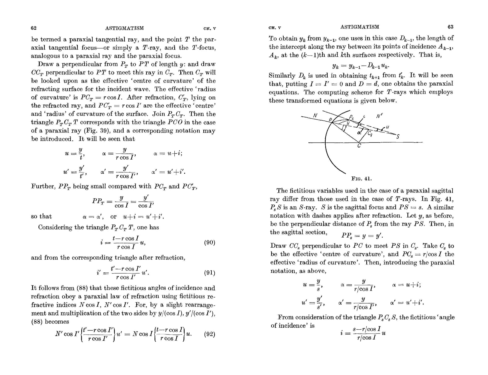
V. ASTIGMATISM 56
Aberration due to one refraction. Equations of refraction of
limitingly small pencils. Transformation of the formulae for
oblique refraction.
H.H.H.
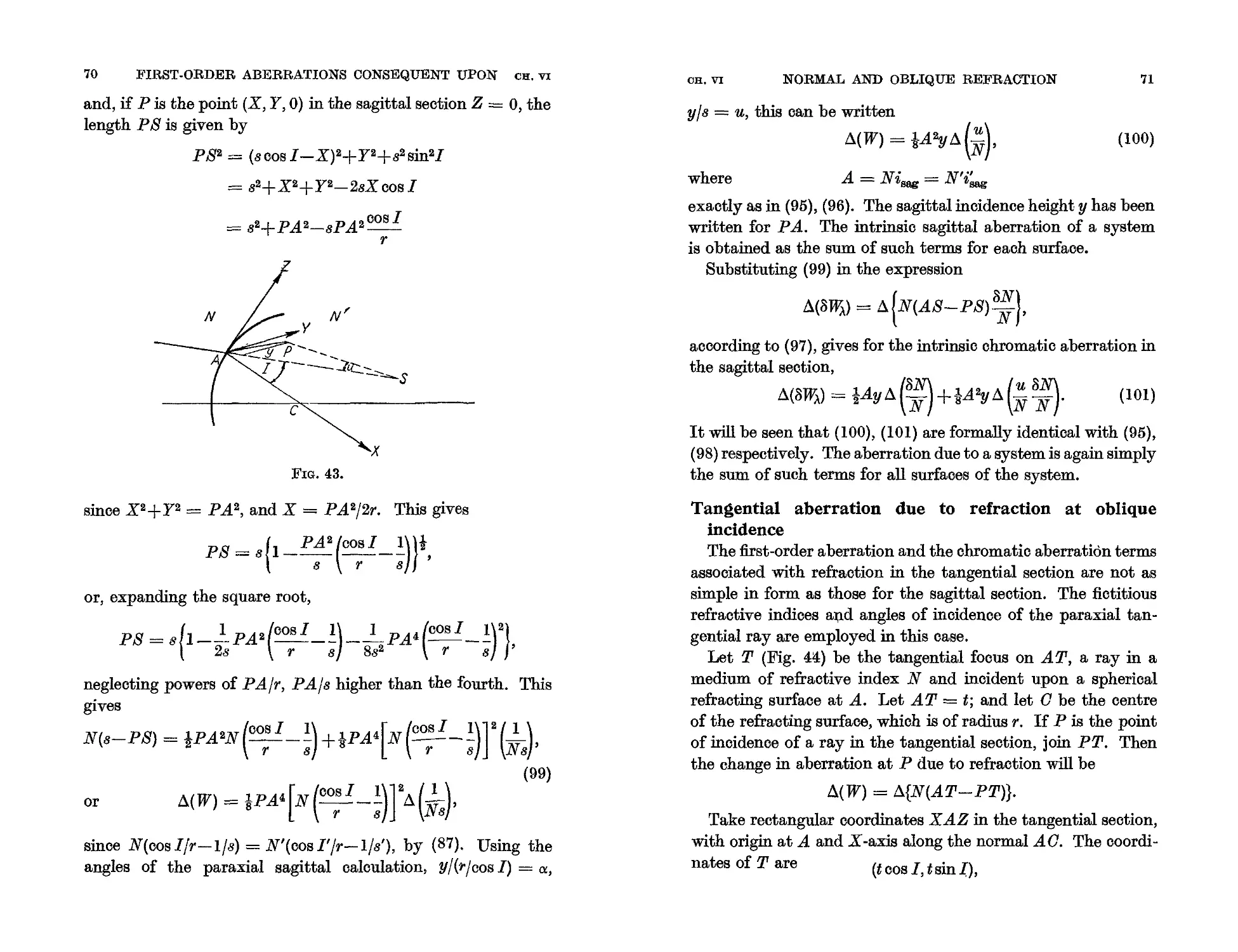
VI. FIRST-ORDER ABERRATIONS CONSEQUENT UPON
NORMAL AND OBLIQUE REFRACTION 66
Aberration due to refraction at normal incidence. Sagittal
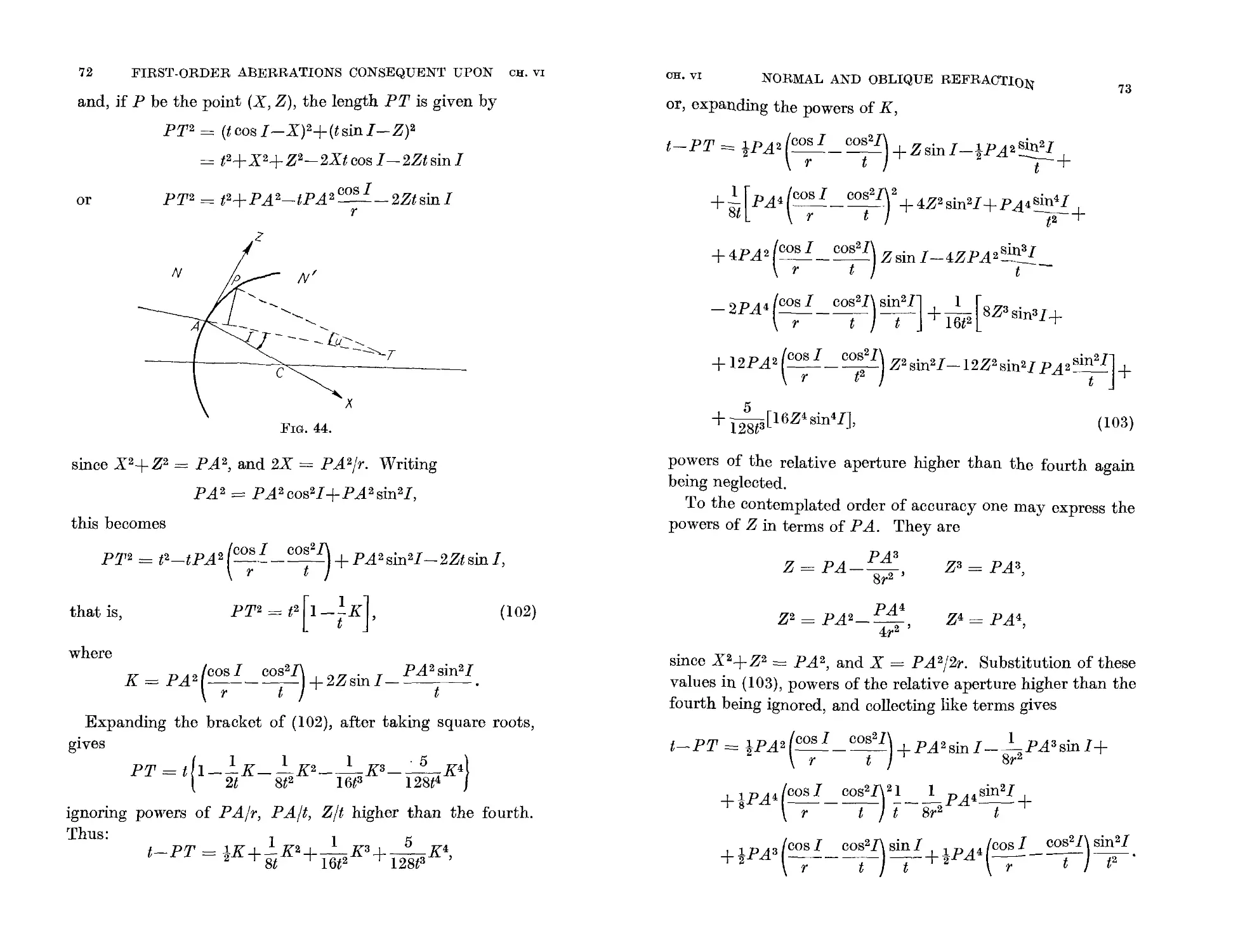
aberration due to refraction at oblique incidence. Tangential
aberration due to refraction at oblique incidence.
IMPERIAL COLLEGE
LONDON, S.w. 7
3 February 1950
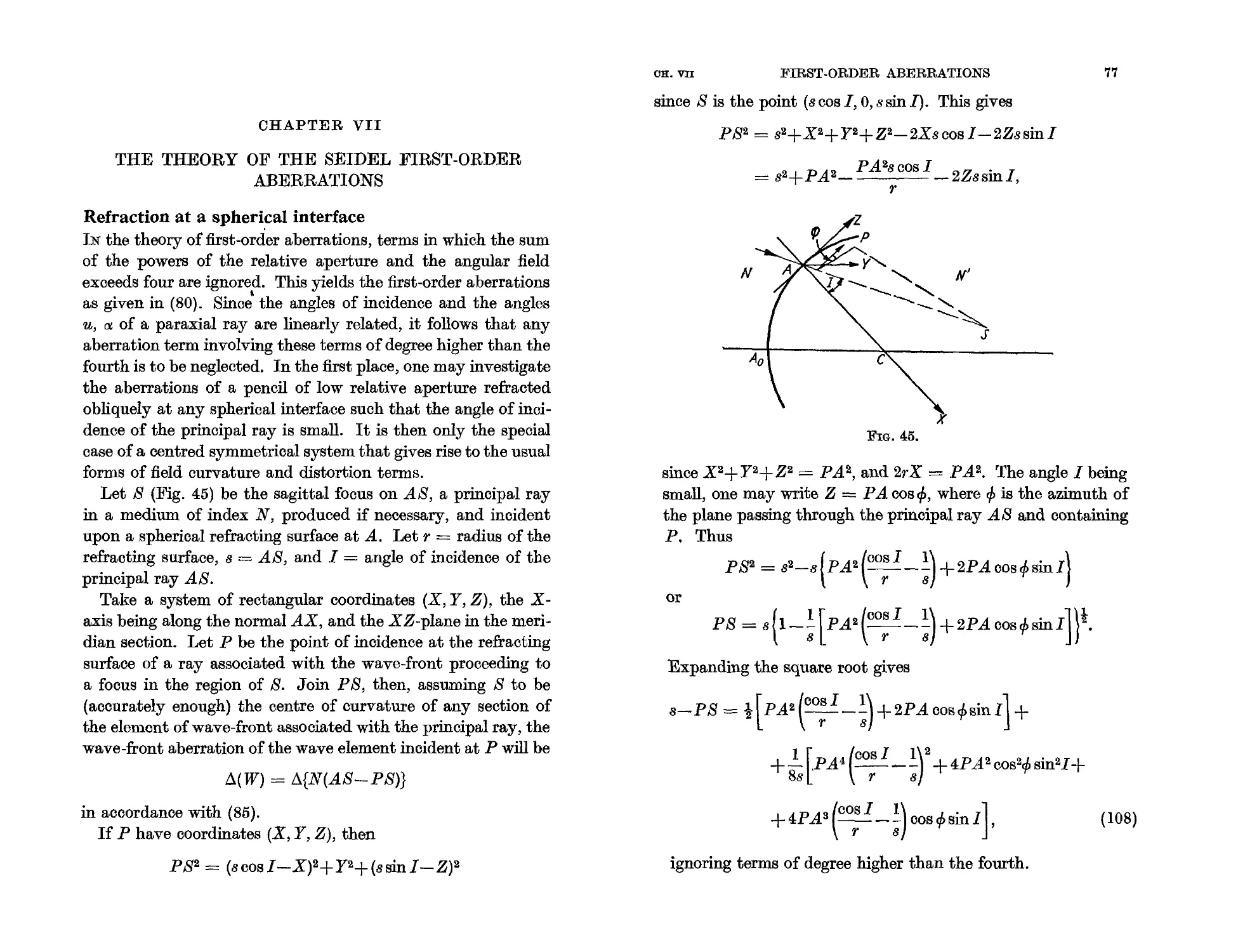
VII. THEORY OF THE SEIDEL FIRST-ORDER ABERRA.
TIONS 76
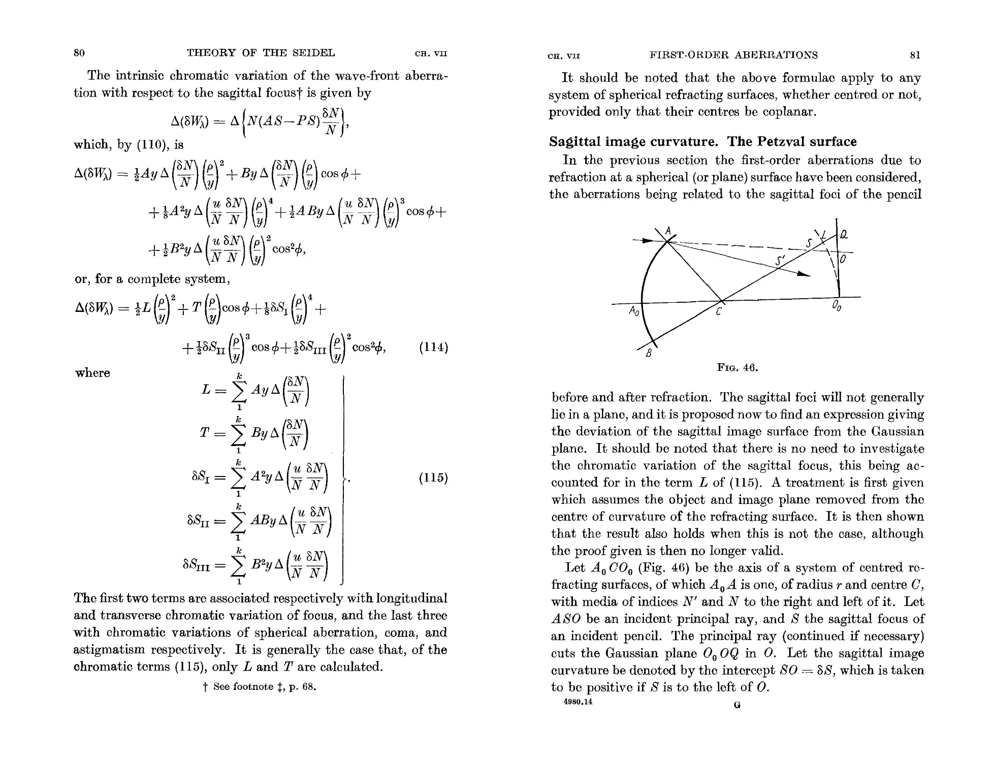
Refraction at a spherical interface. Sagittal image curvature.
The Petzval surface. Distortion of the image. Summary of
the Seidel aberration terms; their geometrical significance.
A difference formula for the paraxial principal ray. The
distortion coefficient, Bv, when A is small.

viii
CONTENTS
VIII. THE COMPUTATION OF THE FIRST-ORDER ABER-
RATIONS . 96
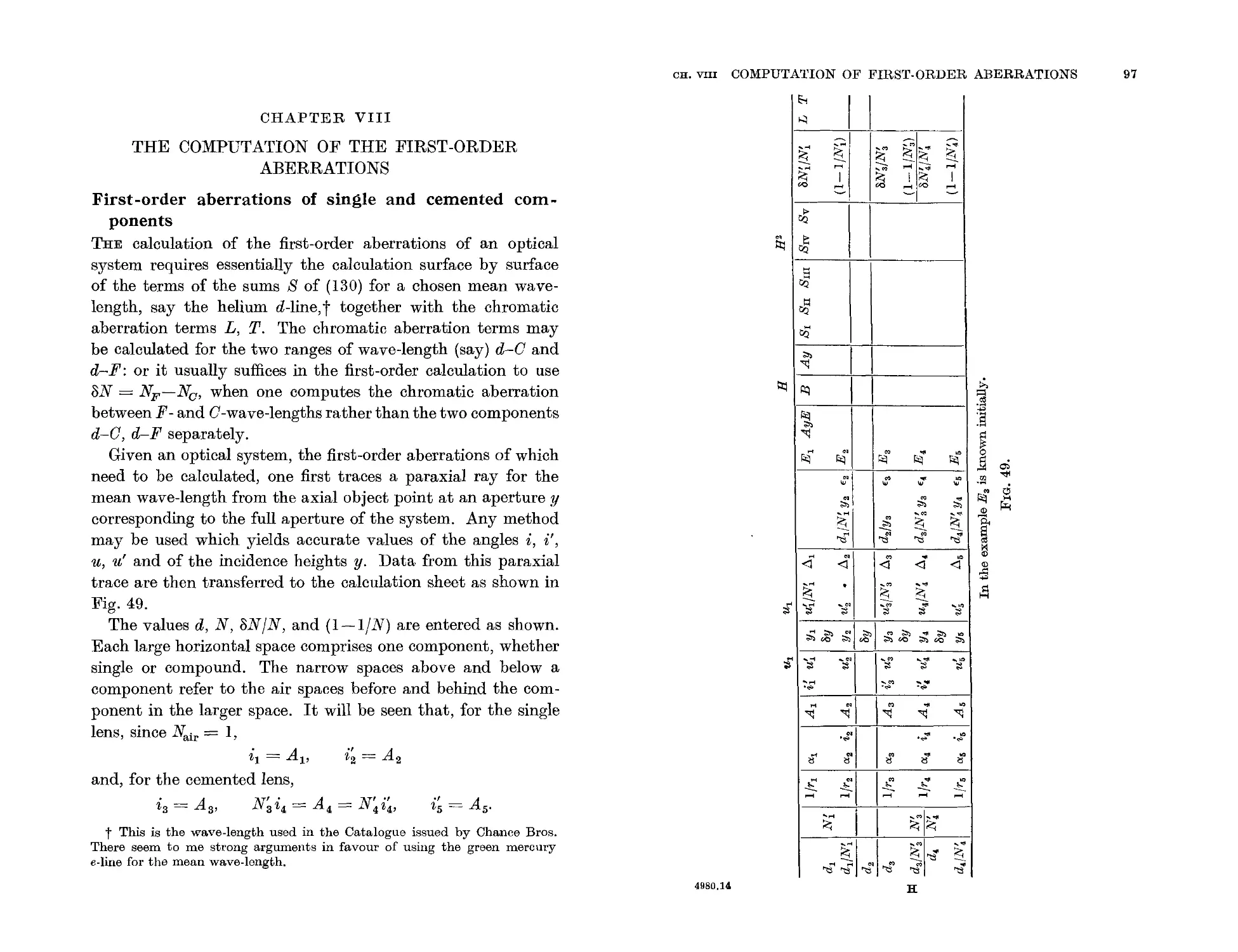
First-order aberrations of single and cemented components.
The changes in the first-order aberrations due to a change in
stop position. Certain first. order aberrations of thin lenses
which are independent of the lens shape. Bending a component
of an optical system. Changing a lens thiclmess or a separation.
Transferring power between two surfaces. Changing the glass
type of a component.
CHAPTER I
WAVE AND RAY ABERRATIONS
APPENDIXES
I. Ray-tracing formulae 159
II. The theory of pupils. Vignetting. Field Lenses 165
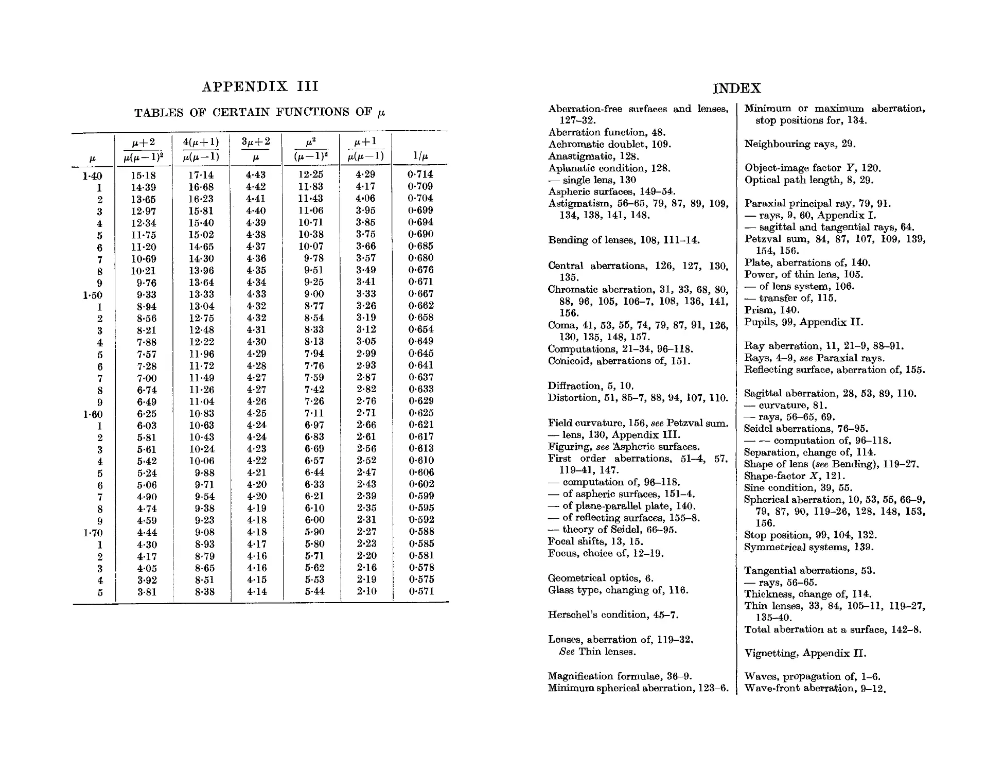
III. Tables of certain functions of fL 168
Introduction
OF the two types of theory which have been proposed to account
for the behaviour of light, the corpuscular and the wave theories,
the latter seem to give a satisfactory explanation of those pheno-
mena which do not involve the interaction of light and matter,
whereas the corpuscular theory does not. The processes of
absorption and emission, it is true, seem to demand a theory
of quanta. These processes, however, are not involved in those
aspects of the eory of lens systems to be considered here, and
accordingly the1iie will be treated from the standpoint of classical
wave theory.
From what follows it will be seen that, in general, the precise
nature of the wave disturbance need not concern one in treat-
ing the theory of aberrations. The wave disturbance will there-
fore be looked upon as a scalar quantity of an unspecified
nature. t
Wave propagation
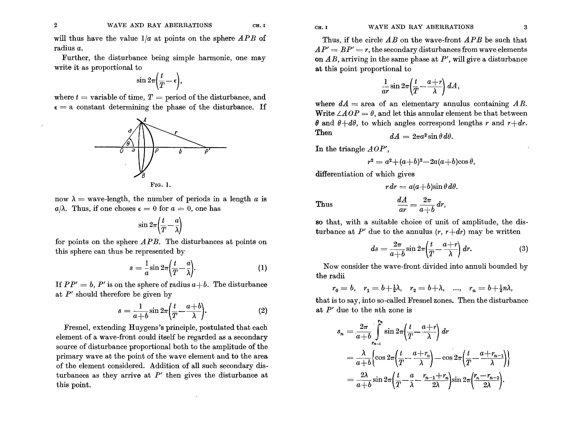
If 0, Fig. 1, is a source of monochromatic light, then a
disturbance emitted at a given instant by 0 will reach points
on a sphere AP B after a given time, and at points on this sphere
the disturbances will be in phase. That is, the sphere AP B is
a wave-front associated with the light emitted by O. Fresnel
has shown how the disturbance at a point P' beyond the wave-
front APB may be found.
Let the amplitude of the disturbance at points on a sphere
of unit radius, and of centre 0, be unity. Then, since the light
intensity is proportional to the square of the amplitude, and
the intensity is proportional to the inverse square of the distance
from the source, it follows that the amplitude must be pro-
portional to the reciprocal of the distance from the source. It
t For the sake of rigour OIle could, in. fact, look upon this scalar aB any of
the three components of the so-called Hertzian vector. See J. Picht, Optische
Abbildung (1931), p. 6.
4»80.14 B
IX. SOME GENERAL PROPERTIES OF THE ABERRA-
TIONS OF SINGLE LENSES AND LENS SYSTEMS 119
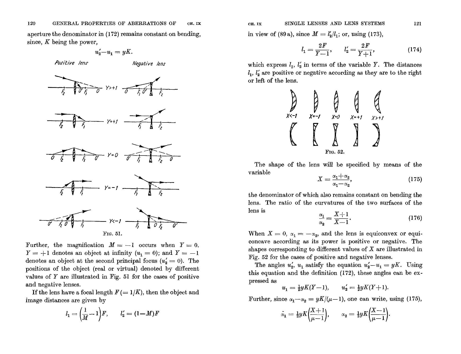
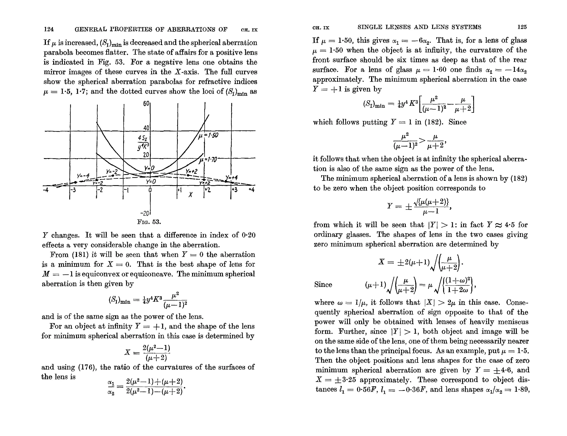
Spherical aberration of a thin lens considered as a function
of its shape. Central coma. Aberration-free lenses and
surfaces. The aberrations of a system considered as a function
of the diaphragm position. Systems of separated thin lenses.
The first-order aberrations of a plane-parallel plate.
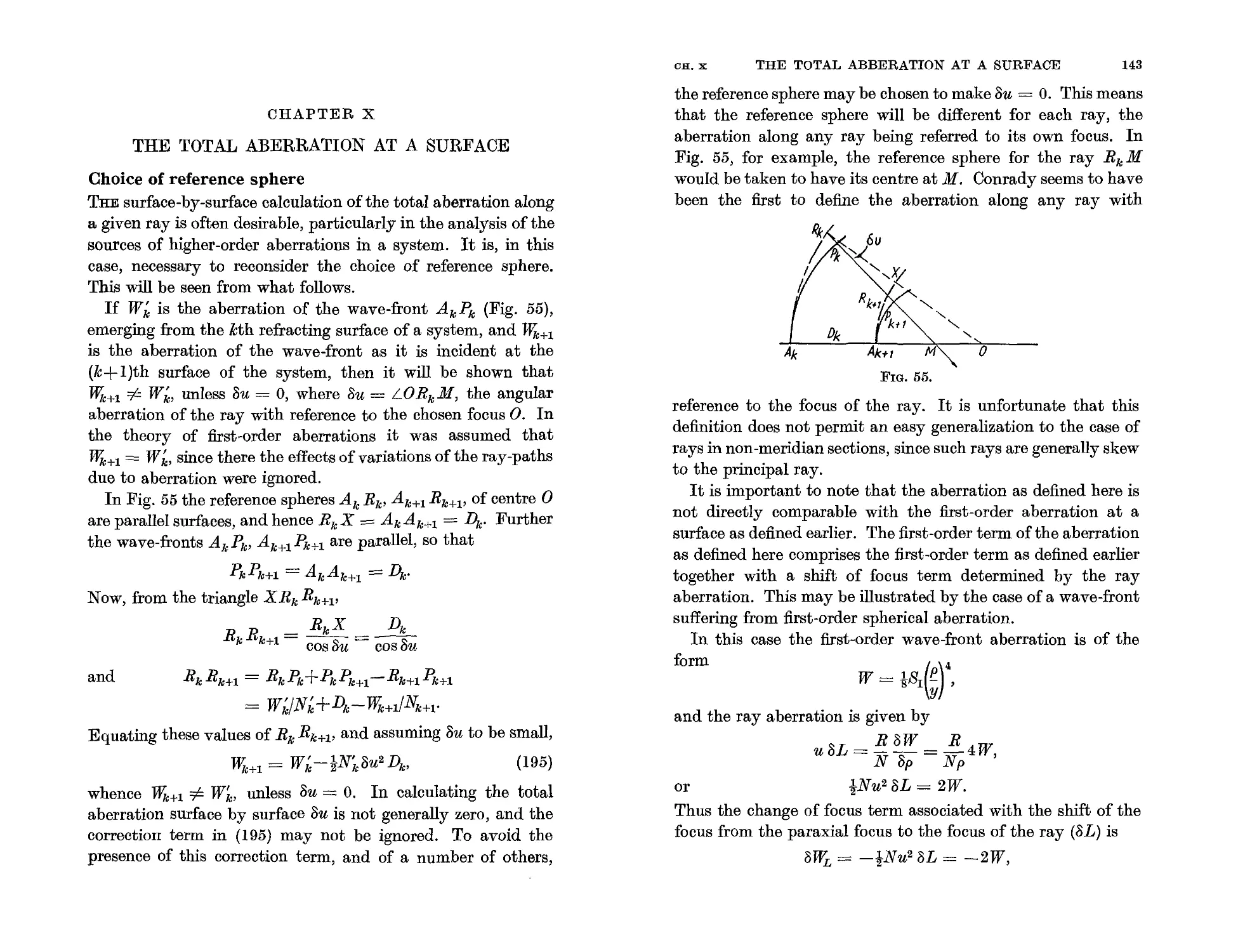
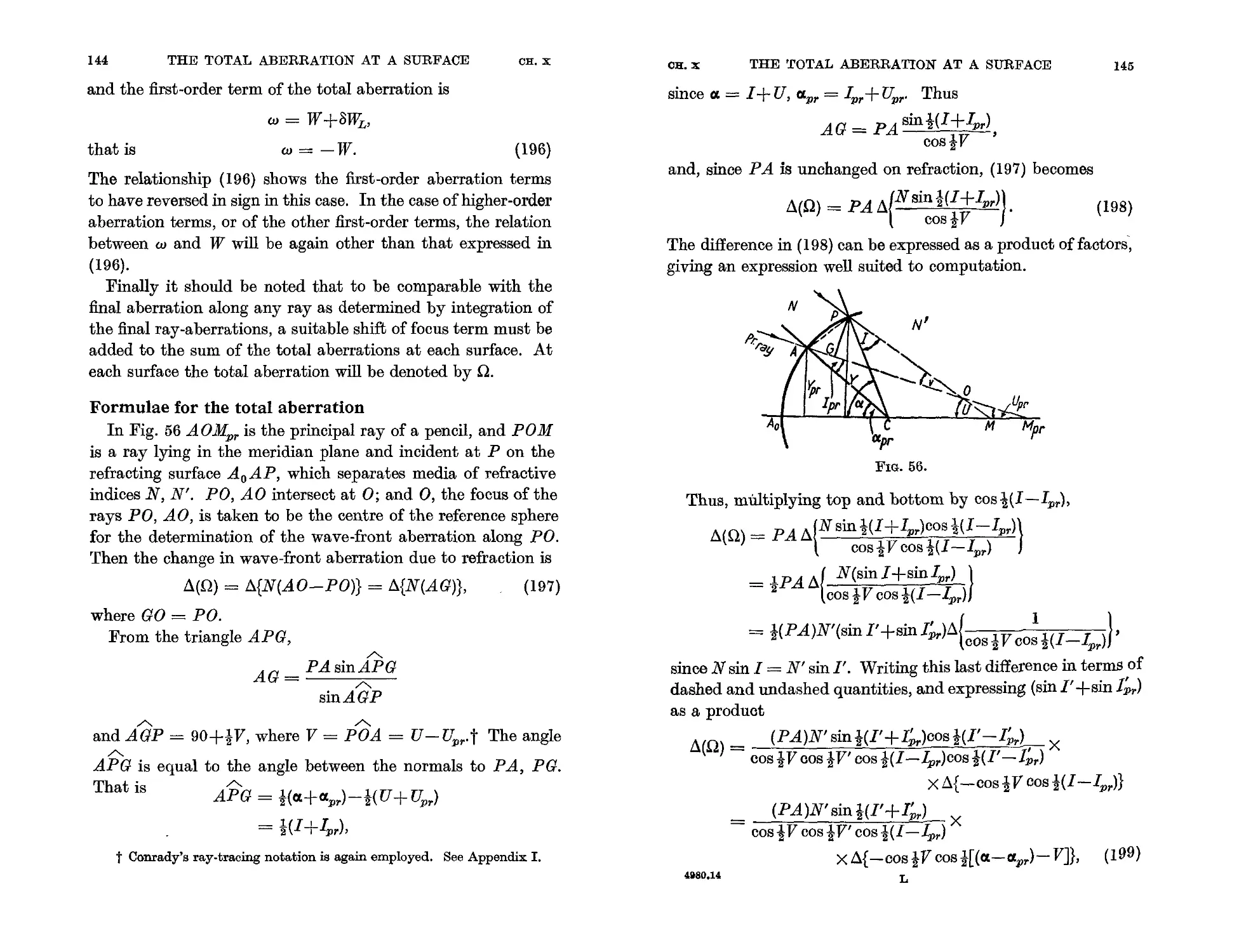
X. THE TOTAL ABERRATION AT A SURFACE. 142
Choice of reference sphere. Formulae for the total aberration.
The first-order terms of the total aberration.
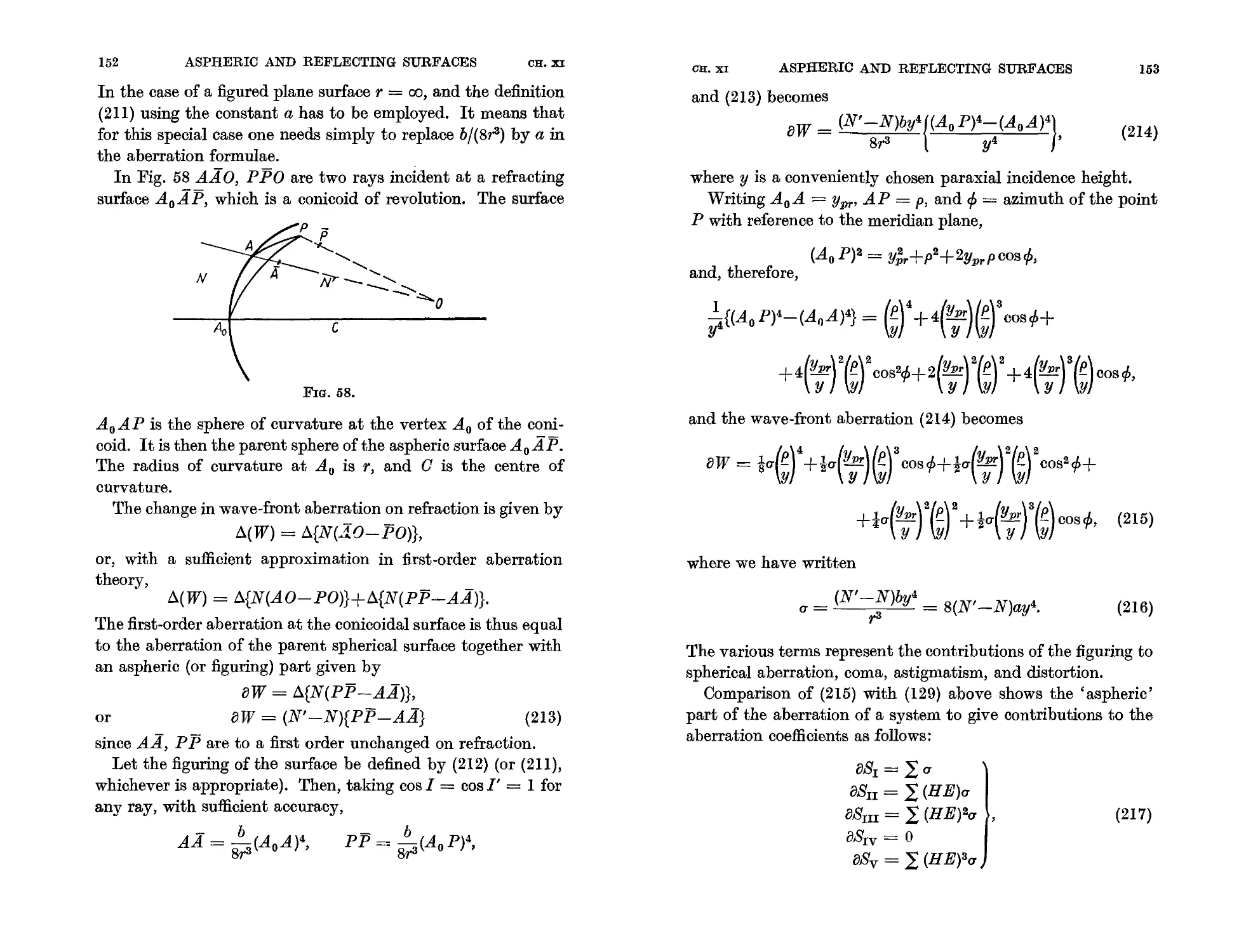
XI. ASPHERIC AND REFLECTING SURFACES 149
Aberration at a figured spherical surface. First-order aberra-
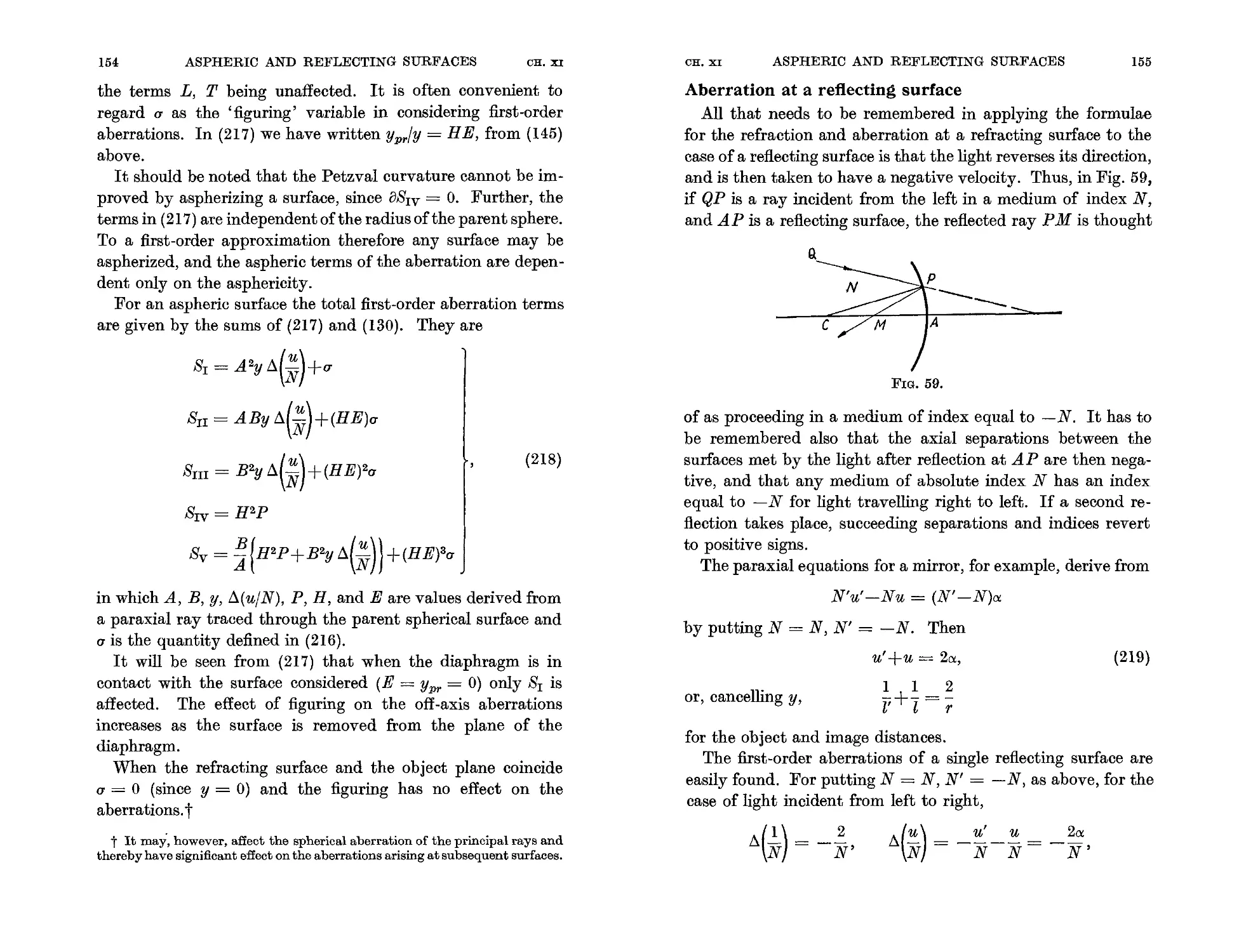
tions of aspheric systems. Aberration at a reflecting surface.
INDEX 169

2
WAVE AND RAY ABERRATIONS
CR. I
CR. I
WAVE AND RAY ABERRATIONS
3
will thus have the value l/a at points on the sphere APB of
radius a.
Further, the disturbance being simple harmonic, one may
write it as proportional to
sin217 ( -€),
where t = variable of time, T = period of the disturbance, and
E = a constant determining the phase of the disturbance. If
pi
Thus, if the circle AB on the wave-front AP B be such that
Api = Bpi = r, the secondary disturbances from wave elements
on AB, arriving in the same phase at pi, will give a disturbance
at this point proportional to
 sin 217 ( !.. _ a+r ) dA,
ar T A
where dA = area of an elementary annulus containing AB.
Write LAOP = (), and let this annular element be that between
8 and ()+d(), to which angles correspond lengths rand r+dr.
Then dA = 217a 2 sin () d().
In the triangle A 0 pi,
r 2 = a 2 +(a+b)2-2a(a+b)cos(),
differentiation of which gives
rdr = a(a+b)sin()d().
Thus dA = 217 dr,
ar a+b
so that, with a suitable choice of unit of amplitude, the dis-
turbance at pi due to the annulus (r, r+dr) may be written
ds = ab sin 217 ( - atr) dr. (3)
Now consider the wave-front divided into annuli bounded by
the radii
ro = b, r 1 = b+tA, r 2 = b+A, ..., r n = b+tnA,
that is to say, into so-called Fresnel zones. Then the disturbance
at pi due to the nth zone is
FIG. 1.
now A = wave-length, the number of periods in a length a is
a/A. Thus, if one choses E = 0 for a  0, one has
sin 217(- X)
for points on the sphere AP B. The disturbances at points on
this sphere can thus be represented by
8 = sin217 ( -X)' (1)
If PP ' = b, pi is on the sphere of radius a+b. The disturbance
at pi should therefore be given by
8 = ab sin 217(- at b ). (2)
Fresnel, extending Huygens's principle, postulated that each
element of a wave-front could itself be regarded as a secondary
source of disturbance proportional both to the amplitude of the
primary wave at the point of the wave element and to the area
of the element considered. Addition of all such secondary dis-
turbances as they arrive at pi then gives the disturbance at
this point.
217 . f r... ( t a+r )
8 = - sm217 --- dr
n 'a+b T A
Tn_l
=  { COS217 ( i- a+rn ) _cos'217 ( i_ a+rn-l ) }
a+b TAT A
_ 2,\ . 2 ( t a r n - 1 +rn ) . 2 ( r n -rn-l )
- a+b sm 17 T -X- 2A sm 17 2A .

4
WAVE AND RAY ABERRATIONS
CH. I
CR. I
WAVE AND RAY ABERRATIONS
5
Substituting
2n-l
i(rn-1+r n ) = b+-A,
4
i(r n -r n - l ) = lA,
fore the later form of a wave-front will be a surface 'parallel'
to the original front.
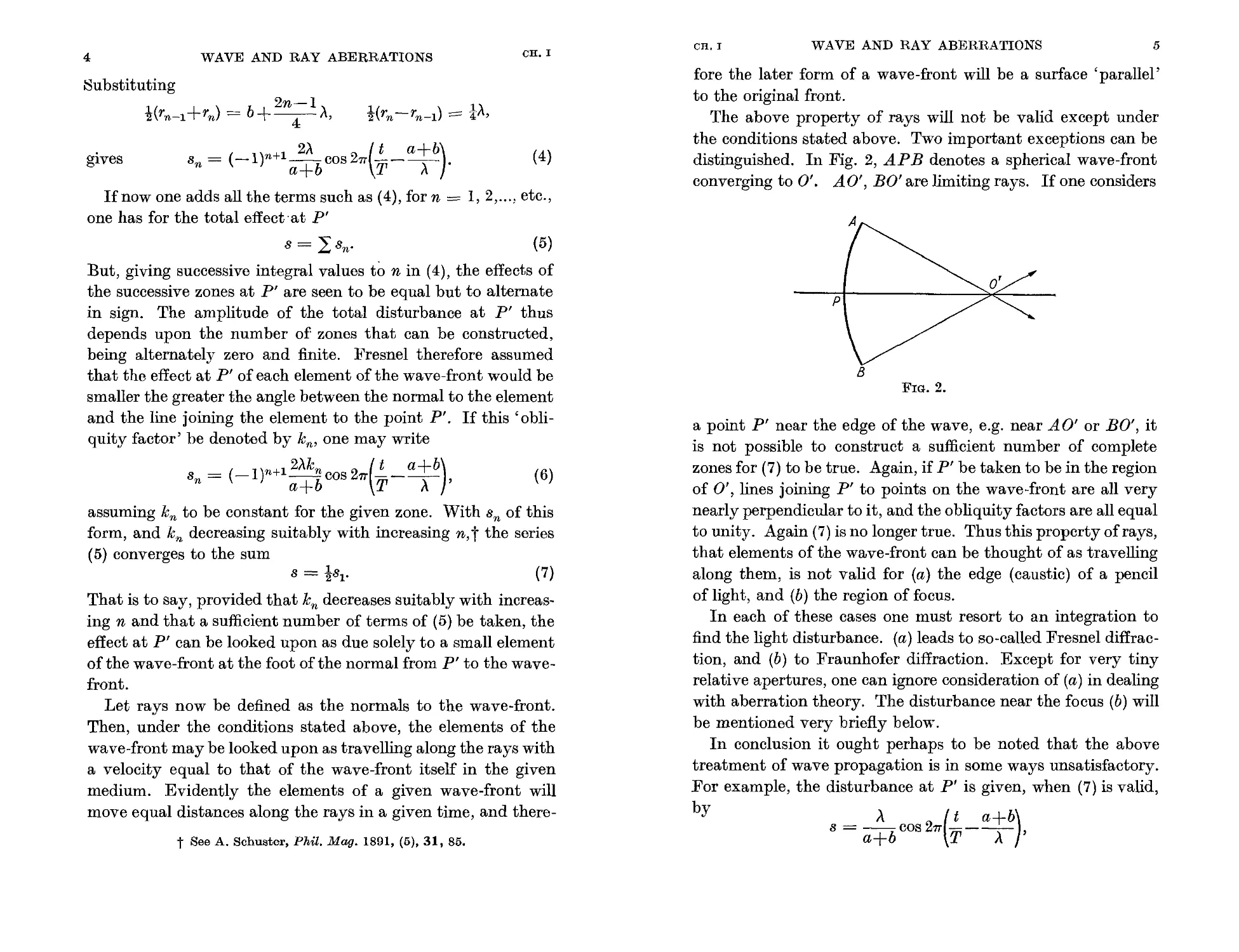
The above property of rays will not be valid except under
the conditions stated above. Two important exceptions can be
distinguished. In Fig. 2, AP B denotes a spherical wave-front
converging to 0'. AO', BO' are limiting rays. If one considers
gives 8n = (-1)n+1cos27T ( - a+b ) (4)
a+b T A.
If now one adds all the terms such as (4), for n = 1, 2,..., etc.,
one has for the total effect 'at p'
S = LSn' (5)
But, giving successive integral values to n in (4), the effects of
the successive zones at P' are seen to be equal but to alternate
in sign. The amplitude of the total disturbance at P' thus
depends upon the number of zones that can be constructed,
being alternately zero and finite. Fresnel therefore assumed
that the effect at P' of each element of the wave-front would be
smaller the greater the angle between the normal to the element
and the line joining the element to the point P'. If this 'obli-
quity factor' be denoted by k n , one may write
8 = ( _I ) n+1 2Akn cos 27T (  _ a+b ) ( 6 )
n a+b T,\'
assuming k n to be constant for the given zone. With 8n of this
form, and k n decreasing suitably with increasing n, t the series
(5) converges to the sum
p
B
FIG. 2.
8 = iSl'
(7)
a point P' near the edge of the wave, e.g. near AO' or BO', it
is not possible to construct a sufficient number of complete
zones for (7) to be true. Again, if P' be taken to be in the region
of 0', lines joining P' to points on the wave-front are all very
nearly perpendicular to it, and the obliquity factors are all equal
to unity. Again (7) is no longer true. Thus this propcrty of rays,
that elements of the wave-front can be thought of as travelling
along them, is not valid for (a) the edge (caustic) of a pencil
oflight, and (b) the region offocus.
In each of these cases one must resort to an integration to
find the light disturbance. (a) leads to so-called Fresnel diffrac-
tion, and (b) to Fraunhofer diffraction. Except for very tiny
relative apertures, one can ignore consideration of (a) in dealing
with aberration theory. The disturbance near the focus (b) will
be mentioned very briefly below.
In conclusion it ought perhaps to be noted that the above
treatment of wave propagation is in some ways unsatisfactory.
For example, the disturbance at P' is given, when (7) is valid,
by
8 = COS27T ( - a+b )
a+b T,\'
That is to say, provided that k n decreases suitably with increas-
ing n and that a sufficient number of terms of (5) be taken, the
effect at P' can be looked upon as due solely to a small element
of the wave-front at the foot of the normal from P' to the wave-
front.
Let rays now be defined as the normals to the wave-front.
Then, under the conditions stated above, the elements of the
wave-front may be looked upon as travelling along the rays with
a velocity equal to that of the wave-front itself in the given
medium. Evidently the elements of a given wave-front will
move equal distances along the rays in a given time, and there-
t See A. Schuster, Phil. Mag. 1891, (5),31,85.

6
WAVE AND RAY ABERRATIONS
CH. I
CH. I
WAVE AND RAY ABERRATIONS
7
and comparison of this with (2) shows a discrepancy of phase.
However, a more rigorous formulation of the Huygens-Fresnel
principle has been given by Kirchhoff, t and a treatment of the
problem based upon Kirchhoff's integral meets both this and
other objections. The general theory of spherical waves has
been treated in detail by Debye upon this basis.t
Geometrical optics
Rays have been defined here as the normals to the wave-
fronts, and it will be seen that rays thus defined correspond, in
fact, with the rays of geometrical optics. For, as shown by
Huygens (Treatise on Light, 1695), wave elements are reflected
and refracted such that their normals obey the ordinary laws
of reflection and refraction. There is one case, however, which
calls for further consideration.
It has been seen that the property which permits one to regard
rays as the paths along which wave elements travel is no longer
valid in the region of focus of converging waves. Nevertheless
one can still treat rays as obeying the ordinary laws of reflection
and refraction even in the region of focus. This can be justified
as follows.
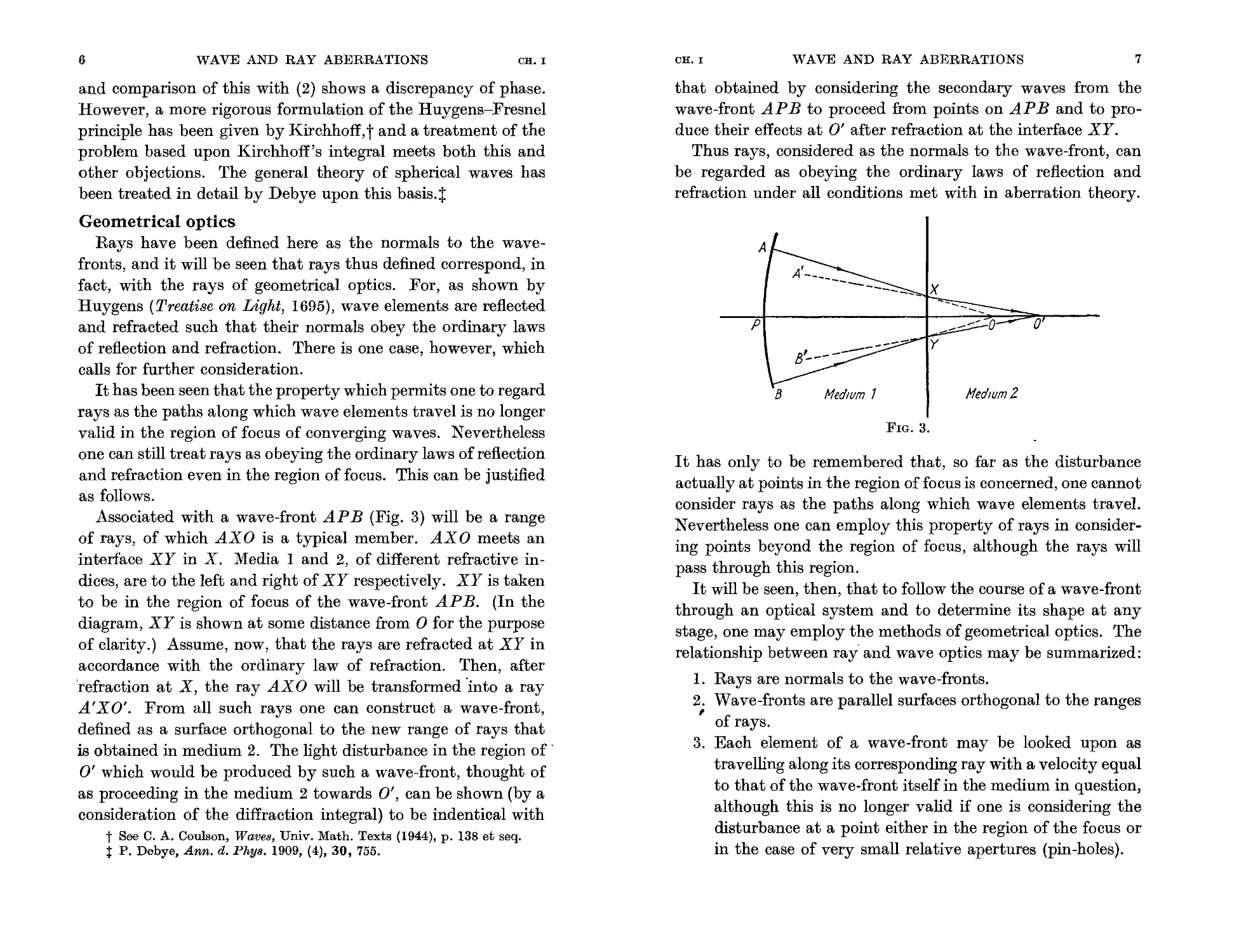
Associated with a wave-front AP B (Fig. 3) will be a range
of rays, of which AXO is a typical member. AXO meets an
interface XY in X. Media 1 and 2, of different refractive in-
dices, are to the left and right of XY respectively. XY is taken
to be in the region of focus of the wave-front AP B. (In the
diagram, XY is shown at some distance from 0 for the purpose
of clarity.) Assume, now, that the rays are refracted at XY in
accordance with the ordinary law of refraction. Then, after
'refraction at X, the ray AXO will be transformed'into a ray
A'XO'. From all such rays one can construct a wave-front,
defined as a surface orthogonal to the new range of rays that
is obtained in medium 2. The light disturbance in the region of'
0' which would be produced by such a wave-front, thought of
as proceeding in the medium 2 towards 0', can be shown (by a
consideration of the diffraction integral) to be indentical with
t See C. A. Coulson, Waves, Univ. Math. Texts (1944), p. 138 et seg.
:t P. Debye, Ann. d. Phys. 1909, (4), 30, 755.
that obtained by considering the secondary waves from the
wave-front AP B to proceed from points on AP B and to pro-
duce their effects at 0' after refraction at the interface XY.
Thus rays, considered as the normals to the wave-front, can
be regarded as obeying the ordinary laws of reflection and
refraction under all conditions met with in aberration theory.
p
o
B
FIG. 3.
It has only to be remembered that, so far as the disturbance
actually at points in the region of focus is concerned, one cannot
consider rays as the paths along which wave elements travel.
Nevertheless one can employ this property of rays in consider-
ing points beyond the region of focus, although the rays will
pass through this region.
It will be seen, then, that to follow the course of a wave-front
through an optical system and to determine its shape at any
stage, one may employ the methods of geometrical optics. The
relationship between ray' and wave optics may be summarized:
1. Rays are normals to the wave-fronts.
2. Wave-fronts are parallel surfaces orthogonal to the ranges
,
of rays.
3. Each element of a wave-front may be looked upon as
travelling along its corresponding ray with a velocity equal
to that of the wave-front itself in the medium in question,
although this is no longer valid if one is considering the
disturbance at a point either in the region of the focus or
in the case of very small relative apertures (pin-holes).

8
WAVE AND RAY ABERRATIONS
CH. I
CR.!
WAVE AND RAY ABERRATIONS
9
To these must be added consideration of the concept of optical
path lengths along the rays.
From the point of view ofthe wave theory oflight, the refrac-
tive index of a medium is defined as the ratio of the velocity of
the wave in a vacuum to the velocity in the medium. For con-
venience one measures and specifies in practice refractive indices
o
o
length of an optically equivalent path in air, taking N to be
the index relative to air. Further, being proportional to
(N/TTair)d = djV,
it is a measure of the time required for the wave to travel a
distance d in the medium. The significance of (8) is then:
4. Optical paths along the rays between corresponding wave-
fronts are all equal.
Knowing the course of a range of rays through a system one
can determine the shape of the wave-front at any stage by using
either of the principles expressed in 2 and 4. It will be seen in
what follows that both these methods find considerable applica-
tion in the theory of aberrations.
p
N z
FIG. 4.
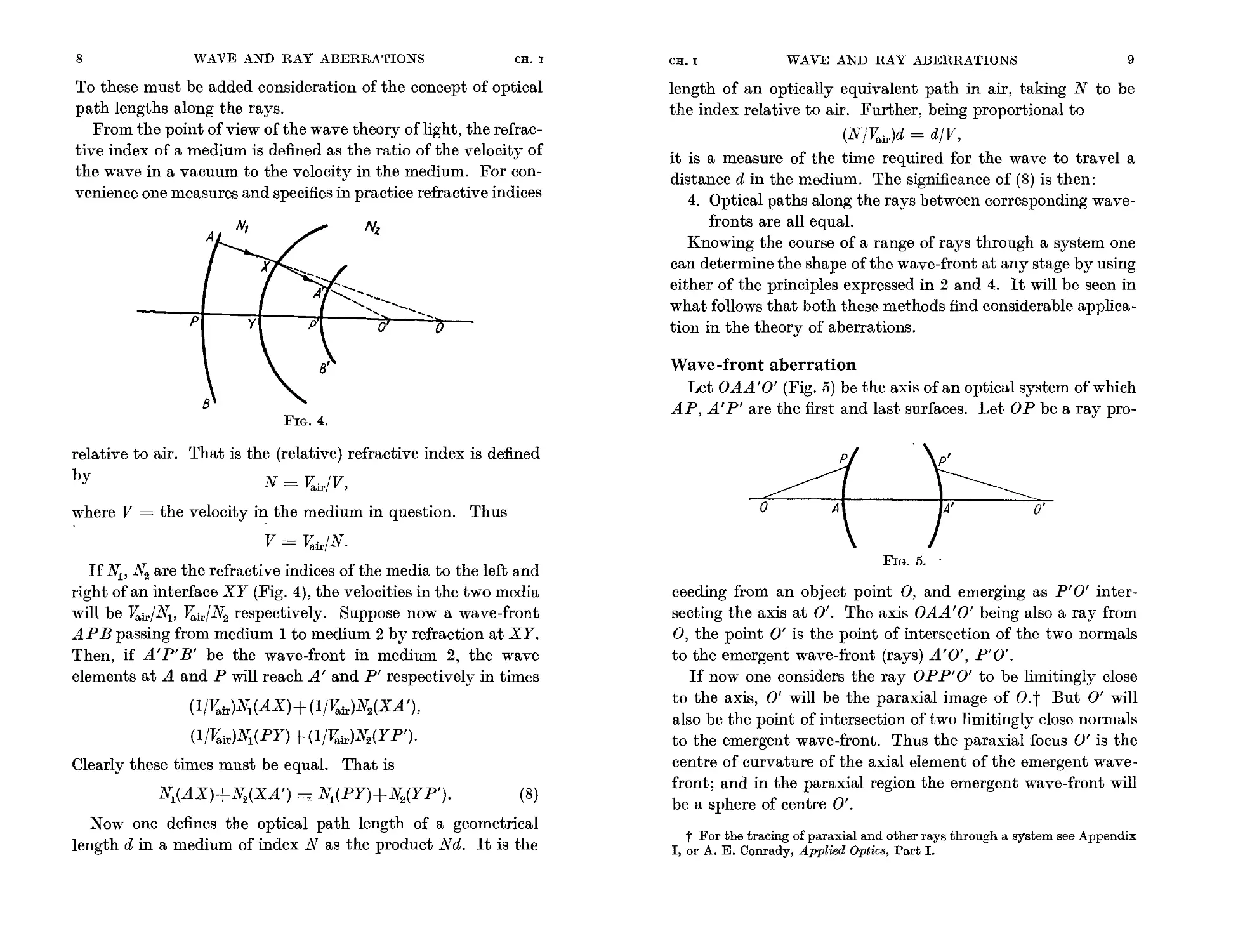
Wave-front aberration
Let OAA'O' (Fig. 5) be the axis of an optical system of which
AP, A'P' are the first and last surfaces. Let OP be a ray pro-
relative to air. That is the (relative) refractive index is defined
by N = Vair/ V ,
where V = the velocity in the medium in question. Thus
V = Vair/N.
If N v N 2 are the refractive indices of the media to the left and
right of an interface XY (Fig. 4), the velocities in the two media
will be TTair/' V air /N 2 respectively. Suppose now a wave-front
AP B passing from medium 1 to medium 2 by refraction at XY.
Then, if A'P'B' be the wave-front in medium 2, the wave
elements at A and P will reach A' and P' respectively in times
o
0'
FIG. 5. -
(1 /TTair)N 1 (AX) + (1 /Vair)N 2 (XA '),
(ljVair)N 1 (PY)+ (1/Vair)N 2 (Y P').
Clearly these times must be equal. That is
N 1 (AX)+N 2 (XA') =T N 1 (PY)+N 2 (YP'). (8)
Now one defines the optical path length of a geometrical
length d in a medium of index N as the product N d. It is the
ceeding from an object point 0, and emerging as P'O' inter-
secting the axis at 0'. The axis OAA' 0' being also a ray from
0, the point 0' is the point of intersection of the two normals
to the emergent wave-front (rays) A'O', P'O'.
H now one considers the ray OPP'O' to be limitingly close
to the axis, 0' will be the paraxial image of O.t But 0' will
also be the point of intersection of two limitingly close normals
to the emergent wave-front. Thus the paraxial focus 0' is the
centre of curvature of the axial element of the emergent wave-
front; and in the paraxial region the emergent wave-front will
be a sphere of centre 0'.
t For the tracing of paraxial and other rays through a system see Appendix
I, or A. E. Conrady, Applied Optics, Part 1.

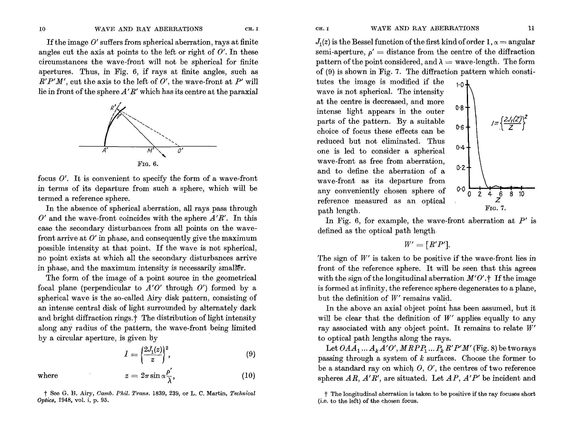
J 1 (z) is the Bessel function of the first kind of order 1, ex = angular
semi-aperture, p' = distance from the centre of the diffraction
pattern ofthe point considered, and.\ = wave-length. The form
of (9) is shown in Fig. 7. The diffraction pattern which consti-
tutes the image is modified if the 1.0
wave is not spherical. The intensity
at the centre is decreased, and more
intense light appears in the outer 0,8
parts of the pattern. By a suitable
choice of focus these effects can be 0'6
reduced but not eliminated. Thus
0'4
one is led to consider a spherical
wave-front as free from aberration,
and to define the aberration of a 0'2.
wave-front as its departure from
any conveniently chosen sphere of
reference measured as an optical
path length.
In Fig. 6, for example, the wave-front aberration at P' is
defined as the optical path length
The sign of W' is taken to be positive if the wave-front lies in
front of the reference sphere. It will be seen that this agrees
with the sign of the longitudinal aberration M' 0'. t If the image
is formed at infinity, the reference sphere degenerates to a plane,
but the definition of W' remains valid.
In the above an axial object point has been assumed, but it
will be clear that the definition of W' applies equally to any
ray associated with any object point. It remains to relate W'
to optical path lengths along the rays.
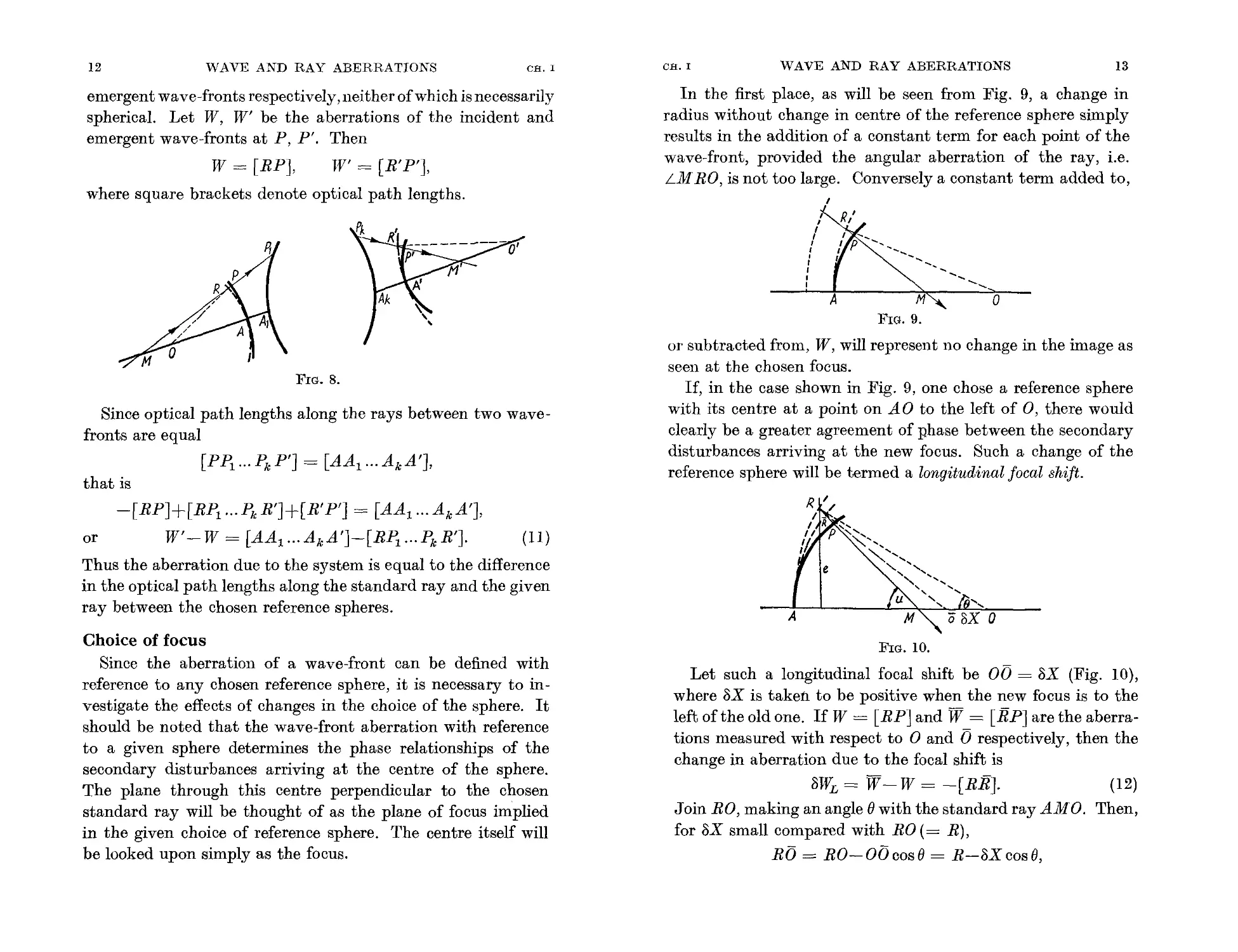
Let OAA1...AkA'0', MRPPr ...PkR' P'M ' (Fig. 8) be two rays
passing through a system of k surfaces. Choose the former to
be a standard rayon whic4 0, 0', the centres of two reference
spheres AR, A'R', are situated. Let AP, A' P' be incident and
10
WAVE AND RAY ABERRATIONS
WAVE AND RAY ABERRATIONS
CR. I
CH. I
If the image 0' suffers from spherical aberration, rays at finite
angles cut the axis at points to the left or right of 0'. In these
circumstances the wave-front will not be spherical for finite
apertures. Thus, in Fig. 6, if rays at finite angles, such as
R' P' M', cut the axis to the left of 0', the wave-front at P' will
lie in front of the sphere A' R' which has its centre at the paraxial
0'
FIG. 6.
focus OJ.. It is convenient to specify the form of a wave-front
in terms of its departure from such a sphere, which will be
termed a reference sphere.
In the absence of spherical aberration, all rays pass through
0' and the wave-front coincides with the sphere A'R'. In this
case the secondary disturbances from all points on the wave-
front arrive at 0' in phase, and consequently give the maximum
possible intensity at that point. If the wave is not spherical,
no point exists at which all the secondary disturbaces arrive
in phase, and the maximum intensity is necessarily smal:mr.
The form of the image of a point source in the geometrical
focal plane (perpendicular to A'O' through 0') formed by a
spherical wave is the so-called Airy disk pattern, consisting of
an intense central disk of light surrounded by alternately dark
and bright diffraction rings. t The distribution of light intensity
along any radius of the pattern, the wave-front being limited
by a circular aperture, is given by
I = { 2J(Z) r (9)
W' = [R'P'].
where
z = 21TSinex t
'\'
(10)
t See G. B. Airy, Oamb. Phil. Tran8. 1839, 239, or L. C. Martin, Technical
Optics, 1948, vol. i, p. 95.
11
1= { 21(L) t
0'0 0 2. 4 6 8 10
Z
FIG. 7.
t The longitudinal aberration is taken to be positive if the ray focuses short
(i.e. to the left) of the chosen focus.

12
WAVE AND RAY ABERRATIONS
CR. I
CR. I
WAVE AND RAY ABERRATIONS
13
W = [RP],
where square brackets denote optical path lengths.
W' = [R'P'],
In the first place, as will be seen from Fig. 9, a change in
radius without change in centre of the reference sphere simply
results in the addition of a constant term for each point of the
wave-front, provided the angular aberration of the ray, i.e.
LM RO, is not too large. Conversely a constant term added to,
emergent wa ve-fronts respectively, neither of which is necessarily
spherical. Let W, W' be the aberrations of the incident and
emergent wave-fronts at P, P'. Then
,
,
I
I
,
,
I
,
,
I
I
o
"
.....,
FIG. 8.
or subtracted from, W, will represent no change in the image as
seen at the chosen focus.
If, in the case shown in Fig. 9, one chose a reference sphere
with its centre at a point on AO to the left of 0, there would
clearly be a greater agreement of phase between the secondary
disturbances arriving at the new focus. Such a change of the
reference sphere will be termed a longitudinal focal shift.
Since optical path lengths along the rays between two wave-
fronts are equal
[PP1...PkP'] = [AAl...AkA'],
that is
-[RP]+[RP1...PkR']+[R'P'] = [AAl...AkA'],
or W'- W = [AAl...AkA']-[R",PkR']. (11)
Thus the aberration due to the system is equal to the difference
in the optical path lengths along the standard ray and the given
ray between the chosen reference spheres.
......
Choice of focus
Since the aberration of a wave-front can be defined with
reference to any chosen reference sphere, it is necessary to in-
vestigate the effects of changes in the choice of the sphere. It
should be noted that the wave-front aberration with reference
to a given sphere determines the phase relationships of the
secondary disturbances arriving at the centre of the sphere.
The plane through this centre perpendicular to the chosen
standard ray will be thought of as the plane of focus implied
in the given choice of reference sphere. The centre itself will
be looked upon simply as the focus.
FIG. 10.
Let such a longitudinal focal shift be 00 = SX (Fig. 10),
where SX is taken to be positive when the new focus is to the
left of the old one. If W = [RP] and W = [EP] are the aberra-
tions measured with respect to 0 and 0 respectively, then the
change in aberration due to the focal shift is
SW L = W - W = -[ RE]. (12)
Join RO, making an angle e with the standard ray AMO. Then,
for SX small compared with RO (= R),
RO = RO- 00 cos e = R-SX cos e,

14
W AVE AND RAY ABERRATIONS
CH. I
CH. I
WAVE AND RAY ABERRATIONS
15
110 = AO '-= R-SX,
so that R11 = SX(l-cosB),
and, by (12), the change in wave-front aberration is
SfJ'L = -N(l-cos 8) SX,
where N = refractive index of the medium concerned.
(13)
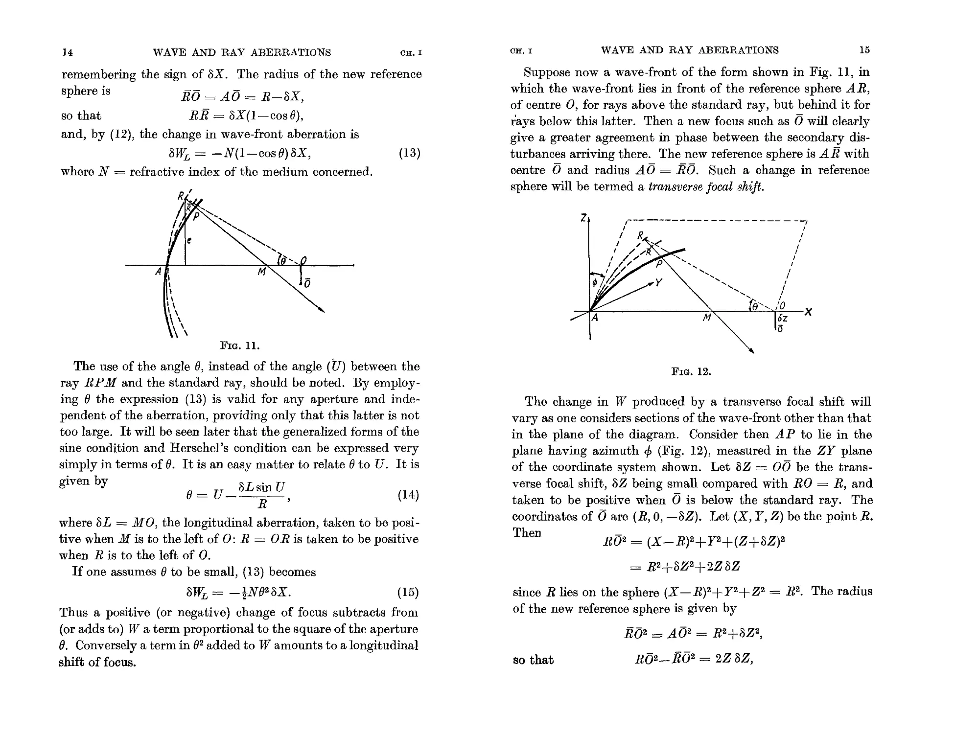
Suppose now a wave-front of the form shown in Fig. 11, in
which the wave-front lies in front of the reference sphere AR,
of centre 0, for rays above the standard ray, but behind it for
rays below this latter. Then a new focus such as 0 will clearly
give a greater agreement in phase between the secondary dis-
turbances arriving there. The new reference sphere is A11 with
centre 0 and radius AO = 110. Such a change in reference
sphere will be termed a transverse focal shift.
remembering the sign of ax. The radius of the new reference
sphere is
z
x
FIG. 11.
The use of the angle B, instead of the angle (U) between the
ray RP M and the standard ray, should be noted. By employ-
ing B the expression (13) is valid for any aperture and inde-
pendent of the aberration, providing only that this latter is not
too large. It will be seen later that the generalized forms of the
sine condition and Herschel's condition can be expressed very
simply in terms of B. It is an easy matter to relate B to U. It is
given by SL sin U
B = U R (14)
where SL = MO, the longitudinal aberration, taken to be posi-
tive when M is to the left of 0: R = ORis taken to be positive
when R is to the left of O.
If one assumes B to be small, (13) becomes
SfJ'L = -tN8 z aX. (15)
Thus a positive (or negative) change of focus subtracts from
(or adds to) W a term proportional to the square of the aperture
8. Conversely a term in BZ added to W amounts to a longitudinal
shift of focus.
FIG. 12.
The change in W produce,d by a transverse focal shift will
vary as one considers sections of the wave-front other than that
in the plane of the diagram. Consider then AP to lie in the
plane having azimuth 4> (Fig. 12), measured in the ZY plane
of the coordinate system shown. Let 3Z = 00 be the trans-
verse focal shift, SZ being small compared with RO = R, and
taken to be positive when 0 is below the standard ray. The
coordinates of 0 are (R, 0, -SZ). Let (X, Y, Z) be the point R.
Then
ROZ = (X-R)z+yz+(Z+SZ)Z
= RZ+Szz+2Z SZ
since R lies on the sphere (X-R)2+YZ+Z2 = R2. The radius
of the new reference sphere is given by
110 2 = A02 = R2+SZ2,
so that
R02- R02 = 2Z SZ,

16
WAVE AND RAY ABERRATIONS
CH. I
OH. t
w AVE AND RAY ABERRATIONS
17
or, ignoring higher powers of 'bZjR,
RH = RO-HO = Z 'bZ .
R
can be treated without any change in the basic definitions,
although the formulae for computation have occasionally to be
adapted to special cases-as exemplified by (18) and (19).
When considering only the plane containing cp = 0, cp = 7T,
it is often convenient to look upon 0 (or p) as positive or negative
according as R is above or below the standard ray, although in
the general case 0 and p are always positive, the change in sign
occurring on account of the factor cas cpo
Hence the change in W due to the transverse focal shift is
given by _ Z
'bW T = -[RR] = -N R 'bZ,
or, since Z = RsinOcoscp,
'bW T = -N sin 0 'bZ cos cpo (16)
Thus a positive transverse shift subtracts a term proportional
to sinO for rays above the standard ray (!cp! < t7T), and adds
a similar term for rays below it (!cpl > !7T). The change in W
is a maximum in the sections cp = 0, 7T, and decreases according
to the factor cos cp, becoming zero for the sections cp = !7T, 37Tj2.
If now 0 be small, one has in the XAZ plane
'bW T = -NOoZ (17)
and the change in W is proportional to the aperture O. Con-
versely the addition to, or subtraction from, W, of such a term
amounts to a transverse shift of foClUS.
When the image 0 is formed at n1finity, one requires only to
express the shift of focus in angular measure, and the aperture
linearly in each case. Let p = distance of R from the standard
ray; then, for small values of e, (13) becomes
SW L = -tN (r SX,
while the angular shift of focus is
SOL = P SXj R2.
aberration for a longitudinal focal shift
()
p
A
w
J \
J \
/ "-
I '..
" ..................E
./
o II
FIG. 13.
Thus the change in
'b0L is
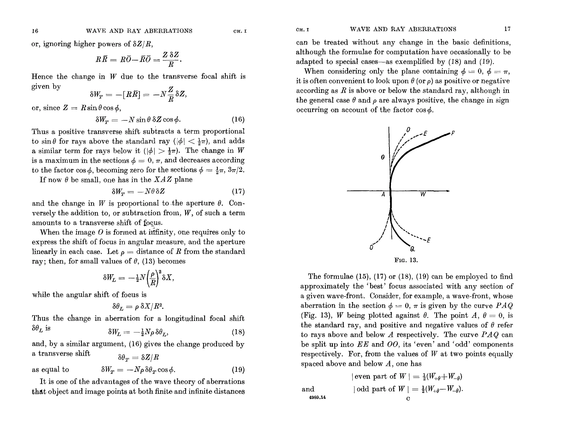
The formulae (15), (17) or (18), (19) can be employed to find
approximately the 'best' focus associated with any section of
a given wave-front. Consider, for example, a wave-front, whose
aberration in the section cp = 0, 7T is given by the curve P AQ
(Fig. 13), W being plotted against O. The point A, 0 = 0, is
the standard ray, and positive and negative values of 0 refer
to rays above and below A respectively. The curve P AQ can
be split up into EE and 00, its 'even' and 'odd' components
respectively. For, from the values of W at two points equally
spaced above and below A, one has
I even part of W I = t(W+ II + W- II )
and I odd part of W I = t(W+ II - W- II ).
4980.14 C
SW L = -tNpSBv (18)
and, by a similar argument, (16) gives the change produced by
a transverse shift
SOT = 'bZjR
as equal to 'bW T = -NpSOTCOSCP' (19)
It is one of the advantages of the wave theory of aberrations
thltt object and image points at both finite and infinite distances

18
WAVE AND RAY ABERRATIONS
CH. I
CR. I
WAVE AND RAY ABERRATIONS
19
One can then investigate separately the effects of longitudinal
and transverse focal shifts on the even and odd components
respectively. To do this it is convenient to adopt the following
procedure.
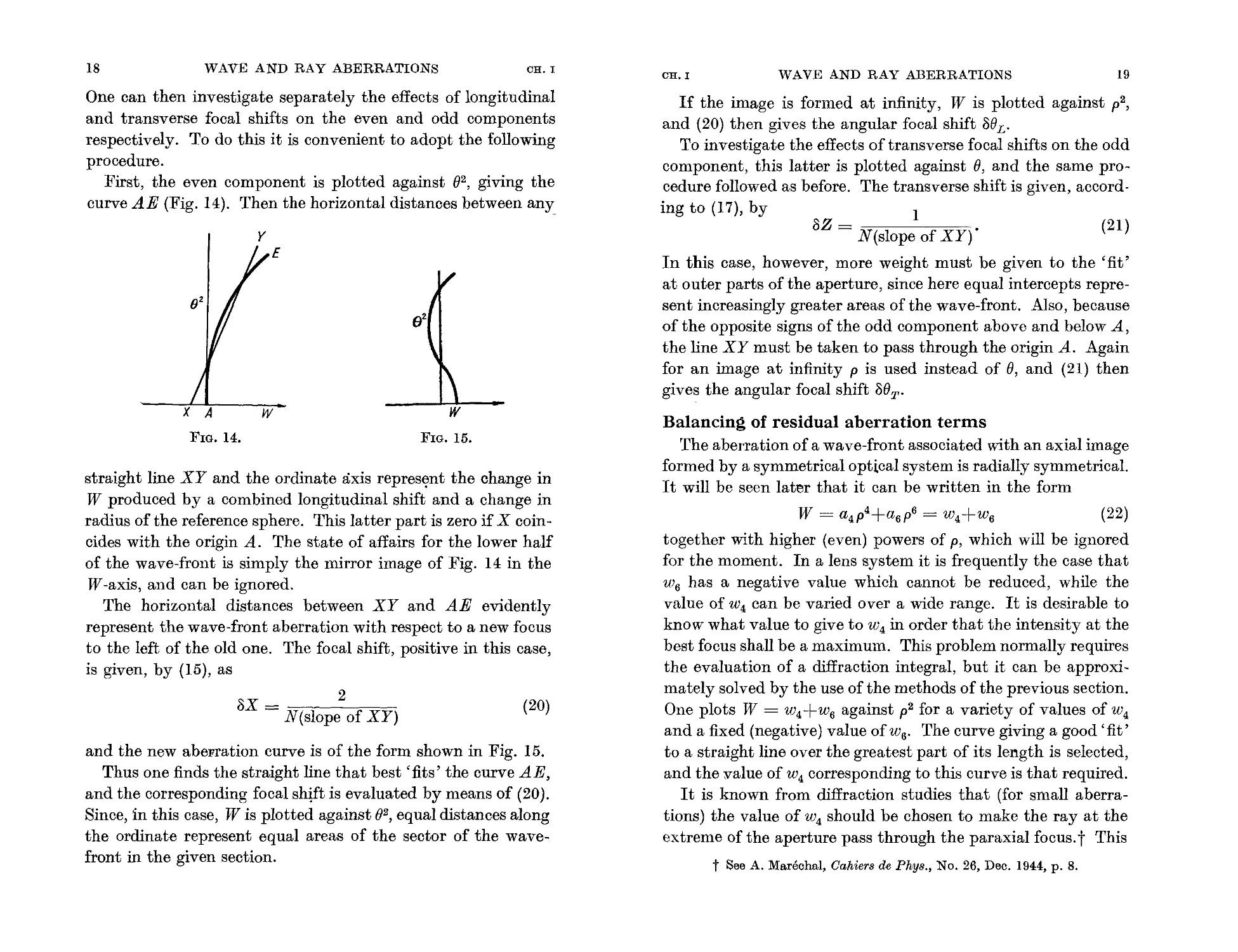
First, the even component is plotted against 8 2 , giving the
curve AE (Fig. 14). Then the horizontal distances between any,
e 2
If the image is formed at infinity, W is plotted against p2,
and (20) then gives the angular focal shift S8 L .
To investigate the effects of transverse focal shifts on the odd
component, this latter is plotted against 8, and the same pro-
cedure followed as before. The transverse shift is given, accord-
ing to (17), by 1
oZ = . ( 21 )
N(slope of XY)
In this case, however, more weight must be given to the 'fit'
at outer parts of the aperture, since here equal intercepts repre-
sent increasingly greater areas of the wave-front. Also, because
of the opposite signs of the odd component above and below A,
the line XY must be taken to pass through the origin A. Again
for an image at infinity p is used instead of 8, and (21) then
gives the angular focal shift o8 T .
Balancing of residual aberration terms
The aberration of a wave-front associated with an axial image
formed by a symmetrical optical system is radially symmetrical.
It will be seen later that it can be written in the form
W = a4p4+a6p6 = W 4 +W 6 (22)
together with higher (even) powers of p, which will be ignored
for the moment. In a lens system it is frequently the case that
W 6 has a negative value which cannot be reduced, while the
value of W 4 can be varied over a wide range. It is desirable to
know what value to give to W 4 in order that the intensity at the
best focus shall be a maximum. This problem normally requires
the evaluation of a diffraction integral, but it can be approxi-
mately solved by the use of the methods of the previous section.
One plots W = W 4 +W 6 against p2 for a variety of values of w 4
and a fixed (negative) value ofw 6 . The curve giving a good 'fit'
to a straight line over the greatest part of its length is selected,
and the value of W 4 corresponding to this curve is that required.
It is known from diffraction studies that (for small aberra-
tions) the value of W 4 should be chosen to make the ray at the
extreme of the aperture pass through the paraxial focus. t This
FIG. 14.
FIG. 15.
straight line XY and the ordinate axis represnt the change in
W produced by a combined longitudinal shift and a change in
radius of the reference sphere. This latter part is zero if X coin-
cides with the origin A. The state of affairs for the lower half
of the wave-front is simply the mirror image of Fig. 14 in the
W -axis, and can be ignored.
The horizontal distances between XY and AE evidently
represent the wave-front aberration with respect to a new focus
to the left of the old one. The focal shift, positive in this case,
is given, by (15), as
oX = 2 ( 20 )
N(slope of XY)
and the new abeFration curve is of the form shown in Fig. 15.
Thus one finds the straight line that best 'fits' the curve AE,
and the corresponding focal shift is evaluated by means of (20).
Since, in this case, W is plotted against 8 2 , equal distances along
the ordinate represent equal areas of the sector of the wave-
front in the given section.
t See A. Marechal, Gahiers de Phys., No. 26, Dec. 1944, p. 8.

20
WAVE AND RAY ABERRATIONS
CH. I
means that the wave-front must be parallel to the reference
sphere at the extreme aperture. The angular aberration of a
ray is given by
CHAPTER II
COMPUTATION OF WAVE-FRONT ABERRATIONS
 oW =  { W4 +W6 } '
N Op N p P
and this has to be zero. That is,
w 4 = -!w 6 .
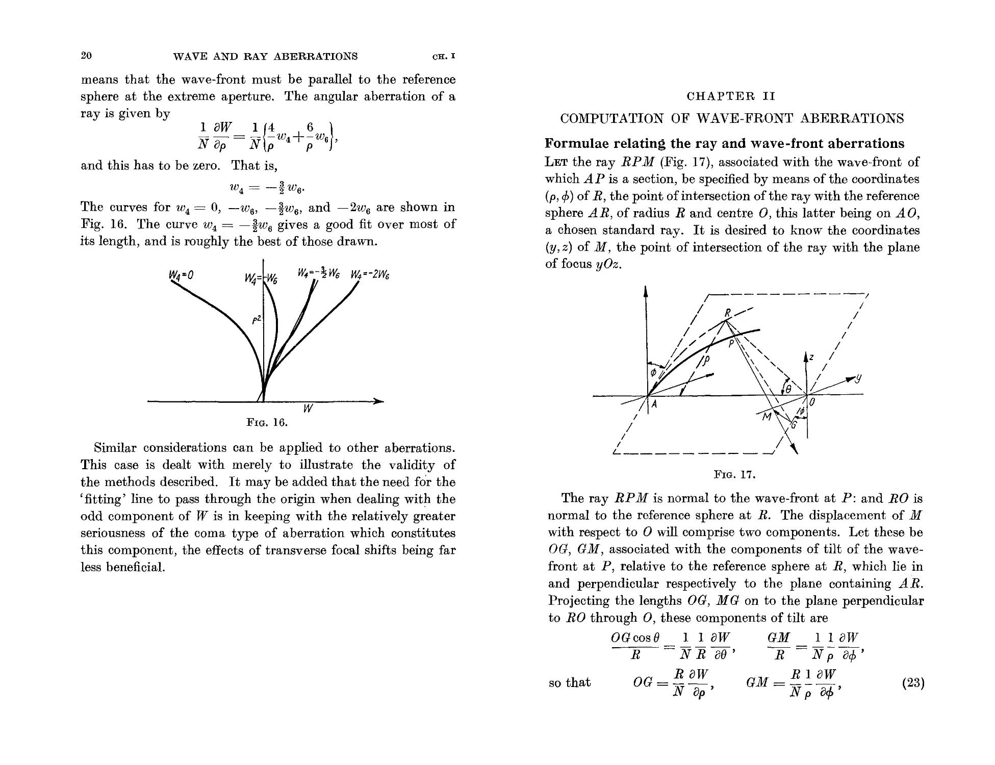
The curves for W 4 = 0, -w 6 , -!w 6 , and -2w 6 are shown in
Fig. 16. The curve W 4 = -!w 6 gives a good fit Over most of
its length, and is roughly the best of those drawn.
=-W6 u.4=-2W 6
Formulae relating the ray and wave-front aberrations
LET the ray RP M (Fig. 17), associated with the wave-front of
which A P is a section, be specified by means of the coordinates
(p, 4» of R, the point of intersection ofthe ray with the reference
sphere AR, of radius R and centre 0, this latter being on AO,
a chosen standard ray. It is desired to know the coordinates
(y, z) of M, the point of intersection of the ray with the plane
of focus yOz.
w
/ A
/
/
/ /
L_________-./
:!I
FIG. 16.
Similar considerations can be applied to other aberrations.
This case is dealt with merely to illustrate the validity of
the methods described. It may be added that the need for the
'fitting' line to pass through the origin when dealing with the
odd component of W is in keeping with the relatively greater
seriousness of the coma type of aberration which constitutes
this component, the effects of transverse focal shifts being far
less beneficial.
FIG. 17.
The ray RP M is normal to the wave-front at P: and RO is
normal to the reference sphere at R. The displacement of M
with respect to 0 will comprise two components. Let these be
OG, GM, associated with the components of tilt of the wave-
front at P, relative to the reference sphere at R, which lie in
and perpendicular respectively to the plane containing AR.
Projecting the lengths OG, MG on to the plane perpendicular
to RO through 0, these components of tilt are
o G cos ell oW G MIl 0 W
- -
R - N R 8ff' R - N p 04> '
so that OG = R oW GM = R  oW ( 23 )
N op , N p 04>'

22
COMPUTATION OF WAVE-FRONT ABERRATIONS
CH. II
CH. II COMPUTATION OF WAVE-FRONT ABERRATIONS
23
in the former of which the substitution dp = R cos 8 dB has been
made. This follows by differentiation of p = R sin 8. W is, of
course, the wave-front aberration at (p, rp); and W = N(RP).
Resolving OG and MG along Oy, Oz respectively, gives for
the coordinates of M,
y = -OGsinrp-GMcosrp,
z = -OGcosrp+GMsinrp.
Substitution of the values of OG, GM from (23) gives
y = _ ; (sinrp 00: + co;rp °o }
(24)
z = _ R ( cos rp 0 W _ sin rp 0 W ) ,
N op p orp
and, by means of these equations, the geometrical aberrations
are obtainable from a knowledge of W as a function of the
variables (p, rp). For an infinitely distant image, (24) give the
coordinates of the angular aberration
fy = -yjR, fz = -zjR.
The equations (24) are essentially those given by Nijboer.t
The results (24) are generally used in demonstrating ana-
lytically the geometrical significance of given wave-front aberra-
tions. In practice it is more frequently the converse of this
problem that has to be solved. Thus, given a number of rays
traced through an optical system and lying in the plane of
azimuth rp, it is required to find the value of W in this azimuth
for different values of p.
Multiplication of the first and second equations of (24) by
sin rp and cos rp respectively, and adding, gives
. A.. A.. RoW
YSlll't'+ZCOS't' = - N ap"
Hence if the values of (y, z) are known for rays in the section of
azimuth rp, the wave-front aberration at the point (p, rp) is
p
W = -  I (ysinrp+zcosrp) dp, (25)
o
t See B. R. A. Nijboer, Thesis, Groningen, 1942, p. 8.
rp remaining constant during the integration. If the image is
at infinity, one uses the angular aberrations fy = -yjR,
fz = -zjR. Then
p
W = N f (fysinrp+fzcosrp)d p .
o
(26)
In calculations dealing with images at finite distances it is often
desirable to employ B rather than p. Substitution of
dp = RcosBdB
in (25) gives, for this case,
o
W = -N f (ysinrp+zcosrp)cosB dB. (27)
o
By the use of these expressions the geometrical aberrations of
a system, determined by the tracing of suitable rays, may
readily be converted to wave-front aberrations.
Calculation of W for an axial image
In the case of an axial image formed by a symmetrical optical
system, the aberration is independent of rp. It suffices, there-
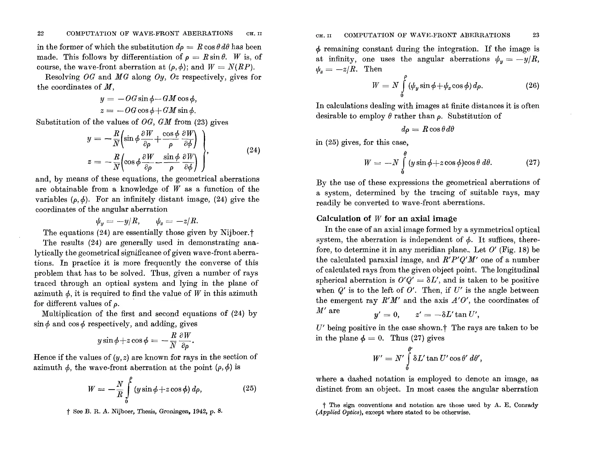
fore, to determine it in any meridian plane.. Let 0' (Fig. 18) be
the calculated paraxial image, and R'P'Q'M' one of a number
of calculated rays from the given object point. The longitudinal
spherical aberration is O'Q' = 8L', and is taken to be positive
when Q' is to the left of 0'. Then, if U' is the angle between
the emergent ray R'M' and the axis A'O', the coordinates of
M' are
y' = 0, z' = -8L'tan U',
U' being positive in the case shown. t The rays are taken to be
in the plane rp = O. Thus (27) gives
0'
W' = N' f 8L' tan U' cos B' dB',
o
where a dashed notation is employed to denote an image, as
distinct from an object. In most cases the angular aberration
t The sign conventions and notation are those used by A. E. Conrady
(Applied Optics), except where stated to be otherwise.

24
COMPUTATION OF WAVE-FRONT ABERRATIONS
CR. II
CH. II COMPUTATION OF WAVE-FRONT ABERRATIONS 25
be very significant. It is important, therefore, to note that the
aberrations of extra-axial image points are considered finally
with reference to the best axial plane of focus.
For an infinite paraxial image one simply evaluates
p'
W' = N' J fdp',
o
according to (26). It will be seen that f = U'.
0' R' M' is sufficiently small for one to write 8' = U' for the
purposes of this integration. Hence
0'
W' = N' I SL' sin U' dU'; (28)
o
e'
M'
I
()
FIG. 18.
a result which can also be derived directly from simple geo-
metrical considerations of the special case cp = O. Thus, equat-
ing expressions for the angular aberration LO' R' M'
SL'sin U' loW'
- - N'R' 88"
2
o Ii/sin lj'
FIG. 19.
o W'
FIG. 20.
from which (28) follows at once.
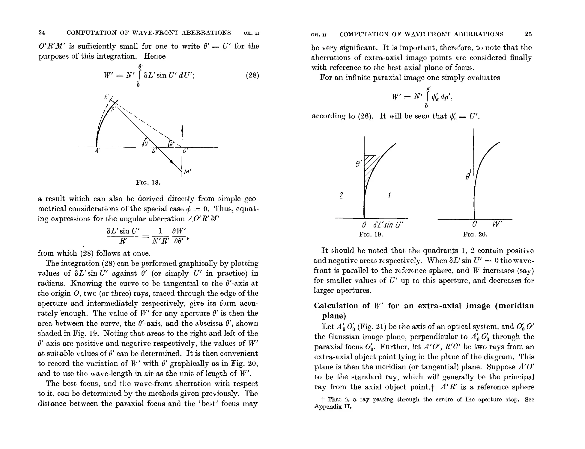
The integration (28) can be performed graphically by plotting
values of SL'sin U' against 8' (or simply U' in practice) in
radians. Knowing the curve to be tangential to the 8'-axis at
the origin 0, two (or three) rays, traced through the edge of the
aperture and intermediately respectively, give its form accu-
rately!enough. The value of W' for any aperture 8' is then the
area between the curve, the 8'-axis, and the abscissa 8', shown
shaded in Fig. 19. Noting that areas to the right and left of the
8'-axis are positive and negative respectively, the values of W'
at suitable values of 8' can be determined. It is then convenient
to record the variation of W' with 8' graphically as in Fig. 20,
and to use the wave-length in air as the unit of length of W'.
The best focus, and the wave-front aberration with respect
to it, can be determined by the methods given previously. The
distance between the paraxial focus and the 'best' focus may
It should be noted that the quadrants 1, 2 contain positive
and negative areas respectively. When SL' sin U' = 0 the wave-
front is parallel to the reference sphere, and W increases (say)
for smaller values of U' up to this aperture, and decreases for
larger apertures.
Calculation of W' for an extra-axial image (meridian
plane)
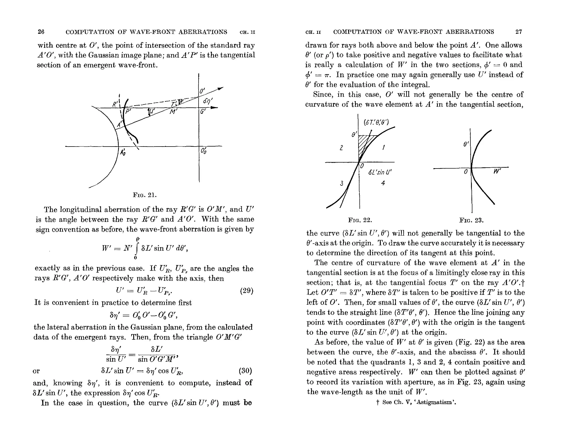
Let A O (Fig. 21) be the axis of an optical system, and O 0'
the Gaussian image plane, perpendicular to A O through the
paraxial focus O. Further, let A'O', R'G' be two rays from an
extra-axial object point lying in the plane of the diagram. This
plane is then the meridian (or tangential) plane. Suppose A'O'
to be the standard ray, which will generally be the principal
ray from the axial object point.t A'R' is a reference sphere
t That is a ray passiDg through the centre of the aperture stop. See
Appendix II.

26
COMPUTATION OF W A VE.FRONT ABERRATIONS
CH.II
OH.n
COMPUTATION OF W AVE-FRONT ABERRATIONS
27
0'
O'r;'
6'
drawn for rays both above and below the point A'. One allows
e' (or pI) to take positive and negative values to facilitate what
is really a calculation of W' in the two sections, 4>' = 0 and
4>' = 7T. In practice one may again generally use U' instead of
e' for the evaluation of the integral.
Since, in this case, 0' will not generally be the centre of
curvature of the wave element at A' in the tangential section,
with centre at 0', the point of intersection of the standard ray
A'O', with the Gaussian image plane; and A' P' is the tangential
section of an emergent wave-front.
(or,'e,'f)')
o
o
FIG. 21.
The longitudinal aberration of the ray R'G' is 0' M', and U'
is the angle between the ray R'G' and A'O'. With the same
sign convention as before, the wave-front aberration is given by
0'
W' = N' I 8L' sin U' de',
o
exactly as i» the previous case. If U'rt, U'pr are the angles the
rays R'G', A'O' respectively make with the axis, then
U' = U'rt - U'pr' (29)
It is convenient in practice to determine first
8r/ = OO'-OG',
the lateral aberration in the Gaussian plane, from the calculated
data of the emergent rays. Then, from the triangle O'M'G'
8r/ 8L'
sin U' = sinO'G'M"
FIG. 22.
FIG. 23.
or 8L'sin U' = 8r/ cos U'rt,
and, knowing 8'Y}', it is convenient to compute,
8L'sin U', the expression 8r/ cos U'rt.
In the case in question, the curve (8L'sin U', e') must be
(30)
instead of
the curve (aL'sin U', e') will not generally be tangential to the
e' -axis at the origin. To draw the curve accurately it is necessary
to determine the direction of its tangent at this point.
The centre of curvature of the wave element at A' in the
tangential section is at the focus of a limitingly close ray in this
section; that is, at the tangential focus T' on the ray A'O'.t
Let O'T' = aT', where 8T' is taken to be positive if T' is to the
left of 0'. Then, for small values of e', the curve (8L'sin U', e')
tends to the straight line (8T'e', e'). Hence the line joining any
point with coordinates (8T'e', 8') with the origin is the tangent
to the curve (8L' sin u.', e') at the origin.
As before, the value of W' at e' is given (Fig. 22) as the area
between the curve, the e'-axis, and the abscissa e'. It should
be noted that the quadrants 1, 3 and 2, 4 contain positive and
negative areas respectively. W' can then be plotted against 8'
to record its variation with aperture, as in Fig. 23, again using
the wave-length as the unit of W'.
t See Ch. V, 'Astigxnatism'.

28
COMPUTATION OF WAVE-FRONT ABERRATIONS
CH. n
CH.n
COMPUTATION OF WAVE-FRONT ABERRATIONS
29
In the case of an image at infinity one plots the curve (1/;, p'),
p' being the perpendicular distance of R' from the ray A'O'.
It will be seen that
.// = U' -U'
'f'z R P,
and p' follows from simple geometry. The tangent at the origin
in this case is the line joining the point (u,p') (p'jt',p') to the
origin. The angle u is that derived from a tangential paraxial
ray trace (see page 62), and t' = distance A'T'.
the tangent to the curve (y' cos ()', 0') at the origin being the line
joining this point with a point having coordinates (8S'B', 8'), 8S'
being the distance from 0' of the sagittal focus of the wave
element associated with the standard ray, 0' being the point
of intersection of this ray with the Gaussian plane. 1/; and p'
are used in the case of an image at infinity.
If one has a number of skew rays in the sagittal section traced
through a system, one can evaluate for each ray the tilt,
loW'
N'p' 04>"
of the corresponding wave element referred to the reference
sphere. Elimination of the terms in oW/op in (24) gives
 0 W' = { Z' sin 4>' -y' cos 4>' }
N' p' 84>' R"
(31)
Calculation of W' for an extra-axial image point (skew
plane)
Given the components (y', z') of the aberrations of a number
of rays lying in an azimuth defined by the sections 4>, 4>+7T, one
can determine W' by evaluating the integral
0'
W' = -N' J (y'sin4>'+z'cos4>')cosB' dB'
o
or, in the case 4>' = l7T,
of (27) above. The values of y', z' are those measured in the
focal plane through 0' and perpendicular to the standard ray
A' 0'. As before - (y' sin 4>' + z' cos 4>')cos B' is plotted against B'
in radians, evaluating the integral as an area.
If 0', lying between S', T' the centres of curvature of the
wave element A' in the sagittal and tangential sections respec-
tively, be the centre of curvature in the given azimuth, and
0'0' = 8l', then the tangent to the curve at the origin is the
line joining this point to any point having coordinates (ol'B', B').
When the image is formed at infinity, the angular aberration
(1/;, 1/;) is employed, and the aperture is measured by p, exactly
as described above. B' (or p') is allowed positive and negative
values corresponding to 4>' = 4>' and 4>' = 4>' +7T.
The case usually met in practice is that of rays in the sagittal
section, 4>' = !7T, 37T/2. Here, on account of symmetry, one need
consider only one half of the aperture, say 4>' = l7T. The integral
to be evaluated then becomes
{ I 8W' } z'
N'p' 04>' 4>'=11T = R' . (32)
(32) gives an indication of the aberration in the quadrants above
and below 4>' = i7T.
0'
W' = -N' J y'cosB' dB',
o
Optical path lengths along neighbouring rays
Before proceeding to the discussion of chromatic aberration,
it is desirable to establish an important result of wide applica-
tion. It is, in effect, a re-statement of Fermat's theorem.
Let A, A' be points on a ray AP A' (Fig. 24) whose path
through an optical system is known. One refraction of the ray,
at P, is shown here. The media to the left and right of P have
indices N, N' respectively. BRB' is a neighbouring ray, that
is, a ray such that the angle between any part of it and the
corresponding part of A P A' is small, and also such that the
distance between the rays is small compared with the radius of
the refracting surface P R. Let AB, A' B' be taken perpendicular
to AP, PA' respectively. Then it is required to find the optical
path length [BRB'] without having recourse to tracing the ray
BRB'.

30
COMPUTATION OF WAVE-FRONT ABERRATIONS
CH.II
CR. II COMPUTATION OF WAVE-FRONT ABERRATIONS
31
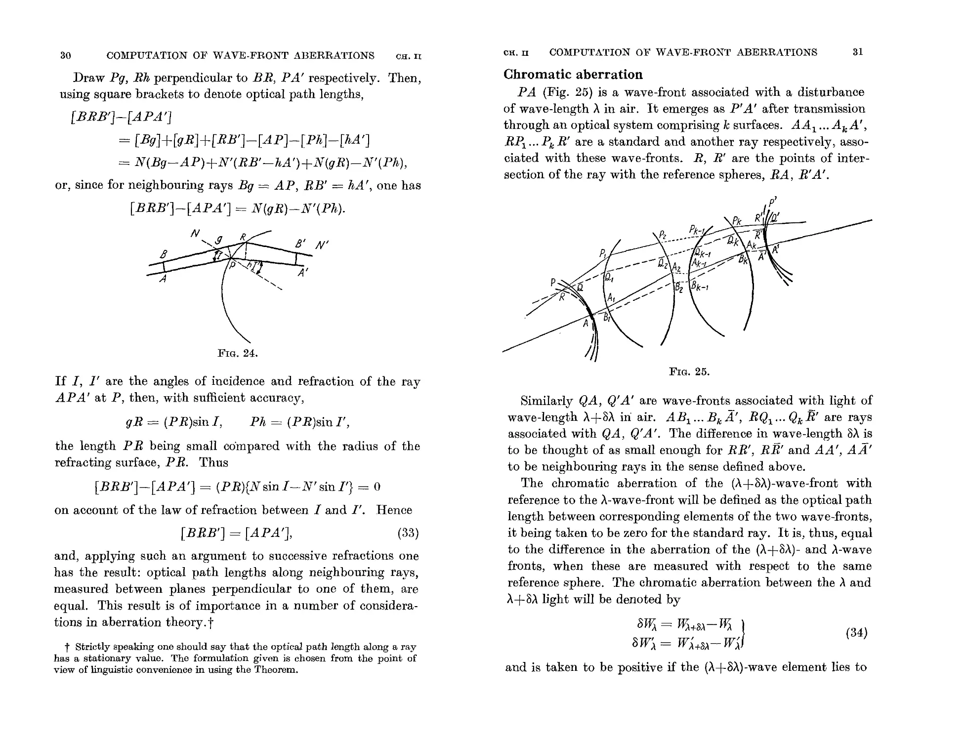
Draw Pg, Rh perpendicular to BR, P A' respectively. Then,
using square brackets to denote optical path lengths,
[BRB']-[APA']
= [Bg]+[gR]+[RB']-[AP]-[Ph]-[hA']
= N(Bg-AP)+N'(RB'-hA')+N(gR)-N'(Ph),
or, since for neighbouring rays Bg = AP, RB' = hA', one has
[BRB']-[APA'] = N(gR)-N'(Ph).
Chromatic aberration
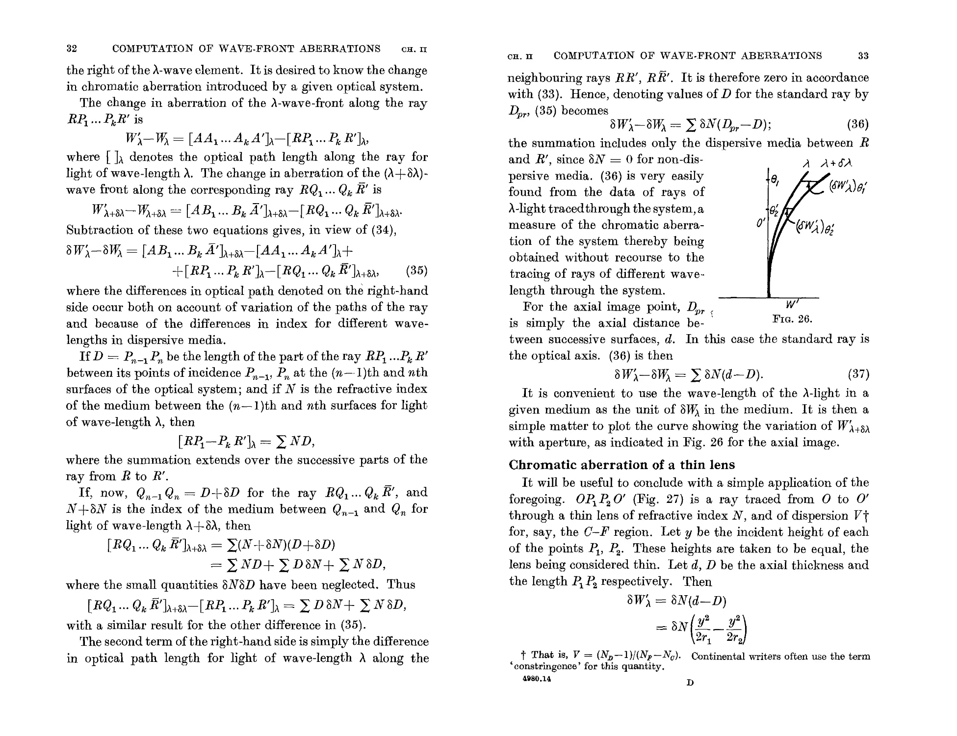
P A (Fig. 25) is a wave-front associated with a disturbance
of wave-length>' in air. It emerges as P'A' after transmission
through an optical system comprising k surfaces. AA1'" Ak A',
RP 1 ... P k R' are a standard and another ray respectively, asso-
ciated with these wave-fronts. R, R' are the points of inter-
section of the ray with the reference spheres, RA, R' A'.
N'
FIG. 24.
If I, I' are the angles of incidence and refraction of the ray
AP A' at P, then, with sufficient accuracy,
FIG. 25.
[BRB'] = [APA'],
(33)
Similarly QA, Q'A' are wave-fronts associated with light of
wave-length >.+0>. in air. AB1'" Bk A', RQ1'" Qk R' are rays
associated with QA, Q'A'. The difference in wave-length 0>. is
to be thought of as small enough for RR', RB' and AA', AA'
to be neighbouring rays in the sense defined above.
The chromatic aberration of the ('\+D>.)-wave-front with
referepce to the >.-wave-front will be defined as the optical path
length between corresponding elements of the two wave-fronts,
it being taken to be zero for the standard ray. It is, thus, equal
to the difference in the aberration of the (>.+0'\)- and >.-wave
fronts, when these are measured with respect to the same
reference sphere. The chromatic aberration between the>. and
>.+0>. light will be denoted by
8TfA = TfA+8'\- TfA }
DW = WA+8A-WA
(34)
gR = (PR)sinI,
Ph = (PR)sin1',
the length P R being small co"mpared with the radius of the
refracting surface, P R. Thus
[BRB']-[APA'] = (PR){NsinI-N'sinI'} = 0
on account of the law of refraction between I and 1'. Hence
and, applying such an argument to successive refractions one
has the result: optical path lengths along neighbouring rays,
measured between planes perpendicular to one of them, are
equal. This result is of importance in a number of considera-
tions in aberration theory. t
t Strictly speaking one should say that the optical path length along a ray
has a stationary value. The formulation given is chosen from the point of
view of linguistic convenience in using the Theorem.
and is taken to be positive if the (>.+D>.)-wave element lies to

32
COMPUTATION OF W A VE.FRONT ABERRATIONS CR. II
CR. II COMPUTATION OF WAVE-FRONT ABERRATIONS
33
the right ofthe A-wave element. It is desired to know the change
in chromatic aberration introduced by a given optical system.
The change in aberration of the A-wave-front along the ray
R ... PkR' is
WA-Tf). = [AAI ".AkA'],\-[RPI",P k R'],\,
where [],\ denotes the optical path length along the ray for
light of wave-length A. The change in aberration of the (A+8A)-
wave front along the corresponding ray RQI'" Qk R' is
W A + 8 ,\- Tf).+8'\ = [ABI'" Bk A'].\+8,\-[RQI'" Qk R'],\+s,\.
Subtraction of these two equations gives, in view of (34),
8W A -8Tf). = [AB I ...B k A'],\+8,\-[AA I ...A k A'],\+
+[RP I ... P k R'],\-[ RQI'" Qk R'],\+8,\, (35)
where the differences in optical path denoted on the right-hand
side occur both on account of variation of the paths of the ray
and because of the differences in index for different wave-
lengths in dispersive media.
If D = P n - I Pn be the length of the part of the ray RP I "'P k R'
between its points of incidence Pn-v Pn at the (n-l)th and nth
surfaces of the optical system; and if N is the refractive index
of the medium between the (n-l)th and nth surfaces for light
of wave-length A, then
[RPI-PkR'],\ = 2,ND,
where the summation extends over the successive parts of the
ray from R to R'.
If, now, Qn-I Qn = D+8D for the ray RQI'" Qk R', and
N +8N is the index of the medium between Qn-I and Qn for
light of wave-length A+8A, then
[RQl'" Qk R'].\+8,\ = 2,(N +8N)(D+8D)
= 2,ND+ 2,D8N+ 2,N8D,
where the small quantities 8N8D have been neglected. Thus
[RQI'" Qk R'].\+8,\-[RP I ... P k R'],\ = 2, D 8N + 2, N 8D,
with a similar result for the other difference in (35).
The second term of the right-hand side is simply the difference
in optical path length for light of wave-length A along the
neighbouring rays RR', RR'. It is therefore zero in accordance
with (33). Hence, denoting values of D for the standard ray by
D pr , (35) becomes
8WA-8Tf). = 2, 8N(D pr -D); (36)
the summation includes only the dispersive media between R
and R', since 8N = 0 for non -dis- '" A + cf).
persive media. (36) is very easily 8,
found from the data of rays of
A-light traced through the system, a
measure of the chromatic aberra-
tion of the system thereby being
obtained without recourse to the
tracing of rays of different wave-
length through the system.
For the axial image point, D pr , W
is simply the axial distance be- ' FIG. 26.
tween successive surfaces, d. In this case the standard ray is
the optical axis. (36) is then
8WA-8Tf). = 2, 8N(d-D). (37)
It is convenient to use the wave-length of the A-light in a
given medium as the unit of 8Tf). in the medium. It is then a
simple matter to plot the curve showing the variation of WA+8'\
with aperture, as indicated in Fig. 26 for the axial image.
Chromatic aberration of a thin lens
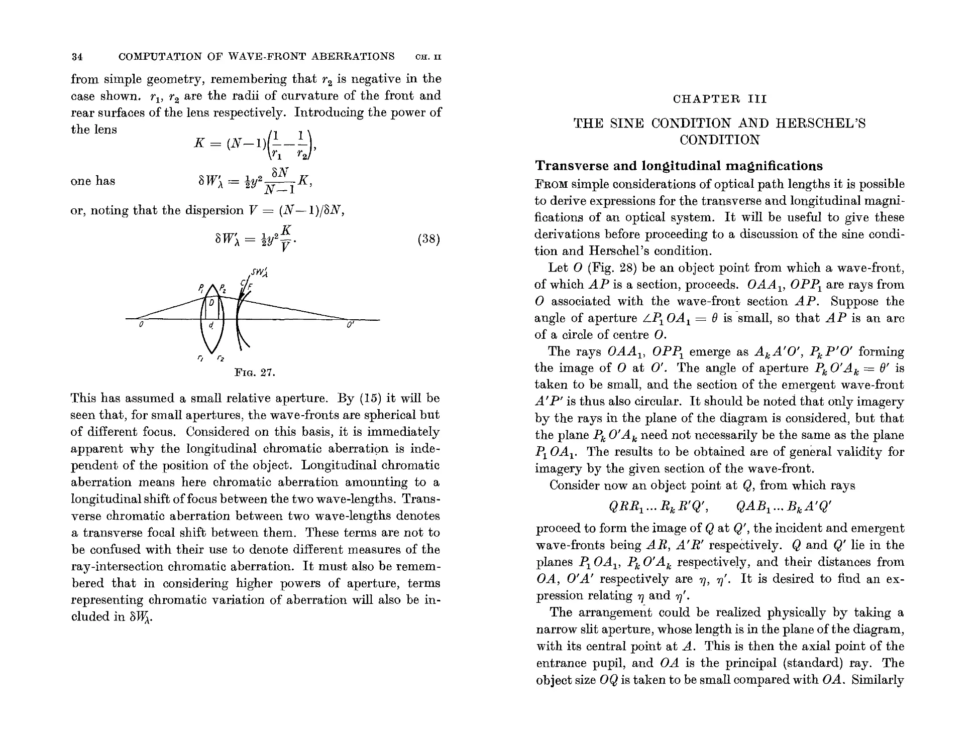
It will be useful to conclude with a simple application of the
foregoing. OP I P 2 0' (Fig. 27) is a ray traced from 0 to 0'
through a thin lens of refractive index N, and of dispersion Vt
for, say, the C-F region. Let y be the incident height of each
of the points Pv P 2 . These heights are taken to be equal, the
lens being considered thin. Let d, D be the axial thickness and
the length PI P 2 respectively. Then
8WA = 8N(d-D)
= 8N ( y2 _ y2 )
2r I 2r 2
t That is, V = (N D -1)/(N p -N a ). Continental writers often use the term
, constringence' for this quantity.
480.I4
(aWA) &/
D

34
COMPUTATION OF WAVE-FRONT ABERRATIONS
CH.II
from simple geometry, remembering that r 2 is negative in the
case shown. rv r 2 are the radii of curvature of the front and
rear surfaces of the lens respectively. Introducing the power of
the lens
CHAPTER III
K = (N-1) ( - ) ,
r l r 2
8 W' - .1 2 8N K
.\ - 2Y N-1 '
or, noting that the dispersion V = (N -1)j8N,
"' W ' - I 2 K
o .\ - 2Y -.
V
THE SINE CONDITION AND HERSCHEL'S
CONDITION
(38)
Transverse and longitudinal magnifications
FROM simple considerations of optical path lengths it is possible
to derive expressions for the transverse and longitudinal magni-
fications of an optical system. It will be useful to give these
derivations before proceeding to a discussion of the sine condi-
tion and Herschel's condition.
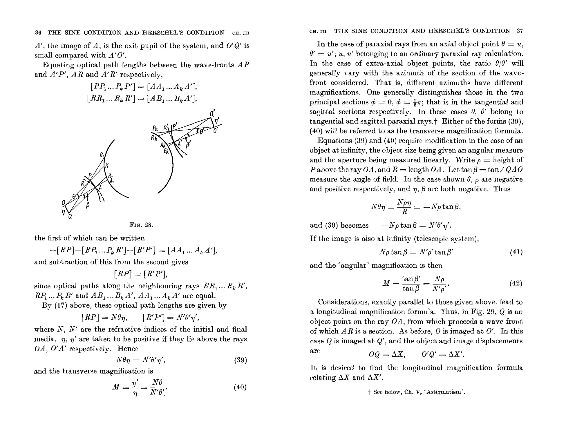
Let 0 (Fig. 28) be an object point from which a wave-front,
of which AP is a section, proceeds. OAA v OPP I are rays from
o associated with the wave-front section AP. Suppose the
angle of aperture LP I OA I = 0 is -small, so that AP is an arc
of a circle of centre O.
The rays OAA v OPP I emerge as AkA'O', PkP'O' forming
the image of 0 at 0'. The angle of aperture P k O'A k = 0' is
taken to be small, and the section of the emergent wave-front
A' P' is thus also circular. It should be noted that only imagery
by the rays in the plane of the diagram is considered, but that
the plane P k 0' A k need not necessarily be the same as the plane
PIOA I . The results to be obtained are of general validity for
imagery by the given section of the wave-front.
Consider now an object point at Q, from which rays
QRR I ... Rk R'Q', QAB I ... BkA'Q'
proceed to form the image of Qat Q', the incident and emergent
wave-fronts being AR, A'R' respectively. Q and Q' lie in the
planes PIOA I , P k O'A k respective!y, and their distances from
OA, O'A' respectively are 1], 1]'. It is desired to find an ex-
pression relating 1] and 1]'.
The arrangement could be realized physically by taking a
narrow slit aperture, whose length is in the plane ofthe diagram,
with its central point at A. This is then the axial point of the
entrance pupil, and OA is the principal (standard) ray. The
object size OQ is taken to be small compared with OA. Similarly
one has
o 
'i rz
FIG. 27.
This has assumed a small relative aperture. By (15) it will be
seen that, for small apertures, the wave-fronts are spherical but
of different focus. Considered on this basis, it is immediately
apparent why the longitudinal chromatic aberratiQn is inde-
pendent of the position of the object. Longitudinal chromatic
aberration means here chromatic aberration amounting to a
longitudinal shift offocus between the two wave-lengths. Trans-
verse chromatic aberration between two wave-lengths denotes
a transverse focal shift between them. These terms are not to
be confused with their use to denote different measures of the
ray-intersection chromatic aberration. It must also be remem-
bered that in considering higher powers of aperture, terms
representing chromatic variation of aberration will also be in-
cluded in 8JJ'A.

CR. III THE SINE CONDITION AND HERSCHEL'S CONDITION 37
36 THE SINE CONDITION AND HERSCHEL'S CONDITION CR. III
A', the image of A, is the exit pupil ofthe system, and O'Q' is
small compared with A'O'.
Equating optical path lengths between the wave-fronts AP
and A' P', AR and A'R' respectively,
[PPI...PkP'] = [AAI...AkA'],
[RRI'" Rk R'] = [ABI'" BkA'],
the first of which can be written
-[RP]+[RPI...PkR']+[R'P'] = [AAI...AkA'J,
and subtraction of this from the second gives
[RP] = [R'P'],
since optical paths along the neighbouring rays RRI'" Rk R',
RP1...PkR' and AB1...BkA', AA1...AkA' are equal.
By (17) above, these optical path lengths are given by
[RP] = NBYj, [R'P'] = N'B'Yj',
where N, N' are the refractive indices of the initial and final
media. Yj, Yj' are taken to be positive if they lie above the rays
OA, O'A'respectively. Hence
NBYj = N'B'Yj', (39)
and the transverse magnification is
Yj' NB
M = - = N'B" (40)
Yj .
In the case of paraxial rays from an axial object point B = u,
B' = u'; u, u' belonging to an ordinary paraxial ray calculation.
In the case of extra-axial object points, the ratio B/B' will
generally vary with the azimuth of the section of the wave-
front considered. That is, different azimuths have different
magnifications. One generally distinguishes those in the two
principal sections g; = 0, g; = -!7T; that is in the tangential and
sagittal sections respectively. In these cases B, B' belong to
tangential and sagittal paraxial rays.t Either of the forms (39),
(40) will be referred to as the transverse magnification formula.
Equations (39) and (40) require modification in the case of an
object at infinity, the object size being given an angular measure
and the aperture being measured linearly. "\Vrite p = height of
P above the ray OA, andR = length OA. Let tan 13 = tanLQAO
measure the angle of field. In the case shown B, p are negative
and positive respectively, and Yj, 13 are both negative. Thus
NpYj
NBYj = R = -Nptanf3,
and (39) becomes -Nptanf3 = N'B'Yj'.
If the image is also at infinity (telescopic system),
Np tan 13 = N'p'tanf3'
FIG. 28.
(41)
and the 'angular' magnification is then
M = tan 13' = N p .
tan 13 N'p'
(42)
Considerations, exactly parallel to those given above, lead to
a longitudinal magnification formula. Thus, in Fig. 29, Q is an
object point on the ray OA, from which proceeds a wave-front
of which AR is a section. As before, 0 is imaged at 0'. In this
case Q is imaged at Q', and the object and image displacements
are
OQ = X,
O'Q' = X'.
It is desired to find the longitudinal magnification formula
relating X and X'.
t See below, Ch. V, 'Astigmatism'.

38 THE SINE CONDITION AND HERSCHEL'S CONDITION CH. III
CR. III THE SINE CONDITION AND HERSCHEL'S CONDITION 39
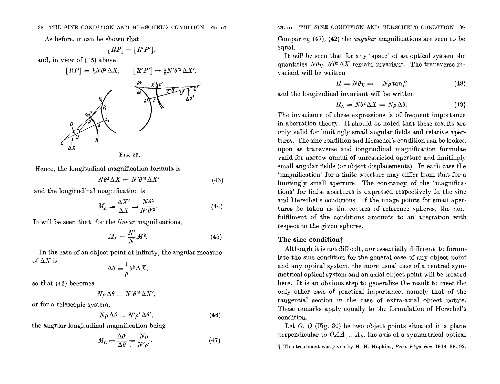
As before, it can be shown that
[RP] = [R'P'],
and, in view of (15) above,
[RP] = iNB2 X,
[R'P'] = tN'B'2X'.
a
FIG. 29.
Hence, the longitudinal magnification formula is
NB2 X = N'B'2 X'
and the longitudinal magnification is
X' NB2
M L = X = N'8'2 '
It will be seen that, for the linear magnifications,
N'
M L = N M2 .
Comparing (47), (42) the angular magnifications are seen to be
equal.
It will be seen that for any 'space' of an optical system the
quantities NB'Yj, NB2 X remain invariant. The transverse in-
variant will be written
(43)
H = NB'Yj = -Nptanf3 (48)
and the longitudinal invariant will be written
H L = NB2X = NpB. (49)
The invariance of these expressions is of frequent importance
in aberration theory. It should be noted that these results are
only valid for limitingly small angular fields and relative aper-
tures. The sine condition and Herschel's condition can be looked
upon as transverse and longitudinal magnification formulae
valid for narrow annuli of unrestricted aperture and limitingly
small angular fields (or object displacements). In each case the
'magnification' for a finite aperture may differ from that for a
limitingly small aperture. The constancy of the 'magnifica-
tions' for finite apertures is expressed respectively in the sine
and Herschel's conditions. If the image points for small aper-
tures be taken as the centres of reference spheres, the non-
fulfilment of the conditions amounts to an aberration with
respect to the given spheres.
(44)
(45)
The sine conditiont
Although it is not difficult, nor essentially different, to formu-
late the sine condition for the general case of any object point
and any optical system, the more usual case of a centred sym-
metrical optical system and an axial object point will be treated
here. It is an obvious step to generalize the result to meet the
only other case of practical importance, namely that of the
tangential section in the case of extra-axial object points.
These remarks apply equally to the formulation of Herschel's
condition.
Let 0, Q (Fig. 30) be two object points situated in a plane
perpendicular to OAA 1 ... A k , the axis of a symmetrical optical
B = !B2X,
p
In the case of an object point at infinity, the angular measure
of x is
so that (43) becomes
NpB = N'B'2X',
or for a telescopic system,
NpB = N'p' B',
the angular longitudinal magnification being
B' Np
M L = B . N'p"
(46)
(47)
t This treatment was given by H. H. Hopkins, Proc. Phys. Soc. 1946, 58,92.

40 THE SINE CONDITION AND HERSCHEL'S CONDITION CH. III
CH. III THE SINE CONDITION AND HERSCHEL'S CONDITION 41
Subtraction ofthis latter from (50), and cancelling optical paths
along neighbouring rays, gives
(W'- W)-(V'- V) = [RPJ-[R'P'J,
(V'- V) = (W'- W)+[R'P'J-[RP].
This result is obviously valid for any azimuth of the aperture.
But, by (16), the optical path lengths in (51) are
[RPJ = N YJ sin 0 cos g;, [ R' p'J = N'r/ sin 0' cos g;
for the azimuth g;; (51) then becomes
V'- V = (W'- W)+{N'YJ' sinB'-NYJ sin O}cos g;. (52)
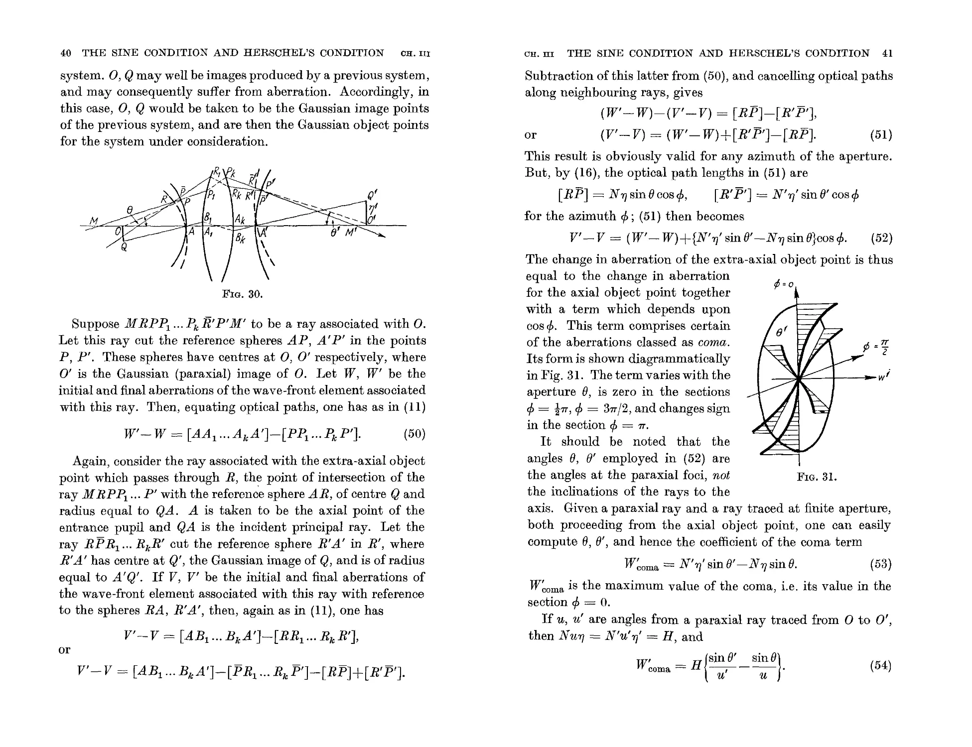
The change in aberration of the extra-axial object point is thus
equal to the change in aberration
for the axial object point together
with a term which depends upon
cos g;. This term comprises certain
of the aberrations classed as coma.
Its form is shown diagrammatically
in Fig. 31. The term varies with the
aperture 0, is zero in the sections
g; = !77, g; = 377/2, and changes sign
in the section g; = 77.
It should be noted that the
angles 0, 0' employed in (52) are
the angles at the paraxial foci, not
the inclinations of the rays to the
axis. Given a paraxial ray and a ray traced at finite aperture,
both proceeding from the axial object point, one can easily
compute e, 0', and hence the coefficient of the coma term
Worn.a = N'r/sinB'-NYJsinO. (53)
Worn.a is the maximum value of the coma, i.e. its value in the
section g; = o.
If u, u' are angles from a paraxial ray traced from 0 to 0',
then Nu'YJ = N'u'YJ' = H, and
W' _ H { sin 0' sin O }
coma - ----;;;:- - u .
system. 0, Q may well be images produced by a previous system,
and may consequently suffer from aberration. Accordingly, in
this case, 0, Q would be taken to be the Gaussian image points
of the previous system, and are then the Gaussian object points
for the system under consideration.
or
fj
FIG. 30.
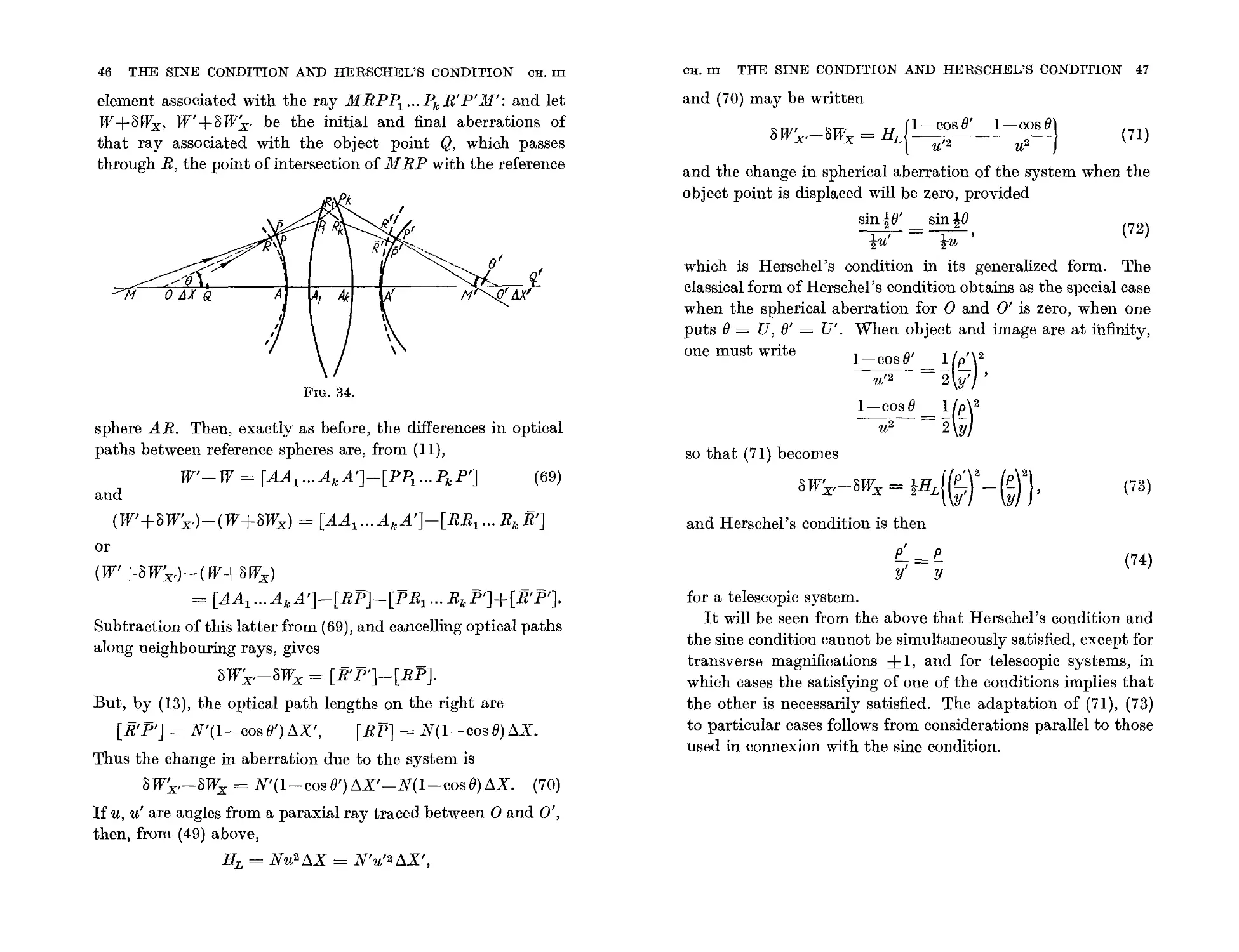
Suppose MRPP1...PkR'P'M' to be a ray associated with O.
Let this ray cut the reference spheres AP, A'P' in the points
P, P'. These spheres have centres at 0, 0' respectively, where
0' is the Gaussian (paraxial) image of O. Let W, W' be the
initial and final aberrations of the wave-front element associated
with this ray. Then, equating optical paths, one has as in (11)
W'- W = [AAl...AkA'J-[PPl,,,PkP']. (50)
Again, consider the ray associated with the extra-axial object
point which passes through R, the point of intersection of the
ray MRPP 1 ... P' with the reference sphere AR, of centre Q and
radius equal to QA. A is taken to be the axial point of the
entrance pupil and QA is the incident principal ray. Let the
ray RP Rl'" RkR' cut the reference sphere R'A' in R', where
R'A' has centre at Q', the Gaussian image of Q, and is of radius
equal to A'Q'. If V, V' be the initial and final aberrations of
the wave-front element associated with this ray with reference
to the spheres RA, R'A', then, again as in (11), One has
V'-V = [ABl...BkA'J-[RRl...RkR'J,
or
V'-V = [ABl...BkA'J-[PRl...RkP'J-[RPJ+[R'PIJ.
(51)
{;=o
y5=1
wi
FIG. 31.
(54)

42 THE SINE CONDITION AND HERSCHEL'S CONDITION CH. III
This is zero, provided
CH. III THE SINE CONDITION AND HERSCHEL'S CONDITION 43
sin ()' sin ()
-u'-u'
(55)
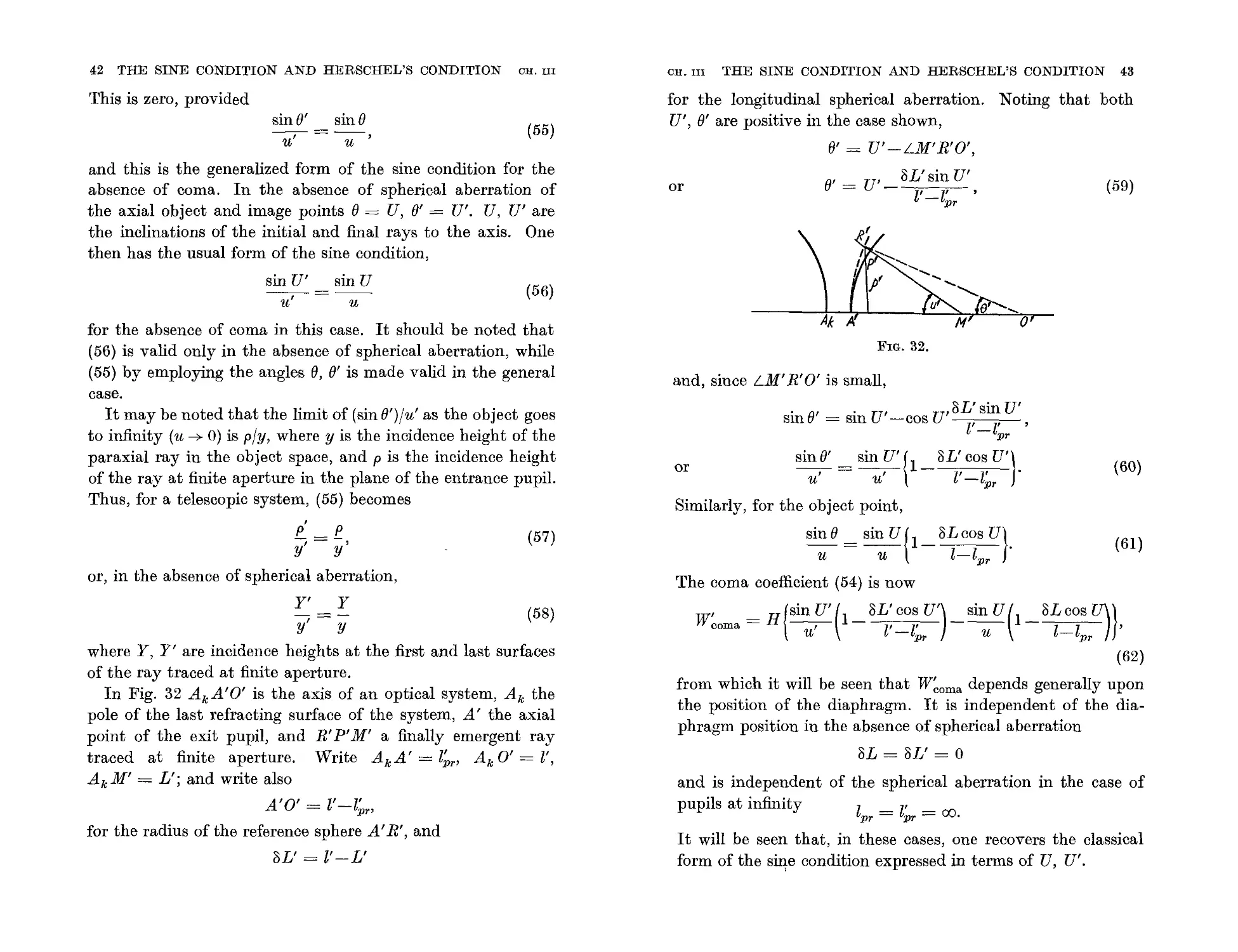
for the longitudinal spherical aberration. Noting that both
U', ()' are positive in the case shown,
()' = U'-LM'R'O',
and this is the generalized form of the sine condition for the
absence of coma. In the absence of spherical aberration of
the axial object and image points () = U, ()' = U'. U, U' are
the inclinations of the initial and final rays to the axis. One
then has the usual form of the sine condition,
sin U' sin U
 u
or
()' = U' _ 8L' sin U'
l' -lr '
(59)
(56)
for the absence of coma in this case. It should be noted that
(56) is valid only in the absence of spherical aberration, while
(55) by employing the angles e, ()' is made valid in the general
case.
It may be noted that the limit of (sin ()')Iu' as the object goes
to infinity (u --+ 0) is ply, where y is the incidence height of the
paraxial ray in the object space, and p is the incidence height
of the ray at finite aperture in the plane of the entrance pupil.
Thus, for a telescopic system, (55) becomes
FIG. 32.
and, since LM' R' 0' is small,
. () ' . U ' U ' 8L' sin U'
SIn = sIn -cos l' -l' ,
pr
p'
!l
p
-,
y
(57)
or sin()' = sin U' { I_ 8L' cos U' } ( 60 )
I , l ' l ' .
u u -pr
Similarly, for the object point,
sin() = SinU { I_ 8Lcos U } . (61)
u u l-lpr
The coma coefficient (54) is now
W' = H { Sin U' ( I_ 8L' cos U' ) _ sin U ( I_ 8Lcos U )}
coma u' l' -lr U l-lpr'
(62)
from which it will be seen that Woma depends generally upon
the position of the diaphragm. It is independent of the dia-
phragm position in the absence of spherical aberration
8L = 8L' = 0
or, in the absence of spherical aberration,
Y' y
-
y' y
where Y, Y' are incidence heights at the first and last surfaces
of the ray traced at finite aperture.
In Fig. 32 AkA'O' is the axis of an optical system, Ak the
pole of the last refracting surface of the system, A' the axial
point of the exit pupil, and R' P' M' a finally emergent ray
traced at finite aperture. Write AkA' = lr' Ak 0' = l',
AkM' = L'; and write also
(58)
A'O' = l'-lr'
for the radius of the reference sphere A'R', and
8L' = l'-L'
and is independent of the spherical aberration in the case of
pupils at infinity
lpr = lr = 00.
It will be seen that, in these cases, one recovers the classical
form of the se condition expressed in terms of U, U'.

44 THE SINE CONDITION AND HERSCHEL'S CONDITION CR. III
CH. III THE SINE CONDITION AND HERSCHEL'S CONDITION 45
For small values of e', writing sin B' = p' j R' and u' = y' j R',
where R' = A'O' and y' = height of the point of intersection
of the paraxial ray with the pupil plane, one has
sin e' p'
-
u' y'
and, similarly for the object point,
sin e
obtains (67). The form of (62) for a telescopic system, for
example, is
Woma = H{ :: (l- L'X, )-(l- LlprX )} (68)
and other cases fall under (63) or (64).
p
-=-.
u Y
Thus the expression for Woma (54) becomes
W' = H { Sin B' _e }
coma u' y
for an infinite object point, or
W' o = H { P' _ SinB }
c ma y' u
for an infinite image point, and
(63)
FIG. 33.
(64)
Herschel's conditiont
In dealing with the sine condition the change in aberration
consequent upon a transverse displacement of the object point
is investigated. This change is zero if the sine condition (55) is
fulfilled. Similarly one can find the change in aberration conse-
quent upon a longitudinal displacement of the object point.
If Herschel's condition is fulfilled this change in aberration is
zero. Since the object point remains on the optical axis there
is in this case rotational symmetry, and one need only consider
one meridian plane.
Let 0, Q (Fig. 34) be paraxial object points, not necessarily
free from aberration, situated on the axis OAA 1 ... AkA'O' of
an optical system and separated by a small distance X. Let
AP, AR be reference spheres having centres at 0, Q respec-
tively. A is taken to be the axial point of the entrance pupil.
Suppose MRPP1",P k R'P'M' to be a ray associated with the
object point O. The paraxial images of 0, Q are 0', Q'respec-
tively, at distance X' apart; and A'R', A'P' are reference
spheres with centres at Q', 0' respectively; A' is the axial point
of the exit pupil.
Let W, W' be the initial and final aberrations of the wave
W' m = H { i_e } ( 65 )
co a y' y
for a telescopic system.
To apply to these cases (sin B)ju, or (sinB')ju', or both, must
be replaced by
sinB' = p' = Y' ( I- lr )
u' y' y' L' -X' (66)
for the image, and
sinB = e = Y ( I--- ) (67)
u Y Y L-X
for the object point. For the paraxial image (or object) point
is at infinity and L' is the intersection distance of the ray at
finite aperture. Then, from Fig. 33,
I Y'
tanU = L'-X"
whence
Y'_ ,_ lrY'
p - L'-X"
from which (66) follows at once. Similarly, for the object, one
t See H. H. Hopkins, Proc. Phys. Soc. 1946,58, 100.

46 THE SINE CONDITION AND HERSCHEL'S CONDITION CH. III
element associated with the ray M RP PI ". P k R' P' M': and let
W +8W x , W' +8W. be the initial and final aberrations of
that ray associated with the object point Q, which passes
through R, the point of intersection of M RP with the reference
CH. III THE SINE CONDITION AND HERSCHEL'S CONDITION 47
M
and (70) may be written
8W',,-8W = H { I-COSO' I-COSO }
x x L U'2 u2
and the change in spherical aberration of the system when the
object point is displaced will be zero, provided
sin to' sin to
1u' = 1u '
2 2
(71)
(72)
FIG. 34.
which is Herschel's condition in its generalized form. The
classical form of Herschel's condition obtains as the special case
when the spherical aberration for 0 and 0' is zero, when One
puts 0 = U, 0' = U'. When object and image are at infinity,
one must write I-cosO' =  ( p' ) 2,
U'2 2 y'
I-cos 0 =  (  ) 2
u 2 2 Y
sphere AR. Then, exactly as before, the differences in optical
paths between reference spheres are, from (11),
and
(W'+8W,)-(W+8Wx) = [AAI".AkA']-[RRI'" Rk R']
W'- W = [AAI...AkA']-[PPI...PkP']
(69)
so that (71) becomes
, _ I {( p' ) 2 ( p ) 2 }
oW x.-8Wx - 'j,HL y' - y ,
and Herschel's condition is then
(73)
or
p'
y'

y
(74)
(W' +8W.)-(W +8W x )
= [AAI...AkA']-[RP]-[PR I ... RkP']+[ R'P'].
Subtraction of this latter from (69), and cancelling optical paths
along neighbouring rays, gives
8W.-oWx = [R' P']-[RPJ.
But, by (13), the optical path lengths on the right are
[R'P'] = N'(I-cosO')X', [RP] = N(I-cosO)X.
Thus the change in aberration due to the system is
8W.-oWx = N'(I-cosO')X'-N(I-cosO)X. (70)
If u, u' are angles from a paraxial ray traced between 0 and 0',
then, from (49) above,
H L = NU2X = N'U'2X',
for a telescopic system.
It will be seen from the above that Herschel's condition and
the sine condition cannot be simultaneously satisfied, except for
transverse magnifications ::!:: 1, and for telescopic systems, in
which cases the satisfying of one of the conditions implies that
the other is necessarily satisfied. The adaptation of (71), (73)
to particular cases follows from considerations parallel to those
used in connexion with the sine condition.

CH. IV
GENERAL THEORY OF ABERRATION TYPES
49
CHAPTER IV
find the aberration function directly in terms of the data of the
system, even in simple cases. One of the chief uses therefore of
this approach to aberration theory is in the analytical investiga-
tion of the types of aberration which may occur in symmetrical
optical systems. The results to be obtained are valid for any
system having rotational symmetry.
GENERAL THEORY OF ABERRATION TYPES
Expansion of the aberration function
LET A'O (Fig. 35) be the optical axis of a symmetrical optical
system, whose (refracting or reflecting) surfaces are surfaces of
revolution about this axis, but not necessarily spherical. Let A'
be the axial point of the exit pupil, and O the paraxial image.
O 0' is the Gaussian image plane, perpendicular to A'O through
O. 0' is the Gaussian image of an extra-axial object point,
and the plane of the diagram, A'O 0', is the meridian (tan-
gential) plane. Write O'O = 'YJ for the Gaussian image height.
With centre 0' describe a reference sphere of radius A' 0' = R'.
Let p' be the perpendicular distance from A'O' of a current
point R' on the reference sphere. R' lies in a plane through
A'O' making an angle g;' with the meridian plane A'OO'.
Then H' has polar coordinates (p', g;'). If LR'O'A' = ()', then
p' = R' sin ()', and for small values of ()' one may write
()' = p'/R'.
It is convenient to introduce variables defining the relative
aperture and size of field as fractions of their maximum values.
Suppose (p')max to be the maximum value of p', and write a new
variable
(75)
FIG. 35.
The aberration W' must have the same value for points sym-
metrically disposed with respect to the meridian plane, so that
the aberration function must remain unchanged if g;' be replaced
by -g;'. Again, keeping r' constant, if the image point at a
distance below the axis equal to that of 0' above the axis be
considered, the aberration for the azimuths TT-:T.g;' must be the
same as at P'. Hence the aberration function must remain un-
changed if a' be reversed in sign and g;' be replaced by TT-:T.g;'.
These conditions, which follow simply from the symmetry of the
system, will be fulfilled provided the variables (a', r', g;') only
occur in the aberration function in the forms
r' = p' /(p')max
for the fractional aperture, and write
a' = 'YJ/( TJ)max (76)
for the fractional field size. The variables (75), (76) have the
advantage of remaining unaffected by the positions of the image
and the exit pupil, be these latter at finite or infinite distances.
The aberration of the element of wave-front associated with
the ray passing through R' will be a function of a', r', and g;'.
Let it be denoted by W(a', r', g;'). This is then the aberration
function of the system, and a knowledge of this function for a
given system would completely describe the aberrations of the
system for all image points. However, it is rarely possible to
a'2, r'2, a'r' cos g;'
and one can then write the aberration function as the most
general power series in these variables. Hence, omitting the
dashes, the aberration function will be of the form
W(a, r, g;) = OC OO + (Oc w r 2 + 1 c n ar cos g;+2COO a 2 )+
+ (oc 40 r 4 + 1 c 31 ar 3 cos g;+2C22 u 2 r 2 COS2g;+2C20 a 2 r 2 +
+3Cn a 3 rcosg;+4cOoa 4 )+.... (77)
4980.14 E

50
GENERAL THEORY OF ABERRATION TYPES
CH. IV
CH. IV
GENERAL THEORY OF ABERRATION TYPES
51
Some of the terms of (77) can be shown to be zero. Thus, for
the element of wave-front associated with the principal ray
(r = 0), W is given by
W(a, 0, rp) = 2COO a 2 + 4,cOO a 4 + ...,
and these terms must be zero, since the wave-front is taken to
coincide with the reference sphere at A', making W zero for
this point. Omitting these terms, the aberration of the axial
image is W(O "- ) 2 + 4 + '
,r,'I' = oc 20 r oc 40 r ...,
the first term of which amounts to a longitudinal change of
focus. Since 0' is chosen to be the paraxial image point, this
first term will also be zero. Again, for small apertures and fields
the aberration function will be
W(a,r,rp) = lcllarcosrp,
the above-mentioned terms being omitted. But this denotes a
lateral shift of focus for each image point proportional to its
distance from the axis. This would amount to a wrong choice
of Gaussian image size. Hence this term may also be omitted.
Thus, in the case considered, the reference spheres having
centres at the Gaussian image points and W being zero for the
principal rays, the aberration function is
W(a, r, rp) = oc 40 r 4 + 1 c 31 ar 3 cos rp+2C22 a 2 r 2 cos 2 rp+
+ 2C20 a 2 r 2 + 3 c ll a 3 r cos rp+ ..., (78)
the general terms in the expansion being
respectively. From the point of view of the distribution of light
in the image, the type of an aberration is determined by the
manner in which W depends upon rand cos rp. Thus the right-
hand subscripts determine the type of aberration, and that to
the left indicates the manner in which the given term depends
upon the distance of the image point from the axis. Thus, as
defined here, each aberration type will consist of an infinite
series, the terms involving ascending powers of a.
It is customary to group the terms of the aberration function
into different orders. The order of an aberration term will be
defined here as
N = t(sum of powers of a and r)-l,
the successive orders of aberration then being the first, second,
third, etc. The terms of different order, up to the fourth, are
shown in Fig. 36. As one considers larger values of a and r the
aberrations of higher order assume significance.
The Seidel aberrations
Assume the relative aperture and size of field to be such that
terms containing powers of these quantities higher than the
fourth can be ignored. The aberration function then has the
form
l+mcn+m,m d+mr n + m cosmrp,
(79)
W(a, r, el» = oc 40 r 4 + 1 c 31 ar 3 cos rp+2c22a2r2 cos 2 rp+
+ 2C20 a 2 r 2 + 3Cll a 3 r cos rp. ( 80)
These first-order terms are the five so-called Seidelt aber-
rations, after von Seidel who investigated them. It will be
useful to consider the significance of each term separately.
The 3Cll term .amounts simply to a lateral shift of the image
point. If the focus be taken to be at the point of incidence of
the principal ray with the Gaussian plane, this term will be zero.
Its significance is appreciated as a difference between the
Gaussian image height and the height of the point of inter-
section of the principal ray with the Gaussian plane, and it
in which l, n are even positive integers or zero, and m is any
positive integer or zero. The terms
n = m = 0,
1 = m = 0,
1 = n = 0,
n= 2,
m=l
being excluded.
The significance of the subscripts to the coefficients is as
follows. The number to the left of c denotes the power of a, the
two numbers to the right denoting the powers of rand cos rp
t L. von Seidel, Astron. Nachrichten, 835, 871,1027,1028,1029.

52
GENERAL THEORY OF ABERRATION TYPES
-e-

rn
0
lQ "

II ..
"b
 --


"'io
;jJ- -e- -e-
.. ..
rn rn rn
0 o 0
" " "
.... .. .. 
.. .. ..
II "10  ..
10 10
 - 0-
;() ..
 00 .. ...... =: :;
II  II " "
II II  ..
-    
"" -e--e--e-
"" + -e- "" -e- -e- +
+ " + " " " " "
" rn rn rn " rn rn rn
0 o 0 000
" ;! " :;: " " ;! " " "
 ;! " ;! "  "  "
.. .. .. .. .. ..
II 0'1 "10 "b "10 .... "10 b 'b
 ...... II 
II II II
 " " "  " " "
 "  "  "  "
"'io  " " "
rtl" uS " .. "
- uS Z uS Z
Z -e- 0  Z -e--e--e- 0 -e--e--e--e-
0 " H 0 " " " H c<I c<I C'I 1:'1
H rn  rn rn H rn rn rn E-< 00 00 U2 00
E-< 0 o 0 E-< 000  0000
 " " "  "" " 00 \,,) \,,)
"" "  " .. c<ll!o."l (Ol!o.  c<I "'" (0 «>
 ..  .. ..  l!o. l!o. l!o. ;..
II "10 <:110 <:'10  .. "  !XI II:! "'" c.:I
 >.:1  10 10 10 >.:1 10 10 10 10
 >.:1 -  >.:1 i=Q
i=Q " " " i=Q " ""  C'o1  .e.:I e<I
 "  " ..  " ..  t:iI "'" I:Q Q'J
"i, '"' "   (.) (.) 10 10
 .. "  00 "'  e<I
 >.:1
- >.:1 >.:1  A
A -e--e-  -e--e--e- A -e- -e--e--e-  -e--e--e--e--e-
 rn rn C? rn rn rn  00 00 00 00 0 00 00 00 00 00
0 o 0 A 000 0 000 0  00000
 " " '"''' " A o \,,) \,,) 0 t.J \,,) \,,) \,,) 0
...... .." Z .."  ;..  IQ t'o E-<    i'" 0)
rtl " .. "b" ..  I:'"' ;..;.. ;.. '" ;.. ;..;..;..
II  10 10 0 "10 10 bbb b  o 1.'-0 'b C":!o b
Q H P
 H i:Q
 >.:1 0
rtl E-<  "'" ...-I .... .... ....
.... .... .... .... .... ,..., .... ........
.... " .... "  .... c":! 1Q r-- ..... I» >r.I t- 
 " " " 10 <:,,) 10 10 1010101010
 " .... I.'- 10 '" .... '" 1'- 1Q '" ....
" " .. " ..  e<I "'" (0 10
.... .. '"-  ;.. ;";"00 ot{1.
° cb ;.. "be<lb ;.. IDO oojIo e<l b ;..
II
 -.
'" '" '" '" '" co 0 Q co o 0 co co 
" ... " ..  e<I "'" cc oc c<I .... III:) 00 0
" " " " " 10 10 10 10 
" '" ... " '" (0 "'" e<I co
:;:1 1°""....1 lo"".... I I o""....oo I lo""....oo
I ,
CR. IV
GENERAL THEORY OF ABERRATION TYPES
53
CR. IV
,.;
0',)
ci

implies a distortion proportional to the cube of the size of
field.
Thus, with a reference sphere centred on the principal ray
and in the Gaussian plane, the remaining terms of (80) are
W(a, r, cp) = OC40r4+1c31 ar 3 cos CP+2C22 a 2 r 2 COS2cp+2C20 a 2 r 2 . (81)
These are respectively spherical aberration, coma and astigma-
tism, and field curvature.
The first, spherical aberration (oc 40 ), is constant for all parts
of the field. It is the only aberration remaining in the case of
the axial image (a = 0). It is symmetrical about the principal
ray, and proportional to the fourth power of the aperture.
The second term, coma lC 3V is zero in the sagittal section
cP = !7T, "37Ti2. Its form is shown in Fig. 31. W is proportional
to the cube of the aperture, and to the first power of the
field.
The third and fourth terms of (81) comprise astigmatism and
field curvature. If the former is zero the wave-front has its focus
on the principal ray, but to the left or right of the Gaussian
plane by an amount proportional to the square of the size of
field. The image surface is then spherical, having the Gaussian
image plane as the tangent plane at its pole. The effect of the
third term is to make the centre of curvature (focus) of the
wave-front vary with cp.
The Seidel a berra tions will be later determined in terms of the
data of the system, in a form suited to computation and use in
design.
The first-order sagittal and tangential aberrations
Formulae are given later for certain of the aberrations in the
sagittal and tangential sections of a given image point, relative
to the sagittal and tangential foci respectively, assuming that
powers of the 'aperture higher than the fourth may be ignored.
These will be termed the first-order sagittal and first-order tan-
gential aberrations respectively. It is desirable to investigate
what terms in the aberration function are included in these
expressions.

54
GENERAL THEORY OF ABERRATION TYPES
CR. IV
CH. IV
GENERAL THEORY OF ABERRATION TYPES
55
In the first place, since the focus is taken to be on the principal
ray, the terms
W(a, r, t17) = (2C20 a 2 r 2 + 4C20 a4r 2 +...)+ (OC 40 r 4 + 2 C 40 a 2 r 4 +...),
terms in powers of r higher than the fourth being omitted, since
only small relative apertures are to be considered. This may be
written
W(a, r, t17) = 8 2 r 2 +8 4 r 4 ,
The Seidel aberrations give simply the first terms in the series
for8 4 , T4' and Ts. For many systems this is a very gross approxi-
mation, and in these cases the calculation of the first-order
sagittal and tangential aberrations is an important supplement
to the usual methods of analysis.
The sine condition aberration terms
The derivation of the sine condition requires the size of field
to be small, so that powers of a higher than the first are ignored.
At the same time the aberrations of the axial image, those inde-
pendent of a, are excluded. Thus the remaining terms of the
aberration function are
W = lCSl ar S cos 1>+lC Sl ar S COs 1>+...,
or W = a(lcSlrs+lcSlrs+...)cos1>, (84)
that is, the sine condition determines the sum of all the coma
terms depending upon the first power of the field and on the
third, fifth,..., powers of the aperture.
Classification of aberration types
A number of attempts have been made to give names to the
higher-order types of aberration, similar to those applying to
the Seidel aberrations. The great variety of higher-order aberra-
tion types makes such classification difficult. On the other hand,
by an obvious extension of the first-order aberration types, one
can usefully employ the following terms for aberration types:
Spherical aberration types independent of 1>, m = O.
comatic types involve odd powers of cos 1>.
Astigmatic types involve even powers of cos 1>.
With this terminology, one sees that the 'even' part of the
aberration in the tangential section involves spherical aberra-
tion and astigmatic types, while the' odd' part comprises the
comatic types. To specify a given term the aberration coefficient
with subscripts is used. Thus the comatic term sC ss is the term
sC ss aSr s cos s 1>.
SC ll aSr COB 1> + SC ll aSr COs 1> + . . .,
= On r cos 1>,
where On = sC n a s + 5 c n a s +...,
representing the various orders of distortion, will be absent.
Now, putting 1> = t17, the aberration function in the sagittal
section, the reference sphere having its centre at the point of
intersection of the principal ray with the Gaussian plane, is of
the form
where
8 2 = 2C20a2+4C20a4+...
8 4 = OC40+2C40 a 2 + 4 C 40 a 4 +...
are the coefficients of terms in the sagittal section proportional
to the square and the fourth power of the aperture respectively.
The former will be absent if the centre of the reference sphere
be taken at the sagittal focus. Thus, the first-order sagittal
aberration with reference to the sagittal focus comprises one
term
Jfsag = 8 4 r 4 (82)
which is proportional to the fourth power of the aperture. It
includes terms depending upon the zeroth, second, fourth,...,
powers of the field size a.
By a similar argument applied to the sections 1> = 0, 17, the
first-order tangential aberration with reference to the tangential
focus comprises two terms
JiJ{ang = T4r4+Tsrs, (83)
each of which is the sum of an infinite series of terms in ascend-
ing powers of a. The forms of T 4 , Ts are
T4 = OC40+2C40u2+2C42a2+4c40a4+...,
Ts = lC 31 a+Sc Sl as+3c33as+r;c31 a s +....

CH.V
ASTIGMATISM
57
CHAPTER V
where  denotes the change in the value of a given quantity
upon refraction. (85) is the starting-point in the derivation of
the formulae for the refraction of limitingly close rays and for
the first-order aberrations.
ASTIGMATISM
Aberration due to one refraction
THE effect of aberration on the rays is to alter their path through
the system. However, the lines joining the incidence points at
the refracting surface to any point in the region of focus and the
actual ray paths are neighbouring in the sense defined above,
when the aberration is not too large. Hence, for smaller relative
apertures, it is permissible to calculate optical path lengths
along such lines instead of along the actual rays. A small varia-
tion of the path of a ray does not affect the optical path lengths
measured along it.
Let QAQ'O' (Fig. 37) be a ray refracted at A, its point of
incidence at the interface AP having media of indices N, N' to
the left and right of it respectively. Let 0, 0' be points on the
incident and refracted parts of QAQ'O', produced if necessary.
0,0' are to be taken in the regions of focus of the wave element
associated with QAQ'O' before and after refraction. Let 0, 0'
be the centres of reference spheres; and let Q R, Q'R' be sections
of these reference spheres.
Let P be a point of incidence of another ray whose aperture
relative to QAQ'O' is small. Join OP to cut QR in R, and PO'
to cut Q'R' in R'. Then, by what has been said above, one may
take optical path lengths along RP, P R', as equal to those along
the corresponding parts of the actual ray incident at P. Hence,
the wave-front aberration due to refraction at the surface is
given by
W'- W = [QAJ+[AQ'J-[RPJ-[PR'J
= N(QA-RP)+N'(AQ'-PR'),
QAQ'O' being taken to be the standard ray, for which
W' = W = O.
Since QO = RO and Q'O' = R'O', one may write
W'- W = N'(AO'-PO')-N(AO-PO),
or (W) = {N(AO-PO)}, (85)
FIG. 37.
Equations of refraction of limitingly small pencils
Let AO, AO' (Fig. 38) be the incident and refracted parts of
a ray, produced if necessary. Take 0, 0' to be the centres of
reference spheres for incident and refracted wave elements
respectively.
z
A
N
FIG. 38.
Let P be a point on the refracting sphere, and join PO, PO'.
Then the change in aberration of the element of wave-front
refracted at P will be
(W) = {N(AO-PO)}
as in (85).
Take rectangular coordinates XYZ, the X-axis being along
AO, the normal at A to the refracting surface. Let this latter

58
ASTIGMATISM
CH.V
CH.V
ASTIGMATISM
59
be a sphere of radius r and centre at O. If AO = l, the point 0
will have coordinates
after refraction, then W = W' = 0, and the equation relating
the centres of curvature follows by putting (W) = ° in (86).
It is
L\ {N ( co; I _ 1-Cos;xsin 2 I )} = 0.
In the sagittal section, let 0, 0' be at distances s, 8' from A.
Then, putting X = !7T in the above equation,
N,( COI' -) = N( CO;I _D
is the equation of the sagittal foci along the ray. This is more
usually written in the form
N' N N'cosI'-NcosI
(87)
(lcosI, 0, lsinI).
If P have coordinates (X, Y, Z) then
P02 = (lcosI-X)2+Y2+(lsinI-Z)2
= l2+X2+Y2+Z2-2Xlcos I-2Zl sin I.
But X2+Y2+Z2 = PA2; and X = PA2j2r, since the equation
of the refracting sphere is X2+Y2+Z2 = 2rX. Hence
PO = l{1_[PA2 (CO;I -)+2ZSinI]}!.
Expanding the square root, and ignoring powers of the relative
aperture higher than the square, gives
PO = l{1_ ;l [PA2( CO;I -)+2ZsinI]-
_  [ p A 2 ( COS I _ ! ) + 2Z sin I J 2 }
8P r 1 '
----
8' 8 - r
that is
N(l-PO) = ! PA 2{N (CO;I _)}+Z{NsinI}+!Z2{ NS2I },
powers higher than the squares of P Ajr, P Ajl, Zjl again being
ignored. The aberration due to refraction is thus
L\(W) = ! PA 2L\{N( CO;I _n}+!Z2L\{ NSn2I }
since L\(N sin I) = 0, by the law of refraction.
Introducing polar coordinates (p, X),
PA2 = p2, Z = pcosX'
Then (W) = !p2{N (CO;I _ I-Cos;xsin2I )}. (86)
p is the perpendicular distance of P from the X -axis, and X is
the angle between the meridian plane and the plane containing
the X -axis and the point P.
If the points 0 and 0' be taken to be at the centres of curva-
ture of the element of wave-front in the section X before and
Again, putting X = 0, one obtains
N' ( cosI' _ COS 2 I' ) = N ( COSI _ C Os 2 I ) (88)
r t' r t'
or, alternatively,
N' cos 2 I' N cos 2 I N' cos l' - N cos I
t' t r
for the equation of the tangential foci along the ray. For normal
incidence all the above equations reduce to
N' ( !_! ) = N ( !_! ) ,
r r r 1
(89)
or
N' N N'-N
Y-T= r =K,
(89 a)
which is the usual form of the paraxial equation of refraction
for an axial object point, when normal incidence necessarily
obtains. K is the power of the surface.
Transformation of the formulae for oblique refractiont
In computations of paraxial rays, both for the purposes of
calculating magnifications or equivalent focal lengths, and also
for the purposes of applying the sine condition and Herschel's
condition, equation (89) is modified by the introduction of a
t See H. H. Hopkins, Proc. Phys. Soc. 1946, 58, 685.

60
ASTIGMATISM
CH.V
CH.V
ASTIGMATISM
61
paraxial incidence height.t In addition, as will be seen later,
the form of paraxial equation so obtained is well suited to the
computation of the Seidel aberrations of a system.
In Fig. 39 is shown the diagram relating to a paraxial ray,
employing the notation of Conrady (loc. cit.) except that
LPOA = IX. It will be seen that
U = ylX, IX = ylr
IX = u+i.
The scheme requires simple modifications if either 1 or r be
infinite. The values of U v u are used to determine the magni-
fication (or equivalent focal length) of the first k surfaces. They
are also employed in the calculation of the coma by means of
the sine condition, and in the calculation of the change of
spherical aberration consequent upon a change of object distance
using Herschel's condition.
_[ 0
Nt
and
FIG. 39.
FIG. 40.
The computing scheme for tracing a paraxial ray may be sum-
marized as follows:
l-r .
-u=
r
u+i = ex
I .
U = IX-
Similar considerations can be applied to imagery by limitingly
small pencils along any ray. In practice it is, of course, generally
a principal ray with which one is concerned. It has been shown
(Hopkins, loco cit.) that, by the use of 'fictitious' radii and
centres of curvature, angles of incidence and refractive indices,
the formulae for oblique refraction may be transformed to be
formally identical with the paraxial formulae, which latter
appear as the special case I = l' = O. The computing schemes
for the sagittal and tangential paraxial rays are then parallel
to that given above. It will be seen later that the formulae for
certain of the first-order aberrations in the sagittal and tan-
gential sections along a ray are also formally identical with those
for paraxial imagery. It is a surprising fact that the use of these
apparently artificial data should result in aberration formulae
having formal identity.
In Fig. 40 is shown an incident ray, PT, together with a close
ray, P T T, in the tangential plane. They intersect at T, the
tangential focus along the ray PT. This ray is looked upon as
analogous to the axis in the case of an axial image. P T T will
y = rlX }
d Check values of y
Yk = Yk-l- k-l Uk
'1 N.
 =-
N'
X I  )
= -r+r
: Check values of l'
l' = ylu '
lk+1 = l-dk
(l-r)u N '
(l' -r)u ' = N (Additional check).
t See A. E. Conrady"Applied Opt,ics, vol. i.

62
ASTIGMATISM
CH.V
CH.V
ASTIGMATISM
63
be termed a paraxial tangential ray, and the point T the par-
axial tangential focus-or simply a T-ray, and the T-focus,
analogous to a paraxial ray and the paraxial focus.
Draw a perpendicular from P T to PT of length y: and draw
CC T perpendicular to PT to meet this ray in 0T' Then 0T will
be looked upon as the effective 'centre of curvature' of the
refracting surface for the incident wave. The effective' radius
of curvature' is POT = rcosI. After refraction, O'p, lying on
the refracted ray, and PO = r cos l' are the effective' centre'
and 'radius' of curvature of the surface. Join PTO T . Then the
triangle PTO T T corresponds with the triangle POG in the case
of a paraxial ray (Fig. 39), and a corresponding notation may
be introduced. It will be seen that
To obtain Yk from Yk-V one uses in this case Dk-l' the length of
the intercept along the ray between its points of incidence A k - V
A k , at the (k-1)th and kth surfaces respectively. That is,
Yk = Yk-l - D k - 1 Uk'
Similarly Dk is used in obtaining t k +1 from t. It will be seen
that, putting 1= l' = 0 and D = d, one obtains the paraxial
equations. The computing scheme for T-rays which employs
these transformed equations is given below.
N
N f
u=¥..
t'
Y
IX=-
r cos l'
IX = u+i;
u'= Y'
t' ,
, y'
IX = rcosI"
IX' = u' +i'.
FIG. 41.
Further, PP T being small compared with POT and PO,
,
PR =  = 
T cos I cos l'
so that
a == ex', or u+i == u'+i'.
The fictitious variables used in the case of a paraxial sagittal
ray differ from those used in the case of T-rays. In Fig. 41,
S is an S-ray. S is the sagittal focus and PS = 8. A similar
notation with dashes applies after refraction. Let Y, as before,
be the perpendicular distance of  from the ray PS. Then, in
the sagittal section,
P = Y = y'.
Draw OOs perpendicular to PO to meet PS in Os' Take Os to
be the effective 'centre of curvature', and PC s = rjcosI the
effective 'radius of curvature'. Then, introducing the paraxial
notation, as above,
Considering the triangle P T 0T T, one has
. t-r cos I
 = --U,
r cos I
and from the corresponding triangle after refraction,
(90)
., t' -r cos l' ,
 = u.
r cos l'
(91)
It follows from (88) that these fictitious angles of incidence and
refraction obey a paraxial law of refraction using fictitious re-
fractive indices N cos I, N' cos I'. For, by a slight rearrange-
ment and multiplication of the two sides by yj(cos I), y'j(cos I'),
(88) becomes
N ' I , { t'-rcos1' } , N I{ t-rcosI }
cos u = COs u.
r cas l' r Cos I
u=¥..
8 '
IX-
- rjcos l'
ex = u+i;
,
u' = '!i. IX' = Y
8" rjcos1"
From consideration ofthe triangle Os S, the fictitious' angle
of incidence' is
IX' = u' +i'.
(92)
. 8-rjcos I
= u
rjcos I

64
ASTIGMATISM
CH.V
CH.V
ASTIGMATISM
65
and, from a corresponding triangle O S',
or
N'i' = Ni,
It will be seen that, using the fictitious variables proposed, the
computing schemes are formally identical with the paraxial
computing scheme. The sagittal and tangential magnifications
and equivalent focal lengths follow from the longitudinal and
transverse magnification formulae given earlier.
The advantages of using these forms of the equations for
oblique refraction are (a) the routine of computation parallels
that of a paraxial ray, (b) the check calculations parallel those
of a paraxial ray, (c) the sagittal and tangential magnifications
are immediately obtained, and (d) they are of use in the calcula-
tion of certain of the first-order sagittal and tangential aberra-
tions along a principal ray.
., s' -r/cos l' ,
 = u.
r/cos l'
Rearrangement of the terms in (87), and multiplication by
Y (= V'), gives
N' { S' -rfcos I' } u' = N { s-r/cos I } U (93)
r/cos l' r/cos I
that is, a paraxial law between i and i' using indices N, N'.
The computing schemes for T- and S-rays are thus:
t-r cos I . s-rjcos I .
U =  Uk = 
r cos I r/cos I
u+i = IX
u+i = IX
y = (r cos I)rx
Yk = Y-l--l Uk
}
Check
( Y = (r/cos I)IX
Yk = Yk-l - D k - 1 Uk
., N cos I .
 = 
N' cos l'
, cos l'
IX = IX-
cosI
., N.
 = N' 
, .,
u = IX-
u' = IX' -i'
t' = i' rcos1'+rcosl'
u'
.,

s' = ,rjcos l' +rjcos l'
u
, cos l'
Y = Y cos I
t' = y'ju'
Check
s' = y/u'
t k +1 = t-Dk
Sk+l = S-Dk
(t-r cos I)u N' } Additional { (s-r/cos I)u , = N' cos 1' .
(t' -r cos 1')u' = N check (s' -rjcos 1')u N cos I
49BO.14
F

CR. VI
NORMAL AND OBLIQUE REFRACTION
67
CHAPTER VI
gives the change in aberration due to refraction at the surface.
The aberration is symmetrical about AO, and constitutes
spherical aberration.
Take AXY as a system of rectangular coordinates and let P
have coordinates (X, Y). Then
P02 = (l- X)2+ Y2
= l2+X2+Y2-2lX.
FIRST-ORDER ABERRATIONS CONSEQUENT UPON
NORMAL AND OBLIQUE REFRACTION
Aberration due to refraction at normal incidence
TIlE equations of the previous section permit the computation
surface by surface of the courses of paraxial, paraxial sagittal,
and paraxial tangential rays through a system. The paraxial
ray determines the centre of curvature of the central element
of the wave-front forming the axial image, while the paraxial
sagittal and tangential rays determine the two principal centres
of curvature of the central element of the wave-front forming
an extra-axial image. This wave element is that associated with
a principal (standard) ray, and the principal sections are the
sagittal and tangential sections. For each of these sections one
can investigate the first-order wave-front aberrations measured
with respect to reference spheres centred on the appropriate
centres of curvature. In ignoring powers of the relative aperture
higher than the fourth, one may again neglect the effect of the
aberrational variation of the paths of the rays upon optical path
lengths measured along them.t It will be seen that the treat-
ment also leads immediately to expressions for certain of the
chromatic aberrations.
Let 0 (Fig. 42) be a paraxial object point in a medium N, at
distance AO = 1 from the pole of a refracting surface AP, of
centre 0 and radius r. Let P be the point of incidence of a ray
at the refracting surface. Join PO. Then, in accordance with
(85) above, the expression
v
N
N'
A
C
FIG. 42.
--...........
u ............
o
x
But X2+Y2 = P A2; and 2X = PA2Ir, since the equation of the
circle AP is X2+Y2 = 2RX. Hence
P02 = 12-lP A2(-n
= l2{ 1- P1 2 (-})},
or, expanding after taking square roots,
(W) = {N(AO-PO)}
PO = l { I_PA2 ( !_! ) _PA4 ( !_ ) 2 }
21 r 1 81 2 r 1 '
neglecting powers of PAir, PAil higher than the fourth. This
gives
N(l-PO) = t PA2N ( - ) +iPA4 [ N ( -! )1 2 (94)
r 1 r 1 Nl'
t This procedure gives only the 'intrinsic' aberrations at the surface when
used for obliquely incident pencils. The presence of aberration terms involving
the cube of the aperture produces a variation in ray path resulting in aberra.
tion terms in the fourth power of the aperture. The' intrinsic' aberrations in
the case of an off-axis object do not include these fourth-power terms, which
depend upon various powers of the field sizes. These terms have been calculated
by W. Weinstein, who has undertaken, at my suggestion, a general analytical
investigation of the problem of oblique refraction.
or (W) = iPA4[NU-Dr (l )
since N(llr-Ijl) = N'(l/r-lll'), by (89) above. It is con-
venient to take the paraxial incidence height y as the value of

68
FIRST-ORDER ABERRATIONS CONSEQUENT UPON CH. VI
CH. VI
NORMAL AND OBLIQUE REFRACTION
69
P A. Then, noting that yjr = ex, yjl = u, i = ex-U, the above
becomes
where
A = Ni = N'i'.
(96)
Thus, from (94) above, the chromatic aberration for the
present case is
L\(8ffA) = iP A 2 [N (-f)] L\ ( 8: ) +
+lPA4[NU-)rL\ (l 8:) ,
L\(offA) = tAYL\ e:) +iA2y (; 8:) ,
or
(98)
(W) = iA2YL\( ; ),
(95)
Given data from a paraxial ray traced through a system, it
is a simple matter, using (95), to compute the first-order spheri-
cal aberration due to the system. For, using suffixes to denote
the different surfaces,
W-»;' = iAiYl(  )
W- Jfz = lA Y2  ( ;: )
these terms, proportional to the square and fourth power of the
aperture, are associated respectively with the chromatic varia-
tions of focus and first-order spherical aberrations. For a system
of surfaces the total aberration is the sum of the terms in (98)
for each surface.
or, by addition,
surfaces, is
W- ffk = lAhk  (;: )
the change in spherical aberration due to k
W-»;. =  i A2y (; )
1
since W{ = Jfz, W = »;, ..., W-l = ffk.t
The chromatic aberration will comprise two parts. In the first
place a variation of focus, and secondly a chromatic variation
of the first-order spherical aberration. From Fig. 39, the change
in chromatic aberration due to refraction at the surface will be
L\(8ffA) = {8N(AO-PO)}
in view of (36) above. It is convenient to write this
(8ffA) = L\{N(AO-PO) S; }.
This expression then serves as a basis for the theory of chro-
matic aberrations.t
(97)
Sagittal aberration due to refraction at oblique incidence
The intrinsic first-order aberration and chromatic aberration
terms associated with refraction in the sagittal section may be
obtained by considerations similar to those given above. They
are found to be identical in form with those for refraction at
normal incidence to which they degenerate in the case of
normal incidence of the principal ray. In the present case,
however, A, y, and L\(ujN) are derived from a paraxial sagittal
ray calculation.
Let S (Fig. 43) be the sagittal focus on AS, a ray in a medium
of refractive index N and incident upon a spherical refracting
surface at A. Let the length AS = 8; and let 0 be the centre
of the refracting surface, which is of radius r. P is the point of
incidence of a ray in the sagittal section; join PS. Then the
change in aberration of the wave element incident at P, due to
refraction, will be
t This is only true if powers of aperture higher than the fourth are ignored.
See Ch. X, eq. (195).
t 0 should strictly be at the point of intersection of the ray itself with the
axis. (97) gives the intrinsic chromatic aberration. There will be additional
terms in the chromatic variation of the aberrations.
L\(W) = L\{N(AS-PS)}.
Take rectangular coordinates XYZ, with origin at A, X-axis
along the normal AO, and the plane XAZ that containing the
ray AS. Then, if I is the angle of incidence LSAO, the coordi-
nates of S are ( I 0 . I)
8 cos , ,8 sm

70
FIRST-ORDER ABERRATIONS CONSEQUENT UPON ca:. VI
ca:. VI
NORMAL AND OBLIQUE REFRACTION
71
and, if P is the point (X, Y, 0) in the sagittal section Z = 0, the
length PSis given by
PS2 = (8cosI-X)2+P+8 2 sin 2 1
= 82+X2+P-28XcosI
= 82+PA2_8PA2 cosI
r
y/8 = 'U, this can be written
A(W) = i A2 y A G}
(100)
FIG. 43.
where A = Nisag = N'i'sa.:
exactly as in (95), (96). The sagittal incidence height y has been
written for P A. The intrinsic sagittal aberration of a system
is obtained as the sum of such terms for each surface.
Substituting (99) in the expression
(im)) = A (N(AS-PS) 8; },
according to (97), gives for the intrinsic chromatic aberration in
the sagittal section,
A(8JJ).) = !AYA e:) +iA2YA (; 8:) . (101)
It will be seen that (100), (101) are formally identical with (95),
(98) respectively. The aberration due to a system is again simply
the sum of such terms for all surfaces of the system.
Tangential aberration due to refraction at oblique
incidence
The first-order aberration and the chromatic aberration terms
associated with refraction in the tangential section are not as
simple in form as those for the sagittal section. The fictitious
refractive indices ad angles of incidence of the paraxial tan-
gential ray are employed in this case.
Let T (Fig. 44) be the tangential focus on AT, a ray in a
medium of refractive index N and incident upon a spherical
refracting surface at A. Let AT = t; and let G be the centre
of the refracting surface, which is of radius r. If P is the point
of incidence of a ray in the tangential section, join PT. Then
the change in aberration at P due to refraction will be
A(W) = A{N(AT-PT)}.
Take rectangular coordinates XAZ in the tangential section,
with origin at A and X-axis along the normal AG. The coordi-
nates of Tare (tcosI, tsinJ),
z
since X2+P = PA2, and X = PA2/2r. This gives
PS = 8{1- P:2(CO;I _)}t,
or, expanding the square root,
PS = S { I_-.!.PA2 ( COSI _! ) _PA4 ( COSI _! ) 2 }
 r 8 8 r 8 '
neglecting powers of PAIr, PA/8 higher than the fourth. This
gives
N(8-PS) = !PA2N (CO; I -) +l PA 4[N (CO;I -)r (8) '
(99)
or
A(W) = i PA4 [N (CO;I -)rA (8) '
since N(cosljr-l/8) = N'(cosI'/r-l/8'), by (87). Using the
angles of the paraxial sagittal calculation, y/Cr/cos I) = ex,

72 FIRST-ORDER ABERRATIONS CONSEQUENT UPON
and, if P be the point (X, Z), the length PT is given by
PT2 = (tcosl-X)2+(tsinl-Z)2
= t 2 +X2+Z2-2Xtcosl-2Ztsinl
cosl .
or PT2 = t 2 +PA2-tPA2--2Ztsml
r
ca:. VI
CH. VI NORMAL AND OBLIQUE REFRACTlO
or, expanding the powers of K,
t-PT = tPA2( CO;I _ CO:21 )+Zsinl_tPA2+
+ [ p A4 ( cos 1 _ COS 2 1 ) 2 + 4Z2sin21 +P A4 sin 4 1 +
8t r t t 2
+ 4PA2 ( cos 1 _ C OS 2 I ) Zsin I _4ZPA2 sin3 I _
r t t
_ 2PA 4 ( cos I C OS 2 I ) Sin2I ] + 1 [8Z 3 .
---:;:- - ------,;-  16t 2 Sln 3 I +
N
Nt
---
----&--..........
- -'''-I
+ 12P A2 (co; 1 _ COt2I) Z2sin21 -12Z2sin21 P A2 Si2I ]+
+ 12t3 [16Z4sin4I],
x
FIG. 44.
since X2+Z2 = PA2, and 2X = PA2Ir. Writing
PA2 = PA 2 cos 2 1+PA 2 sin 2 1,
powers of the relative aperture higher than the fourth again
being neglected.
To the contemplated order of accuracy one may express the
powers of Z in terms of P A. They are
this becomes
( cos I cos 2 £\
PT2 = t 2 -tPA2 r.------,;-j + PA2 sin 2 1-2Zt sin I,
Z=PA_ PA3
8r 2 '
Z3 = PA3,
that is,
PT2 = t 2 [I-fKJ,
Z4 = PA4,
Z2 = PA2_ PA4
4r 2 '
(102)
where
since X2+ Z2 = P A 2, and X = P A 2 12r. Substitution of these
values in (103), powers of the relative aperture higher than the
fourth being ignored, and collecting like terms gives
t-PT = t PA 2 ( COSI _ COS2I ) +PA2sinl_PA3SinI+
r t 
+ i P A4 ( cos I _ C OS21 ) 2_2-PA4 sin21 +
r t t 8r 2 t
( cos I cos 2 I ) sin I ( COS I COS 2 1 ) sin 2 I
+tPA3 -- __+t P A4 -- .
r t t r
K = PA2 ( COS 1 _ COS 2 1 ) +2Zsin 1- PA2sin21 .
r t t
Expanding the bracket of (102), after taking square roots,
gives
_ { I K 1 K2 K3_K4 }
PT - t 1- 2t - W -16t3 128t4
ignoring powers of PAir, P Alt, Zit higher than the fourth.
Thus: I 1 5
- - l.K _K2 _K3 _K4
t PT - 2 + St + 16t2 + 12St 3 '
73
(103 )

74
FIRST-ORDER ABERRATIONS CONSEQUENT UPON CH. VI
CH. VI
NORMAL AND OBLIQUE REFRACTION
75
This last expression can now be written in terms of the
fictitious angles of incidence i, i' and the angles a, u from a
paraxial tangential ray. Thus, writing P A = yjcos I,
By (97) and (104) above, the intrinsic chromatic aberration
is given by
PA -  ( !L ) - 
t - cos I t - cos l'
1 Y
PA- = - = a
r r cos I
A(ofJA) = t A (  ) A ( O!\ +B (  ) A ( ON ) _
cosI N-J cosI N
1 2 B2 ( Y ) A ( ON ) 1 A 2 ( Y ) A ( U O N )
- sa cos I N + S cos I N cos I N +
lAB2 ( y ) A [( U ) 2 ON ]
+2 cosI NcosI N -
( cos I cos2 0 ( Y Y ) .
PA --- = cosI --- = (cosI)
r t r cos I t
and
as above. Substitution of these values gives
_ .la2 B2 (  ) A (  o + .lAB (  ) A ( U 0:)
8 cos I N cos I iT J 2 cos I N cos IN'
(107 )
the various terms now representing longitudinal and transverse
chromatic variation of focus, and chromatic variations of the
terms constituting the' even' and' odd' parts of the wave-front
aberration.
N(t-PT) = tA CI) +B( cI) -la2B CoI )+
+l A 2 ( Y )( u ) 12B2 ( Y )( u ) +
S cos I N cos I - sa cos I N cos I
( ) ( ) ( ) ( ) 2
+ AB ---'1L- u + .lAB2  U
t cos I N cos I 2 cos I N cos I '
(104)
where
A = (N cos I)i tang = (N' cos l')i tang
from a tangential paraxial ray, and
B = NsinI
(105)
for the principal ray; this gives for the first-order intrinsic tan-
gential aberration
( ) ( ) ( ) [( ) 2 ]
A W - .lA2  A  +.lAB2  A U _
( ) - 8 cos I N cos I 2 cos I N cos I
-ia2B2( C I) A( N c:s I) +tAB ( c I) A (N c:s I) ' (106)
from which it will be seen that the factors in the various terms
have a formal similarity to those of (95), but in this case em-
ploying the corresponding quantities from a paraxial tangential
ray. The first three terms in (106) are proportional to the fourth
power of the aperture, and constitute the 'even' part of the
wave-front aberrations. The last term, depending upon the
cube of the aperture, constitutes the comatic or 'odd' part.

CH.vn
FIRST.ORDER ABERRATIONS
77
CHAPTER VII
since S is the point (8cosI, 0, 8 sin I). This gives
PS2 = s2+X2+Y2+Z2-2Xscosl-2Z8sinI
- 2 +PA 2 PA28cosl 2Z . I
- s - - 8S1n,
r
THE THEORY OF THE SEIDEL FIRST-ORDER
ABERRATIONS
Refraction at a spheria1 interface
IN the theory of first-order aberrations, terms in which the sum
of the powers of the relative aperture and the angular field
exceeds four are ignored. This yields the first-order aberrations
,
as given in (80). Since the angles of incidence and the angles
u, ex of a paraxial ray are linearly related, it follows that any
aberration term involving these terms of degree higher than the
fourth is to be neglected. In the first place, one may investigate
the aberrations of a pencil of low relative aperture refracted
obliquely at any spherical interface such that the angle of inci-
dence of the principal ray is small. It is then only the special
case of a centred symmetrical system that gives rise to the usual
forms of field curvature and distortion terms.
Let S (Fig. 45) be the sagittal focus on AS, a principal ray
in a medium of index N, produced if necessary, and incident
upon a spherical refracting surface at A. Let r = radius of the
refracting surface, 8 = AS, and I = angle of incidence of the
principal ray AS.
Take a system of rectangular coordinates (X, Y, Z), the X-
axis being along the normal AX, and the XZ-plane in the meri-
dian section. Let P be the point of incidence at the refracting
surface of a ray associated with the wave-front proceeding to
a focus in the region of S. Join PS, then, assuming S to be
(accurately enough) the centre of curvature of any section of
the elemcnt of wave-front associated with the principal ray, the
wave-front aberration of the wave element incident at P will be
N
x
FIG. 45.
since X2+Y2+Z2 = PA2, and 2rX = PA2. The angle I being
small, one may write Z = P A cos rp, where rp is the azimuth of
the plane passing through the principal ray AS and containing
P. Thus
{ ( cos I 1 ) . }
PS2 = 8 2 -8 PA2 ----;;:--"8 +2PAcosrpsml
or
PS = S{1_}[PA2 (cO;1 -)+2PAcosrpSinl]}l.
Expanding the square root gives
[ (cos I 1 ) . 1
8-PS =! PA\----;;:--"8 +2PAcosrpsml +
Ll(W) = tl{N(AS-PS)}
+ [ ,PA4 ( COSI _! ) 2 +4PA2cos2rpsin21+
88 r 8
in accordance with (85).
If P have coordinates (X, Y, Z), then
PS2 = (8cosI-X)2+Y2+(8sinI-Z)2
( COS I 1 ) . ]
+4P AS ----;;:--"8 cosrpsm I ,
ignoring terms of degree higher than the fourth.
(108)

78
THEORY OF THE SEIDEL
CH.VII
CR. VII
FIRST.ORDER ABERRATIONS
79
If one considers a circle P A = p on the refracting surface, the
rays of the incident and refracted pencils passing through this
circle form two oblique cones with this circle as their common
base. Perpendicular sections of these cones will be ellipses, the
Z-coordinates of points being increased by factors l/cos I,
l/cos I' respectively. Because of this, the azimuthal angl13 rp will
also change upon refraction. However, since I, I' are here taken
to be small, one may write for the present purpose
cosI = cosI' = 1.
For a complete system, since to the required accuracy (ply),
the fractional aperture, and rp remain constant, the total change
in aberration due to k surfaces is
W-»i = lSI(r +tSIIr cosrp+1SIII(r cos 2 rp, (112)
where
k
SI = 2: A2yLl (;)
1
k
SII = 2: ABYLl (;)
1
k
Sm = 2: B2y Ll (;)
1
(113)
Right sections of these cones are then taken to be circles, and
the value of rp for any ray remains constant upon refraction.
Let now y be the incidence height at the given surface of a
paraxial sagittal ray, and write
A = N ( COS 1 _ ! ) y = N' ( cos l' _ !. ) y (109)
r s r s'
B = NsinI pr = N'sinIr
(Ill)
are the sums of the terms at each surface.
In practice, when concerned with a centred lens system, one
computes only a paraxial ray from the axial object point, and
a paraxiat"principal ray. From them one obtains values for the
quantities A, B, y, and u in (113). Thus the factor A is taken
to be equal to (Ni) of the paraxial ray, and B = (Ni pr ) of the
paraxial principal ray. The angle u and incidence height yare
likewise taken to be the quantities from the paraxial ray calcu-
lation. The three sums in (113) are then easily computed. It
should be noticed that the use of the ordinary paraxial angles
instead of those from a sagittal paraxial ray involves only the
neglect of aberration terms of order higher than the first.
It will be seen that the three terms in (112) are respectively
the first-order spherical aberration, coma, and astigmatism.
There remain two terms associated respectively with the sagittal
field curvature, that is the distance of the sagittal focus from
the Gaussian plane; and distortion, that is the difference in the
height of the point of intersection of the principal ray with the
Gaussian plane and the Gaussian image height. These will be
derived below for centred systems and expressed in terms of the
corresponding wave-front aberrations. But firt the chromatic
variations of (113) will be considered.
on account of the equation of refraction in the sagittal section.
Then (108) becomes
N(s-PS) = tAy(r+BY()Cosrp+tA2y (;)( r+
+ tABy (;) (r cos sb+!B2y (;) (r cos 2 rp, (110)
where u = y/s.is the angle from a sagittal paraxial ray, and
denotes the refraction of the principal ray. The change in
aberration of the wave element at P(p, rp) due to refraction at
the surface is thus
Ll(W) = lA2 Y Ll (;) r +tABYLl (;) (r cosrp+
+ tB2y Ll (;)( rCOS2rp
and is referred to the sagittal focus of the pencil.

80
THEORY OF THE SEIDEL
CH.VII
CH.VII
FIRST-ORDER ABERRATIONS
81
The intrinsic chromatic variation of the wave-front aberra-
tion with respect to the sagittal focust is given by
f1(0TJ).) = f1{N(AS-PS) O: },
which, by (llO), is
f1(0TJ).) = !Ay f1 ( 0%) () 2 + By f1 ( 0: ) () cos +
+iA2y f1 ( ; 0% ) (r +!ABy f1 ( ; 0: ) (r cos+
+ !B2y f1 ( ; O% )(r COS2,
or, for a complete system,
f1(0TJ).) = !L (r + T ()cos +ioSI (r +
+tosn (r cos+!oSm (r COS2, (1l4)
It should be noted that the above formulae apply to any
system of spherical refracting surfaces, whether centred or not,
provided only that their centres be coplanar.
Sagittal image curvature. The Petzval surface
In the previous section the first-order aberrations due to
refraction at a spherical (or plane) surface have been considered,
the aberrations being related to the sagittal foci of the pencil
Ao
where
FIG. 46.
k ( ON )
L = L Ay f1 N
1
k ( ON )
T = L By f1 N
1
oSI = i A2y f1 (N 0:)
1
k ( u O N )
oSn = L AByf1 N N
1
oSm = i B2y f1 (; 0:)
1
The first two terms are associated respectively with longitudinal
and transverse chromatic variation of focus, and the last three
with chromatic variations of spherical aberration, coma, and
astigmatism respectively. It is generally the case that, of the
chromatic terms (1l5), only Land T are calculated.
( 115)
before and after refraction. The sagittal foci will not generally
lie in a plane, and it is proposed now to find an expression giving
the deviation of the sagittal image surface from the Gaussian
plane. It should be noted that there is no need to investigate
the chromatic variation of the sagittal focus, this being ac-
counted for in the term L of (115). A treatment is first given
which assumes the object and image plane removed from the
centre of curvature of the refracting surface. It is then shown
that the result also holds when this is not the case, although
the proof given is then no longer valid.
Let Ao 00 0 (Fig. 46) be the axis of a system of centred re-
fracting surfaces, of which Ao A is one, of radius r and centre 0,
with media of indices N' and N to the right and left of it. Let
ASO be an incident principal ray, and S the sagittal focus of
an incident pencil. The principal ray (continued if necessary)
cuts the Gaussian plane 0 0 0Q in O. Let the sagittal image
curvature be denoted by the intercept SO = oS, which is taken
to be positive if S is to the left of O.
4980.14 G
t See footnote t, p. 68.

82
THEORY OF THE SEIDEL
CH. VII
CR. VII
FIRST-ORDER ABERRATIONS
83
Join OS to cut the Gaussian plane in Q. Then, considering
refraction along the auxiliary axis BOSQ, it will be clear that
close rays in the sagittal section suffer the same refraction as
the principal ray, since they are at the same height above the
auxiliary axis. Hence if S' is the point of intersection of
the refracted principal ray with the auxiliary axis, S' will be the
sagittal focus of the refracted pencil.
For the purpose ofthepresent proof the object height 0 0 0 = TJ
is assumed small compared with 00 0 = l-r. Hence to a first-
order accuracy
where
P = -fl ()
(1I9)
and (117) then becomes
fl(Nu 2 SSp) = H2p,
(118)
will be seen later to measure the curvature of the so-called
Petzval surface.
The intercepts 8L = SSA' 8L' = 8S can now be looked upon
as the longitudinal spherical aberrations of the incident and
refracted principal rays along the auxiliary axis with reference
to the paraxial object and image points L, L'. If ii, ii' refer to
the angles the incident and refracted principal rays make with
the auxiliary axis, then, as is shown below (equation 142),
fl(Nii 2 8S A ) = (Nipr)2jj fl (; ),
where y refers to the height of A above the auxiliary axis.
Noting that BL = l (since OL = l-r), and cancelling fj2, gives
fl (NlSA ) = B2  (l )'
where B has been written for N i pr , as above. Multiplication by
y2, the ordinary paraxial incidence height, gives
fl(Nu 2 SSA) = tB2y fl ( ), (120)
where y, u now refer to the paraxial ray calculation along the
axis of the system.
Remembering that oS = OSA+8Sp, (118) and (120) give
!fl(Nu 2 8S) = i{H2P+B2y fl ( )}. (121)
If the aberrations of a pencil be referred to the point of inter-
section of the principal ray with the Gaussian plane, then terms
must be added to the wave-front aberrations corresponding to
the longitudinal focal shifts 8S, oS'. The difference in these
terms upon refraction is fl(tNu2 oS). Hence the wave-front
aberration due to refraction by a system is
W;.- m = iSI r +SII (r cOS+iSIII (r COS2+
+iSIII(r +iSIV(r (122)
8S = SO = SQ.
Draw an arc 0 0 L of radius l-r and centre 0 to cut the auxiliary
axis in L, and write SL = 8S A , LQ = SSp' Then
8S = SL+LQ = SSA+8Sp' (1I6)
It will be seen that the corresponding point L' will be the
paraxial image of L along the auxiliary axis, since 00 0 = OL
and OO = OL'.
To a sufficient accuracy 0 0 Q = 00 0= TJ, and
TJ2
SSp = LQ = 2(l- r)'
N 2 "' s _ N U 2 TJ2 _ 1 H 2 1
or u 0 p - 2(l-r) - 2 N(l-r)'
where H = NUTJ = N'u'TJ' is the transverse invariant. Taking
differences before and after refraction,
fl(Nu 2 8S p ) = -H2{ N(lr) }'
This may be written
fl { 1 ) =fl { u ) =-.--!-fl(U).
N(l-r) rN(l-r)uJr (Ni) r
But u+i = u' +i', or
fl(u) = -fl(i) = -(Ni)fl ( ).
fl{ N(lr) } = -fl ( )
(117)
Hence

84
THEORY OF THE SEIDEL
CH.VII
cn. VII
FIRST-ORDER ABERRATIONS
85
when the reference spheres have centres in the Gaussian planes.
The value of SIV is k
SIV = 2 H2P. (123)
1
It should be noted that the astigmatism is zero if Sm = 0,
and in this case the sagittal (and equally the tangential) image
curvature is measured by SIV'
For a single lens of glass of index N, in air, P has the value
The proof given here is valid in cases other than l-r = O.
A proof valid in this case has been given by Whittaker, t
although this proof is invalid when the object and image are
near to the refracting surface itself.
P = _.!:.. ( -1 ) _.!:.. ( 1-  ) = N -1 ( .!:.. _ 2 )
r 1 N r 2 N N r 1 r 2
P = KIN,
(124)
Distortion of the image
The position of the image patch of light on the Gaussian plane
will be determined by the point of intersection of the principal
ray with this plane. Its height above the axis of the system
may not be the same as that of the Gaussian image. An ex-
pression for this difference in image height will now be derived.
It is defined as the distortion of the image point. The proof
to be given below shows how the distortion is simply related to
the sagittal image curvature.
In Fig. 46, let the intersection height of the principal ray be
0 0 0 = YJpr' Let SYJA = OQ, SYJA being positive if 0 be below Q.
Then in the triangle QSO one has
SYJA SS
sin QSO cos QOOo
or
where K is the power, assuming the lens to be of negligible thick-
ness. The Petzval sum of any lens, representing the field curva-
ture in the absence of astigmatism, depends only on the radii
of the two surfaces and the refractive index of its glass, and is
independent of the thickness. The image surface in the absence
of astigmatism is referred to as the Petzval surface, after Petzval
who first investigated it.
The above demonstration is no longer valid when the object
is at the centre of the refracting surface, when l-r = O. The
result still holds, however, as will be seen from the following.
If the sagittal focus S be vertically above the centre of curvature
0, the auxiliary axis will be perpendicular to the optical axis.
Hence if SS is zero so must SS' be zero, and the change in
sagittal curvature is thus zero. One should therefore find
t(NU2 SS) = O.
In fact, (121) becomes
t(N u 2 SS) = ! {H2 P + N2 ;22 y (r) }
= !{H2P+N2U2YJ2 () }
= !H2{P+ () }
=0
as required. In this case, YJlr = i pr and yjr = u.
But the angle QSO = (3+u pr , where (3 = QOOo (positive as
shown) is the angle the auxiliary axis makes with the optical
axis. Thus
SYJA = oSR sin((3+upr)
cos t'
= SS(tan(3+u pr )
to the required accuracy. But
tan (3 = QOo = 00 0 ,
l-r l-r
again with the necessary accuracy. Writing now
00 0 = (lpr-l)u pr
SYJA = SS { lpr- l + I } upr,
l-r
one has
t The Thoory of Optical Instruments, Camb. Tracts in Mathematics and
Math. Physics, No.7.

86
THEORY OF THE SEIDEL
CH.VII
CH.VII
FIRST-ORDER ABERRATIONS
87
or
Nu ° = Nu 2 0s (lpr-r)u pr lr
1]A (l-r)ulr
= N U 2 oS i I i
pr
B
= - (Nu 2 oS)
A
the value of Sv being given by
with the notation used above. Using (121) above this last result
gives
tl(Nu 01]A) =   {H2P+B2y tl ( ;) }.
In the triangles QOOo, Q'OO one has
(125)
Sv = i  {H2P+B2y tl (;) }.
1
In the case where A is zero, or very small, (128) has to be
given a form which remains determinate. This will be obtained
in what follows. This is, however, the only case demanding a
modification of the formulae for the purposes of computation.
(128)
00Q _ l-r _ (-nl _ N'u'
OQ' - l'-r - ( - ) l' - Nu '
r l'
or N'u'(O Q') = Nu(Oo Q).
Thus writing 0 0 Q = 1]pr+01]A' O Q' = 1]r+o1], one has
tl(Nu1]pr) = -tl(Nu 01]A)'
But if 1],1]' are Gaussian object and image heights, tl(Nu1]) = 0,
and therefore
tl{Nu(1]-1]pr)} = tl{Nu1]}-tl{Nu1]pr} = tl(Nu 01]A)'
or, writing 01] = 1]-1]pr' 01]' = 1]' -1]r' and substituting for
tl(Nu 01]A) from (125), one has
tl(Nu 01]) =   {H2P+B2y tl (;) } (126)
for the change in first-order distortion. The chromatic variation
of distortion is accounted for in the term T of (115).
The total wave-front aberration referred to the Gaussian object
and image points requires the addition of terms corresponding
to the transverse focal shifts 01], 01]'. The difference in these
terms upon refraction is tl(Nu 01]). Hence the total wave-front
aberration due to a system, referred to the Gaussian image, is
Wi- m = iS1 (r +tSn (r cos +tSIII (r COS2+
+iSIIIr +iS1V(r+tsv)cos, (127)
Summary of the Seidel aberration terms j their geo-
metrical significance
It has been seen (127) that the wave-front aberration at the
point (p,) on the wave associated with the object height 1], due
to a centred system of k surfaces and referred to the Gaussian
focus, is, collecting terms in (ply)2,
W-m = iS1r +tSn(r cos+l:{(3SIII+S1V)COS2+
+(SIII+S1V)sin2} (r + tsv () cos, (129)
where the various sums are:
Spherical aberration: S1 = i A2y tl (;)
1
Coma: Sn = i ABy tl (;)
1
Astigmatism: 8m = i B2y tl ()
1
k
Petzval curvature: 8rv = "2 H2 P
1
Distortion: Sv = i  {H2P+B2y tl () }
1
1
. (130)
The various factors.are defined by
A = Ni, B = Ni pr , H = NU1], P = -tl () ,

88
THEORY OF THE SEIDEL
CR. VII
CH. VII
FIRST-ORDER ABERRATIONS
89
the angles and incidence heights belonging to a paraxial ray,
except i pr and TJ which are defined by a paraxial principal ray.
The intrinsic chromatic aberration is
ray aberration of SV' Assuming 8TJl = 0, the Seidel first-order
distortion is, using (17),
8TJk = 2N  , Sv. (134)
kUk
The difference between (133) and (134) indicates the magnitude
of the residual distortion terms of orders higher than the first.
In the case of an image at infinity (133), (134) take the angular
aberration forms
8Wk--8, = tL(r+T()COS+l8SI(r+
+ t 8S n (r cos +i8Sm (r COS2, (131)
the various terms being:
Longitudinal chromatic varia-
tion of focus:
Transverse chromatic varIa-
tion of focus:
Chromatic variation of spheri-
cal aberration:
Chromatic variation of coma:
Chromatic variation of astig-
matism:
L= i Ayf1 e)
1
T = i By f1 e:)
1
8S I = i A 2y  (; 
1
k ( 8N )
as u = 2: ABy f1 ; N
1
k
8S m = I B2y f1 (; 0: )
1
8Uk = tanurk-(tanuh
8Uk = 2N  SV,
kYk
where (tan Uk)G is the value of tan urk given by the Gaussian
magnification and tan u pr " or alternatively by the equivalent
focal length and TJp".
Suppose now the relative aperture to be so small that powers
of (ply) higher than the square may be ignored. The remaining
aberration is
W k = H(3SIIl+SIV)cos2+(SIII+SIV)sin2} (r (135)
taking  = 0, that is assuming an object point free from
aberration. The term (135) constitutes a shift of focus. If 8S k ,
8Tk are the distances of the centres of curvature in the sagittal
and tangential sections respectively from the Gaussian plane,
then putting  = i7T and 0 in (135), and equating correspond-
ing focal shifts,
(132 )
Referring the aberration to the point of intersection of the
principal ray with the Gaussian plane, the distortion term Sv is
absent. The results of ray-tracing give the distortion directly
as the difference in the image heights
o I , ,
TJk = TJGk -TJprk'
(133 )
iNkUk2 8S = HSm+SIv),
i N k U k 2 8Tk = H3S m +S Iv ),
or 8S k = 2N,1 '2 (SIII+SIV)'
kUk
8Tk = 2N,1 '2 (3S III +S IV )' (136)
kUk
In the absence of astigmatism 8m = 0, and 8S k = 8Tk = 8F k ,
the Petzval field curvature. In this case,
8F k = N ,1 '2 SIV' (137)
2 kUk
assuming TJG, = TJpr,; that is assuming a distortion-free object, TJG,
being the Gaussian object height. The aberration of the wave-
front as determined from the results of ray tracing takes the
reference sphere to be centred on the principal ray and in the
Gaussian plane. One is thus concerned with the values of Sv
SIl,SUI> and SIV as wave-front aberrations, and the equivalent

90
THEORY OF THE SEIDEL
CR. VII
CR. VII
FIRST-ORDER ABERRATIONS
91
and from (126) and (131) it will be seen that the distance of the
tangential focus from the Petzval surface is always three times
that of the sagittal focus. Consequently if Sm is changed while
SIV remains constant, the displacement of the T-focus is three
times that of the 51-focus. In the absence of all terms except
simple first-order astigmatism and Petzval curvature, the best
image in the Gaussian plane results when Sm = -iSIV' The
tangential image surface is then flat.
H the image be formed at infinity, the angular aberrations
corresponding with (136), (137) are
3Uk = 2N  (Sm+SIv)
kYk
3Uk = - N  (3Sm+SIv)
2 kYk
(138)
and the longitudinal aberration is
z 4
3L = -- = N 2 W.
U u
Thus (140) takes the forms
Ny3u-YI3ul = tSI' (141)
giving the change in angular aberration; and
Nu23Ilk-NI ui3Ll = tSI' (142)
giving the change in longitudinal spherical aberrations.
It will be seen in the expressions for 3u and 3L given above
that the angular and longitudinal first-order spherical aberra-
tions are proportional to the cube and square of the aperture
respectively, while the wave-front aberration is proportional to
the fourth power of the aperture.
Suppose now one has an aberration-free object point and that
only Sn is other than zero. The final aberration is then
I ( p ) 3
W k = tSn y cosrp,
and, using (24), the coordinates of the ray aberration are
Y = - 21r (r sin rp,
z = _ Sn (  ) 2 (cos 2c/>+2). (143)
2Nu Y
A shift of the origin along the z-axis by an amount u Sn (r
shows the ray intersection locus for the annulus of aperture p
to be a circle of radius 2U Sn (r Since 2rp is the argument of
the sine and cosine terms, it follows that in one revolution of the
aperture the ray intersection point describes this circle twice.
Also, as the aperture is increased, both the displacement of the
centre and the radius of this circle increase as the square of p.
A difference formula for the paraxial principal ray
It is possible to derive the data at any surface belonging to
a second paraxial ray passing through a system, when One
3Uk = 2N  SIV'
kYk
since, for a longitudinal shift of focus, N u 2 3X = Np 3u.
It is desired now to investigate the 'wandering' of the ray
intersection points in the Gaussian planes associated with the
spherical aberration and coma terms respectively.
Suppose that all terms in (129) but SI are zero. Then
and
(139)
W- TJi = 1 S 1
(140 )
for the aperture p = y. It is necessary to find the longitudinal
aberration associated with a wave-front aberration of the form
W = const. X p 4.
W is independent of c/>. Hence putting rp = 0, and noting that
(24) gives for the transverse ray aberrations (the angle e being
small),
z = _ R oW = _ 4R W.
N op N p
The angular aberration, when p = Y, is
z 4
3u=--= -W,
R Ny

92
THEORY OF THE SEIDEL
CH.VII
CH.VII
FIRST-ORDER ABERRATIONS
93
paraxial ray is already calculated, by means of a simple difference
formula. In the expressions for the first-order aberrations (130)
the only quantity deriving from the paraxial principal ray is
B = N i pr ' It will be found convenient to obtain this by means
of the difference formula which is given below.
given medium and perpendicular to the axis of an optical
system. Let this latter be As ASH 0 (Fig. 48) and let Bs B S +1 0
be a paraxial ray whose path is known. Write AsBs = Ys,
A S +1 B S +1 = Ys+v and As 0 = ls' A S +1 0 = lS+1' Let the separa-
tion between the surfaces be
d s = As A S+1'
C,J C S + 1
8,J p
0 r; BS+I
°0 ,
Y.r TJs
As As+/ 0
FIG. 47. FIG. 48.
In Fig. 47, AO is a principal ray, Ao 00 0 the axis of a system,
and 0, 0 0 the extra-axial and axial object points respectively.
The image height 00 0 = TJ. The height of A above Ao 0 0 = Ypr'
By similar triangles OoX = l-r YPr> and hence OX . TJ+ l - r Ypr'
r r
The angle of incidence of the principal ray LOAX is thus
. TJ+{(l-r)jr}Ypr
pr = l '
where l = Ao 0 0 = AO to sufficient accuracy. Thus
Ni pr = NUYJjy+NiYprjy
or, writing B = Ni pr , A = Ni, H = NuYJ, as before,
B = H f1+ A yE},
Y
Let OsOS+1 be a second paraxial ray, associated with a different
object point. In the case of interest this object point will be the
axial point of the entrance pupil, and the second ray will be a
paraxial principal ray. Write AsOs = Ypr" A S +1 OS+1 = Ypr'+1'
Then, by similar triangles,
Ypr, - YJ _ Yprr+,- YJ
ls - lS+1 '
where YJ is the intersection height of the paraxial principal ray
on the Gaussian plane, i.e. YJ = OP.
Again,
Ys _ YS+1
 - lS+1 '
or, dividing these two equations,
(144)
, ,
Ypr,-TJs _ Ypr.+,-YJ s
- ,
Ys YS+l
where E = .!. Ypr . (145)
H Y
The difference formula to be derived gives the value of E at
each surface, whence using (145) it is a simple matter to find B.
In considering the path of a paraxial ray geometrically, one
effectively regards each refracting surface as a plane. Suppose
now any two planes, not necessarily refracting surfaces, in a
that is
( ypr ) ( ypr ) , ( 1 1 )
Y S+1- Y s = '"I/s YS+1 -Jis .
Noting that Ys-Ys+1 = uds' where  is the angle of the known
paraxial ray, this becomes
( ypr ) _ ( ypr ) - U' YJ' 
y s+1 Y s - s sYsYS+1'

94
THEORY OF THE SEIDEL
CR. VII
OR. VII
FIRST -ORDER ABERRATIONS
95
or, since H = NUT} = N'u'T}', and E =  Y;'"
The distortion coefficient is now
(136)
s=p
Ep = Z E s +1'
sy
(147)
Sv =  {H2 P + B 2 y [-YP-AL\ (2) J}
=  {H2_B2 y 2}P_B3 y A (2) '
Squaring the expression for B (144), one has
B2y2 = H2+2H2AyE+H2A2y2E2,
so that Sv now becomes
Sv =  (-2H2AyE-H2A 2y2 E2)P-B3y L\ (2) '
or, finally,
Sv = -H2p ByE(2+AyE)-B3 y A ( 2 )' (148)
The factors in (148) have been grouped as shown, because in
computation the values of H2p and AyE are usually already
known, as will be seen later.
If l(r = 0, i.e. for a plane surface, P = 0, and
Sv = _B3y A (2) ' (149)
Further, if A = 0 but P :f= 0,
Sv = 2H2PByE-B3y L\ (2 )' (150)
It should be observed that no approximation is involved in
any of the results (148), (149), (150). In fact, they may be use-
fully employed as checks in cases where the expression (121) is
still usable.
ES+1-ES = N' d s = Es+l' (146)
sYsYs+1
where N is the refractive index of the medium between As and
A S +1' Thus, between two surfaces the increment in E is simply
E s +1 = dsj(NYsYs+1)' From the definition of E (145) it is clear
that it remains unchanged upon refraction at a surface.
Since E =  y;'" and yp,. is zero in the planes of the entrance
and exit pupils for a given surface of the system, E will be zero
at these pupil planes. Hence kn.owing the diaphragm position
one may find E at a neighbouring surface, and hence using the
difference equation (146) one may find E at any surface in the
system. If y denotes the plane of the diaphragm, then
The computing procedure in different cases will be described
below.
The distortion coefficient Sv when A is small
It has been remarked above that the expressions for the first-
order aberrations remain finite in all cases, except that of the
distortion
Bv =  {H2 P + B2y A ( ; ) }
when A --?o- O. An alternative expression which remains finite in
this case will now be developed.
The difference A(ujN) may be written
A( ; ) = A( ; )-A (; )
= YA ( )-(Ni)A (2)
= -yP-AA (2) '

CR. VIII COMPUTATION OF FIRST. ORDER ABERRATIONS 97
CHAPTER VIII
THE COMPUTATION OF THE FIRST-ORDER
ABERRATIONS
First-order aberrations of single and cemented com-
ponents
THE calculation of the first-order aberrations of an optical
system requires essentially the calculation surface by surface
of the terms of the sums S of (130) for a chosen mean wave-
length, say the helium d-line, t together with the chromatic
aberration terms L, T. The chromatic aberration terms may
be calculated for the two ranges of wave-length (say) d-C and
d-F: or it usually suffices in the first-order calculation to use
oN = NF-N o , when one computes the chromatic aberration
between F- and C-wave-Iengths rather than the two components
d-O, d-F separately.
Given an optical system, the first-order aberrations of which
need to be calculated, one first traces a paraxial ray for the
mean wave-length from the axial object point at an aperture y
corresponding to the full aperture of the system. Any method
may be used which yields accurate values of the angles i, i',
u, u' and of the incidence heights y. Data from this paraxial
trace are then transferred to the calculation sheet as shown in
Fig. 49.
The values d, N, oNJN, and (l-lJN) are entered as shown.
Each large horizontal space comprises one component, whether
single or compound. The narrow spaces above and below a
component refer to the air spaces before and behind the com-
ponent in the larger space. It will be seen that, for the single
lens, since Nair = 1,
i 1 = Av i = A 2
and, for the cemented lens,
i3 = A 3 , Ni4 = A4 = Ni,
i = A5'
t This is the wave-length used in the Oatalogue issued by Chance Bros.
There seem to me strong arguments in favour of using the green mercury
e-line for the mean wave-length.
4980.14

E-! I I
>.:1
31 31    
 ......  ..... .. ......
I I I
'"  ......'" .....
 
ct



r;;
J}
r;;
:;" I I

i:'q I I


  " .. Ri

I " .. '"
IU IU IU
I ;;; 
 " ..

   
<T <i <i  <i
31 .  ..

;!  '£ oJ '"
;:i ;:i
;;; ;;;II;;;  
 I \;r .. '"
;:i ;:i
 "" ..
.'" .". .'"
... I I .. 
 
'::1 I " .. '"
.". .".
 .J 
-f: NI I -f: 

...... ...... ...... ......
 i I I

 II" "I" ..
 
" .-J
i:tI
...
;:i
-$
H
>,

.
;.>
:8
j 0;
. -o:j<
" 
>-I
CD 
1

'"

,:\

98
COMPUTATION OF FIRST-ORDER ABERRATIONS CH. VIU
ca:. VIII COMPUTATION OF FIRST-ORDER ABERRATIONS
99
The space i (or i') is left empty when the value of i (or i') is
the same as that of A.
All the calculations performed subsequently to the initial
paraxial trace in any of the operations concerned in the use of
first-order aberration theory in designing can be accomplished
very rapidly and with sufficient accuracy using a slide rule. t
The slide rule may be set to be ready to multiply or divide
any series of numbers by N. This will be written simply 'set
up N', in what follows. The following operations are first per-
formed in the calculation of the aberrations:
I. (1) Set up N.
(2) Divide d 1 by N to give dl/N.
(3) Check i = Al/N, N i 2 = A 2 .
(4) Divide u;, by N to get u/ N.
The results of (2) and (4) are entered in the places shown. To
deal with the cemented component one sets up N;, N in turn
and performs with each operations identical with those given
above.
Mter completing (4) the slide rule is made ready, by means
of a simple movement of the zero pointer, to multiply or divide
byu.
(5) Check 3y = Udl'
The paraxial part of the calculation is now completed by
writing in
(6) p =  (;t = (,L - (l -l
for each surface.
It is next necessary to introduce the position of the diaphragm
into the calculation. Let it be placed between 1 2 and 1s (say),
so that the upper and lower halves of the calculation will
exemplify the procedures when working respectively upwards
and downwards from a known value of E. The difference in
procedure in the two cases does, in fact, concern only the
calculation of e.
Let the plane of the diaphragm be a distance lr. from 1 2 , and
lpr. from 1s (see Fig. 50). In the diagram the refracting surfaces
are represented by planes A 2 P 2 , As' A2AS is the optical axis,
 Ps the paraxial ray from the axial object point, and DP D the
plane of the diaphragm. This latter is the exit pupil for the
Pe
92
Po

,IJD
!Ja
D
(it) pr (iJ)pr AJ
Az
Diaphragm
I
FIG. 50.
surface 1 2 and the entrance pupil for 1s' By definition the
paraxial principal ray passes through D, so that at the surface
DP D , ED = (Ypr/Y)D is zero.
Writing Es =  Ypr. , then generally (from 146),
Ys
Es-ED = _ ,lpr 3 ,
N 2 YsYD
where YD is the height of the paraxial ray in the plane of the
diaphragm. Thus YD = DP D , and it is easily calculated, lpr. being
negative as shown, from
YD = Ys-u;lpr..
Since ED = 0, one has
Surface 2
SlJrface .3
(151)
t A suitable slide-rule giving 3/4-figure accuracy is the Otis King Slide Rule,
or better, the Fuller Calculator, giving 4/5-figure accuracy, manufactured by
W. F. Stanley & Co., Ltd., New Eltham, London, S.E. 9.
Es = _ lprl (152)
N;YsYD
If lprl is large, then one uses the following:
E _ _ lpr. I
s - N;Ys(Ys-lpr. u;) = - N;Ys{(Ys/lp r 3)-U;}
1
or, when lpr3 = a::>, Es = N' , .
2Y s u 2

100
COMPUTATION OF FIRST-ORDER ABERRATIONS CR. VIII
CR. VIII COMPUTATION OF FIRST-onDER ABERRATIONS
101
It is thus a simple matter to find Ea. If Eis known. at each surface,
then
and
E4 = Ea+ E 4'
E5 = E4+ E 5
(6) and (9) give the contributions of the surface 3 to Land
Sr respectively. All values shown on the calculation sheet are
entered there.
It is now necessary to calculate B = N i pr , using the formula
(144). First, from a knowledge of the aperture and object (or
image) size, one calculates
E 2 = Ea-Ea,
El = E 2 -E2
by virtue of (146), where E s +1 = dsjNYsYs+1'
Similarly one could have computed E 2 = -lr./N; YD Y2' and
then Ea = E2+Ea, the values of E at the remaining surfaces
being formed as above.
It will be clear that working upwards from a known value of
E one uses (146) in the form
or, alternatively,
H = NUT} }
H = -Nytanu pr
(153)
Es  ES+1-E s + 1
if the object (or image) concerned be at infinity. The value of
H is entered above the B-column, and H2 above theSrv column
as shown in Fig. 49.
A slide rule can be set such that the quotient of two numbers
is set up. This is used for the calculation of B. The procedure is:
and working downwards
E S +1 = Es+Es+V
III. (1) Set to multiply by H and divide by Ya'
(2) Multiply l+AaYaEa by H/Ya to obtain
HjYa(l+AaYa E a) = Ba.
(3) Ba is now left set up. Multiply Ya by Ba to find BaYa.
(4) Move zerO to leave BaYa set up.
Multiply 3N;/N; by BaYa to find BaYaA.(3NjNh.
(5) Multiply Ba by BaYa to find BYa'
(6) Move zero to leave Bba set up, and multiply BYa
by A.a to find B Ya A.a.
where upwards and downwards on the calculation sheet denote
to the front and back of the lens system respectively.
The next step in computation, knowing (in the case chosen)
Ea, is to set up Ya' The procedure is then as follows:
II. (1) Set up Ya'
(2) Divide aa by Ya to find 1j r a = aajYa.
(3) Divide d 2 by Ya to find d 2 !Ya (note N; = 1).
(4) Divide dajN; by Ya to find da/N;Ya.
(5) Multiply Aa by Ya to find Aa Ya.
The values shown on the calculation sheet are entered there,
and it will be noted that (4) and (6) give the contributions of
surface 3 to T and Sur respectively.
One now calculates Srv as follows:
Each of these quantities is entered in the appropriate place
shown on the calculation sheet (Fig. 49). By a movement of the
zero pointer, the slide rule has AaYa set up. Then, noting that
3N = 0 for air,
(6) Multiply 3N;/N;{= A.(3NjNh} by AaYa, to find
AaYaA.(3N/N)a.
(7) Multiply Ea by AaYa to find AaYaEa.
(8) Multiply Aa by AaYa to find Aba.
(9) Move zero to leave Aba set up, then multiply Aba
by A.a to find A Ya A.a.
IV. (1) Set up (l-ljN;) which is -A.(ljNJa.
(2) Multiply 1j r a by (l-l/N;) to find Pa = - A.(t.
(3) Move zero to leave Pa set up, and multiply H2 by Pa
to find H2 Pa.
This last value is entered, it being the contribution of surface 3
to Srv.

102
COMPUTATION OF FIRST-ORDER ABERRATIONS CH. VIIT
CR. VIII COMPUTATION OF FIRST-ORDER ABERRATIONS
103
The next step in the calculation is then:
V. (1) Set to multiply by Ba and divide by Aa.
(2) Multiply AYada by BalAa to find AaBaYada.
(3) Multiply AaBaYa Aa by BalAa to find BYada'
(4) Multiply (H2Pa+Bbada) by BalAa to find
BaIAa(H2Pa+B YaL.a)'
(5) Multiply AaYad (':t by BalAa to find BaYad (':t .
The values (2) and (4) give the contributions of surface 3 to Sn
and Sv respectively; and (2) and (5) give a partial check to the
calculation by providing alternative values of the SIlr and T
contributions.
If A is very small compared with B it is better to divide by
BIA and to check S1 and L, starting from SIll and T respec-
tively. The value of the contribution to Sv is then calculated
using (148).
The series of operations III, IV, V do not vary essentially no
matter what calculation is involved. The same is true of opera-
tions (5)-(9) of II. It is only in the calculation of E that II
requires to be changed, depending on whether one is calculating
upwards from the known E or downwards from it. The opera-
tions I, which in this case serve only to check the paraxial data
and to calculate d at each surface, will differ in a number of cases,
e.g. upon bending a component or varying a value of d. These
procedures will be given below.
The procedure II will now be given for the cases of surfaces
above and below that at which E is known. When the surface
is above the known E, the procedure is:
II (a) (1) Set up Y2'
(2) Divide a2 by Y2 to find 1/r 2 = (X2/Y2'
(3) Divide dllN by Y2 to find dlINY2'
(4) Divide d 2 1Ya by Y2 to find d 2 /YaY2 = Ea' Then find
E 2 = Ea-Ea.
(5) Multiply A 2 by Y2 to find A 2 Y2'
The calculation then requires the operations corresponding to
II (6)-II (9).
The procedure required for II when the surface is below that
at which E is known is as follows:
II (b) (1) Set up Y4'
(2) Divide a4 by Y4 to find 1/r4 = 0I.4/Y4'
(3) Divide d4/N by Y4 to find d4/NY4'
(4) Divide da/NYa by Y4 to find da/NYaY4 = E4' Then
find E4 = Ea+E4'
(5) Multiply A4 by Y4 to find A 4 Y4'
the further procedure again being identical with that of II (6)-
II (9).
It will be noted that one always proceeds from a surface at
which E is known, and that only (3) and (4) ofII (a) and II (b)
differ in the two cases. In II (a), dl/NY2 is available for the
calculation of E2 = dl/NY2Yl; while in II (b), d4/NY4 is avail-
able for the calculation of 1:5 = d4/NY4Y5' It should also be
noted that one begins the calculation of the aberrations at a
surface at which E is known, since E is required for the calcula-
tion of B. Then, using surface .by surface the procedures out-
lined, E becomes available at each surface in the Course of
computation.
Thus, no paraxial principal ray (pupil ray) need be traced
explicitly. If the value of Ypr at any surface be desired, it may
be found from the expression E =  Y;r which gives Ypr = HEy.
Likewise the position of the entrance and exit pupils for any
surface may be found. For the entrance pupil, for example,
YD = y-ul pr ,
so that E = _ lpr
N y(y-ul pr )'
solving which for lpr gives
NEy 2
1 --
pr - 1-NuEy'
Similarly the exit pupil is given by
, N'Ey2
l =-
pr 1-N'u'Ey'

104
COMPUTATION OF FIRST-ORDER ABERRATIONS CH. VIII
CH. VIII COMPUTATION OF FIRST-ORDER ABERRATIONS
The changes in the chromatic aberration terms are
aL = 0 }
aT = H aE L
105
Of particular interest are the values of lPTI and lrk' which define
the positions of the entrance and exit pupils for the whole
system.
(156)
The changes in the first-order aberrations due to a
change in stop position
Since between successive surfaces the increment in E is E, and
since this depends only on data from the paraxial ray, any shift
in stop position will alter the values of E at the surfaces of a
system by the same amount. Suppose that the difference pro-
duced in E at any surface due to a shift of the stop is aE.
Then, from the expression for B (144), the change in B at any
surface is
aB = HA cE.
( 154)
It will be noted that if all the aberration coefficients above any
given one be zero, this latter is unchanged by a movement of
the stop.
The expressions (155), (156) serve to find the aberrations for
any position of the diaphragm, once they are known for one
position, without a surface by surface recomputation. They
will later be used analytically in considering certain aberrational
properties of lens systems.
Gertain first-order aberrations of thin lenses which are
independent of the lens shapes
The paraxial law of refraction at a surface (89) is
The change in stop position willleaveS r , Srv' and L unaltered.
The change in the coma coefficient is
Hence
aS n = H aE 2: A2y  (;) .
aS n = H aES v
N' ( - ) = N ( - )
r l' r l'
which, multiplying by y, may conveniently be written
N'u' -Nu = (N' -N)CI. (157)
with the notation used earlier. If one has a lens of index p. in
air, then ' ( I)
p.U 1 -U 1 = p.- Cl. 1
U-P.U2 = (1-P.)Cl.2'
or, adding, one may write
U-Ul = (p.-I)(Cl. 1 -Cl. 2 ). (158)
aS n = L A(B+aB)Y (; )- L ABY (;)
= L A aBY (;) ,
or, using the expression for aB above,
and the change in coma due to a shift of the stop is zero if the
system is free from spherical aberration.
The changes in the other aberration coefficients may be
similarly derived. They are
aSr=o
aS n = H aES r
aS m = 2H aE Sn+(H aE)2S r . (155)
as rv = 0
as v = H aE(Srv+ 3S m)+3(H aE)2Sn+(H aE)3Sr
For a thin lens
U-Ul = Y(P.-I) ( - ) (159)
r 1 r 2
since Yl = Y2 = y.
If U 1 = 0, the equivalent focal length is ylu, and the power,
which is the reciprocal of this, is
K = (P.-I) ( -\. (160)
r 1 r;)
Using (160), one may put the equation of (159) in the form
u;-u 1 = yK. (161)

106
COMPUTATION OF FIRST-ORDER ABERRATIONS CR. VIII
CR. VIII COMPUTATION OF FIRST-ORDER ABERRATIONS
107
Suppose now the suffixes 1, 2,..., etc., refer to thin lenses, not
to surfaces; then for a system of separated lenses
u -u l = Yl K l ,
u;-u z = Yz Kz,
U-Uk = YkKk'
Again, by virtue of (124), the Petzval sum for a system of
separated thin lenses is
p = Kl + K z +...+ Kk . (164)
fLl fLz fLk
It will be seen from (162), (163), and (164) that the combined
power, the longitudinal chromatic variation of focus, and the
Petzval sum depend only on the powers, separations, and glass
types of a system of separated thin lenses. They depend in no
way on either the position of the stop (pupil) or the precise
shapes of the lenses. It will now be shown that the transverse
chromatic variation of focus is also independent of the shapes
of the component lenses, given any fixed stop position.
The transverse chromatic variation of focus for a thin lens is
T = Bly (O:) +BZY( _ 0:)
= (Bl-Bz)y e:) .
Using the expression for B (144),
B l - Bz = H E(Al-Az)
or T = HE(Al-Az)Y (O;) = HEL,
K
that is T = HEy2_
V
or, on adding,
U-Ul = YlKl+YzKz+"'+YkKk'
If U l = 0, the combined power is K = uJyv or
K = Kl+m2Kz+msKs+...+mkKk' (162)
where m z = Y2/YV"" m k = Yk/Yv the y's being those of a
paraxial ray for which II = ro.
The longitudinal chromatic variation of focus of a thin lens
in air is given by
L = Aly (O:) +AZY( _ 0:)
fL-l 1
= (A l -A z )Y7 V '
since, by its definition, V = (fL-l)JOfL. Now, one may write
Al = CXl-U V
Az = cxz-u;
since N l = N; = 1. That is
Al-Az = (CX l -1X 2 )+(U;-u l )
= (u;-u l ) ---.!!:.- = ---.!!:.- yK
fL-l fL-l
using (158) and (161). Hence
L - Z Kl Z Kz Z Kk
- Yl v+ Yz +"'+Yk Tf'
fl 2 k
( 163 )
or, for a system of separated thin lenses,
H{E 2Kl E 2 K 2 E Z Kk } (165)
T = lYl Ii + zYz  +...+ kYk 1{ ,
and again it is seen that the precise shapes of the components
are not involved.
From what has been shown, it will be clear that one may vary
the shapes of the components of a lens system, and thereby
change only the terms SI> SII> SIlI> Sv' That is the power, the
Petzval sum, and the longitudinal and transverse chromatic
variations of focus remain constant; while in general the spheri-
cal aberration, coma, astigmatism, and distortion are altered.
K
L = y2 V
agreeing with (38), since o = tL. For a system of separated
thin lenses, therefore,

108
COMPUTATION OF FIRST-ORDER ABERRATIONS CR. VIII
CH. VIII COMPUTATION OF FIRST-ORDER ABERRATIONS
109
Modifying the shape, or 'bending', the components of a lens
system is consequently one of the basic operations in lens
design.
For a thin lens the deviation of the paraxial ray is
u'-u = yK = Y(IL-1) ( - ) ,
r l r 2
and ifthe lens is to 'fit' the remainder ofthe system the magni-
tudes of u' and u must be preserved when the shape of the lens
is altered. This will be so, for a thin lens, if (lfrI -1/r 2 ) remains
constant. Accordingly it has been the practice to change the
curvatures of a component by exactly equal amounts in varying
its shape. However, in the case of a lens of finite thickness,
this procedure i.s not to be recommended. It will be found to
lead to a very simple and accurate method of bending if, for a
thick lens, the shape is changed keeping (cxI-CX2) constant.
Since, for a thick lens YI is not equal to Y2' this is not the same
as keeping (1/rl-1/r2) constant. Attention does not seem to
have been called previously to this method of bending a lens.
It not only greatly simplifies computation of the new paraxial
ray path through a component, but the chromatic variations
of focus also remains very nearly unchanged even in the case
of a lens of appreciable thickness. The theory of the method is
given below.
First, however, some important results will be derived. They
refer chiefly to systems consisting of thin lenses in contact.
If the stop position for such a system is coincident with the
lenses, then for each component E = 0, and, by (165), T = O.
Further the combined power, the chromatic term and the
Petzval sum P are given by (162), (163), and (164) as
K = KI+K2+...+Kk
L = 2 { KI + K2 + + Kk }
Y Ii V;; ... Tic (166)
P = K 1 + K 2 +...+ Kk
ILl IL2 ILk
If L = 0, then T = 0 for any position of the stop, since aT = 0
in this case. Hence there is no transverse chromatic variation
of focus for such an achromatic cemented combination, no
matter what the stop position.
For a system of two components in contact to be achromatic
(L = 0) and of power K, the powers of the components need
to satisfy, by (166), K = K I +K 2 ,
KI + K 2 = O.
Ii V;;
KI=K }
Ii-V;;
--  K .
K 2 =
Ii-V;;
That is
(167)
The Petzval sum of such a system is, then,
P -  { Ii _  } (168)
- - ILl IL2'
and can only be zero if Iii ILl = / IL2' That is, the glass of higher
index must be the less dispersive, a condition not satisfied by
those glasses which give an aplanatic achromat.
An achromatic system of two or more thin lenses in contact
can be corrected for spherical aberration and coma by a suitable
choice of glass types and shapes. This leaves the Petzval sum
with the constant value given by (168) and the same sign as
the power of the lens. The transverse chromatic variation of
focus is necessarily zero.
It is also possible to find a simple expression for the astig-
matism of a thin lens. Thus, when E = 0, the expression (144)
shows B to be the same for all surfaces of the system. In fact,
B = H/y-a result whose geometrical significance is simple.
Since Ypr = 0, i pr = -up,; and Nu p , is constant on refraction
at each surface. Thus, for a stop position E = 0, the astig-
matism of a thin lens, is
8m = Bi y!i l + B y!i 2
H2
= - (!i l +!i 2 ).
Y
Now
!i l = u _Ul>
IL
A , U 2
D. 2 = U 2 --,
IL

110
COMPUTATION OF FIRST-ORDER ABERRATIONS CH. VIII
CH. VUI COMPUTATION OF FIRST-ORDER ABERRATIONS
111
so that .ill +.il2 = U;-U I = yK.
Hence, Sm = H2K. (169)
The astigmatism of a thin lens has thus a constant (and large)
value when the stop is in contact with it. It is unaltered by
bending the lens. If a system of thin lenses in contact is
aplanatic (SI = Su = 0), SIll is unchanged by a shift of the
stop. For such a system, therefore,
Sm = H21 K (170)
for any position of the stop. It is independent of the glass type
and the lens shapes, being determined solely by the total power
1 K. The Petzval term is SIV = H21 P. Hence one finds,
using (168),
3S m +S Iv = H2K ( 3+ (  -  ) } ,
 -  P-I P-2
Sm+SIv = H2K ( I+ (  - \ } (171)
 -  P-I p-;)
for the tangential and sagittal curvatures of an achromatic
doublet of power K.
Using (171), it is a simple matter to find the size offield giving
good definition in the case of a system of thin lenses in contact.
It is sufficient in most cases to evaluate the astigmatism in the
tangential section W = !H2K, the other terms being nooessarily
smaller.
It will be clear that (170) expresses equally the astigmatism
of any system of separated aplanatic components. Hence no
combination of aplanatic components will give freedom from
astigmatism unless 1 K = O. Because of this, recourse is made
to the use of separated systems of unaplanatic components to
obtain anastigmatism.
It is thus impossible to produce a strictly aplanatic system
of thin lenses in contact of finite focal length having a flat field
free from astigmatism.
If one puts E = 0, then B = H/y, and by substitution in
(130), (132) it will be found that the distortion Sv and the
transverse chromatic aberration T are zero for any system of
thin lenses in contact when the stop is at the lenses.
In bending any component of a system it has to be remem-
bered that in the general case the behaviour of the various
aberration terms on changing the shape of the lens is:
SI ]
Su
vary with shape,
SUI
Sv
SIV }
 remain constant.
Bending a component of an optical system
Suppose there is an optical system of k refracting surfaces,
and it is desired to 'bend' that part of the system included
between r p and r q' Then it is desirable that up and u remain
unaltered by the bending, for then the parts of the system
r l , ..., r p-v r q+1"'" rk will still 'fit' the' bent' component r p' ..., r q'
It will be found that the incidence heights yare changed slightly
owing to bending the component, but in many cases this is of no
consequence, and in others the effect of changed values of y on
the aberrations of the rest of the system is easily found.
The paraxial equations for the refractions at the surfaces rp,
rp+v..., rq are
N u-Np up = (N-Np)Olp,
N+1 U+1-Np+1 Up +1 = (N+1-Np+1)Olp+V
NU-Uq = (N-)(yy
Addition of these equations gives
Nu-Np up = (N-Np)Olp+(N+1-Np+1)Olp+1 +...+
+ (N- )Olq
since u P +1 = u, etc. Since also N = N p + v "" etc., one may
write
Nu-Np up = (NOlq-Np rx p )+(Olp-rx p +1)N p +1 +
+ (rx P +1- rx p+2)N p + 2 +'" + (rxq_I-Olq)'
If now N = N p = N, that is the component rp' ...,rq is 'im-
mersed' in a medium of index N, then
N(u-up) = N(Olq-Olp) + (rx p -Ol p +1)N p +1 +
+ (rx P +1- rx p+2)N p + 2 +'" + (rxq-I-rxq)'

112
COMPUTATION OF FIRST-ORDER ABERRATIONS CH. VIII
CH. VIII COMPUTATION OF FIRST-ORDER ABERRATIONS
113
If either u or up is kept constant, then the other will remain
constant on bending rp' ..., rq provided that
(cxq-cx p ), (cxP-cx P + I ), ..., (CXq_I-CX q )
remain unchanged. This will be so if CX p ' cx p + v "" CX q are changed
by the same amount. Thus, for thick lenses, one may bend all
the surfaces enclosed between any two spaces having the same
refractive index merely by changing the cx at each surface by
the same amount. The new curvatures l/rp, l/r p + v ''', l/rq are
found in practice in the course of computing the aberrations.
A further simplification results from this method of bending
a component. Suppose one has a single lens in air. Then
Ap = cxp+u p ,
A p +1 = cx P +1 +u+1'
since N p = N;+1 = 1. Now up, U+1 remain unchanged on
bending, hence the values of A at each surface change by the
same amount that the cx's have been changed. Thus the values
of cx p ' cx p + v Ap, A p +1 (and, of course, of up, U+1) are known at
once.
The procedure I for the bending of the first component (Fig.
49) now takes the form:
I (a) (1) Write in the new CXv CX 2 ' AI' A 2 , and the unchanged
U v u;.
(2) Set up N (dljN is already known).
(3) Divide Al by N to find i.
(4) Find u = cxl-i, then i 2 = cx2-U,
(5) Multiply i 2 by N to check N i 2 = A 2 .
(6) Divide u by N to find ujN. Find l' 2'
(7) Move zero to leave u set up.
(8) Multiply d l by u to find oy = d l u.
(9) Calculate Y1 = Y2+dl u.
Note that, in order to make the paraxial 'fit', Y2 is kept un-
altered. Also, in order to make the principal ray 'fit', E 2 is kept
unaltered. Thus the procedure II is used at surface 2, and II (a)
is used at surface 1. The procedures III-VI are carried out to
complete the calculation. It will be understood that for a single
component at the rear of a system Yk-V E k - 1 are kept unaltered
one then finds Yk = Yk-I-dk-l U-l and the procedure II (b) is
followed.
It remains to consider the bending of a compound cemented
component. The second component of Fig. 49 will be used to
exemplify the procedure. If one notes that A at any surface 8
is a measure of the angle i that would obtain if the medium
to the right of 8 were air (N = 1), it will be seen that on bend-
ing a cemented component the value of A at a cemented surface
is also changed by the same amount by which the cx's have been
changed. Thus one may write in immediately the values of CX3,
CX4, CX", A 3 , A 4 , A", and, of course, the unchanged quantities
u; ( = u 3 ) and u.
The procedure I now takes the form:
I (b) (1) Write in the new CX3' CX 4 ' CX", A 3 , A 4 , A 5 , and the un-
changed u;, u.
(2) Set up N; (d 3 jN; is already known).
(3) Divide Aa by N; to find i;.
(4) Find u; = cx3-i;; then i4 = CX4-U;,
(5) Multiply i4 by N; to check N;i 4 = A4'
(6) Divide u; by N; to find u;jN;. Find 3'
(7) Move zero to leave u; set up.
(8) Multiply d 3 by u; to find oy = d 3 u;.
(9) Calculate Y4 = Y3-d3U;.
(10) Set up N (d4jN is already known).
(ll) Divide A4 by N to find i.
(12) Find u = cx4-i; then i" = cx,,-u.
(13) Multiply is by N to check N is = A".
(14) Divide u by N to find ujN. Find 4' ".
(15) Move zero to leave u set up.
(16) Multiply d 4 by u to find oy = d 4 u.
(17) Calculate y" = Y4-d4 u.
In this case Y3' E3 are kept unaltered, so that procedure II is
used for surface 3, and II (b) for surfaces 4 and 5.
It should be noted that if there are other components on both
sides of the component to be bent, then since at least one of the
4980.14

114
COMPUTATION OF FIRST-ORDER ABERRATIONS CH. VITI
CH. VIII COMPUTATION OF FIRST-ORDER ABERRATIONS
115
y's will vary, it will not 'fit' the rest of the system on one side
so far as incidence heights are concerned. When new shapes are
selected for the components of the lens system the outer part
of the system on the side on which Y of the bent component has
varied is moved nearer to (or farther from) the rest of the system
to make the incidence heights fit, keeping the paraxial angles
constant as described below. The spherical aberration and L
remain unchanged, but the other aberrations change since E is
altered. If the angle U be small it may be preferable to leave
the separation unaltered and to recalculate the aberrations (and
curvatures of the surfaces) for the rest of the system using the
new values of y.
From the examples given it will be seen that the procedure
for computation does not differ essentially in any special case.
If the component to be bent is 'in' a medium of index N, not
in air, the A's change by N times the, change in cx, but the
computation does not differ from that given apart from this
detail.
changes in the aberrations of a system. If, for example, the
angle u is large, a significant change in the Petzval sum is
effected. Further, if the surface r p +1 be far removed from the
diaphragm, there is generally a large change in the oblique
aberrations. Again, if u be large, and the total spherical aber-
ration of the surfaces r p +1' ..., rk be also large, this aberration will
also suffer a significant change. It will further be seen that the
chromatic terms L, T generally change. If the change in y is
small (or zero) the change in L is correspondingly small (or
zero), while T will generally be changed significantly.
Changing a lens thickness or a separation
Suppose again an optical system of k surfaces in which it is
desired to alter d p the separation between the surfaces rp, r p +1'
To keep u and Uk constant implies that the magnification u1juk
remains unaltered and that the parts of the system r 1 , ..., rp and
r p +1' ..., r k still 'fit' together. The simplest procedure is to leave
all angles of the paraxial ray at each surface unaltered, and there-
fore A and  unaltered. If 8d p is the change in d p , the incidence
height YP+1 is changed by an amount u 8d p , and the incidence
heights at the succeeding surfaces are also changed by this
amount. Thus, a simple recomputation of the incidence heights
completes the paraxial part of the calculation.
Ep is left unaltered, but since d p , Yp+l change, the value
of €p+1 must be recalculated. The procedures II-VI then com-
plete the computation of the aberrations, the new curvatures
Ijr p +1"'" 1/rk appearing during these computations.
It should be noted that changing a separation or thickness in
an optical system often produces very significant (and useful)
Transferring power between two surfaces
The preceding two sections have described two of the most
common changes that are made in an optical system during an
investigation of its aberrations. If it is found impossible to cor-
rect a system using these variables, it is frequently profitable to
transfer power' across the stop', that is to reduce the power
of a surface in front of the stop and increase that of a surface
behind it, or vice versa. The effects of varying the shapes of
the lenses, their positions, and thicknesses are then recalculated.
Suppose, then, a system of k surfaces, and the curvature of
surface p is to be changed together with that of surface q. Let
the part of the system rl' ..., r p - 1 remain unchanged, and let all
the paraxial angles of the part of the system rq+l' ..., r k be un-
changed. A change in the curvature 1/rp will result in a change
in the angle u, and consequently in Y p +1' Keep Ep constant,
and calculate the new u and Yp+l'
If the values of A, and therefore of i and i', at the surfaces
p+ 1, p+2,..., q-l, be kept the same, then the new angles cx, u'
may be found as follows:
. + '
cx p +1 = 2p+l up
I .,
u P +1 = cx p +1- z p+l
a p + 2 = ip+2+U+1
U+2 = ap+2-i+2
. + '
CXq-l = 2q-l U q -2
U-l = CXq-l-i-l

116 COMPUTATION OF FIRST. ORDER ABERRATIONS CH. VIII
so that the new paraxial angles for the surfaces p+ 1, p+2,...,
q-l, are available. There are changes in the values of 3y (due
to the changes in u') at each surface, and the new values of y
have to be calculated.
At the surface q it is desired to choose rxq such that u remains
unaltered, for then the surfaces rq+1'"'' r k will 'fit'. The new
angle U_l is known, and rxq must satisfy:
Nu-N_l U-l = (N-N_l)rxq,
N' , N' ,
t h a t is - q u q - q-l u q - 1
rxq - N' -N'
q q-l
serves to calculate the new rxq'
The recalculation of the paraxial ray for the surfaces r p +1' ..., rq
is completed as follows:
(1) Set up N+1'
(2) Divide U;+1 by N+1 to find u+1/N+1'
(3) Move the zero to leave U+1 set up.
(4) Multiply d p +1 by U+1 to find 3y = d p +1 U+1'
(5) Calculate P+1'
This is'repeated at each of the surfaces r p + 2 , ..., rq'
It remains only to recalculate the new incidence heights y for
the surfaces r q +1' ..., r k , and the procedures II-VI are then used
to recalculate the aberrations.
This type of change is frequently met with in the design of
photographic objectives. It generally affects both the Petzval
sum and the chromatic aberration. This latter can often be
corrected by replacing a positive component of one glass by
another of near enough the same refractive index but of suitably
different dispersion using the method given below. However, a
transfer of power between neighbouring surfaces may also be
used to alter the chromatic aberrations of a system while keep-
ing the total power unchanged, and thereby not resorting to a
change in glass type.
Changing the glass type of a component
Just as a transfer of power in a system generally affects the
chromatic aberration, so a change of dispersion in one of the
CR. VIII COMPUTATION OF FIRST-ORDER ABERRATIONS 117
glasses used effects a change in the distribution and absolute
magnitudes of the powers of the components in the system,
assuming the chromatic aberration to be kept unchanged. The
procedures used for changing the glass of a component in
different cases will be described below.
If the new glass differs from that which it replaces only in
its dispersion, and if the resulting change in chromatic aberra-
tion is either desired or of no consequence the first order
aberration calculation remains unaltered except for the chro-
matic aberration terms. The new values of these latter are
formed as follows:t
VI. Multiply L, T by (3N/N)*/D.(3N/N) at each surface
affected.
If the new glass differs from the old one only in its refractive
index, having the same dispersion, the procedure will be different
depending on whether the glass is that of a single or cemented
component. In both cases, the contribution of the component
to the total power of the system must remain unaltered.
The procedure is as follows for a single glass:
I * - N-1 ( N t N 1 )
VII. (1) Calcu ate rxp - rxp N'*-1 ' 0 e p = .
p
N '* d fi d .,* ,* '* /N '* A'*
(2) Set up p an n P' up , up p.' up .
, N '*'*
* - up+!- p up (N t N ' 1 )
(3) Calculate rx p +1 - I-N'* 0 e pH = .
p
The * again denotes new values. The component still 'fits' the
rest of the system since up, U;+l are unchanged; moreover, the
shape of the component is not changed.
If the glass forms part of a cemented component one is no
longer able to choose a new value of rxp (or CXp+1' as the case may
be), since this must remain unaltered. The rest of the procedure
still applies, but in this case the shape of the component may
change appreciably.
In general a new glass will differ in both refractive index and
t The superscript * denotes new glass constants or new ray data.

U8 COMPUTATION OF FIRST-ORDER ABERRATIONS CH. VIII
dispersion from the glass which it replaces. The procedure is
then first to replace the glass, taking account only of the changed
refractive index:, the new chromatic aberrations being calculated
with the new value of SNjN. This will indicate the change in
chromatic aberrations. This change is then compensated by
transferring power between two neighbouring surfaces belong-
ing preferably to glasses of widely differing dispersions. The
change in chromatic aberration so found is calculated for an
arbitrary transfer of power, the required amount then being
found by simple proportion. The transfer of power is then
repeated using this required change. It should be noted that
for a cemented component this simply entails altering the curva-
ture of the cemented surface, and recalculating ex for the third
surface to preserve u unaltered.
OHAPTER IX
SOME GENERAL PROPERTIES OF THE ABERRA-
TIONS OF SINGLE LENSES AND LENS SYSTEMS
Spherical aberration of a thin lens considered as a func-
tion of its shape
THE first-order aberrations of a lens of appreciable thickness
are of the same order of size and show approximately the same
variation with shape as those of a lens of the same power but
considered to have zero thickness. In view of the simplicity of
the technique described earlier for the bending of a single thick
lens or cemented component, and because of the frequent signi-
ficant differences in the absolute magnitudes of the aberrations
of a thick lens and the corresponding thin lens, the use of for-
mulae for the aberrations of thin lenses will be confined here
largely to the investigation of their general properties.
It has already been shown that the contributions of a thin
lens to the total power of a system, to the Petzval term SIV
and to the two chromatic aberration terms L, T are indepen-
dent of the 'shape of the lens. It remains therefore to investigate
the effects of the shape of the lens on the remaining terms:
i.e. S1' SII> SIll' Sv, representing spherical aberration, coma,
astigmatism, and distortion.
Following previous workers, who were concerned with ray-
aberrations, symmetrical variables are introduced.t The posi-
tions of the object and image will be specified by means of the
dimensionless variable
y = u+Ur ,
U 2 -U 1
which is simply related to the magnification, this being given by
M= u = Y- I. (173)
u 2 Y +1
(172)
It will be noted that for a lens of constant power and linear
t Coddington seems to have been the first to employ such a device.

120
GENERAL PROPERTIES OF ABERRATIONS OF
CH. IX
CR. IX
SINGLE LENSES AND LENS SYSTEMS
121
aperture the denominator in (172) remains constant on bending,
since, K being the power,
U-U1 = yK.
in view of (89 a), since M = l/ll; or, using (173),
2F
1 1 =-,
Y-l
l = 2F ,
Y+l
(174)
I'o.titive len.r Negative Ie n.;
- - Y>+1 Of,
Fz 0 ';' - {;
 f';, y,,+! :,< / r;
Fe o-rll--o l y=O 
0'-   0
4"1  y=-! .
 fj ' Fe
 y<-! O '
FIG. 51.
which express 11' l in terms of the variable Y. The distances
1 1 , l are positive or negative according as they are to the right
or left of the lens.
    
X<-! X=-/ X-O X=+! X>t/
( [ X J J
FIG. 52.
The shape of the lens will be specified by means of the
variable
x = CX 1 +CX 2 ,
cx 1 - cx2
(175)
the denominator of which also remains constant on bending the
lens. The ratio of the curvatures of the two surfaces of the
lens is
CX1 X + 1
cx2 = X- I'
(176)
Further, the magnification M = -1 occurs when Y = o.
Y = +1 denotes an object at infinity (u 1 = 0); and Y = -1
denotes an object at the second principal focus (u = 0). The
positions of the object (real or virtual) denoted by different
values of Yare illustrated in Fig. 51 for the cases of positive
and negative lenses.
If the lens have a focal length F (= IlK), then the object and
image distances are given by
When X = 0, CX 1 = -cx 2 , and the lens is equiconvex or equi-
concave according as its power is positive or negative. The
shapes corresponding to different values of X are illustrated in
Fig. 52 for the cases of positive and negative lenses.
The angles u, u 1 satisfy the equation U-U1 = yK. Using
this equation and the definition (172), these angles can be ex-
pressed as
U 1 = tyK(Y -1),
U = tyK(Y +1).
Further, since CXI-CX2 = yKI(f-L-l), one can write, using (175),
1 1 = ( -I)F,
l = (I-M)F
. _ 1 K( X+l )
CX1 - 7JY -,
f-L-l
( X-I )
CX2 = tyK - .
f-L-l

122
GENERAL PROPERTIES OF ABERRATIONS OF
CR. IX
CH. IX
SINGLE LENSES AND LENS SYSTEMS
123
or
The values of A at each surface of the lens may now be written
Al = CXI-UI = tyK [ X+I _(y - 1) ]
fL-I
A 2 = cx2-U = t yK [ X-I _(y +1) ] ,
fL-l
Al = t YK [( -Y ) + ]}
fL-l fL-l
A 2 = tyK [( -Y ) - ]
fL-l fL-l
(177)
That is
8 1 = - l-?t K3 { Jk+2 X2_ 4(Jk+I) Xy+ fL2 + 3fL+2 p } ,
fL(fL-I)2 fL(fL-I) (fL-l)2 fL
(179 )
from which it will be seen that 8 1 is proportional to the fourth
power of the relative aperture (yK), and to the focal length
(IlK). It is often convenient to rewrite (179) in the form
The equation of refraction at the first surface of the lens is
fLu{-u l = (fL-l) cx l
fL being the refractive index of the glass. This gives
u{ fL-l U I
-= -cxI+-'
fL fL2 fL2
u{ fL-I fL2-1
Hence l = --U I = -CXI--U 1 ,
fL fL2 fL2
and substitution of the values of U v CXI obtained above gives
l = tYK[I+ ( _ fL2 l Y )] }
[ ( X fL2-1 )] ,
2 = tyK 1- fL2 --,;:;-Y
8 1 = iY 4K3 { fL+2 [ X _ 2(fL2_l) Y ] 2 + [ fL2 _ Y2 ]}
Jk(fL-l)2 fL+2 (fL-l)2 fL+2
(180)
by completing the square.
The equation y = a(x-b)2+ c represents a parabola with
vertical axis, whose minimum is at the point (b, c). As (x)  00,
y  ::!:oo according as a is positive or negative, while the' flat-
ness' of the parabola is determined by lal. Thus81 is a minimum
when
2(fL2-I)
X= Y,
fL+ 2
(181)
(178)
which determines the lens shape X giving minimum spherical
aberration for the object position Y, when the lens has an index
fL. The value of 8 1 is then given by
(8 I )min = !y4K3[ (fLI)2 fL2 Y2l (182)
As IXI  00, 8 1  ::!:oo according as the power of the lens, K,
is positive or negative. The spherical aberration-shape curve is
always a parabola since the coefficient of X2 is never zero.
For different values of Y the parabola maintains a constant
'shape' and moves bodily, its minimum describing the inverted
parabola whose parametric equations are (181), (182). Elimi-
nating Y, the equation of this parabola is seen to be
( 8 ) . - l. nA K 3 [ fL2 fL(fL+ 2 ) X2 ]
1 rom - 4Y (fL-l)2 4(fL2-I)2 '
and it cuts the X -axis at the points
X = ::!:2(fL+I)J G2 )'
this second following, since l +2 = yK.
The spherical aberration coefficient of the thin lens is given
by 8 1 = AbI+Ab2'
where y = YI = Y2' Hence, using (177), (178),
8I = [( _y ) + ] 2 [ I+ ( X _ fL2- 1Y )J +
y4K3 fL-I fL-l 2 fL2 fL2
+ [( _y ) _ J 2 [ I_ ( X _ fL2- 1y )]
fL-I fL-I 2 fL2 fL2
( X ) 2 fL2 ( X ) fL ( X fL2-I )
= fL-I -Y + (fL_ l )2 + 2 fL- I - Y fL-I fL2 -Y
_ fL+ 2 X2_ 4(fL+l) XY + fL2 + 3fL+ 2 Y2.
fL(fL-l)2 fL(fL-l) (fL-I)2 fL

124
GENERAL PROPERTIES OF ABERRATIONS OF
CH. IX
OR. IX
SINGLE LENSES AND LENS SYSTEMS
125
+4
If p, = 1,50, this gives CX l = -6cx 2 . That is, for a lens of glass
p, = 1.50 when the object is at infinity, the curvature of the
front surface should be six times as deep as that of the rear
surface. For a lens of glass p, = 1.60 one finds al = -14cx2
approximately. The minimum spherical aberration in the case
Y = +1 is given by
(Sr)min = iJl4 K3 [ (P,21)2 P,  2 ]
which follows putting Y = 1 in (182). Since
p,2 p,
>-,
(p,_1)2 p,+2
it follows that when the object is at infinity the spherical aberra-
tion is also of the same sign as the power of the lens.
The minimum spherical aberration of a lens is shown by (182)
to be zero when the object position corresponds to
Y = ::I: {p,(p,+2)} ,
p,-1
from which it will be seen that IYI > 1: in fact Y:::::: 4,5 for
ordinary glasses. The shapes of lens in the two cases giving
zero minimum spherical aberration are determined by
X = ::I:2(P,+1)J G2) '
(p,+ 1) J C 2) = p, J r: ;22 } ,
Since
If p, is increased, (SI)min is decreased and the spherical aberration
parabola becomes flatter. The state of affairs for a positive lens
is indicated in Fig. 53. For a negative lens one obtains the
mirror images of these curves in the X -axis. The full curves
show the spherical aberration parabolas for refioactive indices
p, = 1,5, 1.7; and the dotted curves show the loci of (SI)min as
60
-4
--
FIG. 53.
Y changes. It will be seen that a difference in index of 0,20
effects a very considerable change in the aberration.
From (181) it will be seen that when Y = 0 the aberration
is a minimum for X = O. That is the best shape of lens for
M = -1 is equiconvex or equiconcave. The minimum spherical
aberration is then given by
2
( s ) - 1. 4K3 P,
I min - 4Y (p,_1)2
and is of the same sign as the power of the lens.
For an object at infinity Y = + 1, and the shape of the lens
for minimum spherical aberration in this case is determined by
X = 2(p,2-1)
(p,+ 2)
and using (176), the ratio of the curvatures of the surfaces of
the lens is
CXl 2(p,2-1)+(p,+2)
CX2 2(p,2-1)-(p,+2)'
where w = lip" it follows that IXI > 2p, in this Case. Conse-
quently spherical aberration of sign opposite to that of the
power will only be obtained with lenses of heavily meniscus
form. Further, since IYI > 1, both object and image will be
on the same side of the lens, one of them being necessarily nearer
to the lens than the principal focus. As an example, put p, = 1.5.
Then the object positions and lens shapes for the case of zero
minimum spherical aberration are given by Y = ::1:4,6, and
X = ::1:3'25 approximately. These correspond to object dis-
tances II = 0.56F, II = -0.36F, and lens shapes CXl/CX2 = 1,89,

126
GENERAL PROPERTIES OF ABERRATIONS OF
CR. IX
CR. IX
SINGLE LENSES AND LENS SYSTEMS
127
(X,lf(X,2 = 0.53. It will be seen from Fig. 52 that for a positive
lens X> +1 denotes a lens concave to the right; and X < -1
denotes a meniscus lens concave to the left. Such components
are frequently employed in microscope objectives and conden-
sers of high numerical aperture.
By treating Y as the independent variable in (179) there can
be given a parallel discussion of the spherical aberration of a
thin lens as a function of the position of the object. For a given
shape of lens the spherical aberration is a quadratic function
ofY.
It will be seen from Fig. 53 that the value of the minimum
spherical aberration remains nearly constant over a large range
of values of Y. ,In fact, if IYI  1 the minimum spherical
aberration is given to a rough approximation by the simple
and the central coma is thus a linear function of both X and Y.
The coma is zero when
X = (2ft+l)(ft-l) Y
ft+ l '
while it has a value
(184)
Sn = l Hy2K2 {  2-1) y ft+l _ 2ft+ l y } ,
ft+ 2 ft(ft-1) ft
Y
Sn = _t,H y 2K2_,
ft+ 2
that is
(185)
when SI is a minimum, for which
expression
X _ 2(ft2-1) Y
- ft+ 2 '
as in (181). The central coma is consequently onJy zero for the
minimum spherical aberration form of lens when Y = 0; that
is at a magnification -1.
The central astigmatism has already been shown (169) to be
given by SIll = H2K. For central refraction the distortion and
transverse chromatic aberration are zero. These two results are
obvious if it is noted that the principal ray has zero incidence
height and traverses effectively a limitingly thin plane-parallel
plate of glass.
w = ty4K3,
where W = iSI> and in which the value of ft has been taken to
be about 1.5. The required shape of lens is given by (181).
Applying this to a simple case it will be seen that a single lens
of I-in. (25.4 mm.) focus and of relative aperture Ff5 has
spherical aberration at full aperture W = U approximately.
Central coma
The coma of a lens is in general a function of the stop position.
When the stop is coincident with the lens, pencils of light from
extra-axial object points pass centrally through the lens, and in
this case one speaks of the central coma of the lens.
For this position of the stop E = 0, and one may write
Bl = B 2 = Hfy
in accordance with (144). The coma term is then
Aberration-free lenses and surfaces
The Petzval sum for a surface is a constant depending only
on the power of the surface and the refractive indices of the
media to the right and left of the surface. It is not affected by
the positions of the object and image relative to the surface.
The same is true for the Petzval sum of a lens, which depends
only on the radii of the bounding surfaces and on the index of
the glass. For a thin lens it is given by P = Kfft in all cases.
In contrast to the Petzval sum the other aberrations can become
zero under certain conditions.
Referring to (130) and (132) it will be seen that
SI = Sn = L = 0,
Sn = H{Al1+A22}'
Substitution for Av A 2 , v 2 from (177), (178) gives, after
some reduction,
Sn = i Hy2K2 { ft+l X- 2ft + 1 Y } (183)
ft(ft-l) ft

128
GENERAL PROPERTIES OF ABERRATIONS OF
CH. IX
ClI. IX
SINGLE LENSES AND LENS SYSTEMS
129
when A = O. This is the case when the object plane passes
through the centre of curvature of the refracting surface, and
the angle of incidence of the paraxial ray is zero. The spherical
aberration, longitudinal chromatic aberration, and coma are
zero while SUI = -SIV' There is thus no change in the sagittal
image curvature, as has been shown earlier in the discussion of
the Petzval term.
When B = 0, Su = Sm = Sv = T = O. In this case the
stop is at the centre of curvature of the surface, and the principal
ray has normal incidence. Coma, astigmatism, distortion, and
transverse chromatic aberration are zero. Only spherical aber-
ration, longitudinal chromatic aberration, and the Petzval term
remain.
The spherical aberration, coma, and astigmatism become zero
if 6..(ufN) = 0 for the surface. This is the so-called aplanatic
condition. The term aplanatic is used to denote freedom from
spherical aberration and coma-such as is aimed at in ordinary
microscope and telescope objectives which are required to cover
only small fields. The term anastigmatic is reserved for systems
which are both aplanatic and free from astigmatism and field
curvature. t Both aplanat and anastigmat are used in practice
to denote systems which are aplanatic and anastigmatic within
accepted limits. In many systems, and notably in microscope
objectives of high aperture, both surfaces and lenses are used
which are strictly, or very nearly, aplanatic for a given wave-
length.
The aplanatic condition for a surface requires 6..(ujN) = 0,
or cancelling y,
The aplanatic condition requires that
1 N'1
r:= N l'
Substitution of this in the above equation gives, after a simple
reduction,
N'+N }
l = r
l ' = N':N '
N' r
the second following by virtue of (186).
It will now be shown that in the aplanatic condition the sur-
face is not only free from first-order spherical aberration, coma,
and astigmatism, but also the higher-order spherical aberration
terms are absent and the sine condition is fulfilled, by which
latter it is seen that all the coma terms depending on the first
power of the field size are also absent.
The trigonometrical equations of refraction for a ray aret
L-r . U . I
-SIn = SIn,
r
N sin I = N' sin !',
L' -r . U ' . I '
-SIn = sIn .
r
(187)
N'l' = Nl.
(186)
From these, one may write
. I ' N L-r . U
SIn = --sm .
N' r
If now the object distance be given by (187), then
N L-r
--=1;
N' r
The condition can be fulfilled only when l, l', and r have the
same sign and when Ill> Irl, WI > Irl. This will be seen from
the following. The equation relating the paraxial object and
image distances is
hence
N' N N'-N
l' - T = ----:;:- .
sin!' = sin U,
sin I = sin U',
the second following by a similar consideration.
Combining these results gives
sin U' sin I N'
sinU = sin!' = N '
(188 )
t This is the conventional usage. Strictly speaking one can (and does)
distinguish between anastigmats and fiat-fielded anastigmats.
'U80.14
t See Appendix 1.
K

130
GENERAL PROPERTIES OF ABERRATIONS OF
CH. IX
CH. IX
SINGLE LENSES AND LENS SYSTEMS
131
The sines of the angles of convergence have thus a constant
ratio, and by virtue of the sine condition all coma terms are
absent.
From the equations of refraction, one may write
N L-r sin U = N' L' - r sin U'
r r'
or when L has the value (187)
L'-r = L-r Nsin U = ( N ) 2 L-r _ N
r r N'sin U' N' r - N'
because of (188), and since N L-r = 1 by (187). This g ives
N' r
to zero gives for zero spherical aberration
1-"+ 2 X2 4(1-"+ 1 )2 X2 1-"2
1-'(1-"-1)2 1-"(1-"-1 )2(21-"+ 1) + (1-"-1)2 +
+ (31-"+2)(1-'+ 1)2
1-"(1-"-1 )2(21-"+ 1)2
X2= O.
The roots of which are
X = :J::(21-"+1) (189)
for the aplanatic lens form. By (184), the object and image are
such that
for L',
L,= N'+N r
N '
which is the value of 1 in (187). Hence if L = 1, L' = l', and
the total spherical aberration is zero.
There is one further case in which certain aberrations become
zero. This is when y = 0, and the object plane coincides with
the pole of the refracting surface. This happens in the case of
a field lens, and it is important to note that in this case it is
not possible to have the aperture stop in contact with the lens.
For the principal rays would then make angles of 90° with the
axis. The expressions given for central coma, astigmatism,
distortion, and transverse chromatic aberration have therefore
no meaning in this case.t
Referring to equations (130), (132) it will be seen that
spherical aberration, coma, astigmatism, and both longitudinal
and transverse chromatic aberrations are zero. There remains
only the Petzval term, and that part of the distortion associated
with it. It will be seen that, in this case, A = -Nu = -N'u'.
It remains now to investigate the object position and shape
of lens which will give an aplanatic image. Using first the
results relating to thin lenses, Sn will be zero when (184) is
satisfied. Substitution of this value of Y in (179) and equating
t Neglect of th fa.ct has led to serious error on occasion. See, for example,
1. C. Garner, Apphcatwn of the Algebraic Aberration Equations to Optical Design,
p.139.
Y = :J:: t:+ l .
1-"-1
These results have a simple geometrical significance.
It was shown above that
(190)
_ I K( X+l )
(Xl - 2Y -.
1-"-1
Substituting the negative values of X, Y shows U I = (Xl' Hence
the object is at the centre of curvature of the first surface.
Again
u = lyK(Y +1), a2 = lYK ( X- l )
1-"-1
and the negative values of X, Y give
I 1
u 2 = a2 1-'+ 1 '
or l = (1-"+ l)r 2 ,
and this, since N 2 = 1-", N = 1, means that the aplanatic condi-
tion is fulfilled at the second surface. It will be appreciated that,
since the object is at the centre of curvature of the first surface
the result obtained is valid for thick lenses also. Further, fro
what has been said above, all orders of spherical aberration and
coma are absent.
From (189), (190) it is clear that for aplanatism IX I > 1,
/YI > 1 (for I-" = 1.5; X = 4, Y = 5). Hence both object and
image are on the same side of the lens, which has a heavily
meniscus shape concave towards the object.
The advantages of employing surfaces and components under
the conditions discussed above will be clear. In the case of
high-aperture microscope objectives, for example, the surface 1
u l = lyK(Y-l),

132
GENERAL PROPERTIES OF ABERRATIONS OF
CH. IX
CH. IX SINGLE LENSES AND LENS SYSTEMS 133
doublet may be corrected for astigmatism when the stop is
placed a good distance from the lens. If the relative aperture
is small the spherical aberration and coma may also still be
tolerable. Equally coma may be corrected by the use of a
diaphragm placed a long way from the lens in the presence of
very small amounts of spherical aberration, as is the case in
most achromatic eyepieces.
One may arrive at some general conclusions of great impor-
tance by a consideration of the expressions for the change in the
aberrations of a system on shifting the stop (155). Obviously
SI' SIV' and L are independent of the diaphragm position.
If all the aberrations are zero, or even if all but Sv and T be
zero, the aberrations are unaffected by a shift of the diaphragm.
This will be self-evident if it is remembered that in this case the
emergent wave-fronts are spheres centred in the Gaussian image
plane. A different stop position simply selects a different part
of each spherical wave-uont, and neither the shape of wave-
front nor its position of focus will change. The advantage of
this fact lies in the possibility of placing the diaphragm in any
position in preliminary analytical consideration of a design.
One may find the diaphragm shift giving a specified change
in any aberration by equating the appropriate expression in
(155) to the change required and solving the resulting equation
for E. This will give a unique root in the case of coma when
SI #- O. The diaphragm position indicated may, however, be
impracticable. It is then necessary to seek to alter the value of
SI and/orSu for the original stop position in order that the coma
may be brought to the desired value with an acceptable position
for the diaphragm.
If SI = 0, Su #- 0 there will be a linear equation for the value
of E giving a desired change in the astigmatism. If also SI #- 0,
E will be given by a quadratic equation, having two roots not
necessarily real. There will then be, in general, two positions
of the diaphragm giving the desired value of Sm.
Similarly, in the case of distortion, Sv may be brought to any
desired value provided that SI'SU, (SIv+3Sm) are not separately
zero. If none of these be zerO E is given by a cubic equation.
(Fig. 54) is close to the object plane and consequently has but
small aberrations. By using a film of oil between the cover-slip
and the front surface of the objective (an oil-immersion system)
the a.berration due to surface 1 may be entirely eliminated.
Surface 2 is made nearly to satisfy the aplanatic condition,
while the second component is an aplanatic meniscus in which,
FIG. 54.
near enough, A = 0 at surface 3 and the aplanatic condition is
satisfied at surface 4. These front components, it should be
noted, suffer from serious chromatic aberration, which has then
to be corrected by subsequent components of the objective.
The aberrations of a system considered as a function of
the diaphram position
The aberrations of a system are changed by a shift of the
diaphragm in accordance with the expression derived earlier in
(155), (156). From these it will be seen that the coma, astig-
matism, and distortion of a system are in general linear, quad-
ratic, and cubic functions respectively of the diaphragm position.
Frequently the monochromatic aberrations of a thin lens are
expressed as the central aberrations together with the terms of
(155) which represent the effects of the shift of the diaphragm
from the position E = o. When E #- 0, the oblique pencils are
said to suffer eccentric, as opposed to central, refraction.
A point of some importance should be noted in connexion
with certain results obtained earlier. While it is true, for
example, that the astigmatism (say) is unaffected by a shift of
the stop when SI = Su = 0, nevertheless quite small amounts
of coma and/or spherical aberration will result in there being
significant changes in SIll if the diaphragm-shift is a large one."
In fact, by this means, a slightly unaplanatic achromatic

CH. IX
SINGLE LENSES AND LENS SYSTEMS
135
134
GENERAL PROPERTIES OF ABERRATIONS OF
CH. IX
d 2 SIn = 2H dSI I = 2H2S
d( 8E)2 d( aE) I
by (191). Hence the astigmatism for the diaphragm position
giving zero coma will be a minimum if SI is positive, and a
maximum if SI is negative. In the design of eyepieces, which
frequently suffer from positive spherical aberration, the astig-
matism will be brought to a minimum if the system is designed
to give freedom from coma for the desired position of the exit
pupil.
In the case of distortion
dS*
d(8) = H(SIV+ 3S m ) + 6H2 aES u +3Hs 8E2S 1
= H{SIv+3[Sm+2(H 8E)Su+(H 8E)2S I J}
= H{SIv+ 3S Iu}
and the turning values of S occur at the two diaphragm posi-
tions which make the tangential field flat. The second derivative
IS d 2 S * dS *
v _ 3H UI - H2S*
d(aE)2 - d(8E) - 6 IV
using the result for dSIuld(aE) found above. Hence the dis-
tortion is a minimum or a maximum according as the coma is
positive or negative. If the coma is zero the distortion curve
has a point of inflexion.
It should be noted that the results obtained above are valid
for any system of surfaces. No restriction to thin lens systems
has been made. In dealing with a thin lens (or a number of
thin lenses in contact) either singly or as part of a system of
separated thin lenses, the spherical aberration, longitudinal
chromatic aberration, and Petzval term, together with the
central aberrations, may be easily calculated (except of course
in the case of a field lens) using the expressions
SI = !y4KS { fL+2 X2_ 4(fL+1) XY +
fL(fL-1)2 fL(fL-1)
+ fL2 + 3fL+ 2 Y2 }
(fL-1)2 fL
Su=i H y 2 K 2 { fL+1 X_ 2fL+1 y }
fL(fL-l) fL
SUI = H2K
SIV = KIfI'
Sv= 0
L = y2KIV
T=O
(192)
It is given by a linear or quadratic equation according as only
(SIv+3Sm) or both this and Sn are other than zero.
It is frequently instructive to plot the values of the first-order
aberrations as a function of E. By this means it is easier to
visualize the most favourable position of the diaphragm having
regard to all the aberrations involved.
If asterisks be used to denote the new values of the aberration
coefficients, one may conveniently rewrite (155), (156) as follows:
SI = SI
SI = Sn+ H 8ES I
SIll = Sm+ 2 (H 8E)Su+(H aE)2S 1
stv = SIV .(191)
S = Sv+(H aE)(SIV+ 3S m ) + 3(H aE)2s n +(H 8E)3S1
L* =L
T* = T+H8EL
Using (191) it is a simple matter to find the value of E for which
either the astigmatism or distortion has a maximum or mini-
mum value, when these aberration terms are considered as
functions of the diaphragm position. .
For example the astigmatism of a system will have a mini-
mum or maximum value when dSIuld(8E) = O. From (191),
dStu = 2HS + 2H2 aES
d(8E) u I
= 2HSIv
and this will be zero when SiI = O. Hence SIn will have its
maximum or minimum value for that position ofthe diaphragm
which makes the coma zero. The second derivative of Sin with
respect to aE is

136
GENERAL PROPERTIES OF ABERRATIONS OF
CR. IX
CR. IX SINGLE LENSES AND LENS SYSTEMS 137
by (191), since  = 0 for central refraction at the second com-
ponent. Thus if 2 T = 0, L 2 must be zero; and since 2 L = 0,
L 1 must also be zero. Hence for a system of two separated
components to be fully achromatized each must be free from
chromatic aberration.
In the case of practical systems of this type it is usually
desirable to give both Land T small positive or negative values
in order to counteract the effects of chromatic variations of the
aberrations. If the diaphragm is placed between 1 and 2, then
in general E 1 will be negative and E 2 positive. The chromatic
aberrations of the whole system are
as in (179), (183), (169), (124), and (163) above. If the dia-
phragm is, in fact, not in contact with a lens the value of E can
be found and the aberrations for the required diaphragm posi-
tion may be found using (191). The computation of the terms
S1 and Su is facilitated by the use of tables of the coefficients
as function of J-t. These are given in the appendix.
It has been seen earlier that the values of SUl> SIV for a system
of thin lenses in contact are
SUI = H2 2 K, Srv = H2 2 K / J-t
and that both Sm and Srv have, in general, the same sign as
the total power of the system 2 K. It is consequently, as has
been shown earlier, impossible to produce an aplanatic system
of thin lenses in contact having a flat field or free from astig-
matism, since 8S m = 0 for a shift of the diaphragm if
S1 =Su = o.
2 L = L 1 +L 2 ,
2 T = E 1 L 1 +E 2 L 2 ,
Systems of separated thin lenses
If one has a system of separated thin components through
which there has been traced a paraxial ray from the axial object
point, it is a simple matter, knowing the diaphragm position,
to find E for any lens ofthe system and hence, using (192), (191),
to find the first-order aberrations of the system. However, as
has been remarked earlier, it is generally more profitable to give
suitable thickness to each component and to calculate the first-
order aberrations surface by surface. There is, however, a num-
ber of important theoretical conclusions which can be derived
from general considerations of separated thin systems.
Consider first the case of two separated thin components, it
being desired that the combined system shall be free from both
longitudinal and transverse chromatic aberration. Since 2 L = 0,
2 T must be zero for any diaphragm position. Let this latter
be taken to be in contact with the first component, and use
suffixes 1 and 2 to denote the two components of the system.
Then T 1 = 0, since E 1 = O. Hence
2 T = T 2 = HE 2 L 2
and, if El and E 2 are of opposite sign, one may change Lv L 2
by equal and opposite amounts, thereby keeping 2 L unchanged
but altering 2 T in any desired manner. Alternatively, by
changing Lv L 2 by suitable amounts ofthe same sign, one may
change 2 L and leave 2 T unaltered. Similarly any desired
changes in both 2 L, 2 T may be obtained.
In the case of (say) a system consisting of two separated thick
cemented doublets the value of L can be changed by altering
the radius of the contact curves (rv r 6 being recalculated to
preserve the values of U v u). This being done by arbitrary
amounts for each doublet, the required changes are found by
simple proportion. In many cases the dispersion of a glass
can be changed with no substantial change in the index.
Where such glasses are used, dense barium crown glasses for
example, it is often possible to control both the chromatic
aberrations with no significant effect on the monochromatic
aberrations.
If a system of two separated thin components has to be free
from distortion, and at the same time corrected for spherical
aberration, coma, astigmatism, and field curvature, the system
must be free from distortion for all positions of the diaphragm.
Let this be placed in contact with component 1. Then the

138
GENERAL PROPERTIES OF ABERRATIONS OF
CH. IX
CR. IX
SINGLE LENSES AND LENS SYSTEMS
139
central distortion being zero, the distortion of component 2 is
given by (191) as
(SV)2 = HE2(Srv+3Sm)2+3(HE2)2(SII)2+(HE2)3(Sr)2'
where (SII)2' etc., denote the central aberrations of L. Since
(Srv+ 3S m)2 is not zero, either (Sub or (8 r )2' or both, must be
other than zero, if (Sv) 2 = O. Equally (Su)!> (Sr)1> must be other
than zero as will be seen by considering the diaphragm to
be placed in contact with lens 1. Hence an aplanatic system
of this type will only be free from distortion provided the com-
ponents are separately unaplanatic.
Similar considerations apply in the case of astigmatism. If
each component is aplanatic, the astigmatism of each will be
given by H2K no matter what the diaphragm position. The
total astigmatism is thus H2 L K, and unless L K = 0, it will
be other than zero. Hence, except when L K = 0, such a
system will not be free from astigmatism unless the components
are separately unaplanatic.
The special case L K = 0 obtains in many telephoto systems,
in which components of equal positive and negative power are
placed at a separation equal to half the focal length of the
positive member. In this case it is also possible to make
L (KIN) zero. Thus an anastigmatic system is then obtained
by the use of two separated aplanatic components. There re-
mains, however, very severe negative (so-called pincushion)
distortion, which can only be reduced by the use of unaplanatic
components.
From the above discussion it will be seen that complete cor-
rection of the first-order aberrations of a separated system of
two thin components can only be obtained if each is separately
achromatic and unaplanatic.
Except in the case of telephoto systems it is usual to control
the Petzval term by arranging that the positive lenses of a
system should be of glass of high refractive index and small
dispersion (dense barium crown, for example), and at the same
time by arranging that the incidence heights of the paraxial
ray are smaller at negative components and larger at positive
ones. The power and Petzval sum are given by
K = Kl+ Y2 K2+...+ Yk Kk'
Yl Yl
p = K 1 + K2 +...+ Kk,
P-l 11-2 I1-k
which expressions suggest immediately the two methods that
have been mentioned. In the practical design of systems the
first-order astigmatism term is often given a value which best
counteracts the effects of higher-order astigmatism (of opposite
sign). The surface of best focus is then not generally plane, and
the size of the Petzval sum is adjusted to make this best
image surface as nearly plane as possible over the required size
of field. It is thus not generally desirable to make P = o.
More usually it needs to have (in positive systems) a significant
positive value, which will be indicated by the total aberration
as found from ray-tracing.
A considerable simplification of certain problems results ifthe
system required is approximately symmetrical. For, if both the
system and the object and image are disposed symmetrically
about the diaphragm, then there is parallel light in the dia-
phragm space; and, at corresponding surfaces on the two sides,
A and !1(8NIN) are equal but of opposite sign, while B, P, and
!1(uIN) are both equal and of the same sign. Hence SrI> Sv,
and T are identically zero. There is thus no coma, distortion,
or transverse chromatic aberration.
If it is required to find a system to work at a small magnifica-
tion, one may consider the system in the first place as working
at unit magnification. An achromatic doublet component
using glasses which do not give freedom from first-order coma
when the first-order spherical aberration is zero (in practice,
say hard crown and dense flint, avoiding medium barium
crowns which tend to give small coma) is found. Parallel light is
traced paraxially through this doublet, and a shape found giving
zero spherical aberration, but not zero coma. The diaphragm
position giving SIlr = -!8rv is then found, and two such

140
GENERAL PROPERTIES OF ABERRATIONS OF
CR. IX
c.II. IX
SINGLE LENSES AND LENS SYSTEMS
141
systems placed together. For the combined system,
Sr = Su = 0, Sur = -lSrv, Sv = 0, L = T = 0,
which is the most favourable (first-order) solution. t If the system
is to be used to image lines perpendicular to a diameter, as in
the case of a graticule, the diaphragm position is again that
for which Sm = -lSrv, since this flattens the tangential
field.
It should be noted that what has been said above refers, in
part, to thin systems only and small departures from strict
accuracy will be found in the case of thick systems. Neverthe-
less the results hold in the case of most practical systems. What
is more important is that these results all refer to first-order
aberrations only. There will, in general, be higher-order terms
whose effects will be determined by ray-tracing methods.
but Y2-Yl = -(ujN)d. Hence
fL2_1
Sr = --u4d.
p..3
B
:Now at each surface Su = A S1> etc. (see above (130)), and
and, similarly
Bl = B 2 = -u pr '
BjA = uprju for each surface in the case in question.
the aberrations are given by
11. 2 -1
Sr = -u4d
fL3
Sn = (U;r) Sr
Sm = (U;rf Sr
Srv = 0
Sv = (rr Sr
The longitudinal chromatic aberration is
L = 'OfL U(Y2-Yl) = _ 'OfL u 2 d,
fL fL2
or, since V = (fL-l)j'OfL,
L = _ fL- l U2d }
fL2V
T = (U;r) L .
Hence
(193)
The first-order aberrations of a plane-parallel plate
In many cases of optical systems one has a plate of glass
having plane-parallel faces. A prism is, in effect, such a plane-
parallel plate of thickness equal to the length of the path of the
optical axis through it. It is a simple matter to derive expres-
sions for the first-order aberrations of such a plate of glass.
Since the surfaces of the plate are plane, al = a2 = O. Hence
Al = A 2 = -u,
(194 )
with an obvious notation. Since u = u 2 = ujp..,
fL2-1 fL2-1
l = -u, 2 = u.
fL fL
If Yv Y2 be the paraxial incidence heights at these two faces,
fL2-1
Sr = U3(Y2-Yl)
fL
If the principal rays are parallel to the axis, then only S1> L
remain finite. On the other hand, if the object is at infinity,
u = 0 and all the aberrations are zero. If, as an example, one
considers a pencil of relative aperture Fj5, u = 0,10, and for
N = 1,5, the spherical aberration is about -fA for d = 1 in.
(25.4 mm.). There is a small amount of negative astigmatism,
which acts in prism binoculars to reduce the inevitable positive
astigmatism of the objective.
t Recent 'work by R. S. Longhurst, so far unpublished, shows that
8 III = -i8rv gives the best image on the Gaussian plane.

CH.X
THE TOTAL ABBERATION AT A SURFACE
143
CHAPTER X
the reference sphere may be chosen to make Su = O. This means
that the reference sphere will be different for each ray, the
aberration along any ray being referred to its own focus. In
Fig. 55, for example, the reference sphere for the ray Rk M
would be taken to have its centre at M. Conrady seems to have
been the first to define the aberration along any ray with
THE TOTAL ABERRATION AT A SURF ACE
Choice of reference sphere
THE surface-by-surface calculation of the total aberration along
a given ray is often desirable, particularly in the analysis of the
sources of higher-order aberrations in a system. It is, in this
case, necessary to reconsider the choice of reference sphere.
This will be seen from what follows.
If W is the aberration of the wave-front AkP k (Fig. 55),
emerging from the kth refracting surface of a system, and m:+1
is the aberration of the wave-front as it is incident at the
(k+l)th surface of the system, then it will be shown that
m:+1 =f=. W, unless Su = 0, where Su = LORkM, the angular
aberration of the ray with reference to the chosen focus O. In
the theory of first-order aberrations it was assumed that
Wk+1 = W, since there the effects of variations of the ray-paths
due to aberration were ignored.
In Fig. 55 the reference spheres Ak R k , A k +1 Rk+l' of centre 0
are parallel surfaces, and hence RkX = AkAk+l = . Further
the wave-fronts AkP k , Ak+l P k +1 are parallel, so that
PkPk+l = AkAk+l = Dk'
Now, from the triangle XR k R k +1'
R R - RkX Dk
k k+l - cos Su = cos Su
o
FIG. 55.
reference to the focus of the ray. It is unfortunate that this
definition does not permit an easy generalization to the case of
rays in non-meridian sections, since such rays are generally skew
to the principal ray.
It is important to note that the aberration as defined here is
not directly comparable with the first-order aberration at a
surface as defined earlier. The first-order term of the aberration
as defined here comprises the first-order term as defined earlier
together with a shift of focus term determined by the ray
aberration. This may be illustrated by the case of a wave-front
suffering from first-order spherical aberration.
In this case the first-order wave-front aberration is of the
form
W = lSI(r
and the ray aberration is given by
uSL = RoW = 4W,
N Sp N p
or tNu 2 SL = 2W.
Thus the change of focus term associated with the shift of the
focus from the paraxial focus to the focus of the ray (SL) is
ofJj, = -tNu 2 oL = -2W,
and Rk R k+1 = RkPk+PkPk+1-Rk+1Pk+l
= W/N+Dk-m:+l/N,.+1'
Equating these values of Rk R k +1' and assuming Su to be small,
Wk+1 = w-tNSu2 D k , (195)
whence "fY,.+1 =f=. W, unless Su = O. In calculating the total
aberration surface by surface Su is not generally zero, and the
correction term in (195) may not be ignored. To avoid the
presence of this correction term, and of a number of others,

144
THE TOTAL ABERRATION AT A SURFACE
CH.X
CH.X
THE '£OTAL ABERRATION AT A SURFACE
145
and the first-order term of the total aberration is
that is
w = w +SW V
w=-W.
(196)
since IX = I + U, IX pr = I pr + U pr ' Thus
AG = PA sint(1+Ipr) ,
costV
and, since PAis unchanged on refraction, (197) becomes
.:l(D) = PA.:l ( NSin!(I+I pr » ) . (198)
cos tV
The difference in (198) can be expressed as a product offactors
giving an expression well suited to computation.
The relationship (196) shows the first-order aberration terms
to have reversed in sign in this case. In the case of higher-order
aberration terms, or of the other first-order terms, the relation
between wand W will be again other than that expressed in
(196).
Finally it should be noted that to be comparable with the
final aberration along any ray as determined by integration of
the final ray-aberrations, a suitable shift of focus term must be
added to the sum of the total aberrations at each surface. At
each surface the total aberration will be denoted by D.
Formulae for the total aberration
In Fig. 56 AOM pr is the principal ray of a pencil, and POM
is a ray lying in the meridian plane and incident at P on the
refracting surface Ao AP, which separates media of refractive
indices N, N'. PO, AO intersect at 0; and 0, the focus of the
rays PO, AO, is taken to be the centre of the reference sphere
for the determination of the wave-front aberration along PO.
Then the change in wave-front aberration due to refraction is
.:l(Q) = {N(AO-PO)} = {N(AG)}, (197)
where GO = PO.
From the triangle APG,
Ao
U pr
Mpr
/'..
AG = PAsinAPG
/'..
sin A G P
Thus, mUltiplying top and bottom by cos!(I-I pr ),
(Q) = PAf NSin!(I+Ipr)COS!(I-Ipr) }
t costVcost(I-Ipr)
= .lp A .:l { N(sin I + sin I pr ) }
2 cost V cost(I-I pr )
= t (PA)N'(sinI'+SinIr).:l { .lV \(1-1 ) } ,
cOS 2 COS pr
since N sin I = N' sin 1'. Writing this last difference in terms of
dashed and undashed quantities, and expressing (sin l' + sin Ir)
as a produot
.:l(D) - (PA)N'sint(1'+Ir)cost(1'-Ir) X
- costv oos tV' cos }(I-lpr)cost(1' -Ir)
X.:l{ -cos tV cos t(I -IprH
_ (PA)N'sint(1'+Ir) X
- costV costV' cost(I-I pr )
X{-costV COSt[(IX-lXpr)- V]}, (199)
41180.14 L
/'.. /'..
and AGP = 90+tV, where V = POA = U-Upr.t The angle
/'..
APG is equal to the angle between the normals to P A, PG.
That is APG = t(1X+<Xpr)-t(U + flpr)
= lei +I pr ),
t Conrady's ray-tracing notation is again employed. See Appendix I.

146
THE TOTAL ABERRATION AT A SURFACE
CR. X
CH.X
THE TOTAL ABERRATION AT A SURFACE
147
since, identically,
I -I pr = (tt- U)-(tt pr - U pr ) = (tt-tt pr )- V
with a similar expression for (1' -Ir)' The product of the
cosines in this last expression may be written
-tcosHtt-ttpr)-i cos[!(tt-tt pr )- V].
Hence, since (1X-lX pr ) is unchanged on refraction,
t1{ -cos tV cos t[(tt-tt pr )- V]}
= !COS[!(IX-lX pr )- V]-!COS[t(IX-lX pr )- V']
= sin[!(V + V')-i(IX-lXpr)]sin !(V' - V).
Substituting this in (199) gives
t1(Q)
= P A N' sin J(I' +Ir)sin !(V'- V)sin t[(V + V')-(IX-lX pr )]
cost Vcos!V'cos!(I-l pr ) .
(200)
The value of P A may oe written in either of the two forms
PA = 2rsinHtt-lX pr ) }
PA _ Y -Y pr ' (201)
- cos.!( 1X+lX pr )
the latter being used when r is large.
Given rays traced trigonometrically through a system, (200)
will yield accurate values of the total aberration at each surface.
The aberration for a complete system is then simply the sum
of such terms.
In the case of an axial image, I pr = I;r = 0, IX pr = 0, and
V = U, V' = U'. In the general case, of course, V = U - U pr ,
V' = U'-U;r'
For an axial image, therefore, (200) becomes
t1(Q) = PA N' sin !1'sin !(U'-U)sin!(U'-I) (202)
cos!U cos !U' cos!1
It will be noted that t1(Q) = 0, in the following cases: P A = 0,
l' = 0, U' = 1'. The first is the case of an object at the pole
of the refracting surface; l' = 0 implies an object at the centre
of curvature (in which case U = U' also); and U' = 1 implies
that the aplanatic condition is satisfied, as has been seen above.
The first-order terms of t1(Q)
Consider first the axial image point. Using in the expression
(202) paraxial values of the angles, and putting P A = y, the
first-order term of t1(Q) is
t1(w) = yN'!i'i(u'-u)t(u'-i)
= !Ay(u' -u)(u'-i).
Now (u'-u)(u' -i) = ui-u'(u+i-u')
= ui-u'i',
and (201) become
PA = 2rSin!lX }
PA= .
COS tlX
(203)
since u+i-u' = OI.-U' = i'. That is,
(u'-u)(u'-i) = -t1(ui)
= -At1 (;) ,
and the first-order term of (202) is then
(w) = -kA2y t1( ;) = -iSv (204)
as is required by (196) above.
For an extra-axial image point one may' write l' - Ir = i',
V = U-r = U, 1X-lX pr = 01., where i, u, 01. come from a
paraxial tangential ray. Using these substitutions in (200),
t1(w) = ----1!- 1 N'sin(I;r+!i')!(u'-u)l(u'-i),
cos pr
these paraxial angles being small. For P A the quantity
y / cos 1 pr = y' / cos 1;'"
has been substituted. For A one writes
A = (N cos1pr)i = (N' cos1)i',
and a reduction similar to that above then gives
(u'-u)(u'-i) = -A (NC:S1"pJ .

148
THE TOTAL ABERRATION AT A SURFACE
CH.X
The above expression then becomes, omitting subscripts,
A(w).= -lA (c I) A  c:s I) N'(Sin l' +ii' cos I'),
or A(w) = -lA2 (CI) A( Nc:sI) -lAB (cI) A Cvc:SI)
(205)
CHAPTER XI
ASPHERIC AND REFLECTING SURFACES
where, as before, B = N sin I pT ' The expression gives the total
first-order aberration in the tangential section referred to the
focus of the ray in question. The equations for the intrinsic
aberration omit terms depending on aberrational variations in
the ray-paths. If the principal ray be taken close to the axis
one has the Seidel equivalent of (205),
A(w) = -lSI-lSu (206)
which are given directly by the first-order Seidel calculation.
The spherical aberration and coma terms of the Seidel aberra-
tions are
Aberration at a fiured spherical surface
A SURFACE which departs from exact sphericity by small
amounts (of the order of a few wave-lengths) is usually referred
to as a figured spherical surface. In Fig. 57, PO is a ray incident
at P, a point on a spherical surface AP of radius AO = PO = r,
and of centre O. Media of indices N, N' are to the left and right
N
N'
--
--0
c
A(W) = lSr+!Su,
and it will be seen that the first-order coma term of the total
aberration is minus one-half of the Seidel term. The spherical
aberration term, as mentioned above, is simply reversed in sign.
The difference is due to the different powers of p involved,
which lead to different focal shifts for a given wave-front aberra-
tion. There is, of course, no astigmatism, field curvature, or
distortion term in the total aberration, since this is referred to
the ray's own focus.
FIG. 57.
respectively of AP. Suppose now the surface AP to be replaced
by an aspheric surface AQP, such that the distances PP are
small. Such a surface can be produced by figuring (retouching)
the parent spherical surface AP. The curvature at A is to be
thought to remain unchanged.
The distance P P being small, the new and original ray-paths
will be neighbouring rays, and optical path lengths along them
may be taken to be equal. The change in optical path length
along the ray is then simply
[PP]-[PP'],
where P' is the point of intersection with the 'deformed' surface
AQP of the ray considered to be refracted at P. Let PQ, the
figuring measured along the normal PQO, be equal to f, and
let f be taken to be positive if the figuring displaces the surface
further to the right of the tangent plane at A, and negative if
in the opposite direction. The figuring shown in Fig. 57 is

150
ASPHERIC AND REFLECTING SURFACES
CH. XI
CH. XI
ASPHERIC AND REFLECTING SURF ACES
151
positive with this sign convention. The above change in optical
path is now
N L_N'_L = _J),. { N ( L )} .
cos I cos l' cos I
If, further, fpr the figuring at the point of incidence of the
principal ray of the pencil to which PO belongs, the change in
aberration along PO is
8W = J),. { N ( L___ )} .
cos I cos I pr
When suitable rays have been traced through the parent spheri-
cal system it is a simple matter to compute the effects of a
figuring by means of (207). In the case of an axial image point
(207) becomes
8W = J),.{N (ci )}
since fpr = 0 in this case.
A useful application of (207), (208) is to the study of the effects
of a slight 'tilting' of a surface (decentering) on the aberra-
tions. The difference between the true surface and the wrongly
centred surface defines a 'figuring' in terms of which the effects
of the tilting may be easily calculated.
To determine the aberrations of a figured system, one traces
rays through the parent spherical system, and the wave-front
aberration is determined by numerical integration as already
described. The figuring terms are then calculated surface by
surface as necessary, and their sum added to (or subtracted
from) the aberration of the parent system.
Unless the figuring of the surface be quite large the chromatic
aberration will not be significantly affected. In cases where
the figuring is large the change in chromatic aberration will be
given by ( f f )}
8(SW).) = J),. { SN - j ---L- l r ,
cos cos pr
o(SW).) = J),.{SN (CI) }
(208)
they suffice in a great many cases; and they form a simple basis
for preliminary investigations in cases where the final figuring
required is large.
First-order aberrations of aspheric systems
In considering the first-order aberrations of a system of
aspheric surfaces, terms expressing the asphericity depending
on powers of (X (or y) higher than the fourth need not be in-
cluded, since such terms produce only aberrations of order
higher than the first. Moreover, if only surfaces having sym-
metry about the axis are to be considered, there will be no term
in (X3 (or y3). The problem then reduces to that of a spherical
surface having a figuring of the form
f = ay4, (211)
where a is a constant which is positive or negative according to
the sign off. The surfaces in question will then be conicoids of
revolution and it is desirable to define f in terms of a different
constant in view of this.
Thus, writing, except in the special case r = 00,
f b 4
= 8r 3 Y ,
the equation of section of the surface for points near to the
axis is
(212)
(207)
(210)
y2 y4
X = 2r + 8r 3 (l+b)
y2 y4
instead of x = 2r + 8r 3
which obtains in the case of a spherical surface. The origin of
coordinates is taken to be at the vertex. The constant b then
measures the deformation, the surface being a sphere if b = O.
The following table shows the type of surface corresponding to
different values of b:
b>O
b=O
o > b > -1
b =-1
b <-1
ellipsoid of revolution
sphere
ellipsoid of revolution
paraboloid of revolution
hyperboloid of revolution.
(209)
for the cases of extra-axial and axial images respectively.
It should be noted that, although the formulae given here
apply only to cases where the asphericity of the surface is small,

152
ASPHERIC AND REFLECTING SURFACES
CR. XI
ca. XI
ASPHERIC AND REFLECTING SURFACES
153
In the case of a figured plane surface r = 00, and the definition
(211) using the constant a has to be employed. It means that
for this special case one needs simply to replace bj(8r3) by a in
the aberration formulae.
In Fig. 58 AAO, PPO are two rays incident at a refracting
surface AoAP, which is a conicoid of revolution. The surface
P p
'I........
,
'......
Nr- .......
--.::::--
O
N
and (213) becomes
oW = (N' -N)by4 { (Ao P)4-(AoA)4 } , (214)
8r3 y4
where Y is a conveniently chosen paraxial incidence height.
Writing AoA = Ypr, AP = p, and rp = azimuth of the point
P with reference to the meridian plane,
(AOP)2 = Y;r+p 2 +2YprPcosrp,
and, therefore,
c
 {(AOP)4_(AoA)4} = (r +4 (Y;r) (r cosrp+
+ 4 (Y;r) 2(r cos 2 rp+ 2 (Y;r) 2() 2 + 4 (Y;rr () cos rp,
FIG. 58.
AoAP is the sphere of curvature at the vertex Ao of the coni-
coid. It is then the parent sphere of the aspheric surface AoAP.
The radius of curvature at Ao is r, and 0 is the centre of
curvature.
The change in wave-front aberration on refraction is given by
L\(W) = L\{N(J:a-PO)},
and the wave-front aberration (214) becomes
oW = ia(r +ta (Y;r) r cosrp+ta (Y;rr (r cos 2 rp+
+la (Y;rr (r+ta (Y;rr ()cosrp, (215)
or, with a sufficient approximation in first-order aberration
theory,
where we have written
L\(W) = L\{N(AO-PO)}+L\{N(PP-AA)}.
The first-order aberration at the conicoidal surface is thus equal
to the aberration of the parent spherical surface together with
an aspheric (or figuring) part given by
oW = L\{N(PP-AA)},
or oW = (N'-N){PP-AA} (213)
since AA, P P are to a first order unchanged on refraction.
Let the figuring of the surface be defined by (212) (or (211),
whichever is appropriate). Then, taking cos I = cos l' = 1 for
any ray, with sufficient accuracy,
AA = (AoA)4, PP =  3 (AoP)4,
8r 3 8r
_ (N' - N)by4 _ 8(N ' - N) 4
a - - ay .
r 3
(216)
The various terms represent the contributions of the figuring to
spherical aberration, coma, astigmatism, and distortion.
Comparison of (215) with (129) above shows the' aspheric'
part of the aberration of a system to give contributions to the
aberration coefficients as follows:
OSI = I a
oSI! = I (H E)a
oSIII = I (H E)2a ,
oSrv = 0
oSv = I (HE)3a
(217)

154
ASPHERIC AND REFLECTING SURFACES
CH. XI
CH. XI
ASPHERIC AND REFLECTING SURFACES
155
the terms L, T being unaffected. It is often convenient to
regard a as the 'figuring' variable in considering first-order
aberrations. In (217) we have written YprlY = HE, from (145)
above.
It should be noted that the Petzval curvature cannot be im-
proved by aspherizing a surface, since 8S IV = O. Further, the
terms in (217) are independent of the radius of the parent sphere.
To a first-order approximation therefore any surface may be
aspherized, and the aspheric terms of the aberration are depen-
dent only on the asphericity.
For an aspheric surface the total first-order aberration terms
are given by the sums of (217) and (130). They are
SI = A2y  (;) +a
Sn = ABy  (;) +(HE)a
Sm = B2y  (;) +(HE)2a
Aberration at a reflecting surface
All that needs to be remembered in applying the formulae
for the refraction and aberration at a refracting surface to the
case of a reflecting surface is that the light reverses its direction,
and is then taken to have a negative velocity. Thus, in Fig. 59,
if QP is a ray incident from the left in a medium of index N,
and AP is a reflecting surface, the reflected ray PM is thought
Q
FIG. 59.
(218)
of as proceeding in a medium of index equal to -N. It has to
be remembered also that the axial separations between the
surfaces met by the light after reflection at AP are then nega-
tive, and that any medium of absolute index N has an index
equal to -N for light travelling right to left. If a second re-
flection takes place, succeeding separations and indices revert
to positive signs.
The paraxial equations for a mirror, for example, derive from
SIV = H2p
Sv = {H2P+B2Y (;) }+(HE)3a
in which A, B, y, (u/N), P, H, and E are values derived from
a paraxial ray traced through the parent spherical surface and
a is the quantity defined in (216).
It will be seen from (217) that when the diaphragm is in
contact with the surface considered (E = Ypr = 0) only SI is
affected. The effect of figuring on the off-axis aberrations
increases as the surface is removed from the plane of the
diaphragm.
When the refracting surface and the object plane coincide
a = 0 (since Y = 0) and the figuring has no effect on the
aberrations. t
N'u'-Nu = (N'-N)rx
by putting N = N, N' = -N. Then
u' +u = 2cx,
(219)
or, cancelling Y,
1 1 2
P+l = r
t It may, however, affect the spherical aberration of the principal rays and
thereby have significant effect on the aberrations arising at subsequent surfaces.
for the object and image distances.
The first-order aberrations of a single reflecting surface are
easily found. For putting N = N, N' = -N, as above, for the
case of light incident from left to right,
 () = -, (N) = --N = -  ,

156
ASPHERIC AND REFLECTING SURFACES
CR. XI
CH. XI
ASPHERIC AND REFLECTING SURFACES
157
using (219). The Seidel coefficients are then
SI = _A2 2y o:
N
Sn = _AB 2y o:
N
Sm = _B2 20: (220)
SIV = H2
Nr
Sv = B { H2_B2 2Yo: }
A Nr N
Since '8N'/N' = '8N/N, there is no chromatic aberration, and
L = T = o.
The absence of chromatic aberration constitutes one of the
great advantages of employing reflecting surfaces. There are
others, however. The field curvature term, for example, is
negative in the case of a converging surface, in contrast to what
happens in the case of refracting surfaces. The monochromatic
aberrations are also smaller for a given power. The 'index
difference' at an air-air surface is 2.00 as against 0,60 (say) in
the refracting case. Hence to get a given convergence much
smaller angles of incidence are needed. The reduction in both
the first and in the other orders of aberration is due to this fact.
The conditions for zero aberration at a surface are the same
as in the case of refraction, except that there is no aplanatic
position, since (u/N) = -20:/N is not zero unless 0: = 0, and
this implies either y = 0 or r = 00.
When the object is at the centre of curvature of the mirror,
A = 0, and there is no spherical aberration and no coma. When
the object is at infinity u = 0, and
A = Ni = No:,
from (219) the spherical aberration is then
(W) = iSI = _lN 2 0:2 2y o:
N
or
 ( W ) = _! Ny4
4 r3 .
(221)
In the usual case the medium will be air, and N = 1.
Above it has been shown that a I-in. (25.4 mm.) focus F/5
refracting lens has a minimum spherical aberration equal to
about 1'\. The focal length of a mirror is given by F = -lr.
Thus r = -2 gives F = 1.0. For a relative aperture F/5,
y = 0.10 for this case of unit focal length. Putting N = 1 (in
(220» the spherical aberration of a I-in. (25'4 mm.) focus mirror
of aperture F/5 is found to be only 1'\, as against 1,\ for the
refractor.
If one takes the diaphragm to be in contact with the mirror,
E = 0 and B = H/y. Calculating H = -ytan u pr for a field
U pr = -2 radian ( 3°), shows the coma to be equal to 1'\
approximately. Thus a mirror of this type used alone gives an
excellent low-aperture microscope objective.
In the case of light incident from the right in a medium of
index N and suffering reflection at a surface, one puts N = -N,
N' = N in the general paraxial and aberration formulae. The
above formulae for mirrors are then modified in an obvious
manner.
If one has a system containing two mirrors, the mirror pair
can be looked upon as a thick lens of a glass of index equal to
-1. The 'lens' can then be bent keeping (0:1-0: 2 ) constant
exactly as has been described for an ordinary lens. The devia-
tion of the ray, u;.-u 1 , remains unaltered; if u 1 is constant the
magnification remains the same; or, in the special case 1 1 = 00,
the system keeps the same equivalent power.
The aberrations of an aspheric reflecting surface may be calcu-
lated exactly as has been described for the refracting case, it
being remembered that the index is reversed in sign on refrac-
tion. Thus putting in (216) the spherical aberration due to a
figuring 'b' is
1 Ny4
oW = lu = --- b
H 4 r3 .
(222)
If the object is at infinity the spherical aberration of a spherical

158
ASPHERIC AND REFLECTING SURFACES
CH. XI
mirror is given by (221). Comparison of this latter with (222)
shows the sum of the' spherical' and' aspheric' terms to be zero
when b = -1. This means that the surface must be a para-
boloid of revolution to be free from spherical aberration for an
infinitely distant axial object point. This is, of course, simply
the known focal property of that surface. The coma is not zero.
The diaphragm may be taken to be at the mirror, for which
position E = 0, aS n = 0 by (217). There remains only the
coma of the parent sphere as given by (220). Thus the coma
of the paraboloid is the same as that of the corresponding
sphere.
APPENDIX I
RAY. TRACING FORMULAE FOR SPHERICAL SURFACES
Trigonometrical formulae
THE elementary laws of reflection and refraction may be used to obtain
formulae for the tracing of the paths of rays through an optical system. t
A brief summary of these formulae will be given here. For a fuller
discussion reference may be made to A. E. Conrady, Applied Optics and
Optical Design, Part I, pp. 1-71, 402-26.
In the diagram (Fig. 60), OPB is a ray incident from the left in a
medium of index N, at a point P on a spherical interface AP, of centre
o and radius r. AOB is the optical axis, and the medium to the right
y
L
0---8)(
FIG. 60.
of AP is of index N'. All angles, points, and lengths are similarly
denoted by undashed and dashed letters for their values before and after
refraction. The plane AP B defines the plane of incidence of the ray
OPE. PR is drawn perpendicular to AOB.
The notation and sign-convention may be summarized as follo..ys:
Construct a system of rectangular coordinates with origin at A, X-axis
along AOB, and Y-axis tangent to the refracting surface at A. Where
the ray OPB does not lie in the plane XAY, a third axis Z is employed
making a left-handed system of rectangular coordinates.
Lengths then have the signs ordinarily adopted in coordinate geo-
metry. Thus, in the case shown in Fig. 60,
AO = PO = r positive
AB = L positive
AR = X positive
RP = Y positive.
t The ray -tracing methods described here are those in common use when
logarithmic computation is employed. They are often modified when machines
are employed. For the tracing of any ray through a general surface of revolu-
tion an iterative method due to Smith should be consulted (T. Smith, Proc.
Phys. Soc. 1945, 57, 286). This is readily adapted to ordinary calculating
machines, and is both simple and accurate.

Angls have, ?n the contrary, usually the opposite sign to that em-
ployed m coordmate geometry. It is always the acute angle between
two lines that is used to measure their inclination. In turning from the
ray OPB, or from the normal PO, to the axis through the acute angles
an anti-clockwise rotation is taken to denote a positive angle. The sign
of the angle of incidence LBPO = I is then defined by the equation
a = U+I, whereet = LPOA, U = LPBA. Thus, in the case shown in
Fig. 60,
and, by the law of refraction,
. I , N. I
sm = N' sm .
The other data of the refracted ray are obtained as follows:
a= U+I }
U' = et- I' ,
sin I'
L ' = -'--- U ' r+r.
sm
Equation (4) follows from an expression similar to (1) applying to the
triangle formed by the refracted ray. Using the equations (1)-(4) the
data L', U', defining the refracted ray, may be obtained from L, U
which define the ray incident at the surface. In transferring from the
kth to the (k+l)th surface
Lk+! = Lk-d k }
Uk+! = Uk '
where d k is the separation between A k , Ak+l' the poles of two successive
surfaces. Equations (1)-(5) permit the tracing ofrays in the meridian
plane through any centred system of spherical surfaces. Knowing L', U'
at the final surface of the system, the point of intersection of the ray
with the focal plane is easily found.
In the case of a reflecting surface (rk) it need only be noted that
N k = -N k and the above results are immediately applIcable. d k will
then be a negative quantity, since Ak+l will lie to the left of Ak' All
refractive indices and separations will then be negative, unless a second
reflection takes place, when they revert to positive signs.
It is also useful to obtain the coordinates (X, Y) of the point of
cidence P. These may be obtained as follows, and employed in check-
mg the rest of the calculation. Having obtained the value of et, as in (3),
X = 2rsiniia.. (6)
160
APPENDIX I
LPOA = et
LPBA = U
LBPO = I = et- U
From the triangle POB,
. 1 L-r. U
sm =-sm
r
positive
positive
positive (since let I >
IU\).
RAY-TRACING FORMULAE
161
(1)
This value of X may be used, together with the value of X at the previous
surface, to find the length
Rk_lRk = dk_l-(Xk_l-Xk)'
The length along the ray P k - 1 P k between the two surfaces is then
Dk_l = {d k _ 1 - (X k _ 1 - Xk)}sec Uk' (7)
This quantity Dk_l is used both in the calculation of the chromatic
aberration and in the tracing of paraxial sagittal, and tangential, foci
along the ray. It is therefore useful to have its value given accurately
in the course of the calculation.
The change in incidence height Y between two surfaces is
8Y = Yk-¥k-l = -Dk_lsin Uk'
whence Y at the new surface is
Y k = Yk_1-Dk_1sin Uk' (8)
A second value of X may now be found, using (8),
X = Psec 2 !a.j2r. (9)
In logarithmic calculations agreement between log X as given by (6)
and (9) may be used as a check on the first part of the ray-tracing
calculation.
Knowing the value of Y k from (8), a second (and generally more
accurate) value of L ' may be found. It is
L ' = YjtanU'+X, (10)
and this may be used to check the value obtained in (4).
In the cases of r or L being infinite, et or U is zero, and the above
formulae simplify in an obvious manner.
(2)
(3)
(4)
(5)
Paraxial formulae
If the angles U, et are considered to be limitingly small the above
equations reduce to the so-called paraxial equations. Thus, writing
small letters for the paraxially considered angles and lengths, the above
equations become
. l-r
=-u
r
'1 N.
 = N/ 
ex = u+i
(11)
u' :=:= ex-i'
'1
l' =  r+r
u '
4980.14
Ik+1 = lk-dk
Uk+! = Uk
M

162
APPENDIX I
RAY-TRACING FORMULAE
163
A 'paraxial' value of D may be obtained, although this is not used ex-
plicitly in a paraxial calculation. It is
D = d _ ( Y-l _ Y ) (12)
k k-l 2rk_l 2rk'
Alternative values of Y may be used to check the first part of the calcula-
tion. They are y = rcx }
(13)
Yk = Yk-l- d k _ 1 uk'
Similarly the check value (10) becomes
l' = yfu' (14)
for the paraxial calculation.
An important point to note in the use of the paraxial equations is
that they refer to rays which are limitingly close to the axis. Since,
however, the equations are linear in the angles u, cx, i rays at finite
apertures may be traced paraxially. They then give approximate
(paraxial) values of the incidence heights" and angles of rays at finite
aperture. These are the values used in the calculation of the first-order
aberrations.
The tracing of limitingly close rays in the sagittal and tangential
sections along a ray is dealt with above in Chapter V.
and in transferring from surface to surface it has only to be remembered
that
(L o )k+1 = (L)k-dk'
(16)
the other three variables remaining unchanged. That is, 7]k+l = 7]k'
(UlI)k+l = (U)k' (U.)k+1 = (U;)k'
y
x
1J
B
FIG. 61.
Skew rays
To trace a ray which does not lie in the meridian plane, that is a skew
ray, the data defining the incident ray are first used to calculate values
of (L-r), U along an auxiliary axis. The refracted ray is then calculated
by the ordinary formulae, which give values of (L' -r), U' along the
auxiliary axis. These variables are then used to find the data defining
the refracted ray, with reference to the principal axis, which data are
then transferred to the next surface.
Consider, for example, a ray PB incident on the refracting surface
at P and intersecting the meridian plane in B. Join BO to form the
auxiliary axis. Draw PR perpendicular to AOB, and PQ perpendicular
to the meridian plane. Join QR. Then the plane PQR is perpendicular
to the auxiliary axis AOE. The plane of incidenoe of the ray PB is
PRB. Let the azimuth of the plane of incidence be denoted by cpo Then
LPRQ = cpo
From B draw BE perpendicular to the principal axis Ao OE, and
write EB = 7], AoE = Lo. The point B is then defined by (Lo,7]) and
similarly the image B' is defined by (L, 7]'). The particular ray passing
through B may be defined by the angles LPBQ = [1., LQDAo = U lI '
where D is the point of intersection of QB with the principal axis.
The incident and refracted rays are then defined by the four variables
(Lo, 7], U lI , [1.) }
(15)
(L,7]', U;, U),
Consider now the ray PB with reference to the auxiliary axis AOB.
Write LPBO = U, and LAOA o = [fc. Then, by simple geometry,
PBsin U = RP = PBsin [1.fsincp
and BRtan U = RP = BRtan(U y - f1c)fcoscp,
where LQBR = U lI - [fc. These two equations give independent values
for the angle U. Thus
sin U = sin [1.fsin cp }
tan U = tan(U!I- [fc)fcoscp
(17)
provide a useful check on the computation. Write now AB = L, then
OB = L-r, and
L-r = -7]fsin [fc (18)
from the triangle OEB. Hence, once cp is known, (17) and (18) give the
data of the ray with reference to the auxiliary axis. Since
QP = QBtan [1.,
QR = QBsin(UlI- [J.,),
the angle cp is determined by
tan</> = tan u.;sin(Uv- [fc). (19)
In computation </> is determined by using (19), whence (U,L-r) are
determined by (17) and (18). The refracted data (U',L'-r) are then
determined exactly as in the case of a ray in the meridian plane.
498o.l4 M 2

164
APPENDIX I
By considering the refracted ray PE', the data of this ray with
reference to the principal axis are then determined as
sin U = sine/> sin U' )
sin(U;- D,,) = tan U;/tan</> .
with the check tan(U;- D,,) = tan U' cos</>
U; is then found from the equation
U; = (U- D"H D",
(U- 0;,) being determined in (20).
In the case of a plane surface it has only to be noted that the auxiliary
axis is parallel to the principal axis, and the above formulae simplify
in an obvious manner.
APPENDIX II
(20)
THE THEORY OF PUPILS. VIGNETTING. FIELD LENSES
IN the accompanying diagram (Fig. 62) are shown the paths of rays
from two object points passing through a simple lens. 0 0 , an object
point on the optical axis, is imaged at O, and an extra. axial object
point 0 is imaged at 0'. In the absence of any diaphragm all light from
0 0 , 0 which lies within cones based on the lens aperture AA will pass
through the lens and take part in the formation of the images O, 0'.
D 0'
0 0
Q'
0
FIG. 62.
Under these conditions the central rays of the light pencils are OoAo,
OA o , and the oblique pencil OAA passes centrally through the lens.
If now a diaphragm, such as DD, is placed between the object plane
and the lens, not only will the light cones admitted by DD be reduced
in cross-section, but the central ray of the oblique pencil is now OE,
and the oblique pencil forming the image 0' now passes eccentrically
through the lens. If DD were placed behind the lens AA, it would select
an oblique pencil whose central ray passed eccentrically through the
lens, but below instead of above the optical axis. Thus, by means of
a diaphragm, the part of a lens used by the image-forming light may be
changed. This has a pronounced effect on the oblique aberrations of an
uncorrected lens, and the positioning of the diaphragm may thus be
employed to change the aberrations of a lens element.
The central ray of a pencil is usually referred to as the principal ray.
By some writers the terms chief ray and pupil ray have been used.
In practice the physical diaphragm is frequently placed between the
separated components of a lens system, such as the diaphragm DD
(Fig. 63) placed between components L 1 , L2' DD is called the iris dia-
phragm, or simply, the iris, The effective diaphragm for the entering
light is the image of DD in L 1 , and is called the entrance pupil; while

166
APPENDIX II
THE THEORY OF PUPILS
167
the effective diaphragm for light leaving the combined lens-system is
the image of DD in L 2 , which is called the exit pupil.
If images of DD are considered to be formed successively by the
surfaces of the system, there will be one of these images which determines
the image-forming pencil of light entering a given surface, and another
0;
The function of a field lens is of importance in relation to the pupils
of optical systems. Consider a lens L1 (Fig. 64) which images an object
0 1 at Of (== O 2 ), the diaphragm for L1 being the diameter of the lens
itself. If it is desired to re-image the point 02 by means of a lens La
the divergence of the cones of light from L1 would demand that the
lens La have a very large diameter. Moreover, the image forming pencil
would pass very eccentrically through L 2 and this is unfavourable from
the point of view of aberrations. A positive lens is therefore placed in
the position F F coinciding with the image plane containing Of-in
practice this condition is often only approximately fulfilled. This lens,
a field lens, is made of such a focal length that it images L1 at L 2 . The
path of rays is then that shown, and the oblique pencil passes centrally
through both L1 and La. In the general case the field lens would be
arranged to image the exit pupil of L1 at the entrance pupil of La, and
is placed in or near to the plane of focus of the intermediate image.
0 0
D
i, 11
o
FIG. 63.
determining the emergent pencil. These two images are conjugates with
respect to the surface. The former is the entrance pupil, and the latter
the exit pupil for the surface. Each diaphragm image will thus be the
exit pupil for the preceding surface, and the entrance pupil for the suc-
ceeding surface.
F
0,
0;
F
FIG. 64.
In many photographic objectives the diameters of the component
lenses, such as L 1 , La are intentionally made too small to admit a full
pencil of light for oblique images formed near the margin of the field of
view which is required to be covered. In Fig. 63, for example, a restricted
diameter on L1 would limit the lower part of the pencil of light from 0;
while L 2 would limit the upper part. This practice is adopted to 'stop-
out' outer parts of the oblique pencils suffering from severe aberration.
The aperture is said to be vignetted. In cases of high aperture lenses (say
Fj2) designed for a total field of 52°, the vignetting is often such that
only the axial image is formed by a full cone of light.

APPENDIX III
TABLES OF CERTAIN FUNCTIONS OF f1-
Aberration-free surfaces and lenses,
127-32.
Aberration function, 48.
Achromatic doublet, 109.
Anastigmatic, 128.
Aplanatic condition, 128.
- single lens, 130
Aspheric surfaces, 149-54.
Astigmatism, 56-65, 79, 87, 89, 109,
134, 138, 141, 148.
1'+2 4(1'+ I) 31'+2 1'2 1'+1
I' 1'(1' _1)2 1'(1'-1) I' (1'-1)2 1'(1'-1) II I'
1.40 15.18 IH4 4.43 12.25 4.29 0.714
1 14.39 16.68 4.42 11.83 4-17 0.709
2 13.65 16.23 4.41 11.43 4.06 0.704
3 12.97 15.81 4.40 Il.06 3.95 0,699
4 12.34 15.40 4.39 10,71 3.85 0,694
5 11.75 15.02 4,38 10.38 3.75 0.690
6 Il.20 14.65 4.37 10.07 3,66 0.685
7 10.69 14.30 4.36 9,78 3,57 0'680
8 10.21 13.96 4.35 9.51 3.49 0.676
9 9.76 13.64 4,34 9.25 3.41 0,671
1.50 9.33 13.33 4.33 9.00 3.33 0,667
1 8'94 13.04 4.32 8,77 3.26 0.662
2 8.56 12.75 4.32 8.54 3-19 0,658
3 8.21 12.48 4.31 8.33 3-12 0,654
4 7.88 12.22 4,30 8.13 3.05 0.649
5 7.57 Il.96 4.29 7.94 2.99 0.645
6 7.28 Il.72 4.28 7'76 2.93 0.641
7 7,00 Il.49 4.27 7,59 2.87 0.637
8 6.74 11.26 4.27 7.42 2.82 0,633
9 6.49 11.04 4.26 7.26 2.76 0,629
1.60 6.25 10.83 4.25 HI 2.71 0,625
1 6.03 10.63 4.24 6,97 2.66 0,621
2 5.81 10.43 4.24 6.83 2.61 0.617
3 5.61 10.24 4.23 6,69 2.56 0.613
4 5.42 10.06 4.22 6.57 2.52 0.610
5 5.24 9.88 4.21 6.44 2.47 0,606
6 5.06 9,71 4.20 6,33 2.43 0,602
7 4.90 9.54 4.20 6.21 2.39 0.599
8 4.74 9.38 4-19 6.10 2.35 0.595
9 4.59 9.23 4.18 6.00 2.31 0.592
1.70 4.44 9,08 4-18 5,90 2.27 0,588
1 4,30 8.93 4-17 5'80 2.23 0.585
2 4.17 8.79 4-16 5,71 2.20 0.581
3 4.05 8.65 4.16 5.62 2.16 0.578
4 j 3.92 8.51 4.15 5.53 2.19 0,575
5 3.81 8.38 4.14 5.44 2.10 0.571
Bending oflenses, 108,111-14.
Central aberrations, 126, 127, 130,
135.
Chromatic aberration, 31, 33, 68, 80,
88, 96, 105, 106-7, 108, 136, 141,
156.
Coma, 41, 53, 55, 74, 79, 87, 91, 126,
130, 135, 148, 157.
Computations, 21-34, 96-Il8.
Co\:ucoid, aberrations of, 151.
Diffraction, 5, 10.
Distortion, 51, 85-7, 88,94, 107, 110.
Field curvature, 156, see Petzval sum.
-lens, 130, Appendix Ill.
Figuring, see :Aspheric surfaces.
First order aberrations, 51-4, 57,
119-41, 147.
- computation of, 96-118.
- of aspheric surfaces, 151-4.
- of plane-parallel plate, 140.
- of reflecting surfaces, 155-8.
- theory of Seidel, 66-95.
Focal shifts, 13, 15.
Focus, choice of, 12-19.
Geometrical optics, 6.
Glass type, changing of, 116.
Herschel's condition, 45-7.
Lenses, aberration of, 119-32.
See Tbin lenses.
Magnifictttion formulae, 36-9.
Minimum spherical aberration, 123-6.
INDEX
Minimum or maximum aberration,
stop positions for, 134.
Neighbouring rays, 29.
Object-image factor Y, 120.
Optical path length, 8, 29.
Paraxial principal rtty, 79, 91.
- rays, 9, 60, Appendix I.
- sagittal and tangential rays, 64.
Petzval sum, 84, 87, 107, 109, 139,
154, 156.
Plate, aberrations of, 140.
Power, of thin lens, 105.
- of lens system, 106.
- transfer of, 115.
Prism, 140.
Pupils, 99, Appendix II.
Ray aberration, 11, 21-9, 88-91.
Rays, 4-9, see Paraxial rays.
Reflecting surface, aberration of, 155.
Sagittal aberration, 28, 53, 89, 110.
- curvature, 81.
- rays, 56-65, 69.
Seidel aberrations, 76-95.
- - computation of, 96-118.
Separation, change of, 114.
Shape of lens (see Bending), 119-27.
Shape-factor X, 121.
Sine condition, 39, 55.
Spherical aberration, 10, 53, 55, 66-9,
79, 87, 90, 119-26, 128, 148, 153,
156.
Stop position, 99, 104, 132.
Symmetrical systems, 139.
Tangential aberrations, 53.
- rays, 56-65.
Thickness, change of, 114.
Thin lenses, 33, 84, 105-11, 119-27,
135-40.
Total aberration at a surface, 142-8.
Vignetting, Appendix II.
Waves. propagation of, 1-6.
Wave-front aberration, 9-12.