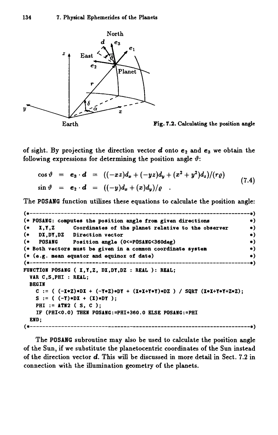
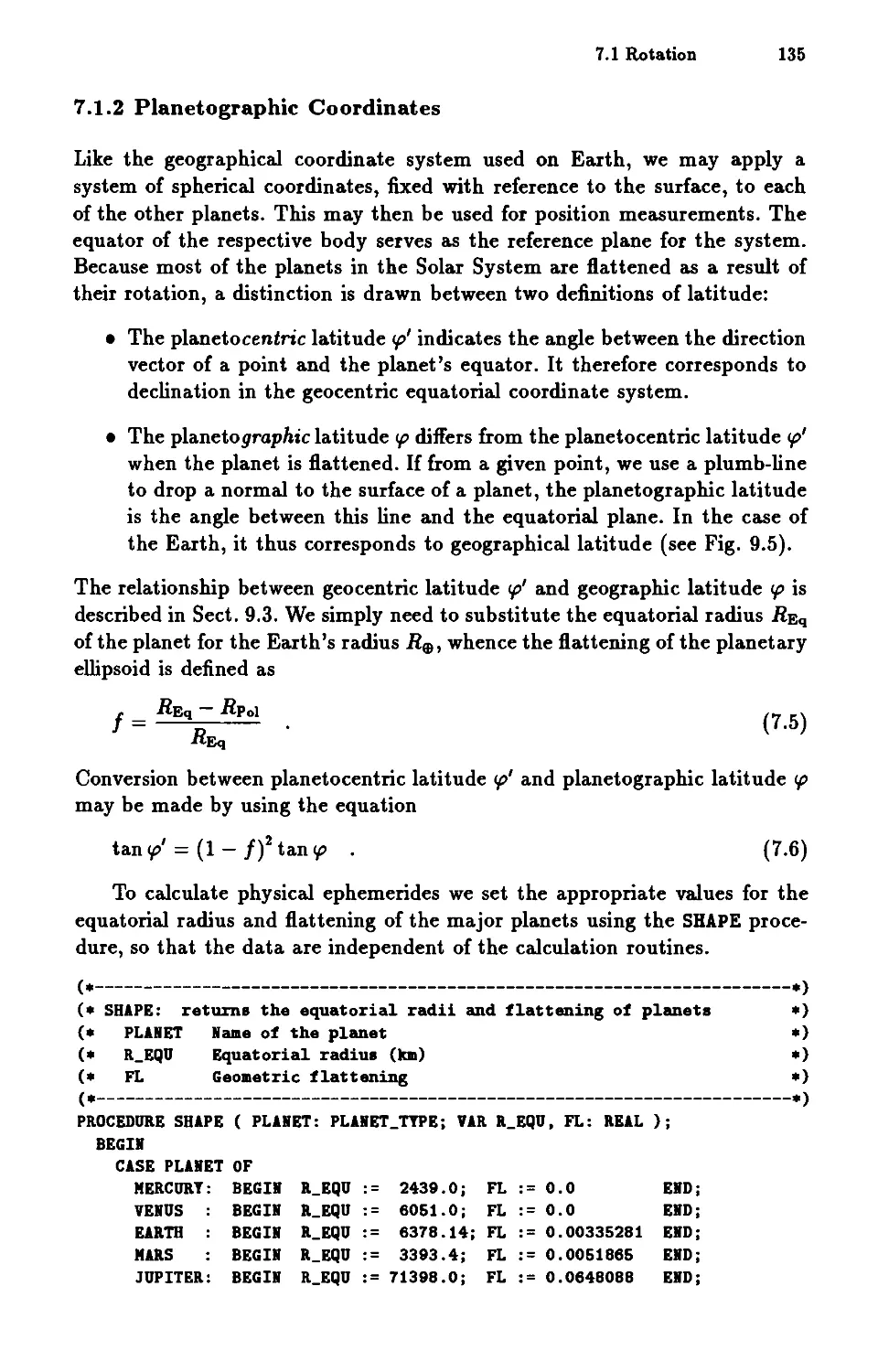
/


Text
Oliver Montenbruck
Thomas Pfleger
Astronomy
onthe
Personal
Computer
"
,
,
"
"
"
"
'ii-",
'" _ r<" .
-
" ,
. \.
';
, "',
.' . ('.. , I
..... ,
A
"
/'
-;. . .)0.
"
,
,
"
"
Springer-Verlag
e
"D . 0
Q)
+-'"D
w
t:"D
OQ)
oe>
"D-
ee
OW
()"D
Q)e
(/)
./
,
,
"
Oliver Montenbruck Thomas Pfleger
Astronomy
on the
Personal Computer
Translated by Storm Dunlop
Second, Corrected and Enlarged Edition
With 45 Figures and a Floppy Disk
Springer-Verlag
Berlin Heidelberg New York
London Paris Tokyo
Hong Kong Barcelona
Budapest
Dr. rer. nat. Oliver Montenbruck
DLR-GSOC, D-82230 WeBling, Germany
Dipl.-Ing. Thomas Pfleger
SchloBstraBe 56, D-53773 Hennef, Germany
Translator:
Dr. Storm Dunlop
140 Stocks Lane, East Wittering, Chichester
West Sussex P020 8NT, United Kingdom
Title of the onginal German edition:
O. Montenbruck, T. Pfleger: Astronomie mit dem Personal Computer
Zweite, uberarbeitete und stark erweiterte Auflage
@ Springer-Verlag Berlin Heidelberg 1989,1994
ISBN 3-540-57701-7 2. Auflage Springer-Verlag Berlin Heidelberg
ISBN 3-540-57700-9 2. Auflage Springer-Verlag Berlin Heidelberg New York
ISBN 0-387-57700-9 2nd Edition Springer-Verlag New York Berlin Heidelberg
ISBN 3-540-52754-0 1. Auflage Springer-Verlag Berlin Heidelberg New York
ISBN 0-387-52754-0 1st Edition Springer-Verlag New York Berlin Heidelberg
Library of Congress Cataloging-in-Publication Data. Montenbruck, Oliver, 1961- . [Astronomie mit
dem Personal Computer. English] Astronomy on the personal computer / O. Montenbruck, T. Pfleger;
translated by S. Dunlop. - 2nd corr. and en!. ed. p. cm. Includes bibliographical references and index
ISBN 3-540-57700-9 (Berlin: acid-free paper). - ISBN 0-387-57700-9 (New York: acid-free paper)
1. Astronomy-Data processing. 2. Microcomputers. I. Pfleger, T. (Thomas), 1964- . II. Title.
QB51.3.E43M6613 1994 522'.85'536-dc20 94-28233
This work is subject to copyright. All rights are reserved, whether the whole or part of the material
is concerned, specifically the rights of translation, reprinting, reuse of illustrations, recitation,
broadcasting, reproduction on microfilm or in any other way, and storage in data banks. Duplication
of this publication or parts thereof is permitted only under the provisions of the German Copyright
Law of September 9, 1965, in its current version, and permission for use must always be obtained from
Springer-Verlag. Violations are liable for prosecution under the German Copyright La w.
@ Springer-Verlag Berlin Heidelberg 1991, 1994
Printed in Germany
The use of general descriptive names, registered names, trademarks, etc. in this publication does not
imply, even in the absence of a specific statement, that such names are exempt from the relevant
protective laws and regulations and therefore free for general use.
Please note: Before using the programs in this book, please consult the technical manuals provided
by the manufacturer ofthe computer - and of any additional plug-in boards - to be used. The authors
and the publisher accept no legal responsibility for any damage by improper use of the instructions
and programs contained herein. Although these programs ha ve been tested with extreme care, we can
offer no formal guarantee that they will function correctly.
The programs on the enclosed diskette are under copyright-protection and may not be reproduced
without written permission by Sprmger-Verlag. One copy of the programs may be made as a back-up,
but all further copies offend copyright la w.
Typesetting: Camera-ready copy from the authors
Cover design: Erich Kirchner, Heidelberg, Germany
SPIN: 10131861
55/3140 - 5 4 3 2 1 0 - Printed on acid-free paper
Foreword
It is said that a typical astronomer of the 19th century spent seven hours
working at a desk for every hour spent at the telescope. That's how long the
routine analysis of data took with pencil, paper, and logarithmic tables. Thus
when Wilhelm Olbers discovered the minor planet Vesta in 1807 and gathered
the necessary observations, his friend Gauss needed almost 10 hours to hand-
calculate its orbit. That achievement astonished many less gifted astronomers
of the time, who might have labored days to work out the orbit of a newfound
comet.
How different things are today! Gauss's method of orbit determination,
presented in Chap. 11 of this book, runs to completion on a home computer
in a few seconds at most. The machine will issue its accurate results in less
time than it takes to key in the observations.
In this book, a landmark in the youthful literature of astronomical com-
puter algorithms, Oliver Montenbruck and Thomas Pfleger cover many topics
of keen interest to the practical observer. For me its most remarkable feature
is the library of interrelated program modules, all elegantly written in PAS-
CAL. Anyone who has tried to create such modules in interpreted BASIC
soon runs into trouble: too few letters for variable names, not enough signifi-
cant digits, and so on. These PASCAL routines are invoked one after another
in coordinate transformations and calendar conversions. As "building blocks"
for writing programs they find application in all corners of astronomy, not
just the specific topics treated. That is reason enough, in my view, for anyone
not so equipped to go out and buy a PASCAL compiler at once.
Any active observer will welcome the power and generality of these pro-
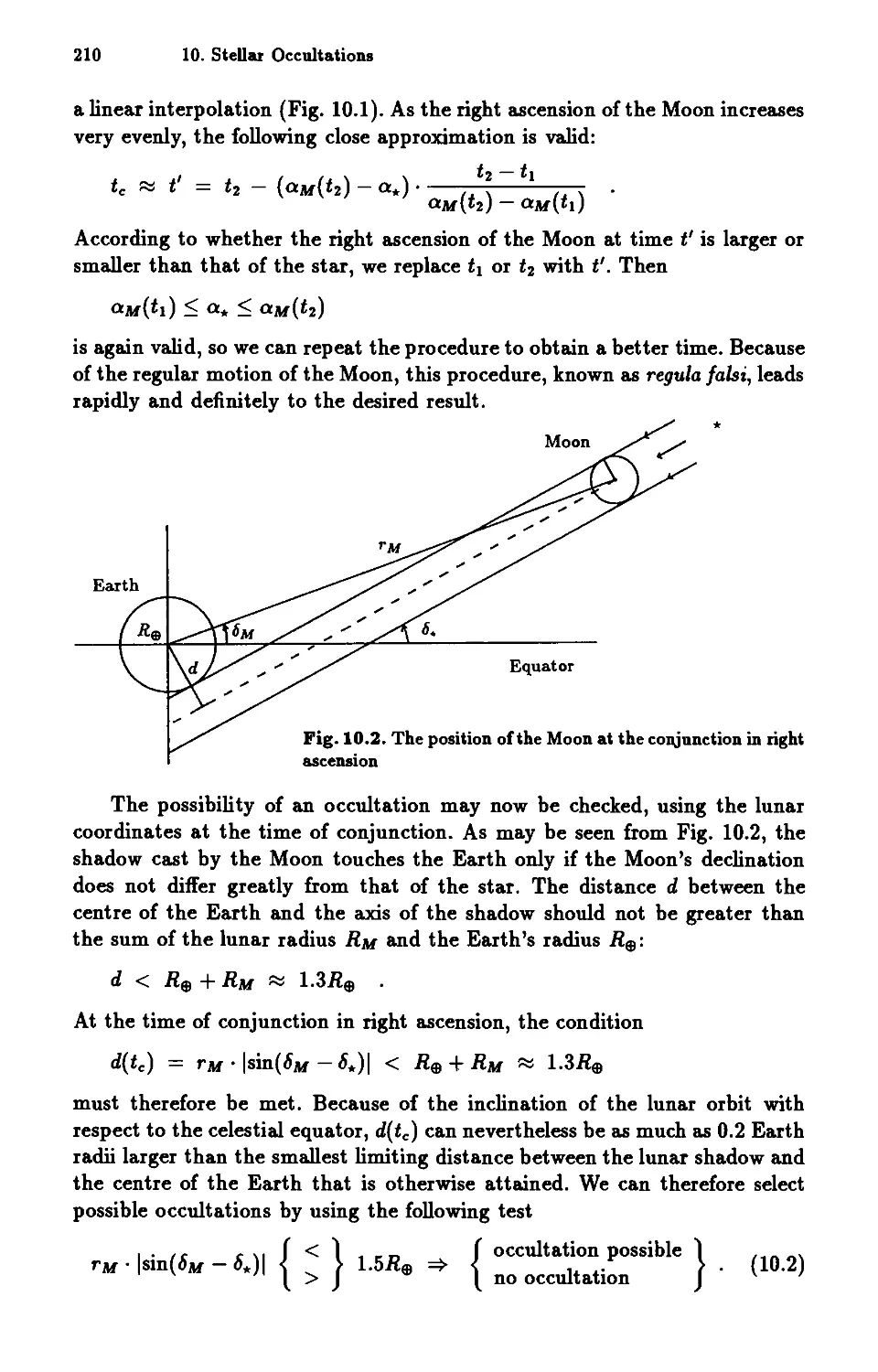
grams. Chapter 10, for example, tells how to make personal predictions of all
stars to be occulted by the Moon for a given spot on Earth. It's exciting to see
a star wink out of sight or pop into view from behind the Moon's limb, but
one has to know when and where to look. For many years, serious amateurs
around the world have carefully timed such events, thereby gathering the raw
data for detailed study of the Moon's limb profile and orbital motion. Astron-
omy magazines can alert their readers to just a few of the most spectacular
occultations each year - yet they happen all the time.
Comets and minor planets offer many opportunities for amateur-professio-
nal cooperation as well. A large observatory can't easily shuffle its schedule
to cope with the sudden appearance of a bright comet. Yet countless ama-
VI Foreword
teurs already possess the telescopes, photographic skills, and enthusiasm to
swing into action at a moment's notice. This book's chapters on measuring
photographs, determining orbits, and calculating an ephemeris are just what
is needed to participate in discovering and publicizing a new comet. Personal
computers, especially when equipped with hard disks and math coprocessors,
are also well suited for the specialized work of identifying and improving the
orbits of minor planets - something that just a few years ago was the exclusive
province of large mainframes.
Total solar eclipses hold a special fascination for astronomers, but accu-
rate prediction has not always been easy. In October of 1780, an expedition
from Harvard College sailed to Penobscot Bay on the coast of Maine and
somehow managed to set up its telescopes 30 km outside the path of total-
ity! Such a blunder is far less likely today, even if official predictions are not
issued until a few months before an eclipse takes place. However, owners of
this book are spared even that frustration; the eclipse program of Chap. 9
will serve quite well for detailed travel plans.
Indeed, the carefully crafted computer programs presented here go a long
way toward freeing us from the need for an almanac or yearbook, the tradi-
tional "astronomer's bible". While I still cherish such works on my bookshelf
for their accurate planet positions, occultations, and eclipse calculations, I'm
starting to look on them differently. Once they seemed great repositories of as-
tronomical knowledge, full of data not abtainable elsewhere. More and more,
they now serve as checks on the wondedully accurate predictions I'm learning
to make with my home computer.
Cambridge, MA
October 1990
Roger W. Sinnott
Preface to the Second Edition
Since the publication of the first edition of Astronomy on the Personal Com-
puter, we have received numerous comments and suggestions. Together with
the publishers' interest in a new edition, this prompted us to revise the book
and to incorporate a wide range of improvements to the text.
The first important addition is a chapter on the calculation of perturba-
tions. This shows how gravitational perturbations by the major planets may
be incorporated into the calculation of ephemerides for minor planets and
comets. The RUMINT program described here enables more accurate positions
to be calculated. This will be of considerable assistance in searching for what
are often extremely faint objects. This tool for calculating perturbations com-
plements the chapters on the calculation of ephemerides, the determination
of orbits, and astrometry.
The second additional chapter discusses the calculation of physical ephe-
merides for the major planets and the Sun, and thus fills a gap in the earlier
edition's coverage. Amateurs now have at their disposal the means of both
predicting and subsequently reducing interesting planetary observations.
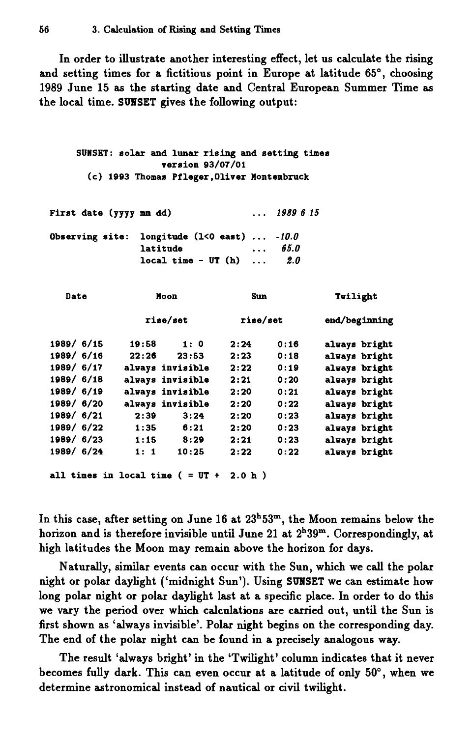
Other changes mainly concern the calculation of rising and setting times
for the planets, and of the local circumstances that apply to solar eclipses.
Finally, there is now a single version of the program diskette that is sup-
plied with the book. Since the firm of Application Systems Heidelberg have
introduced their Pure Pascal compiler for Atari ST /TT computers that is
compatible with Borland's Turbo Pascal, there is no need for a special Atari
version of the program diskette. The enclosed diskette may, therefore, be
used without modifications with Turbo Pascal on IBM-compatible machines
or with Pure Pascal on Atari computers. Details about the appropriate in-
stallation procedures may be found in the AAREADME. DOC file on the diskette.
We should like to thank Springer-Verlag for their helpful co-operation,
and also Application Systems Heidelberg for their technical support.
Munich, July 1994
O. Montenbruck and T. Pfleger
Preface to the First Edition
Nowadays anyone who deals with astronomical computations, either as a
hobby or as part of their job, inevitably turns to using a computer. This is
particularly true now that personal computers have become firmly established
as ubiquitous aids to living. Calculations that could not even be contemplated
a short time ago are now available to a whole range of users, and at no farther
remove than their desks.
Not only has the technical capacity of computers grown, but so has the
need for powerful - i.e., fast and accurate - programs. So the wish to avoid
conventional, astronomical yearbooks as much as possible is quite understand-
able.
We were therefore delighted to take up our publisher's suggestion that we
explain the fundamental principles of spherical astronomy, ephemeris calcu-
lations, and celestial mechanics in the form of this book.
Astronomy on the Personal Computer offers readers who develop their
own programs a comprehensive library of Pascal procedures for solving a
whole range of individual steps that frequently occur in problems. This in-
cludes routines for common coordinate transformations, for time and calen-
dar calculations, and for handling the two-body problem. Specific procedures
allow the exact positions of the Sun, the Moon, and the planets to be calcu-
lated, taking mutual perturbations into account. Thanks to the widespread
use of Pascal as a computing language, and by avoiding computer-specific
commands, the programs may be employed on a wide range of modern com-
puters from the PC to the largest mainframes. The large number of routines
discussed should at least mean that few readers will have to Ire-invent the
wheel', and that they will therefore be free to concentrate on their own par-
ticular interests.
Each chapter of this book deals with a fairly restricted theme and ends
with a complete main program. From simple questions, such as the deter-
mination of rising and setting times or the calculation of the positions of
the planets, more complex themes are developed, such as the calculation of
solar eclipses and stellar occultations. The programs for the astrometric re-
duction of photographs of star fields and for orbit determination enable users
to derive orbital elements of comets or minor planets for themselves. Even
readers without programming experience will be able to use the appropriate
appli cations.
X Preface to the First Edition
Sufficient details are given of the astronomical and mathematical grounds
on which solutions of specific problems are based for readers to understand
the programs presented. This knowledge will enable them to adapt any of
the programs to their individual needs. This close link between theory and
practice also enables us to explain what are sometimes quite complex aspects
in a much easier fashion than the descriptions found in classical textbooks.
To sum up, we hope that we have given readers a fundamental grounding in
using computers for astronomy.
We should like to thank S. Dunlop for producing such an excellent trans-
lation and Dr. G. Wolschin and C.-D. Bachem of Springer-Verlag for their
cordial cooperation and interest during the process of publishing this book.
Our thanks are also due to all our friends and colleagues, who, with their
ideas and advice, and their help in correcting the manuscript and in testing
the programs, have played an important part in the success of this book.
Munich, August 1990
o. Montenbruck and T. Pfleger
Contents
1 Introduction . . . . . . . . . . 1
1.1 Some Examples . . . . . . . 1
1.2 Astronomy and Computing 2
1.3 Programming Languages and Techniques 4
2 Coordinate Systems 7
2.1 Making a Start 7
2.2 Calendar and Julian Dates 11
2.3 Ecliptic and Equatorial Coordinates . 13
2.4 Precession . . . . . . . . . . . . . . . 17
2.5 Geocentric Coordinates and the Orbit of the Sun 23
2.6 The COCO Program . . . . . . . . . . . 27
3 Calculation of Rising and Setting Times 35
3.1 The Observer's Horizon System 35
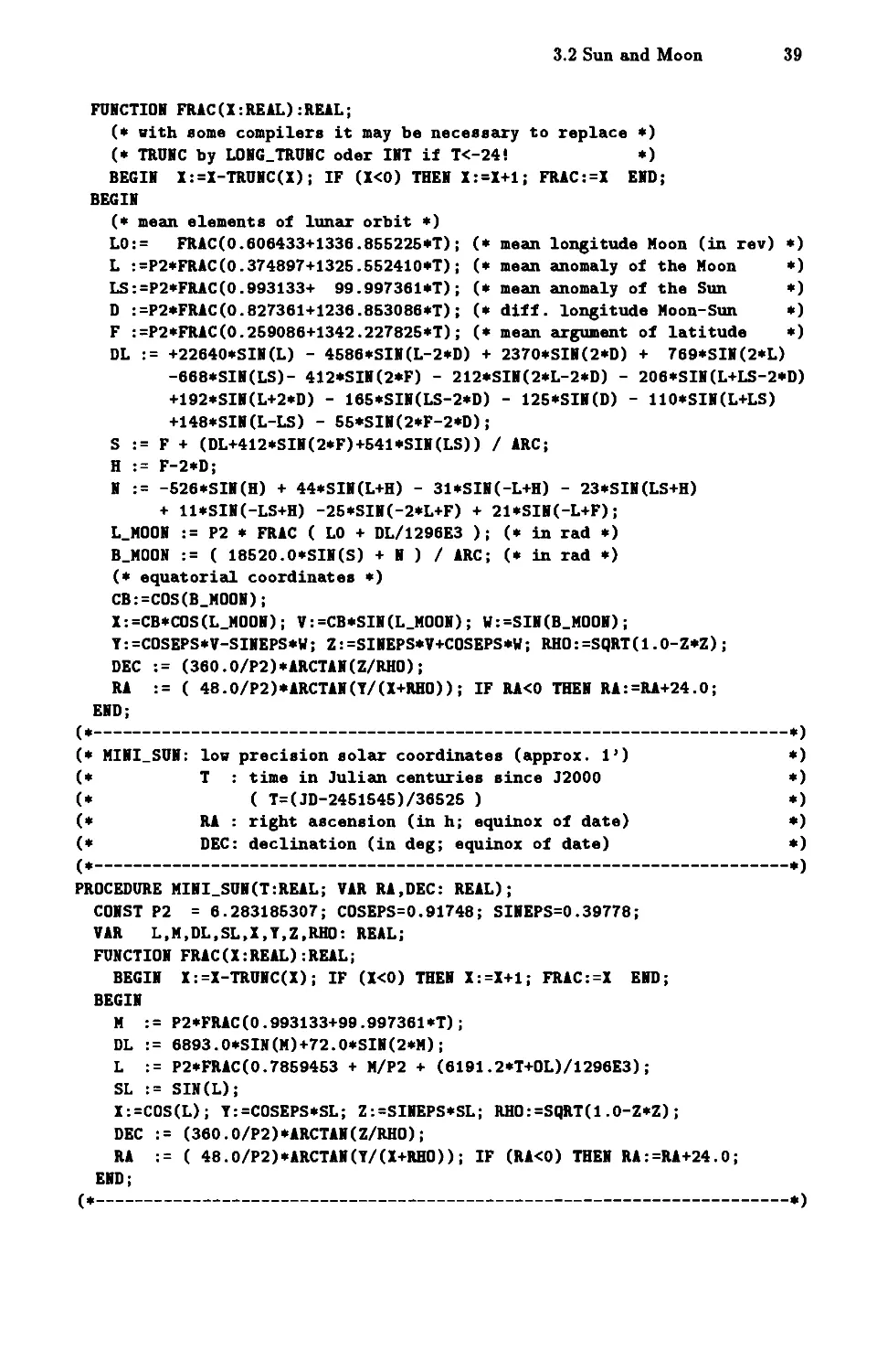
3.2 Sun and Moon. . . . . . . . . . . . . 38
3.3 Sidereal Time and Hour Angle . . . . 40
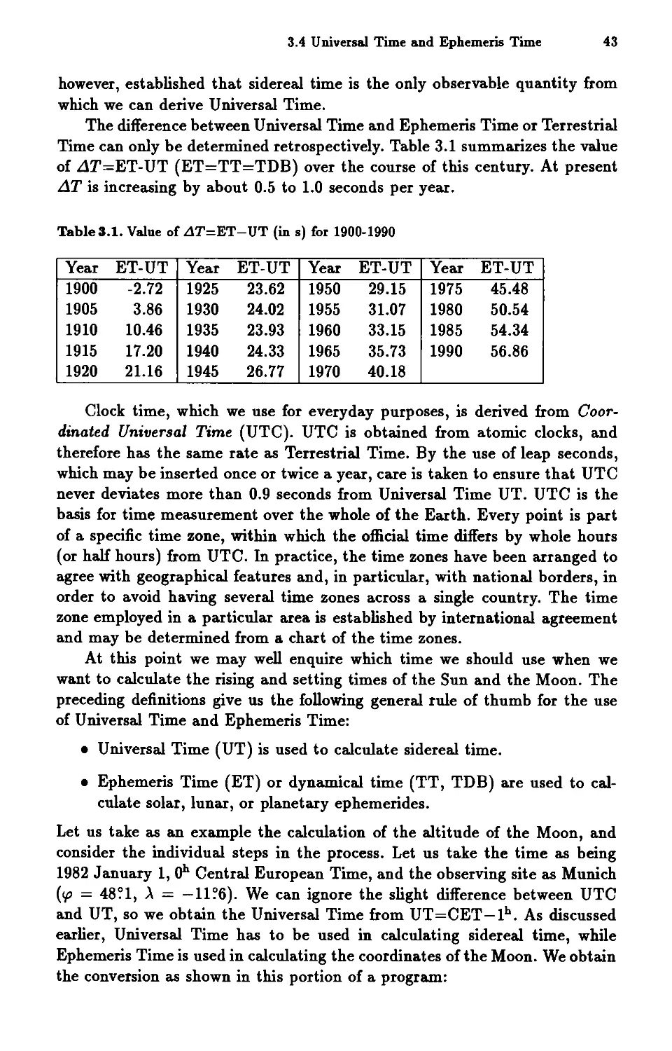
3.4 Universal Time and Ephemeris Time 41
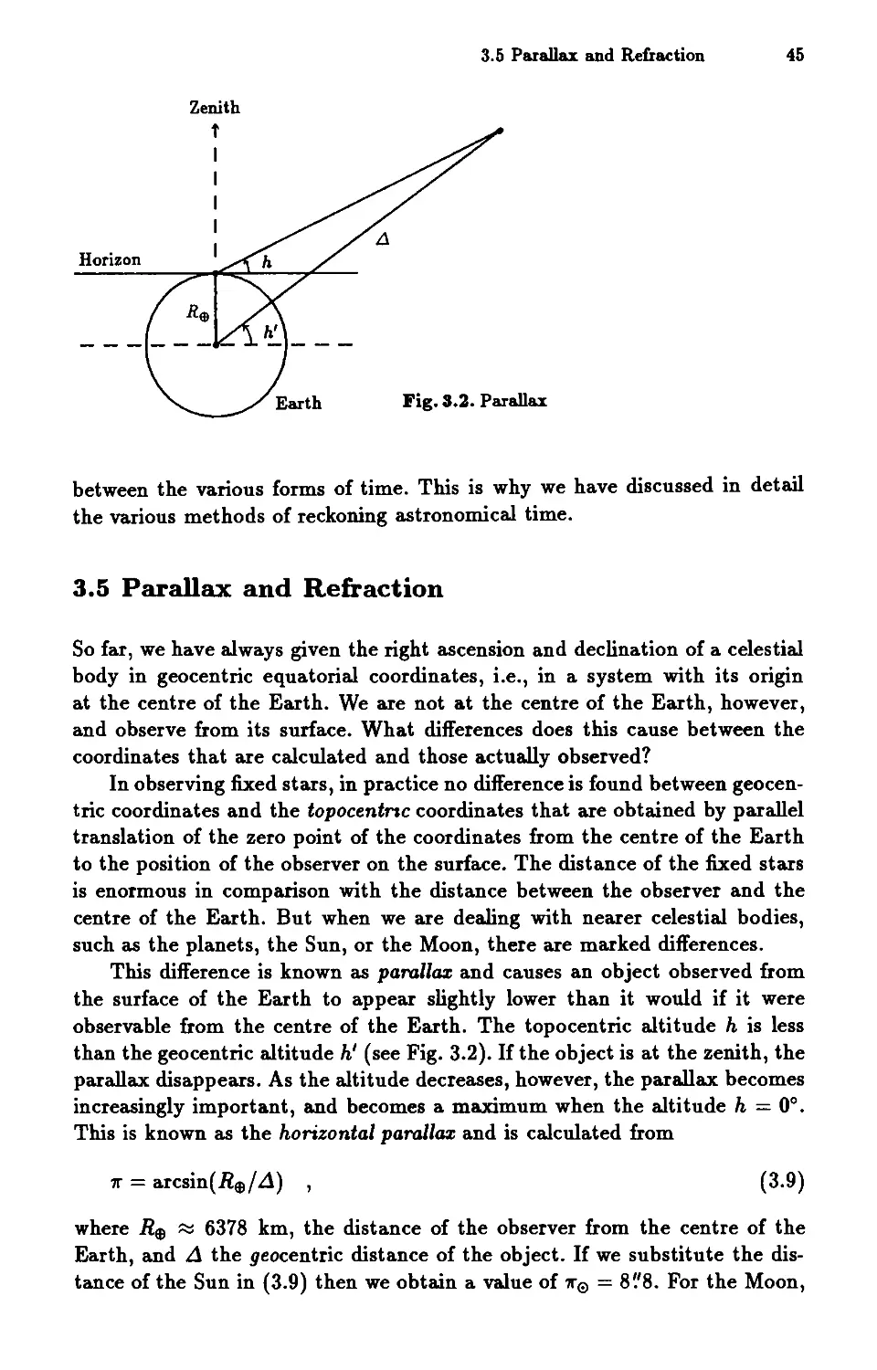
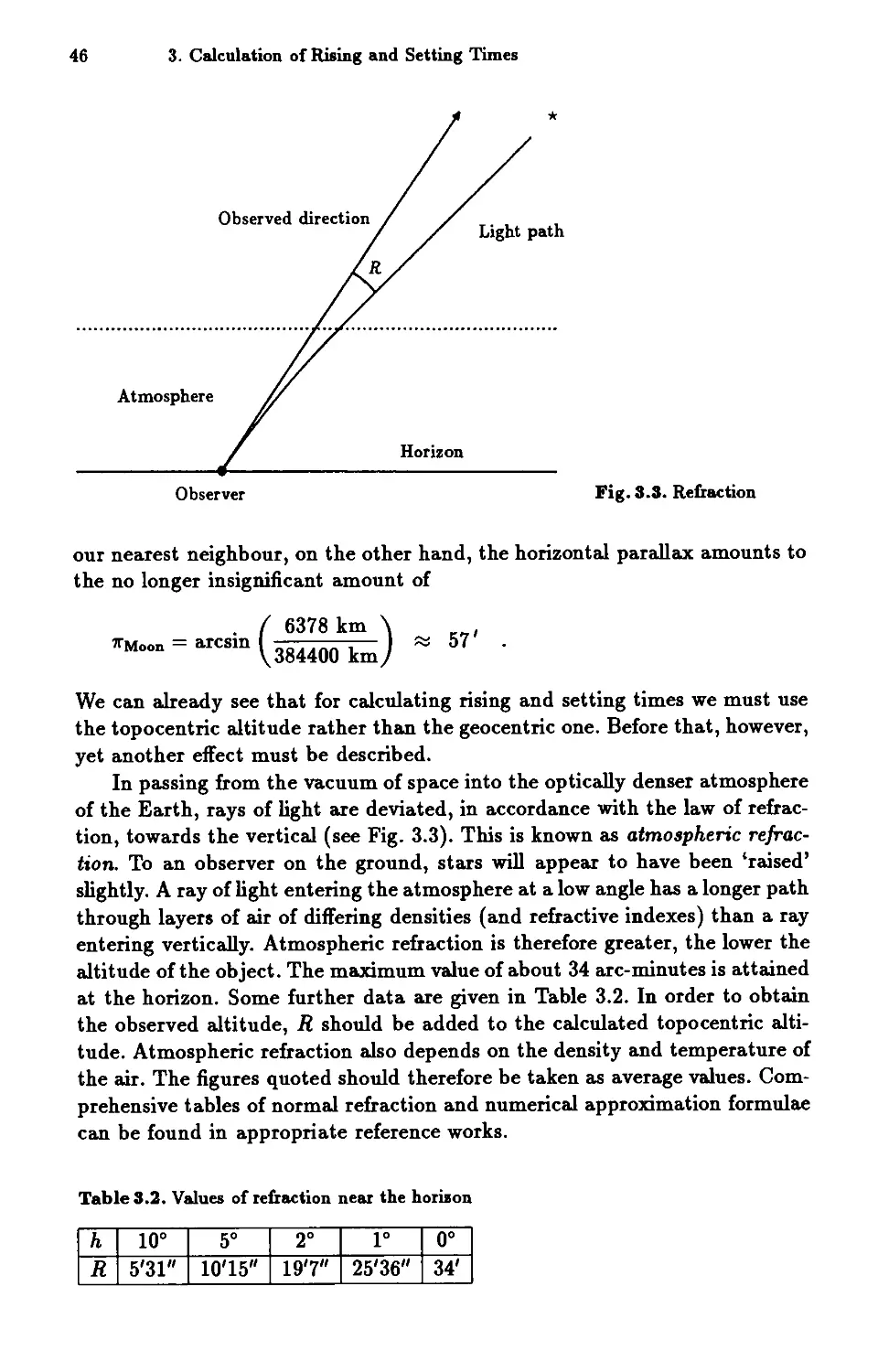
3.5 Parallax and Refraction 45
3.6 Rising and Setting Times. 47
3.7 Quadratic Interpolation 49
3.8 The SUNSET Program . . 50
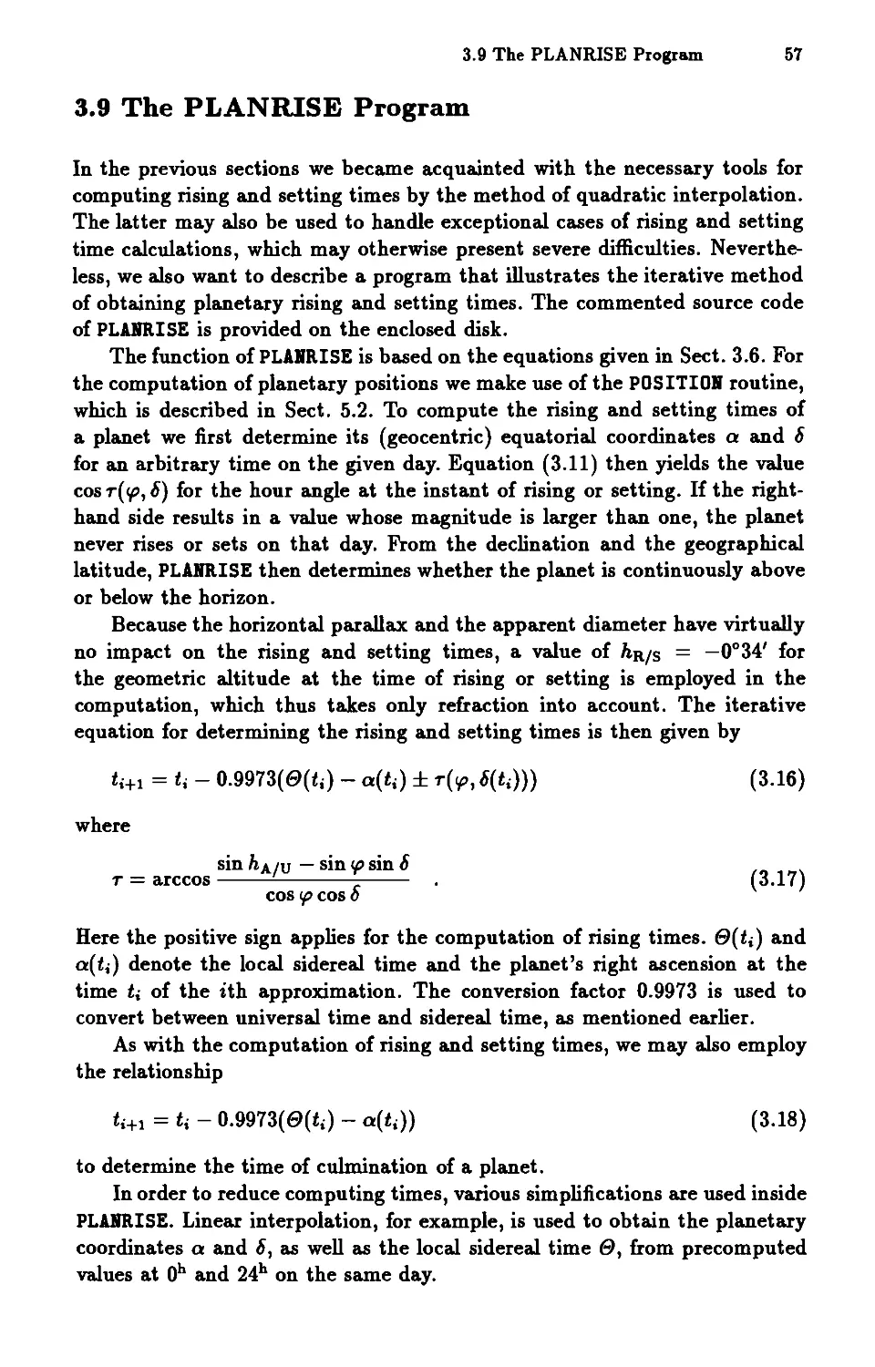
3.9 The PLANRISE Program 57
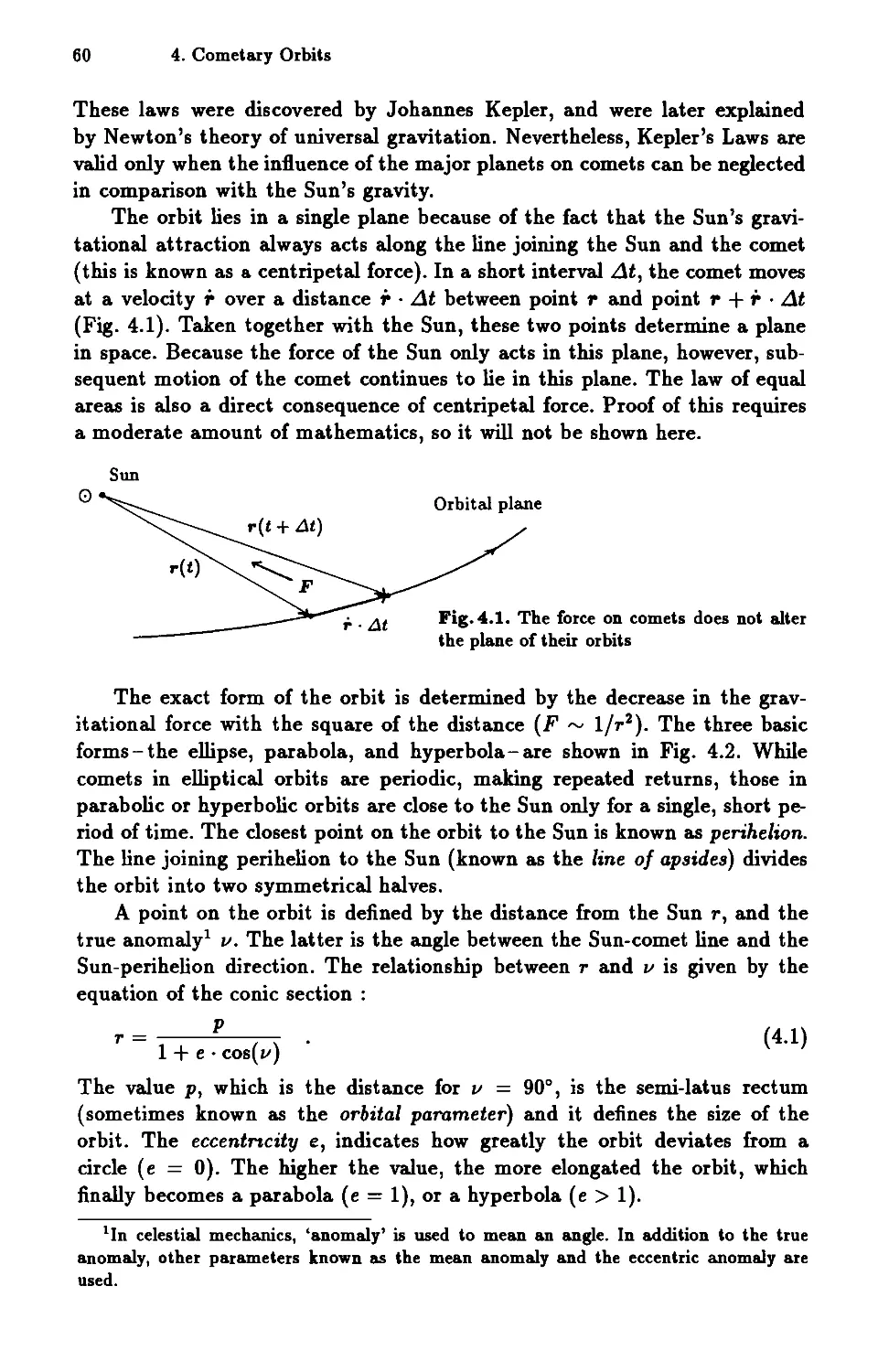
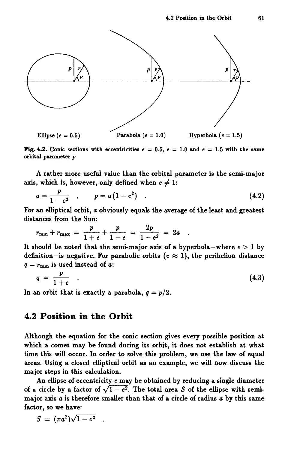
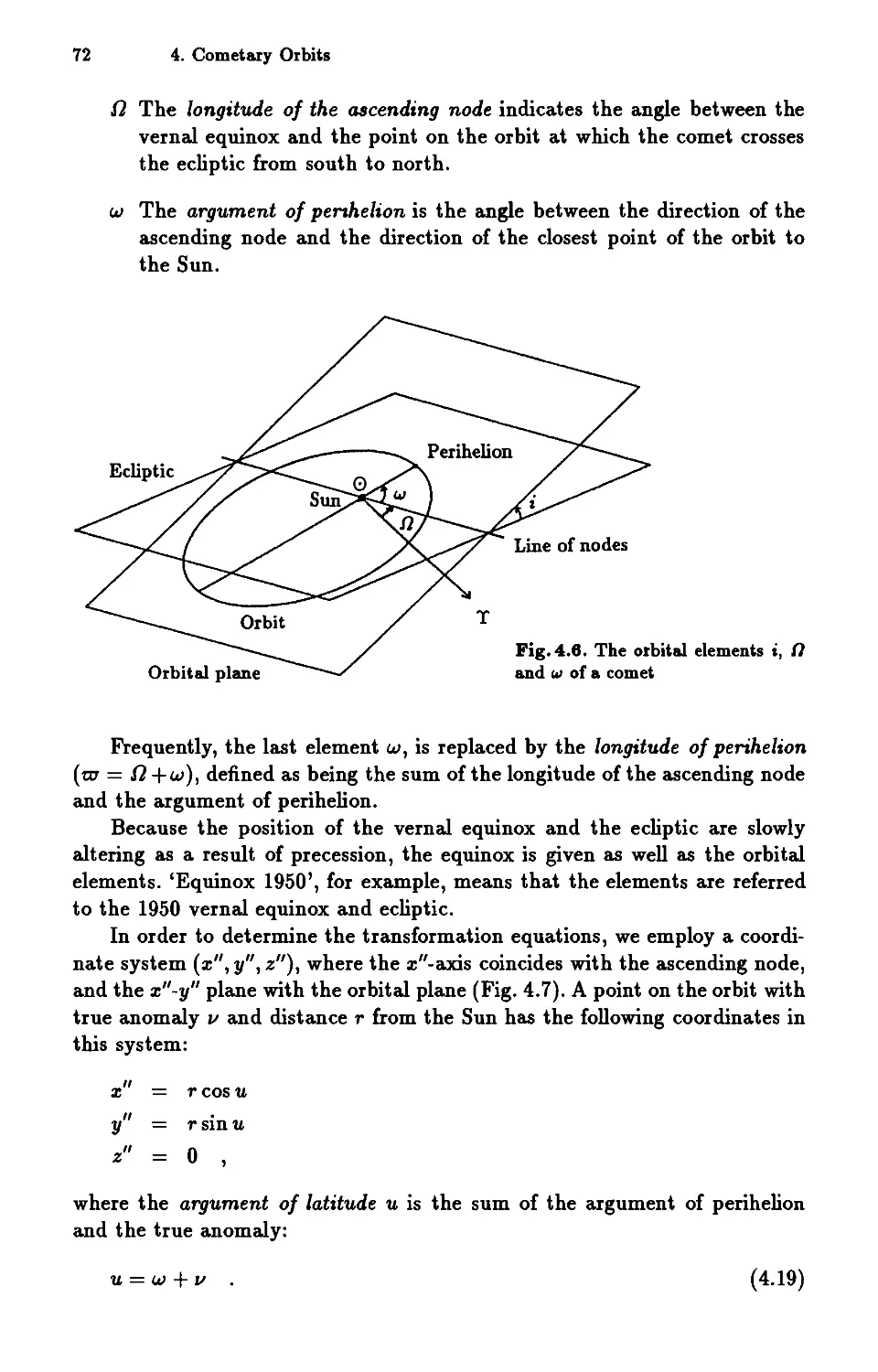
4 Cometary Orbits . . . . . . 59
4.1 Form and Orientation of the Orbit 59
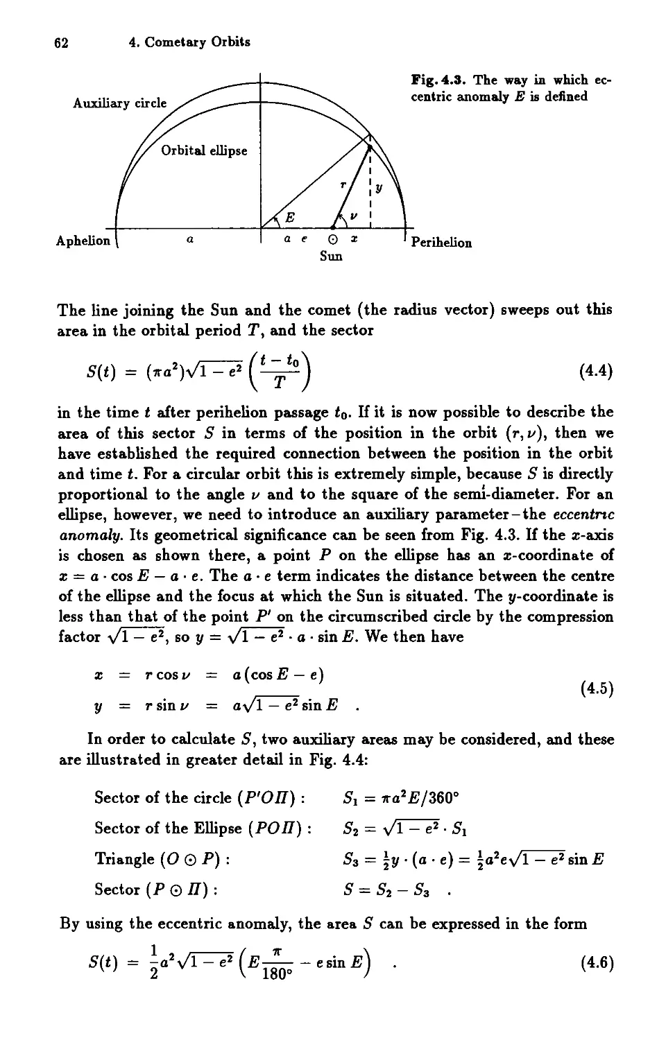
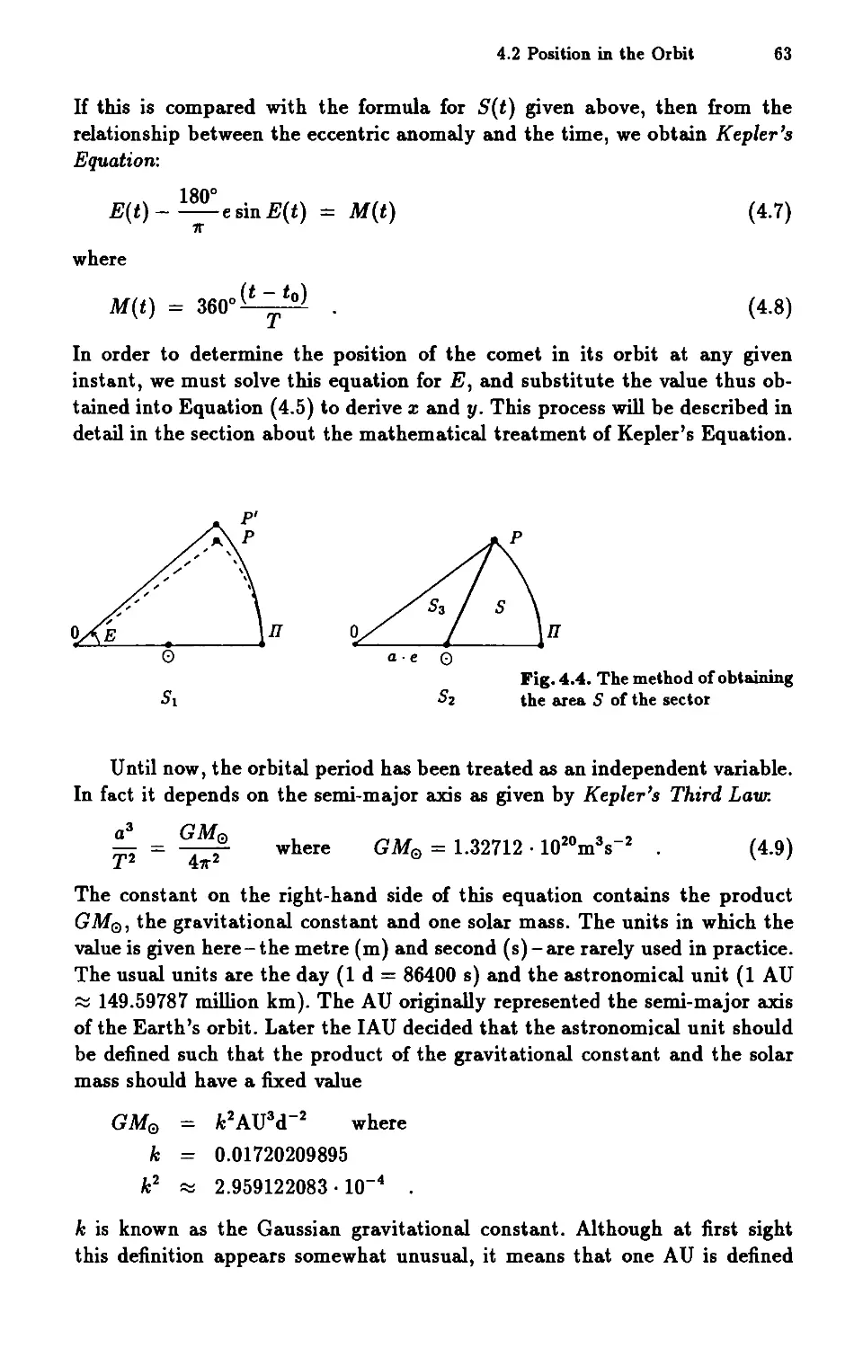
4.2 Position in the Orbit . . . . . . . . 61
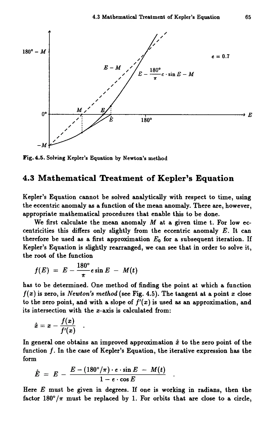
4.3 Mathematical Treatment of Kepler's Equation 65
4.4 Near-Parabolic Orbits 68
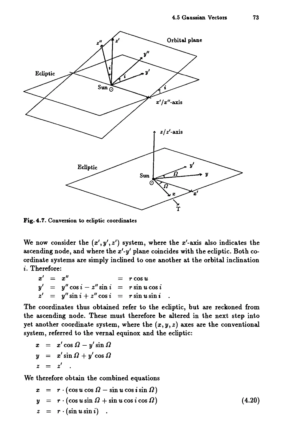
4.5 Gaussian Vectors . . . 71
4.6 Light-Time . . . . . . 76
4.7 The COMET Program 77
XII Contents
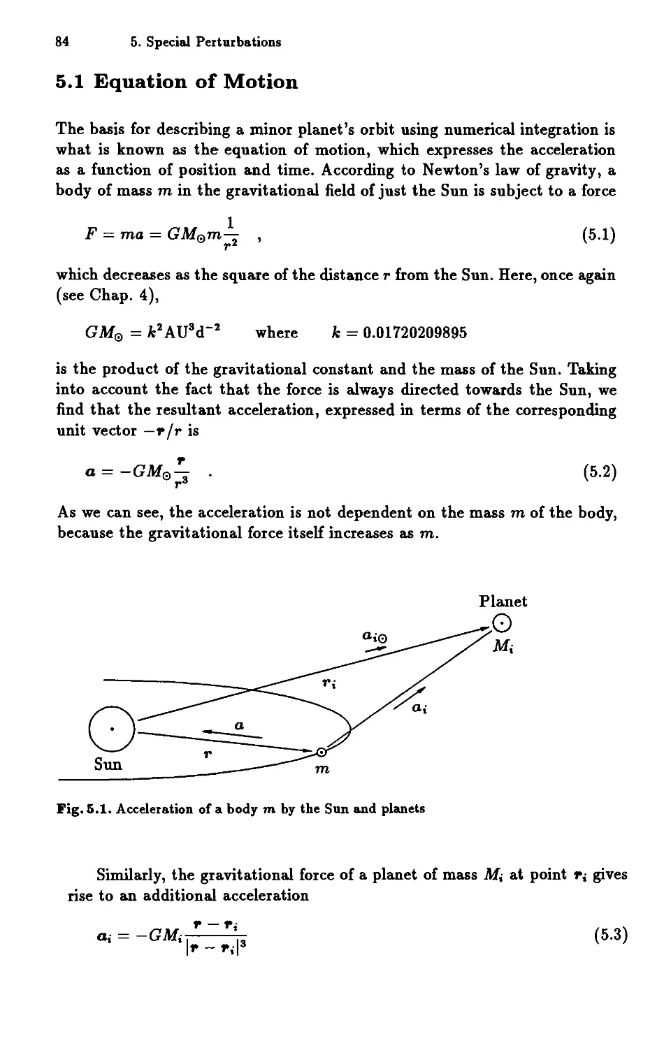
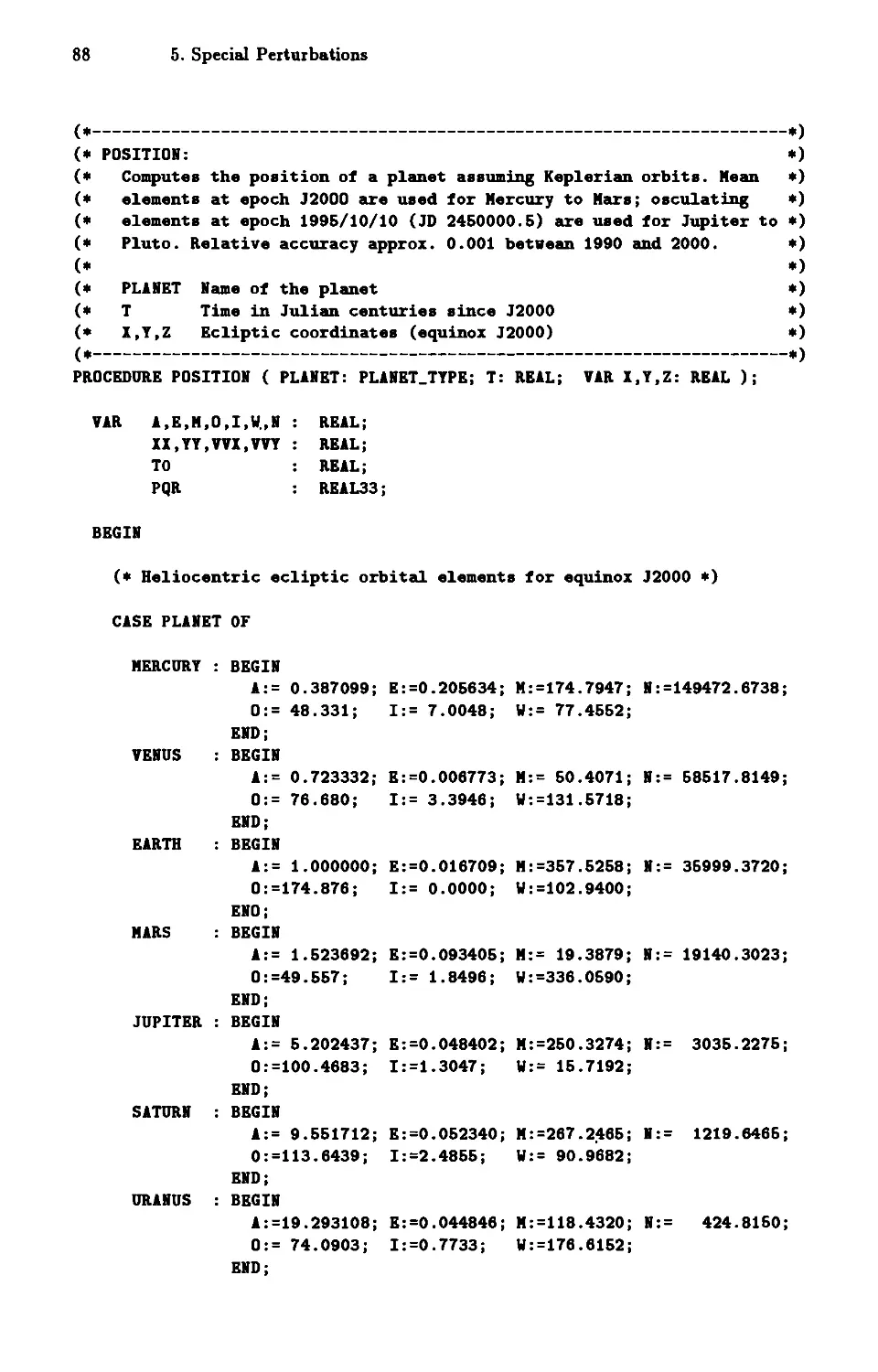
5 Special Perturbations 83
5.1 Equation of Motion 84
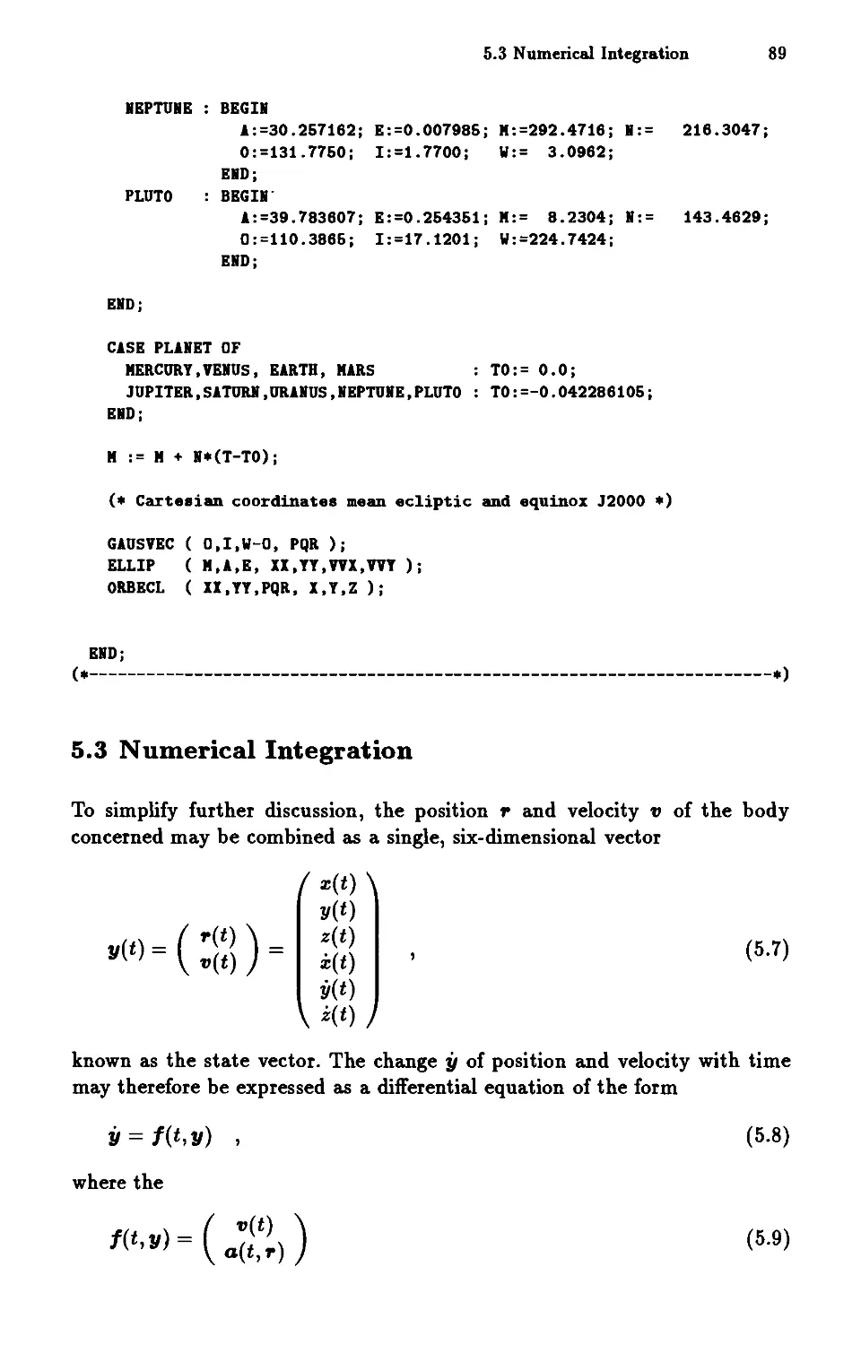
5.2 Planetary Coordinates 87
5.3 Numerical Integration 89
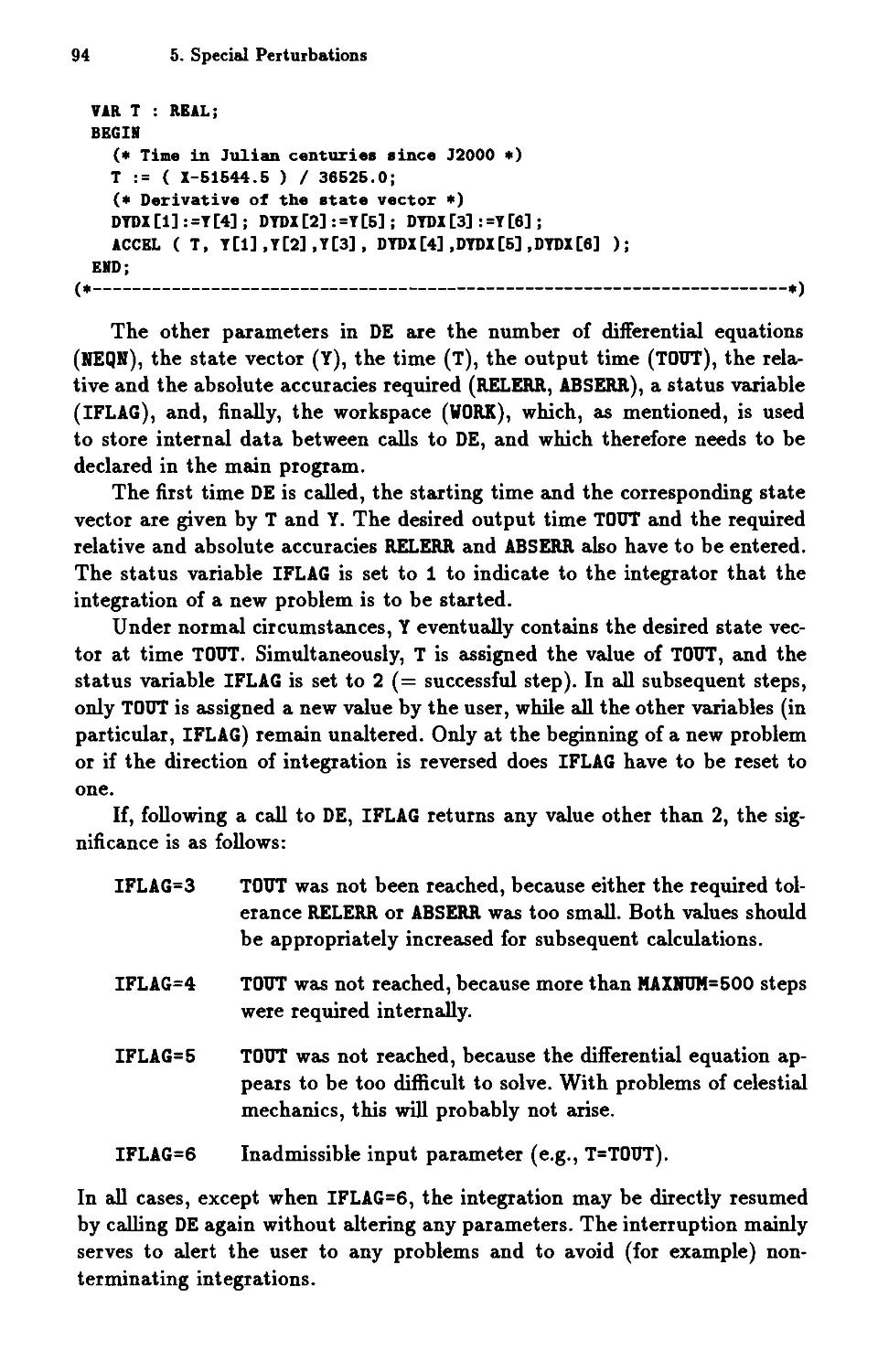
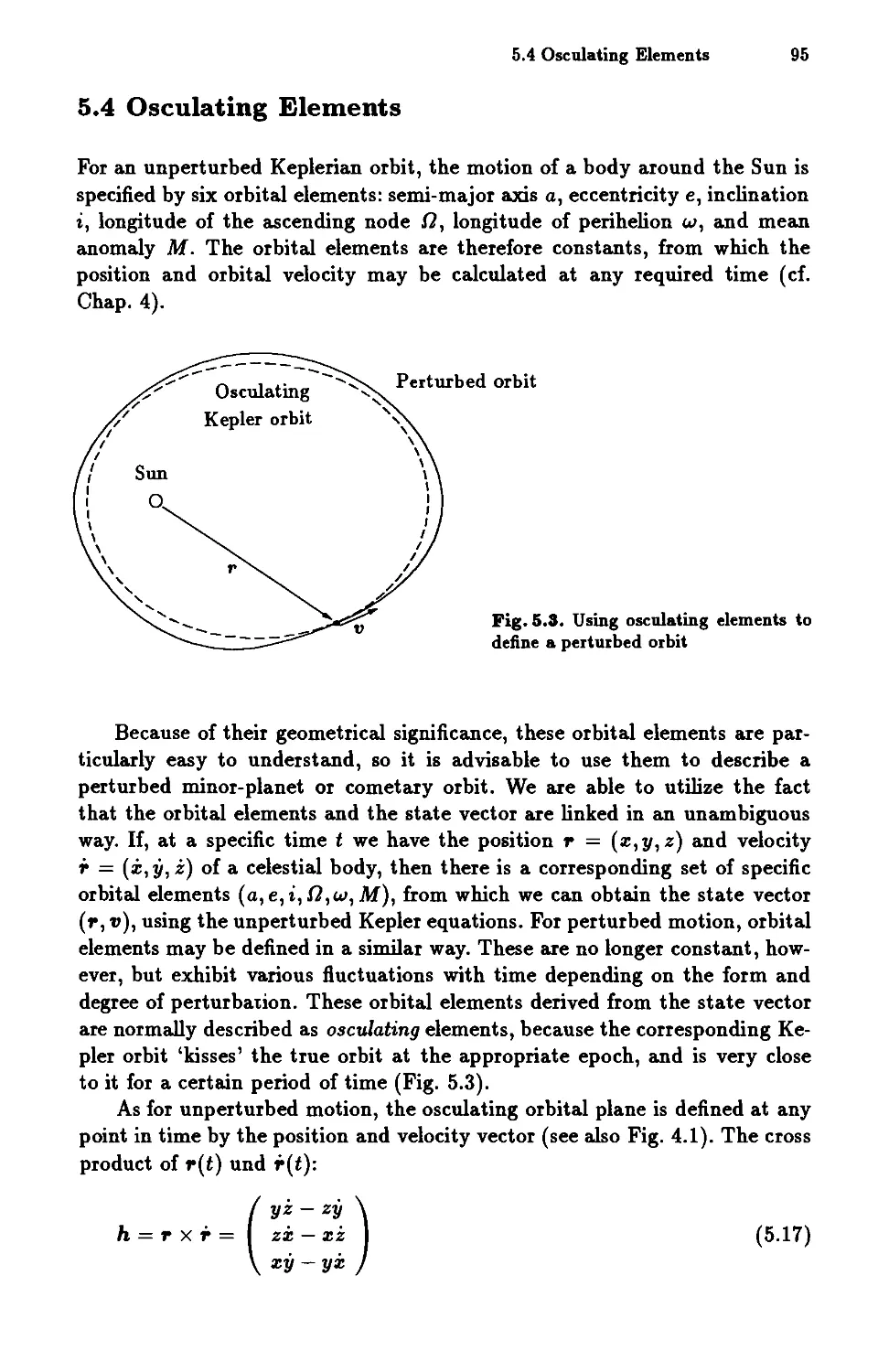
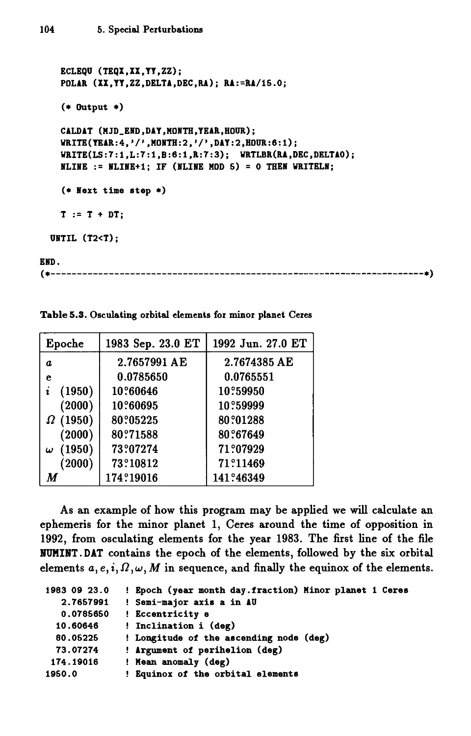
5.4 Osculating Elements . 95
5.5 The NUMINT Program 98
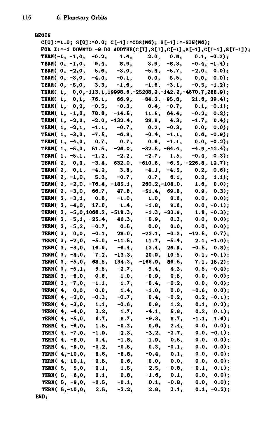
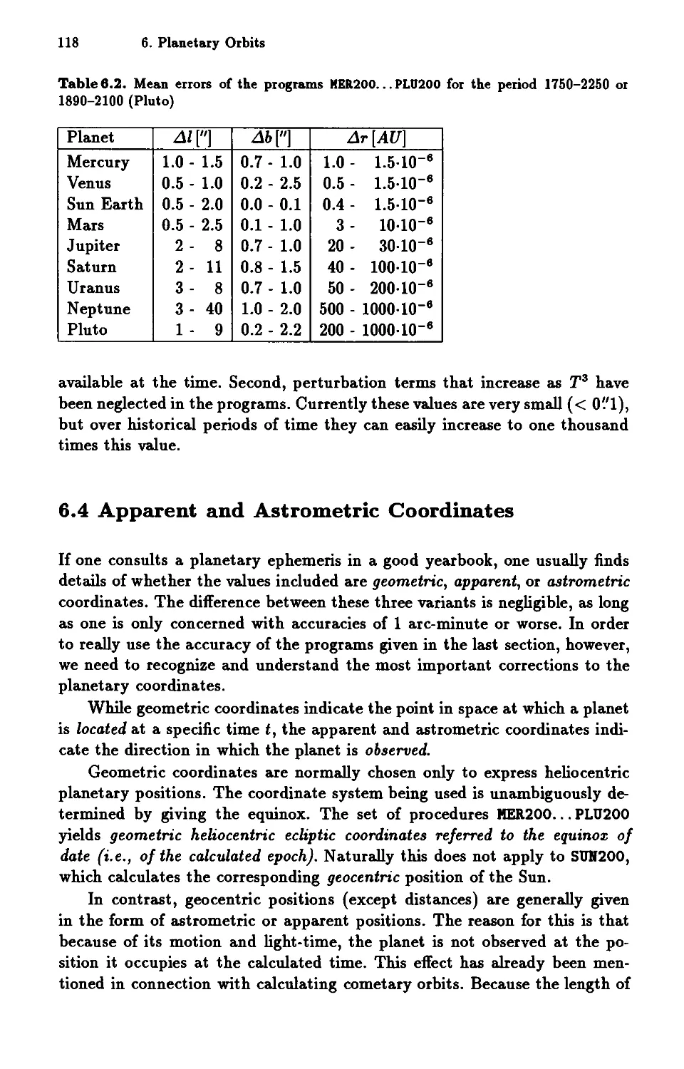
6 Planetary Orbits ..... 107
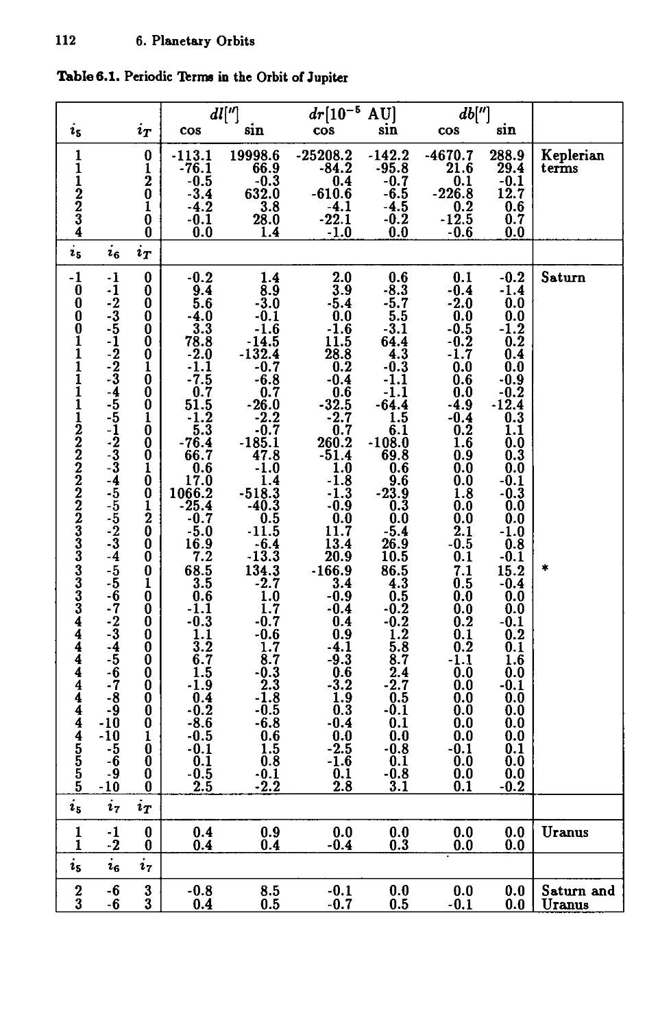
6.1 Series Expansion of the Kepler Problem. 108
6.2 Perturbation Terms. . . . . . . . . . . . 111
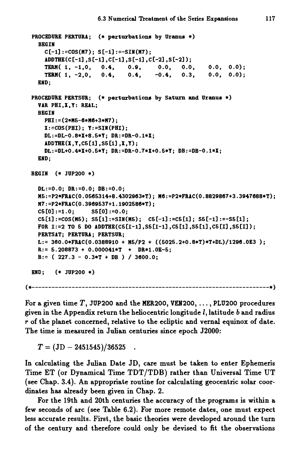
6.3 Numerical Treatment of the Series Expansions 114
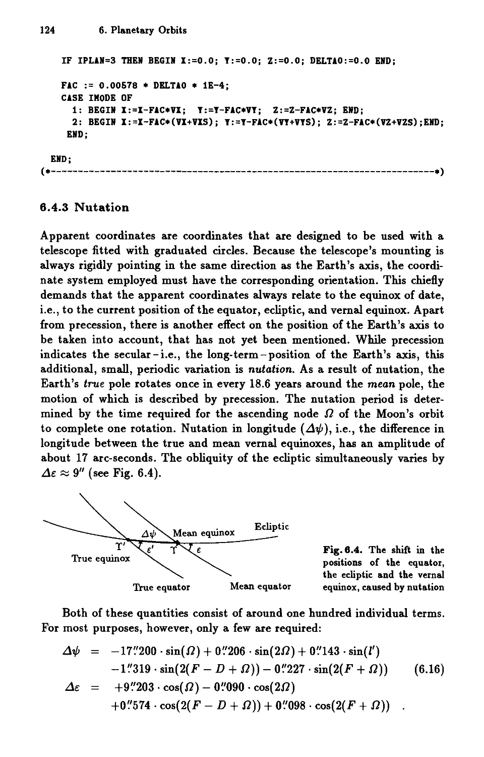
6.4 Apparent and Astrometric Coordinates 118
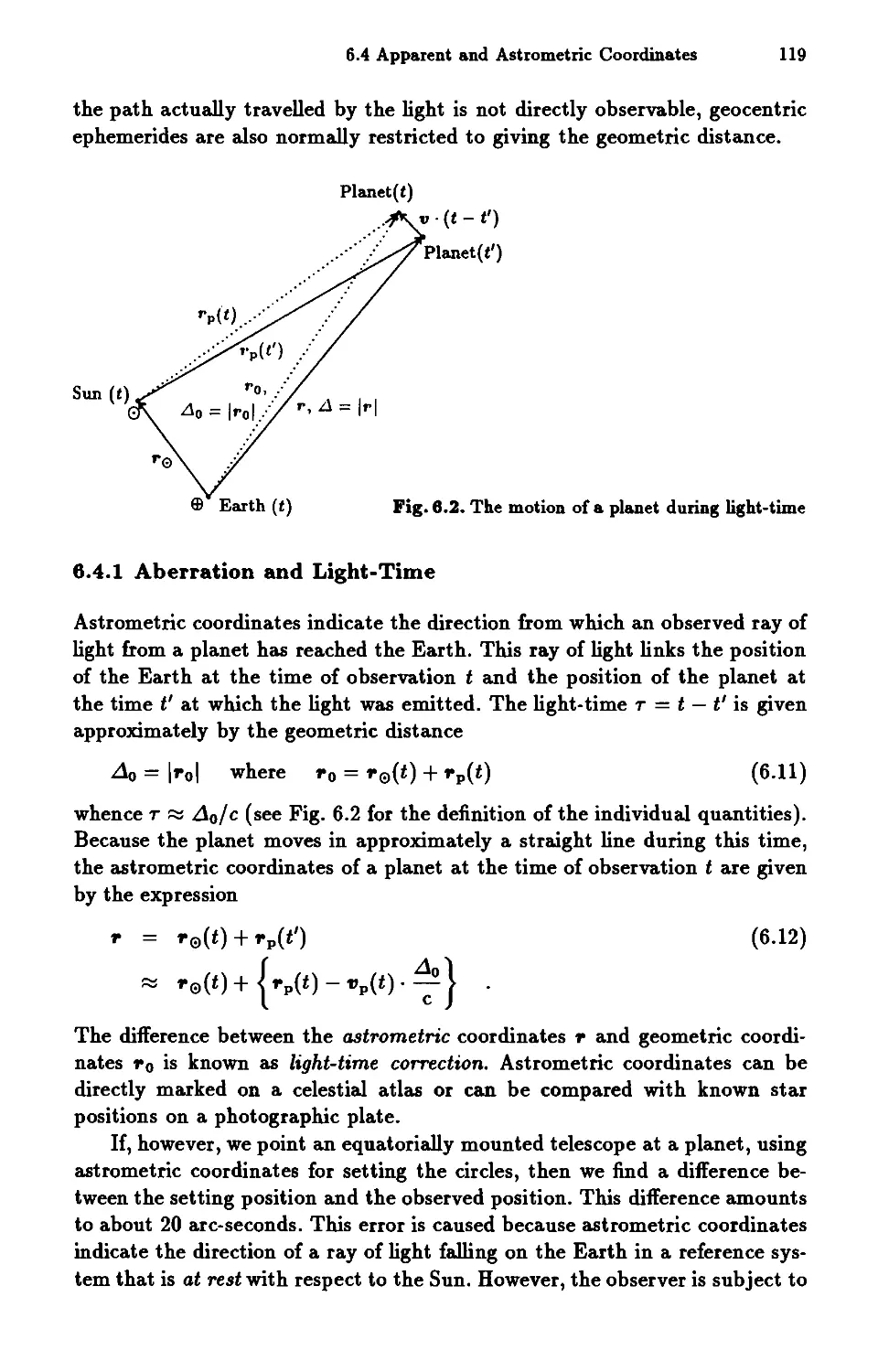
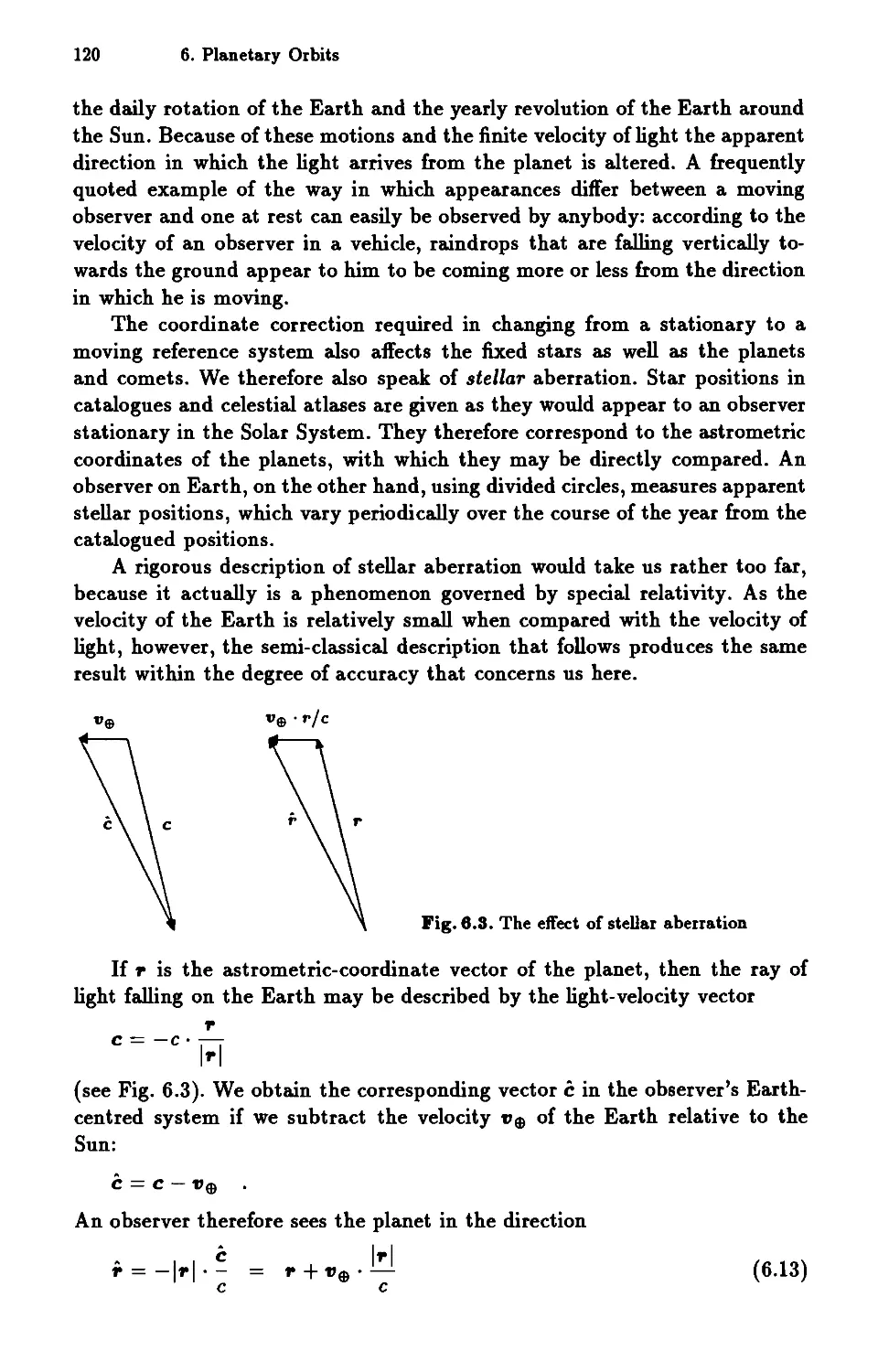
6.4.1 Aberration and Light-Time 119
6.4.2 Velocities of the Planets 121
6.4.3 Nutation...... 124
6.5 The PLANPOS Program . . . . 126
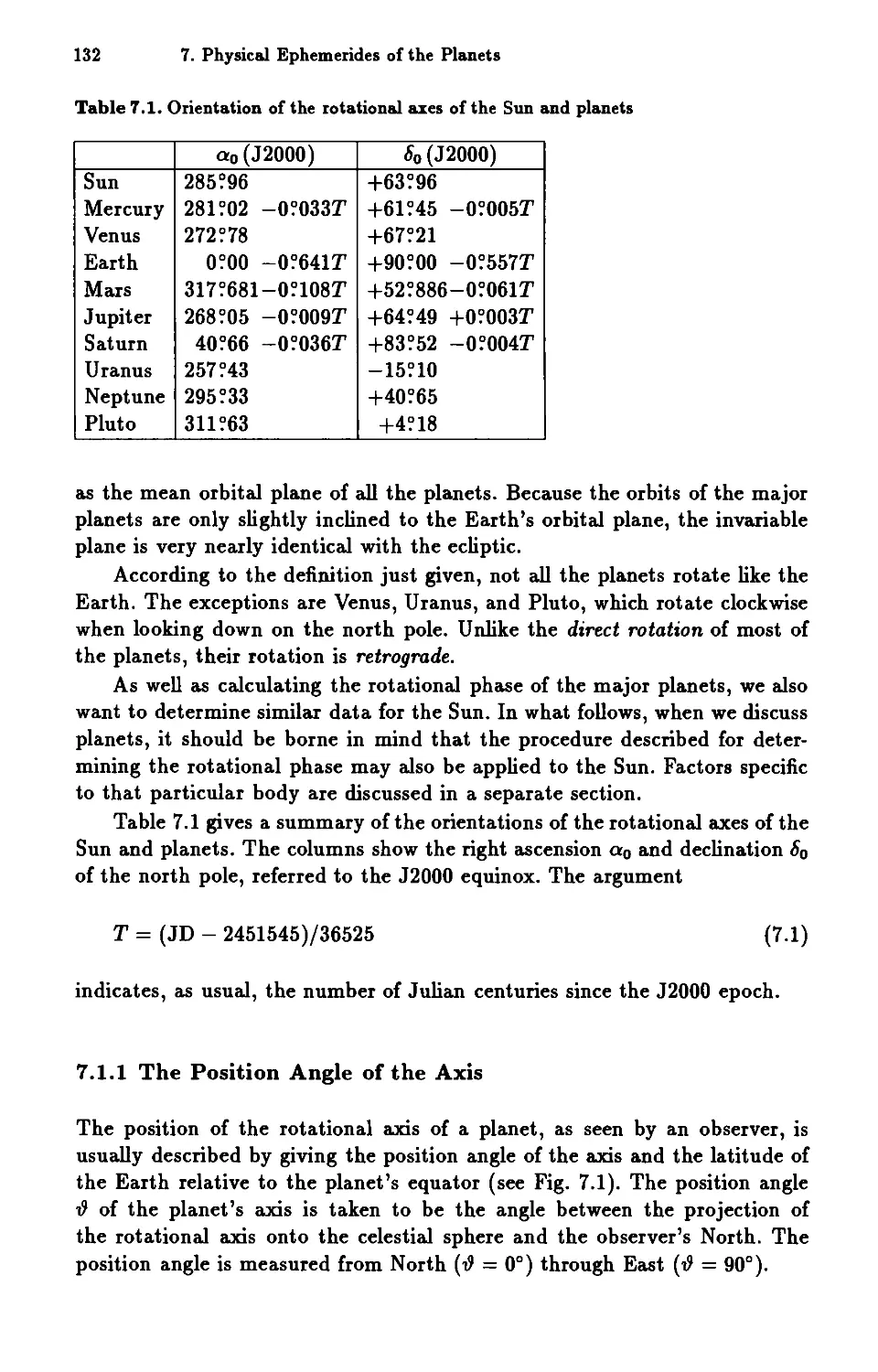
7 Physical Ephemerides of the Planets 131
7.1 Rotation................ 131
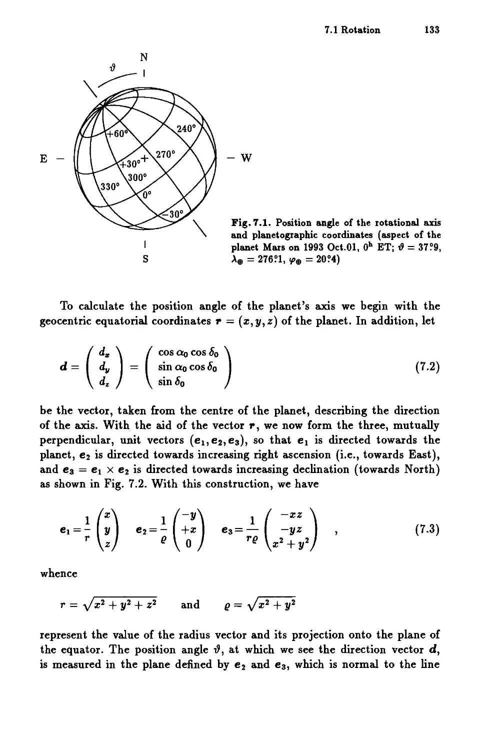
7.1.1 The Position Angle of the Axis 132
7.1.2 Planetographic Coordinates 135
7.2 illumination Conditions ...... 142
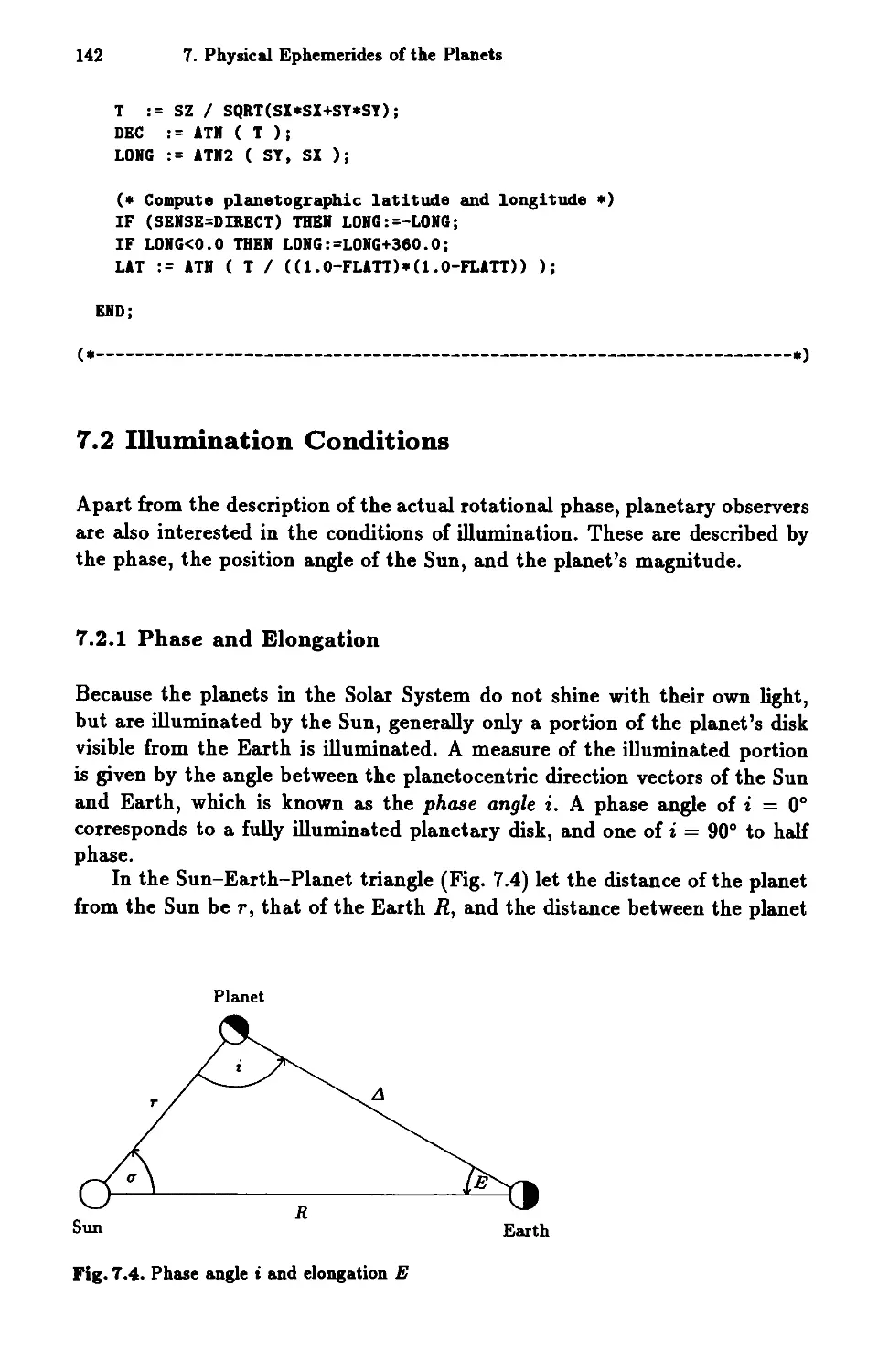
7.2.1 Phase and Elongation 142
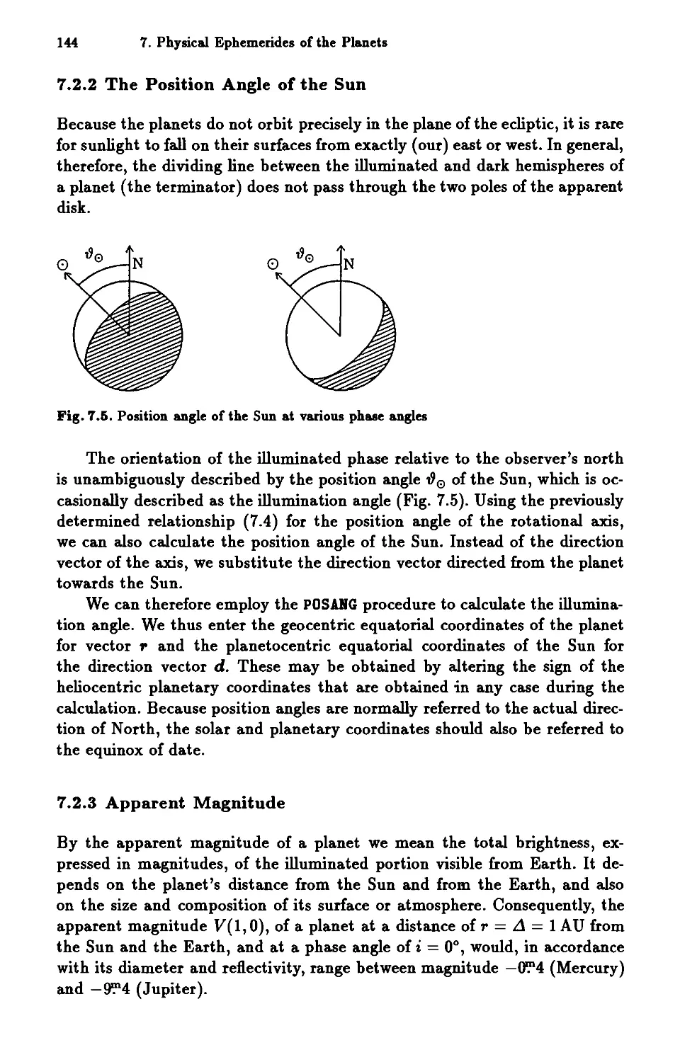
7.2.2 The Position Angle of the Sun. 144
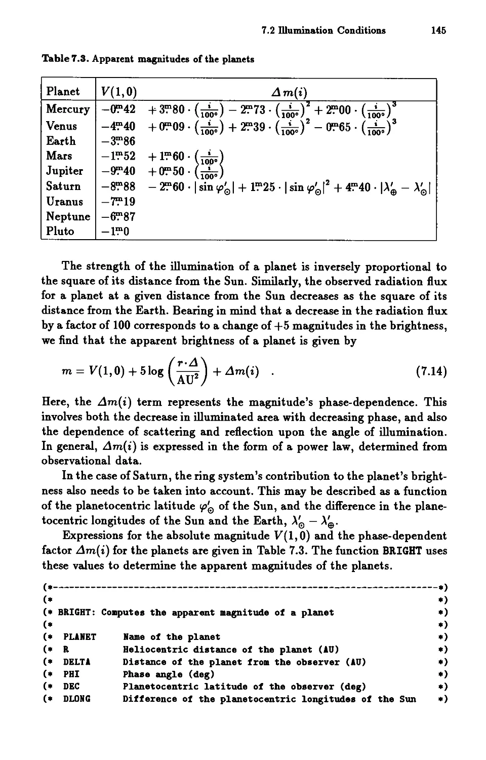
7.2.3 Apparent Magnitude 144
7.2.4 Apparent Diameter 146
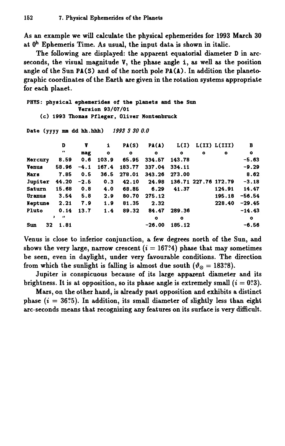
7.3 The PHYS Program 147
8 The Orbit of the Moon 153
8.1 General Description of the Lunar Orbit 153
8.2 Brown's Lunar Theory . . . . . 157
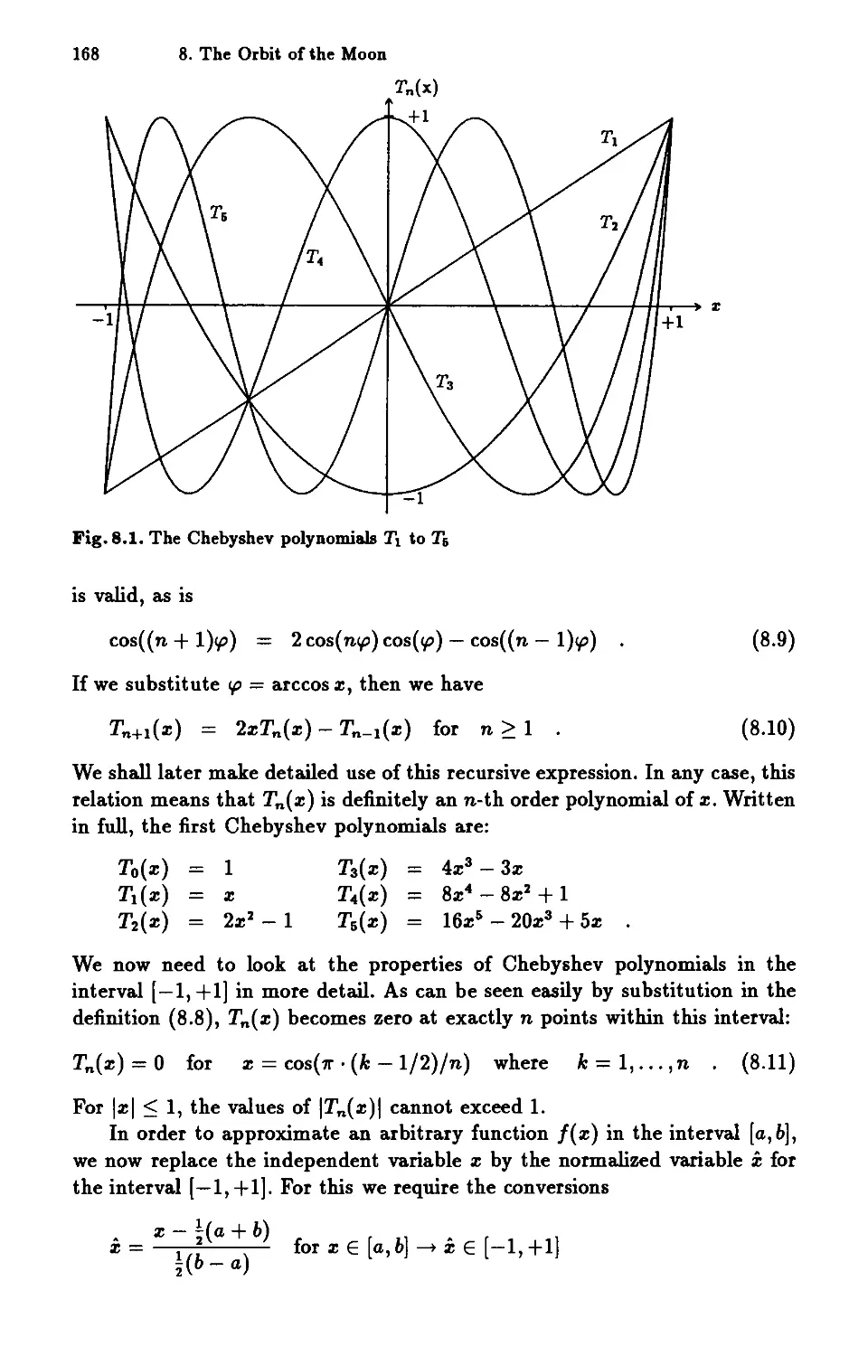
8.3 The Chebyshev Approximation 167
8.4 The LUNA Program 173
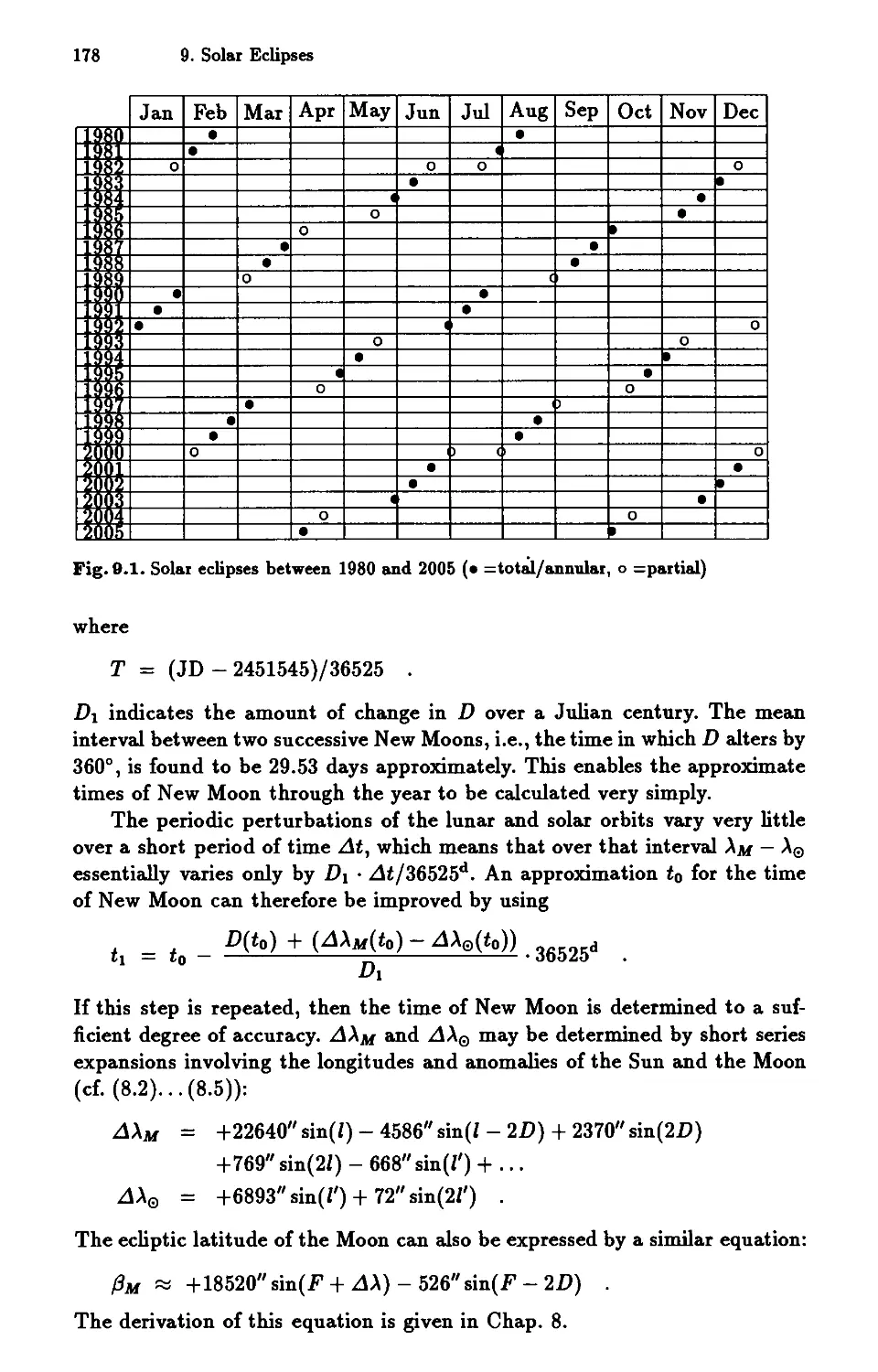
9 Solar Eclipses ..... 177
9.1 Times of New Moon 177
9.2 Geometry of an Eclipse . 181
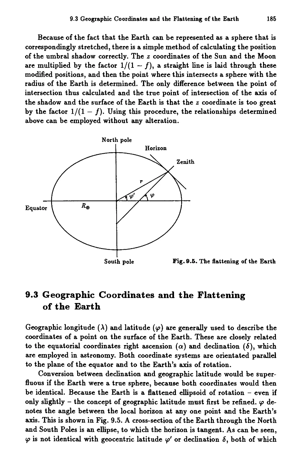
9.3 Geographic Coordinates and the Flattening of the Earth 185
9.4 Duration of an Eclipse . . . . 188
9.5 Solar and Lunar Coordinates. 189
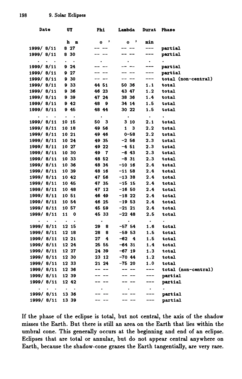
9.6 The ECLIPSE Program . 191
9.7 Local Circumstances . . . 199
9.8 The ECLTIMER Program 202
Contents XIII
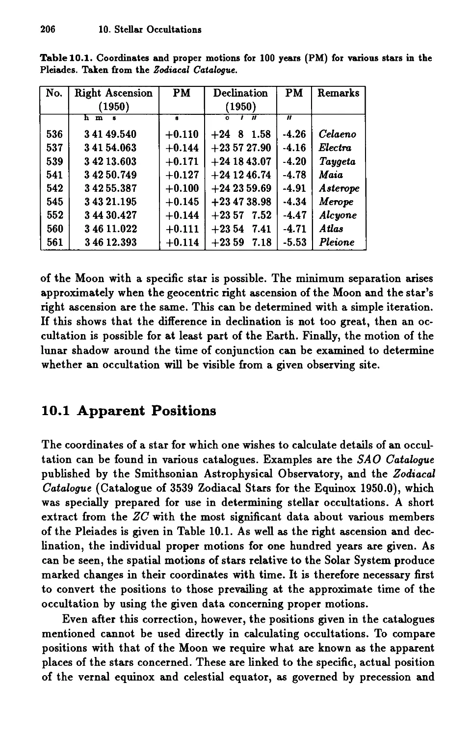
10 Stellar Occultations . . . . 205
10.1 Apparent Positions . . . 206
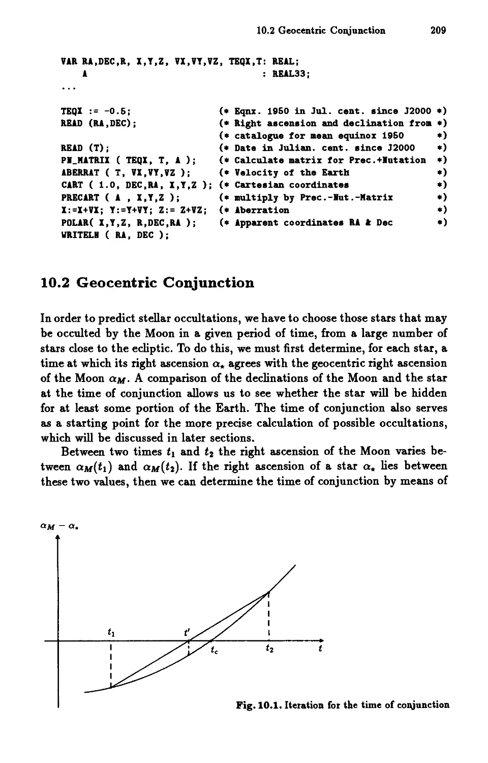
10.2 Geocentric Conjunction. 209
10.3 The Fundamental Plane 213
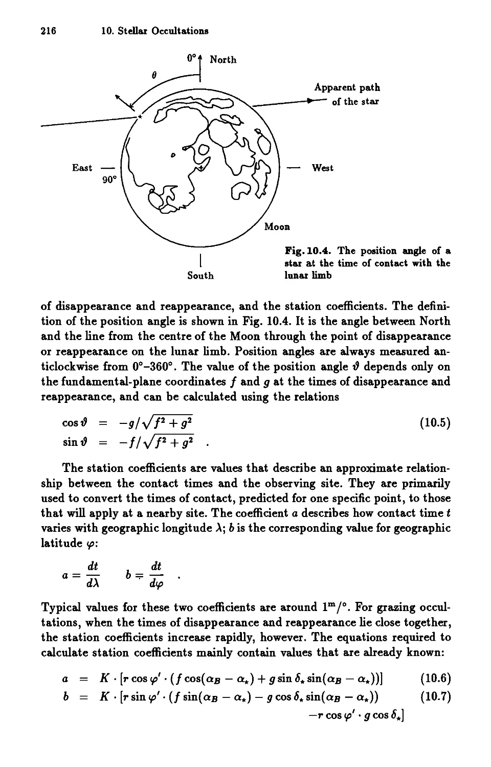
10.4 Disappearance and Reappearance 215
10.5 The OCCULT Program ..... 217
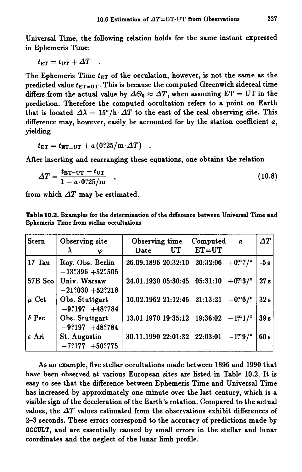
10.6 Estimation of LlT=ET-UT from Observations 226
11 Orbit Determination ............... 229
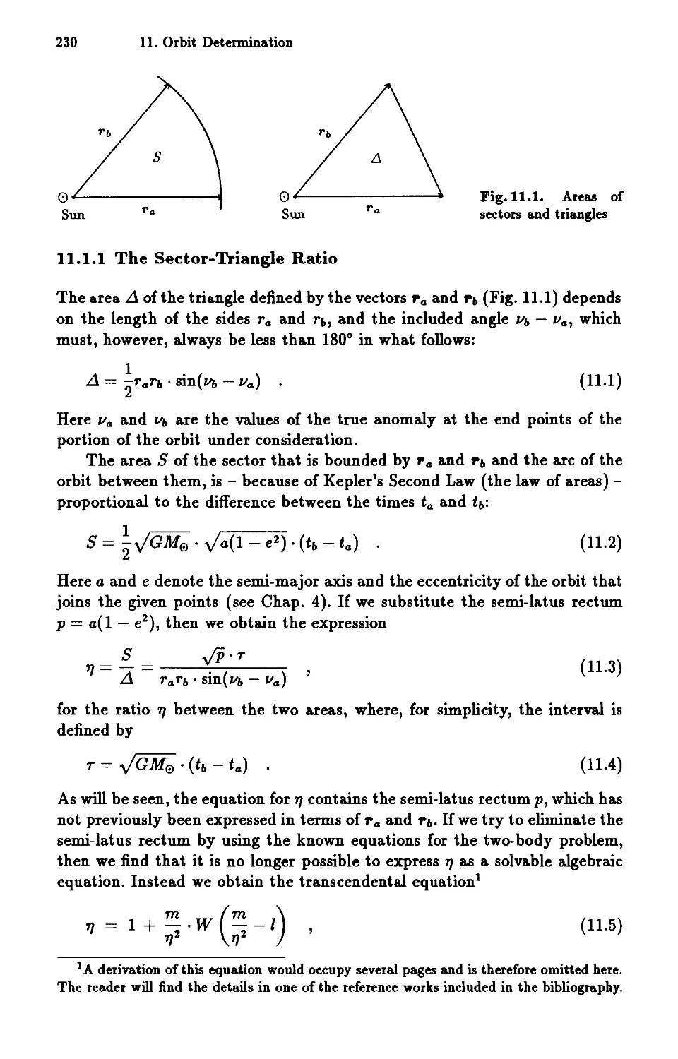
11.1 Determining an Orbit from Two Position Vectors 229
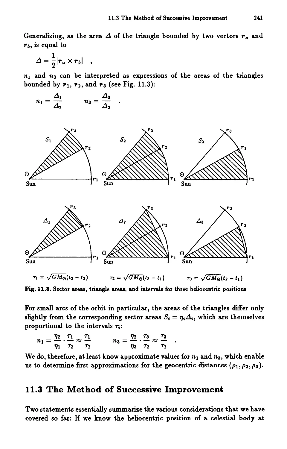
11.1.1 The Sector-Triangle Ratio . . . . . 230
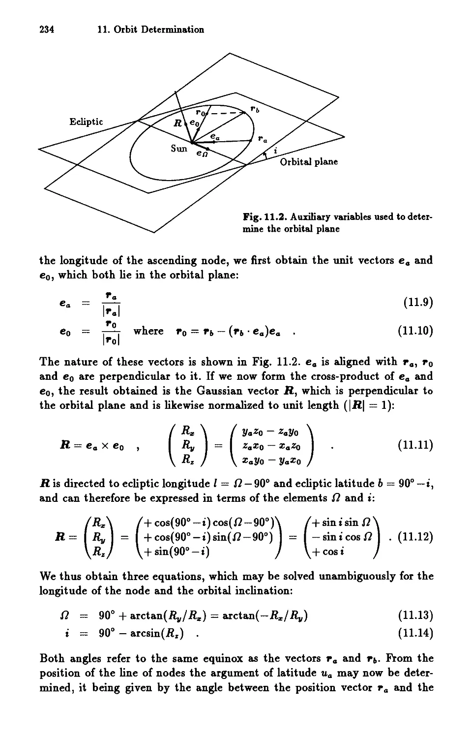
11.1.2 Orbital Elements . . . . . . . . . . 233
11.2 The Geometry of Geocentric Observations 239
11.3 The Method of Successive Improvement. 241
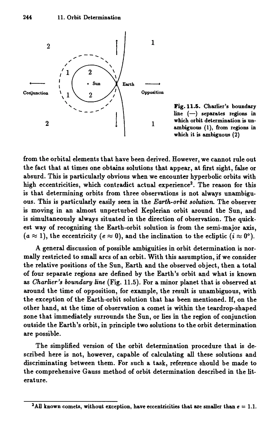
11.4 Multiple Solutions 243
11.5 The ORBDET Program 245
12 Astrometry . . . . . . . . 253
12.1 Photographic Imaging 253
12.2 Plate Constants . . . 256
12.3 Reduction . . . . . . 257
12.4 The FOTO Program 260
Appendix . . . . . . . . . . 267
A.1 Notes on Alterations to Suit Individual Computers 267
A.2 List of Procedures. . . . . . . . . . . . . . . . . . . 271
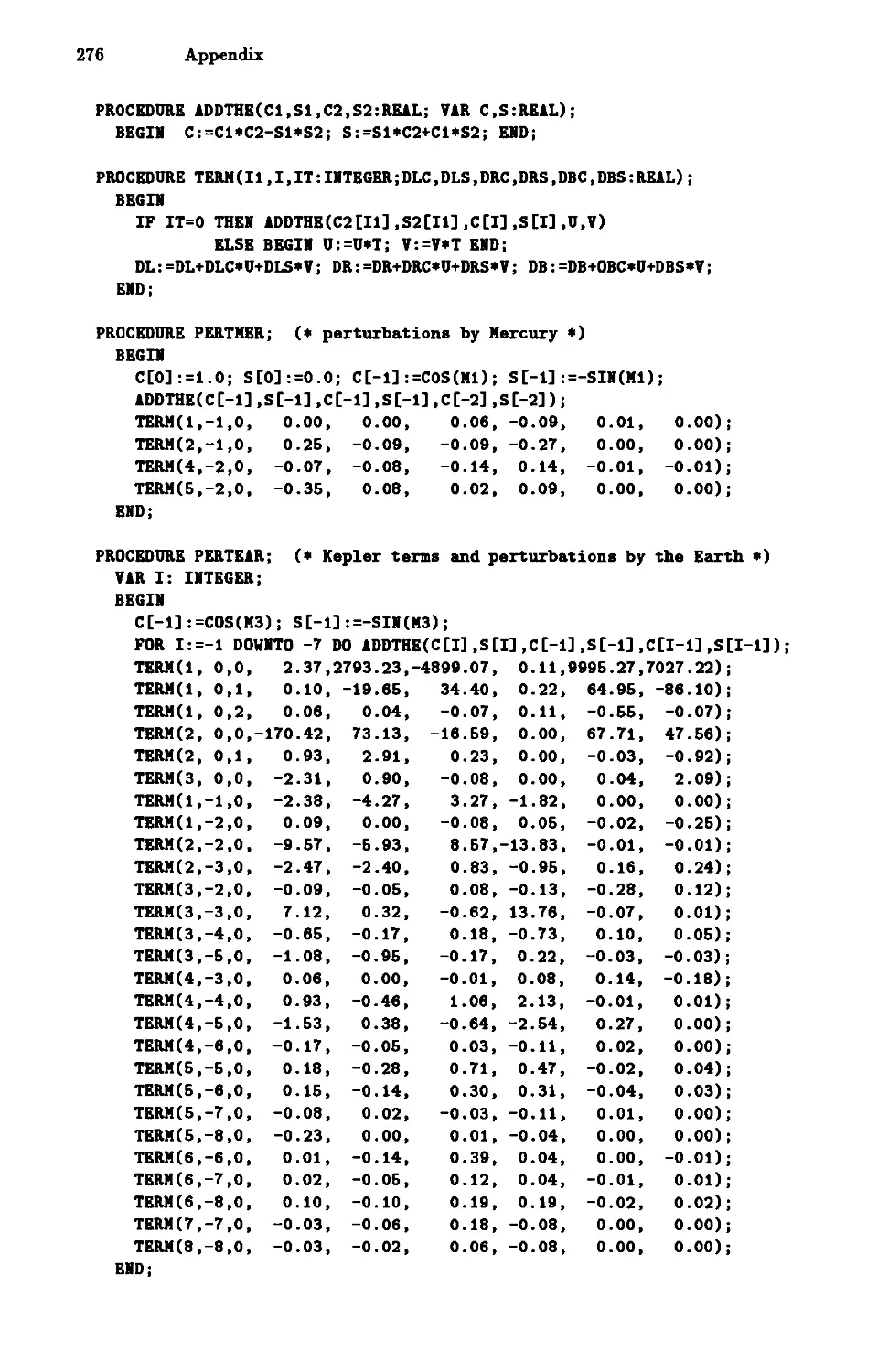
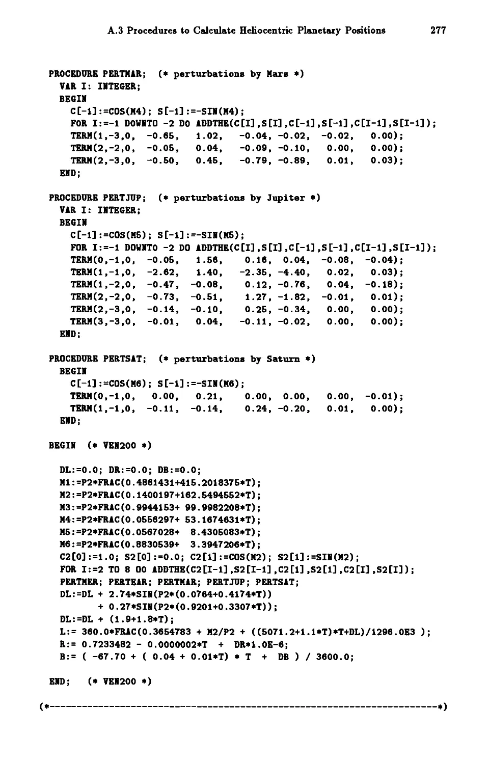
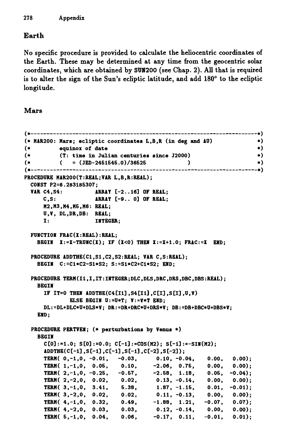
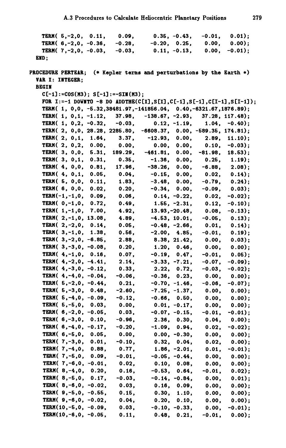
A.3 Procedures to Calculate Heliocentric Planetary PositioI).s 273
Symbols 293
Glossary 297
Bibliography 301
Subject Index 307
1. Introduction
Recent years have seen a continuous increase in the power of small computers
and a simultaneous decrease in their price. As a result many people inter-
ested in astronomy have such equipment at their disposal. This prompts the
idea of using these computers for astronomical computation. What positive
advantages are there in using one's own computer, when one can obtain all
the most important data required for observing, fully as accurately, in one of
the many yearly handbooks?
1.1 Some Examples
Let us first consider the calculation of the rising and setting times of the Sun
and the Moon. Moving from one observation site to another differences in time
soon occur, and these cannot be neglected. Yet in a handbook the rising and
setting times are generally given for just a few places. If one wants the times
at a given position, one is generally advised to use an interpolation routine
or else read the corrections from nomograms. In this case it is significantly
more convenient and more accurate if the computer can give the required
data without further work.
The major portion of an almanac consists of pages and pages of tables of
the positions of the Sun, the Moon, and the planets. Of all the information
published, frequently only a small fraction is of specific interest. Using ap-
propriate programs, just the values actually required can be calculated and
simultaneously expressed in the desired coordinate system.
Even more important is the possibility of being able to calculate the
orbit of a celestial body oneself. With new discoveries, actual ephemerides
are frequently not available or only obtainable after some delay. A single set
of orbital elements is sufficient for the motion of a comet to be followed with
an adequate degree of accuracy.
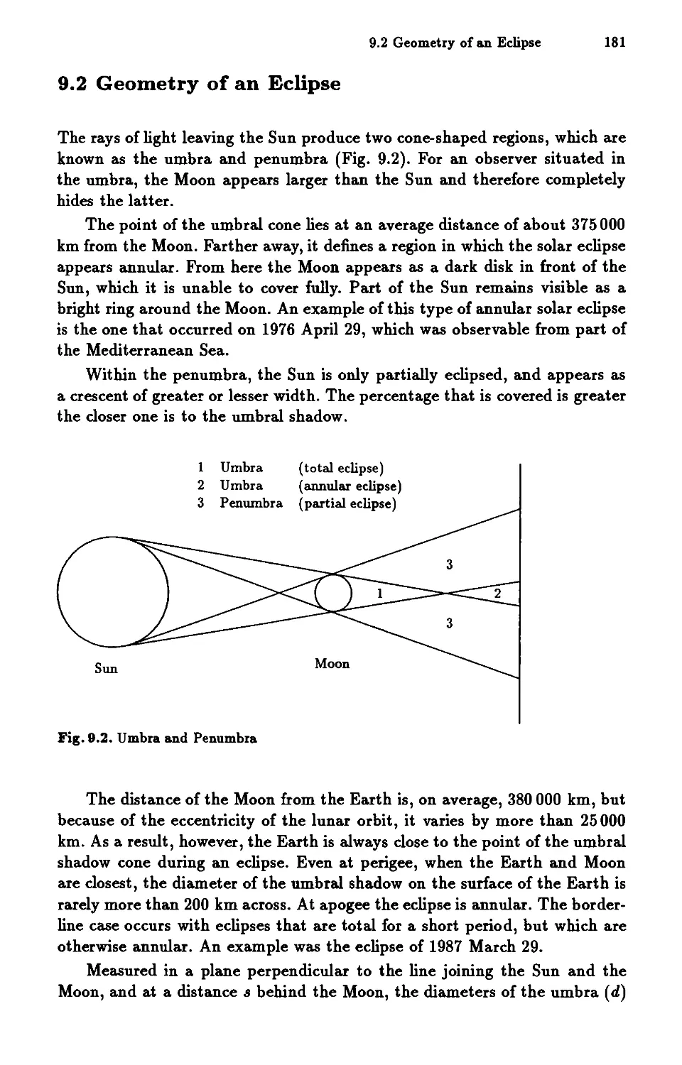
Solar eclipses are impressive celestial phenomena, which often prompt am-
ateur astronomers to undertake long journeys to observe them. Even though
official sources may provide detailed information on a given eclipse, it is often
desirable to plan a trip long before these data are published. If one requires
information for a particular observing site that is not covered in the almanacs,
a special program for computing local circumstances will be extremely useful.
2 1. Introduction
Anyone who wants to observe stellar occultations by the Moon requires
contact times for their observing site. When handbooks contain such predic-
tions, these are generally restricted to a few selected major cities. Anyone
wanting to observe from another site is once again reduced to resorting to
approximations. The OCCULT program given in this book enables both the
occurrence of stellar occultations and precise data about them to be calcu-
lated for any arbitrary selection of stars.
Many amateur astronomers are keen on astrophotography. Using reference
stars with known coordinates, the position of a minor planet or a comet can
be determined from photographs that one has taken oneself. If at least three
exposures, taken at intervals, are available then the orbital elements may
be calculated in the process of determining an orbit. In the programs PHOTO,
ORBDET and COMET we provide the necessary tools for such highly complicated
calculations that are required. Observers of minor planets will appreciate
having the NUMINT program to use for computing precise ephemerides that
take gravitational perturbations by the major planets into account, and that
may be used even if the available orbital elements refer to an epoch that is
several years ago.
1.2 Astronomy and Computing
Any introduction to the calculation of astronomical phenomena using com-
puter programs would be incomplete without a discussion of the accuracy
that can be attained. It is important, however, to first establish that the
value of such programs primarily depends on the mathematical and physical
description of the problem, as well as on the quality of the algorithms that
are employed. It is often incorrectly assumed that the use of double-precision
arithmetic will ensure the accuracy of a specific program. Yet even an accu-
rately calculated program must return inaccurate results if the methods of
calculation are not accurate in themselves.
An example of this is the calculation of ephemerides using the laws gov-
erning the two-body problem. Here the orbit of a planet is represented in a
simplified manner by an ellipse. But apart from the gravitational force ex-
erted by the Sun, which is responsible for this form of orbit, other forces
are produced by the remaining planets. These lead to periodic and long-term
perturbations, which may amount to about one arc-minute for the inner plan-
ets, and up to a degree for the outer planets. A theoretical Keplerian orbit
is therefore only an approximation of the actual circumstances. If we require
greater accuracy, then the use of more complicated descriptions of planetary
orbits that model the mutual perturbations between the planets is unavoid-
able. Using high-precision arithmetic in the computer would not help in the
slightest!
1.2 Astronomy and Computing 3
In developing our programs, we have tried to obtain an accuracy that is
approximately the same as that found in astronomical yearbooks. The errors
in the fundamental routines for determining the coordinates of the Sun, the
Moon, and the planets amount to about 1"-3". This accuracy is sufficient for
the calculation of solar eclipses or stellar occultations, and should therefore
be sufficient for most other purposes.
Anyone who wants to carry out accurate calculations consistently, how-
ever, must first be clear about the exact definitions of the coordinate systems
used. Unfortunately, experience shows that values in different coordinate sys-
tems are cheerfully compared with one another. Then the cry goes up that
the program is not accurate in its calculations, because different values are
given in a yearbook. Frequently the discrepancy can be explained by the co-
ordinates having a slightly different basis, which was not recognized by the
user, who thus suspected an 'error'. We have therefore noted, at all relevant
points, important corrections such as precession and nutation, or aberration
and light-travel-time. The difference between Universal Time and Ephemeris
Time, which repeatedly causes difficulties, is frequently discussed. Readers
should not allow the frequent mention of these effects to confuse them. It is
rather our intention that this form of discussion and its immediate applica-
tion to appropriate programs will enable them to obtain a better feel of the
magnitude and the practical significance of the individual corrections. The
occasional repetitions appear to be necessary, because each chapter - and
with it the description of a very specific topic - may also be read on its own.
But as the programs are frequently constructed around the same routines,
readers should also take the opportunity of reading other relevant chapters.
The power of a program not only depends on the mathematical descrip-
tion of the problem, but also on the use of appropriate computational meth-
ods. These are discussed at the time, in connection with the various applica-
tions. An example of this is the evaluation of angular functions in calculating
the periodic perturbations in the orbit of the Moon and of the planets. By
making use of the addition theorem and recursive relations for the trigono-
metric functions, the computing times required by the programs PLANPOS
and LUNA are significantly reduced. If a particularly large number of posi-
tions, separated by short intervals, of a celestial body are required for some
specific purpose, it is advisable to use Chebyshev polynomial approximations.
It is then possible to obtain, without a loss of accuracy, valid expressions -
covering a limited period of time - that can be particularly easily and quickly
evaluated. Use of this technique is made in the programs ECLIPSE, ECLTIMER
and OCCULT. Other aspects of mathematical computation are discussed in
association with solving equations by Newton's procedure, regula falsi, and
quadratic interpolation. In addition, a simple, but numerically stable algo-
rithm for determining least-squares-fits is described in connection with the
astrometric reduction of photographic plates.
4 1. Introduction
1.3 Programming Languages and Techniques
In devising our programs, we endeavoured to follow certain basic rules, which
can largely be said to be based on the concept of structured programming.
We should perhaps explain in more detail what we understand by this.
First, the programs must be readable and understandable. Comments at
important points in the program listing do not just serve to make it easier for
the user to understand. Even the author of a program frequently forgets the
details after a certain time, and the documentation then helps if the program
has to be expanded at a later date. For the same reason, relevant variable
names are advisable. Indentation of blocks of code or the use of blank lines
makes it easier to appreciate the programs' logical structure. There is no
reason to be sparing of blank space in any source code, because the compiler
ignores it altogether.
As the concept of structured programming suggests, one should try to give
a program the clearest possible logical structure. In practice each algorithm
may be constructed from elementary structures that are statements, carry
out sequences, make selections, or perform iterations (repetitions). Modern
programming languages provide the necessary language elements to translate
these structures into source code. This includes control structures (loops,
conditional instructions), structured data types (records), and program blocks
in the form of functions, sub-routines or separately compiled modules. Readers
must decide for themselves how far unconditional jumps (GOTO-instructions)
are necessary or useful.
If one wants to develop a program in this manner, then it is best to follow
a systematic procedure. Modern software technology offers a variety of meth-
ods for a step-by-step structuring and sub-division of a given problem into
smaller and smaller tasks, until these become easily comprehensible and may
be simply transformed into code. The benefit of following a systematic ap-
proach is most pronounced for large and complex problems, because it helps
to avoid redundancies and interface problems, assists in creating reuasble so-
lutions and saves a lot of development time. Direct coding without a detailed
previous analysis of the problem is the most common error in software devel-
opment. This method of working typically gives rise to programs that do not
perform as expected and have to be modified by trial and error until they run
successfully. Further hints on systematic software development techniques are
given in the bibliography listed in the appendix.
If possible, a procedure designed for a specific task should be written
in a universal way so that it can be used later in other programs. In pro-
ducing astronomical programs, one repeatedly encounters certain basic prob-
lems, where this approach is particularly suitable. Examples of this are the
evaluation of mathematical functions, the conversion of coordinates between
different systems, or the determination of accurate positions for the planets,
the Sun, or the Moon. It would be very laborious if one were forced to repeat
1.3 Programming Languages and Techniques 5
such processes every time. If, however, parts of programs that are repeatedly
required are available in the form of a library of efficient, reliable sub-routines,
then it is possible to concentrate on the functions required from the new por-
tions of the programs, thus achieving the desired result much more easily and
quickly.
The functions and procedures that we describe in this book form the basis
for such a library of astronomical programs. The most important are
. technical and scientific functions, and auxiliary programs related to
mathematical computation,
. routines for time and calendar calculations,
. various procedures concerning spherical astronomy,
. special routines for handling precession and nutation,
. procedures for calculating elliptical, parabolic, and hyperbolic Keplerian
orbits, as well as
. routines for calculating accurate positions of the planets and the Moon,
taking various perturbations into account.
A full list of the individual sub-routines is given in the Appendix.
In developing our programs we chose to use the Pascal language. An
important reason was that Pascal is very widespread, and is implemented on
all major systems from home computers to main-frames. Borland's Turbo-
Pascal is a fast, inexpensive compiler that is available for all IBM-compatible
personal computers. For computers in the Atari ST /TT series, which are
quite popular in Germany, Application Systems Heidelberg offers the Turbo-
Pascal-compatible Pure Pascal development kit. The source codes provided
on the enclosed floppy disk may be used directly with both compilers. An
adaptation to other dialects and standard Pascal should not, however, pose
any difficulties, because the printed listings in the text do not contain Turbo-
Pascal-specific language elements.
In contrast to Basic, which has numerous machine-specific dialects, Pascal
programs can be written so that they are almost completely portable. If one
tries to use only standard language elements in the programming, then the
programs can be implemented on nearly any machine. Any changes necessary
are insignificant, and can be made without problems. Some 'Notes on alter-
ations to suit individual computers' appear in the Appendix. Full portability
naturally involves some restrictions. For this reason, none of the programs
provides graphic output, or uses any special features of the operating system.
Any readers who may, for example, want to incorporate features of the com-
puter's user interface (such as Windows), or have graphical output, can alter
the programs to their own requirements whenever they wish.
Pascal was developed as a language for instruction and learning, and
therefore demands a certain amount of programming discipline on the part
6 1. Introduction
of users. Although people - and not only beginners - repeatedly complain
about the 'ponderous' nature of the language, this does in fact conceal some
distinct advantages. In particular, many unnecessary programming errors are
avoided by one's being forced to declare all variables specifically. In most
versions of languages such as Fortran or Basic one can cheerfully be typing
away, creating an unwanted variable with every typing error. Correcting these
errors can be a severe test of one's patience. A language like Pascal that
requires declarations, discovers inconsistencies at compile time and warns
the user with an appropriate error message. This is of particular importance
in checking the various parameters required by a function or a sub-routine.
Only when the types of variables agree with those that have been declared
can the program be compiled. Forgetting an individual parameter is therefore
impossible. This check by the compiler considerably simplifies the correct use
of a library of previously created programs.
Unfortunately, this advantage of Pascal is accompanied by the disad-
vantage that a program must always be compiled as a whole. More highly
developed languages such as Modula-2 or Ada handle the declaration of a
sub-routine separately from the implementation. So they allow individual
modules to be compiled separately, while retaining overall checking. This is
of particular value in developing large groups of programs. Because of its sim-
ilarities to Pascal, users of Modula-2, which has now become widely used on
personal computers, will have little trouble adapting our programs.
Newer versions of Turbo-Pascal also offer similar possibilities called 'units'.
On the floppy disk accompanying this book we therefore provide some addi-
tional unit definition files for the user's convenience. Aside from being neces-
sary for running some of the larger programs with Turbo-Pascal, it facilitates
the compilation and the use of our software as a standard library for astro-
nomical calculations.
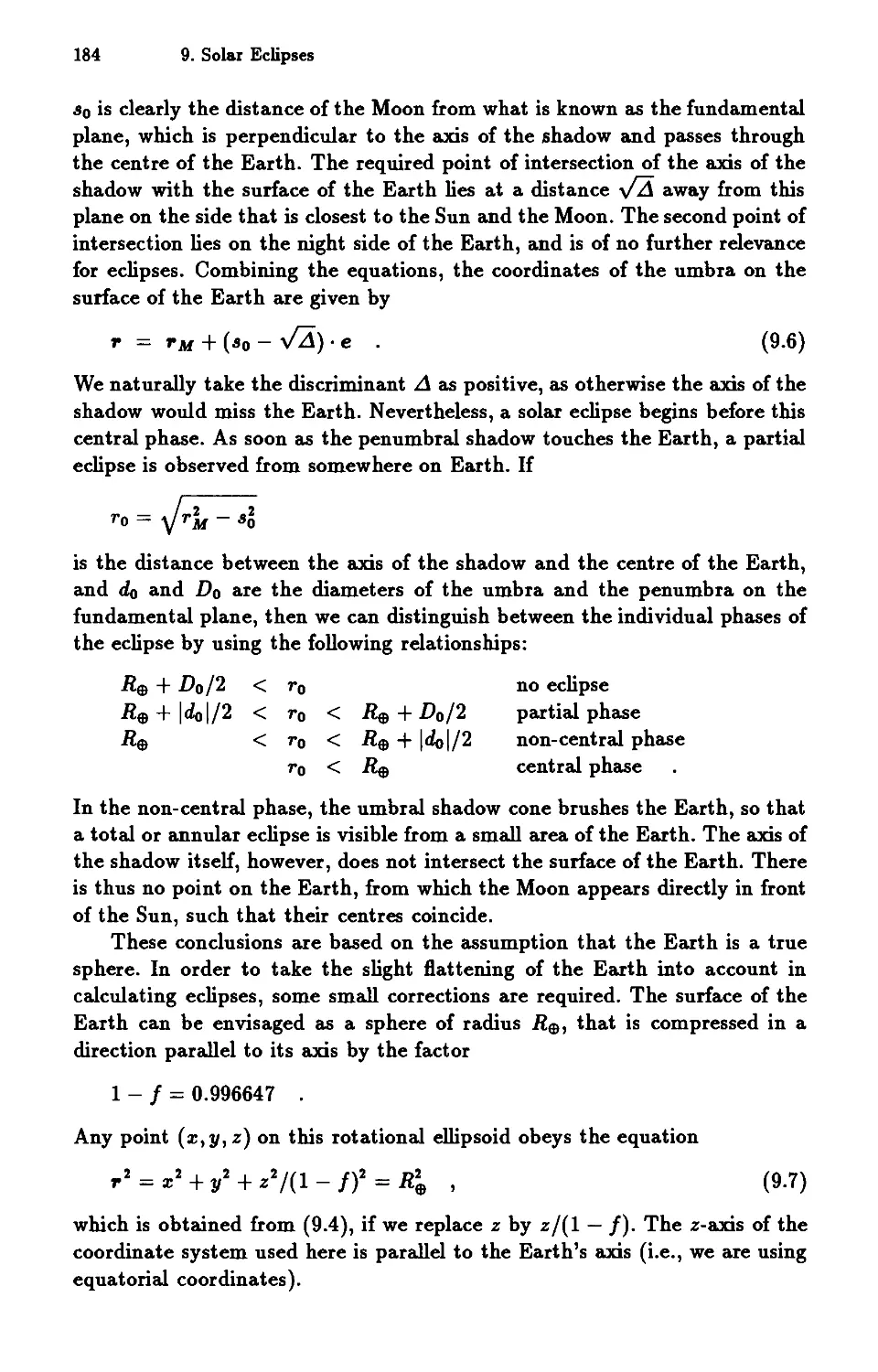
2. Coordinate Systems
Astronomy uses a whole series of different coordinate systems to specify the
positions of stars and planets. Here we must distinguish between heliocentric
coordinates, which are based on the Sun, and geocentric coordinates, which
are centred on the Earth. Ecliptic coordinates refer the position of a point
to the plane of the Earth's orbit, while equatorial coordinates are measured
relative to the position of the Earth's or celestial equators. The slow shift of
this reference plane because of precession means that the equinox of the coor-
dinate system that is being used also has to be taken into account. Although
it would obviously be possible to decide, once and for all, to use a single,
fixed coordinate system, every system has specific advantages that make it
particularly suitable for certain purposes.
Because there are various coordinate systems, it is often necessary to
convert coordinates given in one system to those of another. The coco ('Co-
ordinate Conversion') program is designed to do just this. It provides accurate
conversions between ecliptic and equatorial coordinates, and between geocen-
tric and heliocentric coordinates, for various epochs. The individual transfor-
mations, which will be described shortly, are written as separate sub-routines.
They can therefore be used elsewhere, and are an important basis for later
programs.
2.1 Making a Start
Anyone who tries to write mathematical formulae in Pascal soon finds that
some methods are unavailable, because - unlike Fortran or Basic - the lan-
guage is very poorly provided with the required functions. This problem can
be rapidly solved by including a few, suitable, short procedures and functions.
Trigonometric functions and their inverse functions are among those re-
quired, because they are either not available at all, or are only available in
radians.
(.-----------------------------------------------------------------------.)
(. SN: sine function (degrees) .)
(.-----------------------------------------------------------------------.)
FUNCTION SN(X:REAL):REAL;
CONST RAD=0.0174632926199433;
BEGIN
8 2. Coordinate Systems
SI:=SII(I*RAD)
EIDj
(.-----------------------------------------------------------------------.)
(. CS: cosine function (degrees) .)
(.-----------------------------------------------------------------------.)
FUJCTIOI CS(I:REAL):RE&Li
COIST R&D=0.0174632926199433i
BEGII
CS:=COS(I.RAD)
EIDj
(.-----------------------------------------------------------------------.)
(. TI: tangent function (degrees) .)
(.-----------------------------------------------------------------------.)
FUICTIOI TI(I:REAL):RE&Lj
COIST R&D=0.0174632926199433i
ViR II: RE&L j
BEGII
II: =I.R&D j TI:=SII(II)/COS(II)j
EIDj
(.-----------------------------------------------------------------------.)
(. &SI: arcsine function (degrees) .)
(.-----------------------------------------------------------------------.)
FUICTIOI &SI(I:RE&L):RE&Lj
COIST R&D=0.0174632926199433i EPS=1E-7j
BEGII
IF &BS(I)=1.0
THEI &SI:=90.0.I
ELSE IF (&BS(I»EPS)
THEI &SI:=&RCT&I(I/SQRT«1.0-I).(1.0+I»)/RAD
ELSE &SI:=I/R&Dj
EIDi
(.-----------------------------------------------------------------------.)
(. &CS: arccosine function (degrees) .)
(.-----------------------------------------------------------------------.)
FUICTIOI &CS(I:RE&L):RE&Lj
COIST R&D=0.0174632926199433i EPS=1E-7i C=90.0i
BEGII
IF &BS(I)=1.0
THEI &CS:=C-I*C
ELSE IF (&BS(I»EPS)
THEI &CS:=C-&RCT&I(I/SQRT«1.0-I).(1.0+I»)/R&D
ELSE &CS:=C-I/R&Dj
EIDj
(.-----------------------------------------------------------------------.)
(. &TI: arctangent function (degrees) .)
(.-----------------------------------------------------------------------.)
FUICTIOI &TI(I:RE&L):RE&Lj
COIST R&D=0.0174632926199433i
BEGII
&TI:=&RCT&I(I)/RAD
EIDi
(.-----------------------------------------------------------------------.)
2.1 Making a Start 9
The CUBR function calculates the cube root of its argument. It is used in later
chapters and is only given here for the sake of completeness:
(*-----------------------------------------------------------------------*)
(* CUBR: cube root * )
(*-----------------------------------------------------------------------*)
FUICTIOI CUBR(I:RE&L):RE&L;
BEGII
IF (1=0.0) THEI CUBR:=O.O ELSE CUBR:=EIP(LI(I)/3.0)
EID;
(*-----------------------------------------------------------------------*)
A variant of the ATN function, which is also known in Fortran as ATN2,
enables the arctangent of a fraction y /:z: to be calculated, but also simultane-
ously caters for the case where :z: = 0, when the fraction is undefined.
(*-----------------------------------------------------------------------*)
(* &TI2: arctangent of y/x for two arguments *)
(* (correct quadrant: -180 deg <= &T12 <= +180 deg) *)
(*-----------------------------------------------------------------------*)
FUICTIOI &TI2(Y,I:RElL):RE&L:
COIST R&D=0.0174632926199433:
ViR &I,&Y,PHI: RE&L:
BEG II
IF (1=0.0) &ID (Y=O.O)
THEI &Tl2:=0.0
ELSE
BEG II
&I:=&BS(I): &Y:=&BS(Y):
IF (U>U)
THEI PHI:=&RCT&I(&Y/&I)/R&D
ELSE PHI:=90.0-&RCT&I(&I/&Y)/R&D:
IF (1<0.0) THEI PHI:=180.0-PHI:
IF (Y<O.O) THEI PHI:=-PHI:
&Tl2:=PHI:
EID:
EID:
(*-----------------------------------------------------------------------*)
This function is used, in particular, for converting the plane Cartesian coordi-
nates (:z:,y) ofa point into the polar coordinates rand tp. Although ATN(y/x)
returns an angle between -90 0 and +90 0 (lot and 4 th quadrants), ATN2(y,x)
takes into account the fact that for negative :z:, the angle tp corresponding to :z:
and y lies between +90 0 and +270 0 . Note that (as in Fortran) angles between
180 0 and 360 0 are expressed as negative values between -180 0 and 0 0 .
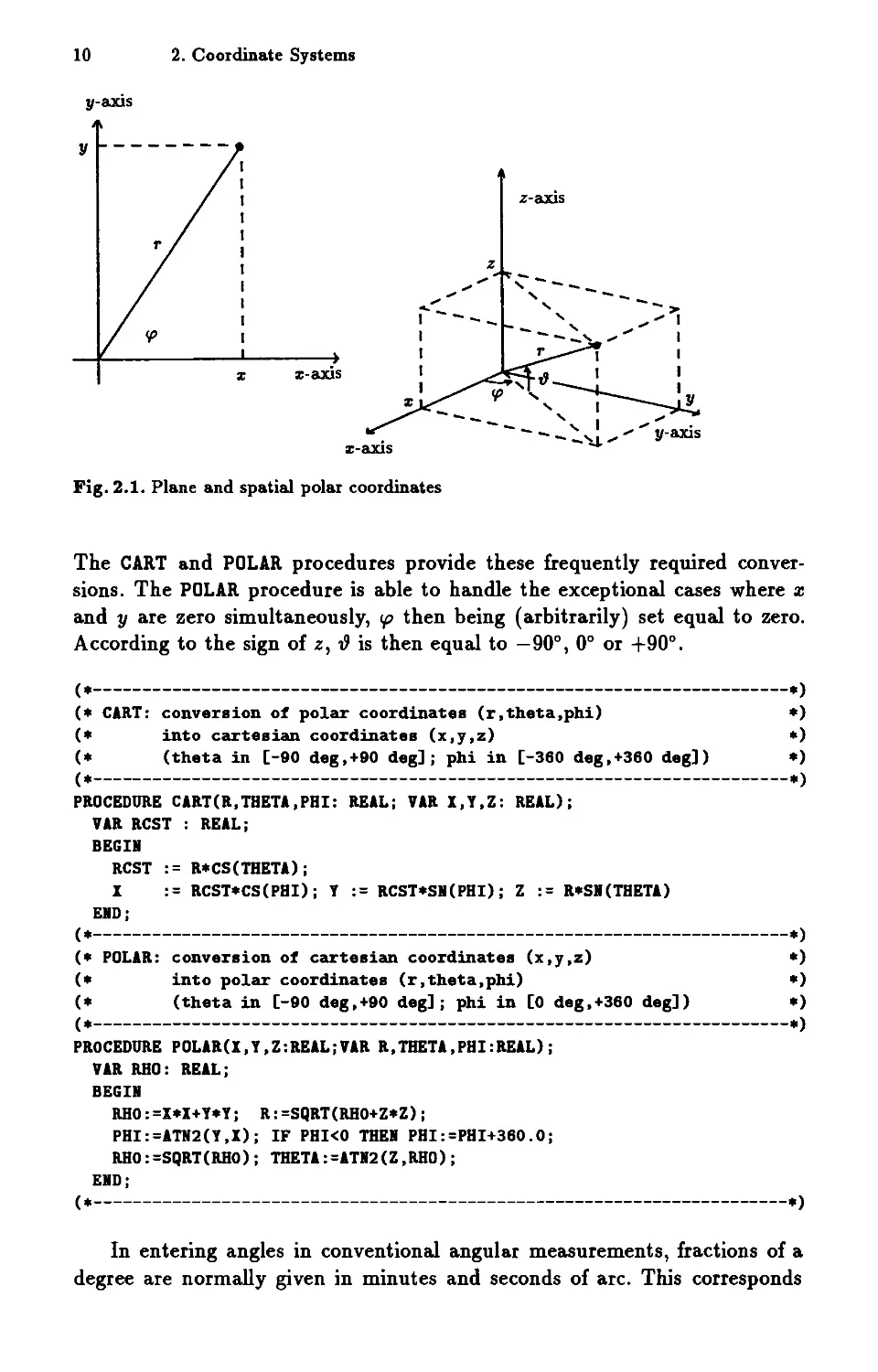
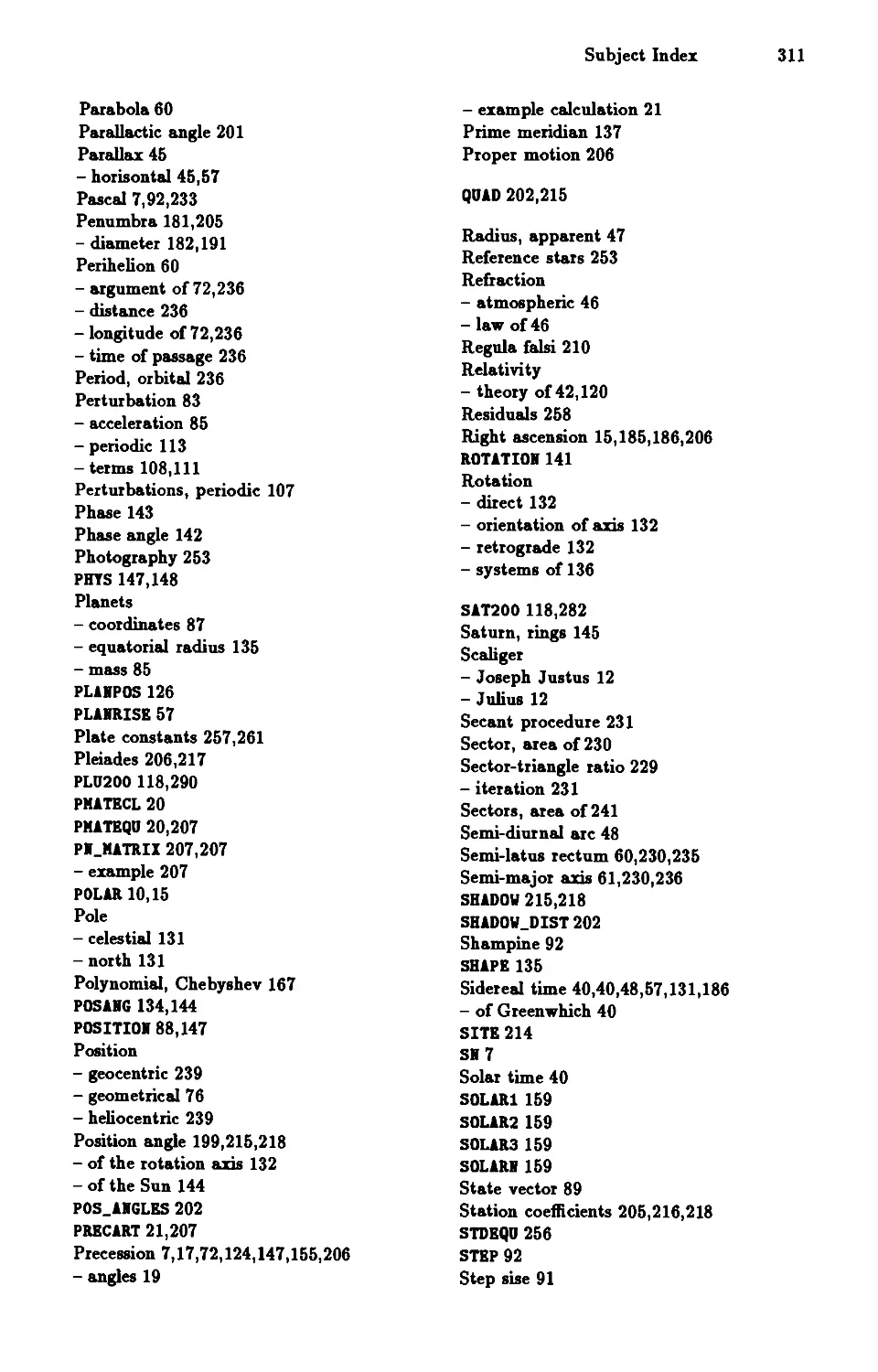
The conversion between the three-dimensional rectangular coordinates
(:z:, y, z) and the polar coordinates (r, 1?, tp) is slightly more complicated. The
relationships between them (Fig. 2.1) are:
:z: rcos..?costp
y r cos ..? sin tp
z = r sin ..?
r
...;' :z:2 + y2 + Z2
y/:z:
Z/ ...;' :z:2+y2
(2.1)
tan tp
tan..?
10 2. Coordinate Systems
y-axis
y
z-axis
z
;:
;:-axis
...
",
",
",
.--
I
I
I
1
;:
---
->
",'" I
",'" I
r I I
." I 1
' I..
',_ I
, ",
- - - - ' 1 ", ", Y -axis
- - "
;:-axis
Fig. 2.1. Plane and spatial polar coordinates
The CART and POLAR procedures provide these frequently required conver-
sions. The POLAR procedure is able to handle the exceptional cases where :z:
and yare zero simultaneously, tp then being (arbitrarily) set equal to zero.
According to the sign of z, {) is then equal to -90 0 , 0 0 or +90 0 .
(*-----------------------------------------------------------------------*)
(* CART: conversion of polar coordinates (r,theta,phi) *)
(* into cartesian coordinates (x,y,z) *)
(* (theta in [-90 deg,+90 deg]; phi in [-360 deg,+360 deg]) *)
(*-----------------------------------------------------------------------*)
PROCEDURE CART(R,THETA,PHI: REAL; VAR X,Y,Z: REAL);
VAR RCST : REAL;
BEGII
RCST
X
EID;
(*-----------------------------------------------------------------------*)
(* POLAR: conversion of cartesian coordinates (x,y,z) *)
(* into polar coordinates (r,theta,phi) *)
(* (theta in [-90 deg,+90 deg]; phi in [0 deg,+360 deg]) *)
(*-----------------------------------------------------------------------*)
PROCEDURE POLAR(X,Y,Z:REAL;VAR R,THETA,PHI:REAL);
ViR RHO: REAL j
BEGII
RHO:=X*X+Y*Y; R:=SQRT(RHO+Z*Z);
PHI:=ATN2(Y,X); IF PHI<O THEI PHI:=PHI+360.0;
RHO:=SQRT(RHO); THETA:=ATI2(Z,RHO);
EID;
(*-----------------------------------------------------------------------*)
R*CS(THET&) ;
.- RCST*CS(PHI); Y := RCST*SI(PHI); Z := R*SI(THETA)
In entering angles in conventional angular measurements, fractions of a
degree are normally given in minutes and seconds of arc. This corresponds
2.2 Calendar and Julian Dates 11
to the usual method of expressing times in minutes and seconds. Conversion
of these two forms is normally required no more than once in entering or
returning a value. In principle, provided all values are positive this poses no
problems. Neverthdess we need to take precautions to ensure that negative
values are also correctly handled. The effect of the DDD and DMS procedures
is best explained by a few examples:
DD D M S
16.60000 16 30 00.0
-8.16278 -8 09 10.0
0.01667 0 1 0.0
-0.08334 o -6 0.0
In converting a negative value DD into degrees, minutes and seconds, at any
one time only the leading value of the three D, M and 5 is negative. It should
be noted that in both procedures, D and M, which naturally can take only
whole values, are defined as INTEGER while 5 is defined as REAL.
(*-----------------------------------------------------------------------*)
(* DDD: conversion of degrees, minutes and seconds into *)
(* degrees and fractions of a degree *)
(*-----------------------------------------------------------------------*)
PROCEDURE DDD(D,M:IlTEGERiS:REALiVAR DD:REAL)j
ViR SIGI: REALi
BEGII
IF ( (D<O) OR (M<O) OR (S<O) ) THEI SIGI:=-1.0 ELSE SIGI:=1.0j
DD:=SIGI*(ABS(D)+ABS(M)/60.0+ABS(S)/3600.0)j
EIDi
(*-----------------------------------------------------------------------*)
(* DMS: conversion of degrees and fractions of a degree *)
(* into degrees, minutes and seconds *)
(*-----------------------------------------------------------------------*)
PROCEDURE DMS(DD:REALjVAR D,M:IITEGERiVAR S:REAL)i
ViR D1:REALj
BEGII
D1:=ABS(DD)i D:=TRUIC(D1)i
D1:=(D1-D)*60.0i M:=TRUIC(D1)j S:=(D1-M)*60.0i
IF (DD<O) THEI
IF (D<>O) THEI D:=-D ELSE IF (M<>O) THEI M:=-M ELSE S:=-Sj
EIDi
(*-----------------------------------------------------------------------*)
2.2 Calendar and Julian Dates
When calculating ephemerides, the difference in time between two given dates
is generally required. A running day number, as has been commonly used
in astronomy for a very long time, is therefore extremely convenient. The
Julian Date gives the total number of days that have elapsed since 4713
12 2. Coordinate Systems
B.C. January 1. It is named after Julius Scaliger, the father of Joseph Justus
Scaliger, who was the first to use it for chronological purposes. As the count
begins in biblical times, the Julian Date has now reached a very high value.
At noon on 1980 July 23 it amounted to 2444444.0 days, for example. When
we recall that a second is approximately equal to 0.00001 day, then we find
that we require a twelve-figure Julian Date to express an accurate time. The
first two numbers hardly alter over a period of three centuries, however, and
therefore the Modified Julian Date
MJD = JD - 2400000.5
is employed alongside the true Julian Date. The MJD is the total number of
days that has elapsed since 1858 November 17 00:00 hours. Like the ordinary
civil date, the MJD therefore changes at midnight, and not at noon like the
Julian Date.
(*-----------------------------------------------------------------------*)
(* MJD: Modified Julian Date *)
(* The routine is valid for any date since 4713 BC. *)
(* Julian calendar is used up to 1582 October 4, *)
(* Gregorian calendar is used from 1682 October 16 onwards. *)
(*-----------------------------------------------------------------------*)
FUICTIOI MJD(DAY,MOITH,YEAR:IITEGER;HOUR:REAL):REAL;
VAR A: REAL; B: IITEGER;
BEG II
A:=10000.0*YEAR+100.0*MOITH+DAY;
IF (MOITH<=2) THEI BEGII MOITH:=MOITH+12; YEAR:=YEAR-1 EID;
IF (A<=16821004.1)
THEI B:=-2+TRUIC«YE&R+4716)/4)-1179
ELSE B:=TRUIC(YEAR/400)-TRUIC(YEAR!100)+TRUIC(YEAR/4):
A:=365.0*YEAR-679004.0;
MJD:=A+B+TRUNC(30.6001*(MOITH+1»+DAY+HOUR/24.0;
EID;
(*-----------------------------------------------------------------------*)
Here is an example:
VAR HOUR,MODJD,JD: REAL;
BEG II
DDD(3,30,10.0,HOUR);
MODJD := MJD(14,1,1961,HOUR);
JD := MODJD + 2400000.6;
WRITELI(' 1961 Jan.14, 3h30m10s:');
WRITELI(' MJD =' MODJD:20:6);
WRITELI(' JD = , JD:20:6);
EID.
(* date 1961 Jan.14, 3:30:10 *)
(* Modified Julian Date *)
(* Julian Date *)
MJD takes into account the fact that, because of the Gregorian calendar re-
form, 1582 October 4 (JD 2299159.5) was followed by 1582 October 15 (JD
2299160.5). Until that date the Julian calendar is used, in which every fourth
year included February 29. After that date, leap days are omitted in every
2.3 Ecliptic and Equatorial Coordinates 13
century year that is not evenly divisible by 400. As a result, the average length
of the year according to the Gregorian calendar is
365 + 1/4 - 1/100 + 1/400 = 365.2425 days,
slightly shorter than the 365.25 days of the Julian year.
CALDAT is a procedure to calculate the normal calendar date from the
Modified Julian Date. Because it is closely linked to the subject of this section
it will be given here.
(*----------------------------------------------------------------------*)
(* CALDAT: Finds the civil calendar date for a given value *)
(* of the Modified Julian Date (MJD). *)
(* Julian calendar is used up to 1682 October 4, *)
(* Gregorian calendar is used from 1682 October 16 onwards. *)
(*----------------------------------------------------------------------*)
PROCEDURE CALDAT(MJD:REALi VAR DAY,MOITH,YEAR:IITEGERiVAR HOUR:REAL)i
VAR B,D,F IITEGERi
JD,JDO,C,E: REALi
BEGII
JD := MJD + 2400000.6i
(* JDO := TRUIC(JD+0.6)i
JDO := IIT(JD+0.6)i
(* JDO := LOIG_TRUIC(JD+0.6)i *)
IF (JDO<2299161.0)
THEI BEGII C:=JDO+1624.0 EID
ELSE BEG II
B:=TRUIC«JDO-1867216.26)/36624.26)i
C:=JDO+(B-TRUNC(B/4»+1626.0
EIDi
:= TRUIC«C-122.1)/366.26)i
:= TRUIC«C-E)/30.6001)i
:= TRUIC(C-E+0.6)-TRUNC(30.6001*F)i MOITH:= F-1-12*TRUIC(F/14)i
:= D-4716-TRUIC«7+MOITH)/10)i HOUR:= 24.0*(JD+0.6-JDO)j
*)
(* Standard Pascal *)
(* TURBO Pascal *)
(* ST Pascal plus *)
(* calendar: *)
(* -> Julian *)
(* -> Gregorian *)
D
F
DAY
YEAR
EIDi
(*-----------------------------------------------------------------------*)
E
:= 366.0*D+TRUIC(D/4)j
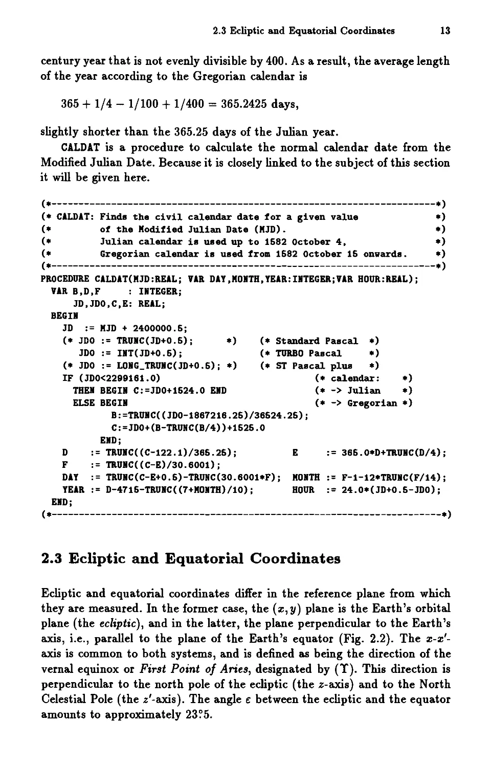
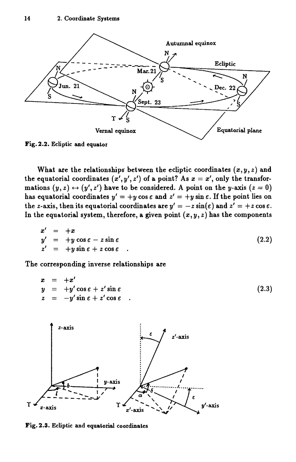
2.3 Ecliptic and Equatorial Coordinates
Ecliptic and equatorial coordinates differ in the reference plane from which
they are measured. In the former case, the (:z:,y) plane is the Earth's orbital
plane (the ecliptic), and in the latter, the plane perpendicular to the Earth's
axis, i.e., parallel to the plane of the Earth's equator (Fig. 2.2). The :z:-:z:'-
axis is common to both systems, and is defined as being the direction of the
vernal equinox or First Point of Aries, designated by (1'). This direction is
perpendicular to the north pole of the ecliptic (the z-axis) and to the North
Celestial Pole (the z'-axis). The angle g between the ecliptic and the equator
amounts to approximately 23? 5.
14 2. Coordinate Systems
Autumnal equinox
Vernal equinox
Fig. 2.2. Ecliptic and equator
What are the relationshipS' between the ecliptic coordinates (:z:,y,z) and
the equatorial coordinates (:z:', y', z') of a point? As :z: = :z:', only the transfor-
mations (y, z) +-+ (y', z') have to be considered. A point on the y-axis (z = 0)
has equatorial coordinates y' = +y cos g and z' = +y sin g. If the point lies on
the z-axis, then its equatorial coordinates are y' = - z sin( g) and z' = + z cos g.
In the equatorial system, therefore, a given point (:z:, y, z) has the components
:z:'
y'
z'
+:z:
+y cos g - z sin g
+y sin g + z cos g
(2.2)
The corresponding inverse relationships are
y
z
+:z:'
+y' cos g + z' sin g
-y'sin g + z' cos g
(2.3)
:z:
z-axis
y-axis
,
1
1
.. Q < .""."./"" . .....
...... " , .
, .".. \. 1/ Y -IlX1S
:c -IlX1S .. .y
y
y
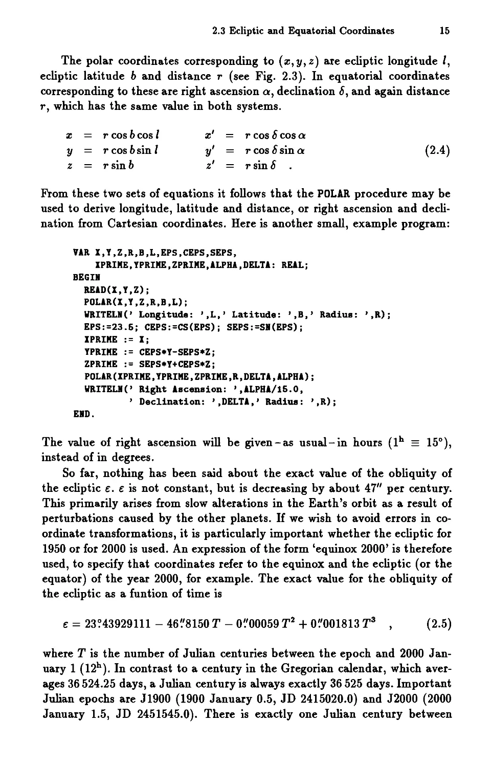
Fig. 2.3. Ecliptic and equatorial coordinates
2.3 Ecliptic and Equatorial Coordinates 15
The polar coordinates corresponding to (:z:, y, z) are ecliptic longitude 1,
ecliptic latitude b and distance r (see Fig. 2.3). In equatorial coordinates
corresponding to these are right ascension a, declination 6, and again distance
r, which has the Same value in both systems.
y
z
r cos b cos 1
r cos b sin 1
r sin b
:z:'
y'
z'
r cos 6 cos a
r cos 6 sin a
rsin6
(2.4)
:z:
From these two sets of equations it follows that the POLAR procedure may be
used to derive longitude, latitude and distance, or right ascension and decli-
nation from Cartesian coordinates. Here is another small, example program:
VAR I,Y,Z,R,B,L,EPS,CEPS,SEPS,
IPRIME,YPRIME,ZPRIME,ALPHA,DELTA: REALi
BEG II
READ(I,Y,Z);
POLAR(I,Y,Z,R,B,L);
WRITELI(' Longitude: ',L,' Latitude: ',B,' Radius: ',R)j
EPS:=23.6j CEPS:=CS(EPS); SEPS:=SI(EPS);
IPRIME := I;
YPRIME := CEPS*Y-SEPS*Zj
ZPRIME := SEPS*Y+CEPS*Z;
POLAR(IPRIME,YPRIME,ZPRIME,R,DELTA,ALPHA);
WRITELI(' Right Ascension: ',ALPHA/i6.0,
, Declination: ',DELTA,' Radius: ',R);
EID.
The value of right ascension will be given-as usual-in hours (l h == 15°),
instead of in degrees.
So far, nothing has been said about the exact value of the obliquity of
the ecliptic g. g is not constant, but is decreasing by about 47" per century.
This primarily arises from slow alterations in the Earth's orbit as a result of
perturbations caused by the other planets. If we wish to avoid errors in co-
ordinate transformations, it is particularly important whether the ecliptic for
1950 or for 2000 is used. An expression of the form 'equinox 2000' is therefore
used, to specify that coordinates refer to the equinox and the ecliptic (or the
equator) of the year 2000, for example. The exact value for the obliquity of
the ecliptic as a funtion of time is
g = 23?43929111 - 46 '8150 T - 0 '00059 T 2 + 0 '001813 T 3 (2.5)
where T is the number of Julian centuries between the epoch and 2000 Jan-
uary 1 (12 h ). In contrast to a century in the Gregorian calendar, which aver-
ages 36524.25 days, a Julian century is always exactly 36525 days. Important
Julian epochs are J1900 (1900 January 0.5, JD 2415020.0) and J2000 (2000
January 1.5, JD 2451545.0). There is exactly one Julian century between
16 2. Coordinate Systems
these dates. T may be calculated for a given epoch with the Julian Date JD
from
T = JD - 2451545
36525
To a close approximation, the value of T may be obtained from the year y by
T::::: (y - 2000)/100
(.-----------------------------------------------------------------------.)
(. ECLEQU: Conversion of ecliptic into equatorial coordinates .)
(. (T: equinox in Julian centuries since J2000) .)
(.-----------------------------------------------------------------------.)
PROCEDURE ECLEQU(T:REAL;VAR I,Y,Z:REAL);
VAR EPS,C,S,V: REAL;
BEG II
EPS:=23.43929111-(46.8160+(0.00069-0.001813.T).T).T/3600.0;
C:=CS(EPS); S:=SI(EPS);
V:=+C.Y-S.Z; Z:=+S.Y+C.Z; Y:=V;
EID;
(.-----------------------------------------------------------------------.)
(. EQUECL: conversion of equatorial into ecliptic coordinates .)
(. (T: equinox in Julian centuries since J2000) .)
(.-----------------------------------------------------------------------.)
PROCEDURE EQUECL(T:REAL;VAR I,Y,Z:REAL);
VAR EPS,C,S,V: REAL;
BEG II
EPS:=23.43929111-(46.8160+(0.00069-0.001813.T).T).T/3600.0;
C:=CS(EPS); S:=SI(EPS);
V:=+C.Y+S.Z; Z:=-S.Y+C.Z; Y:=V;
EID;
(.-----------------------------------------------------------------------.)
The ECLEQU and EQUECL procedures are formulated so that the coordinates
(:z:, y, z) entered are transformed into the appropriate system. If both routines
are called one after the other (with the same value of T), then the original
values are obtained.
The example given above may be expressed as follows using EQUECL (with
Epoch J1950 = JD 2433282.50):
COIST JD2000 = 2461646.0;
JD1960 = 2433282.6;
VAR I,Y,Z,R,B,L,
T,DELTA,ALPHA: REAL;
BEGII
READ(I,Y,Z);
POLAR(I,Y,Z,R,B,L);
WRITELI(' Longitude: ',L,' Latitude: ',B,' Radius: ',R);
T := (JD1960-JD2000) / 36626.0;
ECLEQU(T,I,Y,Z);
2.4 Precession 17
POLAR(I,Y,Z,R,DELTA,ALPHA);
WRITELN(' Right Ascension: ',ALPHA/i6.0,
, Declination: ',DELTA,' Radius:' R);
END.
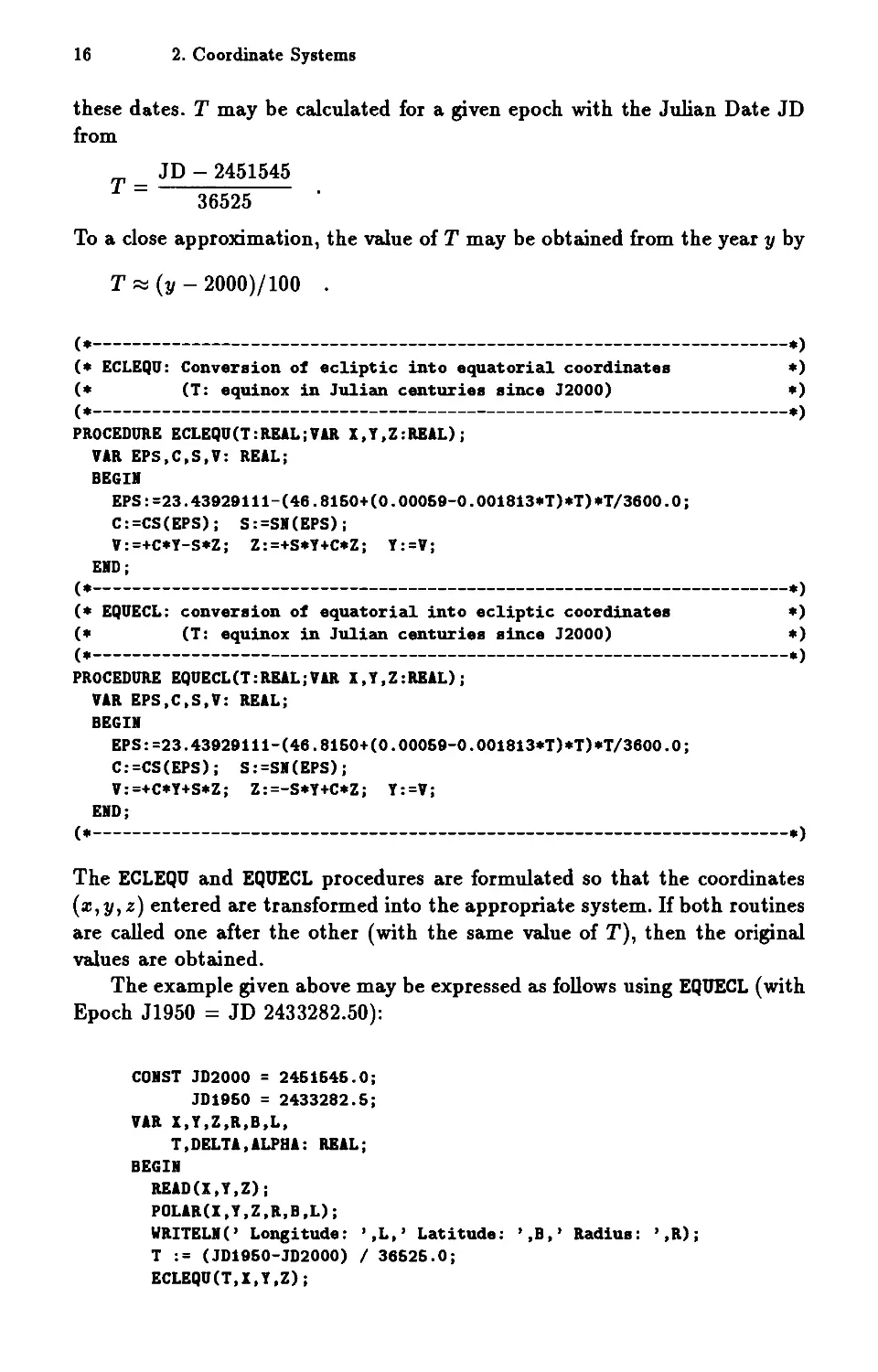
2.4 Precession
The shift in the position of the Earth's axis and of the ecliptic caused by
forces exerted by the Sun, Moon and planets does not only cause a slight
change in the angle g between the equator and the ecliptic, but also a shift
of the vernal equinox by about I? 5 per century (1' per year). For precise
calculations, therefore, the equinox of the coordinate system used must be
stated. The equinoxes most frequently used are
. the equinox of date,
. equinox J2000 and
. equinox B1950.
"Equinox of date" means that the values used are those for the equator,
ecliptic, and vernal equinox for the actual date under consideration. Such daily
alteration of the coordinate system is sensible if one requires the coordinates
of a planet, for example, for use in conjunction with the setting circles on
an equatorially mounted telescope, or on a transit circle. Because of the shift
in the Earth's axis, the orientation of the polar axis of a telescope will also
alter. On the other hand, if one wants to study the actual spatial motion of a
planet, then it is better to use a fixed equinox, such as that for Julian Epoch
J2000 (2000 January 1.5 = JD 2451545.0), which was generally introduced
in 1984. Before that, the older equinox B1950 had been used for a long time,
and was employed for many stellar catalogues and atlases (such as the SA 0
Star Catalog and Atlas Coeli). The prefix B indicates that it is not half-way
between the epochs J1900 and J2000 (which would, of course, be J1950 = JD
2433282.5), but the beginning of the Besselian year 1950 (1950 Jan. 0.923 =
JD 2433282.423).
Transformation of coordinates from one equinox to another requires sim-
ilar steps to those required in converting from ecliptic to equatorial coordi-
nates. Whereas those two coordinates systems could be brought into coinci-
dence by a simple rotation about the z-axis, we now have to deal with a total
of three rotations: first about the z-axis, second about the z-axis, and finally
about the z-axis again.
If we first consider the ecliptic at time To and time To + T, then the angle
between the two planes is
11' = (4 7 '0029 - 0 '06603 . To + 0 '000598 . T;) . T (2.6)
+( -0 '03302 + 0 '000598 . To) . T 2 + 0 '000060 . T 3
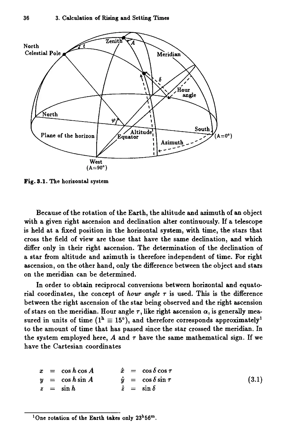
18 2. Coordinate Systems
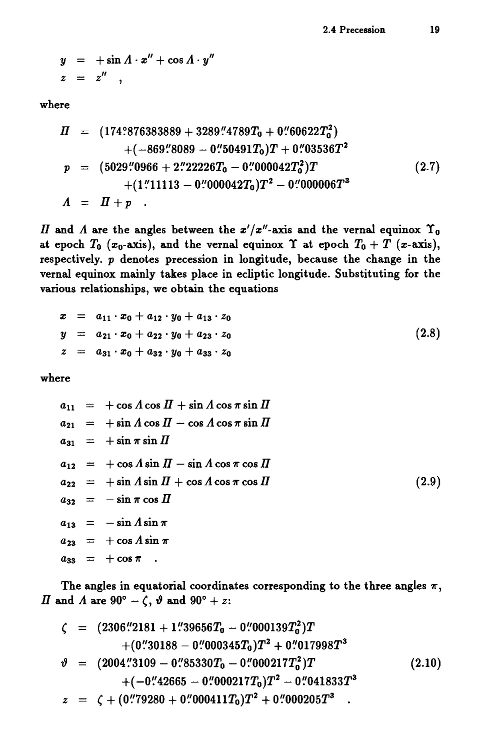
Fig. 2.4. The effects of precession on the ecliptic, equator, and vernal equinox
If two coordinate systems (z', y', z') and (z", y", z") are established, such that
the z'-y'-plane coincides with the ecliptic for time To, and the z"-y"-plane
with that for time To + T, then we have:
z" = z'
y" = +COS'll'. y' + sin 11' . z'
" = - sin 11' . y' + cos 11' . z'
Z
This assumes that the z'-axis and the z"-axis coincide with the line of in-
tersection of the two planes. Let (zo, Yo, zo) be the ecliptic coordinates corre-
sponding to the epoch To and (z, y, z) the coordinates at epoch To + T. We
then have
z' = + cos II . Zo + sin II . Yo
y' = - sin II . Zo + cos II . Yo
,
z = Zo
and
z = + cos A . z" - sin A . y"
2.4 Precession 19
y + sin A . z" + cos A . y"
"
z = z
where
II (174?876383889 + 3289 '4789To + 0 '60622T;)
+( -869 '8089 - 0 '50491To)T + 0 '03536T2
p (5029 '0966 + 2 '22226To - 0 '000042T;)T
+(1 '11113 - 0 '000042To)T2 - 0 '000006T3
A = II+p .
(2.7)
II and A are the angles between the z' /z"-axis and the vern-aI equinox To
at epoch To (zo-axis), and the vernal equinox T at epoch To + T (z-axis),
respectively. p denotes precession in longitude, because the change in the
vernal equinox mainly takes place in ecliptic longitude. Substituting for the
various relationships, we obtain the equations
z = all' Zo + al2 . Yo + al3 . Zo
y = a21' Zo + a22 . Yo + a23 . Zo
Z a31 . Zo + a32 . Yo + a33 . Zo
(2.8)
where
all + cos A cos II + sin A cos 11' sin II
a21 = + sin A cos II - cos A cos 11' sin II
a31 = + sin 11' sin II
al2 = + cos A sin II - sin A cos 11' COS II
a22 = + sin A sin II + cos A cos 11' COS II
a32 = - sin 11' cos II
al3 -sinAsin'll'
a23 = + cos A sin 11'
a33 = +COS'll'
(2.9)
The angles in equatorial coordinates corresponding to the three angles 11',
II and A are 90° - (, and 90° + z:
( = (2306 '2181 + 1 '39656To - 0 '000139T;)T
+(0 '30188 - 0 '000345To)T2 + 0 '017998T3
(2004 '3109 - 0 '85330To - 0 '000217T;)T (2.10)
+( -0 '42665 - 0 '000217To)T2 - 0 '041833T3
Z = ( + (0 '79280 + 0 '000411To)T2 + 0 '000205T3
20 2. Coordinate Systems
This gives corresponding formulae where
all = - sin z sin ( + cos z cos -{} cos (
a21 + cos z sin ( + sin z cos -{} cos (
a3l = +sin-{}cos(
al2 = -sinzcos( -coszcos-{}sin(
a22 +coszcos( - sin z cos-{} sin ( (2.11)
a32 = -sin-{} sin (
a13 = - cos z sin-{)
a23 = - sin z sin -{}
a33 = +cos-{}
The most onerous part of calculating precession is determining the values
for the various angles and for aij. However, these values only depend on the
two epochs To and To + T, and can be reused if a whole series of different
positions are to be converted from one fixed epoch to another. Individual
procedures are therefore given for this purpose.
(*-----------------------------------------------------------------------*)
(* PMATECL: calculates the precession matrix A[i,j] for *)
(* transforming ecliptic coordinates from equinox T1 to T2 *)
(* ( T=(JD-2461646.0)/36626 ) *)
(*-----------------------------------------------------------------------*)
PROCEDURE PMATECL(T1,T2:REALiVAR A: REAL33)i
CORST SEC=3600.0i
VAR DT,PPI,PI,PA: REALi
C1,S1,C2,S2,C3,S3: REALi
BEGIR
DT:=T2-T1i
PPI .- 174.876383889 +( «3289.4789+0.60622*T1)*T1) +
«-869.8089-0.60491*T1) + O.03636*DT)*DT )/SECi
(47.0029-(O.06603-0.000698*T1)*T1)+
«-O.03302+0.000698*T1)+O.000060*DT)*DT )*DT/SECi
(6029.0966+(2.22226-0.000042*T1)*T1)+
«1.11113-0.000042*T1)-O.000006*DT)*DT )*DT/SECi
C1:=CS(PPI+PA)i C2:=CS(PI)i C3:=CS(PPI)i
S1:=SR(PPI+PA)i S2:=SR(PI)i S3:=SR(PPI)i
A[1,1]:=+C1*C3+S1*C2*S3i A[1,2]:=+C1*S3-S1*C2*C3i
A[2,1]:=+S1*C3-C1*C2*S3i A[2,2]:=+S1*S3+C1*C2*C3i
A[3,1]:=+S2*S3i A[3,2]:=-S2*C3i
ERDi
PI
PA
1[1,3] :=-S1*S2i
1[2,3]:=+C1*S2i
A [3 ,3] : =+C2i
(*-----------------------------------------------------------------------*)
(* PMATEQU: calculates the precession matrix A[i,j] for *)
(* transforming equatorial coordinates from equinox T1 to T2 *)
(* (T=(JD-2461646.0)/36626 ) *)
(*-----------------------------------------------------------------------*)
PROCEDURE PMATEQU(T1,T2:REALiVAR A:REAL33)i
2.4 Precession 21
CaNST SEC=3600.0;
VAR DT,ZETA,Z,THETA: REAL;
Cl,Sl,C2,S2,C3,S3: REAL;
BEG!R
DT: =T2-Tl ;
ZETA . -
( (2306.2181+(1.39666-0.000139*Tl)*Tl)+
«0.30188-0.000346*Tl)+0.017998*DT)*DT )*DT/SEC;
Z .- ZETA + ( (0.79280+0.000411*Tl)+0.000206*DT)*DT*DT/SEC;
THETA.- «2004.3109-(0.86330+0.000217*Tl)*Tl)-
«0.42666+0.000217*Tl)+0.041833*DT)*DT )*DT/SEC;
Cl:=CS(Z); C2:=CS(THETA); C3:=CS(ZETA);
Sl:=SN(Z); S2:=SN(THETA); S3:=SN(ZETA);
A[l,l]:=-Sl*S3+Cl*C2*C3; A[l,2]:=-Sl*C3-Cl*C2*S3;
A[2,l]:=+Cl*S3+S1*C2*C3; A[2,2]:=+Cl*C3-S1*C2*S3;
A[3,l]:=+S2*C3; A[3,2]:=-S2*S3;
END;
1[1,3] : =-C1*S2;
1[2,3] : =-S1*S2;
1[3,3]:=+C2;
(*-----------------------------------------------------------------------*)
(* PRECART: calculate change of coordinates due to precession *)
(* for given transformation matrix A[i,j] *)
(* (to be used with PMATECL und PMATEQU) *)
(*-----------------------------------------------------------------------*)
PROCEDURE PRECART(A:REAL33; VAR I,Y,Z:REAL);
VAR U,V,W: REAL;
BEG!R
U .- A[l,l]*I+A[l,2]*Y+A[l,3]*Z;
V := A[2,l]*I+A[2,2]*Y+A[2,3]*Z;
W := A[3,l]*I+A[3,2]*Y+A[3,3]*Z;
I:=U; Y:=V; Z:=W;
END;
(*-----------------------------------------------------------------------*)
The matrix A is defined as data type REAL33. A corresponding global type
declaration
TYPE REAL33 = ARRAY[1..3,l..3] OF REAL;
should be included in the initialization section of the main program.
In order to give an idea of the effects of precession, and also to allow
some practice in using the various routines, a somewhat longer example will
be given. A set of coordinates for equinox B1950 is to be converted to a
corresponding set for equinox J2000. This may be carried out in two ways,
according to whether precession or the conversion between ecliptic and equa-
torial coordinates is applied first.
CaNST B1960 = -0.600002108; (* B1960=(2433282.423-2461646)/36626 *)
J2000 = 0.0;
VAR A
R,B,L,IO,YO,ZO,
I,Y,Z,DEC,RA
I
REAL33;
REAL;
!RTEGER ;
22 2. Coordinate Systems
BEGIR
(. ecliptic coordinates B1960 (angles in degrees): .)
L := 200.0j B:=10.0j R:=1.0;
CART (R,B,L,IO,YO,ZO)j
(. method 1: .)
PMATECL(B1960,J2000,A); (. Matrix B1960->J2000 ecliptic: .)
FOR 1:=1 TO 3 DO WR1TELI(A[1,1]:16:10,A[1,2]:16:10,A[1,3]:16:10);
1:=10; Y:=YOj Z:=ZOj (. eel. B1960.)
PRECART(A,I,Y,Z)j (. eel. J2000.)
POLAR(I,Y,Z,R,B,L);
WR1TELI(L:16:10,B:16:10,R:16:10)j
ECLEQU(J2000,I,Y,Z); (. equ. J2000.)
POLAR(I,Y,Z,R,DEC,RA);
WR1TELI(RA/16.0:16:10,DEC:16:10,R:16:10)j
(. method 2: .)
PMATEQU(B1960,J2000,A)j (. Matrix B1960->J2000 equatorial: .)
FOR 1:=1 TO 3 DO WR1TELI(A[1,1]:16:10,A[1,2]:16:10,A[1,3]:16:10);
1:=10; Y:=YOj Z:=ZOj (. eel. B1960 .)
ECLEQU(B1960,I,Y,Z)j (. equ. B1960 .)
POLAR(I,Y,Z,R,DEC,RA);
WR1TELI(RA/16.0:16:10,DEC:16:10,R:16:10)j
PRECART(A,I,Y,Z); (. equ. J2000 .)
POLAR(I,Y,Z,R,DEC,RA)j
WR1TELI(RA/16.0:16:10,DEC:16:10,R:16:10);
EID.
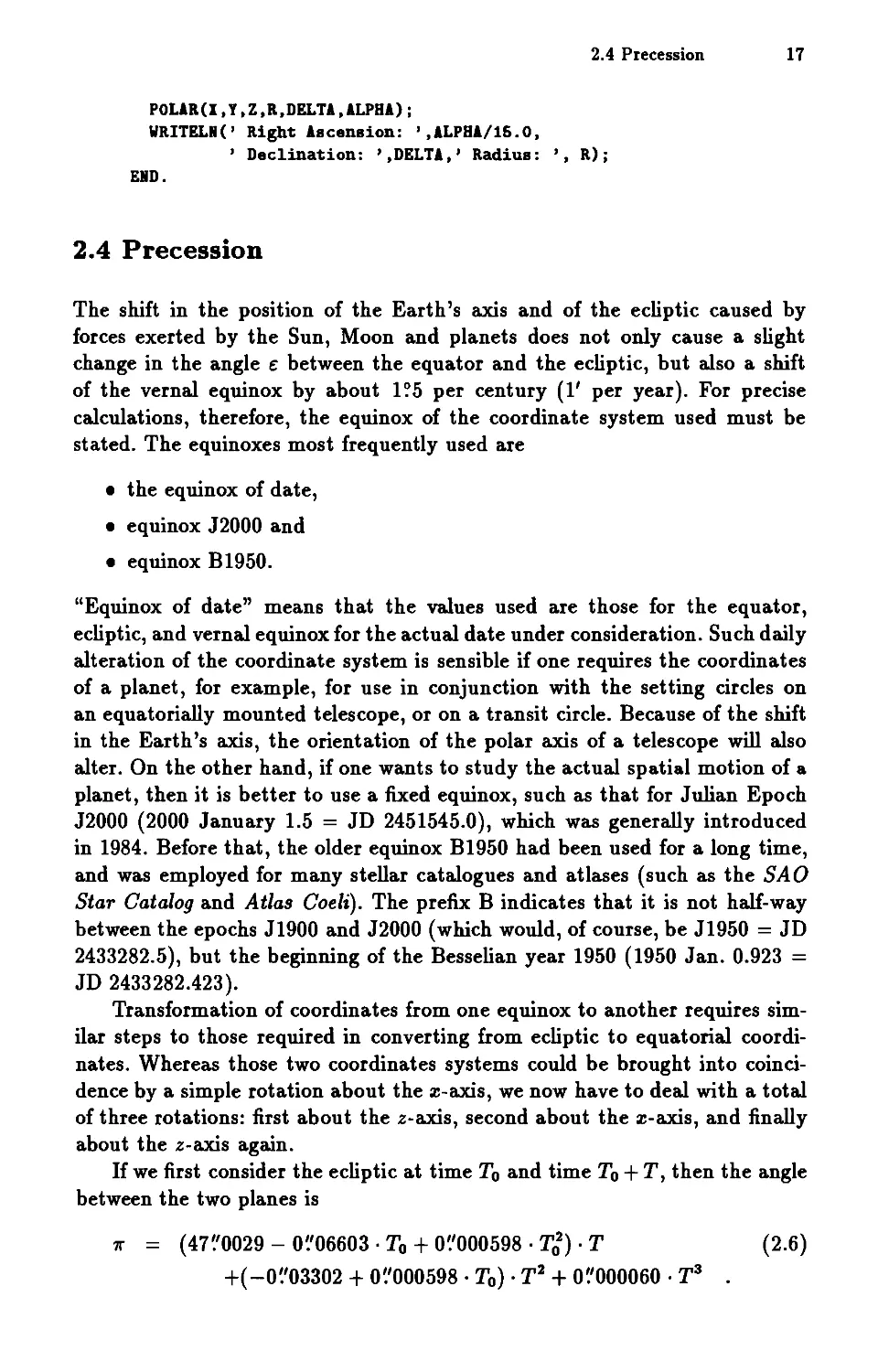
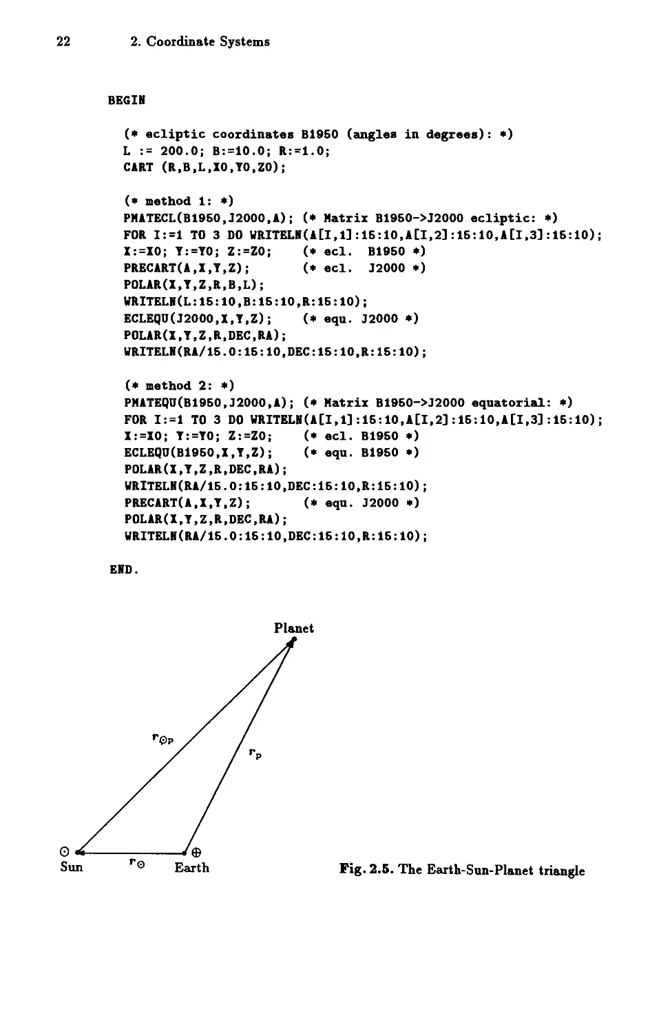
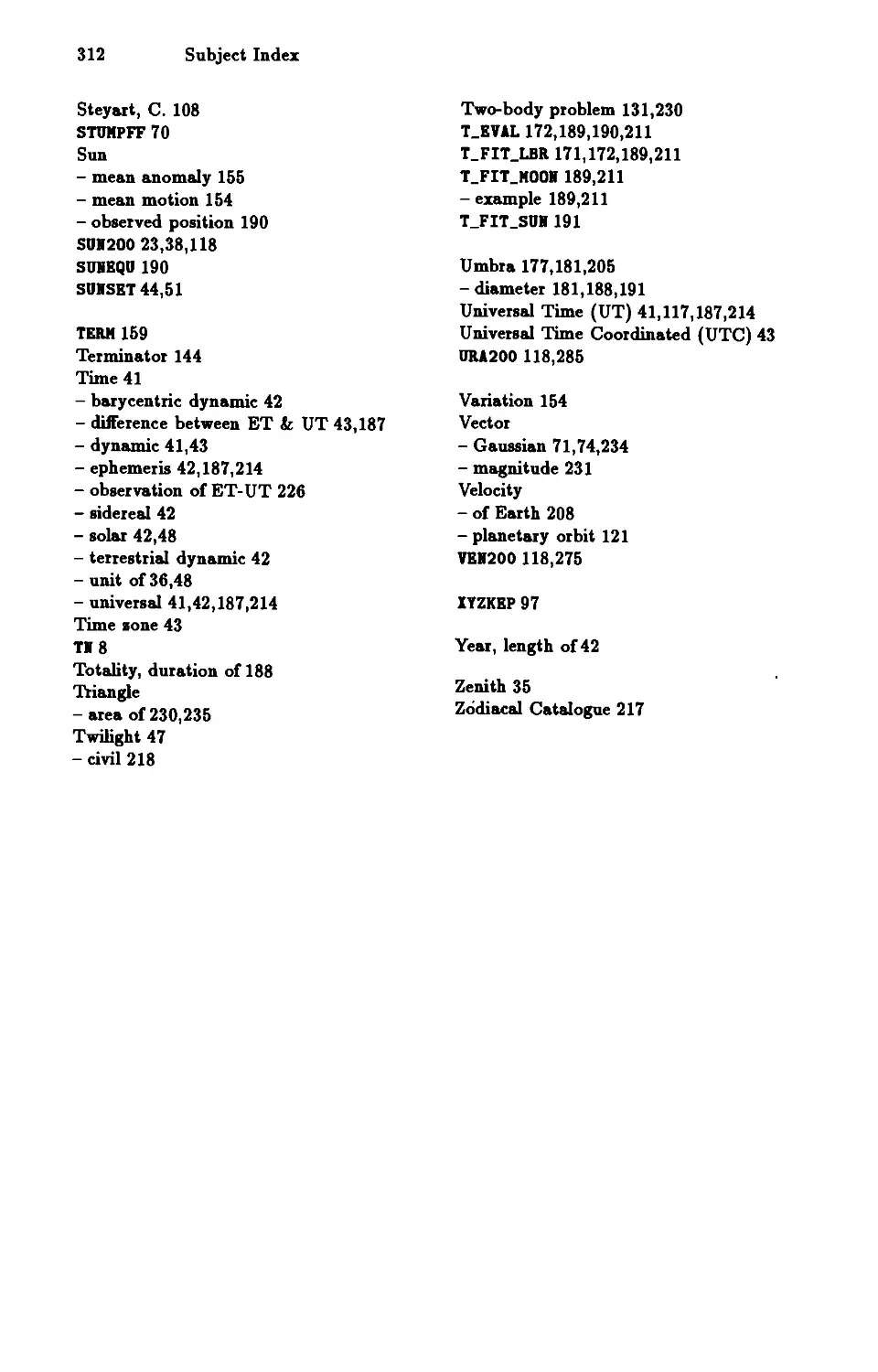
Planet
re
Fig. 2.5. The Earth-Sun-Planet triangle
2.5 Geocentric Coordinates and the Orbit of the Sun 23
2.5 Geocentric Coordinates and the Orbit of the Sun
All that is now required to complete the program is a method for converting
heliocentric coordinates (referred to the centre of the Sun) into geocentric
ones (referred to the centre of the Earth), and the converse. Conversion of
the origin of the coordinates is described by the equations
fOp = '"ep + '"e and '"ep = fOp - '"e
(2.12)
which are derived from the Sun-Earth-Planet triangle illustrated in Fig. 2.5.
Here '"ep and fOp are the heliocentric and geocentric position vectors of a
point P, and '"e is the geocentric position of the Sun. Written in the form of
individual components, the transformation equations are
Zp = zep + Ze zep = zp - Ze
YP Yep + Ye and Yep = YP - Ye
Zp Zep + Ze zep = Zp - Ze
where it makes no difference whether ecliptic or equatorial coordinates are
employed to express the various vectors.
As any error in the position of the Sun inevitably affects the accuracy
of the conversions, it is worthwhile taking some trouble in calculating the
coordinates of the Sun. The SUR200 procedure, introduced here, attains an
accuracy of about I", which should be more than sufficient for most purposes.
For a time
T = (JD - 2451545}/36525
it provides the ecliptic longitude (L) and latitude (B) of the Sun, and its
distance (R) from the Earth. From these we can determine the ecliptic coor-
dinates
Ze Rcos B cos L
Ye R cos B sin L
ze = R sin B
Like L and B these initially refer to the equinox of date, but can be converted
to another equinox by means of the procedures already discussed.
(.-----------------------------------------------------------------------.)
(. SUR200: ecliptic coordinates L,B,R (in deg and AU) of the .)
(. Sun referred to the mean equinox of date .)
(. (T: time in Julian centuries since J2000) .)
(. (= (JED-2461646.0)/36626) .)
(.-----------------------------------------------------------------------.)
PROCEDURE SUR200(T:REALiVAR L,B,R:REAL)i
CORST P2=6.283186307i
24 2. Coordinate Systems
VAR C3,S3:
C,S:
M2,M3,M4,M6,M6:
D,A,UU:
U,V,DL,DR,DB:
I:
ARRAY [-1..7] OF REAL;
ARRAY [-8..0] OF REAL;
REAL;
REAL;
REAL;
IRTEGER ;
FURCTIOR FlUC (I: REAL) : REAL;
(* for some compilers TRURC has to be replaced by LORG_TRURC *)
(* or IRT (Turbo-Pascal) if the routine is used with T<-24 *)
BEGIR I:=I-TRURC(I); IF (1<0) THER 1:=1+1.0; FlUC:=1 ERD;
PROCEDURE ADDTHE(C1,S1,C2,S2:REAL; VAR C,S:REAL);
BEGIR C:=C1*C2-S1*S2; S:=S1*C2+C1*S2; ERD;
PROCEDURE TERM(11,I,IT:IRTEGER;DLC,DLS,DRC,DRS,DBC,DBS:REAL);
BEGIR
IF IT=O THER ADDTHE(C3[11],S3[11],C[I] ,S[I] ,U,V)
ELSE BEGIR U:=U*T; V:=V*T ERD;
DL:=DL+DLC*U+DLS*V; DR:=DR+DRC*U+DRS*V; DB:=DB+DBC*U+DBS*V;
ERD;
PROCEDURE PERTVER; (* Keplerian terms and perturbations by Venus *)
VAR I: IRTEGER;
BEGIR
C[0]:=1.0; S[O]:=O.O; C[-1]:=COS(M2); S[-1]:=-SIR(M2);
FOR 1:=-1 DOWRTO -6 DO ADDTHE(C[I],S[I],C[-1],S[-1],C[I-1],S[I-1]);
TERM(1, 0,0,-0.22,6892.76,-16707.37, -0.64,0.00, 0.00);
TERM(1, 0,1,-0.06, -17.36, 42.04, -0.16, 0.00, 0.00);
TERM(1, 0,2,-0.01, -0.06, 0.13, -0.02,0.00, 0.00);
TERM(2, 0,0, 0.00, 71.98, -139.67, 0.00,0.00, 0.00);
TERM(2, 0,1, 0.00, -0.36, 0.70, 0.00,0.00, 0.00);
TERM(3, 0,0, 0.00, 1.04, -1.76, 0.00, 0.00, 0.00);
TERM(O,-1,O, 0.03, -0.07, -0.16, -0.07,0.02,-0.02);
TERM(1,-1,O, 2.36, -4.23, -4.76, -2.64, 0.00, 0.00);
TERM(1,-2,O,-0.10, 0.06, 0.12, 0.20, 0.02, 0.00);
TERM(2,-1,O,-0.06, -0.03, 0.20, -0.01, 0.01,-0.09);
TERM(2,-2,O,-4.70, 2.90, 8.28, 13.42, 0.01,-0.01);
TERM(3,-2,O, 1.80, -1.74, -1.44, -1.67, 0.04,-0.06);
TERM(3,-3,O,-0.67, 0.03, 0.11, 2.43,0.01, 0.00);
TERM(4,-2,O, 0.03, -0.03, 0.10, 0.09,0.01,-0.01);
TERM(4,-3,O, 1.61, -0.40, -0.88, -3.36,0.18,-0.10);
TERM(4,-4,O,-0.19, -0.09, -0.38, 0.77, 0.00, 0.00);
TERM(6,-3,O, 0.76, -0.68, 0.30, 0.37, 0.01, 0.00);
TERM(6,-4,O,-0.14, -0.04, -0.11, 0.43,-0.03, 0.00);
TERM(6,-6,O,-0.06, -0.07, -0.31, 0.21, 0.00, 0.00);
TERM(6,-4,O, 0.16, -0.04, -0.06, -0.21, 0.01, 0.00);
TERM(6,-6,O,-0.03, -0.03, -0.09, 0.09,-0.01, 0.00);
TERM(6,-6,O, 0.00, -0.04, -0.18, 0.02, 0.00, 0.00);
TERM(7,-6,O,-0.12, -0.03, -0.08, 0.31,-0.02,-0.01);
ERD;
PROCEDURE PERTMAR; (* perturbations by Mars *)
2.5 Geocentric Coordinates and the Orbit of the Sun 25
VAR I: IRTEGER;
BEGIR
C[-1]:=COS(M4); S[-1]:=-SIR(M4);
FOR 1:=-1 DOWRTO -7 DO ADDTHE(C[I] ,S[I] ,C[-l] ,S[-l] ,C[I-l] ,S[I-l]);
TERM(l,-l,O,-0.22, 0.17, -0.21, -0.27,0.00, 0.00).
TERM(l,-2,O,-1.66, 0.62, 0.16, 0.28,0.00, 0.00).
TERM(2,-2,O, 1.96, 0.67, -1.32, 4.66, 0.00, 0.01).
TERM(2,-3,O, 0.40, 0.16, -0.17, 0.46, 0.00, 0.00);
TERM(2,-4,O, 0.63, 0.26, 0.09, -0.22, 0.00, 0.00);
TERM(3,-3,O, 0.06, 0.12, -0.36, 0.16,0.00, 0.00).
TERM(3,-4,O,-0.13, -0.48, 1.06, -0.29, 0.01, 0.00).
TERM(3,-6,O,-0.04, -0.20, 0.20, -0.04, 0.00, 0.00).
TERM(4,-4,O, 0.00, -0.03, 0.10, 0.04,0.00, 0.00);
TERM(4,-6,O, 0.06, -0.07, 0.20, 0.14,0.00, 0.00);
TERM(4,-6,O,-0.10, 0.11, -0.23, -0.22, 0.00, 0.00);
TERM(6,-7,O,-0.06, 0.00, 0.01, -0.14, 0.00, 0.00);
TERM(6,-8,O, 0.06, 0.01, -0.02, 0.10, 0.00, 0.00);
ERD;
PROCEDURE PERTJUP. (* perturbations by Jupiter *)
VAR I: IRTEGER;
BEGIR
C[-1]:=COS(M6); S[-1]:=-SIR(M6);
FOR 1:=-1 DOWRTO -3 DO ADDTHE(C[I] ,S[I] ,C[-l] ,S[-l] ,C[I-l],S[I-l]);
TERM(-l,-l,O,O.Ol, 0.07, 0.18, -0.02,0.00,-0.02).
TERM(O,-l,O,-0.31, 2.68, 0.62, 0.34,0.02, 0.00).
TERM(l,-l,O,-7.21, -0.06, 0.13,-16.27,0.00,-0.02);
TERM(l,-2,O,-0.64, -1.62, 3.09, -1.12, 0.01,-0.17);
TERM(l,-3,O,-0.03, -0.21, 0.38, -0.06,0.00,-0.02).
TERM(2,-l,O,-0.16, 0.06, -0.18, -0.31,0.01, 0.00).
TERM(2,-2,O, 0.14, -2.73, 9.23, 0.48, 0.00, 0.00).
TERM(2,-3,O, 0.07, -0.66, 1.83, 0.26,0.01, 0.00);
TERM(2,-4,O, 0.02, -0.08, 0.26, 0.06, 0.00, 0.00).
TERM(3,-2,O, 0.01, -0.07, 0.16, 0.04, 0.00, 0.00).
TERM(3,-3,O,-0.16, -0.03, 0.08, -0.64, 0.00, 0.00).
TERM(3,-4,O,-0.04, -0.01, 0.03, -0.17, 0.00, 0.00);
ERD;
PROCEDURE PERTSAT; (* perturbations by Saturn *)
BEGIR
C[-1]:=COS(M6); S[-1]:=-SIR(M6);
ADDTHE(C [-1] ,S [-1] ,C[ -1] ,S [-1] ,C [-2] ,S[ -2]) ;
TERM(O,-l,O, 0.00, 0.32, 0.01, 0.00,0.00, 0.00).
TERM(l,-l,O,-0.08, -0.41, 0.97, -0.18, 0.00,-0.01).
TERM(l,-2,O, 0.04, 0.10, -0.23, 0.10,0.00,0.00);
TERM(2,-2,O, 0.04, 0.10, -0.36, 0.13, 0.00, 0.00);
ERD;
PROCEDURE PERTMOO.
BEGIR
DL .- DL +
(* difference between the Earth-Moon *)
(* barycenter and the center of the Earth *)
6.46*SIR(D) - 0.42*SIR(D-A) + 0.18*SIR(D+A)
+ 0.17*SIR(D-M3) - 0.06*SIR(D+M3);
DR .- DR + 30.76*COS(D) - 3.06*COS(D-A)+ 0.86*COS(D+A)
- 0.68*COS(D+M3) + 0.67*COS(D-M3).
26 2. Coordinate Systems
DB := DB + 0.676*SIR(UU)j
ERD;
BEGIR (* SUR200 *)
DL:=O.Oj DR:=O.O; DB:=O.O;
M2:=P2*FRAC(0.1387306+162.6486917*T);
M3:=P2*FRAC(0.9931266+99.9973604*T);
M4:=P2*FRAC(0.0643260+ 63.1666028*T);
M6:=P2*FRAC(0.0661760+ 8.4293972*T)j
M6:=P2*FRAC(0.8816600+ 3.3938722*T)j D :=P2*FRAC(0.8274+1236.8631*T);
A :=P2*FRAC(0.3749+1326.6624*T); UU:=P2*FRAC(O.2691+1342.2278*T)j
C3[0]:=1.0; S3[0]:=0.Oj
C3[1]:=COS(M3)j S3[1]:=SIR(M3); C3[-1]:=C3[1]; S3[-1]:=-S3[1]j
FOR 1:=2 TO 7 DO ADDTHE(C3[1-1],S3[1-1] ,C3[1] ,S3[1],C3[1],S3[1]);
PERTYER; PERTMARj PERTJUPj PERTSATj PERTMOOj
DL:=DL + 6.40*SIR(P2*(0.6983+0.0661*T»+1.87*SIR(P2*(0.6764+0.4174*T»
+ 0.27*SIR(P2*(0.4189+0.3306*T»+0.20*SIR(P2*(0.3681+2.4814*T»;
L:= 360.0*FRAC(0.7869463 + M3/P2 + «6191.2+1.1*T)*T+DL)/1296.0E3 )j
R:= 1.0001398 - 0.0000007*T + DR*1E-6;
B:= DB/3600.0;
ERD; (* SUR200 *)
(*-----------------------------------------------------------------------*)
The extent of the SUR200 procedure is explained by the fact that the
relative motion of the Sun and the Earth cannot be described to the required
accuracy by simple elliptical orbits. Apart from the perturbations of the other
planets-particularly those of Venus and Jupiter- there is also the monthly
oscillation of the centre of the Earth around the barycentre of the Earth-
Moon system. Strictly speaking, not the Earth itself, but rather the position
of the barycentre, is moving in the plane of the ecliptic. The Moon's orbit
around the Earth is therefore reflected in a small periodic perturbation of
the geocentric orbit of the Sun. The details of the procedure and its basis
will not be discussed here. Both will be treated thoroughly in Chap. 6, where
appropriate routines for all the planets will be given.
2.6 The COCO Program 27
2.6 The COCO Program
The various procedures described will now be incorporated into a complete
program. Only the input and output routines and the main program are given
here. The procedures already discussed should be incorporated at the points
indicated.
(.-----------------------------------------------------------------------.)
(. coco .)
(. coordinate conversion .)
(. version 93/07/01 .)
(.-----------------------------------------------------------------------.)
PROGRAM COCO(IRPUT,OUTPUT);
TYPE REAL33 = ARRAY[1..3,1..3] OF REALi
VAR I,Y,Z,IS,YS,ZS:
T,TEQI,TEQU
LS,BS,RS
A
ECLIPT
MODE
REALi
REALi
REAL;
REAL33;
BOOLEUi
CHAR;
(.-----------------------------------------------------------------------.)
(. The following procedures should be entered here in the given order: .)
(. SR, CS, ATR, ATR2, CART, POLAR, DDD, DMS .)
(. MJD .)
(. ECLEQU, EQUECL .)
(. PMATECL, PMATEQU, PRECART, SUR200 .)
(.-----------------------------------------------------------------------.)
(.-----------------------------------------------------------------------.)
PROCEDURE GETEQI(VAR TEQI:REAL);
BEGIR
WRITE (, equinox (yyyy) ? ')i
READLR (TEQI)i TEQI := (TEQI-2000.0)/100.0;
ERD;
(.-----------------------------------------------------------------------.)
PROCEOURE GETDAT(VAR T:REAL);
VAR O,M,Y IRTEGER;
HOUR, JD: REAL;
BEGIR
WRITE (' Date (year month day hour) ? ')i
READLR (Y,M,D,HOUR);
JD := MJD(D,M,Y,HOUR) + 2400000.6;
WRITELR; WRITELR (, JD',JD:13:4)i WRITELR;
T := (JD-2461646.0) / 36626.0;
ERD;
28 2. Coordinate Systems
(.-----------------------------------------------------------------------.)
PROCEDURE GETIIP (VAR I,Y,Z,TEQI:REAL;VAR ECLIPT:BOOLEAI)j
VAR I,D,M IITEGERj
L,B,R,S: REALj
BEGII (. GETIIP .)
WRITELI ;
WRITELI( ,
WRITELI ( ·
WRITELI ( ·
WRITELI;
WRITELI ('
WRITELI;
WRITELI ('
WRITELI ('
WRITELI ;
WRITE ( ,
COCO: coordinate conversion
version 93/07/01
(c) 1993 Thomas Pfleger, Oliver Montenbruck
.) ;
.) ;
.) ;
Coordinate input: please select format required .);
1 ecliptic cartesian
3 equatorial cartesian
2 ecliptic polar')j
4 equatorial polar')j
,); READLI (I)j WRITELI;
CASE I OF
1: BEGII
WRITE (' Coordinates (x y z)? ')j READLI(I,Y,Z); ECLIPT:=TRUE;
EID;
2: BEGII
WRITE (' Coordinates (L (0 ., n) B (0 ,. n) R)? ')j
READ(D,M,S); DDD(D,M,S,L)j READLI(D,M,S,R); DDD(D,M,S,B);
CART(R,B,L,I,Y,Z)j ECLIPT:=TRUE;
EID;
3: BEGII
WRITE (' Coordinates (x y z)? ')j READLI(I,Y,Z);ECLIPT:=FALSEj
EID;
4: BEGII
WRITE (' Coordinates (RA (h m s) DEC (0 ,. n) R)? ') j
READ(D,M,S); DDD(D,M,S,L); READLI(D,M,S,R)j DDD(D,M,S,B);
L:=L.15.0; CART(R,B,L,I,Y,Z)j ECLIPT:=FALSE;
EID;
EID; (. CASE .)
GETEQI (TEQI); (. read equinox .)
EID; (. GETIIP .)
(.-----------------------------------------------------------------------.)
PROCEDURE RESULT (I,Y,Z: REAL; ECLIPT: BOOLEAI)j
VAR L,B,R,S: REAL;
D,M IITEGER;
BEGII (. RESULT .)
2.6 The COCO Program 29
WRITELI; WRITELI (' (x,y,z)
WRITELI ;
(, ,x:13:8,',' ,y:13:8,',' ,z:13:8, ') ,);
POLAR (X,Y,Z,R,B,L);
IF ECLIPT
THEI
BEGII
WRITELIf (, ':5,' 0 " "',' ':8,' 0 " "');
DMS(L,D,M,S); WRITE(' L ',D:3,M:3,S:6:1,' ':3);
DMS(B,D,M,S); WRITE(' B = ',D:3,M:3,S:5:1,' ':3);
EID
ELSE
BEGII
WRITELI (' ':5,'
DMS(L!15,D,M,S);
DMS(B,D,M,S);
EID;
h m 8 J, J J: 10, J 0 ' J II J);
WRITE(' RA = ',D:2,M:3,S:5:1,' ':3);
WRITE(' DEC = ',D:3,M:3,S:6:1,' ':3);
WRITELI (' R = ',R:12:8); WRITELI; WRITELJ;
EID; (. RESULT .)
(.-----------------------------------------------------------------------.)
BEGII (. COCO .)
GETIIP (X,Y,Z,TEQX,ECLIPT);
RESULT (X,Y,Z,ECLIPT);
REPEAT
WRITE (' Command (?=Help): '); READLI (MODE);
WRITELIf ;
IF MODE II ['?', 'P', 'p', 'E', 'e', 'H', 'h', 'G', 'g'] THEI
CASE MODE OF
'? J
BEGII (. help .)
WRITELI ;
WRITELI (,
WRITELI ('
WRITELI ('
WRITELIf ;
EID;
E: equatorial <-) ecliptic
P: -) precession G: -) geocentric
H: -) heliocentric S: -) STOP
, ) ;
, ) ;
, ) ;
'P','p': BEGII (. precession.)
WRITE (, lew');
GETEQX(TEQXI); (. read new equinox .)
IF ECLIPT THEI PMATECL(TEQX,TEQXI,A)
ELSE PMATEQU(TEQX,TEQXI,A);
PRECART(A,X,Y,Z);
TEQX := TEQII;
WRITELI ;
WRITELI (, Coordinates referred to equinox T ='
30 2. Coordinate Systems
TEQI:13:10);
EIID;
'E','e': BEGIII (. ecliptic <-) equatorial.)
WRITELlli
IF (ECLIPT) THEil
BEGIII ECLEQU(TEQI,I,Y,Z); WRITE(' Equatorial')i EIID
ELSE
BEGIII EQUECL(TEQI,I,Y,Z)i WRITE(' Ecliptic')i EIIDi
WRITELII (' coordinates: ')i
ECLIPT .- lOT ECLIPTi
EIIDi
'G','g', (. -) geocentric coordinates .)
'H','h': (. -) heliocentric coordinates .)
BEGIN
GETDAT(T); (. read date .)
SUII200(T,LS,BS,RS);
CART(RS,BS,LS,IS,YS,ZS)i
PMATECL(T,TEQI,A)i
PRECART(A,IS,YS,ZS)i
IF lOT ECLIPT THEil ECLEQU(TEQI,IS,YS,ZS)i
IF MODE III ['G', 'g']
THEil (. -) geocentric .)
BEGIII
1:=1+15; Y:=Y+YSi Z:=Z+ZSi
WRITELII(' Geocentric coordinates: ')i
EIID
ELSE (. -) heliocentric .)
BEGIII
1:=I-ISi Y:=Y-YSi Z:=Z-ZS;
WRITELII(' Heliocentric coordinates: ');
EIIDi
ENDi
EIID;
IF NOT (MODE III ['?','S','s']) THEN RESULT(I,Y,Z,ECLIPT)i
UIITIL MODE III ['5' ,'S']i
EIID. (. COCO .)
(.-----------------------------------------------------------------------.)
A simple menu enables the individual functions to be chosen. After entering
the ecliptic or equatorial coordinates of a point, various commands allow any
required coordinate system to be selected:
E Conversion between ecliptic and equatorial coordinates,
P Precession (Choice of equinox),
G Conversion to geocentric coordinates,
2.6 The COCO Program 31
H Conversion to heliocentric coordinates,
S STOP (Quit program).
The following example should illustrate the use and possibilities offered by
coco. The coordinates to be converted may be entered in either the equatorial
or the ecliptic form. One can also choose between Cartesian coordinates or
polar coordinates. This choice is offered by coco at the beginning. All entries
are indicated in italic.
coco: coordinate conversion
version 93/07/01
(c) 1993 Thomas Pfleger,Oliver Montenbruck
Coordinate input: please select format required
1 ecliptic cartesian
3 equatorial cartesian
2 ecliptic polar
4 equatorial polar
4
We will choose equatorial polar coordinates, and enter the coordinates of
the vernal equinox for epoch 1950. The distance is arbitrarily set at 1 AU.
coco accepts the initial entry and displays the data in Cartesian and polar
coordinates.
Coordinates (RA (h m s) DEC (0 ' ") R)? 000.0 000.0 1.0
equinox (yyyy)? 1950.0
(x,y,z) = ( 1.00000000, 0.00000000, 0.00000000)
h m s
RA = 0 0 0.0
o
DEC = 0 0 0.0
R = 1.00000000
We first want to convert the given position to epoch 2000, and therefore choose
option p to calculate the precession. After entering the year, we obtain the
position of the vernal equinox for 1950 referred to the new epoch 2000. The
precession amounts to slightly more than half a degree.
Command (?=Help):
Jew equinox (yyyy) ?
P
2000.0
Coordinates for equinox T = 0.0000000000
(x,y,z) = ( 0.99992571, 0.01117889, 0.00485898)
h m s
RA = 0 2 33.7
o
DEC = 0 16 42.2
R = 1.00000000
We now need the given equatorial coordinates to be converted into the eclip-
tic system. We therefore choose option E and obtain the converted coordi-
nates - again in Cartesian and polar forms. Instead of right ascension RA and
32 2. Coordinate Systems
declination DEC we now have ecliptic longitude L and latitude B. As in the
previous step, the distance remains unchanged.
Command (?=Help): E
Ecliptic coordinates:
(x,y,z) =
0.99992671, 0.01218922, 0.00001132)
o
L = 0 41 64.3
o
B = 0 0 2.3
R = 1.00000000
It is now possible to convert the given coordinates from geocentric to heliocen-
tric coordinates using option H. COCO does not check in any way to determine
in which of these two systems the actual data are expressed. It is therefore
possible to call options H or G several times one after the other, but the re-
sults will be meaningless! The user is responsible for checking this particular
aspect of the program. When the 'geocentric---theliocentric' (H) conversion or
its converse (G) is selected, the date and time must be entered. COCO answers
with the appropriate Julian Date and the converted data in the current coor-
dinate system. As in the previous step we chose ecliptic coordinates, we now
obtain heliocentric ecliptic coordinates. It will be noted that the distance has
changed.
Command (?=Help):
Date (year month day hour) ?
H
1989 1 1 0.0
JD 2447627.5000
Heliocentric coordinates:
(x,y,z) =
0.81726249, 0.97838163, 0.00003596)
o
L = 60 7 39.6
o
B = 0 0 5.8
R = 1. 27480675
The conversion into ecliptic coordinates can be reversed by selecting option
E again, which converts the current (ecliptic) coordinates into equatorial co-
ordinates.
Command (?=Help): E
Equatorial coordinates:
(x,y,z) = ( 0.81725249, 0.89763329, 0.38921086)
h m s
RA = 3 10 44.1
o
DEC = 17 46 36.5
R = 1.27480675
Let us now recalculate the coordinates for the original equinox of 1950.
2.6 The COCO Program 33
Command (?=Help): P
Hew equinox (yyyy)? 1950.0
Coordinates referred to equinox T =-0.5000000000
(x,y,z) =
0.82911749, 0.88843066, 0.38521086)
h m s
RA = 3 7 54.7
o
DEC = 17 35 17.2
R = 1.27480676
Conversion of these coordinates into geocentric coordinates should now yield
the original coordinates of the vernal equinox, because we have applied inverse
transformation to the three conversions that we invoked. This assumes that
the same date and time are entered as were used previously in calculating the
heliocentric coordinates. Unavoidable rounding errors within the computer
will almost always prevent exactly the same coordinates as those entered at
the beginning of this example from being obtained.
Command (?=Help): G
Date (year month day hour) ?
JD 2447527.6000
1989110.0
Geocentric coordinates:
(x,y,z) =
1.00000000, 0.00000000, 0.00000000)
h m s
RA = 23 59 60.0
o
DEC = 0 0 0.0
R
1.00000000
Entering S exits the program.
Command (?=Help): S
The values shown here may differ slightly depending on the particular Pascal
compiler being used.
3. Calculation of Rising and Setting Times
3.1 The Observer's Horizon System
The ecliptic and equatorial coordinates discussed so far are specified in terms
of the mean plane of the Earth's orbit and of the position of the Earth's axis.
Neither of these systems is particularly suitable, however, for an observer
situated on the surface of the Earth. As such an observer (without being
aware of it) takes part in the Earth's daily rotation, it appears as if the Sun,
Moon, and stars follow large arcs across the sky from East to West during
the course of a day, reaching their highest point above the horizon when they
are on the meridian.
The stars' apparent paths depend on the geographical latitude of the
point of observation. In the Southern Hemisphere most stars do not reach
their greatest altitude in the South, but in the North. As a result, orienting
themselves on the sky is more difficult for observers who are used to the
appearance of the sky at moderate northern latitudes. All the well-known
constellations appear to be standing on their heads.
Two points on the celestial sphere are particularly significant: the zenith
(the point directly above the observer), and the North Celestial Pole (Fig. 3.1).
The latter is taken to be the point on the celestial sphere towards which the
Earth's axis is pointing, and about which, in consequence, all the stars appear
to be moving in concentric circles. The altitude of this point above the hori-
zon corresponds to the observer's geographic latitude 'P' A great circle drawn
through the North Celestial Pole and the zenith, known as the mendian,
intersects the horizon at the exact North and South points.
The coordinates used in the horizontal system are azimuth (A) and alti-
tude (h), which may, for instance, be determined by the use of a theodolite
(see Fig. 3.1). The altitude is simply the angular height above the horizon.
The azimuth, determined by rotating the theodolite around its vertical axis,
is defined as the angle between the South point and the required position.
On this basis, the azimuth of the West point is A = 90° and, correspond-
ingly, for the East point A = 270° (or A = -90°). Unfortunately, alongside
the definition just given, there is a second one that is used, in particular, in
navigation. Here, azimuth is taken to originate at the North point. According
to this method, the East point therefore has an azimuth of 90°. In case of
any doubt, it is essential to check which of these two definitions of azimuth
is being used!
36 3. Calculation of Rising and Setting Times
1
1
1
Altitude.
Equator 1
.
.
I
Fig. 3.1. The horizontal system
Because of the rotation of the Earth, the altitude and azimuth of an object
with a given right ascension and declination alter continuously. If a telescope
is held at a fixed position in the horizontal system, with time, the stars that
cross the field of view are those that have the same declination, and which
differ only in their right ascension. The determination of the declination of
a star from altitude and azimuth is therefore independent of time. For right
ascension, on the other hand, only the difference between the object and stars
on the meridian can be determined.
In order to obtain reciprocal conversions between horizontal and equato-
rial coordinates, the concept of hour angle T is used. This is the difference
between the right ascension of the star being observed and the right ascension
of stars on the meridian. Hour angle T, like right ascension a, is generally mea-
sured in units of time (l h == 15°), and therefore corresponds approximately 1
to the amount of time that has passed since the star crossed the meridian. In
the system employed here, A and T have the same mathematical sign. If we
have the Cartesian coordinates
y
cos h cos A
cos h sin A
sin h
z
z
y
z
cos 6 cos T
cos 6 sin T
sin 6
(3.1)
z
lOne rotation of the Earth takes only 23 b 56 m .
3.1 The Observer's Horizon System 37
the following transformations apply:
y
z
+:i: sin 'P - Z cos 'P
+!i
+:i: cos 'P + z sin 'P
:i:
!i
z
+z sin 'P + z cos 'P
+y
-z cos 'P + z sin 'P
(3.2)
z
Here'P is the geographical latitude of the observer, and. indicates equatorial
coordinates. Substitution then yields a system of three equations
cos h cos A =
cos h sin A
sin h
+ cos 6 cos T sin 'P - sin 6 cos 'P
= + cos 6 sin T
+ cos 6 cos T COS 'P + sin 6 sin 'P
(3.3)
for computing azimuth and altitude from hour angle and declination. Con-
versely, the hour angle and declination may be determined from
cos 6 cos T
COS 6 sin T
sin 6
+ cos h cos A sin 'P + sin h cos 'P
+ cosh sin A
- cos h cos A cos 'P + sin h sin 'P
(3.4 )
for a given azimuth and altitude. The transformation between the equatorial
system and the horizontal system may be accomplished by the sub-routines
EQUHOR and HOREQU, which are given here for the sake of completeness.
(.-----------------------------------------------------------------------.)
(. EQUBOR: conversion of equatorial into horizontal coordinates .)
(. DEC declination (-90 deg .. +90 deg) .)
(. TAU hour angle (0 deg .. 360 deg) .)
(. PHI geographical latitude (in deg) .)
(. H altitude (in deg) .)
(. AZ azimuth (0 deg .. 360 deg, counted S->W->I->E->S) .)
(.-----------------------------------------------------------------------.)
PROCEDURE EQUBOR (DEC,TAU,PHI: REAL; VAR H,AZ: REAL);
VAR CS_PHI,SI_PHI, CS_DEC,SI_DEC, CS_TAU, I,Y,Z, DUMMY: REAL;
BEGII
CS_PHI:=CS(PHI); SI_PHI:=SI(PHI);
CS_DEC:=CS(DEC); SI_DEC:=SI(DEC); CS_TAU:=CS(TAU);
I:=CS_DEC.SI_PHI.CS_TAU - SI_DEC.CS_PHI;
Y:=CS_DEC.SI(TAU);
Z:=CS_DEC.CS_PHI.CS_TAU + SI_DEC.SI_PHI;
POLAR (I,Y,Z, DUMMY,H,AZ)
EID;
(.-----------------------------------------------------------------------.)
(. HOREQU: conversion of horizontal to equatorial coordinates .)
(. H,AZ azimuth and altitude (in deg) .)
(. PHI geographical latitude (in deg) .)
(. DEC declination (-90 deg .. +90 deg) .)
(. TAU hour angle (0 deg .. 360 deg) .)
(.-----------------------------------------------------------------------.)
PROCEDURE HOREQU (H,AZ,PHI: REAL; VAR DEC,TAU: REAL);
VAR CS_PHI,SI_PHI, CS_H,SI_H, CS_AZ, I,Y.Z, DUMMY: REAL;
38 3. Calculation of Rising and Setting Times
BEGII
CS_PHI:=CS(PHI); SI_PHI:=SI(PHI);
CS_H :=CS(H); SI_H :=SI(H); CS_AZ:=CS(AZ);
I .- CS_H.SI_PHI.CS_AZ+SI_H.CS_PHI;
Y := CS_H.SI(AZ);
Z := SI_H.SI_PHI-CS_H.CS_PHI.CS_AZ;
POLAR (I,Y,Z, DUMMY,DEC,TAU)
EID;
(.-----------------------------------------------------------------------.)
For determining the times of rising and setting, which is the aim of this
chapter, only one equation is required, namely
sin h = cos cp cos 6 cos T + sin cp sin 6
(3.5)
It allows the altitude h to be calculated from given values of geographical
latitude cp, declination 6, and hour angle T.
Before we can carry out this conversion, however, some preparation is
required. First, we lack the means of determining the coordinates (a, 6) of
the Sun and the Moon. Then we need to clarify how we can calculate the
hour angle from the known right ascension at a particular time. Finally, we
have to take into account a whole series of corrections that affect the height
of the observed horizon. Only after these steps will we return to the equation
just mentioned.
3.2 Sun and Moon
Calculation of rising and setting does not make demands for a high degree
of accuracy in the coordinates of the Sun and the Moon. The MINI_SUN
and MINI_MOON procedures therefore contain only the most important terms
describing the respective orbits. They are greatly reduced versions of SUN200
and MOON, which will be described in detail in Chap. 6 and Chap. 8. Conversion
of ecliptic longitude and latitude into equatorial coordinates is also included,
therefore both procedures can be used without further operations to obtain
the right ascension and declination of the object in question.
(.-----------------------------------------------------------------------.)
(. MIll_MODI: low precision lunar coordinates (approx. 6'/1') .)
(. T time in Julian centuries since J2000 .)
(. ( T=(JD-2461646)/36626 ) .)
(. RA right ascension (in h; equinox of date) .)
(. DEC: declination (in deg; equinox of date) .)
(.-----------------------------------------------------------------------.)
PROCEDURE MIll_MODI (T: REAL; VAR RA,DEC: REAL);
CoNST P2 =6.283186307; ARC=206264.8062;
CoSEPS=0.91748; SIIEPS=0.39778; (. cos/sin(obliquity ecliptic) .)
VAR LO,L,LS,F,D,H,S,I,DL,CB REAL;
L_MooN,B_Mool,V,W,I,Y,Z,RHo: REAL;
3.2 Sun and Moon 39
FUICTIOI FRAC(I:REAL):REAL;
(* with some compilers it may be necessary
(* TRUIC by LOIG_TRUIC oder liT if T<-24!
BEGII I:=I-TRUIC(I); IF (1<0) THEI 1:=1+1j
BEG II
(* mean elements of lunar orbit *)
LO:= FRAC(0.606433+1336.866226*T); (* mean longitude Moon (in rev) *)
L :=P2*FRAC(0.374897+1326.662410*T); (* mean anomaly of the Moon *)
LS:=P2*FRAC(0.993133+ 99.997361*T); (* mean anomaly of the Sun *)
D :=P2*FRAC(0.827361+1236.863086*T)j (* diff. longitude Moon-Sun *)
F :=P2*FRAC(0.269086+1342.227826*T)j (* mean argument of latitude *)
DL := +22640*SII(L) - 4686*SII(L-2*D) + 2370*SII(2*D) + 769*SII(2*L)
-668*SII(LS)- 412*SII(2*F) - 212*SII(2*L-2*D) - 206*SII(L+LS-2*D)
+192*SII(L+2*D) - 166*SII(LS-2*D) - 126*SII(D) - 110*SII(L+LS)
+148*SII(L-LS) - 66*SII(2*F-2*D)j
S .- F + (DL+412*SII(2*F)+641*SII(LS» / ARCj
H .- F-2*D;
I .- -626*SII(H) + 44*SII(L+H) - 31*SII(-L+H) - 23*SII(LS+H)
+ 11*SII(-LS+H) -26*SII(-2*L+F) + 21*SII(-L+F)j
L_MOOI := P2 * FRAC ( LO + DL/1296E3 ); (* in rad *)
B_MOOI := ( 18620.0*SII(S) + I ) / ARC; (* in rad *)
(* equatorial coordinates *)
CB:=COS(B_MOOI);
I:=CB*COS(L_MOOI); V:=CB*SII(L_MOOI); W:=SII(B_MOOI);
Y:=COSEPS*V-SIIEPS*Wj Z:=SIIEPS*V+COSEPS*Wj RHO:=SQRT(1.0-Z*Z)j
DEC .- (360.0/P2)*ARCTAI(Z/RHO)j
RA := ( 48.0/P2)*ARCTAI(Y/(I+RHO»j IF RA<O THEI RA:=RA+24.0;
EIDj
(*-----------------------------------------------------------------------*)
(* MIll_SUI: low precision solar coordinates (approx. 1') *)
(* T time in Julian centuries since J2000 *)
(* ( T=(JD-2461646)/36626 ) *)
(* RA right ascension (in hj equinox of date) *)
(* DEC: declination (in degj equinox of date) *)
(*-----------------------------------------------------------------------*)
PROCEDURE MIII_SUI(T:REALj VAR RA,DEC: REAL);
COIST P2 = 6.283186307j COSEPS=0.91748j SIIEPS=0.39778j
VAR L,M,DL,SL,I,Y,Z,RHO: REALj
FUICTIOI FRAC(I:REAL):REALj
BEGII I:=I-TRUIC(I); IF (1<0) THEI 1:=1+1j FRAC:=I EID;
BEG II
M .- P2*FRAC(0.993133+99.997361*T)j
DL ,- 6893.0*SII(M)+72.0*SII(2*M);
L .- P2*FRAC(0.7869463 + M/P2 + (6191.2*T+OL)/1296E3)j
SL .- SII(L);
I:=COS(L); Y:=COSEPS*SL; Z:=SIIEPS*SL; RHO:=SQRT(1.0-Z*Z)j
DEC .- (360.0/P2)*ARCTAI(Z/RHO);
RA := ( 48.0/P2)*ARCTAI(Y/(I+RHO»; IF (RA<O) THEI RA:=RA+24.0;
EID;
(*-----------------------------------------------------------------------*)
to replace *)
*)
mC:=1 EIDj
40 3. Calculation of Rising and Setting Times
3.3 Sidereal Time and Hour Angle
The right ascensions of the Sun and Moon are not sufficient to calculate their
altitudes above the horizon. We also need to know the right ascension of stars
on the meridian and, from that, determine the hour angle. Precisely which
stars these are depends on the observer's location and the exact time. As the
Earth rotates around its axis once a day, an observer sees all right ascensions
between Oh and 24 h transit the meridian. Over an hour, the right ascension
of the stars that culminate alters by about 1 h.
The regular motion of the stars is very suitable for forming the basis for
another system of time reckoning, which is known as sidereal time. For any
given place, it is defined as the right ascension of the stars that are on the
meridian at that particular instant. Because of this definition, sidereal time
can be determined directly by observation of the sky.
The need for sidereal time, in addition to solar time, arises from the slight
difference between the length of a solar day and one rotation of the Earth.
Clocks, which we use continually to tell the time, are arranged to divide the
day into 24 hours. One day is therefore the alternation of light and dark,
which is determined by the Sun, and 24 hours are the amount of time, on
average, between one meridian passage of the Sun and the next. If, however,
we measure the corresponding interval for a star, we find that this takes only
23h56m4 091. This shorter period, known as a sidereal day in distinction to a
solar day, is exactly the duration of one rotation of the Earth. The cause of the
difference of about 4m arises from the Earth's year-long orbit around the Sun.
Because of this motion, the Sun's right ascension changes by 360° == 24 h per
year, which is about 4m per day. So the time between two meridian transits
of the Sun is greater than that for a star by this amount.
For any given Universal Time UT, the sidereal time at Greenwich may
be determined from
eo = 24110 54841 + 8640184 812866. To + 1.0027379093. UT
+0 093104 . T 2 - 0 0000062 . T 3 (3.6)
where
To _ JD o - 2451545
o - 36525
and
T = JD - 2451545
36525
JD and JD o are the Julian Date of the time of observation, and the Julian
Date at Oh UT on the date of observation. For a position with a geographical
longitude A, the local sidereal time differs by A/15° hours from the sidereal
time at Greenwich:
e=e o -A.1 h /15°
(3.7)
3.4 Universal Time and Ephemeris Time 41
Here, longitude A is reckoned positive towards the west (for Munich in Ger-
many, for example, A = -11 6). The hour angle T of a star of right ascension
a is therefore given by
T=8-a
(3.8)
(*-----------------------------------------------------------------------*)
(* LMST: local mean sidereal time *)
(*-----------------------------------------------------------------------*)
FUICTIOI LMST(MJD,LAMBDA:REAL):REAL;
VAR MJDO,T,UT,GMST: REAL;
FUlCTIOI FRAC(I:REAL):REAL;
BEGII I:=I-TRUIC(I); IF (1<0) THEI 1:=1+1; FRAC:=I EID;
BEGII
(* MJDO:=TRUlC(MJD); *) (* Standard Pascal *)
MJDO:=IIT(MJD); (* TURBO Pascal *)
(* MJDO:=LOIG_TRUlC(MJD); *) (* ST Pascal plus *)
UT:=(MJD-MJDO)*24; T:=(MJDO-61644.6)/36626.0;
GMST:=6.697374668 + 1.0027379093*UT
+(8640184.812866+(0.093104-6.2E-6*T)*T)*T/3600.0;
LMST:=24.0*FRAC( (GMST-LAMBDA/16.0) / 24.0 );
EID;
(*-----------------------------------------------------------------------*)
As an example for the use of sidereal time in the conversion of right ascension
and hour angle, the following sample program computes the azimuth and
altitude of the star Deneb (a Cyg) for a given place and time:
VAR LAMBDA, PHI, RA, DELTA, MODJD, TAU,H, A: REAL;
BEGII
LAMBDA:=-11.6; PHI:=48.1;
DDD (20,41,12.8, RA);
DDD (46,16,26.8, DELTA);
MODJD := MJD (1,8,1993,21.0); (* Date: Aug 1, 1993, 21:00 UT
TAU := 16.0 * (LMST(MODJD,LAMBDA) - RA);
EQUHOR ( DELTA,TAU,PHI, H,A );
WRITELI ('DEIEB:');
WRITELI ('altitude =',H:7:2,' deg');
WRITELI ('azimuth =',A:7:2,' deg');
EID.
(* observing site Munich *)
(* equatorial coordinates of Deneb *)
*)
3.4 Universal Time and Ephemeris Time
We have already frequently used the concept of "Time", without considering
it in more detail. In astronomy, however, we encounter a whole series of ways
of reckoning time that are employed alongside one another. In general, they
may be divided into two classes, the most important members of which are
42 3. Calculation of Rising and Setting Times
dynamical time (TT, TDB) and Universal Time (UT). The different objec-
tives that are the reasons for these different times need to be explained in
moderate detail.
The concept behind dynamical time is that it is a time that allows as-
tronomical processes to be described in terms of physics. One second of dy-
namical time is defined by the period of a specific transition occurring in the
caesium atom, and is correspondingly measured nowadays by atomic clocks.
Since 1984, dynamical time has replaced Ephemeris Time (ET). The basis
on which the latter had previously been established was that of tables of the
motion of the Sun, the Moon, and the planets, which had been calculated ac-
cording to classical mechanics. Ephemeris Time could be determined by com-
paring the observed positions of these celestial bodies with the ephemerides
calculated earlier. The grounds for the introduction of dynamical time lay
in relativity theory, which established that there is no truly universally ap-
plicable time, but that its rate also depends on the position and motion
of the reference system in which time is being measured. This necessitates,
in particular, differentiating between Terrestrial (Dynamical) Time (TT or
TDT), which refers to the centre of the Earth, and Barycentric Dynamical
Time (TDB), which relates to the centre of gravity of the Solar System. For
our purposes, however, the three forms of time ET, TT, and TDB may be
regarded as equivalent.
In contrast to Ephemeris Time and dynamical time, Universal Time (UT)
is a non-uniform timescale. UT is the best current realization of a solar time.
It was established to try to ensure that over several thousand years one day
has an average length of 24 hours. But the result of this is that the length of
one second of Universal Time is not constant, because the actual mean length
of a day depends on the rotation of the Earth and the apparent motion of the
Sun (i.e., the length of the year). Unfortunately, it is not possible to determine
Universal Time by a suitable conversion from dynamical time, because the
rotation of the Earth cannot be predicted accurately. Every change in the
Earth's rotatian alters the length of the day, and must therefore be taken into
account in UT. Universal Time is therefore defined as a function of sidereal
time, which directly reflects the rotation of the Earth. For any particular
day, Oh UT is defined as the instant at which Greenwich Mean Sidereal Time
(GMST) has the value
GMST(OhUT) = 24110 54841 + 8640184 812866. To
+O 093104 . T; - O 0000062 . T;
where
T, _ JD(OhUT) - 2451545
o - 36525
We have already encountered this equation in Sect. 3.3 where we used it to
calculate sidereal time for a given instant of Universal Time. We have now,
3.4 Universal Time and Ephemeris Time 43
however, established that sidereal time is the only observable quantity from
which we can derive Universal Time.
The difference between Universal Time and Ephemeris Time or Terrestrial
Time can only be determined retrospectively. Table 3.1 summarizes the value
of L1T=ET-UT (ET=TT=TDB) over the course of this century. At present
L1T is increasing by about 0.5 to 1.0 seconds per year.
Table 3.1. Value of ..:1T=ET-UT (in s) for 1900-1990
Year ET-UT Year ET - UT Year ET - UT Year ET-UT
1900 -2.72 1925 23.62 1950 29.15 1975 45.48
1905 3.86 1930 24.02 1955 31.07 1980 50.54
1910 10.46 1935 23.93 1960 33.15 1985 54.34
1915 17.20 1940 24.33 1965 35.73 1990 56.86
1920 21.16 1945 26.77 1970 40.18
Clock time, which we use for everyday purposes, is derived from Coor-
dinated Universal Time (UTC). UTC is obtained from atomic clocks, and
therefore has the same rate as Terrestrial Time. By the use of leap seconds,
which may be inserted once or twice a year, care is taken to ensure that UTC
never deviates more than 0.9 seconds from Universal Time UT. UTC is the
basis for time measurement over the whole of the Earth. Every point is part
of a specific time zone, within which the official time differs by whole hours
(or half hours) from UTC. In practice, the time zones have been arranged to
agree with geographical features and, in particular, with national borders, in
order to avoid having several time zones across a single country. The time
zone employed in a particular area is established by international agreement
and may be determined from a chart of the time zones.
At this point we may well enquire which time we should use when we
want to calculate the rising and setting times of the Sun and the Moon. The
preceding definitions give us the following general rule of thumb for the use
of Universal Time and Ephemeris Time:
. Universal Time (UT) is used to calculate sidereal time.
. Ephemeris Time (ET) or dynamical time (TT, TDB) are used to cal-
culate solar, lunar, or planetary ephemerides.
Let us take as an example the calculation of the altitude of the Moon, and
consider the individual steps in the process. Let us take the time as being
1982 January 1, W' Central European Time, and the observing site as Munich
(If' = 48?1, A = -11?6). We can ignore the slight difference between UTC
and UT, so we obtain the Universal Time from UT=CET-1 h . As discussed
earlier, Universal Time has to be used in calculating sidereal time, while
Ephemeris Time is used in calculating the coordinates of the Moon. We obtain
the conversion as shown in this portion of a program:
44 3. Calculation of Rising and Setting Times
COIST DAY=l; MOITH=l; YEAR=1982; CET=O.O;
UT_MIIUS_CET = -1.0;
ET_MIIUS_UT = 62.17;
PHI=48.1; LAMBDA=-11.6;
VAR UT,MJD_UT,MJD_ET,T_UT,T_ET
RA,DEC,THETA,TAU,SII_H
REAL;
REAL;
BEGII
UT
MJD_UT
MJD_ET
.- CET + UT_MIIUS_CET;
.- MJD(DAY,MOITH,YEAR,UT);
.- MJD_UT + (ET_MIIUS_UT/86400.0);
T_ET .- (MJD_ET-61644.6)/36626.0;
MIII_MOOI(T_ET,RA,DEC);
THETA
TAU
.- LMST(MJD_UT,LAMBDA);
.- 16.0 * (THETA-RA);
SII_H .-
SI(PHI).SI(DEC)+CS(PHI).CS(DEC).CS(TAU);
EID.
(. Date .)
(. Zone time difference .)
(. in seCt for 1982 .)
(* geogr. coordinates .)
(* MJD Universal Time
(. MJD Ephemeris Time
.)
.)
(. centuries since J2000 .)
(. equatorial cordinates .)
(. loc.sidereal time (h) .)
(. hour angle (h) .)
(. sine of altitude .)
(. above the horizon .)
We can also ask what errors occur if we ignore the difference between Univer-
sal Time and Ephemeris Time. If the coordinates of the Moon are calculated
with the simplification that we use UT instead of ET, the example just given
becomes:
UT
MJD UT
.- CET + UT_MIIUS_CET;
.- MJD(DAY,MOITH,YEAR,UT);
T_UT .- (MJD_UT-61644.6)/36626.0;
MIII_MOOI(T_UT,RA,DEC);
THETA
TAU
.- LMST(MJD_UT,LAMBDA);
.- 16.0 . (THETA-RA);
SII_H .-
SI(PHI)*SI(DEC)+CS(PHI)*CS(DEC)*CS(TAU);
(. MJD Universal Time
.)
(. centuries since J2000 .)
(* equatorial cordinates *)
(. loc.sidereal time (h) .)
(. hour angle (h) .)
(* sine of altitude .)
(* above the horizon .)
Although the sidereal time is calculated correctly, the coordinates of the Moon
are now calculated for a time that is L1T=ET-UT too early. At present, L1T
is about one minute, an interval of time in which the Moon moves by about
30 arc-seconds. This error is even smaller than the error obtained by using
the simplified MINI_MOON procedure. The times of moonrise and moonset will
be in error by only about 3". For the Sun, these values are even smaller. In
the SUNSET program, we can therefore ignore L1 T with a clear conscience. In
later applications, such as the calculation of exact planetary positions or in
predicting stellar occultations, it is, however, essential to distinguish carefully
3.5 Parallax and Refraction 45
Horizon
Zenith
f
I
I
I
I
I
Fig. 3.2. Parallax
between the various forms of time. This is why we have discussed in detail
the various methods of reckoning astronomical time.
3.5 Parallax and Refraction
So far, we have always given the right ascension and declination of a celestial
body in geocentric equatorial coordinates, i.e., in a system with its origin
at the centre of the Earth. We are not at the centre of the Earth, however,
and observe from its sudace. What differences does this cause between the
coordinates that are calculated and those actually observed?
In observing fixed stars, in practice no difference is found between geocen-
tric coordinates and the topocentnc coordinates that are obtained by parallel
translation of the zero point of the coordinates from the centre of the Earth
to the position of the observer on the sudace. The distance of the fixed stars
is enormous in comparison with the distance between the observer and the
centre of the Earth. But when we are dealing with nearer celestial bodies,
such as the planets, the Sun, or the Moon, there are marked differences.
This difference is known as parallax and causes an object observed from
the surface of the Earth to appear slightly lower than it would if it were
observable from the centre of the Earth. The topocentric altitude h is less
than the geocentric altitude h' (see Fig. 3.2). If the object is at the zenith, the
parallax disappears. As the altitude decreases, however, the parallax becomes
increasingly important, and becomes a maximum when the altitude h = 0°.
This is known as the horizontal parallax and is calculated from
11' = arcsin( R ED / L1)
(3.9)
where RED 6378 km, the distance of the observer from the centre of the
Earth, and L1 the geocentric distance of the object. If we substitute the dis-
tance of the Sun in (3.9) then we obtain a value of 11'0 = 8!'8. For the Moon,
46 3. Calculation of Rising and Setting Times
*
Light path
Atmosphere
Horizon
Observer
Fig. 3.3. Refraction
our nearest neighbour, on the other hand, the horizontal parallax amounts to
the no longer insignificant amount of
. ( 6378 km ) 57'
1I'Moon = arCSIn 384400 km
We can already see that for calculating rising and setting times we must use
the topocentric altitude rather than the geocentric one. Before that, however,
yet another effect must be described.
In passing from the vacuum of space into the optically denser atmosphere
of the Earth, rays of light are deviated, in accordance with the law of refrac-
tion, towards the vertical (see Fig. 3.3). This is known as atmospheric refrac-
tion. To an observer on the ground, stars will appear to have been 'raised'
slightly. A ray of light entering the atmosphere at a low angle has a longer path
through layers of air of differing densities (and refractive indexes) than a ray
entering vertically. Atmospheric refraction is therefore greater, the lower the
altitude of the object. The maximum value of about 34 arc-minutes is attained
at the horizon. Some further data are given in Table 3.2. In order to obtain
the observed altitude, R should be added to the calculated topocentric alti-
tude. Atmospheric refraction also depends on the density and temperature of
the air. The figures quoted should therefore be taken as average values. Com-
prehensive tables of normal refraction and numerical approximation formulae
can be found in appropriate reference works.
Table 3.2. Values of refraction near the horizon
3.6 Rising and Setting Times 47
We have seen that when dealing with rising and setting times, we must
use topocentric altitudes. In addition, we also have to take refraction near
the horizon into account. Because rising and setting times are always referred
to the upper limb of the Sun or the Moon, we also need to make allowance
for the apparent radius 8e or 8Moon' At the instant the body rises or sets, it
therefore has the geocentric altitude
h R / S = 0° + 11' - Rh=o - 8 .
(3.10)
Our task now consists of finding, for a given date, the time at which the
body being observed reaches an altitude of h = h R / S ' Because there is no
sense in trying to obtain the times to an accuracy better than a few minutes,
we can forgo accurate calculation of 11' and 8 and use average values. The
values normally taken in calculating rising and setting times are therefore:
. Sunrise or sunset
. Moonrise or moonset
. for Stars or Planets
h R / S = _0° 50',
h R / S = +0°08',
h R / S = -0°34'.
As our program also calculates the times of the beginning and end of twilight,
the necessary definitions should also be discussed here. The types of twilight
are
. astronomical twilight when he = -18°,
. nautical twilight when he = -12° and
. civil twilight when he = -6°.
No further corrections are applied to these values for parallax, refraction,
or apparent semi-diameter. Twilight therefore begins or ends, by definition,
when the geocentric altitude of the Sun attains one of the values quoted.
We now only have to solve the general problem of finding the instant of
time at which a celestial body reaches a predetermined altitude.
3.6 Rising and Setting Times
Equation (3.5) allows us to determine the altitude h, given the geographical
latitude cp, the declination 6, and the hour angle T. The hour angle is obtained
for a given local sidereal time from (3.8).
If, on the other hand, we have the altitude h, we can rearrange (3.5), and
obtain a relationship for the hour angle:
sin h - sin cp sin 6
cos cp cos 6
COST =
(3.11)
We can therefore calculate the hour angle of a star when it is observed at an
altitude h above the horizon. The equation is not, however, valid for every
48 3. Calculation of Rising and Setting Times
possible value of h, but only for the altitudes that the star can actually
attain. At a geographical latitude of I() = 50°, a star of declination h = 60°,
for example, is circumpolar, and can only be observed between h = 20° and
h = 80°. If, for a predetermined altitude h, the value of I cos TI is consistently
greater than 1, then the star will always be found either above or below that
altitude.
For the rising and setting of stars, we substitute the altitude hRls =
-0°34' in (3.11), the hour angle thus obtained being expressed in units of
time (15° == 1 h ). It gives the number of hours in sidereal time that a star
that is just rising requires to reach culmination. A sidereal day is equal to
23h56m4 091 solar time, giving a factor of 23h56m4 091/24h = 0.9972696 by
which an interval stated in sidereal time may be converted into solar time. If
we multiply the hour angle by this factor, we obtain what is known as the
semi-diurnal arc. This is half the overall time that the star is visible above
the horizon.
For a given right ascension Q* of a star, the sidereal time at the instant
of rising or setting is given by
.a { Q* - T for rise
oR I s -
- Q* + T for set .
If the Local Sidereal Time at oJ> is given by eo, then the star rises
0.9973 . (eo - e R )
before midnight, and sets
0.9973. (e s - eo)
after midnight.
In contrast to the coordinates of the stars, those of the Sun and the Moon
alter noticeably during the course of a day. In order to calculate the hour angle
and the times of rising and setting from the equations just given, however, we
require the right ascension and declination at the moment the bodies cross
the horizon. This requires an iterative procedure. The rising and setting times
are first calculated for the coordinates at an arbitrary time for that particular
day (in general, t = 12 h is chosen). With the approximation thus obtained,
improved coordinates can be determined, and these then again used to obtain
more accurate rising and setting times. In the case of the Moon, these steps
are repeated until the times obtained differ by less than one minute. For the
Sun and the planets, the first iteration gives a sufficiently accurate result.
Unfortunately, there are a few problem cases, particularly in determining
the times of moonrise and moonset, where the simple iteration method is
difficult to apply. The following points need to be borne in mind:
. As the Moon orbits the Earth from West to East, it remains longer
in the sky than stars with the same declination. As a result, moonrise
3.7 Quadratic Interpolation 49
is, on average, about 50 m later each day. This means that there is one
day in every month on which the Moon does not rise, and also another
day on which the Moon does not set. To give an example: On 1988
February 8 at Munich, the Moon rose at 23 h 30 m and set at 9 h 41 m on
the following day. Because of its motion relative to the stars, it then
remained below the horizon until after midnight. So the next moonrise
did not take place on February 9, but on February 10, at oJ>43 m .
. At high geographical latitudes, the Sun and the Moon frequently re-
main below the horizon for days. The rising and setting times are then
primarily determined by the daily change in declination. Possible graz-
ing contacts with the horizon are thus difficult to establish using the
iteration method.
Because of this, the SUBSET program is based on another principle. The rising
and setting times are determined by inverse interpolation of a series of solar
and lunar altitudes. This does require a greater computational effort, but
leads to a significant simplification of the program's structure.
3.7 Quadratic Interpolation
If we calculate a table of altitudes at hourly intervals, it is then possible
to represent the behaviour of the altitudes as a function of time through
a simple interpolation function. Quadratic interpolation is suitable for our
purposes: from three values we may calculate the coefficients of a parabola,
which approximates the behaviour of the function between the given points.
We work from three values of the function:
y- = J(z=-l), Yo = J(z=O) and y+ = J(z=+l)
We require the coefficients a, band c of a parabola
y = a . Z2 + b . z + c ,
(3.12)
which runs through the points (-l,y_), (O,Yo) and (l,y+). Substituting into
the formula for the parabola, we have the three equations
y_ a - b + c
Yo c
y+ a + b + c
from which the required coefficients of the parabola may be obtained:
a (y+ + y_)/2 - Yo
b = (y+ - y_ )/2
(3.13)
c Yo
50 3. Calculation of Rising and Setting Times
For b 2 4ac, this parabola is zero at the points:
ZI,2 =
-b ::I: yb 2 - 4ac
2a
(3.14)
and has an extreme value
ZE
-b
2a
a . z + b . ZE + C
(3.15)
YE
The QUAD procedure solves these equations and also chooses just the zero
points that lie between Z = -1 and Z = + 1.
(.-----------------------------------------------------------------------.)
(. QUAD: finds a parabola through 3 points .)
(. (-1 ,Y_MINUS) , (O,Y_O) und (1,Y_PLUS), .)
(. that do not lie on a straight line. .)
(. .)
(. Y_MINUS,Y_O,Y_PLUS: three y-values .)
(. IE,YE x and y of the extreme value of the parabola .)
(. ZER01 first root within [-1,+1] (for NZ=1,2) .)
(. ZER02 second root within [-1,+1] (only for NZ=2) .)
(. NZ number of roots within the interval [-1,+1] .)
(.-----------------------------------------------------------------------.)
PROCEDURE QUAD(Y_MINUS,Y_O,Y_PLUS: REALj
VAR IE,YE,ZER01,ZER02: REALj VAR NZ: INTEGER)j
VAR A,B,C,DIS,DI: REALj
BEGIN
NZ .- 0;
A .- O.S.(Y_MINUS+Y_PLUS)-Y_Oj B := O.S.(Y_PLUS-Y_MINUS)j C .- Y_O;
IE .- -B/(2.0.A)j YE := (A.IE + B) . IE + Cj
DIS := B.B - 4.0.A.Cj (. discriminant of y = axx+bx+c .)
IF (DIS >= 0) THEN (. parabola intersects x-axis .)
BEGIN
DI := O.S.SQRT(DIS)/ABS(A); ZER01 := IE-DI; ZER02 := IE+DI;
IF (ABS(ZER01) <= +1.0) THEN NZ := NZ + 1j
IF (ABS(ZER02) <= +1.0) THEN NZ := NZ + 1j
IF (ZER01<-1.0) THEN ZER01:=ZER02j
END;
ENDj
(.-----------------------------------------------------------------------.)
3.8 The SUNSET Program
The program SUBSET calculates the rising and setting times of the Sun and
the Moon, as well as the beginning and ending of nautical twilight over a
period of 10 days. Data to be entered are the starting date, the geographical
3.8 The SUNSET Program 51
sin(h) - sin(ho)
Oh 2 h
L to t+ .
24 h t
Fig. 3.4. Determining rising and setting times
coordinates of the observing site, and the difference between Local Time and
Universal Time.
The search for the times of the various events is made by the method
shown diagrammatically in Fig. 3.4. The 5I1_ALT procedure calculates the
sine of the solar or lunar altitude at hourly intervals. These values are inter-
polated in QUAD and examined for zero points. If a zero point is found, and
the Sun or Moon was below the horizon at the beginning of the day, then the
event is a sunrise or moonrise. Otherwise, the Sun or Moon is setting. Finally,
it may happen that two zero points are discovered in the interval being ex-
amined. In order to determine which of these two points is a rising and which
a setting, we check to see if the altitude at the vertex is above or below the
horizon. The process continues until the end of the day. It is then possible
to determine whether the celestial body being considered is circumpolar, or
whether it remains below the horizon for the entire day.
The times of nautical twilight are calculated in a similar manner, in that
a constant value of sin( -12°) is subtracted from the sine of the height of the
horizon. If the times of civil or astronomical twilight are required, then the
value of 511HO [3] may be appropriately altered.
(.-----------------------------------------------------------------------.)
(. SUNSET .)
(. solar and lunar rising and setting times .)
(. version 93/07/01 .)
(.-----------------------------------------------------------------------.)
PROGRAM SUNSET(INPUT,OUTPUT);
VAR ABOVE,RISE,SETT
DAY ,MONTH ,YEAR, I,IOBJ,NZ
LAMBDA ,ZONE ,PHI ,SPHI ,CPHI
BOOLEAN;
INTEGER;
REAL;
52 3. Calculation of Rising and Setting Times
TSTART,DATE,HOUR,HH,UTRISE,UTSET
Y_MINUS,Y_O,Y_PLUS,ZER01,ZER02,IE,YE
SINHO
REAL;
REAL;
ARRAY[1..3] OF REAL;
(.-----------------------------------------------------------------------.)
(. The following procedures are to be entered here in the order given .)
(. SN, CS, QUAD .)
(. MJD, CALDAT, LMST .)
(. MINISUN, MINIMOON .)
(.-----------------------------------------------------------------------.)
(.-----------------------------------------------------------------------.)
(. SIN_ALT: sin(altitude) .)
(. 10BJ: 1=moon, 2=sun .)
(.-----------------------------------------------------------------------.)
FUNCTION SIN_ALT(IOBJ:INTEGER;MJDO,HOUR,LAMBDA,CPHI,SPHI:REAL): REAL;
VAR MJD,T,RA,DEC,TAU: REAL;
BEGIN
MJD := MJDO + HOUR/24.0;
T := (MJD-51544.5)/36525.0;
IF (IOBJ=l)
THEN MINI_MOON(T,RA,DEC)
ELSE MINI_SUN (T,RA,DEC);
TAU := 15.0 . (LMST(MJD,LAMSDA) - RA);
SIN_ALT := SPHI.SN(DEC) + CPHI.CS(DEC).CS(TAU);
END;
(.-----------------------------------------------------------------------.)
(. WHM: write time in hours and minutes .)
(.-----------------------------------------------------------------------.)
PROCEDURE WHM(UT:REAL);
VAR H,M:INTEGER;
BEGIN
UT := TRUNC(UT.60.0+0.5)/60.0; (. round to 1 min .)
H:=TRUNC(UT); M:=TRUNC(60.0.(UT-H)+0.5); WRITE(H:5,':',M:2,' ');
END;
(.-----------------------------------------------------------------------.)
(. GETINP: read input data .)
(.-----------------------------------------------------------------------.)
PROCEDURE GETINP(VAR DATE,LAMBDA,PHI,ZONE: REAL);
VAR D,M,Y: INTEGER;
BEGIN
WRITELN ;
WRITELN( ·
WRITELN ( ·
WRITELN ( ·
WRITELN;
WRITELN ;
WRITE (' First date (yyyy mm dd)
WRITELN;
WRITE (' Observing site:
WRITE ( ·
WRITE ( ,
WRITELN;
SUNSET: solar and lunar rising and setting times ');
version 93/07/01 ');
(c) 1993 Thomas Pfleger, Oliver Montenbruck .);
'); READLN(Y,M,D);
longitude (1<0 east)
latitude
local time - UT (h)
'); READLN(LAMSDA);
'); READLN(PHI);
'); READLN(ZONE);
3.8 The SUNSET Program 53
WRITELN; WRITE('
WRITELN( ,
WRITELN; WRITE('
WRITELN ( ,
WRITELNj
ZONE := ZONE /24.0;
DATE := MJD(D,M,Y,O)-ZONE;
END;
(.-----------------------------------------------------------------------.)
Date');
Moon
') ;
rise/set
Sun
Twilight ') j
rise/set
end/beginning');
BEGIN (. SUNSET .)
SINHO[1] .- SN ( +8.0/60.0)j (. moonrise at h= +8' .)
SINHO[2] .- SN (-50.0/60.0) j (. sunrise at h=-50' .)
SINHO[3] .- SN ( -12.0 )j (. nautical twilight at h=-12 degrees .)
GETINP (TSTART,LAMBDA,PHI,ZONE);
SPHI := SN(PHI)j CPHI:= CS(PHI);
FOR I:=O TO 9 DO (. loop over 10 subsequent days .)
BEGIN
DATE := TSTART + I;
CALDAT(DATE+ZONE,DAY,MONTH,YEAR,HH)j
WRITE(YEAR:5,'/',MONTH:2,'/',DAY:2,' '); (. print current date .)
FOR IOBJ .- 1 TO 3 DO
BEGIN
HOUR .- 1.0 j
Y_MINUS .- SIN_ALT(IOBJ,DATE,HOUR-1.O,LAMBDA,CPHI,SPHI)
- SINHO [IOBJ] j
ABOVE := (Y_MINUS>O.O)j RISE := FALSE; SETT := FALSE;
(. loop over search intervals from [Oh-2h] to [22h-24b] .)
REPEAT
Y_O .- SIN_ALT(IOBJ,DATE,HOUR,LAMBDA,CPHI,SPHI)
- SINHO[IOBJ];
Y_PLUS .- SIN_ALT(IOBJ,DATE,HOUR+1.O,LAMBDA,CPHI,SPHI)
- SINHOUOBJ];
(. find parabola through three values Y_MINUS,Y_O,Y_PLUS .)
QUAD ( Y_MINUS, ,Y_O,Y_PLUS IE,YE, ZERO 1 ,ZER02 , NZ )j
CASE (NZ) OF
0:
1: IF (Y_MINUS<O.O)
THEN BEGIN UTRISE:=HOUR+ZER01j RISE:=TRUEj END
54 3. Calculation of Rising and Setting Times
ELSE BEGIN UTSET :=HOUR+ZER01i SETT:=TRUEj ENDj
2: BEGIN
IF (YE<O.O)
THEN BEGIN UTRISE:=HOUR+ZER02iUTSET:=HOUR+ZER01j END
ELSE BEGIN UTRISE:=HOUR+ZER01iUTSET:=HOUR+ZER02j ENDi
RISE:=TRUEi SETT:=TRUEj
ENDi
ENDi
Y_MINUS := Y_PLUSi (. prepare for next interval .)
HOUR := HOUR + 2.0j
UNTIL ( (HOUR=25.0) OR (RISE AND SETT) )j
IF (RISE OR SETT) (. output .)
THEN
BEGIN
IF RISE THEN WBM(UTRISE)
IF SETT THEN WBM(UTSET)
END
ELSE
BEGIN
IF ABOVE
THEN CASE IOBJ OF
1 ,2: WRITE ('
3 : WRITE ('
END
ELSE CASE IOBJ OF
1 ,2: WRITE ('
3 : WRITE ('
ENDi
ENDi
ENDj
WRITELN i
ENDi (. end of loop over 10 days .)
ELSE WRITE('----- ':9)j
ELSE WRITE('----- ':9)i
always visible ')i
always bright ')j
always invisible')j
always dark ' ) j
WRITELNj WRITE (' all times in local time ( = UT ')j
IF ZONE>=O THEN WRITE('+')i WRITELN(ZONE.24.0:5:1,'h )')j
END.
(.-----------------------------------------------------------------------.)
We will demonstrate the use of SUBSET with some examples, which will show
some of the factors that arise in calculating rising and setting times.
SUBSET calculates the desired times for a period of ten days, beginning
with the date entered. The geographical longitude is entered with negative
values for those places east of the Greenwich meridian. Finally the difference
between Local Time and UT is entered in hours. A value of 1, for example,
3.8 The SUNSET Program 55
would be used for Central European Time (CET), or 2 for Central European
Summer Time (CEST). For time zones in North America, negative values are
entered: -5 for Eastern Standard Time (EST), for example, or -8 for Pacific
Standard Time (PST).
Let us, for example, calculate the rising and setting times of the Sun and
Moon for Munich (A = 11?6 East, I() = 48?1 North), beginning with 1989
March 23. We require the output for Central European Time (1 h different
from Universal Time). First the starting date must be entered in the form:
Year, Month, Day. Then SUBSET asks for the geographical coordinates and
the difference between LT and UT. (In the following, all data entered are
shown in italic.) From the data that we have entered, SUBSET determines the
rising and setting times of the Sun and Moon, as well as the beginning and
end of twilight. As the value for the altitude of the Sun that is used in the
program is set at -12 0 , the output here and in the following example is for
nautical twilight.
SUNSET: solar and lunar rising and setting times
version 93/07/01
(c) 1993 Thomas Pfleger,Oliver Montenbruck
First date (yyyy mm dd)
1989929
Observing site: longitude (1<0 east) -11.6
latitude 48.1
local time - UT (h) 1.0
Date Moon Sun Twilight
rise/set rise/set end/beginning
1989/ 3/23 19:57 6:13 6:11 18:30 5: 3 19:39
1989/ 3/24 21: 5 6:28 6: 9 18:32 5: 1 19:40
1989/ 3/25 22:15 6:45 6: 7 18:33 4:59 19:42
1989/ 3/26 23:26 7: 6 6: 5 18:35 4:56 19:44
1989/ 3/27 7:33 6: 2 18:36 4:54 19:45
1989/ 3/28 0:34 8: 9 6: 0 18:38 4:52 19:47
1989/ 3/29 1:38 8:58 5:58 18:39 4:50 19:48
1989/ 3/30 2:31 10: 0 5:56 18:41 4:48 19:50
1989/ 3/31 3:14 11:14 5:54 18:42 4:45 19:52
1989/ 4/ 1 3:47 12:35 5:52 18:43 4:43 19:53
all times in local time ( = UT + 1.0 h )
It will be seen that there is no entry in the column under 'Moon rise' for
1989 March 27. On that night the Moon rose after midnight, so it is recorded
under March 28. In general, there is one day per month on which it neither
rises or sets.
56 3. Calculation of Rising and Setting Times
In order to illustrate another interesting effect, let us calculate the rising
and setting times for a fictitious point in Europe at latitude 65°, choosing
1989 June 15 as the starting date and Central European Summer Time as
the local time. SUBSET gives the following output:
SUNSET: solar and lunar rising and setting times
version 93/07/01
(c) 1993 Thomas Pfleger,Oliver Montenbruck
First date (yyyy mm dd)
1989 6 15
Observing site: longitude (1<0 east) -10.0
latitude 65.0
local time - UT (h) 2.0
Date Moon Sun Twilight
rise/set rise/set end/beginning
1989/ 6/15 19:58 1: 0 2:24 0:16 always bright
1989/ 6/16 22:26 23:53 2:23 0: 18 always bright
1989/ 6/17 always invisible 2:22 0:19 always bright
1989/ 6/18 always invisible 2:21 0:20 always bright
1989/ 6/19 always invisible 2:20 0:21 always bright
1989/ 6/20 always invisible 2:20 0:22 always bright
1989/ 6/21 2:39 3:24 2:20 0:23 always bright
1989/ 6/22 1:35 6:21 2:20 0:23 always bright
1989/ 6/23 1:15 8:29 2:21 0:23 always bright
1989/ 6/24 1: 1 10:25 2:22 0:22 always bright
all times in local time ( = UT + 2.0 h
In this case, after setting on June 16 at 23 h 53 m , the Moon remains below the
horizon and is therefore invisible until June 21 at 2 h 39 m . Correspondingly, at
high latitudes the Moon may remain above the horizon for days.
Naturally, similar events can occur with the Sun, which we call the polar
night or polar daylight ('midnight Sun'). Using SUBSET we can estimate how
long polar night or polar daylight last at a specific place. In order to do this
we vary the period over which calculations are carried out, until the Sun is
first shown as 'always invisible'. Polar night begins on the corresponding day.
The end of the polar night can be found in a precisely analogous way.
The result 'always bright' in the 'Twilight' column indicates that it never
becomes fully dark. This can even occur at a latitude of only 50°, when we
determine astronomical instead of nautical or civil twilight.
3.9 The PLANRISE Program 57
3.9 The PLANRISE Program
In the previous sections we became acquainted with the necessary tools for
computing rising and setting times by the method of quadratic interpolation.
The latter may also be used to handle exceptional cases of rising and setting
time calculations, which may otherwise present severe difficulties. Neverthe-
less, we also want to describe a program that illustrates the iterative method
of obtaining planetary rising and setting times. The commented source code
of PLABRISE is provided on the enclosed disk.
The function of PLAIRISE is based on the equations given in Sect. 3.6. For
the computation of planetary positions we make use of the POSITIOI routine,
which is described in Sect. 5.2. To compute the rising and setting times of
a planet we first determine its (geocentric) equatorial coordinates a and h
for an arbitrary time on the given day. Equation (3.11) then yields the value
cos r( I(), h) for the hour angle at the instant of rising or setting. If the right-
hand side results in a value whose magnitude is larger than one, the planet
never rises or sets on that day. From the declination and the geographical
latitude, PLAIRISE then determines whether the planet is continuously above
or below the horizon.
Because the horizontal parallax and the apparent diameter have virtually
no impact on the rising and setting times, a value of h R / S = -0°34' for
the geometric altitude at the time of rising or setting is employed in the
computation, which thus takes only refraction into account. The iterative
equation for determining the rising and setting times is then given by
ti+l = t; - 0.9973(e(t;) - a(t;)::I: r(lf',h(t;)))
(3.16)
where
sin h A / U - sin I() sin h
r = arccos c
cos If' cos u
(3.17)
Here the positive sign applies for the computation of rising times. e( ti) and
a(ti) denote the local sidereal time and the planet's right ascension at the
time ti of the ith approximation. The conversion factor 0.9973 is used to
convert between universal time and sidereal time, as mentioned earlier.
As with the computation of rising and setting times, we may also employ
the relationship
ti+l = t; - 0.9973(e(t i ) - a(ti))
(3.18)
to determine the time of culmination of a planet.
In order to reduce computing times, various simplifications are used inside
PLABRISE. Linear interpolation, for example, is used to obtain the planetary
coordinates a and h, as well as the local sidereal time e, from precomputed
values at Oh and 24 h on the same day.
58 3. Calculation of Rising and Setting Times
As an example we will compute the rising and setting times of the planets
on 1994 January 1 in Munich (A = 11.6°East, '" = 48.1°North). All input data
for the PLAHRISE program are shown in italic.
PLARRISE: planetary and solar rising and setting times
veraion 93/07/01
(c) 1993 Thomas Pfleger, Oliver Montenbruck
Date (yyyy IDID dd) 1994 1 1
Observing site: longitude (1<0 east) -11.6
latitude 48.1
local time - UT (h) 1.0
rise culmination set
Mercury 08:11 12:12 16:13
Venus 07:63 12:01 16:09
Sun 08:04 12:17 16:30
Mars 08:06 12:11 16:17
Jupiter 03:02 08:02 13:02
Saturn 10:29 16:29 20:28
Uranus 08:48 13:04 17: 19
Reptune 08:38 12:68 17:19
Pluto 03:47 09:22 14:68
all times in local time ( = UT + 1.0h )
4. Cometary Orbits
Whereas the orbits of the major planets are often calculated and published
years in advance, predictions of cometary orbits are generally restricted to
short-term ephemerides and the determination of orbital elements. The five
or six orbital elements describe the orbit in space and time in a significantly
shorter form than a long listing of positions. In general, the orbital elements
of newly discovered comets are published by the International Astronomical
Union (IAU) in the fA U Circulars. In addition, there are various catalogues
that give the corresponding data for periodic comets and minor planets.
From the orbital elements, and using a suitable program, it is possible to
calculate the position of a comet relative to the Earth and the Sun at any
time. The COMET program that is described in this chapter is not restricted
to the calculation of elliptical orbits, such as those of the planets and minor
planets. It is also suitable for calculating cometary orbits that are parabolic,
near-parabolic, or hyperbolic.
The following sections discuss the motion of comets relative to the Sun
and to the ecliptic, neglecting perturbations by the major planets. Taking
them into account would require an enormous, additional amount of work.
The various coordinate conversions that are required for conversion into geo-
centric, equatorial coordinates have already been described in Chap. 2. Details
of the following procedures, which are used by COMET, may be found there:
51, C5, ATI, ATI2, CART, POLAR, DM5, CUBR,
MJD, CALDAT
ECLEQU, PMATECL, PRECART,
5U1200.
4.1 Form and Orientation of the Orbit
The motion of comets around the Sun is governed by the same laws that
control the orbits of the major planets:
1. The orbit is an ellipse, a parabola, or a hyperbola (i.e., a conic section),
with the Sun at the focus (or at one of the two foci in the case of an
ellipse). This means, in particular, that the orbit lies in a fixed plane.
2. The line joining the Sun and the comet (the radius vector) sweeps out
equal areas in equal periods of time. This is known as the law of equal
areas.
60 4. Cometary Orbits
These laws were discovered by Johannes Kepler, and were later explained
by Newton's theory of universal gravitation. Nevertheless, Kepler's Laws are
valid only when the influence of the major planets on comets can be neglected
in comparison with the Sun's gravity.
The orbit lies in a single plane because of the fact that the Sun's gravi-
tational attraction always acts along the line joining the Sun and the comet
(this is known as a centripetal force). In a short interval Lit, the comet moves
at a velocity" over a distance " . Lit between point ,. and point ,. + " . Lit
(Fig. 4.1). Taken together with the Sun, these two points determine a plane
in space. Because the force of the Sun only acts in this plane, however, sub-
sequent motion of the comet continues to lie in this plane. The law of equal
areas is also a direct consequence of centripetal force. Proof of this requires
a moderate amount of mathematics, so it will not be shown here.
Sun
o
Orbital plane
Fig.4.1. The force on comets does not alter
the plane of their orbits
The exact form of the orbit is determined by the decrease in the grav-
itational force with the square of the distance (F '" 1/r 2 ). The three basic
forms-the ellipse, parabola, and hyperbola-are shown in Fig. 4.2. While
comets in elliptical orbits are periodic, making repeated returns, those in
parabolic or hyperbolic orbits are close to the Sun only for a single, short pe-
riod of time. The closest point on the orbit to the Sun is known as perihelion.
The line joining perihelion to the Sun (known as the line of apsides) divides
the orbit into two symmetrical halves.
A point on the orbit is defined by the distance from the Sun r, and the
true anomaly1 v. The latter is the angle between the Sun-comet line and the
Sun-perihelion direction. The relationship between r and v is given by the
equation of the conic section :
p
r = 1 + e. cos(v) (4.1)
The value p, which is the distance for v = 90 0 , is the semi-latus rectum
(sometimes known as the orbital parameter) and it defines the size of the
orbit. The eccentncity e, indicates how greatly the orbit deviates from a
circle (e = 0). The higher the value, the more elongated the orbit, which
finally becomes a parabola (e = 1), or a hyperbola (e > 1).
1 In celestial mechanics, 'anomaly' is used to mean an angle. In addition to the true
anomaly, other parameters known as the mean anomaly and the eccentric anomaly are
used.
Ellipse (e = 0.5)
4.2 Position in the Orbit 61
Parabola (e = 1.0)
Hyperbola (e = 1.5)
Fig.4.2. Conic sections with eccentricities e = 0.5, e = 1.0 and e = 1.5 with the same
orbital parameter p
A rather more useful value than the orbital parameter is the semi-major
axis, which is, however, only defined when e 1:
a= p=a(1-e 2 ) (4.2)
1 - e 2
For an elliptical orbit, a obviously equals the average of the least and greatest
distances from the Sun:
p p 2p
Tmm+Tmax = -+- = - = 2a
1 + e 1 - e 1 - e 2
It should be noted that the semi-major axis of a hyperbola-where e > 1 by
definition - is negative. For parabolic orbits (e 1), the perihelion distance
q = Tmm is used instead of a:
p
q = 1 + e ( 4.3)
In an orbit that is exactly a parabola, q = p/2.
4.2 Position in the Orbit
Although the equation for the conic section gives every possible position at
which a comet may be found during its orbit, it does not establish at what
time this will occur. In order to solve this problem, we use the law of equal
areas. Using a closed elliptical orbit as an example, we will now discuss the
major steps in this calculation.
An ellipse of eccentricity e may be obtained by reducing a single diameter
of a circle by a factor of Vf=e2. The total area S of the ellipse with semi-
major axis a is therefore smaller than that of a circle of radius a by this same
factor, so we have:
S = (1I'a 2 )Vf=e2 .
62 4. Cometary Orbits
Fig.4.3. The way in which ec-
centric anomaly E is defined
Aphelion
a
a e 0:J:
Sun
Perihelion
The line joining the Sun and the comet (the radius vector) sweeps out this
area in the orbital period T, and the sector
( t-to )
S( t) = (1I'a 2 )v 1 - e 2 ----;y-
(4.4)
in the time t after perihelion passage to. If it is now possible to describe the
area of this sector S in terms of the position in the orbit (r, II), then we
have established the required connection between the position in the orbit
and time t. For a circular orbit this is extremely simple, because S is directly
proportional to the angle II and to the square of the senU-diameter. For an
ellipse, however, we need to introduce an auxiliary parameter - the eccentnc
anomaly. Its geometrical significance can be seen from Fig. 4.3. If the x-axis
is chosen as shown there, a point P on the ellipse has an x-coordinate of
x = a . cos E - a . e. The a . e term indicates the distance between the centre
of the ellipse and the focus at which the Sun is situated. The y-coordinate is
less than that of the point pi on the circumscribed circle by the compression
factor , so y = . a . sin E. We then have
x r cos II
= a(cosE - e)
= a sinE
(4.5)
y = r Sill II
In order to calculate S, two auxiliary areas may be considered, and these
are illustrated in greater detail in Fig. 4.4:
Sector of the circle (P'OIl) :
Sector of the Ellipse (POll) :
Triangle (0 0 P) :
Sector (P 0 II) :
Sl = 1I'a 2 E /3600
S2 = . Sl
S3 = iy' (a. e) = a2e sinE
S = S2 - S3
By using the eccentric anomaly, the area S can be expressed in the form
S(t) = a2 ( E - e sin E )
2 180 0
(4.6)
4.2 Position in the Orbit 63
If this is compared with the formula for S(t) given above, then from the
rdationship between the eccentric anomaly and the time, we obtain Kepler's
Equation:
180 0
E(t) - -e sin E(t) = M(t)
11'
(4.7)
where
M(t) = 360 0 (t - to)
T
(4.8)
In order to determine the position of the comet in its orbit at any given
instant, we must solve this equation for E, and substitute the value thus ob-
tained into Equation (4.5) to derive z and y. This process will be described in
detail in the section about the mathematical treatment of Kepler's Equation.
II
o
II
a.e 0
51
52
Fig. 4.4. The method of obtaining
the area 5 of the sector
Until now, the orbital period has been treated as an independent variable.
In fact it depends on the semi-major axis as given by Kepler's Third Law:
a 3 GMe
T2 411'2
The constant on the right-hand side of this equation contains the product
GMe, the gravitational constant and one solar mass. The units in which the
value is given here - the metre (m) and second (s) - are rarely used in practice.
The usual units are the day (1 d = 86400 s) and the astronomical unit (1 AU
149.59787 million km). The AU originally represented the semi-major axis
of the Earth's orbit. Later the IAU decided that the astronomical unit should
be defined such that the product of the gravitational constant and the solar
mass should have a fixed value
where
GMe = 1.32712. 10 2o m 3 s- 2
(4.9)
GMe
k
k 2
k 2 AU 3 d- 2 where
0.01720209895
2.959122083. 10- 4
k is known as the Gaussian gravitational constant. Although at first sight
this definition appears somewhat unusual, it means that one AU is defined
64 4. Cometary Orbits
irrespective of any possible long-term changes in the diameter of the Earth's
orbit.
As well as the position of the comet in its orbit, we shall also require its
velocity. The equations for determining this may be given here:
:i: = _ JGMe sin E (4.10)
a 1-eco sE
= + / GMe(l - e 2 ) cos E
y V a 1-ecosE
For hyperbolic orbits we can determine equations similar to those for
an elliptical orbit. Instead of the angular functions, we use the hyperbolic
functions sinh z = (e'" - e-"')/2 and cosh z = (e'" + e-"')/2. We therefore have:
z = r cos II = lal (e - cosh H) (4.11)
y = r sm II = lal sinh H
and
:i: = V GMe sinh H
lal ecoshH-1
GMe(e2 - 1) cosh H
y = +
lal ecoshH-l
(4.12)
The parameter H, which corresponds to the eccentric anomaly, allows us to
obtain a modified form of Kepler's Equation:
. h V G M. ( )
e sm H - H = M h = . t - to .
lal
( 4.13)
With parabolic orbits, z and yare first expressed in terms of tan(II/2):
z = r cos II = q' (1 - tan 2 ( ) )
y = r sin II = 2q. tan ( )
(4.14 )
As mentioned earlier, q is the perihelion distance. The true anomaly II is
expressed in terms of time by Barker's Equation:
( II ) 1 3 ( II ) VGM. ( )
tan - + - tan - = - t - to .
2 3 2 2q3
This is a third-order equation of tan(II/2). In contrast to Kepler's Equation
it can be solved directly for II for a given time t. If we set
A VGM. (t t.) and B 3/ A + '/A'+1 ,
2 2q3 V
then
(4.15)
tan(II/2) = B - 1/ B ,
II = 2 arctan(B - 1/ B) .
4.3 Mathematical Treatment of Kepler's Equation 65
00
II
'"
'"
E - M '" '" 1800
'" E--c.sinE-M
'" 11'
'"
'"
'"
'"
'"
'"
'"
M ",'"
e = 0.7
180 0 - M
E
180°
-M
Fig. 4.5. Solving Kepler's Equation by Newton's method
4.3 Mathematical Treatment of Kepler's Equation
Kepler's Equation cannot be solved analytically with respect to time, using
the eccentric anomaly as a function of the mean anomaly. There are, however,
appropriate mathematical procedures that enable this to be done.
We first calculate the mean anomaly M at a given time t. For low ec-
centricities this differs only slightly from the eccentric anomaly E. It can
therefore be used as a first approximation Eo for a subsequent iteration. If
Kepler's Equation is slightly rearranged, we can see that in order to solve it,
the root of the function
180°
J(E) = E - -esinE - M(t)
11'
has to be determined. One method of finding the point at which a function
J(x) is zero, is Newton's method (see Fig. 4.5). The tangent at a point x close
to the zero point, and with a slope of f'( x) is used as an approximation, and
its intersection with the x-axis is calculated from:
. J(x)
x = x - J'(x)
In general one obtains an improved approximation z to the zero point of the
function J. In the case of Kepler's Equation, the iterative expression has the
form
E = E _ E-(1800/1I').e.sinE - M(t)
1-e.cosE
Here E must be given in degrees. If one is working in radians, then the
factor 180°/11' must be replaced by 1. For orbits that are close to a circle,
66 4,. Cometary Orbits
three steps are typically sufficient to obtain a solution for E accurate to ten
decimal places. Nevertheless, one should be careful not to apply Newton's
method indiscriminately in cases of high eccentricity. It is suggested that
readers should see for themselves what happens when the iteration is carried
out with e = 0.99 and Eo = M = 50. Safety suggests that here another initial
value should be used, namely Eo = 11' = 180 0 . This initial value is used in the
ECCANOM function for eccentricities above e = 0.8.
(.-----------------------------------------------------------------------.)
(. ECCAIOM: calculation of the eccentric anomaly E=ECCAIOM(MAI,ECC) .)
(. from the mean anomaly MAl and the eccentricity ECC. .)
(. (solution of Kepler's equation by lewton's method) .)
(. (E, MAl in degrees) .)
(.-----------------------------------------------------------------------.)
FUICTIOI ECCAIOM(MAI,ECC:REAL):REALj
COIST PI=3.141692664j TWOPI=6.283186308j RAD=O. 0174632926199433 j
EPS = 1E-11; MAIIT = 16j
VAR M,E,F: REAL; I: IITEGERj
BEG I
M:=MAI/360.0; M:=TWOPI.(M-TRUIC(M»j IF M<O THEI M:=M+TWOPI;
IF (ECC<0.8) THEI E:=M ELSE E:=Plj
F := E - ECC.SII(E) - Mj 1:=0,
WHILE ( (ABS(F»EPS) AID (I<MAIIT) ) DO
BEGIR
E := E - F / (1.0-ECC.COS(E»; F:= E-ECC.SII(E)-Mj 1:=1+1j
EID;
ECCAROM:=E/RADj
IF (I=MAIIT) THEI WRITELI(' convergence problems in ECCAIOM');
EIDj
(.-----------------------------------------------------------------------.)
It is now possible to determine the eccentric anomaly by calling this func-
tion just once. The remaining steps that are required to calculate an orbital
position on the ellipse are included in the ELLIP procedure:
(.-----------------------------------------------------------------------.)
(. ELLIP: calculation of the position and velocity vectors .)
(. for elliptical orbits .)
(. .)
(. M mean anomaly in degrees I,Y position (in AU) .)
(. A semimajor axis VI,VY velocity (in AU/day) .)
(. ECC eccentricity .)
(.-----------------------------------------------------------------------.)
PROCEDURE ELLIP(M,A,ECC:REALjVAR I,Y,VI,VY:REAL);
COIST KGAUSS = 0.01720209896j
VAR K,E,C,S,FAC,RHO: REALj
BEGIR
K := KGAUSS/SQRT(A)j E:= ECCAIOM(M,ECC); C;=CS(E); S:=SI(E);
FAC:= SQRT«1.0-ECC).(1+ECC»; RHO:=1.0-ECC.C;
I := A.(C-ECC)j Y :=A.FAC.S; VI:=-K.S/RHO; VY:=K.FAC.C/RHOj
EIDj
(.-----------------------------------------------------------------------.)
4.3 Mathematical Treatment of Kepler's Equation 67
Kepler's Equation can be solved in a similar manner for hyperbolic orbits.
Here the iterative expression is:
iI = H _ e. sinh H - H - Mh (t)
e . cosh H - 1
A suitable initial value is
Ho = { +In(+1.8+2Mh/e)
-In( +1.8 - 2Mh/e)
for M h 0
for M h < 0
(*-----------------------------------------------------------------------*)
(* HYPANOH: calculation of the eccentric anomaly H=HYPANOH(HH,ECC) from *)
(* mean anomaly HH and eccentricity ECC for *)
(* hyperbolic orbit. *)
(*-----------------------------------------------------------------------*)
FUNCTION HYPANOH(HH,ECC:REAL):REAL;
CONST EPS=1E-10; HAIIT=16;
VAR H,F,EIH,SINHH,COSHH: REAL;
I INTEGER;
BEGIN
H:=LN(2.0*ABS(HH)/ECC+1.8);
IF (HH<O.O) THEN H:=-H,
EIH:=EIP(H);
SINHH:=0.6*(EIH-1.0/EIH); COSHH:=0.6*(EIH+1.0/EIH);
F := ECC*SINHH-H-HH; 1:=0;
WHILE ( (ABS(F»EPS*(1.0+ABS(H+HH») AND (I <HAl IT» DO
BEGIN
H := H - F / (ECC*COSHH-1.0);
EIH:=EIP(H); SINHH:=0.6*(EIH-1.0/EIH); COSHH:=0.6*(EIH+1.0/EIH);
F := ECC*SINHH-H-HH; 1:=1+1;
END;
HYPANOH:=H;
IF (I=HAIIT) THEN WRITELN(' convergence problem. in HYPANOH');
END;
(*-----------------------------------------------------------------------*)
The rectangular coordinates of the comet along its orbit can be calculated
with the HYPERB procedure from the formulae given in the previous section.
Unlike ELLIP, the times of perihelion passage and the required instant are
entered, instead of the mean anomaly M h . The reason for the different choice
of variables passed is that the ELLIP procedure also has to be suitable for
the calculation of the orbits of minor planets and planets. With these bodies,
unlike the situation with comets, the time of perihelion passage is rarely
employed as an orbital element. Instead, the mean anomaly M Ep and the
mean daily motion n at a specific epoch tEp are generally available. The
mean anomaly M = MEp + n( t - tEp) at a given time t can then be used
directly as input to ELLIP. On the other hand, hyperbolic orbits are generally
encountered only among cometary orbits, where it is customary for the time
of perihelion passage to be given as one of the orbital elements.
68 4. Cometary Orbits
(*-----------------------------------------------------------------------*)
(* HTPERB: calculation of the position and velocity vectors *)
(* for hyperbolic orbits *)
(* *)
(* TO time of perihelion pauage 1,1 position *)
(* T time VI,VY velocity *)
(* A semimajor axis (arbitrary sign) *)
(* ECC eccentricity *)
(* (TO,T in Julian centuries since 32000) *)
(*-----------------------------------------------------------------------*)
PROCEDURE HIPERB(TO,T,A,ECC:REAL;VAR I,I,VI,VY:REAL);
COIST KGAUSS = 0.01720209895;
VAR K,MH,H,EIH,COSHH,SIIHH,RHO,FAC: REAL;
BEGII
A
K
MH
H
EIH
FAC
I
VI
EID;
(*-----------------------------------------------------------------------*)
:= ABS(A);
:= KGAUSS / SQRT(A);
:= K*36525.0*(T-TO)/A;
:= HIPAIOM(MH,ECC);
.- EIP(H); COSHH:=0.5*(EIH+1.0/EIH); SIIHH:=0.5*(EIH-1.0/EIH);
:= SQRT«ECC+1.0)*(ECC-1.0»; RHO:= ECC*COSHH-1.0;
:= A*(ECC-COSHH); I := A*FAC*SIIHH;
:=-K*SIIHH/RHO; VI:= K*FAC*COSHH/RHO;
4.4 Near-Parabolic Orbits
As we indicated in the previous section, the calculation of elliptical or hyper-
bolic orbits with eccentricities close to one, and with small anomalies, is not
always easy. We can avoid these difficulties from the start by making use of
the fact that orbits with the characteristics described are very similar to a
parabola. The method used here is that devised by Karl Stumpff.
From Kepler's equation
E(t) - e sin E(t) = JG:;e . (t - to)
here expressed in radians (1800 = 11'), and as
a=q/(l-e) and ca=(E-sinE)/E a
we have first
(l-e)-E+e-c,(E)-E' J GM0 C e )'-(t-to)
and, introducing a new variable
u=
3e . ca( E) . E
1- e
4.4 Near-Parabolic Orbits 69
we obtain the modified form
1 s V V GMe
U + -U = 6ecs(E). -. (t - to)
3 2 q s
This equation has the same general form as Barker's equation and can be
solved for U, the right side being known. With Cl (E) = sin( E) / E and C2( E) =
(1 - cos(E))/ E2 we further obtain
q q' (1- [ ] U 2 )
:I: rcosv -(cos E - e)
1 - e
Y rSlDV -LJI=e2 sin E 2q. '[ ]'Cl'U (4.16)
1- e 2e 6cs
r q . (1 + [ ] U 2 )
Later the equations for the velocity of a comet will be required, but their
derivation is involved and will, therefore, be omitted here:
x
GMe ( Y )
q( 1 + e) r
(4.17)
Y
+
GMe ( :I: )
- +e
q( 1 + e) r
In addition, the relationship between U and the true anomaly v is
tan ( ) = [ fl+e . C2 ] .U ,
2 V Cl
which is mentioned here for the sake of completeness.
All the terms that are enclosed in square brackets in the preceding equa-
tions have the property of tending to a value of 1 for E --+ 0 and e --+ 1. In
this limiting case, the equations reduce to the equations for a parabolic orbit,
which have already been discussed.
These rearranged forms do not, of course, alter the fact that Kepler's
equation must still be solved iteratively. What is important, however, is that
the iteration no longer presents mathematical difficulties. We begin with the
assumption that E :::::: 0 (cs(E) :::::: 1/6) and determine the appropriate value
for U by solving Kepler's/Barker's equation
U = B-l/B
where
3/ 3 _/ VGM.
B= yA+vA2+1 and A=-v 6ecs(E) .(t-to)
2 2q
70 4. Cometary Orbits
From this we obtain improved values
E = U.
1 - e
3e. cs(E)
and cs(E)
E-sinE
E2
with which we again obtain a more accurate value u. These steps are repeated
until U no longer varies beyond the desired degree of accuracy. Nevertheless it
is important that the functions cl(E), C2( E) and cs(E) are correctly evaluated
for small values of E. By virtue ofthe fact that individual terms cancel out, it
is not possible to do this by directly evaluating the trigonometrical functions.
Instead, we use the Taylor expansions of Cll C2 and Cs, which have the following
form:
sinE E 2 E4 00
Cl (E) E 1-,+,-... Lan
3. 5. n=l
1- cosE 1 E 2 E 4 00
C2( E) E2 ,-,+,-... L n (4.18)
2. 4. 6.
n=l
E - sin E 1 E 2 E4 00
cs(E) = ,-,+V-'" L')'n
ES 3. 5. .
n=l
All three series contain even powers of E exclusively, and therefore con-
verge very rapidly. The summands can conveniently be obtained by the fol-
lowing recursive procedure:
al = 1
1
/3n = an . -,
2n
1
')'n = n . 2n + 1 '
an+! = - E 2 . ')'n (n = 1,. . .)
This process is carried out in the STUMPFF procedure until a summand be-
comes smaller than the required accuracy EPS.
(.-----------------------------------------------------------------------.)
(. STUMPFF: calculation of Stumpff's functions C1 = sin(E)!E , .)
(. C2 = (1-cos(E»!(E..2) and C3 = (E-sin(E»!(E..3) .)
(. for argument E2=E..2 .)
(. (E: eccentric anomaly in radians) .)
(.-----------------------------------------------------------------------.)
PROCEDURE STUMPFF(E2:REAL;VAR C1,C2,C3:REAL);
CORST EPS=1E-12;
VAR R,ADD: REAL;
BEG IR
C1:=0.0; C2:=0.0; C3:=0.0; ADD:=1.0; R:=1.0;
REPEAT
C1:=C1+ADD; ADD:=ADD!(2.0.R);
C2:=C2+ADD; ADD:=ADD!(2.0.R+1.0);
C3:=C3+ADD; ADD:=-E2.ADD; R:=R+1.0;
URTIL ABS(ADD)<EPS;
ERD;
(.------------------------------------------------------------- ---------.)
4.5 Gaussian Vectors 71
The remaining equations for parabolic and near-parabolic cometary orbits
are coded in routine PARAB, which is called in the same way as HYPERB.
(*-----------------------------------------------------------------------*)
(* PARAB: calculation of position and velocity for *)
(* parabolic and near-parabolic orbits according to Stumpff *)
(* *)
(* TO time of perihelion passage 1,1 position *)
(* T time VI,VI velocity *)
(* Q perihelion distance *)
(* ECC eccentricity *)
(* (TO,T in julian centuries since 32000) *)
(*-----------------------------------------------------------------------*)
PROCEDURE PARAB(TO,T,Q,ECC:REAL;VAR I,I,VI,VI:REAL);
CONST EPS 1E-9;
KGAUSS = 0.01720209896;
MAIIT = 16;
VAR E2,E20,FAC,C1,C2,C3,K,TAU,A,U,U2: REAL;
R: REAL;
I: IRTEGER;
BEGIR
E2:=0.0; FAC:=0.6*ECC; 1:=0;
K := KGAUSS ! SQRT(Q*(1.0+ECC»;
TAU := KGAUSS * 36626.0*(T-TO);
REPEAT
1:=1+1;
E20:=E2;
A:=1.6*SQRT(FAC!(Q*Q*Q»*TAU; A:=CUBR(SQRT(A*A+1.0)+A);
U:=A-1.0!A; U2:=U*U; E2:=U2*(1.0-ECC)!FAC;
STUMPFF(E2,C1,C2,C3); FAC:=3.0*ECC*C3;
UNTIL (ABS(E2-E20)<EPS)OR(I>MAIIT);
IF (I=MAIIT) THEN WRITELN(' convergence problems in PARAB');
R :=Q*(1.0+U2*C2*ECC!FAC);
I :=Q*(1.0-U2*C2!FAC); VI:= K*(I!R+ECC);
I :=Q*SQRT«1.0+ECC)!FAC)*U*C1; VI:=-K*I!R;
END;
(*-----------------------------------------------------------------------*)
4.5 Gaussian Vectors
The various procedures described so far enable us to calculate the position
of a comet in the plane of its orbit. In order to be able to determine the
ecliptic coordinates of the comet, we must first establish the orientation of
the orbit relative to the ecliptic. For this we use three additional orbital
elements (Fig. 4.6):
The inclination gives the angle of intersection between the orbital plane
and the ecliptic. An inclination of more than 90° means that the comet
is retrograde, its direction of revolution around the Sun being opposite
to that of the planets.
72 4. Cometary Orbits
n The longitude of the ascending node indicates the angle between the
vernal equinox and the point on the orbit at which the comet crosses
the ecliptic from south to north.
w The argument of penhelion is the angle between the direction of the
ascending node and the direction of the closest point of the orbit to
the Sun.
Fig. 4.6. The orbital elements i, n
and w of a comet
Frequently, the last element w, is replaced by the longitude of perihelion
(aT = n + w), defined as being the sum of the longitude of the ascending node
and the argument of perihelion.
Because the position of the vernal equinox and the ecliptic are slowly
altering as a result of precession, the equinox is given as well as the orbital
elements. 'Equinox 1950', for example, means that the elements are referred
to the 1950 vernal equinox and ecliptic.
In order to determine the transformation equations, we employ a coordi-
nate system (x", y", z"), where the x"-axis coincides with the ascending node,
and the x"-y" plane with the orbital plane (Fig. 4.7). A point on the orbit with
true anomaly v and distance r from the Sun has the following coordinates in
this system:
"
x r cos 11,
y" r sin 11,
z" 0
where the argument of latitude 11, is the sum of the argument of perihelion
and the true anomaly:
u=w+v
(4.19)
4.5 Gaussian Vectors 73
z/z'-axis
Fig. 4.7. Conversion to ecliptic coordinates
We now consider the (x', y', z') system, where the x'-axis also indicates the
ascending node, and where the x'-y' plane coincides with the ecliptic. Both co-
ordinate systems are simply inclined to one another at the orbital inclination
i. Therefore:
x' x"
y' = y" cos i - z" sin i
z' = y" sin i + z" cos i
rcosu
rsinucosi
rsinusini
The coordinates thus obtained refer to the ecliptic, but are reckoned from
the ascending node. These must therefore be altered in the next step into
yet another coordinate system, where the (x, y, z) axes are the conventional
system, referred to the vernal equinox and the ecliptic:
x x' cos n - y' sin n
y x' sin n + y' cos n
z z'
We therefore obtain the combined equations
x r . ( cos u cos n - sin u cos i sin n)
yr. (cos u sin n + sin u cos i cos n)
z r.(sinusini)
( 4.20)
74 4. Cometary Orbits
Using the addition theorems, we may replace
cos u by cos w CDS v - sin w sin v and
sin u by sin w cos v + cos w sin v
to obtain a formulation first suggested by Gauss that is particularly suitable
for practical calculations:
z
y
z
where
Pz
PIJ
Pz
and
Qz
QIJ
Qz
r cos v . Pz + r sin v . Qz
r cos v . PIJ + r sin v . Q IJ
r cos v . Pz + r sin v. Qz
(4.21 )
+ cos w cos n - sin w cos i sin n
+ cos w sin n + sin w cos i cos n
+sinwsini
( 4.22)
- sin w cos n - cos w cos i sin n
- sin w sin n + cos w cos i cos n
+ cos w sin i
( 4.23)
The variables (Pz'PIJ'Pz) and (Qz,QIJ,Qz) may be taken as the components
oftwo vectors P and Q, known as the Gaussian vectors, which both lie in the
plane of the orbit, are at right-angles to one another and have unit length.
P points towards perihelion. P and Q thus form the z- and y-axes of the
coordinate system in which we expressed the orbital motion of the comet, as
covered in t he preceding sections. Using (x, y) = (r cos v, r sin v) and (i, y) to
distinguish between the position and velocity expressed in these coordinates
and those in ecliptic coordinates (" = ( z, y, z) and tI = (:i:, y, z)), we have
"
xp + yQ
ip + yQ
(4.24)
tI
The use of these relationships is particularly recommended when we want
to calculate a whole series of heliocentric cometary positions at a time. The
Gaussian vectors then only have to be determined once at the beginning, as
they only depend on the orbital elements and not on time.
(*-----------------------------------------------------------------------*)
(* GAUSVEC: calculation of the Gaussian vectors (P,Q,R) from *)
(* ecliptic orbital elements: *)
(* LAR longi tude of the ascending node *)
(* IRC = inclination *)
(* AOP = argument of perihelion *)
(*-----------------------------------------------------------------------*)
4.5 Gaussian Vectors 75
PROCEDURE GAUSVEC(LAR,IRC,AOP:REALjVAR PQR:REAL33)j
VAR C1,S1,C2,S2,C3,S3: REALi
BEGIR
C1:=CS(AOP)i C2:=CS(IRC)i
S1:=SR(AOP)i S2:=SR(IRC)j
PQR[1,1]:=+C1.C3-S1.C2.S3i
PQR[2,1]:=+C1.S3+S1.C2.C3i
PQR[3,1] :=+S1.S2i
ERDi
(.-----------------------------------------------------------------------.)
(. ORBECL: transformation of coordinates II,YY referred to the .)
(. orbital plane into ecliptic coordinates I,Y,Z using .)
(. Gauuian vectors PQR .)
(.-----------------------------------------------------------------------.)
PROCEDURE ORBECL(II,YJ:REALiPQR:REAL33iVAR I,Y,Z:REAL)i
BEGIR
1:=PQR[1,1].II+PQR[1,2].YJi
Y:=PQR[2,1].II+PQR[2,2].YYi
Z:=PQR[3,1].II+PQR[3,2].YYi
ERDj
(.-----------------------------------------------------------------------.)
C3:=CS(LAR)i
S3:=SI(LAR)i
PQR[1,2]:=-S1.C3-C1.C2.S3j
PQR[2,2]:=-S1.S3+C1.C2.C3j
PQR[3,2]:=+C1.S2j
PQR[1,3]:=+S2.S3i
PQR[2,3]:=-S2. C3 i
PQR[3,3] :=+C2j
The GAUSVEC procedure uses the elements of the orbit to calculate the vectors
P and Q, as well as the vector R, which is perpendicular to P and Q, and
like these has unit length. Although R is not absolutely essential, it is simple
to calculate, and is useful for other purposes. PQR is a 3 x 3-matrix, which is
declared as data type REAL33. A corresponding definition
TYPE REAL33: ARRAY[1..3,1..3]j
has to be included in the relevant main program. We are now able to use the
routine ORBECL to determine the three-dimensional coordinates of a comet
relative to the ecliptic from the corresponding Cartesian coordinates in the
orbital plane.
The various routines that have been developed may be combined into
an overall procedure that is suitable for all types of orbit, and which yields
heliocentric ecliptic coordinates directly.
(.-----------------------------------------------------------------------.)
(. KEPLER: calculation of position and velocity for unperturbed .)
(. elliptic, parabolic and hyperbolic orbits .)
(. .)
(. TO time of perihelion passage I,Y,Z position .)
(. T time VI,VY,VZ velocity.)
(. Q perihelion distance .)
(. ECC eccentricity .)
(. PQR matrix of Gaussian vectors .)
(. (TO,T in Julian centuries since J2000) .)
(.-----------------------------------------------------------------------.)
PROCEDURE KEPLER(TO,T,Q,ECC:REALjPQR:REAL33jVAR I,Y,Z,VI,VY,VZ:REAL)j
CORST MO=6.0i EPS=0.1j
KGAUSS = O. 01720209896 i DEG = 67.29677961j
76 4. Cometary Orbits
VAR M,DELTA,TAU,IIVAI,II,YY,VVI,VVY: REAL;
BEGIR
DELTA := ABS(1.0-ECC);
IIVAI := DELTA I Q;
TAU := KGAUSS*36626.0*(T-TO);
M := DEG*TAU*SQRT(IIVAI*IIVAI*IIVAI);
IF ( (M<MO) AID (DELTA<EPS) )
THEI PARAB(TO,T,Q,ECC,II,YY,VVI,VVY)
ELSE IF (ECC<1.0)
THEI ELLIP (M,1.0/IIVAI,ECC,II,YJ,VVI,VVY)
ELSE HYPERB(TO,T,1.0/IIVAI,ECC,II,YJ,VVI,VVY);
ORBECL(II,YY,PQR,I,Y,Z); ORBECL(VVI,VVY,PQR,VI,VY,VZ);
EID;
(*-----------------------------------------------------------------------*)
4.6 Light-Time
The light observed from a comet requires a certain amount of time to reach
us. Depending on the comet's distance, this time may range from a few min-
utes to a few hours. As the comet continues to move during this light-time,
the observed position of the comet is slightly behind the actual geometrical
position. The velocity of light is significantly greater than the typical velocity
of a comet, which means that taking light-time into account generally in-
volves a small correction of the order of only a few arc-seconds to about one
arc-minute. We can therefore use a few approximations, which allow us to
deal with light-time relatively simply. In order to calculate the position ,,(t)
at which the comet will be seen at time t, we first calculate the comet's he-
liocentric coordinates "k(t) and the geocentri'c coordinates of the Sun "e(t).
The geometrical distance of the comet from the Earth at time t is then given
by
L10 = 1"01 = I"e(t) + "k(t)1 = V (Ze+ Z k)2 + (Ye+1Ik)2 + (Ze+ Z k)2 .
It differs only slightly from the distance actually traversed by a ray of light,
which is
L1 = I"e(t) + "k(t')1 where t' = t _ L1
c
but which can only be calculated iteratively, because the point in time t' at
which the light is emitted by the comet cannot be known in advance. Light-
time is therefore T :::::: 110/ c, and the heliocentric position of the comet at time
t' can be obtained to a good approximation from
"k(t') :::::: "k(t) - tlk(t). L10
c
4.7 The COMET Program 77
Using these retarded heliocentric coordinates of the comet, the observed, geo-
centric position vector is
f' :::::: f'e(t) + {f'k(t) - tlk(t) . O }
(4.25)
With the units employed here (AU and d), the factor lie has a value of
lie = <f.00578/AU
Cometary coordinates corrected in the manner described are known as astro-
metric coordinates. They are suitable for directly comparing the position of a
comet with stellar coordinates taken from a star atlas. It should be noted that
it is customary to give the geocentric distance as the value of the geometrical
distance ..10 (and not ofthe light-path ..1).
4.7 The COMET Program
The COMET program calculates ephemerides of comets and min.or planets on
the basis of the two-body problem. Perturbations of the body under con-
sideration by other planets are not taken into account. This simplification
generally suffices for most practical applications. In comparing the results
given by this program and those from other sources, however, we must re-
member that the data given in the latter may not have been calculated with
the same assumptions. The user does not have to bother with the type of
orbit (ellipse, parabola, or hyperbola). COMET recognizes this from the given
eccentricity and chooses the appropriate method of calculation. Elongated,
high eccentricity ellipses are handled by the mathematically sound method
devised by Stumpff.
COMET calculates heliocentric ecliptic and geocentric equatorial coordi-
nates. In both cases, precession to the required equinox is taken into account.
In addition, the geocentric coordinates are corrected for light-time effects.
Geocentric coordinates in this form (including precession and light-time ef-
fects) are designated astrometric coordinates. They are directly comparable
with positions in a star catalogue, or may be used to plot the position of the
object on a star chart with the same equinox!
In comparing the results with other sources, it is important to check
whether the latter do really give astrometric coordinates with the same equi-
nox, or even if perhaps they are apparent coordinates (in which nutation and
aberration are also taken into account).
78 4. Cometary Orbits
(*-----------------------------------------------------------------------*)
(* COMET *)
(* calculation of unperturbed ephemeris with arbitrary eccentricity *)
(* for comets and minor planets *)
(* version 1993/07/01 *)
(*-----------------------------------------------------------------------*)
PROGRAM COMET(IIPUT,OUTPUT,COMIIP);
TYPE REAL33 = ARRAY[1..3,1..3] OF REAL;
VAR DAY,MOITH,YEAR,ILIIE
D,HOUR,TO,Q,ECC,TEQIO,FAC
MODJD,T,T1,DT,T2,TEQI
I,Y,Z,VI,VY,VZ,IS,YS,ZS
L,B,R,LS,BS,RS,RA,DEC,DELTA,DELTAO
PQR,A,AS
COMIIP
IITEGER;
REAL;
REALj
REAL;
REAL;
REAL33j
TEIT;
(*-----------------------------------------------------------------------*)
(* The following procedures are to be entered here in the order given *)
(* 51, CS; ASI, ATI, ATI2, CART, POLAR, DMS, CUBR *)
(* MJD, CALDAT *)
(* ECLEQU, GAUSVEC, ORBECL *)
(* PMATECL, PRECART *)
(* ECCAIOM, ELLIP, HYPAIOM, HYPERB, STUMPFF, PARAB, KEPLER *)
(* SUI200 *)
(*-----------------------------------------------------------------------*)
(*-----------------------------------------------------------------------*)
(* GETELM: reads orbital elements from file COM liP *)
(*-----------------------------------------------------------------------*)
PROCEDURE GETELM (VAR TO,Q,ECC:REALjVAR PQR:REAL33jVAR TEQIO:REAL);
VAR IIC,LAI,AOP: REAL;
BEGII
WRITELlj
WRITELI ('
WRITELI ('
WRITELI ('
WRITELI;
WRITELI ('
WRITELlj
COMET: ephemeris calculation for comets and minor planets');
version 93/07/01 ');
(C) 1993 Thomas Pfleger, Oliver Montenbruck ,);
Orbital elements from file COMIIP: ')j
(* open file for reading *)
(* RESET(COMIIP)j *)
ASSIGI(COMIIP,'COMIIP.DAT'); RESET(COMIIP);
(* RESET(COMIIP,'COMIIP.DAT'); *)
(* Standard Pascal *)
(* TURBO Pascal *)
(* ST Pascal plus *)
4.7 The COMET Program 79
(* display orbital elements *)
READLI (COMIIP,YEAR,MOITH,D);
WRITELI(' perihelion time (y m d) ',YEAR:7,MOITH:3,D:6:2};
READLI(COMIIP,Q};
WRITELI(' perihelion distance (q)' Q:14:7,' AU '};
READLI(COMIIP,ECC};
WRITELI(' eccentricity (e) ',ECC:14:7};
READLI(COMIIP,IIC};
WRITELI(' inclination (i) ',IIC:12:6,' deg'};
READLI(COMIIP,LAI};
WRITELI(' long. of ascending node ',LAI:12:6,' deg'};
READLI(COMIIP,AOP);
WRITELI(' argument of perihelion ',AOP:12:6,' deg'};
READLI(COMIIP,TEQIO};
WRITELI(' equinox ',TEQI0:9:2};
DAY:=TRUIC(D}; HOUR:=24.0*(D-DAY};
TO := ( MJD(DAY,MOITH,YEAR,HOUR) - 61644.6} / 36626.0;
TEQIO := (TEQI0-2000.0}/100.0;
GAUSVEC(LAI,IIC,AOP,PQR);
EID;
(*-----------------------------------------------------------------------*)
(* GETEPH: reads desired period of time and equinox of the ephemeris *)
(*-----------------------------------------------------------------------*)
PROCEDURE GETEPH(VAR T1,DT,T2,TEQI:REAL};
VAR YEAR,MOITH,DAY
EQI,HOUR,JD
!lTEGER ;
REAL;
BEG!I
WRITELI ;
WRITELI(' Begin and end of the ephemeris: '};
WRITELI;
WRITE (' first date (yyyy mm dd hh.hhh)
READLI (Y AR,MOITH,DAY,HOUR);
T1:= (MJD(DAY,MOITH,YEAR,HOUR) - 61644.6
WRITE (' final date (yyyy mm dd hh.hhh)
READLI (YEAR,MOITH,DAY,HOUR);
T2:= (MJD(DAY,MOITH,YEAR,HOUR) - 61644.6
WRITE (' step size (dd hh.hh)
READLI (DAY,HOUR);
DT:= (DAY + HOUR/24.0 ) / 36626.0;
WRITELI;
WRITE (' Desired equinox of the ephemeris (yyyy.y)
READLI (EQI);
TEQI := (EQI-2000.0}/100.0;
WRITELI; WRITELI;
WRITELI (' Date
Ra
h m s
') ;
} / 36626.0;
, } ;
} / 36626.0;
, } ;
. .. '};
ET
Sun
Dec
1
b r',
Distance '};
(AU) '};
WRITELI (' ':46,'
EID;
o
"
80 4. Cometary Orbits
(*-----------------------------------------------------------------------*)
(* WRTLBR: write L and B in deg,min,sec and R *)
(*-----------------------------------------------------------------------*)
PROCEDURE WRTLBR(L,B,R:REAL)j
VAR H,M: IITEGERj
5 : REALj
BEGII
DM5(L,H,M,5)j WRITE (H:6,M:3,5:6:1);
DM5(B,H,M,5)j WRITELI(H:6,M:3,TRUIC(5+0.6):3,R:11:6)i
EIDj
(*-----------------------------------------------------------------------*)
BEGII (* COMET *)
GETELM (TO,Q,ECC,PQR,TEQIO)j
GETEPH (Tl,DT,T2,TEQI)i
(* read orbital elements
(* read period of time and equinox
*)
*)
ILIIE := OJ
PMATECL (TEQIO,TEQI,A)j
(* calculate precession matrix *)
T := Tli
REPEAT
(* date *)
MODJD := T*36626.0+61644.6j CALDAT (MODJD,DAY,MOITH,YEAR,HOUR)i
(* ecliptic coordinates of the SUD, equinox TEQI *)
5UI200 (T,L5,B5,RS)i
PMATECL (T,TEQI,A5)j
CART (R5,B5,L5,15,Y5,Z5)j
PRECART (A5,15,Y5,Z5)j
(* heliocentric ecliptic coordinates of the comet *)
KEPLER (TO,T,Q,ECC,PQR,I,Y,Z,VI,VY,VZ)j
PRECART (A,I,Y,Z)j PRECART (A,VI,VY,VZ)j POLAR (I,Y,Z,R,B,L)j
(* geometric geocentric coordinates of the comet *)
1:=1+15; Y:=Y+Y5i Z:=Z+Z5i DELTAO:= 5QRT ( 1*1 + Y*Y + Z*Z )i
(* first order correction for light travel time
*)
FAC:=0.00678*DELTAOj
ECLEQU (TEQI,I,Y,Z)i
I: =I-FAC*VIi Y:=Y-FAC*VYi Z:=Z-FAC*VZi
POLAR (I,Y,Z,DELTA,DEC,RA)i RA:=RA/16.0i
4.7 The COMET Program 81
(* output *)
WRITE(YEAR:4,'/',MOITH:2,'/',DAY:2,HOUR:6:1)i
WRITE(LS:7:1,L:7:1,B:6:1,R:7:3); WRTLBR(RA,DEC,DELTAO)i
ILIIE := NLIIE+1i IF (ILIIE MOD 6) = 0 THEI WRITELNi
(* next time step
*)
T:=T+DTi
UNTIL (T2<T);
EID.
(*-----------------------------------------------------------------------*)
As an example for the use of COMET we will calculate an ephemeris for Comet
Halley for its period of visibility during its last return. First, the orbital
elements should be entered into a data file with the name COMIllP. DA T. The
comments (the exclamation marks and succeeding words on each line) are
only there for information, and may be omitted if not required. For Comet
Halley at its 1985/1986 return the details are:
1986 2 9.43867
0.6870992
0.9672726
162.23932
68.14397
111 .84668
1960.0
Time of perihelion (year month day. fraction)
Perihelion distance q in AU
Eccentricity e
Inclination i
Longitude of the ascending node
Argument of perihelion
Equinox for the orbital elements
When run, COMET displays the data read from the data file COMIllP. DAT as a
check, before asking the user to enter the time interval, the step width and
the required equinox:
COMET: ephemeris calculation for comets and minor planets
version 93/07/01
(C) 1993 Thomas Pfleger, Oliver Montenbruck
Orbital elements from file COMIIP:
perihelion time (y m d)
perihelion distance (q)
eccentricity (e)
inclination (i)
long. of ascending node
argument of perihelion
equinox
1986 2 9.44
0.6870992 AU
0.9672726
162.23932 deg
68.14397 deg
111 .84668 deg
1960.00
We want an ephemeris for the period between 1985 November 15 and 1986
April 1, in ten-day steps. We choose 2000 for the equinox. The extreme dates
82 4. Cometary Orbits
for the ephemeris are to be given in the form: Year, Month, Day and Hour
with decimal fraction. User input is shown in italic.
Begin and end of the ephemeris:
first date (yyyy mm dd hh.hhh) 1985 11 15 0.0
final date (yyyy mm dd hh.hhh) 198604 01 0.0
step size (dd hh.hh) 10 00.0
Desired equinox of the ephemeris (yyyy.y) 2000.0
COMET now calculates the ephemeris for the data entered:
Date ET Sun 1 b r RA Dec Distance
h m s 0 J (AU)
1986/11/16 0.0 232.6 66.9 0.6 1.720 4 o 40.3 22 4 28 0.736822
1986/11/26 0.0 242.7 63.2 1.8 1. 672 2 16 19.1 18 24 12 0.623063
1986/12/ 6 0.0 262.8 48.7 3.2 1.422 o 28 47.6 10 39 0 0.666666
1986/12/16 0.0 263.0 43.1 6.0 1.269 23 18 18.6 3 63 22 0.821662
1986/12/26 0.0 273.1 36.9 7.1 1.114 22 36 66.1 0-20 6 1.019722
1986/ 1/ 4 0.0 283.3 26.2 9.8 0.961 22 10 36.0 -3 o 26 1.216960
1986/ 1/14 0.0 293.6 12.8 13.0 0.814 21 60 68.9 -4 68 44 1.388260
1986/ 1/24 0.0 303.7 363.4 16.2 0.687 21 33 26.2 -6 47 36 1.611970
1986/ 2/ 3 0.0 313.9 326.3 17.7 0.604 21 16 33.4 -8 49 26 1. 663479
1986/ 2/13 0.0 324.0 294.8 14.9 0.692 20 67 11.7 -11 16 68 1.620206
1986/ 2/23 0.0 334.1 267.2 8.7 0.668 20 39 33.7 -14 9 18 1. 383203
1986/ 3/ 6 0.0 344.1 247.1 2.6 0.776 20 22 12.2 -17 39 46 1.179038
1986/ 3/16 0.0 364.1 232.8 -1.9 0.918 20 o 46.1 -22 28 16 0.936978
1986/ 3/26 0.0 4.1 222.6 -6.2 1.070 19 22 34.1 -30 13 41 0.686468
The first two columns contain date and time. The column headed Sun then
gives the geocentric ecliptic longitude of the Sun. One can use this informa-
tion to estimate the elongation of the comet (or minor planet) from the Sun.
This gives a clue as to whether the object is accessible for observation. The
three following columns (headed 1, b, and r) give the heliocentric ecliptic co-
ordinates of the body. The last three columns give the geocentric coordinates
right ascension and declination, and the geocentric, geometric distance of the
comet in astronomical units (not corrected for light-time.)
5. Special Perturbations
The calculation of cometary and planetary orbits, based on a solution of the
unperturbed two-body problem, offers a simple and easily understood method
of predicting the position of such a body at any desired time. In addition, the
analytical description of the motion in terms of conic sections also provides
a particularly clear way of describing the relationship between the various
orbital elements and the position in the orbit.
There is, however, the disadvantage that the perturbations caused by
the major planets cannot be incorporated. Although the gravitational at-
traction exerted by the planets is generally an order of magnitude smaller
than that of the Sun, over a period of many years it can lead to consid-
erable deviations from an unperturbed orbit. The perturbations are partic-
ularly significant when a comet or a minor planet repeatedly passes close
to one of the major planets. In this case, substantial changes are possible
- as may be observed with various periodic comets. Examples are Comet
P /Pons- Winnecke (1819 III), whose orbital inclination increased from 10° to
22° between 1819 and 1976 because its aphelion lay close to Jupiter, and
Comet P /Wol£ (1884 III), whose orbital period increased from 6.8 years to
8.3 years, following an encounter with Jupiter in 1922.
Although the perturbations caused by the major planets to most minor-
planet orbits are far smaller than those mentioned in these examples, they
still generally prevent satisfactory predictions of the orbits over a period of
many years on the basis of a simple Keplerian orbit. This means that to find
and identify faint minor planets it is essential to take these perturbations
into account in calculating the ephemerides. Basically, there are two different
procedures that may be used to do this. In the special perturbations method,
we begin with the position and velocity of the minor planet at an initial epoch,
and calculate the orbit step by step, using numerical integration, taking the
accelerations caused by the Sun and all the planets into account, until we
reach the desired end-point. The second possibility, the general perturbations
method, consists of expressing the deviations from an unperturbed orbit as
a periodic series, which then enables us to calculate the perturbed position
at any given time. The advantage of an analytical method is, however, offset
by having to devote considerable effort to developing the series expansions,
which prevents the method from being applied to the several thousand minor
planets. Analytical perturbation theories are therefore generally available for
just the major planets (see Chap. 6).
84 5. Special Perturbations
5.1 Equation of Motion
The basis for describing a minor planet's orbit using numerical integration is
what is known as the equation of motion, which expresses the acceleration
as a function of position and time. According to Newton's law of gravity, a
body of mass m in the gravitational field of just the Sun is subject to a force
1
F = ma = GMem2
r
(5.1)
which decreases as the square of the distance r from the Sun. Here, once again
(see Chap. 4),
GMe = k 2 AU 3 d- 2
where
k =0.01720209895
is the product of the gravitational constant and the mass of the Sun. Taking
into account the fact that the force is always directed towards the Sun, we
find that the resultant acceleration, expressed in terms of the corresponding
unit vector -f'/r is
f'
a = -GMes
r
(5.2)
As we can see, the acceleration is not dependent on the mass m of the body,
because the gravitational force itself increases as m.
0 -
Sun
Planet
o
Mi
r
Fig. 5.1. Acceleration of a body m by the Sun and planets
Similarly, the gravitational force of a planet of mass Mi at point f'i gives
rise to an additional acceleration
f' - f'i
ai = -GMi l 1 3
f' - f'i
(5.3)
5.1 Equation of Motion 85
of the body under consideration. However, because the planet also simulta-
neously imposes an acceleration of magnitude
-"i
aie = -GM i 1 1 3
- ,..
(5.4)
on the Sun, the overall acceleration acting on the mass m is
( ,. - "i "i )
L1a. = ai - aie = -GMi I,. _ ".13 + 1,..1 3
relative to the Sun. Here, the first term is also known as the direct perturba-
tion acceleration, and the second as the indirect acceleration.
If the contributions of all nine planets are taken together, then the fol-
lowing equation gives the overall acceleration of a comet or minor planet:
(5.5)
9 ( )
,. ,. - "i "i
a = -GMe r 3 - GM. I,. _ ".13 + 1,..1 3
(5.6)
Table 5.1 gives the ratios of the masses of the Sun and the planets and from
this we can see that, in general, even the largest planets, Jupiter and Sat-
urn, will produce only minor perturbations. If, however, the distance of these
planets is less than 1/10 AU, and certainly if less than 1/100 AU, then the
corresponding acceleration may be of the same order of magnitude as that
caused by the Sun's own gravitational attraction.
Table 5.1. Ratio of planetary masses to that ofthe Sun (Me) (IAU 1976)
Planet mass ratio
Mercury Me / M 1 = 6023600.0
Venus Me/ M 2 = 408523.5
Earth/Moon Me / M3 = 328900.5
Mars Me/ M4 = 3098710.0
Jupiter Me/ Mr, = 1047.355
Saturn Me / M6 = 3498.5
Uranus Me / M7 = 22869.0
Neptune Me / Ms = 19314.0
Pluto Me/ M 9 = 3000000.0
The acceleration a = (a z , all' a z ) acting on a body at heliocentric coordi-
nates,. = (z,y,z) at a given time
T = JD - 2451545 = MJD - 51544.5
36525 36525
may be calculated, using the ACCEL subroutine. This assumes that there is
an appropriate procedure
86 5. Special Perturbations
PROCEDURE POSITIOI ( PLAIET: PLAIET_TTPEi T: REAL; VAR I,Y,Z: REAL );
where
TYPE PLAIET_TYPE
MERCURY, VEIUS, EARTH, MARS,
JUPITER, SATORI, URAIUS, IEPTUIE, PLUTO )i
available to provide the corresponding, heliocentric, planetary coordinates.
In principle, there is freedom to chose any coordinate system, but in what
follows, we assume that the coordinates are based on the J2000 ecliptic and
vernal equinox.
(*-----------------------------------------------------------------------*)
(* ACCEL: computes the acceleration *)
(* T Time in Julian centuries since J2000 *)
(* I,Y,Z Heliocentric ecliptic coordinates (in AU) *)
(* AI,AY,AZ Acceleration (in AU/d**2) *)
(*-----------------------------------------------------------------------*)
PROCEDURE ACCEL ( T, I,Y,Z: REAL; VAR AI,AY,AZ: REAL );
COIST K_GAUSS = 0.01720209896i (* Gaussian gravitational constant *)
VAR PLAIET PLAIET_TYPE;
GM_SUI, R_SQR,R,MU_R3 REAL;
IP,YP,ZP, DI,DY,DZ REAL;
MU ARRAY[PLAIET_TYPE] OF REAL;
BEGII
(* Grav. constant * solar and planetary masses in AU**3/d**2 *)
GM_SUI := K_GAUSS*K_GAUSSi
MU[MERCURY] .- GM_SUJ / 6023600.0;
MU[VEIUS] .- GM_SUJ / 408623.6i
MU[EARTH] .- GM_SUI / 328900.6;
MU[MARS] .- GM_SUI / 3098710.0;
MU[JUPITER] .- GM_SUI / 1047.366;
MU[SATORI] .- GM_SUI / 3498.6;
MU[URAIUS] .- GM_SUI / 22869.0;
MU[IEPTUIE] .- GM_SUI / 19314.0;
MU[PLUTO] .- GM_SUI / 3000000.0i
(* Solar attraction *)
R_SQR := ( 1*1 + Y*Y + Z*Z)i R.- SQRT(R_SQR)i
MU_R3 := GM_SUI / (R_SQR*R)i
AI := -MU_R3*1; AY:= -MU_R3*Yi AZ.- -MU_R3*Zi
(* Planetary perturbation *)
FOR PLAIET := MERCURY TO PLUTO DO
BEGII
(* Planetary coordinates *)
POSITIOI ( PLAIET, T, IP,YP,ZP )i
DI:=I-IPi DY:=Y-TP; DZ:=Z-ZP;
(* Direct acceleration *)
R_SQR := ( DI*DI + DY*DY + DZ*DZ); R:= SQRT(R_SQR);
MU_R3 := MU[PLAIET] / (R_SQR*R)i
AI := AI-MU_R3*Dli AY:= AY-MU_R3*DYi AZ:= AZ-MU_R3*DZ;
(* Indirect acceleration *)
R_SQR .- ( IP*IP + YP*YP + ZP*ZP)i R:= SQRT(R_SQR);
MU_R3 := MU[PLAIET] / (R_SQR*R);
5.2 Planetary Coordinates 87
AI .- AI-MU_R3*IPi AY:= AY-MU_R3*YPi AZ:= AZ-MU_R3*ZP;
ENDi
ENDi
(*-----------------------------------------------------------------------*)
Table 5.2. Planetary orbital elements for the period 1990-2000 relative to the J2000 ecliptic
and vernal equinox. The Epoch to is 2000 January 1.5 (JD 2451545.0) for the inner planets
Mercury to Mars, and 1995 October 10.0 (JD 2450000.5) for the planets Jupiter to Pluto.
Planet a (AE) e M n {J i w
Mercury 0.387099 0.205634 174?794 149472?6738/cy 48?331 7?004 77?455
Venus 0.723332 0.006773 50?407 58517?8149/cy 76?680 3?394 131 ?571
Earth 1.000000 0.016709 357?525 35999?3720/cy 174?876 O?OOO 102?940
Mars 1.523692 0.093405 19?387 19140?3023/cy 49?557 1?849 336?059
Jupiter 5.202437 0.048402 250?327 3035?2275/cy 100?468 1?304 15?719
Saturn 9.551712 0.052340 267?246 1219?6465/cy 113?643 2?485 90?968
Uranus 19.293108 0.044846 118?432 424?8150/cy 74?090 0?773 176?615
Neptune 30.257162 0.007985 292?471 216?3047/cy 131?775 1?770 3?096
Pluto 39.783607 0.254351 8?230 143?4629/cy 110?386 17?120 224?742
5.2 Planetary Coordinates
To be able to calculate the acceleration at any given time using (5.6), we
require the heliocentric coordinates P of the body concerned, and the corre-
sponding coordinates Pi for the nine planets from Mercury to Pluto. For highly
accurate calculations we may obtain the latter from previously calculated
planetary ephemerides, such as those prepared by NASA's Jet Propulsion
Laboratory and made available for scientific use. Although such ephemerides
are highly accurate, they do, however, have the disadvantage of being ex-
tremely comprehensive (taking as many as 10000 coefficients into account
for each year). Luckily, in many cases, considerably simpler, approximate
ephemerides are adequate for calculating the perturbations of a cometary or
minor-planetary orbit to arc-second accuracy. Apart from close encounters,
the perturbational acceleration is small in comparison with the acceleration
produced by the Sun. As a result, small errors in the planetary coordinates
normally produce negligible, second-order errors in the calculated coordinates
of the perturbed body.
The simplest possibility is obviously that of making an approximation
of the planetary coordinates oneself, using Keplerian orbits. The accuracy
obtained in this way is, however, limited, especially for the outer planets. For
predictions over a period of ten years, for example, the errors may amount
to a few minutes of arc. An appropriate set of orbital elements for the period
1990 to 2000 is given in Table 5.2.
88 5. Special Perturbations
(.-----------------------------------------------------------------------.)
(. POSITION: .)
(. Computes the position of a planet assuming Keplerian orbits. Mean .)
(. elements at epoch J2000 are used for Mercury to Mars; osculating .)
(. elements at epoch 1995/10/10 (JD 2450000.5) are used for Jupiter to .)
(. Pluto. Relative accuracy approx. 0.001 betvean 1990 and 2000. .)
(. .)
(. PLANET Name of the planet .)
(. T Time in Julian centuries since J2000 .)
(. I,Y,Z Ecliptic coordinates (equinox J2000) .)
(.-----------------------------------------------------------------------.)
PROCEDURE POSITION ( PLANET: PLANET_TYPE; T: REAL; VAR I,Y,Z: REAL );
VAR A,E,M,O,I, ,N
II,YY,VVI,VVY
TO
PQR
REAL;
REAL;
REAL;
REAL33;
BEGIN
(. Heliocentric ecliptic orbital elements for equinox J2000 .)
CASE PUNET OF
MERCURY : BEGIN
A'- 0.387099; E:=0.205634; M:=174.7947; N:=149472.6738;
.-
0'- 48.331; 1'- 7.0048; W'- 77.4552;
.- .- .-
END;
VENUS BEGIN
A'- 0.723332; E:=0.006773; M'- 50.4071; N'- 58517.8149;
.- .- .-
0'- 76.680; 1'- 3.3946; W:=131.5718;
.- .-
END;
EARTH BEGIN
A'- 1.000000; E:=0.016709; M:=357.5258; N'- 35999.3720;
.- .-
0:=174.876; 1'- 0.0000; W:=102.9400;
.-
END;
MARS BEGIN
A'- 1.523692; E:=0.093405; M:= 19.3879; N'- 19140.3023;
.- .-
0:=49.557; 1'- 1. 8496 ; W:=336.0590;
.-
END;
JUPITER BEGIN
A'- 5.202437; E:=0.048402; M:=250.3274; N'- 3035.2275;
.- .-
0:=100.4683; 1:=1.3047; W'- 15.7192;
.-
END;
SATURN BEGIN
A'- 9.551712; E:=0.052340; M:=267.2:165; N'- 1219.6465;
.- .-
0: =113.6439; 1:=2.4855; W'- 90.9682;
.-
END;
URUUS BEGIN
A:=19.293108; E:=0.044846; M:=118.4320; N'- 424.8150;
.-
0'- 74.0903; 1:=0.7733; W:=176.6152;
.-
END;
5.3 Numerical Integration 89
IEPTUIE BEG II
A:=30.257162; E:=0.007985; M:=292.4716; 1:= 216.3047;
0:=131.7750; 1:=1.7700; W:= 3.0962;
EID;
PLUTO BEGII'
A:=39.783607; E:=0.254351; M:= 8.2304; 1:= 143.4629;
0:=110.3865; 1:=17.1201; W:=224.7424;
EID;
EID;
CASE PUIET OF
MERCURY, VEIUS, EARTH, MARS
JUPITER,SATURI,URAIUS,IEPTUIE,PLUTO
EID;
TO:= 0.0;
TO:=-0.042286105;
M := M + I.(T-TO);
(. Cartesian coordinates mean ecliptic and equinox J2000 .)
GAUSVEC
ELLIP
ORBECL
O,I,W-O, PQR );
M,A,E, II,YY,VVI,VVY );
II,YY,PQR, I,Y,Z );
EID;
(.-----------------------------------------------------------------------.)
5.3 Numerical Integration
To simplify further discussion, the position,. and velocity v of the body
concerned may be combined as a single, six-dimensional vector
y(t) = ( : : ) =
z(t)
y(t)
z(t)
z(t)
y(t)
z(t)
(5.7)
known as the state vector. The change y of position and velocity with time
may therefore be expressed as a differential equation of the form
y=f(t,y)
(5.8)
where the
( v(t) )
f(t,y)= a(t,,.)
(5.9)
90 5. Special Perturbations
function combines the velocity and acceleration, which are themselves depen-
dent on time and position.
The basic, numerical integration procedure may be simply expressed using
this convention. If we know the state vector Yo at a time to, then we can
calculate the approximate state vector at a later time t l = to + h from the
approximation
y(t 1 ) YI = y(t o ) + h.y(t o ) = Yo + h. f(t o , Yo)
(5.10)
If this step is carried out, we can then obtain an approximation for the state
vector at time t 2 = t o +2h from t l and Yll and, in a similar way, corresponding
approximate values for the position and velocity at any other times ti = to +
ih. This simple procedure is not, however, particularly suitable for practical
use, because it gives accurate results only when the step values h are very
small, which means that an extremely large number of steps must be taken
to calculate a complete orbit.
To obtain usable results with larger step values, the procedure adopted
is the so-called multistep method, with improved approximations, which are
based on several earlier values of f. To illustrate the principle behind this
procedure, let us assume that we have approximations y j for the state vector
y(tj) at times tj = to + jh, where j = 0,1,... ,i. If we then integrate both
sides of
y = f(t,y)
(5.11)
with respect to time t from t i to ti+1, we then obtain the equivalent equation
I t ,+h
y(ti+d = y(t i ) + t, f(t, y(t))dt
(5.12)
The integral cannot be calculated directly in this form, however, because
it depends on the unknown state vector y(t). To avoid this problem, the
integrand is replaced by a polynomial p(t), that interpolates some of the
values of the function
f j = f(tj, yj)
(5.13)
at earlier times tj, which, in accordance with the assumption that we made
above, are already known.
As an example, Fig. 5.2 shows a 3rd-order polynomial, which is deter-
mined by the four values fi-3' fi-2' fi-l and fi at times ti-3, ti-2, ti-l and
ti' If this polynomial is written in the form
p(t) = ao + alO' + a20'2 + a30'3
with
1
0' = -(t - ti)
h
(5.14)
5.3 Numerical Integration 91
/
p(t)
/i-3
/;-2
/;-1
Fig. 5.2. Interpolating earlier val-
ues of a function and integrating for
the next time interval
ti-3h ti- 2h
ti-h
t.
.
ti+h
and the appropriate coefficients
ao ( 6fi)/6
al = (-2fi-S +9fi_2- 18 fi_l +11fi)/6
a2 (-3fi_S+12fi_2-15fi_l +6fi)/6
as (-lfi_s +3fi-2 -3fi-l +lfi)/6
(5.15)
are entered, we obtain the Adams-Bashforth 4th-order equation
I t ;+h h
Yi+l = Yi+ t; p(t)dt = Yi+ 24 (-9fi_S+ 37 fi_2- 59 fi_l +55fi) ,(5.16)
which gives a good approximation of the state vector for larger step sizes.
Repeating the procedure enables us to obtain corresponding values for sub-
sequent times ti + j h.
In general, the more terms are used in the interpolation polynomial (and
thus the higher the degree), the higher the procedure's accuracy. With large
step values, however, instabilities may occur, so the order of the polynomial
and the step value must be appropriately chosen depending of the desired
accuracy.
The DE subroutine, which will be used in what follows to calculate per-
turbed minor-planetary orbits, is also, in principle, an Adams multistep pro-
cedure. In contrast to the simplified form that has just been outlined - i.e.,
a multistep procedure with fixed order and step-width - DE has some special
features that are of particular value for practical applications:
. The number of earlier points, and thus the order of the procedure is not
fixed, but is independently selected by DE itself. When extremly high
accuracies are required, DE uses 12th-order polynomials.
. Similarly, the step-width employed may vary from one step to the next,
and thus be chosen to agree with the changes in the state vector with
92 5. Special Perturbations
time. This is particularly useful when dealing with highly eccentric or-
bits, which require significantly smaller steps near perihelion than at
aphelion.
. In contrast to simple fixed-order, fixed-step-size, multistep procedures,
no special initial calculation is required to obtain the first points /0'
/11 '" . Instead, DE begins with a small step of order 1, and increases
the order and step-width at each step until optimal values are reached.
Consequently, DE is self-starting.
. The state vector y(t) may be obtained at arbitrary output times, and
the values at the reference points used internally will be automatically
interpolated. The choice of the step-size is not, therefore, affected by
the choice of output points.
The DE procedure was developed by L.F. Shampine and M.K. Gordon,
and implemented as a Fortran program. Because of space considerations, we
can discuss neither the extremely comprehensive program code, nor details
of the implementation. The reader is referred to the book Computer Solution
of Ordinary Differential Equations, in which the basis of the procedure is
thoroughly explained.
For our current application, DE has been translated into Pascal, and
adapted to certain specific features of the latter language. Overall, the code
includes the three sub-routines DE, STEP and INTRP, but where only DE is
directly called by the user. The other two routines are used within DE, and
are employed to calculate an individual integration step (STEP), and to in-
terpolate the state vector at the initial points in time. For the Pascal version
used here, certain constants and data types need to be globally declared:
COIST DE_EQI = 6; (. Dimension of the state vector .)
TWOU = 4.0E-12; (. Accuracy of the REAL data type .)
FOURU = 8.0E-12;
TYPE DE_EQI_VECTOR = ARRAY[1..DE_EQI] OF REAL;
DE_12_VECTOR = ARRAY[1..12] OF REAL;
DE_13_VECTOR = ARRAY[1..13] OF REAL;
DE_PBI_ARRAY = ARRAY[1..DE_EQI,1..16] OF REAL;
DE_WORKSPACE_RECORD = RECORD
YY,WT,P,YP,YPOUT
PBI
ALPBA,BETA,V,W,PSI
SIG,G
I ,B,BOLD ,TOLD ,DELSGI
IS,K,KOLD,ISIOLD
PBASE1,START,IORID
EID;
DE_EQI_VECTOR;
DE_PBI_ARRAY;
DE_12_VECTOR;
DE_13_VECTOR;
REAL;
IITEGER;
BOOLEAN;
The constant DE_EQN is the length of the state vector and serves to de-
fine the number of dimensions of various fields. When integrating individ-
ual minor-planet orbits, the state vector consists of precisely six components
5.3 Numerical Integration 93
(defining both position and velocity). In other applications, DE_EQN needs to
be adjusted appropriately. The constants TWOU and FOURU are, respectively,
twice and four times the value of the machine accuracy u. Depending on
the computer and compiler, typical values of u for the REAL data type lie
between 10- 7 and 10- 15 . For current PC compilers with 6-byte arithmetic
u:::::2.1O- 12 .
The data type DE_EQN_ VECTOR is a vector, and thus compatible with
DE_EQN. It is used to store and transfer the state vector and related values with
similar dimensions. The next three data types, DE_12_ VECTOR, DE_13_ VECTOR
and DE_PBI_ARRAY, are mainly required for the declaration of certain, inter-
nal, intermediate values. Finally, DE_WORKSPACE_RECORD combines all those
values in a single, global variable, which have to be stored between successive
calls to DE.
(*-----------------------------------------------------------------------*)
(* DE: variable order and step size multistep method of Shampine and *)
(* Gordon. *)
(. F Function to be integrated *)
(* NEQN Number of differantial equations *)
(. Y State vector *)
(. T Time *)
(. TOUT Output time *)
(* RELERR Relative tolerance *)
(* ABSERR Absolute tolerance *)
(* IFLAG Return code *)
(* WORK Work area for global storage between subsequent calls *)
(*-----------------------------------------------------------------------*)
PROCEDURE DE ( PROCEDURE F(I:REALiY:DE_EQN_VECTORiVAR YP:DE_EQN_VECTOR)i
NEQN: INTEGERi VAR Y: DE_EQN_YECTORi VAR T,TOUT: REALi
VAR RELERR,ABSERR: REAL; VAR IFLAG: INTEGERi
VAR WORK: DE_WORKSPACE_RECORD )i
The first parameter required by routine DE is the name of a subroutine of
the form
PROCEDURE F( X:REALj Y:DE_EQN_VECTORj VAR YP:DE_EQN_VECTOR )j
which calculates the derivative YP = dy / dz of a differential equation dy / dz =
f(z, y) for given arguments X = z und Y = y. A corresponding subroutine
for the equation of motion of a minor planet, using the expressions for the
acceleration as a function of position and time (which have been described
earlier), may be written as follows:
(*-----------------------------------------------------------------------*)
(* F: computes the time derivative of the state vector *)
(. 1 Time (Modified Julian Date) *)
(* Y State vector (x,y,z in AU, vX,vy,vz in AU/d) *)
(* YP Derivative (vx,vy,vz in AU/d, 8%,ay,az in AU/d**2 *)
(*-----------------------------------------------------------------------*)
PROCEDURE F ( I: REALi Y: DE_EQN_VECTORi VAR DYDI: DE_EQN_VECTOR )i
94 5. Special Perturbations
ViR T REAL j
BEGIN
(. Time in Julian centuries since J2000 .)
T := ( 1-51544.5 ) / 36525.0j
(. Derivative of the state vector .)
DYDI[1]:=Y[4]j DYDI[2]:=Y[5]j DYDI[3] :=Y[6]j
ACCEL ( T, Y[1] ,Y[2] ,Y[3] , DYDI[4],DYDI[5],DYDI[6] )j
ENDj
(.-----------------------------------------------------------------------.)
The other parameters in DE are the number of differential equations
(NEQN), the state vector (Y), the time (T), the output time (TOUT), the rela-
tive and the absolute accuracies required (RELERR, ABSERR), a status variable
(IFLAG), and, finally, the workspace (WORK), which, as mentioned, is used
to store internal data between calls to DE, and which therefore needs to be
declared in the main program.
The first time DE is called, the starting time and the corresponding state
vector are given by T and Y. The desired output time TOUT and the required
relative and absolute accuracies RELERR and ABSERR also have to be entered.
The status variable IFLAG is set to 1 to indicate to the integrator that the
integration of a new problem is to be started.
Under normal circumstances, Y eventually contains the desired state vec-
tor at time TOUT. Simultaneously, T is assigned the value of TOUT, and the
status variable IFLAG is set to 2 (= successful step). In all subsequent steps,
only TOUT is assigned a new value by the user, while all the other variables (in
particular, IFLAG) remain unaltered. Only at the beginning of a new problem
or if the direction of integration is reversed does IFLAG have to be reset to
one.
1£, following a call to DE, IFLAG returns any value other than 2, the sig-
nificance is as follows:
IFLAG=3
TOUT was not been reached, because either the required tol-
erance RELERR or ABSERR was too small. Both values should
be appropriately increased for subsequent calculations.
IFLAG=4
TOUT was not reached, because more than MAXNUM=600 steps
were required internally.
IFLAG=6
TOUT was not reached, because the differential equation ap-
pears to be too difficult to solve. With problems of celestial
mechanics, this will probably not arise.
IFLAG=6
Inadmissible input parameter (e.g., T=TOUT).
In all cases, except when IFLAG=6, the integration may be directly resumed
by calling DE again without altering any parameters. The interruption mainly
serves to alert the user to any problems and to avoid (for example) non-
terminating integrations.
5.4 Osculating Elements 95
5.4 Osculating Elements
For an unperturbed Keplerian orbit, the motion of a body around the Sun is
specified by six orbital elements: semi-major axis a, eccentricity e, inclination
i, longitude of the ascending node n, longitude of perihelion w, and mean
anomaly M. The orbital elements are therefore constants, from which the
position and orbital velocity may be calculated at any required time (d.
Chap. 4).
Fig.5.3. Using osculating elements to
define a perturbed orbit
Because of their geometrical significance, these orbital elements are par-
ticularly easy to understand, so it is advisable to use them to describe a
perturbed minor-planet or cometary orbit. We are able to utilize the fact
that the orbital elements and the state vector are linked in an unambiguous
way. 1£, at a specific time t we have the position,. = (z, y, z) and velocity
;. = (z, y, i) of a celestial body, then there is a corresponding set of specific
orbital elements (a,e,i,n,w,M), from which we can obtain the state vector
(,., v), using the unperturbed Kepler equations. For perturbed motion, orbital
elements may be defined in a similar way. These are no longer constant, how-
ever, but exhibit various fluctuations with time depending on the form and
degree of perturbation. These orbital elements derived from the state vector
are normally described as osculating elements, because the corresponding Ke-
pler orbit 'kisses' the true orbit at the appropriate epoch, and is very close
to it for a certain period of time (Fig. 5.3).
As for unperturbed motion, the osculating orbital plane is defined at any
point in time by the position and velocity vector (see also Fig. 4.1). The cross
product of ,.(t) und ;.(t):
( yi - zy )
h = ,. x ;. = z - z
zy - yz
(5.17)
96 5. Special Perturbations
therefore defines a vector h(t), that is perpendicular to the corresponding
orbital plane, and is therefore parallel to the Gaussian vector normal to the
orbit:
R = ( ) ( : : :.:: ) = ( :: : )
Rz +cos hzlh
From this we may obtain the osculating orbital inclination i and the
longitude of the ascending node n as
(5.18)
. -1 ( y h + h )
= tan h z
n = tan- 1 C J
(5.19)
By solving (4.20) for u we also obtain the additional expression
u = v + w = tan -1 ( _ h zh h )
Z I/+Y '"
as the argument for the latitude u, which we shall require later to calculate
the argument of perihelion.
As may be seen by the relevant equations (4.5) and (4.10), the semi-
major axis of the orbit depends solely on the distance r from the Sun, and
the magnitude v = 1;'1 of the velocity:
(5.20)
( 2 V2 ) -1
a = ; - G Me
Accordingly, we always obtain an ellipse with a positive semi-major axis as
an osculating Kepler orbit if the velocity of the body r elative to the Sun is
smaller than the corresponding escape velocity V oo = y 2GM e lr.
In this case we may rewrite the equations (4.5) and (4.10) for position
and velocity as functions of the eccentric anomaly, to give us
(5.21)
e cos( E)
e sin( E)
1 - ria
(zz + yiJ + zz) I ..;rJM;a
(5.22)
and enable us to determine the eccentricity e and the eccentric anomaly E.
From the Kepler equation (4.7) we then obtain the required mean anomaly
180 0
M = E - -esin(E)
71'
(5.23)
at time t. Finally, from the true anomaly
-1 V1=f2 sin( E)
v = tan
cos(E)-e
(5.24)
5.4 Osculating Elements 97
corresponding to E, we obtain the sixth orbital element, the argument of
perihelion
w=v-u
(5.25)
There are corresponding expressions for parabolic and hyperbolic orbits,
which are, however, not required for calculation of the orbits of minor planets
or periodic comets. The following XYZKEP subroutine is therefore restricted
to elliptical orbits alone.
(.-----------------------------------------------------------------------.)
(. .)
(. IYZKEP: conversion of the state vector into Keplerian elements .)
(. for elliptical orbits .)
(. .)
(. I,Y,Z Position [AU] .)
(. VI,VY,VZ Velocity [AU/d] .)
(. AX Semi-major axis [AU] .)
(. ECC Eccentricity .)
(. INC Inclination [deg] .)
(. LAN Longitude of the ascending node [deg] .)
(. AOP Argument of perihelion [deg] .)
( . MA Mean anomaly [deg] . )
(. .)
(.-----------------------------------------------------------------------.)
PROCEDURE IYZKEP ( I,Y,Z, VI,VY,VZ
VAR AI,ECC,INC,LAN,AOP,MA
REAL;
REAL );
CONST DEG
KGAUSS
57.29577951308i
0.01720209895;
(. Conversion from radian to degrees .)
(. Gaussian gravitational constant .)
VAR HI,HY,HZ,H, R,V2
GM, C,S,E2, EA,U,RU
REALi
REALi
BEGIR
HI .- Y.VZ-Z.VY;
HY .- Z.VI-UVZ;
HZ .- UVY-Y.VI;
H .- SQRT ( HUHI + HY.HY + HZ.HZ );
UN .- ATR2 ( HI, -HY );
IRC .- ATR2 ( SQRT(HI.HI+HY.HY), HZ );
U ATR2 ( Z.H, -UHY+Y.HI );
GM .- KGAUSS.KGAUSS;
R .- SQRT ( 1.1 + Y.Y + Z.Z ) ;
V2 .- VI.VI + VY.VY + VZ.VZi
AX .- 1.01 (2.0/R-V2/GM);
C .- 1.0-R/AX;
(. Areal velocity.)
(. Long. ascend. node .)
(. Inclination .)
(. Arg. of latitude .)
(. Distance .)
(. Velocity squared .)
(. Semi-major axis .)
(. e.cos(E) .)
98 5. Special Perturbations
S .- (I.YI+Y.YY+Z.YZ}/(SQRT(iI}.KGiUSS);
(. e..in(E)
.}
E2 := C.C + S.S;
ECC := SQRT ( E2 );
Ei := iTN2 ( S, C );
(. Eccentricity .)
(. Eccentric anomaly.)
Hi := Ei - S.DEG;
(. Hean anomaly
.)
NU := iTN2 ( SQRT(1.0-E2}.S, C-E2 }j
iOP := U - NU;
(. True anomaly .)
(. irg. of perihelion .)
IF (LiN<O.O) THEN LiN:=LiN+360.0;
IF (iOP<O.O) THEN iOP:=iOP+360.0;
IF (Hi <O.O) THEN Hi :=Hi +360.0;
END;
(.-----------------------------------------------------------------------.)
5.5 The NUMINT Program
The NUMINT program may be used for accurate calculation of the orbits of
minor planets or periodic comets. Its structure and use closely resemble the
COMET program discussed in Chap. 4. Through the use of a numerical inte-
gration procedure both the Sun's gravitational attraction and perturbations
caused by the major planets may be taken into account in orbital predictions.
In particular, significantly more accurate results may be obtained for predic-
tions covering long periods of time. Against this higher accuracy there is the
disadvantage that the time required for the integration increases in propor-
tion to the span of the ephemerides required, and is generally significantly
greater than for the COMET program.
When the program is called, the orbital elements and the corresponding
equinox are read from the data file IlUMINT. DAT and displayed on the screen
for checking purposes, before the user enters the time-span, the step value,
and the equinox required for the ephemerides. Using these values, the position
and velocity of the minor planet are determined relative to the fixed equinox of
J2000, and then predicted for the beginning of the ephemerides by numerical
integration from the epoch of the orbital elements. If one is working with
orbital elements whose epoch is some years earlier than the starting date, then
the integration may take a number of minutes, depending on the computer's
processing power.
U sing the state vector thus obtained, IlUMINT then calculates the cor-
responding osculating elements and displays these on the screen. From the
changes in the individual elements relative to those for the original epoch one
can gain a good idea of the effect of the perturbations caused by the major
planets. In addition, the orbital elements thus obtained may be used, when re-
peating calculations with old orbital elements, to avoid having to span major
intervals of time prior to the start of the ephemerides.
5.5 The NUMINT Program 99
Finally, as in the COMET program, an ephemeris of the minor planet is
calculated, using the required step-width and duration, and output. Light-
time is taken into account, so the resulting, astrometric coordinates may be
directly compared with star charts or catalogues. The position of the Earth
relative to the Sun is calculated - again as in COMET - using the SUN200
subroutine, to avoid errors in the conversion of heliocentric to geocentric
coordinates for the minor planet.
(.-----------------------------------------------------------------------.)
(. .)
(. NUMINT .)
(. Numerical integration of perturbed minor planet orbits .)
(. version 93/07/01 .)
(. .)
(.-----------------------------------------------------------------------.)
PROGRAM NUMINT INPUT ,OUTPUT , NUMINP }i
CONST J2000
DE_EQN
TWOU
FOURU
O.Oj
6j
4.0E-12i
8.0E-12j
(. Dimension of the state vector .)
(. Accuracy of the Turbo Pascal REAL .)
(. data type u=2..(-39}=1.81E-12 .)
TYPE REAL33 ARAAY[1..3,1..3] OF REALj
PLANET_TYPE = ( MERCURY, VENUS, EARTH, MARS,
JUPITER, SATURN, URANUS, NEPTUNE, PLUTO }i
DE_EQN_VECTOR ARAAY[1..DE_EQN] OF REALi
DE_12_VECTOR ARRAY[1..12] OF REALi
DE_13_VECTOR ARAAY[1..13] OF REALi
DE_PHI_ARRAY ARAAY[1..DE_EQN,1..16] OF REALj
DE_WORKSPACE_RECORD = RECORD
TY,WT,P,YP,YPOUT DE_EQN_VECTORi
PHI DE_PHI_ARRAYj
ALPHA,BETA,V,W,PSI DE_12_VECTORj
SIG,G OE_13_VECTORj
I,H,HOLD,TOLD,DELSGN REAL;
NS,K,KOLD,ISNOLD INTEGERj
PHASE1,START,NORND BOOLEANj
ENDj
VAR DAY,MONTH,YEAR,NLINE,IFLAG
D,HOUR,T_EPOCH, TEQIO,TEQ1, FAC
A,E,M,INC,LAN,AOP
MJD_START,MJD_END, T,T1,DT,T2
II,YY,ZZ, Vl,VY,VZ, IS,YS,ZS
L,B,R,LS,BS,RS,RA,DEC,DELTA,DELTAO
PQR
EQIO_TO_J2000, J2000_TO_EQI, AS
Y
WORK
NUMINP
INTEGERj
REALi
REALi
REALi
REALi
REALi
REAL33i
REAL33j
DE_EQN_VECTORi
DE_WORKSPACE_RECORDi
TEITi
100 5. Special Perturbations
(.-----------------------------------------------------------------------.)
(. The following procedures are to be entered here in the order given .)
(. SN,CS,TN,ACS,ATI,ATN2,POLAR,CART,DMS,CUBR, MJD,CALDAT, .)
(. ECLEQU,GAUSVEC,ORBECL, PMATECL, ,PRECART ECCANOM,ELLIP,IYZKEP, .)
(. SUN200, POSITION, INTRP,STEP,DE, ACCEL, F .)
(.-----------------------------------------------------------------------.)
(.-----------------------------------------------------------------------.)
(. WRTELM: writes orbital elements .)
(.-----------------------------------------------------------------------.)
PROCEDURE WRTELM ( YEAR, MONTH: INTEGER; D: REAL;
A,E,INC,LAN,AOP,M, TEQI: REAL );
BEGIN
WRITELN( ,
WRlTELN ( ,
WRITELN ( ,
WRITELN ( ,
WRITELN ( ,
WRITELN ( ,
WRITELN ( ,
WRITELN( ,
ENDj
Epoch (y m d)
Semi-major axis (a)
Eccentricity (e)
Inclination (i)
Long. of ascending node
Argument of perihelion
Mean anomaly (M)
Equinox
',YEAR:7,MONTH:3,D:6:2};
A:14:7,' AU ,};
E:14:7}j
',INC:12:6,' deg'}j
',LAN:12:6,' deg'}j
',AOP:12:6,' deg'};
M:12:6,' deg'};
',2000.0+100.0.TEQI:9:2};
(.-----------------------------------------------------------------------.)
(. GETELM: reads orbital elemants from file NUMINP .)
(.-----------------------------------------------------------------------.)
PROCEDURE GETELM (VAR T,A,E,M: REALj VAR PQR: REAL33; VAR TEQIO: REAL);
VAR YEAR,MONTH.DAY INTEGER;
D,HOUR REAL;
INC,LAN,AOP REALj
BEGIN
WRITELN;
WRlTELN ('
WRITELN (' Numerical
WRITELN (,
WRITELN (,
WRITELN;
WRITELN (, Orbital elements from file NUMINP: '}j
WRITELNj
(. Open file for reading .)
RESET(NUMINP}; (. Standard Pascal.)
(. ASSIGN(NUMINP,'NUMINP.DAT'); RESET(NUMINP}j .} (. TURBO Pascal.)
(. Display orbital elements .)
READLN (NUMINP,YEAR,MONTH,D}j
REAOLN (NUMINP,A);
READLN (NUMINP,E);
READLN (NUMINP,INC);
READLN (NUMINP,LAN);
READLN (NUMINP,AOP}j
READLN (NUMINP,M}j
READLN (NUMINP,TEQIO}j
DAY:=TRUNC(D); HOUR:=24.0.(D-DAY};
T := ( MJD(DAY,MONTH,YEAR,HOUR) - 61644.6} / 36626.0;
NUMINT
integration of perturbed minor planet orbits
version 93/07/01
1993 Thomas Pfleger, Oliver Montenbruck
'} j
,} ;
'} ;
'} ;
(c)
5.5 The NUMINT Program 101
TEQIO := (TEQIO-2000.0}/100.0;
GAUSVEC(LAN,INC,AOP,PQR);
END;
(.-----------------------------------------------------------------------.)
(. GETEPH: reads desired period of time and equinox of the ephemeris .)
(.-----------------------------------------------------------------------.)
PROCEDURE GETEPH ( VAR T1,DT,T2,TEQI: REAL );
VAR YEAR,MONTH,DAY INTEGER;
EQI,HOUR,JD REAL;
BEGIN
WRITELN ;
WRITELN(' Begin and end of the ephemeris: ,};
WRITELN ;
WRITE (, First date (yyyy mm dd hh.hhh) ,};
READLN (YEAR,MONTH,DAY,HOUR);
T1:= (MJD(DAY,MONTH,YEAR,HOUR) - 51544.5 } I 36525.0;
WRITE (, Final date (yyyy mm dd hh.hhh) '};
READLN (YEAR,MONTH,DAY,HOUR);
T2:= (MJD(DAY,MONTH,YEAR,HOUR) - 51544.5 } I 36525.0;
WRITE (, Step size (dd hh.hh) '};
READLN (DAY,HOUR);
DT:= (DAY + HOUR/24.0 ) I 36525.0;
WRITELN ;
WRITE (' Desired equinox of the ephemeris (yyyy.y) ... ');
READLN (EQI);
TEQI .- (EQI-2000.0}/100.0;
END;
(.-----------------------------------------------------------------------.)
(. WRTLBR: write L and B in deg,min,sec and R .)
(.-----------------------------------------------------------------------.)
PROCEDURE WRTLBR(L,B,R:REAL};
VAR H,M: INTEGER;
S : REAL;
BEGIN
DMS(L,H,M,S}; WRITE (H:5,M:3,S:5:1);
OMS(B,H,M,S}; WRITELN(H:5,M:3,TRUNC(S+0.5}:3,R:11:6};
END;
(.-----------------------------------------------------------------------.)
(. INTEGRATE: Integrates the equation of motion .)
(. Y State vector (x,y,z in AU, vx,vy,vz in AUld) .}
(. MJD Epoch (Modified Julian Date) .}
(. MJD_END Final epoch (Modified Julian Date) .}
(. IFLAG Return code .)
(. WORK Work space .)
(.-----------------------------------------------------------------------.)
PROCEDURE INTEGRATE ( VAR Y DE_EQN_VECTOR;
VAR MJD, MJD_END REAL;
VAR IFLAG INTEGER;
VAR WORK DE_WORKSPACE_RECORD );
CONST EPS 1.0E-8; (. Accuracy.)
102 5. Special Perturbations
VAR RELERR, ABSERR: REAL;
BEGIN
RELERR := EPS;
ABSERR := 0.0;
IF ( MJD_END <>
BEGIN
REPEAT
DE ( F, 6, Y, MJD, MJD_END, RELERR , ABSERR , IFLAG, WORK );
UNTIL «ABS(IFLAG}=2) OR (IFLAG=6});
IF (IFLAG=6) THEN WRITELN (, Illegal input in DE ');
END;
END;
(. Relative accuracy requirement .)
(. Absolute accuracy requirement .)
MJD } THEN
(.-----------------------------------------------------------------------.)
BEGIN (. NUMINT .)
(. Read orbital elements, prediction interval and equinox .)
GETELM (T_EPOCH,A,E,M,PQR,TEQIO);
GETEPH (T1,DT,T2,TEQI);
(. Calculate precession matrices .)
PMATECL (TEQIO,J2000,EQIO_TO_J2000);
PMATECL (J2000,TEQI,J2000_TO_EQI);
(. Heliocentric position and velocity vector at epoch .)
(. referred to ecliptic and equinox of J2000 .)
ELLIP (M,A,E, II,YT,VI,VY );
ORBECL ( II,YY,PQR, Y[1] ,Y[2] ,Y[3] );
ORBECL ( VI,VY,PQR, Y[4],Y[6],Y[6] );
PRECART ( EQIO_TO_J2000,Y[1],Y[2],Y[3] );
PRECART ( EQIO_TO_J2000,Y[4],Y[6],Y[6] );
(. Start integration: propagate state vector from epoch .)
(. to start of ephemeris .)
MJD_START .-
MJD_END
IFLAG
T EPOCH.36626.0 + 61644.6;
T1.36626.0 + 61644.6;
.- 1; (. Initialization flag .)
INTEGRATE ( Y, MJD_START, MJO_END, IFLAG, WORK );
(. Orbital elements at start of ephemeris .)
11:=Y[1]; YY:=Y[2]; ZZ:=Y[3]; (. Copy J2000 state vector.)
VI:=Y[4]; VY:=Y[6]; VZ:=Y[6];
PRECART (J2000_TO_EQI,II,YT,ZZ); (. Precession .)
PRECART (J2000_TO_EQI,VI,VY,VZ);
5.5 The NUMINT Program 103
IYZKEP ( II,YY,ZZ,VI,VY,VZ, A,E,INC,LAN,AOP,M }j (. Convert .)
WRITELN; WRITELN j
WRITELN (, Orbital elements at start epoch:');
WRITELN;
CALDAT (MJD_END,DAY,MONTH,YEAR,HOUR}j
WRTELM YEAR,MONTH,DAY+HOUR/24.0,
A,E,INC,LAN,AOP,M, TEQI );
(. Print elements .)
(. Create ephemeris .)
WRITELNj WRITELNj
WRITELN (, Date ET
RA
WRITELN (, ': 46 , ' h m s
SWl
Dec
o
1 b r',
Distance '}j
" (AU) '}j
NLINE
T
.- 0;
.- T1;
REPEAT
(. Integrate orbit to time T .)
MJD_END := T.36626.0 + 61644.6;
INTEGRATE ( Y, MJO_START, MJD_END, IFLAG, WORK );
(. Heliocentric ecliptic coordinates, equinox TEQI .)
II:=Y[1]j YY:=Y[2]; ZZ;=Y[3]j (. Copy J2000 state vector.)
VI:=Y[4]; VY:=Y[6] j VZ:=Y[6] j
PRECART (J2000_TO_EQI,II,YY,ZZ}j (. Precession .)
PRECART (J2000_TO_EQI,VI,VY,VZ}j
POLAR (II,YY,ZZ,R,B,L);
(. Ecliptic coordinates of the SWl, equinox TEIQ .)
SUN200 (T,LS,BS,RS);
PMATECL (T,TEQI,AS);
CART (RS,BS,LS,IS,YS,ZS}j
PRECART (AS,IS,YS,ZS);
(. Geometric geocentric coordinates .)
II:=II+IS; YY:=YY+YS; ZZ:=ZZ+ZS;
(. First order correction for light travel time .)
DELTAO
FAC
.- SQRT ( 11.11 + yy.yy + ZZ.ZZ );
.- 0.00678.DELTAO;
II:=II-FAC.VI; YY:=YY-FAC.VYj ZZ:=ZZ-FAC.VZ;
104 5. Special Perturbations
ECLEQU (TEQI,II,TY,ZZ);
POLAR (II,YY,ZZ,DELTA,DEC,RA); RA:=RA/16.0;
(. OUtput .)
CALDAT (MJD_END,DAY,MONTH,YEAR,HOUR);
WRITE(YEAR:4,'/',MONTH:2,'/',DAY:2.HOUR:6:1};
WRITE(LS:7:1,L:7:1,B:6:1,R:7:3}; WRTLBR(RA,DEC,DELTAO};
NLINE := NLINE+1; IF (NLINE MOD 6) = 0 THEN WRITELN;
(. Next time step .)
T := T + DT;
UNTIL (T2<T);
END.
(.-----------------------------------------------------------------------.)
Table 5.3. Osculating orbital elements for minor planet Ceres
Epoche 1983 Sep. 23.0 ET 1992 Jun. 27.0 ET
a 2.7657991 AE 2.7674385 AE
e 0.0785650 0.0765551
i (1950) 10 60646 10 59950
(2000) 10 60695 10 59999
n (1950) 80 05225 80 01288
(2000) 80 71588 80 67649
w (1950) 73 07274 71 07929
(2000) 73 10812 71 11469
M 174 19016 141 46349
As an example of how this program may be applied we will calculate an
ephemeris for the minor planet 1, Ceres around the time of opposition in
1992, from osculating elements for the year 1983. The first line of the file
IlUMINT. DAT contains the epoch of the elements, followed by the six orbital
elements a, e, i, n ,w, M in sequence, and finally the equinox of the elements.
1983 09 23.0
2.7667991
0.0786660
10.60646
80.06226
73.07274
174.19016
1960.0
Epoch (year month day.fraction) Minor planet 1 Ceres
Semi-major axis a in AU
Eccentricity e
Inclination i (deg)
Longitude of the ascending node (deg)
Argument of perihelion (deg)
Mean anomaly (deg)
Equinox of the orbital elements
5.5 The NUMINT Program 105
Corresponding data for other numbered minor planets are published yearly
in the Ephemerides of Minor Planets (EMP) by the Institute for Theoretical
Astronomy in St. Petersburg (formerly Leningrad), and in the Smithsonian
Astrophysical Observatory's Minor Planet Circulars, as well as in various
other yearbooks.
The method of entering the required time-span and the step-size for the
ephemeris and the equinox is similar to that in the COMET program. As usual,
the user's input is indicated in italics.
NUHINT
Numerical integration of perturbed minor planet orbit8
ver8ion 93/07/01
(c) 1993 Thoma8 Pfleger, Oliver Montenbruck
Orbital element8 from file NUHINP:
Epoch (y m d)
Semi-major axi8 (a)
Eccentricity (e)
Inclination (i)
Long. of a8cending node
Argument of perihelion
Mean anomaly (M)
Equinox
Begin and end of the ephemeri8:
Fir8t date (yyyy mm dd hh.hhh)
Final date (yyyy mm dd hh.hhh)
Step 8ize (dd hh.hh)
1983 9 23.00
2.7657991 AU
0.0785650
10.60646 deg
80.05225 deg
73.07274 deg
174.19016 deg
1950.00
1992062700.0
1992 0725 00.0
200.0
De8ired equinox of the ephemeri8 (yyyy.y)
2000.0
Orbital element8 at 8tart epoch:
Epoch (y m d)
Semi-major axi8 (a)
Eccentricity (e)
Inclination (i)
Long. of a8cending node
Argument of perihelion
Mean anomaly (M)
Equinox
1992 6 27.00
2.7674385 AU
0.0765551
10.59999 deg
80.67649 deg
71.11469 deg
141.46349 deg
2000.00
Date ET SWl 1 b r RA Dec Di8tance
h m 8 0 (AU)
1992/ 6/27 0.0 95.6 297.9 -6.5 2.939 20 55 54.2 -27 0 46 2.042442
1992/ 6/29 0.0 97.5 298.2 -6.5 2.940 20 54 53.1 -27 13 47 2.029176
1992/ 7/ 1 0.0 99.4 298.6 -6.6 2.941 20 53 46.4 -27 26 57 2.016813
1992/ 7/ 3 0.0 101.3 299.0 -6.6 2.942 20 52 34.4 -27 40 13 2.005382
1992/ 7/ 5 0.0 103.2 299.4 -6.7 2.942 20 51 17.3 -27 53 33 1.994909
106 5. Special Perturbations
1992/ 7/ 7 0.0 106.1 299.7 -6.7 2.943 20 49 66.3 -28 6 63 1. 986418
1992/ 7/ 9 0.0 107.0 300.1 -6.8 2.944 20 48 28.8 -26 20 11 1.976927
1992/ 7/11 0.0 108.9 300.6 -6.8 2.946 20 46 66.0 -26 33 24 1.969466
1992/ 7/13 0.0 110.9 300.9 -6.9 2.946 20 46 23.3 -28 46 29 1. 963017
1992/ 7/16 0.0 112.8 301. 2 -6.9 2.946 20 43 46.1 -28 69 23 1. 967629
1992/ 7/17 0.0 114.7 301.6 -7.0 2.947 20 42 3.7 -29 12 3 1.963304
1992/ 7/19 0.0 116.6 302.0 -7.0 2.946 20 40 19.4 -29 24 27 1.960066
1992/ 7/21 0.0 118.6 302.4 -7.1 2.949 20 36 32.8 -29 36 32 1. 947892
1992/ 7/23 0.0 120.4 302.7 -7.1 2.960 20 36 44.3 -29 48 14 1.946826
1992/ 7/26 0.0 122.3 303.1 -7.2 2.960 20 34 64.2 -29 69 33 1.946860
Following the data input, a few minutes - depending on the computer-
are required for the orbit to be integrated over nine years, before the oscu-
lating elements for 1992 Jun.27 are displayed. Subsequent calculation of the
ephemeris over a period of one month takes merely a few seconds.
Comparison with a yearbook shows that, despite the simplifications made
in calculating the planetary coordinates, the accuracy of the ephemeris is
about 1", and is therefore of the same degree of accuracy as the solar coordi-
nates used in converting between heliocentric and geocentric coordinates.
If the calculation is carried out without the perturbations caused by the
planets, such as would be possible, for example, by commenting out the appro-
priate lines in the ACCEL subroutine, then the following ephemeris is obtained:
Date E1 SWl 1 b r RA Dec Di8tance
h m 8 0 (AU)
1992/ 6/27 0.0 96.6 298.6 -6.6 2.938 21 o 36.9 -26 49 66 2.049622
1992/ 6/29 0.0 97.6 299.0 -6.6 2.939 20 69 37.9 -27 2 66 2.036691
1992/ 7/23 0.0 120.4 303.6 -7.2 2.960 20'41 66.4 -29 39 16 1.948277
1992/ 7/26 0.0 122.3 303.9 -7.3 2.961 20 40 6.3 -29 60 61 1. 947831
It will be seen that the perturbations mainly affect the heliocentric longitude
of the minor planet, and amount to O 7-0 8, while the latitude shows smaller,
but still significant differences amounting to about O 1. Because of the smaller
distance to the Earth, the right ascension of the unperturbed ephemeris differs
from the actual orbit by about five minutes of time or 1 3 angular degrees.
6. Planetary Orbits
Excluding Mercury and Pluto, the major planets are very similar in the
low eccentricities and low inclinations of their orbits relative to the eclip-
tic. Cometary orbits, by contrast, are distributed at random in space and
have very varied shapes. The near-circular orbits of the planets are so widely
separated that they never come close to one another.
These properties of planetary orbits have two important consequences for
the calculation of ephemerides. The first concerns the way of handling the
non-perturbed Kepler orbit, which was described in Chap. 4 for the various
general forms of orbit. Because of the low eccentricity, the true anomaly
shows only slight periodic departures from the mean anomaly. It can therefore
be determined quicker by using a series expansion than by solving Kepler's
equation. The same applies to the distance from the Sun, which in general
differs only by a range of about one percent from the value of the semi-major
axis. Furthermore, the orbit's departure from the ecliptic can be described by
a brief approximation, thus doing away with the complication of calculating
Gaussian vectors. These approximations will be described in greater detail in
the next section.
The second point concerns the alterations to planetary orbits as a result of
their mutual gravitational forces. Because close approaches of the planets do
not occur, these forces are always several orders of magnitude smaller than the
Sun's gravitational attraction. Major changes in orbits, like those that occur
when comets approach Jupiter or Saturn, are not found among planetary
motions. Their orbits may therefore be described by average Kepler ellipses,
on which are superimposed small periodic perturbations.
In general, planetary ephemerides are nowadays calculated by using nu-
merical integration methods, the results being stored in an appropriate form
on magnetic media. Thanks to the introduction of modern computers, this
method is remarkable for its simplicity and accuracy. There is a corresponding
disadvantage, however, in that an analytical description of the planetary mo-
tions is no longer available, as was the case with the purely two-body problem.
One of the greatest achievements of celestial mechanics was, and remains, the
derivation of series expansions from which the deviations of planetary orbits
from unperturbed motion can be calculated for any given time. As can be
seen from the length of these series, their derivation is an exceptionally la-
borious and long-winded process, which is far beyond the scope of this book.
For our purposes - the accurate calculation of planetary positions - however,
108 6. Planetary Orbits
it suffices to have an understanding of the basic structure of the series ex-
pansions and how they may be calculated mathematically. Anyone taking a
greater interest in the development of perturbation series should refer to the
various textbooks on celestial mechanics.
Among the best-known analytical descriptions of planetary motions are
the tables of the motions of the inner planets from Mercury to Mars, prepared
by Simon Newcomb at the U.S. Naval Observatory. Although they were pro-
duced around the turn of the century, until only a few years ago they still
formed the basis of the corresponding ephemerides in the Astronomical Al-
manac. There are similar tables by G.W. Hill for Jupiter and Saturn, and
by Newcomb for Uranus and Neptune. These were soon replaced by the first
numerically integrated ephemerides, however, because they did not attain the
same accuracy over long periods of time as the tables for the inner planets.
The works mentioned, together with the series expansion for the orbit of
Pluto by E. Goffin, J. Meeus and C. Steyart, form the basis for this chapter.
The various formulae for the perturbation terms sometimes differ so greatly
for individual planets, however, that it is not possible to convert them directly
into a program in a simple and uniform manner. Because of this, all the se-
ries were first processed by a formula-manipulation program. This enabled the
Kepler motion and the perturbation terms to be expressed independently of
their original description as periodic motion in longitude, latitude, and radius.
In addition, a large number of terms were excluded, which, because of their
low values (generally I"), have no influence on the observed accuracy of
the series. This reorganisation allows comparatively short and compact pro-
gramming, without reducing the accuracy of the expansions to any significant
degree.
6.1 Series Expansion of the Kepler Problem
The orbit of a planet in an unperturbed Kepler ellipse is a strictly periodic
function of the mean anomaly M. If the mean anomaly alters by 360 0 , the
planet has completed one orbit and reached exactly the same point. Any
function of the orbital position can therefore be expressed as a Fourier series,
i.e., as the sum of the sine and cosine functions for multiple arguments of M.
Examples of this are the series expansions
v - M = al sin(M) + a2 sin(2M) + a3 sin(3M) + ...
for the difference between true and mean anomaly and that for the distance
r in units of the semi-major axis a:
ria = b o + b 1 cos(M) + b 2 cos(2M) + ...
The coefficients aj and b j in these series are functions of the orbital eccentricity
e. The most important terms for v - M (known as the equation of the centre)
6.1 Series Expansion ofthe Kepler Problem 109
and ria up to powers of e 2 are:
v - M = 2e sin( M) + e2 sin(2M) + . . . (radians)
(6.1)
and
ria = (1 + e2) - e cos(M) - e2 cos(2M) + ...
(6.2)
For small eccentricities both series converge very quickly, because from term
to term the individual components become smaller by a factor that is of the
order of e. For the Earth's orbit, where e = 0.0167, we have
v M + 0.0334 sin(M) + 0.00035 sin(2M) + ... (radians)
M + 1?916 sin(M) + 0?020 sin(2M) + ...
r a . (1.00014 - 0.0167 cos(M) - 0.00014 cos(2M) + ...)
The error in these shortened formulae amounts to only about 1 arc-second or
10- 5 AU, and can be reduced even further if one includes additional terms.
Because the full description of these formulae requires a rather deeper
understanding of the mathematics involved, we will only derive the first term
of the equation of the centre. We begin by taking Kepler's equation (4.7):
E-esinE=M
As E and M differ by a term of order e only, we may substitute e sin M for
e sin E to a close approximation, and obtain
E-M::::::esinM
for the difference between the eccentric and the true anomaly. In addition,
from the equation of a conic section r = a( 1- e 2 )1 (1 + e cos v), where r cos v =
a( cos E - e), it follows that
cos v:::::: cos E - e(l - cos vcos E)
In the second term on the right-hand side we can now again substitute cos E
for cos v, obtaining
cos v :::::: cos E -:- {e sin E} sin E
If we compare this with the Taylor expansion of the cosine function,
cos( x + .11 x ) :::::: cos x - .I1x sin x
then we can see that for small eccentricities, v - E is approximately equal
to e sin E. Therefore, as indicated, the first component of the equation of the
centre is
v - M = (v - E) + (E - M):::::: esinE + esinM:::::: 2e sin M
110 6. Planetary Orbits
For small orbital inclinations i, the orbits are always close to the eclip-
tic. A planet's ecliptic longitude 1 therefore differs from the sum w + v of
the perihelion longitude and the true anomaly only by a small correction R
(known as the reduction to the ecliptic). R disappears for i = 0, and for small
inclinations has, to a first approximation, a value of
R = 1- (v + w) :::::: - tan 2 ( ) . sin(2u) (radians)
where u = v + w = v + w - n. As v :::::: M (u :::::: M + w), R may also be
expressed in the form
(6.3)
R :::::: -tan 2 ( ) . {sin(2w)cos(2M)+cos(2w)sin(2M)}
The value of R in degrees can be obtained by multiplying by 180 0 17r.
Finally, the ecliptic latitude b of the planets can also be handled in a
similar manner. Taking equation (4.20)
z = r . (sin( v + w) sin( i»
(6.4 )
for the z-coordinate as a function of the orbital elements and
sin(b) = zlr
(6.5)
for small orbital inclinations i and ecliptic latitudes b, we have the approxi-
mation
b:::::: isin(v+w) = {isinw}cos(v)+{icosw}sin(v) .
If we replace v by v :::::: M + 2e sin M, then the Taylor expansion gives
cos v :::::: cos M - (2esin M)sin M = cos(M) - e(l - cos(2M»
sin v :::::: sin M + (2e sin M) cos M = sin( M) + e sin(2M)
and thus
b :::::: {isinw}. {cos(M) - e(l- cos(2M»} +
{icosw}. {sin(M) + esin(2M)} .
The most important components in a description of unperturbed plane-
tary orbits using trigonometric series therefore are:
1 = w+M
180 0
+-. {2e}. sin(M)
7r
180 0 { 52 2 ( i ) ( } . (
+---;-. :i e - tan 2' cos 2w) . SIn 2M)
(6.6)
6.2 Perturbation Terms III
180 0 { ( i ) . }
+---;-. - tan 2 2' sm(2w) . cos(2M)
b -{iesinw} (6.7)
+{i sinw} cos(M) + {icosw}sin(M)
+{ ie sin w} cos(2M) + {ie cos w} sin(2M)
r = {a(1+e 2 /2)}-{ae}.cos(M)-{ae 2 /2}.cos(2M) (6.8)
If specific values for the orbital elements are entered in these equations, then
we obtain very compact formulae for ecliptic coordinates (I, b, r) as functions
of the mean anomaly M. Taking Jupiter as an example, where
a = 5.2AU n = 100?0 w 274?0
e = 0.048 i 1?31 w = 14?0
we obtain the following series:
I M + 14?0 + 19800" sin(M) + 620" sin(2M) + 4" cos(2M)
b +226" - 4700" cos(M) + 329" sin(M) - 226" cos(2M) + 16" sin(2M)
r (5.206 - 0.250cos(M) - 0.006cos(2M» AU .
6.2 Perturbation Terms
The mutual perturbations of the planets, which are responsible for the depar-
tures from a keplerian orbit, result in additional terms in the series expansions,
which contain both the anomaly of the perturbed planet and that of the per-
turbing planet. In the following, M n indicates the mean anomaly of the n-th
planet, Ms being that of Jupiter, for example, and M6 that of Saturn:
M 1 0 4855407 + 415 2014314 . T (Mercury)
M 2 0 1400197 + 162 5494552 . T (Venus)
M3 0 9931266 + 99 9973604. T (Sun, Earth)
M4 0 0538553 + 53 1662736. T (Mars)
Ms 0 0565314 + 8 4302963. T (Jupiter) (6.9)
M6 = 0 8829867 + 3 3947688. T (Saturn)
M7 0 3967117+ E1902849.T (Uranus)
Ms 0 7214906 + 0 6068526. T (Neptune)
Me 0 0385795 + 0 4026667. T (Pluto).
The values are given here in multiples of an orbit (l r )l. If they are multiplied
by 360 0 or 211', then we obtain the mean anomalies in the customary degrees
1 In some cases the values used in the programs differ slightly from the values given here.
This is not an error, but a consequence of the different theories that form the basis of the
series expansions.
112 6. Planetary Orbits
Table 6.1. Periodic '!erms in the Orbit of Jupiter
dl['1 sin dr[10-5 AV] db ["]
5 T COS COS SIn cos sIn
1 0 -113.1 19998.6 -25208.2 -142.2 -4670.7 288.9 Keplerian
1 1 -76.1 66.9 -84.2 -95.8 21.6 29.4 terms
1 2 -0.5 -0.3 0.4 -0.7 0.1 -0.1
2 0 -3.4 632.0 -610.6 -6.5 -226.8 12.7
2 1 -4.2 3.8 -4.1 -4.5 0.2 0.6
3 0 -0.1 28.0 -22.1 -0.2 -12.5 0.7
4 0 0.0 1.4 -1.0 0.0 -0.6 0.0
5 6 T
-1 -1 0 -0.2 1.4 2.0 0.6 0.1 -0.2 Saturn
0 -1 0 9.4 8.9 3.9 -8.3 -0.4 -1.4
0 -2 0 5.6 -3.0 -5.4 -5.7 -2.0 0.0
0 -3 0 -4.0 -0.1 0.0 5.5 0.0 0.0
0 -5 0 3.3 -1.6 -1.6 -3.1 -0.5 -1.2
1 -1 0 78.8 -14.5 11.5 64.4 -0.2 0.2
1 -2 0 -2.0 -132.4 28.8 4.3 -1.7 0.4
1 -2 1 -1.1 -0.7 0.2 -0.3 0.0 0.0
1 -3 0 -7.5 -6.8 -0.4 -1.1 0.6 -0.9
1 -4 0 0.7 0.7 0.6 -1.1 0.0 -0.2
1 -5 0 51.5 -26.0 -32.5 -64.4 -4.9 -12.4
1 -5 1 -1.2 -2.2 -2.7 1.5 -0.4 0.3
2 -1 0 5.3 -0.7 0.7 6.1 0.2 1.1
2 -2 0 -76.4 -185.1 260.2 -108.0 1.6 0.0
2 -3 0 66.7 47.8 -51.4 69.8 0.9 0.3
2 -3 1 0.6 -1.0 1.0 0.6 0.0 0.0
2 -4 0 17.0 1.4 -1.8 9.6 0.0 -0.1
2 -5 0 1066.2 -518.3 -1.3 -23.9 1.8 -0.3
2 -5 1 -25.4 -40.3 -0.9 0.3 0.0 0.0
2 -5 2 -0.7 0.5 0.0 0.0 0.0 0.0
3 -2 0 -5.0 -11.5 11.7 -5.4 2.1 -1.0
3 -3 0 16.9 -6.4 13.4 26.9 -0.5 0.8
3 -4 0 7.2 -13.3 20.9 10.5 0.1 -0.1
3 -5 0 68.5 134.3 -166.9 86.5 7.1 15.2 *
3 -5 1 3.5 -2.7 3.4 4.3 0.5 -0.4
3 -6 0 0.6 1.0 -0.9 0.5 0.0 0.0
3 -7 0 -1.1 1.7 -0.4 -0.2 0.0 0.0
4 -2 0 -0.3 -0.7 0.4 -0.2 0.2 -0.1
4 -3 0 1.1 -0.6 0.9 1.2 0.1 0.2
4 -4 0 3.2 1.7 -4.1 5.8 0.2 0.1
4 -5 0 6.7 8.7 -9.3 8.7 -1.1 1.6
4 -6 0 1.5 -0.3 0.6 2.4 0.0 0.0
4 -7 0 -1.9 2.3 -3.2 -2.7 0.0 -0.1
4 -8 0 0.4 -1.8 1.9 0.5 0.0 0.0
4 -9 0 -0.2 -0.5 0.3 -0.1 0.0 0.0
4 -10 0 -8.6 -6.8 -0.4 0.1 0.0 0.0
4 -10 1 -0.5 0.6 0.0 0.0 0.0 0.0
5 -5 0 -0.1 1.5 -2.5 -0.8 -0.1 0.1
5 -6 0 0.1 0.8 -1.6 0.1 0.0 0.0
5 -9 0 -0.5 -0.1 0.1 -0.8 0.0 0.0
5 -10 0 2.5 -2.2 2.8 3.1 0.1 -0.2
5 7 T
1 -1 0 0.4 0.9 0.0 0.0 0.0 0.0 Uranus
1 -2 0 0.4 0.4 -0.4 0.3 0.0 0.0
5 6 7
2 -6 3 -0.8 8.5 -0.1 0.0 0.0 0.0 Saturn and
3 -6 3 0.4 0.5 -0.7 0.5 -0.1 0.0 Uranus
6.2 Perturbation Terms 113
or radians. Time is reckoned, as usual, in Julian centuries since epoch J2000:
T = (JD - 2451545)/36525
The various perturbation terms can obviously be described in a table,
such as Table 6.1, which applies to Jupiter. This shows the complete periodic
variations in ecliptic longitude (d/) and latitude (db), as well as distance from
the Sun (dr). Terms with equal arguments in the trigonometric series are
brought together in a single line, which is of assistance in later calculations.
Expressed in full, and taking the line marked with an asterisk (*) as an
example, the values
dl =
dr
db
68 /5'cos(3M5 - 5M 6 ) +
(-166.9.cos(3M5 - 5M 6 ) +
7 /1'cos(3M5 - 5M 6 ) +
134 /3'sin(3M5 - 5M 6 )
86.5.sin(3M5 - 5M6»' 10- 5 AU
15 /2'sin(3M5 - 5M 6 )
are to be added to the longitude, latitude and radius. Terms that are addi-
tionally to be multiplied by T or T2, are indicated by 1 or 2 in the column
headed iT.
The influence of other planets is not confined to periodic perturbations
but is also detectable in long-term (secular) variations in the mean orbital
elements. This means that now components dependent on time T appear
even in terms that actually describe purely Keplerian motion. In the JUP200
procedure the following equations are used to calculate Jupiter's coordinates:
I M5 + 14?00076 + (5025 /2 + 0 /8T)T + dl
b = 227 /3 - 0 /3T + db
r (5.208873 + 0.000041T)AU + dr
where d/, db and dr are the complete periodic contributions to the orbit, and
therefore include the Kepler terms and perturbations by Saturn and Uranus.
The values of ecliptic longitude and latitude determined in this manner are
referred to the mean equinox of date. The formula for I therefore contains the
conspicuously large secular term +5025 /2.T, which reflects the motion of the
vernal equinox.
Reasons of space forbid us from giving all the perturbation terms for every
planet. Because the individual series expansions have a uniform structure,
however, the details of Jupiter's orbit should suffice for readers to recognize
the formulae and terms employed in the programs.
There are, nevertheless, differences in the way in which the Earth's orbit is
handled from the treatment of the orbits of the other planets. The Earth orbits
the Sun in company with the Moon, and one can imagine the two bodies being
combined at their common centre of gravity (the barycentre). The motion of
this centre of gravity (which moreover defines the mean ecliptic), can be
envisaged as a perturbed Kepler orbit, like those of the other planets, and
expressed as an appropriate series expansion. Because of the relative masses
114 6. Planetary Orbits
Moon
Ecliptic
Earth
Fig.6.1. The position of the centre of
gravity of the Earth and the Moon
of the Earth and the Moon, the distance between the centre of the Earth
and the barycentre is 1/81 of the distance of the Moon from the Earth, and
therefore amounts to about 3/4 Earth radii (see Fig. 6.1). Seen from the Sun,
the ecliptic longitude of the Earth therefore varies over the course of a month
by as much as 7 arc-seconds from its mean position. At the same time the
Earth's ecliptic latitude varies by 0.5 arc-second.
6.3 Numerical Treatment of the Series Expansions
In order to obtain accuracies that are of the order of seconds of arc, several
hundred perturbation terms are required for each planet. If these were all
specifically programmed, then not only would the code for the program be
very long and unintelligible, but we would also have to accept unnecessar-
ily long calculation times. This is because the evaluation of trigonometrical
functions is relatively complex and slow when compared with simple compu-
tational processes such as addition and multiplication. Because of the large
number of angular functions in the series expansions, this overhead becomes
quite obvious even with fast computers.
We can, however, avoid a major part of this work, if we use the sine and
cosine addition theorems. They enable angular functions to be calculated as
the sum or difference of angles, the functions of the individual angles being
known:
cos( 0:1 + 0:2)
sin( 0:1 + 0:2)
cos 0:1 cos 0:2 - sIn 0:1 SIn 0:2
sin 0:1 cos 0:2 + COS 0:1 sin 0:2
(6.10)
Using this method, we can very conveniently compute and store cos(iM) and
sin( iM) for multiples i = 2,3,... of the mean anomaly M, from cos M and
sin M. This can be illustrated by a short piece of code:
VAR C,5: ARRAY[O..5] OF REAL;
M : REAL;
I : INTEGER;
PROCEDURE ADDTHE(C1,51,C2,52:REAL;
BEGIN
C := C1*C2 - 51*52;
5 := 51*C2 + C1*52;
END;
(* Arrays for cos(i*M), sin(i*M) *)
ViR C,5:REAL);
(* cos(a1+a2)=cos(a1)cos(a2)-sin(a1)sin(a2) *)
(* sin(a1+a2)=sin(a1)cos(a2)+cos(a1)sin(a2) *)
6.3 Numerical Treatment of the Series Expansions 115
BEGIN
WRITE{'M (rad) ?')j READLN{M)j (. input mean anomaly M .)
C[O] := 1.0j C[l] := COS{M)j (. cos{O.M), cos{l.M) .)
S[O] := O.Oj S[l] := SIN{M) j (. sin{O.M), sin{l.M) .)
FOR 1:=2 TO 5 DO (. calculate cos{iM),sin{iM),i=2..5 .)
ADDTHE ( C[l] ,S[l], C[I-l] ,S[I-l], C[I] ,S[I] ) j
FOR 1:=0 TO 5 DO (. output .)
WRITELN{ 1:5, C[I]:12:7, S[I]:10:7 )j
END;
The following example of the JUP200 procedure shows how all the perturba-
tion terms can be evaluated and summed by this method. The TERM subrou-
tine calculates the values of u = COS(i5M5 + ijM j } and v = sin(i5M5 + ijM j }
with the indices i5 and i;, multiplies these with the corresponding coefficients
and finally adds them to dl, dr and db. If we make the assumption that all
terms with equal i5 and i;, but different iT = 0,1, . . ., may be evaluated one
after the other, it suffices - as is done in TERM - to calculate u and v just for
iT = 0, and simply multiply by T each time to obtain iT = 1 or iT = 2.
Although at first sight this may suggest a greater amount of labour, it soon
pays off when - as in this case - one is working with a large number of terms.
(.-----------------------------------------------------------------------.)
{. JUP200: Jupiter; ecliptic coordinates L,B,R (in deg and AU) .)
(. equinox of date .)
(. T: time in Julian centuries since J2000 .)
{. = (JED-2451545.0)!36525 .)
(.-----------------------------------------------------------------------.)
PROCEDURE JUP200{T:REALjVAR L,B,R:REAL)j
CONST P2=6.283185307;
VAR C5,S5: ARRAY [-1..5] OF REALj
C,S: ARRAY [-10..0] OF REALj
M5,M6,M7: REALj
U,V,DL,DR,DB: REALj
I: INTEGER;
FUNCTION FRAC{I:REAL):REALj
BEGIN 1:=I-TRUNC{I)j IF (I<O) THEN 1:=I+l.0j FRAC:=I ENDj
PROCEDURE ADDTHE{Cl,Sl,C2,S2:REAL; VAR C,S:REAL)j
BEGIN C:=Cl.C2-S1.S2j S:=Sl.C2+Cl.S2j EID;
PROCEDURE TERM{15,I,IT:IITEGERjDLC,DLS,DRC,DRS,DBC,DBS:REAL)j
BEGIN
IF IT=O THEN ADDTHE{C5[15] ,S5[15],C[I] ,S[I] ,U,V)
ELSE BEGIN U:=U.T; V:=V.T ENDj
DL:=DL+DLC.U+DLS.Vj DR:=DR+DRC.U+DRS.V; DB:=DB+DBC.U+DBS.Vj
END;
PROCEDURE PERTSATj (. Kepler terms and perturbations by Saturn .)
ViR I: INTEGERj
116
6. Planetary Orbits
BEGIN
C[0]:=1.0; 5[0]:=0.0; C[-l] :=C05(M6); 5[-1] :=-5IN(M6);
FOR 1:=-1 DOWNTO -9 DO ADDTHE(C[I] ,5[1] ,C[-l] ,5[-1] ,C[I-l] ,5[1-1]);
TERM(-l, -1,0, -0.2, 1.4, 2.0, 0.6, 0.1, -0.2);
TERM( 0, -1,0, 9.4, 8.9, 3.9, -8.3, -0.4, -1.4);
TERM( 0, -2,0, 5.6, -3.0, -5.4, -5.7, -2.0, 0.0);
TERM( 0, -3,0, -4.0, -0.1, 0.0, 5.5, 0.0, 0.0);
TERM( 0, -5,0, 3.3, -1.6, -1.6, -3.1, -0.5, -1.2);
TERM( 1, 0,0,-113.1,19998.6,-25208.2,-142.2,-4670.7,288.9);
TERM( 1, 0,1, -76.1, 66.9, -84.2, -95.8, 21.6, 29.4);
TERM ( 1, 0,2, -0.5, -0.3, 0.4, -0.7, O. 1, -0.1);
TERM( 1, -1,0, 78.8, -14.5, 11.5, 64.4, -0.2, 0.2);
TERM( 1, -2,0, -2.0, -132.4, 28.8, 4.3, -1.7, 0.4);
TERM( 1, -2,1, -1.1, -0.7, 0.2, -0.3, 0.0, 0.0);
TERM( 1, -3,0, -7.5, -6.8, -0.4, -1.1, 0.6, -0.9);
TERM( 1, -4,0, 0.7, 0.7, 0.6, -1.1, 0.0, -0.2);
TERM( 1, -5,0, 51.5, -26.0, -32.5, -64.4, -4.9,-12.4);
TERM( 1, -5,1, -1.2, -2.2, -2.7, 1.5, -0.4, 0.3);
TERM( 2, 0,0, -3.4, 632.0, -610.6, -6.5, -226.8, 12.7);
TERM( 2, 0,1, -4.2, 3.8, -4.1, -4.5, 0.2, 0.6);
TERM( 2, -1,0, 5.3, -0.7, 0.7, 6.1, 0.2, 1.1);
TERM( 2, -2,0, -76.4, -185.1, 260.2,-108.0, 1.6, 0.0);
TERM( 2, -3,0, 66.7, 47.8, -51.4, 69.8, 0.9, 0.3);
TERM( 2, -3,1, 0.6, -1.0, 1.0, 0.6, 0.0, 0.0);
TERM( 2, -4,0, 17.0, 1.4, -1.8, 9.6, 0.0, -0.1);
TERM( 2, -5,0,1066.2, -518.3, -1.3, -23.9, 1.8, -0.3);
TERM( 2, -5,1, -25.4, -40.3, -0.9, 0.3, 0.0, 0.0);
TERM( 2, -5,2, -0.7, 0.5, 0.0, 0.0, 0.0, 0.0);
TERM( 3, 0,0, -0.1, 28.0, -22.1, -0.2, -12.5, 0.7);
TERM( 3, -2,0, -5.0, -11.5, 11.7, -5.4, 2.1, -1.0);
TERM( 3, -3,0, 16.9, -6.4, 13.4, 26.9, -0.5, 0.8);
TERM( 3, -4,0, 7.2, -13.3, 20.9, 10.5, 0.1, -0.1);
TERM( 3, -5,0, 68.5, 134.3, -166.9, 86.5, 7.1, 15.2);
TERM( 3, -5,1, 3.5, -2.7, 3.4, 4.3, 0.5, -0.4);
TERM( 3, -6,0, 0.6, 1.0, -0.9, 0.5, 0.0, 0.0);
TERM( 3, -7,0, -1.1, 1.7, -0.4, -0.2, 0.0, 0.0);
TERM( 4, 0,0, 0.0, 1.4, -1.0, 0.0, -0.6, 0.0);
TERM( 4, -2,0, -0.3, -0.7, 0.4, -0.2, 0.2, -0.1);
TERM( 4, -3,0, 1.1, -0.6, 0.9, 1.2, 0.1, 0.2);
TERM ( 4, -4,0, 3.2, 1. 7 , -4.1 , 5.8, 0.2, 0.1) ;
TERM( 4, -5,0, 6.7, 8.7, -9.3, 8.7, -1.1, 1.6);
TERM( 4, -6,0, 1.5, -0.3, 0.6, 2.4, 0.0, 0.0);
TERM( 4, -7,0, -1.9, 2.3, -3.2, -2.7, 0.0, -0.1);
TERM( 4, -8,0, 0.4, -1.8, 1.9, 0.5, 0.0, 0.0);
TERM( 4, -9,0, -0.2, -0.5, 0.3, -0.1, 0.0, 0.0);
TERM( 4,-10,0, -8.6, -6.8, -0.4, 0.1, 0.0, 0.0);
TERM( 4,-10,1, -0.5, 0.6, 0.0, 0.0, 0.0, 0.0);
TERM( 5, -5,0, -0.1, 1.5, -2.5, -0.8, -0.1, 0.1);
TERM( 5, -6,0, 0.1, 0.8, -1.6, 0.1, 0.0, 0.0);
TERM ( 5, -9,0, -0 . 5 , -0 . 1 , 0 . 1 , -0 . 8 , 0 . 0 , 0 .0) ;
TERM( 5,-10,0, 2.5, -2.2, 2.8, 3.1, 0.1, -0.2);
END;
6.3 Numerical Treatment of the Series Expansions 117
PROCEDURE PERTURAi (* perturbations by Uranus *)
BEGIN
C[-l] :=C05(M7)i 5[-1]:=-5IN(M7)i
ADDTHE(C [-1] ,5 [-1] ,C[ -1] ,5 [-1] ,C[ -2] ,5 [-2]) j
TERM( 1, -1,0, 0.4, 0.9, 0.0, 0.0,
TERM( 1, -2,0, 0.4, 0.4, -0.4, 0.3,
ENDi
0.0, O.O)j
0.0, O.O)j
PROCEDURE PERT5URi (* perturbations by 5aturn and Uranus *)
VAR PHI,X,Y: REALj
BEGIN
PHI:=(2*M5-6*M6+3*M7)i
X:=C05(PHI)i Y:=5IN(PHI)j
DL:=DL-0.8*X+8.5*Yi DR:=DR-0.1*Xj
ADDTHE(X, Y ,C5 [1] ,55 [1] ,X, Y) i
DL:=DL+0.4*X+0.5*Yi DR:=DR-0.7*X+0.5*Yi DB:=DB-0.1*Xj
ENDi
BEGIN (* JUP200 *)
DL:=O.Oj DR:=O.Oi DB:=O.Oj
M5:=P2*FRAC(0.0565314+8.4302963*T)j M6:=P2*FRAC(0.8829867+3.3947688*T)i
M7:=P2*FRAC(0.3969537+1.1902586*T)j
C5[0] :=1.0j 55[0] :=O.Oj
C5[1]:=C05(M5)i 55[1]:=5IN(M5)j C5[-1]:=C5[1]j 55[-1]:=-55[1]j
FOR 1:=2 TO 5 DO ADDTHE(C5[1-1],55[1-1],C5[1] ,55[1],C5[1],55[1])i
PERT5ATj PERTURAj PERT5URj
L:= 360.0*FRAC(O.0388910 + M5!P2 + «5025.2+0.8*T)*T+DL)!1296.0E3 )j
R:= 5.208873 + 0.000041*T + DR*1.0E-5j
B:= ( 227.3 - 0.3*T + DB ) ! 3600.0j
END i (* JUP200 *)
(*-----------------------------------------------------------------------*)
For a given time T, JUP200 and the HER200, VEN200, . . . , PLU200 procedures
given in the Appendix return the heliocentric longitude I, latitude b and radius
r of the planet concerned, relative to the ecliptic and vernal equinox of date.
The time is measured in Julian centuries since epoch J2000:
T = (JD - 2451545}/36525
In calculating the Julian Date JD, care must be taken to enter Ephemeris
Time ET (or Dynamical Time TDT/TDB) rather than Universal Time UT
(see Chap. 3.4). An appropriate routine for calculating geocentric solar coor-
dinates has already been given in Chap. 2.
For the 19th and 20th centuries the accuracy of the programs is within a
few seconds of arc (see Table 6.2). For more remote dates, one must expect
less accurate results. First, the basic theories were developed around the turn
of the century and therefore could only be devised to fit the observations
118 6. Planetary Orbits
Table 6.2. Mean errors of the programs MER200... PLU200 for the period 1750-2250 or
1890-2100 (Pluto)
Planet Lil [/] Lib ["] Lir [AU]
Mercury 1.0 - 1.5 0.7 - 1.0 1.0 - 1.5.10- 6
Venus 0.5 - 1.0 0.2 - 2.5 0.5 - 1.5.10- 6
Sun Earth 0.5 - 2.0 0.0 - 0.1 0.4 - 1.5.10- 6
Mars 0.5 - 2.5 0.1 - 1.0 3 - 10.10- 6
Jupiter 2 - 8 0.7 - 1.0 20 - 30.10- 6
Saturn 2 - 11 0.8 - 1.5 40 - 100.10- 6
Uranus 3 - 8 0.7 - 1.0 50 - 200.10- 6
Neptune 3 - 40 1.0 - 2.0 500 - 1000.10- 6
Pluto 1 - 9 0.2 - 2.2 200 - 1000.10- 6
available at the time. Second, perturbation terms that increase as T 3 have
been neglected in the programs. Currently these values are very small « 0 /1),
but over historical periods of time they can easily increase to one thousand
times this value.
6.4 Apparent and Astrometric Coordinates
If one consults a planetary ephemeris in a good yearbook, one usually finds
details of whether the values included are geometric, apparent, or astrometric
coordinates. The difference between these three variants is negligible, as long
as one is only concerned with accuracies of 1 arc-minute or worse. In order
to really use the accuracy of the programs given in the last section, however,
we need to recognize and understand the most important corrections to the
planetary coordinates.
While geometric coordinates indicate the point in space at which a planet
is located at a specific time t, the apparent and astrometric coordinates indi-
cate the direction in which the planet is observed.
Geometric coordinates are normally chosen only to express heliocentric
planetary positions. The coordinate system being used is unambiguously de-
termined by giving the equinox. The set of procedures MER200... PLU200
yields geometric heliocentric ecliptic coordinates referred to the equinox of
date (i.e., of the calculated epoch). Naturally this does not apply to SUR200,
which calculates the corresponding geocentric position of the Sun.
In contrast, geocentric positions (except distances) are generally given
in the form of astrometric or apparent positions. The reason for this is that
because of its motion and light-time, the planet is not observed at the po-
sition it occupies at the calculated time. This effect has already been men-
tioned in connection with calculating cometary orbits. Because the length of
6.4 Apparent and Astrometric Coordinates 119
the path actually travelled by the light is not directly observable, geocentric
ephemerides are also normally restricted to giving the geometric distance.
Planet( t)
v.(t-t')
Planet(t')
Fig. 6.2. The motion of a planet during light-time
6.4.1 Aberration and Light-Time
Astrometric coordinates indicate the direction from which an observed ray of
light from a planet has reached the Earth. This ray of light links the position
of the Earth at the time of observation t and the position of the planet at
the time t' at which the light was emitted. The light-time T = t - t' is given
approximately by the geometric distance
Llo = 11'01 where 1'0 = 1'e(t) + 1'p(t)
(6.11 )
whence T ::::: Llo/c (see Fig. 6.2 for the definition of the individual quantities).
Because the planet moves in approximately a straight line during this time,
the astrometric coordinates of a planet at the time of observation t are given
by the expression
l' 1'e( t) + 1'p( t')
::::: 1'e(t) + {1'p(t) - 11p(t). o }
The difference between the astrometric coordinates l' and geometric coordi-
nates 1'0 is known as light-time correction. Astrometric coordinates can be
directly marked on a celestial atlas or can be compared with known star
positions on a photographic plate.
If, however, we point an equatorially mounted telescope at a planet, using
astrometric coordinates for setting the circles, then we find a difference be-
tween the setting position and the observed position. This difference amounts
to about 20 arc-seconds. This error is caused because astrometric coordinates
indicate the direction of a ray of light falling on the Earth in a reference sys-
tem that is at rest with respect to the Sun. However, the observer is subject to
(6.12)
120 6. Planetary Orbits
the daily rotation of the Earth and the yearly revolution of the Earth around
the Sun. Because of these motions and the finite velocity of light the apparent
direction in which the light arrives from the planet is altered. A frequently
quoted example of the way in which appearances differ between a moving
observer and one at rest can easily be observed by anybody: according to the
velocity of an observer in a vehicle, raindrops that are falling vertically to-
wards the ground appear to him to be coming more or less from the direction
in which he is moving.
The coordinate correction required in changing from a stationary to a
moving reference system also affects the fixed stars as well as the planets
and comets. We therefore also speak of stellar aberration. Star positions in
catalogues and celestial atlases are given as they would appear to an observer
stationary in the Solar System. They therefore correspond to the astrometric
coordinates of the planets, with which they may be directly compared. An
observer on Earth, on the other hand, using divided circles, measures apparent
stellar positions, which vary periodically over the course of the year from the
catalogued positions.
A rigorous description of stellar aberration would take us rather too far,
because it actually is a phenomenon governed by special relativity. As the
velocity of the Earth is relatively small when compared with the velocity of
light, however, the semi-classical description that follows produces the same
result within the degree of accuracy that concerns us here.
Ve
Ve . r/c
Fig. 6.3. The effect of stellar aberration
If l' is the astrometric-coordinate vector of the planet, then the ray of
light falling on the Earth may be described by the light-velocity vector
l'
c = -c . -
11' I
(see Fig. 6.3). We obtain the corresponding vector c in the observer's Earth-
centred system if we subtract the velocity "ED of the Earth relative to the
Sun:
c = C - "ED
;. = -11'1'
c
An observer therefore sees the planet in the direction
11' I
l' + "ED . -
c
(6.13)
6.4 Apparent and Astrometric Coordinates 121
..10
::::: l' + "ED . -
c
The coordinates thus determined are known as the apparent position of the
planet, if the coordinate system chosen is additionally oriented in exactly
the same direction as the current position of the Earth's axis. The choice of
equinox required for this to be the case, and the allowance for nutation are
the subject of the next section but one.
6.4.2 Velocities of the Planets
We must next consider how to calculate the heliocentric velocity vector for an
individual planet, which is required to take account of the various aberration
effects.
If we differentiate ecliptic coordinates (1, b, r) with respect to time and
only retain the major terms, then the derivatives (i, b, r) are obtained as
short trigonometric series, which depend only on the mean anomaly M of the
planet concerned:
1
b
M . (1 + 2e cos(M) + 5/4e 2 cos(2M) + ...)
iM . ( - sin(w) sin(M) + cos(w) cos(M) + ...)
aM. ( e sin( M) + e 2 /2 sin(2M) + . . . )
(6.14 )
r
The total number of terms included follows from the orbital eccentricity and
inclination. For Jupiter, for example, only the following terms are required:
1 (+14.50 + 1.41cos(M)) .10- 4 rad/d
b 0.33 sin( M) . 10- 4 rad/ d
r 3.66sin(M) .10- 4 AU/d
From the time derivatives of the polar coordinates (i, b, r) we can now derive
the components of the velocity vector in ecliptic coordinates:
i: r . cos 1 cos b - i . r sin 1 cos b - b . r cos 1 sin b
y
r . sin 1 cos b + i . r cos 1 cos b - b . r sin 1 sin b
(6.15)
z
r . sin b
+b.rcosb.
All the steps required to calculate geocentric coordinates taking light-
time and aberration into account are combined in the GEOCEB procedure.
Depending on the value of the variable IHODE, corrections for planetary
(IHODE=1,2) and stellar aberration (IHODE=2) are applied to the geomet-
ric coordinates. In addition, the geometric, geocentric distance ..10 is always
given.
122 6. Planetary Orbits
(*-----------------------------------------------------------------------*)
(* *)
(* GEOCEN: geocentric coordinates (geometric and light-time corrected) *}
(* *)
(* T: time in Julian centuries since J2000 *)
(* T=(JD-2461646.0}/36626.0 *)
(* LP.BP,RP: ecliptic heliocentric coordinates of the planet *)
(* LS.BS,RS: ecliptic geocentric coordinates of the sun *)
(* *)
(* IPLAN: planet (0=Sun,1=Mercury.2=Venus.3=Earth,...,9=Pluto *)
(* IMODE: desired type of coordinates (see description of I,Y.Z) *}
(* (O=geometric .1=astrometric. 2=apparent) *}
(* IP.YP.ZP: ecliptic heliocentric coordinates of the planet *)
(* IS,YS,ZS: ecliptic geocentric coordinates of the Sun *)
(* I, Y, Z ecliptic geocentric cordinates of the planet (geometric *)
(* if IMODE=O. astrometric if IMODE=1, apparent if IMODE=2) *}
(* DELTAO: geocentric distance (geometric) *)
(* *)
(* (all angles in degrees. distances in AU) *}
(* *)
(*-----------------------------------------------------------------------*)
PROCEDURE GEOCEN(T. LP,BP,RP. LS,BS.RS: REAL; IPLAN.IMODE: INTEGER;
VAR IP,YP,ZP. IS,YS.ZS, I,Y.Z.DELTAO: REAL};
CONST P2=6.283186307;
VAR DL,DB,DR, DLS,DBS,DRS, FAC: REAL;
VI,VY,VZ. VIS.VYS.VZS. M REAL;
FUNCTION FRAC(I:REAL}:REAL;
BEGIN I:=I-TRUNC(I}; IF (I<O) THEN 1:=1+1; FRAC:=I END;
PROCEDURE POSVEL(L.B.R,DL,DB.DR: REAL; VAR I.Y.Z,VI.VY,VZ:REAL};
VAR CL,SL.CB,SB: REAL;
BEGIN
CL:=CS(L}; SL:=SN(L}; CB:=CS(B}; SB:=SN(B};
I .- R*CL*CB; VI.- DR*CL*CB-DL*R*SL*CB-DB*R*CL*SB;
Y := R*SL*CB; VY.- DR*SL*CB+DL*R*CL*CB-DB*R*SL*SB;
Z := R*SB; VZ .- DR*SB +DB*R*CB;
END;
BEGIN
DL:=O.O; DB:=O.O; DR:=O.O; DLS:=O.O; DBS:=O.O; DRS:=O.O;
IF (IMODE>O) THEN
BEGIN
M := P2*FRAC(0.9931266+ 99.9973604*T};
DLS := 172.00+6.76*SIN(M}; DRS:= 2.87*COS(M}; DBS
(* Sun
.- 0.0;
*)
6.4 Apparent and Astrometric Coordinates 123
(* dl,db in 1e-4 rad/d, dr in 1e-4 AUld *)
CASE !PLAN OF
0: BEGIN DL:=O.O: DB:=O.O: DR:=O.Oj EID:
1: BEGIN
M := P2*FRAC(0.4866407+416.2014314*T}:
DL := 714.00+292.88*COS(M}+71.98*COS(2*M}+18.16*COS(3*M}
+4.61*COS(4*M}+3.81*SIN(2*M}+2.43*SIN(3*M}
+1.08*SIN(4*M}:
DR .- 66.94*SIN(M}+11.36*SIN(2*M}+2.80*SIN(3*M}j
DB .- 73.40*COS(M}+29.82*COS(2*M}+10.22*COS(3*M}
+3.28*COS(4*M}-40.44*SIN(M}-18.66*SIN(2*M}
-6.68*SIN(3*M}-1.72*SIN(4*M}j
(* Sun *)
(* Mercury *)
ENDj
2: BEGIN
M := P2*FRAC(0.1400197+162.6494662*T}j
DL .- 280.00+3.79*COS(M}: DR:= 1.37*SIN(M}:
DB := 9.64*COS(M}-13.67*SIN(M}j
ENDj
3: BEGIN DL:=DLSj DR:=DRS: DB: =-DBS j ElDj
4: BEGIN
M :=
DL .-
DR .-
DB .-
END:
6: BEGIN
M := P2*FRAC(0.0666314+8.4302983*T}:
DL := 14.60+1.41*COS(M}: DR:=3.66*SIN(M}: DB:=0.33*SIN(M};
END:
6: BEGIN
M := P2*FRAC(0.8829867+3.3947888*T}j
DL := 6.84+0.66*COS(M}j DR:=3.09*SIN(M}: DB:=0.24*COS(M}:
ENDj
7: BEGIN
M := P2*FRAC(0.3967117+1.1902849*T}:
DL := 2.06+0.19*COS(M}j DR:=1.88*SIN(M}; DB:=-0.03*SIN(M}:
END:
8: BEGIN
M := P2*FRAC(0.7214906+0.8068626*T}j
DL := 1.04+0.02*COS(M}: DR:=0.27*SIN(M}: DB:=O.03*SIN(M}j
ENDj
9: BEGIN
M :=
DL .-
DR .-
DB .-
ENDj
(* Venus
*)
(* Earth
(* Mars
*)
*}
P2*FRAC(0.0638663+63.1662736*T}:
91.60+17.07*COS(M}+2.03*COS(2*M}:
12.98*SIN(M}+1.21*COS(2*M}j
0.83*COS(M}+2.80*SIN(M}j
(* Jupiter *)
(* Saturn *)
(* Uranus *)
(* Neptune *)
(* Pluto
*)
P2*FRAC(0.0386796+0.4026667*T}j
0.69+0.34*COS(M}+0.12*COS(2*M}+0.06*COS(3*M}:
6.66*SIN(M}+1.84*SIN(2*M}:
-0.08*COS(M}-0.17*SIN(M}-0.09*SIN(2*M}:
END:
ENDj
POSVEL (LS,BS,RS,DLS,DBS,DRS,IS,YS,ZS,VIS,VYS,VZS):
POSVEL (LP,BP,RP,DL ,DB ,DR, IP,YP,ZP,VI ,VY ,VZ ):
I:=IP+IS: Y:=YP+YS: Z:=ZP+ZSj DELTAO:= SQRT(I*I+Y*Y+Z*Z}j
124 6. Planetary Orbits
IF IPLAN=3 THEN BEGIN 1:=0.0; Y:=O.O; Z:=O.O; DELTAO:=O.O END;
FAC := 0.00678 * DELTAO * 1E-4;
CASE IMODE OF
1: BEGIN I:=I-FAC*VI; Y:=Y-FAC*VY; Z:=Z-FAC*VZ; END;
2: BEGIN I:=I-FAC*(VI+VIS}; Y:=Y-FAC*(VY+VYS}; Z:=Z-FAC*(VZ+VZS};END;
END;
END;
(*-----------------------------------------------------------------------*)
6.4.3 Nutation
Apparent coordinates are coordinates that are designed to be used with a
telescope fitted with graduated circles. Because the telescope's mounting is
always rigidly pointing in the same direction as the Earth's axis, the coordi-
nate system employed must have the corresponding orientation. This chiefly
demands that the apparent coordinates always relate to the equinox of date,
i.e., to the current position of the equator, ecliptic, and vernal equinox. Apart
from precession, there is another effect on the position of the Earth's axis to
be taken into account, that has not yet been mentioned. While precession
indicates the secular - i.e., the long-term - position of the Earth's axis, this
additional, small, periodic variation is nutation. As a result of nutation, the
Earth's true pole rotates once in every 18.6 years around the mean pole, the
motion of which is described by precession. The nutation period is deter-
mined by the time required for the ascending node {} of the Moon's orbit
to complete one rotation. Nutation in longitude (Ll,p), i.e., the difference in
longitude between the true and mean vernal equinoxes, has an amplitude of
about 17 arc-seconds. The obliquity of the ecliptic simultaneously varies by
Lie::::: 9" (see Fig. 6.4).
Ecliptic
True equator
Mean equator
Fig.6.4. The shift in the
positions of the equator,
the ecliptic and the vernal
equinox, caused by nutation
Both of these quantities consist of around one hundred individual terms.
For most purposes, however, only a few are required:
Lle
-17 '200 . sin( (}) + 0 /206 . sin(2{}) + 0 /143 . sin(l')
-1 '319. sin(2(F - D + (})) - O '227. sin(2(F + (}))
+9 /203. cos({}) - O /090 . cos(2{})
+0 /574 . cos(2(F - D + (})) + O /098. cos(2(F + (}))
(6.16)
Ll,p
6.4 Apparent and Astrometric Coordinates 125
Apart from the longitude of the ascending node {}, these terms depend on
various additional arguments (F, D, I'), derived from the mean longitudes
and anomalies of the Sun and Moon (see (8.2)... (8.5)). The true equatorial
coordinates (Z/, y/, Z/) -are obtained from the mean coordinates (z, y, z), used
hitherto, by adding a small correction (Llz, Lly, Llz):
Llz
Lly
Llz
-(y cosc + z sin e) . Ll1f;
z cosc . Ll1f; - z . Lle
z sin e . Ll1f; + y . Lle
( 6.17)
Here e is the mean obliquity of the ecliptic from (2.5).
The NUTEQU procedure takes as input the mean equatorial coordinates of
a planet and turns these into true coordinates with respect to the time T. In
the process the input data are overwritten.
(*-----------------------------------------------------------------------*)
(* NUTEQU: tran8formation of mean to true coordinate8 *)
(* (including term8 >0.1" according to !AU 1980) *}
(* T = (JD-2461646.0}/36626.0 *)
(*-----------------------------------------------------------------------*)
PROCEDURE NUTEQU(T:REALiVAR I,Y,Z:REAL}i
CONST ARC=208284.8062i
P2 =6. 283186307 i
(* arc8econd8 per radian = 3800*180/pi *)
(* 2*p i *)
VAR LS,D,F,N,EPS: REALi
DPSI,DEPS,C,S: REALi
DI,DY,DZ REALi
FUNCTION FRAC(I:REAL}:REALi
(* with 8everal compiler8 it may be nece88ary to replace TRUNC *)
(* by LONG_TRUNC or INT if T<-24! *)
BEGIN FRAC:=I-TRUNC(I} ENDi
BEGIN
LS := P2*FRAC(0.993133+ 99.997306*T}i (* mean anomaly Sun *)
D := P2*FRAC(0.827382+1236.863087*T}i (* diff. longitude Moon-Sun *)
F := P2*FRAC(0.269089+1342.227826*T}i (* mean argument of latitude *)
N := P2*FRAC(0.347346- 6.372447*T}i (* longit. a8cending node *)
EPS := 0.4090928-2.2696E-4*Ti (* obliquity of the ecliptic *)
DPSI.- -17.200*SIN(N} - 1.319*SIN(2*(F-D+N}} - 0.227*SIN(2*(F+N}}
+ 0.206*SIN(2*N} + 0.143*SIN(LS} } / ARCi
DEPS.- + 9.203*COS(N} + 0.674*COS(2*(F-D+N}} + 0.098*COS(2*(F+N}}
- 0.090*COS(2*N} } / ARCi
C := DPSI*COS(EPS}i S:= DPSI*SIN(EPS}i
DI .- -(C*Y+S*Z}i DY .- (C*I-DEPS*Z}i DZ .- (S*I+DEPS*Y}i
1 := 1 + Dli Y:= Y + DYi Z:= Z + DZi
ENDi
(*-----------------------------------------------------------------------*)
126 6. Planetary Orbits
6.5 The PLANPOS Program
The PLANPOS program calculates the position of the Sun and of the nine major
planets for a given date. Because of the restricted validity of the PLU200 pro-
cedure, Pluto's coordinates are given only between the years 1890 and 2100.
As well as the date, the equinox to which the calculated positions are referred
can be specified. There are three choices: apparent coordinates and astro-
metric coordinates for either of the two equinoxes currently employed, B1950
and J2000. Apparent coordinates are referred to the true equinox of date and
contain corrections for precession, nutation, aberration and light-time. They
can, for example, be either set on the circles of an equatorially mounted tele-
scope, or read from such circles. Astrometric coordinates are required if we
want to plot planetary positions on a star chart for the appropriate equinox.
They take precession and light-time into account.
(.-----------------------------------------------------------------------.)
(. PLANPOS .)
(. heliocentric and geocentric planetary p08itions .)
(. ver8ion 93/07/01 .)
(.-----------------------------------------------------------------------.)
PROGRAM PLANPOS(INPUT,OUTPUT};
CONST J2000 = 0.0;
B1960 = -0.600002108;
TYPE REAL33 = ARRAY[1..3,1..3] OF REAL;
VAR DAY, MONTH, YEAR, IPLAN, IMODE, K
HOUR, MODJD, T, TEQI
I,Y,Z, IP,YP,ZP, IS,YS,ZS
L,B,R, LS,BS,RS, RA,DEC,DELTA,DELTAO
A
MODE
INTEGER;
REAL;
REAL;
REAL;
REAL33;
CHAR;
(.-----------------------------------------------------------------------.)
(. The following procedure8 are to be entered here in the order given .)
(. SN, CS, TN, ATN, ATN2, POLAR, DMS, MJD .)
(. ECLEQU, PMATECL, PRECART, NUTEQU .)
(. MER200, VEN200, MAR200, JUP200, SAT200, URA200, NEP200, PLU200 .)
(. SUN200, GEOCEN .)
(.-----------------------------------------------------------------------.)
(.-----------------------------------------------------------------------.)
(. PRINTOUT: print coordinate8 of one planet .)
(.-----------------------------------------------------------------------.)
PROCEDURE PRINTOUT(IPLAN:INTEGER;L,B,R,RA,DEC,DELTA:REAL};
VAR H,M: INTEGER;
S : REAL;
BEGIN
DMS(L,H,M,S}j WRITE (H:3,M:3,S:6:1}j
DMS(B,H,M,S}j WRITE (H:4,M:3,S:6:1}j
IF IPLAN<4 THEN WRITE (R:11:6)
ELSE WRITE (R:10:6,' ,);
6.5 The PLANPOS Program 127
DMS(RA,H,M,S); WRITE (H:4,M:3,S:6:2);
DMS(DEC,H,M,S); WRITE (H:4,M:3,S:6:1);
IF IPLAN<4 THEN WRITE (DELTA:11:6)
ELSE WRITE (DELTA:10:6,' ');
END;
(.-----------------------------------------------------------------------.)
BEGIN (. PLANPOS .)
WRITELN;
WRITELN ( ,
WRITELN ( ,
WRITELN ( ,
WRITELN;
PLANPOS: geocentric and heliocentric planetary positions ');
version 93/07/01 ');
(c) 1993 Thomas Pfleger, Oliver Montenbruck ');
REPEAT
WRITELN;
WRITELN (,
WRITELN (,
WRITELN ;
WRITE ( ,
WRITELN ;
(J) J2000 astrometric
(A) apparent coordinates
(B) B1960 astrometric
(E) end
, ) ;
') ;
enter option: '); READLN (MODE);
IF MODE IN ['A','a','J','j','B','b'] THEN BEGIN
(. read date .)
WRITE (' date (year month day hour) ? ');
READLN (YEAR,MONTH,DAY,HOUR); WRITELN; WRITELN; WRITELN; WRITELN;
MODJD := MJD (DAY,MONTH,YEAR,HOUR); T:=(MODJD-61644.6)/38626.0;
WRITE (' date: " YEAR:4,'/',MONTH:2,'/',DAY:2,' "
HOUR:6:1,'(ET)');
WRITE ('JD:':6,(MODJD+2400000.6):12:3,'equinox ':18);
CASE MODE OF
'A','a': WRITELN ('of date');
'J','j': WRITELN ('J2000');
'B','b': WRITELN ('B1960');
END;
WRITELN ;
(. header .)
WRITE (' ':10,'1':6,'b':12,'r':11);
WRITELN (, ':7, 'RA' :6, 'Dec': 13, 'delta': 13);
WRITE (' ':9,' 0 " ''',' ':3,' 0 "
WRITELN (, ':2,' h m s',' ':4,' 0 "
"',' ':6, 'AU','
II',' ':6, 'AU');
':4) ;
(. ecliptic coordinates of the SUD, Equinox T .)
SUN200 (T,LS,BS,RS);
(. planetary coordinates; include Pluto between 1890 and 2100 .)
IF ( (-1.1<T) AND (T<+1.0) ) THEN K:=9 ELSE K:=8;
FOR IPLAN:=O TO K DO
128 6. Planetary Orbits
BEGII
(. heliocentric ecliptic coordinates of the planet
CASE IPLU OF
1: MER200(T,L,B,R); 2: VEI200(T,L,B,R};
4: MAR200(T,L,B,R}; 6: JUP200(T,L,B,R}; 6: SAT200(T,L,B,R};
7: URA200(T,L,B,R}j 8: IEP200(T,L,B,R}; 9: PLU200(T,L,B,R};
0: BEGII L:=O.O; B:=O.Oj R:=O.O; EID;
3: BEGII L:=LS+180.0j B:=-BSj R:=RS; EIDj
EID;
(. geocentric ecliptic coordinates (light-time corrected) .}
IF MODE II ['A','a'] THEI IMODE:=2 ELSE IMODE:=1;
GEOCEI (T, L,B,R, LS,BS,RS, IPLAI,IMODE,
IP,YP,ZP, IS,YS,ZS, I,Y,Z,DELTAO);
(. precession, equatorial coordinates, nutation
CASE MODE OF
'J','j': TEQI:=J2000; 'B','b': TEQI:=B1960;
EIDj
IF MODE II [' A' , 'a']
THEN
BEGII
ECLEQU(T,I,Y,Z}j RUTEQU(T,I,Y,Z}j
EID
ELSE
BEGII
PMATECL(T,TEQI,A); PRECART (A,IP,YP,ZP);
PRECART (A,I,Y,Z); ECLEQU (TEQI,I,Y,Z}j
ENDj
(. spherical coordinates .)
POLAR (IP,YP,ZP,R,B,L)j
POLAR (I,Y,Z,DELTA,DEC,RA); RA:=RA/16.0;
(. output .)
CASE IPLU OF
0: WRITE(' Sun '};
2: WRITE(' Venus '};
4: WRITE(' Mars '};
6: WRITE(' Saturn '};
8: WRITE(' leptune '};
EIDj
PRIITOUT(IPLAI,L,B,R,RA,DEC,DELTAO}j WRITELI;
EIDj
WRITELlj
WRITELI (,
WRITE ( ,
IF MODE II
.)
.}
1: WRITE ( ,
3: WRITE('
6: WRITE('
7: WRITE('
9: WRITE('
Mercury
Earth
Jupiter
Uranus
Pluto
');
'} ;
'} ;
'} ;
'} ;
WRITELI (' delta:
WRITELlj
END;
l,b,r: heliocentric ecliptic (geometric) '}j
RA,Dec: geocentric equatorial ');
['A','a'] THEI WRITELI('(apparent}')
ELSE WRITELI('(astrometric}'};
geocentric distance (geometric)');
UITIL MODE II ['E','e']
EID. (. PLAIPOS .)
(.-----------------------------------------------------------------------.)
6.5 The PLANPOS Program 129
To begin with, PLANPOS asks for the equinox to which the positions to be
calculated should be referred. Possible entries are A (apparent coordinates, to
the equinox of date), J (J2000, astrometric) and B (B1950, astrometric). This
choice is always redisplayed after the coordinates have been computed, not
just at the beginning of the program. It is always possible to exit from the
program at this point by entering (E).
In the following example, we first choose apparent coordinates. After the
appropriate response, we enter the exact time for which the coordinates are
to be calculated. Note that the time must be given in Ephemeris Time (ET)!
In the example, we select 1989 January 1 at 00:00 ET. (As usual, all data
entries are shown in italic.) PLANPOS now returns the desired coordinates.
PLANPOS: geocentric and heliocentric planetary positions
version 93/07/01
(c) 1993 Thomas Pfleger, Oliver Montenbruck
(J) J2000 astrometric
(A) apparent coordinates
(B) B1960 astrometric
(E) end
enter option: A
date (year month day hour) ?
1989 1 1 0.0
date: 1989/ 1/ 1 O.O(ET} JD: 2447627.600
equinox of date
1 b r RA Dec delta
0 0 AU h m s 0 AU
Sun 0 0 0.0 0 0 0.0 0.000000 18 46 63.71 -23 1 26.6 0.983309
Mercury 347 66 36.7 -6 6 21. 6 0.370100 19 69 16.66 -22 34 11.9 1.176632
Venus 226 6 16.0 1 43 26.9 0.723666 17 7 16.24 -22 3 67.6 1.622289
Earth 100 33 9.4 0 0 0.2 0.983309 0 0 0.00 0 0 0.0 0.000000
Mars 60 32 61.9 o 21 19.3 1.49746 1 13 47.46 8 24 6.3 0.97649
Jupiter 64 30 7.8 0-46 63.2 6.03196 3 38 36.12 18 33 7.6 4.27637
Saturn 276 6 63.6 o 47 14.6 10.04364 18 24 14.66 -22 36 28.2 11.02274
Uranus 271 18 42.6 0-13 47.8 19.31483 18 7 39.26 -23 39 0.8 20.28699
Neptune 279 64 36.7 o 66 66.8 30.21917 18 42 64.14 -22 10 16.6 31.20230
Pluto 222 66 16.8 16 62 34.6 29.66861 16 6 36.07 -1 16 18.2 30.17673
l,b,r: heliocentric ecliptic (geometric)
RA,Dec: geocentric equatorial (apparent)
delta: geocentric distance (geometric)
It should be noted that the heliocentric ecliptic coordinates of the Sun, and
the geocentric equatorial coordinates of the Earth are always set to zero.
For comparison purposes, we now want to calculate the positions of the
planets for the same time, but referred to equinox J2000. The small differences
that result are caused by precession over a period of 11 years.
130 6. Planetary Orbits
(J) J2000 astrometric
(A) apparent coordinates
(B) B1960 astrometric
(E) end
enter option: J
date (year month day hour) ?
1989 1 1 0.0
date: 1989/ 1/ 1 O.O(ET} JD: 2447627.600 equinox J2000
1 b r RA Dec delta
0 0 AU h m s 0 AU
Sun 0 0 0.0 0 0 0.0 0.000000 18 46 34.67 -23 o 32.4 0.983309
Mercury 348 6 49.4 -6 6 22.1 0.370100 19 69 66.66 -22 32 12.3 1.176632
Venus 226 14 28.3 1 43 22.9 0.723666 17 7 66.77 -22 4 40.7 1.622289
Earth 100 42 22.6 0 0 6.2 0.983309 0 0 0.00 0 0 0.0 0.000000
Mars 60 42 6.0 o 21 24.1 1.49746 1 14 21.40 8 27 27.8 0.97649
Jupiter 64 39 21.0 0-46 48.3 6.03196 3 39 11.60 18 36 3.6 4.27637
Saturn 276 16 6.7 o 47 9.6 10.04364 18 24 66.40 -22 36 66.0 11 .02274
Uranus 271 27 66.8 0-13 62.9 19.31483 18 8 20.47 -23 38 44.9 20.28699
Neptune 280 3 48.9 o 66 60.8 30.21917 18 43 34.77 -22 9 26.4 31.20230
Pluto 223 4 29.9 16 62 30.6 29.66861 16 7 9.66 -1 18 40.7 30.17673
l,b,r:
RA,Dec:
delta:
heliocantric ecliptic (geometric)
geocentric equatorial (apparent)
geocentric distance (geometric)
It will be seen that the differences are very small, but still to be taken into
account. In comparing such results with yearbooks some care should be taken.
Sometimes only the positions of the planets from Mercury to Neptune are
given in apparent coordinates, while the ephemeris for Pluto uses astrometric
coordinates. The reason for this is that in observing this faint planet it is
advisable to use an atlas or a finder chart, in order to be sure of identifying
it.
(J) J2000 astrometric
(S) apparent coordinates
(B) B1960 astrometric
(E) end
enter option: E
After the next response E the program terminates.
7. Physical Ephemerides of the Planets
In the previous chapter we have provided the means of accurately calculat-
ing the positions of the major planets. Anyone who frequently observes the
planets, the Sun, or the Moon, is also interested in data that describe the
aspect of the various bodies. The visual magnitude and the apparent angular
diameter are data of fundamental importance. Anyone who wants to observe
and plot surface markings or atmospheric structure also needs to know the
orientation ofthe planet's axis ofrotation (and thus ofthe planetographic co-
ordinate system), relative to the line of sight, together with the conditions of
illumination. We intend to show how these data may be calculated. In doing
so, we shall try to achieve an accuracy that should suffice, in most instances,
for practical observations.
The data on the size, form and rotation of the planets that are required
for calculation are generally taken from the Report o/the [AU Working Group
on Cartographic Coordinates and Rotational Elements of 1982, which is listed
in the Bibliography. The physical ephemerides calculated using these data are
consistent with the values currently given in the Astronomical Almanac.
Because the physical ephemerides depend on the relative position of the
Sun, the Earth, and a planet, we require the heliocentric coordinates of the
Earth and the planet. The planetary coordinates that we calculated in our
discussion of the two-body problem have sufficient accuracy for practical ob-
servational purposes. An appropriate subroutine (POSITION) has already been
described in Sect. 5.2. When necessary, we can, of course, also fall back on the
routines discussed in Chap. 6 for accurate planetary coordinates. The method
of determining physical ephemerides remains the same.
7.1 Rotation
Just as the rotation of the Earth is determined by the direction of the North
Celestial Pole and sidereal time, the rotation of the other planets may be de-
scribed by the position of the corresponding north poles and rotation through
a specific angle. Following a recommendation of the International Astronom-
ical Union (IAU) the north pole is defined as the pole of a planet, minor
planet, or satellite, that lies on the northern side of what is known as the in-
vanable plane of the Solar System. This plane is normal to the Solar System's
combined angular momentum vector, but for simplicity it may be visualized
132 7. Physical Ephemerides of the Planets
Table 7.1. Orientation of the rotational axes of the Sun and planets
ao(J2000) 6 0 (J2000)
Sun 285?96 +63?96
Mercury 281 ?02 -0?033T +61 ?45 -0?005T
Venus 272?78 +67?21
Earth O?OO -0?641T +90?00 -0?557T
Mars 317?681-0?108T +52?886-0?061T
Jupiter 268?05 -0?009T +64?49 +0?003T
Saturn 40?66 -0?036T +83?52 -0?004T
Uranus 257?43 -15?10
Neptune 295?33 +40?65
Pluto 311 ?63 +4? 18
as the mean orbital plane of all the planets. Because the orbits of the major
planets are only slightly inclined to the Earth's orbital plane, the invariable
plane is very nearly identical with the ecliptic.
According to the definition just given, not all the planets rotate like the
Earth. The exceptions are Venus, Uranus, and Pluto, which rotate clockwise
when looking down on the north pole. Unlike the direct rotation of most of
the planets, their rotation is retrograde.
As well as calculating the rotational phase of the major planets, we also
want to determine similar data for the Sun. In what follows, when we discuss
planets, it should be borne in mind that the procedure described for deter-
mining the rotational phase may also be applied to the Sun. Factors specific
to that particular body are discussed in a separate section.
Table 7.1 gives a summary of the orientations of the rotational axes of the
Sun and planets. The columns show the right ascension ao and declination 6 0
of the north pole, referred to the J2000 equinox. The argument
T = (JD - 2451545)/36525
(7.1)
indicates, as usual, the number of Julian centuries since the J2000 epoch.
7.1.1 The Position Angle of the Axis
The position of the rotational axis of a planet, as seen by an observer, is
usually described by giving the position angle of the axis and the latitude of
the Earth relative to the planet's equator (see Fig. 7.1). The position angle
fJ of the planet's axis is taken to be the angle between the projection of
the rotational axis onto the celestial sphere and the observer's North. The
position angle is measured from North (fJ = 00) through East (fJ = 90 0 ).
7.1 Rotation 133
N
-a I
'\
E -
-w
I
S
Fig. 7.1. Position angle of the rotational axis
and plane to graphic coordinates (aspect of the
planet Mars on 1993 Oct.01, Oh ETj fJ = 37 9,
$ = 276 1, 'P$ = 20 4)
To calculate the position angle of the planet's axis we begin with the
geocentric equatorial coordinates" = (:I:, y, z) of the planet. In addition, let
( d", ) ( coso:o cos 50 )
d = d" = s n 0:0 cos 50
d z sm 50
(7.2)
be the vector, taken from the centre of the planet, describing the direction
of the axis. With the aid of the vector", we now form the three, mutually
perpendicular, unit vectors (el,e2,eS), so that el is directed towards the
planet, e2 is directed towards increasing right ascension (i.e., towards East),
and es = el x e2 is directed towards increasing declination (towards North)
as shown in Fig. 7.2. With this construction, we have
1 ( X ) 1 ( -y ) 1 ( -xz )
e l =; Y e2=- +x e s =;:- -yz
z e 0 e x 2 + y2
(7.3)
whence
r = .J x 2 + y2 + Z2
and
e= .J X 2 +y2
represent the value of the radius vector and its projection onto the plane of
the equator. The position angle f}, at which we see the direction vector d,
is measured in the plane defined by e2 and es, which is normal to the line
134 7. Physical Ephemerides of the Planets
z
y
Earth
Fig. 7.2. Calculating the position angle
of sight. By projecting the direction vector d onto e2 and es we obtain the
following expressions for determining the position angle f};
cosf} = es.d = ((-:z:z)d., + (-yz)dy + (:z:2 +y2)d z )/(re)
sinf} e2.d ((-y)d.,+(:z:)dy)/e
(7.4)
The POSANG function utilizes these equations to calculate the position angle:
(.-----------------------------------------------------------------------.)
(. POSANG: computes the position angle from given directions .)
(. I,Y,Z Coordinates of the planet relative to the observer .)
(. DI,DY,DZ Direction vector .)
(. POSANG Position angle (O<=POSANG<360deg) .)
(. Both vectors must be given in a common coordinate system .)
(. (e.g. mean equator and equinox of date) .}
(.-----------------------------------------------------------------------.)
FUNCTION POSANG ( I,Y,Z, DI,DY,DZ : REAL ): REALi
VAR C,S,PHI : REALi
BEGII
C := ( (-I.Z}.DI + (-Y.Z}.DY + (I.I+Y.Y}.DZ ) I SQRT (1.I+Y.Y+Z.Z)i
S := ( (-Y}.DI + (I}.DY }i
PHI := ATN2 ( S, C }i
IF (PHI<O.O) THEN POSANG:=PHI+360.0 ELSE POSANG:=PHI
ENDi
(.-----------------------------------------------------------------------.)
The PO SANG subroutine may also be used to calculate the position angle
of the Sun, if we substitute the planetocentric coordinates of the Sun instead
of the direction vector d. This will be discussed in more detail in Sect. 7.2 in
connection with the illumination geometry of the planets.
7.1 Rotation 135
7.1.2 Planetographic Coordinates
Like the geographical coordinate system used on Earth, we may apply a
system of spherical coordinates, fixed with reference to the surface, to each
of the other planets. This may then be used for position measurements. The
equator of the respective body serves as the reference plane for the system.
Because most of the planets in the Solar System are flattened as a result of
their rotation, a distinction is drawn between two definitions of latitude:
. The planetocentric latitude 1fJ' indicates the angle between the direction
vector of a point and the planet's equator. It therefore corresponds to
declination in the geocentric equatorial coordinate system.
. The planetographic latitude IfJ differs from the planetocentric latitude 1fJ'
when the planet is flattened. If from a given point, we use a plumb-line
to drop a normal to the surface of a planet, the planetographic latitude
is the angle between this line and the equatorial plane. In the case of
the Earth, it thus corresponds to geographical latitude (see Fig. 9.5).
The relationship between geocentric latitude 1fJ' and geographic latitude IfJ is
described in Sect. 9.3. We simply need to substitute the equatorial radius REq
ofthe planet for the Earth's radius RID' whence the flattening of the planetary
ellipsoid is defined as
f = REq - RPol
REq
(7.5)
Conversion between planetocentric latitude 1fJ' and planetographic latitude IfJ
may be made by using the equation
tan 1fJ' = (1 - 1)2 tan IfJ
(7.6)
To calculate physical ephemerides we set the appropriate values for the
equatorial radius and flattening of the major planets using the SHAPE proce-
dure, so that the data are independent of the calculation routines.
(.-----------------------------------------------------------------------.)
(. SHAPE: returns the equatorial radii and flattening of planets .)
(. PLANET Name of the planet .)
(. R_EQU Equatorial radius (km) .)
(. FL Geometric flattening .)
(.-----------------------------------------------------------------------.)
PROCEDURE SHAPE ( PLANET: PLANET_TYPE; VAR R_EQU, FL: REAL );
BEGIN
CASE PLARET OF
MERCURY: BEGIN
VENUS BEGIN
EARTH : BEGIN
MARS BEGIN
JUPITER: BEGIN
R_EQU
R_EQU
R_EQU
R_EQU
R_EQU
.- 2439.0; FL
.- 6061.0; FL
.- 6378.14; FL
.- 3393.4; FL
:= 71398.0; FL
:= 0.0
:= 0.0
:= 0.00335281
:= 0.0061866
:= 0.0648088
END;
END;
END;
END;
END;
136 7. Physical Ephemerides of the Planets
SATURN :
URUUS :
NEPTUNE:
PLUTO
END;
END;
(.-----------------------------------------------------------------------.)
BEG II
BEG II
BEG II
BEGII
R_EQU
R_EQU
R_EQU
R_EQU
:= 60000.0;
:= 26400.0;
:= 24300.0;
.- 1500.0;
FL : = 0.1076209
FL := 0.030
FL := 0.0269
FL := 0.0
END;
END;
END;
END;
Here the previously defined type
TYPE PLANET_TYPE = ( MERCURY, VENUS, EARTH, MARS,
JUPITER, SATURI, URANUS, NEPTUNE, PLUTO );
is employed to designate the individual planet.
As with the determination of the latitude of a point, we differentiate
between planetocentric and planetographic longitude:
. Planetocentnc longitude A' is measured positively towards the east,
irrespective of the direction of rotation.
. Planetographic longitude A is reckoned in the opposite sense to the
rotation. Because of this definition, the longitude of what is known as
the central meridian, which runs through the centre of the disk as seen
from Earth, always increases with increasing time.
For the planets Venus, Uranus, and Pluto, which have retrograde rotations,
both longitude definitions are identical (A = A'). On the other hand, the
planetocentric and planetographic longitudes differ in sign (A = -A') for the
planets Mercury, Mars, Jupiter, Saturn and Neptune, which, like the Earth,
rotate from West to East. In the case of the Sun, however, it should be noted
that what is known as heliographic longitude increases in the direction of
rotation, and is thus identical with heliocentric longitude, despite the fact
that the Sun has direct rotation.
Establishment of a reference point (the prime meridian) for longitude
measurements either makes use of prominent features on the surface, or,
failing these, is defined in an appropriate manner. With the giant planets
Jupiter, Saturn, Uranus, and Neptune, which do not rotate like solid bodies
with a rigid surface, rotation systems with constant angular velocities have
been introduced. For Jupiter's atmosphere, which rotates with a period of
9 h 30 m at the equator, and 9h56 m at higher latitudes, System I applies to
regions near the equator (11t'1 :S 9°), and System II for all higher latitudes.
Radio-astronomical studies of the outer planets have shown that these plan-
ets' magnetic fields rotate with periods that do not agree with the optically
determined periods for System I or II. The reason for this is that the basic
causes of the radio emission lie in the planetary interiors, which essentially
rotate as solid bodies, quite independently of the atmospheric layers. Sys-
tem III has therefore been introduced to describe the rotation relative to the
radio emission. For Uranus and Neptune only System III is used nowadays.
7.1 Rotation 137
Fig. 7.3. Orientation of the prime meridian
For Saturn, in addition to System III, we also give details for System I, so
that comparisons with older drawings will still be possible.
We use the angle W to describe the position of a planet's prime meridian.
It is measured
. from the intersection of the planes of the Earth's equator (J2000) and
the planet's equator (point Q)
. along the planet's equator
. increasing in the direction of rotation
. to the intersection of the prime meridian and the planet's equator (point
B).
Ofthe two points at which the planes ofthe Earth's and the planet's equators
intersect, point Q is thus defined as the one at which a co-rotating point on
the planet's equator crosses the plane of the Earth's equator from south to
north (see Fig. 7.3). The angle W increases linearly with time and may be
calculated from the data given in Table 7.2. The term
d = JD - 2451545
(7.7)
indicates the number of days that have elapsed since the standard epoch
J2000.
The numerical values of the parameters (Xo, 6 0 and W, used to describe the
position of the rotational axis and the prime meridian., are brought together
in the ORIENT procedure. As a result, any future changes in the rotational
parameters may be taken into account very easily. As well as the time and
138 7. Physical Ephemerides of the Planets
Table 7.2. Orientation of the prime meridian of the Sun and planets
W (J2000)
Sun 84? 11 + 14?1844000d
Mercury 329?71 + 6?1385025d
Venus 159?91 - 1?4814205d
Earth 100?21 + 360?9856123d
Mars 176?655 + 350?8919830d
Jupiter System I 67?1 + 877?900d
System II 43?3 + 870?270d
System III 284?95 + 870?536d
Saturn System I 227?2037 + 844?300d
System III 38?90 + 810?7939024d
Uranus System III 261?62 - 554?913d
Neptune System III 107?21 + 468?75d
Pluto 252?66 - 56?364d
the name of the relevant planet, ORIENT requires the rotation system to be
entered. For this we use the variable SYSTEM which is of type
TYPE SYSTEM_TYPE = ( SYS_I, SYS_II, SYS_III );
Depending on the value of this parameter, and for the planets Jupiter and
Saturn, ORIENT will return (in W) the position of the prime meridian for the
equatorial regions, for higher latitudes, or for the radio emission.
(.-----------------------------------------------------------------------.)
(. .)
(. ORIEIT: returns the elements describing the planetocentric .)
(. coordinate system of a planet .)
(. .)
(. PLAIET lame of the planet .)
(. SYSTEM System of rotation (I, II or III) .)
(. T Time in Julian centuries since J2000 (ET or TDB/TDT) .)
(. A Right ascension of the axis of rotation .)
(. D Declination of the axis of rotation .)
(. W Orientation of the prime meridian with respect to the .)
(. intersection of the Earth's equator (J2000) and the .)
(. planetary equator of date .)
(. SEISE Sense of rotation (DIRECT or RETROGRADE) .)
(. .)
(.-----------------------------------------------------------------------.)
PROCEDURE ORIEIT ( PLAIET: PLAIET_TYPE; SYSTEM: SYSTEM_TYPE; T: REAL;
VAR A,D,W: REAL; VAR SEISE: ROTATIOI_TYPE );
VAR TD : REAL ;
BEGII
(. Compute right ascension and declination of the axis of .)
(. rotation with respect to the equator and equinox of J2000 .)
CASE PLARET OF
MERCURY
VEIUS
EARTH
MARS
JUPITER
SATURI
UllAIUS
IEPTUIE
PLUTO
EID;
(* Compute orientation of the prime meridian *)
TD := 36626.0 * T;
CASE PUIET OF
MERCURY W:= 329.710 + 6. 1386026*TD;
VEIUS W .- 169.910 - 1.4814206*TD;
EARTH W := 100.21 + 360.9866123*TD;
MARS W := 176.666 + 360.8919830*TD;
JUPITER CASE SYSTEM OF
SYS_I W .-
SYS_I1 W.-
SYS_I1I W.-
EID;
CASE SYSTEM OF
SYS_I, SYS_II W.- 227.2037 + 844.3000000*TD;
SYS_III W.- 38.90 + 810.7939024*TD
EID;
W := 261.620 - 664.913*TDj (* System III *)
W := 107.210 + 468.76 *TD; (* System III *)
W := 262.660 - 66.364*TD
SATURI
7.1 Rotation 139
BEGII A
BEGII A
BEGII A
BEG II A
BEGII A
BEGII A
BEG II A
BEGII A
BEGII A
:= 281.02 - 0.033*Tj D
:= 272.78 D
.- 0.00 - 0.641*T; D
:= 317.681- 0.108*T; D
:= 268.06 - 0.009*T; D
:= 40.66 - 0.036*T; D
:= 267.43 D
:= 296.33 D
:= 311.63 D
.- 61.46 -0.006*T EIDj
.- 67.21 EID;
.- 90.00 -0.667*T EID;
.- 62.886-0.061*T EIDj
.- 64.49 +0.003*T EID;
.- 83.62 -0.004*T EID;
.- -16.10 EID;
.- 40.66 EID;
.- 4.18 EID
67.10 + 677.900*TDj
43.30 + 870.270*TD;
284.96 + 670.636*TD
UllAIUS
IEPTUIE
PLUTO
EIDj
W := W/360.0; W:= 360.0*(W-TRUIC(W»;
(* Define sense of rotation *)
CASE PUIET OF
MERCURY, EARTH ,MARS,
JUPITER,SATURI,IEPTOIE
VEIUS,URAIUS,PLUTO
EIDj
EID;
(*-----------------------------------------------------------------------*)
SEISE := DIRECT;
SEISE := RETROGRADE;
If we know the position of a planet's rotational axis and prime meridian, we
can determine the planetocentric and planetographic coordinates of the Sun
and Earth, which are of particular importance for observation of a planet.
These values describe, for example, how far the planet's north pole is inclined
towards the Earth; which point of the planet's surface is at the centre of the
apparent disk; and which point is vertically illuminated by the Sun.
To calculate the planetocentric longitude and latitude of the Earth or the
Sun, we employ a fixed coordinate system that rotates with the planet and
that is specified by the three, mutually perpendicular, unit vectors (eJ, e2, e3)'
The vector e3lies parallel to the rotational axis, while el is directed from the
centre of the planet to the intersection of the equator and the prime meridian.
140 7. Physical Ephemerides of the Planets
Expressed in full, the components of these vectors, in equatorial coordinates,
are
( - cos W sin Qo - sin W sin 6 0 cos Qo )
el + cos W COS Qo - sin W sin 6 0 sin Qo
+ sin W cos 6 0
e2
( + sin W sin Qo - COS W sin 6 0 cos Qo )
- sin W cos Qo - COS W sin 6 0 sin Qo
+ cos W cos 6 0
(7.8)
e3 ( : :: : ::: )
+ sin 6 0
These expressions are easily obtained from the known relationships between
the Gaussian vectors P, q and R (see Sect. 4.5), if we replace the orbital
elements i, nand w, respectively, by: the angle 90 0 - 6 0 between the Earth's
and the planet's equator; the right ascension Qo+90° ofthe line of intersection
of the Earth's and the planet's equator; and the angle W between this line
of intersection and the prime meridian. Similarly, to convert equatorial coor-
dinates into the planet's fixed coordinate system, the matrix E = (el,e2,e3)
may be calculated by a call to the GAUSVEC routine in the form of
GAUSVEC ( 90.0+A, 90.0-D, W, E )
If we represent the geocentric planetary coordinates by " = (:I:, y, z),
then, by projecting -" onto the direction vectors ell e2 and e3, we obtain
the Cartesian planetocentric coordinates of the Earth
( 8"' ) ( -el . " )
81/ -e2 . "
8z -e3 . "
( r cos cp' cos N )
= r cos cp' sin N
rsin cp'
(7.9)
from which, by using
8z
. / 8 2 + 8 2
V '" 1/
81/
8",
tancp'
(1 - 1)2
{ +N (retrograde rotation)
- ' (direct rotation)
we may determine the corresponding values for the planetocentric and plan-
etographic longitude and latitude of the Earth.
tancp' =
tan '
(7.10)
tancp
7.1 Rotation 141
The planetocentric and planetographic coordinates of the Sun may be
calculated in precisely the same way. We simply need to substitute the helio-
centric planetary coordinates for the geocentric planetary coordinates.
The steps required to calculate the various rotational parameters of a
planet that have been mentioned are all combined in the ROTATION sub-
routine. Apart from planetographic longitude and latitude, which are nor-
mally given in yearbooks, the routine also returns the planetocentric latitude,
which will be required later when we come to calculate the illumination. The
direction vector of the rotational axis, which is also calculated, additionally
serves to determine the position angle of the axis by means of the POSANG
function. If the heliocentric coordinates of the planet are entered instead of
the geocentric ones, we obtain the planetographic coordinates of the Sun.
(.-----------------------------------------------------------------------.)
(. ROTATIOI: computes the rotation parameters of a planet .)
(. I,Y,Z Geocentric equatorial coordinates of the planet (AU) .)
(. A Right ascension of the axis of rotation (J2000) .)
(. D Declination of the axis of rotation (J2000) .)
(. W Orientation of the prime meridian with respect to the .)
(. intersection of the Earth's equator (J2000) and the .)
(. planetary equator of date .)
(. SEISE Sense of rotation (DIRECT or RETROGRADE) .)
(. FLATT Geometric flattening of the planet .)
(. AI,AY,AZ Rotation axis unit vector (J2000) .)
(. LOIG Planetographic longitude of the Earth (deg) .)
(. LAT Planetographic latitude of the Earth (deg) .)
(. DEC Planetocentric latitude of the Earth (deg) .)
(. The heliocentric coordinates of the planet may be substituted for .)
(. I,Y,Z to obtain the planetographic coordinates of the Sun. .)
(.----- -----------------------------------------------------------------.)
PROCEDURE ROTATIOI (I,Y,Z, A,D,W: REAL; SEISE: ROTATIOI_TYPE; FLATT: REAL;
VAR AI,AY,AZ, LOIG,LAT,DEC: REAL );
VAR SI,SY,SZ,T: REAL;
E REAL33 ;
BEGII
(. Compute unit vectors E(.,l) (intersection of prime meridian and .)
(. planetary equator), E(.,3) (parallel to the rotation axis) and .)
(. E(.,2) perpendicular to E(.,l) and E(.,3» .)
GAUSVEC ( 90.0+A,90.0-D,W, E );
(. Copy rotation axis unit vector .)
AI := E[l,3]; AY:= E[2,3]; AZ:= E[3,3];
(. Compute planetocentric latitude and longitude .)
SI
SI .- -
SZ .-
:= -
E[l,l].1 + E[2,l].Y + E[3,l].Z );
E [1 ,2].1 + E [2,2].Y + E [3,2].Z );
E[l,3].1 + E[2,3].Y + E[3,3].Z );
142 7. Physical Ephemerides of the Planets
T := SZ I SQRT(SI*SI+ST*ST);
DEC := ATI ( T );
LOIG := ATI2 ( ST, SI );
(* Compute planetographic latitude and longitude *)
IF (SEISE=DIRECT) THEI LOIG:=-LOIG;
IF LOIG<O.O THEI LOIG:=LOIG+360.0;
LAT := ATI ( T I «l.O-FLATT)*(l.O-FLATT» );
liD;
(*-----------------------------------------------------------------------*)
7.2 Illumination Conditions
Apart from the description of the actual rotational phase, planetary observers
are also interested in the conditions of illumination. These are described by
the phase, the position angle of the Sun, and the planet's magnitude.
7.2.1 Phase and Elongation
Because the planets in the Solar System do not shine with their own light,
but are illuminated by the Sun, generally only a portion of the planet's disk
visible from the Earth is illuminated. A measure of the illuminated portion
is given by the angle between the planetocentric direction vectors of the Sun
and Earth, which is known as the phase angle i. A phase angle of i = 0 0
corresponds to a fully illuminated planetary disk, and one of i = 90 0 to half
phase.
In the Sun-Earth-Planet triangle (Fig. 7.4) let the distance of the planet
from the Sun be r, that of the Earth R, and the distance between the planet
Planet
Sun
Earth
Fig. 7.4. Phase angle i and elongation E
7.2 illumination Conditions 143
and the Earth ..1. The phase angle may be obtained from the cosine law
..1 2 + r 2 _ R 2
2r ..1
The illuminated fraction of the planetary disk, known as the phase is obtained
from
k= l+cosi
2
Note that k does not apply to the spherical surface of the planet, but to the
surface of the planet's apparent disk.
As with the phase angle, the cosine law may also be applied to the Sun-
Earth-Planet triangle to give us
..1 2 + R 2 _ r 2
cos E = 2R..1 (7.13)
where E is the elongation of the Sun, i.e., the angular distance between the
Sun and the planet as seen from Earth. The elongation is an easy way of
estimating whether the planet can be observed, or whether it is too close to
the Sun in the sky to be visible.
The equations required to calculate the elongation and phase of a planet
are combined in the ILLUM routine. The values to be entered are the helio-
centric coordinates of the planet and the Earth. They must be given in a
common coordinate system and for the same equinox.
(.-----------------------------------------------------------------------.)
(. ILLUM: Computes the illumination parameters of a planet .)
(. I,Y,Z Heliocentric coordinates of the planet .)
(. IE,YE,ZE Heliocentric coordinates of the Earth .)
(. R Heliocentric distance of the planet .)
(. D Geocentric distance of the planet .)
(. ELOIG Elongation (deg) .)
(. PHI Phase angle (deg) .)
(. K Phase .)
(. lote: All coordinates must refer to the same coordinate system. .)
(.-----------------------------------------------------------------------.)
PROCEDURE ILLUM ( I,Y,Z, IE,YE,ZE: REALj VAR R,D,ELOIG,PHI,K: REAL )j
VAR IP,YP,ZP, RE, C_PHI: REALj
BEG II
(. Compute the planet's geocentric position .)
IP:=I-IEj YP:=Y-TEj ZP:=Z-ZE;
(. Compute the distances in the Sun-Earth-planet triangle .)
R := SQRT ( 1.1 + y.y + Z.Z)j (. Sun-planet distance .)
RE := SQRT ( IE. IE + YE.YE + ZE.ZE)j (. Sun-Earth distance .)
D := SQRT ( IP.IP + YP.YP + ZP.ZP)j (. Earth-planet distance .)
(. Compute elongation, phase angle and phase .)
ELOIG := ACS ( ( D.D + RE.RE - R.R ) I ( 2.0.D.RE ) )j
C_PHI := ( D.D + R.R - RE.RE ) I ( 2.0.D.R ) j
PHI := ACS ( C_PHI )j
K := O.6.(1.0+C_PHI);
EID;
(.-----------------------------------------------------------------------.)
COSt =
(7.11)
(7.12)
144 7. Physical Ephemerides ofthe Planets
7.2.2 The Position Angle of the Sun
Because the planets do not orbit precisely in the plane of the ecliptic, it is rare
for sunlight to fall on their surfaces from exactly (our) east or west. In general,
therefore, the dividing line between the illuminated and dark hemispheres of
a planet (the terminator) does not pass through the two poles of the apparent
disk.
Fig. 7.5. Position angle of the Sun at various phase angles
The orientation of the illuminated phase relative to the observer's north
is unambiguously described by the position angle f)e of the Sun, which is oc-
casionally described as the illumination angle (Fig. 7.5). Using the previously
determined relationship (7.4) for the position angle of the rotational axis,
we can also calculate the position angle of the Sun. Instead of the direction
vector of the axis, we substitute the direction vector directed from the planet
towards the Sun.
We can therefore employ the POSiNG procedure to calculate the illumina-
tion angle. We thus enter the geocentric equatorial coordinates of the planet
for vector ,. and the planetocentric equatorial coordinates of the Sun for
the direction vector d. These may be obtained by altering the sign of the
heliocentric planetary coordinates that are obtained in any case during the
calculation. Because position angles are normally referred to the actual direc-
tion of North, the solar and planetary coordinates should also be referred to
the equinox of date.
7.2.3 Apparent Magnitude
By the apparent magnitude of a planet we mean the total brightness, ex-
pressed in magnitudes, of the illuminated portion visible from Earth. It de-
pends on the planet's distance from the Sun and from the Earth, and also
on the size and composition of its surface or atmosphere. Consequently, the
apparent magnitude V(l, 0), of a planet at a distance of r = ..1 = 1 AU from
the Sun and the Earth, and at a phase angle of i = 0 0 , would, in accordance
with its diameter and reflectivity, range between magnitude -(F.'4 (Mercury)
and -!F.'4 (Jupiter).
7.2 illumination Conditions 145
Table 7.3. Apparent magnitudes of the planets
Planet V(I,O) .1 m( i)
Mercury -(F.'42 +3'."'80. C;o. ) - 2'."'73. ( 1;0. )2 + 2'."'00. C;o. t
Venus -4'."40 + (F.'09 . Co . ) + 2'."'39 . Co . ) 2 - (F.'65 . C;o. ) 3
Earth -3'."'86
Mars -1'."52 + 1'."60. 1;r
Jupiter -9'."'40 + (F.'50. 100.
Saturn -8'."88 - 2'."'60.1 sin cp 1 + 1'."25,1 sin cp 12 + 4'."40 'I - I
Uranus -7'." 19
Neptune -6'."'87
Pluto -1'."0
The strength of the illumination of a planet is inversely proportional to
the square of its distance from the Sun. Similarly, the observed radiation flux
for a planet at a given distance from the Sun decreases as the square of its
distance from the Earth. Bearing in mind that a decrease in the radiation flux
by a factor of 100 corresponds to a change of +5 magnitudes in the brightness,
we find that the apparent brightness of a planet is given by
( r..1 )
m = V(I,O) + 510g AU 2 + .1m(i)
(7.14)
Here, the .1m(i) term represents the magnitude's phase-dependence. This
involves both the decrease in illuminated area with decreasing phase, and also
the dependence of scattering and reflection upon the angle of illumination.
In general, .1m(i) is expressed in the form of a power law, determined from
observational data.
In the case of Saturn, the ring system's contribution to the planet's bright-
ness also needs to be taken into account. This may be described as a function
of the planetocentric latitude cP of the Sun, and the difference in the plane-
tocentric longitudes of the Sun and the Earth, - .
Expressions for the absolute magnitude V(l,O) and the phase-dependent
factor .1m(i) for the planets are given in Table 7.3. The function BRIGHT uses
these values to determine the apparent magnitudes of the planets.
(*-----------------------------------------------------------------------*)
(* *)
(* BRIGHT: Computes the apparent magnitude of a planet *)
(* *)
(* PUIET lame of the planet *)
(* R Heliocentric distance of the planet (AU) *)
(* DELTA Distance of the planet from the observer (AU) *)
(* PHI Phase angle (deg) *)
(* DEC Planetocentric latitude of the observer (deg) *)
(* DLONG Difference of the planetocentric longitudes of the Sun *)
146 7. Physical Ephemerides of the Planets
(. and the observer (deg) .)
(. .)
(. Magnitudes V(l,O) from Astronomical Almanac 1984. DEC and DLOIG are .)
(. only required to compute the apparent brightness of Saturn, which .)
(. depends on the ring orientation. .)
(. .)
(.-----------------------------------------------------------------------.)
FUICTIOI BRIGHT ( PLAIET: PLAIET_TYPEi R,DELTA,PHI,DEC,DLOIG: REAL ): REALi
COIST Lll0 = 2.302686093i (. latural logarithm of 10 .)
VAR P,SD,DL,MAG: REALi
BEGII
P := PHI/l00.0i
CASE PUIET OF
MERCURY MAG.- -0.42 + 3.80 - 2.73 - 2.00.P . P . Pi
VEIUS MAG.- -4.40 + 0.09 + 2.39 - 0.66.P . P . Pi
EARTH MAG .- -3.86i
MARS MAG .- -1.62 + 1.6 . Pi
JUPITER MAG:= -9.40 + 0.6 . Pi
SATURI BEGII
SD := ABS ( SI(DEC) )i
DL := ABS(DLOIG/l00.0)i IF (DL>1.6) TBEI DL:=ABS(DL-3.6)i
MAG := -8.88 - 2.60 . SD + 1.26 . SD.SD + 4.40 . DLi
EIDi
MAG := -7.19i
MAG := -6.67i
MAG := -1.0i
URUUS
IEPTUIIE
PLUTO
EIDi
BRIGHT .-
MAG +. 6.0 . LI ( R.DELTA ) / Lll0i
EIDi
(.-----------------------------------------------------------------------.)
7.2.4 Apparent Diameter
The apparent diameter of a planet is the angle that the planet sub tends at
the Earth. It is obtained from the equatorial radius REq of the planet at a
distance ..1 as
0Eq = 2. arcsin ( R: ) (7.15)
With planets that have polar flattening, we have to differentiate between the
equatorial and polar diameters. The apparent polar diameter is always smaller
than the apparent equatorial diameter and depends both on the flattening and
on the planetocentric latitude If' of the Earth. For small values of flattening,
the apparent polar diameter may be obtained, to a first approximation, from
0Pol = (1 - f COS21f' ) 0 Eq (7.16)
7.3 The PHYS Program 147
7.3 The PHYS Program
The PHYS program calculates a table of physical ephemerides for the major
planets and the Sun. It uses the subprograms previously described to deter-
mine the planetographic coordinates of the Earth, the illumination conditions
and the position angle of the north pole of the rotational axis.
The coordinates of the bodies that are required are calculated by the
POSITION procedure in accordance with the two-body problem, for the equi-
nox J2000. The effects of nutation and aberration are small enough for them
to be ignored in the context of the limited accuracy that is required for
practical observational purposes. On the other hand, the light-time between
the planet and the Earth does have to be taken into account. Consequently,
the first step is to determine the geometrical distance between the Earth and
the body, from which the light-time is derived. Later in the calculation, the
coordinates and rotation angle that are derived are based upon the time at
which the light is emitted by the body.
We do not need to take account of precession to the current equinox of
date in determining the planetographic or heliographic coordinates of the
Earth. These values are determined by the relative positions of the celestial
bodies and are thus independent of the coordinate system used. Only in cal-
culating the position angle, which is with respect to the actual direction of
North, and thus to the equinox of date, do we need to carry out an appropriate
coordinate transformation.
After the physical ephemerides for the planets have been calculated, the
Sun's apparent diameter, the position angle of the axis and the heliographic
coordinates of the Earth are determined. The coordinates Qo and 6 0 of the
Sun's rotation axis and the orientation of its prime meridian Ware passed
directly to ROTATION. The geocentric coordinates of the Sun (which are also
required for the calculation of the position angle) are obtained by inverting
the signs of the heliocentric coordinates of the Earth. In addition, it must
be noted that heliographic longitude is measured in the opposite direction to
the way in which planetographic longitudes are defined. The Earth's helio-
graphic longitude always increases. To avoid having to incorporate a method
of differentiating for this specific case, ROUTION is called with RETROGRADE
as argument for the direction of rotation. In addition, it is the normal con-
vention to give the position angle of the Sun's axis as lying within the range
-180 0 . . . 180 0 , and this is taken into account by special instructions within
the program.
148 7. Physical Ephemerides of the Planets
(.-----------------------------------------------------------------------.)
(. PHYS .)
(. Physical ephemerides of the major planets and the Suo .)
(. Version 93/07/01 .)
(.-----------------------------------------------------------------------.)
PROGRAM PHYS
INPUT, OUTPUT };
CONST AU
C_LIGHT
J2000
149697870.0; (. 1 AU in km .)
173.14; (. Velocity of light ( AU/d) .}
0.0; (. Reference epoch J2000 .)
ARRAY[1..3] OF REAL;
ARRAY[1..3] OF REAL3;
( MERCURY, VENUS, EARTH,
JUPITER, SATURN, URANUS,
DIRECT, RETROGRADE );
SYS_I, SYS_II, SYS_III };
TYPE REAL3
REAL33
PLANET_TYPE
ROTATION_ TYPE =
SYSTEM_TYPE
VAR PLARET
DAY ,MONTH, YEAR
HOUR, T,TO
I,Y,Z, IE,YE,ZE
II,YY,ZZ, R, DELTA
R_EQU, F, D_EQU
DD, DM
DS
L1,L2,L3, B, BSUN, D
AO,DO,W1,W2,W3
SENSE
AI,AY,AZ, POSAI
ELONG, PHI,K, MAG
LSUN, DSUN, POSSUR
PMAT
MARS,
NEPTUlE, PLUTO };
PLANET_TYPE;
INTEGER;
REAL;
REAL;
REAL;
REAL;
INTEGER;
REAL;
REAL;
REAL;
ROTATION_TYPE;
REAL;
REAL;
REAL;
REAL33;
(.-----------------------------------------------------------------------.)
(. The follGwing procedures are to be entered here in the order given .)
(. SN, CS, TN, ACS, ATN, ATN2, DOT, DMS .)
(. MJD .)
(. ECLEQU, GAUSVEC, ORBECL .)
(. PMATEQU, PRECART .)
(. ECCANOM, ELLIP .)
(. POSITION .)
(. SHAPE, ORIENT, ROTATION, POSANG, BRIGHT, ILLUM .)
(.-----------------------------------------------------------------------.)
BEGIN
(. Print header
WRITELR;
WRITELR ('
WRITELR ('
WRITELR ('
and read desired date .)
PHYS: physical ephemerides of the planets and the suo'};
Version 93/07/01 '};
(c) 1993 Thomas Pfleger, Oliver Montenbruck '};
7.3 The PHYS Program 149
WRITELR;
WRITE (' Date (yyyy mm dd hh.hhh) '}i
READLR (YEAR,MORTH,DAY,HOUR);
WRITELRi
T := ( MJD(DAY,MORTH,YEAR,HOUR}-61644.6 ) I 36626.0i
WRITE ('D' : 13, 'V':7,' i' :7, 'PA(S)' :9, 'PA(A}' :6};
WRITELR ('L(I}':8, 'L(II)' :7, 'L(III}':7, 'B' :6};
WRITELR ('''': 13 , 'mag' : 8, ' 0' : 6, , 0' : 7 , ' 0' : 8 , ' 0' : 8, ' 0' : 7 , ' 0' : 7 , ' 0' : 8) ;
(. Precession matrix (J2000 -> mean equinox of date) .}
(. for equatorial coordinates .)
PMATEQU (J2000, T, PMAT);
(. Equatorial coordinates of the Earth, mean equinox of J2000 .)
POSITIOR
ECLEQU
EARTH, T, IE,YE,ZE };
J2000, IE,YE,ZE }i
(. Physical ephemerides of the planets .)
FOR PLARET: =MERCURY TO PLUTO DO
IF PLARET<>EARTH THER
BEGIR
(. Compute the planet's geocentric geometric position and the .)
(. light time (in days) .}
POSITIOR ( PLARET, T, I,Y,Z );
ECLEQU (J2000, I,Y,Z }i
DELTA .- SQRT ( (I-IE}.(I-IE) + (Y-YE}.(Y-YE) + (Z-ZE}.(Z-ZE) );
TO := T - (DELTAIC_LIGHT) I 36626.0i
(. Compute the antedated planetary position at emission of light .)
(. (i.e. apply a first order light time correction) .}
POSITIOR
ECLEQU
PLARET, TO, I,Y,Z };
J2000, I,Y,Z };
(. Light time corrected geocentric coordinates .)
II := I-IE; YY:= Y-YE; ZZ:= Z-ZEi
(. Compute apparent equatorial diameter (in ") '.}
SHAPE ( PLARET, R_EQU, F );
D_EQU := 3600.0 . 2.0.ASR(R_EQu/(DELTA.AU}};
(. Compute right ascension and declination of the axis of .)
150 7. Physical Ephemerides of the Planets
(. rotation with respect to the equator and equinox of J2000j .)
(. compute orientation of the prime meridian .)
ORIERT
ORIERT
ORIERT
PLARET,SYS_I ,TO, AO,DO,Wl,SERSE }j
PLARET,SYS_II ,TO, AO,DO,W2,SERSE }j
PLARET,SYS_III,TO, AO,DO,W3,SERSE }j
(. Compute planetocentric longitude and latitude of the Earth .)
ROTATIOR
ROTATIOR
ROTATIOR
Il,YY,ZZ,AO,DO,Wl,SERSE,F, Al,AY,AZ,Ll,B,D }j
II,YY,ZZ,AO,DO,W2,SERSE,F, AI,AY,AZ,L2,B,D }j
II,YY,ZZ,AO,DO,W3,SERSE,F, AI,AY,AZ,L3,B,D };
(. Compute planetocentric longitude and latitude of the Sun .)
ROTATIOR ( I,Y,Z,AO,DO,Wl,SERSE,F, AI,AY,AZ,LSUR,BSUR,DSUR );
(. Compute illumination and apparent magnitude .)
ILLUM ( I,Y,Z, IE,YE,ZE, R,DELTA,ELORG, PHI,K }j
MAG := BRIGHT ( PLARET, R,DELTA,PHI,DSUR,LSUR-Ll }j
(. Compute position angles of the axis of rotation and of the .)
(. Sun with respect to the mean equinox of date .)
PRECART
PRECART
PRECART
PMAT, I, Y, Z }j
PMAT, II,YY,ZZ };
PMAT, AI,AY,AZ }j
POSAI
POSSUR .-
.- POSARG
POSARG
II,YY,ZZ, AI,AY,AZ };
II,YY,ZZ, -I,-Y,-Z };
(. Print results .)
CASE PLARET OF
MERCURY: WRITE ( , Mercury ') j
VEHUS WRITE ( , Venus ' ) ;
MARS WRITE ( , Mars ') j
JUPITER: WRITE ( , Jupiter ') j
SATURR : WRITE (' Saturn ') j
URARUS : WRITE ( , Uranus ') ;
REPTURE: WRITE ( , Reptune ') j
PLUTO WRITE ( , Pluto ')
ERD;
WRITE
WRITE
D_EQU:6:2, MAG:6:1, PHI:7:1 };
POSSUR:8:2, POSAI:8:2 };
CASE PLARET OF
MERCURY ,VERUS ,MARS ,PLUTO:
JUPITER:
SATURR:
URARUS ,REPTURE :
WRITE (Ll:8:2, ' , :14);
WRITE (Ll:8:2, L2:7:2, L3:7:2);
WRITE (Ll:8:2, L3:14:2);
WRITE (L3:22:2)
7.3 The PHYS Program 151
END;
WRITELN (B:8:2);
END;
(. Physical ephemerides of the Sun .)
(. Compute light time corrected equatorial coordinates of .)
(. the Earth with respect to the equator and equinox of J2000 .)
DELTA := SQRT ( IE.IE + YE.YE + ZE.ZE );
TO := T - (DELTAIC_LIGHT) I 36626.0;
POSITION ( EARTH, TO, IE,YE,ZE );
ECLEQU (J2000, IE,YE,ZE );
(. Right ascension and declination of the Sun's axis (J2000), .)
(. orientation of the prime meridian and equatorial radius (km) .)
AO .- 286.96;
DO .- 63.96;
Wl .- 84.11 + 14.1844000 . 36626.0.T;
Wl .- W1/360.0; Wl:=360.0.(Wl-TRURC(Wl}};
R_EQU := 696000.0;
(. Compute heliographic coordinates of the Earth .)
ROTATION ( -IE,-YE,-ZE, AO,DO,Wl, RETROGRADE, 0.0, AI,AY,AZ,Ll,B,B );
(. Compute position angle of the axis of rotation .)
(. with respect to the mean equinox of date .)
PRECART ( PMAT, IE,YE,ZE );
PRECART ( PMAT, AI,AY,AZ );
POSAI .- POSANG ( -IE,-YE,-ZE, AI,AY,AZ );
(. Express position angle of the Sun's axis within -180..180 deg .)
IF POSAI>180.0 THEN POSAI:=POSAI-360.0;
(. Compute apparent equatorial diameter (in n) .}
D_EQU := 2.0.ASN(R_EQu/(DELTA.AU}};
(. Print results .)
DMS (D_EQU, DD,DM,DS);
WRITELN ("": 1 0, ' n, : 3 , ' 0' : 29 , ' 0 ' : 8 , ' 0' : 22) ;
WRITELN (' Sun ',DM:3, DS:6:2, POSAI:29:2, Ll:8:2, B:22:2 )
END.
(.-----------------------------------------------------------------------.)
162 7. Physical Ephemerides of the Planets
As an example we will calculate the physical ephemerides for 1993 March 30
at Oh Ephemeris Time. As usual, the input data is shown in italic.
The following are displayed: the apparent equatorial diameter D in arc-
seconds, the visual magnitude V, the phase angle i, as well as the position
angle of the Sun PA(S) and ofthe north pole PA(A). In addition the planeto-
graphic coordinates of the Earth are given in the rotation systems appropriate
for each planet.
PHYS: physical ephemerides of the planets and the Sun
Version 93/07/01
(c) 1993 Thomas Pfleger, Oliver Montenbruck
Date (yyyy mm dd hh.hbh) 19933300.0
D V i PA(S} PA(A} L(I} L(II} L(III} B
mag 0 0 0 0 0 0 0
Mercury 8.69 0.6 103.9 66.96 334.67 143.78 -6.63
Venus 68.96 -4.1 167.4 183.77 337.04 334.11 -9.29
Mars 7.86 0.6 36.6 278.01 343.26 273.00 8.62
Jupiter 44.20 -2.6 0.3 42.10 24.98 136.71 227.76 172.79 -3.18
Saturn 16.68 0.8 4.0 68.86 6.29 41.37 124.91 14.47
Uranus 3.64 6.8 2.9 80.70 276.12 196.18 -66.64
Neptune 2.21 7.9 1.9 81. 36 2.32 228.40 -29.46
Pluto 0.14 13.7 1.4 89.32 84.47 289.36 -14.43
0 0 0
Sun 32 1.81 -26.00 186.12 -6.66
Venus is close to inferior conjunction, a few degrees north of the Sun, and
shows the very large, narrow crescent (i = 167?4) phase that may sometimes
be seen, even in daylight, under very favourable conditions. The direction
from which the sunlight is falling is almost due south (1?0 = 183?8).
Jupiter is conspicuous because of its large apparent diameter and its
brightness. It is at opposition, so its phase angle is extremely small (i = 0?3).
Mars, on the other hand, is already past opposition and exhibits a distinct
phase (i = 36?5). In addition, its small diameter of slightly less than eight
arc-seconds means that recognizing any features on its surface is very difficult.
8. The Orbit of the Moon
8.1 General Description of the Lunar Orbit
The motion of the Moon is principally determined by two bodies, the Earth
and the Sun. If we consider the gravitational forces that affect the Moon,
we find that it is not its nearest neighbour, the Earth, that has the greatest
effect, but the more distant Sun. Although gravitational force decreases as the
square of the distance, the Sun's gravity exceeds that of the Earth, because of
its far greater mass. Putting figures to this (Earth-Moon distance r ::::i 380000
km, Sun-Moon distance R::::i 150 million km, Sun/Earth mass ratio M/m ::::i
330000), we find that the Sun's gravitational attraction is about twice as
great as that of the Earth:
Fe = M / m ::::i 2
Fe R2 r 2
Regardless of the relative positions of the Sun, Earth, and Moon, the sum
of the two forces therefore always has a component directed towards the
Sun, and never away from it. The Moon may thus be described as following
an elliptical orbit around the Sun at a distance of some 150 million km,
superimposed upon which there are small monthly oscillations. Because the
gravitational force is never directed away from the Sun, the orbit, despite
these oscillations, is always concave towards the Sun.
Although the Moon's orbit is primarily determined by the Sun's gravity,
it does not seem to be particularly advisable to describe it in heliocentric
coordinates. We are, after all, primarily interested in its motion around the
Earth. Because the Earth and the Moon are relatively close neighbours, they
are subject to almost identical gravitational forces exerted by the Sun. If these
forces were exactly equal, then the Sun would have no overall influence on the
relative positions of the Earth and the Moon. It would only be responsible for
their common yearly orbit around the Sun, while the Earth's gravity would
determine the Moon's monthly motion. The difference between the forces
exerted by the Sun on the Moon and on the Earth is about r / R times the
amount of the force itself, and is thus about 200 times smaller than the force
that the Earth exerts on the Moon. The most useful description of the Moon's
orbit is therefore one expressed in a geocentric reference frame. In it, the Moon
moves around the Earth in a monthly Keplerian orbit, which is perturbed to
a greater or lesser degree by the Sun.
154 8. The Orbit of the Moon
The mean orbital ellipse has an eccentricity of e = 0.055 and is inclined to
the ecliptic at about 5?1. The orbital period from perigee to perigee (known
as the anomalistic month) has an average value of 27.55 days. This is almost
exactly 2 days less than the time between the dates of two successive New or
Full phases (the synodic month), 29.53 days. This difference arises from the
apparent motion of the Sun against the background sky, which amounts to
about 30° in one month. After one orbit around the Earth, the Moon requires
roughly another two days to catch up with the Sun, and show the same phase.
Because of the eccentric orbit, the Moon varies by up to 6?3 from its mean
position. This most apparent irregularity is known as the major inequality.
It has nothing to do with solar perturbations, but is solely caused by the
elliptical shape of the orbit. The amount of the major inequality follows from
the equation of the centre (6.1), which was described in connection with the
series expansions of planetary orbits. Ptolemy pointed out in the Almagest
that it alone was not sufficient to explain the Moon's orbit satisfacto ly.
He was the first to notice evection, a perturbation amounting to 1 ?3, which
depends on the relative location of the Sun and Moon. Considerably later,
two further perturbations (vanation and annual inequality were discovered by
Tycho Brahe from his more accurate observations, before Newton provided
the basis for a theoretical understanding of lunar motion with his theory of
universal gravitation. In 1770, Mayer published the first lunar tables that
were sufficiently accurate for determining position and time at sea. Nowadays
a total of more than one thousand individual periodic perturbation terms are
known.
As well as the greater or lesser periodic oscillations in the Moon's orbit,
the influence of the Sun also causes a series of secular effects, the most impor-
tant of which is a slow rotation of the plane of the lunar orbit. The line of the
nodes, i.e., the intersection between the lunar orbit and the ecliptic, rotates
by a full 360° in 18.6 years, while the inclination remains almost fixed. The
rotation of the line of nodes is retrograde, which means that the longitude of
the ascending node decreases relative to the vernal equinox by about 20° per
year. The reason for this shift is that the Sun's gravity constantly tries to
pull the Moon down towards the ecliptic and to force the axis of symmetry
of the orbit to lie at right-angles to that plane. Like the axis of a gyroscope,
however, this is not aligned with the force, so it begins a slow precessional
motion, which causes it to rotate once around the pole of the ecliptic in the
18.6 years already mentioned.
The position of perigee, i.e., the orientation of the semi-major axis of the
orbit in space, also varies. Perigee has a direct (or prograde) shift along the
orbit of more than 40° per year. A complete rotation takes about 8.5 years.
The various parameters for the mean motion of the Sun and the Moon
that have to be taken into account in theories of lunar motion, with the
8.1 General Description of the Lunar Orbit 155
customary designations and with
T= JD - 2451545
36525
are:
. the mean longitude of the Moon (Lo)
Lo 218?31617 + 481267?88088 . T - 4 /06. T 2
= 0 60643382 + 1336 85522467. T - 0 00000313. T 2 , (8.1)
e the Moon's mean anomaly (I)
134?96292 + 477198?86753 . T + 33 /25 . T 2
0 37489701 + 1325 55240982 . T + 0 00002565. T 2 (8.2)
. the Sun's mean anomaly (I')
I'
357?52543 + 35999?04944. T - 0%8 . T 2
0 99312619 + 99 99735956. T - 0 00000044 . T 2
(8.3)
. the mean distance of the Moon from the ascending node (F)
F 93?27283 + 483202?01873 . T - 11 /56 . T 2
= 0 25909118 + 1342 22782980 . T - 0 00000892 . T 2 , (8.4)
. and the mean elongation of the Moon (D), i.e., the difference between
the mean longitudes of the Sun and the Moon,
D 297?85027 + 445267?11135 . T - 5 /15 . T 2
= 0 82736186 + 1236 85308708 . T - 0 00000397 . T 2 (8.5)
The individual values are given in radians and units of one revolution (lr =
360°). Lo refers to the mean equinox of date whereas the remaining quan-
tities are angles, which are not affected by precession. The longitude of the
ascending node {} is not explicitly employed. It is obtained from the difference
{} = Lo - F.
The true ecliptic longitude of the Moon (A) differs from the mean longi-
tude by a series of periodic terms, which have I, I', F and D as arguments:
A = Lo + LlA
156 8. The Orbit of the Moon
where
LU
+ 22640" .sin( I)
-4586" .sin( I - 2D)
+ 2370" .sin( 2D)
+ 769" .sin(21)
-668" .sin( I')
-412" .sin(2F)
-212".sin(21- 2D)
- 206" .sin( I + I' - 2D)
+192".sin(1 + 2D)
-165".sin(I' - 2D)
+148".sin(I-I')
-125".sin(D)
-llO".sin(1 + I')
-55".sin(2F - 2D)
(major inequality)
( evection)
( variation)
(major inequality)
(annual inequality)
(reduction to the ecliptic)
(parallactic inequality)
For an unperturbed orbit, the ecliptic latitude {3 depends on
sin /3 sin i . sin u
{3 i.sinu
that is, on the orbital inclination i and the position in the orbit. Here u denotes
the argument of latitude, i.e. the angle between the position vector and the
line of nodes. Taking perturbations by the Sun into account, the latitude of
the Moon may be expressed, to a first approximation, by a slightly altered
equation, namely:
(3 18520" sin(S) + N
where S = F + LiS. LiS consists of a series of terms, which are mainly the
same as in the expansion for Li . If we consider only the most important
differences, we have:
LiS Li + 412" sin(2F) + 541" sin(l')
The quantity N incorporates a small number of additional latitude variations,
which are caused by an oscillation of the inclination of the orbit:
N = -526" sin( F - 2D) + 44" sin( 1+ F - 2D) - 31" sin( -I + F - 2D) ... .(8.6)
This greatly simplified description will serve to give a rough idea of the
way lunar theory is expressed and how the Moon's ecliptic longitude and
latitude are calculated. The equations just described are evaluated in the
MINI_MOON program, which was given in Chap. 3 without detailed discussion.
A glance at this program should clarify the individual steps taken in the
calculation.
8.2 Brown's Lunar Theory 157
A point that should be mentioned is that we have knowingly avoided
using a series expansion of {3 itself to calculate the ecliptic latitude. Such a
series, whose most important terms are
(3 = 18461" sin(F) + 1010" sin(I+F) + 1000" sin(l-F) - 624" sin(F-2D)
-199" sin(I-F-2D) - 167" sin(l+F-2D) + ...
is certainly easier to employ, but requires, an unnecessarily high expenditure
of computational effort. This is because the individual terms contain just odd
multiples of F, whereas the terms in the expansions of LU and L15 always
incorporate only even multiples of F. For each term in L1 , there is a corre-
sponding term in L15, requiring the same angular function. If the program is
appropriately arranged, therefore, no additional trigonometric terms have to
be evaluated in calculating L15. Conversely, the series for L1 and L1{3 have
no terms that can be evaluated together.
8.2 Brown's Lunar Theory
The lunar theory developed by E. W. Brown at the beginning of the 20th
century is one of the best-known analytical expressions of lunar motion.
The version presented here is the Nautical Almanac Office's Improved Lu-
nar Ephemeris of 1954. Only a fraction of the theory's more than one thou-
sand perturbation terms are used in the MOON program. The accuracy thus
obtainable is about one second of arc.
The calculation begins by determining the mean arguments L, I, I', F and
D from (8.1) to (8.5). The time T is expressed as Julian centuries Ephemens
Time since epoch J2000. The mean arguments are also subject to small long-
period oscillations, which are to be added to the values given above as cor-
rections:
L1Lo L11 L11' L1F L1D
+0 '84 +2 '94 -6 '40 +0 '21 +7 '24. sin(211'(0.19833 + 0.05611T))
+0 '31 +0 '31 O 'O +0 '31 +0 '31. sin(211'(0.27869 + 0.04508T))
+14 '27 +14 '27 O 'O +14 '27 +14 '27 . sin(211'(0.16827 - 0.36903T))
+7 '26 +9 '34 O 'O -88 '70 +7 '26. sin(211'(0.34734 - 5.37261T))
+0 '28 + 1 '12 O 'O -15 '30 +0 '28. sin(211'(0.10498 - 5.37899T))
+0 '24 +0 '83 -1 '89 +0 '24 +2 '13. sin(211'(OA2681 - OA1855T))
O 'OO O 'OO O 'OO -1 '86 O 'OO . sin(211'(0.14943 - 5.37511T))
(8.7)
Using the improved mean arguments thus obtained, five series of pertur-
bation terms are calculated:
L1 perturbations in ecliptic longitude,
L15, N, "'(1 C perturbations in ecliptic latitude and
L1 sin II perturbations in parallax .
158 8. The Orbit of the Moon
All these series have a common structure:
{ ..1A, ..1 , N } = L { an, b n , c,. } . { sin } (Pnl + qn l ' + rnF + Sn D )
''/1 G, ..1 sm II d,., en cos
n
The array (p, q, r, s) describes how an individual summand depends on I, I', F
and D and hence the periodicity of the term. An effective way of carrying out
the calculation is to combine all the terms that have similar characteristics.
The following is just a small portion of the whole table of perturbation terms:
..1 A ..1S "/1 G ..1 sin II P q r s
+22639 '500 +22609 '07 +0 '079 +186%398 +1 0 0 0
- 4586 ' 465 -4578 '13 -0 '077 +34 '3117 +1 0 0 -2
+2369 '912 +2373 '36 +0 '601 +28 '2333 0 0 0 +2
+ 769 '016 + 767 '96 +0 '107 +10 '1657 +2 0 0 0
-668 '146 -126 '98 -1 '302 -0 '3997 0 +1 0 0
-411 '608 -0 '20 +O 'OOO -0 '0124 0 0 +2 0
Because of its different coefficients, the series for the quantity N cannot be
calculated at the same time as the other series. However, it contains only a
few terms.
Because of the large number of perturbation terms, it is worthwhile taking
some pains over the calculation of the various angular functions that occur.
The calculation of a sine or cosine function - when compared with elementary
operations like the four basic functions - requires a relatively large amount
of effort and time. It is not, however, necessary to calculate every angular
function explicitly, if use is made of the addition theorems
cos( 0:1 + 0:2)
sin( 0:1 + 0:2)
COS 0:1 COS 0:2 - sm 0:1 sm 0:2
sin 0:1 cos 0:2 + COS 0:1 sin 0:2
Using the short ADDTHE routine
PROCEDURE ADDTHE(C1,S1,C2,S2:REALjVAR C,S:REAL)j
BEGIN C:=C1*C2-S1*S2i S:=S1*C2+C1*S2i ENDj
we can first calculate sines and cosines for multiples of the mean arguments:
{ cos( il)
CO [I ,K] = cos( I')
cos( F)
cos(iD)
For I (K=l) and using
(k = 1)
(k = 2)
(k = 3)
(k = 4)
{ sin( il)
S1[1,K] = s n( I')
sm( F)
sin( iD)
(k = 1)
(k = 2)
(k = 3)
(k = 4)
CO[O,K]:=1.0j CO[1,K]:=COS(L)i SI[O,K]:=O.Oj SI[1,K]:=SIN(L)i
FOR I := 2 TO MAl DO
ADDTHE(CO [I-1,K] ,S1[I-1 ,K] ,CO [1,K] ,S1[1,K] ,CO [I ,K] ,S1[I,K]) j
FOR I := 1 TO MAl DO
BEGIN CO[-I,K]:=CO[I,K]i SI[-I,K]:=-SI[I,K]i ENDi
8.2 Brown's Lunar Theory 159
we can obtain all the values of cos(il) and sin(il) for 1=-MAX... +MAX with
only two calls of the sine or cosine functions. The procedure TERM, which uses
the values of co [I , K] and S1 [I ,K], then allows
x = cos(pl+ql'+rF+sD) and y = sin(pl+ql'+rF+sD)
to be calculated simply for given coefficients (p, q, r, s).
PROCEDURE TERM(P,Q,R,S:INTEGER;VlR I,Y:REAL);
VAR I: ARRAY[1..4] OF INTEGER; K: INTEGER;
BEGIN
1[1] :=P; 1[2] :=Q; 1[3] :=R; 1[4] :=S; 1:=1.0; Y:=O.O;
FOR K:=1 TO 4 DO
IF (I[K]<>O) THEN ADDTHE(I,Y,CO[I[K],K].SI[I[K],K],I,Y);
END;
The application of this procedure can be explained very clearly by taking the
series for the latitude perturbation N as an example. The procedure SOLAM
is designed to sum all the terms in the perturbation series mentioned into
the variable N. An individual term is evaluated in the sub-routine ADDN. The
parameters passed to this sub-routine are the coefficient and the characteristic
values (p, q, r, s) ofthe term. Using TERM, the value ofthe associated angular
functions are calculated. The sine terms is then multiplied by the coefficients
and added to N. Naturally, before SOLAM is called, all the values ofthe arrays
CO[1,K] and SI[1,K] must be determined.
PROCEDURE SOLARI(VlR I: REAL);
ViR I,Y: REAL;
PROCEDURE ADDI(COEFFI:REAL;P,Q,R,S:IITEGER);
BEGII TERM(P,Q,R,S,I,Y); N:=I+COEFFI.Y END;
BEGIN
N := 0.0;
ADDN(-626.069, 0, 0,1,-2); ADDN( -3.362, 0, 0,1,-4);
ADDN( +44.297,+1, 0,1,-2); ADDN( -6.000,+1, 0,1,-4);
ADDI( +20.699,-1, 0,1, 0); ADDN( -30.698,-1, 0,1,-2);
ADDI( -24.649,-2, 0,1, 0); ADDN( -2.000,-2, 0,1,-2);
ADDN( -22.671, 0,+1,1,-2); ADDN( +10.986, 0,-1,1,-2);
EID;
BEGIN
. .. CO and SI are calculated here
SOLARN(N); WRITELN(N);
END;
The ADDSOL, SOLARi, SOLAR2, and SOLAR3 procedures, which calculate the
series Lt , 11S, ')'1 G, and 11 sin II, function in precisely the same way.
The treatment of the solar perturbation terms in the method just de-
scribed is not completely comprehensive, however. The reason for this is that,
strictly speaking, the coefficients of the perturbation terms are slightly dif-
ferent from the values quoted. Each coefficient in the series for 11A, 11S, N,
160 8. The Orbit of the Moon
')'1 G, and ..1 sin II is actually a function of various parameters - such as the
eccentricity of the solar orbit, for example - for which Brown took specific
numerical values. In order to take the correct values for these parameters into
account, each term (which is characterized by the array (p, q, r, s)) must be
multiplied by a factor
(1.000002208)lpl.(1.0- 0.002495388(T + 1))191.(1.000002708+ 139.978..1')')lr l .
Here ..1')' is given by the value of
..1')' = -0.000003332. sin(211'(O.59734 - 5.37261T))
-0.000000539 . sin(211'(O.35498 - 5.37899T)}
-0.000000064. sin(211'(O.39943 - 5.37511T))
which is calculated in LONG_PERIODIC. Anyway, these corrections can be
taken into account very simply, if in calculating the arrays CO [I, K] and
SI[I,K] as described above, we multiply the values
CO [1,1] and SI[l,l]
CO [1,2] and SI[l, 2]
CO[l,3] and SI[1,3]
by (1.000002208),
by (1.0 - 0.002495388(T + 1)) and
by (1.000002708 + 139.978..1')')
The appropriate correction factors will already have been taken into account
in all the previously calculated angular functions, therefore, when the re-
peated calls to ADDTHE are made. For example, SI [3,2] contains the value
of (1.0 - 0.002495388(T + 1))1 3 1. sin(31') instead of sin(31'). This small change
enables all the terms to be automatically, and without great difficulty, multi-
plied by the right factors.
This concludes the calculation of the various lunar perturbations that
are caused by the Sun. However, the Sun is not the only body in the Solar
System that affects the orbit of the Moon. A complete theory of the lunar
orbit cannot neglect planetary perturbations. In the MOON program the most
important contributions by Venus and Jupiter are also taken into account:
..1A p l an = +0 '82 sin(O 7736 -62 5512T) + 0 '31 sin(O 0466 -125 1025T)
+0 '35 sin(O 5785 -25 1042T) + 0 '66 sin(O 4591+1335 8075T)
+0 '64sin(O 3130 -91 5680T) + 1 '14sin(O 1480+133E2898T)
+0 '21 sin(O 5918+1056 5859T) + 0 '44 sin(O 5784+1322 8595T)
+0 '24 sin(O 2275 -5 7374T) + 0 '28 sin(O 2965 +2 6929T)
+0 '33 sin(O 3132 +6 3368T) .
These perturbations in ecliptic longitude are calculated in PLANETARY.
Now all the necessary values are known. The ecliptic longitude of the
Moon is obtained by adding the solar and planetary perturbations to the
mean longitude:
A = Lo + ..1A + ..1A p l an .
8.2 Brown's Lunar Theory 161
Lo here is the value of the mean longitude already corrected as given in (8.7).
To obtain the ecliptic latitude (3, 11S is first added to the mean distance F
from the node:
S = F + 11S
We then have
(3 = (1.000002708 + 139.97811')') . {18519 '70 + ')'lG}.sin(S)
-{6 '24}'sin(3S) + N
The distance of the Moon is calculated from the sine of the horizontal
parallax:
T = (1/ sin ll) Re (radius of the Earth Re :::::: 6378.14 km)
sin II has the value
sin II = 0.999953253. (3422 '7 + 11 sin ll) . 180 . 60011
The factor
11'
1
206264'!81
180 . 3600"
here merely serves to convert seconds of arc into radians.
The complete MOON procedure follows. For a given time T, (expressed
in Julian centuries Ephemeris Time since epoch J2000), the longitude and
latitude of the Moon are calculated in geocentric ecliptic coordinates, as well
as its distance from the centre of the Earth in Earth radii. The coordinates
are referred to the mean equinox of date.
(.-----------------------------------------------------------------------.)
(. MOON: analytical lunar theory by E.W.Brown (Improved Lunar Ephemeris) .)
(. with an accuracy of approx. 1" .)
(. .)
(. T: time in Julian centuries since J2000 (Ephemeris Time) .)
(. (T=(JD-2451545.0)!36525.0) .)
(. LAMBDA: geocentric ecliptic longitude (equinox of date) .)
(. BETA: geocentric ecliptic latitude (equinox of date) .)
(. R: geocentric distance (in Earth radii) .)
(.-----------------------------------------------------------------------.)
PROCEDURE MOON ( T:REAL; VAR LAMBDA,BETA,R: REAL );
CONST PI2 = 6.283185308;
ARC = 206264.81;
(. 2.pi; pi=3 .141592654. . . .)
(. 3600.180!pi = arcsec per radian .)
VAR DGAM,FAC REAL;
DLAM,N,GAM1C,SINPI REAL;
LO, L, LS, F, D ,S REAL;
DLO,DL,DLS,DF,DD,DS: REAL;
CO,SI: ARRAY[-6..6,1..4] OF REALi
162 8. The Orbit of the Moon
(* fractional part of a numberi with several compilers it may be *)
(* necessary to replace TRUIC by LOIG_TRUIC or lIT if T<-24! *)
FUICTIOI FRAC(I:REiL):REAL;
BEGII 1:=I-TRUIC(I)i IF (1<0) THEI 1:=1+1; FRAC:=I EID;
(* calculate c=cos(a1+a2) and s=sin(a1+a2) from the addition theo- *)
(* rems for c1=cos(a1), s1=sin(a1), c2=cos(a2) and s2=sin(a2) *)
PROCEDURE ADDTHE(C1,S1,C2,S2:REAL;VAR C,S:REAL);
BEGII C:=C1*C2-S1*S2; S:=S1*C2+C1*S2; EID;
(* calculate sin(phi)i phi in units of 1 revolution 360 degrees *)
FUICTIOI SIIE (PHI:REAL):REiL;
BEGII SIIE:=SII(PI2*FRAC(PHI»; EID;
(* calculate long-periodic changes of the mean elements
(* l,l',F,D and LO as well as dgamma
PROCEDURE LOIG_PERIODIC ( T: REAL; VAR DLO,DL,DLS,DF,DD,DGAM:
VAR S1,S2,S3,S4,S5,S6,S7: REAL;
BEGII
S1:=SIIE(0.19833+0.05611*T);
S3:=SIIE(0.16827-0.36903*T);
S5:=SIIE(0.10498-5.37899*T);
S7:=SIIE(0.14943-5.37511*T);
DLO:= 0.84*S1+0.31*S2+14.27*S3+ 7.26*S4+ 0.28*S5+0.24*S6;
DL := 2.94*S1+0.31*S2+14.27*S3+ 9.34*S4+ 1.12*S5+0.83*S6;
DLS:=-6.40*S1 -1.89*S6;
DF := 0.21*S1+0.31*S2+14.27*S3-88.70*S4-15.30*S5+0.24*S6-1.86*S7;
DD := DLO-DLS;
DGAM .- -3332E-9 * SIIE(0.59734-5.37261*T)
-539E-9 * SIIE(0.35498-5.37899*T)
-64E-9 * SIIE(0.39943-5.37511*T);
*)
*)
REAL );
S2:=SIIE(0.27869+0.04508*T);
S4:=SIIE(0.34734-5.37261*T)j
S6:=SIIE(0.42681-0.41855*T)j
EIDj
(* lIlT: calculates the mean elements and their sine and cosine *)
(* 1 mean anomaly of the Moon l' mean anomaly of the Sun *)
(* F mean distance from the node D mean elongation from the Sun *)
PROCEDURE IIITj
VAR I,J,MAI IITEGERi
T2,ARG,FAC: REALj
BEGIR
T2:=T*Ti
DLAM :=0; DS:=O; GAM1C:=0; SIIPI:=3422.7000;
LOIG_PERIODIC ( T, DLO,DL,DLS,DF,DD,DGAM );
LO .- PI2*FRAC(0.60643382+1336.85522467*T-0.00000313*T2) + DLO/ARC;
L .- PI2*FRAC(0.37489701+1325.55240982*T+0.00002565*T2) + DL IARCj
LS .- PI2*FRAC(0.99312619+ 99.99735956*T-0.00000044*T2) + DLS/ARC;
F .- PI2*FRAC(0.25909118+1342.22782960*T-0.00000892*T2) + DF IARC;
D .- PI2*FRAC(0.82736166+1236.85308708*T-0.00000397*T2) + DD IARC;
FOR I .- 1 TO 4 DO
BEGII
CASE I OF
1 :
2:
3:
4:
END;
CO [0, I] : =1.0; CO [1,1] : =COS(ARG)*FAC;
SI[O,I]:=O.O; SI[l,I]:=SIN(ARG)*FAC;
FOR J := 2 TO MAl DO
ADDTHE(CO[J-l,I] ,SI[J-l, I] ,CO [l,I] ,SI[l,l] ,CO [J ,I] ,sI[J, I]) ;
FOR J := 1 TO MAl DO
BEGIN CO[-J,I]:=CO[J,I]; SI[-J,I]:=-SI[J,I]; END;
END;
END;
BEGIN ARG:=L;
BEGIN ARG:=LS;
BEGIN ARG:=F;
BEGIN ARG:=D;
MAI:=4;
MAI:=3;
MAI:=4;
MAI:=6;
8.2 Brown's Lunar Theory 163
FAC:=1.000002208;
FAC:=0.997504612-0.002495388*T;
FAC:=1.000002708+139.978*DGAM;
FAC:=1.0;
END;
END;
END;
END;
(* TERM calculates l=cos(p*argl+q*arg2+r*arg3+s*arg4) and *)
(* Y=sin(p*argl+q*arg2+r*arg3+s*arg4) *)
PROCEDURE TERM(P,Q,R,S:INTEGER;VlR I,Y:REAL);
VAR I: ARRAY[1..4] OF INTEGER; K: INTEGER;
BEGIN
I[l]:=P; I[2]:=Q; 1[3]:=R; 1[4]:=S; 1:=1.0; Y:=O.O;
FOR K:=l TO 4 DO
IF (I[K] <>0) THEN ADDTHE(I, Y ,CO [I[K] ,K] ,SI [I [K] ,K] ,I, Y);
END;
PROCEDURE ADDSOL(COEFFL,COEFFS,COEFFG,COEFFP:REAL;P,Q,R,S:INTEGER);
ViR I,Y: REAL;
BEGIN
TERM(P,Q,R,S,I,Y);
DLAM :=DLAM +COEFFL*Y; DS :=DS +COEFFS*Y;
GAM1C:=GAM1C+COEFFG*I; SINPI:=SINPI+COEFFP*I;
END;
PROCEDURE SOLAR1;
BEGIN
ADDSOL( 13.902, 14.06,-0.001,
ADDSOL( 0.403, -4.01,+0.394,
ADDSOL( 2369.912, 2373.36,+0.601,
ADDSOL( -125.154, -112.79,-0.725,
ADDSOL( 1.979, 6.98,-0.445,
ADDSOL( 191.953, 192.72,+0.029,
ADDSOL( -8.466, -13.51,+0.455,
ADDSOL(22639.500,22609.07,+0.079,
ADDSOL( 18.609, 3.59,-0.094,
ADDSOL(-4586.465 ,-4578.13,-0.077,
ADDSOL( +3.215, 5.44,+0.192,
ADDSOL( -38.428, -38.64,+0.001,
ADDSOL( -0.393, -1.43,-0.092,
ADDSOL( -0.289, -1.59,+0.123,
ADDSOL( -24.420, -25.10,+0.040,
ADDSOL( 18.023, 17.93,+0.007,
ADDSOL( -668.146, -126.98,-1.302,
ADDSOL( 0.560, 0.32,-0.001,
ADDSOL( -165.145, -165.06,+0.054,
0.2607,0,
0.0023,0,
26.2333,0,
-0.9781,0,
0.0433,1,
3.0861,1,
-0.1093,1,
186.5398,1,
0.0118,1,
34.3117,1,
-0.0386,1,
0.6008,1,
0.0086,1,
-0.0063,0,
-0.3000,0,
0.1494,0,
-0.3997,0,
-0.0037,0,
1. 9178,0,
0, 0, 4);
0, 0, 3);
0, 0, 2);
0, 0, 1);
0, 0, 4);
0, 0, 2);
0, 0, 1);
0, 0, 0);
0, 0,-1);
0, 0,-2);
0, 0,-3);
0, 0,-4);
0, 0,-6);
1, 0, 4);
1, 0, 2);
1, 0, 1);
1, 0, 0);
1, 0,-1);
1, 0,-2);
164 8. The Orbit of the Moon
ADDSOL(
ADDSOL(
ADDSOL(
ADDSOL(
ADDSOL(
ADDSOL(
ADDSOL(
ADD SOL (
ADDSOL(
ADDSOL(
ADDSOL(
ADDSOL(
ADDSOL(
ADDSOL(
ADDSOL(
ADDSOL(
END;
PROCEDURE SOLAR2;
BEGIN
ADDSOL(
ADDSOL(
ADDSOL(
ADDSOL(
ADDSOL(
ADDSOL(
ADDSOL(
ADDSOL(
ADDSOL(
ADDSOL(
ADDSOL(
ADDSOL(
ADDSOL(
ADDSOL(
ADDSOL(
ADDSOL(
ADDSOL(
ADDSOL(
ADDSOL(
ADDSOL(
ADDSOL(
ADD SOL (
ADDSOL(
ADDSOL(
ADDSOL(
ADDSOL(
ADDSOL(
ADDSOL(
ADDSOL(
ADDSOL(
ADDSOL(
ADDSOL(
ADDSOL(
-1. 877 ,
0.213,
14.387,
-0.686,
769.016,
+1. 760,
-211.666,
+1. 226,
-30.773,
-0.670,
-2.921,
+1. 267,
-109.673,
-206.962,
0.233,
-4.391,
0.283,
14.677,
147.687,
-1.089,
28.476,
-0.276,
0.636,
-0.189,
-7.486,
-8.096,
-6.741,
0.266,
-411.608,
0.684,
-66.173,
0.264,
+0.026,
1. 060 ,
36.124,
-13.193,
-1.187,
-0.293,
-0.290,
-7.649,
-8.627,
-2.740,
1. 181,
9.703,
-0.362,
-2.494,
0.360,
-1.167,
-7.412,
-6.46,-0.416,
1.02,-0.074,
14.78,-0.017,
-1.20,+0.064,
767.96,+0.107,
2.01,-0.018,
-162.63,+6.679,
0.91,-0.030,
-34.07,-0.308,
-1.40,-0.074,
-11. 76,+0.787,
1.62,-0.022,
-116.18,+0.461,
-182.36,+2.066,
0.36, 0.012,
-9.66,-0.471,
1. 63 ,-0 .111,
31.70,-1.640,
136.76,+0.679,
0.66,+0.021,
23.69,-0.443,
-0.38,-0.006,
2.27,+0.146,
-1. 68 ,+0 .131,
-0.66,-0.037,
-16.36,-0.740,
-0.04, 0.0
0.0 , 0.0
-0.20, 0.0
0.84, 0.0
-62.14, 0.0
0.26, 0.0
-1.67,0.0
2.96,-0.166,
60.64,-1.300,
-16.40,+0.268,
-0.74,+0.042,
-0.31,-0.002,
-1.46,+0.116,
-10.66,+0.269,
-7.69,+0.076,
-2.64,+0.022,
3.32,-0.212,
11.67,-0.161,
-0.37,+0.001,
-1.17,-0.003,
0.20,-0.012,
-1.26,+0.008,
-6.12,+0.117,
0.0339,0, 1, 0,-4);
0.0064,2, 0, 0, 4);
0.2833,2, 0, 0, 2);
-0.0100,2, 0, 0, 1);
10.1667,2, 0, 0, 0);
0.0166,2, 0, 0,-1);
-0.3039,2, 0, 0,-2);
-0.0088,2, 0, 0,-3);
0.3722,2, 0, 0,-4);
0.0109,2, 0, 0,-6);
-0.0484,1, 1, 0, 2);
0.0164,1, 1, 0, 1);
-0.9490,1, 1, 0, 0);
+1.4437,1, 1, 0,-2);
-0.0026,1, 1, 0,-3);
0.0673,1, 1, 0,-4);
+0.0060,1,-1, 0,+4);
+0.2302,1,-1, 0, 2);
+1.1628,1,-1, 0, 0);
0.0 ,1,-1, 0,-1);
-0.2267,1,-1,0,-2);
-0.0036,1,-1, 0,-3);
-0.0102,1,-1, 0,-4);
-0.0028,0, 2, 0, 2);
-0.0086,0, 2, 0, 0);
0.0918,0, 2, 0,-2);
-0.0009,0, 0, 2, 2);
0.0 ,0, 0, 2, 1);
-0.0124,0, 0, 2, 0);
+0.0071,0, 0, 2,-1);
-0.1062,0, 0, 2,-2);
-0.0017,0, 0, 2,-3);
+0.0031,0, 0, 2,-4);
0.0243,3, 0, 0,+2);
0.6216,3, 0, 0, 0);
-0.1187,3, 0, 0,-2);
0.0074,3, 0, 0,-4);
0.0046,3, 0, 0,-6);
-0.0061,2, 1, 0, 2);
-0.1038,2, 1, 0, 0);
-0.0192,2, 1, 0,-2);
0.0324,2, 1, 0,-4);
0.0213,2,-1, 0,+2);
0.1268,2,-1, 0, 0);
-0.0028,2,-1, 0,-1);
-0.0017,2,-1, 0,-2);
-0.0043,2,-1, 0,-4);
-0.0106,1, 2, 0, 0);
0.0464,1, 2, 0,-2);
ADDSOL(
ADDSOL(
ADDSOL(
ADDSOL(
ADDSOL(
ADDSOL(
ADDSOL(
ADDSOL(
ADDSOL(
ADDSOL(
ADD SOL (
ADDSOL(
ADDSOL(
END;
PROCEDURE SOLAR3;
BEGIN
ADDSDL(
ADDSOL(
ADDSDL(
ADDSOL(
ADDSOL(
ADD SOL (
ADDSOL(
ADDSOL(
ADDSOL(
ADDSOL(
ADDSOL(
ADDSOL(
ADDSOL(
ADDSOL(
ADDSOL(
ADDSOL(
ADDSOL(
ADDSOL(
ADDSOL(
ADDSOL(
ADDSOL(
ADDSOL(
ADDSOL(
END;
-0.311,
+0.757,
+2.580,
+2.533,
-0.3 ,
-0.992,
-45.099,
-0.179,
-0.301,
-6.382,
39.628,
9.366,
0.202,
0.416,
-2.162,
-1.440,
0.384,
+1. 938,
-0.962,
-0.661,
-0.482,
0.681,
-0.297,
0.264,
-0.260,
-3.996,
0.667,
-0.469,
-1. 298,
0.638,
0.263,
0.426,
-0.304,
-0.372,
+0.418,
-0.330,
-0.66,-0.032,
1.82,-0.106,
2.32,+0.027,
2.40,-0.014,
-0.67,-0.026,
-0.02, 0.0
-0.02, 0.0
-9.62, 0.0
-0.33, 0.0
-3.37, 0.0
86.13, 0.0
0.71, 0.0
0.02, 0.0
8.2 Brown's Lunar Theory-
0.0044,1, 2, 0,-4);
0.0112,1,-2,0, 2);
0.0196,1,-2, 0, 0);
-0.0212,1,-2, 0,-2);
+0.0036,0, 3, 0,-2);
0.0 ,1, 0, 2, 2);
-0.0010,1, 0, 2, 0);
-0.0833,1, 0, 2,-2);
0.0014,1, 0, 2,-4);
-0.0481,1, 0,-2, 2);
-0.7136,1, 0,-2, 0);
-0.0112,1, 0,-2,-2);
0.0 ,1, 0,-2,-4);
0.10, 0.0 0.0013,0, 1, 2, 0);
-2.26, 0.0 ,-0.0066,0, 1, 2,-2);
-1.30, 0.0 ,+0.0014,0, 1,-2, 2);
-0.04, 0.0 0.0 ,0, 1,-2,-2);
+3.60,-0.146, +0.0401,4, 0, 0, 0);
-1.68,+0.062, -0.0130,4, 0, 0,-2);
-0.94,+0.032, -0.0097,3, 1, 0, 0);
-0.67,+0.006, -0.0046,3, 1, 0,-2);
0.96,-0.026, 0.0116,3,-1, 0, 0);
-0.27, 0.002, -0.0009,2, 2, 0,-2);
+0.21,-0.003, 0.0 ,2,-2, 0,-2);
-0.22, 0.004, 0.0014,1, 3, 0,-2);
0.0 , 0.0 , +0.0004,2, 0, 2, 0);
-0.76, 0.0 , -0.0090,2, 0, 2,-2);
-0.38, 0.0 ,-0.0063,2, 0,-2, 2);
0.74, 0.0 ,+0.0004,2, 0,-2, 0);
1.14, 0.0 ,-0.0141,2, 0,-2,-2);
o . 02, O. 0 0 . 0 , 1, 1, 2, 0);
+0.07, 0.0 ,-0.0006,1, 1,-2,-2);
+0.03, 0.0 ,+0.0003,1,-1, 2, 0);
-0.19, 0.0 , -0.0027,1,-1,-2, 2);
0.0 , 0.0 0.0 ,0, 0, 4, 0);
-0.04, 0.0 0.0 ,3, 0, 2, 0);
(* part N of the perturbations of ecliptic latitude
PROCEDURE SOLARN(VlR N: REAL);
ViR I,Y: REAL;
PROCEDURE ADDN(COEFFN:REAL;P,Q,R,S:INTEGER);
BEGIN TERM(P,Q,R,S,I,Y); N:=N+COEFFN*Y END;
BEGIN
N := 0.0;
ADDN(-626.069, 0,
ADDN( +44.297,+1,
ADDN( +20.699,-1,
ADDN( -24.649,-2,
0,1,-2);
0,1,-2);
0,1, 0);
0,1, 0);
ADDN(
ADDN(
ADDN(
ADDN(
-3.362, 0,
-6.000,+1,
-30.698,-1,
-2.000,-2,
0,1,-4);
0,1,-4);
0,1,-2);
0,1,-2);
165
*)
166 8. The Orbit of the Moon
ADDN( -22.571, 0,+1,1,-2); ADDN( +10.985, 0,-1,1,-2);
END;
(* perturbations of ecliptic latitude by Venus and Jnpiter *)
PROCEDURE PLANETARY(VAR DLAM:REAL);
BEGIN
DLAM := DLAM
+0.62*SINE(0.7736 -62.5512*T)+0.31*SINE(0.0466 -125.1025*T)
+0.35*SINE(0.5785 -25.1042*T)+0.66*SINE(0.4591+1335.8075*T)
+0.64*SINE(0.3130 -91.5680*T)+1.14*SINE(0.1480+1331.2898*T)
+0.21*SINE(0.5918+1056.5859*T)+0.44*SINE(0.5784+1322.8595*T)
+0.24*SINE(0.2275 -5.7374*T)+0.28*SINE(0.2965 +2.6929*T)
+0.33*SINE(0.3132 +6.3368*T);
END;
BEGIN
INIT; SOLAR1; SOLAR2; SOLAR3; SOLARN(N); PLANETARY(DLAM)i
LAMBDA .-
S .-
FiC .-
BETA .-
SINPI .-
R .-
END;
360.0*FRAC( (LO+DLAM/ARC) / PI2 );
F + DS/ARC;
1.000002708+139.978*DGAM;
(FAC*(18518.511+1.189+GAM1C)*SIN(S)-6.24*SIN(3*S)+N)/3600.0;
SINPI * 0.999953253;
ARC / SINPI;
(*-----------------------------------------------------------------------*)
The MOON procedure can be supplemented by MOONEQU, which calculates the
true equatorial coordinates Right Ascension and Declination, instead of mean
ecliptic coordinates.
(*-----------------------------------------------------------------------*)
(* MOONEQU: geocentric equatorial coordinates of the Moon *)
(* referred to the true equinox of date *)
(* T time in Julian centuries ephemeris time since J2000 *)
(* ( T = (JD-2451545.0)/36525 ) *)
(* RA right ascension (deg) *)
(* DEC declination (deg) *)
(* R distance (in earth radii) *)
(*-----------------------------------------------------------------------*)
PROCEDURE MOONEQU(T:REAL;VAR RA,DEC,R:REAL);
VAR L,B,I,Y,Z: REAL;
BEGIN
MOON(T,L,B,R)i
CART(R,B,L,I,Y,Z);
ECLEQU(T,I,Y,Z);
NUTEQU(T,I,Y,Z);
POLAR(I,Y,Z,R,DEC,RA);
END;
(*-----------------------------------------------------------------------*)
(*
(*
(* transform into
(* nutation
ecliptic coordinates (mean equinox *)
of date) *)
equatorial coordinates *)
*)
8.3 The Chebyshev Approximation 167
8.3 The Chebyshev Approximation
Despite all the tricks used in evaluating the perturbation series, the calcula-
tion of lunar coordinates using the MOON procedure is still relatively costly in
time and effort. This is particularly noticeable when numerous positions of
the Moon are required at anyone time. In the next chapter, for example, we
want to predict occultations of stars by the Moon and we shall use an iterative
procedure to determine the time of conjunction of the Moon and a specific
star. In order to be able to solve such computation ally intensive calculations
efficiently, we will now develop two procedures by which the coordinates of a
body can be approximated in a form that is suitable for practical use. This
will then enable us to save computing time, when more coordinate values are
required, than we expend in obtaining the approximation.
One simple example of an approximation has already been discussed in
Chap. 3, when we represented the altitude of the Sun or the Moon by a
parabola. There, for every three points on the function, we determined a
second-order polynomial, which approximately represented the change in the
actual function over that interval. Similarly, we can take n different points
(Xi,Yi) where i = 1. ..n, and unambiguously determine a polynomial Pn(x)
of order n - 1, that fits the given points exactly. There is a whole series of
procedures that can be used to ascertain what this polynomial is. Here we
will only mention Lagrange's and Newton's methods.
Unfortunately, in many practical cases a polynomial determined in such
a way proves to be unsuitable. The given values of the function are always
correctly represented, but between these fixed points the polynomial shows
variations, which are not related to the actual curve of the function that is
being approximated, and these variations grow in an uncontrolled manner at
each end of the interval covered. This effect is greater, the higher the order of
the polynomial chosen. Usable results are therefore generally obtained with
Lagrange's interpolation method only for low orders (up to about n = 5). We
require a procedure that guarantees a smooth approximation even with high-
order polynomials. We shall now show how such an approximation may be
obtained. The key to this are the so-called Chebyshev polynomials (Fig. 8.1).
The n-th order Chebyshev polynomial (for Ixi 1) is defined as
Tn( x) = cos( n . arccos x)
(8.8)
It is not immediately obvious from this trigonometric representation that we
are actually dealing with a polynomial. This is seen easily only for n = 0
(To = 1) and n = 1 (Tl = x). By using the addition theorem for the cosine
function, however, we can rapidly derive a recursive relation for Tn' from
which it is quite obvious that (8.8) actually defines polynomials. In general,
cos( 0: + ,8) + cos( 0: -,8) = 2 cos( 0:) cos(,8)
168 8. The Orbit of the Moon
:c
Fig. 8.1. The Chebyshev polynomials T 1 to T&
is valid, as is
cos( (n + 1)<p) = 2 cos( n<p) cos( <p) - cos((n - 1)<p)
(8.9)
If we substitute <p = arccos z, then we have
TnH(z) = 2zT n (z) - Tn-l(Z) for n 1
(8.10)
We shall later make detailed use of this recursive expression. In any case, this
relation means that Tn(z) is definitely an n-th order polynomial of z. Written
in full, the first Chebyshev polynomials are:
To(z) 1
Tl(Z) = Z
T 2 (z) = 2Z2 - 1
T3(Z) = 4Z3 - 3z
T4(Z) = 8Z4 - 8Z2 + 1
Ts(z) = 16z s - 20z 3 + 5z
We now need to look at the properties of Chebyshev polynomials in the
interval [-1, +1] in more detail. As can be seen easily by substitution in the
definition (8.8), Tn(z) becomes zero at exactly n points within this interval:
Tn(z)=O for z=cos(7r.(k-l/2)/n) where k=I,...,n. (8.11)
For Izi 1, the values of ITn(z)1 cannot exceed 1.
In order to approximate an arbitrary function /(z) in the interval [a,b],
we now replace the independent variable z by the normalized variable z for
the interval [-1, +1]. For this we require the conversions
. z-i(a+b)
z - for z E [a,b] - z E [-1,+1]
- Hb - a)
8.3 The Chebyshev Approximation 169
and
z = X. (b- a) + (a+ b) for x E [-1',+1]_ Z E [a,b]
2 2
A function I( z) can then be expressed in the form
n
I(z) I*(z) = L cjTj(x) - eo/ 2
j=O
(8.12)
by Chebyshev polynomials up to order n. The coefficients Cj in this sum are
calculated from
n+l
_ 2 " /( n+l )T( An+l )
Cj - L..J z" j z"
n + "=1
(8.13)
where x +1 represents the k-th zero point of T n +1' Written in full, the indi-
vidual terms in this equation, because of (8.8) and (8.11), are:
n+1 = (b-a) ,cos ( 1r 2 k- 1 ) + (a+b)
z" 2 2n + 2 2
( 2k - 1 )
T;(x;+1) = cos j1r-
2n+ 2
We can see that in order to calculate the coefficient Cj, the given function 1
must be evaluated at (n+ 1) points. These are fixed as the points at which T n +1
is zero, and cannot be chosen freely as in the Lagrangian interpolation. This
is the secret of the Chebyshev approximation's success. f* is not just an n-th
order polynomial that agrees with 1 at (n + 1) points U*(z;+1) = l(z;+1)).
By choosing points that are closer spaced at the ends of the interpolation
interval than they are in the centre, a far smoother, overall approximation
error is guaranteed. This is particularly well seen if, in calculating 1*, we do
not sum all the terms in (8.12). If we neglect (say) the highest term CnTn,
then we can definitely say that, because ITnl 1 for all values in [a, b], the
resulting error is smaller than ICnI. Such an estimate is impossible in other
interpolation procedures.
Naturally the Chebyshev approximation can be used in this form only
if we can also calculate the required values of the function for all the given
points. However, we want to approximate the coordinates of celestial bodies
that, in principle, are available for any arbitrary time. Because of this, this
restricted form is suitable for our application.
The evaluation of equation (8.13) in its current form is still computation-
intensive. For every expansion coefficient Cj in the second factor of the sum,
(n + 1) cosine terms have to be calculated. In calculating the n-th order
approximation, we are thus forced to evaluate the cosine (n + 1)2 times. We
shall see if we can find a better solution.
170 8. The Orbit of the Moon
For example, the points £;+1 can be easily calculated recursively. For
k = 1,2,... ,(n + 1) is in fact
-n+l ( 11" ) ( 311" ) ( 511" ) ( (2n + 1)11" )
Z" =cos - ,cos - ,cos - ,...,cos
2n + 2 2n + 2 2n + 2 2n + 2
We can obtain this series of values very rapidly by using equation (8.9), if we
set t.p = 11"/ (2n + 2). This can be rewritten as a program as follows:
PHI:=PI/{2.1+2)j (. h{k)=cos{pi.k/I/2) .)
H[0]:=1.0j H[1]:=COS{PHI)j
FOR K:=2 TO (2.1+1) DO H[K]:=2.H[1].H[K-1]-H[K-2];
The array element H [2*K-1] then contains the zero point £;+1. The values
cos(j1l"(2k - 1)/ (2n + 2))
can also be calculated in precisely the same way.
Here and later we have to start from a series expansion of lunar positions
between times To and Tb. The specific points T [K] as well as the lunar coor-
dinates in longitude L [K] and latitude B [K], and the distance R [K] at these
times are determined as follows:
BMA := (TB-TA)/2.0;
BPA := (TA+TB)/2.0j
FOR K:=1 TO 1+1 DO T[K] := H[2.K-1].BMA+BPA
FOR K :=1 TO 1+1 DO MOOI{T[K],L[K],B [K],R[K]);
FOR K:=2 TO 1+1 DO
IF (L[K-1]<L[K]) THEI L[K]:=L[K]-360.0;
(. half width of interval.)
(. middle of interval.)
(. subdivision points .)
(. value of function .)
The last loop ensures that there are no gaps in the longitudes because of
a jump from 360 0 to 0 0 . Such an increment must, in any case, be made
continuously, in order to avoid erroneous results in the expansion.
In order that we do not have to continually pass individually the interval
range, the expansion's order, and the vectors of the polynomial coefficients,
it is advisable to define a data structure of the form:
COIST MAI_TP_DEG = 13j
TYPE TPOLYIOM = RECORD
M
A,B:
C
EID;
IRTEGER ;
REALj
ARRAY [O..MAI_TP_DEG] OF REAL;
(. Chebyschev polynomial.)
(. degree .)
(. interval.)
(. coefficients .)
in the main program. The T_FIT_MOON procedure calculates the Chebyshev
expansion ofthe lunar coordinates. The T_FIT_LBR sub-routine that is called
from it can also be applied to the general expansion of solar and planetary
coordinates. Instead of the POSITION parameter, SUN200 or one of the sub-
routines MER200,. . . ,PLU200 from Chap. 6 may then be included.
8.3 The Chebyshev Approximation 171
(*-----------------------------------------------------------------------*)
(* T_FIT_LBR: expands lunar or planetary coordinates into series of *)
(* Chebyshev polynomials for longitude, latitude and radius *)
(* that are valid for a specified period of time *)
(* *)
(* POSITIOI: routine for calculating the coordinates L,B,R *)
(* TA first date of desired period of time *)
(* TB last date *)
(* N highest order of Chebyshev polynomials (I<=MAI_TP_DEG) *)
(* L_POLY coefficients for longitude *)
(* B_POLY coefficients for latitude *)
(* R_POLY coefficients for radius *)
(* *)
(* note: *)
(* the interval [TA,18] must be shorter than one revolution! *)
(* . the routine will only work for heliocentric planetary or *)
(* geocentric lunar but not for geocentric planetary coordinates! *)
(*-----------------------------------------------------------------------*)
PROCEDURE T_FIT_LBR ( PROCEDURE POSITIOI (T:REAL; VAR LL,BB,RR: REAL);
TA,18: REAL; I: IITEGER;
VAR L_POLY,B_POLY,R_POLY: TPOLYIOM);
COIST PI = 3.1416926636898;
IDIM = 27;
ViR I , J ,K IRTEGER ;
FAC,BPA,BMA,PHI: REAL;
T,H,L,B,R ARRAY[O..NDIM] OF REAL;
BEGIR
IF (NDIM<2*MAI_TP_DEG+1) THEI WRITELR(' IDIM
IF (N)MAI_TP_DEG) THEI WRITELI(' I too large
L_POLY.M .- I; B_POLY.M.- I; R_POLY.M
L_POLY.A := TA; B_POLY.A:= TA; R_POLY.A
L_POLY.B := TB; B_POLY.B:= 18; R_POLY.B
BMA := (18-TA)/2.0; BPA:= (18+TA)/2.0;
FAC := 2.0/(1+1);
PHI:=PI/(2*1+2);
H[0]:=1.0; H[1]:=COS(PHI);
FOR 1:=2 TO (2*1+1) DO H[I]:=2*H[1]*H[I-1]-H[I-2];
FOR K:=1 TO 1+1 DO T[K] := H[2*K-1]*BMA+BPA; (* subdivison points
FOR K:=1 TO 1+1 DO POSITIOI(T[K],L[K],B[K],R[K]);
FOR K := 2 TO 1+1 DO (* make L continuous *)
IF (L[K-1]<L[K]) THEI L[K]:=L[K]-360.0; (* in [-360,+360]! *)
FOR J := 0 TO I DO (* calculate Chebyshev *)
BEGIN (* coefficients C(j) *)
PHI:=PI*J/(2*1+2); H[1]:=COS(PHI);
FOR 1:=2 TO (2*1+1) DO H[I] := 2*H[1]*H[I-1]-H[I-2];
L_POLY.C[J]:=O.O; B_POLY.C[J]:=O.O; R_POLY.C[J]:=O.O;
FOR K:=1 TO 1+1 DO
BEGIR
L_POLY.C[J] .-
B_POLY.C[J] .-
R_POLY.C[J] .-
EID;
too small in T_FIT_LBR');
in T_FIT_LBR');
.- I;
.- 11;
.- 18;
(* h(k)=cos(pi*k/I/2)
*)
*)
L_POLY.C[J] + H[2*K-1]*L[K];
B_POLY.C[J] + H[2*K-1]*B[K];
R_POLY.C[J] + H[2*K-1]*R[K];
172 8. The Orbit of the Moon
L_POLY.C[J]:=L_POLY.C[J]*FACi B_POLY.C[J]:=B_POLY.C[J]*FACi
R_POLY.C[J]:=R_POLY.C[J]*FACi
ERD;
ERD;
(*-----------------------------------------------------------------------*)
(* T_FIT_MOOR: approximates the equatorial coordinates *)
(* of the Moon by Chebyshev expansions for a *)
(* gi ven period of time of at most one month *)
(* *)
(* TA first date (in Julian centuries since J2000) *)
(* TB last date ( TB < TA + 1 month) *)
(* R highest order *)
(* RA POLY: coefficients for right ascension *)
(* DE_POLY: coefficients for declination *)
(* R_POLY: coefficients for geocentric distance *)
(*-----------------------------------------------------------------------*)
PROCEDURE T_FIT_MOOR ( TA,TB: REALi R: IRTEGERi
VAR RA_POLY,DE_POLY,R_POLY: TPOLYROM);
BEGIR
T_FIT_LBR MOOREQU, TA,TB,R, RA_POLY,DE_POLY,R_POLY );
ERDi
(*-----------------------------------------------------------------------*)
In evaluating a given expansion with Chebyshev polynomials, it is not
necessary to calculate the polynomials explicitly as well. An algorithm given
by Clenshaw, when applied to the recursive relation from (8.10) yields the
following rule for evaluating a Chebyshev expansion (8.12) of order n with
coefficients (eo, Clo . . . , c,.):
e Set In+! = 0 and In+2 = 0
e Calculate with the normalized argument z the series
Ii = 2z IHI - IH2 + c.; for i = n, n - 1, . . . , 0
e The required value of the function is then
I(x) = (10 - 12)/2 = zll - h + eo/ 2
The function T_EVAL evaluates a Chebyshev-expansion using this method:
(*-----------------------------------------------------------------------*)
(* T_EVAL: evaluates the approximation of a function by Chebyshev *)
(* polynomials of maximum order F.M over the interval [F.A,F.B] *)
(* F: record containing the Chebyshev coefficients *)
(* I: argument *)
(*-----------------------------------------------------------------------*)
FURCTIOR T_EVAL(F: TPOLYROM; I: REAL): REAL;
VAR F1,F2,OLD_F1,11,112 : REAL;
I : IRTEGER;
BEGIR
8.4 The LUNA Program 173
IF ( (I<F.A) OR (F.B<I) ) THEI
BEGII WRITELI(' T_EVAL : x not within [a,b]'); EIDj
Fl := 0.0; F2:= 0.0;
II := (2.0.I-F.A-F.B)/(F.B-F.A)j 112:= 2.0.11;
FOR I := F.M DOWITO 1 DO
BEGIIOLD_Fl := Fl; Fl := 112.Fl-F2+F.C[I]j F2:= OLD_Fl; EIDj
T_EVAL := II.Fl-F2+0.6.F.C[0]
ERD;
(.-----------------------------------------------------------------------.)
8.4 The L UN A Program
The LUlU program combines the various routines given in this chapter in one
small application. It can be used to calculate a lunar ephemeris-i.e., a table
of lunar positions -like those found in many yearbooks. The output consists
of the apparent equatorial coordinates of the Moon (referred to the equinox
of date), its distance in Earth radii, and its horizontal parallax. LUlU expands
the lunar coordinates as a series of Chebyshev polynomials over an interval
of ten days at a time. This series-expansion can then be easily and rapidly
evaluated. Thirteen lunar positions are calculated so that the approximation
given by this series can be determined to the required accuracy. If we therefore
require lunar coordinates at intervals of only about one day or more, the series
expansion causes a certain penalty in increased computation. On the other
hand, ephemerides at smaller intervals (as are required for navigation, for
example), can be prepared with a considerable gain in the amount of time
required.
(.-----------------------------------------------------------------------.)
(. LURA .)
(. lunar ephemeris .)
(. 1993/07/01 .)
(.-----------------------------------------------------------------------.)
PROGRAM LUIA(INPUT,OUTPUT)j
COIST MAI_TP_DEG = 13; (. highest order .)
T_OVERLAP = 3.42E-6; (. 3h in Julian centuries .)
T_DEVELOP = 2.737860787E-4; (. 10d in Julian centuries .)
TYPE TPOLYIOM = RECORD
M IRTEGER;
A,B: REAL;
C ARRAY [O..MAI_TP_DEG]
EID;
(. Chebyschev polynomial.)
(. degree .)
(. interval.)
OF REALj (. coefficients .)
174 8. The Orbit ofthe Moon
VAR RA,DE,R,PAR, MODJD,HOUR :
T,DT,T_START,T_EID,TA,TB:
DAY ,MOITH ,YEAR,ILIIE
RA_POLY ,DE_POLY ,R_POLY
REAL;
REAL;
IRTEGER ;
TPOLYROM;
(.-----------------------------------------------------------------------.)
(. The following procedures are to be entered here in the order given .)
(. SI, CS, ASI, ATI, ATI2, CART, POLAR, DMS, T_EVAL, T_FIT_LBR .)
(. MJD, CALDAT, ECLEQU, RUTEQU .)
(. MOOI, MOOIEQU, T_FIT_MOOI .)
(.-----------------------------------------------------------------------.)
(.-----------------------------------------------------------------------.)
(. GETEPH: reads the period of time for the ephemeris .)
(.-----------------------------------------------------------------------.)
PROCEDURE GETEPH(VAR T1,DT,T2:REAL);
VAR YEAR,MOITH,DAY: IITEGER;
HOUR REAL;
BEGII
WRITELI;
WRITELI(' LUIA: lunar ephemeris ');
WRITELI(' Version 93/07/01 ');
WRITELI(' (c) 1993 Thomas Pfleger, Oliver Montenbruck ');
WRITELI ;
WRITELI(' Begin and end of the ephemeris: ,);
WRITELR;
WRITE (' first date (yyyy mm dd hh.hhh) ');
READLI (YEAR,MOITH,DAY,HOUR);
T1:= (MJD(DAY,MOITH,YEAR,HOUR) - 61644.6 ) / 36626.0;
WRITE (' last date (yyyy mm dd hh.hhh) ');
READLI (YEAR,MOITH,DAY,HOUR);
T2:= (MJD(DAY,MOITH,YEAR,HOUR) - 61644.6 ) / 36626.0;
WRITE (' step size (dd hh.hh) ');
READLI (DAY,HOUR);
DT.- (DAY + HOUR/24.0 ) / 36626.0;
EID;
(.-----------------------------------------------------------------------.)
(. WRTLBRP: formatted output .)
(.-----------------------------------------------------------------------.)
PROCEDURE WRTLBRP (L,B,R,P:REAL);
VAR H,M: IITEGER;
S REAL;
BEGIR
DMS(L,H,M,S);
DMS(B,H,M,S);
WRITE (H:6,M:3,S:6:1);
WRITE (H:6,M:3,5:6:1);
WRITE (R:10:3);
8.4 The LUNA Program 175
DMS(P,H,M,S); IF (H>O) THER M:=M+60; WRITELR (M:6,S:6:2);
ERD;
(.-----------------------------------------------------------------------.)
BEGIR
(. main program .)
GETEPH(T_START,DT,T_ERD); (. read desired dates .)
WRITELR;
WRITE ( , Date ET
WRITELR (' Parallax ') ;
WRITE ( , h
WRITELR (' " , ) ;
RA
Dec
Distance ' ) ;
h m s
o
"
Earth radii');
T := T_START;
TB := T_START;
RURE .- 0;
WHILE (T<=T_ERD) DO
BEGIR
IF (T>TB-T_OVERLAP) THER (. new expansion of the coordinates .)
BEGIR
TA := T-T_OVERLAP; TB.- T+T_DEVELOP+T_OVERLAP;
T_FIT_MOOR (TA,TB,MAI_TP_DEG,RA_POLY,DE_POLY,R_POLY);
ERD;
(. date .)
MODJD := T.36626.0 + 61644.6; CALDAT (MODJD,DAY,MORTH,YEAR,HOUR);
WRITE (YEAR:6,'/',MORTH:2,'/',DAY:2,HOUR:6:1);
(. coordinates .)
RA := T_EVAL(RA_POLY,T)/16.0; IF RA<O.O THER RA .- RA + 24.0;
DE .- T_EVAL(DE_POLY,T);
R .- T_EVAL(R_POLY, T);
PAR .- ASR(1.0/R);
(. print coordinates .)
WRTLBRP (RA,DE,R,PAR);
RLIRE := RLIRE + 1;
IF (RLIRE MOD 6) = 0 THER WRITELR;
T:=T+DT;
ERD;
ERD.
(.-----------------------------------------------------------------------.)
When LUlU is run, the expansion of the lunar coordinates is first cal-
culated, which takes a few seconds. The coordinates are then displayed in
rapid sequence, until a new series expansion (for the subsequent interval) is
required.
176 8. The Orbit of the Moon
To illustrate the operation of the program, we will calculate a lunar
ephemeris for 1989 January, with a step of two days. LUlU requires only
the limiting dates for the ephemeris, in the form: Year, Month, Day, and
Hours, together with the step interval in the form: Days and Hours. It must
be noted that here (as with calculations of planetary positions), all times are
in Ephemeris Time. The input data are shown here in italics.
LURA: lunar ephemeris
Version 93/07/01
(c) 1993 Thomas Pfleger, Oliver Montenbruck
Begin and end of the ephemeris:
first date (yyyy mm dd hh.hhh)
last date (yyyy mm dd hh.hhh)
step size (dd hh.hh)
1989 1 1 0.0
19891 31 0.0
0.0
Date ET RA Dee Distance Parallax
h h m s 0 " Earth radii
1989/ 1/ 1 0.0 13 6 26.2 -10 42 68.7 63.063 64 31.41
1989/ 1/ 3 0.0 14 38 16.3 -20 23 19.2 61. 961 66 29.10
1989/ 1/ 6 0.0 16 26 11.9 -26 61 42.9 60.407 66 64.71
1989/ 1/ 7 0.0 18 27 62.8 -27 43 3.3 68.861 68 24.44
1989/ 1/ 9 0.0 20 29 66.2 -21 44 30.6 67.789 69 29.44
1989/ 1/11 0.0 22 21 11.9 -10 29 61. 2 67.442 69 61.00
1989/ 1/13 0.0 0 3 44.1 2 64 49.4 67.767 69 31.44
1989/ 1/16 0.0 1 46 21.7 16 30 4.6 68.481 68 47.18
1989/ 1/17 0.0 3 36 64.1 24 39 14.7 69.389 67 63.29
1989/ 1/19 0.0 6 36 18.6 28 13 6.1 60.376 66 66.67
1989/ 1/21 0.0 7 31 1.7 26 29 44.7 61.406 66 69. 16
1989/ 1/23 0.0 9 14 3.9 17 61 26.1 62.408 66 6.27
1989/ 1/26 0.0 10 44 27.6 7 31 36.2 63.194 64 24.13
1989/ 1/27 0.0 12 8 36.2 -3 38 69.4 63.612 64 7.79
1989/ 1/29 0.0 13 34 26.4 -14 17 66.9 63.141 64 26.88
1989/ 1/31 0.0 16 10 2.7 -23 1 46.6 62.014 66 26.26
What is striking here are the high declinations that the Moon reached on
approximately 1989 January 7 and 19. In that year the lines of nodes of the
lunar orbit lay in such a position that the obliquity of the ecliptic (ca. 23?5)
and the inclination of the lunar orbit (ca. 5?1) were superimposed with the
same sign, so the declination could exceed 28 0 . At specific times during that
year, therefore, the Moon was particularly high or low in the sky, and the
azimuths of its rising and setting points reached extreme values.
9. Solar Eclipses
Approximately every 30 days the Moon turns its unilluminated face towards
the Earth at New Moon. An observer looking down on the north pole of the
ecliptic would then see the Sun, Moon and Earth in a straight line. Despite
this, the shadow cast by the Moon rarely touches the Earth. Because of the
inclination of its orbit, at the time of New Moon the Moon is usually above
or below the Earth's orbital plane, so its shadow misses the Earth. The Moon
crosses the ecliptic on only two days each month, but if one of these dates
coincides with New Moon, then the Sun, Moon and Earth are in line, and the
Moon's shadow falls on part of the Earth. Overall, such a solar eclipse occurs
twice a year. Anyone within the umbra, which is about 100 km across, sees
a total eclipse of the Sun. This is a relatively small area, so few persons ever
have the opportunity of witnessing a solar eclipse.
If the plane of the Moon's orbit remained fixed in space, all eclipses would
take place in two specific months. Because of the regression of the line of nodes
of the lunar orbit, the dates of eclipses shift by an average of three weeks each
year. The period of 18.6 years taken for one complete regression of the line
of nodes is therefore directly reflected in the pattern of solar eclipses (see
Fig. 9.1).
9.1 Times of New Moon
In order to obtain an idea of possible solar eclipses in a year, we can first
determine the dates of New Moon for every month and then investigate the
position of the Moon relative to the ecliptic. The time of New Moon is the
moment when the ecliptic longitudes of the Sun and Moon (Ae and AM,
respectively) agree, i.e., when the difference AM - Ae dIsappears. The latter,
for its part, consists of the difference D between the mean longitudes, plus
the difference between the periodic perturbations:
AM - Ae = D + (L1AM - L1Ae)
The value of the elongation D is given by (8.5):
D Do + Dl . T
29 85027 + 44526 11135 . T
178 9. Solar Eclipses
Jan Feb Mar Apr May Jun Jul Aug Sep Oct Nov Dec
. .
.
0 0 0 0
.
.
0 .
0
. .
. .
0
. .
. .
. 0
0 0
.
.
0 0
I .
. .
. .
0 0
. .
.
.
0 0
.
Fig. 9.1. Solar eclipses between 1980 and 2005 (e =tot /annular, 0 =partial)
where
T = (JD - 2451545)/36525
Dl indicates the amount of change in D over a Julian century. The mean
interval between two successive New Moons, i.e., the time in which D alters by
360 0 , is found to be 29.53 days approximately. This enables the approximate
times of New Moon through the year to be calculated very simply.
The periodic perturbations of the lunar and solar orbits vary very little
over a short period of time L1t, which means that over that interval M - 0
essentially varies only by Dl . L1t/36525 d . An approximation to for the time
of New Moon can therefore be improved by using
D(t o ) + (L1 M(tO) - L1 0(tO» d
t 1 = to - Dl . 36525
If this step is repeated, then the time of New Moon is determined to a suf-
ficient degree of accuracy. L1 M and L1 0 may be determined by short series
expansions involving the longitudes and anomalies of the Sun and the Moon
(cf. (8.2)... (8.5»:
L1 M = +22640" sin(l) - 4586" sin(1 - 2D) + 2370" sin(2D)
+ 769" sin(2/) - 668" sin(l') + . . .
L1 0 = +6893" sin( I') + 72" sin(2/')
The ecliptic latitude of the Moon can also be expressed by a similar equation:
13M +18520" sin(F + L1 ) - 526" sin(F - 2D)
The derivation of this equation is given in Chap. 8.
9.1 Times of New Moon 179
The steps that have been mentioned are combined in the following IEVMDDII
program. After entering the required year, the individual dates of New Moon
are determined, together with the corresponding values of the Moon's eclip-
tic latitude /3. The occurrence of solar eclipses can be assessed sufficiently
accuratdy from this information.
Because of the inclination of the Moon's orbit rdative to the ecliptic, /3
varies over the course of the year between _5° and +5°. In general, solar
eclipses occur at the two dates when New Moon has the (relatively) smallest
ecliptic latitude. Nevertheless in some years more than two eclipses may occur.
Recent examples are the years 1982 and 2000 with four partial eclipses, each.
The greatest ecliptic latitude at which a total eclipse may still occur is around
one degree. On the other hand, a partial eclipse may occur up to /3 ::::: 1.5°.
In addition, we can already see approximatdy where a specific eclipse will be
visible. If the Moon is north of the ecliptic (/3 > 0), then the area covered by
the shadow will lie mainly in the Earth's northern hemisphere.
(*-----------------------------------------------------------------------*)
( * IEWMOOI * )
(* Date of lew Moon and ecliptic latitude of the Moon *)
(* version 93/07/01 *)
(*-----------------------------------------------------------------------*)
PROGRAM IEWMOOI (IIPUT,OUTPUT):
(*-----------------------------------------------------------------------*)
(* The procedures MJD and CALDAT should be entered here *)
(*-----------------------------------------------------------------------*)
DO +0.827361:
(* rate of change dD/dT of the mean elongation *)
(* of the Moon from the Sun (in revol./century) *)
(* mean elongation D of the Moon from the sun *)
(* for the epoch J2000 in units of 1rev=360deg *)
COIST D1 = +1236.863086:
VAR DAY ,MOITH ,YEAR ,YEAR_CALC
HOUR
LUIATIOI_O,LUIATIOI_I
T_IEW_MOOI,MJD_IEW_MOOI
B_MOOI
IIUGER:
REAL;
IIUGER:
REAL;
REAL;
(*-----------------------------------------------------------------------*)
(* IMPROVE: improves an approximation T for the time of lew Moon and *)
(* finds the ecliptic longitude B of the Moon for that date *)
(* ( T in julian cent. since J2000, T=(JD-2461646)/36626 ) *)
(*-----------------------------------------------------------------------*)
PROCEDURE IMPROVE ( VAR T,B: REAL):
COIST P2 =6.283186307; (* 2*pi *)
ARC=206264.8062: (* arcsec per radian *)
VAR L,LS,D,F,DLM,DLS,DLAMBDA: REAL:
180 9. Solar Eclipses
(e with some compilers it may be necessary to replace TRUIC e)
(e by LOIG_TRUIC or liT if T<-24! e)
FUICTIOI FRAC(I:REIL):R&1L:
BEG II I:=I-TRUIC(I): IF (1<0) THEI 1:=1+1: FRAC:=I EID:
BEGII
(e mean elements L,LS,D,F of the lunar orbit e)
L := P2eFRAC(0.374897+1326.662410eT); (e mean anomaly of the Moon e)
LS := P2eFRAC(0.993133+ 99.997361eT): (e mean anomaly of the Sun e)
D := P2e(FRAC(0.6+DO+D1eT)-0.6): (e mean elongation Moon-Sun e)
F := P2eFRAC(0.269086+1342.227826eT): (e 10ng.Moon-long.asc.node e)
(e periodic perturbations of the lunar and solar longitude (in") e)
DLM := + 22640.SII(L) - 4686eSII(L-2eD) + 2370eSII(2eD) + 76geSII(2eL)
- 668eSII(LS) - 412eSII(2eF) - 212eSII(2eL-2eD)
- 206eSII(L+LS-2 e D) + 192eSII(L+2eD) - 166eSII(LS-2eD)
- 126 e SII(D) - 110 e SII(L+LS) + 148eSII(L-LS) - 66 e SII(2eF-2eD);
DLS := + 6893eSII(LS) + 72eSII(2eLS):
(e difference of the true longitudes of Moon and Sun in revolutions e)
DLAMBDA := D 1 P2 + (DLM - DLS) 1 1296000.0:
(e correction for the time of newmmon e)
T := T - DLAMBDA 1 D1;
(e ecliptic latitude B of the moon (in deg) e)
B := ( + 18620.0eSII(F+DLM/ARC) - 626eSII(F-2eD) ) 1 3600.0:
EID:
(e-----------------------------------------------------------------------e)
BEGII (e main program e)
WRITELI:
WRITELI ('
WRITELI ('
WRIT ELI ('
WRITELI:
WRITE ( ,
WRITELI:
WRITELI ('
WRITELI ('
IEWMOOI: Date of lew Moon and ecliptic latitude of the Moon'):
version 93/07/01 '):
(c) 1993 Thomas Pfleger, Oliver Montenbruck ,);
Dates of lew Moon for the year '); RElDLI(YEAR_CALC):
Date ': 16, 'UT':7, 'Latitude' :12): WRITELI;
h' :23, '0' :9):
LUIATIOI_O := TRUIC( D1 e (YEAR_CALC-2000)/100 );
FOR LUIATIOI_I := LUIATIOI_O TO LUIATIOI_O + 13 DO
BEGII
T_IEW_MOOI := ( LUIATIOI_I - DO ) 1 D1:
IMPROVE ( T_IEW_MOOI, B_MOOI ):
IMPROVE ( T_IEW_MOOI, B_MOOI );
MJD_IEW_MOOI := 36626.0 e T_IEW_MOOI + 61644.6;
CALDAT ( MJD_IEW_MOOI, DAY,MOITH,YEAR,HOUR )j
IF YEAR=Y&1R_CILC THEI
WRITELI(YEAR:12,'/',MOITH:2,'I',DAY:2,HOUR:6:1,B_MOOI:9:1)
EID:
WRITELI:
EID.
(e-----------------------------------------------------------------------e)
9.2 Geometry of an Eclipse 181
9.2 Geometry of an Eclipse
The rays of light leaving the Sun produce two cone-shaped regions, which are
known as the umbra and penumbra (Fig. 9.2). For an observer situated in
the umbra, the Moon appears larger than the Sun and therefore completely
hides the latter.
The point of the umbral cone lies at an average distance of about 375000
km from the Moon. Farther away, it defines a region in which the solar eclipse
appears annular. From here the Moon appears as a dark disk in front of the
Sun, which it is unable to cover fully. Part of the Sun remains visible as a
bright ring around the Moon. An example of this type of annular solar eclipse
is the one that occurred on 1976 April 29, which was observable from part of
the Mediterranean Sea.
Within the penumbra, the Sun is only partially eclipsed, and appears as
a crescent of greater or lesser width. The percentage that is covered is greater
the closer one is to the umbral shadow.
1 Umbra (total eclipse)
2 Umbra (annular eclipse)
3 Penumbra (partial eclipse)
3
2
3
Sun Moon
Fig. 9.2. Umbra and Penumbra
The distance of the Moon from the Earth is, on average, 380000 km, but
because of the eccentricity of the lunar orbit, it varies by more than 25000
km. As a result, however, the Earth is always close to the point of the umbral
shadow cone during an eclipse. Even at perigee, when the Earth and Moon
are closest, the diameter of the umbral shadow on the surface of the Earth is
rarely more than 200 km across. At apogee the eclipse is annular. The border-
line case occurs with eclipses that are total for a short period, but which are
otherwise annular. An example was the eclipse of 1987 March 29.
Measured in a plane perpendicular to the line joining the Sun and the
Moon, and at a distance 8 behind the Moon, the diameters of the umbra (d)
182 9. Solar Eclipses
and of the penumbra (D) are:
De ( ) -DM ( 1+ )
reM reM
De ( ) +DM ( 1+ )
reM reM
Here De and DM are the diameters of the Sun and Moon respectively:
d(8)
and
(9.1)
D( 8) =
De =
DM =
1 392 000 km
3 476 km
= 218.25 RID
= 0.5450 RID
reM is the distance between the Sun and the Moon.
d/2
r0M
s
Fig. 9.3. Calculating the diameter of the shadow
The derivation of the equations for the diameter of the shadow is illus-
trated in Fig. 9.3. There f is half of the apex angle of the shadow cone, and
v the distance of the apex from the centre of the Moon. If Re and RM are
the radii of the Sun and Moon, respectively, then
sin(f) . v = RM and sin(f). (v + reM) = Re
or rearranged
s in (f) = Re - RM d _ RM' reM
an v - R R
reM e - M
The diameter of the shadow at a distance 8 from the Moon is therefore
2( 8 - v) . tan(f)
2(8 - v). sin(f)
2Re ( ) - 2RM ( 1 + )
reM reM
The equation for the semi-diameter D of the shadow can be derived in a
similar way. The sign of d in the above equations is chosen such that in the
true shadow, i.e., for a total eclipse, d is negative, and is positive for a partial
eclipse. Whereas the semi-diameter of the shadow D close to the Earth is
approximately half the size of the Earth itself, the diameter d of the umbra
varies between -0.04 RID (250 km) and +0.06 RID (350 km).
d =
.....,
.....,
=
9.2 Geometry of an Eclipse 183
e
Sun
Moon
Earth
Fig.9.4. The intersection of the axis of the
shadow with the Earth
Fundamental
plane
The position of the umbra on the Earth is obtained if we draw a straight
line through the centres of the Sun and Moon, and determine where this
intersects the surface of the Earth (see Fig. 9.4). The direction of this straight
line is described by the vector
'I'M -'I'e
e =
I'I'M-'I'el
of unit length, which may be calculated from the coordinates 'I'e and 'I'M of
the Sun and Moon. For a point 'I' of the shadow we then have
(9.2)
'I' = 'I'M + se
(9.3)
or, expressing this as individual components
(n ( :) +, - ( )
Here s is the distance between the point and the centre of the Moon. Because
the tip of 'I' lies on the surface of the Earth, and if we initially assume the
Earth to be a true sphere with radius R$ we have:
'1'2 = x2 + y2 + z2 = R
Combining, we have the quadratic equation
(9.4)
s2+2('I'M'e)s+(Ti,-R ) = 0
This has two solutions
s = {
So - vL1
So + vL1
day side of the Earth
night side of the Earth
where
So = -'I'M.e = -(xMe z + YMf" + ZMe z )
A 2 R 2 2
L.I = So + $ - TM
and
(9.5)
184 9. Solar Eclipses
So is clearly the distance of the Moon from what is known as the fundamental
plane, which is perpendicular to the axis of the shadow and passes through
the centre of the Earth. The required point of intersection of the axis of the
shadow with the surface of the Earth lies at a distance JL1 away from this
plane on the side that is closest to the Sun and the Moon. The second point of
intersection lies on the night side of the Earth, and is of no further relevance
for eclipses. Combining the equations, the coordinates of the umbra on the
surface of the Earth are given by
,. = ,. M + (So - JL1) . e
(9.6)
We naturally take the discriminant L1 as positive, as otherwise the axis of the
shadow would miss the Earth. Nevertheless, a solar eclipse begins before this
central phase. As soon as the penumbral shadow touches the Earth, a partial
eclipse is observed from somewhere on Earth. If
TO = J Tit - S
is the distance between the axis of the shadow and the centre of the Earth,
and do and Do are the diameters of the umbra and the penumbra on the
fundamental plane, then we can distinguish between the individual phases of
the eclipse by using the following relationships:
RID + Do/2 < TO
RID + Id o l/2 < TO < RID + Do/2
RID < TO < RID + Idol/2
TO < RID
no eclipse
partial phase
non-central phase
central phase
In the non-central phase, the umbral shadow cone brushes the Earth, so that
a total or annular eclipse is visible from a small area of the Earth. The axis of
the shadow itself, however, does not intersect the surface of the Earth. There
is thus no point on the Earth, from which the Moon appears directly in front
of the Sun, such that their centres coincide.
These conclusions are based on the assumption that the Earth is a true
sphere. In order to take the slight flattening of the Earth into account in
calculating eclipses, some small corrections are required. The surface of the
Earth can be envisaged as a sphere of radius RID, that is compressed in a
direction parallel to its axis by the factor
1 - f = 0.996647
Any point (x, y, z) on this rotational ellipsoid obeys the equation
,.2 = x 2 + y2 + z2/(1 - J)2 = R
(9.7)
which is obtained from (9.4), if we replace z by z/(l - J). The z-axis of the
coordinate system used here is parallel to the Earth's axis (i.e., we are using
equatorial coordinates).
9.3 Geographic Coordinates and the Flattening of the Earth 185
Because of the fact that the Earth can be represented as a sphere that is
correspondingly stretched, there is a simple method of calculating the position
of the umbral shadow correctly. The z coordinates of the Sun and the Moon
are multiplied by the factor 1/(1 - f), a straight line is laid through these
modified positions, and then the point where this intersects a sphere with the
radius of the Earth is determined. The only difference between the point of
intersection thus calculated and the true point of intersection of the axis of
the shadow and the surface of the Earth is that the z coordinate is too great
by the factor 1/(1 - f). Using this procedure, the rdationships determined
above can be employed without any alteration.
North pole
Horizon
Equator
South pole
Fig. 9.5. The flattening of the Earth
9.3 Geographic Coordinates and the Flattening
of the Earth
Geographic longitude ( ) and latitude (I(') are generally used to describe the
coordinates of a point on the surface of the Earth. These are closely related
to the equatorial coordinates right ascension (a) and declination (6), which
are employed in astronomy. Both coordinate systems are orientated parallel
to the plane of the equator and to the Earth's axis of rotation.
Conversion between declination and geographic latitude would be super-
fluous if the Earth were a true sphere, because both coordinates would then
be identical. Because the Earth is a flattened ellipsoid of rotation - even if
only slightly - the concept of geographic latitude must first be refined. I(' de-
notes the angle between the local horizon at anyone point and the Earth's
axis. This is shown in Fig. 9.5. A cross-section of the Earth through the North
and South Poles is an ellipse, to which the horizon is tangent. As can be seen,
I(' is not identical with geocentric latitude 1(" or declination 6, both of which
186 9. Solar Eclipses
indicate the angle between the position vector and the equatorial plane. cp
and cp' are linked by the equations
r . cos( cp/) RID
= V I - e 2 sin 2 cp cos cp
r . sin( cp/) = (1 - e 2 )RID sin cp (9.8)
V I - e 2 sin 2 cp
tan( cp/) = (1- e 2 )tancp
Here RID = 6378.14 km is the Earth's equatorial radius. e is the eccentricity
of the terrestrial ellipsoid. Because of the centrifugal force produced by the
Earth's rotation, the Earth is deformed such that the equatorial radius is
about 20 km larger than the distance RPol between the centre and the poles.
The relationship between these two values defines the flattening
1 = RID - RPol = 21.385 km = 1
98 7 = 0.003353
RID 6378.14 km 2 .25
From this the eccentricity of the solid ellipsoid may be derived as
(9.9)
e = V I - (1 - 1)2 = v 21 - J2
(9.10)
Instead of the exact equations (9.8), we can use the perfectly adequate ap-
proximation
cp = cp' + 0 1924 . sin(2cp/)
(9.11 )
to determine geographic latitude. This clearly indicates that the difference
between cp and cp' is a maximum for intermediate latitudes where it amounts
to about twelve arc-minutes. At the poles and the equator, the difference
vanishes.
The second coordinate used to describe the position of a point on the
Earth is geographic longitude. It essentially corresponds to right ascension in
an equatorial coordinate system. But whereas right ascension is reckoned from
the vernal equinox, a fixed point in space, geographic longitude is measured
from the (earth-fixed) Greenwich meridian. The two coordinates therefore
differ essentially by an angle eo(t), which is dependent on the rotation ofthe
Earth in time t:
a = eo(t) + (--\)
(9.12)
The negative sign of -\ takes into account the fact that, in geography, by con-
vention, latitude -\ is measured positively towards the West, whereas right
ascension a increases in the opposite direction, towards the East. eo(t) is the
corresponding right ascension of the zero meridian, and is therefore simply
Greenwich Sidereal Time. The calculation of Sidereal Time has already been
described in Section 3.3, where a suitable procedure (LMST) has been given.
9.3 Geographic Coordinates and the Flattening of the Earth 187
An important difficulty that arises here is the necessity for careful discrimina-
tion between Universal Time (UT) and Ephemeris Time (ET or TDB/TDT).
Although the coordinates of the Sun and Moon must always be calculated
only as a function of uniform Ephemeris Time, Universal Time is required as
an argument for calculating Sidereal Time. Universal Time cannot, however,
be measured with a clock, but, because of its definition, can only determined
from observations. As a result it is only possible to take account retrospec-
tivdy of the correct difference L1T = ET - UT between the two time systems.
Some of the measured values for this difference are given in Table (3.1) for the
period between 1900 and 1990. In order to avoid having to enter the values
every time, we can also resort to using a polynomial approximation of the
values given in the table:
L1T ET - UT (9.13)
= +62 14 + 13 34T - 387 70T2 - 783 42T3 - 449 50T4
with T = (JD - 2451545)/36525 and - 1.00 ::; T ::; -0.05
This approximation, which is accurate to about 1-2 s, can only be used
for the period between 1900 and 1995. Outside this range it gives incorrect
results. The ETMINUT procedure tests for this condition, and if it is not met
returns the value FALSE in the variable VALID. Because the value of ET-
UT must be determined from observations, it is unfortunately not possible
to give long-term predictions. The current data are, however, published in
various yearbooks, where they may be found.
(.-----------------------------------------------------------------------.)
(. ETMINUT: Difference of Ephemeris Time and Universal Time .)
(. (polynomial approximation valid from 1900 to 1996) .)
(. T: time in Julian centuries since J2000 .)
(. ( = (JD-2461646.0)/36626.0 ) .)
(. DTSEC: DT=ET-UT in sec (only if VALID=TRUE) .)
(. VALID: TRUE for times between 1900 and 1996, FALSE otherwise .)
(.-----------------------------------------------------------------------.)
PROCEDURE ETMINUT(T: REAL; VAR DTSEC: REAL; VAR VALID: BOOLEAN);
BEGIN
VALID := ( (-1.0<=T) AND (T<=-0.06) );
IF (VALID) THEN
BEGIN
DTSEC .- ««-449.60.T-783.42).T-387.70).T)+13.34).T+62.14;
END;
END;
(.-----------------------------------------------------------------------.)
The value of the difference between ET and UT varies very slowly and may,
therefore, be regarded as constant for the duration of a solar eclipse.
188 9. Solar Eclipses
9.4 Duration of an Eclipse
The duration of the total or annular phase of an eclipse is not the same for
every point on the central line. Apart from the diameter of the umbra, it
largely depends on the velocity with which the shadow moves across the sur-
face of the Earth. An accurate calculation of the duration of totality requires
an iterative determination of the times at which the total phase of the eclipse
begins and ends, and is thus computation-intensive. To assess the course of
the eclipse and choose a favourable observing site on the central line, however,
the following method is completely adequate.
The equatorial coordinates
( ) d I ( I I I )
1'= x,y,z an l' = x,y,z
of the points at which the axis of the shadow intersects the Earth at times t
and t+L1t that are close together, may be calculated from equations (9.5) and
(9.6), which have already been discussed 1 . The difference between these two
vectors is a measure of the velocity at which the umbral shadow is moving.
Nevertheless, 1"_1' does not give us the required motion ofthe shadow relative
to the surface of the Earth.
The angle w through which the Earth rotates in a time L1t is derived from
the duration of a complete rotation, 23 h 56 m , and is
L1t
w=211"-
1436 m
(radians)
For a point on the surface of the Earth that has the equatorial coordinates
1" = (x', y/, Z/) at time t + L1t, the coordinates at time tare
( +X' . cos w + y' . sin w ) ( X' + wy' )
1''' = -x' . sin w + y' . cos w y' - wx '
+
which are derived from 1" by rotation around the z-axis through angle w.
The path that the centre of the umbra traces across the surface of the Earth
during the time L1t is therefore
..11' = 1''' - l'
or
on
( X' + wy' - X )
y' - wx ' - Y
z' z
IBecause of other approximations that are made here, the flattening of the Earth is
ignored in this section.
9.5 Solar and Lunar Coordinates 189
If e = (e"" ell' e z ) describes the direction of the axis of the shadow, as in
(9.3), then ..11' may be resolved into one component ..11'11 parallel to e and
another ..11'.1 perpendicular to the axis of the shadow. The lengths of these
two components are
L1rll = ..11" e = L1xe", + L1ye ll + L1ze z
and
L1r.l = V (L1r)2 - (L1rll)2
L1r.l is the length of the path traced out, perpendicular to the direction of
incidence of the shadow, by the umbra's point of contact in time L1t. The
duration T of totality or of the annular phase, for a diameter Idl of the umbral
cone, thus equals
T =
.L1t
L1r .1
9.5 Solar and Lunar Coordinates
Accurate coordinates of the Sun and the Moon are naturally important pre-
requisites for calculating solar eclipses. In order to be able to determine the
central line to an accuracy of about 10 km, for example, the position of the
Moon in its orbit must be known with comparable accuracy. For an average
distance of 380000 km, this corresponds to an angle of 5". The geocentric so-
lar coordinates must be known with similar accuracy. These requirements are
fully met by the SUN200 and MODI procedures, which have already been dis-
cussed. The basis of perturbation series that they use need not be examined
here. They can be found in Chap. 6 and Chap. 8.
For our purposes, however, it is desirable to use procedures that are not
only accurate, but also fast, because of the large number of solar and lunar
positions that are required in calculating the course of an eclipse. So the first
step is to derive a Chebyshev expansion of the individual coordinates. By
this we mean obtaining specific polynomials that express the orbits of the
Sun and Moon over a short period of time with sufficient accuracy, but which
are significantly simpler to evaluate than complete, universally applicable, se-
ries expansions. This method was adopted in calculating lunar ephemerides
(Chap.6). The basis for Chebyshev expansions, and the corresponding pro-
cedures (T_EVAL, T_FIT_LBR, and T_FIT_MOOIl) were discussed there, so the
reader should already be familiar with them.
The expansion of the lunar coordinates merely requires calling the routine
T_FIT_MOOI. It is assumed that the appropriate data type TPOLYlIOM has
previously been declared. As solar eclipses never last more than a few hours,
it is sufficient to use polynomials of order eight for the expansion.
190 9. Solar Eclipses
COIST MAI_TP_DEG = 8;
TYPE TPOLYIOM = RECORD
M
A,B:
C
EID;
VAR T_BEGII,T_EID
RAM_POLY,DEM_POLY,RM_POLY
IITEGER;
REAL;
ARRAY [O..MAI_TP_DEG] OF REAL;
(. C-polynomial expan8ion order .)
(. ChebY8hev polynomial .)
(. Degree .)
(. Interval.)
(. Coefficiant8 .)
REAL;
TPOLYlOM;
(. Expan8ion of the lunar coordinate8 Right A8cen8ion, Declination .)
(. and Radiu8 by ChebY8hev polynomial8 (to order MAI_TP_DEG=8) .)
T_FIT_MOOI ( T_BEGII,T_ElD, MAI_TP_DEG, RAM_POLY,DEM_POLY,RM_POLY );
The polynomials for the lunar coordinates can be evaluated later using the
procedure T_EVAL.
In order to express the solar coordinates in a comparable way, we require
another two small procedures. SUNEQU calculates the equatorial coordinates
right ascension and declination of the Sun for a given time. This also incor-
porates two corrections that are required in order to compare the positions
of the Sun and Moon correctly. One of these corrects for light-time, which
amounts to about 8.32 minutes between the Sun and the Earth. Over this
interval the Sun moves about 20" along its orbit. As the observed position of
the Sun at a specific instant t corresponds to its geometrical position at an
earlier time t-8':"32 at which the light was emitted, the calculation ofthe solar
coordinates must be correspondingly adjusted. With the Moon, the effect has
already been incorporated in Brown's theory of lunar motion, and therefore
does not require to be specifically calculated. In addition, however, nutation
(see Sect. 6.4.3) must be taken into account after conversion of the ecliptic
solar coordinates into equatorial coordinates. The corrected right ascension
and declination thus obtained express the position of the Sun in a coordinate
system that is oriented parallel to the actual (and not to the mean) position
of the Earth's axis and equator. Nutation is already taken into account in a
corresponding manner for the lunar orbit in the MOOIlEQU procedure.
(.-----------------------------------------------------------------------.)
(. SUIEQU: apparent equatorial coordinate8 of the Sun .)
(. (right a8cen8ion RA, declination DEC in deg, R in AU) .)
(. T in Julian centurie8 8ince J2000 (T=(JD-2461646.0)/36626) .)
(.-----------------------------------------------------------------------.)
PROCEDURE SUIEQU(T:REAL;VAR RA,DEC,R:REAL);
VAR DT,L,B,I,Y,Z: REAL;
BEGII
DT := (8.32/1440.0)/36626.0; (.
SUI200(T-DT,L,B,R); (.
CART(R,B,L,I,Y,Z); (.
ECLEQU(T,I,Y,Z); (.
IUTEQU(T,I,Y,Z); (.
POLAR(I,Y,Z,R,DEC,RA); (.
END; (.
light-time correction of 8.32 min
geocentric ecliptic coordinate8
carte8ian ecliptic coordinate8
equatorial ecliptic coordinate8
correction for nutation
8pherical coordinate8;
true equinox of date
.)
.)
.)
.)
.)
.)
.)
9.6 The ECLIPSE Program 191
(.-----------------------------------------------------------------------.)
(. T_FIT_SUII: approximates the equatorial coordinates of the .)
(. Sun by Chebyshev expansions for a given period of time .)
(. .)
(. TA first date (in Julian centuries since J2000) .)
(. TB last date ( TB < TA + 1 year) .)
(. II highest order .)
(. RA_POLY: coefficients for right ascension .)
(. DE_POLY: coefficients for declination .)
. (. R_POLY: coefficients for geocentric distance .)
(.-----------------------------------------------------------------------.)
PROCEDURE T_FIT_SUII ( TA,TB: REAL; II: IIiTEGER;
VAR RA_POLY,DE_POLY,R_POLY: TPOLYIIOM);
BEG III
T_FIT_LBR (SUIIEQU,TA,TB,II,RA_POLY,DE_POLY,R_POLY);
EIID;
(.-----------------------------------------------------------------------.)
T_FIT_SUN is used like T_FIT_MOOI to calculate the Chebyshev expansion of
the solar coordinates. Because of the Sun's very slow motion, a lower-order
expansion suffices.
9.6 The ECLIPSE Program
The program ECLIPSE calculates the central line of a solar eclipse and the
duration of the total or annular phases, starting with the date of the next
New Moon.
The core of the program is the IITSECT sub-routine, in which the inter-
section of the axis of the shadow with the sudace of the Earth is determined
from the geocentric coordinates of the Sun and the Moon. In addition, the
diameters of the two shadow cones near the Earth are calculated, from which
the respective phases of the eclipse are determined. The COTRAL procedure
converts the equatorial coordinates of the umbra provided by IITSECT into
geographic coordinates, and also determines the duration of totality.
The program requests the date of New Moon, the difference between
Universal Time and Ephemeris Time, and the output step size to be entered.
The value L1T=ET-UT is, nevertheless, only known for earlier dates, and can
otherwise be only approximately estimated. Normally, in predicting eclipses,
a value ET-UT=O is assumed. The coordinates of a point on the central
line thus calculated are shifted in geographic longitude relative to the correct
ones. This difference corresponds to the rotation of the Earth during the short
interval L1T. If N is the calculated longitude, then for the convention adopted
here ( > 0 towards the West), the actual geographic longitude is:
= ' - O?25jm . LiT
For the present-day value of L1T 1 m , the coordinates predicted by using
192 9. Solar Eclipses
L1T = 0 are thus about 1/40 too far West. At the equator this amounts to
about 28 km.
(.-----------------------------------------------------------------------.)
(. ECLIPSE .)
(. central line and duration of a solar eclipse .)
(. 1993/07/01 .)
(.-----------------------------------------------------------------------.)
PROGRAM ECLIPSE(IIPUT,OUTPUT)j
COIST MAI_TP_DEG
H
8j
1.14E-6i
(. max. degree of Chebyshev polyn. .)
(. 1h in jul.cent. (1/(24.36626» .)
TYPE REAL33 ARRAY[1..3,1..3]
TPOLYIOM = RECORD
M
A,B:
C
EIDj
PHASE_TYPE = ( 10_ECLIPSE, PARTIAL,
101_CEI_AII, 101_CEI_TOT,
!lTEGER j
REALi
ARRAY [O..MAI_TP_DEG] OF REALj
OF REALi
(. Chebyshev polynomial .)
(. Degree .)
(. Interval.)
(. Coefficients .)
AlIULAR, TOTAL) i
VAR T_BEGII,T_EID,T,DT,MJDUT
ETDIFUT
LAKBDA,PHI,T_UMBRA
RAM_POLY ,DEM_POLY ,RM_POLY
RAS_POLY,DES_POLY,RS_POLY
PHASE
REALj
REALi
REALj
TPOLYlOMi
TPOLYlOMj
PHASE_TYPEj
(.-----------------------------------------------------------------------.)
(. The follolling procedures should be entered here in the given order: .)
(. SI, CS, ASI, ATI, ATI2, CART, POLAR, DMS, T_EVAL, T_FIT_LBR .)
(. ECLEQU .)
(. PMATEQU, PRECART, IUTEQU .)
(. MJD, CALDAT, LMST, ETMIIUT .)
(. SUI200, SUIEQU, T_FIT_SUI .)
(. MOOI, MOOIEQU, T_FIT_MOOI .)
(.-----------------------------------------------------------------------.)
(.-----------------------------------------------------------------------.)
(. GET_IIPUT: determines search interval, step size and ET-UT .)
(. (T_BEG!I,T_ERD,DT in Julian centuries since J2000 UTj ET-UT in sec) .)
(.-----------------------------------------------------------------------.)
PROCEDURE GET_IIPUT ( VAR T_BEGII, T_EID, DT, ETDIFUT: REAL )j
VAR D,M,Y IITEGERj
UT,T,DTAB REALj
VALID BOOLEAlj
BEG!I
WRITELI j
WRITELI ('
WRITELI ('
WRITELI ('
ECLIPSE: solar eclipses
93/07/01
(c) 1993 Thomas Pfleger, Oliver Montenbruck
,) i
') i
,) i
9.6 The ECLIPSE Program 193
WRITELII;
WRITE (' Date of lev Moon (yyyy mm dd UT): '); READLI(Y,M,D,UT);
WRITE (' Output step size (min) ')i READLI(DTAB)i
DT := (DTAB/1440.0)/36626.0i
UT := TRUIC ( UT.60.0/DTAB + 0.6 ) . DTAB/60.0 ; (. round to 1 min .)
T := (MJD(D,M,Y,UT)-61644.6)/36626.0;
T_BEGII := T-0.26/36626.0i T_EID:= T+0.26/36626.0;
ETMIIUT ( T, ETDIFUT, VALID)i
WRITE (' Difference ET-UT (sec) : ');
IF (VALID) THEI WRITE (, (proposal:',TRUIC(ETDIFUT+0.6):4,' sec) ')i
READLI(ETDIFUT)i
WRITELlii
WRITELII ('
WRITELII i
WRITELII (.
EIDi
Date
UT
Phi
Lambda
Durat Phase ,);
h m
o
"
o
"
min
, ) i
(.-----------------------------------------------------------------------.)
(. WRTOUT: formated output .)
(.-----------------------------------------------------------------------.)
PROCEDURE WRTOUT ( MJDUT,LAKBDA,PHI,T_UMBRA: REAL; PHASE: PHASE_TYPE );
VAR DAY,MOITH,YEAR,H,M: IITEGERi
HOUR,S : REAL;
BEGII
CALDAT ( MJDUT,DAY,MOITH,YEAR,HOUR );
WRITE (YEAR:6,'/',MOITH:2,'/',DAY:2);
DMS(HOUR+0.6/60.0,H,M,S)i WRITE (H:4,M:3)i (. time rounded to 1 min .)
IF ( ORD(PHASE)<ORD(AIIULAR) )
THEI
WRITE ('
ELSE
BEGII
DMS(PHI,H,M,S)i WRITE (H:9,M:3)i
DMS(LAMBDA,H,M,S)i WRITE (H:7,M:3)i WRITE (T_UMBRA:7:1);
EIDi
CASE PHASE OF
10_ECLIPSE :
PARTIAL
101_CEN_AlI:
101_CEI_TOT:
UIULAR
TOTAL
EID;
WRITELlii
EIDi
(. date .)
---,)
WRITE ( ,
WRITE( ,
WRITE ( ,
WRITE ( ,
WRITE ( ,
WRITE( ,
partial
annular (non-central)
total (non-central)
annular
total
,) ;
, ) ;
,) ;
,) i
,) i
') i
(.-----------------------------------------------------------------------.)
(. IITSECT: calculates the intersection of the shadov axis vith the .)
(. surface of the Earth .)
(. .)
(. RAM,DEM,RN, equatorial coordinates of Moon and Sun (right asc. RA .)
(. RAS,DES,RS: and declination in degi distance in Earth radii) .)
194 9. Solar Eclipses
(. I,Y,Z: equatorial coord. of the shadov point (in Earth radii) .)
(. E1,EY,EZ: unit vector of the shadov axis .)
(. D_UMBRA: umbra diameter in Earth radii .)
(. PHASE: phase of the eclipse .)
(.-----------------------------------------------------------------------.)
PROCEDURE IITSECT ( RAM,DEN,RM, RAS,DES,RS: REAL;
VAR I,Y,Z, E1,EY,EZ, D_UMBRA: REAL;
VAR PHASE: PHASE_TYPE );
COIST FAC 0.996633; (. ratio polar/equatorial Earth radius .)
D_M 0.6460; (. lunar diameter in units of 1 Earth radius .)
D_S 218.26; (. solar diameter in units of 1 Earth radius .)
VAR 1M,YM,ZM, lS,YS,ZS, 1MS,YMS,ZMS, RMS: REAL;
DELTA, RO, SO, S, D_PEIUKBRA : REAL;
BEGII
CART(RM,DEM,RAM,IM,YM,ZM); ZM:=ZM/FAC; (. solar and lunar coordinat. .)
CART(RS,DES,RAS,lS,YS,ZS); ZS:=ZS/FAC; (. scale z-coordinate .)
1MS:=lM-1S; YMS:=YM-YS; ZMS:=ZM-ZS; (. vector Sun -> Moon, .)
RMS := SQRT(lMS.IMS+YMS.YMS+ZMS.ZMS); (. distance Sun -> Moon .)
E1:=lMS/RMS; EY:=YMS/RMS; EZ:=ZMS/RMS;(. unit vector Sun -> Moon .)
SO := -( 1M.E1 + YM.EY + ZM.EZ ); (. dist. Moon -> fundamental plane .)
DELTA := SO.SO+1.0-1M.1M-!M.Y"-ZM.ZM;
RO := SQRT(1.0-DELTA); (. dist.center Earth - shadov axis .)
D_UKBRA
D_PEIUKBRA
.- (D_S-D_M).SO/RMS-D_M;
.- (D_S+D_M).SO/RMS+D_M;
(. diameter of pen-/umbra
(. on the fundamental plane
.)
.)
(. determine phase and shadov coordinates if required
IF ( RO < 1.0 )
THEI
BEGII
S := SO-SQRT(DELTA);
D_UMBRA := (D_S-D_M).(S/RMS)-D_M; (. umbra diameter on Earth .)
1:=lM+S.E1; Y:=YM+S.EY; Z:=ZM+S.EZ;
Z:=Z.FAC; (. rescale z-coordinate
IF D_UKBRA>O THEI PHASE:=AIIULAR ELSE PHASE:=TOTAL;
EID
ELSE
IF ( RO < 1.0+0.6.ABS(D_UMBRA) )
THEI (. non-central eclipse
IF D_UMBRA>O THEI PHASE:=IOI_CEI_AII ELSE PHASE:=IOI_CEI_TOT
ELSE
IF ( RO < 1.0+0.6.D_PEIUMBRA)
THEI PHASE .- PARTIAL
ELSE PHASE := IO_ECLIPSE;
.)
(. shadov axis intersects the Earth
(. -> total or annular eclipse
.)
.)
.)
.)
(. partial eclipse
(. no eclipse
.)
.)
EID;
9.6 The ECLIPSE Program 195
(.-----------------------------------------------------------------------.)
(. CEITRAL: central line, phase and duration of the eclipse .)
(. .)
(. T_UT: time in Julian centuries since J2000 UT .)
(. ETDIFUT: difference Ephemeris Time - Universal Time (in sec) .)
(. RAM_POLY ,DEM_POLY ,RM_POLY, RAS_POLY,DES_POLY,RS_POLY: .)
(. Chebyshev coefficients for solar and lunar coordinates .)
(. LAMBDA, PHI: geographic long. and latit. of the shadov center (deg) .)
(. T_UMBIlA: duration of the total or lIDJlular phase (min) .)
(. PHASE: phase of the eclipse .)
(.-----------------------------------------------------------------------.)
PROCEDURE CEITRAL ( T_UT, ETDIFUT REAL;
RAM_POLY ,DEM_POLY ,RM_POLY: TPOLYIOM;
RAS_POLY,DES_POLY,RS_POLY: TPOLYIOM;
VAR LAMBDA,PHI,T_UMBRA REAL;
V AR PHASE PHASE_TYPE );
COIST AU 23464.78; (. 1AU in earth radii (149697870/6378.14) .)
DT 0.1; (. small time interval; dt = 0.1 min .)
MPC 62696000.0; (. minutes per Julian century (1440.36626) .)
OMEGA 4.3766E-3; (. angular velocity of the earth (rad/min) .)
VAR RAM,DEM,RM, RAS,DES,RS, RA,DEC,R, DI,DY,DZ,D, MJDUT REAL;
T,I,Y,Z,EI,EY,EZ,D_UMBRA, II,YY,ZZ,EII,EYY,EZZ,DU, W : REAL;
PH : PHASE_TYPE;
(. calculate lunar and solar coordinates from Chebyshev coefficients .)
PROCEDURE POSITIOI ( T: REAL; VAR RAM,DEM,RM, RAS,DES,RS : REAL );
BEGII
RAM:=T_EVAL(RAM_POLY,T);
DEM:=T_EVAL(DEM_POLY,T);
RM :=T_EVAL(RM_POLY,T);
EID;
RAS:=T_EVAL(RAS_POLY,T);
DES:=T_EVAL(DES_POLY,T);
RS :=T_EVAL(RS_POLY,T);
RS:=RS.AU;
BEG II
(* julian centuries since J2000 ET .)
T := T_UT + ETDIFUT/(86400.0.36626.0);
(. phase of eclipse and coordinates of the shadov at time T .)
POSITIOI ( T, RAM,DEM,RM, RAS,DES,RS );
IITSECT ( RAM,DEM,RM, RAS,DES,RS, I,Y,Z,EI,EY,EZ, D_UMBRA,PBASE );
(* for central phase only: geogr. coord. and duration of totality.)
IF ( ORD(PHASE) < ORD(AIIULAR) )
THEI BEGII LAMBDA:=O.O; PHI:=O.O; T_UMBRA:=O.O; EID
ELSE
BEGII
(. geographic coordinates: .)
MJDUT := 36626.0.T_UT + 61644.6;
POLAR ( I,Y,Z, R,DEC,RA );
PHI := DEC + 0.1924.SI(2.0.DEC);
LAMBDA := 16.0.LMST(MJDUT,O.0)-RA;
IF LAMBDA>+180.0 THEI LAMBDA:=LAMBDA-360.0;
IF LAMBDA<-180.0 THEI LAMBDA:=LAMBDA+360.0;
(. duration of totality for this place .)
196 9. Solar Eclipses
(. (a) shadov coordinates at time T+DT (or T-DT) .)
POSITIOI ( T+DT/MPC, RAM,DEM,RM, RAS,DES,RS)i W:=+DT.OMEGA;
IITSECT ( RAM,DEM,RM, RAS,DES,RS, II,TY,ZZ,EII,ETY,EZZ, DU, PH )i
IF (ORD(PH)<ORD(AIIULAR» THEI
BEGII
POSITIOI ( T-DT/MPC, RAM,DEM,RM,RAS,DES,RS); W:=-DT.OKEGA;
IITSECT (RAM,DEM,RM,RAS,DES,RS, II,YY,ZZ,EII,EYY,EZZ, DU,PH)i
EID;
(. (b) displacement DI,DY,DZ of the shadov on Earth .)
(. and fraction D perpendicular to the shadov axis .)
DI .- II-X+W.Yi DY:= YY-Y-W.li DZ:= ZZ-Zi
D .- SQRT( DI.DI+DY.DY+DZ.DZ -
(DI.EI+DY.EY+DZ.EZ).(DI.EI+DY.EY+DZ.EZ) )i
T_UMBRA .- DT . ABS(D_UMBRA) / D;
EIDi
EIDi
(.-----------------------------------------------------------------------.)
BEGII (. main program .)
(. read search interval.)
GET_IIPUT ( T_BEGII,T_EID, DT, ETDIFUT )i
(. Chebyshev approximations .)
T_FIT_MOOI (T_BEGII-H,T_EID+H,8,RAM_POLY,DEM_POLY,RM_POLY);
T_FIT_SUI (T_BEGII-H,T_EID+H,3,RAS_POLY,DES_POLY,RS_POLY);
(. calculate phase and central line of the eclipse .)
T : = T_BEGII i
REPEAT
CEITRAL ( T,ETDIFUT,
RAM_POLY,DEM_POLY,RM_POLY, RAS_POLY,DES_POLY, ,RS_POLY
LAMBDA, PHI, T_UMBRA, PHASE );
IF PHASE<>IO_ECLIPSE THEI
BEGII
MJDUT := 36626.0.T + 61644.6i
WRTOUT ( MJDUT, LAMBDA, PHI, T_UMBRA, PHASE );
EIDi
T := T+DT;
UITIL (T > T_EID)i
EID.
(.-----------------------------------------------------------------------.)
As an example we will calculate the path of the total eclipse that can be
seen in 1999 from central Europe. The central line of this eclipse runs very
close to Stuttgart and Munich. First we call NEWHOON, in order to determine
the dates of New Moon in 1999. The various likely eclipse periods can then
be estimated from the ecliptic latitude of the Moon. A rule of thumb is that a
9.6 The ECLIPSE Program 197
total or annular eclipse is possible when the latitude of the Moon is less than
one degree. Partial eclipses can occur if the latitude does not exceed 1 ?5.
NEWMOOI: Date of lev Moon and ecliptic latitude of the Moon
version 93/07/01
(c) 1993 Thomas Pfleger, Oliver Montenbruck
Date
Dates of lev Moon for the year 1999
1999/ 1/17
1999/ 2/16
1999/ 3/17
1999/ 4/16
1999/ 6/16
1999/ 6/13
1999/ 7/13
1999/ 8/11
1999/ 9/ 9
1999/10/ 9
1999/11/ 8
1999/12/ 7
UT
h
16.8
6.7
18.7
4.2
12.0
19.2
2.6
11.2
22.0
11.7
4.0
22.6
Latitude
o
2.2
-0.6
-3.0
-4.6
-6.0
-4.0
-2.1
0.4
2.9
4.6
6.0
3.9
On 1999 February 16 and August 11 the ecliptic latitude of the Moon at
New Moon is extremely small, so this is when eclipses will occur. Closer
investigation with ECLIPSE shows that the regions of visibility are:
1999 Feb.16: Southern Indian Ocean, Prince Edward Islands, TIes
Crozet, Australia (annular)
1999 Aug.11: North Atlantic, Southern England, Central Europe,
Near East, India (total)
The path of the total eclipse of 1999 August 11 should now be determined
with ECLIPSE. To do this we enter the date of New Moon just determined,
the desired step value in minutes, and a figure for the difference between
Ephemeris Time and Universal Time. The approximation for L1T=ET-UT
that can be calculated by the ETKIRUT subroutine is only valid between 1900
and 1995. For the required eclipse we therefore enter an estimated value of 60..
All input is shown in italic in the example that follows. In order to avoid an
unnecessarily long output, some values for times of partial phase are omitted
from the following print-out.
ECLIPSE: solar eclipses
93/07/01
(c) 1993 Thomas Pfleger, Oliver Montenbruck
Date of nev moon (yyyy mm dd UT):
Output step size (min)
Difference ET-UT (see)
19998 11 11.2
9.0
60.0
198 9. Solar Eclipses
Date UT Phi Lambda Durat Phase
h m 0 0 min
1999/ 8/11 8 27 partial
1999/ 8/11 8 30 partial
1999/ 8/11 9 24 partial
1999/ 8/11 9 27 partial
1999/ 8/11 9 30 total (non-central)
1999/ 8/11 9 33 44 61 60 36 1.1 total
1999/ 8/11 9 36 46 23 43 47 1.2 total
1999/ 8/11 9 39 47 24 38 36 1.4 total
1999/ 8/11 9 42 48 9 34 14 1.6 total
1999/ 8/11 9 46 48 44 30 22 1.6 total
1999/ 8/11 10 16 60 3 3 10 2.1 total
1999/ 8/11 10 18 49 66 1 3 2.2 total
1999/ 8/11 10 21 49 46 0-68 2.2 total
1999/ 8/11 10 24 49 36 -2 66 2.3 total
1999/ 8/11 10 27 49 22 -4 61 2.3 total
1999/ 8/11 10 30 49 7 -6 43 2.3 total
1999/ 8/11 10 33 48 62 -8 31 2.3 total
1999/ 8/11 10 36 48 34 -10 16 2.4 total
1999/ 8/11 10 39 48 16 -11 68 2.4 total
1999/ 8/11 10 42 47 66 -13 38 2.4 total
1999/ 8/11 10 46 47 36 -16 16 2.4 total
1999/ 8/11 10 48 47 12 -16 60 2.4 total
1999/ 8/11 10 61 46 49 -18 22 2.4 total
1999/ 8/11 10 64 46 26 -19 63 2.4 total
1999/ 8/11 10 67 46 69 -21 21 2.4 total
1999/ 8/11 11 0 46 33 -22 48 2.6 total
1999/ 8/11 12 16 29 8 -67 64 1.6 total
1999/ 8/11 12 18 28 8 -69 63 1.6 total
1999/ 8/11 12 21 27 4 -62 4 1.6 total
1999/ 8/11 12 24 26 66 -64 31 1.4 total
1999/ 8/11 12 27 24 39 -67 19 1.3 total
1999/ 8/11 12 30 23 12 -70 44 1.2 total
1999/ 8/11 12 33 21 24 -76 20 1.0 total
1999/ 8/11 12 36 total (non-central)
1999/ 8/11 12 39 partial
1999/ 8/11 12 42 partial
1999/ 8/11 13 36 partial
1999/ 8/11 13 39 partial
If the phase of the eclipse is total, but not central, the axis of the shadow
misses the Earth. But there is still an area on the Earth that lies within the
umbral cone. This generally occurs at the beginning and end of an eclipse.
Eclipses that are total or annular, but do not appear central anywhere on
Earth, because the shadow-cone grazes the Earth tangentially, are very rare.
9.7 Local Circumstances 199
Eclipses of this sort are not worth observing, because of their short duration,
and also because they generally occur at high geographic latitudes.
9.7 Local Circumstances
As well as the position of the central line, information about the local cir-
cumstances describing the course of a solar eclipse in greater detail for a
given point on the Earth are of considerable significance in the observation
of eclipses.
Apart from the maximum phase, the magnitude and the duration, the
contact times, i.e., the times at which the limbs of the Sun and Moon touch,
are particularly important. First and fourth contact denote the times of en-
tering and leaving the penumbral shadow (i.e., of the beginning and end of
the partial phases), and thus the duration of the whole eclipse. Similarly, sec-
ond and third contact (which are also known as internal contacts) define the
extent of the total or annular phase, provided the observer is sited at a point
that is crossed by the umbra.
Generally the contact times are supplemented by stating the position
angle. At first and fourth contacts, the position angle (which is measured
from North through East), indicates the point on the solar limb at which the
Moon first touches or finally leaves the disk of the Sun. The position angles
of the two internal contacts indicate the positions at which the disk of the
Sun finally disappears or first reappears (in a total eclipse), or the points at
which it begins and ends as an unbroken ring (in an annular eclipse).
The geometrical requirement for observing first or fourth contact at solar
eclipses is that the observer shall be located somewhere on the curved bound-
ary of the Moon's penumbra. Second and third contact, in contrast, occur
when the observer is at the boundary of the umbral shadow.
As in our discussion of stellar occultations (see Sect. 10.3), we can best
describe the situation by using a system of coordinates based on the funda-
mental plane, which lies perpendicular to the axis of the shadow, and passes
through the centre of the Earth (Fig. 9.4). The z-axis and the y-axis lie in
the fundamental plane, and the z-axis indicates the direction from the Moon
to the Sun. The z-axis is additionally chosen such that it lies through the
intersection of the Earth's equator and the fundamental plane. The unit vec-
tors i, j and k directed along the z-, yo, and z-axes of the coordinate system
based on the fundamental plane may then be represented by
( -k / k2 + k2
1/ '" 1/
i = +k",/ k; + k
j
k x i
k
'"e-'"M
I'"e - '" MI
(9.14)
where the vectors '"e and '"M denote the equatorial coordinates of the Sun
and Moon. By projecting '"M onto the vector bases i, j and k, we obtain the
200 9. Solar Eclipses
coordinates
( :: ) = ( ;:: )
ZM 1'M.k
of the Moon in the fundamental-plane system.
Because, by definition, the line joining the Sun and Moon is parallel to
the z-axis, ZM and YM simultaneous are the z- and y-coordinates of the
shadow axis on the fundamental plane. It follows from the orientation of
the fundamental plane, moreover, that both the umbral and the penumbral
cones intersect the fundamental plane as circles, where, in accordance with
(9.2), the radii are given by
I Re =F RM R
= ZM =F M
reM
(9.15)
Here, Re and RM are the radii of the Sun and Moon respectively, and reM =
l1'e - 1'MI is the distance between them. The negative sign applies to the
umbra, and the positive sign to the penumbra.
To determine when the observer lies on the boundary of one or other of
the shadow zones, the geocentric position of the observer is projected onto
the fundamental plane. As shown in Sect. 9.3, the equatorial coordinates of
an observer at geocentric longitude A, geocentric latitude !p', and distance r
from the centre of the Earth, are
( r cos(!p/)cos(8o(t) - A) )
1'0 = r cos(!p/)sin(8o(t) - A)
r sin ( !p')
where 80(t) is Greenwich Sidereal Time. The observer's coordinates (ZO,YO,zo)
in the system based on the fundamental plane are again similarly obtained by
projecting 1'0 onto the vector bases i, j and k. From the height Zo of the ob-
server above the fundamental plane, together with a knowledge of the angular
semi-diameter f of the shadow cone and its diameter I on the fundamental
plane, we can calculate the radius
(9.16)
L = I - Zo tan f
(9.17)
of the shadow cone at the observer's position. For partial and annular eclipses,
L is always positive, whereas, by convention, the radius of the umbral region
in a total eclipse is negative.
A requirement for the observer's position to lie on the shadow cone is
therefore that the distance of the observer from the axis of the shadow should
be equal to the radius of the shadow cone at the observer's position. This is
equivalent to saying that the distance, as expressed by the function
f(t) = (ZM - zo? + (YM - yo? - L 2
(9.18)
9.7 Local Circumstances 201
should become equal to zero. The contact times may be determined by itera-
tively determining the points at which j(t) becomes zero. The time of maxi-
mum eclipse may be similarly derived from the point at which j(t) reaches a
rmmmum.
Because the relative positions of the observer and the shadow axis directly
reflect the apparent positions of the Sun and Moon, as seen by the observer,
the position angle of contacts may be obtained simply from the known coor-
dinates in the fundamental plane. If the position angle of the point of contact
is measured from the point due north of the centre of the Sun, positive to-
wards the East, then, irrespective of the type of eclipse, internal and external
contacts are given by
( cosP ) _ ( (YM - yo)/L )
sinP - (zM-zo)/L
(9.19)
In solving these equations for P, it is important to remember that, as already
mentioned, for total eclipses the radius L takes negative values.
Apart from the position angle P, relative to the direction of North, it
is also useful to have, for solar eclipses, the position angle relative to the
direction of the observer's zenith, V = P - C. The parallactic angle C thus
corresponds to the position angle of the zenith, and may be calculated suffi-
ciently accurately from the observer's coordinates on the fundamental plane,
using
( cos C ) ( Yo/ y'z + Y )
sin C zo/ y' zb + Yb
(9.20)
To give specific information about the maximum extent of a solar eclipse,
we make use of a quantity, M, known as the magnitude of the eclipse. It is
defined as the fraction of the apparent solar diameter that is covered by the
Moon at the instant of maximum eclipse. M may be calculated directly from
the radii LI and L 2 of the penumbral and umbral cones at the observer's
position. For total or annular eclipses it is given by
M 2 = (LI - L 2 )/(L 1 + L 2 )
the ratio of the apparent radii of the Sun and Moon. For a partial eclipse we
have
M 1 = (LI - m)/(LI + L 2 )
which also depends on the observer's distance m from the axis of the shadow
at the time of maximum. It is important to note that the magnitude M is
not identical to the eclipsed fraction of the solar disk and, in particular, that
at total solar eclipses it assumes values that are greater than one.
202 9. Solar Eclipses
9.8 The ECLTIMER Program
Although the track of the central line for a solar eclipse is often known and
published years in advance, yearbooks generally contain no details of the local
circumstances of an eclipse for a specific observing site. As an extension to
the ECLIPSE program we will describe the ECLTlMER program, which enables
the local circumstances of an eclipse to be calculated for any given point.
For reasons of space, we will describe just the basic structure of the pro-
gram, which follows the method of calculation described in the preceding
section. The complete, fully commented source code is contained in the file
ECLTlMER.PAS on the diskette that accompanies this book.
To determine the contact times, the subroutine CORTACTS is used to cal-
culate the points at which the function, describing the observer's distance
from the shadow, f(t) = m 2 (t) - L2(t) (where m is the observer's distance
from the axis of the shadow, and L is the radius of the shadow) becomes
zero. The shadow distance is calculated by the function SHADOW..DIST, which
itself involves the two procedures BESSEL and OBSERVER, which determine
the orientation of the fundamental plane, the parameters of the shadow cone,
and the observer's coordinates.
By means of quadratic interpolation, we next determine the first and
fourth contact, when the observer lies on the penumbral cone. Here we use
the interpolation routine QUAD, dis.cussed in Chap. 3, which also enables us to
determine when the distance between the observer and the shadow axis is a
mimimum. Provided we have a partial eclipse (at the very least), CORTACTS
calculates the magnitude of the eclipse for the time of maximum.
If, from the distance of the observer from the axis of the shadow and the
shadow's diameter at the time of maximum, the eclipse proves to be total
or annular, then the times of second and third contacts may be determined.
Given that the duration of the total or annular phase can never exceed a
value of approximately 13 minutes, second and third contacts must lie within
a corresponding interval of time before and after maximum. We can, therefore,
employ a procedure similar to regula falsi, which gives a faster result than
quadratic interpolation. In ECLTlMER we use a variant of regula falsi, known
as the Pegasus method.
Finally, using the POS...ARGLES procedure, the position angles of the in-
ternal and external contacts are calculated relative to the direction of North
and of the zenith.
When the program is run, ECLTlMER first requests the date of New Moon,
and the difference between ET and UT, L1T = ET - UT. The geographic
coordinates of the observing site are then entered. A summary of possible
eclipse times may be obtained by using the REWHOOR program.
As an example, we will calculate the local circumstances for the annular
eclipse of 1994 May 10. Let us take the observing site as being Rabat in
Morocco, with geographical coordinates A = 6.8333° West and Ip = 33.95°.
9.8 The ECLTIMER Program 203
As an estimated value for the time difference L1T, we may take a predicted
value of 60., All input data are shown in italics (as usual).
ECLTlMER: Local circumstances of solar eclipses
version 93/07/01
(c) 1993 Thomas Pfleger, Oliver Montenbruck
Date of new moon (TTTT MM DD UT)
Difference ET-UT (proposal: 60 sec)
Observer's coordinates: longitude (>0 west)
latitude
1994 5 10 17.1
60.0
6.8999
99,95
Annular eclipse with M=0.931 (0.87). Maximum at 18:68:42 UT.
h m s [UT] P [0] V [0]
1st contact: 1994/ 6/10 17 60 47 267 207
2nd contact: 1994/ 6/10 18 66 40 236 179
3rd contact: 1994/ 6/10 19 o 29 120 66
4th contact: 1994/ 6/10 19 69 19 89 38
During the annular phase, which lasts about four minutes for the chosen
observing site, the Moon's apparent diameter is about 7% smaller than that
of the Sun. In total, only about 87% of the Sun's apparent area is covered by
the Moon. Because the eclipse occurs during the evening, the position angles
relative to the zenith (V) are about 50°-60° smaller than those relative to
North (P). It should also be noted that the Sun sets at Rabat around 19 h 18 m
UT on the day of the eclipse, so that the end of the eclipse itself cannot be
observed.
10. Stellar Occultations
In the course of a day the Moon covers about 13° of its orbit, moving from
West to East across the sky. This motion is easiest to see when its orbit takes
it close to bright stars. It is particularly striking when a stellar occultation
occurs: a star suddenly vanishes behind the eastern limb of the Moon, and
then reappears on the other side after a certain interval. In total, there are
about one thousand stars visible to the naked eye that the Moon may occult.
They lie in a narrow band to the north and south of the ecliptic, and are
never more than 8° distant from it.
An occultation is like a solar eclipse in many respects. Because light from
the distant star is parallel, however, the Moon's shadow is not conical, but
cylindrical with constant diameter. Similarly there is no difference between
umbra and penumbra. The shadow of the Moon cast by starlight is as large
as the Moon itself (1/4 Earth diameter), and is therefore unable to cover the
whole Earth. As a result, anyone stellar occultation can only be seen from
part of the Earth's surface.
The lack of a lunar atmosphere means that a star disappears suddenly
behind the Moon, rather than gradually, and that it reappears with equal
abruptness. The times of disappearance and reappearance are therefore easy
to measure, enabling the position of the Moon to be determined very accu-
rately. The observation of stellar occultations has been used for a long time
to improve our knowledge of the motion of the Moon and of the rotation of
the Earth.
Basic data for planning the observation of occultations are published in
various astronomical yearbooks and journals. The information is, however,
restricted to certain specific, major sites. The times of disappearance and
reappearance can, however, be calculated for any other observing sites by use
of what are known as station coefficients. The calculation of such predictions
does not generally require the highest degree of accuracy, so certain simplifi-
cations can be made rather than following a rigorous procedure. For example,
the irregular profile of the lunar limb can be ignored. Nevertheless, the pre-
diction of stellar occultations is computation-intensive, because a whole series
of stars much first be checked to see whether an occultation may occur in the
period under consideration.
The OCCULT program calculates possible occultations over a period of ten
days for any arbitrary selection of stars. During this period of time, which
corresponds to about one third of a lunar orbit, a maximum of one appulse
206 10. Stellar Occultations
Table 10.1. Coordinates and proper motions for 100 years (PM) for various stars in the
Pleiades. Taken uom the Zodiacal Catalogue.
No. Right Ascension PM Declination PM Remarks
(1950) (1950)
h m . . 0 I 11 11
536 341 49.540 +0.110 +24 8 1.58 -4.26 Celaeno
537 34154.063 +0.144 +235727.90 -4.16 Electra
539 3 42 13.603 +0.171 +241843.07 -4.20 Taygeta
541 34250.749 +0.127 +241246.74 -4.78 Maia
542 34255.387 +0.100 +242359.69 -4.91 Asterope
545 34321.195 +0.145 +234738.98 -4.34 Merope
552 3 44 30.427 +0.144 +2357 7.52 -4.47 Alcyone
560 3 46 11.022 +0.111 +2354 7.41 -4.71 Atlas
561 346 12.393 +0.114 +2359 7.18 -5.53 Pleione
of the Moon with a specific star is possible. The minimum separation arises
approximately when the geocentric right ascension of the Moon and the star's
right ascension are the same. This can be determined with a simple iteration.
If this shows that the difference in declination is not too great, then an oc-
cultation is possible for at least part of the Earth. Finally, the motion of the
lunar shadow around the time of conjunction can be examined to determine
whether an occultation will be visible from a given observing site.
10.1 Apparent Positions
The coordinates of a star for which one wishes to calculate details of an occul-
tation can be found in various catalogues. Examples are the SAO Catalogue
published by the Smithsonian Astrophysical Observatory, and the Zodiacal
Catalogue (Catalogue of 3539 Zodiacal Stars for the Equinox 1950.0), which
was specially prepared for use in determining stellar occultations. A short
extract from the ZC with the most significant data about various members
of the Pleiades is given in Table 10.1. As well as the right ascension and dec-
lination, the individual proper motions for one hundred years are given. As
can be seen, the spatial motions of stars relative to the Solar System produce
marked changes in their coordinates with time. It is therefore necessary first
to convert the positions to those prevailing at the approximate time of the
occultation by using the given data concerning proper motions.
Even after this correction, however, the positions given in the catalogues
mentioned cannot be used directly in calculating occultations. To compare
positions with that of the Moon we require what are known as the apparent
places of the stars concerned. These are linked to the specific, actual position
of the vernal equinox and celestial equator, as governed by precession and
10.1 Apparent Positions 207
nutation, i.e., to the true equinox of date. The orientation of the coordinate
system is always parallel to the rotation axis of the Earth at any moment.
The coordinate system in which positions are given in the various stellar
catalogues, on the other hand, is defined in terms of the mean equator and
vernal equinox for a fixed epoch. In many cases the epoch and equinox are
those for 1950, but there are some catalogues that are based on equinox 2000,
which was introduced in 1984.
Precession, which describes the mean, long-term changes in the position of
the vernal equinox, can be calculated by Equations (2.10) and (2.11). The stel-
lar coordinates for the mean equinox at the epoch given in the catalogues can
be converted to the mean equinox of date by using the procedures PMATEQU
and PRECART. Because of the varying gravitational attraction of the Sun and
the Moon, an additional periodic variation - nutation - is superimposed
on the precession of the Earth's axis. Nutation is described by the two angles
L1E: and L11/J, whose maximum values are 9" and 17" (cf. (6.16)). A star's true
coordinates differ by about this amount from its mean coordinates. The re-
quired conversion may be accomplished using Equation (6.17). The routines
PMATEQU and RUTEQU can be combined in a general procedure. PH_MATRIX
gives a matrix, with which the stellar coordinates for the mean equinox given
in a catalogue can be converted directly into coordinates for the true equinox
of date. This matrix is defined as an array of type REAL33, which must be
declared once at the beginning of the program:
TYPE REAL33 = ARRAY[1..3,1..3] OF REALi
(.-----------------------------------------------------------------------.)
(. PI_MATRII: combined precession and nutation matrix for transformation .)
(. from mean equinox TO to true equinox T .)
(. TO,T in Julian cent. since J2000i T=(JD-2461646.0)/36626 .)
(.-----------------------------------------------------------------------.)
PROCEDURE PI_MATRII ( TO,T:REALi VAR A: REAL33 )i
BEG II
PMATEQU(TO,T,A)i
IUTEQU(T ,AU, 1] ,H2, 1] ,H3, 1]) i
IUTEQU(T,A[1,2],A[2,2],A[3,2])i
IUTEQU(T,A[1,3],A[2,3],A[3,3])i
EIDi
(.-----------------------------------------------------------------------.).
(. precession matrix TO->Ti .)
(. transform column vectors of .)
(. matrix A from mean equinox T .)
(. to true equinox T .)
The way in which this procedure is used is very similar to that with PMATEQU
and may be explained by a short example:
VAR RA,DEC,R,I,Y,Z,TEQI,T: REALi
A REAL33i
TEQI := -0.6i
READ (RA,DEC)i
READ (T);
(. Catalogue equinox 1960 .)
(. RA and Dec. in degrees .)
(. Date in Julian cent. since J2000 .)
208 10. Stellar Occultations
PI_MATRII ( TEQI, T, A );
CART ( 1.0, DEC,Ri, I,I,Z );
PRECART ( A , I,I,Z );
POLAR( I,I,Z, R,DEC,Ri );
WRITELI ( RA, DEC );
(. Calculate the Matrix .)
(. Cartesian stellar coordinates .)
(. multiply by the Matrix .)
(. new polar coordinates Ri and DEC .)
Another necessary correction has to be applied to stellar coordinates and
this is aberration, which arises from the finite speed of light. To an observer
moving round the Sun with the Earth, the light from a star appears to arrive
from a slightly different direction than it would to an observer stationary
with respect to the Sun. The observed stellar position can be determined
to sufficient accuracy by adding the expression ve/c (the velocity of the
Earth relative to that of light) to the rectangular stellar coordinate vector
e = (:I:, y, z). The right ascension and declination of the star, taking aberra-
tion into account, may then be obtained from these adjusted Cartesian coor-
dinates. Making the simplifying assumption that the Earth moves in a circle
around the Sun, we obtain the velocity of the Earth (expressed in equatorial
coordinates) from the three equations
vez/ c
vell/ c
vez/ c
= -0.994. 10- 4 . sin( L)
+0.912 . 10- 4 . cos( L)
+0.395 . 10- 4 . cos( L)
(10.1)
in which
L = 211' . (0.27908 + 100.00214T)
describes the heliocentric longitude of the Earth (in radians). As usual, Tis
the number of Julian centuries since epoch J2000.
(.-----------------------------------------------------------------------.)
(. ABERRAT: velocity vector of the Earth in equatorial coordinates .)
(. (in units of the velocity of light) .)
(.-----------------------------------------------------------------------.)
PROCEDURE ABERRAT(T: REAL; ViR VI, VI ,VZ: REAL);
COIST P2=6.283186307;
ViR L,CL: REAL;
FUICTIOI FRAC(liREiL):REAL;
BEGII I:=I-TRUIC(I); IF (1<0) THEI 1:=1+1; FRAC:=I EID;
BEG II
L := P2.FRAC(O.27908+100.00214.T); CL:=COS(L);
VI := -0.994E-4.SII(L); VI := +0.912E-4.CL; VZ := +0.396E-4.CL;
EID;
(.-----------------------------------------------------------------------.)
Coordinates taken from a catalogue may be fully corrected taking preces-
sion, nutation, and aberration into account, by using the following program
segment:
10.2 Geocentric Conjunction 209
VAR RA,DEC,R, I,Y,Z, VI,VY,VZ, TEQI,T: REAL;
A REAL33 ;
REiD (T);
PI_MATRII ( TEQI, T, A );
ABERRAT ( T, VI,VY,VZ );
CART ( 1.0, DEC,RA, I,Y,Z );
PRECART ( A , I,Y,Z );
I:=I+VI; Y:=Y+VY; Z:= Z+VZ;
POLAR( I,Y,Z, R,DEC,RA );
WRITELI ( Ri, DEC );
(* Eqnx. 1960 in Jul. cent. since J2000 *)
(* Right ascension and declination from *)
(* catalogue for mean equinox 1960 *)
(* Date in Julian. cent. since J2000 *)
(* Calculate matrix for Prec.+lutation *)
(* Velocity of the Earth *)
(* Cartesian coordinates *)
(* multiply by Prec.-Iut.-Matrix *)
(* Aberration *)
(* Apparent coordinates RA t Dee *)
TEQI := -0.6;
READ (Ri,DEC);
10.2 Geocentric Conjunction
In order to predict stellar occultations, we have to choose those stars that may
be occulted by the Moon in a given period of time, from a large number of
stars close to the ecliptic. To do this, we must first determine, for each star, a
time at which its right ascension a. agrees with the geocentric right ascension
of the Moon aM. A comparison of the declinations of the Moon and the star
at the time of conjunction allows us to see whether the star will be hidden
for at least some portion of the Earth. The time of conjunction also serves
as a starting point for the more precise calculation of possible occultations,
which will be discussed in later sections.
Between two times t 1 and t 2 the right ascension of the Moon varies be-
tween aM(t 1 ) and aM(t2)' If the right ascension of a star a. lies between
these two values, then we can determine the time of conjunction by means of
aM - a.
Fig. 10.1. Iteration for the time of conjunction
210 10. Stellar Occultations
a linear interpolation (Fig. 10.1). As the right ascension of the Moon increases
very evenly, the following close approximation is valid:
, t 2 - t 1
t e t = t 2 - (aM( t 2 ) - a.) . ( ) ( )
aM t 2 - aM t 1
According to whether the right ascension of the Moon at time t' is larger or
smaller than that of the star, we replace t 1 or t 2 with t'. Then
aM(t 1 ) :::; a. :::; aM(t 2 )
is again valid, so we can repeat the procedure to obtain a better time. Because
of the regular motion of the Moon, this procedure, known as regula falsi, leads
rapidly and definitely to the desired result.
.
Equator
Fig. 10.2. The position oHhe Moon at the conjunction in right
ascension
The possibility of an occultation may now be checked, using the lunar
coordinates at the time of conjunction. As may be seen from Fig. 10.2, the
shadow cast by the Moon touches the Earth only if the Moon's declination
does not differ greatly from that of the star. The distance d between the
centre of the Earth and the axis of the shadow should not be greater than
the sum of the lunar radius RM and the Earth's radius R(9:
d < R(9 + RM 1.3R(9
At the time of conjunction in right ascension, the condition
d{te) = rM 'lsin(6M - 6.)1 < R(9 + RM 1.3R(9
must therefore be met. Because of the inclination of the lunar orbit with
respect to the celestial equator, d{te) can nevertheless be as much as 0.2 Earth
radii larger than the smallest limiting distance between the lunar shadow and
the centre of the Earth that is otherwise attained. We can therefore select
possible occultations by using the following test
rM 'lsin(6M - 6.)1 { < > } 1.5R => { occultation. Possible } . (10.2)
(9 no occultation
10.2 Geocentric Conjunction 211
In searching for a time of conjunction, as well as in other stages of the com-
putation, a whole series o£lunar positions therefore has to be determined. It is
thus worthwhile employing the expansion of lunar coordinates as Chebyshev
polynomials as already discussed in Chap.8. From a few, precisely calculated
positions we are able to obtain a simple description of the lunar orbit as a
polynomial, which, in just a few operations, may then be evaluated for any
number of points in time.
For this we already have the procedure T_FIT_MOOI, which itself calls the
procedures MOOI, MOOIEQU and T_FIT_LBR. In order to use these, the data
type TPOL VIOM
COIST MAI_TP_DEG = 13;
TYPE TPOLYIOM = RECORD
M
A,8:
C
EID;
IIUGER ;
REAL;
ARRAY [O..MAI_TP_DEG] OF REAL;
(. Chebyshev polynomial .)
(. Order .)
(. Interval .)
(. Coefficients .)
must be included as a global definition. The highest order of the polynomials
used ensures that the lunar coordinates can be expressed over a period of
about ten days without loss of accuracy. The lines
VAR TA,18: REAL;
RA_POLY,DE_POLY,
T_FIT_MOOI (TA,18,MAI_TP_DEG,RA_POLY,DE_POLY,R_POLY);
can be used to obtain the coefficients for the approximation of the lunar equa-
torial coordinates right ascension and declination, as well as the geocentric
distance. The corresponding polynomials can be evaluated for any time T
within the expansion interval, by means of the procedure T_EVAL, which has
already been discussed.
RA := T_EVAL RA_POLY, T ) ; (. Right ascension in deg. .)
(. -360 < =RA <= +360 .)
DEC := T_EVAL DE_POLY, T ) ; (. Declination in deg. .)
R : = T_EVAL R_POLY , T ) ; (. Distance in Earth radii .)
The coordinates thus determined refer to the true equinox of date, Le., to the
actual positions of the vernal equinox and the celestial equator as affected by
precession and nutation.
The first part of our stellar occultation program can now be written.
COIJUNCT first determines whether the right ascension of the star actually
lies within the range of right ascensions covered by the Moon between the
two given times Tl and T 2 . If this is the case, then the time of conjunction
is established and a test is carried out to see if the shadow of the Moon
touches the Earth. If all the conditions are met, then the time of conjunction
is returned to the calling program.
212 10. Stellar Occultations
(.-----------------------------------------------------------------------.)
(. COIJUICT: .)
(. .)
(. checks whether there is a conjunction of Moon and star between TA .)
(. and TB during which the Moon's shadow hits the Earth .)
(. .)
(. TA,TB: time interval for search of conjunction .)
(. RAPOLY,DEPOLY,RPOLY: Chebyshev coefficients for lunar coordinates .)
(. RA,DEC: right ascension and declination of the star (0<=RA<=360) .)
(. COIJ: TRUE/FALSE (conjunction found / no conjunc ion found) .)
(. T_COIJ: time of conjunction in right ascension (0.0 if COIJ=FALSE) .)
(. .)
(. All times are counted in Julian centuries since J2000. .)
(. The Chebyshev expansion of the lunar right ascension has to yield .)
(. values between -360 and +360 degress and cover less than one orbit. .)
(.-----------------------------------------------------------------------.)
PROCEDURE COIJUICT ( TA,TB: REALj RAPOLY,DEPOLY,RPOLY: TPOLYIOMj
RA,DEC: REALj VAR COIJ: BOOLEAlj VAR T_COIJ: REAL)j
COIST EPS=1E-3j (.
ViR RA_A ,RA_B
T1,T2,T_IEW,DRA1,DRA2,DRA_IEW:
DE_COI, R_COI
accuracy in degrees RA .)
REALj
REALj
REAL;
BEGII
T_COIJ := 0.0;
RA_' := T_EVAL(RAPOLY,TA);
RA_B := T_EVAL(RAPOLY,TB)j
(. check if RA_A <= RA <= RA_B .)
COIJ := (RA_A<=RA) AID (RA<=RA_B)j
IF (lOT COIJ) THEI (. check again with RA-360deg .)
BEGII RA:=RA-360.0j COIJ := «RA_A<=RA) AID (RA<=RA_B»; EID;
IF COIJ THEI BEGII
(. determine time of conjunction using 'regula falsi' .)
(. ([T1,T2] always contains T_COIJ) .)
T1 := TAj DRA1 :=RA_A-RAj
T2 := TBj DRA2 :=RA_B-RAj
REPEAT
T_IEW := T2 - DRA2.(T2-T1)/(DRA2-DRA1)j
DRA_IEW := T_EVAL(RAPOLY,T_IEW) - RAj
IF DRA_IEW>O THEI BEGII T2:=T_IEWj DRA2:=DRA_IEW EID
ELSE BEGII T1:=T_IEWj DRA1:=DRA_IEW ElDj
UITIL (ABS(DRA_IEW)<EPS)j
T_COIJ := T_IEWj
(. check if lunar shadow hits the Earth .)
DE_COI := T_EVAL(DEPOLY,T_COIJ)j
R_Cor := T_EVAL(RPOLY, T_COIJ)j
COIJ.- (ABS(SI(DE_COI-DEC).R_COI) < 1.6 );
EID;
EID;
(.-----------------------------------------------------------------------.)
10.3 The Fundamental Plane 213
10.3 The Fundamental Plane
The parallel light from a star casts a cylindrical shadow of the Moon onto
the Earth. The shadow appears as a circle on any plane perpendicular to
the axis of the shadow, and this has the same diameter as the Moon itself.
Such a plane, which also passes through the centre of the Earth, is known as
the fundamental plane. The relative positions of the Moon's shadow and an
observer can be particularly well represented by projecting the positions onto
the fundamental plane.
FUndamental plane
Fig. 10.3. The fundamental plane
If we lay a rectangular coordinate system through the centre of the Earth,
as shown in Fig. 10.3, with the z-axis pointing in the direction of the star,
which has the coordinates (a*, 6*), and the z-axis in the Earth's equatorial
plane, then the z- and y-axes define the fundamental plane. A point at right
ascension a and declination 6 at a distance r from the Earth then has the
following coordinates in this system
( Z ) ( -cOS6Sin(a-a*) )
y = r. sin 6 cos 6* - cos 6 sin 6* cos( a - a*)
z sin 6 sin 6* + cos 6 cos 6* cos( a - a*)
(10.3)
If we substitute the lunar coordinates (aM, 15 M , rM) for (a, 6, r), then ZM
and YM are the coordinates of the centre of the lunar shadow on the funda-
mental plane.
In a similar manner, from the equatorial coordinates of the observer, we
can obtain the point (zo, YO) on the fundamental plane that represents the
projection of a ray of light from the star through the observer. The declination
of the observing site thus describes the angle between the geocentric position
vector and the plane containing the terrestrial and celestial equators. In this
214 10. Stellar Occultations
context it is also known as the geocentric latitude <p', which must not be
confused with the geographic latitude <p. The latter value, which is far more
frequently used, is the angle between the Earth's axis and the local horizon,
and is, for example, a measure of the altitude of Polaris above the horizon.
The flattening of the Earth is the reason for the difference between <p and <p'
(d. Fig. 9.5). Because of its rotation the Earth is not shaped like a sphere,
but is instead an ellipsoid of rotation. The distance of the poles from the
centre of the Earth is about 20 km less than the Earth's radius at the equator
rEI! = 6378.14 km. The ratio of this difference to the Earth's radius is the
flattening 1 / 1/298. In general the geocentric latitude of a point is not
available, and it has to be calculated from the geographic latitude. The latter
can be taken from current atlases or reference works. The procedure SITE
uses (9.8) to determine the values of r cos <p' and r sin <p' required in (10.3).
(*-----------------------------------------------------------------------*)
(* SITE: calculates geocentric from geographic coordinates *)
(* RCPHI: r * cos(phi') (geocentricj in earth radii) *)
(* RSPHI: r * sin(phi') (geocentric i in earth radii) *)
(* PHI: geographic latitude (deg) *)
(*-----------------------------------------------------------------------*)
PROCEDURE SITE ( PHI: REALj VAR RCPHI,RSPHI: REAL )i
COIST E2 = 0.006694i (* e**2=f(2-f) for flattening f=1/296.267 *)
VAR I,SIPHI: REALi
BEGII
SIPHI := SI(PHI)j 1:= 1.0/SQRT(1.0-E2*SIPHI*SIPHI)j
RCPHI := I*CS(PHI)i RSPHI:= (1.0-E2)*I*SIPHIi
EIDj
(*-----------------------------------------------------------------------*)
The right ascension of the observing site is identical to the right ascension
of the stars that are on the observer's meridian, and is therefore equal to
the local sidereal time. This may be calculated using (3.6) and (3.7). Here
we need to consider the different forms of time measurement yet again. In
calculating the position of the Moon we have tacitly assumed all the times
to be in Ephemeris Time ET (= Dynamic Time TDB/TDT). This form of
time-measurement, which is physically uniform, is always used in calculating
the orbits of celestial bodies. This is basically what the name Ephemeris
Time implies. But in calculating sidereal time (using the procedure LMST
in Sect. 3.3) a knowledge of Universal Time is required, which essentially
corresponds to ordinary clock time (if time zones are taken into account).
The difference between ET and UT currently amounts to about one minute
and can be taken from Table 3.1. In addition, a procedure ETMIRUT is given
in Sect. 9.3 that calculates the desired value for the period between 1900
and 1985 using a polynomial approximation. For later years actual values are
given in various astronomical almanacs. As the difference between Universal
If is traditionally used to denote the flattening as well as one of the two coordinates in
the fundamental plane. This should not, however, give rise to confusion.
10.4 Disappearance and Reappearance 215
Time and Ephemeris Time alters very slowly, it only has to be determined
once at the beginning of our program.
10.4 Disappearance and Reappearance
The actual circumstances of an occultation depend on the differences
f ZM - Zo
9 YM - Yo
between the coordinates of the Moon and of t he observer on the fundamen-
tal plane. If the observer's distance .J f2 + g2 from the centre of the lunar
shadow is less than the radius of the Moon RM, then the star will be occulted
by the Moon for that particular observer. The times of disappearance and
reappearance are governed by the condition
f(t)2 + g(t)2 = R = k 2 . R
(10.4)
Here
k = RM / R(9 = 0.2725
is the ratio between the radii of the Moon and the Earth.
In its orbit around the Earth, the Moon covers a distance equivalent to the
diameter of the Earth in about four hours. During this time the occultation
shadow moves across the Earth. In searching for times of contact it therefore
suffices to begin about two-and-a-half hours before the time of conjunction.
To determine the two times that fulfil condition (10.4), the value of
s{t) = f2(t) + l(t) - k 2 R
is calculated for intervals of 15 m . Initially s is positive, because the observing
site is still outside the lunar shadow. When s becomes negative, the star
disappears behind the limb of the Moon. From three consecutive values L,
So, and s+ a parabola may now be determined that closely approximates
the changes in s(t) over a period of half an hour. If s reaches zero once
or twice during this period, then these points can be obtained by solving
a quadratic equation. If not, the next three values for s are taken, and the
same calculation is made. This procedure is precisely the same as that used
to determine rising and setting times in Chap.3, where the procedure QUAD
was also introduced to provide quadratic interpolation and to determine the
zero points of a function from three given points. This procedure is employed
within SHADOW to determine the times of disappearance and reappearance.
SHADOW is given in full at the end of this chapter.
In addition to the times of contact, other data of particular interest to ob-
servers are given in predictions of occultations: the position angle of the point
216 10. Stellar Occultations
90°
North
Apparent path
. of the star
East
- West
South
Fig. 10.4. The position angle of a
star at the time of contact with the
lunar limb
of disappearance and reappearance, and the station coefficients. The defini-
tion of the position angle is shown in Fig. 10.4. It is the angle between North
and the line from the centre of the Moon through the point of disappearance
or reappearance on the lunar limb. Position angles are always measured an-
ticlockwise from 0°-360°. The value of the position angle depends only on
the fundamental-plane coordinates f and 9 at the times of disappearance and
reappearance, and can be calculated using the relations
cos
sin
- 9 / ...; J2 + g2
- f / ...; J2 + g2
(10.5)
The station coefficients are values that describe an approximate relation-
ship between the contact times and the observing site. They are primarily
used to convert the times of contact, predicted for one specific point, to those
that will apply at a nearby site. The coefficient a describes how contact time t
varies with geographic longitude Aj b is the corresponding value for geographic
latitude <p:
dt
a = dA
b=
. dIp
Typical values for these two coefficients are around 1 m /0. For grazing occul-
tations, when the times of disappearance and reappearance lie close together,
the station coefficients increase rapidly, however. The equations required to
calculate station coefficients mainly contain values that are already known:
b
K. [r cos <p' . (fcos(aB - a*) + gsin6*sin(aB - a*))]
K . [r sin <p' . (f sin( aB - a*) - 9 cos 6* sin( aB - a*))
-r cos <p' . 9 cos 6*]
(10.6)
(10.7)
a
10.5 The OCCULT Program 217
where
1 047 r
K=- .
(ff + giJ)lh
Here j and iJ are the time derivatives of f and g, which for the sake of
simplicity may be expressed as the following differences:
j ( t ) f(t + 0.25 h ) - f(t)
0.25 h
. ( ) g(t + 0.25 h ) - g(t)
9 t 0.25 h
t is the time of disappearance or reappearance, respectively. The difference
between geographic (Ip) and geocentric (Ip') latitudes can be neglected in
calculating the station coefficients.
10.5 The OCCULT Program
The OCCULT program calculates stellar occultations by the Moon over the
required period and for a given point. The times of the star's disappearance
and reappearance at the lunar limb are calculated together with the corre-
sponding position angles, the altitudes of the Moon above the horizon at the
times of contact, and the station coefficients that can be used to convert the
times to those that apply at a nearby site.
The coordinates of the stars, whose occultations are being sought, must
be entered into a data file called OCCIIP (. DA T). The first line of this file
contains the epoch and the equinox of the appropriate catalogue (generally
1950.0 or 2000.0). These data allow for proper motion to be taken into account
and for the stellar positions to be converted to the true equinox. Finally each
star has a separate line containing
e right ascension (in h m S),
e proper motion in right ascension per hundred years (in S),
. declination (in 0 , "),
e proper motion in declination per hundred years (in ") and
. the name
The length of the name is limited to a maximum of 17 letters, but may be
increased at any time by altering the constant IAME_LERGTH. The following
example of the structure of the data file gives the data for the Pleiades, taken
from the Zodiacal Catalogue (d. Table 10.1).
1960.0 1960.0
3 41 49.640 0.110
3 41 64.063 0.144
3 42 13.603 0.171
24 8 1.68 -4.26 Celaeno
23 67 27.90 -4.16 Electra
24 16 43.07 -4.20 Taygeta
218 10. Stellar Occultations
3 42 50.749
3 42 55.387
3 43 21.195
3 44 30.427
3 46 11.022
3 46 12.393
0.127
0.100
0.145
0.144
0.111
0.114
24 12 46.74 -4.78 Maia
24 23 59.69 -4.91 ABterope
23 47 38.98 -4.34 Merope
23 57 7.52 -4.47 Alcyone
23 54 7.41 -4.71 AtlaB
23 59 7.18 -5.53 Pleione
A t the beginning of the program the geographic coordinates of the observ-
ing site are requested, together with the times between which occultations are
to be determined. The overall interval is evaluated in steps of ten days, for
which the Chebyshev polynomials are first determined. For each star in the
data file, after calculating the apparent coordinates (with APPARElIT), a check
is carried out to see if there is a possible occultation (with the procedure
EXAMINE). The CONJUNCT routine, which has already been mentioned, next
determines the time of conjunction of the Moon and the star, and checks the
distance of the axis of the shadow from the centre of the Earth. SHADOW then
determines the times of disappearance and reappearance for the given observ-
ing site, as well as the corresponding position angle and station coefficients.
However, of the occultations thus determined, an output is generated only for
those that occur at least 5° above the horizon and when it is sufficiently dark.
DARKNESS tests whether the Sun is at least 6° below the horizon (civil twi-
light). In contrast to the usual predictions of occultations, no check is made
to determine whether the star disappears and reappears at the illuminated or
unilluminated limb of the Moon. It must also be mentioned that the output
is not necessarily in chronological order of the individual occultations, but
instead depends on the order of the entries in the data file.
(*-----------------------------------------------------------------------*)
(* *)
(* OCCULT *)
(* prediction of Btellar occultationB by the Moon *)
(* 93/07/01 *)
(* *)
(*-----------------------------------------------------------------------*)
PROGRAM OCCULT(IRPUT,OUTPUT,OCCIRP);
CORST MAI_TP_DEG = 13;
TOVLAP = 3.42E-6;
T_SEARCH = 2.737850787E-4;
RAME_LERGTH = 17;
(* max. ChebYBhev polynom. order *)
(* 3h in Julian centurieB *)
(* 10d in Julian centUrieB *)
(* maxim.length of a Btar'B name *)
TYPE REAL33 = ARRAY[1..3,1..3] OF REAL;
RAME_STaIRG = ARRAY[1..RAME_LERGTH] OF CHAR;
TPOLYROM = RECORD (* ChebYBhev polynomial *)
M IRTEGER; (* Order * )
A,B: REAL; (* Interval *)
C ARRAY [O..MAI_TP_DEG] OF REAL; (* CoefficientB *)
ERD;
10.5 The OCCULT Program
VAR T_BEGIR,T_ERD,T1,T2,TM,T_EQI,T_EPOCH
ETDIFUT
RA_STiR,DE_STiR
VI,VY,VZ
LAMBDA ,PHI,RCPHI ,RSPHI
RAPOLY,DEPOLY,RPOLY
PRMiT
OCCIRP
RiME
219
REAL;
REAL;
REAL;
REAL;
REAL;
TPOLYROM;
REAL33;
TEIT;
RiME_STRIRG;
(.-----------------------------------------------------------------------.)
(. The following procedureB Bhould be entered here in the given order: .)
(. SR, CS, ASR, ATR, ATR2, CART, POLAR .)
(. DDD, DMS, T_EVAL, T_FIT_LBR, QUAD .)
(. ECLEQU, ABERRAT, SITE, PMATEQU, PRECART, RUTEQU, PRMATRII .)
(. MJD, CALDAT, LMST, ETMIRUT .)
(. MOOR, MOOREQU, T_FIT_MOOR, MIRISUR .)
(. CORJURCT .)
(.-----------------------------------------------------------------------.)
(.-----------------------------------------------------------------------.)
(. GET_IRPUT: read deBired period of time and obBerver'B coordinateB .)
(.-----------------------------------------------------------------------.)
PROCEDURE GET_IRPUT(VAR T_BEGIR,T_ERD,ETDIFUT,LAMBDA,PHI: REAL);
VAR D,M,Y: IRTEGER;
T REAL;
VALID: BOOLEiR;
BEGIR
WRITELR;
WRITELR ('
WRITELR ('
WRITELR ('
WRITELR;
WRITELg (' Period of time for prediction of occultatioDB ');
WRITE (' firBt date (yyyy mm dd) ,);
READLR(Y,M,D);
T_BEGIR := (MJD(D,M,Y,0)-51544.5)/36525.0;
WRITE (' laBt date (yyyy mm dd)
READLR(Y,M,D);
T_ERD := (MJD(D,M,Y,O)-51544.5)/36525.0;
T := ( T_BEGIR + T_ERD ) / 2.0;
ETMIRUT ( T, ETDIFUT, VALID);
IF (VALID)
THER WRITE(' Difference ET-UT (propoBal:',
TRURC(ETDIFUT+0.5):3,' Bec)
ELSE WRITE(' Difference ET-UT (Bec)
READLR(ETDIFUT);
WRITE (' ObBerver"B coordinateB: longitude (>0 weBt) ... ');
READLR(UMBDA);
WRITE ('
READLR(PHI);
ERD;
OCCULT: occultationB of BtarB by the Moon
verBion 93/07/01
(c) 1993 ThomaB Pfleger, Oliver Montenbruck
, ) ;
, ) ;
, ) ;
latitude
... ');
... ')
, ) ;
... ');
220 10. Stellar Occultations
(.-----------------------------------------------------------------------.)
(. HEADER: print header .)
(.-----------------------------------------------------------------------.)
PROCEDURE HEADER;
BEGIR
WRITELR;
WRITELR ('
Date
h
a
UT
b
D/R POB',
Star') i
WRITELR ('
o
h m B
m m
0' ,
') i
ERD;
(.-----------------------------------------------------------------------.)
(. GETSTAR: read Btar coordinateB from file OCCIRP and correct for .)
(. proper motion .)
(.-----------------------------------------------------------------------.)
PROCEDURE GETSTlR ( T_EPOCH,T: REALi
VAR RA,DEC: REALi VAR RAME: RAME_STRIRG)i
IRTEGERi
PM_DEC: REAL;
VAR G,M,I
S, PM_RA,
BEGIR
READ(OCCIRP,G,M,S); DDD(G,M,S,Ri);
READ(OCCIRP,PM_Ri )i
READ(OCCIRP,G,M,S); DDD(G,M,S,DEC);
READ(OCCIRP,PM_DEC);
RA := RA + (T-T_EPOCH).PM_RA /3600.0; (. proper motion right aBC. .)
DEC := DEC + (T-T_EPOCH).PM_DEC/3600.0i (. proper motion declination.)
FOR 1:=1 TO RAME_LERGTH DO (. name of the Btar .)
IF (ROT EOLR(OCCIRP) ) THER READ(OCCIRP,RAME[I]) ELSE RAME[I]:=' ';
READLR(OCCIRP);
Ri := 15.0 . Ri;
ERDi
(. right aBceDBion at epoch .)
(. declination at epoch
.)
(. Ri in deg
.)
(.-----------------------------------------------------------------------.)
(. APPARERT: apparent coordinateB of a Btar .)
(. PRMAT matrix for preceBBion and nutation .)
(. VI,VY,VZ: velocity of the earth (equatorial coord.i in unitB of c) .)
(. RA,DEC : right aBcenBion and declination .)
(.-----------------------------------------------------------------------.)
PROCEDURE APPAREIT ( PRMAT: REAL33i VI,VY,VZ: REAL; VAR Ri,DEC: REAL )i
VAR I,Y,Z,R: REALi
BEGIR
CART ( 1.0, DEC,Ri, I,Y,Z ); (. carteBian coordinateB of the Btar .)
PRECART ( PRMAT , I,Y,Z)i (. correct for preceBBion and nutation .)
1:=I+Vli Y:=Y+VYi Z:= Z+VZi (. aberration .)
POLAR( I,Y,Z, R,DEC,RA )i (. apparent right aBcenBion,declination .)
EIDi
(.-----------------------------------------------------------------------.)
(. SHADOW: .)
(. .)
(. Btarting from the time of conjunction the timeB, pOBition angleB .)
(. and longitude and latitude coefficientB of diBappearance and .)
10.5 The OCCULT Program
221
(. reappearance are calculated for a Bpecific obBerving Bite .)
(. .)
(. RAPOLY ,DEPOLY ,RPOLY ChebYBhev approximatioDB of lunar coordinateB .)
(. T_CORJ_ET time of conjunction in right aBcenBion .)
(. (in Julian centurieB ET Bince J2000) .)
(. ETDIFUT ET-UT in BeC .)
(. LAMBDA,RCPHI,RSPHI geocentric coordinateB of the obBerver .)
(. RA_STAR,DE_STAR right aBcenBion and declination of the Btar .)
(. EVERT TRUE occultation takeB place; FALSE otherwiBe .)
(. MJD_UT_IR, MJD_UT_OUT: timeB of contact (Modified Julian Date UT) .)
(. POS_IR, POS_OUT pOBition angleB .)
(. H_IR, H_OUT Btar'B altitude above the horizon .)
(. A_IR, A_OUT longitude coefficient .)
(. B_IR, B_OUT latitude coefficient .)
(.-----------------------------------------------------------------------.)
PROCEDURE SHADOW
( RAPOLY, DEPOLY, RPOLY
T_CORJ_ET , ETDIFUT, LAMBDA,RCPHI,RSPHI, RA_STlR,DE_STAR:
ViR EVERT
VAR MJD_UT_IR, MJD_UT_OUT
VAR POS_IR,POS_OUT, H_IR,H_OUT, A_IR,A_OUT, B_IR,B_OUT
TPOLYROMj
REAL;
BOOLEiRj
REAL;
REAL
) ;
CORST DTiB 0.25j (. Bearch Btep Bize in hourB .)
RARGE = 2.25j (. Bearch interval = +/-(RARGE+DTAB) in hourB .)
K = 0.2725j (. ratio earth radiuB / lunar radiuB .)
CERT = 876600.0j (. hourB per Julian century .)
SID 1.0027379j (. ratio Bolar time / Bidereal time .)
VAR I, RZ, RFOURD
K_SQR, MJD_CORJ_UT, HOUR, F, G
THETA_CORJ, CSDEST, SRDEST
S_MIRUS, S_O, S_PLUS, IE, YE
Z, TIME
IRTEGER;
REALj
REAL;
REALj
ARRAY[1..2] OF REAL;
(. FG: f-g coordinateB in the fundamental plane .)
PROCEDURE FG ( HOUR: REAL; VAR F,G: REAL);
VAR T,DEM,RM,RCDEM,RSDEM,DRAM,DRA: REAL;
BEGIR
T := T_CORJ_ET + HOUR/CERTj
DEM .- T_EVAL(DEPOLY,T); RM .- T_EVAL(RPOLY,T);
RCDEM := RM . CS(DEM)j RSDEM .- RM . SR(DEM);
DRAM := T_EVAL(RAPOLY,T) - RA_STlRj
DRA := 15.0 * ( THETA_CORJ + HOUR*SID ) - RA_STAR;
F .- +RCDEM*SR(DRAM) - RCPHI.SR(DRA) ;
G := + RSDEM*CSDEST - RCDEM*SRDEST*CS(DRAM)
- RSPHI.CSDEST + RCPHI*SRDEST*CS(DRA)j
ERDj
(. CORTACT: pOBition angle, altitude and longitude/latitude coeffic. .)
PROCEDURE CORTACT ( HOUR: REAL; VAR POS,H,A,B: REAL )j
VAR F,G,FF,GG,DF,DG,FAC,DRA,CDRA,SDRA: REAL;
BEGIR
222 10. Stellar Occultations
FG ( HOUR, F, G); FG ( HOUR+DTAB , FF, GG )j
DF := (FF-F)/DTAB; DG:= (GG-G)/DTAB;
POS .- ATR2(-F,-G)j IF POs<o.O THER pOS:=POS+360.0j
FAC := 1.047 / (F*DF+G*DG)j
DRA := 15.0 * ( THETA_CORJ + HOUR*SID ) - Ri_STAR;
CDRA := CS(DRi); SDRA := SR(DRi);
A .- -FAC * RCPHI * ( F*CDRi + G*SDRA*SRDEST );
B := -FAC*( RSPHI * (F*SDRA-G*SRDEST*CDRA) - RCPHI*G*CSDEST )j
H:= ASR ( RSPHI*SRDEST + RCPHI*CSDEST*CDRA )j
ERD;
BEGIR
(* modified julian date and Bidereal time at time of conjunction *)
MJD_CORJ_UT .- T_CORJ_ET*36525.0 + 51544.5 - ETDIFUT/66400.0;
THETA_CORJ := LMST ( MJD_CORJ_UT, LAMBDA );
(* auxiliary valueB *)
K_SQR := K*Kj CSDEST:= CS(DE_STAR); SRDEST := SR(DE_STAR)j
(* Bearch for time of contact *)
RFOURD := OJ TIME[1]:=0.Oj TIME[2]:=0.Oj
HOUR := -RARGE-2.0*DT1B;
FG (-RARGE-DTAB,F,G)j S_PLUS:= F*F+G*G-K_SQRj
REPEAT
HOUR := HOUR + 2.0*DTABj
S_MIRUS := S_PLUS;
FG ( HOUR ,F,G)j S_O := F*F+G*G-K_SQRj
FG ( HOUR+DTAB,F,G)j S_PLUS:= F*F+G*G-K_SQRj
QUAD ( S_MIRUS,S_O,S_PLUS, IE,YE, Z[1] ,Z[2] ,RZ )j
FOR 1:=1 TO RZ DO TIME[RFOURD+I] := HOUR+DTAB*Z[I];
RFOURD := RFOURD + RZ; EVERT:= (RFOURD=2)j
URTIL ( (EVERT) OR (HOUR>=RARGE) ) ;
(* calculate detailB of an occultation *)
IF EVERT THER
BEGIR
MJD_UT_IR := MJD_CORJ_UT + TIME[1] / 24.0j
MJD_UT_OUT := MJD_CORJ_UT + TIME[2] / 24.0j
CORTACT ( TIME[1] , POS_IR, H_IR, A_IR, B_IR );
CORTACT ( TIME [2] , POS_OUT,H_OUT,A_OUT,B_OUT )j
ERD;
ERD;
(*-----------------------------------------------------------------------*)
(* DARKNESS: teBt for civil twilight *)
(* MODJD: Modified Julian Date *)
(* LAMBDA: geographic longitude (>0 weBt of Greenwich) *)
(* CPHI,SPHI: Bine and cOBine of the geographic latitude *)
(*-----------------------------------------------------------------------*)
FURCTIOR DARKRESS ( MODJD, LAMBDA,CPHI,SPHI: REAL ): BOOLEAR;
VAR T,RA,DEC,TAU,SIR_HSUR: REAL;
10.5 The OCCULT Program
223
BEGIR
T := (MODJD-51544.5)/36525.0;
MIRI_SUR (T,RA,DEC);
TAU := 15.0 * (LMST(MODJD,LAMBDA) - RA);
SIR_HSUR := SPHI*SR(DEC) + CPHI*CS(DEC)*CS(TAU);
DARKRESS .- ( SIR_HSUR < -0.10 );
ERD;
(*-----------------------------------------------------------------------*)
(* EIAMIRE: *)
(* checkB whether an occultation takeB place, calculateB the *)
(* circumBtanceB and printB the reBultB *)
(* *)
(* T1,T2 Bearch interval in Julian cent. Bince J2000 *)
(* RAPOLY,DEPOLY,RPOLY ChebYBhev approximationB of lunar coordinateB *)
(* ETDlFUT ET-UT in BeC *)
(* LAMBDA,RCPHI,RSPHI geocentric coordinateB of the obBerver *)
(* RA_STAR,DE_STAR Btar'B coordinateB *)
(* RAME Btar'B name *)
(*-----------------------------------------------------------------------*)
PROCEDURE EIAMIRE ( T1,T2: REAL; RAPOLY,DEPOLY,RPOLY: TPOLYROM;
ETDlFUT,LlMBDA,RCPHI,RSPHI,RA_STAR,DE_STAR: REAL;
RAME: RAME_STRIRG);
CORST H_MIR=5.0; (* minimum altitude above the horizon (deg) *)
VAR DAY,MORTH,YEAR,H,M,I
S,HOUR, T_CORJ_ET, MJD_UT_IR, MJD_UT_OUT
POS_IN,POS_OUT, H_IR,H_OUT, A_IR,A_OUT, B_IR,B_OUT
CORJ, TAKES_PLACE
IRTEGER;
REAL;
REAL;
BOOLEiR;
BEGIN
(* teBt for conjunction in RA and find time of conjunction *)
CORJUNCT ( T1,T2. RAPOLY,DEPOLY,RPOLY,
RA_STlR,DE_STAR, CORJ, T_CORJ_ET );
IF CONJ THEN
BEGIR
(* check a pOBBible occultation for the given obBerving Bite *)
(* and calculate timeB of contact, altitudeB and longitude and *)
( * latitude coefficientB *)
SHADOW ( RAPOLY,DEPOLY,RPOLY, T_CORJ_ET, ETDlFUT,
LAMBDA,RCPHI,RSPHI, RA_STAR, DE_STAR, TAKES_PLACE,
MJD_UT_IR, MJD_UT_OUT, POS_IR,POS_OUT,
H_IR,H_OUT, A_IR,A_OUT, B_IR,B_OUT );
(* print reBultB if the occultation takeB place during the *)
224 10. Stellar Occultations
(. night and high enough above the horizon
.)
IF TAKES_PLACE THER
IF ( (H_IR>H_MIR) OR (H_OUT>H_MIR) ) THER
IF DARKRESS ( (MJD_UT_IR+MJD_UT_OUT)/2.0, LAMBDA,RCPHI,RSPHI )
THER
BEGIR
(. diBappearance .)
CALDAT ( MJD_UT_IR, DAY,MORTH,YElR,HOUR); DMS (HOUR,H,M,S);
WRITE «YEAR MOD 100):3, '/',
MORTH:2, ' /', DAY:2, H:5, M:3,
TRURC(S+0.5):3,' D ',TRURC(POS_IR+0.5):5,
TRURC(H_IR+0.5):6, A_IR:8:1, B_IR:6:1,' ':3 );
FOR 1:=1 TO RAME_LERGTH DO WRITE(RAME[I]); WRITELR;
(. reapparence .)
CALDAT ( MJD_UT_OUT, DAY,MORTH,YEAR,HOUR); DMS (HOUR,H,M,S);
WRITELR ( (YEAR MOD 100):3, '/',
MORTH:2, '/', DAY:2, H:5, M:3,
TRUlC(S+0.5):3,' R ',TRUlC(POS_OUT+0.5):5,
TRURC(H_OUT+0.5):6, A_OUT:6:1, B_OUT:6:1 );
ERD;
ERD;
ERD;
(.-----------------------------------------------------------------------.)
BEGIR (. main program .)
(. read Bearch interval and geographic coordinateB
.)
GET_IRPUT ( T_BEGIR,T_ERD, ETDIFUT, LAMBDA,PHI );
(. calculate geocentric coordinateB of the obBerver
.)
SITE ( PHI, RCPHI,RSPHI );
(. Bearch occultationB in BubBequent time intervalB
.)
T2 := T_BEGIR;
REPEAT
T1:=T2; T2:=T1+T_SEARCH;
(. approximate lunar coordinateB by ChebYBhev polynomialB
.)
T_FIT_MOOR ( T1-TOVLAP,T2+TOVLAP,MAl_TP_DEG,RAPOLY,DEPOLY,RPOLY );
10.5 The OCCULT Program 225
(. print header .)
HEADER ;
(. open Btar catalogue file, read epoch and equinox
.)
(. RESET ( OCCIIP ); .)
ASSIGI (OCCIIP,'OCCIIP.DAT'); RESET(OCCIIP)j
(. RESET ( OCCIIP,'OCCIIP.DAT'); .)
(. Standard PaBcal .)
(. Turbo PaBcal .)
(. ST PaBcal pluB .)
READLI ( OCCIIP, T_EPOCH, T_EQl );
T_EQl .- (T_EQl -2000.0) / 100.0j
T_EPOCH := ( T_EPOCH-2000.0 ) / 100.0j
(. calculate tranBformation matrix between the mean equinox of the .)
(. Btar catalog and the true equinox of the Bearch interval center .)
TM := (T1+T2)/2.0j
PI_MATRIl ( T_EQl, TM, PIMAT )j
(. heliocentric velocity of the earth for calculation of aberration .)
ABERRAT ( TM, Vl,VY,VZ )j
(. loop through liBt of BtarB and Bearch for pOBBible occultatioDB .)
WHILE lOT EOF(OCCIIP) DO
BEGII
(. read new Btar coordinateB .)
GETSTAR ( T_EPOCH, TM, Ri_STAR,DE_STlR,IAME )j
(. calculate apparent coordinateB .)
APPAREIT ( PIMAT, Vl,VY,VZ, Ri_STAR,DE_STlR )j
(. check for occultation .)
ElAMIIE ( T1,T2, RAPOLY,DEPOLY,RPOLY,
ETDIFUT, LAMBDA,RCPHI,RSPHI, RA_STAR,DE_STAR,IAME );
EIDj
WRITELR;
UITIL (T2 >= T_EID);
EID.
(.-----------------------------------------------------------------------.)
As an example, we will now use OCCULT to calculate two series of Pleiades
occultations that occurred in 1989. As search period we will take the inter-
val between 1989 September 15 and November 15. The predictions are for
Munich, which is at longitude 11?6 East, and latitude 48?1 North. We will
assume that the future difference between Ephemeris Time and Universal
Time is unknown (as it would be in making predictions), and will estimate
the amount to be allowed for this, choosing 56 seconds.
226 10. Stellar Occultations
The overall period is searched in steps of ten days, and all occultations
discovered are output. In the following list, the output of header lines is
suppressed when no occultations of the Pleiades occur in a particular interval.
Data entered by the user are in italics.
OCCULT: occultationB of BtarB by the Moon
version 93/07/01
(c) 1993 ThomaB Pfleger, Oliver Montenbruck
Period of time for prediction of occultatioDB
firBt date (yyyy mm dd)
laBt date (yyyy mm dd)
Difference ET-UT (propoBal: 58 Bec)
ObBerver'B coordinateB: longitude (>0 weBt)
latitude
Date
89/ 9/19
69/ 9/19
89/ 9/19
89/ 9/19
89/ 9/19
89/ 9/19
89/ 9/19
89/ 9/19
Date
89/11/13
89/11/13
89/11/13
89/11/13
89/11/13
89/11/13
89/11/13
89/11/13
89/11/13
89/11/13
UT D/R
h m B
21 49 45 D
22 41 3 R
22 1 60 D
23 0 40 R
22 15 35 D
23 7 34 R
22 21 1 D
23 20 38 R
UT D/R
h m B
18 3 47 D
18 48 58 R
17 54 51 D
18 49 35 R
18 27 22 D
19 14 37 R
18 43 45 D
18 50 46 R
19 0 9 D
19 36 7 R
o
36
285
73
248
37
284
153
168
122
198
POB
o
96
222
67
251
98
220
62
256
POB
h
o
25
34
27
37
30
38
31
41
h
a
m
0.3
-0.7
0.0
-0.2
0.2
-0.8
-5.0
4.2
-1.1
0.4
a
m
-0.3
-0.0
-0.1
-0.5
-0.5
-0.1
-0.1
-0.6
m
2.0
1.1
1.5
1.7
2.1
1.1
-4.8
7.7
0.6
2.9
19890915
1989 11 15
56.00
-11.60
48.10
b
Star
o
24
31
22
31
28
35
30
31
33
39
m
1.3
2.1
1.7
1.7
1.3
2.3
1.8
1.6
Celaeno
Taygeta
Maia
iBterope
b
Star
Celaeno
Electra
Maia
Merope
ilcyone
10.6 Estimation of L1T=ET- UT from Observations
After observing a stellar occultation, it requires little effort to estimate the
difference between Universal Time and Ephemeris Time and thus keep track
of the decrease in the Earth's rate of rotation.
To do this, we compare the time of the observed appearance or disappear-
ance at the lunar limb with the value tET=UT predicted on the asssumption
that L1T = ET - UT = O. Provided the time of observation tUT is referred to
10.6 Estimation of .::1T=ET-UT from Observations 227
Universal Time, the following relation holds for the same instant expressed
in Ephemeris Time:
tET = tUT + LlT
The Ephemeris Time tET of the occulation, however, is not the same as the
predicted value tET=UT. This is because the computed Greenwich sidereal time
differs from the actual value by Lle o LlT, when assuming ET = UT in the
prediction. Therefore the computed occultation refers to a point on Earth
that is located Ll,\ = 15° /h. LlT to the east of the real observing site. This
difference may, however, easily be accounted for by the station coefficient a,
yielding
tET = tET=UT + a(0?25/m.LlT)
After inserting and rearranging these equations, one obtains the relation
LlT = tET=UT - tUT (10.8)
1 - a.0?25/m
from which LlT may be estimated.
Table 10.2. Examples for the determination of the difference between Universal Time and
Ephemeris Time from stellar occultations
Stern Observing site Observing time Computed a LlT
,\ cp Date UT ET=UT
17 Tau Roy. Obs. Berlin 26.09.1896 20:32:10 20:32:06 +()';"7;o -5 s
-13?396 +52?505
57B Sco Univ. Warsaw 24.01.1930 05:30:45 05:31:10 +()';"3;o 27s
- 21 ?030 +52?218
p Cet Obs. Stuttgart 10.02.196221:12:45 21:13:21 -()';"6;o 32s
-9?197 +48?784
8 Psc Obs. Stuttgart 13.01.1970 19:35:12 19:36:02 -l l;o 39s
-9?197 +48?784
g Ari St. Augustin 30.11.1990 22:01:32 22:03:01 -1 9 ;0 60s
-7?177 +50?775
As an example, five stellar occultations made between 1896 and 1990 that
have been observed at various European sites are listed in Table 10.2. It is
easy to see that the difference between Ephemeris Time and Universal Time
has increased by approximately one minute over the last century, which is a
visible sign of the deceleration of the Earth's rotation. Compared to the actual
values, the LlT values estimated from the observations exhibit differences of
2-3 seconds. These errors correspond to the accuracy of predictions made by
OCCULT, and are essentially caused by small errors in the stellar and lunar
coordinates and the neglect of the lunar limb profile.
11. Orbit Determination
The classical aim of orbit determination is to obtain the orbital elements of
a planet, comet, or minor planet from the smallest possible number of ob-
served positions. This is therefore essentially the opposite to determining an
ephemeris, where positions are obtained from known orbital elements. Any ob-
servation made from Earth at a specific time gives two spherical coordinates.
We may chose whether these relate to the celestial equator (right ascension
and declination) or to the ecliptic (ecliptic longitude and latitude). On the
other hand, the distance cannot be measured, so knowledge of it cannot be
used in orbit determination. To derive six orbital elements, the same number
of independent observational values are required, so three observations must
be available.
Bucerius' method of orbit determination described here, is mainly derived
from that of Gauss, but certain points have been considerably simplified.
There are some restrictions on its use, therefore, but it is easier to understand
and to employ.
11.1 Determining an Orbit from Two Position Vectors
The orbital elements are generally employed to describe a planetary or come-
tary orbit, because they enable one to obtain a particularly clear interpre-
tation of the individual values. For orbit determination, however, it is more
convenient to use another method of description. The orbit is equally well
defined if we know the position and velocity of a celestial body at a specific
instant, or alternatively, two positions on the orbit and the times at which
they were reached. The former description is used in Laplace's method of
orbit determination, but Gauss' method employs two position vectors. This
section will deal with calculating the elements of an orbit that is described
by two known positions "a and "b at times t a and tb. The problem of deter-
mining an orbit then reduces to determining two heliocentric positions from
three observed directions.
First, we will discuss the intermediate step of calculating the sector-
triangle ratio, which is the most difficult part of determining an orbit. Yet this
value plays an exceedingly important part in the later steps in determining
an orbit, as will be seen from later sections.
230 11. Orbit Determination
o
Sun
ra
Fig. 11.1. Areas of
sectors and triangles
o
SWl
ra
11.1.1 The Sector-Triangle Ratio
The area L1 of the triangle defined by the vectors" a and "b (Fig. 11.1) depends
on the length of the sides ra and rb, and the included angle v" - 11 0 , which
must, however, always be less than 180 0 in what follows:
L1 = rarb . sin(v" - 11 0 )
2
(11.1 )
Here 110 and v" are the values of the true anomaly at the end points of the
portion of the orbit under consideration.
The area S of the sector that is bounded by "a and "b and the arc of the
orbit between them, is - because of Kepler's Second Law (the law of areas) -
proportional to the difference between the times to and tb:
1
S = - ..jGMe . ..j a(l - e 2 ). (tb - to)
2
(11.2)
Here a and e denote the semi-major axis and the eccentricity of the orbit that
joins the given points (see Chap. 4). If we substitute the semi-latus rectum
p = a(l - e 2 ), then we obtain the expression
S ..;p'T
.,.,---
- L1 - rarb' sin(v" - 11 0 )
for the ratio .,., between the two areas, where, for simplicity, the interval is
defined by
T = ..jGMe . (tb - to)
(11.3 )
(11.4 )
As will be seen, the equation for.,., contains the semi-latus rectum p, which has
not previously been expressed in terms of" a and "b. If we try to eliminate the
semi-latus rectum by using the known equations for the two-body problem,
then we find that it is no longer possible to express.,., as a solvable algebraic
equation. Instead we obtain the transcendental equation 1
.,., = 1 + m . W ( m _ I )
.,.,2 .,.,2
(11.5 )
1 A derivation of this equation would occupy several pages and is therefore omitted here.
The reader will find the details in one of the reference works included in the bibliography.
11.1 Determining an Orbit from Two Position Vectors 231
with the (positive) auxiliary variables
r 2
m y 2(rorb + 1'0' I'bt
1 ro + rb 1
= -
2 y 2(rorb + 1'0 . I'b) 2
(11.6 )
from which 7] has to be determined. Here the function W is defined by:
2g - sin(2g) 9 = 2 arcsin .;w O<w<l
sin 3 (g)
W(w) 4 4.6 4.6.8 2 w::::::O (11. 7)
- + -w + -----.,w +...
3 3.5 3.5.
sinh(2g) - 2g 9 = 2 arsinh .; -w w<O
sinh 3 (g)
To determine." iteratively, it is appropriate to use the secant procedure.
If we write
I(z) = 1 - z + m . W ( m -I )
Z2 Z2
then the desired value of 7] is that at which the function 1 becomes zero.
Using two approximations 7]i-l and 7]i, we obtain an improved value 7]Hl via
7]i - 7]i-l
7]Hl = 7]i - f(7]i)' 1(7]i) - 1(7]i-J)
Geometrically, this gives us the zero-point of the secant that passes through
the points (7]i-1o f(7]i-J)) and (7]i, 1(7]i)) on the curve given by I. If this step
is repeatedly carried out, the iteration soon converges to the desired value of
the sector-triangle ratio. Suitable starting values
7]1 = 7JHan.oen + 0.1 and 7]2 = 7]Han.oen
are given by what is known as the Hansen Approximation
12 10
7JHan.oen = 22 + 22
44 m
1 + 9 1 + 5/6
(11.8)
In order to program the equations given above, the data type
TYPE INDEX = (X,Y,Z);
VECTOR = ARRAY[INDEX] OF REAL;
and the functions
232 11. Orbit Determination
(.-----------------------------------------------------------------------.)
(. DOT: dot product of two vectorB .)
(.-----------------------------------------------------------------------.)
FUNCTION DOT(A,B:VECTOR):REAL;
BEGIN
DOT : = 1[I].B [I] +A [Y].B [Y] +A [Z].B [Z] ;
END;
(.-----------------------------------------------------------------------.)
(. NORM: magnitude of a vector .)
(.-----------------------------------------------------------------------.)
FUNCTION NORM(A:VECTOR):REAL;
BEGIN
NORM := SQRT(DOT(A,A»;
END;
(.-----------------------------------------------------------------------.)
must first be defined. We then obtain the following sub-routine for calculating
the sector-triangle ratio.
(.-----------------------------------------------------------------------.)
(. FIND_ETA: determineB the Bector/triangle ratio .)
(. from two pOBitioDB and the time difference .)
(.-----------------------------------------------------------------------.)
FUNCTION FIND_ETA ( RA,RB: VECTOR; TAU: REAL ): REAL;
CONST DELTA = 1.0E-9; MAXIT = 30;
VAR KAPPA,M,L,SA,SB,ETA_MIN,ETA1,ETA2,F1,F2,D_ETA: REAL;
I: INTEGER;
(. F(eta) = 1 - eta + (m/eta..2).W(m/eta..2-l) .)
FUNCTION F ( ETA,M,L: REAL ): REAL;
CONST EPS =1.0E-10;
VAR W,WW,A,S,N,G,E: REAL;
BEGIN
W := M/(ETA.ETA)-L;
IF (ABS(W)<0.1)
THEN (. BerieB expansion .)
BEGIN
A:=4.0/3.0; WW:=A; N:=O.O;
REPEAT
N:=N+1; A:=A.W.(N+2.0)/(N+1.5); WW:=WW+A;
UNTIL ABS(A)<EPS;
END
ELSE
IF (W>O)
THEN (. W=(2g-Bin2g)/(Bin(g)..3), g=2.arcBin(Bqrt(w» .)
BEGIN
G := 2.0.ARCTAN(SQRT(W/(1.0-W»); 5:= SIN (G);
WW := (2.0.G-SIN(2.0.G»/(S.S.S);
END
ELSE (. W=(Binh2g-2g)/(Binh(g)..3), g=2.arBinh(Bqrt(-w» .)
BEGIN
11.1 Determining an Orbit from Two Position Vectors 233
G := 2.0.LI(SQRT(-W)+SQRT(1.0-W»j
E := EIP(G)j S:=0.5.(E-1.0/E)j E:=E.Ej
WW := (0.5.(E-1.0/E)-2.0.G)/(S.S.S)j
EIDj
F := 1.0-ETA+(W+L).WWi
EIDi (. FIID_ETA.F .)
BEGII
SA := 10RM(RA)j SB := 10RM(RB)i KAPPA := SQRT(2.0.(SA.SB+DOT(RA,RB»)j
M := TAU.TAU / (KAPPA.KAPPA.KAPPA)j L:= (SA+SB)/(2.0.KAPPA) - 0.5;
ETA_MIl := SQRT(M/(L+1.0»;
(. start with Hansen's approximation .)
ETA2 := ( 12.0 + 10.0.SQRT(1.0+(44.0/9.0).M/(L+5.0/6.0» ) / 22.0;
ETA1 := ETA2 + 0.1i F1:= F(ETA1,M,L)i F2:= F(ETA2,M,L); 1:= 0;
(. secant method .)
WHILE ( (ABS(F2-F1»DELTA) AID (I<MAIIT) ) DO
BEGII
D_ETA:=-F2.(ETA2-ETA1)/(F2-F1)j ETA1:=ETA2; F1:=F2;
WHILE (ETA2+D_ETA<=ETA_MII) DO D_ETA:=0.5.D_ETAj
ETA2:=ETA2+D_ETA; F2:=F(ETA2,M,L); 1:=1+1;
EIDi
IF (I=MAXIT) THEI WRITELI(' convergence problems in FIID_ETA')i
FIID_ETA := ETA2;
EIDi
(.-----------------------------------------------------------------------.)
Because Pascal does not recognize hyperbolic functions, these are expressed
in terms of exponential and logarithmic functions:
sinh z
1
-(expz -ljexpz)
2
1
-«expz)2 -lj(expz)2)
2
lo(z + VI + Z2 )
sinh(2z)
arsinh z
In a similar way, we also have
. z
arcsm(z) = arctan
1- z2
11.1.2 Orbital Elements
The orbit of a celestial body that passes through the points "0 and "b, is
always restricted to the plane determined by these two points and the Sun.
In order to determine the inclination i of this plane to the ecliptic as well as
234 11. Orbit Determination
Fig. 11.2. Auxiliary variables used to deter-
mine the orbital plane
the longitude of the ascending node, we first obtain the unit vectors eo and
eo, which both lie in the orbital plane:
"0
eo
1"01
"0
1"01
where "0 = "b - ("b' eo)e o
(11.9)
(11.10)
eo
The nature of these vectors is shown in Fig. 11.2. eo is aligned with "0' "0
and eo are perpendicular to it. If we now form the cross-product of eo and
eo, the result obtained is the Gaussian vector R, which is perpendicular to
the orbital plane and is likewise normalized to unit length (IRI = 1):
R = eo x eo
( R", ) ( YoZo - ZoYo )
14 = ZoZo - ZoZo
Rz ZoYo - YoZo
(11.11)
R is directed to ecliptic longitude 1 = il - 90° and ecliptic latitude b = 90° -i,
and can therefore be expressed in terms of the elements il and i:
( R"' ) ( + cos(90° -i) C OS(il-90 0 ) ) ( + sin i sin il )
R= 14 = +cos(900-i)sin(il-900) = -sinicosil
Rz + sin(90° -i) + cos i
. (11.12)
We thus obtain three equations, which may be solved unambiguously for the
longitude of the node and the orbital inclination:
il
90° + arctan(14/ R",) = arctan ( -R",/ 14)
90° - arcsin(Rz)
(11.13)
(11.14)
Both angles refer to the same equinox as the vectors "0 and "b. From the
position of the line of nodes the argument of latitude U o may now be deter-
mined, it being given by the angle between the position vector "0 and the
11.1 Determining an Orbit from Two Position Vectors 235
direction of the ascending node of the orbit. For this angle we have
COS U a
cos( U a + 90°)
ea' en = Za . COS {} + Ya . sin {}
eo. en = Zo . cos {} + Yo . sin {}
where
'0 ( )
is the unit vector directed along the line of nodes. We therefore have
( -zo' cos {} - YO' sin (} )
U a = arctan .
+za . cos {} + Ya . SIn {}
arctan ( +zo' 14 - YO' R"' ) (11.15)
-Za' 14 + Ya' R",
To determine the remaining orbital elements we require the sector-triangle
ratio, which is calculated in the manner described in the previous section.
Using this, we are next able to express the semi-latus rectum
p= ( 2. .q r
in terms of the area of the triangle defined by the vectors "a and "b
L1 = rarb' sin(v" - va) = raro
and the interval T.
The shape of the orbit is defined by the eccentricity e, which may be
determined from the equation for the conic section
P
1 + e . cos v
Solving for e cos v, we have
r=
e . cos v"
plr a - 1
plrb - 1
e . COS Va
If we take into account the fact that
cos v"
COS Va cos(v" - va) - sin Va sin(v" - va)
( "b.ea ) . ( r o )
COSV a ' - sIn Va . rb
then, by substitution, we obtain the two equations
e . SIn Va
plr a - 1
{ ( "b.ea ) } ( ro )
(plr a - 1) - (plrb - 1) I rb
e . COS Va
236 11. Orbit Determination
which may themselves be solved for the eccentricity and the true anomaly at
time ta:
y (e. coS(va))2 + (e. sin(v a ))2
( e. sin(va) )
arctan
e . cos( va)
The argument and longitude of perihelion are obtained from the difference
between the argument of latitude and the true anomaly, being
e
Va
W = U a - Va
(11.16)
(11.17)
W U a - Va + {}
The eccentricity enables us to determine whether the orbit between "a and "b
is an ellipse (e < 1) or a hyperbola (e > 1). Parabolic orbits are not considered
further here, because in determining an orbit in practice it is highly unlikely
that e will turn out to be exactly equal to one. From the semi-latus rectum
and the eccentricity we can now also obtain the semi-major axis and the
perihelion distance:
P
1 - e 2
p
l+e
Here it should be noted that, by definition, the semi-major axis of a hyperbolic
orbit is a negative value.
We now know all the orbital elements that determine the orbit's shape (e),
size (a), and orientation in space (i, {}, w). The sixth and last element to be
determined is therefore the time of perihelion passage, which defines when the
body will pass (or passed) the point closest to the Sun. For elliptical orbits,
we first need to determine the eccentric anomaly Ea from the equations
a
(11.18)
q =
(11.19)
sin Ea =
COS Va + e
1 + e . COS Va
JI=e2 sin Va
1 + e . COS Va
cos Ea
We obtain these equations by eliminating the radius from (4.5) by using the
equation for the conic section, and then solving for the eccentric anomaly.
The value for the mean anomaly M corresponding to E is obtained from the
Kepler equation
Ma = Ea - e . sin Ea
(radians)
For an orbital period of
r;;;-
T = 27r' V GM;, ,
11.1 Determining an Orbit from Two Position Vectors 237
as obtained from Kepler's Third Law, the mean anomaly varies daily by
1 d JGMe d
n=211" T = .1
so the time of perihelion passage is given by
to = t a - Ma/ ..j GMe/a3
(11.20)
For hyperbolic orbits the corresponding equations are
Ma
to
Je2=1 sin Va
1 + e . COS Va
e . sinh Ha - Ha
t a - M a / ..j GM e /laI 3
(11.21 )
(11.22)
(11.23)
sinh Ha =
The complete method of determining orbital elements from two given points
on the orbit is given in the procedure ELEMEBT. In order to facilitate data
entry, "a and "b are again combined as fields of type VECTOR, which was
defined earlier.
(.-----------------------------------------------------------------------.)
(. CROSS: cross product of two vectors .)
(.-----------------------------------------------------------------------.)
PROCEDURE CROSS(A,B:VECTORjVAR C:VECTOR);
BEGI.
C[X] := A [Y].B[Z]-A[Z].B[Y] ;
C[Y] := A[Z].B[I]-A[I].B[Z];
C[Z] .- A [I].B[Y]-A[Y].B [I] ;
E.D;
(.-----------------------------------------------------------------------.)
(. ELEME.T: calculates orbital elements from two positions .)
(. for elliptic and hyperbolic orbits .)
(. .)
(. JDA.JDB: time of paBBage of points A and B (Julian Date) .)
(. RA, RB position vectors of points A and B .)
(. TP perihelion time (in Julian centuries since J2000) .)
(. Q perihelion distance .)
(. ECC eccentricity .)
(. IRC inclination (in deg) .)
(. LA. longitude of the ascending node (in deg) .)
(. AOP argument of perihelion (in deg) .)
(.-----------------------------------------------------------------------.)
PROCEDURE ELEMERT ( JDA.JDB: REAL; RA.RB: VECTOR;
VAR TP,Q.ECC.I.C.LA..AOP: REAL);
CO.ST KGAUSS = 0.01720209895;
RAD 0.01745329252; (. 180/pi .)
VAR TAU.ETA.P,AX....Y.E.M,U : REALj
238 11. Orbit Determination
SA,SB,SO,FAC,DUMMY,SBB
COS_DRY,SIR_DRY,ECOS_IY,ESIR_RY
EA,RO,EO,R
I
REALj
REALj
VECTOR;
INDEX;
BEGIN
(* calculate vector RO (fraction of RB perpendicular to RA) *}
(* and the magnitudes of RA, RB and RO *)
SA := RORM(RA}j FOR I:=X TO Z DO EA[I]:=RA[I]/SA;
SB := RORM(RB};
FAC := DOT(RB,EA}; FOR I:=X TO Z DO RO[I]:=RB[I]-FAC*EA[I];
so := RORM(RO}; FOR I:=X TO Z DO EO [I] :=RO[I]/SOj
(* inclination and ascending node *)
CROSS (EA,EO,R}j
POLAR ( -R[Y] ,R[X],R[Z], DUMMY,IRC,LAR}j IRC:= 90.0-IRC;
U := ATR2 ( (+EO [X] *R[Y]-EO [Y] *R[X]) , (-EA[X] *R[Y] +EA[Y] *R[X]) } j
IF IRC=O.O THER U:=ATR2(RA[Y],RA[X]}j
(* semilatus rectum p *)
TAU := KGAUSS * ABS(JDB-JDA}; ETA.- FIRD_ETA(RA,RB,TAU};
P := SA*SO*ETA / TAU; P:= P*Pj
(* eccentricity, true anomaly and longitude of perihelion *)
COS_DRY := FAC/SB; SIR_DRY:= SO/SB;
ECOS_RY := P/SA-1.0; ESIR_RY:= (ECOS_RY*COS_DRY-(P/SB-1.0}}/SIR_DRYj
POLAR ( ECOS_RY,ESIR_RY,O.O, ECC,DUMMY,RY }j
AOP := U-RY; WHILE (AOP<O.O) DO AOP:=AOP+360.0;
(* perihelion distance, semimajor axis and mean daily motion *)
Q .- P/(1.0+ECC}; AX := Q/(1.0-ECC};
R := KGAUSS / SQRT(ABS(AX*AX*AX}};
(* mean anomaly and time of perihelion passage *)
IF (ECC<1.0)
THER
BEGIN
E .- ATR2 ( SQRT«1.0-ECC}*(1.0+ECC}}*ESIR_RY, ECOS_RY+ECC*ECC );
E .- RAD*Ej M:= E-ECC*SIR(E}; ;
ERD
ELSE
BEGIN
SBB .- SQRT«ECC-1.0}*(ECC+1.0}}*ESIR_RY / (ECC+ECC*ECOS_RY)
M .- ECC*SBB - LR(SBB+SQRT(1.0+SBB*SBB}}
ERD;
TP .- ( (JDA-M/R) - 2461646.0 ) / 36626.0;
ERD;
(*-----------------------------------------------------------------------*)
11.2 The Geometry of Geocentric Observations 239
11.2 The Geometry of Geocentric Observations
If the vector 'I' is the position of a planet relative to the Sun, and R the
geocentric position of the Sun, then the planet's geocentric position is given
by
pe = R+'I'
(11.24)
Here p is the distance of the planet from the Earth, and e is a vector of unit
length, directed from the Earth towards the planet. In ecliptic or equatorial
coordinates, e has the components
( cos A cos P )
sin A cos p
sinp
or
( c s 0: COS 6 )
SID 0: COS 6
sin 6
where A and p are the ecliptic longitude and latitude and 0: and 6 are the
right ascension and declination of the planet as seen from Earth.
If the coordinates of the planet on the apparent celestial sphere (i.e., 0:
and 6) are determined, then the observing direction - and thus e - is defined.
The distance p is unknown, and must be calculated during the process of
determining the orbit. For a planetary orbit to be determined unambiguously
at least three observations el, e2 and ea must be available. We may also
assume that the coordinates of the Sun at the times of observation R 1 , R 2
and Ra, are known. We must try to calculate the distances PI, P2 and pa
from these data. Only when the distances are known can we determine the
heliocentric positions that define the orbit and derive the orbital elements.
The geometrical relationships that are obtained from a set of three planetary
positions, now need to be expressed in a form suitable for orbit determination.
At the times t l < t 2 < t a the planet is at positions '1'10 '1'2, 'l'a with respect
to the Sun. Since for unperturbed Keplerian motion all the points and the Sun
lie in a single plane, it is always possible to express one position vector using
an appropriate combination of the other two. For this purpose we choose '1'2,
and may then write
'1'2 = nl'l'l + na'l'a (equation of the orbital plane)
(11.25)
The factors nl and na depend on the relative position of '1'10 '1'2, and 'l'a. In
what follows, if we assume that the entire arc of the orbit is less than 180 0 ,
then both factors are positive. We now combine (11.24) and (11.25), obtaining
(P2e2 - R 2 ) = nl . (Plel - Rd + na . (paea - Ra)
or, rearranging,
nlplel - P2 e 2 + napaea
nlR I - R 2 + naRa
(11.26)
240 11. Orbit Determination
If we now define the vectors
d l = e2 X ea d 2 = ea X el d a = el X e2
then, because of the properties of the cross-products, d l is perpendicular to
e2 and ea, d 2 is perpendicular to ea, and el and d a perpendicular to el and
e2' Consequently, the dot product ei . d j only differs from zero for i = j. If we
multiply (11.26) by d lo d 2 and d a individually, then we obtain the equations
nlPI . (el . dJ)
-P2 . (e2 . d 2 )
napa' (ea' d a )
(nIRI - R 2 + naRa)' d l
= (nIRI - R 2 + naRa)' d 2
(nIRI - R 2 + naRa)' d a
If we introduce the abbreviations
D
el . (e2 x ea) =
el . d l
e2.(ea xe J)
e2' d 2
ea.(el xe 2)
= ea' d a
and
D ij = d i . Rj
then we obtain the three equations
P2
1
- D (nl DB - D 12 + na D 13)
nl
1
-(nID21 - D 22 + na D 2a)
-D
1
- D (nl Dal - D a2 + naDaa)
na
( 11.27)
PI
pa
The distances PI, P2 and pa can therefore be expressed in terms of nl and na
as well as the vectors el .a and RI .a. At first it would seem that we have
not gained much, because nl and na are unknown. By using the equation of
the orbital plane, we have at least reduced the number of unknowns from
three (PI .a) to two (nl,a). The newly introduced coefficients are particularly
important, however, because - as will now be shown - they can be closely
approximated by expressions involving the known intervals between the ob-
servations.
Consider the equation of the orbital plane (11.25). If we form the cross-
product of both sides with 7'a or 7'10 and, remind ourselves that the cross-
product of a vector with itself cancels out, we obtain the expressions
(7'2 X 7'a) = nl' (7'1 X 7'a)
(7'1 X 7'2) = na' (7'1 X 7'a)
and
17'2 X 7'al
nl=
17'1 x 7'al
17'1 X 7'21
na =
17'1 x 7'al
11.3 The Method of Successive Improvement 241
Generalizing, as the area .::1 of the triangle bounded by two vectors 7'0 and
7'1>, is equal to
1
.::1 = 2"17'0 X 7'1>1
nl and n3 can be interpreted as expressions of the areas of the triangles
bounded by 7'10 7'2, and 7'3 (see Fig. 11.3):
.::1 1 .::13
nl = - n3 = -
.::1 2 .::1 2
o
Sun
o
TI = ..jGMe( t3 - '2)
r3
rl
rl
rl
o
o
rl
rl
rl
Sun
T2 = ..jG M 0 (t3 - td
Fig. U.s. Sector areas, triangle areas, and intervals for three heliocentric positions
T3 = ..jGM0 (t2 - td
For small arcs of the orbit in particular, the areas of the triangles differ only
slightly from the corresponding sector areas Si = 17i.::1 i , which are themselves
proportional to the intervals Ti:
172 Tl Tl 172 T3 T3
nl = - . - - na = - . - -
171 T2 T2 173 T2 T2
We do, therefore, at least know approximate values for nl and n3, which enable
us to determine first approximations for the geocentric distances (plo P2, P3).
11.3 The Method of Successive Improvement
Two statements essentially summarize the various considerations that we have
covered so far: If we know the heliocentric position of a celestial body at
242 11. Orbit Determination
two given times, then the whole orbit is unambiguously determined. The
same applies to the orbital elements and the sector-triangle ratio. 1£, on the
other hand, we know the value of the sector-triangle ratio for a set of three
observed positions, then the geocentric and heliocentric position vectors may
be calculated. The shortened Gaussian method of orbit determination to be
described now is based upon this.
Let three geocentric observed directions (elo e2, ea), the corresponding
geocentric coordinates of the Sun (RIoR2,Ra) and the intervals (TI,T2,Ta)
be given. The steps in the calculation, using these initial data, are:
1. Set nl = TI/T2 and na = Ta/T2 as initial approximations for the ratios
of the areas of the triangles.
2. Repeat steps (a). . . ( d), until nlo na and the other values no longer vary
significantly.
(a) Calculate the geocentric distances (pIoP2,pa) with (11.27).
(b) Thence calculate the heliocentric position vectors (7'10 7'2, 7'a) from
(11.24).
(c) Calculate the sector-triangle ratios (7]107]2,7]a) from each pair of
heliocentric position vectors and the corresponding interval with
(11.5).
(d) Calculate improved values nl = (7]2/7]d. (TI! T 2) and na = (7]2/7]a)'
(Ta/T2) for the triangle area ratios,
3. Calculate the orbital elements from the last values of 7'1, 7'a and T2'
The orbit calculated in this way has the properties desired, in that any body
moving along it is located at the times t lo t 2 and ta at the points 7'10 7'2 and
7'a, which themselves lie in the directions elo e2 and ea relative to the Earth.
<:)
SWl
Earth's orbit
Fig. 11.4. How light-time is taken into ac-
count
We have therefore, in principle, solved the problem of determining an
orbit. Only one small change is required for this method to be employed
in practice. The way in which the problem of determining an orbit has been
11.4 Multiple Solutions 243
handled until now has assumed that the observed position of a planet or comet
is always identical with the instantaneous, geometrical position. In reality,
however, there is a certain lapse of time between the light being emitted and
its being observed, and this interval is determined by the finite speed of light
e 173.1AU/d
l/e O'!-05776/AU
The vectors ei, which represent the directions of observation, therefore are
directed from the heliocentric positions -R.;, where the Earth is located at
the times of observation, to the three points 'l'i = Piei - R.;, where the planet
was at the slightly earlier times t i < t (see Fig. 11.4). The time t - ti that
elapses between when the light is emitted and when it is observed, is thus
equal to the time light requires to cover the distance Pi:
Pi = c . (t - ti)
We immediately have the problem that the times of emission of the light ti
that are required for calculating the intervals Ti are unknown. In the course of
determining the orbit, however, we obtain increasingly accurate values for the
geocentric distances (plo P2, ps), so the effect of light-time may be regarded
as not posing any problems. We employ the observational times solely in
determining the initial approximations
Tl t - t
nl=-::::::-
T2 t - t
TS t - t;
n3=-::::::-
T2 t - t
for the ratios of the areas of the triangles. Afterwards the intervals are re-
calculated at each iteration, as soon as the actual geocentric distances are
known:
Tl = VGMe (ts - t 2 ) T2 = VGMe(t s - tI) TS = V GM e(t 2 - tI)
using
ti = t: - Pi' O'!-05776/AU (i = 1. ..3)
The auxiliary geometrical variables d i , D ij and D depend only on the direc-
tion vectors ei and the solar coordinates R." and therefore do not require
correction.
11.4 Multiple Solutions
Apart from exceptional cases when the iteration does not converge, the sim-
plified Gaussian method always provides a result that correctly satisfies all
the equations involved in determining an orbit. In doubtful cases it can always
be confirmed by appropriate subsequent calculation of the three observations
244
11. Orbit Determination
2
1
----
<--
'"
.-
I 1
I
,
I
\ 1
\
\
"
----0
Corijunction
Opposition
2
1
Fig.11.5. Charlier's boundary
line ( -) separates regions in
which orbit determination is un-
ambiguous (1), from regions in
which it is ambiguous (2)
----
from the orbital elements that have been derived. However, we cannot rule out
the fact that at times one obtains solutions that appear, at first sight, false or
absurd. This is particularly obvious when we encounter hyperbolic orbits with
high eccentricities, which contradict actual experience 2 . The reason for this
is that determining orbits from three observations is not always unambigu-
ous. This is particularly easily seen in the Earth-orbit solution. The observer
is moving in an almost unperturbed Keplerian orbit around the Sun, and
is simultaneously always situated in the direction of observation. The quick-
est way of recognizing the Earth-orbit solution is from the semi-major axis,
(a 1), the eccentricity (e 0), and the inclination to the ecliptic (i 0 0 ).
A general discussion of possible ambiguities in orbit determination is nor-
mally restricted to small arcs of an orbit. With this assumption, if we consider
the relative positions of the Sun, Earth and the observed object, then a total
of four separate regions are defined by the Earth's orbit and what is known
as Charlier's boundary line (Fig. 11.5). For a minor planet that is observed at
around the time of opposition, for example, the result is unambiguous, with
the exception of the Earth-orbit solution that has been mentioned. 1£, on the
other hand, at the time of observation a comet is within the teardrop-shaped
zone that immediately surrounds the Sun, or lies in the region of conjunction
outside the Earth's orbit, in principle two solutions to the orbit determination
are possible.
The simplified version of the orbit determination procedure that is de-
scribed here is not, however, capable of calculating all these solutions and
discriminating between them. For such a task, reference should be made to
the comprehensive Gauss method of orbit determination described in the lit-
erature.
2 All known comets, without exception, have eccentricities that are smaller than e = 1.1.
11.5 The ORBDET Program 245
11.5 The ORBDET Program
Using the DRBDET program described here, the orbital elements of a cometary
or minor-planet' orbit may be determined from three observations. First the
unit vectors of the directions of observation and the coordinates of the Sun are
determined from the given values of right ascension and declination (START).
As the required orbital elements must, as usual, be relative to the ecliptic, all
the values are calculated in a system of ecliptic coordinates, whose equinox
may be chosen at liberty. The orbit determination proper, using the sim-
plified Gauss procedure follows, in the GAUSS procedure. Two sub-routines
(DUMPELEM, SAVEELEM) write the orbital elements on the screen and to a data
file with predefined name DRBDUT(. DAT). The format of this output file cor-
responds to the format of the data entry in the COMET program in Chap. 4,
so it is possible to calculate a subsequent ephemeris without any problems.
Because of the length of the data that have to be entered, these are as-
sembled in an input file DRBINP(.DAT). The data file begins with a single
comment line, which enables the data to be easily identified. The three fol-
lowing lines each contain the date (Year, Month, Day, and Hour with decimal
fraction), the observed equatorial coordinates (right ascension being given as:
Hours, Minutes, and Second with decimal fraction; declination as: Degrees,
Minutes, and Seconds with decimal fraction), as well as an optional comment.
The next two lines contain the equinox to which the observed positions relate,
and the equinox in which the desired orbital elements should be specified. The
following data file, for example, contains some observations of Ceres, which
Gauss used as an example of his method of determining orbits:
Ceres (Gauss's example)
1806 09 06 24.166 6 23 67.64 22 21 27.08
1806 01 17 22.096 6 46 14.69 30 21 24.20
1806 06 23 20.399 8 07 44.60 28 02 47.04
1806.0
1806.0
Three observations
Format: Date (ymdh),
RA (hms), Dee (dms)
Equinox
Required Equinox
In determining orbits all observations are expected to be in the form of astro-
metric coordinates, i.e., free from the effects of stellar aberration. Amongst
others, this is always the case when the coordinates are derived by comparison
with surrounding stars from a star catalogue. One example is the measure-
ment of the photograph of a star field, which is the method most frequently
employed to follow the movement of a comet or a minor planet.
(.-----------------------------------------------------------------------.)
(. ORBDET .)
(. Gaussian orbit determination from three observations .)
(. using the abbreviated method of Bueerius .)
(. version 93/07/01 .)
(.-----------------------------------------------------------------------.)
246 11. Orbit Determination
PROGRAM ORBDET(INPUT,OUTPOT,ORBINP,ORBOOT}i
TYPE INDEX
VECTOR
REAL3
REAL33
MAT3X
CHAR80
ViR TEQX
TP,Q,ECC,INC,LAN,AOP:
JDO
RSUN,E
HEADER
ORBINP ,ORBOUT
(X,Y,Z);
ARRAY[INDEX]
AIUlAY[I.. 3]
ARRAY[1.. 3]
AIUlAY[1.. 3]
ARRAY[I. .80]
OF REAL;
OF REAL;
OF REAL3;
OF VECTOR;
OF CHARi
REAL;
REAL;
REAL3 ;
MAT3X;
CHAR80;
TEXT;
(.-----------------------------------------------------------------------.)
(. The following procedures should be entered here in the order given .)
(. SN, CS, TN, ATN, ATN2, CART, POLAR, DDD, DMS, DOT, NORM, CROSS .)
(. MJD, CALDAT .)
(. EQUECL, PKATECL, PRECART .)
(. SUN200 .)
(. FIND_ETA, ELEMENT .)
(.-----------------------------------------------------------------------.)
(.-----------------------------------------------------------------------.)
(. START: reads the input file and preprocesses the observational data .)
(. .)
(. output: .)
(. RSUN: matrix of three Sun position vectors in ecliptic coordinates .)
(. E: matrix of three observation direction unit vectors .)
(. JD: julian date of the three observation times .)
(. TEQX: equinox of RSUN and E (in Julian centuries since J2000) .}
(.-----------------------------------------------------------------------.)
PROCEDURE START (VAR HEADER: CHAR80;
VAR RSUN,E: MAT3X; VAR JDO: REAL3; VAR TEQX: REAL);
VAR DAY,MONTH,YEAR,D,M,I
UT,S,DUKMY
EQXO,EQX,TEQXO
LS,BS,RS,LP,BP,RA,DEC,T
A,AS
ORBINP
INTEGER;
REAL;
REAL;
REAL3 ;
REAL33;
TEXT;
BEGIN
(. open input file
.)
(. RESET(ORBINP); .}
ASSIGN(ORBINP,'ORBINP.DAT'}i RESET(ORBINP};
(. RESET(ORBINP,'ORBINP.DAT'); .}
(. Standard Pascal.)
(. Turbo Pascal.)
(. ST Pascal plus .)
(. read data from file ORBINP
.)
11.5 The ORBDET Program 247
FOR 1:=1 TO 80 DO (. header .)
IF NOT(EOLl(ORBINP}} THEN READ(ORBINP,HEADER[I]} ELSE HEADER[I]:=' ';
READLR(ORBINP} ;
FOR I := 1 TO 3 DO
BEGIN
READ (ORBINP,YEAR,MONTH,DAY,UT);
READ (ORBINP,D,M,S); DDD(D,M,S,RA[I]};
READLN(ORBINP,D,M,S}; DDD(D,M,S,DEC[I]};
RA[I]:=RA[I].16.0;
JDO[I] .- 2400000.6+MJD(DAY,MONTH,YEAR,UT};
T[I] . - (JDO [I] -2461646 .0}/36626. 0;
END;
WRITELR;
READLN(ORBINP,EQIO); TEQIO:=(EQIO-2000.0}/100.0; (. equinox
(. 3 observations .)
(. date .)
(* RA .)
(. Dee .)
.}
(. desired equinox of the orbital elements
.)
READ(ORBINP,EQI }; TEQI :=(EQI -2000.0}/100.0;
(. calculate initial data of the orbit determination
*)
PMATECL(TEQIO,TEQI,A};
FOR I := 1 TO 3 DO
BEGIN
CART (1.0 ,DEC[I] ,RA [I] ,E[I ,I] ,E[I, Y] ,E[I ,Z]) ;
EQUECL ( TEQIO ,E[I,I],E[I, Y],E[I,Z]);
PRECART( A ,E[I,I] ,E[I, Y] ,E[I,Z]};
POLAR (E[I,I],E[I,Y] ,E[I,Z] ,DUMMY,BP[I] ,LP[I]);
PMATECL( T[I] ,TEQI,AS};
SUN200 (T[I] ,LS[I],BS[I],RS[I]);
CART (RS[I],BS[I] ,LS[I] ,RSUN[I,I] ,RSUN[I,Y] ,RSUN[I,Z]);
PRECART( AS ,RSUN[I,I] ,RSUN[I,Y] ,RSUN[I,Z]};
END;
WRITELR <'
WRlTELR <'
WRITELN(' (c)
WRITELN; WRITELN;
WRITELN(' Summary of orbit determination '};
WRlTELR ;
WRITE ('
WRlTELR ;
WRITELN(' Initial data (ecliptic geocentric coordinates (in deg)}'};
WRITELR;
WRITELN(' Julian Date " JDO[1]:12:2,JDO[2]:12:2,JDO[3]:12:2};
WRITELN(' Solar longitude LS[1]:12:2, LS[2]:12:2, LS[3]:12:2};
WRITELN(' Planet/Comet Longitude',LP[1]:9:2, LP[2]:12:2, LP[3] :12:2};
WRITELN(' Planet/Comet Latitude ',BP[1]:9:2, BP[2]:12:2, BP[3] :12:2};
WRITELN; WRITELN;
ORBDET: orbit determination from three observations '};
version 93/07/01 '};
1993 Thomas Pfleger, Oliver Montenbruck ,};
'}; FOR 1:=1 TO 78 DO WRITE(HEADER[I]}; WRITELN;
END;
248 11. Orbit Determination
(.-----------------------------------------------------------------------.)
(. DUKPELEK: output of orbital elements (screen) .)
(.-----------------------------------------------------------------------.)
PROCEDURE DUKPELEK(TP,Q,ECC,IIC,LAI,AOP,TEQI:REAL);
VAR DAY,KOITH,YEAR: IITEGER;
KODJD,UT REAL;
BEGII
KODJD := TP.36525.0 + 51544.5;
CALDAT( KODJD, DAY,KOITH,YEAR,UT)i
WRITELI(' Orbital elements',
, (Equinox ','J',100.0.TEQI+2000.0:8:2,')')i
WRITELI ( ,
WRITELI ( ,
WRITELI ( ,
WRITELI( ,
WRITELI <'
WRITELI ( ,
WRITELI <'
WRITELI;
EID;
WRITELI;
WRITELI(' Perihelion date tp
YEAR:4,' /' ,KOITH:2,' /, ,DAY:2,UT:8:4, 'h',
(JD',KODJD+2400000.5:11:2,')');
Perihelion distance q[AU] , Q:12:6);
Semi-major axis a [AU] , Q/(1-ECC):12:6);
Eccentricity e ECC: 12: 6) ;
Inclination i IIC:10:4,' degrees');
Iscending node Omega' LAI:10:4,' degrees');
Long. of perihelion pi IOP+LAI:10:4,' degrees')i
Arg. of perihelion omega' IOP:10:4,' degrees')i
(.-----------------------------------------------------------------------.)
(. SAVEELEK: output of orbital elements (file) .)
(.-----------------------------------------------------------------------.)
PROCEDURE SIVEELEK(TP,Q,ECC,IIC,LAI,AOP,TEQI:REAL;HEADER: CHAR80)i
VAR I,DAY,KOITH,YEAR: IITEGER;
KODJD,UT REAL;
BEGII
(. open file for writing .)
(. REWRITE(ORBOUT); .)
ASSIGI(ORBOUT,'ORBOUT.DAT'); REWRITE(ORBOUT);
(. REWRITE(ORBOUT,'ORBOUT.DAT'); .)
(. Standard Pascal.)
(. Turbo Pascal .)
(. ST Pascal plus .)
KODJD := TP.36525.0 + 51544.5;
CALDAT( KODJD, DAY,KOITH,YEAR,UT)i
WRITE (ORBOUT,YEAR:5,KOITH:3,(DAY+UT/24.0):7:3,'!':6)i
WRITELI(ORBOUT,' perihelion time TO (y m d.d) JD "
(KODJD+2400000.6):12:3);
WRITELI(ORBOUT, Q :12:6,'!': 9,' q (a =',Q/(1-ECC):10:6,' )')i
WRITELI(ORBOUT,ECC:12:6,'!': 9,' e ')i
WRITELI(ORBOUT,IIC:10:4,'!':11,' i ');
WRITELI(ORBOUT,LAI:10:4,'!':11,' long.asc.node ')i
WRITELI(ORBOUT,AOP:10:4,'!':11,
11.5 The ORBDET Program 249
, arg.perih. ( long.per. = ',AOP+LAI:9:4,' ),);
WRITELI(ORBOUT,TEQI.100.0+2000.0:8:2,'!':13,' equinox (J)');
WRITE (ORBOUT,'! ,);
FOR 1:=1 TO 78 DO WRITE(ORBOUT,HEADER[I]);
RESET(ORBOUT); (. close file .)
EID;
(.-----------------------------------------------------------------------.)
(. RETARD: light-time correction .)
(. JDO: times of observation (t1',t2',t3') (Julian Date) .)
(. RHO: three geocentric distances (in AU) .)
(. JD: times of light emittance (tt,t2,t3) (Julian Date) .)
(. TAU: scaled time differences .)
(.-----------------------------------------------------------------------.)
PROCEDURE RETARD ( JDO,RHO: REAL3; VIR JD,TAU: REAL3);
COIST KGIUSS = 0.01720209895; A = 0.00578;
VIR I: IITEGER;
BEGII
FOR 1:=1 TO 3 DO JD[I] :=JDO[I]-A.RHO[I];
TAU[1] .- KGIUSS.(JD[3]-JD[2]); TAU[2] := KGAUSS.(JD[3]-JD[1]);
TAU [3] .- KGIUSS.(JD[2]-JD[1]);
EID;
(.-----------------------------------------------------------------------.)
(. GAUSS: iteration of the abbreviated Gauss method .)
(. .)
(. RSUI: three vectors of geocentric Sun positions .)
(. E three unit vectors of geocentric observation directions .)
(. JDO three observation times (Julian Date) .)
(. TP time of perihelion passage (Julian centuries since J2000) .)
(. Q perihelion distance .)
(. ECC eccentricity .)
(. IIC inclination .)
(. LAI longitude of the ascending node .)
(. lOP argument of perihelion .)
(.-----------------------------------------------------------------------.)
PROCEDURE GAUSS ( RSUI,E: KAT31; JDO:REAL3;
VAR TP,Q,ECC,IIC,LAI,AOP: REAL );
CO 1ST EPS_RHO =1.0E-8;
VAR I,J
S
RHOOLD,DET
JD,RHO,I,TAU,ETA
DI
RPL
DD
IITEGER;
IIDEI;
REAL;
REAL3 ;
VECTOR;
KAT31;
REAL33;
BEGII
250 11. Orbit Determination
(* calculate initial approximations of nl and n3 *)
1[1] .- (JDO[3]-JDO[2]) / (JDO[3]-JDO[1]); 1[2].- -1.0;
1[3] := (JDO[2]-JDO[1]) / (JDO[3]-JD0[1]);
(* calculate matrix D and its determinant (det(D) = e3.d3) *)
CROSS(E[2] ,E[3] ,DI); FOR J:=l TO 3 DO DD[l,J]:=DOT(DI,RSUI[J]);
CROSS(E[3],E[1],DI); FOR J:=l TO 3 DO DD[2,J]:=DOT(DI,RSUI[J]);
CROSS(E[l] ,E[2] ,DI); FOR J:=l TO 3 DO DD[3,J]:=DOT(DI,RSUI[J]);
DET := DOT(E[3],DI);
WRITELI; WRITELI(' Iteration of the geocentric distances rho [AU] ');
WRlTELI;
(* Iterate until distance rho[2] does not change any more *)
RHO[2] .- 0;
REPEAT
RHOOLD := RHO[2];
(* geocentric distance rho from nl and n3 *)
FOR I := 1 TO 3 00
RHO[I]:=( l[l]*DD[I,l] - DD[I,2] + 1[3]*DD[I,3] ) / (I[I]*DET);
(* apply light-time correction and calculate time differences *)
RETARD (JDO,RHO,JD,TAU);
(* heliocentric coordinate vectors *)
FOR I := 1 TO 3 DO
FOR S := X TO Z DO
RPL[I,S] := RHO[I]*E[I,S]-RSUI[I,S];
(* sector/triangle ratios eta[i] *)
ETA[l] .- FIID_ETA( RPL[2] , RPL[3] , TAU[l] );
ETA[2] .- FIID_ETA( RPL[l] , RPL[3] , TAU[2] );
ETA[3] .- FIID_ETA( RPL[l] , RPL[2], TAU[3] );
(* improvement of the sector/triangle ratios *)
1[1] := ( TAU[l]/ETA[l] ) / (TAU[2]/ETA[2]);
1[3] := ( TAU[3]/ETA[3] ) / (TAU[2]/ETA[2]);
WRITELI(' rho',' ':16,RHO[1]:12:8,RHO[2]:12:8,RHO[3]:12:8);
UITIL ( ABS(RHO[2]-RHOOLD) < EPS_RHO );
WRITELI; WRITELI(' Heliocentric distances [AU]:'); WRITELI;
WRITELI(' r ' " ': 16,
IORM(RPL[1]):12:8,IORM(RPL[2]):12:8,IORM(RPL[3]):12:8);
WRITELI; WRITELI;
(* derive orbital elements from first and third observation *)
ELEKEIT ( JD[l] ,JD[3] ,RPL[l] ,RPL[3] , TP,Q,ECC,IIC,LAI,AOP );
EID;
11.5 The ORBDET Program 251
(.----------------------------------------------------------------------.)
BEGII
START(HEiDER,RSUI,E,JDO,TEQI);
GAUSS(RSUI,E,JDO,TP,Q,ECC,IIC,LAI,AOP);
DUKPELEK(TP,Q,ECC,IIC,LAI,AOP,TEQI);
SAVEELEK(TP,Q,ECC,IIC,LAI,AOP,TEQI,HEiDER);
(. check solution .)
WRlTELI;
IF (DOT(E[2],RSUI[2]»0) THEI
WRITELI (, Warning: observation in hemisphere of conjunction;',
possible second solution');
IF (ECC>1.1) THEI
WRITELI (' Warning: probably not a realistic solution (e>1.1) ');
IF ( (ABS(Q-0.985)<0.1) AID (ABS(ECC-0.015)<0.05) ) THEI
WRITELI (, Warning: probably Earth"s orbit solution');
EID.
(.-----------------------------------------------------------------------.)
Once ORBDET is called, no input is required from the user, because all the
necessary information is held in the file ORBINP(. DAT) For the values given
above we obtain the following report:
ORBDET: orbit determination from three observations
version 93/07/01
(c) 1993 Thomas Pfleger, Oliver Kontenbruck
Summary of orbit determination
Ceres (Gauss's example)
Initial data (ecliptic geocentric coordinates (in deg»
Julian Date
Solar Longitude
Planet/Comet Longitude
Planet/Comet Latitude
2380570.51
162.91
95.54
-0.99
2380704.42
297.21
99.82
7.28
2380830.35
61.95
118.10
7.65
Iteration of the geocentric distances rho [AU]
rho 3 . 17388664 1.65960684 3.26891774
rho 2.97212839 1.81606981 3.04726038
rho 2.92283402 1.63070368 2.98636286
rho 2.90839087 1.63497331 2.96755085
rho 2.90390666 1.63628877 2.96157698
rho 2.90248678 1.63670369 2.95966629
rho 2.90203220 1.63683587 2.95906411
252 11. Orbit Determination
rho
rho
rho
rho
rho
rho
rho
rho
rho
2.90188709
2.90184056
2.90182566
2.90182089
2.90181936
2.90181886
2.90181871
2.90181866
2.90181864
1.63687808 2.95885777
1.63689162 2.96879486
1.63689595 2.95877488
1.63689734 2.95876820
1.63689778 2.96876612
1.63689792 2.95876645
1.63689797 2.95876524
1.63689798 2.96876517
1.63689799 2.95876515
r
Heliocentric distances [AU]:
2.68083158 2.58787040 2.54398482
Orbital elements (Equinox J 1806.00)
Perihelion date
Perihelion distance
Semi-major axis
Eccentricity
Inclination
Ascending node
Long. of perihelion
Arg. of perihelion
(JD 2380865.54)
tp
q[AU]
a [AU]
e
i
Omega
pi
omega
1806/ 6/28 0.9118h
2.641677
2.767167
0.081488
10.6178 degrees
80.9788 degrees
147.0171 degrees
66.0383 degrees
In addition, the orbital elements are output to the file ORB OUT .DAT:
1806 6 28.038
2.541677
0.081488
10.6178
80.9788
66.0383
1806.00
! Ceres (Gauss's
perihelion time TO (y m d.d) = JD 2380865.638
q (a = 2.767167)
e
i
long.asc.node
arg.perih. ( long.per.
equinox (J)
example)
147.0171 )
This may be used as input to the COMET program (see Chap. 4) in order to
ensure that the observed positions are correctly reproduced:
Date ET Sun 1 b r RA Dec Distance
h m s 0 (AU)
1805/ 9/ 6 0.2 162.9 75.2 -1.1 2.681 6 23 57.5 22 21 27 2.901867
1806/ 1/17 22.1 297.2 106.4 4.6 2.588 6 45 14.7 30 21 24 1.636882
1806/ 5/23 20.4 61.9 137.7 8.9 2.544 8 7 44.6 28 2 47 2.958699
As can be seen from the ecliptic coordinates of the Sun and Ceres, the minor
planet was close to opposition at the time of observation. In the example
chosen, there is no danger of a double solution to the orbit determination.
12. Astrometry
Photography provides a relatively simple method of determining the coordi-
nates of a comet or planet with respect to the known positions of stars. All
that is required apart from the plate itself is a stellar catalogue and possibly
an atlas to make it easier to identify the neighbouring stars.
An actual photograph of Comet Bradfield in 1982 is shown diagrammat-
ically in Fig. 12.1 to help in the following discussion. Comparison with a
star atlas shows that the picture covers an area ::I:4 m in right ascension and
::I: lOin declination, and that it is centred on the point (a1960 = 12 h 26 m 15",
15 1960 = 44?25). Apart from the comet, a number of stars can be identified,
whose coordinates can be obtained from the Smithsonian Astrophysical Ob-
servatory's SAO Catalog. This covers the whole of the northern and southern
skies and contains about 250000 stars. The average distance between two
neighbouring stars is about half a degree. At least three reference stars with
known coordinates are required to determine the position of a celestial ob-
ject from a photograph. With a view to obtaining the most accurate results,
we nevertheless usually try to determine the required coordinates using the
largest possible number of neighbouring stars. First, we will discuss how a sec-
tion of the sky containing stars of different right ascensions and declinations
will be reproduced on the plate.
12.1 Photographic Imaging
An ideal camera or telescope objective brings the rays of light from a star to
a point on the film-plane. This lies at a distance F, known as the focal length,
behind the objective. The point P, at which the star is imaged, can be found
by the projection of the ray of light through the centre of the objective 0
(Fig. 12.2).
In a coordinate system defined by u, v, and 1D,
( COS(b)COS(a-a o ) )
e = cos(b)sin(o:-o:o)
sin( b)
254 12. Astrometry
N y
.4 .1
.9 .3
.6
W
E z
0
.8 .7 .2
.
S
Fig. 12.1. An example of a star field
Comet Bradfield on 198£ Sept. -4
Reference stars:
1 SAO 044166
2 SAO 044175
3 SAO 044177
4 SAO 044187
5 SAO 044199
6 SAO 044207
7 SAO 044208
8 SAO 044220
9 SAO 044221
o Comet
Plate centre:
a :::::: 12 h 26"'15'
5 :::::: 44°15'
is the direction of a star at right ascension a and declination b. Correspond-
ingly,
( cos( bo) )
eo = 0
sin( bo)
defines the point (ao,bo) on the sky at which the axis of the camera is pointing.
The vectors F = - F . eo and p = -p' e describe the paths followed by a ray
of light from the objective to the centre of the plate, and to the image P of
the star. They include the angle cp, where
cos(cp) eo.e
cos( bo) cos( b) cos( a - ao) + sin( bo) sin( b)
Within the film-plane, the vectors
ex (n
and
( +sin(bo) )
ey = 0
- cos(bo)
define a system of coordinates that is used to measure the plate, and which
is oriented North-South and East-West. If the coordinates X and Y of point
P are measured in units of the focal length F, p may be expressed as:
p = F + (F. X). ex + (F. y). ey
12.1 Photographic Imaging 255
to
Camera lens
Fig. 12.2. Image formation in photographing a star field
If we write this equation in component form, the relationship between (a, b)
on one side and (X, Y) on the other can be expressed by the three equations
p cos( b) cos( a - ao)
p cos( b) sin( a - ao)
p sin( b)
F cos( 15 0 ) FY sin( 15 0 )
FX
Fsin(bo) + FYcos(bo)
(12.1 )
where
p = Ipl
F .1l + X2 + Y2
or
p F/ cos(cp)
F/(coS(bo)cos(b)cos(a - ao) + sin(bo)sin(b))
Solving for the spherical coordinates gives us the equations
ao + arctan { . }
cos(bo) = sm(bo)
. { sin( 15 0 ) + Y cos( b O ) }
arcsm
V I + X2 + Y2
Rearranging (12.2) we can similarly obtain
a
(12.2)
15
Cos(b)sin(a - ao)
cos( 15 0 ) cos( b) cos( a - ao) + sin( 15 0 ) sin( b)
sin(bo) cOS(b) cos(a - ao) - cOS(bo) sin (b)
cos(bo) cOS(b) cos(a - ao) + sin(bo) sin (b)
from (12.1).
Both of these transforms can be simply expressed in sub-routines:
X
(12.3)
Y
256 12. Astrometry
(*-----------------------------------------------------------------------*)
(* STDEQU: transformation from standard coordinates into *)
(* equatorial coordinates *)
(* RAO,DECO: right ascension and declination of the optical axis (deg) *)
(* 11,11: standard coordinates *)
(* RA,DEC: right ascension and declination (deg) *)
(*-----------------------------------------------------------------------*)
PROCEDURE STDEQU ( RAO,DECO,II,TY: REALi VAR RA,DEC: REAL)i
BEOII
RA := RAO + ATI ( -II / (CS(DECO)-TY*SI(DECO» )i
DEC := ASI ( (SI(DECO)+TY*CS(DECO»/SQRT(1.0+II*II+TY*TY) )i
EIDi
(*-----------------------------------------------------------------------*)
(* EQUSTD: transformation of equatorial coordinates into *)
(* standard coordinates *)
(* RAO,DECO: right ascension and declination of the optical axis (deg) *)
(* RA ,DEC: right ascension and declination (deg) *)
(* 11,11: standard coordinates *)
(*-----------------------------------------------------------------------*)
PROCEDURE EQUSTD ( RAO,DECO,RA,DEC: REALi VAR 11,11: REAL);
ViR C: REAL;
BEOII
C .-
II .-
TY .-
ElDi
(*-----------------------------------------------------------------------*)
CS(DECO)*CS(DEC)*CS(RA-RAO)+SI(DECO)*SI(OEC)i
( CS(OEC)*SI(RA-RAO) ) / Ci
- ( SI(DECO)*CS(DEC)*CS(RA-RAO)-CS(DECO)*SI(DEC) ) / Ci
12.2 Plate Constants
The dimensionless coordinates X and Y are described as standard coordi-
nates, because, by definition, they are not dependent on the focal length of
the optics employed, and refer to a system of coordinates that is oriented ex-
actly parallel to the meridian that passes through the centre ((ao,bo) of the
plate. If this coordinate system is also to be used as the basis for the plate
reduction, then the measured coordinates z and y only have to be divided by
the focal length to obtain the standard coordinates:
X = zlF
Y = ylF
In general, the origin ofthe coordinate system used will, nevertheless, not pre-
cisely coincide with the intersection of the optical axis with the film-plane. An
offset of this nature, amounting to (L1z,L1y) can, however, be accommodated
by a small alteration to the equation just given:
X = z I F - (L1z) I F
Y = yIF-(L1y)IF
If, in addition, the coordinate axes are rotated through an angle"Y with respect
to the North-South line, then the transformation equations become:
X = (z'cosb)-y.sinb))IF-(L1z)IF
12.3 Reduction 257
Y = (z. sin(-y) + y' cos(-y»/ F - (L1y)/ F .
However, offset and rotation of the coordinate system are not the only fac-
tors that affect the relationship between the measured coordinates and the
standard coordinates. Optical errors, or possible tilt or distortion of the film
generally mean that further corrections have to be made. In general, therefore,
the equations are expressed in the form:
x
Y
a.z+b.y+c
d'z+e'y+f
(12.4)
with six plate constants a, b, c, d, e, and f, allowing conversion between the
(z,y) and (X,Y) coordinate pairs. The plate constants cannot be know in
advance, but must be determined by the use of reference stars. If we know the
equatorial coordinates (ai, bi),=1.2.3 of three reference stars, then from (12.3),
we obtain the three equations
XI
X 2
X 3
Zl . a + YI . b + C
Z2 . a + Y2 . b + C
Z3 . a + Y3 . b + c
(12.5 )
which may be solved for a, b, and c by appropriate manipulation. The re-
maining plate constants d, e, and f are correspondingly obtained from the
equations for ¥t. The focal length of the camera optics is not required. This
is of particular advantage when one is working with an enlargement whose
scale is unknown, rather than with an original plate.
12.3 Reduction
As we have just seen, the plate constants may be determined by solving two
equations, each with three unknowns, if at least three reference stars with
known right ascension and declination are available. As the measurement of
stellar coordinates can never be completely free from errors, it is desirable to
use as many reference stars as possible in determining the plate constants.
Normally, however, a set of equations of the form
XI Zl . a + YI . b + c
(12.6)
X n = Zn' a + Yn . b + c ,
with n > 3 equations for the three desired plate constants is overdetermined
and can therefore no longer be solved. To avoid this problem, the reduction
procedure about to be described uses the method of least squares.
In general, if we want to determine m unknowns Sl,. . . , Sm from n equa-
tions
t, = A'I'SI+...+A,m,sm (i=l,...,n)
(12.7)
258 12. Astrometry
with given coefficients ti and A.j, then when n > m, we cannot expect all the
equations to be satisfied simultaneously. We therefore first introduce terms
known as residuals, the values of which are
ri = Ai1'S1+...+Aim'Sm - ti (i=l,...,n)
(12.8)
Instead of trying to obtain S1,. . . , Sm where all the values of ri are zero (which
would mean that all the equations were satisfied), we can content ourselves
with minimizing the value of the sum
n
S = L r?
i=1
of the squares of the residuals.
In order to do this, the equations (12.8) are first subjected to a series of
transformations that give an equivalent system of the form
r' = A 1 . S1 + A 2 . S2 + + A m' Sm t'
1 1
r' A 2 . S2 + + A m . Sm t'
2 2
r' A:" m . Sm t' (12.9)
m m
r:"+1 t:"+1
r' t'
n n
where A j is equal to zero whenever (i > j), which means that the system is
significantly easier to handle.
If p and q are two real numbers where p2 + q2 = 1, then the sum of the
squares of the residuals does not alter, for example, when r1 is replaced by
r = p' r1 - q' r2 and r2 by r = q' r1 + p' r2, because, given the assumption
that we have made
,2 + ,2
r 1 r 2
22 2 22 22 2 22
P r 1 - pq r 1 r 2 + q r 2 + q r 1 + pq r 1 r 2 + p r 2
(p2 + l) . (r + r )
is equal to r + r . If we specifically choose
p +All/h and
q -A2l/ h where h = V A 1 + A 1
then, as we require, A2l is replaced by
A 1 = qAll + pA 2l = (-A2lAll + A ll A 21 )/h 0
12.3 Reduction 259
Using similar rearrangements, which are also known as Givens rotations, one
after the other A 31 ... AnI, A 32 .. . An2' . . ., and A...+!,m . . . Anm are also elimi-
nated, until finally we obtain a system of equations in the form of (12.9). The
sum of the residuals squared can now be written as two terms
m
S = L r 2 +
i=1
n
L t 2
i=m+1
of which only the first is still dependent on the unknown Sic. The least sum
will obviously be obtained when all values of ri disappear for i = 1 . . . m. The
corresponding values of Sic are obtained as follows:
Sm
t:" / A:" m
(12.10)
m
Sic (t - L A ,sl)/A 1c (k = m - 1,...,1)
1=1c+1
The rearrangement of the set of equations and the subsequent solution are
combined in the LSQFIT procedure, which provides an easy method of solving
any linear problem of this sort.
(.-----------------------------------------------------------------------.)
(. LSQFIT: .)
(. solution of an overdetermined system of linear equations .)
(. A[i,1].s[1]+.. .A[i,mJ.s[m] - A[i,m+1] = 0 (i=1,.. ,n) .)
(. according to the method of least squares using Givens rotations .)
(. A: matrix of coefficients .)
(. I: number of equationa (rows of A) .)
(. M: number of unkn01lI1S (M+1=columns of A, M=elements of S) .)
(. S: solution vector .)
(.-----------------------------------------------------------------------.)
PROCEDURE LSQFIT ( A: LSQMAT; I, M: IITEGERj VAR S: LSQVEC );
COIST EPS = 1.0E-10j (. machine accuracy.)
VAR I,J,K: IITEGER;
P,Q,H: REAL;
BEGIN
FOR J:=1 TO M DO (. loop over columns 1...M of A .)
(. eliminate matrix elements A[i,j] with i>j from column j .)
FOR I:=J+1 TO I DO
IF A[I,J]<>O.O THEI BEGII
(. calculate p, q and new A[j,j]; set A[i,j]=O .)
IF ( ABS(A[J,J])<EPS.1BS(A[I,J]) )
THEI
BEGIN
P: =0.0; Q:=1.0; A [J ,J] : =-A [I, J]; A [I, J] : =0.0;
EID
ELSE
BEGIN
260 12. Astrometry
8: =SQRT(1[J ,J] *1[J ,J] +1[1, J] *1[1, J]) j
IF A[J,J]<O.O THEN 8:=-8j
P:=1[J,J]/8j Q:=-1[I,J]/8j 1[J,J]:=8j 1[I,J]:=O.Oj
END:
(* calculate rest of the line *)
FOR K:=J+1 TO M+1 DO
BEGIN
8 := P*A[J,K] - Q*A[I,K]:
1[I,K] := Q*1[J,K] + P*1[I,K]j
1[J,K] := 8;
END:
END:
(* backsubstitution *)
FOR I:=M DOVNTO 1 DO
BEGIN
8:=A[I,M+1] j
FOR K:=1+1 TO M DO 8:=8-A[I,K]*S[K]j
S[I] := 8/1[1,1] j
ENDj
ENDj (* LSQFIT *)
(*-----------------------------------------------------------------------*)
The array A stores the coefficients Ai; (i = 1... n, j = 1... m) in the first
m columns, and the values of t i (i = 1... n) in another column. After the
procedure is called, S contains the desired values for the unknowns 81 m' In
working with the LSQFIT procedure the two types
TYPE LSQVEC = ARRAY[1..KDIM] OF REAL:
LSQMAT = ARRAY[1..NDIM,1..M1DIM] OF REALj
must be declared. The dimensions MDIM and NDIM should be chosen to be at
least as large as the number of unknowns (m) and equations (n) respectively.
MiDIM gives the number of columns of A and should not, therefore be less
than m + 1.
It should also be noted that storage of the matrix A is not absolutely
necessary in the procedure described for solving for the best fit. The individ-
ual coefficients Ai; may be eliminated by rows, rather than by columns. By
appropriate programming, large problems with many equations can thus be
handled efficiently. Nevertheless, the version of LSQFIT given here is somewhat
easier to use, and is quite adequate for the task in mind.
12.4 The FOTO Program
The FOTO program enables accurate positions of stars, comet, or minor plan-
ets to be obtained from photographic plates of the sky. It will relieve the
user of the considerable amount of computational work that is required in
determining standard coordinates, and solving for the residuals.
12.4 The FOTO Program 261
Before calling FOTO, however, a certain amount of preparation is required
to obtain the necessary input data. First, using a star chart, a few of the
brighter stars must be identified, thus establishing the approximate coor-
dinates of the field covered by the plate. Then suitable reference stars are
chosen, whose equatorial coordinates can be found in a star catalogue, such
as the SAO Catalog. If necessary, the proper motions of the stars between
the epoch of the catalogue and the date of the exposure must be taken into
account. The reference stars should be evenly distributed across the plate,
and should be as point- like as possible, to make it easier to obtain accurate
measurements. The positions of the reference stars and the object being exam-
ined can be determined without difficulty, by laying a transparent millimetre
grid, oriented approximately North-South, over an enlargement. Finally, we
determine the right ascension and declination of the plate centre, which are
required in calculating the standard coordinates. As errors in the coordinates
of the plate centre have little effect on position determination, it suffices to
take these values from an atlas.
The various pieces of data are all entered in a data file FOTIRPeDAT).
Its first line contains the right ascension (in h,m, ") and declination (in 0,',")
of the plate centre. This is followed by details of the individual objects on the
plate. Reference stars that are to be used to determine the plate constants are
indicated by an asterisk (.) in the first column. After the name, which may
contain up to 11 letters, the measured coordinates (z,y in mm) are given,
and additionally for reference stars, their equatorial coordinates (a in h,m, ",
b in 0,',"). The data given in the following example refer to the plate shown
diagrammatically in Fig. 12.1.
CENTRE 12 26 16.0 44 16 00.0
*510 044166 +47.6 +73.3 12 22 40.293 46 04 33.40
*510 044176 +41. 2 -62.1 12 23 32.960 43 23 42.69
*510 044177 +29.9 +66.2 12 23 66.037 44 69 16.14
*510 044187 +6.6 +71.1 12 26 39.308 46 04 14.33
*510 044199 -4.8 -72.7 12 26 43.694 43 17 28.86
*510 044207 -33.0 +21.0 12 28 27.666 44 27 63.23
*510 044208 -31. 2 -62.0 12 28 27.766 43 26 04.19
*510 044220 -61.2 -69.7 12 29 62.083 43 28 33.76
*510 044221 -66.7 +60.6 12 29 66.624 44 67 27.66
BRADFIELD +29.2 -42.1
The procedure GETIRP reads and stores these values. Then the standard
coordinates of the reference stars, which are required to evaluate the plate
constants, are determined. From the plate constants, the procedure can be
reversed: the standard coordinates and equatorial coordinates of all the ob-
jects on the plate being determined from the measured coordinates. With the
reference stars, this enables one to obtain a good estimate of the error that
one can expect in reducing the plate. In addition, any gross errors can be rec-
ognized, such as individual reference stars having been incorrectly identified
or measured.
262 12. Astrometry
(*-----------------------------------------------------------------------*)
(* FOTO *)
(* astrometric analysis of fotographic plates *)
(* version 93/07/01 *)
(*-----------------------------------------------------------------------*)
PROGRAM FOTO (IIPUT,OUTPUT,FOTIIP);
COIST MAIDIM = 30; (* maximum number of objects on the foto *)
IAME_LEIGTH = 12;
ARC = 206264.8j (* arcseconds per radian *)
TYPE lAME_TYPE
LSQVEC
LSQMAT
REAL_AIUlAY
IAME_AIUlAY
ARRAY[1..IAME_LEIGTH] OF CHAR;
ARRAY[1..3] OF REALj
AIUlAY[1..MAIDIM,1..S] OF REALj
AIUlAY[1..MAIDIM] OF REALj
ARRAY[1..MAIDIM] OF IAME_TYPEj
VAR I,J,K, IREF,IOBJ, DEG,MII
RAO,DECO, A,B,C,D,E,F, SEC
RA_OBS,DEC_OBS, D_RA,D_OEC
DET, FOC_LEI, SCALE
RA,DEC, I,Y, II,YY, DELTA
S
Ai
lAME
FOTlIP
INTEGERj
REALj
REALj
REAL;
REAL_ARRAYj
LSQVECj
LSQMATj
lAME_ARRAY;
TEIT;
(*-----------------------------------------------------------------------*)
(* The following procedures are to be entered here in the order given *)
(* SI, CS, ATI, ASI, DDD, DMS, LSQFIT *)
(* EQUSTD, STDEQU *)
(*-----------------------------------------------------------------------*)
(*-----------------------------------------------------------------------*)
(* GETIIP: read input data from file FOTIIP *)
(*-----------------------------------------------------------------------*)
PROCEDURE GETIIP ( VAR RAO,DECO: REALj VAR IOBJ: IITEGER;
VAR lAME: lAME_ARRAY; VAR RA,DEC,I,Y: REAL_ARRAY )j
INTEGERj
REALj
CHARj
VAR I,K,H,M:
S
C
BEGIN
WRITELlj
WRITELI ('
WRITELI ('
WRITELI ('
WRITELI;
FOTO: astrometric analysis of photographic plates ');
version 93/07/01 ');
(c) 1993 Thomas Pfleger, Oliver Montenbruck ');
(* open file for reading *
(* RESET(FOTIIP)j *)
ASSIGI(FOTIIP,'FOTIIP.DAT'); RESET(FOTIIP);
(* RESET(FOTIIP,'FOTIIP.DAT'); *)
(* Standard Pascal *)
(* TURBO Pascal *)
(* ST Pascal plus *)
12.4 The FOTO Program 263
WRITELN (' Input data file: FOTINP'); WRITELNj
(*read coordinates of the plate center *)
FOR K:=1 TO N1ME_LENGTH DO RE1D(FOTINP,C)j
REID (FOTINP,H,M,S); DDD(H,M,S,Rl0)j Rl0:=1S.0*Rl0;
RE1DLN(FOTINP,H,M,S); DDD(H,M,S,DECO)j
(* read name, plate coordinates (and equatorial coordinates) *)
I := OJ
REPEAT
I := 1+1;
FOR K:=1 TO N1ME_LENGTH DO RE1D(FOTINP,N1ME[I] [K])j (* name *)
IF N1ME[I] [1]='*'
THEN (* reference star *)
BEGIN
REID (FOTINP,I[I],Y[I])j
REID (FOTINP,H,M,S)j DDD(H,M,S,R1[I])j Rl[I]:=1S.0*Rl[I];
RE1DLN(FOTINP,H,M,S); DDD(H,M,S,DEC[I]);
END
ELSE (* unknown object *)
BEGIN
RE1DLN (FOTINP,I[I] ,Y[I]); Rl[I]:=O.O; DEC[I]:=O.Oj
END;
UNTIL EOF(FOTINP);
NOBJ .- I;
END;
(*-----------------------------------------------------------------------*)
BEGIN (* FOTO *)
(* read input from file *)
GETINP ( Rl0,DECO, NOBJ, N1ME, Rl,DEC,l,Y );
(* calculate standard coordinates of reference stars; *)
(* fill elements of matrix 11 (column 11[*,S] serves *)
(* as intermediate storage) *)
J:=O;
FOR 1:=1 TO NOBJ DO
IF N1ME[I] [1]='*' THEN
BEGIN
J := J+1;
EQUSTD ( Rl0,DECO, Rl[I],DEC[I] , II[I],YY[I] )j
11[J,1]:= 1[1]; 11[J,2]:= Y[I]; 11[J,3]:=1.0j
11[J,4] :=+11[1]; 11[J,S]:=+YY[I];
END;
NREF := Jj (* number of reference stars *)
264 12. Astrometry
(* calculate plate constants a,b,c *)
LSQFIT ( II, IREF, 3, S); 1:=S[1]; B:=S[2]; C:=S[3];
(* calculate plate constants d,e,f *)
FOR 1:=1 TO IREF DO 11[1,4]:=11[1,6]; (* copy column 1[*,6]->1[*,4] *)
LSQFIT ( II, IREF, 3, S); D:=S[1]; E:=S[2]; F:=S[3];
(* calculate equatorial coordinates (and errors for reference stars) *)
FOR 1:=1 TO 10BJ DO
BEGIN
II [I] : = 1*1 [I] +H*Y [I] +C;
YY[I] := D*I[I]+E*Y[I]+F;
STDEQU ( Rl0,DECO, II[I],YY[I], Rl_0BS,DEC_OBS );
IF liME [I] [1]='*' THEI (* find error in arcseconds *)
BEGIN
D_Rl .- (Rl_0BS-Rl[I])*CS(DEC[I]);
D_DEC .- (DEC_OBS-DEC[I]);
DELT1[1] := 3600.0 * SQRT ( D_Rl*D_Rl + D_DEC*D_DEC );
EID;
Rl[l] .- Rl_0BS; DEC[I] .- DEC_OBS;
EID;
(* focal length *)
DET := l*E-D*B;
FOC_LEI := 1.0/SQRT(lBS(DET»;
SC1LE := lRC / FOC_LEI;
(* output *)
WRITELI (, Plate constants:' );
WRITELI;
WRITELI (' a =' ,a:12:8,' b =' ,b:12:8,' c =' ,c:12:8);
WRITELI (' d =',d:12:8,' e =',e:12:8,' f =',f:12:8);
WRITELI;
WRITELI (, Effective focal length and image scale:');
WRITELI;
WRITELI (' F =',FOC_LEI:9:2,' mm');
WRITELI (' m =' SC1LE:7:2,' "/mm');
WRITELI;
WRITELI (' Coordinates:');
WRITELI;
WRITELI (' lame':11, 'x':9,'y':7,'I':8,'Y':8,
'Rl':12, 'Dec':13, 'Error':9 );
WRITELI (, mm' : 20, , mm' : 7, , ': 23 ,
'h II 8 " '0 JI II ':12, J .. ':6)j
FOR 1:=1 TO 10BJ DO
BEGIN
WRITE(' '); FOR K:=1 TO I1ME_LEIGTH DO WRITE (liME [I] [K]);
12.4 The FOTO Program 265
WRITE (I [I] :7: 1, Y[I] :7: 1,11 [I] :9:4, YY[I] :8 :4) j
DM5(Rl[I]/16.0,DEG,MIN,5EC)j WRITE(DEG:6,MIN:3,5EC:6:2)j
DM5(DEC[I],DEG,MIN,5EC)j WRITE(DEG:4,MIN:3,5EC:6:1)j
IF N1ME[I] [1]='*' THEN WRITE(DELT1[1]:6:1)j
WRITELN j
ENDj
WRITELN j
END. (* FOTO *)
(*-----------------------------------------------------------------------*)
Using the data given earlier, FOTO produces the following output:
FOTO: astrometric analysis of photographic plates
version 93/07/01
(c) 1993 Thomas Pfleger, Oliver Montenbruck
Input data file: FOTINP
Plate constants:
a = 0.00021648 b = 0.00000791 c = 0.00013818
d = -0.00000789 e = 0.00021643 f = -0.00103320
Effective focal length and image scale:
F = 4616.86 mm
m = 44.68 "/mm
Coordinates:
Name x y I Y R1 Dee Error
mm mm h m s 0
*510 044166 47.6 73.3 0.0110 0.0146 12 22 40.82 46 4 29.1 7.0
*510 044176 41.2 -62.1 0.0086 -0.0148 12 23 32.90 43 24 0.7 18.1
*510 044177 29.9 66.2 0.0071 0.0128 12 23 66.46 44 69 3.6 13.4
*510 044187 6.6 71.1 0.0019 0.0143 12 26 38.18 46 4 11.4 12.3
*510 044199 -4.8 -72.7 -0.0016 -0.0167 12 26 42.88 43 17 29.4 7.8
*510 044207 -33.0 21.0 -0.0068 0.0038 12 28 26.78 44 27 63.3 9.4
*510 044208 -31.2 -62.0 -0.0071 -0.0142 12 28 29.66 43 26 6.1 19.7
*510 044220 -61.2 -69.7 -0.0114 -0.0136 12 29 61.32 43 28 12.6 22.8
*510 044221 -66.7 60.6 -0.0114 0.0126 12 29 67.32 44 67 49.1 23.1
BR1DFIELD 29.2 -42.1 0.0061 -0.0104 12 24 18.67 43 39 16.4
After the plate constants, the effective focal length (= Camera focal length
x Enlargement) and the image scale are displayed. These are followed by
the measured rectangular coordinates (z,y) for each object, together with
the standard coordinates (X, Y) calculated from them, and the equatorial
coordinates right ascension and declination. The reference stars show typical
departures from the catalogued places of between 10" to 20". This corresponds
266 12. Astrometry
to measurement errors of about 1/4-1/2 mm, which are to be expected in
determining errors with millimetre grid overlays. More accurate results can
generally be obtained by using a special measuring machine.
The proper motion during the interval between the epoch of the SAO
Catalog and the time of the exposure (1982.8) was not taken into account. It
amounts to 7" at most for the chosen reference stars, and is therefore smaller
than the scatter found in determining the positions.
Appendix
A.l Notes on Alterations to Suit Individual Computers
Although programs that are written in Pascal can generally be implemented
easily on different computers, there are, however, some minor differences be-
tween different implementations of the language. One reason for this is the
need to adapt the compiler to the machine and operating system architec-
ture, in order to make optimum use of the hardware. The following section
considers some of the most important problems that can arise in adapting
the programs. More information can usually be found in the manuals that
accompany the computer.
Integer Arithmetic
Particularly obvious differences occur from computer to computer with regard
to the range of values that can be handled for REAL and IITEGER numbers,
and the relative accuracy of REAL arithmetic. Both largely depend on the
number of bytes l that are used to store a number. Most commonly encoun-
tered are 2- and 4-byte INTEGER numbers, which cover the range -32767
...+32767 and -2147483647 ...+2147483647, respectively. Various com-
pilers offer the use of both forms, because computations using 2-byte numbers
are generally significantly faster. They are differentiated by the use of the type
LONG_INTEGER, for example, in addition to INTEGER.
In the programs given here, it is generally unimportant which form of the
type IITEGER is used to represent integers. The only exception is in obtaining
the integer part of a decimal value, for which the standard function
FUBCTION TRUBC ( X: REAL): INTEGER;
is generally available. If the argument exceeds the range of the IITEGER type,
this leads to a run-time error when the program is implemented. For this
reason in the two procedures CALDAT and LaST it is absolutely essential to
employ the function
FUBCTION LONG_TRUBC ( X: REAL): LONG_INTEGER;
11 byte = 8 bits. One bit is the smallest storage unit in a computer. It stores a single
binary digit with a value of 0 or 1.
268 Appendix
instead ofTRUBC, ifthe compiler being used supports 2-byte IITEGER numbers
by default. Not all versions of Turbo Pascal, which is a very widespread
implementation of the language, provide 4-byte arithmetic, but all versions
supply a function FUlCTIOI IIT ( X: REAL): REAL j which may be used in
the programs mentioned instead of TRUBC.
The range of IITEGER numbers may, in principle, also be exceeded when
using the TRUBC function in the SUB200, HIII_HOOI, IUTEQU and HOOI pro-
cedures, as well as within IMPROVE in the program HOOI, although only in
calculations for dates prior to the year -400. If problems occur, TRUBC may
be replaced by LOIG_TRUBC or IIT here as well.
Floating-Point Arithmetic
For most of the programs discussed in this book, the accuracy of the cal-
culations carried out with floating-point arithmetic is generally of secondary
importance. This needs to be briefly explained. In calculating the coordinates
of the Moon or of the planets, the basic model and the numerical constants
permit us to obtain an accuracy of about 1", for example. This corresponds
to a number being correct to 5-6 decimal places, to which another 2-3 places
need to be added to allow for rounding errors that can occur in evaluating var-
ious equations. If we are working with 11-12 decimal-place arithmetic, which
is available with all modern compilers running on personal computers, work-
stations, or main-frames, we have no need to worry about encountering any
noticeable computational errors. This is also true for the numerical integra-
tion of minor planet orbits in the BUMIIT program, unless one is interested
in long-term integrations over many revolutions. In this case a 15-16 digit
accuracy is recommended. Aside from this it is advisable not to work with
less than 8-place accuracy, however, because this can cause problems in the
routines used for calendar calculations.
In some procedures constants are employed that require a machine ac-
curacy of u 10- 11 .. .10- 12 . Here u is the smallest positive number that
yields a result different from 1.0 when added to 1.0. If necessary, it can be
determined by the function EPSHACH for arbitrary compilers.
(.-----------------------------------------------------------------------.)
(. EPSK1CB computes the machine accuracy u (1.0+u>1.0,1.0+u/2=1.0) .)
(.-----------------------------------------------------------------------.)
FUICTIOI EPSK1CB: RE1L:
V1R OIE,TWO,U: RE1L:
BEGII
0IE:=1.0j TWO:=2.0: U:=1.0:
REPE1T U:=U/TWO: UITIL ( (OIE+U)=OIE ):
EPSK1CB := TWO.U;
EIDj
(.-----------------------------------------------------------------------.)
The dependent constants are collated in the following table.
A.I Notes on Alterations to Suit Individual Computers 269
Routine Constant Value
ASI EPS =1.0E-7 O.lV u
ACS EPS =1. OE-7 O.lVU
ECCnOH EPS =1. OE-11 u
HYPAlOH EPS =1.0E-10 IOu
STUHPFF EPS =1.0E-12 O.lu
PAUB EPS =1. OE-9 10 2 u
DE FOURU =8.0E-12 4u
STEP TVOU =4.0E-12 2u
STEP FOURU =8.0E-12 4u
FIID_ETA DELTA =1. OE-9 10 2 u
GAUSS EPS_RHO=1.0E-8 10 3 u
LSQFIT EPS =1.0E-10 IOu
These values may be adjusted to suit the available accuracy if required. A
modification is advisable for DE and STEP to make full use of the available
accuracy in the numerical integration. Aside from this, a change is only really
necessary if the routines ECCAIOH, HYPAlOH, PAUB, FIID_ETA or GAUSS do
not converge while using low computational accuracy.
With compilers that support single- or double-precision arithmetic, gen-
erally single-precision accuracy (ca. 7 places) is not sufficient. To employ the
higher precision, however, other type declarations (for example DOUBLE or
LONG_FLOAT instead of REAL) are required to carry out floating-point .arith-
metic. In most cases one can avoid having to make alterations throughout
by including the global definition TYPE REAL=DOUBLE; at the beginning of
the program. In addition, it should be noted that a series of literal constants
must be specifically declared as double-precision. This generally means that
they need to be written in exponential form, with E replaced by D, such as
PI = 3. 141592654DO instead of PI = 3.141592654.
Data Files
In nearly all implementations of Pascal the handling of external data files
has led to extensions to the basic standard, which is poorly suited to the
data-handling used by most modern operating systems. The most important
consequence is the relationship between the names of the file variables within
a program and the external names that the operating system uses to refer
to the data files. A program to read two numbers from a data file and then
output them again would be written as follows in Standard-Pascal:
PROGRAM READII ( IIPUT, OUTPUT, F )j
VAR I,Y: REAL; F: TEIT;
BEG II
RESET(F); READ(F,I,Y); WRITE(I,Y);
EID;
270 Appendix
The file variable F is declared in the first line, because the corresponding data
file is permanently available, and does not just exist while the program exe-
cutes. In order to read the required data from a file with the name DATA.DAT,
there are various variants of the RESET command, the most common of which
are given in the following table.
Compiler Commands to open the data file before a read
Turbo Pascal ASSIGN(F,'DATA.DAT')j RESET(F)j
ST Pascal plus RESET(F,'DATA.DAT')j
DEC Vax OPEN(F,'DATA.DAT')j RESET(F)j
Similarly, data files may be opened before a write instruction by modifying
the REWRITE command.
Procedures as Parameters
Pascal allows procedures and functions to be passed as parameters to sub-
routines. Use of this is made in the routine T_FIT_LBR, which expands co-
ordinates by Chebyshev polynomials. As some compilers (e.g. early versions
of Turbo Pascal) do not allow this, the routines T_FIT_HOON and T_FIT_SUN
must, if necessary, be rewritten. However, it is possible to do this without too
much difficulty. It is only necessary to replace the instruction lines in the two
procedures mentioned by the declaration and instruction lines of T_FIT_LBR
and then to change the variable names L_POLY and B_POLY into RA_POLY
and DE_POLY, as well as Land B into RA and DE. Correspondingly modified
versions of T_FIT_HOOI and T_FIT_SUN are included on the diskette of the
programs in this book.
Variable Names
In the programs given in this book, the names of many variables and proce-
dures contain an underscore (_). This is not in accordance with the ANSI or
ISO standards. However, because of the greater clarity and legibility that can
be obtained by using _, we decided not to forego its use.
As nowadays nearly all the compilers recognize and allow this extension
to the permissible set of letters, this should cause few problems. If it does,
the underscore can be replaced by some other letter (such as X).
A.2 List of Procedures 271
A.2 List of Procedures
The following list provides a summary of the functions and procedures that
are not linked to a specific main program and which are therefore particularly
suitable for use in any new programs. Apart from a short description, the list
gives the section in which the procedure's listing is given, and a note of the
procedures that it calls.
stellar aberration
arccos (in degrees)
apparent coordinates (CART ,POUR,PRECART)
arcsin (in degrees)
arctan (in degrees)
arctan (in degrees, correct quadrant)
apparent brightness of a planet (SN)
calender date
Cartesian coordinates from polar coordinates (CS, SN)
cross-product of two vectors
cos (in degrees)
cube root
decimal degrees from minutes and seconds
variable order, variable step size, multistep method for
numerical integration (STEP, INTRP)
minutes and seconds from decimal degrees
dot product of two vectors
eccentric anomaly (ellipse)
transformation ecliptic equatorial (CS, SN)
orbital elements from two positions
(ATN2 ,CROSS ,DOT,NORM,POLAR)
position and velocity in an elliptical orbit (ECCANOH)
transformation equatorial ecliptic (CS, SN)
transformation equatorial horizontal (CS, SN ,POLAR)
standard coordinates from equatorial coordinates (CS, SN)
approximation of difference ET-UT
sector-triangle ratio
Gaussian vectors (CS, SN)
geocentric coordinates (CS, SN)
transformation horizontal equatorial (CS, SN ,POLAR)
eccentric anomaly (hyperbola)
position and velocity in a hyperbolic orbit (HYPANOH)
illumination parameters (ACS)
heliocentric Jupiter coordinates
position and velocity of a comet (two-body problem for
all forms of orbit) (ELLIP,HYPERB,PARAB,ORBECL)
local mean sidereal time
ABERRA T 10.1
ACS 2.1
APPARENT 10.5
ASN 2.1
ATN 2.1
ATN2 2.1
BRIGHT 7.2
CALDAT 2.2
CART 2.1
CROSS 11.1
CS 2.1
CUBR 2.1
DDD 2.1
DE 5.3
DHS 2.1
DOT 11.1
ECCANOH 4.3
ECLEQU 2.3
ELEMENT 11.1
ELLIP 4.3
EQUECL 2.3
EQUHOR 3.1
EQUSTD 12.1
ETHINUT 9.3
FIND_ETA 11.1
GAUSVEC 4.5
GEOCEN 6.5
HOREQU 3.1
HYPANOH 4.3
HYPERB 4.3
ILLUH 7.2
JUP200 6.3
KEPLER 4.5
LHST 3.3
272 Appendix
LSQFIT 12.3
MAR200 A.3
MER200 A.3
HINI_HOON 3.2
HINI_SUN 3.2
HJD 2.2
HOON 8.2
HOONEQU 8.2
NEP200 A.3
NORM 11.1
NUTEQU 6.4
ORBECL 4.5
ORIENT 7.1
PAUB 4.4
PLU200 A.3
PMATECL 2.4
PMATEQU 2.4
PN_MATRIX 10.1
POUR 2.1
PO SANG 7.1
POSITION 5.2
PRECART 2.4
QUAD 3.7
ROTATION 7.1
SAT200 A.3
SHAPE 7.1
SITE 10.3
SN 2.1
STDEQU 12.1
STUHPFF 4.4
SUN200 2.5
SUNEQU 9.5
T_EVAL 8.3
T_FIT_LBR 8.3
T_FIT_HOON 8.3
T_FIT_SUN 9.5
TN 2.1
URA200 A.3
VEN200 A.3
XYZKEP 5.4
calculating best fit (least-squares method)
heliocentric Mars coordinates
heliocentric Mercury coordinates
reduced-accuracy lunar coordinates
reduced-accuracy solar coordinates
Modified Julian Date
more accurate lunar ecliptic coordinates
more accurate lunar equatorial coordinates
(CART,ECLEQU,HOON,NUTEQU, POLAR)
heliocentric Neptune coordinates
length of a vector (DOT)
nutation in equatorial coordinates
ecliptic coordinates of a point in the plane of the orbit
rotational elements of the planets
position and velocity in a parabolic orbit (STUHPFF)
heliocentric Pluto coordinates
precession matrix (ecliptic coordinates) (CS, SN)
precession matrix (equatorial coordinates) (CS, SN)
matrix for precession and nutation (PMATEQU ,NUTEQU)
polar coordinates from Cartesian coordinates (ATN2)
position angle (ATN2)
Cartesian planetary coordinates based on Keplerian or-
bits (GAUSVEC, ELLIP, ORBECL)
precession in Cartesian coordinates
quadratic interpolation from three points
rotation parameters (ATN, ATN2, GAUSVEC)
heliocentric Saturn coordinates
shape and size of the planets
coordinates of a point on the Earth's surface (CS, SN)
sin (in degrees)
equatorial coordinates from standard coordinates (CS, SN)
Stumpff functions
ecliptic solar coordinates
equatorial solar coordin. (CART, ECLEQU ,NUTEQU , SUN200)
evaluation of a Chebyshev polynomial
approximation by Chebyshev polynomials
approximation of lunar coordinates by Chebyshev poly-
nomials (HOONEQU, T ..FIT -LBR)
approximation of solar coordinates by Chebyshev poly-
nomials (SUNEQU, T_FIT-LBR)
tan (in degrees)
heliocentric Uranus coordinates
heliocentric Venus coordinates
orbital elements from position and velocity (ATN2)
A.3 Procedures to Calculate Heliocentric Planetary Positions 273
A.3 Procedures to Calculate
Heliocentric Planetary Positions
Mercury
(.-----------------------------------------------------------------------.)
(. MER200: Mercury; ecliptic coordinates L,B,R (in deg and lU) .)
(. equinox of date .)
(. (T: time in Julian centuries since J2000) .)
(. (= (JED-2451545.0)/36525) .)
(.-----------------------------------------------------------------------.)
PROCEDURE MER200(T:RE1LjVIR L,B,R:RE1L);
COIST P2=6.283185307;
V1R C1,S1: lRR1Y [-1..9] OF RE1Lj
C ,S: llUlU [-5..0] OF REALj
M1,M2,M3,M5,M6: RE1L;
U,V, DL,DR,DB: RE1L;
I: IITEGERj
FUJCTIOI FR1C(I:REAL):RE1L;
BEGII 1:=I-TRUIC(I)j IF (1<0) THEI 1:=1+1.0j FR1C:=1 EIDj
PROCEDURE lDDTHE(C1,S1,C2,S2:RE1Lj V1R C,S:RE1L)j
BEGII C:=C1.C2-S1.S2j S:=S1.C2+C1.S2j
EIDj
PROCEDURE TERM(11,1,IT:IITEGERjDLC,DLS,DRC,DRS,DBC,DBS:RE1L)j
BEGII
IF IT=O THEI lDDTHE(C1[11] ,S1[11] ,C[I],S[I] ,U,V)
ELSE BEGII U:=U.T; V:=V.T EIDj
DL:=DL+DLC.U+DLS.Vj DR:=DR+DRC.U+DRS.tj DB:=DB+DBC.U+DBS.Vj
EID;
PROCEDURE PERTYElj (. Kepler terms and perturbations by Venus .)
ViR I: IITEGER;
BEG II
C[0]:=1.0; S[O]:=O.O; C[-1] :=COS(M2)j S[-1]:=-SII(M2)j
FOR 1:=-1 DOWITO -4 DO lDDTBE(C[I],S[I],C[-1] ,S[-1],C[I-1],S[I-1])j
TERM( 1, 0,0, 259.74,84547.39,-78342.34, 0.01,11683.22,21203.79)j
TERM( 1, 0,1, 2.30, 5.04, -7.52, 0.02, 138.55, -71.01);
TERM( 1, 0,2, 0.01, -0.01, 0.01, 0.01, -0.19, -0.54);
TERM( 2, 0,0,-549.71,10394.44, -7955.45, 0.00, 2390.29, 4306.79);
TERM( 2,0,1, -4.77, 8.97, -1.53,0.00, 28.49, -14.18);
TERM ( 2, 0,2, 0 . 00 , 0 . 00 , 0 . 00, 0.00, -0 . 04 , -0 . 11) j
TERM( 3, 0,0,-234.04, 1748.74, -1212.86, 0.00, 535.41, 984.33);
TERM( 3,0,1, -2.03, 3.48, -0.35,0.00, 6.56, -2.91);
TERM( 4, 0,0, -77.64, 332.63, -219.23, 0.00, 124.40, 237.03)j
TERM( 4, 0,1, -0.70, 1.10, -0.08, 0.00, 1.59, -0.59);
TERM( 5, 0,0, -23.59, 67.28, -43.54, 0.00, 29.44, 58.77)j
TERM( 5, 0,1, -0.23, 0.32, -0.02, 0.00, 0.39, -0.11)j
TERM( 6, 0,0, -6.86, 14.06, -9.18, 0.00, 7.03, 14.84)j
274 Appendix
TERM ( 6, 0,1, -0.07, 0.09, -0.01, 0.00, 0.10, -0.02);
TERM ( 7, 0,0, -1.94, 2.98, -2.02, 0.00, 1.69, 3.80);
TERM ( 8, 0,0, -0.54, 0.63, -0.46, 0.00, 0.41, 0.98);
TERM ( 9, 0,0, -0.15, 0.13, -0.11, 0.00, 0.10, 0.25);
TERM(-1,-2,O, -0.17, -0.06, -0.05, 0.14, -0.06, -0.07) ;
TERM ( 0,-1,0, 0.24, -0.16, -0.11,-0.16, 0.04, -0.01);
TERM ( 0,-2,0, -0.68, -0.25, -0.26, 0.73, -0.16, -0.18);
TERM ( 0,-5,0, 0.37, 0.08, 0.06,-0.28, 0.13, 0.12);
TERM ( 1,-1,0, 0.58, -0.41, 0.26, 0.36, 0.01, -0.01) ;
TERM ( 1,-2,0, -3.51, -1. 23, 0.23,-0.63, -0.05, -0.06);
TERM ( 1,-3,0, 0.08, 0.53, -0.11, 0.04, 0.02, -0.09);
TERM ( 1,-5,0, 1.44, 0.31, 0.30,-1.39, 0.34, 0.29);
TERM ( 2,-1,0, 0.15, -0.11, 0.09, 0.12, 0.02, -0.04);
TERM ( 2,-2,0, -1. 99, -0.66, 0.65,-1.91, -0.20, 0.03);
TERM ( 2,-3,0, -0.34, -1. 28, 0.97,-0.26, 0.03, 0.03);
TERM ( 2,-4,0, -0.33, 0.35, -0.13,-0.13, -0.01, 0.00);
TERM ( 2,-5,0, 7.19, 1.56, -0.05, 0.12, 0.06, 0.05);
TERM ( 3,-2,0, -0.52, -0.18, 0.13,-0.39, -0.16, 0.03);
TERM ( 3,-3,0, -0.11, -0.42, 0.36,-0.10, -0.05, -0.05);
TERM ( 3,-4,0, -0.19, 0.22, -0.23,-0.20, -0.01, 0.02);
TERM ( 3,-5,0, 2.77, 0.49, -0.45, 2.56, 0.40, -0.12);
TERM ( 4,-5,0, 0.67, 0.12, -0.09, 0.47, 0.24, -0.08);
TERM ( 5,-5,0, 0.18, 0.03, -0.02, 0.12, 0.09, -0.03);
EID;
PROCEDURE PERTE1R; (. perturbations by the Earth .)
ViR I: lITEGER;
BEGII
C[-1]:=COS(M3); S[-1]:=-SII(M3);
FOR 1:=-1 DOVITO -3 DO lDDTHE(C[I],S[I],C[-1],S[-1],C[I-1],S[I-1]);
TERM( 0,-4,0, -0.11, -0.07, -0.08, 0.11, -0.02, -0.04);
TERM( 1,-1,0, 0.10, -0.20, 0.15, 0.07, 0.00, 0.00);
TERM( 1,-2,0, -0.35, 0.28, -0.13,-0.17, -0.01, 0.00);
TERM( 1,-4,0, -0.67, -0.45, 0.00, 0.01, -0.01, -0.01);
TERM( 2,-2,0, -0.20, 0.16, -0.16,-0.20, -0.01, 0.02);
TERM( 2,-3,0, 0.13, -0.02, 0.02, 0.14, 0.01, 0.00);
TERM( 2,-4,0, -0.33, -0.18, 0.17,-0.31, -0.04, 0.00);
EID;
PROCEDURE PERTJUP; (. perturbations by Jupiter .)
ViR I: lITEGER;
BEGII
C[-1]:=COS(M5); S[-1]:=-SII(M5);
FOR 1:=-1 DOVITO -2 DO lDDTHE(C[I],S[I],C[-1],S[-1],C[I-1],S[I-1]);
TERM(-1,-1,O, -0.08, 0.16, 0.15, 0.08, -0.04, 0.01);
TERM (-1 ,-2,0, 0.10, -0.06, -0.07,-0.12, 0.07, -0.01);
TERM( 0,-1,0, -0.31, 0.48, -0.02,0.13, -0.03, -0.02);
TERM( 0,-2,0, 0.42, -0.26, -0.38,-0.50, 0.20, -0.03);
TERM( 1,-1,0, -0.70, 0.01, -0.02,-0.63, 0.00, 0.03);
TERM( 1,-2,0, 2.61, -1.97, 1.74, 2.32, 0.01, 0.01);
TERM( 1,-3,0, 0.32, -0.15, 0.13, 0.28, 0.00, 0.00);
TERM( 2,-1,0, -0.18, 0.01, 0.00,-0.13, -0.03, 0.03);
TERM( 2,-2,0, 0.75, -0.56, 0.45,0.60, 0.08, -0.17);
A.3 Procedures to Calculate Heliocentric Planetary Positions 275
TERM( 3,-2,0, 0.20, -0.15,
EID;
0.10, 0.14,
0.04, -0.08);
PROCEDURE PERTS1Tj (* perturbations by Saturn *)
BEG II
C[-2]:=COS(2*K6); S[-2]:=-SII(2*K6);
TERM( 1,-2,0, -0.19, 0.33, 0.00, 0.00,
EID;
0.00,
0.00);
BEGII (* KER200 *)
DL:=O.Oj DR:=O.Oi DB:=O.Oi
K1:=P2*FR1C(0.4855407+415.2014314*T)j
K2:=P2*FR1C(0.1394222+162.5490444*T);
K3:=P2*FR1C(0.9937861+ 99.9978139*T);
K5:=P2*FR1C(0.0558417+ 8.4298417*T)j
M6:=P2*FR1C(0.6823333+ 3.3943333*T)j
C1[0]:=1.0; S1[0]:=0.Oj
C1[1]:=COS(M1); S1[1]:=SII(K1); C1[-1]:=C1[1]; S1[-1] :=-S1[1];
FOR 1:=2 TO 9 DO lDDTHE(C1[1-1],S1[1-1],C1[1],S1[1],C1[1],S1[1])j
PERTVElj PERTE1R; PERTJUP; PERTS1Tj
DL := DL + (2.8+3.2*T);
L:= 360.0*FR1C(0.2151379 + K1/P2 + «5601.7+1.1*T)*T+DL)/1296.0E3 );
R:= 0.3952829 + 0.0000016*T + DR*1.0E-6j
B:= ( -2522.15 + (-30.18 + 0.04*T) * T + DB) / 3600.0;
EID; (* KER200 *)
(*-----------------------------------------------------------------------*)
Venus
(*-----------------------------------------------------------------------*)
(* VE1200: Venusj ecliptic coordinates L,B,R (in deg and lU) *)
(* equinox of date *)
(* (T: time in Julian centuries since J2000) *)
(* (= (JED-2451545.0)/36525) *)
(*-----------------------------------------------------------------------*)
PROCEDURE VEI200(T:RE1LjVIR L,B,R:RE1L);
COIST P2=6.283185307j
V1R C2,S2:
C,S:
K1,K2,K3,K4,K5,K6:
U,V, DL,DR,DB:
I:
lRR1Y [ 0..8] OF RE1Li
lRR1Y [-8..0] OF RE1Lj
RE1L;
REAL;
lITEGER;
FUICTIOI FR1C(I:RE1L):RE1Li
BEGII I:=I-TRUIC(I); IF (1<0) THEI 1:=1+1.0j FR1C:=1 EIDj
276 Appendix
PROCEDURE 1DDTHE(C1,S1,C2,S2:RE1L: V1R C,S:RE1L);
BEGII C:=C1*C2-S1*S2; S:=S1*C2+C1*S2; EID;
PROCEDURE TERM(11,I,IT:IITEGER;DLC,DLS,DRC,DRS,DBC,DBS:RE1L);
BEGII
IF IT=O THEI 1DDTHE(C2[11] ,S2[11] ,C[I] ,S[I],U,V)
ELSE BEGII U:=U*T; V:=V*T EID;
DL:=DL+DLC*U+DLS*V; DR:=DR+DRC*U+DRS*V; DB:=DB+OBC*U+DBS*V;
EID;
PROCEDURE PERTMER: (* perturbations by Mercury *)
BEGII
C[0]:=1.0; S[O]:=O.O; C[-1]:=COS(M1); S[-1]:=-SII(M1);
1DDTHE(C[-1] ,S[-1] ,C[-1] ,S[-1] ,C[-2] ,S[-2]);
TERM(1,-1,O, 0.00, 0.00, 0.06, -0.09,
TERM(2,-1,O, 0.25, -0.09, -0.09, -0.27,
TERM(4,-2,O, -0.07, -0.08, -0.14, 0.14,
TERM(5,-2,O, -0.35, 0.08, 0.02, 0.09,
EID;
0.01,
0.00,
-0.01,
0.00,
0.00);
0.00);
-0.00 ;
0.00);
PROCEDURE PERTE1R; (* Kepler terms and perturbations by the Earth *)
ViR I: IITEGER;
BEGII
C[-1]:=COS(M3); S[-1]:=-SII(M3);
FOR 1:=-1 DOWITO -7 DO 1DDTHE(C[I] ,S[I],C[-1] ,S[-1] ,C[I-1],S[I-1]);
TERM(1, 0,0, 2.37,2793.23,-4899.07, 0.11,9995.27,7027.22);
TERM(1, 0,1, 0.10, -19.65, 34.40, 0.22, 64.95, -86.10);
TERM(1, 0,2, 0.06, 0.04, -0.07, 0.11, -0.55, -0.07);
TERM(2, 0,0,-170.42, 73.13, -16.59, 0.00, 67.71, 47.56);
TERM (2 , 0,1, 0.93, 2.91, 0.23, 0.00, -0.03, -0.92);
TERM (3 , 0,0, -2.31, 0.90, -0.08, 0.00, 0.04, 2.09);
TERM(1,-1,O, -2.38, -4.27, 3.27, -1.82, 0.00, 0.00);
TERM(1,-2,O, 0.09, 0.00, -0.08, 0.05, -0.02, -0.25);
TERM(2,-2,O, -9.57, -5.93, 8.57,-13.83, -0.01, -0.01);
TERM(2,-3,O, -2.47, -2.40, 0.83, -0.95, 0.16, 0.24);
TERM(3,-2,O, -0.09, -0.05, 0.08, -0.13, -0.28, 0.12);
TERM(3,-3,O, 7.12, 0.32, -0.62, 13.76, -0.07, 0.01);
TERM(3,-4,O, -0.65, -0.17, 0.18, -0.73, 0.10, 0.05):
TERM(3,-5,O, -1.08, -0.95, -0.17, 0.22, -0.03, -0.03);
TERM(4,-3,O, 0.06, 0.00, -0.01,0.08, 0.14, -0.18);
TERM(4,-4,O, 0.93, -0.46, 1.06, 2.13, -0.01, 0.01);
TERM(4,-5,O, -1.53, 0.38, -0.64, -2.54, 0.27, 0.00);
TERM(4,-6,O, -0.17, -0.05, 0.03, -0.11, 0.02, 0.00):
TERM(5,-5,O, 0.18, -0.28, 0.71, 0.47, -0.02, 0.04);
TERM(5,-6,O, 0.15, -0.14, 0.30, 0.31, -0.04, 0.03);
TERM(5,-7,O, -0.08, 0.02, -0.03, -0.11, 0.01, 0.00):
TERM(5,-8,O, -0.23, 0.00, 0.01, -0.04, 0.00, 0.00);
TERM(6,-6,O, 0.01, -0.14, 0.39, 0.04, 0.00, -0.01);
TERM(6,-7,O, 0.02, -0.05, 0.12,0.04, -0.01, 0.00:
TERM(6,-8,O, 0.10, -0.10, 0.19,0.19, -0.02, 0.02);
TERM(7,-7,O, -0.03, -0.06, 0.18, -0.08, 0.00, 0.00);
TERM(8,-8,O, -0.03, -0.02, 0.06, -0.08, 0.00, 0.00);
EID;
A.3 Procedures to Calculate Heliocentric Planetary Positions 277
PROCEDURE PERTII1R; (* perturbations by liars *)
ViR I: lITEGER;
BEGII
C[-1]:=C05(1I4); 5[-1]:=-511(114);
FOR 1:=-1 DOWITO -2 DO 1DDTHE(C[I] ,5[1] ,C[-1] ,5[-1] ,C[I-1],5[1-1]);
TERK(1,-3,O, -0.65, 1.02, -0.04, -0.02, -0.02, 0.00);
TERK(2,-2.0. -0.05, 0.04, -0.09, -0.10, 0.00, 0.00);
TERK(2,-3,O, -0.50, 0.45, -0.79, -0.89, 0.01, 0.03);
EID;
PROCEDURE PERTJUP; (* perturbations by Jupiter *)
ViR I: IITEGER;
BEGII
C[-1]:=C05(1I5); 5[-1]:=-511(115);
FOR 1:=-1 DOWITO -2 DO 1DDTHE(C[I] ,5[1] ,C[-1] ,5[-1] ,C[I-1],5[1-1]);
TERK(O,-1,O, -0.05, 1.56, 0.16,0.04, -0.08, -0.04);
TERM(1,-1,O, -2.62, 1.40, -2.35, -4.40, 0.02, 0.03);
TERK(1,-2,O, -0.47, -0.08, 0.12, -0.76, 0.04, -0.18);
TERK(2,-2,O, -0.73, -0.51, 1.27, -1.82, -0.01, 0.01);
TERK(2,-3,O, -0.14, -0.10, 0.25, -0.34, 0.00, 0.00);
TERK(3,-3,O, -0.01, 0.04, -0.11, -0.02, 0.00, 0.00);
EID;
PROCEDURE PERT51T; (* perturbations by 5aturn *)
BEG II
C[-1]:=C05(1I6); 5[-1]:=-511(116);
TERK(O,-1,O, 0.00, 0.21,
TERK(1,-1,O, -0.11, -0.14,
EID;
0.00, 0.00,
0.24, -0.20,
0.00,
0.01,
-0.01);
0.00);
BEGII (* VEI200 *)
DL:=O.O; DR:=O.O; DB:=O.O;
111:=P2*FR1C(0.4861431+415.2018375*T);
112:=P2*FR1C(0.1400197+162.5494552*T);
113:=P2*FR1C(0.9944153+ 99.9982208*T);
114:=P2*FR1C(0.0556297+ 53.1674631*T);
115:=P2*FR1C(0.0567028+ 8.4305083*T);
116:=P2*FR1C(0.8830539+ 3.3947206*T);
C2[0]:=1.0; 52[0]:=0.0; C2[1]:=C05(1I2); 52[1]:=511(112);
FOR 1:=2 TO 8 00 1DDTHE(C2[1-1] ,52[1-1] ,C2[1] ,52[1],C2[1] ,52[1]);
PERTIIER; PERTE1R; PERTII1R; PERTJUP; PERT51T;
DL:=DL + 2.74*511(P2*(0.0764+0.4174*T»
+ 0.27*511(P2*(0.9201+0.3307*T»;
DL:=DL + (1.9+1.8*T);
L:= 360.0*FRJC(0.3654783 + 112/P2 + «5071.2+1.1*T)*T+DL)/1296.0E3 );
R:= 0.7233482 - 0.0000002*T + DR*1.0E-6;
B:= ( -67.70 + ( 0.04 + 0.01*T) * T + DB) / 3600.0;
EID; (* VEI200 *)
(*-----------------------------------------------------------------------*)
278 Appendix
Earth
No specific procedure is provided to calculate the heliocentric coordinates of
the Earth. These may be determined at any time from the geocentric solar
coordinates, which are obtained by SUN200 (see Chap. 2). All that is required
is to alter the sign of the Sun's ecliptic latitude, and add 180 0 to the ecliptic
longitude.
Mars
(.-----------------------------------------------------------------------.)
(. MAR200: Marsj ecliptic coordinates L,B,R (in deg and AU) .)
(. equinox of date .)
(. (T: time in Julian centuries since J2000) .)
(. (= (JED-2461646.0)j36626) .)
(.-----------------------------------------------------------------------.)
PROCEDURE MAR200(T:RE1LjVAR L,B,R:REAL);
COIST P2=6.2S31S6307;
VAR C4,S4: ARRAY [-2. .16] OF REAL;
C,S: ARRAY [-9.. 0] OF REAL;
M2,M3,M4,M6,M6: REAL;
U,V, DL,DR,DB: REAL;
I: IITEGER;
FUICTIOI FRAC(I:REAL):REAL;
BEGII I:=I-TRUIC(I); IF (1<0) THEI 1:=1+1.0; FRAC:=I EID;
PROCEDURE ADDTHE(C1,S1,C2,S2:REAL; VAR C,S:REAL);
BEGII C:=C1.C2-S1.S2; S:=S1.C2+C1.S2; EID;
PROCEDURE TERM(I1,I,IT:IITEGER;DLC,DLS,DRC,DRS,DBC,DBS:RE1L);
BEG II
IF IT=O THEI ADDTHE(C4[I1],S4[I1],C[I],S[I],U,V)
ELSE BEGII U:=U.T; V:=V.T EID;
DL:=DL+DLC.U+DLS.V; DR:=DR+DRC.U+DRS.V; DB:=DB+DBC.U+DBS.V;
EID;
PROCEDURE PERTVEI; (. perturbations by Venus .)
BEG II
C[0]:=1.0; 5[0]:=0.0; C[-1]:=COS(M2); S[-1]:=-SII(M2);
ADDTHE(C[ -1] ,5 [-1] ,C[ -1] ,5 [-1] ,C[ -2] ,5 [-2]);
TERM( 0,-1,0, -0.01, -0.03, 0.10, -0.04,
TERM{ 1,-1,0, 0.06, 0.10, -2.06, 0.76,
TERM{ 2,-1,0, -0.26, -0.67, -2.68, 1.18,
TERM( 2,-2,0, 0.02, 0.02, 0.13, -0.14,
TERM( 3,-1,0, 3.41, 6.38, 1.87, -1.16,
TERM( 3,-2,0, 0.02, 0.02, 0.11, -0.13,
TERM( 4,-1,0, 0.32, 0.49, -1.88, 1.21,
TERM( 4,-2,0, 0.03, 0.03, 0.12, -0.14,
TERM( 6,-1,0, 0.04, 0.06, -0.17, 0.11,
0.00,
0.00,
0.06,
0.00,
0.01,
0.00,
-0.07,
0.00,
-0.01,
0.00);
0.00);
-0.04);
0.00);
-0.01);
0.00);
0.07) ;
0.00);
0.01) ;
A.3 Procedures to Calculate Heliocentric Planetary Positions 279
TERM ( 6,-2,0, 0.11, 0.09, 0.36, -0.43, -0.01, 0.00 ;
TERM ( 6,-2,0, -0.36, -0.28, -0.20, 0.26, 0.00, 0.00);
TERM ( 7,-2,0, -0.03, -0.03, 0.11, -0.13, 0.00, -0.00;
EID;
PROCEDURE PERTE1R; (. Kepler terms and perturbations by the Earth .)
VAR I: I1TEGER;
BEGII
C[-1]:=COS(M3); S[-1]:=-SII(M3);
FOR 1:=-1 DOWITO -8 DO lDDTHE(C[I],S[I],C[-1] ,S[-1] ,C[I-1] ,S[I-1]);
TERM( 1, 0,0, -6.32,38481.97,-141866.04, 0.40,-6321.67,1876.89);
TERM( 1, 0,1, -1.12, 37.98, -138.67, -2.93, 37.28, 117.48);
TERM( 1, 0,2, -0.32, -0.03, 0.12, -1.19, 1.04, -0.40);
TERM( 2, 0,0, 28.28, 2286.80, -6608.37, 0.00, -689.36, 174.81);
TERM( 2,0,1, 1.64, 3.37, -12.93, 0.00, 2.89, 11.10);
TERM( 2,0,2, 0.00, 0.00, 0.00, 0.00, 0.10, -0.03);
TERM( 3, 0,0, 6.31, 189.29, -461.81, 0.00, -81.98, 18.63);
TERM( 3, 0,1, 0.31, 0.36, -1.36, 0.00, 0.26, 1.19);
TERM( 4,0,0, 0.81, 17.96, -38.26, 0.00, -6.88, 2.08);
TERM( 4, 0,1, 0.06, 0.04, -0.16, 0.00, 0.02, 0.14);
TERM( 6, 0,0, 0.11, 1.83, -3.48, 0.00, -0.79, 0.24);
TERM( 6, 0,0, 0.02, 0.20, -0.34, 0.00, -0.09, 0.03);
TERM(-1,-1,O, 0.09, 0.06, 0.14, -0.22, 0.02, -0.02);
TERM( 0,-1,0, 0.72, 0.49, 1.66, -2.31, 0.12, -0.10);
TERM( 1,-1,0, 7.00, 4.92, 13.93,-20.48, 0.08, -0.13);
TERM( 2,-1,0, 13.08, 4.89, -4.63, 10.01, -0.06, 0.13);
TERM( 2,-2,0, 0.14, 0.06, -0.48, -2.66, 0.01, 0.14);
TERM( 3,-1,0, 1.38, 0.66, -2.00, 4.86, -0.01, 0.19);
TERM( 3,-2,0, -6.86, 2.88, 8.38, 21.42, 0.00, 0.03);
TERM( 3,-3,0, -0.08, 0.20, 1.20, 0.46, 0.00, 0.00);
TERM( 4,-1,0, 0.16, 0.07, -0.19, 0.47, -0.01, 0.06);
TERM( 4,-2,0, -4.41, 2.14, -3.33, -7.21, -0.07, -0.09);
TERM( 4,-3,0, -0.12, 0.33, 2.22, 0.72, -0.03, -0.02);
TERM( 4,-4,0, -0.04, -0.06, -0.36, 0.23, 0.00, 0.00);
TERM( 6,-2,0, -0.44, 0.21, -0.70, -1.46, -0.06, -0.07);
TERM( 6,-3,0, 0.48, -2.60, -7.26, -1.37, 0.00, 0.00);
TERM( 6,-4,0, -0.09, -0.12, -0.66, 0.60, 0.00, 0.00);
TERM( 6,-6,0, 0.03, 0.00, 0.01, -0.17, 0.00, 0.00);
TERM( 6,-2,0, -0.06, 0.03, -0.07, -0.16, -0.01, -0.01);
TERM( 6,-3,0, 0.10, -0.96, 2.36, 0.30, 0.04, 0.00);
TERM( 6,-4,0, -0.17, -0.20, -1.09, 0.94, 0.02, -0.02);
TERM( 6,-6,0, 0.06, 0.00, 0.00, -0.30, 0.00, 0.00);
TERM( 7,-3,0, 0.01, -0.10, 0.32, 0.04, 0.02, 0.00);
TERM( 7,-4,0, 0.88, 0.77, 1.86, -2.01, 0.01, -0.00;
TERM( 7,-6,0, 0.09, -0.01, -0.06, -0.44, 0.00, 0.00);
TERM( 7,-6,0, -0.01, 0.02, 0.10, 0.08, 0.00, 0.00);
TERM( 8,-4,0, 0.20, 0.16, -0.63, 0.64, -0.01, 0.02);
TERM( 8,-6,0, 0.17, -0.03, -0.14, -0.84, 0.00, 0.01);
TERM( 8,-6,0, -0.02, 0.03, 0.16, 0.09, 0.00, 0.00);
TERM( 9,-6,0, -0.66, 0.16, 0.30, 1.10, 0.00, 0.00);
TERM( 9,-6,0, -0.02, 0.04, 0.20, 0.10, 0.00, 0.00);
TERM(10,-6,O, -0.09, 0.03, -0.10, -0.33, 0.00, -0.01);
TERM(10,-6,O, -0.06, 0.11, 0.48, 0.21, -0.01, 0.00);
280 Appendix
TERM(11,-6,0, 0.10, -0.36, -0.62, -0.16, 0.00, 0.00);
TERM (11 ,-7 ,0, -0.01, -0.02, -0.10, 0.07, 0.00, 0.00);
TERM(12,-6,0, 0.01, -0.04, 0.18, 0.04, 0.01, 0.00);
TERM(12,-7,0, -0.06, -0.07, -0.29, 0.20, 0.01, 0.00);
TERM(13,-7,0, 0.23, 0.27, 0.26, -0.21, 0.00, 0.00);
TERM(14,-7,0, 0.02, 0.03, -0.10, 0.09, 0.00, 0.00);
TERM(14 , -8 ,0, 0.06, 0.01, 0.03, -0.23, 0.00, 0.03);
TERM(16,-8,O, -1. 63, 0.27, 0.06, 0.42, 0.00, 0.00);
TERM(16,-8,0, -0.14, 0.02, -0.10, -0.66, -0.01, -0.02);
TERM(16,-9,O, 0.03, -0.06, -0.26, -0.11, 0.00, 0.00);
EID;
PROCEDURE PERTJUP; (. perturbations by Jupiter .)
VAR I: I1TEGER;
BEG II
C [-1] : =COS(M6); S[-1]:=-SII(M6);
FOR 1:=-1 DOWITO -4 DO 1DDTBE(C[I] ,S[I] ,C[-1] ,S[-1] ,C[I-1] ,S[I-1]);
TERM(-2,-1,0, 0.06, 0.03, 0.08, -0.14, 0.01, -0.01) ;
TERM(-1,-1,0, 0.39, 0.27, 0.92, -1. 60, -0.03, -0.06);
TERM(-1,-2,O, -0.16, 0.03, 0.13, 0.67, -0.01, 0.06);
TERM(-1,-3,O, -0.02, 0.01, 0.06, 0.09, 0.00, 0.01) ;
TERM( 0,-1,0, 3.66, 1.13, -6.41, -7.18, -0.26, -0.24);
TERM( 0,-2,0, -1. 44 , 0.26, 1.24, 7.96, 0.02, 0.31) ;
TERM ( 0,-3,0, -0.21, 0.11, 0.66, 1.04, 0.01, 0.06);
TERM( 0,-4,0, -0.02, 0.02, 0.11, 0.11, 0.00, 0.01) ;
TERM ( 1,-1,0, 16.67, -19.16, 61. 00, 63.36, -0.06, -0.07) ;
TERM ( 1,-2,0,-21.64, 3.18, -7.77,-64.64, -0.31, 0.60);
TERM ( 1,-3,0, -2.82, 1.46, -2.63, -6.73, 0.01, 0.07) ;
TERM ( 1,-4,0, -0.31, 0.28, -0.34, -0.61, 0.00, 0.00);
TERM( 2,-1,0, 2.16, -2.29, 7.04, 6.94, 0.33, 0.19) ;
TERM( 2,-2,0,-16.69, 3.31, -16.70,-73.17, -0.17, -0.26);
TERM ( 2,-3,0, -1. 73, 1.96, -9.19, -7.20, 0.02, -0.03);
TERM( 2,-4,0, -0.01, 0.33, -1.42, 0.08, 0.01, -0.01) ;
TERM( 2,-6,0, 0.03, 0.03, -0.13, 0.12, 0.00, 0.00);
TERM( 3,-1,0, 0.26, -0.26, 0.73, 0.71, 0.08, 0.04);
TERM( 3,-2,0, -2.06, 0.46, -1. 61 , -6.72, -0.13, -0.26);
TERM ( 3,-3,0, -1. 28, -0.27, 2.21, -6.90, -0.04, -0.02);
TERM( 3,-4,0, -0.22, 0.08, -0.44, -1.26, 0.00, 0.01) ;
TERM( 3,-6,0, -0.02, 0.03, -0.16, -0.08, 0.00, 0.00);
TERM( 4,-1,0, 0.03, -0.03, 0.08, 0.08, 0.01, 0.01) ;
TERM( 4,-2,0, -0.26, 0.06, -0.17, -0.70, -0.03, -0.06);
TERM( 4,-3,0, -0.20, -0.06, 0.22, -0.79, -0.01, -0.02);
TERM( 4,-4,0, -0.11, -0.14, 0.93, -0.60, 0.00, 0.00);
TERM( 4,-6,0, -0.04, -0.02, 0.09, -0.23, 0.00, 0.00);
TERM( 6,-4,0, -0.02, -0.03, 0.13, -0.09, 0.00, 0.00);
TERM( 6,-6,0, 0.00, -0.03, 0.21, 0.01, 0.00, 0.00);
EID;
PROCEDURE PERTS1T; (. perturbations by Saturn .)
VAR I: I1TEGER;
BEG II
C[-1]:=COS(M6); S[-1]:=-SII(M6);
FOR 1:=-1 DOWITO -3 DO 1DDTBE(C[I],S[I],C[-1],S[-1],C[I-1],S[I-1]);
A.3 Procedures to Calculate Heliocentric Planetary Positions 281
TERM(-1,-1,O, 0.03, 0.13, 0.48, -0.13, 0.02, O.OO)j
TERM( 0,-1,0, 0.27, 0.84, 0.40, -0.43, 0.01, -0.01) ;
TERM( 0,-2,0, 0.12, -0.04, -0.33, -0.66, -0.01, -0.02);
TERM ( 0,-3,0, 0.02, -0.01, -0.07, -0.08, 0.00, 0.00);
TERM ( 1,-1,0, 1.12, 0.76, -2.66, 3.91, -0.01, 0.01) j
TERM ( 1,-2,0, 1.49, -0.96, 3.07, 4.83, 0.04, -0.06)j
TERM ( 1,-3,0, 0.21, -0.18, 0.66, 0.64, 0.00, 0.00);
TERM( 2,-1,0, 0.12, 0.10, -0.29, 0.34, -0.01, 0.02)j
TERM( 2,-2,0, 0.61, -0.36, 1.61, 2.26, 0.03, 0.01) ;
TERM( 2,-3,0, 0.10, -0.10, 0.60, 0.43, 0.00, 0.00);
TERM( 2,-4,0, 0.01, -0.02, 0.11, 0.06, 0.00, 0.00);
TERM( 3,-2,0, 0.07, -0.06, 0.16, 0.22, 0.01, 0.01) ;
EIDj
BEG II (* M1R200 *)
DL:=O.O; DR:=O.O; DB:=O.O;
M2:=P2*FR1C(0.1382208+162.6482642*T);
M3:=P2*FR1C(0.9926208+99.9970236*T);
M4:=P2*FR1C(0.0638663+ 63.1662736*T)j
M6:=P2*FR1C(0.0648944+ 8.4290611*T)j
M6:=P2*FR1C(0.8811167+ 3.3936260*T);
C4[0]:=1.0; S4[0]:=0.Oj C4[1]:=COS(M4); S4[1]:=SII(M4);
FOR 1:=2 TO 16 DO lDDTHE(C4[1-1] ,S4[1-1] ,C4[1] ,S4[1] ,C4[1] ,S4[1])j
FOR 1:=-2 TO -1 DO BEGII C4[1]:=C4[-I]j S4[1]:=-S4[-I] EID;
PERTVElj PERTE1R; PERTJUPj PERTS1Tj
DL:=DL + 62.49*SII(P2*(0.1868+0.0649*T»
+ 0.61*SII(P2*(0.9220+0.3307*T»
+ 0.32*SII(P2*(0.4731+2.1486*T»
+ 0.28*SII(P2*(0.9467+0.1133*T»;
DL:=DL + (0.14+0.87*T-0.11*T*T);
L:= 360.0*FRAC(0.9334691 + M4/P2 + ((6616.6+1.1*T)*T+DL)/1296.0E3 )j
R:= 1.6303362 + 0.0000131*T + DR*1.0E-6j
B:= ( 696.32 + (-2.92 - 0.10*T) * T + DB) / 3600.0;
EIDj
(*-----------------------------------------------------------------------*)
Jupiter
The complete program listing for the JUP200 procedure is given and discussed
in Chap. 6.
282 Appendix
Saturn
(.-----------------------------------------------------------------------.)
(. SAT200: Saturn; ecliptic coordinates L,B,R (in deg and AU) .)
(. equinox of date .)
(. (T: time in Julian centuries since J2000) .)
(. (= (JED-2461646.0)/36626) .)
(.-----------------------------------------------------------------------.)
PROCEDURE SAT200(T:REALiVAR L,B,R:REAL)i
COIST P2=6.283186307i
VAR C6,S6: ARRAY [ 0..11] OF REAL;
C,S: ARRAY [-6.. 1] OF REAL;
M6,M6,M7,M8: REALi
U,V, DL,DR,DB: REALi
I: IITEGERi
FUICTIOI FRAC(I:REAL):REALi
BEGII I:=I-TRUIC(I); IF (1<0) THEI 1:=I+l.0i FRAC:=I ElDi
PROCEDURE ADDTHE(Cl,Sl,C2,S2:REALi VAR C,S:REAL);
BEGII C:=Cl.C2-S1.S2i S:=Sl.C2+Cl.S2; EID;
PROCEDURE TERM(16,I,IT:IITEGER;DLC,DLS,DRC,DRS,DBC,DBS:REAL);
BEGII
IF IT=O THEI ADDTHE(C6[16] ,S6[16] ,C[I] ,S[I] ,U,V)
ELSE BEGII U:=U.T; V:=V.T ElDi
DL:=DL+DLC.U+DLS.Vi DR:=DR+DRC.U+DRS.Vi DB: =DB+DBC.U+DBS.V i
EID;
PROCEDURE PERTJUP; (. Kepler terms and perturbations by Jupiter .)
VAR I: IIUGER;
BEG II
C[0]:=1.0; S[O]:=O.Oi C[1]:=COS(M6)i S[1]:=SII(M6)i
FOR 1:=0 DOWITO -6 DO ADDTHE(C[I] ,S[I] ,C[l] ,-S[l],C[I-l] ,S[I-l])i
TERM( 0,-1,0, 12.0, -1.4, -13.9, 6.4, 1.2, -1.8)i
TERM( 0,-2,0, 0.0, -0.2, -0.9, 1.0, 0.0, -0.1);
TRRM( 1, 1,0, 0.9, 0.4, -1.8, 1.9, 0.2, 0.2);
TERM( 1, 0,0, -348.3,22907.7,-62916.6, -762.2,-3266.6,8314.4)i
TERM( 1, 0,1, -226.2, -146.2, 337.7, -621.3, 79.6, 17.4)i
TERM( 1, 0,2, 1.3, -1.4, 3.2, 2.9, 0.1, -0.4);
TERM( 1,-1,0, -1.0, -30.7, 108.6, -816.0, -3.6, -9.3)i
TERM( 1,-2,0, -2.0, -2.7, -2.1, -11.9, -0.1, -0.4);
TERM( 2, 1,0, 0.1, 0.2, -1.0, 0.3, 0.0, 0.0);
TERM( 2, 0,0, 44.2, 724.0, -1464.3, -34.7, -188.7, 469.1)i
TERM( 2, 0,1, -17.0, -11.3, 18.9, -28.6, 1.0, -3.7)i
TERM( 2,-1,0, -3.6, -426.6, -646.6, -26.6, -1.6, -2.7)i
TERM( 2,-1,1, 3.6, -2.2, -2.6, -4.3, 0.0, O.O)i
TERM( 2,-2,0, 10.6, -30.9, -130.6, -62.3, -1.9, 0.2) i
TERM( 2,-3,0, -0.2, -0.4, -1.2, -0.1, -0.1, 0.0);
TERM( 3,0,0, 6.6, 30.6, -61.1, 0.4, -11.6, 28.1);
TERM( 3, 0,1, -1.2, -0.7, 1.1, -1.8, -0.2, -0.6);
TRRM( 3,-1,0, 29.0, -40.2, 98.2, 46.3, 3.2, -9.4);
TERM( 3,-1,1, 0.6, 0.6, -1.0, 1.3, 0.0, 0.0);
A.3 Procedures to Calculate Heliocentric Planetary Positions 283
TEM( 3,-2,0, -27.0, -21.1, -66.6, 8.1, -19.8, 6.4);
TEM( 3,-2,1, 0.9, -0.6, -0.4, -2.0, -0.1, -0.8);
TEM( 3,-3,0, -6.4, -4.1, -19.1, 26.2, -0.1, -0.1) ;
TEM( 4, 0,0, 0.6, 1.4, -3.0, -0.2, -0.6, 1.6) ;
TEM( 4,-1,0, 1.6, -2.6, 12.4, 4.7, 1.0, -1.1) ;
TEM( 4,-2,0, -821.9, -9.6, -26.0, 1873.6, -70.6, -4.4);
TEM( 4,-2,1, 4.1, -21. 9, -60.3, -9.9, 0.7, -3.0);
TEM( 4,-3,0, -2.0, -4.7, -19.3, 8.2, -0.1, -0.3);
TERM ( 4,-4,0, -1.6, 1.3, 6.6, 7.3, 0.0, 0.0);
TERM ( 6,-2,0,-2627.6,-1277.3, 117.4, -344.1, -13.8, -4.3);
TEM( 6,-2,1, 63.0, -98.6, 12.7, 6.7, 0.1, -0.2);
TEM( 6,-2,2, 1.7, 1.2, -0.2, 0.3, 0.0, 0.0);
TEM( 6,-3,0, 0.4, -3.6, -11.3, -1.6, 0.0, -0.3);
TERM ( 6,-4,0, -1.4, 0.3, 1.6, 6.3, -0.1, 0.0);
TERM ( 6,-6,0, 0.3, 0.6, 3.0, -1.7, 0.0, 0.0);
TEM( 6,-2,0, -146.7, -73.7, 166.4, -334.3, -43.6, -46.7);
TERM ( 6,-2,1, 6.2, -6.8, 16.1, 11.4, 1.7, -1.0) ;
TERM ( 6,-3,0, 1.6, -2.9, -2.2, -1.3, 0.1, -0.1) ;
TEM( 6,-4,0, -0.7, -0.2, -0.7, 2.8, 0.0, 0.0);
TERM ( 6,-6,0, 0.0, 0.6, 2.6, -0.1, 0.0, 0.0);
TERM ( 6,-6,0, 0.3, -0.1, -0.3, -1.2, 0.0, 0.0);
TEM( 7,-2,0, -9.6, -3.9, 9.6, -18.6, -4.7, -6.3);
TEM( 7,-2,1, 0.4, -0.6, 1.0, 0.9, 0.3, -0.1) ;
TERM ( 7,-3,0, 3.0, 6.3, 7.6, -3.6, 0.0, 0.0);
TEM( 7,-4,0, 0.2, 0.4, 1.6, -1.3, 0.0, 0.0);
TERM ( 7,-6,0, -0.1, 0.2, 1.0, 0.6, 0.0, 0.0);
TERM ( 7,-6,0, 0.2, 0.0, 0.2, -1.0, 0.0, 0.0);
TERM ( 8,-2,0, -0.7, -0.2, 0.6, -1.2, -0.4, -0.4);
TEM( 6,-3,0, 0.6, 1.0, -2.0, 1.6, 0.1, 0.2);
TEM( 8,-4,0, 0.4, 1.3, 3.6, -0.9, 0.0, -0.1) ;
TERM ( 9,-4,0, 4.0, -8.7, -19.9, -9.9, 0.2, -0.4);
TERM ( 9,-4,1, 0.6, 0.3, 0.8, -1.8, 0.0, 0.0);
TERM(10,-4,O, 21.3, -16.8, 3.3, 3.3, 0.2, -0.2);
TEM(10,-4,1, 1.0, 1.7, -0.4, 0.4, 0.0, 0.0);
TEM(11,-4,O, 1.6, -1.3, 3.0, 3.7, 0.8, -0.2);
EID;
PROCEDURE PERTUR1; (. perturbations by Uranus .)
VAR I: I1TEGER;
BEGII
C[-1]:=C05(M7); 5[-1]:=-5II(M7);
FOR 1:=-1 DOWITO -4 DO lDDTBE(C [I] ,5 [I] ,C [-1] ,5 [-1] ,C[I-1] ,5 [1-1]);
TERM ( 0,-1,0, 1.0, 0.7, 0.4, -1.6, 0.1, 0.0);
TERM ( 0,-2,0, 0.0, -0.4, -1.1, 0.1, -0.1, -0.1) ;
TEM( 0,-3,0, -0.9, -1.2, -2.7, 2.1, -0.6, -0.3);
TEM( 1,-1,0, 7.8, -1.6, 2.3, 12.7, 0.0, 0.0);
TERM ( 1,-2,0, -1.1, -8.1, 6.2, -0.3, -0.3, -0.3);
TEM( 1,-3,0, -16.4, -21. 0, -2.1, 0.0, 0.4, 0.0);
TERM ( 2,-1,0, 0.6, -0.1, 0.1, 1.2, 0.1, 0.0);
TEM( 2,-2,0, -4.9, -11.7, 31.6, -13.3, 0.0, -0.2);
TERM ( 2,-3,0, 19.1, 10.0, -22.1, 42.1, 0.1, -1.1) ;
TEM( 2,-4,0, 0.9, -0.1, 0.1, 1.4, 0.0, 0.0);
TERM ( 3,-2,0, -0.4, -0.9, 1. 7, -0.8, 0.0, -0.3);
284 Appendix
TERM ( 3,-3,0, 2.3, 0.0, 1.0, 6.7, 0.3, 0.3)j
TERM ( 3,-4,0, 0.3, -0.7, 2.0, 0.7, 0.0, 0.0);
TERM ( 3,-6,0, -0.1, -0.4, 1.1, -0.3, 0.0, 0.0);
EID;
PROCEDURE PERTIEPj (* perturbations by leptune *)
BEG II
C[-1]:=C05(M8); 5[-1]:=-511(M8)j
lDDTBE(C [-1] ,5 [-1] ,C[ -1] ,5 [-1] ,C [-2] ,5 [-2]) j
TERM( 1,-1,0, -1.3, -1.2, 2.3, -2.6,
TERM ( 1, -2 ,0 , 1 . 0 , -0 . 1 , O. 1 , 1. 4 ,
TERM( 2,-2,0, 1.1, -0.1, 0.2, 3.3,
EIDj
0.0,
0.0,
0.0,
0.0);
0.0);
0.0);
PROCEDURE PERTJURj (* perturbations by Jupiter and Uranus *)
V1R PHI,X,Y: RE1L;
BEG II
PHI::(-2*M6+6*M6-3*M7)j X:=C05(PHI); Y::511(PHI);
DL:=DL-0.8*X-0.1*Y; DR::DR-0.2*X+1.8*Yj DB:=DB+0.3*X+0.6*Yj
lDDTBE(X,Y,C6[1],56[1],X,Y)j
DL:=DL+(+2.4-0.7*T)*X+(27.8-0.4*T)*Y; DR:=DR+2.1*X-0.2*Yj
lDDTBE(X, Y ,C6[1] ,56[1] ,X, Y);
DL::DL+0.1*X+1.6*Y; DR:=DR-3.6*X+0.3*Y; DB::DB-0.2*X+0.6*Y;
E!l D ;
BEGII (* 51T200 *)
DL:=O.O; DR:=O.Oj DB:=O.Oj
M6::P2*FR1C(0.0666314+8.4302963*T); M6:=P2*FRAC(0.6629867+3.3947668*T)j
M7::P2*FRAC(0.3969637+1.1902686*T); M8::P2*FRAC(0.7208473+0.6068623*T);
C6[0]::1.0j 56[0]::0.0; C6[1]::C05(M6)j 56[1]::511(M6);
FOR 1:=2 TO 11 DO lDDTBE(C6[1-1] ,56[1-1] ,C6[1] ,56[1] ,C6[1] ,56[1]);
PERTJUPj PERTURlj PERTIEPj PERTJURj
L:: 360.0*FRAC(0.2661136 + M6/P2 + ((6018.6+T*1.9)*T +DL)/1296.0E3 )j
R:: 9.667684 - 0.000186*T + DR*1.0E-6;
B:= ( 176.1 - 10.2*T + DB ) / 3600.0j
EIDj (* 51T200 *)
(*-----------------------------------------------------------------------*)
A.3 Procedures to Calculate Heliocentric Planetary Positions 285
Uranus
(.-----------------------------------------------------------------------.)
(. URA200: Uranus; ecliptic coordinates L,B,R (in deg and AU) .)
( . equinox of date . )
(. (T: time in Julian centuries since J2000) .)
(. (= (JED-2461646.0)/36626) .)
(.-----------------------------------------------------------------------.)
PROCEDURE URA200(T:RE1L;VAR L,B,R:REAL);
CO 1ST P2=6.283166307;
VAR C7,S7: ARRAY [-2..7] OF REAL;
C,S: ARRAY [-6. .0] OF REAL;
M6,M6,M7,M8: REAL;
U,V, DL,DR,DB: REAL;
I: IITEGER;
FUICTIOI FRAC(I:REAL):REAL;
BEG II I:=I-TRUIC(I); IF (1<0) THEI 1:=1+1.0; FRAC:=I EID;
PROCEDURE ADDTHE(C1,S1,C2,S2:REAL; VAR C,S:REAL);
BEGII C:=C1.C2-S1.S2; S:=S1.C2+C1.S2; EID;
PROCEDURE TERM(17,I,IT:IITEGER;DLC,DLS,DRC,DRS,DBC,DBS:RE1L);
BEGII
IF IT=O THEI ADDTHE(C7[17],S7[17],C[I],S[I],U,V)
ELSE BEGII U:=U.T; V:=V.T EID;
DL:=DL+DLC.U+DLS.V; DR:=DR+DRC.U+DRS.V; DB:=DB+DBC.U+DBS.V;
EID;
PROCEDURE PERTJUP; (. perturbations by Jupiter .)
BEG II
C[0]:=1.0; S[O]:=O.O; C[-1]:=COS(M6); S[-1]:=-SII(M6);
ADDTHE(C[-1] ,S[-1] ,C[-1] ,S[-1] ,C[-2] ,S[-2]);
TERM(-1,-1,O, 0.0, 0.0, -0.1, 1.7,
TERM( 0,-1,0, 0.6, -1.2, 18.9, 9.1,
TERM( 1,-1,0,-21.2, 48.7, -466.6,-198.8,
TERM( 1,-2,0, -0.6, 1.2, -10.9, -4.8,
TERM( 2,-1,0, -1.3, 3.2, -23.2, -11.1,
TERM( 2,-2,0, -0.2, 0.2, 1.1, 1.6,
TERM( 3,-1,0, 0.0, 0.2, -1.8, 0.4,
EID;
-0.1,
-0.9,
0.0,
0.0,
0.3,
0.0,
0.0,
0.0);
0.1) ;
0.0);
0.0);
0.1) ;
0.0);
0.0);
PROCEDURE PERTSAT; (. perturbations by Saturn .)
VAR I: IITEGER;
BEGII
C[-1] :=COS(M6); S[-1]:=-SII(M6);
FOR 1:=-1 DOWITO -3 DO ADDTHE(C[I],S[I],C[-1],S[-1],C[I-1],S[I-1]);
TERM( 0,-1,0, 1.4, -0.6, -6.4, 9.0, -0.4, -0.8);
TERM( 1,-1,0,-16.6, -12.6, 36.7,-336.8, 1.0, 0.3);
TERM( 1,-2,0, -0.7, -0.3, 0.6, -7.6, 0.1, 0.0);
TERM( 2,-1,0, 20.0, -141.6, -687.1,-107.0, 3.1, -0.8);
TERM( 2,-1,1, 1.0, 1.4, 6.8, -4.0, 0.0, 0.0);
TERM( 2,-2,0, 1.6, -3.8, -36.6, -16.0, 0.0, 0.0);
286 Appendix
TEaM ( 3,-1,0, 76.3, -100.9, 128.9, 77.6, -0.8, 0.1) ;
TERM ( 3,-1,1, 0.2, 1.6, -1.9, 0.3, 0.0, 0.0);
TERM ( 3,-2,0, 2.3, -1.3, -9.6, -17.9, 0.0, 0.1) ;
TERM ( 3,-3,0, -0.7, -0.6, -4.9, 6.8, 0.0, 0.0);
TERM ( 4,-1,0, 3.4, -6.0, 21.6, 14.3, -0.8, -0.6);
TERM ( 4,-2,0, 1.9, 0.1, 1.2, -12.1, 0.0, 0.0);
TERM ( 4,-3,0, -0.1, -0.4, -3.9, 1.2, 0.0, 0.0);
TERM ( 4,-4,0, -0.2, 0.1, 1.6, 1.8, 0.0, 0.0);
TERM ( 6,-1,0, 0.2, -0.3, 1.0, 0.6, -0.1, 0.0);
TERM ( 6,-2,0, -2.2, -2.2, -7.7, 8.6, 0.0, 0.0);
TEaM ( 6,-3,0, 0.1, -0.2, -1.4, -0.4, 0.0, 0.0);
TERM ( 6,-4,0, -0.1, 0.0, 0.1, 1.2, 0.0, 0.0);
TEaM ( 6,-2,0, -0.2, -0.6, 1.4, -0.7, 0.0, 0.0);
EID;
PROCEDURE PERTIEP; (. Kepler terms and perturbations by Neptune .)
VAR I: I1TEGER;
BEG II
C [-1] : =COS(M8); S [-1] : =-SII(M8) ;
FOR 1:=-1 DOWITO -7 DO lDDTHE(C[I],S[I],C[-1],S[-1],C[I-1],S[I-1]);
TERM( 1, 0,0,-78.1,19618.1,-90718.2,-334.7,2769.6,-311.9);
TERM( 1, 0,1,-81.6, 107.7, -497.4,-379.6, -2.8, -43.7);
TERM( 1, 0,2, -6.6, -3.1, 14.4, -30.6, -0.4, -0.6);
TERM( 1, 0,3, 0.0, -0.6, 2.4, 0.0, 0.0, 0.0);
TERM( 2, 0,0, -2.4, 686.1, -2146.2, -16.3, 130.6, -14.3);
TERM( 2, 0,1, -4.6, 6.6, -24.2, -17.8, 0.7, -1.6);
TEaM( 2,0,2, -0.4, 0.0, 0.1, -1.4, 0.0, 0.0);
TEaM( 3,0,0, 0.0, 24.6, -76.2, -0.6, 7.0, -0.7);
TERM( 3, 0,1, -0.2, 0.4, -1.4, -0.8, 0.1, -0.1);
TERM( 4, 0,0, 0.0, 1.1, -3.0, 0.1, 0.4, 0.0);
TERM(-1,-1,O, -0.2, 0.2, 0.7, 0.7, -0.1, 0.0);
TERM( 0,-1,0, -2.6, 2.6, 8.7, 10.6, -0.4, -0.1);
TERM( 1,-1,0,-28.4, 20.3, -61.4, -72.0, 0.0, 0.0);
TERM( 1,-2,0, -0.6, -0.1, 4.2, -14.6, 0.2, 0.4);
TERM( 1,-3,0, 0.2, 0.6, 3.4, -1.6, -0.1, 0.1);
TEaM( 2,-1,0, -1.8, 1.3, -6.6, -7.7, 0.0, 0.3);
TEaM( 2,-2,0, 29.4, 10.2, -29.0, 83.2, 0.0, 0.0);
TERM( 2,-3,0, 8.8, 17.8, -41.9, 21.6, -0.1, -0.3);
TERM( 2,-4,0, 0.0, 0.1, -2.1, -0.9, 0.1, 0.0);
TERM( 3,-2,0, 1.6, 0.6, -1.7, 6.1, 0.1, -0.2);
TERM( 3,-3,0, 4.4, 14.6, -64.3, 26.2, 0.1, -0.1);
TEaM( 3,-4,0, 2.4, -4.6, 12.0, 6.2, 0.0, 0.0);
TERM( 3,-6,0, 2.9, -0.9, 2.1, 6.2, 0.0, 0.0);
TERM( 4,-3,0, 0.3, 1.0, -4.0, 1.1, 0.1, -0.1);
TERM( 4,-4,0, 2.1, -2.7, 17.9, 14.0, 0.0, 0.0);
TERM( 4,-6,0, 3.0, -0.4, 2.3, 17.6, -0.1, -0.1);
TEaM( 4,-6,0, -0.6, -0.6, 1.1, -1.6, 0.0, 0.0);
TERM( 6,-4,0, 0.2, -0.2, 1.0, 0.8, 0.0, 0.0);
TERM( 6,-6,0, -0.9, -0.1, 0.6, -7.1, 0.0, 0.0);
TERM( 6,-6,0, -0.6, -0.6, 3.8, -3.6, 0.0, 0.0);
TERM( 6,-7,0, 0.0, -0.6, 3.0, 0.1, 0.0, 0.0);
TERM( 6,-6,0, 0.2, 0.3, -2.7, 1.6, 0.0, 0.0);
TERM( 6,-7,0, -0.1, 0.2, -2.0, -0.4, 0.0, 0.0);
A.3 Procedures to Calculate Heliocentric Planetary Positions 287
TEM( 7,-7,0,
TERM( 7,-8,0,
EID;
0.1,
0.1,
-0.2,
0.0,
1.3,
0.4,
0.6,
0.9,
0.0,
0.0,
0.0);
0.0);
PROCEDURE PERTJSU; (* perturbations by Jupiter and Saturn *)
VAR I: I1TEGER;
BEG II
C[-l] :=COS(M6); S[-l] :=-SII(M6);
C[-4]:=COS(-4*M6+2*M6); S[-4]:= SII(-4*M6+2*M6);
FOR 1:=-4 DOWITO -6 DO 1DDTHE(C[I] ,S[I] ,C[-l] ,S[-l] ,C[I-l],S[I-l]);
TERM(-2,-4,O, -0.7, 0.4, -1.6, -2.6, 0.0, 0.0);
TERM (-1 ,-4,0, -0.1, -0.1, -2.2, 1.0, 0.0, 0.0);
TERM( 1,-6,0, 0.1, -0.4, 1.4, 0.2, 0.0, 0.0);
TERM ( 1, -6 , 0 , 0 .4, 0 . 6 , -0 . 8 , -0 . 8 , 0 . 0 , 0 . 0) ;
TERM( 2,-6,0, 6.7, 6.3, 28.6, -26.6, 0.0, 0.0);
TERM( 2,-6,1, 0.1, -0.2, -1.1, -0.6, 0.0, 0.0);
TERM( 3,-6,0, -1.4, 29.2, -11.4, 1.1, 0.0, 0.0);
TERM( 3,-6,1, 0.8, -0.4, 0.2, 0.3, 0.0, 0.0);
TERM( 4,-6,0, 0.0, 1.3, -6.0, -0.1, 0.0, 0.0);
EID;
BEGII (* UR1200 *)
DL:=O.O; DR:=O.O; DB:=O.O;
M6:=P2*FR1C(0.0664472+8.4302889*T); M6:=P2*FR1C(0.8829611+3.3947683*T);
M7:=P2*FR1C(0.3967117+1.1902849*T); M8:=P2*FRAC(0.7216833+0.6068628*T);
C7[0]:=1.0; S7[0]:=0.0; C7[1]:=COS(M7); S7[1]:=SII(M7);
FOR 1:=2 TO 7 DO 1DDTHE(C7[I-l],S7[I-l] ,C7[1] ,S7[1],C7[1] ,S7[1]);
FOR 1:=1 TO 2 DO BEGII C7[-I]:=C7[1]; S7[-I]:=-S7[1]; EID;
PERTJUP; PERTS1T; PERTIEP; PERTJSU;
L:= 360.0*FRAC(0.4734843 + M7/P2 + ((6082.3+34.2*T)*T+DL)/1296.0E3 );
R:= 19.211991 + (-0.000333-0.000006*T)*T + DR*1.0E-6;
B:= (-130.61 + (-0.64+0.04*T)*T + DB ) / 3600.0;
EID; (* UR1200 *)
(*-----------------------------------------------------------------------*)
288 Appendix
Neptune
(*-----------------------------------------------------------------------*)
(* IEP200: leptunej ecliptic coordinates L,B,R (in deg and AU) *)
(* equinox of date *)
(* (T: time in Julian centuries since J2000) *)
(* (= (JED-2461646.0)/36626) *)
(*-----------------------------------------------------------------------*)
PROCEDURE IEP200(T:REALjVlR L,B,R:REAL)i
COIST P2=6. 283186307 i
ViR C8,S8: ARRAY [ O. .6] OF REALi
C,S: ARRAY [-6. .0] OF REAL;
M6,M6,M7,M8: REALj
U,V, DL,DR,DB: REALj
I: IITEGERi
FUICTIOI FRAC(I:REAL) :R&ALi
BEGII 1:=I-TRUIC(I)i IF (1<0) THEI 1:=1+1.0j FRtC:=1 RlDj
PROCEDURE ADDTHE(C1,S1,C2,S2:REALj VAR C,S:REAL)j
BEGII C:=C1*C2-S1*S2i S:=S1*C2+C1*S2i RlDj
PROCEDURE TERM(11,I,IT:IITEGER;DLC,DLS,DRC,DRS,DBC,DBS:R&AL)j
BEGII
IF IT=O THEI ADDTHE(C8[11] ,S8[11],C[I],S[I],U,V)
ELSE BEGII U:=U*Tj V:=V*T RlDj
DL:=DL+DLC*U+DLS*Vj DR:=DR+DRC*U+DRS*Vi DB:=DB+DBC*U+DBS*Vi
EIDi
PRDCEDURE PERTJUPi (* perturbations by Jupiter *)
BEGII
C[0]:=1.0j S[O]:=O.Oj C[-1]:=COS(M6)i S[-1]:=-SII(M6)j
ADDTHE(C[ -1] ,5 [-1] ,C[ -1] ,5 [-1] ,C[ -2] ,5 [-2]) i
TERM(O,-1,O, 0.1, 0.1, -3.0, 1.8, -0.3,
TERM(1, 0,0, 0.0, 0.0, -16.9, 9.0, 0.0,
TERM(1,-1,O,-17.6, -29.3, 416.1,-260.0, 0.0,
TERM(1,-2,O, -0.4, -0.7, 10.4, -6.2, 0.0,
TERM(2,-1,O, -0.2, -0.4, 2.4, -1.4, 0.4,
EID;
-0.3)j
O.O)j
O.O)j
O.O)j
-0.3);
PROCEDURE PERTSATj (* perturbations by Saturn *)
BEGII
C[0]:=1.0i S[O]:=O.Oj C[-1]:=COS(M6)j S[-1]:=-SII(M6)i
ADDTHE(C[-1] ,5[-1] ,C[-1] ,5[-1] ,C[-2] ,5[-2]) j
TERM(O,-1,O, -0.1, 0.0, 0.2, -1.8, -0.1,
TERM(1, 0,0, 0.0, 0.0, -8.3, -10.4, 0.0,
TERM(1,-1,O, 13.6, -12.7, 187.6, 201.1, 0.0,
TERM(1,-2,O, 0.4, -0.4, 4.6, 4.6, 0.0,
TERM(2,-1,O, 0.4, -0.1, 1.7, -3.2, 0.2,
TERM(2,-2,O, -0.1, 0.0, -0.2, 2.7, 0.0,
RlDi
-0.6)i
O.O)i
O.O)i
O.O)i
0.2)i
0.0);
PROCEDURE PERTURAj (* Kepler terms and perturbations by Uranus *)
A.3 Procedures to Calculate Heliocentric Planetary Positions 289
ViR I: I1TEGER;
BEGII
C[0]:=1.0; 5[0]:=0.0; C[-1]:=CD5(M7); 5[-1]:=-511(M7);
FOR 1:=-1 DOWITD -6 DO ADDTHE(C[I] ,5[1] ,C[-1] ,5[-1] ,C[I-1],5[1-1]);
TERM(1, 0,0, 32.3,3649.6,-26880.2, 236.8,-6360.6,374.0);
TERM(1, 0,1, 31.2, 34.4, -261.4,227.4, 34.9, 29.3);
TERM(1, 0,2, -1.4, 3.9, -28.6, -10.1, 0.0, -0.9);
TERM (2 , 0,0, 6.1, 68.0, -111.4, 2.0, -64.7, 3.7);
TERM (2 , 0,1, 0.8, -0.2, -2.1, 2.0, -0.2, 0.8);
TERM(3, 0,0, 0.1, 1.0, -0.7, 0.0, -0.8, 0.1);
TERM(O,-1,O, -0.1, -0.3, -3.6, 0.0, 0.0, 0.0);
TERM(1, 0,0, 0.0, 0.0, 6.6, -6.9, 0.1, 0.0);
TERM(1,-1,O, -2.2, -1.6, -116.3, 163.6, 0.0, -0.1);
TERM(1,-2,O, 0.2, 0.1, -1.2, 0.4, 0.0, -0.0;
TERM(2,-1,O, 4.2, -1.1, -4.4, -34.6, -0.2, 0.1);
TERM(2,-2,O, 8.6, -2.9, -33.4, -97.0, 0.2, 0.0;
TERM(3,-1,O, 0.1, -0.2, 2.1, -1.2, 0.0, 0.1);
TERM(3,-2,O, -4.6, 9.3, 38.2, 19.8, 0.1, 0.1);
TERM(3,-3,O, -0.6, 1.7, 23.6, 7.0, 0.0, 0.0);
TERM(4,-2,O, 0.2, 0.8, 3.3, -1.6, -0.2, -0.0;
TERM(4,-3,O, 0.9, 1.7, 17.9, -9.1, -0.1, 0.0);
TERM(4,-4,O, -0.4, -0.4, -6.2, 4.8, 0.0, 0.0);
TERM(6,-3,O, -1.6, -0.6, -2.2, 7.0, 0.0, 0.0);
TERM(6,-4,O, -0.4, -0.1, -0.7, 6.6, 0.0, 0.0);
TERM(6,-6,O, 0.2, 0.0, 0.0, -3.6, 0.0, 0.0);
TERM(6,-4,O, -0.3, 0.2, 2.1, 2.7, 0.0, 0.0);
TERM(6,-6,O, 0.1, -0.1, -1.4, -1.4, 0.0, 0.0);
TERM(6,-6,O, -0.1, 0.1, 1.4, 0.7, 0.0, 0.0);
EID;
BEGII (* IEP200 *)
DL:=O.O; DR:=O.O; DB:=O.O;
M6:=P2*FRAC(0.0663867+8.4298907*T); M6:=P2*FRAC(0.8826086+3.3967748*T);
M7:=P2*FRAC(0.3966368+1.1902861*T); M8:=P2*FRAC(0.7214906+0.6068626*T);
C8[0]:=1.0; 58[0]:=0.0; C8[1]:=C05(M8); 58[1]:=511(M8);
FOR 1:=2 TO 6 DD ADDTHE(C8[1-1] ,58[1-1] ,C8[1] ,58[1],C8[1] ,58[1]);
PERTJUP; PERT5AT; PERTURA;
L:= 360.0*FRAC(0.1264046 + M8/P2 + «4982.8-21.3*T)*T+DL)/1296.0E3 );
R:= 30.072984 + (0.001234+0.000003*T) * T + DR*1.0E-6;
B:= ( 64.77 + ( 0.26 + 0.06*T) * T + DB) / 3600.0;
RID; (* IEP200 *)
(*-----------------------------------------------------------------------*)
290 Appendix
Pluto
The structure of the PLU200 routine differs from the other procedures. The
coordinates are first calculated relative to the fixed ecliptic of 1950, and then
transformed to the equinox of date. This method is necessary because of
the high inclination of Pluto's orbit. Complete expansion of the coordinates
would lead to numerous secular terms. It should also be noted that PLU200
can only be used for calculations relating to the years between 1890 and 2100.
The reason for this is that the series expansion used was not derived from
perturbation theory, but from a Fourier analysis of a numerically integrated
ephemeris covering that period of time. Even a few years before 1890 or after
2100, the errors in the calculated coordinates grow very sharply, reaching
values of more than 0?5.
(.-----------------------------------------------------------------------.)
(. PLU200: Pluto; ecliptic coordinates L,B,R (in deg and AU) .)
(. equinox of datei only valid between 1890 and 2100!! .)
(. (T: time in Julian centuries since J2000) .)
(. (= (JED-2461646.0)/36626) .)
(.-----------------------------------------------------------------------.)
PROCEDURE PLU200(T:REAL;VlR L,B,R:REAL)i
COIST P2=6.283186307;
VAR C9,S9: ARRAY [ 0..6] OF REALi
C,S: ARRAY [-3..2] OF REAL;
M6,M6,M9: REAL;
DL,DR,DB: REAL;
I : I1TEGER;
FUICTIOI FRAC(I:REAL):REAL;
BEGII I:=I-TRUIC(I); IF (1<0) THEI 1:=1+1.0i FRAC:=I EIDi
PROCEDURE ADDTHE(C1,S1,C2,S2:REALi VAR C,S:REAL)i
BEGII C:=C1.C2-S1.S2; S:=S1.C2+C1.S2i EID;
PRDCEDURE TERM(19,1:IITEGER;DLC,DLS,DRC,DRS,DBC,DBS:REAL);
ViR U,V: REALi
BEGII
ADDTHE( C9 [19] ,59 [19] ,C [I] ,5 [I] ,U, V) i
DL:=DL+DLC.U+DLS.V; DR:=DR+DRC.U+DRS.V; DB:=DB+DBC.U+DBS.V;
EIDi
PRDCEDURE PERTJUP; (. Kepler terms and perturbations by Jupiter .)
ViR I: I1TEGER i
BEGII
C[O] :=1.0; 5[0]:=0.0; C[1]:=CDS(M6); S[1]:=SII(M6);
FDR 1:=0 DDWITO -1 DD ADDTHE(C[I] ,S[I],C[1] ,-S[1],C[I-1] ,S[I-1])i
ADDTHE(C[1] ,5 [1] ,c[1] ,5 [1] ,C[2] ,5 [2]);
TERM(1, 0, 0.06,100924.08,-960396.0,16966.1,61987.68,-24288.76);
TERM(2, 0,3274.74, 17836.12,-118262.2, 3632.4,12687.49, -6049.72)i
TERM (3 , 0,1643.62, 4631.99, -21446.6, 1167.0, 3604.00, -1863.10)i
TERM (4 , 0, 688.99, 1227.08, -4823.4, 213.6, 1048.19, -648.26)i
A.3 Procedures to Calculate Heliocentric Planetary Positions 291
TERM (6 , 0, 242.27, 416.93, -1076.4, 140.6, 302.33, -209.76);
TERM (6 , 0, 138.41, 110.91, -308.8, -66.3, 109.62, -93.82);
TERM(3,-1, -0.99, 6.06, -26.6, 19.8, 1.26, -1. 96) ;
TERM(2,-1, 7.16, 6.61, -96.7, 67.2, 1.64, -2.16);
TERM(1,-1, 10.79, 23.13, -390.4, 236.4, -0.33, 0.86);
TERM(O, 1, -0.23, 4.43, 102.8, 63.2, 3.16, 0.34);
TERM(1, 1, -1.10, -0.92, 11.8, -2.3, 0.43, 0.14);
TERM (2 , 1, 0.62, 0.84, 2.3, 0.7, 0.06, -0.04) ;
TERM(3, 1, -0.38, -0.46, 1.2, -0.8, 0.04, 0.06);
TERM (4 , 1, 0.17, 0.26, 0.0, 0.2, -0.01, -0.00;
TERM(3,-2, 0.06, 0.07, -0.6, 0.3, 0.03, -0.03);
TERM(2,-2, 0.13, 0.20, -2.2, 1.6, 0.03, -0.07) ;
TERM(1,-2, 0.32, 0.49, -9.4, 6.7, -0.01, 0.03);
TERM(O,-2, -0.04, -0.07, 2.6, -1.6, 0.07, -0.02);
END;
PRDCEDURE PERTSAT; (* perturbations by Saturn *)
ViR I: !lTEGER;
BEG!I
C[1]:=COS(M6); S[1]:=SII(M6);
FOR 1:=0 DDWNTO -1 DO ADDTHE(C[I] ,S[I],C[1] ,-S[1],C[I-1] ,5[1-1]);
TERM(1,-1, -29.47, 76.97, -106.4, -204.9, -40.71, -17.66);
TERM(O, 1, -13.88, 18.20, 42.6, -46.1, 1.13, 0.43);
TERM(1, 1, 6.81, -23.48, 16.0, -6.8, -7.48, 3.07);
TERM(2, 1, -10.27, 14.16, -7.9, 0.4, 2.43, -0.09);
TERM(3,1, 6.86, -10.66, 7.3, -0.3, -2.26, 0.69);
TERM(2,-2, 4.32, 2.00, 0.0, -2.2, -0.24, 0.12);
TERM(1,-2, -6.04, -0.83, -9.2, -3.1, 0.79, -0.24);
TERM(O,-2, 4.26, 2.48, -6.9, -3.3, 0.68, 0.02);
END;
PROCEDURE PERT JUS; (* perturbations by Jupiter and Saturn *)
VAR PHI,X,Y: REAL;
BEG!I
PHI:=(M6-M6); X:=COS(PHI)j Y:=SIN(PHI);
DL:=DL-9.11*X+0.12*Y; DR:=DR-3.4*X-3.3*Y; DB:=DB+0.81*X+0.78*Y;
ADDTHE(X,Y,C9[1],S9[1],X,Y);
DL:=DL+6.92*X+0.26*Y; DR:=DR+2.3*X-3.8*Y; DB:=DB-0.67*X-0.61*Y;
END;
PROCEDURE PREC(T:REAL;VAR L,B:REAL); (* precess. 1960->equinox of date *)
CONST DEG=67.2967796;
VAR D,PPI,PI,P,C1,S1,C2,S2,C3,S3,X,Y,Z: REAL;
BEGIR
D:=T+0.6; L:=L/DEG; B:=B/DEG;
PPI:=3.044; PI:=2.28E-4*D; P:=(0.0243764+6.39E-6*D)*Dj
C1:=COS(PI); C2:=COS(B); C3:=CDS(PPI-L);
S1:=SIN(PI); S2:=SII(B); S3:=SII(PPI-L);
X:=C2*C3j Y:=C1*C2*S3-S1*S2; Z:=S1*C2*S3+C1*S2;
B := DEG * ARCTAN( Z / SQRT«1.0-Z)*(1.0+Z» );
IF (X>O) THEN L:=360.0*FRAC«PPI+P-ARCTAI(Y/X»/P2)
ELSE L:=360.0*FRAC«PPI+P-ARCTAI(Y/X»/P2+0.6);
END;
292 Appendix
BEGII (* PLU200 *)
DL:=O.Oi DR:=O.Oj DB:=O.Oj
M6:=P2*FRAC(0.0666314+8.4302963*T)i M6:=P2*FRAC(0.8829867+3.3947688*T)i
M9:=P2*FRAC(0.0386796+0.4026667*T)j
C9[0]:=1.0i 59[0]:=0.Oj C9[1]:=C05(M9)j 59[1]:=511(M9)j
FOR 1:=2 TD 6 DO ADDTHE(C9[1-1] ,59[1-1] ,C9[1] ,59[1],C9[1] ,59[1])i
PERTJUPj PERT5ATi PERTJU5j
L:= 360.0*FRAC( 0.6232469 + M9/P2 + DL/1296.0E3 )i
R:= 40.7247248 + DR * 1.0E-6i
B:= -3.909434 + DB / 3600.0j
PREC(T,L,B)j
EIDi (* PLU200 *)
(*-----------------------------------------------------------------------*)
Symbols
a
a
A
b
b
b
B
c
c.(E)
C
d
d
db
dl
dr
D
D
e
e
E
E
ET
f
f
f
F
F
F
9
G
GMST
h
h
H
. . .
semI-maJor axIS
station coefficient in longitude
azimuth
ecliptic latitude
station coefficient in latitude
change in ecliptic latitude with time
ecliptic latitude of the Sun
velocity of light ( c = 299792458 m/s)
Stumpff functions
parallactic angle
diameter of the umbra on the Earth
rotation axis unit vector
perturbation of ecliptic latitude
perturbation of ecliptic longitude
perturbation of distance
mean elongation of the Moon from the Sun
diameter of the penumbra on the Earth
eccentricity
vector of unit length
eccentric anomaly
elongation
Ephemeris Time
flattening of the Earth or a planet
half apex angle of umbral and penumbral cone
coordinate difference in the fundamental plane
general: gravitational attraction between two bodies
mean distance of the Moon from the ascending node of its orbit
focal length
coordinate difference in the fundamental plane
gravitational constant (G = 2.959122083 .1O-4AU3Meld-2)
Greenwich Mean Sidereal Time
altitude
step size
eccentric anomaly for a hyperbolic orbit
294
,
J
JD
k
k
k
Ie
I
I
I
I
I'
i
L
L
La
m
m
M
M
M h
Me
MJD
n
n
p
p
p
q
Q
Symbols
r
l'
r
R
R
R
R
R
R
S
t
T
orbital inclination to the ecliptic
phase angle
unit vector in the fundamental plane (z-axis)
unit vector in the fundamental plane (y-axis)
Julian Date
Gaussian gravitational constant (k = 0.01720209895)
phase
ratio of lunar radius to radius of the Earth (k 0.2725)
unit vector perpendicular to the fundamental plane (z-axis)
ecliptic longitude
shadow radius in the fundamental plane
mean anomaly of the Moon
distance between apex of umbral cone and centre of the Earth
mean anomaly of the Sun
change in ecliptic longitude with time
ecliptic longitude of the Sun
shadow radius at the observer's site
mean longitude of the Moon
apparent magnitude
observer's distance from the shadow axis
mean anomaly
magnitude of a solar eclipse
mean anomaly (hyperbola)
mass of the Sun
Modified Julian Date
triangle area ratio
daily motion
semi-latus rectum
position angle of the contact points of a solar eclipse
Gauss vector (in direction of perihelion)
perihelion distance
Gauss vector (perpendicular to perihelion)
general: distance
general: position vector
change in distance
Earth-Sun distance
radius of a celestial body
reduction to the ecliptic
refraction
Gauss vector perpendicular to the orbital plane
vector of the geocentric position of the Sun
area of sector
general: time
general: time in Julian centuries since J2000
T
To
Tn(z)
LlT
TDB
TDT
u
U
UT
UTC
v
V
V(l,O)
W
z,y,z
y
X,Y
z
et
eto
{3
o
00
Ll
Ll
E:
LlE:
(
11
-&
-&
-&
e
eo
N
A
1/
11'
11'
11'
Symbols 295
orbital period
time of perihelion passage
Chebyshev polynomial of the n-th order
Ephemeris Time - Universal Time difference
Barycentric Dynamic Time
Terrestrial Dynamic Time
argument of latitude
auxiliary variable for near-parabolic orbits
Universal Time
Coordinated Universal Time
general: velocity vector
position angle of the contact points of a solar eclipse
visual magnitude at unit distance
orientation of the prime meridian
general: Cartesian coordinates
state vector
standard coordinates (astrometry)
auxiliary angle in description of precession
right ascension
right ascension of the rotation axis
ecliptic latitude
declination
declination of the rotation axis
geocentric distance
area of triangle
obliquity of the ecliptic
nutation in ecliptic latitude
auxiliary angle in description of precession
sector-triangle ratio
general: spherical coordinate
auxiliary angle in description of precession
position angle
local sidereal time
Greenwich sidereal time
ecliptic longitude
geographical longitude (positive westwards)
planetographic longitude (positive opposite to the rotation)
planetocentric longitude (positive towards east)
auxiliary angle in description of precession
true anomaly
3.1415926. . .
equatorial horizontal parallax
auxiliary angle in description of precession
296
n
tt7
p
T
T
If'
If'
If"
J1.,p
w
{}
o
"f
ffi
<:)
cy
d
h
m
m
r
o
Symbols
auxiliary angle in description of precession
longitude of perihelion
geocentric distance
hour angle
interval
general: spherical coordinate
geographical (planetographic) latitude
geocentric (planetocentric) latitude
nutation in ecliptic longitude
argument of perihelion
longitude of ascending node
diameter
vernal equinox (First Point of Aries)
Earth
Sun
century
day
hours
minutes
magnitudes
revolutions
seconds
degree
Glossary
Aberration: The shift of the apparent position of a celestial body with respect to the
geometric position, caused by the finite speed of light. (-stellar aberration; -light-time).
Altitude: In spherical astronomy, the angle between a celestial body and the -homon, as
measured by an observer at the surface of the Earth. The actual and the observed altitude
of a body differ, because of -refraction, by up to 35'.
Apparent Coordinates: The coordinates of a celestial body that are required, for ex-
ample, for use with setting circles on a telescope. Apparent coordinates refer to the actual
orientation of Earth's axis, and include corrections for -precession and -nutation. In ad-
dition, -stellar aberration is taken into account, and, in the case of Solar-System bodies,
--+light-time.
Ascending Node: The point on an orbit at which the celestial body crosses the ecliptic
from south to north.
Astrometric Coordinates: Coordinates to be compared with catalogued stellar posi-
tions. Astrometric coordinates generally relate to the mean -vernal equinox of a standard
epoch (--+J2000, --+BI950), and take into account -light-time in the case of planets or
comets.
Astrometry: The measurement of stellar positions using divided circles or photographic
plates.
Astronomical Unit: A unit oflength that is used to specify distances within the Solar
System. One astronomical unit (AU) is approximately equal to the mean distance between
the Earth and the Sun, and amounts to approximately 149.6 million km.
Azimuth: One of the coordinates in the --+homontal system. A.imuth is the angle, mea-
sured positive towards the west, between south and the direction in which an object is
observed.
B1950: The beginning ofthe Besselian year 1950 (B1950 = JD 2433282.423 = Jan 0':'923,
1950). A reference epoch that has been used for a very long time, but which has now been
superseded by the standard epoch of -J2000.
Central Meridian: The meridian passing through the center of the apparent disk of a
planet as seen from Earth..
Culmination: The moment at which a celestial body reaches its greatest (or least) altitude
above the --+homon. Culmination occurs when a body crosses the -meridian.
Declination: The angle, at right-angles to the -equator, measured between the equator
and a celestial body. Together with -right ascension, declination forms the equatorial
system of coordinates. (--+equinox)
Dynamical Time (TDB, TDT): A physical measure oftime, such as that obtained by
the use of atomic clocks, for example. Dynamical Time is, like --+ Ephemeris Time, a uniform
measure of time, but which takes into account the relationship between time and space
required by relativity theory. While Barycentric Dynamical Time (TDB) gives the time
that would be measured by an observer at the Solar System's centre of gravity, Terrestrial
Dynamical Time (TDT) gives the time that would be shown by a clock at the centre of
298
Glossary
the Earth. Both definitions of time differ between themselves and from --+Ephemeris Time
by just a few milliseconds. In 1991 it was agreed that Terrestrial Dynamical Time (TDT)
should just be called --+Terrestrial Time (TT).
Ecliptic: The imaginary great circle, representing the intersection of the plane of the
Earth's orbit with the celestial sphere. As seen from the Earth, the Sun appears to travel
along the ecliptic in the course of a year. The ecliptic serves as reference plane for the
ecliptic system of coordinates, which uses the coordinates ecliptic longitude and ecliptic
latitude (--+ecliptic coordinates).
Ecliptic Coordinates: The position of a body is established relative to the --+ecliptic and
the equinox of some reference epoch, using the coordinates longitude and latitude. Ecliptic
longitude is measured from the --+vernal equinox, positive towards the east. Ecliptic latitude
is the angle, measured perpendicular to the ecliptic, between the body and the ecliptic.
Elongation: The angle between two bodies, as seen by an observer.
Ephemeris: A table giving the coordinates of a planet, comet or minor planet for a specific
period of time.
Ephemeris Time (ET): A uniform measure of time, which is used to calculate the
coordinates of a planet, comet, or minor planet. Ephemeris Time was introduced to be
independent of the irregular, unpredictable variations in the rotation of the Earth, which
forms the basis for measuring --+Universal Time. The difference between Universal Time
(UT) and Ephemeris Time (ET) was, by definition, zero at the beginning of the 20th cen-
tury, and now amounts to about one minute. Within the framework of relativistic theories
of motion, Ephemeris Time has been replaced by --+Terrestrial Time (TT).
Equator: An imaginary great circle on the celestial sphere, which is perpendicular to the
Earth's axis of rotation. The equator separates the northern and southern celestial hemi-
spheres, and is simultaneously the reference plane for the equatorial system of coordinates,
which uses the coordinates --+right ascension and --+declination.
Equatorial Coordinates: Coordinates referred to the equator (--+right ascension, --+dec-
lination).
Geocentric Coordinates: Coordinates referred to the centre of the Earth.
Geographic Coordinates: Two values (geographic longitude and geographic latitude),
which specify the position of a point on the Earth's surface. The reference plane is the ter-
restrial equator, and longitude is, by international agreement, measured from the Greenwich
--+meridian.
Heliocentric Coordinates: Coordinates referred to the centre of the Sun.
Heliographic Coordinates: Coordinates for uniquely describing a point on the surface
of the Sun, defined by analogy with --+geographic and --+planetographic coordinates.
Horizon: The imaginary line of intersection between a plane tangent to the surface of the
Earth at the observer and the celestial sphere. The horizon is the reference plane for the
--+horizontal system with coordinates --+azimuth and --+altitude.
Horizontal System: A coordinate system related to the local horizon of an observer, and
where the coordinates used are --+azimuth and --+altitude. The horizontal system is used,
for example, in calculating the rising and setting times of celestial bodies. It is, however,
not suitable for ephemerides in an almanac, because the azimuth and altitude of a body
depend on the observing site, and constantly alter because of the rotation of the Earth.
Hour Angle: Difference between the local --+sidereal time and the --+right ascension of a
star. The hour angle measures the sidereal time that has passed since the last --+culmination.
J2000: A standard epoch, which is widely used in astronomy. It represents midday on
2000 January 1 (2000 Jan. 1.5 = JD 2451545.0). The letter 'J' indicates that it is a Julian
standard epoch. Successive Julian epochs normally differ by a full Julian century, consisting
of 36525 days (e.g. J1900 = JD 2415020.0). (--+BI950)
Glossary
299
Kepler problem: Another description for the --+two-body problem.
Light-Time During the time that light requires to cross the distance to the Earth (499
seconds per astronomical unit), a planet moves slightly farther along its orbit. The observed
position therefore does not correspond to the actual point at which the planet was located
at the time of observation.
Many-Body Problem: The task of calculating the motion of more than two bodies,
taking into account their mutual gravitational attraction. Whereas the two-body allows
for a closed-form solution, this is not generally the case with the many-body problem.
Numerical methods are used to treat it, together with analytical approximations (series
expansions) .
Meridian: In astronomy, this is used to designate the great circle on the celestial sphere
that passes through the observer's --+zenith and intersects the --+horizon at the north and
south points (--+culmination). In geography, the term 'meridian' means a great circle on the
surface of the Earth that lies in the plane of the Earth's axis. All meridians pass through
both of the Earth's poles and intersect the equator at a right angle. Meridians serve to
define the geographical longitude of a point on the Earth.
Nutation: An oscillation of the Earth's axis about its mean position, which is superim-
posed on --+precession. The period of nutation is 18.6 years, and is determined by the
period for one rotation of the Moon's ascending node.
Parallax: The apparent alteration in the position of a celestial body relative to the back-
ground offixed stars, and caused by changes in the observer's position. Parallax is greatest
for the nearest celestial body, and is therefore most noticeable with the Moon and (to a far
lesser extent) with comets and minor planets that pass close to the Earth (--+topocentric
coordinates) .
Perigee: The closest point of the Moon's or a satellite's orbit to the Earth.
Perihelion: The closest point of a planetary or cometary orbit to the Sun.
Physical Ephemerides: Quantities describing the appearance of a planet as seen through
the telescope, including e.g. the apparent diameter, the brightness, the location of the
--+central meridian and the --+position angle of the rotation axis.
Planetographic Coordinates: Angles describing the location of a point on the surface
of a planet, corresponding to --+geographic coordinates on Earth.
Position Angle: The apparent angle on the celestial sphere between a reference direction
and a given direction (e.g. pointing towards the Sun or the pole of a planet). Usually, the
position angle is measured in degrees from North to East.
Prime Meridian: The reference meridian for determining longitude in the system of
--+planetographic coordinates.
Precession: The long-term shift in the positions of the ecliptic and the celestial equator.
Because of perturbing forces exerted by the Sun and the Moon, the Earth's axis is not
stationary in space. It sweeps out the circumference of a cone, centred on the mean pole
of the ecliptic, with a period of 26000 years. As a result, the orientation of the celestial
equator also changes. The forces exerted by the other planets also lead to a slow shift in
the position of the ecliptic. The motion of the equator, --+ecliptic, and --+vernal equinox
means that in giving the --+equatorial and --+ecliptic coordinates of a body the reference
date must always be specified. Commonly the coordinates are referred to the equinox of
date, the equinox of --+BI950, or the equinox of --+J2000.
Refraction: The change in the direction of rays of light in the Earth's atmosphere. A
celestial body appears at a slightly greater altitude to an observer on the ground than it
would without the effect ofrefraction. Close to the horizon, a ray of light has to pass through
a particularly long portion of the atmosphere. Refraction is therefore most noticeable when
a celestial body is rising or setting.
300
Glossary
Right Ascension: One of the coordinates in the --+equatortaI system of coordinates. Right
ascension is measured positive eastwards along the --+equator from the --+vernal equinox.
The resulting angle is normally expressed as time (150 == I h ), subdivided into hours,
minutes and seconds.
Semi-diurnal Arc: Half of a star's apparent arc above the --+honzon. When measured
in hours, the semi-diurnal arc gives the --+sidereal time between rising and --+culmination
and between culmination and setting.
Sidereal Time: The right ascension of a star that appears exactly on the observer's
meridian. One sidereal day corresponds to the time taken for the Earth to rotate once, and
lasts approximately 23 h 56 m Universal Time.
Stellar Aberration: The difference between the direction of a ray of light as seen by an
observer stationary with respect to the Sun, and one moving with the Earth.
Terrestrial Time (TT): Terrestrial Time is the relativistic timescale that nowadays
replaces --+Ephemenz Time (ET) as the time reference for apparent geocentric ephemerides
( --+ Dynamical Time). For practical purposes both time scales may be considered to be
equivalent.
Topocentric Coordinates: Coordinates related to the position of the observer on the
surface of the Earth. Topocentric and --+geographic coordinates differ by the amount of
--+ parallax.
Two-Body Problem: The task of calculating the motion of two bodies under the in-
fluence of their mutual gravitational attraction. The two-body problem iz a simplified
representation of the motion of a planet, comet, or minor planet around the Sun, where
perturbations caused by other bodies in the Solar System are neglected. The importance
of the two-body problem for the calculation of ephemerides is that it is relatively simple
to solve mathematically.
Universal Time: A measurement of time related to the rotation of the Earth, which
forms the basis for civil time. Universal Time may be determined by the observation of
the meridian transit of celestial bodies of known --+right ascension. Because the rotation
of the Earth is subject to irregular variations, Universal Time is not a uniform time scale
(--+Ephemeris Time, --+Dynamical Time).
Vernal Equinox (First Point of Aries): The point of intersection of the --+ecliptic
and the --+equator, at which the Sun crosses the equator from south to north, during its
yearly passage along the ecliptic. This currently occurs about March 21 each year. The
exact instant of this event defines the beginning of spring. The vernal equinox provides
the reference point for the measurement of ecliptic longitude (--+ecliptic coordinates) and
--+right ascension. Because the positions of the ecliptic and equator alter over the course
of time through the effects of --+precession, the date to which the coordinates refer must
always be stated. Most frequently the equinox of date, the equinox of --+BI950, and the
equinox of --+J2000 are employed.
Zenith: The imaginary point on the celestial sphere directly above the observer. The
--+altitude of the zenith therefore amounts to 90 0 .
Bibliography
The following listing contains a selection of basic and more comprehensive works on spher-
ical astronomy and celestial mechanics, together with various items on mathematics and
programming. They should serve to help the reader explore various individual points more
deeply which cannot be treated in detail here.
General Works
[ 1] Astronomical Almanacj U. S. Government Printing Office, Her Majesty's Stationery
Officej Washington, London.
The leading English-language almanac. The 1984 edition contains a summary of the
numerical values and constants (sidereal time, precession and nutation, planetary
masses and diameters, elements for physical ephemerides, etc.), that had just been
recommended by the IAU for astronomical calculations.
[ 2] H. Bucerius, M. Schneiderj Himme18mechanik I-II; Bd. 143/144, Bibliographisches In-
stitutj Mannheim (1966).
A modern description of celestial mechanics. Among other subjects discussed are gen-
eral perturbation theory, lunar theory, and orbital determination.
[ 3] L. E. Doggett, G. H. Kaplan, P. K. Seidelmannj Almanac for Computerll for the Year
19x Xj Nautical Almanac Office, United States Naval Observatoryj Washington.
This yearly publication contains descriptions of the coordinates of the Sun, Moon
and planets in terms of Chebyshev polynomials, which allow simple and accurate
calculation of any required ephemerides, even on small computers. The introductory
chapter gives advice, and simple formulae for calculation of astronomical phenomena.
[ 4] Ezplanatory Supplement to the American Ephemerill and Nautical Almanacj U. S. Gov-
ernment Printing Office, Her Majesty's Stationery Officej Washington, London (1974).
Completely revised edition by P. K. Seidelmann (ed.)j University Science Books (1992).
The volume supplements the yearly Astronomical Almanac. Details of the data used
and calculation methods.
[ 6] R. M. Greenj Spherical Astronomy; Cambridge University Press; Cambridge (1986).
The modern standard work on spherical astronomy.
[ 6] R. Herschel, F. Pieper; Pallcal und Pallcal-Systemej Oldenbourg Verlagj Munchen,
6. Auf!. (1986).
Textbook on the Pascal language.
[ 7] D. McNallyj POllitional Astronomyj Muller Educational; London (1974).
Introduction to spherical astronomy.
[ 8] J. Meeusj Alltronomical Algorithmllj Willmann-Bell; Richmond, Virginia (1991).
302 Bibliography
Revised and greatly extended edition of Astronomical Formulae for Calculators. Prac-
tically orientated collection of interesting and unusual calculation procedures for am-
ateur astronomers. Comprehensive examples, which also can be implemented on small
computers. In addition floppy disks with Basic, Pascal or C programs are available.
[ 9] J. Meeus; Astronomical Tables of the Sun, Moon and Planets; Willmann-Bell; Rich-
mond, Virginia (1983).
Comprehensive collection of interesting astronomical data and results include: phases
of the Moon, solar and lunar eclipses, planetary conjunctions, occultations of planets
by the Moon, etc.
[10] I. I. Mueller; SpheMcal and practical astronomy; Frederick Ungar Publishing Co.; New
York (1969).
Description of spherical astronomy and its applications to geodesy. Among other topics
covered are: the basis for the various definitions of time and their practical application;
and the prediction and reduction of solar eclipses and lunar occultations.
[11] W. H. Press, S. A. Teukolsky, W. T. Vetterling, B. P. Flannery; Numerical Recipes;
Cambridge University Press; Cambridge, 2nd ed. (1992).
A comprehensive collection of important procedures covering all fields of mathematical
computation. Converted into Fortran, Pascal or C-programs, which are also available
on diskette.
[12] A. E. Roy; Orbital Motion; Adam Hilger Ltd.; Bristol, 2nd ed. (1982).
General introduction to celestial mechanics.
[13] H. R. Schwarz; Numerische Mathematik; B. G. Teubner Verlag; Stuttgart, 2. Aufl.
(1988).
Practically orientated description of important algorithms in mathematical computa-
tion.
[14] K. Stumpff; Himmelsmechanik I-III; VEB Deutscher Verlag der Wissenschaften; Berlin
(1959,1965,1974).
Comprehensive discussion of celestial mechanics.
[15] R. S. Pressman; Software Engineering - A Beginner's Guide; McGraw-Hill, Inc. (1988).
Practically orientated discussion of modern software engineering techniques.
Chapter 2 (Coordinate Systems)
[16] J. H. Lieske, T. Lederle, W. Fricke, B. Morando; Ezpreuions for the Precession Quan-
tities Based upon the IAU (1976) System of Astronomical Constants; Astronomy and
Astrophysics, vol. 58, pp. 1-16 (1977).
A list of the various auxiliary angles required to describe precession in ecliptic and
equatorial coordinates. The numerical values are based upon the IAU's 1976 system
of astronomical constants.
[17] G. Moyer; The OMgin of the Julian Day System; Sky and Telescope, vol. 61, pp. 311-
313 (April 1982).
Article on the history ofthe Julian Date, with formulae to convert between the running
date number and the ordinary calendar.
Bibliography 303
Chapter 3 (Rising and Setting Times)
[18] L. D. Schmadel, G. Zechj EmpiMcal tranllformationll from UT to ET for the period
1800-1988j Astronomische Nachrichten, vol. 309, pp. 219-221 (1988).
Representation of the observed difference between Universal Time and Ephemeris
Time by a 12th-order polynomial, with validity over a period of almost 200 years.
Algorithms for the calculation of rizing and setting of objects and for handling refraction
are given in Almanac for Computerll [3].
Chapter 4 (Cometary Orbits)
[19] J. M. A. Danby, T. M. Burkhardt; The Solution of Kepler'lI Equation I-II; Celestial
Mechanics, vol. 31, pp. 95-107, pp. 317-328 (1983);
Discussion of various iterative procedures for solving the Kepler equation and the
corresponding starting values.
[20] B. Marsdenj Catalogue of Cometary Orbits; Smithsonian Astrophysical Observatoryj
Cambridge, Mass.;
Regularly revised listing of osculating elements for all known comets.
[21] EphemeMdell of Minor Planetllj Institute for theoretical Astronomy; St. Petersburg.
Orbital elements and ephemerides for the known minor planets. Appears yearly.
Methods for handling near-parabolic orbits after Stumpft"are described in Himmeillmechanilc I
[14].
Chapter 5 (Perturbations)
[22] L. F. Shampine, M. K. Gordonj Computer Solution of Ordinary Differential Equationllj
Freeman and Comp., San Fransisco (1975).
Introduction to the theory of multistep methods for the numerical solution of ordinary
differential equations and description of the variable order variable step size Adams
method DE.
The most recent orbital elements of minor planets are published annually in the Ephemeri-
dell of Minor Planetll [21] of the St. Petersburg Institute of Theoretical Astronomy as well
as in various astronomical yearbooks.
Chapter 6 (Planetary Orbits)
[23] P. Bretagnon, J .-L. Simon; Tablell for the motion of the lIun and the five bright planetll
from -4000 to +2800; Tablell for the motion of Uranull and Neptune from +1600 to
+2800; Willmann-Bellj Richmond, Virginia (1986).
Series expansions and programs, with which the motion of the inner planets during
historical times can be calculated with sufficient accuracy. The coordinates of the
outer planets are represented by polynomials.
[24] T. C. van Flandern, K. F. Pulkkinenj Low precillion formulae for planetary pollitionll;
Astrophysical Journal Supplement Series, vol. 41, p. 391; (1979).
Series expansions for the calculation oflow-accuracy (ca. 1') heliocentric and geocen-
tric planetary coordinates.
304 Bibliography
[25] E. Goffin, J. Meens, C. Steyaert; An accurate representation of the motion of Pluto;
Astronomy and Astrophysics, vol. 155, p. 323; (1986).
Representation of Pluto's orbit by a trigonometric series, which was obtained by fitting
a numerically integrated ephemeris.
[26] G. W. Hill; Tables of Jupiter, Tables of Saturn; Astronomical Papers of the American
Ephemeris, vol. VII, part 1-2; Washington (1898).
Analytical series expansions of the motions of Jupiter and Saturn.
[27] M. P. Jarnagin, jr.; Ezpansions in elliptic motion; Astronomical Papers of the Amer-
ican Ephemeris, vol. XVIII; Washington(1965).
Series expansions for the equation of the centre and radius, as well as other coordinates
in the non-perturbed Kepler problem to high orders of eccentricity.
[28] S. Newcomb; Tables of the motion of the Earth, Tables of the heliocentric motion
of Mercury, Tables of the heliocentMc motion of Venus, Tables of the heliocentric
motion of Mars; Astronomical Papers of the American Ephemeris, vol. VI, part 1-4;
Washington (1898).
Analytical series expansions for the motions of the inner planets.
[29] S. Newcomb; Tables of the heliocentric motion of Uranus, Tables of the heliocentMc
motion of Neptune; Astronomical Papers of the American Ephemeriz, vol. VII, part
3-4; Washington (1898).
Series expansions of Uranus and Neptune coordinates
[30] X. X. Newhall, E. M. Standish Jr., J. G. Williams; DE102: a numerically integrated
ephemeris of the moon and planets spanning forty-four centuries; Astronomy and As-
trophysics, vol. 125, pp. 150-167 (1983);
The description of what is currently the best ephemeris over a period of several thou-
sand years.
[31] F. E. Ross; New Elements of Mars; Astronomical Papers of the American Ephemeris,
vol. IX, part 2; Washington (1917).
Improvement of the orbital elements in Newcomb's tables of the martian orbit.
Chapter 7 (Physical Ephemerides)
[32] M. E. Davies, V. K. Abalakin, J. H. Lieske, P. K. Seidelmann, A. T. Sinclair, A.M. Sinzi,
B. A. Smith, Y. S. Tjuflin; Report of the IAU Working Group on Cartographic Coordi-
nates and Rotational Elements of the Planets and Satellites: 1982; Celestial Mechanics,
vol. 29, pp. 309-321 (198 ).
Describes the rotational elements of the major planets used in the Astronomical AI-
mananc [1] since 1984. Recent results ofthe working group on cartographic coordinates
of International Astronomical Union are published approximately every three years.
(Celestial Mechanics vol. 22, pp. 205-230 (1980), vol. 39, pp. 103-113 (1986), vol. 46,
pp. 187-204 (1989), vol. 53, pp. 377-397 (1992)).
A detailed description of the computation of physical ephemerides is furthermore given in
the Ezplanatory Supplement [4].
Chapter 8 (The Orbit of the Moon)
[33] E. W. Brown; An introductory treatise on the Lunar Theory; Cambridge University
Press (1896), Dover Publications (1960).
Bibliography 305
Description of the various perturbation-theory methods of analytically handling the
motion of the Moon.
[34] M. Chapront-Touze, J. Chapront; ELP 2000-85: a semi-analytical lunar ephemeMs
adequate for histoMcal timesj Astronomy and Astrophysics, vol. 190, p. 342j (1988).
Mean orbital elements and perturbation terms describing the orbit of the Moon over
long periods of time.
[35] M. C. Gutzwiller, D. S. Schmidt; The motion of the moon 116 computed by the method of
Hill, Brown and Eckertj Astronomical Papers of the American Ephemeris, vol. XXIII,
part Ij Washington (1986).
Analytical series expansions of the main problem relating to the motion of the Moon
(without taking planetary perturbations into account).
[36] Improved Lunar EphemeMs 1952-1959; Nautical Almanac Office; Washington, 1954.
Revised version of Brown's lunar theory of 1954 with all necessary perturbation terms
and mean arguments.
A good introduction to the theory of the lunar orbit and the basic perturbations can be
found in the volume Himmeumechanik II by Bucerius and Schneider [2]. The method of
approximating functions by Chebyshev polynomials is explained in textbooks on numerical
mathematics (see [11] and [13]).
Chapter 9 (Solar Eclipses)
[37] T. Oppolzerj Canon der Finsterniue; Denkschriften der Math.-Naturw. Classe der
Kaiserlichen Akademie der Wissenschaften Bd. 52, Wien (1883); Dover Publications,
Inc., New York (1962).
Elements for solar and lunar eclipses for the period -1207 to 2163. Maps of the paths
of the centre line for total solar eclipses.
[38] H. Mucke, J. Meeusj Canon of Solar Eclipses, -2009 to 2526; Astronomisches Buro,
Hasenwartgasse 32, Wien (1984).
Elements for 10774 solar eclipses for about 4500 years on the basis of Newcomb's theory
of the solar orbit, and Brown's lunar theory. Simple diagrammatic charts showing the
approximate path of the centre line.
The book Astronomical Al90Mthms by J. Meeus [8] describes various methods, which are
particularly suitable for rapid prediction and assessment of possible eclipse dates. Ready to
use tables for all kind of solar eclipses are given in [9]. The classical method of calculating
solar eclipses using Besselian elements is described in the Ezplanatory Supplement [4] and
in Mueller [10].
Chapter 10 (Stellar Occultations)
[39] J. Robertsonj Catalog of 9599 Zodiacal Stars for the Equinoz 1950.0 Astronomical
Papers of the American Ephemeris, vol. X, part 2j Washington (1917).
Reference catalogue for the prediction and assessment of stellar occultations. Contains
stars near the ecliptic down to about ninth magnitude that may be occulted by the
Moon.
The prediction of stellar occultations is described in various textbooks on spherical as-
tronomy (for example, Green [5]) and in the Ezplanatory Supplement [4]. More detailed
treatment of the orbit of the Moon and the rotation of the Earth is discussed in SpheMcal
and practical astronomy [10].
306 Bibliography
Chapter 11 (Orbit Determination)
[40] C. F. Gauss; Theory of the Motion of the Heavenly Bodiell Moving about the Sun in
Conic Sectionllj Dover Publicationsj New York;
English translation of TheoMa motull corporum coelelltium, in which Gauss describes
his method of orbital determination. The book is mainly of historical interest, but it
is less suitable as a textbook on orbital determination.
[41] H. Buceriusj Bahnbutimmung alII Randwertproblem 1- Vj Astronomische Nachrichten,
vol. 278, 280, 281, 282 (1950-1955);
A series of five papers, in which Gauss' simplified and full methods of orbital determi-
nation are examined, amongst other subjects. Numerous examples illustrate possible
problems that may occur in determining orbits.
[42] D. L. Bouletj Methodll of orbit determination for the micro computer; Willmann-Belli
Richmond, Virginia (1991).
Principles and methods of ephemeris calculation and orbit determination, including
special perturbations and the orbit determination methods of Laplace, Olbers and
Gauss. The listed Basic programs are also available on floppy disk.
An up-to-date introduction to orbital determination is also given by the corresponding
chapter in Himmeillmechanilc Iby Bucerius and Schneider [2].
Chapter 12 (Astrometry)
[43] SAO Star Catalog; Smithsonian Astrophysical Observatory; Cambridge, Massachusetts
(1966);
Four-volume star catalogue with positions, proper motions and magnitudes of 258 997
stars. Epoch and equinox 1950.0. The accuracy of the positions is around 1".
[44] W. Dieckvoss; AGK9 Star Catalogue of POllitionll and Proper Motionll North of -2?5
Declinationj Hamburg-Bergedorf (1975).
Comprehensive catalogue of positions for the northern hemisphere for astrometric
work. Based on photographic surveys carried out by the Bonn and Hamburg-Bergedorf
Observatories. Equinox 1950.0.
[45] S. Roser, U. Bastiani PPM Star Catalogue; Spektrum Abdemischer Verlag, Heidel-
berg (1991).
Successor of the SAO Catalog with positions and proper motions of approximately
360000 stars of the northern and southern hemisphere referred to the equinox J2000
(FK5).
[46] W. Tirion, B. Rappaport, G. Lovi; Uranometria 2000.0; Willmann-Bell; Richmond,
Virginia (1987).
Atlas of the whole northern and southern skies with 473 charts at a scale of 1.85 cm=1 0
for equinox 2000. Contains stars down to !F.5 based on the Bonner Durchmusterung,
the southern Bonner Durchmusterung, and the Cordoba Durchmusterung.
The calculation of standard coordinates is treated in many textbooks on spherical astron-
omy (cf. [5]). Details ofregression fitting can be found in books on numerical mathematics,
such as [11] and [13].
Subject Index
ABERRAT 208
Aberration 121,147,208
- planetary 119
- stellar 120
ACCEL 86
ACS 8
Adams 91
Addition theorems 114,158
ADDSOL 159
ADD THE 158,160
Algorithm 4
Altitude 35
- geocentric 45
- topocentric 45
Angular measurements 10
Anomaly
- eccentric 62,236
- mean 95,108,236
- mean,daily variation 237
- true 60,230,236
APPAREIT 218
Apparent places 206
- example 208
Approximation
- Chebyshev 167
- error 169
- Hansen 231
ASI8
Astrometry, error estimation 261
Astronomical Almanac 108
Astronomical unit 63
ATl8
ATl2 9
Axis
- semi-major 61,230,236
Azimuth 35
BRIGHT 145
Brightness, apparent 144
Brown
- E.W. 157
- lunar theory 157
Bucerius 229
Barker's equation 64
Bashforth 91
Basic 7
BESSEL 202
Besselian year 17
Brahe, Tycho 154
CALDAT 13
Calender
- Julian 12
- reform 12
Camera, axis of 254
CART 10
Celestial Pole 35,131
Central meridian 136
Centre
- equation of the 108,154
Centripetal force 60
Century
- Gregorian 15
- Julian 15
Charlier, boundary line 244
Chebyshev approximation 167,169
Chebyshev expansion 211
- calculation of coefficients 169,170
- evaluation 172
Chebyshev polynomials 167
- recursion 168,170
- roots 168,170
Circumpolar star 48
Clenshaw, algorithm us of 172
Clocks, atomic 42
COCO 7,27
- menu 30
Coefficients
- Chebyshev 169
- Fourier 108
- station 205,216,218
COMET 59,78,245
Comet Bradfield 253
Conic section
- equation of60,235,236
COIJUICT 212,218
308 Subject Index
Conjunction 206
- iterative determination 210
Contact times 199
COITACTS 202
Coordinates
- apparent 118,124
- astrometric 77,118,120
- Cartesian 9,9,36,75,208
- derivatives 121
- ecliptic 7,13,71
- equatorial 7,13,14,184,245,257
- fundamental plane 213
- geocentric 7,23,45
- geographic 135
- geometric 118
- heliocentric 7,23,75,76,117,118,131
- lunar 170
- mean 207
- planetographic 135
- polar 9
- retarded 77
- solar 23,76
- spherical 229,255
- standard 256,261
- topocentric 45
- true 207
CROSS 237
Cross-product 95,237
CS 8
CUBR 9
Culmination 57
DARKIESS 218
Day
-length of 40,42
- sidereal 40
DDD 11
DE 91,93
Declination 15,185
Diameter
- apparent 57,146
Differential equation 89
Distance 239,240
- geometric 119
DMS 11
DOT 232
Dot product 231,240
Earth
- axis of 13
- flattening 184,214
- mean pole 124
- orbit perturbations 26
- revolution of 120
- rotation of 120
- true pole 124
- velocity of 208
Earth-orbit solution 244
ECCUOM 66
Eccentricity 60,230,235
ECLEQU 16
ECLIPSE 191,192
Eclipse
- annular 181,202
- central line 191
- central phase 184
- contact times 199
- duration 191
- local circumstances 199
- magnitude 201
- partial 184
- position angle 199
- solar 177,205
Ecliptic 13,17,73,124,154,177,205,233
- obliquity of 15,124
- reduction to 110
ECL TIMER 202
ELEMEIT 237
Elements
- orbital 59,71,229,234,242
ELLIP 66
Ellipse 60,108,236
Ellipsoid
- rotational 184,214
Elongation 143
Ephemeris
- Improved Lunar 157
- lunar 173
- physical 131
Ephemeris Time (ET) 42,117,187,214
Epoch 207,217
- Jl900 15
- J2000 15,208
- Julian 15
EPSMACH 268
Equation
- Barker's 64
- differential 89
- Kepler's 63,109,236
- of conic section 60,235,236
- of motion 84
- of orbital plane 239,240
- oCthe centre 108,154
Equator 13,124
- celestial 206
EQUECL 16
EQUHOR 37
Subject Index 309
- example 41
Equinox 7,17,72,118,217
- B1950 17
- J2000 17,147
- mean of date 155
-of date 17,117,124,207
- vernal 13,72,73,124,206
EQUSTD 256
ETMIIUT 187,214
Evection 154
EIAMIIE 218
Inclination 71,233
Inequality, annual 154
Integration, numerical 89
Interpolation
- Lagrangian 167
- polynomial 167
- quadratic 49,215
Interval 235,241
IImP 92
IITSECT 191
Invariable plane 131
F 93
Film-plane 254
FIID_ETA 232
First Point of Aries 13
Flattening 146
- planetary 135
- terrestrial 184,186,214
Focal length 253
Fortran 7,92
FOTIIP 261
FOTIIP, example 261
FOTO 262
Fourier series 108
Functions
- hyperbolic 64
- Stumpff 70
- trigonometric 7,158
Fundamental plane 184,199
- coordinates 213
Julian Date 11,117
JUP200 115,118
KEPLER 75
Kepler, Johannes 60
Kepler's equation 63,109,236
- hyperbolic orbits 64,67
- iteration 65
- solution 65
Kepler's laws
- first 59
- second 59,230
- third 63,237
ILLUM 143
IDumination angle 144
Improved Lunar Ephemeris 157
Lagrange, J.L 167
Latitude
- argument of 156,234
- ecliptic 15
- geocentric 185,214
- geographic 35,185,214,216
- planetocentric 135
- planetographic 135
Law
- Kepler's first 59
- Kepler's second 59,230
- Kepler's third 63,237
- of equal areas 61,230
- of gravity 84
Leap seconds 43
Least-squares, method of 257
Light
- velocity of 76,120,208,243
Light-time 76,76,118,119,121,190,243
Line of nodes 156
LIIST 41,186,214
Local circumstances 199
Longitude
- ecliptic 15,177
- geographic 185,186,216
- heliographic 136,147
- of node 72
- planetocentric 136
Gauss, C.F. 229
Gaussian vector 71,74,234
GAUSVEC 74
GEOCER 122
GETIIP 261
Givens rotations 259
Goffin, E. 108
Gordon 92
Gravitational constant 84
- Gaussian 63
Greenwich, meridian of 186
Hansen approximation 231
HOIlEQU 37
Hour angle 36,40,41
HTPAlOM 67
HTPERB 68
Hyperbola 60
310 Subject Index
- planetographic 136
LSQFIT 259,260
LUll 173
Lunar theory, mean arguments 157
Machine accuracy 93,268
Magnitudes 144
MAR200118,278
Mayer
-lunar tables by 154
- Tobias 154
Meeus, J. 108
MER200 118,273
Meridian 35,256
- central 136
- of Greenwich 186
- prime 137
MIII_MOOI38,156
MIlL SUI 39
MJD 12
Modified Julian Date 12
Month
- anomalistic 154
- synodic 154
M00138,157,161,211
Moon
- altitude 43
- ascending node 154
- attraction by the Earth 153
- attraction by the Sun 153
- Brown's theory 190
- declination 166
- ecliptic longitude 155
- horizontal parallax 161
- inclination of orbit 154,156,177,210
- Keplerian orbit 153
- latitude 178
- mean anomaly 155
- mean distance from node 155
- mean elongation 155
- mean longitude 155
- mean motion 154
- mean orbit of 154
- orbit of 205
- perturbation by Sun 153
- phases of 154
- planetary perturbations of 160
- precession 154
- right ascension 166
- secular perturbations 154
- series expansion 170
- shadow of 205
MOOIEQU 166,211
Motion
- equation of 84
- Keplerian 108,113
Multistep method 90
IEP200 118,288
New Moon 177
- date 0077,191
IEWMOOI 179
Newton
- Isaac 60,154
Newton's method 65,167
Node
- line of 156
- longitude of 234
IORK 232
Numerical integration 89
IUMIIT 99
Nutation 124,147,190,207
- in longitude 124
IUTEQU 125
Objective 253
OBSERVER 202
OCCULT 205,218
Occultation
- stellar 44,167,205
ORBDET 245,245
ORBECL 75
ORBIIP.DAT, example 245
Orbit
- cometary 59
- lunar 153
- near-parabolic 68
- non-periodic 60
- periodic 60
- planetary 107
- trigonometric series 110
- undisturbed Keplerian 107
Orbit determination 229
- comprehensive Gauss method 244
- Gauss's method 229
- Laplace method 229
Orbital elements 59,229,234,242
- minor planet Ceres 104
- of the planets 87
- osculating 95
Orbital parameter 60
Orbital period 236
Orbital plane
- equation of 239,240
ORIEIT 137
URAB 71
Subject Index 311
Parabola 60
Parallactic angle 201
Parallax 45
- horisontal 45,57
Pascal 7,92,233
Penumbra 181,205
- diameter 182,191
Perihelion 60
- argument of 72,236
- distance 236
- longitude of 72,236
- time of passage 236
Period, orbital 236
Perturbation 83
- acceleration 85
- periodic 113
- terms 108,111
Perturbations, periodic 107
Phase 143
Phase angle 142
Photography 253
PHTS 147,148
Planets
- coordinates 87
- equatorial radius 135
- mass 85
PL1IPOS 126
PL1IRISE 57
Plate constants 257,261
Pleiades 206,217
PLU200 118,290
PMATECL 20
PMATEQU 20,207
PI_MATRU 207,207
- example 207
POLAR 10,15
Pole
- celestial 131
- north 131
Polynomial, Chebyshev 167
POS1IG 134,144
POSITIOl88,147
Position
- geocentric 239
- geometrical 76
- heliocentric 239
Position angle 199,215,218
- of the rotation axis 132
- ofthe Sun 144
POS_1IGLES 202
PRECART 21,207
Precession 7,17,72,124,147,155,206
- angles 19
- example calculation 21
Prime meridian 137
Proper motion 206
QUAD 202,215
Radius, apparent 47
Reference stars 253
Refraction
- atmospheric 46
-law of46
Regula falsi 210
Relativity
- theory of 42,120
Residuals 258
Right ascension 15,185,186,206
ROTATIOl141
Rotation
- direct 132
- orientation of axis 132
- retrograde 132
- systems of 136
SAT200 118,282
Saturn, rings 145
Scaliger
- Joseph Justus 12
- Julius 12
Secant procedure 231
Sector, area of 230
Sector-triangle ratio 229
- iteration 231
Sectors, area of 241
Semi-diurnal arc 48
Semi-latus rectum 60,230,235
Semi-major axis 61,230,236
SHADOW 215,218
SHADOW_DIST 202
Shampine 92
SHAPE 135
Sidereal time 40,40,48,57,131,186
- of Greenwhich 40
SITE 214
SI7
Solar time 40
SOLARi 159
SOUR2 159
SOUR3 159
SOURI 159
State vector 89
Station coefficients 205,216,218
STDEQU 256
STEP 92
Step sise 91
312 Subject Index
Steyart, C. 108
STUMPFF 70
Sun
- mean anomaly 155
- mean motion 154
- observed position 190
SUI200 23,38,118
SUlEQU 190
SUISET 44,51
TEIUt 159
Terminator 144
Time 41
- barycentric dynamic 42
- dift'erence between ET & UT 43,187
- dynamic 41,43
- ephemeris 42,187,214
- observation of ET - UT 226
- sidereal 42
- solar 42,48
- terrestrial dynamic 42
- unit of 36,48
- universal 41,42,187,214
Time lone 43
TI8
Totality, duration of 188
Triangle
- area of 230,235
Twilight 47
- civil 218
Two-body problem 131,230
T_EVAL 172,189,190,211
T_FIT_LBR 171,172,189,211
T_FIT_KOOI189,211
- example 189,211
T_FIT_SUI191
Umbra 177,181,205
- diameter 181,188,191
Universal Time (UT) 41,117,187,214
Universal Time Coordinated (UTC) 43
URA200 118,285
Variation 154
Vector
- Gaussian 71,74,234
- magnitude 231
Velocity
- of Earth 208
- planetary orbit 121
VEI200 118,275
IYZKEP 97
Year, length of42
Zenith 35
Zodiacal Catalogue 217