/

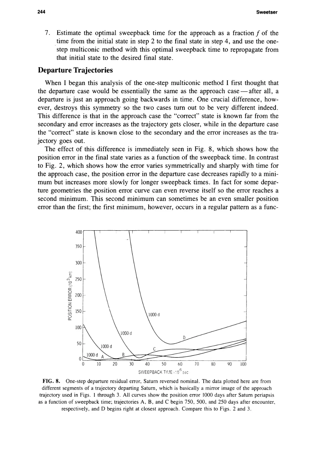


Text
VOLUME 37, No. 3 JULY-SEPTEMBER, 1989
Special Issue on Mission Design
Guest Editors: Gail A, Klein and David Sonnabend
CONTENTS
EDITORIAL Gail A. Klein and David Sonnabend 211
THEORETICAL AND METHODOLOGICAL PAPERS
Trajectory Optimization Software for Planetary Mission Design
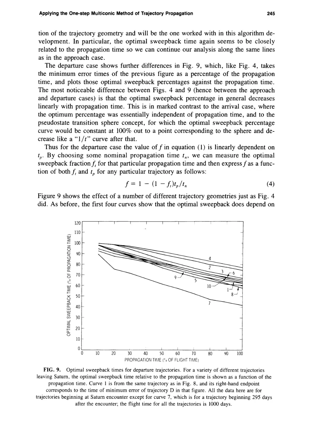
Louis A. D’Amario 213
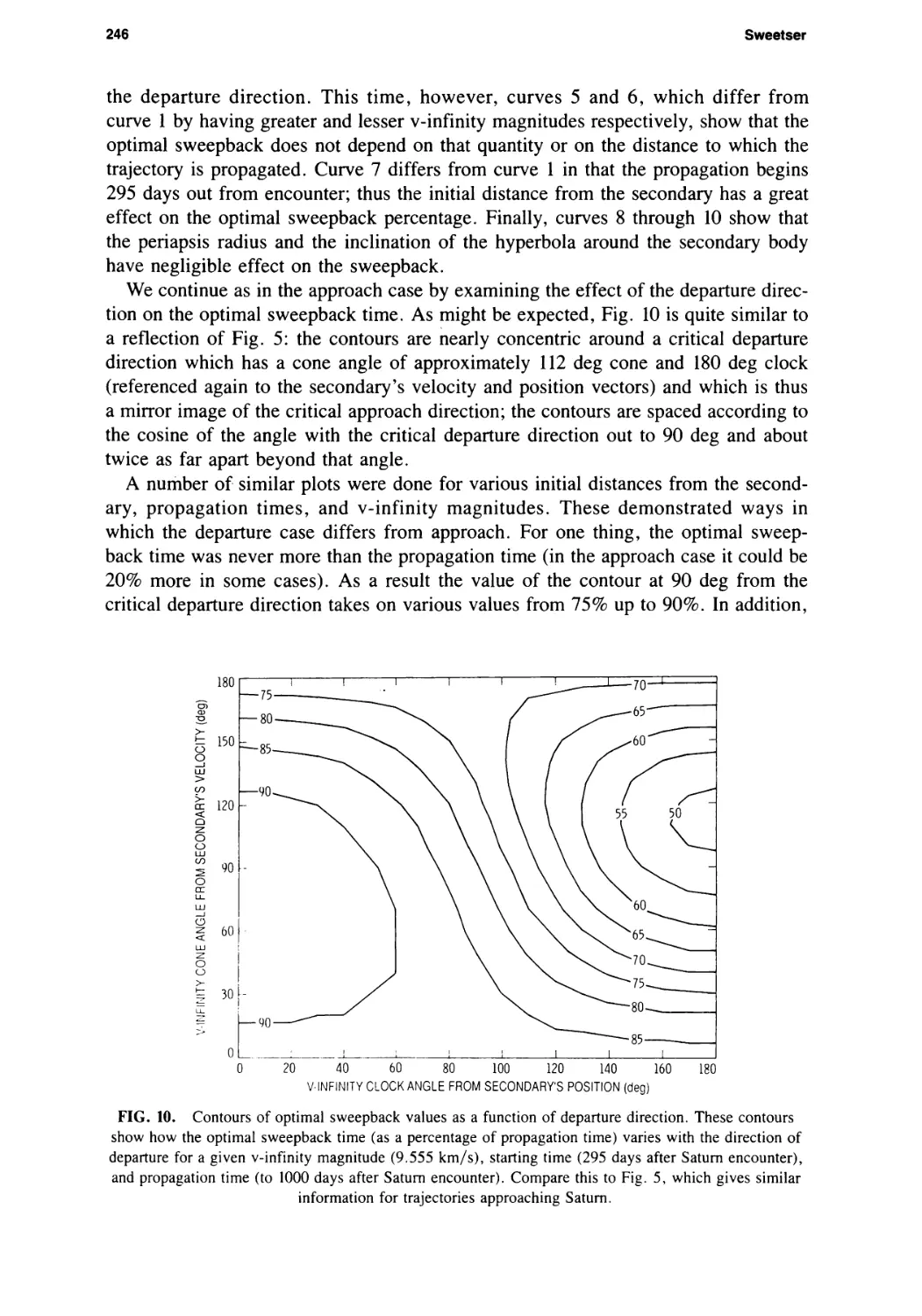
Application of the Pseudostate Theory to the Three-Body Lambert Problem
Dennis V. Byrnes 221
Some Notes on Applying the One-step Multiconic Method of Trajectory Propagation
Theodore H. Sweetser 233
MIDAS: Mission Design and Analysis Software for the Optimization of Ballistic
Interplanetary Trajectories
Carl G. Sauer, Jr. 251
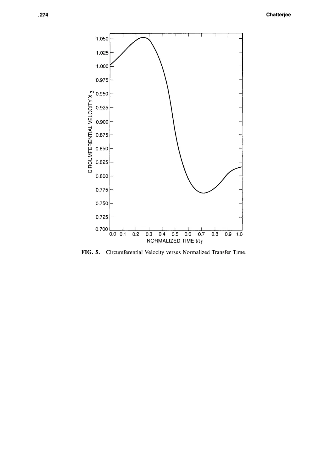
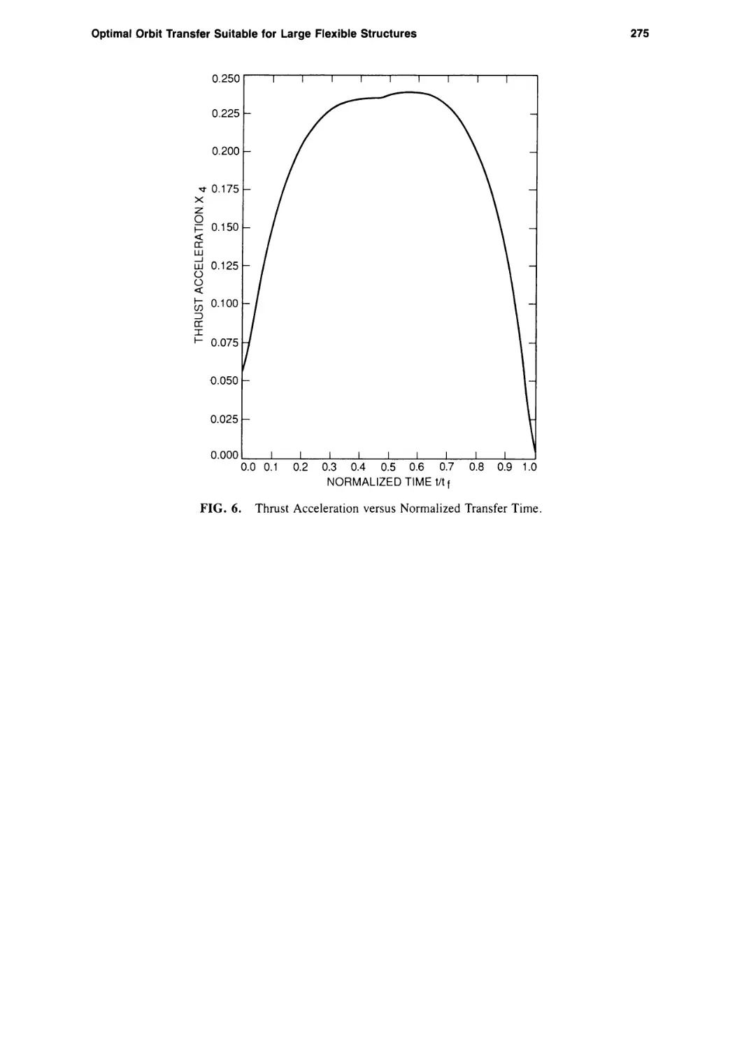
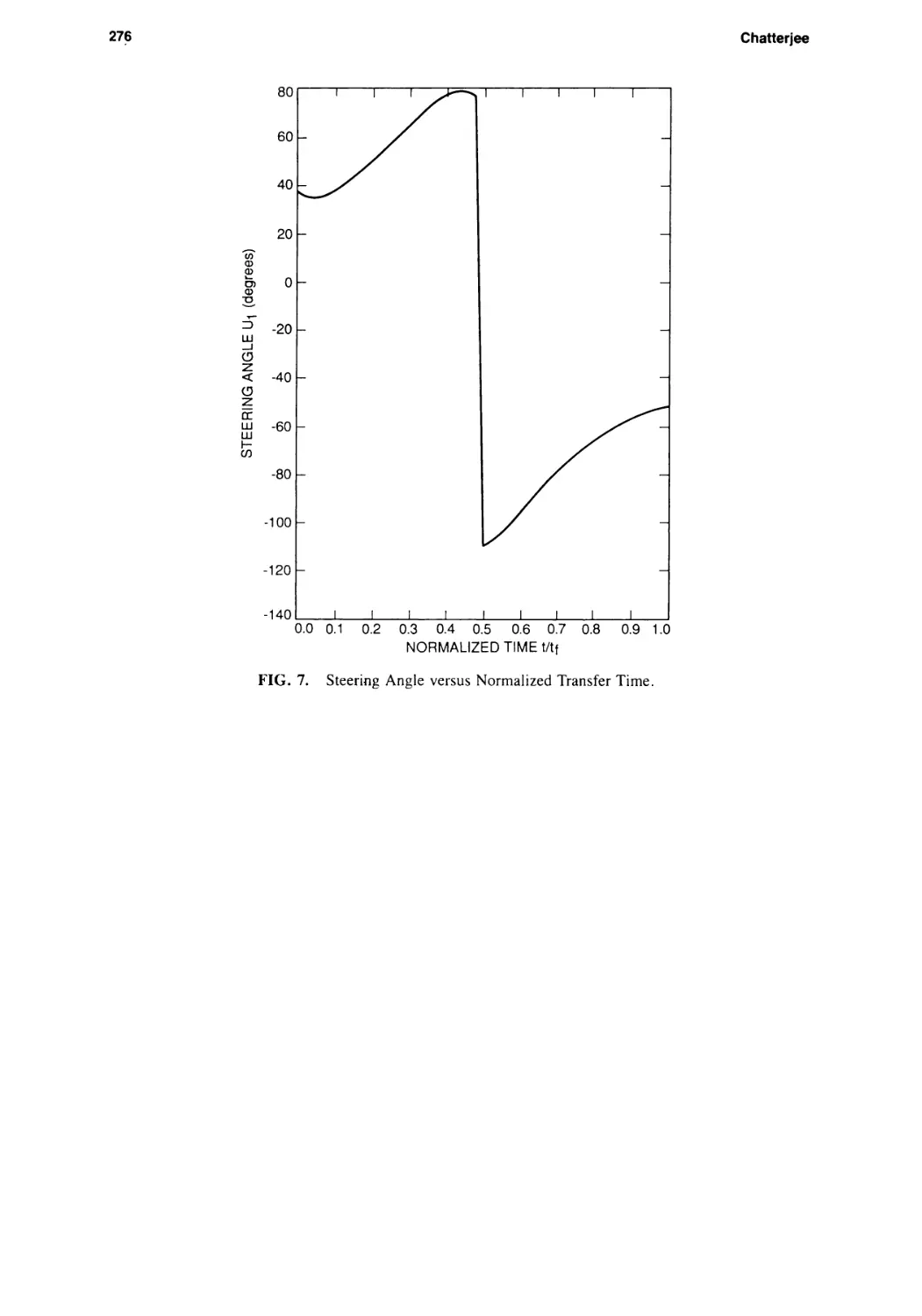
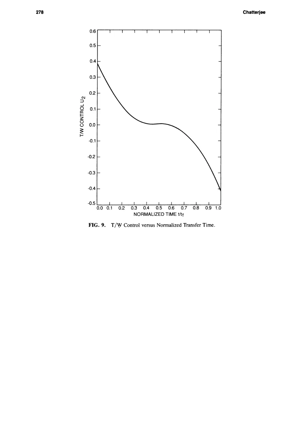
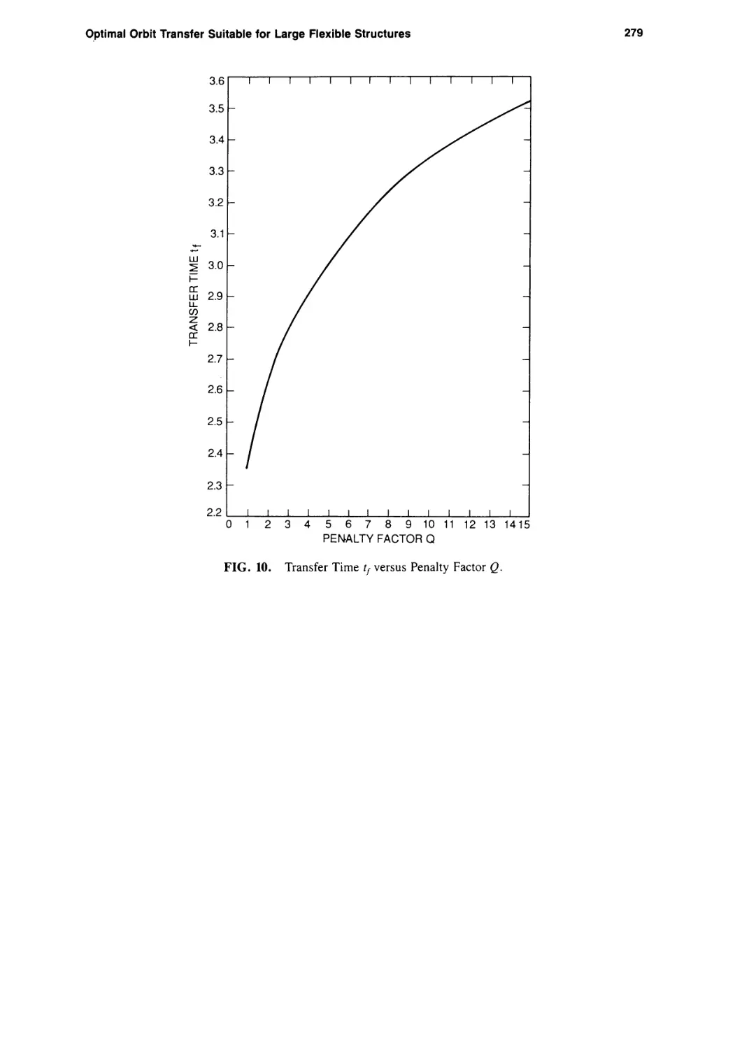
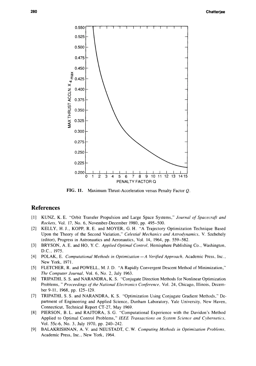
Optimal Orbit Transfer Suitable for Large Flexible Structures
Alok K. Chatterjee 261
APPLICATION PAPERS
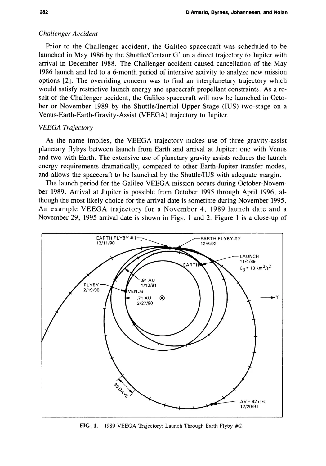
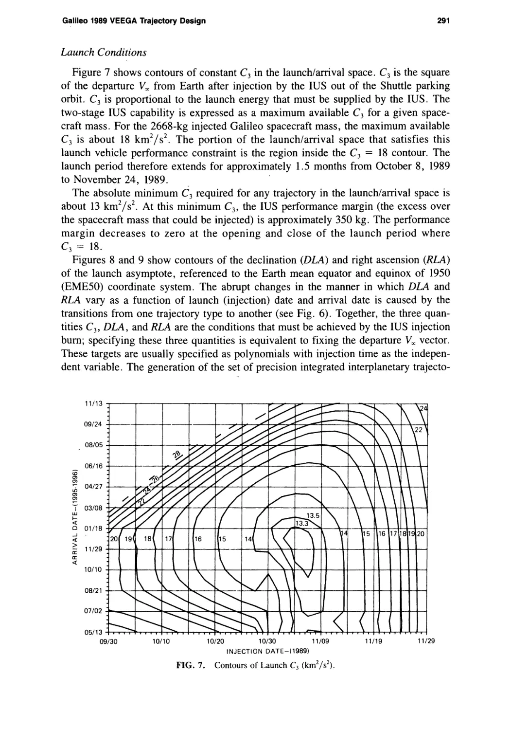
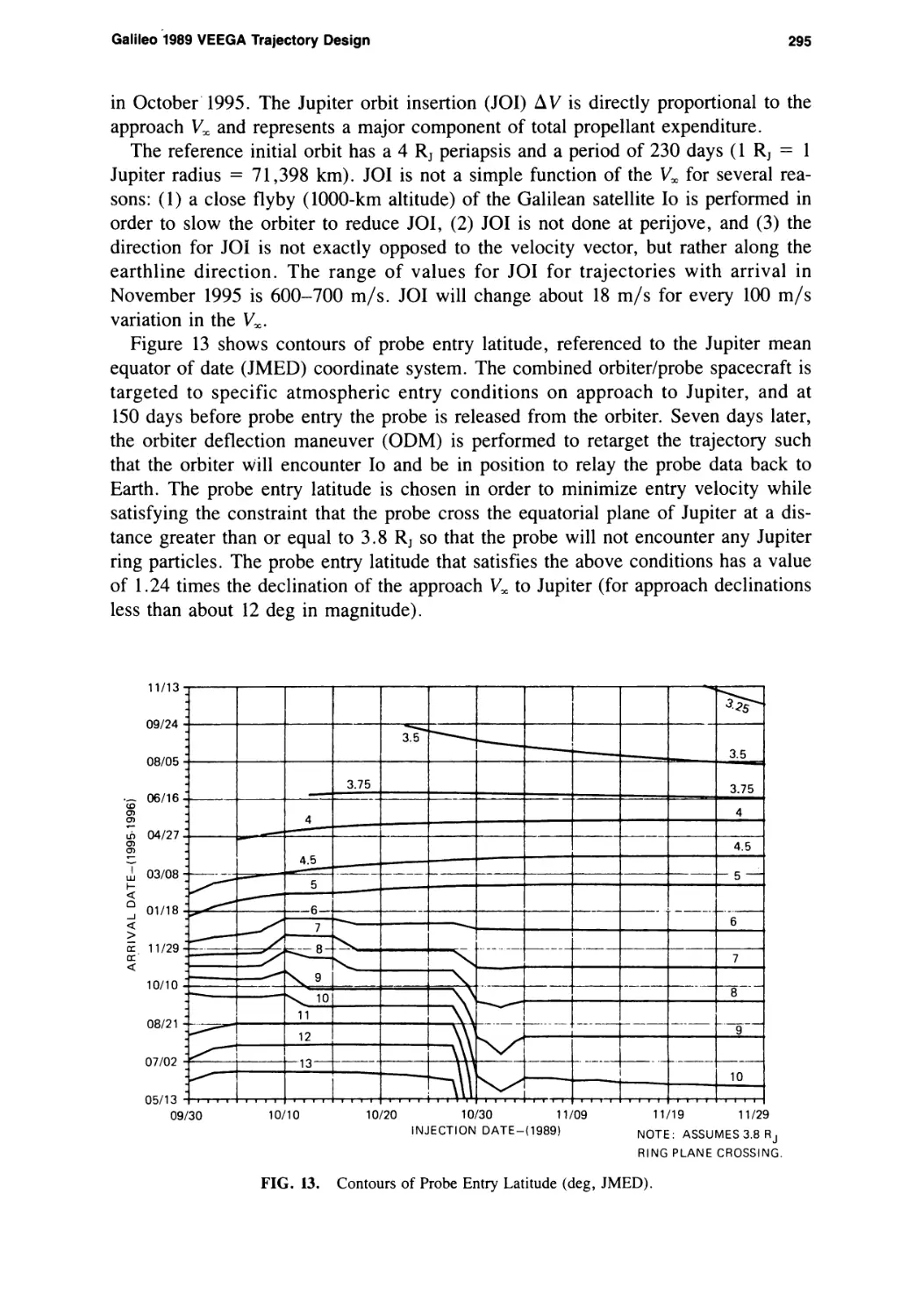
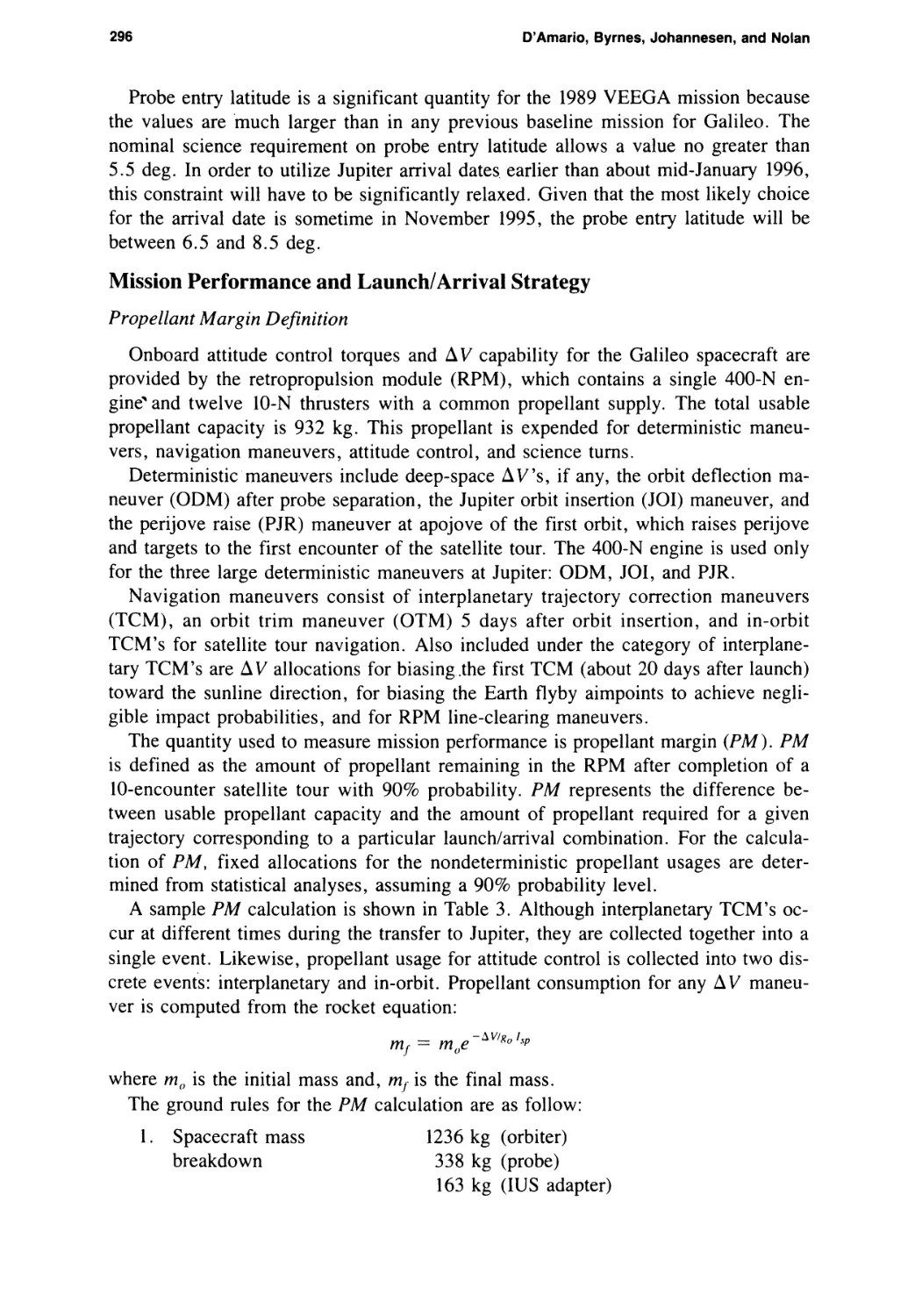
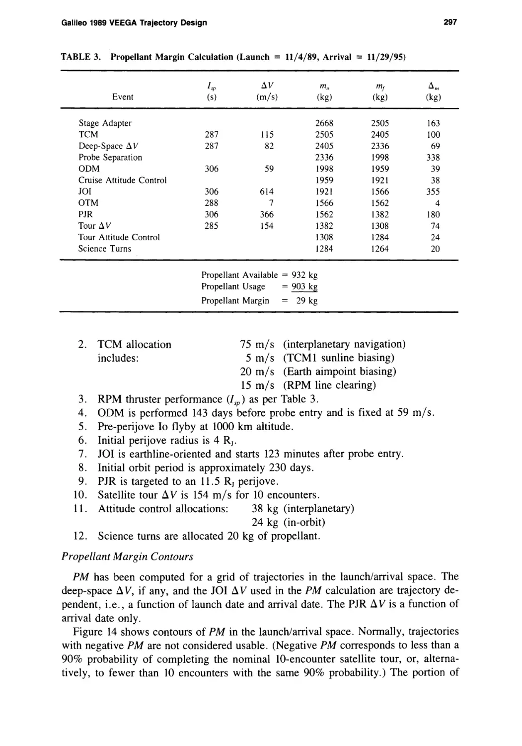
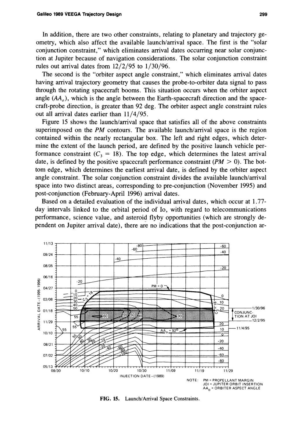
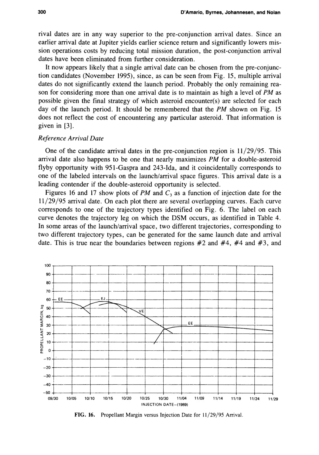
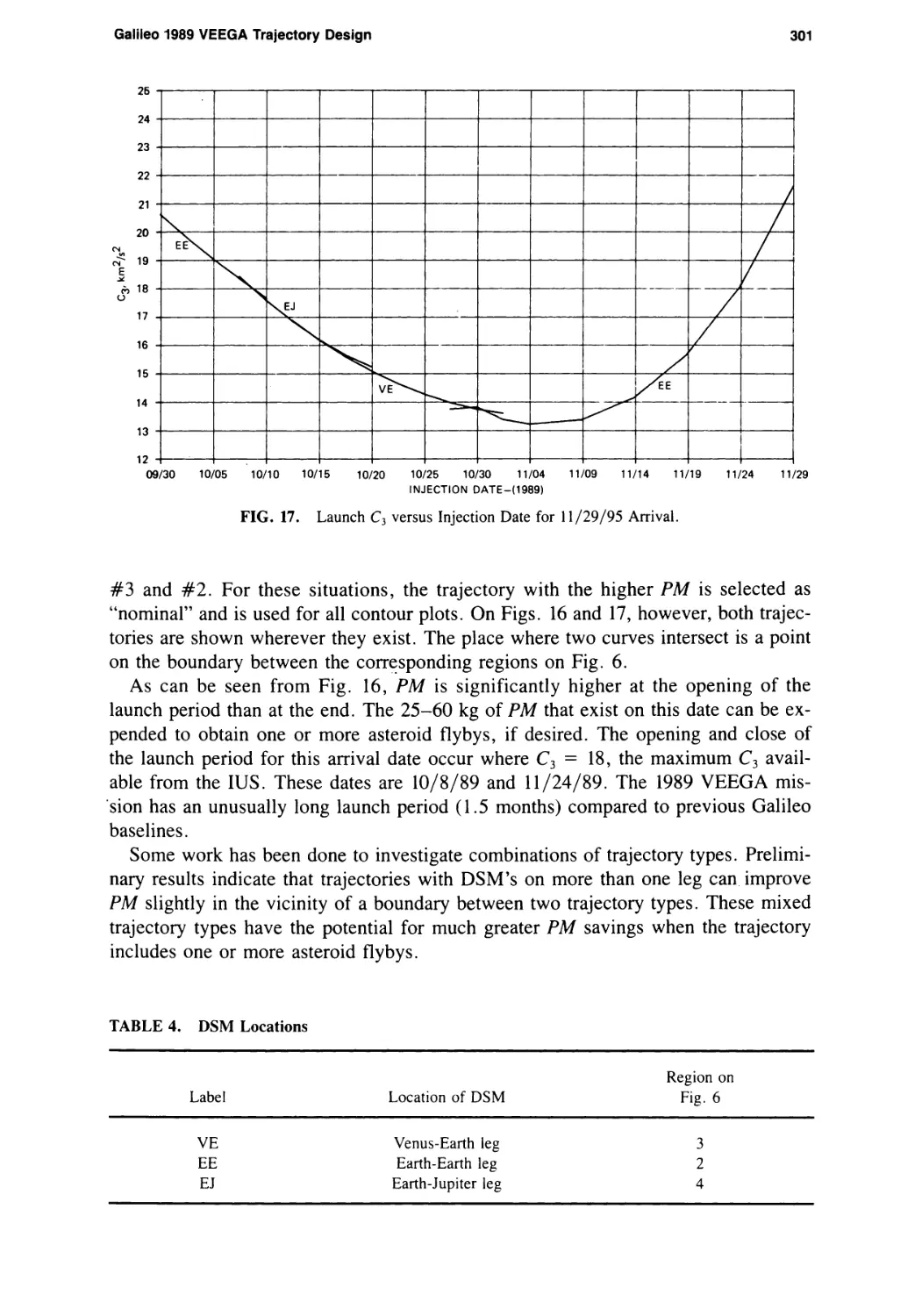
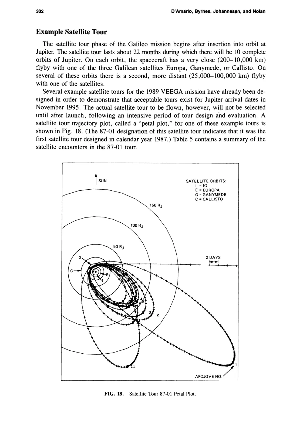
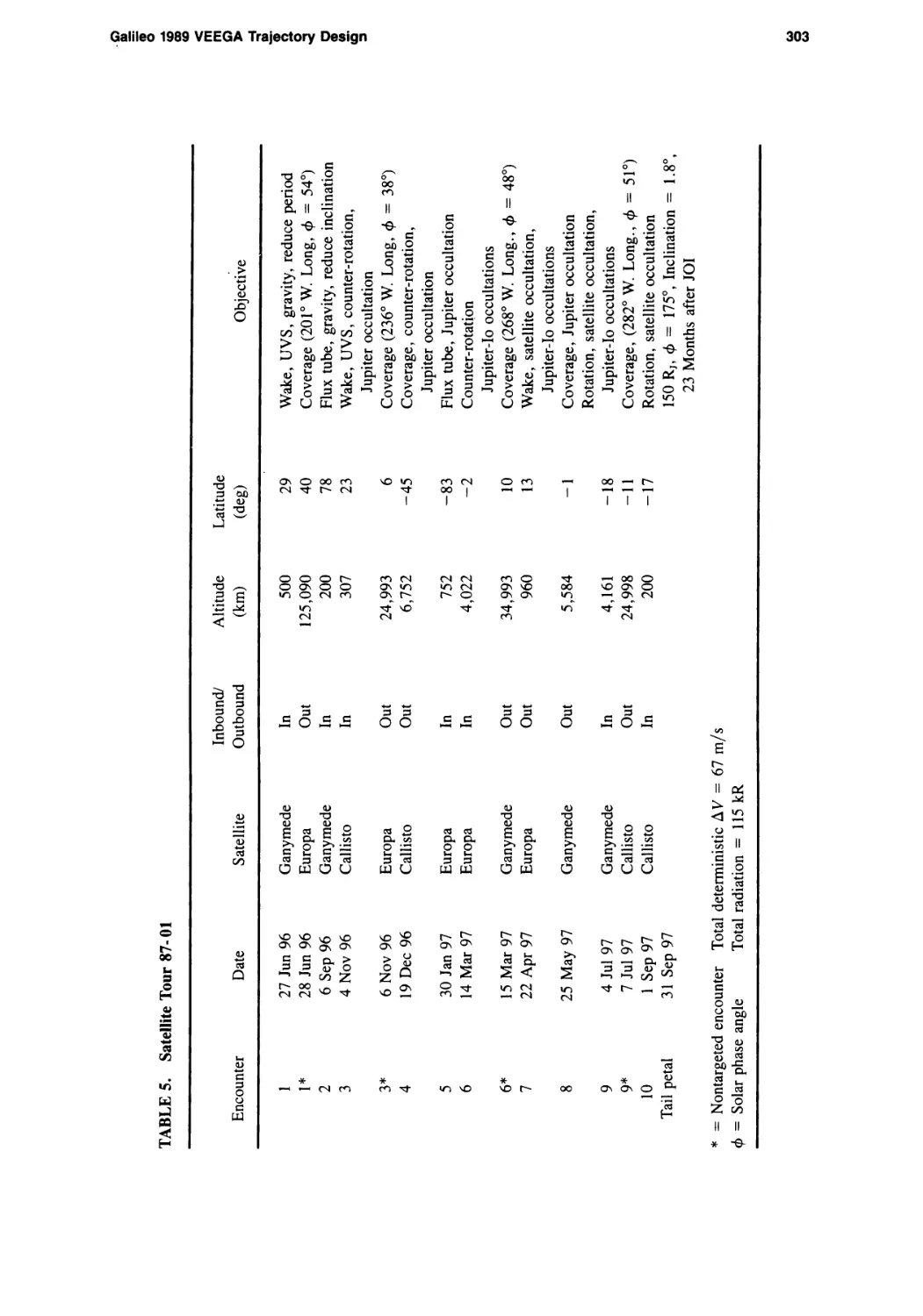
Galileo 1989 VEEGA Trajectory Design
Louis A. D’Amario, Dennis V. Byrnes, Jennie R. Johannesen, and
Brian G. Nolan 281
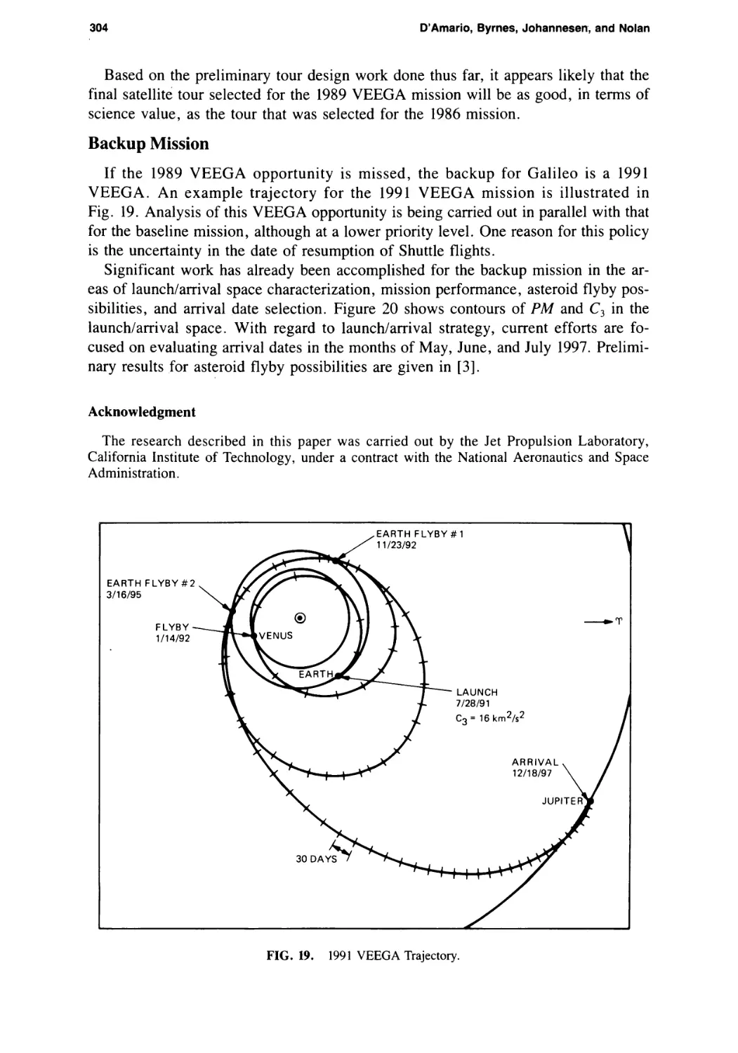
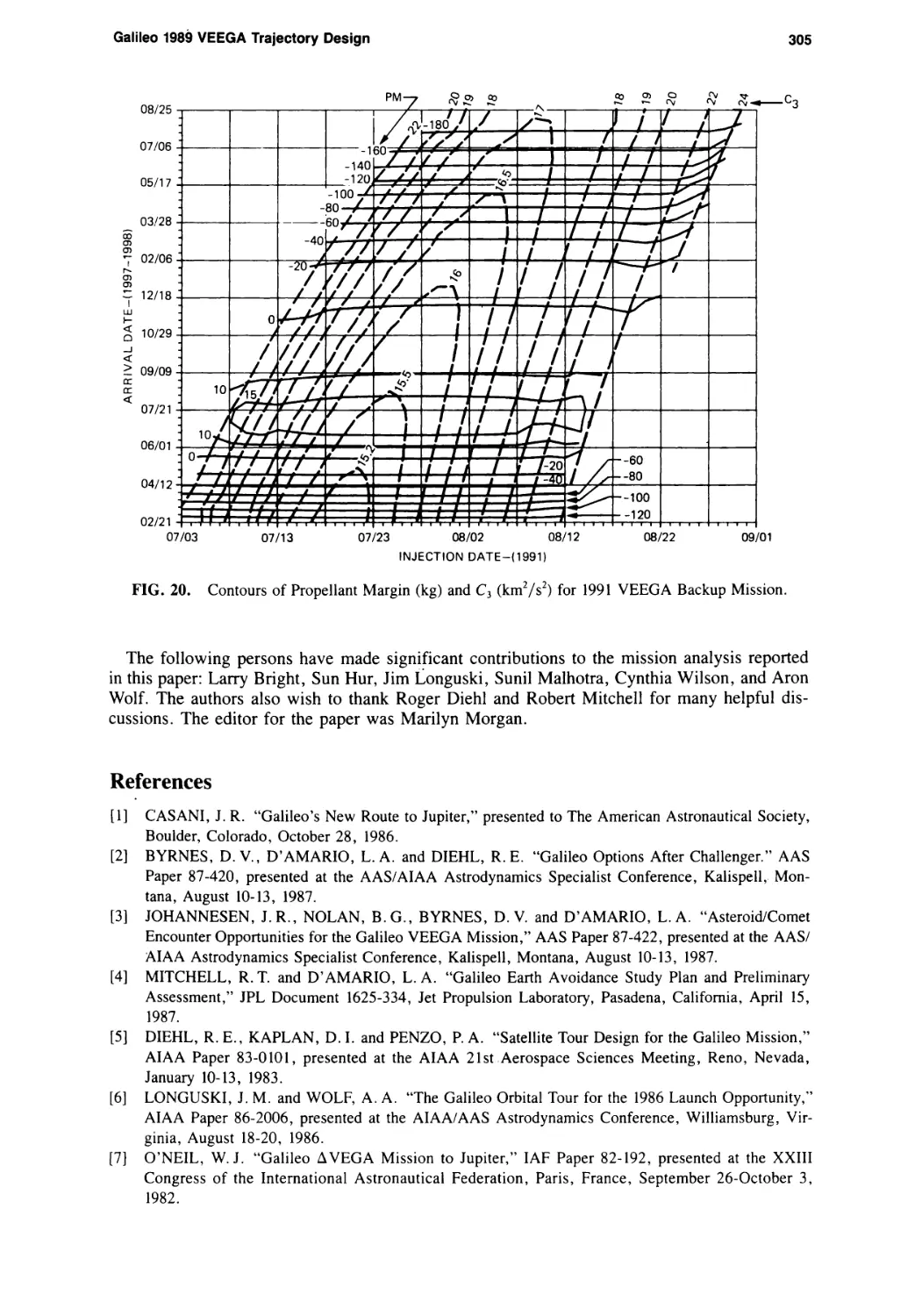
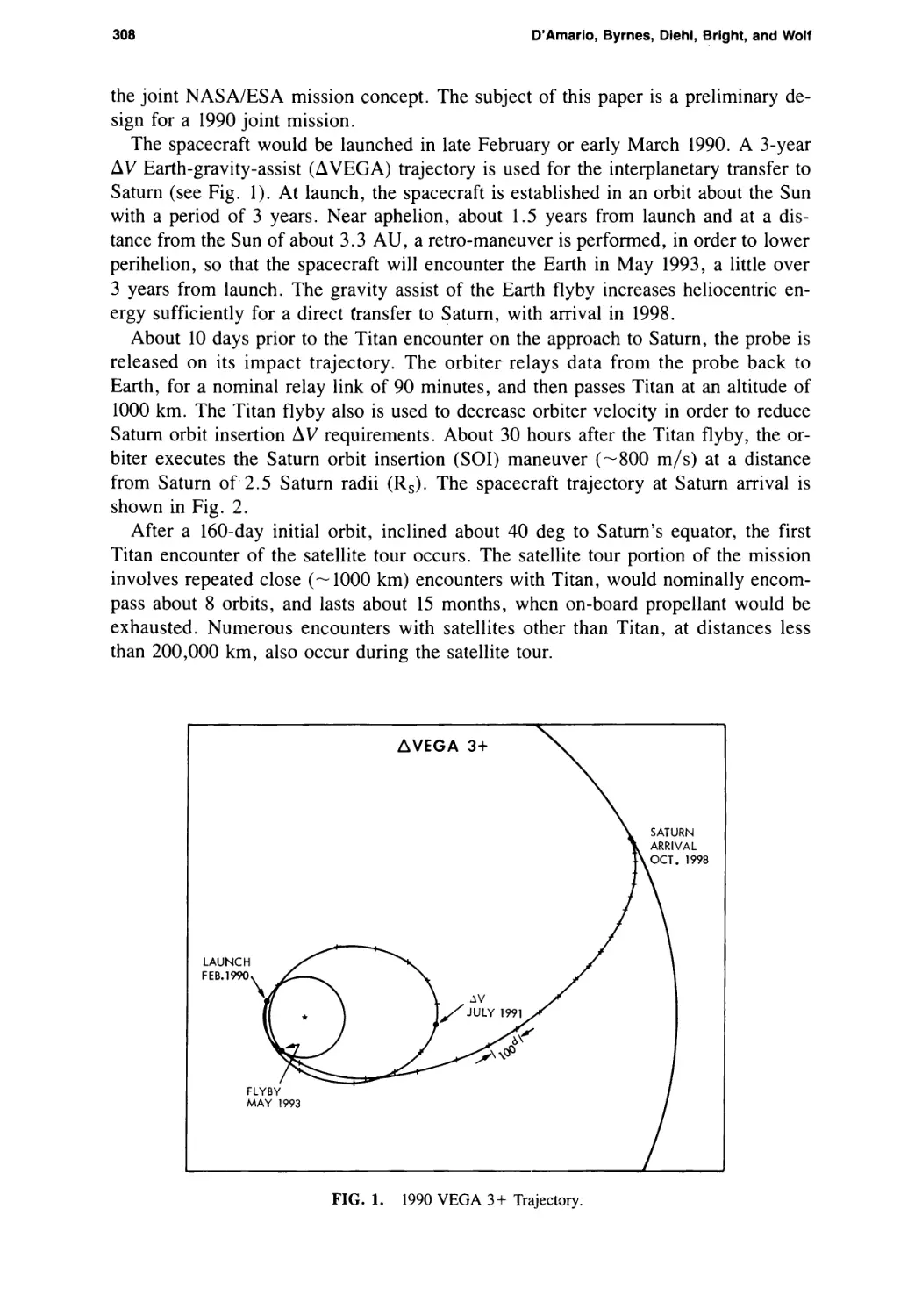
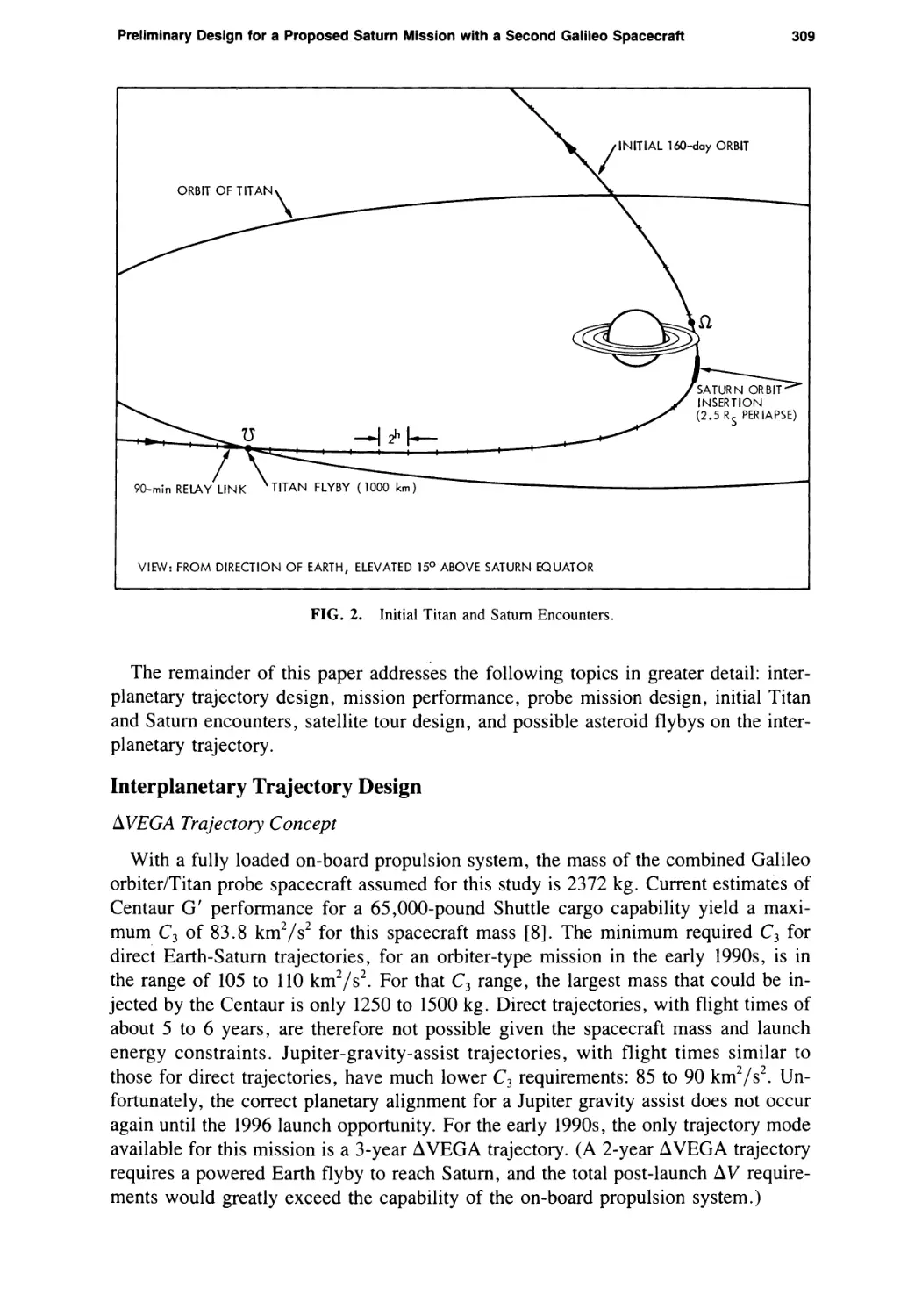
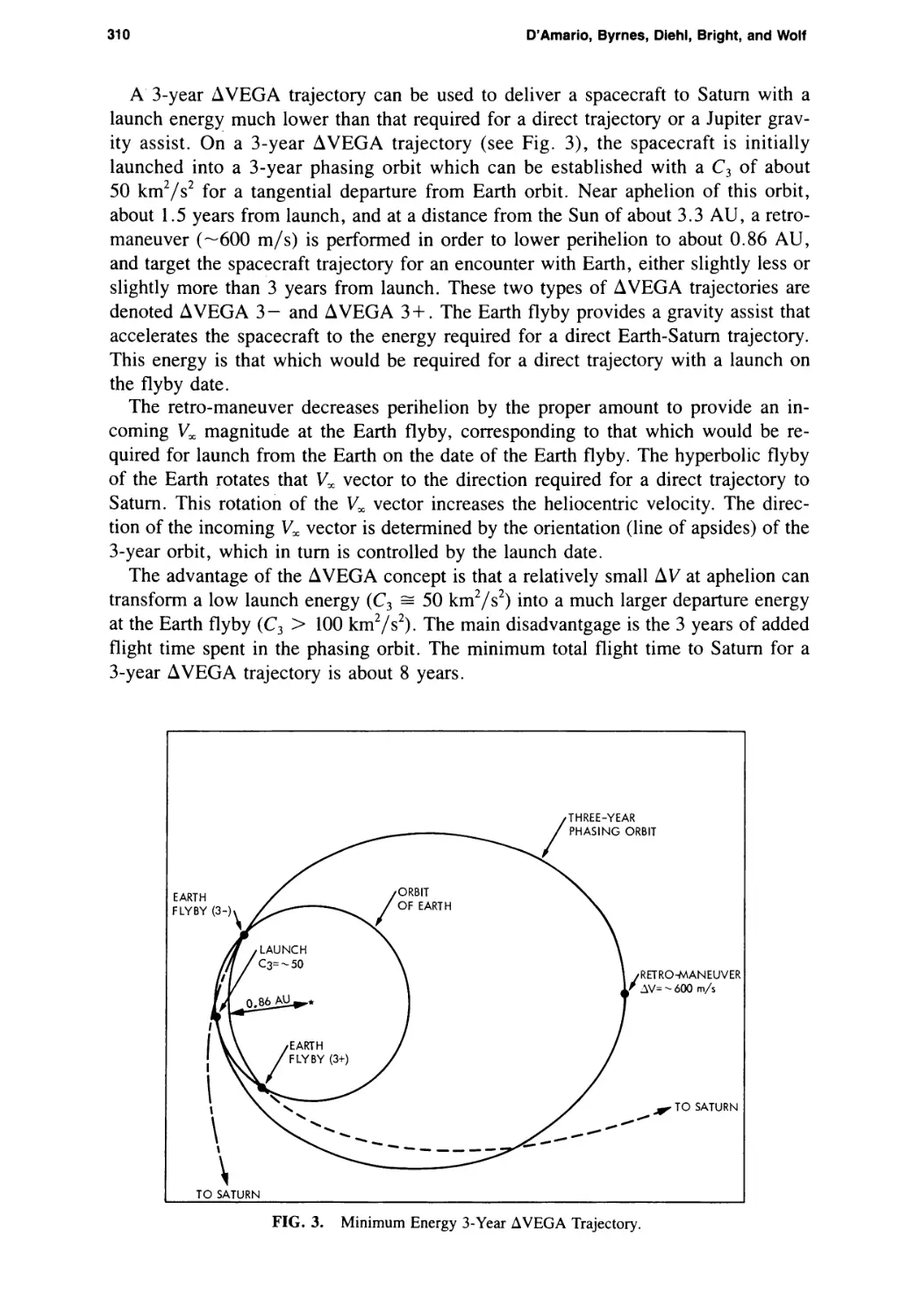
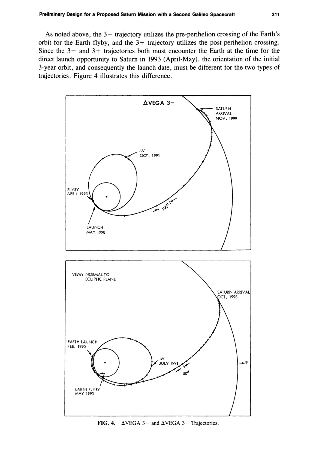
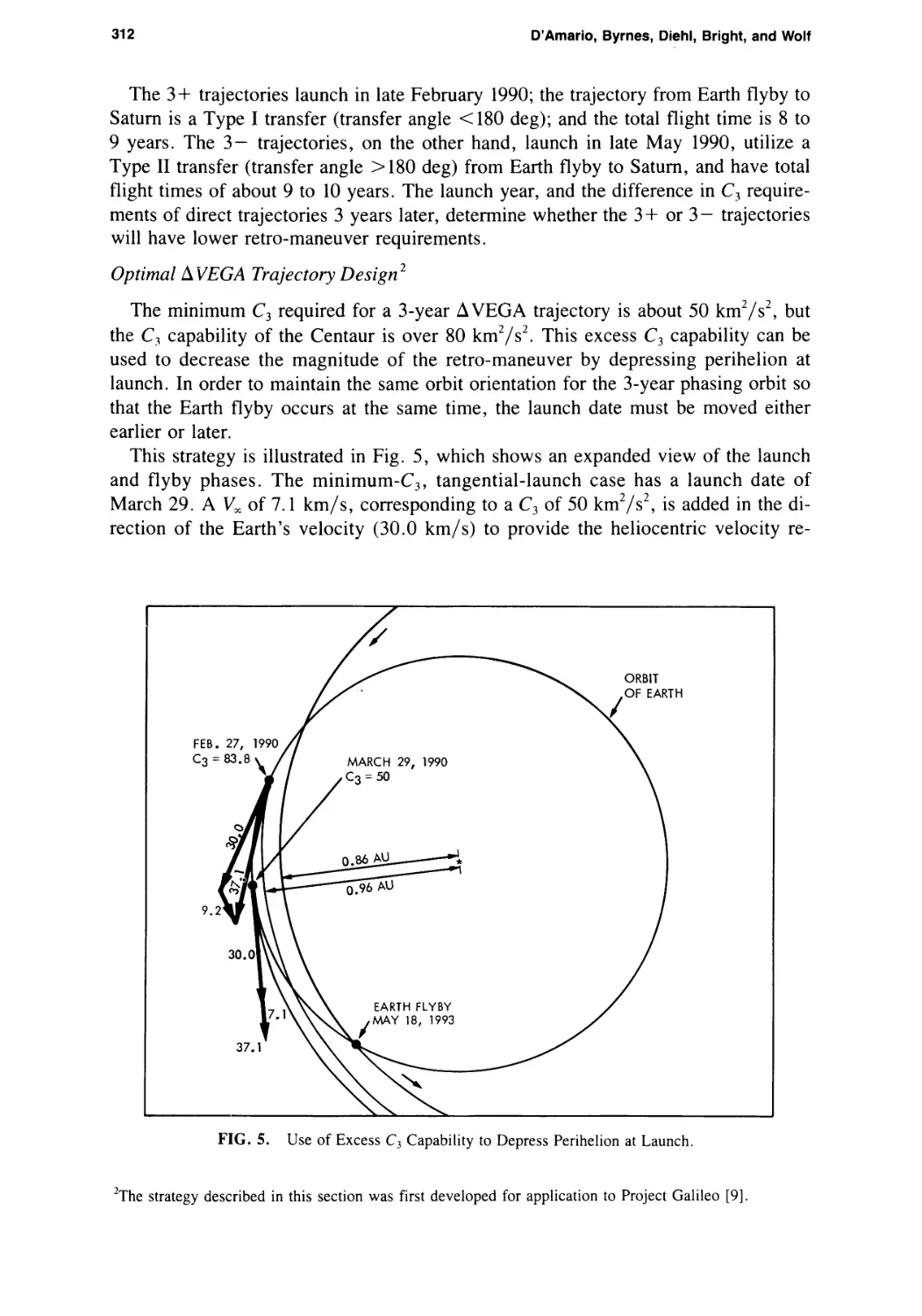
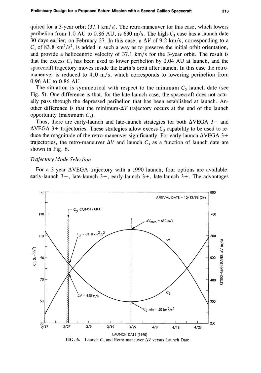
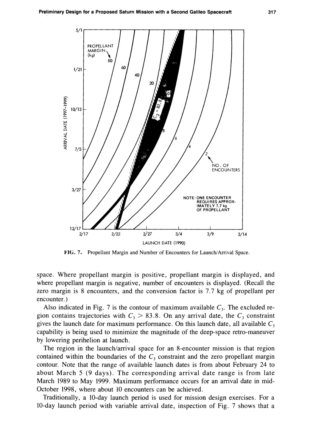
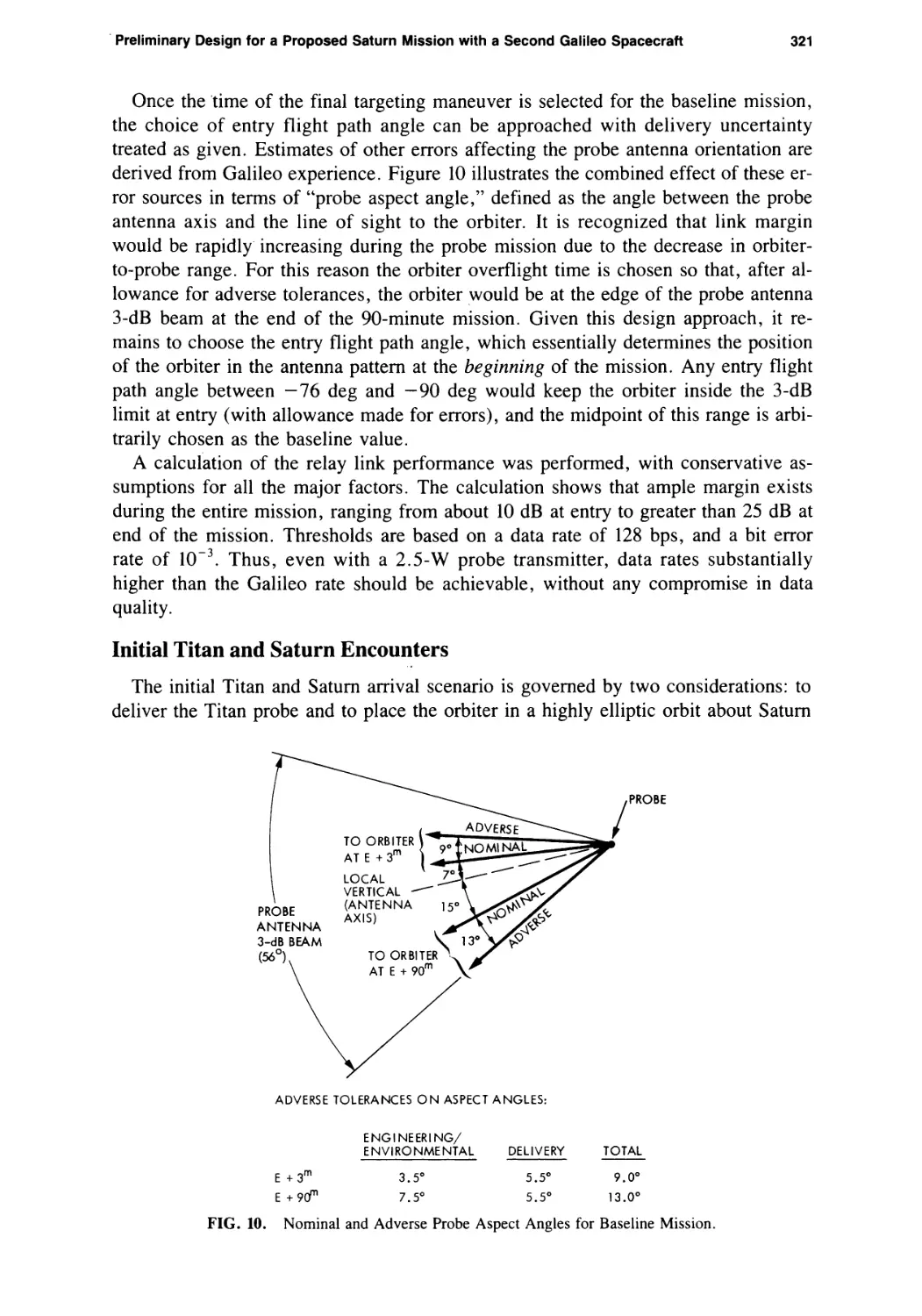
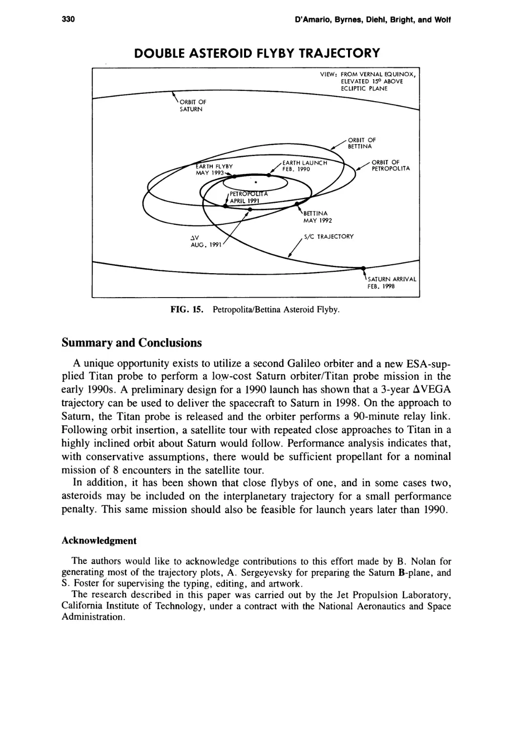
Preliminary Design for a Proposed Saturn Mission with a Second Galileo Spacecraft
Louis A. D’Amario, Dennis V. Byrnes, Roger E. Diehl, Larry E. Bright,
and Aron A. Wolf 307
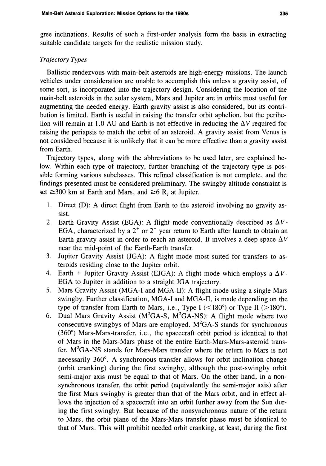
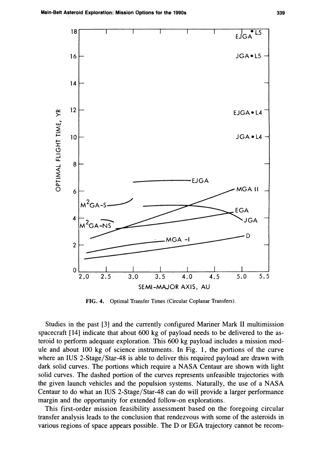
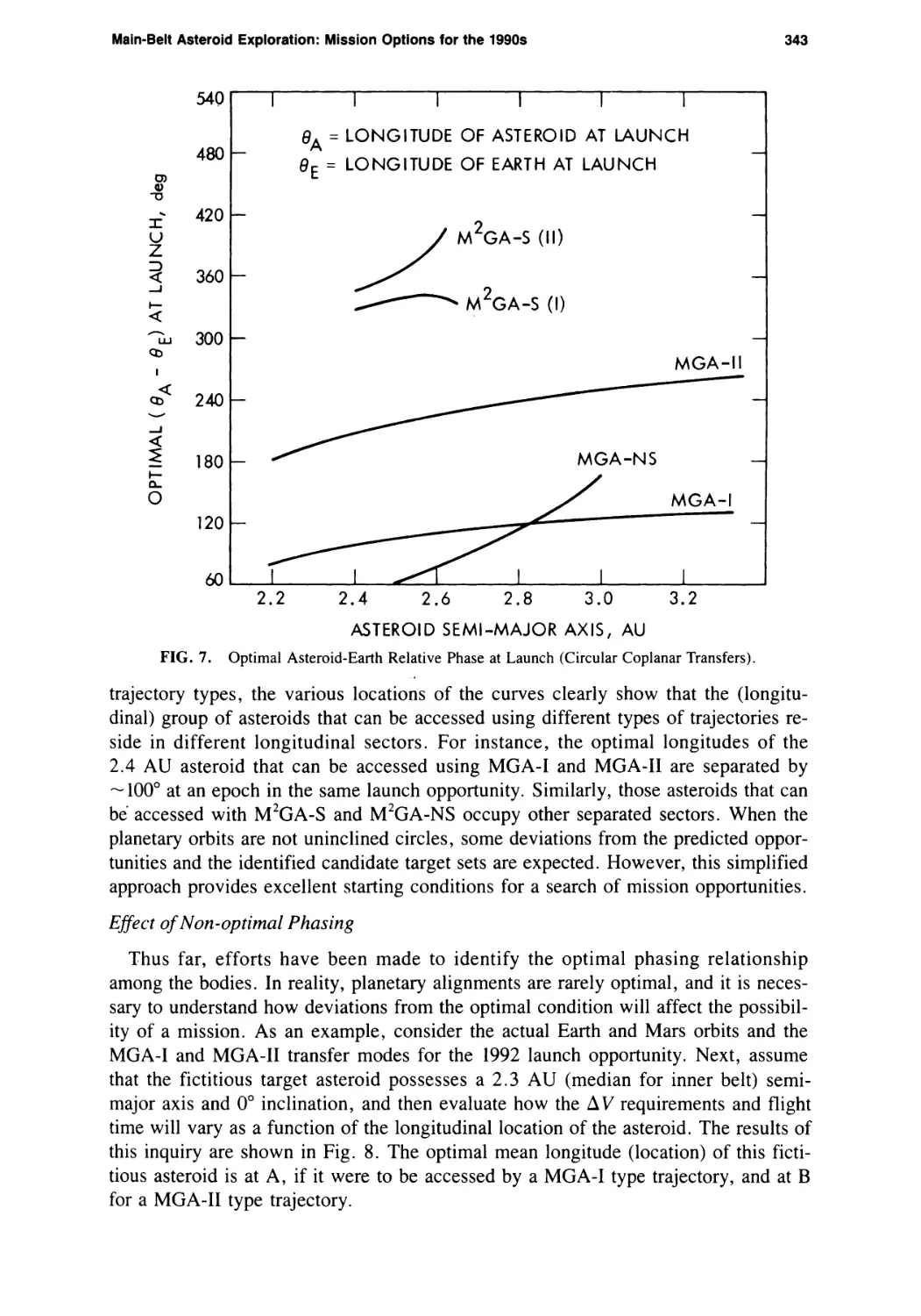
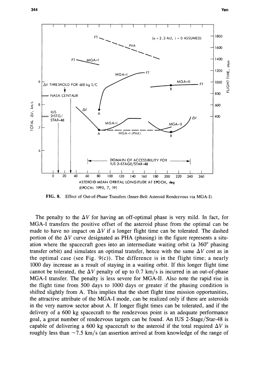
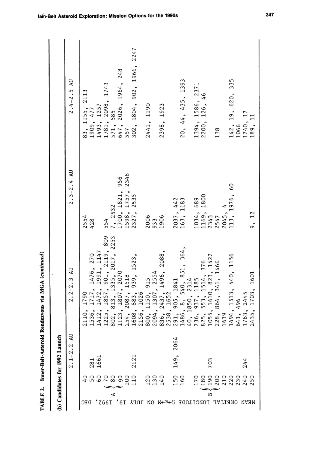
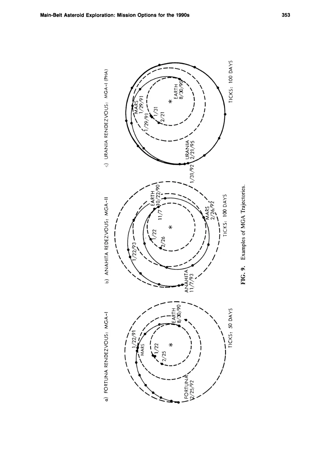
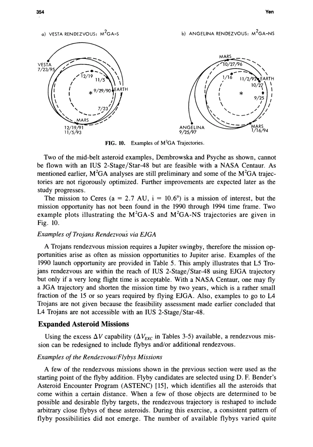
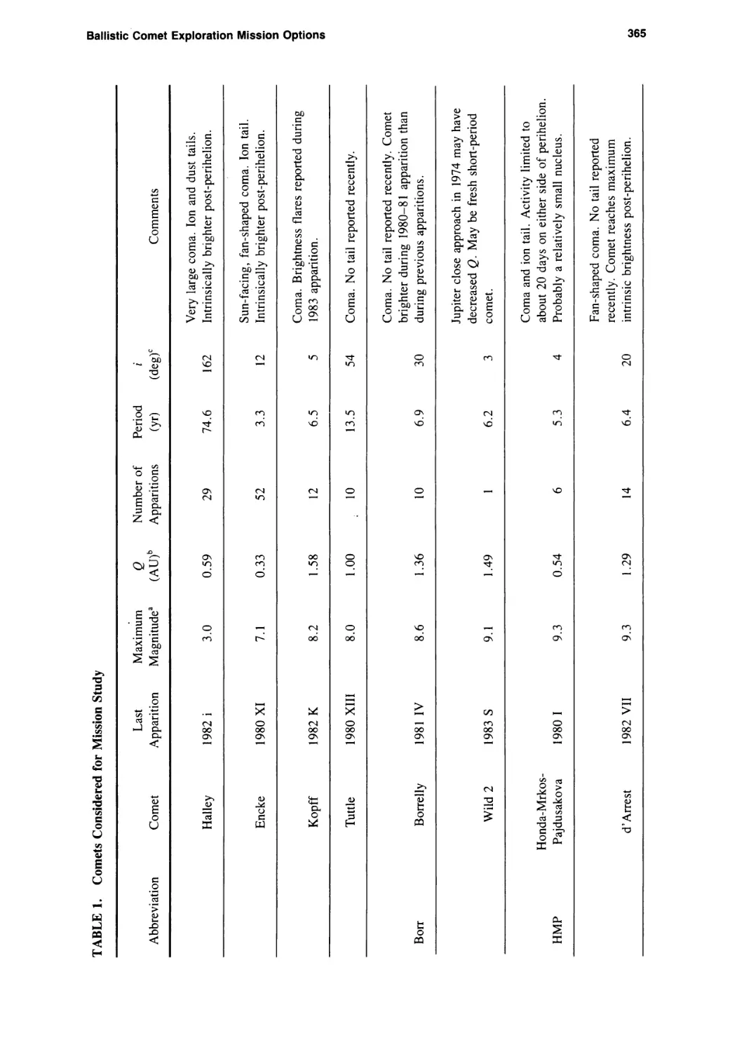
Main-Belt Asteroid Exploration: Mission Options for the 1990s
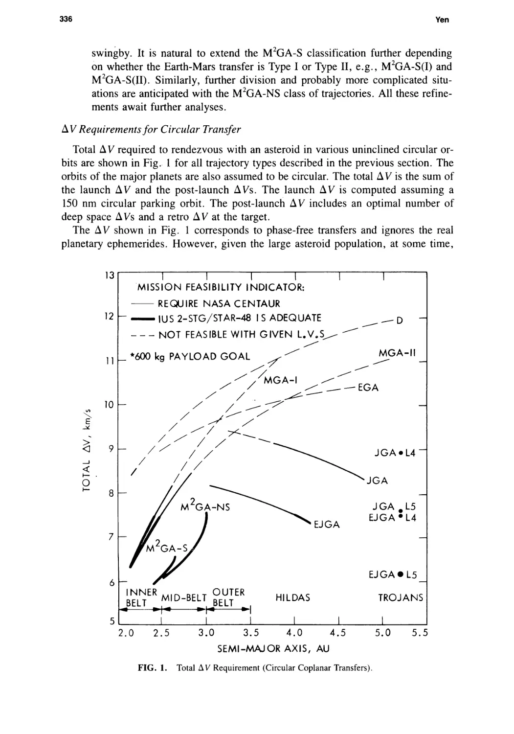
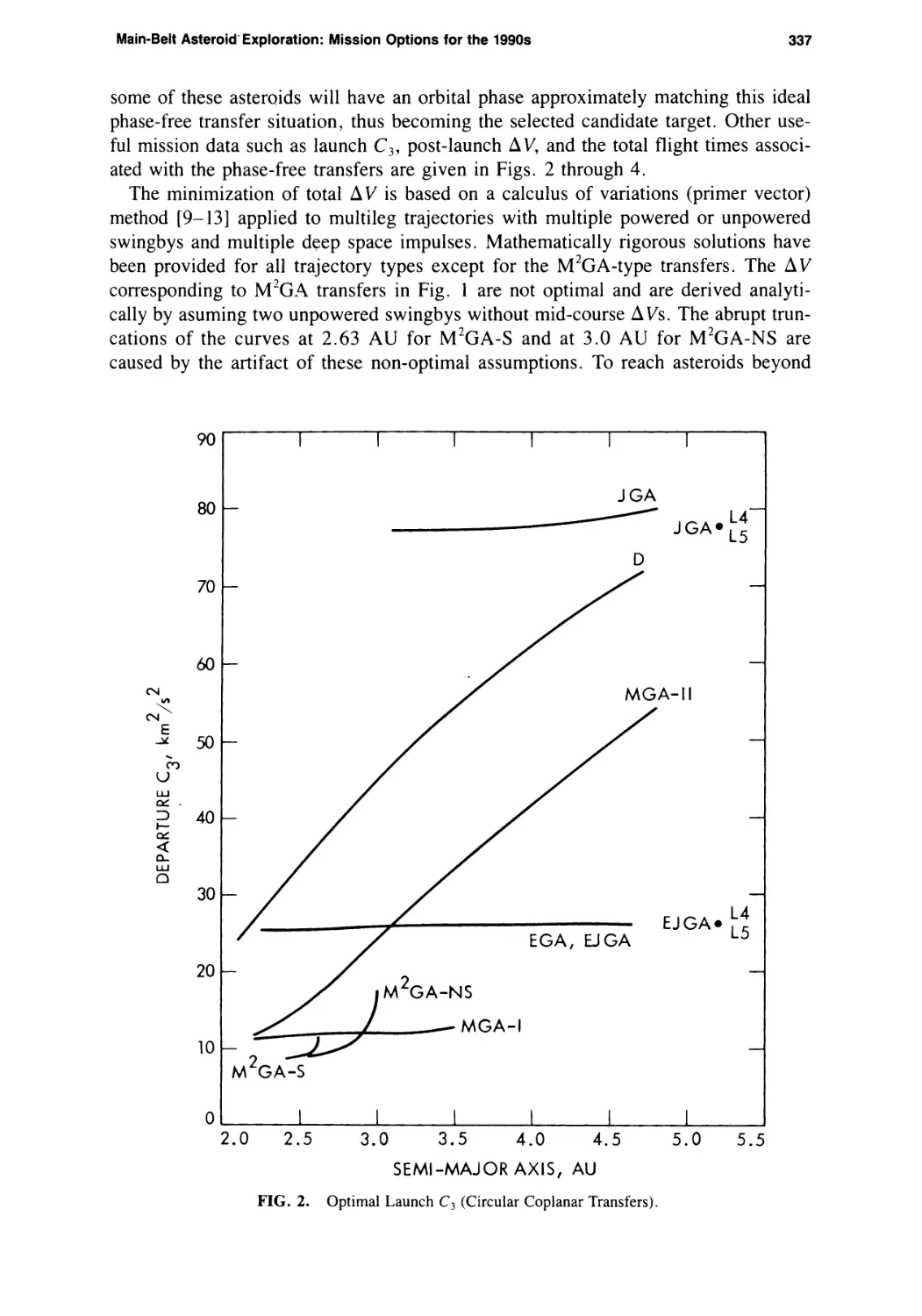
Chen-wan L. Yen 333
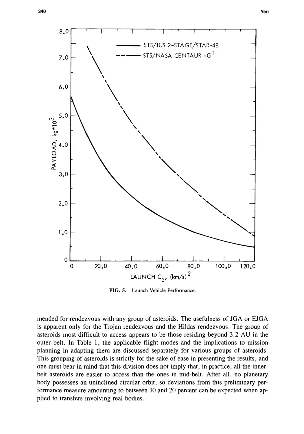
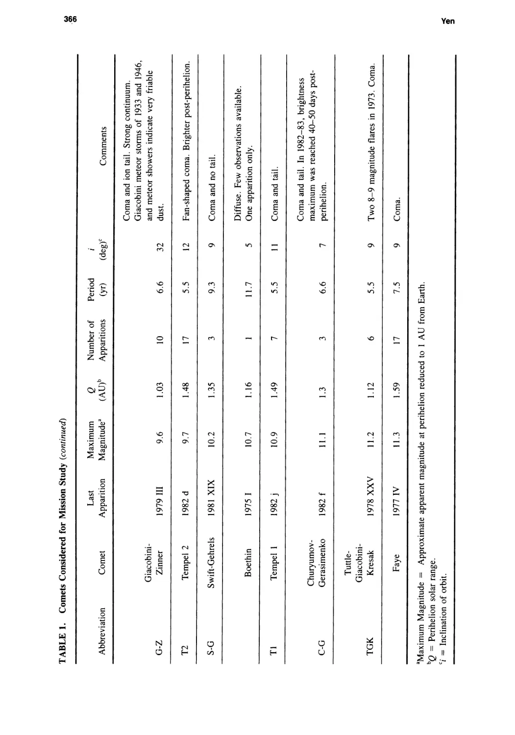
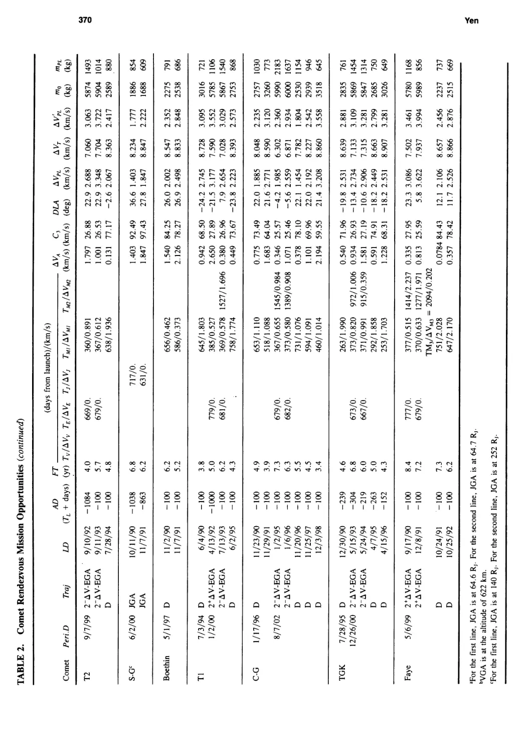
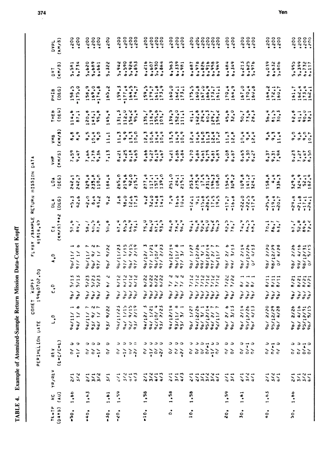
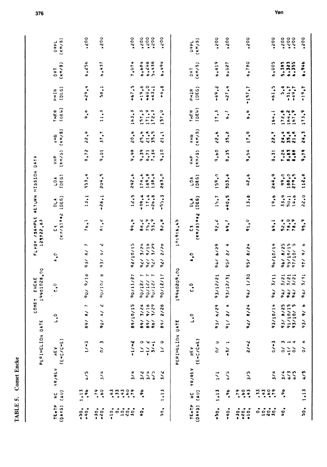
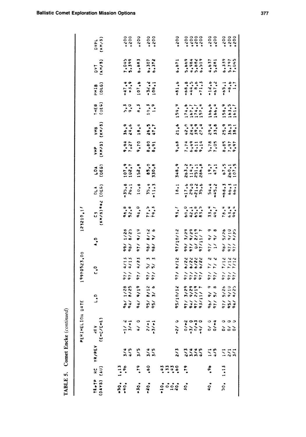
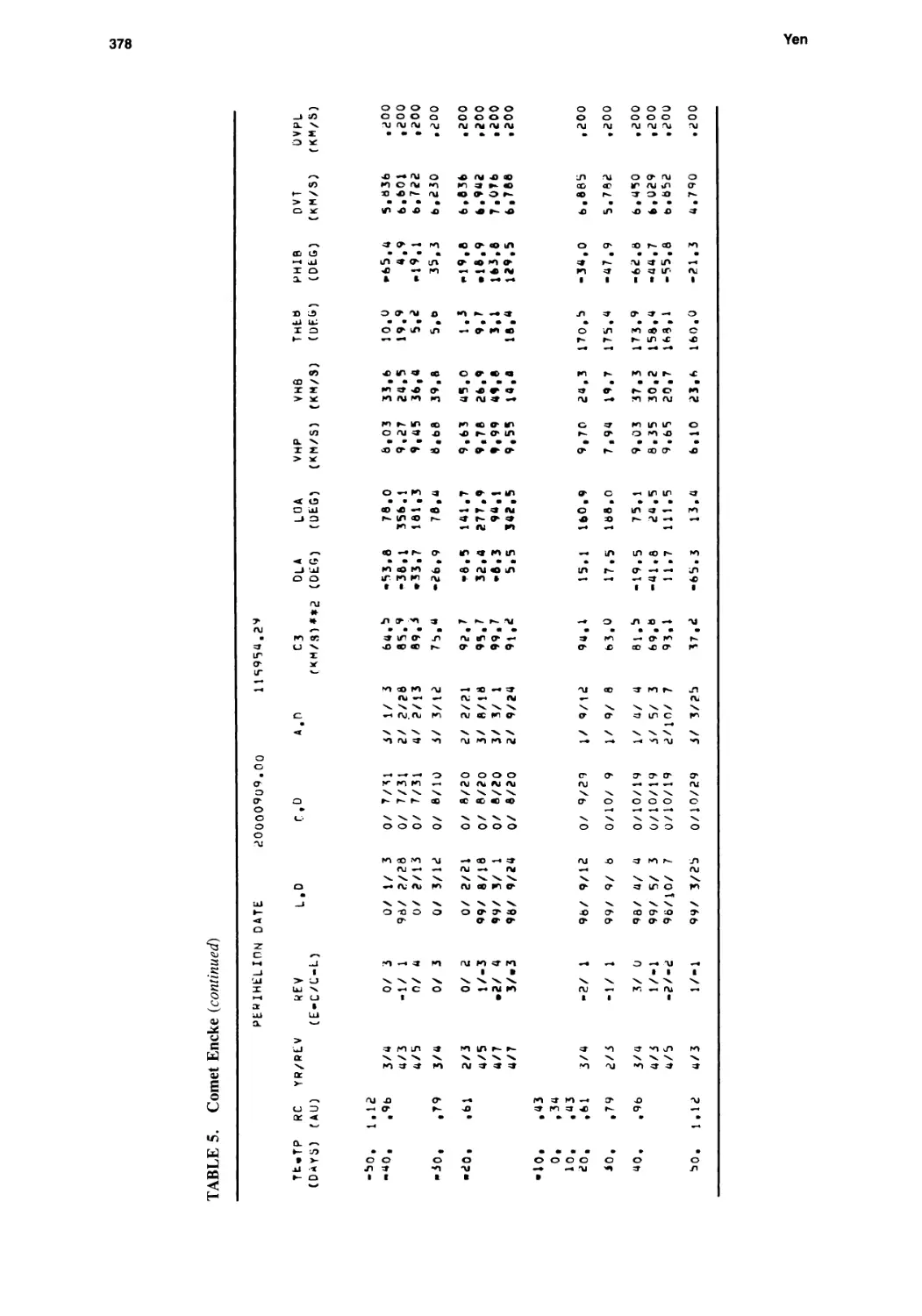
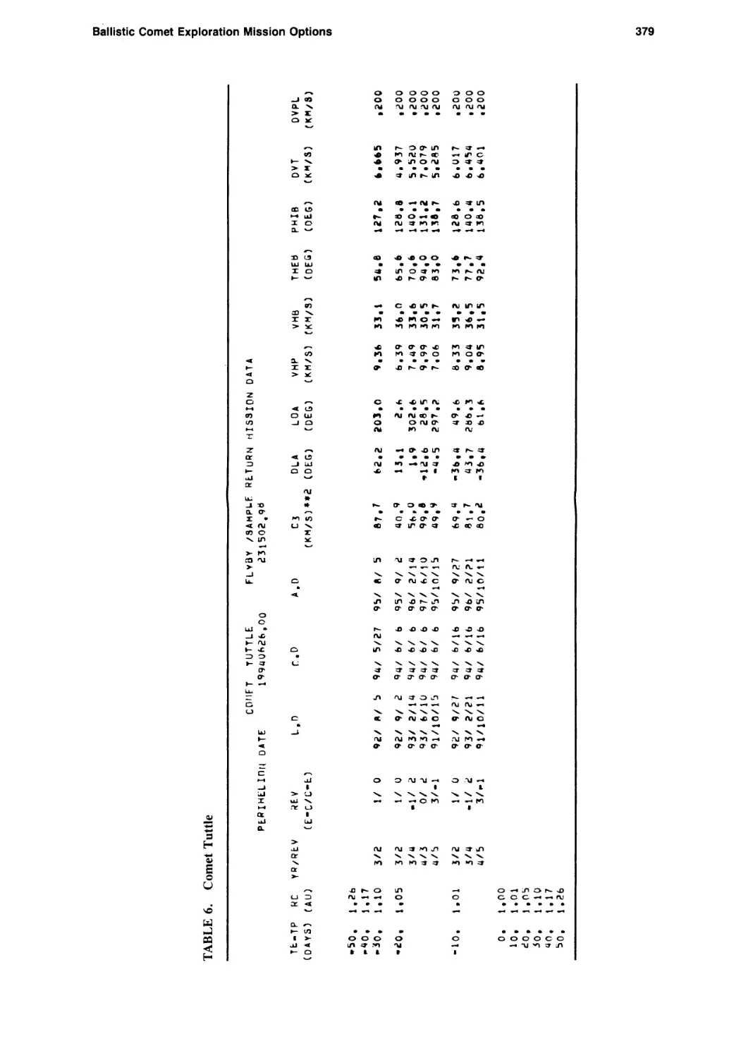
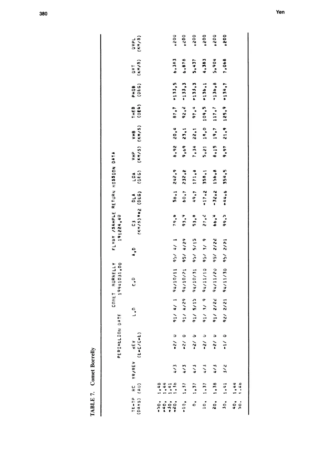
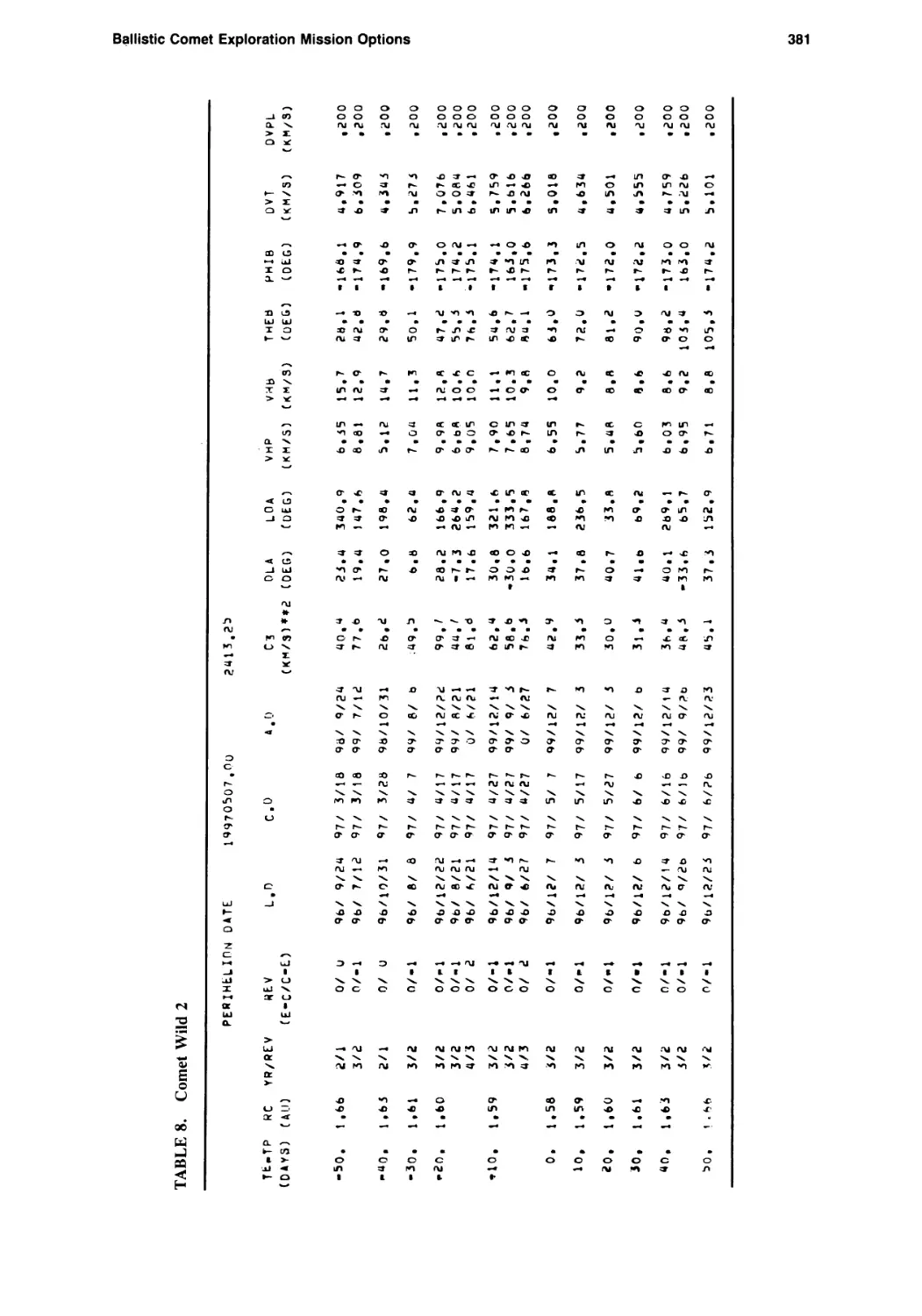
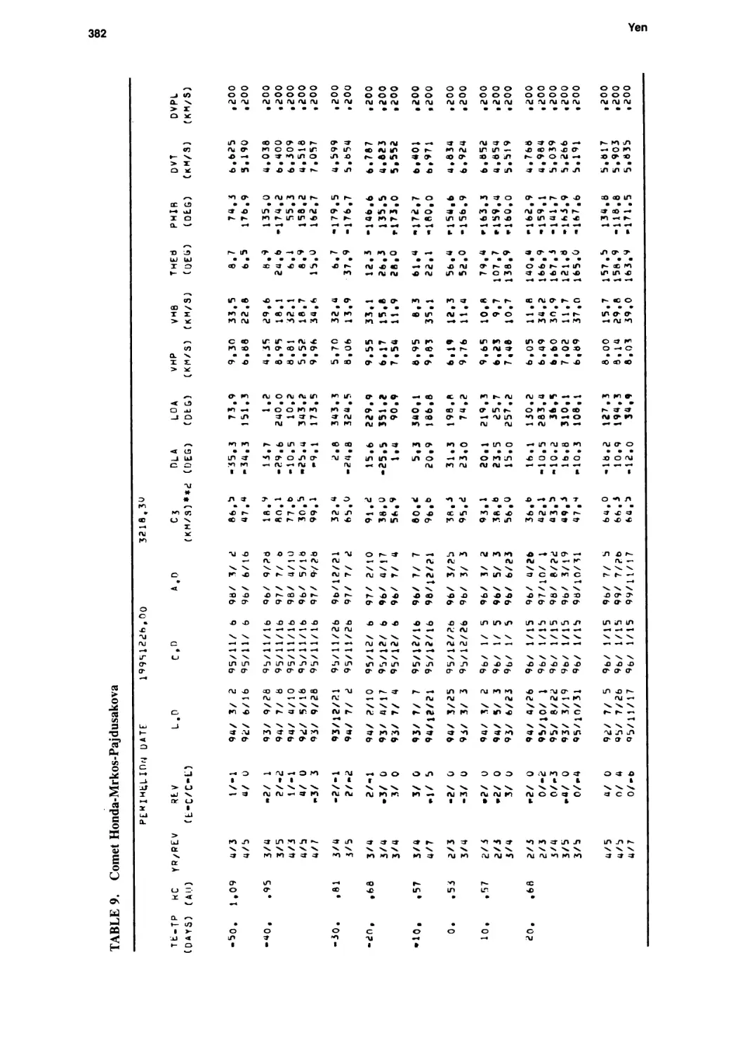
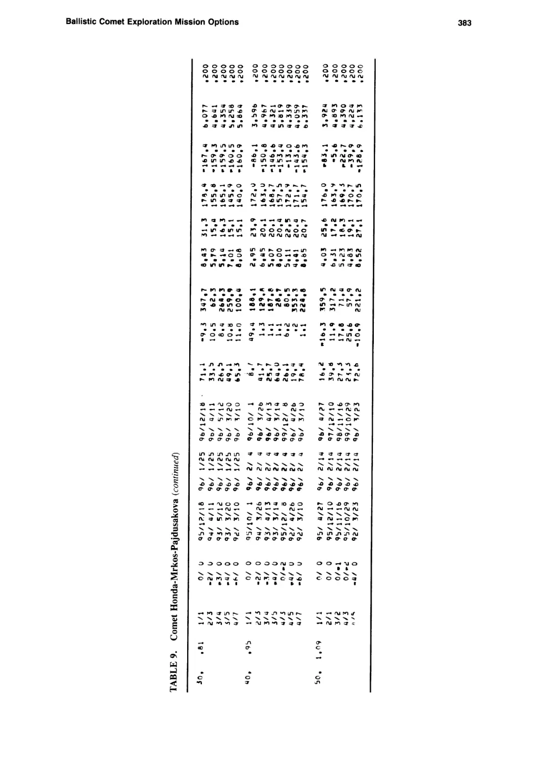
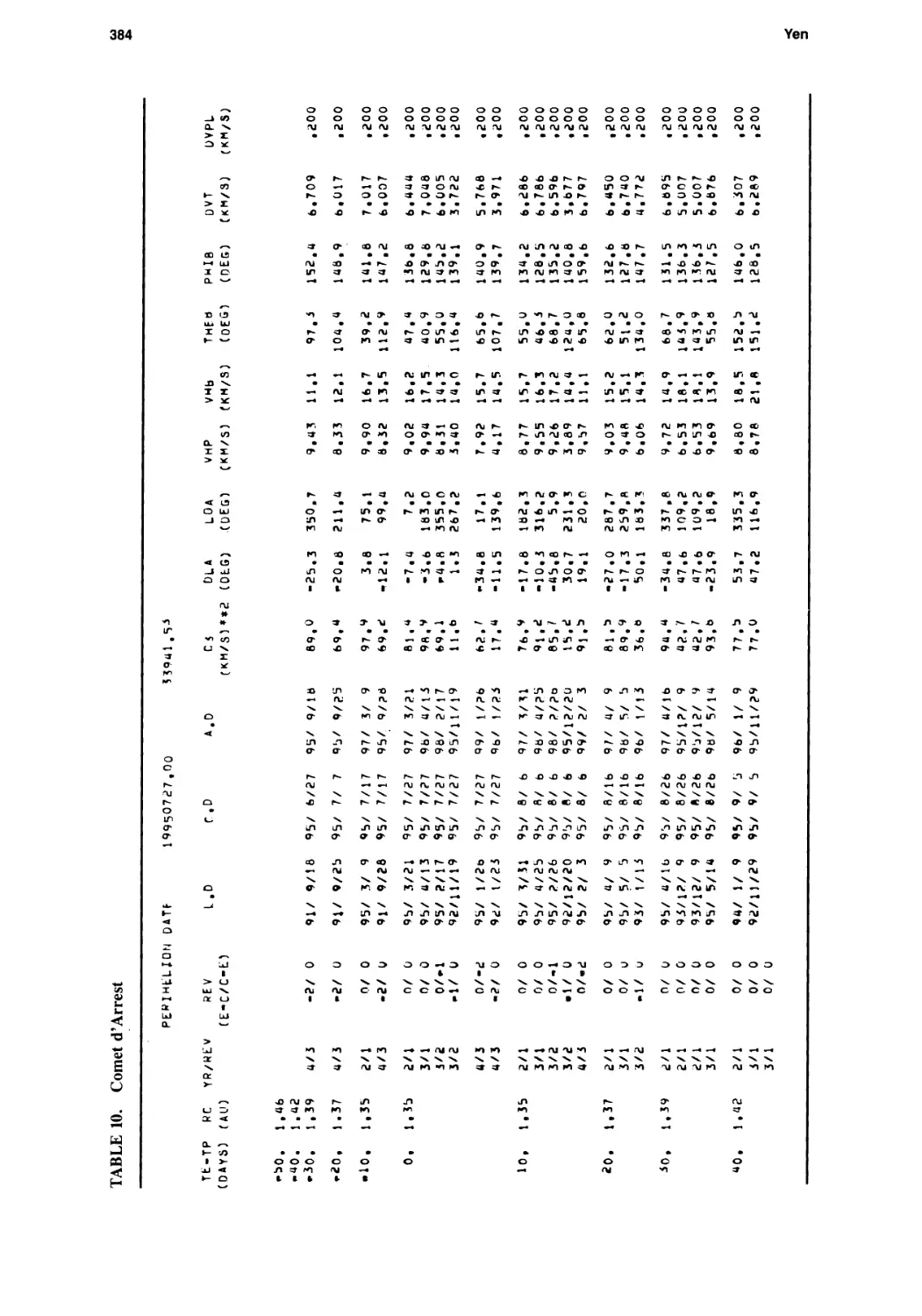
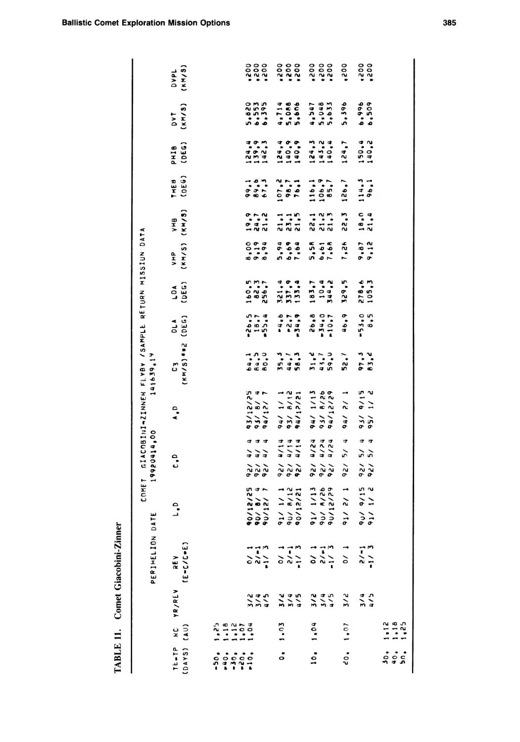
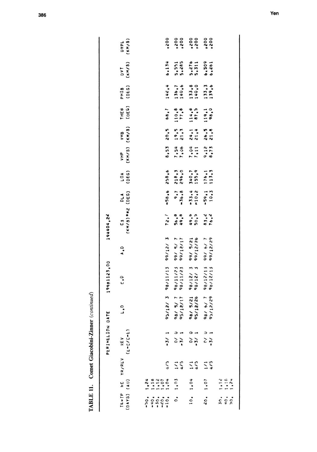
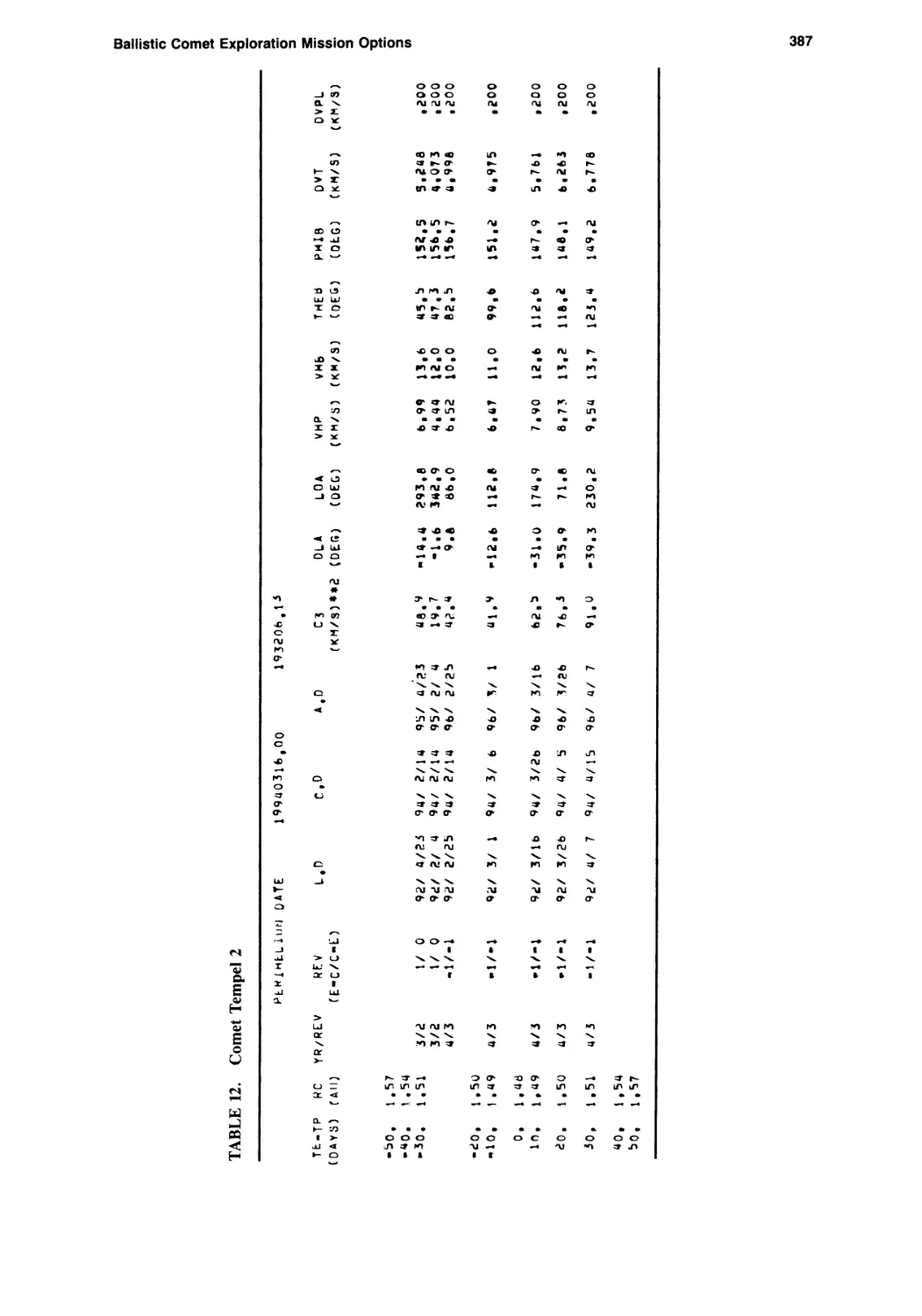
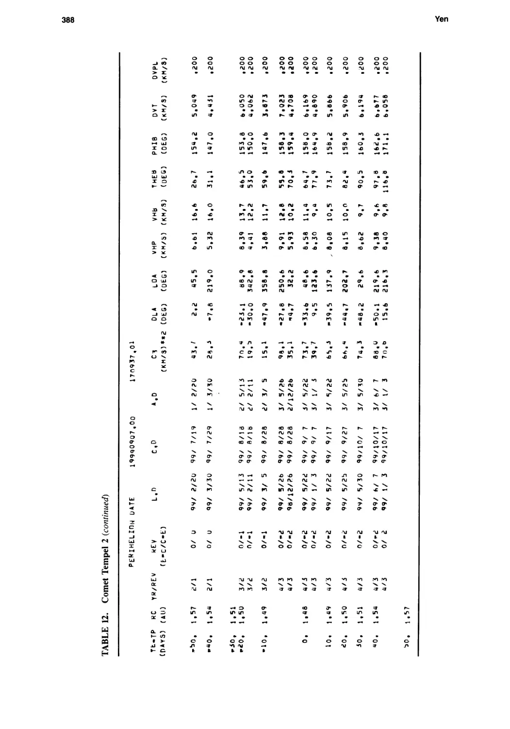
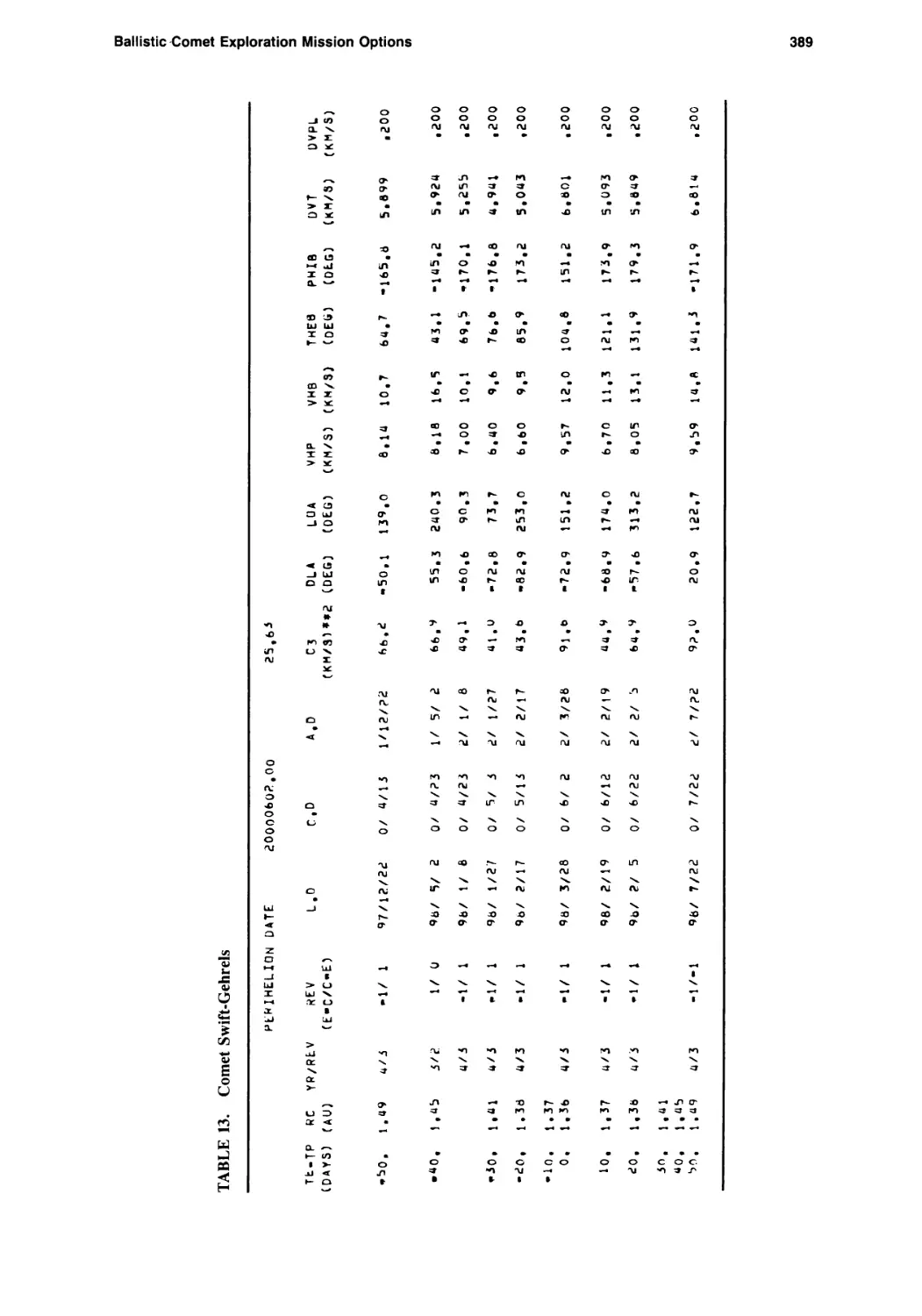
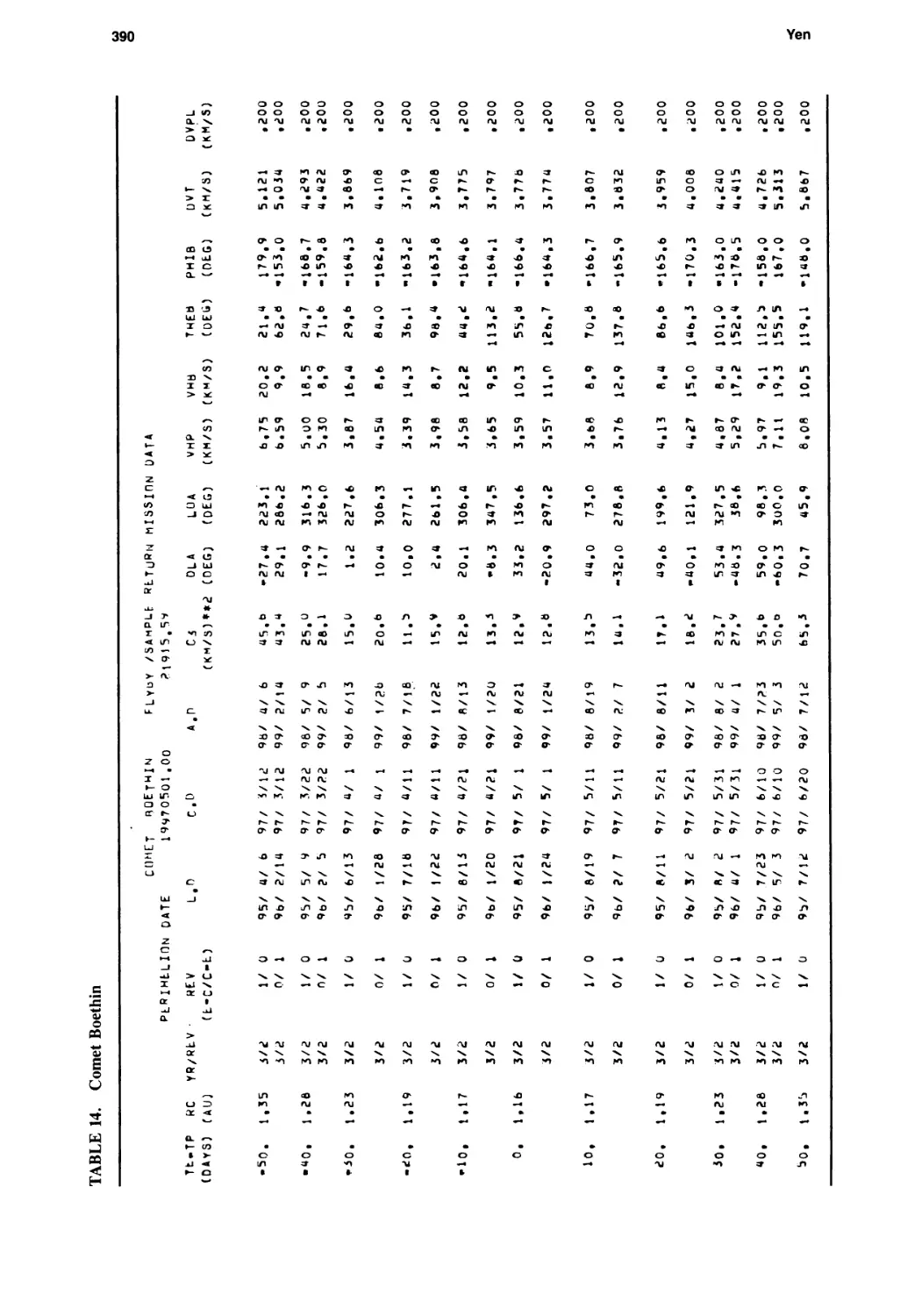
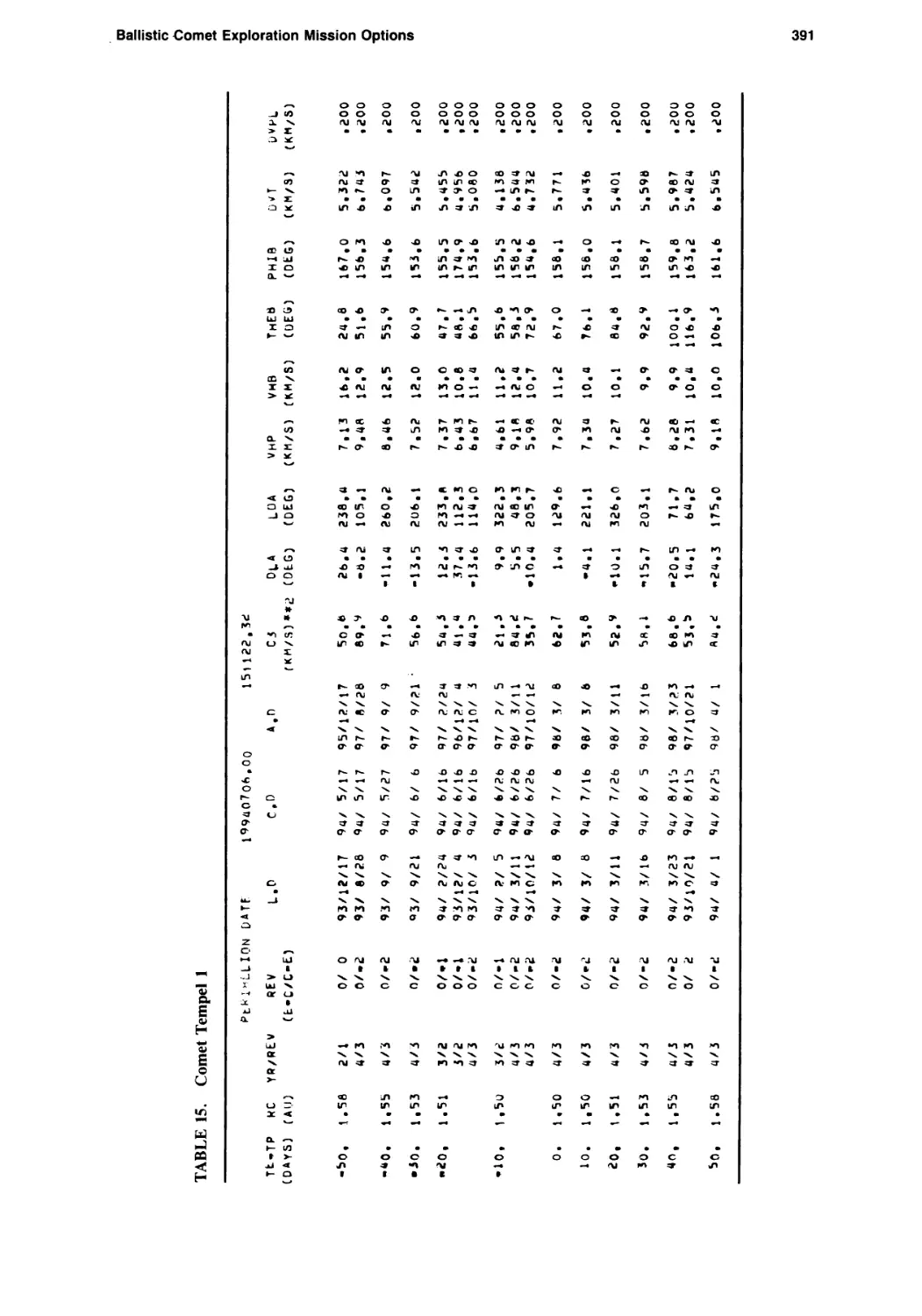
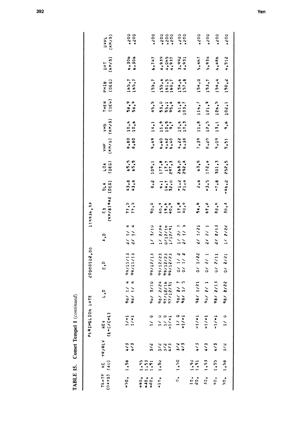
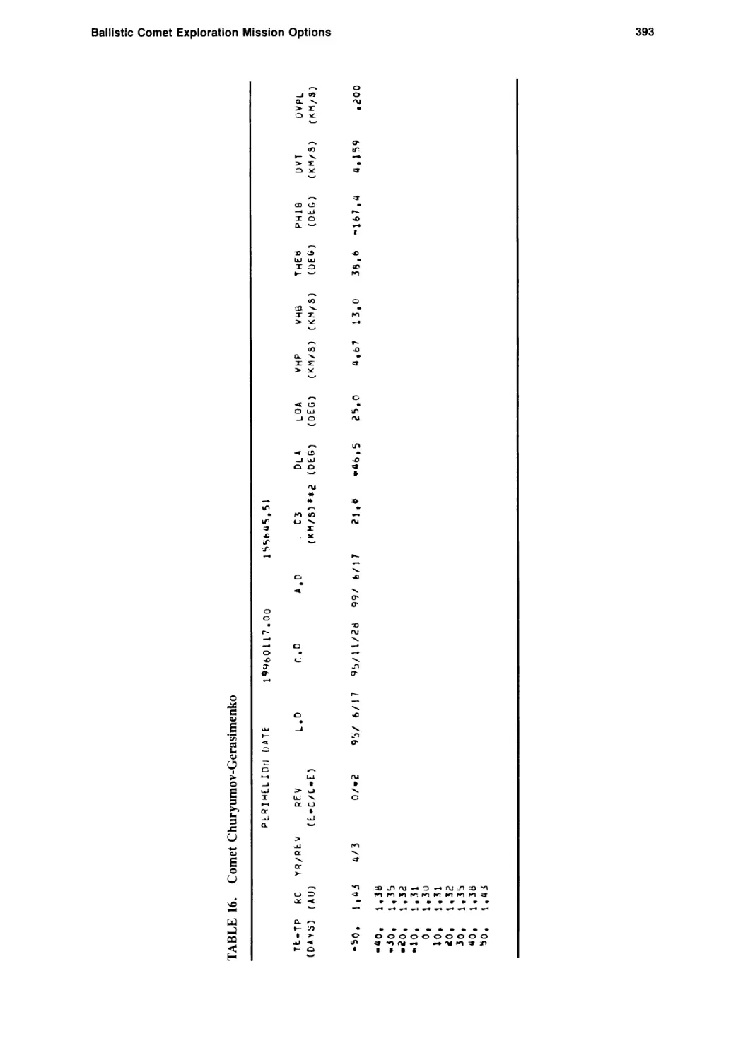
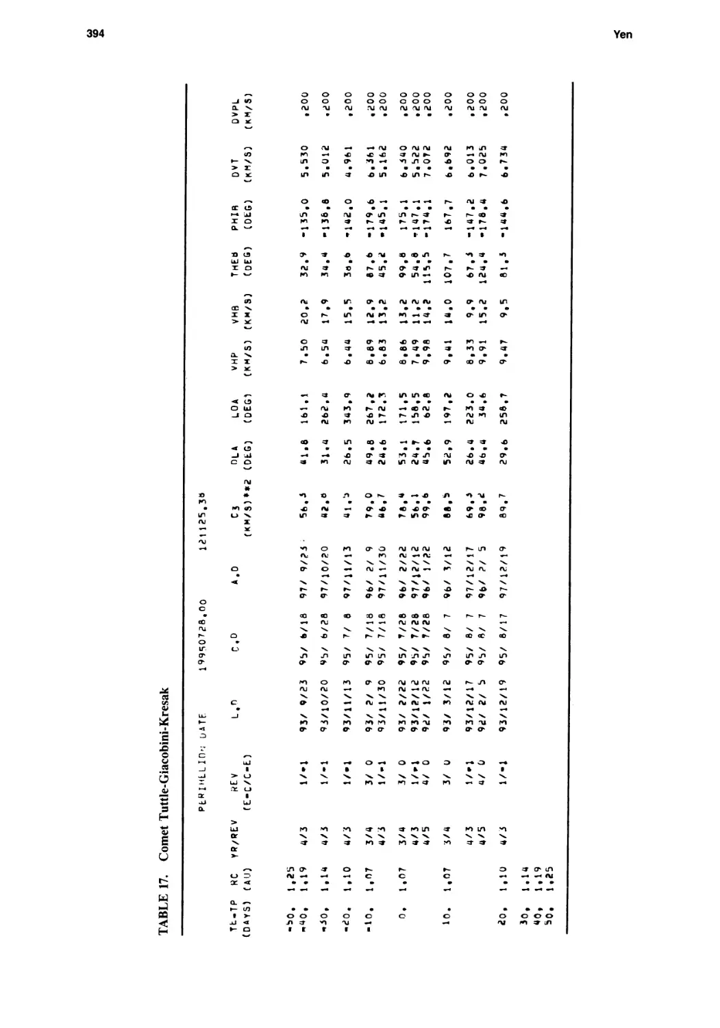
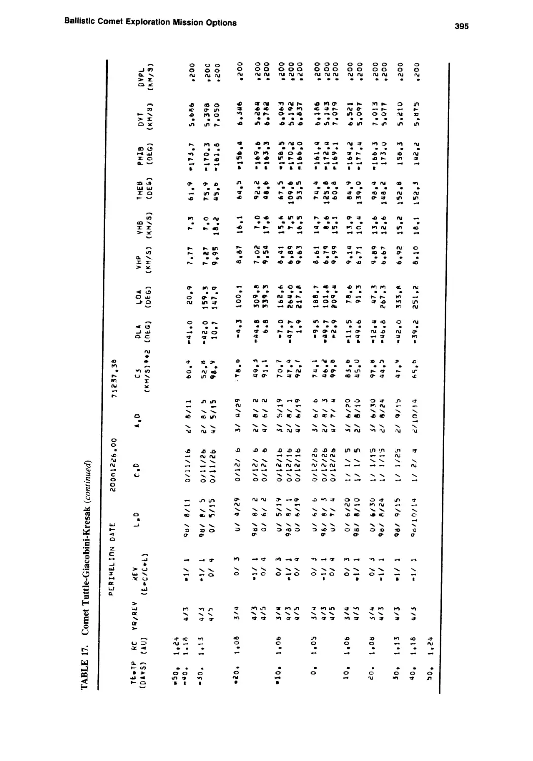
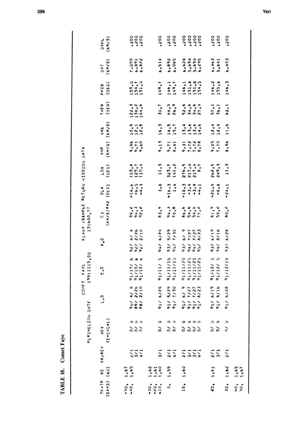
Ballistic Comet Exploration Mission Options
Chen-wan L. Yen 363
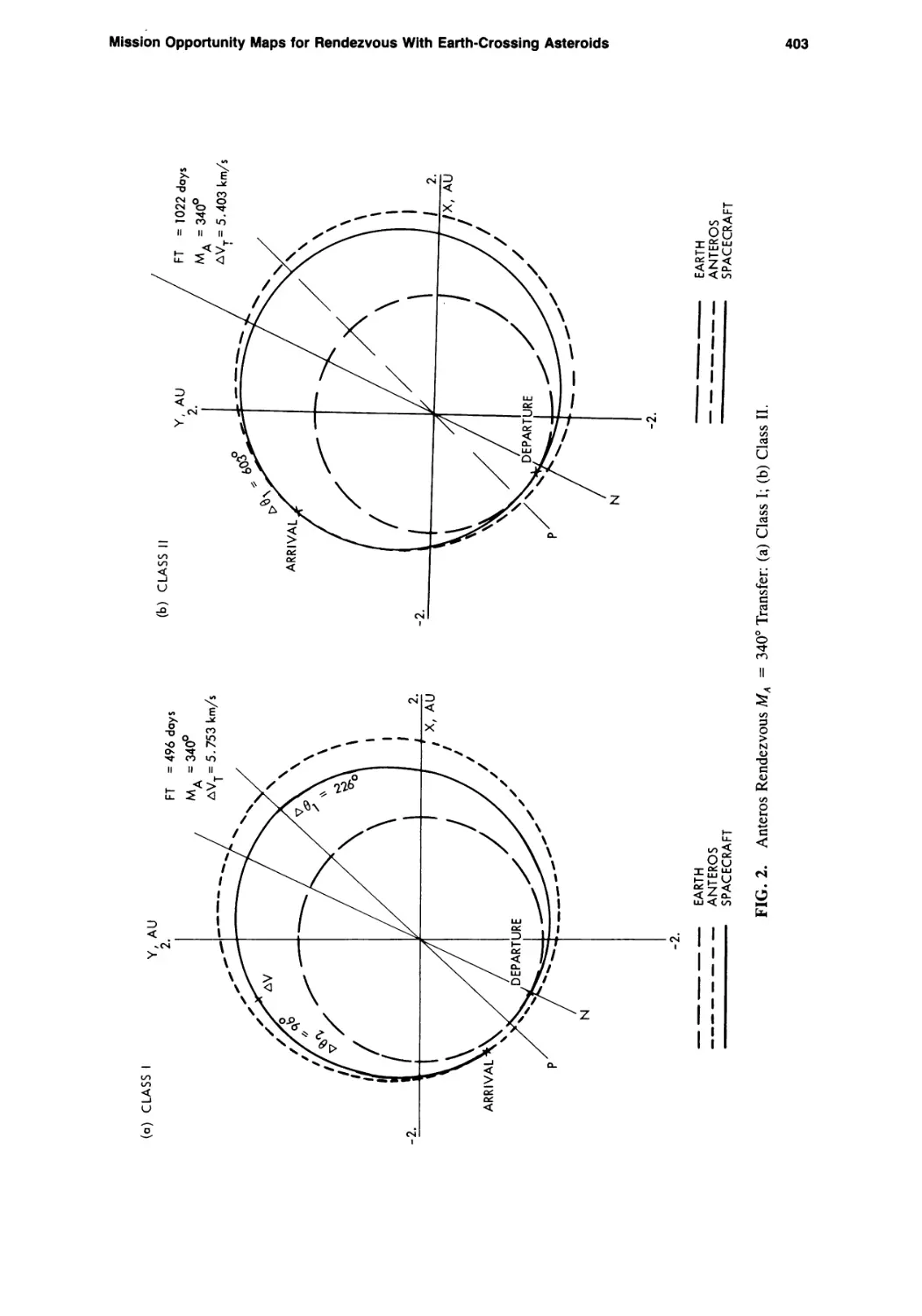
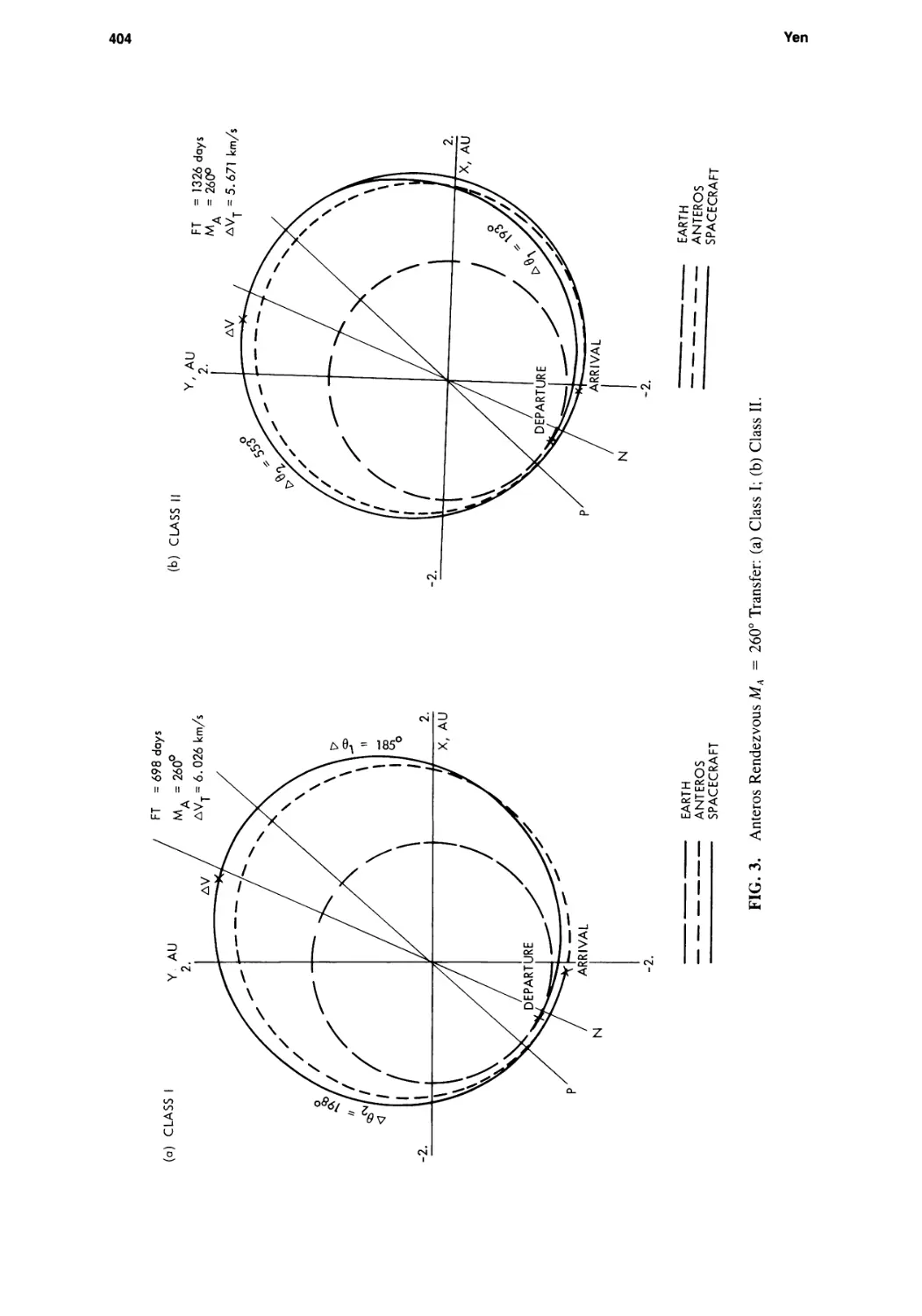
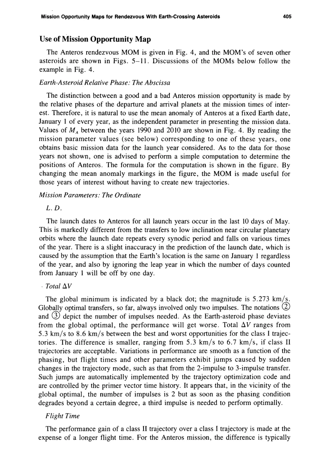
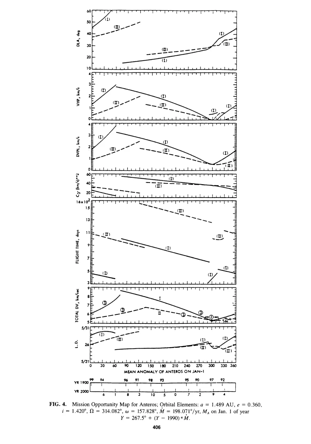
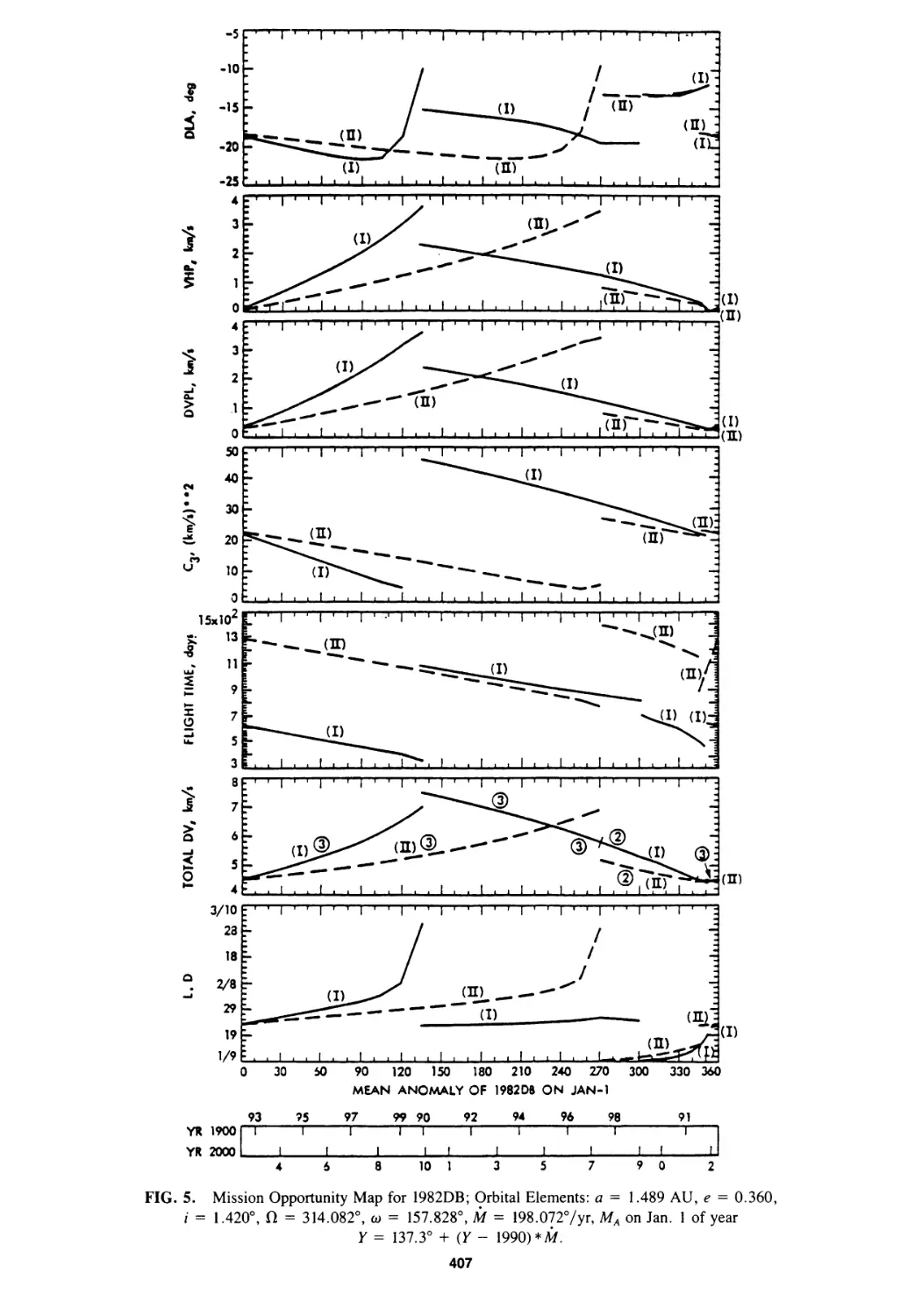
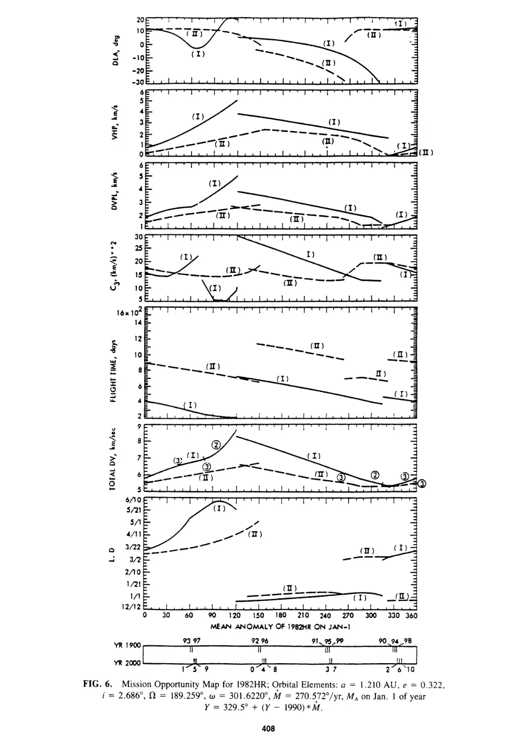
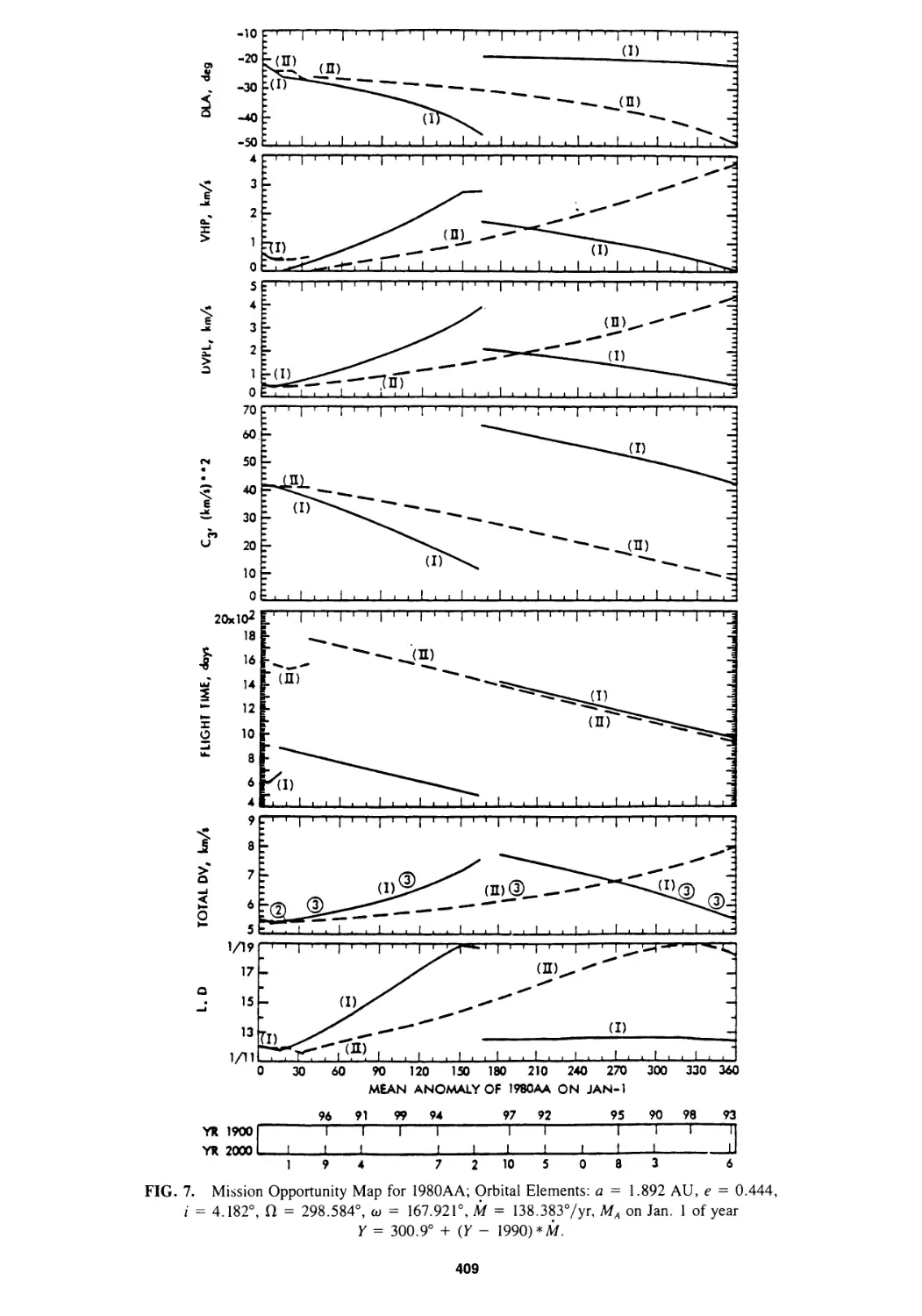
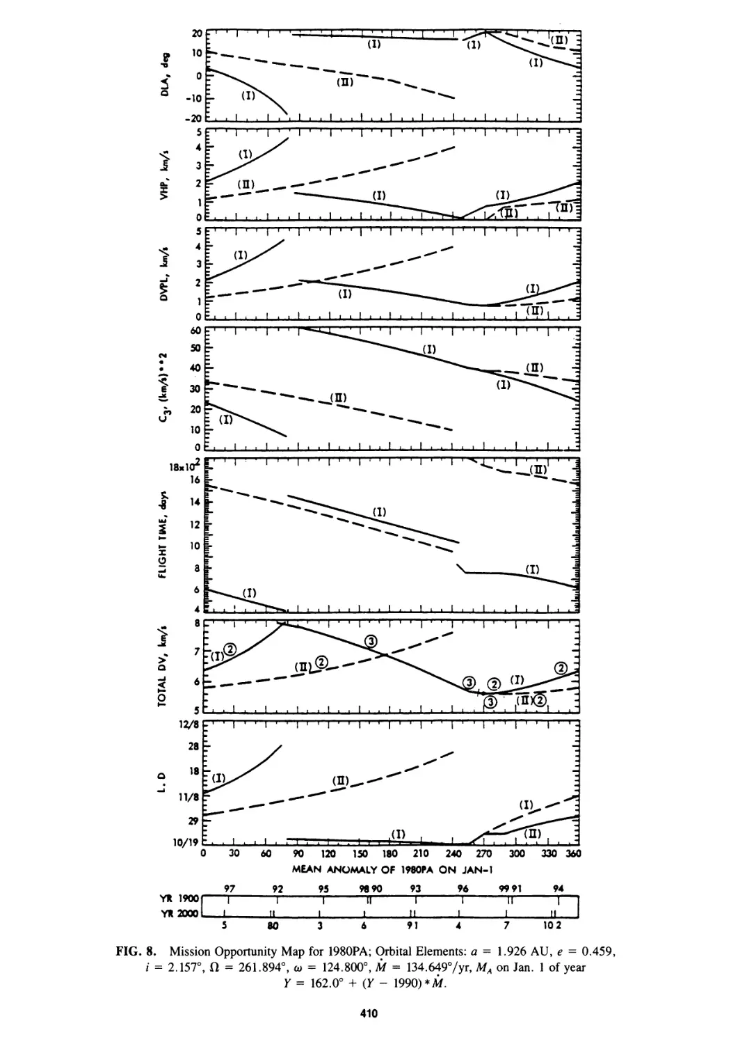
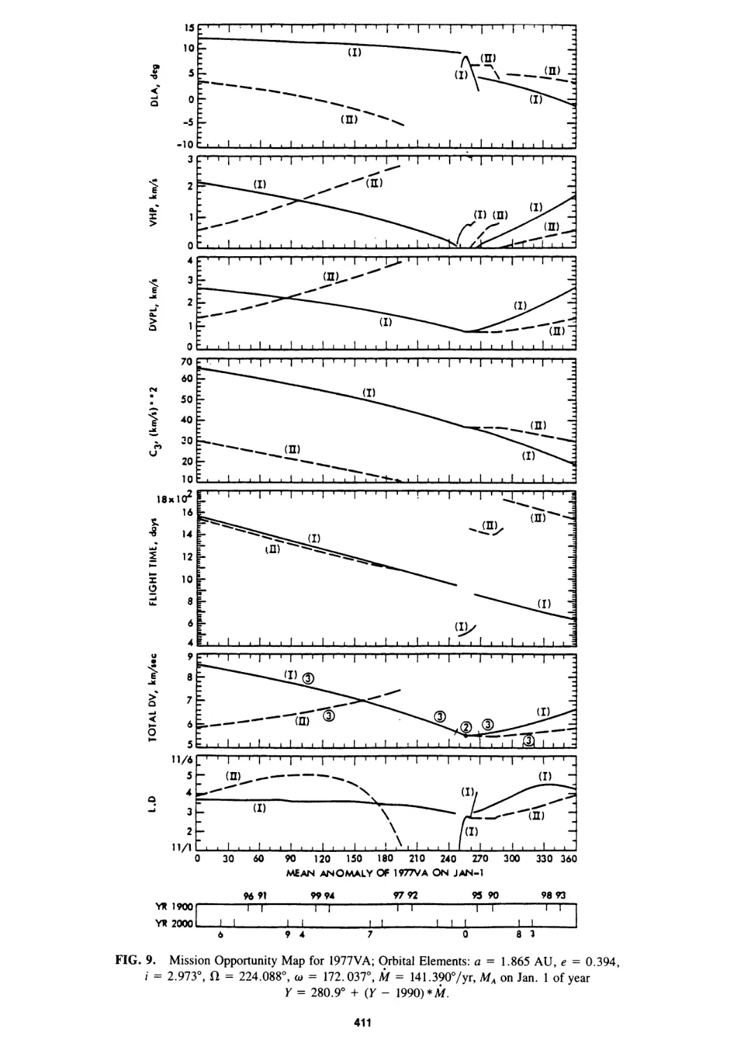
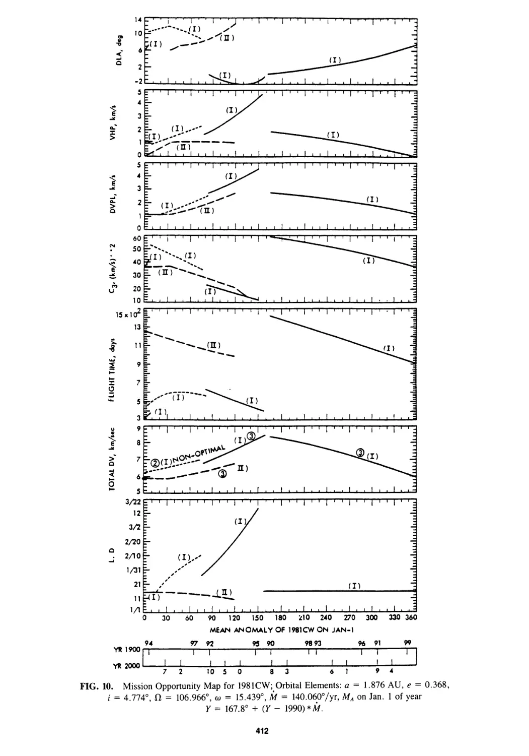
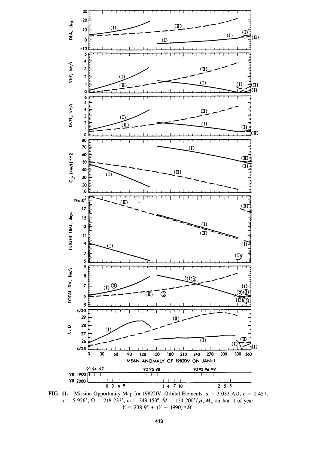
Mission Opportunity Maps for Rendezvous With Earth-Crossing Asteroids
Chen-wan L. Yen 399
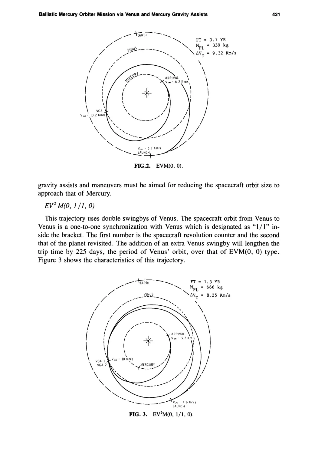
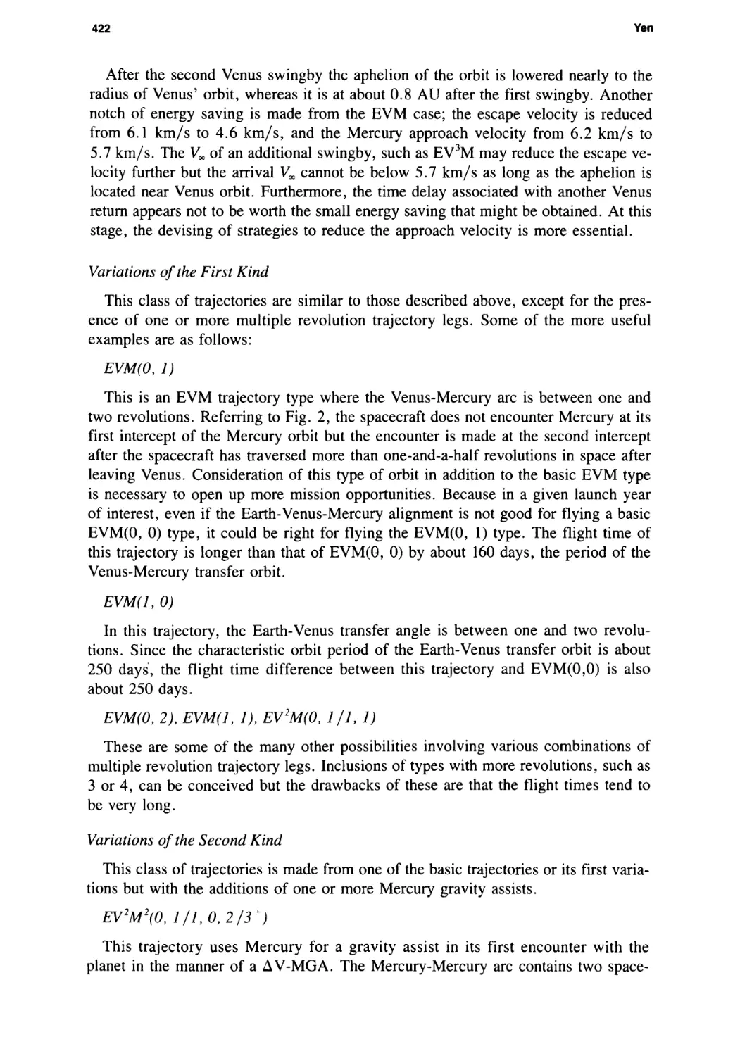
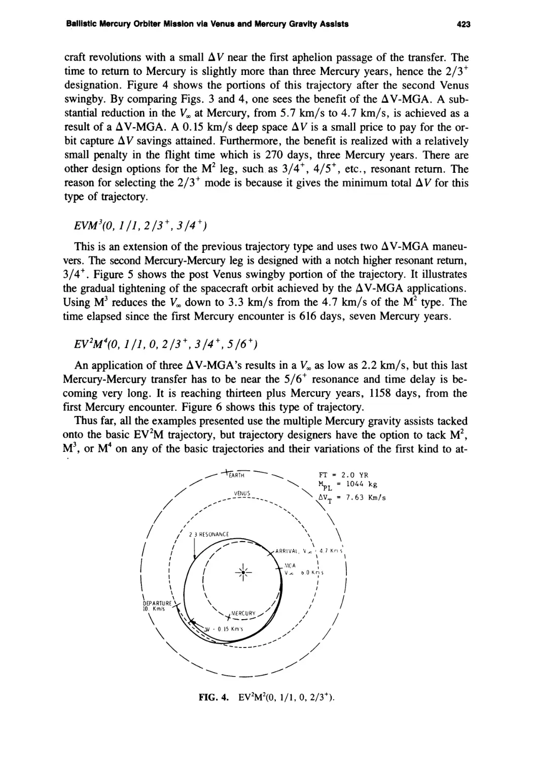
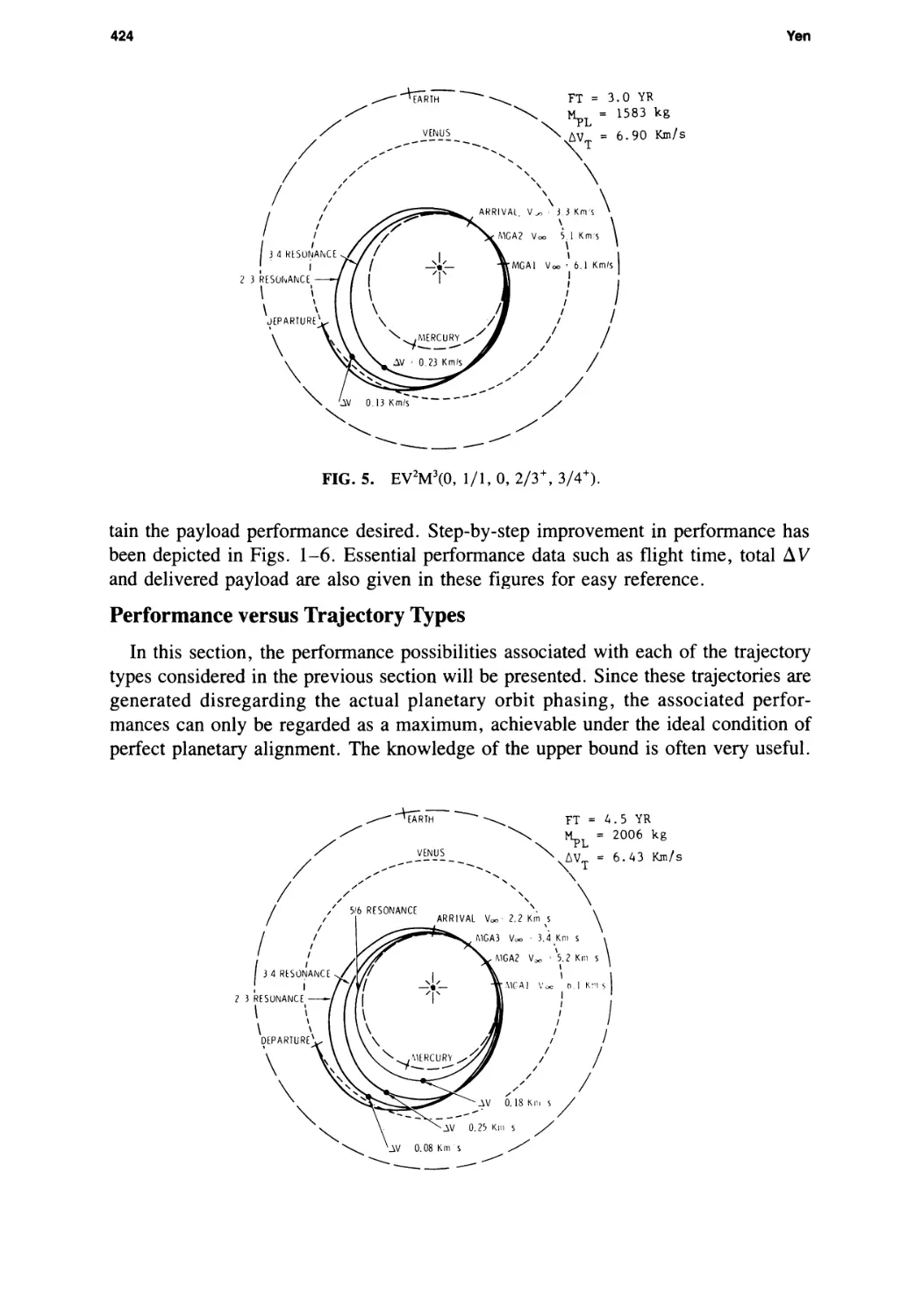
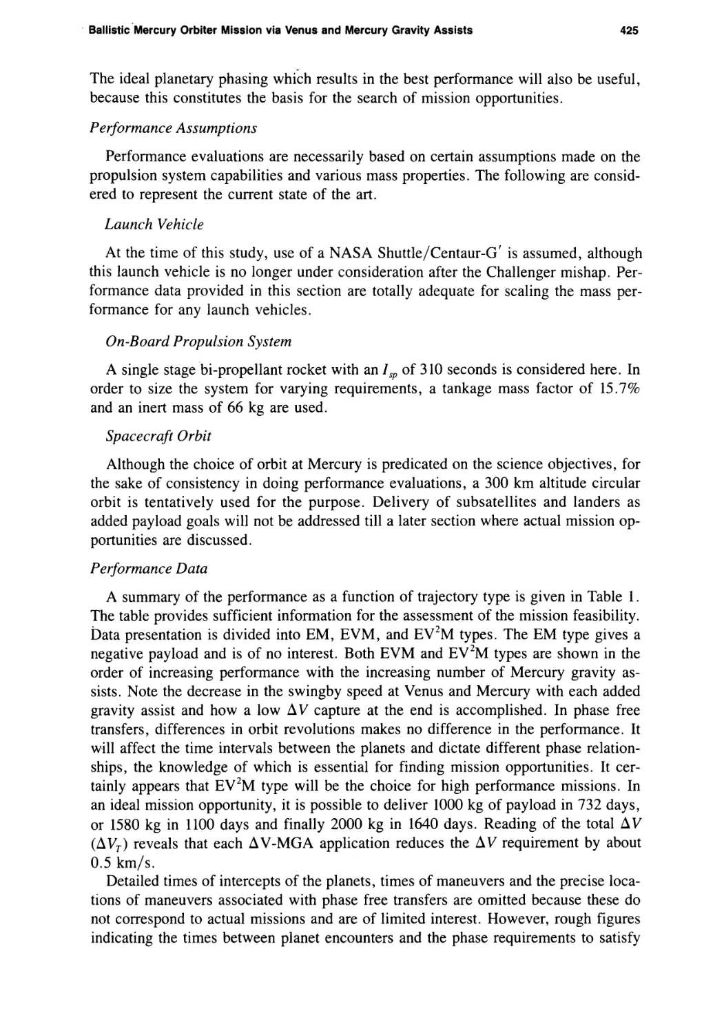
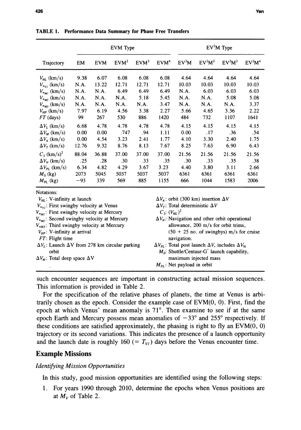
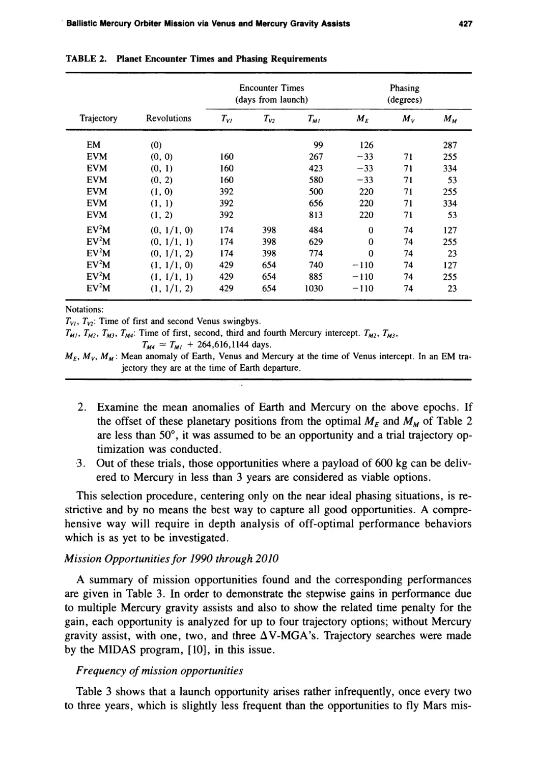
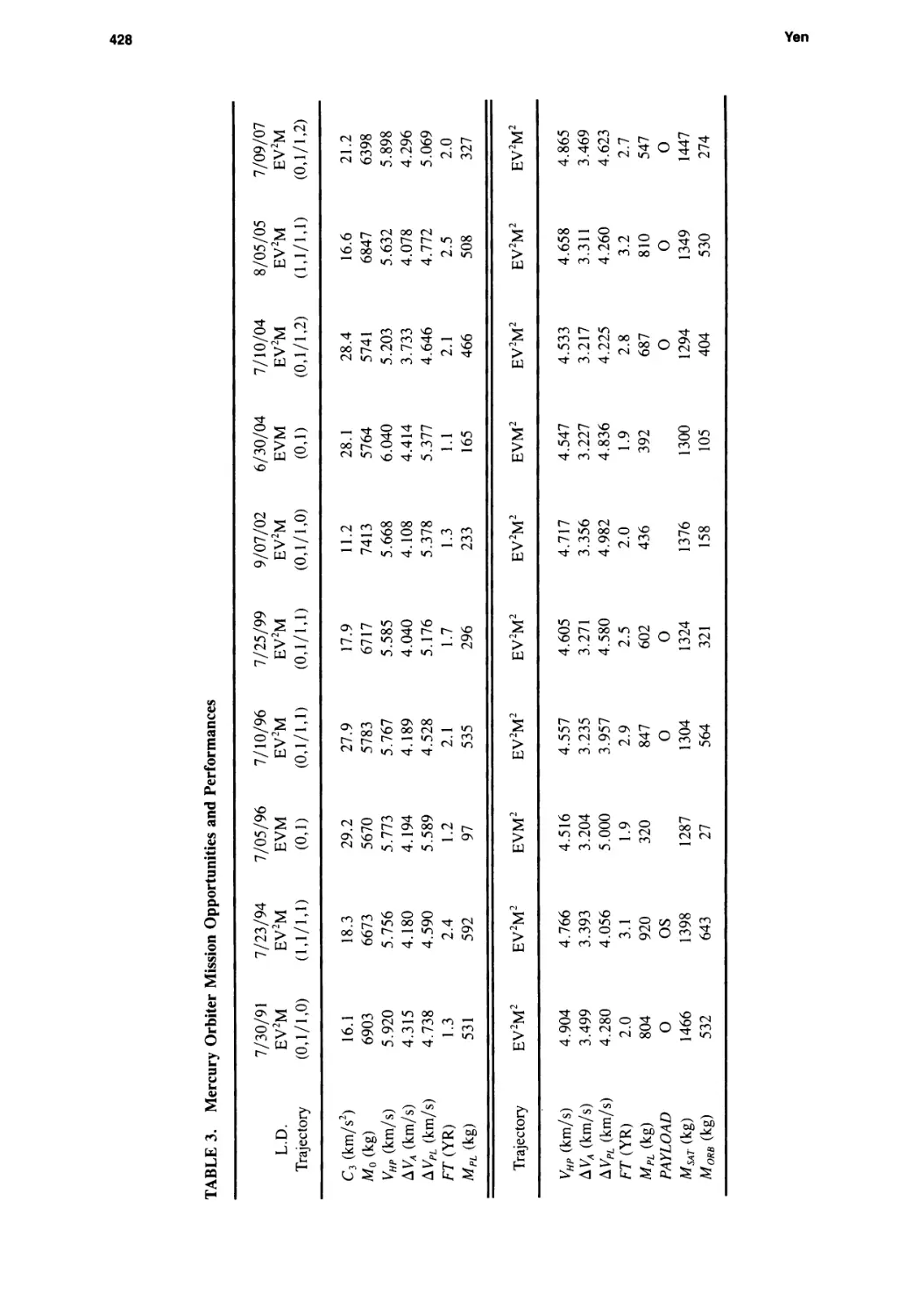
Ballistic Mercury Orbiter Mission via Venus and Mercury Gravity Assists
Chen-wan L. Yen 417
ISSN: 0021-9142
■ PUBLISHED BY THE AMERICAN A S T R О N A U T I C A L SOCIETY
INC.
THE JOURNAL OF THE ASTRONAUTICAL SCIENCES
(USPS 283-960)
THE JOURNAL OF THE ASTRONAUTICAL SCIENCES (ISSN 0021 9142) is published quarterly by the American Astronautical So¬
ciety, 6212 Old Keene Mill Ct., Springfield, VA 22152. AAS annual dues include a $35.00 subscription to the JOURNAL OF THE AS¬
TRONAUTICAL SCIENCES. Second Class postage paid at Springfield, VA. POSTMASTER: Send address changes to the JOURNAL
OF THE ASTRONAUTICAL SCIENCES, 6212 Old Keene Mill Ct., Springfield, VA 22152.
EDITOR-IN-CHIEF
David B. Schaechter, Ph.D., Lockheed Palo Alto Research Laboratory, Bldg. 250, Org. 92-30, 3251 Hanover Street,
Palo Alto, CA 94304
MANAGING EDITOR
Kathleen Howell, Ph.D., School of Aeronautics and Astronautics, Purdue University, West Lafayette, IN 47907
ASSOCIATE EDITORS
Thomas A. Dwyer III, Ph.D., Air Force Weapons Laboratory — Control of Hexible Structures and Attitude Control
Donald Hitzl, Ph.D., Lockheed Palo Alto Research Laboratory — Orbital Mechanics and Space Mission Analysis
Kenneth D. Mease, Ph.D., Princeton University — Orbital Mechanics and Orbit Transfer Optimization
Angelo Miele, Dr. Ing., Rice University — Optimization and Aeronautics
Vinod J. Modi, Ph.D., University of British Columbia — Dynamics and Control
Robert Schutz, Ph.D., University of Texas at Austin — Satellite Orbit Determination and Prediction
C.T. Sun, Ph.D., Purdue University — Structural Dynamics and Composite Materials
PRODUCTION MANAGER
Carolyn F. Brown, AAS, 6212 Old Keene Mill Ct., Springfield, VA 22152
SUBMISSION OF MANUSCRIPTS
Four copies of the complete manuscript should be submitted to the Technical Editor, D.B. Schaechter, Lockheed Palo Alto Research Laboratory,
Bldg. 250, Org. 92-30, 3251 Hanover Street, Palo Alto, CA 94304. If possible, the covering letter should include the names and addresses of
three suggested reviewers. Authors are responsible for the security clearance by an appropriate agency of the material contained in the pa¬
pers. For scope of journal and format of technical papers consult inside back cover. Page Charges at the rate of $50.00 per printed page will
be billed. In return 50 reprints of the article will be supplied without charge.
THE AMERICAN ASTRONAUTICAL SOCIETY, INC.
OFFICERS
E. Larry Heacock, National Oceanic and Atmospheric Administration, President
Philip E. Culbertson, External Tanks Corporation, Executive Vice President
John A. Sand, Ball Aerospace Systems Group, Vice President-Technical
Walter Froehlich, International Science Writers, Vice President-Publications
Dr. Marc S. Allen, СТА Incorporated, Vice President-Membership
Kathleen J. Charles, Department of State, Vice President-Finance
Dr. Peter M. Bainum, Howard University, Vice President-International
S. Neil Hosenball, Esq., Davis, Graham and Stubbs, Legal Counsel
Carolyn F. Brown, Executive Director
Term Expires 1989
Leonard David, Space Data Resources and Information, Inc.
Stephen E. Dwornik, Ball Aerospace Systems Group
Robert A. Frosch, General Motors Corporation
John H. McElroy, Ph.D., University of Texas at Arlington
Colonel Gerald M. May, USAF, United States Air Force
Jesse W. Moore, Ball Aerospace Systems Division
Arnauld Nicogossian, Ph.D., NASA Headquarters
Donald H. Parsons, Martin Marietta Denver Aerospace
Ian Pryke, European Space Agency
Lt. Colonel S. Peter Worden, USAF, United States Air Force
A. Thomas Young, Martin Marietta Orlando Aerospace
Elizabeth L. Young, Ph.D., COMSAT Maritime Services
BOARD OF DIRECTORS
Term Expires 1990
Dr. Lennard A. Fisk, NASA Headquarters
Dr. Noel W. Hinners, NASA Headquarters
David S. Johnson, National Research Council
Richard L. Kline, Grumman Space Station: Program Support Division
Dr. George W. Morgenthaler, University of Colorado
William J. Shea, Lockheed Missiles and Space Company
David W. Thompson, Orbital Sciences Corporation
Term Expires 1991
James Beggs, Consultant
N. William Cunningham, Hughes Aircraft Company
Roger G. Dekok, USAF, United States Air Force
Dr. Ashok R. Deshmukh, ANSER
Daniel J. Fink, D. J. Fink Associates, Inc.
Douglas A. Heydon, Arianespace, Incorporated
Captain David C. Honhart, USN, Office of the Chief of Naval Research
Dr. Franklin D. Martin, NASA Headquarters
G. Lynwood May, G. Lynwood May & Associates. Inc.
Albert Naumann, Jr., Lockheed Engineering and Sciences Co.
Honorable Bill Nelson, Member of Congress
Copyright © 1989 by the AMERICAN ASTRONAUTICAL SOCIETY, INC.
Subscription orders should be addressed to the American Astronautical Society, 6212 Old Keene Mill Ct., Springfield, VA 22152.
Subscription rates: Domestic Institutions $95.00. Foreign Institutions $105.00. Single copies: Domestic $23.75. Foreign $26.25.
The Journal of the Astronautical Sciences, Vol. 37, No. 3, July-September 1989, pp. 211
Editorial
The intent of this single topic special issue is to illuminate/the .methbds of design¬
ing interplanetary missions, and to provide several application examples from studies
over the last few years. Of the many excellent papers available to us on this topic, the
papers in this journal were chosen more for their pedagogical value than for their
relevance to future NASA programs. In this light, we have included several papers
on missions which will not fly, but which provide good illustrations of applications of
the above mission design methods.
The issue is divided into two sections: 5 papers on the theory and software used in
mission design, followed by 6 papers which illustrate use of the software to search
out practical missions. The basic theory is not new, and has been extensively covered
in published papers referenced here. However, there exists no archival publication
which describes the core programs of JPL’s mission design software. Along these
lines, the papers by Lou D’Amario and C. Sauer attempt to shed light on the subject.
Although it may be believed that trajectory search theory is complete, we have in¬
cluded in this journal papers from Dennis Byrnes and Ted Sweetser on pseudostate
methods, which may be the wave of the future. Finally, Alok Chatterjee shows how
to solve a simplified optimal control problem to transfer large flexible structures from
low to high orbits using a medium to low thrust propulsion system.
Theory has its adherents, but this issue would not be complete without addressing its
applications, particularly in the face of a set of awkward constraints. If you’ve peeked,
you’ll have noticed that there are 6 such application papers from only 2 authors —
Lou D’Amario, who also covers mission design software, and Chen-wan Yen. There
were several other candidate papers, but these papers best revealed the process.
All of the authors in this issue are Members of the Technical Staff of the Jet Propul¬
sion Laboratory, California Institute of Technology, Pasadena, CA 91109, and work
in the Mission Design Section. We, your editors are also at JPL and have served time
in Mission Design. We would like to acknowledge the continued support for this under¬
taking from the Mission Design Section, and especially by its manager, Mr. Robert
T. Mitchell for his unflagging support and for supplying secretarial help.
All of the research for the papers in this issue was carried out at the Jet Propulsion
Laboratory, California Institute of Technology, under a contract with the National
Aeronautics and Space Administration.
Gail A. Klein
David Sonnabend
211
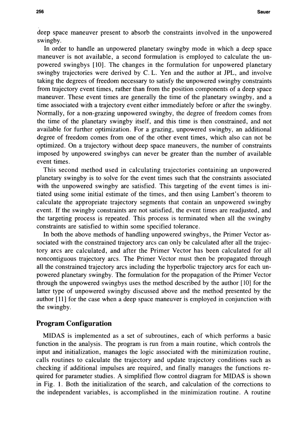
The Journal of the Astronautical Sciences, Vol. 37, No. 3, July-September 1989, pp. 213-220
Trajectory Optimization Software for
Planetary Mission Design
Louis A. D’Amario
Abstract
This paper contains a discussion of the development of an interactive trajectory optimization
software package. A detailed example based on the Galileo mission is presented.
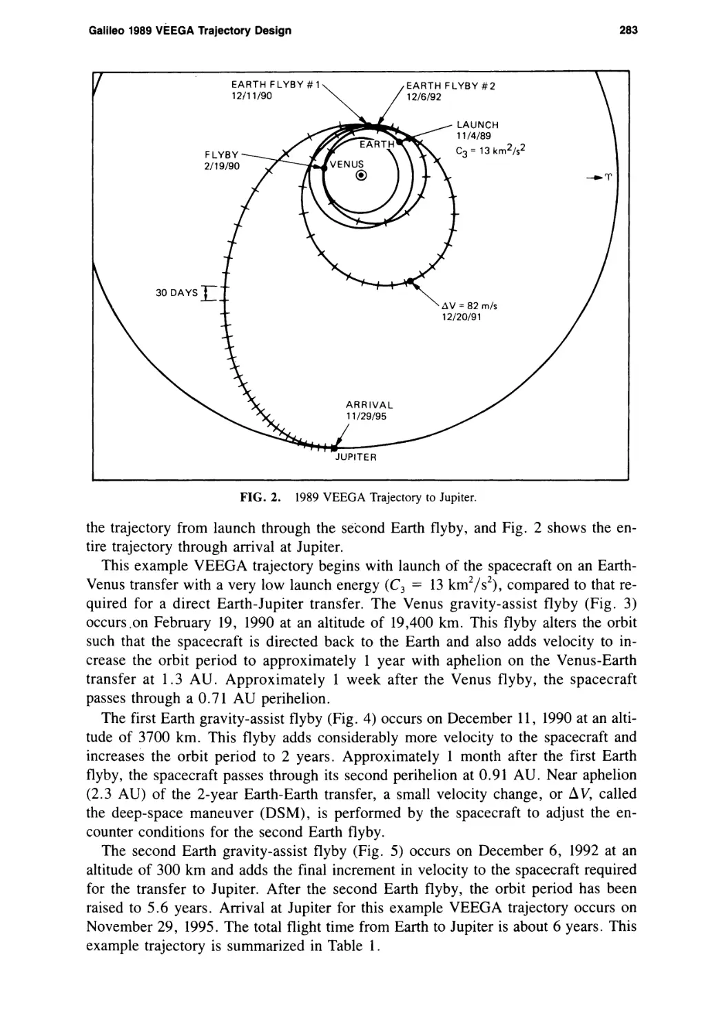
Motivation: The Galileo Satellite Tour
In October, 1989, the Galileo orbiter/probe spacecraft, mated to an Inertial Upper
Stage (IUS), will be carried into Earth orbit by the Space Shuttle. Following de¬
ployment, the IUS will inject the spacecraft into a transfer trajectory to Jupiter. Upon
arrival at Jupiter on December 7, 1995, the orbiter, separated from the probe some
five months earlier, will relay the probe’s measurements back to Earth as the probe
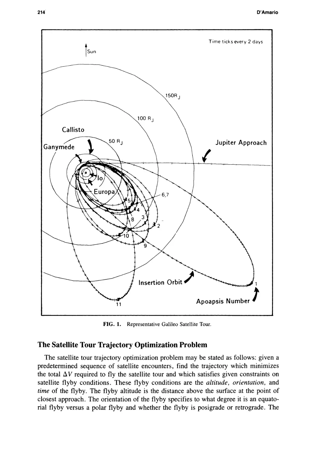
descends through Jupiter’s atmosphere. The orbiter will then conduct a 22-month,
10-orbit “tour” of the Jovian system (see Fig. 1). On each orbit, the spacecraft will
have a close flyby with one of the three outermost Galilean satellites (Europa,
Ganymede, and Callisto) — typically at distances 10 times closer than Voyager’s.
These flybys always occur near periapsis of the orbit about Jupiter. The gravity assist
derived from the close satellite encounter on each orbit modifies the orbit about Jupi¬
ter in just the precise manner to target the spacecraft for an encounter with another
(or the same) satellite on the next orbit.
In order for the Galileo mission to be able to conduct such a satellite tour, sophisti¬
cated trajectory optimization software had to be developed, so that a minimal amount
of on-board propellant is required for trajectory shaping maneuvers. Such a maneuver
is modeled as an instantaneous change in velocity, or “AV”. Minimizing total satel¬
lite tour AV is crucial, because only a small amount of the limited on-board propel¬
lant capacity is available for the orbital phase of the mission. The large orbit changes
required to conduct a satellite tour, if accomplished by the spacecraft’s rocket propul¬
sion system, would consume 6000-8000 m/s of AV (depending on the particular
tour), which is equivalent to between four and five times the total amount of propel¬
lant carried on board for the entire mission. In actuality, the AV for planned orbit
modifications during the satellite tour should not exceed about 75 m/s. This small
AV budget calls for great ingenuity on the part of trajectory designers.
213
214
D’Amario
The Satellite Tour Trajectory Optimization Problem
The satellite tour trajectory optimization problem may be stated as follows: given a
predetermined sequence of satellite encounters, find the trajectory which minimizes
the total AV required to fly the satellite tour and which satisfies given constraints on
satellite flyby conditions. These flyby conditions are the altitude, orientation, and
time of the flyby. The flyby altitude is the distance above the surface at the point of
closest approach. The orientation of the flyby specifies to what degree it is an equato¬
rial flyby versus a polar flyby and whether the flyby is posigrade or retrograde. The
Trajectory Optimization Software for Planetary Mission Design
215
flyby time is the time of closest approach to the satellite. The altitude, orientation,
and time of each satellite flyby determine what change to the orbit about Jupiter will
be caused by the satellite encounter.
There are two factors which complicate the satellite tour optimization problem.
The first is that there are constraints on the satellite flyby conditions. These con¬
straints arise from science requirements and mission operations limitations. For ex¬
ample, a particular satellite flyby may be constrained to be no higher than 1400 km
and within 15 deg of the equator in order to satisfy a gravity experiment. Another ex¬
ample is that navigation requirements dictate that the first three flybys of the satellite
tour can be no closer than 500, 400, and 300 km respectively; thereafter, a lower
limit of 200 km is allowed. If there were no constraints on flyby conditions, celestial
mechanics considerations indicate that it should be possible to find a trajectory which
requires zero, or nearly zero, Д V and which has the prescribed sequence of satellite
flybys. Even for the unconstrained problem, finding a 10-orbit ballistic trajectory,
with a close satellite flyby on each orbit, is by itself very difficult. Minimizing the
required Д V and satisfying all the constraints on the flybys together raise the level of
difficulty significantly.
The second complicating factor is related to trajectory modelling. There are several
different ways to model a spacecraft trajectory under the influence of multiple gravi¬
tational bodies. At one extreme are the simple two-body, or “conic,” methods, which
are computationally very fast but which lack sufficient accuracy for many applica¬
tions. At the other extreme are the precision numerical integration methods, which
are very accurate but which require much more computational effort. It is vital in any
trajectory optimization process to model the dynamics accurately enough so that the
total Д V of the resulting trajectory can be duplicated when the trajectory is regener¬
ated with high-precision numerical integration software. Early in the Galileo mission
design process, the accuracy of conic methods for satellite tour optimization was
demonstrated to be inadequate. In addition, the computer execution time required by
numerical integration methods precluded their use in an optimization program, where
hundreds of complete 10-orbit satellite tour trajectories would have to be generated
during the optimization process.
Formulation of the Solution
The satellite tour trajectory optimization problem challenged the Galileo mission
designers at JPL. An intense software development effort began in August, 1978, and
not until approximately two years later was a truly successful formulation for the so¬
lution demonstrated in terms of accuracy, runtime, and reliability. During this period,
the author and two other engineers (Dennis Byrnes and Richard Stanford) worked on
the problem nearly full time.
The computer program which solves the satellite tour trajectory optimization prob¬
lem is called MOSES (Multiple Orbit Satellite Encounter Software) [1]. The mathe¬
matical approach taken toward finding the solution is to formulate the trajectory
optimization problem as a “parameter optimization problem.”
In a parameter optimization problem, a minimum is sought for a quantity, called
the “cost”, which is a function of one or more “parameters” (also referred to as “inde¬
pendent variables”). If the problem also has equality or inequality constraints on
216
D’Amario
quantities which are functions of the independent variables, then the problem is
called a “constrained parameter optimization problem”. The functional dependency of
the cost and the constraints on the independent variables is often mathematically very
complex, so that iterative numerical techniques must be used to solve for the set of
independent variables which minimize the cost and satisfy the constraints. A whole
branch of mathematics is concerned with deriving the algorithms (and software) to
solve parameter optimization problems.
For MOSES, the cost function to be minimized is the total AV of the satellite tour,
and the independent variables are the complete set of satellite flyby conditions: alti¬
tudes, orientations, and flyby times. Thus the total number of independent variables
is 3 x TV where TV is the number of flybys in the satellite tour. With this formulation,
the science and mission operations constraints on the flyby conditions translate into
simple bounds (i.e., upper and lower limits) on the independent variables. The choice
of the independent variables (and there are many possible choices for this problem)
probably has more effect than anything else on the program complexity and on the
performance (computer execution time, convergence properties, etc.) of the resulting
optimization procedure. The software routines which contain the mathematical al¬
gorithms for iteratively varying the independent variables (within bounds) to mini¬
mize the cost are taken from a numerical optimization software library developed at
the National Physical Laboratory of England.
On each iteration of the optimization process in MOSES, a complete trajectory
must be generated in order to evaluate the cost — the total AV of the satellite tour. In
order to accomplish this, the trajectory is broken into segments, one segment for each
satellite flyby. On each segment, beginning with the first and proceeding to the last,
the trajectory is targeted to the upcoming satellite flyby conditions and then propa¬
gated to the next breakpoint. The sum of the magnitudes of all the velocity disconti¬
nuities at the breakpoints is the total AV required for the satellite tour. The objective
of the optimization process is to minimize this total AV. In an optimized satellite
tour, typically only two or three individual AV’s make up the entire cost; all the rest
are zero.
A key ingredient in MOSES is the use of multi-conic methods for modelling the
gravitational attraction of Jupiter, its satellites, and the Sun. Multi-conic methods,
which use combinations of conics with respect to all of the gravitational bodies, are
much more accurate than simple conic methods, but require far less computational ef¬
fort than numerical integration. Two versions of MOSES have been implemented
with two different multi-conic methods. One method, tailored for speed, eliminates
about 90% of the error of conic methods and is used for the initial stage of satellite
tour optimization. The other method is almost as accurate as numerical integration,
but much faster, and is used for the final stage of the optimization. One particular ad¬
vantage of using multi-conic methods is that the calculation of trajectory sensitivities,
which are necessary inputs for the optimization algorithm, uses only a small amount
of additional computer execution time beyond that required for the generation of the
trajectory itself.
MOSES is a computer program which is run in an interactive mode. The user ob¬
serves the progress of the optimization at each iteration and changes various program
controls which affect the manner in which the optimization proceeds. Due to the ex¬
Trajectory Optimization Software for Planetary Mission Design
217
treme sensitivity of the satellite tour to small variations in the flyby conditions, con¬
siderable skill is required by the user to converge successfully to an optimal solution.
MOSES has been successfully used for the past eight years in Galileo mission de¬
sign activities, leading up to the selection of the actual satellite tour to be flown at
Jupiter. MOSES will also be used in mission operations during the orbital phase of
the mission to reoptimize the remainder of the satellite tour in support of the naviga¬
tion process. (One function of navigation deals with the effects of perturbations to the
trajectory from inexact knowledge of the masses and ephemerides of the planets and
satellites, inexact force models, maneuver execution errors, etc. which cause the ac¬
tual trajectory to diverge from the planned trajectory.)
Optimized Satellite Tour
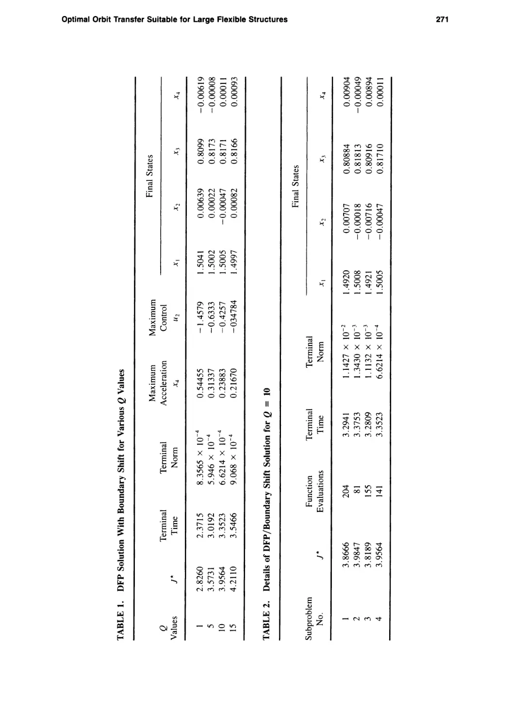
While it is not possible to demonstrate here the lengthy and complex satellite tour
optimization process which occurs during a MOSES computer run, the end product
can at least be presented. The satellite tour shown in Fig. 1 is the one which was fi¬
nally selected for the 1986 Galileo mission (prior to the launch delay caused by the
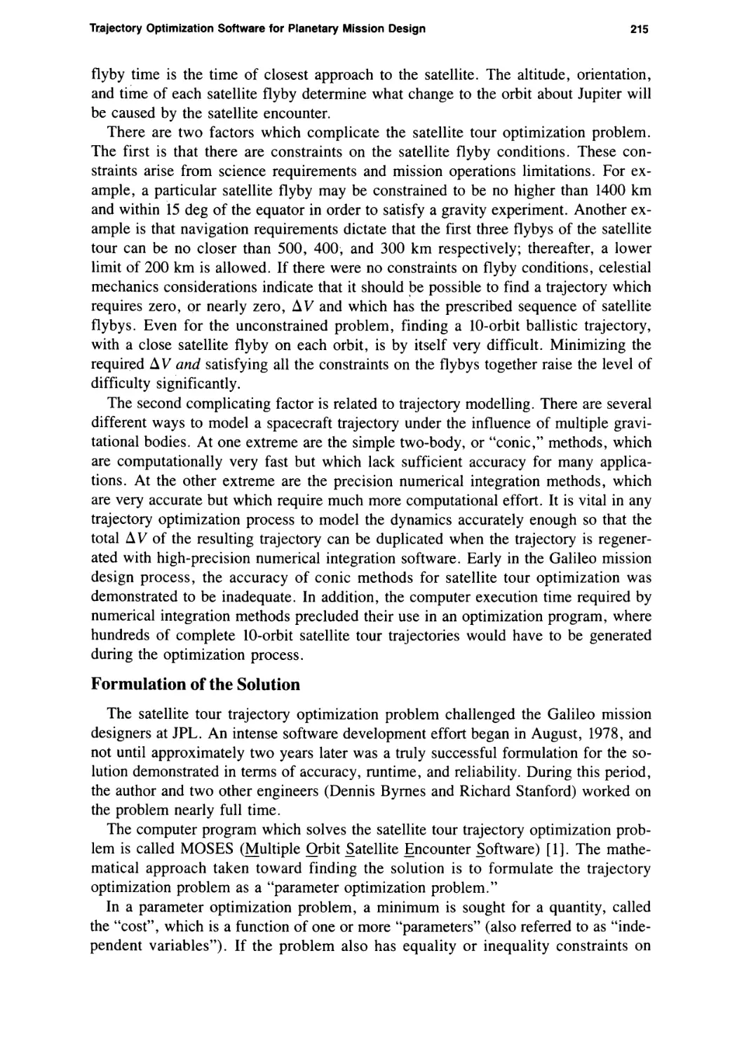
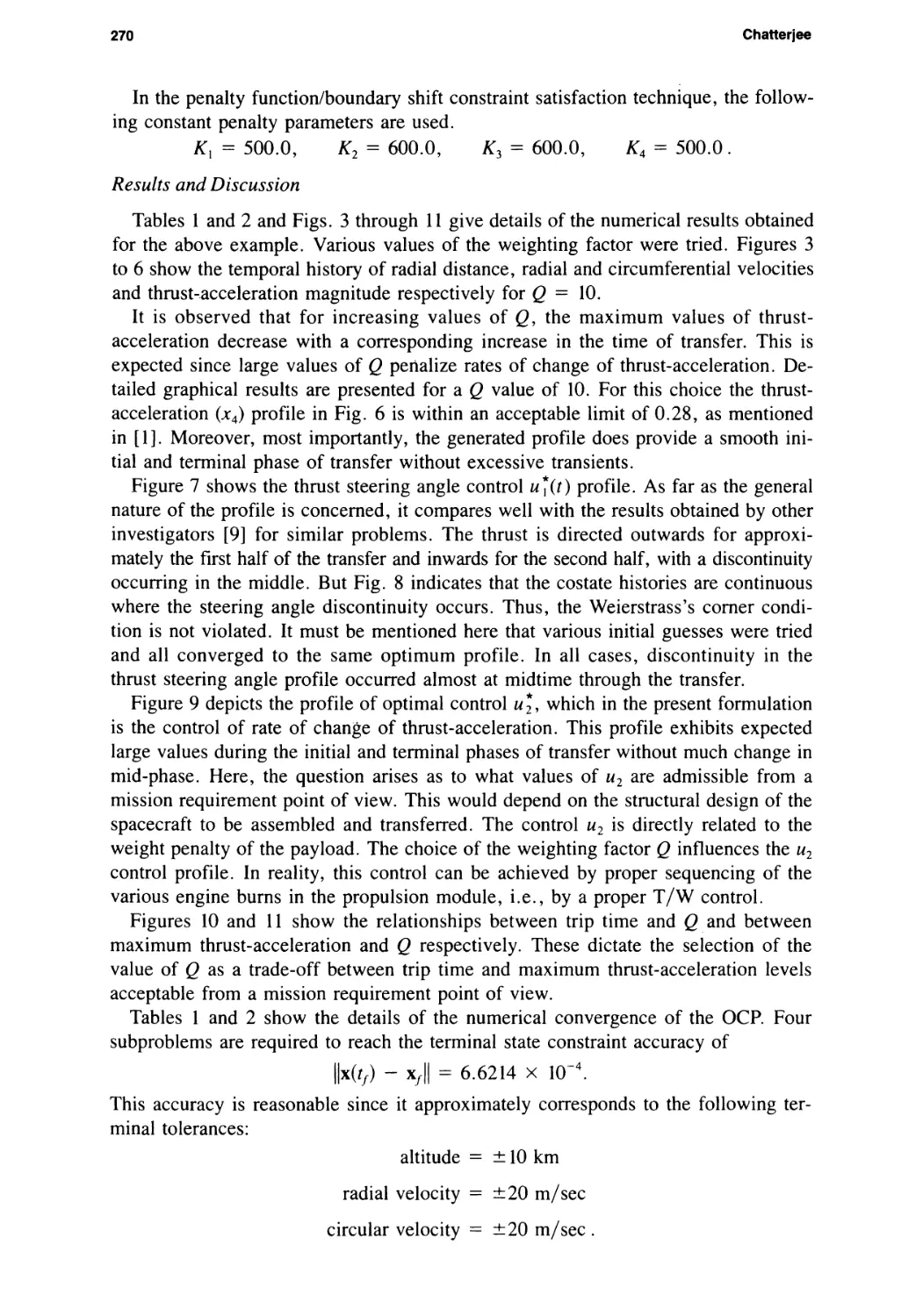
Challenger accident). Table 1 lists data pertaining to the satellite tour. In 10 orbits
about Jupiter, there are 15 encounters with the three outermost Galilean satellites:
10 close flybys under 10,000 km, four distant flybys between 25,000 and 50,000 km,
and one additional Europa flyby at 123,000 km. Two of the flybys are at 200 km (the
minimum flyby altitude), and five of the orbits have two flybys.
TABLE 1. Galileo Satellite Tour
Jupiter Orbit
Flyby
Date
Altitude
(km)
Latitude
(deg)
Period
(days)
Inclination
(deg)
G1
03 Jul 1989
830
-15
65
3.7
G2
05 Sep 1989
792
-80
56
0.3
C3
29 Oct 1989
1403
- 4
40
0.1
E3A
31 Oct 1989
123174
- 4
40
0.1
E4
09 Dec 1989
315
- 3
27
0.0
G4A
11 Dec 1989
29343
5
29
0.0
E5A
07 Jan 1990
48022
- 5
29
0.0
G5
08 Jan 1990
6564
19
36
0.4
E6
12 Feb 1990
200
68
36
2.1
E7
19 Mar 1990
200
-71
35
0.2
G8
22 Apr 1990
945
-18
63
1.1
C8A
25 Apr 1990
25002
1
67
1.1
C9
01 Jul 1990
1636
-15
48
0.3
G10
14 Aug 1990
597
-11
117
0.8
E10A
15 Aug 1990
25118
18
114
0.8
Notes:
1. Flyby names consist of a satellite designation (Europa, Ganymede, Callisto) followed by the orbit num¬
ber. An “A” appended to the flyby name denotes a secondary, distant flyby on the same orbit.
2. Orbit period and inclination are post-flyby elements.
3. Inclination is relative to Jupiter’s equator.
218
D’Amario
This satellite tour requires a total А V for planned trajectory modifications of only
47 m/s. The breakdown of this total is shown in Table 2. To be able to generate a
15-flyby, 10-orbit satellite tour which requires a total AV of only 47 m/s is quite an
accomplishment. Without the optimization capability of MOSES, this satellite tour
would not be feasible, because it would cost many hundreds of meters per second.
Interplanetary Trajectory Optimization
The concept of minimizing total AV for a satellite tour has a natural extension to
interplanetary trajectories. The central body becomes the Sun, and the flyby bodies
are planets. Interplanetary trajectories with one or more gravity-assist flybys of
planets have been used already for planetary missions (Mariner Venus/Mercury,
Pioneers 10 and 11, and Voyager) and will become more common in the future —
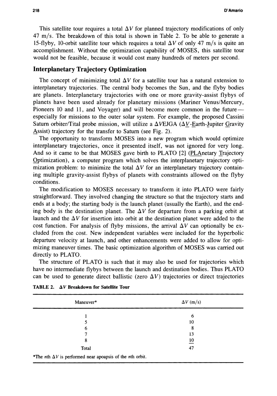
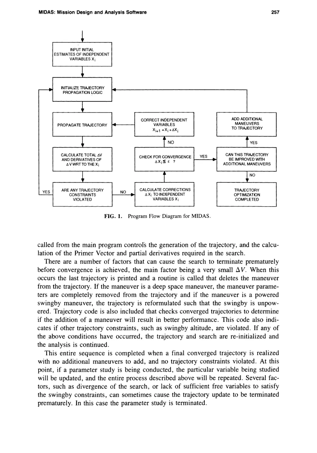
especially for missions to the outer solar system. For example, the proposed Cassini
Saturn orbiter/Tital probe mission, will utilize a AVEJGA (AV-Earth-Jupiter Gravity
Assist) trajectory for the transfer to Saturn (see Fig. 2).
The opportunity to transform MOSES into a new program which would optimize
interplanetary trajectories, once it presented itself, was not ignored for very long.
And so it came to be that MOSES gave birth to PLATO [2] (PLAnetary Trajectory
Optimization), a computer program which solves the interplanetary trajectory opti¬
mization problem: to minimize the total AV for an interplanetary trajectory contain¬
ing multiple gravity-assist flybys of planets with constraints allowed on the flyby
conditions.
The modification to MOSES necessary to transform it into PLATO were fairly
straightforward. They involved changing the structure so that the trajectory starts and
ends at a body; the starting body is the launch planet (usually the Earth), and the end¬
ing body is the destination planet. The AV for departure from a parking orbit at
launch and the AV for insertion into orbit at the destination planet were added to the
cost function. For analysis of flyby missions, the arrival AV can optionally be ex¬
cluded from the cost. New independent variables were included for the hyperbolic
departure velocity at launch, and other enhancements were added to allow for opti¬
mizing maneuver times. The basic optimization algorithm of MOSES was carried out
directly to PLATO.
The structure of PLATO is such that it may also be used for trajectories which
have no intermediate flybys between the launch and destination bodies. Thus PLATO
can be used to generate direct ballistic (zero AV) trajectories or direct trajectories
TABLE 2. AV Breakdown for Satellite Tour
Maneuver*
AV (m/s)
1
6
5
10
6
8
7
13
8
10
Total
47
*The nth AV is performed near apoapsis of the nth orbit.
Trajectory Optimization Software for Planetary Mission Design
219
FIG. 2. Cassini 1996 VEJGA Trajectory to Saturn.
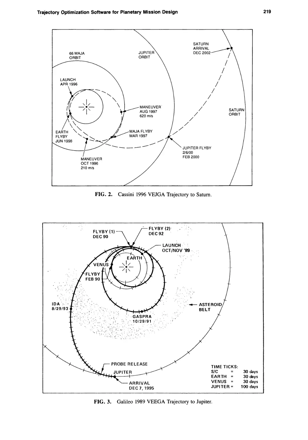
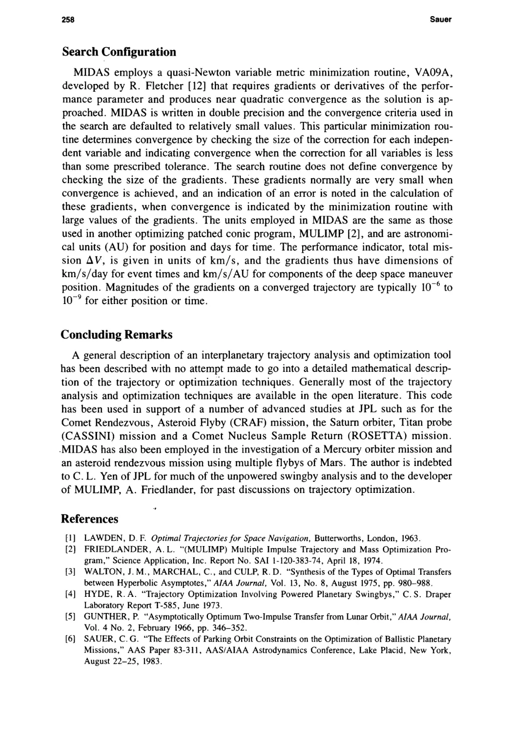
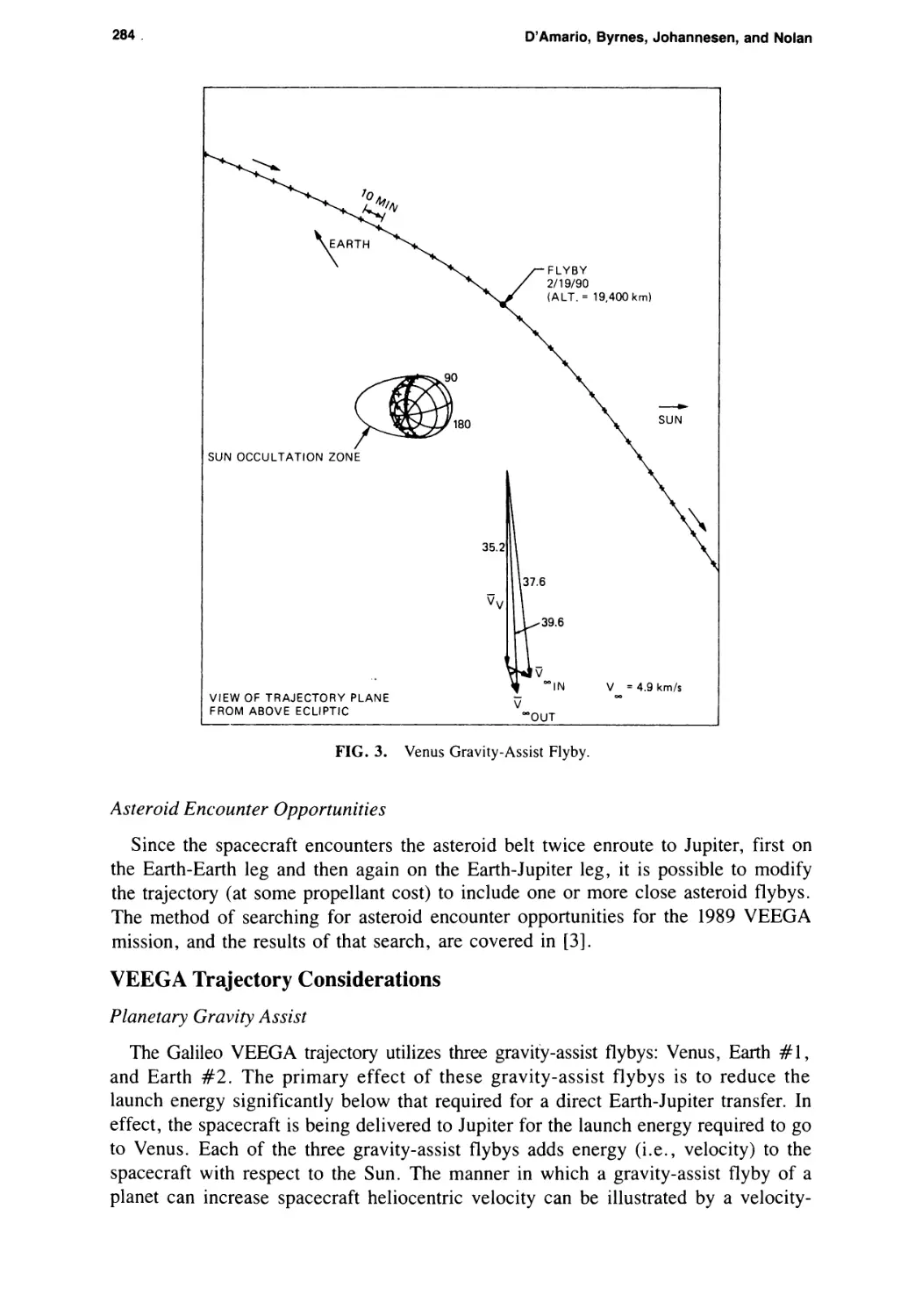
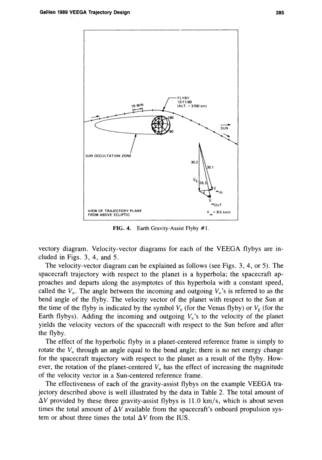
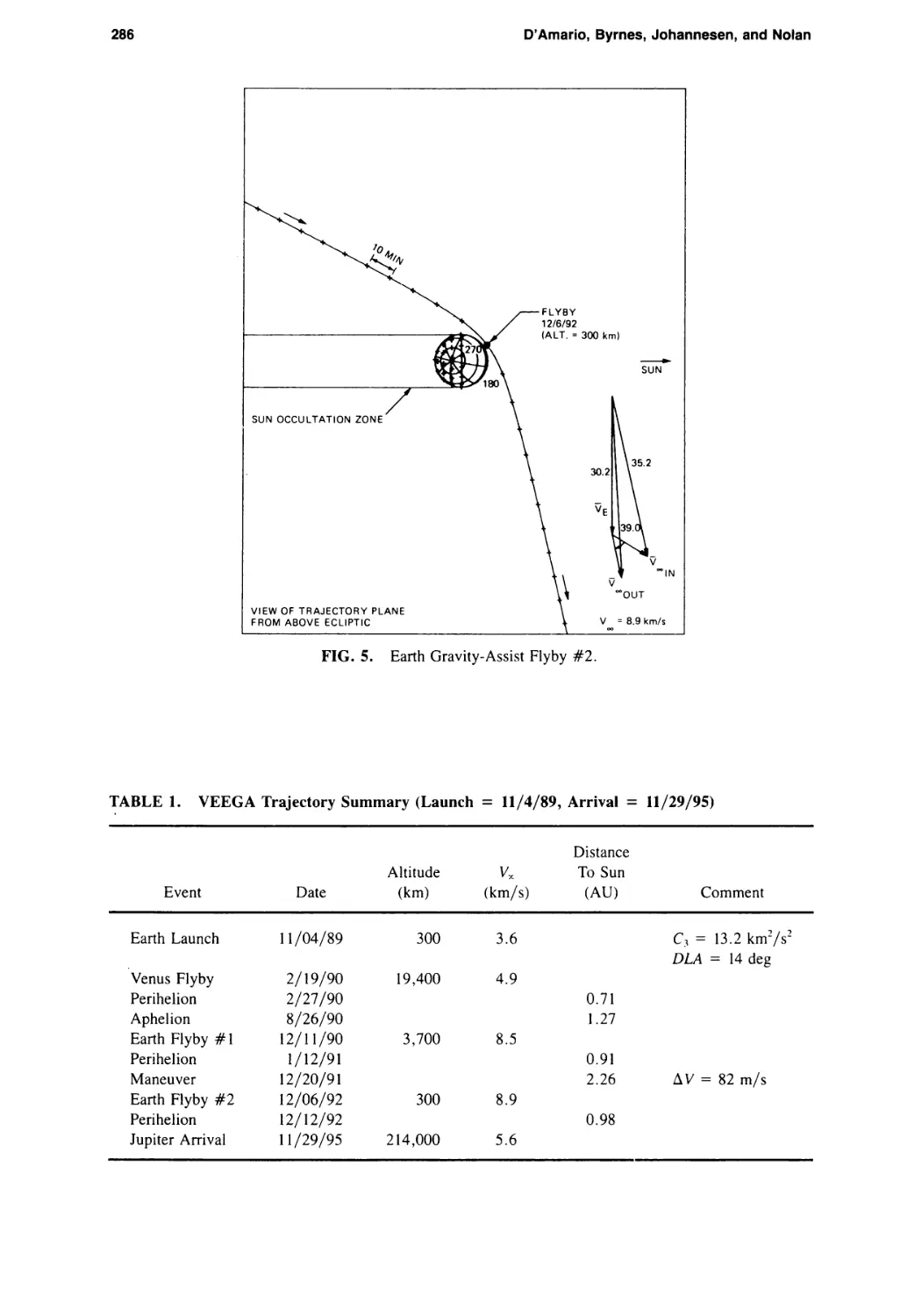
FIG. 3. Galileo 1989 VEEGA Trajectory to Jupiter.
220
D’Amario
with multiple large deep-space maneuvers. In addition, the launch, intermediate, and
destination bodies need not be planets — asteroids and comets are allowed.
Extensive use of PLATO has been made for interplanetary mission design at JPL.
It’s first application was for the Galileo Mission. Galileo has been subject to several
delays and injection-stage changes which have necessitated analysis of many different
interplanetary transfer modes, including a powered Mars flyby, VEGA (Venus-Earth
Gravity Assist), Д VEGA, and direct Earth-Jupiter transfers with large interplanetary
plane-change maneuvers. PLATO has been used in Galileo mission planning to de¬
sign and analyze the current baseline — a VEEGA (Venus-Earth-Earth Gravity Assist)
trajectory (see Fig. 3).
Non-Galileo applications for PLATO have occurred mostly in the area of future
outer-solar-system missions. Flyby and/or orbiter missions to Saturn, Uranus, Nep¬
tune, and Pluto were analyzed as candidates for a mission which would have utilized
a second Galileo spacecraft. Direct transfer, Jupiter gravity assist, and Д VEGA tra¬
jectory modes were investigated, where applicable. Rendevous missions to asteroids
and comets, some involving multiple Mars flybys or a Jupiter gravity assist were also
considered. Although a second Galileo spacecraft will not be built, the Cassini Saturn
orbiter/Titan probe mission, utilizing a new-generation Mariner Mark II spacecraft,
remains a high priority for NASA’s planetary program. Preliminary interplanetary
mission design for Cassini has been performed with PLATO. PLATO has also been
used to design trajectories for another mission in the Mariner Mark II program, the
CRAF (Comet Rendezvous/Asteroid Flyby) mission.
Conclusions
This paper documents the development of two software packages for optimizing
trajectories for planetary missions. Together, these two programs have significantly
enhanced the trajectory analysis and design capabilities at JPL for application to cur¬
rent and future missions which involve gravity assist flybys of planets and satellites
and/or large propulsive maneuvers.
References
[1] D’AMARIO, L. A., BYRNES, D. V., and STANFORD, R.H. “A New Method for Optimizing
Multiple Flyby Trajectories,” Journal of Guidance and Control, Vol. 4, No. 6, November-
December 1981, pp. 591-596.
[2] D’AMARIO, L. A., BYRNES, D. V., and STANFORD, R. H. “Interplanetary Trajectory Optimiza¬
tion with Application to Galileo,” Journal of Guidance, Control and Dynamics, Vol. 5, No. 5,
September-October 1982, pp. 465-471.
The Journal of the Astronautical Sciences, Vol. 37, No. 3, July-September 1989, pp. 221-232
Application of the Pseudostate Theory
to the Three-Body Lambert Problem
Dennis V. Byrnes
Abstract
The Pseudostate Theory, which approximates 3-body trajectories by overlapping the conic
effects of both massive bodies on the third body, has been used to solve boundary value prob¬
lems. Frequently, the approach to the secondary is quite close, as in interplanetary gravity assist
trajectories, or satellite tour trajectories. In this case the orbit with respect to the primary is
radically changed so that perturbation techniques are time consuming, yet higher accuracy than
point-to-point conics (Vx matching) is necessary. This method reduces the solution of the 3-
body Lambert problem to solving two conic Lambert problems and inverting a 7 X 7 matrix,
the components of which are all found analytically. Typically 90-95% of the point-to-point
conic error, with respect to an integrated trajectory, is eliminated.
Introduction
Many current or recent trajectory design problems include successive close ap¬
proaches to several different bodies. Interplanetary examples include Mariner Venus-
Mercury, Voyager and other Grand Tour type missions, and the interplanetary
portion of the Galileo mission which flies by Mars on the way to Jupiter. Even more
complex, from the design point of view, are the satellite tour trajectories for the Galileo
and proposed Saturn orbiter missions. The Galileo mission may involve as many as
11 or even more successive close approaches to some or all of the four Galilean satel¬
lites. Thus preliminary mission design requires a fast trajectory generation tool that
is as accurate as possible. Frequently point-to-point conic trajectories, which match
hyperbolic approach and departure magnitudes at the center of each flyby satellite,
have been used for much of the preliminary work. This approximation, when com¬
pared to integrated trajectories, is often not nearly good enough. The primary purpose
of this paper is to detail the application of the Pseudostate Theory due to Wilson [1],
to the solution of the 3-body Lambert problem, when a close flyby to the secondary
is involved. A second purpose is the derivation of the equations for the state transi¬
tion matrix (STM) associated with a particular trajectory segment.
The Pseudostate Theory solves, in an approximate manner, the equation of motion
for the tertiary body, in a restricted 3-body system, where the tertiary is of negligible
221
222
Byrnes
mass, its energy is positive with respect to the secondary, and the mass of the second¬
ary is small relative to the primary. This approximate solution is derived in detail in
[1], along with many numerical examples and comparisons with conic and integrated
trajectories for the Earth-Moon problem. Similar approximate solutions which are ap¬
plied successively over several steps form the basis for the various Multi-Conic tra¬
jectory propagation techniques (for details see Stumpff and Weiss [2], Byrnes and
Hooper [3], and D’Amario [4]). The common approximation made by all these meth¬
ods is that the individual terms in the equation of motion may be integrated indepen¬
dently, using conic solutions. This results in the true trajectory being approximated
by overlapping conics with respect to both the primary and the secondary, which are
combined in an appropriate fashion with constant velocity segments arising from the
constants of integration.
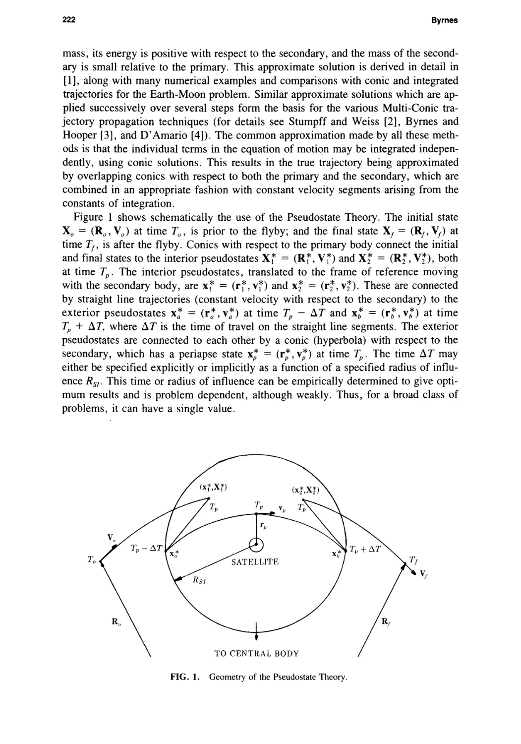
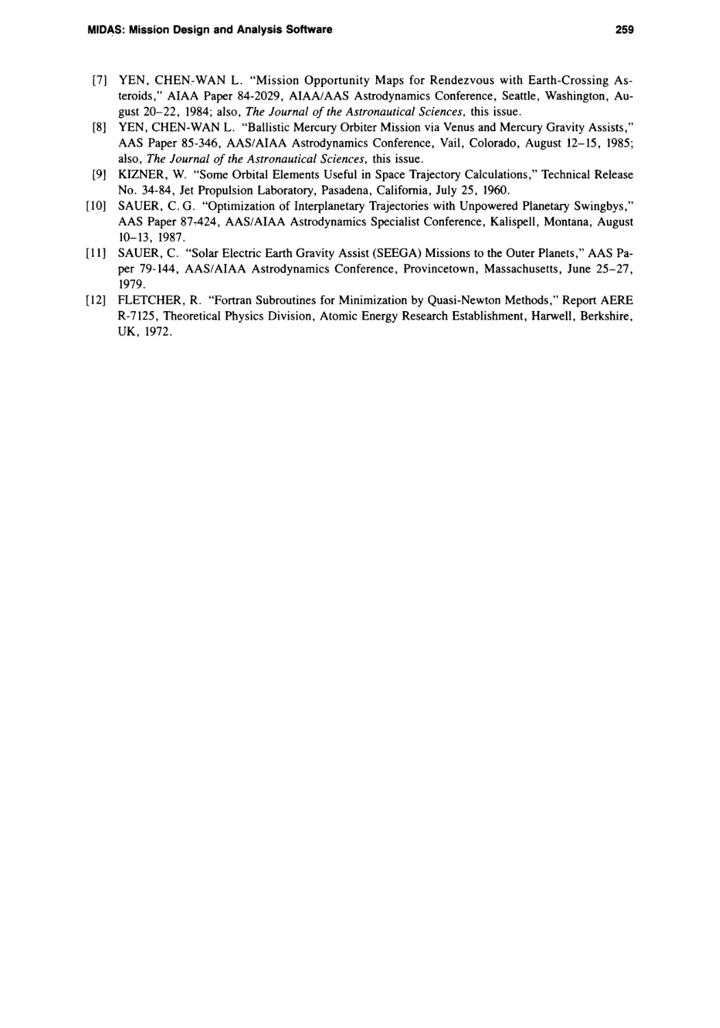
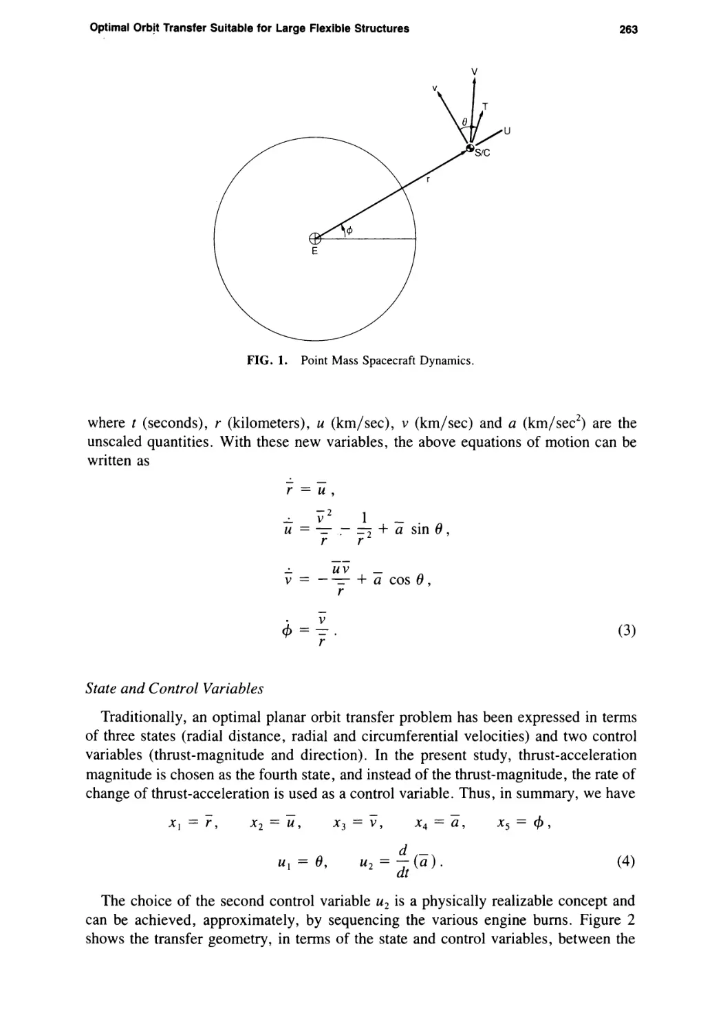
Figure 1 shows schematically the use of the Pseudostate Theory. The initial state
Xo = (Ro, VJ at time To, is prior to the flyby; and the final state Xf = (Rz, Vz) at
time Tf, is after the flyby. Conics with respect to the primary body connect the initial
and final states to the interior pseudostates X* = (R*, V*) and X* = (R*, V*), both
at time Tp. The interior pseudostates, translated to the frame of reference moving
with the secondary body, are x* = (r*, v*) and x* = (r*,v*). These are connected
by straight line trajectories (constant velocity with respect to the secondary) to the
exterior pseudostates x* = (r*,v*) at time Tp - AT and x* = (r*,v*) at time
Tp + AT, where AT is the time of travel on the straight line segments. The exterior
pseudostates are connected to each other by a conic (hyperbola) with respect to the
secondary, which has a periapse state x* =.(r*,v*) at time Tp. The time AT may
either be specified explicitly or implicitly as a function of a specified radius of influ¬
ence Rsl. This time or radius of influence can be empirically determined to give opti¬
mum results and is problem dependent, although weakly. Thus, for a broad class of
problems, it can have a single value.
t0
FIG. 1. Geometry of the Pseudostate Theory.
Application of the Pseudostate Theory to the Three-Body Lambert Problem
223
Trajectory Generation
Propagation
The use of the theory for propagation is quite simple:
1. Propagate a conic with respect to the primary from the initial time To to an esti¬
mate of the time of periapse Tp,
2. Translate to the secondary frame of reference and propagate back along a con¬
stant velocity trajectory to time Tp — AT, or to distance RSI,
3. Propagate a conic with respect to the secondary to time Tp + AT, or distance
4. Propagate back along a constant velocity trajectory to time Tp and translate to
the primary frame of reference,
5. Propagate a conic with respect to the primary to the final time 7},
6. If the actual time of periapse of the conic in Step 3 is not close enough to the
estimated Tp, replace Tp with the actual time of periapse, and repeat the process.
If the initial and/or final states are within the radius of influence, or if both initial and
final states are on the same side of periapse, some minor modification is necessary. If
Tp - To < AT, then in Step 2 the constant velocity trajectory must only go back to
To. Similarly, if Tf - T„ < AT, then in Step 3 the trajectory with respect to the sec¬
ondary must go only to Tf. If 7} is prior to periapse, then Steps 1 and 3 both go to 7},
and Steps 4 and 5 are eliminated. If To is after periapse, then Steps 1 and 2 are elimi¬
nated, and Step 4 goes back to To.
State Transition Matrix
The STM Ф(7}, To), relating changes in the final state Xf to changes in the initial
state Xo is given formally as
dRz/dRo dRf/dVo
dNf/dR0 dNf/dVo_
(1)
Referring to Fig. 1 and the first 5 steps discussed above for propagation, it is seen
that each step has associated with it an STM. These are denoted as Ф1а, Фа1, ФЬа,
Ф2Ь, and ФГ2; where Ф1о, ФЬа, and Ф/2 are the standard conic STM’s for 2-body
motion (for example see Goodyear [5]), and
ФО1 = Ф
I -IkT
0 7
(2)
are simply the STM along a constant velocity trajectory for a time increment of - AT.
The 3 x 3 identity matrix is denoted by 7.
An approximation to Ф/о, denoted by Ф/о, can be found by
% = O)
This is only an approximation, since equation (3) explicitly assumes that Tp does not
change. For the exact STM, Tp must in fact change in the differential sense due to the
224
Byrnes
variation in Xo. Thus, regarding Xf as depending explicitly on Xo, as well as Tp
which in turn depends on Xo:
xz= ХДХ^Г/Х,,)] (4)
the exact STM may be written as
dXf dXf dT . dXf dTD
Ф, = —f- + —- —- = Ф, + —- —- (5)
f0 дхо дтр axo f0 дтр dxo v 7
For many applications the approximation Ф/о is sufficiently accurate (usually good to
about 2-3 significant figures). If an STM exactly consistent with the trajectory model
is required, the additional terms on the right hand side of equation (5) must be com¬
puted. The derivation of these terms is given in Appendix A.
3-Body Lambert Solution
The 3-Body Lambert problem is a direct analog of the conic Lambert problem, in
that the initial and final positions and times are specified with the initial and final ve¬
locities to be found, thus determining the trajectory. Referring to Fig. 1; R6;, To, Ry,
and Tf are specified; No and Nf are to be found.
The use of the theory for the solution of boundary value problems presents several
alternatives. The simplest method is to use the STM partition relating final position to
initial velocity, varying initial velocity to reach a desired final position. A disadvan¬
tage of this method is that for a relatively close flyby, the sensitivity of end condi¬
tions to initial conditions is large, and there is also a very small region of linearity for
the STM. The outline of a much better behaved method with a far larger region of
linearity is as follows:
1. Using an estimate of the periapse state and time (Xp,Tp) generate the corre¬
sponding interior pseudostates X* and X*,
2. Using a standard Lambert method, solve the 2 conic boundary value problems
(R0,TJ ~ (R*,Tp) and (R*,Tp)
3. If the Lambert velocities at Tp on the primary conics are not sufficiently close
to V* and V*, vary (Xp,Tp) to zero the velocity differences, using the equa¬
tions derived in Appendix B.
The latter method has a large region of convergence primarily due to the fact that most
of the nonlinearity of the problem is involved in the 2 (conic) Lambert solutions. The
problem is thus reduced to solving 2 conic Lambert problems and a set of 7 linear
equations, the components of which are all found analytically. All this is given in de¬
tail in Appendix B. A great advantage of this method of solution, in addition to its
speed and large region of convergence, is that it is very similar to the solution to the
same problem using the point-to-point conic approximation. In that approximation
the state of the secondary is found at an estimate of the flyby time, and 2 Lambert
solutions are found between that state and the initial and final points. The flyby time
is then varied to match the incoming and outgoing V/s at the secondary. Thus the
point-to-point solution reduces to solving two 2 conic Lambert problems and iteration
on a scalar. Since the majority of the computation time is taken in the Lambert solu¬
tions, it is seen that the Pseudostate Theory solution, which iterates on 7 quantities
Application of the Pseudostate Theory to the Three-Body Lambert Problem
225
instead of 1, does not take a great deal more computation time than the point-to-point
solution. As will be seen below, however, a dramatic increase in accuracy is achieved.
Results
A number of test cases using the described method for solving the 3-Body Lambert
problem have been made. These test cases are from preliminary satellite tours for
the Galileo mission [6]. All of the Jupiter orbits are large eccentricity ellipses which
have periapses in the region of the Galilean satellites and apoapses much farther from
Jupiter. Each case is defined by taking subsequent pairs of Jovian apoapse states from
the point-to-point conic tour and solving the equivalent case both with the pseudostate
method and with a high precision integrated trajectory generator. The resulting veloci¬
ties Vo and Vy for each trajectory are then used to define errors for the point-to-point
conic and pseudostate data with respect to the precision data. The error measure is the
RSS of the 3 components of the velocity error at To and the 3 components of velocity
error at Tf taken together for each case. By having precision results available the
sphere radius or time ДТ can be varied for each pseudostate case to minimize the error
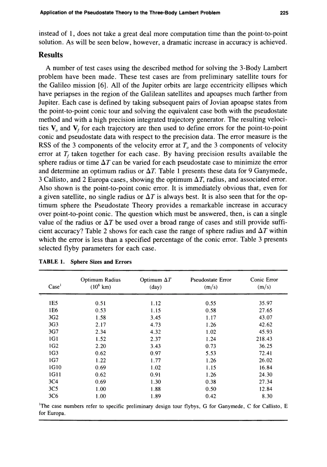
and determine an optimum radius or ДТ. Table 1 presents these data for 9 Ganymede,
3 Callisto, and 2 Europa cases, showing the optimum ДТ, radius, and associated error.
Also shown is the point-to-point conic error. It is immediately obvious that, even for
a given satellite, no single radius or ДТ is always best. It is also seen that for the op¬
timum sphere the Pseudostate Theory provides a remarkable increase in accuracy
over point-to-point conic. The question which must be answered, then, is can a single
value of the radius or ДТ be used over a broad range of cases and still provide suffi¬
cient accuracy? Table 2 shows for each case the range of sphere radius and ДТ within
which the error is less than a specified percentage of the conic error. Table 3 presents
selected flyby parameters for each case.
TABLE 1. Sphere Sizes and Errors
Case1
Optimum Radius
(106 km)
Optimum ДТ
(day)
Pseudostate Error
(m/s)
Conic Error
(m/s)
1E5
0.51
1.12
0.55
35.97
1E6
0.53
1.15
0.58
27.65
3G2
1.58
3.45
1.17
43.07
3G3
2.17
4.73
1.26
42.62
3G7
2.34
4.32
1.02
45.93
1G1
1.52
2.37
1.24
218.43
1G2
2.20
3.43
0.73
36.25
1G3
0.62
0.97
5.53
72.41
1G7
1.22
1.77
1.26
26.02
1G10
0.69
1.02
1.15
16.84
1G11
0.62
0.91
1.26
24.30
3C4
0.69
1.30
0.38
27.34
3C5
1.00
1.88
0.50
12.84
3C6
1.00
1.89
0.42
8.30
’The case numbers refer to specific preliminary design tour flybys, G for Ganymede, C for Callisto, E
for Europa.
226
Byrnes
TABLE 2. Sphere Sizes for Specified Error Levels
10% Error Level
20% Error Level
Case
Radius (106 km)
ДГ (day)
Radius (106 km)
ДГ (day)
1E5
0.21-1.26
0.45-2.76
1E6
0.21-1.34
0.45-2.91
3G2
0.76-3.19
1.71-6.94
0.37-6.68
0.82-14.56
3G3
1.21-3.90
2.64-8.52
0.64-7.30
1.41-15.95
3G7
1.07-5.08
1.98-9.39
0.48-11.37
0.89-21.03
1G1
0.01-223.
0.02-340.
0.01-395.
0.01-600.
1G2
1.06-4.58
1.64-7.13
0.50-9.75
0.78-15.17
1G3
0.36-1.08
0.56-1.68
0.13-3.00
0.20-4.66
1G7
0.62-2.40
0.89-3.49
0.27-5.49
0.39-7.99
1G10
0.48-0.99
0.71-1.47
0.27-1.76
0.40-2.60
1G11
0.35-1.10
0.51-1.63
0.17-2.28
0.25-3.38
3C4
0.15-3.08
0.29-5.78
3C5
0.52-1.91
0.98-3.59
3C6
0.67-1.49
1.26-2.81
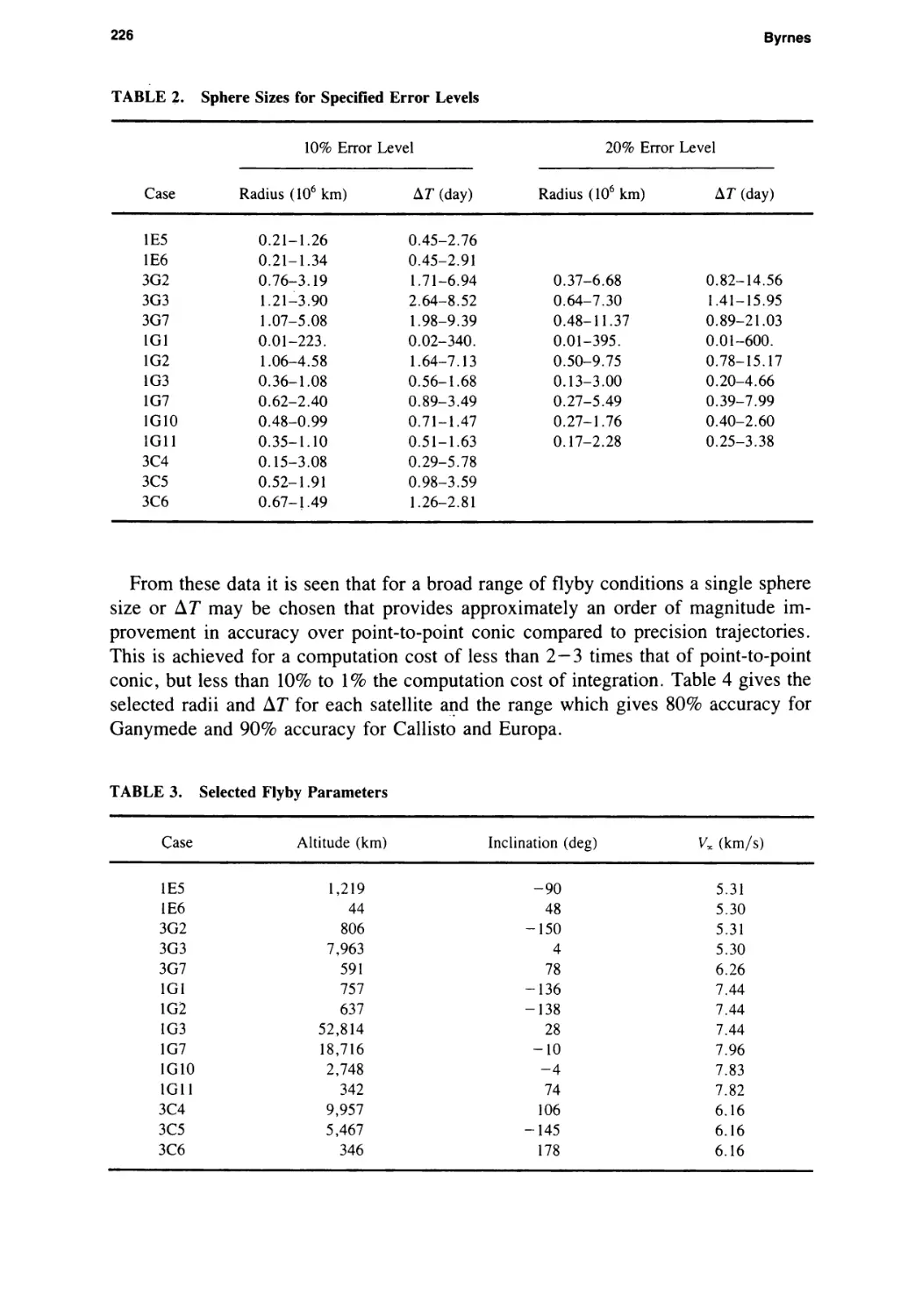
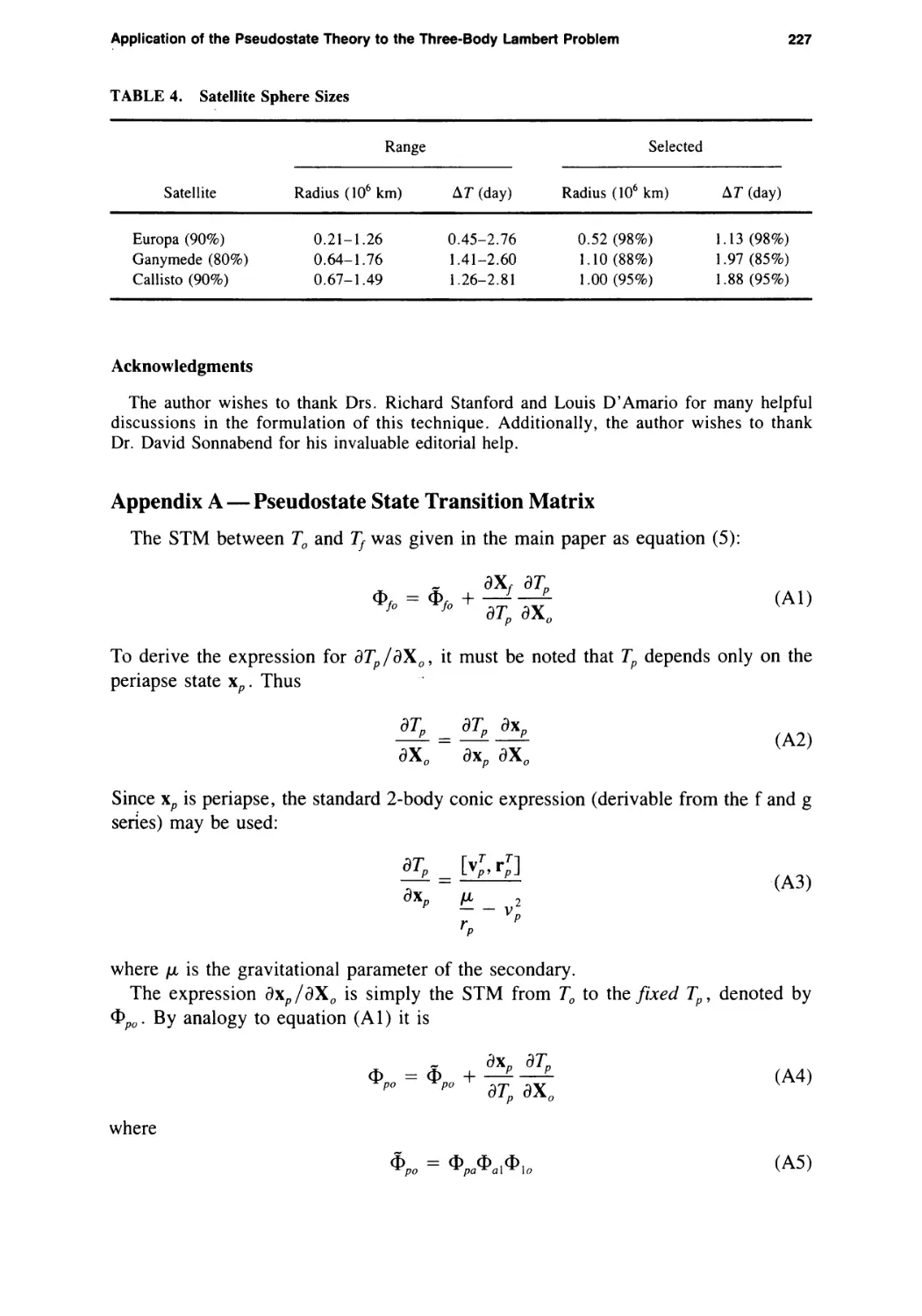
From these data it is seen that for a broad range of flyby conditions a single sphere
size or ДТ may be chosen that provides approximately an order of magnitude im¬
provement in accuracy over point-to-point conic compared to precision trajectories.
This is achieved for a computation cost of less than 2-3 times that of point-to-point
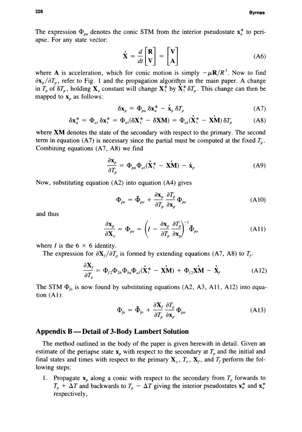
conic, but less than 10% to 1% the computation cost of integration. Table 4 gives the
selected radii and ДТ for each satellite and the range which gives 80% accuracy for
Ganymede and 90% accuracy for Callisto and Europa.
TABLE 3. Selected Flyby Parameters
Case
Altitude (km)
Inclination (deg)
Vx (km/s)
1E5
1,219
-90
5.31
1E6
44
48
5.30
3G2
806
-150
5.31
3G3
7,963
4
5.30
3G7
591
78
6.26
1G1
757
-136
7.44
1G2
637
-138
7.44
1G3
52,814
28
7.44
1G7
18,716
-10
7.96
1G10
2,748
-4
7.83
1G11
342
74
7.82
3C4
9,957
106
6.16
3C5
5,467
-145
6.16
3C6
346
178
6.16
Application of the Pseudostate Theory to the Three-Body Lambert Problem
227
TABLE 4. Satellite Sphere Sizes
Satellite
Range
Selected
Radius (106 km)
ДТ (day)
Radius (106 km)
ДТ (day)
Europa (90%)
0.21-1.26
0.45-2.76
0.52 (98%)
1.13 (98%)
Ganymede (80%)
0.64-1.76
1.41-2.60
1.10 (88%)
1.97 (85%)
Callisto (90%)
0.67-1.49
1.26-2.81
1.00 (95%)
1.88 (95%)
Acknowledgments
The author wishes to thank Drs. Richard Stanford and Louis D’Amario for many helpful
discussions in the formulation of this technique. Additionally, the author wishes to thank
Dr. David Sonnabend for his invaluable editorial help.
Appendix A — Pseudostate State Transition Matrix
The STM between To and Tf was given in the main paper as equation (5):
Ф/о = Ф/О +
axz дтр
дтр ax„
(Al)
To derive the expression for dTp/dX0, it must be noted that Tp depends only on the
periapse state xp. Thus
дТр = дТр дхр
дХ0 ~ дхр дХо
(А2)
Since хр is periapse, the standard 2-body conic expression (derivable from the f and g
series) may be used:
9TP [vj.rj]
(A3)
where fjL is the gravitational parameter of the secondary.
The expression dxp/dXo is simply the STM from To to the/zxeJ Tp, denoted by
Фри. By analogy to equation (Al) it is
where
ф — Ф H-
Y po po
этр
дТр дХ0
(А4)
(А5)
ф = ф ф ,ф,
ро ^ра^а\^\о
228
Byrnes
The expression Фра denotes the conic STM from the interior pseudostate x* to peri¬
apse. For any state vector:
d
R
V
dt
V
A
(A6)
where A is acceleration, which for conic motion is simply —/jlR/R3. Now to find
dxp/dTp, refer to Fig. 1 and the propagation algorithm in the main paper. A change
in Tp of dTp, holding Xo constant will change X* by X* 8Tp. This change can then be
mapped to xp as follows:
8xp = Фра 8x* - xp 8TP (A7)
8x* = Фа18х* = Ф0|(8Х* - 8XM) = ФО|(Х* - XM)8TP (А8)
where ХМ denotes the state of the secondary with respect to the primary. The second
term in equation (A7) is necessary since the partial must be computed at the fixed Tp.
Combining equations (A7, A8) we find
Now, substituting equation (A2) into equation (A4) gives
and thus
(A9)
(A10)
(All)
where I is the 6 x 6 identity.
The expression for 3Xf/dTp is formed by extending equations (A7, A8) to 7}:
= Ф/2ФЙФЛ№ - ХМ) + ФрХМ - Xf (A12)
The STM Ф/о is now found by substituting equations (A2, A3, All, A12) into equa¬
tion (Al):
dXf dTp
ф'--ф" + й-^ф- (A13)
Appendix В — Detail of 3-Body Lambert Solution
The method outlined in the body of the paper is given herewith in detail. Given an
estimate of the periapse state xp with respect to the secondary at Tp and the initial and
final states and times with respect to the primary Xo, To, Xf, and Tf perform the fol¬
lowing steps:
1. Propagate xp along a conic with respect to the secondary from Tp forwards to
Tp + AT and backwards to Tp - AT giving the interior pseudostates x* and x*
respectively,
Application of the Pseudostate Theory to the Three-Body Lambert Problem
229
2. Compute the exterior primary centered pseudostates as:
R* = r* + v* ДТ + RM; V* = v* + VM (Bl)
R* = r? - v* ДТ + RM; V* = v? + VM (B2)
where RM and VM are the position and velocity of the secondary with respect
to the primary,
3. Using a standard Lambert method, solve the 2 conic Lambert problems be¬
tween the initial and final positions and R* and R* respectively:
(R0,T0) (R*,rp)=> Vo, V, (B3)
(R*, TJ (Rp Tf) V2, Nf (B4)
where Vj and V2 are the Lambert velocities at R* and R* respectively,
4. Form the differences in velocity at R* and R* as:
AVi = V* - V,; ДV2 = V* - V2 (B5)
5. Using the components of xp and Tp as 7 independent variables, reduce the 6
components of Д Vj and Д V2 to zero while holding a = rp • vp = 0 (forcing xp
always to be a periapse state).
The process described in Step 5 is accomplished by using a Newton iteration on the 7
independent parameters. The equations are:
(B6)
where W = [ДV1? AV2, a]. The partials necessary for equation (B6) can all be found
analytically. Needed are the STM’s from xp to X* and X* given by
Ф>„ = ФЛ; Ф2Р =
(B7)
where Фар and Ф(,р are the 2-body STM’s corresponding to Step 1 above, and
Ф.О
/ /ДТ
0 /
ф» =
/ -/ДТ
0 I
(B8)
with I being the 3 X 3 identity.
The four 3x3 partitions of any STM will be denoted as
(B9)
Then,
ЭДУ) _ av£ _ av,
drp Эгр Эгр
where
dV* _ d(v* + VM) _ 3yt _ c
drp drp drp lp
(BIO)
(Bll)
230
Byrnes
and
ay, av, aR*
drp ~ dR* drp
(B12)
The partial derivative dVj/dR* is one of the Lambert Problem partials, and can be
found from consideration of 2-body formulae as in [7], or from general considerations
as in [8]. It is given simply as
—-L = n R~l
dR* 10 10
and
dR* _ d(r* + RM) _ dr* _
drp drp drp A[p
Thus combining equations (B10) through (B14)
(B13)
(B14)
DioB
-i
lo
(B15)
4
In a similar fashion
аду,
дУр
(B16)
Using the other Lambert partial from [8]
aR?
— Bf2 A.f2
(B17)
it is immediately seen that
and
аду2
— Qp + ^f2 ^f2^2p
(B18)
(B19)
The partials with respect to Tp are found as
аду, av? jv,
dTp ~ dTp dTp
where
(B20)
av? _ a(v? + vm)
dTp ~ dTp
AM
(B21)
AM is used for the acceleration of the secondary with respect to the primary and is
simply
AM = -(Mp + Ms)RM/(W
(B22)
Application of the Pseudostate Theory to the Three-Body Lambert Problem
231
where ц,р and are the gravitational parameters of the primary and secondary re¬
spectively. Next, since Vj in the conic Lambert problem depends on Tp both explicitly
and implicitly through R*, the partial has 2 terms
dTp
The Lambert partial from [8] is
dVj эк*
dTp dRf dTp
(B23)
where the acceleration is
and
av.
dTp
+ A,
(B24)
A, =
(B25)
9R* _ 8(r* + RM)
dTp ~ dTp
(B26)
Thus, combining equations (B20) through (B26)
= DloBrJ(V, - VM) - A, + AM
dTp
(B27)
Similarly,
dAV2
dTp
-B^2'Af2(y2 - VM) - A2 + AM
(B28)
The partials of a are given as
(B29)
where the superscript T denotes the transpose.
With equations (B15), (B16), (B18), (B19), and (B27) through (B29) defining the
partials, equation (B6) can be solved iteratively, updating the estimated xp and Tp.
References
[1] WILSON, S. W. “A Pseudostate Theory for the Approximation of Three-Body Trajectories,” AIAA
Paper No. 70-1061, presented at the AIAA Astrodynamics Conference, Santa Barbara, California,
August 1970.
[2] STUMPFF, K. and WEISS, E. H. “Applications of an N-Body Reference Orbit,” Journal of the
Astronautical Sciences, Vol. XV, No. 5, September-October 1968, pp. 257-261.
[3] BYRNES, D.V. and HOCKER, H. L. “Multi-conic: A Fast and Accurate Method of Computing
Space Flight Trajectories,” AIAA Paper No. 70-1062, presented at the AIAA Astrodynamics Confer¬
ence, Santa Barbara, California, August 1970.
[4] D’AMARIO, L. A. “Minimum Impulse Three-Body Trajectories,” Ph.D. Dissertation, Massachu¬
setts Institute of Technology, June 1973.
[5] GOODYEAR, W. H. “A General Method for the Computation of Cartesian Coordinates and Partial
Derivatives of the Two-Body Problem,” NASA CR-522, September 1966.
232 Byrnes
[6] DIEHL, R. E. and NOCK, K.T. “Galileo Jupiter Encounter and Satellite Tour Trajectory Design,”
AIAA Paper No. 79-141, presented at the AAS/AIAA Astrodynamics Specialist Conference,
Provincetown, Massachusetts, June 1979.
[7] BAYLISS, S. “Precision Targeting for Multiple Swingby Planetary Trajectories,” AIAA Paper
No. 71-191, presented at the AIAA 9th Aerospace Sciences Meeting, New York, New York, January
1971.
[8] D’AMARIO, L.A., BYRNES, D. V., SACKETT, L. L. and STANFORD, R. H. “Optimization of
Multiple Flyby Trajectories,” AIAA Paper No. 79-162, presented at the AAS/AIAA Astrodynamics
Specialist Conference, Provincetown, Massachusetts, June 1979.
The Journal of the Astronautical Sciences, Vol. 37, No. 3, July-September 1989, pp. 233-250
Some Notes on Applying the One-step
Multiconic Method of Trajectory
Propagation1
Theodore H. Sweetser
Abstract
The one-step multiconic method (also called the pseudostate method) has been known for
years to offer up to an order of magnitude of improvement over the patched-conic method for
propagating trajectories under the gravitational influence of two bodies. In these notes I will
first describe the method and some of its variations. Then I will examine a crucial parameter of
this method, the sweepback duration, and show that the traditional wisdom concerning this pa¬
rameter should be replaced by an algorithm which relates it to the trajectory characteristics.
Remarkably, this algorithm is independent of the masses of the primary and secondary bodies.
Introduction
The one-step multiconic method of trajectory propagation is a simplified version of
the overlapped conic method, first presented by S. Wilson at the Astrodynamics Con¬
ference in 1970 [1]; he called this simplification the pseudostate method. The method
is much more accurate than the patched conic method, and yet is a computationally
comparable way to propagate a trajectory of a spacecraft under the gravitational influ¬
ence of two bodies when the mass of the secondary is small compared to the primary
and the trajectory is hyperbolic with respect to the secondary.
The development of the one-step multiconic method was originally motivated by
the problem of propagating trajectories in the Earth-Moon system for the Apollo pro¬
gram. While trajectory integrators existed which could do such propagations with
very high precision, such methods are too computationally demanding to allow their
use in solving targeting and optimization problems when many propagations need to
be done to find the solution. On the other hand, conic and even patched-conic propa¬
gations are too inaccurate — targeting and optimization in the conic model do not
translate to solutions in the more accurate integrated model. Multiconic methods of¬
fered an effective compromise between computational speed and accuracy.
'Based on Paper No. AAS 87-469, AAS/AIAA Astrodynamics Conference, Kalispell, Montana, August
10-13, 1987.
233
234
Sweetser
The same advantages apply to interplanetary mission design. The Galileo mission
in particular has used a multiconic optimizer to plan both the transfer trajectory to Ju¬
piter and the satellite tour around Jupiter. Similarly, a multiconic trajectory optimizer
has proved to be an essential tool in the planning of the Comet Rendezvous/Asteroid
Flyby and Cassini (Saturn orbiter/Titan probe) missions being proposed by NASA.
In these notes I will first describe the one-step multiconic method, then present a
number of variations, mostly taken from the literature. Then in the context of the
classical one-step method and what I call the v-infinity variation, I will examine in
more detail a crucial parameter of the method — the duration of the linear sweepback
which connects the two conics alluded to in the name of the method. Remarkably, it
turns out that the optimal value for this parameter depends only on the geometry of
the trajectory, and is independent of the masses (both absolute and relative) of the
primary and secondary bodies and of the distance between them.
The method itself falls into two classes according to whether the trajectory is ap¬
proaching or departing from the secondary. Given an initial time and state of the
spacecraft relative to the primary, where the spacecraft is approaching the secondary,
the steps are as follows:
1. Propagate the trajectory to the desired time as a conic relative to the primary
body;
2. Transform the primary-centered state to a state with respect to the secondary
body;
3. Back up in a straight line along the new velocity vector for some fixed time;
4. Propagate forward for the same fixed time as a conic relative to the secondary
body.
This algorithm can be seen more graphically in Figs. 1(a) and 1(b).
For a trajectory departing from a secondary body, simply reverse the order of the
steps: transform to a secondary-relative state if necessary, do the conic around the
secondary body for a fixed time, back up in a straight line for the same fixed time,
transform to a primary-centered state, and follow a conic around the primary to the
desired time.
Other types of trajectories can be handled as combinations of these two types. For
example, a flyby can be handled as an approach followed by a departure, where an
iterative search may be needed to find the correct flyby time. Or a transfer trajectory
from one secondary body to another can be treated as a departure from the first
secondary body to some intermediate time followed by an approach to the second
secondary body. State transition matrices can also be calculated for one-step propaga¬
tions [2].
Variations on the One-step Multiconic Method
The Rectilinear Pseudostate Method [3]
This method is implicit in the work presented by Sergeyevsky et al., who actually
described a way to fit a modified multiconic transfer between two secondary bodies
where the approach and departure conditions are not known. As a propagation
method it applies more clearly to a departure; in this case the initial state is primary¬
centered and coincides in position with that of the secondary body at the initial time.
Applying the One-step Multiconic Method of Trajectory Propagation
235
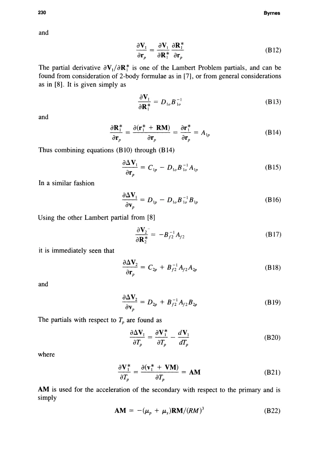
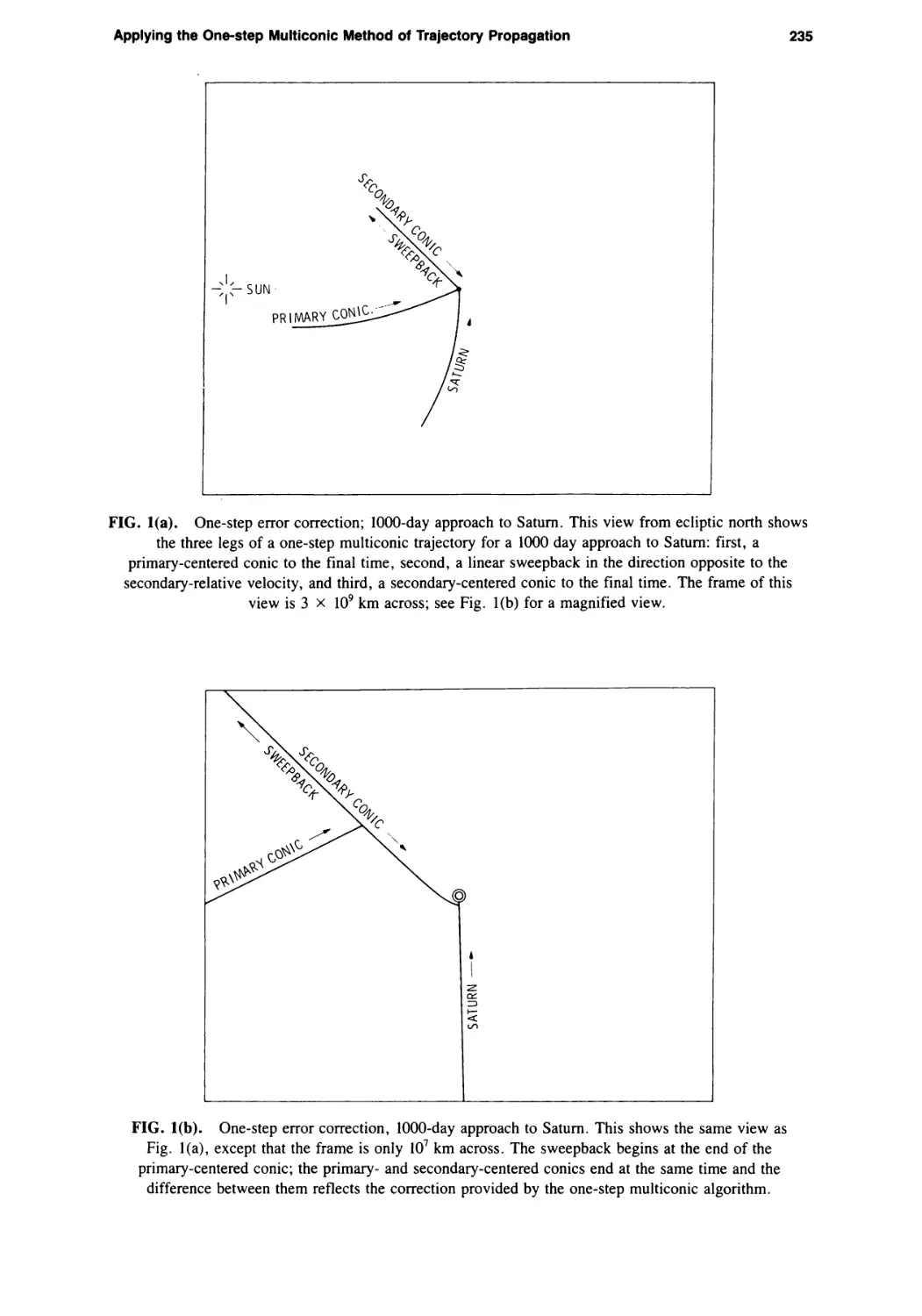
FIG. 1(a). One-step error correction; 1000-day approach to Saturn. This view from ecliptic north shows
the three legs of a one-step multiconic trajectory for a 1000 day approach to Saturn: first, a
primary-centered conic to the final time, second, a linear sweepback in the direction opposite to the
secondary-relative velocity, and third, a secondary-centered conic to the final time. The frame of this
view is 3 x Ю9 km across; see Fig. 1(b) for a magnified view.
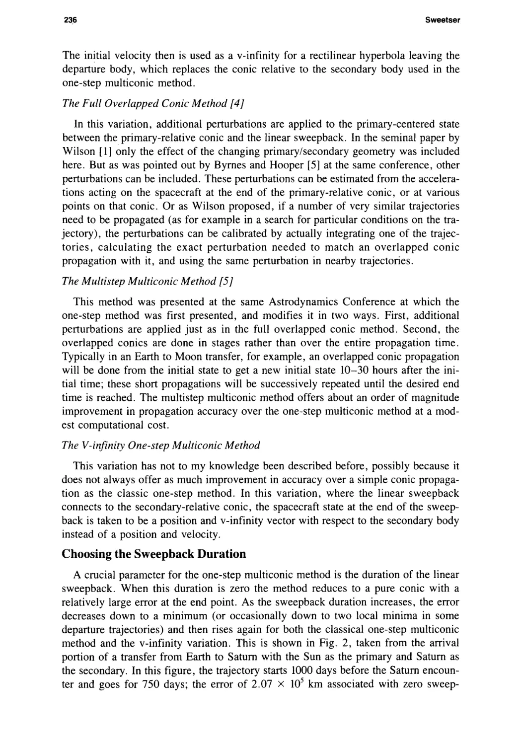
FIG. 1(b). One-step error correction, 1000-day approach to Saturn. This shows the same view as
Fig. 1(a), except that the frame is only 107 km across. The sweepback begins at the end of the
primary-centered conic; the primary- and secondary-centered conics end at the same time and the
difference between them reflects the correction provided by the one-step multiconic algorithm.
236
Sweetser
The initial velocity then is used as a v-infinity for a rectilinear hyperbola leaving the
departure body, which replaces the conic relative to the secondary body used in the
one-step multiconic method.
The Full Overlapped Conic Method [4]
In this variation, additional perturbations are applied to the primary-centered state
between the primary-relative conic and the linear sweepback. In the seminal paper by
Wilson [1] only the effect of the changing primary/secondary geometry was included
here. But as was pointed out by Byrnes and Hooper [5] at the same conference, other
perturbations can be included. These perturbations can be estimated from the accelera¬
tions acting on the spacecraft at the end of the primary-relative conic, or at various
points on that conic. Or as Wilson proposed, if a number of very similar trajectories
need to be propagated (as for example in a search for particular conditions on the tra¬
jectory), the perturbations can be calibrated by actually integrating one of the trajec¬
tories, calculating the exact perturbation needed to match an overlapped conic
propagation with it, and using the same perturbation in nearby trajectories.
The Multistep Multiconic Method [5]
This method was presented at the same Astrodynamics Conference at which the
one-step method was first presented, and modifies it in two ways. First, additional
perturbations are applied just as in the full overlapped conic method. Second, the
overlapped conics are done in stages rather than over the entire propagation time.
Typically in an Earth to Moon transfer, for example, an overlapped conic propagation
will be done from the initial state to get a new initial state 10-30 hours after the ini¬
tial time; these short propagations will be successively repeated until the desired end
time is reached. The multistep multiconic method offers about an order of magnitude
improvement in propagation accuracy over the one-step multiconic method at a mod¬
est computational cost.
The V-infinity One-step Multiconic Method
This variation has not to my knowledge been described before, possibly because it
does not always offer as much improvement in accuracy over a simple conic propaga¬
tion as the classic one-step method. In this variation, where the linear sweepback
connects to the secondary-relative conic, the spacecraft state at the end of the sweep-
back is taken to be a position and v-infinity vector with respect to the secondary body
instead of a position and velocity.
Choosing the Sweepback Duration
A crucial parameter for the one-step multiconic method is the duration of the linear
sweepback. When this duration is zero the method reduces to a pure conic with a
relatively large error at the end point. As the sweepback duration increases, the error
decreases down to a minimum (or occasionally down to two local minima in some
departure trajectories) and then rises again for both the classical one-step multiconic
method and the v-infinity variation. This is shown in Fig. 2, taken from the arrival
portion of a transfer from Earth to Saturn with the Sun as the primary and Saturn as
the secondary. In this figure, the trajectory starts 1000 days before the Saturn encoun¬
ter and goes for 750 days; the error of 2.07 x 10⁵ km associated with zero sweep-
Applying the One-step Multiconic Method of Trajectory Propagation
237
SWEEPBACK TIME (106 sec)
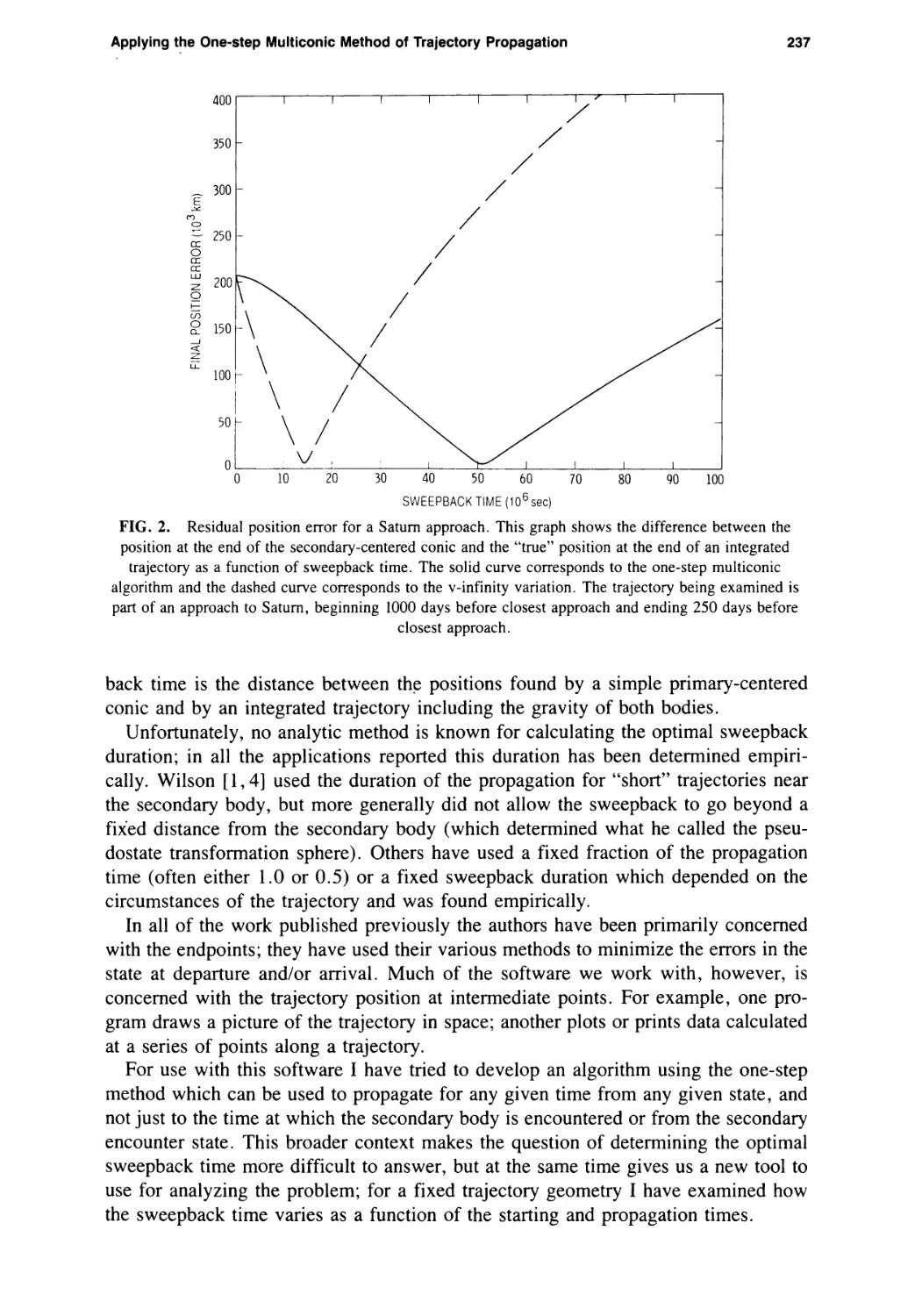
FIG. 2. Residual position error for a Saturn approach. This graph shows the difference between the
position at the end of the secondary-centered conic and the “true” position at the end of an integrated
trajectory as a function of sweepback time. The solid curve corresponds to the one-step multiconic
algorithm and the dashed curve corresponds to the v-infinity variation. The trajectory being examined is
part of an approach to Saturn, beginning 1000 days before closest approach and ending 250 days before
closest approach.
back time is the distance between the positions found by a simple primary-centered
conic and by an integrated trajectory including the gravity of both bodies.
Unfortunately, no analytic method is known for calculating the optimal sweepback
duration; in all the applications reported this duration has been determined empiri¬
cally. Wilson [1,4] used the duration of the propagation for “short” trajectories near
the secondary body, but more generally did not allow the sweepback to go beyond a
fixed distance from the secondary body (which determined what he called the pseu¬
dostate transformation sphere). Others have used a fixed fraction of the propagation
time (often either 1.0 or 0.5) or a fixed sweepback duration which depended on the
circumstances of the trajectory and was found empirically.
In all of the work published previously the authors have been primarily concerned
with the endpoints; they have used their various methods to minimize the errors in the
state at departure and/or arrival. Much of the software we work with, however, is
concerned with the trajectory position at intermediate points. For example, one pro¬
gram draws a picture of the trajectory in space; another plots or prints data calculated
at a series of points along a trajectory.
For use with this software I have tried to develop an algorithm using the one-step
method which can be used to propagate for any given time from any given state, and
not just to the time at which the secondary body is encountered or from the secondary
encounter state. This broader context makes the question of determining the optimal
sweepback time more difficult to answer, but at the same time gives us a new tool to
use for analyzing the problem; for a fixed trajectory geometry I have examined how
the sweepback time varies as a function of the starting and propagation times.
238
Sweetser
Approach Trajectories
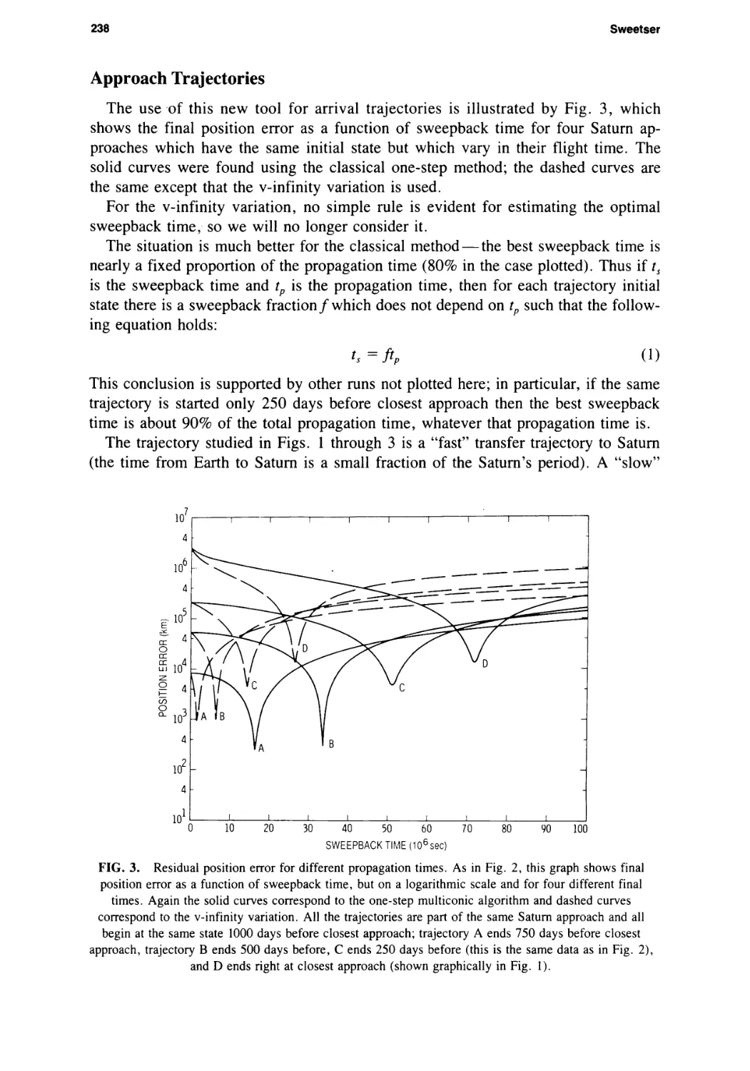
The use of this new tool for arrival trajectories is illustrated by Fig. 3, which
shows the final position error as a function of sweepback time for four Saturn ap¬
proaches which have the same initial state but which vary in their flight time. The
solid curves were found using the classical one-step method; the dashed curves are
the same except that the v-infinity variation is used.
For the v-infinity variation, no simple rule is evident for estimating the optimal
sweepback time, so we will no longer consider it.
The situation is much better for the classical method — the best sweepback time is
nearly a fixed proportion of the propagation time (80% in the case plotted). Thus if ts
is the sweepback time and tp is the propagation time, then for each trajectory initial
state there is a sweepback fraction /which does not depend on tp such that the follow¬
ing equation holds:
ts=ftP (1)
This conclusion is supported by other runs not plotted here; in particular, if the same
trajectory is started only 250 days before closest approach then the best sweepback
time is about 90% of the total propagation time, whatever that propagation time is.
The trajectory studied in Figs. 1 through 3 is a “fast” transfer trajectory to Saturn
(the time from Earth to Saturn is a small fraction of the Saturn’s period). A “slow”
FIG. 3. Residual position error for different propagation times. As in Fig. 2, this graph shows final
position error as a function of sweepback time, but on a logarithmic scale and for four different final
times. Again the solid curves correspond to the one-step multiconic algorithm and dashed curves
correspond to the v-infinity variation. All the trajectories are part of the same Saturn approach and all
begin at the same state 1000 days before closest approach; trajectory A ends 750 days before closest
approach, trajectory В ends 500 days before, C ends 250 days before (this is the same data as in Fig. 2),
and D ends right at closest approach (shown graphically in Fig. 1).
Applying the One-step Multiconic Method of Trajectory Propagation
239
transfer from near Earth to the Moon (nearly Hohmann and taking 14 days) was also
studied. In this latter case the one-step method only offered significant improvement
for propagations taking less than half the time of the total lunar approach, but again
for those propagations the best sweepback time stayed fixed at about 50% of the
propagation time.
An immediate conclusion is that the pseudostate sphere of influence hypothesized
by S.Wilson is not useful for general propagation; the first two propagations shown
in Fig. 3 had the endpoint of the optimal sweepback well outside the pseudostate
transformation sphere given in [4].
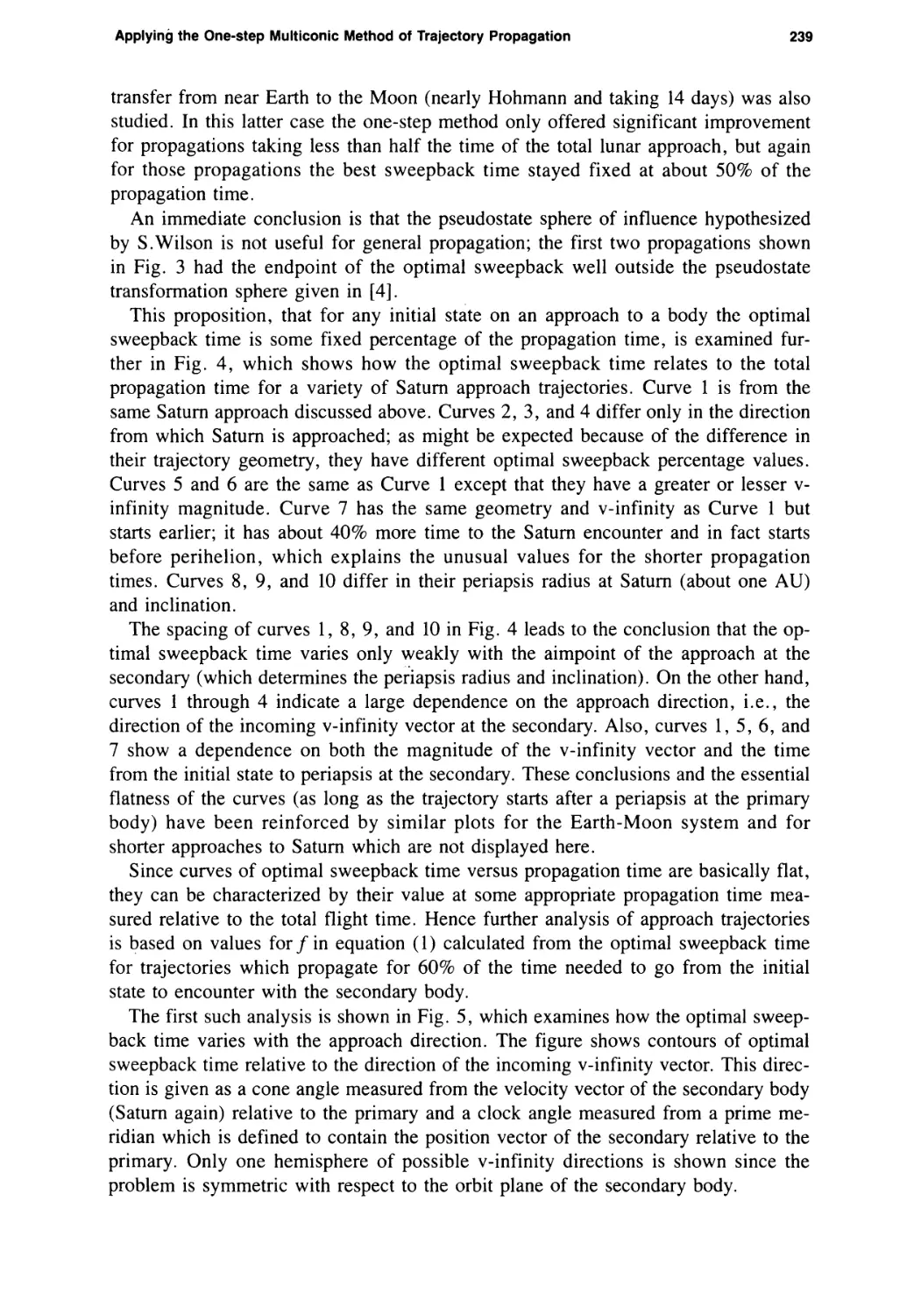
This proposition, that for any initial state on an approach to a body the optimal
sweepback time is some fixed percentage of the propagation time, is examined fur¬
ther in Fig. 4, which shows how the optimal sweepback time relates to the total
propagation time for a variety of Saturn approach trajectories. Curve 1 is from the
same Saturn approach discussed above. Curves 2,3, and 4 differ only in the direction
from which Saturn is approached; as might be expected because of the difference in
their trajectory geometry, they have different optimal sweepback percentage values.
Curves 5 and 6 are the same as Curve 1 except that they have a greater or lesser v-
infinity magnitude. Curve 7 has the same geometry and v-infinity as Curve 1 but
starts earlier; it has about 40% more time to the Saturn encounter and in fact starts
before perihelion, which explains the unusual values for the shorter propagation
times. Curves 8,9, and 10 differ in their periapsis radius at Saturn (about one AU)
and inclination.
The spacing of curves 1, 8, 9, and 10 in Fig. 4 leads to the conclusion that the op¬
timal sweepback time varies only weakly with the aimpoint of the approach at the
secondary (which determines the periapsis radius and inclination). On the other hand,
curves 1 through 4 indicate a large dependence on the approach direction, i.e., the
direction of the incoming v-infinity vector at the secondary. Also, curves 1,5,6, and
7 show a dependence on both the magnitude of the v-infinity vector and the time
from the initial state to periapsis at the secondary. These conclusions and the essential
flatness of the curves (as long as the trajectory starts after a periapsis at the primary
body) have been reinforced by similar plots for the Earth-Moon system and for
shorter approaches to Saturn which are not displayed here.
Since curves of optimal sweepback time versus propagation time are basically flat,
they can be characterized by their value at some appropriate propagation time mea¬
sured relative to the total flight time. Hence further analysis of approach trajectories
is based on values for/in equation (1) calculated from the optimal sweepback time
for trajectories which propagate for 60% of the time needed to go from the initial
state to encounter with the secondary body.
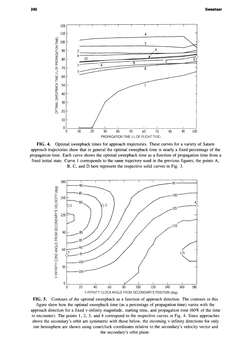
The first such analysis is shown in Fig. 5, which examines how the optimal sweep-
back time varies with the approach direction. The figure shows contours of optimal
sweepback time relative to the direction of the incoming v-infinity vector. This direc¬
tion is given as a cone angle measured from the velocity vector of the secondary body
(Saturn again) relative to the primary and a clock angle measured from a prime me¬
ridian which is defined to contain the position vector of the secondary relative to the
primary. Only one hemisphere of possible v-infinity directions is shown since the
problem is symmetric with respect to the orbit plane of the secondary body.
240
Sweetser
FIG. 4. Optimal sweepback times for approach trajectories. These curves for a variety of Saturn
approach trajectories show that in general the optimal sweepback time is nearly a fixed percentage of the
propagation time. Each curve shows the optimal sweepback time as a function of propagation time from a
fixed initial state. Curve 1 corresponds to the same trajectory used in the previous figures; the points A,
В, C, and D here represent the respective solid curves in Fig. 3.
V-INFINITY CLOCK ANGLE FROM SECONDARY'S POSITION (deg)
FIG. 5. Contours of the optimal sweepback as a function of approach direction. The contours in this
figure show how the optimal sweepback time (as a percentage of propagation time) varies with the
approach direction for a fixed v-infinity magnitude, starting time, and propagation time (60% of the time
to encounter). The points 1, 2, 3, and 4 correspond to the respective curves in Fig. 4. Since approaches
above the secondary’s orbit are symmetric with those below, the incoming v-infinity directions for only
one hemisphere are shown using cone/clock coordinates relative to the secondary’s velocity vector and
the secondary’s orbit plane.
Applying the One-step Multiconic Method of Trajectory Propagation
241
The function contoured in Fig. 5 is actually a function defined on the sphere of
possible approach directions; the figure projects one hemisphere onto the flat page by
plotting the contours against cone and clock. The key step in this analysis is to find
an analytic formula for this function, or which approximates this function. As it turns
out, the function contoured in Fig. 5 is simple enough that visual inspection alone
suggests a type of analytic approximation — when the contours are plotted on the di¬
rection sphere itself they are very nearly concentric circles, just as latitude circles are
concentric circles around the poles of a globe.
This continues to be true for different v-infinity magnitudes, times-to-encounter,
and most significantly for different primary-secondary pairs. Furthermore, most of
the other features of the contour plot stay very close to the same, as those parameters
vary: in all cases the common center of the contours, which I will call the critical ap¬
proach direction, is within a couple degrees of 112 cone, 0 clock. By visually com¬
paring the contours in Fig. 5 with contours generated by various spacings of circles
on the sphere centered at the critical approach direction, it was found that the func¬
tion contours are spaced approximately as the cosine of the angle from the critical ap¬
proach direction to the “sweepback equator” 90 deg from the critical approach
direction, and they are farther apart beyond that; the value of the optimal sweepback
percentage at the sweepback equator is within 102% ±2%.
The only significant difference between contour plots as the v-infinity magnitude,
etc., change is the value of the optimal sweepback percentage at the critical approach
direction. Thus if this value, which we shall denote/,, (as a fraction rather than a per¬
centage) and which characterizes the data shown in Fig. 5, is known then the entire
function for the value of / can be approximated by one which varies from this value
to 1.02 (i.e., 102%) at the sweepback equator according to the cosine of the angle A
between the actual approach direction and the critical approach direction, and which
further varies half as fast around to the opposite pole. This is expressed by the fol¬
lowing equation:
f =
1.02 - (1.02 -/.) cos A
1.02 - ((1.02 —/c)/2) cos A
A < 90 deg
A > 90 deg
(2)
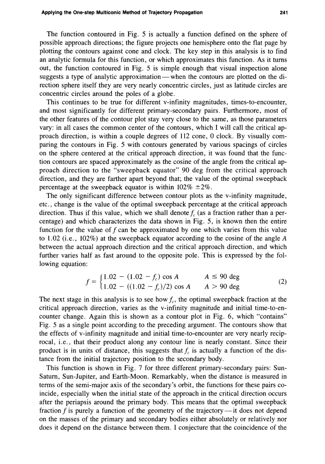
The next stage in this analysis is to see how /, the optimal sweepback fraction at the
critical approach direction, varies as the v-infinity magnitude and initial time-to-en-
counter change. Again this is shown as a contour plot in Fig. 6, which “contains”
Fig. 5 as a single point according to the preceding argument. The contours show that
the effects of v-infinity magnitude and initial time-to-encounter are very nearly recip¬
rocal, i.e., that their product along any contour line is nearly constant. Since their
product is in units of distance, this suggests that /. is actually a function of the dis¬
tance from the initial trajectory position to the secondary body.
This function is shown in Fig. 7 for three different primary-secondary pairs: Sun-
Saturn, Sun-Jupiter, and Earth-Moon. Remarkably, when the distance is measured in
terms of the semi-major axis of the secondary’s orbit, the functions for these pairs co¬
incide, especially when the initial state of the approach in the critical direction occurs
after the periapsis around the primary body. This means that the optimal sweepback
fraction /is purely a function of the geometry of the trajectory — it does not depend
on the masses of the primary and secondary bodies either absolutely or relatively nor
does it depend on the distance between them. I conjecture that the coincidence of the
242
Sweetser
V-iNFINITY MAGNITUDE (km/s)
FIG. 6. Contours of the optimal sweepback percentage for the critical approach direction. These curves
show how the optimal sweepback time (as a percentage of the propagation time) for the critical approach
direction varies with both the time before encounter of the initial state and the magnitude of the incoming
v-infinity. The single point marked in the graph is the value for the contour “pole” (112 deg cone, 0 deg
clock) of Fig. 5 and completely characterizes that plot.
0 0.2 0.4 0.6 0.8 1.0 1.2 1.4 1.6 1.8 2.0
DISTANCE (UNITS OF SECONDARY S.M. AXIS)
110
100
У 90
о
CL
g 80
Ll_
| 70
| 60
Q-
g 50
<
co
Q_
Ш 40
S
30
s
L 20
о
10
0
FIG. 7. Percentage values for the critical approach direction for different bodies. These remarkably
coincident curves demonstrate that the optimal sweepback time depends only on the trajectory geometry.
For three different primary/secondary pairs the optimal sweepback time (as a percentage of propagation
time) is plotted first (solid curves) as a function of the initial distance from the primary and second
(dashed curves) as a function of the initial distance from the secondary, where the unit of distance is the
distance from the secondary to the primary.
Applying the One-step Multiconic Method of Trajectory Propagation
243
functions would be exact if the secondary bodies involved all had circular orbits
around their respective primaries.
The trajectories in Fig. 7 were all such that the magnitude of the v-infinity velocity
at encounter equalled the velocity of the secondary with respect to the primary and
they were all propagated 60% of the way to encounter. When the same trajectories
are tried with half that v-infinity, there is no significant difference in the curves of in¬
terest relating the optimal sweepback to the initial distance from the secondary (the
solid curves in that case show that the periapsis to the primary occurs at about twice
the distance, but this fact is of only minor interest). On the other hand, if the curves
are generated with propagation times that are different fractions of the flight time to
encounter, they are the same only out to about 60% of the primary-to-secondary dis¬
tance; beyond that the curves continue to coincide but move up or down as the propa¬
gation time increases or decreases. In other words, fc and thus/are independent of tp
only as long as the initial position is closer to the secondary than about 60% of the
primary-secondary distance. The dependence, however, for more distant initial states
is weak and can be ignored for our purposes — the amount of difference is not more
than about ±10 in the value of the optimal sweepback percentage at an initial dis¬
tance equal to the primary/secondary distance. This allows us, by approximating the
dashed curve in Fig. 7, to write the following equation for / as a function of x, where
x is the trajectory initial distance from the primary measured in units of the primary/
secondary distance:
(3)
By putting the above results together, we are now in a position to write down a
general algorithm for estimating the optimal sweepback time for an approach trajectory:
1. If the initial state is farther from the secondary than the primary is, propagate
along a primary-centered conic to a new initial state at least as close to the sec¬
ondary as the primary is (this is like the pseudostate transformation sphere ap¬
proach, but with a much larger sphere);
2. Calculate the optimal sweepback fraction / from the ratio x of the distance of
the initial position from the secondary body to the primary-secondary distance
according to equation (3);
3. Propagate forward along a primary-centered conic until the final time or until
encounter with the secondary body, whichever comes first, to get a final state
(note that the actual encounter time changes when the one-step multiconic
method is applied, but this is not critical to this estimation algorithm);
4. Transform the final velocity to a secondary-relative velocity in a coordinate
system which uses the secondary’s velocity relative to the primary as a pole
vector and the secondary’s position relative to the primary to determine a
prime meridian;
5. Find the angle A between the transformed velocity vector and the critical ap¬
proach direction vector, which has latitude 112 deg and longitude 0 in the co¬
ordinate system defined in step 4 above; as a practical matter A itself is not
calculated — cos A is found directly by taking dot products;
6. Calculate the optimal sweepback fraction / from equation (2);
244
Sweetser
7. Estimate the optimal sweepback time for the approach as a fraction/of the
time from the initial state in step 2 to the final state in step 4, and use the one-
step multiconic method with this optimal sweepback time to repropagate from
that initial state to the desired final state.
Departure Trajectories
When 1 began this analysis of the one-step multiconic method I first thought that
the departure case would be essentially the same as the approach case — after all, a
departure is just an approach going backwards in time. One crucial difference, how¬
ever, destroys this symmetry so the two cases turn out to be very different indeed.
This difference is that in the approach case the “correct” state is known far from the
secondary and error increases as the trajectory gets closer, while in the departure case
the “correct” state is known close to the secondary and the error increases as the tra¬
jectory goes out.
The effect of this difference is immediately seen in Fig. 8, which shows how the
position error in the final state varies as a function of the sweepback time. In contrast
to Fig. 2, which shows how the error varies symmetrically and sharply with time for
the approach case, the position error in the departure case decreases rapidly to a mini¬
mum but increases more slowly for longer sweepback times. In fact for some depar¬
ture geometries the position error curve can even reverse itself so the error reaches a
second minimum. This second minimum can sometimes be an even smaller position
error than the first; the first minimum, however, occurs in a regular pattern as a func-
FIG. 8. One-step departure residual error, Saturn reversed nominal. The data plotted here are from
different segments of a trajectory departing Saturn, which is basically a mirror image of the approach
trajectory used in Figs. 1 through 3. All curves show the position error 1000 days after Saturn periapsis
as a function of sweepback time; trajectories A, B, and C begin 750, 500, and 250 days after encounter,
respectively, and D begins right at closest approach. Compare this to Figs. 2 and 3.
Applying the One-step Multiconic Method of Trajectory Propagation
245
tion of the trajectory geometry and will be the one worked with in this algorithm de¬
velopment. In particular, the optimal sweepback time again seems to be closely
related to the propagation time so we can continue our analysis along the same lines
as in the approach case.
The departure case shows further differences in Fig. 9, which, like Fig. 4, takes
the minimum error times of the previous figure as a percentage of the propagation
time, and plots those optimal sweepback percentages against the propagation time.
The most noticeable difference between Figs. 4 and 9 (hence between the approach
and departure cases) is that the optimal sweepback percentage in general decreases
linearly with propagation time. This is in marked contrast to the arrival case, where
the optimum percentage was essentially independent of propagation time, and to the
pseudostate transition sphere concept, for which the optimal sweepback percentage
curve would be constant at 100% out to a point corresponding to the sphere and de¬
crease like a “1/z” curve after that.
Thus for the departure case the value of/in equation (1) is linearly dependent on
tp. By choosing some nominal propagation time tn, we can measure the optimal
sweepback fraction / for that particular propagation time and then express/as a func¬
tion of both / and tp for any particular trajectory as follows:
f= 1 - (1 (4)
Figure 9 shows the effect of a number of different trajectory geometries just as Fig. 4
did. As before, the first four curves show that the optimal sweepback does depend on
PROPAGATION TIME (% OF FLIGHT TIME)
FIG. 9. Optimal sweepback times for departure trajectories. For a variety of different trajectories
leaving Saturn, the optimal sweepback time relative to the propagation time is shown as a function of the
propagation time. Curve 1 is from the same trajectory as in Fig. 8, and its right-hand endpoint
corresponds to the time of minimum error of trajectory D in that figure. All the data here are for
trajectories beginning at Saturn encounter except for curve 7, which is for a trajectory beginning 295 days
after the encounter; the flight time for all the trajectories is 1000 days.
246
Sweetser
the departure direction. This time, however, curves 5 and 6, which differ from
curve 1 by having greater and lesser v-infinity magnitudes respectively, show that the
optimal sweepback does not depend on that quantity or on the distance to which the
trajectory is propagated. Curve 7 differs from curve 1 in that the propagation begins
295 days out from encounter; thus the initial distance from the secondary has a great
effect on the optimal sweepback percentage. Finally, curves 8 through 10 show that
the periapsis radius and the inclination of the hyperbola around the secondary body
have negligible effect on the sweepback.
We continue as in the approach case by examining the effect of the departure direc¬
tion on the optimal sweepback time. As might be expected, Fig. 10 is quite similar to
a reflection of Fig. 5: the contours are nearly concentric around a critical departure
direction which has a cone angle of approximately 112 deg cone and 180 deg clock
(referenced again to the secondary’s velocity and position vectors) and which is thus
a mirror image of the critical approach direction; the contours are spaced according to
the cosine of the angle with the critical departure direction out to 90 deg and about
twice as far apart beyond that angle.
A number of similar plots were done for various initial distances from the second¬
ary, propagation times, and v-infinity magnitudes. These demonstrated ways in
which the departure case differs from approach. For one thing, the optimal sweep-
back time was never more than the propagation time (in the approach case it could be
20% more in some cases). As a result the value of the contour at 90 deg from the
critical departure direction takes on various values from 75% up to 90%. In addition,
V-INFINITY CLOCK ANGLE FROM SECONDARY'S POSITION (deg)
FIG. 10. Contours of optimal sweepback values as a function of departure direction. These contours
show how the optimal sweepback time (as a percentage of propagation time) varies with the direction of
departure for a given v-infinity magnitude (9.555 km/s), starting time (295 days after Saturn encounter),
and propagation time (to 1000 days after Saturn encounter). Compare this to Fig. 5, which gives similar
information for trajectories approaching Saturn.
Applying the One-step Multiconic Method of Trajectory Propagation
247
the whole pattern of contours was more variable than that for approach — the critical
departure direction varied more and in some geometries anomalous higher valued
contours appeared below the critical departure direction.
Because of the apparent irregularity of these features and because the “width” of
the error curves in Fig. 8 allow greater latitude in our estimation algorithm, I decided
to treat the directional dependency of the optimal sweepback time as if it were as
regular as Fig. 10 would suggest. Just as in the approach case, the function then is
constant along circles centered around a critical departure direction and the spacing
between these circles is twice as great (i.e., the function changes half as fast) in the
hemisphere away from the critical departure direction as in the hemisphere toward it.
In the departure case, however, the value for f along the “sweepback equator” is not
constant, so two numbers are needed to characterize that dependency: the value of the
optimal sweepback fraction fc for the critical departure direction and the value fa at its
antipode 180 deg away. When these functions are known we can calculate the opti¬
mal sweepback fraction fe at the “sweepback equator” by
fe=fC + ^fa~fc)/3 (5)
According to our analysis of Fig. 9, the next step is to find out how these numbers
for the critical departure direction and its antipode vary with the initial distance from
the secondary. This is done for the critical departure direction in Fig. 11. Because
Fig. 9 showed that the optimal sweepback percentage changes linearly with the
propagation time, we fix the propagation time to be 1/20 of the secondary’s period.
DISTANCE (UNITS OF SECONDARY S.M. AXIS)
FIG. 11. Percentage values for the critical departure direction for different bodies. For three different
primary/secondary pairs, the optimal sweepback percentage is plotted first (solid curves) as a function of
the final distance from the primary and second (dashed curves) as a function of initial distance from the
secondary. As in Fig. 7, the curves using the initial secondary distance are remarkably coincident.
248
Sweetser
Once again the curves for three different primary/secondary pairs coincide remark¬
ably and this was also true for trajectories departing in the opposite direction.
Fig. 11 was redone for a number of different v-infinity magnitudes (the one shown
is for that magnitude equal to the secondary’s velocity). It was found that the slope of
the line relating the optimal sweepback percentage to the initial distance remained
constant — only the intercept changed, and that was linear in v-infinity. Then letting
v be the v-infinity measured in units of the secondary velocity and x be the initial dis¬
tance from the secondary measured in units of the primary/secondary distance, I ob¬
tained the following estimate:
fc = 0.95 - 0.19v - 1.07x
(6)
When the same analysis was done for trajectories going out opposite to the critical
departure direction, the slope was very slightly positive and the intercept was close to
95%, so I use the value 0.95 for fa.
We now have all the information we need to write a general estimation algorithm
for the departure case:
1. Calculate the optimal sweepback fraction f. according to equation (6) from the
ratio v of the v-infinity magnitude to the secondary’s velocity and the ratio x of
the distance of the initial position from the secondary body to the distance
of the secondary from the primary body, but of course do not let fc (the value
for the critical departure direction) go negative;
2. Compute fe from equation (5), with fa = 0.95;
3. Find the angle A between the secondary-relative velocity vector and the critical
departure direction vector, which has 112 deg cone and 180 deg clock relative
to the secondary’s velocity and position vectors as discussed before;
4. Calculate the optimal sweepback fraction f( for the nominal propagation time
from the formula (analogous to equation (2))
f =
fe ~ (fe ~ fc) COS A
fe ~ ((fe ~fe)/2) COS A
A < 90 deg
A > 90 deg
(7)
note that in any case 0 < f < 0.95;
5. Let t be the propagation time desired or the time it takes for the trajectory to
get as far from the secondary as the secondary is from the primary, whichever
is smaller (it is not necessary that t be exact in the latter case);
6. Letting p be the secondary’s period and using the value of p/20 for the nomi¬
nal propagation time tn, the calculation of the optimal sweepback fraction /in
equation (4) becomes
f = 1 ~ 20(1 -f()t/p (8)
and then use equation (1) to obtain the optimal sweepback time ts for the full
propagation.
This procedure gives a good estimate of the optimal sweepback time but it is not ex¬
act. According to Fig. 8 it is better to overestimate the sweepback time than to under¬
estimate it, so you might want to add 0.05 to /in the last step.
Applying the One-step Multiconic Method of Trajectory Propagation
249
Accuracy of This Method
The algorithms derived above have been implemented and compared to other
propagation methods [6]. In the case of interplanetary and Earth/Moon trajectories
these algorithms are significantly better than patched conic and other single-step mul¬
ticonic methods (up to an order of magnitude or more reduction in final position and
other errors), with negligible increase in computational cost when the secondary-en¬
counter time is known from other considerations. Indeed, the patched conic method
incurs an increased cost when it has to search for the crossing of the sphere of influ¬
ence of the secondary body. As would be expected, multistep multiconic methods of¬
fer another order of magnitude improvement (making them equivalent to trajectory
integrators) but at a comparable increase in computational cost.
Further testing, however, uncovered an unexpected (but obvious in hindsight) limi¬
tation to this and other multiconic methods — experiments with orbits from a Galileo
satellite tour around Jupiter found that when a satellite is approached from far beyond
the satellite orbit (hence for a long enough time for the secondary to go around the
primary body) then single-step multiconic methods (including patched conic) offer
essentially no improvement over a simple primary-centered conic. In further investi¬
gation of one of these cases it was found that by replacing the primary-centered conic
with a barycentered conic the final position error could be reduced almost to zero
with an optimal sweepback time.
Suggestions for Future Work
It is still astonishing to me that the optimal sweepback time is independent of the
bodies’ masses and distance from each other. One of the reasons this is so exciting is
that it suggests that an analytic solution might be possible for the problem examined
here. A good beginning might be to verify this independence in an idealized setting
where the secondary moves in a circular orbit about the primary.
Throughout this analysis, the sweepback time is defined by the problem at hand to
be optimal when it minimizes the position error at a given propagation time. This is
not always the right error to be measuring; in particular, one might want to minimize
the error in other state quantities at the time of closest approach, where that time it¬
self may be one of the quantities. Would the optimum still be purely a function of tra¬
jectory geometry? This entire analysis could be repeated to solve this new problem.
The entire analysis also could be repeated for the case when the propagation dura¬
tion is more than a significant fraction of the secondary body’s period around the sec¬
ondary. As mentioned above, evidence indicates that an alternative method where
barycentered conics replace primary-centered conics is more appropriate for trajecto¬
ries which come from or go far from both bodies. Does such a method always offer
significant improvement? Is there an algorithm for estimating the optimal sweepback
time in such cases? And what criterion should be used to decide between such a
method and the one described in this paper?
References
[1] WILSON, S.W., Jr. “A Pseudostate Theory for the Approximation of Three-Body Trajectories,”
AIAA Paper 70-1071, presented at the AIAA Astrodynamics Conference, Santa Barbara, California,
August 1970.
250
Sweetser
[2] BYRNES, DENNIS V. “Application of the Pseudostate Theory to the Three-Body Lambert Prob¬
lem,” AAS Paper 79-163, presented at the AAS/AIAA Astrodynamics Specialist Conference,
Provincetown, Massachusetts, June 1979; also Journal of the Astronautical Sciences, Vol. 37, No. 3,
July-September 1989, pp. 221-232.
[3] SERGEYEVSKY, ANDREY B., BYRNES, DENNIS V. and D’AMARIO, LOUIS A. “Ap¬
plication of the Rectilinear Impact Pseudostate Method to Modeling of Third-Body Effects on Inter¬
planetary Trajectories,” AIAA Paper No. 83-0015, presented at the AIAA 21st Aerospace Sciences
Meeting, Reno, Nevada, January 1983.
[4] WILSON, S. W., Jr. “Investigation of Recursive Pseudostate Iteration Procedures for Solving Split
Boundary Value Problems Associated with Interplanetary Trajectories,” TRW report to NASA
Manned Spacecraft Center No. 5521.4-18, May 17, 1971.
[5] BYRNES, D. V. and HOOPER, H. L. “Multi-Conic: a Fast and Accurate Method of Computing
Space Flight Trajectories,” AIAA Paper No. 70-1062, presented at the AIAA Astrodynamics Confer¬
ence, Santa Barbara, California, August 1970.
[6] KIEDRON, KRYSTYNA and SWEETSER, THEODORE H. “A Comparison between Onestep and
Other Multiconic Trajectory Propagation Methods,” AIAA Paper No. 88-4286, presented at the
AIAA/AAS Astrodynamics Conference, Minneapolis, Minnesota, August 1988.
The Journal of the Astronautical Sciences, Vol. 37, No. 3, July-September 1989, pp. 251-259
MIDAS: Mission Design and Analysis
Software for the Optimization of
Ballistic Interplanetary Trajectories
Carl G. Sauer, Jr.
Abstract
A patched conic trajectory optimization program MIDAS is described that was developed to
investigate a wide variety of complex ballistic heliocentric transfer trajectories. MIDAS in¬
cludes the capability of optimizing trajectory event times such as departure date, arrival date,
and intermediate planetary flyby dates and is able to both add and delete deep space maneuvers
when dictated by the optimization process. Both powered and unpowered flyby or gravity as¬
sist trajectories of intermediate bodies can be handled and capability is included to optimize
trajectories having a rendezvous with an intermediate body such as for a sample return mis¬
sion. Capability is included in the optimization process to constrain launch energy and launch
vehicle parking orbit parameters.
Introduction
The analysis of future planetary space missions involving complex trajectory
modes requires software tools that are capable of generating these heliocentric trajec¬
tories quickly and with sufficient accuracy to enable reliable estimates of spacecraft
performance to be made. Because of the many constraints likely to be placed on the
spacecraft and launch vehicle combination it is important to find the best possible
transfer trajectory for a particular mission. This best trajectory is found by optimiza¬
tion of the free parameters of the trajectory, which may be event times such as launch
date, arrival date, or planetary swingby date, or intermediate maneuvers included in
the trajectory to improve performance. The introduction of these maneuvers results in
additional free parameters available for optimization. The software required to gener¬
ate these trajectories must include the ability to either add or delete these intermediate
maneuvers from the trajectory when this will result in an improvement in perfor¬
mance. These intermediate maneuvers can include both deep space maneuvers and
powered maneuvers during a planetary swingby.
A general purpose heliocentric trajectory optimization tool known by the acronym
MIDAS is described that enables the generation and optimization of many complex
trajectory modes. For preliminary mission design studies a trajectory tool that uses a
patched conic simulation for the heliocentric trajectory segments is fast and produces
relatively accurate estimates of performance. Such patched conic trajectory software
generates performance estimates adequate for preliminary mission design and feasi¬
bility studies.
In a trajectory simulation tool there is a tradeoff between speed and complexity.
Performance estimates using a patched conic simulation are generally quite good for
251
252
Sauer
terrestrial or small body missions, but decrease in accuracy for the missions to the
major outer planets because of the relatively large gravity fields of these bodies.
However a patched conic trajectory tool is useful in that it can quickly isolate trajec¬
tories that can then be investigated with more sophisticated, but much slower, trajec¬
tory generators. Employment of a patched conic trajectory simulation results in very
fast calculation of heliocentric trajectories using existing software such as routines for
solving Lambert’s problem, and routines for generating state transition matrices.
The confidence level associated with the results of a trajectory optimization depend
greatly on the accuracy of the partial derivatives that are used in the optimization pro¬
cess. Generation of these partial derivatives is relatively straightforward using
“Primer Vector Theory” [1]. Primer Vector Theory, which involves the generation of
a multiplier or costate vector and its derivatives on each trajectory segment, is well
understood and has been employed in a number of trajectory optimization programs
[2]. It is also possible to draw upon previous studies to implement the conditions that
allow optimization of the powered maneuvers that might occur during a flyby of an
intermediate planetary body [3,4].
Implementation
MIDAS is currently configured to include up to eight intermediate planetary bodies
and eight deep space maneuvers. The program is normally initialized to minimize total
mission AV which is defined as launch and arrival AV plus the additional AV from
both deep space maneuvers and powered planetary swingbys. Minimizing total mis¬
sion AV is independent of both launch vehicle and spacecraft propulsion system per¬
formance and is frequently used as a general performance indicator for preliminary
mission design studies. In addition an option exists to apply weights to the different
velocity impulses in the trajectory. This allows minimization of post-launch AV or
optimization of flyby trajectories to be performed.
MIDAS also includes a rudimentary mass optimization capability which requires a
detailed definition of both launch vehicle and spacecraft propulsion systems. In most
cases the difference between performing an optimization minimizing total AV and
maximizing delivered spacecraft mass is small. Only in instances where there is a
wide disparity between the launch vehicle specific impulse and the spacecraft propul¬
sion specific impulse or where there is a jettison of a large fraction of the spacecraft
mass during the trajectory, will the different performance criteria result in trajectories
that differ significantly.
Features
One of the problems that many of the patched conic trajectory programs have not
addressed adequately is that of unpowered planetary gravity assists or swingbys.
MIDAS incorporates the capability of accurately simulating and optimizing many
classes of unpowered planetary swingby trajectories. Also, the program has the capa¬
bility of deleting deep space or planetary swingby maneuvers, when the magnitude of
the maneuver is less than some prescribed tolerance. The deletion of very small ma¬
neuvers is important, since the partial derivatives or gradients deteriorate in accuracy
with the magnitude of a maneuver. Additional features include optimization of reso¬
MIDAS: Mission Design and Analysis Software
253
nant transfers or returns to the same intermediate planetary body. Special techniques
are necessary to allow accurate gradients to be derived for optimization of these reso¬
nant transfer trajectories because of singularities occurring due to the resonance con¬
straint.
Both launch energy and elements of the departure parking orbit of the launch vehicle
can also be constrained. This parking orbit is an intermediate orbit that the launch
vehicle injection stage is placed in following launch and preceding injection, and is
selected to optimally match the launch site with the desired injection position on the
Earth escape hyperbola. The inclusion of a parking orbit constraint, for example, al¬
lows missions departing from a space station in a fixed orbit to be examined. Analysis
of launch from a constrained parking orbit was studied in support of the Apollo pro¬
gram [5] for Earth-Moon transfer trajectories. These results are implemented in MI¬
DAS [6] and have proven useful in the investigation of an Eros rendezvous mission.
Either parking orbit inclination or ascending node can be constrained, and either will
result in an out-of-plane injection maneuver that must be factored into the optimiza¬
tion. Launch energy is constrained by removing the degrees of freedom associated
with the position vector of a deep space maneuver and using one of these degrees of
freedom to constrain the injection energy at departure. The two remaining degrees of
freedom, declination and right ascension of the departure asymptote, are then are
available to be optimized.
Another feature included in MIDAS is the ability to calculate and optimize trajec¬
tories where the planetary positions are not constrained by an ephemeris date. In this
option the position of the planet is determined by allowing the mean anomaly of the
planet to be a free variable that can be either specified or optimized. The use of this
so-called “ephemeris free” option allows the calculation of mission maps that can be
used to predict performance for future launch opportunities. This option has proven
particularly useful in the analysis of small body missions [7] and in the investigation
of Mercury orbiter missions that involved multiple swingbys of both Venus and
Mercury [8].
In order to generate a specific interplanetary trajectory, an initial estimate of the
event times must be made available to the program. An input list of free variables to
be optimized must also be included. Normally most of the trajectory event times are
specified in the optimization list as are also the time and the position vector for any
deep space maneuver. A capability is also included for performing a one or two pa¬
rameter study of any of the free variables in the trajectory. These variables are speci¬
fied in a separate parameter list and are not to be included in the list of variables to be
optimized.
A highly desirable feature in a trajectory optimization program which uses a mini¬
mization routine requiring partial derivatives, is the ability to verify the accuracy of
these analytic derivatives or gradients. This verification is accomplished by including
code that calculates the derivatives of the independent variables by taking small cen¬
tral differences about a nominal value. A comparison of these finite difference partial
derivatives with those calculated analytically, verifies the analytic derivatives. It is
important that these gradients be calculated accurately, since the minimization routine
used in the optimization process will terminate prematurely with large values of the
gradients if the gradients are not correct. In such a case, the trajectories may not be
254
Sauer
completely optimized and there exists some doubt as to the additional improvement
possible in the trajectory.
Powered Planetary Swingby Trajectories
The analysis for powered planetary swingby trajectories was formally presented in
1973 by J. M. Walton [3] for a doctoral thesis at the University of Colorado. This
analysis included identification of a number of classes of powered swingby trajecto¬
ries which were dependent upon both the magnitude and direction of the incoming
and outgoing hyperbolic excess velocity vectors. This analysis was extended to the
calculation of the asymptotic values of the Primer Vector, both on the incoming and
outgoing asymptotes of the hyperbola, by R. A. Hyde [4] at MIT.
A number of types of powered swingby trajectories were considered in the above
analyses and the more likely classes are implemented in MIDAS. Those that are not
considered involved types that are either not practical or types that are not normally
encountered in a fully optimized planetary trajectory. The swingby types incorporated
in MIDAS include a grazing swingby trajectory at the constraint altitude with an im¬
pulse at either or both asymptotes and both grazing and non-grazing swingby trajecto¬
ries with an impulse at some finite distance from the body. Types not included in the
program are transfers with more than one impulse, one at a finite distance and one at
infinity on the asymptote, and transfers involving an intermediate parabolic transfer
to infinity. Although all these swingby trajectories are calculated as time-free trans¬
fers, the only effect on the heliocentric patched conic trajectories is to define the ve¬
locity increment that must be added and the value of the Primer Vector on each side
of the swingby point.
Trajectory Formulation and Generation
Given a pair of position vectors and the transfer time between them, the trajectory
arc between two bodies, or between a body and a maneuver, is calculated from the
solution of Lambert’s theorem. The velocity vectors at each endpoint of the trajectory
segment are then found from the resulting conic path. At an ephemeris body, the dif¬
ference between the heliocentric velocity vector of the spacecraft and the velocity
vector of the body itself yields a hyperbolic excess velocity vector at the body. At an
intermediate body there is both an incoming and outgoing hyperbolic excess velocity
vector defined that is used by the powered swingby code to determine the actual ve¬
locity increment that must be added by the propulsion system. In the case of an inter¬
mediate deep space maneuver, the difference between the heliocentric velocity
vectors on either side of the maneuver directly yield the velocity increment that must
be added.
In the above scenario, in which a trajectory is defined by either powered planetary
swingby trajectories, deep space maneuvers, or both, the parameters that are avail¬
able for optimization include all the event times and the position vectors of any deep
space maneuvers. Applying Primer Vector Theory and using the powered swingby
analysis mentioned previously, it is relatively straightforward to calculate the partial
derivatives of total launch and spacecraft AV with respect to any of the above free
variables. In the above discussion, the velocity components at the endpoints of the
MIDAS: Mission Design and Analysis Software
255
trajectory segments are unconstrained, in the sense that they are unaffected by the ad¬
jacent trajectory arcs.
Unpowered Planetary Swingby Trajectories
In the process of optimization of a trajectory containing a powered swingby seg¬
ment, it is possible that the magnitude of the swingby impulse can become very small
and disappear. In such a case the planet swingby becomes unpowered, and the condi¬
tions which yielded the asymptotic values of the Primer Vector on the swingby hyper¬
bola for a powered planetary swingby become invalid and do not give the correct
values for the Primer Vector. As a consequence, the gradients which depend upon
these values of the Primer Vector are no longer correct.
In an unpowered planetary swingby, a constraint exists between the velocity vec¬
tors of the trajectory arc immediately before and after the swingby, since the mag¬
nitude of the incoming and outgoing hyperbolic excess velocity vectors at the planet
are the same. In addition, if the unpowered swingby occurs with a closest approach
distance to the planet at the constraint altitude, an additional constraint exists between
the bend angle of the incoming and outgoing hyperbolic excess velocity vectors. Be¬
cause of the constraints which are imposed on the heliocentric velocity vector on each
side of the planetary swingby, the two adjacent trajectory arcs cannot be solved inde¬
pendently using Lambert’s theorem. Effectively, a single degree of freedom is lost
from the optimization for each constraint imposed by an unpowered planetary
swingby.
MIDAS handles these constraints in two separate ways. If a deep space maneuver
exists on the trajectory arc on either side of the planetary swingby, the constraints can
be handled by taking the necessary degrees of freedom from the position components
of this deep space maneuver, and using them for the unpowered swingby. Since there
are three degrees of freedom available from the position components of the deep
space maneuver there is an excess of one or two degrees of freedom that is available
to optimize some parameter of the unpowered planetary maneuver. These degrees of
freedom are chosen as the closest approach distance to the planet during the swingby,
and the impact or В-plane angle of either the incoming or outgoing hyperbola asymp¬
tote [9]. If the swingby occurs at the constraint altitude, then the altitude is con¬
strained, and only the impact plane angle can be optimized. If the swingby occurred
with a closest approach distance above this constraint altitude, then this altitude can
also be optimized.
This formulation for an unpowered planetary swingby was originally included in
MIDAS to handle a AV-EGA trajectory in which there was an Earth return 2 to 3
years following launch. This type of trajectory has a deep space maneuver near aphe¬
lion of the Earth to Earth phase of the mission to shape the return trajectory to Earth
such that a gain in heliocentric energy results from the ensuing swingby of the Earth.
This method of handling an unpowered swingby is suitable as long as there is a deep
space maneuver present either before or after the planetary swingby. However, many
of the more complex trajectory modes presently under investigation can have one or
more unpowered planetary swingbys with no associated deep space maneuver. The
above method of handling unpowered swingby trajectories thus fails since there is no
256
Sauer
deep space maneuver present to absorb the constraints involved in the unpowered
swingby.
In order to handle an unpowered planetary swingby mode in which a deep space
maneuver is not available, a second formulation is employed to calculate the un¬
powered swingbys [10]. The changes in the formulation for unpowered planetary
swingby trajectories were derived by C. L. Yen and the author at JPL, and involve
taking the degrees of freedom necessary to satisfy the unpowered swingby constraints
from trajectory event times, rather than from the position components of a deep space
maneuver. These event times are generally the time of the planetary swingby, and a
time associated with a trajectory event either immediately before or after the swingby.
Normally, for a non-grazing unpowered swingby, the degree of freedom comes from
the time of the planetary swingby itself, and this time is then constrained, and not
available for further optimization. For a grazing, unpowered swingby, an additional
degree of freedom comes from one of the other event times, which also can not be
optimized. On a trajectory without deep space maneuvers, the number of constraints
imposed by unpowered swingbys can never be greater than the number of available
event times.
This second method used in calculating trajectories containing an unpowered
planetary swingby is to solve for the event times such that the constraints associated
with the unpowered swingby are satisfied. This targeting of the event times is ini¬
tiated using some initial estimate of the times, and then using Lambert’s theorem to
calculate the appropriate trajectory segments that contain an unpowered swingby
event. If the swingby constraints are not satisfied, the event times are readjusted, and
the targeting process is repeated. This process is terminated when all the swingby
constraints are satisfied to within some specified tolerance.
In both the above methods of handling unpowered swingbys, the Primer Vector as¬
sociated with the constrained trajectory arcs can only be calculated after all the trajec¬
tory arcs are calculated, and after the Primer Vector has been calculated for all
noncontiguous trajectory arcs. The Primer Vector must then be propagated through
all the constrained trajectory arcs including the hyperbolic trajectory arcs for each un¬
powered planetary swingby. The formulation for the propagation of the Primer Vector
through the unpowered swingbys uses the method described by the author [ 10] for the
latter type of unpowered swingby discussed above and the method presented by the
author [11] for the case when a deep space maneuver is employed in conjunction with
the swingby.
Program Configuration
MIDAS is implemented as a set of subroutines, each of which performs a basic
function in the analysis. The program is run from a main routine, which controls the
input and initialization, manages the logic associated with the minimization routine,
calls routines to calculate the trajectory and update trajectory conditions such as
checking if additional impulses are required, and finally manages the functions re¬
quired for parameter studies. A simplified flow control diagram for MIDAS is shown
in Fig. 1. Both the initialization of the search, and calculation of the corrections to
the independent variables, is accomplished in the minimization routine. A routine
MIDAS: Mission Design and Analysis Software
257
FIG. 1. Program Flow Diagram for MIDAS.
called from the main program controls the generation of the trajectory, and the calcu¬
lation of the Primer Vector and partial derivatives required in the search.
There are a number of factors that can cause the search to terminate prematurely
before convergence is achieved, the main factor being a very small AV. When this
occurs the last trajectory is printed and a routine is called that deletes the maneuver
from the trajectory. If the maneuver is a deep space maneuver, the maneuver parame¬
ters are completely removed from the trajectory and if the maneuver is a powered
swingby maneuver, the trajectory is reformulated such that the swingby is unpow¬
ered. Trajectory code is also included that checks converged trajectories to determine
if the addition of a maneuver will result in better performance. This code also indi¬
cates if other trajectory constraints, such as swingby altitude, are violated. If any of
the above conditions have occurred, the trajectory and search are re-initialized and
the analysis is continued.
This entire sequence is completed when a final converged trajectory is realized
with no additional maneuvers to add, and no trajectory constraints violated. At this
point, if a parameter study is being conducted, the particular variable being studied
will be updated, and the entire process described above will be repeated. Several fac¬
tors, such as divergence of the search, or lack of sufficient free variables to satisfy
the swingby constraints, can sometimes cause the trajectory update to be terminated
prematurely. In this case the parameter study is terminated.
258
Sauer
Search Configuration
MIDAS employs a quasi-Newton variable metric minimization routine, VA09A,
developed by R. Fletcher [12] that requires gradients or derivatives of the perfor¬
mance parameter and produces near quadratic convergence as the solution is ap¬
proached. MIDAS is written in double precision and the convergence criteria used in
the search are defaulted to relatively small values. This particular minimization rou¬
tine determines convergence by checking the size of the correction for each indepen¬
dent variable and indicating convergence when the correction for all variables is less
than some prescribed tolerance. The search routine does not define convergence by
checking the size of the gradients. These gradients normally are very small when
convergence is achieved, and an indication of an error is noted in the calculation of
these gradients, when convergence is indicated by the minimization routine with
large values of the gradients. The units employed in MIDAS are the same as those
used in another optimizing patched conic program, MULIMP [2], and are astronomi¬
cal units (AU) for position and days for time. The performance indicator, total mis¬
sion ДУ, is given in units of km/s, and the gradients thus have dimensions of
km/s/day for event times and km/s/AU for components of the deep space maneuver
position. Magnitudes of the gradients on a converged trajectory are typically 10"6 to
10~9 for either position or time.
Concluding Remarks
A general description of an interplanetary trajectory analysis and optimization tool
has been described with no attempt made to go into a detailed mathematical descrip¬
tion of the trajectory or optimization techniques. Generally most of the trajectory
analysis and optimization techniques are available in the open literature. This code
has been used in support of a number of advanced studies at JPL such as for the
Comet Rendezvous, Asteroid Flyby (CRAF) mission, the Saturn orbiter, Titan probe
(CASSINI) mission and a Comet Nucleus Sample Return (ROSETTA) mission.
MIDAS has also been employed in the investigation of a Mercury orbiter mission and
an asteroid rendezvous mission using multiple flybys of Mars. The author is indebted
to C. L. Yen of JPL for much of the unpowered swingby analysis and to the developer
of MULIMP, A. Friedlander, for past discussions on trajectory optimization.
References
[1] LAWDEN, D. E Optimal Trajectories for Space Navigation, Butterworths, London, 1963.
[2] FRIEDLANDER, A. L. “(MULIMP) Multiple Impulse Trajectory and Mass Optimization Pro¬
gram,” Science Application, Inc. Report No. SAI 1-120-383-74, April 18, 1974.
[3] WALTON, J. M., MARCHAL, C., and CULP, R. D. “Synthesis of the Types of Optimal Transfers
between Hyperbolic Asymptotes,” AIAA Journal, Vol. 13, No. 8, August 1975, pp. 980-988.
[4] HYDE, R.A. “Trajectory Optimization Involving Powered Planetary Swingbys,” C.S. Draper
Laboratory Report T-585, June 1973.
[5] GUNTHER, P. “Asymptotically Optimum Two-Impulse Transfer from Lunar Orbit,” AIAA Journal,
Vol. 4 No. 2, February 1966, pp. 346-352.
[6] SAUER, C. G. “The Effects of Parking Orbit Constraints on the Optimization of Ballistic Planetary
Missions,” AAS Paper 83-311, AAS/AIAA Astrodynamics Conference, Lake Placid, New York,
August 22-25, 1983.
MIDAS: Mission Design and Analysis Software
259
[7] YEN, CHEN.-WAN L. “Mission Opportunity Maps for Rendezvous with Earth-Crossing As¬
teroids,” AIAA Paper 84-2029, AIAA/AAS Astrodynamics Conference, Seattle, Washington, Au¬
gust 20-22, 1984; also, The Journal of the Astronautical Sciences, this issue.
[8] YEN, CHEN-WAN L. “Ballistic Mercury Orbiter Mission via Venus and Mercury Gravity Assists,”
AAS Paper 85-346, AAS/AIAA Astrodynamics Conference, Vail, Colorado, August 12-15, 1985;
also, The Journal of the Astronautical Sciences, this issue.
[9] KIZNER, W. “Some Orbital Elements Useful in Space Trajectory Calculations,” Technical Release
No. 34-84, Jet Propulsion Laboratory, Pasadena, California, July 25, 1960.
[10] SAUER, C. G. “Optimization of Interplanetary Trajectories with Unpowered Planetary Swingbys,”
AAS Paper 87^424, AAS/AIAA Astrodynamics Specialist Conference, Kalispell, Montana, August
10-13, 1987.
[11] SAUER, C. “Solar Electric Earth Gravity Assist (SEEGA) Missions to the Outer Planets,” AAS Pa¬
per 79-144, AAS/AIAA Astrodynamics Conference, Provincetown, Massachusetts, June 25-27,
1979.
[12] FLETCHER, R. “Fortran Subroutines for Minimization by Quasi-Newton Methods,” Report AERE
R-7125, Theoretical Physics Division, Atomic Energy Research Establishment, Harwell, Berkshire,
UK, 1972.
The Journal of the Astronautical Sciences, Vol. 37, No. 3, July-September 1989, pp. 261-280
Optimal Orbit Transfer Suitable for
Large Flexible Structures1
Alok K. Chatterjee
Abstract
The problem of continuous, low thrust, planar orbit transfer of large flexible structures is
formulated as an optimal control problem with terminal state constraints. The dynamics of the
spacecraft motion are treated as a point mass central force field problem. In the optimal control
problem formulation, the thrust-acceleration magnitude is treated as an additional state variable
and the rate of change of thrust-acceleration as a control variable. To ensure “smooth” transfer,
essential for flexible structures, an additional quadratic term is appended to the time cost func¬
tional. This term penalizes any abrupt change in acceleration. The optimal control problem is
solved numerically by Davidon Fletcher Powell’s (DFP) direct method in conjunction with the
boundary-shift technique of terminal constraint satisfaction. Numerical results are presented for
the special case of a planar transfer.
Introduction
Many advanced missions of the future will involve assembly of large flexible
structures in low Earth orbits (LEO). These assembled structures/platforms, typically,
will consist of large area/mass ratio and low stiffness elements and possess low fre¬
quency modes of vibrations. In view of these special characteristics, the orbit transfer
maneuver should avoid large transients which give rise to unwanted modes of vibra¬
tion. Therefore, specially designed propulsion systems are needed to transfer these
flexible structures. These systems will incorporate a number of engine modules
which operate in sequence to provide long periods of continuous low thrust. More¬
over, this sequential operation of engines can effectively control the rate of thrust¬
acceleration change (T/W control) along the transfer.
Kunz [ 1 ] has provided a meaningful study of the various propulsion system options
available and the importance of T/W control from a structural/propulsive interaction
point of view.
Over the decades, both Earth bound and interplanetary optimal orbit transfer prob¬
lems have received wide attention. But there is a definite lack of work dealing specifi¬
cally with optimal orbit transfer of large structural systems. In this paper a simple and
'Presented at the AIAA/AAS Astrodynamics Conference, Williamsburg, Virginia, August 1986.
261
262
Chatterjee
effective optimal solution of a new orbit transfer problem, suitable for large struc¬
tures, is attempted. Here, in the optimal orbit transfer formulation, thrust-acceleration
magnitude is assumed continuous and to vary with time. To avoid large transients
along the transfer, the rate of change of this thrust-acceleration needs to be controlled.
In an engineering context, this can be achieved by controlling the sequence of various
engine bums in the propulsion module [1].
In an optimal control context, such a philosophy can be realized by including a
quadratic integral term in the cost functional which penalizes the thrust-acceleration
change. Also, the transfer should be achieved in the shortest possible time to mini¬
mize fuel expenditure. Thus, in the present study, the Optimal Control Problem
(OCP) is formulated as a Bolza problem in the Calculus of Variations. The terminal
state constraints are satisfied by the boundary shift technique [2]. The OCP is solved
numerically by using the DFP direct method, and results are presented for a typical
planar orbit transfer example.
Problem Formulation
Figure 1 depicts the variables involved in the dynamics of a point mass spacecraft
in planar transfer from an initial circular parking orbit about a spherical planetary
body to a final desired coplanar circular orbit. An inverse square gravitational field is
assumed and a planet centered inertial polar coordinate system is chosen.
Equations of Motion
From the notations shown in Fig. 1, the familiar point mass planar equations of
motion can be written as
r =
u =
2 + a sin 0,
r r
v = 1- a cos 0,
r
v
(1)
Here, r is radial distance, и is radial velocity, v is circumferential velocity, a is thrust¬
acceleration, ф is the transfer angle and 0 is the thrust vector angle.
Scaling of Variables
For computational ease and convenience, the following normalization of the vari¬
ables is adopted.
/ _ r _ и _v _ a a
t = I r = ct, r = —, u = — , v = — and a = — = —?,
VW r0 roc roc g0 roc
(2)
Optimal Orbit Transfer Suitable for Large Flexible Structures
263
FIG. 1. Point Mass Spacecraft Dynamics.
where t (seconds), r (kilometers), и (km/sec), v (km/sec) and a (km/sec2) are the
unsealed quantities. With these new variables, the above equations of motion can be
written as
r = и ,
v2 1 _ . л
и — — a smf),
r r
- uv _
v = —— + a cos 0,
r
v
Ф = = ■ (3)
r
State and Control Variables
Traditionally, an optimal planar orbit transfer problem has been expressed in terms
of three states (radial distance, radial and circumferential velocities) and two control
variables (thrust-magnitude and direction). In the present study, thrust-acceleration
magnitude is chosen as the fourth state, and instead of the thrust-magnitude, the rate of
change of thrust-acceleration is used as a control variable. Thus, in summary, we have
Xj = г, x2 — и, x3 = v, x4 = a, x5 = ф,
U| = в, u2 = у (a). (4)
at
The choice of the second control variable u2 is a physically realizable concept and
can be achieved, approximately, by sequencing the various engine bums. Figure 2
shows the transfer geometry, in terms of the state and control variables, between the
264
Chatterjee
FIG. 2. States and Controls of Optimal Control Problem.
initial and final circular coplanar transfer orbits. With this choice of variables, the
normalized equations become
*i = x2
*3 1 ,
X2 = 2 + *4 Sin
*1 X|
*2*3 .
X3 = h X4 COS W]
*1
*4 =
*3
*5 = — •
(5)
*1
The normalized boundary conditions to accompany the above equations are
x,(0) = 1.0,
x2(0) = 0.0, x3(0) = 1.0, x4(0) = x4o,
Xpf) = X\r
/ 1 \1/2
x2(/z) = 0.0, x3(rz) = 1 — 1 , x4(rz) = x4/
(6)
'p
The values of x4o, xif, and x4/r are specified.
As can be observed, the state x5 (the planetocentric transfer angle) does not appear
in the first four equations of (5) nor in the stated boundary conditions and hence can
be left out of the optimization process.
Optimal Control Problem
The orbit transfer problem formulated thus far can be cast into a Bolza problem of
the Calculus of Variations in the realm of Optimal Control Theory. Mathematically,
the Bolza problem is to determine the m-vector control function u(r), to < t < tf,
which minimizes the cost functional
Optimal Orbit Transfer Suitable for Large Flexible Structures
265
subject to the nth order, nonlinear dynamical system
x = f(x,u,r); x(r„) = x0 (8)
with x0 and to given.
Additional constraints on both state and control can also be imposed depending on
the nature of the problem. For example, in the orbit transfer problem terminal state
constraints of the type
Ф[х(гу)] = 0, (9)
are imposed.
In the present study, an OCP of the following type is formulated. Determine the
2-vector control function u(r) which minimizes the cost functional
J = tf + f ~^Qu\dt, (10)
ro
subject to the 4th order system differential constraint equations in (5) with x(zo) and t0
given and subject to the terminal state constraints
^,[x(rz)] = - xif = 0, (11)
where i = 1,2, 3,4. Here, xo and xf are specified initial and final state vectors, re¬
spectively. Q is a scalar weighting constant penalizing the control effort. It is a pre¬
selected constant which depends on both the degree of smoothness desired in the
acceleration profile and the time of transfer.
Method of Solution
The above OCP can be solved by satisfying the necessary conditions of optimality.
Necessary Conditions
The necessary conditions for optimality can be obtained by defining the Hamilto¬
nian [3]
H = L + prf,
(12)
where p(z) is the costate vector for the dynamical system. For J to have a stationary
value, it is necessary that
x(r„) = xo,
pr(tz) = A,
(13)
where A is a vector of Lagrange multipliers. The symbol T is used to indicate trans¬
pose of a vector.
266
Chatterjee
Variable End Time Problem
The free end time OCP is converted to a fixed end time problem by using a differ¬
ential time transformation [4]
dt (5) = v(s)2ds, s E [0, 1]. (14)
The OCP, then, is to minimize
L[x(s), u(s), f(j)]v(j)2</5,
subject to
x(s) = f[x(s), u(s), t ($)]v(s)2, (15)
where
e [0,1], x(o) = x0,
and
~t(s) = v(s)2, s£[l,0], r(0) = 0.
as
The functions L and f are the same as in the original optimization problem. But the
dimension of the state and control vector is greater (by one) than the corresponding
dimension of the earlier optimization problem. Here, t and v2 are the new additional
state and control, respectively. Thus,
4 = t,
U3 = V2. (16)
Terminal State Constraint
In the present OCP, terminal state constraints of the type
Ф[х(Г/)] = о, (17)
are imposed.
A “boundary shift” technique [2], is used to convert the constrained optimization
problem into an unconstrained one through the use of penalty constants. This tech¬
nique is numerically superior to a pure penalty function approach. Here, after some
degree of convergence is reached (by using the penalty function method) with values
Xе '(tf)
and an error
ДхС1(0 = xf- Xc‘(ry) (18)
where xf represents the desired states, the problem is restarted with the penalty func¬
tion augmented cost functional
J1 =J + - xt + Д^'О/)]2.
i=\
(19)
Optimal Orbit Transfer Suitable for Large Flexible Structures
267
This simply biases the desired final value by the error in achieving the desired final
value from a previous group of iterations. This method of shifting boundary values is
repeated several times to achieve a desired accuracy in terminal constraint satisfac¬
tion. This method has been found to be computationally successful [2].
Davidon Fletcher Powell (DFP) Method
This method is a powerful iterative gradient [5] method of finding local minima of
an unconstrained function of several variables. This quadratically convergent algo¬
rithm seeks to determine u* - u from dJ/du in order to avoid convergence diffi¬
culties near the minimum. This is done by approximating J(u) near iT by a sequence
of quadratic functions. Tripathi and Narendra [6,7] extend this method to solve
OCPs. The DFP method is usually superior to the Conjugate Gradient method, at
least for problems which do not involve a large number of variables [8].
One iteration of the DFP method for the fixed end time problem involves the fol¬
lowing steps [8]:
1. Guess an initial control 11(5). Choose e > 0. Set i = 0.
2. Numerically integrate the state equations x = f(x, u, s) forward in time from 0
to 1 and store Xj(s).
3. Define the Hamiltonian function
H = L + prf,
and integrate the costate equations
(20)
(21)
where
(22)
from 1 to 0.
4. Compute the gradient vector
(23)
Stop if (gf, g,) < e where (v, w) denotes the inner product
(24)
5. If i > 0, compute the auxiliary functions
У.O) = S, - g,-i ,
z,-^) = u, - u,_!,
(25)
268
Chatterjee
(26)
6. Compute the direction of search
-g,, i = 0
S' -gf ~ S[(b7,g,)by - (cpg,)cy], ;>0. (27)
1 j=i
7. Compute the new control
ui+1(s) = u,(s) + a,*s,(s), (28)
where a* is determined by performing a one-dimensional minimization of
J; i.e.;
/[и/s) + a*s,-(5)] = min J[u;(s) + адС?)], (29)
ai
for all positive ct,.
8. Replace i by i + 1; if i = q, where q is the predetermined restart integer, set
i = 0 before returning to step 2.
In the actual solution procedure a sequence of subproblems are solved, where each
subproblem is stopped when the norm of the gradient
(g, g)"* < s. (30)
Here, denotes the optimal solution and
(31)
Within each subproblem, a restart mechanism is implemented after five iterations.
Restarting is an efficient way to minimize the effects of round-off errors in the com¬
putations. A good strategy is to restart the algorithm after every n (number of states
of the OCP) iterations [8].
Numerical Results and Discussion
In this section, numerical results and discussion are presented for a specific case of
a planar transfer.
Numerical Example
The numerical example considered in this work is a variable end time transfer from
an initial parking orbit of
Optimal Orbit Transfer Suitable for Large Flexible Structures
269
Xlo = 1.0 (r0 = 6578.15 km)
x2o = 0.0 (radial velocity 0 km/sec)
x3o = 1.0 (circular velocity 7.7842 km/sec)
x4o - 0.05 (initial T/W = 0.05)
to a desired final orbit of
= 1.5 (rf = 9867.225 km)
x2f = 0.0
x3 = 0.8165 (circular velocity 6.356 km/sec)
x4f = 0.0.
The cost functional for minimization is
with terminal state constraints
- x^tf) ~ 1.5 - 0.0
% = *2('/) “ 0.0 = 0.0
% = x3(tf) - 0.8165 = 0.0
% = - 0.0 = 0.0.
Thus, the augmented cost functional with penalty function is
+ y^2[x2(rz) - O.o]2 + |k,[x3((/) - .8165]2 + |tf4[x4(rz)]2.
The initial control functions chosen are
U\(t) = 1.05 radians
u2(t) = 0.0
u3(r) = v(s) =1.8 ,
for t E
u}(t) = —1.57 radians
w2(r) = 0.0
u3(t) = 1.8
■ for t e
'1
2 tf'tf
L J
The numerical integration of state and costate equations is performed by using
Adam’s 12th order, implicit linear multistep method. Simpson’s ’Ard integration rule
is used to evaluate all the inner products and the cost functional. A quadratic inter¬
polation scheme is used for 1-D minimization to evaluate the optimum step size a* at
each iteration. This scheme uses function values to compute the optimum step size.
270
Chatterjee
In the penalty function/boundary shift constraint satisfaction technique, the follow¬
ing constant penalty parameters are used.
K} = 500.0, K2 = 600.0, K. = 600.0, K, = 500.0.
Results and Discussion
Tables 1 and 2 and Figs. 3 through 11 give details of the numerical results obtained
for the above example. Various values of the weighting factor were tried. Figures 3
to 6 show the temporal history of radial distance, radial and circumferential velocities
and thrust-acceleration magnitude respectively for Q = 10.
It is observed that for increasing values of Q, the maximum values of thrust¬
acceleration decrease with a corresponding increase in the time of transfer. This is
expected since large values of Q penalize rates of change of thrust-acceleration. De¬
tailed graphical results are presented for a Q value of 10. For this choice the thrust¬
acceleration (x4) profile in Fig. 6 is within an acceptable limit of 0.28, as mentioned
in [1]. Moreover, most importantly, the generated profile does provide a smooth ini¬
tial and terminal phase of transfer without excessive transients.
Figure 7 shows the thrust steering angle control w*(7) profile. As far as the general
nature of the profile is concerned, it compares well with the results obtained by other
investigators [9] for similar problems. The thrust is directed outwards for approxi¬
mately the first half of the transfer and inwards for the second half, with a discontinuity
occurring in the middle. But Fig. 8 indicates that the costate histories are continuous
where the steering angle discontinuity occurs. Thus, the Weierstrass’s comer condi¬
tion is not violated. It must be mentioned here that various initial guesses were tried
and all converged to the same optimum profile. In all cases, discontinuity in the
thrust steering angle profile occurred almost at midtime through the transfer.
Figure 9 depicts the profile of optimal control u2, which in the present formulation
is the control of rate of change of thrust-acceleration. This profile exhibits expected
large values during the initial and terminal phases of transfer without much change in
mid-phase. Here, the question arises as to what values of u2 are admissible from a
mission requirement point of view. This would depend on the structural design of the
spacecraft to be assembled and transferred. The control u2 is directly related to the
weight penalty of the pay load. The choice of the weighting factor Q influences the u2
control profile. In reality, this control can be achieved by proper sequencing of the
various engine burns in the propulsion module, i.e., by a proper T/W control.
Figures 10 and 11 show the relationships between trip time and Q and between
maximum thrust-acceleration and Q respectively. These dictate the selection of the
value of Q as a trade-off between trip time and maximum thrust-acceleration levels
acceptable from a mission requirement point of view.
Tables 1 and 2 show the details of the numerical convergence of the OCP. Four
subproblems are required to reach the terminal state constraint accuracy of
||x(rr) - xr|| = 6.6214 x Ю-4.
This accuracy is reasonable since it approximately corresponds to the following ter¬
minal tolerances:
altitude = ± 10 km
radial velocity = ±20 m/sec
circular velocity = ±20 m/sec .
Optimal Orbit Transfer Suitable for Large Flexible Structures
271
0J
л
сл
Е
э
Е
и
s'
04 oo — co
— О —• 04
40 О О О
О О О О
О О О О
О О О О
I I
04 СО — 4©
04 Г- Г- 4©
о — — —
ОО 00 ОО 00
о о о о
04 СЧ Г" СЧ
со сч Tt oo
о о о о
о о о о
О О О О
О О О О
Tf
О
40
N 1Г, >
О О 04
О О 04
V) 40 Tf
04 со Г~
Г" со 40
«О СО СЧ
Tf 40 Tf
— О О
Tf
ОО
с-
Tf
СО
о
I
к'
Л
(75
и*
Tf 04 Tf
О Ch.
Ch О OO
ООО
ООО
doo
I
Tf СО 4©
ОО — —
ОО 00 04
0 — 0
ОО ОО ОО
ООО
г-
о
С"-
о
о
ОО
о
о
о
4©
S
ООО
I I
О 00
СЧ О
04 О
Tf ю
о
о
о
о
о
г-
00
о
г-
Tf
о
о
о
о
I
СЧ
04
Tf
TABLE 1. DFP Solution With Boundary Shift for Various Q Values
Е
я
Е
’х
л
к
л
с
Е
U.
Е
н
40 г-
40 СО
Tf СП
Th —
«О СО
о о
СО о
00 г-
ОО 4©
СО —
сч сч
о о
7
у
о
о
о
О
X
X
X
X
40
Tf
4©
4©
00
«О
Tf
СЧ
4©
со
04
4©
О
ОО
40
4©
04
40 сч со чо
— 04 СЧ 40
Г" — m Tf
СО О СО МП
СЧ СО СО СО
40 СО
СЧ Г"
ОО *о
СЧ со
Tf о
чо —<
ю —
04 СЧ
СО Tf
— <О о 40
Л
е
о
Z
о
Z
X X X X
г- о сч Tf
СЧ со со —
Tf Tf —' сч
— СО — 4©
— —: — 4©
— СО 04 СО
Tf 40 о СЧ
04 Г- ОО 40
СЧ СО СЧ СО
СО СО СО СО
сч
— 40
ОО <о
Tf
4© Г" 04 Tf
4© -f эо 4©
4© 00 — 40
ОО 04 ОО 04
со со со со
00
272
Chatterjee
NORMALIZED TIME t/tf
FIG. 3. Radial Distance versus Normalized Transfer Time.
These tolerances are relevant from the orbit injection point of view. Thereafter, a
final precision orbit could be achieved accurately by in-orbit maneuvers, using
on-board propulsion.
The number of subproblems required for convergence depends on the terminal ac¬
curacy prescribed. The minimum time converged to a scaled value of 3.3523 (un¬
sealed time of 2832.9 seconds) for Q = 10. This transfer time is feasible within the
constraint of a cryogenic propulsion module where there is a provision for sequential
burning of the engines. This also suggests that long burn-time technology be incorpo¬
rated in the transfer propulsion system. Ion engine concept would entail very low
T/W ratios and hence considerably higher transfer time.
Summary and Conclusion
The present study has shown that for preliminary mission and propulsion system
design, a simple approach can be adopted for the complicated large flexible space
structure orbit transfer problem. This was achieved by formulating an optimal control
problem with terminal state constraints using a point mass trajectory dynamics model.
The performance index was designed for a minimum time transfer and to include a
quadratic term to penalize any abrupt change in the rate of change of thrust-acceleration.
Optimal Orbit Transfer Suitable for Large Flexible Structures
273
NORMALIZED TIME t/tf
FIG. 4. Radial Velocity versus Normalized Transfer Time.
This was to effect quick transfer and yet prevent large transients so as not to excite
unwanted modes of vibration in the flexible structure.
This analysis has also shown that smooth changes in thrust-acceleration levels is
possible. The length of the trip time is dependent on the maximum thrust-acceleration
levels that can be tolerated from a mission requirement point of view. The present re¬
sults give an indication of the propulsion system required for large flexible structure
orbit transfer. Such a system would be a low thrust (can be chemical) propulsion sys¬
tem with acceleration control (sequential start/shutdown) and gimballing capabilities.
The DFP method in combination with the boundary shift technique of terminal
state constraint satisfaction is found to be a powerful method of solving orbit transfer
optimal control problems. Usually a few trials give good initial control functions for
the solution to converge in a few subproblems with considerable accuracy.
Acknowledgment
The author is grateful for the encouragement and help offered by Prof. Bion L. Pierson
of Iowa State University and T. S. Jayaraman of the Indian Space Research Organization,
Trivandrum, India. The spirit of support from Stuart Kerridge, Gail Klein, and others of Jet
Propulsion Laboratory is also appreciated.
274
Chatterjee
NORMALIZED TIME t/tf
FIG. 5. Circumferential Velocity versus Normalized Transfer Time.
Optimal Orbit Transfer Suitable for Large Flexible Structures
275
NORMALIZED TIME t/tf
FIG. 6. Thrust Acceleration versus Normalized Transfer Time.
276
Chatterjee
-120
-140 I I I I I I I I I I
0.0 0.1 0.2 0.3 0.4 0.5 0.6 0.7 0.8 0.9 1.0
NORMALIZED TIME t/tf
FIG. 7. Steering Angle versus Normalized Transfer Time.
Optimal Orbit Transfer Suitable for Large Flexible Structures
277
NORMALIZED TIME t/tf
FIG. 8. Costates versus Normalized Transfer Time.
278
Chatterjee
NORMALIZED TIME t/tf
FIG. 9. T/W Control versus Normalized Transfer Time.
Optimal Orbit Transfer Suitable for Large Flexible Structures
279
PENALTY FACTOR Q
FIG. 10. Transfer Time tf versus Penalty Factor Q.
280
Chatterjee
PENALTY FACTOR Q
FIG. 11. Maximum Thrust-Acceleration versus Penalty Factor Q.
References
[1] KUNZ, К. E. “Orbit Transfer Propulsion and Large Space Systems,” Journal of Spacecraft and
Rockets, Vol. 17, No. 6, November-December 1980, pp. 495-500.
[2] KELLY, H.J., KOPP, R. E. and MOYER, G.H. “A Trajectory Optimization Technique Based
Upon the Theory of the Second Variation,” Celestial Mechanics and Astrodynamics, V. Szebehely
(editor), Progress in Astronautics and Aeronautics, Vol. 14, 1964, pp. 559-582.
[3] BRYSON, A. E. and HO, Y. C. Applied Optimal Control, Hemisphere Publishing Co., Washington,
D.C., 1975.
[4] POLAK, E. Computational Methods in Optimization—A Verified Approach, Academic Press, Inc.,
New York, 1971.
[5] FLETCHER, R. and POWELL, M. J. D. “A Rapidly Convergent Descent Method of Minimization,”
The Computer Journal, Vol. 6, No. 2, July 1963.
[6] TRIPATHI, S. S. and NARANDRA, K. S. “Conjugate Direction Methods for Nonlinear Optimization
Problems, ” Proceedings of the National Electronics Conference, Vol. 24, Chicago, Illinois, Decem¬
ber 9-11, 1968, pp. 125-129.
[7] TRIPATHI, S. S. and NARANDRA, K. S. “Optimization Using Conjugate Gradient Methods,” De¬
partment of Engineering and Applied Science, Dunham Laboratory, Yale University, New Haven,
Connecticut, Technical Report CT-27, May 1969.
[8] PIERSON, B.L. and RAJTORA, S.G. “Computational Experience with the Davidon’s Method
Applied to Optimal Control Problems,” IEEE Transactions on System Science and Cybernetics,
Vol. 55c-6, No. 3, July 1970, pp. 240-242.
[9] BALAKRISHNAN, A. V. and NEUSTADT, C. W. Computing Methods in Optimization Problems,
Academic Press, Inc., New York, 1964.
The Journal of the Astronautical Sciences, Vol. 37, No. 3, July-September 1989, pp. 281-306
Galileo 1989 VEEGA Trajectory
Design
Louis A. D’Amario, Dennis V. Byrnes,
Jennie R. Johannesen, and Brian G. Nolan
Abstract
The new baseline for the Galileo Mission is a 1989 Venus-Earth-Earth-Gravity-Assist
(VEEGA) trajectory, which utilizes three gravity-assist planetary flybys in order to reduce
launch energy requirements significantly compared to other Earth-Jupiter transfer modes. The
launch period occurs during October-November 1989. The total flight time is about 6 years,
with November 1995 as the most likely choice for arrival at Jupiter. Optimal 1989 VEEGA tra¬
jectories have been generated for a wide range of Earth launch dates and Jupiter arrival dates.
The minimum required launch energy is approximately 13 km2/s2. Many of the trajectories are
purely ballistic, although a small deep-space AV (<100 m/s) is required for the earliest pos¬
sible arrival dates. The launch/arrival space contains several distinct trajectory types which can
be differentiated by the location of the deep-space maneuver, if any, and by the altitudes of the
two Earth flybys.
Launch/arrival space contour plots are presented for various trajectory parameters, including
propellant margin, which is used to measure mission performance. The accessible region of the
launch/arrival space is defined by propellant margin and launch energy constraints; the avail¬
able launch period is approximately 1.5 months long. Various arrival date constraints which
further restrict possible arrival dates are also discussed.
Introduction
Galileo Mission Objectives
The scientific objectives of the Galileo mission are to investigate: (1) the chemical
composition and physical state of Jupiter’s atmosphere, (2) the chemical composition
and physical state of the Jovian satellites, and (3) the structure and physical dynamics
of the Jovian magnetosphere.
These objectives will be accomplished by a combined orbiter/atmospheric probe
spacecraft. The probe will make measurements for up to 75 minutes as it descends by
parachute through Jupiter’s atmosphere; data from the probe will be relayed in real
time to the Earth by the orbiter. The orbiter mission lasts 22 months during which it
will complete 10 orbits about Jupiter with a close flyby of one of the large Galilean
satellites on each orbit. (See [1] for a more detailed description of the mission objec¬
tives, science pay load, and spacecraft configuration.)
281
282
D’Amario, Byrnes, Johannesen, and Nolan
Challenger Accident
Prior to the Challenger accident, the Galileo spacecraft was scheduled to be
launched in May 1986 by the Shuttle/Centaur G' on a direct trajectory to Jupiter with
arrival in December 1988. The Challenger accident caused cancellation of the May
1986 launch and led to a 6-month period of intensive activity to analyze new mission
options [2]. The overriding concern was to find an interplanetary trajectory which
would satisfy restrictive launch energy and spacecraft propellant constraints. As a re¬
sult of the Challenger accident, the Galileo spacecraft will now be launched in Octo¬
ber or November 1989 by the Shuttle/Inertial Upper Stage (IUS) two-stage on a
Venus-Earth-Earth-Gravity-Assist (VEEGA) trajectory to Jupiter.
VEEGA Trajectory
As the name implies, the VEEGA trajectory makes use of three gravity-assist
planetary flybys between launch from Earth and arrival at Jupiter: one with Venus
and two with Earth. The extensive use of planetary gravity assists reduces the launch
energy requirements dramatically, compared to other Earth-Jupiter transfer modes,
and allows the spacecraft to be launched by the Shuttle/IUS with adequate margin.
The launch period for the Galileo VEEGA mission occurs during October-Novem¬
ber 1989. Arrival at Jupiter is possible from October 1995 through April 1996, al¬
though the most likely choice for the arrival date is sometime during November 1995.
An example VEEGA trajectory for a November 4, 1989 launch date and a
November 29, 1995 arrival date is shown in Figs. 1 and 2. Figure 1 is a close-up of
FIG. 1. 1989 VEEGA Trajectory: Launch Through Earth Flyby #2.
Galileo 1989 VEEGA Trajectory Design
283
the trajectory from launch through the second Earth flyby, and Fig. 2 shows the en¬
tire trajectory through arrival at Jupiter.
This example VEEGA trajectory begins with launch of the spacecraft on an Earth-
Venus transfer with a very low launch energy (C3 = 13 km2/s2), compared to that re¬
quired for a direct Earth-Jupiter transfer. The Venus gravity-assist flyby (Fig. 3)
occurs.on February 19, 1990 at an altitude of 19,400 km. This flyby alters the orbit
such that the spacecraft is directed back to the Earth and also adds velocity to in¬
crease the orbit period to approximately 1 year with aphelion on the Venus-Earth
transfer at 1.3 AU. Approximately 1 week after the Venus flyby, the spacecraft
passes through a 0.71 AU perihelion.
The first Earth gravity-assist flyby (Fig. 4) occurs on December 11, 1990 at an alti¬
tude of 3700 km. This flyby adds considerably more velocity to the spacecraft and
increases the orbit period to 2 years. Approximately 1 month after the first Earth
flyby, the spacecraft passes through its second perihelion at 0.91 AU. Near aphelion
(2.3 AU) of the 2-year Earth-Earth transfer, a small velocity change, or AV, called
the deep-space maneuver (DSM), is performed by the spacecraft to adjust the en¬
counter conditions for the second Earth flyby.
The second Earth gravity-assist flyby (Fig. 5) occurs on December 6, 1992 at an
altitude of 300 km and adds the final increment in velocity to the spacecraft required
for the transfer to Jupiter. After the second Earth flyby, the orbit period has been
raised to 5.6 years. Arrival at Jupiter for this example VEEGA trajectory occurs on
November 29, 1995. The total flight time from Earth to Jupiter is about 6 years. This
example trajectory is summarized in Table 1.
284 .
D’Amario, Byrnes, Johannesen, and Nolan
Asteroid Encounter Opportunities
Since the spacecraft encounters the asteroid belt twice enroute to Jupiter, first on
the Earth-Earth leg and then again on the Earth-Jupiter leg, it is possible to modify
the trajectory (at some propellant cost) to include one or more close asteroid flybys.
The method of searching for asteroid encounter opportunities for the 1989 VEEGA
mission, and the results of that search, are covered in [3].
VEEGA Trajectory Considerations
Planetary Gravity Assist
The Galileo VEEGA trajectory utilizes three gravity-assist flybys: Venus, Earth #1,
and Earth #2. The primary effect of these gravity-assist flybys is to reduce the
launch energy significantly below that required for a direct Earth-Jupiter transfer. In
effect, the spacecraft is being delivered to Jupiter for the launch energy required to go
to Venus. Each of the three gravity-assist flybys adds energy (i.e., velocity) to the
spacecraft with respect to the Sun. The manner in which a gravity-assist flyby of a
planet can increase spacecraft heliocentric velocity can be illustrated by a velocity-
Galileo 1989 VEEGA Trajectory Design
285
FIG. 4. Earth Gravity-Assist Flyby #1.
vectory diagram. Velocity-vector diagrams for each of the VEEGA flybys are in¬
cluded in Figs. 3,4, and 5.
The velocity-vector diagram can be explained as follows (see Figs. 3, 4, or 5). The
spacecraft trajectory with respect to the planet is a hyperbola; the spacecraft ap¬
proaches and departs along the asymptotes of this hyperbola with a constant speed,
called the Vx. The angle between the incoming and outgoing Vx’s is referred to as the
bend angle of the flyby. The velocity vector of the planet with respect to the Sun at
the time of the flyby is indicated by the symbol Vv (for the Venus flyby) or VE (for the
Earth flybys). Adding the incoming and outgoing Vx’s to the velocity of the planet
yields the velocity vectors of the spacecraft with respect to the Sun before and after
the flyby.
The effect of the hyperbolic flyby in a planet-centered reference frame is simply to
rotate the Vx through an angle equal to the bend angle; there is no net energy change
for the spacecraft trajectory with respect to the planet as a result of the flyby. How¬
ever, the rotation of the planet-centered Vx has the effect of increasing the magnitude
of the velocity vector in a Sun-centered reference frame.
The effectiveness of each of the gravity-assist flybys on the example VEEGA tra¬
jectory described above is well illustrated by the data in Table 2. The total amount of
AV provided by these three gravity-assist flybys is 11.0 km/s, which is about seven
times the total amount of AV available from the spacecraft’s onboard propulsion sys¬
tem or about three times the total AV from the IUS.
286
D’Amario, Byrnes, Johannesen, and Nolan
TABLE 1. VEEGA Trajectory Summary (Launch = 11/4/89, Arrival = 11/29/95)
Event
Date
Altitude
(km)
vx
(km/s)
Distance
To Sun
(AU)
Comment
Earth Launch
11/04/89
300
3.6
C, = 13.2 km2/s2
DLA = 14 deg
Venus Flyby
2/19/90
19,400
4.9
Perihelion
2/27/90
0.71
Aphelion
8/26/90
1.27
Earth Flyby #1
12/11/90
3,700
8.5
Perihelion
1/12/91
0.91
Maneuver
12/20/91
2.26
ДУ = 82 m/s
Earth Flyby #2
12/06/92
300
8.9
Perihelion
12/12/92
0.98
Jupiter Arrival
11/29/95
214,000
5.6
Galileo 1989 VEEGA Trajectory Design
287
TABLE 2. VEEGA Gravity-Assist Flyby Summary (Launch = 11/4/89, Arrival = 11/29/95)
Flyby
Heliocentric
Velocity Increase
(km/s)
Post-Flyby
Period
(yrs)
Post-Flyby
Aphelion
(AU)
Venus
2.0
1.0
1.3
Earth #1
5.2
2.0
2.3
Earth #2
3.8
5.6
5.3
Earth Flyby Altitude
An important relationship between the radius of closest approach rp, the Vx magni¬
tude, and the bend angle в (a measure of the effectiveness of the gravity assist) is
given by:
This equation demonstrates a basic fact of gravity-assist theory; namely, that for a
fixed Vx magnitude, a closer flyby (smaller rp) will result in a larger rotation of the
Vx and hence a larger change in the Sun-centered velocity. In other words, the effec¬
tiveness of a gravity-assist flyby increases as the closest approach distance decreases.
Eventually, however, an optimum value of rp is reached which corresponds to the
amount of Vx rotation that maximizes the magnitude of the post-flyby heliocentric ve¬
locity. This condition can be visualized by inspecting the velocity-vector diagram in
Fig. 4 or Fig. 5. An rp smaller than this optimum value causes the heliocentric veloc¬
ity magnitude to decrease because the Vx has been over-rotated.
The effectiveness of a gravity-assist flyby is limited by the physical radius of the
flyby body, assuming that the optimum rp corresponds to a subsurface flyby. How¬
ever, the lower limit for the closest approach altitude is actually dictated by concerns
over atmospheric heating effects and impact probability. For the Galileo VEEGA tra¬
jectory, the lower limit for the Earth flyby altitude is 300 km. The 300-km altitude
constraint was selected as a value that is low enough to minimize the propellant
required for trajectory design, and at the same time is high enough to guarantee that
the spacecraft will not come close enough to suffer damage due to aerodynamic
heating [4].
The limitation to the effectiveness of a gravity-assist flyby due to the flyby altitude
constraint discussed above explains why the VEEGA trajectory requires two Earth
flybys. In order for the first Earth flyby to add sufficient energy to the spacecraft to
enable it to reach Jupiter, the Sun-centered velocity would have to be increased to
39.0 km/s. This would require a bend angle for the flyby of about 90 deg and a cor¬
responding flyby radius of 2100 km, equivalent to an altitude of -4300 km. Allow¬
ing a second Earth gravity-assist flyby results in flyby altitudes at or above 300 km
for both flybys.
288
D’Amario, Byrnes, Johannesen, and Nolan
Relationship to VEGA and &VEGA Trajectories
The VEEGA trajectory concept was discovered by the application of satellite tour
design techniques to the interplanetary trajectory design problem [2]. Jupiter was re¬
placed by the Sun as the central body, and the Galilean satellites were replaced by the
planets as gravity-assist bodies. The problem of delivering a spacecraft from Earth to
Jupiter using flybys of the inner planets was seen to be analogous to the problem of
using multiple satellite flybys to “pump up” the orbit period in a satellite tour [5,6].
Only after the discovery of the VEEGA trajectory did it become obvious that this
new class of trajectories was simply a combination of two other well-known trajec¬
tory types which also utilize planetary gravity assists. These two trajectory types are
the Venus-Earth-Gravity-Assist (VEGA) and the A V-Earth-Gravity-Assist (AVEGA).
Both VEGA and AVEGA trajectories had been studied extensively. In fact, a VEGA
trajectory was once considered for Galileo, and a 1985 AVEGA trajectory was the
Galileo baseline for a brief time [7].
After launch from Earth, a VEGA trajectory utilizes a Venus flyby to return the
spacecraft to the Earth with a higher Vx than was established at launch. The Earth
flyby then increases the spacecraft velocity sufficiently to enable a transfer to the de¬
sired destination, normally an outer planet, asteroid, or comet. One disadvantage of
the VEGA trajectory is that usually a significant AV is required immediately after the
Earth flyby because the gravity assist cannot add all the energy needed to reach the
destination body. The bending of the Vx vector necessary at the Earth flyby to remove
the required AV results in a subsurface flyby. The launch C3 for a VEGA trajectory is
typically only 10-20 km2/s2.
A AVEGA trajectory, on the other hand, is launched from Earth into a phasing or¬
bit about the Sun whose period is a multiple of the Earth’s period, usually 2 or 3
years. Near aphelion of this phasing orbit, a large AV is performed to lower perihe¬
lion and increase the Vx with respect to the Earth. The Earth flyby increases the
spacecraft velocity sufficiently to reach the desired destination, again normally an
outer planet, asteroid, or comet. The disadvantage of the AVEGA trajectory is the
large aphelion maneuver. This AV can only be decreased by increasing the launch C3
above the minimum value required to establish the phasing orbit and using the excess
to reduce perihelion at launch. A 2-year AVEGA requires a minimum launch C3 of
abour 26-30 km2/s2.
Both the VEGA and AVEGA trajectories use gravity-assist flybys to lower launch
energy requirements, but they both have the disadvantage of requiring large deep¬
space AV’s. The VEEGA trajectory is a combination of a VEGA and a AVEGA
which retains the very low launch energy of the VEGA while eliminating all, or
most, of the deep-space AV which is characteristic of both options at the expense of a
longer flight time.
The VEEGA trajectory essentially consists of the Earth-Venus-Earth portion of a
VEGA trajectory connected to a AVEGA trajectory (in the case of Galileo, a 2-year
AVEGA). One way to view a VEEGA trajectory is to consider that the phasing
orbit of a AVEGA trajectory has been inserted into a VEGA trajectory in order to re¬
move the post-Earth-flyby AV by providing the required energy increase with two
Earth flybys instead of just one. Another way of viewing a VEEGA trajectory is to
Galileo 1989 VEEGA Trajectory Design
289
consider that the Venus flyby of the VEGA trajectory is being used to increase the
“launch” Vx of the A VEGA trajectory sufficiently to eliminate all, or most, of its
aphelion maneuver.
VEEGA Trajectory Optimization
The generation of VEEGA trajectories is a difficult trajectory optimization prob¬
lem, and is similar in many aspects to the problem of optimizing a satellite tour [8].
The injection from Earth onto the departure hyperbola and the aimpoints of each of
the three planetary flybys must be determined very precisely in order to minimize, or
eliminate (if possible), the total amount of postlaunch AV required to reach Jupiter.
Optimization of VEEGA trajectories is accomplished with a computer program [9]
which is essentially an interplanetary version of the original program developed to
solve the satellite tour problem. The method uses a parameter optimization technique
to minimize a cost function (spacecraft propellant consumption) which depends on
various trajectory parameters, also referred to as the independent variables. These
variables are the launch Vx vector, and the altitude, В-plane angle, and flyby time of
the three gravity-assist flybys. (The В-plane angle is a quantity that specifies the ori¬
entation of the hyperbolic flyby.) If the trajectory includes any deep-space AV’s, the
maneuver times are additional varriables. Bounds constraints are allowed on any of
the independent variables. In particular, the Earth flyby altitudes are constrained to a
lower limit of 300 km.
For many VEEGA trajectories, i.e., for certain combinations of Earth launch date
and Jupiter arrival date, the solution is a purely ballistic trajectory up to the orbit in¬
sertion AV at Jupiter. For early arrival dates in particular, a small deep-space AV
(<100 m/s) is required.
Launch/Arrival Space Characterization
Launch!Arrival Space
The mission analysis of the 1989 VEEGA launch opportunity for Galileo utilizes
the concept of a “launch/arrival space” extensively. The launch/arrival space is a two-
dimensional space which has Earth launch date on the horizontal axis and Jupiter ar¬
rival date on the vertical axis. Optimal trajectories are generated at even intervals of
launch date and arrival date in order to cover systematically the launch/arrival space.
Given this database of trajectories, any trajectory parameter can be displayed as con¬
stant-value contours on the launch/arrival space. These contour plots allow one to de¬
termine the dependency of any quantity on launch date and arrival date.
VEEGA Trajectory Types
Analysis of the 1989 VEEGA launch opportunity to Jupiter has shown that six dif¬
ferent trajectory types exist, depending on the particular Earth launch date and Jupiter
arrival date. These trajectory types are differentiated by where the deep-space maneu¬
ver (DSM), if any, is located (Venus-Earth leg, Earth-Earth leg, or Earth-Jupiter leg)
and by whether either Earth flyby altitude is at the nominal lower limit of 300 km.
Figure 6 shows the different regions of the launch/arrival space according to trajec-
290
D'Amario, Byrnes, Johannesen, and Nolan
LOCATION
OF
DSM ДУ
® -
(2) E1 —E2
@ V—E1
® E2—J
® E1 —E2
@ E1 —E2
V =VENUS FLYBY
E1 = EARTH FLYBY # 1
E2 = EARTH FLYBY #2
INJECTION DATE —(1989)
FIG. 6. Trajectory Types for the 1989 VEEGA Mission.
ALTITUDE (km)
El
E2
>300
>300
>300
300
300
300
300
300
300 > 300
> 300 > 300
tory type; for each trajectory type, the location of the DSM, if any, and the Earth
flyby altitude characteristics are indicated.1
In almost all cases, the existence of a DSM is linked to the condition of one or
both of the Earth flyby altitudes being at the 300-km lower limit. For instance, in re¬
gion #1, optimal VEEGA trajectories have both Earth flyby altitudes above 300 km,
and there is no DSM; the trajectory is completely ballistic from Earth launch to Jupi¬
ter. In region #2, however, optimal VEEGA trajectories have the second Earth flyby
altitude at 300 km, and these trajectories require a DSM on the Earth-Earth leg. The
example trajectory shown in Figs. 1 and 2 is of this type.
In regions #3 and #4, both Earth flyby altitudes are at 300 km, and the DSM is
located either on the Venus-Earth leg or on the Earth-Jupiter leg. In region #5, the
first Earth flyby altitude is at 300 km, and a DSM is required on the Earth-Earth leg.
Finally, region #6 contains trajectories which have the property that there is a DSM
(on the Earth-Earth leg), but neither Earth flyby altitude is at 300 km.
The reason why the existence of a DSM is directly linked to the condition that one
or both Earth flyby altitudes are at the 300-km lower limit (except for region #6) can
be explained as follows. For any particular launch/arrival combination, the optimal
VEEGA trajectory with unconstrained Earth flyby altitudes is always a ballistic tra¬
jectory, i.e., no DSM. One or both of the optimum Earth flyby altitudes of this bal¬
listic trajectory are below 300 km. Applying the 300-km constraint to the optimal
unconstrained trajectory design means that all of the necessary orbit changes can no
longer be accomplished solely by the gravity-assist flybys, and, consequently, the tra¬
jectory becomes nonballistic, and a DSM is required. Region #6 is the exception to
this rule; a DSM is required even though both Earth flyby altitudes are above
300 km. This phenomenon is not yet fully understood.
’On Fig. 6 and some later figures, the label “injection date” is used. In this paper the terms “launch date”
and “injection date” are used interchangeably to refer to the time of injection onto the Earth-departure hy¬
perbola, and not the liftoff time of the Shuttle.
Galileo 1989 VEEGA Trajectory Design
291
Launch Conditions
Figure 7 shows contours of constant C3 in the launch/arrival space. C3 is the square
of the departure Vx from Earth after injection by the IUS out of the Shuttle parking
orbit. C3 is proportional to the launch energy that must be supplied by the IUS. The
two-stage IUS capability is expressed as a maximum available C3 for a given space¬
craft mass. For the 2668-kg injected Galileo spacecraft mass, the maximum available
C3 is about 18 km2/s2. The portion of the launch/arrival space that satisfies this
launch vehicle performance constraint is the region inside the C3 = 18 contour. The
launch period therefore extends for approximately 1.5 months from October 8, 1989
to November 24, 1989.
The absolute minimum C3 required for any trajectory in the launch/arrival space is
about 13 km2/s2. At this minimum C3, the IUS performance margin (the excess over
the spacecraft mass that could be injected) is approximately 350 kg. The performance
margin decreases to zero at the opening and close of the launch period where
C3 = 18.
Figures 8 and 9 show contours of the declination (DLA) and right ascension (RLA)
of the launch asymptote, referenced to the Earth mean equator and equinox of 1950
(EME50) coordinate system. The abrupt changes in the manner in which DLA and
RLA vary as a function of launch (injection) date and arrival date is caused by the
transitions from one trajectory type to another (see Fig. 6). Together, the three quan¬
tities C3, DLA, and RLA are the conditions that must be achieved by the IUS injection
bum; specifying these three quantities is equivalent to fixing the departure Vx vector.
These targets are usually specified as polynomials with injection time as the indepen¬
dent variable. The generation of the set of precision integrated interplanetary trajecto-
INJECTION DATE—(1989)
FIG. 7. Contours of Launch C3 (km2/s2).
292
D'Amario, Byrnes, Johannesen, and Nolan
ARRIVAL DATE—(1995-1996) ARRIVAL DATE-(1995-1996)
INJECTION DATE —(1989)
FIG. 8. Contours of Declination of Launch Asymptote (deg, EME50).
INJECTION DATE—(1989)
FIG. 9. Contours of Right Ascension of Launch Asymptote (deg, EME50).
Galileo 1989 VEEGA Trajectory Design
293
ries upon which the injection target polynomials are based is one of the major tasks
of pre-launch mission design for Galileo.
Perihelion Distance
Figure 10 shows contours of perihelion distance after the Venus flyby. This perihe¬
lion is the lowest of the three perihelion passages for the 1989 VEEGA trajectory.
This quantity is important because the Galileo spacecraft was originally designed to
fly no closer to the Sun than 1 AU. For a perihelion of 0.70 AU, which occurs for
arrival dates in November 1995, the spacecraft thermal environment is twice as
severe as it is at 1 AU. Major modifications to the spacecraft are being made to add
sunshades to insure spacecraft safety for the worst-case perihelion [1].
Figure 11 shows contours of perihelion distance after Earth flyby #2. This quantity
is a major consideration in the decision as to when to deploy the spacecraft’s high-
gain antenna. The high-gain antenna is furled at launch and is not normally deployed
until the spacecraft is beyond 1 AU. If it is determined that the high-gain antenna will
not sustain damage in a 0.98 AU perihelion passage, which occurs for a November
1995 arrival date, then the antenna can be deployed 2 years earlier in the mission,
shortly after Earth flyby #1. In that case, the high-gain antenna would be available
for an asteroid encounter on the Earth-Earth leg of the trajectory and would greatly
increase the amount of imaging data that could be returned.
Jupiter Arrival Conditions
Figure 12 shows contours of Jupiter approach Vx. The Jupiter approach Vx is essen¬
tially a function only of Jupiter arrival date. The minimum Vx occurs for arrival dates
FIG. 10. Contours of Perihelion Distance After Venus Flyby (AU).
294
D’Amario, Byrnes, Johannesen, and Nolan
ARRIVAL DATE-11995-1996) ARRIVAL DATE-(1995.1996)
INJECTION DATE —(1989)
FIG. 11. Contours of Perihelion Distance After Earth Flyby #2 (AU).
INJECTION DATE-(1989)
FIG. 12. Contours of Jupiter Approach Vx (km/s).
Galileo 1989 VEEGA Trajectory Design
295
in October 1995. The Jupiter orbit insertion (JOI) AV is directly proportional to the
approach Vx and represents a major component of total propellant expenditure.
The reference initial orbit has a 4 R} periapsis and a period of 230 days (1 R} = 1
Jupiter radius = 71,398 km). JOI is not a simple function of the Vx for several rea¬
sons: (1) a close flyby (1000-km altitude) of the Galilean satellite Io is performed in
order to slow the orbiter to reduce JOI, (2) JOI is not done at perijove, and (3) the
direction for JOI is not exactly opposed to the velocity vector, but rather along the
earthline direction. The range of values for JOI for trajectories with arrival in
November 1995 is 600-700 m/s. JOI will change about 18 m/s for every 100 m/s
variation in the Vx.
Figure 13 shows contours of probe entry latitude, referenced to the Jupiter mean
equator of date (JMED) coordinate system. The combined orbiter/probe spacecraft is
targeted to specific atmospheric entry conditions on approach to Jupiter, and at
150 days before probe entry the probe is released from the orbiter. Seven days later,
the orbiter deflection maneuver (ODM) is performed to retarget the trajectory such
that the orbiter will encounter Io and be in position to relay the probe data back to
Earth. The probe entry latitude is chosen in order to minimize entry velocity while
satisfying the constraint that the probe cross the equatorial plane of Jupiter at a dis¬
tance greater than or equal to 3.8 R3 so that the probe will not encounter any Jupiter
ring particles. The probe entry latitude that satisfies the above conditions has a value
of 1.24 times the declination of the approach Vx to Jupiter (for approach declinations
less than about 12 deg in magnitude).
RING PLANE CROSSING.
FIG. 13. Contours of Probe Entry Latitude (deg, JMED).
296
D’Amario, Byrnes, Johannesen, and Nolan
Probe entry latitude is a significant quantity for the 1989 VEEGA mission because
the values are much larger than in any previous baseline mission for Galileo. The
nominal science requirement on probe entry latitude allows a value no greater than
5.5 deg. In order to utilize Jupiter arrival dates earlier than about mid-January 1996,
this constraint will have to be significantly relaxed. Given that the most likely choice
for the arrival date is sometime in November 1995, the probe entry latitude will be
between 6.5 and 8.5 deg.
Mission Performance and Launch/Arrival Strategy
Propellant Margin Definition
Onboard attitude control torques and AV capability for the Galileo spacecraft are
provided by the retropropulsion module (RPM), which contains a single 400-N en¬
gine'and twelve 10-N thrusters with a common propellant supply. The total usable
propellant capacity is 932 kg. This propellant is expended for deterministic maneu¬
vers, navigation maneuvers, attitude control, and science turns.
Deterministic maneuvers include deep-space AV’s, if any, the orbit deflection ma¬
neuver (ODM) after probe separation, the Jupiter orbit insertion (JOI) maneuver, and
the perijove raise (PJR) maneuver at apojove of the first orbit, which raises perijove
and targets to the first encounter of the satellite tour. The 400-N engine is used only
for the three large deterministic maneuvers at Jupiter: ODM, JOI, and PJR.
Navigation maneuvers consist of interplanetary trajectory correction maneuvers
(TCM), an orbit trim maneuver (OTM) 5 days after orbit insertion, and in-orbit
TCM’s for satellite tour navigation. Also included under the category of interplane¬
tary TCM’s are AV allocations for biasing.the first TCM (about 20 days after launch)
toward the sunline direction, for biasing the Earth flyby aimpoints to achieve negli¬
gible impact probabilities, and for RPM line-clearing maneuvers.
The quantity used to measure mission performance is propellant margin (PM). PM
is defined as the amount of propellant remaining in the RPM after completion of a
10-encounter satellite tour with 90% probability. PM represents the difference be¬
tween usable propellant capacity and the amount of propellant required for a given
trajectory corresponding to a particular launch/arrival combination. For the calcula¬
tion of PM, fixed allocations for the nondeterministic propellant usages are deter¬
mined from statistical analyses, assuming a 90% probability level.
A sample PM calculation is shown in Table 3. Although interplanetary TCM’s oc¬
cur at different times during the transfer to Jupiter, they are collected together into a
single event. Likewise, propellant usage for attitude control is collected into two dis¬
crete events: interplanetary and in-orbit. Propellant consumption for any AV maneu¬
ver is computed from the rocket equation:
mf = moe~^v'g°,sp
where m0 is the initial mass and, mf is the final mass.
The ground rules for the PM calculation are as follow:
1. Spacecraft mass 1236 kg (orbiter)
breakdown 338 kg (probe)
163 kg (IUS adapter)
Galileo 1989 VEEGA Trajectory Design
297
TABLE 3. Propellant Margin Calculation (Launch = 11/4/89, Arrival = 11/29/95)
Event
(s)
AV
(m/s)
m0
(kg)
(kg)
A„,
(kg)
Stage Adapter
2668
2505
163
TCM
287
115
2505
2405
100
Deep-Space AV
287
82
2405
2336
69
Probe Separation
2336
1998
338
ODM
306
59
1998
1959
39
Cruise Attitude Control
1959
1921
38
JOI
306
614
1921
1566
355
OTM
288
7
1566
1562
4
PJR
306
366
1562
1382
180
Tour AV
285
154
1382
1308
74
Tour Attitude Control
1308
1284
24
Science Turns
1284
1264
20
Propellant Available
= 932 kg
Propellant Usage
= 903 kg
Propellant Margin
= 29 kg
2.
TCM allocation
includes:
75 m/s (interplanetary navigation)
5 m/s (TCM1 sunline biasing)
20 m/s (Earth aimpoint biasing)
15 m/s (RPM line clearing)
3.
4.
5.
6.
7.
8.
9.
10.
11.
12.
RPM thruster performance (Isp) as per Table 3.
ODM is performed 143 days before probe entry and is fixed at 59 m/s.
Pre-perijove Io flyby at 1000 km altitude.
Initial perijove radius is 4 Rj.
JOI is earthline-oriented and starts 123 minutes after probe entry.
Initial orbit period is approximately 230 days.
PJR is targeted to an 11.5 R} perijove.
Satellite tour AV is 154 m/s for 10 encounters.
Attitude control allocations: 38 kg (interplanetary)
24 kg (in-orbit)
Science turns are allocated 20 kg of propellant.
Propellant Margin Contours
PM has been computed for a grid of trajectories in the launch/arrival space. The
deep-space AV, if any, and the JOI AV used in the PM calculation are trajectory de¬
pendent, i.e., a function of launch date and arrival date. The PJR AV is a function of
arrival date only.
Figure 14 shows contours of PM in the launch/arrival space. Normally, trajectories
with negative PM are not considered usable. (Negative PM corresponds to less than a
90% probability of completing the nominal 10-encounter satellite tour, or, alterna¬
tively, to fewer than 10 encounters with the same 90% probability.) The portion of
298
D’Amario, Byrnes, Johannesen, and Nolan
INJECTION DATE—(1989)
FIG. 14. Contours of Propellant Margin (kg).
the launch/arrival space that satisfies the spacecraft performance constraint corre¬
sponding to PM > 0 is the region bounded by the two PM = 0 contours. The latest
possible arrival date is April 1996, and the earliest possible arrival date is October
1995, assuming a constant arrival date strategy for the entire launch period.
The highest value of PM in the entire launch/arrival space is about 60 kg. PM is
maximized across the launch period for arrival dates occurring in the months of
December 1995 and January 1996. As will be explained below, certain arrival date
constraints unrelated to launch vehicle or spacecraft performance preclude using these
arrival dates. Nevertheless, for a likely arrival date in November 1995, the PM values
are still quite good.
In general, the values of PM available for this mission are significantly higher than
for any previous Galileo baseline. This mission has been referred to as being
“margin-rich.” The inclusion of asteroid encounters in the trajectory design, however,
tends to use up much of this margin [3].
Launch!Arrival Strategy
The development of a launch/arrival strategy involves selecting an arrival date at
Jupiter for every day in the launch period. A single arrival date for the entire launch
period, if possible, is advantageous, since it greatly simplifies satellite tour design
and science planning. More than one arrival date might be selected if the launch period
could be significantly extended over what is feasible with only a single arrival date.
The region of the launch/arrival space available for developing a launch/arrival
strategy must satisfy two important performance constraints. Launch vehicle perfor¬
mance margin must be positive, which is true if C3 < 18, and spacecraft performance
margin must be positive, which is true if PM > 0.
Galileo 1989 VEEGA Trajectory Design
299
In addition, there are two other constraints, relating to planetary and trajectory ge¬
ometry, which also affect the available launch/arrival space. The first is the “solar
conjunction constraint,” which eliminates arrival dates occurring near solar conjunc¬
tion at Jupiter because of navigation considerations. The solar conjunction constraint
rules out arrival dates from 12/2/95 to 1/30/96.
The second is the “orbiter aspect angle constraint,” which eliminates arrival dates
having arrival trajectory geometry that causes the probe-to-orbiter data signal to pass
through the rotating spacecraft booms. This situation occurs when the orbiter aspect
angle (ААД which is the angle between the Earth-spacecraft direction and the space¬
craft-probe direction, is greater than 92 deg. The orbiter aspect angle constraint rules
out all arrival dates earlier than 11/4/95.
Figure 15 shows the launch/arrival space that satisfies all of the above constraints
superimposed on the PM contours. The available launch/arrival space is the region
contained within the nearly rectangular box. The left and right edges, which deter¬
mine the extent of the launch period, are defined by the positive launch vehicle per¬
formance constraint (C3 = 18). The top edge, which determines the latest arrival
date, is defined by the positive spacecraft performance constraint (PM > 0). The bot¬
tom edge, which determines the earliest arrival date, is defined by the orbiter aspect
angle constraint. The solar conjunction constraint divides the available launch/arrival
space into two distinct areas, corresponding to pre-conjunction (November 1995) and
post-conjunction (February-April 1996) arrival dates.
Based on a detailed evaluation of the individual arrival dates, which occur at 1.77-
day intervals linked to the orbital period of Io, with regard to telecommunications
performance, science value, and asteroid flyby opportunities (which are strongly de¬
pendent on Jupiter arrival date), there are no indications that the post-conjunction ar-
INJECTION DATE-(1989)
NOTE: PM = PROPELLANT MARGIN
JOI = JUPITER ORBIT INSERTION
AA = ORBITER ASPECT ANGLE
FIG. 15. Launch/Arrival Space Constraints.
300
D’Amario, Byrnes, Johannesen, and Nolan
rival dates are in any way superior to the pre-conjunction arrival dates. Since an
earlier arrival date at Jupiter yields earlier science return and significantly lowers mis¬
sion operations costs by reducing total mission duration, the post-conjunction arrival
dates have been eliminated from further consideration.
It now appears likely that a single arrival date can be chosen from the pre-conjunc-
tion candidates (November 1995), since, as can be seen from Fig. 15, multiple arrival
dates do not significantly extend the launch period. Probably the only remaining rea¬
son for considering more than one arrival date is to maintain as high a level of PM as
possible given the final strategy of which asteroid encounter(s) are selected for each
day of the launch period. It should be remembered that the PM shown on Fig. 15
does not reflect the cost of encountering any particular asteroid. That information is
given in [3].
Reference Arrival Date
One of the candidate arrival dates in the pre-conjunction region is 11/29/95. This
arrival date also happens to be one that nearly maximizes PM for a double-asteroid
flyby opportunity with 951-Gaspra and 243-Ida, and it coincidentally corresponds to
one of the labeled intervals on the launch/arrival space figures. This arrival date is a
leading contender if the double-asteroid opportunity is selected.
Figures 16 and 17 show plots of PM and C3 as a function of injection date for the
11/29/95 arrival date. On each plot there are several overlapping curves. Each curve
corresponds to one of the trajectory types identified on Fig. 6. The label on each
curve denotes the trajectory leg on which the DSM occurs, as identified in Table 4.
In some areas of the launch/arrival space, two different trajectories, corresponding to
two different trajectory types, can be generated for the same launch date and arrival
date. This is true near the boundaries between regions #2 and #4, #4 and #3, and
FIG. 16. Propellant Margin versus Injection Date for 11/29/95 Arrival.
Galileo 1989 VEEGA Trajectory Design
301
INJECTION DATE—(1989)
FIG. 17. Launch C3 versus Injection Date for 11/29/95 Arrival.
#3 and #2. For these situations, the trajectory with the higher PM is selected as
“nominal” and is used for all contour plots. On Figs. 16 and 17, however, both trajec¬
tories are shown wherever they exist. The place where two curves intersect is a point
on the boundary between the corresponding regions on Fig. 6.
As can be seen from Fig. 16, PM is significantly higher at the opening of the
launch period than at the end. The 25-60 kg of PM that exist on this date can be ex¬
pended to obtain one or more asteroid flybys, if desired. The opening and close of
the launch period for this arrival date occur where C3 = 18, the maximum C3 avail¬
able from the IUS. These dates are 10/8/89 and 11/24/89. The 1989 VEEGA mis¬
sion has an unusually long launch period (1.5 months) compared to previous Galileo
baselines.
Some work has been done to investigate combinations of trajectory types. Prelimi¬
nary results indicate that trajectories with DSM’s on more than one leg can improve
PM slightly in the vicinity of a boundary between two trajectory types. These mixed
trajectory types have the potential for much greater PM savings when the trajectory
includes one or more asteroid flybys.
TABLE 4. DSM Locations
Label
VE
EE
EJ
Location of DSM
Region on
Fig. 6
Venus-Earth leg
Earth-Earth leg
Earth-Jupiter leg
3
2
4
302
D’Amario, Byrnes, Johannesen, and Nolan
Example Satellite Tour
The satellite tour phase of the Galileo mission begins after insertion into orbit at
Jupiter. The satellite tour lasts about 22 months during which there will be 10 complete
orbits of Jupiter. On each orbit, the spacecraft has a very close (200-10,000 km)
flyby with one of the three Galilean satellites Europa, Ganymede, or Callisto. On
several of these orbits there is a second, more distant (25,000-100,000 km) flyby
with one of the satellites.
Several example satellite tours for the 1989 VEEGA mission have already been de¬
signed in order to demonstrate that acceptable tours exist for Jupiter arrival dates in
November 1995. The actual satellite tour to be flown, however, will not be selected
until after launch, following an intensive period of tour design and evaluation. A
satellite tour trajectory plot, called a “petal plot,” for one of these example tours is
shown in Fig. 18. (The 87-01 designation of this satellite tour indicates that it was the
first satellite tour designed in calendar year 1987.) Table 5 contains a summary of the
satellite encounters in the 87-01 tour.
FIG. 18. Satellite Tour 87-01 Petal Plot.
Galileo 1989 VEEGA Trajectory Design
303
oo
cn
c
3
о
X)
Й
Э
о
os O oo сп
(N Tt > (N
С о £ 3
so m СП CM
00 I
I I
СП CM CM СЧ
os m *n cm
os r- О
xt SO "st
CM
с
с
О
cn
cn
СП
Os
Os
oo ~
7 7
7
_1
OO
О
00
SO
os
О
m
Os
CM
tn
Tfr
тГ
CM
Й
с
TABLE 5. Satellite Tour 87- 01
о
л
Q
so
os
SO
Os
so
os
SO
Os
SO
Os
SO
Os
OS
Г'
OS
1^-
Os
C-
OS
r-
Os
Os
Os
os
Os
Й
3
•—1
Й
Э
CL
<D
GO
О
Z
>
О
Z
О
<u
Q
c
Л
£
s
s
EX
<
s
3
1
3
CL
<D
GO
CL
<D
GO
>■
CM
00
CM
SO
SO
Os
о
СП
tn
CM
CM
tn
CM
r-
СП
*
СМ
СП
М’
tn
SO
*
SO
Г"
оо
os
*
Os
Nontargeted encounter Total deterministic ДУ = 67 m/s
Solar phase angle Total radiation = 115 kR
II II
* -е-
304
D’Amario, Byrnes, Johannesen, and Nolan
Based on the preliminary tour design work done thus far, it appears likely that the
final satellite tour selected for the 1989 VEEGA mission will be as good, in terms of
science value, as the tour that was selected for the 1986 mission.
Backup Mission
If the 1989 VEEGA opportunity is missed, the backup for Galileo is a 1991
VEEGA. An example trajectory for the 1991 VEEGA mission is illustrated in
Fig. 19. Analysis of this VEEGA opportunity is being carried out in parallel with that
for the baseline mission, although at a lower priority level. One reason for this policy
is the uncertainty in the date of resumption of Shuttle flights.
Significant work has already been accomplished for the backup mission in the ar¬
eas of launch/arrival space characterization, mission performance, asteroid flyby pos¬
sibilities, and arrival date selection. Figure 20 shows contours of PM and C3 in the
launch/arrival space. With regard to launch/arrival strategy, current efforts are fo¬
cused on evaluating arrival dates in the months of May, June, and July 1997. Prelimi¬
nary results for asteroid flyby possibilities are given in [3].
Acknowledgment
The research described in this paper was carried out by the Jet Propulsion Laboratory,
California Institute of Technology, under a contract with the National Aeronautics and Space
Administration.
FLYBY
1/14/92
EARTH FLYBY #1
11/23/92
EARTH FLYBY #2
3/16/95
VENUS
30 DAYS
LAUNCH
7/28/91
C3= 16km2/s2
ARRIVAL
12/18/97
JUPITER
1
T
FIG. 19. 1991 VEEGA Trajectory.
Galileo 1989 VEEGA Trajectory Design
305
FIG. 20. Contours of Propellant Margin (kg) and C3 (km2/s2) for 1991 VEEGA Backup Mission.
The following persons have made significant contributions to the mission analysis reported
in this paper: Larry Bright, Sun Hur, Jim Longuski, Sunil Malhotra, Cynthia Wilson, and Aron
Wolf. The authors also wish to thank Roger Diehl and Robert Mitchell for many helpful dis¬
cussions. The editor for the paper was Marilyn Morgan.
References
[1] CASANI, J. R. “Galileo’s New Route to Jupiter,” presented to The American Astronautical Society,
Boulder, Colorado, October 28, 1986.
[2] BYRNES, D. V., D’AMARIO, L. A. and DIEHL, R. E. “Galileo Options After Challenger.” AAS
Paper 87-420, presented at the AAS/AIAA Astrodynamics Specialist Conference, Kalispell, Mon¬
tana, August 10-13, 1987.
[3] JOHANNESEN, J.R., NOLAN, B.G., BYRNES, D. V. and D’AMARIO, L. A. “Asteroid/Comet
Encounter Opportunities for the Galileo VEEGA Mission,” AAS Paper 87-422, presented at the AAS/
AIAA Astrodynamics Specialist Conference, Kalispell, Montana, August 10-13, 1987.
[4] MITCHELL, R.T. and D’AMARIO, L. A. “Galileo Earth Avoidance Study Plan and Preliminary
Assessment,” JPL Document 1625-334, Jet Propulsion Laboratory, Pasadena, California, April 15,
1987.
[5] DIEHL, R. E., KAPLAN, D. I. and PENZO, P. A. “Satellite Tour Design for the Galileo Mission,”
AIAA Paper 83-0101, presented at the AIAA 21st Aerospace Sciences Meeting, Reno, Nevada,
January 10-13, 1983.
[6] LONGUSKI, J. M. and WOLF, A. A. “The Galileo Orbital Tour for the 1986 Launch Opportunity,”
AIAA Paper 86-2006, presented at the AIAA/AAS Astrodynamics Conference, Williamsburg, Vir¬
ginia, August 18-20, 1986.
[7] O’NEIL, W. J. “Galileo A VEGA Mission to Jupiter,” IAF Paper 82-192, presented at the XXIII
Congress of the International Astronautical Federation, Paris, France, September 26-October 3,
1982.
306 D’Amario, Byrnes, Johannesen, and Nolan
[8] D’AMARIO, L. A., BYRNES, D. V. and STANFORD, R. H. “A New Method for Optimizing Mul¬
tiple-Flyby Trajectories,” Journal of Guidance and Control, Vol. 4, No. 6, November-December
1981.
[9] D’AMARIO, L. A., BYRNES, D. V. and STANFORD, R. H. “Interplanetary Trajectory Optimiza¬
tion with Application to Galileo,” Journal of Guidance, Control and Dynamics, Vol. 5, No. 5, Sep¬
tember-October 1982.
The Journal of the Astronautical Sciences, Vol. 37, No. 3, July-September 1989, pp. 307-331
Preliminary Design for a Proposed
Saturn Mission with a Second
Galileo Spacecraft
Louis A. D’Amario, Dennis V. Byrnes, Roger E. Diehl, Larry E. Bright,
and Aron A. Wolf
Abstract
A study has been performed to assess the feasibility of using a second Galileo spacecraft for
a Titan probe/Saturn orbiter mission that would be launched on a Shuttle/Centaur in the early
1990s. The interplanetary transfer is accomplished by means of a AV Earth-gravity-assist
(AVEGA) trajectory with a 3-year flight time from launch to Earth flyby. Just prior to arrival at
Saturn, the Titan probe is released, and the orbiter is used to relay data from the probe back to
Earth as it performs a close gravity-assist flyby of Titan to reduce orbit insertion AV require¬
ments. The orbiter then conducts a satellite tour containing multiple encounters with Saturn’s
satellites. Discussed in detail are: optimal AVEGA trajectory design, Saturn approach trajec¬
tory design (Titan flyby, probe relay, and initial orbit selection), satellite tour design, and mis¬
sion performance.
Introduction
This paper addresses a preliminary design for a joint NASA/ESA 1990 Saturn
orbiter/Titan probe mission, proposed as a successor to the Galileo mission to Jupiter.1
This new mission would utilize a second Galileo orbiter, and a newly designed Ti¬
tan probe, to be supplied by the European Space Agency (ESA). The launch vehicle
would be the same Shuttle/Centaur system that Galileo will use, and the Galileo mis¬
sion operations system would also be used for this mission. By borrowing heavily on
Galileo, this Saturn mission could be accomplished at minimial cost.
In the original design studies for a Galileo follow-on mission to Saturn (carried out
in 1982), a 1987 launch for a solely U.S. mission was assumed, using an exact dupli¬
cate Galileo spacecraft (orbiter plus probe). Options for either a Saturn or a Titan
probe were studied. This initial Galileo/Satum mission concept was later changed to
’Excellent background material on Project Galileo can be obtained from a set of seven papers presented at
a special session of the AIAA 21st Aerospace Sciences Meeting [1-7].
307
308
D’Amario, Byrnes, Diehl, Bright, and Wolf
the joint NASA/ESA mission concept. The subject of this paper is a preliminary de¬
sign for a 1990 joint mission.
The spacecraft would be launched in late February or early March 1990. A 3-year
AV Earth-gravity-assist (AVEGA) trajectory is used for the interplanetary transfer to
Saturn (see Fig. 1). At launch, the spacecraft is established in an orbit about the Sun
with a period of 3 years. Near aphelion, about 1.5 years from launch and at a dis¬
tance from the Sun of about 3.3 AU, a retro-maneuver is performed, in order to lower
perihelion, so that the spacecraft will encounter the Earth in May 1993, a little over
3 years from launch. The gravity assist of the Earth flyby increases heliocentric en¬
ergy sufficiently for a direct transfer to Saturn, with arrival in 1998.
About 10 days prior to the Titan encounter on the approach to Saturn, the probe is
released on its impact trajectory. The orbiter relays data from the probe back to
Earth, for a nominal relay link of 90 minutes, and then passes Titan at an altitude of
1000 km. The Titan flyby also is used to decrease orbiter velocity in order to reduce
Saturn orbit insertion AV requirements. About 30 hours after the Titan flyby, the or¬
biter executes the Saturn orbit insertion (SOI) maneuver (—800 m/s) at a distance
from Saturn of 2.5 Saturn radii (Rs). The spacecraft trajectory at Saturn arrival is
shown in Fig. 2.
After a 160-day initial orbit, inclined about 40 deg to Saturn’s equator, the first
Titan encounter of the satellite tour occurs. The satellite tour portion of the mission
involves repeated close (—1000 km) encounters with Titan, would nominally encom¬
pass about 8 orbits, and lasts about 15 months, when on-board propellant would be
exhausted. Numerous encounters with satellites other than Titan, at distances less
than 200,000 km, also occur during the satellite tour.
FIG. 1. 1990 VEGA 3+ Trajectory.
Preliminary Design for a Proposed Saturn Mission with a Second Galileo Spacecraft
309
The remainder of this paper addresses the following topics in greater detail: inter¬
planetary trajectory design, mission performance, probe mission design, initial Titan
and Saturn encounters, satellite tour design, and possible asteroid flybys on the inter¬
planetary trajectory.
Interplanetary Trajectory Design
Д VEGA Trajectory Concept
With a fully loaded on-board propulsion system, the mass of the combined Galileo
orbiter/Titan probe spacecraft assumed for this study is 2372 kg. Current estimates of
Centaur G' performance for a 65,000-pound Shuttle cargo capability yield a maxi¬
mum C3 of 83.8 km2/s2 for this spacecraft mass [8]. The minimum required C3 for
direct Earth-Saturn trajectories, for an orbiter-type mission in the early 1990s, is in
the range of 105 to 110 km2/s2. For that C3 range, the largest mass that could be in¬
jected by the Centaur is only 1250 to 1500 kg. Direct trajectories, with flight times of
about 5 to 6 years, are therefore not possible given the spacecraft mass and launch
energy constraints. Jupiter-gravity-assist trajectories, with flight times similar to
those for direct trajectories, have much lower C3 requirements: 85 to 90 km2/s2. Un¬
fortunately, the correct planetary alignment for a Jupiter gravity assist does not occur
again until the 1996 launch opportunity. For the early 1990s, the only trajectory mode
available for this mission is a 3-year Д VEGA trajectory. (A 2-year ДVEGA trajectory
requires a powered Earth flyby to reach Saturn, and the total post-launch AV require¬
ments would greatly exceed the capability of the on-board propulsion system.)
310
D’Amario, Byrnes, Diehl, Bright, and Wolf
А 3-year A VEGA trajectory can be used to deliver a spacecraft to Saturn with a
launch energy much lower than that required for a direct trajectory or a Jupiter grav¬
ity assist. On a 3-year AVEGA trajectory (see Fig. 3), the spacecraft is initially
launched into a 3-year phasing orbit which can be established with a C3 of about
50 km2/s2 for a tangential departure from Earth orbit. Near aphelion of this orbit,
about 1.5 years from launch, and at a distance from the Sun of about 3.3 AU, a retro-
maneuver (—600 m/s) is performed in order to lower perihelion to about 0.86 AU,
and target the spacecraft trajectory for an encounter with Earth, either slightly less or
slightly more than 3 years from launch. These two types of AVEGA trajectories are
denoted AVEGA 3- and AVEGA 3 + . The Earth flyby provides a gravity assist that
accelerates the spacecraft to the energy required for a direct Earth-Saturn trajectory.
This energy is that which would be required for a direct trajectory with a launch on
the flyby date.
The retro-maneuver decreases perihelion by the proper amount to provide an in¬
coming Vx magnitude at the Earth flyby, corresponding to that which would be re¬
quired for launch from the Earth on the date of the Earth flyby. The hyperbolic flyby
of the Earth rotates that Vx vector to the direction required for a direct trajectory to
Saturn. This rotation of the Vx vector increases the heliocentric velocity. The direc¬
tion of the incoming Vx vector is determined by the orientation (line of apsides) of the
3-year orbit, which in turn is controlled by the launch date.
The advantage of the AVEGA concept is that a relatively small AV at aphelion can
transform a low launch energy (C3 = 50 km2/s2) into a much larger departure energy
at the Earth flyby (C3 > 100 km2/s2). The main disadvantgage is the 3 years of added
flight time spent in the phasing orbit. The minimum total flight time to Saturn for a
3-year AVEGA trajectory is about 8 years.
FIG. 3. Minimum Energy 3-Year AVEGA Trajectory.
. Preliminary Design for a Proposed Saturn Mission with a Second Galileo Spacecraft
311
As noted above, the 3— trajectory utilizes the pre-perihelion crossing of the Earth’s
orbit for the Earth flyby, and the 3+ trajectory utilizes the post-perihelion crossing.
Since the 3— and 3+ trajectories both must encounter the Earth at the time for the
direct launch opportunity to Saturn in 1993 (April-May), the orientation of the initial
3-year orbit, and consequently the launch date, must be different for the two types of
trajectories. Figure 4 illustrates this difference.
FIG. 4. A VEGA 3- and A VEG A 3+ Trajectories.
312
D’Amario, Byrnes, Diehl, Bright, and Wolf
The 3+ trajectories launch in late February 1990; the trajectory from Earth flyby to
Saturn is a Type I transfer (transfer angle <180 deg); and the total flight time is 8 to
9 years. The 3— trajectories, on the other hand, launch in late May 1990, utilize a
Type II transfer (transfer angle >180 deg) from Earth flyby to Saturn, and have total
flight times of about 9 to 10 years. The launch year, and the difference in C3 require¬
ments of direct trajectories 3 years later, determine whether the 3+ or 3— trajectories
will have lower retro-maneuver requirements.
Optimal &VEGA Trajectory Design2
The minimum C3 required for a 3-year Д VEGA trajectory is about 50 km2/s2, but
the C3 capability of the Centaur is over 80 km2/s2. This excess C3 capability can be
used to decrease the magnitude of the retro-maneuver by depressing perihelion at
launch. In order to maintain the same orbit orientation for the 3-year phasing orbit so
that the Earth flyby occurs at the same time, the launch date must be moved either
earlier or later.
This strategy is illustrated in Fig. 5, which shows an expanded view of the launch
and flyby phases. The minimum-C3, tangential-launch case has a launch date of
March 29. A Vx of 7.1 km/s, corresponding to a C3 of 50 km2/s2, is added in the di¬
rection of the Earth’s velocity (30.0 km/s) to provide the heliocentric velocity re-
FIG. 5. Use of Excess C3 Capability to Depress Perihelion at Launch.
2The strategy described in this section was first developed for application to Project Galileo [9].
Preliminary Design for a Proposed Saturn Mission with a Second Galileo Spacecraft
313
quired for a 3-year orbit (37.1 km/s). The retro-maneuver for this case, which lowers
perihelion from 1.0 AU to 0.86 AU, is 630 m/s. The high-C3 case has a launch date
30 days earlier, on February 27. In this case, a AV of 9.2 km/s, corresponding to a
C3 of 83.8 km2/s2, is added in such a way as to preserve the initial orbit orientation,
and provide a heliocentric velocity of 37.1 km/s for the 3-year orbit. The result is
that the excess C3 has been used to lower perihelion by 0.04 AU at launch, and the
spacecraft trajectory moves inside the Earth’s orbit after launch. In this case the retro-
maneuver is reduced to 410 m/s, which corresponds to lowering perihelion from
0.96 AU to 0.86 AU.
The situation is symmetrical with respect to the minimum C3 launch date (see
Fig. 5). One difference is that, for the late launch case, the spacecraft does not actu¬
ally pass through the depressed perihelion that has been established at launch. An¬
other difference is that the minimum-AV trajectory occurs at the end of the launch
opportunity (maximum C3).
Thus, there are early-launch and late-launch strategies for both A VEG A 3- and
A VEGA 3+ trajectories. These strategies allow excess C3 capability to be used to re¬
duce the magnitude of the retro-maneuver significantly. For early-launch A VEGA 3 +
trajectories, the retro-maneuver AV and launch C3 as a function of launch date are
shown in Fig. 6.
Trajectory Mode Selection
For a 3-year A VEGA trajectory with a 1990 launch, four options are available:
early-launch 3-, late-launch 3-, early-launch 3 + , late-launch 3 + . The advantages
314
D’Amario, Byrnes, Diehl, Bright, and Wolf
and disadvantages of all four options are considered with regard to mission perfor¬
mance, flight time, and spacecraft design. The objective was to select the option that
maximizes mission performance and minimizes flight time with little or no change to
the Galileo orbiter hardware. The question of 3- versus 3+ is addressed first.
Since the 3— trajectories require Type II transfers from Earth flyby to Saturn, their
total time of flight is considerably longer. The range of flight time for 3- trajectories
is 9 to 10 years, as compared to 8 to 9 years for 3+ trajectories. The 3+ trajectories,
therefore, have a 1-year shorter minimum time of flight.
Because Saturn’s equator is inclined 27 deg to the ecliptic, the difference between
3— trajectories (Type II) and 3+ trajectories (Type I) results in a different value for
the declination of the approach Vx vector: -23 deg for 3- trajectories versus
— 15 deg for 3+ trajectories. The approach declination strongly influences the mini¬
mum periapse distance at Saturn following a Titan flyby inbound to Saturn. The SOI
maneuver is performed at periapse, and this maneuver increases rapidly for increas¬
ing periapse radius. The approach declination of the 3+ trajectory allows a periapse
distance of 2.5 Rs. The higher approach declination of the 3— trajectory results in a
minimum periapse distance of 3 Rs, which causes about a 100-m/s increase in SOI.
Primarily for this reason, but also because of slightly higher retro-maneuver AV re¬
quirements, the performance for 3— trajectories is significantly worse than for 3+.
Expressed in terms of the number of encounters achievable in a satellite tour, given
the fixed on-board AV capability, a mission utilizing 3- trajectories allows only one
encounter. With 34- trajectories, about 10 encounters are possible.
There are two factors related to spacecraft design that differ for 3— and 34- trajec¬
tories. Since the 3+ trajectories utilize the post-perihelion Earth flyby opportunity,
the spacecraft actually passes through the depressed perihelion of 0.86 AU, resulting
in a more severe thermal environment. This situation would necessarily impact space¬
craft design. Also, the particular geometry of the post-perihelion Earth flyby of the
34- trajectories means that radio communication with the spacecraft through the Sun¬
pointing high-gain antenna (which is used as a sunshade for the spacecraft near peri¬
helion) is not possible for the 30 days prior to the Earth flyby, one of the crucial
navigation phases of the mission. This situation would necessitate adding a second
rearward-pointing low-gain antenna to the spacecraft. Since any changes to spacecraft
hardware are to be avoided for cost reasons, the thermal and communications prob¬
lems associated with the 3+ trajectories are important factors.
In the final analysis, the 34- trajectory mode was selected. The performance and
flight time advantages are great enough to warrant the spacecraft design changes re¬
quired to fly a 34- trajectory. Another consideration that favors 34- trajectories is
that, since the 3+ launch opportunity occurs about 2 months earlier than for the 3-,
a launch delay would allow use of the 3- launch opportunity as a contingency
backup.
The second question of trajectory mode selection involves the options of early
versus late launches. The advantages of the early-launch option are that (1) the
maximum-performance trajectory occurs at the opening of the launch opportunity
rather than at the end, (2) the overall performance is about one encounter better, and
(3) selection of the early-launch option allows use of late launches as a contingency
backup in the event of launch delays. The disadvantages are, at first glance, that the
spacecraft passes through a 0.96 AU perihelion after launch, and that communication
Preliminary Design for a Proposed Saturn Mission with a Second Galileo Spacecraft
315
is not possible with the spacecraft for about 15 days after launch without an addi¬
tional antenna. But given the selection of a 3+ trajectory, which requires addition of
a second low-gain antenna for the Earth flyby and a spacecraft design for survival of
a 0.86 AU thermal environment, early launches pose no problems.
The final trajectory mode selected for this preliminary mission design and used in
the remainder of the paper, is an early-launch A VEGA 3+ trajectory. This trajectory
is illustrated in Fig. 1. The arrival date shown is a near-maximum performance case.
Mission Performance
Ground Rules and Assumptions
Mission performance for this preliminary mission design is measured in terms of
propellant margin or, alternatively, the number of encounters achievable in a satellite
tour. Propellant margin is the amount of propellant remaining in the on-board propul¬
sion system after completion of a nominal mission. A nominal mission is defined as
containing 8 encounters — that is, 8 orbits about Saturn. Propellant is required for de¬
terministic maneuvers, navigation maneuvers, and attitude control. The capacity of
the on-board propulsion system is 932 kg, which provides about 1500 m/s. For any
given trajectory corresponding to a given launch date and arrival date, propellant
margin is determined by starting at injection and proceeding through each propellant¬
consuming event of the mission to determine the total propellant consumption.
Large deterministic maneuvers consist of the following:
1. The deep-space maneuver (DSM), which lowers perihelion.
2. The orbiter deflection maneuver (ODM), which deflects and retards the orbiter
trajectory after Titan probe release to set up the 90-minute relay link.
3. The Saturn orbit insertion (SOI) maneuver.
4. The periapse raise maneuver (PRM) at the first Saturn orbit apoapsis, which
raises periapse and targets to the first Titan encounter of the satellite tour.
It is assumed that ODM is performed 10 days prior to probe entry and provides a 90-
minute relay link. A constant value of 85 m/s is used for ODM. The SOI maneuver
is performed at 2.5 Rs and establishes a 160-day initial orbit (10 times Titan’s orbit
period). The orbiter flyby of Titan that provides the relay link is targeted at 1000 km
and is also used to reduce orbiter velocity in order to decrease SOI by about 115 m/s.
Navigation maneuvers include interplanetary trajectory correction maneuvers
(TCM), an orbit trim maneuver (OTM) performed shortly after SOI, and in-orbit
satellite tour navigation maneuvers. For propellant margin calculations, the inter¬
planetary TCMs are lumped into a single event with an allocation of 60 m/s. For
OTM, the allocated value is 25 m/s. For tour navigation AV, it is assumed that 8 en¬
counters (8 orbits) can be accomplished with 90 percent probability for 64 m/s
(8 m/s per encounter).
Attitude control propellant is divided into two allocations: interplanetary and in-
orbit. The interplanetary allocation is 25 kg, and the tour allocation is 4.1 kg per en¬
counter, which includes 2 kg per encounter of spin-up and spin-down for Titan radar
mapping.
The on-board propulsion system utilizes a single 400-N engine and six 10-N en¬
gines with a common propellant supply. The 400-N engine is used only for the large
deterministic maneuvers after probe release: ODM, SOI, and PRM. The assumed
316
D’Amario, Byrnes, Diehl, Bright, and Wolf
lsp’s are 280 s for the 10-N engines and 302 s for the 400-N engine (based on Galileo
estimates).
The spacecraft mass breakdown assumes a slightly modified Galileo oribiter with
an ESA-supplied Titan probe:
Orbiter dry mass 1170 kg
Titan probe 150 kg
Propellant 932 kg
Adapter (to Centaur) 120 kg
2372 kg
The maximum C3 available from the Centaur G' for this spacecraft mass is
83.8 km2/s2.
The total propellant required per encounter (orbit) in the satellite tour is 8 m/s
(3.6 kg) for navigation AV plus 4.1 kg for attitude control, or approximately 7.7 kg
per encounter. Thus mission performance may be expressed in terms of kilograms of
propellant margin or number of encounters. Propellant margin is always referenced to
a nominal 8-encounter tour, so that zero propellant margin corresponds to 8 encoun¬
ters. A sample propellant margin calculation is shown in Table 1.
Launch!Arrival Space
Optimal A VEGA 3+ trajectories for a 1990 launch are generated with a computer
program called PLATO [10]. Once a grid of trajectories has been generated for a
launch/arrival space, and the propellant margin (or number of encounters) has been
computed for each launch date/arrival date combination, performance contours can be
displayed. Figure 7 shows contours of constant performance in the launch/arrival
TABLE 1. Propellant Margin Calculation Summary for Launch Date = 2/27/90, Arrival
Date = 7/5/98
Event
л,
(s)
SV
(m/s)
(kg)
(kg)
Sm
(kg)
Stage Adapter
2372
2252
120
I/P тем
280
60
2252
2203
49
Deep-Space SV
280
421
2203
1890
313
Stage Probe
—
—
1890
1740
150
ODM
302
85
1740
1691
49
I/P Attitude Control
—
—
1691
1666
25
SOI
302
804
1666
1270
396
OTM
280
25
1270
1259
11
PRM
302
52
1259
1237
22
Tour Navigation SV
280
64
1237
1208
29
In-Orbit Attitude Control
—
—
1208
1176
32
Propellant Capacity = 932 kg
Propellant Usage = 926 kg
Propellant Margin = 6 kg
Preliminary Design for a Proposed Saturn Mission with a Second Galileo Spacecraft
317
FIG. 7. Propellant Margin and Number of Encounters for Launch/Arrival Space.
space. Where propellant margin is positive, propellant margin is displayed, and
where propellant margin is negative, number of encounters is displayed. (Recall the
zero margin is 8 encounters, and the conversion factor is 7.7 kg of propellant per
encounter.)
Also indicated in Fig. 7 is the contour of maximum available C3. The excluded re¬
gion contains trajectories with C3 > 83.8. On any arrival date, the C3 constraint
gives the launch date for maximum performance. On this launch date, all available C3
capability is being used to minimize the magnitude of the deep-space retro-maneuver
by lowering perihelion at launch.
The region in the launch/arrival space for an 8-encounter mission is that region
contained within the boundaries of the C3 constraint and the zero propellant margin
contour. Note that the range of available launch dates is from about February 24 to
about March 5 (9 days). The corresponding arrival date range is from late
March 1989 to May 1999. Maximum performance occurs for an arrival date in mid¬
October 1998, where about 10 encounters can be achieved.
Traditionally, a 10-day launch period is used for mission design exercises. For a
10-day launch period with variable arrival date, inspection of Fig. 7 shows that a
318
D’Amario, Byrnes, Diehl, Bright, and Wolf
minimum of about 7 encounters would be achieved. (It is assumed that the 10-day
launch period is chosen such that performance is equal on day 1 and day 10.) A con¬
stant arrival date strategy, however, has several advantages, including being able to
use the same satellite tour for any launch date. For a 10-day launch period with a
constant arrival date of October 13, 1998, the number of encounters would decrease
from about 10 on the opening day to not quite 3 on the closing day. A combination
strategy, employing variable arrival dates for the first few days of the launch period,
and then a constant arrival day thereafter, would perhaps be a good compromise be¬
tween maximizing mission performance over a 10-day launch period and minimizing
total mission costs (i.e., total mission duration).
It should be pointed out that the performance shown in Fig. 7 is directly dependent
on the values of various parameters assumed for the propellant margin calculation. A
variation of 1 or 2 encounters could be caused by relatively moderate changes in
launch vehicle performance, spacecraft mass components, relay link duration, etc.
Probe Mission Design
This section provides an overview of the Titan probe mission, designed as a base¬
line to establish the feasibility of the Titan probe portion of this proposed 1990 Saturn
mission.
Assumptions and Constraints
All relevant characteristics of the orbiter spacecraft and particularly of the radio re¬
lay hardware are assumed to be the same as the corresponding Galileo characteristics.
The probe system, however, is assumed to be specifically designed for a Titan mis¬
sion. Its characteristics are based on one of several probe concepts developed by
B. Swenson of NASA’s Ames Research Center [11], and referred to as the “80-cm
full-instrumentation probe.” The probe’s radio subsystem characteristics are assumed
to be the same as those of the Galileo probe except that the transmitter power, owing
to the much smaller orbiter-to-probe distances involved, is reduced to 2.5 W (from
25 W).
For the physical constants of Titan, it is assumed that the gravitational constant
(GM) has a value of 9140 km3/s2; that the rotation period is 15.94 days; and that the
satellite radius is 2575 km. The rotation period is based on the assumption that the
satellite rotates synchronously with its revolution about Saturn. The radius is adopted
from [12].
The atmosphere model utilized is from D. Hunten [13] and agrees well with the
data derived in [12] from Voyager 1 measurements. The atmosphere is assumed to be
mostly N2. For the purpose of defining the probe entry point, it is assumed that the
atmosphere extends 1000 km above the Titan surface.
The orbiter’s flyby trajectory is highly constrained by factors outside of the probe
mission, and is taken as given for the purposes of probe mission design. Based on or¬
biter heating constraints, projected navigation capabilities, and the desire to fly as
closely as possible to achieve a gravity assist, the closest approach altitude selected is
1000 km. This value is adopted as a constraint in designing the probe mission. The
following additional constraints are also adopted: (1) The orbiter shall be within the
3-dB beam width of the probe antenna from probe entry to entry plus 90 minutes
Preliminary Design for a Proposed Saturn Mission with a Second Galileo Spacecraft
319
under adverse navigation, engineering, and environmental tolerances. (2) The angle
between the Earth-to-orbiter direction and the orbiter-to-probe direction shall not ex¬
ceed 92 deg. Constraint (1) guarantees favorable geometry for the radio relay link
during the period of probe descent from entry to touchdown on the Titan surface.
Constraint (2) is inherited from Galileo. It is necessitated by the desire to avoid inter¬
ference by the orbiter’s rotation magnetometer boom with the probe-to-orbiter relay
link. This constraint, mainly a function of arrival geometry, is satisfied for most or
all of the arrival dates considered, and is not discussed further.
Probe Mission Description3
At about 10 days prior to probe entry (E - lOd), a final targeting/trajectory correc¬
tion maneuver is performed to place the still-coupled orbiter and probe on a trajectory
that will intercept the Titan upper atmosphere at the point selected for probe entry.
The probe is subsequently separated from the orbiter, which then performs an ODM
to place it on its Titan flyby trajectory, and to establish the required timing relation¬
ship between the probe and orbiter trajectories. The final targeting maneuver, probe
separation, and ODM all occur within the span of a few hours, with ODM nominally
at E — lOd. Shortly after separation, the probe deploys a set of decelerator panels de¬
signed to increase its aerodynamic surface area for the supersonic phase of its entry
into the Titan atmosphere.
When the probe enters the Titan atmosphere (assumed to extend 1000 km above
the surface), it is moving nearly vertically with a flight path angle of -83 deg. Entry
speed is approximately 11 km/s. Deceleration due to atmospheric drag builds
quickly, reaching a maximum value of about 474 m/s2, or 48 Earth g’s, at about
E + 70s. Maximum dynamic pressure is approximately 5200 N/m2. By E + 130s,
the probe’s speed has decreased to Mach one. The deployable decelerator panels are
now jettisoned and a large (Galileo-inherited) parachute is deployed. The probe’s alti¬
tude is about 200 km. (A major objective of the probe design [11] is to achieve sub¬
sonic speed at an altitude of at least 200 km, in order to obtain atmospheric samples
from as high as possible within the presumed “haze layer.”) The probe is now aligned
so that its spin axis is oriented vertically. Atmospheric sample analysis by the probe’s
scientific instruments, and transmission of data to the orbiter begin at this point.
Throughout the probe’s descent, the orbiter relays the probe data to Earth. The probe
continues to descend, reaching an altitude of about 80 km at E + 130m. Here it jetti¬
sons the large parachute and deploys a smaller one that is just large enough to main¬
tain the probe in a stable attitude as it falls. The rate of descent increases sufficiently
to allow the probe to reach Titan’s surface within 90 minutes after entry. Impact
speed is about 10 m/s. The probe’s descent profile (altitude and pressure versus time)
is shown in Fig. 8, and the relay geometry is illustrated in Fig. 9.
Probe Mission Design Considerations
Two major choices in the design of the probe mission resulted from consideration
of adverse tolerances in navigation delivery accuracy, and in engineering and envi-
3The mission described in the following paragraphs is a “baseline” on which many variations in details are
possible.
320
D’Amario, Byrnes, Diehl, Bright, and Wolf
TIME PAST ENTRY (min.)
FIG. 8. Pressure and Altitude Profile for Baseline Probe Mission.
PROBE APPROACH TRAJECTORY
TITAN
PROBE
ENTRY
POINT
SUN
EARTH
■> s,
ORBITER OVERFLIGHT TRAJECTORY /
RELAY PERIOD
TITAN ENTRY CONDITIONS
SATURN
INCOMING HYPERBOLIC
EXCESS VELOCITYz Voo
SPEED 11 km/s
DECLINATION -15°
RIGHT ASCENSION 355°
ALTITUDE 1000 km
LATITUDE 14° N
LONGITUDE 215° E
VELOCITY 11 km/s
FLIGHT PATH ANGLE -83°
FIG. 9. Titan Probe Relay Geometry for Baseline Mission.
ronmental factors affecting probe aspect angles: (1) the time of the probe separation
from the orbiter and (2) the entry flight path angle.
The probe delivery accuracy is a strong function of the time at which the final
probe targeting maneuver is performed. This is primarily due to the fact that optical
navigation images of Titan taken at close range can be used to reduce considerably
the a priori uncertainties in the Titan ephemeris. Thus, the later the final targeting
maneuver (hence, of necessity, probe separation) is performed, the better the probe
delivery accuracy. For example, with the maneuver at E — 20d, the delivery uncer¬
tainty is about 640 km (99 percent), but at E - lOd it is only about 180 km. Delivery
uncertainty maps directly into the orbiter-probe geometry, and so must be limited, in
order to satisfy the requirement that the orbiter remain within the probe antenna’s
3-dB beam during the probe descent. This fact, when considered in the light of other
sources of uncertainty in the geometry, leads to the choice to perform probe separa¬
tion at about E — lOd.
Preliminary Design for a Proposed Saturn Mission with a Second Galileo Spacecraft
321
Once the time of the final targeting maneuver is selected for the baseline mission,
the choice of entry flight path angle can be approached with delivery uncertainty
treated as given. Estimates of other errors affecting the probe antenna orientation are
derived from Galileo experience. Figure 10 illustrates the combined effect of these er¬
ror sources in terms of “probe aspect angle,” defined as the angle between the probe
antenna axis and the line of sight to the orbiter. It is recognized that link margin
would be rapidly increasing during the probe mission due to the decrease in orbiter-
to-probe range. For this reason the orbiter overflight time is chosen so that, after al¬
lowance for adverse tolerances, the orbiter would be at the edge of the probe antenna
3-dB beam at the end of the 90-minute mission. Given this design approach, it re¬
mains to choose the entry flight path angle, which essentially determines the position
of the orbiter in the antenna pattern at the beginning of the mission. Any entry flight
path angle between —76 deg and —90 deg would keep the orbiter inside the 3-dB
limit at entry (with allowance made for errors), and the midpoint of this range is arbi¬
trarily chosen as the baseline value.
A calculation of the relay link performance was performed, with conservative as¬
sumptions for all the major factors. The calculation shows that ample margin exists
during the entire mission, ranging from about 10 dB at entry to greater than 25 dB at
end of the mission. Thresholds are based on a data rate of 128 bps, and a bit error
rate of 10"3. Thus, even with a 2.5-W probe transmitter, data rates substantially
higher than the Galileo rate should be achievable, without any compromise in data
quality.
Initial Titan and Saturn Encounters
The initial Titan and Saturn arrival scenario is governed by two considerations: to
deliver the Titan probe and to place the orbiter in a highly elliptic orbit about Saturn
ADVERSE TOLERANCES ON ASPECT ANGLES:
ENGINEERING/
ENVIRONMENTAL
DELIVERY
TOTAL
E +3m
3.5°
5.5°
9.0°
E + 9(T
7.5°
5.5°
13.0°
FIG. 10. Nominal and Adverse Probe Aspect Angles for Baseline Mission.
322
D’Amario, Byrnes, Diehl, Bright, and Wolf
with minimum propellant usage. To achieve these goals, the Earth flyby and inter¬
planetary trim maneuvers target the spacecraft to encounter Titan before Saturn peri¬
apsis. The Titan and Saturn aim points are chosen to allow the SOI to be performed
as deeply as possible in the gravity well of Saturn without the orbiter passing through
the rings of Saturn.
Titan Aim Point Selection
About 10 days prior to the Titan encounter, the probe is released, and then the or¬
biter executes about an 85-m/s maneuver, so it does not follow the probe on its Titan
impact trajectory. This maneuver also retards the orbiter in order to set up the re¬
quired phasing for the relay link.
Navigation and spacecraft safety concerns restrict the Titan flyby altitude to a
minimum of 1000 km. In order to provide the greatest propellant savings, the Titan
encounter is a near-equatorial flyby of the leading side of the satellite to remove en¬
ergy from the orbiter’s trajectory. By doing this, the subsequent SOI maneuver is re¬
duced by about 115 m/s.
A trajectory pole view of the initial Titan encounter is given in Fig. 11. This figure
shows that the orbiter does not pass through the Earth occultation zone, which allows
a gravity measurement of Titan. The orbiter does pass through the wake of Titan
caused by the rotating plasma of the Saturnian magnetic field, which is moving faster
than the satellite in its orbit.
To define the initial orbit at Saturn, it is also necessary to determine where to en¬
counter Titan in its orbit. This becomes an important consideration in the selection of
the Saturn aim point.
FIG. 11. Initial Titan Encounter.
Preliminary Design for a Proposed Saturn Mission with a Second Galileo Spacecraft
323
Saturn Aim Point Selection
There are two major considerations in the selection of the aim point for the initial
approach to Saturn. The first consideration is to encounter Titan before Saturn periap¬
sis; the second is to avoid crossing through the rings of Saturn by constraining node
crossings to be greater than 3 Rs. These considerations can be mapped into the classi¬
cal В-plane as shown in Fig. 12 for the approach trajectory to Saturn. This В-plane is
centered at Saturn and oriented perpendicularly to the approach Vx vector. The T-axis
is chosen to be parallel to the ecliptic. The direction parallel to the Saturn equator is
also shown.
A contour is provided showing the locus of all Saturn aim points that allow a Titan
inbound-to-periapsis encounter. Different points along the contour are distinguished
by different Titan encounter times. Contours showing Saturn aim points that have
2.5-Rs periapsis or a 3-Rs node crossing are also shown. Aim points lying inside
these contours have smaller values than the contour value.
Two Saturn aim points are shown on the В-plane. The first aim point is at the in¬
tersection of the Titan inbound contour with the 3-Rs ascending node crossing con¬
tour providing a posigrade Saturnian orbit. (The descending node crossing occurs
FIG. 12. В-Plane Map for Saturn Approach Trajectory.
324
D’Amario, Byrnes, Diehl, Bright, and Wolf
when the orbiter crosses the Saturn equatorial plane at the orbit of Titan). Selection
of this aim point minimizes the SOI maneuver for the given Titan and ring crossing
constraints.
This aim point, however, is only valid if Titan were massless and no SOI maneu¬
ver were performed, since the В-plane contours do not reflect orbit changes due to
the Titan gravity assist or SOI maneuver. Because the Titan gravity assist and SOI
maneuver cause a reduction in the periapsis and ascending node crossing distance,
the chosen Saturn aim point is biased along the Titan contour to the right of the node
crossing contour. This aim point results in an orbit inclination of about 40 deg with
respect to the Saturn equator. If the Saturn aim point were chosen farther to the right
along the Titan contour, the orbit inclination would decrease. However, the orbit
periapsis would increase, leading to a higher orbit insertion AV.
Figure 13 shows the orbiter trajectory near Saturn periapsis as seen from Earth.
The SOI maneuver (—800 m/s) is centered about Saturn periapsis and places the or¬
biter in a highly elliptic 160-day orbit about Saturn (a 10-to-l resonance with Titan’s
orbit period). Following SOI the orbiter is occulted by the rings of Saturn for about
78 minutes.
Periapse Raise Maneuver Design
Near the first apoapsis a maneuver of about 60 m/s, designated PRM for peri apse
raise maneuver, is performed. This maneuver serves two purposes: (1) to target the
orbiter back to Titan for the first encounter of the satellite tour and (2) to raise periap¬
sis to a specified value. Performance considerations require the orbiter be injected
into a large period orbit, with Titan flybys in the satellite tour used to decrease the
FIG. 13. Initial Orbit Periapsis.
Preliminary Design for a Proposed Saturn Mission with a Second Galileo Spacecraft
325
orbit period. Using satellite encounters to remove energy from the orbit causes the or¬
bit periapsis to drop. A periapsis raise is required to insure that the orbiter avoids the
ring hazard.
For inclined-orbit satellite tours, the rings are avoided by keeping the radius of the
ascending node above 3 Rs. An equatorial satellite tour would require a larger PRM
AV, since it would be necessary for the orbit periapsis to remain about 3 Rs. For the
1990 launch opportunity, a PRM AV of 200 m/s is required to allow an equatorial
tour. There is insufficient performance to allow such a large maneuver; therefore,
only inclined tours were analyzed for this mission.
Titan is selected for the first encounter of the satellite tour because it is the only
massive satellite available to provide a significant gravity assist. An inbound-to-
periapsis encounter is chosen, since the PRM AV is much less than for an outbound
encounter. This is a consequence of the approach Titan flyby being an inbound
encounter. To achieve an inbound encounter, the PRM AV restores the orbit geometry
that has been perturbed by the SOI maneuver.
Satellite Tour Design
Tour Design Considerations
The satellite tour phase of the mission, consisting nominally of 8 orbits about Sat¬
urn, occurs after SOI and PRM. On each of these orbits, a close, targeted flyby with
one of the Saturnian satellites is planned. This satellite tour not only greatly improves
on the Voyager resolution and coverage of the Saturnian satellites but also allows a
time study of the Saturnian atmosphere and exploration of regions of the magneto¬
sphere not sampled by Pioneer or Voyager.
The influence of a satellite’s gravity may be used to shape and control the orbiter’s
trajectory. This gravity assist resulting from a satellite encounter is used to target the
orbiter to the next satellite encounter. In this manner, severely limited orbiter AV ca¬
pability need only be used for trajectory fine tuning and navigation.
A major challenge in encountering the Saturnian satellites is that Titan is the only
massive satellite available for gravity assist. Therefore, to encounter a satellite other
than Titan, the orbiter must be on a near-free-retum trajectory to Titan. If not, sub¬
stantial propellant is required to target the orbiter to the next satellite encounter. Per¬
formance considerations dictate that the satellite tour objectives be achieved at a
minimum propellant cost. Fortunately, Titan is an effective satellite for changing both
orbit period and inclination.
Table 2 provides orbital data for the major Saturnian satellites. Except for Iapetus
(15 deg inclination) and Phoebe (150 deg inclination), these satellites are nearly in
circular orbits in the equatorial plane.
The question of encountering the Saturnian satellites with an equatorial satellite
tour has been previously addressed [14]. Encountering the Saturnian satellites from
inclined orbits is even more challenging, since the encounters must be at either the
descending or ascending node. It is possible to encounter the inner satellites, Mimas
through Rhea, in a satellite tour by aligning the ascending node at the orbit of the
satellite. The descending node is always kept in the vicinity of Titan’s orbit to allow
the orbiter to be easily retargeted to Titan. Therefore, the basic strategy for satellite
tour design is to use Titan for the first several encounters in order to reduce the orbit
326
D’Amario, Byrnes, Diehl, Bright, and Wolf
TABLE 2. Satellite Orbital Data
Satellite
GM
(km3/s2)
Surface
Radius
(km)
Mean Orbit
Radius
(km)
Radius
(R?)
Period
(days)
Mimas
2.5
196
186,000
3.09
0.94
Enceladus
2
250
238,000
3.97
1.37
Tethys
44
530
295,000
4.91
1.89
Dione
77
560
377,000
6.29
2.74
Rhea
173
765
527,000
8.79
4.52
Titan
8978
2575
1,222,000
20.36
15.95
Hyperion
1
205 x 130
1,481,000
24.68
21.28
Iapetus
117
730
3,561,000
59.35
79.33
Phoebe
1
110
12,954,000
215.90
550.45
*RS = Saturn radius (60,000 km)
period to 32 days (a 2-to-l resonance with Titan’s orbit period). Subsequent Titan en¬
counters would be used to move the ascending node to provide targeted or close,
nontargeted encounters with the inner satellites. A nontargeted encounter occurs
when the orbiter passes relatively close to a satellite other than the primary targeted
satellite on a given orbit.
Candidate Satellite Tour
A representative satellite tour is presented in this section to illustrate the tour design
concepts previously discussed. Table 3 shows pertinent information about each of the
targeted and nontargeted encounters in the tour.
The first three satellite encounters are Titan-inbound encounters. They are similar
flybys since they are all being used to reduce the orbital period to a final value of
32 days. The Titan aim points are chosen to minimize the resulting periapsis de¬
crease; and, consequently, the orbit inclination increases with each flyby to a final
value of 68 deg. The third Titan flyby is also used to adjust the ascending node to
allow an Enceladus targeted encounter on the next orbit. The encounter is targeted to
be a lightside flyby to allow imaging at closest approach. The slight gravity assist
from the Enceladus flyby targets the orbiter back to Titan at the next descending node
crossings. Before the Enceladus flyby is a Titan nontargeted encounter with a closest
approach altitude of about 28,500 km. It should be noted that the gravity assist from
the Titan nontargeted encounter is greater than the gravity assist from the Enceladus
targeted encounter.
The fifth Titan encounter (occurring on orbit 5) is used to set up a close lightside
nontargeted flyby of Mimas at about 13,600 km. This flyby of Titan is at a high lati¬
tude, allowing passage through the Titan flux tube. The flux tube consists of plasma
trapped in the magnetic field lines of Saturn that interact with Titan. The next three
Titan encounters are used to shape the trajectory to provide the following sequence of
nontargeted encounters: Tethys (13,900 km), Mimas (81,500 km), and Dione
Preliminary Design for a Proposed Saturn Mission with a Second Galileo Spacecraft
327
TABLE 3. Satellite Orbital Data
' СП
СП | CM
*
*
00 r—
<N |
CM
*
CM
CM
Os
CM
cn
<u <u <v
73 73 -O
3
cn
so —
sO OO
■n oo cn
OO —< Tt
—< —< cn
Os SO — SO Os Os
| СП CM SO CM
m Tt
cm ~
«П Os
oo oo
CM oo
OS
os
OS
OS
о
in
os
Os
OO OS
CM
CM
CM
00 SO CM
2 3 3
cn cn qo
Os
CM so
00
3 8
8 3
О
00
os
Os
CM
CM
os
Os
cn
CM
Tt
m
m
in
SO
СП
I
SO О C-
m so so
СП in Г"
CM 00 о
о «п
О Os —<
SO — CM
CM so
О in
> OS О
см cn cn
WM Os
so
SO
*Indicates nontargeted encounter
328
D’Amario, Byrnes, Diehl, Bright, and Wolf
(93,100 km). The eighth (and final) Titan encounter increases the orbit period to
48 days in order to provide an Earth occultation by Titan.
There are no Earth occultations by Saturn for this satellite tour. Such an occultation
can be designed for orbit inclinations between 20 deg and 30 deg. However, there is
a AV penalty at PRM to compensate for the periapsis drop during the satellite tour
associated with the inclination decrease below 30 deg.
The Saturnian orbits for this satellite tour are illustrated in Fig. 14, showing the
progression of orbits from the initial 160-day orbit. The view is from about 10 deg
above the equatorial plane towards the vernal equinox. The ability of Titan to change
the orbiter trajectory about Saturn is dramatically shown.
The satellite tour described above is representative of the satellite tours that could
be designed for a Saturn mission launched in 1990. Equatorial tours, which would al¬
low encounters with satellites outside the orbit of Titan, become possible for later
launch years.
Targets of Opportunity
Targets of opportunity are asteroids for which close flybys may be designed into
the interplanetary trajectory with little or no performance penalty. These opportunities
arise because, on a 3-year AVEGA trajectory, the spacecraft passes through the main
asteroid belt once on each trajectory leg: Earth launch to deep-space maneuver,
deep-space maneuver to Earth flyby, and Earth flyby to Saturn. The Earth-to-Earth
3-year orbit lies in the ecliptic plane, so that any asteroid encounters must occur at
the node of the asteroid’s orbit. The Earth-flyby-to-Satum leg is, in general, inclined
FIG. 14. Candidate Satellite Tour.
Preliminary Design for a Proposed Saturn Mission with a Second Galileo Spacecraft
329
to the ecliptic, so that asteroid encounters occur at a position that is above or below
the ecliptic.
The method used to search for targets of opportunity is as follows. A program is
run that systematically checks the distance to —2900 asteroids and —500 comets. The
search includes Earth-crossing, Mars-crossing, and Trojan asteroids as well as main-
belt asteroids. Then, the most likely candidates are investigated by including close,
targeted flybys of those bodies on the A VEGA trajectory to determine the exact
launch and Saturn arrival dates, and the associated performance cost. The flyby dis¬
tance is arbitrarily set at 1000 km.
A preliminary search for targets of opportunity on A VEG A 3+ trajectories has
identified one asteroid target of opportunity on each leg. Data for these targets of op¬
portunity are given in Table 4. Note that these asteroids are all moderately large
main-belt asteroids. The performance cost for achieving these targets of opportunity
is relatively small: 2 to 3 encounters.
For the first time in the analysis of targets of opportunity for any mission, double
opportunities have been identified. It is possible to combine flybys of Petropolita and
Bettina or Petroplita and Philia on the same trajectory. The additional performance
cost is about one encounter. One such trajectory that illustrates the Petropolita/Bettina
opportunity is shown in Fig. 15. The point of view in this figure is from a location
15 deg above the ecliptic plane in the direction of the vernal equinox. Note that each
asteroid encounter occurs in the ecliptic plane at one of the nodes of the asteroid’s
orbit.
The targets of opportunity discussed here are not exhaustive. Others almost cer-
tianly exist; these three were chosen for study primarily because of their size.
TABLE 4. Orbital Elements and Encounter Data for Asteroid Targets of Opportunity
Parameter
830-Petropolita
250-Bettina
280-Philia
Type
Silicate
?
?
Period (yr)
5.77
5.59
5.04
Semi-Major Axis (AU)
3.22
3.15
2.94
Eccentricity
0.068
0.126
0.109
Inclination* (deg)
3.8
12.9
7.5
Ascending Node* (deg)
-18.2
24.7
9.9
Argument of Pericenter* (deg)
64.4
66.8
88.3
Radius (km)
25
64
13
Encounter Date
April 1991
April 1992
Dec. 1993
Trajectory Leg
Earth to DSM
DSM to Earth
Earth to Saturn
Approach Vx:
Vx (km/s)
7.7
7.9
17.4
Declination* (deg)
-8
-30
-10
Right Ascension* (deg)
297
258
319
Sun-Asteroid Range at
Encounter (AU)
3.11
2.96
3.11
S/C-Asteroid-Sun Angle:
Approach (deg)
46
121
13
Departure (deg)
134
59
167
Saturn Arrival Date
May 1998
Feb. 1998
May 1998
*Ecliptic
330
D’Amario, Byrnes, Diehl, Bright, and Wolf
DOUBLE ASTEROID FLYBY TRAJECTORY
Summary and Conclusions
A unique opportunity exists to utilize a second Galileo orbiter and a new ESA-sup¬
plied Titan probe to perform a low-cost Saturn orbiter/Titan probe mission in the
early 1990s. A preliminary design for a 1990 launch has shown that a 3-year AVEGA
trajectory can be used to deliver the spacecraft to Saturn in 1998. On the approach to
Saturn, the Titan probe is released and the orbiter performs a 90-minute relay link.
Following orbit insertion, a satellite tour with repeated close approaches to Titan in a
highly inclined orbit about Saturn would follow. Performance analysis indicates that,
with conservative assumptions, there would be sufficient propellant for a nominal
mission of 8 encounters in the satellite tour.
In addition, it has been shown that close flybys of one, and in some cases two,
asteroids may be included on the interplanetary trajectory for a small performance
penalty. This same mission should also be feasible for launch years later than 1990.
Acknowledgment
The authors would like to acknowledge contributions to this effort made by B. Nolan for
generating most of the trajectory plots, A. Sergeyevsky for preparing the Saturn В-plane, and
S. Foster for supervising the typing, editing, and artwork.
The research described in this paper was carried out by the Jet Propulsion Laboratory,
California Institute of Technology, under a contract with the National Aeronautics and Space
Administration.
Preliminary Design for a Proposed Saturn Mission with a Second Galileo Spacecraft
331
References
[1] O’NEIL, W. J. and MITCHELL, R.T. “Galileo Mission Overview,” Paper AIAA-83-0096, AIAA
21st Aerospace Sciences Meeting, Reno, Nevada, January 1983.
[2] LANDANO, M. R. and JONES, С. P. “The Galileo Spacecraft System Design,” Paper AIAA-83-
0097, AIAA 21st Aerospace Sciences Meeting, Reno, Nevada, January 1983.
[3] VOJVODICH, N.S., DREAN, R.J., SCHAUPP, R.W., and FARLESS, D. L. “Galileo Atmo¬
spheric Entry Probe Mission Description,” Paper AIAA-83-0100, AIAA 21st Aerospace Sciences
Meeting, Reno, Nevada, January 1983.
[4] GIVENS, J. J., NOLTE, L.J., and POCHETTINO, L. R. “Galileo Atmospheric Entry Probe Sys¬
tem: Design, Development,” Paper AIAA-83-0098, AIAA 21st Aerospace Sciences Meeting, Reno,
Nevada, January 1983.
[5] D’AMARIO, L. A. and BYRNES, D. V. “Interplanetary Trajectory Design for the Galileo Mis¬
sion,” Paper AIAA-83-0099, AIAA 21st Aerospace Sciences Meeting, Reno, Nevada, January
1983.
[6] DIEHL, R.E., KAPLAN, D.I., and PENZO, P. A. “Satellite Tour Design for the Galileo Mis¬
sion,” Paper AIAA-83-0101, AIAA 21st Aerospace Sciences Meeting, Reno, Nevada, January
1983.
[7] MILLER, L. J., MILLER, J.K., and KIRHOFER, W. E. “Navigation of the Galileo Mission,”
Paper AIAA-83-0102, AIAA 21st Aerospace Sciences Meeting, Reno, Nevada, January 1983.
[8] GRAY, W. B. private communication, 1983.
[9] O’NEIL, W. J. “Galileo AVEGA Mission to Jupiter,” Preprint IAF-82-192, the XXXIII Congress of
the International Astronautical Federation, Paris, France, September-October 1982.
[10] D’AMARIO, L.A., BRYNES, D.V., and STANFORD, R. H. “Interplanetary Trajectory
Optimization with Application to Galileo,” Journal of Guidance, Control and Dynamics, Vol. 5,
No. 5, September-October 1982, pp. 465-471.
[11] SWENSON, B.L. private communication, 1983.
[12] LINDAL, G.F., WOOD, G.E., HOTZ, H.B., SWEETNAM, D.N., ESHLEMAN, V.R., and
TYLER, G. L. “The Atmosphere of Titan: an Analysis of the Voyager 1 Radio Occultation Mea¬
surements,” Icarus, Vol. 53, pp. 348-363.
[13] HUNTEN, D.M. private communication, 1983.
[14] DIEHL, R.E. “Touring the Satellites of Saturn,” Paper 81-188, AAS/AIAA Astrodynamics Spe¬
cialist Conference, Lake Tahoe, Nevada, August 1981.
The Journal of the Astronautical Sciences, Vol. 37, No. 3, July-September 1989, pp. 333-361
Main-Belt Asteroid Exploration:
Mission Options for the 1990s
Chen-wan L. Yen
Abstract
Ballistic rendezvous missions to explore mainbelt asteroids have not received much attention
in the past. It has been regarded as the class of mission most suited for the application of the
Solar Electric Propulsion Stage (SEPS), particularly because of the feasibility of multiple ren¬
dezvous with SEPS. Since NASA has postponed the development of SEPS, it appears that as¬
teroid exploration in the 1990s needs to rely on chemical rockets. In this paper, an extensive
investigation of the ways to rendezvous with diverse groups of asteroids residing between 2.0
and 5.0 AU is made, and the extent of achievable missions using the Space Transportation Sys¬
tem (STS) upper stage launch vehicles, IUS 2-Stage/Star-48 or NASA Centaur, is examined.
With judicious use of Earth, Mars, and Jupiter gravity assists, rendezvous with some as¬
teroids in all regions of space is possible. It is also shown that the STS upper stages considered
are capable of carrying out missions beyond a single rendezvous, namely with several flybys
and/or multiple rendezvous.
This paper discusses the systematic approach taken to identify the mission opportunities and
the candidate targets, and provides useful sample missions for the early 1990s.
Introduction
Asteroids are a unique component of the solar system, and space missions to as¬
teroids are an important integral part of the overall NASA solar system exploration
program. Limitations inherent in the knowledge acquired through ground-based ob¬
servations can be improved with close range observations and in situ measurements,
possible only with the launching of a space probe to the asteroids. Present under¬
standing of the asteroids and their relationship to the rest of the solar system, and the
role of a space mission in expanding this understanding, has been well summarized in
[1,2].
In planning asteroid missions, an overriding concern is the diversity of the asteroid
population in sizes, physical and chemical compositional characteristics, and their
distances from the Sun. An asteroid science working group sponsored by NASA has
established mission selection criteria stating that an exploration mission must include
visits to several asteroids in order to adequately encompass the diversity of these ob¬
jects. If this objective cannot be accomplished in one mission, then more than one
launch ought to be considered in the total exploration.
333
334
Yen
Among the various modes of asteroid exploration (flybys, rendezvous with or
without docking, sample returns) considered in the past, NASA has emphasized mul¬
tiple asteroid rendezvous, since this is possible with a solar electric propulsion stage
(SEPS) to achieve the most satisfactory first asteroid mission [3-5].
In 1981, NASA decided to postpone the development of SEPS, thus alternate
modes of asteroid missions using chemical rockets must be conceived. A ballistic
multiple flyby of asteroids is easy to do in terms of energy. It has been known for
some time that by injecting a spacecraft into an uninclined orbit extending to the as¬
teroid belt, one can expect to target to fly by several asteroids with small AV
(<1.5 km/s) [6]. The European Space Agency (ESA) has been contemplating such a
mission using the Arianne launch vehicle [7]. The typical flyby speed for such a mis¬
sion is about 5 km/s and the quality of investigation achievable at such a speed is un¬
certain, thus rendezvous is still a preferred mode of exploration. For many
Earth-crossing asteroids, rendezvous is considered relatively easy, and Stancati,
et al., have conducted a fairly extensive survey of the AV requirements [8]. The re¬
sults indicate that some rendezvous missions can be carried out with a Shuttle IUS 2-
Stage. However, Earth-crossing asteroids constitute only a small fraction of the
asteroid population, and, because of their peculiar orbit, the probability of encounter¬
ing (flying by) other asteroids is small. Thus there is a need to reach the rest of the
asteroid population (the majority) residing in the main belt ranging from 2.0 to
5.0 AU. Moreover, once the spacecraft is in the main belt, the possibility of addi¬
tional encounters, either flybys or rendezvous, are greatly enhanced because of the
dense asteroid population, thus allowing for more expanded exploration.
In this paper, an extensive investigation of the ways to reach asteroids in various
regions of space is made. Specifically, for ease of presentation, asteroid populations
are divided into five groups, the inner belt (2.1 to 2.5 AU), the midbelt (2.5 to
3.0 AU), the outer belt (3.0 to 3.5 AU), the Hildas (about 4.0 AU), and the Jupiter
Trojans (objects leading (ahead) and lagging (behind) 60 degrees in phase with re¬
spect to Jupiter). In the following sections, a general assessment of accessibility to
these various groups of asteroids is made, the method of search for mission opportu¬
nity is discussed, and many example rendezvous missions are provided. In addition,
examples of expanded missions are given.
At the time of writing, a STS-IUS 2-Stage is available for launches in the 1980s.
An IUS 2-Stage/Star-48 is being developed for the 1985 Galileo mission and, if
available, the use of such a vehicle is a realistic assumption for missions in the
1990s. The most powerful rocket designated for space missions is the NASA Centaur
(28 feet wide tank version) launch vehicle, but its availability is not certain. This
work will emphasize the assumed use of the IUS 2-Stage/Star-48, but indications of
the enhancement of missions that are possible with the use of the NASA Centaur will
be noted.
Main-Belt Asteroid Rendezvous Feasibility Assessment
An assessment of the accessibility, the launch opportunities, and the propulsion re¬
quirements, etc., for a rendezvous with a large number of possible targets (—3000
catalogued in D. F. Bender’s asteroid file) [1] can best be carried out with an initial
simplified general approach. A first-order estimate can be based on an assumption
that the asteroid orbits are circles with radii ranging from 2.0 to 5.0 AU with 0 de¬
Main-Belt Asteroid Exploration: Mission Options for the 1990s
335
gree inclinations. Results of such a first-order analysis form the basis in extracting
suitable candidate targets for the realistic mission study.
Trajectory Types
Ballistic rendezvous with main-belt asteroids are high-energy missions. The launch
vehicles under consideration are unable to accomplish this unless a gravity assist, of
some sort, is incorporated into the trajectory design. Considering the location of the
main-belt asteroids in the solar system, Mars and Jupiter are in orbits most useful for
augmenting the needed energy. Earth gravity assist is also considered, but its contri¬
bution is limited. Earth is useful in raising the transfer orbit aphelion, but the perihe¬
lion will remain at 1.0 AU and Earth is not effective in reducing the AV required for
raising the periapsis to match the orbit of an asteroid. A gravity assist from Venus is
not considered because it is unlikely that it can be more effective than a gravity assist
from Earth.
Trajectory types, along with the abbreviations to be used later, are explained be¬
low. Within each type of trajectory, further branching of the trajectory type is pos¬
sible forming various subclasses. This refined classification is not complete, and the
findings presented must be considered preliminary. The swingby altitude constraint is
set >300 km at Earth and Mars, and >6 R; at Jupiter.
1. Direct (D): A direct flight from Earth to the asteroid involving no gravity as¬
sist.
2. Earth Gravity Assist (EGA): A flight mode conventionally described as AV¬
EGA, characterized by a 2+ or 2” year return to Earth after launch to obtain an
Earth gravity assist in order to reach an asteroid. It involves a deep space AV
near the mid-point of the Earth-Earth transfer.
3. Jupiter Gravity Assist (JGA): A flight mode most suited for transfers to as¬
teroids residing close to the Jupiter orbit.
4. Earth + Jupiter Gravity Assist (EJGA): A flight mode which employs a AV¬
EGA to Jupiter in addition to a straight JGA trajectory.
5. Mars Gravity Assist (MGA-I and MGA-II): A flight mode using a single Mars
swingby. Further classification, MGA-I and MGA-II, is made depending on the
type of transfer from Earth to Mars, i.e., Type I (<180°) or Type II (>180°).
6. Dual Mars Gravity Assist (M2GA-S, M2GA-NS): A flight mode where two
consecutive swingbys of Mars are employed. M2GA-S stands for synchronous
(360°) Mars-Mars-transfer, i.e., the spacecraft orbit period is identical to that
of Mars in the Mars-Mars phase of the entire Earth-Mars-Mars-asteroid trans¬
fer. M2GA-NS stands for Mars-Mars transfer where the return to Mars is not
necessarily 360°. A synchronous transfer allows for orbit inclination change
(orbit cranking) during the first swingby, although the post-swingby orbit
semi-major axis must be equal to that of Mars. On the other hand, in a non-
synchronous transfer, the orbit period (equivalently the semi-major axis) after
the first Mars swingby is greater than that of the Mars orbit, and in effect al¬
lows the injection of a spacecraft into an orbit further away from the Sun dur¬
ing the first swingby. But because of the nonsynchronous nature of the return
to Mars, the orbit plane of the Mars-Mars transfer phase must be identical to
that of Mars. This will prohibit needed orbit cranking, at least, during the first
336
Yen
swingby. It is natural to extend the M2GA-S classification further depending
on whether the Earth-Mars transfer is Type I or Type II, e.g., M2GA-S(I) and
M2GA-S(II). Similarly, further division and probably more complicated situ¬
ations are anticipated with the M2GA-NS class of trajectories. All these refine¬
ments await further analyses.
AV Requirements for Circular Transfer
Total AV required to rendezvous with an asteroid in various uninclined circular or¬
bits are shown in Fig. 1 for all trajectory types described in the previous section. The
orbits of the major planets are also assumed to be circular. The total AV is the sum of
the launch AV and the post-launch A Vs. The launch AV is computed assuming a
150 nm circular parking orbit. The post-launch AV includes an optimal number of
deep space A Vs and a retro AV at the target.
The AV shown in Fig. 1 corresponds to phase-free transfers and ignores the real
planetary ephemerides. However, given the large asteroid population, at some time,
FIG. 1. Total AV Requirement (Circular Coplanar Transfers).
Main-Belt Asteroid Exploration: Mission Options for the 1990s
337
some of these asteroids will have an orbital phase approximately matching this ideal
phase-free transfer situation, thus becoming the selected candidate target. Other use¬
ful mission data such as launch C3, post-launch AV, and the total flight times associ¬
ated with the phase-free transfers are given in Figs. 2 through 4.
The minimization of total AV is based on a calculus of variations (primer vector)
method [9-13] applied to multileg trajectories with multiple powered or unpowered
swingbys and multiple deep space impulses. Mathematically rigorous solutions have
been provided for all trajectory types except for the M2GA-type transfers. The AV
corresponding to M2GA transfers in Fig. 1 are not optimal and are derived analyti¬
cally by asuming two unpowered swingbys without mid-course A Vs. The abrupt trun¬
cations of the curves at 2.63 AU for M2GA-S and at 3.0 AU for M2GA-NS are
caused by the artifact of these non-optimal assumptions. To reach asteroids beyond
FIG. 2. Optimal Launch C3 (Circular Coplanar Transfers).
338
Yen
these breakpoints using M2GA requires either powered swingby(s) and/or mid-course
A Vs. Because of the complications induced by consecutive unpowered swingbys and
synchronous transfers, correct solutions to this class of problem cannot be provided at
this time. Nonetheless, there is a clear indication that M2GA is the best type of trajec¬
tory to use to reach the majority of the main-belt asteroids.
For Trojans, the phase-free transfer analysis described so far cannot be applied
when it involves JGA because their orbits have fixed-phase relationships with respect
to that of Jupiter. A constrained Jupiter-Trojan phase-transfer mode must be used in
obtaining the A Vs. For this class of asteroid, approximate AV requirements are ob¬
tained by assuming that the Trojan orbit has a radius equal to that of Jupiter, but with
constrained longitudes (phase) either 60° lagging (L5) or leading (L4) Jupiter. Points
designated as L4, L5, etc., in Figs. 1 through 4 refer to transfers to the Trojans.
Performance of IUS 2-Stage /Star-48 and NASA Centaur
Given the post-launch AV and C3 requirements, it is possible to determine which
trajectories are most suited for accessing certain asteroids using the available launch
vehicles and propulsion (post-launch) systems. The assumed performance capabilities
of the launch vehicles under consideration are given in Fig. 5.
Main-Belt Asteroid Exploration: Mission Options for the 1990s
339
Studies in the past [3] and the currently configured Mariner Mark II multimission
spacecraft [ 14] indicate that about 600 kg of pay load needs to be delivered to the as¬
teroid to perform adequate exploration. This 600 kg payload includes a mission mod¬
ule and about 100 kg of science instruments. In Fig. 1, the portions of the curve
where an IUS 2-Stage/Star-48 is able to deliver this required payload are drawn with
dark solid curves. The portions which require a NASA Centaur are shown with light
solid curves. The dashed portion of the curves represents unfeasible trajectories with
the given launch vehicles and the populsion systems. Naturally, the use of a NASA
Centaur to do what an IUS 2-Stage/Star-48 can do will provide a larger performance
margin and the opportunity for extended follow-on explorations.
This first-order mission feasibility assessment based on the foregoing circular
transfer analysis leads to the conclusion that rendezvous with some of the asteroids in
various regions of space appears possible. The D or EGA trajectory cannot be recom-
340
Yen
mended for rendezvous with any group of asteroids. The usefulness of JGA or EJGA
is apparent only for the Trojan rendezvous and the Hildas rendezvous. The group of
asteroids most difficult to access appears to be those residing beyond 3.2 AU in the
outer belt. In Table 1, the applicable flight modes and the implications to mission
planning in adapting them are discussed separately for various groups of asteroids.
This grouping of asteroids is strictly for the sake of ease in presenting the results, and
one must bear in mind that this division does not imply that, in practice, all the inner-
belt asteroids are easier to access than the ones in mid-belt. After all, no planetary
body possesses an uninclined circular orbit, so deviations from this preliminary per¬
formance measure amounting to between 10 and 20 percent can be expected when ap¬
plied to transfers involving real bodies.
MainrBelt Asteroid Exploration: Mission Options for the 1990s
341
Group of Applicable Flight. Time Required
Asteroids Trajectory (years) L.V.X Comments
too
С
1
4-1
1—1
X
•гЧ
П5
X
nJ Ju
и
>
с
Ju
00
C CD
с
nJ
•гЧ
ф
Ju
X toO
□
СЛ
4->
X
>>
ф
х пз Ju
60 Ju
nJ
о
□
X
X
>
о Е си
J-i nJ
X
с
о
X >
HJ i—1
1
X
X
с
сл х ф
e
X
ф
пз
о
Ju СХ Э
ju
СЛ
<
X
X
о
X
X
пз о о
ф о
о
и
ОС
4-4
X
X
X
Ф X
о
сх
S
X
X
о
' ф
0^ с
с с
X
с
о
•гЧ
X
ф ф
nj о
>U
J-i
nJ
пз
X > о
Е X
ф
Ф
о
J-I
ф
СЛ
х С
5-1 4-1
х
>
4-4
СЛ
СХ
Xi
X
О 00 пз
О nJ
00
О
пз •
СХ
X
4-4 Е
Mu С
•н
СЛ
•гЧ XI
>>
X
ф Ju
Ju X
X
ф
J-I
О Ф
ПЗ
СХ X о
(V I—1
о
ф
J-i СЛ
с
X
X х X
CU и
СЛ
с
М-4
ф СЛ
о
Зн
о
Ju
с
ф
nJ
СЛ
СЛ
4-4 ф
Е Ф
X
Ju
е
с
ф
СЛ о
ф
с
ф
• о сх
X
>-<
nJ
6
< и
X
о
00
Ф Ju
0)
3
о
J-I
nJ
X
X
Е X С
е о
ст
X
4-4
4-4
ф
X X
X LQ
Ф
»->
• ф
X
ф
х пз
X Л
Ju
ф
СЛ
4—1
Ф X
СЛ
X
Ju
Ф с
сх
ф
X
о
о
ф
ф
X о О
X
х
1—1
00
С 4-4
Е
1—1
X
X □ х
X
ф
X
X
пз о
X
СХ
□
00 пз X
00 00
<
х
nJ
1—1
6 a
nJ
Е
о •
X ф и
X -гЧ
и
X
с
М-Ч
J-I с
о
ф
X М 3
х х
S
ы
о пз
ПЗ СХ
о
Ф и
ф
X ПЗ
X
ОС
00
м-1 CJ
с □
с
X с
X
ф ф
X
с
с
J-4
пз о
X
X ПЗ
X
X X Ju
X 4-1
о
ф 4-4
Ju
Е
X
ПЗ
>U ’гЧ
СЛ
4-4
>
X
СХ >-4
Ф 00
СЛ
Ju Ju
СЛ
Е >> ф
о 3
*гН |_|
СЛ
<
ф
>
X
о о
пз
X пз X
X
X 1
о
l-ч X
X СЛ
с
X X
ф
х Е х
ф
И ПЗ
пз <
о
СЛ
ПЗ
X X
СЛ О
Ju
X
сх пз
>
со
X
СЛ
а ф
и X
>. ф
О Ф X
о
ф о
Ju х
е
4-4
•гЧ X
пз X
СЛ X
X Q-
Е сх
X
> р
О
с
Dd
•гЧ
00 4-1
Ju
пз
с
X
00 X ф
nJ
X ф
•X С
X
дз
Ju
X J-I
о х
С X о
X X
я СО
1—1
Ju
nJ М-ч
х о
пз о
пз
пз
о и
СЛ
О СЛ
е
г—1
о
е о
пЗ X
с сх
|—1 с
с
X X пз
ПЗ
nJ nJ
□
4-1
ПЗ ПЗ
2 -гЧ
X
J-I
X 4-1
X
□
с
>> ф
X ф
J-I
X 00
00
>> оох
ф
4-1 J-I
е сл
ф
о
о
J-I 00
СЛ X)
ф X
ф Ju
Ju
Ju X X
Е
4-1 О
ф >
(Л
X
X
Ф XI
о о
X X
СЛ ПЗ
ПЗ
ф X X
nJ
< X
СЛ <
X
П5
4-4
> ф
S Е
Е-ч Ф
X Е
S
> х >
со
о
и
CD
CD
CD
\ Ju
J-I
J-I
\ Ju
>>
> . >->
>>
Ju
и О
и
о
X
\ о
CD О
г—1
X
и
о
Н
Е-ч
с
CD
Е-Ч
с
с
с с
с
Е-ч
со оо
со
00
о
Е-4 оо
со оо
о
о
о о
о
со
00
1 <г
1
<г
со <г
1 <г
1
<r
СЧ СО
сч
со
и
сч со
сч со
CD
CD
и и
CD
сч
со
00 00
r-Ч СЧ
140
г г
X
Ю Ш
О сч
X
00
<г
СО)
сч со
<г
X X
г--
1—1 1—1
г—1
X СЧ
г
г
г х
л г л 1
г
г
г г
г
г
со
со
со
|—|
со
X
X
со X
со X
1—4 X
1
1
X 1—1
1 1
1 1
1 1
<
1 1
< <
< <
<
<
<
<
< <
о
о
<£ <
CD CD
CD О
CD
CD
< CD
<
CD
cd и
сч сч
о о
сч сч
сч сч
X
CD X
и
х
S S
S S
S S
S S
ы
ы
Х ы
X
1X1
X
зэ
<
<
<
4-> Ю
о
X X
140
X •
1—1 •
X
X
ф сч
X со
Ф X
X
X
1—1
X
<
СЛ
ф 1
1
СЛ
с
J-I
X
Ju
пз стч
nJ
ф о
1 X
Ф о
ПЗ •
•х
с •
х> •
X .
X X
о
С сч
•гЧ СЧ
□ X
х г
Ju
1—1 'S
S
О
н
2-STG/S48: IUS 2-STAGE/STAR-48
C: NASA Centaur
342
Yen
Mission Opportunity and Candidate Target Identification
Optimal Planetary Phasing Requirements
In analyzing phase-free circular transfers, the optimal relative phasing among the
planetary bodies involved are generated and assumed to be realizable. These optimal
phase relationships are given in Figs. 6 and 7. Only the transfers using trajectories
MGA-I, MGA-II, M2GA-S, M2GA-NS are shown. Figure 6 shows the optimal longi¬
tude of Mars relative to Earth at launch. For MGA-I this is —40° and remains nearly
constant (i.e., a nearly fixed launch date) and independent of the target orbit. In the
case of MGA-II, this phase difference varies with the target orbit, but the variation is
from 0° to 40° in the domain (2.0 to 2.5 AU) where this flight mode is applicable.
This translates to a 2 to 3 month variation in launch dates. This type of Earth-Mars
phasing situation will occur in the mid-1990s and represents a launch opportunity.
The Earth-Mars phasing requirements for trajectories M2GA-S and M2GA-NS are
similar to the MGA-I and MGA-II cases and have about the same launch opportuni¬
ties. This phase relationship can be repeated every Earth-Mars synodic period, hence
a launch opportunity occurs every 25.6 months.
Figure 7 shows the optimal relative longitude of the target asteroid at launch, and
those asteroids occupying these longitudes constitute the candidate target sets. Since
the launch opportunity, dictated by Earth-Mars phasing, varies little among different
ASTEROID SEMI-MAJOR AXIS, AU
FIG. 6. Optimal Mars-Earth Relative Phase at Launch (Circular Coplanar Transfers).
Main-Belt Asteroid Exploration: Mission Options for the 1990s
343
ASTEROID SEMI-MAJOR AXIS, AU
FIG. 7. Optimal Asteroid-Earth Relative Phase at Launch (Circular Coplanar Transfers).
trajectory types, the various locations of the curves clearly show that the (longitu¬
dinal) group of asteroids that can be accessed using different types of trajectories re¬
side in different longitudinal sectors. For instance, the optimal longitudes of the
2.4 AU asteroid that can be accessed using MGA-I and MGA-II are separated by
— 100° at an epoch in the same launch opportunity. Similarly, those asteroids that can
be accessed with M2GA-S and M2GA-NS occupy other separated sectors. When the
planetary orbits are not uninclined circles, some deviations from the predicted oppor¬
tunities and the identified candidate target sets are expected. However, this simplified
approach provides excellent starting conditions for a search of mission opportunities.
Effect of N on-optimal Phasing
Thus far, efforts have been made to identify the optimal phasing relationship
among the bodies. In reality, planetary alignments are rarely optimal, and it is neces¬
sary to understand how deviations from the optimal condition will affect the possibil¬
ity of a mission. As an example, consider the actual Earth and Mars orbits and the
MGA-I and MGA-II transfer modes for the 1992 launch opportunity. Next, assume
that the fictitious target asteroid possesses a 2.3 AU (median for inner belt) semi¬
major axis and 0° inclination, and then evaluate how the AV requirements and flight
time will vary as a function of the longitudinal location of the asteroid. The results of
this inquiry are shown in Fig. 8. The optimal mean longitude (location) of this ficti¬
tious asteroid is at A, if it were to be accessed by a MGA-I type trajectory, and at В
for a MGA-II type trajectory.
344
Yen
ASTEROID MEAN ORBITAL LONGITUDE AT EPOCH, deg
(EPOCH: 1992, 7, 19)
FIG. 8. Effect of Out-of-Phase-Transfers (Inner-Belt Asteroid Rendezvous via MGA-I).
FLIGHT TIME, days
The penalty to the AV for having an off-optimal phase is very mild. In fact, for
MGA-I transfers the positive offset of the asteroid phase from the optimal can be
made to have no impact on AV if a longer flight time can be tolerated. The dashed
portion of the AV curve designated as PH A (phasing) in the figure represents a situ¬
ation where the spacecraft goes into an intermediate waiting orbit (a 360° phasing
transfer orbit) and simulates an optimal transfer, hence with the same AV cost as in
the optimal case (see Fig. 9(c)). The difference is in the flight time; a nearly
1000 day increase as a result of staying in a waiting orbit. If this longer flight time
cannot be tolerated, the AV penalty of up to 0.7 km/s is incurred in an out-of-phase
MGA-I transfer. The penalty is less severe for MGA-II. Also note the rapid rise in
the flight time from 500 days to 1000 days or greater if the phasing condition is
shifted slightly from A. This implies that the short flight time mission opportunities,
the attractive attribute of the MGA-I mode, can be realized only if there are asteroids
in the very narrow sector about A. If longer flight times can be tolerated, and if the
delivery of a 600 kg spacecraft to the rendezvous point is an adequate performance
goal, a great number of rendezvous targets can be found. An IUS 2-Stage/Star-48 is
capable of delivering a 600 kg spacecraft to the asteroid if the total required AV is
roughly less than —7.5 km/s (an assertion arrived at from knowledge of the range of
Main-Belt Asteroid Exploration: Mission Options for the 1990s
345
C3 associated with MGA transfers). Given this 7.5 km/s as the accessibility thresh¬
old, the conclusion is reached that nearly half (a 180° sector) of the inner-belt as¬
teroids can be accessed in a given launch opportunity. Due to other penalizing
factors, such as the asteroid orbit inclination nodal and apsidal misalignment, and the
fact that 2.3 AU is an assumed median semi-major axis, the actual number of as¬
teroids accessible will be considerably reduced, still there are many inner-belt as¬
teroids with which it is possible to rendezvous.
When the NASA Centaur launch vehicle is used, the acceptable total AV threshold
for a 600 kg payload is roughly 8.4 km/s. This will give an excess AV capability of
about 1 km/s over that of IUS 2-Stage/Star-48 for the same mission. This excess ca¬
pability may be a source for extra flybys and rendezvous, provided the post-launch
propulsion system can be expanded to exert another 1 km/s in AV. The number of
accessible asteroids may also be increased because of this added capability.
A similar analysis is needed to fully understand the potential of the M2GA flight
mode, and this is yet to be carried out.
A similar analysis will also unveil mission opportunities to Trojans. Exposition of
the procedure will only be redundant, hence the validation of previous analyses will
be provided with examples.
Examples of Rendezvous Missions
The candidate target identification procedure described in the previous section was
used to compile a list of prospective targets for various mission opportunities. An ex¬
tensive and systematic investigation has been made for launch opportunities in 1990,
1992, and 1994, for trajectories using a single Mars swingby. For each of these op¬
portunities, a computerized scan of the ephemerides of all catalogued asteroids was
made to compile the target list. Included in the list are all the asteroids residing in the
mean orbital longitude sector designated as the “domain of accessibility” in Fig. 8.
Those with high inclination (^7°) and/or unfavorable argument of periapsis
(co 60°) are excluded from the list because the AV cost is expected to be too high
for them to be viable candidates. The list represents only a first guess of good candi¬
dates, and it is possible that some of these missions may fall short of the expected
performance. The experienced fallout rate has been about 20 percent when these can¬
didates are picked for the actual targeting and performance evaluations.
Fewer examples using dual Mars swingbys trajectories are provided. Only the 1990
launch opportunity is considered for the Trojans rendezvous examples. Trojan mis¬
sion opportunity arises every 13 months — the Earth-Jupiter synodic period. Example
missions are presented separately for different trajectory types.
Example Missions Using Single Mars Swingby—Mostly Inner-Belt Asteroid
Rendezvous
Candidate target lists for 1990, 1992, and 1994 launch opportunities are shown in
Table 2. The numbers in the table are the asteroid numbers as catalogued in the aster¬
oid file at JPL. The mean orbital longitude at a given epoch and the semi-major axis
of the asteroids are indicated. Letters A and В point to the location of the optimal
longitudes for MGA-I and MGA-II transfers (Fig. 8). They are intended to help iden¬
tify short flight time candidate targets (near A), and the class of trajectory (I, II, or
346
Yen
04
О
UO
04
UO
04
I
04
00
О
04 04
t—l
co
r>
О
00
04
t—l
О
•4
00 о
4©
CO
04
* 04 04
04
00
Px
04
t—l
о
CO 04 r-4
О
Px
04
t—4
CO
04
О
<T г-1 04
04
1—1
04
i—4
r—1
r-4
04
CO
4©
00
4© о
* 1—1 Px
xd-
Px
r—l
Px
4©
00
xt
04
r-4
CO
Px
04
* 4© <Г
UO 00 04
Px
О 04
О
00
r-4
4©
00
UO
UO
04
UO
04
04 О Px
CO CO UO
04
O 04
UO
xtf
CO
Px
Px
r—4
UO
04
04
r—1 t—4 r—4
i—l i—4 04
04
04 04
04
04
04
t—l
t—l
04
i—1
i-4
i—1
00
O-
CO
04
CO
04
§
40
04
00
00
LQ
04
04
UO
xT
•xt
00
04
О
xt
CO
1—1
04
04
r—l
«4
04
r-4
e.
uO
4©
О
04
04
CO
04
04
04
<1- О <Г 04
H Оч| 04 Г^.
CO CO 40 UO <r
i—I 04 t—I i—I 04
UO
04
04
<
О •
.2
’>
СЛ
9
g
N
V
C
'O
2
04
Ы
«
2
CO
04
I
04
04
<r
40
CO
40
О
9
u
8
a
5
СЛ
44
Я
-9
1
<s
5
04
04
I
04
UO
«4
О
4©
UO
Px
О
Px
00
CO
i—1
co
CO
Px
04
04
r—l
x^-
co
1—1
04
04
04
04
00
04
t—4
л
uo
UO
»ч
4©
*>
О
04
px oo
r-4 00
1 1 Px
UO
Px 04
px
CO
О
04
04
px
04
Г".
00
04
UO
4© 1—4
r-4 04
CO -
О CO 4©
Гх- xj- 4©
H <t CO
04
UO
CO
04
О *>
04 04
04 00
r-4 4©
Px
о
04
О
UO
04
04
00
О
CO CO
00 04
О r—I r—l
04 CO <T
Px
UO
00
CO
UO
04
04
O\
00
px
CO
UO
04
О
04
*> UO
Px UO
04 00
px i—4
04
04
<■
CO
04
Px
oo
О
04
UO
4©
CO
04
UO
CO
00
О
xj-
04 4©
04
О
*3-
СО СО
04
1—1
04
г-1 04
г-4
00
О
О
О О
О О
о
г—4
OI СО
хГ U0
4©
о
px
04
Ox
о
О
00
r.
UO
00
i—1
x^-
О
«ч
•ч
04
О
О
00 *
00 px
Px
o
04
4©
uo
r-4
fx.
00 CO
CO r-l
О
px.
Г'Х
CO
OJ
i—1
О
px
r-4 00
xj- 04
04
1—1
t—l
uo
OJ
04
04
CO
04
t—4
1—1
* OJ
4©
04
i—4
4©
* О
Px
00
О
л
ГЧ
Px
UO
О
r—4
xj- •>
О
UO 04
r—l
00
1—1
О
i—4
CO
СО
xj-
О
CO co
00
i—1 00
i—l
t—4
1—1
px
О
00
СО
04
04
04 xt
i—1
CO t-l
t-l
t—l
04
04
04
r-4
г-4
04
04
i—1
04
4©
r—l
00
Px
xT
1—1
t—l
04
. л
4©
px
О 4©
r—4
uo
4©
CO 4©
r—l
4©
UO
4©
00 4©
00
4©
04
1—1
r4 1-1
04
t—l
О
О О
О
о о
О
О
О
О
о
О
О
О
04
О r-l
04
CO xf
UO
4©
Px
00
04
О
i—1
04
r—l t—4
r—l
r—l r—4
t—l
r—I
i—1
1—1
1—1
04
04
04
PQ
эяа ‘0661
‘T
ЯЫПГ no ьн-^+б aaniioNoi tviioo nvsw
Iain-Belt Asteroid Exploration: Mission Options for the 1990s
347
00
04
<r
Ol
04
UO
04
I
04
§
04
CO
Г'- 00
LT| 04
04 О
r—I 04
U0
00
U0
O'
uo
4©
04
40
04
О
04
O' O>
<r uo
4© uo
40
ио
04
40
<г
со
04
!—I 00
04
co
04 04
CO
04
гЧ
СО
О'.
1—1
СО
04
40
гч
<г
ио
гч
СО
40
Гч
<Т
00
40
ио
04
гч
1—1
1—1
л
гч
о
гч
04
о
00
О
СО
04
СО
04
1—1
04
Г—1
UO
CO
CO
О
04
40
о
40
<±
U0 00
U0 ‘ ‘
04
04
<Г
<■
UO
L/0
04
00
04 I—I
СО
U0 ->
04 О
О
•' О'
О' I—I
о-
U0
UO
СО
UO
04
04
<-
СО
00
04
00
40
о
о
00
<r
40
О'
04
00
04
U0
О'
04
СО
04
40
о
о
04. 04
СО
СО
40
О
04
со
о
04
СО
40
<Г
СО
О
04
40
СО
<Г
СО
04
О»
ио
04
МО
О
04
CO
О>
О
00
TABLE 2. Inner-Belt-Asteroid Rendezvous via MGA {continued)
и
с
9
Я
S
а
5
м
3
'О
с
я
и
л
со
'■Г}
04
04
co
04
I
04
04
04
04
I
04
<r
о
04
гч
00
40
oi
4©
О'
1—1
I—1
СО
00
СО
04
ио
04
г—1
1—1
I—1
04
О
40
40
1—1
04
О
U0
04
ГЧ
О'
1—1
40
1—1
г»
Гч
04
|—1
1—1
со
40
1—1
гч
О
<г
гч
ио
ГЧ
1—1
Гч
О'
04
г—1
гч
О'
00
Гч
ио
40
00
гч
СО
О
<3-
04
о
ио
о
т—1
04
ио
U0
04
т—1
<г
ио
04
ГЧ
г-1
t—1
04
СО
04
ио
СО
т—1
04
<Г
<t
ГЧ
I—1
00
1—1
00
1—1
<■
со
г—1
04
04
г—1
00
о
со
1—1
ио
<г
гч
Гч
гч
1—1
гч
Гч
1—1
04
1—1
г-1
Гч
СО
ГЧ
о
О'
04
О'
О'
гч
40
Гч
О'
ГЧ
04
ио
о
со
04
1—1
О-
ио
гч
О
О'
СО
04
О
о
О'
U0
ГЧ
гч
ГЧ
гч
1—1
гч
г—1
о.
00
СО
00
00
00
О
ио
СО
со
4©
ио
ГЧ
о
со
40
<г
ио
<—1
г-1
1—1
Т—1
Т-1
1—1
о
00
1—1
1—1
1—1
I—1
О
00
ио
со
ио
г—1
40
1—1
00
04
г-1
04
04
00
04
U0
00
гч
гч
ГЧ
гч
»>
Гч
гч
Гч
гч
Гч
1—1
ГЧ
Гч
О
40
04
U0
Гч
со
ГЧ
00
40
Гч
<г
гч
оо
ГЧ
40
ГЧ
гч
ио
ГЧ
04
<г
г—1
СО
г—1
04
04
04
<г
о
ио
О
04
40
со
1—1
00
гч
4©
ио
ио
00
t-Ч
04
1—1
ио
<Г
04
О
г—1
ио
40
1—1
о
о
СО
ио
04
<г
о
со
04
О
04
40
04
г—1
г—1
г—1
00
Т 1
04
т—1
04
00
04
00
04
04
1—1
О'
00
I—1
04
1—1
1—1
<г
40
40
04
<г
о
<г
00
04
40
40
04
04
О
UO
зла
ООО
40 О' 00
О _
04 о
О
О
о
04
О О
СО <Г
<Г
40
О
04
04
СО
О
о о
UO 40
О
О'
О
00
о
04
О
о
04
о
04
о
04
04
о
СО
04
240 244 1763, 2445 1740, 17
250 2435, 1703, 1601 9, 12 189, 11
PQ
Z66T ‘6Т хтлг no ннч-б яапиэыот iviisao nvsw
348
Yen
uO
CM
I
st
CM
o
о
00
i—I 04
00
40
40
о
* 00
1-1 co
00
CM
co
co
о
UO
CM
00
о
CXI
co
r-
CXI
uo
CM
CM
о
00
r^
CM
CM
40
04
о
CM
00
Г—
st
CM
CXI
CM
I
co
C\l
co
40
st
CO
О
04
04
04
CM
CM
uo
uo
04
st
CO
CM
CM
CM
о
CM
co
O'-
r^.
co
uo
CM
О
UO
чО
CO
CM
Г-Н co
г-н 00
r^
uo
CM
04
О
04
CO
co
St
oo
st
CM
st
40
04
*1 о
UO 04
co гЧ
t—I CM
CO
st
co
40
04
00
CXI
о
r-
rs
о
CM
04
uo
st
o
CM
о
CXJ
uo
r^
co
00
40
o-
CM
uo
r^
st
00
r^-
CO
>-
CM
r-
sr
co
о
UO
40
CM
о
CM
CM
CM
uo
st
uO
st
st
st
uo
<t
00
<■
CXJ
uo
r^.
st
00
r^-
00
- 04
04
40 <r
T-H CM
04
UO
uo
00
1—1
uo
CM
CM
t—I
о
CM
40
UO
uo
04 I—I
uO i—I
СМ О
CM CM
00
r^-
co
co
CM
CM
co
CM
uo
00
04
sr
00
CM
CM
co
40
о
st
UO
CXI
CM
CM
co
uo
CM
TABLE 2. Inner-Belt-Asteroid Rendezvous via MG A [continued)
§
CO
CM
I
CM
CXI
я
J
Tf
04
04
5
СЛ
Oj
я
2
-5
c
я
о
и
§
CXJ
CXJ
о
ио
04
см
СМ
40
1—1
st
00
г-~
•Ч
Г".
о
Г^ч
UO
ио
со
СО
со
00
04
st
04
sr
1—1
см
40
см
СО
1—1
см
см
>-
I—1
1—1
1—1
см
04
1—1
гч
л
см
Гч
Гч
гч
•4
см
гч
см
ио
40
гч
04
Гч
см
Г^ч
о
00
04
1—1
ио
Гч
U0
00
1—1
Г^ч
st
1—1
sr
40
st
40
г—1
1—1
00
о
о
со
со
1—1
ио
о
st
1—1
-Cl¬
1—1
см
см
1—1
1—1
st-
00
со
1—1
Г^ч
1—1
1—1
CO
1—1
Г".
см
1—1
Гч
eo
1—1
ио
л
04
04
ио
1—1
Гч
со
гч
00
1—1
40
гч
04
40
uo
1—1
со
о
оо
СО
о
00
Г-.
40
со
40
00
ио
г-»
Г^ч
ио
о
st
04
00
uo
40
40
см
st
st
о
со
о
о
СО
40
1—1
1—1
о
о
1—1
см
40
1—1
rH
г-
1—1
см
st
см
1—1
о
1—1
см
st
см
о
СО
см
см
см
1—1
1—1
1—1
1—1
г—1
см
см
оо
см
1—1
гч
st
о
гч
со
ио
Г"-
о
04
гч
СО
см
Гч
1—1
СО
Г^ч
о
Г"-
40
00
гч
40
1—1
О
st
04
1—1
sf-
о
СО
г-
04
00
04
40
OJ
st
гч
СО
Г^ч
еч
СО
Г"ч
Г-ч
00
со
СО
04
st
40
st
00
sr
Г"-
st
о
04
со
о
1—1
со
ио
со
со
Г^.
со
00
о
СО
см
1—1
1—1
U0
04
UO
00
iH
1—1
40
1—1
см
см
1—1
1—1
1—1
04
1—1
см
СО
см
<г
1—1
1—1
1—1
1—1
1—1
00
1—1
04
1—1
1—1
st
о
г^
о
см
04
о
04
00
40
СО
1—1
см
rs
см
04
1—1
40
00
U0
st
1—1
1—1
1—1
о
1—1
1—1
40
см
1—1
40
st
см
г-
г—1
00
Гч
04
см
40
04
Гч
о
st
см
ио
40
СО
40
о
см
см
ио
40
со
1—1
г^
st
СО
1—1
St
00
со
1—1
1—1
00
ио
ио
00
1—1
см
1—1
1—1
см
1—1
см
00
СМ
1—1
см
1—1
sr
см
О
О
О
о
о
о
о
о
о
о
о
о
о
о
о
о
о
о
о
о
о
о
st
00
04
о
1—1
см
со
st
ио
40
00
о
1—1
см
со
sr
ио
40
Г^ч
00
04
1—1
1—1
1—1
1—1
1—1
г—1
1—1
1—1
1—1
см
см
см
см
см
см
см
см
см
OJ
pq
oaa
<
4661 ‘
L
NO Н+^+У
яапиэыот. tviiseo
NV3H
Main-Belt Asteroid Exploration: Mission Options for the 1990s
349
PH A) to be flown. The example missions chosen from the lists are summarized in
Table 3. А1Гof these are inner-belt asteroid rendezvous, because that is the only re¬
gion the single Mars swingby is able to reach with a comfortable performance
margin. Although there are more examples available, only those asteroid missions
with a radius greater than 10 km are shown. Exceptions are made in the 1992 exam¬
ples where short flight time missions to objects with radius greater than 10 km could
not be found.
Tabulation of the example is ordered roughly according to the flight time. Five
short flight (<1000 days) mission opportunities are offered in 1990 to fairly good-
sized asteroids. In addition to the customary mission parameters and payload perfor¬
mance, the asteroid name, number, radius, and the spectral class, as coded in the
asteroid file, are shown. An IUS 2-Stage/Star-48 can perform most of these missions
and possesses an excess capability to do more. Since the mission planners will want
to know how far a rendezvous mission can be expanded to incorporate flybys and/or
additional rendezvous, an indicator of the excess performance available will be of in¬
terest. The available AV, beyond that required for a rendezvous, appears to be a good
quantity to indicate this extra capability. These excess performance capabilities are
given in the last two columns of the table and are computed assuming the rubber retro
system parameters of Isp = 297 sec, tankage factor of 0.146, and inert mass of 89 kg.
In the course of the exercise to generate these examples, it became evident that
1990 is the best performing year of the three and offers the most short flight time
missions possible with an IUS 2-Stage/Star-48. The poorest performing years appear
to be 1994 and 1996 and an upward turn is expected in 1998. In these examples, an
excess AV capability of up to 0.88 km/s exists if an IUS 2-Stage/Star-48 were used,
and roughly 1 km/s more can be added if a NASA Centaur were used. Although not
included in the table, there are examples which show AV£XC in excess of 1 km/s with
an IUS 2-Stage/Star-48. The post-launch AVPL required to achieve a rendezvous mis¬
sion is generally greater than 2.5 km/s and in most cases requires nearly 3.0 km/s. It
shows that the NASA Centaur is capable of injecting a 600 kg spacecraft and a pro¬
pulsion system capable of exerting more than 4 km/s of AV if a propulsion system of
this- size can be designed. Illustrations of MGA-I, MGA-I (PHA), and MGA-II tra¬
jectories are given in Fig. 9.
Examples of Dual Mars Gravity-Assists—Inner-Belt and Mid-Belt Asteroid
Rendezvous
In providing examples here, some members of the inner- and mid-belt asteroids,
which are known to be of significant interest to the asteroid scientists [3] are chosen
for the study. These results are given in Table 4. Trajectory modes (M2GA-S or -NS),
semi-major axis and the inclination of the asteroids are also shown.
Vesta, which appears in Table 3(b), is not accessible using an IUS 2-Stage/Star-
48, and requires a 4.062 km/s AVP£. It has an orbital inclination of 7.1° and rendez¬
vous with it is inherently difficult, but it is shown that a second swingby of Mars can
reduce the total AV requirement by 0.7 km/s, and the mission is made possible with
an IUS 2-Stage/Star-48. Likewise, total AV requirements are reduced by 0.8, 1.0,
and 1.3 km/s, respectively, for the Massalia, Flora, and Nysa missions. The maxi¬
mum deliverable mass substantially exceeds the required 600 kg in these cases, and
the excess AV capability is greater than 1 km/s with the IUS 2-Stage/Star-48 and is
2 km/s or greater with a NASA Centaur.
350
Yen
и
40<rM00Csl\0tN(NMNOr-1 OO id (Г О
Ch<N<t<MCOOOHO'(N®OOinOr-I xt Ш Гх
^inLa-cnmminini—iO'<ni©OcMO'ixin
00 чО хГ гх ч© I— 00 Гх
СМ хГ О' О СП xt ч© xt
00 гх гх о 00 О' in 00
|хгхнпно©г4
ОГхООСПГхОООО'
хГтгхООхГСПСМГх
195
00
о
>
о
I r-ч I—I I О О кЧ о
OOOi-4i-4-4^4Or-4
см ,-ч cn tn о co см ч©
смгхщооогхгх,-1
inxtinxfxtxt'Orx
oooooooo
оочоспкчоогхст'сош
ч© oo rx oo <— in cn xt cn
СМОШчООк^Огхч©
OOOOOOOOO
ч© I— О' ч© 00
О' ч© ч© xt СП
ГХ ГХ оо О О
о о о о о
О т см
О' ГХ гх
-ч гх О
ООО
СП'ЗСМОООШГхсПгЧ
ЧОООСМООСМГХШГХОО
си I—lOoomcncMi—I г—I
OOOOOOOOO
co
00
MMOl^CNCINM^HNO'lTiriinO'O
00ППНГ^Г^Н1х\ОМ'О001ЛГ'г-1\0М
оочочотттгхгхспсмчогхсмспсмоогх
|—<1—II—IfII—II—II—<1—<1—lr—II—II—I Г—I кЧ |—II—I
т см о
гх щ см
СП
СМ О' 00 00
т ч© i-ч гх
ОО О' r-Ч О'
00
СП
ч©
СП
О'
хГ
5 00
хГ о
kJ
Pu
00
■3-
сл
e
н
СЛ
I
CM
Osfa\din<orxxro\0®inooo'H^o>
■—lO'xtrxOOOcMOcnino'CMxr-—i>—irx
<3гхс0гх00000'0'гхч©00 00 ч0ч©ч©0'00
о
со
СЧгЧОГ-00<ГО('1('1СОчГСП1ПгЧч£)('|1П
спсп~3’спсп'3’спспспспг—icnmcncncncn
г-чоо'сп<Гч©сюсП'3-1-ч«3'3-1Пспгхгхгх
CO
о
H
>
<
ЗчОГхЗаОООШГхчОИЗЯЗчОСОСПЗ
CM CM I—I i—I i—I i—I I—I i—I i—I i—I i—I CM i—I СМ г-1 СМ г—I
xt oo >n щ tx о
ч© O' СП CM 00 00
I— \O O' О O' O'
-3” fx CO CO i—I СП
О O' OO O' 'О
O' fx CM СП О ч©
cm ■—i m O' ч©
хГ О кЧ О Гх
СП О хГ UH ix
СП CM CM СП CM CM CM CM
O'oomtxo'oomcM
Гх-ЗООГххГЩчОСМ
ooinoooooocnmcn
спспспсмспспспсмсм
OOini—llxcHi—It—Ixt
ч© in Гх О xt г—I 00 xt in
xt О ч© СП 00 Ш --1 H <J
OCMCMCMO.-ICMCM
CMOOi-IOkHOOO
O'CHO'i—1ЩСМГхГх
4©oorxcninmini—i
00 00гх0чо000ч©ч©
1ПОО\£)1хЗООЗОООО
\0М'1Л1ЛиП0'0'О'О'
О CM I— ч© CM r—I CM UH ч©
ix
Ч© чО ч© ч© ч© 4© ч© Гх Гх чО ч© Гх Гх
Гх
ч© чО
ч© ч© СМ СМ О'
СП СП О Гх гх
О' О' о in in
хГ оо хГ гх гх
Гх ч© CM
ч© О' ч©
00 см о
О' О ч© Гх О' Гх СП см
СП хГ 'З СП I СМ СП СП
О' О' СП о см гм оо О
ч© оо О' т т
I—I т т I—I т
хГ т in см т
СМ СМ СМ СП СП
Гх in СМ СП ч© 1П i—I О' xt
хЗ-кЧООСМ1ПОЧСМч©
хГ1Пч00001Хч©1Пч©
00 00 СМ ч© О' ч© xt ч©
|-ЧО'ООСМСМ<ГОО|-ЧО'
СПСМСМЗЗЗСПЗГП
00<Г<П1П|—ICHO'CMO'
СМСМСМООО'ЧГ—‘СП
I—II—li—I СМ СМ гЧ CM CM CM
СП СП О'
СП 00 1—1
т оо чО
СП СМ СП
СМО'ГхООчОСПчЛГхО'
ч0О'О'О''©1П1ПСМч©
ооочсзооозто
хГСПСПСМСМСПСМСПСП
ч© I—I см ч© оо см <г ■—1 т
ч© xt СП СМ СП СП О' I—1 СП
см I—I оо т кч I см хГ о
CM CM I—I О СМ СМ СМ 1-4
ч© СП I—I ■—I О
т гх ч© о гх
т т хГ хГ сн
<гОтспоо»згхсм
ЮчООЗООСМчОЗ
тоосмо'О'чсо'ш
СПСПСМСМгЧкЧСМкЧкЧ
смоз т ао
сп т т оо о
I—I т см ч© щ
гх ч© гх гх гх
О' сп т О' ч© о т
О' in о т О' •—I ч©
см xt оо О' о т i-ч
ГХ ч© ч© ч© гх Гх Гх
TABLE 3. Examples of Inner-Belt Asteroid Rendezvous via Single Mars GA
m oo 1—1 O' ш
СП 00 Гх ОО см
Гх О' <r I—I <и
О СП СП <-Ч xt СО СМ Гх СМ
Гха'1ПСМ'ЗСПч©1ПГх
CMi—IO'CMCHCHOOO'i—I
сп си 2
in сп см
Q
J
T5
•i4
о
n
Ф
co
<c
О О О СП
•—I гЧ О СМ
Ш
00
<г
О' Гх 00 СП Гх fx СО Гх Q4
ГччОНСММиОО'ГчИ
minrxoocn<trxinin
СП
о
xt
OOOOOOOOO
х-х^х-,х^х-_х^х^х^х^
001ПСП|хсПч©ГхСМО
хГхГО'ГхоОг-ЧШО'ОО
гНННгННСММММ
|х Щ О i—I
О <r М IX
|х 1Л Ш чО
О .-I
О Гх
00 О
СП
о
о
хГ
о
О'
00
(X
сл
о
О' о
о
О'
СП I-Ч О 1-4
i-Ч СП xt СМ
ы
О О S о о
хГ хГ О' ч©
Гх О' <-Ч 00
<г чп ин сн
СП I-Ч см
00 О' см
СМ О' см
ОООООкЧОО
Х-Х^х^х^х^х^х^х^
00СМОСМСП|-ЧкЧО
СО О' ч© Гх xt 00 1П fx
СП xt
ч© ,—1
СП
О чО
~ гх
гх
чО
чО О 1Л Н
Ш хГ СП I-H
чО ЧО чО чО
см О О
Гх О' О'
т I—I ч©
О Ч© ч©
xt Ч© СП
xt СП 00
ООО
xt --I о
т СП оо
т О' О' I—I о гх
xt I—I Ч© оо ч© Гх
I-ч . СП .-ч <t СП
•О----
О "х О О О •—i
О I-Ч ч© 00 со см
т I—I гх см гх см
оо I—I т <t см ч©
о
о
О'
о
О'
о
О'
см
СП
хГ 00 О'
ОО хГ Ш
сл о
о
О о сл сл
СЛ СЛ U1
гх щ
т гх
ООО
О т
ГХ гх
о
ГХ
О'
о
о
ч©
xt ч© О' О' гЧ
см О' i-ч см т
in •3’ in I—I О'
см см см см см
О' О' О' О' О'
'X х^ х^_ Х^ х^
СМ ОО СП 00 I—I
Хх х^ Х^ х^
О О О О -Хх
1-4 1-4 1-4 I-Ч О'
ч©
ч©
ч©
СП
ч©
т
т
оо
О' СП О'
оо сп I—1
СП xt xt
см см
СМ О' О'
О' -X Хх
Хх гх 00
ООО
гх т ч©
(X 00 00
00 »—1 ч©
ООО
X- х^ х-^
о
ч©
т xt
см т
т •
• о
о о
о
СП ч© I—I СП IX хГ СП О' 00
ОО'О'ООООО'чОГхч©
зспспнн-чгчнгч
IX
о
о
О гх
00 xt
О' о
хГ ч©
ОО О'
сп т
см
О' см
хГ
xt
т
О'
хГ
ГХ
см см
О' О'
гхщгхтоо'О-зч©
гх см I—I гч оо in |х т г—<
см
ф
PL
о
с
ф
V)
ф
Ф о.
Pl,
о
I-Ч см
00 .-ч
CM хГ
ИО СЛ СЛ ГЛ
оооослслслш
т гх
см
см
СП
ч©
ч© г-Ч оо
гх хГ СП
сп сп i-i
хГ СП СМ О' 00
хГ <■
О О хГ
xt см xt
т
СП
ф
•|Ч ф
4-1 кЧ ф
Ф 3 с
(-1 >-< Ф сл
о ао --Ч -4
3 Ф М VI
-О _1 < гч
ф
с
о
00
•н
ы
ф ф
со Г-Ч
к-1
г ш
Main-Belt Asteroid Exploration: Mission Options for the 1990s
351
СЛ
о
|х 1Л М 1Л ГХ
О UO О' СО Гх
•—I 00 о <г ио
О' о о>оо <г
■—I Гх Ш ч© о
О' OJ <г Ш с
ио <г го О' о>
ГО СЧ ■—I чО СП
СЧ fx U4 г4 чО
ОС
о
X
>
<]
ы
ОС
xt
C/0
о
н
ОО
о
— с -4 о с
О О О -4 —
-4 0-4—1-4
on <— хТ СО О'
хТ U0 Гх СП иО
О —1 он оч -4
ч0 UO UO 00 Гх
рх со ч© хГ 0ч
-4 LO СО ч© -4
СЧ МТ Гх О' иО
хГ гх СЮ со со
хТ СО СО СЧ ио
о с о о о
о о о о о
о о о о о
О ио 00 04 СМ
О' 00 гх о Гх
СЧ — СО О' О'
О' .-ч с> хГ ,—I
СЧ ч© 00 СО 00
<N IX оо Гх СЧ
00
хТ
ио о
-4 О'
О U0
СО 00
оо о
со гх
и
00
u
Рй
UO <—> ч0 СЧ UO
О ч© чО О' СЧ
чО чС ГХ <т UO
— Гх О гх О'
гх 00 иО 00 гх
ч© СО хТ 00 ч©
00 00 со чО о
О ио со О' О
Гх <г Гх чО 00
О' ОС ио О ГХ
<г хг о хг мт
оо со со •—I -4
40 иО О' г-4 О'
СЧ СЧ СЧ с-ч CJ
СЧ 00 СЧ СЧ О'
СЧ <-■ хГ со со
СО чО ио СЧ чО
хГ СЧ СЧ СО СЧ
4J гЧ иО г- СП чО со >-Ч гЧ <г 00 ио О U0 00
40 О О О -4 . —J хГ ио О' хТ СО СО О О' ОС
СЧ н г- г-1 ^ч | ,4 Н ,—1 см СО 1-4 СЧ
СО ч© Гх —4 00 г— ГН О О' Гх
О ЦЧ -4 СЧ -4 Гх Гх Гх 00 со
<—I чО О О' UO|—1 О' Гх хГ
чО ГХ tx nJ чО
1—1 хГ СЧ СО см
СЧ хТ чО <—I ио
со со со хТ со
СО хТ СО СЧ со
со co сч со сч
СП
СХ-^
X Е
>
н
>
<
х:
>
д
00 О' гх СМ со
СО хТ ио иО xj-
00 00 ч© СО СО
СЧ о 00 чО ио
хТ ио О' СЧ хГ
ч© О ГО О' СЧ
О' иО I— ио О'
сч сч СЧ СЧ <—I
О ио О' СО чО
сч О гч сч сч
CM СМ СЧ -4 О
0 0 -4 0 0
|-ч —ч со ио О'
гЧчОчТиОГх
СО гЧ о> U0 хГ
хТ иО чО СО <—I
хГ чО О' 00 со
- СО чО чО Н
ио иО оо хГ чО
ч© СО гх О' СЧ
О гх О' о 00
гх Гх 40 ГХ Гх гх гх I— 40 ГХ гх Гх ч© Гх ч©
СО xj 40
40 UO 00
О' г- о
ио О О' сч со
ч© ч© ГХ со СЧ I—I
СО О Гх 04 xj Гх
. . . UO
О 1-4 О • -4 О
00 ио СО 42 I—I ГХ
О' О' 00 сч Гх со
СЧ xj СЧ СО чО 00
О О 4© СЧ хГГ 40 00
00 хГ —4 Гх СО о ио
-4 СО СЧ гх сч гх гх
—4 —4 СО СЧ СЧ СЧ —4
Хх ~х \ х^ Х^ х^ х^
О' ч© Гх —4 гх рх 04
хД- гх СО СЧ иО ио 00
СМ 4© ио хГ 40 хГ
ио со ч© со ио
<-4 04 ио со ч©
■—I ч© ОС <Т СО
о о о о о
ио чО со ио со
и> СО 40 IX. О
—4 со со СО хТ
О'
со
хТ 40 О' xj 40
о
о
со гх
со оо
хГ хТ
О' о
О' со
О' сч
со
хЗ"
00
<т
О'
хД- —4 О' СЧ 40
о о о о о
О' О' О'
хГ xj- хТ
СЧ -4 -4
СО О'
00 хГ
40
00
хГ О 00
гх 00 О'
хТ хГ
хТ О' О'
О' Хх \
ио сч
-О’
хГ О'
О' х
U0
СЧ СО —4 со ио
си
0L
>4
о
Z
тз
о
о
44
СП
(Л СЮ СП
О' см со
ио хГ
со
о
СП
о о
о
ш
т: о
О О О О СП
IX гх со О сч
со
ос Гх со
гх со
СЧ О' СО Гх
СЧ хТ хТ О
хТ хТ СО СЧ
Гх
сч
Maximum payload deliverable by the given launch vehicle.
Л
•н
0) с
л с о ч
СП -4 ПО ОС -н
—< и Я -Н -4
4-> Л -Н JZ л
Ф •-< Р ПХ 44
Г О < н н
-л л
СМ Ф
•Н р Л Си
-4 0 Р Я Р
О X) Я 13 Ф
Р Е 44 Ю 44
ф л (Я Ф 0
с?, г: о х ш
о
л
о
с
ф
Е
о
е
н
СП
00
хЗ-
СП
сх
X
>
352
Yen
0)
a
cj
X
СЛ
PL,
d
(Л
£
о
x>
E
cd
a
d
!—I
d
н
oo
м
H
d
c
CD '
00
c
<
d
•i—i
4-1
co
CD
X
TABLE 4. Examples of Inner- and Mid-Belt Asteroid Rendezvous via Dual Mars GA
d
co
x
d
о
d
•H
i—i
d
co
co
d
2
d
■U
CO
CD
>
•o
•H
о
S-i
d
4->
CO
<
О
Гх
Гх
хУ
t—1
хУ
co
CXJ
2
ОЧ
о
О
CN
1
О
хУ
CN
сл
CD
а
Сч|
<
04
<T
х~^
40
О
04
О
о
04
хУ
Гх
СП
00
00
xr
04
1—1
о
00
00
00
хУ
40
хУ
00
Гх
40
хУ
о
40
ч©
<N
CXJ
о
CH
04
СП
CN
00
CN
04
40
о
!—1
s
r—1
CXI
СП
2
1 1
CN
СП
1—1
г—1
Гх
О
СП
i—l
CN
СП
О
1
о
04
ГХ
00
СП
Гх
хГ
хУ
CN
О
co
04
2
о
О
СП
1
<r
о
04
хУ
CN
сП
04
CN
<
CN
fx
х^
CN
СП
хУ
I—1
00
СП
СП
О
Гх
04
о>
CN
о
oo
о
о
1П
40
40
I—1
1—1
40
СП
00
СП
сП
CXI
CXI
о
xT
СП
СП
00
00
40
СП
co
a
rx
CN
00
2
1—1
CN
СП
I—1
1—1
ГХ
О
хУ
04
CN
хУ
00
о
1
О
оо
СП
CN
00
co
04
2
x^
о
о
1
чО
о
ш
40
хУ
1—1
СП
ип
<
t—1
СП
\
хУ
СП
СП
1—1
О
04
О
СП
04
40
ч©
00
cd
СП
СП
00
40
40
О
о
хУ
04
40
хУ
о
<y
CN
О
о
1—1
СП
CN
CN
CN
CN
40
ir>
о
<r
CN
CXI
2
CN
хУ
40
CN
СП
1—1
СП
04
о
1—1
co
о
2
04
о
1
x^_
о
х^
О
00
00
00
00
оо
<
CN
04
Х^
40
1—1
Гх
CN
1—1
40
г—1
40
СП
cd
i—1
00
,—1
сл
04
О
CN
1—1
40
хУ
CN
хУ
о
CXI
x^
|X
хУ
хУ
хГ
CN
04
хГ
40
Ы
СП
CN
f—1
2
04
i—l
хУ
г—■1
40
сП
СП
СП
Гх
о
i—l
04
40
CN
co
О
co
04
о
О
1
о
04
C4J
CN
г—1
СП
<
CN
ГХ
Х^
о
чО
Ш
CN
хУ
04
00
гх
04
сП
СП
о
t—1
о
СП
40
Гх
О
04
СП
ю
i—l
хУ
CN
О
40
гх
CN
ю
Гх
О
CN
<У
t—1
сП
хУ
о
ч0
СХ|
CXJ
2
04
1-1
СП
г—1
ГХ
CN
СП
1—1
00
Гх
1—1
О
40
О
Ш
О
co
04
О
1
о
О
1—1
СП
04
СП
CXJ
<
i—1
СП
\
40
CN
CN
Гх
00
ш
хУ
00
(
О
<r
ix
о
СП
<г
о
гх
00
CN
Гх
СП
хУ
00
Г-Н
о
<y
хГ
CXJ
CN
о
00
Гх
IX
1—1
1—1
<y
ы
СП
CXI
СП
2
oo
CN
CN
00
i—l
40
г-4
CN
1—1
хУ
1—1
CN
1—1
<xj
сл
CD
co
о
О
1
04
о
о
х^_
СП
СП
сП
о
хУ
о
<
x^_
О
'х.
Х^
1—1
04
t—1
40
1—1
1—1
(X
40
04
сП
CXJ
оч
О
CN
00
хУ
1—1
i—1
Гх
сп
40
04
CN
чО
40
о
CN
хГ
CN
I—1
о
1—1
Гх
хУ
04
00
co
00
CXI
UH
2
00
CN
CN
04
CN
LH
1—1
CN
Ш
CN
CN
Гх
хУ
Гх
о
co
04
О
l
x^
о
о
i—l
Гх
СП
CN
О
T—1
<
о
О
Х^,
Х^_
сП
ш
04
04
CN
Ш
хУ
04
00
оо
<r
rx
О
СП
04
Ю
CN
CN
хГ
СП
CN
Ю
О
04
о
о
CXJ
\
CN
г—|
о
Гх
00
40
t—1
i—l
CN
сл
гх
OJ
о
2
00
CN
CN
04
40
1-1
CN
i—l
хУ
г—1
CN
’-|
о
co
04
о
1
x^_
о
04
О
О
CN
СП
40
<
04
00
СП
СП
СП
О
хУ
CN
04
CN
гх
СП
1—1
о
CN
СП
40
СП
О
i—l
СП
О
Гх
CN
i—l
гх
CXJ
Гх
хГ
1—1
Ю
00
CN
СП
<y
a
CN
CXJ
rx
2
04
|—1
хУ
1—1
ГХ
сП
СП
CN
Гх
О
сл
сл
00
Е
Е
СЛ
хУ
дг
00
со
Ч_Х
Е
хУ
Х~_
х^
а
/-Х
со
CD
TJ
ПО
х-'
/~х
СЛ
X
Н
Е
Х\
сл
СЛ
Х^ Сч]
о
СО
л
г.
rs
по
Х^
х^.
Е
н
1
CD
1—1
CN
Е
Е
СЛ
00
со
CN
о
PQ
«
-
X
0)
1
и
со
00
ПО
>
>
2
Е
тз
CN
a
CD
<
<
>
О
СЛ
CD
•Н
<
-o
’O
<•
а
'—'
X
a
'О
d
Q
н
1—1
CN
"Х-.
н
а
а
л
<
а
00
а
Е
о
X
d
PQ
CQ
2
>
до
>
СП
а
а
а
>
а
2
H
се:
d
■i—l
H
J
[J-!
н
H
Н
<3
>
<
и
а
2
<
■к
Time of first and second Mars swingby.
Main-Belt Asteroid Exploration: Mission Options for the 1990s
353
<
0
5
Z)
О
>
N
LXJ
Q
z
LXJ
CtT
<
z
Z)
f—
CXL
p
354
Yen
a) VESTA RENDEZVOUS: M2GA-S
b) ANGELINA RENDEZVOUS: M2GA-NS
VES1
7/22
FIG. 10. Examples of M2GA Trajectories.
Two of the mid-belt asteroid examples, Dembrowska and Psyche as shown, cannot
be flown with an IUS 2-Stage/Star-48 but are feasible with a NASA Centaur. As
mentioned earlier, M2GA analyses are still preliminary and some of the M2GA trajec¬
tories are not rigorously optimized. Further improvements are expected later as the
study progresses.
The mission to Ceres (a = 2.7 AU, i = 10.6°) is a mission of interest, but the
mission opportunity has not been found in the 1990 through 1994 time frame. Two
example plots illustrating the M2GA-S and M2GA-NS trajectories are given in
Fig. 10.
Examples of Trojans Rendezvous via EJGA
A Trojans rendezvous mission requires a Jupiter swingby, therefore the mission op¬
portunities arise as often as mission opportunities to Jupiter arise. Examples of the
1990 launch opportunity are provided in Table 5. This amply illustrates that L5 Tro¬
jans rendezvous are within the reach of IUS 2-Stage/Star-48 using EJGA trajectory
but only if a very long flight time is acceptable. With a NASA Centaur, one may fly
a JGA trajectory and shorten the mission time by two years, which is a rather small
fraction of the 15 or so years required by flying EJGA. Also, examples to go to L4
Trojans are not given because the feasibility assessment made earlier concluded that
L4 Trojans are not accessible with an IUS 2-Stage/Star-48.
Expanded Asteroid Missions
Using the excess AV capability (A V£XC in Tables 3-5) available, a rendezvous mis¬
sion can be redesigned to include flybys and/or additional rendezvous.
Examples of the Rendezvous!Flybys Missions
A few of the rendezvous missions shown in the previous section were used as the
starting point of the flyby addition. Flyby candidates are selected using D. F. Bender’s
Asteroid Encounter Program (ASTENC) [15], which identifies all the asteroids that
come within a certain distance. When a few of those objects are determined to be
possible and desirable flyby targets, the rendezvous trajectory is reshaped to include
arbitrary close flybys of these asteroids. During this exercise, a consistent pattern of
flyby possibilities did not emerge. The number of available flybys varied quite
Main-Belt Asteroid Exploration: Mission Options for the 1990s
355
CD
<u
c
О
•H
i-l
Ф
о
CD
О
i—I
CJ
CD
4
CD
Рч
о
z
04 о
гх uo
CD
&
о
X
0-
•H
CD
Q
CO
40
CO
cxj
гх
UO
CO
СЧ
xt
СЧ
CXI
x~
40 Ы
00 X
r-l о
04
00
СЧ
I—I rx
\ 00
CD CXI CX|
XT r-d uO
04
00
о
xr
00
xr
CO
uo
СЧ
co
о
о
co
40
co
хГ
CX| CM
"x CXI
cxi co
r—( 40
4© t—I
00 О
CXJ 40
40 О
|X СЧ
О 40
uO uO
40 О
co
о
1—I
CX)
xr
co
cxj
О (N in
• гх гх о
40 . О CO
CXJ CO r-l CXI
UO 04 Гх
• • 00 rx
UO О uO 04
CXJ | 04 I—I
40 04
40 >4
CD --I
i—I CXI
oo -—I
XT 04
00 00
О r—I
TABLE 5. Examples of L5 Trojans Rendezvous—1990 Launch Opportunity
0
Рч
CD
0
t—I
u
о
0
4_>
CCJ
P-,
П0
•rd
о
i-t
Ф
■M
CD
<
xr
00
00
s
CJ
о
04
rx
XT
40
• о
о
co
40
о
CD
XT
rx
00
о
co
о
CXI
CXJ
ix
CXI
40
r—1
!—1
|X
xt
1—I
rx
00
r—d
XT
40
UO
1 1
40
40
CXI
1—1
co
40
о
r—I
CXI
<T
CXI
40
О
40
04
о
x^_
о
о
1—1
rx
CXJ
о
x_
40
rx
x^
1—1
о
<XJ
00
00
XT
(X
04
Гх
CO
x^
rx
Гх
co
co
40
40
1—1
40
40
CXJ
t—d
co
UO
о
un
uo
40
04
40
1—1
00
rx
x^
CD
00
о
x^
о
О
04
1—1
XT
XT
40
xT
xr
x^.
co
40
о
00
co
40
CXI
CXJ
co
гх
rx
I—1
40
uo
1—1
40
40
r—1
CXJ
co
40
о
00
о
04
04
rx
f—d
00
40
x„
о
CD
CD
\
CD
XT
CXJ
co
xt
x^
co
1—1
■\
r—l
Гх
\
40
о
40
04
CO
40
r-d
CXJ
rx
00
04
00
40
xT
1—1
uo
40
r—l
CXJ
co
40
о
40
co
uo
CXI
1—i
ГХ
о
r-d
04
о
x^_
o
un
oo
\
oo
x^
r-l
x^
UO
rx
xT
XT
40
CXJ
co
UO
oo
uo
40
CXI
ix
uo
40
CM
CXJ
40
40
CN
Г~-
co
40
о
rx
1—I
40 ID
UO
uo о
04
00
Гх
CXI
CXI
о
XT
X
CD
04
CXJ
О
UO’
xr
UO
XT
CO
Гх
oo
CD -x
xr
UO
1—1
04
CXI
xT
(x
о
40
CXI
Гх
ГХ
40
i—1
CXJ
co
XT
40
о
XT
rx
04
J
J
I
о
Z
Q
d
TJ
H
U-i
XT
U0
о
CXI
xr
rx
о
rx
r—<
CXI
04
xr
CXJ
04
rx
40
CXI
40 . О CO
CXJ 04 CO
U0 r—I CXI 40
CXI | 1—1 CXI
co
00 • co
• 40 CO UO
UO I—' 04 40
CJ | rx <—
Гх <—I rx
. о UO UO
UO • i—i CO
CXI CXI <— CXI
40 О 04 CX)
• О rx
UO 00 r-l CXJ
CXI I r-l CXJ
XT 04
XT 00
Xt XT
I-Ч CXJ
40 XT 00
• u0 xt XT
UO -0 1—1
CX| r—l I—d CX)
uO CO O> XT
• • UO Гх
UO CO О r-l
cxi | t—i cxi
00 Гх
04 XT
xT uO
о —
co
uO
CXJ
CXJ
Nomenclature: See Table 3.
356
Yen
widely and depended on which rendezvous mission had been chosen as a starting
point. Still a few examples involving a good number of interesting asteroids were
found, and two examples with four flybys were chosen to illustrate the mission possi¬
bilities. Table 6 lists the event times and AV requirements. They are merely examples
and by no means the best possible. The flyby speed of an asteroid can be as low as
2.65 km/s, but it appears that it is more likely to be —5 km/s. Total mission time is
long, mainly because the AV saving was given higher priority over mission time. It
certainly is possible, particularly with a NASA Centaur, to construct a scenario with
a short mission time, but with a larger AV.
Examples of the Multiple Rendezvous
Feasibility of achieving a second rendezvous is illustrated by examples given in
Table 7. Three of the eight examples are marginally feasible with an IUS 2-
Stage/Star-48. If a NASA Centaur is used, all examples are feasible and in some
cases have an excess AV of nearly 1 km/s. The quantity pertinent to the feasibility
assessment is the magnitude of the AV required for the additional rendezvous. It is
desirable to obtain this knowledge using a statistical approach, that is, by studying
the phase space distribution of the asteroid population, but this is beyond the scope of
this study. Instead, the author has resorted simply to the method of “trial and error.”
First, the rendezvous target was always chosen to be one with substantial perfor¬
mance margin, such as AVEXC >0.8 km/s, then a second target was chosen based on
the similarity of the orbital elements to the first rendezvous body, and finally an opti¬
mal transfer trajectory generated. This procedure was repeated until a case with a fa¬
vorable wait time at the first target and a small AV requirement was found. This
method, although awkward and inefficient, always found a second rendezvous with a
AV cost of about 1.0 to 1.5 km/s. Because of the propulsion system constraints im¬
posed at the time of the study, i.e., assumed use of an IUS 2-Stage/Star-48 and the
retro AV capability ^3.5 km/s, the multiple rendezvous target set considered was
limited. However, with the availability of the NASA Centaur, injection of a large
retro propulsion system can become possible and the prospect of achieving two ren¬
dezvous with two favored asteroids [3] is greatly enhanced. With luck, a third ren¬
dezvous may even be possible. The one unavoidable characteristic of the mission is
the long flight time. In order to enable multiple rendezvous, savings of AV achiev¬
able by a second Mars swingby is favored but this results in at least a two-year mis¬
sion time penalty. Because of the preliminary stage of the analysis involving M2GA,
examples using M2GA were limited to the rendezvous starting with Nysa and Mas-
salia. It is interesting to note that rendezvous with these two asteroids could be ac¬
complished within a year if one gets to one of them leaving AV of about 1.5 km/s for
the second rendezvous.
Conclusions
This study has clearly demonstrated that it is possible to perform meaningful asteroid
exploration in the 1990s using chemical rockets. The extent of science objectives
attainable may be assessed from the following:
1. Single Rendezvous Mission: It is possible to achieve a single rendezvous with
some of the asteroids residing in almost all parts of the main belt (2.0-5.0 AU)
Main-Belt Asteroid Exploration: Mission Options for the 1990s
357
either with an IUS 2-Stage/Star-48 or a NASA Centaur vehicle with a gravity
assist(s) from Mars or Jupiter, or Jupiter and Earth.
2. Inner-Belt Asteroid Exploration: Many single rendezvous mission opportunities
exist with this group of asteroids, using a single Mars gravity assist. The flight
time ranges from 500 days to 1800 days. The mission can be expanded to
include a few flybys or to achieve two rendezvous with an IUS 2-Stage/Star-
48. Two rendezvous with fairly interesting asteroids will certainly be possible
with the NASA Centaur, but will require a propulsion system with up to 4 km/s
AV capability. At the expense of about a two-year longer flight time, a dual
Mars gravity assist can be used to further enhance the mission possibilities.
Perhaps two rendezvous with an IUS 2-Stage/Star-48 and three rendezvous
with a NASA Centaur will be possible.
3. Mid-Belt Asteroid Exploration: A single rendezvous with a member of this
group is feasible using a single Mars gravity assist (short flight time) only if a
NASA Centaur is used. The performance margin is expected to be too small to
allow additional flybys or rendezvous. Besides, the post-launch AV require¬
ment will be about 4 km/s. The most practical flight mode is the dual Mars
gravity assist. Here, the IUS 2-Stage/Star-48 is adequate. Again, a few flybys
can be added to the mission, depending on the excess AV available at the end
of the first rendezvous. A second rendezvous may be possible with a NASA
Centaur, but will probably be beyond the capability of the IUS 2-Stage/Star-48.
4. Outer-Belt Asteroid and Hildas Exploration: This is the most difficult group
(also fewer in number available) to access. Preliminary indications are that it is
feasible to achieve a single rendezvous using dual Mars gravity assist for the
outer-belt bodies. An Earth-Jupiter gravity assist is required to rendezvous
with the Hildas, and is likely to require a NASA Centaur. The marginal ren¬
dezvous performance will prohibit an expanded mission.
5. Trojans Exploration: L5 (lagging behind Jupiter) Trojans are energetically least
demanding of all the main-belt asteroid rendezvous, and there are many pos¬
sible targets each year. The very long mission time (>14 years) is the unattrac¬
tive attribute of this mission. A few years of mission time may be reduced at
an expense of performance margin, still it is longer than 10 years.
Acknowledgment
The author gratefully acknowledges the generous assistance of C.G. Sauer who has con¬
structed the trajectory optimization code and made countless modifications to facilitate this
study (see [16]). Thanks are also due to Cynthia Lee and Helen Ling for the generation of tra¬
jectory plots and computational assistance.
References
[1] Asteroids, T. Gehrels (editor), The University of Arizona Press, Tucson, Arizona, 1979.
[2] “Asteroids: An Exploration Assessment,” Proceedings of University of Chicago Workshop, NASA
Conference Publication 2053, D. Morrison and W. Wells (editors), January 19-21, 1978.
[3] BENDER, D.F. “Asteroid Multiple Rendezvous Mission Concept,” JPL Publication 710-26, Jet
Propulsion Laboratory, Pasadena, California, February 1979.
[4] BENDER, D. F. and FRIEDLANDER, A. L. “Multiple Asteroid Rendezvous Missions,” Paper No.
79-114, AAS/AIAA Astrodynamics Specialist Conference, Provincetown, Massachusetts, June 25-
27, 1979.
358
Yen
c
(a) Example 1: 1990 Euterpe Rendezvous 4- Flybys
СО
•гЧ
ПО
Ф
pei
СО
СО
СО
00
Г'-
г-.
00
00
<г
<г
<г
о
О
LO
04
О
О
CO
О
ч©
40
LO
О О
00
C4
О
<г
04
о
LT)
00
40
04
00
О
<г
40
UO
1—1
1—1
О>
о
1—1
1—1
04
<Г
U0
40
00
00
>
ы
Ю)
СО
со
□О
СО
00
со
ст*
со
О
о>
со
г^-
со
04
СО
О
1—1
t—1
00
1—1
00
и
04 UO
р со
пр
ф
ф
ф
>-|
гр
Ф
СО
ф
ф
р
Рч
£
nJ
1-4
$-1
О
О
ТЗ
Ф
ф
>
я
Ри
ф
е
Р
N
о
<
Р
Ф
с
СО
до
1 1
сч
гР
ы
HJ
р
5-1
5>ч
У
СО
Ф
ф
Ф
!—1
>
О
Г—Ч
р>
I—1
г-1
О'-
Ф
нД
S
<
04
р^
<
1—1
Р=-<
04
Рч
Рч Р
Ф Р
Q Н
СО
04
О 40
Ш 00
04 04
О СО
t—I 40
1—I •<t
со
со
С ••
40
ф
ф
Up
6
1—1
ф
р
м
ф.
•н
f—1
Ф
•н
си
ф
Ф
>
М
<
00
>
>
<г
о
<
<
1
р
р:
X
ф
о
и
р
с
с
со
Ф
ф
ф
ф
ф
i—1
1—1
00
1
1
ф
•.
р
р
р
*
ф
СО
со
со
ф
о
о
о
1
ф
о
с
Рч
Рч
04
с
•н
ф
ф
р
е
1—1
1—1
со
•н
ф
р
ф
ф
ф)
р4
00
о
р
р
1-1
гР
•н
Р
о
о
1—1
>ч
>
м
н
н
UO
Г-Н
ф
ф
fe
г
рц
$-1
Р
Ф
Р
С
Ф
О
<
СО
<
Main-Belt Asteroid Exploration: Mission Options for the 1990s
359
TABLE 6. Asteroid Rendezvous with Flyby Mission (continued)
Total post-launch AV Requirement 3.122
Total post-launch AV Capability:
IUS 2-Stage/Star-48 3.437
NASA Centaur 4.357
360
Yen
L.D: Departure date from Earth or asteroid 1., FT: transfer time between bodies.
A.D.: Arrival date, TT: Total mission time (up to the second rendezvous).
AVpLT: Total post-launch AV required for 2 rendezvous.
AVPI: Post-launch AV required for each rendezvous, includes 0.15 km/s navigational allowance.
Main-Belt Asteroid Exploration: Mission Options for the 1990s
361
[5] YEN, C. L. “Mission Options for the First SEPS Application,” Paper No. 81-186, AAS/AIAA As¬
trodynamics Specialist Conference, Lake Tahoe, Nevada, August 3-5, 1981.
[6] BROOKS, D. R. and HAMPSHIRE, W. F. “Multiple Asteroid Flyby Missions,” in Physical Studies
of Minor Planets, T. Gehrels (editor), NASA SP-267, U.S. Government Printing Office, Washing¬
ton, D.C., pp. 527-537.
[7] THOMAS, A. A. “Off to the Asteroids,” Spacecraft, Vol. 24, January 1982, pp. 7-9.
[8] STANCATI, M. L. and SOLDNER, J. K. “Near Earth Asteroids: A Survey of Ballistic Rendezvous
and Sample Return Missions,” Paper No. 81-185, AAS/AIAA Astrodynamics Special Conference,
Lake Tahoe, Nevada, August 3-5, 1981.
[9] LAWDEN, D. F. Optimal Trajectories for Space Navigation, Butterworths, London, 1963.
[10] LION, P. M. and HANDELSMAN, M. “The Primer Vector on Fixed Time Impulsive Trajectories,”
AIAA Paper No. 67-54, 1967.
[11] LION, P. M. “A Primer on the Primer,” STAR Memo No. 1, Department of Aerospace and Me¬
chanical Sciences, Princeton University, Princeton, New Jersey, April 21, 1967.
[12] WALTON, J. M., MARCHAL, C. and CULP, R. D. “Synthesis of the Types of Optional Transfers
Between Hyperbolic Asymptotes,” AIAA Journal, Vol. 13, No. 8, February 1975.
[13] EDELBAUM, T. N. “How Many Impulses?,” Aeronautics and Astronautics, Vol. 5, November
1967, pp. 64-69.
[14] WALLACE, R. D., et al. “Mission Design for Low-Cost Mariner Mark II Missions,” Paper 82-077,
AAS/AIAA Astrodynamics Specialist Conference, San Diego, California, August 9-11, 1982.
[15] BENDER, D. “Asteroid Encounter Program (ASTENC),” IOM 312/81.3-1751, (internal docu¬
ment), Jet Propulsion Laboratory, Pasadena, California, May 18, 1981.
[16] SAUER, C. G., JR. “MIDAS: Mission Design and Analysis Software for the Optimization of Bal¬
listic Interplanetary Trajectories,” The Journal of the Astronautical Sciences, Vol. 37, No. 3, July-
September 1989, pp. 251-259.
The Journal of the Astronautical Sciences, Vol. 37, No. 3, July-September 1989, pp. 363-397
Ballistic Comet Exploration Mission
Options1
Chen-wan L. Yen
Abstract
The 1986 apparition of comet Halley offered a brief glimpse of the most active and famous
comet. Well-coordinated international observations were executed involving Earth based obser¬
vations and five space probes dispatched by Europeans (1), Japanese (2) and Soviets (2) to in¬
tercept Halley at close ranges. Another spacecraft, the U.S.-made International Cometary
Explorer (ICE) was targeted for a flyby of comet Giacobini-Zinner on September 11, 1985.
These represent only a beginning in the spacecraft exploration of comets in general. The sci¬
ence returns attained from these very brief high speed encounters are limited. To attain the fun¬
damental goals of cometary exploration, rendezvous and sample return missions are necessary.
This paper investigates various trajectory options and provides a comprehensive set of mis¬
sion opportunities available for launches in the 1990s. The modes of explorations considered
are rendezvous and flybys with atomized-sample-retum missions. For each type of exploration,
this paper describes various classes and modes of trajectories available, their inherent charac¬
teristics and the techniques of identifying useful trajectories. The energy requirement associ¬
ated with these missions and the performance possibilities are provided.
Introduction
The 1986 apparition of Halley was eagerly awaited by the members of the well-or¬
ganized International Halley Watch and by the dispatchers of the international fleet of
five space probes intended for close encounters with Halley. The fleet consists of
spacecrafts MS-T5 and Planet A of Japan, two Vegas of the U.S.S.R., and Giotto of
the European Space Agency. Narratives of the planned sequence of events, scientific
objectives, and returns expected from these encounters are given by M. Neugebauer
[1]. These encounters of Halley at very high speed (—60 km/s) may add considerable
knowledge to the nature of comet comae and tails, but can provide only a very brief
glimpse of Halley. The motives for planning follow-on missions reside in obtaining
much more substantial science data. Gaining an understanding of the detailed physical
and chemical nature of the cometary nucleus, coma, and tail, and of the coma and
tail formation and evolutionary processes are some of the major objectives of come¬
tary explorations [2]. A general consensus [2] of cometary scientists is that a rendez-
‘Presented at the AIAA/AAS Astrodynamics Conference, Seattle, Washington, August 20-22, 1984.
363
364
Yen
vous class, and preferably a sample-return class, of mission must be attempted to
answer these questions adequately.
Studies done in 1979 of a Halley Flyby/Tempel 2 Rendezvous mission using a so¬
lar electric propulsion spacecraft [3,4] illustrate one rendezvous-mission concept.
With the availability of the Shuttle and the high-energy upper stage, Centaur-G',
many comet rendezvous missions are possible ballistically. Recent studies on a Comet
Kopff rendezvous mission conducted at the Jet Propulsion Laboratory (JPL) centers
on the application of a Mariner Mark II multi-mission spacecraft [5] and the NASA
Shuttle/Centaur-G' launcher. This exemplifies the possibilities of the early 1990s.
There are many ballistic mission delivery options: various types of direct Earth-comet
paths, and trajectories involving gravity assists from Earth, Venus, and Jupiter. Dis¬
cussions on these various options and useful example missions are given below.
There are two separate classes of sample-return missions, the atomized sample
return and the nucleus sample return. The atomized-sample-retum mission can be a
very low-energy mission in which samples of cometary dust and gases are returned to
Earth by way of a fast (10-60 km/s) fly-through of the cometary coma on a free-fall
Earth-comet(flyby)-Earth trajectory. The science rationale for this class of mission
hinges on the expectation that accurate laboratory analyses of the return samples,
which are the products of outgassing from the nucleus, are possible and will serve to
determine the elemental and isotopic compositions of a comet nucleus. The mission
requirement is to collect and return sufficient cometary materials with minimum dis¬
turbance for laboratory analyses. Extensive discussions on the science rationale, ex¬
perimental concepts, sample collector designs and sample capture options are found
in [6,7]. For effective sample collections, it is desirable to intercept a comet during
its peak of activity, usually within ±50 days of its perihelion passage. The occur¬
rence of an intercept at a given point on a free Earth-return path may be possible in
many ways or none at all. To find the best path, in the sense of satisfying low-energy
requirements or other criteria such as low flyby velocity, correct flyby direction, etc.,
all possibilities must be examined. The procedure by which all possibilities are ac¬
counted for is discussed below and useful example missions are provided.
The most desirable and ambitious mode of exploration, the nucleus-sample-retum
mission, is not considered in this study.
Comets of Interest
In carrying out mission feasibility studies, it is necessary to focus the analysis on a
selected set of comets that are of interest to comet scientists and to their investigative
objectives. One set of comets, as shown in Table 1, is chosen following the selection
criteria of Yeomans [8]:
1. The comet’s orbital motion must be well-understood.
2. The comet must exhibit quiescent and active stages.
3. The comet must have a relatively high gas production rate, such as brighter
than 12th magnitude at perihelion.
The approximate orbital periods, inclinations, perihelion distances, and notes on
the physical characteristics of these are also given in Table 1. Missions to intercept
these comets during their perihelion passages are sought.
Ballistic Comet Exploration Mission Options
365
<z>
C
<D
E
E
о
a 2
40
Г"
04
CM
O\
Ш
о
о
CO
см
1П
CO
CO
CM
in
cn
cn
о
С"
in
40
(N
in
co
о
00 О
in о
CM о
об об
о
со
04
40
о
Ю
СО
40
об
СО
см
40
04
■'t
СП
ш
ш
о
СП
04
TABLE 1. Comets Considered for Mission Study
<u
E
о
О
е
о
Л
■>
Е
X)
X
CM
oo
04
00
04
со
00
04
(Ч
3
£
Fan-shaped coma. No tail reported
recently. Comet reaches maximum
d’Arrest 1982 VII 9.3 1.29 14 6.4 20 intrinsic brightness post-perihelion.
366
Yen
<D
£
E
о
TABLE 1. Comets Considered for Mission Study (continued)
<D
£
о
о
2
’>
£
X
X)
<
N
6
О
<Z)
tri
Г"
сл
■^r
сч
00
Ch
О
О
IT)
<ri
40
СЧ
<N
>
X
X
oo
t"-
04
О
О
04
IT)
r-
04
1Г4
aMaximum Magnitude = Approximate apparent magnitude at perihelion reduced to 1 AU from Earth.
bQ = Perihelion solar range.
ci = Inclination of orbit.
Ballistic Comet Exploration Mission Options
367
Comet Rendezvous Mission
A rendezvous with a comet is considered to be achieved when a space probe is de¬
livered to the comet with a zero relative velocity. The time of arrival is designed in
this study to occur at 100 days before the perihelion time, or earlier if it is optimal to
do so. Once a rendezvous is achieved, it is possible for the spacecraft to stay with the
comet for as long as station-keeping fuel is available or for the lifetime of the space¬
craft. The current trend in desiring early arrival stems from the consideration that the
close-range observation of the comet at its quiescent stage poses minimal dust hazard
and permits early determination of its mass distribution and rotational characteristics,
which are essential for achieving accurate navigation and for establishing a sound
strategy for the exploration. Although the duration of the post-rendezvous operation
and the mode of exploration dictates the delta-V required for this phase of the mission, a
rough figure of 300 m/s is budgeted for the post-encounter activity, which is more
than adequate to conduct experiments of the kind planned for in the 1979 study of the
Tempel 2 rendezvous mission [3].
Trajectory Options
Direct Trajectories
A flight path with a direct transfer from Earth to the comet is classified as a direct
trajectory. It generally includes one or more deep space impulses in addition to the
impulses required at Earth and at the comet. The qualitative roles of these impulses
are for plane changes, perihelion/aphelion raising or lowering, nodal and apsidal rota¬
tion, etc., and are optimally inserted to achieve minimum total delta-V. The optimal
departure point in a circular to high-eccentricity orbit transfer roughly coincides with
the apsidal line of the elliptic orbit, and more or less fixes the launch date. Subclassi¬
fication of direct transfers according to the flight times or, equivalently, the launch
years, can be introduced. If the desirable rendezvous time is near the comet perihe¬
lion, the longest flight time that makes sense to fly is roughly the orbital period of the
comet. Beyond this, unnecessary energy is expended in over-pumping of the transfer
orbit, and the performance worsens. All useful subclasses of trajectories are included
in this study.
AV-EGA Trajectories
Adjunct to each direct trajectory is a AV-EGA (Earth-A V-Earth-comet) transfer,
which always offers improved performance. For most of the easy-to-access comets, a
2~-year, or 2+-year return to Earth is the optimal mode, but to go to a comet with a
long period, a 3+/_ year AV-EGA trajectory is sometimes more effective. The disad¬
vantage of a AV-EGA trajectory is the 2 or 3 years of flight time spent in the Earth-
Earth leg. The energy-saving is achieved at the expense of adding 2 to 3 years in the
total flight time, compared to the direct path.
Jupiter Gravity Assist (JGA)
On rare occasions, Jupiter can be in a fortuitous position to gravity-assist comet
rendezvous transfers. Rendezvous with comets that have high inclinations and long
orbital periods are difficult to realize using a direct or AV-EGA type of trajectory,
368
Yen
difficult in the sense that the chemical propulsion systems available now are not ade¬
quate for delivering a pay load in excess of 600 kg. But with the power obtained from
a swingby of Jupiter, rendezvous with some of the difficult-to-get-to targets are pos¬
sible, provided that the Jupiter-comet phasing is just right for such usage. A fairly
comprehensive search of Jupiter gravity-assist opportunities has been conducted for
those comets given in Table 1. The steps used in identifying such opportunities are as
follows:
1. Consider a Jupiter-comet transfer.
2. Optimize the Jupiter-comet trajectory for minimum post-Jupiter delta-V’s. The
location of Jupiter (mean anomaly Mj) at a comet perihelion time is included
in the optimization parameter in addition to the launch and arrival times. The
post-Jupiter delta-V’s required turned out to be much less than 1 km/s for
most cases.
3. If the examination of the position of Jupiter at each comet perihelion time indi¬
cates that it is near the optimal Mj values obtained in Step 2, then a Jupiter
gravity-assist opportunity is indicated.
4. If the Jupiter departure Vx resulting from Step 2 lies between 5 and 10 km/s, it
is also an indication that a smooth Earth-Jupiter leg to connect the Jupiter-
comet leg exists and a reasonable total delta-V (less than 8.5 km/s) is ex¬
pected.
5. Then do an actual Earth-Jupiter-comet trajectory optimization.
Since the spacecraft tavels to Jupiter, and then to a comet near perihelion, the total
flight time for a JGA is at least 5 years. A 5-year flight time is roughly comparable to
the flight time required for many direct trajectories.
VEGA Trajectories
An extensive search for opportunities to utilize the combined gravity-assists of
Venus and Earth has not been conducted. One HMP rendezvous opportunity, which
was initially discovered at Science Applications, Inc. by A. Friedlander is included in
this paper.
Comet Rendezvous Mission Opportunities
Opportunities to rendezvous with all the comets of Table 1 during their perihelion
passages occurring in the years 1990 to 2005 are sought, and Table 2 presents the
available launch opportunities that occur after 1990. The associated mission parame¬
ters and the performance data are also provided. For brevity, Table 2 includes some
notational abbreviations. Peri.D represents perihelion date. Traj identifies the type of
trajectory: D, direct; N± AV-EGA, N± year-return-to-Earth Earth gravity assist;
JGA, Jupiter gravity assist; EJGA, AV-EGA + JGA; and VEGA, Venus and Earth
gravity assists. LD and AD are launch date and comet arrival date, respectively, while
FT is flight time between launch and initial rendezvous. The performance data in¬
cludes the following quantities. Tv/AVv is the Venus swingby time counted from
launch and the magnitude of delta-V at Venus, with corresponding quantities at Earth
(T£/AVf) and Jupiter (T7/AV7). A “0” entry indicates an unpowered swingby.
TM]/AVM] and TM2/&VM2 identify any deep space maneuver times (days from launch)
Ballistic Comet Exploration Mission Options
369
TABLE 2. Comet Rendezvous Mission Opportunities
Os
Os
vs
cn
CN
OO
vs
cn
oo
Г"
os cn
—■ vs
OS CN
CN CN
OS
sO
os
nt-
oo
OS OO
— >
vs oo
cn —<
—< о
CN
— co
I I
SO oo
Tt —<
Г—■ sO
CN OO
oo oo
vs r-
oo oo
о
so
SO
d
’’t
oo
co
CO CN
SO nt
§ §
Г- Tt VS СП OO —' VS
Г- OO CO Os OO SO vs
OS OO SO SO — os r-
sO OS CN co О О oo
Os О OO VS Г- CN Os
co г- cn r- r- vs os
CN CN СО V) VS CN CN
cn nt —' SO — CN
СО О so oo cn oo
cn cn cn cn m cn
CN —■ so Tt
—' vs — r-~
—< cn os r~-
06 oo oo so
Г- oo
cn
oo
nt
SO
oo
cs tj- cn "t
oo VS —i — VS cn vs
sO ' Tt О OO SO
CN cn CN cn CN
Os SO Os
CN —< —<
Os
о
CN
so
CN
OS
so
VS (D OS Os О fO
Os Tt so so cn oo
d nt m so so об oo
OO r~ SO CN CN r~ SO
oo
о
vs
CN
oo
nt-
о.
co
nt
oo
CN
oo
cn
CN
oo
d
vs
OS
d
CN
CN
oo
so
vs cn oo cn cn oo cn
Г- Г- os OO SO so о
so sO VS nt so Г-
о
о
о
so
Г~
vs
SO
о
cn
OS
Г-
VS
SO
cn
d
о
oo
so
О cn
Г- Os
cn
о
vs
oo
so
Г-
o
OS
VSC-'r-VSO — —
СП nt СП VS SO VS nf
8 8 8 ” 8 8 8
OO^ — SO’— — —
I I I I I I I
CN
Os
CN
CN
Г"
vs
Os
sO
Os
Q 0
0
Г—
CN
OO
CN
Г-
vs
cn
Os
so
oo
oo
vs
vs
cn
so
О
cn
so
r-
sd
о
nt
7
OS
Os
oo
vs
nt
so
cn
OS
CN
oo
VS О
> SO
SO so
CN CN
cn os
CN Г-
vs cn
CN d
nt
e'¬
en
CN
OO
Os
sO
О
CN
OO
SO
О
cn
oo
SO
0000CNSOCNOSCNSO
vscnntvssdcnntcn
VS nt sO О Os CN
СП r- CN os Os cn so
nt oo СП Г- CN Г- CN
I I I I I I I
§
7
о
os
Os
CN
Os
VS
Os
so
Os
Г-
Os
OO
os
vs cn
cn nt
CN СП cn
cn
о
vs
CN
2
d d
vs vs
r- r-
SO so
r-
OO Q
oo О
о
370
Yen
9/7/99 2"AV-EGA 9/10/92 -1084 4.0 669/0. 360/0.891 1.797 26.88 22.9 2.688 7.060 3.063 5874 1493
2’AV-EGA 9/11/93 -100 5.7 679/0. 367/0.612 1.001 26.53 22.9 3.348 7.704 3.722 5904 1014
D 7/28/94 -100 4.8 638/1.936 0.131 77.17 -2.6 2.067 8.363 2.417 2589 880
sO
oo
oo
(N
OO
$
SO
40
Os
(N
OS
m
О
О
m
oo
OO
oo
40
СЧ
СЧ
Г"-
Tf
oo
oo
oo
oo
(N
Os
Г-
■'t
oo
oo
m
Ш
SO
OO
SO
m
oo
oo
oo
oo
Г'
(N
OO
t~~-
SO
<N
OO
os
Os
SO
r-J
СЧ
SO
•sf
6
SO
so
о
OS
Г-
co
oo
so
о
OS
Г-
SO
oo
so
OO СЧ
so so
oo
en
О
7
tn
so
oo
I
8
(N
SO
СЧ
so" in
g §
7 7
<N Г'-
Q
OO о <N <*S
os os tn m in in M"
rt ri SO US Tt f<i
6
СЛ
j=
8
ш
n IT) SO st
о о
\ \
m r-
r-~ so
so so
so oo о О m
■4 so sb in Tt
OS
(N
I
(N
<n
7
m
so
СЧ
I
OS
cn
СЧ
I
Faye 5/6/99 2+AV-EGA 9/17/90 -100 8.4 777/0. 377/0.515 1414/2.237 0.335 27.95 23.3 3.086 7.502 3.461 5780 1168
2+AV-EGA 12/8/91 -100 7.2 679/0. 370/0.633 1277/1.971 0.813 25.59 5.8 3.622 7.937 3.994 5989 856
TM3/AVM3 = 2094/0.202
D 10/24/91 -100 7.3 751/2.028 0.0784 84.43 12.1 2.106 8.657 2.456 2237 737
D 10/25/92 -100 6.2 647/2.170 0.357 78.42 11.7 2.526 8.866 2.876 2515 669
Ballistic Comet Exploration Mission Options
371
and the magnitudes of the maneuvers. Д VA is the comet approach speed and also the
retro delta-V to achieve rendezvous. C3 is Vl at Earth and DLA is the declination of
the launch asymptote. Additional delta-V values include: AVPL, sum of the post¬
launch delta-V’s, excluding navigational allowance; ДУГ, the performance index,
i.e., the sum of the launch ДУ (from a 278 km parking orbit) and ДУРЛ; &VPL, total
post-launch delta-V, including 300 m/s for the post-rendezvous operation, 50 m/s
cruise-phase navigation and an additional 25 m/s allowed for each gravity assist
navigation requirement. Two mass quantities of interest are: w0, the NASA Shuttle/
Centaur G' injection capability at the given C3 minus 150 kg of spacecraft-launch ve¬
hicle adapter; mPL, useful payload mass, i.e., end-of-mission spacecraft mass,
excluding propulsion system mass (see Table 3). Among the many mission options
available, an arbitrary cut-off has been made to include only those opportunities that
offer the delivery of at least 600 kg using a launch vehicle with an equivalent capabil¬
ity as the previously planned NASA Shuttle/Centaur-G' and an Earth-storable type of
propulsion system. The pay load performance computations are based on the rubber
retropropulsion system parameters depicted in Table 3. The navigational ДУ al¬
lowances assumed have previously been mentioned.
It is interesting to note that rendezvous with all the comets of interest except Hal¬
ley, Tuttle, and Giacobini-Zinner are possible. The shortest possible time to rendez¬
vous is 3.5 years, which is found in a 1990 launch Kopff mission. With a AV-EGA
trajectory, the flight time will generally exceed 5 years, but a larger payload, in ex¬
cess of 1500 kg, may be delivered.
i
Comet Flyby Atomized-Sample-Return Missions
To attain the objective of acquiring adequate quantities of the cometary dust/gas
sample, the flyby must be designed to occur while the comet is active. The time of
peak activity is near perihelion and varies from comet to comet, but the time of en¬
counter to be chosen will depend on many other factors, such as the encounter veloc¬
ity, the spacecraft-Earth communications geometry, and the launch energy
requirement. In carrying out the search for free Earth-return trajectories, if the en¬
counter time is set free to minimize the launch energy, the resulting trajectory may
not yield a desirable encounter point. It has been concluded that this exercise is most
useful if the problem is posed as a search for a free Earth-return trajectory with a
fixed encounter point. Then the problem is reduced to a simple one-parameter (launch¬
date) search, provided the type of trajectory to be considered is known. The compli¬
cation in the process of identifying desirable opportunities arises from the presence of
many different classes of trajectories that will have free Earth-comet-Earth encoun¬
ters, and unless one takes a systematic and exhaustive approach, a good opportunity
TABLE 3. Chemical Propulsion System Parameters
Type:
Tankage Factor:
Inert Mass:
Earth-storable
310 seconds
0.157
66 kg
372
Yen
might be missed. The many classes of trajectories require consideration, and the
method of obtaining these free Earth-return trajectories is discussed below.
Trajectories
On a free-fall Earth-comet-Earth path, the positions of Earth at departure and ar¬
rival must be identical, because it is not possible, in general, to contain four distinct
points (the positions of the Sun, Earth, comet, and Earth) in one orbit plane. Thus the
total trip time must be an integral multiple (N) of a year. But an А-year flight path
may be created in many different ways. This is because the return to Earth can be
made after M revolutions in space. As a result, the period of the transfer orbit may be
one of many possibilities. For the class of А-year trajectories, the shortest period, or
the maximum revolutions, possible to consider is determined by the solar range of the
comet encounter point or that of Earth, whichever is larger. Assuming that the Earth’s
solar range is the greater of the two, then the minimum orbital period allowed is
(0.5)3/2 years, because the minimum semi-major axis allowed is 0.5 AU. In that case,
a 1-year class of trajectory can have three subclasses of paths: a 1-year/1-revolution
(1-yr/l-rev), a l-yr/2-rev, and a l-yr/3-rev type. The same argument leads to the
possibilities of 2-yr/(l ,3,5)-rev, 3-yr/(l,2,4,5,7)-rev, and 4-yr/(l,3,5,7,9,ll)-rev,
and so forth. In addition to the above classification, one must note that the encounter
with the comet could occur in any one of the M revolutions the spacecraft traverses
before the return. Furthermore, in a given /th revolution of the orbit, the comet inter¬
cept may be made if Earth is situated at one of four possible positions, as illustrated
in Fig. 1. In Fig. 1, C stands for the comet and A, A', B, and B' are the four pos¬
sible Earth locations. АСА and A'CA' intercept the comet at a post-aphelion point of
the transfer orbit, and BCB and B'CB' intercept the comet at a pre-aphelion point.
FIG. 1. Earth-Comet-Earth Orbit Geometry Showing Four Possible Locations of Earth.
FIXED ENCOUNTER
POS IT ION
Ballistic Comet Exploration Mission Options
373
Search Procedure
Steps taken to exhaust all the possibilities discussed above are as follows:
1. Select a comet encounter time/position.
2. Consider N-yr/M-rev class of trajectory. The maximum N allowed in this
study is 4. The maximum revolution allowed is determined by the location of
the comet as explained previously.
3. Consider an orbit with a period of N/M years, and choose an eccentricity of
the orbit. The eccentricity initially chosen must be such that it crosses the orbit
of Earth and the comet. The minimum eccentricity to start with is
if the comet solar range is greater than 1 AU, where a is the semi-major axis
of the orbit and rc and rE are the solar ranges of the comet and the Earth.
4. Place the orientation of the above orbit as (I) and (II) shown in Fig. 1, deter¬
mine the times of the Earth-orbit crossing (А, А', В, В') during each of the or¬
bits from the first to the Afth and investigate if Earth happens to be at this
location on any of these dates.
5. If the actual location of the Earth is off by more than X degrees in all four lo¬
cations, then increase the eccentricity of the orbit by a certain amount, e.g.,
0.05.
6. Repeat 4 and 5 until the Earth is found to be in the vicinity of А, А', В, B'.
When this is confirmed, do a final interation to nail down the exact eccentric¬
ity at which the Earth-comet-Earth intercepts are realized. This is essentially a
simple one-parameter (eccentricity) search.
7. Repeat procedures 1 through 6 for all applicable A-yr/M-rev orbits.
Atomized-Comet-Sample-Return Mission Opportunities
The procedure described in the previous paragraph is applied to identify the mis¬
sion opportunities available for all the comets whose orbital elements are catalogued
in JPL’s comet file. This file contains orbits corresponding to about 500 apparitions
(perihelion passages) of various comets, but only those apparitions occurring in the
years 1988 to 2000 are investigated. Table 4 is a sample output from a computer run
and shows the many ways in which to intercept Comet Kopff at various times within
the ±50 days of perihelion passage. The notation contained in the table is defined as
follows. TE-TP is the time of encounter (T£) counted from the time of perihelion (TP)
and RC is the comet range from the Sun. YR/REV indicates the class of trajectory —
number of years/number of revolutions. LD, CD and AD are launch date, comet
flyby date and Earth return date, respectively. C3 is again at Earth and DLA is dec¬
lination of launch asymptote, as before, with the addition of LOA, longitude of the
launch asymptote. Velocities include VHP, Earth return Vx, and VHB, comet flyby
speed. THEB is the phase angle of the comet flyby approach where 0° means from
the Sun side. PH1B is the off-the-comet-orbit-plane angle of the flyby approach.
Finally, the delta-Vs are given: AVr, total delta-V and equals the launch delta-V;
374
Yen
£
я
-i w
tU X
>■ X
О
Ф
> X
a it
I
Ok
43
I О
CO
tn x
>■
О О ООО
О О ООО
ГЦ ”XI ru ru ги
-« О О О —
Ф K! ru CO 43
/lb' 4) 43 43
in 4> Л in 4>
1Л о
<O л
in N
43
I
О
— CD
CO О
ф ф
O' о <O
О O' о
1Л 43 F*-
о
о
ru
IT.
V
CO
X in
О O'
о о
О' о о
о о о о о
о о о о о
ru r\l ru ru ru
ru <U О О
<u O' ru
XI О кЛ О
о о о о о
о о о о о
ru ru ru ru ги
*n 43 г- о <r
in — c tn 4:
co AJ 43 O' <O
in in 43 Л
43 «О «О >Л kD
ru
■£>
T
in
co
*1 JI s
Л Ь- Ф О
о о о о о о
о о о о о о
<U ru ru <U ru (U
m o' —• n
<0 m ф co
Л X» O' Ф
4> -о 43 43
О
O' x- О О О О — И О
in r- kD Ь- Л Ь kC r< 43
t
И О Л1 T
O' 43
Л
~ ru O’ Л in ® in X
XI -4 in O' X —< in о
XO'XC XkDOO
о о о о о
о о о о о
ru nj ru 'XI ru
Ф 43 43 <0 О
ru — in 4!
О co О О о
43 43 43 43 43
1Л Ф О О r*-
о о ООО
О о ООО
ru ru ru ru ru
TO -n in 43
CCT —' fU I'k
T *3 ru 43 O'
43 43 43 43 л
T O'
О co Ф
ru X Ш О Г» 43 X — о О Гкк о о
4) Хк b Л X кС N С Г- 43 kO S Л
о
о ru
X in
<0 О X»
U no
43 и
ru O' О O' co
О T ru 4> ru in
ox®
in ru
in О' О' О кС © X О’ ги
ru О О © X о о
ru о о
ru
X) CC
txt
ru
С О ru
О О о о
о о о с
ru ru ru ru
О ru 43
X! *n C
о 43 Ф
43 43 Л
ru
O’ ru о
kD Гк <£
ТЛИ
43 — О
in CC X)
kC XI о
О' О
-Л O' ru
ir O' ir
O H 1^- —
1Л 1П 43 43
т т
—« "U X nj
.с kO ь j)
•o
о
ru —• о ru
4i О O' X
О kC с г-
О' О' О' о
СОНЕТ КОРЕЕ FLYBY /SAMPLE RETURN MISSION DATA
PERIHELION DATE 19960702.00 AH14,0
in
a. x
X X
> ж
•« о
о о
X
о
о
•<
о
и
о
«и
□г
>
.и
ar
X
о
'и
со
X
г
ЗС
в
G3
X
1_>
в
(-3 о
аг <*
а.
I- л
г >-
-XI Ф
о
о
in т
X О
О
о <c с о
— ш ф ш
ru ru -• 43
j> s a tk. — 43 т
43 ru —• 43 ru Ф ф
о о — in — X Ф r-
fkk ф kC г* CO со О Ю
ф О Ф О Ю О Ф О
О ф О O' О О О О О O' co
to О' ®
со О Г-
ф
О Ф
С 41 О
a
с-
о
Ф ru
ф т ш
о о
о
ru ru
T CT
ru ru
in
43
ru
О' ru in
О —
ru ru
ru
r- O'
in XI
in
ru
о m
ru -»
ru
O' «-> T
O co ru
co
in
о о ru ru
ru 'U tn <0
X XI ~
К) 43 С О ru ru
Л ru ru СО X Qk
lot о
43 л 43 «
О'
ф
Ш Ф in кС Ф in
кО
XJ
ru
О'
СО о 43 X
X CO ru
43 -u т О
X —* —
T ПО'-» о о — л
Г- Л кГ X
кО «О ■£. О'
1Л кС F- X
N С 4: О'
ги о ги
О Л О'
о о s
X ф — —
О
О' О'
X X
ги ги ги
Ш сП Ш
X X
43 43 4) 43 43
О' О' О' О О'
о
О'
Л1
X
4>
43
О'
— 43 Гк- ru IX ru
ги
XX XXX X
—О' -к о
XX XXX X
т су ст m ст in
О' О' О ОО о
о о
ООО о
XX XXX X
© ^ сс — о
• в
— 4J
X X
ги 'Л
ги
о о
Л Т
в в
>4 \ >ч
kD г- -о
О О' О' О'
X X X X
43 43 43 43
О' О' О' О'
nj
СП
“Л Т ст
о с
И -и
В I
Хк \ X.
кО Г'- кО г-
О О' О' О'
AJ ru nj ги
ru ru ru ги
X X X X
43 4! 43 4)
•*1 — ст -Л
ги ги
X X X X
ги — с ru
X X X X
TOM’*!
О' О О О'
о о о о
X X X X
с —• о ги
I I
W -\J W VI
ru m ст ст
о
43 О ru O' Л co Г- O' Jkk kD rurufk-
— — — ru — —' — — ru ru ~
I It I I I I I
л о о
ru —' ru
■ It
О — r*. O’
ru ru — ru
I I I I
-• п о и
о <с <
ес О
ги ги
X X.
4> 4) Г«-
О4 О' о
ru
ги ги
X X
»к~ 1<-
XXX
43 43 43
О' О' О'
ZT
X
ги
ф
X X
Т XI ю
ООО
ООО
X
о о ги
— — ГН
XXX
ru m т
о 4: ru in х kC-
О' О' О' О' О' О'
Г- 4J Т Fk (к.
Ф 4> О' Ф Г- кО
О О' О О' О' О'
•и nj ги -и Л! ги
X X X X X X
О кО кО 43 кф ф
О' О' О' О' О' О'
|Х 43 —• Т |х ГХ
ru ги —
X X X X X X
ru гг ги ги
X X X X X
43 Т 43 -ГЗ Т -и
о о о о о о
о о
о
в
о о
X X X X X X
С ООО—©
— — Al -и -•
X X X X X X
ги ги И М КЗ ст
ф ф
in
in
о о
ги Ф
Ф г-
43 X
X X
Ф О'
о о
-J *и
ги си
43 43
О' О'
43 'О
X X
ru К»
43 43
о о
о о
X X
с о
ги КЗ
о
1Л
о кГ ф
XXX
Ф Ф о
О' о
XXX
ф ф ф
XXX
43 43 43
О' О' О'
XXX
43 Л 43
ООО
0—0
I
XXX
о о с
— <и —
XXX
•и *Л ст
4)
о о
О кО х Гк ru О' ru
S с J 43 Ш ф b-
о
ru
ги
ф
О'
43
О'
О' Ф
ги ги
ги о
X X
Ф о
О'
X X
43 43
О' О'
О О Ф
ги ги ги
XXX
ги ги СТ
43
о
о
X
с
Л 43
о о
в
X
с
ги
*Л
кС
о
•О
ru
X
ги
О'
XXX
О' Ф о
о о
X X X X
43 43 43 43
О О О О'
л
43 43
ги —
X X X X
си ст ги ш
X X X X
43 43 Л 43
о о о о
о
X
с
И ст
— — <и —
X X X X
ги кз m о
43
43
о
л
Ballistic Comet Exploration Mission Options
375
&VPL is the (arbitrary) navigational allowance. The responsibility of selecting one
from among the many available orbits rests on the users. In the case of 1996 Kopff,
the lowest launch energy (C3) requirement is about 50 (km/s)2. It shows that the
spacecraft encounters Kopff at 30 days pre-perihelion, the distance to the Sun is 1.61
AU, the orbit is of the 3-yr/l-rev class, the revolution counter of the orbit for the
Earth to the comet is 0 (meaning less than 1 rev) and also 0 for the comet-to-Earth
leg, the flyby speed is 11.1 km/s (dark-side approach), and so on. The launch date is
in September 1993, the comet encounter is in June 1996, and the spacecraft is back at
Earth in September 1996.
Another low-C3 opportunity with an intercept of Kopff at 50 days post-perihelion
exists. In this case the launch occurs in April 1996, and the spacecraft arrives at the
comet in August 1996, but it will not be back at Earth until 1999. This may be disad¬
vantageous from the standpoint of preserving the sample, but the flyby velocity is
lower, at 9.6 km/s, compared to the former opportunity, and the approach phase
angle is 41° (bright). Other similar tables of mission data are shown in Tables 5-18.
These additional tables contain missions to all the comets given in Table 1, with peri¬
helion passages occurring in the years 1988 to 2000. The cutoff in flight time is
4 years, and the missions requiring C3 > 100 km2/s2 are excluded. If a table contains
no entry, an opportunity to encounter with a flight time of 4 years or less and with a
C3 < 100 km2/s2 does not exist.
Summary
There are ways and opportunities to do a rendezvous mission with most of the
comets of interest. The propulsion requirement for these missions can be met with the
currently available chemical propulsion systems. The mission time, from launch to
perihelion, is usually 4 years or longer. It is possible to deliver much more than the
minimum 600 kg pay load, such as 1000 to 2000 kg, if a long flight time of 6 to
8 years can be tolerated. A thorough survey of Jupiter gravity assist opportunities to
go. to comets of interest has been conducted. An exhaustive and simple search
method to capture all the available free Earth-comet-Earth intercept opportunities has
been constructed as well. Examples of the useful opportunities to intercept comets of
interest during ±50 days of perihelion passages have been provided.
Acknowledgment
The trajectory searches were performed by Carl Sauer’s MIDAS program [9].
376
Yen
с
е
о
о
с/
ы
mJ
CQ
<
н
a.
о
СЕ
I
а.
■в
ид
т
сП
I
X-
л
X
1?
3C
е>
uJ
о
Л
X
I
О О
о о
nj ги
су
<у
ги
а
л
(У
<3
<и
ги
х>
л
X
О ООО о
О ООО о
ги fU fU ГЦ ru
У со <ю
г- «О су XI СУ
О -О "U :У СУ
У~ чО Л Л Л
Л <О О —« со
СУ О X» zr
Л —• С» с» »
* , В I
X X
о
из
о
си
и> <с л
л ~ л
ги ги X»
ги
_1 Л
о. X
>■ X
О мг
л
п X
I X
■>
о о
о о
ru ru
о
о
ги
о
о
ги
COMET ЕНСКЕ FL.YUY /SAMPLE RETURN MISSION DATA
PERIHELION DATE 1990Ю28.О0 123722.8-5
о.
X
>
о
л
X
X
си
г—
=3
МП
л
х
о
СУ
СУ
У Ю N
СУ
<п
Q. х
X X
>■ зс
о
-о
СУ
л
X
ю
л
СУ
•« CJ
-J LU
о о
ги
*
х
о
о
о
о
ас
X
ОС
л
X
X
из
со
X
СУ
43
X
СУ
о
СУ
<с
СУ
л
X
л
CJ о
□t <х
CL ~
»— л
» >-
U1 •«
►— о
■ л
о
ги
со
ги
и
<С
си
XI
СУ
со
о
X
ст
су
о
СУ
X
X
с
zr
<£
и: «с сз
с
ги за-® XI
О' Г*- СО X и
ги ~ ~ ги
л
У У ®
СУ х
X X
"U -и
СУ СУ
X СУ
— А
Г"-
ги
Г- У-
ги ги ги
X XXX
О ООО
СУ СУ СУ (У
ги —• r\J
X СУ X
XXX
3 Я СТ
СУ СУ из
® ® «
XI
о
ги
X
ги
А
СУ
гм
о
СУ
33
ги
X
си
СУ
«
л
X
X О СУ О X XX о СУ
—•СУ У- из л X л л У-
ОО ОО ООООО
л л хги —» -»*и X
a a Il a
ги =з л
из
СУ
о
л
Л
•и
X
X
с
л
<« е
-I из
О о
с
СУ
л
л
о
л
о
UJ
ги
<У
л
л
из
с
о
о
о
ги
о
СУ
СУ
о
г
с
ОС
из
а.
о
из
о
>■
а
ас
из о
X с
а.
»- л
a >
LU <
У- о
■и
ги СУ
СУ л
X
л л
СУ СУ
ги
X
ги
X
X
СУ
СУ
ги
X
и-
X
СУ
о
о
X
ги
СУ
л
ги
СУ
л
из
СУ
ООО
X ги -*
a а> •
л
ги
л
СУ
о
X
5»
СУ
=3
ги
43
(У
<и
a
X
си
л
X
л
о
л
СУ
(У
л
о
Ct
(У о х X X о СУ
Г- и> л X л из г-
о о о о
-* ги X
3/4 О/ 3 93/ 8/25 94/ 3/21 96/ 8/25 52.4 33.9 99.0 7.24 24,4 172.8 5.4 5,385 .200
4/3 -1/ 1 91/10/15 94/ 3/21 95/10/15 78.0 5о,1 188.0 8.83 35,8 164.2 -31.7 6,323 .200
4/5 0/ 4 93/10/ 5 94/ 3/21 97/10/ 5 78.** 14.6 279.5 8.68 21,8 167,9 -49,7 6.355 ,200
из
СУ
о
л
о
л
Ballistic Comet Exploration Mission Options
377
о
ги
СМ
о
о
о
о
_* c/j
CL
О
>■
о
«о
X
ж
о
X
cl
S3
»
о.
со
л
•« о
о ш
-J о
•< сэ
-I UJ
с о
-и
*
ГЛ <г
О х
X
о
о
Lj
о о о
о о о
nj си ги
Л СУ ЯЛ
з о в
О «Л з>
у ю л
Ф л
см см
3 Ф
3 3
'Л
3
3
X
У
О 3
У
Ф л
ги си
«
О'
СУ
гм
3
X
3
3
3
о о
о о
см ги
у ги
о у
ГЛ ГЛ
Л Л
о «
№ О
гм
л
X
X
О'
О'
л л
X X
о- а
ги л
о
о
ГМ
о о о о
о о о о
<v ru ru ГЦ
—• СУ 3 -и О'
У ф Ф Ф —•
Ф Л СУ Ф Л
Л Л 3 Л Л
Л
<с
i
СУ
О'
Л
ф Л Ф *Л
ш з о -<
л з у
il 1
л с з о з
~ (\i 3 О' У
си 3 ги «Л
3 3 — 3
О О ООО
О О ООО
ги л/ nj ги гм
У О' у Л
гл « «л ст л
л ги ГЛ г- о
3 Л Л Л У
■О <М —• л у
AJ У Л ф —•
Л Л I
• • <
Л 3
Л Л
Л Л
СУ
Л
« *Л —
т л л
3 ® О' гл —<
О' гл л л ®
ги «л гм *л гл
® л
л у з —• у о
о» S Л Ф ст
Ш У
1Г У- У
Ф СУ 3
Ф У О
О'
гл
СМ У —t «
У- —• Ю 1Л
л
ф —< Ш ф
СМ см си
л о см л
о — ф л
С си Л ?л
О Л 3 Ф <ю
ГЦ
о
О'
ги
X
л
У
3
гм
с
3 3 3
см си —■
гл О' СМ
3 У
3 3
о
о
nj Л1 си *и
CM си см си
X X X X
Л Л л л
У У У У
0 0 0 3
О 3 О У
«и ги
X X X X
ГЛ О ги
О' У- У О У
—• 3 л л о
ги —‘
3 гм
ЯЛ *Л —•
Ф л л
л л л
3 у 3 3 3
СУ
О СО
О' tr
У
3
см -и
X X
У У
3 3
3 со
X X
3 л
ф «Л О'
У Л CT-
л
CV
1Л
ф
О
nj
Ч.
сг
ф
ги
л
о л
— см
X X
о л
X X
У У
3 о
-и си
X X
У У
о о
о л
—< ги
О 3
TABLE 5. Comet Encke (continued)
Л 3
3 3
ГЦ -•
»
I
3 л
ял л
— 3
3
3
о
3
л
3
X X
л л
3 3
3 л
о
о о о о
Л 3 ГЛ СМ
t I It
л
о
си
I
см
о о о о
«• — СМ
У 3 У *Л
0 3 3 3
ГЛ 3 3 л
X X X X
см ял гл з
3
о
Л У
о 3
О 3
»
о о
л
л
3
3
3
о
о
Л 3
3 3
о о
X X
о о
о о
3 л
378
Yen
LT
ст
1Г
о
с
ст
о
ст
о
о
о
о
nj
-J 40
x x
» X
о 3C
>•
c.
<O
X
X
13
■xk
X
SC
I*)
oJ
О
о
co
CO >4
>■
X
X
>■
УЗ
X
3t
о о
с.
о
о
ООО
ООО
-3J ги гм
о о
о о
ги
•О -» ru О
ИЗ О 31 «3
О 4> Г«- ГЦ
• • • •
Л 43 43 43
О СТ <U о
о СТ Л
л
45 Л СТ ф
ИЗ СТ 4» Ст
ИЗ IM ИЗ КЗ
из и- г» со
О 31 4)
• • • •
43 СТ СТ СТ)
® "«И Ст
• • • •
ИЗ <О 1*3 4»
Л ИЗ ИЗ ГЪ
t I » I
Л СТ ИЗ СТ
СТ из СТ J3
43 СТ? «3
XXX X
*3 ги СТ ■*!
XXX X
ООО о
— си си ИЗ
XXX
о-оо о
ст
ООО
ООО
ru ги си
43 « Г- 43
И1 СТ) СТ Л
4> СТ U3
СТ СТ СТ СТ
л ст из л
со ги <3 из
>■ ИЗ »
ь» *4
Г\1 Л СТ «■**
ст ст ст ст
X
си
из г*з ги
О о о о
ги ги ги си
X X X X
се ® О С©
X X X X
о о о о
о
ст ст ®
ст ст ст
о о
о о
ги си
о ст ги о
Л ги J3 Ст
ст о 4> г-
Л 4 Л СТ
ИЗ
■
ст
ст
I
ст
ст
ги -•
ст
ООО о
ООО о
ru ru лл nj
О И- СО
• ■ •
М СТ из
43 СТ Л
I I I
ст ст
ИЗ
ги
о
43
ИЗ ги г- 4
г- о о ИЗ
ИЗ ИЗ си ги
ИЗ из л о
О ИЗ 43 -•
СТ СТЭ СТ 43
-» о
СТ ИЗ
СТ 43
«3
СТ
XXX
ООО
СТ ИЗ Г'-
XXX
ст л с
XXX
—« ^3 -3J
СТ СТ СТ
XXX
ООО
СТ НЗ И-
XXX
СТ из о
XXX
со Ст '43
СТ СТ СТ
л
ги
ст
си
о
о
Л
ги
X
ст
СТ
TABLE 5. Comet Encke (continued)
>
а.
X
CJ
X
О
из •—» ст
О —' с
I
-ст нз л
ИЗ
о
ст
ИЗ ст СТ ИЗ
си 43
— Ст
О о
л ст
I I
ГЦ ИЗ Ст ИЗ
I в
X X X X
о — ги ИЗ
ИЗ из г-
ги ст ст ст
4)
в
ст
•п
X
с\1
СТ л
XXX
ИЗ СТ СТ
о
ст
ст
Ballistic Comet Exploration Mission Options
379
о
tc
X
о
Z
о
т
<л
х
2-
а
о
□с
_» -О
а. ср
г •
4 Лк
СП о
х in
>- m
СЯ
с
СО
X
X
п
33
X
X
X
3>
о
UJ
о
о
UJ
о
СП
у:
со
X
X
ж
4 о
О Ш
_J о
4 О
_J UJ
о о
о
о
с
о о о о о
о о о о о
СЫ 3J ru HJ OJ
кл г- о ср л
■Л МП rv г- а?
Ф о \п о т
■Л ZP л Л
ru е wtwx
г- ® о «-• ®
гы nj мн мп
U1
М3
ООО
ООО
ru OJ I-U
Р- —
л с
Э 4 3
■Л 43 X
4> z» л
Ф О 43
л* =» мп
43 Ф О О
if о 4 гл
43 СР Ф
С Ф IP Р-
4> мп о -•
*1 *1 *1
•4 СР СР СР 43
м» m =р ст о
СР 4) Г- СР р~
О <£ 4> IP CV
мп л> гм ф Р-
О О Л1 СР
Ш МП Ак
Лк -« СР 43 Л
си *1 -• ’М 3
ф —• —• I
РОСТ
о
in
л
СР
Лк
IP
zp
СР
Л
X
ГЦ
СР
о
С X СР СР
« л ср а
"U zp О Л
СР
X
л
СР
43
fU 4 С
XXX
4) Г- Л
СР СР СР
43 4) 43
•Л 43 4) 43
X X X X
zp zr zr ZT
СР СР СР СР
HJ zr о л
X X х X
СР Л1 43 О
О Лк -и
I
Ф г- ЧР
• • ■
МП X Ок
Р- СР
ш ш ш
Л 4> —
мз мп мп
М) Z4 IP
МП О <Р
® а «
43 Ml 4.
СР 43 —
ZP 43 43
Лк
=» г-
43 т 43
мп мп
I I
г» Л1
СР —' о
4; а? ф
Р-
Л! л.
СР
л
СР
43
ги с
43 Л
СР СР
43 43
4) 43 Ф
XXX
zr zp
СР СР СР
Лк ги --
XXX
<Р CU о
о и
>
UJ
а
X
а
CU
мн
гы л
х х х
хп *1 ZP
CJ о
X 4
X Р- о л
о
4D
О.
к- 1/3
■ >-
ак 4
»- О
ООО о
Л zp XI Л1
► II I
о
I
О О О О с о
—• лк *з zr л
380
Yen
о
o
tn
tn
z
a
UJ
UJ
-I о
CL 9
X •
<«
03 ru
X
>- о
n ~t
>■
u.
>- о
_» о
□С УЗ
at о
о —
СС
сг
ст
c
о
a
_J tn
CL X
о
tn
>■ X
О X
(X> <J
«-» OJ
X Q
a.
aj <B
UJ ш
X о
tn
X X
tn
x x
X X
>- ж
« о
о ш
—1 о
•* CD
—I \11
a о
о
о
с
I—1
Ballistic Comet Exploration Mission Options
381
-1 CD
CL
>• X
О
о о о о
ООО о
XXX X
ООО
ООО
X X X
ООО
ООО
XXX
о
о
X
ООО
ООО
X X X
О О о
о о о
X X X
>•
о
со
X
X
V"
Г-- СУ *Л *» 43 — СУ 43 4» Ю —• Л СУ 43 —
— о з- г- г*- а: 4 л —• 43 -* гл о л л х о
СУ *1 ГЛ X О О Г- 43 X О 43 Л Л ►- X —
43 Л S 1Л 4 1Л 1Г Л tn =3 Л Л
m
I
X
о
cU
о
-• СУ 43 СУ О X — •— О 43 гл Л
х
О X О О ru
ru х гл m =r
Г— r- r- 43 r-
a I I I
-» -D X3 -< X Л Л 4> r- -• о
О ru
О X :» *3
X
СП
X
X
аз x cr о г- л x ru з -л
x a ru Л <r Л r- tn 43 a? 43
r- <y r- n a: 4 c — гл а: о
X О X> *Л Л
Г- С© СУ (TOO
ru <C 4 4 X Oj
03
a? a> су «3
CL
• I
>■
(Л
X
X
мс
л —• ru =a a « tn o л =9 л г- а, c
*1 03 — О СУ 43 О СУ 43 Г» Л г- =3 4»
4) аз л г- су 4) су г- г- аз 4» л л л
о
CS
-I UJ
о о
ГЛ Ц1 —•
О СУ р-
43 43 43
су 4 а су х s? 4 л а? < л а: ги — р-су
or- аз
« СУ
<Г О'
о
х
43
аз
43 СУ —«Юг- аз 43 1*1 СУ
43 43 Л ru гл 43 03 ял "Л 4»
-*ги— тк|~и —> х
СУ л ги
43 Л Л
X
аз о 4>
аз
43
43
■л су Г- аз аз г^ »- о о 43 JT г— о — о гл г-
X’ ги х a —• т гл -< гл гл =з 1*3 гл
г a
л
X
гл
О'
х
Or- 43
а- г- ги
СУ
<г
СУ 3 —1 ги ® 4 ги
су аз 41 л t-
43
аз
HJ
о
с
X X X
аз ст аз
СУ СУ СУ
XXX
а-
СУ СУ
СУ СУ
X
СУ О' о
СУ СУ
СУ
а-
(У
СУ
X X X
СУ СУ СУ
СУ СУ СУ
о
л
о
ст
tr
о
о
Г- г- Г—
ги х си
з- а а
X
о
о
X X X
г- г- г-
СУ СУ О'
X
г-
су
X X X
г- г- г-
СУ СУ СУ
X X X
г- г- г—
О' СУ СУ
X
О'
СУ
г—
СУ
X
г-
СУ
XX X
г- •- г-
СУ СУ СУ
гл
X
о
43
О'
аз
X
аз
X
43
СУ
X
с
ги —« —1
XXX
х аз 4
43 43 43
СУ СУ (У
ги
I
о о
3- «л
—• ги
х х х
ги СУ 41
Л 43 43
СУ СУ СУ
■
X
о
о о
X
4)
СУ
г
X
о
43
СУ
43
4)
X
X
ги
X ст
X X
43 43
СУ СУ
X’
X
43
СУ
TABLE 8. Comet Wild 2
UJ
аг
X X X
си ГЛ ги
43 «Л
43
ги
X
гл
X X гл
X X X
m m sr
—« о
43 43 43
X X гл
X X
сл л з
X
X
ГЛ
X
X
гл
X X
X
гл гл
XX X
X X X
гл ’Л Г*.
СУ
л
о о
ООО
о
Yen
382
О
ru
к
о
c
43
*U
ru
Л
0
0
CL
5>
О
>•
о
cc
X
a.
<D
T
a.
X
5>
«<
о
c.
X
X
X
CD
«xl
о
CO
X
3C
cn
X
X
*
lD
о
-u
к> СП
О X
X
1C
о
a
CJ
о о о о о о о
о о о о о о о
ru ГЦ ru ru ru ru ru
in о
ru 0
43 -*
*» 0
0 43
tn
Ф 41
tn ф
ki ru
KI ru
c <c
KI co
Ш 0 Ю Ф ги
КЗ г- tn Ш 43
a
0 43
0 о
Ф 0 4) Ф сП
ru
43
Г 4
0 ф ги Ф 0
<U К> -» К1
IT Ш ги 45
ГЛ 0 Ф Ш 0
О 43 0 Ф Ф сП 0
r- Л
КЗ КЗ
tn
I
n
43
«3
•U
X
Ф
0
43
tn
0
43
4)
43
O'
43
in
0
r- 43 in 0
К) 0
—ч ги
I
О Л 0
—> ги I
I в
0
о n
Ф С Г- С 0
ф Р- К1 0
■о о
ru
4? 43
-' ru
O' I- LP (j-
X X X X X
43 r- aO 43 »*-
О 0 0 0 0
43 43 41 43 41
X X X X X
jn in in Л in
0 0 0 0 0
о о ООО о о
о О ООО о о
ru ГМ f\l nj GJ ru ru
0 0
0 in
in 43
0 Л
О О ООО
О О ООО
ru ги ru ru ru
О О О О о
о о о о о
ru ru ru ru ru
ООО
ООО
ru ru ru
p- ki ru
«ю ru m
c*> <3 tn
4> 0 tn
4> Л О
0 43 43 Ш КЗ
X Р- 0 КЗ Р^
а а
t
O r-
0 0
0 0
ki ru
Ф 0
03 0 0
Л 1П —
Ф Ф Л
Ф 0 0 43 —»
43 ф КЗ 43 0
Р~- 0 о ru
4> 41
0 -Л
4> 0 in
0 0 Л Л Л
л л л
К» О
"U о
cc
к
V
0 *1 И O 0
43
0 0
C 45
г- о
Л ф
K> IT
Ф co
ru 0
ru
■
0 о
-• "U
ги
eu r-
43
0
43
ru
X
Л
0
41
ru
X
л
O'
Ф (Г
0 43
tn tn
L
I
о
КЗ 0 О
ki 0 о
4) tn 4)
i a> t
0 p^ 0
0
Г- О 43
л CO in
ги 0 -• КЗ К-
43 Ш 0 X 45
0 ф
4
а а а а
® a- •*> о
а а
л 0 o
ги 41 СО — ги
—» ги ги 4> ги
43 ru
m in
0 Г- Ф
г- о ki
О 4) Г" —• Л
0 43 4) ги 43
p- <c кз
in in 43
in
« 0
Ki a
CC r-
000
<r N О' Ь C
tn O' О ru O'
О 0 43 О Ф
P>- Ф О
in 0 0
—« ГЦ K|
О 0 к
о -• с
0 43 К- Ф 0 41 0
0 tv 0
0 «-• О
ru tn 0
ru KI
4> in 5»
in
M
0
О
ru
O'
4)
ru
X
m
0
a. ru
a* 4>
43 4) 43 Г-- 43
К Г- ги ги 0 ш
Ф Ф Ф
О 43
0 CO
KI
«3 0
0 r-
0 1П Г-
-U Щ
ги ги
о КЗ 0 О Ф
К| Ф KI —• о
^1 ru КЗ —•
кз 0
KI o
tn о
in ru Ф Ki
ru <r о
in
ru
а
о
Ф О CU
О 0
cc 4
KI in
к- 0
0 P"
X X
43 43
43 4)
ru ru
X X
Л Л
0 0
и 43 -n М
Ф О 43
о
0
ru
ru
I I
n *з
L
V
I
0
О *3 Л
43
0
43
0
43 4)
ru ru
in л
0 0
CC in
K> 0
л кз
CU
KI K>
43 43
0 0
41 0
ru ru
X X
ru ru
in Л
0 0
0
Ф 43
К! Л
ru
43
0
КЗ КЗ
си
in 4)
4» 4)
0 O'
tn
X
43
0
tn Л
43 43
0 0
43 ru KI 0 Г-
К1 0 0 0 0
ru
0
X
43
0
•Ц O'
ru —>
X X X X
I'- Ф 43 co
0 0 0 0
in
Л tn in Л
45 43 43 ~D 4)
0 0 0 0 0
0
43
41 0
43 4
Л
4)
ru
r- r-
43 0
0 0
tn m
X X
X X
41 43
0 0
TABLE 9. Comet Honda-Mrkos-Pajdusakova
ги 43
ф
ги
X
0
43
Г— —• 1П КЗ
X
ги
X
ги
X
РП
ги кз кз
ги
XXX
аг ю 4)
X X X X X
КЗ 0 0 -и КЗ
0 0 0 0 0
0
0
КЗ КЗ
0 0
X X
КЗ 0
0 К»
0 0
XXX
0 0 КЗ
0 0 0
41 ги 0
ги ги — КЗ
X X X X X
0 О Ф К1 с
X X X X X
0 «П in КЗ 1Л
0 0 0 0 0
Л 43
ги
X X
-и л
0 о
о
и
-• м о о
а а а
XX ххх
ru ru ru KI КЗ
I а
о л
О О ООО
О ;М КЗ О 0
а а а
ги ги КЗ
О 0
X X
0 С
КЗ Л 0 1Л К1 л *«-
XX X X X X X
0 0 КЗ КЗ 0 0 0
0
о
л
0
ф
ф
45
0
КЗ 0
КЗ 0 К| •*! 0
ги КЗ <U ги К|
КЗ КЗ 0 Л Л
X X X X X
ги ги «3 KI КЗ
Л Л
ц/7 0/-Ь 45/11/17 4Ь/ 1/15 99/Ц/
о
л
о
0
в
о
КЗ
I
с
Л1
I
о
КЗ Г"
л л
ф
43
о
о
о
ги
Ballistic Comet Exploration Mission Options
383
о о о о о
о о о о о
rxj ru ru ru <м
о о о о о о о
о о о о о о о
<"U гм ru fu f\J ru ru
о о о о о
о о о о о
ru AJ ги ГЦ ru
Г— 44 3 СО 3
Г- 3 1П IT X
О Л И J\J СО
Л 3 3 «Л 1Л
>0 Ь- —• О О' О' t*.
О' X r\J х *1 Л У)
•П » ® ,*1 ЭГО
РЛ 3 3 1П 3 3 О
3 Ю О 3 1И
AI О' О' ги К1
о ® гн гц —•
• • 4 » •
♦н з з з х
3 И Л 1Л о
Г- О' О' о о
X 1Л Ш X X
■ » Ь I I
—• <О X 3 О X Л
•о о х гн к» л з
<С 1Л 5 1Л 1Л
■ а _
til It
—• X г- о o'
Л Щ <14 O' 4)
® t at и л
» I. I 44
3 X -•!? О
О О P- n О r^
О O' Л г*- in
<r tn in tn о
г 1Л x a з
ru л ® ru 3
r- x x> in Г- r- tn
rn 3 PH 44 44 O' 44 44 3 Ml 3 r-
— tn XI in tn Л О О О ru о о
>л ru ai ru m ru ru ru
(Л (С (Г Ь
*U 4« 44 4« (U
1*1 О' а
«ж ►- а о
« П <Л К®
tn tn f- О — —> tn
О' 3 о О —• 3 X
ш х in « л з о
ан -4 m Ki «V
о л ru <о <л
• • • • •
3 X ш з ю
Г- Л *Л О' 3 •* ® «о г- 1Л tn о
ip м а О' м
n ги в о о ® О' ьв оиз
з х х ш о ® <v « <u « щ ru
л ru ru -4 »* «-» -4 mm
СГ П- -< Г- -4
<n «4 tn <v
rr PH nj
Л tn 3 ® О =3 PH -4 44 ru ru 44 m O' « x
0 0X0-4 О -4 44 —. x> —• X -4 tn о
| 44 44 44 3 44 -4 _4 fU 4
» I
-• n л -4 гл к- о -♦ з з m « 'Л и xj
4 ГО 4 O' /1
r- к> си з x
X О <U
4 n ru ru
® -4 *\J О О
X Л 3 X X О
ru — «F4 PU —
о x о- л
ft 4 ru (L
c
3 ru
c л
X X X X X
X £> X X -О
O' O' О O' О
X
O'
X X X X X X
X X X О X X
О О О О O' О
X X X X >4
X t-~ X O' X
O' О O' O' O'
tn in in л in
<U ru ft ru ru
ru
3 3 3 3 3 3 3
3 3 3 3 3
\ X \ X X X
ru ruiu turutu
X X X X X
X X X X X
СТ O' O' О О
X X X X X X X
X X X X X X X
O' O' O' О O' O' O'
X X X X X
X X X X X
О О O' O' О
<o »4 nj о о
X X X X X
ru з in m Ki
X X X X X
л з л m -u
о о a a 3
о о о о о
X X X X X
о ru ГЛ 3 X
I В I I
44 РЛ 3 in X
X X X X X
-4 ru л л з
c
in
о
о
X
с
OS
X PH 3 x> X о
ru — — fU 44
X X X X X X
m з m ru з л
3
о
Л Л in *u nj
О О О O' O'
о о о ги о о
1
X X X X X X
ru PH 3 С- 3 X
II» » I
•4 Л 3 Л Л Щ г-
X X X X X X X
44 ги PH Л 3 3 3
О X O' PH
ru 44 _ ru ru
X X x X X
3 ru 44 с K!
in tn л in ru
O' O- O' O O-
о о
44 -U О
в в
С 0 0 0 3
I
X X
-4 ги
ГМ Л <Г
X X >
ГН 3 -
384
Yen
и
IT
а
Hl
о
с
ru
о
in
ст
су
_1 <л
CL X
>• X
О tL
>■
о
<п
X
X
О О
О О
41 ru
о о
о о о о
о о
оо оооо оо
41 ru ru 'Ll ru 41 41 41
о о о о о
о о о о о
ru ru ru ru ru
ООО
ООО
ru ru ru
СУ X X к- 9 Ф in ru ф —• ф Ф ф X X О О 41
О -- —О 9 9 о ru ФХ Ф Ф СУ X СУ If 4 Г-
X О ОО 9 О О X X СГ 4 К 1Л л ь 9 х х
ф Ф X Ф Ф X Ф HI 1Л HI 4> 4) 49 Н> 49 ф ф 9
О О О о
ОООО
ru 41 ru ru
о о
о о
ru ГЦ
Л К X X СУ
СГ С О X ОФ
49 О О 49 XI 41
49 Л Л ф Ф ф
СЕ
X
CL
п
1X1
I
л
т
>•
tn
9 СГ 49 41 49 Ф 41 СУ X
41 Л 41 Ф Ф Ф 49 X Л Н> *4 Л
О л
41 49
Л 9
9 9
49 СУ Л СУ
И! 41 9 HI
О СУ 9
9 Н) HI
49 Л О СГ
(V Н1 9 \П
41 х г- — 49 4> х
И) ги 9 HI HI И 41
49 49
9 (U
*3
9
9
О
41 СУ
9 СГ О 9
ф X О *1 X О Ф
О 4J О N (Г 3 С
Л 41
СУ 41 X О Л Ф Л X
Н1 —• 9 9 1П — 490
—| X Л 41 1Л HI С X 1Г.
Л Ф Ф 9 Л
Ш 9 49 41 49
X И 4J 9 ~ 4/ И
Л 49 X 9
1Л Л 9
41
СГ ~ СУ
Л «
Ф —
—• 41
CL
X
>
о
о
о
о
(Л
о
ш
о
IS
uJ
о
ru
tn
X
X
It
И И О 41
9 HI СУ И|
41 9 «-< О 41 X
О СУ И 9 СУ
К1Л4(ГГ-
X Л 41 49 Л
Hl CD 4? 41 HI Hi СУ
0 9 0 Г- 1Л 1Л 49
О Ф
ф х
СГ Ф
9
СГ Ф СГ СУ Ф *1 х 9 Ф О' СУ HI СУ СГ СГ 49 СГ 49 49 СГ
ф ф
9
Л СГ
х ст
41 О С 41
ф Н141СУН1С X ф Hi
9 ф ф И) ф л
л
41
I
о
41
I
41
I
I
HI 9
» В.
9 -I
Hi —>
I I
о
СГ
о*
43
г
■и
9
У
49
Ф
X
СГ
X
л
<г
х
41
X
ф
л
(Г
<г
<у
л
41
СГ
СГ
X
X
л
СГ
Л
ги
о
СГ
X СУ
СТ Ф
ст Ф
4
X X
w ст
X л
СУ СГ
х
X X
л л
СУ О'
СГ ю
41
X X
Л -•
СУ СУ
— Ф СУ
Ф СУ Ф
41 X
Ф —
4;
•л Г- СГ
Н 9 4J
Г- -О ф л
О' О' (У (Г
г~. Г- X-
41 4 41 41
г- х
X X X X
л л л л
О' СГ СУ О'
Н1 х ст
X X X X
Н< 9 41 «>•
X X X X
Л Л Л 41
СГ СГ СГ СУ
ф '4
4 4
X
СГ
ст
X
ф
СГ
х х
41 41
X X
л л
СГ О'
49
41 41
X X
Л 41
СГ СУ
41 Ф Л — о
Ф HI ги
—• И 41
ф «Л ф
х о Л О СУ
-• и
1 С I
X X о
ги Л
t >
У 41 '
-и л
Л СГ ю
4)
— л л ~
СУ ф СУ
Н 9 А_ 41 41
X ф ф л СУ
СУ СГ СГ СГ СГ
Ф -О Ф 49 49
X X X X X
ф ф ф ф ф
X X X X X
л л л л л
СУ СУ СГ СГ СУ
X X X X X
Л Л Л 41 Л
(Г (У СГ СГ СУ
Ф ф Ф СУ X си
9 X X Hl
Hl 9 9 41
I I
1П 9
9 г
Ф
Л О
—» СУ
ф ф
СГ л
И)
9
X
СГ
Ф
Л
ф ф
СГ СГ
Ф Ф
<С Ф Ф
XXX
л л л
СУ СГ СУ
О' Л 'Л
9 1П.
XXX
Л Л И|
СУ СГ СУ
9 41 41 И
СГ 9 9 СГ
X X
49
X
9
СГ СГ 9
XXX
4. 41 Л
СУ СУ
41
X л л хз
СГ СУ СГ СУ
ф ф ф ф
41 41 41 41
X X X X
ф ф < ф
X X X X
л л л л
СУ СГ СУ СУ
Ф СГ СУ 9
X X X X
9 4. 4* Л
ф л
ст ст
л л
X X
СУ СУ
Л Л
СУ СУ
СУ СУ
ги
X X
9 41
<У СУ
TABLE 10. Comet d’Arrest
о
41
I
X
9
о
41
I
ООО о
Л 9 Hl 41
II» •>
о о
С 41
HI
X X
41 9
о
в
о о
о
X X X X
с с о «-•
I
ги 41
X X X X
41 Н1 «1 Н1
о
-и о
I
С 41
■
9 9
о о
ХОМ
Г V
ООО
оооо
ООО
с
о
о о
к
С с. с о
ООО
-х 41 4J И)
X X X X X
41 Hl HI Hl 9
л
о
41
41 Л Hl
41
9
о
X
3/1
Ballistic Comet Exploration Mission Options
385
«X
о
Z
о
•J)
Vi
X
от
о
4
V)
Ч О'
m о
> М3
—: х
X
UJ
9
ги
г
■Z. о
»ч о
аз •
с 9
о -4
-X 9
►ч о
е х
9
с.
O.
>•
о
>
о
ОЭ
<п
Ч
X
<хэ о
►ч LU
X о
X
•п о
LL1 XI
X о
4 СЗ
О UJ
_» о
4 43
—I ш
о о
ги
ю
о
VI
Ч
X
ж
о
о
о
ООО
ООО
x x x
о ю л
X Л О'
О Л Г*1
Л 4) 4)
9 О' ги
ги m '9
4) *»
О' О' г-
О' 4) 43
ООО
ООО
x x x
9 <О 4»
~ х с
О 4)
5* Л Л
9 0 0
«19 9
ги
ООО о
ООО о
х ги х х
9 *1 О
(W 9 9
о
40 4) 4> 4J Л
О О' t- — о «ю
о о
о о
ги ги
9 9 м>
Л О 4>
9 л л
4> О'
О' о
9 Л
4> 4)
9
ги
4>
ги
О' г- ги —• л —• х мз м»
О' 9 —
-ч ги ги
О О' 9
О -Ч О'
® О' аз
л п г-
О ги 43
4J <О Л
ги
Л Г- 9
4> Ю Л
ги — Л
в к
-ч Л О
9 9 0
4) СО X
Л 9
ги
О' О' О'
9 9 9
Ч
9 9 9
Ч Ч Ч
XXX
О' О' О'
Л 9
X
9
ги
о
9 4J
-ч О'
С 9
М1 Си —• —' X
ги ги ги
9 О' 9
О' 4> 4)
Л 4J Г-
4J Г- О'
9 <U 9
В в м»
*1
ги ги ги
<£ — а?
Л 4> 4>
Л 41 Г*-
<о о Г-
4> 9 О
r\j W Ч
В в.
X ч Э
ги
О'
4>
9
Л 9 ® —< О' Ги
М1 9 Л М> 9 Л Л
ги со ги
О' О' О'
9 9 9
9 9 9
Ч Ч Ч
XXX
О' О' о
X ® X
Ч Ч Ч
•ч О О
О О' о
m 4J О'
-Ч X X
X
О' О О'
9 9 9
XXX
9 9 9
X
О'
X X
О' О'
® —
-Ч X
г^ ги
Ю -ч
О' О'
43 Ml
® Л
Г' о
ги —
О Л
•п СО
Л
Л -и
г- м>
О ®
Л X
О'
9
о
о-
л
О'
Л
X
О'
X
9 9
Ч Ч
Л Л
X
О'
X
О'
Л X
Ч Ч
О' —’
TABLE 11. Comet Giacobini-Zinner
о
о
X
I— 40
I >-
-U 4
>- о
ч ч ч
ООО
О О О'
о
о <ч
О О'
X 9 Л
ч ч ч
m mi 9
о о о о о
л 9 m х -ч
I в в в в
X 9 Л
*1 И 9
о
X 9 Л
X
9 Л
ч ч
Л 9
1 • 12
о
о
X
ООО
■*1 9 Л
386
Yen
CL
«3
о
о
ги
о о
о о
ги ги
о о
о о
<и си
о о
о о
ги ги
o
tn
9
Л
"U
ги
9
о
9
9
О'
о
о
ru
«3
О'
О'
>•
о
X
О.
сп
X
>
Q.
о
X
ж
u
Q
15
UJ
а
СП
X
X
ж
V3
ru
**1 tn
о х
о
о
LJ
9
U
ст
in
о
га
К
л
ж
Л «
Л си
in Л
Г-- 3)
-О о
KI 9
<o CO
о
in К
О' —
—• си
9 «о
л о
ф КО
л
ru
■o
ш
г
ru
ru
О'
О'
Ki
O'
>o
in in
co О
U Л
СТ
— во
CT
СТ —>
ги ги
о
о
« <£
-• О'
ги ги
г- <o
CT ru
<r -o
•л о
L
XJ n
X
О'
9
О' о
ст Щ
CU ru
IT
X
О'
О'
ru
ru
о
а
К
ги
о <о
О О'
in ru
О' О'
О' О'
X X
си ги
X X.
со СО
О' о
сг —
О ■£>
1Л ги
<0 4>
О
О' ®
— О'
■£> ~
ги ги
ru К
O' co
X K|
ki
О' о
Щ
■u "U
К <£
О'
ги
X?
О'
О'
ru
ru
О'
о
ru
X.
X
со 33
О' О'
о
X
ru
X. X
tn ш
си ги
X X.
ш си
О'
ги
■n ru
о
X
с.
КЛ1
X
a
о»
л
О'
X X
33 л
О' -
о
O'
X \
« —
О'
л
О'
о
ос о
I
X
о
К
к
о
>
ОС
ОС
л
X
9
Л
л
X "Ч.
—• СТ
X С
а.
т
>-
I
с
ст Ю ги Г- X
ги — — о с
о о о о о
И О' К -U
I I I ■
I
К
с
9
о
о
о
X X
со Л
О' О'
э
О KI
I
—• л
X X
о
о
ги
'U
3
ги
со с
К 3 л
Ballistic Comet Exploration Mission Options
387
388
Yen
tn
> 37
О Ж.
О о
о о
ru ru
о о о
о о о
ги ги ги
о о о о о
о о о о о
ru ru ru ги AJ
ООО
ООО
ги Л» ГЦ
>•
Ш
X
17
О ru
1Л X Ь-
о о 43
4> IA
m ® о о
«ио 43 <р
О Г- —» со
■ • « •
Г- 43
43
43
о
1Л
о
о
CD о
UJ
X о
О- ~
ОО СР
1Л 1Л
-D X
X X
О 3£
о.
X
>
in
X
X
ж
с о
о ш
_» о
по ~о
О 1*> СР
1Л 1Л
«Г «О во
<» ги
со
сл
43
хз
AI
Ш
<f
Ю
CP
CP
X
CP
CP
CP
CP
ГЛ
in
в "П ъ- СР Г-
Ш О Г- 1*1
1Г Г- 4) Р Р
X <С
СР СР
—• к» <е с ®
СР СР 1Л г*> О
СР 1Л ® 45 «3
о «и О « СР
о ги ® И Р
1Л *п ги п
си
со Р чО ш
Р Г*1 СР
AI Г
г а
43 43
AJ AJ
X -ч.
tn nj
CO <O
ru AC
CO <D
CP CP
CP O'
1Л
p p
CP CP
X X
P CP
CP O'
сП
СР
К1
I
AJ
Al
X
IT
p
CP
X
CP
CP
116,6 171,1 6,056 ,200
си СО о
о т
р из
ги СР
о ru
Al
43 n
СР 43
CV AJ
p
ru
p
CP
CP
CP
о
CP
CP
о о
O' CP
CP CP
TABLE 12. Comet Tempel 2 (continued)
X X
1Л ru
cp p
<P O'
CP
CP
X
а. «-Ч
►— CD
I >-
a- c.
Al
ru
m
о
in in
О О
n
a *
о о
•A ru
ft ft
О
a
43 43
ru ru
X X
tn ru
X X
CP ®
CP <P
Al r*l
ru
СП
X X
P CP
CP CP
AJ AJ Al AJ
II II
X X
о о
О C
о
AJ
ru
O'
CP
Al
O
Л
ru
СП
p
CP
AJ
I
X
C
О
ст
P
CP
AJ
I
X
e
*i *n
X X
о
о
AJ
О
X X
4: —>
X x
CP CP
CP CP
AJ AJ
I
X X
о о
m m
X X
<3 <3
in
О
kH
Ballistic Comet Exploration Mission Options
389
_j co
CL X
>• X
О Ж
ООО о
ООО о
Гц гм OJ гм
so
О Ж
о
О'
ф
л
-• то-
О ст
со О «
4> л л
3-
со
43
CD LD
X О
a.
Лп О
43
Г*1
9
опт
4) Ф
<О
о
о
tn
tn x.
>• ж
IT
п
о
43
tn
о о
о
гм
ф
3
co
CL X
X X
Ж
3
со
о
о
о о
3 п
П 4)
л
о
с Л
о
43 Ф
<г
л
о-
<X CD
О LkJ
—I О
с
(Г
к» во
о с
3 о
txj
о
m
л
f\J
ru
л
о
3
<U
1*1
ru
ГЦ
«« IS
-I 1x1
О о
о
л
л
л
гц
4) СО О
О ги ГЦ
43 Ь- Ф
■ It
ст
<М
О'
о
ГМ
*1
43
Л
AJ
"и
4)
4:
43
4)
О
ж
4»
3
о
гм
ги
X
гм
X
гм
ги
-и
о
о
ru
о
п
о
с
о
о
ГЦ
о
о
■м
гм
о
о
о
о
о
ГЦ
ф
о
TABLE 13. Comet Swift-Gehrels
>
ас
ас
m
3
о -•
m m m
XXX
а- з з
UJ О
□С <с
а.
►— со
в >-
Jj <г
к- а
О'
3
•о
3
г*»
X
3
.*>
X
3
—• л сг-
5 С 3
о с со
**» -м -«
в-в в
о О С О С-
-• -М m з л
390
Yen
о
Z
с
С/2
л
x
а
о
ос
а
т
т
л
л
т —
х О'
>- а
о
>-
о
Z о
о
Z
с
_J V)
Q-. X
о
co
> X
О SC
cn (J
X с.
а_
СГ2
Ф X
X I
>
02
а. х
Т X
> УС
OJ
•п СП
О X
г
3^
С-
о
с
о о
о о
ги AJ
—•
ru "Н
-• о
in in
су о
(У ш
г- л
Г
« t2
си
ги 42
ru cr
О СУ
ги
л сг
Г- Л
42 42
OJ
Ю 4J
ги <о
ги ги
=3
ги ги
в
-О
л
=3
42
ст
Ф
СГ
'J
X
г-
СУ
СТ
ги
О'
сг
ги
X
СУ
42
ги
Л 42
СГ СУ
о о
о о
ги ги
РП ги
ст ги
ги с»
Ф ст
42 Л
V в
СЗ
ги
42
in cr
ф ф
о о
о m
m c
42 42
ги
cr r-
СГ Г-
■ —
о
Л Ф
ги ги
ст л
л ги
ф
ст
сг
сг
ги
ги
X
ги
ги
X
сг ст
СУ л
л ги
Л 42
СГ ст
О
о
ги
О'
42
Ф
m
=3
42
I
4)
сг
ги
4)
Ф
42
ги
CV
ru
о
л
п
4)
Ф
СГ
сг
4)
л
а
О
о
ги
c
42
ги
4»
(
О
о
ф
43
Ф
in
Ю
43
о
42
о
ги
ф
ги
СГ
сг
X
сз
сг
ги
X
42
(У
о
о
ги
CT
ru
к»
4>
В
42
m
cr
У-
ги
о
о
л
GO.
Ф
СУ
сз
X
сг
X.
л
СУ
о
о
си
ф
с
СУ
ф
42
О
«
ф
ст
Ю
42
ги
CU
л
ги
ги
X
О'
СУ
a
ст
Л1
ги
42
а
о
о
ги
1Л
42
■V
3-
а
<u
<V
ф
л
a
О
о
си
X)
ги
ш
«с
X
ф
сг
ги
и
сг
СО
л
ст
о
о
ги
cr
а-
42
I
ru
in
cr
л
42
Л
^з
в
о
ги
X
СУ
СУ
ги
X
ст
о
ги
42
сг
о
о
ги
X)
in
<з
42
42
Ф
Л
л
о
ст
л
4J
ru
т
ги
ги
ф
со
л
<т
ги
ф
л
сг
о
о
ги
<3
42
в
42
ги
c
in
m
<u
сг
ги
cr
о
си
(
х>
ги
а-
ги
X
О'
СУ
л
ги
•о
<г
о
о
ги
c
42
42
в
Ф
О
cr
Ф
Ф
42
О
FH
о
а
л
ст
Ф
СГ
л
сг
ст
л
СУ
о
о
ги
СУ
л
42
I
cr
ru
n
ru
о
си
гг
(
a
ги
(Г
СУ
л
а-
ги
42
СУ
о
о
ги
сг
л
ст
4>
л
4)
B'
42
41
41
СУ
сг
4>
ст
=3
СО
Ф
СУ
ги
л
X
г-
СУ
ас
Л
СГ
о
о
ги
о
о
о
I
42
а
о
in
nj
=з
cr
ru
о
в
"М
HJ
СТ
СУ
ги
л
X
сг
nj
вл
42
СТ
о о
о о
ги ги
о л
ги
« 3-
о in
42
ф
в
I
о
<3
о
о
си
о
о
си
о
о
си
42 Ю Г-
си -* 42
« in
о о
1П 42
t
n in
<и ги л
о л л
=3 ru
Ф O'¬
г- СУ
Ф ги
in
in 41
Л
О
ф
а
<У
FH
in
er СУ
о
cr
ф
о
Л r—
PC C
cr
ф ФО
ги »п СУ о
г- Т
ги
ru
ф
X
ф
сг
сг
О'
СУ
m
л л
X X
г*- г—
СУ СУ
ги
X X
ас
X X
Л 42
а сг
сг
л
4»
о-
о
43
X
л
=3
о о
42 Г-
I
О
л
42
<U
X
л
СУ
СУ
о
X
42
ст сг
л
х х
Л 42
СУ СУ
ф
СУ
о
ги
X)
X
сг
"U
X
л
СУ
TABLE 14. Comet Boethin
X
а
а
аг
ar
л
в
о
о о
ос -*
CL
»— СГ2
в >■
р- а
о
о
о
о
о
о
а
о
о
о
X X
с
-и -и
X X
П -П
о
л
в
с
с
X
с
о
о
X
о
о
X X
о
с
ги ги
tn рп
ru
о
в
HJ
rn
п
ги
о
ги
X
CU
m
nj
X
ги
X
ги
ги
гп
cr
с
■и
■
r-
42
ги
ги
ги
X
ги
X
РП
nj
ги ги
IT
Ф
CU
Л
о
о
о
о
TJ
о
О
О
о
л
Ballistic Comet Exploration Mission Options
391
о
<х>
а.
п
UJ
X
сс
X
>•
о.
X
>
и
К1
AJ
AJ
in
tn
x
X
<п
X
X
ж:
о
4J
о
сп
ж:
<л
X
с о
О LH
_» о
о
о
UJ
о
О О о
о о о
AJ AJ aj
aj m
па а <r
K| о
in 45 45
О M 45
О ООО
О ООО
AJ aj aj aj
ООО
ООО
aj aj aj
о
о
AI
о о
о о
CM AJ
Al Л 45 О oo Л1 -• 4)
ar in in <D mo-KI r- К
in O’ O' о -4 in Г' r«- &
о о о
о о о
AI aj гм
о O'
a in
Ф AJ
о O'
in n О n 9 45 a in in in n in in
4) in O' 45 in AJ 4) -• О -к b-
Л 3 *1
in r- in
Л a 4
in m in
tn
ф Al
<X> 45 O' О *>- -« Л
O' — Ш О N c 4!
aj in in 4» a a 4>
CU О
« aj
in
о
C CO ay
CM
~D *1 (Г о -4 ®
in c m n x ar aj
tn m Г» « ►- <D O'
ru a r-
aj
о
о
<r
<r
>n i 4) ru Ki s —• вс «< aj
-« a- in ki a 4J -л -Ч cr o'
Г- CT aO г- Г- 4) 45 & O' in r-
о
о
АД
in
ЧГ
in
4)
4)
O' 5* О
O' О о
О Г- ru (D —• «
ki ai 4> ai rn —•
Г- к- Г- 4» S O'
а — А1 — « К1 О ГАК1Г- 45 *4 С -4 Г- А* О
CO in о
mo 4>
(XI -4 AJ
45 KI AJ 5 Al ® in O' — 45
о m -4 —« Al ar О AJ Al Al
Al Al —• -« KI AJ-4 Al KI
KI -4 ay Ш
О Г«- 4) b-
Al —
45® -4 ki ai г-- m O' m c —* at о m оз
Al I -4 -4 m. -« — I -4 — AJ 4-
II I • I г ft
«т ® 4> man n aj г- к- ю &
C O' —
m co
4> a -4 a
in in a a
44 a W"| aj
AJ CO KI <45
in
AJ
in
<£
O'
a
>4
O'
о
r- 45 Г-
O' O' о
r- 4>
o~ cr o-
45 n
45 in
ay
Al
1
AJ
a
AJ
X
tn
4)
45
-O 4> 4)
XXX
45 4? 45
45
A
«
45 45
Al Al
45 45
4)
ay ay
O' O'
a
O'
ar ar ar ar
O' O' O' O'
a a ar
O' O' O'
ar
O'
X
ar
a»
O'
ar
O'
XX x
ar ay ay
O' O' O'
r~- co
4-4 Ai
O'
AJ Ф
O'
AJ
X
O'
ar ar m
A
X X
Ai Aj C
in — Al
TABLE 15. Comet Tempel
AJ ar
O'
KI
о
AJ
t • i
XXX
ООО
m
ar
m
X
ar
X X X
A> KI c.
x x X
ar ay m
O' O' O'
X
ar
O'
4~* AJ (U Al
• lb >
coo
'U K) KI
о
ao
X
К»
O'
ar
о
45
X
aj
ar
O'
ar
O'
о о
m
in
Kl Л
in
in
in
о
о
о о
с
а
с
Л
392
Yen
х
СУ
1Г
a.
о
о
03
X
X
<n
<n
X
о
о
1x3 1x3
х а
СП
X X
>■ х:
X
л
■>
X
х:
о
L1J
о _
_» о
-< о
-I UJ
о о
03
*•
КЗ <о
4J X.
X
о о
о о
03 OJ
X X
о о
N1 КЗ
X X
л л
X X
су су
л л
X X
о о
о о
СО ф
ф ф
л л
л л
X X
ф ф
КЗ КЗ
о о
л л
О ООО
О ООО
О1 OJ AJ гм
a
X
Л
л
о о
о о
03 03
У 1Л N
кз х КЗ
СУ О су
О' 3-
Л К-
Л —• о
Л X X
л о —
• • ■ •
Л к» Л Л
9 Л Л СУ
СУ л
О СУ
СУ о оз о
о-
СУ X О' X
СУ
О
03
СУ КЗ
СУ СУ
КЗ
X Ф
г-
л л
X о
X КЗ
о с
OJ ф
03 КЗ
О X
в У- К1 ОФ
• • ■ • •
у- у- у- ф оз
—< су X СУ
ги АЗ C3J
О У X
О С СУ о
СУ о —> чг
X
СУ
Л Л
х оз
ф ~
О- Л
X
СУ с
КЗ 03
л- ф
СУ —
О л
СУ л
ФО X
У- о о
-* о л
03 О *3
►- ги о
X Ф КЗ
OJ 03
оз
У
СУ
XXX
СУ СУ СУ
СУ СУ СУ
X» X.
о о
о о
у- л
си
X X
ф ф
СУ СУ
X X
ф ф
СУ X
» I
о- о
X
о о
oj
СУ
о
СУ
03
о
АЗ
во
СУ
X
о
oj
Ли
ф
СУ
03
X
03 03 КЗ
КЗ *3 О'
кз о
«3
о
о
X
о
оз
х
КЗ
о
л
ф
л
О О О О с
•Л О 03 -*
I в с в с-
с
• • • • •
ООО О о
оз *з о л
Ballistic Comet Exploration Mission Options
393
Ц0
м~
•А
<Г
J0
О
сг
О'
tn
x
ж
oo
x
00 о
—I aJ
I Q
O.
-D СЭ
l»j ш
X О
tn
X X
>■ ж
CX.
tn
X.
X
ж
о
_i a
«Г ID
_J UJ
о о
nj
tn
о >»
X
. ж
Cl
с
с
о
о
OJ
о
ю
43
<т
с
J0
1Л
43
с
43
ст
о
uJ
I
а
а.
•
>■ О
LC X.
at о
I
uJ
ги
о
>
а
а
S©
щ
<
н
Г-0
о —
□г ■<
cl
tn
■ >-
»- о
3-
njjnxi'H
о оооооооооо
1Л <Г *0 OI —• —» О* *0 тГ z>
• > » ■ к
394
Yen
-J v>
a. 'x
> x
a x.
ooo
ООО
CU "U CU
О О ООО о
О О ООО о
ги си ru ru ru
О О о
о о о
ги ги ги
>
о
<п
'х
X
ж:
О
Л
Л
сг
X
(к
о
.и
о
о
л
>
ги
о
XI
СУ
—• CU
х> хз
о ги ги
ГУ ги у-
*1 л о
ги
СУ
х>
о
л
си
о
in
X)
a
О
ги
ГУ
г
xj in
х>
СУ л
У-
>
в
>O 1Л N
Л У~ ГТ
У- ГУ у-
а' а
>0
X)
X)
X)
ги
X)
=у
а а
а
в СЭ
ш и>
X о
О'
х>
X) ги
® <Ю Л
гч л
<О ГУ
СУ ГУ л
СУ л —
о
х> ги
«о
Ш
СЕ
X X
>• М3
ги
1П
О' «и
ги ги Л1
о
V ги
in
о
ги
in
ги ю
СУ Л
О'
а.
X
>
и>
о
л
a
in
ГУ
ГУ
Х> (У Ф
Ф гу СУ
X
ж
X)
х>
<О х>
<О У- СУ
О'
со су
су
■« CD
О IU
_С О
СУ
ги аг
in in «
ги
О X)
О
CD
и!
О
— ги
х> х>
—• »и
у- ги
X) у-
ги —
—• ф си
У- л х>
О'
ф
л
ги
ГУ
о
Л
X)
<и
СО х>
СУ ГУ
ГУ си
о
У- х>
О'
х>
хз
ш
ги
гх
г»
СУ х>
У- 4
ги
о
си
СУ о
СУ
СУ
Ф
л
СУ
о
СУ
ф
ги
X)
X
л
О'
СУ
X
л
СУ
ги
X X
X) У-
СУ СУ
со Ф
X >4
л л
СУ СУ
«Л ГУ л
Л си г»
ги
л
X» X)
ги 3
СУ
ги
9
X*
Л
*> -и
<3 Х> СУ
Г- Л СУ
ги ги си
ги
ги
ги
XI о
у- л
ги ги
ги ГС
о
«о
СУ
ги
X) У- Х>
СУ СУ СУ
Ф СО Ф
ги си си
лл л
«у СУ СУ
х
X»
СУ
СО
X
л
СУ
СУ СУ
г-
X X
ф
л л
СУ О'
сг
ь-
Л
СУ
TABLE 17. Comet Tuttle-Giacobini-Kresak
ги
>х
о
ги
CU ги си
си —• ги
ги
л
О'
о
CU
ги си
>4 X
ги си
си
СУ
СУ
m
СУ
в
а
о
о
о
>ч
о
в
а
m
<У
ГУ
ГУ
гг
гу
m in
а- су
г»
Л (У
си —•
о о
Л ГТ
а г
ГУ
О
г
о
о
•и
а
с
С
с
о
ГУ (у
924
о
о
о
I
о
ги
ООО
X) л
Ballistic Comet Exploration Mission Options
395
о
a. x
О В
л
>■ X
о *
СВ о
X о
о.
V3
аз х
X I
:>
си
X
>
сЛ
if
5Б
•« СЭ
о о
ги
ГЛ «о
О X
г
о
о о о
о о о
ги гиги
в
в
в
Л
л
гл
о
к.
1
сг
в
о
Л
о
V
сг в
Л Л
►- 3
о ги
О' Ml о>
о
ги
о
1
3
о
в
о
-и
в
сг
Л 3
о
ги о
3
I
в >
ги ®
Л <г
Л Л
в л
X X
ги 3
о
о
ги
в
3
a
Л
*>
л
3
в
в
<в
о
о
3
I
в
сг
ги
X
3
ел
О О ООО
О О ООО
ги ги ги ги ги
3 СМ
в в
ги ►-
Л в
I
t
ги В
ги в
сг в
о в
ги а
о л
3 в
3
I
сг
3
сг
ги
ги
X
/и
в
в
о
л
Л
ги у-
О' гл
«
Л В
ги о
ВОВ
л ► в
V
к. К
Л В л
г- о гл
В О 1Л
В Л Л
1Л •» в
® в сг
во®
ги ги
о r- O'
к 3
■
3
О си
h~ 3 СГ
сг
сг
XXX
л ® в
X X X
*1 .и 3
ООО
ООО
ги ги ги
В «Л
3 3
-* ги о
в в
к
к к
3 <О В
3 1Л о
ги в
Г" в
О О
о о
ги ги
си <г
л о
В Л
<и 3
3
в У-
I
3“ о
СУ 3
—• СУ (У 3
в хсу
в л су
У- « 9
«о сг
в о о
~ си
л
cr
СГ СГ /и
к з к
»
3
сг в
В ГЛ
®
о о
о о
ги ги
о о
Г- Л
*1 о
к
з си
(Г 3
в в
су Г^
в в
о
о
ги
о
-и
Л
гл
в
Л
в
ги
л
ги
Л
ги
ст
7* В В
ГЛ К1
ги
л в з в
-< (Г
3
к к
ги В
—• 3
к
I
о
ги
3
V
'и В во
В (У
3 сг
л
3
в
в
® г-
X X
ГМ 3
в л
СГ 3
г
3
о
ги
о
в
л
X
«
ги
О 3
к. ги
в В
X X
'Л U
л
сг
ГМ
о
с
ги
Л
■XJ
л
ги
ги
3
см
Л
ю
о
<о
ги
Л
ги
ГМ
в
л
в
3
с
"U
TABLE 17. Comet Tuttle-Giacobini-Kresak (continued)
ги
ги
о
X
в в
си ги
в
в
в
в в в
в в
с
о
о
ги
о
<□ о
□с
о
в
су
о о
В О
<г
X
ги
X
сг
си
о
ги ги
о о
ги nj
® в
В о
сг
в
ги ги ги
ги ги си
Л Л
1Л л
л
ги
3
ги
XXX
ООО
:г
сг
В *Л 3
X
X
X
X
XXX
Л сг в
XXX
О со О
сг
гл *n л
X XX
3 3 3
о о о
Л 3 л
в ( к
в СБ Г»
о о
ги —
X X
в «
л
X
СУ
3
о
X
о в о
X X
СУ
о в
СУ
в
СУ
в
СУ
3
X
о
о
ги
ГЛ in
X X
3 3
3 гл Л
XXX
m з з
3 гл л
■л 3 3
3 «л
X X
з гл гл
XX X
•л 3 3
X
3
1,24
396
Yen
о
аз
I
CL
л
X
Л
X
=>
О.
X
z>
a
>
X
3£-
СП
X
ООО
ООО
OJ ru ru
О' -• Л1
л О' ги
О го ф
Г- £ .О
О'
«с
о ги ги
45 — С
О' Г— 4)
О' О' <г
о о о
о о о
ru ru ru
ги л
— сг о
Л О о
о -о 4»
Р» Л О'
о «43
К| 53 ги
PH
о
л
л
о о о о
о о о о
ru ru ru ги
Л 3 3 Л
GJ Л Л О'
45 -О 45 ги
4) Л Л 4>
45 4» 45 Л
aj з з
Л К1 К1 ги
53
4) 43 4)
О' О' « О' Р- Ю
о о о
о о о
ги ги ги
К1 —. -Н
4> 53 о
53 -о 53
-О л 4)
ги 4>
4> л
53 л
Н1
о
р^ 4) ги
Л ГН 4>
53 =3
ги ги
Л С 4?
О Г~- О'
О' Г- ®
о
СП
сП
о
ГИ к- ги л <т ч г*-
4> Г- Р“~ О
ги ги ги
л ГН XI
<и О'
45 53
ги ги
а
о
о
а
о л *п
53 XJ 53
— I »
СО ИЗ
• • •
*1 ~О —
а
*
О' со —
О сю 53
ги I ги
f I
ги
о.
X •
•« о
СП о
\ л
■С 4/3
О "ч
X
X
и *5 -и
О' а ги
О' О' О'
О' но
W5 5» О
ас О' Г-
4) 4) 4) Л1
•4) О' О' Р'-
со Л Л Г-
О' -и -и
— О' О
со Л «3
>- К-1
о —•
>-
53 О' о
ги ги к>
О'
г*- г- л
ги ги ги
о
43 Л Р-
£ К (Г
О' 45 СО
— — ги
"ч \ >4
43 Ф 43
V. "ч.
rU -U -U
О' О' а-
>ч "Ч \
О- л л
О О' О'
53
О' О'
л
О'
о
О
о
45 4» 43
53 45 О
ги
ги
53 <U Ги
4)
О О' «О
О ф &
>ч
О' О' О'
о о э
о о о
ООО
о о о
Л Л Л Л
ги ги ги ги
>ч \ \ \
о г- «н
ги ги ги
X \ \ \
4) Ь Г- «
О' О' О' О'
о о о о
о о о о
О'
45
'х
СО
ги
4) ф
О' О'
о о
о
о
4
О'
о
с
TABLE 18. Comet Faye
'ч
ги
1,65
1.67
о о
Л 53
I I
Ballistic Comet Exploration Mission Options
397
References
[1] NEUGEBAUER, M. “The Comet Fleet,’’ Mercury, publication of the Astronomical Society of the
Pacific, Vol. 13, May-June 1984, p. 66.
[2] “Report of the Comet Science Working Group,” NASA TM-80543, Jet Propulsion Laboratory, Pasa¬
dena, California, August 1979 (Internal document).
[3] SACKETT, L., HASTRUP, R. C., YEN, C. L. and WOOD, L. L. “Comet Rendezvous Mission De¬
sign Using Solar Electric Propulsion,” AAS Paper No. 79-117, AAS/AIAA Astrodynamics Specialist
Conference, Provincetown, Massachusetts, June 25-27, 1979.
[4] JONES, J.B., YEN, C. L. and HOWELL, К. C. “Near-Comet Trajectory Design,” AIAA Paper
No. 80-114, AIAA 18th Aerospace Sciences Meeting, Pasadena, California, January 14-16, 1980.
[5] DRAPER, R. F. “The Mariner Mark II Program,” AIAA Paper No. 84-0214, AIAA 22nd Aerospace
Sciences Meeting, Reno, Nevada, January 9-12, 1984.
[6] TSOU, P. “Halley Sample Return Experiment,” Final Report, JPL D-797, Jet Propulsion Laboratory,
Pasadena, California, September 1983 (Internal document).
[7] TSOU, P., BROWNLER, D. and ALBEE, A. “Comet Flyby Sample Return Experiment,” Proceed¬
ings of the International Cometary Exploration Conference, Vol. II, Central Research Institute for
Physics, Budapest, Hungary, 1983, pp. 215-223.
[8] YEOMANS, D. K. “Selection of Comets for Future Space Missions,” Proceedings of I AC Collo¬
quium No. 83 on Dynamics of Comets: Their Origin and Evolution, A Carufi and G. B. Valsecchi
(editors), Rome, Italy, June 11-15, 1984.
[9] SAUER, C. G., JR. “MIDAS: Mission Design and Analysis Software for the Optimization of Ballis¬
tic Interplanetary Trajectories,” The Journal of the Astronautical Sciences, Vol. 37, No. 3, 1989,
pp. 251-259.
The Journal of the Astronautical Sciences, Vol. 37, No. 3, July-September 1989, pp. 399-415
Mission Opportunity Maps for
Rendezvous With Earth-Crossing
Asteroids
Chen-wan L. Yen
Abstract
Rendezvous missions to Earth-crossing asteroids are of interest to NASA, for scientific pur¬
poses as well as for technological applications and ecological implications. To provide a com¬
prehensive data base for planners of such missions, a mission opportunity map (MOM) has
been created for eight relatively easy-to-access asteroids. A MOM presents such mission data
as launch dates, flight times, and launch and postlaunch delta-V requirements for all useful
mission opportunities. The merits of a MOM are: (1) searches for all useful mission opportuni¬
ties are completed in the process of generating a MOM, and (2) a MOM provides a clear view
of good and bad opportunities, the extent of performance variations, and the repeatability of
the missions.
Introduction
Earth-crossing asteroids, such as Atens, Apollos, and Amors [1], are a collection
of minor planets, a few kilometers in diameter or smaller, on orbits that, as a conse¬
quence of secular perturbations, eventually make close approaches to Venus, Earth,
or Mars, and result in ejection or impact on typical time scales of less than 108 years.
The total population of Earth-crossing asteroids is estimated to be about 1 x 10³, of
which about 50 have been observed sufficiently to allow their orbits to be fairly well
determined. For these 50 asteroids, exploration missions may be contemplated.
Interest in this particular group of bodies stems from purely scientific investigation
as well as from considerations of potential technological and ecological applications.
The idea of using Earth-crossing asteroids as a viable future extraterrestrial resource
of precious minerals and other basic materials has been under evaluation in recent
years [2-5].
The probability of an asteroidal impact with Earth is nonzero, and the ecological
consequences of an impact may be devastating. The estimated asteroidal collision
rate is about 3.5 x 10⁻⁶ per year. This rate is based on the estimated population of
Earth-crossing asteroids, which have absolute visual magnitudes brighter than 18
[1,6,7].
399
400
Yen
Exploration missions to some of these Earth-crossing asteroids must precede the
planning of ambitious mining or collision-aversion missions. Targets of interest in the
early stages of exploration naturally are some of the easily accessible bodies. A mis¬
sion opportunity map (MOM) is created to provide essential data relevent to the plan¬
ning of such missions. In a single map, all available practical mission opportunities
and the associated mission parameters, such as launch dates, flight times, launch con¬
ditions, and required delta-Vs, are given. The reasons for creating the MOMs are:
1. To alleviate the repetition of mission/trajectory analyses on a launch-year basis
and create a long-term applicable mission data base.
2. To provide an all-encompassing mission data display where superior mission
opportunities and the pertinent mission parameters may be identified at a
glance. This is especially desirable for advanced mission planning, where
launch-year scheduling is an important part of the task.
3. To produce a map that indicates the extent of variability in performance and
explains the repeatability of the excursion. Unlike the transfers to near-circular
orbits of major planets and main-belt asteroids, circular-to-elliptic transfers do
not allow repetition of mission opportunities with every synodic period. The
fairly constant performance from opportunity to opportunity afforded by the
equivalence of phases in near-circular to circular transfers cannot be expected,
and this creates considerable fluctuations in performance from one optimal
opportunity to the next. If repeated access to the body is of ultimate interest,
which may be the case for asteroid-resource mining, such a map would be
useful.
Eight relatively easy-to-access asteroids are considered for the creation of MOMs.
The procedures of MOM construction and the method of MOM usage are discussed.
Mission Opportunity Map
A mission opportunity map is a graph of seven key mission parameters (Y-values)
plotted against the departure-arrival planet phasing conditions (X-values).
Performance and the associated optimal mission parameters of a rendezvous mis¬
sion are dependent on the relative phase of the planets at the time of the launch year
of interest, for instance, on January 1 of a given year. The position of Earth on
January 1 is almost a constant, and the position or equivalently the mean anomaly MA
of the asteroid on January 1 always lies between 0° and 360°. Therefore, the graphic
exhibit of mission parameters as a function of MA essentially provides the answers for
every possible planetary alignment and gives a comprehensive mission opportunity
display.
Trajectory Optimization
Performance Index
The performance index chosen for minimization in generating a trajectory is the to¬
tal delta-V required to achieve rendezvous starting from a 150 nm Earth parking or¬
bit. Total delta-V is a fundamental physical quantity, because it gives a good measure
of the propulsion requirements of a mission and is independent of spacecraft mass
and performance properties of the launch vehicle or the retropropulsion system. Al¬
Mission Opportunity Maps for Rendezvous With Earth-Crossing Asteroids
401
though pay load mass is often the ultimate quantity of interest for mission planning,
this performance index is not convenient because it requires specific propulsion sys¬
tem definitions and removes the long-term applicability of this study’s results. The
best stategy is to first determine the delta-V requirements and then fit the propulsion
systems needed for the particular mission objectives.
Optimized Parameters
Creation of a MOM requires computations of trajectories where all relevant trajec¬
tory parameters are optimized with the exception of two imposed constraints. The
first constraint pertains to the choice of the type of trajectory and the second pertains
to the Earth-asteroid phase restriction characterizing the actual phases of the Earth
and the asteroid at various epochs of interest. The parameters optimized are launch
date, arrival date, and the time, location, and number of deep-space maneuvers. The
local minimum delta-V solution of a phase-constrained orbital transfer problem is ob¬
tained using an algorithm derived from the optimal multiple impulse orbital transfer
theory [8-10,12].
Classification of Trajectories
Categorization of trajectories based on the transfer orbit revolution count is a natu¬
ral approach. When the Earth-asteriod transfer involves more than two impulses,
there is more than one trajectory arc. In this paper, trajectories consisting of arcs that
are all less than 1 revolution are designated as class I. Trajectories containing one arc
between 1 and 2 revolutions are designated as class II. Further classes (III, IV, etc.)
involving arcs greater than 2 revolutions are possible but the transfer time will be
successively longer and they are not a practical option for the mission.
Illustrations of class I and II trajectories are given in Figs. 1-3 using the Anteros
rendezvous orbits. Flight time (FT), total delta-V (AVr) and the width of trajectory
arcs (Д0И A02, etc ) are provided in these figures. Apsidal (P) and nodal (N) lines of
the asteroid orbit are also depicted. Figures 1(a) and 1(b) are the globally optimal
transfers, i.e., the phase, characterized by mean anomaly MA, of Anteros on an
epoch January 1 is the most favorable. It occurs when MA = 299.75° for the class I
transfer and MA = 314.70° for the class II transfer. Since MA = 314.70° is an off-op¬
timal phasing condition for the class I transfer, the performance will be below the
maximum if a class I trajectory is flown. By allowing the spacecraft to stay in an or¬
bit for more than one revolution, however, the maximum performance of the class I
path is matched by employing a class II transfer. If MA lies between 299.75° and
314.70°, this same maximum performance is also expected if a class II path is em¬
ployed; the intermediate revolution of the spacecraft then is a phasing orbit [11]. In
years when Anteros’ phase is ahead of the optimal condition, e.g., when MA = 340°,
the transfer orbits are tighter (shorter period) than the globally optimal path, as shown
in Figs. 2(a) and 2(b). The class I trajectory requires a deep-space AV and the perfor¬
mance is worse than the class II by 350 m/s. If MA is behind the optimal condition,
e.g., when MA = 260°, the transfer orbits are looser (longer period) than the globally
optimal path (see Fig. 3); again the performance of the class II orbit is better by
350 m/s. Naturally the class II flight time is longer than that of class I by about the
period of the transfer orbit. Note that the departure point near the nodal line is consis¬
tent with the fact that Anteros’ orbit inclination is relatively high at 8.7°.
402
Yen
FIG. 1. Anteros Rendezvous Global Optimal Transfer: (a) Class I; (b) Class II.
Mission Opportunity Maps for Rendezvous With Earth-Crossing Asteroids
403
FIG. 2. Anteros Rendezvous MA = 340° Transfer: (a) Class I; (b) Class II.
404
Yen
FIG. 3. Anteros Rendezvous MA = 260° Transfer: (a) Class I; (b) Class II.
Mission Opportunity Maps for Rendezvous With Earth-Crossing Asteroids
405
Use of Mission Opportunity Map
The Anteros rendezvous MOM is given in Fig. 4, and the MOM’s of seven other
asteroids are shown in Figs. 5-11. Discussions of the MOMs below follow the
example in Fig. 4.
Earth-Asteroid Relative Phase: The Abscissa
The distinction between a good and a bad Anteros mission opportunity is made by
the relative phases of the departure and arrival planets at the mission times of inter¬
est. Therefore, it is natural to use the mean anomaly of Anteros at a fixed Earth date,
January 1 of every year, as the independent parameter in presenting the mission data.
Values of MA between the years 1990 and 2010 are shown in Fig. 4. By reading the
mission parameter values (see below) corresponding to one of these years, one
obtains basic mission data for the launch year considered. As to the data for those
years not shown, one is advised to perform a simple computation to determine the
positions of Anteros. The formula for the computation is shown in the figure. By
changing the mean anomaly markings in the figure, the MOM is made useful for
those years of interest without having to create new trajectories.
Mission Parameters: The Ordinate
L. D.
The launch dates to Anteros for all launch years occur in the last 10 days of May.
This is markedly different from the transfers to low inclination near circular planetary
orbits where the launch date repeats every synodic period and falls on various times
of the year. There is a slight inaccuracy in the prediction of the launch date, which is
caused by the assumption that the Earth’s location is the same on January 1 regardless
of the year, and also by ignoring the leap year in which the number of days counted
from January 1 will be off by one day.
• Total AV
The global minimum is indicated by a black dot; the magnitude is 5.273 km/s.
Globally optimal transfers, so far, always involved only two impulses. The notations @
and (3) depict the number of impulses needed. As the Earth-asteroid phase deviates
from the global optimal, the performance will get worse. Total AV ranges from
5.3 km/s to 8.6 km/s between the best and worst opportunities for the class I trajec¬
tories. The difference is smaller, ranging from 5.3 km/s to 6.7 km/s, if class II
trajectories are acceptable. Variations in performance are smooth as a function of the
phasing, but flight times and other parameters exhibit jumps caused by sudden
changes in the trajectory mode, such as that from the 2-impulse to 3-impulse transfer.
Such jumps are automatically implemented by the trajectory optimization code and
are controlled by the primer vector time history. It appears that, in the vicinity of the
global optimal, the number of impulses is 2 but as soon as the phasing condition
degrades beyond a certain degree, a third impulse is needed to perform optimally.
Flight Time
The performance gain of a class II trajectory over a class I trajectory is made at the
expense of a longer flight time. For the Anteros mission, the difference is typically
10L.J_ I I I I I I I I t 1 L i I I 1 t 1 1 I I I ! I ! t i .X X 1 .i 1 I I
99
YR 1900 ij-
YR 2000 L-
96 91 98 93 95 90 97 92
1 1 1 1 1 1 1 г
J I Illi ! I I L
I 83 10 50 72 94
94
T"
6
FIG. 4. Mission Opportunity Map for Anteros; Orbital Elements: a = 1.489 AU, e = 0.360,
i = 1.420°, fl = 314.082°, co = 157.828°, M = 198.071°/yr, MA on Jan. 1 of year
Y = 267.5° + (У - 1990)
406
3/10 Е 1 1 | 1 1 | 1 1 | 1 1 | '■ 1 | 1 1 I 1 1 I 1'1 I 1 1 I 1 1 I 1 ■'T
0 30 50 90 1 20 150 180 210 240 270 300 330 360
MEAN ANOMALY OF 1982DB ON JAN-1
93 95 97 99 90 92 94 96 98 91
YR 1900 ГП I I I Г I I I I I
YR 20001 1 I I II 1 1 1 1 » 1
4 6 8 10 1 3 5 7 90 2
FIG. 5. Mission Opportunity Map for 1982DB; Orbital Elements: a = 1.489 AU, e = 0.360,
i = 1.420°, П = 314.082°, w = 157.828°, M = 198.072°/yr, MA on Jan. 1 of year
Y = 137.3° + (Г - 1990) *M.
407
FIG.
i
6. Mission Opportunity Map for 1982HR; Orbital Elements: a = 1.210 AU, e = 0.322,
' = 2.686°, О = 189.259°, co = 301.6220°, M = Т10.ГПо/уг, MA on Jan. 1 of year
Y = 329.5° + (Y - 1990) *M.
408
-10
0 30 60 90 120 150 180 210 240 270 300 330 360
MEAN ANOMALY OF 1980AA ON JAN-1
96 91 99 94 97 92 95 90 98 93
1 1 1 1 1 1 1 1 1 Г
1 1 1 i i 1 l i| 1 L
YR 1900
YR 2000
194 72 10 5083 6
FIG. 7. Mission Opportunity Map for 1980AA; Orbital Elements: a = 1.892 AU, e = 0.444,
i = 4.182°, О = 298.584°, w = 167.921°, M = 138.383°/yr, MA on Jan. 1 of year
Y = 300.9° + (Y - 1990) *M.
409
YR 19001 1 1 1 П 1 1 П Г
YR 20001 1 U I L U I I IL
5 80 3 6 91 4 7 102
FIG. 8. Mission Opportunity Map for 1980PA; Orbital Elements: a = 1.926 AU, e = 0.459,
i = 2Л57°, О = 261.894°, w = 124.800°, M = 134.649°/yr, MA on Jan. 1 of year
Y = 162.0° + (У - 1990)*Xf.
410
96 91 99 94
97 92
95 90 98 93
I
II 'll
1 1 I
1 .1
1 1
1
II" II
II 11
6
9 4
7
0 8 3
YR 1900
YR 2000
FIG. 9. Mission Opportunity Map for 1977VA; Orbital Elements: a = 1.865 AU, e = 0.394
i = 2.973°, О = 224.088°, co = 172.037°, M = 141.390°/yr, MA on Jan. 1 of year
Y = 280.9° + (У - 1990) *M.
411
i—r
360
YR 1900 rq
YR 2000
FIG. 10. Mission Opportunity Map for 1981CW; Orbital Elements: a — 1.876 AU, e — 0.368,
i = 4.774°, О = 106.966°, co = 15.439°, M = 140.060°/yr, MA on Jan. 1 of year
Y = 167.8° + (У - 1990) *M.
412
MEAN ANOMALY OF 1982DV ON JAN-1
91 94 9 7 92 95 98 90 93 96 99
YR 1900 ГГП I ГП Г Г"ГП I
YR 2000 Illi till 1 1 1
0369 147 10 258
FIG. 11. Mission Opportunity Map for 1982DV; Orbital Elements: a = 2.033 AU, e = 0.457,
i = 5.926°, О = 218.233°, co = 349.153°, M = 124.200°/yr, MA on Jan. 1 of year
Y = 238.9° + (Y - 1990) *M.
413
414
Yen
600 days for all opportunities. This is roughly the orbital period of the intermediate
transfer orbit in which the spacecraft makes the phase adjustment to encounter the
asteroid with an improved geometry. Class II trajectory flight times are very long in a
region where MA is less than the global optimal value. It is suspected that such a path
is impractical and of little interest to most users. Therefore, that portion of the
class II trajectory data is deleted from the MOMs of the other asteroids (Figs. 5-11).
C3
C3 = Vi. This quantity is used to obtain the mass that a specific launch vehicle is
able to inject into space.
DVPL
This is the total delta-V imparted, post-launch, and is a quantity needed to size the
on-board propulsion system. DVPL includes the deep space impulses and the retro
delta-V at the asteroid. Additional delta-V for navigation and postrendezvous opera¬
tions must be budgeted by the mission designers.
VHP
VHP is the approach Vx at the target and is equal to the retro delta-V needed to
rendezvous with a very small planet. VHP jumps from a zero to a nonzero value in
the region of transition from a 3 impulse to a 2 impulse. The disappearance of VHP
suggests that rendezvous can be achieved earlier at the time of midcourse delta-V;
thus the shift to 2 impulse and shorter flight time. These are the behavioral patterns of
optimal trajectories and by no means indicate the absence of nonoptimal trajectories
that are well connected.
DLA
Declinations of launch asymptote are pertinent to the range-safety consideration of
launch and to the Shuttle Orbiter delivery capability.
Acknowledgment
The trajectory searches were performed by Carl Sauer’s MIDAS program [12], in this issue.
References
[1] SHOEMAKER, E. M., et al. “Earth-Crossing Asteroids: Orbital Classes, Collision Rates With
Earth, and Origin,” Asteroids, T. Gehrels (editor), University of Arizona Press, Tucson, Arizona, 1979.
[2] O’LEARY, B. “Asteroid Mining,” Astronomy, Vol. 6, 1978, pp. 6-15.
[3] HERRICK, S. “Exploration and 1994 Exploitation of Geographos,” Asteroids, T. Gehrels (editor),
University of Arizona Press, Tucson, Arizona, 1979.
[4] STEURER, W. N. “Extraterrestrial Materials Processing,” JPL Publication 82-41, Jet Propulsion
Laboratory, Pasadena, California, April 15, 1982.
[5] “NASA Summer Workshop on Near-Earth Resources,” workshop sponsored by the University of
California, San Diego, and the Lyndon B. Johnson Space Center, held at La Jolla, California, Au¬
gust 6-13, 1977; also NASA Conference Publication 2031, J. R. Arnold and M. Duke (editors), 1978.
[6] OPIK, E. J. “Collision Probabilities With The Planets and Distribution of Interplanetary Matter,” in
Proceedings Roy, Irish Academy 54A, 1951, pp. 165-199.
[7] SHOEMAKER, E. M. and Helin, E. F. “Earth-Approaching Asteroids: Populations, Origin and Com¬
positional Types,” NASA Conference Publication 2053, 1978, pp. 161-175.
Mission Opportunity Maps for Rendezvous With Earth-Crossing Asteroids
415
[8] LAWDEN, D. E Optimal Trajectories for Space Navigation, Butterworths, London, 1963.
[9] LION, P. M. “A Primer on Primer,” STAR Memo No. 1, Department of Aerospace and Mechanical
Sciences, Princeton University, Princeton, New Jersey, April 21, 1967.
[10] EDELBAUM, T. N. “How Many Impulses?” Astronautics and Aeronautics, Vol. 5, 1967, pp. 64-69.
[11] YEN, C. L. “Main-Belt Asteroid Exploration Mission Options for the 1990s,” Paper No. 82-1463,
AIAA/AAS Astrodynamic Conference, San Diego, California, August 9-11, 1982; also, The Journal of
the Astronautical Sciences, Vol. 37, No. 3, 1989, pp. 333-361.
[12] SAUER, C. G., JR. “MIDAS: Mission Design and Analysis Software for the Optimization of Ballistic
Interplanetary Trajectories, ” The Journal ofthe Astronautical Sciences, Vol. 37, No. 3,1989, pp. 251-259.
The Journal of the Astronautical Sciences, Vol. 37, No. 3, July-September 1989, pp. 417-432
Ballistic Mercury Orbiter Mission via
Venus and Mercury Gravity Assists
Chen-wan Liu Yen
Abstract
This paper shows that it is possible to deliver a payload of 600 to 2000 kg to a 300 km circu¬
lar orbit at Mercury, using presently available NASA Space Transportation Systems and a
single stage bipropellant chemical rocket. This superior payload performance is attained by
swingbys of Venus, plus more importantly, the use of the “reverse AV-EGA” process. In con¬
trast to the familiar AV-EGA process used to boost the launch energy by returning to Earth for
a gravity assist, the “reverse AV-EGA” process reduces the Mercury approach energy each
time a spacecraft makes a near resonant return to Mercury for a gravity assist and reduces the
orbit capture AV requirement. The mission sequences for such high performance missions are
described and example mission opportunities for the years 1990 to 2010 are presented.
Introduction
As a follow up to the 1974-75 Mariner 10 flybys, an orbiter class mission to Mer¬
cury is a desirable sequence for the exploration of the planet. Science objectives for
such a mission are succinctly described in a report [1] by the U.S. Terrestrial Planet
Science Working Group. It is envisioned that the mission, as a minimum, will acquire
a global geographical map of the planet from a spacecraft in a low altitude circular
orbit, probe the origin of the magnetic field and conduct investigations of the magne¬
tospheric processes either with the same spacecraft or preferably with a second sub¬
satellite placed in a highly eccentric orbit. Performance permitting, the deployment of
penetrators or landers may also be included in the payload for surface and core com¬
positional analysis and seismic experiments. Solar physics and relativity experiments
will be an integral part of the pay load and mission design considerations.
Difficulties in realizing a Mercury Orbiter Mission stem from the inherently high
energy requirement, the complications in the spacecraft design and the cost increase
implied because of the necessity to assure the spacecraft survival and adequate func¬
tion in a 10-Sun environment. The objective of this study is to look for ways to over¬
come the first difficulty and nominate viable ballistic mission options suitable for
achieving the level of science objectives set forth in [1].
417
418
Yen
In 1976, NASA directed a technology development research project for a 20-kw
(3.2 concentrator) solar electric propulsion system and a solar sail capable of impart¬
ing 1 mm/s2 acceleration with the objective of achieving a Halley rendezvous mis¬
sion as well as various other difficult planetary missions, including a Mercury Orbiter
Mission with a lander [2,3]. These advanced propulsion systems were shown to be
adequate for the delivery of a 600 kg orbiter and a 600 kg lander to Mercury in 400
to 600 days. However, little progress has been made since then in the development of
these advanced propulsion systems and they are certainly not available for some years
to come.
The Mercury transport study [4] of Friedlander and Feingold in 1977 considered
three pay load delivery options; use of solar electric propulsion, solar sail, and the bal¬
listic mode. It gave comparative performance analyses of the three flight modes for
achieving a 500 km circular orbit at Mercury and concluded that low-thrust propul¬
sion is far superior to ballistic propulsion, and that although conventional ballistic
missions can be flown to Mercury, the flight time tends to be long with marginal per¬
formance. Based upon their performance data, with the use of a currently available
NASA Shuttle/Centaur-G' launch vehicle and a conventional on-board bipropellant
chemical rocket, one can at the most, place a 250 to 600 kg pay load in a 300 km
Mercury orbit in 1.1 to 3.4 years of flight time. Past Mercury Orbiter Mission analy¬
ses [4-6] considered using the gravity assists of Venus to reduce the transfer energy
but found the energy savings insufficient to make ballistic flight an attractive option.
This study shows that, this inferior performance can be improved significantly by the
use of Mercury gravity assists. The performance can be enhanced to the extent that
payload performance will exceed those predicted for advanced propulsion systems
considered before, but a flight time of 3-5 years is the tradeoff one has to make to
achieve this result.
A quick inspection of the AV requirements for the Mercury Orbiter reveals that the
problem exists in the large orbit capture AV. It is always greater than 4.1 km/s for a
300 km circular orbit. This is due to the weak gravitation Mercury possesses in con¬
trast to the other major planets and to the high approach Vw, typically 8 km/s to
6 km/s depending on whether the last planet the spacecraft left before arriving at
Mercury was Earth or Venus. Further reduction of orbit insertion AV cannot be ob¬
tained by going back to Venus for another gravity assist because the minimum V» at
Mercury is 6 km/s as long as the spacecraft path intersects the orbit of Venus. The
possibility of reducing Vn at Mercury exists only if we break away from Venus and
use Mercury, the target planet, as the gravity assist body. This idea of self-braking to
save AV is a reverse AV-EGA procedure where the approach V» at the target planet is
reduced as a result of a A V-EGA (Earth Gravity Assist) type maneuver. This is ex¬
actly the symmetric reversal of the intention as applied at the launch planet for high
energy escape, first introduced by Hollenbeck [7]. In the case of the ordinary “2+/_
year AV-EGA” trajectory, the AV saving is made at the expense of flight time, 2+/~
target plane years, because the spacecraft must return to the planet at about the same
position in space to obtain the gravity assist. Fortunately, one Mercury year is only
88 days in length which will permit use of a reverse A V-MGA (Mercury Gravity As¬
sist) procedure without causing an unduly long flight time penalty. It is quite obvious
that the application of this capture process at Jupiter, for instance, is impractical be-
Ballistic Mercury Orbiter Mission via Venus and Mercury Gravity Assists
419
cause at least an eleven year penalty in flight time is implied. On the other hand, the
process can be used many times to save energy at short orbital period bodies such as
the Jupiter Galilean satellites and Titan, a satellite of Saturn.
In the following sections, the paper describes various trajectories for Mercury Or¬
biter Missions and the associated performance, and illustrates the step-by-step perfor¬
mance enhancement that is possible to realize as a result of reverse AV-MGA
applications. The opportunities to fly these missions are found by spotting the times
when Earth, Venus, and Mercury possess near ideal phasing conditions. Mission op¬
portunities between the years 1990 and 2010 and the related mission data are given.
Discussions of the performance possibilities associated with each of these mission op¬
portunities are discussed.
Trajectory Types for Mercury Orbiter Missions
This section provides discussions of many different trajectories which can be con¬
sidered for the Mercury Orbiter Mission. Complications arise from the need to use
gravity assists of Venus and Mercury for the energy savings and from the need to
consider multiple revolution trajectory legs. For outer planet missions, multiple revo¬
lution paths are uninteresting because the time to go around the Sun once is long in
an outbound transfer orbit where the semi-major axis is generally greater than 1 AU.
However, intermediate transfer orbits to Mercury are basically of short duration and
worth exploring. Mission opportunities are dictated by the favorable alignment of
Earth, Venus, and Mercury. Since such alignments are rare, the consideration of
many trajectory options is imperative. In other words, the attempt here is to gain mis¬
sion opportunities through a multitude of trajectory modes rather than reliance on the
common recurrence of one favorable phasing condition.
Trajectory classifications and the notational conventions used to designate them are
as follows. Each trajectory type will be designated with the planets encountered, such
as E for Earth, V for Venus, and M for Mercury, in the order of encounters. For in¬
stance EVM stands for the trajectory which goes from Earth to Mercury via a
swingby of Venus. In addition, the revolution counter for each trajectory leg between
bodies must be accounted for if we are considering multiple revolution trajectory
legs. This will be contained in a bracket. Take as an example EVM(l,0); the first
number 1 in the bracket is used to indicate that the trajectory arc between Earth to
Venus is between one and two revolutions and it is less than one revolution between
Venus and Mercury.
Characteristics of various trajectories such as departure and arrival velocities, A V’s
and the trip time requirements are discussed below. The trajectories to be characterized
henceforth are phase free optimal types, i.e., they disregard actual planetary positions
and hence, orbit phasing. Trajectory optimizations are based on the minimization of
the total AV. The total AV in this study includes the following AV’s: AV to escape
from a 278 km Earth parking orbit, deep space AV’s and the AV for capture into a
300 km circular orbit. Orbit parameters such as the times and locations of planet en¬
counters, the numbers and locations of deep space AV’s are optimized for the mini¬
mum total AV. In a phase free transfer, the positions of planets, contrary to reality, are
optimized to yield the minimum total AV. Therefore, it represents a best performing
420
Yen
ideal path. The inequality constraint of the swingby altitude at Venus and Mercury is
set at 300 km and 200 km respectively, in carrying out the trajectory optimization.
Basic Trajectories
There are three basic types of trajectories with the designations of EM, EVM and
EV2M and they are all trajectories without multiple revolution trajectory arcs. This is
the class of trajectories from which two kinds of variations are made to expand the
number of trajectory options.
EM(0)
This is a direct trajectory from Earth to Mercury and is a short flight time path with
a high energy requirement and a poor performance. Figure 1 gives the plot of the
flight path. The performance is poor because both the departure and the arrival are
very large as indicated on the figure.
EVM(0,0)
This trajectory contains a single swingby of Venus enroute to Mercury. As indi¬
cated in the bracket the two trajectory legs are both less than 1 revolution transfers.
The effect of a Venus swingby is seen in the reduced launch and orbit capture ener¬
gies. The escape velocity at Earth is reduced to 6.1 km/s from 9.4 km/s of the EM
trajectory type. Likewise, the Vx at Mercury is reduced to 6.2 km/s from 8.0 km/s.
The swingby velocity at Venus is 13.2 km/s and the transfer from Earth to Venus is
of type II. Figure 2 shows this trajectory. The aphelion distance after the Venus
swingby is about 0.8 AU and there is a possibility of a further drop in this aphelion
distance if another swingby of Venus is used. It is understood that the orbit capture
energy is smaller the less the Vx at Mercury approach. This can be brought about if
the orbit of the spacecraft is shaped as close as possible to that of Mercury. In the
limiting case of zero the spacecraft orbit is equal to the Mercury orbit. Use of
FIG. 1. EV(0).
Ballistic Mercury Orbiter Mission via Venus and Mercury Gravity Assists
421
gravity assists and maneuvers must be aimed for reducing the spacecraft orbit size to
approach that of Mercury.
EV2 M(0, 1/1,0)
This trajectory uses double swingbys of Venus. The spacecraft orbit from Venus to
Venus is a one-to-one synchronization with Venus which is designated as “1/1” in¬
side the bracket. The first number is the spacecraft revolution counter and the second
that of the planet revisited. The addition of an extra Venus swingby will lengthen the
trip time by 225 days, the period of Venus’ orbit, over that of EVM(0, 0) type.
Figure 3 shows the characteristics of this trajectory.
422
Yen
After the second Venus swingby the aphelion of the orbit is lowered nearly to the
radius of Venus’ orbit, whereas it is at about 0.8 AU after the first swingby. Another
notch of energy saving is made from the EVM case; the escape velocity is reduced
from 6.1 km/s to 4.6 km/s, and the Mercury approach velocity from 6.2 km/s to
5.7 km/s. The Vx of an additional swingby, such as EV3M may reduce the escape ve¬
locity further but the arrival Vx cannot be below 5.7 km/s as long as the aphelion is
located near Venus orbit. Furthermore, the time delay associated with another Venus
return appears not to be worth the small energy saving that might be obtained. At this
stage, the devising of strategies to reduce the approach velocity is more essential.
Variations of the First Kind
This class of trajectories are similar to those described above, except for the pres¬
ence of one or more multiple revolution trajectory legs. Some of the more useful
examples are as follows:
EVM(0, 1)
This is an EVM trajectory type where the Venus-Mercury arc is between one and
two revolutions. Referring to Fig. 2, the spacecraft does not encounter Mercury at its
first intercept of the Mercury orbit but the encounter is made at the second intercept
after the spacecraft has traversed more than one-and-a-half revolutions in space after
leaving Venus. Consideration of this type of orbit in addition to the basic EVM type
is necessary to open up more mission opportunities. Because in a given launch year
of interest, even if the Earth-Venus-Mercury alignment is not good for flying a basic
EVM(0, 0) type, it could be right for flying the EVM(0, 1) type. The flight time of
this trajectory is longer than that of EVM(0, 0) by about 160 days, the period of the
Venus-Mercury transfer orbit.
EVM(1, 0)
In this trajectory, the Earth-Venus transfer angle is between one and two revolu¬
tions. Since the characteristic orbit period of the Earth-Venus transfer orbit is about
250 days, the flight time difference between this trajectory and EVM(0,0) is also
about 250 days.
EVM(0, 2), EVM(1, 1), EV2M(0, 1/1,1)
These are some of the many other possibilities involving various combinations of
multiple revolution trajectory legs. Inclusions of types with more revolutions, such as
3 or 4, can be conceived but the drawbacks of these are that the flight times tend to
be very long.
Variations of the Second Kind
This class of trajectories is made from one of the basic trajectories or its first varia¬
tions but with the additions of one or more Mercury gravity assists.
EV2M2(0, 111,0, 2/3+)
This trajectory uses Mercury for a gravity assist in its first encounter with the
planet in the manner of а Д V-MGA. The Mercury-Mercury arc contains two space¬
Ballistic Mercury Orbiter Mission via Venus and Mercury Gravity Assists
423
craft revolutions with a small Д V near the first aphelion passage of the transfer. The
time to return to Mercury is slightly more than three Mercury years, hence the 2/3+
designation. Figure 4 shows the portions of this trajectory after the second Venus
swingby. By comparing Figs. 3 and 4, one sees the benefit of the Д V-MGA. A sub¬
stantial reduction in the V„ at Mercury, from 5.7 km/s to 4.7 km/s, is achieved as a
result of а Д V-MGA. A 0.15 km/s deep space Д V is a small price to pay for the or¬
bit capture Д V savings attained. Furthermore, the benefit is realized with a relatively
small penalty in the flight time which is 270 days, three Mercury years. There are
other design options for the M2 leg, such as 3/4+, 4/5+, etc., resonant return. The
reason for selecting the 2/3+ mode is because it gives the minimum total Д V for this
type of trajectory.
EVM3(0, l/l,2/3+,3/4+)
This is an extension of the previous trajectory type and uses two Д V-MGA maneu¬
vers. The second Mercury-Mercury leg is designed with a notch higher resonant return,
3/4+. Figure 5 shows the post Venus swingby portion of the trajectory. It illustrates
the gradual tightening of the spacecraft orbit achieved by the Д V-MGA applications.
Using M3 reduces the down to 3.3 km/s from the 4.7 km/s of the M2 type. The
time elapsed since the first Mercury encounter is 616 days, seven Mercury years.
EV2M4(0, 7/7, 0, 2/3\3/4+, 5/6+)
An application of three Д V-MGA’s results in a Vx as low as 2.2 km/s, but this last
Mercury-Mercury transfer has to be near the 5/6+ resonance and time delay is be¬
coming very long. It is reaching thirteen plus Mercury years, 1158 days, from the
first Mercury encounter. Figure 6 shows this type of trajectory.
Thus far, all the examples presented use the multiple Mercury gravity assists tacked
onto the basic EV2M trajectory, but trajectory designers have the option to tack M2,
M3, or M4 on any of the basic trajectories and their variations of the first kind to at-
FIG. 4. EV2M2(0, 1/1, 0, 2/3+).
424
Yen
FIG. 5. EV2M3(O, 1/1, 0, 2/3+, 3/4+).
tain the pay load performance desired. Step-by-step improvement in performance has
been depicted in Figs. 1-6. Essential performance data such as flight time, total AV
and delivered pay load are also given in these figures for easy reference.
Performance versus Trajectory Types
In this section, the performance possibilities associated with each of the trajectory
types considered in the previous section will be presented. Since these trajectories are
generated disregarding the actual planetary orbit phasing, the associated perfor¬
mances can only be regarded as a maximum, achievable under the ideal condition of
perfect planetary alignment. The knowledge of the upper bound is often very useful.
Ballistic Mercury Orbiter Mission via Venus and Mercury Gravity Assists
425
The ideal planetary phasing which results in the best performance will also be useful,
because this constitutes the basis for the search of mission opportunities.
Performance Assumptions
Performance evaluations are necessarily based on certain assumptions made on the
propulsion system capabilities and various mass properties. The following are consid¬
ered to represent the current state of the art.
Launch Vehicle
At the time of this study, use of a NASA Shuttle/Centaur-G' is assumed, although
this launch vehicle is no longer under consideration after the Challenger mishap. Per¬
formance data provided in this section are totally adequate for scaling the mass per¬
formance for any launch vehicles.
On-Board Propulsion System
A single stage bi-propellant rocket with an lsp of 310 seconds is considered here. In
order to size the system for varying requirements, a tankage mass factor of 15.7%
and an inert mass of 66 kg are used.
Spacecraft Orbit
Although the choice of orbit at Mercury is predicated on the science objectives, for
the sake of consistency in doing performance evaluations, a 300 km altitude circular
orbit is tentatively used for the purpose. Delivery of subsatellites and landers as
added payload goals will not be addressed till a later section where actual mission op¬
portunities are discussed.
Performance Data
A summary of the performance as a function of trajectory type is given in Table 1.
The table provides sufficient information for the assessment of the mission feasibility.
Data presentation is divided into EM, EVM, and EV2M types. The EM type gives a
negative payload and is of no interest. Both EVM and EV2M types are shown in the
order of increasing performance with the increasing number of Mercury gravity as¬
sists. Note the decrease in the swingby speed at Venus and Mercury with each added
gravity assist and how a low AV capture at the end is accomplished. In phase free
transfers, differences in orbit revolutions makes no difference in the performance. It
will affect the time intervals between the planets and dictate different phase relation¬
ships, the knowledge of which is essential for finding mission opportunities. It cer¬
tainly appears that EV2M type will be the choice for high performance missions. In
an ideal mission opportunity, it is possible to deliver 1000 kg of payload in 732 days,
or 1580 kg in 1100 days and finally 2000 kg in 1640 days. Reading of the total AV
(AVr) reveals that each AV-MGA application reduces the AV requirement by about
0.5 km/s.
Detailed times of intercepts of the planets, times of maneuvers and the precise loca¬
tions of maneuvers associated with phase free transfers are omitted because these do
not correspond to actual missions and are of limited interest. However, rough figures
indicating the times between planet encounters and the phase requirements to satisfy
426
Yen
TABLE 1. Performance Data Summary for Phase Free Transfers
EVM Type EV2M Type
Trajectory
EM
EVM
EVM2
EVM3
EVM4
ev2m
ev2m2
ev2m3
ev2m‘
VHL (km/s)
9.38
6.07
6.08
6.08
6.08
4.64
4.64
4.64
4.64
Vlv/ (km/s)
N.A.
13.22
12.71
12.71
12.71
10.03
10.03
10.03
10.03
(km/s)
N.A.
N.A.
6.49
6.49
6.49
N.A.
6.03
6.03
6.03
Vx„2 (km/s)
N.A.
N.A.
N.A.
5.18
5.45
N.A.
N.A.
5.08
5.08
VXMJ (km/s)
N.A.
N.A.
N.A.
N.A.
3.47
N.A.
N.A.
N.A.
3.37
VHP (km/s)
7.97
6.19
4.56
3.38
2.27
5.66
4.65
3.36
2.22
FT (days)
99
267
530
886
1420
484
732
1107
1641
ДУ£ (km/s)
6.68
4.78
4.78
4.78
4.78
4.15
4.15
4.15
4.15
AV„ (km/s)
0.00
0.00
.747
.94
1.11
0.00
.17
.36
.54
ДУд (km/s)
0.00
4.54
3.23
2.41
1.77
4.10
3.30
2.40
1.75
ДУГ (km/s)
12.76
9.32
8.76
8.13
7.67
8.25
7.63
6.90
6.43
C3 (km/s)2
88.04
36.88
37.00
37.00
37.00
21.56
21.56
21.56
21.56
ДУ« (km/s)
.25
.28
.30
.33
.35
.30
.33
.35
.38
ДУ«. (km/s)
6.34
4.82
4.29
3.67
3.23
4.40
3.80
3.11
2.66
Wo (kg)
2073
5045
5037
5037
5037
6361
6361
6361
6361
WPL (kg)
-93
339
569
885
1155
666
1044
1583
2006
Notations:
VHL : V -infinity at launch
VXyi: First swingby velocity at Venus
VXM/: First swingby velocity at Mercury
VxM2: Second swingby velocity at Mercury
VW Third swingby velocity at Mercury
^HP- V-infinity at arrival
FT: Flight time
AVL: Launch AV from 278 km circular parking
orbit
Total deep space AV
AVX: orbit (300 km) insertion AV
AVr: Total deterministic AV
C3: (VHL)2
A VN: Navigation and other orbit operational
allowance, 200 m/s for orbit trims,
(50 4- 25 no. of swingbys) m/s for cruise
navigation.
AVpl: Total post launch AV, includes AVN
Mq. Shuttle/Centaur-G' launch capability,
maximum injected mass
MPL: Net payload in orbit
such encounter sequences are important in constructing actual mission sequences.
This information is provided in Table 2.
For the specification of the relative phases of planets, the time at Venus is arbi¬
trarily chosen as the epoch. Consider the example case of EVM(0, 0). First, find the
epoch at which Venus’ mean anomaly is 71°. Then examine to see if at the same
epoch Earth and Mercury possess mean anomalies of —33° and 255° respectively. If
these conditions are satisfied approximately, the phasing is right to fly an EVM(0, 0)
trajectory or its second variations. This indicates the presence of a launch opportunity
and the launch date is roughly 160 (= Tvl) days before the Venus encounter time.
Example Missions
Identifying Mission Opportunities
In this study, good mission opportunities are identified using the following steps:
1. For years 1990 through 2010, determine the epochs when Venus positions are
at Mv of Table 2.
Ballistic Mercury Orbiter Mission via Venus and Mercury Gravity Assists
427
TABLE 2. Planet Encounter Times and Phasing Requirements
Encounter Times Phasing
Trajectory
Revolutions
(days from launch)
(degrees)
Tvl
TV2
TMI
ME
My
MM
EM
(0)
99
126
287
EVM
(0, 0)
160
267
-33
71
255
EVM
(0, 1)
160
423
-33
71
334
EVM
(0, 2)
160
580
-33
71
53
EVM
(1,0)
392
500
220
71
255
EVM
(1, 1)
392
656
220
71
334
EVM
(1,2)
392
813
220
71
53
ev2 3m
(0, 1/1,0)
174
398
484
0
74
127
ev2m
(0, 1/1, 1)
174
398
629
0
74
255
ev2m
(0, 1/1,2)
174
398
774
0
74
23
ev2m
(1, 1/1,0)
429
654
740
-110
74
127
ev2m
(1, 1/1, 1)
429
654
885
-110
74
255
ev2m
(1, 1/1,2)
429
654
1030
-110
74
23
Notations:
Ту/, Л?: Time of first and second Venus swingbys.
Тм/, Л/2, TM3, TM4: Time of first, second, third and fourth Mercury intercept. TM2. TM3,
TM4 = TMI + 264,616,1144 days.
ME, Mv, MM: Mean anomaly of Earth, Venus and Mercury at the time of Venus intercept. In an EM tra¬
jectory they are at the time of Earth departure.
2. Examine the mean anomalies of Earth and Mercury on the above epochs. If
the offset of these planetary positions from the optimal ME and MM of Table 2
are less than 50°, it was assumed to be an opportunity and a trial trajectory op¬
timization was conducted.
3. Out of these trials, those opportunities where a payload of 600 kg can be deliv¬
ered to Mercury in less than 3 years are considered as viable options.
This selection procedure, centering only on the near ideal phasing situations, is re¬
strictive and by no means the best way to capture all good opportunities. A compre¬
hensive way will require in depth analysis of off-optimal performance behaviors
which is as yet to be investigated.
Mission Opportunities for 1990 through 2010
A summary of mission opportunities found and the corresponding performances
are given in Table 3. In order to demonstrate the stepwise gains in performance due
to multiple Mercury gravity assists and also to show the related time penalty for the
gain, each opportunity is analyzed for up to four trajectory options; without Mercury
gravity assist, with one, two, and three Д V-MGA’s. Trajectory searches were made
by the MIDAS program, [10], in this issue.
Frequency of mission opportunities
Table 3 shows that a launch opportunity arises rather infrequently, once every two
to three years, which is slightly less frequent than the opportunities to fly Mars mis-
428
Yen
TABLE 3. Mercury Orbiter Mission Opportunities and Performances
643 27 564 321 158 105 404 530
Ballistic Mercury Orbiter Mission via Venus and Mercury Gravity Assists
429
>
>
Щ
>
Ш
>
Ш
>
Ш
о m
m m о
xt vt os
СП CM rn
r-
rn
О
oo
os
n
m
os
in os \O (T
so os *П CM z, —1
m m >n • rrs (Z)
- о
in
Г"
SO
>
Ш
*
О
m
CM
CM
*
>П
so
*
CO
О
•n
cn
CM
iri
* 1
oo —1
so CO
CM 0
•П
о
r~
m
Os
co
£
cn
r-
r-
>
Щ
>
Щ
in
О
Г-
>
Ш
*
m
so
r-~
*
>П
ICS
Г"
CO
*
oo
SO
os
CM
<П
SO
о p CO
cn os О
m so
сП о
Os so
£
>
Ш
*
IZS
so
Г-
CM
*
in in
О OS
r-~ 00
TABLE 3. Mercury Orbiter Mission Opportunities and Performances (continued)
>
Ш
XI ч m \гэ
Tt OO OS Tt pr) CO £JS
""“иoOg
cn cm co
m
cn
Г"
>
Ш
>
Щ
>
UJ
>
Щ
о
>
Ш
m см о
m os oo
ГС СП ГС
Г; ci Tf
OS
CM
о ~
— o\
os CM
>
Ш
* * *
О iCi О
in s© 00
CM Г- Os
CM — cc
тГ
*
•n
oo
Os
Os
>
Ш
>
Ш
e?
о
CM О CM
О Tj- СП
CM r- 00
CM —' CM
SO
in
00
OS
so
о
SO
430
Yen
sions. This is the picture for the 20 years between 1990 and 2010 and cannot be arbi¬
trarily extrapolated to the next 20 years and beyond. It is anticipated that these
opportunities are unevenly distributed and the absence of an opportunity beyond the
year 2007 in Table 3 may even by taken as an indication that a long period of poor
opportunity lies beyond the year 2007.
Performance
In Table 3, the illustration of the performance is made in two different ways.
Firstly, it is measured in terms of the maximum mass (MPL) delivered to a 300 km
Mercury orbit. Secondly, it is measured in terms of the possibility of delivering a
pay load set containing main orbiter, sub-satellite and a number of penetraters/landers.
To do the latter, the following mission scenarios are assumed: i) Upon arrival at Mer¬
cury, a 500 kg sub-satellite equipped with a solid rocket (Isp = 285 sec and inert
mass factor of 0.087) is separated from the main spacecraft; ii) The sub-satellite, us¬
ing its on-board retro rocket, is inserted in a near equatorial 300 km by 12 hour orbit;
iii) The main orbiter and landers are deflected for a 300 km polar orbit capture;
iv) Following a period of site selections, landers are deployed from the 300 km orbit.
Assumed mass for each lander is 200 kg.
In Table 3, the pay load option possible is given using a symbolic form such as
OSLn where O, S, and L stands for a main orbiter, a sub-satellite and a lander. The
exponent N gives the number of landers. The sub-satellite system mass (MSAT) given
in the table includes the 500 kg sub-satellite and the retro system mass required for
the 12 hour orbit insertion. M0RB is the maximum mass brought into a 300 km orbit
after separating from the sub-satellite. This can be allocated for an orbiter and a num¬
ber of landers.
The choice of a trajectory option in a given launch opportunity ought to be depen¬
dent on the pay load goal and perhaps on the trip time length one is willing to tolerate.
Realistically, flight times less than two years at best will allow the delivery of a light
orbiter (—500 kg). It is necessary to spend 2.5 to 3 years to deliver a 600 to 900 kg
orbiter. If a sub-satellite (e.g., —500 kg) and/or landers [8,9] (e.g., —200 kg each)
are in the pay load set, at least a three year mission time is required. With the use of
three AV-MGA processes and trip times of 4.5 to 5.5 years, it is possible to send a
most ambitious set of payload to Mercury.
Example mission scenarios
Detailed mission sequences are provided for the 1994 and 1996 launch opportuni¬
ties. Tables 4 and 5 contain the times of the main events, the Д V’s applied and vari¬
ous trajectory and mass data. In the 1994 example a scenario corresponding to a
EV2M3 trajectory is given but a EV2M4 trajectory is used for the 1996 example.
Conclusions
It is shown that Mercury gravity assists are very effective in aiding the Mercury or¬
biter mission performance and that an ambitious Mercury orbiter mission can be
flown without an advanced propulsion system. Using a currently available launch ve¬
hicle, Shuttle/Centaur-G', and a state-of-the-art single stage chemical rocket, it is
possible to cany7 out missions requiring relatively large payloads. Good mission op-
Ballistic Mercury Orbiter Mission via Venus and Mercury Gravity Assists
431
TABLE 4. 1994 Mercury Orbiter Mission Sequencel/Trajectory: EV2M3(1, 1/1, 1, 2/3+, 3/4+)
Event
Date
Time
(days)
AV’s
(km/s)
Mass
(kg)
Comments
Launch
7/23/94
0
6673
C3 = 18.34 (km/s)2
AVJ
11/20/94
120
0.043
Venus GA
9/25/95
428
AIT = 2840 km, V. = 9.18 km/s
Venus GA
5/05/96
653
0.067
Powered gravity assist
AIT = 300 km, Vx = 9.21 km/s
AV2
7/13/96
690
0.066
Mercury GA
12/14/96
875
AIT = 200 km Vx = 6.10 km/s
AV3
2/16/97
938
0.074
Mercury GA
9/05/97
1140
AIT = 200 km, Vx = 5.50 km/s
AV4
11/05/97
1201
0.289
ДУдик
0.150
-1353
Cruise navigation allowance
Cruise propellant
Mercury Arr.
8/31/98
1500
5320
VHP = 3.414 km/s
Sub-satellite separation
-926
Sub-satellite system mass
Orbiter/lander deflection
0.050
-72
300 km Orbit insertion
2.431
-2380
Orbit trims
0.200
-124
Landers (2) deployment
-400
Lander mass = 200 kg each
Totals
3.370
1419
Summary
Trip time = 4.11 year
Payloads:
Propulsion:
Main orbiter
735 kg
Bi-Propellant
3929 kg
Sub-satellite
500 kg
Dry mass
683 kg
Two landers
400 kg
Sub-satellite Propulsion
426 kg
1635 kg
Total Injected Mass = 6673 kg
5038 kg
portunities exist, for the best to worst, in years 1994, 1991, 1996, 2005, 2004, 1999,
2007, and 2002. One orbiter mission requires a trip time of two to three years, two
orbiters and up to two landers can be delivered in three to four years, and more lan¬
ders up to five is possible with a trip time of 4.5 to 5.5 years.
References
[1] “Report of the Terrestrial Bodies Science Working Group, Volume II, Mercury,” JPL Publication
77-51, Jet Propulsion Laboratory, Pasadena, California, October 14, 1977.
[2] FRIEDMAN, L., et. al. “Solar Sailing-The Concept Made Realistic,” Paper No. 78-82, AIAA 16th
Aerospace Sciences Meeting, Huntsville, Alabama, January 16-18, 1978.
[3] “Ion Drive/Solar Sail Assessment Study,” SAI Final Presentation to Assessment Steering Committee,
Office of Aeronautics and Space Technology, by Science Applications, Inc., Schaumburg, Illinois,
July 13, 1977.
[4] FRIEDLANDER, A. L. and FEINGOLD, H. “Mercury Orbiter Transport Study,” Report No. SAI
1-120-580-T6, Contract No. NASW-2893, Science Applications, Inc., Schaumburg, Illinois, January
1977.
432
Yen
TABLE 5. 1996 Mercury Orbiter Mission Sequence/Trajectory: EV2M4 (0,l/l,2,2/3+,3/4+,4/5+)
Event
Date
Time
(days)
A V’s
(km/s)
Mass
(kg)
Comments
Launch
7/10/96
0
5783
C3 = 27.90 (km/s)2
Venus GA
12/19/96
161
ALT = 2412 km, Vx = 11.64 km/s
Venus GA
7/31/97
386
0.039
Powered gravity assist
ALT = 300 km, Vx = 11.57 km/s
AV7
4/06/98
634
0.014
AV2
7/11/98
730
0.073
Mercury GA
8/26/98
776
0.040
Powered gravity assist
ALT = 200 km, Vx = 6.35 -> 6.31 km/s
AV3
3/15/99
978
0.166
Mercury GA
5/20/99
1044
ALT = 200 km, Vx = 4.95 km/s
AV4
7/23/99
1108
0.219
Mercury GA
5/12/00
1402
ALT = 200 km, Vx = 3.34 km/s
AV5
7/12/00.
1463
0.167
A Vnav
0.175
Cruise navigation allowance
-1472 Cruise propellant
Mercury Arr. 10/14/01
1922
4311
VHP = 2.248 km/s
Sub-satellite separation
-704
Sub-satellite system mass
Orbiter/lander deflection
0.050
-59
300 km Orbit insertion
1.762
-1561
Orbit trims
0.200
-127
Landers (3) deployment
-600
Lander mass = 200 kg each
End of Mission
Totals
2.905
1261
Summary
Trip time = 5.26 year
Payloads: Propulsion:
Main orbiter 688 kg Bi-Propellant 3219 kg
Sub-satellite 500 kg
Dry mass
572 kg
Three landers 600 kg
Sub-satellite Propulsion
204 kg
1788 kg
3995 kg
Total Injected Mass = 5783 kg
[5] BENDER, D. F. “Ballistic Trajectories for Mercury Orbiter Missions Using Optimal Venus Flybys,
A Systematic Search,” Paper No. 76-796, AIAA/AAS Astrodynamics Conference, San Diego, Cali¬
fornia, August 18-20, 1976.
[6] HOLLENBECK, G. et al. “Study of Ballistic Mode Mercury Orbiter Missions,” Report Series
NASA CR-2298, CR-114618, Martin Marietta Corporation, July 1973.
[7] HOLLENBECK, G. R. “A New Flight Technique for Outer Planet Missions,” Paper No. 75-087,
AAS/AIAA Astrodynamics Conference, Nassau, Bahamas, July 1975.
[8] FRIEDLANDER, A. L. and DAVIS, D. R. “Penetrator Mission Concepts for Mercury and the
Galilean Satellites,” Report No. SAI 1-720-399-M5, Science Applications, Inc., February 1976.
[9] FRENCH, J.R. “Alternate Planetary Lander Study Report,” JPL Publication 760-149, Jet Propul¬
sion Laboratory, Pasadena, California, July 1976.
[10] SAUER, C. G., JR. “MIDAS: Mission Design and Analysis Software for the Optimization of Bal¬
listic Interplanetary Trajectories,” The Journal of the Astronautical Sciences, Vol. 37, No. 3, 1989,
pp. 251-259.
U.S. Postal Service
STATEMENT OF OWNERSHIP, MANAGEMENT AND CIRCULATION
Required by 39 U.S.C. 3685)
1A. Title of Publication
The Journal of the Astronautical Sciences
1B. PUBLICATION NO.
2. Date of Filing
9/28/89
2
8
3
-
9
6
0
Frequency of Issue
Quarterly
ЗА.
No. of Issues Published
Annually
4
3B. Annual Subscription Price
Domestic $95.00
Foreign $105.00
4. Complete Mailing Address of Known Office of Publication (Street. Ciry, County, State and ZIP + 4 Code) (Not printers)
American Astronautical Society, 6212 Old Keen Mill Ct., Springfield, VA 22152
5. Complete Mailing Address of the Headquarters of General Business Offices of the Publisher (Not printer)
American Astronautical Society, 6212 Old Keene Mill Ct., Springfield, VA 22152
6. Full Nemes and Complete Mailing Address of Publisher, Editor, end Managing Editor (This item MUST NOT be blank)
Publisher (Name and Complete Mailing Address)
American Astronautical Society, 6212 Old Keene Mill Ct., Springfield, VA 22152
Editor (Name and Complete Mailing Address)
Palo Alto, CA 94304
David B. Schaechter, Lockheed Palo Alto Research Lab, Bldg 250, Org 92-30, 3251 Hanover St
Managing Editor (Name and Complete Mailing Address) 47907
Kathleen Howell, School of Aeronautics and Astronautics, Purdue Univ, W. Lafayette, IN
7. Owner (If owned by a corporation, its name and address must be stated and also immediately thereunder the names and addresses of stockholders owning or holding
I percent or more of total amount of stock. If not owned by a corporation, the names and addresses of the individual owners must be given. If owned by a partnership
or other unincorporated firm, its name and address, as well as that of each individual must be given. If the publication is published by a nonprofit organization, its
name and address must be stated.) (Item must be completed.)
Full Name
Complete Mailing Address
American Astronautical Society
6212 Old Кррпр Mill Court.
Non-profit Corporation
Springfipld, VA 22162
Professional Societv
(703) 866-0020
8. Known Bondholders, Mortgagees, and Other Security Holders Owning or Holding 1 Percent or More of Total Amount of Bonds, Mortgages or Other
Securities (If there are none, so state)
Full Name
Complete Mailing Address
9. For Completion by Nonprofit Organizations Authorized To Mail at Special Rates (DMM Section 423.12 only)
. The purpose, function, and nonprofit status of this organization and the exempt status for Federal income tax purposes (Check one)
(1)
□ Has Not Changed During
Preceding 12 Months
(2)
□ Has Changed During
Preceding 1 2 Months
(If changed, publisher must submit explanation of
change with this statement.)
1O- Extent and Nature of Circulation
(See instructions on reverse side)
Average No. Copies Each Issue During
Preceding 1 2 Months
Actuel No. Copies of Single Issue
Published Nearest to Filing Date
A. Total No. Copies (Net Press Run)
1,866
2,000
B. Paid and/or Requested Circulation
1. Sales through dealers end carriers, street vendors and counter sales
-0-
-0-
2. Mail Subscription
(Paid and/or requested)
1,678
1,761
C. Total Paid and/or Requested Circulation
(Sum or I OBI and I0B2)
1,678
1,761
D. Free Distribution by Mail, Carrier or Other Means
Samples, Complimentary, and Other Free Copies
51
63
E. Total Distribution (Sum of C and D)
1.729
1,824
F. Copies Not Distributed
1. Office use, left over, unaccounted, spoiled after printing
137
176
2. Return from News Agents
-0-
-0-
G. TOTAL (Sum of E, Fl and 2—should equal net press run shown in A)
1.866
2.000
SioMture and Title of Editor, Publisher, Business Manager, or Owner
Signature and Title of Editor, Publisher, Business I.
X’qjJ.sdrfYS )
(See instructions on reverse)
11 I certify that the statements made by
me above are correct and complete
Production Manager
PS Form 3626, Feb. 1989
THE JOURNAL OF THE ASTRONAUTICAL SCIENCES
SCOPE AND FORMAT
SCOPE — The Journal is an archival publication devoted to the sciences and technology of astronautics.
Articles are published which present significant new results, important insights, or state of the art surveys
in all areas of astrodynamics, celestial mechanics, atmospheric flight mechanics, navigation and guidance,
and space related sciences. Authors are encouraged to submit papers on attitude dynamics, orbit determina¬
tion, trajectory optimization, space mission analysis, numerical methods, maneuvering flight vehicles,
dynamics and control of large flexible space structures, and space sciences related to new astronautical
systems and their applications.
MANUSCRIPTS — Four copies of the complete manuscript should be sent to the Editor at the address
listed on the inside front cover. The manuscript should be typed on one side of the paper, double spaced,
with wide margins. Authors are responsible for obtaining security clearance of the manuscript by an
appropriate agency.
TITLE AND ABSTRACT — The title should be brief, but should express adequately the subject of the
paper. A footnote reference to the title should indicate any meeting at which the paper has been presented.
The name of the author should be written beneath the title. A footnote reference should indicate the name
of the organization with which the author is associated. The paper can be divided into principal sections
as appropriate. A one paragraph abstract not exceeding 200 words covering the contents of the paper should
precede the introduction. Headings or paragraphs are not numbered.
FIGURES —Drawings should be made with black ink on white paper or tracing cloth, and should be at
least the width of a journal page. The width of the lines and the size of the lettering must allow for the
necessary reduction. Reproducible glossy photographs are acceptable. However, drawings which are
unsuitable for reproduction will be returned to the author for redrawing. The figure number should be
marked with soft pencil in the margin or on the back of the drawing. Legends accompanying the drawings
should be typewritten on a separate sheet, properly identified. References to figures in the text should be
cited as Fig. 4 (or Figure 4 at the beginning of a sentence).
EQUATIONS — Whenever possible, formulas should be typewritten. Greek letters and other symbols not
available on the typewriter should be carefully inserted in ink. Each such symbol should be identified
unambiguously in pencil in the margin of the master copy the first time it appears. The distinction between
capital and lower-case letters should be clearly shown. Avoid confusion between zero (0) and the letter
O; between the number (1), the letter 1, and the prime ('); between alpha and a, kappa and k, mu and u,
nu and v, eta and n.
Each mathematical symbol employed should be defined in the text immediately preceding the place
where it is first used. Do not include a nomenclature section.
The level of subscripts and exponents should be clearly indicated. Avoid subscripts on subscripts. Vec¬
tors will be set in boldface type. Authors should indicate this in their manuscripts by a wavy underscore.
• Equations are centered, numbered, and referred to in the text as equation (2), not as Eq. (2). Complicated
exponents and subscripts should be avoided or represented by special symbols. To save space, the solidus
should be used for fractions. To avoid misunderstanding, the order of symbols should therefore be carefully
considered. For example,
abl(ef) is preferable to ^7
(a + bx) cos t is preferable to cos t(a + bx).
Particular attention should be paid to the proper use of braces, brackets, and parentheses (which should
be used in this order). For example,
{[a + (b + ex)"] cos ky}2
is required rather than ((a + (Z? + ex)") cos ky)2.
REFERENCES — References should be grouped together at the end of the text in the order in which they
are first cited in the paper and should be typed double spaced. References in the text should be cited by
means of the reference number in square brackets as [4] or [4,5] or [4-6]. The following examples show
the approved arrangements:
For books:
[1] RAUCH, HERBERT E. (editor) Control Applications of Nonlinear Programming, Pergamon Press,
New York, 1980, pp. 115-120.
For periodicals:
[2] BAHCALL, JOHN N. and O’DELL, C. R. “The Space Telescope Observatory,” Journal of the Astro¬
nautical Sciences, Vol. 28, April-June 1980, pp. 107-121.
For technical reports:
[3] SCHAECHTER, DAVID B. “Distributed Control of Large Space Structures,” Jet Propulsion Labora¬
tory, Pasadena, California, 81-15, May 1981.
PUBLICATIONS OF THE
AMERICAN ASTRONAUTICAL SOCIETY
Advances in the Astronautical Sciences
Vol. 44
Vol. 45
Vol. 46
Vol. 47
Vol. 48
Vol. 49
Vol. 50
Vol. 51
Vol. 52
Vol. 53
Vol. 54
Vol. 55
Vol. 51
Vol. 52
Vol. 53
Vol. 54
Vol. 55
Vol. 56
Vol. 57
Vol. 58
Vol. 59
Vol. 60
Vol. 61
Vol. 1
Vol. 2
Vol. 3
Space—Enhancing Technological Leadership,
1981, 580 pages, Hard Cover $65; Soft Cover
$50; Microfiche Suppl. $5
Guidance and Control 1981, 506 pages, Hard
Cover $60; Soft cover $50; Microfiche Suppl. $10
Astrodynamics 1981, 1982, Part I, 552 pages,
$55; Soft Cover $45; Part II, 572 pages, $55;
Soft Cover $45; Microfiche Suppl. $40
Leadership in Space — For Benefits on Earth,
1982, 310 pages, Hard cover $45; Soft Cover $35
Guidance and Control 1982, 558 pages, Hard
Cover $65; Soft Cover $50; Microfiche Suppl. $5
Spacelab, Space Platforms and the Future,
1982, 502 pages, Hard Cover $55; Soft Cover
$45; Microfiche Suppl. $5
Engineering Sciences and Mechanics, 1983,
1570 pages, in two parts, Hard Cover $120; Mi¬
crofiche Suppl. $6
Guidance and Control 1983, 494 pages, Hard
Cover $60; Soft Cover $50; Microfiche Suppl. $6
Developing the Space Frontier, 1983, 436
pages, Hard Cover $55; Soft Cover $45
Space Manufacturing 1983, 496 pages, Hard
Cover $60; Soft Cover $50
Astrodynamics 1983, 1370 pages, Hard Cover
$120, Soft Cover $90; Microfiche Suppl. $40
Guidance and Control 1984, 500 paaes, Hard
Cover $60; Soft Cover $50; Microfiche Suppl. $15
Science and Technology, a Supplement
Commercial Operations in Space 1980-2000,
1981, 214 pages, Hard Cover $30; Soft Cover
$20; Microfiche Suppl. $5
International Space Technical Applications, 1981,
186 pages, Hard Cover $30; Soft Cover $20
Space in the 1980’s and Beyond, 17th European
Space Symposium, 1981, 302 pages, Hard Cover
$40; Soft Cover $30
Space Safety and Rescue 1979-1981 (with ab¬
stracts 1976-1978), 1983, 456 pages, Hard Cover
$45, Soft Cover $35; 1976-1981 on Microfiche $39
Space Applications at the Crossroads, 1983,
308 pages, Hard Cover $45; Soft Cover $35
Space: A Developing Role for Europe, 18th Eu¬
ropean Space Symposium, 1984, 278 pages,
Hard Cover $45; Soft Cover $35; Microfiche
Suppl. $20
The Case for Mars, 1984, 348 pages, Hard
Cover $45, Soft Cover $25
Space Safety and Rescue 1982-1983, 1984,
378 pages, Hard Cover $50; Soft Cover $40
Space and Society—Challenges and Choices,
1984, 442 pages, Hard Cover $55; Soft Cover
$35
Permanent Presence — Making it Work, 1985,
190 pages, Hard Cover $40; Soft Cover $30
Europe/United States Space Activities—With a
Space Propulsion Supplement, 1985, 442 pages,
Hard Cover $55; Soft Cover $45
Vol. 56 From Spacelab to Space Station, 1985, 270
pages, Hard Cover $50; Soft Cover $40
Vol. 57 Guidance and Control 1985, 618p, Hard Cover
$65; Soft Cover $50; Microfiche Suppl. $15
Vol. 58 Astrodynamics 1985, 1556p, Hard Cover $140;
Soft Cover $110; microfiche suppl. $60
Vol. 59 Space Station Beyond IOC, 1986, 188p, Hard
Cover $40; Soft Cover $30
Vol. 60 Space Exploitation and Utilization, 1986, 740p,
Hard Cover $70; Soft Cover $55; microfiche
suppl. $10
Vol. 61 Guidance and Control 1986, 460p, Hard Cover
$60; Soft Cover $50; microfiche suppl. $15
Vol. 62 Tethers in Space, Proceedings of First Interna¬
tional Conference on Tethers in Space, 1986,
Hard Cover $80; Soft Cover $70
Vol. 63 Guidance and Control 1987, 1987, Hard Cover
$75; Soft Cover $60
Vol. 64 Aerospace Century XXI, 33rd AAS Annual Meet¬
ing, 1986, all three parts, Hard Cover $225; Soft
Cover $180
Vol. 65 AAS/AIAA Astrodynamics Conference, 1987,
1774 pages, Hard Cover $180; Soft Cover $150
Vol. 66 Guidance and Control 1988, 576 pages, Hard
Cover $75; Soft Cover $60
Vol. 67 Space—A New Community of Opportunity, 34th
Annual Meeting, 1987, 472 pages, Hard Cover
$70; Soft Cover $55
Advances in the Astronautical Sciences
Vol. 62 The Case for Mars II, 1985, 730 pages, Hard
Cover $60; Soft Cover $40
Vol. 63 Proceedings of 4th International Conference on
Applied Numerical Modeling, 1986, 800p, Hard
Cover $70
Vol. 64 Space Safety and Rescue 1984-1985, 1986,
400p, Hard Cover $55; Soft Cover $45
Vol. 65 The Human Quest in Space, 24th Goddard
Memorial Symposium, 1986, Hard Cover $55;
Soft Cover $45
Vol. 66 Soviet Space Programs 1980-1985, 1987, Hard
Cover $55; Soft Cover $45
Vol. 67 Low-Gravity Sciences, Seminar Series 1986,
Hard Cover $55; Soft Cover $45
Vol. 68 Proceedings of the Fourth Annual L5 Space De¬
velopment Conference, 1985, Har’d Cover $50;
Soft Cover $35
Vol. 69 Visions of Tomorrow: A Focus on National Space
Transportation Issues, 25th Goddard Memorial
Symposium, 1987, Hard Cover $55; Soft Cover
$45
Vol. 70 Space Safety and Rescue, 1986-87, 360 pages,
Hard Cover $55; Soft Cover $45
Vol. 71 The NASA Mars Conference, 1986, 570 pages,
Hard Cover $50; Soft Cover $30
Vol. 72 Working in Orbit and Beyond: The Challenges
for Space Medicine, 1987, Hard Cover $45; Soft
Cover $35
AAS History Series, a Supplement to Advances
Two Hundred Years of Flight in America, A Bi- Vol. 4
centennial Survey, Third Printing, 1981, 326
pages, Hard Cover $35; Soft Cover $25
Twenty-Five Years of the American Astronautical
Society, Historical Reflections and Projections, Vol. 5
1952-1979, 1980, 248 pages, Hard Cover $25;
Soft Cover $15
Between Sputnik and the Shuttle, New Perspec- Vol. 6
tives on American Astronautics, 1981, 350 pages,
Hard Cover $40; Soft Cover $30 Vol. 7
Special Volumes
Numerical/Chronological/Author Index (1954- 2.
1978) — An Index of Publications of the Ameri¬
can Astronautical Society, 1979, 458 pages,
Hard Cover $40; Soft Cover $30
in the Astronautical Sciences
The Endless Space Frontier, A History of the
House Committee on Science and Astronautics
1959-1978, by Ken Hechler, 1982, 460 pages,
Hard Cover $45; Soft Cover $35
Science Fiction and Space Futures, Past and
Present, 1982, 278 pages, Hard Cover $35; Soft
Cover $25
First Steps Toward Space, 1986, 318 pages,
Hard Cover $45; Soft Cover $35
History of Rocketry and Astronautics, 1986,
Part I, 250 pages, Part II, 502 pages (sold as a
set), Hard Cover $100; Soft Cover $80
Numerical/Chronological/Author Index (1979-
1985/86) — An Index of Publications of the
American Astronautical Society, 1986, Approx.
325 pages, Hard Cover $60; Soft Cover $45
AAS members are entitled to a 25% discount off the list prices
For information on earlier volumes and Special Volumes not listed here contact Univelt, Inc.
Order from Univelt, Inc., P.O. Box 28130, San Diego, CA 92128
Telephone (619) 746-4005
1.