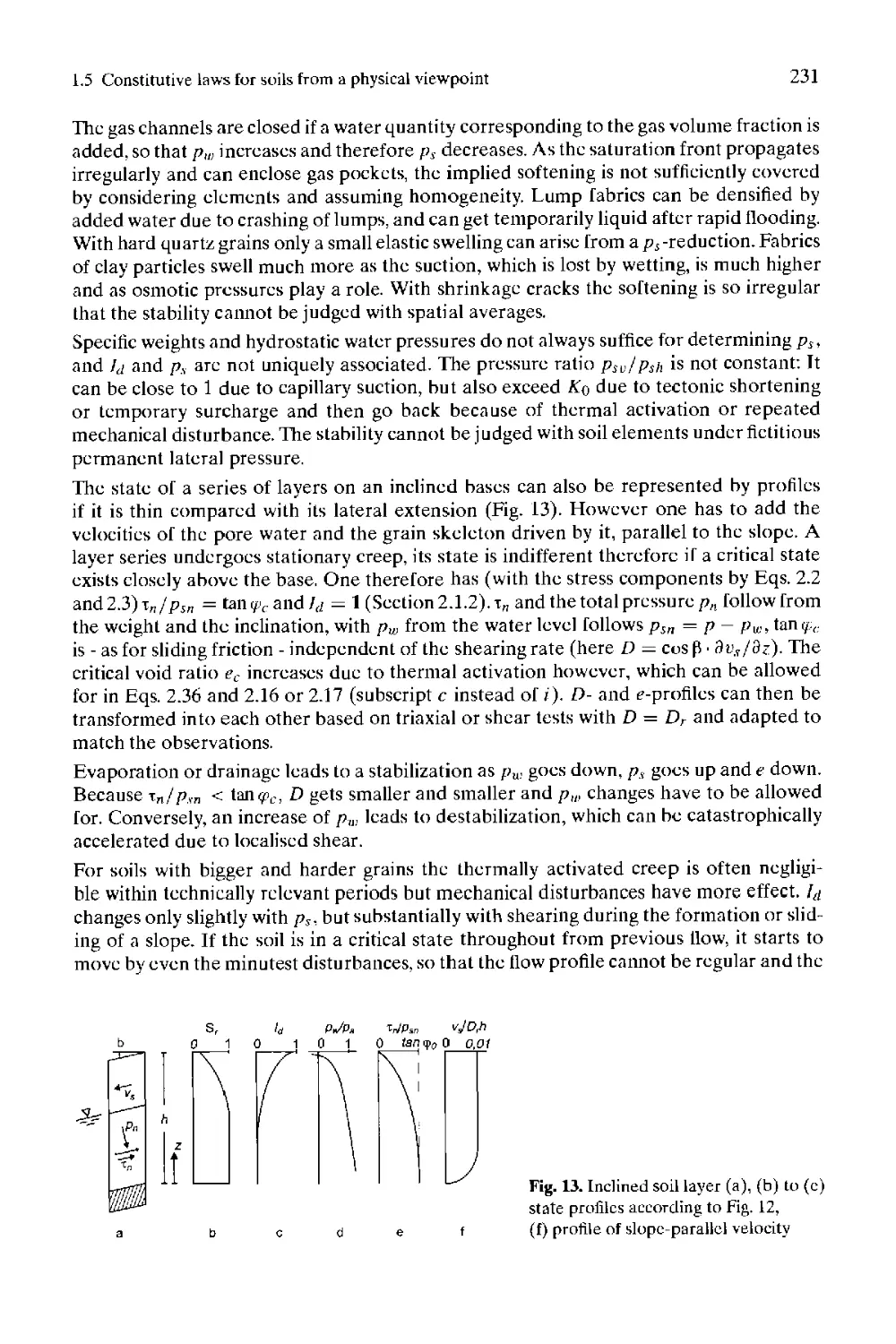
/


Text
Geotechnical Engineering Handbook
Editor:
Ulrich Smoltczyk
rnst & Soh
A Wiley Compa
n
ny
Editor:
Professor Dr.-lng. Ulrich Smoltczyk
Adlerstrafie 63
D-71032 Boblingen
Cover: Campo Valle Maggia, Tessin
Instrumentation for investigating an extensive 250 m deep sliding mass, Solexperts AG
This book contains 616 figures and 82 tables
Die Deutsche Bibliothek - CIP-Cataloguing-in-Publication-Data
A catalogue record for this publication is available from Die Deutschen Bibliothek
ISBN 3-433-01449-3
©2002 Ernst & Sohn Verlag fur Architektur und technische Wissenschaften GmbH und Co. KG, Berlin
All rights reserved, especially those of translation into other languages. No part of this book may be reproduced in any form - i.e. by photocopying, microphotography, or any other process - or be rendered or translated into a language useable by machines, especially data processing machines, without written permission of the publisher.
Typesetting: Mitterweger & Partner Kommunikationsgesellschaft mbH, Plankstadt
Printing: Betz-Druck GmbH, Darmstadt
Binding: Litges & Dopf Buchbinderei GmbH, Heppenheim
Printed in Germany
Preface to Volumes 1 to 3
It was in the early 1950s that a German consultant in Berlin came to the conclusion that structural engineers needed much more guidance on the special problems which they faced on a daily basis due to geotechnical difficulties associated with designing structures. He discussed this with his professional friends in civil engineering companies, administration and science and with a publisher who became quite interested in editing an appropriate “pocket book” about geotechnical matters. This was the birth of the German “Grundbau-Taschenbuch” (ground engineering pocket book). The first edition had already been quite a success for the publisher but some professionals thought it could be improved. The editor at that time was assisting his professor of soil mechanics and foundation engineering at the Technical University in Berlin, who was also a member of the editorial board. He asked me to consider the concerns that had been raised, and as a result of I was given the job of criticizing authors who were much more experienced and prominent than myself. I hope, however, that those authors who are still alive, will forgive the ‘youngster’ for some of the things he wrote.
In subsequent editions we added material that we thought might provide additional professional help. This, however, made the “pocketbook” expand until today it comprises three volumes of a handbook that was published at the beginning of the 21st century in its sixth edition. There is a general topic to each volume: the first one deals with the fundamentals, the second with geotechnical procedures and the third one with foundation elements and structures. Potential subscribers asked me why I thought they might be persuaded to spend money on a sixth edition when they already had the fifth one? I was glad to point out the fact that firstly, we have been lucky enough to obtain new and famous authors to bring a fresh viewpoint to many of the problems, and secondly that the significant harmonisation of design rules in Europe has produced new types of verification procedures due to limit state design which will be new to some practitioners.
Recently, globalization has also become an essential topic, both in the field of publishing and in international civil engineering activities. Ernst & Sohn, Berlin, a publisher of technical literature for more than 150 years, became associated with Wiley of New York, and the question was asked as to why such a handbook on geotechnics was not available in English. You are now holding the result of this discussion but we should confess that it has not been an easy job. It was realized that for many of the chapters, a one-by-one translation would not have been appropriate. The authors of the various chapters were therefore asked to review their texts on behalf of the readers outside German speaking countries and to consider the international state of the art to that extent that would, at the very least, allow further concise guidance to be given by appropriate references. As a book devoted to daily practice of experts, it also had to take account of the considerable bulk of technical rules already in place, the contents of which should not be repeated simply to fill pages but should be commented on, controversially if necessary.
Volume 1 starts with an overview of the state of international geotechnical harmonisation, which has been achieved by the civil engineering Eurocode programme in which design is now based on the concept of limit state analysis and the establishment of characteristic values for actions and resistances. Since the editor for more than the last two decades participated in this work, he became well aware of the difficulties raised by the need to find the relationship between conventionally applied geotechnical parameters and characteristic values. Chapter 1.2 is therefore devoted to finding the characteristic values for geotechnical parameters. The next two chapters deal with field and laboratory testing whilst emphasising the state of knowledge documented in the pre-standard versions of Eurocode 7 - Parts 2 and 3, Chapters 1.5 to 1.9 describe the scientific background and calculation models to be used in geotechnical design, whilst Chapter 1.10 explains how these numerical tools can be used nowadays in design practice.
As surveying has always been a most important method of controlling the performance of geotechnical structures during construction and thereafter - especially when observational methods are used - the state of modern geodetic know-how, including satellite positioning is covered in Chapter 1.11. To supplement field-testing, Chapter 1,12 gives details of the recent developments in measurement equipment. The special issues associated with defining the actions caused by ice and ice flows are described in Chapter 1.14. Finally, Chapters 1.13 and 1.15 focus on the engineering geology problems of mass movements and rock mechanics problems of slope stability.
Volume 2 collects together 14 chapters dealing with the various procedures available for ground improvement (Chapter 2.1), grouting (Chapter 2.2), underpinning (Chapter 2.3), freezing techniques (Chapter 2.4), anchoring (Chapter 2.5), drilling (Chapter 2,6), driving and pulling (Chapter 2.7), offshore processing (Chapter 2,8), ground dewatering (Chapter 2.9), rock excavation (Chapter 2,10), tube jacking (Chapter 2,11), earth works (Chapter 2.12), application of geotextiles (Chapter 2.13), and engineering biology (Chapter 2.14).
Each of these chapters has been produced by authors who are experts in their specific professional field. They outline the most recent developments that have occurred and provide the information necessary for geotechnical designers to select the proper method to achieve their foundation proposals. The broad variety of techniques used required a very concise treatment of the information, often leaving the technical details to those who are especially familiar with these.
Volume 3 is concerned with the geotechnical design of structures, starting with spread foundations (Chapter 3.1), pile foundations (Chapter 3.2), and caissons (Chapter 3,3). The application of the new limit state concept is illustrated by examples. This also applies to Chapter 3.4 on the stability of excavations, in which German and British practice are compared. Chapters 3.5 and 3.6 are concerned with excavation pits protected by trench retaining walls or sheet pile walls, and in Chapter 3.7 a general outline of gravity walls is presented. The special aspects of machine foundations and foundations in areas of subsidence are dealt with in Chapters 3.8 and 3.9 and finally the waterproofing of structures is discussed in Chapter 3.10.
Hopefully, the three volumes will enable the practicing engineer to interpret test results in a more meaningful way, to judge the likely limitations of any chosen method with more confidence and to therefore find the most appropriate solution to the foundation problems that he is faced with solving in his daily practice. The object of this handbook is also to close the credibility gap between geotechnical science and practice that is often seen in either type of congress and symposium.
The editor gratefully acknowledges the involvement of the authors who have spent a considerable amount of extra time producing the chapters, over and above their daily professional duties - especially as not all of them are sufficiently familiar with the English language. Where such difficulties arose, the authors were asked to focus on providing the correct translation of their technical terms. The linguistic improvement, was then provided by Robert W. East, of Aylesbury, UK, whose help reviewing the papers is much appreciated.
October 2002 Ulrich Smoltczyk
Dipl.-Ing. Christophe Bauduin N.V. BESIX S.A.
Avenue des Communautes 100 1200 Bruxelles
Belgium
(Chap, i.l International agreements, Chap. 1.2 Determination of characteristic values)
Ulf Bergdahl
Chief Engineer
Swedish Geotechnical Institute
58193 Linkoping
Sweden
(Chap. 1.3 Geotechnical field investigations)
Dr. Jan Bohac
Department of Engineering Geology Charles University
Albertov 6 12843 Praha 2 Czech Republic (Chap. 1.4 Properties of soils and rocks and their laboratory determination)
Dr.-Ing. Clans Erichsen
WBI - Beratende Ingenieure fur Grundbau und Eelsbau GmbH HenricistraBe 50
52072 Aachen
Germany
(Chap. 1.15 Stability of rock slopes)
Prof. Dr .-I ng. Dr. h.c. Gerd Gudehus Tnstitut fur Bodenmechanik
und Grundbau
Universitat Karlsruhe
POB 6980
76128 Karlsruhe
Germany
(Chap. 1.5 Constitutive laws for soils from a physical viewpoint,
Chap. 1.9 Earth pressure determination)
Prof. Dr.-Ing. Peter Gussmann
Am Baechle 3
74629 Untersteinbach
Germany
(Chap. 1.10 Numerical methods)
Prof. Dr.-Ing. Martin Hager
Merler Allee 99
53125 Bonn
Germany
(Chap. 1.14 Ice loading actions)
Prof. Dr.-Ing. Gunter Klein
OstfeldstraBe 64a
30559 Hannover
Germany
(Chap. 1.8 Soil dynamics and earthquakes)
Prof. Dr. Edmund Krauter
geo-international
Mombacher StraBe 49-53
55122 Mainz
Germany
(Chap. 1.13 Phenomenology of natural slopes and their mass movement)
Prof. Dr.-Ing. Dr. sc. techn. h.c,
Klaus Linkwitz
Obcrc TanncnbcrgstraBc 24
71229 Leonberg
Germany
(Chap. I.Il Metrological monitoring of slopes, embankments and retaining walls)
Dr.-Ing. Klaus Jurgen Melzer
KJM Industry Consult
Drossclwcg 7a
61440 Oberursel
Germany
(Chap, 1.3 Geotechnical field investigations)
Prof. Dr. Roberto Nova
Politecnico di Milano
Piazza Leonardo da Vinci, 32
20133 Milano
Italy
(Chap. 1.7 Treatment of geotechnical ultimate limit states by the theory of plasticity)
Prof. PhD DSc (Eng.) Harry Poulos
PO Box 125
North Ryde
New South Wales
Australia 2113
(Chap. 1.6 Calculation of stress and settlement, in soil masses)
Priv.-Doz. Dr.-Ing. Herrmann Schad ReinsburgstraBe 11 lb
70197 Stuttgart
Germany
(Chap. 1.10 Numerical methods)
Prof. Dr.-Ing. Willfried Schwarz
Am Appelgraben 50
59425 Weimar-Tau bach
Germany
(Chap. 1.11 Metrological monitoring of slopes, embankments and retaining walls)
Prof, PhD Ian M. Smith
Simon Engineering
c/o University of Manchester
Brunswick Street
Manchester M13 9PL
Great Britain
(Chap. 1.10 Numerical methods)
Prof. Dr.-Ing. habil. Dr.-Ing. E.h,
Ulrich Smoltczyk
AdlerstraBe 6.3
71032 Boblingen
Germany
(Chap. 1.1 International agreements)
Dipl.-Ing. Paul von Soos
ReuBweg 30
81247 Munchen
Germany
(Chap. 1.4 Properties of soils and rocks and their laboratory determination)
Dr.-Ing. Frank Sperling
Spinozawej 12
2202 AV Nordwijk
The Netherlands
(Chap. 1.8 Soil dynamics and earthquakes)
Dr. Arno Thut
Solexperts AG
POB 230
8603 Schwcrzcnbach
Switzerland
(Chap. 1.12 Geotechnical measurement procedures)
Prof. Dr.-Ing. Walter Wittkc
WBI - Beratende Ingenieure fur
Grundbau und Felsbau GmbH
HenricistraBe 50
52072 Aachen
Germany
(Chap. 1.15 Stability of rock slopes)
Tony Barley
Geotechnical Consultant
High View
Harlow Pines, Harrogate HG3 1PZ England (Chap. 2.5 Ground anchors)
Dipl.-Ing. Bernd Braun 620 Dover Court
Coppell, TX 75019-2866
USA
(Chap. 2.4 Ground freezing)
Jacob Gerrit de Gijt
Gemeentewerken Rotterdam Galvanistraat 15
Postbus 6633
3002 AP Rotterdam
The Netherlands
(Chap. 2.S Foundations in open water)
Dipl.-lng. Regine Jagow-Klaff
Heltorfer StraBe 91
47269 Duisburg
Germany
(Chap. 2.4 Ground freezing)
Prof. Dr.-Ing. Hans-Ludwig JessbergeH (Chap. 2.4 Ground freezing)
Dipl.-lng. Klaus Kirsch
Keller Grundbau GmbH
KaiserleistraBe 44 63067 Offenbach Germany
(Chap. 2,1 Groundimproveme.nl)
Dr.-Ing. Helmut Ostermayer
Drosselweg 13 82152 Krailing
Germany
(Chap. 2.5 Ground anchors)
Dr.-Ing. Thomas Rumpelt
Smoltczyk & Partner GmbH
Untere Waldplatze 14
70569 Stuttgart
Germany
(Chap. 2.12 Earthworks)
Dr.-Ing. Fokke Saathoff
BBG Bauberatung
Geokunststoffe GmbH
Alter Bahndamm 12
49448 Lemforde
Germany
(Chap. 2.13 Geosynthetics in geotechnical and hydraulic engineering)
Prof. h. c, Dr.-Ing, Hugo M. Schiechtf (Chap. 2.14 Slope protection by b io engineering techniq и es)
Prof. Dr.-Ing, Hans-Henning Schmidt
Smoltczyk & Partner GmbH
Untere Waldplatze 14
70569 Stuttgart
Germany
(Chap. 2.12 Earthworks)
Prof, Dr.-Ing. Stephan Semprich
Institut fur Bodenmechanik
und Grundbau
Technische Universitat Graz
RechbauerstraBe 12
8010 Graz
Austria
(Chap. 2.2 Grouting in geotechnical engineering)
Prof. Dr.-Ing, Ulrich Smoltczyk
AdlerstraBe 63
71032 Boblingen
Germany
(Chap. 2.3 Underpinning, undercutting;
Chap. 2.9 Ground dewatering)
Dr.-Ing. Wolfgang Sondermann Keller Grundbau GmbH KaiserleistraBe 44 63067 Offenbach Germany
(Chap. 2.1 Ground improvement)
Prof. Dr.-Ing. Gert Stadler
Institut fur Baubetrieb und Bauwirtschaft
Technische Universitat Graz RechbauerstraBe 12 8010 Graz
Austria
(Chap. 2.2 Grouting in geotechnical engineering)
Prof. Dr.-Ing. Axel C. Toepfer
Alter Weg 10a 38302 Wolfenbiittel
Germany
(Chap. 2.10 Construction methods for cuttings and slopes in rock;
Chap. 2.11 Microtunneling)
Dr.-Ing. Georg Ulrich Baugrundinstitut Zum Brunnentobel 6
88299 Leutkirch-Herbrazbofen
Germany
(Chap. 2.6 Drilling technoloy)
em. Prof. Ir. Abraham К Van Weele
Hofstede 12
2821 VX Stolwijk
The Netherlands
(Chap. 2.7 Driving and extraction)
Prof. Dr.-Ing. Karl J. Witt
MarienstraBe 7
99421 Weimar
Germany
(Chap. 2.3 Underpinning, undercutting)
Prof. Kurt Dieter Eigenbrod, PhD Department of Civil Engineering Lakehead University 955 Oliver Road, Thunder Bay Ontario P7B 5E1
Canada
(Chap. 3.2 Pile foundations)
Dipl.-lng. Karl-Friedrich Emig Griiningweg 27d
22119 Hamburg
Germany
(Chap. 3.10 Watertight buildings and structures)
Prof. Dr.-Ing. Alfred Haack c/o STUVA-Koln Mathias-Briiggen-StraBe 41 50827 Koln
Germany
(Chap. 3.10 Watertight buildings and structures)
Prof. Dr.-Ing. habil. Achim Hcttler Rottcrerberg straBe 4
76437 Rastatt
Germany
(Chap. 3.4 Stability of excavations)
Prof. Dr.-Ing. Manfred Капу VestnerstraBe 5b
90513 Zirndorf
Germany
(Chap. 3.1 Spread foundations)
o. Prof. Dr.-Ing. Hans-Georg Kcmpfert Universitat Gesamthochschule Kassel Fachbereich 14
MonchcbergstraBe 7
34125 Kassel
Germany
(Chap. 3.2 Pile foundations)
Dr.-Ing. Dietrich Klein SteinstraBe 23
97270 Kist
Germany
(Chap. 3.8 Machine foundations)
Prof. Dr.-Ing. Gunter Klein OstfeldstraBe 64a 30559 Hannover Germany
(Chap. 3.8 Machine foundations)
Dipl.-lng. Hans Lingenfelser
Meyerhofener Weg 8 61352 Bad Homburg Germany (Chap. 3.3 Caissons)
Prof. Dr. Dr.-Ing. h. c.
Boleslav Mazurkiewicz
ul. Syrokomli 7
81-439 Gdynia
Poland
(Chap. 3.6 Sheet pile walls for harbours and waterways)
Prof. Dr.-Ing. Dieter Netzel Ingenieurgemeinschaft Bauen GcbelsbergstraBe 4!
70199 Stuttgart
Germany
(Chap. 3.1 Spread foundations)
Prof. Dr.-Ing. Dietmar Placzek Erdbaulaboratorium Essen SusannastraBe 31 45136 Essen
Germany
(Chap. 3.9 Foundations in mining regions)
Brian Simpson, PhD
Arup Geotechnics
13 Fitzroy Street
London W1P 6BQ
Great Britain
(Chap. 3.4 Stability of excavations)
Prof. Dr.-Ing. Dr.-Ing. E. h.
Ulrich Smoltczyk
AdlerstraBe 63
71032 Boblingen
Germany
(Chap. 3.1 Spread foundations,
Chap. 3.2 Pile foundations,
Chap. 3.7 Gravity retaining walls)
Dr.-Ing. Manfred Stocker Bauer Spezialtiefbau GmbH WittelsbacherstraBe 5
86529 Schrobenhausen
Germany (Chap. 3.5 Bored pile walls, diaphragm walls, cult-off walls)
o. Prof. Dr.-Ing. Bernhard Walz Bergische Universitat GH Wuppertal Fachbereich Bauingenieurwesen PauluskirchstraBe 7
42285 Wuppertal
Germany
(Chap. 3.5 Bored pile walls, diaphragm walls, cut-off walls)
o. Prof. Dr.-Ing, Anton Weissenbach Am Geholz 14
22844 Norderstedt
Germany
(Chap. 3.4 Stability of excavations)
Contents of Volume 1: Fundamentals
Snwltczyk/Bauduin, International agreements
Bauduin, Determination of characteristic values
Melzer/Bergdahl, Geotechnical field investigations
von Soos/Bohdc, Properties of soils and rocks and their laboratory determination
Gudehus, Constitutive laws for soils from a physical viewpoint
Poulos, Calculation of stress and settlement in soil masses
Nova, Treatment of geotechnical ultimate limit states by the theory of plasticity
Klein/Sperling, Soil dynamics and earthquakes
Gudehus, Earth pressure determination
Gussmann/Schad/Smith, Numerical methods
Linkwitz/Sehwarz, Metrological monitoring of slopes, embankments and retaining walls
Thut, Geotechnical measurement procedures
Krauter, Phenomenology of natural slopes and their mass movement
Hager, Ice loading actions
Wlttke/Erichsen, Stability of rock slopes
Contents of Volume 2: Procedures
Kirsch/Sondermann, Ground improvement
Semprich/Stadler, Grouting in geotechnical engineering Witt/Smoltczyk, Underpinning, undercutting Jessberger/Jagow-Klaff/Braun, Ground freezing Ostermayer/Barley, Ground anchors
Ulrich, Drilling technology
Van Weele, Driving and extraction de Gijt, Foundations in open water Smoltczyk, Ground dewatering Toepfer, Construction methods for cuttings and slopes in rock Toepfer, Microtunnelling Schmidt/Rumpelt, Earthworks
Saathoff, Geosynthetics in geotechnical and hydraulic engineering Schiechtl, Slope protection by bioengineering techniques
Preview
Contents of Volume 2: Procedures
Kirsch/Sondermann, Ground improvement Semprich/Sladler, Grouting
Witt/Smoltczyk, Underpinning and undercutting
Jessberger/Jagow-Klaff/Brown, Ground freezing Ostermayer/Barley, Ground anchors Ulrich, Drilling technology
van Weele, Driving and extraction
de Gijt, Foundations in open water
Riefi/Kordonis, Ground water flow and drainage techniques Toepfer, Construction methods for cuttings and slopes in rock Toepfer, Microturmeling
Schmidt/Rumpelt, Earthworks
Saathoff Application of geotextiles
Schiechtl, Slope protection by bioengineering techniques
Contents of Volume 3: Structures
Smoltczyk/Netzel/Kany, Spread foundations Kempfert/Eigenbrod/Smoltczyk, Pile foundations Lingenfelser, Caissons
Weifienbach/Hettler/Simpson, Stability of excavations
Stocker/Walz, Trench walls
Mazurkiewicz, Sheet-pile walls for harbours and waterways Haack/Emig, Waterproofing of buildings and structures Klein/Klein, Machine foundations
Plaezek, Foundations in mining regions
Brandl, Slope protection and retainment
Contents of Volume 1: Fundamentals
Smoltczyk/Bauduin, International agreements
Bauduin, Determination of characteristic values
Melzer/Bergdahl, Geotechnical field investigations
von Soos/Bohdc, Properties of soils and rocks and their laboratory determination
Gudehus, Constitutive laws for soils from a physical viewpoint
Poulos Calculation of stress and settlement in soil masses
Nova, Treatment of geotechnical ultimate limit states by the theory of plasticity
Klein/Sperling, Soil dynamics and earthquakes
Gudehus, Earth pressure determination
Gussmann/Schad/Smith, Numerical methods
Linkwitz/Schwarz, Metrological monitoring of slopes, embankments and retaining walls
Thut, Geotechnical measurement procedures
Krauter, Phenomenology of natural slopes and their mass movement
Hager, Ice loading actions
Wittke/Erichsen, Stability of rock slopes
Contents of Volume 3: Structures
Smoltczyk/Nelzel/Kany, Spread foundations
Kempfert/Eigenbrod/Smoltczyk, Pile foundations
Lingenfelser, Caissons
Weiflenbac№Hettler/Simpson, Stability of excavations
StockerfWalz, Trench walls
Mazurkiewicz, Sheet pile walls for harbours and waterways
Smoltczyk, Gravity retaining walls
Klein/Klein, Machine foundations
Placzek, Foundations in mining regions
Haack/Emig, Waterproofing of buildings and structures
Contents
1.1 International agreements
Ulrich Smoltczyk and Christophe Bauduin
1 Classification of geotechnical literature................................... 1
2 Symbols..................................................................... 3
3 International rules for foundation engineering.............................. 4
4 Basic terms by EN 1990 and EN 1997 ......................................... 6
4.1 Classification of assessments in Eurocodes (EN 1990,1.4; EN 1997-1,1.3). 6
4.2 Limit states (EN 1990)...................................................... 6
4.3 Design situations (EN 1990, 3.5)............................................ 7
4.4 Geotechnical categories (EN 1997-1,2.1)..................................... 7
4.5 Observational method (EN 1997. 2.7)......................................... 7
4.6 Partial safety factor method................................................ 8
5 Geotechnical report........................................................ 12
5.1 Ground investigation report (EN 1997-1,3.4)................................ 13
5.2 Ground design report (EN 1997-1. 2.8)...................................... 14
6 References ................................................................ 16
1.2 Determination of characteristic values
Christophe Bauduin
1 Introduction .............................................................. 17
2 From derived value to design value......................................... 17
2.1 Sequential steps........................................................... 17
2.2 Points of view when analyzing test results............................... 19
2.3 Points of view when determining characteristic values of ground parameters (EN 1997-1,2.4.5)..................................................... 25
2.4 Use of statistical methods................................................. 28
3 Examples .................................................................. 37
3.1 Local sampling............................................................. 37
3.2 Local sampling with V well-known........................................... 38
3.3 Soil property increasing linearily with depth.............................. 39
3.4 Analysis of shear tests.................................................... 41
3.5 Example: Boulder clay...................................................... 45
4 References ................................................................ 49
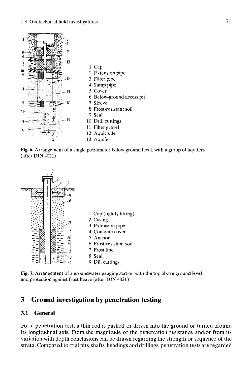
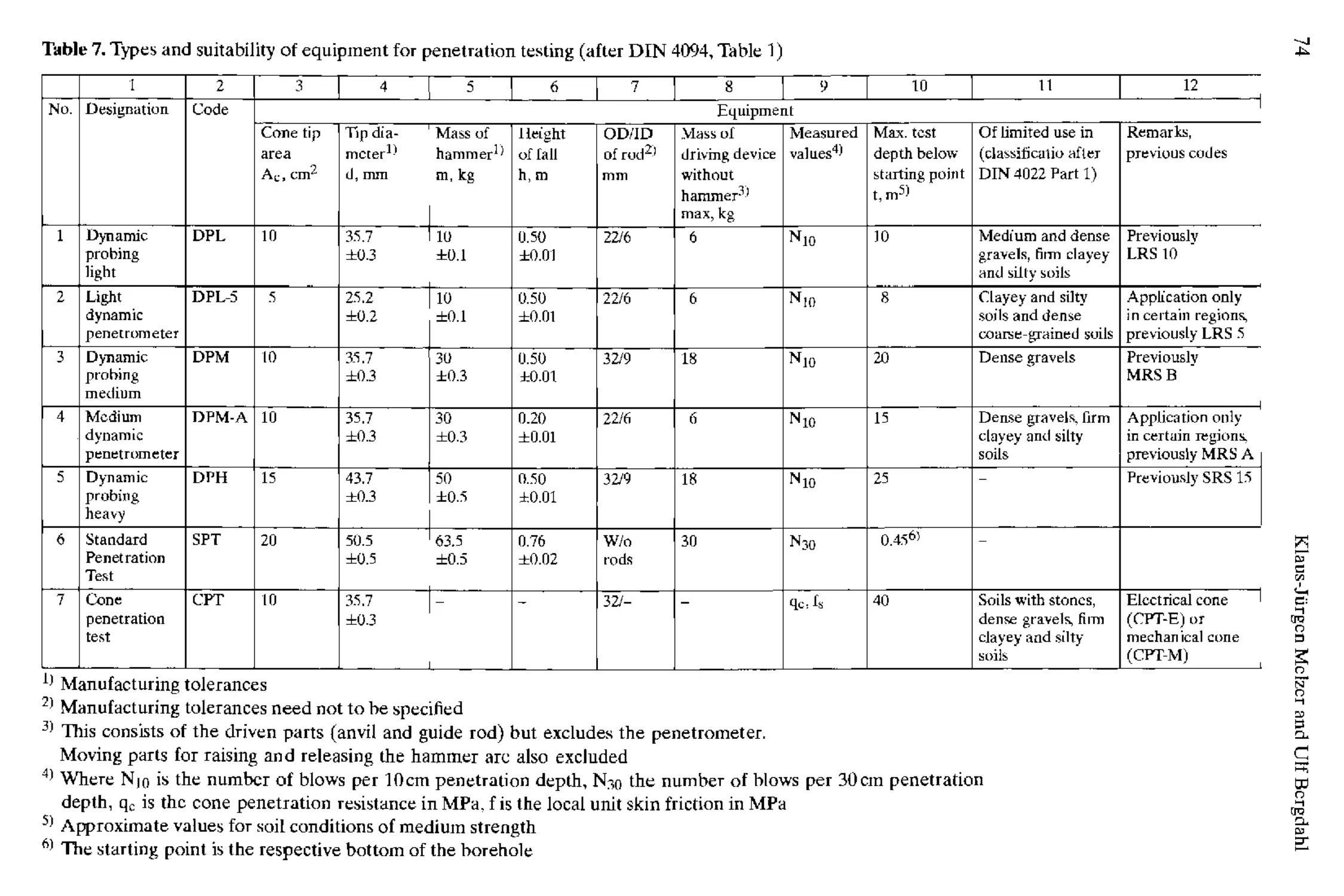
1.3 Geotechnical field investigations
Klaus-Jiirgen Melzer and Ulf Bergdahl
1 Basics..................................................................... 51
1.1 Standards ................................................................. 51
1.2 Preliminary investigations ................................................ 52
1.3 Design investigations...................................................... 53
2 Ground investigation by excavation, drilling and sampling.................. 53
2.1 General.................................................................... 53
2.2 Investigation of soils .................................................... 56
2.3 Investigation of rocks..................................................... 62
2.4 Obtaining special samples ................................................. 67
2.5 Investigation of groundwater conditions.................................... 68
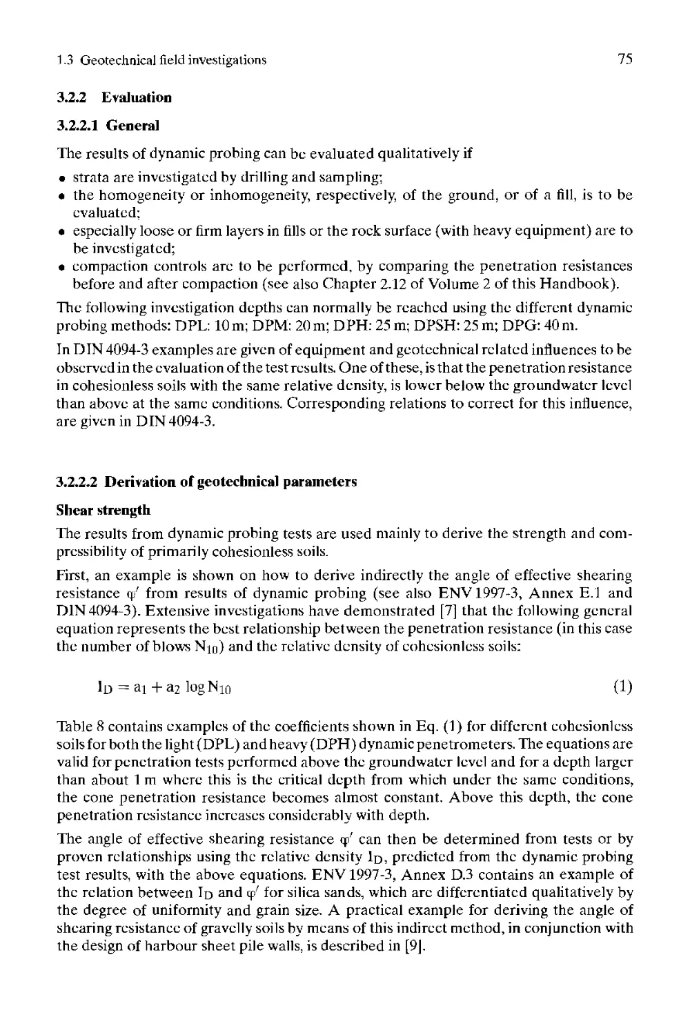
3 Ground investigation by penetration testing................................ 71
3.1 General.................................................................... 71
3.2 Dynamic probing............................................................ 73
3.3 Standard penetration test.................................................. 77
3.4 Cone penetration test...................................................... 82
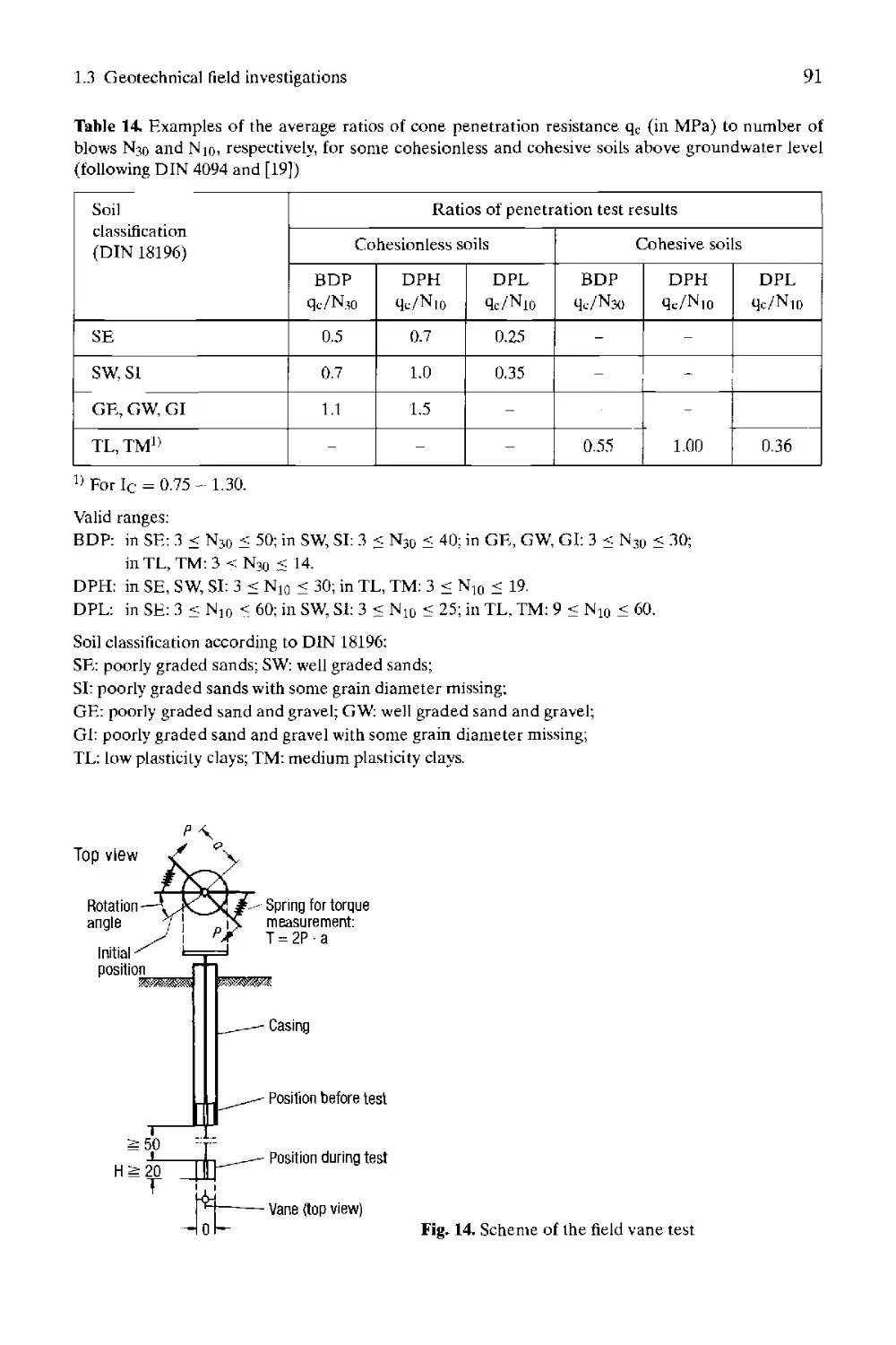
3.5 Field vane test............................................................ 90
3.6 Weight sounding test....................................................... 93
4 Lateral pressure tests in boreholes ....................................... 96
4,1 Equipment and test procedures ............................................. 96
4.2 Evaluation................................................................ 102
5 Determination of density.................................................. 106
5.1 Sampling methods.......................................................... 106
5.2 Radiometric methods....................................................... 107
6 Geophysical methods....................................................... 109
6.1 General................................................................... 109
6.2 Brief descriptions of some methods........................................ 110
7 References ............................................................... 111
8 Standards ................................................................ 116
1.4 Properties of soils and rocks and their laboratory determination
Paul von Soos and Jan Bohac
1 Soils and rocks - origins and basic terms................................. 119
2 Properties of soils ...................................................... 119
2.1 Soil layers............................................................... 119
2.2 Soil samples.............................................................. 120
2.3 Laboratory investigation - performing and evaluating...................... 120
2.4 Soil properties and laboratory testing.................................... 121
3 Properties of rocks....................................................... 126
4 Characteristics and properties of solid soil particles.................... 126
4.1 Particle size distribution................................................ 126
4.2 Density of solid particles ............................................... 129
4.3 Mineralogical composition of soils ....................................... 130
4.4 Shape and roughness of particles ......................................... 132
4.5 Specific surface ......................................................... 132
4.6 Organic content................................................................ 133
4.7 Carbonate content.............................................................. 134
5 Characteristics and properties of soil aggregates.............................. 134
5.1 Fabric of soils................................................................ 134
5.2 Porosity and voids ratio....................................................... 135
5.3 Density........................................................................ 138
5.4 Relative density............................................................... 138
5.5 Water content.................................................................. 140
5.6 Limits of consistency - Atterberg limits....................................... 140
5.7 Water adsorption............................................................... 144
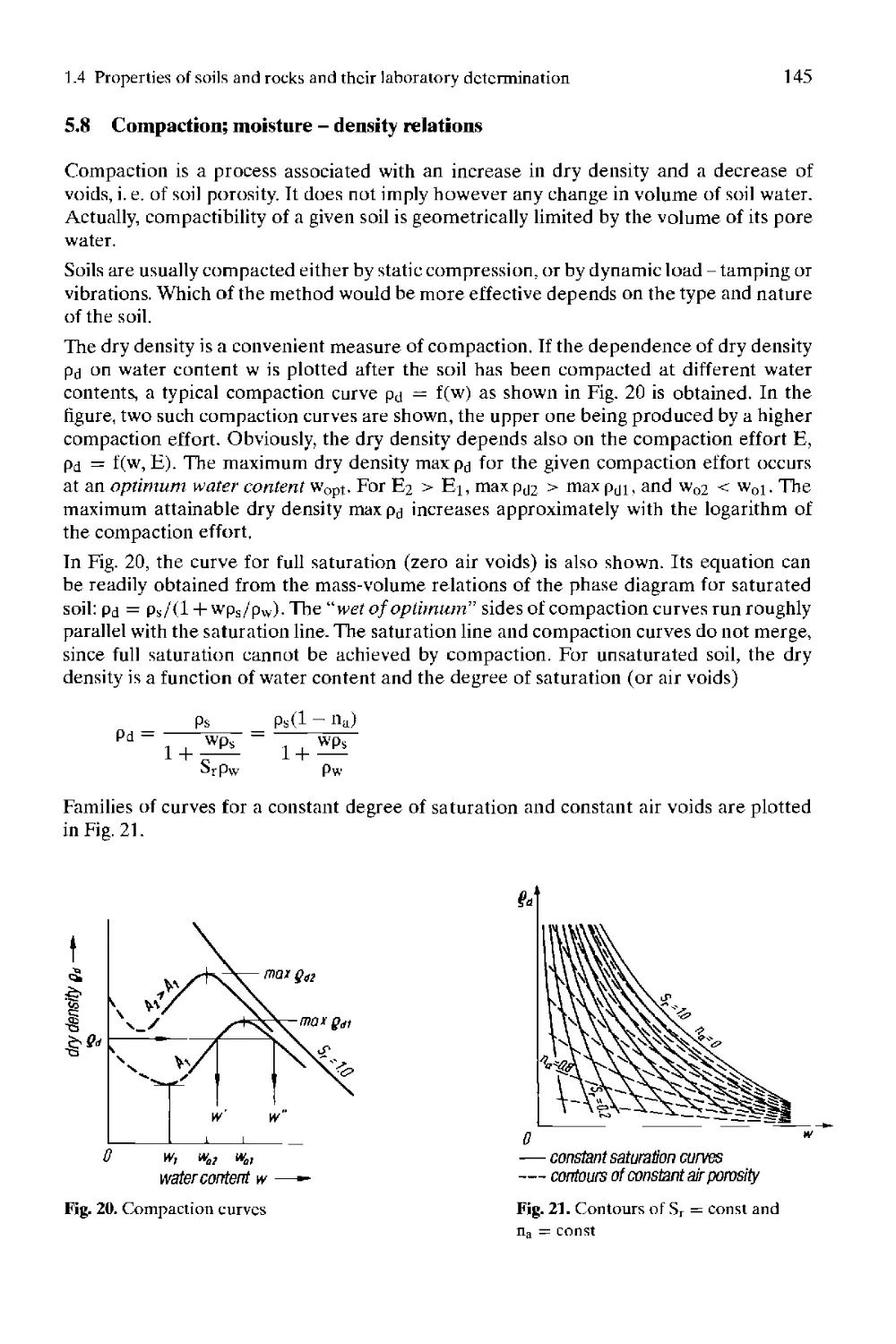
5.8 Compaction; moisture - density relations....................................... 145
5.9 Size of voids; filters ........................................................ 146
5.10 Capillarity.................................................................... 147
5.11 Water permeability ............................................................ 150
5.12 Air permeability .............................................................. 152
6 Stress-strain behaviour........................................................ 153
6.1 General considerations......................................................... 153
6.2 One-dimensional compression and consolidation (oedometer) test................. 157
6.3 Tri axial compression test..................................................... 164
6.4 Unconfined compression test.................................................... 168
6.5 Tests with the general state of stress - true triaxial test and biaxial test .... 168
6.6 Measurement of time dependent deformation...................................... 169
7 Determination of shear strength parameters..................................... 171
7.1 General aspects of strength testing............................................ 171
7.2 Triaxial compression test ..................................................... 176
7.3 Determination of unconfined compressive strength and sensitivity. 179
7.4 Shear box test................................................................. 180
8 Determination of tensile strength.............................................. 182
9 Determination of slake durability of rock...................................... 183
10 Correlations .................................................................. 183
10.1 Proctor density and optimum water content of fine-grained soils ............... 183
10.2 Water permeability ............................................................ 184
10.3 Stress-strain relations lor soils ............................................. 185
10.4 Parameters of shear strength .................................................. 187
11 Classification................................................................. 189
11.1 Soil classification............................................................ 189
11.2 Rock classification............................................................ 197
12 References .................................................................... 200
1.5 Constitutive laws for soils from a physical viewpoint
Gerd Gudehus
1 Introduction .................................................................. 207
1.1 Motive and objective........................................................... 207
1.2 Contents....................................................................... 208
2 Slates and changes of state.................................................... 210
2.1 States ........................................................................ 210
2.2 Changes of state............................................................... 220
2.3 Special sequences of state and stability.................................. 227
3 Stress-strain relations................................................... 237
3.1 Finite constitutive laws.................................................. 237
3.2 Elastoplasticity ......................................................... 241
3.3 Hypoplasticity............................................................ 248
4 Further constitutive laws ................................................ 253
4.1 Physico-chemical and granulometric changes................................ 253
4.2 Transport laws............................................................ 254
4.3 Granular interfaces....................................................... 254
5 References ............................................................... 256
1.6 Calculation of stress and settlement in soil masses
Harry Poulos
1 Introduction ............................................................. 259
2 Basic relationships from the theory of elasticity......................... 260
2.1 Definitions and sign convention........................................... 260
2.2 Principal stresses........................................................ 260
2.3 Maximum shear stress...................................................... 261
2.4 Octahedral stresses ...................................................... 261
2.5 Two-dimensional stress systems ........................................... 262
2.6 Analysis of strain........................................................ 263
2.7 Elastic stress-strain relationships for an isotropic material............. 265
2.8 Summary of relationships between elastic parameters....................... 266
3 Principles of settlement analysis......................................... 267
3.1 Components of settlement.................................................. 267
3.2 Application of elastic theory to settlement calculation................... 267
3.3 Allowance for effects of local soil yield on immediate settlement......... 269
3.4 Estimation of creep settlement............................................ 269
3.5 Methods of assessing soil parameters ..................................... 270
4 Solutions for stresses in an elastic mass................................. 272
4.1 Introduction ............................................................. 272
4.2 Kelvin problem............................................................ 272
4.3 Boussinesq problem........................................................ 273
4.4 Cerruti’s problem......................................................... 273
4.5 Mindlin’s problem no. 1................................................... 274
4.6 Mindlin’s problem no. 2................................................... 276
4.7 Point load on finite layer................................................ 278
4.8 Finite line load acting within an infinite solid.......................... 278
4.9 Finite vertical line load on the surface of a semi-infinite mass.......... 279
4.10 Horizontal line load acting on the surface of a semi-infinite mass........ 279
4.11 Melan’s problem I......................................................... 280
4.12 Melan’s problem II ....................................................... 281
4.13 Uniform vertical loading on a strip....................................... 281
4.14 Vertical loading increasing linearly...................................... 281
4.15 Symmetrical vertical triangular loading................................... 282
4.16 Uniform vertical loading on circular area ................................ 283
4.17 Uniform vertical loading on a rectangular area........................... 284
4.18 Other cases.............................................................. 285
5 Solutions for the settlement of shallow footings......................... 285
5.1 Uniformly loaded strip footing on a homogeneous clastic layer............ 285
5.2 Uniformly loaded circular footing on a layer............................. 285
5.3 Uniformly loaded rectangular footing on a layer.......................... 287
6 Rate of settlement of shallow lootings................................... 289
6.1 One dimensional analysis................................................. 289
6.2 Effect of non-linear consolidation....................................... 291
6.3 Consolidation with vertical drains....................................... 291
6.4 Two- and three-dimensional consolidation................................. 293
6.5 Simplified analysis using an equivalent coefficient of consolidation.... 293
7 Solutions for the settlement of strip and raft foundations............... 297
7.1 Point load on a strip foundation......................................... 297
7.2 Uniform loading on a strip foundation ................................... 297
7.3 Uniform loading on a circular raft....................................... 299
7.4 Uniform loading on a rectangular raft.................................... 301
7.5 Concentrated loading on a semi-infinite raft............................. 303
8 Solutions for the settlement of pile foundations......................... 305
8.1 Single piles ............................................................ 305
8.2 Pile groups ............................................................. 309
9 References .............................................................. 310
1. 7 Treatment of geotechnical ultimate limit states by the theory of plasticity
Roberto Nova
1 Fundamentals ol ultimate limit states.................................... 313
1.1 Introduction ............................................................ 313
1.2 Definitions.............................................................. 314
1.3 Fundamental theorems for standard materials.............................. 317
2 Limit analysis of shallow foundations on a purely cohesive soil.......... 319
2.1 Introduction ............................................................ 319
2.2 Lower bound analysis..................................................... 320
2.3 Upper bound analysis..................................................... 321
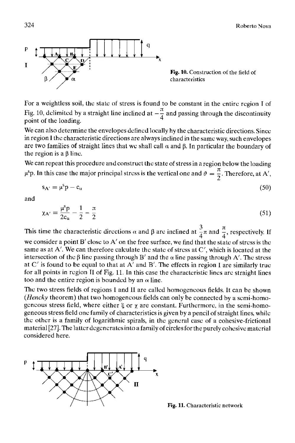
2.4 Refined lower bound analysis: method of characteristics.................. 322
2.5 Refined upper bound: slip lines.......................................... 325
2.6 Strip footing ........................................................... 326
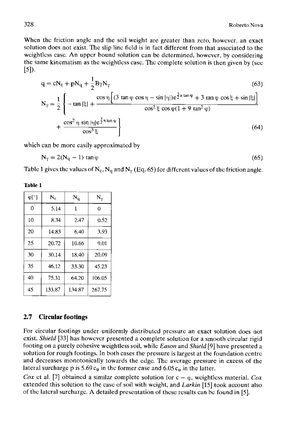
2.7 Circular footings........................................................ 328
3 Limit analysis for non-standard materials................................ 329
3.1 Introduction ............................................................ 329
3.2 Fundamental theorems for non-standard materials.......................... 329
4 Further limitations of limit analysis - slope stability.................. 332
4.1 Introduction ............................................................ 332
4.2 Simple lower bound analysis.............................................. 333
4.3 Simple upper bound analysis ............................................. 333
4.4 Improvement of bound estimates........................................... 334
4.5 Actual critical height of a vertical cut................................. 335
5 Elastoplastic analysis of shallow foundations............................ 336
5.1 Introduction .......................................................... 336
5.2 Fundamental experimental findings ..................................... 337
5.3 Behaviour in unloading-reloading ...................................... 338
5.4 Permanent displacements and rotations ................................. 339
5.5 Parameter determination................................................ 341
5.6 Comparison with experimental data...................................... 342
5.7 An application to the settlement of the Pisa bell-tower ............... 345
6 References ............................................................ 351
1.8 Soil dynamics and earthquakes
Gunter Klein and Frank Sperling
1 Introduction .......................................................... 353
2 Basic mechanical considerations........................................ 354
2.1 Time dependent processes............................................... 354
2.2 Basics of technical vibration systems.................................. 357
3 Dynamics of foundation structures...................................... 363
3.1 Vibration excitation................................................... 363
3.2 Model systems for foundation structures................................ 368
3.3 Fundamentals of the half-space theory.................................. 375
4 Dynamics of subsoil................................................... 378
4.1 Dynamical properties of soils.......................................... 378
4.2 Characteristic parameters of dynamic soil properties................... 380
4.3 Design parameters for rigid foundations................................ 382
4.4 Shock protection and vibration isolation............................... 384
5 Dynamics of earthquakes................................................ 388
5.1 Basic seismological concepts........................................... 388
5.2 Design methods for buildings........................................... 393
5.3 Effect of earthquakes on foundation engineering........................ 398
6 Literature............................................................. 403
7 References ............................................................ 404
1.9 Earth pressure determination
Gerd Gudehus
1 Introduction .......................................................... 407
1.1 Objectives............................................................. 407
1.2 Selection and organization of material in the paper.................... 408
2 Limit states without pore water ....................................... 408
2.1 Plane slip surface..................................................... 408
2.2 Curved slip surfaces and combined mechanisms .......................... 412
2.3 Three-dimensional effects.............................................. 418
3 Limit states with pore water........................................... 421
3.1 Air-impervious soils................................................... 421
3.2 Air-pervious soils..................................................... 426
4 Deformation-dependent earth pressures.................................. 428
4.1 Granular soils......................................................... 428
4.2 Clayey and organic soils............................................... 431
5 References ............................................................ 435
1.10 Numerical methods
Peter Gussmann, Hermann Schad, Ian Smith
1 General methods....................................................... 437
1.1 Difference procedures................................................. 437
1.2 Integral equations and the boundary element method.................... 440
2 Basics of the finite element method (FEM)............................. 441
2.1 Matrices of elements and structures................................... 442
2.2 Calculation techniques for non-linear problems........................ 448
3 The application of FEM in geotechnics................................. 452
3.1 Static problems....................................................... 452
3.2 Time dependent problems............................................... 455
4 The kinematical element method (КЕМ) and other limit load methods . . . 460
4.1 Basics................................................................ 460
4.2 A static approach: the method of characteristics from Sokolovski...... 461
4.3 Kinematical methods: КЕМ.............................................. 462
4.4 Slice methods ........................................................ 471
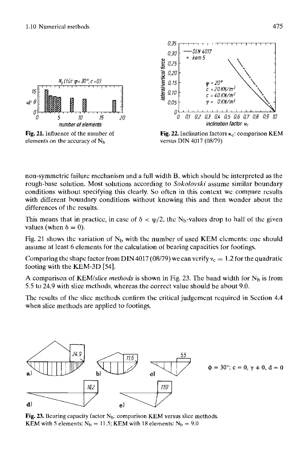
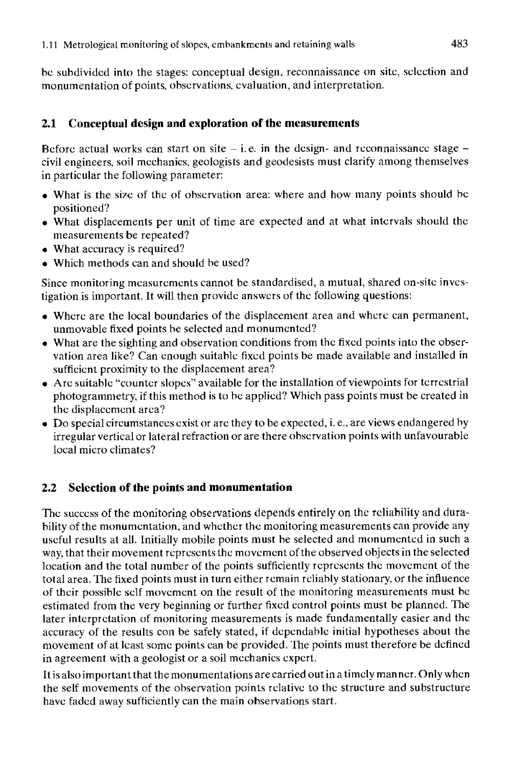
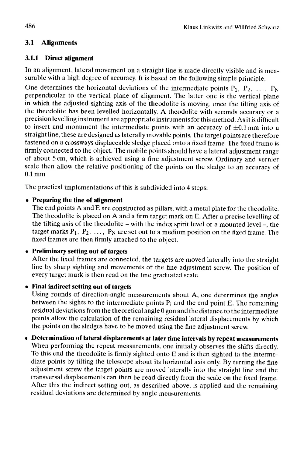
4.5 Application to bearing capacity of footings: comparison investigations .... 474
4.6 Design formulas and design tables or charts for standard slopes... 477
5 References ........................................................... 477
1 .11 Metrological monitoring of slopes, embankments and retaining walls
Klaus Linkwitz and Willfried Schwarz
1 Task and objective.................................................... 481
2 About the practical organisation, solution and carrying out of the task .... 482
2.1 Conceptual design and exploration of the measurements................. 483
2.2 Selection of the points and monumentation............................. 483
2.3 Observations.......................................................... 484
2.4 Evaluations........................................................... 484
2.5 Interpretation........................................................ 484
3 Geodetic methods of monitoring measurements........................... 485
3.1 Alignments............................................................ 486
3.2 Polygonal traverses .................................................. 491
3.3 Trigonometrical determination of individual points; nets.............. 500
3.4 Automated methods..................................................... 512
3.5 Inclination measurements.............................................. 519
4 Photogrammetrical methods of monitoring measurements.................. 526
4.1 Methodology and procedures............................................ 526
4.2 Aerial photogrammetry................................................. 527
4.3 Terrestrial photogrammetry............................................ 532
4.4 Digital photogrammetry................................................ 533
5 Satellite supported methods........................................... 535
5.1 System structure of GPS............................................... 536
5.2 Procedures for absolute positioning................................... 540
5.3 Procedures for relative positioning................................... 542
5.4 Monitoring measurements with satellite supported procedures........... 545
6 Evaluation and analysis of the measurements............................ 546
6.1 Geodetic analysis and interpretation................................... 546
6.2 Structural-physical analysis and interpretation........................ 548
6.3 Integral analysis and interpretation................................... 549
7 References ............................................................ 551
1.12 Geotechnical measurement procedures
Amo Thut
I Introduction .......................................................... 561
2 Objectives of geotechnical measurements................................ 561
3 Measured parameters.................................................... 563
3.1 Parameters in the foundation soil...................................... 563
3.2 Parameters during construction ........................................ 564
3.3 Parameters in the supporting structure................................. 564
3.4 Parameters at adjacent structures...................................... 565
3.5 Parameters for permanent structures ................................... 565
3.6 Parameters for the rehabilitation of buildings......................... 566
4 Measuring instruments, installation and costs ......................... 566
4.1 Geodetical measurements ............................................... 566
4.2 Geotechnical measurements.............................................. 567
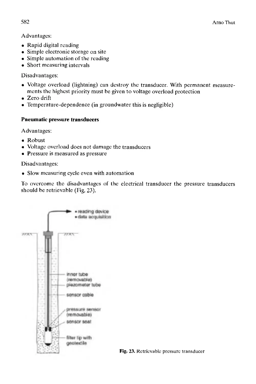
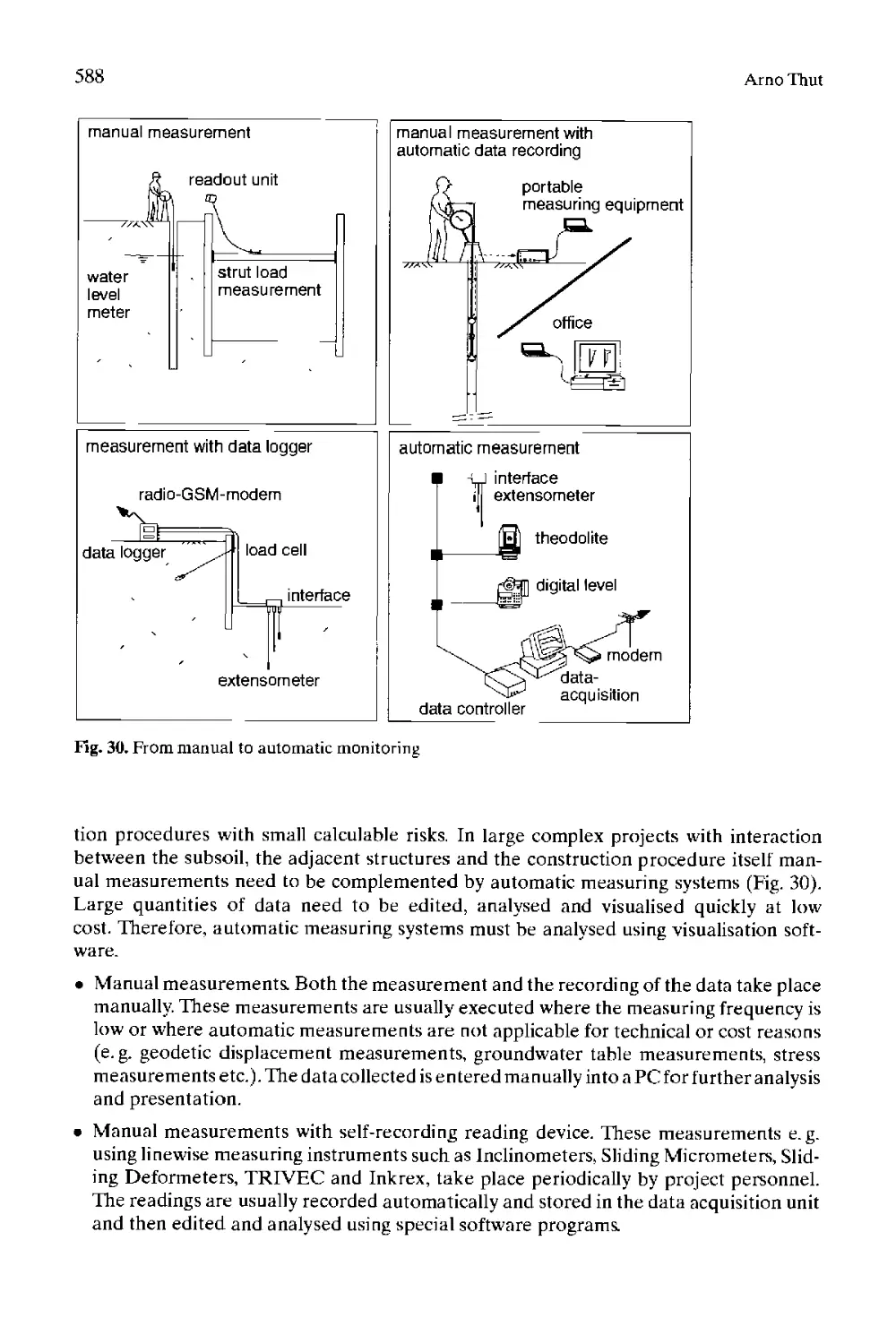
5 Execution of the measurements, reporting............................... 587
5.1 Manual measurements.................................................... 589
5.2 Automatic measuring systems............................................ 589
5.3 Data visualisation software............................................ 590
6 Case histories ....................................................... 590
6.1 Deep excavations, adjacent structures.................................. 590
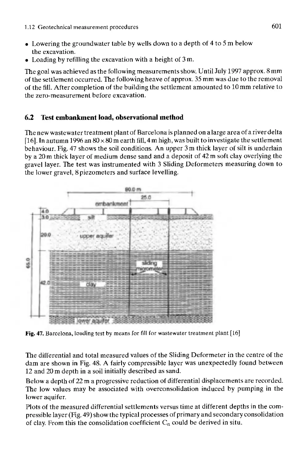
6.2 Test embankment load, observational method............................. 601
6.3 Adler Tunnel - readjustment of a structure............................. 603
6.4 Monitoring of unstable slopes.......................................... 607
6.5 Test loading of supporting structure, pile tests, displacement measurements in pile foundation........................... 611
7 References ............................................................ 615
1.13 Phenomenology of natural slopes and their mass movement
Edmund Krauler
1 Definitions............................................................ 617
2 Introduction .......................................................... 617
3 Slope shapes........................................................... 618
4 Mass movement of slopes................................................ 621
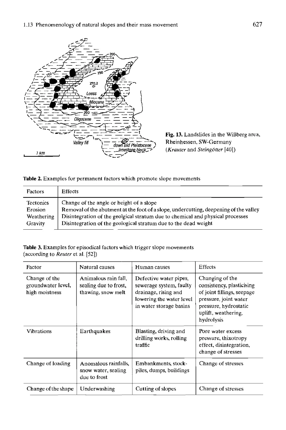
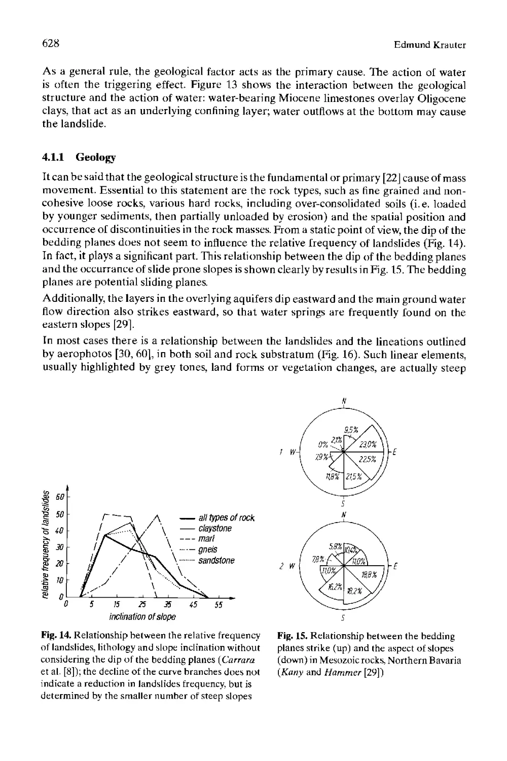
4.1 Causes, factors........................................................ 626
4.2 Classification, types.................................................. 638
4.3 Shapes of sliding surfaces and failure mechanisms...................... 651
4.4 Sequences of movements and hazard assessment........................... 654
4.5 Identification and investigation....................................... 662
5 References ............................................................ 664
1.14 Ice loading actions
Martin Hager
1 Preliminary remarks........................................................ 669
2 Types of ice loads and ice-structure interactions.......................... 669
3 Properties of ice.......................................................... 670
3.1 Mass density of ice........................................................ 670
3.2 Elasticity of ice ......................................................... 671
3.3 Thermal expansion of ice................................................... 671
3.4 Strength of ice............................................................ 672
4 Definitive values of the ice strength for calculation ..................... 674
5 Thickness of ice........................................................... 676
6 Calculation of the ice loads............................................... 677
6.1 Ice loads on wide structures............................................... 677
6.2 Ice loads on narrow slender structures .................................... 678
6.3 Thermal ice pressure loads................................................. 682
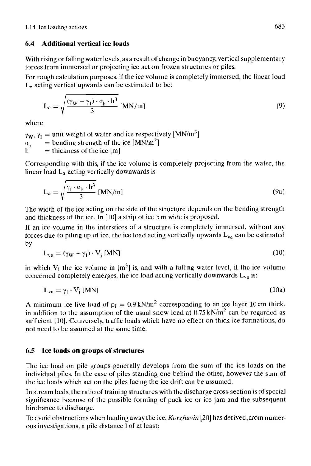
6.4 Additional vertical ice loads.............................................. 683
6.5 Ice loads on groups of structures.......................................... 683
6.6 Ice loads under special climatic and ice conditions...................... 684
7 References ................................................................ 685
1.15 Stability of rock slopes
Walter Wittke. and Claus Erichsen
1 Introduction .............................................................. 687
2 Structural models of rock mass............................................. 688
3 Mechanisms of failure of rock slopes....................................... 693
4 Model for the stress-strain behaviour of rock.............................. 696
4.1 General.................................................................... 696
4.2 Intact rock................................................................ 698
4.3 Discontinuities............................................................ 698
4.4 Rock mass.................................................................. 701
4.5 Model for the mechanical behaviour of a rock mass with respect to a refined stress displacement behaviour of persistent discontinuities with no fillings . 705
5 Model for seepage flow through a rock mass................................. 707
6 Stability investigations according to the finite element method............ 712
6.1 General.................................................................... 712
6.2 Computation of stresses and displacements.................................. 712
6.3 Computation of a seepage flow.............................................. 716
6.4 Presentation and interpretation of the computed results ................... 718
6.5 Influence of shear parameters of discontinuities on the stability of a slope . 720
6.6 Support of a slope with prestressed anchors................................ 723
6.7 Influence of high horizontal in-situ stresses.............................. 725
6.8 Stability investigations on the wall of a construction pit using a refined conceptual model of the mechanical behaviour of a rock mass...................... 731
7 Stability analysis on the basis of rigid-body mechanics.................... 735
7.1 General.................................................................... 735
7.2 Possibilities of translation and rotation of rock mass wedges.............. 735
7.3 Stability analysis of planar rock mass wedges............................ 740
7.4 Stability analysis of three-dimensional rock mass wedges supported by two discontinuities......................................................... 748
7.5 Stability analysis of three-dimensional rock mass wedges supported by three discontinuities ...................................................... 757
8 Buckling problems........................................................ 758
9 Example for the stabilization of a slope failure......................... 759
9.1 General.................................................................. 759
9.2 Landslide and immediate action........................................... 759
9.3 Results of the measurements and explorations ............................ 764
9.4 Concepts for stabilization of the slope.................................. 766
9.5 Chosen measure for stabilization ........................................ 769
9.6 Drainage measures ....................................................... 770
10 References .............................................................. 771
Subject index ................................................................. 775
Contents
2.1 Ground improvement
Klaus Kirsch and Wolfgang Sondermann
1 Introduction/overview................................................... 1
2 Ground improvement by compaction........................................ 3
2.1 Static methods.......................................................... 3
2.2 Dynamic methods........................................................ 14
3 Ground improvement by reinforcement.................................... 31
3.1 Methods without a displacing effect.................................... 31
3.2 Methods with a displacing effect....................................... 39
4 Conclusion ............................................................ 50
5 References ............................................................ 50
2 .2 Grouting in geotechnical engineering
Stephan Semprich and Gert Stadler
1 Introduction .......................................................... 57
2 Aims of grouting....................................................... 57
3 Groutability of soil and rock.......................................... 58
3.1 General................................................................ 58
3.2 Geometry of pores in soil.............................................. 59
3.3 Void volume of a rock mass............................................. 63
3.4 Water in soil and rock mass ........................................... 65
4 Grouting materials and their basic constituents........................ 66
5 Methods of grouting.................................................... 67
5.1 Flow regimes of grouts................................................. 67
5.2 Classification of grouting applications................................ 69
5.3 Grouting parameters.................................................... 74
6 Design of grouting works............................................... 77
6.1 Exploration of the subsoil............................................. 77
6.2 Choice of grouting material............................................ 78
6.3 Contract and compensation.............................................. 78
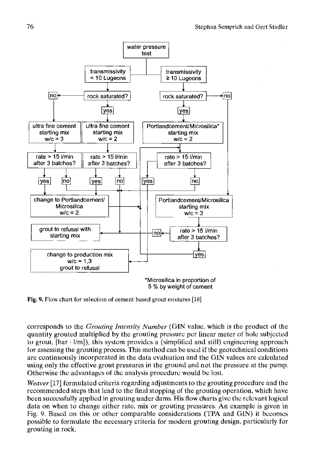
7 Examples of application................................................ 80
7.1 Grouting test in weathered rock........................................ 80
7.2 Kolnbrein dam.......................................................... 85
7.3 Debis excavation pit................................................... 88
8 References ............................................................ 89
2.3 Underpinning, undercutting
Karl J. Witt and Ulrich Smoltczyk
1 Terms.................................................................. 91
2 General aspects........................................................ 91
3 Underpinning and its adaptations....................................... 92
3.1 Traditional technique.................................................. 92
3.2 Grouting and jetting technique......................................... 96
3.3 Micropiling........................................................... 100
4 Undercutting.......................................................... 105
4.1 Cut-and-cover methods................................................. 105
4.2 Underground excavation methods ....................................... 110
5 Final remarks......................................................... 112
6 References ........................................................... 113
7 Standards and recommendations ........................................ 115
2.4 Ground freezing
Hans-Ludwig Jessberger, Regine Jagow-Klaff, and Bernd Braun
1 Introduction ......................................................... 117
2 Exploration of subsurface conditions ................................. 118
3 Ground freezing techniques............................................ 120
3.1 Brine freezing........................................................ 120
3.2 Liquid nitrogen (LNj) freezing........................................ 120
4 Characteristics of freezing and frozen soils ......................... 122
4.1 Thermal properties ................................................... 122
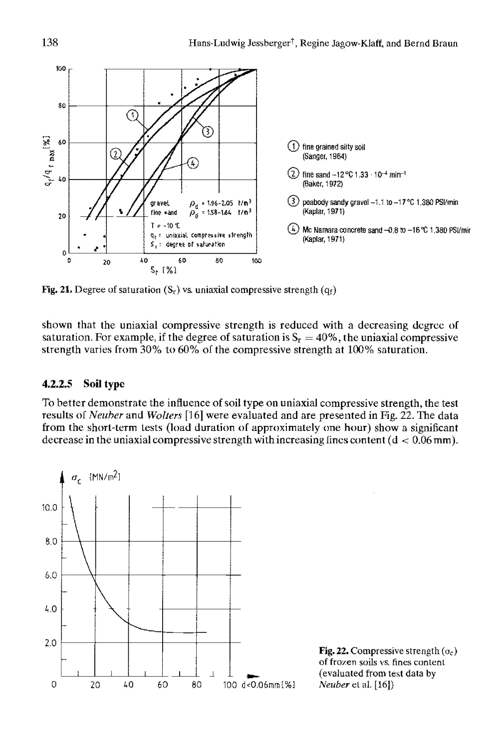
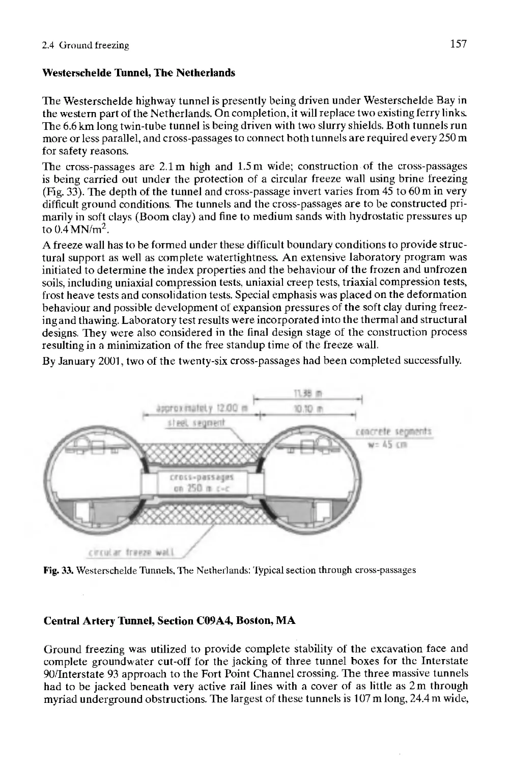
4.2 Strength and deformation properties................................... 126
5 Freeze wall design.................................................... 141
5.1 Structural design..................................................... 141
5.2 Thermal design ....................................................... 146
6 Ground movements due to freezing ..................................... 151
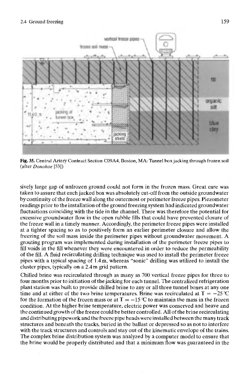
7 Ground freezing applications and recommendations for its use ......... 152
8 References ........................................................... 164
2 .5 Ground anchors
Helmut Ostermayer and Tony Barley
1 General............................................................... 169
2 Standards, recommendations, technical approvals....................... 169
3 Function and structural elements of anchor systems.................... 171
3.1 General requirements ................................................. 171
3.2 Steel tendon and anchor head.......................................... 171
3.3 Grout body............................................................ 174
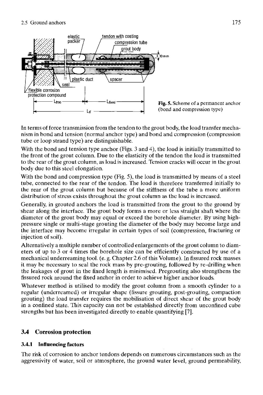
3.4 Corrosion protection.................................................. 175
4 Execution............................................................. 177
4.1 Drilling.............................................................. 177
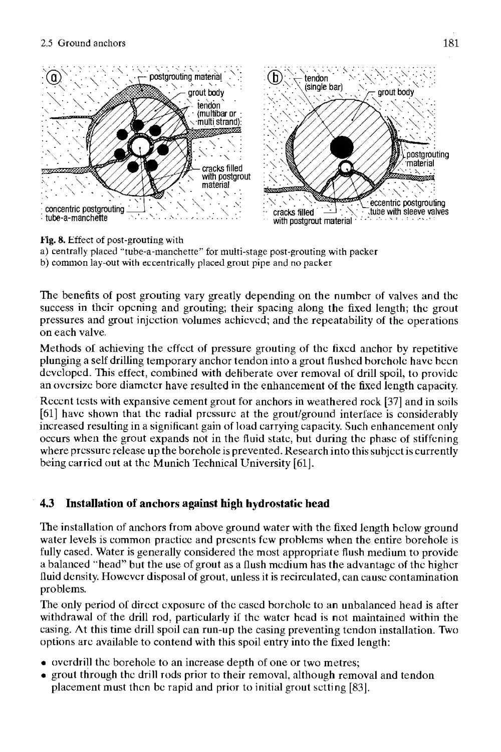
4.2 Installation, grouting and postgrouting............................... 179
4.3 Installation of anchors against high hydrostatic head................. 181
4.4 Corrosion protection measures on site ................................ 184
4.5 Removable anchors..................................................... 184
5 Testing, stressing and monitoring ..................................... 185
5.1 Stressing equipment and procedure ..................................... 185
5.2 System test ........................................................... 186
5.3 Investigation and suitability test..................................... 186
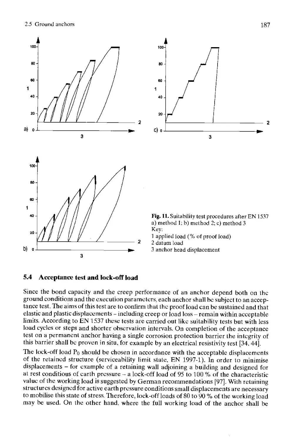
5.4 Acceptance test and lock-off load...................................... 187
5.5 Monitoring............................................................. 188
6 Fixed anchor design.................................................... 189
6.1 General................................................................ 189
6.2 Ultimate load capacity in non-cohesive soil............................ 191
6.3 Ultimate load capacity in cohesive soil................................ 196
6.4 Working loads.......................................................... 201
6.5 Creep displacements and load losses.................................... 202
6.6 Performance under alternating actions.................................. 204
6.7 Performance under dynamic actions...................................... 205
6.8 Influence of spacing (group effect).................................... 205
7 Design of anchored structures ......................................... 206
7.1 Design requirements.................................................... 206
7.2 Prerequisites for applying ground anchors.............................. 206
7.3 Design of the individual anchor ....................................... 206
7.4 Design of anchors in a group .......................................... 208
7.5 Choice of appropriate anchor systems and methods of execution.......... 214
8 References ............................................................ 215
2 .6 Drilling technology
Georg Ulrich
1 Methods ............................................................... 221
1.1 Dry drilling system.................................................... 221
1.2 Drilling with water flushing .......................................... 224
1.3 Raise boring .......................................................... 237
1.4 Full diameter drilling of smaller diameters ........................... 239
1.5 Soil investigation drilling............................................ 241
2 Cranes and rigs........................................................ 241
2.1 Percussion drill crane................................................. 241
2.2 Universal rotary drilling rig ......................................... 244
2.3 Excavator attachments.................................................. 245
2.4 Large diameter and deep drilling....................................... 246
2.5 Slimhole drilling equipment............................................ 247
2.6 Casing................................................................. 248
3 Drilling tools......................................................... 249
4 Natural drilling obstructions.......................................... 251
5 Directional drilling with flushing..................................... 251
6 References ............................................................ 254
2.7 Driving and extraction
Abraham E Van Weele
1 Application of driving techniques...................................... 255
2 Principle of impact driving............................................ 255
3 Piling hammers......................................................... 257
3.1 Free fall hammers ...................................................... 257
3.2 Diesel hammers.......................................................... 258
3.3 Hammers for cast-in-situ piles ......................................... 261
3.4 Driving with a mandrel.................................................. 261
4 Alternative installation methods for displacement piles................. 262
4.1 Pile jacking............................................................ 262
4.2 Pile screwing with simultaneous pushing................................. 263
4.3 Grouted steel piles, MV-piles........................................... 264
4.4 Coupled piles........................................................... 265
5 Jetting assistance...................................................... 266
6 Driving cap............................................................. 267
7 Piling machines......................................................... 269
8 Stresses during impact driving ......................................... 273
8.1 Maximum compressive stresses............................................ 273
8.2 Relationship between wave length and pile length for concrete piles .... 274
8.3 Driving timber piles.................................................... 276
8.4 Driving steel piles .................................................... 276
9 Sheet piles............................................................. 277
9.1 Profiles................................................................ 277
9.2 Sheet pile locks........................................................ 277
9.3 Lock cleaning and lubrication........................................... 278
10 Impact driving of piles - general....................................... 278
11 Impact driving of sheet piles........................................... 279
11.1 Successive installation ................................................ 279
11.2 Intermittent installation............................................... 280
11.3 Concrete and timber sheet piling ....................................... 281
11.4 Combined sheet pile walls .............................................. 282
12 Vibratory driving and extraction........................................ 283
12.1 Principle of vibratory driving.......................................... 283
12.2 Additional static pull down............................................. 284
12.3 Vibratory extraction.................................................... 285
12.4 Piling vibrators ....................................................... 285
12.5 High frequency vibration................................................ 286
12.6 Working procedure ...................................................... 287
12.7 Vibratory driving of sheet piles........................................ 288
12.8 Influence on bearing capacity........................................... 288
13 Accessibility of the working site....................................... 289
14 Stone layers and underground obstacles.................................. 289
15 Foot sensors............................................................ 290
16 Driving and extraction close to adjacent structures..................... 290
16.1 Consequences of driving................................................. 290
16.2 Consequences of extraction.............................................. 291
17 Driving under special circumstances..................................... 292
17.1 Driving in calcareous soils ............................................ 292
17.2 Driving in, or near slopes.............................................. 293
17.3 Driving behind earth retaining structures .............................. 294
18 Dynamic quality tests on piles.......................................... 294
18.1 Integrity testing....................................................... 294
18.2 Dynamic load testing.................................................... 296
18.3 “Soft” dynamic load testing............................................. 297
19 Admissibility of vibration emission..................................... 299
2,8 Foundations in open water
Jacob Gerrit de Gift
1 General................................................................ 301
1.1 Appropriate planning documents......................................... 302
1.2 Load assumptions ...................................................... 303
1.3 Design and construction................................................ 306
2 Equipment for construction work at sea................................. 307
2.1 The most important pieces of equipment................................. 307
2.2 Lifting island......................................................... 309
2.3 Dredgers............................................................... 309
2.4 Procedures for breaking down rock...................................... 319
2.5 Cable- and pipe-layers................................................. 320
2.6 Block layers........................................................... 321
3 Foundations in an open excavation...................................... 321
4 Floating structures.................................................... 324
4.1 Preparation of the bed................................................. 324
4.2 Construction of the floating structures................................ 325
4.3 Towage................................................................. 328
4.4 Setting down........................................................... 330
4.5 Caissons as quay wall.................................................. 331
4.6 Caissons for moles and breakwaters..................................... 332
4.7 Floating structures for lighthouses, offshore platforms and storage.... 336
4.8 Floating structures for tunnels underwater ............................ 343
5 Caisson foundations.................................................... 348
5.1 "Alte Weser'' lighthouse (1960/63) .................................... 350
5.2 “GroBcr Vogelsand” lighthouse (1973/74)................................ 353
6 Piled foundations...................................................... 354
6.1 Kohlbrand viaduct, Hamburg (1971-75)................................... 356
6.2 Goeree Lighthouse, The Netherlands (1971).............................. 356
6.3 Drilling platform. Cognac, USA (1978).................................. 358
6.4 Suction pile technology ............................................... 358
7 References ............................................................ 362
2.9 Ground dewatering
Ulrich Smoltczyk
1 General code requirements ............................................. 365
2 Basic assumptions and solutions for dewatering scheme analyses......... 366
3 Methods of dewatering.................................................. 367
3.1 Dewatering by bored wells.............................................. 368
3.2 Dewatering by open drainage or slit pumping (line source).............. 384
3.3 Dewatering by electro-osmosis.......................................... 388
4 Field tests ........................................................... 391
4.1 General................................................................ 391
4.2 Tests.................................................................. 391
5 Groundwater recharge................................................... 396
5.1 Steady state........................................................... 396
5.2 Initial time-dependant state........................................... 396
5.3 Capacity of a recharge well............................................ 397
5.4 Interaction of recharge wells.......................................... 397
5.5 Interaction of suction and recharge wells.............................. 398
6 References ............................................................ 398
2 .10 Construction methods for cuttings and slopes in rock
Axel C. Toepfer
1 Introduction .......................................................... 399
2 Cuttings in rock....................................................... 400
2.1 Mechanical loosening by ripping........................................ 400
2.2 Loosening by blasting methods.......................................... 403
3 Construction method for rock slopes.................................... 417
3.1 Mechanical construction method for the production of rock slopes....... 418
3.2 Smooth blasting methods................................................ 418
4 References ............................................................ 427
2.11 Microtunnelling
Axel C. Toepfer
1 Introduction .......................................................... 429
2 'Die microtunnelling construction method for non-man-sized entry pipes . . 430
2.1 Hie components of the construction method.............................. 430
2.2 Description of soil and rock........................................... 431
2.3 Pipe material.......................................................... 431
2.4 Microtunnelling system ................................................ 432
2.5 Driving and reception shaft ........................................... 437
2.6 Construction sequence.................................................. 438
2.7 Further development.................................................... 440
3 References ............................................................ 440
2 .12 Earthworks
Hans-Henning Schmidt and Thomas Rumpelt
1 Introduction .......................................................... 441
2 Standards, environmental legislation................................... 441
3 Terms and definitions.................................................. 443
4 Construction materials, classifications and characteristic values ..... 444
4.1 Gcrneral introduction ................................................. 444
4.2 Characteristic parameters.............................................. 445
5 Design of earthwork structures......................................... 448
5.1 Site investitgation .................................................. 448
5.2 Design calculations ................................................... 448
5.3 Standardised slope angles.............................................. 450
5.4 Assessment of the stability of slopes.................................. 450
5.5 Drainage measures for earthworks....................................... 453
5.6 Landscape planning..................................................... 455
6 Larthwork processes/earthworks equipment............................... 455
6.1 Machines for digging, transporting and placing......................... 456
6.2 Loading with hydraulic excavators ..................................... 458
6.3 Hauling equipment ..................................................... 461
6.4 Equipment for placing and spreading.................................... 461
6,5 Compaction.......................................................... 461
6.6 Special equipment................................................... 464
7 Planning and organisation of earthworks sites....................... 464
7.1 Site survey......................................................... 464
7.2 Mass distribution................................................... 465
7.3 Determination of performance........................................ 465
7.4 Methods excavating or borrowing of material......................... 473
7.5 Methods of placement and compaction................................. 475
7.6 Compaction techniques............................................... 477
7.7 Compaction criteria................................................. 478
8 Quality assurance: tests, specifications and observations........... 479
8.1 General remarks..................................................... 479
8.2 Tests............................................................... 479
8.3 Compaction requirements for road construction....................... 481
8.4 Testing methods in road construction ............................... 487
8.5 Compaction control in rockfills..................................... 488
8.6 Observational methods .............................................. 488
9 Soil treatment: soil improvement, stabilisation and cementation..... 489
10 Excavation of cuts.................................................. 489
11 Dams and embankments................................................ 490
12 Excavations and trenches............................................ 492
12.1 Excavations......................................................... 492
12,2 Trenches............................................................ 493
1 2.3 Narrow trenches .................................................... 494
13 Backfills and fills covering structures............................. 494
14 Sound protection embankments........................................ 495
15 Synthetic and clay liners........................................... 496
16 Recultivation....................................................... 497
17 Embankment construction by means of hydraulic fills................. 498
17.1 General............................................................. 498
17.2 Hydraulic transport of sand-water mixtures (slurries) .............. 498
17.3 Equipment .......................................................... 500
17.4 Some operational details............................................ 500
17.5 Sedimentation impoundment........................................... 501
17.6 Economical aspects.................................................. 502
18 References ......................................................... 503
2.13 Geosynthetics in geotechnical and hydraulic engineering
Fokke Saathoff
1 General............................................................. 507
2 Basic parameters and terms.......................................... 507
2.1 Classification of geosynthetics..................................... 507
2.2 Geotextiles ........................................................ 509
2.3 Geotextile-related products......................................... 512
2.4 Geomembranes........................................................ 513
2.5 Geomembrane-related products........................................ 514
2.6 Raw materials....................................................... 515
2.7 Functions .......................................................... 515
2.8 References to the execution......................................... 521
2.9 Test methods............................................................ 522
3 Fields of application................................................... 523
3.1 Coastal protection...................................................... 523
3.2 Waterways engineering .................................................. 540
3.3 Small-scale hydraulic engineering...................................... 551
3.4 Dam construction ....................................................... 552
3.5 Landfill construction .................................................. 559
3.6 Road construction, railway track construction and tunnelling............ 569
4 Notes on the form of contract........................................... 592
4.1 Delivery terms.......................................................... 592
4.2 Quality management...................................................... 592
4.3 Advice on contract tenders.............................................. 593
4.4 Invoicing and warranties ............................................... 594
5 Summary................................................................. 594
6 References ............................................................. 594
2 .14 Slope protection by bioengineering techniques
Hugo Meinhard Schiechtl^
1 Introduction ........................................................... 599
2 Bioengineering slope protection......................................... 599
2.1 Preliminary works using inert material.................................. 599
2.2 Combined methods........................................................ 607
2.3 Ground stabilizing techniques........................................... 627
2.4 Soil protection techniques ............................................. 641
2.5 Supplementary construction techniques .................................. 654
3 Requirements for bioengineering materials............................... 662
3.1 General................................................................. 662
3.2 Biotechnical suitability of plants...................................... 663
3.3 Materials for ground stabilizing techniques............................. 664
3.4 Seed mixes ............................................................. 665
4 Effectiveness of bioengineering slope protection........................ 665
4.1 Technical requirements ................................................. 665
4.2 Ecological requirements................................................. 665
4.3 Effects in terms of landscape architecture.............................. 666
4.4 Economic requirements................................................... 666
5 Design and execution of bioengineering works for slope protection...... 666
6 Maintenance of bioengineering structures................................ 668
7 References ............................................................. 670
Subject index ............................................................... 671
Contents
3.1 Spread foundations
Ulrich Smoltczyk, Dieter Netzel, and Manfred Капу
1 Definitions ............................................................... 1
2 Basis of design ........................................................... 1
3 Footings .................................................................. 3
3.1 General aspects of design ................................................. 3
3.2 Geotechnical design....................................................... 13
3.3 Structural design ........................................................ 39
4 . Slab foundations ..................................................... 46
4.1 General................................................................... 46
4.2 Vertical interaction...................................................... 46
4.3 Horizontal interaction, restraints........................................ 61
5 Mat foundations (tank foundations) ....................................... 71
5.1 General................................................................... 71
5.2 Geotechnical verifications................................................ 72
5.3 Ground water protection................................................... 75
6 Tension foundations ...................................................... 76
7 References, standards and software........................................ 77
7.1 References................................................................ 77
7.2 Programmes and guidebooks................................................. 80
7.3 European codes (Status 2002) ............................................. 81
7.4 German standards referenced in this chapter .............................. 81
3.2 Pile foundations
Hans-Georg Kempfert, Kurt Dieter Eigenbrod, and
Ulrich Smoltczyk (Section 8)
1 Introduction.............................................................. 83
1.1 Applications ............................................................ 83
1.2 Governing codes and safety concepts....................................... 83
1.3 Preliminary investigations for pile foundations .......................... 84
1.4 Terminology .............................................................. 85
2 Pile types and construction methods....................................... 87
2.1 Selection of appropriate pile type........................................ 87
2.2 Quality assurance and control ............................................ 88
2.3 Displacement piles........................................................ 89
2.4 Bored piles ..............................................................104
2.5 Micropiles................................................................109
2.6 Measures to increase pile resistance .....................................113
3 Axial pile resistance....................................................115
3.1 Single piles.............................................................115
3.2 Compression pile groups..................................................141
3.3 Pile-raft foundations....................................................149
3.4 Tension pile groups .....................................................157
4 Lateral pile resistance and moment actions...............................157
4.1 Single piles.............................................................157
4.2 Lateral resistance of pile groups........................................163
5 Soil action..............................................................167
5.1 Negative skin friction...................................................167
5.2 Lateral pressure and bending due to settlement ..........................170
6 Bearing capacity and serviceability .....................................173
6.1 General..................................................................173
6.2 Bearing capacity (ULS) ..................................................174
6.3 Calculation of serviceability ...........................................181
7 Testing of piles ........................................................184
7.1 General..................................................................184
7.2 Static axial load tests .................................................184
7.3 Static horizontal pile load tests .......................................192
7.4 Dynamic pile testing.....................................................196
8 Analysis of pile structures..............................................202
8.1 General..................................................................202
8.2 Piling systems ..........................................................203
8.3 Analysis of axially loaded pile systems..................................203
8.4 Special simple cases.....................................................206
8.5 Deviations from initial assumptions .....................................211
8.6 Design of non-axially loaded pile foundations............................213
8.7 Check for buckling.......................................................218
8.8 Sheet pile wall as part of a piled foundation............................218
8.9 Eigenfrequencies of a spatial piling system..............................219
8.10 Example .................................................................220
9 References...............................................................223
3. 3 Caissons
Hans Lingenfelser
1 General..................................................................229
1.1 Terms....................................................................229
1.2 Typical features of pneumatic caissons...................................230
1.3 Typical features of open caissons (wells) ...............................231
1.4 Fields of application....................................................232
2 Structural concept and equipment.........................................234
2.1 General..................................................................234
2.2 Construction materials ..................................................234
2.3 Caisson edges ...........................................................235
2.4 Caisson working chamber and working chamber ceiling......................237
2.5 Open caisson bottom .....................................................238
2.6 Caissons walls...........................................................240
3 Construction of caissons ................................................241
3.1 Manufacture on land......................................................241
3.2 Construction in open water................................................242
3.3 Construction in a dock and floating in ...................................243
4 Sinking the caissons......................................................245
4.1 Soil excavation ..........................................................245
4.2 Control of sinking .......................................................247
4.3 Sinking tolerances .......................................................247
4.4 Ballasting ...............................................................249
5 Pneumatic installation and works..........................................250
5.1 Regulations governing pneumatic works.....................................250
5.2 Essential pneumatic equipment ............................................251
6 Caisson calculation.......................................................253
6.1 General...................................................................253
6.2 Calculation of the lowering diagram.......................................254
6.3 Loads working on the caisson cutters......................................255
6,4 Dimensioning for the lowering phases .....................................257
7 Construction examples ....................................................259
8 References................................................................271
3 .4 Stability of excavations
Anton Weissenbach, Ac him Hettier, and Brian Simpson
1 Construction measures for the stability of excavations ..................273
1.1 Unlined excavations......................................................273
1.2 Timbered trenches .......................................................275
1.3 Sheet pile walls ........................................................278
1.4 Soldier pile walls.......................................................279
1.5 Solid walls .............................................................284
1.6 Support by bracing.......................................................287
2 Basic design assumptions ................................................290
2.1 Soil properties, loads and general rules.................................290
2.2 Active earth pressure for cantilever walls ..............................291
2.3 Active earth pressure for walls supported by props and anchors...........293
2.4 Active earth pressure from surcharges ...................................301
2.5 Earth pressure under backfill conditions ................................304
2.6 Passive earth pressure...................................................306
3 Calculation procedures ..................................................310
3.1 Walls with fixed earth support...........................................310
3.2 Walls with free earth support............................................313
3.3 Multiple supported walls.................................................315
3.4 Calculation using subgrade reaction .....................................318
3.5 Numerical analysis.......................................................320
3.6 Equilibrium of vertical forces ..........................................329
3.7 Determination of the vertical component of the earth resistance..........333
3.8 Equilibrium of horizontal forces in soldier pile walls...................334
3.9 Heave of the excavation bottom...........................................337
4 Safety concepts .........................................................339
4.1 British design approach..................................................339
4.2 German design approach...................................................347
4.3 General regulations in EC 7 .............................................351
4.4 Design Approach 1........................................................354
4.5 Design Approach 2.....................................................357
5 Special constructions ................................................361
5.1 Anchored walls .......................................................361
5.2 Excavation walls supported by raking props ...........................364
5.3 Large excavations ....................................................365
5.4 Some features related to specific shapes of excavations ..............368
5.5 Excavation with asymmetric cross sections.............................374
5.6 Excavation walls adjacent to existing buildings.......................377
5.7 Excavations under water...............................................382
5.8 Excavations in jointed, unstable rock ................................392
5.9 Excavations in soft soils.............................................394
6 Calculation examples .................................................397
6.1 Problem ..............................................................397
6.2 German design approach................................................398
6.3 Eurocode 7: Design Approach 2 ........................................401
7 References............................................................404
3 .5 Bored pile walls, diaphragm walls, cut-off walls
Manfred Stocker and Bernhard Walz.
1 Bored pile walls........................................................409
1.1 Field of application ...................................................409
1.2 Advantages .............................................................410
1.3 Disadvantages ..........................................................411
1.4 Standards and references................................................411
1.5 Purpose and wall types..................................................411
1.6 Construction ...........................................................412
1.7 Quality assurance.......................................................414
2 Diaphragm walls ........................................................414
2.1 Field of application ...................................................414
2.2 Advantages .............................................................415
2.3 Disadvantages ..........................................................415
2.4 Standards and references................................................416
2.5 Purpose.................................................................416
2.6 Wall types..............................................................416
2.7 Construction ...........................................................421
2.8 Construction materials .................................................425
2.9 Characteristics.........................................................426
2.10 Quality assurance.......................................................427
3 Thin cut-off walls......................................................428
3.1 Field of application ...................................................428
3.2 Advantages .............................................................429
3.3 Disadvantages ..........................................................429
3.4 Standards and references................................................429
3.5 Purpose and types of wall...............................................429
3.6 Construction of a vibrated thin cut-off wall or vibwall.................430
3.7 Construction materials .................................................433
3.8 Characteristics.........................................................434
3.9 Quality assurance.......................................................434
4 Stabilizing of earth walls using fluids.................................435
4.1 Supporting fluids......................................................435
4.2 Fluid supporting force and stability determination ....................436
4.3 Mechanisms for transferring the fluid pressure difference onto the grain skeleton .....................................................437
4.4 Proof of the „internal" stability .....................................440
4.5 Proof of the „external" stability......................................442
4.6 Structural facilities close to suspension stabilized earth walls ......446
5 Standards and recommendations..........................................447
5.1 Standards .............................................................447
5.2 Recommendations .......................................................448
6 References.............................................................448
3 .6 Sheet pile walls for harbours and waterways
Boleslav Mazurkiewicz
1 Sheet pile wall structures, their performance and field of application .... 451
1.1 General..................................................................451
1.2 Application purpose......................................................451
1.3 Usability of different construction materials ...........................452
2 Regulations concerning sheet pile walls .................................452
2.1 Sheet pile wall structures, EN 12063/1999 .............................. 452
2.2 Recommendations of the Committee for Waterfront Structures, Harbours and Waterways, EAU 1996 ............................................. 453
2.3 Eurocode 3: Design of steel structures - Part 5; Piling..................453
2.4 Other recommendations and handbooks .....................................453
3 Sheet pile types, profiles and anchoring parts, quality and steel grades . . . 454
3.1 Steel sheet pile walls ..................................................456
4 Basic design of sheet pile walls.........................................457
4.1 Safety concept...........................................................457
4.2 Actions and resistances..................................................457
4.3 Load cases ..............................................................458
4.4 Ultimate limit state design of sheet pile wall structures ...............459
5 Calculation methods for sheet pile walls.................................460
5.1 Calculation of a single-anchored sheet pile wall according to Blum......461
5.2 Special cases of sheet pile wall calculation.............................465
5.3 Calculation principles for combined steel sheet pile walls...............468
5.4 Calculation principles of sheet pile cofferdams .........................469
6 Calculation of a sheet pile wall anchorage and its fittings..............474
6.1 Verification of stability of an anchorage at a lower failure plane
and of safety against failure of the anchoring soil .....................474
6.2 Calculation and sizing of anchor walls and anchor plates ................475
6.3 Calculation and sizing of anchors and hinges, walings and capping beams made of steel and reinforced concrete....................................477
6.4 Calculation and sizing of anchor piles ..................................485
6.5 Calculation and sizing of hinged and fixed supports for a quay wall superstructure on steel sheet pile walls.......................................488
7 Further structural remarks and recommendations ..........................489
7.1 Estimation of sheet pile wall driving depth and selection of its profile and material ..................................................................489
7.2 Steel sheet pile walls ..................................................490
8 Construction of waterfront structures made of steel sheet piles ........494
8.1 General.................................................................494
8.2 Construction of new waterfront structures...............................494
8.3 Protection and deepening of existing water front structures ............501
9 Corrosion and corrosion protection......................................506
9.1 General considerations .................................................506
9.2 Expected corrosion of steel sheet piles.................................506
9.3 Corrosion protection of steel sheet piles ..............................506
10 References..............................................................509
10.1 Books and papers........................................................509
10.2 Standards ..............................................................510
3.7 Gravity retaining walls
Ulrich. Smoltczyk
1 Introduction............................................................511
2 General design considerations ..........................................513
3 Gravity wall ...........................................................514
4 Cantilever wall ........................................................515
5 Drainage................................................................516
References..............................................................518
3.8 Machine foundations
Giinter Klein and Dietrich Klein
1 Overview ...............................................................519
1.1 Classification of machine foundations...................................519
1.2 Requirements for machine foundations....................................519
2 Loads on machine foundations............................................521
2.1 Static loads............................................................521
2.2 Periodic loads .........................................................522
2.3 Transient loads.........................................................525
2.4 Random loads ...........................................................530
3 Analysis and design of machine foundations..............................532
3.1 Types of supports.......................................................532
3.2 Rigid foundations.......................................................536
3.3 Elastic foundations.....................................................539
3.4 Spring foundations......................................................545
3.5 Design recommendations..................................................546
4 Examples ...............................................................547
4.1 Hammer foundation ......................................................547
4.2 Reinforced concrete box foundation for a 100 MW steam
turbine-generator set...................................................550
5 References..............................................................557
5.1 Standards ..............................................................557
5.2 Books and Papers........................................................557
3.9 Foundations in mining regions
Dietmar Placzek
1 General remarks on mining-induced effects.................................559
2 Ground movements .........................................................559
2.1 Ground movements above deep mine workings.................................559
2.2 Ground movements above shallow and near-surface mine workings............563
3 Influence of ground movements on the foundation...........................564
3.1 Influence of equal vertical subsidence ...................................564
3.2 Influence of tilt - differential vertical subsidence......................564
3.3 Influence of curvature....................................................566
3.4 Influence of strain ......................................................566
3.5 Influence of ground movements above near-surface mine workings...........567
3.6 Influence of discontinuous ground movements...............................568
4 Preventive measures in areas with deep mine workings .....................568
4.1 Types of preventive measures .............................................568
4.2 Basic considerations on layout and design of surface structures...........569
4.3 Bearing capacity and functionality of a structure ........................570
4.4 Provisions for tilt......................................................570
4.5 Provisions for curvature ................................................571
4.6 Provisions for extensional strain........................................575
4.7 Provisions for compressive strain........................................577
4.8 Provisions for discontinuous ground movements ...........................579
5 Preventive measures in areas with near-surface mine workings .............579
5.1 Types of preventive measures .............................................579
5.2 Preventive measures for structures........................................580
5.3 Stabilisation of the ground by injection..................................581
6 Preventive measures for tunnels...........................................584
6.1 General remarks...........................................................584
6.2 Options for preventive measures ..........................................585
7 Upgrading of existing structures..........................................585
7.1 Preliminary remarks.......................................................585
7.2 Provisions for equal vertical subsidence .................................586
7.3 Provisions for differential vertical subsidence ..........................586
7.4 Provisions for horizontal ground movements................................587
8 References................................................................589
3 .10 Watertight buildings and structures
Alfred Haack and Karl-Friedrich Emig
1 General...................................................................501
2 General aspects of design ......................................502
2.1 Geotechnical and structural influences ................................502
2.2 Serviceability provisions.................................................504
3 Selection and applicability of materials................................504
4 Systems ..................................................................505
4.1 Bonded layers ............................................................505
4.2 Polymere modified bitumen compound for bonding............................506
4.3 Loose plastic sheets .....................................................507
4.4 Steel board sealing.......................................................508
4.5 Watertight concrete structures („white tub“) ............................508
4.6 Special design considerations............................................509
5 Design provisions codified in DIN 18195..................................510
5.1 General..................................................................510
6 Structural factors ......................................................513
6.1 Watertight systems according to German Code 18195.....................513
6.2 Joint seals in watertight concrete.......................................539
7 Supervision .............................................................544
8 References...............................................................545
8.2 German recommendations and guidelines (examples).........................546
8.3 References...............................................................546
Subject index .................................................................639
1.1 International agreements
Ulrich Smoltczyk and Christophe Bauduin
1 Classification of geotechnical literature
The International Society of Soil Mechanics and Foundation Engineering (ISSMFE) have since 1981 used a classification scheme of geotechnical literature (IGC) as in Table 1.
There has also been a joint agreement with the Swedish Geotechnical Institute (SGI) since 1998 which enables access to their Information Retrieval System for Geotechnical Literature (IRS-Geo) available worldwide via the Internet. Their continuously updated database provides about 54,000 literature references from 1976 onwards. Each reference is described by TGC key words and classification codes (for combining key words, use and, or and not). Subscription is available via the SGI website at bttp://www.swcdgco.sc/ indcx-c.html. The references are 69 % English, 16 % Swedish, 6 % German, 4 % French and 5 % with other tongues.
A General
A 1 Geotechnical Engineering-Scope
A 2 Historical Aspects
A 3 Information Services, and Literature
Classification
A 4 Textbooks. Handbooks, and Periodicals
A 5 Terminology
A 6 Companies, Institutes, and I laboratories
A 7 Societies, Meetings, and International
Cooporation
A 8 Professional Ethics, Legal Require-
ments, Codes of Practice, and Standard-
ization
A 9 Education
A 10 Research Activities
В Geological and Environmental Aspects (Basic Geology, see Principal Group T)
В 0 General
В 1 Formation of Soil and Rocks
В 2 Hydrogeological Aspects
В 3 Mass Movements and I .and Subsidence
В 4 Seismic Activity and Crustal Move-
ments
В 5 Climatic Conditions
В 6 Submarine Geological Aspects
В 7 -
Table 1. International geotechnical classification system, published in March 198'1
В 8 Extraterrestrial Soil and Rock Conditions
В 9 Geomorphologic Aspects and Terrain Classification
В 10 Mineralogical Aspects
в 11 Description of Regional Soil and Rock Conditions
в 12 Other Environmental Aspects
C Site Investigations
Equipment and Techniques of Exploration, Prospection, Sampling, and Field Testing of Soils and Rocks (excl. determination of engineering properties), Presentation of Result
C 0 General
С 1 Airphoto Surveys and Remote Sensing
C 2 Geophysical Surveys
C 3 Probings (Soundings)
C 4 Visual Exploration Techniques
C 5 Boring Techniques and Equipment
(cf. C IO)
C 6 Sampling
C 7 Measurement of Field Conditions
(incl. Post-Construction Monitoring)
C 8 Field Testing (excl. tests for engineering properties, see Groups D and F)
C 9 Presentation of Results, Data Base
C 10 Underwater Site Investigations
D Soil Properties: Laboratory and In-Situ Determinations
(incl. Rockfill, Artificial Soils, Waste Materials) Concepts, Theories, Methods of Determination, Equipment, and Results
D 0 General
D 1 Classification and Description of Soils
D 2 Physico-Chemical Properties
D 3 Composition, Structure, Density, and Water Contents
D 4 Hydraulic Properties
D 5 Compressibility and Swelling
D 6 Shear-Deformation and Strength Properties
D 7 Dynamic Properties
D 8 Thermal Properties
D 9 Compactibility
D 10 Properties of Soil-Additive Mixtures
E Analysis of Soil-Engineering Problems
Theoretical, Empirical, and Practical Methods of Analysis
E 0 General
E 1 Stress Analysis
E 2 Deformation and Settlement Problems
E 3 Bearing Capacity of Shallow Foun-
dations
E 4 Bearing Capacity of Piles and other Deep Foundations, Anchors
E 5 Earth Pressure Problems
E 6 Stability of Slopes and Excavations
E 7 Seepage and other Hydraulic Problems
E 8 Dynamic Problems
E 9 Frost Action and Heat-Transfer
Problems
E 10 Analysis of Layered Systems and Pavements Behaviour
E 11 Soil-Vehicle and Soil-Tool Interaction
E 12 Soil-Structures Interaction
E 13 Mathematical Methods, Computer Analysis
E 14 Model Test Analysis
F Rock Properties: Laboratory and In-Situ Determinations
Concepts, Theories, Methods of Determination, Equipment, and Results
F 0 General
F 1 Classification and Description of Rocks and Rock Masses
F 2 Physico-Chemical Properties
F 3 Composition, Density, and Structural
Features
F 4 Hydraulic Properties
F 5 Compressibility and Swelling
F 6 Shear-Deformation and Strength Properties
F 7 Dynamic Properties
F 8 Thermal Properties
G Analysis of Rock-Engineering Problems
Theoretical, Empirical, and Practical Methods of Analysis
G 0 General
G 1 Stress Analysis
G 2 Deformation and Displacement Problems
G 3 Bearing Capacity of Rock Masses
G 4 -
G 5 Rock Pressure on Tunnels and Underground Openings
G 6 Stability of Rock Slopes and Open Excavations
G 7 Seepage and other Hydraulic Problems
G 8 Dynamic Problems
G 9 Frost Action and Heat-Transfer Problems
G 10 -
G 11
G 12 Rock-Structure-In teraction
G 13 Mathematical Methods, Computer Analysis
G 14 Model Test Analysts
H Design, Construction, and Behaviour
of Engineering Works
Description and Case Records of Engineering Works
H 0 General
H 1 Foundations of Structures (other than dams)
H 2 Retaining Structures and Cut-off Walls
H 3 Offshore Structures
H 4 Dams and Reservoirs, Embankments
H 5 Tunnels and Underground Openings
H 6 Roads, Railroads and Airfields
H 7 Harbours, Canals, and Coastal Engineering Works
H 8 Conduits and Culverts
H 9 Slopes and Unsupported Excavations
H 10 Land Use
H 11 Waste Depositories
К Construction Methods and Equipment
К 0 General
К 1 Drainage Methods
К 2 Sealing and Grouting Processes
К 3 Preloading and Soil Replacement
К 4 Earthworks and Rock Excavation, Processing and Transportation
к 5 Compaction Processes
к 6 Soil Stabilization and Erosion Control
к 7 Piles and Pile Driving, incl. Sheet Piles
к 8 Construction of Caissons and Deep Piers
к 9 Construction Methods for Shallow Foundations
к 10 Slurry-Assisted Construction of Foundations and Cut-off Walls
к 11 Support of Soil and Rock, Anchoring
к 12 Offshore Construction
к 13 Protection Measures against Frost
к 14 Measures for Improving Deformation and Stability Conditions. Reconstruction of Foundations
M Materials of Construction*
M 0 General
M 1 Steel
M 2 Wood
M 3 Bituminous Materials
M 4 Plastics and Similar Materials
M 5 Cement and Chemicals
M 6 Concrete
M 7 Paints and Coatings
M 8 Construction Elements
S Snow and Ice Mechanics and Engineering
S 0 General
S 1 Snow and Ice Cover
S 2 Properties of Snow and Ice
S 3 Snow and Ice Engineering
T Related Disciplines*
T 0 General
T 1 Pure Sciences
T 2 Geosciences
T 3 Agriculture and Pedology
T 4 Meteorology and Climatology
T 5 Biosciences
T 6 Civil Engineering
T 7 Mining Engineering and Ore
Prospecting
T 8 Mechanical Engineering
T 9 Electrical Engineering
T 10 Ocean Engineering
T 11 Military and Naval Engineering
T 12 Instrumentation and Measuring Techniques
T 13 Library Science
T 14 Environment Problems and Nature Conservation
T 15 Oil Prespecting
* The principal groups M and T are not to be used with “Geotechnical Abstracts”
2 Symbols
Existing international agreements on symbols are not always consistent. For civil engineering purposes an international standard, ISO 3898 Basis for design of structures -Notations - General symbols, was published in 1997 and was accepted by the European Commission of Standards (CEN). The standard for SI units, ISO 1000: 1992(E), was also accepted by CEN.
For geotechnical literature, the International Society agreed in 1977 to apply the following symbols:
A area 1c consistency1 index
В breadth of foundation Tl liquidity index
Ca rate of secondary consolidation Id density index
Cc compression index Ip plasticity index
Cs swelling index К modulus of compressibility
Cu uniformity coefficient K0 coefficient of earth pressure at rest
D depth of foundation beneath ground K,; active earth pressure coefficient
E modulus of linear deformation Kp passive earth pressure coefficient
Тона oedometric modulus N blow count
F factor of safety- Nc bearing capacity factor as a
G modulus of shear deformation function of c
Nq bearing capacity factor as a function of embedment depth uw u;i pore waler pressure pore air pressure
N,,. bearing capacity factor as a function V discharge velocity
of weight density у w water content
QP point resistance WL liquid limit
Qs total shaft resistance Wp plastic limit
R residual factor ws shrinkage limit
Sr degree of saturation ₽ angle of slope to horizontal
Sr sensitivity a inclination of load
Tv time factor a angle of wall friction
и degree of consolidation £ linear strain
V volume f1,2,3 principal strains
a wall adhesion К linear strain rate
a acceleration ф' or ф' effective angle of internal friction
cr effective cohesion intercept фи ОГ фи apparent angle of internal friction
CR residual cohesion intercept <₽r or Фи residual angle of internal friction
Cu apparent cohesion intercept Y shear strain
Cr remoulded undrained shear strength У shear strain rate
Cv coefficient of consolidation Y weight density
d drainage path y' weight density of submerged soil
d grain diameter Yd weight density of dry soil
e eccentricity Ys weight density of solid particles
e void ratio Yw weight density of water
g acceleration due to gravity n coefficient of viscosity
Стах void ratio in loosest state R coefficient of friction
Cmin void ratio in densest state V Poisson’s ratio
fs local side friction P mass density of soil
h hydraulic head or potential p' mass density of submerged soil
i hydraulic gradient Pd mass density of dry soil
ic, iq, i7 inclination factors Ps mass density of solid particles
j seepage force Pw mass density of water
к coefficient of permeability О total normal stress
ks modulus of subgrade reaction o' effective normal stress
m mass 01,2.3 principal stress
n porosity Ooct octahedral normal stress
4 rate of discharge O«, effective overburden pressure
qc static point resistance (CPT) preconsolidation pressure
4d dynamic point resistance T shear stress
ЯР point resistance pressure toct octahedral shear stress
qs unit shaft resistance Tf shear strength
qi limit pressure TR residual shear strength
s settlement T average shear strength mobilized
u pore pressure along sliding surface
3 International rules for foundation engineering
The only internationally established codification of rules for foundation engineering purposes that existed until now was produced by the European Commission of Standards (CEN), the aim being the introduction of a consistent system of common technical rules for the design and construction of structures in the field of civil engineering. Eventually, this will replace the differing national standards that exist in the various member states of the European Community. By removing the problems caused by the national standardiza
tion of technical rules, a common market of products and services will be established. This will improve the competitions! capability of European contractors and their consultants when working in countries off the European Community.
Structural Eurocodes generally include codified assessments for the design of structures. Construction and supervision are only covered as required for quality assurance checks of the designer’s assumptions. At present, the following documents are published or in preparation:
Technical Committee 250:
EN 1990 Basis of design for structural Eurocodes
EN 1991 Actions
EN 1992 Concrete structures. Part 1: General rules,... Part 3; Concrete foundations
EN 1993 Steel structures. Part 1: General rules,... Part 5: Steel piles
EN 1994 Mixed steel and concrete structures
EN 1995 Timber structures
EN 1996 Masonry structures
EN 1997 Geotechnical design. Part 1: General rules, Part 2; Laboratory and field testing
EN 1998 Seismic actions. Part 1: General rules,... Part 5: Foundations, retaining structures and geotechnical aspects (in addition to EN 1997-1)
EN 1999 Design of aluminium alloy structures
Technical committee 288:
EN 1536 Execution of special geotechnical work: Bored piles
EN 1537 Execution of special geotechnical work: Anchors
EN 1538 Execution of special geotechnical work: Diaphragm walls
EN 12063 Execution of special geotechnical work: Sheet piles
EN 12699 Execution of special geotechnical work: Displacement piles
EN 12715 Execution of special geotechnical work: Grouting
EN 12716 Execution of special geotechnical work: Jet-grouting
EN ... Execution of special geotechnical work: Micro-piles
EN ... Execution of special geotechnical work: Reinforced soil
Technical committee 182:
By introducing existing ISO documents into the CEN system:
ISO 14688 Identification and classification of soils
ISO 14689 Identification and classification of rock
Technical committee 189:
Several standards for testing geotextiles have been published, see Chapter 2.15.
Note: Developing European Codes from a first draft into an officially accepted document generally takes several years time. It is recommended therefore that the national standardization bodies or the appropriate CEN secretariat are asked to confirm the latest situation for each code (as to TC 250, contact NN1, POB 5059, NL-2600 GB Delft, Fax +31152690190. As to TC 288, contact AFNOR, F 92049 Paris La Defense Ccdex).
4 Basic terms by EN 1990 and EN 1997
4.1 Classification of assessments in Eurocodes (EN 1990,1.4; EN 1997-1,1.3)
Depending on the character of the individual assessments, distinction is made in EN 1990, 1.4, between Principles and Application Rules, lire codes include a main text and annexes;
Principles are rules to which no exemption or alternative is permitted.
Application Rules are internationally acknowledged rules that are recommended for application. in this case alternatives are possible, if they provide the same level of reliability and are consistent to the relevant principles. They can include the use of national specifications.
Annexes contain additional information, including numerical values of partial safety factors. The values suggested in an annex may either be accepted or modified by national determination as the level of responsibility for the reliability of the works remains with the national authorities in charge of civil engineering control.
4.2 Limit states (EN 1990)
According to EN 1990, 6.4.1, in EN 1997-1, 2.4, the following limit states are defined:
Ultimate limit states (2.4.7.1):
• Loss of equilibrium of the structure or the ground, considered as a rigid body, in which the strengths of the structural materials and the ground provide insignificant resistance (EQU).
• Internal failure or excessive deformation of the structure or structural elements, including footings, piles, basement walls etc,, in which the strength of structural materials is significant in providing resistance (STR).
• failure or excessive deformation of the ground, in which the strength of soil or rock is significant in providing resistance (GEO).
• Loss of equlibrium of the structure or the ground due to uplift by water pressure (UPL).
• Hydraulic heave, internal erosion and piping in the ground caused by hydraulic gradients (HYD).
Serviceability limit states (2.4.8):
States when deformations, displacements or any non-structural damage affect the intended function of a structure in terms of comfort and appearance, where "appearance” is concerned with, for example, extensive cracking rather than with aesthetics.
Anticipated deformations and settlements are the main consideration here. For these. Annex H of EN 1997-1 gives some guidance (see also Chapter 3.1 of Volume 3 of the Handbook).
EN 1990, 2.3, also requires that the function of the structure shall be warranted during its design working life. For example, in normal buildings Table 2.1 of EN 1990 indicates a design life time of 50 years.
43 Design situations (EN 1990,3.5)
In relation to a specified time interval the following design situations are identified:
• persistent design situations which comply with the normal use of a structure;
• transient situations which refer to temporary conditions as for example during execution or repair;
• accidental design situations by fire, explosion, impact or localised failure etc;
• seismic design situations.
Note: A ’design situation’ constitutes a complete scenario, comprising a number of various load cases and load combinations.
4.4 Geotechnical categories (EN 1997-1,2.1)
To describe the minimum requirements for the extent and content of ground investigations, design analyses and site supervision and the risks to property and life, three different geotechnical categories may be applied as follows:
GC1: Small and relatively simple structures for which basic stability and performance requirements can be fulfilled by experience and qualitative ground investigation and for which risks are negligible. Examples arc simple one- or two-storey buildings, storage sheds, garages
This classification assumes that ground conditions arc known by experience. The design of the building should therefore be routine and straightforward.
Rules which help to classify a structure into GC1 are determined nationally.
GC2: Conventional structures and foundations that can be designed by routine geotechnical procedures. These should normally include quantitative analyses to verify that the fundamental design requirements are satisfied.
Some guidance on the extent of ground investigations is given in EN 1997, 3.2. The decision, however, should be supported by local or regional experience.
GC 3: All circumstances other than those covered by GC 1 and 2.
Note: All parts of a project need not to be classified in the same category.
4.5 Observational method (EN 1997,2.7)
It is often difficult to make a reliable prediction about the performance of a structure and in such cases an observational method may be appropriate, in which the design data and
assumptions can be controlled during the execution and adapted if necessary.
This method makes the following assumptions:
• the allowable values of the performance parameters shall be assessed prior to design;
• the potential variance of performance shall be determined such that the real performance remains within the predicted limits by a sufficient level of reliability;
• the type and extent of monitoring shall be pre-determined;
• remedial measures shall be included in design and contract to allow for situations when allowable limit values become surpassed.
Smoltczyk [2] commented on the problems of this procedure and emphasized that a reaction in due time requires the consideration of the following:
Activating remedies needs some time which should be considered during design. The method is not suitable for situations where reaction will most probably not be possible in time even though alarm signals have been recorded. It should not be used therefore where brittle failure phenomena may occur.
The method should only be applied in situations where assurance can be given that a proper reaction can be implemented prior to an ultimate limit state occuring. The method should not be abused as a cheap protection against catastrophes. It should be understood as a means to provide economic alternatives within serviceability scenaria.
The monitoring scheme should be redundant. Redundance, however, should be provided by applying independant methods rather than by multiple records. It is not only economy but also the practicality using large numbers of recorded data which should make the designer think carefully about the necessary amount of gauges and readings.
It is the sudden change of a recorded parameter or its rate rather than the absolute magnitude which gives the warning of a deviating performance. Parameters taken for monitoring are mainly displacements, strains, pore pressures and water levels (Peck [1]).
4.6 Partial safety factor method
According to EN 1990, section 6, the verification of limit states shall be achieved by applying partial factors of safety as follows:
• the representative values of actions, Frep (see 4.6.1), multiplied by a partial safety factor yr;
• the characteristic values of material strength parameters. Xt, divided by a partial safety factor уга;
• the characteristic value of a resisting force, Rt, which is determined directly, divided by a partial safety factor yr.
Thus the design values (index !‘d") arc derived by Fj = Frep yf and Xj — Xk/ym or = Rk/YR-
The design values for the effects of actions in structural elements (moments, shear forces, normal forces), Ej, are then obtained by either a statical calculation
• based on Fj and Xd or Rj, or
• based on Frep and R^, multiplied by the partial safety factor yf.
Uncertainty about the calculation model of actions may be allowed for by an additional model factor, ysd> which in the first case (see EN 1990. 6.3.2, eq. 6.2) effects of actions are multiplied by. In the second case (see EN 1990, 6.3.2, eq. 6.2a) this uncertainty is covered by the partial safety factor yf = ysd • Yf-
A similar rule with a model factor YRd is included for resisting forces (e. g. earth resistance) such that ум — YRd'Ym- This model factor however, is rarely applied in geotechnics because normally Ym will be assessed to cover this uncertainty, too. For the same reason, in EN 1997-1 no special conversion factor r| (see EN 1990, 6.3.3) is required to consider effects such as load duration, model scale, temperature etc.
Unless required by national determination, partial factors for accidental situations and for limit states of serviceability shall equal 1.0.
The design values of geometrical data (a) are generally represented by a nominal value
ad — ®nom
In situations where possible or actual deviations of geometrical data would cause a significantly adverse effect on the reliablity of the predicted limit states, this shall be taken into account by adding a safety margin:
a^ = anom zb Да
4.6.1 Representative value of an action
According to EN 1990, 6.3.1, the representative value of an action is generally given by
Frep = 41 ' Fk
where гр — 1 for
- the characteristic value of permanent unfavourable actions: Gki
- the characteristic value of a variable unfavourable action, Qj, which shall be analysed as being the governing variable action to be taken at its full magnitude.
For persistent and transient situations the other variable unfavourable actions, Qj (i > 1) shall be reduced by a combination factor ip — ipo < 1, to allow for the fact that all variable actions will not occur simultaneously by their maximum value.
The representative value of an action for an accidental situation is also combined, but by applying special reduction factors vil (frequent value) for Qi and ip2i (quasi-permanent value) Lor Qi > 1, associated with a time interval (EN 1990,6.4.3). In addition, the nominal value of an accidental action, Ak, is to be taken into account (e. g.: collision force).
For earthquake situations, the representative value consists of Gk, the variable unfavourable actions Qki, reduced by ip2i and an earthquake action Ae-
The numerical values of these reduction ip-factors are separately tabled in the Annexes of EN 1990, for buildings and traffic structures. For example, ipo — 0.6 applies to wind as an accompanying action with traffic structures.
If it is not obvious which variable action is the governing one, then each relevant variable action shall be analysed in turn as Qj.
4.6.2 Load cases (combinations of actions)
The combinations of actions concerning the various verifications of ultimate limit states are collected in EN 1990, 6.4.3, and in 6.5.3 those for serviceability limit states.
These combinations are based on the representative values of actions, both from the structure and the ground. In foundation engineering, where actions from the structure normally act in conjunction with actions from the ground, the following equations apply:
1. Ultimate limit states for permanent and transient design situations
‘ Gk;j “ + ” YQ;1 ' Qk; I “+” Yp;i '
j>l i>l
where
“+” means in combination with;
Gk - characteristic value of a permanent action from the structure and/or from the ground such as earth pressure or water pressure. According to EN 1997-1, for the weight density of the soil ygj = 1 applies (see Table A.2.2 of the Code);
Qk - characteristic value of a variable action from the structure and/or from the ground allowing for the representative values mentioned in 4.6.1. Applying these combination factors, the different load combinations are obtained by substituting Qk for Qi to determine the governing one;
Yg - partial safety factor of G with distinct numbers for unfavourable (yG:sup) and favourable (YG:inf) actions. It should be noted that the factor yg — 1-35 (EN 1990, Annex A 1.3.1 and EN 1997-1, Table A.2.1) with a minor factor of about 1.1 covers possible uncertainties of weight. The larger factor takes account of uncertainties resulting from load re-distributions during construction and thereafter;
Yq - partial safety factor for unfavourable variable actions Q with a value 1.50 for any ultimate limit state (EN 1990, Annex Al .3.1, and EN 1997-1, Table A.2.1). Favourable variable actions shall not be considered.
No special reduced values for transient design situations during construction arc given in EN 1997-1. The introduction of such values is permitted by national standards because reductions of this kind will depend significantly on distinct regional construction methods.
2. Ultimate limit state for an accidental design situation
“ + ” Ad “+" (Vl;l or ^2:1) ' Qk: 1 ”+” ’ Qk;i
j>l i>l
where
Ad - the design value for the accidental action that shall be assessed as a nominal value by contract.
Vi;t or 4’2;t shall be determined according to the type of accident or its consequences (EN 1990,6.4.3.3).
This combination also applies to the situation after an accident when A = 0.
3. Ultimate limit state for an earthquake design situation
Gk;j „+“ AE;d „+“ 'Ч’гй • Qk;j j>l i>l
where
AE;d- the design value of the action caused by an earthquake that shall be determined by EN 1998 (see also chapter 1.8).
4. Irreversible limit state of serviceability (characteristic combination)
••+" Qk-,1 »+“ £2^’ ' Gk:i j>l i>l
5. Frequent limit state of serviceability (see 4.6.1)
y2Gk;j «+“ ЧЧ;! ' Ok;l „+“ ’ Gk;i
j>l b I
6. Quasi-permanent limit state of serviceability (see 4.6.1)
‘Gk;i
j>l 1>1
4.6.3 Geotechnical verification of ultimate limit states
Verification methods defined in EN 1997-1 for ultimate limit states STR and GEO differ depending on where the partial safety factors are applied in the course of analysis.
There are principally two possibilities to introduce partial factors: either on the input data of the calculation models or on their output data. In the first case this applies to the material parameters (shear strength, concrete strength, yield strength of steel etc. -material factor approach, MFA). In the second case this applies to the output from the model used to calculate a ground resistance (pile load capacity, bearing capacity, earth resistance etc. - resistance factor approach, RFA).
As calculation models in geotechnics depend either linearily on the shear strength (sliding, skin friction, slope stability of undrained cohesive ground) or non-linearily (earth pressure, bearing capacity, slope stability of drained ground), different design results are obtained when a foundation element is sized by each procedure. For this reason, the choice of one of the verification procedures indicated in EN 1990, A. 1.3.1, with appropriate partial factors given in EN 1997-1, Annex A, remains with the national standardization bodies.
Three alternatives are offered for the STR and GEO ultimate limit states:
• Design approach 1: Two verification types are required; (1) based on factored actions and non-factored shear strength parameters and (2) factored shear strength parameters and non-factored permanent actions with variable actions factored by yq = 1.3. The sizing and positioning of the foundation elements depends on both types, with the more adverse to be adopted. The factors are given in Annex A of EN 1997-1, Tables A.2.1 and A.2.2.
(1) provides safety against adverse deviations of the actions from their characteristic values and (2) provides safety against adverse deviations of the shear parameters.
• Design approach 2: Uses only one type of analysis, based on characteristic values. Actions are then factored as in approach 1(1) and resistances are divided by partial factors given in Annex A, Tables 2.3, of EN 1997-1.
• Design approach 3: Again uses one type of analysis, based on design values of structural actions, applying the same partial factors given by approach 1(1). On ground actions and resistances partial factors are applied as in approach 1(2).
For ultimate limit states EQU, UPL, HYD straighforward procedures (EN 1997-1,2.4.7.2, 2.4.7.4 and 2.4.7.5) are required similar to the traditional global safety concept. Equal partial safety factors for the three approaches are recommended in EN 1997-1, Annex A (Tables A.l, A.3 and A.4) but depend, of course, on national requirements and standards.
4.6.4 Verification of the limit state of serviceability (SLS)
The limit state of serviceability can be checked by proving that a limit value, Cd;s, of a chosen quality of the structure does not occur thereby confirming the normal use of the structure (EN 1997-1,2.4.8). The analysis may be based on checking limit values of action effects, settlements, displacements, tilting angles, accelerations etc.
For the definition of movement modes see EN 1997-1, 2.4.9, and Annex H which give some limit values (for further details, see chapter 3.1 of volume 3 of the Handbook).
Design values
Normally, design values for the SLS are equal to the characteristic values (see 4.6.2). However, partial factors >1.0 may be appropriate if a deterioration of soil qualities or a change of boundary conditions cannot be excluded during the lifetime of the structure, see EN 1997-1,2.4.8(3).
If the check on the limiting values of deformation or movement is not required, it may be sufficient in simple cases and based on comparable experience, to prove that the level of mobilized shear strength in the ground is sufficiently low (EN 1997-1, 2.4.8(4)).
5 Geotechnical report
A geotechnical design report and a ground investigation report are detailed in EN 1997-1 for the documentation of soil investigation results and the appropriate conclusions.The information required for these reports is summarized in clauses 2.8 and 3.4.
The following notes should be read as comments with accompanying remarks by the second author (see [3]).
The aim of a geotechnical report generally, is the expert desciption of geotechnical conditions, premises and assumptions for the design and construction of a structure classified in category 2 or 3. Expertise on a category 1 structure will normally only be made when this classification looks dubious or if it is required by court proceedings for example.
The statements in the geotechnical report may
a) be prepared for a project during design,
b) accompany a project with site consulting,
c) provide guidance during construction in terms of supervision, lor example by suggested monitoring etc, especially when the observational method is applied.
At the stage of contract negotiations (a) normally is considered, whilst (b) often becomes necessary during construction. It is recommended that the layout of the report is retained in a way that allow later supplements to be added easily in a clear and logic order.
With very extensive projects such as traffic lots, the official request of public consensus only needs a rather general description of the ground conditions. In these cases, distinction can reasonably be made between preliminary investigations (see EN 1997-1, 3.2.2) and design investigations for individual structures and problems (see EN 1997-1, 3.2.3). This may even be done by different consultants.
5.1 Ground investigation report (EN 1997-1,3.4)
The ground investigation report should start by explaining the reasons for the investigation. This is especially important in cases where facts have become obvious during investigation which were not realized at the time when it was planned and contracted. To manage these situations, a list of unit prices for tests and services should be in the contract. Following EN 1997-1,3.4(2) this report should contain
• a summarizing documentation of the investigation results and the methods applied with reference to EN 1997-2,
• a critical commentary on the results and the parameters derived from them.
It is recommended that the expert who does the test supervision is also involved in writing the report to ensure a consistent description is produced.
When the general situation is explained, it should be said whether the investigations had to be done in an area complety unknown until now or if reference was possible to previous geological findings and earlier investigations. Furthermore, valuable general information may have been obtained from people who are familiar with the environment (for example; “a hunderd years ago, there was a lake here”, "this area was used for dumping for a long time”, or “the ground water level was pumped down” etc).
Next, the report should contain the soil succession, the spatial geometry of the soil layers and the surface, the ground and free water levels and the How rates and directions and the existing structures and their recognizable sensitivity to excavations or any other change of topography. Special risks such as creeping slopes, geological faults, changing water levels, erosion phenomena should be included wherever possible.
All of these more general remarks should be checked to determine whether or not they are relevant for inclusion in the design report. Arguments should be given for risks that can be neglected, although the public is frightened about a risk-bearing phenomenon.
The description of the soil situation to a large degree is already an expert interpretation because it provides a suggested spatial coordination between successions investigated at singular locations. It is therefore always possible (especially from a scientific point of view) to question this interpretation. This does not mean however that it should not be tried, since an expert description should provide overall information of the ground character for contractual purposes - it is reasonable to clarify in the report what is fact and what is supposition. This may be indicated by introducing classes of reliability:
Class 1: Areas where interpolation between investigation points is easy and, therefore, possible to a very high degree of probability.
Class 2: Areas with remaining uncertainty although the available facts appear to allow interpolation.
Class 3: Areas where the results allow distinct interpretation which necessitates assumptions based on facts derived from additional sources of information (for example: evaluation of geological statements).
Class 4: Areas where additional investigations are necessary, as available information allows only limited assumptions to be made.
Records which contain the results of the visual inspection of bored cores by an expert soil engineer or geologist and the details of sounding or test pit inspections should he included in an annex to the report, This makes the main text clearer where not all details need to be considered. The report should rather clarify which details listed in the annex are of major importance in understanding the total situation. As an example, a thin cohesive interlayer, detected in but a few borings, would be insignificant when mainly normal stresses are mobilized for the bearing capacity of a foundation embedded in plane terrain, but would have to be taken into account in sloping ground where shear strength plays the dominant role, Consideration should also be given to the fact that the results of geotechnical calculations often have an integral character.
For example, it would not make much sense to produce an earth pressure calculation when the soil succession is detailed into layers of 30 cm each. On the other hand, thin less permeable interlayers will have great significance for the flow of groundwater or for consolidation time predictions.
Where organic matter is found in the boreholes, the borehole readings should be supplemented by indicating the distribution of this matter in a sufficiently long section (e. g. 1 m) and its degree of deterioration. For instance, it would be misleading if a layer is described as “highly organic clayey silt layer’’ when within a clayey silt layer a peat interlayer has been found,
In EN 1997-1, 3.4.2, it is mandatory to explain the reasons for defective or incomplete investigation results.The report shall also specify where additonal or special investigations are still missing.
5.2 Ground design report (EN 1997-1, 2.8)
The ground design report contains the conclusions drawn by the geotechnical expert from the investigation report as well as calculations which he has made to verify limit states. The extent of work connected with this should only be given in a preliminary way: like the service of a doctor or a lawyer, the real amount of consulting often becomes obvious only as the project proceeds. The consultant should be charged by established experience and mutual confidence in his capacity, rather than on a comparison of prices. The client should understand that the cheaper such work is offered, the more general and undetailed the report will be with a tendency to shift hidden risks to the client - often without him recognizing it.
In EN 1997-1,2.8, it is recommended that the report should also contain statements on the suitablity of a site with respect to the proposed construction and the level of acceptable risks.
There will, however, be little freedom for alternatives when a site is located in an area which is already densely populated. In such situations, the guidance should focus on finding a suitable type of foundation in terms of its feasibility, economy, ground water conditions, compatibilty with the above ground parts of the structure etc. Suitable alternatives may therefore be apt for discussion where traffic routes are to be built.
The ground design report, if not contracted otherwise, will he limited to findings in terms of geotechnical verifications and duration against adverse environmental effects. This marks the boundary between geotechnical and structural engineering works. The “external" sizing of foundation elements like footings or retaining walls depends on geotechnical points of view, the sizing of concrete or steel sections and the reinforcements is truly a structural task.
Even with such delimitation, the work of a geotechnical engineer contains a significant amount of quantifying engineering by analyses. General phenomenological considerations will not yield the kind of information that is of real value to a client. Although the details of a structure may not he known at the time when the report is delivered, the ground design report should provide examples of typical calculations - especially when the design shall he based on the partial safety factor method.
For legal reasons it should be clearly indicated to the client for each number in a design report whether it is the result of an investigated fact which can be proved, if queried by anyone, or an expert assumption. The expert is obliged to state his assumptions where sufficient facts or established rules are missing. When established application rules are not used, arguments shall he provided in such a way that they can be understood and realized by a user or supervisor who may not have scientific geotechnical training but a good general knowledge of civil engineering problems. Regional terminology should not be used to avoid misunderstanding by users from outside the region.
Recommendations for foundation procedures should contain all the possible alternatives to avoid a restricted competition. Methods that are acknowledged by the profession but can be implemented by only a few contractors must not be recommended exclusively but they may be considered by allowing for a special additional tender.
In EN 1997-1, 2.8(4) it is recommended that the geotechnical design report should also deal with items which require checking during construction or which require maintenance after construction from geotechnical point of view. It would be reasonable to provide concise "directions of use” guidance note to the as-built documents, delivered to the user when the work is finished, giving for example the recommended settlement checks to be carried out at later time intervals.
As the design report follows the completed site investigation, it may become apparent during negotiations with contractors - especially when special tenders are evaluated - that the choice of a particular method of construction would need additional soil investigations. In such situations the consultant that compiled the design report should be asked for his advice and possibly to provide to necessary supplements to his report. However, it often happens (maybe even by intention, maybe just forgotten) that these additional soil investigations do not become an item in the tender contract. If at a later stage an unacceptable construction yields a legal case, it will be important that the geotechnical consultant can prove that he had pointed to the need for additional investigations and when. On the other hand, excessive additonal investigations should not be asked for as an alibi to avoid straightforward decisions. They should always remain in reasonable relation to the value of the project. In this way design reports will always have a degree
of compromise: documenting the art of realizing the works in relation to ground risk avoidance.
Large geotechnical design reports should have a summary containing the most important technical statements in a concise manner with examples referring to the annexes enclosed in the documents published for tenders.
6 References
[1] Peck, R.B.: Advantages and limitations of the observational method in applied soil mechanics. 9th Rankine Lecture: G6otechnique 9 (1969). 171-187.
[2] Smoltczyk, U: Beobachten -aber methodisch rich tig. Vortrage Christian Veder-Symposium, Graz 1999,1-11.
[3] Smoltczyk, LL: Internationale Vereinbarungen. In: Grundbau-Taschenbuch Teil 1, 5th edition, brnst & Sohn, Berlin 1996,1-23.
1.2 Determination of characteristic values
Christophe Bauduin
1 Introduction
One of the most difficult tasks in geotechnical engineering is the selection of the “characteristic value” of a geotechnical property, this is the value of the property that governs the behaviour of the geotechnical structure at the limit state considered. The difficulty results from the variability of a property in the soil, from differences between test conditions and real conditions and from the small number of tests usually available. Therefore, all relevant information complementary to the test results should be considered.
This chapter illustrates the various aspects leading from test results to characteristic and design values of material properties and gives some statistical methods to assess characteristic values from a sample of test results.
A clear insight can only be obtained by dividing the process into sequential, well defined steps and by knowing exactly what has been done, what information is requested, and what output is obtained by each individual step. The first part of the chapter therefore identifies these steps and indicates the type of uncertainty covered by the calculation procedure of the step being considered.
When soil or rock tests are evaluated, the limit state on which the test results shall be applied should be taken into account. Once all the tests are analysed, a set of (derived) values of the ground parameter are obtained giving stochastic variations from which the characteristic value for the limit state considered has to be assessed (Section 2.2). Statistical methods may be useful to do this.
In Section 2.3 a flow chart is given, as a schedule of factors affecting the choice of the characteristic value and a description of application rules in practice. Finally, in Section 3, the different approaches are exemplified for some typical soils.
2 From derived value to design value
2.1 Sequential steps
The design value of a soil parameter is obtained through a sequence of steps, starting with some site measurements and a subdivision of the soil succession into “homogeneous” layers. This subdivision is based on previous soil investigations and if available, engineering geology judgement. Homogenity means that the parameters of a soil layer show only stochastic variance, i. e. variations that are at random around the true value or follow a well established trend such as a linear increase with depth.
It should be noted that homogenity need not be an absolute category: a soil layer may be homogeneous with respect to a particular property (e. g. shear strength expressed through angle q/) but not to another one. Homogenity is also related to scaling; considering a soil mass at a small scale may lead to the conclusion that it is not homogeneous but it may be assumed to be homogeneous when considering a soil mass as a whole.
The sequence from test result to design value comprises the following main steps. In some situations they may be performed simultaneously or in a different order:
Step 1: Measuring of the soil behaviour on site or in the laboratory
An example of this step is carrying out a CPT or a SPT, where the resistance opposed by the soil to the (static or dynamic) penetration of a measuring device is measured as a function of depth. Another example is the use of an oedometer test where the axial strain is registered as a function of the applied stress (and also sometimes as a function of time).
Step 2: From measurement to measured soil property
Examples of this are the assessment of the undrained shear strength of the soil, from the measured cone resistance or blow count, or the assessment of the compression modulus and consolidation coefficient from the oedometer test results.
Step 3: From measured soil property to in situ property
In this step, the measured soil property is adjusted/corrected to fit to the real conditions in the soil for the problem under consideration. This step therefore needs a good insight in the expected behaviour of the soil and the geotechnical structure. Examples are the adjustment of the undrained shear strength, obtained in previous steps, to a very different stress level in the real problem, or the establishment of the value of the compression modulus for the expected stress increase.
Step 4: From in situ property to characteristic (representative) value
In this step, all individual values of the in situ property are brought together to select a representative value for the soil layer. This step includes some conservatism. This requires that not only the values obtained from devoted tests be considered, but also all other information which might increase the knowledge of the soil should be included. For example, water content and grain size distribution may also contain some information to be considered when selecting the characteristic value of the undrained shear strength. Previous knowledge is extremely valuable and should be included wherever possible. Also, previous knowledge may be test results in the same soil, or the observed behaviour of existing structures.
Another important point to consider at this stage is the variability of the soil parameter, so that not only the expected (mean) value of the parameter is established, but also the magnitude of its variation,
Of course the larger the number of tests and other relevant information, the higher the confidence one can have of the representativity of the value chosen and the less conservative the choice needs to be.
Step 5: From characteristic value to a design value for use in a calculation model, applying a partial safety factor ym : Xj = X^/ym
When considering the above described process of determination of geotechnical parameters. one realizes that it involves a lot of uncertainties:
• Step 1 contains rather few uncertainties, especially as testing material and procedures are more and more standardized. Any measurement corrections should be performed at that step;
• Step 2 contains more uncertainty, as some interpretation is involved. For example, triaxial tests, even when well performed, may include some difficulties in trying to establish the values of c; and qp' by drawing a straight line tangent to the failure circles. When deriving a parameter value through an empirical relationship (e. g. undrained shear strength from cone resistance) the uncertainty and validity of the relationship used arises. So this step contains more uncertainty than is usually admitted;
• llie uncertainty related to step 3 is often wrongly neglected. For example, the soil is much stiffer at small strains than at large strains; the stiffness of the soil is often strongly influenced by the stress path. The adjustment from the measured soil property to the in situ property requires good soil mechanics judgement
• Step 4 contains often the largest contibution to the uncertainty. A difficulty in this step is that the engineer has either very little information, or has to deal with a lot of diverse, sometimes contradicting information. Statistical techniques are helpful to complement sound judgement in this crucial step.
• The partial factor, introduced in step 5, aimed to cover unfavourable deviations of the real value of the soil property from the characteristic value, also includes some uncertainty
Table 1 summarizes the aspects of proceeding.
2.2 Points of view when analyzing test results
Properties of soil and rock and rock masses are quantified by geotechnical parameters which are used in design calculations. EN 1997-1 Section 3 requires ground properties to be derived from the results of field and laboratory tests and other relevant data.
The test results should be presented in such a way that the determination of geotechnical parameter values is understandable.
The values of geotechnical parameters are either directly obtained from test results or as derived values based on tests. "Derived values” are defined in Eurocode 7 part 3 as: “ a value of a geotechnical parameter obtained by theory, correlation or empiricalism from test results”.
Examples of soil parameters that may be obtained directly, are the results of triaxial tests (shear strength: peak value, at critical state, at a given strain; E-modulus at a given stress level, e. g. E50) and oedometer tests (compression modulus at a given stress interval; consolidation coefficient at a given stress interval) etc.
Derived values are mainly obtained from field tests. Examples of this are undrained shear strength or the angle of internal friction deduced from cone resistance (CPT) or blow count (SPT). Part 3 of Eurocode 7 gives correlations for finding derived values for geotechnical parameters from most standard field tests (see Table 2 for some examples).
Table 1. Scheme of investigation steps (LS - limit state)
Activity Method Applied on Requested info Output Part of EC 7 Asepct of uncertainty convened
Measured value Measuring on site or in the lab Testing procedures Each single test NA
Test results Analysis of measured values Validation procedures and presentation of the measurement Each single test NA Validated value of parameter or relationship between parameters 2-3 Test errors
Geotechnical parameter value Evaluation of test results Each single test - Calculation model intended to be used for analysis of the limit state considered - Assumed behaviour at the LS; range of stress or strains if relevant Value of the geotechnical parameter for the LS considered 2-3 Adequacy between test result and calculation model for LS considered
Derived value Derivation of para-meter(s) as needed in the calculation model, converting and - if necessary -correcting the test result into soil parameters) assumed to modelise the soil behaviour Applying on test results: - Empirical relations - Semi-empirical relations - Theoretical formulas - Calibration factors Each single test result, after idealisation if relevant - Calculation model intended to be used for analysis of the limit state considered - Assumed behaviour at the LS; range of stresses or strains if relevant Derived value out of each test result, which can be: - geotechnical parameter value - coefficient or resistance in indirect method 2-3 - Adequacy between test result and calculation model for LS considered - Calibration of mode]
Christophe Bauduin
Table 1 (continued)
Activity Method Applied on Requested info Output Part of EC 7 Asepct of uncertainty convercd
Characteristic value Selection of a cautious estimate of the value governing the occurrence of the limit state under consideration, taking into account soil variability within the homogeneous layer, and incl. all relevant soil parameter knowledge from previous experience - Statistical methods - Engineering judgement All available relevant derived values and complementary information (a priori knowledge previous experience) - Limit state considered - Statistical type of data (local -regional - previous knowledge) - Ability of soil and/ or structure to redistribute The characteristic value(s) for the limit state considered 1 (2.4.3(F)) Spatial stochastic variations of the soil parameters around its value or established trend in homogeneous soil layer
Design value Deriving tile value to be used in the verification of the LS under consideration Dividing value by material factor yM Characteristic value Design value 1 Safety margin: - Unfavourable deviations from char, values - Inaccuracy in conversion factor - Uncertainties geometry and calc, model
1.2 Determination of characteristic values
Table 2. Examples of geotechnical parameters derived from field tests
Field test Test results Derived value B/R11 Reference to ЕС 7-3, Annex
CPT Qc ф' Em В В B.l в.з
CPT Qc pile resistance R B.4
PMT РГт bearing capacity R С1
PMT P settlement С-2
PMT РГт pile resistance R с.з
SIT DP <Ni)C0 Nio Id Ф Id cp' for bearing capacity calculations В В D.2 D.4 ЕЛ Е.2
DP Nii) Eoed В Е.З
WST half turns/ 0.2 m ф' Em В В F F
FVT Cfv Cfu R G
9 B: parameter to be used in analytical method
R: resistance [F/L2] or coefficient in semi-empirical methods
Note that derived values can be a “basic’’ parameter (strength parameter c' or ip'; cu, Cc etc.) or a soil resistance (bearing capacity). An example of this is the bearing capacity of a shallow foundation or a pile deduced from the results of pressuremeter tests.
As examples of laboratory tests, derived values are only applied when shear strength parameters are derived from the results of classification tests (e. g. gradation, water content, Atterberg limits, density).
A very important point when dealing with derived values, is the kind of correlation used. EN 1997-1, Section 2, further requires
• Values obtained from test results, derived values and other data shall be interpreted appropriately for the limit state considered (2.4.3 (2)).
• The characteristic value of a geotechnical parameter shall be selected as a cautious estimate of the value affecting the occurrence of the limit state (2.4.5.2(2)).
In the process from measurement to characteristic values therefore the adequacy between the value of the geotechnical parameter and the limit state considered should be introduced. To obtain reliable data, the following points shall be taken into account (2.4.3 (4)):
• many geotechnical parameters are not true constants but depend on stress level and the mode of deformation;
• soil and rock structure (fissures, laminations, large particles, etc.) that may play a different role in the test and in the geotechnical structure;
• time effects;
• the softening effect of percolating water on soil and rock strength;
• the softening effect of dynamic actions;
• the brittleness or ductility of the soil and. rock tested;
• the method of installation of the geotechnical structure;
• the influence of workmanship on artificially placed, or improved, ground;
• the effect of construction activities on the properties of the ground.
In subclause (5), the need to consider relevant published information and any kind of useful experience is also emphasized.
A calibration factor shall be applied where necessary to get laboratory and field test results to represent the behaviour of the soil and rock in the ground (2,4,3 (6)), An example of such a calibration factor is the factor 1.1 to convert a <p' value from triaxial tests to plane strain conditions.
Preferably calibration factors should be applied to each individual test result before summing them up and selecting the characteristic value.
Illustration of the points mentioned above
1. Effect of stress and strain dependency: strain compatibility
As hard and soft layers differ significantly in their stress-strain performance, the shear strength of a soil succession is influenced such that the hard layers yield their peak strength at small strain, when the soft layers are still far from mobilizing their maximum strength. When ultimate limit states are to be verified therefore, it is not appropriate to apply peak strength values of the different layers involved without careful consideration. In the same way, deformation moduli of the soil should be chosen in accordance with the stress level.
2. Effect of differences in the soil structure between the test and the real structure
A typical example of the different effect of a fissured soil structure on the test results and on the real structure is the size effect on CPT results in stiff fissured tertiary clays. For these cases, the bearing capacity for piles based on the CPT method (according to [1]) has to be reduced by a factor depending on the ratio of the pile diameter to the cone diameter. Any corrections related to the specific test or test conditions should be performed at this early stage of the process.
Some considerations about the use of correlation to obtain derived values
One of the difficulties often encountered in applying derived values is the lack of knowledge about the variance and safety contained in a correlation. A correlation might be
• a “mean” correlation,
• a “conservative estimate”correlation,
• provide a “characteristic” value,
• provide a “design” value.
If a correlation is a “conservative estimate”, how conservative is it? (e. g. a cautious guess of a mean value, a lower bound correlation?).
Some existing national codes provide “characteristic values” of geotechnical parameters derived from the results of field tests or identification tests (see e. g. NEN 6740 or DIN 4014). The characteristic values in this case are often given for “classes” of measured values.
Other national codes give “design values” to he derived from (field) tests that are often denoted as “allowable values”, mostly related to a deterministic design approach (i. e, unfactored loads). Here also the design values are given for “classes” of measured values. In these latter two cases homogeneous conditions are usually assumed without specifying some criteria to check if homogenity is fulfilled or not.
The test results available to establish derived values are often results given as a function of depth for different test locations. To manage this information, some “idealization” of the obtained profiles is usually made. However, with natural soils, variations of measured properties may indicate significant variations in site conditions. It is therefore very important that weak zones are identified.
Summarizing test results from several test locations at too early stage, by using statistics, may mask the variability of the geotechnical parameter value and/or the presence of weaker zones. Therefore, both the idealization of the soil succession and the determination of derived values should be done for each test location separately.
When correlations are applied to derive a shear parameter or deformation moduli from measured values, a diagram as illustrated by Fig, 1 is produced (e, g. taking the horizontal axis lor measured water contents, the vertical axis for derived shear parameter values).
Fig. 1. Example for a cautious choice of derived values from scattering measured values
As it is not evident if the correlation already considers the variance of values, it seems logical to choose a lower bound curve in terms of a “cautious estimate” when characteristic input data for verifying calculations are to be developed taking account of the spatial distribution in the next step. The reason for this is the fact that the applied correlations are normally based on wide-spread regional experiences and need not necessarily reflect local conditions.
If however, it is possible to base a correlation (for example between Atterberg limits and cu) on a sufficiently large number of site samples, a “mean” correlation will be appropriate.
Derived values used in semi-empirical models
When using a semi-empirical model, a test result (usually from field tests) is transformed into a resistance value. The transformation rule is often the result of the comparison between the test result and the behaviour of the geotechnical structure that has been
measured experimentally: e. g. pile shaft unit skin friction deduced by cone resistance, is based on the comparison of the skin friction obtained by pile tests and CPT results.
A calibration factor may be introduced to adapt the value of the test result or derived value to the limit state considered. Such factors also aim to increase the reliability of the prediction by covering its scatter.
Examples are:
• The correction factor on the field test result to obtain the value of undrained shear strength for slope stability design (see EN 1997-3, Annex G). The factors given are based on local experience and back calculations of slope failures.
• The factor § to derive the ultimate compressive pile resistance from semi-empirical methods (in situ tests, EN 1997-1, 7.6.2.3(6)P and Annex A). If for example CPTs are applied, the factor should be such as to have a probability of less than 5 % from a deviating individual result.
Remarks:
a) The value of the calibration factor depends on the level of reliability chosen. This in turn depends on the total safety required for the type of geotechnical structure considered and the load and material factors applied.
b) The calibration factor is linked with the calculation method used.
2.3 Points of view when determining characteristic values of ground parameters (EN 1997-1, 2.4.5)
Once a set of values for the geotechnical parameters has been determined, the characteristic value for the problem being analyzed has to be evaluated from it. The selection of the characteristic values of soil and rock properties shall take account of the following (EN 1997-1,2.4.5.2(4)P):
• geological and other background information, such as data from previous projects;
• the variability of the measured property values and other relevant information, e. g. from existing knowledge;
« the extent of the field and laboratory investigation;
• the type and number of samples;
• the extent of the zone of ground governing the behaviour of the geotechnical structure at the limit state being considered;
• the ability of the geotechnical structure to transfer loads from weak to strong zones in the ground.
Complementary sources of relevant information may include databases, known variation coefficients of the geotechnical parameter considered and test results from nearby locations.
1. Effect of soil volume and/or ability of the structure to transfer loads
The local (point) values of a geotechnical parameter fluctuate in the soil around its mean value (or trend). It is always necessary to identify the specific volume of ground which governs the behaviour of the structure in the limit state considered.
As the characteristic value is required to be a cautious estimate of the value affecting the occurrence of the limit state (EN 1997-1, 2.4.5.2(2)P), the first question to be answered is: what magnitude of the soil parameter governs the limit state in relation with the extent of the soil influence zone?
A value close to the mean value may govern the limit state when (see 2.45.2(7) and (9))
• a large soil volume within the homogeneous layers is involved, allowing for compensation of (stochastically occurring) weaker by stronger areas;
• the structure carried by the soil allows a transfer of forces from weaker to stronger foundation points.
A value close to the (stochastically occurring) lowest value of the soil parameter may govern the limit state when
• a small soil volume is involved that does not allow for compensation: a kinematically possible failure surface may develop mainly within the weak soil volume;
• the structure may reach its ultimate limit state before the transfer of forces from weak to strong parts can occur.
The extent of the influence zone depends on several factors:
• The type and size of the structure have the most significant effect on the influenced soil. As an example, in the case of a raft resting on a sand soil containing some loam lenses, the behaviour is governed by the sand, while in the case of a foundation on individual pads, the behaviour can be governed by a weak spot occurring under a single pad.
• The stiffness of the structure: a stiff structure will allow load transfer from weak to stronger zones, allowing it to reduce the emphasis on the local weak spots. As an example, in the case of a stiff structure founded by strip footings on a sand soil containing some loam lenses, the behaviour is governed by the sand, while in the case of a weak structure foundation on individual pads, the behaviour can be governed by a weak spot occurring under a single pad.
• The loads involved: for example, the shape of the failure surface under a strip footing depends on the ratio between vertical and horizontal components of the load.
It should be emphasized here that “large” and “small” are related to the distance over which the stochastic fluctuation of the property occurs around its mean value (autocorrelation length): the smaller this distance (i. e. quick variations around the mean value), the easier a “mean” value can be obtained. For a long auto-corrclation length (i.e. slow variations of the soil property around the mean value) a significant part of the influence zone can be located within the part of the soil having the low point values.
Remark: The influenced volume of soil should not be confused with the volume of soil which needs to be investigated by borings and in situ tests, as part of the soil investigation, prior to the design.
2. Processes governed by extreme values of soil properties
When carrying out the design analysis, it should be noted that processes in the soil may be governed by “extreme” values of the soil parameters, despite the fact that a large soil volume is involved or that the stiffness of the structure allows transfer of loads.
Examples of this are deposits formed by thin, parallel layers (sandwich formation) that are often modelled as homogeneous layers, although for special calculations they behave in a non-homogeneous way. Examples are:
• groundwater-flow perpendicular to layered deposit, governed hy lowest vertical permeability;
• ground water-flow parallel to layered deposit, governed hy highest horizontal permeability;
• compression of a layered deposit, governed hy compressibility of weakest component;
• reactivation of slip movements along previously developed slip surfaces;
• a kinematically admissible slip surface through a “chain” of weak ground section.
When it is recognized that a process for a limit state is governed by the extreme values of a soil property within the influence zone of soil, the characteristic value should be selected as a cautious estimate of the governing extreme value, and not as a mean or fractile value of the property. For instance: in a layered deposit, the mean value of the compressibility of the most compressible strata should be considered rather than the point value of the tests including compressible and non-compressible strata.
When soil or rock masses show a brittle (or strongly expressed softening ) behaviour, one should be extremely careful wben considering “mean values” or “redistribution from strong to weak areas”; brittle materials do show a brutal rupture, together with a loss of all strength compared to ductile materials, which more or less maintain their strength when strained continuously after reaching their full strength. Failure systems in ductile soils are more or less parallel systems, while they are close to series systems in brittle soils. This is illustrated in Fig. 2 by a stiff structure supported by four foundation points, having ultimate bearing capacities of 125 kN and 200 kN. In the example, “brittle” corresponds to a complete loss of strength after the peak value is reached, while ductile means that the maximum resistance is retained even after the maximum value is attained.
125 200 200 125 Fig. 2. Example of footing support
For ductile behaviour the ultimate bearing capacity of the foundation is 650 kN (125 + 125 + 200 + 200) and is related to the mean value of the individual foundation points. For brittle behaviour, the ultimate bearing capacity is reached once the first foundation element reaches its maximal bearing capacity and is 500 (there is no redistribution possible as once 125 is reached at supports 1 and 4, further loading means loss of strength in these points as the two other supports are loaded to more than 250 kN, what they cannot carry). The strength in the latter case is determined by the lowest value.
3. Type of sampling, extent of investigation and complementary information
Distinction should be made between “local” and “regional” sampling, taking account of the fact that the same formation may deviate in its performance, Local sampling means that the test are taken at (or close to) the site of the intended geotechnical structure.
In the case of regional sampling, the results of tests taken over a wide area are brought together (maybe in a databank). Examples of tbis are road, railway or dyke projects. In these cases spatial variation has to be considered: the same soil layer may have rather
different property values at different locations along the project. Special account has to be taken for this source of uncertainty,
Clearly the more information available, the more reliable the prediction of the characteristic value will be.
The Eurocode insists on adding all the complementary information relevant to the test results of the local soil investigation because with local sampling only a few tests are normally available,
The complementary information may be introduced through:
• A good knowledge of the coefficient of variation of the property. Within a soil layer, the coefficient of variation does not vary much, especially if compared with the mean value. When the coefficient is known, this notably reduces the uncertainty of assessing the characteristic value. The statistical formula used will therefore be different when both the mean value and the coefficient of variation have to be determined from a set of results, compared with one used when the coefficient of variation is already known and only the mean value has to be determined,
« Bayesian statistics, in which a prior knowledge of values of the soil property (established by regional databases or previous comparable projects) is used as a starting point and in which the results of samples from a given location are used to verify it, if the prior values are used or need to be updated. This method is especially useful when a good prior knowledge is available and it is not intended to perform many tests at a given construction site. However, if only local investigation results are available and any kind of pre-information is lacking, then very conservative characteristic values should be assumed due to the small number of local tests.
2.4 Use of statistical methods
EN 1997-1 allows the use of statistical methods to select the characteristic value. When they are used, in 2.4,5.2(11) it requires:
If statistical methods are used, the characteristic value should be derived such that the calculated probability of a worse value governing the occurrence of the limit state under consideration is not greater than 5 %.
In this respect, a cautious estimate of the mean value is the selection of the mean value of the limited set of geotechnical parameter values, with a confidence level of 95 %; a cautious estimate of the low value is a 5 % fractile,
The difference between these cases is illustrated in Fig. 3.
The flow charts in Figs. 4 and 5 sum up all the previously mentioned essentials leading to a mathematical formulation for the assessment of characteristic values. These essentials are summarized as follows:
a) local or regional sampling;
b) homogeneous soil or trend;
c) large or small soil volume involved - load redistribution by structural stiffness;
d) useful experience available, prior knowledge.
The flow charts do not give all of the possible combinations between items (a) to (d), but only those that are most relevant for daily practice. Bayesian analysis is not treated further here.
Fig. 3. Example of 95 % confidence required for a mean and of a 5 % fractile
Fig. 4. Local sampling as starting point
Fig. 5. Regional sampling as starting point
Note: Statistical methods are inappropriate when very few test results are availaible, except if they can be used in conjunction with previous experience and/or Baysian analysis. Very often the 14previous experience” is summarized in standard tables, giving characteristic values of soil properties, cautiously estimated on basis of regional experience (see Section 2.2).
2.4.1 Statistical formulas to assess the characteristic value
A normal distribution is assumed, This assumption is discussed in more detail in Section 2,4.2.
Case 1
No significant trend; no experience available.
In this first case the characteristic value will be an estimate of the real mean value from n tests, with a confidence level of 95 % (50 % fractile with 95 % confidence level). In other words the characteristic value with will be estimated such that there is a probability of 95 % that the “real” mean value is more reliable than the estimated one:
x^x-li-t^v. 2=
(i)
where
X - arithmetical mean of n values X1 of the geotechnical parameter V = s/X - coefficient of variation
n - 1 “
1=1
t?n9-!) ~ factor with (n — 1) degrees of freedom at 95 % confidence
Table 3 gives the values of = Xk/X as a function of n and V.
Table 3. Numerical values of
v= 0.05 0.10 0.15 0.20 0.25
n = 3 0.92 0.83 0.75 0.66 0.58
4 0.94 0.88 0.82 0.76 0.71
5 0.95 0.90 0.86 0.81 0.76
6 0.96 0.92 0.88 0.84 0.79
8 0.97 0.93 0.90 0.87 0.84
10 0.97 0.94 0.91 0.89 0.86
20 0.98 0.96 0.94 0.92 0.90
40 0.99 0.97 0.96 0.95 0.93
Case 2
As Case 1, but calculating a low value where there is only a 5 % chance of finding a location in the soil having a worse value:
Xk=X-
-X.§2
(2)
It should be noted that there is a small difference between the statistical aspects of the formulas for the mean value and for the fractile value. The mean value (5(1 % fractile) at 95 % confidence level considers the stochastic variation and the statistical uncertainty as two different sources of uncertainty that should be covered by the statistical formula.
The 5 % fractile considers both uncertainties together. The mean value at 95 % has a more “predictive aspect’" while the fractile has an “observation from test result set” aspect. A “95 % reliable 5 % fractile” value leads to extremely low 1= values. Conversely, the £ values given for the 5 % fractile in Table 4 are close to a 75 % reliability guess of a 5 % fractile.
Table 4. Numerical values of
V= 0.05 0.10 0.15 020 025
n = 3 0.83 0.66 0.49 0.33 0.16
4 0.87 0.74 0.61 0.47 0.34
5 0.88 0.77 0.65 0.53 0.42
6 0.89 0.78 0.67 0.56 0.46
8 0.90 0.80 0.70 0.61 0.51
10 0.90 0.81 0.71 0.62 0.52
20 0.91 0.82 0.73 0.65 0.56
40 0.92 0.83 0.75 0.66 0.58
Case 3
Useful well-known experience available.
When enough test results (including on site and off site information) are available to state that the variation coefficient V of the particular soil parameter is well-known and
that locally V does not much differ from that known value, advantage may be taken of well established experience in terms of V by replacing t^j) by 1.645 in the previous formulae.
The decision to consider V as being well-known depends on the judgement of the responsible engineer. Such a statement normally requires a supporting database of acknowledged test results.
Case 4
Experience available but V not fully known.
This case might be approached by using Bayesian analysis ([3, 6,7]). However, its usefulness for standard problems seems to be questionable, especially when comparing the two limit situations (V unknown - V known) mentioned above.
Remark: The following cases refer to situations where the value of a soil property increases (linearly) with depth or the shear resistance -1 increases with the mean principal stress s.
Case 5
No useful experience available, characteristic mean value at a 95 % confidence for a linear trend.
Statistical methods are available to calculate the confidence interval with a given probability and the prediction interval of a linear regression curve. The lower bound of the confidence interval, when calculated with a confidence level of 95 %, gives the characteristic value of the real mean.
The best estimate, X(z), of the ground parameter at a depth z, follows the Student’s t-distribution with (n — 2) degrees of freedom. The mean value equals to the true mean of the ground parameter at this depth, and the standard deviation, s-j, as follows:
si = z-^- -+-H------------ -^[(Xi-xj-bfzi-z)] (3)
£(zi-z)2 i=i i=l
Thus, the characteristic value of X at depth z is:
Xk x + b (z - z) - t<n952) si (4)
x = x + b(z-z) (5)
where
1
x= -(Xi + x2 + ... +xn) n
z=-(zi+z2 + ...+z„) (6)
П
£(Xi -X)(Zi -z)
E(Zi -Z)2 i=l
It should be noted that the calculated characteristic values are not a linear but a slightly hyperbolic function of depth due to the term t^2> ' si- distance between the linear regression and the characteristic value is smallest at the centre of gravity of the readings. This shows the advantage of performing the tests both within the relevant problem interval and slightly outside.
As many calculation methods and computer codes use linear relationships, the hyperbolic relation in the relevant (stress) interval has to be linearized, but subsequent errors are usually insignificant,
Remark: The significance of the presumed trend can easily be proven by a statistical test.
Case 6
As Case 5 but for point value 5 % fractile.
Statistical methods arc available to calculate the confidence interval with a given probability and the prediction interval of a linear regression curve. The lower bound of the prediction interval gives the characteristic value of the lower (point) value (only 5 % of the test results should be lower, i. e. 5 % fractile).
The difference between the local value of the ground parameter and its best estimate at a depth z follows Student’s t-distribution with (n — 2) degrees of freedom. The mean value is equal to zero and the standard deviation, S2, is:
1
n - 2
2 _
2 —
1 + j ‘ У [<Xi - X) “ b(^ “ Z>2]
£(Zi-z)2 [=l
i=l J
Thus the local characteristic value Xk at depth z is
Xk = X + b • (z - z) - 1^2) s2
(?)
(S)
Case 7
As Cases 5 and 6, but with pre-information.
Available experience may be used. When very complicated statistical methods are to be avoided, pragmatic approaches can be followed as below:
a) to qualitatively check the assumption of an existing significant trend;
b) to verify the b-value (semi-quantitative evaluation);
c) to add complementary measurements to the local set.
(a) and (b) evaluations should always be made. Usually, when a significant trend is established by local test results and checked according to (a) and (b), there is not much to gain by (c). This last one should always be done with care as the value of (b) may have some regional consistency but might vary on site at z = 0 due to different values of overburden.
Case 8
Regional soil sampling with no regional or local trend versus depth and no local soil test available. Mean value at a 95 % confidence level.
This case has to be calculated taking care to consider the variability at one point (along vertical axis) and the global variability. A formulation according to [2] may be:
.0.95
Ч1-П)
Xk = X
(9)
with the symbols are as before plus
a = s?/(s?+slm)
Sf - standard deviation at a specific test location (variations around the local mean value) assumed to be the same at all test locations,
sxm - standard deviation of the local mean values around the overall mean value.
Table 5 gives numerical values tjj(a) = Xk/X for different values of V and n. Values given for small test numbers (c. g. n < 8) should be disregarded: a regional data set based on so few results is very questionable.
Remarks:
• a — 0 means dominant stochastic variations over the area under consideration. The characteristic value is then the 5 % fractile.
• a = 1 means no stochastic variations over the area, only local variations. The characteristic value is the mean value at a 95 % confidence level.
• A major difficulty is the choice of an appropriate u value. Dutch experience based on a small number of measurements indicates values between 05. and 0.7 [2].
• The formula was established for embankment stability analyses. It may be used where large soil volumes (e. g. embankments, long retainments etc) arc involved in the limit state under consideration. Where small volumes are involved (e. g. strip footings), it probably provides too optimistic values; a 5 % fractile from the regional sample would then probably he a better approach.
Case 9
Local tests combined with regional sampling (sec Cases 3 and 4).
Calculate the local mean value and the characteristic value as in Case 3, with V produced according to regional experience. Care should be taken if the local mean value differs significantly from the regional mean value, either much lower or much higher. Additional tests would then be required.
Prior to using this method it should be confirmed that there is no underlying regional trend (e. g. linear variation of the parameter value in horizontal direction). This can only be established from large data bases. Statistical analysis of such regional databases is beyond the scope of this chapter.
Table 5. Numerical values of §3
v= 0.05 0.10 0.15 0.20 0.25
u — 1.0
n/t(n-n = 8/1-860 0.96 0.93 0.90 0.87 0.84
10/1.812 0.97 0.94 0.91 0.89 0.86
a = 0.9
8/1.860 0.96 0.91 0.87 0.82 0.78
10/1.812 0.96 0.92 0.88 0.84 0.80
a = 0.8
8/1.860 0.95 0.89 0.84 0.79 0.73
10/1.812 0.95 0.90 0.85 0.80 0.75
ci = 0.7
8/1.860 0.94 0.88 0.82 0.76 0.70
10/1.812 0.94 0.89 0.83 0.77 0.71
a = 0.6
8/1.860 0.93 0.87 0.80 0.73 0.66
10/1.812 0.94 0.87 0.81 0.74 0.68
a = 0.5
8/1.860 0.93 0.85 0.78 0.71 0.63
10/1.812 0.93 0.86 0.79 0.72 0.65
tt = 0.4
8/1.860 0.92 0.84 0.76 0.68 0.60
10/1.812 0.92 0.85 0.77 0.70 0.62
a = 0.3
8/1.860 0.92 0.83 0.75 0.66 0.58
10/1.812 0.92 0.84 0.76 0.68 0.59
a = 0.2
8/1.860 0,91 0,82 0.73 0.64 0,55
10/1,812 0,91 0,83 0.74 0,66 0,57
a = 0.1
8/1.860 0.91 0,81 0,72 0.62 0,53
10/1.812 0.91 0.82 0,73 0.64 0.55
a = 0
8/1.860 0.90 0.80 0,70 0.61 0.51
10/1.812 0.90 0.81 0,71 0.62 0.52
2.4.2 Choice of a distribution
The formulae in Section 2.4.1 have been established assuming a normal distribution of the geotechnical parameters. Is this assumption plausible? A definite answer is not possible but some general thoughts might help reflexion on this matter.
• The log-normal distribution (i. e. the logarithm of the parameter has a normal distribution) may be used by transforming each value as follows:
= log Xi
(io)
Eot-xy n — 1
• As geotechnical parameter values are always positive, they are in fact not normal-distributed.
• Enough tests are very seldom available to make a definite choice of the best distribution.
• For large values of V, the log-normal distribution should be adopted.
• For small values of V, the difference between the results of both distributions is small.
Note that for the processes governed by extreme values, the data assembly should be reduced to the extreme values before making an assumption about the distribution of the relevant extreme values
What should be done when only very few tests are available? It is a common situation in geotechnical engineering that only 1 or 2 tests are made.
It is impossible to apply statistical methods to such small samples. Engineering judgement and complementary information become then of enormous importance.
As a first step, one should try to increase the amount of local information by using values obtained as derived values from other tests performed at the site. If there a large database is available, correlations can be cross-checked and a regional approach or Bayesian techniques applied.
“Regional” information is often recorded in standard tables, indicating characteristic values (or ranges of values) of the usual soil properties as a function of some sample in-situ or laboratory measurements (qc, sounding tests, classification tests etc).
Comparison of the few test results with this complementary information should lead to the selection of the characteristic value. It is, however, impossible to establish definite rules indicating the relative importance of either source of information, and the few test results. Taking the most conservative value for both will probably yield a safe design, although in many cases not the most economic one.
2.4.3 Characteristic values in the light of geotechnical categories
For geotechnical Category 1 problems there are usually only a few field tests (soundings) or a bore-log with some classification tests and maybe some general geological information. Characteristic values may then be taken from standardized tables based on regional experience, with the results of the field or classification tests used as input. The values in such tables are of course conservative estimates.
The problem of choosing characteristic values is most complicated for geotechnical Category 2 problems, at least theoretically. Indeed, more sophisticated calculation methods
are used requiring “accurate” input values, whilst usually lew (or no) appropriate test results are available. Tt is clear that the standard charts mentioned for geotechnical Category 1 provide a first estimate. However, this usually leads to a conservative design. The use of a more detailed analysis by comparing the few test results with those of (regional) databases allows lor a better estimate of the characteristic value. Normally the extreme assumptions concerning the knowledge of V (known or totally unknown, see Section 2.4.1) are sufficient to estimate parameters for calculations on Category 2 level problems, although sometimes Bayesian analysis should be used. The specialism however, related to this kind of analysis usually prohibits the application to geotechnical Category 2 problems.
For problems in geotechnical Category 3. the extent of field and laboratory testing is usually such that local knowledge becomes more important than the regional information. Comparison of both, however, is always advisable.
2.4.4 Conclusions: advantages and pitfalls of statistical methods
in geotechnical engineering
The use of statistical methods without sound judgement might lead to completely erroneous results despite the appearance of some accuracy due to the use of mathematical formulae. That is why statistics should never be applied without good understanding of the problem; statistics are not a method that yields automatically a correct result. They are only an objective tool to support sound reasoning. If the reasoning is false, then the statistical methods will not eliminate the faults and the results will remain false.
On the other hand an engineer who is trained to justify the selection of a characteristic value based on all available information, will have no difficulty in choosing the most adequate statistical approach.
3 Examples
3.1 Local sampling
Assume the data set illustrated in Fig. 6 and calculate the characteristic mean value at a confidence level of 95 %.
Fig. 6. Shear angles from 10m deep investigation (example)
(a) All tests considered
The analysis is performed on tan qJ:
tan ip = 0.6914; ф — 34.6е
8(1апф) — 0.060; (sfip) = 3.4°)
V(tanip) = 0.087
tan фу — 0.6914 — 0.58 0.060 = 0.656; фу — 33.3е
(b) Less tests considered
To illustrate the effect of the number of tests, only some of the test results of Fig. 6 are considered:
Tests tamp <P s tanepk фк
1 to 5 0.699 35.0° 0.0677 3.9е 0.635 32.4°
1,2,3,7 0.735 36.3 е 0.0770 4.4е 0.644 32.8°
1,2,3 0.720 35.7:: 0.0867 4.9:: 0.574 29.9е
1,2,7,8 0.707 35.2е 0.0943 5.4е 0.596 33.4°
With only a few tests available, the characteristic mean value is rather low when the formula from Case 1 in Section 2.4.1 is used as a method of evaluation.
The reasons why and a proposal to get much closer to the reality is given in Section 3.4 “Analysis of strength tests”.
There are also suggestions [9] that a simplified rule Ху — X • (1 — 0.5 V) might be applied which does not consider explicitly the number of tests. In this example this formula would yield values of rpy between 33.4е and 34.0е.
3.2 Local sampling with V well-known
The same test results in Fig. 6 are taken but V is assumed to be known with a value of 0.087.
This is the value of the sample. Of course, normally many more tests would be required than are shown here but for this example it allows easy comparison of results.
(a) l\vo tests are performed. From regional sampling tan ip = 0,691 (ip = 34.6°) and V = 0.087 are known. Applying the equation 1ипфу — tanipfl — 1.645 • 0.087(1 /V2)] the calculation of the local characteristic value will now be based on the various sets of measured values;
2 values of ф tamp tan (pt Фк
32° and 32° 0.625 0.562 29.3е
38° and 38.5е 0.788 0.709 35.3 е
32° and 38° 0,703 0.632 32.3е
32е and 34° 0.650 0.584 30.3е
It is now possible to check that no errors have been made by introducing the knowledge of V to a set of only two measurements:
• the characteristic value is about 10 % lower than the mean value;
• except in the second example (38°; 38.5°) the calculated characteristic value is lower than the regional mean value of the layer (34.6е). As both tests are close together and significantly higher than the mean value of the soil layer, the calculated characteristic value would be acceptable if other tests on the site (e. g. CPT, DPT,SPT) indicate that the soil is denser locally.
(b) Comparison of the benefit of knowing V by using the results of example (b) in Section 3.1:
Tests Values of <p V known V unknown
tan Tk tan tpk Tk
1 to 5 32"; 38-5‘ ; 36.5' ; 33.5‘ ; 34‘ 0.655 33.2“' 0.635 32.4"
1,2,3,7 32°; 38.5°; 36.5°; 38- 0.683 34.3° 0.644 32.8°
1,2,3 323; 38.5°; 36.5“ 0.661 33.4° 0.574 29.9°
1,2, 7, 8 38.5"; 32"; 38"; 32'1 0.656 33.3" 0.596 30.8'
It can be seen that the values for a known V arc 5 % to 10 % higher than those for an unknown V. The difference increases with decreasing numbers of tests. The simplified formula by Schneider [9] mentioned in Section 3.1 yields a value close to the value of qy when V is known.
3.3 Soil property increasing linearity with depth
The next example illustrates Case 5, leading to the “characteristic mean value” and to the “point value” as a function of depth. The available data include n — 20 vane test results of cu which clearly show (see Fig. 7) a linear trend versus depth.
The characteristic mean value and point value are calculated by applying the Case 5 equations and arc plotted in Fig. 7 together with the measured values.
As the fluctuations of the measured values are low, the characteristic mean value is close to the regression line.
cu[kN/ms]
Fig. 7. cy profile in a normally-consolidated clay
1'est value s Regression value cu [kPa] Characteristic values of cu.t [kPa]
depth [m] cu [kPa] depth [m] mean value fractile value
0.5 10.0 1.509 10.05 0.0 8.71 6.97
1.0 11.5 0.962 11.39 0.5 10.05 8.26
1.5 13.0 0.537 12.73 1.0 11.39 9.54
2.0 17.0 4.059 14.06 1.5 12.73 10.83
2.5 19.0 7.631 15.39 2.0 14.07 12.10
3.0 15.5 3.960 16.71 2.5 15.39 13.38
3.5 18.0 0.551 18.03 3.0 16.72 14.65
4.0 21.0 1.011 19.33 3.5 18.03 15.92
4.5 22.0 0.568 20.62 4.0 19.33 17.18
5.0 24.0 2.253 21.89 4.5 20.62 18.44
5.5 25.0 1.560 23.14 5.0 21.89 19.70
6.0 22.0 9.020 24.37 5.5 23.14 20.95
6.5 27.0 0.554 25.59 6.0 24.37 22.20
7.0 28.0 0.242 26.79 7.0 26.79 24.69
7.5 26.0 7.618 27.99 8.0 29.17 27.15
8.0 30.0 0.000 29.17 9.0 31.52 29.61
8.5 32.0 0.541 30.34 10.0 33.84 32.05
9.0 31.5 1.034 31.52 12.0 38.48 36.89
9.5 34.0 0.053 32.68 14.0 43.09 41.68
10.0 36.0 0.958 33.84 16.0 47.69 46.44
mean: 5.25 mean: 23.125 sum: 44.622
Another example, Fig. 8 shows measured values of the modulus of elasticity versus depth. The linear regression line, an engineering judgement of a cautious estimate of the mean value and a 95 % reliable mean value, as function of depth, are shown.
modulus of elasticity [MPa]
Fig. 8. Modulus of elasticity depth profile (example)
Test value s(z) Regression value E(z) [MPa] characteristic values of E^ [MPa]
depth [m] E(z) [MPa] depth z [m] mean value fractile value
0 12 0.47 5.99 0 5.99 -4.23
1 14 0.53 8,54 1 8.54 -1.99
2 18 1.51 11.07 2 11.07 0.23
3 15 14-57 13.58 3 13.58 2.42
4 20 0.74 16.06 4 16.06 4.60
5 26 9.59 18.50 5 18.50 6,76
6 23 3.79 20.88 6 20.88 8.39
7 25 3.96 23.21 7 23.21 11.00
8 25 16,28 25,45 8 25,45 13.09
9 21 101.57 27.59 9 27.59 15.16
10 45 141.09 29.64 10 29,64 17.20
11 55 393.41 31.58 11 31.58 19.22
12 38 0.63 33.42 12 33.42 21.22
13 36 10.58 35.19 13 35,19 23.20
14 35 39.64 36.89 14 36.89 25.15
15 35 69.55 38.54 15 38.54 27.08
16 56 112.71 40.15 16 40.15 28,99
17 62 212.37 41.73 17 41.73 30.88
18 32 305.22 43.28 18 43.28 32,75
19 49 6.32 44.82 20 46.34 36.43
mean: mean:
9.5 32.10
3.4 Analysis of shear tests
The following applies in principle to all tests nsed to measure the shear resistance of a soil as a function of the effective normal stress. For the sake of simplicity triaxial tests have been used to illustrate the analysis.
3.4.1 Cautious estimate of the mean value of shear resistance
Using the equations in Section 2.4.1, Case 1, often leads to characteristic values that are lower than the purely arithmetical mean values. This is especially true when only a few tests are available, which normally happens, and when V is not very small, which seldom happens. When three to five tests are available, the characteristic mean value is frequently as low as the lowest test result. This does not support the adaption of a “cautious estimate of the mean value”.
Two main reasons basically cause this and understanding them will lead to a better procedure to cautiously estimate the mean shear resistance:
« As few tests are available, high values of t®^ have to be applied (e.g.: 5 tests => t/д/п — 0.953). This means that the characteristic value is less than the arithmetical mean minus about one standard deviation.
• The procedure for determining effective shear strength parameters is applied to c' and tan ip' independently. However, it is well known that they are negatively correlated (low cf values often go together with high q/ values and conversely). This favourable effect is neglected when c'k and q/k are calculated separately.
Remembering that the soil behaviour is in fact not governed by c' and q/ (in ULS) but by the ultimate shear resistance, and that the shear resistance is a linear function of normal stress (in the stress ranges of the geotechnical problems), all points {tqh: оиц} of the triaxial test results should be treated together, to look for a characteristic mean shear resistance as function of the effective normal stress according to Section 2.4.1. Case 5,
For triaxial tests, the easiest method is to plot all the 3n test results in coordinates p — (oj + o^); q = (cq — 02). see Fig. 9. The criterion for determining the relevant {p': q} will be based on physical considerations about the geotechnical problem being considered, e. g. peak strength, residual strength or strength at a certain strain level to allow for strain compatibility in multi-layered systems. As most of the calculation models use c' and q/, the hyperbolic relationship has to be linearized eventually for the relevant stress interval.
Remark: If the above equations yield results in the range p < 0, these shall be omitted.
Fig- 9. Scheme of plotting measured (qin) and calculated characteristic values (q^)
3.4.2 Estimate of the 5 % fractile
The same can be said concerning the cautious estimate of the mean value holds for the assessment of the point value of the shear resistance, if the equations of Cases 2 and 3 in Section 2.4.1 result in поп-realistic values of c' and tp'. especially when few tests are available and V is unknown.
3.4.3 Shear parameters that are not negatively correlated
If the analysis of the test results shows that c' and cp' are not negatively correlated, the above- procedure should only be used with extreme care or not applied at all.
3.4.4 Numerical examples
The procedure described above has been applied to a set of 10 triaxial tests of clay specimens out of which one test was rejected as being completely unreliable. In the first stage, all nine relevant tests are analysed, comparing the “p'; q" approach with the analysis of independent shear parameters cf and rp' (local sampling, V unknown).
In a second stage the procedure is repeated for the more usual situation that only lour tests are made. The results of the “p'; q” approach are then compared with those from an analysis of independent shear parameters (local sampling, V known, taken from the value obtained with 9 tests). The data of classification of the 9 clay samples were:
Sample В1/38 В 5/41 B7/43 В 7/48 В 9/45 В10/46 В11/49 В12/52 В12/61
w [%] 32.8 31.2 31.2 27.8 30.4 34.9 33.6 32.7 -
weight density [kN/m3] 19.1 17.4 19.3 18.7 19.4 18.7 19.1 19.2 -
Ip [%J 48.5 62.6 64.8 47.2 86.4 94.3 84.3 78.0 96.9
Vgl [%] 0.8 1.0 2.0 1.9 0.8 1.7 2.7 1.7 2.3
vc;i [%] 3.2 2.2 3.7 2.2 4.2 4.7 1.7 5.2 3.2
and the results of CU tests are:
Sample В1/38 В5/41 В7/43 В 7/48 В9/45 В10/46 В11/49 В12/52 В12/61
с' [kN/m2] 20 25 30 15 10 40 55 85 65
ф' [°1 25 22 24 29 25 15 16 16 15
From these results the arithmetic mean values and the characteristic mean values (95 % confidence) for a separate evaluation of c' and q/ are obtained:
Arithmetic mean Standard deviation Characteristic mean
с’ [kN/m2] 38.3 25.2 23.0
ф' [°] 20.95 6.14 17.54
1st stage of calculation
Fig. 10. Results of the 1st stage of calculation
p' [kN/m2] q [kN/m2] Standard deviation qi [kN/m2] P' [kN/m2] qk (mean) qk (fractile)
275 152 0,000 153 0 40 10
464 236 0,000 227 20 49 18
698 335 0,000 311 40 57 26
273 151 0.000 152 60 65 33
472 261 0,000 231 80 73 41
636 291 0,000 289 100 82 49
245 157 0.000 141 120 90 57
403 230 0.000 204 140 98 64
741 361 0.000 326 160 106 72
262 151 0.000 148 180 114 80
380 215 0.000 195 200 123 88
694 365 0,002 310 250 143 107
144 79 0,001 100 300 163 126
295 138 0.001 161 350 183 145
668 305 0,000 301 400 203 164
309 164 0.000 167 450 222 183
467 225 0.000 229 500 241 201
760 286 0.004 332 600 277 239
232 169 0.000 136 700 312 275
457 259 0.001 225 800 346 312
734 308 0.001 323 900 379 348
213 143 0.000 128 1000 413 384
464 300 0.004 228 1200 480 455
815 400 0.001 351 1400 546 524
310 210 0.001 167 1600 613 593
518 245 0.000 248 1800 679 662
924 377 0.001 388 2000 746 730
mean: 476 mean: 241
2nd stage of calculation
With 4 selected samples having parameter values
В 7/43 В 7/48 B9/45 В10/46
c], [kN/m2] 30 15 10 40
<fk [°] 24 29 25 15
by separate evaluation of these two parameters the characteristic mean values are determined as:
Arithmetic mean Standard deviation Characteristic mean
c' [kN/m2] 24 14 8
гр' р] 23,43 6,84 16.29
For comparison, the characteristic values of {p': q] are determined as being:
p' [kN/m2] q [kN/m2] Si q. [kN/m2] p; [kN/m2] qk (Mittei) [kN/m2]
245 157 0.000 120 0 7
403 230 0.001 190 50 30
741 361 0.000 315 100 54
262 151 0.000 128 200 100
380 215 0.000 180 300 145
694 365 0.002 299 400 188
144 79 0.000 74 500 229
295 138 0,001 143 600 256
668 305 0.000 290 700 301
309 164 0,000 149 800 335
467 225 0,000 216 900 369
760 286 0.004 322 1000 402
mean: 450 mean: 220
The results are shown in Fig. 11.
Fig. 11. Results of 2nd stage of calculation
3,5 Example: Boulder clay
The German Federal Institution of Hydraulic Works has a database to collect test results obtained from regionally typical soils [8], As an example, data from a boulder clay from Northern Germany will be evaluated that has been obtained by direct shear tests. Figure 12 shows histograms of shear parameters c’ and q/.
3.5.1 Regional sampling; no local tests available
The procedure according Case 8 in Section 2.4.1 is based on established experience collected in the database. A cautious characteristic mean value will therefore be determined to be applied to the stability analysis of an embankment.
%
’00
2Q П & ft 29 П tt 34 39 39 *9
•Ф f’l
ft»,
SD,
•20 -10 0 10 M JO
40 99
Fig. 12. Histograms of c and cp' measured by direct shear tests of boulder clay [10]
From n = 131 tests one obtains the arithmetic mean values
tan? = 0.627; ? = 32.1° with V = 0.09;
c' = 9 kPa with V = 0.95.
Standard deviations are assumed as follows:
- for each vertical section op(tan?) = 0.07(4°); of(c) = 15 kPa;
- for the variation over the whole area oc(tan?'mean) = 0.04; oc(Cmean) = 9kPa.
Therefore
a(tan<p) = 0.072/(0.042 + 0.072) = 0.75; a(c) - 152/(152 + 92) = 0.73 => take 0.7.
Then by applying the equations in Section 2.4.1:
tanrpfc = 0.627 •
1 - 1.65.0.09-
151+l-°-7
= 0.546 and
< = 9-
1 - 1.65 - 9 -
= 0.9kN/m2; chosen c^ = 1 kN/m2
These characteristic values are valid for the whole region in locations without tests. If the confirmation of stability fails using these values, local testing should be performed, as there will be a good chance that the local value of shear resistance will be higher.
3.5.2 Regional sampling; 4 local tests
The local soil investigation gave the following results;
Sample Clay Sild Sand Gravel Ip Cu [kN/m2] Weight density [kN/m3] ф' П c' [kN/m2]
1 17% 37% 45% 0 0-25 600 20.7 23 55
2 11% 17% 67% 5% 0.17 550 19.7 27 15
3 8% 39% 52% 1% 0.20 300 21.3 29 16
4 10% 30% 60% 0 0.17 300 21.9 33 13
Figure 13 shows the results of the shear tests and a failure line determined by engineering judgement.
Fig. 13. Mohr-Coulomb diagram with results of direct shear tests of a boulder clay
(a) Statistical method. local sampling, V unknown
Assuming a statistically homogeneous soil, in the sense that the shear strength has a random variability around a “constant" mean value and that the ULS considered is governed by the mean values of the shear parameters c' and <p', the equations from Case 1 in Section 2.4.1 give the following characteristic values:
tanq/ — 0.534 (28е); standard deviation 0.068 (3.9°); V = 0.127
cf = 24.8 kPa; standard deviation 20.2 kPa; V — 0.81 (11)
For n = 4 is = 1.176. Thus the characteristic value of <p becomes
tanipfc = 0.534 - 1.176 0.068 = 0.451; - 24.3°
0^= 24.8 - 1.176 - 20.2 ^0
The characteristic values are low, especially for the value of c^. This is due to the very large standard deviation originating from one sample with very high cohesion. As there is no reason to disregard this sample and the other three samples have c values close together but much larger than cj., the validity of a normal distribution for this set of test results might well be questioned. Since in this example no other information is known about
the soil, the log-normal distribution should be used to find a better fit. For the cohesion intercept this gives the following:
Test c' [kN/m2] logc'
1 13 1.114
2 15 1.176
3 16 1.204
4 55 1.740
Mean value of log c': 1.309; standard deviation of log c’: 0.29
Characteristic value of log c': 0.968 —> ck — 9.28 kPa
(b) Statistical method; local sampling; V known
Starting with the same four tests, the elements of the database arc now introduced (sec Section 2.4.1, Case 3). In Section 3.5.1 the values were
q/ = 32.1° with a standard deviation of 2.86° and V — 0.089
c' — 9.4 kPa with a standard deviation of 9.0 kPa and V = 0.95
Using the mean values determined in (a) the characteristic values then become
tanq/k = 0.543 [1 - 1.645 • (VCL25) - 0.089] - 0.50; <pk = 26.7е
ck = 24.8 • [1 - 1.645 • (V025) • 0.95] - 5.4 kN/m2
Note that the local coefficients of variation are close to the regional ones.
(c) Statistical method using the o'/t-relationship
The calculation is based on n — 3 • 4 — 12 tests:
Test [kN/m2] [kN/m2] Standard deviation Tk;regr [kN/m2] o' [kN/m2] rk (mean) [kN/m2] тк (fractile) [kN/m2]
1 100 70 0.5 56.2 0 -11.8 -24.8
2 100 75 18.5 56.2 25 5.3 —8.7
3 150 75 603.4 89.3 50 22.4 7.3
4 150 100 0.2 89.3 75 39.3 23.1
5 150 125 646.9 89.3 100 56.2 38.7
6 200 125 11.8 120.2 125 72.9 54.1
7 200 130 2.5 120.2 150 89.3 69.2
8 250 150 53.2 147.5 200 120.2 98.7
9 250 150 53.2 147.5 250 147.5 127.1
10 300 165 447.5 172.4 300 172.4 154.4
11 300 195 78.3 172.4 350 196.4 180.9
12 300 210 568.6 172.4 400 220.0 206.7
mean: 204.2 mean: 130.8
3.5.3 Comparison of results
4V C^ [kN/m2] Regional Local; V unknown Local, V known ik of n = 12 (mean)
30°; 1.0 24.3 ’; 9.0 26.7"; 5.4
or as function of
o' [kN/m2] - 0 тк = 10 9.0 5.4 0
50 29.9 31.6 30.5 29.8
100 58.7 54.2 55.7 59.5
150 87.6 76.7 80.8 89.3
200 116.5 99.3 106.0 120.2
250 145.3 121.9 131.1 147.5
300 174.2 144.5 156.3 172.4
350 203.1 167.0 181.4 196.4
400 231.9 189.6 206.6 220.0
Note that considering the linear dependency of shear strength against the effective stress yields values that closely lit those of the database.
4 References
[1] De Beer, E., Lousberg, E., Wallays, M., Carpentier, R., De Jaeger, J., Paquay,J.: Bearing capacity of displacement piles in stiff fissured clays, 1RS1A-1W0NL, Comptes Rendus de Recherches -Verslagen over Navorsingen No. 39 (1 УТГ), Brussels.
[2] Calle, E.O.E: Probabilistic analysis of stability of earth slopes. Proc. 1 Uh ICSMFE, II, 1985, p. 809-812.
[3] Denver, H., Detlevsen, O., Tarp-Johansen, N.J.: Ground properties derived from censored data. Proc. 14lh ICSMFE, Hamburg 1997,1, p. 465^168.
[4] Deutekom, J.R., Calle, E.O.E, Termaat, R.J.: Local strength parameters, calculation model and testing results. Delft Geotechnics, Delft 1994.
[5] Deutekom, J. R., Calle, E.O.E, Termaat, R.J.: Economical optimization of soil investigations. Proc. 14th ICSMFE, Hamburg 1997,1, p. 469^472.
[6] Hanisch, J.t Struck, W.-Charakteristischer Wert einer Boden- oder Materialeigenschaft aus Stich-probenergebnissen und zusatzlicher Information. Bautechnik 10 (1985), p. 338-348.
[7] Hanisch, J., Struck, J.: Estimation of the characteristic value of a soil property based on random sampling results and additional information. Proc. 14th ICSMFE, Hamburg 1997,1, p. 503-506.
[8J Kiekbusch, Л7..- Beziehung zwischen der Konsistenzzahl und der undranierten Scherfestigkeit. Bautechnik 76 (1999), p. 775-784.
[9] Schneider, H.: Definition and determination of characteristic soil properties. Proc. 14th ICSMFE Hamburg 1997, IV, p. 2271-2274.
[10] Schuppener, B.: written contribution to Working Group 1 of CEN/TC250/SC7 (1998).
1.3 Geotechnical field investigations
Klaus-Jurgen Melzer and Ulf Bergdahl
1 Basics
1.1 Standards
Section 3 of Eurocode EN 1997 Part 1 (see also Chapter 1.1) covers geotechnical investigations. Section 3.1 contains the requirement that field investigations are to be carried out according to internationally recognised standards and recommendations. Regarding the requirements for equipment and test procedures for laboratory and field investigations, reference is made to Parts 2 and 3 (ENV 1997-2; ENV 1997-3); these documents also demonstrate possibilities and examples for deriving geotechnical parameters from the test results. Besides investigations related to soil and rock mechanics properties, the field investigations have to include explorations relating to the engineering hydrology and hydrogeology and also consider aspects relevant to the environment. The scope of the investigations should be adjusted to the geotechnical category (sec Chapter 1.8, Section 4.4). This has to be supplemented in case unforeseen conditions are encountered.
The geotechnical investigation shall provide all data necessary for determining the groundstructure-system dependent characteristic geotechnical parameters and those relevant to the planning and design of a structure or to determining construction materials.
Only general requirements were given in EN 1997-1 regarding the most commonly used field tests. Thus, preparing Part 3 became difficult because only a very limited number of internationally acknowledged standards for equipment and test procedure exist. For this reason, ENV 1997-3 was prepared not only to describe means of deriving values of geotechnical parameters from the results of field investigations (the original purpose of Part 3 of the code) but also to define essential requirements for the corresponding equipment, test procedures and evaluation (differences to the German status of standardisation arc reported in [1,2]). Existing gaps arc filled by complementary national standards in different countries, This has been done in Germany by adjusting the existing established DIN Standards to the corresponding ENV 1997-3 procedures.
The following German standards are relevant to this chapter:
• DIN 4020 Geotechnische Untersuchungen fur bautechnische Zwecke (Geotechnical investigations for civil engineering purposes)
• DIN 4021 Baugrund - AufschluB durch Schurfe und Bohrungen sowie
Entnahme von Probcn
(Ground - Exploration by excavation, boring and sampling)
• DIN 4022 Baugrund und Grundwasser (3 Teile)
(Subsoil and groundwater, 3 Parts)
• DIN 4023 Baugrund- und Wasscrbohrungcn; ZcichncTischcDarstcllungdcrErgcbnissc (Subsoil and water borings; graphic presentation of the results)
• DIN 4030 Beurteilung betonangreifender Wasser, Boden und Gasc (2 Teile) (Assessment of water, soil and gases for their aggressiveness to concrete)
In particular DIN 4094, Baugrund - Erkundung durch Sondicrungcn (Ground - Exploration by penetration tests) was re-written as DIN 4094, Baugrund - Felduntersuchungen (Ground - Field investigations):
• DIN 4094-1 Drucksondierungen (CPT)
(Cone penetration tests)
• DIN 4094-2 Bohrlochrammsondierung (BDP)
(Borehole dynamic probing)
• DIN 4094-3 Rammsondierungen (DP)
(Dynamic probing)
9 DIN 4094-4 FliigclschcTvcrsuchc (FVT)
(Field vane test)
• DIN 4094-5 Bohrlochaufwcitungsvcrsuchc (PMT)
(Borehole deformation tests)
In the meantime, the CEN Technical Committee 341 on Geotechnical Investigation and Testing has been established to develop European Method Standards.
1.2 Preliminary investigations
Preliminary investigations are necessary to decide:
• whether a proposed structure can be constructed at all, at the intended location and to an acceptable cost, with regard to the ground conditions;
• which technical and economic requirements for the design of the foundation, the structure and the construction have to be considered.
In Germany, sueb preliminary investigations are the basis of the legal procedures for development planning. This means that these preliminary investigations have to also show' w'hat influences there are on the vicinity of the construction site, what environmental effects have to be considered and to what extent the ground in the vicinity of the planned structure can be loaded (e. g. by anchors).
The extent of the investigation depends on the existing information available, which especially in densely populated areas, may consist of geological maps, ground maps, ground expert opinions in the vicinity, aerial photography (important to the assessment of war damage), hydrological and geotechnical assessments, historical knowledge (filled cavities, quarries, underground air raid shelters, caverns, cavities in lime stone formations, old slopes or creeping slopes, mining activities etc.) and so on. In all other cases, ground and groundwater conditions have to be determined at least in a coarse grid. Hydrological data should be available for a significant period, generally, at least a full year. The same is applicable for meteorological data if construction in open w'aters is considered.
Preliminary investigations of soil and rock for the purpose of obtaining construction materials should give information on whether, where and to what amount suitable material is available, considering the economic aspects.
1.3 Design investigations
Design investigations are the topic of this chapter. They consist of:
• carrying out excavations, drilling, penetration tests and other tests for the determination of geotechnical parameters (sec Chapter 1.2);
• determining the ground strata and all relevant geotechnical properties of the soil and rock necessary for the design, the invitation to bid, the construction and for the geotechnical observation of the behaviour a structure or for deciding on the suitability of materials for construction purposes;
• determining potential difficulties during construction of the chosen foundation;
• recovering soil and water samples from excavations and drilling (especially special samples for laboratory tests for the determination of geotechnical parameters).
Field investigations include, in a wider sense:
• load tests of foundation elements, for example spread foundations (ENV 1997-3, 1 1), of piles (Chapter 3.2 and ENV 1997-1, 7) or of anchors (Chapter 2.5 and ENV 1997-1, 8). These tests arc not covered by this chapter;
• measurements of settlements and deformations which are treated in Chapters 1.11 and 1.12,
Additionally, reference is also made to DIN 4020, Supplement 1, and relevant references [3-5].
It is in the hands of the engineer with geotechnical experience to design the ground investigation program and to select the tests to be carried out in such a way that the selection of tests, equipment or an intelligent combination of different methods results in the best technical and economical solution for the intended purpose. It is not always the “best” test equipment that ensures the most appropriate solution for given boundary conditions and circumstances.
2 Ground investigation by excavation, drilling and sampling
2.1 General
Trial pits, including headings (horizontal or with slight inclination) and shafts (vertical or with steep inclination), drilling and so called small-scale drilling are direct investigation methods which allow an inspection of soil and rock, their sampling and their performance evaluation in the field. Table 1 gives an overview of the suitability of some of the direct investigation methods for soils and rocks.
Trial pits give the best investigation results because details of the ground strata and the soil condition can be clearly identified and high quality sampling is possible. However, the investigation only reaches moderate depths and is in general only possible above the groundwater level. The cost rises considerably with increasinginvestigation depth because of the need to retain the ground or possible groundwater lowering.
Table 1. Suitability of some direct investigation methods (following DIN 4020, Supplement 1, Table 5)
1 2 3 4
Suitability of direct investigation methods
Investigation methods Type of soil/rock strata, density Weathering, state of loosening, (in rock) Discontinuities (strata, cleavage, joints)
1 Existing, inspectable explorations ++ 4-- +
2 Excavation 4-4- down to moderate depth and above groundwater level 4 4 +4 also width of joints, filling, roughness, smoothness, direction
3 Shaft 4-4- difficult in the presence of groundwater and if immediate lining is necessary ++ 4-4- also width of joints, filling, roughness, smoothness, direction
4 Heading ++ ++ 4-4
5 Rotary core drilling 4-4- in rock + in stiff cohesive soils 4- to judge rock material and filling of joints 4- in directional drilling, known strata or combination of different drilling directions, with TV probing
6 Percussive core drilling (also with tube or hose) 4 + only in soils; narrow strata also delectable, often changes in density and structure
7 Grab drilling (dry) 4- in soils at strata thickness of > 50 cm; in admixtures of coarse graveol, stones and boulders
8 Flush drilling 4— in conjunction with borehole geophysics: 4- — —
+ 4-~ very suitable, partly optimum investigation method suitable, generally sufficient results partly sufficient, sufficient only if supplementing by other investigation methods and for special problems
— not sufficient, partial results to be expected in exceptions only
5 6 7 8
Suitability of direct investigation methods
Geological faults Investigation of groundwater Borehole/ field-tests Remarks
+ + + -
+ + + + + Optimum sampling, especially recommendable for investigating weathered/loosened zones in rock
++ 4— + - often difficulties due to water and lack of wall stability For deep foundations in difficult ground, e.g. subways, power plants
4—к + on heading level only all tests possible Caverns, large tunnels, reservoir dams, field tests
+ often core loss in faults + in rock +- in soil water pressure tests, PBP tests, SPT, BDP measurements of primary stresses Most frequent investigation method. In case of complex geological conditions and difficult structures, completed by shafts and headings
+- only by comparing adjacent boreholes + permeability tests, SPT, BDP High quality drilling method for coarse soils and changing strata, appropriate with difficult structures in such soils
only by comparing adjacent boreholes + + + permeability tests, SPT, BDP Suitable for coarse soils
only by correlating of boreholes — + geophysical borehole measure- ments Simple deep exploration, groundwater gauge
With drilling, soil and rock as well as water samples can be obtained also from greater depths and in addition, tests can be conducted in the borehole. The drilling itself is not hindered in case of groundwater, however, the presence of the groundwater has an influence on the selection of the sampling equipment.
Small-scale drilling requires less sophisticated equipment compared to the normal drilling equipment, however it generally provides only small samples unsuitable for soil mechanics investigations. Samples of higher quality (Table 4) can only seldomly be obtained. Therefore, DIN 4020 and DIN 4021 require that small-scale drilling is used for preliminary investigations under strong restrictions only and the drilling required for design investigations must not be replaced by small-scale drilling. Hie latter primarily serves the purpose of supplementing other investigation methods and for example of examining the ground at the base level of foundations. A combination of small-scale drilling with sampling and high quality penetration testing may be used as well, for example in certain clays.
The type and extent of the investigation depends on the laboratory and field investigation programme designed by the geotechnical expert and with this on the type and extent of the planned structure. DIN 4020 (Section 6.2.4.3) gives guidelines for the spacing of investigation points (e. g. 20-40 m for high-rise and industrial structures) and for the investigation depth for simple structures, large-area structures (e. g. industrial complexes), linear structures (e.g. roads and airfields), special structures (e.g. bridges) and water retaining structures. Tire reference level for the investigation depth is the lowest level of the structure or the structural element or of the excavation depth respectively. Tn cases where the stability of slopes or effects on neighbouring structures have to be considered, the investigations have to be extended beyond the area covered by the structure.
DiN 4021 describes the investigation of the ground by excavations, drilling, small-scale drilling and sampling. Tn the following reference will be made to major deviations from ENV 1997-3, especially when essential requirements are not met by DTN 4021.
2.2 Investigation of soils
In ENV 1997-2, Table 1, soil samples for laboratory investigations are divided into five quality classes according to soil properties, remaining unchanged during the sampling process and the subsequent treatment (transport etc.). This table was also included in ENV 1997-3. 12. The quality classes are described here in Table 2. Undoubtedly, the quality class of a sample for laboratory tests, obtained by using a certain soil sampling method, will depend on the soil type and also significantly on the design of the sampler and the care taken during sampling, transport, storage and handling in the laboratory. Quality classes 1 to 5 were introduced in DIN4021 for the first time in the early 1970’s. The quality class describes what parameters and what properties can be determined from one class of samples. The system is based on six parameters and properties:
• Particle size Z
• Water content w
• Density q
v Permeability к
• Linear modulus of elasticity Eoed
• Shear strength xf
Table 2. Quality classes of soil samples for laboratory investigations and corresponding sampling categories (after ENV 1997-3. Table 12.1)
Soil properties / quality class 1 2 3 4 5
Unchanged soil properties particle size water content density, density index, permeability compressibility, shear strength X X X X X X X X X X
Properties that can be determined sequence of layers boundaries of strata, broad boundaries of strata, fine Atterberg limits, particle density, organic content water content density, density index, porosity, permeability compressibility, shear strength X X X X X X X X X X X X X X X X X X X X X
Sampling category to be used
O;
Samples of the highest quality class (Class 1) retain all the indicated soil properties, most desirably unchanged. The state and composition of samples of the lowest quality class (Class 5) have been changed completely. These samples can only be used to draw conclusions regarding the ground layering. With the introduction of these quality classes, the selection of a suitable drilling and sampling method has improved. Only samples of a particular quality class are necessary to be sampled to allow the correct determination of the required soil parameters.
Table 3 gives an overview of drilling methods appropriate for certain soil types. Table 3 also shows the quality class for laboratory tests that can be reached (column 9) and the soil parameters that can be determined from those samples (column 10). Table 4 shows probable applications of small-scale sampling in soils.
When drilling methods with non-continuous sampling are applied, one sample has to be taken from each separate layer or each meter for layers of considerable thickness, These samples should reflect the composition and state of the actual soil conditions as much as possible.
Contrary to above, ENV 1997-3, 12.2.1 uses an equipment related approach by characterising the sampling methods by means of the following three sampling categories;
• Category A: By using these methods, the intention is to obtain samples in which no or only slight disturbance of the soil structure has occurred during the sampling procedure or in handling of the samples. The water content and the void ratio of the soil correspond to that in situ. No changes in constituents or in the chemical composition of the soil have occurred.
« Category B: By using these methods, samples contain all the constituents of the soil in situ in their original proportions and the soil has retained its natural water content, The general arrangement of the different soil layers or components can be identified. The structure of the soil has been disturbed.
Table 3. Drilling methods in soils (after DIN 4021, Table 1)
Column 1 1 3 4 5 6
Line Drilling method Equipment
Soil loosening technique Use of flushing medium Extraction of sample by Drilling technique Drilling tool Borehole diameter raugeb
Drilling involving continuous coring
1 Rotary drilling No Drilling tool Rotary dry core drilling Single-tube core barrel 65to 200
Hollow-stemmed auger 65to 300
1 Yes Drilling tool Rotary core drilliug Single-tube core barrel Double-tube core barrel 65 to 200 -
3 Yes Drilling tool Rotary core drilling Double-tube core barrel with screwed cutting shoe 100 to 200
4 Hammer driving No Drilling tool Percussive core drilling Percussive clay cutter with cutting edge inside; also with sleeve or hose, or hollowstemmed auger 80 to 200
5 No Drilling too] Percussive-rot ary core drilling Percussive clay cutter with cutting edge outside 150 to 300
6 Rotary hammer driving Yes Drilling tool Percussive-rota ry core drilling Single- or double-tube core barrel 100 to 200
7 Pneumatic No Drilliug tool Pneumatic core drilling Single-tube core barrel with cutting edge inside, or hollow-stemmed auger 50 to 150
Drilling involving continuous recovery of bulk samples
8 Rotary drilling No Drilling tool Rotary drilliug Drill rods with shell auger or worm auger 100 to 2000
9 Percussion No Drilling tool Light cable percussion drilling Wire line with percussion shell auger 150 to 500
10 Grabbing No Drilling tool Grab drilliug Wire line with grab 400 to 2500
b Guideline values.
2:1 Dc is the internal diameter of the drilling tool.
The quality classes given in brackets can only be achieved in particularly favourable ground conditions.
I 9 10 11
Applications and limitations Sample quality^1
Unsuitable for1! Preferred method for1 > Probable quality class (cf. Table 2) for soil as in column 8 Sample unaffected with respect to Remarks
Coarse gravel, cobbles, boulders Clay, silt, silty fine sand 9, (3 to 2) Z, (w, q) Good interior, outside dried out
Clay, silt, sand, organic soil 3, (2 to 1) Z, w, (p, Eoed,if, k) -
Nou-cohesive soils, silt Clay, clayey and cemented composite soils, boulders 4, (3 to 2) Z, (W, Q)
3. (2 lol) Z, W, (p.Eoed,Tf, k)
Gravels, cobbles, boulders Clay, silt 2,(1) Z, w, (? (Eoed, Tf 1 -
soils with a particle size Larger than De/32’ Clay, silt and soils with a particle size up to De /3 Cohesive soil: 2,(1) Z, w. (o. Eccd-TtA) Plotting of driving chart on the basis of number of impacts
Non-cohesive soil: 3,(2) Z. (w)
Dense soils with a particle size Larger than De/3 Gravel, soils with a particle size up to De/3 4 Z
Composite and pure sands with a particle size larger than 0.2 mm, as well as gravels, firm and stiff clays Clay, silt, fine sand Cohesive soil: 2.(1) Z? W,
Non-cohesive soil: 4.(3) Z. (w)
Boulders, cobbles, gravel, dense sand Soils with a particle size up to De/5 Cohesive soil: 2,(1) Z, w, (Z, w, p, k)
Non-cohesive soil: 3, (2) Z, (Z, w)
Boulders of size larger than De/3 All soils above water table, all cohesive soils below water table 4, (3) Z, (w), below water table (only from cuttings drilled with large diameter shell auger) Maximum length of auger: 0,5 m
Gravel above water table, silt, sand and gravel below water table Clay and silt above water table, clay below water table 4, (3) Z, (w)
Firm, cohesive soils, boulders of size larger than De/2 Gravel, boulders of size less than De/2. cobbles Above water table: 3 Z, (w)
Below water table: 5. (4) (Z)
Table 3 (continued)
Column 1 2 3 3 5 6
Drilling involving recovery of incomplete samples
11 Ro I ary drilling Yes Direct flushing Wash boring (rotary drilling) Drill rods with roler bit, jet bit, step bit, etc. 100 to 500
12 Yes Reverse flow of drilling fluid Reverse circulation drilling As in line 11, but with hollow chisel 60 to 1000
13 Percussion No Drilling tool Light cable percussion drilling Wire line with valve auger 100 to 1000
14 No Drilling tool/ auxiliary flushing Drilling by chisels Wire line or drill rods, with chisels 100 to 1000
Guideline values.
25 De is the internal diameter of the drilling tool.
Table 4. Methods for small-scale drilling in soils (after DTN 4021, Table 3)
Column 1 2 3 4 5 6
Drilling method2-' Equipment
Line Soil loosening technique Use of flushing medium Extraction of sample by Drilling technique Drilling tool Borehole diameter range1 J
1 Rotary drilling No With drilling tool Hand auger drilling Shell auger, worm auger or spiral auger 60 to 80
2 Hammer driving No With drilling tool Small-scale hammer driving Hammer-driving linkage, with tube sampler 30 to 80
3 Pneumatic No With drilling tool Small-scale pneumatic drilling Pneumatic linkage, with tube sampler 30 to 40
Guideline values.
2) See limitations described in subclause 5.3. De is the internal diameter of the drilling tool.
• Category C: Here, the structure of the soil in the sample has been totally changed. The general arrangement of the different soil layers or components has been changed so that the in situ layers cannot be identified accurately. The water content may not represent the natural water content of the soil layer sampled.
Table 2 defines which of the three categories A, В or C of the sampling methods should be used in order to obtain a corresponding quality class for laboratory tests. Using this a connection to DIN 4021 has been established.
7 8 10 11
- All soils (5) Samples unsuitable for soil mechanics tests Limited to penetration of irrelevant upper strata
- AH soils 5. (4) (Z), Z, if core pieces arc produced -
Recovers'from above water table Gravel and sand in water 5, (4) (Z) Can also be used in cohesive soils if water is added
- All soils, to remove obstructions 5 Samples unsuitable for soil mechanics tests -
3) The quality classes given in brackets can only be achieved in particularly favourable ground conditions.
7 8 10 11
Applications and limitations Samples’^
Unsuitable for1' Preferred method for1) Probable quality class (cf. Tabic 2) for soil as in column 8 Sample unaffected with respect io Remarks
Coarse grave] with a particle size larger than De /331 and dense soils Clay to medium grave] above waler table; cohesive soils below water tabic Above waler table: 4, (3) Z, (w) Only to be used for small depths
Below water table: 4 Z
— Soils with a particle size larger than De/2 Soils with a particle size up toDc/5 Cohesive soil: 3,(2) z. w, to)
Non-cohesive soil: 4, (3) Z, (w)
Firm and coarse-grained soils Clay, sill, fine, sand 3, (2) z, w, to)
4) The quality classes given in brackets can only be achieved in particularly favourable conditions.
While DIN 4021 only defines five quality classes that can be obtained, ENV 1997-3, 12 specifies minimum requirements for the sampling equipment - especially lor category A - to be used for taking samples of a required quality. On the other hand. DIN 4021 is generally more strict regarding certain dimensions such as inside diameters, cylinder length etc. [1,2] because the Eurocode states essential requirements only.
For each borehole, a qualified field foreman has to record the results on site in a borehole log according to DIN 4022 Part 1 which reflects the results of the drilling, using the
nomenclature for the different soil types specified in this standard. DIN 4022 Part 3 has to be applied when drilling methods with continuous core sample recovery are used because the sample material can be inspected only after opening the liner or tube. The fine strata also have to be described.
2.3 Investigation of rocks
The above quality classes for soils are not applicable for drilling in rock because other aspects are relevant to the assessment of rock properties, e.g. degree of weathering, discontinuities, joint planes, striping and dipping planes (see ENV 1997-1, 3.3.2). These topics are also detailed in DIN 4021. Table 5 shows different drilling methods in rock with respect to suitability and results.
Table 5. Drilling methods for rock investigations (after DIN 4021, Table 2)
Column 1 2 3 4 5
Drilling method Equipment
Line Breaking the rock Flush. medium Extraction of samples by Drilling technique Drilling tool
1 Drilling involving continuous coring
1 Rotary drilling yes Drilling tool attached to drill rods Rotary core drilling Single-tube core barrel, usually with hardfaced core
2 Rotary drilling no Drilling tool attached to drill rods Rotary dry core drilling Single-tube core barrel, with hardfaced core
3 Rotary drilling yes Drilling tool attached to drill rods Rotary core drilling Double-tube core barrel with hollow bit
4 Rotary drilling yes Drilling tool attached to drill rods Rotary core drilling Triple-tube core barrel
5 Rotary drilling yes Drilling tool attached to drill rods, with wireline extractable inner barrel Wireline core drilling Wireline core barrel with hollow bit, or triple-tube barrel
6 Rotary hammer driving yes Drilling tool attached to drill rods Percussive rotary core drilling Rotary percussion clay cutter
2 Drilling involving recovery of incomplete samples
7 Rotary drilling yes Drilling tool attached to drill rods Rotary open hole drilling Solid bit, roller bit
Guidelines.
Frequently, rotary open hole drilling is used in rock and also in soils for preliminary investigations, for example to assess the level of rock surfaces, weathered zones in rock, or the occurrence of cobbles or boulders in soils. Besides the penetration resistance (measured in sec/0.2m of penetration), the following parameters can be recorded using the MWD-technique (Measuring While Drilling): pushing pressure, revolutions/min, applied torque, fluid pressure and fluid volume (Vmin). Together with the drill mud flushed up, these parameters give indications of the ground layers penetrated. Based on these results, additional drilling using high-quality drilling methods is planned to determine the ground strata accurately and for core sampling purposes.
Table 6 shows properties of rock materials and rock mass that can be determined by drilling. Fifteen mechanical properties of rock materials and rock mass respectively, are listed in the table which can, cannot, or can only partly be determined from drilling or from tests in the borehole.
6 7 8 9 10
Equipment Drilling method less suitable for11 Sample
Borehole outer diameter range Cores1) Drill cuttings Remarks
100 to 200 Rock of medium to high hardness Jointed, soft rock Sieve residue, suspended matter Flushing medium may cause disturbance of core material
100 to 200 Rock of medium to high hardness Soft, erosive, water-sensitive rock; short core runs None To prevent overheating of the bit, core runs shoult not exceed 0.5 m
50 to 200 Erosive, watersensitive rock All types of rock As 1 -
50 to 200 - All types of rock As 1 -
50 to 200 Erosive, watersensitive rock All types of rock As 1
100 to 200 Rock of medium to high hardness Medium to hard rock Asl With drive device at the equipment or as in-borehole hammer
50 to 200 — None As 1 —
Table 6. Characteristics of rock material and rock mass that can be determined by drilling (after DIN 4021, Table 5)
Klaus-Jurgen Melzer and Ulf Bergdahl
For each borehole, a qualified field foreman has to record the results on site in a borehole log according to DIN 4022 Part 2. The log shall contain all the facts and observations made during the core drilling in rock.
In general, it has to be stated that ENV 1997-3,13 is more comprehensive than DIN 4021 regarding rock sampling, especially in view of the requirements for sampling equipment and quality control [1,2]. However, DIN4021 shows a higher degree of detail in descriptions of the drilling methods (Table 5) and the properties of rock materials and rock mass that can be determined from borings (Table 6).
Similar to soil sampling, ENV 1997-3,13 defines the following methods for rock sampling:
• Category A: By using these sampling methods, the intention is to obtain samples in which no or only slight disturbance of the rock structure has occurred during the samplingprocedure or in handling of the samples. The strength and deformation properties, water content, density, porosity and permeability of the rock sample correspond to the in situ values. No change in constituents or in chemical composition of the rock mass has occurred.
• Category B: By using these sampling methods, the samples contain all the constituents of the in situ rock mass in their original proportions and the rock pieces have retained their strength and deformation properties, water content, density, porosity. The discontinuities in the rock mass may be identified. The structure of the rock mass has been disturbed and thereby the strength and deformation properties, water content, density, porosity and permeability of the rock mass itself.
• Category C: By using these sampling methods, the structure of the rock mass and its discontinuities have been totally changed. The rock material may have been crushed. Some changes in constituents or in chemical composition of the rock material may have occurred. The rock type and its matrix, texture and fabric may be identified.
Furthermore, ENV 1997-3,13.2.3 defines the following parameters for the degree of rock recovery from rotary core drilling that should be evaluated in context, not individually:
• Rock quality designation (RQD): The sum length of all core pieces that are 10 cm and longer, measured along the centre line of the core, expressed as a percentage of the total length of the core run.
• Solid core recovery (SCR): The sum of the length of all core pieces, expressed as a percentage of the total length of the core run. A core piece must possess one full diameter but not necessarily a full circumference.
• Total core recovery (TQR): The total length of core sample recovered, expressed as a percentage of the total length of the core run.
ENV 1997-3, 13.3.2 recommends the following methods as sampling techniques for the categories A-В that are inevitable depending on the structure and the decomposition grade of the rock and on the requirements of the laboratory testing to be performed:
• Category A or B: Rotary core sampling in which a tube with a cutter at its lower end is rotated into the rock mass thereby processing a core sample.
• Category A or B: Drive sampling in which a tube or a split-tube sampler having a sharp cutting edge at its lower end is forced into highly or completely weathered rock mass either by a static thrust or by dynamic impact. Drive samplers are usually piston samplers or open tube samplers.
• Category C: Shell or auger sampling where the sample is taken from the actual drilling tool.
• Category C: Cuttings sampling in which the rock mass, remoulded or crushed, by cable or rod handled percussion or cutting tools is brought up to the surface by means of a bailer or circulation of a transporting substance.
• Category C: Block sampling made by hand cutting from a trial pit, shaft or heading or by using specially made block samplers.
The selection of the appropriate method is to be made in accordance with the required sample quality for the classification of the rock mass and for the laboratory tests to be performed.
Furthermore, precise requirements are defined for core barrels for sampling according to category A and for sampling with rotary core drilling for the categories A and B: ENV 1997-3,13.3.3 and 13.4. Regarding rotary core drilling, special attention is drawn to the different requirements on equipment checks and controls before and during sampling operation: ENV 1997-3,13.4.1.
This move towards improvement of quality assurance is continued in the Eurocode in the requirements for the documentation (ENV 1997-3,13.5). Here, the requirements of DIN 4021 and of ENV 1997-3 are in agreement regarding the labelling of the core samples. However, in the latter, information on the sampling category and the sampling equipment are added. In addition, a sampling log is required that must contain the usual information also detailed in DIN 4021 and DIN 4022Part 2 but in addition, the signature of the qualified field foreman or the project manager.
The following details (ENV 1997-3,13.5.2) have to be reported:
- date of sampling;
- position and elevation of drilling location;
- borehole direction, inclination and orientation;
- whenever possible the depth of the free groundwater level;
- the method of pre-drilling if used;
- the use of casing and depth of casing tip;
- the use of drilling fluid and the level of the drilling fluid in the borehole;
- colour and colour shifts of drilling fluid;
- loss, if any, of drilling fluid;
- drilling fluid pressure and circulated volume;
- the specification and type of sampler used;
- the diameter or the size of the sample;
- the depth (top and bottom of the sample) and the length of the sample;
- the core run interval;
- pressure on the cutting edge;
- the rock mass type, discontinuities and grade of decomposition based on the visual inspection of the sample by the field foreman and his judgement of the sampling category;
- any obstructions and difficulties encountered during the sampling operation (including unsuccessful sampling attempts).
2.4 Obtaining special samples
Methods for taking special samples are included in category A.
2.4.1 Soils
Special samples of fine-grained soils and sands can be obtained quite simply from the base of construction excavations and roads, foundation base levels, slopes and trial pits by means of thin walled cylinders with sharp cutting edges. This method is particularly suitable in cohesive soils of firm consistency and in fine sands of medium density. The test is standardised in DIN 18125 Part 2. In loose and dense cohesionless and cohesive soils of stiff and very stiff consistency, the equipment for obtaining special samples from trial pits according to DIN4021 should be used (Fig. 1). Cubes with side length of 10 to 30 cm can also be cut out from cohesive soils.
Fig. 1. Obtaining special samples from trial pits (after DIN 4021) a) Arrangement of sampler, b) Sampler tube, c) Sampling process
1 Percussion drill rods
6 Guide hood
2 Drop weight 7 Sampler tube
3 Anvil 8 Guide plate
4 Driving device 9 End caps (sealed with adhesive tape)
5 Ring mark 10 Metal plate for limiting depth of penetration
Obtaining undisturbed samples from boreholes is more difficult and time consuming because the normal drilling operation has to be interrupted. Nevertheless, it is necessary because only in this way will laboratory investigations of soil properties yield reliable results. However, it is not always possible to obtain completely undisturbed samples from cohesionless soils. In this case, penetration testing is suitable and generally sufficient as a complementary investigation.
Table 6 of DIN 4021 contains details about obtaining special samples, the required equipment, the suitability of various equipment and the achievable laboratory quality classes of the samples obtained with the corresponding equipment.
2.4.2 Rocks
In general, only rotary core drilling is suitable for the ground investigation in rock because only with this method it is possible to obtain sufficiently large and undisturbed core samples, accurate identification of the rock and the determination of the rock properties by strength tests (ENV 1997-3,13). With rotary open hole and percussion drilling, cuttings arc only obtained which are just suitable for the identification of the rock type. In water sensitive strata or in rock with strong discontinuities, double and triple-tube core barrels have to be used to avoid the flushing medium disturbing the core sample.
2,5 Investigation of ground water conditions
ENV 1997-3,14 contains the corresponding requirements for groundwater measurements. Furthermore, DIN 4021, 8 describes the different types of water in the ground and the problems with groundwater observations during drilling operations. It stresses the point that groundwater gauging stations are necessary to obtain reliable data, and describes their arrangement for short and long-term observations. DIN402I also contains guidance for measuring the direction of flow and the flow velocity of the groundwater and describes how to obtain water samples (for pumping tests see Chapter 2.9). It describes the test arrangements using single and double packers necessary for drilling in rock to measure the water pressure in different aquifers, and the associated packer test for determining the permeability of the rock mass. The following Figs. 2 to 7 show some examples,
In the case of more than one aquifer and the borehole being drilled with a single run of casing, it is only possible to get an approximate measurement of the groundwater level or piezometric level in the uppermost aquifer (Fig. 2a-d). In general, an adequate seal along the casing through each aquifer cannot be achieved. Therefore, the measurement of the piezometric level in the lower aquifer can be distorted (Fig. 2c and d). If the piezometric level of a second, lower aquifer is to be measured, the first run (fl casing has to be sealed by drilling into the aquiclude. A second run of a casing is brought down inside the first and the drilling continued until the lower aquifer has been reached (Fig. 2b) ; the piczometric level of the lower aquifer can then be determined in the second casing.
Packers also have to be installed for measuring the pressure head of groundwater in fissured rock. A single packer seals off the measuring section c, that reaches down to the bottom of the borehole (Fig. 3). Double packers can be used to define the measuring section c between the two packers (Fig. 4). If pressure heads in different joint systems are to measured within one borehole, multiple packers must be used.
c)
Fig. 2. Possible effect on water level measurement when drilling through an aquiclude (after DIN 4021)
a) Correct measurement of ground water level
b) Correct measurement of the piezometric level of the lower aquifer
c) and d) Erroneous measurement of the piezometric level of the lower aquifer
1 Groundwater level
2 Piezometric level of lower aquifer
3 Aquifer
4 Aquiclude (clay layer), measured water level, direction of flow
1 Spreading device
2 Inner tube of packer
3 Outer tube of packer
4 Annular space
5 Rubber sleeve
6 Piezometer
7 Clamps
8 Observation jar
9 Recording pressure gauge
10 Compressed air bottle
c Measuring section
Fig. 3. Arrangement of single packer and air pressure gauge for water pressure measurements (after DIN 4021)
The arrangement of groundwater gauging stations obviously has to take into account the ground conditions, the hydrological requirements, the engineering task and the length of the observation period. An installation plan for each groundwater gauging station has to be documented (Figs. 5 to 7). The piezometer for a gauging station consists of a sump pipe, a filter pipe and extension pipes that can be closed off at the top whilst allowing for ventilation. The filter pipe is surrounded by filter sand (Fig. 5). Figs. 6 and 7 show examples
1 Spreading device
2 Inner tube of packer
3 Outer tube of packer
4 Annular space
5 Rubber sleeve
6 Perforated section of inner and outer tube
7 Clamps
c Measuring section
Fig. 4. Double packer arrangement (after DIN 4021)
1
1 Cap
2 Extension pipe
3 Filter pipe
4 Sump pipe
5 Concrete cover
6 Frost-resistant soil material
7 Seal
8 Drill cuttings
9 Filter gravel
Fig. 5. Arrangement of a piezometer with free groundwater in the uppermost aquifer.
For example above ground level with precautions against frost heave (after DIN 4021)
of various arrangements of groundwater gauging stations (top below and above ground level etc.).
Contrary to DIN 4021. where mainly ground water measurements with open system are treated, ENV 1997-3,14 covers in addition measurements of groundwater pressures with closed systems, i. e. the measurement of pore pressure in fine-grained soils.
The requirements for records and the presentation of groundwater gauging station results are given in ENV 1997-3,14.5 and 14.6 (see also DIN 4020, 8.1). DIN 4023 is relevant for the presentation itself.
1 Cap
2 Extension pipe
3 Filter pipe
4 Sump pipe
5 Cover
6 Below-ground access pit
7 Sleeve
8 Frost-resistant soil
9 Seal
10 Drill cuttings
11 Filter gravel
12 Aquiclude
13 Aquifer
Fig. 6. Arrangement of a single piezometer below ground level, with a group of aquifers (after DIN 4021)
1 Cap (tightly fitting)
2 Casing
3 Extension pipe
4 Concrete cover
5 Anchor
6 Frost-resistant soil
7 Frost line
8 Seal
9 Dill cuttings
Fig. 7. Arrangement of a groundwater gauging station with the top above ground level and protection against frost heave (after DIN 4021)
3 Ground investigation by penetration testing
3.1 General
For a penetration test, a thin rod is pushed or driven into the ground or turned around its longitudinal axis. From the magnitude of the penetration resistance and/or from its variation with depth conclusions can be drawn regarding the strength or sequence of the strata. Compared to trial pits, shafts, headings and drillings, penetration tests are regarded
as indirect investigations, i. e. direct visual inspection or sampling of the strata is generally not possible.
Penetration tests are indirect investigations which always have to be supplemented by direct investigations (e. g. key boreholes with sampling) for an accurate identification of the ground because the measured value of the “penetration resistance” by itself does not allow any conclusions regarding the soil type. On the other hand, the penetration resistance diagram can be used as additional information to allow the selection of sampling depths.
The derivation of geotechnical parameters has to be viewed carefully. Many investigations on the topic of establishing reliable relations between penetration resistance and geotechnical parameters, e. g. cohesion, angle of shearing resistance, modulus of elasticity either directly or indirectly (via consistency or relative density, etc.) have been made. Approaches to find direct relations between bearing capacity of foundation elements, e. g. the skin friction and the pile resistance are also well known. However, the validity and the suitability of such relations has to be evaluated critically for each case and area because of potential superimposing influences. For instance in cohesive soil, the penetration resistance at the penetrometer tip can be relatively constant; it maybe, however, that this result is falsified by skin friction along the rods.
Difficulties can also occur in the interpretation of results obtained in cohesionless soils. For instance, the penetration resistance depends not only on the relative density but also on the degree of uniformity and the compactibility of the soil. Tn this case, the determination of the relative density is valuable only if the grain size distribution or the maximum and minimum voids respectively, are known [6-10].
Especially in silty cohesionless soils, the measured penetration resistance can be higher than the one corresponding to the actual relative density, due to false cohesion. Peaks also occur in the penetration resistance measured in gravelly soils because of cobble admixtures. These peaks should be disregarded in the evaluation.
The widespread use of penetration testing in practice and numerous research programmes have through the years led to equipment related improvements giving reproducible results at compatible conditions and to reliable relations for the derivation of geotechnical parameters, for example [11-13]. However, it has to be pointed out that all possibilities to derive geotechnical parameters shown in the following sections are examples that are valid only for the corresponding conditions investigated (e.g. soil types etc.), because it is not possible to establish relations which are valid world-wide.
Furthermore, the origin of the individual examples has to be observed. For instance, all equations regarding dynamic probing, cone penetration tests and borehole dynamic probing as quoted from DIN 4094 in the following sections, are deterministic relations taken as conservative estimates. Other examples have been taken from statistical regression analysis or are just tables with a range of geotechnical parameters. Therefore, different safety concepts have to be considered to suit the application. For this reason, it is recommended that the original source is checked for a closer review of the corresponding examples and that any local experience is collected.
In the meantime, the development of some penetrometers and the presentation of the test results are being coordinated on international level [14,15] and were initially harmonised on European level in the ENV 1997-3. Among other tests, this document contains the essential requirements for the following tests:
• Cone penetration test (CPT)
• Standard penetration test (SPT)
• Dynamic probing (DP)
• Field vane test (FVT)
• Weight sounding test (WST)
The German standardisation work in the newly edited DIN4094 is consistent with these international efforts.
3.2 Dynamic probing
3.2.1 Equipment and test procedures
Dynamic probing as mentioned in ENV-1,1.3.3.10.2. and in accordance with DIN 4094 is the in situ measurement of the penetration resistance from driving a cone vertically into the ground. A hammer of a given mass at a constant height of fall is used to drive the cone, while the number of blows Njq for a penetration depth of 10 cm is counted (ENV 1997-3. 6 also allows N20). The dynamic penetrometer consists of a cone and preferable hollow rods. Common penetrometers are listed in Table 7.
In the new edition of DIN 4094-3, only the light penetrometer DPL, the heavy penetrometer DPH and the superheavy penetrometer DPG (hammer mass = 200 kg, height of fall - 50cm, cone cross section - 50cm2 [16, 17]) appear in the standard itself. The light pcncLrometer DPL-5 and the medium heavy penetrometers DPM, which are used on a regional level only, appear in an informative annex. ENV 1997-3, 6 agrees generally with DIN 4094 except in Table 7 above, which contains a DPSH with the dimensions of the standard penetration test instead of the DPL-5. The trend to penetrometers with higher hammer masses can be observed also more recently in Japan, Canada and the U.S.A. [18]; the background to this is the desire to he ahle to also investigate strata of very high strength e. g. tills, gravels, soft rock etc..
The diameter of the cone is somewhat larger than that of the rod to reduce skin friction, allowing the penetration resistance of the cone to he measured more accurately (Fig. 8). Retrieving the penetrometer from the ground is easier if it is equipped with a sacrificial cone that is not fixed to the rod instead of a retainable cone. The rods have to be turned at least 1,5 revolutions after each meter of penetration to the reduce skin friction and to ensure that the rod threads are kept tight. If a torque measuring wrench is used, the skin friction can be estimated from the measured torque. To avoid skin friction, a fluid medium (preferable water of drinking quality) can be injected through horizontal or upwards holes in the hollow rods near the cone. Sometimes, a casing is used for the same purpose.
Fig. 8. Cone for dynamic probing (d = 1; after DIN 4094-3)
Table 7. Types and suitability of equipment for penetration testing (after DIN 4094, Table 1)
1 2 3 7 _ * 7 8 10 12
No. Designation Code Equipment
Cone tip area Ac, cui^ Tip di a- ' Mass of meter1! hammer1! d, mm m, kg Height of fall h, m OD/ID of rod2’ mm Mass of driving device without hammer31 max, kg Measured values4! Max. test depth below starting point t, m5! Of limited use in (classifjcaiio after DIN 4022 Part 1) Remarks, previous codes
ko
1 Dynamic probing light DPL 10 35.7 ±0.3 ±0.1 0.50 ±0.01 22/6 6 N10 10 Medium and dense gravels, firm clayey and silty soils Previously LRS 10
2 Light dynamic penetrometer DPL-5 5 25.2 ±0.2 10 ±0.1 0.50 ±0.01 22/6 6 N10 8 Clayey and silty soils and dense coarse-grained soils Application only in certain regions, previously LRS 5
3 Dynamic probing medium DPM 10 35.7 ±0.3 30 ±0.3 0.50 ±0.01 32/9 18 Njo 20 Dense gravels Previously MRS В
4 Medium dynamic penetrometer DPM-A 10 35.7 ±0.3 30 ±0.3 0.20 ±0.01 22/6 6 N10 15 Dense gravels, firm clayey and silty soils Application only in certain regions, previously MRS A
5 Dynamic probing heavy DPH 15 43.7 ±0.3 50 ±0.5 0.50 ±0.01 32/9 18 N10 25 - Previously SRS 15
6 Standard Penetration Test SPT 20 50.5 ±0.5 63.5 ±0.5 0.76 ±0.02 W/o rods 30 N30 0.4561 -
7 Cone penetration test CPT 10 35.7 ±0.3 - 32/- qc,fs 40 Soils with stones, dense gravels, firm clayey and silty soils Electrical cone (CPT-E) or mechan ical cone (CPT-M)
11 Manufacturing tolerances
2) Manufacturing tolerances need not to be specified
This consists of the driven parts (anvil and guide rod) but excludes the penetrometer.
Moving parts for raising and releasing the hammer arc also excluded
4) Where Njo is the number of blows per 10cm penetration depth, N30 the number of blows per 30cm penetration depth, qc is the cone penetration resistance in MPa, f is the local unit skin friction in MPa
У| Approximate values for soil conditions of medium strength
6) The starting point is the respective bottom of the borehole
Klaus-Jurgen Melzer and Ulf Bergdahl
3.2.2 Evaluation
3.2.2.1 Genera]
The results of dynamic probing can be evaluated qualitatively if
• strata are investigated by drilling and sampling;
• the homogeneity or inhomogeneity, respectively, of the ground, or of a fill, is to be evaluated;
• especially loose or firm layers in fills or the rock surface (with heavy equipment) are to be investigated;
« compaction controls arc to be performed, by comparing the penetration resistances before and after compaction (see also Chapter 2.12 of Volume 2 of this Handbook).
The following investigation depths can normally be reached using the different dynamic probing methods: DPL: 10 m; DPM: 20 m; DPH: 25 m; DPSH: 25 m; DPG: 40 m.
In DIN 4094-3 examples are given of equipment and geotechnical related influences to be observed in the evaluation of the test results. One of these, is that the penetration resistance in cohesionless soils with the same relative density, is lower below the groundwatcr level than above at the same conditions. Corresponding relations to correct for this influence, are given in DIN 4094-3.
3.2.2.2 Derivation of geotechnical parameters
Shear strength
The results from dynamic probing tests are used mainly to derive the strength and compressibility of primarily cohesionless soils.
First, an example is shown on how to derive indirectly the angle of effective shearing resistance q/ from results of dynamic probing (see also ENV 1997-3, Annex E.l and DIN 4094-3). Extensive investigations have demonstrated [7] that the following general equation represents the best relationship between the penetration resistance (in this case the number of blows Nkj) and the relative density of cohesionless soils:
1D - ai+ a2 logNio (1)
Table 8 contains examples of the coefficients shown in Eq. (1) for different cohesionless soils for both the light (DPL) and heavy (DPH) dynamic penetrometers. The equations are valid for penetration tests performed above the groundwatcr level and for a depth largcr than about 1 m where this is the critical depth from which under the same conditions, the cone penetration resistance becomes almost constant. Above this depth, the cone penetration resistance increases considerably with depth.
The angle of effective shearing resistance q/ can then be determined from tests or by proven relationships using the relative density Id, predicted from the dynamic probing test results, with the above equations. ENV 1997-3, Annex D.3 contains an example of the relation between Id and q/ for silica sands, which arc differentiated qualitatively by the degree of uniformity and grain size. A practical example for deriving the angle of shearing resistance of gravelly soils by means of this indirect method, in conjunction with the design of harbour sheet pile walls, is described in [9].
Table 8. Examples of coefficients in Eqs. (1), (3) and (4) for deriving relative density Id and stiffness coefficient v from results of dynamic probing above groundwater level (after ENV 1997-3 and DIN 4094-3)
Soil classification (DIN 18196) Conditions Relative density Id Stiffness coefficient v
U” Ic2) DPL DPH DPL DPH
ai a2 ai a2 bi b2 bi b2
SE <3 - 0.15 0.260 0.10 0,435 71 214 161 249
SW, GW >6 - - - -0.14 0.550 - - - -
TL, TM - 0.75-1.30 - - - - 30 4 50 6
Degree of uniformity, d^/d^. Consistency, unit: 1
Valid ranges:
For the relative density: 3 < Nio < 50-
For the stiffness coefficient in SE: with DPL: 4 < Nkj < 50: with DPH: 3 < Nkj <10.
For the stiffness coefhcient in TL, TM: with DPL: 6 < Nj0 < 19; with DPH: 3 < Nio < 13.
Soil classification according to DIN 18196:
SE: poorly graded sands; SW: well graded sands; GW: well graded sand-gravel mixtures: TL: low plasticity clays; TM: medium plasticity clays.
Compressibility
The following is an example of deriving directly the stress dependent modulus of linear elasticity from results of dynamic probing tests above the groundwater level (ENV 1997-3, Annex E.3 and DIN4094-3).
The definition of the modulus of linear elasticity Eoe(j derived from oedometer tests and used for the calculation of the settlement of spread foundations, is the basis for the determination of compressibility:
EOed =V-pa[((< + 0.5up)/pa]W (2)
with: v - stiffness coefficient w = stiffness exponent; for sands and sand-gravel mixtures: w = 0.5;
for slightly plastic clays with low plasticity index (wp < 10; wl < 35): w = 0,6 o(. = effective vertical stress at the base of the foundation or at any depth below it due to the overburden of the soil
tjp - effective vertical stress caused by the structure at the base of the foundation or at any depth below it
pa = atmospheric pressure wP - plasticity index wp - liquid limit
If soil shear deformations during the settlement process are to be considered, the corresponding modulus of linear elasticity can be assumed to be approximately 0.75 Eoed-
Corresponding investigations in cohesionless and cohesive soils [7, 19] resulted in the following equations for the determination of the stiffness exponent v of Eq. (2) above.
• For sands and gravelly sands: v = bi + It 2 logNio (3)
• For slightly and medium plastic clays: v = bi + b2 • Nio (4)
The stress dependent modulus Eoe<i. according to Eq. (2), can then be derived directly using the coefficients from Table 8 for determining v from Eqs. (3) and (4) and with w = 0.5 for cohesionless soils and w = 0.6 for cohesive soils.
3.2.2.3 Bearing capacity of piles
Results from dynamic probing tests have been used for some time to predict the drive ability of piles and sheet piles, as well as of the bearing capacity of piles (see EN 1997-1, 7 and also [16,17,20-22]). This is due to similarities in the driving and testing techniques used.
3.2.2.4 Relations between the results from different penetration tests
It should also be noted that a number of relations have been established between the results from different dynamic probing tests and between these and the results of standard penetration and cone penetration tests, see DIN 4094 and e. g. [7.19].
It has to be stated that the various types of penetrometers have different penetrability and sensitivity for variations in soil types. It can therefore be appropriate to use different types of penetrometers in parallel for a certain project to obtain the best information about the ground to be investigated in the most economical way possible.
3.3 Standard penetration test
3.3.1 Equipment and test procedures
The standard penetration test mentioned in EN 1997-1, 3.3.10.2, covers, according to ENV 1997-3, 5, the determination of the resistance of the soil at the bottom of a borehole to the dynamic penetration of a split barrel sampler and the recovery of disturbed samples for soil identification purposes.
The test consists in driving the sampler (outer diameter: 51 mm, inner diameter: 35 mm) by dropping a hammer of 63.5 kg mass from a height of 76 cm on to an anvil. The number of blows necessary to achieve a penetration of the sampler of 30 cm (after its penetration under gravity and below a seating drive of 15 cm) is defined as the penetration resistance N (blows/30cm penetration).
The standard penetration test is the oldest form of dynamic probing [11,23]. Its first known use goes back to beginning of the 20th century. The original attempts to standardise the equipment stem from the early 1930’s in the U.S.A. Even today, the standard penetration test is the most widely used in situ test for bearing capacity and stability investigations [12, 24]; ref. [11] contains a very good survey. The best known standards for SPT are ASTMD 1586 in North America and BS 1377 in Great Britain, which are referred to on a world-wide basis. National standards are also available, for example in Australia, Brasilia, Denmark, India, Japan and Sweden. With the “International Test Procedures
for SPT” [14], the Technical Committee TC 16 of ISSMFF. succeeded for the first time in harmonising the test on an international level. This document was the basis for ENV 1997-3, 5.
However, difficulties occurred in interpreting the results because the actual value of the energy which is induced in the rods has to be known. In addition, energy losses can occur due to the rods in the borehole not being supported, Today, methods for determining these energy losses or corresponding values from experience arc available [11, 24 26], and are induced in various standards, e, g, ASTMD4633 and ENV 1997-3, 5,
Recent extensions of the equipment and the test procedures include devices for measuring the torque at the rods [23, 27] to obtain additional information about the soil types encountered.
In the early 1950’s in Germany, this uncertainty about the energy losses led to an essential modification of the equipment, whilst maintaining the original technical specifications (height of fall etc,), with the following aims:
• transmission of as much of the full energy as possible on to the anvil;
• essential reduction of the rod influence.
The equipment was improved [3, 28, 29] by the drive mechanism being encapsulated in a water tight casing directly above the penetrometer (Fig. 9) .The equipment as a whole is lowered into the borehole. The hammer is released by means of an automatic release mechanism. The sampler is closed by a cone (apex angle = 60°) because disturbed or
1 Rope
2 Stuffing box
3 Automatic release mechanism
4 Hammer
5 Water proof casing
6 Anvil
7 Penetrometer
3 to 6 Driving device
Fig. 9. Borehole dynamic probing BDP (after DIN 4094)
undisturbed samples (depending on the soil type) can be obtained from the borehole itself between penetration tests,
The use of a closed sampler or solid penetrometer (of about 90 cm length) with a cone (apex angle: 60°) for performing tests in gravelly soils and in soft weathered rock is also current practice in countries like Australia, Great Britain, Portugal, Spain and South Africa [11]. The abbreviation for this test is generally SPT(C) or SPT(cone).
Since the early 1950’s, the equipment described in Fig. 9 was standardised in DIN4094 and also covered by ENV 1997-3, 5. It is defined as follows - Borehole dynamic probing (BDP) is a penetration test where the penetrometer is driven into the ground from the bottom of a borehole for a defined penetration depth. As in the case of SPT, the number of blows N30 is determined for a penetration depth of 30 cm after the penetration under gravity and an initial drive of 15 cm. Recently, the use of additional weights, mounted directly above the penetrometer, are recommended for investigation depths of > 20 m below water level (see DIN 4094-2 and [30]).
Special care has to be taken when performing the test in cohesionless soils below the groundwater level - for example, the soil below the bottom of the borehole could be disturbed by the drilling. Using drilling tools causing suction, should be avoided. It is also possible that the penetration test is performed with the casing in soil subjected to buoyancy. The soil would then be constrained between the penetrometer and the casing, leading to an increased number of blows, Therefore, a lowered water level in the casing has to be avoided by for example, maintaining the water or drilling fluid level in the borehole at a sufficiently high level at all times.
The standard penetration testis primarily performed in key boreholes to obtain indications about the strength and deformation properties of the ground.
3.3.2 Evaluation
3.3.2.1 General
The opportunities to applying SPT results for different design purposes is considerable. The test is mostly used for the determination of strength and deformation characteristics of cohesionless soils, however, valuable data can be also determined for other types of soil under certain circumstances, e. g. [31]. Table 9 gives an overview of the current application of SPT results on an international level for geotechnical design. ENV 1997-3, 5 and [11] give examples of corresponding applications.
In applying relations between the SPT results and geotechnical parameters, the following conditions should be considered in addition to the effects of the different performance of the test and the equipment used. The soil type to which a relationship was established has to be described because relative density not only influences the number of blows in cohesionless soils but also the compactibility, the grain size and possible cementing [7,32]. This of course affects the derivation of geotechnical parameters. The same is also valid for the other penetration test methods covered by this chapter, e. g. [6-9]. It is also necessary to know whether, and by which method, the number of blows used in the relation, has been corrected in respect of said energy losses,
As for the dynamic probing tests (Section 3.2.2.1), the following has to be considered in evaluating the SPT results obtained in cohesionless soils; at the same relative density, the penetration resistance below the groundwater level is smaller than above the groundwater
Table 9. Examples of the application of SPT results in international geotechnical design (following [11])
Derivation of geotechnical parameters
• Angle of shearing resistance of cohesionless soils
• Undrained shear strength of clays
• Unconfined compressive strength of weak rocks
• Modulus of elasticity or stiffness coefficient, respectively: of cohesionless and cohesive soils
• Maximum shear modulus
Direct calculations
• Settlements of spread foundations on sand
• Acceptable bearing pressure of foundations on sand
« Acceptable bearing pressure of rafts on sand
• Liquefaction potential of sands
• Shaft and end resistance of piles
• Sheet pile drive ability
level. DIN 4094-2 gives some relationships to correct for this effect (see also Section 3.3.2.2).
3.3.2.2 Derivation of geotechnical parameters
Shear strength
The following example shows a possible method of deriving indirectly the angle of effective shearing resistance q/ for cohesionless soils. Similarly to Eq, (1), the following general relation between number of blows N30 and relative density Tn applies:
Td = Cl + C2 log N30 (5)
Table 10 shows examples for the coefficients ci and C2 in Eq. (5) for BDP results obtained in different cohesionless soils above the groundwater level.
Using the relative density I|>. determined from SPT/BDP results, the angle of effective shearing resistance q/ can be derived. For instance, DIN 1054 and ENV 1997-3, Annex D.3 contain corresponding estimations of cp' for different cohesionless soils. For more detailed investigations of the relation between the penetration resistance of dynamic penetrometers and cone penetrometers in cohesionless soils on the one hand and their relative density and angle of shearing resistance on the other hand, reference is made to [6-11, 28, 33-35]. A good overview of the options to derive the shear parameters for cohesive soils, limestone and soft rock can be found in [11, p, 83 ff.]1.
Compressibility
Similarly to the evaluation of dynamic probing results, the stiffness coefficient v in Eq. (2) can be derived directly from the number of blows N30 as shown in the following example.
1
In the following text, ref- [11] is the secondary reference; the page numbers refer to the original source.
Table 10. Examples of coefficients in Eqs. (5) to (7) for deriving relative density Iq and stiffness coefficient v from BDP results (after DIN 4094)
Soil classification (DIN 18196) Conditions Relative Density Io Stiffness coefficient v
Ic2) above GW under GW Cl C2 di d2
SE <3 - X - 0.10 0.385 146 217
SE <3 - - X 0.18 0.370 -
SW, GW >6 - X - -0.03 0.455 -
TL, I'M - 0.75- 1.30 X - - - 50 4
9 Degree of uniformity, d^o/djo 2> Consistency, unit: 1
Valid ranges:
For the relative density: 3 < N30 < 50.
For the stiffness coefficient: in SE: 3 < N30 < 25; in TL, TM: 3 < N30 < 23.
Soil classification according to DIN 18196:
SE: poorly graded sands; SW: well graded sands; GW: well graded sand-gravel mixtures;
TL: low plasticity clays; TM: medium plasticity clays.
Investigations into cohesionless and cohesive soils [7, 19] resulted in the following equations to determine directly the stiffness coefficient in Eq. (2):
• For sands: v = di + 62 logNso (6)
• For slightly and medium plastic clays: v = di + d2 N3Q (7)
With the coefficients dj and d2 from Table 10, the stiffness coefficient v can be derived and by applying w = 0.5 for sands and w = 0.6 for the cohesive soils considered, the stress dependent modulus of elasticity Eoej is determined.
ENV 1997-3, Annex D.4 gives an example for determining directly the settlement of spread foundations in cohesionless soils from SPT results.
3.3.23 Bearing capacity of spread foundations and piles
Spread foundations
Numerous attempts have been made since the late 1940’s to determine the bearing capacity of spread foundations in cohesionless soils from SPT results. However, these have to be accepted as methods that result in rough estimates only. On the other hand, some methods, developed during the last 25 years, use statistical evaluations of settlement observations of structures as a basis for determining the relationships between allowable bearing pressure, settlements, foundation geometry and SPT results [11, p. 95 ft]. Even in these cases however, large deviations can occur. Because of these uncertainties, international practice prefers to derive the geotechnical parameters for shear strength and compressibility
from SPT results and use these as input to the design methods when only SPT results are available,
Piles
Boundary conditions are more favourable for determining the bearing capacity of piles (pile base resistance, shaft resistance) from SPT results, Methods are available for cohesive and cohesionless soils, limestone and soft rocks [11, p, 101 ff.]. These are mainly based on the results from pile load tests on various pile types. The approach is similar to that used in Germany (Section 3.4.2.3).
3.3.2.4 Relations between the results from different penetration tests
Finally, reference has to be made to relationships established between SPT/BDP results and those from dynamic probing and cone penetration tests in DIN 4094 and refs. [7,19, 36—38] (see also Section 3.4.2.4).
3.4 Cone penetration test
3.4.1 Equipment and test procedures
The cone penetration test (CPT) - mentioned in EN 1997-1, 3.3.10.1 and according to ENV 1997-3, 3 - consists of a penetrometer being pushed vertically into the soil at a relatively constant rate of penetration of 2cm/sec. The penetrometer comprises a series of rods ending in a penetrometer tip, consisting of a cone and a cylindrical shaft, During the penetration, the resistance of the cone and, if possible, the local friction on a sleeve (friction sleeve) located in the cylindrical shaft are measured. The cone resistance qc (penetration resistance Qc divided by the cross sectional area of the cone Ac) and the local unit skin friction fs (frictional force Qs acting on the sleeve divided by its area As) are used for further evaluation.
Today the electrical cone is the most used equipment on a world-wide basis. One example of this is shown in Fig. 10. Generally, the cone has a cross sectional area of 10 cm2. During the recent 10 years, a cone with a cross sectional area of 15 cm2 (followed by a series of rods with a cross sectional area of 10cm2) has also come into use [12] to increase the penetration depth and measurement accuracy but also to allow the incorporation of other measuring devices into the cone. Compared to the electrical cone, other equipment [12] for example the mechanical (“Dutch”) cone penetrometer is now only seldomly used.
At the beginning of the 1970’s, the additional measurement of the pore water pressure using the so called piezocone was introduced. According to ENV 1997-3, 3, the cone penetration test CPTU is a CPT which includes the measurement of the pore water pressure generated at the base of the cone during the penetration, Fig. 11 shows an electrical cone, and Fig, 12 shows the corresponding definitions. Other equipment allows the measurement of the pore water pressure in the middle of the cone and at a defined distance above the friction sleeve [12]. Corrections and the methods of interpreting these test results are also given in reference [12].
The widespread use of the cone penetration test also outside Europe, which started in the 1970’s, increased the need for international harmonisation. Initially, recommendations for CPT were made by the Technical Committee TC 16 of the ISSMFE [14] which were
1 Cone, Ae — 10cm2, apex angle = 60"
2 Load cell
3 Strain gauges
4 Friction sleeve, A. = 150 cm2
5 Adjustment ring
6 Waterproof cable bushing
7 Signal cable
8 Rod connection
Fig-11- Scheme of a piezocone for the cone penetration test CPTU (after ENV 1997-3)
Fig. 10. Tip of the cone penetration test CPT (after DIN 4094)
Fig. 12. Critical dimensions for a piezocone test CPTU (after ENV 1997-3)
followed recently by recommendations for the CPTU [15]. These were also the basis for ENV 1997-3, 3. In addition, there exist a number of comprehensive national standards for example in the Netherlands, Norway, Sweden and the U.S.A. [12]. As the content of DIN 4094 was less comprehensive, it made its new edition, DIN 4094-1, even more important.
During the last 30 years, the cone penetration test has gone through an enormous development not only because of its widespread use outside Europe, but also because of changes to the equipment, Ref. [12]2 gives an excellent overview of the current situation and [39] summarises the state of the art for aspects like earthquake and environmental engineering. Today the standard penetration test is perhaps still the leading test used world-wide.
2
In the following text, [12] is the secondary reference; the page number refers to the original source.
However, the cone penetration test has reached or even passed it for many applications because of a higher accuracy in the interpretation of the test results and the numerous possibilities it offers in equipment and operations. This has also intensified the investigations on comparisons of the results from the two tests methods [40], to transfer the SPT know how to the evaluation of the cone penetration test results (and vice versa). In the long run, the application of the two test methods will most probably follow the trend in Germany during the last 50 years: Within a ground investigation project, the cone penetration test (or if applicable, a corresponding dynamic probing test) will be used as the main test, and the SPT will be used as a valuable supplement in the key boreholes, including sampling as for example required by DIN 4094 or EN 1997-1, 3.
The state of development of the technical equipment is as follows: Generally, a deadweight of up to 100 kN is sufficient to overcome the total penetration resistance. The dead weight is usually obtained by self-propelled thrust machines (mostly trucks). For light weight machines the counterweight can be increased by using screw anchors. A corresponding measuring capacity of the cone of 50 MPa is usually sufficient to measure the cone penetration resistance. There is also off-shore equipment now available, with dead-weights up to 200 kN, for penetrations of very stiff and very dense grounds (tertiary clays, glacial sands, soft rock). The corresponding cones possess measuring capacities of up to 120 MPa [12, p. 8 ff., 41]. By comparison, the cone penetration resistance is usually low in cohesive soils: a value of 5 MPa can already characterise a soil of very stiff consistency [42] and values of qc < 1.5 MPa could indicate a firm to stiff consistency [33]. This means, however, that an “all-purpose cone” [41] would need to have a measuring capacity from 1.5-120 MPa which is hardly feasible. Therefore, [15] recommends cone classes of different measuring capacities depending on the required use.
While the electrical cones with and without the capability to measure pore water pressure, belong to today’s standard equipment, the following additional measuring devices made possible by fast sensor development, were introduced for practical applications during the last ten years:
• Cones for measuring lateral stresses [12, p. 172 ff,]
• Cones with pressurcmeters [12, p. 175 ff., 43, 44]
• Cones for seismic measurements [12, p. 179 ff., 45]
• Acoustic cones [12, p. 190 ff., 46, 47]
• Cones for measuring permeability [12, p. 80 f., 48]
• Cones with liquid samplers to obtain pore fluid for chemical investigations [12, p. 199 ff,, 49, 50]
• Cone for measuring electrical conductivity/resistivity [12, p, 193 f,, 49, 50]
• Cones for radiometric measurements [12, p, 186 ff., 51-53]
• Cones with build-in cameras [54, 55]
• Vibratory cones [12, p, 132]
3.4.2 Evaluation
3.4.2.1 General
The aim of the evaluation of cone penetrometer test results is principally the same as that for the results from the dynamic probing and the standard penetration test. The primary aim is a qualitative evaluation of the ground strata (together with the results from key boreholes). However, in this case the sensitivity is larger than from the dynamic penetrometers.
The ability to measure the local unit side friction fs on the friction sleeve, in addition to the cone penetration resistance qc, has already led early to the use of the parameters qc and fs as a means to classify the penetrated soil strata [56, 57]. Fig. 13 shows such an example. Further investigations demonstrated [12, p. 51 ff.. 58,59] that the accuracy of the prediction can be improved by using the corrected cone penetration resistance qt (Fig. 12) and/or the pore water pressure itself instead of qc. This had led to the recommendation in ENV 1997-3, 3 to use the results from investigations with the CPTU for soil classification purposes. Further improvements were obtained using refined statistical evaluations [59], additional evaluation methods (e. g. Fuzzi logic) [60] or by using cameras in the cone.
There is no doubt that classification systems, as the example in Fig. 13 shows, can be a valuable tool in identifying the penetrated soil strata. However, it must be stated that such a system established for a certain geographic/geological region cannot necessarily be applied in other areas without additional calibration [61]. This fact was confirmed by recent comparisons of different classification systems [58]. Therefore, DIN 4094-1 and ENV 1997-3 insist that in addition to indirect ground investigations (here: cone penetration tests), direct ground investigations (e. g. key boreholes) with sampling and laboratory investigations are also performed.
Thanks to the variety in available measuring techniques, a considerable number of parameters representative of different soil properties can now be quantitatively determined. Table 1 in [12] presents a good overview of what can be obtained with common field testing. Besides the consolidation ratio, sensitivity, permeability etc., the following evaluation options should be mentioned: the description of in situ stress conditions including the coefficient of earth pressure [12, p. 61 f., 88 f.. 172ff.], seismic properties [43]. soil liquefaction [12, p, 166 f., 39, 62-64], porewater pressure distribution [12, p. 74 ff.] and with increasing investigations of soil contamination, the quality of pore liquid, electrical resistivity and conductivity [12, p. 194 ff, 49, 50]. The application of cone penetration test
Fig. 13. Example of a semi-logarithmic relation between the cone penetration resistance and the friction ratio in various soils (designation after DIN 4022) from measurements by the GEOSOND company
results in geotechnical design has, on an international level, at least reached and maybe even passed, the application of SPT results (see Table 9). Advanced measuring techniques and numerous basic investigations in test chambers [12, p. 291 ff., 65, 66] have both contributed to this fact. In these tests, the influences of individual parameters, such as in situ stress conditions, have been investigated systematically. This has contributed essentially, at least qualitatively, to the clarification of the penetration processes around the cone. However, the results cannot be directly transferred to reality because of limited test conditions (partially too small chambers; “non-grown” soils) [12, p, 291 ff., 39] although the transfer was possible in some isolated cases as described in [67].
3.4.2.2 Derivation of geotechnical parameters
Shear strength
In the following sections, some examples are presented for deriving geotechnical parameters from CPT results. Firstly, there are two examples of the indirect determination of the angle of effective shearing resistance cp' of cohesionless soils. In these cases, the relative density Id is initially derived and, by the means of this parameter, q/ can be determined from a corresponding relationship.
From Eqs. (1) and (5), confirmed by recent investigations [12. p. 81 ff.], DIN 4094 gives the following general equation as an example of the derivation of the relative density Id from the cone penetration resistance qc:
Id = ei + e2 logqc (8)
Table 11 contains examples of the coefficients ei and e2 for sands and sand-gravel mixtures for CPT with a 10-cm2 cone. These relations are valid for CPT performed above the groundwater level and for a depth larger than about 1 m where this is the critical depth
Table 11. Examples of coefficients in Eqs. (8), (13) and (14) for deriving relative density Id and stiffness coefficient v from cone penetration resistance qc (in MPa; 10-cm2-cone) above groundwater level (after DIN 4094)
Soil classification (DIN 18196) Conditions Relative density Id Stiffness coefficient v
U1’ Ic2) ei e2 fl f2
SE <3 - -0.33 0.73 113 167
SW >6 - - - -13 463
SW, GW >6 - 0.25 0.31 - -
TL, TM - 0.75-1.30 - - 50 15.2
Ь Degree of uniformity, d^o/d jо. 2) Consistency, unit: 1
Valid ranges (in MPa):
For the relative density: 3 < qc < 30.
For the stiffness coefficient: in SE, SW: 5 < qc < 30; in TL, TM: 0.6 < qc < 3.5.
Soil classification according to DIN 18196;
SE: poorly graded sands; SW: well graded sands; GW: well graded sand-gravel mixtures;
TL; low plasticity clays; TM: medium plasticity clays.
Table 12. Example of a relation between cone penetration resistance qL (1 ()-cm2-cone) and relative density Id for naturally moist medium sands (after [68-70])
Cone penetration resistance qc, MPa Relative density Id Designation
<2.5 <0.15 Very loose
2.5-7.5 0.15-0.35 Loose
7.5-15.0 0.35-0.65 Medium dense
15.0-25.0 0.65-0.85 Dense
>25.0 >0.85 Very dense
from which under the same conditions, the cone penetration resistance becomes almost constant. Above this depth, the cone penetration resistance increases considerably with depth.
The second example (Table 12) shows in tabular form, the relation between cone penetration resistance qc and relative density Id for moist uniform medium sands (“Berlin Sands”) based on numerous tests [68-70]. With comparable boundary conditions, this relation could be used also for deriving indirectly <p' from qc via Id.
Comparative penetration tests have shown that the cone penetration resistance in non-uniform cohesionless soils is smaller than in uniform soils at the same relative density [6, 7]. This is due to the higher compactibility - (emax - cI)lltl )/cniin of the non-uniform soils. Additional investigations [7, 8] revealed that not only the compactibility, but also the average grain size, influences the cone penetration resistance at the same relative density (Section 3.1). This means that an absolute determination of the relative density from the cone penetration resistance itself is not possible. For this, the grain size distribution and the maximum and minimum void ratios must be known. In addition, the existence of groundwater has a certain influence on the penetration resistance. Consequently, DIN 4094 differentiates between cases of “with and without groundwater” in the correlations for deriving Id (see also Tables 8, 10 and 11). The tables also show the boundary conditions (soil types etc.) for which the correlations have been established. In case of the CPT, however, the influence of the ground water may often be negligible.
A number of theoretical and empirical investigations of the relationship between the relative density Id and the angle of effective shearing resistance qf are also available in [9,12, p. 90ff., 35,39] and ENV 1997-3. Most of these relations are dependent on the type of cohesionless soil investigated. The stress dependency of <p' is also increasingly being considered.
Some examples for deriving the angle of effective shearing resistance qp' directly, are given below. The similarity of a cone penetration test with a deep foundation led to attempts to derive empirically as well theoretically from the cone penetration resistance, as can be seen from a number of investigations [12, p. 90ff, 39]. Some of the references refer again to the stress dependency of cp\ The dependency on the type of cohesionless soil is also mentioned.
Tabic 13 shows a tabular relationship between cone penetration resistance qc and the angle of shearing resistance q/ for natural quartz and feldspar sands according to [71] which was also included in ENV 1997-3.
Another example is the approximated relation between qc and qp' for different sands according to [72] which was additionally confirmed for a sand (U = 2.2) and a sand-
Table 13. Example of a relation for deriving the angle of shearing resistance q/ and the drained Young’s modulus Em from cone penetration resistance qc for natural cohesionless soils (quartz- and feldspar sands) (after [71])
Cone penetration resistance 4c, MPa Angle of shearing resistance1/ q/, deg. Drained Young’s modulus21 Em, MPa
0-2.5 29-32 <10
2.5-5.0 32-35 16 20
5.0-10.0 35-37 20-30
10.0-20.0 37-40 30-60
>20.0 40-42 60-90
b The values are valid for sands. For silty soils a reduction of 3° should be made. For gravels 2° should be added.
Em is approximated by the stress and time dependent secant modulus. Values given for the drained modulus correspond to settlements for 10 years. They are obtained assuming that the vertical stress distribution follows the 2:1 approximation [71, p. 64ff.]. Furthermore, some investigations indicate that these values can be 50 % lower in silty soils and 50 % higher in gravelly soils. In overconsolidated cohesionless soils the modulus can be considerably higher. When calculating settlements for ground pressures greater than 2/3 of the design bearing pressures in ultimate limit state, the modulus should be set to half of the values given in this table.
gravel mixture (U = 5.7) [10, 70, 73, 74]. this relation can be described by the following equation with a valid range of 6.9 MPa < qc < 42.5 MPa:
<p' = 26.8 + 4.5 lnqc±l" (9)
with qc in MPa.
The trend and order of magnitude agree with the deterministic equation in DIN4094-1 for narrowly graded sands (SE, U < 3) within the range of 5 MPa < qc < 28 MPa:
cp' — 23 + 13.5 logqc
(10)
with qc in MPa.
Theoretical and empirical investigations are also available for the derivation of the undrained shear strength cu in cohesive soils [12, p. 63 ff., 33, 39, 75]. As examples, the two following equations are mentioned, which were also included in ENV 1997-3, 3.
With qc from CPT:
cu — (Qc “ °vo)/Nk
But preferably with qt from CPTU:
cu = (qt - Ovo)/Nkt
(11)
(12)
where:
ovn - total vertical stress (due to overburden)
Nk, Nkt = factors to be estimated from local experience
Nk can take values between 11 and 19 and Nkt between 8 and 20 respectively depending on the actual cohesive soil and its plasticity index [12, S. 64 ff., 75]
Compressibility
Especially in international practice, the Young’s modulus Em is frequently used as a geotechnical design parameter. Investigations under controlled laboratory conditions indicate that Em in sand under drained conditions depends primarily on the relative density, the consolidation ratio and the actual stress condition. Consequently, the methods for the determination of Em from the cone penetration resistance qc reflect this fact [12, p. 93]. A simple example is given in Table 13 [71] (see also ENV 1997-3, Annex B.l). The Eurocode contains further examples for settlement calculations of spread foundations in sands (ENV 1997-3, Annex B.2 and [12, p. 158 f.]). For similar investigations in cohesive soils reference is made to [12, p. 71 f.] and [33].
In Germany, the modulus Eneci from oedometer tests is primarily used for settlement calculations. The same type of investigations, as used for the dynamic penetration tests in cohesionless and cohesive soils [7,19], resulted in the following equations for deriving the stiffness coefficient v in Eq. (2) directly from the cone penetration resistance qc (in MPa):
• For sands: v = fx + f2 logqc (13)
• For slightly and medium plastic clays: v = f i + f2 • qc (14)
Examples of the coefficients fi and f2 are given in Table 11. Using w = 0.5 for the investigated sands and w = 0.6 for the corresponding cohesive soils, the stress dependent modulus Enej can be derived directly.
On the other hand, a direct correlation between the modulus of elasticity Eoecj from settlement measurements (e. g. from plate loading tests with model foundations) and the cone penetration is not possible because parameters such as loading conditions, shape and size of the foundation and thickness of the compressible layer beneath the foundation, have an additional influence [10], The well known relation Eue{] — aqc (for values of a see [33] and ENV 1997-3, Annex B.3) should therefore be considered as a rough approximation only.
3.4.23 Bearing capacity of spread foundations and piles
Spread foundations
As already mentioned when discussing the relation between cone penetration resistance and angle of shearing resistance (Section 3.4.2.2), it was obvious to correlate theoretically the coefficients in the equation for calculating the bearing resistance of spread foundations with qc because of the similarity of a cone penetrating the ground.
In practice however, early successful attempts were made to estimate the bearing resistance of spread foundation directly from CPT results [12, p. 157 f.]. In Germany, the evaluation of numerous large-scale load tests showed that cone penetration resistance and bearing resistance are directly proportional to each other [10, 70, 73, 74]. This method for direct application in the design of spread foundations is reflected in the standardisation (see DIN 1054).
Piles
The determination of pile bearing resistance (see also EN 1997-1, 7.6.2.3) can be viewed as the original intention of quantitative evaluation of the cone penetration test results because the transferability of the results appeared to be obvious. Consequently, there are more empirical approaches, mainly validated by pile load tests, available today than theoretical methods. State of the art methods are detailed in [12, p. 151, 76] respectively. There are, however, indications that the empirical use of CPTU results is more accurate [77J. ENV 1997-3, Annex Б.4 gives an example of a common method that stems from the early use of deriving pile bearing resistance from CPT.
Germany primarily followed the approach to correlate the results from pile load tests with the CPT results. This was based on a large number of related parameters (ultimate pile base bearing resistance, normalised settlement = settlement/pile diameter) from pile load test results in cohesionless soils with known cone penetration resistances qc from which conservative estimates were taken [78]. These comprehensive investigations are reflected in the German standardisation codes (DIN 1054, DINEN 1536). These standards contain required minimum values of cone penetration resistances in the ground in the case of the bearing resistance of driven displacement piles. For bored piles, values for pile base resistance and skin friction are given as a function of the cone penetration resistance from CPT within a range of 10 MPa < qc < 25 Mpa. For the pile base resistance, the normalised settlement of the pile head is given as additional parameter.
3.4.2Д Relations between results from different penetration tests
The opportunity to derive the bearing capacity of foundations directly from the results of cone penetration tests, has led to numerous relationships between the results from different penetration test methods (e. g. SPT and CPT), see [7, 12, p. 149 ff., 36-38, 40]. These efforts were enforced to utilise and to complement the comprehensive existing knowledge for the future. Table 14 shows examples of some of these relationships.
3.5 Field vane test
3.5.1 Equipment and test procedures
The field vane test (FVT) is an in situ test (ENV 1997-3, 8); it is performed with a rectangular vane, consisting of four plates fixed at 90° angles to each other, pushed from the bottom of a borehole (or excavation pit) to the desired depth and then rotated (loaded by torque). The ratio of the height H of the vanes to the diameter D must be 2:1. The vane should be equipped with a device that allows the torque of the vane to be separated from that of the extension rods. A casing or a slip coupling can be used for this purpose.
The test is used in very soft to very stiff cohesive soils to determine the undrained shear strength and sensitivity. It maybe used also to determine the undrained shear strength of silts and clayey glacier deposits. The reliability of the test results varies with soil type.
In Germany, the field vane test has been standardised in DIN 4096. which was adapted to suit ENV 1997-3, 8 by the new edition DIN 4094-4. The equipment consists of the vane apparatus i.e. the vane and shaft (with protective sleeve, if appropriate), the rotating device, the extension rods (if appropriate) and the measuring device for measuring the torque and the angle of rotation (if appropriate) (Fig. 14).
Table 14. Examples of the average ratios of cone penetration resistance qe (in MPa) to number of blows N30 and Nio, respectively, for some cohesionless and cohesive soils above groundwater level (following DIN 4094 and [19])
Soil classification (DIN 18196) Ratios of penetration test results
Cohesionless soils Cohesive soils
BDP qt/NTO DPH Чс/Nio DPL qc/Nio BDP 4c/N3o DPH Чс/Nio DPL 4c/Nio
SE 0.5 0.7 0.25 - -
SW,S1 0.7 1.0 0.35 - -
GE, GW, GI 1.1 1.5 - 1.00
TL, TM1 - - - 0.55 0.36
n For Ic - 0.75 - 1.30.
Valid ranges:
BDP: in SE; 3 < N30 < 50; in SW, SI: 3 < N30 < 40: in GE, GW, GI: 3 < < 30;
inTL, TM: 3 < N30 < 14.
DPH: in SE, SW, SI: 3 < N10 < 30; in TL, TM: 3 < N10 < 19.
DPL: in SE: 3 < Nio < 60; in SW, SI: 3 < N10 < 25; in TL. TM: 9 < Nw < 60.
Soil classification according to DIN 18196:
SE: poorly graded sands; SW; well graded sands;
SI: poorly graded sands with some grain diameter missing;
GE: poorly graded sand and gravel; GW: well graded sand and gravel;
GI: poorly graded sand and gravel with some grain diameter missing;
TL: low plasticity clays; TM: medium plasticity clays.
Position during test
Vane (top view)
H 20
T
Fig. 14. Scheme of the field vane test
The vane height/diameter ratios are H/D — 100mm/50mm (FVT 50) and H/D = 150 mm/75 mm (FVT 75). The selection of the vane dimensions depends on the strength of the soil. For example FVT 75 is for low consistency and FVT 50 is for higher consistency. The vane apparatus is pushed into the soil until the required depth is reached; driving, vibrating or rotating are not allowed during the push-in process. When a casing is used to reduce skin friction, the apparatus is pushed into the soil only after the casing has reached a required depth; then, the apparatus is rotated; the required depth should be >5 D but at least 0.3 m below the bottom of the borehole/pit,
The rate of rotation should be 0.5c/sec in soft soils at low sensitivity and 0.1-0.2°/sec in soils with high sensitivity respectively The maximum torque TmaX]U required to shear the soil along the undisturbed cylindrical soil surface for the first time, is measured (the angle of rotation is also recorded on occasions to obtain additional information about the shear behaviour of the soil). After the initial shearing process and the recording of Tmax.u, the vane is rotated at least ten times with a rate of rotation of 10°/sec. After that, the above shearing procedure is repeated and the maximum torque TnLlx for this remoulded condition is recorded.
3.5.2 Evaluation
3.5.2.1 General
The maximum shearing resistance is determined by the following formula from the measured torque, with D as vane diameter, assuming a simplified stress distribution along the failure surfaces of the sheared soil cylinder [3, 79]:
cfv = 0.273 Tmax,u/D3 (15)
where:
Cfv = maximum shearing resistance of the soil during the initial shearing process Tmax.u = maximum torque during the initial shearing process
D - vane diameter
For the determination of the shearing resistance for the remoulded condition crv. Tmax,u is replaced by Tmax:
Crv = 0.273 Tmax/D3 (16)
The sensitivity Stv determined from the field vane test is defined as the ratio CfV/crv
3.5.2.2 Derivation of geotechnical parameters
The measured shearing resistance cannot be separated into effective friction and cohesion because the effective horizontal stress conditions in the soil being investigated are not known. Therefore, the field vane test can only be applied where the soil can be assumed to be frictionless for undrained conditions, i. e. in saturated normally consolidated cohesive soils of soft to stiff consistency. The shearing resistance CfV can then be determined from the FVT as equivalent to the shear strength Cfu during soil failure under undrained conditions (for normal clays).
At low shear stresses - for example creep movements in slopes - the shear strength of high plasticity clays is smaller [80]. Therefore, the shearing resistance obtained from FVT has to be corrected by means of empirical factors:
Cfu = P ’ Cfv (17)
The correction factor g has to be determined from local experience. In general, it is correlated to the plasticity index or the liquid limit and perhaps to the effective normal stress. The correction factor increases in the case of ovcrconsolidatcd clays with increasing plasticity index [81-83] or in the case of normally consolidated clays with decreasing liquid limit [84]. In other cases - for example earth pressure calculations - the derived Cfu values are considered as minimum values because they were measured primarily in vertical failure planes, where they are under normal conditions smaller than in horizontal or inclined planes. In these cases, Cfu can be increased [81].
Examples of the correction factor g arc given in ENV 1997 3, Annex G and in DIN 4094-4. In fissured clays and in heavily silty or sandy clays, the correction factor g has sometimes to be reduced to as low as 0.3.
The undrained shear strength CfU derived from the results of field vane tests is mainly used for the calculation of bearing resistance of spread foundations and piles or for stability analyses of slopes using analytical methods. The use of common field tests in environmental investigations (see also Section 3.4.1) has also led to the first applications of the field vane test in this area of site investigations [85].
3.6 Weight sounding test
3.6.1 Equipment and test procedures
The weight sounding test (WST) mentioned in EN 1997-1, 3.3.10.3 was developed by the geotechnical department of the Swedish Railway Administration in about 1915 and became a national standard by 1917. Today, the method is the most commonly used penetration test in Scandinavia and Finland. The weight sounding test is normally used for preliminary investigations in differing soils. The test results could also be used for design and inspection investigations in most common soils but are primarily applied in very soft to stiff cohesive soils and very loose to dense cohesionless soils. In very dense sand and gravel and tills pre-drilling could be necessary. The results are generally used to evaluate the thickness and extent of different soil layers but also for the assessment of the design parameters for spread foundations and piles.
The first international harmonisation of the weight sounding test took place in 1989 [14], The method was also included in the European standardisation (ENV 1997-3, 7),
The weight pcnctromctcr in its original form consists of a screw shaped point (diameter: 25 mm), a set of weights (1 x 5 kg, 2 x 10 kg and 3 x 25 kg), a number of rods (diameter: 22mm) and a handle (Fig. 15), The point is manufactured from a 25 mm square steel bar with a total length of 200 mm. The bar has an 80 mm long pyramidal tip and is twisted one turn to the left over a length of 130 mm (see ENV 1997-3, Fig. 7.1). It is used in general as a static pcnctromctcr in very soft and very loose soils where the penetration resistance is less than 1 kN (corresponding to a total load of 100 kg). The weight sounding test can be performed manually or mechanically. Today, most tests arc performed mechanically (by hydraulic machines) and the recording of loads and number of halfturns is made automatically by means of electrical sensors.
In the static phase of the test, the penetrometer should be loaded in stages as follows: 0,05kN, 0.15kN, 0.25 kN, 0,50kN, 0.75kN and 1.00kN, The load is then adjusted from these standard loads to keep the penetration rate at about 50 mm/sec. If the penetration resistance is greater than 1,00 kN or the penetration rate is less than about 20 mm/scc the
Connection
Handle
Weights 25 kg
Weights 10 kg Clamp 5 kg Wood
Scraper
0.00 m
Fig. 15. Test equipment for the manual weight sounding test
Rod, diameter: 22 mm
Screw-shaped cone
Fig. 16. WST results presentation
WST 22: Weight sounding test, Rod diameter: 22 mm
ht/0.2 m: Revolution per 0,2 m penetration fb(Spfc^80): Pre-boring to the designated depth (encrusted surface layer); diameter; 80 mm
penetrometer has to be rotated. The load of 1.00kN is then maintained and the number of halfturns required to give a 0.2 m of penetration is recorded.
The weight sounding test is terminated at a depth when a certain penetration resistance is reached or when the penetrometer cannot be driven any deeper, i. e. the so called “firm bottom” for the weight penetrometer is reached. The criteria chosen for the termination of a weight sounding test depends on the ground conditions and the purpose of the investigations. When the so called “firm bottom” criteria is used, the final resistance should be checked by sledgehammering on top of the penetrometer, by blows using the weights or by a percussion machine to ensure the “firm bottom” has actually been reached. The chosen procedure must be recorded in the test report.
The results from a weight sounding test are presented in diagrams showing the penetration resistance versus depth (Fig. 16).
3.6.2 Evaluation
3.6.2.1 Genera]
When considering the evaluation of the weight sounding diagrams, both the magnitude of resistance and its variations are used. One has to remember that the variations of the resistance can also depend on the variations in the soil layer sequence. In very soft to firm
clays the penetration resistance is often less than 1 kN or the resistance against turning is rather constant and low with less than 10 halfturns/0.2 m of penetration. As the sensitivity of the clay also influences the penetration resistance, the strength of the clay cannot be determined directly from the penetration resistance without a separate calibration from each site.
In very loose to loose sediments of silt and sand rather low and constant penetration resistances are also obtained. In medium dense to dense silts and fine sands higher (10-30 half turns/0.2m of penetration) resistances are obtained, which remain rather constant with depth. In sand and gravel sediments, the variation in penetration resistance increases with the grain size. When evaluating the weight sounding test results from silty sands and coarse gravel, one should note that a high penetration resistance does not always correspond to higher density or strength and deformation properties.
The soil layer sequence evaluated from the weight sounding tests and any additional sampling on a site, including the “firm bottom” criteria, is used for the evaluation of the suitability of a site for a certain structure, for the evaluation of the type of foundation (spread or pile foundation) and for the derivation of geotechnical parameters.
3.6.2.2 Derivation of geotechnical parameters
Weight sounding test results are used as the basis for the design of foundations in cohesionless soils. In [71], it is shown how shear strength and deformation properties can be derived from weight sounding test results and can be used as input for the design methods used for spread foundations (Table 15).
Vn fine-grained silts and clayey cohesionless soils, geotechnical parameters should be determined by specific tests - for example by in situ pressuremeter tests or in the laboratory using good quality samples.
Table 15. Example of a relation for deriving the angle of shearing resistance q:' and the drained Young’s modulus Em for natural cohesionless soils (quartz- and feldspar sands) from the results of weight sounding tests (after [71])
Weight sounding test, half revolutions/0,2 m Angle of shearing resistance11 cp', deg. Drained Young’s modulus21 Em, MPa
0-10 29-32 <10
10-30 32-35 10-20
20-50 35-37 20-30
40-90 37^10 30-60
>90 40-42 60-90
h The values are valid for sands. For silty soils a reduction of 3° should be made. For gravels 2° should be added.
2- Em is approximated by the stress and time dependent secant modulus. Values given for the drained modulus correspond to settlements for 10 years. They are obtained assuming that the vertical stress distribution follows the 2:1 approximation [71, p. 64-ff.]. Furthermore, some investigations indicate that these values can be 50 % lower in silty soils and 50 % higher in gravelly soils. In overconsolidated cohesionless soils the modulus can be considerably higher. When calculating settlements for ground pressures greater than 2/3 of the design bearing pressures in ultimate limit state, the modulus should be set to half of the values given in this table.
3.6.2.3 Bearing capacity of piles
The weight sounding test results can also be used directly for pile design [86].
The required length of end bearing concrete piles can be determined from the so called “firm bottom” criteria where the tests have been terminated. Normally, the required end bearing pressure is achieved at the “firm bottom” or up to 2 m deeper. However, dynamic probing is considered to be a more accurate method in determining the length of such piles.
Norwegian experience with friction piles indicates how the average weight sounding resistance along the pile length can also be used to calculate the magnitude of the skin friction (bearing capacity of the pile) in sands.
4 Lateral pressure tests in boreholes
4Л Equipment and test procedures
The equipment for lateral pressure tests in boreholes (see also ENV1997-3, 10.4) can generally be defined as follows [87]: The equipment normally consists of a cylindrical device that can apply a uniform pressure to the pocket wall in soil and rock; the pocket is created specially for the test. The term “pocket” is intentionally used rather than borehole to distinguish between the pocket created specially for the lateral pressure test and the borehole created for advancing between test positions. The borehole diameter should be either equal or larger than the pocket diameter, Methods for creating the pocket are summarised in Table 2 of [87]. During the test, the volume change and the radial or lateral displacement of the cylindrical device are measured, From the resultSs strength and deformation properties of soils and rock, as well as for fills (quality control), can be derived,
The first investigations of this type were described by Kogler [88, 89]. In the 19304 he developed a lateral pressure device (borehole jacking probe) where two cylindrical halfshells are pressed mechanically against the pocket wall. This device was later replaced by a cylindrical probe closed on all sides by a rubber membrane with steel plates at the top and the bottom of the cylinder. The probe was inflated by air pressure [90, 91]. In the 1950’s, this method was developed further by Menard into the three-cell pressuremeter test (upper guard cell, test cell, lower guard cell). The lateral pressure device developed by Goodman for application in rock [92] should also be noted.
After this, the world-wide dissemination of the “prebored pressuremeter” (PBP) of the Menard type and of other devices began. Tn France [93] and Great Britain [94], “self-boring pressuremeters” (SBP) for applications in soil and rock were developed independent of each other, to reduce, as far as possible, the disturbance of the pocket walls during drilling and lowering of the probe, with the drilling device integrated into the probe. Finally, offshore application initiated a third generation of lateral pressure tests: the “pushed-in” or "full displacement pressuremeter” (FDP) [43, 44, 95]. In this case, the pressuremeter is incorporated with the cone in a cone penetrometer. In the broadest sense, the NGT dilatometer, as further development of the flat dilatometer (DMT) by Marchetti., belongs to this group of tests [96, 97]. An overview of the present state of development of lateral pressure tests in boreholes can be found in [87].
A number of countries have now standardised certain devices such as the prebored pressuremeter. The best known are probably the French Standard NF P94-110 and the American ASTMD4719. Other standards for self-boring pressure meters are in preparation. The first international harmonisation on an European level is described in ENV 1997-3,4, where the essential requirements for the equipment and test procedures are defined. Subsequently, DIN4094-5 was written to cover the equipment commonly used in Germany (PBP). Whilst internationally the equipment is divided into the three methods of bringing the probes into place (see above), DIN 4094-5 describes the equipment commonly used in Germany (PBP) as follows:
The dilatometer (Fig. 17) is a cylindrical device where a flexible rubber membrane is used to apply uniform pressure (by gas or fluid) to the walls of the pocket (borehole). The displacement of the pocket is measured by displacement transducers in selected radial directions. The applied pressure is measured at the same time.
The pressuremeter (Fig. 18) is a cylindrical device where a flexible rubber membrane is also used to apply uniform pressure to the walls of the pocket (borehole). The displacement of the pocket is determined by measuring the volume of fluid injected into the test cell The applied pressure is measured at the same time.
The borehole jacking probe (Fig. 19) is a device where two half-shells made of steel are pressed diametrically against the pocket walls (borehole) by hydraulic pressure. The expansion between the half-shells is measured by displacement transducers. The applied pressure is measured at the same time.
The types and operational possibilities for these pressuremeters are summarised in Table 16.
Recent experiences with some of the equipment are published in [19, 98-101]. Table 17 gives an overview of some data for self-boring and full displacement pressuremeters. For instance in [104-107] and [43, 44] comparable investigations with these two types of equipment are presented.
Fig. 17. Scheme of the dilatometer equipment (after DIN 4094-5)
Guide rod
Fig. 18. Scheme of the pressuremeter equipment (after DIN 4094-5)
Cable
тетепетататЕП]
Data acquisition Pressure control
Pressure hose
QHydraulic pump
L'd I Hl Ы IHI H IH IH IHI HIHIH I ЫП=!1ЫIЫIЫIЫIHIHI HI HIHIUTUIH 11J IHIHIH IH IH11=
Sediment catcher
Borehole jacking probe
Fig. 19. Scheme of the borehole jacking test equipment (after DIN 4994-5)
The special case of the flat dilatometer (DMT) - see also ENV 1997-3, 9 and [96, 97] - includes the determination of the ground strata (supplemented by key boreholes), in situ stress conditions, the shear strength and deformation properties of cohesive soils and sand with a blade-shaped probe (Fig. 20). The flat dilatometer has a thin circular steel membrane mounted on the outside of one side of the blade. The test is especially suitable for use in soils where particles are small compared to the size of the membrane (e. g. clays, silts, sands).
Table 16.Types and suitability of dilatometer, pressuremeter and borehole jacking tests (after DIN 4094-5)
No. 1 2 3 4 5 6 7 8 9
Test designation (international) Code Device for borehole expansion Type of loading Measurement of borehole expansion Test result Recommended borehole diameter mm Recommended use at a modulus of compressibility Еде^МРй Limited use in
1 Rock dilatometer test RDT One test cell, membrane Radial-symm etric With electric displacement transducers at the pocket wall Dilatometer modulus Ed Creep index kD 86 101 Up to 50000 Rock with strong discontinuities and soft soils
2 Soil dilatometer test SDT One test cell, membrane Radial-symm etric With electric displacement transducers inside the membrane Dilatometer modulus Ed Creep index kD 73 101 Up to 50000 Firm rock without discontinuities
3 Menard pressuremeter test MPT One test cell, two guard cells (top and bottom) membranes Radial-sym etric Volumetricaily Menard modulus Em Limit pressure of the soil, PLM 66 10 to 1500 Firm rock without discontinuities
4 Borehole jacking test BJT One test cell, two cylindrical half shells Diametrical With electric displacement transducers Borehole jacking modulus EB Creep index kB 101 146 5 to 1 000 Firm rock without discontinuities
1.3 Geotechnical field investigations
SD
SD
Table 17. Overview of some commercially available self-boring and pushed-in pressuremeters (following [87]) о
Group, international code International designation Reference Device for pocket expansion Measurement of borehole displacement Diameter mm L engt h/diameter Use in
Self-boring, SBP Cambridge self-boring pressure meter (CSBP) [94] One test cell membrane Electric transducers, three radial directions 84 6 All soils containing little or no gravel
PAF76 [93] One test cell, reinforced membrane Volumetrically 132 2 All soils containing little or no gravel
Weak rock self-boring pressure meter (RSBP) [102] One test cell, membrane Electric transducers three radial directions 73 5.5 Hard clays, very dense sands and weak rocks
Pushed-in, FDP Cambridge cone pressure meter [103] One test cell, membrane Electric transducers three radial directions 44 10 All soils except gravel
Penccl Pressurein el er [87] One test cell, membrane Volumetrically 31 4 AU soils except gravel
Fugro McClelland cone pressurein eter [12] One test cell, membrane Electric transducers three radial directions 44 10.3 All soils except gravel
APE AG О mini-pressiometre [87] One test cell, membrane Volumetrically 32 10 All soils except gravel
Klaus-Jurgen Melzer and Ulf Bergdah
i
Pneumaticelectric cable
Push rods
Control and Calibration unit
Pressure tube
-----1
Ground cable
Pressure source
R
I
Fig. 20. Scheme of the DMT equipment and the measuring principle (after ENV 1997-3)
The basic the test method is as follows. The blade is pushed vertically into the soil by a thrust machine (for example, as used in cone penetration tests). At the selected test depth, the contact pressure po is initially measured while the membrane is just about to lift off the blade. Subsequently, the pressure pi (applied by gas) which is necessary to deform the membrane for 1/10 mm is measured. Fig. 20 shows the equipment and the measuring principle. Recent examples of investigations are published in [108-112].
The parameters obtained from these lateral pressure tests, such as the modulus of elasticity I'm from the MPT (Table 16 and Section 4.2), are not real geotechnical parameters but equipment specific parameters. Therefore, it should be noted that the tests have to be performed and evaluated exactly in accordance with the standard procedures for each test in order to obtain reproducible and reliable results [87]. In addition, it is important to gain local experience with the test to be able to use the results for design purposes.
Depending on the particular equipment, the main steps of the test procedures are:
1. Calibration before the test (pressure or measuring system, volume or displacement transducer system, system compliance, correction factor for membrane stiffness).
2. Preparation of the test pocket (pre-drilling, special drilling of the pocket or push-in) and insertion of the probe minimising the disturbances of the pocket walls.
3. Performance of the test and the corresponding data acquisition, pressure application in constant load steps (stress control) or the creation of stages of constant pocket deformation (strain control), initial load and unload-reload cycles,
4. Recording of the test results (raw data).
5, Evaluation and correction of the measured values (hydrostatic pressure, membrane stiffness, system compliance, pore water pressure).
6. Reporting (number of the borehole and the test, equipment and component types used, borehole log etc., see also ENV 1997-3, 4.6).
7. Calibration after each test series (see step 1).
4.2 Evaluation
4.2.1 General
The determination of equipment specific parameters from each test is far more complex than in the case of all other field tests treated in this Chapter. For example, the evaluation of the test data of a pressuremeter test (MPT) are summarised below (see also ENV 1997-3,4 and DIN 4094-5).
The Menard modulus of elasticity Em and the limit pressure рьм are determined from the corrected test results according to Fig. 21. The diagram shows the injected fluid volume V versus the applied pressure p (upper part of Fig. 21) and AV/Др versus p (lower part of
Fig, 21. Determination of Em and рьм from the results of a pressuremeter test (after DIN 4094-5)
Table 18. Examples of the determination of the modulus of elasticity Eoecj from different lateral pressure tests
Test Test results Modulus of elasticity Explanations in
L-oed Eq. no.
RDT Modulus of elasticity; Ed = (1 + v) d/Ad Apd Creep index: kD = (d2 d])/log(t2/ti) _ Epy(l - v) oed“ (1 + v)(l 2v) (18) ENV 1997-3; DIN 4094-5
MPT Modulus of elasticity: Em — 2.66 V • Др/AV Limit pressure: Plm from Fig. 21 or Plm = 1-7 pt - 0.7 <iHS E-oeri = Em / (19) ENV 1997-3: DIN 4049-5
BJT Modulus of elasticity: Eg — f d Ap/Ad Creep index: kD = (d2 - di >/ log(t2/t]) F _ Евро - v) °ed “ (1 + v)(l — 2v) (20) DIN 4094-5
DMT Material index: Idmt = (pl - po)/(po - Uo) Horizontal stress index: Kdmt — (po - Uo)/<o Eoed = RmEDMT (21) ENV 1997-3
Fig. 21). The limit pressure plm is defined as the pressure required to double the volume of the test cell and corresponds to the injected fluid volume of V = Vt + Vr where Vc is the deflated volume of the probe and V, is the injected volume measured at pr, the latter being the pressure where AV/Др is a minimum.
Table 18 contains the essential test results from some types of equipment. For further details reference should be made to the relevant standards.
Due to the wide variety of the types of equipment, which enables the user to test soils and rock, and due to the almost 50 years of experience in this area, a number of parameters can nowadays be derived from the test results which represent certain soil properties (see Table 1,1 in [12], Table 10 in [87]). Among others, these are: the consolidation ratio, relative density, soil liquefaction , horizontal stress conditions, stress-strain relations, pore water pressure and permeability.
The results of lateral pressure tests at international level are applied to the geotechnical design for spread and pile foundations. Series of large-scale tests and rigorous standardisation, e.g. [98] and Fascicule 62, together with detailed laboratory investigations, i.e. [113], have contributed to this fact. The applications of the test results in the design of sheet pile walls, in slope stability analyses and in tunnel design are also well known [87]. Principally, one has to distinguish, as in the case of penetration test results, between two methods of application [87]: on the one hand empirical or theoretical derivation of geotechnical parameters serving as input to design methods or on the other hand empirical or semi-empirical methods, where the test results serve directly as input into the design methods. However, it has to be noted that for of all empirical and semi-empirical methods local experience plays a decisive role.
4.2.2 Derivation of geotechnical parameters
Shear strength
For the determination of the angle of effective shearing resistance <p' of sands using these methods, the approach is generally to develop a model for the behaviour of the sample soil and adjust it according to the test results. <p' then can be derived from this semi-empirical model. Examples for empirical and semi-empirical methods are given in [44, 87, 113, 114]. Only results from SBP tests are generally used for this approach and not many examples are available today [87]. Tn addition, the SBP methods strongly depend on the local conditions for which they were specifically developed.
The undrained shear strength cu in cohesive soils can be determined directly from the upper part of the pressure-deformation diagram of an SBP test. However, empirical and semi-empirical methods are used in the case of results from PBP tests. For instance, the limit pressure рьм is correlated with cu from laboratory tests or in situ field vane tests [87, 99,101]. Eq. (22) from ref. [99], where further relations are given, is an example for deriving cu from MPT results in clays:
cu = 25 + (рьм - uh)/10 (22)
where:
Plm = limit pressure according to Fig. 21 oh - horizontal stress at the tested depth
Eq. (23) is an example of the derivation of cu from DMT results according to ENV 1997-7, 9:
cu — 0.22o(.o(0.5 Kdmt)1'25 (23)
where:
<4o = average normal stress at the tested depth before insertion of the probe
Komt = horizontal stress index (Table 18)
Pressuremeter tests are suitable for the determination of the shear modulus for soils and also for rocks during initial and cyclic loading [43, 44, 100, 101, 106]. According to the relevant evaluations procedures (e. g. NFP94-110, ASTMD 4719), the shear modulus for the initial loading condition is determined from the middle, almost linear elastic part of the curve of the test results (Fig. 21):
GM = (Vo + Vm) Ар/AV (24)
where:
Vo - volume of the test cell before loading
Vm = average value of the volume in the almost linear elastic part of the test curve
A modified evaluation method is suggested in [100] to make the results from MPT and SBP tests compatible.
Compressibility
Tn Table 18, equations for deriving the modulus Eoej from the results of tests are summarised (Eqs. 18-21). Eqs. (19) and (21) for MPT and DMT are empirical relations. The values for a in Eq. (19) and Rm in Eq. (21) are given in ENV 1997-3, 4.
While deriving the modulus Eoed from RDT and BJT results (Table 18), the following should he noted (see DIN 4094-5, Fig. D.l). Experience shows that the moduli for unloading conditions Edu and Ebib respectively, determined as the secant modulus from the middle section of the unloading curve, are close to the Young's modulus Em of the material being investigated. The middle section is defined as the part of the pressure-deformation curve from 30 to 70 % of the pressure between the upper turning point of the cycle and the full unloading pressure (representing 0 %). Assuming that rock and soil exhibit linear elastic, homogeneous and isotropic behaviour, Eoea can be derived from Eqs. (18) and (20), respectively.
4.2.3 Bearing capacity of spread foundations and piles
Spread foundations
The direct application of MPT results in the calculation of the bearing resistance of spread foundations is an excellent example of how a semi-empirical calculation method can be systematically converted into a standard method, see Fascicule 62 and [98]. For instance, the bearing resistance under vertical loads can be determined in accordance with ENV 1997-3, Annex C.l by the following equation:
R/A' = ovo + k(pLM - po) (25)
where:
R = resistance of the foundation to vertical loads
A' - effective base area
Ovu - total initial vertical stress at the level of the foundation base
Plm - representative value of the Menard limit pressures beneath the foundation base p0 = K0(ctv — u) + u; with Ko normally equal to 0.5, nv as the total vertical stress at test level and u as the pore pressure at the same depth
к = bearing resistance factor depending on soil type and Plm; given in ENV 1997-3, Table C.l as a function of B, L and De
В = width of the foundation
L = length of the foundation
De - equivalent depth of the foundation
ENV 1997-3, Annex C.2 also gives an example for MPT results serving as input to a method for calculating settlements, which is of special importance for spread foundation design.
Piles
The bearing resistance Q of piles can also be determined based on MPT results as follows (ENV 1997-3, Annex C.3):
Q = A k(pLM - po) + PE (qsi • z,) (26)
where;
A - base area of the pile equal to the actual area for closed ended piles and part of that area for open ended piles
Plm - representative value of the limit pressure at the base of the pile corrected for any weak layers below
po = K0(nv — u) + u; with Ko normally equal to 0.5, nv as the total vertical stress at the test level and u as the pore pressure at the same depth
к = bearing resistance factor depending on soil type, р^м and pile type; given in ENV 1997-3, Table C.4
P - pile perimeter
qSi = unit shaft resistance for the soil layer i, given by Fig. C.l and Table C.5; for both see ENV 1997-3, Annex C.3
Zi = thickness of soil layer i
There are also methods available for estimating the settlement of pile foundations [87, 115]. Furthermore, it is important to note that a series of well-tried methods is available for determining the horizontal resistance of piles [87, 116].
4.2.4 Comparison with the results from other field tests
If the results from lateral pressure tests in accordance with Tables 16 and 17 (including DMT) are used in conventional design, it has to be shown that the geotechnical parameters derived from these results correspond to those parameters used in traditional design methods. This has led to series of investigations to compare geotechnical parameters from lateral pressure tests with those determined from common laboratory tests (e. g. triaxial tests) and from other field tests (e.g. DP, SPT, CPT). Examples are given in [43, 99—109, 111].
5 Determination of density
5.1 Sampling methods
Field tests for determining the density are important, especially in cohesionless soils, because it is not possible to obtain undisturbed samples from boreholes (see Section 2.4). In Germany, the required tests are standardised in DIN 18125-2. Essentially, all tests follow the same principle: a defined volume of soil is measured in situ and its mass weight is determined. From this the density is given by:
p - m/V (27)
where:
m = mass weight of the sample (moist or dry)
V = volume of the sample
Whilst the determination of the mass by weighing is relatively simple, the selection of the method for determining the volume depends on the soil type encountered. For instance, recovering undisturbed samples is possible with sampler tubes from trial pits and the base of excavations, roads, foundations etc. if the soil does not contain gravel, i. e. particles a diameter larger than 2 mm. In this case, the replacement methods should be used, i.e. the cavity produced by the sampling procedure is filled with a standardised replacement material in a standardised way. The volume of the cavity is then determined by the volume of the replacement material necessary to fill the cavity. The different tests are defined by the means of determining the volume of the cavity. Table 19 contains an overview of the different methods.
Table 19. Designation and suitability of tests for volume determination (following DIN 18125-2)
Code Method Designation of test after DIN 18125-2 Applicable in
Cohesive soils soils Cohesionless Stones and boulders b
A Cutting cylinder DIN 18125-2-F-A Without coarse grain Fine to medium sands -
В Balloon DIN 18125-2-F-B All Fine to medium sands, gravel-sand mixtures, gravel with little sand -
F Replacement by fluid DIN 18125-2-F-F All Fine to medium sands, gravel-sand mixtures, gravel with little sand -
G Replacement by gypsum DIN 18125-2-F-G All Fine to medium sands, gravel-sand mixtures, grave] with little sand -
S Replacement by sand DIN 18125-2-F-S All Fine to medium sands, gravel-sand mixtures -
Sch Trial pit DIN 18125-2-F-Sch All Fine to medium sands, gravel-sand mixtures All
0 With little admixtures.
In cases where soils have to be investigated in depths that cannot be reached by the above close to surface methods, the density could be determined by radiometric methods (see Section 5.2), by dynamic probing (including SPT) or by cone penetration tests (see Sections 3.2 to 3.4).
5.2 Radiometric methods
In radiometric methods, the radiation of radioactive isotopes is measured by Geiger counters and the results are correlated to the density and the moisture content of the soil (it was for this reason that the method was formerly called the "isotope penetrometer test”). Two types ofradiation methods arc used:
1. Gamma radiation (y radiation), consisting of electromagnetic waves of high energy or gamma particles (y-y penetrometer).
2. Neutron radiation (n radiation), consisting of electrical neutral particles with the mass number 1 (neutron pcnctromctcr).
The equipment consists of a radiation source, a detector for measuring the radiation intensity and an impulse counter. The combination of the radiation source and the detector is called a radiometric probe. Two main types of equipment arc used: devices for closc-to-surface operations, e. g. compaction control (“close-to-surface probes”), and probes
Fig. 22. Example of a y-y penetrometer (left hand side) and a neutron penetrometer (right hand side) without radiation protection (after [7])
used for deep investigations of the ground (’’depth-probes”). Fig. 22 shows the arrangement of the components for a y-y penetrometer and of a neutron penetrometer as depthprobes.
The use of radiometric methods is subjected to legal regulations and legal permission has to be obtained. Regulations for radiation protection control, transport, storage and calibration of the radiometric probes apparently still restrict their use. DIN 18125-2 refers to [117] where the methods are described in detail (definitions, terminology, equipment, calibration, performance of measurements, radiation protection etc.).
Radiometric devices for use at greater depths are sometimes already integrated within the cones of cone penetration penetrometers [12, p. 186 ff., 51-53,118]. For the evaluation, the density p, the water content w and the dry density pj are plotted against depth (Fig. 23). Their application for the compaction control of fills is well established. The combination with key borings and for example, cone penetration tests [119] results in valuable information about the ground strata of natural soils and their properties. This type of application
has gained importance recently by combining the radiometric device with CPTU equipment. In general, radiometric methods arc suitable for use in cohesionless soils [54,118]. Examples of their use in clayey soils are reported in [53].
6 Geophysical methods
6.1 General
Geophysical investigation methods can be used in conjunction with key boreholes
• in preliminary investigations of large-scale projects for determining the stratification of the top layers;
• in design investigations, to complement the geotechnical investigation;
• for locating geological joints, discontinuities and anomalies in the strata;
• for locating historical or unknown objects and cavities in the ground;
« for locating seepage and gradients in the groundwater flow;
• for determining geophysical parameters;
« for controlling contaminated groundwater fronts, salt water fronts etc.
Tables 6 and 7 of Supplement 1 of DIN 4020 give overviews of surface and borehole methods and their characteristics. The interpretation of the test results requires experience and special knowledge. In numerous practical applications it has proven appropriate to combine different independent methods to avoid misinterpretations [120-123]; the cost remains justifiable because the requirements for equipment and personnel are relatively small for most of the available methods.
In Germany, common geophysical methods were investigated on a scientific basis within the framework of an extensive research programme “Methods for the ground investigation and description of landfills and toxic waste deposits”. The results were published in [124j. A theoretical study is also available from Finland [125].
“Geophysics” on the Internet:
• Deutsche Geophysikalische Gesellschaft (DGG):
http://www-seismo-hannover.bgr.de/dgg/dgg.html
• DMT-Gesellschaft fur Forschung und Priifung, Essen: http://www.fp.dmt.de
• Harbour Dom, Koln: http://www.harbourdom.de
• GeoPager: http://www.geopager.de
• Deutsche WWW-Server-Liste der Geologie Clausthal:
http://www.inggeo.tu-clausthal.de/geo-server/geoserver-ger many.html
6.2 Brief descriptions of some methods
• Soil dynamics and soil seismic testing: see Chapter 1.8 and [12. p. 179.126]
• Gravimetric methods: the measurement of anomalous deviations, unit is mgal, to explore underground close-to-surface hidden objects or cavities in sufficiently level terrain. The application of gravimetrics should always be combined with other geophysical methods.
• Radiometric methods: see Section 5.2.
• Geo-electric methods: by pushing two electrodes into the ground at a set distance a, a direct current field is created in the soil. Using this field, the specific electric resistivity in [Qm] is determined from the potential difference in a soil mass reaching to a depth of about a/4. Approximate values for the resistivity are given in [127]: rock, solid: > 5000 Qm, rock, weathered: 100-1000 Qm, sand, moist: >100 Qm, sand, wet: > 50 Qm, silt, moist: > 20 Qm, fresh water: 20 Qm. An extension of this method consists of progressively increasing the distance of the electrodes outside the measuring probes.
• Geo-radar: Uses a transmitter/receiver antenna (transducer) pulled over the ground surface inducing electromagnetic impulses into the ground. The signals reflected from, for example, the strata boundaries in the ground, are registered. The wave propagation depends primarily on the dielectric properties and conductivity of the ground. At discontinuities, the signal is spread, reflected, inflected and partially absorbed. Approximate values for penetration depths in soils: up to 10 m [127].
• Geomagnetic methods: The measurement of anomalies in the ground’s magnetic field, caused by a ferromagnetic rock mass or other objects (for example, unexploded bombs, cables etc.). With magnetometers (sensors set at two different heights above the ground; Forster probe or proton-magnetometer) the intensity and gradient in a vertical plane are measured. A depth of only about 4 m can be reached because measurable values caused by objects decrease with the third power of the depth.
• Electromagnetic methods (ТЕМ): Using a mobile probe, an artificial (reacting to all metals) electromagnetic field is created. After turning off the transmitted current, the voltage induced into a receiver spool is registered. The method is characterised by high measuring speed and insensitivity against technical disturbances. Obtainable measuring depths are similar to those for geomagnetic methods.
• Soil thermionics: The measurement of temperature anomalies below a depth of 1.5 m with temperature sensors (at depth increments of about 1 m) placed in driven hollow rods. Measuring accuracy is to ± 0.1° [128.129]. The primary application of this method is the location of leakages in the ground.
7 References
[1] D IN Deutsches Institut fiir Normunge. V.:BaueninEuropa-Felduntersuchungenund Labor ver -suche fiir die geotechnische Bemessung. Beuth Verlag GmbH, Berlin/Wien/Zilrich 2001.
[2] Stolben, E, Elmer, V.: Wesentliche Anforderungen bei der Probenentnahme in Boden und Fels nach Eurocode 7. bbr 11 (1999), 30-33.
[3] Schultze, E., Muhs, IL: Bodenuntersuchungen fiir Tngenieurbauten, 2nd. Edition, Springer-Verlag, Berlin/Heidelberg/New York 1967.
[4] Swedish Geotechnical Society: Geotesnisk Falthandbok. SGF Rapport 1:96. Velent AB, Stockholm 1996.
[5] Bakke, T, Braathen, O.A., Eilertsen, O., Myklebust, L: Quality assurance of field work. Nordiska Ministerradet, TemaNord 1997:590. Kopenhagen 1997.
[6] Kahl, H., Muhs, H., Meyer, W: Ermittlung der GroBe und des Verlaufs des Spitzendrucks bei Drucksondierungen in ungieichformigemSandJn Sand-Kies-Gemischen undim Kies. Mitteil ungen der Degebo, No. 21,1968.
[7] Melzer, K.-J.: Sondenuntersuchungen in Sand. Mitt. Inst. f. Verkehrswasserbau, Grundbau und Bodenmechanik an der TH Aachen, No. 43, 1968.
[8] Melzer, K.-J.: Measuring soil properties in mobility research; relative density and cone penetration resistance. Technical Report No. 3-652, Report 4, U.S.A.E. Waterways Experiment Station, Vicksburg 1971.
[9] Melzer, K.-J.: Relative density - Three examples from research and practice. Special Technical Publication 523, American Society for Testing and Materials, Philadelphia 1973, 463-477.
[10] Muhs, IL: 50 years of deep sounding with static penetrometers. In: A half century in geotechnics. Jubilaumsheft zu Ehren von Professor A. Hamdi Peynirciogiu, Techn. Univ. Istanbul, 1978, 40-54.
[11] Clayton, C.R.I.: The Standard Penetration Test (SPT): methods and use. Construction Industry Research Information Association, Report 143, London 1995.
[12] Lunne, T, Robertson, P.K., Powell, J.J.M.: Cone penetration testing in geotechnical practice. E & FN Spon/Rou Hedge, London, New York 1997.
[13] Robertson, P.K., Mayne, PVV? Proc. 1st IC on Site Characterization, Atlanta, A.A. Balkema, Rotterdam, Brookfield 1998.
[14] Int. Soc. Soil Meeh. Found. Eng.: Report of the Technical Committee on Penetration Testing of Soils - TC 16 with Reference Test Procedures CPT-SPT-DP-WST Swedish Geotech. Inst., Information 7, Linkdping 1989.
[15] Int. Soc. Soil Meeh. Geot. Eng.: International Reference Test Procedures for Cone Penetration Test (CPT) and Cone Penetration Test with Pore Pressure (CPTU). Report of the Technical Committee on Ground Characterisation from In Situ Testing-TC 16. Proc. 12th Europ. CSMGE, Amsterdam 1999 (corrected 2001), Vol. 1, 2196-2222.
[16] Kramer, H.-J.: Untersuchung der bearbeitungstechnischen Bodenkennw'erte mit schwerem Ramm-Druck-Sondier-Gerat zur Beurteilung des Maschineneinsatzes im Erdbau. Veroff. Inst, f. Maschinenwesen im Baubetrieb der Universitat Karlsruhe, Reihe F / No. 14, 1976.
[17] Kramer, H.-J.: Geratetechnische EinfluBparameter bei Ramm- und Drucksondierungen und ihre Auswirkungen auf den Eindringwiderstand. Veroff. Inst. f. Maschinenwesen im Baubetrieb der Universitat Karlsruhe, Reihe F / No. 26, 1981.
[18] Koester, J.P., Daniel, C, Anderson, M.: In situ investigation of liquified gravels at Seward, Alaska. Proc. Conf, on Innovations and Applications in Geotechnical Site Characterizations, Geo Denver 2000. ASCE Spec. Publication No. 97, Denver 2000, 33—48.
[19] Biedermann, B.: Vergleichende Untersuchungen mit Son den in Schluff. Forschungsberichte aus Bodenmechanik und Grundbau, published by Prof. Dr.-Ing, E, Schultze, Heft 9, Aachen 1984.
[20] Rollberg, D.; Bestimmung der Tragfahigkeit und des Rammwiderstands von Pfahlen und Sondierungen, Forschungsberichte aus Bodenmechanik und Grundbau, published by Prof, Dr.-Ing, E. Schultze, No. 3, Aachen 1977.
[21] Magnusson, O., Anderson, H., Astedt, B., Holrn, G.: The drivability of friction piles based on penetration testing. Proc. 14th ICS MG E, Hamburg 1997, Vol, 1, 539-542,
[22] Schumacher, L.: Spitzendruck bei Sondierungen, EinfluBgroBen und Prognose, Bautechnik 76 (1999), 568-580,
[23] Decourt, L.: A more rational utilization of some old in situ tests. Proc. 1st IC on Site Characterization, Atlanta, 1998, Vol. 2, 913-918,
[24] Butler, JJ., Caliendo, J. A,, Goble, G.G.: Comparison of SPT energy measurements methods. Proc, 1st IC on Site Characterization, Atlanta 1998, Vol, 2, 901-905.
[25] Farrar, J.A.: Summary of Standard Penetration Test (SPT) energy measurements experience. Proc. 1st IC on Site Characterization, Atlanta 1998, Vol. 2, 919-926.
[26] A bou-Matar, H., Goble, G. G.: SPT dynamic analysis and measurements, ASCE, Journ, Geotechnical and Geoenvironmental Engineering 123 (1997), 921-928.
[27] Lutenegger, A.J., Kelley, S.P: Standard Penetration Tests with torque measurements, Proc. 1st IC on Site Characterization, Atlanta 1998, Vol. 2, 939-945.
[28] Menzenbach, E.: Die Anwendbarkeit von Sonden zur Priifung der Festigkeitseigenschaften des Baugrundes. Forschungsberichte des Landes Nord-Rhein-Westfalen, No. 713, Westdeutscher Verlag, Kbln 1959.
[29] Schultze, E,: Diskussionsbeitrag. Sth ICSMFE, Paris 1961, Vol. 3,183-184.
[30] Kiekbusch, M., Siebenkorn, G.: Der Standard Penetration Test (SPT). bbr 8 (1999), 2-7.
[31] Barros, J.M. C., Pinto, C.S.: Estimation of maximum shear modulus of Brazilien tropical soils from Standard Penetration Test. Proc. 14th ICSMGE, Hamburg 1997, Vol, 1, 29-30.
[32] Kokusho, T: Formulation of SPT N-value for gravelly soils with different particle gradings. Proc. 14th ICSMGE, Hamburg 1997, Vol. 1, 523-526.
[33] Sanglerat, G: The penetrometer and soil exploration. Interpretation of penetration diagrams - theory and practice. Elsevier Publication Company, Amsterdam/London/New York 1972.
[34] Schultze, E., Melzer, K.-J.: The determination of the density and the modulus of compressibility of non-cohesive soils by sounding. Proc. 6th ICSMFE, Montreal 1965, Vol, 1,354-358.
[35] Teferra, A.: Beziehungen zwischen Reibungswinkel, Lagerungsdichte und Sondierwiderstiinden nichtbindiger Boden mit verschiedener Kornverteilung. Forschungsberichte aus Bodenmechanik und Grundbau; published by Prof. Dr.-Ing. E, Schultze, No, 1, Aachen 1975.
[36] Coutinho, R.Q., Oliveira, J. T.R.: Geotechnical characterization of a Recife soft clay - Labororatory and in-situ tests. Proc. 14th ICSMGE, Hamburg 1997, Vol, 1, 69-72.
[37] Danziger, F.A.B., Politano, C.F., Danziger, B.: CPT-SPT correlations for some Brazilian residual soils. Proc. 1st IC on Site Characterization, Atlanta 1998, Vol. 2, 907-622.
[38] Vianna da Fonseca, A., Fernades, M.M., Cardoso, A.S: Correlations between SPT, CPT, and Croos-Hole testing results over granite residual soil of Porto. Proc. 14th ICSMGE, Hamburg 1997, Vol. 1,619-622.
[39] Mitchell, J.K., Brandon, T.L.: Analysis and use of CPT in earthquake and environmental enginering. Proc, 1st IC on Site Characterization, Atlanta 1998, Vol. 2, 69-97.
[40] Susuki, Y, Sanematsu, T, Tokimatsu, K.: Correlation between SPT and seismic CPT. Proc. 1st IC on Site Characterization, Atlanta 1998, Vol. 2, 1375-1380.
[41] Peuchen. J.: Comercial CPT profiling in soft rocks and hard soils. Proc. 1st IC on Site Characterization, Atlanta 1998, Vol. 2, 1131-1137.
[42] IVeris, K: Die Haupthodenarten in Berlin als Baugrund. Vortrage Baugrundtagung Berlin 521. Deutsche Gesellschaft fur Erd- und Grundbau. Essen 1978.
[43] Post, M.L., Smits, M. Kolk, H.J.: Comparison of cone pressuremeter data with results from other in-situ and laboratory tests. Proc. 14th ICSMGE, Hamburg 1997, Vol. 1, 569-572.
[44] Powell, J.J.M., Shields, C.H.: The cone pressure meter - A study of its interpretation in Holmen sand. Proc. 14th ICSMGE. Hamburg 1997, Vo]. I, 573-575.
[45] Mayne, P.W., Robertson, P.K., Lunne, T: Clay history evaluated from seismic piezocone tests. Proc. 1st IC on Site Characterization, Atlanta 1998. Vol. 2,1113-1118.
[46] Houlsby, G.T., Ruck, B.M.: Interpretation of signals from an acoustic cone penetrometer. Proc. 1st IC on Site Characterization, Atlanta 1998, Vol. 2,1075-1080.
[47] Menge, R: Acoustic emissions cone penetration testing (AE-CPT). Proc. 1st IC on Site Characterization. Atlanta 1998, Vol. 2,1119-1124.
[48] Burns, S.E., Mayne, P.W.: Penetrometers for soil permeability and chemical detection. Georgia Institute of Technology, School of Civil and Environmental Engineering. Report GIT-CEEGEO-98-1. Atlanta 1998.
[49] Campanella, R.G., Davies, M.P.: In-situ testing for geo-environmental site characterization: Л mine tailing example. Proc. 14th ICSMGE, Hamhurg 1997, Vol. 1, 43—46.
[50] Campanella R.C., Kristiansen, H., Daniel, C, Davies, M.P: Site characterization of soil deposits using recent advances in piezocone technology. Proc. 1st IC on Site Characterization, Atlanta 1998, Vol. 2, 995-1000.
[51] SRE: Radio-isotope cone penetrometers, Brochure, Soil and Rock Engineering Co.. Ltd., Osaka 1999.
[52] Mimura, M., Shrivastava, A.K.: Application of Rl-cone penetrometers in sandy foundations. Proc. 14th ICSMGE, Hamhurg 1997, Vol. 1, 547-550.
[53] Mimura, M., Shrivastana, A.K., Shibata, T, Nobuyama, M.: In-situ measurements of wet density and natural water content with Rl-cone penetrometers, Proc. 5th Int. Symp. Field Measurements, Singapore 1999, 559-564.
[54] Raschke, S.A., Hryciw, R.D.: Vision cone penetrometer for direct subsurface soil observation. ASCE, Journ. Geotechnical and Geoenvironmental Engineering 123 (1997), 1074-1076.
[55] Hryciw, R D-, Raschke, SA: In-situ soil characterization using vision cone penetrometer (Vis-CPT). Proc. 1st IC on Site Characterization, Atlanta 1998, Vol. 2,1081-1086.
[56] Begemann, H.K.S.: Improved method of determining resistance to adhesion by sounding through a loose sleeve placed behind the cone. Proc. 3rd ICSMFE. Zurich 1953. Vol. 1. 213-217.
[57] Begemann, H.K.S.: The friction jacket cone as an aid in determining the soil profile. Proc. 6th ICSMFE, Montreal 1965 Vol. 1.17-21.
[58] Berry, K.M., Olson, S.M., Larnie, M.: Cone penetration testing in the Mid-Mississip pi River Valley. 1st IC on Site Characterization. Atlanta 1998, Vol. 2. 983-987.
[59] Hegazy, У.А. , Mayne, P.W.: Delineating geostratigraphy by cluster analysis of piezocone data. 1st IC on Site Characterization, Atlanta 1998, Vol. 2,1069-1074.
[60] Zangh, Z., Tatnay, M.T.: Statistical to fuzzy approach toward CPT soil classification. ASCE, Journ. Geotechnical and Geoenvironmental Engineering 125 (1999). 179-186.
[61] Melzer, K-J.: Uber Erfahrungen mit der Begemann-Spitze. Bauingenieur 43 (1968), 340-342.
[62] Robertson. P.K., Wride, C.E.: Evaluating cyclic liquifaction potential using cone penetration. Canadian Geotechnical Journal 35 (1998). 442-459.
[63] Salgado, R., Boulanger, R. IV’., Mitchell, J.K.: Lateral stress effects on CPT liquifaction resistance corelations. ASCE, Journ. Geotechnical and Geoenvironmental Engineering 123 (1997), 726-735.
[64] Zangh, L.: Assessment of liquifaction potential using optimum seeking. ASCE, Journ. Geotechnical and Geoenvironmental Engineering 124 (1998), 739-748.
[65] Konrad, J.M.: Sand state from cone penetrometer tests: a framework considering grain cruhing stress. Geotechnique 48 (1998), 201-215.
[66] Salgado, R., Milch till, J.K., Jamiolkowski, M.: Calibration chamber size effects on penetration resistance in sand. ASCE, Journ. Geotechnical and Geoenvironmental Engineering 124 (1998), 878-888.
[67] Tanaka, H., Tanaka, M.: Characterization of sandy soils using CPT and DMT. Soils and Foundations 38 (1998), 55-65.
[68] Kahl, H., Muhs, H.: liber die Untersuchung des Baugrundes mit einer Spitzendrucksonde. Bautechnik 29 (1952), 81-88.
[69] Muhs, H.: Die Priifung des Baugrundes und der Boden, Handbuch der Werkstoffpriifung, 2nd Edition, Kapitel XXIII, p. 819-988. Springer-Verlag, Berlin-GOttingen-Heidelberg 1957.
[70] Muhs, H.: Neue Erkenntnisse uber die Tragfahigkeil von flachgegriindelen Fundamenten aus GroBversuchen und ihre Bedeutung fiir die Berechnung. Bautechnik 46 (1969), 181-191.
[71] Bergdahl, U., Ottosson, E., Malmborg, B.S.: Plattgrundlagning. AB Svens к Byggtjanst, Stockholm 1993.
[72] Meyerhof, G.G: General Report. Proc. European Symposium on Penetration Testing, Stockholm 1974, Vol. 2.1, 41^18.
[73] Muhs, H., Weifi, K.: Untersuchung von Grenztragfahigkeit und Setzungsverhalten flachgegriin-deter Einzelfundamente in ungleichformigen nichtbindigem Boden. Mitteilungen der Degebo, No. 26, 1971.
[74] Muhs, H.: On the relation of the bearing capacity factors, the modulus of elasticity and the cone resistance. Proc. Europ. Symp. on Penetration Testing, Stockholm 1974, Vol. 2-1,141-142.
[75] Eidt, H. T, Stark, T.D.: Undrained shear strength from cone penetration test. Proc. 1st 1C on Site Characterization, Atlanta 1998, Vol. 2, 1021-1025.
[76] Bandini, P., Salgado, R.: Methods of pile design based on CPT and SPT results. Proc. 1st IC on Site Characterization, Atlanta 1998, Vol. 2, 967-976.
[77] Eslami, A., Fellenius, B.H.: Pile capacity estimated from CPT data - Six methods compared. Proc. 14th ICSMGE, Hamburg 1997, Vol. 1,91-94.
[78] Grundlagen zur Festlegung von Sicherheitsanforderungen fiir bauliche Anlagen. Beuth Verlag 1981,
[79] Zweck, H.: Baugrunduntersuch ungen durch Son den. В auingenieur-Praxis, No. 71. Ernst & Sohn, Berlin/ Munchen 1969.
[80] Helenelund, К. K; Methods for reducing undrained shear strength of soft clay. Swedish Geot. Inst., Report No. 3, Linkoping 1977.
[81] Bjerrum, L.: Embankments on soft ground. State-of-the-art Report. Proc. ASCE Conf., Purdue, Indiana 1972, Vol. 2,1-54.
[82] Bjerrum, L.: Problems of soil mechanics and construction of soft clays, State-of-the-art Report. Proc. 8th ICSMFE, Moscow 1973, Vol. 3,111-159.
[83] Norwegian Geot. Ind.: Veiledning for utfofelse ov vingeborr; Melding No, 4, Oslo 1982, Rev. 1 1989.
[84] Swedish Geotechnical Society: Recommended standard for Held shear test. SGF Report 2:93E, Velenl AB, Stockholm 1996.
[85] Zdlesky, J., Kos, J., Saldk, J., Halama, V, Karlin, P, Horejst, V.: Vane Lest used for very soft soil-like materials characterization. Proc. 1st 1C on Site Characterization, Atlanta 1998, Vol. 2,1201-1206.
[86] Bergdahl, U., Broms, B., Muromachi, T: Weight sounding test (WST): International reference test procedure. Proc. 1st Int. Symposium on Penetration Testing, ISOPT-1, Orlando 1988, Vol. 1, 71-90.
[87] Int. Soc. Soil Meeh. Geot. Eng.: Pressiometer testing in onshore ground investigations. Report of the Technical Committee on Ground Characterisation from In Situ Testing - TC 16. Proc. 1st IC on Site Characterization, Atlanta 1998, Vol. 2,1429-1468.
[88] KOgler. E: Baugrundprtifung im Bohrloch. Bauingenieur 14 (1933), 266-270.
[89] Kogler, E, Scheiding, S.: Baugrund und Bauwerk. Ernst & Sohn, Berlin, 1938, 4th Edition 1944.
[90] Menard, L.: Mesures in situ des proprietes physiques des sols. Ann. des Ponts et Chaussees 127 (1957), 357-377.
[91] Gibson, R.E., Anderson, W.F.: In situ measurement of soil properties with the pressurementer. Civ. Engng. and Publ. Works Review 56 (1961), 615-618.
[92] Goodman, R.E.: Measurement of rock deformability in boreholes. Proc. 10th Symposium Rock Mechanics, Austin 1968, University of Texas.
[93] Baguelin, E, Jezequel, J.F., Shields, D.H.: The pressuremeter and foundation engineering. I>ab. Central des Fonts et Chaussees, Paris, and R.M. Hardy & Ass., Kanada. 1978
[94] Wroth, C.P., Hughes, J.M.O.: An instrument for the in-situ measurement of the properties of soft clays. 8th ICSMFE, Moscow 1973. Proc., Vol. 1.2, 487—494.
[95] Reid, W.M., St, John, H.D., Fyffe, S, Rid gen, W.J.: The push-in pressiometer. Proc. Symposium on the pressiometer and its marine application. Paris, 1982, 247-261.
[96] Marchetti, S.: In situ tests by flat dilatometer, ASCE Journal of Geotechnical Engineering, No. 106, (1980), 299-321.
[97] Schmertmann, J.H.: Suggested method for performing the flat dilatometer test. ASTM Subcommittee 18.02. ASTM Geotechnical Testing Journal 9 (1986) 99-101.
[98] Amar, S., Baguelin, E, Сапёра, Y., Frank, R.: New design rules for the bearing capacity of shallow foundations based on Menard pressuremeter tests. Proc. 1st IC on Site Characterization, Atlanta 1998, Vol. 2, 727-733.
[99] Bahar, R.: Properties of clays from Menard pressuremeter test results. Proc. 1st IC on Site Characterization, Atlanta 1998, Vol. 2, 735-740.
[100] Gambin, M.P., Jezequel, J.F.: A new approach to the Menard PMT parameters. Proc. 1st IC on Site Characterization, Atlanta 1998, Vol. 2, 777-782.
[101] Hughes, J.M.O., Gertje, H, Wu, M.J.: Pressuremeter testing for drilling shafts in gravelly clays. Proc. 1st IC on Site Characterization, Atlanta 1998, Vol. 2, 789-793.
[102] Clarke, B.G., Allan, P.G.: Self-boring pressuremeter for testing weak rock. Proc. 12th ICSMFE, Rio de Janeiro 1989, Vol. 1,211-213.
[103] Whiters, N.J., Howie, J,A., Hughes, J.M.O., Robertson, P.K.: The development of a full displacement pressuremeter. Special Technical Publication 950, American Society for Testing and Materials, Philadelphia 1986, 38-56.
[104] Cunha, R.P.: Quantification of the soil disturbance generated by selfboring pressuremeters. Proc. 1st IC on Site Characterization, Atlanta 1998, Vol. 2, 753-758.
[105] Hughes, J.M.O., Campanella, R.G., Debasis, R.; A simple understanding of the liquifaction potential of sands from self-boring pressuremeter tests. Proc. 14th ICSMGE, Hamburg 1997, Vol. 1,515-518.
[106] Macklin, S.R., Yimsiri, S., Soga, K.: Assessment of the strength and stiffness of the London Clay Formation at Crown Wharf, London. Proc. 5th Int. Symp. Field Measurements, Singapore 1999, 565-570.
[107] Pinto, C.S., Abramento, M.: Pressure meter tests on gneissig residual soil in Sa о Paulo, Brazil. Proc, 14th ICSMGE, Hamburg 1997, Vol. I, 175-176.
[108] Mello Vieira, M.V.C., Danziger, F.A.B., Almeida, M.S.S., Lopes, P.C.C.: Dilatometer tests at the Sarapui soft clay site. Proc. 14th ICSMGE, Hamburg 1997, Vol. 1, 161-162.
[109] Mulabdic, M.: Comparison of piezocone, Marchetti dilatometer and vane test results for the Danube-Sava canal. Proc. 14th ICSMGE, Hamburg 1997, Vol. 1,561 563.
[110] Redel, C., Blechmann, D., Feferbaum, S.: Flat dilatometer testing in Israel. Proc. 14th ICSMGE, Hamburg 1997, Vol. 1, 581-584.
[Ill] Tanaka, A., Bauer, G.E.: Dilatometer tests in a Leda clay crust. Proc. 1st IC on Site Characterization, Atlanta 1998, Vol. 2, 877-882.
[112] Toran i, M., Calabrese, M.: In situ determination of c^ by flat dilatometer (DMT). Proc. 1st IC on Site Characterization, Atlanta 1998, Vol. 2, 883-888.
[113] Biarez, J-, Gambin, M., Gomes-Correia, A,, Flavigny, E., Branque, D.: Using pressuremeter to obtain parameters to elastic-plastic models for sand. 1st IC on Site Characterization, Atlanta 1998, Vol. 2,747-752.
[114] Fukagawa, R., Muro, 1'., Hata, K., Hino, N.: A new method to estimate the angle of internal friction using a pressuremeter test. 1st IC on Site Characterization, Atlanta 1998, Vol. 2, 771-775.
[115] Fujiyasu, Y., Orihara, K.: Elastic modulus of weathered rock of Jurong Formation in Singapore. Proc. 5th Int. Symp. Field Measurements. Singapore 1999,183-186.
[116] Seeger, K.: Beitrag zur Ermittlung des horizontalen Bettungsmoduls von Boden durch Seiten-druckversuche im Bohrloch. Baugrundinstitul Stuttgart, 1980, Mitteilung Nr. 13.
[117] Forschungsgesellschafl fiir das StraBenwesen: Anwendung radiomelrischer Verfahren zur Bes-timmung der Dichte und des Wassergehaltes von Boden. Technische Priifvorschrift TP B-STB, Part B.4.3, Koln 1999.
[118] Shrivastava, A.K., Mimura, M.: Radio-isotope cone penetrometers and the assessment of foundation improvement. 1st IC on Site Characterization, Atlanta 1998, Vol. 1, 601-706.
[119] Homilius, J., Lorch, S., Muhs, H.: Vergleich von MeBergebnissen der Isotopensonde und der Drucksonde. Berichte aus der Bauforschung, No. 37,1-14,1964.
[120] Niedermeyer, S-, Rahn, W, Effenberger, K.: Ingenieurgeophysikalische Unlersuchungen fiirTun-nelbauwerke an der Neubaustrecke Han no ver-Wurzburg der Deutschen Bundesbahn. DGEG-Symposium Messtechnik im Grundbau, Munchen 1993, 43-48.
[121] Lehmann, B.: Einblick in unbekannte Tiefen - Geophysikalische Erkundungsmethoden. Geospektrum 4,1998, 11-15.
[122] Gelbke, C, Rakers, E,, Swoboda, U.: Hochaufliisende Baugruben- und Baugrunderkundung mil kombinierten geophysikalischen Verfahren im zentralen Bereich Berlin. Vortrage Baugrund-tagung Stuttgart 1998, 167-177. Deutsche Gesellschaft fiir Geotechnik, Essen.
[123] Lehmann, B., Falk, C„ Dickmann, T.: Neue Entwicklungen zur Baugrunderkundung fiir die 4. Rohre Elbtunnel - Bericht iiber ein Forschungsvorhaben. Vortrage Baugrundtagung Stuttgart 1998, 189-200. Deutsche Gesellschaft fiir Geotechnik, Essen.
[124] Knodel, K., Krummel, H., Lange, GGHandbuclizur Erkundung des Untergrundes von Deponien und Altlasten, Vol. 3: Geophysik. Springer-Ver lag, Heidelberg 1997.
[125] Saksa, P., Korkealaakso, J.: Application of geophysical methods in environmental and municipal engineering. Research Report 505, ESPOO 1987, Technical Research Centre of Finland.
[126] Schulze, B.-M., Tietze, G.: Neue Entwicklungen in der Seismik zur Erkundung des oberflachen-nahen Untergrundes. DGEG-Symposium MeBtechnik im Erd- und Grundbau, Miinchen 1993, 15-19.
[127] Gesellschaft fiir Geophysikalische Unlersuchungen (GGU): Informationsmappe, Edition 2a, Karlsruhe 2000.
[128] Dornstadter, Sensitive monitoring of embankment dams. “Repair and Upgrading of Dams'" Symposium, Stockholm 1996.
[129] Dornstadter, J., Huppert, E: Thermische Leckortung an Trogbaulen mit tiefliegenden Sohlen. Vortrage Baugrundtagung Stuttgart 1998, 179-187. Deutsche Gesellschaft fiir Geotechnik, Essen.
8 Standards
ASTM D 1586-84: Standard test method for penetration test and split barrel sampling of soils. American Society for Testing and Materials, Philadelphia 1992.
ASTM D 4633-86: Standard lest method for stress wave energy measurements for dynamic penetrometer testing systems. American Society for Testing and Materials, Philadelphia 1986.
ASTM D 4719-94: Standard test method fiir pressuremeter testing in soils. American Society for Testing and Materials, Philadelphia 1994.
BS 1377: Part 9: British standard methods of test for soils for civil engineering purposes. Part 9: In situ tests. British Standards Insitution, London 1990.
DIN 1054: Baugrund - Sicherheitsnachweise im Erd- und Grundbau. Draft, 2000.
DINEN 1536: Ausfuhrung von besonderen geotechnischen Arbeilen (Spezialtiefbau) - Bohrpfahle, 2000.
DIN4020: Geolechnische Unter such ungen fiir bautechnische Zwecke; einschl. Beiblall 1: Anwen-dungshilfen, Erlauterungen, 1990 (New edition in preparation).
DIN 4021: Baugrund - AufschluB durch Schiirfe und Bohrungen sowie Entnahme von Bodenproben, 1990 (New edition in preparation).
DIN 4022-1: Baugrund und Grundwasser - Benennen und Beschreiben von Boden und Fels; Schicht-enverzeichnis fiir Bohrungen ohne durchgehende Gewinnung von gekernten Probe n im Boden und Fels. 1987.
DIN 4022-2: Baugrund und Grundwasser - Benennen und Beschreiben von Boden und Fels; Schicht-enverzeichnis fiir Bohrungen imFels (Festgestein), 1981.
DIN 4022-3: Baugrund und Grundwasser - Benennen und Beschreiben von Boden und Fels; Schicht-enverzeichnis fiir Bohrungen mit durchgehender Gewinnung von gekernten Prohen im Boden (Locker gestein), 1982.
DIN 4023: Baugrund - und Wasserbohrungen; Zeichnerische Darstellung der Ergebnisse, 1984.
DIN4030: Beurleilung belonangreifender Wasser, Boden und Gase (2 Teile), 1991.
DIN4094: Baugrund - Erkundung durch Sondierungen, einschl. Beiblatt 1: Anwendungshilfen, Erklarungen, 1990.
DIN 4094-1: Baugrund - Felduntersuchungen, Teil 1: Drucksondierungen. Draft, 2001.
DIN 4094-2: Baugrund - Felduntersuchungen, Teil 2: Bohrlochrammsondierung. Draft, 2002.
DIN 4094-3: Baugrund -Felduntersuchungen, Teil 3: Rammsondierungen. Draft, 2001.
DIN 4094-4: Baugrund - Felduntersuchungen, Teil 4: Fliigelscherversuche. Draft, 2001.
DIN 4094-5: Baugrund - Felduntersuchungen, Teil 5: Bohrlochaufweitungsversuche, 2001.
DIN 4096: Baugrund - Flugelsondierung; MaBe des Gerates, Arbeitsweise, Auswertung, 1980.
DIN 18125-2: Baugrund - Untersuchung von Bodenproben, Bestimmung der Dichte des Bodens, Part 2: Feldversuche, 1999.
DIN 18196: Erd- und Grundbau - Bodenklassifi/ierung fur bautechnische Zwecke, 1988.
EN 1997-1: Eurocode 7, Geotechnical Design-Part 1: General Rules (in preparation for 2002; German edition: DINEN 1997-1).
ENV 1997-2: Eurocode 7, Geotechnical Design - Part 2: Design Assisted by Laboratory Testing, 1999 (German edition: DIN V ENV 1997-2).
ENV 1997-3: Eurocode 7, Geotechnical Design - Part 3: Design Assisted by Field Testing, 1999 (German edition: DIN V ENV 1997-3).
Fascicule 62: Regies sur techniques de conception et de calcul des foundation des ouvrages du genie civil. Fascicule 62 Titre V, 1993. Ministere de 1’Equipment, du Logement et des Transport, Paris.
NF P94-110: Essai pressiometrique Menard, AFNOR, Paris la Defense, ] 998.
1.4 Properties of soils and rocks and their laboratory determination
Paul von Soos and .Jan Bohdc
1 Soils and rocks - origins and basic terms
In the civil engineering context, soil means the sedimentary material of the upper part of the Earth’s crust, which is relatively loose, not strongly cemented or highly compressed. Generally, soil can be worked without drilling or blasting.
Rock, on the other hand, is the hard, rigid deposit with strongly cemented constituents. Its properties arc governed by the cementation, and by any joint system (discontinuities), along which the cohesive effect of cementation would be lost.
Products due to the weathering of solid rocks that have not been transported are called residual soils. If transported by wind, water or ice, they form deposits (sediments). In organic soils, along with the mineral constituents, remnants of organic matter arc present. Solid rocks are classified according to their mode of formation into three main categories: igneous rocks (c. g, granite) derived from molten material, sedimentary rocks (c. g. sandstone) formed by sediments settling in water, and metamorphic rocks formed by the re-crystallization of igneous or sedimentary rocks due to high pressure and/or temperature. The soil and rock forming processes, expressed in the cycle of weathering - transport -deposition and rock-forming, can be interrupted or renewed at any stage. Differences in the origins and histories of soils and rocks therefore result, which can explain the vast diversity and heterogeneity of their geotechnical properties.
Soil and/or rock within the influence zone of structural loading is frequently called subsoil, despite different usage of the term in the pedology. Besides this role of supporting structures, soil or rock often represent building materials when the structure is constructed of them,
2 Properties of soils
2.1 Soil layers
Soils deposited under constant conditions form practically continuous homogeneous strata - layers. In engineering practice, their properties may be considered constant within individual layers. However, even in apparently homogeneous layers the properties of soils change from point to point. The extent of the fluctuation depends on the origin and the nature of the property in question: moraines transported by ice are less homogeneous than clays deposited in stationary water and, for example, the scatter in density of the solid particles in a given soil is very much smaller than the variability of its coefficient of permeability.
Inhomogeneity of soils becomes obvious only alter studying a larger number of soil samples. This inhomogeneity stems either from a random variation of soil properties, or from a systematic one which depends on direction, or from the combination of the two, A good representation of the variation of soil properties can be obtained by sounding (see Chapter 1,3).
Statistically satisfactory descriptions of the properties may require a large number of samples. However, for economic reasons the interval of variation is often determined only for basic parameters that can be easily obtained (water content, particle size distribution, Atterberg limits), Established correlations then allow us to limit the determination of more costly parameters to statistically significant intervals. Generally, expertise is required for effective choice of samples. Moreover, the results should be critically examined to find whether sampling or testing could cause any systematic or random errors.
For a reliable assessment of the characteristic values lor ground parameters used in design, all aspects of ground conditions should be thoroughly investigated (DfN 4020 [25, 47]).
2.2 Soil samples
In German practice, distinction is made between ‘‘individual samples” (elements cut from the soil, for example undisturbed samples), samples taken, for example, from the face of an excavation and finally samples procured after the soil was excavated, for example from a dump.
The samples to be tested in the laboratory must satisfy the following criteria:
1, The properties investigated must be changed as little as possible (see also Chapter 1.3). Fulfilling this requirement depends on the means of sampling, handling and transporting, storing and processing in the laboratory, as well as on the nature of the particular soil. Gravel without fines, for example, can hardly be sampled successfully for density testing. Where there is any doubt about the applicability of laboratory testing for a particular property (e, g,, permeability, compressibility, etc.), supplementary field investigation should be carried out (Chapter 1,3),
2, The mass and dimensions of samples to be tested in the laboratory must be sufficient for all necessary testing.
The required mass and dimensions of samples depend on the maximum grain size and the size of the apparatus, or on specific recommendations (Table 1). Some properties can exhibit anisotropy (e.g. permeability, compressibility, stiffness and strength) and testing of oriented specimens may therefore be required (e, g. setting up specimens perpendicular to the direction of sampling).
Testing procedures may change soil properties, so material which has been used for an analysis, e, g. for determining the water content, may not be appropriate for further testing, for say, particle size distribution. The size of the samples should therefore correspond to the sum of all the required specimens,
2.3 Laboratory investigation - performing and evaluating
In the laboratory, physical properties (e. g, grain size) or conventional characteristics (e. g. Atterberg limits) are determined. To guarantee comparable results, unification of testing procedures and of data evaluation is necessary. In Germany, standardization is represented by the DIN Codes of Practice (DIN 18121 to DIN 18137 [46a-s]), by the regulations of the
Road Research Society (TPBE- StB [59a, b]), by recommendations of the German Society for Geotechnics (DGGT, [53a-j]), etc. Internationally, the most common references are the documents by the American Society for Testing and Materials (ASTM [3-5]) and the American Association of State Highway and Transportation Officials (AASHTO, [1]), or British Standards (BS 1377 [25, 26]). Recommendations lor laboratory testing have also been produced within the International Society for Soil Mechanics and Geotechnical Engineering (ISSMGE) by different Technical Committees of the Society (e. g., the document by the regional European Technical Committee ETC5 issued in 1998 [83]) and by the International Society for Rock Mechanics (ISRM).
Despite the codification of testing techniques and equipment, there is generally a scatter of the results. Repeatability of the results obtained by a single operator is generally better than comparability of the results from different laboratories. An experimental determination of the variation by comparative studies may involve a further error, induced by the distribution of the samples to individual laboratories, portioning/subdividing of the samples etc.
Variations due to individual testing techniques (see column e in Table 1) are markedly smaller than the variations exhibited by natural soils in situ (column/in Table 1). Nevertheless, they should still be considered in data evaluation and quality control [144].
Testing variations result in random errors, while systematic errors may be related to the testing procedure and can be caused, for example, by wall friction, or by the influence of end platens. If the testing technique cannot be improved, systematic errors should be taken into account in evaluating the tests (see also EN 1997-1,2.4.3).
2.4 Soil properties and laboratory testing
Soils consist of solid particles and voids - pores - filled by liquid (water) and/or gas (air), forming two-phase or three-phase systems.
Some soil properties and characteristics either depend only on the nature of the solid particles, (c. g. particle size distribution, mineral composition, density of solid particles, shape and roughness of particles and limit densities) or express some interaction between the solid and liquid phases, (c. g. Attcrbcrg limits, water absorption, or water content-compaction relationships). For the testing of these properties, the only sampling requirement is to preserve the shape of particles and their size distribution (sample quality 4 according to DIN 4021, see Chapter 1.3).
Other properties and characteristics depend on the proportion of solids in the total volume of the soil, and also partly on the arrangement of particles (fabric) and the proportion of the liquid and gaseous phases, (c. g. density, water and air permeability, capillarity, swelling pressure, or slake-durability). Sample quality 2 is required to test them.
Strcss-strain relations and strength properties depend on the fabric and on the forces interacting between the solid particles. They can be measured only approximately, even with sample quality I, since all sampling cause changes in stresses.
The tests for particle size distribution, Attcrbcrg limits and organic content arc called classification tests. The water content together with the consistency limits, or the current density with the maximum and minimum limit densities, represent the tests identifying the soil state. An overview of the typical characteristics of different types of soils is given in Table 2.
Table 1. List of important laboratory tests on soils
a Test b c d
Minimum sample Required sample quality DIN 4021 Characteristics
Fine-grained soil Sand Gravel
1 Sieving - 4 Grading curve U, Cc, dw
2 Sedimen tation 50 g - 4 Grading curve
3 Particle density 50 g 50 g up to 2000 g 4 0s
4 Loss on ignition >10g > 100 g up to 10 kg 4 vgl
5 Carbonate content 10 g of ground sample 4 VCa
6 Density 70 cm3 400 cm3 > 2200 cm3 2 Q, Qd, with3: n, e, Sr with 7: D, ID
7 Minimum and maximum density 1 to 3 kg 6 to 90 kg 4 max n min n max e min e min Qd max Qd If
8 Water content >10g 100 g up to 10 kg 3 w; together with 9: Ic
9 Atterberg limits 200 g - - 4 wL, wP, Ip
10 Shrinkage limit 200 g - - 4 w*
11 Water adsorption 2g of pulverized sample — - 4 WA,
12 Water permeability Specimens 0 > 50 mm 200 to 1000 cm3 up to 10 I and more 2(1) k, (kh), (kv)
13 Air permeability Specimens 0 > 50 mm 200 to 1000 cm3 up to 10 1 and more 2(1)
14 Capillary rise Specimens 0 > 50 mm > 50 cm3 > 1000 cm3 4(2) hkp, hta
15 Proctor test 3 to 12 kg 3 to 12 kg 6 to 90 kg 4 e0(,t’ mod фф!, mod wOpL
16 Oe do me ter test Specimens 0 > 50 mm Specimens 0 70 mm Specimens 0 250 mm or 0 6 dm„ 1 s'(ct); e(tr); E^fn); Cc, c,; Ca
17 Unconfined compression lest Specimens 0 36 mm h >2 0 only for mixedgrained soils Specimens0>6dmai;h ^20 1 Qui E
18 Triaxial compression test at least 3 specimens as in 17 1 tp', c'; <pu, cu; <pw, c„ E; К
19 S hear box test 1000 cm3 1000 cm3 (101) 4 ср, c; <p\ с
L: alter Lamb [107], T: alter Tiedemann [ 151 ], A: after ASTM,
F: after’’Ringanalysen Forschungsgesellschaft fiir das StraBenwesen", Kofn.
e Test data scatter I Variance V = 1 \ X/ f In situ scatter V = s X g Time for one test h DIN-Code
Comparability Repeatability All data: (K)
5 + ^(%)° (F) 2 + ^(%)° (F) 1 day DIN 18123
< 0,002 mm; 11.4% (L) 0.7 % (L) 2 days DIN 18123
0.3 % (F) 1.4% <L) 0.15% (F) 0.2% (L) Q,: 1 to 2% Iday DIN 18124
2 days DIN 18128
1 day DIN 18129
q: 3 to 8% 1 hour to 1 day DIN 18125 Part 1
max 1.3 % (T) min pd: 1.8% (T) 0.7 % (A) 0.6% (A) 1 to 2 days DIN 18126
w; 10 to 22% IP: 10 to 27% Iday DIN 18121
wL: 6.0% (L) wp: 8.7% <L) 1.2% (L) 2.9% (L) wL: 9 to 28% wp; 6 to 16% I,.: 18 to 40% 1 to 3 days DIN 18122 Part 1
1 to 2 days DIN 18122 Part 2
3 hours to 1 day DIN 18132
- 20% 1 to 14 days DIN 18130
1 to 3 days -
1 day -
Q()p|: 1.3% (Fl w 1 ;21 4.0 to 25% (F) eOpt: 1.6% (L) 0,5% (F) 2.0 to 7.0% (F) 0.7% (L) 1 to 3 days DIN 18127
- Cc: 10% (L) cv: 32% (L) Cc: 26 to 47% Ct: 26 to 53 % Es: 25 to 49% 7 to 20 days DIN 18135
q„: 15 to 62% 1 day DIN 18136
Sand, Silt tantp': 6% (L) Clay: D-Test tan<p': 2% (L) d: 14% (L) UU-Test cu: 14% (L) tanrp1: coarse grained soils 5 to 14% fine-grained soils 6 to 19% C„: 25 to 68% 2 to 14 days DIN 18137 Part 2
Sand tan rp’: 13.5% (L) 6% <L) 2 to 7 days DIN 18137 Part 3
b The value corresponds to particles retained on sieve A in %, Lower limit: soil class UL; upper limit: soil class GW.
Table 2. Soil characteristics
a b Group symbol after DIN 18196 c
Soil designation Grading Uniformity coefficient CU Atterberg limits of particles < 0.4 mm
<0.06 mm % < 2.0 mm %
WL % wP % Ip %
1 Gravel, uniform GE < 5 < 60 2 5 -
2 Gravel sandy, with small amount of fines GW, GI < 5 < 60 10 100 - - -
3 Gravel, sandv, with silt or clay admixture not dividing skeleton GU. GT 8 15 < 60 30 300 20 45 16 25 4 25
4 Gravel, sandy soil with fines dividing skeleton GU.GT 20 40 <60 100 1000 20 50 16 25 4 30
5 Sand a) line sand uniform SE < 5 100 1.2 3 - -
b) coarse sand SE < 5 100 1.2 3 - - -
6 Sand, well graded and sand, gravelly SW, SI < 5 > 60 6 15 - - -
7 Sand with fines not dividing skeleton SU, ST 8 15 > 60 10 50 20 45 16 25 4 25
8 Sand with fines dividing skeleton SO, ST 20 40 V V 30 500 20 50 16 30 4 30
9 Silt of low plasticity UL > 50 >80 5 50 25 35 21 28 4 11
10 Silt of intermediate or high plasticity UM, UA > 80 100 5 50 35 60 22 25 7 25
11 Clay of low plasticity TL > 80 100 6 20 25 35 15 22 7 16
12 Clay of intermediate plasticity TM > 90 100 5 40 40 50 18 25 16 28
13 Clay of high plasticity TA 100 100 5 40 60 85 20 35 33 55
14 Silt ur clay, organic OU, ОТ > 80 100 5 L 30 45 70 30 45 10 30
15 Peat HN, HZ - -
16 Mud F - - - 100 250 30 80 50 170
Note: The soils designated in column (a) should be interpreted more properly than just according to the group symbols in column (b). Their limits are defined in terms of the parameters given in column (c).
d e f g h i Coefficient of permeability к m/s
Unit weight w % Proctor-values Compressibility of normally consolidated soils Ди Shear strength parameters
Y kN/m3 Y kN/m3 Qopi t/m3 WOPt <P' Grad _c' <Pi Grad
V=
16.0 9.5 4 1,70 8 400 0.6 34 — 32 2.10“1
19.0 10.5 1 1.90 5 900 0.4 0 42 - 35 1.10"2
21.0 11.5 6 2.00 7 400 0.7 35 — 32 1,10 2
23.0 13.5 3_ 2,25 4 1100 0.5 45 - 35 1.10"
21.0 11.5 9 2,10 7 400 0.7 0 35 0,01 32 1,10"5
24.0 14,5 3 2,35 4 1200 0.5 + 43 0 35 1.10 “B
20.0 10,5 13 1,90 10 150 0.9 28 0.02 22 1,10“’
22.5 13,0 6 2.20 5 400 0.7 + + 35 0.008 30 1.101*
16.0 9,5 22 ' 1.60 15 150 0.75 32 - 30 1,10“*
19.0 11.0 8 1.75 10 300 0.60 40 - 32 2,10“s
16.0 9.5 16 1.60 13 250 0.70 34 - 30 l,10“3
19.0 11.0 6 1.75 8 700 0.55 42 - 34 5,10"*
18.0 10.0 12 1.90 10 200 0.70 33 - 32 5.10"4
21.0 12.0 5 2.15 6 600 0.55 0 41 - 34 2.10“5
19.0 10.5 15 2.00 11 150 0.80 32 0,01 30 2.10“5
22.5 13,0 4 2,20 7 500 0.65 + 40 0 32 5.10-7
18.0 9.0 20 1.70 19 50 0.90 25 0.03 22 2,10“6
21.5 11.0 8 2.00 12 250 0.75 + + 32 0.01 30 1.10"9
17.5 9,5 28 1,60 22 40 0.80 28 0,01 25 1,10 s
21,0 11.0 15 1,80 15 110 0.60 35 0.003 30 1.10“7
17.0 8.5 35 1.55 24 30 0,90 25 0.02 22 2.10 — 6
20.0 10.5 20 1.75 18 70 0.70 33 0.007 29 1.10“9
19.0 9.5 28 1.65 20 20 1.00 24 0,04 20 l,10“7
22.0 12.0 14 1.85 15 50 0,90 + + 32 0.015 28 2,10“9
18,0 8.5 38 1.55 23 10 1,00 20 0,06 10 5,10“B
21.0 11.0 18 1.75 17 30 0.95 + + 28 0.02 20 1,10 10
16.5 7.0 55 1.45 27 6 1.00 12 0.10 6 1.10“9
20.0 10.0 20 1.65 20 20 1.00 20 0.03 15 l,10“12
15,5 5.5 60 1.45 27 5 1.00 18 0.05 15 1.10“9
18.5 8,5 26 1.70 18 20 0,90 + + + 26 0.02 22 2.10“11
104 0,4 800 - — 3 1.00 24 0,025 1.10"5
12.5 2.5 80 8 1.00 + + 30 0,008 1.10~s
12.5 2.5 160 - - 4 1.00 . . . 18 0.025 l,10“7
16.0 6.0 50 10 0.90 +++ 26 0,008 1,10 9
The two lines in column (d) to indicate upper and lower values for the characteristics of the soils in column (a). Further, values in a row are only valid for columns linked under a headline letter such as for example (e). The values given in (c), (e) and (f) depend only on the physical behaviour of the solid particles.
The values in the other columns depend also on the consistency index к or on the relative density ID.
3 Properties of rocks
A rock mass is composed of intact blocks of rock material divided by joints. Consequently, the permeability, stress-strain behaviour and strength of rocks arc governed by the nature, history, geometry and frequency of joints, as well as by any filling material.
The geometrical and physical properties of joints and their influence on the properties of the rock have usually to be determined in situ since the effective volumes to be tested arc generally very large, typically many cubic metres. Only in the case of relatively soft, thin-bedded or fissured sedimentary rocks, core samples of adequate dimensions can be sufficiently representative. Rock samples tested in the laboratory can generally yield only properties of the rock material itself, which are independent of the joints, and cannot give the properties of the rock mass. However, the roughness of the joints and the properties of the filling material can be determined in the laboratory.
In rocks, the bonds between particles arc so strong that splitting them into individual particles is impossible in the laboratory. Therefore, texture and structure are examined on joints and density, permeability, strain and strength properties on the most intact cores possible.
The anisotropy of rock is usually even more important than in soils. Moreover, the axes of anisotropy of the rock material and of the rock mass do not have to coincide.
Recommendations for the laboratory testing of rocks were published by the German National Society of ISRM (“Deutsche Gesellschaft fiir Gcotcchnik”)'
4 Characteristics and properties of solid soil particles
4.1 Particle size distribution
Particle size distribution is one of the most important physical characteristics of soil. It expresses the percentage by mass of individual size ranges. Many geotechnical properties are closely related to particle size, which is therefore a convenient indicator of the probable soil behaviour, and serves as a main classification attribute for soil description and classification (see Sections 11.1 and 11.2). The size of soil particles varies roughly from 0.0001 to 200 mm. Table 3 shows the individual particle size classes used in the geotechnical description and classification of soils.
Silt, sand and gravel sized particles are further subdivided into the subclasses of fine, medium and coarse (see also Fig. 3). Although the divisions between individual classes,
Table 3. Definition of particle size groups
Grain size range Name
smaller than 0.002 mm Clay
0.002 to 0.063 mm Sih
0.063 to 2.0 mm Sand
2.0 to 63 mm Gravel
63.0 to 200 mm Cobbles
greater than 200 mm Boulders
Fig. 1. Definition of particle size d
especially between sand, silt and clay, arc rather arbitrary, they have proved useful for engineering purposes. In practice, the term “clay” may be used to express either mineralogy or particle size, or type of soil, which may sometimes be confusing.
Clay, silt and sand fractions can be represented as a single point in a triangle diagram (Fig. 2). A similar diagram may be used for fines (< 0.063 mm), sand and gravel, i. e., all particles smaller than 63 mm.
The distribution of clay, silt, sand and gravel+cobble fractions can alternatively be expressed by the so called grain size distribution index, in which the percentage of the individual fractions is rounded to tens and then stated, starting with the clay fraction. For example, the soil in Fig. 2, with 33 % of clay particles, 52 % of silt and 15 % of sand would have the grain size distribution index 3520.
Particle sizes over 0.06 mm arc determined by sieving, the fines, smaller than 0.06 mm, arc subdivided by sedimentation (DIN 18123 [46e]; ISSMGE, 1998 [83]; AASHTO T88 [1]; BS1377 [26]; ASTM D422, etc.).
0,002 to 0053mm
Si/t
Fig. 2. Representation of particle size classes in the triangle diagram Example: Sand 15%
Silt 52%
Clay 33%
Fig. 3. Particle size distribution curves
4.1.1 Sieving
In sieving, particle size classes are separated by the use of sieves constructed of metal wire cloth or of perforated metal plate in accordance with an appropriate standard (c. g., DIN 4187). An adequate number of sieves should be used to gain a continuous grading curve in the range from 0.063 to 125 mm. The individual particle size classes arc classified by the aperture of the last sieve passed, Therefore, because of the tolerance of the sieve aperture and the large variety of shapes of particles, the size intervals determined arc nominal values rather than strict physical dimensions of the particles (Fig. 1).
The results are plotted as cumulative percentages of the dry weight passing each sieve against particle size, as a semi-logarithmic grading curve.
A steep portion of the grading curve indicates the prevalence of the corresponding interval of particle size, while a flat part shows alack of particles. The shape of agradingcurvc can be
quantified using its three characteristic points Dio, B.vj and Вбо, defined as the maximum size of the smallest 10 %, 30 % and 60 % of the sample. Both uniformity coefficient Cu — Вбо/Dio and coefficient of curvature (or coefficient of gradation) Q = D|0/(Deo x Dm) reflect the shape of the grading curve. Cu = Cc = 1 represents a single-sized soil. Cu < 5 indicates a uniform (poorly graded) soil, 5 < Cu < 15 a non-uniform soil and Cu > 15 a strongly non-uniform soil. Cc expresses the relative position of the characteristic points. A small value indicates that D30 lies close to Diq, and a high value that D30 lies close to Dfio- Most well graded soils have a Cc in the range from 0.5 to 2.
In preparing specimens for sieving, particles smaller than 0.06 mm (i. e. fines) should be washed (the so called wet method). Specimens without fines can however be subjected to oven drying at 105 °C prior to sieving. According to the maximum particle size, representative specimens can be prepared from samples by riffling or quartering. The minimum dry masses required for sieving are given in Fig. 4.
Fig. 4. Recommended sample mass with respect to particle size
4.1.2 Sedimentation
The procedure for sedimentation is based on Stoke's law, which states that in a suspension (soil-water in this case) the larger particles sink more quickly than the small ones. Stoke's law assumes the particles to be spherical. The diameter of the spheres that settle a particular distance in a measured time interval may then be obtained. The soil-water suspension is placed in a glass cylinder and at a number of suitable time intervals the density of the suspension is measured at a reference depth using a hydrometer (Fig. 5). Corresponding equivalent diameters of spheres that would sink at the same velocity as the soil particles are then computed from Stoke's law. Using equivalent diameters as particle sizes, a grading curve of fines can be drawn [34].
This method is applicable for particles from 0.001mm to about 0.100 mm, using 20 to 50 g of soil in 1 litre of water. A dispersing agent is added to the suspension to prevent flocculation. Haas [68] has suggested the use of less than 20 g of soil to keep flocculation under control and to measure the density of the suspension by the uplift force acting on the hydrometer to avoid errors connected with the hydrometer readings.
4.1.3 Sieving and sedimentation
Soils composed of a substantial fraction of both fine and coarse particles are analysed by a combination of sieving and sedimentation. The fraction of particles larger than 0.125 mm is
05
9/cm3 ’
0995 -
1000
Fig. 5. Hydrometer after
Bouyoucos/Casagrande
Fig. 6. Density bottle
obtained by washing and then sieved separately, while fines are subjected to a hydrometer analysis. The results are then presented in one graph. If a discontinuity arises in combining the data, priority is given to the results of the sieving [83].
Brittle particles (e. g„ of residual soils) are susceptible to breakage by an intense mechanical treatment during specimen preparation. Fines produced by abrasion of the particles may also distort the results of the analysis.
The time required for separation of fines from coarse-grained particles for hydrometer analysis may be reduced by using the sedimentation technique after Haas and by using small amounts of fines (TPBF-StB Part В 5.2 [59b]).
4.2 Density of solid particles
The density of solid particles ps is their mass Mj divided by their volume Vs; ps = Mj/Vs. Soil particles sometimes contain enclosed voids which are included in the volume Vs. Therefore an apparent density of solid particles is determined.
The standard procedure for determination of density makes use of the density bottle (pycnometer) to determine the volume of the soil specimen by the water displacement method (Fig. 6; DIN 18124 [46f]). With particles up to 4mm, about 30g of dry mass of soil is placed into the density bottle. Distilled water is added and the content de-aired. From the measured masses and the known density of water, ps is calculated. For soils with constituents that react with water (e. g., anhydrite, organic soils), a different control liquid may be used, for example trichlorcthylcn, kerosene, toluene etc.
To increase the accuracy of measuring particle density on larger specimens in pycnometers, Haas's or Neuber's methods can be used (TPBF-StB PartB3.2 [59a] and DIN 18124 [46f], respectively). In the Neuber method the dry specimen is de-aired before de-aired water is added in the pycnometer. The procedure has proved effective especially in testing rocks.
Typical values of particle density, which depends primarily on mineralogy, are given in Table 4.
Table 4. Particle density of some minerals in Mgm 3 (gem 3)
Gypsum 2.32 Montmorillonite 2.75-2.78
Feldspar 2.55 Mica 2.8-2.9
Kaolinite 2.64 Dolomite 2.85-2.95
Quartz 2.65 Biotite 2.8-3.2
Na-feldspar 2.62-2.76 Amphibole 3.1-3.4
Calcite 2.72 Barite 4.48
Illite 2.60-2.86 Magnesite 5.17
4.3 Mineralogical composition of soils
Mineralogy is a decisive factor controlling the size and shape of the soil particles, the soil-water interactions and the mechanical behaviour of soils (plasticity, fluid conductivity, compression, strength). It is governed mainly by the origin of the particular soil. Two main groups of soils can be distinguished: coarse-grained soils consisting primarily of non-clay particles, and fine-grained soils composed of a substantial proportion of clay minerals.
Coarse-grained soils originate from mechanical weathering. They are therefore primarily formed by rock-forming minerals, for example quartz, feldspar, mica, calcite and dolomite and are mostly of bulky shape. Clay-sized particles of fine-grained soils are primarily composed of clay minerals which are the products of chemical weathering of rocks. Clay particles are platy, some are needle-shaped or tubular.
Dominant clay minerals are hydrous aluminum silicates, whose structure is constructed from two simple structural units, the silicon tetrahedron and the aluminium octahedron. Individual clay mineral groups, e. g. kaolinite, halloysite, montmorillonite, illite, chlorite etc, are formed by sheets or chains of the basic structural units and are characterized by the manner in which two successive two- or three-sheet layers are stacked and held together [113]. In Table 5 for example it can be seen that montmorillonite does not exhibit a constant distance between layers, which enables water to enter the structure and cause swelling.
In clay minerals, some of the tetrahedral and octahedral positions are occupied by other cations than those in the ideal mineral structure. For example silicon can be replaced by aluminium, aluminium by magnesium, and magnesium by iron. As a result of this so called isomorphous substitution the clay particles obtain a net negative charge. To maintain electrical neutrality, other cations, most of which are exchangeable cations, e. g. Na, K, Ca, Mg, Fe, are attracted and kept within the particles [113]. The quantity of exchangeable cations, cation exchange capacity, of typical clay minerals is given in Table 5 in milliequivalents per 100 g of dry clay. The exchange capacity and the nature of exchangeable cations strongly influences the engineering properties of clay minerals.
The bulky particles of coarse-grained soils can be distinguished with the use of a magnifying glass or an optical microscope. For studying clay particles and their mineralogy, X-ray diffraction analysis, thermal analysis (DTA), optical (polarizing) and electron microscopy can be used. The X-ray diffraction method makes use of the typical differences in the angles of reflection of different crystals. The X- ray diffraction is particularly well suited for the identification of clay minerals. The common non-clay minerals of soils are also detectable
Tabic 5. Structure of clay minerals
Structural model Symbol of the sheet
/)\ Si-O-Tetrahedral / J* \ unit (-}с1а*ге«1га1 unit • Si о О or (OH) • Al3+ or Mg2 + у \ Si-Tetrahedral ।—-—। Octahedral 1—-—1 with Al as cation (Gibbsite) Octahedral with Mg as cation (Brucite)
1 2 3 4 5 6
Clay mineral Symbol Bond Cation exchange capacity Shape Note
1. Kaolinite ^|—g— \~G—*72 J O-OH strong 3 to 15 platelet
2, Halloysite p rp | O-OH 5 to 40 needle 2 or 4 H2O between sheets
3. Illite ~-|Гп~|Гп~~ "J К strong 10 to 40 platelet "micaceous clay mineral"
4. Montmorillonite P—g—\9.5^tooo 0-0 very week 80 to 150 thin platelet swelling
5. Chlorite very strong 10 to 40 as illite
by this method. DTA is based on the phenomenon that endothermic and exothermic reactions are triggered at different temperatures, and that individual minerals exhibit typical characteristic thermograms. The curves obtained in the analysis arc compared with those for known material so that the soil composition can be determined [113],
4.4 Shape and roughness of particles
The shape of soil particles describes their geometric form, which reflects their origin, history and internal lattice structure. The form varies widely and in particles precipitated by organisms may be exceedingly complex. The measure of particle shape is sphericity, defining the degree to which a particle approximates the shape of a sphere (see, e. g., [62]). However, for engineering purposes the following shapes of particles may be distinguished: spherical, semi-spherical, prismatic, flat, tabular or needle-shaped and platy (Fig. 7).
According to their roundness, particles can be very angular, angular, subangular, subrounded, rounded, and well rounded (Fig. 8). Roundness is related to the sharpness of curvature of the edges and corners. Therefore, roundness may be viewed as a measure of the macroscopic roughness of particles. Roundness is geometrically independent of sphericity: particles of both high and low sphericity can exhibit any class of roundness. On the micro-scale, roundness can be studied by scanning electron microscope.
In coarse-grained soils, bulky particles prevail. Their shape and roundness depend on the parent rock and on the history of weathering and transport. The more transportation has occurred the higher rounding of the edges and breaking of asperities. However, weathering that can follow may increase the roughness again. With fine-grained soils the shape of particles is controlled by the mineralogy. Most clay minerals are platy, halloysit is needle-shaped, and quartz, calcite and dolomite are bulky to prismatic (see Section 4.3).
The shape of particles influences soil fabric and anisotropy and their roundness (roughness) affects stress-strain behaviour and strength.
The roughness of grains in a sand can be determined from the exit velocity when poured through a nozzle. Roughness coefficient r is computed from the comparison of the exit times of the investigated sand and of a reference material. For the reference material (crushed quartzite) r — 1.0, for ideally smooth spheres r — 0. Correlations have been suggested between r and shear strength and stiffness ([88, 89]; see Section 10).
Fig. 7. Shape of particles
1. spherical, 2. semispherical, 3. prismatic,
4. flat, 5. tubular, needle-shaped, 6. platy
Fig. 8. Roundness of particles
1, very angular, 2, angular, 3. subangular,
4. subrounded, 5. rounded-well rounded
4.5 Specific surface
The specific surface As is the area of a particle expressed with respect to 1 g of its dry mass
A -A-_?_ md d • ps where shape factor a becomes
- for bulky grains (e. g. quartz) a = 6
- for platy particles up to depth/diameter ratio 0,1 (e. g. kaolinite, illite) a — 24
- for platy particles up to depth/diameter ratio 0,01 (e, g. montmorillonite) a = 204
Fig. 9. Particle size and specific surface of some minerals
Dependence of the specific surface of some common minerals on the particle diameter is shown in Fig. 9.
The specific surface obviously increases with reducing the particle size, since the volume and area are proportional to the particle diameter cubed and squared, respectively. Therefore, as the soil solids dimensions are decreased, the proportion of surface area to weight becomes larger. The same applies for bonds, unbalanced surface electrical forces, etc. Thus specific behaviour and properties studied by colloidal and surface chemistry become more pronounced with smaller clay particles.
The amount of water that can be adsorbed by the surface of minerals is also proportional to surface area.
In the laboratory, specific surface area can be estimated by the amount of, e. g., ethylene glycol or glycerol, adsorbed on the clay surface [113].
4.6 Organic content
Even a small admixture of organic matter can bind a substantial amount of water into the soil, increasing porosity and influencing deformation and strength properties. Organic matter content in soils is responsible for high plasticity and shrinkage, high compressibility, low permeability and low strength.
Organic content is very well determined by treating the soil with hydrogen peroxide solution. The most common laboratory method determines the loss on ignition of mass of an oven-dried specimen at 550cC (D IN 18128 [46j]; 450 CC according to A AS НТО T267-86 [1]). The results are expressed as a percentage of the dry original mass of the specimen. They may easily be distorted however by the additional loss of water bound by clay minerals and by other chemical reactions. Wet combustion can be used for organic carbon content determination, especially for soils with the humus-like easily oxidized organic material other than fresh plant and similar undecayed vegetative matter (AASHTO T194-87 [1,132]).
4.7 Carbonate content
Carbonate minerals, calcite and dolomite, can be present in soils in the form of particles, shells, precipitates and segregations. According to the form of occurence, they can markedly influence plasticity, compressibility, strength, collapsible behaviour etc.
The carbonate content can be indicated qualitatively by treating the soil with dilute hydrochloric acid (HC1), which results in strong effervescence if carbonates are present (DIN 4022-1 [48]).
For quantitative analysis, Scheibler's device can be used (Fig. 10), in which the amount of carbon dioxide produced during the test is measured. Since the reaction of dolomite to HC1 is delayed in comparison to the reaction of calcite, the carbonate content of the two constituent parts can be approximately distinguished in the test (DIN 18129 [46k]).
Fig. 10. Apparatus for carbonate content after Scheibler a) initial water level
b) water level after COt development
c) water level at volume reading
5 Characteristics and properties of soil aggregates
5.1 Fabric of soils
The nature and behaviour of soils depends not only on the properties of individual particles, but also on the properties controlled by the arrangement of the particles in the soil fabric. Its nature depends primarily on the origin, nature and size of the particles. With gravel, sand and silt the influence of molecular attractions and electrical charge is relatively small and the particles can freely occupy soil voids and arrange themselves in single-grain fabric (Fig. 11-1). These are rare however in soils with clay-size particles, where interparticle forces induce typical associations of particles; aggregated (face-to-face associated) or dispersed (with no face-to-face association). Particles usually associate in edge-to-edge or edge-to-face flocculated fabrics, or can remain deflocculated.
Dispersed edge-to-face or edge-to-edge flocculated arrangement, cardhouse fabric. Fig. 11-2, is commonly found in freshwater sediments. In salt water however, due to high electrolyte concentrations and lower ion concentrations, aggregated and flocculated cardhouse fabric occurs, which is even more open (Fig. 11-3). In residual soils, an open fabric can develop as a result of leaching.
In compression, the particles or their parallel aggregations of the cardhouse fabric tend to re-arrange themselves perpendicular to the loading (oriented compression fabric), in
1 single grain fabric
2 card house fabric
3
flocculated and aggregated fabric
Fig. 11. Fabric of soils
shearing they take the direction of the shear load to form shear planes or shear bands (oriented shear fabric). During kneading or other kinds of dynamic compaction the inter-particle bonds deteriorate and flocculated aggregations get broken. This is manifested generally by loss of strength (see sensitivity in Section 7.3). On the macroscopic scale, a more homogeneous fabric is built up, in which large pores are generally eliminated, although some macropores may still be present (see Section 5.8).
Fabric can be studied by direct observations using an optical or electron microscope, by X-ray diffraction, electrical or thermal conductivity and magnetic susceptibility. Indirectly fabric can be described using phase relations, e. g. by pore size distribution. Other indirect methods are represented by (phenomenological) studies of the mechanical behaviour, which can yield an indication of the soil texture and structure. Fabric can therefore be estimated on the basis of the soil permeability, compressibility, strength etc. [113].
5.2 Porosity and voids ratio
The ratio of the volume of voids to the total volume of soil, porosity n, can be depicted in a phase diagram where each of the three phases (solid particles, liquid and gas) are represented separately as shown in Fig. 12. The portion of voids filled with water and air are nw and na, respectively, where n = nw + na.
The ratio of the volume of voids to the volume of solid particles is called the voids ratio e. From the phase diagram it can be easily shown that
n nw na e
e — ------; ew —-----------; ea = ---------; n = ---------
1 — n 1-n 1 — n 1 + c
If masses and volumes are considered in the phase diagram, a relationship between voids ratio, ratio of mass densities ps/pw (see Section 5.3), and water content w (Section 5.5) can be expressed:
Ps ew = w— Pw
A list of phase relations is given in Table 6.
The degree of saturation Sr — nw/n = ew/e = Vw/Vv expresses the portion of the voids filled with water (often given as percentage).
Fig. L2. Definition of porosity and void ratio
o>
Table 6. Phase relations
ps and pw are known21)
Known Unknown Generally valid
П e Pd w p
Generally valid Porosity n П e 1 - e 1 ?d-Ps 1-—-E— (1 + w) ps
Void ratio e n 1 — П e РЛ-1 Pd (l+w)- -t p
Saturation Sr nw П Sw e W - Pd Ps pw (Ps - Pd) w p ps Pwl(l +w) ps - p]
Dry density Pd (1 - 0) Ps Ps 1 -e Pd P 1 - w
Density of particles Ps”) pr - n Pw 1 - n pr - e (pr ~ pw) Pd • Pw Pw -w ' Pd Р•pw p - (1 + w) (pr - pw)
Saturated Water content n Pw 1 - n ps pw e — Ps / 1 1\ Pw 1 1 \Pd Ps/ /l+w 1 \ pw I \ P Ps /
Soil density Psat (1 - n) ps - n pw ps — e pw 1 -e (1 - — V + pd \ Ps / _L P Л P* 1 4 w \ Pr /
Partially saturated Water content w - - w w
Water porosity nw - - Pd w —— pw w p 1 - W pw
Water voids rat in eW - - Ps w - Pw ps w pw
Soil density P - - (1 - w) pd p
31 In practice pw = 1.0 t/m3 -1.0 g/cm3
b) In this row psat, pd and p are known instead of p$
c) Relations in this column are valid only for water content of saturated soil (w = wiat)
Paul von Soos and Jan Bohac
Table 6 (continued)
ps and pw arc knowna^
Known Unknown'’\ Saturated (Sr = 1,0 wa = 0) Partially saturated
wo Psat w air porosity пя = ii“iiw w ST <1 nw □ ew c
nerally valid Porosity ii wsat Ps wsat ‘Ps + Pw Ps~ Pt Ps - Pw wps+iiapw wps+pw W'Ps w Ps i + 'Pw n l+e
Void ratio e Ps wsat Pw Ps~ Pr pr-pw W [^+na pw (1 na)Pw W-Ps Srpw n T^n e
Saturation Sr 1 1 (l-naj)-wpw wps+napw w wges nw n ew e
1# о Dry density Pd ps • Pw wsat ‘ps + pw Pr —Pw ps Ps —Pw- (1 — Па)'Ря ‘Pw w-Ps + Pw SrPs Pw Wps+SrPw (l-n)'Ps Ps_ 1+e
Density of particles Ps^11 Pr' Pw pw —Wsat (Pr —Pw) pr-pw pr-(l 1 w)-(pr-Pw) P Pw (l+w)(1-na)pw-wp Sr p pw (l+w)Srpw-wp P — nw • Pw 1-n (1 +e) P — ew Pw
Saturated 1 Water content w w Ps- Pr Pw Pr~Pw Ps na'(w-ps + pw) wh — (1—na)’Ps w Sr n Pw 1-n ps Pw e- — PS
Soil density Psat (1 + Wsat )‘Ps ‘Pw Wsat Ps + pw Pr (l+w)(l-na)pspw , + na’Pw w-Ps + pw (Sr + W)-p w w-ps + srpw (1 — n)-ps+n-pw Ps 1 epw l + e
j Partially saturated Water content w - - w w nw Pw 1-n Ps Pw CW" Ps
Water porosity nw - - wps(l-iia) *Ps + Pw Sr-wps W'Ps+Srpw nw Cw l + e
Water voids ratio Cw - - Ps w Pw Ps w Pw Ow 1-n ew
Soil density P - - (1-| W)-(1 na/ps -Pw W'Ps +pw (l+w)-Sr-ps pw w'ps + Srpw (l-n)ps + nwP Ps + ewPw l+e
a) In practice pw = 1.0 t'm3 - 1.0 g/cm3
b) In this row ps0t, p,j and p are known instead, of ps
Relations in this column arc valid only for waler content of saturated soil (w = wsat)
1.4 Properties of soils and rocks and their laboratory determination 137
P-
Pd -
Ps =
Pw -
In the capillary zone above the groundwater table (the free water surface), two zones with capillary water can be distinguished. Below the capillary saturation level there is full saturation. Sr = 1. Above the capillary saturation level, there is a partially saturated zone. Its extent depends on the nature of the soil, predominantly on the particle size. Nevertheless, for simplicity full saturation is often considered in ground investigations and in design. Therefore, for most of the laboratory testing full saturation is required in practice.
Even on the samples procured deep below the ground water table, Sr < 1 is often found, since sampling results in a decrease of pore pressures, which can cause the release of gas bubbles from the pore waler of the sample.
5.3 Density
Density is mass per unit volume. However, several densities are used in gcomcchanics: the total (wet, bulk) density p, the dry density pd, the saturated density psat> the density of particles (solid density, Section 4.2) ps and the density of water pw:
Mt _ Md + Mw
V? ' vt
Md
Vt
Md
V3
Mw
Vw
where M is mass, V is volume, and subscripts w and d denote mass or volume of water and dried specimen (skeleton), respectively; subscripts sat and t mean saturated and total.
In measuring p and pd in the laboratory, the total volume of the specimen must be determined. With specimens of regular shape, the dimensions can be measured directly. The volume of an irregular specimen can be determined by immersing the specimen in water and either weighing its mass (immersion in water method), or measuring the volume of displaced water. Prior immersing into water, the surface of the specimen must be treated: all the surface air voids must be filled by a suitable material insoluble in water (plasticine, putty) and then the surface coated by paraffin wax ([73, 83], DIN 18125 [46g]).
From the phase diagram, useful relations for densities can then be derived, for example
pd = (1 - n)ps => n - 1 - pd/ps
p = (1 + w)pd = nw • pw + pd
Psat — П • pw + pd
5.4 Relative density
In its loosest state an ideal packing of spheres of an equal diameter (Fig. 13a) will have porosity n — 0.476 (e = 0.908), while the densest packing (Fig. 13b) will result in n = 0.259
Fig. 13. Loosest (a) and densest (b) packing of spheres
(e = 0.350), With typical particle density of soils ps = 2.65 Mgm-3, the minimum and maximum dry densities of spherical particles would be minpd — 1.35 and maxpd = 1.96 Mgm-3,
Minimum and maximum densities of poorly graded (uniform) coarse-grained soils will not be very much different from these theoretical values for the packing of equal spheres. However, if platy particles are present, e. g. mica, both the limit values can increase substantially. For well graded mixtures of gravel, sand and silt sized fractions, both the values, especially min n can drop considerably below the values for the packing of spheres.
Relative density Dj (ASTM D 4254 [5]; density index Id according to ISSMFE rules (see Chapter 1.1, Section 2) is defined using minimum and maximum voids ratio
„ max e — e
Dd — Id = -------:—
max e — min e
The density index Id (ASTM D 4254 [5]) is defined using density or porosity
max n - n pd — min pd 1+minc pd _
Id — U — —--------;— = —---------—;-----— —г--------Id —--------Id
max n - min n max pj min pd 1 + e max pj
Index If = (max e — min e)/ min e was defined by Terzaghi [150] to describe compactibility of soils.
In the laboratory, the densest packing, max pd, of coarse-grained soils with particles larger than 0.06 mm (no silt fraction) can be achieved by a tapping method. After being flooded with water, the soil is compacted in layers by tapping the test mould with a tool as shown in Fig. 14. The details of the method are given in DIN 18126 [46h], After the prescribed compaction, the height of the specimen is measured to 0.1 mm and from the mass and volume of the soil maxpd is calculated.
For soils with a silt fraction of up to 15 % a vibrating device (shaking table, Fig. 15) can be used. The specimen is compacted in a cylindrical mould under prescribed vertical normal stress applied via a plunger (DIN 18126 [46h]).
Fig. 14, Maximum density
Fig. 15. Maximum density test using shaking tabic
To determine min pj. the same mould as used for the densest paeking test is carefully filled with oven-dried soil using a spoon or a funnel (DIN 18126 [46hJ).
Five relative compaction states of soils distinguished hy the value of the density index arc given in Table 7.
Table 7. Relative compaction states
Density index Ij = D [%1 0-15 15-30 30-50 50-80 >80
State of compaction very loose loose medium dense very dense
5.5 Water content
Water content w is defined as the ratio of the mass of water Mw to the mass of solids Mj
From the gravimetric water content w, the volumetric water content 0w (0w — nw, see Section 5.2) can be defined as the ratio of the volume of pore-water to the total volume of the soil. It is used mainly in pedology and hydrogeology and is also quite often used in the mechanics of unsaturated soils.
The most common laboratory method for determining water content is oven-drying at 105 °C until a constant mass of the specimen is achieved (c. g. DIN 18121-1 [46a, 83]). Adsorbed or chemically bound water may not evaporate at 105 C, and in evaluating its mass this is added to the mass of solid particles. Generally, quartz sands are almost completely dry after the procedure, while clayey soils containing significant amount of montmorillonite, gypsum or organic matter would lose more water in further drying at temperatures higher than 105 °C.
More rapid methods of drying can he used, for example the sand hath method, infra-red or microwave drying, Where appropriate, methods other than drying can be applied, e, g, density hottie, pycnometer, air-pycnometer, or the indirect method using the development of gas pressure after treating the specimen with calcium carbide (DIN 18121-2 [46b]). However these methods all exhibit different accuracies. When rapid drying or indirect methods are used, a check by the standard method of oven-drying is recommended [83].
5.6 Limits of consistency - Atterberg limits
In the case of fine-grained soils, any change in water content brings about a change in engineering properties. With the decreasing water content, deformability (plasticity) of clayey soils becomes lower, while strength increases. Four consistency states may be distinguished: solid, semi-plastic solid, plastic and liquid state. Soils of different mineralogy and grading pass from one of these states into the next one at different water contents, that arc typical for the particular soil. These water contents can therefore be used for description and classification of soils. Although the transition between the statesis gradual, three arbitrarily determined consistency limits - Atterberg limits - arc used in practice: liquid limit W]_ at the transition from the liquid state to the plastic state, plastic limit wp where soil becomes a semi-plastic solid, and shrinkage limit W’s- which is the water content
at which the soil ceases to shrink with further drying. The Atterberg limits are measured on remoulded soil [8]. Nevertheless, they are useful parameters of clayey soils.
The liquid limit wl and plastic limit wp represent the upper and lower bounds of water content within which the soil is in the plastic state. This range of water content is called plasticity index Ip = wl — wp. The plasticity index depends on the soil’s grading and on its mineralogical composition and exhibits good correlation with some of the engineering properties of soils. Therefore it serves as an important classification attribute.
The relationship between the natural water content of the soil and its consistency limits is expressed by its consistency index Ic
T WL - w
Ic - ---------
WL - Wp
or by its liquidity index II
w — Wp
Il =----------
wl — wp
where Ic + Il — 1-
Using the value of its consistency or liquidity index, the in-situ consistency of the soil can be classified according to Table 8. Since the Atterberg limit tests are carried out on a remoulded soil, cementation and any other kind of bonding are lost. Liquidity or consistency indexes cannot therefore correlate with the peak strength of soils.
The Atterberg limits represent the plasticity of the aggregate clay and silt particles of the soil and depend on both the type and the amount of the clay fraction. The dependence of the plasticity (Ip) of the aggregate on the amount of the clay fraction is represented by activity A (activity index 1д) after Skempton [137]
A __Ip (% )
% by weight of particles < 0,002 mm
A < 0.75 characterizes inactive clay minerals (e. g. kaolinite), 0.75 < A < 1.25 suggests normal and A > 1.25 high activity (e. g. montmorillonite). Typical values of activity A of some clay minerals are given in Table 9.
The Atterberg limits wl, wp and wg are determined by laboratory test procedures, that are specified in detail by individual standards (e. g., DIN 18122 [46c]; BS 1377 [26]; AASHTO D T89-90, T90-87, T92-88 [1]; ISSMGE, 1998 [83], etc.).
Table 8. Consistency of soil
Ic II Consistency; designation Identification by observation in hand samples
<0 >1 Liquid; slurry Cannot be worked, flows as a slurry
0 to 0.5 1 to 0.5 Plastic; very soft Extrudes between fingers
0.5 to 0.75 0.5 to 0.25 Plastic; soft Can be easily moulded
0.75 to 1 0.25 to 0 Plastic; firm Can be moulded with substantial pressure; threads 3 mm in diameter can be moulded
> 1; w < ws <0 Semi-solid; stiff 3 mm dia threads cannot be made, the soil crumbles; can be re-worked into lumps
Table 9. Liquid limit, activity, and waler absorption capability (Section 5.7) of typical minerals
Minerals wL % Activity A WA '
Quartz flour - 0 30
Kaolinite 60 0.4 80
Illite 100 0.9 -
Ca-Montmorillonite 500 1.5 300
Na-Monlmorillonilc 700 7 700
For liquid limit determination two different techniques are adopted. The first uses the Casagrandc device described, e.g., in DIN 18122 [46c], AASHTO D T89-90 [1], etc (Fig. 16). The second technique uses a fall-cone apparatus, either the British version (BS 1377 [26]), or the Swedish one (Swedish Standard SS 02 71 20; Fig, 17). The two fall-cone apparatuses are based on the same principle, the only major difference between them being the geometry and mass of the cones.
Prior to determining the Atterberg limits the soil should not be dried, since the properties of clay minerals can change on drying. Wherever possible, the natural water content should be preserved in preparing the sample. If necessary, the sample may be air-dried prior sieving on a 0.4 (0.5) mm sieve.
Fig. 16. Liquid limit - Casagrande method, a) Casagrande apparatus, b) data evaluation
Fig. 17. Fall cone
In the Casagrande method according to DIN 18122 [46c], remoulded soil of an adequate water content is placed in the cup of the apparatus and a groove of standard shape is cut through it. It is then subjected to shocks by repeated lifting and dropping the cup. The sample has the water content at the liquid limit when the groove closes at a length of 10 mm (in accordance with DIN) after 25 shocks. Normally the liquid limit is determined by interpolating between at least 4 measurements made at different water contents (Fig. 16b). When appropriate, a one-point method based on only one measurement and on an empirical relation may be adopted (DIN 18122-1 [46c]).
In the fall-cone method, the sample is placed under the cone, which is then released and allowed to penetrate the soil for five seconds. The soil has the water content at the liquid limit if the depth of penetration is 10 mm or 20 mm in the case of the Swedish and British apparatus, respectively. Similarly, as with Casagrande device, the liquid limit is determined by interpolating between at least 4 measurements made at different water contents. A one-point method has also been developed (e. g., [83]).
In general, the Casagrande method is more operator sensitive, offers worse repeatability and comparability. The apparatus is also more difficult to standardize. Therefore, the fall-cone method is preferred [83]. A comparative study by Farrell et al. showed that there is no practical difference between the results obtained by Swedish and British fall-cone apparatus [58].
Prior to determining the plastic limit, the sieved soil is remoulded at an adequate water content. A small amount of the prepared soil is moulded by hand into a small ball, which is then rolled on a flat surface using one’s fingers and a light pressure until the thread reaches 3 mm diameter. If the soil just crumbles at this diameter, it has the water content at the plastic limit. If not, the moisture content is lowered by re-working the sample by hand and repeating the procedure until crumbling at 3 mm diameter occurs and the water content of the sample at the plastic limit wp is determined. To avoid manual rolling of the soil threads and to minimize subjectivity of the method, a device has been developed by Kaiser and Gay [92].
The liquid and plastic limits correspond to characteristic strengths of the soils. At the liquid limit the undrained shear strength su is about 2 kPa: values of su = 2.3 kPa and su = 1.4 were found for soils at their liquid limit of 35 % and 150 %, respectively [161]. Farrell et al. [58] arrived at su = 1.6 for London Clay at its liquid limit, using both the British and Swedish fall-cone methods. Despite the plastic limit test being less consistent than the liquid limit, it is also a type of strength, test and the approximate average value of soil strength at the plastic limit is 200 kPa. It has been suggested that determination of the plastic limit as the state where the undrained strength occurs is lOOtimes the strength at the liquid limit [160]. The relationship of the soil strengths at the liquid and plastic limits justifies, within the framework of the critical states, the correlations between Atterberg limits and soil strength and compressibility [159].
When soil is slowly dried after being remoulded at high water content (at or above wl), its volume gradually decreases. The soil then has the water content at the shrinkage limit when a further decrease in water content docs not cause any substantial decrease of the soil volume (Fig. 18).
If the residual shrinkage between the shrinkage limit and full drying (oven-drying) is neglected, the shrinkage limit can be computed using the dry mass of the specimen, ws = (Vd/mj - 1 /ps)pw (DIN 18122-2 [46d]). During this procedure, reaching the shrinkage limit is obvious, due to a change in the colour of the soil. The volume of the specimen
Fig. 18. Shrinkage limit
after drying can then be determined bv any appropriate method, for example., according to DIN 18125, Part 1 [46g].
As a rule, an open soil fabric produces a high shrinkage limit, while an oriented fabric results in low w$. Due to remoulding at high water contents, samples prepared for shrinkage limit determination can be expected to exhibit a random, dispersed fabric. Therefore, natural soils with an undisturbed compression fabric can shrink at w < w$. Rolling the threads in the plastic limit test induces more aggregation of platy clayey particles and produces a fabric which is again more oriented than in shrinkage limit specimens. For low plasticity soils the difference in the fabric can lead to wp < ws as determined in the laboratory.
The volume strain of a specimen due to drying from the natural state to the shrinkage limit, Vs — (Vq — Vj)/Vo, is a measure of its susceptibility to shrinkage (Vo is the initial volume, Vd is the final volume after drying). Linear (one-dimensional) shrinkage is similarly defined as Ls — (Lq — Ld)/Lo, andLs — ^Vs. This linear shrinkage can be determined by direct measurement of a longitudinal specimen before and after drying.
5.7 Water adsorption
The water adsorption capability wa indicates the nature of the clay minerals that arc present in the tested soil. It also provides a good correlation with some soil properties, especially with the swelling potential.
Laboratory determination (DIN 18132 [46m, 117]) is carried out on particles smaller than 0.4 mm using the apparatus by Enslin and Neff (Fig. 19). The apparatus is filled with water up to the filter platen and a small amount of the oven-dried ground soil is placed on the platen. At suitable time intervals, the amount of absorbed water is measured on the graduated capillary. The water adsorption capability wa is the ratio of the final mass of absorbed water to the dry mass of the specimen. Typical values for some minerals are shown in Table 9.
specimen
fitter platen ofhcp -
50 mm capillary
Fig. 19. Water adsorption after Enslin and Neff
5.8 Compaction; moisture - density relations
Compaction is a process associated with an increase in dry density and a decrease of voids, i. e. of soil porosity. It does not imply however any change in volume of soil water. Actually, compactibility of a given soil is geometrically limited by the volume of its pore water.
Soils are usually compacted either by static compression, or by dynamic load - tamping or vibrations. Which of the method would be more effective depends on the type and nature of the soil.
The dry density is a convenient measure of compaction. If the dependence of dry density pd on water content w is plotted after the soil has been compacted at different water contents, a typical compaction curve pa — f(w) as shown in Fig. 20 is obtained. In the figure, two such compaction curves are shown, the upper one being produced by a higher compaction effort. Obviously, the dry density depends also on the compaction effort E, pd — f(w, E). The maximum dry density max pj for the given compaction effort occurs at an optimum water content wopt. For E2 > Ei, max pj2 > max pji, and w02 < woi. The maximum attainable dry density max pj increases approximately with the logarithm of the compaction effort.
In Fig. 20, the curve for full saturation (zero air voids) is also shown. Its equation can be readily obtained from the mass-volume relations of the phase diagram for saturated soil: pd = ps/(l + wps/pw). The “wet of optimum” sides of compaction curves run roughly parallel with the saturation line. The saturation line and compaction curves do not merge, since full saturation cannot be achieved by compaction. For unsaturated soil, the dry density is a function of water content and the degree of saturation (or air voids)
_ Ps _ Ps(l - na)
Pd “ , wPs “ Wps 1 + —— 1+ —
Sr pw pw
Families of curves for a constant degree of saturation and constant air voids are plotted in Fig. 21.
water content w ——
Fig. 20. Compaction curves
— constant saturation curves
— contours of constant air porosity
Fig. 21. Contours of Sr = const and na = const
At w < wopt (“dry of optimum”), compaction is hindered by capillary effects. The attainable dry density decreases with decreasing water content. At w -> 0 (dry soil) however, it can increase again, depending on the nature of the soil (Fig. 20).
As shown in Fig. 20, for soils at w' < w < w" the required dry density pj can be achieved with a compaction effort A < Ap For w < w' with an increased effort A > Ap and for w > w" it cannot be achieved by increasing the compaction effort.
Fine-grained soils get a different fabric when compacted wet or dry of optimum. Generally, on the wet side, pores and solids arc morc uniformly distributed and the soil exhibits lower permeability and higher shrinkage. Dry of optimum, the pores between larger lumps of solids are greater and therefore have higher permeability and also higher swelling potential. Soils compacted dry of optimum are prone to subsidence on saturating.
Laboratory determination of compaction behaviour of fine-grained soils was developed by Proctor [124]. DIN 18127 [46i] gives a procedure appropriate for all soils, including coarse-grained soils.
Before the test, the soil is air-dried to a water content lower than wp, i.c., lower than wOpt. Coarse-grained soils without plastic constituents are oven-dried at 105 °C. The choice of the mould diameter depends on the largest particle in the specimen. The smallest eligible diameter should be used. In testing coarse-grained soils, grains larger than 31.5mm, or 63mm, are removed. When large particles are excluded, a correction for them has to be applied in computing water contents and dry densities. Details of this procedure can be found in DIN 18127 [46i] or in, for example, AASHTO D T99-90 and T180-90 [1].
The soil is placed in the mould in layers and each layer is subjected to the specified compaction effort. Three layers are made in the standard test and five in the so called modified test, where a higher compaction effort is applied. After compacting the last layer, the bulk density is determined, and samples arc taken to measure the water content from which the dry density pj = p/(l + w) can be calculated. The soil is then removed from the mould, re-mixed with additional water added to increase the water content and the procedure is then repeated. Using at least five measurements a smooth compaction curve can be plotted to determine the optimum water content (wopt = wpr after DIN) and maximum dry density (termed the Proctor density ppr) for a compaction energy of Ai = 0.6MNm/m3, or the modified Proctor density modppr for Аг = 2.7MNm/m3 (in DIN 18127 [46i]).
5.9 Size of voids; filters
The size of soil porcs is important primarily for filter design and in soil capillarity. The design of such filters is based on several criteria. For soils with a uniformity coefficient Cu less than 2 the filter criterion by Tcrzaghi can be used. It requires Dps of the coarser soil to be smaller than 4Dfj5 of the finer soil, D15 < 4Dg5 (Fig. 22). For gap-graded soils it is possible to apply the filter criterion to the idealized grading curves of the two constituent parts of the original soil in estimating their susceptibility to piping.
Th c requirements for D50 and Cu of a filter for soils of 2 < Cu < 20 (filter criterion by Cis tin and Ziems) are shown in Fig. 23. For soils of Cu > 20, the filter criterion can be represented by the ratio of the permeability coefficients of the soils, which should be less than 100.
Fig. 22. Filter criterion by Terzaghi
Fig. 23. Filter criterion by Cistin and Ziems as reported in [158]
There is no routine method for determination of absolute size of soil pores, not even in the case of the most simple single-grain fabric. Pore size can be estimated, for example, from the soil grading, by mercury intrusion, or by the capillary condensation method [96, 113], For uniform, poorly graded soils, the pore size can reach approximately | to | of the particle size.
5.10 Capillarity
In a glass capillary of diameter d, water can rise to a height of hc above the water table due to surface tension Ts in the contractile skin (air-water interface) and due to the tendency of water to wet the glass surface (solid-liquid interface). Therefore:
, 4 - Ts
hc — -------- cos a
d • yw
where a is the contact angle (Fig. 24).
For yw — lOkNm-3, surface tension of water Ts — 0.074Nm"1, and for soils with an approximation of a — 0, the capillary height hc[m] ~ 3 x 10⁻⁵/d[mJ. This approximate capillary rise however may not be achieved in real soils.
Tn natural soils, the dimensions of pores vary similarly to the capillary action shown in Fig. 25. The non-uniform openings prevent the full development of the capillary height and the water can rise only to the active capillary height hca, governed by the larger capillary diameter di. On lowering the water level (on drying) however, a passive (drying) capillary height hcp will develop, which may correspond to the full capillary rise for diameter d2 shown in Fig. 25,
The capillary rises hca and hep depend primarily on the pore size distribution. Some typical values of capillary rise hcp can be found in Table 10,
<r*=z*7»
Fig. 24. Capillary rise
Fig. 25. Active and passive capillary rise
Table 10. Empirical values of capillary rise hcp
type of soil Effective particle size d4. [mm] hcp[m]
Sandy gravel 0.7 mm 0.08 m
Medium to coarse sand 0.35 mm 0.20 m
Fine to medium sand 0.10 mm 0.50 m
Silty sand 0.045 mm 1.0 m
Silt 0.01 mm 5.0 m
Clay 0.001 mm 50 m
The negative capillary pore pressure induced by a capillary height hc creates the pore water capillary suction which corresponds with the matric suction ua — uw component o! the total suction in soils: (ua — uw) — ywhc — 4Ts/d, where a = 0 for water (e. g., [61]). According to the principle of effective stress, the tensile stress of the pore water acts as a compressive stress in the soil structure. With a decrease of water content it causes shrinkage and contributes to the shear strength. The strength increase is independent of external load and may be dealt with as a form of cohesion - capillary cohesion.
In Fig. 26, line AB CD shows a schematic representation of the dependence of the capillary height on the degree of saturation for a lowering of the water table (drying path). Capillary height hcp corresponds to the rise in the saturated soil below the capillary saturation level and is markedly lower than maximum capillary rise max hc. The air entry value (ua — uw)b, the matric suction which must be exceeded for air to start entering the soil pores, is reached at hcp. Above max hc, when the residual degree of saturation Sru was reached, the remaining soil water is retained by surface tension at the contacts of particles, and there is practically no change in saturation and no How of water. Line EFG in Fig. 26 represents the process of saturating a soil from its dry state. At equilibrium, the maximum saturation (Sr < 1) reaches the height min hc above the free water surface.
In the laboratory, hcp and the air entry value of sands and silts can be determined using the apparatus developed by Beskow (Fig. 27). Water saturated soil is placed in the container A, which is connected with the vessel В by a flexible tubing. Initially, the sample is flooded by lifting the water level above the base of the sample. Capillary suction is then produced in the sample by slowly lowering the vessel B. As the air entry value of the soil is exceeded, air bubbles can be observed in the sample. The corresponding height difference is equal to hcp.
The active capillary rise hca can be estimated by another simple laboratory test. The dried soil is placed in contact with water and the capillary rise can be determined as the height at which the colour of the soil changes.
Fig. 26. Capillary height and saturation
Fig. 27. Determination of hep after Beskow
The matric (capillary) suction of partially saturated soil samples can be studied in a pressure plate apparatus shown schematically in Fig. 28. A sample of unsaturated soil is placed on a high air entry ceramic disk, which acts as the interface, preventing pore air from entering the measuring system in the pore-water pressnre. On setting up the sample the suction in the soil induces negative pore pressure readings of the pore-w'ater pressure transducer. To avoid any increase of suction, which conld lead to cavitation in the pore water system, a zero w'ater pressure reading is maintained by increasing the air pressure in the cell. Once equilibrium is achieved, the matric snetion in the sample is determined as ua — uw (or ua> in the case of uw = 0). In the test, the reference value lor the pore-w'ater pressnre is translated from the atmospheric state to the final pressure in the cell. The procedure is therefore called the axis translation technique [77]. It is commonly used in the mechanics of unsaturated soils to avoid cavitation.
The apparatus shown in Fig. 28 can also be used to determine the soil water characteristic curve, the relation between suction and water content (or saturation) of the sample. From the soil water characteristic curve engineering properties of nnsatnrated soils, for example their strength, water permeability etc. can be estimated [61].
Fig. 28. Principle of pressure plate apparatus
5.11 Water permeability
Tn saturated soils, the laminar flow of water is governed by Darcy’s law
q . • .Ah v — — — к • i — к—-
А Д
where q is the quantity of water flowing in unit time (flow rate), A is the area through which the flow occurs, v is the apparent flow velocity, i is the hydraulic gradient, Ah is the difference in pressure head, Д1 is the flow path, and к is coefficient of permeability.
Laminar flow occurs, and Darcy’s law is valid, if the hydraulic gradient is lower than a critical value i < 0.1 /d^ = icr [119]. where dw is the effective particle size, which generally lies between Dio and D25. For a hydraulic gradient of i > icr, к is not linear (post-linear range) and decreases with increasing i. However, before the initial gradient is overcome, there is also a pre-li near range of flow, where к increases with i (e. g., D TN 18130 [461]).
Permeability is a highly anisotropic soil property. Tn the case of the oriented fabric of clayey soils, a higher к may be expected in the direction parallel to the platy particles. The ratio of horizontal to vertical permeability kh/kv of apparently homogeneous soils commonly reaches 2 to 10. In stratified sediments, permeability parallel to stratification (assumed to be horizontal) kh = (kidi + kjd2 + ... + kodn)/d is greater than in the perpendicular direction (serial drag) kh — d/(d^ /k^ + d2/kj + ... + dn/kn).
For water flow through unsaturated soils Darcy's law also applies, the coefficient of permeability however is not constant. Tt is a variable, depending on the water content, or the matric suction. Several expressions for prediction of the coefficient of permeability of unsaturated soils ku from the matric suction have been proposed. For example, Brooks and Corey [28] (as reported in [61]) suggested that the coefficient of water permeability of saturated soil should be taken as ku = ksat for suctions below the air entry value of the soil. For higher suctions ku — ksat((Sr — STU)/( 1 — Sru))6, where Sru is the residual degree of saturation (see Section 5,10) and S is an empirical constant, related to the pore size distribution of the soil. According to Kezdi 3 = 3 [96].
Coefficients of permeability of coarse-grained soil can be measured using a constant head permeameter as shown schematically in Fig. 29. The water is allowed to flow through the specimen from a tank where a constant water level is maintained. The flow rate is measured. The coefficient of permeability is then given by:
k=— — A • t Ahw
where A is the specimen’s cross section and t is the time interval.
For testing fine-grained soils with к < 10-5 ms-1, a constant head apparatus as shown in Fig. 30 can be adopted. The cell is similar to a triaxial apparatus, where a cell pressure, top and bottom drainage and axial load can be applied. The hydraulic gradient is given by the back pressure difference between the top and bottom ends and is controlled by suitable instrumentation, for example by a ram connected to the drainage leads at the base of the specimen (e. g. [2]).
Another way of measuring the coefficient of permeability of fine-grained soils is the falling head test arrangement, shown in Fig. 31. The quantity of water flowing through the
Fig. 30. Permeability test in a triaxial cell
specimen in time t is measured by a standpipe of diameter a, and
al hi к —----- In —
At ha
The testing procedures arc described in, for example, DIN 18130 [461 or 83].
The coefficient of permeability can also be evaluated from the consolidation data obtained by a one-dimensional compression in an oedometer (sec Section 6.2).
Determination of the coefficient of permeability in the laboratory results in a number of difficulties. Firstly, there is the problem of reliability of the laboratory equipment. For example variations of saturation and possible occurrence of air in the pore water, or fluctuation of temperature, which changes the viscosity of the permeating fluid (water). Saturation of the pore-water system can be facilitated by the application of back pressure. To limit changes in viscosity, the codes of practice require that the ambient temperature during laboratory testing is constant ±27’C. Also, for comparability of the results, measured coefficients of permeability are converted to the reference temperature of 10°C using a correction factor (e. g., DIN 18130 [461]). Similarly to other laboratory tests, any porous stones should be prevented from clogging, since this may cause erroneous data.
Fig. 31. Falling head permeameter
The possibility of seepage along the rigid side walls of the cell should be minimised. The best solution to this is to avoid rigid walls by using flexible membranes, and a cell pressure. In this case, an effective cell pressure (the difference between the cell pressure and the back pressure) of at least 30 kPa is required.
For permeability measurements to be reliable, the flow into the specimen must equal the outward flow (steady state flow). This condition is fulfilled if the volume of voids is constant at full saturation of the specimen (Sr = 1 and AVp = 0). Volume changes of specimens, swelling of an overconsolidated soil or compression of a soft normally consolidated soil, can be effectively suppressed by controlling the cell pressure and the hydraulic gradient. Finally, the main problem in the laboratory determination of the coefficient of permeability is the accurate reproduction of the in-situ conditions. Laboratory specimens can hardly ever preserve the in-situ microstructure of the soil, i. e., porosity, grading, fabric, stress conditions etc. Disparity in porosity can be dealt with by a parametric study, if required. Unfortunately, the inadequacy of small laboratory samples in reproducing flow direction, bedding, fissuration, anisotropy, etc., cannot be overcome. Where appropriate, laboratory tests should therefore be supplemented by field experiments.
A number of empirical approximations of the coefficient of permeability have been proposed. For coarse-grained soils they are based on particle size and/or voids ratio, in the case of fine-grained soil on consistency limits, grading and voids ratio. Table 11 shows typical values of к for some soils.
Table 11. Typical values of coefficient of permeability
Soil к [ms -1]
Sandy gravel 2-IO-2 tol -1СГ4
Sand 1-10"3 tol - IO-5
Sand-silt mixture 510“5 to 1 • IO'7
Silt 5-10 6 tol-IO”8
Clay 2-10 8 tol-IO-12
5.12 Air permeability
In unsaturated soils, the air phase can either be continuous, approximately at Sr < 0.85, or in the form of occluded air bubbles at higher saturation. With occluded air, the flow of air is limited to a diffusion process through the pore-water.
The flow of air in the continuous air phase is controlled by the pressure gradient, which is usually considered as the only driving potential, or by concentration. Both Fick's and Darcy's laws can then be used to describe the flow.
Steady state air flow is produced by applying an air pressure gradient between the two ends of a soil element. The air coefficient of permeability is assumed constant throughout the specimen. The amount of air flowing through is measured under constant pressure conditions, usually at I0I.3 kPa absolute, or zero gauge pressure. An equation similar to Darcy’s law can be derived:
, dha va = ka — dy
where ka is the air coefficient of permeability, va is the flow rate, ha is the pore-air pressure head, and dha/dy is the pore-air pressure head gradient in the у direction [28, 61].
As the matric suction in the soil increases, or the degree of saturation decreases, the air coefficient of permeability ka increases. Similarly to the water coefficient of permeability, the prediction of ka can be based on the pore-size distribution and the matric suction (see Section 5,11). According to Brooks and Corey, ka = 0 for suctions below the air entry value (ua —uw)b of the soil. For higher suctions ka = kj((1 -Src)2 x (1-Src)/2+Xj/'A, where Sre is the effective degree of saturation Sre = (Sr — Sru)/(1 — Sru), Snj is residual degree of saturation, X is a pore size distribution index and kj is the air coefficient of permeability at zero saturation Sr = 0 [61].
The air coefficient of permeability is significantly higher than the water permeability value at any water content of a soil. The main reason for the difference is the variation in the viscosity, which is (at the reference temperature of 10°C) about 70 times higher for water than for air. Assuming that the volume-mass properties of soils do not change with a change in suction, the (saturated) water coefficient of permeability would be 70 times smaller than the air coefficient of permeability of the dry soil [61].
A laboratory instrument for the determination of air permeability is shown in Fig. 32 [13].
Fig. 32. Air permeability after Biczok
6 Stress-strain behaviour
6.1 General considerations
6.1.1 Representation of stresses and stress changes
In the laboratory, the stress-strain relationships of soils are often investigated on cylindrical specimens that are loaded by normal stresses in the axial and radial directions. During such tests the principal stress directions do not change. Due to axial symmetry two of the principal stresses are equal, ш = 03, and a Mohr circle for two-dimensional stresses in the r : о diagram (Fig. 33a) can be used to represent the stress state in the specimen. The stress state can also be represented by the coordinates t == (iq — 03)/2 and s = (cq + «з)/2 of the apex of the Mohr stress circle. In this way it is possible to represent each Mohr circle of stress by a single point in the plane s : t (Fig. 33b). s and t represent an appropriate set of stress variables for the plane stress conditions, which are relevant in many geotechnical situations. For three-dimensional stress conditions though, the relevant stress variables are octahedral normal and shear stresses aoct and Toct; which for a common situation of axial symmetry can be reduced to the mean normal principal stress p = j(ua + 2or) and
Fig. 33. Representation of plane stress a) in i/cr-diagram
b) in 0.5(ui — оз)/0.5(oi + crO-diagram
Fig. 34. Stress paths in t : s diagram
deviatoric stress q — (oa — or), where oa and or are the axial and radial stresses, respectively. In the following text however, for simplicity the variables t and s are also used for axial symmetry.
For a change of stresses сц and/or uj. the Mohr circle of stresses and the position of its apex change. Correspondingly, the point representing the Mohr circle in the t : s plane moves into a new position. Its trajectory is called stress path, e.g., the stress path AB shown in Fig. 33. The direction of the stress paths gives information about the relation and sense of the change in principal stresses. This is demonstrated in Fig. 34, showing 8 basic directions of principal stress changes. They divide the stress plane t : s into eight regions in which more general stress paths are situated. For example, in region 1 in Fig. 34, Доз > Лаз > 0, or in region 2. Acq > 0 > Л03, etc.
Stress changes under three-dimensional stress conditions with 02 / 03 can also be represented by stress paths in a space with coordinates o[, 02, °3 (Fig- 35). For co = the representation reduces to the plane situation ui : 03 v'2.
-----9
rtf?
Fig. 35. Representation of stresses under three-dimensional conditions
6.1.2 Total and effective stresses; pore pressure
If an external total stress increment Да is applied to a saturated soil, the immediate effect is an increase in the pore-water pressure Au, which can be either negative or positive, depending on the load increment and the nature (state) of the soil. This excess pore-water pressure Ди produces a potential in the pore-water to seep through the soil. The seepage enables Ди to dissipate while producing an increase in effective stress До', according to
the principle of effective stresses До = До' + Ди. As expressed by Terzaghi, the effective stress, which represents an excess over the neutral stress u, has its basis exclusively in the solid phase of the soil, and is controlling the strength and deformation behaviour of soils. For effective stresses in unsaturated soils Bishop [16] suggested the relation o' = (or—ua) + x(ua — uw), where ua and uw are pore-air and pore-water pressures, and x is a parameter related to the degree of saturation. Further extensions to this theory, including the solute suction component and discussions on the stress state variables for unsaturated soils are presented, for example, by Fredlund and Rahardjo in [61].
Both total and effective stress paths can be plotted in one diagram t : s, t ~ (O| — 03)/2, s = (01 + 03)/2 (Fig. 36). The abscissas of the individual stress points then differ by the value of mean stress, since t' = t and s' = s — u. Therefore a simultaneous representation of total and effective stresses (stress paths) at a single plot depicts the development of pore pressures.
Development of pore pressures in a saturated soil under undrained conditions can be quantified using pore pressure coefficients after Skempton [138]
Ди = В [Доз + А(ДО1 — Доз)]
The pore pressure coefficient В expresses the influence of the all-round (hydrostatic) pressure increment on the change of pore pressure Ди, Ди = В Д0Г3. With the degree of saturation, В increases from zero to В = 1 for saturated soils (Fig. 37); however if the soil skeleton is not relatively stiff, В can be less than 1 even at full saturation. This coefficient can be determined in a triaxial apparatus by varying the cell pressure and measuring the response in pore pressure under undrained conditions.
The pore pressure coefficient A shows the influence of the increase in shear stress (principle stress difference Д01 — Д0Г3), Ди = ВА(Доц — Д«з):
A < | indicates a tendency to dilate at undrained shear (AV — 0); negative excess pore-water pressures are built in the soil, Ди < 0;
A > indicates a tendency to compress (negative dilation) at undrained shear (AV = 0); positive excess pore-water pressures are built in the soil, Au > 0.
Hie coefficient A varies with the state of the soil (OCR, relative density) and with the strain level. The value Af at failure is considered a reference value for a soil (see Fig. 38). It can be measured in the triaxial test. For an ideally elastic material A = Au = 0.
Fig. 36. Total and effective stress paths
Fig. 37. Dependence of pore pressure coefficient В on saluraiion Sr (after Skempton)
Fig. 38. Dependence of pore pressure parameter A (Af at failure) on strain level and OCR
For normal three-dimensional stress conditions, the change of the pore pressure in an undrained loading condition can be expressed according to Henkel [74]
Au - В
Дст| + Дог + Д03
+aJ (Aci - Д02)2 + (Д<В - Aa3)2 + (Леи - Лаз)2
where a is the pore pressure coefficient after Henkel. For axial symmetry A = a>/2 +
6.1.3 Factors influencing stress-strain relations
Depending on the type of soil, the stress-strain equations depend on the stress history, stress level, mobilisation of the shear strength, and on the nature of the stress changes, i.e. the direction and form of the stress paths. Moreover, the soil behaviour is timedependent.
A soil is said to be normally consolidated, if its current level of stress has not been exceeded in its stress history, and overconsolidated if it has experienced higher loads, for example if the effective geological pre-loading <jp was greater than the current effective overburden pressure o/Q = yz. The ratio of the yield stress and the current stress is called the overconsolidation ratio, OCR = g^/c^q. OCR plays an important role in the deformation behaviour of soils. For example, the response of normally consolidated soils to a stress increase is higher sensitive than that of overconsolidated soils. The behaviour of finegrained soils, which are not cemented or sensitive, tested under different stresses but at the same OCR, can be normalised with respect to their consolidation stress. After normalisation their stress paths coincide and they reach a unique ultimate (or critical) state (e. g., [101, 122]). Normalisation with respect to the consolidation stress is hardly possible for quartz sands as the slope of their normal compression line is smaller and more difficult to establish than with clays, since it requires testing at much higher stresses (tens of MPa), However, there is experimental evidence that the stress-strain behaviour of sands fits into the same framework as the behaviour of clays (e. g., [159 or 42]).
Due to the nature of the behaviour of soils, the in-situ stress conditions and stress paths should be simulated as closely as possible in all tests. A further condition for reliable tests however is that the in-situ effective stresses do not change in sampling and setting up the specimens. If this cannot be guaranteed, the sample disturbance must be taken into account both in the testing procedures and in interpreting the results.
6.2 One-dimensional compression and consolidation (oedometer) test
6.2.1 Apparatus - oedometer
A soil specimen in the form of a disc is contained in a stiff metal ring so that radial strains remain zero throughout the whole test. The specimen is sandwiched between two porous discs that act as drains. Static axial load is then applied from the top via a loading cap. The upper filter plate has a slightly smaller diameter than the ring to be allowed to penetrate into the ring and compress the specimen. The vertical load and vertical deformation are both recorded.
In the fixed ring assembly, the ring does not move with respect to the bottom porous plate (Fig. 39a). In a floating ring cell, the diameter of the hottom porous plate is smaller than the ring and both plates can penetrate the ring. This latter arrangement limits the wall friction between the soil and the ring.
In addition to the wall friction, other sources of errors in the oedometer tests are caused by the seating and bedding effects of the top and hottom plates. A height to diameter ratio of the specimens h : d «a 1 : 5 is recommended to minimize the errors. With higher h : d ratios, the wall friction should also be measured [121]. The usual diameters of oedometer rings are 50, 70 or 100 mm. Specimens of coarse-grained soils, which are generally reconstituted, should not contain particles larger than 1/8 of the ring diameter and 1/5 of its height.
Fig. 39. Oedometer a) with fixed ring, b) with floating ring
6.2.2 Incremental loading test
This is the standard test in which the vertical loading is normally applied through a lever system by adding or removing weights. The loading is therefore stress controlled and applied in increments. After each load increment is applied, the readings of vertical deformation are recorded until the specimen is fully consolidated, usually over 24 hours. Further load increments are then applied, each being double the previous one. The number and the size of the stress steps are specified according to the type of the soil tested. The duration of every load increment throughout the test should be the same, usually 24 hours. It is recommended that the maximum stress applied in a test is at least 1.5 times higher
Fig. 40a. Effective stress versus void ratio diagram
Fig. 40b. Positions of compression lines in e ; log o' plot
than the operating stress in-situ. and in determining the compression index Cc is at least 800 kPa. After the final loading increment, the specimen is unloaded and allowed to swell, again preferably in several steps. Then the cell is dismantled and the final water content of the specimen is determined. The test procedure is described in DIN 18135 [46n] and in, for example, [83 or 73J.
The main purpose of this test is to determine the parameters of the soil compressibility and the primary consolidation. Also, secondary compression, swelling characteristics and, where appropriate, preconsolidation pressure can be estimated.
According to Fig. 40a
c = co — Cc log and de — —Cc • 0.434—^—
(У + (Ус
where a' is the distance in the straight line of the gradient Cv from the stress point oj on the one-dimensional compression line and s' is the relative vertical settlement during the oedometer test, where s' = ДН/Hj = — (e — e;)/(l + e^) (Fig, 41) and the subscript; means initial. The tangent oedometer modulus is Eocd — dcr'/de — — (1 + c)do//dc = (1 — s')/ds' du'/ds' for small s' (Fig. 41).
Hg. 41. Deformations in oedometer
From the experimental test data the following secant parameters for compressibility may be determined:
лс • # r > .lT< Hi-Hf 1
coefficient of volume compressibility mv =-or mv = ----------- -----— [83]
AOy °v2 “ °vl
and/or (secant) oedometer modulus Eoed = —-
— Де and/or compression index Cc =-------—
Д log o(,
—Де and/or (secant) coefficient of compressibility av —-
До(
where ev is the vertical strain, o(, is the effective vertical stress. H; and Hf are the initial and final height of the specimen in the loading increment, cf'v1 and arc the effective stresses applied to the specimen in the previous and in the current increment, e is the voids ratio and Д refers to an increment along a chosen section of the experimental compressibility curve.
During the first loading after deposition, without any cementation or swelling, the state of the soil travels down the normal compression line NCL for one-dimensional loading. In the laboratory, linear NCL is obtained for soils reconstituted at w > wl- In Fig, 40b NCL lines are shown for soils of different liquid limits [136, 141]. The compression line of a cemented soil lies above, while the line for an overconsolidated soil lies below the corresponding NCL of the reconstituted soil (sedimentation line). Both the compression lines join the NCL at high enough stresses [32,152],
Unloading (swelling) from the normal compression line brings the specimen into an over-consolidated state. On rccomprcssion, the yield point can be identified as the intersection of the swelling line with the NCL (Op in Fig. 40a). The yield stress may correspond to the maximum past stress - preconsolidation pressure.
As a result of hysteresis, there is no unique relationship between e and a' during unloading and reloading from the NCL (Fig, 40a). However there is a unique stress c£ on the NCL corresponding to the states, which was called the equivalent stress by Terzaghi [150], The equivalent stress o^, is used as a reference point for normalising test data.
Knowledge of the yield (preconsolidation) pressure is needed for predictions of settlement and the interpretation of geologic history. However, since the present voids ratio can be reached by unloading and/or by creep in the e : or diagram, the yield point observed in the oedometer test may represent an apparent preconsolidation pressure rather than the real maximum pressure experienced by the soil in the past,
There are several methods for estimating the yield point from oedometer test results (e.g., [83]). In testing ovcrconsolidatcd specimens, the yield stress appears as a kink on the compression curve, which can also be identified on the compression line of cemented soils (Fig. 40b). The development of settlement and the oedometer modulus with the effective stress for normally consolidated and overconsolidated soil is shown in Fig, 42.
Passing the yield point at В on the normal compression line is associated with a decrease in Eocd.
Table 12. Values of coefficients for estimating Eoec] of normally consolidated soils after Ohde [119]
Soil ve
Organic soil 3 to 15 0.85 to 1.0
Clay 5 to 20 0.85 to 1.0
Silt 20 to 80 0.80 to 0.95
Sand to sand with gravel 100 to 750 0.55 to 0.70
The oedometer modulus of normally consolidated soil increases with increasing effective vertical stress. Ohde [118] proposed an empirical relation:
/o' \We
Eoed — Ve°at I I
\ °at /
the values of ve and we after Ohde [119] are shown in Table 12.
During the one-dimensional compression in the oedometer, for any change of the horizontal stress changes by До^ = Кг, До',, where Kq is the coefficient of earth pressure at rest. Therefore, in the oedometer generally oj^, which means that there are shear stresses in the specimens and individual soil elements undergo shear distortion.
On the NCL where OCR = 1, Kq for normally consolidated soils Kone can be approximated by an empirical expression Konc = 1 — sin q/, where <p' is the angle of friction of the soil. The stress path for one-dimensional compression can be seen in Fig. 43. A load increment applied at the stress point E, brings the oedometer specimen into state F and after consolidation and dissipation of excess pore pressures the stress point G on the Konc line is reached. On the Konc line, the mobilized friction angle is mob <p' = arcsinfsin cp'/(2—sin q/)). The ratio tanfmob q?')/ tan cp' is 0,542 for cp' = 10° and 0.641 for cp' = 40°.
Fig. 42. Oedometer modulus Eoe(j AB or A'D': overconsolidated CD or EF: normally consolidated
Fig. 43. Stress paths in oedometer test
During unloading under Ko conditions, the value of Ko increases with overconsolidation since decreases more quickly than o^. For overconsolidated soils Kq can exceed 1 as cr^ exceeds o', and its value can be estimated by Ko — OCR11. According to Mayne and Kulhawy [110] n = sinq/. Hamouche et al. [71] however claim that n = 1,15 for highly sensitive soils. The stress path for Kq unloading (swelling) and re-compression is represented by the line ABC in Fig. 43.
In sampling, the stress state changes from its in-situ position on the Ko line to an al-round stress as shown for normally consolidated soil by line HJ in Fig, 43. Specimens tested in the oedometer without flooding travel back to the Ko line by JK. However, on flooding specimens at J, the capillary pressures built after sampling decrease and the soil swells, following approximately the stress path JL. Therefore, specimens procured from the capillary fringe should not be flooded until the in-situ overburden stress is reestablished. Loose loess and silty sands sampled above the water table should be prevented from wetting to avoid the collapse of their structure by loss of suction, Generally, the water used in testing should correspond to the in-situ chemism.
6.2.3 Time-deformation behaviour in the oedometer
According to the theory of one-dimensional consolidation no further compression occurs after the end of the primary compression, i, e. after Ut = 1 (Fig. 44a), In reality however, the semilogarithmic time-settlement (time-voids ratio) curve is sloping and approximately linear (Fig. 44c), This phenomenon is called secondary compression (and sometimes, rather inconsistently, secondary consolidation), or creep.
The most important parameter of the time-deformation behaviour is the coefficient of consolidation cv. From the theory of one-dimensional consolidation
к • EpeJ Cv — Yw
To estimate cv from the oedometer data it is convenient to plot the settlement of a single load step against square root of time (Fig. 44b) or against log t (Fig. 44c). The experimental curve is then fitted to the theoretical relationship between the degree of consolidation Ut = s/Sf and the time factor T = cvt/H^, where Нн,- is the flow path (Hjr = ^H for a specimen of height H allowed to drain from both sides).
Taylors ^/(time) method makes use of the initial straight portion of the experimental curve. First the time for Ut = 0.6 is determined as the point where the experimental curve begins to depart from the initial straight line. From the theory of one-dimensional consolidation it can then be deduced that the gradient for Ut — 0.9 would be 1.15 times higher than
Fig. 44. Taylor's and Casagrande.'s methods for determining the coefficient of consolidation.
a) Theoretical curve of degree of consolidation versus logarithm of time factor
b) Taylor's method
c) Casagrande.'s method
for Ut = 0.6. From this the experimental point of U( = 0.9 and the corresponding time n/tijo can be identified on the experimental curve (see Fig. 44b). Then the coefficient of consolidation cv = T^jH^/tyo = 0.848 • /tyo.
In the log10(/ime) method suggested by Casagrande, the theoretical and experimental curves are fitted at Ut = 0.5, when half of the consolidation is completed. In the semi-logarithmic plot the theoretical initial point of Ut =0 may be identified assuming that the first part of the curve is a parabola (see Fig. 44c). The point representing Ut — 1, the end of primary compression, is located at the intersection of the tangent at the inflection point and at the final part of the curve (Fig. 44c). Then tsn is obtained and the value of cv calculated using cv = T5oHjr/t5O = 0.197 • Hjr/t50.
The secondary compression index [coefficient) is the gradient of the straight line in the semilogarithmic plot of voids ratio versus the logarithm of time after the end of consolidation, Ca = Де/ Д log t (Fig. 45). Ca serves as a parameter in analysing creep settlement.
With decreasing OCR, Ca increases reaching its final value at OCR = 1. A plot of Ca against log OCR can be used in estimating the preconsolidation stress [116].
6.2.4 Continuous loading oedometer test
An oedometer test with continuous loading requires the measurement or controlling of the pore pressures in the sample. The specimen is therefore drained on one side only and the pore pressures are measured on the opposite side.
Fig. 45. Definition of secondary compression index and its dependence on OCR
Several testing techniques for continuous loading in the oedometer have been developed. In the constant rate of strain (CRS) and constant rate of loading (CRL) tests, the rate of strain or load increase must be low enough to produce allowable pore pressures that can be measured at the impermeable base of the specimen (e.g., [31]; ASTM D 4186 [4]). During the constant gradient (CG) test the loading rate is controlled to maintain a constant value of pore pressure. This gives a constant gradient of pore pressures since the pore pressure at the opposite side of the specimen is also constant due to the applied back pressure. In the constant pore pressure ratio (CPR) test the ratio of the pore pressure to the total vertical stress u/av is kept constant (“continuous loading test” after Janbu et al. [87]). The two latter techniques (CG and CPR tests) require computer control during the test, for the first two (CRS and CRL tests) computer data logging is sufficient.
The main advantage of continuous loading tests is the continuous definition of compressibility and consolidation parameters as functions of effective stress. Also, a shorter time is required for a test to be completed than with the incremental loading apparatus. On the other hand, it is not possible to look at secondary compression effects. The effective vertical stress <i'v is not constant along the height of the specimen. Therefore the relationship against e (or strain) may not be reproduced correctly, for example its non-linearity may be misrepresented.
6.2.5 Determination of swelling behaviour
The swelling of soils is an increase of volume as a result of a decrease in effective stress caused by unloading, and/or of the addition of water.
The swelling of fine-grained soils due to the addition of water is controlled by physicochemical interactions between particles, which depend on particle surface forces, or by chemical changes (e. g., anhydrite - gypsum). Soils containing clay minerals that exhibit a specific surface sufficient for the existence of unsatisfied water adsorption forces, e.g., smectite or vermiculite, are highly expansive. The effects of crystal lattice configuration, osmotic pressure and water adsorption are dealt with by Mitchell [113].
In an oedometer, swelling pressure can be measured on specimens that are re-compressed to their in-situ total overburden stress and then flooded. The swelling pressure is deter
mined from the load that is necessary to maintain zero axial strains after flooding the specimen (DIN 18135 [46n, 73], DGGT E 11 [53f]).
Alternatively a .swelling test can be performed, in which the specimen is step-wise unloaded after free access to water is allowed. The only difference from the standard oedometer test is that the initial height of the specimen must be lower than the height of the oedometer ring to maintain the Ко-condition of zero lateral strain in unloading and swelling [73].
6.3 Triaxial compression test
The triaxial compression test is the standard and most common version of all tests carried out in the triaxial apparatus. Generally, the advantage of triaxial tests is that all stresses in the specimen are known, and two of the principal normal stresses are equal. The stress conditions can therefore be represented by a two-dimensional Mohr stress circle. The triaxial apparatus offers a great flexibility with respect to possible stress changes and drainage conditions. The most common undrained and drained triaxial testing of soil strength is described in Section 7.2.
The basic features of the conventional triaxial test arc shown in Fig. 46. A cylindrical specimen (1) is enclosed in a rubber sheath (2), which is sealed against the bottom and top cap. The specimen is contained in a cell (3) filled with water, through which all-round stress аз is applied. A frictionlcss ram passing through a bushing in the top of the cell applies a force P = A(aj — аз), where A is the specimen cross section area and cq is the vertical principal stress. A duct leading through the base pedestal allows water to drain from the voids of the specimen and permits measuring its volume by a suitable device (4 in Fig. 46). In this way the pore pressure can be controlled. Alternatively, drainage can be prevented and the pore pressure measured. The cell with the specimen is placed inside a loading frame, which typically allows both strain and stress controlled axial loading. The change of specimen height and the axial force are conventionally measured outside the cell. A full account of conventional triaxial tests is given by Bishop and Henkel [19].
For stress-strain measurements however, strains and the axial force should be measured internally in the cell. Further, strains should be homogeneous, i.c. friction between the soil and the top and bottom platens should be eliminated (see, e. g., [9], or DIN 18 137-2 [46r]).
Radial strains are typically computed from the axial and volume change. Volume change of saturated specimens is measured by the amount of water flowing in or out of the specimen.
Fig. 46. Triaxial cell
1 specimen, 2 membrane, 3 cell wall, 4 volume change/роге pressure
Fig. 47. Stress path in triaxial shear tests
For direct measurement of radial strains, strain helts with displacement transducers, or proximity transducers can be used. Volume changes of partially saturated soils can be measured using local strain gauges, proximity transducers or determined from the volume change of the cell fluid (water) using double cells, etc. (for example, [6, 61, 73]).
Tn a typical drained triaxial compression test the specimen is first isotropically consolidated, as shown by path OA in Fig. 47, and then brought to failure along the total stress path AB. If the loading is strain controlled, with 03 kept constant throughout the shearing stage of the test, the constant increase in axial deformation should be slow enough to enable the full drainage. The recommended strain rates can be found, for example, in DIN 18137-2 [46r] (see Table 13) or in [19, 83] etc. The triaxial apparatus enables the specimen to follow any stress path in the 01 : 03 ("triaxial”) plane. Tn the stress controlled test the rate of loading should not cause any excessive increase of pore pressures either. Because of the development of excess pore pressures and differences in the effective stress paths, step-wise loading in undrained increments, shown schematically by the effective stress path CDE in Fig. 47, should be avoided. Continuous loading and computer control is therefore required in stress path testing.
Full saturation, if required, can be achieved by applying a back pressure, i. e., hy increasing the pore pressure within the soil, simultaneously balancing the cell pressure to maintain the effective stress. A continuous increase of pressures is preferred to a step-wise application. The required back pressure can be estimated by 0sat = ua(l — Sr)/0.02Sr, where ua is atmospheric pressure [19].
If the isotropic consolidation stage of the test is carried out as a continuous compression, compression parameters may be derived, e. g., the bulk modulus К, К = E/(3(l — 2v)) =
Table 13. Recommended maximum strain rates for a drained test on fine-grained soil specimens of diameter 36 mm and height 72 mm (DIN 18137, Part 2 [46r])
Index of plasticity Ip [%] Maximum rate of axial displacement [mm per minute]
up to 10 0.01
10 to 25 0.005
25 to 50 0.002
over 50 0.001
Fig, 48, Typical stress-strain curves and volume changes in standard triaxial test (03 — const.)
Др'/Дву = Acj/Ae». where Aev is the volume strain, determined conventionally from the change of volume of pore-water. On the other hand, step-wise (incremental) isotropic loading makes it possible to look at the time-strain consolidation behaviour.
In Fig. 48 there are typical stress-strain curves of soils tested under constant cell pressure in. The full line represents the behaviour of overconsolidated fine-grained or dense coarse-grained soil, the dashed line is for normally consolidated or loose soils. Normally consolidated and loose soils contract (compress), while over consolidated or dense soils dilate (expand) after only a small compression (Fig. 48, bottom).
In Fig. 47 there are two examples of other stress paths. The path AF in Fig. 47 is for a test with aj constant and 03 decreasing, in which the stress-strain diagram is qualitatively similar to Fig. 48. AG in Fig. 47 is an example of the triaxial extension test, with cq constant and из increasing.
In undrained tests, saturated specimens deform under constant volume (AV = 0, w = const.). The effective stress paths deviate from the total paths by the value of the pore pressures which develop during the test. The stress paths of undrained tests represent contours of constant void ratio. Henkel [74]. following the work by Rendu He [125], showed the uniqueness of the state boundary surface for fine-grained soils by plotting the contours of constant voids ratio for both drained and undrained tests, and showing that they are of the same shape (Fig. 49).
With sands such correspondence between drained and undrained tests has not been observed. Coop and Lee [39] showed that undrained tests on reconstituted specimens of quartz sand exhibited a very brittle response on shearing at elevated stresses, with a rapid unloading to lower p' than expected from drained tests. It was suggested that this feature is caused by differences in the structure of the specimens which is destroyed during the drained loading which requires large shear and volumetric strains to reach the critical state. Experimental data of high pressure tests suggest that even the behaviour of structured coarse-grained soils can be normalised and fitted into the framework of critical states, if the soil fabric and structure are accounted for [42].
Fig. 49. Contours of constant w for drained and undrained tests on a) normally consolidated, b) overconsolidated clay
Tn the standard conventional triaxial cell without local measurement of strain, secant Young’s modulus E50 = qso/eso, can be determined. However, the strain £50 at 50 % of the maximum deviatoric stress q should be corrected for possible false displacements caused by bedding, seating and compliance errors.
There is plenty of experimental evidence that the “initial*’ Young’s or shear moduli measured in the standard triaxial apparatus misrepresent the soil stiffness (e. g., [41,146,147]). Soils have been shown to be highly non-linear and the initial (elastic) stiffness can only be measured in the so called (very) small strain range of the order of 10-7 to 10“4, depending on the nature of the soil (Fig. 50; after Atkinson and Sallfors [7]). However, very precise local instrumentation resolving axial strains down to 10“6 is available even for static, continuous loading, tests. Clayton and Heyman [37] reported an accuracy of ±0.027 pm of the submergible LVDTs which were used as local gauges mounted on the triaxial specimens.
Fig. 50. Schematic representation of nonlinearity of soils (shear modulus versus shear strain)
Bender elements [54] can be used for propagating shear waves through the specimen and determining elastic stiffnesses at very small strains. The main limitation of the bender elements technique, the accuracy of determining arrival times of the shear waves travelling through the soil specimen, seems to have been solved [91]. The non-linearity of the stress-strain behaviour and the elastic stiffness of clays have been studied by Viggiani and Atkinson [154]. and the coarse-grained soils - quartz and biogenic carbonate sands and decomposed granite - have been dealt with by Jovicic and Coop [90].
Georgiannou et al. [63] suggested that stiffnesses measured at static loading in the triaxial apparatus at strains down to 10 J are of the same order as stiffnesses measured by dynamic methods (resonant column). Further comparisons of measurements by dynamic methods (both in the laboratory and in-situ) and by local gauges at very small strains during continuous loading showed that the difference between the “static11 and “dynamic11 stiffnesses of soils is primarily due to the magnitude of strain and not due to any rate effects. It has been demonstrated that in the triaxial apparatus elastic moduli can only be measured with special instrumentation. Standard triaxial apparatus serves primarily for determining shear strength parameters.
6.4 Unconfined compression test
According to ETC5 of the ISSMGE [83], the unconfined compression test is not suitable for stiffness measurements. Without the instrumentation referred to in Section 6.3 the non-linearity of stiffness cannot be accounted for and the test can serve only for a rough estimate of stiffness. With rocks however, it can be used for the determination of Young's modulus (DGGT El [53a]).
An approximate value of unconfined compressive strength qu and undrained shear strength cu (su) can be determined under the condition 02 — 03 — 0. The cylindrical or square specimen is placed between the platens of the load frame and axial load and axial deformations are recorded. Since no provisions are taken to prevent drainage, the test is suited only for soils of very low permeability. The axial strain rate is usually 0.5 % to 1 % per minute. Details can be found in DIN 18136 [46 o] and in [83].
6.5 Tests with the general state of stress - true triaxial test and biaxial test
Due to the dependence of the mechanical behaviour of soils on stress paths, attempts have been made to develop devices with a general three-dimensional state of stress in the specimens. To date however, because of the complexity and cost of testing, their use has been limited to basic research into pre-yield behaviour and the limit states of soils.
There are two kinds of apparatuses capable of producing general state of stress in soil specimens. Tn the torsional apparatus the specimen has the shape of a hollow cylinder and the larger principal stress rotates [76]. In the “true triaxial" devices for testing prismatic samples, the directions of the principal axes of the stress and strain tensors are constant throughout the test. Several modifications have been designed, the main difference being the method of transmitting stresses into the sample. This can be done either by flexible membranes, with homogeneous stresses assumed [98], by stiff platens producing homogeneous deformations (Fig. 51a) [69,123], or by a combination of flexible and rigid platens within one device [65].
Fig. 51. a) An example of true triaxial apparatus; ui > 02 > 03
b) An example of plane strain apparatus; <tj > от > <73; e-i — 0
cross section A-A
p
i
A simplified version of the true triaxial device is represented by the bi-axial apparatus. A prismatic specimen is confined in one direction while loaded and allowed to deform in the remaining two directions ([40, 45, 70] or [64]; Fig. 51 h).
6.6 Measurement of time dependent deformation
Soils exhibit time-dependent stress and strain behaviour, represented by stress relaxation and creep. The extent of the rheological behaviour depends primarily on plasticity, activity, water content and organic content of the soil. Generally, volumetric and distortional creep can be investigated by all of the usual devices in a soil mechanics laboratory, i. e. in the true triaxial apparatus, triaxial apparatus, oedometer, or shear box. The device used should allow long-term measurements while maintaining constant stress, or constant strain (strain rate).
Secondary compression, as measured in the oedometer, represents creep deformation under the condition of free change in the specimen volume. The process is characterized by the secondary compression index Ca (see Section 6.2 and Fig. 45).
If the influence of stress anisotropy on creep behaviour is investigated, the oedometer will not be sufficient due to the constant stress ratio. Apparatuses allowing more general stress conditions will have to be used. The relationship between the secondary compression index under triaxial and the oedometer stress conditions is
ni — 03
Cajtriax = 2Ca - -
max(ai — 03)
where max(ai — 03) is the stress difference at failure [101].
Creep at constant volume can be investigated in undrained tests of saturated specimens in the triaxial or in the biaxial apparatus. The possible test arrangements are listed in Table 14.
Table 14. Possible test arrangements
Type of test Variable held constant Measured time dependent variable
Creep test Constant strain rate test Relaxation test Deviator stress q Strain rate = (diT/dt)<1/1T) Specimen height H Normal strain & — ДН/Н Deviator stress q Deviator stress q
After Leinenkugel [105] (as reported in [66]) the influence of the strain rate on the undrained strength of normally consolidated soils can be characterized by the viscosity index Iva
Tp - T(t
Iva - —
ln^
Ivadetermined in a triaxial test with a step-wise change of the axial strain rate between stages a and fl, usually by a factor of 10 (Fig. 52). oe = j(oi + оз)е is the equivalent stress corresponding to the specimen void ratio.
Iva is independent of shear strength mobilisation. The strain rate dependence of the shear strength can be expressed as
(y \
1 T Iva ‘ In I
Ya/
where ia is the shear resistance at strain rate ya (about 1 % per hour in the laboratory test). It has been suggested that both undrained and drained strength can be expressed in this way. Gudehus and Leinenkugel [67], found a good correlation between lva and the liquid limit, Ivu = 2.59(ln wl - 2.7), where wl is in %.
In rocks, logarithmic creep e = eq + A • In t may be adopted with
/ о \n /0( _ 0-j\ n
Л~ \Ё/ = 1, 2G )
where the exponent n is dependent on the stress level (Fig. 53) [57].
Recommendations on creep testing of rocks, including temperature influence can be found in DGGT E 16 [53i]. Relaxation tests are dealt with in DGGT E 17 [53j].
г log scale ё9=Ю'} ёр-Ю° fl/N
Fig. 52. Triaxial tests with a stepwise change of strain rate to determine the viscosity index
Fig. 53. Dependence of the creep exponent n on normal stress
7 Determination of shear strength parameters
7.1 General aspects of strength testing
Fig. 48 shows stress-strain diagrams obtained in a shearing test. Dense coarse-grained and overconsolidated fine-grained soils dilate (expand) after a small initial compression and exhibit peak shear strength at relatively low strains. With further straining the shear stress decreases (softening) until it reaches the critical stale (ultimate state, steady state), in which it shears at constant volume and stresses - critical strength тсг at the critical voids ratio eCT [35, 133]. These soils are said to be initially on the dry side of critical (the dilative zone [113]). Normally consolidated fine-grained soils and very loose coarse-grained soils compress (contract) during shear since they arc on the wet side of critical (the contractive zone). They harden during shear and reach the critical state without any previous softening (without peak shear stress).
Shear failure can take place in a relatively broad plastic zone (zone rupture), or it can be concentrated in a thin shear band with a width of about 16dso, ;1S shown by both experimental and numerical studies [115]. At very large displacements, residual strength тг develops in the shear planes of fine grained plastic soils [140, 151]. The drop of strength from the peak to the residual value may be quantified by the brittleness index Ib = (tp тг)/тр after Bishop [17]. Ib increases with both OCR and with plasticity index Ip.
The stresses т and о that occur on the shear plane at failure are represented by a point in the т ; a plane. Data points from several tests carried out on the same soil at different normal stresses lie approximately on a straight line which can be expressed by the Coulomb failure criterion T| = с I otgep.
For a limit state of zone rupture (homogeneous strain), the principal stresses <q and 03 can be represented by a Mohr circle in the т : a diagram (Fig. 54). The envelope to the Mohr circles drawn for the limit states under different stresses 03 can be expressed by the Mohr failure criterion. If the failure envelope is a straight line, it is called Mohr-Coulomb failure envelope
oi — 03 2c coscp
= h Sin <p 01 + 03-----01 + 03
The shear strength parameters cp and care the slope and intercept of the Coulomb (Mohr-Coulomb) envelope, respectively. In the t: s diagram (see Section 6.1.1) the limiting Mohr
Fig. 54. Representation of failure points and envelopes;
a) in t : <r diagram, b) in t : s diagram, drained test, c) undrained test
Fig. 55. Criteria for failure
circles are represented by single points that lie on the failure line Kf. For the failure line on the t : s plot it can be easily shown that the slope a = arctan(sin <p) and the intercept is c cos cp (Fig. 54),
According to the Mohr failure hypothesis the intermediate principal stress docs not have any influence on the limit state. Laboratory tests have shown that this assumption is plausible for line-grained soils [75, 153], for sands however its validity is limited. The differences between strength measured under axial symmetry and at 02 > 03 have been studied, e. g., by Lade and Duncan [102]. The influence of the intermediate principal stress 02 on the strength increases with the initial density of sand specimens (Fig. 56) [40].
For saturated soils under drained loading, the shear parameters arc the effective angle of friction q/ and the effective cohesion c'.
1. The parameters depend on the stress history or density of the soil, i, e. on its current state with respect to the critical state line. The strength of soils initially on the wet side of critical is represented by the critical state friction angle q?^r (Ccr = 0). On the dry side it is represented by the peak strength parameters and Cp > 0. Fig. 57 shows that on unloading the peak friction angle is lower then on reloading (q»^ < Фр2 < Фсг) while the peak cohesion intercept is greater on unloading (c^ > Cp2 > 0).
Fig. 56. Angle of friction of a sand from triaxial and plane strain tests
Fig. 57. Definition of ([/ and
Fig. 58. Definition of peak secant friction angle фу
Fig. 59. Definition of фи and cu
2. For coarse-grained soils on the dry side of critical, the strength can be approximated by the peak secant friction angle defined according to Fig. 58.
3, The residual strength is given by the residual friction angle cpj. (c'r = 0).
4. According to Hvorslev [82J. for soils on the dry side of critical, shear parameters at identical water contents my be expressed by <p(v and cw as shown in Fig. 57. Since cw is proportional to the equivalent stress o'c, it is also a function of the water content w (DIN 18137, Part 1). Fig. 57 shows that < cpp and c(v > Cp.
According to, for example [66], or DIN 18137 [46p], the strength of normally consolidated fine-grained (cohesive) soil may be expressed as:
= a tancp', or о] — 02 — (о) — cA) sincp'
In the DIN code, an English equivalent “angle of total shear strength” is suggested for <p' ("Winkel der Gesamtscherfestigkeit"). By definition, cp' corresponds rather to the critical state friction angle cp^r (e. g.. [133]).
The undrained strength of a saturated soil и = cu (often su), <pu — 0. According to Fig. 59 cu = j(01 — 03). This is the strength of a given soil at constant void ratio, i. e., at a specific state. If cavitation occurs in the pore-water (for example in undisturbed specimens tested at a stress level lower than the in-situ stress), the failure envelope for specimens is curved at the low normal stress, giving cpu > 0. In determining cu (<pu = 0) it is essential to carry out the test with the water content identical to the in-situ value.
Fig. 60. Mobilization of rp! and c? in shear [131]
From consolidated undrained tests on saturated specimens with measurement of pore pressures (CU tests), the failure envelope can be derived in terms of both effective and total stresses. The total stress envelope depends on the soil state and on the conditions of the tests, cpu and cu are not true soil parameters. Therefore cpu and cu values cannot be used in design. The closely related ratio cQ/o' however is useful in estimating the increase of undrained shear strength if consolidation takes place due to step-wise loading, e. g., in constructing a fill in stages.
With fine-grained soils <]/.,. depends primarily on mineralogy and peak values q', on over-consolidation. The residual friction angle q] depends on the percentage of bulky and of platy particles, i. e. on the contribution of particle rearrangement and rolling shear to the sliding shear of platy particles [108], and on the amount of active clay minerals. It has been reported that this decreases with an increasing stress level [145] and a decreasing rate of shear [142]. The critical friction angle of coarse-grained soils q;^r » cp' depends on the shape and roughness of the particles.The peak friction angle of coarse-grained soils depends (subject to the shape and roughness of the particles) on the density, gradation and confining pressure. The influence of soil structure and creep on drained strength is discussed, e. g., by Mitchell [113], Some typical values and ranges of the effective friction angle are given in Table 15.
Table 15.The shear parameter (after Olson [120]) and cp[ (after Kenney [94])
of some minerals
Mineral <Pp Фг
Montmorillonite 7.5" to 16" 4" to 10"
Hite 16.5" to 25.5° -
Kaolinite 24.5" to 31" 15=
Mica - 16" to 26"
Quartz 30" to 45" 30е to 35°
The cohesion intercept c' is primarily the result of a linear approximation of the curved failure envelopes, the main reason of the curvature being overconsolidation or density, with subsidiary possible effects due to the soil structure (gradation, rearrangement, etc). True (effective) cohesion is, according to the Coulomb failure criterion, the strength at zero effective normal stress, which is very difficult to measure. The possible sources of the true cohesion may be cementation, or electrostatic and electromagnetic attractions and primary valence bonding [113]. Cementation plays a decisive role in the true cohesion. In the absence of cementation only very small cohesions have been measured to date - up to a few kPa, i. e., at the limit of the accuracy of soil mechanics laboratory equipment. Failure envelopes are therefore likely to be curved as the effective normal stress decreases down to zero value.
The apparent cohesion, which does not depend on particle cementation or bonding, can be attributed to capillary stresses or to apparent mechanical forces (particle geometry and packing, e.g., locking [113]).
Schmertmann and Osterberg [131] have demonstrated the difference in the mobilization of c' and <p'. Cohesion U is usually mobilized earlier than q/, and decreases soon after its mobilization (Fig. 60).
According to DIN 18137 Part 1 [46p], the increase of effective cohesion with the increase of consolidation pressure (max o', or max o'.) can be expressed by a “cohesion constant":
c' — max (Acs and
c; — max o(,Xc
where kc or Xcs are cohesion constants for zone failure and shear band failure, respectively.
Hie strength of unsaturated soils may be expressed according to Bishop [16] as
Tf = c' + ((cr - ua) + x(ua - uw))tancp'
where ua and uw are pore-air and pore-water pressures, (ua — uw) is matric suction, x is a parameter related to the degree of saturation. Khalili and Khabaz. [97], proposed that x is given by the relationship x — tantp^/lancp', where x = ((ua — uw)/(ua — uw)t>)n-55. The influence of matric suction on the shear strength within the concept of effective stress for unsaturated soils is shown in Fig. 61.
Fig. 61. Influence of suction (ua — uw) on shear strength (after [97])
Alternatively, the stength of unsaturated soils can be expressed after Fredlund and Rahardjo [61]
if — c' + (a - ua) tan tp + (ua - uw) tan
where is the angle indicating the increase of shear strength with respect to matric suction.
When testing the strength of unsaturated soils, the suction in specimens must be either measured or controlled during the tests, see, for example, [61].
For determining peak strength, failure is usually taken as the point on a plot of deviator stress q against axial strain ea giving the maximum deviator stress, or the point of maximum stress ratio 01/03 (Figs. 54b, c and 55). DIN 18137, Part 1 [46p] gives the following criteria for determining failure in individual types of standard triaxial tests (Sections 7.2.1 to 7.2.4):
1. In drained tests and undrained tests evaluated in total stresses at maximum deviatoric stress q = Oj — 03.
2. In undrained tests evaluated using effective stresses
- on normally consolidated specimens at maximum stress ratio Uj/o^ > 1,
- on overconsolidated soils when the effective stress path reaches the Mohr-Coulomb envelope.
3. In tests with shear bands when t reaches a maximum value of if or a minimum value of tr-
Measuring strength parameters of natural soils in the laboratory is not an easy task because of the general problems of reliability and representativeness of specimens and the influence of, for example, anisotropy, fissuration, scale factor etc. (see, e. g., [109]).
Generally, two basic types of tests for soil strength can be distinguished:
a) Test procedures allowing free development of shear zones or shear bands. The specimen is loaded on its boundary by principal stresses that are increased up to the limit value while their directions are constant. The shear planes develop at the angle a = 45v — cp'/2 to the direction of the major principal stress, These conditions are applied in triaxial tests and in bi-axial tests with 02 > 03, etc.
b) Tests with the predetermined position of the shear plane or direction of shear. The induced kinematic conditions cause rotation of the principal stress directions - the state of stress changes to suit the deformations. Typical examples are direct (translational) and torsion shear box test, and the simple shear test.
7.2 Triaxial compression test
Tests for strength without frictionless top and bottom platens (see also Section 6.3) are carried out on specimens with a height to diameter ratio h/d = 2 to 2.5. The typical diameter of specimens of fine-grained soils is 38 mm (36 mm according to DIN 18137-2), for coarse-grained soils at least 8 times the largest particle size. In the case of using frictionless platens h/d = 1, Depending on the consolidation and drainage conditions, three basic tests arrangements may be distinguished: consolidated drained test, consolidated undrained test and unconsolidated undrained test (DIN 18137-2 [46r]J.
If appropriate (for example if there are not enough specimens available) multistage tests can be carried out. In such tests one specimen undergoes several stages of consolidation and shearing, the consolidation stress being increased prior to each stage. An important issue of multistage testing is the selection of an appropriate criterion of failure. Generally, the stages should be stopped just at the verge of failure. Three stages are usually performed, the third one with a possibility of continuing after the peak failure is reached (e. g,, [73] or [83]). Two types of loading were proposed by Ho and Fredlund, as reported in [61 ]. In the cyclic loading procedure the specimen is unloaded to the zero deviator stress prior to the next stage, while in the sustained loading method the deviator stress is kept at its maximum value when starting the next stage.
The technique is applicable for both drained and undrained tests of saturated and partially saturated specimens. Tests with many types of soils yielded drained (effective) strength parameters that were practically identical with the results of a standard procedure using a similar set of specimens. However, when distinct shear surfaces develop in the specimen, the strength may be reduced from its peak value. Other properties, for example compressibilitv. dilatancy etc. may not compare as well with the results of standard tests [73].
7.2.1 Consolidated drained test (CD test)
Typically, three or more specimens are initially subjected to different all round stresses and allowed to consolidate (isotropic consolidation), After consolidation they are subjected to drained shear, during which the volume changes are measured. In the standard test
the loading is applied by a constant rate of axial deformation. However, stress controlled loading may also be used. Care must be taken in choosing the appropriate stress level, since strength parameters depend on overconsolidation (dry or wet side of critical) and on the stress level generally.
The type of strength parameters (cu. фр, cp^., etc.), required stress level, axial strain level and other particulars of the testing programme may vary according to the aim of testing (i. e. the design situation). In the triaxial test the specimens do not reach the residual state. However, the residual friction angle can be estimated in a test on specimens which are cut at the angle a = 45° - q//2 prior the set up.
The rate of loading must be slow enough to avoid pore pressure increase in the specimens (see Section 6.3). For specimens without side drains and with back pressure applied at one end, the rate of loading can be checked by measuring pore pressure at the opposite end. If the difference between the pore-water pressures at the opposite ends is greater then allowable, the loading rate is to be decreased.
Since there are no excess pore pressures in the specimens during the drained test, the effective stress paths are straight lines. Their end points at the maximum deviator stress define the effective stress parameters cp' and c' (Fig. 54b). If no maximum of deviatoric stress is reached, the stresses at axial strain — 20 % can be taken as failure.
Drained tests are easier to perform than undrained tests, since measuring volume changes of saturated specimens is not difficult. On the other hand the time required for a test is longer. Details on specimen preparation, saturation, consolidation, shearing stage, data processing and reporting are given, for example, in DIN 18137-2 [46r], or in [83].
7.2.2 Consolidated undrained test (CU test)
After consolidation (usually isotropic), the specimens are sheared undrained, while pore pressures are measured. With the exception of testing stiff, fissured clays, the rate of shear can be higher than in drained tests (see. e.g., [83]). For pore pressure measurement full saturation of the soil is important, which is usually achieved by using an appropriate back pressure (see Section 6.3). The effective stress paths depend on the OCR (Fig. 62).
Both effective stress strength parameters cp' and c7, and total stress parameters can be obtained from CU tests. Although the total stress strength parameters q?u and cu have not much practical use, the test yields the undrained strength cu at different void ratios (i.c at different normal stress levels).
Fig. 62. Stress paths and evaluation of shear parameters in CU tests a) normally consolidated b) overconsolidated soil
7.2.3 Consolidated test at constant volume and pore pressure (CCV test)
This test is carried out basically as a CU test on a saturated specimen, the only difference being that the cell pressure 03 is adjusted throughout the shearing to prevent any change in the pore pressure (i.e. in the initial back pressure). Therefore, despite the drainage leads being closed, the test can be viewed as a type of a drained test (Ди = 0). with the volume of the specimen maintained at a constant value (AV = 0). Due to the change in 03 the stress path deviates from the drained stress path to follow the effective stress path of an undrained test. The effective shear parameters <p' and c' can therefore be determined.
7.2.4 Unconsolidated undrained test (UU test)
Saturated specimens (usually three “identicaF’specimens, i. e., of the same water content) arc set up in the cell and sheared to failure without consolidation. The drainage valve is closed and pore pressures are not measured. A high rate of axial strain can therefore be adopted, typically in the range 0,5 % to 2 % per minute.
Tn this test, any increment of the all-round pressure is taken by an increase in the pore-water pressure of the saturated specimen and the effective stress remains equal to the initial negative pore pressure. Since the strength depends only on effective stress. Mohr stress circles of the same diameter are obtained for all the specimens regardless of the applied cell pressure (Fig. 59). Without cavitation therefore cpu = 0 and cu — i maxfcq — 03).
For sensitive soils Bjerrum [21] suggested that anisotropic consolidation by in-situ vertical stresses Oyo and Kq(jvo should be performed prior to UU tests.
7.2.5 Triaxial compression tests on rock
Depending on the type of rock to be tested, cell pressures of 03 up to 60 MPa and axial stresses 01 up to 600 MPa are necessary. The minimum diameter of the specimen should be 30 mm. or 10 times the size of the largest particle. Tn the standard test, after isotropic consolidation, the specimen is sheared by strain-controlled loading. The maximum rate of axial strain loading should correspond to a strain rate that would bring an identical specimen to failure in an unconfined compression test in not less than 5 minutes (DGGT E2 [53b]). Data of at least three tests should be evaluated in total stresses, the failure criterion being the maximum deviator stress oj — 03. To determine the residual strength or shear resistance on slant joints, the top and bottom platens should be free to move sideways to ensure kinematic compatibility.
Tn order to gain more information from an individual specimen, Kovari and Tisa [100] suggested a modified test procedure. Shortly before reaching failure the cell pressure 03 should be continuously increased by such a difference that the stress-strain line changes its direction from <t| to <0. a? < «] (points A an В in Fig. 63, left). The stress path therefore runs from A to В close to the failure line (Fig. 63, right). With 03 kept constant the specimen is then sheared farther, up to the residual state - point C in Fig. 63) and finally unloaded along the residual strength envelope by decreasing 03. From Fig. 63 q? — arcsin((m — l)/(m + 1)) and c = k/(2v5n), where m — Д^/Диз and к is the intercept on the Qi axis.
By testing large diameter specimens (600 mm) of densely fissured rock in the triaxial apparatus. the strength of the rock mass can also be determined. Multistage testing technique
described in Section 7.2.2 can be used (see DGGT E 3 [53c]). The main condition for the use of this technique is that the rock docs not exhibit brittle failure (DGGT E 12 [53g]).
7.3 Determination of unconfined compressive strength and sensitivity
The unconfined compressive strength qu is the maximum stress oj sustained by an axially compressed cylindrical specimen at the radial stress of 03 = 0. To minimize the influence of end friction, the height to diameter ratio of cylindrical specimens should be 1.8 to 2.5 for square specimens 2 to 2.8, The results may be used to derive the undrained shear strength cu of soils. However, during the test no provision is made to prevent drainage and therefore the derived value of the unconfined strength is only valid for soils of low permeability that can be considered to behave as undrained throughout the test. The specimens must be tested at the in-situ water content, otherwise the results are not relevant to the in-situ strength. Therefore, the method should not be applied for fissured or varved clays, silts and peats [83].
The test also serves for determining the sensitivity St of clays: firstly qB is found for undisturbed specimen, then the soil is remoulded without any change of the original water content, and the test is repeated to obtain the strength of the remoulded soil qBr. The soil sensitivity is then given by St = qu/qur- The sensitivity can also be measured using the UU test, giving more reliable results due to provisions against drainage, or by the fall-cone apparatus (see Section 5.6 and Fig. 17).
The sensitivity of fresh water sediments is usually small (1 to 2), intermediate (2 to 4) and seldom high (4 to 8). For leached marine sediments however it can exceed 100 (Fig. 64) [20, 143]. As a result of thixotropy, soils with small to intermediate sensitivity regain a substantial part of their strength with time.
The unconfined compression test on rock yields au, the unconlincd strength (see DGGT E 1 [53a]). Slender specimens should be tested, h/d = 2 to 2.5, otherwise the measured strength must be reduced by multiplying by 8/(7 + 2d/h).
The unconfined strength of rock aL1 can be also estimated from the strength index ls derived from the point-load test, au = 24 Ts. Tn this test, rock core specimens of at least 50 mm diameter are loaded axially or radially to failure between two conical platens (Fig. 65), Irregular lumps can also be tested. The failure load F and the initial distance between the platens a are measured and the strength index Is = F/a2 calculated. Correction factors arc applied to account for specimen size and shape ([27], DGGT E 5 [53d]).
Fig. 64. Dependence of sensitivity on salt concentration
7.4 Shear box test
7.4.1 Direct (translational) shear box test
A cylindrical or square specimen of 60 mm minimum diameter (or 60 x 60 mm) is contained in a split box, sandwiched between two porous filter plates (Fig. 66). The specimen is firstly consolidated one-dimensionally at zero horizontal strain and then sheared along a horizontal plane defined by the halves of the box. The normal stress is applied by weights (load Pin Fig. 66) and the shear forceS is usually produced by a constant rate of horizontal displacement. During the test the box shall be submerged in water to prevent capillary forces. The design of the top platen and of the movable half of the box should prevent any effect of tilting or rotation of the top platen and any wall friction on the vertical face (DIN 18137-3 [46s, 83] or [156]).
To measure the drained strength the rate of shear displacement must be slow enough to prevent any build up of excess pore pressures in the specimen [82]. The measured vertical and horizontal stresses arc then taken to be effective. From the volume changes, the angle of dilation can be estimated [156]. Tests under constant volume are possible by changing the vertical load to maintain zero vertical displacement during the shearing stage [148],
1 piston
2 fixed half
3 movable half
4 filter stones
5 specimen
6 strain gauge
7 water level
Fig. 66. Direct shear box
[23]. The failure states of individual specimens represented by normal stress с/ and shear stress if arc then plotted inar : tf1 diagram. The best fit straight line yields the shear strength parameters q/ and c'.
The recognised problem of the actual direction of a slip plane in the direct shear test, and its influence on the experimental results was dealt with by Hansen [72] and Rowe [129]. This showed that the direct shear strength of loose quartz sand was conservative, while there was practically no significant difference between triaxial and direct shear box strength of dense quartz sand.
The residual strength can be measured in the translational direct shear box test by reversing the direction of shearing [23]. The residual state is achieved when there is no drop in shear resistance after repeated reversals (DIN 18137-3 [46s, 73]).
The main disadvantages of the direct shear box are that there is no possibility of controlling the drainage and that the principal stresses arc not known (Mohr circles). At every point in the specimen and along the shear plane there is a different state of stress with different principal stresses and principal planes. On applying the shear force, principal stresses rotate. In evaluating the peak strength, the soil is assumed to have reached the condition of plasticity and is obeying Coulomb’s law at all points of the shear plane. This requirement is obviously not fulfilled. The stress strain curves from direct shear box tests are also not reliable [130]. Despite the weaknesses the test is widely used in practice.
In rock mechanics the shear box is used mainly to determine the friction in cracks and joints, often using the multi-stage test technique (DGGT E 12 and E 13 [53g. 53h, 126]).
7.4.2 Ring shear test
In this test an annular specimen is placed and consolidated in a split box similarly as in the translational direct shear apparatus. However the shear force is produced by torsion (Fig. 67) [82,151]. The main advantage of this test against the translational direct shear box is the constant size of the contact (shear) surface between the upper and lower half of the specimen at any value of shear displacement. This makes the apparatus expedient in determining the residual strength [18]. Data processing is similar to the direct (translational) shear box test.
Fig. 67. Ring shear apparatus
7.4.3 Simple shear
A cylindrical or square specimen is loaded by a vertical normal stress and sheared horizontally whilst the shear strain is uniform along the height of the specimen (see Fig. 68) [128]. A different, easier to use design of the simple shear apparatus enables the sides of the specimen to rotate by sealing the soil in a rubber sheath reinforced by a spiral wire [22]. With this apparatus, pore pressure measurement is also possible and the tests can be either drained or undrained.
During the test, as in the direct shear box, the volume of the specimen is allowed to change. Due to the plane strain conditions, the angle of dilation can be computed from the volumetric and shear strains
AV (f] + f3)
Sin V —--------—--------------
A? (^1 - ез)
The specimen is supposed to fail in simple shear along a horizontal plane (parallel to the top and bottom platens). The shear and normal stresses on the plane are then measured while principal stresses are unknown. The shear parameters cp' and are relevant to plane strain conditions.
8 Determination of tensile strength
Tensile strength is associated with cohesion regardless of its physical nature. Soils with capillary forces, like stiff clays and marls, or compacted soils, can apparently exhibit tensile strength when simple tests, like unconfined compression, are evaluated in total stress terms.
Generally, tensile strength of rock or cemented soils (including stabilised soils) can be tested by the Brazilian strength, test ([95], DGGT E К) [53с]. This test belongs to the indirect tensile strength tests. Combined tension and compression is generated using loading applied by rigid platens diametrally to a core specimen of h : d 1 (Fig. 69).
A *
'///7//////, ’ Fig. 69. Brazilian test
Strain rates arc similar to the unconfined compression test (see Section 7.3). The Brazilian tensile strength is then given by oz — 2Pq/(n;hd). It approximates well the unconfined tensile strength of rocks [84].
9 Determination of slake durability of rock
AU rocks are to some extent affected by wetting and drying, and rocks containing clay minerals, e. g., shales and some igneous rocks, can disintegrate when exposed to wetting and drying cycles. Slake durability, defined as the resistance of a rock to wetting and drying cycles, can be tested by a standardized test [60].
Ten lumps of rock, each weighing from 40 g to 60g, arc oven-dried at 105° (mass rnjo), placed in a sieve mesh drum and immersed in water (Fig. 70). During 10 minutes of slow rotation the specimens are allowed to disintegrate while fragments leave the drum through the mesh of 2 mm aperture. After re-drying (mass mdi) the second cycle of slaking is applied and the final mass determined (md2)- The second cycle slake durability index Id2 = таг/mao serves as a reference for rock classification. For < 0.1, the results of the first cycle may be considered, for Id2 > 0.6 it is useful to carry our additional slaking cycles. Low values of Id2 indicate a material (soil) highly susceptible to slaking, for more rocklike materials approaches 1 (100%).
Fig. 70. Slake durability test
10 Correlations
Reliably measuring parameters for the stress-strain behaviour and strength of soils often requires expensive laboratory tests on good quality, usually undisturbed, samples. This is generally more difficult and more costly than carrying simple descriptive tests, for example grain size distribution, Atterberg limits, water content etc. To facilitate cost effective management of site investigation and sampling, and to estimate soil and rock properties in preliminary investigations, correlations may therefore be used between the simple tests and the parameters of soil behaviour.
10.1 Proctor density and optimum water content of fine-grained soils
a) pPr = f(wL, Ip); wopt = wPr = f(pPr)
See Fig. 71; these are shown by the arrow in the figure [55].
Fig. 71. Proctor maximum density and optimum water content as a function of Attcrbcrg limits
b) pPr = 2.29 - 0.887wl - 1.165wP + 1.360wL • wP - O.l44Aasilt
wopl = wPr — 0.0763 + 0.237wl, or
wopt = wPr = 0.0446 + 0.62wp
wl, wp and the silt fraction Aasnt are shown as decimal fractions, pPr in t/m3 and wOpt arc decimals [106].
10.2 Water permeability
10.2.1 Coarse-grained soils
For 0.06 < dip < 0.6 mm and 1 < Cu = dfi()/dm < 20
к — [A/(CU + B) + C]d|0
where for dm in cm, к is in m/s and the coefficients depend on density (data from Beyer 112]):
Loose Medium Dense
A = 3,49 2,68 2.34
B = 4.40 3.40 3.40
c = 0.80 0.55 0.39
10.2.2 Fine-grained soils
a) к = 0.0174 • {[c - 0.027 x (wP - 0,242 x IP)J/Ip}4'2y/(l + e)
For wp and Ip in % and for soils of e > 0.8, the equation gives к in m/s [33].
b) к = 6,5 x 10 11 [e/a x (1A + I)]4
For a (the percentage of clay particles <0.002 mm) and 1д (the index of activity) expressed as a decimal fraction the equation gives к in m/s for soils of e > 0.8 [112].
10.3 Stress-strain relations for soils
10.3.1 Compression index
a) Cc — N (wL - 10)
For wl in % and N — 0.007 for disturbed soil and N = 0.009 for undisturbed soil [136].
b) Cc = 0.5 • Ip ps
For Ip as a decimal fraction and ps in g/cm3 [160].
c) Cc = f(w), sec Fig. 72 [99,103]
d) Ce = 0.0126-wn-0.162
For wn in % [106],
e) Cc = 0.496-с;-0.195
Where e; = initial voids ratio [106].
Fig. 72. Compression index Cc as a function of liquid limit wl
10.3.2 Coefficient of consolidation
Cv = f(wL)
Sec Fig. 73 after U.S. Navy 1962, as reported in [103].
Fig. 73. Coefficient of consolidation cv as a function of liquid limit wl
10.3.3 Index of secondary compression
a) Ca = 0.00018 w
For w in % [135].
b) Ca = a • Cc where a = 0.04 ± 0.01 for inorganic clays, a — 0.05 ± 0.01 for organic clays [111].
10.3.4 Parameters of the equation for oedometer modulus Eoed — veoal ( — |
Vat/
a) For coarse-grained (cohesionless) soils at 0,1 < def [in mm] <9mm, 1 < Cu < 8 and 0,66 < r < 1.0 (r is roughness coefficient, see Section 4,4 and [89]).
• Normally consolidated soil
390r2dV 300r28d"?345
ve = Vss for def <0.6mm; and ve = 08 — for def > 0.6mm
u.fjzO J-. ..iJ
2.8r4-“d“f87/r1' 0.9r7'Md-.l,123-'r272
we = 1---------5—^-------for def < 0.3 and we = 1----------------
с0.64Л-2el.l5/r^ C0.74d-58ei.i5/r2.76
for def > 0.3 mm|1J
(l) for roughness coefficient r > 0.85 the correlation is valid for Cu > 1.9 and e > 0.7 only.
• Overconsolidated soil
1000r-°'’5dl’f47'“ и 430r-1'54-f(U25r°1'
Vs = Co,545.™j6^ k,r < °-33 mm; = —Co.sel.^«
lor dCf > 0.33 mm
0,16г°-4Ш158г1°5 0.15г°М:68
ws = 1------------------- for def < 0.7 mm; and ws = 1-----------,..... —
s c0-837r°- e2.48 ’ s ri.i/r0446 24S
for def > 0.7 mm
b) For fine-grained soils
ve = 5.5/Ip758; vs = A/Ip
where A = 11; 14; or 20,
and В = 0.88; 0.96; or 1.04,
for stiff, firm or soft consistency, respectively (Janke in [89] after Ohde. [119]).
c) For any soil we = f(n), see Fig. 74
vc — f(n), see Fig. 75
ve = f(w), see Fig. 76 [86].
Fig* 74. Exponent we as a function of porosity n
Fig. 75. Compressibility coefficient ve as a function of porosity n
Fig. 76. Compressibility coefficient vc as a function of water content w
OCR
Fig. 77. Dependence of Eu/cu on overconsolidation ratio OCR and plasticity index Ip (after Duncan and Buchignani)
10.3.5 Undrained stiffness Eu
Eu/cu dependent on the overconsolidation ratio (OCR) and the plasticity index (Ip) is shown in Fig. 77 (after Duncan and Buchignani, as reported in [38]),
10.4 Parameters of shear strength
10.4.1 Peak effective angle of friction of coarse-grained soils <p'
a) cot cp' — 3.36ej + 0.005
where e^ is the initial voids ratio [134]
b) cotq/ = a • e; + b
where a = 2.105 + 0.097dg5/di5 b_ 0.845 -0.398a [149].
c) sing/ = k/(l + e)
where к — 1.5 — 0.475 • IogCu for crushed soils, к = 1.1 — 0.35 • log Cu for natural soils [114].
0 hSr^d"00697^
d) tanq/ = —--------------+ 0.6r-0 225(1.2 - e)
This relation is only valid for the limits given in 10.3.4a [89].
10.4.2 Effective angle of friction of normally consolidated fine-grained soils q c
< = f (Ip)
see Fig. 78 [101].
q)'r = 0.81 - 0.223 log IP
where Ibe plasticity index Ip is in % [93].
Fig. 78. Dependence of cp' (— on plasticity index (after [101])
10.4.3 Effective angle of friction of overconsolidated fine-grained soils (p'
tan<p' = [(tan <Pcr)/0.86]1,608 [56]
10.4.4 Effective angle of friction of fine-grained soils after Hvorslev сри
a) tan— tan(pcr(1.07 — 0.0465 1д)
where 1д is expressed as a decimal fraction.
This is only valid for 0.2 < 1д < 1.4, data from [137].
b) <|w - 11.76 - 14.7 loglp ± 3.37
where the plasticity index Ip is expressed as a decimal fraction [80].
10.4.5 Strength of undrained soils cu
a) cu - (0.11 + 0.37 Ip)
For normally consolidated soils, with Ip as a decimal fraction [139].
b) log cu = 3.23 —3.44w
where w is a decimal fraction and cu is in kPa [134].
6.33
0.166
c) Cu — Oat
0.163 +
37.le - Wp
Ip(4.14 + 1/1A) _
For soils of c > 0.8. wp, Ip in %, 1д as a decimal fraction and cu in the units of oat [33].
d) cu = M exp[-4.6(Ic - 1)]
For normally consolidated young (not aged) sediments M = 170.
For fully remoulded sediments M = 52.6.
For Ic as a decimal fraction: cu in kPa [160].
e) cu = yz(0.23 ± 0.04)OCRn 8
For soils of Ip < 60 % and relatively low overconsolidation [85].
11 Classification
11.1 Soil classification
Soil classification aims to categorise soils according to their probable engineering behaviour into classes or groups. The divisions arc carried out on the basis of standard index tests and each group is defined by given limits of appropriate characteristics. Besides offering access to previous experience, classification should also provide a common language for communication. Many soil classifications exist that are problem-oriented and designed for different fields of activities. Hie early systems that were developed for road, highway and aviation geotechnical purposes focused mainly on pavement design.The classification attributes were particle size distribution (disregarding cobbles and boulders), Attcrbcrg limits and partly organic content. The density of coarse-grained soils and consistency of fine-grained soils were neglected.
A soil classification developed for the US Bureau of Public Works by Hogentogler and Terzaghi [78] was later modified and has been in standard use as an ASTM Designation [3]. By using sieves No 10 (2.0 mm), No 40 (0.42 mm) and No 200 (0.074 mm) coarse-grained particles arc divided into three main groups Al to A3. Fine-grained soils, containing more than 36 % particles smaller than 0.074 mm, arc divided into four main groups A4 to A7. The groups Al, A2 and A7 arc further subdivided into subgroups. The ‘A-classification” is used mainly in the USA in road engineering, and more especially in the field of soil stabilisation.
The '"Airfield classification system” formulated by Casagrande [36] was adopted by the U.S. Corps of Engineers. It introduced 15 soil groups, each of which was assigned a name consisting of two capital letters. Hie first letter expresses the type of soil, G (gravel),
Fig. 79. Plasticity chart after Casagrande, with group symbols after DIN
S (sand), M (silt), C (clay), О (organic soil, Pt for peat), the second capital letter represents the grading of coarse-grained soils (W for well graded, P for poorly graded) or an admixture of clay (C) or of fines (F). The groups of fine-grained soils where then designated according to their position in the Plasticity chart (Fig. 79). Soils that plot above the A-line are clays (C), while silts (M) plot below the A-line, H (the second letter) expresses high soil plasticity if wl > 50 %, L denotes low plasticity for wl < 50 %.
The system was further developed into the “Unified Soil Classification System” (USCS) in 1952 by A. Casagrande and the U.S. Bureau of Reclamation ([30,155]; Table 16. after [79]). The four major groups are coarse-grained, fine-grained, organic soils and peat. The classification is carried out on soil passing a 75 mm sieve. The coarser fraction is documented and if appropriate subdivided into boulders (>300 mm) and cobbles (75 to 300 mm). Coarse-grained soils arc those having 50 % or more material greater than 0.075 mm (No 200 sieve). They are then subdivided into sand and gravel, the limit being 4.75 mm. Fine-grained soils have more than 50% passing the No 200 sieve (0.075 mm), Gradation symbols are W for well graded soil (sand with uniformity coefficient Cu > 6 or gravel at Cu > 4, and with the coefficient of curvature Cc from 1 to 3) and P for poorly graded when not meeting the criteria for W. The coarse-grained soils arc called clean at fines < 5 %. Admixture is reflected by the second letter in the symbol, if greater than 12 %. Borderline cases with admixtures of fine from 5 % to 12 % require dual symbols, for example GW-GC, SP-SM etc.
The German standard has been based on the USCS (DIN 18196, sec Tabic 17). Since the limits between fine-grained and coarse-grained soils, and between sand and gravel were changed to the metric scale (0.06 and 2.0 mm, respectively), the limit for distinguishing between fine-grained and coarse-grained soils has changed to 40 %. This yields almost identical grading in both systems. Some symbols for soil groups were modified to correspond to the German words (C was replaced by T, M by U, P in poorly graded by E). Low (L), intermediate (M) and high (A) plasticity of fine-grained soils is distinguished (Fig. 79). The term “mixed grained soil” for soils with 5 % to 40 % of fines was introduced,
Table 16. Unified soil classification system (USA)
Soil characteristics Laboratory classification (based on grain-size curve to quantify fractions of soil) Group symbol Typical descriptive names
Coarse-grained soils (more than 50% retained by sieve No. 200) Gravels (>50% of coarse fraction retained sieve No. 4) Clean gravel <5% passing sieve No. 200 double symbols Cu greater than 4; Cc between 1 and 3 GW Well graded gravels, gravel and sand mixtures, little or no fines
Not satisfying all requirements for GW GP Poorly graded gravels, gravelsand mixtures, little or no fines
Gravels with fines >12% passing sieve No. 200 nd 12% require Atlerberg limit below “A” line or Ip less than 6 GM Silty gravels, poorly graded gravel-sand-silt mixtures
Atlerberg limit above “A” line with Ip greater than 6 GC Clayey gravels, poorly graded gravel-sand-clay mixtures
Sands (>50% of coarse fraction passing sieve No. 4) Clean sand <5% passing sieve No. 200 is between 5% a Cu greater than 6; Cc between 1 and 3 SW Well graded sands, gravelly sands, little or no fines
Not satisfying all requirements for SW SP Poorly graded sands, gravelly sands, little or no fines
Sand with fines >12% passing sieve No. 200 Borderline case Atlerberg limit below “A” line or Ip less than 6 SM Silty sands, poorly graded sandsilt mixtures
Atlerberg limit above “A” line with Ip greater than 6 sc Clayes sands, poorly graded sand-clay mixtures
ML
Classification of soils on the basis of liquid limit and plasticity index
Z .5 60
CD 50
.E о g 40
с ж
« S 5 f , p. ! TO 'ё'ЗО
2
□ с" " 20
c <=? vy
* й Я 10
s
A
1
in soils with the same liquid limit, tenacity and dry strength increase with plastic index
0
100
10 20 30 40 50 60 70 80 90 liquid limit
plasticity chart for classification of fine soils in laboratory
Highly organic soils
CL
OL
MH
CH
OH
Inorganic silts, rock flour, sandy silts and clayey silts with slight plasticity
Inorganic clays of low to medium plasticity, gravelly clays, sandy clays, silty clays, lean clays
Organic silts and silty clays of low plasticity
Inorganic silts, micaceous or diatomaceous, elastic silts
Inorganic clays of high plasticity, fat clays
Organic clays of medium to high plasticity, organic silts of medium plasticity
Peat and other highly organic soils
Table 17* Soil classification system for engineering purposes
Co. 1 2 3 4 5 6
[ Row Identification and description
Basic soil type Fraction, percentage by mass Position with respect to A-line Soli groups Symbol 2)
Particle size, in mm
0,06 or less 2 or less
i Coarse-grained soils Less than 5% Up to 60% - 1 Gravel Uniformly graded gravel GE
2 Well graded gravel/sand mixtures GW
3 Poorly graded gravel/sand mixtures Gl
4 Over 60% - Sand Uniformly graded sand SE
5 Well graded sand/gravel mixtures SW
6 Poorly graded sand/gravel mixtures SI
7 Mixed-grained soils 5 to 40% Up to 60% - Gravel/silt mixtures 5 to 15 % not exceeding 0,06 mm GU
8 Over 1 5 up to 40 % nor exceeding 0,06 mm GU*
9 10 Gravel/clay mixtures 5 to 1 5 % not exceeding 0,06 mm GT
Over 1 5 up to 40 % not exceeding 0,06 mm GT-
11 Over 60% - Sand/sllt mixtures 5 to 15 % not exceed Ing 0,06 mm SU
12 Over 15 up to 40 % not exceeding 0,06 mm su-
13 Sand/cl ay mixtures 5 to 1 5 % not exceeding 0,06 mm ST
14 Over 15 up to 40 % not exceeding 0,06 mm st-
s 9 10 12 13 | 14 15l1e 17 bi. _19_ 20 21 Co.
Characteristics (subcolumns applying to line* 15 to 21 only) —1 Dilatancy ! Plasticity strength 1 ' Notes 1) for/es | Row
Examples Engineering properties Material suitable
Shear strength Compactlbilrty Compressibility Permeabil ity 1 Susceptibility to erosion end weathering Susceptibility to frost Foundations soil Unpaved roads construction Road and railway | embankments Impervious elements of dams Shells of dams Drainage systems
G rading curve steep due to one fraction being overrepresented River, beach, and terrace gravel, volcanic slag < + O + + — + + + + + - 4- — + ++ 1
Grading curve continuous over several fractions 4-4- 4-4- + + „о 4- + 4- ++ 4-4- ++ — 4-4- +O 2
Grading curve mostly discontinuous since one or more fractions ere not represe nted -1- -1- 4- + + - О ++ 4-4- + ++ — 4-4- +O 3
Grading curve steep due to one fraction being overrepresented Dune send, aeolian sand, quicksand, Berlin sand, basin sand, tertiary sand -1- +c + + - - + + 4- — +o — 0 4- 4
Greding curve continuous over several fractions Sandy moraine, terra ce send, granite debris -1- + 4- + 4- + -o 4-0 4- 4- + + + 4- -- 4- +o 5
Grading curve mostly discontinuous since one or more fractions are not represented 4- 4-4- -0 +o 4- + 4- + 3 4- — 4- +o 6
Well or poorly graded; fines are silty Gravelly moraine, gravelly weathered material, hillfoot debris, decalcified glacial till 4-4- 4- 4-4- о + Q -0 4- + 4- 4-4- 4- - 4- - 7
+ +o + 4- —C — +o -o +Q - — 8
Well or poorly graded; fines are clayey + + + +CJ +o -o 4-4- + + 4- -o +o - 9
+0 о +o 4-+ +o - + O +0 +o + — — 10
Well or poorly graded; fines are silty Tertiary sand + + 4- 4- о о о + + о 4-0 о -O - 11
Riverine loam, sandy loess 4- О +0 4- - c -о -o +o — — 12
Well or poorly graded; fines are clayey Terrace sand, quicksand 4- +O +c +o о -o 4- + +o о - — 13
Decalcified glacial and calcareous glacial till +o + 0 + + -о - о о о 4- — — 14
Tabic 17 (continued)
Co. 1 2 3 4 5 6 7
15 Fine-grained soils Over 40% - Ips4%, or below A-line Silt Silts of low plasticity wl < 35% UL
16 Silts of intermediate plasticity 35% < «ml < 50 % UM
17 18 Silts of high compressibility a>L > 50% UA
Ip >7%, and above A-line Clay Cleys of low plasticity u’l < 35% IL
19 20 intermediate plasticity 35% < < 50% TM
Clays of high plasticity L TA
21 22 Organogenic soils3} end воц8 with organic components Over 40% - 7p £7%, and below A-line Non-combustlble or non-smouldering Silts with organic components, and 35% < k'l < 50% organogenic3) sjfts OU
Clays with organic components end WL > 50% organogenic3] clays ОТ
23 Up to 40% Coarse to composite soils with humic components OH
24 Coarse to composite soils with calcareous or siliceous components OK
25 Organic soils - - Combustible or smouldering Not decomposed to moderately decomposed pests HN
26 Decomposed peats HZ
27 Mud, collective term comprising putrid mud, peaty mud, gyttja, dy and sapropel F
28 Made ground - - Made ground of natural material (with relevant group symbol given .In square brackets) [J
29 Made ground of altered or artificial material A
11 For guidance only, column! 10 to 21 provide a general information on engineering properties end the suitability of soils (with examples glwn In column 9).
2) The stroke above the symbols U and T, or the asterisk may be omitted.
3) Soils formed with the cooperation of organisms.
Key to symbols used in columns 10 to 21
Column 10 Column 11 Columns 12 to 15 Columns 16 to 21
-- Very low — Very low — Very high — Unsuitable
- Low - Low - High - Lets suitable
В 9 10 11 12 13 14 15 16 17 18 19 20 21 Со.
Low High None to low Loess, flood loam -0 -о + 0 +о -- — + 0 — -0 0 — — 15
Low to medium Slow Low to Intermediate Lacustrine clary, basin silt -0 - -О + - — о - -о +о -- — 16
High No reaction to low 1 nter-medlete to high Volcanic soils, pumice soils - - - 44 -О -О -о - - -о — — 17
Medium to high No reaction to low Low Calcareous glacial till, bedded clay -o -0 о + - — о - -о ++ — — 18
High No reaction 1 nter-mediate Loes loam, basin clay, Keuper clay, lacustrine clay - - -о ++ -0 -о о - -0 + — — 19
Very high No reaction High Terras, Lauenburg ctay, basin clay — ++ 0 +а -О — - - — — 20
Medium Low to high Intermediate Lacustrine lime, kieselguhr, topsoil -o - -о +о — 21
High No reaction High Mud, saa-marsh soil, tertiary coal clays — — - ++ -о -о — — — - — — 22
Containing plant material, mostly dark colour, musty odour, loss on ignition up to about 20% by тем Topsoil, fossil oil о -о -о о +0 -0 - О - — — — 23
Containing mineral components, mostly light colour, of low density and high porosity Calcareous sand, tufa sand, bog lime + о -о -0 о +о -о о -0 — 24
Organic material Degree of decomposition 1 to 5, fibrous, rich in wood, light brown to brown Low moor peat, raised bog - — — о +о - — 25
grown at site Degree of decomposition 6 to 10, dark brown to black peat, forest-swamp peat — +о - — 26
Deposited by water, consisting of plant remains, faecal pellets, microorganisms, often containing sand, clay, lime; blueish black or greenish to yellowish brown; elastic, soft/Spongy Peaty mud, putrid mud — +о - — 27
28
Domestic waste, slag, rubble, industrial waste 29
Key to symbol» used in columns 10 to 21
Column 10 Column 11 Columns 12 to 15 Columns Ifi to 21
-О Moderate -O Moderate -O High to medium -O Moderately Suitable
0 Medium О Medium О Medium О Fairly suitable
+ 0 High to medium +o Fair to medium +o Low to medium +0 Suitable
+ High + Fair + Vary low 4 Very suitable
4 + Very high ++ Excellent ++ Extremely low ++ Highly suitable
with symbols GU, GT, SU or ST. The content of fines over 15 % is indicated by a prime or star (Table 17). This made it possible to avoid the dual symbols of the USCS, Coarsegrained and mixed-grained soils qualify as well graded (W) if Cu > 6 and 1 < Cc < 3, and uniformly graded (E) for Cu <6 regardless of Q. A gradation class “intermittent (or poorly) graded" with its symbol T was added for soils of Cu > 6 and C\ either <1 or >3. Organogenic and organic soils are distinguished and subdivided into 4 and 6 subgroups, respectively. Fills are introduced as a separate group in which a distinction is made between fills of natural soils (with the corresponding symbol in square brackets, for example [CT]), and other fills (designation A).
For individual soi 1 groups, engineering properties and the possibility of the use in practice arc also included in Table 17 (columns 10 to 20). The classification in DIN 18196 [51] is therefore frequently utilised by other German codes of practice. For example the Classification of frost susceptibility (ZTVE-StB-94 [29]) distinguishes the following classes on the basis of the DTN18196 designations:
• Fl - not susceptible; all coarse-grained soils according to DIN 18196.
• F2 - low to medium frost susceptibility; ТА, ОТ, OH, OK. Mixed-grained soil groups with a small percentage of fines belong to the F2 classification at 5 % of fines if Cu > 6, or at 15 % of fines if Cu > 15, otherwise they belong to Fl.
• F3 - high frost susceptibility; all other soil groups according to DIN 18196.
Tn Britain, intermediate plasticity (I) for 35 % < wl < 50 % has been added to the original Casagrandc’s Plasticity Chart ([127]), and they are other similarities with the DIN standard for soil classification. One of the main differences however is the designation of composite soils. Tn the British code the classes of fine-grained soils begin on exceeding 35 % by the mass of particles smaller than 0.06 mm; coarse grained soils may have up to 35 % of fines. There is also a difference in the further subdivisions, for example “slightly clayey sand” for sand with a clay fraction <5 %, “clayay sand” with fines 5 to 15 %, and “very clayey sand” with a clay fraction from 15 to 35 %. For some soils the system requires three-letter designations, for example GWC, or MIS. Finally, “very high” and “extremely high” plasticities are defined by wl = 70 to 90 % and wl > 90 %, respectively.
Recently the need to internationally unify the soil classification systems has led to formulating TSO 14688-2 “Geotechnical Engineering - Identification and classification of soils - Part 2 Classification”.
Many specialised standards that are widely used in practice use further attributes in their classification systems. For example DIN 18300 “Earthworks” [52a] makes use of soil workability to designate 7 classes:
Class 1; topsoil
Class 2: slurries and soils of very low strength
Class 3: soils of high workability
Class 4: soils of medium workability
Class 5: soils of low workability
Class 6: rocks of high workability
Class 7: rocks of low workability
The main attribute is grading, especially the amount of boulders up to 0.1 nr\ for fine grained soils plasticity and consistency are also important. Hard and cemented soils are rated as easily workable rocks (Class 6). However, since there are no criteria or guide
lines defining hard soil, the shrinkage limit, which is hardly appropriate, is often used. In DIN 18319 [52c] relative density is also considered in the classification of soils for driving pipes.
11.2 Rock classification
Due to the important role of joints (discontinuities) in the rock mass behaviour, rocks are more difficult to classify than soils. A classification based only on the properties of the rock material is insufficient and it is necessary to introduce characteristics that evaluate joints and their influence.
Spacing of joints is defined as the average distance between adjacent joints measured normal to the joint plane. As a rule, drill cores are available for rock characterisation, and the spacing of joints is usually measured along the core axis. The orientation, dip and strike however cannot be determined from the cores. Often, only segments of the core of various lengths, together with broken material, are recovered and documented as a result of exploratory core drilling. The state and quality of the core obtained, as well as the lengths of individual core segments are affected hy the quality of the rock and the quality of the drilling, i.e. the technique used and the experience of the drill operators (see Chapter 1.3). Therefore, rock characteristics based on core recovery can be too conservative. The main rock characteristics from this kind of investigation are:
1, Core recovery R which is the ratio of the length of recovered core to the total length of the drillhole (DIN 4022-2 [49]). The characteristic depends on the length of the minimum piece of core considered. Wittke [157] suggested the limit of 50 mm.
2. Rock quality designation RQD is the sum of the lengths of the pieces of the core that are longer than 100 mm, expressed as the percentage of the total length of the drillhole [43].
3. The number of discontinuities per metre, i, e. frequency (or intensity) of jointing F [49], or joint spacing.
The effect of discontinuities on the mechanical properties of rocks is often manifested by a substantial difference in the deformation mod uli of rock material and rock mass, or in their wave propagation velocities. The differences can be used in characterising the soundness of the rock. For example rock mass factor (soundness index) can be defined as the ratio of Young’s moduli determined in the field (Ef) and in the laboratory (Ej, “intact” rock material of core specimens), I = (Ep)/(E[). Alternatively, comparison of compressive wave velocities measured in situ by cross hole or up hole tests vf with laboratory velocities V[ yields the velocity ratio vp/vj, which can be used in rock quality description.
No single rock mass classification is generally accepted. In practice, the important classification systems are based on the behaviour of underground openings, In the stand-up time classification system developed for tunnelling, rock is ranked into seven rock classes A to G (Fig. 80) according to the stand-up time and the rock span of unsupported tunnel excavation [104].
Rock class A В C D E F G
Rock behaviour stable fragile very fragile friable very friable compressed very compressed
Fig. 80. Span versus stand-up time diagram with classification (after Lauffer)
The first attempt to base a rock classification on characteristics was made by Deere and Miller [44], by defining five rock classes according to ROD. By introducing further rock properties, other classification systems were developed- For example rock mass rating (RMR) system by Bieniawski [15], or Q system (rock mass quality index developed in NGT) by Barton et al. [11].
The rock mass rating system RMR is a sum of the influences of the following parameters:
• uniaxial strength or point-load test 0 to 30 pts
• ROD value 3 to 20 pts
• spacing of joints 5 to 30 pts
• condition of joints (filling and coarseness) 0 to 25 pts
• groundwater condition 0 to 10 pts
Allowance for the orientation of the joints was introduced by Bieniawski [14] for individual types of geotechnical structures: for tunnels down to —12, lor foundations down to —25, for slopes down to —60 points.
According to the sum of points a rating is designated:
ROD 0 to 0.25 0.25 to 0,50 0.50 to 0.75 0.75 to 0.90 0.90 to 1.00
RMR 0 to 20 21 to 40 41 to 60 61 to 80 81 to 100
designation very poor poor fair good very good
The NGI Q system considers six parameters. Their values are based on a large number of tunnelling case histories. The range of the values (shown from the best to the worst rock quality) is as follows:
ROD 100 to 0
In number of joint sets 0.5 to 20
Jr roughness of the most unfavourable joint 4 to 0.5
Ja degree of alteration or filling of the weakest joint 0.75 to 20
Jw water inflow 1.0 to 0.05
SRF stress conditions - stress reduction factor 0.5 to 400
The rock mass quality Q is then expressed as a combination of the six parameters
ROD Jr Jw
Jn JaSRF
The first ratio in the equation is related to the block size, the second and the third factors reflect the strength of joints (interblock shear strength) and “active” stress, respectively. According to the values of the index Q, nine classes of rocks are distinguished, from exceptionally poor to exceptionally good rock.
Q 0.001-0.01 0.01-0.1 0.1-1 1^f 4-10 1CM0 40-100 100-400 400-1000
valuation exceptionally poor extremely poor very poor poor fair good very good extremely good exceptionally good
Comparative analyses between RMR and Q systems have also been carried out. Bieni-awski [15] reports an analysis of 111 case histories which yielded a relationship between the two systems:
RMR — 9 x InQ + 44
On the basis of case histories, the classes of the RMR system were incorporated into a stand-up time vs. span diagram, and can therefore be compared with classifications based on such diagrams (Fig. 81). Barton and Grimstad [10] suggested that the design of supports can be based on the values of Q using factors (ESR) that depend on the type of structure: 2 to 5 for temporary openings down to 0.5 to 0.8 for the excavations required for underground nuclear power plants.
Fig. 81. Roof span versus stand-up lime diagram (after Bieniawski)
Correlations have been developed between some rock characteristics and classifications, which can be used as estimates in comparisons and preliminary design [81]:
Deformation modulus Ef — exp((RMR - 40)/10) inWOOMNm 2
Rock quality (soundness) indexes I = Ef/Ej = 0.5 x (RQD/100)2
I = Ef/Ej - 0.72 x (RMR/100)2
For rocks without unfavourable joints:
Lower limit of the friction angle
Lower limit of the cohesion
Compressive strength of the rock material
for RMR < 42
for RMR > 42
min (pi = 0.50 x RMR+ 7.5 in grad
min cy = 0.020 x RMR in MNm-2
odi = 0 02 x (RMR — 11) in MNm 2
Odi = 0.17 x (RMR — 30) in MNm-2
According to Barton and Grimstad [10]
«di - 7yQ1/3
in MNm 2
Some classification systems consider and evaluate further features of the rock mass, such as stratification and tectonics (c. g., classification by Brautigam and Hesse [24]).
The above classification systems aim to predict the rock behaviour for planning and preliminary design. However the rock classes according to DIN 18319 [52c] and DIN 18312 [52b] serve as a basis for pricing. The first document distinguishes rock classes according to one-dimensional strength (4 grades) and discontinuities (2 grades), the latter makes use of the rock behaviour in underground openings and the support needed.
12 References
[1] AASHTO (American Association of State Highway and Transportation Officials): Standard specification for transportations materials and methods of sampling and testing, Part 2. 1990, ISBN 1-56051-005-6.
[2] Alban, 5.Л., Znidarcic, D.: Evaluation of the flow pump and constant head techniques for permeability measurements, Geotechnique, 39 (4), 1989, 655-666.
[3] ASTM Designation: D 2487-98: Standard Practice for Classification of Soils for Engineering Purposes (Unified Soil Classification System).
[4] ASTM Designation: D 4186-82: One-Dimensional Consolidation Properties of Soils Using Controlled-Strain Loading.
[5] ASTM D 4254-91: Standard test method for minimum index density and unit weight of soils and calculation of relative density.
[6] ASTM STP 977: Advanced triaxial testing of soil and rock, ASTM STP 977, R.T. Donaghe. R.C. Chaney and M.L. Silver (eds), American Society for Testing and Materials, Philadelphia, 1988.
[7] Atkinson, J. H., Sallfors, G.: Experimental determination of stress-strain-time characteristics in laboratory and in situ tests. Proc. I Ith ECSMFE, Florence, 1991, Balkema, 915-956.
[8] Atterberg, A.: Die Plastizitat der Tone. Int. Mitt, fiir Bodenkunde 1,1911.10 pp.
[9] Baldi, G., Hight, D. И7., Thomas, G. E.: A reevaluation of conventional triaxial test method. Advanced triaxial testing of soil and rock, ASTM STP 977, R. T. Donaghe, R. C. Chaney and M. L. Silver (eds), American Society for Testing and Materials, Philadelphia. 1988, 219-263.
[10] Barton, N., Grimstad, E.: The Q-System Following Twenty Years of Application in NMT Supports Selection. Felsbau 12, 1994,428-436.
[11] Barton, N., Lien, R., Lunde, J.: Engineering classification of rock masses for the design of tunnel support. Rock Mechanics, Vol. 6.1974,189-236.
[12] Beyer, IV..* Zur Bestimmung der Wasserdurchlassigkeit von Kiesen und Sanden aus der Korn-verteilungskurve. Wasserwirtschaft u. -technik 14, 1964.
[13] Biczok, E.: Untersuchung der Luftdurchlassigkeit von Kornhaufen. Proc. 3rd Budapest Conf, on Soil Mechanics and Found. Engng., 1968,11-22.
[14] Bieniawski, Z. T: The Geomechanics Classification in Rock Engineering Applications. Proc. 4th Conf. ISRM Montreaux, 1979, Vol. 2, 41-48.
[15] Bieniawski, 7. T: Engineering rock mass classifications. 1989, J. Wiley &. Sons, 251 pp.
[16] Bishop, A. W. The principle of effective stress. Tecknish Ukeblad, 106,1959, 859-863.
[17] Bishop. ATT: Progressive Failure - with Special Reference to the Mechanism Causing it. Proc. Geot. Conf. Oslo 1967. Vol. 2. 142-150.
[18] Bishop, A. W, Green, G.E., Garga, V.K., Andresen, A., Brown, J.D.: A new Ring-Shear Apparatus and its Application to the Measurement of Residual Strength. Geotechnique 21. 1971,273-328.
[19] Bishop, AW, Henkel, D.J.: The Measurement of Soil Properties in the Triaxial Test, 2nd ed. Edward Arnold, London, 1962.
[20] Bjerrum, L.: Geotechnical Properties of Norwegian Marine Clays. Geolechnique 4,1954,49-69.
[21] Bjerrum, L,.’Problems of Soil Mechanics and Construction on Soft Claysand Structurally Unstable Soils (collapsible expansive and others). Proc, Sth ICSMFE Moscow 1973, Vol. 3,111-153.
[22] Bjerrum, L., Landva, A.: Direct simple shear tests on a Norwegian quick clay. Geolechnique 16 (1), 1966, 1-20.
[23] Borovicka, IL: Der Wiener Routinescherversuch, Mitt, d, Inst. f. Grundbau und Bodenmech., T. H. Wien, No. 5, 1963.
[24] Brdutigam, E, Hesse. K.H.: Ingenieurgeologische Gebirgstypisierung fiir TUnnelbauten an der DB-Neubaustrecke Hannover-Wtirzhurg in Osthessen. Ber. 4. Nat. Tag. Ing. Geol., Goslar 1983, 151-165.
[25] British Standard Institution: Code of Practice for Site Investigation. BS 5930, London 1981.
[26] British Standard Institution: Methods of test for soils for civil engineering purposes. BS 1377, 1975.
[27] Broch, E., Franklin, J. A.: The point-load strength test. Int. J. Rock Meeh. Min. ScL. 9, 1972, 669-697.
[28] Brooks, R, H,, Corey, A. 7': Hydraulic properties of porous media. Colorado State Univ, Hydro!. Paper, No. 3, Mar. 1964, 27 pp.
[29] Bundesministerium fiir Verkehr: Zusatzliche Technische Vertragsbedingungen und Richtlinien fiir Erdarbeiten im StraBenbau ZTVE-StB 94.
[30] Bureau of Reclamation: Earth Manual, Denver, 1960.
[31] Burghignoli, A.: An experimental study of the structural viscosity of soft clays by means of continuous consolidatin tests. Proc. 7th ECSMFE, Brighton 1979, Vol. 2, 23-28.
[32] Burland, J.B.; On the compressibility and shear strength of natural clays. Geotechnique 40,1990, 329-378.
[33] Carrier, W.F., Beckman, J.F.: Correlation between index tests and the properties of remoulded clays. Geotechnique 34, 1984, 211-228.
[34] Casagrande, A.: Die Araometermethode zur Bestimmung der Kornverteilung. Springer-Verlag, Berlin, 1934.
[35] Casagrande, A.: Characteristics of cohesionless soils affecting the stability of slopes and earth fills. J. Boston Soc. Civ. Eng., 1936.
[36] Casagrande, A.: Classification and identification of soils. Proc. Amer. Soc. Civ. Engrs., 1947, Vol. 73,783-810.
[37] Clayton, С. R. L, Heymann, G.: Stiffness of geomaterials at very small strains. Geotechnique 51, 2001, No. 3,245-255,
[38] Clough, G. W, Schmidt, B.: Design and Performance of excavations and tunnels in soft clay. In: “Soft Clay Engineering11, Elsevier 1981, 569-634.
[39] Coop, M. R., Iле, I. K.: The behaviour of granular soils at elevated stresses. Proc of С. P Wroth Memorial Symposium, Oxford, T. Telford. 1993,186-198.
[40] Cornforth, D. H.: Some experiments on the influence of strain conditions on strength of sand. Geolechnique 14, 1964, 143-167.
[41] Cuccovillo, T., Coop, M. R.: The measurement of local axial strains in triaxial tests using LVDTs. Geolechnique 47, No. 1,1997,167-171.
[42] Cuccovillo, T., Coop, M. R.: On the mechanics of structured sands. Geotechnique 49, No. 6,1999, 741-760.
[43] Deere, D. U: Technical description of rock cores for engineering purposes. Felsmechanik und Ingenieurgeotogie, 1963, Vol, 1/1, 16-22.
[44] Deere, D, U-, Miller, R.R: Engineering classification properties for intact rock. Technical Report No. AFNL-TR-65-116, Air Force Weapons Laboratory, New Mexico, 1966.
[45] Dickey, J, И/, Ladd, С. C,, Rixfier. J. J.: A plane strain shear device for testing clays. Res. Rep. R68-3. Soils publication 237, Mass, Inst, of Technology, 1968, 158 pp.
[46] DIN-Normen des NABau; Baugrund - Versuche und Versuchsgerate. '‘Untersuchung von Bodenproben” = UvB.
[46a] DIN 18121-1; UvB; Wassergehalt - Bestimmung durch Ofentrocknung, Apr. 1998.
[46b] DIN 1812L2: UvB; Wassergehalt - Bestimmung durch Schnellverfahren, Sept. 1989.
[46c] DIN 18122-1; UvB; Zustandsgrenzen (Konsistenzgrenzen) - Bestimmung der FlieB- und Aus-rollgrenze, Juli 1997.
[46d] DIN 18122-2: UvB; Zustandsgrenzen (Konsistenzgrenzen)-Bestimmung der Schrumpfgrenze, 2000.
[46e] DIN 18123: UvB; KorngroBenverteilung, Nov. 1996,
[46f] DIN 18124: UvB; Bestimmung der Korndichte, Kapillarpyknometer - Weithalspyknometer, Juli 1997.
[46g] DIN 18125-1: UvB; Bestimmung der Dichte des Bodens, Laborversuche, Aug. 1997.
[46h] DIN 18126: UvB; Bestimmung der Dichte nichtbindiger Boden bei lockerster und dichtester Lagerung, Nov. 1996.
[46i] DIN 18127: UvB; Proctorversuch, Nov, 1997.
[46j] DIN 18128: UvB; Bestimmung des Gliihverlusts, Nov, 1990.
[46k] DIN 18129: UvB; Kalkgehaltsbestimmung, Nov. 1996,
[461] DIN 18130-1 UvB; Bestimmungdes Wasserdurchlassigkeitsbeiwerts, Laborversuche, Mai 1998.
[46m] DIN 18132: UvB; Bestimmung des Wasseraufnahmevermbgens, Dez. 1995.
[46n] DIN 18135: UvB; Eindimensionaler Kompressionsversuch, 2002.
[46o] DIN 18136: UvB; Bestimmung der einaxialen Druckfestigkeit, Aug. 1996.
[46p] DIN 18137-1: UvB; Bestimmung der Scherfestigkeit. Begriffe, Aug. 1990.
[46r] DIN 18137-2; UvB; Dreiaxialversuch, Dez. 1990.
[46s] DIN 18137-3: UvB; Direkter Scherversuch, Entwurf 10.1997.
[47] DIN 4020: Geotechnische Untersuchungen fiir bautechnische Zwecke, Okt. 1990.
[48] DIN 4022-1: Benennen und Beschreiben von Boden und Fels, Sept. 1987.
[49] DIN4022-2: Benennen und Beschreiben von Boden und Fe1s,Schichtenverzeichnis fiir Bohrun-gen im Fels, Marz 1981,
[50] DIN4023: Baugxund- und Wasserbohrungen -zeichnerische Darstellung dei Ergebnisse, Marz 1984.
[51] DIN 18196: Erd-und Grundbau; Bodenklassifikation fiir bautechnische Zwecke, Okt. 1988.
[52] DIN 18299 and DIN 18300 to DIN 18384: Verdingungsordnung fiir Bauleistungen VOB TeiJ C, 1996.
|52a] DIN 18300: Erdarbeilen, Juni 1996.
[52b] DIN 18312: Untertagebauarbeiten, Dez. 1992.
[52c] DIN 18319: Rohrvortriebsarbeiten, Juni 1996.
[53] Deutsche Gesellschaft fur Geotechnik (DGGT): Empfehlungen fiir die Versuchstechnik im Fels:
[53a] E 1: Einaxiale Druckversuche an Gesteinsproben, 1979/1986.
{53b] E 2: Dreiaxiale Druckversuche an Gesteinsproben, 1979/1986.
[53c] E 3: Dreiaxiale Druckversuche an gekliifteten GroBbohrkernen im Labor, 1979/1986.
[53d] E 5; Punkllastversuche an Gesteinsproben, 1982/1986,
[53e] E 10: Indirekter Zugversuch an Gesteinsproben - Spaltzugversuch, 1985/1986.
[53f] Ell: Quellversuche an Gesteinsproben, 1986.
[53g] E 12: Mehrstufentechnik bei dreiaxialen DruckverSuchen und direkten Schervcrsuchen, 1987.
[53h] E 13: Laborscherversuch in Felstrennflachen, 1988.
[53i] E 16: Ein- und dreiaxiale Kriechversuche an Gesteinsproben, 1994.
[53j] E 17: Einaxiale Relaxationsversuche an Gesteinsproben, 1994.
[54] Dyvik, R., Madshus, C: Laboratory measurements of Gmax using bender elements. Proc. ASCE Convention "Advances in the art of testing soils under cyclic conditions”, Detroit, Michigan, 1985.
[55] Eberle, H.: Zusammenhang zwischen ppr und wpr mit den Plastizitatsgrenzen. Diplomarbeit TU Munchen. 1966.
[56] Engel, J., Franke, D.: Improved methods for the calculation of geotechnical properties from the results of classification tests. Proc. 15th ICSMFE, Hamburg 1997. Vol. 1, 283-285.
[57] Farmer, J. W: Engineering properties of rock. E & F. N. Spoon Ltd, London, 1968, p. 180.
[58] Farrell, E., Larsson, R. and Schuppener, B.: Determination of Atterberg limits, ECSMFE, Copenhagen, 1995, Workshop 2.
[59] Forschungsgesellschaft fur StraBen- und Verkehrswesen: Technische Priifvorschriflen fiir Boden und Fels im StraBenhau (TPBF-StB).
[59a] Teil B3.2: Bestimmung der Komdichte mit dem TauchgefaB nach Dr. Ing. Haas, 1988.
[59b] Teil В5.2: Bestimmung von Feinkornanteilen in grobkornigen Boden und Baustoffen mit dem Absetzgerat nach Dr. Ing. Haas, 1988.
[60] Franklin, J.A., Chandra, R.: The Slake Durability Test. Int. J. Rock Meeh. Min. Sci. 9, 1972,
325-341.
[61] Fredlund, D. G., Rahardjo, H.: Soil mechanics for unsaturated soils. J. Wiley & Sons, 1993.
[62] Friedman, G. M., Sanders, J. E.: Principles of sedimentology. J. Wiley & Sons, 1978.
[63] Georgiannou, V. N., Rampello, S., Silvestri, F.: Static and dynamic measurements of undrained stiffness on natural overconsolidated clays. Proc. 11th ECSMFE, Florence, Balkema, 1991, 91-95.
[64] Goldscheider, M., Vardoulakis, I.: Biaxialgerat zur Untersuchung der Festigkeit und Dilatanz von Scherfugen in Boden. Geotechnik 3,1980,19-31.
[65] Green, G. E.: Strength and deformation of sand measured in an independent stress control cell. Proc. Roscoe Mem. Symp. "Stress-Strain Behaviour of Soils”, G.T Foulis & Co, 1972, 285-323.
[66] Gudehus, G.: Bodenmechanik. F. Enke Verlag, Stuttgart. 1981,268 pp.
[67] Gudehus, G., Leinenkugel, H. J.: FlieBdruck und FlieBbewegung in bindigen Boden: neue Methoden. Vortrage der Baugrundtagung 1978 in Berlin, DGEG. 411-429.
[68] Haas, H.: Verbesserungen des Analysenverfahrens zur Ermittlung der KorngroBenverteilung feinkorniger Boden und Bodenanteile nach DIN 18123. Forschungsarbeiten aus deni StraBen-und Verkehrswesen, Heft 107, Kirschbaum Verlag, Bonn, 1997.
[69] Hambly, E. C.: A new triaxial apparatus. Gdotechnique, 19 (2), 1969, 307-309.
[70] Hambly, E. C.: Plane strain behaviour of remoulded normally consolidated kaolin. Geotechnique. 12(2). 1972, 301-317.
[71] Hamouche, H.K., Laroueil, S., Roy, M., Liitenegger, A.J.: In situ evaluation of Ko in eastern Canada clays. Can. Geotech. Journal, Vol. 32, 1995, 677-688.
[72] Hansen, B.: Shear-Box-Tests on Sand. Proc. 5th 1CSMF 1961, Vol. 1,127-132.
[73] Head, K.H.: Manual of Soil Laboratory Jesting, Pentech Press, London, Vol. 1, 1980; Vol. 2, 1982, Vol. 3, 1986.
[74] Henkel, D.J.: The shear strength of saturated remoulded clays. Res. Conf on Shear Strength of Cohesive Soils, Boulder, CO. 1960, 533.
[75] Henkel, D.J., Wade, N.H.: Plane strain tests on a saturated remoulded clay. JSMFD, ASCE, Vol. 92, 1966, No. SM 6, 67-80.
[76] Hight, D. W, Gens, A., Symes, M. J.: The development of a new hollow cylinder apparatus for investigating the effects of principal stress rotation in soil. G6otechnique 33, No. 4. 1983, 355-383.
[77] Hilf, J. W.: An investigation of pore-water pressure in compacted cohesive soils. PhD Diss, Tech Memo 654, Bureau of Reclamation, Denver, CO, 1956.
[78] Hogentogler, C. A., Terzaghi, C: Interrelationship of road, load and subgrade, Vol. 3, Public Roads, Washington 1929. 37-64.
[79] Holtz, R. D., Kovacs, И' D.: An introduction to geotechnical engineering. Prentice-Hall, 1981.
[80] Horn, A.: Die Scherfestigkeit von Schluff. Forschungsberichte des Landes Nordrhein-Westfalen. Westdeutscher Verlag, Koln, 1964.
[81] Hanisch, K.: Zur Strategic der Gestaltung groBer Krafthauskavernen. Schriftenreihe Lehrst. und Priifamt fiir GB. BM und FM der TU Miinchen, No. 20.1994.
[82] Hvorslev, M. J.: Uber die Festigkeitseigenschaften gestorter bindiger Boden. Ingenior-videnskabelige Skrifter, Series A, No. 45, Copenhagen, 1937,159.
[83] ISSMGE: Recommendations of the ISSMGE for geotechnical laboratory testing. ISSMGE -DIN, Beuth Verlag, 1998.
[84] Jaeger, S: Friction of Rocks and Stability of Rock Slopes. Geotechnique 21, No. 2, 1971, 97-134.
[85] Jamiolkowski, M., Ladd, C.C., Germaine, J.T, Lancelotla, R.: New developments in held and laboratory testing of soils. Proc. 11th ICSMFE., San Francisco 1985, Vol. 1, 57-153.
[86] Jaribu, Air Soil Compressibility as Determined by Oedometer and Triaxial Tests. Proc. Europ. Conf. Problems of Settlements and Compressibility of Soils, Wiesbaden, 1963, Vol. 1.19-25.
[87] Janbu, N., Tokheim, O., Senneset, K: Consolidation tests with continuous loading. Proc. 10th ICSMFE. Stockholm, 1981, Vol. 1, 645-654.
[88] Janke, S.: Verfahren zur Bestimmung des Rauhigkeitsgrades von Sanden. Baumaschine und Bautechnik 1961, No. 10, 417-422.
[89] Janke, S.: Zusammendriickbarkeit und Scherfestigkeit von Erdstoffen in Abhangigkeit ein-facher Kennwerte. Verbffentlichungen des LGA-Grundbauinstituts. No. 77, 2000,109-143.
[90] Jovicic, V., Coop, M. R.; Stiffness of coarse-grained soils at small strains. Geotechnique, 47, No. 3,1997,545-561.
[91] Jovicic, V., Coop, M. R., Simic, M.: Objective criteria for determining Gmax from bender element tests. Geotechnique 46, No. 2. 1996. 357-362.
[92] Kaiser, W., Gay, G.C.H': Die Mechanisierung der Bodenprobenaufbereitung und der Bestim-niung der Ausrollgrenze nach Atterberg. StraBe und Autobahn, 23. 1972, 3, 118-119.
[93] Kenney, TC.: Discussion Proc. ASCE, Vol. 85,1959, No. 1, SM3, 67-79.
[94] Kenney, TC.: The Influence of Mineral Composition on the Residual Strength of Natural Soils. Proc. Geotech. Conf. Oslo, Vol. 1, 1967, 123-129.
[95] Kezdi, A.: Handbuch der Bodenmechanik, Bd. 3, Bodenmechanisches Versuchswesen, Akademiai Kiado, Budapest, 1973,170-173.
[96] Kezdi, Л..-Fragen der Bodenphysik. VDI-Verlag, Dusseldorf, 1976.
[97] Khalili, N., Khabbaz, M.H.: A unique relationship for x for the determination of the shear strength of unsaturated soils. Geotechnique 48,1998, 681-687.
[98] Ko, H.-Y, Scott, R. E: A new soil testing apparatus. Geotechnique, 17,1967. 40-57.
[99] Korhonen, K.H.: Uber die Zusammendriickbarkeit von Bodenarten. Proc. Europ. Conf. Problems of Settlements and Compressibility of Soils. Wiesbaden, 1963. VoL 1, 37-40.
[100] Kovari, K., Tisa, A.: Multiple Failure State and Strain-Con trolled Triaxial Tests. Rock Mechanics, Vol. 7, 1975,No. ]. 17-33.
[101] Ladd, C.C., Eoott, R, Ishihara, K., Schlosser, E, Poulos, H. G.: Stress-Deformation and Strength Caracteristics. VoL 2, Proc. 9th ICSMFE. 1977. Tokyo, 421—494.
[102] Lade, P., Duncan, J.AL: Cubical Triaxial Tests on Cohesionless Soil. JSMFD, ASCE, Vol. 99, 1973,793-812.
[103] Lambe, T.W., Whitman, R. V.: Soil Mechanics, John Wiley. New York, 1969.
[104] Lauffer, H: Gebirgsklassifizierung fiir den Stollenbau. Geol. und Bauwesen 24.1958, 46-51.
[105] Leinenkugel, H.J.: Deformations- und Festigkeitsverhalten bindiger Erdstoffe. Veroffent-lichungen des Inst. f. Bodenmech. und Felsmech. der Uni. Karlsruhe. 1976. No. 66.
[106] Lo, Y.K., Lovell, C.W.: Prediction of Soil Properties from Simple Indices. Transportation Research Record 873,1983, 43-49.
[107] Lumh, P: Application of Statistics in Soil Mechanics. In: Lee. J.K.: Soil Mechanics-New Horizons. Newnes - Butterworts, London 1974, 44-111.
[108] Lupini, J.F., Skinner. A.E., Vaughan, PR.: Ute drained residual strengths of cohesive soils. Geotechnique 31,1981, 181-213.
[109] Marsland, A.: The shear strength of stiff fissured clays. Stress-strain behaviour of soils, R-H-G. Parry (ed.), 1972, G. T Foulis & Co, 59-68.
[110] Mayne. P.W. and Kulhavy, F.H.: Ко-OCR-Relationships in Soil. Journal Geotech. Eng. Div. ASCE, Vol. 108, 1982, 851-872,
[111] Mesri, G., Castro, A.: C7CC concept and Kq during secondary compression, J, Geotech, Engng, Div. ASCE, Vol. 113, 1987,230-249.
[112] Mesri, G., Feng, T.W., AU S., Hayat, T.M.: Permeability Characteristics of soft Clays, Proc. 13th ICSMFE, New Delhi 1994, Vol. 1, 187-192.
[113] Mitchell, J.K.: Fundamentals of Soil Behaviour, 2nd ed, J. Wiley & Sons, 1993.
[114] Mogarni, I., Yoshikoshi, H.: On the Angle of Internal Friction of Coarse Materials. Proc. 3rd Budapest Conf, on Soil Meeh, and Found, Engng. 1968, 190-196,
[115] Muhlhaus, H.B., Vardoulakis, The thickness of shear bands in granular materials, Geotechnique 37, 1987,271-283.
[116] Murayama, S., Shibata, T.: On the secondary consolidation of clay. Proc, 2nd Japan Congr, Test. Mat., Non-Metallic Mat., Kyoto, 1958,
[117] Neff 77..-Der Wasseraufnahme-Versuchin derbodenphysikalischenPriifungund geotechnische Erfahrungswerte. Bautechnik 65, 1988, 153-163.
[118] Ohde, 1: Bauingenieur 1939, 454 pp.
[119] Ohde, J.: Grundbaumechanik, Hiitte, Vol. Ill, 27. edition, 1956, 886-902.
[120] Olson, R. E.: Shearing Strength of Kaolinite, Illite, Montmorillonite. ASCE, Vol. II, 1974, 1215-1229,
[121] Ostermayer, H.: Die Zusammendriickbarkeit gemischtkdrniger Boden, Bauingenieur 52,1977, Heft 7, 269-276.
[122] Parry, R.H.G.: Triaxial Compression and Extension Tests on Remoulded Saturated Clay. G^otechnique 10,1960,166-180,
[123] Pearce, .J.A.: A new true triaxial apparatus. Proc. Roscoe Mem. Symp. “Stress strain behaviour of soils”, R. H, G. Parry (ed,), 1972, G. T, Foulis & Co, 330-339,
[124] Proctor R.R.: The design and construction of rolled earth dams, Engng. News Rec. Ill, 1933, (9) 245-248, (10) 216-219, (12) 348-351, (13) 372-376,
[125] Rendulic, L.: Relation between void ratio and effective principal stresses for a remoulded, silty clay. Proc 1st ICSMFE, Cambridge (Mass), 1936, Vol. 3, 48-51.
[126] Rengers: Unebenheit und Reibungswiderstand von Gesteinsflachen. Verof. des Inst, ftlr Boden-mech. und Fels mech, Uni Karlsruhe, No. 47,1971.
[127] Road Research Laboratory: Soil Mechanics for Road Engineers. London 1952.
[128] Roscoe, K.H.: An apparatus for the application of simple shear to soil samples. Proc. 3rd. ICSMFE, Zurich, 1953, Vol. 1, 186-191.
[129] Rowe, P.W.: The Relation between the Shear Strength of Sands in Triaxial Compression, Plane Strain and Direct Shear. Gdotechnique 19, 1969, 75-86.
[130] Saada, A. S., Townsend, E C.: State of the Art: Laboratory strength testing of soils. Laboratory shear strength of soils. ASTM STP740, R. N, Yong and F, C. Townsend (eds.), American Society for Testing and Materials, 1981, 7-77.
[131] Schmertmann, J.N., Oster berg, J.-O.: An experimental study of the development of cohesion and friction with axial strain in saturated cohesive soils. ASCE Research Conference on Shear Strength of Cohesive Soils, Boulder (CO), 1960, 643-694,
[132] Schmidt, N. O.: Suggested method of test for organic carbon content of soil by wet combustion. ASTM STP 479 “Special procedures for testing soil and rock for eng. purposes”, 1970, 217-278.
[133] Schofield , A. N, Wroth, С. R: Critical state soil mechanics. McGraw-Hill, 1968, London.
[134] Schultze, E.: Some Aspects Concerning the Application of Statistics and Probability to Foundation Structures. Proc. 2nd Int. Conf Application Statistics and Probability in Soil, Aachen, 1975, 457A94.
[135] Simons, N.E.: Normally consolidated and lightly over-consolidated cohesive materials. General Report Session 2, Conf on Settlement of Structure, London 1975, 500-530.
[136] Skempton, A. W1 Notes on the Compressibility of Clays. Quart. J. GeoL Soc. London, Vol. C, 1944,119-135.
[137] Skempton, A. W The Collodial "Activity” of Clays, Vol. 1, Proc. 3rd ICSMFE, 1953, 57-61.
[138] Skempton, A. W The Pore-Pressure-Coeflicient A and B. Geolechnique 4, 1954, 143-147.
[139] Skempton, A. W' Disc, on Paper Grace and Henry in Proc. Inst. Civil. Eng. 7.1957.
[140] Skempton, A.W’.- Long-term stability of clay slopes. Geolechnique 14, 1964, 77-101.
[141] Skempton, A. W The consolidation of clays by gravitational compaction. Quart. J. Geol. Soc. London, 125, 1970, 373АГ1.
[142] Skempton, AW' Residual strength of clays in landslides, folded strata and the laboratory. Geotechnique 35,1985. 3-18.
[143] Skempton, A.W, Northey, R.D.: The Sensitivity of Clays. Geolechnique 3, 1952, 30-53.
[144] Soos v., P.: Zur Ermittlung der Bodenkennwerte mit Berucksichligung von Streuung und Kor-relation. Vortr. Baugrundtagung 1982, 83-103.
[145] Stark, T.D., Eid, H.T.: Drained Residual Strength of Cohesive Soils. ASCE, Vol. 31, 1993, 856-871.
[146] Tatsuoka, E, Kohata, W Stiffness of hard soils and soft rocks in engineering applications. Proc. 1st Int Conf “Pre-failure deformation characteristics of geomaterials”, S. Shibuya, T. Mitachi and S. Miura (eds.), 1995, Balkema, 947-1066.
[147] Tatsuoka, E, Shibuya, S.: Deformation characteristics of soils and rocks from field and laboratory tests. Report of Inst, of Industrial Science, University of Tokyo, March 1992,137 pp.
[148] Taylor, D.W.: A Direct Shear Test with Drainage Control. Symp. Direct Shear Testing of Soils. ASTM Spec. Tech. Publ. 1952, No. 131.
[149] Teferra, A.: Beziehungen zwischen Reibungswinkel, Lagerungsdichte usf, Forschungsberichte Bodenmech. und Grundbau, E. Schultze (Hrsg.), Aachen, No. 1, 1975.
[150] Terzaghi, K.: Erdbaumechanik, Franz Deutike, Leipzig-Wien, 1925.
[151] Tiedemann, B.: Uber die Scherfestigkeit bindiger Boden, Bautechnik 15, 1937, 400-403 and 433A35.
[152] Tsuchida, T.: A unified concept of e-logp relationship of clays. Proc. 12th ICSMFE, Vol. 1, New Delhi 1994,71-74.
[1531 Vaid, Y.P., Campanella, R.G.: Triaxial and Plane Strain Behavior of Natural Clay. JGED, ASCE Vol. 100, 1974, No. GT 3, 207-224.
[154] Viggiani, G., Atkinson, J. H.: Stiffness of fine-grained soil at very small strain. Geotechnique 45, 1995, No. 2,249 265.
[155] Wagner, A. A.; The Use of the Unified Soil Classification System by the Bureau of Reclamation. Proc. 4th. ICSMFE 1957, Vol. 1,125-134.
[156] Wernick, E.: A “true direct shear apparatus" to measure soil parameters of shear bands. Proc. ECSMFE 1979, Brighton, Vol. 2,175-182.
[157] Wittke, W' Felsmechanik, Springer-Verlag, Berlin-Heidelberg-New York, 1984,1050.
[158] Wittmann, L.: Sicherheitsaspekte bei der Filterbemessung. Wasserwirtschaft 72. 1982.
[159] Wood, D. M.: Soil behaviour and critical state soil mechanics. Cambridge University Press, 1990.
[160] Wroth, C.P., Wood, D.M.: The correlation of index properties with some basic engineering properties of soils. Canad. Geotech. J. 15,1978,137-145.
[161] Youssef M.S., El Rumli, A.IL, El Demery, M.: Relationships between Shear Strength, Consolidation, Liquid Limit and Plastic Limit for Remoulded clays. Proc. 6th ICSMFE, Montreal 1965, Vol. 1,126-129.
1.5 Constitutive laws for soils from a physical viewpoint
Gerd Gudehus
1 Introduction
1.1 Motive and objective
When a block foundation was pushed into the ground by a skew load near Karlsruhe 1990, the participating experts were disappointed that none of their predictions agreed satisfactorily with the observations. The ground, with horizontal layers of silt, fine and gravelly sand, had been meticulously investigated, but apparently its behaviour could not be adequately described by the different constitutive relations and material parameters. Nobody had anticipated the pre-stress in the grain skeleton due to capillarity in the unsaturated region which only made some of the calculations realistic afterwards. A sheet-pile wall was later driven into the same ground and a pit was excavated down to groundwater next to it. Again predicted and observed displacements deviated substantially from each other, but some predictors could at least calculate reasonably the limit state caused by yielding struts. The results of the calculations and observations could only be brought close to each other afterwards by adaption of the soil parameters. One must therefore ask - what is the use of constitutive laws and material parameters, which apparently play a key role, if even in such simple cases big differences occur between different predictions and reality?
The problem is not new, but has been aggravated by the increasing power of computers and correspondingly increased expectations. The user would like to know - which constitutive relation is applicable, how can the material parameters be determined practicably and reliably, which initial and boundary conditions are compatible with the latter and which numerical discretization and iteration is appropriate for solving the problem. Objectivity and robustness of mechanical models depend mainly on the constitutive relation and the associated data. The attempts at prediction mentioned above were not the first efforts towards clarification and agreement. Constitutive laws have been compared with each other and with laboratory data in several workshops. New and modified constitutive laws are continuously published in periodicals and conference proceedings. Many of these papers are not even tractable, others are only available to a few insiders and the determination of the parameters is rarely outlined. On the other hand, over-simplified and often unverified constitutive relations are often used in practice.
At the Xlth International Conference for Soil Mechanics and Foundation Engineering, a Japanese working group produced the report ’Constitutive Laws of Soil’ [19]. Micromechanical aspects, elastoplastic constitutive relations, viscous effects and dynamical problems were clearly outlined and have remained mostly valid until now. A survey was missing however, and little was said about the application of the laws. My own contribution on constitutive laws in the previous Grundbau-Taschenbuch gives a more concise overview, but even this is not enough for the user.
The present contribution is therefore the result of a thorough review of the situation and should better meet the wishes of users. It is confined to soils with unccmcntcd grain skeletons and therefore already covers a very wide range. The approach is physical and therefore uncommon to many experts on constitutive relations. In my opinion, constitutive laws have to relate to physical state variables and their changes realistically, In the first main section soil states and their changes are therefore covered in detail. Constitutive laws in a narrower sense follow in the second main section and some extensions of the theory are included at the end, The selection, organisation and representation of the material is unusual.
This contribution is mainly directed at users, but also to developers of constitutive equations. Some knowledge of physics and continuum mechanics is assumed, as a handbook cannot give such a detailed explanation as a textbook. Above all the reader should keep in mind the characteristics of the real soil and its change by geotechnical actions, and should critically review constitutive laws before working with them.
1.2 Contents
The description of the soil state (Section 2.1.1) starts from the fundamental difference between molecules and grains. The latter arc changed by encounters and therefore are never all equal, can not be precisely described and their interaction is dissipative. The position of fictitious marker grains is appropriate as a state variable, whereas the deformation does not say anything about the soil state. The state of simple grain skeletons is widely described by the solid fraction and the grain pressure tensor, Pressure and mass fractions of pore water have to be included too and exceptionally gas pressure and ion fractions. Instead of the symbols o1 and u, which arc reserved for tensile stress and displacement in mechanics, ps and pw are used for the partial pressures of the solid and the water and pw is not reduced by the atmospheric pressure, Velocities of the solid and the pore water normally have to be added. Further state quantities for describing fluctuations and localization zones can also be introduced for a better description of the material.
Relations between state quantities are denoted as ’state conditions’ in which deformations do not occur (Section 2.1.2). These are of a thermodynamic nature for pore liquid and gas. The well-known separation into skeleton and pore water pressure is justified by the pressure-independency of both fractions and can be extended to unsaturated grain skeletons. Pressure-dependent void ratios are presented in a granular phase diagram as asymptotic values for proportional compression, constant volume monotonous deformation and isobaric cyclic deformation of simple grain skeletons, as long as these are granu-lometrically permanent. These asymptotic states substitute conventional limit states and serve as restraints for constitutive relations. Boundary conditions are briefly indicated, as they have to be compatible with the material properties. The role of initial conditions is emphasized for fixing initial states, although they are rarely distinguished in a physical sense.
The section on fabric (Section 2.1,3) illustrates that mean values do not generally suffice for describing the state of soil. Systematic irregularities in the arrangement and the forces of particles can be described in principle, but they are rarely allowed for in constitutive laws. Different length scales from particle size to layer thickness are neglected when restricting the assessment to mean values, although they can play a big role.
Changes of state of simple grain skeletons are described with the aid of so-called soil elements (Section 2.2.1). Shortening is used for deformation related to pressure to precisely define some material properties with the aid of familiar diagrams, in particular friction and dilatancy. The grain skeleton behaviour under alternating loading patterns, particularly stress or strain cycles, is represented with the aid of associated paths and the differential stiffness is represented by so-called response polars.
The thermal activation is treated in detail (Section 2.2.2), as it is decisive for the viscoplastic grain skeleton behaviour and the fluid transport in the pore space. The associated mechanical activation is only briefly indicated, as it is physically less understood and can therefore only be covered heuristically by constitutive relations. Inevitably heuristical relationships are also stability considerations, with soil elements following molecular dynamics. This illustrates that conventional rupture and failure criteria for describing soil behaviour are not adequate from a physical viewpoint, and also not required.
Some geotechnically relevant mechanisms in earth bodies and on structural parts in contact with them are briefly introduced (Sections 2.3.2 and 2.3.3). Features of stabilization and destabilization, including rearrangements and pressure changes for the grain skeletons and also thermal activation in the grain skeleton and the pore fluid, are emphasized. This leads to hints on constitutive laws.
The next main section starts with elasticity allowing for skeleton pressure and the degree of saturation (Section 3.1.f). Pscudoelastic finite constitutive relations are only briefly mentioned, as they can at best only be used for crude estimates (Section 3.1.2). How the accumulation of anelastic changes of shape and stress under alternating loadings can be approximated by analytical expressions (Section 3.1.3) is also briefly covered. Flow and creep laws related to thermal activation arc treated with similar brevity.
Starting from perfect solids, elastoplasticity with simple flow condition and associated flow rule is outlined without special representations of functions (Section 3.2.1). Volumetric hardening or softening is covered by means of an equivalent skeleton pressure, which covers several of the usual constitutive relations. Extensions to the relations are briefly introduced by diagrams, and criteria are proposed for selection from a wide choice of elastoplastic constitutive relations (Section 3.2.2). The extension into viscoplasticity then is simple, due to the uniform effect of thermal activation (Section 3,2.3).
For describing changes of state due to the deformation of grain skeletons by rearrangements, hypoplasticity has become equivalent to elastoplasticity in many applications (Section 3.3.1). It is also more easily outlined and used. The few easily determinable material parameters are valid for a wide range of density and pressure. The default of too rapid an increase of changes of pressure and shape under alternating loading with small deformation amplitudes and a number of cycles, is removed by the so-called intergranular strain. The evolution of this and the differential stiffness related to it are briefly outlined (Section 3.3.2). An extension of the theory for viscous effects is very briefly outlined (Section 3.3.3),
Physico-chemical and granulometric changes ares only mentioned in passing as they arc. as yet, scarcely allowed by constitutive relations (Section 4.1). Transport laws for the pore fluid are related to thermal activation and the mechanically activated transport of grains is briefly indicated (Section 4.2). Some 'proaches for dealing with shear bands arc introduced as they can be used for interface elements. The cracking of grain skeletons is only briefly referred to as physically justified interface elements are scarcely available for it yet (Section 4.3).
The list of references has been kept small with only a few books and papers given as examples. This is not to emphasize or set aside any of the numerous contributions on constitutive relations. I asked 13 experts to give detailed information on the mathematical, physical and experimental aspects as well as on the range of applications and verification.
1 would like to thank Profs Arslan, Hashiguchi, Molenkamp, Nova and Vogt for their valuable contributions. However, the fact that even they could not answer some questions shows the size of the problem. My proposal to release some of the procedures for constitutive relations on the Internet has only been accepted until now (July 2000) by followers of hypoplasticity.
2 States and changes of state
2.1 States
2.1.1 Description of state
The state of a system of permanent atoms or molecules is fully described by the positions and velocities of all the particles [4]. Changes of state result from conservation laws and interaction potentials, generally including external gravitational and electromagnetic fields. The forces among the particles (called conservative) result from their relative position via the spatial derivative of the interaction potentials, in general, and also from relative velocities. For the macroscopic description of the equilibrium states of gases and fluids, temperature and density suffice, from which the pressure is uniquely obtained by equations of state. For ideal solids, i. e. homogeneous crystals, the stress tensor is obtained from the stretching of the crystal lattice compared to the stress-free state. In colloid physics, identical permanent particles and interaction forces determined by their mutual position (and in general velocity) are assumed, and equations of state are obtained for the mean values.
For soils, however, the solid particles (grains) are never all equal and are also not permanent, and the non-conservative interaction forces do not follow from the mutual position as the particles arc changed by encounters. The methods of thermodynamics can only be applied to the pore fluid and to interlaces between solid, liquid and gaseous constituents. The numerical following-up of all grains (granular dynamics) can, as yet, yield only qualitative results because of inevitable simplifications. Atlcmpts arc made to catch size, shape and hardness of grains statistically. Such granulometric quantities cannot precisely be defined and are therefore fuzzy and partially subjective. The boundaries of granule metrically homogeneous regions as layers, inclusions and faults therefore have to be suitably simplified.
The state of a simple grain skeleton is sufficiently described by mean values. The required state variables are, as a minimum, the solid volume fraction ns and the symmetric partial stress tensor T5 of the skeleton or an equivalent (e.g. the void ratio e = ns/(l — nJ, or the density index /,/ as outlined in Section 2.1.2 and the grain pressure tensor where P5 — — Tj). The position is described by the coordinate x.s of fictitious marker grains. Other than for an elastic solid, the deformation is not a state variable of the soil.
Cross sections with isolines, grey or colour tints (Fig. 1) arc appropriate for graphical representation of the field of solid fractions. A loosened shear zone appears as band or
Fig. 1. Representation of the Held of pressure-corrected density index (Eq. 2.20) using grey tints
line. If the picture is not the same for parallel planes (plane-parallel or plane state) several cross sections are required.
With the grain pressure | trPs averaged over all directions (// in soil mechanics convention) the deviator
t;=ts + p.,i (p; = p.,-p.,i) (2.1)
is obtained. From the stress vector t. = Т.п, related to the direction n, the normal pressure
Psn = nrP4 n (2.2)
(conventionally o') and the shear stress
тл = у/1 Рл n I2 ~p]„ (2.3)
are obtained. The principal stress or pressure components psi(— — '/’si), P.s2 and Р.5з with = 0 act in the three principal directions. Useful invariants are, apart from the spatially averaged shear stress
rm = ^/trT*2/5 (2.4)
and the so-called Lode-parameter (Fig. 3c)
cos 3©$ = V6 trT*3/(trT*2)3''2 (2.5)
For graphical representation of the skeleton stress field, sections with principal stress crosses can be used (Fig. 2a). Two principal stress components psi and ps2 and their directions are thus represented for plane-parallel states, but not the third principal stress component pS3 (рл3 як (psi+pS2)/3 nearly holds). The directional field leads to trajectories which can be seen as pressure-spreading lines, for curvatures with only one sign and also as arching lines. Non-plane-parallel states can be represented by projection into two orthogonal families of parallel section planes. Except for symmetry planes, there are no trajectories and also no lines of arching or pressure spreading, lhe vectors of pressure
Fig- 2. Representation of grain pressure fields with stress crosses (a) or vectors (b)
and shear stress can be represented along section lines (Fig. 2b). Spatial states require two orthogonal families of parallel section planes. One can represent simplified pressure fields with sectionally assumed distributions and resultants and can also allow for equilibrium conditions (including uplift and seepage force from pore water).
Different diagrams are suitable for representing local stresses (Fig. 3). Stresses and principal components are represented by stress circles, where the pole also shows directions (a). Principal pressure components appear as points on the planes in a stress space. The plane ps2 = р5з (b) is frequently used, and also the central projection to ps = 1 (c). Several points of an earth body can thus be represented in one figure, however this representation is not complete.
The state of the grain skeleton is widely represented by the field of solid fractions and grain pressure tensors with marked positions, but not completely. If the grain properties are substantially changed hy technical actions - e. g. under pile footings or in a ballast track - one has to introduce granulometric variables. The mechanical behaviour is also substantially changed by irregularities of the mutual positions and forces of the solid particles (Section 2.1.3).
The state of pore water and gas is also extensively described by mass and pressure fractions, but not completely- Volume fraction nw and pressure pw are taken for the pore water (or the water content w = pi^w/CPs^), or the degree of saturation Sr = nw/(1. — ns) and
Fig. 3. Representation of stress states by stress circles (a), two principal components (b) and pressure-normalised deviators (c)
the pore pressure и = pv, — pa referred to the atmospheric pressure pa). The gas fraction ng = 1 — nx — n-и,, the gas pressure pgt and the molar fractions m, and mg of ions and gas molecules dissolved in the pore water also have to be added, With gas pockets or channels, such mean values do not suffice (Section 2,1,3).
The description of state is completed hy including velocities. The velocity and the stretching rate D — (Vvs - vsV)/2 belong to the grain skeleton. The velocity v^, of the pore water is frequently used as state variable and is objectively replaced by vy, - vA in the case of grain skeleton rearrangements, Partial velocities of other fluid fractions rarely have to be added. The absolute temperature T is seldom explicitly allowed for, although it is at least effective via thermal activation (Sections 2.2.2 and 2.3.1).
The state of the pore water can be graphically represented by the potential and the velocity fields. The potential, which can be represented by the hydraulic head, can also imply suction in unsaturated regions. The representation with streamlines is only adequate in case of stationary, otherwise the paths of water deviate from them. Two families of parallel section planes are required for spatial states. Simplified representations are obtained with sectionally assumed distributions and resultants of water pressure and flow, which can be used for estimating forces at the grain skeleton and for taking into account the mass balance.
2.1.2 Conditions of stale
Apart from extremely rapid changes of state, which arc only encountered with blasting, local (i.e. in regions covering a few grain sizes) pore liquid and gas are practically in thermodynamic equilibrium [1]. The ideal gas equation
pgVg (2.6)
in which the gas constant is R can be used if the gas quantity nj/. expressed in mol, of the gas volume is known. The Vg of a closed soil sample can then be determined (e. g. by the pyknometer test). One can also calculate the volume or the pressure of gas bubbles with Eq. 2.6 if these remain closed and the gas quantity is known, i. e. if also the fraction of gas dissolved in water is allowed for.
Pore water is incompressable in the pressure range of soil mechanics. Its pressure pw is bounded from below: At the interfaces between water and air the equations of Kelvin
Pg ~ Pw = RTv~l ln(l/y?) (2.7)
and of Laplace
Pg Рш — 2<7ц1/гц| (2.8)
hold. Where y? — pv/pvs, is defined by the vapor pressure pv and its value pvs for vapor saturation as relative humidity, i?;iJ is the molar volume of water, cru, the surface energy between water and air, and rU! is the resultant curvature of the interface, given by
2/rv; = X/R\+l/R2 (2.9)
with the principal curvature radii /?i und R2. If gas penetrates into the pore space between grains of the mean size 7, (capillary entry) the curvature has the order of magnitude
1/гИ1 10/J(, which with a,„ % 7 • 10-5kNm-1 leads to the estimate p? — pw
10-3 kN m-1/J5, The grain pressure of a humid soil at a free surface under atmospheric pressure (p — pa) is therefore
ps = p - pw = pa - pw 10-3 kN m 1 /dx (2.10)
For instance, fine sand with <4 10-4mhasa ps =» lOkNm-2 at capillary entry, which is visible from the change of colour.
In the soil interior an increase of water underpressure leads to the appearance and growth of gas bubbles. Depending on the grain size, negative pw - pa values (and corresponding grain skeleton pressures without total pressure) can reach between about 1 kPa for coarse sand and 1 MPa for silty clay. Even bigger underpressures can act near the contacts of extremely fine soil particles. Eq. 2.7 gives the humidity ip at which as many water molecules evaporate and condensate at the same time. With RT/vw = 1,3- 105 kPa and using the numbers given above for pg — pWi humidities over 99 % arc obtained for grain sizes over 10-6 m. Soil surfaces exposed to the air are therefore seldom saturated.
The grain stress tensor Тл of a water saturated simple grain skeleton, which may also contain gas bubbles between the grains, is related to the total stress tensor T, the water pressure pw and the unit tensor 1 via
T? =T+ pwl (2.11a)
With Pv = — Ts and P = —T this can be replaced by
Ps =P-pu.l (2.11b)
(or conventionelly o’ — a — и with the effective pressure <j' and the total pressure и). P, is therefore a partial pressure tensor. Eq. 2.11 holds as long as the mechanical behaviour of the grains is independent of the pressure of the surrounding water (the frequently given explanation, with a wavey intersecting surface passing through grain contacts, is not necessary).
Pcs^s
e = 0,5
Fig. 4, Saturation-dependent capillary grain pressure
For an unsaturated simple grain skeleton with gas channels through the soil one can write instead of Eq. 2.11b
P; — P + p^.1
(2.12)
with the capillary grain pressure pcs. As geometrically similar simple grain skeletons have geometrically similar distributions of pore water for the same degree of saturation, p(;i by Eq. 2.8 has the order of magnitude aw/dx. Where pcsdtjvw depends on the degree of saturation Sr and the void ratio e as shown in Fig.4. It therefore reaches a maximum at
Sr ~ 0.5 and vanishes for Sr = 0and5r = Srg .The upper bound Srf> for almost no through-going gas channels, is not sharply determinable. The assumed uniform distribution of pore water can at best appear in simple grain skeletons after a long waiting time or with higher temperature, Gas pockets appear in the pore space (Section 2.1.3) after rapid wetting or drying.
The mole fraction mg of dissolved gas in the w'ater increases with the gas pressure approximately by Henry's law,
= (2.13)
w'ith a factor Kg depending on the kind of gas and proportional to T. Eq. 2.13 holds also for partial fractions and pressures of a gas mixture, but it has to be replaced by a non-linear relation for high pressures. One can then estimate how the gas quantity is changed w'ith the change of pressure in gas bubbles fixed by the grain skeleton if equilibrium is achieved between the bubbles by diffusion in the water. Eqs. 2.7 and 2.8 also hold true at the same time.
Salts arc dissociated into ions after solution in the pore water. With the mole fraction mt of one species of ions the osmotic pressure at an impermeable membrane is obtained by van't Hoff's law' as
p(7S - RTmt (2.14)
For example, pos « 2 MPa holds for a solution of 3 % by weight of common salt. As the interface between water and gas is impervious for ions one has instead of Eq. 2.7
Pg - Pw = KT [u”1 111(1 /y>) - Ш,] (2,15)
w'ith ions, whereas Eq. 2.8 remains unchanged. Osmotic pressure and underpressure due to evaporation are compensated for at a plane interface in thermodynamic equilibrium. The determination of the pore water underpressure with Eq. 2.7 leads to an overestimation if the ion concentration is neglected.
The difference Am, replaces m, in the case of different ion concentrations on both sides of a membrane which is impervious for ions. As m, is mostly bigger at solid surfaces, for compensation of their charge deficit, than in free pore water, an intergranular osmotic pressure p}) arises analogously w'ith the capillary grain pressure, which has to be added in Eqs, 2.11 or 2,12. This is the intergranular fraction of the swelling pressure which can be determined experimentally with a fixed saturated grain skeleton by changing the ion fraction in the mobile pore water, i. e. with unchanged bonded ion fraction. A second osmotic pressure acts inside the grains and can lead to the decay of clay particles after a reduction of the ion fraction in the pore water. We cannot deal here with the difficult and partially unclarified details of the ion layers of minutest particles. (Apart from the osmotic swelling, there is an elastic one, due to rebound of the grain skeleton and a hygroscopic one, due to reduction of the capillary grain pressure. The swelling due to expansion of the gas bubbles has to be added.)
The stress components of a simple grain skeleton arc restricted by requirements in certain cases, depending on the void ratio. The reduction of the void ratio with the mean grain pressure can then be represented by a granular phase diagram (Fig. 5) with at least three curves [10]. p, is normalized by the so-called granulate hardness й4.. Tire biggest void ratio
Fig. 5. Pressure-dependent special void ratios of a simple grain skeleton (granular phase diagram)
ej holds for an isotropic compression in the case of loosest packing. It can be approximated by
e, =eio exp
(2-16)
in the geotechnically relevant pressure range. Therein, el() is the ei for px — 0. Because of the intergranular osmotic pressure elo for clayey soils cannot be determined for ps = 0, but only by extrapolation from the anticipated pressure range. The lower bound e, — 0 for px oo makes sense for elastoplastic grains, but due to grain crashing there is an upper bound roughly at = 10-3ftv. Instead of Eq. 2.16 one can use the conventional relation
e, = elr - Ccln(ps/pr)
(2.17)
for the pressure range wherein the e — ]n(ps/hs) curve is nearly a straight line, e, then has the value e-tf for the arbitrarily chosen reference pressure pr, and Cc is the slope of the straight line. Eqs. 2.16 and 2.17 hold, with ec, instead of for uniaxial compression, as in the oedometer with e0 < e,. The ratio of principal pressure components is then a material constant
Psl/Ps\ =
(2.18)
called coefficient of earth pressure at rest. The relation, which can be approximated by Eq. 2.16 or 2.17, holds also for other proportional compressions and the stress components have constant ratios as given by Eq. 2.18. These conditions of state hold asymptotically for sufficiently large deformation. The asymptote can be unattainable however for too low an initial e due to grain crashing.
The curve ec holds for critical states and can be approximated by Eq. 2.16 or 2.17, replacing the subscript i by c. These states are achieved by constant-volume stretching with constant rate. They are also characterized by a fixed ratio of principal stress components which can be expressed by
Ps\/Ps2 = (1 + Sintjoc)/(l -sintjty)
(2.19)
with the critical friction angle <pc for cylindrical shortening. Other stress ratios depending on are obtained for other stretching ratios, whereas the critical void ratio ec has virtually always the same dependence on ps. For a certain ps, is smaller than the asymptotic void ratio for proportional compression, but the upper and lower bounds of the pressure range
are nearly the same. If pressures and not stretehing rates are prescribed, critical states are achieved asymptotically, without shear localisation, only if the void ratio is above the critical value related to the given pressure so that no dilatancy occurs (Section 2.1.3).
The lower curve e^ in Fig. 5 represents the void ratio for maximum densification by rearrangement under constant grain pressure pv. This can also be approximated by Eq. 2.16 when replacing the subscript i by d. The value e^o comes close to the conventional densest packing for coarse-grained soil, whereas efo comes close to the void ratio of the loosest packing. One can replace e by the pressure-corrected density index
id = (ec - e)/(ec. - ed) (2.20)
wherein ec and depend on ps. The quantities explained in Fig. 5 are appropriate for coarse- to fine-grained soils as long as ps substantially exceeds the intergranular osmotic pressure (and therefore not for colloid mud).
One can define the relations given above with the granular phase diagram as granular equations of state, but they are essentially different from thermodynamic phases and equations of state. Whereas thermodynamic equilibria in closed systems arise spontaneously, simple grain skeletons can reach the named states only after certain deformations, and waiting times are less important (Section 3.2.3). A pressure-free grain skeleton can have void ratios between e^ and e^, depending on the previous deformation. For small pressures Eq. 2.16 can be approximated by
Л « |a.(1 - (2.21)
3 e,o
where the subscript i has to be replaced by c? or d respectively. This power law is typical for a percolation that occurs due to the flattening of the contacts with increasing pressure. The exponent 1/n can be empirically related to the grain roughness.
Other than a solid, a pressure-free simple grain skeleton is at its existence limit. For a certain ps, void ratios outside the range between e, and ej cannot be reached by rearrangements of simple grain skeletons. Very loose skeletons with e > e:. which can have a metastable existence with gas bubbles and channels, are densified by any rearrangement and therefore tend towards total liquefaction. Grain skeletons with e < ej can arise by cracking of rock or by compression beyond ej and decompression thereafter and are extremely dilatant like dry masonry. They cannot undergo the uniform changes of stress and shape assumed for simple grain skeletons.
The pore water restrains the states that are covered by the granular phase diagram. For full saturation, and also with gas bubbles enclosed between the grains, one can work with the grain pressure given by Eq. 2.11b. The relations are more complicated for saturated clayey soils in the range of low grain pressures because of the osmotic pressure. As a result of the low granulate hardness (hs < 1 MPa) the grains can substantially change within the geotechnical pressure range. For low degrees of saturation, which enable through-going gas channels, one can at best assume simple grain skeletons for grain sizes above about 10-4 m (Section 2.1.3).
Boundary conditions may be briefly touched here, as they have to be compatible with material properties. The grain skeleton pressure vanishes at the transition from soil to free water, and the water pressure or the entrance velocity of water is prescribed. At a soil surface exposed to air the pressure relations explained by Eq. 2.10 hold. The rate of
evaporation, which is equal to the filtration velocity nw(vw — vs) in the normal direction, can then be estimated. Tire normal pressure is equal to the gas or fluid pressure outside the soil at an impervious membrane. The same holds true for a membrane supporting the grain skeleton but not water, e.g. a filter-cake, and the grain skeleton pressure is obtained from the water pressure. Inside the membrane the seepage force provides for the increase in the grain pressure. Complete expressions for pressures and shear stresses are not possible for interfaces between soil and solid structural parts and forces in the latter can at best be related to the resultant soil forces. If an interface between a structural part and soil acts as shear zone its state can be estimated (Sections 2.1.3 and 4.3).
Tire initial stale for the calculation of deformations and stability cannot be completely determined from all the named conditions and good measurement results, let alone special cases such as at rest pressure and statically determined limit stress fields. A purely statical construction by means of assumed distributions, stress ratios and principal stress directions, is justified in simple cases but in more difficult ones is unclear and too cumbersome, as it could scarcely be computerised. One is therefore left with the construction of initial states with the aid of conservation laws and constitutive laws and with simplified initial and boundary conditions assumed to be valid prior to the start time. A fictitious initial state is freqently assumed without gravity and the dead weight is then imposed step by step. A younger section of the mechanical history can be followed up with differential constitutive laws, where the erasion of traces of earlier processes may be presumed. Uris makes no sense without measurement values (at least of the void ratio and the degree of saturation).
2.1.3 Fabric
The granulometric fine structure can substantially deviate from a simple grain skeleton. A sandwich soil can be described as a composite of simple grain skeletons to realistically model mechanical properties in large regions. Tire order of layers is topologically lost by intensive rooting and fabrics with lumps and macroporcs can arise instead of simple grain skeletons.
Shear bands in simple grain skeletons arc recognized from a higher void ratio than the surroundings in a zone of about 3-30 grain diameters thickness. Inside the shear bands the grain stress tensor is no longer symmetric and an additional couple stress occurs. The fluctuations of grain contact forces are substantially bigger than outside the shear band. Macroscopically measurable and relevant state quantities of the earth body are still only position, mean void ratio and normal and shear stress along the shear band. Special consideration is required for shear zones with a granulometric fine structure as, c. g., faults with smeared clay seams or bentonite films in slurry trenches.
Hie state of simple grain skeletons can be more precisely described with the aid of fabric tensors than with only the grain skeleton tensor and the void ratio. On the one hand one can describe the orientation of particles or contacts. The probability density for a direction n of principal grain axes or contact normals can then be approximated by
p(n) — nrSn (2.22)
where S is normalized by
p(n)dn -- 1
(2.23)
as any direction will certainly appear. Alternatively one can try to describe the directiondependent irregularity of the distribution of contact normal forces by statistical measures. Approaches for internal variables within elastoplasticity (Section 3.2.2) and hypoplasticity (Section 3.3.3) arc as yet heuristic i.e. such tensors are not yet well settled in a micromcchanical-statistical sense. The question is therefore open on how far force fluctuations in all length scales appear and are fractal. The usual separation of fabric-dependent or inherent and stress-dependent or induced anisotropy, points to two different fabric tensors.
The pore water in unsaturated grain skeletons is rarely distributed so regularly as assumed in Fig. 4. Gas pockets or channels arise with the rapid entry or departure of water, especially in the case of fluctuating void ratios, so that the soil is inhomogeneous in respect of the degree of saturation. The spreading of a saturation or desiccation front is mechanically instable, whereas a non-homogeneous pore water distribution can be thermodynamically metastable [1] and remain so for a long time. A spatial mean value of the capillary grain pressure follows with Fig. 4 from the non-uniform distribution of the degree of saturation. With coarse-grained soils down to silt one can get along with empirical spatial mean values pcs. Soils with very fine grains and crack systems can be approximated as composites. Two pressures arc often used in the mechanics of unsaturated soils: the net pressure p — p% and the suction pa - p&- This is empirically, but not physically justified. Only the grain pressure is relevant for stiffness and strength but it can be as irrcgulary distributed as the pore gas.
Soils with lumps and macropores can be considered as composites of simple grain skeletons with capillary action. Lumps result from mechanical partition of capillary bonded soils and arc often nearly saturated. One can consider a fabric of lumps to be a simple grain skeleton with a very low granulate hardness determined by capillary suction. If the capillary suction gets lost by drying or cracking, or by access of water, a fabric of the lumps becomes a collapsible structure. Flooding of the lump fabric or gas production can lead to gas-filled macropores which are larger than single grains. Such a soil can be metastabile by capillary action or weak cementation, but can be transformed into a suspension by a small disturbance and then flow catastrophically.
Polydispersed soils can also be considered as composites of simple grain skeletons. Tn the case of very big differences of grain sizes one has to differentiate between large grains floating in a skeleton of finer grains or forming a skeleton themselves, for which the granular phase diagram is useful. Gas-filled macropores have to be allowed for: like floating coarse grains they can be understood as highly compressible inclusions without strength.
Cemented grain skeletons have solid condensate bridges at the grain contacts. Simple grain skeletons of this type obtain a prestress comparable to a capillary grain pressure, which gets lost irreversibly during rearrangements. Grain fabrics with lumps or macropores can become stable by cementation, but they are brittle. The cementation often plays only a minor role for soils, whereas it is decisive for rock and concrete.
Cracks appear in soils due to extension. A single crack, e. g. at a structural part or behind the shoulder of a slope, appears as free soil surface in the description of state, in general with water pressure. Crack patterns are of a fractal nature: a primary pattern first arises, with big distances in between, then a secondary one appears etc. One can assume simple grain skeletons only in regions which are not yet cracked; a composite of the same type appears to be a more suitable model because of the variable crack width.
2.2 Changes of state
2.2.1 Changes of simple grain skeletons
The velocity of fictitious marker grains is described by v< — d*s/dt. From the gradient of the velocity the stretching rate [15] is given by
D = (W5+v5V)/2 (2.24)
and the rate of rotation
W= (Vv, -vfV)/2 (2.25)
are derived. (For the propagation of transversal elastic sinusoidal waves, the shear strain Y = vs/cs is obtained from and the propagation velocity c, and from it the change of shear stress At — Gy (Section 3.1.1). This formula suffices for estimates even in the case of slightly anelastic behaviour.) The displacement or change of position is
IL — y* Vfdr (2.26)
6)
where the symbol (5) denotes a material point which is unchanged during integration. Geotechnically relevant displacement paths are often markedly different from straight lines, and their gradients cannot always be determined, ff the displacements are small they can be described with the tensor
E = (Vuf+u5V)/2 (2.27)
and with
D = dK/dt (2.28)
In relation for the grain pressure tensor the shortening tensor and its rate (S = —E, S = --D) are used. Tensors for large deformations are at most required for the evaluation of tests without rotation of principal axes; then Eq. 2.28 holds for the logarithmic stretching tensor. The coherence of a grain skeleton can get lost at a gap close to a structure or in the soil interior. Deformation tensors become insufficient if different granulometric fractions are mixed or segregated.
The temporal change of grain stress is called grain stress rate Tj = dTs/dt. For rotation rates which are large compared to the stretching rate and in the vicinity of limit states with principal axis rotations, one has to replace I\ by an objective, i. e. a frame-indifferent co-rotated stress rate, e. g. the one by Jaumann.
t.T = T, 4- WT - TW (2.29)
Alternatively one can use the grain pressure rate PT = —T, .
A simple grain skeleton remains homogeneous in a so-called element test when its state is altered by changes of stresses or displacements at the boundary. Strictly speaking this is impossible even with initial homogeneity: pressure can only be imposed via membranes, displacement via plates, so samples become inhomogeneous at the boundary and along the edges. For an ideal element test grain displacements and contact forces would have the same fluctuations at the boundary as in the interior. This can at best be achieved
by granular dynamic calculations, but these can only give qualitative results because of inevitable simplifications. Even then the homogeneity is not always preserved, as fluctuations can spontaneously grow locally. With such localisations, leading to a new fabric, the grain skeleton cannot remain simple (i. e. mean values do not suffice), but it can become simple again under suitable boundary conditions (i. e. inhomogeneities are ‘ironed out'). Sections of the grain skeleton behaviour can be represented by conventional diagrams (Fig. 6). In the case of axi-symmetric deformation, i.e. 52 = without principal axis rotation, and with pS2 — psi for axi-symmetric grain skeletons, is often kept constant (conventional drained triaxial test). The axial pressure p^ and the volume change A V/ Vo can then be plotted against the axial shortening si (a and b), or the pressure difference ps\ — pS2, the pressure ratio pS[/pS2 and the void ratio e. For constant-volume axi-symmetric deformation (undrained triaxial test with saturated sample) another evolution of psi is obtained with the same initial state of the grain skeleton and instead of the now constant e, the pore pressure pw is plotted (c and d). For a uniaxial deformation, as provided by an oedometer, the axial pressure is plotted against the axial shortening я, or e versus ln(Pji/Pr) with a reference pressure pr (e and f). For shearing, with constant vertical pressure or constant void ratio, the shear stress r and the volume change, or the pore pressure is plotted against the shearing angle y. The diagrams are similar to the ones for axial symmetry. The influence of the deformation rate or the waiting time under constant pressure is thus not allowed for.
Definitions and material properties are often derived from such diagrams, following concepts used for solids, which can lead to misunderstandings. dps\/ds\ or Ap^i/Asi is defined as the deformation modulus Ev for triaxial and as the stiffness modulus Es for oedometer tests. Both are so variable that they are of use only in special cases (Section 3.1.2). The notions loading, un- and reloading are linked with special processes and can only be generalized to arbitrary changes of state with certain constitutive relations (Section 3.2.1).
Fig. 6. Working lines for monotonous cylindrical deformation with constant lateral pressure (a and b), constant volume (c and d) and constant radius (e and f)
Th c so-called preload pressure, i, e. the biggest pressure ever imposed, cannot objectively be generalized and is not a state quantity. The lateral pressures ps2 in the oedometer test and and ps3 in the shear test are difficult to measure and are usually not considered.
Strength quantities arc normally derived from stress components for limit states defined by dp'\/ds\ = 0 or di/dy = 0, The so-called drained and undrained shear strength parameters, and c! or cpu and cu, are justified for conventional stability assessment, but they depend on ps, e and D and are therefore not material constants.
lire volume change under cylindrical shortening with constant lateral pressure is given by the measure of dilatancy b = —+ 2sf)/ds\. The angle of sliding up v = arctanfrfe/tfy) is determined correspondingly by simple shearing with constant vertical pressure. One can also consider contractancy for negative 6 or v [5]. For a drained triaxial or shear test with constant lateral or vertical pressure, b or v is largely negative in the beginning (densification), then positive (loosening) up to a maximum close to the limit state. 6 = 0 or v = 0 holds for critical limit states and often a critical friction angle , independent of is observed (Section 2.1.2). A non-dilating grain skeleton can remain homogeneous up to the critical state, otherwise ec arises only in shear bands.
The grain skeleton behaviour is more completely represented by associated paths of stress and deformation, which are possible for a plane of axial symmetry (Fig. 7). The paths are three-dimensional for biaxial or cuboid al deformation (52 = 0 or .?| # $2 / -’3 in general) and thus require a projection to two non-parallel planes. This is not shown here although test results with this representation have substantially contributed to the evolution of
Fig. 7. Associated stress (I) and deformation paths (II) for axial symmetry and (a) proportional compression, (b) volume-preserving deformation, (c) constant mean pressure
constitutive laws. Four-dimensional spaces would be required for shearing because of the additional rotation of principal axes and a twofold projection lor representation in planes, but the limited and disputable test results do not justify this amount of work.
Proportional compressions are defined by straight deformation paths with densificaton (Fig. 7a). Independently of the initial stress, the pressure path then tends to a straight line the slope of which is determined by The transition to the asymptote is shorter if the initial pressures are closer to it. As the subsequent behaviour is then determined only by stress and density one can speak of a swept out memory [6] as internal variables are determined then by the pressures and the void ratio. For sufficiently strong densification, a void ratio independent of the initial state is achieved, as represented in the granular phase diagram. This is not reached for a too low void ratio, however, as the grains are destroyed due to high pressure.
For deformation with constant volume (Z?i + 2/F = 0), the stress path tends to a critical state with a constant stress ratio
{Psi - Psl)2/(Ps\ + Pa2)2 = sill2 <pc (2.30)
and remains there as long as the grains are not damaged (Fig. 7b). The mean pressure Ps tends to the critical value related to the void ratio, as given from the beginning and is approximated by Eq. 2.16 or 2.17 (using subscript c instead of /). For e > eco the grain skeleton decays and can then be considered collapsible.
The void ratio does not remain constant for constant ps. If the void ratio is initially smaller than ec(ps) the pressure ratio reaches a maximum which is described by the peak friction angle
(Pp = maxarcsin[(pH - pi2)/(Psi + 7Лг)1 (2.31)
This depends strongly on the previous path and is therefore not a soil constant. Shear localisation occurs in the vicinity of such limit states.
Instead of using paths, the differential stress-deformation behaviour can be represented by responsepolars (Fig. 8). For unit stretching rates (sj + 2s? = 1) with different directions .<i /С, the stress rates (psl and plotted from the stress point are ellipse-like curves [7]. The more they deviate from ellipses with the stress point as centre, the less elastic is the behaviour. The diameter, which can be understood as a measure of differential stiffness, increases sublinearly with рл from zero, which can be described by the power law
ps = 2(e)hs(pjhs)l~n (2.32)
where hs and n are the same quantities as in Eqs. 2.16 and 2.21, and the factor Л depends on the void ratio e. Statical limit states are characterized by having a response polar at the stress point for a certain direction of shortening. Critical states lie on the two straight lines described by Eq. 2.30, whereas other statical limit states can at best be approximated by straight line sections depending on e. The representation is only sufficient if the state at a stress point, which is reached by the previous history, is the same for all rates. For cycles this is not achieved by the void ratio in addition to the grain pressure, which is represented anyway. Response polars are good for judging and comparing differential constitutive laws. They can principally be extended to more than two different components and can then be represented by projections onto planes.
a b
Fig. 8. Response polars (a) of a simple grain skeleton for axi-sym metric unit shortening rates (b)
Fig. 9. Shortening paths (b) and changes of void ratio (c) for stress cycles (a) with small (I) and large amplitudes (II)
For alternating loadings a representation with associated zig-zag paths is more adequate than with conventional diagrams or response polars, but even for axial symmetry it is incomplete. It is however useful to differentiate between large and small deformation amplitudes. These become larger if grain stress cycles arc imposed with a repeated approach towards limit states (Fig. 9a). The deformation paths (b) do not then become cyclic, The stepwise increase (accumulation) is bigger for larger amplitudes. The void ratio (c) tends to a minimum depending on ps for small amplitudes and to a maximum ec for very large amplitudes. As long as granulometric changes arc negligible, the changes of void ratio and fabric arc cyclic in the asymptote, and are smaller with decreasing amplitude, and the accumulation becomes the same in each step.
If deformation cycles are imposed there is a stepwise change of grain stresses (also a kind of accumulation) and asymptotical grain stress cycles can arise if granulometric changes
Fig. 10. Stress paths (a) and grain pressure changes (c) for shortening cycles (b) with small (I) and large amplitudes (II)
are negligible (Fig. 10). The grain pressure vanishes if the void ratio exceeds edo for small amplitudes and eco for very big ones (cf. Fig. 5). In the case of water saturation and without filtration, this decay of the grain skeleton is denoted as liquefaction but a suspension capable to flow can only arise for e > eco. Otherwise the mean grain pressure ps, associated with e = ed, is reached for small amplitudes and the one for e — ec with big amplitudes.
Cumulative changes of state become negligible for extremely small amplitudes and the grain skeleton behaviour is then - and only then - elastic. Grains become rounder and smaller by abrasion and fragmentation, ed and ec are reduced so that asymptotic cycles under alternating loading are reached only after a bigger number of cycles or never. Changes of fabric are not observable from outside and their representation is more difficult. The processes represented by Figs. 9 and 10 are idealized special cases, which are of use for the development and selection of constitutive laws. Real alternating processes are more complicated.
State changes of the pore fluid are described by the pore pressure rate pw in the case of full saturation. The rate of flow velocity and concentration of gas and ions is rarely added explicitly. Changes to the volume fraction of gas bubbles among the grains and their pressure - and thus the compressibility of the pore fluid - can be calculated by Eq. 2,6, where the change of the dissolved gas fraction has to be allowed for if sufficient time is given for diffusion. The break-through of gas channels (capillary entry) can be estimated with Eq. 2.10, and the closure of gas channels can be recognised by means of the limit degree of saturation S, s shown in Fig. 4. Such estimates remain coarse as spatially irregular gas channels and pockets arise.
2.2.2 Thermal and mechanical activation
Spontaneous changes of state can arise from thermal activation without external changes [24]. Position changes of neighboured molecules (Section 2,3.1) have a mean rate per unit of time given by
kT
= 2 — exp h
Ea\ . .
— sinh kT I
IF \ / ijm I
(2.33)
with the absolute temperature T, the Boltzmann constant k, the Planck constant h, the activation energy Ea and the energy Em enhancing a change of position. The kinetic energy per particle fluctuates maximally and chaotically around the mean value 1.5 kT, as described by the exponential Boltzmann distribution. (If Ea and Em are referred to one mol - with 1 kT per molecule - 25 kJ/mol - they have to be divided by RT in Eq. 2.33). The evaporation of water requires Ea ~ 9kT per molecule (cohesion energy, [12]) and reaches noticeable rates only at high temperature or big tensile stress. For shear flow Ea ~ kT holds, and Em is often even smaller so that Eq. 2.33 can be linearized with respect to Elfl/ kT. Newton's linear flow law can thus be justified and the linear permeability relation by Darcy (Section 4.2). The pore water in diffuse interfaces has higher activation energies caused by caught counter-ions and therefore a lower mobility than free water.
Typical solid soil particles have cohesion energies from about 30 кT (montmorillonite) up to about 200&T (quartz). Shear dislocations in perfect crystals can reach appreciable rates only if Em has at least the same order of magnitude. For shear melting, i. e. loss of molecular contacts by sliding, Eq. 2.33 leads to the shear rate
D % Do exp
(t — t?)a3 kf
(2.34)
with the shear stress t, the molecular cohesion t? and the molecule distance a. The shear rate forr = c is Dq = 2kT/h.ca3 which corresponds to the deviatoric deformation energy during plastiflcation associated with one molecule (Section 3.2.1).
Soil grains have dislocations and eigen stresses, so that the spatial mean of Em is already substantial without external action. One can consider Eq. 2.34 as a viscoplastic constitutive relation but then has to replace c and Do by empirical quantities, which are difficult to be estimated from molecular dynamics. Eq. 2.34 is nearly valid for insular solid bridges at grain contacts where the rate of position change for т = c is
kT [g
D0 % —рй — ctE у p
(2.35)
with the island size d, the shear modulus G and the density p. Eqs. 2.34 and 2.35 hold even for variable contact islands as only the islands near the activion threshold are relevant
124].
Changes of state of simple grain skeletons due to thermal activation therefore cannot be sufficiently allowed for in general, as rearrangements and grain pressure changes modify the contact properties. Monotonous processes with practically constant stretching rate are an exception. The mean grain pressure p. then increases with the amount of stretching rate D nearly via
P.s * Psr [I + E ln(D/DJ] AAD/Dr)^
(2.36)
where psr is the amount of ps at the reference stretching rate D = Dr. рлг depends on the void ratio e from Eqs. 2.16 or 2.17 with the subscript for the axial stretching direction. The number of activated contact molecules per unit volume is proportional to pxr [16,19]. The viscosity index fL, is obtained from tests with widely varied stretching rates between ca 0.01 for quartz to 0.07 for montmorillonite. One can estimate the contact island size d from Eqs. 2.34 to 2.36 with the aid of the molecular cohesion c and with E-
Thermal and mechanical activation usually act together in grain skeletons. A kind of creep relaxation can arise due to irregular vibrations and can evolve similar to the thermally activated one. Thermal activation leads to rearrangements and acoustic emissions, causing further movements in a chain reaction.
Granulometric changes are mostly thermally and mechanically activated. This is not fully achieved with contact mechanics, starting from fracture mechanics, as spherical grains are then assumed. Approximations with Eq. 2.34 do not lead very far as in each case a wide spectrum of particles, activation energies and modes of motion is involved. The mechanical part of activation tends to be bigger for hard-grained and the thermal one for soft-grained soils, but the quantification still remains heuristic-empirical (Section 4.1).
2.3 Special sequences of state and stability
2.3.1 From molecules to soil elements
To visualize thermal activation and some stability properties of molecular systems, we can consider a frictionless magnet suspended above a row of repelling magnets adhering to the base (Fig. 11). The horizontal force at the pendulum is obtained from the gradient of the potential distribution. There are two potential minima near the row of magnets where the position of the swinging magnet is stable. The position is labile at the saddle point in between, elevated by the amount Ea. The pendulum moves chaotically after disturbances of the base or of the suspension points. The bigger the disturbances are, the more frequently the position changes from left to right. There is a gravity-induced energy difference Em between the two energy depressions because of eccentricity of the suspension point. The position in the higher depression is metastable compared to the lower one. The kinetic energy is Boltzmann-distributed in the case of maximally chaotic motion and the changes of position are quasi-thermally activated (Eq. 2.33).
The equilibrium position is stabilized (i. e. the rate of position change is reduced) by increase in Ea and/or decrease in Em, and destabilized in the opposite case. One can speak of active stabilization if the magnet gate gets narrower or the base slope gets smaller, the opposite is active destabilization. Ea and Em can be changed passively by repeated disturbances, which gradually change the position of the base magnets and the inclination. In our model system, however, the gate can only get wider spontaneously and the inclination smaller.
This system with two degrees of freedom already enables chaotic motions but is unrealistically restrained by the pendulum rod. Systems with more degrees of freedoms and particles cannot be imagined mechanistically and can only be represented graphically in a restricted sense by projections. One can imagine a grid pattern of base particles representing a mono-molecular film with adsorbates above, moving in a field of attractive and repulsive forces [24]. The base pattern can be irregular due to dislocations and can change with time. The energy distribution of an adsorbate changes with its distance from the base and with other sufficiently close adsorbates. The position of a single adsorbate can be stabilized or destabilized against thermal disturbances, relative to a neighbouring position, by changes of the base grid or of attraction. The path of an adsorbate is erratic and leads spontaneously - in the mean - to lower energy depressions. Energy losses are taken up from the hase as increased vibration (heating) and radiated.
Fig. 11. Magnet pendulum over row of magnets (a and b) with energy distribution (c and d, darker means deeper)
A stochastically homogeneous collection of particles is obtained by unlimited continuation of the pattern and its adsorbates. The mean particle distance corresponds to density, and the mean repulsive force to pressure. The latter is also determined by the distance from the base. Depending on temperature, i. e. mean chaotic kinetic energy, the two-dimensional gaseous, fluid or solid phase is thermodynamically stable or not. For constant pressure, stability is indicated by an increase of the free energy (for constant density free enthalpy) in the case of a phase transition, for instability the opposite holds [1]. For numerical simulation a section is considered at the rim of which particles enter and leave. Only with a careful selection of interaction potentials and the inevitably fictitious boundary conditions can realistic equations of state and statements on stability based on them be obtained.
With transition zones phase limits can also be modelled, e.g. between a liquid and a gaseous region. Thus surface energies and capillary pressures depending on the curvature of the interface are obtained (cf. Eq. 2.8). Transition and surface energies vanish at critical points so that phase transitions occur spontaneously, and the transition limit gets fuzzy. The critical phenomena occuring then imply the spontaneous formation of fractal capillary structures and the approximation of equations of state in the vicinity of the critical points by power laws with universal exponents [3].
In grain skeletons fixed by filter plates, pore water and air including dissolved fractions and vapor, can have a variety of metastable equilibrium states for given pressures and
mass fractions. Those with the lowest total energy are the most stable ones and correspond to the most uniform distribution in phase space. For some neighbouring metastable states the transition energy vanishes and critical phenomena appear. Other metastable states with non-uniform distribution can exist for a long time because of high energy barriers. Experiments and molecular dynamic calculations can yet only give an intuitive impression of this diversity, but not a quantification. One therefore has to use spatial averages and can at best crudely estimate systematic inhomogeneities.
Granular dynamics has not very much in common with molecular dynamics. Irregular grains are changed by each encounter so that they are not permanent, and tbeir interactions are not energy-conserving. One is left with heuristic approaches for modelling grain changes and interactions. Concepts for the dynamics of conservative systems up to thermodynamics cannot be transferred to grain skeletons. This holds also true for notions of stability, which at best can have a similar meaning in a heuristic sense.
A simple grain skeleton which is homogeneous in a statistical sense is called a soil element and may contain statistically homogeneously distributed pore fluid. A group of grains is postulated with changes of state, which are sufficiently described by evolution equations for mean values - called constitutive laws. Within the framework of this simplification some of the stability notions introduced above can be heuristically transferred. The notions temperature, entropy and total energy are of little use, but density and pressure remain useful quantities.
The state of an element can be practically stable if its changes of state due to thermal and subsequent mechanical activation is negligible within relevant periods. Tbis notion is however subjective, as the neglection rests on arbitrary tolerance criteria. A soil element undergoes a stabilization in this sense if the density increases for a given grain pressure ps, if the relative mean shear stress Tin/ps is reduced or if the mean grain pressure ps increases for a given mean shear stress rm. Stabilization is also obtained by equalization of inhomogeneites (fluctuations) of grain positions and forces. The internal variables which are then required are heuristic. The distribution of pore water in unsaturated grain skeletons - which cannot sufficiently be described by mean values - is an example of such inhomogeneities.
The stabilization may be called passive, if it is spontaneous due to thermal and subsequent mechanical activations. It is recognizable from a decreasing rate of changes of state. It is active, however, if it occurs due to changes of mechanical and hydraulic boundary conditons.
The state of a soil element is indifferent if it does not change under a permanent stretching rate. It is called critical in soil mechanics (there are other critical states in a physical sense, Bruce and Wallace [3]). Granulometry, void ratio and grain pressure tensor remain unchanged, Eq. 2.16 or 2.17 and 2.36 (with subscript c instead of () are approximately valid for the grain pressure. One can also consider an indifferent sequence of states if the same state of the soil element is achieved repeatedly under periodical mechanical action (Figs. 9 and 10).
A soil element may be called collapsible if its stretching rate under fictitiously permanent stresses increases with time due to thermal activation only so that kinetic energy arises. Peak states in soil mechanics convention occur if a collapse is prevented by deformation control or if instead, a reduction of shear stress - called softening - occurs. Both definitions are heuristic and neither mechanically nor physically strict. For calculating the energy excess and strictly speaking the change of boundary stresses due to boundary
deformations also has to be allowed for. The softening of saturated undrained soil elements comes from the increase of pore water pressure, the one for drained soil elements from dilatancy. There is a spontaneous formation of inhomogeneities. The loosening is concentrated in narrow shear zones and the spontaneous pore pressure increase is also localized.
A soil element undergoes a destabilization if it comes closer to an indifferent or collapsible state. Illis may happen passively, due to thermal activation, or actively due to imposed changes of stress or shape.
2,3,2 Earth bodies
For a granulometrically homogeneous or horizontally layered earth body with a free or uniformly pressure-loaded horizontal surface, vertical profiles suffice for describing the state and its change. A series of layers of fine sand and fine silt with a ground water table (definded by pw — pa) somewhat below the surface may serve as example (Fig. 12). The pore gas may be in channels above the ground water table or in bubbles below it. The density index Iti may initially be high above the ground water table due to shrinkage and small below it and - due to flooding of a lump fabric - partially negative. The pore water pressure is smaller than pa above the ground water table and may be partially higher than hydrostatic below. The ratio of horizontal and vertical grain pressures above the ground water table is psh/pso % 1 due to capillary action, whereas Eq, 2.18 with a material-dependent Ko holds below, lire total vertical pressure pv is obtained from the specific weights related to Sr and Zj, and from it with Eq. 2,11b or 2,12, in the range with gas channels.
Such a ground is only slowly stabilized by thermal activation. Pore water evaporates near the surface, except in very high air humidity, so that ps and Id increase. The pore water flows off gradually from regions with higher than hydrostatic pressure so that ps and Id increase (primary settlement, finite compression law). Under constant pSV1 Id and Kq increase very slowly (secondary settlement, finite creep law). The densification-induced stabilization is strengthened by small mechanic disturbances, e. g. vibrations from traffic, A temporary destabilization can occur with strong disturbances, e. g. by blasting or strong earthquakes, as pw increases due to prevention of contractancy (accumulation formula or differential constitutive law). Collapsible soil regions (Zj < 0) can become liquid (p,s — 0), and small geysers and volcanos can arise from the eruption of suspension bubbles. A subsequent stabilization with a pWJ-reduction and a /^-increase is thus substantially accelerated compared to a primary consolidation.
a
b
d
e
Fig. 12. Partially percolated clayey layers (a), profiles of degree of saturation (b), density index (c), pore water pressure (d), stress ratio (e)
The gas channels are closed if a water quantity corresponding to the gas volume fraction is added, so that pw increases and therefore ps decreases. As the saturation front propagates irregularly and can enclose gas pockets, the implied softening is not sufficiently covered by considering elements and assuming homogeneity. Lump fabrics can be densified by added water due to crashing of lumps, and can get temporarily liquid after rapid Hooding. With hard quartz grains only a small elastic swelling can arise from a ps -reduction. Fabrics of clay particles swell much more as the suction, which is lost by wetting, is much higher and as osmotic pressures play a role. With shrinkage cracks the softening is so irregular that the stability cannot be judged with spatial averages.
Specific weights and hydrostatic water pressures do not always suffice for determining pSt and Lj and p.v arc not uniquely associated. The pressure ratio psv/p$h is not constant: It can be close to 1 due to capillary suction, but also exceed A'o due to tectonic shortening or temporary surcharge and then go back because of thermal activation or repeated mechanical disturbance. The stability cannot be judged with soil elements under fictitious permanent lateral pressure.
The state of a series of layers on an inclined bases can also be represented by profiles if it is thin compared with its lateral extension (Fig. 13). However one has to add the velocities of the pore water and the grain skeleton driven by it, parallel to the slope. A layer series undergoes stationary creep, its state is indifferent therefore if a critical state exists closely above the base. One therefore has (with the stress components by Eqs. 2.2 and2.3)T„/pin = tan^ and/,/ = 1 (Section 2.1.2). r„ and the total pressure pn follow from the weight and the inclination, with pw from the water level follows psn — p pw, tan^6. is - as for sliding friction - independent of the shearing rate (here D — cos p Эv.T/9z). The critical void ratio ec increases due to thermal activation however, which can be allowed for in Eqs. 2.36 and 2.16 or 2.17 (subscript c instead of / ). D- and e-profilcs can then be transformed into each other based on triaxial or shear tests with D = Dr and adapted to match the observations.
Evaporation or drainage leads to a stabilization as pu: goes down, p, goes up and e down. Because < tanyc, D gets smaller and smaller and pu> changes have to be allowed for. Conversely, an increase of pul leads to destabilization, which can be catastrophically accelerated due to localised shear.
For soils with bigger and harder grains the thermally activated creep is often negligible within technically relevant periods but mechanical disturbances have more effect. Id changes only slightly with ps, but substantially with shearing during the formation or sliding of a slope. If the soil is in a critical state throughout from previous How, it starts to move by even the minutest disturbances, so that the How profile cannot be regular and the
Fig. 13. Inclined soil layer (a), (b) to (c) state profiles according to Fig. 12, (f) profile of slope-parallel velocity
surface cannot remain plane. Starting from an indifferent state, a stabilization is obtained only with substantial changes of position, For very loose packing (G < 0), which can result from the flooding of lump fabrics with a low slope angle, even the minutest disturbances can lead to catastrophic increase of pore pressure and velocity, as the expulsion of water due to contractancy is prevented by the low permeability. Densities higher than critical, (Д/ > 0) and т„/Psn < tan (pc, lead to shearing and loosening in narrow zones due to small disturbances. Because of shear localization in a nearly surface-parallel zone, the velocity shown above increases rapidly if ps does not increase due to /^„-reduction because of prevention of dilatancy in the case of full saturation and low permeability. Shear bands can also have other positions resulting in earth blocks that come to rest after a substantial change of position.
Even the stability of geometrically simple slopes cannot, in general, be sufficiently judged by conventional earth statics, The critical state concept yields a critical slope angle and the void ratio of the shear zone, in the case of known pore water pressure, but not the creep velocity and its change with pore pressure. One can calculate a grain pressure field, assuming the critical state everywhere, but the origin and stability of it are debatable. With shear strength and pore pressure parameters based on triaxial tests having other state paths, states are constructed which are far from reality and therefore do not enable statements to be made on stability.
Three methods are worth consideration for a better judgment of stability. Most expensive is a detailed follow-up of states with initial and boundary conditions and with conservation laws and differential constitutive laws. Generally inertial forces and branchings have to be allowed for and constancy along slope-parallel planes cannot be assumed. A simpler method is the calculation of the excess kinetic energy by assuming a velocity profile. As the velocity distribution then assumed need not occur simultaneously everywhere as in a kinematic chain the analysis of propagation of plane shear waves with the aid of differential constitutive laws (Ossinov [23]) gives a better approximation to reality. With very loose packing and full saturation a shear wave causes a transition to flow if the energy criterion indicates a loss of equilibrium. With loose packing and near saturation with gas bubbles, all stability criteria nearly coincide and a shear wave triggers the generation of further waves in the earth body. If the wave meets a dense region it can be held there by the formation of a shear band. Repeated shear waves with amplitudes typical of strong earthquakes can lead to such an increase of pore pressure in saturated soil that shear waves cannot be propagated for lack of shearing resistance and the soil flows away. Without pore pressure increase, repeated shear waves in slopes with lower than critical inclination cause a gradual change of density and position in the sense of stabilization, otherwise destabilization occurs.
A cut which is very long perpendicularly to the plane of representation (Fig. 14) with an initial state profile as shown in Fig. 12 does not behave like a slope. Mass and stiffness of structural parts near the surface may be negligible compared to those of the soil. Neglecting inertia and viscosity effects, one can replace time by the depth of the excavation monotonously increasing with it, Changesof position can be crudely estimated at best, with finite constitutive laws for stress paths estimated for it. They are more reliably obtained with differential constitutive relations. Changes of pore water pressure, due to changed hydraulic conditions and the density index, due to pressure changes and dilatancy, have to be allowed for. Shearing and loosening concentrate increasingly in narrow zones. This localisation is obtained by extended constitutive laws independently of the mesh.
A Joss of stability is indicated by a divergence of changes of position (shown by an arrow in Fig. 14c). In conventional earth statics, such limit states, characterized by neighbouring equilibrium positions, are investigated with assumed slip surfaces and shear resistances along them. It remains an open question whether other limit equilibria, with other slip surfaces and state quantities assumed along them, arise and whether the limit state is indifferent or labile. More revealing are numerical limit load and bifurcation analyses of states changed by excavation. An iterative approach to failure modes (i.e. velocity fields related with the verge of bearing capacity or bifurcation) are required, as this is not an eigenvalue problem as for a system with conservative forces. Indifferent or collapsible states can more easily be recognized by calculating the energy excess with semi-empirically assumed failure modes, which require differential constitutive laws. Filtration flow has to be excluded for caution in stability analyses, the volume changes are thus restricted according to the gas fraction.
The stability is actually time-dependent due to thermal activation. A first approximation is the use of instationary pore pressures, calculated with a fictitious unchanged grain skeleton but with changed hydraulic boundary conditions and degrees of saturation. The coupling of grain skeleton and pore pressure motions is better allowed for by changes of void ratio from changes of grain pressure and dilatancy or contractancy. This coupling is
Fig. 14. Cut (a) with increasing depth (b), changes of position (c), pore water pressure (d). mean shear stress (e) and density index (f) of some points with time
simplified in the stability analysis if a filtration flow is excluded. Finally, one can allow for creep relaxation of the grain skeleton due to thermal activation of the grain contacts. This is crudely achieved with finite constitutive laws, but differential relations with viscosity are better.
Weather and pipe bursts can change the soil state considerably, but this happens fairly irregularly. One should prevent development of cracks and softening from drying or wetting by providing a cover rather than follow up with voluminous investigations. Pore pressure measurements are more useful than calculations of the pore pressure evolution in the unsaturated zone if considerable instationary pore pressures are expected.
Currently, changes of state due to variable loads and vibrations can at best be estimated with constitutive laws. Cumulative changes of state due to quasistatic alternating loads can be estimated by cumulation laws (Section 3.1.3), which requires a realistic determination of initial and intermediate states. Changes of state from alternating loads are more reliably obtained with differential constitutive laws. Depending on alternation and waiting times, the pore pressure change due to hydraulic-mechanical coupling and the creep-relaxation from thermal activation can then be considered.
For impacts and vibrations, changes of state can likewise be followed up with an allowance for inertial effects. Nearly cyclic changes of pore and grain pressure due to small rapid actions - e. g. passage of vehicles or earthquake waves - can be adequately estimated with the theory of elasticity. Cumulative changes of state due to repeated rapid small actions can be estimated with cumulation laws if they are small compared to the initial state. For longer waiting times, the thermal activation has to be allowed for but not in a collapse analysis. For strong impacts and explosions the theory of elasticity and cumulation laws fail in the range of large deformations, so that changes of state can only be followed up with differential constitutive laws.
2.3.3 Structural bodies
The explanations shown in Fig. 14 can be transferred analogously to some other geometrical conditions and initial states. This holds in particular for earth bodies produced in layers (e.g, dams) and their underground. Other aspects are also induced for structural parts in contact with soil, as shown for the vertical displacement of a rigid cylinder (Fig, 15). Depending on the installation method, the soil state in the vicinity of the cylinder is different from the one without it, In a narrow zone near the surface of the cylinder the soil generally remains in another state, which can be explained with extended constitutive laws. The evolution of the vertical force F or the vertical displacement и with time f may be given (actually the evolutions of F and и arc coupled). The development of soil state quantities can be represented as shown in Fig. 14, the interface zone between the cylinder and the soil has to be added. If pore water flow and creep-relaxation can be neglected the representation of the result with a line F(u) is of use. This is roughly obtained with finite constitutive laws based on assumed stress or deformation paths and more reliably with differential constitutive laws. The point of bearing capacity defined by dF/du = 0 is almost obtained by conventional calculation of base failure and more precisely by differential analysis of neighbouring equilibrium positions. If the speed of penetration exceeds the permeability by several orders of magnitude, the filtration flow has to be neglected in the limit state analysis so that the volume change of the soil is constrained depending on the gas fraction. With low density and high permeability, the limit load point is not reached because of geometrical stabilization from substantial penetration. With very low
Fig. 15. (a) Axi-symmetric ground and structural body, (b) force and (c) displacement evolution, force-displacement lines for monotonous (d) and alternating (e) loading. Dashed for higher penetration velocity.
density and low permeability a collapse-like sinking after the limit load point is possible, as can be seen from the energy excess with the aid of a state field, an assumed failure mode and a differential constitutive law. In the case of high density shear bands grow from the edge of the cylinder so that the bearing load is reduced, a collapse becomes possible if it is exceeded.
Similar diagrams are of use with thermal activation if the velocity of penetration is nearly constant (dashed i n Fig. 15 for nearly tenfold velocity). Due to the i ncreasc in the resistance to rearrangement from Eq, 2.36, similarly increased penetration resistances arc obtained. For force control, an increase in displacement under constant force is nearly obtained with finite creep laws and more precisely with differential constitutive laws with viscous extension. If the penetration velocity is much higher than the permeability the penetration is delayed hy restricted compression and the temporary excess pore pressures related to it, which can be approximately calculated with finite constitutive laws (conventional consolidation theory) and more precisely with differential constitutive laws, A delayed collapse (creep rupture) can occur in strongly compactable, rather impermeable soils. For alternating loading, the penetration with equal maximal force is bigger than for monotonic loading. For constant pore water pressure this is due to additional densifi-cation, with constant density due to saturation and without filter How because of pore pressure increase, which in both cases is justified by a stronger tendency for contractancy than dilatancy. Cycles with small amplitude can be followed up with the theory of elasticity and small changes of state from cycles with accumulation formulae. For a large intended penetration - e.g. vibratory driving - this is no longer sufficient and the soil behaviour near the cylinder has to be covered by interface elements (Section 4.3),
Diagrams such as Fig. 15d and e do not suffice for structural bodies with more than one degree of freedom in representing the evolution of states and for the analysis of stability. One gets farther with force and displacement paths as shown in the example of a rotating and penetrating block (Fig. 16). For monotonous increase of forces and displacements (I), limit states can be reached (dashed in Fig, 16b) which arc characterized by the existence
Fig. 16. Force (a) and displacement paths (b) of a rotating and penetrating block (a)
of differentially neighbouring equilibrium positions. These can be labile (e. g. in Fig. 16a) because of the increase of M with //>, or indifferent (not in the figure). Because of the equalizing effect of the structural body which deforms little compared with the soil, the determination of force and displacement paths is achieved with few soil elements and simplifying assumptions for distribution of state quantities in the soil. Finite constitutive relations are of use for coarse estimations but for the analysis of stability, differential constitutive laws are indispensable. Mutually associated paths (as in Fig. 16b and c) are also suitable for more than two degrees of freedom (e. g. simultaneous settlement, tilting and sliding). An extension to cover foundation groups held together by a superstructure is also possible.
As in the case of Fig. 15, thermal activation in the grain skeleton can be allowed for with the aid of Eq. 2.36, if the soil is homogenous with respect to the viscosity index. Thus limit state curves depending on the rate of displacement are obtained, or displacements depending on the load duration. The time effect of filtration has to be allowed for, depending on permeability and hydraulic boundary conditions.
Special effects can occur for paths with several strong changes of direction (alternating paths, e.g. II in Fig. 16). It suggests, as with soil elements far from limit states, that one should assume linearly elastic behaviour and to allow for small changes of state by finite cumulation laws. This is insufficient however, if parts of the ground, in spite of sufficient overall stability, repeatedly reach limit states (e.g. for Fig. 16 near the edge), leading to softening and rocking of the structural body. Only a refined follow-up of states can show how far simplified approaches suffice for the paths and whether local softening can be avoided by structural modifications.
We now turn to the mutual influence of neighbouring structural bodies through the ground (Fig. 17). Changes of state in the near-held of a structural body act upon its neighbours largely independently of their spatial distribution, so that a simplification of boundary conditions is justified. Therefore a linearly distributed bottom pressure under a structural body suffices to calculate its quasistatic action upon the neighbour with respect to displacements or forces (a). Changes of the pressure distribution arc limited by the plasticity of the soil. Small changes of grain pressure under the neighbouring structural body can be estimated with linear elasticity, larger changes can be followed up with differential constitutive laws.
Fig. 17. Simplified near-fields of neighbouring structural bodies: foundation base (a), penetration (b), excavation (c), building pit (dj
This holds true also for dynamically loaded neighbouring structural bodies (e, g, driving. Fig, 17b). Resulting forces and their temporal evolution, which are obtained from detailed analysis, may be distributed at the shaft and the foot of the penetrating structural body in a simplified manner. Nearly cyclic state changes under the neighbouring structural body can be estimated with linear elasticity and gradually increasing state changes with the number of cycles by cumulation laws. This is not as easy for substantial pore pressure development due to the tendency for contractancy and bad drainage, but this case should be avoided geotechnically.
In the case of a neighbouring excavation the density change caused by the tool is considerable only in a narrow near-held (Fig. 17c). The action upon a structure is adequately allowed for by a stepped reduction of the original soil pressures in the region of excavation. Analogously, the bottom pressure under a neighbouring fill is increased in steps and simply distributed as redistributions, Spreading shear stress scarcely influences the neighbouring structure, Apart from the bigger mass and stiffness of the neighbouring structure the explanations given in Fig. 14 still hold. The interaction is complicated more by combination and smaller distances (Fig, 17d). To avoid a large amount of numerical calculation it is still covered in the simplest possible manner. Simplified distributions also suffice for neighbouring changes of pore water motions and pressures (e. g. due to injection or sinking). However, hydraulic localization because of predetermined or widening channels has to be exempted,
3 Stress-strain relations
3.1 Finite constitutive laws
3.1.1 Elasticity
A small deformation E can be related to a small stress change AT, in a fictitious isotropic grain skeleton by
A'E = 2GE + 2G ——ltrE (3.1)
1 — 2v
Where the symbol A indicates that - other than with solids - a non-vanishing initial stress
Ts is necessary. According to Eq. 2.32 the shear modulus increases with the mean grain
pressure as follows:
G =gdhs(y)1~n (3.2)
and vanishes for ps — 0. Granulate hardness hs and the exponent n depend on the grain properties, the factor gd changes with the density index ld. The Poisson’s ratio v lies between about 0.3 und 0.45. Molenkamp [17] gives a similar formula.
Elastic behaviour is observed for deformations below typical threshold values, ranging from about 10“5 for clay to 10-8 for ballast. The parameters in Eq. 3.2 can be determined from resonant column tests [26, 28] or estimated according to Section 3.3.3. The propagation speeds of elastic compression and shear waves are obtained from Eq. 3.1 as
cp = V2CT-v)G/(1 -2v)p, cs = JgJv (3.3)
so that v can be determined from cp(cs.
Application limits have to be kept in mind when calculating wave propagations and vibrations with Eq. 3.1. Eq. 3.2 shows that even a granulometrically homogeneous soil with horizontal surface is inhomogeneous with respect to G. A homogenization is obtained with pore water underpressure in the vicinity of the soil surface, which is bigger with smaller grains. When the deformation threshold is exceeded the application of linear elastokinetics is empirically justified at best.
As the speed of wave propagation exceeds the permeability by several powers of ten, a filtration of pore water is impossible during vibrations. Volume changes are therefore increasingly constrained with increasing degree of saturation If gas bubbles between the grains are so big that the pressure difference pg-pw compared to the pore water pressure pu; is negligible, its change with the volume change tr E is obtained by
1 + e
^Pw = -Pw-T,------TTtrE O'4)
t?(l - \)
Eqs. 3.1 and 3.4 have to be combined using Eq. 2.11a, resulting into reversible pore pressure changes for the propagation of longitudinal waves. Eq. 3.4 is not valid for very small gas bubbles due to capillary action and pressure-dependent solubility of gas. For full saturation (5r = 1), the constraint trE = 0 replaces Eq. 3.4, so that compression waves become theoretically impossible.
The linearly elastic behaviour of simple grain skeletons is generally anisotropic. An orthotropic generalization of Eq. 3.1 can be considered for compact clay soils, but the directional parameters can as yet only be obtained from experiments (inherent anisotropy). The anisotropy related with grain stress (called induced) can be allowed for with differential constitutive laws (Sections 3.2.3 and 3.3.3).
3.1.2 Pseudo-elasticity
For alternating loading of the soil with small amplitudes, the changes of state are mostly reversible so that only their cumulation can be registered after many directional changes (Section 3.1.3). Changes of state within one cycle can be sufficiently explained using Eq. 3.1, and in the case of pore water with gas bubbles Eq. 3.4 can also be used. (The energy dissipation is not allowed for in a physically adequate way by linear viscous damping or with complex shear moduli.)
Pseudo-moduli can be given as ratios & TS/&E of particular components for particular monotonous paths for anelastic changes of state. For uniaxial compression in the oedome-tcr test one can use the so-called stiffness modulus
Ел = ДЛ1/ДЕ1 (3-5)
with the axial components ДТя and A£j. ДГн/Afii is called the deformation modulus Ev for cylindrical shortening with constant lateral pressure. For shearing with constant pressure a pseudo-modulus
Gs = Дт/Ду (3.6)
can be used. These quantities are called tangent moduli for the transition from differences to differentials and secant moduli when using the differences between path reversal points. For a given initial grain stress, void ratio and path direction they lie between minimal values (Esp, Evp or G5p) and maximal ones (Ese, Evi or Gti) for maximum plastic or maximum elastic behaviour, (The notions static and dynamic moduli are misleading, as the differences have nothing to do with different velocities for static or dynamic cases. It is also not advisable to use the notions first loading, unloading and reloading, as these could be made objective only by means of special constitutive laws, which are physically not necessary.) For uncemcntcd grain skeletons the difference comes from bigger or smaller irregularitiy of the grain contact forces (Sections 2.1.1, 3.2.3 and 3.3.3). The ratio of highest and lowest values is nearly constant,
Ese/ESp Eve/Evp GXt>IGt,p = rtie (3.7)
with me between about 3 and lb,
Assuming isotropy, one can transform the maximal values by using Eq. 3.1. This is no longer allowed if anelastic portions dominate because of bigger deformations. In particular, dilatancy and contractancy have nothing to do with Poissons’s ratio and decreasing differential stiffness, when approaching limit states, has nothing to do with elasticity. The smallest values can be estimated using hypoplasticity in their dependence on grain pressure and void ratio (Section 3.3.2). For monotonous processes, upper bounds are obtained for displacements with given forces, and lower bounds for forces with given displacements. Such an application of elasticity theory can only serve as crude approximation, as the physical suppositions (reverseability and linearity) arc not given. Pressure distributions in the soil can thus also be approximated {Poulos [25]),
There are non-linear finite constitutive laws for special monotonous paths, For proportional compression, the pseudo-equations of state given in Section 2.1.2 arc of use. If the assumed initial states are not given however, this leads to a scarcely tractable underestimation of stiffness. Working lines for special loading conditions can be approximated by different formulae, which can be used to fit differential constitutive laws, but for lack of objectivity not for solving initial boundary value problems. An exception is made by power laws like
Д7; (3.8)
using a reference pressure p5o, a state-dependent factor gp and an exponent p. As long as p is constant, which can empirically be the case at least for constant pressure, forcedisplacement-laws of the same form are concluded from Eq. 3.8.
Pseudo-elastic finite constitutive laws require certain stress and deformation paths that can be estimated on this basis, but more precisely determined only with differential constitutive laws. They are only suitable for estimating displacements or forces. After judging all the other requirements, one should decide whether a differential constitutive law is necessary.
3.1.3 Accumulation and creep-relaxation
Nearly cyclic changes of state arise from alternating loading of simple grain skeletons with small deformation amplitudes. If thermal activation is negligible, there is a rateindependent accumulation of state quantities. Finite constitutive laws are then generally not suitable. Calculations with differential constitutive laws are so cumbersome for large numbers of cycles however, that one has to work with simplified approximation formulae. One can refer to a series of cycles if stress and deformation amplitudes remain nearly constant inside it. An elastic constitutive law holds approximately true within each cycle where the shear modulus depends on void ratio and pressure (Section 3,1,1), For almost constant pressure the void ratio tends to a pressure-dependent lower bound ed (Fig. 10). The reduction of void ratio with the number of cycles W can then be approximated by
de. = —(e - ed)xEcdN (3.9)
where Ec is the deformation amplitude and к a material constant. It therefore follows that
e - ed + - ed) exp(-icEcN) (3.10)
with the initial void ratio ea.
For grain pressure cycles the deformations increase with each cycle. It is often assumed that a deformation component increases by
dE = KedN/N (3.11)
so that the increase is reduced by increasing jV, and
E = Ev + KelnN (tf>l) (3.12)
is obtained. Ke depends on grain pressure components.
Similar approaches can be derived for the mean pressure reduction with deformation cycles and constant volume (Fig. 10). These approaches and the parameters therein, are often fitted to the results of special cyclic tests, but this is debatable because of the arbitrariness of the initial states without an allowance for asymptotic properties of the grain skeleton. Better accumulation formulae and more relevant parameters can be obtained by integration with differential constitutive laws (Sections 3.2,3 and 3.3,3), They serve for numerical simplification in order to avoid a non-linear integration over numerous cycles. At the end of a series of cycles - arbitrarily delimited by tolerances - cumulative changes of state quantities have to be corrected by means of a constitutive law for a monotonous correction path, so that equilibrium and compatibility relations are satisfied. Continuity of the differential stiffness matrix is a necessary assumption for such an approximation method.
The stationary viscous flow due to thermal activation has already be dealt with in Section 2.2.2. In Eq. 2.17 the mean grain pressure (instead of Eq. 2.36) is given by
ps — psr exp
1 + /„In
(3.13)
Wherein p„r is the ps for stationary How with D = Dr and e — er. In Eqs. 2.34 and 2.35 the viscosity index is
(3.14)
where only the proportionality with T and G is of use, whereas the contact quantities c and d can only be crudely estimated. According to Eqs. 3.13 and 3.14, ps increases for constant void ratio due to an increase of D or T, whereas for constant p, the void ratio increases with an increase of D or Г.
Eq. 3.13 holds for proportional compression with a lower e\, and e goes down gradually. For uniaxial shortening D is related to the rate of void ratio ё by D = e/(l + ei). With constant grain pressure (рл = 0), Eq. 3.13 then gives
^*'4 <3-15)
Cc e2
With the initial condition e — cq, ё — cq and for t — to one can conclude
e = e0 - Cc/V(l + e0) ln(t/to) (t > to)
(3.16)
When using this empirically known relation for secondary consolidation [27], one takes the duration of primary consolidation as to. However Eq. 3.16 is not fully correct: The factor 1 + Iv ln( D/Dr) has been replaced by 1 in Eq. 3.15, j?q — CcIv/tQ docs not generally hold for t = to and Eq. 2.17 cannot hold for very small and very big values of ps . Eq. 2.36 has to be replaced by a linear viscosity relation for extremely small D, so e tends to a limit value for ps = 0, but only after extremely long periods.
The reduction of void ratio can also be described by Eq. 3.16 for other creep cases with constant skeleton pressure. For estimating the increase in deformation components, one can consider their ratio as constant for a proportional compression. Such simple approaches are no longer justified for small deformations after a change of path direction, as the grain skeleton’s state is no longer described then only by void ratio, grain pressure tensor and stretching rate. There are also no physically justified finite constitutive laws for the relaxation of a fixed grain skeleton.
3.2 Elastoplasticity
3.2.1 Simple flow condition and associated flow rule
For plastic deformations of a perfect solid one has to consider only the deviators
T*=T-|ltrT, F’-E 'lirT (3.17)
as the volume changes are elastic if extremely high pressures or tension stresses are excluded [20]. The deviatoric deformation energy per unit volume in the case of isotropy, t/* — trT*2/2G (3.18)
is the potential of the elastic deviatoric deformation,
e* = эсг/эт* (3.19)
in accordance with Eq. 3.1. If U* satisfies they?oiv condition
F := U* - |c2/G =0 (3.20)
with cohesion c, a plastic deformation rate Ep will arise, the direction of which is given by the associated flow rule
Ep =A3F/3T* (3.21)
with an as yet undetermined factor A > 0. As a result of Eqs. 3.18 and 3.19. E/; is proportional to T* and E*.
By dislocations, which arise already during crystallisation and continue during plastic deformations, spatially fluctuating eigenstresses arise and the isotropy is lost. One can follow up the composite behaviour with an assumed initial array and stress-field for perfect crystallites. However, frequently one works instead with a fictitious cigenstress a and uses Eqs. 3.18 to 3.21 with the stress difference [18]
T* = T* - a (3.22)
instead of T*. The change of a with plastic deformation is described by a hardening law, a= AT*tr(EpT*) (3.23)
where A denotes a constant and T* = T*/ | T* | is the deviatoric stress direction. Using the consistency condition required for continued plastic deformation,
/ i)F • dF -\
F = tr T* + —a - 0 (3.24)
VT* 3a J '
one obtains
A = G tr(T T*)M tr(T*T*) tr(T*T*) (3.25)
With the decomposition
E = + Ep (3.26)
of the deformation rate into an elastic and a plastic portion, one then obtains the differential constitutive law
Ё* = (T*- -< A > 3F/3T*)/G (3.27)
where -< A >= A holds for F — 0 and simultaneously tr(T*T*) > 0 (called loading), otherwise -< A >= 0.
Eqs. 3.21, 3.22, 3.24 and 3.27 are mostly contained in modifications of this theory, whilst other flow conditions and hardening rules are proposed instead of Eqs. 3.20 and 3.23. A crystal-physical justification of a has not yet been achieved and is not strictly possible. Eq. 3 .23 is intended to cover the equalization of eigenstresses by plastilication, which is analogous with annealing, but the initial value «о and the asymptotic value aa for unlimited plastic deformation arc not clear. To determine the asymptote. Eq. 3.23 should be modified so that a — Ois obtained fora —> aa. Plastic volume changeshave to be added
Fig. 1Я. Simple flow condition and flow rule for cylindrically symmetric grain skeletons
for solids with pores, which can be described by changes of the pore volume fraction np. The equations have to be extended by volumetric portions and c also depends on nj}.
With this theory the behaviour of mineral grains can be covered as far as abrasion and fragmentation can be excluded. Skeletons composed of such grains show another behaviour for two reasons, however. With increasing grain pressure the solid contacts (flats) grow and contacts appear and disappear with rearrangements. Pressure and void fractions therefore play a far greater role than with metals, and the transitions between elastic and plastic behaviour are less marked. The numerous variants of elastoplastic constitutive laws therefore describe the behaviour rather crudely in a simple, or more precisely in a complicated manner [19].
Simple elastoplastic constitutive laws can be formulated for grain skeletons, as illustrated with Fig. 18. To allow for changes of void ratio, the grain pressure is normalized by
Pe = psr exp
er -e
Cc
(3.28)
In Eq. 2.17, pe is the ps for an isotropic first loading, leading to e = er for ps — psr. Cylindrically symmetric deformations are represented by the plastic portions of shortening rates, (si + 2i2) and Ci — si), in the plane of normalized pressure components ps[pe — (p.sl + Ip^y/'ipc and (p.vi — ps7)[pe. An ellipse-like curve is assumed as the limit of the elastic range. The tangent of this curve on the pA./pe-axis at the points 0 and 1 is vertical and is horizontal at the points described by Eq. 2.30. For elastic deformations Eq. 3.1 holds in the special form for cylindrical symmetry. Plastic deformations arise if the flow condition
F
Ps
Pe'
PA ~ Ps2 \ _ у Pe /
(3.29)
is satisfied with a function F representing the curve in the case of loading defined by
3F . DF . . ч n
—Ps + ------------Apsi ~ pa) > 0
aPs vfPsl - Ps2)
(3.30)
Similarly to Eq. 3.21, the plastic deformation rate has to satisfy the normality conditions sjp + 2s2P = M)F/d(ps\ + 2p.v2) (3.31a)
sip - s2p = ldF/d(pa - ps2) (3.31b)
In isotropic states with p, — pe or ps = 0 indicates an isotropic compression or extension in critical states with a constant-volume deformation. A follows from the consistency condition
dF 8 F , d F
-^—p* + ------------= 0
dp.v d(F>l - Ps2) dpe
where, from Eq, 3.28 ё — (1 + e)(j[p + 2s2p), and
Pe = Pe(sip + 2s2p)( 1 + e)
are substituted. This leads to the differential constitutive law
Si + 2S'2 =
Ps , 9F
F(1 - 2v) + 8p.J?s
/М - Ps2 , 3F
=-------------h < A > ------------APs\ ~ P«2)
G d(ps] - pa)
(3.32)
(3.33)
(3.34a)
(3.34b)
For stress paths I and II in Fig. 18, with Д = 0, the working lines represented in Fig. 19 are obtained. Before reaching the How limit, the pressure difference and the void ratio change linearly with axial shortening. The void ratio increases or decreases by plastification until a critical value ee related to ps is reached if (pa — pa)2/(Pa + Psi)2 is smaller or larger than sin2 <pe. px] — pa changes reversibly for un- and reloading and e remains constant. After reaching the critical state p.\ — pa and e remain constant. (The peak of ps\ — pa can be described by a conventional limit condition with c' and q/ depending on e. c' and A are therefore not material constants and the limit condition is not a flow condition.) For constant void ratio (pe = 0) the elastic behaviour is as before, for plastification and
Fig. 19. Elastoplastic changes of the stress difference (a) and the void ratio (h) for axial symmetry and constant mean pressure, stress changes with constant void ratio (c)
Fig. 20. Isotropic flow condition and flow rule in the deviator plane
I Psi — Psi | decrease or increase as long as — P$2)2/(Psi + P$2)2 is smaller or bigger than sin2 q)c respectively (paths III and IV).
For general cuboidal deformations this theory can be extended to three principal components. Apart from a cross section as shown in Fig. 18, the projection onto a deviator plane pA. — const is then useful (Fig. 20). The ellipse-like flow condition . /Л2. /Лз) = 0 appears as a closed convex curve with 120o-symmctry in the case of isotropy. Similarly to Eq. 2.5, the normal gives the direction s* js^ of the deviatoric plastic shortening rate. Hie cylindrically symmetric case shown in Fig. 19 is implied if Eq. 2.30 holds for critical states with V|a + = 0. For arbitrary deformations of grain skeletons, assumed to
be isotropic, the flow condition can be represented as
F ( —, tan [T, tan ) — 0 (3.35)
\ Pe /
with the functions
tanp5 = у4гT^/ps, cos == V6trT*3/(trT*3)3'2 (3.36)
of the angles 0, and shown in Figs. 18 and 20. The factor 4 in the flow rule
Ьр=лэт/ат5 (3.37)
follows from the consistency condition
( $F - \ 3F
\ 3TV / dp(;
with pe given by Eq. 3.23 and - trDp instead of + 2i2p. From Eqs. 3.1 and 3.2 for the clastic portion, one obtains the differential constitutive law Eq. 3.27 with T( instead of
With different approaches for F in Eqs. 3.29 or 3.35 the plastic behaviour for monotonous processes can be modelled well. Hie pseudo-elastic behaviour can be covered with a pressure-dependent shear modulus from Eq. 3.2. pe can be described for a wider pressure range with better accuracy than with Eq. 3.38 (see Fig. 5). A variable plastic anisotropy can be described with a fabric tensor and a substitute stress in accordance with Eq. 3.22. The flow condition therefore loses the symmetry provided in Figs. 18 and 20. An evolution equation for a has to be added, which can be Eq. 3.23 with an additional pressuredependent term [19]. Some experimental observations - e.g., the behaviour under cylindrically symmetric shortening after stretching or vice versa - can thus be better modelled, but the initial and asymptotic values of a are not clear. The determination of the additional constitutive parameters is cumbersome and debatable.
3.2.2 Extensions and selection criteria
To model the observed behaviour more precisely, different extensions have been proposed (Fig. 21). Plastic compression and dilation can be better represented by two flow curves or surfaces. The plastic shortening rates arc superimposed in the vertex or rim and must not give volume changes, as the critical state then has to prevail. A jump of the differential stiffness matrix is inevitable. Instead of the flow rule Eq. 3.37, related to the flow condition F — 0, in the range of dilation
D„ = Л (3.39)
is used with a plastic potential g deviating from F (b). The differential stiffness matrix then becomes non-symmetric and can no more be uniquely inverted [22].
With an additional flow rule one tries to cover the observation that plastic deformations occur even though the initial flow condition is not satisfied (Fig. 21c). A fabric tensor characterising the anisotropy is required, which is mostly related to stress by Eq. 3.22. The evolution law for a has to be formulated, so that again the initial flow condition is obtained for a sufficiently large deformation. More complicated changes of the clastic range for repeated path reversals arc covered by several nested flow surfaces (d). The stress at the last path reversal is often used as an additional state variable. The additional flow surfaces arc often assumed as geometrically similar to each other and to the initial one to avoid crossings [10]. Corresponding figures arc obtained for the deviator plane and for tensorial generalization one has to work with invariants.
Fig. 21. Extended flow conditions and flow rules for cylindrically symmetric deformation: a) with vertex, b) not associated, c) sequence of cycles
Instead of a more detailed explanation some selection criteria are given here which arc of use also for other constitutive laws. Firstly, the constitutive law must be given explicitly and by tractable equations. Secondly, it must be objective, i.e. independent of the reference system (therefore tensorial) and of units (therefore only material-dep end ent reference values). A unique and robust procedure for determining the material parameters from test results is also indispensable. Uniform material parameters arc desirable for a wide range of states and wherever possible correlations with granulometric properties.
Numerical element tests arc of use for further checking. For selected test paths of stress, deformation or a combination of both, one calculates the path response for deformation, stress or a combination of both with a constitutive law. As long as the grains are granulometrically permanent the asymptotes shown in Fig. 5 must be achieved with the associated paths. For deformations with volume increase or constant void ratio, if this exceeds eC(j for monotonous paths or for cyclic ones, the grain pressure will disappear (ps -> 0) and tensile grain stresses must not arise. It should be noted here that the plastic deformation is not a physical state variable. For stress cycles not leading to limit states (i. e. the determinant of the differential stiffness matrix does not disappear) a stabilization must occur so that the stiffness increases from cycle to cycle (Fig. 9). This stabilization ends when reaching the smallest void ratio e^ associated with ps: With each further cycle the same plastic deformation is added (this is not achieved with most of the elastoplastic constitutive laws).
Investigations of the differential stiffness matrix arc numerically and physically revealing. The disappearance of the determinant indicates the loss of invertibility, which plays a role in several numerical methods (such statements on soil elements say little on stability and the uniqueness of earth body displacements, however). Response polars are also revealing (Fig. 22). With one flow surface and the associated flow rule these consist of two concentric ellipse sections for the case of plastification (a). With a non-associated flow rule the ellipse section related to plastification does not have its centre in the stress reference point anymore (b). Given elastic behaviour due to sufficient hardening, the response polar is an ellipse with the centre in the reference point (not in the figure). The jump of the differential stiffness matrix for the clastic-plastic transition appears as a sharp bend in the response polar. This can disappear in the case of two nesting flow surfaces (c), which appears to be closer to reality and is numerically advantageous. Plastic hardening or softening due only to a change of void ratio can be represented by normalization of the grain pressures with pe (not in the figure). Families of response polars are obtained for each reference point with internal variables, depending on their values.
Fig. 22. Response polars of elastoplastic constitutive laws with (a) and without (b) associated flow rule and with nested flow surfaces (c)
3.2.3 Viscoplasticity
As anclastic grain deformations rely on thermal activation, plastic soil deformations are actually always viscoplastic. With an increase in the value Dp —1| Dp || the plastic deformation resistance arises (Fig. 23). For an increase or decrease of Dp compared to a reference value Dr the flow limit is widened or narrowed affinously (a). For constant stress direction T,, the plastic deformation direction Dp is independent of Dp because of the flow rule and in a critical state Ts is independent of f)p. The prcssure-void-ratio-lincs for isotropic first dcnsification are affinous for different Dp (b). If the reference pressure from Eq. 3.36 is replaced by
Psv — Psr
1 + Iv In
psr(DpDr) 1
(3.40)
the curves coincide. For very small Dp the power law is better. The equivalent pressure pe depends also on Dp.
For a stationary plastic flow (critical state) Eqs. 2.30 and 3.13 hold. The compression creep with constant stress direction then follows from Eq. 3.16, Creep-relaxation is therefore also covered. Variants of viscoplastic constitutive laws are obtained by different approaches for prcssure-void-ratio-lincs, flow curves and flow rules. The elastic portion is independent of the deformation rate.
Fig. 23. Simple flow condition (a) and isotropic compression (b) for different rates of deformation
3.3 Hypoplastid ty
3.3.1 Without internal variables
Constitutive laws of the rate type such as
tA. =H(Ta.,D) (3,41)
with an objective stress rate T, arc mostly invariant against time stretching (i. e. H(2D) = zH(D) fiir л > 0) and are therefore called rate-independent. If the stress rate depends linearly on the stretching rate (i.e. H(Dj + Di) = H(Dj) + H(D2> for arbitrary Dj und D2), they are called hypoelastic. As anelastic behaviour can thus not be described, different pseudo-hypoclastic constitutive laws have been proposed for which, depending on the direction sector between T5 and D (e. g. characterized by the sign of tr(TsD)), H
is represented by different functions. Such representations of H have turned out to be of little use since H has jumps at the transitions between the direction sectors [7]. It was later found that the differential stiffness matrix
M - ЭН/aD (3.42)
should not have jumps at changes of directions and also should not have a negative determinant. This means that the response polar should be smooth and convex. Comparative investigations showed that these requirements can be satisfied by the representation
Н:=Ь(Т4.О)+К(Т5) || D|| (3.43)
where L depends linearly on D. The response polar is then an ellipse, the centre of which, against the stress-reference-point, is shifted according to the second term. By positive homogenity of H with respect to T5 (i.e. H(AT.S) — AmH(Ty) with A > 0 and m > 0) the observation shows that the stress direction coincides asymptotically with the direction of the stress rate under proportional compression. Static limit states are characterized by disappearing H for certain values of T5 und D. Constitutive laws of this kind are called hypoplastic as they describe the plastic behaviour of simple grain skeletons without the formulism of elastoplasticity [14].
The constitutive law becomes more realistic if H also depends on the void ratio e which changes with the equation
ё = (1 + e) trD (3.44)
with the stretching rate in the case of grains with constant volume. To achieve this, Eq. 3.43 is extended by factors depending on e and ps — — tr T5/3 [8] into
t = f, [b(TA, D) + ^N(TJ II D ||] (3.45)
Suitable representations for these functions depending on the stress direction Ty are
L = «2D + Ty tr(T,D) (3.46)
and
N^aCt+f;) (3-47)
with a factor a depending on the critical friction angle tpc and the invariant cos 30s [2,29]. For a stationary flow (critical state) = 1, ё = 0 and 1\ = 0. For constant stretching rates D = D£ without volume change (trDc — 0), certain stress directions TJC are then obtained from Eq. 3.45. The principal components are represented in a deviator plane and can be interpreted as a plastic flow condition and flow rule which are determined by the function d{tpc, cos3fc>5).
fd in Eq. 3,45 is expressed by
fd - (1 - W (3-48)
where a is a material constant in the range 0.1 < u <0.4, and is the density index given hy Eq. 2.20. For constant mean pressure (ps — 0) and e < ec one obtains from Eq. 3.45 the dilatancy ratio
trD//tr D2 = - trT5 [tr(T,D) + /ул] /л2 (3.49)
with the direction D — D/ || D || of the stretching rate. It is, in accordance with Fig. 18, bigger, the smaller is (i.c. the bigger Zj) and the bigger the directional difference between Тл and D (i.e. the bigger tr(TjD)) is. It is at its maximum value for peak states defined by Tv = 0, which lie outside the cones for critical states in the space of stress components. These can be expressed by Eq. 2.31, with a friction angle cpp > <pc depending on e and ps (or, neither needed nor physically justified, by the conventional shear strength relationship with??' and c' depending on e and pf). = 90е for = 0 cannot be achieved by shortening, as e increases with a transition from an isotropic state with e — to apeak. A uniaxial stress state with <pp = 9(F and e < ej can be reached, however, by compression and decompression of a very dense grain skeleton, but the dry masonry example given docs not then behave like a simple grain skeleton any more.)
The dilatancy ratio becomes negative (contractancy) with increasing values if fa is larger (i.c. the looser the grain skeleton is) and for smaller deviations of the directions of T5 und D. Contractancy exceeds dilatancy as long as e > holds, therefore e tends to ea for repeated reversal of direction with ps = 0. (The contractancy behaviour which has thus been observed [5] is anelastic, therefore an elastic range as in Fig. 18 cannot exist.)
The factor fa in Eq. 3.45 is
Л = 0)" A* A P-50)
where e, from Eq. 2.16 depends on ps, is a constant in the range 1 < 0 < 1.5, and fa* depends on the T*-invariants, so that the response polars depend on the direction T* in the observed manner. The factor fa is obtained from the comparison of Eqs. 2.16 and 3.45 for isotropic compression as
fa =
fa 1 + €j
n ej
(.-> x I — n г / \ a
-— 3aq + 1 - V3a0 --------
«л- / L \<()-^o/
(3-51)
where oo is the a for Тл = — рл1. With equations for a and fafa (not given here for lack of space) the hypoplastic constitutive law is then complete. Together with Eq. 3.44, it describes the changes of state of simple grain skeletons from rearrangements realistically in a wide range of states. This is particularly true for the asymptotic states explained with Fig. 5, which are therefore called attractors. Granulometric permanence is induced i. e. abrasion and fragmentation, as well as agglomeration and decay of grains is excluded.
The material constants are obtained from element tests and can be estimated based on granulometric properties [11]: <pr follows from a shear or triaxal test and is nearly the slope angle at loose packing (under water for soils with very fine grains), fa and n arc given by a compression test with high initial void ratio and can be estimated with the grain hardness and shape, and are obtained from extrapolation of test results towards = 0 and can be estimated from the grain size distribution and grain shape, a follows from <pp and can be estimated from the grain properties, ер) and (3 come from compression tests, but for many applications the estimates e/o/eco =1-2 and [3 — 1.2 suffice.
33.2 With internal variable
Hypoplastic constitutive laws cover changes of state due to rearrangements and have already been validated for many applications. They can also suffice for alternating paths, characterized by strong changes of directions, if the deformation in each monotonous path
Fig. 24. Evolution of stress (a), shape (b) and intergranular strain (c)
section exceeds about 10 4 for coarse up to 10-2 for fine-grained soils. Otherwise an unrealistic increase of deformation with the number of reversals is obtained for stress cycles, or an unrealistic change of grain pressure for deformation cycles. The basic assumption of hypoplasticity, that the state of a simple grain skeleton is sufficiently described by its stress tensor and void ratio, is apparently insufficient for such cases, The bigger differential stiffness for small deformations after substantial changes of path direction, can be explained by the fact that the contact shapes and forces can change almost without rearrangements of the grain skeleton. An additional internal state variable is needed therefore, which should be a second order tensor.
The extension of hypoplasticity by an intergranular strain tensor ft has been validated in different applications with alternating paths and small section amplitudes [21]. The main ideas can be shown by two components, although this is sufficient only for special cases such as axial symmetry (Fig. 24). At the beginning (0) the grain pressure may be small and nearly isotropic (a) and the intergranular strain may be arbitrary except for the limitation of its size (c). State 1 is produced by proportional compression (b), where grain pressure and intergranular strain have been adapted to each other as far as possible. Under further deformation in this direction the portional stress path would be continued and the intergranular strain would remain constant with respect to size and direction (ft2 + ft| = R and ft] /ft2 — const), so that this is not explicitly required. State 2 is reached by a new, nearly proportional deformation with nearly reversed direction, where 6i and 62 arc again maximally adapted to the grain pressure and therefore are not required explicitly. With a new direction of deformation (3), fq can change its sign, which initially has a strong influence on the differential stiffness. The stress path section is relatively short, the amount by + ft| docs not change. If the deformation path is continued almost transversely to the previous course (e), p.,2, bi and 62 undergo stronger changesagain.
For mathematical representation it is useful to differentiate between nearly equal and opposite directions of intergranular strain and stretching rate, or more precisely between
&1 /J>1 + 262D2 > 0 (3.52)
and < 0. Tn the first case ftj and 62 will be developed from the equation
i „ ft] Di + 263D2 bi — ------------------
У(6] Di)2 + 2(&2^2)2
3.53
6/ (/ = 1,2)
In the second case rearrangements are excluded, so that — D, holds, i, e. the deformation is only intergranuler then. The relevant differential constitutive law reads
-РЛ= (3.54)
The differential stiffness matrix .'Wz; for full deformation path reversal or more precisely for Di -&/, is given by
Mij = mRLij (3.55)
with a constant and the first term of the hypoplastic constitutive law, which is linear in D, given here in two components. If the direction of Dis exactly transversal to the direction of 6 (i.e. tr(dD) = 0) Eq. 3.55 stands with a constant m? < instead of mR. For a large monotonous deformation instead,D and 6 have the same direction and 6 remains constant in accordance with Eq. 3.53 with the maximal value of R. The hypoplastic constitutive law then holds without intergranular strain, as this is already determined by Ts and e. For other differences of directions of d and D, Мц is smoothly interpolated between the named special cases. Tensorial equations are given for the fourth order differential stiffness matrix defined by
t = AID (3.56)
so that the evolution equations for T4, e and 6 are objective.
At least two material constants are required for applications; The largest possible value R of & and the factor in Eq, 3.55. is about ten times the size of the elastic range expressed by strain and lies between about 10-6 for coarse* and about 10-:i for finegrained soils. The ratio mj/mR and two auxiliary quantities required for interpolation are virtually independent of granulometric properties. This constitutive law has been checked by numerical element tests and response polars. The extreme values of grain pressure and void ratio, which can be reached by monotonous deformations, are the same as without explicit intergranular strain, the latter has a limited value. With stress cycles accompanied by section-wise small deformations, e tends to slower than without 6 and after it is reached the deformation increases with each cycle by the same very small amount. There is no exact elastic range therefore, but it may often be practically assumed as a good approximation. For deformation cycles with a small amplitude, tends to 0 for e > slower than without 6 (decay for full saturation without drainage). Otherwise asymptotic stress cycles with (small) hysteresis are obtained.
The continuity of the differential stiffness matrix M is of advantage for the numerical application to vibration problems. For any state characterized by T5, e and 6, the grain skeleton may have different values of Л4, depending on the sign of tr(dD),butthe required iteration converges rapidly. As the initial field of 6 is mostly unknown, it has to be calculated with the aid of an earlier fictitious monotonous deformation. After a few changes of path direction, due to alternating boundary conditions, d takes values independently of the start; in other words the fabric described by 6 is rapidly adapted in the case of alternating paths. The stiffness obtained with M. is also physically better justified than the discontinuity in Eq. 3.45, due to the term with || D || for D > 0.
3.3.3 Visco-hypoplasticity
The rate dependence of an clastic changes of state due of thermal activation can be built into the hypoplastic constitutive law by means of a granulate hardness, depending on the amount of the stretching rate D ~ || D || as
Л.Ч,1 — h$r
1
(3.57)
[8]. Limit void ratios depending on D as shown in Fig. 23b are thus obtained. The stress direction is independent of D in critical states, whereas the void ratio ec decreases with D, which is obtained by inserting of hsv instead of hs into Eq. 2.16. For proportional compression with constant grain pressure a pore pressure reduction is obtained by using Eq. 3.16 if e and ё have suitable initial values. Transitions between these simple special cases can also be covered by Eq. 3.57 as long as D is not extremely large or small and the paths with small deformation amplitudes are excluded.
4 Further constitutive laws
4.1 Physico-chemical and granulometric changes
One can presume equilibrium transitions if the transition time is smaller than the relaxation time by orders of magnitude [13]. This holds true for gas bubbles in the void space for geotechnical cases, but not for changes of the dissolved gas fraction in the case of vibrations if the diffusion time is larger than the vibration period. Changes of the ion concentration within the diffuse double layers of the solid particles and associated changes of the osmotic pressure, can be considered as equilibrium transitions only for quasistatic cases. The increase or decrease of the solid fraction by condensation or solution in the pore fluid can be covered by equations of state. Thermally induced volume changes can also be considered as equilibrium transitions as long as phase transitions do not occur.
Thermal activation must be assumed if encounter and relaxation times do not differ from each other by more than some orders of magnitude. As both times can only just be estimated for soils, only crude empirical rules can be given. The diffusion of pore water and substances dissolved in it can at most be described by linear methods (i. e. in Eq. 2.33 Em << kT holds so that 2sinhyp drops out). Therefore chemical and biological reactions in the pore space can also be covered by linear kinetics [1]. The activation energies of the diffuse ion layers of the solid particles are so big however, that geotechnically caused changes to them require nonlinear viscosity laws. This holds more for the solid particles, so that their thermal activation is better covered by Eq. 2,36- The behaviour lies then between that of fluids and of solids.
If the relaxation times exceed the encounter times by several orders of magnitude, changes of grains and grain skeleton arise rather from mechanical activation. Plastic changes of grain shapes are often not granulomctrically recognizable, so that changes of state of grain skeletons can be described with elastoplasticity or hypoplasticity with (often tacitly assumed) granulometric permanence. At present the brittle fracture of grains leading to abrasion and fragmentation can at best be allowed for by assuming a gradual change of material parameters correlated with granulometric properties. The brittle fracture of solid grain bridges (cementation) is currently only heuristically allowed for capillary bridges.
For the change of lumps (pseudo-grains) constitutive laws arc not yet available. Physicochemical effects are relevant for clay particles differently composed of platelets, which is as yet widely unclarified. Lumps and other aggregates of many solid particles may be imagined as grain skeletons kept together by suction. Л fabric of such particles may be considered as an elastoplastic or hypoplastic composite with hollows, but this can only lead to crude estimates because of the large geometrical variety.
4.2 Transport laws
The transport of pore fluid and dissolved substances is based on thermal activation. Therefore the objectively generalized Darcy law
Яц;(Ьи, — bj) = k\/(pw Yu.-s) (4.1)
with the specific weight yw of water, height z and the permeability
k = Ск(1;у^/г\ (4.2)
with a constant Ck and a mean diameter ds contains the viscosity
h f Eu\
expl - — (4.3)
a- \ kT /
from Eq. 2.33 with the molecular distance a. Similarly, in the diffusion law
q(. - = Dye? (4.4)
with the volume flux qc relative to the pore water due to the gradient of concentration cc, the diffusion constant [1] is
I) = ИТДбттш!) (4.5)
Analogous expressions hold for the ion transport due to electrical potential gradients and for coupling between hydraulic and electrophoretic transport. The поп-linear permeability of soils composed of very fine grains can be explained with the far higher viscosity of the diffused ion layers, which reduces for high hydraulic gradients as Ea reduces by a kind of stripping [30].
There are only heuristic-empirical approaches for the mechanically activated transport of grains in the pore space. For hydraulic activation of solid particles, i. e. for inner erosion, one can calculate the drag force from the hydraulic gradient, but the resistance from grain contacts can only be geometrically estimated (filter rules). The seepage-induced transport of a clay matrix into a skeleton of coarse grains can be estimated somewhat better [31]. For the granulometric mixing and unmixing, i. e. the mechanical dispersion of grains relative to each other due to shearing, vibration or seepage flow, there are as yet only heuristic approaches. Only for very large vibrations and correspondingly loosening, a thermodynamic analogy with granular temperature and entropy is physically justifiable.
4.3 Granular interfaces
The polar quantities and the higher fluctuations in shear bands need not be followed up in detail for most geotechnical applications. For a shear band at a wall with a roughness
Fig. 25. Diagrams of shear bands for constant pressure following an elasto-plastic (a) or hypoplastic approach (b)
depth below the grain size, often the approximation
I — Psn tan <pw
(4-6)
suffices with the grain pressure pin in the normal direction, the shear stress t,; opposite to the sliding direction and a wall friction angle <pw. For rough walls compared with the grain size Eq. 4.6 with q>w = <pc does not suffice: There is no wall slip, w is not constant and changes of the shear band thickness hj can imply substantial changes of psn if the former are prevented by the surroundings. If psn is assumed constant the shear stress rate тя can be linked with the sliding velocity й by theapproximation (Fig. 25a)
Тц/Psn =KtU (|тл I < pSn tan </?„;)
= d (l^-nl — Psn tail^-u;)
(4.7)
Kt is a transversal subgrade modulus which can be determined from shear tests. Alternatively one can use the hypoplastic approximation
= -------------1«|
\ ps„tan?U!
(4.8)
so that transitions are smooth except for reversal (Fig. 25b).
Changes of pressure and thickness of the shear band cannot be allowed for with analogous subgrade methods even if the subgrade modulus depends on pressure and density. Investigations with polar extensions of constitutive laws show that the thickness h f of a shear band depends on the density index, defined by Eq. 2.20 and shown in Fig. 26. For the densest packing the shear band is about five times as thick as the mean grain size. In the critical state it can be as thick as the earth body. Changes of grain stress at the
Fig. 26. Reduction of shear band thickness with density index
rim of a shear band due to its displacement relative to the wall, are sufficiently described by assuming a homogeneous shearing without polar effect. Elastoplastic or hypoplastic constitutive laws can be used for it with a density-dependent shear band thickness.
The spontaneous formation of shear bands in the interior of grain skeletons is based on the local increase of void ratio and polar stresses, starting from fluctuations [9]. This occurs in the vicinity of peak states, i. e, if the stress ratio is tn/psn > <pc, if the density index is Id < 1 and if dilatancy is given. The orientation of the shear band normal to the direction of the biggest grain pressure is roughly 45° — <pp/2 and is more precisely obtained from a bifurcation analysis with the aid of the differential stiffness matrix. The thickness is twice as big as by Fig. 26, and in the interior one can again assume an alternative homogeneous shearing without polar effects.
By cracking of simple grain skeletons the grain pressure vanishes along a surface which may be given as the boundary of a granular region or arise spontaneously in the interior. This may happen when pumping in a fluid so that the pore pressure increases and the seepage force drives apart the grain skeleton halves at the crack. A humid grain skeleton with continuous gas channels and therefore with capillary grain pressure, can crack by evaporation of the pore water due to rapid increase of underpressure. A positive feedback which is necessary for localization occurs as the permeability increases with widening. For an analysis of widening the velocities of widening and fluid transport have to be allowed for therefore. The vanishing of the total pressure often suffices as the crack criterion.
5 References
[1] Atkins, P И’ (1994): Physical Chemistry, 5th Ed., Oxford Univ. Press.
[2] Bauer, E. (2000): Conditions for embedding Casagrande’s critical states into hypoplasticity. Meeh. Cohes.-Fric. Mat. 5, 125-148.
[3] Bruce, Л., Wallace, D. (1989): Critical print phenomena: universal physics at large length scales. In: The New Physics. Ed. P. Davies, Cambridge Univ. Press.
[4] Feynman, R.P., I Dighton, R.B., Sands, St. (1995): The Feynman lectures on physics. Volume I, Wiley, New York.
[5] Goldscheider, M. (1975): Dilatanzverhalten von Sand bei geknickten Verformungswegen. Meeh, Research Comm., 2, 143-148,
[6] Gudehus, G., Goldscheider, M., Wimer, H. (1977): Mechanical properties of sand and clay. In: Finite Elements in Geomechanics, Ed. G. Gudehus, Wiley, London etc.
[7] Gudehus, G. (1979): A comparison of some constitutive laws for soils under radially symmetric loading and unloading. Proc. 3rd Int. Conf. Num. Meth. Geomech,. Balkema, 1309-1323.
[8] Gudehus, G. (1996): A comprehensive constitutive equation for granular materials. Soils and Found., 36.1, 1-12.
[9] Gudehus, G. (2000): Forced and spontaneous polarization in shear zones. Proc. 5th Int. Conf. Localization and Bifurcation in Soils and Rocks. Balkema.
[10] fdashiguchi, K. (1995): A generalized formulation of the concept of nonhardening region; Int. J. Plasticity, 11, 347-365.
[11] Herle, L, Gudehus, G. (1999): Determination of parameters of hypoplastic model from properties of grain assemblies. Meeh. Cohes.-Frict. Mater. 4, 461—486.
[12] Israelachvili, J. (1994): Intermolecular and Surface Forces, Academic Press, London.
[13] Israelachvili, J.N. (1995): Surface Forces and Microrheology of Molecularly Thin Liquid Films. Handbook of Macro/Nanotribology. CRC Press.
[14] Kolymbas, D. (2000): Introduction to Hypoplasticity: Advances in Geotechnical Engineering and TUnnelling, No. 1, Balkema, Rotterdam.
[15] Malvern, I. (1977): Introduction to the Mechanics of Continuous Media. Prentice Hall, N.Y,
[16] Mitchell, J.K. (1976): Fundamentals of Soil Behaviour, Wiley, New York.
[17] Molenkamp, E (1988): A simple model for isotropic non-linear elasticity for frictional materials. Int. J. Num. Anal. Meth. Geomech., 12. 467-475.
[18] Mroz, Z. (1967): On the Description of Anisotropic Workhardening. Journ. Meeh. Phys. Solids, 15, 163-175.
[19] Murayama, S. (1985): Constitutive Laws of Soils. Japanese Soc. of Soil Meeh, and Found. Engng.
[20] Natiai, A. (1963): Theory of Flow and Fracture of Solids. Mac-Graw Hill, New York.
[21] Niemunis, A., Eberle, E (1997): Hypoplastic model for cohesionless soils with elastic strain range. Meeh. Cohes.-Frict.Mat.. 2, 279-299.
[22] Nova, R. (1992): Mathematical modelling of natural and engineered geomaterials; Eur. J. Meeh. Solids, 11, 135-154.
[23] Ossinov, К (1998): Theoretical investigation of large-amplitude waves in granular soils. Soil Dyn. andEarthq. Engg., 17.13-28.
[24] Persson, B.N.J. (1998): Sliding Friction, Physical Principles and Applications. Springer, Berlin.
[25] Poulos, H.G. (2000): Computational models of soil mechanics. Chapter 1.0.6, Handbook of Foundaton Engineering, Ernst &. Sohn, Berlin,
[26] Richart, F.E., Hall, J. /?., Woods, R.D. (1970): Vibrations of Soils and Foundations. Prentice-Hall, N.Y.
[27] Sukle, L, (1969): Rheological Aspects of Soil Mechanics. Wiley. London.
[28] Studer, J., Ziegler, A. (1986): Bodendynamik; Grundlagen, Kennziffern, Probleme. Springer, Berlin.
[29] v. Wolffersdorff, P. (1996): A hypoplastic relation for granular materials with a predefined limit state. Meeh. Cohes.-Fric. Mat.. 1, 251-271,
[30] Zou, Y (1996): A non-linear permeability relation depending on the activation energy of pore fluid. Geolechnique, 46.4, 769-774.
[31] Zou, Y. (2000): Der vom Spannungszustand und dem Bodengefiige abhangige Erosionsdurch-bruch bindiger Boden. Die Wasserwirtschaft, November 2000.
Internet address hypoplasticity: http://wwwrz.rz.uni-karlsruhe.de/gn25/ibf/hypoplastizitat/index.html
1.6 Calculation of stress and settlement in soil masses
Harry Poulos
1 Introduction
It is wcll-rccognizcd that soils do not behave as elastic solids, hnt elastic continuum theory is nevertheless widely used to compute stresses and displacements in soil profiles. The success which has been experienced in nsing this simplistic model, lor a very complex natural material such as soil, may hc attributed to the fact that the stress distribution given by elastic theory is at least statically permissible, even if it does not satisfy precisely the strain compatibility requirements of a real non-linear soil mass. Furthermore, the vertical surface settlement in elastic theory is obtained by integration of strain in a vertical line, and can therefore be considered equally as an integration of the stresses. Minor departures from the stress distribution of clastic theory will tend to be smoothed by this integration process, allowing a reasonable estimate to be made of the settlement in a real soil mass. The key requirement for the successful use of elastic theory is that the clastic "constants" should be values estimated for a range of stress appropriate to the problem at hand. This means that elastic moduli for a spread footing may well be different to those relevant to a deep foundation, because of the differences in the initial stress state (due to the installation effects of the deep foundation) and the different foundation-induced stresses in the two cases.
Elastic analysis of soil deposits is now widely implemented by computer programs including the finite clement and finite difference methods. Despite the wide availability of such programs, standard elastic solutions still have a useful rolc to play in soil mechanics, for the following reasons:
1. They provide a quick and convenient means of obtaining preliminary estimates of foundation settlements without the need for a computer.
2. They provide a means of checking the results of computer analyses for use in the development of new programs.
3. They provide a means of checking the results of computer programs with respect to the accuracy of the numerical simulation of a geotechnical problem.
This chapter therefore summarizes some of the fundamental relationships from the theory of elasticity and then outlines the principles of foundation settlement analysis. Solutions arc presented for the stresses within a soil mass subjected to various types of loading and for the settlement of various types of foundation. Some results for the rate of settlement of shallow foundations are also given. Attention is confined to cases involving vertical and horizontal static loading of a soil or a foundation.
2 Basic relationships from the theory of elasticity
2.1 Definitions and sign convention
Since it is often convenient in soil mechanics to consider compressive stresses as positive, this convention has been adopted here. The positive normal and shear stresses acting on an element are shown in Fig. 1.
The normal stresses ox, oy, oz are positive when directed into the surface.
The notation for the shear stress is as follows:
тц is the shear stress acting in the j direction on a plane normal to the i axis.
The sign convention for shear stress is as follows: The shear stress is positive when directed in a negative Cartesian direction while acting on a plane whose outward normal points in a positive direction, or, when directed in a positive Cartesian direction, while acting on a plane whose outward normal points in a negative Cartesian direction.
Equilibrium requires that
Txy ~ Tyx
TVZ — Tzy
Tzx = Txz
Fig. 1. Sign convention for stresses
2.2 Principal stresses
It is possible to show that there is one set of axes, with respect to which all shear stresses are zero and the normal stresses have their extreme values. The three mutually perpendicular planes where this condition exists are called the principal planes, and the normal stresses acting on these planes are the principal stresses.
The principal stresses, oi, 02 and 03 (the maximum, intermediate and minimum stresses respectively) may be found as the roots of the equation:
of “ Ji°? + J2°i h = 0 (1)
where
Jj = ox + Gy + az — 0 bulk stress (2a)
b = °x°y + UyO7 + o7ox — тХу — TyZ — t“x (2b)
J3 — axOyaZ — °xtyz ““ ’b’T'ZX _ °ZTXy + ^Txy'tyz'tzx (2c)
Jx (or 8), J2 and J3 arc often known as the first, second and third stress invariants, as they
remain constant, irrespective of the coordinate system. In terms of the principal stresses,
J( = 0 — о 1 +02 + СГ3 (3a)
J? = opj? + O2°3 + (3b)
J3 = U1°2°3 (3c)
The directions of the normals to the principal planes are given by:
A-cos(ni? x) = - 1 (4a)
V^F+bT+c?
cos(n;, y) = B| = (4b)
Q.
cos(nj, z) = 1 (4c)
where
Aj = (Oy Oj) (oz — Oj) Т7уТу7
Bj = TzyTxz Гху(°7 — Oj)
Ci — TxyTyz — Txz(oy — Oj)
and o, are the principal stresses (i = 1,2, 3),
The maximum shear stress occurs on a plane whose normal makes an angle of 45° with the O[ and 03 directions.
2.3 Maximum shear stress
The maximum shear stress, ттах at a point is given by:
Tmax ~ 2^Ql — °3) (5)
2.4 Octahedral stresses
The octahedral normal stress оой and the octahedral shear stress Toct at a point are the stresses acting on the eight planes of an imaginary octahedron surrounding the point. The
normals to the faces of the octahedron have direction cosines of ±1/V3 to the direction of the principal stresses.
The magnitudes of the octahedral stresses are:
Ooct = Jl/3
Toct = -у/(ai - O2)2 + (02 - 03)2 + (03 - )2
= - uy)2 + (oy - oz)2 + (nz - ox)2 + 6(r2y + t27 + t2z)
(6)
(?)
2.5 Two-dimensional stress systems
Many situations in soil mechanics can be treated as two-dimensional problems in which only the stresses in a single plane need to be considered. The most important case is that of plane strain, in which the strain in one of the coordinate directions (usually the у direction) is zero. Another class of problems are those involving plane stress conditions, in which the stress in one of the coordinate directions (again usually the у direction) is zero.
In two-dimensional stress situations, the stress relationships are considerably simplified in relation to the general three-dimensional case. For example, referring to Fig. 2, the stresses on a plane making an angle 6 with the z direction are:
не = + °z) + - и?.) • cos 26 + sin 26 (8)
1
Tfl - Txz • cos 26 - - (ox - OZ) sin 20 (9)
The principal stresses are given by:
z
Fig. 2. Plane state of stress
llie principal planes are inclined at an angle:
0i ~ - arctan-------—
2 ox - oz
СП
and
0] + 90° to the z axis
The maximum shear stress occurs on planes inclined at 45° to the principal planes and is of magnitude:
Tmax — 2 V (°x O/) +
(12)
2.6 Analysis of strain
Considering first the case of two-dimensional strain (Fig. 3), the normal strains £x and are defined as:
where px, pz are the displacements in the x and z directions. A positive normal strain corresponds to a decrease in length.
В
Fig. 3. Definition of strains.
A'O'B' is the final position and configuration of the original right angle AOB. Shear strain yX7 = —0; — 02
The shear strain yxz is the angular change in a right angle in the material and is related to the displacements px and pz by the equation:
_ 3px 3pz
Vxz “ “'ai'
(14)
A positive shear strain represents an increase in the right angle and a negative shear strain represents a decrease in the right angle.
Considering the xy and yz planes similarly, the six strain components are related to the displacements px, py, pz in the x, у and z directions as:
£x — “ dx Yxy = Эрх Эу ЭРу Эх (15a)
Эру ay Yyz = Эру 3z Эу (15b)
__ 3pz “ 3z Yzx = Эрг. Эх _ clpx Э/ (15c)
As for shear stresses, yjj = yji>
Considering again a two-dimensional strain situation, the normal strain eq in a plane inclined at 0 to the x axis is:
Ef) =
£X + £z
2
E\ — E? Yxz .
+ —-— • cos 20 + sin 20
(16)
and the shear strain is
Ye = Yxz cos 20 - (t\ - ez) • sin 20
(П)
(Note that the above expressions correspond to those for the normal and shear stresses, except for a factor of 1 in the last term).
Analogous to the principal planes of stress, there arc three principal planes of strain. The shear strains in these planes arc zero and the normal strains arc the principal strains. The major and minor principal strains are respectively, the greatest and least normal strains at the point. For an isotropic clastic material, the principal planes of strain can be shown to coincide with the principal planes of stress.
The principal strains are determined, in a similar manner to principal stresses, as the roots of the equation:
е?-11£? + 12Е1-1з=0 (18)
where
Г] = ex + Ey + ez (19a)
I,_,xF^IyE7 + EzEx-lb (19b)
J 4 4 4
ExYyz EyYzx , YxyYxzYyz
h = ExEyEz - —-------4--------------------- (19c)
II, I2, I3 are the strain invariants, corresponding to the stress invariants. In two-dimensional systems, the principal strains ₽i, £3 are:
4;3 = ± У fc - t‘/)2 + ','5z)
(20)
and the principal planes are inclined at an angle 0i to the x and z axes, where
м -1,-1 Yxz
= x tan ---------
2 — i:7
The maximum shear strain is given by:
Углах — El —
(21)
(22)
where £i = maximum principal normal strain £3 = minimum principal normal strain
Утах occurs on a plane whose normal makes an angle of 45° with the £i and £3 directions.
2.7 Elastic stress-strain relationships for an isotropic material
Strains in terms of stresses are as follows:
1 Ex = ~E>x - V(OV + OZ)] L. (23a)
1 (23b)
£y = =r[ov - v(ox + Oz)l ts
Ez = -^[Oz - V(OX + Oy)] E (23c)
1 Yxy = (j|TxY (23d)
1 Yyz — (23e)
1 Yzx — “Tzx (230
where E = Young’s modulus
v — Poisson's ratio G = shear modulus
E (24)
—
2(1 4-v)
Also, volume strain:
(1 - 2v) 0 ev — 0 = — (25)
E 3K
where £v = £x + £y + £z
8 - ox + ov + (j7 - bulk stress К = bulk modulus
The stresses can also be expressed in terms of strains as follows:
□x — Xev + 2Gex (26a)
<jy = Xe.v + 2Gt.y (26b)
o7 = Xev + 2Ge7 (26c)
тХу = Gyxy etc. (26d)
where X, G are Lame's parameters
vE
(1 + v)(l - 2v)
(27)
and G the shear modulus as before.
For the special case of plane stress e. g. in the x-z plane, ay — 0 in the above equations.
For the special case of plane strain in the x-z plane, ey = 0, therefore:
(28)
Equations (23a to 23f) then reduce to
E
= 0
(29a)
(29b)
(29c)
(29d)
E 1 Yxz — 77 Txz Ст
Solutions for a plane strain problem can be used for the corresponding plane stress problem provided that the following equivalent values of E and v are used:
_ (1 +2v)E.
e “ (1 + v)2 ;
(30)
Conversely, to use solutions for a plane stress problem for the corresponding plane strain problem, the equivalent moduli are:
E
ET = -----у; vq
1 — vz
(31)
Plane stress solutions which do not involve the elastic parameters are therefore identical to the corresponding plane strain solutions, e, g, stresses within a semi-infinite plate and stresses due to line loading on a semi-inlinite mass.
2.8 Summary of relationships between elastic parameters
E
G (or p.) = —---
v 2(1+v)
1 Ev
X = (1 +v)(1 -2v)
К. — E — +
“ 3(1 - 2v) “ 3(1 — 2v)
9KG
3K + G
(32)
(33)
(34)
(35)
(36)
(37)
(38)
_ 3K - 2G
6K + 2G
к 2v
G = 1 - 2v
and the Constrained Modulus as used in soil mechanics:
F - 1 С1 ~ V) F oed mv (1 +v)(l -2v)
3 Principles of settlement analysis
3.1 Components of settlement
Under normal three-dimensional conditions, a loaded foundation will experience the following types of settlement:
a) Immediate (or undrained) settlement, which occurs immediately upon application of the load and which, in a saturated soil, arises from shear deformations under constant volume conditions.
b) Consolidation settlement, which occurs primarily due to the dissipation of excess pore pressure in the soil and is therefore time-dependent. This component of settlement arises mainly from volumetric deformations, although shear deformations are also involved.
c) Creep settlement (frequently termed secondary consolidation), which most frequently manifests itself as a time-dependent settlement after the completion of excess pore pressure dissipation. However, significant creep settlements can also occur under undrained conditions. Creep settlements generally involve both shear and volumetric deformations.
Ignoring creep settlements, the total final settlement stf of a foundation is given by:
Stf = Si + SCF (39)
where
Sj = immediate settlement
Scf = final consolidation settlement
At any time t after the application of the foundation load, the settlement sp is
sn = Si + Us scf (40)
w here Us - a proportion of the consolidation settlement.
3.2 Application of elastic theory to settlement calculation
lire immediate settlement s; and total final settlement sff can be calculated from clastic theory, using cither the summation of vertical strains below the foundation, or alternatively, by using elastic displacement theory directly.
Summation of Strains (sec also EN 1997-1, Annex F)
This procedure corresponds to the classic one-dimensional method, developed by Terzaghi [63], except that the strains arc calculated on a three dimensional basis. It is useful for computing the settlement of shallow foundations on non-homogcncous or stratified soil deposits.
stf is given by
stf = J2(1/E')[oz - v (ox + oy)}6h (41)
where
E' and v' - are the drained Young's modulus and Poisson's ratio of the soil skeleton, the values being those appropriate to the changes of stress in each layer
Ox, oy, oz - are the stress increases due to the foundation, estimated from elastic stress distribution theory, for the value of v!
&h - is the thickness of each stratum or layer
Similarly, the immediate settlement is calculated as:
Sj = ^2(1/Eu){gz - vu(crx + cry)}5h (42)
where
Eu and vu - are the undrained Young's modulus of the soil (for a saturated soil where vu — 0.5)
ox, Oy, az - arc the stress increases due to the foundation, for the value of vu
A number of solutions for the stresses beneath a foundation have been compiled by Poulos and Davis [54] and Giroud [23]. Some of these solutions are presented in Section 4, It is also possible to utilize the strain integration method directly by making use of solutions for strain distribution within the soil beneath the foundation, as described in Section 5.
Elastic displacement theory
If the soil stratum is reasonably homogeneous and appropriate average values of the soil moduli can be assigned to the whole soil profile, or the soil stiffness increases in a regular manner with depth, the clastic settlements may be calculated from equations of the following general form:
where
q = average foundation pressure
В - some convenient dimension of the foundation (e. g. breadth)
T = influence factor given by elastic displacement theory for Poisson’s ratio v — vf and for the particular geometry of the problem
E' = drained Young’s modulus of soil
Similarly, for undrained conditions:
where
I = influence factor from elastic displacement theory for v — vu
Eu = undrained Young's modulus of soil
Elastic displacement theory is very useful for determining the settlement of all types of foundations including pads, piles, strips and rafts (see Chapter 3.1 in Volume 3).
One difficulty in applying this theory is the limited availability of solutions for stratified soil deposits; most solutions are for either homogeneous soils, or for soils whose stiffness increases linearly with depth. A number of these are summarised in references [23] and [54], and some are presented later in this chapter.
3.3 Allowance for effects of local soil yield on immediate settlement
A useful extension to elastic settlement analysis, to allow for поп-elastic deformations of shallow foundations on clay, has been described by D’Appolonia et al. [12] for shallow foundations. This method involves the use of elastic theory to calculate the immediate and final settlements, with a correction factor Fr being applied to the immediate settlement to allow for the effects of local yielding and non-elastic deformations under undrained loading conditions. In this modified elastic method the total final settlement sh is given by
STF = ----(STF - Si) (45)
Fr
where
Sj - immediate settlement calculated from elastic theory (see Section 3.2) sjf = total final settlement calculated from elastic theory (see Section 3.2) Fr - factor to account for possible local yield under undrained conditions
The above method assumes that the magnitude of the consolidation settlement is unaffected by the occurrence of undrained local yield, and is given by the difference between the elastic total final and the immediate settlements.
The yield factor Fr has been evaluated for a strip footing on a layer by [12] using an clasto-plastic finite clement analysis. For shallow foundations Fr is primarily a function of the applied stress ratio p/qu (the inverse of the factor of safety), where qu is the bearing capacity for undrained conditions (sec EN 1997-1, Annex D.2) and an initial shear stress ratio f, which is the ratio of the initial in-situ geostatic shear stress, to the undrained shear strength of the soil.
3.4 Estimation of creep settlement
The estimation of creep settlements is probably the least well-developed aspect of foundation settlement analysis [28]. Most practical methods of estimation still rely on the early
observations of Huisman [7] that creep is characterized by a linear relationship between settlement and the logarithm of time. Thus the vertical strain due to creep, f?cr is given by:
Ar - 1 C" log10(t/t0) (46)
l + eo
where
Сы = coefficient of secondary compression
co = initial void ratio t - time
to - time at which creep is assumed to commence
The creep settlement is computed by summation of the creep strains over the depth of the soil profile.
According to [60] the creep intensity depends on the ratio of mobilized shear strength. Thus the applicability of Eq. (46) requires a suitable safety factor as normally given in practice.
Mesri and Godlewski [40] have found that Ca is related to the compression index Cc of a soil, being typically (0.04 ± 0.01) times Cc. In the overconsolidated range, this ratio applies to the rccomprcssion index, so the creep settlement rate is significantly smaller in the overconsolidated state than in the normally consolidated state.
There arc at least three difficulties with the application of the simple approach (Eq. 46):
1. The time to at which the creep is assumed to commence is not well defined. Some researchers assume that creep only commences at the end of consolidation (e. g. [41]) while others contend that it takes place simultaneously with primary consolidation (e.g. [32]).
2. The creep strains and settlements are independent of the magnitude and distribution of the stresses induced in the soil by the foundation loading.
3. The creep strains and settlements do not terminate with time, but increase indefinitely.
Consequently, the use of the simple approach can only, at best, be expected to give an approximate estimate of creep settlements within a limited time period.
3.5 Methods of assessing soil parameters
The key to the successful application of any method which relies on elastic theory is the estimation of appropriate values of the soil deformation moduli Eu, vu, E' and v'. It is of course recognized that soil is far from being the ideal elastic material assumed in the theory. Nevertheless, over a limited stress range the stress-strain response of the soil can reasonably be assumed to be linear and, provided that the soil moduli can be determined over the correct ranges of initial effective stress and stress increments, the use of elastic theory can lead to satisfactory settlement predictions.
Shallow foundations
Soil parameters required for settlement predictions arc generally determined either from field (in-situ) tests or laboratory tests. Many of these tests do not measure directly the required deformation parameter, but rely on empirical correlations between the test result
and that parameter (sec Chapters 1.2 to 1.4). Typical of these correlations is that between drained Young’s modulus E' and cone penetration resistance qc (ENV 1997-3,3.7.1) which is of the form:
EOed ~ aQc (47)
Typical ti factors for various types of soil are listed in ENV 1997-3, Annex B.3. However, care is needed in their choice. Indeed, in [17] it was found that the cone penetration test does not lend itself to a reliable estimate of the compressibility of clay. For overconsol-idated sand, higher values of a can be used than for normally consolidated sands (see [35,43]).
For many years, the oedometer test was the primary laboratory test carried out for settlement prediction and the results were used in conjunction with the conventional one-dimensional method of analysis. With the development of three-dimensional methods of analysis, increasing use has been made of triaxial tests for determining soil parameters for shallow foundation settlement prediction.
Two rational approaches to laboratory triaxial testing have been widely employed:
• the "stress-path” approach, in which the soil sample is subjected to the field stress path and the resulting strains used to calculate the required soil parameters [13,14],
• the “SHANSEP” approach [30] in which the soil parameters are normalized with respect to initial overburden stress and related to the overconsolidation ratio.
"Typical” values of soil parameters should always be treated with considerable caution, as many factors may influence the characteristic values of these parameters for the problem under consideration (see Chapter 1.2). This is especially true for simple soil models such as the elastic or elasto-plastic models, where the parameters may depend very markedly on the initial stress level and stress state and the level of stress increments. Nevertheless, "typical” values may serve a useful purpose in indicating the order of magnitude of the parameters (sec Chapters 1.3 and 1.4).
Pile foundations
Experience has shown that conventional laboratory tests do not give reliable values of soil Young’s modulus E for pile foundation problems, due largely to the effects of installation of the pile. However, it has been possible to back-calculate the values of E from the results of pile load tests, and to apply these values to calculate the settlement of a pile of different diameter or proportions. The test pile need not necessarily be a prototype pile; it may be, for example, of considerably smaller diameter, although it is desirable to have a length similar to that of the prototype pile. The calculation of E from pile load tests involves fitting the measured settlement of the pile to the theoretical value and finding the values of E and К for this fit.
A useful development is the modified interpretation of in-situ tests, such as the static cone penetration test, to obtain the distribution of E along and beneath the pile. The value of a in Eq. (47) is twice the value which is used for shallow footing settlement calculations. In cases where no other data is available, a rough estimate of the average drained Young’s modulus (assuming a homogeneous soil) may be obtained from correlations given by [55]. The drained Poisson's ratio v' is generally unimportant for settlement calculations, and a value of 0.3 can be taken for long-term settlements in both sands and clays.
4 Solutions for stresses in an elastic mass
4.1 Introduction
In this section, a number of solutions will be presented for the stress distribution in an clastic soil due to various forms of surface and subsurface loading. The stresses within the soil may be used to compute strains (and hence settlements), and also to compute the initial excess pore pressures which arc developed in a clay soil due to foundation loading. The loadings include concentrated point and line loads, and distributed uniform and non-uniform loadings. In general, the elastic soil mass is assumed to be semi-infinite (i. e. of infinite lateral extent and depth) unless stated otherwise. For completeness, lor the concentrated point loading cases, solutions are also presented for the vertical displacement pz, and the horizontal displacements pr, px and py. However, for the line loading cases, only the solutions for stresses arc presented, since displacements due to line loading on or in a semi-infinite mass are only meaningful if evaluated as the displacement of one point relative to another; both points being located neither at the origin of loading nor at infinity. The absolute value of displacement at any point is infinite.
4.2 Kelvin problem
Point load acting within an infinite clastic mass (Fig. 4)
3z3 (1 - 2v)z
Rs + R3
P z ГЗг2 , '
=----z,----т -^--(l-2v)
8n(l—v)R3 R2
P 8л (1 — v)
_ —P(l - 2v) z
6 8л(1 — v) R3
P 8л(1 — v)
P 8л (1 — v)
2(1 +v)z
R3
(48a)
(48b)
(48c)
(48d)
(48c)
Pz
Fig. 4, Kelvin problem
PCI + v)
8n(l — v)ER
3-4v + iv
(48f)
- P(1 + v) rz 8л(I - v)E ' R3
(48g)
4.3 Boussinesq problem [4]
Point load acting on the surface of a semi-infinite mass (Fig, 5).
3Pz3 , л.. .
“z-2nR5 (49a)
P F-3r2z C1-2v)R1 ,.Q.A
°r = —2nR2 _R3 + R + z (49b)
(l-2v)Prz _R_j 2л R2 |_R R + zJ
8=(1+V)PZ (49d)
3Prz2 .
Trz г (49e) 2nR5
P(1 + v) Z2 2(1 V)+R’ (49£)
P(1 + v) Г rz (l-2v)r] . Pl- 2nER [r2 R + z J (49g)
Fig. 5. Boussinesq problem
4.4 Cerruti’s problem [10]
Horizontal point load acting along the surface of a semi-infinite mass (Fig, 6), 3Pxz2 O7 = ----------—z-
2nR
(50a)
-Px
°x - 2лR3
—3x2 1 — 2v / 2 2
---------1-----------R — v
R2 (R + z)2
2Ry2 V R + z j
__ -Px 'y “ 2л R3
(l+v)Px
U —------z--
ttR3
l-2v
(R + z)2
3R2 - x2
2Rx2
R + z
_ "Py Txy 2nR3 3x2 ~ R3 d-2v) / + (R + z)2 \ -R2 + x2 + 2Rx2 V R + zy
3Pxyz Tyz“ 2jtR5 3Px2z Tzx- 2nR5 _ P(1 + v) Pz 2^ER P(1 + v) ' xz .R2 (1 -2v)x’ + R + z X2 / R X2
Px“ 2^ER 1 + + (1 - 2v) R2 \R + z (R + z)2
_ P(1 + v) Г xy (1 - 2v)xy
Py = 2л ER |_R2 “ (R + z)2
(эОс)
(50d)
(50e)
(50f)
(50g)
(50h)
(50i)
(50j)
Fig. 6. Cerruti problem
4.5 Mind]in's problem no. 1 [42]
Vertical point load P acting beneath the surface of a semi-infinite mass (Fig. 7).
_ -P (1 - 2v)(z - c) 3x2 (z — c) (1 - 2v)[3(z — c) - 4v(z + c)l
°s “ 8n(l - v) r3 r5 + R3
3(3 — 4v)x2(z — c) — 6c(z + c) [(1 — 2v)z — 2vc] 30cx2z(z + c)
4(1—v)(l-2v) / x2 x2\l
—~---------------x I 1--------------------¥ ) (
R2CR2 + z + с) у R2(R2 + z + c) Rj i
-P (l-2v)(z-c) 3y2(z - c) (1 - 2v)[3(z - c) — 4v(z + c)]
8л(1 - v) R3 r5 + R3
3(3 - 4v)y2(z — c) - 6c(z + c)[(l - 2v)z - 2vcJ 30cy2z(z + c)
4(1 - v)(l - 2v) / y2 y2 \
R2(R2 + z + C) \ R2(R2+z + c) R2/
—P (1 — 2v)(z — c) (1 — 2v)(z — c) 3(z — c)3
“ 8л(1 - v) R3 + r| ^5
3(3 - 4v)z(z + c)2 - 3c(z + c)(5z - c) 30cz(z + c)3
_ -Ру Г (1 - 2v) 1 - 2v 3(z - c)2
~ 8л(1 - v) R3 + “r| R3
3(3 - 4v)z(z 4- c) - 3c(3z + c) 30cz(z + c)2
1 - 2v 3(z - c)2
“r3 r3-
3(3 - 4v)z(z 4- c) — 3c(3z + c) 30cz(z + c)2
к] _
—Pxy 3(z — c) 3(3 — 4v)(z — c)
Txy-8n(l-v) r5 r|
4(1 — v)( 1 — 2v) /1 1 \ 30cz(z + c)
R^ (R2 + z + c) \ R2 + z + c + R2 ) R2
-Px Г 1 - 2v 8л(1 - v) Rj
-P (1 - 2v)(z - c) (1 - 2v)(z + 7c)
8n(l - v) R3 R3
4(1 — v)(l — 2v) 3r2(z — c)
R2(R2+z + c) Rj
6c(l - 2v)(z + c)2 - 6c2(z + c) - 3(3 - 4v)r2(z - c) 30cr2(z + c)
4” ___<; _
—P(1 — 2v) z — c (3 — 4v)(z + c) — 6c
°0 “ 8л(1 - v) R3 + r|
4(1 - v) , 6c(z + c)2 6c2(z + c)
R2(R2 + z + c) + r| (1 -2v)R5
(51c)
(5 Id)
(51c)
(51f)
(51h)
-Pr (1 - 2v) ( 1 - 2v 3(z - c)2
8л(1 - V) R3 + “r| r5
(3(3 - 4v)z(z + c) - 3c(3z + c) 30cz(z + c)2
^2 Щ
(51i)
Pr pr“ 16nG(l -v)
z-c , (3 — 4v)(z - c) 4(l-v)(l-2v) 6cz(z + c)
R2(R2 + z + c)
L R1
8(1 - v)2 - (3 - 4v)
3 — 4v ’R?
(3 — 4v)(z + c)2 — 2cz 6cz(z + c)2
R2
(51j)
(51k)
P
Pz 16jiG(1 — v)
+ (Z~G)2 + R1 R32
Influence factors for oz, and or and oo on the loading axis have been tabulated in [22].
4,6 Mindlin’s problem no. 2 [42]
Horizontal point load Q acting beneath the surface of a semi-infinite mass (Fig. 7).
-Ox (1 — 2v) , (l-2v)(5-4v) 3x2
8л(1 - v) R2 + R| Rf
3(3 — 4v)x2 4(l-v)(l-2v)
Rj R2(R2 + z + c)2
x2(3R2 + z + c)\ 6c r| (R2 + z + с) у r|
5x2z
3c - (3 - 2v)(z + c) +
r2
(52a)
Fig. 7. Mindlin problems
-Qx (1 — 2v) (1—2v)(3 —4v)
Гу “ &r(l - v) R? + r| 3(3—4v)y2 _ 4(l-v)(l-2v) x /
R2(R2 + z + с)- у
3y2
R1
y2(3R2 + z + c)
R^(R2 + Z + C)
6c I 5y2z
4—F I c - (1 - 2v)(z + c) + —z-
R| I R2
-Qx 1 -2v (1 -2v) 3(z — c)2
8=r(i - v) [Hr2 r|
3(3 - 4v)(z + c)2
RS
(52b)
. , 5z(z + c)2
c + (1 - 2v)(z + с) 4------z----
-Qxy 3(z - c)2 3(3- 4v)(z + c)
8=t(1 - v) r5 ’ R|
6c
R|
—Q (1 — 2v)(z — c) ( (1 — 2v)(z — c)
8n(l - v) r^ + r|
3x2(z-c) 3(3 — 4v)x2(z + c)
r5 r|
6c rI
, , . ? 5x2z(z + c)
z(z + c) - (1 - 2v)x“ -
R2
(52c)
(52d)
(52e)
-Qy Г (1 - 2v)
T^-8n(l_v) [ R3
(1 - 2v)
2
3x2 c
4(1 -v)(l -2v)
R2(R2 + z + c)2
x2(3R2 + z + c) R|(R2 + Z + C)
3(3 - 4v)x2
6cz / 5x2\
(52f)
J
Q F(3-4v) 1 x2 (3 — 4v)x2 2cz / 3x2\
16лС(1 — v) “ R + R2 + + R2 + R2 \ ~ RF/
4(1 -V)(l-2v) / x2 V
4------------- x I 1 — ---------- I
R2 + z + c \ R2(R2 + z + c) /
(52g)
Qxy 1 (3 — 4v) 6cz 4(1 — v)(l — 2v)
16nG(l —v) Rj + R| R| R2(R2+z + c)2
(52h)
Qx z — c (3 — 4v)(z — c)
16reG(l - v) R2 + Rj
6cz(z + c)
R'l
4(1 - v)(l — 2v) R2(R2 + Z + C)
4.7 Point load on finite layer
The condition of a vertical point load acting at the surface of a layer underlain by a rough rigid base (Fig. 8) has been studied in detail by Burmister [8].
Numerical values for the stresses and displacements in this problem have been tabulated by Poulos [49].
Fig. 9. Integrated Kelvin problem
4.8 Finite line load acting within an infinite solid (integrated Kelvin problem) (Fig. 9)
p z (3 — 2v) x2
°2 “ 2я(1 - v) R 2 R2
2a(l — v) R2 2 R2 p v z
= 2л (1 - v) R2
p x (1 — 2v) z2 Txz = 2л (1 - v) R2 2 + R2
(53a)
(53b)
(53c)
4.9 Finite vertical line load on the surface of a semi-infinite mass (integrated Boussinesq problem) (Fig. 10)
2p x2z
T R4
(54a)
2p z3
°z я R4
2pv z
2p xz2
X’Z = V R1
Principal stresses:
2p z ot - or = —
(54b)
(54c)
(Md)
(Me)
02 — = 0
(54f)
p z ,
xmax = ~ 7Г? (Mg)
JT
Lociof constants ,«2 andTmax are circles tangent to x-axis at 0. Trajectories of сц are radial lines through 0. Trajectories of 02 arc a family of semi-circles, centres at 0. Trajectories of Tmax are two orthogonal families of equiangular spirals intersecting the radial lines at ±45".
Fig. 10. Integrated Boussinesq problem
q/unit length
Fig. 11. Integrated Cerruti problem
4.10 Horizontal line load acting on the surface of a semi-infinite mass (integrated Cerruti problem) (Fig. 11)
2qxz2 .tR4
(55a)
2qx3 ttR4
2qxz2
= nR4
2qx2z
Txz= nR4
(55c)
(55d)
4.11 Melan’s problem I [39]
Vertical line loading p/unit length beneath the surface of a semi-infinite mass (Fig. 12).
p m + 1 л 2m
(z — d)3 (z + d)[(z + d)2 + 2dz] Л I d
8dz(d + z)x2
m — 1/z-d 3z + d 4zx2
+ 4m у r2 + r2 r4
m + 1 2m
(z - d)x2 ( (z + d)(x2 + 2d2) - 2dx2 8dz(d + z)x2
m - 1
4-----
4m
z + 3d r2
Fig. 12. Mclan problems
(56a)
(56b)
(56c)
4.12 Melan’s problem II [39]
Horizontal line load q/unit length acting beneath the surface of a semi-infinite mass (Fig-12).
qx
m + 1
2m
Gc d)2 r|
d2 - z2 + 6dz 8dzx2
------7------1---7~
m - 1 1 1 4z(d 4- z)
4m r2 r| d
qx m 4-1
□x = —
2m
x2 x2 — 4dx — 2d2 8dz(d 4- z)2
“7 "I-------3-------h ’----7“
(57a)
m - 1 4m
4z(d 4-z)
(57b)
л
(z — d)x2 2dz 4-x2)(d 4-z)
~Л F Л
8dz(d 4- z)x2
r2
m - 1 4m
4z(d 4- z)2
(57c)
4.13 Uniform vertical loading on a strip (Fig. 13)
oz — у [a 4- sin a cos (a 4- 28)] (58а)
ax = - [a — sin a cos(a 4- 28)J (58b)
л
0¥ = —та (58c)
л
ти-- sin a sin(« 4- 28) (58d)
01 = - [« F sin a] (58e)
л
03 — — [a — sin «1 (58f)
л
Tmax = P *ino. (58g)
4.14 Vertical loading increasing linearly (Fig. 14)
o2 = Г-а — sin 2&1
2 л Lb J
Fig. 14. Linearly varying strip loading
Fig. 13. Uniform strip loading
X z
-a - - loge b b
r2
-4 + s‘n
R2
(59b)
TXZ = y- [1 + cos 28 - (59c)
2л L b J
4.15 Symmetrical vertical triangular loading [24] (Fig. 15)
oz = - [(«] + «2) + г (Qi - (t2)"| (60a)
л L b J
p X z
ox = - (a-| + a2) + -(«1 - U2) - 2- loge л b b
H i R2
(60b)
pz
Txz = --r(“l “ «2) jib
(60c)
P x z .
«1 = - («1 + a?) + r(«l “ a2) - Г loge b b
p
JI
/ \ '/2
pz i ? R1R2 7 \
+ I l°ge —2 + 04 - "2)2 I
Jib у Rq ]
P x Z
03 = - («I + «2) + Г (at - аг) - r log, Л b b
P
+ P£ 10g2^
Jib \
\ 1/2
—у + (“1 “ tt2)2 ) R0 /
tmax —
)l/2
R1R2
“rT
R1R2
“«Г
(60d)
(60e)
(60f)
4.16 Uniform vertical loading on circular area (Fig. 16)
On the axis (r = 0),
1
1 + (a/z)2
3/2"
(61a)
сгг = о0 = (1 +2v) -
2(1 + v)z (a + z2)l/2
z3
(a2 + z2)3/2
(61b)
«2 ~ P
z
e = 2P(1 + v) 1 -
[ (a2 + z2)1/zJ
(61c)
2pa(1 — v2)
Pz=------
(2-Z
z/a
2(l-v)v/l + (z/a)2_
(61 d)
Values of crz, or, ere, Trz and pz for v = 0.5 have been presented in graphical form by [20] and, a complete tabulation of stresses, strains and deflections for all values of v has been presented hy [1]. The above results are also reproduced by [54].
4.17 Uniform vertical loading on a rectangular area
Beneath the corner of a rectangle (see Fig. 17), the following expressions for stresses for v — 0.5 apply [26, 34]:
2л
tan
£b €bz / 1 1 \ zR.3 R3 \R2 R2 /
p _i £b £.bz oK = — tan-------------s—
2л ZR3 R|Ra
p 1 £b £bz tan-1 -----------z—
2л ZR3 R2R3
p b z2b
2л R2 R2R3
p £ z2£
yz “2л Ri “ r|r3
(62a)
(62b)
(62c)
(62d)
(62e)
(62f)
where
Ri = (£2+z2)^2
R2 = (b2+z2)l/2
R3 = (£2 + b2 + Z2)l/2
Influence factors for oz beneath the corner have heen presented by Fadum [18] and arc reproduced in [54]. For points other than the corner, the principle of superposition may be employed.
uniform vertical stress p/unit area
Fig. 17. Uniform loading on a rectangular area
4.18 Other cases
Solutions for many other cases exist, including uniform, non-uniform and rigid loadings on elastic layers and multi-layer systems. Some of these solutions can hc found in [3, 23, 27, 33,36, 38, 39, 44—46, 54].
5 Solutions for the settlement of shallow footings
5.1 Uniformly loaded strip footing on a homogeneous elastic layer (Fig. 18)
-----1--------1 p/unit area
T V T T T T T
Fig. 18. Uniform strip loading on a layer
The settlement at the edge of a uniformly loaded strip footing is given by:
рг= лЕ
The influence factor Ist has been calculated by Poulos [49] and is shown in Fig. 19, For points other than at the edges the settlement can be computed by superposition of the solutions for edge settlement.
5.2 Uniformly loaded circular footing on a layer
Mayne and Poulos [37] have presented approximate solutions for the settlement of a circular footing on a layer, taking account of footing rigidity and embedment and the non-homogeneity of the soil. The solutions have been derived by integration of the strains computed from Boussinesq’s equations and compare closely with more accurate solutions. The settlement of the centre of the circular footing is given by:
Pz -
pdlGlpIbd - v2)
En
(64)
where
p = applied pressure d = footing diameter
Eq = Young's modulus of the soil at the surface
v - Poisson's ratio of the soil
Ig = displacement influence factor, plotted in Fig, 20
If - correction factor for footing rigidity
Ie = correction factor for footing embedment
Ig If Ie
Fig* 19. Settlement at the edge of uniform strip loading on a layer
In Fig. 20, кв is the rate of increase of Young's modulus of the soil with depth.
If is approximated by:
л i 1
4 + (4.6 + 10KF)
(65)
where
Kf - footing flexibility factor
- (Ef/Esav)(t/a)3
Ef - elastic modulus of the footing
Esav = representative elastic soil modulus at a depth z. = a a - footing radius
t - footing thickness
Normalized Gibson modulus,|3 - H0/(kFd)
Fig. 20. Influence factors for a flexible circular foundation on a finite layer [37J
Ie is approximated by:
3.5 cxp(1.22v - 0,4)[(d/ze) 4- 1.61
(66)
where Ze = embedment depth of the footing base below soil surface.
5.3 Uniformly loaded rectangular footing on a layer
The well-known tables of [62] are given for settlements in a half space. For a homogeneous elastic layer underlain by a rough rigid base, influence factors for the settlement of the corner of a rectangle loaded with a uniform vertical stress p, have been presented by Ueshita and Meyerhof [67]. The settlement of the corner is given by:
Pz —
pBlrc
E
(67)
where
В - shorter side of rectangle
E = Young’s modulus of the soil
Irc = displacement influence factor
Irc is shown in Fig. 21 for v = 0.5 (relevant to undrained loading of a clay soil) and in Fig. 22 for v — 0.3 (a typical value of drained Poisson’s ratio for soils).
For a point other than at the corner, the settlement can be computed by the use of superposition of rectangles whose corners meet at that point.
Displacement influence value I,
For a rigid rectangular footing, the settlement r can be approximated as:
Pz (2pzc + Pze)/3 (68)
where PzC = settlement at centre of flexible footing Pzc - settlement at corner of flexible footing
For rectangles with a length-to-breadth ratio of up to about 4, the average settlement can be approximated by the settlement of a circular footing of equal area.
6 Rate of settlement of shallow footings
6.1 One dimensional analysis
The theory of consolidation developed by Terzaghi [63] is still very widely used in practice.
It uses the following assumptions:
1. the strains in the soil are small and vertical only (and hence one-dimensional),
2. the flow of pore water is one-dimensional (vertical) to drainage boundaries at the top and/or base of the compressible layer,
3. the external load is applied instantaneously and does not change with time,
4. both the coefficient of permeability and the permeability are constant over the relevant stress range and with depth.
For this case, the equation of consolidation is:
Эи a2u
-- — CV —=- (69)
at az2
where
u = excess pore pressure [kPa]
cv = coefficient of consolidation for one-dimensional strain [m2/s]
= k/mvYw
к - coefficient of permeability [m/s]
mv = coefficient of volume decrease [kPa]-1
yw = unit weight of water [kN/m3]
For an initial excess pore pressure that is constant with depth, the solution to Eq, (69), at a time t and depth z, can be expressed as:
u(z, t) = £2 2^ sin ^1z CXp(-M2Tv) (70)
“ M H n=0
where
uo = initial excess pore pressure (equal to the applied vertical stress increment)
Tv = Cvt/H2 = dimensionless time variable
H = drainage path
M = л(2п + l)/2
For one-way drainage, H = h, the total depth of the compressible layer and for two-way drainage H = h/2.
The degree of consolidation settlement Us, at a point in time is defined as
Us — Sct/scF (71)
where
Sd = consolidation settlement at time t
scf = final consolidation settlement
In Terzaghfs theory, the degree of settlement is equal to the average degree of pore pressure dissipation, Up, which is defined as
/OH(1 - u/u0)dz p “ rH , Jo “(id? For constant initial excess pore pressure, uo, with depth (72)
Lip = 1 - V U2 exp(-M2Tv) n=() (73)
For three different distributions of initial excess pore pressure with depth, Fig. 23 shows the variation of Up (= LJS) with time factor Tv.
For the case of loading that increases linearly with time, from zero at time t = 0, to qc at time t = tc, the following solutions are given by [47]:
a) for T < Tc:
2qc . /Mz\ , 7 U = r Sin( и ) (1 exP< M Tv)) IvP 1 c \H/ n=0 z (74)
T f 2 1 Up = 1 - — £m-4(1 — exp(—M2Tv)) lc I lv J n=0 (75)
b) for T > Tc:
2qc 7 /Mz\ э u = У2 ’ r (exp(M2Tc) l)sin ) exp( M2TV) (76)
Up - 1 - £м-4 (exp(—M2Tc) - 1) exp(—M2TV) 1 c (77)
where Tc = cvtc/H2
Fig. 23. Curves for one dimensional consolidation.
For uOi uo? is Up = Upi + [(uoi - ura)/(uni + u02)](Upi - Upm)
6.2 Effect of non-linear consolidation
Experimental evidence on clay soils indicates that, in contrast to the assumptions made in the classical Terzaghi theory, both the coefficient of volume decrease mv and the permeability к vary during the consolidation process, with both tending to decrease as the effective stress increases. However, the coefficient of consolidation cv (which involves the ratio k/mv) tends to remain more or less constant. Davis and Raymond [16] have developed a theory which takes the variability of к and mv into account. Two important conclusions emerge from this theory:
1. The rate of dissipation of excess pore pressure with time depends on the ratio of the final to initial effective stress, with the rate tending to decrease as this ratio increases (however, the Terzaghi solution holds for a ratio approaching unity).
2. The rate of settlement is identical with that given by the Terzaghi theory.
The latter finding may explain why TerzaghTs theory has been used with some success for estimating the rate of settlement of clays under one-dimensional loading conditions.
6.3 Consolidation with vertical drains
Vertical drains are used frequently to accelerate the consolidation of clay deposits by shortening the drainage path. In addition, many natural soil deposits have anisotropic flow properties, with the horizontal permeability being greater than the vertical value. Thus, the use of vertical drains offers the dual advantage of inducing more rapid radial consolidation with a smaller (and controllable) drainage path. However, in most cases, the strain conditions are essentially vertical and one-dimensional, although the drainage is three-dimensional.
Considering first the radial flow, Hansbo [25] has developed the following solution for the average degree of dissipation Ur, taking into account the effects of smear around the drain:
Ur = 1 ~exp{-8Tr/F(n)}
(78)
where
Тг = crt/d2
cr = radial coefficient of consolidation
t = time
de = diameter of the equivalent soil cylinder
- 1.05s for a triangular drain pattern, or
1.128s for a square drain pattern
s - drain spacing
F(n) = ln(n/S) - 0.75 + kh/kr ln(S)
S = smear zone ratio - ds/dw
n = de/dw
dw = diameter of the drain
kh = radial permeability of undisturbed soil
kr - radial permeability of smeared soil
ds = diameter of outer limit of smear zone
For combined vertical and radial drainage, the overall average degree of pore pressure dissipation, Urv, at any time t can be obtained from the following expression:
(1 - Urv) = (1 - Ur)(l - Uv)
(79)
where
Ur - degree of radial consolidation at time t
Uv = degree of vertical consolidation at time t
For time-dependent loading in which the load increases linearly from zero to a maximum value at time tc, [47] gives the following expressions for the average degree of pore pressure dissipation, Up:
a) Tr < Tc
1 1
Up = — (T;--(l-exp(-AT;)) 1 c A
b) t; > Tc:
UP = iCF (exP<ATr) - 1) exp(—ATp))
A 1 c
(80)
(81)
where
Tc = crtc/r2
TJ. = crt/r^
re = 0.5de = radius of equivalent soil cylinder, and
A = 2/F(n)
6.4 Two- and three-dimensional consolidation
For most foundations, the basic assumptions of the Terzaghi theory, namely onedimensional strain and flow conditions, are not realized. The two- or three-dimensional geometry of the foundation problem allows both strain and flow of water in the horizontal directions as well as the vertical direction. Terzaghi'^ one-dimensional theory was extended by Rendulic [1957] to include the horizontal flow of pore water, but did not properly consider the three-dimensional nature of the strains in the soil. This theory is often referred to as the “diffusion” theory of consolidation. The complete theory of consolidation, considering both the three-dimensional nature of the strains and water flow, was developed by Biot [2]. In [31], the limitations of the diffusion theory are summarized as follows:
1. The diffusion theory only predicts the pore pressure dissipation with time, and can therefore only provide a solution for the degree of pore pressure dissipation.
2. The Biot theory predicts, for some cases, an increase in excess pore pressure prior to its decay (the so-called ‘"Mandel-Cryer effect” [11]) which the diffusion theory cannot predict.
3. The degree of pore pressure dissipation is usually slower or equal to the degree of consolidation settlement.
Despite the limitations of the diffusion theory, Davis and Poulos [15] have shown that it can be used to give approximate solutions for the rate of consolidation of strip and circular foundations, provided that the coefficient of consolidation used in the solutions is the one-dimensional value defined in Section 6.1. Their solutions are shown in Fig. 24 for a strip footing and in Fig. 25 for a circular footing respectively.
Four combinations of hydraulic boundary conditions are considered, involving:
PT - permeable upper surface
IF - impermeable footing (but a permeable surface outside the footing)
PB - permeable base
IB - impermeable base
For relatively shallow layer depths relative to the footing size (i.e. small values of h/B or h/R), the rate of settlement approaches that given by the Terzaghi one-dimensional theory.
6.5 Simplified analysis using an equivalent coefficient of consolidation
From a practical viewpoint, it may not always be feasible to employ a full two-or-three dimensional consolidation analysis. However, it is possible to adopt a one-dimensional analysis to take account of three-dimensional strain and drainage effects by using an equivalent coefficient of consolidation, cve, which is obtained as follows:
Tv=cit/h2
Fig. 25. Rate of settlement of a circular footing on a layer (radius a) [15]
cve — Rf • Ra cv (82)
where
cv = actual coefficient of consolidation
Rf = geometry correction factor
Ra - anisotropy correction factor for anisotropic permeability effects
Values of Rf and Ra can be derived from three-dimensional rate of settlement solutions, such as those presented in [15]. Figures 26 and 27 [53] show values of Rf as a function of the larger depth to footing size ratio, h/h or h/a, for strip and circular footings and for various combinations of boundary conditions. Rf increases as h/a (or h/b) increases, reflecting the increased rate of settlement due to two-or three-dimensional drainage effects.
For a circular footing, values of Ra are plotted in Figs. 28 and 29, as a function of the ratio Ch/cv of horizontal to vertical coefficient consolidation, for permeable and impermeable footings. Ra increases as сь/су increases, and it is clear that the combined effects of three-dimensional geometry and anisotropy of the soil can result in a rate of settlement substantially more rapid than predicted by one-dimensional theory.
An example of a comparison between solutions for the rate of settlement of a large flexible circular foundation on a layered clay soil profile (assuming isotropic permeability) is shown in Fig. 30.
Three solutions are shown: a three-dimensional solution from a numerical analysis using the program CONTAL [61], a modified one-dimensional analysis in which the coefficient of consolidation of each layer has been modified for three dimensional geometry effects by the factor Rf and a one-dimensional numerical analysis in which the original values of the coefficient of consolidation are used. The modified one-dimensional analysis is in reasonable agreement with the three-dimensional solution. The one-dimensional analysis (without modification of the coefficient of consolidation) significantly under-predicts the rate of settlement.
Fig. 26. Geometry factor Rf for 1-D analysis of rate of settlement - strip footings
Fig. 27. Geometry factor Rf for 1-D analysis of settlement - circular footing
Anisotropy factor К
Fig. 28. Anisotropy factor for circular footing permeable upper surface
Fig. 29. Anisotropy factor for circular footing -impermeable footing
a = 20
Time (years)
I rnuu
5 j рслйсаЫе
is i
j -— impermeable
77T777777777T
E’ MPa v' mv m2/MN cv m2/yr к m/yr
20 0.35 0.0312 80 0.0249
10 0.4 0.0467 20 0.0093
40 0.3 0.0186 60 0.0111
Fig, 30. Example of comparison between 3-D and modified 1-D rate of settlement analysis
7 Solutions for the settlement of strip and raft foundations
7.1 Point load on a strip foundation
Brown [5] has presented solutions for the settlement and bending moment distributions below a strip footing on a semi-infinite mass, subjected to a single concentrated load. The problem is shown in Fig. 31, and the dimensionless stiffness factor is defined as:
16ErIr(l -v2)
Л. =---------1---
nEsU
where
Er = Young’s modulus of strip
I, - moment of inertia of the strip Es = Young’s modulus of the soil vs = Poisson's ratio of the soil
L = length of strip
P
strip Er, vr
______1_____________________________________ 1_________
L
(83)
soil Es, vs
—x
Fig. 31. Strip footing with concentrated loading
Settlement distributions along the strip are shown in Fig. 32 for three values of К and various positions of the applied load. For multiple loads, superposition of the settlement profiles can be employed.
7.2 Uniform loading on a strip foundation
Solutions for the central settlement and maximum differential settlement along a uniformly loaded strip foundation are shown in Fig. 33 [5]. The strip and soil properties are as shown in Fig. 32, and q is the uniformly applied loading. The factor К is defined in Eq. (83). For increasing values of the stiffness K, the maximum differential settlement reduces significantly, but the central settlement is reduced only slightly.
x/L
Fig. 32. Settlement of a strip footing at various stiffnesses K, under concentrated load P
Fig. 33. Differential deflections and central settlement of uniformly loaded strip footing, a) Differential settlement, b) central settlement
7.3 Uniform loading on a circular raft
The problem of a uniformly loaded raft on a finite elastic layer has been considered by Brown [6]. The relative stiffness of the circular raft is defined by a factor Kc, where
Kc
Ег(1-уЬ /t\3
Es \a/
(84)
where
Er = Young's modulus of the raft t - raft thickness a = raft radius
Es - Young's modulus of the soil vs - Poisson's ratio of the soil
Solutions are shown in Fig. 34 with the central settlement as a function of the ratio a/h of radius a to layer depth h. The variation of differential settlement (centre-to-edge) with stiffness factor Kc is shown in Fig. 35. In each case, q is the uniform applied loading.
Differential settlement x EJ(1 - vs2)qa Central settlement Es/(1
Fig. 34. Central settlement (v = 0.3) [6]
ICT3
ICT1
101 102
Fig.35.Differential deflections (V - 0.3) [6]
к
7.4 Uniform loading on a rectangular raft
In ref. [21] solutions for the settlement and differential settlement of a uniformly loaded rectangular raft on a homogeneous isotropic elastic layer are presented. The problem is defined in Fig. 36. The relative stiffness factor for this case is defined as:
4 Er(l — v^)t3
3 Es(bv>3
(85)
where
Er and vr - Young's modulus and Poisson's ratio of raft Es and vs = Young's modulus and Poisson's ratio of soil t - raft thickness
b = raft width (shorter side)
Fig. 36. Rectangular raft on a homogeneous layer
The settlements are calculated as follows:
s =
pb(l - V^) Es
IRh
(86)
where
p = applied uniform pressure
I - settlement influence factor
- correction factor for layer depth
s and I can have the following subscripts: A, for the central settlement and AB for the differential settlement between the centre (A) and mid-edge (B) (see Fig. 36).
Figures 37 and 38 give solutions for I and for a square (€/b — 1), while the corresponding solutions for a 2:1 rectangle (£/b = 2) are shown in Figs. 39 and 40.
Fraser and Wardle [21] also present an approximate method to obtain the equivalent Young's modulus of a layered soil system and of an anisotropic soil mass. In each case, the real soil profile is represented as a single layer having equivalent uniform isotropic values of Young's modulus and Poisson's ratio.
Fig. 37. Settlement influence factor 1
for f/b = 1
Fig. 38. Settlement correction factor
Rh for Ji/b = 1
Fig. 39. Settlement influence factor I for f/b = 2
7.5 Concentrated loading on a semi-infinite raft
Tn ref. [59] solutions are reproduced, derived in Russia, for the settlement, contact pressure and bending moment developed in a raft of infinite or semi-infinite extent, resting on a semi-infinite elastic homogeneous isotropic soil layer.
For a raft of infinite extent, the settlement is given by the following expression:
(0 • (1 - v^) - P Es • a
(87)
where
ш = settlement factor
P = applied load
Es - Young's modulus of the soil
vs = Poisson's ratio of the soil
a = characteristic length of the raft
- t
Ei
E.
1 (1-Tj)
6 (1 - •»?)
-]t/3
t - raft thickness
Er = Young's modulus of the raft vr = Poisson's ratio of the raft
0 0.2 0.4 0.6 0.8 1.0 0.8 0.6 0.4 0.2 0 h/b b/h
Fig. 40. Settlement correction factor for £/b — 2
Figure 41 plots a/t as a function of the raft to soil Young's modulus ratio Er/Es. Figure 42 plots the settlement factor as a function of r/a, where r is the distance of the point from the applied load.
For a semi-infinite plate, the settlement factor w directly below the load is plotted in Fig. 43 as a function of the dimensionless distance x/a, where x is the distance of the concentrated load to the edge of the plate.
Fig. 42. Settlement factor ш for concentrated loading on an infinite raft
Fig. 43. Settlement factor w directly below a concentrated load on a semi-infinite raft
8 Solutions for the settlement of pile foundations
8.1 Single piles
Useful, but approximate, closed-form solutions for the settlement of a single pile have been derived by [56]. The problem is illustrated in Fig. 44 for an elastic soil layer with a shear modulus which increases linearly with depth.
Fig. 44. Single axially loaded pile [56] a) Friction pile, b) end bearing pile
For an applied load Pt, the pile head settlement (6t) of a compressible pile is given by the following approximate closed-form solution:
4i]r 2лр tanh(pL) L
Pt = (l-VS)g + T Ш rU
btr0GL j 1 4 T|r tanh(pL) L 1 '
ял (1 - vs) § (pL) r0
where
т]г - гь/го (го is the radius of pile shaft and гь is radius of pile base)
£ - Gt/Gb (Gl and Gb is shear modulus of soil at depth L and pile base respectively)
P = Gl/2/Gl
X - Ep/Gl (pile stiffness ratio)
pL = (L/r0) • VWW
£ = 1ПЦ0.25 + (2,5p(l - vs) - O.25)^]L/ro}
vs - Poisson's ratio of the soil
The settlement profile with depth may be approximated by:
8 = [Pb(l - vs)/4rbGbJ cosh{p(L - z)}
(89)
where Рь = load at pile base. For a поп-circular pile. Ep may be taken as: Ep = (ЕА)р/лГд. Where the slenderness ratio Ud is < 0,25(Ep/Gl)1,/2, the pile may be treated as effectively rigid and the pile head stiffness is given by:
Pt 4цг 2лр1.
httoGt (1 - vs)£ Го
(90)
Fig. 45. Charts for settlement of a single pile [52]
a) Settlement of a single pile in homogeneous clay
b) Settlement of a single pile in soil with linearly increasing modulus
-----K= Ep/Nvd = 15000
Where L/d is > 1.5(Ер/Сь)1/2» the pile may be treated as infinitely long. In this case, the effective pile head stiffness is given by:
p
—i—= np(2X/?)1/2 (91a)
(OtroCj]J
or
Pt^2pr0(EpGLac)1/2 (91b)
For this case, Gtac is the soil shear modulus at the bottom of the active pile length Lac, where Lac = 3ro(EpGL).
Poulos [52]) has derived charts from the above expressions, derived in terms of Young's modulus of the soil Es rather than shear modulus. For the cases of a uniform soil and a “Gibson” soil, each with an underlying stiffer bearing stratum, Fig. 45 shows these settlement charts.
For the case of a relatively short pier in a uniform soil, Poulos [52] has derived more accurate solutions from finite element analyses, and these are shown in Fig, 46. Solutions are given for both the settlement and the proportion of load transferred to the pile base. These solutions may also be used to estimate the settlement of pile groups via the equivalent pier method [51].
Fig, 46. Settlement and base load for short pier [51] a) Settlement of an equivalent pier in a soil layer b) Proportion of base load for an equivalent pier
For layered soil profiles, the solutions for a homogeneous soil can be used approximately, if an average soil modulus is used along the length of the pile and an equivalent modulus is used for the soils on which the pile is founded.
8.2 Pile groups
A number of methods arc available for estimating the settlement of a pile group (sec, for example, [52]). From a practical viewpoint, the most convenient methods are:
1. The equivalent raft method, in which the pile group is replaced by an equivalent raft at a representative depth along the pile length.
2. The equivalent pier method, in which the pile group is replaced by a pier containing the piles and the soil, and having an equivalent axial stiffness.
3. The settlement ratio method, in which the group settlement sg is related to the single pile settlement Si by sg — Rs • Pav • S|, where Pav — average load per pile.
Theoretical solutions for the settlement ratio Rs have been presented by several authors (e. g. [9,55]. However, a very useful approximation has been developed by Randolph [19], in the form:
Rs nw (92)
where n = the number of piles in the group w - exponent depending on pile geometry and spacing, soil characteristics, and relative stiffness of the piles
w is in turn approximated as:
w wuwrwswpwv (93)
where
wq - factor depending on length to diameter L/d wr = factor depending on relative pile rigidity ws - factor depending on centre-to-centre spacings between piles wp - factor depending on soil modulus distribution wv - factor depending on Poisson's ratio of the soil
The above factors arc plotted for typical cases in Fig. 47, and the various parameters are defined, in relation to Randolph and Wroth's method, in Eq. (88).
ft is suggested [50] that, for typical floating pile groups in which the centre-to-centre spacing is about 3 diameters, w is approximately 0.5 for clays and 0.33 for sands.
Further information on this subject is given in Chapter 3.2 in Volume 3 of the Handbook.
9 References
[1] Alvin, R.G., Ulery, H.H.: Tabulated values for determining the complete pattern of stresses, strains and deflections beneath a uniform load on a homogeneous half space. Highway Res. Board, Bull. 342 (1962), p. 1-13.
[2] Biot, M.A.: General theory of three-dimensional consolidation. J. Applied Physics 12 (1941), p. 155-165.
[3] Borowicka, H.: Die Spannungsverteilung im elastisch-isotropen Halbraumunter einer tiefliegen-den Streifenlast. Mitt. Inst. Grundbau Bodenmechanik TL1 Wien, 1 (1958), p. 51-68.
[4] Boussinesq, J.: Application des potentials a 1’etude de 1’equilibre de mouvement des soli des elastiques. Ed. Gauthier-Villars, Paris 1854.
[5] Brown, P.T: Raft foundations. Postgraduate course on Analysis of the Settlement of Foundations. Dept. Civil Engineering, University of Sydney, Australia 1969.
[6] Brown, P.T.: Numerical analyses of uniformly loaded circular rafts on elastic layers of finite depth. Geotechnique 19 (1969), p. 399-404.
[7] Buis man, A.S.: Results of long duration settlement tests. Proc. 1st ICSMFE (1936) I, p. 103-106.
[8] Burrnister, D.A.: The theory of stresses and displacements in layered systems and applications to the design of airport runways. Proc. Highway Research Board 23 (1943), p. 127-148.
[9] Butterfield, R„ Douglas, R.A.: Flexibility coefficients for the design of piles and pile groups. CIRIA Technical Note 108, London 1981.
[10] Cerruti, V: Sulla deforma/ione di uno slralo isotropo indefinilo limilalo da due piani parallel!. Atti dell’Accademia dei Lincei, Rend., Serie 4 (1882), Vol. 1. p. 521-522.
[11] Cryer, C.W.: A comparison of the Three-Dimensional Consolidation Theories of Riot and Ter/aghi. Quarterly I Mechanics Appl.Mathematics 16 (1963). p. 401—412.
[12] DAppolonia, DJ., Poulos, H.G., Ladd, C.C.: Initial settlement of structures on clay. ASCE Journal SMF Div. 97 (1971). p. 1350-1377.
[13] Davis, E.H., Poulos, 11.G.: Triaxial testing and three-dimensional settlement analysis. Proc. 4th Australia - New Zealand CSMFE Adelaide 1963.1, p. 233-243.
[14] Davis, E.H., Poulos, H.G.: The use of elastic theory for settlement prediction under three-dimensional conditions. Geolechnique 18 (1968), p. 67-91.
[15] Davis, E.H., Poulos, H.G. (1972): Rate of settlement under three-dimensional conditions. Geotechnique 22 (1972), p. 95-114.
[16] Davis, E.H., Raymond, G.P: A non-linear theory of consolidation. Geotechnique 15 (1965), p. 166-173.
[17] De Ruiter, J.: The sialic penetration test: state-of-the-art report. Proc. 2nd ESOPT Amsterdam 1982. Ed. Balkema, p. 389^105.
[18] Fadum, R.E.: Influence values for estimating stresses in elastic foundations. Proc. 2nd ICSMFE 1948, HI. p. 77.
[19] Fleming, WG.K. et al.: Piling engineering (2nd Ed.), Surrey University Press (1992).
[20] Foster, C.R., Ahlvin, R.G.: Stresses and deflections induced by a uniform circular load. Proc. Highway Research Board 33 (1954), p. 467^470.
[21] Fraser, R.A., Wardle, L.J. (1976): Numerical analysis of rectangular rafts on layered foundations. Geolechnique 26 (1976), p. 613-630.
[22] Geddes, J.D.: Stresses in foundation soils due to vertical surface loading. Geolechnique 16 (1966), p. 231-255.
[23] Giroud, J.-P: Tables pour le calcul des fondations. Ed. Dunod, Vol. 1, Paris 1972.
[24] Gray, H.: Progress Report on Research on the Consolidation of Fine Grained Soils. Proc. 1st ICSMFE 1936, 2, p. 138-141.
[25] Hansbo, Consolidation of fine-grained soils by prefabricated drains. Proc. lOlh ICSMFE 1981, I.p. 677-682.
[26] Holl, D.L.: Stress transmission in earths. Proc. Highway Research Board 20 (1940), p. 709-721.
[27] Kezdi, A.: Beit rag zur Berechnung der Spannungsverleilung im Boden. Der Bauingenieur 33 (1958), p. 54-58.
[28] Krieg, S.: Unlersuchungen z. viskosen Bodenverhallen an Mudden. Diss, Univ. Karlsruhe, 2000.
[29] Ladd, C.C.: Strength parameters and stress-strain behavior of saturated clays. Soils Publ. No. 278, MIT, Cambridge, Mass. 1971.
[30] Ladd, C.C., Food, R: New design procedure for stability of soft clays. ASCE Journ. Geot. Div. 100 (1974), p. 763-786.
[31] Lancellotta, R.: Geotechnical engineering. Ed. Balkema, Rotterdam 1995.
[32] Leroueil, S.: Compressibility of clays: fundamental and practical aspects. ASCE Geot. Spec. Publ. No. 40 (1994), 1, p. 57-76.
[33] Lorenz, H., Neumeuer, H.: Spannungsberechnung infolge Kreislasten unler beliebigen Punklen innerhalb und auBerhalb der Kreisflache. Bautechnik 30 (1953), p. 127-129.
[34] Love, A.E.H.: The Stress Produced in a Semi-Infinite Solid by Pressure on Part of the Boundary. Phil. Trans. Royal Society, London 1928, Series A, 228, p. 377-420.
[35] Lunne, T, Christofferson: Interpretation of cone penetrometer data for offshore sands. Proc. 15th Annual OTC, Houston 1983,1, p. 181-192.
[36] Mar guerre, K.: Druckverleilung durch eine elastische Schichte auf starrer, rauher Unterlage. Ingenieur-Archiv, 2 (1931), p. 108-117.
[37] Mayne, P.W., Poulos, H.G.: Approximate displacement influence factors for elastic shallow foundations. ASCE Journal Geot. & Geoenv. Eng. 125 (1999), p. 453^460.
[38] Mehta, M.R., Veletsos, A.S.: Stresses and displacements in layered systems. Civ. Eng. Studies Structural Research Series No. 178, Univ. Illinois 1959.
[39] Melon, E.: Die Druckverteilung durch eine elastische Schicht. Beton und Eisen, 18 (1919), p. 83-85.
[40] Mesri, G., Godlewski, P.M.: Time- and stress-compressibility interrelationship. ASCE Journal Geot. Eng. 103 (1977), p. 417^130.
[41] Mesri, G-, Lo, D.O.K., Feng, EW’ Settlement of embankment on soft clays. ASCE Geot. Spec. Publ.No. 40 (1994), p. 8-56.
[42] Mindlin, R.D.: Force at a point in the interior of a semi-infinite solid. J. Appl. Physics 7 (1936), p. 195-202.
[43] Mitchell, J. K., Gardner, WS.: In-situ measurements of volume change characteristics. Proc. ASCE Spec. Conference On In-Situ Measurement of Soil Properties, Raleigh, N.C. 1975, 2, p. 279-345.
[44] Newmark, N.M.: Simplified computation of vertical pressures in elastic foundations. Bull. 40. No. 12, University of Illinois 1935.
[45] Ohde, J.: Zur Theorie der Druckverteilung im Baugrund. Der Bauingenieur 20 (1939), p. 451-459.
[46] Ohde, J.: Waagerechte Einzellasl, Druckverteilungskurven fiir den gesetzmaBig aufgebauten Viertelraum. Hut te III, 28. Auflage, Ernst & Sohn, Berlin 1956, p. 929.
[47] Olsen, R.A.: Consolidation under time-dependent loading. ASCE J. GE Div. 103 (1977).
[48] Osterberg, J.O.: Influence values for vertical stresses in a semi-infinite mass due to an embankment loading. Proc. 4th ICSMFE 1957,1, p. 393-394.
[49] Poulos, H.G.: Stresses and displacements in an elastic layer underlain by a rough rigid base. Geotechnique 17 (1967), p. 378-410.
[50] Poulos, H.G.: Pile behaviour - theory and application. Geotechnique 39 (1989), p. 365-415.
[51] Poulos, H. G.: Settlement of bored pile groups. Deep Founds, on Bored and Auger Piles. Ed. W.F van Impe, Balkema Rotterdam 1993, p. 103-117.
[52] Poulos, H.G.: Settlement prediction for driven piles and pile groups. ASCE Spec. Tech. Publ. No.40 (1994). p. 1629-1649.
[53] Poulos, H.G.: Common procedures for foundation settlement analysis - are they adequate? Keynote Lecture. Proc. 8lh Auslr.-New Zealand Conf. Geomechanics 1999, Hobarl, Inst. Engrs. Aust.. 1, p. 1-3.
[54] Poulos, JI.G., Davis, E.JL: Elastic solutions for soil and rock mechanics. Wiley, New York 1974.
[55] Poulos, H.G., Davis. E.H.: Pile foundation analysis and design. Ed. Wiley, New York 1980.
[56] Randolph, M.F., Wroth, C.P.: Analysis of deformalion of vertically loaded piles. ASCE J. GE Div.. 104 (1978), p. 1465-1488.
[57] Rendulic, L.: Porenziffer und Porenwasserdruck in Tonen. Der Bauing.17 (1936), p. 559-564.
[58] Schmertmann, J.A.: Guidelines for cone penetration test in performance and design. US Dept. Transportation, F.H.A.. Washington DC. 1978.
[59] Selvadurai, A. P.S.: Elastic analysis of soil-foundation interaction. Developments in Geotechn. Engng. Vol. 17, Elsevier, Amsterdam 1979.
[60] Singh, A., Mitchell, J.K.: General stress-strain-time function for soils. ASCE J. SMF Div. 94 (1968), p.21^6.
[61] Small, J.C.: CONTAL users guide. Centre Geot. Research, Univ, of Sydney, Austr. (1998).
[62] Steinbrenner: Tafeln zur Setzungsherechnung. StraBe 1 (1934), p. 121-124. Siehe auch: Proc. 1st ICSMFE (1936) 2, p. 142-143.
[63] Terzaghi, K.: Erdbaumechanik auf bodenphysikalischer Grundlage. VerlagDeuticke, Wien 1925.
[64] Trofimenkov, J.G-: Penetration testing in Eastern Europe. Proc. ESOPT-1 Stockholm 1974, 2.1, p. 24—28.
[65] Tblke, E: Spannungs- und Verschiebungszustande im Halbraum nach der linearen Elas-tizitatstheorie. Unveroff. Manuskript (1969), verwendet im Grund ba utaschenbuch I, 5. edition 1996. p. 199-223.
[66] Vesic, A.S.: Bearing capacity of shallow foundations. Chapter 3: Foundation Engineering Handbook, Ed. H.E Winterkorn and H.T. Fang, Verlag Van Nostrand Reinhold, New York 1975.
[67] Ueshita, K., Meyerhof, G. G.: Surface displacements of an elastic layer under uniformly distributed loads. Highway Research Record No. 288 (1968), p. 1-10.
1.7 Treatment of geotechnical ultimate limit states by the theory of plasticity
Roberto Nova
1 Fundamentals of ultimate limit states
1.1 Introduction
The complete solution of any geotechnical boundary value problem requires the determination of the fields of displacements, effective stresses and strains and the hydraulic head in a wide soil domain, Even by limiting our interest to problems where regions of soil can be considered either totally dry or fully saturated with water, the fields of 16 independent quantities have to be determined by integrating the same number of partial differential equations under appropriate initial and boundary conditions. This is of overwhelming complexity and it is seldom justified in practice.
Approximate numerical analyses of the complete problem, using the finite element method, are becoming increasingly more popular. For most geotechnical problems, however, engineers are interested in predicting the value of a few quantities of engineering relevance, such as the maximum load a foundation can bear or the safety factor of an existing slope. Under certain hypotheses, which are unfortunately very restrictive, as shown later, it is possible to determine at least the order of magnitude of such quantities, without solving the entire problem in detail.
The starting point, common to all of the methods that will be presented in the first part of this chapter, is to consider the geotechnical structure at the state of impending collapse. In such conditions the state of stress in soil must be still in equilibrium with the external loading and cannot exceed the soil strength. Furthermore, at least part of the structure must be involved in a rigid body movement. Lines of velocity discontinuity (of infinitesimal width), called slip lines, or shear bands, separate the static part of the soil from the part in motion. Along such discontinuity lines, the soil strength must be fully mobilized.
The goal of the analysis is therefore to determine a factor called the safety factor, which either amplifies the current loading or reduces the estimated strength parameters, in such a way that the geotechnical structure is in a condition of impending failure. This can be accomplished by imposing equilibrium conditions and other constraints, either static or kinematic, as specified in the following sections.
1.2 Definitions
1.2.1 Statically admissible stress field
A stress field u? defined over a soil domain £2 (Fig. 1), will be statically admissible if:
a) It is in equilibrium with the external loads
»ij.j +Y&iz = 0in£2 (1)
~ g pojOnclQf (2)
where у is the unit weight of the soil, 6jZ is a vector whose components are all zero except for the vertical (z) component, which is equal to one, n is a vector orthogonal to the boundary 3£2f of the domain £2 on which the loadings, often called tractions, pof are specified, and ps is a scalar multiplier,
Fig. 1. Soil domain and boundary conditions
b) At each point of the domain £2
k„) < 0 (3)
where is the tensor of effective stresses defined as
CTij = °ij - u6ii (4)
u being the pore water pressure and the Kronecker symbol.
The function f is called the loading function and ka are a set of hardening parameters, which depend in general on the plastic strain history of the soil. In the following, however, we shall consider such parameters as constants. This assumes
f(o[j, ka) = 0 (5)
as a bounding surface in the stress space within which all the admissible stress states must lie. Furthermore, we shall assume f to be of the Mohr-Coulomb type, defining a cone of admissible stress states, as shown in Fig. 2.
From a rigorous viewpoint, the loading function should be defined in terms of effective stresses, since a basic principle of soil mechanics states that the stiffness and the strength and any other mechanical property of a soil, depend only on the effective stress tensor. Traditionally, however, for short-term analyses of geotechnical structures interacting with low permeability soils such as clay (undrained conditions), the so-called total stress approach has been widely employed. In the following, therefore, when problems of this
Fig. 2. Mohr-Coulomb loading function
kind arc dealt with, f will be assumed to be a function of total stresses instead of effective stresses. In fact, from now onwards we shall omit the dash for the sake of brevity.
1.2.2 Kinematically admissible strain rate field
A strain rate field defined over the same Q domain will be kinematically admissible if it is compatible with a displacement rate Uh that fulfils the boundary conditions:
= -i(Uh,k + Uk,h)inQ (6)
Uh=0on3S2u (7)
where the minus sign in Eq. (6) indicates that compression is taken as positive for strains (as usual in soil mechanics), and stresses. The boundary indicates that part of the boundary where displacements are prescribed (see Fig. 1),
1.2.3 Kinematism
A kinematically admissible strain rate field can be as shown in Fig. 3a, in which region I undergoes a rigid body movement, region III is static and in region IT a constant strain rate field (e.g. plane shear, Fig. 3b) takes place. Such a transition region is the only one in which the strain field is non-zero. This region will be denoted by S2p. When rigid body movements are compatible with a static region through a transition zone, we define the kinematically admissible strain rate field a ki nematism. A kinematism may occur without any change in the external loading. In any kinematism, therefore, the elastic strain rates are zero and only plastic strain rates occur in region Qp. Note however that the transition zone is not restricted to be a slip line as in Fig. 3a, but can occupy a finite (or even infinite) portion of the domain Qp.
Fig. 3. a) Rigid body kinematism, b) displacements across shear band
1.2.4 Properties of stresses and strain rates at collapse
At the state of impending collapse, the state of stress o- is a statically admissible stress field, while the corresponding strain rate field ё£к is kinematically admissible. It is assumed that plastic strain rates can be derived from a potential g(a;j) called the plastic potential:
where Л is a non-negative scalar called the plastic multiplier. Since at the point of collapse the work of the stress field over the associated strain field must be positive (plastic dissipation), it therefore follows that
(9)
and, using Eq. (8). this locally constrains the direction of the normal. In particular, in the region Qp shown in Fig. 3b, for a plane strain problem, the vector of plastic strain rates must belong to the cone, of amplitude (this being the friction angle) formed by the vertical and the normal to the loading function. By hypothesis, this is in fact a straight line inclined of cp to the horizontal (see Fig. 4).
Fig. 4. Dilatancy angle
When the plastic strain rate is normal to the loading function (g — f) the material obeys the so-called normality rule and is said to be standard. In any other case, we speak of a non-standard material. In some instances, when the plastic strain rate is vertical (pure shear), we also use the term Coulomb material.
The angle to the vertical of the plastic strain rate direction is called the dilatancy angle, ip. In a Coulomb material therefore, ip — 0, while for a standard material ip = (p.
If normality holds true, interesting properties can be proven. In particular, the elastic domain is convex. Furthermore, for any admissible stress state c':
Ц - > ° (10)
and, when at is very close to a?
> 0 (11)
1.3 Fundamental theorems for standard materials
1.3.1 Static theorem
The so-called static theorem of limit analysis states that: the load factor associated with collapse |ic is the supremum among the statically admissible load factors gs.
In order to prove this, we can make use of the virtual work theorem1. At the point of collapse the internal and external works are equal, therefore:
f YU'dV+ [ HWJfdS = f a§8?cdv n 7anf Jqp }
(12)
However, is a strain rate field compatible with the displacement rate field U?, while a* is a stress field in equilibrium with the tractions p^poi on 3 and the soil weight. Therefore by the virtual work theorem
fYtJ=dV+/' |?poiUfdS = [ a^dV
(13)
Since the terms are such that by definition Eq, (5) is fulfilled, by subtracting Eq. (13) from Eq. (12) and solving for — gs we get
/sQ.PoiUfdS
(14)
The denominator of Eq. (14) is positive, since it is the work done by the external loading on the displacement field created by it. The numerator of Eq. (14) is positive as well, for property (10). Therefore, for any gs,
s c
H — Ц
or
|LLC = SUp{|LLS}
(15)
(16)
1.3.2 Uniqueness theorem
The uniqueness theorem states that: the load factor associated with collapse is unique (although different displacement and strain rate fields can be associated with it).
Let us assume in fact that there exist two such factors and associated with and U?2, respectively. Let p) iL and rewrite the virtual work equation assuming U£, as the displacement field and as the stress field firstly the one associated with and secondly that associate to p£.
1 Actually, here and throughout the entire text, we shall make reference to virtual powers. In Eq. (12) and the following, an unessential, infinitesimal time increment St has been omitted, as it is equal for the left and right hand side of the equations.
We have
f -V‘2 + f Poinds = [ u^e^dV
J£2 JflP2 J
[ yU^2 + [ P2PoiUi2dS = f ^‘2^dV
Jq Jafif AiP2 J
(П)
(18)
Since o^? is statically admissible and o^ is associated with collapse, using the static theorem we obtain
И1 - М2
(19)
which contradicts the hypothesis. Therefore
Ml = М2 = MC
(20)
1.3.3 Kinematic theorem
The so-called kinematic theorem of limit analysis states that: the load factor associated with collapse pc is the infimum among the kinematically admissible load factors gk. Choosing a kinematically admissible displacement rate field LJk compatible with a strain rate field Ё?к. We then have
f YLJ7kdV+ [ p.kpoiUkdS = [ £2 JOQf
a^EkdV
On uj- is such that
f(Q^ka) = 0
while, for c£ being statically admissible.
(21)
(22)
f(ujj,ka) < 0
By making use of the theorem of virtual work
I 7UjdV + / |icpoiUikdS= / „‘-4’kdV £2 JOQi J
therefore
t c = Poinds
And again for property (10) we get g.k > p.c
(23)
(24)
(25)
(26)
or
pc = inf{gkJ
(27)
1.3.4 Mixed theorem
The mixed theorem is a combination of the static and kinematic theorems and gives simply:
sclc
Ц — P — M-
(28)
2 Limit analysis of shallow foundations on a purely cohesive soil
2.1 Introduction
When the loading conditions of a clay layer are changed rapidly with respect to the time necessary for drainage to occur within the layer (undrained conditions), the strength of the soil, expressed in terms of total stresses, is given by the condition
т 5 cu (29)
In Eq. (29), cu is a material parameter, called the undrained cohesion, which depends in a complex way on the previous history of the soil layer, the geostatic stress state and the way the load is changed (plane strain or axisymmetric conditions, compression or extension loading etc.)
When all the principal stresses are positive (compression), Eq. (29) coincides with the Tresca failure condition (Fig. 5). Since isochoric conditions (constant volume) hold true, for the assumed incompressibility of the pore water and the grains composing the soil skeleton, the material obeys the normality rule, as shown in Fig. 5a, since only pure shear may take place along a shear band (Fig. 5b). In this case, all the theorems in Section 1.3 apply and in particular we can exploit the mixed theorem, Eq. (28), to establish lower and upper bounds to the true value of the collapse factor.
As an example, in the following we shall make reference to the problem shown in Fig. 6, where a clay half space is loaded by a stepwise uniform loading distribution. The purpose is to determine the load
q = HCP (30)
Fig. 5. a) Tresca failure condition using total stresses for short term (undrained) analyses; b) simple shear across a shear band
(b)
Fig. 6. Step-wise loading on an undrained half-space
where p is a known surcharge pressure, causing the occurrence of a kinematism (collapse) in the layer, which is characterised by a unit weight у and an undrained strength cu.
2.2 Lower bound analysis
Since hy virtue of the static theorem, [ic is larger than or equal to all statically admissible gs, a lower bound solution for [ic can be obtained by constructing a statically admissible stress field and maximizing gs.
This can be accomplished in the simplest way by assuming that the stress field induced by the external loading and the overburden is divided in two regions, separated by a vertical discontinuity plane, as shown in Fig. 6. By further assuming that vertical and horizontal stresses are principal stresses, equilibrium demands that
a) in region 1:
। Эсгх,1 n n
crz.i=Yz + p; ——=0; tkz1=0
Эх
(31)
b) in region 2:
<42 = yz + p.sp; = 0; rxz>2 = 0 (32)
c) and on the discontinuity line (x = 0):
<41 — Oji.Zi Txz,l — Txz,2
(33)
It can then be readily shown that any function ux(z) fulfils equilibrium. In order to maximize gs, without violating condition (29) in either one of the two regions, as shown in Fig, 7, the horizontal stress at any point at depth z must be
crx(z) = p + yz + 2cu (34)
and the vertical stress in region 2 must be
yz + gsp - ax(z) + 2cu (35)
from which we obtain
|is = 1 + (36)
P
2.3 Upper bound analysis
Since by virtue of the kinematic theorem pc is lower than or equal to all kinematically admissible pk, an upper bound solution for pc can be obtained by constructing a kinematically admissible strain field at collapse and minimizing pk.
Choosing the rotational kinematism shown in Fig. 8, characterized by an angular velocity ф in the direction of the tangent to the failure line.
LlkpR sin a
Fig. 8. Circular rigid body kinematism
|Rtjj sin<i pR sina ^Rty sinot =
(37)
a
from which
к i , 4a cu
P ~ 1 + —— ~ sin a p
By varying the angle a. it is possible to find the minimum for gk. Thus when
a = a = 1.16rad
(38)
(39)
we obtain
gk = 1+5.53 —
P
which is the best estimate for the class of kinematisms analysed.
2.4 Refined lower bound analysis: method of characteristics
In Section 2.2 the statically admissible stress field was constructed in a very simply manner. A more general procedure consists of imposing the following equilibrium equations at any point of Q:
I 3txz
Эх 9z
9uz "эх" + ’э?
(41)
For the sake of simplicity, in Eq. (41) the soil weight has been neglected. In fact it can be derived from Eqs. 36 and 40, for the purely cohesive material used so far, it plays no role in the determination of ц.с. From a rigorous standpoint using the mixed theorem, since zero is the factor of у in the expressions of both the lower and upper bound of pc, zero must also be the factor of у in the expression of the true value gc.
Since we are looking for the maximum value of q that the soil can bear, there will be a region Qp с П where the strength of the soil will be fully mobilized, therefore
+ 4 = ^ in Яр (42)
We can define two new variables s and P and express the stress components in Qp as a function of them
— s + cu cos2t?
= s — cu cos2t? txz = cu sin2P
(43)
so that the equilibrium equations become
-----2cu sin 2P-----h 2cu cos 2P — — 0
ax ax az
(44)
as „ ap эр
-----h 2cu cos 2P---1- 2cu sin 2P — — 0
az ax az
which gives a hyperbolic system of partial differential equations.
To integrate such a system, we can make use of the Kotler/Reissner equations [14, 29]. It can be shown, as described in references [30, 35], that at each point of £2p there are two particular directions a and p, called characteristics, such that
dz / n\
— =tan(p±-l (45)
dx \ 4/
and along which the variables
s
—+ P
2c ц
s
5---
2cu
Fig. 9. Mechanical meaning of characteristic directions
are constant. In particular x is constant along the direction a inclined of t? + — with respect л
to the horizontal (x). while £ is constant along the direction [3 inclined of d — - with respect to the horizontal [35].
These directions have a clear mechanical meaning. If wc consider the Mohr circle shown in Fig. 9, we see that the characteristic directions are inclined as the faces on which the limit strength is achieved.
Wc can then consider a point A on the free boundary where the normal pressure is p. The vertical stress is a principal stress (txz — 0), and referring to the solution in Section 2.2, is shown to be the minor one. The major principal stress is therefore ox and ?E\ = 0, Also,
sA - p + CU (47)
and
?л = ХА=^- + ^ (48)
where a is inclined at - and В at — - with x 4 4
At a point В close to A, the state of stress is the same as at A. We can therefore find two л z-,
characteristic directions that are inclined of ±— to the horizontal. A further point C can be found which is located at the intersection between the a line passing through A and the [J line passing through B. Therefore, since £ is constant along fl lines and x is constant along a lines:
I = (49)
I Xc = Xa
from which we can derive that the state of stress at C is equal to that at A and B.
In a similar way, wc can determine the characteristic lines for all the points between —oo and 0 on the free boundary and also for all the points on a horizontal line passing through C. On this line wc can repeat the procedure, combining the stress state at points C and D to find the stress state at a new, deeper, point E and so on.
Fig. 10. Construction of the field of characteristics
For a weightless soil, the state of stress is found to be constant in the entire region I of Fig. 10, delimited by a straight line inclined at —and passing through the discontinuity point of the loading.
We can also determine the envelopes defined locally hy the characteristic directions. Since in region 1 the characteristic directions are always inclined in the same way, such envelopes are two families of straight lines that we shall call n and p, In particular the boundary of the region is a p line.
We can repeat this procedure and construct the state of stress in a region below the loading jisp. In this case the major principal stress is the vertical one and 0 = -. Therefore, at A',
sA’ = gsp - cu
and
. = ЁЕ _ 1 _ л
XA' 2cu 2 2
(50)
(51)
3 7Г
This time the characteristic directions « and p are inclined at -n and —, respectively. If we consider a point B' close to A' on the free surface, we find that the state of stress is the same as at A'. We can therefore calculate the state of stress at C', which is located at the intersection of the p line passing through B' and the « line passing through A'. The stress at C' is found to be equal to that at A' and B'. The effects in region 1 are similarly true for all points in region II of Fig. 11. In this case the characteristic lines arc straight lines too and the entire region is bounded by an a line.
The two stress fields of regions 1 and 11 are called homogeneous fields. It can be shown (Hencky theorem) that two homogeneous fields can only be connected by a semi-homo-gcncous stress field, where either £ or x are constant. Furthermore, in the semi-homo-geneous stress field one family of characteristics is given by a pencil of straight lines, while the other is a family of logarithmic spirals, in the general case of a cohesive-frictional material [27]. The latter degenerates into a family of circles for the purely cohesive material considered here.
Fig. 11. Characteristic network
The final picture of the characteristic net is given in Fig. II. The intermediate region II is called the Prandtl fan. If we compare this diagram with that of the initial lower bound solution, we see that the main difference consists in this transition zone that was absent in the former case.
Since x must be constant along n lines, it is a straight forward process to get from Eqs. (48) and (51)
P 1 _ flsP 1 л 2cu 2 2cu 2 2
from which we obtain
= 1+(2+л) — P
(52)
(53)
which is a better lower bound estimate compared to the previous solution given by Eq. (36).
2.5 Refined upper bound: slip lines
We have seen in the previous section that a characteristic line is directed along the face on which the full strength of the soil is mobilized. Failure therefore occurs on this face and the local velocity direction is determined by the flow rule. For the standard material considered, the velocities of the soil elements are shown by the characteristic lines that also become slip lines. We can therefore use the characteristic network to define a new kinematism providing a better upper bound of the actual solution.
Tn particular we can choose the kinematism of Fig. 12 in regions T and 11 where the soil moves as a rigid body, while in the transition region 111 the local velocity can be determined by imposing displacement compatibility.
Let V be the velocity of block IT in the direction of the a line. The continuity of motion means that the velocity component along the slip line, which separates the region of soil that is moving from the static part, retains a constant modulus, while it varies in direction, being at each point at a tangent to the slip line. As a consequence, each slice of amplitude dip of region 111 is moved orthogonally to V, i. e. radially, by a quantity Vdip, that can be determined by constructing the hodograph shown in Fig, 13, where each vector originating at 0 indicates the velocity of each slice with respect to the static part of the soil,
Fig. 13. Velocity hodograph
The balance of virtual powers is therefore
Fy Г 7 / л/2 \ Г ? л/2
p.kpBV-—-pBV—=2cuB —v+/ cu IB —diplV+J cuB — (Vdtp) (54) 2 2 2 Jo \ 2 / Jq 2
giving
pk = 1 + (2 + л) — (55)
P
which is a lower estimate of the upper bound solution given by Eq. (40), and therefore a better upper bound.
It should be noted immediately however that the lower bound solution, Eq. (53), and the upper bound solution, Eq. (55), coincide. Either one therefore gives, by virtue of the mixed theorem, the exact solution to the problem.
2.6 Strip footing
For a strip footing of width В with lateral overburden p on both sides of the foundation, Eq. (55) still gives the exact collapse load. In other words, the foundation width has no influence on the bearing capacity of a foundation over a purely cohesive soil.
The limit load can be expressed in a more convenient way as
q = cu(2 + n) + p (56)
In this case, however, two kinematisms are associated with the same limit load: the lllll kinematism (Fig. 14), similar to that already considered in the previous section, and the Prandtl kinematism (Fig. 15).
The failure value determined by the latter method is the same for either a smooth or a rough foundation. For the Hill kinematism, however, the rough foundation has a higher bearing capacity, because some energy is dissipated in the relative movement of the soil relative to the foundation. The actual failure kinematism for a physical foundation is therefore of the Prandtl type [27].
For a weightless, standard material with cohesion c and friction angle q>, the exact solution can be determined either by means of the method of characteristics or by means of the
Fig. 14 Hill kinematism for a strip fooling on a purely cohesive soil
Fig. 15. Prandtl kinematism for a strip footing on a purely cohesive soil
kinematic analysis
q = cNc(cp) + pNq(tp) (57)
where
Nq(<p) = ел tan2 Q + I) (58)
Nc(tp) = (Nq - 1) Cotcp (59)
For a rough foundation, the kinematism is of the Prandtl type, shown in Fig. 16. Tn the region immediately below the foundation, the slip lines are inclined of an angle
(«»
to the horizontal, while in the region under the lateral surcharge they are inclined of an angle p.
,=±(М) (61)
Tn the transition region, the Prandtl fan, the slip lines are a pencil of straight lines and logarithmic spirals of equation
p = pcie("-<ltan<1’ (62)
where d is the angle between the direction of the maximum principal stress and the horizontal.
Fig. 16. Prandtl kinematism for a strip footing on a cohesive-frictional soil [27]
When the friction angle and the soil weight are greater than zero, however, an exact solution does not exist. The slip line field is in fact different from that associated to the weightless case. An upper bound solution can be determined, however, by considering the same kinematism as the weightless case. The complete solution is then given by (sec [5])-
1
q — cNc + pNq + -ByNy
cos^ (3 tan cp cos ri - sin |г]|)е^1г1апч’ + 3 tan cp cos h; + sin
— tan |^| 4-----------------------------=------------—--------5---------------------
cos2 £ cos cp(l + 9 tan2 cp)
cos21| sin |t]|eг cos^
(63)
(64)
which can be more easily approximated by
Ny = 2(Nq - 1) tanep (65)
Table 1 gives the values of Nc, Nq and N-. (Eq. 65) for different values of the friction angle.
Table 1
Nc Nq ny
0 5.14 1 0
10 8.34 2.47 0.52
20 14.83 6,40 3.93
25 20.72 10.66 9.01
30 30.14 18,40 20.09
35 46,12 33.30 45.23
40 75,31 64.20 106.05
45 133.87 134.87 267.75
2.7 Circular footings
For circular footings under uniformly distributed pressure an exact solution does not exist. Shield [33] has however presented a complete solution for a smooth circular rigid footing on a purely cohesive weightless soil, while Eason and Shield [9] have presented a solution for rough footings. In both cases the pressure is largest at the foundation centre and decreases monotonically towards the edge. The average pressure in excess of the lateral surcharge p is 5.69 cu in the former case and 6.05 cu in the latter.
Cox et al. [7] obtained a similar complete solution for c — cp, weightless material. Cox extended this solution to the case of soil with weight, and Larkin [15] took account also of the lateral surcharge. A detailed presentation of these results can be found in [5].
3 Limit analysis for non-standard materials
3.1 Introduction
In the proofs of all the theorems described in Section 1, a key role was played by the property expressed by Eq. (10), which can only be proven when the normality rule holds true. Apart from the case considered in Section 2 (purely cohesive material in isochoric (constant volume) conditions), the flow rule is non-associated, however, and the normality rule is violated. As a consequence, property (10) is not valid and the theorems of Section 1 cannot be proven. It is possible to prove instead, however, two (weaker) theorems for non-standard materials for which plastic strain rates can be derived from Eq. (8) with g/ f-
Since gP must belong to the cone defined in Fig. 4 by the normal to f and the normal to the axis o, and g can be defined by choosing any convenient constant, we can take g for all stress states such that
g(oj) < 0 (66)
are safe states, according to Eq. (3). It is then straightforward to verify from Fig. 17 that for any o-j fulfilling Eq. (66), property (10) still holds true.
Fig. 17. Safe stress states with respect to a conveniently defined plastic potential
3.2 Fundamental theorems for non-standard materials
3.2.1 Lower bound theorem [23]
The load factor associated with collapse pc is greater than or equal to any in equilibrium with a stress field o* fulfilling Eq. (66).
The proof follows directly from the static theorem. In fact at collapse
vU^dV+ / pcpolU‘dS = / a^PcdV й J3Qf Jap J ,]
(67)
On the other hand, ЁТС is a strain rate field compatible with the displacement rate field Uc, while o*j is a stress field in equilibrium to the loading ggpoi on 3Qf and the soil weight.
Therefore:
I YUzJV+ / jiSpoiUfdS = / o^cdv S2 ./3S2f JQp
By subtracting Eq. (68) from Eq. (67) and solving for gc - pg, we get
fofoii - °;)eHdv
C _ g -------4----------
/sQt PoiUfdS
(68)
(69)
Since the denominator is positive and the numerator cannot be negative by construction,
PS < |ic
(70)
3.2.2 Upper bound theorem [28]
The load factor, which produces collapse for a material with the associated flow rule, will produce collapse for the same material with a non associated flow rule.
The proof follows again from the static theorem. The collapse load for a material with a non-associated flow rule must be in equilibrium with a stress field that nowhere violates the conformity condition (Eq. 4). Such a stress field is therefore also statically admissible for a material with an associated flow rule.
Therefore:
(71)
where the lower index s indicates that the load factor refers to a standard material.
3.2.3 Practical use of boundary theorems for non-standard materials
In order to use the previous theorems in practice, we have to determine the failure condition f and the plastic potential g. For the sake of simplicity, let us make reference to sand in drained plane strain conditions. Fig. 18 shows typical experimental data obtained in biaxial tests.
Fig. 18. Stress strain behaviour of a dense sand specimen in a biaxial test
If cq and 03 arc the major and minor in plane principal stresses (while 02 is the off-plane principal stress), admissible stress states are those for which
f = 01 - N(pO3 < 0 where
_ 1 + sin tp Nq; = q 1 — sin cp
In an analogous way, we can define the plastic potential g as g = «1 - N.(|,o3 where
1+sinip
Nip — - :
1 — sin Ip
and гр is the dilatancy angle, The dilatancy angle can hc derived from the test results at failure. In fact from Eq. (8) we have
de? = A
(76) deP = - A Nip
which, being zero from the off-plane plastic strain, we obtain
(72)
(73)
(74)
(75)
de.y „ —2 sinip
У”P = Nip — :
def 1-sintp
(77)
The dilatancy angle is therefore linked to the slope of the volumetric strain-axial strain curve at failure, as shown in Fig. 18,
If гр = cp, the normality rule holds true. In general, however. ± ф. According to Bolton [3]
гр ~ 1.25(cp - cpcv) (78)
where cpcv is the mobilized friction angle at constant volume (corresponding approximately to the point at which the volumetric strain is a maximum in Fig. 18). Table 2 shows the гр values given by Eq. (78) for various friction angles and a value of qpcv = 30е.
Table 2
<p[°] <1
40 12.5
35 6.25
30 0
This tabulation clearly shows how different cp and гр are.
This result has profound consequences is practice. In fact, given a material with a friction angle cp and a dilatancy angle гр, to calculate the lower bound we have to consider an ideal material with an associated flow rule and a friction angle гр. Conversely, in order
to calculate the upper bound we have to consider an ideal material with associated flow rule and therefore a dilatancy angle q?. For the simple case of a strip foundation on sand without lateral surcharge the estimated load is
q = |bvNy (79)
which by normalising gives
x=iT = Nr (««)
By
Table 3 gives the lower and upper bounds.
Table 3
<₽[=] 4>[°] XLB 'XUB xlb/xub
30 0 0 20.09 0
35 6.25 0.17 45.23 0.00366
40 12.5 0.94 106.05 0.00864
It is apparent however that such bounds are of little value in practice.
The upper bound is usually assumed as a good estimate of the actual collapse load. It should be borne in mind, however, that such a value, based on the assumed validity of the normality rule, is certainly on the unsafe side, and considerable caution should be exercised when using such values as design values.
4 Further limitations of limit analysis - slope stability
4.1 Introduction
We have seen, so far, that the normality rule only holds true in the case of undrained total stress analysis and an exact solution can be obtained. Even in this case, however, care should be exercised for problems in which part of the soil is subjected to tensile stresses, as for instance in slope stability problems.
Consider the following classical problem of determining the maximum height of a vertical cut in a Tresca material with a shear strength cu, as shown in Fig. 19.
Fig. 19. Excavation of a vertical cut in a purely cohesive soil
4.2 Simple lower bound analysis
As in Section 2.2 we can try to construct a simple solution that fulfils equilibrium and conformity. Firstly we divide the soil region in three zones, as shown in Fig. 19 and assume that in region 1 the vertical and horizontal stresses are principal stresses everywhere. Equilibrium therefore demands that:
°Z,1 — 0X.1 = 0 TXZ,1 = 0 Z (81)
Along the discontinuity line between zones 1 and 2 vertical and shear stresses must be continuous. Assuming again therefore that vertical and horizontal stresses are principal stresses, equilibrium demands that:
o2 7 = yz = о tX2 7 = 0 Vx, z (82)
Эх
Along the discontinuity line between zone 2 and 3, it is nx which must be continuous together with rK7. By assuming again that, even in region 3, vertical and horizontal stresses are principal stresses, equilibrium demands that:
Oz.3 = Y(z - H) = 0 гК7,з = 0 Vx, z (83)
dx
and
ox,2 = ох,з (84)
Having constructed a stress field in equilibrium, we have now to maximize H, without violating the conformity. Ibis can be accomplished in zone 1 by assuming
H = — (85)
Y
The shear stress fully mobilizes the strength of the material at the base of the cut. The horizontal stress in zones 2 and 3 must then satisfy the following inequalities:
Yz “ Ox < 2cu
oz — Yz + yH _ 2cq
From which we can derive that any value of ox such that
0 < yz - 2cl1 < nx < yz (87)
also fulfils the conformity condition. The constructed stress field is therefore statically admissible and the value of H given by Eq. (85) is a lower bound solution of the actual limit height of the cut.
4.3 Simple upper bound analysis
We can now assume kinematism as the simple sliding of a block along a line inclined of fl to the horizontal (Fig. 20).
Fig. 20. Simple kinematism for a vertical cut
By applying the principle of virtual work
WV sinp = CuH V Sin p
where W is the weight of the sliding block
W = |yH2 cot p
Hie height of cut causing collapse is therefore
H = 2C-------1----
У Sin P cos P
Since Eq. (90) gives an upper bound to the actual failure value estimate by minimizing H with respect to p. This occurs for p
(88)
(89)
Y
(90)
, we can determine our best 71
— - such that
4
(91)
is the best estimate of the critical height.
4.4 Improvement of bound estimates
At present, the value of the upper bound is exactly twice as much as the lower bound. We can improve this result, however, by increasing the number of regions in which the plane is subdivided, Heyman [12] provided that a lower bound for the critical height is
H = 2V2 — (92)
Y
Pastor [25] improved this result further by numerically constructing a stress field in equilibrium that maintained conformity everywhere. To obtain this result, he used the finite element method formulated in terms of forces (not the usual displacement method) with locally equilibrated (but not compatible) stress fields. Since equilibrium and conformity are fulfilled everywhere, the result obtained is a lower bound. Tire calculated value of H is;
H = 3.64— (93)
Y
If, on the other hand, we choose as kinematism a planar rotation around a pivot, it is possible to improve the upper bound estimate. Take for instance, as a centre of rotation, the vertex of the cut, as shown in Fig. 21.
Fig- 21- Rotational kinematism for a vertical cut
By giving a constant angular virtual velocity Ф = V/H to the circle sector, delimited by the boundaries of the excavation and the assumed failure line, and using the theorem of virtual work, it is possible to get a critical value of H equal to
H = -л— ~ 4.71 — (94)
2 у у
This value is higher than that determined in tbe previous section. If however we cboose other points as centres of rotation, we can find smaller values for the critical height. The least value found is in fact:
H-3.S3-- (95)
Y
The actual value of the critical height will therefore be within a small range
yH
3.64 < — < 3.83 (96)
cu
This result would be largely satisfactory from an engineering viewpoint, if the soil obeyed the Iresea failure condition, as assumed so far.
4.5 Actual critical height of a vertical cut
Generally however, soils are not able to bear tensile stresses. The failure condition of an undrained clay specimen in total stresses is not therefore a true Tresca condition, since a tension cut-off must be introduced. In the foundation case such a cut-off has no relevance, since it can be easily shown that all normal stresses are compressive. On the contrary, in the case of the vertical cut, in the static solutions, for which the critical height is larger than 2cu/y, tensile stresses can occur. This violates conformity and therefore such solutions are not admissible. The maximum beight tbat can be computed using a static approach is then given by 2cu/y.
Since, in the soil adjacent to the cut, the least principal stress is zero, a tensile failure can take place. In fact the allowable tensile strength is achieved. A vertical tension crack can therefore occur anywhere, from the free surface down to a depth of 2cu/y, at a distance of say b from the cut face (Fig. 22). Taking kinematism as that shown in Fig. 22, the theorem of virtual work gives:
(-ДН + — .^y sjn p _ = p (97)
\2 у / cos₽
Fig, 22. Sliding kinematism with tension crack
Thus
AH = 2Cd (------1-----2
Y \sinp cosp
(98)
and the minimum ДН, occurring for (3 = is nil. Therefore 2cu/y is also a critical height from a kinematic point of view and is the exact value of the maximum height of a vertical cut in a Trcsca material with a tension cut-off.
For a cohesive-frictional material with tension cut-off the critical height is:
2c / л (L1 \
H=-tan(- + ^) (99)
у X 4 2 /
which coincides with the original critical height given by Terzaghi [36] and obtained by intuition.
5 Elastoplastic analysis of shallow foundations
5.1 Introduction
The bearing capacity factors calculated in Section 2 are theoretical values based on the hypothesis that the soil is standard and has infinite stiffness. No displacement is therefore allowed before the failure kinematism is fully developed. Both hypotheses are not realistic, however. We have already discussed the validity of the normality rule in Section 3. Once the foundation is loaded, some movement of the foundation takes place no matter how small the loading is and how far it is from the loading that would theoretically cause collapse [34].
Actually, especially but not exclusively when dealing with sands, the design of a shallow foundation is controlled by the amount of settlement that the superstructure can tolerate. Settlement prediction is therefore a major concern and many semi empirical methods have been proposed in the literature (see Chapters 1.6 and 2.1). Such methods arc usually based on in situ test results combined with the theory of linear elasticity, even if this is done implicitly. In the Schmertmann [31] or the Parry [24] methods, for instance, the settlement of a rigid foundation under a central vertical load is assumed to be linearly dependent on it. Since the experimental load-displacement curve is indeed quasi linear at normal working levels, predictions are often in good agreement with the observed behaviour.
When loads are inclined or eccentric, however, formulae based on linear elasticity are not successful in predicting settlements. In fact, linear elasticity implies that the effects of each loading component can be considered independently and the overall displacement can be simply obtained by superposition. Experimental evidence indicates however that for a given increment of the horizontal load, the larger the existing vertical load, the larger the horizontal displacement. Also at variance with the predictions of the theory of elasticity, the horizontal loading causes not only horizontal displacements but also vertical ones.
Such a coupling of forces and displacements in different directions is an indication that plastic strains occur in the soil mass even at low loading levels. Of course, an elasto-plastic numerical analysis with the finite element method is possible. When neither plane strain nor axisymmetric conditions hold true, however, as for instance in a circular foundation under vertical but eccentric loading, such an analysis is still very expensive even today and is seldom justified in practice.
In this section an alternative approach will be therefore presented, in which the foundation and the soil are considered as a unique macroelement. The goal is to construct a "constitutive law” for this macroelement, which connects increments of forces and moments, called “generalised stresses”, and increments of displacements and rotations, called “generalised strains”, as detailed in [26]. The framework in which such a law will be defined here is that of plasticity theory with strain hardening.
5.2 Fundamental experimental findings
Several experimental tests on model strip foundations on sand were performed under inclined [17], eccentric [18], or combined inclined and eccentric loading [21]. The load displacement curve under a central vertical load (Fig. 23), can be very well approximated by a simple exponential expression [4].
^=1-exp
Rpv\
Vm /
(100)
where V is the current vertical load, v the vertical displacement, Vm the maximum vertical load (theoretically associated with infinite displacements) and Ro is the initial stiffness of the system. Figures 24 and 25 show the normalised experimental law for inclined and
v: mm
Fig. 23. Load-displacement curve under vertical load (after [21])
j
36
Fig. 24. Failure locus for foundations under inclined load (after [21])
Fig. 25. Failure locus for foundations under eccentric load (after [21])
eccentric loading, respectively. The expression of the failure locus under general loading conditions is assumed to be:
/ H \2 ff(V, H, M, VM) = 0 = I —— I +
\hVm/
м у
1рВУм/
V У / V yp
Vm/ \ Vm/
(101)
where H and M indicate the horizontal loading and the overturning moment, В is the foundation width, ц and ip are non dimensional coefficients which determine the tangent plane to the locus at the origin of axes and [3 is another coefficient, taken as equal to 0.95. With this value of p, the mathematical expression for f is very close to a rotational paraboloid, but w'ith a vertical tangent plane orthogonal to the V axis when V — Vm-Such an expression for ff fits very well with the experimental data in the planes V, H and V, M relative to purely inclined and purely eccentric load respectively, as shown in Figs. 24 and 25.
5.3 Behaviour in unloading-reloading
The recoverable displacement during unloading, under purely vertical centred loading, is given by:
Vе = (102)
where Ry is the elastic stiffness of the system. This is experimentally much larger than Ro (from 4 to 10 times larger). Tn fact even under very small loads, irrecoverable displacements occur.
When unloading a foundation subjected to inclined or eccentric loading, horizontal displacements and rotations & are partially recovered and:
uc
?7e
(ЮЗ)
Rh
” Kt M
where R^ and are elastic stiffness parameters. These can be determined, together with Ry, from the assumed values of the elastic moduli of the soil {Young modulus E and Poisson ratio v) and the geometry of the foundation, using classical solutions of elasticity theory.
Note that when only vertical central loads are acting, neither horizontal displacements nor rotations can take place for reasons of symmetry. Therefore, the elastic stiffness terms coupling vertical loading and horizontal displacement or rotation are zero. From Betti's reciprocity theorem, this also implies that the stiffness terms, coupling vertical displacement and horizontal force or overturning moment must be zero.
When the Poisson's ratio is not zero, however, there exist small coupling terms between the moment and horizontal displacement and between the horizontal force and rotation. Such terms are of minor relevance and will be disregarded in the following for the sake of simplicity.
5.4 Permanent displacements and rotations
The permanent (or plastic) incremental displacements and rotations are calculated from the increments of the forces and the moment in a similar manner to that used to calculate plastic strain rates from stress increments.
It will be assumed therefore that there exists a loading function f:
£ ( H \2 / H \2 /v\2 / V\2P
f= —- | + ——I - — 1-— <0
(W4)
The loading function is essentially identical to the function giving the failure locus except that the current Vc value is used here instead of the failure value VM. Tn this way, the failure locus can be seen as a bounding (or limit) surface for the family of surfaces given by Eq. (104) with variable Vc. On the other hand, Vc plays the role of a preconsolidation isotropic pressure in an elastoplastic constitutive model such as Cam Clay [32].
Permanent displacements and rotation occur only if the state of generalised stress (V, H, M) is such that f = 0 and the generalised stress increment (V, H, M) is such that
,, _ 3f • 3f 3f • 3f • df= avv+?нн+амм+avZv
(105)
Geometrically, this means that the permanent generalised strains can only occur if the state of stress is on the current locus given by Eq. (104) with the equality sign and the
generalised stress increment is directed outwards (as shown by segment AB in Fig. 26). In all other cases, e. g. increment AC or DE in Fig. 26, only recoverable generalised strains occur, which can be calculated by means of Eqs. (102) and (103).
It is further assumed that permanent generalised strains can be derived from a plastic potential g in the following way
vP uP
9g
av
ан
9g
ам
where Л is the plastic multiplier.
For the sake of simplicity, g is assumed to be similar to f, thus:
н \2 / м \2 /v\2/ v\2p
Pg^g/ \ipgBVg/ \Vg/ \ Vg/
(106)
(107)
In Eq. (107) gg and ipg are non-dimensional constitutive parameters. The value of Vg, that can be determined from Eq. (107) once the state of generalised stress is given, is irrelevant, since only the derivatives of g matter.
If
Mg = И
U'g = 4'
(Ю8)
f and g coincide (the normality rule). However, experimental evidence suggests that and tpg are larger than p and гр respectively.
If the normality rule held true the model would, in fact, give unrealistic responses. Consider for instance a case in which M = 0 and the vertical load is small. From Eq. (101), the horizontal load at collapse would be given by
H- |iV
(Ю9)
and from Eqs. (107) and (108)
vP = -piiP (110)
Thus a typical failure by sliding would be associated with an unrealistically high foundation heave.
In practice the range of ratios and is from 2 to 4.
The coefficient Л in Eq. (106) can he determined using Eq. (105), by considering that Vc, must be a function of the generalised plastic strains as inferred from Eq. (100):
Vc = Vc(vp, up, t?P)
Therefore
Vc = —vp + —llp + ^?>p 3vP ЭиР dt>P
and from Eq. (106)
Vc — Л
avc ag svc sg ]
SUP ЭН + S£P ЭМ J
(111)
(112)
(113)
| SvP SV +
By inserting Eq. (113) in Eq. (10b) and solving for Л,
Sf • Sf . Sf •
-—V 4----H q-----M
_______SV SH SM________________ af f aye sg avc ag avc sg SVC SvP SV + SuP SH + Si>P SM
(114)
Finally, to determine Л and therefore the permanent displacements and rotations we have to use Eq. (Ill) or Eq. (112) directly. In the following we shall therefore assume that
Vc = (1 - Vc/VM)R0{dvP + a|dup| + yB|di?p|}
(П5)
constitutes a generalisation of Eq. (100). Eq. (lib) plays the role of a hardening law.
In Eq. (115) a and у are two non-dimensional constitutive parameters. On the basis of the experimental evidence gained so far, their range of values is between 1 and 3.
5.5 Parameter determination
Before trying to compare the predictions of the ahove theory with experimental data, it is necessary to provide a procedure for determining the constitutive parameters, which are apparently numerous. In fact the model is characterised hy as many as 11 constitutive parameters. Two (E or G and v) characterise the elastic behaviour in unloading/reloading and determine the elastic stiffness parameters Ry, R^ and R^. They can he determined with any method that relates the soil stiffness to very small strains, (of the order of. say, 10-5), e. g. the resonant column test or geophysical in situ testing.
The initial stiffness Rq can again be considered as an elastic parameter, although it has already been mentioned that this stiffness is associated with some plastic strains. It is
therefore conceptually similar to Ry, but it is associated with much larger, although still small, strain levels (say 10“4).
The parameter Vm is the maximum load under a central vertical loading. It depends on the soil strength (friction angle and cohesion) and can be estimated, for a given foundation geometry, with the usual bearing capacity formulae (see Chapter 3,1). In practical problems, Vm is not relevant per se. but, for the above theory, it has an influence on the stiffness of the foundation response, as is apparent from Eq. (WO).
The parameter g is linked to the base friction of the foundation, as can be determined from Eq. (109). The order of magnitude of jj is 0.5 and, for a sandy soil, it is independent of the density.
If the parameter ip is taken as equal to 0.33, the numerical values of the overturning moment causing foundation failure are very close to the corresponding ones given by Meyerhof [16]. However, ip is likely to be slightly higher to match actual experimental data.
The range of the values for pg, -qjg, « and у has already been discussed in Section 4. while can be considered as a constant and equal to 0.95.
Although this set of parameters is large, an estimate of the foundation behaviour under complex loading conditions can be made by simply starting from the knowledge of a few of them. In the limit, only the elastic stiffness of the soil and the strength parameters are relevant. If the other parameters are taken in the suggested ranges, it is the structure of the model itself that allows the apparently complex non-linearity of the foundation behaviour to be taken into account.
5.6 Comparison with experimental data
Half a dozen sets of experimental tests of 1g model foundations have been performed in the laboratory on different sands, densities and apparatus to test the validity of the theory presented. In general the agreement between calculated results and experimental data was very good, even in complex tests. An example is given in Figs. 27 to 29.
In order to model rectangular (or circular) foundations and the effect of the embedment [19]. the parameters Vm, P and ip were taken as linearly dependent on the depth of the foundation base. Fig. 30 shows the comparison between the calculated results and experimental data for three rectangular foundations of different aspect ratio a (equal to the ratio of foundation length to foundation width) under eccentric loading. Fig. 31 shows the results for a square embedded foundation with d being the ratio of the foundation depth to the foundation width.
Using the theory shown, it was possible to predict the behaviour of a model foundation tested by the Institut fiir Bodenmechanik, Felsmechanik und Grundbau of the University of Karlsruhe [38]. The Institute organised a symposium where a number of participants were asked to predict the behaviour of a foundation loaded eccentrically with an assigned inclination (fig. 32). In general, the predictions were not very good, including those by the author. It was possible, however, to try to interpret the experimental data in the light of the theory.
Having estimated the friction angle and the foundation stiffness from in situ tests, it is possible to determine Vm and Rq. The base friction p. is then estimated from the value of the friction angle at the critical state (or ultimate state for large strains), which was
0-08 r
0-06
V: kN 0 36
0-36
о experimental results — theoretical prediction « experimental results — theoretical prediction
£0-04 i
002
M/BH 0’3
16
Fig. 27. Comparison between calculated and experimental results for constant vertical loading tests in which M/HB is constant: a) horizontal load-displacement; b) moment rotation; c) horizontal displacement-rotation; d) vertical displacement-rotation (after [21])
1ЭВ: mm (b>
Fig. 28. Comparison between calculated and experimental results for eccentric loading tests at constant eccentricity: a) moment rotation curve; b) vertical displacement against rotation (after [21])
M/B: kN Н: kN M/B: kN
M/B: kN
Fig. 29. Comparison between calculated and experimental results: a) load path, b) vertical loaddisplacement, c) moment-rotation, d) horizontal load-displacement, e) horizontal displacement-rotation, f) vertical displacement-rotation (after [21])
— experimental - - calculated
Fig.30. Comparison of calculated results and experimental data for a typical test on a rectangular foundation with vertical eccentric loading (e/B = 0.125) and various aspect ratios (after [19])
— experimental
---- calculated
v: mm
u: mm
Fig. 31. Comparison of experimental data and calculated results for a typical inclined test (H/V = 0.25) on a square foundation with different embedment ratios (after [19])
available from drained triaxial test results. The other parameters can be estimated by considering the set of values employed for all the test series considered. As shown in [19], their exact value does not in fact affect the computed results very much.
The back calculated results arc compared to the Karlsruhe experimental data in Fig. 33. It is apparent that the trend of the calculated generalised strains does not differ much from the actual data.
5.7 An application to the settlement of the Pisa bell-tower
The theory was also applied to the study of the stability of the Pisa bell-tower [22]. In this case, the main loadings are the vertical force due to the tower self weight and
Fig. 32. Karlsruhe foundation and loading scheme [38]
OB: mm
v: mm
-10 0 10 20 30 40
OB; mm
Fig. 33. Comparison of experimental data and calculated results for the foundation of Fig, 22 (after [19])
•* experimental
— calculated
the overturning moment caused by the eccentricity of that force. Precision levelling [13] has shown that, before the recent remedial measures the inclination of the bell-tower was increasing with time, with a noticeable acceleration, as shown in Fig. 34 [1]. Such a continuous movement can be due either to the viscosity of the subsoil; essentially a deep layer of slightly over consolidated clay, or to the subsidence of the entire area around the bell-tower.
Fig. 34. Increase in foundation tilt with time for Pisa bell-tower (after [1])
To model a continuous movement of this type, it is assumed that the increments of settlement and rotation of the base are given by two contributions: one linked to the load variation and the other to the viscous or subsidence phenomena. The former will be considered as elasto plastic and will be given by the generalised stress strain relationship discussed in the previous sections, while the latter will be considered as viscous in nature. It will be further assumed that the viscous part is given by:
3g
av
3g
ам
(116)
where rt is a new constitutive parameter, t is the time increment and g(V, M) is the plastic potential used for the determination of the elasto-plastic part of the law (Eq. 107).
The choice of Eq. (116) is somewhat arbitrary. The rationale for this choice comes from the similarity of the behaviour of the bell-tower in time and the viscous behaviour of clay specimens where a law of that type is appropriate (see e.g. [8]). The potential does not need to coincide with the plastic potential, but such a hypothesis is convenient, because it reduces the number of constitutive parameters. Moreover. Nova [20] showed that, by using such a structure for the constitutive law of clay specimens, it was possible to accurately reproduce the observed behaviour even allowing for time effects.
The relationship between displacement and rotation increments, load variation and time is then given by
Cvv Cvm
Cmv Cmm
+ rt
3g
ov
3g
ам
(117)
Where, from Eqs. (102), (103), (106) and (114)
1 1 9g Of
+ к av ov
/м К OV ЭМ
i og af
(118)
J к эм av
I 1 3g Of
1 P । X < > Л
Emm + K aM aM
! 3g
V
M
In Eq. (118) the parameter К is given by
Of [ 3VC Og 0Vc 3g ovc I ovp ov + ai?p ам
(119)
and can be calculated from Eqs. (104), (107) and (115).
(120)
(121)
The elastic stiffness parameters are given by
RC ; EDe 1
v 2(l-v2)W(Di/De)
ED3 nc _ i:iJc
6(1 -V3)
where Dc = 19.58 m is the external diameter of the annulus constituting the foundation base, D[ = 4.5 m is the internal diameter, while w, which is a function of the diameter ratio in this case is, according to [10], equal to 0.5.
In fact, Eq. (121) gives the stiffnessof a full circular foundation subjected to an overturning moment [11]. since, to the author’s knowledge, a formula for an annular foundation on an elastic soil subjected to an overturning moment does not exist. In this case, the stiffness of the annular foundation should differ only slightly from that given by Eq. (121), since the ratio Dj/Dc is small and the internal circle provides a small contribution to the global foundation inertia.
Since the vertical load is constant, V - 0, and, by assuming that the tower is rigid, the moment increment is only due to the increment in rotation:
M = VhG6 (122)
where hG is the height of the centre of gravity from the centre of the foundation base. From the second line of Eq. (117) we can then derive the rotation increment with time:
r e =______>_______t
1 - CMMVhG
It is therefore clear that if the product CmmV1ig is small with respect to 1, the entire rotation practically coincides with the viscous rotation. The more the foundation rotates however, the larger the overturning moment and the larger the compliance Cmm, since, as shown previously, the relationship between loading and movements is non linear.
In particular when
Cmm = rji- (124)
VhG
the denominator of Eq. (123) goes to zero and the rotation increment is unlimited.
Such a situation is by no means associated with the ordinary collapse condition for a foundation, subjected to external load and overturning moment. As recently proposed by Cheney et al. [6], this is a condition of instability of equilibrium.
It is interesting to note that the condition of instability does not depend on the assumed viscosity law, which determines only the rate at which such a condition is achieved.
According to Eq. (123), the increase of rotation with time can be calculated as follows. On the basis of the data available from in situ and laboratory tests [2], it is possible to estimate the friction angle of the clay layer (<р = 25c) from which it is possible to calculate VM = 233 MN using the Vesic formula for a purely centred vertical loading [37]. This value is largely bigger than the actual vertical loading (V = 147 MN) and, even taking the
Meyerhof reduced foundation width [16] to account for the load eccentricity (e = 2.16 m), in terms of the traditional bearing capacity analysis the bell-tower would not run any risk of collapse. This is instead due to the instability of equilibrium shown by Eq. (124).
The other parameters have been estimated either on the basis of previous back-analyses on model foundations (ф = 0.35, фё = Зф, у = V3) or by reconstructing the settlement history of the tower. Since the present settlement is of the order of 2.5 m, the tentative value for Ro should be of the order of 130 MN/m.
Finally, rt is determined by introducing the rotation rate in year 1940 at 3”p.a., as shown in the measurement records.
The rotation time curve derived from these parameters did differ from the measured one by a certain amount. The initial values for the model parameters were therefore modified slightly and after several attempts, a final set of parameters was determined, as shown in Table 4.
Table 4
Vm(MN) Ro(MN/m) Ф V/4'g у rt (rad/a)
Initial values 233 130 0.35 3 1.71 1.52 10“b
Final values 262.8 100.51 0.3725 3 1.71 1.52 10"6
The resultant calculated curve was in excellent agreement with the measured rotations, as shown in Fig. 35
Fig. 35 shows that, without remedial measures, the hell-tower would have collapsed in about 40 years time. Clearly, due to the many uncertainties of the analysis used, such a result must be considered as a mere guide. Nevertheless, the analysis shows without any doubt that the tower was on the verge of collapse from instability and that the remedial measures recently undertaken were necessary and could not be delayed.
As a provisional stabilising measure, the com mittee in charge of the bell-tower restoration [13] decided to put a number of lead blocks on the heaving side of the tower foundation. They acted as a counter weight of about 5.6 MN, increasing the vertical loading by a little more than 5 %, but reducing the overturning moment by about 15 %.
T (years)
Fig. 35. Comparison between measured and calculated rotations (after [22])
144 146 148 150 152
V (MN)
Fig. 36. Load path associated to the ring construction and lead weight loading [22]
The generalised stress path followed is shown in Fig. 36 while the corresponding rotation and settlement of the tower are given in Fig. 37. Line AB in Fig. 36 indicates the phase of construction of a ring linked to the tower base on which the lead weights had to be placed. According to the model it is apparent that this was one of the most delicate parts of the work, since a small yielding and consequent large vertical displacement was induced. Although the measured data do not agree precisely with the predictions (the vertical displacement was larger than predicted but the small incremental rotation predicted was not observed), it is clear that the qualitative trend of generalised strains is similar in both the model and in the real world.
It can be concluded, therefore, that the model presented here has significant potential in predicting, at least in a qualitative way, the behaviour of foundations under inclined and eccentric loading.
Fig. 37. Comparison between measured and calculated; a) rotation, b) vertical settlement [22]
6 References
[1] Associazione geotecnica italiana:The leaning tower of Pisa - Present situation. Proc. XECSMFE, Firenze 1991.1437-1447.
[2] Berardi, G., Caroli, L., Giunta, G., Jamiolkowski, M., Lancellotta R.: Mechanical properties of upper Pisa clay. Proc. X ECSMFE, Firenze 1991, 1-21.
[3] Bolton, M.D.: The strength and dilatancy of sands. Geotechnique 36 (1986); 65-78.
[4] Butterfield, R.: A simple analysis of the load capacity of rigid footings on granular materials. Journee de Geolechnique, 128-134.
[5] Chen, W.E: Limit Analysis and soil plasticity. Elsevier 1975.
[6] Cheney, J. Abghari, A., Kutter, B.L.: Stability of learning towers. J. Geotech. Eng. ASCE, 117 (1991)2, 297-318.
[7] Cox, A.D., Eaxon, G., Hopkins, G.: Axially symmetric plastic deformation in soils. Trans. R. Soc. London Ser. A (1961), 254. 1.
[8] Dragon, A., Mroz, Z.: A model for plastic creep of rock-like materials accounting for the kinetic of fracture. Int. J. Rock Meeh. Min. Sc. 16 (1979), 253-259.
[9] Eason, G., Shield, R.T.: The plastic indentation of a semi-infinite solid by a perfectly rough circular punch. J. App. Math. Phys. (ZAMP) 11 (1969), 33—43.
[10] Egorov, K.E.: Calculation of bed for foundation with ring footing. Proc. 6th ICSMFE, Montreal. (1965), 2, 41—45.
[11] Egorov, К. E., Nichiporovich, A. A.: Research on the deflection of foundations. Proc. 5th ICSMFE, Paris 1961,1,861-866.
[12] Heyman, J.: The stability of a vertical cut. Int. J. Meeh. Sc. 15 (1973). 845-854.
[13] Jamiolkowski, M.: The leaning tower of Pisa, in: Proc. Int. Cong. Urban Heritage and Building Maintenance. Problems and Possibilities. L.G.W. Verhoef (ed.), Delft 1999,115-146.
[14] Kotter, E: Die Bestimmungdes Drucks an gekrtimmten Gleitflhchen, eine Aufgabe aus der Lehre vom Erddruck. Sitzungsberichte Berliner Akademie, Phys.-Math.Klasse (1903), 229.
[15] Larkin, L.A.: 'Iheoretical bearing capacity of very shallow footings. J. Soil Meeh. Found. Eng. ASCE 94 (1968), SM6 1347-1357.
[16] Meyerhof, G.G.: The bearing capacity of foundations under eccentric and inclined loads. Proc. 3rd Int. Conf. Soil Meeh Fndn. Engng, Zurich 1953,1. 440-445.
[17] Montrasio, L., Nova, R.: Assestamenti di una fondazione modello sotto carico inclinato: risultati sperimentali e modellazione matematica. Ri vista Italiana di Geotecnica 22 (1988), 35—49
[18] Montrasio, L., Nova, R.: Un metodo di calcolo degli assestamenti di fondazione superficial! sottoposte alia azione di carichi eccentrici ed inclinati. Proc. Conv. Naz. Monselice (1988), 2, 141-152.
[19] Montrasio, L., Nova, R.: Settlements of shallow foundations on sand: geometrical effects. Geotechnique 47 (1997), 49-60.
[20] Nova, R.: A viscoplastic constitutive model for normally consolidated clay. Proc. 1UTAM Symp. Deformation and Failure of Granular Materials, (eds.: P.A. Vermeer &. Luger), Delft 1982, 287-295.
[21] Nova, R., Montrasio, L.: Settlements of shallow foundations on sand. Geolechnique 41 (1991), 243-256.
[22] Nova, R., Montrasio, L.: Un’analisi di stability del campanile di Pisa. Ri vista italiana di Geotecnica, 29 (1995), 83-93.
[23] Palmer, A.C.: A limit theorem for materials with non-associated flow laws. J. M£canique 5, (1966), 217-222.
[24] Parry, R.H.G.: A direct method of estimating settlements in sand from SPT values. Proc. Int. Symp. Structure and Fndns, Midlands Soil Meeh. Fndn. Engng. Soc., Birmingham 1971, 29-37.
[25] Pastor, J.: Analyse limite: determination num£rique de solutions statiques completes. Application au talus vertical. J. Meeh. App. 2 (1978), 167-196.
[26] Prager, И'/ General Theory of Limit Design. Proc. 8th Int. Conf. App. Meeh. Istanbul 1952, 2, 65-72.
[27] Prandtl, L.: Uber die Harte plastischer Korper. Nachrichten Ges. Wiss. Gottingen (1920/22), Math.-Phys.Klasse, 74.
[28] Radenkovic, D.: Theorie des charge limitees; extension a la mecanique des sols. Seminaires de Plasticite, F.cole Polytechnique, Publ. Sci. Tech. 116 (1961).
[29] Reissner, Erddruckproblem. Sitzungsberichte Berliner Math. Gesellschaft XXIII, Berlin
1924,14.
[30] Salengon, L: Theorie de la plasticite pour les applications a la mecanique des sols. Eyrolles Paris 1974.
[31] Schmertmann, J.H.: Static cone to compute static settlement over sand. ASCE J. Soil Meeh. Fndn. Engng. 96 (1970), SM6,1011 -1046.
[32] Schofield, A.N., Wroth, C.P.: Critical State Soil Mechanics. Wiley, New York 1968.
[33] Shield, R.T: On the plastic flow of metals under conditions of axial symmetry. Proc. R. Soc. London (1955), Ser. A, 233-267.
[34] Smoltczyk, H.-U: F.rmittlung eingeschrankt plastischer Verformungen im Sand unter Flachfun-damenlen. Ernst & Sohn, Berlin 1960.
[35] Sokolovski, И: Theorie der Plastizitat. VFB Verlag Technik, Berlin 1955. Russ, edition, Moskow 1946.
[36] Terzaghi, K.: Theoretical Soil Mechanics. Wiley, New York 1943.
[37] Vesic, A S.: Bearing capacity of shallow foundations. In: Foundation Engineering Handbook, H.F Winterkorn and H.Y. Fang eds, New York 1975, Van Nostrand Rheinhold, 121-147.
[38] Von Wolfferdorffi P.A.: Probebelastung zur Baugrundtagung 1990. Versuchsergebnisse und Auswertung des Prognosewettbewerbes. Geotechnik 14 (1991), 16-21.
1.8 Soil dynamics and earthquakes
Gunter Klein and Frank Sperling
1 Introduction
The fundamental characteristic of dynamic design is that the influence of the time factor on loading and resistance values must be taken into consideration. This complicates the approach to, and the design of, dynamically loaded buildings, since the dynamic problems can only be solved with the help of mathematical relations other than those commonly used for static problems, and which are, therefore, not universally known in civil engineering. In addition, the development of ultra strong construction materials has led to lightweight and hence more vibration susceptible designs. In addition, these are subjected to higher loads due to technical developments, especially in the fields of traffic and energy. Furthermore, the heightened requirements of today’s society for protection and security against risk increases the necessity to pay particular attention to the vibration and shock susceptibility of buildings.
Though the state of knowledge in structural dynamics has been extended rapidly in the last thirty years, not least aided by digital computing methods, it still seems opportune to briefly present the mechanical basics of building dynamics and dynamically loaded buildings in a handbook such as this. Most importantly, it must be realized that dynamic problems can not be reduced to those of static design, i. e. the classical design methods of civil engineering cannot be applied. This simplification might be possible in special cases, but not generally. In more complicated designs it leads to errors.
Soil dynamics does not lend itself to analytical treatment as readily as structural dynamics. Soil is the “building material” and the “foundation” for all buildings, but its non-homogenous nature and its unlimited extension complicate the analytical treatment. Therefore, it seems appropriate to present this field and its recognised methods in more detail - albeit with the necessary brevity. The application of these methods has been significantly facilitated by the development of digital computation techniques. However, these are not elaborated here. Suitable programs and source codes are presented by many authors, e. g. Meskouris [31], Paz [40], Petersen [42].
The loading caused by an earthquake, also dynamic in nature, has assumed a prominent role as a critical test case for the protection of sensitive buildings, especially in the last few decades. Therefore, the basic considerations and the established analytical methods for this loading case are presented here, with soil interaction often a decisive factor.
2 Basic mechanical considerations [20,31,42]
2.1 Time dependent processes
2.1.1 Vibrations and waves
A vibration can be defined as the motion of a body, or a mass element, about a reference position with the motion following certain rules. An unaltered periodicity of the motion is not a precondition. With respect to the regularity of the motion, the following types of vibrations can be distinguished:
1. Stochastic vibrations, i. e. continuous irregular motions as, for example, caused by wind (Fig. 1).
2. Transient vibrations, i, e. singular irregular motions as, for example, caused by an earthquake (Fig. 2).
3. Periodic vibrations, i.e. motions repeating themselves after a fixed period of time, as, for example, the motion of a piston in a Diesel engine (Fig. 3).
4. Harmonic vibrations, i. e. motions that can be represented by the sinusoidal curve as a function of time, as, for example, the projection of a circular motion (Fig. 4).
Fig. 1. Stochastic vibrations
Fig. 2. Transient vibrations
Fig. 3. Periodic vibrations
Fig. 4. Harmonic vibrations
The characteristics describing an harmonic vibration are:
Period
Frequency
Angular frequency
Displacement amplitude
Phase angle
Displacement versus time function
Velocity versus time function
Acceleration versus time function
Velocity amplitude
Acceleration amplitude
w = 2jrf — —
Z
T
z = Z sin((ot + rp)
2 — Zio Cos(cot -f- <p)
2 = —Zen2 sinfwt + <p) V - Z - Ztn
A = Z - Zw2
All periodic vibrations can, by means of a Fourier analysis, be represented by an infinite row of harmonic vibrations:
q - f(t) — f(t + T) = — + ^(an cos nwot + bn sin nrogt) 2 n=l
2л
where wq = 2nf — — with:
(1)
I f(t) cos nwot dt t=0
bn — — I f(t) sinnwotdt T Jt=o
2 ao = ^fCUdt
Hence each periodic vibration is composed of harmonic vibrations with discrete frequencies. The in tensity of the individual harmonic vibrations as a function of frequency is shown in the frequency spectrum, representing the frequency content of the periodic vibration (Fig-5).
Applying the Fourier analysis to a transient vibration results in a continuous frequency spectrum, also known as the power spectral density (Fig. 6).
Fig. 5. Discreet Fourier spectrum
Fig. 6. Continuous Fourier spectrum
Stochastic vibrations are analysed with the help of probability calculus. This allows, for example, the determination of the probability of exceeding a certain value of the vibration velocity.
As opposed to vibrations, processes that do not have only a periodicity in time but also a periodicity in space are called waves. A planar harmonic wave is described by the function:
q = Q sin(kx — rot)
(2)
where:
к = 2л/?. is the wave number
л = cT is the wave length
c is the velocity of the wave
x is the distance traveled by the wave
2.1.2 Mathematical representation of harmonic vibratory processes
Correlation between vibration and circular motion
A harmonic vibration can be regarded as the projection of a circular motion with constant angular velocity upon a straight line. A radius vector Q (Fig. 7) rotates with the constant angular velocity cu, completing a full rotation in time T (duration of one period).
Hence the angular velocity cu — 2л/Т equals the circular frequency co of the vibration.
Fig. 7. Harmonic vibrations as a circular motion
Fig. 8. Vibration in the complex plane
Representation of a vibration in the complex plane
The coordinates of the end point of the radius vector Q shown in Fig. 8 can be represented as complex numbers. In Cartesian coordinates this gives
Q = x + iy
and in polar coordinates
Q — Qo e^ with [3 — cot + cp
Hence:
Q = Qo ei(toH - Qo eic₽ ei(1)t = Qo eiwt (3)
The expression Qo = Qo е1ф, the complex amplitude of the vibration, is called the null vector, since it represents the position of the radius vector О at time t = 0. The vibration is represented by the real or imaginary component of the complex number Q. Therefore:
у = lm(Q) = Im(Qoeiwt)
or
x = Re(Q) = Re(Qoe1(Dt)
Using Euler’s relation
cli? — cos i? + i sin
and using the assumption cp = 0, i. e. Qo = Qo, one obtains the complex relations in real terms as:
у — Qo sin cot (4)
x = Qo cos cut
2.2 Basics of technical vibration systems
2.2.1 Basic considerations
The characteristic parameters for translatory vibrations are mass m, spring constant k, and damping factor c. For rotational vibrations, the corresponding parameters are mass moment of inertia 0, rotational spring constant кф, and rotational damping factor сф. The elastic spring constant к or кф respectively is the force, or torque, that must be applied to compress the spring length, or the angle, respectively, by a unit value.
Generally: к = F/6 in FL1 or k(; = M/<p, respectively. (F stands for the dimension of force, L stands for the dimension of length).
Spring arrangements
If a load is supported by several springs, an imaginary spring combining the properties of all of the springs in the system can be defined, the properties of which depend on the arrangement of the physical springs.
Series arrangement (Fig. 9)
The deflections of springs 1 and 2 must he added, the resultant deflection is therefore d = Ehn, and the reciprocal value of the resultant spring constant is the sum of the reciprocal values of the individual spring constants.
Parallel arrangement (Fig. 10)
The resultant elastic resistance is stiffer than that of the individual springs, hence the spring constants must be added according to к = Ekn, The resultant deflection can be determined from
Inclined springs (Fig. 11)
For oblique springs with an inclination angle a, arranged symmetrically to the horizontal or the vertical, the following approximations for the resultant spring constants can be used if only small displacements are assumed
kx — Skn cos2 an and kz = Ekn sin2 tin (7)
У/////////////
x Ew
Fig. 9. Springs in series
Fig. 10. Springs in parallel
Fig. 11. Inclined springs
Spring constants К and S of a plane
A spring “cushion”, composed of numerous infinitely small springs, which deflects under loading G by 6 — G/k, has the spring constant k. Each element of this cushion with a surface area A has the area spring constant К = к/A {FL-3} which, because of its dimension, is also called the dynamic bedding modulus. Elastic deformations can also be caused by shear forces acting on the surface A. The spring constant resisting shear deformations is called ks, and the corresponding area spring constant is called S - ks/A {FL-3} [30],
Damping
Damping of a free vibration manifests itself as a continuous decrease of the vibration amplitude. It is always due to a loss of energy during a vibration period. This energy loss has two main causes in systems of interest to soil dynamics [4, 26]:
- internal damping due to permanent deformation of the subsoil (damping of the material);
- external damping due to dispersion into the subsoil (damping by the surrounding soil).
The damping of the material is expressed by the damping capacity ip, i.e. the quotient between damping energy W and deformation energy U, as shown in the hysteresis loop (Fig. 12), In the Ke/vi/i-Vbigr-model (Fig. 13), (i. e. a parallel arrangement of a spring and a damping mechanism) the damping capacity is
— 4nD
The damping force caused by permanent deformation of the soil is independent of the frequency and proportional to the velocity. Generally, this force is negligible in comparison to the damping, due to dispersion into the surroundings. This loss of energy is the result of a damping proportional to the vibration velocity. The associated damping force is not negligible however and can be easily calculated according to [19] (see Section 4.3),
Fig. 12. Hysteresis loop
Fig. 13. One-mass vibrator (Kelvin- Vbi£/-model)
2.2.2 One-mass systems (Fig. 13)
Natural frequencies and free vibrations
A free undamped vibration system with mass m, damping coefficient c, and spring constant к can be described analytically by the following homogeneous differential equation:
m d2z/dt2 + c dz/dt + к • z = 0
This equation yields the natural frequency
/Т i /Т
“ = Vm 0Г f=2^Vm (8)
and the vibration period
T = (9)
(in practical calculations f — 5/Vb is frequently used if 6 is specified in cm)
ft further yields the time function for free vibrations with the initial conditions
z(t = 0) = zu and v(t = 0) = zq in the form:
/ 9 /Zll V - / z0c,)\ ллх
z(t) — . । т - sin (cut + arctan -— ) (10)
V \W/ \ ZQ 7
With velocity proportional damping (viscous damping), one obtains for the natural frequency
T
uj|) = 1 — D2 and for the natural period Tp = — _ -— (11)
v l - L)?
c
with a degree of damping D = —------- lying between 0 (undamped) and 1 (aperiodic
2Vmk
damping). The natural frequency of the damped system is always smaller than that of the free system. In building engineering, the damping is usually small (D 5 0.2), in which case the natural frequency calculated according to (8) provides an approximation to sufficient accuracy.
A free vibration has the time function
z(t) = e-a)Dt (7.o cos cupt + Z° + sjn (12)
\ O)D /
The degree of damping D can then be determined by computing the logarithmic decrement A from a free vibration amplitude decay test (Fig. 14):
Zi
Fig. 14. Damped vibration
Zn 2л
Л = In —— = wTdD = w--------D (13)
Zn+2 (1»D
or for small damping
Л = In — — 2jiD and D ~ — Zn+2 2л
Occasionally, the constant of decline 6 = c/2m is used as a measure for damping. Table 1 summarizes the relations between the various damping indicators.
Forced undamped vibrations
The solution of the equation of motion for a forced undamped vibration, neglecting the components of the free vibration, is
Z = F/(k - mQ2) (14)
With F — Fq as a constant force of excitation yields 6 — Fo/k the static dellection of the spring under the action of the excitation force. Dividing the right hand side of the equation (14) by к gives
Fo
Finally, dividing the dynamic amplitude Z by the static deflection 6, and introducing r| ~ Q/w, one obtains the dimensionless magnification function
This function is shown in Fig. 15, The fact that the amplitude curve is situated in the negative range for frequencies in the region t] > 1 shows that a sudden phase shift
Fig. 15. Magnification function of an undamped vibration with constant excitation
Fig. 16. Phase angle between vibration and excitation for an undamped vibration
(Fig. 16) from 0° to 180° takes place for undamped vibrations at the resonance frequency (n -1).
For a quadratic excitation, the force has with mass excentricity г the general form F = morQ2.
This provides a magnification function
Zm л2 mor 1 — г]2
(16)
as shown in Fig. 17. It differs from the magnification function under constant excitation insofar as it has the value zero for q = 0 and it approaches the value 1 asymptotically for t] = oo. with, as a consequence, Z^, = m(jr/m.
Fig. 17. Magnification function of an undamped vibration with quadratic excitation
Forced damped vibrations
The solution of the equation of motion for a forced damped vibration of a one-mass system is:
У(к — mfi2)2 + c2Q2
cQ
tan co — --—г-
к — mQ2
(17)
Fig. 18. Magnification function and phase angle of a damped vibration
Dividing by the spring constant yields the magnilication function for constant excitation
VD - —— 1 — =- (18)
У(1 - p2)2 + 4D2r(2
and for quadratic excitation
Vd = -f_______ 11? ---- (19)
D v/(I^n2)2+4D2T|2
Fig. 18a shows these functions, the solid line for constant excitation, the dashed line for quadratic excitation. The phase angle is shown in Fig. 18b.
The shape of the magnification function of a forced damped vibration shows the peak magnification near, but not precisely at, the value tj — 1 of the frequency quotient i|.
For a forced damped vibration with the complex excitation force the representation in the complex plane, already mentioned under Section 2.1.2, gives
F = Fein‘
and, for z = z(t) in the form
z = Zei(fi,-4')
and Z(t) in the following form
F
Ze^ltp =_________________
к - mfl2 + icQ
with e-14> = cos qp — i sin qp one obtains
F
Z(cos qp - i sin qp) = --
к - mil2 + icQ
The absolute values of this complex number, with 6 = F/k for the amplitude, give
- = — * ------------= (20)
6 vz (1 — t]2)2 + 4D2r)2
and the phase angle
2Dt]
tan ф = -----у
1 — ip
In soil dynamics, к and c are frequency dependent quantities, the combination of which, called R, constitutes the phase shifted reaction of the subsoil to an excitation. The frequency dependent relation between the complex soil reaction force and the complex deformation amplitude К — R(t)/z(t) is called the impedance function [54],
Force transmission
The transmission of a force via a spring, or a spring plus damping, into the subsoil, for constant as well as quadratic excitations, follows the relation
vF=T-4 (21)
1 — ip
yF _ v’1 + 4D2t]2
D У(1 — q2)2 + 4D2T]2
As the graph in Fig. 19 shows, the force transmitted into the subsoil for q v'l is smaller than the force of excitation (isolation effect). For the case of no damping, a value for q between 3 and 5 is usually tried, reducing the force transmitted into the subsoil between about 90 and 95 % of the peak value of the excitation force [25].
Fig. 19. Magnification function for force transmission
3 Dynamics of foundation structures
3.1 Vibration excitation
3.1.1 Types of excitations
The excitation forces causing vibrations in foundation structures can be of a periodic or impact nature. The periodic excitation forces originate from the centripetal accelerations of eccentric masses on rotating machinery, or from linear accelerations of masses moving back and forth. Impact type excitation forces originate from machine masses that are suddenly arrested. Periodically occurring impact type excitations constitute a combination of both types of excitations [25]. More details of these forces are presented in Chapter 3.8 in Volume 3.
axis of rotation
s = Center of mass
Fig. 20. Designations for an eccentrically running rotor
The most important dynamic loads are the periodic excitation forces caused by imbalances due to manufacturing tolerances, which can not be totally eliminated by balancing, hence the center of gravity is not situated at the axis of rotation (Fig. 20). This results in a rotating centrifugal force
F — mrsQ2 (22)
which can be split into two excitation force components perpendicular to each other
Fx — mrs£22 sin Qt
Fz — mrsQ2 cos Qt
The mass eccentricity r5 and the excitation speed of rotation Q are assumed to be known for the ensuing computations. However precise measurements for mass eccentricity are often not available, in which case one can obtain the necessary values from ISO 1940/1 ‘‘Mechanical vibration - Balance quality requirements of rigid rotors - Part 1: Determination of permissible residual unbalance” (Table 2).
Fig. 21. One-mass system with base-point excitation
For base point excitations. Fig. 21, caused by active vibrations of the surroundings, e.g., earthquakes etc., the following relation applies
mz + c(z - zu) + k(z - zu) = 0
and for r = z — zu.
mf + cr + kr — —mzu (23)
For transient base point excitations, especially for excitations due to earthquakes, one uses a method of assessment that corresponds to the reaction of a one-mass system to such excitation. A diagram of maximum reactions of one-mass systems with various natural frequencies versus the natural frequencies, or natural vibration periods, is called a Response Spectrum as shown in Fig. 22. It can he used directly to determine the peak amplitudes of one-mass systems under transient excitations. The measured val ues of such response spectra are usually replaced by a smoothed-out curve to produce a representative spectrum. For the ensuing computations, the appropriate spectra must be available.
Table 2. Balancing quality grades and reference values (according to TSO 1940/1)
Balance quality grade Product of the relationship (rs Q)1-12) mm/s Rotor types - General examples
G4000 4000 Crankshaft/drives3^ of rigidly mounted slow marine diesel engines with uneven number of cylinders4-1
G1600 1600 CrankshafFdrives of rigidly mounted large two-cycle engines
G630 630 Crankshaft/drives of rigidly mounted large four-cycle engines Crankshaft/drives of elastically mounted marine diesel engines
G250 250 Crankshaft/drives of rigidly mounted fast four-cylinder diesel engines4-1
G100 100 Crankshaft/drives of fast diesel engines with six or more cylinders4j Complete engines (gasoline or diesel) for cars, trucks and locomotives5^
G40 40 Car wheels, wheel rims, wheel sets, drive shafts Crankshaft/drives of elastically mounted fast four-cycle engines (gasoline or diesel) with six or more cylinders4^ Crankshaft/drives of engines of cars, trucks and locomotives
G16 16 Drive shafts (propeller shafts, cardan shafts) with special requirements Parts of crushing machines Parts of agricultural machinery Individual components of engines (gasoline or diesel) for cars, trucks and locomotives Crankshaft/drives of engines with six or more cylinders under special requirements
G63 6,3 Parts of process plant machines Marine main turbine gears (merchant service) Centrifuge drums Paper machinery rolls; print rolls Fans Assembled aircraft gas turbine rotors Flywheels Pump impellers Machine-tool and general machinery parts Medium and large electric armatures (of electric motors having at least 80 mm shaft height) without special requirements Small electric armatures, often mass produced, in vibration insensitive applications and/or with vibration-isolating mountings Individual components of engines under special requirements
Table 2 (continued)
Balance quality grade Product of the relationship (rs fi)1'2' mm/s Rotor types - General examples
G2.5 2.5 Gas and steam turbines, including marine main turbines (merchant service) Rigid turbo-generator rotors Computer memory drums and discs TUrbo-compressors Machine-tool drives Medium and large electric armatures with special requirements Small electric armatures not qualifying for one or both of the conditions specified for small electric armatures of balance quality grade G6,3 Turbine-driven pumps
G1 1 Tape recorder and phonograph (gramophone) drives Grinding machine drives Small electric armatures with special requirements
G0.4 0.4 Spindles, discs, and armatures of precision grinders Gyroscopes
S2 — 2nn/60 as n/10, if n is measured in revolutions per minute and S2 in radians per second.
2) For allocating the permissible residual unbalance to correction planes, see clause 7.
A crankshaft/drive is an assembly which includes a crankshaft, flywheel, clutch, pulley, vibration damper, rotating portion of connecting rod. etc. (see Section 3.5).
4| For the purpose of this part of ISO 1940, slow diesel engines are those with a piston velocity of less than 9m/s. fast diesel engines are those with a piston velocity of greater than 9in/s.
In complete engines, the rotor mass comprises the sum of all masses belonging to the crankshaft/drive described in note 3 above.
k,c
Fig. 22. Idealized model of a response spectrum
9b b
3.1.2 Stress loads due to dynamic excitations
For dimensioning of structural elements, hoth the dynamic loads and the static loads must be considered, i. e. they must be superimposed. This is insofar difficult as building materials resist oscillating loads not in the same as stationary loads. Fatigue effects must he taken into account, Since the admissible stress values upon which the computations for dimensioning are based are valid for static loads, the dynamic loads must be augmented hefore they are superimposed on the static loads. The appropriate magnification factor p is to be determined from the fatigue stress diagram of the design or the material. These diagrams are hased on experimental measurements of static strengths and strengths under oscillating loads. If, as it is often the case, no such experimental data are available, a value of g. = 3 is recommended for continuous loads. In cases where the dynamic component of the loading is less that 10 % of the admissible load under static conditions, a factor of safety for fatigue is not necessary.
For the such augmented dynamic loads, the admissible stresses under static conditions are applicable. For loads following linear elastic characteristics, the magnification factors may have already heen applied to the forces of excitation,
3.1.3 Tuning
“Timing”, means the adjustment of the natural frequency, or natural frequencies, of a system relative to the given frequency of excitation. The objective of such adjustment is not to make the excitation and natural frequencies coincide, but, on the contrary, to separate them from each other as far as possible.
Shifting the natural frequency fc well above the excitation frequency f is called high tuning, shifting fc below the excitation frequency f is called low tuning. For a system with multiple natural frequencies, all frequencies must lie below or above the excitation frequency to use the above terminology. If some natural frequencies lie below and others above the frequency of excitation, this is called mixed tuning.
To implement tuning in a practical way, the designer of a machine foundation has the following options at his disposal:
- Varying the dimensions of the foundation. However, these must take into account the fact that the design of the foundation usually dictates minimum dimensions.
- Varying the mass of the foundation by adding weight or incorporating cavities, also changing the mass moment of inertia.
- Improving the soil by changing the elastic and damping properties of the subsoil, - Incorporating mechanical springs and dampers.
High tuning is achieved with rigid springs and small masses, or small moments of inertia, respectively. Soft springs and large masses result in low natural frequencies, i. e. low tuning (Table 3).
The decision on whether to employ high or low tuning depends primarily on the value of the excitation frequency. An existing high excitation frequency makes it difficult to tune the system significantly higher. In any case, the advantages and disadvantages of the two tuning approaches must be weighed carefully against each other. For quadratic excitations, which are by far the most common, low tuning has the advantage that the vibration amplitudes can be kept as small as required, while with high tuning an amplitude value smaller than mpr/m is not possible.
Table 3. Building measures required for high tuning and low tuning
High tuning fe > f Low tuning fe < f
Spring к hard soft
Weight G small large
Area A large small
Stat, pressure о — — small large
The advantage of high tuning on the other hand, is that during startup of the machinery the excitation frequency docs not have to run through the natural frequency of the system. With low tuned systems, attention must be paid to the fact that the natural frequency is being crossed during startup and shutdown. Finally, the proper choice of tuning depends on the degree to which the excitation frequency can be kept constant or on its specific variation with the loading of the machinery.
The mechanical engineer, with his eye primarily on the moving parts of his machinery, uses the phrase sub-critical run for high tuning (the frequency of rotation f lies below the natural frequency fc), and super-critical run for low tuning (the frequency of rotation f lies above the natural frequency fc).
3.2 Model systems for foundation structures
3.2.1 Two-mass systems and disk systems [13, 25, 29]
Natural frequencies
The two systems shown in Figs. 23 and 24, both with two degrees of freedom, arc essentially the same provided that the disk is symmetrical with respect to the z-axis, in which case the vibrations in the z direction can be uncoupled, i. c. they can be treated in parallel.
The differential equations of motion arc:
Two-mass system:
mizi + kizi - kiZ2 = 0 (24)
m2z2 + (ki + k2)z2 - kizx = 0
Fig. 23. Two-mass system
Fig. 24. Disk system
Disk system:
mx T kxx H- кхгрф — 0
©Ф + kipxX + кч,<р — 0
(25)
Substituting
k] + kj 2 ki ki
= (o2 — - p — m2-------------------irq m2
- ш2 kxlf = n bx _
© 2 m 1 ©
one obtains the natural frequencies
Qt,n -
(26)
This equation for the natural frequencies has a form similar to the relation for primary stresses in planar stress conditions. It is therefore possible to construct a circular natural frequency diagram analogous to Mo/zr’s circular stress diagram. This diagram clearly shows that the natural frequencies of these systems always lie outside of the frequency region bordered by the auxiliary frequencies (Fig. 25).
Fig. 25. The natural frequency circle
Fig. 26. Mechanical model for approximate solutions
For two-mass systems, the following approximate solutions (Fig. 26) for the case of ki/k2 > 1 are sufficiently accurate:
1
------J—
2л у nt! + m2
(27)
mi + m2 mim2
In the two-mass system, the natural modes are defined as one vibration with both masses in phase (fundamental natural frequency) and a second one with both masses out of phase (upper natural frequency). The natural modes of disk systems are pendulum vibrations about a lower pendulum fix point (fundamental natural frequency) and a higher pendulum fix point (upper natural frequency) respectively. The distances of the pendulum fix points
from the center of gravity of the disk are
0
2 2
(Oj — (n|
(28)
a2 -
e
2 2
шп - <;'l
Forced undamped vibrations of two-mass systems (Fig. 23)
The differential equations of motion for these systems are:
mjZ[ + — kTz2 — FT cosQt (29)
m2z2 + (kj + k2)z2 — k[zj = F2 cos Qt
With the exception of the poles at the natural frequencies, only the forced mass has zero amplitude at one point, in case it alone is being forced. The unforced mass has a minimum between the poles. For optimum tuning between the poles the system parameters should be adjusted such that the point of zero amplitude and the minimum coincide.
Appropriate standardization allows development of magnification functions that are especially helpful for parameter investigations [30]. The solutions for forced vibrations of damped two-mass systems are presented more detailed in [30].
Forced undamped vibrations of disk systems symmetrical to the z-axis (Fig. 24)
Tn this case the z-vibrations are uncoupled and are to be treated as one-mass systems. The differential equations of motion under rotational excitation are therefor:
mx -I- kxx + кх<рф = Fx cos Qt
Оф + k(pXx + кф<р — Fxh cos Qt
file usual solution approach gives the following system of equations
(30)
where
X Ф abs.
co2 — Q2 Y kx 2 — -- at, m P €u| — £!2 kq, _ 2 к П1 Fx-h 0
kxq;
--- = 0
m
k(px "o’
One then obtains
(w? - Q2)X + рФ = — m
and
yX + (ш^ - Й2)Ф = —
r 2 0 0
The vibration amplitudes are then given by
with
N = (w2 — <72)(oj| - Q2) - qy
At
2 2 M 2 7 i2Fx
Q =Ш2“ЖР "r =0Ji-lvrY
the displacement amplitude X, or the angular amplitude Ф, assumes the value zero, which can he taken advantage of for tuning.
Utilizing the disk as a model for a rigid foundation placed on subsoil and supplementing Section 2.2.1 according to Fig. 27. for the angular spring constant кф(р one obtains
k,p¥ - kxe2 + k7i^ = SAe2 + КА1д (32)
and for the cross coupling spring constant kX(p = кфХ
кХф - kxe = SAe (33)
The solutions for coupled damped systems are shown in [30].
Rigid body systems
Disk systems are usually derived from planar idealizations of rigid body systems (Fig. 28) with six degrees of freedom and six natural frequencies. The differential equations of motion for these systems in the case of no damping are:
mx + kxxx + kXyy + kxzz + кХфх<рх + kxtpycpy + кХфгц?7 = 0
my + kyXx + kvvy + kyZz + куфхфх + куФусру + куфгф7 — 0
mz + kzxx + kzyy + k7Zz + kZq:>; qx + kZifyq)y + kz(p7<pz = 0
®хфх + + кфхуУ + kq^z + кфхфхфх + кфлфуфу + kq!xq!z = 0
Йуфу + кфуХх + кЧ;ууу + kq,yZz + кфуфХфх + кфуфуфу + кфу(р^фг = 0
+ кф_,хХ + кф7уУ + k(pz7Z + k(jpzq;x q;x + kq!zq!yipy + кф7ф7 cpz — 0
Fig. 27. Spring constants of the subsoil with the dynamic properties of the soil represented hy the hedding moduli К and S
Fig. 28. Rigid body system with six degrees of freedom
Reference [25] contains details concerning the solutions of these systems. Moreover, numerous computer programs are available for systems of coupled differential equations.
3.2.2 Multi-mass systems
Distributed structures can, for the purpose of their dynamic design, be represented by multi-mass systems (Fig. 29).
Fig. 29. Vibration model of a skeleton building
Extending the method developed for two-mass systems previously, one obtains for free vibrations a system of coupled differential equations of the type
n
mi4i + J2kik4k = o k=i
with kp generally defined as the spring force (spring torque) acting on mass i, induced by a unit displacement (unit angular displacement) of mass k.
Substituting qi = Q; sin(wt + <p), one obtains a system of equations which allows to calculate n natural frequencies and natural modes. The number of masses determines the number of natural frequencies that can be calculated, the lower half of which can be regarded as constituting sufficiently accurate approximations to the natural frequencies of the actual system. Hence, if one wishes to consider properly n natural frequencies, a system with 2n to 3n masses must be employed as a model.
Numerous computer program routines for the solution of these systems of equations have been developed.
3.2.3 Beam systems [6]
Analyses of the dynamic behavior of beams arc now almost exclusively carried out by computer programs. Therefore only the basic consideration for such analyses are summarized in the following together with standardized results.
Rigidly supported beams (Fig. 30)
From the differential equation
Э2ш El
—у 3- ’------T ~ 0
at2 p t)x4
(34)
follows, with the product setup, the differential equation for the spatial function of the natural mode shapes in the form
d4 о pm2
—---------w = 0
dx4 EI
Using k4 = pru2/EI and Table 4, one can compute the natural frequencies as
fn=^ (35)
The associated natural mode shapes follow from the order numbers of the natural frequencies.
Fig, 30. Rigidly supported beam
Table 4. Natural frequencies and natural mode shapes for bending vibrations of rigidly supported beams with various boundary conditions
Boundary conditions Vibration modes
1 2 3 4 n
hinged-hinged к J = л kJ = 2tc kJ = 3л kJ ="471 ПЛ
free-free kJ = 4,730 kJ = 7,853 kJ = 10,996 kJ = 14,137 л (2n+l)y
fixed-fixed kJ = 4,730 kJ = 7,853 kJ = 10,996 kJ = 14,137 Л (2n+l)-
fixed-free kJ = 1,875 kJ - 4,694 kJ = 7,855 kJ = 10,996 s* ! w! a
fixed-hinged kj = 3,927 kJ ^7,069 kJ- 10,210 kJ ='13,352 (4n + l)^
Elastically supported beams (Fig. 31)
The basic solution approach is the same as for rigidly supported beams except where different boundary conditions exist.
Fig. 31. Elastically supported beam
Tire natural frequencies can again be determined from
kj;
2 л у ц
(36)
In this case, the parameter л (the ratio of the spring constant of the support, 2k, to the "spring constant” of the beam, EI/P) must be taken into account as a parameter. According to [55], Table 5 can be used with the help of the values kn to determine the natural frequencies of the first three natural modes for an at both ends elastically supported beam, for various spring ratios к = 2kl3/EL
Table 5. Natural frequencies and natural mode shapes for bending vibrations of beams supported elastically at both ends
Elastically bedded beams (Fig. 32)
For this type of support, the second row in Tahlc 4 applies (both ends free), with
4 _ pm2 - Kz
n “ El
where Kz represents the spring constant related to the length of the beam, i. c. k/1 or Kb.
The natural frequencies are then
Fig. 32. Elastically bedded beam
3.3 Fundamentals of the half-space theory
In order to define substitutive quantities that can be utilized to represent the suhsoil dynamically, one employs the theory of the clastic, homogenous, isotropic half-space. According to this theory, the significant waves (Fig, 33) are compression or longitudinal
Rayleigh-wave
--------direction of motion of the wave
--------► direction of motion of soil particles
Fig. 33. Representation of the wave types in half-space
waves (P-wavc)
with vK = J-—(38) у у 1 — v — l\'
shear or transverse waves (S-wave)
with vs — . — -— -— (39)
\ у 2(1 + v) у у V 7
Rayleigh-waves (LR-wave)
with vR = vs • f(v) (40)
and Love-waves (LQwave)
with a velocity between vs and vR.
In accordance with Fig. 34 and depending on Poisson's ratio v the velocities of the P-waves, S-waves, and LR-waves follow the order
vk > vs > Vr
The share of energy diverted by these three types of waves from a dynamically excited foundation are shown in the displacement field (Fig. 35), and according to [32], they have the following values
vK: 7%
vs: 26%
vr: 67%
The P-wavcs and S-waves are spatial waves progressing and vibrating horizontally and vertically, respectively. The LR- and LQ-waves arc surface waves and arc notable because their amplitudes decrease with depth. Their effective penetration depth corresponds
Fig. 34. Wave velocities in half-space
Fig. 35. Displacement field of the wave types in half-space for v = 0.25
E excitation by a circular foundation
a compression wave
b shear wave
c Rayleigh wave, vertical component
d Rayleigh wave, horizontal component
roughly to their wave length X = vR/f. These waves move the soil particles elliptically with the vertical component domineering or with the horizontal component perpendicular to the direction of progression respectively [22].
The dynamic properties of the half-space are described by the three characteristics E, G, and v, but only two need to be known, since the third one can be determined from the relation G = E/2(l + v).
The values for the Poisson's ratio can be taken from Table 6.
Table 6. Poisson's ratio values for soils
Soil type V
Clay 0.40-0.45
Sand 0.30-0.40
Rock 0.15-0.25
Independent of these elastic substitutive values, a damping coefficient represents the energy dissipation by the waves into the half-space.
A dynamically loaded foundation situated on the half-space must be examined for two translatory excitations (vertically and horizontally), as well as for two rotational excitations (about a horizontal axis and about a vertical axis) (Fig. 36).
/у (in two axis)
7777777777S7777/77777777/'a
M? (around two axis)
777777777777777777777777777
Fig. 36. Types of excitations for a foundation on the half-space
Reissner [43] discovered that a vertically excited circular plate has natural frequencies and amplitude maxima located at a phase angle of 90' between the excitation and the displacement of the foundation. Hence, damping is present even in a half-space with purely elastic properties, the so-called dispersion damping, which has already been discussed in Section 2,2.1.
The correct solutions of the four modes of excitation of a rigid circular plate require a major computational effort and can be found in [16, 44]. Simplified methods lead to substitutions for elasticity and damping of a substitutive system (see Section 4.3). These investigations assume a rigid non-imbedded circular plate situated on a linearly elastic homogenous and isotropic half-space. The results are valid only for small displacements. The fact that the elastic and damping properties of the subsoil are in reality frequency dependent is neglected. The resulting errors are small, particularly in the vicinity of the resonance.
4 Dynamics of subsoil
Next to the design parameters of the strueture and the types and magnitudes of the excitation, the dynamic properties of the soil are of principal importance for the design of a dynamically loaded foundation structure. These can be modeled as either a spring-damping system, or as an elastic continuum. The dynamic properties of the soil are generally nonlinear, but may be assumed to be linear for small deformations (y < 10 5), i. e. the dynamic properties of the soil can be regarded as constant. The extent of the determination of the soil properties must be appropriate to the presented task, i. e. the necessary effort must be commensurate with the size and the importance of the project, giving due regard to the potential consequences of a possible collapse of the structure.
Suitable approaches are:
- Assessment based on the results of static subsoil examinations.
- Assessment based on tables of characteristics for various types of subsoil.
- Calculations based on dynamic subsoil examinations.
4.1 Dynamical properties of soils
One must distinguish between the dynamic deformation behaviour and the dynamic rupture behaviour of soils. The deformation behaviour is, according to Section 3.3, predominantly influenced by the shear modulus, the damping, and Poisson's ratio. The significance of the relevant soil parameters is shown in Table 7, taken from [26]. Generalizing, one can state that the shear modulus decreases and the damping increases, with increasing shear expansion. Indicative values for the dynamic shear modulus for very small shear extensions can be taken from Table 8 [21]. The decrease of the shear modulus and the increase of the damping, related to their dependancy on the shear expansion, are shown in Fig. 37a and b. Both quantities have a relatively large dispersion, i. e. the accuracy of dynamic subsoil computations definitely leaves more room for interpretation than for static subsoil computations. As a consequence, it is of particular importance to conduct experimental investigations to determine the dynamic soil characteristics for sensitive buildings exposed
Table 7. Influence quantities and their significance
Influence on Soil parameter Significance for soil type
G D noncohesive cohesive
1 1 Amplitude of shear strain у 1 1
1 1 Mean uniform static pressure nm 1 1
1 1 Porosity 1 1
3 1 Number of load cycles 1 1
1 Degree of saturation 3 1
2 2 Overconsolidation (OCR) 3 2
2 2 Stale of shear stresses 2 2
3 2 Frequency' 3 2
2 2 Other time dependent influences 3 2
1 = important, 2 - scarcely important, 3 = unimportant
Table 8. Mean values for the shear modulus
Soil type G[MN/m2]
Noncohesive soils Sand, loose Sand, medium dense Gravel with Sand, dense 50-120 70-170 100-300
Cohesive soils Silt, sea silt Loam, soft to stiff Clay, semistiff to stiff 3- 10 20- 50 80-300
Rock Stratified, brittle Solid 1000- 5000 4000-20000
Fig. 37. a) Decrease of the shear modulus as it depends on the shear distortion, b) increase of damping as it depends on the shear distortion
to dynamical loads. In such cases, parameter investigations will be indispensable for the proper dynamic design of the structure.
The inherent material damping of the soil is characterized by the damping capacity ip, i. e. the ratio between the energy dissipated and the potential energy during one cycle (see Fig. 12). Close to the point of resonance, ip assumes the value ip = 4ipD. The mate
rial damping capacity is negligible compared to the dispersion damping. The latter can be determined approximately by regarding it as viscous damping as shown in [19]. FE-methods [10] allow more accurate examinations.
A groundwater horizon changes a homogenous subsoil into a layered subsoil. In the groundwater region, waves are transmitted not only through the grain structure hut also by the water in the pores. However, only compression waves are being transmitted, since water does not transmit shear waves. This is another reason for judiciously choosing to determine the dynamic soil properties with the help of the shear modulus.
4.2 Characteristic parameters of dynamic soil properties
Table 9 presents first estimates for static and dynamic moduli of elasticity for various types of soil. If results of static subsoil examinations are available for the dynamic computations, which is quite often the case, Fig. 38 can be utilized. It shows the order of magnitude of the ratios between the dynamic modulus of elasticity and the static modulus of elasticity, versus the static modulus of elasticity [2],
For known wave velocities, the modulus of elasticity and Poisson's ration can be calculated using the method shown in Section 3.3. Tn the literature [5.54], one finds ample information about wave velocities, particularly those resulting from field examinations. Fig. 39 [12] shows a compilation of these for various types of soil.
More precise values for dynamic soil properties can be obtained from dynamic subsoil investigations. One should distinguish between field and lab tests. Lab tests allow determination of the soil properties for isolated points, but strictly speaking they yield no information at other points. Field tests encompass larger areas, but interpreting the results of the measurements is more difficult. The test parameters of field and lab tests are basically
Table 9. Dynamic elastic moduli for various types of soil
Soil type E-modulus ——
m2
Lstntie Fi ^dynamic
Afoncofte-nve soils
Sand, loose, round 40-80 150-300
Sand, loose, cornered 50-80 150-300
Sand, medium dense, round 80-160 200-500
Sand, medium dense, cornered 100-200 200-500
Gravel without sand 100-200 300-800
Crushed stone, sharp edged 150-300 300-800
Cohesive soils
Clay, hard 3-50 100-500
Clay, semistiff 6-20 40-150
Clay, stiff 3-6 30-80
Loam, glacial clay 6-50 100-500
Loam, loess loam 4-8 50-150
Silt 3-8 30-100
Silt, sea silt, organic 2-5 10-30
Fig. 38. Ratio between the dynamic shear modulus and the static shear modulus
different because the strain behaviour of the material examined in field tests is usually orders of magnitude higher than in lab tests (Fig. 40). As a consequence, different moduli of shear and elasticity are obtained in these two types of tests. For larger projects therefore the dynamic characteristics should be determined by field as well as lab subsoil tests.
Test techniques and evaluations are described in [9, 11, 21, 26, 54]. A summary is also presented in Table 10.
Fig. 40. Shear straining range for dynamic soil examinations
Table 10. Test methods for dynamic soil parameters
Test Modulus of shear Modulus of elasticity Damping
Field tests
Reflection test x
Seismic crosshole test X X
Vibration test X X
Vibration decay test X possibly
Water-canon X possibly
Lab tests
Ultrasonic test X X
Resonant-column X X X
Cyclic shear test X x
Cyclic triaxial test X X
Cyclic torsion test X X
Vibration table X
4.3 Design parameters for rigid foundations
The design of dynamically loaded foundations requires establishment of the clastic and damping properties of the subsoil for use as design parameters. From the analysis of the circularly loaded half-space, one obtains (according to [21, 44]) for circular foundations (rigid bodies with six degrees of freedom) on an ideal subsoil (elastic, homogenous, isotropic) the following spring and damping values relative to the center of the foundation area. These values occupy the main diagonal in the spring-damping matrix
In vertical direction
к 4Gdr-
k°s =
Co7 -
and in horizontal direction
kox - 4 =
cqx — c0.
(41)
2 — v ’
In vertical rotary direction (torsion)
. IbGjr3
4, =
2 3r4 _____
c"’‘ = TT2BTB'pGd;
and in horizontal rotary direction (tilt)
8Gdr3 _
Cv _ 2(1 — v) ’ — C°'
0-8r4 Гг^. ..
B<(1 =
3(1 - v)Qi
8pr5
i = x, у
with
koj Spring constant lor degree of freedom i, [kN/m] (translat.), [kN m] (rotat.)
Cty Damping factor for degree of freedom i, [kNs/m] (translat.), [kNs • m] (rotat.)
г Radius of the circular foundation [m]
v, p Poisson’s ratio [-] and specific density [t/m1] of the subsoil respectively
6;, 0z Moment of inertia around the respective axis through the centre of the
foundation area [tm2]
For rectangular foundations with length 1 and width b, approximate calculations can be performed by using the following fictional radii:
Vertical and horizontal translation r =
Rotation around b (x)
Rotation around 1 (y)
Torsion
(42)
For more precise calculations, the frequency dependency of the elasticity and the damping due to the relevant soil mass motion and the dispersion damping must be taken into account [52]. Diagrams of corresponding correction factors and sample calculations for dynamically loaded foundations are presented in [21].
For non-homogenous conditions, c. g. layering of the subsoil or embedding of the foundation, special investigations have been discribcd [28,36,61 ] which accommodate adaptation of the design parameters. For layered subsoils, the design parameters can be approximated by using the weighted mean value of the moduli of elasticity for the various layers of soil. The depth to which the subsoil must be taken into consideration should be four times the radius of a circular plate with the same surface area as the foundation. Usually, foundations are embedded into the subsoil. As one wouldexpect, this results in a stiffening effect
Fig. 41. Magnification factor for vertical elasticity for a rigidly embedded circular foundation
that can be taken into account by increasing the spring constant. The factor « for settled and loosely embedded rigid circular foundations versus depth of embedding H is shown in Fig. 41 of [57].
4.4 Shock protection and vibration isolation
44.1 Protection measures and processes of expansion
The strain on people due to mechanical emanations, i.e. disturbances due to traffic, construction activities, production machinery, explosive blasts, etc., is constantly increasing. This requires suitable measures to be taken at the sources of these disturbances and emanations to keep the effect on people, but also on machinery, apparatus, buildings, and building elements, within tolerable limits.
Before deciding where and what kind of measures are to be used, the following must, as a minimum, be determined;
- Is the disturbance of a periodic or impact nature?
- How large is the maximum vibration velocity?
- Which frequencies are predominant in the case of periodic disturbances?
- Is there a preferred direction for the dissipation of the vibrations?
- The absorption of the predominant frequencies.
- The degree of amplitude and frequency sensitivity of the object to be protected.
Measures at the vibration source (active isolation)
The primary objective of this measure is to eliminate the transfer of vibration energy from the source into the subsoil. Possible methods of achieving this are:
- elastic and damping base supports,
- proper tuning,
- correct foundation dimensions, in particular of the base area,
- correct footing depth, depending on the flow of the layers and the dynamic properties of the subsoil.
Measures at the object to be protected (passive isolation)
If one distinct excitation frequency is predominant, fluctuating only within a narrow region, high or low tuning are possible protection measures. They are, however, only economically feasable for smaller objects, such as particularly sensitive rooms.
In cases of broad frequency spectra or shock excitations, isolation of the object to be protected by means of a small trench should be considered [51, 62]. Here, the lowest excitation frequency fmjn with a transversal propagation velocity vs determines the largest excitation wave le ngth X.max = vs/fmjn which gives an approximation to the required trench depth t rs /-тих, The length of the trench is determined by the mutual position of source and object, such that the object lies behind the trench in its “wind shade”. The line connecting the source and the object should be perpendicular to the length of the trench; otherwise the trench must be made considerably deeper than the above rule indicates. The effectiveness of the isolation decreases with increasing distance from the trench. Instead of a trench, rows of drilled holes can also provide a certain degree of shielding [60].
Shock propagation
Propagation processes play an important role in shock protection considerations, especially in locating residential areas and similarly sensitive regions, where effects from industrial areas and traffic lines need to be minimized. Fundamentally, measurements will need to be carried out to determine the anticipating effects since, soil is a very irregular transfer medium and therefore difficult to predict analytically.
The propagation of shocks in soil is predominantly characterized by a decrease in effective intensity with progression. The vibration velocity is regarded as the indicative value. Its decrease depends on the type of shock source and the nature of the excited wave. The intensity itself decreases largely due to geometrical spreading. A further decrease is caused by material damping.
Spatial waves determine the dissipation in the immediate vicinity of the source. In the far field, beginning at approximately one wavelength distance (see Section 2.1.1) from the source, surface waves are predominantly responsible for the dispersion. For the more distant areas, the decrease in intensity follows the relation [21, 46]:
where V; indicates the vibration amplitude at a reference distance Rj from the source, and V the corresponding amplitude at a distance R. The exponent n depends on the geometry of the shock source (point source or line source), on the nature of excitation (stationary or impulse type) and on the predominant wave type (Rayleigh-waves at the surface or spatial waves at depth). For point sources (e. g. machine foundations), n = 0.5 applies for surface waves at stationary excitation, n = 1.0 for impulse type excitations. For spatial waves, values of n = 1.0 and n — 1.5 apply respectively. For line shaped sources (e.g. traffic lines), one uses n — 0 for surface waves and stationary excitations, n = 0.5 for impulse type excitations, and n = 0.5 and n = 1.0 for spatial waves respectively.
The damping factor d is given by d — exp[-a(R - R[)l with the decay factor u « 2nD/k, D is the critical damping of the transfer medium, which for loose soils is given by D 0.01. The decrease in velocity for the case of no damping is shown in Fig, 42.
Assessments according to the decrease relation are valid primarily for the so-called far field, where surface waves dominate and where material damping can play a decisive role. For the near field, up to about one wavelength from the shock source, special experimental and analytical investigations are necessary.
Since the decrease in amplitude can extend over several powers of 10, the value for the decay is often given in Decibel (dB), following the definition:
dB = 20 log10(Q/Qi)
(44)
where Q; constitutes a fixed reference velocity amplitude of 5 • 10-8m/s. Actual amplitudes at the source and at a point inside the transfer medium are measured and put into the equation to obtain the reference value. This produces two values in dB, the difference of which represents a measure of the decrease in the shock amplitudes over the corresponding distance between the two points examined.
42. Undamped amplitude decrease in the free field line source point source
harmonic / stationary
impulse type
surface wave spatial wave
However, non-homogenous qualities of the subsoil such as soil layering, groundwater, trenches, dams, etc,, can cause significant deviations from the above estimates.
4.4.2 Effects on building structures
The German standard DIN 4150, part 3, distinguishes between short time shocks and continuous excitations. Generally, the intensity of the excitation is diminished at the interface between subsoil and structure. The transfer value here is strongly dependent on the frequency of the predominant vibration; it increases with increasing frequency. In loose soil, values around 0.5 have been measured, on bedrock very little reduction is to be expected due to its nature.
The shock effects on buildings can only be determined by measurements. The peak values of the three components of the vibration velocity v at the foundation of the structure are used as tbe criterion for short time excitations; Table 11 shows typical frequency dependent reference values for various buildings. Table 12 shows the corresponding reference values for underground pipelines.
As an indicator for assessing continuous excitations on buildings, the greater of the two horizontal components of the vibration velocity vj on the uppermost ceiling is being used. Reference values for v( are presented in Table 13, For underground pipelines, approximately 50 % of the reference values given in Table 12 apply in the case of continuous excitations.
Vibrations of ceilings resulting from short time shock excitations generally do not lower the utilization value of a building, provided the peak vertical vibration velocity - normally measured at the center of the ceiling - is less than 20mm/s. For continuous excitations, a maximum value of Wmm/s applies.
Individual structural elements, in particular ceilings, are frequently excited to vibrations close to their resonance. In these cases, tbe maximum bending stresses can be calculated directly from measured vertical vibration velocities.
Table 11. Reference values for the vibration velocity to assess the effect of short term vibration on buildings
Line Building type Indicative reference values for vibration velocity in mm/s
Foundation frequencies Highest ceiling level, horizontal
1 Hz to 10 Hz 10 Hz to 50 Hz 50 Hz to 100 Hz1* All frequencies
1 Professionally used buildings industrial buildings and similarly designed buildings 20 20 to 40 40 to 50 40
2 Residential buildings and those similar in design and/or use 5 5 to 15 15 to 20 15
3 Buildings not covered by 1 and 2 and especially sensitive to vibrations (e.g., protected monuments) 3 3 to 8 8 to 10 8
0 At frequencies above 100Hz it is permissible to use, as a minimum, the indicative reference values for 100 Hz
Table 12. Reference values for the vibration velocity to assess the effect of short term vibrations on underground pipelines
Line Pipeline material Indicative reference values for vibration velocity in mm/s on the pipeline
1 Steel, welded 100
2 Stone material, concrete, reinforced concrete, prestressed contrete, metal with or without flanges 80
3 Masonry, plastic 50
Table 13. Reference values for the vibration velocity to assess the effect of continuous vibrations on buildings
Line Building type Indicative reference values for vibration velocity in mm/s
Highest ceiling level, horizontal, all frequencies
1 Professionally used buildings, industrial buildings and similarly designed buildings 10
2 Residential buildings and those similar in design and/or use 5
3 Buildings not covered by 1 and 2 and especially sensitive to vibrations (e.g., protected monuments) 2,5
4.4.3 Effects on people in buildings
The governing German standard DIN 4150, part 2, has been thoroughly revised due to the rapid developments in measurement instrumentation and techniques over the last few years and the numerous reports reflecting relevant experiences. As an assessment criterion, one uses a value depending on the type of excitation, the place of excitation, the duration of excitation, and the time of the day, based on frequency weighted and time weighted vibration signals. For details, DIN 4150, part 2, should be consulted.
5 Dynamics of earthquakes
5.1 Basic seismological concepts
5.1.1 Earthquakes and their characteristics [7,14, 48]
Earthquakes are felt on the surface of the earth as irregular shocks, They are caused by the relief of internal stresses within the earth’s crust. One can distinguish between subsidence earthquakes, volcanic quakes, and tectonic quakes. The most important are the tectonic quakes, which have their origin in faults at break junctions in the earth’s mantle. The areas prone to these quakes lie near the young mountain ranges of the earth. The main earthquake areas in Europe are located in and around the Mediterranean at the interface between the African and Eurasian continental plates. Most at risk arc the “boot” of Italy including Sicily, the southern Alps, the Balkan states, Greece and TUrkey. Moreover, the entire Alps region is exposed to the direct influence from the tectonic processes of the continental plates in the Mediterranean area. Earthquakes to the north of the Alps arc associated with the tectonic processes of the Rheingraben. The Rhcingrabcn belongs to a system of similarly unstable faults stretching across Europe from Scandinavia down to Eastern Africa.
The most important conceptual terms lor earthquake analysis arc the hypocenter or locus, regarded analytically as the source of the seismic waves of the earthquake, the epicenter and the region of disturbance on the surface of the earth (Fig. 43), The effects of earthquakes arc normally indexed using macro-seismic scales, The most common one is the MKS-scale [7], based on the description of physiologically perceptible effects, damage to buildings and changes in the topography. This scale is subdivided into degrees of intensity 1 from 1 = I to I = XII (Table 14). A new scale, also divided into 12 levels of intensity, the European Macroscismic Scale 1998 (EMS-98), has also been developed in [23] (for a summary see Table 15). So-called isoscismic curves separate the areas of different intensities, which vary depending on the building history, building materials, habitation density, as well as on the nature of the subsoil and the geological conditions of the substrate.
around surface 8
H - hypocenter or focus A - epicentral distance s - focal distance
E = epicenter h0= focal depth
8 - observation point Fig. 43. Fundamentals of loading by an earthquake
Table 14. Simplified MSK-scale (Medwedew, Sponheuer, Karnik) of the effects of earthquakes
Intensity Description
I Not felt.
II Felt by persons at rest.
III Felt indoors. May not be recognized as an earthquake.
IV Hanging objects swing, glasses clink.
V Felt outdoors Sleepers wakened.
VI Felt by all. Weak plaster and masonry cracked.
VII Cracks in masonry. Weak chimneys broken. Fall of tiles and loose bricks.
VIII Fall of masonry walls. Partial collapse. Fall of factory stacks.
IX Masonry destroyed, Damage of foundations. Cracks in ground.
X Most masonry and frame structures destroyed. Large landslides.
XI Rails bent greatly. Underground structures out of service.
XII Damage nearly total. Large ground displacements.
The intensity scale does not deliver an objective measure for an earthquake, since it is based on subjective damage assessments. Terrain surveys and seismographic evaluations however allow determination of the spatial order of magnitude of earthquake focus. One can scale the seismic effects on this basis per magnitude. Because of the large band-width of earthquake intensities, as expressed by the measured amplitudes, the logarithms of the intensity values are used to indicate magnitude. Richter [45] defines an earthquake with a maximum amplitude causing a specific seismograph located at a distance of 100 km from the epicenter to deflect by 1 mm as magnitude 3; he calls this near quake amplitude or local amplitude. The Richter magnitude is widely used in the media, however, it does not specify the wave type and the seismograph stipulated in the above definition is no longer in use. Better indicators are therefore the magnitude of the surface waves M4 (s stands for surface) for planar quakes, and the spatial wave amplitude M|, (b stands for body) for depth quakes. For Ms, the amplitudes of the Rayleigh-waves and Love-waves with periods of approximately T «s 20 s are evaluated, for Mb the amplitudes of the P-wavcs and S-waves with an approximate period T ;- I s. These magnitudes are used as a measure of the “force’1 of an earthquake, but they do not represent a physical quantity as such. To resolve this the concept of seismic momentum was developed in the USA between 1960 and 1970, corresponding to the product of the modulus of shear, the focus area, and the dislocation.
For the inherent energy in an earthquake, the following empirical relation exists
log E — 4.8 + 1.5M1 with E in Joule
Table 16 shows values of magnitude for typical earthquakes.
Table 15. European Macroseismic Scale 1998 (EMS-98)
EMS intensity Definition Description of typical observed effects (abstracted)
I Not felt Not felt.
II Scarcely felt Felt only by very few individual people at rest in houses.
III Weak Felt indoors by a few people. People at rest feel a swaying or light trembling.
IV Largely observed Felt indoors by many people, outdoors by very few. A few people are awakened. Windows, doors and dishes rattle.
V Strong Felt indoors by most, outdoors by few. Many sleeping people awake. A few are frightened. Buildings tremble throughout. Hanging objects swing considerably. Small objects are shifted. Doors and windows swing open or shut.
VI Slightly damaging Many people a re frightened and run outdoors. Some objects fall. Many houses suffer slight non-structural damage like hair-line cracks and fall of small pieces of plaster.
VII Damaging Most people are frightened and run outdoors. Furniture is shifted and objects fall from shelves in large numbers. Many well built ordinary buildings suffer moderate damage: small cracks in walls, fall of plaster, parts of chimneys fall down; older buildings may show large cracks in walls and failure of fill-in walls.
VIII Heavily damaging Many people find it difficult to stand. Many houses have large cracks in walls. A few well built ordinary buildings show serious failure of walls, while weak older structures may collapse.
IX Destructive General panic. Many weak constructions collapse. Even well built ordinary buildings show very heavy damage: serious failure of walls and partial structural failure.
X Very destructive Many ordinary well built buildings collapse.
XI Devastating Most ordinary well built buildings collapse, even some with good earthquake resistant design are destroyed.
XII Completely devastating Almost all buildings are destroyed.
Table 16. Magnitude M of typical earthquakes with a focus length 1q = 0.1...1000km
Type of earthquake Magnitude M
Still felt earthquakes Strongest earthquakes in central europe Earthquakes with heavy damage Strongest earthquakes since 1900 1-2 5-6 7-8 9-10
5.1.2 Seismograms and response spectra
Seismograms are used as objective criteria for earthquakes. These are recorded at earthquake stations, located on the surface of the earth, with recordings in the vertical and two horizontal directions. They record the quantities of motion (displacement, velocity, acceleration) as functions of time. Fig. 44 shows an acceleration record and the associated velocity and displacement records obtained by integration [1]. Typical seismograms show recordings of three different types of waves:
- Compression or longitudinal waves
called P-wavcs (primary waves) since they appear first on the seismograms.
- Shear or transversal waves
called S-waves (secondary waves) as they appear second on seismograms.
- Rayleigh-waves (LR-waves) and Cove-waves (LQ-waves) as surface waves
(this is of interest for building dynamics).
For a quantitative assessment of an earthquakes, it is necessary to determine the relation between intensity I and magnitude M on the one hand, and the measured maximum horizontal acceleration ahmax on the other hand. Developments in measuring instrumentation through the years have lead to changes in the relations used. However, geological and tectonic circumstances and the mechanical properties of the soil also have an effect. Approximate values for the respective correlations can be obtained from Fig. 45. In [34], the following formula for an empirical interrelation between the macro-seismic intensity I and the mean value of the peak horizontal acceleration aj, in cm/s2 is presented:
log10 аь — 0.25 • I + 0.25
The frequency range of earthquakes generally lies between 0.1 and 10 Hz. The duration extends from a few seconds to several minutes. The time period At of a seismogram
Fig. 44. Acceleration progression in the Parkfield earthquake (1966) with velocity progression and displacement progression obtained by integration
Fig. 45. Correlation between intensity, magnitude, peak acceleration, and duration of the maximum soil tremors
encompassing 90 % of the total energy of the earthquake is called the strong motion phase [8].
Seismograms can be evaluated using either the distribution of the amplitudes over various frequencies, or with respect to their effect on model systems. In the first case, one obtains a Fourier spectrum, in the second case a response spectrum. The Fourier spectra show that the essential frequency content of earthquakes lies below 100 Hz. The response spectrum (see Fig. 22) is a graphical representation of the peak response of a one-mass vibrator to the exerted excitation depending on the natural period (or frequency) of the system. Damping of the one-mass vibrator is substituted as a parameter. The excitation of the one-mass vibrator is assumed to be given by the motions acting at the base point, which can be obtained from seismograms. The response spectra in Fig. 46 were derived from seismograms of the Friaul earthquake (1976).
Fig. 46. Close to the focus recorded acceleration seismograms (Friaul earthquake 1976) with response spectra calculated from the seismograms
Extreme accelerations in these seismograms appear in the response spectrum as the acceleration value for T = 0, i.c. f = oo. They are regarded as reference points, since the response spectra are frequently normalized with respect to these values. Each response spectrum, been developed for a specific seismogram, has a very individual character. Therefore, a smoothed spectrum is usually developed from several response spectra for different seismograms and then used as a basis for further calculations. Computer programs based on digitized seismograms are available for these evaluations [31].
5.2 Design methods for buildings [3, 13-15. 17, 20]
5.2.1 One-mass systems
As shown in Fig. 47, an earthquake excitation corresponds to a base point excitation in the horizontal direction. The differential equation of motion
mx + c(x — xc) 4- k(x — xc) — 0
converts with г = x — xc into
mf + cr + kr = — mxe (45)
A direct integration of the differential equation, to obtain the earthquake time function f(t) = xe(t), is generally not advisable since each earthquake proceeds differently. This makes it difficult to assess the potential for inaccuracies for computations of future cases. The solution produced with the help of the response spectrum has the advantage of simplicity, since this spectrum of the accelerations immediately yields the peak acceleration value for the mass m caused by a given earthquake (base point excitation).
This solution also offers a better probability of valid predictions for future earthquakes, provided that the response spectrum is not based on a singular quake but on a number of earthquakes with the individual spectra combined into a smoothed graph (Fig. 48), The spectral graphs are frequently drawn on vibration paper which allows all three motion characteristics to read off (Fig. 49).
For structural damping of buildings, the values shown in Table 17 can be used. However, these values do not include the influence of subsoil inherent damping (see Section 2.2.1).
Fig. 47. One-mass vibrator with base point excitation due to an earthquake
Fig. 48. Smoothed response spectra for accelerations at various degrees of damping
Fig. 49. Smoothed response spectra on vibration paper at various degrees of damping
Table 17. Damping grades for building materials
Building material Damping degree D
Elastic range Elasto-plastic range
Welded steel Prestressed concrete Reinforced concrete 0.004 0.04 0.008 0.05 0.01-0.02 0.07
5.2.2 Multi-mass systems
Representing buildings as one-mass systems is only possible in a small number of cases. With the help of a modal analysis, it is also possible to apply the response spectrum approach to multi-mass systems. This requires the п-mass system to be converted by coordinate transformations into n one-mass systems with the same natural frequencies as the n-mass system (developed in accordance with the natural modes). For these n one-mass systems, the response spectrum allows the extraction of individual reactions for the various natural frequencies, or natural periods. They must then be superimposed appropriately. For details of this method see [12, 20, 35. 42].
5.2.3 Approximation methods for buildings
For conventional structures, especially buildings, standardized and coded approximation methods can be applied. For the European Union, Eurocode 8, “Design of structures for earthquake resistance”, has been devised as an overriding standard to harmonize and eventually replace the differing national design rules.
The Eurocode 8 consists of the following parts:
1. General rules, seismic actions and rules for buildings
2. Bridges
3. Strengthening and repair of buildings
4. Silos, tanks and pipelines
5. Foundations, retaining structures and geotechnical aspects
6. Towers, masts and chimneys
Part 1 requires that the ultimate limit states, as well as the serviceability limit states, must be demonstrated under a design seismic loading. This loading is characterized by the design value of the ground acceleration, i.e the effective peak value of the ground acceleration in rock or firm soil. This value must correspond to a reference return period of the earthquake of approximately 475 years, assuming a Poisson distribution for the quakes. For nationally determined earthquake zones, these design values arc to be regarded as constants. Zones with a design ground acceleration ag < 0.1 g are classified as low seismicity zones, here reduced seismic design procedures can be applied. For zones with design ground accelerations ag < 0.04 g the earthquake design rules in Eurocode 8 need not be apllied.
The underground geology can be grouped into the following subsoil classes: (A) rock with vs > 800 m/sec, or very stiff deposits of low thickness with vs > 400m/sec at a depth of approximately 10 m; (B) medium dense thickly layered sediments with vs > 200 m/sec at a depth of approximately 10 m, up to vs > 350 m/sec at a depth of approximately 50 m; and (C) loose sediments with vs < 200 m/sec in the upper soil layer up to a depth of 20 m. Buildings are classified by using a factor of safety in respect to public safety and the protection of human lives.
The effect of a seismic loading is represented by an clastic response spectrum which can, for linear calculations, be simplified to a design spectrum by introducing a behaviour factor. This behaviour factor depends on the building materials and the structural system and it characterizes the energy dissipation capacity of the structure from the ductile behaviour of its elements. The design spectrum S(T) shown in Fig. 50 is essentially based on the design value of the ground acceleration, the classification of the geology and the periodicity limits Tb andTc (sec Table 18). For all classifications of geology the same spectral acceleration amplification factor po — 2.5 applies, as well as the periodicity limit Td = 3.0 sec. The value t] represents a damping correction factor.
For buildings that fulfill the criteria for structural symmetry, enabling a representation in two planar models, the horizontal earthquake force can be obtained using a simplified computational method, i.e. by multiplying the lowest vibration ordinate of the design spectrum with the overall weight of the building. This approach takes advantage of the fact that the behaviour of a structure in two vertical planes is essentially dependent on the lowest vibration modes only. This earthquake force must be distributed in accordance with the size of the masses of the various building levels over the entire height of the building. Torsional effects can, in this simplified approach, be taken into account by applying a
Tabic 18. Edge values of design spectrum
Soil class s TB Tc
A 1.0 0.10 0.40
В 1.0 0.15 0.60
c 0.9 0.20 0.80
magnification factor to the section forces. Because of the possibility of a collision with neighbouring buildings, the horizontal displacements must be determined in addition to the section forces. Tn the area of the foundation, the bearing strength of the subsoil and that of the elements of the foundation structure must be checked. Differing foundation depths should be avoided wherever possible. Solitary foundations are to be interconnected with tension bars. For inclined piles, additional horizontal forces due to horizontal ground movements must also be taken into account.
If several vibration modes must be considered, a modal analysis (see Section 5.2.2) should be conducted, either for the two planar models, or, in case the regularity criteria are violated, lor a three-dimensional model.
5.2.4 Interaction between subsoil and building structures [27, 58, 59]
Substitute values for elasticity and damping
For the design computations, it is necessary to know the influence of the soil with respect to elasticity and damping. Utilizing the relations presented in Sections 4.2, 4.3 provides sufficiently accurate results. Only in special cases it will be sensible and necessary to model the subsoil by means of a finite element analysis, thereby allowing the soil influence to be taken into account in more detail.
Soil liquefaction [44]
Under earthquake loading, soil, especially soil made up of uniform fine sand, tends to lose its shear strength, i. e. tends to become liquefied. The danger of liquefaction increases with
the intensity and the duration of the quake as well as the height of the groundwater level. It decreases with increased compaction density of the soil. For an assessment of the danger of liquefaction, a procedure has been developed by the German Nuclear Industry (KTA 2201). Similar procedures are also specified in Eurocode 8, part 5.
Firstly, the critical borderline z of the liquefaction (Fig. 51) is established by plotting the grain size distribution curve as shown in Fig. 52. ЗЪеп the factor
Ft =
о
must be determined, where о indicates the total stress (stress due to the building load and the weight of the saturated soil at the highest groundwater level) in the soil at depth t, с/ indicates the effective stress (stress due to the building load and the weight of the soil at the highest ground water level, reduced by the force of buoyancy) in the soil at depth t and rj indicates the reduction factor according to Fig. 53. The compaction density Id associated with the value Ft is determined allowing the point with coordinates (Ft, Id) to be entered into Fig. 51.
If this point lies below the critical borderline, no danger of liquefaction exists, if it lies above the critical borderline, liquefaction can not be excluded. If this is the case, a dif-
Fig. 51. Diagram for an assessment of the danger of soil liquefaction
Fig. 52. Liquefaction endangered grain distribution ranges
Fig. 53. Reduction factorrj as it depends on depth t
ferenl location should be selected, wherever possible, or dynamic tests on the soil under conditions accurately reflecting the actual load situation as far as possible must be carried out, e. g. direct dynamic shear tests, or dynamic triaxial tests.
Settlement due to earthquakes
The effect of vibrations and shock, produced by earthquakes acts to compact soils, especially layers of loose sand. The degree to which the soil compacts depends on many factors and is therefore difficult to predict. A suggested method of estimating the degree of compaction is
s = ~ C II (46)
1 — e
with
ekr ~ emin H" (emax — emin) exP ~0.75 g
where e is the soil porosity, and H is the thickness of the layer sensitive to compaction.
5.3 Effect of earthquakes on foundation engineering
Recent work on the Eurocodes has led to a critical re-examination of the design methods used in foundation engineering for earthquakes. The draft version of Eurocode 8 contains generally agreed methods that reflect recent research results. Since the official release of the Eurocodes is expected in the near future, a list of the relevant earthquake codes is presented here explicitly:
Eurocode 0: Basis of design.
Eurocode 1: Actions on structures.
Eurocode 7: Geotechnical design.
Eurocode 8: Design provisions for earthquake resistance of structures.
5.3.1 Pile foundations
For buildings with pile foundations, it is generally sufficient to consider only the horizontal earthquake loading. This is normally a combination, by superposition, of the reaction of the piles to the earthquake induced motion of the soil xe, assuming that the building has no mass (kinematic interaction), and the reaction to the earthquake induced inertia forces of the building Mx is form the piles alone, i. e. without excitation from the soil (dynamic interaction) (Fig. 54).
For piled foundations that arc “soft” in the horizontal direction, i.c. without significantly inclined piling, the loading due to the kinematic interaction can be neglected. As a simplification, one can substitute springs for the piles, the characteristics of which correspond to unit displacements at the head of the piles.
Reference [33] presents the details of these design methods. For an overall presentation see also [37].
interaction interaction
Fig. 54. Superposition principle for pile foundations
5.3.2 Earth pressure and earth resistance
As shown in [18], the influence of earthquakes on earth pressure and earth resistance is generally determined according to Coulomb, with the following additional forces, caused by the earthquake, taken into account:
ДН = e^G
where:
eh — ao/g vibration coefficient (47)
G = force due to the weight of the sliding body in question
The weight of the earth wedges must be assumed to be non-vertically. It must act at an angle deviating from the vertical because the horizontal earthquake acceleration ao induces a horizontal force on the earth wedges. In the calculations according to Krey, this is best taken into account by relating the inclination of the reference plane of the earth pressure, or earth resistance, and the inclination of the surface topography, to the new direction of the force [24]. This results in fictional inclination angle changes for the reference plane (TAa) and for the topographic surface (±Ap).
th = |tanA(i| or Eh — I tan др| (48)
The earth pressure and the earth resistance, respectively, can then be computed for a system where the reference plane is thought to be rotated by the angle Да, and the topographic surface by др.
According to Fig. 55, this can usually be accomplished by basing the computation of earth pressure and earth resistance respectively, on a wall inclination of аТДа and a topographic inclination of P ± Др.
When determining earth pressure below the groundwater level, attention must be paid to the fact that the mass and not the weight of the of the soil under buoyancy is accelerated, together with the mass of the water enclosed in the pores of the soil. The reduction of the specific weight of the soil under water still applies and the water in the pores automatically excavates itself downward. It is advisable for computations of the area below the groundwater level to use an augmented vibration coefficient, the so-called fictitious vibration coefficient e^.
In the cross section shown in Fig. 56. we have
Sov — P + hi У1 T hj • Y2 and
= Qi 1P + hi yi + h2 (уз + Yw)l
Fig. 55. Determination of the fictional angles Да and Др and presentation of the systems rotated by the angles Да and Др. respectively (with signs by Krey) a) for calculating the earth pressure b) for calculating the earth resistance
ЖЖШШИЙЗЖЖp
S » water table t------------------------------------
S y'2 und
I
Fig. 56. Sketch for the solution approach to determine e^
The fictitious vibration coefficient for determining the earth pressure beneath the groundwater level is then
У _ Ecrh fch у 2^ 0v
p + hi yi + h2 • (Y? + Yw)
-----------------------------------f'h
p + hi • Y1 + h2 • Y2
(49)
To determine the earth resistance, an analogous procedure can be employed.
For the special case when the groundwater level is at the topographical surface and there is no top loading, one obtains for yw = 10 kN/m3 the earth pressure:
= —= (50)
where:
Y - weight density of the soil under buoyancy (kN/m3)
Yr = weight density of the saturated soil (kN/m3)
The conservative value for the earth pressure determined above is, in the interest of simplification, commonly also used as a basis for computations of cases with a lower groundwater level, and where loading due to traffic exists.
surface
calculated earth pressure ordinates \
sheeting wall base
equalizing line
with computed
\ earth pressure
with Xait(£f>i computed earth pressure water table
Fig. 57. Simplified approach to determine the earth pressure
With the earth pressure coefficients Kah, obtained by applying the parameters eh and r/h, the calculation produces a hreak in the earth pressure loading at groundwater level, sec Fig. 57. Depending on the ratio between the horizontal force due to the earthquake acceleration and the effective vertical force, the earth pressure parameter E'h. and hence the value Kah, change with depth. These inter-relationships can be neglected if a very precise determination is not required, in which case an approximation to the earth pressure can be obtained directly from Fig. 57.
This simple extension of Coulomb's earth pressure theory of into a quasi-static method is somewhat questionable, if for no other reason than the danger of the soil resonating during an earthquake not being taken into consideration [24]. The advantages are a simple solution compared to more sophisticated methods, which still have their own shortcomings and the fact that it apparently gives a sufficient margin of safety. A summary review of the classical computation methods is given in [47].
5.3.3 Embankments
The stability of embankments is being reduced by earthquakes [44] since vibrations decrease the angle of repose. In practice, the additional forces due to an earthquake are produced in a disadvantageous direction to the momentum balance (Fig. 58). For the stability of embankments at an earthquake this gives
rfES 4- E(G cos p - thG sin p - N) tanep]
n -------------------------—------------ (51)
ZGr sin p + EthG z
Fig. 58. Forces at an embankment lamella a) in the static case, b) in. an earthquake
Tliis quasi-static method also does not consider the dynamic properties of the soil, but it generally provides an ample margin of safety.
5.3.4 Earth dams
The customary method for demonstrating earthquake safety in earth dams is a substitute load procedure known as the pseudo-static method [e.g, 41]. The dynamic loads are emulated by substituting static forces in both vertical and horizontal directions, which are determined by an embankment failure investigation, as the products of the weight G of the sliding mass and the seismic coefficients ; v or eh, respectively (Fig. 59). Depending on the earthquake and on the height and the construction of the dam the seismic coefficients lie between 0.1 and 0.4 [50].
Fig. 59. Arrangement of earthquake forces according to the pseudo-static method
This method, as with all substitute load methods, docs not account adequately for the actual dynamic processes. More detailed computational methods, which represent the dynamic processes better, can be found in [49].
53.5 Underground structures
Tunnels and larger pipelines in earthquake sensitive areas are exposed to stresses caused by seismic waves and displacements at faults. Underground structures crossing faults should be avoided, since these cases require very complex analyses [56]. The strain inducing seismic waves near the epicenter are essentially spatial waves (P- and S-waves). Further from the epicenter surface-waves (R- and L-waves) predominant. The interaction between the underground structure and the surrounding ground is minimally affected by forces of inertia but the forces generated by earthquake induced displacements are significant.
Under the influence of the waves, structures are racked locally, i. e. the cross sections are being deformed in themselves. A circular cross section deflects into an oval, a rectangular cross section warps in parallel (Fig. 60). Starting from the static calculations for underground structures, relationships have been developed that allow estimation of the size of these section forces. The structure/soil interaction can be taken into account realistically with the help of a finite element analysis. Ideas for a rough calculation are given in [56].
tunnel before wave motion
tunnel during wave motion
Fig. 60. Local loading of underground structures
X
bending moment due to curvature deformation in the horizontal plane
z
bending moment due to curvature deformation in the vertical plane
forces due to axial deformation
Fig. 61. Global loading of underground structures
Beside these local loadings on the underground structures, the seismic waves will act also on these structures by axial and flexural deformations (Fig. 61). The following methodology is discussed extensively in [56]. The structure behaves in principle like an elastic beam under the deformations of the surrounding soil, which interacts with the structure through pressure and friction. The starting point for the calculations of ground movements due to incipient waves is the wave equation presented in Section 2.1.1
u(x, t) = U sin(kx — cut)
where к = 2л/cT — co/c, with c as the wave velocity.
The maximum longitudinal axial strain acting on the structure from the surrounding ground follows from
Эи cu
— — — U cos(kx — cot) (52)
Эх c
as cuU/с, where roll constitutes the maximum velocity of the ground elements.
The maximum curvature strain on the structure follows from
«2 2
—sin(kx — cot) (53)
Эх2 c2
as m2U/c2, where cu2U constitutes the peak acceleration of the ground elements.
6 Literature
Standards
ISO Standards
TSO 1940/1: Mechanical vibration - Balance quality requirements of rigid rotors Part 1: Determination of permissible residual unbalance. 1986.
TSO 2041: Vibration and shock - Vocabulary. 1990.
ISO 3010: Basis for design of structures - Seismic actions on structures. 1988.
ISO 4866: Mechanical vibration and shock - Vibration of buildings - Guidelines for the measurements of vibrations and evaluation of their effects on buildings. 1990. With amendments 1,1994 and 2,1996.
Eurocodes (partly in preparation)
Eurocode 0: Basis of design.
Eurocode 1: Essential actions.
Eurocode 7: Geotechnical design.
Eurocode 8: Design provisions for earthquake resistance of structures.
DIN (Deutsches Institut fiir Normung)
DIN 4024 Part 1: Machine foundations; elastic supporting constructions for machines with rotating masses. April 1988.
DIN 4024 Part 2: Machine foundations; rigid supporting constructions for machines with rotating masses. April 1991.
DIN 4025: Fundamcntc fiir AmboBhammer (Schabotte-Hdmmer). Hinweisc fiir die Bc-mcssung und Ausfiihrung. Oktober 1958.
DIN 4150: Vibrations in buildings; Part 1: Prediction of vibration parameters. June 2001.
DIN 4150: Vibrations in buildings; Part 2: Effects on persons in buildings. June 1999.
DIN 4150: Vibrations in buildings; Part 3: Effects on structures. February 1999.
VDI (Verein Deutscher Ingenieure)
VDI 2057: Assessment of the effect of mechanical vibrations on human beings.
Part 1 to 4. Mai 1987.
VDI 2062 Part 1: Shock and vibration isolation; Conceptions and principles. Jan. 1976.
VDI 2062 Part 2: Shock and vibration isolation; Elements, materials and component parts of isolation. Jan. 1976.
KIA (Kemtechnischer Ausschufl)
KTA 2201: Auslegung von Kcrnkraftwcrkcn gegen seismische Erregungen.
7 References
[1] A kt, K.: Seismic displacements near a fault. Journal Geophys. Res., 1973, p. 5359.
[2] Alpan, L: Hie Geotechnical Properties of Soils, Earth-Science Proceedings, 1970.
[3] Bachmann, IL: Erdbebensicherung von Bauwerken. Basel, Birkhauser, 1995.
[4] Bachmann, H.: Vibration problems in structures. Basel, Birkhauser, 1995.
[5] Barkan. D.: Dynamics of Bases and Foundations. New York. Mc-Graw-HiII. 1962.
[6] Blevins, RD.: Formulas for natural frequency and mode shape. New York, Van Nostrand Reinhold, 1979.
[7] Boh, B.A.: Erdbeben. Heidelberg, Spectrum, 1995.
[8] Bolt, B.A.: Estimating seismic ground motion. Earthquake Spectra 15 (1999), p. 187.
[9] Borm, G. W.: Methods from Explorations Seismology: Reflection, Refraction and Borehole Prospecting. Proc, Dyn. Methods in Soil and Rock Mechanics, Vol. 3, p. 87.
[10] Brebbia, C.A. et al.: Soil Dynamics and Earthquake Engineering. Berlin, Springer, 1985.
[11] Butcher, A.B., Powell, J.: Determining the mod ulus of the ground from in-situ geophysical testing. Proc. 14th Intern. Conf. Soil Mechanics and Found. Engineering. Rotterdam, Balkema, 1997.
[12] CEB: Vibration Problems in Structures. Lausanne, CEB Bulletin d’Information No. 209, 1991.
[13] Clough. R.W., Penzien, L: Dynamics of Structures. New York, Mc-Graw-Hill, 1975.
[14] Davidovici, V.: Genie Parasismique. Paris, Presses Ponts et Chaussees, 1985.
[15] Dowrick, D.: Earthquake Resistant Design. Chichester, J.Wiley, 1987.
[16] Dynamical Methods in Soil and Rock Mechanics. Proceeding, Karlsruhe, 5.-16. Sept. 1977, Rotterdam, Balkema, 1978.
[17] Earthquake Resistant Regulations, A World List. Tokyo, International Association for Earthquake Engineering, 2000.
[18] EAU 1990. Empfehlungen des Arbeitsausschusses “Ufereinfassungen”, Hafen und Wasser-straBen, 8. edition. Berlin. Ernst & Sohn, 1990.
[19] Ehlers, G.: Der Baugrund als Federung in schwingenden Systemen. Beton und Eisen 41 (1942), p. 197.
[20] Eibl, J., Haussler-Combe, U: Baudynamik. Beton-Kalender 1997. Berlin, Ernst & Sohn, 1997.
[21] Empfehlungen des AK 1.4 “Baugrunddynamik” der DGGT.
[22] Ewing, W.M., Jardetsky, 1ТЛ., Press. E: Elastic Waves in Layered Media. New York, McGraw-Hi]], 1957.
[23] Grilnthal, G: European Macroseismic Scale 1998. Luxembourg, European Seismological Commission, 1998.
[24] Hanzal, A.: Aktiver Erddruck bei Erdbeben. Bautechnik, 1973, p. 370.
[25] Harris, C.: Shock and Vibration Handbook, 4. edition. New York, McGraw-Hill, 1995.
[26] Haupt, ТЕ: Bodendynamik. Braunschweig, Vieweg, 1986
[27] Holzlolmer, U.: A Contribution Io Soil Structure Interaction CREST. Specialist Meeting on Antiseismic Design of Nuclear Power Plants, Pisa, 1972,13 p.
[28] Katisel, E. et al.: The spring method for embedded foundations. Nuclear Eng. and Design 48 (1978), p. 377.
[29] Klotter, K: Technische Schwingungslehre, 2 Vols. Berlin. Springer. 1951 and 1960.
[30] Lorenz, H.: Grundbau-Dynamik. Berlin, Springer, 1960.
[31] Meskouris, K: Baudynamik. Berlin, Ernst & Sohn. 1999.
[32] Miller, G.E, Pursey, IL: On the Partition of Energy Between Elastic Waves in a Semi-Infinite Solid. Proc. Royal Society. London, A, v. 233,1955, pp. 55-69.
[33] Miiller, F.P., Keintzel, E.: Erdbebensicherung von Hochbauten. Berlin. Ernst & Sohn. 1984.
[34] Murphy, J.R., О ’Brien, L.J.: The correlation of peak ground acceleration amplitude with seismic intensity and other physical parameters. Bull. Seism. Soc. Am. 1967, p. 877.
[35] Newmark, N, Rosenblueth, E.: Fundamentals of Earthquake Engineering. Englewood Cliffs, Prentice-Hall, 1973.
[36] Novak, M., Sachs, K.: Torsional and coupled vibrations of embedded footings. Earthquake Eng. and Struct. Dynamics 2 (1973), p. 11.
[37] Novak, M.: Piles under dynamic loads: state-of-the-art. Proc. 2nd Int. Conf. RecentAdv. in Gcotech. Earthq. Engrg. and Soil Dyn., Ill Vol., Univ. Missouri-Rolla, 1991.
[38] Okamoto, S.: Introduction to Earthquake Engineering. Tokyo, University of Tokyo Press, 1973.
[39] Osinski, Z.: Damping of Vibrations. Balkema, Rotterdam, 1998.
[40] Paz, M.: Struct ural Dynamics. New York, Van Nostrand Reinhold, 1980.
[41] Papakyriakopoulos, P, Klein, G.: Griindungvon Erd- und Steinschuttdammen in Erdbebenge-bieten. Felsbau 1 (1983), p. 31.
[42] Petersen, Ch.: Dynamik der Baukonstruktionen. Braunschweig, Vieweg, 1996.
[43] Reissner, E.: Stationare axialsymmetrische, durch eine schuttelnde Masse erregte Schwingung eines homogenen elastischen Halbraums. Ing. Arch. 7 (1936), p. 381.
[44] Richart, F.E., Hall, I.R., Woods, R.D.: Vibrations of Soils and Foundations. Englewood Cliffs, NJ., Prentice-Hall, 1970.
[45] Richter, C.F.: An Instrumental Earthquake Magnitude Scale. Bull. Seism. Soc. Am. 25 (1935), p. 1.
[46] Rucker, W..- Schwingungsausbreitung im Untergrund. Bautechnik 66 (1989), p. 343.
[47] Savidis, S.A. e/a/./Klassische Verfahren zur Berechnung des seismischen Erddruckes. Veroffentl. Grundbauinslilul Techn. L’niversilal Berlin, No. 8, 1980.
[48] Schneider, G.: Erdbebengefahrdung. Darmstadt, Wiss. Buchges., 1992.
[49] Seco e Pinto, P. S.: Dynamic analysis of embankment dams. Proc. Seminar Soil Dynamics and Geotechnical Earthquake Engineering. Rotterdam, Balkema, 1993.
[50] Seed.B., Martin, G.: The Seismic Coefficient in Earth Dam Design. Journal SMF Div. ASCE 92 (1966).
[51] Segal, G., Lee, P.C.Y., Abel, LE: Amplitude Reduction of Surface Waves by drenches. Journal EM Div. ASCE 104 (1978), p. 621.
[52] Sieffert, J.-G., Cevaer, E: Manuel des Fonctions d’Impedance. Nantes, Presses Academiques, Quest-Edition, 1992.
[5. 3] de Silva, C.: Vibration. Boca Raton, CRC Press, 1999.
[54] Studer, I., Ziegler, A.: Bodendynamik. Berlin, Springer, 1986.
[55] Tobias, S.A., Fishwick, W..- The Vibrations of Machine Tool Structures. Engineering 76 (1953), p. 707.
[56] Wang, J.: Seismic Design of Tunnels. Parsons Brinckerhoff, New York, 1993.
[57] Whitman, R.V., Richart, F.E.,Jr (1967): Design Procedures for Dynamically Loaded Foundations. Journal SMF Div., Proc. ASCE, Vol. 93, No. SM 6, pp. 169-193.
[58] Wolf, L: Dynamic Soil-Structure Interaction. Englewood Cliffs, Prentice Hall, 1986.
[59] Wolf, J. P: Soil-structure interaction analysis in the time domain. Englewood Cliffs, Prentice Hall, 1988.
[60] Wolf, J.P.: Foundation Vibration analysis using simple physical models. Des Meines, Prentice Hall, 1994.
[61] Wong, H.L., Luco, J.E.: Tables of Impedance Functions for Square Foundations on Layered Media. Soil Dynamics and Earlquake Eng. 4 (1985).
[62] Woods, R.D.: Isolating of elastic surface waves by trenches. Ann Arbor, Diss. University of Michigan, 1967.
1.9 Earth pressure determination
Gerd Gudehus
1 Introduction
1.1 Objectives
More than 100 years after Coulomb (1773). earth pressure theory and soil mechanics were still considered synonymous. Darwin (1883) showed with model tests, that the pressure of dry fine sand on a wall rotated about its foot increases proportionally with depth. He did this without obtaining the value of the pressure as calculated by Rankine or Bousinesq. He also showed the strong influence of filling sequence and density. This was called the “historical element” by Maxwell and has not been sufficiently allowed for until now,
Coulomb had already suggested the effect of pore water on strength. Since then cohesion has mostly been used only as a quantity for calculation without considering its variation. Changes of pore water pressure and void ratio are principally known from the work of Terzaghi, but rarely allowed for. For a field test near Karlsruhe with a sheet pile wall in sand made in 1993, earth pressures and displacements were calculated in advance. All of the predictions differed significantly from reality, Above all as the capillary action was not anticipated, A similar field test with soft clay in Holland was made in 1999 to demonstrate the spontaneous evolution of earth pressures and displacements. A comparison of this test with calculated predictions has not heen made until now (June 2000),
Most readers are certainly familiar with the classical methods for the calculation of active and passive earth pressures. Several observation and calculation methods for earth pressures and associated soil deformations have been developed. The following question has therefore become more critical ‘'By which methods and under what conditions can earth pressures and associated soil displacements be determined reliably and practicably”.
For assessing the bearing capacity of retaining structures, limit earth pressures, at rest pressures or values in between arc taken as so-called actions and resistances, This is often done with the tacit assumption that the composite system of soil and structural elements is ductile, i, e, that it does not collapse with acceleration after a small disturbance. The responsible user must understand however that this is not always so. For example struts can buckle or anchors can break if the earth pressure gradually exceeds the active one, The active limit earth pressure can gradually increase by soil softening and the passive one can decrease. A main objective of this paper is therefore to outline the limits of application for limit earth pressures, The “historical clement”, i, c. the history of the soil and retaining structure and the role of pore water will not he neglected.
For the assessment of serviceability, the major factor is soil deformation, as a cause of deterioration of structures. Deformations of a retaining structure are less relevant than changes of internal forces in neighbouring structures associated with soil deformations. As outlined in Section 1.5 “Constitutive Laws” of this Handhook, one must also assess changes
of soil states. A major aim of this contribution is therefore to clarify the relationship between changes of forces and the shape of the soil near the retaining structures.
1.2 Selection and organization of material in the paper
Firstly limit earth pressures without pore water are outlined. Section 2.1 contains, apart from the simple statics of a sliding wedge, information on system parameters and distributions. More detail is then given about curved slip surfaces and combined mechanisms (Section 2.2). Coefficients of passive earth pressure for rotation and translation are approximated by formulae. The paper then shows how several sliding bodies can be reduced to a single one by means of limit carth pressures for terraces and retaining structures. The theories of Rankine and Sokolovski have been omitted, as the limit stress states assumed for them can rarely occur. Section 2.3 shows when and how spatial limit earth pressures can be calculated from plane ones.
Limit earth pressures influenced by pore water are initially dealt with for saturated soils containing gas bubbles (Section 3.1). For granular soils it is usually sufficient to work with uplift and seepage force. It is outlined for clayey soils how capillary cracks, viscosity, pore pressure changes and kinematic restraints change the results. Within certain limits this can be achieved by the cu-method. Effective shear and pore pressure parameters are omitted as they cannot - at least for earth pressure - be given in a reliable manner. For humid soils, which arc pervious for gas, limit earth pressures are determined by means of the capillary grain pressure (Section 3.2). Therefore wetting and drying also have to be considered.
Deformation dependent earth pressures arc introduced for granular soils (Section 4.1). Limit earth pressures or the rest pressure can only appear for special mechanical histories. An empirical earth pressure can suffice for the assessment of bearing capacity. Displacements of neighbouring structures can be recorded by surveying measurements, combined with numerical calculations provided by physically justified constitutive relations. Approaches connecting earth pressure and wall displacement are not given as they are rarely justified. For clayey soils changes of pressure and position occur due to pore pressure equilibration and creep relaxation even with unchanged boundary conditions (Section 4.2). Methods of displacement control for unpreloaded soils are briefly covered in addition to carth pressures. Similar details arc then given for preloaded soils. Little can be calculated in advance and measurements alone cannot suffice either. Above all an understanding of the physics is important.
The list of references has been kept short. References to the chapter on constitutive laws in this Handbook are given by CL and the section number.
2 Limit states without pore water
2.1 Plane slip surface
For the situation shown in Fig. 1 the active resulting limit earth pressure per unit of length is
E
h~ cos a cos
/7 +qh—i _l/a K< 2 cos(a + p) f
(1)
Fig. 1. Notations for active earth pressure
where the earth pressure coefficient is
cos2(^ 4- a)
sinftp + t5) si л (<£? 4- /3) cosfa — d) cosfa 4- /3)
1 cosfa — d)
(2)
The slip plane with the most unfavourable inclination
i>fJ — 4- arccot
t , 1 /sin(<jp 4- й) cosfa 4-/3)
tan (a 4- 9>) H----------------J---------------------------
cosfa 4- <¥>) V Sinf^J — fl) cosft? — a)
(3)
is caused by irrotational yielding of the wall by a homogeneous cohesionless soil with at least medium density. If the soil was in the rest state (Section 4.1) before yielding, the required wall displacement is between about 0.2 % of the wall height for dense soil and 2 % for loose soil.
The earth pressure inclination angle <5 equals the wall friction angle ф„„ which can as a maximum equal the soil friction angle qc, if the yielding of the wall leads to sliding of the slip wedge along the same plane. This is the case with retaining walls which are just safe against base failure.
With an uneven ground surface and with an uneven or inclined surface load, the graphical method by Engesser can be used (Fig. 2). The earth body is divided into wedges by control slip surfaces starting from the wall foot, and the volume and surface forces acting upon them are calculated. (In case of soil under water with uplift, and with seepage forces for
t ig- 2. Earth pressure determination by Engesser
streaming water, Section 3.1). The force vectors drawn together produce an earth pressure for each control slip surface by means of a resultant of pressure Q and friction inclined at q to the normal. This method is still justified, even in the age of computers, to demonstrate the influence of the separate factors.
Eqs. 1 and 3 can be formally extended for earthquakes by assuming a uniformly distributed acceleration in the soil. This procedure is debatable, however: A slip wedge is rather displaced a little by each earth shock from the base.
If a slip wedge is shifted upwards, by pushing a wall into the earth, the wall obtains the passive limit earth pressure
E
h2 cos a cos ft
у----H qh---------
2 cos(a + Д)
(4)
where the coefficient
cos2(a — <j?)
sin(y> — d) sin((jc + /?) cos(o! — 6) cos(a + ft)
1
cos (a — 6)
(5)
The signs of a, and ft are as shown in Fig. 1. The inclination вр of the slip surface follows from Eq. 3 with у instead of q. A plane slip surface may be assumed if the direction of Ep is not into the ground, i. e. for <5 + a > ft (otherwise see Section 2.2). If the rest pressure acts from the onset, a wall displacement of about 1 % of the wall height for dense soil, up to about 10 % for loose soil is produced. The inclination d can be obtained from statics but is limited by the wall friction: | ft |< <pw < y;.
Using weighted averages the formulae in this section can be applied to cases other than the one of Fig. 1 (Fig. 3). Wall and ground surfaces with sharp bends can be replaced by planes with mean inclinations a and ft respectively, so that the same slidi ng body volume is obtained (a). The mean specific gravity у of a soil, which is non-homogeneous with respect to y, yields the same weight of the sliding wedge (b). Suitable weighting factors for the mean friction angle q are estimated with resulting pressure in sections of the slip plane, which are homogeneous with respect to q (c). A non-uniform surface load can be replaced by a uniform substitute pressure q with the same resultant above the sliding wedge (d). For determining these mean values the sliding wedge inclination given by Eq. 3, with — q instead of q in the passive case, can be used. (For the influence of ground and capillary water see Section 3,1),
The distribution of the limit earth pressure along the wall is only determined roughly by the generation of a sliding wedge. It is usually assumed that the portion due to soil weight increases linearly with depth, whereas the portion due to surface load is independent of depth (Fig. 4), This method is sufficient for dimensioning wall cross sections, if the wall is not sensitive to the inevitable and unpredictable redistribution of earth pressure.
The limit earth pressures calculated using Eqs. 1 to 5 are suitable for the assessment of the bearing capacity of simple retaining structures and abutments (e.g. as shown in Figs. 6, 8, 10, 12, 13) that yield sufficiently. They can also be used for combined mechanisms (Section 2.2). The decisive factor is the friction angle q and with it the angle of earth pressure inclination d. As q varies significantly with grain properties and also with the void
Fig. 3. Weighted averages of surface inclinations (a), specific weight (b), friction angle (c) and surface load (d)
ratio and the skeleton pressure, (i. e. with variable and imprecise quantities (CL 2.2.1)), the determination of the spatial mean value ф is of primary importance.
For layered and partly submerged soils, a formal extension of Rankings theory is frequently adapted, leading to sharp bends and steps in the earth pressure distribution at layer boundaries. For non-uniformly distributed surface loads, different distributions of the associated earth pressure are used in a heuristic-empirical manner. Such proposals have little to do with the theory of sliding wedges and can only be derived using soil mechanics theory, but they are nonetheless empirically justified and laid down in several codes of practice.
H H
Fig. 4. Simplified assumed carth pressure distribution
2.2 Curved slip surfaces and combined mechanisms
If a wall gives way to the soil by an amount such that the earth pressure reduces to a lower bound, a simple wedge sliding on a plane does not generally develop in the soil. Depending on the displacement mode, several plane or curved slip surfaces can arise. However, resultant earth pressures differ only slightly from those for a simple slip wedge. Considering the inevitable insecurity of the friction angle, the calculation of Ea with Eq. 1 therefore suffices. Several curved or plane slip surfaces also arise in the passive case. If the direction of the force is into the ground (i. e. for a + <5 < /3) Ep is overestimated by Eq. 4 to an unjustifyable extent, so that a different calculation procedure is necessary.
Behind a wall that is free to rotate an almost circular-cylindrical slip surface can arise (Fig. 5). The direction of the resultant Q on the slip surface is obtained from the intersection of the earth pressure E and the weight W of the sliding body with the tangent to the friction circle. Depending on the pressure distribution on the slip surface, the lever arm of (2, with respect to the centre of the slip circle, is actually slightly larger, so that the friction circle assumption is on the safe side. E is then obtained from the equilibrium with W and Q. By varying the two degrees of freedom of the slip circle the minimum of E is obtained. It can be written as:
Epr = -yh2Kpr (6)
with a coefficient Кру depending on <p, a, and d. Kpr values have been obtained by numerical analysis and are given in tables [6]. For the most frequent case a — /3 = 0 they can be approximated by the formula
where ar — 0.24(d/^)2 + 0.41 d/g? + 0.71
br = 10,29(d/V)2 + 17.03(<5/<p) + 1.81 (in degrees)
cr = 14.65(d/V)2 + 26,27(<5/<p) + 22,15 (in degrees)
Considering the inevitable uncertainty of <p, these coefficients and those from slip line fans [1] are practically equivalent.
Two slip bodies can arise behind a comparably rigid wall pressed into the soil, which move past each other and push against the undeformed ground (Fig. 6). The position of forces does not play a role because of the assumed translation. For each assumed configuration of slip surfaces an earth pressure E is obtained from the force equilibrium and the friction condition at each slip surface, The lower bound Ep follows from variation of slip surface
Fig. 5. Determination of Ep with curved slip surface
Fig. 6. Determination of EP with two sliding wedges
inclinations as
= + (8)
with a coefficient Kpt depending on y, a, fl and d which has been tabulated [6]. For a = fl = 0
/ <p + bt \
К pt = at exp ------ (9)
\ ct /
holds approximately true where at — 0.04(d/(p)2 + 0.426/ф + 0.75
bt = 8.12fd/(p)2 + 18.916/?; + 2.80 (in degrees) ct = 14.02(6/?)2 + 29.196/?+23.01 (in degrees)
The prevention of wall rotation needed for a combined mechanism as shown in Fig. 6 requires a special support to the wall which is rarely achievable in practice.
Ruptures with several plane or curved slip surfaces can be reduced to the translation or rotation of a single sliding body by means of active and passive limit earth pressures. Wedgedike active and passive zones, with several slip surfaces, arise at a layer in a slope on a relatively smooth base (Fig. 7a). They are allowed for by taking Ea and Ept with the inclinations d — <p above and 6 — — ? below (b). Taking Epr instead of Ept gives a more conservative result. If such slips achieve larger displacements a critical state has to be assumed at the base slip surface for safety, i. e. </ — <pc (CL 2.3.2).
Fig* 7. Ea and Ep at a sliding inclined layer
An L-shaped retaining wall on a hard base slides on the latter in the limit state and the slip surfaces behind the wall form a slip wedge (Fig. 8). Ea, with 6 = acts on a nearly vertical slip plane behind the rim of the foot plate. One can use Ept for 6 = —? at a fictitious vertical surface in front of the wall foot if a future excavation can be safely excluded. The position of forces is irrelevant for the translation considered here.
An L-shaped retaining wall on yielding soil tilts forward in the limit state so that curved slip surfaces arise (Fig. 9). Several circular cylindrical surfaces, the rotation centres of which have to lie on a straight line of intersection points, can closely approach reality (a). This can be simplified further by taking Ea at a slip plane as shown in Fig. 8 and a ground
Fig. 8. Ea and Ept
at an L-shaped retaining wall on a rigid base
Fig. 9. Sliding body at an L-shaped retaining wall (a), simple alernative (b)
resistance S at the base. The deviation of S from the vertical follows from and the weight IV, including the soil weight between the structure and the slip surface on which Ea acts. The eccentricity e of 5 is obtained from the magnitude, inclination and position of Ea and W. As slip line families arise behind the wall and in front of its foot the point of application of Ea can be taken as shown in Fig. 4. For the calculation of 5, the soil in front of the wall has to be taken as dead load only. Ep does not act at the wall foot, as its base gives way laterally, differently from Fig. 8 for a hard base.
Massive or earth-filled retaining structures (Fig, 10) can be similarly dealt with as shown in Fig. 9. One has to take Ea with 6 — <pw on the rear face for a massive wall (a), and Epr at the foot is preferably omitted. S at the base is obtained using and e from Ea and IV, As two families of nearly plane slip surfaces arise with sufficient yielding of the wall, Ea is distributed as given in Fig. 4. A retaining wall of earth-filled structural elements (b), does not differ from a wall with respect to the resulting forces Ea, IV and 5, if it is strong enough as a whole. For assessment, one determines the forces transmitted into the joints of the wall, as calculated from weight and earth pressure above (shown for Section 2 in the drawing). A similar approach is adequate for a retaining structure of geosynthetic mats wrapped around earth fill (c). Even for a hard base, this structure yields sufficiently so that several slip surfaces form behind it and Ea acts as shown in Fig. 10a. Tension and friction forces in and at the mat surfaces can thus be estimated as shown in Fig. 10b.
Fig. 10. Earth pressure for massive (a) and earth-filled retaining structures (b and c)
Fig. 11. Forces (a) and their equilibrium (b) for a nailed earth body
At limit equilibrium, nailed earth bodies normally develop two sliding bodies with nearly plane slip surfaces (Fig. Ila). Simplifying, one can take a slip plane with an inclination given by Eq. 3 and a weight IV and surcharge P of the wedge with the inclination of the resulting force Q on the slip surface. The resulting pull-out resistance Л, of the tension elements beyond the slip surface can then be determined (b). As no further slip surfaces arise in the wedge, because of the tension elements, the earth pressure at the wall is not determined by the limit equilibrium. It is only given by measurements and the consideration that its resultant acts nearly at mid-height of the wall and amounts to about 60 % of 52 Af (5]. In a more detailed statics calculation, one can allow for another sliding wedge with its earth pressure Eai, and the shearing resistance of the tension elements, but the earth pressure at the wall remains undetermined.
Retaining structures with flexible tension elements constructed layer by layer (reinforced earth, Fig. 12) have forces at the foot of the slender wall. Two sliding bodies arise as in the case of a hard base which can be substituted, as shown in Fig, Ila, by a single one; the base resistance S however can only be crudcly estimated (a). As with Fig. 11, one can take a slip plane starting from the foundation and can thus calculate the resulting pull-out resistance of the tension elements heyond the slip surface, whereas the earth pressure at the wall remains statically indeterminate. If instead, the wall is hinged on a hard base, with sufficient rotation around the foot several slip surfaces can arise behind it (b). Similarly, as in Fig. 10b, one can then determine the internal wall forces for different heights and from them the forces in the tension elements hy neglecting transversal forces in the wall. A transfer of axial forces from a tension element into the soil can only be assumed beyond the slip surfaces.
A retaining wall with one row of anchors and an earth support below has a preferred tendency to slide with part of the soil behind it on a slightly curved slip surface, accompanied by smaller sliding bodies above the anchors and in front of the wall foot (Fig. 13a). For the assessment of design anchor lengths it suffices to take a slip plane from the wall foot to the centre of the anchor body, Ep using Eq. 6 with <5 = —q>w in front of the wall foot and Ea\ from Eq. 1 with <5 — 0 at a fictitious vertical surface above the centre of the anchor body (b). An additional force at the wall foot does not appear as the slip surfaces include the narrow wall foot, A limit equilibrium is given if the statically required anchor force
Fig. 12. Slip surfaces in reinforced earth with a settling wall (a) or rotating around the foot (b)
Fig. 13. Slip surfaces (a) and simplified forces (b) at an anchored retaining wall
c
b
A equals the pull-out resistance of the anchor sections beyond the slip surface. Internal forces of the wall and the anchor heads remain indeterminate in this analysis. A statically consistent limit equilibrium can only be obtained if the resultant active limit pressure behind the wall and the passive limit earth pressure in front of it is taken for determining the wall depth.
With due care earth pressures based on slip surfaces are also justified for anchored retaining structures with limited kinematic freedom (Fig. 14). With very long anchors which cannot be pulled out in a limit state, a slip plane behind the wall can develop nearly vertically with respect to the tension elements and a combined mechanism in front of the wall foot (a). Prestressing forces in the anchors are then not lost by sliding (whereas they arc irrelevant for the mechanism in Fig. 13). If the anchors are flatter than the normal to the slip surface the anchor force is increased by sliding, which can be neglected however when considering the limit equilibrium. For safety one should take Epr from Eq. 6 at
Fig. 14. Slip surfaces at retaining walls supported by very long anchors (a) or clamped at the foot (b)
the wall foot, as a pure translation cannot be guaranteed. Several curved slip surfaces can also arise by rotation around the foot of a retaining wall which is clamped below. Conventionally limit earth pressures with linear distribution are therefore obtained. For limit state design this would imply a plastic hinge with unchanged rotational resistance. This is best demonstrated with sheetpile walls of ductile steel. Concrete walls are seldom sufficiently reinforced to be so ductile. A type of plastic hinge develops in the soil (shown dashed in Fig. 13) in the case of sufficient wall stiffness. This is kinematically imprecise and generally not ductile, as the soil resistance against rotation is variable with the degree of dilatancy. Blum’s method, with a substitute force, is empirically justified even today. Calculations with subgrade moduli are apparently more precise, but only a detailed calculation of changes of stress and shape can supply consistent information (Section 4.2).
Mechanisms with slip surfaces cannot normally arise at retaining structures with struts (Fig. 15). Symmetrical walls strutted against each other do not yield sufficiently for the formation of limit states (a), as long as the struts do not buckle (which would be equivalent to a loss of ductility of the system). A combined mechanism can only occur with strongly asymmetric systems where the struts are part of a kinematic chain (b). A simplification with the aid of active and passive limit earth pressures is then possible. Otherwise detailed changes of stress and shape have to be investigated (Section 4,1),
Fig. 15. Walls strutted against each other al rest (a) or in sliding motion (b)
23 Three-dimensional effects
If a plate of width b and height h gives way near fixed walls by a sufficient amount, part of the soil behind it slides down on a shell-shaped slip surface (Fig. 16a). For estimating the active limit earth pressure Ea, one can work with two shear forces 7\ at the sides of a sliding wedge as in Fig. 1 b. These are calculated from the earth pressure forces Es at the flanks as 'E = Es tan??. The earth pressure at rest at the flanks can be taken for EA (Section 4.1). Ea is obtained as the maximum of E by variation of the slip surface inclination 6. The use of the earth pressure at rest is debatable as the soil near the flanks is deformed. The reality is better approached by tetrahedric lateral slip bodies (c). The directions of the friction forces at the tetrahedra result from the velocities of the three slip bodies. Thus the suporting force is statically determined for assumed inclinations of slip surfaces including the flank angle v in the ground plan, tension forces at the tetrahedra have to be avoided, however. Ea results as the maximum of E by variation of the slip surface inclinations. Other methods work with statical assumptions for the pressures at the slip bodies. Ea can also be determined by model tests if the similarity laws are satisfied. The results can be represented by
Ea = uab + qhj %a (10)
wherein Ka = tan2(45е — <p/2) holds. The factor pa depends on h/b as given in Fig. 16d, the plane strain case (h/b — 0) is implied with = 1 (for a = = 0). Different values of ua are obtained for h/b > 0 depending on the method so that there is an inevitable
a b
Fig. 16. Spatial active earth pressure: a) rupture shell, b) sliding wedge, c) with lateral sliding bodies, d) reduction factor
inaccuracy. Even less is known about the distribution of the earth pressure, one proposal is given in Fig. 18e.
Situations as in Fig. 16 will occur rarely in practice, but the factory is apt for estimations in similar cases (Fig. 17). A section of a trench for producing a wall can temporarily be secured by clay suspension and filter cake so that the soil caves in from the sides up to the formation of a slip body similarly as in Fig. 16a (a). The trench cannot collapse if the resultant pressure of the supporting liquid is safely bigger than Ea by Eq, 10. (With ground water the resulting pore water pressure acts against the supporting liquid in addition to the effective earth pressure E'a calculated with /), A smaller earth pressure acts at a retaining wall with yielding foundation close to a non-yielding wall, but not connected with it due to lateral wall friction (b). A spatial active earth pressure arises at the back face of a block foundation sliding on a rigid base (c). Ea can play a role if Ep at the front face can get lost due to excavation or base failure. A spatial Ea acts also on the back face of an anchor plate (d), but it is low as against the spatial Ep, If the upper rim of the plate is slightly below the earth surface - as in the figure - the full depth is relevant.
Fig. 17. Spatial active earth pressure at a trench (a), a wall (b), a foundation (c) and an anchor plate (d)
Only exceptionally slip surfaces apt for determining an active earth pressure can arise behind walls which arc curved or bent in the ground plane (Fig. 18). A convex corner of a flexible back-tied wall can slide down (a) if the resulting pull-out resistance of the tension elements is too small. One is on the safe side with a design of the wall and the tension elements as for the plane strain case, hut the intersection of the tension elements impedes their execution. As in Fig. 11, the required pull-out resistance of tension elements pointing to the corner can be determined with a tetrahedral slip wedge (b). Slip wedges as in the plane strain case support each other at a concave corner (c). As estimated with the aid of Fig. 16h, the earth pressure Ea at the flanks is bigger therefore than the earth pressure at rest and can increase up to the passive earth pressure. A calculation with several sliding bodies according to Fig. 16c is cumbersome. It should practically suffice to design wall sections of length b — h near the corner with the earth pressure reduced with = 0.8 from Fig. 16d. (If the wall comer cannot give way due to disc action or diagonal struts it has to be designed for the earth pressure at rest, Section 4.1).
A theoretical lower bound of the active earth pressure is obtained for a cylindrical wall if slip surface families and a supporting ring stress equal to the vertical stress (o« = oc) are assumed (d). The earth pressure at the ground surface is then oro = pKa, the asymptotic value is approximately
Uroo = У^оу/(by/Ka tan 9? — 1) (11)
in between one can interpolate (e). The necessary radial displacement for the formation of such a limit state can arise at a shaft with yielding wall or at a borehole with liquid support. An earth pressure reduced as by Fig. 18e can also arise at a retaining wall which is curved in the ground plan (f), if this has a yielding foundation and a low resistance against tangential shortening (e. g. gabions or earth-filled prefah parts). In comparison, the earth pressure at a yielding deeply buried wall section - as for an underpinning section or at the front of a tunnel - cannot only be determined hy statical limit conditions (Section 4.1).
Hg. 18. Active earth pressure at a convex (a, b) and a concave corner (c), at a shaft (d, c) and a wall (f)
c
Fig. 19. Spatial passive earth pressure: a) magnification factor, b) lateral pressure, c) pile row
The spatial passive earth pressure of a wall section pushed into the ground is bigger in the limit state than the plane strain limit value calculated for the section length. One can replace the shell-shaped slip surface by a plane and use additional flank forces as in Fig. 16b. or instead by lateral slip bodies. With an amplification factor pp depending on h/b (Fig. 19), obtained from model tests and statical calculations, one has
Ep =ppb(^h2 4- qh~)Kp (12)
Thus the spatial Ep at the front face of a foundation or an anchor plate (Fig. 17c and d) can be calculated. Thus a limit value pf of the lateral pressure of a pillar or pile shifted past the soil can also be estimated (Fig. 19b). The lateral pressure averaged over the cylindre diameter b is
Pf +q)Kp (13)
wherein p.p depends on z/b instead of h/b by Fig. 19a. This approximation is very crude. For a row of cylinders the resulting spatial earth pressure cannot exceed the plane one at a fictitious substitute wall (c). A passive earth pressure at a deeply buried body pushed into the soil cannot be calculated with the aid of limit states. A safe lower bound estimate is the value from Eq. 13 for the lower section pushed in.
3 Limit states with pore water
3.1 Air-impervious soils
Soils are air-impervious if the pore space is fully or almost completely filled with water, so that there are no through-going gas channels. This is the case below the ground water table and in closed capillary zones. One can define two extreme cases by means of the velocities, vy for the solid and vw for the pore water: The soil is at rest compared to the water (uu: » vs) or moves with it (Vs = vw). The first case is typical for granular soils, the second one for clayey ones.
For granular soils (with grain size Jjo > about 10-4m) pressure pw and velocity of the pore water can be determined by assuming the soil as fixed (v4 = 0) from the
a
Fig. 20. Effective earth pressures reduced by uplift
hydraulic boundary conditions and the permeability, as long as rapid soil deformations do not occur. Without pore water flow, the pore water pressure is hydrostatic and acts on the grain skeleton only as uplift. Fig. 20 shows two examples. Behind a retaining structure the ground water level hw is the same as for the open water in front of it if its rate of change is far below the permeability (| hw |<< k) and the ground is as pervious (a). The earth pressures E'a and E'p, transmitted by the grain skeleton, are then obtained by Section 2.1 with the specific weight / reduced by uplift instead of y. The bearing capacity then has to be analysed with a slip surface going downwards from the backward rim of the foundation. Two different values of can arise at a retaining wall connected to a hydraulic barrier (b). Provided there is a sufficient wall displacement, this gives E'a and E'p with y’ (and a water pressure difference at the wall) in granular soil regions.
Part of the soil is frequently above the ground water table, as shown in Fig. 20. There is no uplift in this area but the pore water is suspended in the grain skeleton and has a pressure less than atmospheric (pw < pa). There are gas channels in the soil and an additional skeleton pressure pcs therefore acts, reducing E(l and increasing Ep (Section 3.2). Without pes, i. e. on the safe side, one obtains E'a and E'p using the weighted mean value of the specific weight
y = y[l-(W*)2]+y'(M*)2 (14)
according to Fig. 3b. The earth pressure distribution in the limit state is generally indeterminate, as in the case of no pore water. A distribution similar to the vertical pressure, estimated from soil weight and surcharge, is acceptable lor walls with yielding foundation (Fig. 20a). Depending on the previous soil history, filling and excavation, other distributions (Section 4.1) are obtained for a wall supported at different heights (b).
If the water levels on either sides of a retaining structure on impervious ground are different, seepage forces occur. Fig. 21 shows two examples. For a wall (a) like the one in Fig. 20a, the average specific seepage force fsa in the sliding wedge increases E'a, as this is calculated using y’ + fsa instead of yr. The nearly equal fsp with an opposite sign on the sliding body in front of the wall reduces E'p, as this is determined using y' — fsp instead of y'. The seepage force at an excavation wall acts in a similar way if the seepage flow goes around the wall (b). (The base resistance is omitted as shown in Fig. 13. The rotational resistance by clamping shown in Fig. 14b is only minimally reduced by Д.)
Limit states without mutual displacement of the solid and the pore water can occur in granular soils only in case of large, very rapid deformations, e. g. due to strong earthquakes.
Fig. 21. Seepage forces reducing effective earth pressures
For clayey or organic soils, where differences of water level are balanced spontaneously only after months or years however, such initial limit states often occur because of unilateral loading or unloading of the retaining structures.
In unpreloaded and therefore soft soils the horizontal pressure
Ph = Psh + Pw ~ Pv (15)
can develop behind a wall with yielding supports (Fig. 22a) immediately after the excavation (and also after surface loading of the soil). This pressure is composed of the horizontal skeleton pressure pxh and the pore water pressure pw (a), where pv is the total vertical pressure and cu the shear strength of the undrained soil. This produces a horizontal wall displacement of about 0.5 % to 5 % of the wall height depending of the kind of soil and wall placement. As the soil is markedly viscous, cu must be accordingly reduced to the lower rate of deformation in situ (Eq. 21). Because of viscosity the wall yields gradually (creep) or develops an increasing earth pressure (relaxation) as long as the soil is not densified with expulsion of water (consolidation).
A similar state can arise near a trench supported by a suspension (Fig. 22b). As the pressure transmitted to the soil via the filter cake is imposed, a creep motion with almost constant velocity occurs after the initial displacement during the excavation, so that the standing time becomes relevant to the amount of deformation. In a cut excavated down
Fig. 22. Earth pressures in unpreloaded undrained clayey soil, at a retaining wall (a), a trench (h) and an excavation (c)
to bearing soil, with the aim of achieving soil exchange, the resultant force Fw of the water acts for a short time to support the total earth pressure (c). Sliding on a slip plane with the most unfavourable inclination в = 0/2 occurs if the component of F; in this direction, together with a cohesion force C, equals the component of the weight IV in the sliding direction, The creep velocity almost corresponds to c« required by statics, in accordance with the viscosity of the soil (Eq, 21). It does not decrease gradually in this case due to consolidation, but increases due to swelling and dilatancy as the skeleton pressure ps gradually reduces. The standing time up to accelerated sliding cannot exceed the diffusion time for equalization of pore pressures
dlywCs/(psk) (16)
where dg is the drainage length of the soil, Cv the swelling coefficient, ps the initial mean grain pressure and к the permeability. With sand and silt bands dg is smaller and к larger so that rupture occurs earlier,
With Eq. 15 tension stresses are obtained up to a depth
he — (2cu — q)/y (17)
but they rarely act on a wall and certainly not on an excavation, In reality confined prevented shrinking and cracking occurs at each soil surface exposed to the air by capillary entry (CL 2.1.2). The crack propagation is limited by shortening of the soil columns formed by cracks in the same way as in a uniaxial pressure test, leading to Eq, 17.
In an excavation with a low remaining free water depth, a crack with a depth given by Eq. 17 develops immediately, so that the cohesion force only acts on the nearly plane slip surface section below (indicated in Fig. 22c). Collapse occurs even without access of water from above because cu is reduced by equalization of the initial pore water underpressure. Structurally sensitive (collapsible) soils are not ductile, as the highly porous grain skeleton is unstressed by undrained deformation and can decay so that the shear resistance reduces down and can even disappear (CL 2.1.2). This can occur for a large monotonous deformation or for small alternating deformations. The total horizontal pressure can therefore equal the vertical pressure in the most unfavourable case. If larger monotonous deformations or disturbances cannot be avoided, the higher initial shear resistance of the soil must not be used like the cohesion of a ductile material, particularly as a collapse can occur progressively. An earth pressure as in a heavy liquid can also develop after flooding in a very loose fill of clayey lumps.
Active earth pressures can also arise in preloaded soils similarly as in unpreloaded ones. Cracks, which are often predetermined by previous shrinkage, reach a depth calculated by Eq. 17. Therfore a steep cut (Fig. 23a) initially stands as long as h < he holds. The cut soil then decays gradually by shrinkage. The worst case is the sliding of earth blocks on slip surfaces where the shear strength has been reduced by pore pressure increase and shear-induced dilation, The standing time, reduced by water ingress could rarely be predicted until now, as the permeability of the crack system, with possible inclusions of silt and sand, is very non-uniform.
A wall built prior to excavation, with yielding supports provided by tension elements or struts, can get both active and passive earth pressure at its foot (Fig. 23b). With a crack depth given by Eq. 17 the resulting active earth pressure is
Ea |y(/i - hc)2 + q(h - hc) (18)
Fig. 23. Excavation (a) and retaining wall (b) in a prcloadcd clayey soil
Its distribution can be taken as uniform below a depth hc for the design of structural elements, above рд = 0 holds. The limiting resistance of the wall foot at depth d is
Ep ~ +
(19)
and may be assumed to be uniformly distributed. Ea and Ep develop with wall displacements due to the excavation ranging from about 0.002 h to 0.01 h and 0.01 d to 0.03 d respectively, depending on the type of soil and displacement. For larger displacements Ea increases and Ep decreases due to soil softening. As the ductility provided for plastic limit states is not given, a displacement control by pre-calculation, measurement survey and stressing of the wall supports is indispensable.
The passive limit earth pressure at a plate forced into a saturated undrained clayey soil (Fig. 20a) is
Ep — p,J2.Cu(yh T <7)
(20)
with a factor pc depending on h/b (b). Depending on the wall motion, the height of application of Ep is between about 0.4 h and 0.6 h, so that the assumption of a uniform distribution suffices. Other than with friction (Fig. 16), pressure distribution and shape of the sliding body have little influence upon Ep, but changes of cu are important. cu changes due to the soil viscosity (CL 2.2.2) with the rate of shortening v/h given by
cUr (у/ hEb) ’
(21)
where v is the horizontal displacement velocity of the wall,cu/ the cohesion at the reference rate Dr, and /v the viscosity index. For a force E, remaining unchanged after its application, a constant displacement velocity (1 in Fig. 24c) is obtained from Eqs. 20 and 21. If increases gradually by compression with expulsion of water, v goes down (11). For a displacement which is too rapid for such a consolidation, cu can go down and v can increase however (111). As such creep evolutions have not been reliably calculated until now, one is left with test loadings and measurement surveys. If the soil initially has a pore water underpressure, cu and then Ep decreases gradually due to ingress of water. This
Fig. 24. Earth resistance of cu-soil at a plate (a), magnification factor (b), development of creep (c)
Fig. 25. Flow pressure at a pile row in cu-soil
softening is larger with the access of fresh water due to the osmotic intergranular pressure (CL 2.1.2).
These explanations also hold lor the lateral pressure at a row of piles pushed sufficiently relative to the soil (Fig. 25). Below a depth of about 5d the resulting lateral pressure, called flow pressure, per unit of depth is
Hf = xcud (22)
with a factor к depending on d/а. Near the ground surface Hf is smaller as the soil bulges upwards and without a surcharge к я» 2 holds for z — 0.
3.2 Air-pervious soils
Fine-grained soils with degrees of saturation between about 5 % and 85 % have a substantial capillary cohesion q as the pore water suction presses the grains against each other. This cohesion can be expressed by q = psc tan p, with the capillary grain pressure psc which acts as skeleton pressure without total pressure (CL 2.1.2). lliis leads to lower active and higher passive limit earth pressures (Fig. 26). Behind a yielding wall (a) cracks
Fig. 26. Capillary cohesion at a retaining wall (a) and a back-tied wall (b)
b
occur up to a depth of
2a
he =----------------------q I /у
Vy tan(45° - <p/2)
(23)
the active limit earth pressure
= -*,)+?] &-hc}Ka
(24)
acts with Ka given by Eq. 2 and the application height ha « (Л — h.c)/2. As long as q is not reduced by drying or wetting a retaining wall is not required therefore for h < hc. Use of this can only be made for short-term excavation. Slender retaining walls can stand longer if the earth behind them is protected against drying and wetting and if masonry and the ground can support the forces due to weight and earth pressure.
Therefore an undercxcavatcd back-tied wall can be stable in a construction state, as the cohesion force of uncracked soil reduces the required pull-out resistance (Fig. 26b, cf. Fig. 11). Vibrations of such an intensity and duration that considerable rearrangements of the grain skeleton can occur, are not allowed if such use is made of the capillary cohesion. Otherwise this would lead to subsequent ruptures and, for higher degrees of saturation with nearly closed gas channels, to their closure and in the end to soil flow.
Passive limit earth pressures are higher due to c^. In the plane strain case
Ep 2 / Kpr + 2c'kh\/Kpr
(25)
holds using the symbols from Fig. 1 and Kpr given by Eq. 7. The height of application of it is between 0.4 h and 0.5 h. depending on the wall motion and the portions of cohesion and surcharge. The spatial earth resistance on the front faces as shown in Figs. 16 and 24 can be estimated by
Г 1 /---
h T qh)Кpr T ficC/( у Кpr
(26)
where the factors fip and fic can be obtained from Figs. 19a and 24b.
Air-impervious clayey soils can have large pore water underpressure due to capillary action. As long as the degree of saturation is unchanged, they have friction and cohesion
similarly to humid sand. The intact partial bodies are far softer however and more brittle than soil grains. Shear parameters c and <p for total stresses can be determined by tests with samples which are large as compared to the crack distance or the size of lumps [8]. Standing height and limit earth pressures are obtained from Eqs. 23 to 26 as long as the degree of saturation docs not change markedly. This is rarely the case for soils with numerous cracks, as the softening proceeds rapidly with the entry of air and water. More than for other humid soils, it is of major importance to avoid drying and wetting. A retaining wall breathing like a skin only needs to carry a small and barely calculable earth pressure if it gives way by a few thousandths of its height and water cannot penetrate into the soil behind it.
Gas-pervious soils may be mentioned where limit earth pressures do not occur as they can collapse. Highly porous loess or loess loam is stable due to lime cementation even after complete drying. The lime bridges break after substantial disturbance (whereas capillary bridges rapidly develop again and can therefore give the soil ductility). The lime bridges arc dissolved by wetting, and the collabsible grain skeleton can then liquefy. Uncompacted fills of clayey clumps or lumps are very water sensitive and are best avoided.
4 Deformation-dependent earth pressures
4.1 Granular soils
The earth pressure at a backfilled wall does not only depend on granular properties and filling height, but also on the filling method and the wall motion (Fig. 27). Layered backfilling (a) closely approximates to the earth pressure at rest if the wall does not yield (b). The coefficient Ko of carth pressure at rest reduces slightly under strong vibrations and the specific weight у increases, ff a narrow space is filled, a higher earth pressure develops due to partial suspension of the fill at the sides (dashed in Fig. 27a and b), which can approach to the earth pressure at rest with strong vibration. Compaction from the surface leads to an earth pressure higher than the rest pressure, which is reduced by vibration (c). For a wall with a yielding support and partial backfill an carth pressure as shown in Fig. 27b or c arises, but with full backfill this becomes the active earth pressure if the displacement is sufficient (d). The earth pressure increases, compared to that due to soil weight, as a result of surcharge of the free surface (e); it must then exceed the active pressure, otherwise the wall would yield without limit. After removing the surcharge, the
Fig. 27. Earth pressures in granular tilled soil (a) with non-yielding wall, without (b) and with surface compaction (c), with yielding wall (d), with alternating surface load (e)
earth pressure is smaller than that for a yielding wall (shown dashed in the figure), but larger with a non-yielding wall. A wall with an inelastic yielding support deflects more and more under repeated load changes, whereas the earth pressure increases up to an asymptote lor a non-yielding wall. Under repeated backward and forward motion of the wall the earth pressure increases up to an asymptote (not in the figure).
Such changes of state can be followed up and predicted with a suitable constitutive relation, but the size of calculation is too big for many applications. Statements on asymptotic states are more easily obtained. The earth pressure at rest with Kq fc 1 - sin q> develops gradually, independently of the initial state, if the soil behind a fixed wall is rearranged by strong vibration or forward and backward motions of the wall. The void ratio e then tends to the pressure dependent lower bound ej (CL2.1.2), leading to a greater settlement in the case of a larger initial e. Changes of pressure and shape with small amplitudes are related in a nearly elastic manner with a grain pressure dependent shear modulus (CL 3.1.1). One can therefore estimate changes of earth pressure due to variable surface loads with the theory of elasticity as long as the deformations are very small. With the earth pressure at rest and a pressure dependent shear modulus for small deformations, one can also estimate a subgrade modulus for walls by comparison with solutions from linear elasticity. The additional earth pressure due to surface compaction can be estimated empirically or by the theory of elasticity. The active earth pressure with almost linear distribution appears after sufficient yielding of the wall. The amount of displacement given in Section 2.1, and the coefficients of earth pressure depend strongly on the sequence of soil filling, the kind of compaction and the mode of wall displacement, and are therefore only estimates. A design using active earth pressure is therefore only adequate without alternating loads or the wall would yield without limit. Less yielding walls or wall sections, e. g. at the vertical part of an L-retaining wall or at a concave corner, obtain a higher earth pressure than the active one which cannot precisely be determined, but can remain below the earth pressure at rest. For calculation purposes, the deformation of the wall and the soil below have to be developed up from the beginning step by step; relationships between wall displacement and change of earth pressure are therefore generally inaccurate.
Other changes of earth pressure and shape appear at excavated strutted walls (Fig. 28). Careful installation of piles for a wall with horizontal timber sheeting (a) does not change the horizontal pressure which is higher with neighbouring buildings (0). (The horizontal pressure increases slightly when driving in the piles as the vibrations lead to densification and settlements.) The earth pressures reduces slightly on both sides of a partial excavation
Fig. 28. Changes of earth pressure in granular soil due to excavation and bracing at a timbered wall (a), a concrete wall (b) and an underpinning body (c)
(1), and increases slightly again on the upper side from installation and bracing using a layer of struts (2). For the full excavation the earth pressure on the back of the wall especially underneath, and the pressure on the front on the face approaches the passive limit earth pressure, mainly due to the reduction of vertical pressure (3). The earth pressure reduces markedly with the installation of a slurry trench or soldier pile wall (b) as the soil moves in this direction (0). (If the soil undergoes an alternating deformation the earth pressure is reduced less, but dcnsilication occurs near the wall leading to settlements.) Using partial excavation and simultaneous or prior installation of struts the earth pressure behind the wall is marginally reduced but in front it is significantly reduced (1). This continues with further excavation and bracing (2). Tae earth pressure is hardly changed (0) by careful installation of an injected or frozen body (c). The earth pressure goes down slightly behind the wall and more in front of it by partial excavation and the installation of a first layer of struts (1). This trend continues with further excavation, as in the previous two cases (2).
To determine suitable dimensions of such retaining structures, empirical earth pressure formulae with earth pressure coefficients between Ka and A'o for the backfacc, and between Ky and Kp for the front respectively, are appropriate. Observed wall displacements can only be simulated afterwards with adapted subgrade moduli and limit earth pressures. Tae true displacements of neighbouring building elements are therefore not obtained. They can at best be estimated based on the repetition of the construction method with the same soil conditions. It is possible, with suitable constitutive relations, however, to predict changes of position and pressures realistically by detailed calculations. This is advisiblc for less approved constructon methods and small tolerances [7]. Spatial effects are allowed for anyway, so that they don’t cause additional difficulties.
If the type of walls shown in Fig. 28 arc supported by anchors instead of struts similar developments of earth pressures arise during excavation, but with larger displacements. For the design of structural parts one can again use empirical earth pressures between the at rest value and the active or passive limit respectively. Additional deformations due to the installation of anchors and the transfer of forces between the anchor bodies and the soil could not be calculated until now and were only estimated empirically. The soil deformations and earth pressure changes due to the vertical components of the anchor forces and because of the compliance of the soil around the anchor bodies can be predicted by calculation and also the changes of shape and pressures due to excavation, if a sufficient description of state is given and the constitutive law represents changes of state realistically. The earth pressures behind the wall can be controlled within certain limits by repeated stressing of the anchors, but deformations arc then not arbitrarily limited. They remain lower generally if the earth pressures behind the wall deviate marginally little from the ones prior to its installation.
The displacement dependent soil resistance of an earth support shown in Figs. 13, 14,20 or 21 strongly depends on the soil state after installation and is therefore extremely variable as the soil state (CL 2.1.1). Estimations of the displacements using the values given in Section 2.1 can be inaccurate as the method of installation can cause very different pressures and densities. The compliance of the earth support increases with the one of the soil beneath. If the latter is displaced outwards, e. g. near a foundation (Fig. 17c) or at the front of a wall foot (Fig. 20), functional approaches relating earth pressure and wall displacement are inadequate. Empirically estimated displacements can only be transferred using the same soil conditions and installation methods. Internal forces in slender pillars and
piles can be calculated with sufficient accuracy for dimensioning using subgrade moduli as the coupling of earth pressure changes at different depths through weak ground. Reliable predictions of displacements can be obtained using the rules outlined in Figs. 27 and 28.
Alternating processes, i. e. the evolution of soil state with repeated and substantial changes of direction and length of the state path sections (CL 2.2.1), cannot be covered by displacement dependent earth pressure approaches. They can arise however from variable surcharges which are significant compared to the weight of the sliding wedge (e.g., a vessel near a retaining wall), by alternating excavation (e.g.. trenching at different places) or by large vibrations (e.g. a strong earthquake). The idea that a substantial increase of passive earth pressure can occur due to dynamic effects (e. g., near a pile for transferring impact forces into the soil) is misleading. At most the stiffness can be increased because of previous alternating loadings with small deformation amplitudes. Physically justified and consistent calculation models will be used more and more when the risk of alternating loading is exceptionally high.
Pore pressure effects can and must be allowed for in granular soils. If the solid velocity is lower than the filter velocity by orders of magnitude, the influence of the pore water below the ground water table upon changes of pressure and shape of the ground is adequately explained by uplift and seepage forces. One can therefore predict changes of earth pressure and shape, c. g., the effect of different sequences of ground water lowering [7]. It is different in the case of rapid alternating loading of almost saturated fine sands and silts: Due to the tendency for densification, increased by larger deformations in the vicinity of gas-filled macropores, excess pore pressures develop, the spontaneous dissipation of which needs anything from minutes to days to occur depending on permeability and layer thickness. An example of this is the temporary softening of soil in front of retaining walls caused by the installation of bottom anchors by vibration. Another is the temporary pore pressure increase at retaining structures caused by strong earthquakes. Conventional approaches for earth pressures and displacements arc not generally suitable as the real mechanisms are totally different to the theoretical cases and practical experience does not cover it. Predictions with secured calculation methods come more and more into question, but they are still too cumbersome for cases with numerous changes of path directions.
The capillary action in gas-pervious granular soils can be allowed for using the capillary grain pressure pcs as for limit states. If cracking and rupturing of the structural parts, due to changes of pressure and shape of the soil, comes into question then numerical calculations are adequate to allow for pcs.
Silo effects can be mentioned briefly [4]. Depending on the kind of filling and emptying and the wall properties, very different and variable wall pressures can develop. The pressure approach by Janssen suffices for conventional types of construction and operation but it fails for exceptional cases (e.g. siloquakes or earthquakes). One can now follow complicated evolutions of state with calculation methods, but in practice construction and operation methods which avoid strongly variable stressing of the granular material are more important,
4.2 Clayey and organic soils
In unpreloaded nearly saturated clayey and organic soils adjacent to retaining structures, the earth pressures are usually higher than with limit states, as the displacements for their development are too small (Fig. 29), The horizontal pressure pf, = pw + p.j, due
Fig. 29. Horizontal pressure (a), pore pressure (b) and effective horizontal pressure (c) in unpreloaded clayey soil
to the soil weight and water pressure acts behind a non-yielding wall (a). The pore water pressure p(j; is lower than atmospheric pressure pa due to evaporation above the water table (defined by = pfl). Below the water table, ptl. is often higher than hydrostatic due to incomplete consolidation, in particular if the soil has a stagnation gradient (b). The horizontal grain pressure pxh — Ko(pv — pu>) is obtained from pw and the vertical pressure pv (calculated using total specific weights) using the earth pressure coefficient at rest Ko- This can be higher at layer boundaries than in between due to excess pore pressure (c). Kq = 1 — sin<pc holds approximately true with the friction angle in the critical state. psh reaches this value a few hours or days after wall installation due to relaxation of the grain skeleton if the state of the surrounding soil was initially disturbed. Ko increases gradually by about 10 % due to further relaxation. psh increases as a result of equalization of excess pore pressure. Decreases in the total horizontal pressure рл are not dangerous to the wall itself, but consolidation settlements develop behind it. Above the ground water table, down to the depth hc given by Eq. 17, there is no horizontal pressure due to shrinkage cracks, so that the cracked soil acts on the uncracked one as a uniform surcharge. pw increases with surface loading (not in the figure), but decreases after it with an increase of p,v and p,h- Ph has a maximum value at the beginning of densification (consolidation).
If the wall gives way, because of excavation in front of it or due to yielding of struts or anchors, the pore pressure increases and the grain pressure decreases (3 in Fig. 29). This is due to the tendency for pressure reduction in the grain skeleton in the case of deformation without densification. During wall displacement, squeezing out of pore pressure occurs only at the boundaries of the unpreloaded layer. In the interior gas bubbles enable a slight compression of the soil, p>, goes down at most by 2cM due to wall displacement (Section 3.1). Only with wall displacements below about 0.1 % of the wall height (more for fibrous and felt-like soils) is the pressure decrease elastic.
If the retaining structure and its earth support is not prone to creep the soil displacements behind it caused by densification are widely stabilized and the earth pressures do not increase further. For dimensioning ductile structural parts it is sufficient to take the initial total earth pressure using cu (with an adequate saftey factor).
There is no stabilising effect with a wall in unpreloaded clayey and/or organic soil, as the latter flows round the foot and comes up from the base (Fig. 30). The grain pressure reduces
Fig. 30. Braced wall in unpreloaded clayey soil
due to soil creep without emission of pore water and the pore water pressure increases with a practically constant vertical pressure, so that the creep rate increases. The earth pressure behind the wall increases therefore and reduces in front of the wall, so that the internal forces in the retaining structure increase which can lead to rupture. A creep rupture of this type can be avoided by designing the construction for the earth pressure at rest and by rapidly closing the base after excavation. Reliable and practicable methods of prediction by calculation are not yet available so a measurement survey is indispensable. An increase in the creep rate and pore pressures requires immediate counteraction by closing the base.
Retaining structures near buildings upon unpreloaded soil must not collapse due to the low deformation tolerances (Fig. 31). Installation, excavation and hydraulic measures have a stronger effect than with granular soils. There is also a creep relaxation (CL 2.2.2) without external changes. The distribution of grain pressure and density, which are both higher under the building due to consolidation, is needed to characterize the initial state. The horizontal grain pressure psk is larger than the earth pressure at rest due to soil weight, because of the weight of the building at the site of the future wall. The pore water pressure pw is greater than hydrostatic if it is not yet completely equalized. If the soil is much stronger under the anticipated base of the excavation and if the ground water is not initially lowered, a strutted or deeply anchored slurry trench or soldier pile wall gives the best solution (a). The earth pressure at the wall in soft soil tends rapidly to the earth pressure at rest by creep-relaxation prior to excavation. (The installation itself leads to settlements if the soft soil contains lenses or bands of line sand or silt, as
a
Fig. 31. Non-yielding retaining structure at (a) and in (b) unpreloaded clayey soil
alternating deformations occur due to construction machinery, so that temporarily excess pore pressures develop followed by densification due to the expulsion of pore water.) For wall design in the range of soft soil, the horizontal pressure given above has to be taken (for other soil regions earth pressures according to Fig. 28 shold be used). The total horizontal pressure in the region of soft soil can at best be reduced by 2c u if the earth support of the wall is temporarily softened by vibration so that the wall yields using anchors with bottom plate. This additional displacement can be avoided by careful installation of anchors. The earth pressure in the soft soil behind the wall is not substantially modified by pumping out the pit after installation of the bottom plate.
If the foot of the wall under the base of the excavation docs not reach more solid ground it must be supported by an injected body prior to excavation (Fig. 31b). Even with struts with minimum yield or very deep anchors however, the excavation leads to wide-ranging soil deformations which increase spontaneously due to creep-relaxation. Internal and support forces in the wall arc obtained for design purposes with sufficient accuracy using the horizontal pressure prior to wall installation assumed as constant. For designing the injected body the soil pressure at its base can be taken from the equilibrium of vertical forces after excavation, with an assumed uniform distribution. The changes of pressure and shape of the soil due to the excavation can then be roughly calculated. A crude estimate is obtained using linear elasticity with a shear modulus proportional to c„, and simple elastoplasticity can provide a more accurate answer. Reality can therefore be well modelled when incorporating measurement values from comparable building sites and from intermediate stages of excavation. Better predictions can also be obtained by allowing for changes in the injected body, creep-relaxation and pore pressure equalization in the ground.
Changes of pressure and shape of the soil are more easily confined for retaining structures in sufficiently preloaded and therefore stiff clayey soils (Fig. 30), but they can spontaneously reach dangerous situations. A thin wall (a) supported by nails or unprestressed anchors undergoes a gradual increase of pressures and displacements during excavation and after it. Keeping in mind the issues given with Fig. 23, the development of pressures and deformations can be well controlled within acceptable values if sufficiently long tension elements are automatically stressed further. At present this can not be calculated in advance. The more sensitive neighbouring buildings arc, the more carefully drying and wetting of the soil has to be avoided. This can be achieved by surveying with displacement and suction transducers. A wall on a creeping slope, stiffly supported by deep anchors (b), reduces the motion of the slope immediately behind, but the earth pressure then gradually increases. At the slip surface shown dashed in the figure the passive limit value Ep can arise. The wall pressure remains below Ep due to friction at the base of the almost fixed earth wedge underneath. The creep-relaxation of the soil therefore leads to an increase of forces in the structural parts, so that the anchors and the wall parts can fail progressively. Until now this process could not be calculated in advance. Instead of a very robust structure designed with Ep, one can work with a yielding retaining structure allowing for a reduction of creep motion using dowels or drainage.
Changes of pressure and shape on walls in an excavation are smaller due to shorter standing times. Changes of pressure and shape are widely excluded by using struts (Fig. 32c) if the wall has a very solid foot support and the standing time is far below the time for equalization of pore pressure differences, calculated using Eq. 16. Structural parts then have to be designed for the initial soil pressure due to ground water and the dead weight
Fig. 32. Retaining structures in unpreioaded clayey soil with soil nails (a), non-yielding anchors (b), struts (c) and anchors (d)
of soil and structure. Larger changes of pressure and shape are inevitable if the wall foot and anchors lie in stiff clay (d). The earth pressures outlined with Fig. 23b are usually sufficient for the design of the structural parts. The wall displacement can be roughly estimated as an empirical fraction of the wall height. The estimation of deformation is not improved by using subgrade moduli. Changes of state can be followed up and predicted with ideally elastic or preferrably elastoplastic constitutive relations, if the soil parameters are adapted with the aid of measurement results. Better predictions were impossible until now because of the complicated force transfer from the anchors to the soil and above all because of the non-uniformity of water movement and soil due to cracking.
Displacement dependent earth resistances of stiff clayey soils are time-dependent due to pore water movement and creep-relaxation and could not be calculated in advance until now so that estimations based on in situ observations were necessary. For the lateral thrust on pile rows as shown in Fig. 25, a linear subgrade can be used up to a limit value Hf for a limit displacement cfd using an empirical value eу from about 1 % to 3 % without allowing for viscosity. This is adequate for determining structural forces. Deformations can therefore be estimated in advance on the basis of load tests.
Swelling pressure is briefly mentioned at the end as this can develop at a non-yielding wall due to water ingress into the soil behind. Its hygroscopic portion is due to the transition from suction to pore pressure and a simultaneous reduction of the skeleton pressure. This portion can initially be calculated using stress-strain relations in combination with permeability relationships, but the temporal development cannot be estimated because of the cracks. The osmotic portion in case of water ingress with other ions also cannot be calculated in advance. One should avoid the ingress of water, especially water with other ions or use fill with non-swelling soil.
5 References
[1J Caquot, A., Kerisel, J. (1948): Tables for the calculation of passive earth pressure etc., Gauthier-Villars, Paris.
[2J Coulomb, C.-A. (1775): Essai sur une application etc.; Reprint: Ed. Science et Industrie, Paris 1979.
[3J Darwin, G.H. (1883): On the Horizontal Thrust of a Mass of Sand; Min. Proc. Inst. Civ. Eng., 71, 350-378.
[4] Eibl, J., Gudehus, G. (2000): Silobauwerke und ihre spezifischen Beanspruchungen. SFB-Ab-schlussbericht, Wiley-VCH und DFG.
[5] Gassier, G. (1988): Soil nailing - theoretical basis and practical design. Proc. Int. Conf. Retain. Struct., Kyushu.
[6] Gudehus, G. (1996): Erddruckermittlung: in Grundbau-Taschenbuch Teil 1, 5. Auflage, Ernst & Sohn, Berlin.
[7] Mayer, P., Gudehus, G.f Nussbauer, M. (2000): Druck- und Forman derun gen in Sandboden durch Schlitzwandherstellung und Grubenaushub, Vortrage Baugrundtagung Hannover,
[8] Wichter, Л. (1979): On the geotechnical properties of a Jurassic clay, Proc. 4th. Int. Congr. Rock Meeh., Balkema.
1.10 Numerical methods
Peter Gussmann, Hermann Schad, Ian Smith
1 General methods
The common use of program controlled computers for the calculation of technical problems, forces one to deal with the numerical methods of mathematics, because these are generally more suitable for complex tasks than classical analytical methods. A typical route from the experiment, or the given task involving a building, to the solution of foundation engineering problems by numerical methods, can be seen in Fig. 1. For information on the availability of computer programs see [9] or consider making inquiries on the internet. By definition the methods of numerical mathematics used in geotechnical problems are the same as in for example aeronautics. This means that most textbooks do not refer to a single area of use, but are devoted to the mathematics itself. In this case therefore, it is appropriate to have a closer look only at the numerical methods of special importance for geotechnical practice. For the basic methods (approximation and interpolation of functions, iteration procedures for the computation of the roots, numerical differentiation and integration) one should refer to the standard mathematical textbooks. Reference [6] is mostly cited, but these subjects can be found in similar books of practical mathematics.
1.1 Difference procedures
The idea behind all difference procedures is to substitute the derivatives of a differential equation with suitable difference quotients. This means that in the latter case one does not look at a connected continuous field but at a mesh of discrete abscissae. This process results in a system of equations, whose solution is an approximation towards the integration of the original differential equation.
The search for suitable difference quotients is mathematically related with the approximation of a function at a given point by a combination of the values of the function in the close vincinity of the point. For a simple solution of the system of equations, algebraic polynomials are used as approximation functions for the difference methods. Generally the Taylor expansi on using the Thy tor-series is the basis for the setting up of the difference formulae.
For equidistant abscissae according to [2] one obtains according by, for example [15], the first and second derivatives of the function y(x) at the abscissae x, from
y^ = Y[ + remainder; y" = Y" + remainder (1)
The different difference formulae for the approximation values Y; and Y" according to Table 1, result from the use of the function values at different abscissae. The remainder is used for the estimation of the approximation error.
1. Step*. Idealisation
a) idealisation of the ground choice of constitutive model and material parameters
b) load history
e.g. lor a high-rise building: raft, core, storeys
2. Step: Discretisation
a) external discretisation selection of the limited governing zone
b) internal discretisation subdivision into elements, choice of the abscissae
3. Step: Representation
a) iterative calculation
of the non-linear relations
b) rounding error
due to the limited lengths of computer words
Fig. 2. Scheme of equidistant abscissae
Apart from the criterion of the simplest solution algorithm possible, the question of convergence is of major importance for the choice of the most suitable difference quotient. Even though most engineers disregard these problems, they should at least realize that for example both the choice of a non suitable difference quotient and an unsuitable scheme of abscissae can cause solutions which are divergent, or even worse - seem to be convergent but are wrong.
Regarding the system of equations that has to be solved, one finds in many cases a formal identity between difference methods and finite elements The identity is only given if
• difference methods are considered as numerical methods for the solution of problems which are based upon a system of differential, integral or integral/differential equations, or in which the solution can be obtained by finding the extreme value of a functional;
• the so-called improved difference methods are used, which in addition to the classical methods apply variation principles or integration techniques based on higher order derivatives with close abscissae in regions of steep gradients;
• the so-called multiple-step procedures are applied,
Table 1. Simple difference formulae for the first and the second derivative of a function
Number of abscissae Difference formulae for Y' and Y" Remainder
2 Y- = -1- Vi+i) rising difference
2 Yj = £(—y'i-i + j’i) descending difference £y"£)
3 YJ ~ + 4yj_i - y1+2) rising difference ^у"'(ё)
3 YJ = 2fi(-yi-i + yi+i) central difference А у'"®
3 Yj = zk “ ^yi i + 3yj) rising difference тА)
3 Y” — (J’i ” 2yi+i + yi+2) descending difference -hy;"(£i)+ ^у';'(й)
3 Y" — j^tyi i -2yri + yi+]) central difference -ПУ'"®
3 Y" = j”? (J'i-2 ~ 2yj_i + yp descending difference hy"4^i) - ^y"'O
1.2 Integral equations and the boundary element method
Many problems can be equally treated using differential or integral equations. For an integral equation there are different strategies for solution [6]. But in technical applications these integral equation methods do not have the same importance as numerical methods and here boundary element methods (BEM), which are derived from integral equation methods, are normally used. Some authors such as Hartmann [24] regard these as not being independent methods, but others considers them to be so.
With differential or finite element methods (FEM) there are nodes or mesh points within the area where the unknowns must be calculated, but in the boundary element method there are nodes on the boundary. Integral theorems by Gauss, Green and Stokes are relevant for BEM. For the FEM, assumptions of polynomials are taken within the area being analysed, whereas the BEM makes use of fundamental solutions, for example by Mindlin and Boussinesq (Chapter 1.6) for static half-space problems. One can therefore calculate the integral within the region by calculating across the boundary with less effort. One has fewer points and therefore a smaller system of linear equations, but because all points on the boundary influence one another the matrices are fully populated and often unsymmetric.
The concept of the BEM is related to influence lines in static analysis of bar and beam structures.
A simple flowchart for the BEM for linear problems is as follows:
1. Input
2. Calculation of matrices for the boundary
3. Implementation of the boundary conditions
4. Solution of the linear system of equations for the boundary unknowns
5. Calculation of other quantities within the region
6. Output
The advantage of better accuracy for small systems only exists if the material properties are constant or vary marginally within the region. If there are layers or an irregular distribution of material properties - e. g. the onset of plasticity due to increasing loads -additional calculation effort is involved. For example one can then create substructures and try to move the non-linear effects to the right hand side of the equation system, solving the problem by iterative methods.
In ideal situations the advantages of FEM and BEM can be combined by solving within the region by FEM and on the boundary by BEM. Tn this way problems with infinite boundaries can be solved economically.
Alternatively, “semi-infinite” finite elements can be used with polynomials which approximate to the properties of the far field boundaries. The basic methodologies for the combination of BEM and FEM can be found in [50] or [53],
The most efficient use of the boundary element method comes in three-dimensional problems with complicated geometries but homogeneous properties within the domains. There are also advantages in using BEM for problems where the boundaries are at infinity or singular points assume great importance. The analytical solution of the singularity can then be implemented as a boundary element. Tn most static problems the influence of the boundary conditions decreases rapidly with distance from the boundary and so finite
elements are a reasonable approximation. In dynamic problems reflections at boundaries and layer interfaces mean that additional care must be taken (see [5, 24]).
It is very often stated that the BEM docs not take as much calculation time as FEM because the fewer equations to be solved lead to a lower number of arithmetic operations to be performed by the computer. However, this number of numerical operations is not the only criterion for efficient resolution of problems by numerical techniques. As important is case of data preparation and ease of visualisation of the results by “pre- and postprocessing” programs. The other advantage of the smaller input for the BEM (information for boundary nodes only) may be compensated for FEM by the use of automatic mesh generation programs. The BEM is mainly chosen if the principal advantages listed above arc paramount.
2 Basics of the finite element method (FEM)
The finite element method (FEM) was originally developed for use in static and dynamic calculations in structural mechanics and has been used most frequently there until today. In accordance with the standard FEM literature, the regulation of signs in this section corresponds to the usual convention in structural mechanics. Forces in the direction away from the intersection and tensile stresses are positive. As the methods dealt with in Section 4 (the kinematicai element method (КЕМ) and other limit load methods) are almost exclusively used in geotechnics and are based on Coulomb's Criterion, compression forces and compression stresses are both positive.
The multi purpose character of the FEM and the success in the solution of static problems have meant that today FEM is widespread in all areas of engineering. Table 2 gives an overview of the different fields of application in civil engineering.
FEM can be understood as a combination of the engineer’s intuition to split up a continuum into discrete elements (e.g. the method of girder grilles) with the application of direct variational principles. The overall perspective of the FEM is shown in Fig. 3 as taken from [8].
Fig. 3. Mathematical and physical derivation of the FEM
Table 2. Application of finite element procedures in geotechnics
Field of application Equilibrium problems Eigen problems Propagation problems
1. Mechanical engineering Analysis of plate, beam and shell structures. Analysis of complex or hybrid structures. 2D and 3D stress analysis. Stability of structures. Natural frequencies and modes of vibration of structures. Viscoelastic damping. Propagation of stress waves. Dynamic response of structures to aperiodic loads. Coupled thermoviscoelastic problems.
2. Geo-mechanics, foundation engineering 2D and 3D stress analysis. Construction and excavation problems. Slope stability, soil-structure interaction. Steady state seepage. Fluids in soil and rock. Natural frequencies and modes of vibration of soilstructure interaction. Transient seepage in soils and rocks. Flow-consolidation in deformable porous media. Propagation of stress waves through soils and rocks. Dynamic soil-structure interaction.
3. Hydrodynamics, hydraulic engineering Solutions for potential flow of fluid. Solutions for viscous flow. Steady state seepage in aquifers and porous media. Analysis of hydraulic structures and dams. Seiche of lakes and harbors (natural periods and modes of oscillation). Sloshing of fluids in rigid and flexible containers. Salinity and pollution studies (diffusion). Sediment transport. Unsteady fluid flow. Wave propagation. Transient seepage in porous media and aquifers.
Tlie idea of splitting up an area into easily calculable subareas and defining the variables at the coupling points as unknowns, corresponds to the engineering procedure in the calculation of statically unknown systems. The corresponding mathematical model uses the principles of variation in the subareas (elements).
The relation between the unknown variables, the structure and the external effects can be shown in matrix style. The matrix that determines the structure within a sub area -the element - is called an element matrix. The matrix that defines the interdependencies between the unknown variables of all the coupling points and the loading of the whole structure is accordingly called the structure matrix.
2.1 Matrices of elements and structures
2.1.1 Variational principles
As the derivation of the element matrix on the basis of the principles of variation is better founded mathematically it will be outlined briefly (a detailed description and explanation are given in [2, 8,12, 46, 53]). The problem is to make a functional П in a particular area an extremum. A functional is a function of unknown functions. The functional that one has to extremize in statical problems generally is the amount of potential energy. If |~[ is
the amount of the potential energy given by
(2)
in which V is a specific area. S a part of the boundary of V and a is the unknown function, the determining function for every element (a part of the area V) can be expressed in the form
a = INael
(3)
The vector ael contains the values at the nodes of the corresponding subarea and IN contains the shape functions which depend only on coordinates. (In [2] the matrix is called the interpolation matrix H.) To make the functional fj an extremum with regard to all parameters of a - in this particular case a minimum - we must obtain
ш da
(4)
In the case where ] ] is a quadratic functional of a and its derivatives are always linear one obtains a system of linear equations for the area of an element, given by
r-rel
* — kelael — fei = 0 and for the complete region V Ka — F = 0 (5)
Between the linear equation systems exists the relationship
К = £2 kcl and F = 22 fd (6)
The assemblage of the structure matrices К and F from the clement matrices kel and fel is not a conventional sum. It is therefore better to use the symbol |J instead of Wc then obtain the equations
K--(Jkd and F = |Jfcl (7)
If the conditions leading to a system of linear equations are not given, the methods described in Section 2.2 are used. These methods have proved successful, even though in most cases mathematical evidence for stability, consistence and convergence could not be found.
The following sections describe how the matrices for equilibrium problems can be obtained.
2.12 Displacement elements and the principle of virtual displacements
In strcss-deformation problems elements are normally used in which the terms in a are the displacements. The displacements arc then primary variables and the elements arc called displacement elements. The continuum is divided into elements and the elements are connected at the nodes so that only the displacements are compatible.
The following description is limited to volume elements due to the fact that they have the greatest significance in geotechnics (for plate and shell elements see [2,39]).
Displacement elements can be derived both by the principle of minimum potential energy and the principle of virtual displacements, As the principle of virtual displacements is dominant in mechanical engineering this method has been chosen here.
To ensure the derivation of the element matrices is cicar an operator L is introduced. In the two dimensional case it is a 3 x 2 matrix and in the three dimensional case a 6 x 3 matrix.
1/- 0 \ dx 1
0 ~ a у
ay ax /
(8)
The “product” of the displacement vector у and the V-vector gives the spatial derivative of the displacements H - a second-order tensor
II-vV
/ ay* Эух 3vx \ ax ay az
Svy avy avy ax ay az 9vz 3v2 3vz \ ax ay az /
(9)
For infinitesimally small strains the strain tensors is the symmetric part of H
?=|(S + BT)
(10)
In non-linear calculations Green's strain tensor E is used for some formulations:
E = | (Н + У+ип)
(U)
A quadratic term is necessary for the consideration of finite strains. The strain tensors t and E are symmetric and can therefore be written as column vectors:
f-Lv -
£yy £zz 2 £xy 2 £yz \ 2 £zx /
( £xx) £yy £zz Yxy Yyz \Yzx/
(12)
In a domain with a volume force p the equilibrium condition is:
LT и — p = 0 (13)
The matrix equation substitutes for the two equations of the two dimensional case or the three equations of three dimensional problems:
3oxx 3nXy _ ъг + ^у+р*=0 ^ + ^+pv=0 Эх Эу Э^хх d»xy Эх Эу ЗСТуу “aF + “эТ" Эпгх doyz Эх Эу + + + -^+Px = 0 az Fx 8(Jzz _ n ~эГ+Рг=0 (14)
On the boundary the stress vector
t — a • n (15)
acts whereby n is the normal vector on the boundary of the domain S.
The linear elastic constititutive model - the stress-strain condition - is therefore
° = C £ (16)
C or C is the material or constitutive tensor/matrix. In tensor terms the name constitutive tensor (a fourth-order tensor) is common.
For the geometry the compatibility condition forms the equation between displacements and strains:
T T T
£ — L V or £ — V L
The principle of virtual displacements states that the sum of internal and external virtual work is zero. Therefore
dWext + SWLnt = 0
-&Wint = &Wext
(17)
(18)
and
&£TodV
&vTpdV + / &vTt dA
(19)
Internal work is given by the virtual strains be. It equals the external work which comes from
• the work of the distributed loads (the product of the virtual displacemnts Sv and distributed load p) and
• the work of the boundary loads (the product of the virtual displacements dv and boundary load t).
In addition, the conditions constitutive model/stress-strain condition and geometry/com-patibility condition must be fulfilled, so we obtain:
6vTLTCLvdV= / 6vTpdV+ / 6vTtdA
(20)
The discretisation (subdivison into elements) means that the continous displacement field v is approximated by the distinct nodal values and the shape functions N. (The shape function determines how the values in the element arc generated from the node values.) Using displacement elements the displacements in the element are then functions of the displacements at the nodes
v —Nv (21)
and therefore the strains
/?-LNv (22)
The kinematic operator matrix В is introduced from the product of the operator matrix L and the shape function N. One frequently refers to the strain-displacement matrix B,
В — IN (23)
For a single clement:
6vУ Bl CBdV v = 6v (У NTpdV+ j NTtdA^ (24)
к fel
and for arbitrary but permissible virtual displacements 6v, the following equation is generated;
kelvel =fel (25)
with the element stiffness matrix kel, the vector of the nodal displacements vel and the vector of the clement loads fel.
From element matrices keI and fcl the structure matrices К and F are assembled by adding the rows and columns of the element matrices to the structure matrix according to the global degrees of freedom. If one uses the sum/combination symbol (J, the equation for the structure is:
Generally isoparametric elements are applied to geotechnical problems. In these elements for both the description of the geometry and the shape function for the variables, the same function N is used. For plane stress, plane strain and rotation symmetric calculations square elements with four or eight nodes, which can degenerate to triangles, are often used. But triangles with 6 or 15 nodes are also available (see Fig. 4). For general three-dimensional analyses hexahedral-clemcnts with eight nodes or pentahedral-elements with 6 nodes are used. The most important elements used in geotechnics arc shown in Fig, 4.
Only in simple elements, such as a plane triangle element with 3 nodes or a pentahedral element with 4 nodes, can the inner work be analytically integrated. In most elements one integrates numerically by transformation into a parameter space. (For details of numerical integration see [1, 40, 53] etc,).
The vector using the coordinates of the nodes is called x and for the local coordinates (coordinates within the parameter space) the term £ is introduced. Thus the calculation of the element matrix can be described as shown in Fig, 5,
quadrilateral element with bilinear shape function
triangular element with quadratic shape function
triangular element with
4th order shape function
elements for plane and axisymmetric analysis
hexahedral element with pentahedral element with
multi-linear shape function multi-linear shape function
volume elements for 3-dimensional analysis
Fig. 4. Various element types
1. Assembly of the matrix with the coordinates of the element nodes —* X
2. Assembly of the matrix for the shape function N and the derivatives 3N/yt- —* N
3. Calculation of the /«cobi-Matrix J, J = УМ л
the inverse (upper triangular) and the determinant —* J"1, det J
4. Calculation of the matrix 9N/3x 3N Ух _ i-i 3N -J У5
5. Assembly of the В-Matrix from the elements of yN/9x 3N "fix —> в
6. Multiplication : det J w С В
7. Matrix multiplication k, - в1 к;
Loop over the n integration points (Gaw.csian-points) k- Ei=i
Fig. 5. Numerical integration of the element matrix
2.1.3 Assemblage of the structure matrix
In dividing the structure into elements, at the nodes, i.e. the junctions between the elements, the compatibility of the primary variables is determined and one can then combine the element matrices into a structure matrix by the use of connection matrices. This type of procedure can be found in all areas of analysis, not only of frames but also of nets of electric resistors, pipeline systems for the supply and disposal of water etc. The basic principle is illustrated by the example of a framework with 6 bars (Fig. 6).
With the structure matrix К as the assemblage of the individual elements kel (|J kel), the equation Kv = F results, in which v is the vector of the nodal displacements and F is the vector of the loads.
Fig. 6. Assemblage of the element matrices to form the structure matrix of a framework
The FE calculation is carried out as described by the flowchart in Fig. 7. The generality of the method lies in the fact that not only are the 11 stages of Fig. 7 problem independent, but that one can also use most parts of the program blocks i. e. construction of the structure matrix, solution of the system of equations, numeric integration, (those parts of the program that take most calculation time) for very different problems. The FE method therefore gives the opportunity to solve very different tasks within the framework of one program system.
If the mathematical formulation is to produce a linear system of equations, kinematic linearity and a linear elastic material model (physical linearity) or Darcy’s law etc. are basic conditions. Non-linear behaviour of the material and the kinematic non-linearity can only be considered by solving the non-linear system of equations iteratively when the process is divided into small increments in which linear relations are implied. The structure matrix, that is valid for an increment is then called the tangent matrix, and in the displacement method is called the tangent stiffness matrix.
2.2 Calculation techniques for non-linear problems
The problems of dealing with non-linear finite element equations can be reduced to the basic mathematical task of solving a multidimensional computation of the roots. The process of extending the Newton method (tangent method) from one dimensional to the multidimensional case is described in [6], Section 7. This extended Newton method is called the Newton/Raphson- or Newton/Kantarowitsch-melhod.
In this section the following terms are used:
r vector of the nodal point forces, which are equivalent to the element stresses v vector of displacemnets
К tangent stiffness matrix.
p vector of loads (supposed to be independent from the displacements)
q vector of the out-of-balance-forces (residuals)
1
2
3
4
5
6
7
8
9
10
11
Fig. 7. Flow chart for FE-analyses
Using these terms the implicit equation
q(v*) = p — r(v*) — 0, where K(v) — (27)
9v
has to be solved iteratively for the zeropoint v* (for terminology see Fig. 9 and Eq. 28).
Apart from the basic requirement for convergence, the following aspects have to be considered depending on the problem:
• matrix К can be singular
• matrix К can be asymmetrical
• there can be a bifurcation problem, i. e. there may be several zeropoints
• round off errors can endanger convergence
In addition to this, there is a requirement for the calculation program to be efficient, i. e. generally that the total calculation time should be as short as possible. Using the iteration technique, this depends largely upon
• the frequency of the build-up of the stiffness matrix
• the type and frequency of the exact solution of equations, or
• the type and frequency of an approximated, recursive solution of equations with the aid of vector multiplications
Newton method and variations
If one develops the equation q(v) = p — r(v) = 0 at a point v, where an approximate solution K(v) is already known by a Taylor- expansion, and sets it to zero at the point v + A v according to the equation:
9q(v) 3r(v)
q(v + Av) Se q(v) + Av —— = q(v) - Av------- = q(v) - AvK(v) = 0 (28)
dv 8v
one obtains for a given loadstep p with
K* = K(v) q' = q(v) (29)
for the corresponding stepwidth Av
Д? = [К;]”1Ч1 (30)
vl+1 = v1 + |3 Av1 (31)
in which it is usually assumed that (3 = 1. For convergence acceleration one can determine P more exactly from the equation
(Av*)1 qi+1 - 0 (32)
because q1+1 = q (vl + p Av*). This procedure is often called line search.
These equations are then used recursively until the residual is smaller than a given error tolerance. The variations of the Newton method are primarily distinguished by the way in which the inverse K-1 is calculated or approximated.
Newton/Raphson methods
The distinguishing features of the two methods are:
• The “real” Newton/Raphson method according to Fig. 8 a): generally, only a few iterations are necessary, but construction of a new matrix К and factorization (calculation of the upper triangular) is always required; there can be difficulties in the proximity of a singularity.
• The “modified” Newton/Raphson method according to Fig. 8 b): numerous iterations must be performed with the same upper triangular (inverse) matrix; convergence is uncertain if the stepwidth doesn’t fit. With automatic control of the stepwidth the method is very efficient and robust; “singular” points can be overlooked.
Fig. 8. Iteration schemes of the Newton/Raphson methods
a) Standard Newtan/Ruphson method
b) Modified Newton/Raphson method
“Qiiasi’’-AcH7r>n method: The principle of the “ Qu as i”-We w tort method (also called the secant method) is shown in Fig. 9. The inverse termK-1 is approximated by several update formulas. A description of the methods and an analysis of their efficiency can be found in [2,11, 30]. However, the following methods should be mentioned first:
• BGFS according to Broyden/Fletcher/Goldfarb/Shanno (see [2])
• DFP according to Davidon (see [13])
• Broyden (asymmetrical update)
v
q out-of-balance-force К stiffness matrix
Fig. 9. Principle of the Quasi-Wervton methods
Arclength methods: While in the Newton methods the load step p has to be provided, the arclength methods, dating back to7?i/csand Wempner, use a given arclength ds to guarantee convergence. Usually, ds is assumed to be constant (Fig. 10). The arclength method can be combined with the Quasi-Wewton method. A detailed description of iteration techniques can be found in [1].
Fig. 10. Arclength method
3 The application of FEM in geotechnics
3.1 Static problems
The majority of issues that have to he solved in foundation engineering are equilibrium problems. For tasks with sophisticated boundary conditions, great economic importance and/or high risks, expensive methods of numerical mathematics are used for the calculation of single buildings. However, the proof of displacements in the serviceability state demanded by EC 7 is leading to a growing number of calculations for boundary and initial value problems, where the conventional calculation of settlements is not enough. Therefore the method of finite elements is often used because one can calculate the stresses and deformations for every nodal point of the analysed area. Special emphasis is put on the question of the constitutive model (Chapter 1.5). Even for one and the same soil however, it would be inefficient, even if one is willing to solve all tasks with a uniform constitutive model. Instead, one has to examine which deformation characteristics will be predominant and to use constitutive relations which are as simple as possible and as sophisticated as necessary.
In FE programs with elastoplastic models the angle of dilatancy is used to describe the flow rule. Apart from that the admitted state of tension is often described by a tension cutoff criterion. Therefore, even in the most simple non-linear constitutive models, there are two more parameters than in conventional calculations, whose meaning can be estimated by variations of the parameters.
If only the shear strength parameters c and cp are known, additional calculations using the method of kinematic elements or other limit load methods should be used.
In problems where the safety is defined by the acting forces (e.g. bearing capacity) the limit load and the deformation in the serviceability state can be obtained from the same FEM calculation with an elastoplastic model.
If safety is defined by the shear strength parameters (e.g. according to Fellenius) two calculation steps are usually necessary:
• For the calcualtion of the deformations the building process (excavation or filling) is simulated. It is assumed that the result is path dependent.
• The limit load is determined by computer controlled automatic “reduction of shear strength parameters” (tp/c-reduction) or another method (e.g. КЕМ, slice method, etc.). The reduction of the shear strength parameters in this case is not a conversion of the characteristic values to the design values, but a decrease in every integration point of the elements with the intention of controlling whether one can achieve equilibrium with the lowest parameters possible. The safety factor is then the relation of input parameters to the lowest parameters possible for equilibrium.
If one does not do calculations using this “reduction of the shear parameters”, but manages with a calculation of deformation with shear strength parameters reduced in advance, one can admittedly prove that the required safety exists, but does not reach realistic displacements (they can be far too large), and that there is no quantitative statement co n cer n i n g s afe t y.
To be able to compare FEM analyses with КЕМ calculations or slice circle methods, one should firstly do a calculation with “reduction of shear strength parameters”, but without activating the tension cut-off criterion.
Correct deformation assessments concerning the excavation of pits or slopes are not usually possible using linear elastic ideal plastic constitutive models. One normally has to implement isotropic hardening and has to differentiate between parameters for loading, unloading and reloading (see [44]).
This procedure will be explained by the following example of an excavation pit (Fig. 12). This example can also be transferred to dynamic or other time dependent problems. Initially the region of interest has to be chosen (external discretisation) and must then be divided into elements (internal discretisation). The variables within the vector v are usually the displacements (hence the terms “displacement elements” and “displacement method”). If additional assumptions for the stress field within an element are made, these are called hybrid elements. If the coefficients of v are displacements and stresses then one has mixed elements. Because of the simplicity of the method and the analogy with other problems, the displacement method is usually used. To simulate the contact between a building andthesuhsoil or for the characterisation of joints, transversally isotropic volume elements (Fig. Ila), special contact elements (Fig. 11b) or double nodes (Fig. 11c) can be used. The coupling via douhle nodes (coupling of nodes) is generally the best solution, but the assemblage of the structure matrix is then slightly more difficult.
The subdivision of the continuum into elements, that is the generating of the mesh, is adjusted to the expected gradient of displacements and stresses (using small elements where the gradient is large). The required number of elements depends largely on the shape function within the elements. In geotechnics the use of elements with quadratic or linear shape functions has proven to be the most suitable. However a plane displacement element with a 4th-order shape function has proven successful in a program of foundation engineering practice [35]. Usually square or hexahedral elements are used, as far as the geometry of the problem and the element mesh allow, because they are more accurate than the corresponding triangles and tetrahedral elements respectively.
As Section 2.2 explains, loading has to be done in increments, as it is the case in the example shown, a non-linear constitutive model has to be assumed. In problems with excavation or filling, the increments are simulated by changing the material parameters of element groups.
The influence of kinematic non-linearity can be added to physical non-linearity without a significant increase in the computer time for the calculation. The validation of the calculation however becomes more complicated. Gradual progress is therefore recommended.
parameters for transversal isotropic material (hexagonal symmetrical):
E;;V1:E2:V2:G
Fig. 11. Simulation of contact a) Volume element b) Contact element c) Double node
one pair tangential)
the inner nodal point are eliminated by static condensation on the element level
definition of stress level
tan ?m<>b tan tp
Detail A
Fig. 12. Displacements and stress level of the soil when excavating a pit
(Linear analysis -> infinitesimal displacements and strains, non-linear constitutive model large displacements, large rotations, large strains, materially non-linear.)
After the calculation (see Fig. 7), one obtains the displacements and stresses at every nodal point and with them the stress level, which is the reciprocal of the local safety. The description of the deformations by arrows, contours or the overlapping of deformed and non-deformed meshes enables the engineer to have an idea of the behaviour of the soil and the interaction between the building and the ground.
The use of numerical methods will only be efficient when realiable material parameters arc available from extensive explorations, or numerical studies have to be done with clearly defined, simplified assumptions for the optimisation of structures.
3.2 Time dependent problems
To solve numerical problems where the unknowns are variables in space and time, there are two basic methods:
• Partial discretisation: The problem is decoupled in space and time using a formula developed from spatial discretisation in terms of finite elements and an appropriate integration procedure in the time domain. This can be written as:
a(x, y, z, t) = Ns (x, y, z) v(t) (33)
with
a Displacement
x. y. z Spatial coordinates
I Time
Ns Matrix of spatial shape functions
v Nodal displacements
The time integration can be accomplished for example by a recursion method:
v(t) = Nt (t. At) v(t - At) (34)
where Nt is the matrix of temporal functions over a number of timesteps.
The advantage of this method is that the number of unknowns is not increased and in principle all non-linearities can be treated in the normal spatial discretisation.
In addition to simple time discretisation, there are differential methods such as Euler and Crank-Nlcolson or variational principles like Galerkin or Least Squares.
One should not forget that in practical applications there are more restrictions than in time-independent problems because there arc more difficulties of convergence, accuracy and the propagation of errors. Maintenance of well structured matrices should be sought.
• Full discretisation: This is accomplished in space and time according to the following:
a(x, y, z, t) = Nst (x, y, z, t) (35)
where Nb] is the matrix of spatial and temporal “shape” functions. Until now the high number of space-time unknowns has meant that this alternative has not been widely used in practice.
3.2.1 Flow in rigid porous media
Flow in porous media assumes great importance in many areas of engineering science. In geotechnics the llowing fluid is mainly water and the porous medium is mainly soil or jointed rock. In general the water flows due to gravity and the potential gradient. The assumptions and conditions for theoretical treatment are given in other Chapters (see Chapter 1.5, Gudehus, and Chapter 2.9, Riefl).
For the different conditions in jointed rock see the expansion of the theory given in Chapter 1.15 (Wittke/Erichseri),
For anisotropic material where the directions of the space coordinates coincide with the directions of the permeability tensor, the following differential equation applies:
a ax
д / аф\ a / Эф kx—- I И- — I kx— I + — I kx — . ax у 9y \ Эу / az V az
аф at
(36)
where
kK, ky kz Permeabilities in x, у und z-directions x, y, z Spatial coordinates
ф = £ + z Potential
p Pressure
у Weight density of fluid
n Porosity
Q Source term
The application of the FEM to potential problems (e, g, [2,52]) starts with the above differential equation and uses variational methods or weighted residuals. Spatial discretisation (partial discretisation) is carried out in terms of the unknown potential function:
ф = ^е] (37)
where ф Desired potential within element el
N Matrix of shape functions
фе1 Unknown nodal potentials for element el One then has the solution to a matrix equation in the form:
Нф + С(Эф/Э0 = F (38)
where H Permeability matrix
ф Vector of nodal potentials
C Porosity matrix
(Эф/Э1) Time derivative of the potential
F Vector of nodal inflow/outflow at the nodal points
For unsteady state problems, solutions must be carried out step-by-step in time, whereas for the steady state case the following simple linear equation system applies:
Ф - H 1 F (39)
For those problems where the ilow regime does not contain a free surface, a single solution suffices. For problems with a free surface the boundary condition on that surface is p = 0 and stream function ip = constant. Because of the dual boundary condition the solution is necessarily iterative to establish the free surface position. This can be done by adjusting the mesh accordingly, or by maintaining a fixed mesh and altering the flow properties in the saturated and unsaturated regions. The solution can be done in terms of potential or stream function or indeed a hybrid involving both.
3.2.2 Flow in deformable porous media (consolidation)
Physically, consolidation can be considered as a coupled problem of flow through a deformable medium. The much-used diffusion theory in one dimension, classically called the “Terzaghi” theory, can only be an approximation in two- and three-dimensional situations.
Using analogies to the extension of the FEM to non-steady problems, the coupled consolidation problem can be analysed by FEM. The derivation in terms of semi-discretisation of the differential equation can be found in [7, 35].
Spatial discretisation yields the matrix equation:
K y + Su - P r G (40)
where
K' Stiffness matrix of the soil skeleton
v Unknown nodal displacements
S Coupling matrix of shape functions for solid and fluid
u Unknown porefluid pressures
P Load vector
G Body forces
Equation (40) is formulated according to the first three equations for the unknown displacements in the theory of Biot. The next matrix equation is then:
Hu + S1 (dv/dt) - G (41)
with the first time derivative of the nodal displacements (according to the 4th differential equation of the theory of Biot) and H is the flow matrix.
The coupled system then can be solved according to the last equation for a single timestep, A simple finite difference method, using the central difference approximation, yields the following recursion scheme:
/К' S pt+At + Gt+it \
\ST $нДл|+4,1 \ AtG,, л. - STv, - Hut / 1 J
This method can also be used to solve for excess porewater pressure in “undrained” situations as At — ()
One can also consider non-linear relations through varying matrices K', S and H. The porefluid is usually assumed to be incompressible, but compressible porefluids can be approximated by perturbations of the flow matrix. In principle one can also calculate consolidation problems for unsaturated soils using this technique.
The analysis of multiphase systems in this way bearing in mind the non-linear properties of the different phases, requires very careful treatment, due to the approximate nature of the formulation and the difficulty of obtaining the relevant physical input parameters.
3.2.3 Soil dynamics
The solution of dynamic soil problems (see also Chapter 1.8) begins with the general differential equation for a simple mass-spring system in matrix form:
M V +c V Kv = R(t) (43)
This equation forms the basic equation for a system of finite elements. M is the "mass” matrix, C a "damping” matrix, К the spring constants and R(t) the vector of disturbing forces.
The reduction to the displacements can be formulated by the product:
v = 0X(t) (44)
where fc) is a matrix describing the mode shapes and X(t) the vector of amplitudes. The matrix 0 has m columns for the m modal shapes, the first being the fundamental mode and the second, third ... i the higher modes each with an cigen frequency m,. The product equation means that damping is assumed to have no influence on the mode shape. This is the case under special circumstances. For example, when C is proportional to M and К (the so-called “Rayleigh7’ damping), one has the equation:
(45)
The damping of a single eigen mode is usually given as a proportion of the so-called "critical” damping (see Chapter 1.8) and expressed by Xp If C is known one can calculate X from the following equation:
0? C »i = 2 X, 0,1 M (46)
Very often however, the damping matrix C is not known. In this case the damping values к, are chosen empirically, perhaps on the basis of experimental data. With w? and if, one can calculate the amplitude of each component of the motion for each value of i from:
X[ +Xi wj+ Xj Twj Xi — (4?)
The time integration is conducted in timesteps, which must be related to the periods of the eigen modes of the system. For t = 0, the values for the displacement and velocity arc usually known, but the value of the acceleration must be calculated to complete the initial conditions. The total amplitudes are calculated by superposition of the single modes [12, 52].
As well as the above-mentioned superposition principle, one can solve the equations for each mode by following a time-stepping procedure. For example, assuming a central difference approximation:
"t= -^2 ( - 2 vt + Vt+At) (48)
and for the velocity:
Vt= (Vt+At - vt+At) (49)
Implementing this procedure for the original differential equation leads to the equation:
(xp M + 2Tt C) VH “ = R‘ " (K + ZP M) Vt _ (z? M + 2~Zt c) V,-i*(50)
So the solution at time t + At is therefore obtained from previous information by solving a linear equation system for every step in time. One can also produce a solution at the new timestep “explicitly”, that is without solving equations every time ([2], Section 9,5.2),
When using this method one must he careful with the selection of finite element sizes relative to the frequencies of waves that can be transmitted by the numerical approximation. Typically elements must not be larger than 1/4 of the minimum wavelength to be transmitted.
There is also the question of numerical “stability” of the calculations. Most “explicit” methods of time integration arc potentially “unstable”, i. e., errors may grow uncontrollably from step to step, unless the timestep At is chosen to he extremely small. On the other hand useful “implicit" methods, i.e. those needing a linear equation solution to proceed from one time to the next, are unconditionally stable numerically and errors cannot grow out of control. However, these solutions can still be inaccurate due to the introduction of unwanted oscillations by the numerical process or the introduction of spurious “numerical damping” ([6], Section 7.1.2.9.1),
The major advantage of explicit methods is that no equation solution is necessary to pass from one time to the next if the mass matrix M can be diagonalised. On the other hand because of numerical stability concerns, the solutions can be wrong and not capable of checking.
For a relatively high computational price one can use time-stepping algorithms that select an appropriate timestep to maintain an input limit on the errors introduced by the numerical scheme. Moreover, because of the computational costs most engineering programs work with fixed timesteps or change them only a few times during a calculation. For further information on element types and timestep selection sec Bathe ([2], Section 9,4,4).
The lateral boundaries of the mesh have a big influence on soil dynamics problems, so that the assumption of either a free or rigid boundary can lead to erroneous results. To avoid spurious reflections from these boundaries one can choose to impose damping boundaries which dissipate some modal energy as it arrives. Alternatively the finite clement mesh can be coupled to boundary or “infinite” finite elements to ensure transmission of all the significant energies.
Often, problems of soil dynamics can be solved by discrete Fourier transformation because of the fact that hysteretic material damping and radiation damping can be calculated accurately within the frequency domain. Other solutions involve coupling with analytical solutions, BEM, semi-infinite elements and so on. For further information see [43,51].
4 The kinematical element method (КЕМ) and other limit load methods
4.1 Basics
In the literature one can find a great number of quite different methods for limit load or slope stability problems. However, one can generally classify the existing methods into the three classes, independent of the single definition of the factor of safety;
• A Finite element solutions (FEM), assuming clasto-plastic material behaviour
• B.l Lower bound solutions (assuming plastic behaviour), see Chapter 1,7
• B,2 Upper bound solutions (assuming plastic behaviour), see Chapter 1,7
There is no doubt that FEM (together with an adequate material law and realistic soil parameters) models reality best, because one calculates not only the static limit state, but also the deformations and the stress-strain path to the limit state. However, there arc also some aspects which reduce this advantage in practice: calculation time and the amount of input are always higher and convergency is sometimes difficult or even poor. Control of results can be done only in a global visual sense, not in detail.
We may classify further considering:
• Failure criteria: Mohr-Coulomb is mainly chosen in gcomechanics; other criteria are not so common.
• Calculations for the initial and the final situation: the first is done with total stresses and shear parameters cu and qpLl of the undrained case, the latter with effective stresses and shear parameters c' and <p'. In the following we do not distinguish these important differences in the formal notation and use just qp and c for simplicity,
• Soils with constant volume change while shearing, represented by the angle of dilatancy (v or ip) v = 0. or soils with volume increase up to the maximum v = <p (sec Chapter 1,7),
• Soils with continuous and soils with discontinuous stress or strain fields.
• 2D or 3D geometries.
Lower bound solutions of group B.l are on the safe side. These approximate upwards to the “real” solution.
Upper bound solutions of group B,2 approximate downwards and therefore they have to be considered as intrinsically unsafe.
Solutions which obey both criteria are called “real” or “full” solutions.
In practice the following details complicate the correct classification of the methods and their solutions:
• Discretisation errors
• (Not admissible) simplifications, as there are slight violations of equilibrium equations • Conflicts between statics and kinematics
• Incorrect boundary conditions
From the wide range of calculation methods available we have only considered:
• Method of characteristics due to Sokolovski [48]
• КЕМ according to Gussmarm [20]
• Slice methods [3, 26, 29, 32, 49]
These methods are briefly described in the following, but only the КЕМ will be developed in detail. A (personal) interpretation of the advantages and disadvantages of each method is given at the end of each section.
4.2 A static approach: the method of characteristics from Sokolovski
Starting with the two equilibrium equations for the infinitesimal, plane element
^XZX __ Q_ ^z । Этхг _
Эх Oz ' 8z Эх
the identity of the two shear stresses due to the equation of moments is given by
Txz = Tzx
and Mohr-Coulomb's failure criterion is:
(51)
(52)
(53)
у [(«z - Пх)2 /4 + т£г] = (ox + CJZ) sin q: + c cos cp
This is assumed to be fulfilled within each point of the specified continuum. We can then derive two partial differential equations of the hyperbolic type, which are often called the Koeller!Reissner [28, 41] differential equations of the plastic limit equilibrium. They can be integrated analytically only for certain situations, such as bearing capacity for a weightless undrained soil [36].
The other cases can only be solved by graphical or numerical methods. The best known method stems from Sokolovski [48], who implemented the mathematical tool of characteristics for the integration (see also Chapter 1.7 and [47]). This leads to a new, but now curved, coordinate systems of stress characteristics, where only total differentials occur and which can be solved in terms of finite differences numerically. Fig. 13 [42] shows the results for the bearing capacity of a footing.
Interpretation and classification of the method of characteristics
This method has great advantages for homogeneous soils to develop design tables or charts, for example the passive earth pressure problem or the bearing capacity problem for footings [37]. This method seems indispensible for the calibration of the solutions of other methods.
It is important to remember that only statical but not kinematical boundary conditions can be handled. So only a selected group of soil problems can be solved and even for static boundary conditions the method is not very flexible. The disadvantage is therefore that one cannot solve problems with arbitrary boundary conditions or layered soil geometries and the arbitrary slope stability problem. The latter disadvantage is not a question of principle, but more of the state of the art of this technique.
Problem
Fig. 13. Scheme of calculation for the method of characteristics from Sokolovski [48] using the example of bearing capacity
4.3 Kinematical methods: КЕМ
4.3.1 Introduction to КЕМ
This method developed by Gussmann [20,21] is named the Kinematical Element Method (КЕМ) following the name FEM for the Finite Element Method. It can be applied for arbitrary limit load problems and their modification in the case of slope stability problems. The continuum is discretisised using finite, rigid elements, which can be displaced by sliding only within the discontinuous boundaries. Besides the kinematical and statical considerations (see later) the geometry of a chosen failure system has to be varied for
the final solution. This is the main task of this method, which requires a mathematical optimisation.
If we restrict the method to linear but not curved boundary surfaces, we simplify the kinematics to just translations but no rotations. But this is only true if we further assume a constant angle of dilatancy within each boundary. In the following we therefore assume the specific case of v = 0 — 0).
These very crude assumptions are not all necessary in principle but we have simplified the statics and therefore must not introduce further approximations.
Within all soil-to-soil or soil-to-structure boundaries we again assume the Mohr/Coulornb failure criterion
т = (o - u) tan ср + c (54)
but we now apply this criterion in terms of forces instead of stresses. This also means a discrete and not a continuous solution.
The calculation is progressed as follows:
1. Development of an appropriate failure mechanism (or the selection of a known one from a list)
2. Defining the geometry and topology, together with the soil parameters
3, Solving the kinematics for initial virtual displacements by a linear set of equations
4. Solving the statics by another set of linear equations
5, Definition of an appropriate objective function (several options) for minimisation
6. Variation of the geometry with respect to the objective function and several restrictions: optimisation
For limit load problems we choose the external virtual work as objective function. Alternatively, we can choose the limit load directly, but we then have to distinguish between minimisation and maximisation, In the case of slope problems, where the external forces at a now fictitious footing are generally zero, we have to introduce the factor of safety instead.
We approximate the relevant objective function by varying the geometry and failure discretisation. This means a discrete but not continuous solution to the problem.
The КЕМ can therefore be applied to limit load problems in the fields of soil and rock mechanics and in certain cases also for some ice mechanics or structure problems involving concrete. КЕМ can be implemented easily within the context of probability [34].
The method itself can be described either as a generalisation of the general slice method [19] or as an extension of the differently formulated analytical solutions from Gudehus [18] and Goldscheider [17]. The origin of all these methods is Coulomb’s extremal method [10], but the КЕМ from Gussmann [20, 21] is an independent method with a broad basis. 2D-problems can be solved quickly and the specific 3D-problem of footings besides slurry trenches has been solved by Lee [27].
4.3.2 The 2D-problem
Geometry
The geometry of an arbitrary plane element with linear boundaries can be described fully by its nodal coordinates and the sequence of nodes and boundaries (topology).
Fig. 14. Kinematical element, a) Element, b) boundary and outward normal vector
As the weight of such an element f is based on its area A, according to Fig. 14a, we have firstly to calculate,
1
2
n
J2(Xi-Zi+l -xL+1 ’ Z[)
_i=l
! Pn+1 — Pl
(55)
Boundary s, which separates either
• two neighbouring elements c and f
• soil element f and rigid surrounding soil (element 0)
• the “flexible” boundary element f (wall or footing) and soil element f, or
• element f and an empty surrounding (air)
may hc defined by its outward normal as shown in Fig. 14b. With the abbreviations:
etc/t = «s = <4j
X[j = X[ Xj — Xj d4 = + z?j = di-i
Yc/I = Ys = Yi.j zi,j = Zj — Zj = — Zj j
(56)
we can derive the simple relations for the unit vector of the outward normal and its cosine directions by
ex — lc/f — COS nC/f — —lc/f
cz — nc/I — cosYc/f = — ~ — nc/f
I2 + n2 — 1
„ / lc/f \ „
Cc/f — I ) — Cf/c \nc/f/
(57)
(5H)
Failure mechanism and kinematics
In general, a failure mechanism in soil mechanics consists of:
• rigid parts
• failure lines
• elastic parts
• plastic and elasto-plastic parts
The КЕМ simplifies these factors to just rigid parts (the elements) which are separated by linear boundaries
Despite these crude assumptions, wc are able to model plastic zones or even bending of walls to some certain extent.
From the definition of sliding wc can deduce the relevant kinematical compatibility equations. Together with the notation for the relative displacement vc/f and the absolute displacements vf and vc
Vc/f = vf - Vе (59)
we firstly obtain from the condition that the normal component of the relative displacement must vanish, i.c.
Vc/f,x ‘ COSU-иД + Vc/f.z • COSyc/f — 0 (60)
and after separation
lc/f vj + nc/f v£ + lf/(. v£ + nf/c • = 0 (61)
we have derived the first compatibility equation. The position of such a 2D-element is exactly defined by the position of two neighbouring elements (with non-parallcl boundaries) and we therefore have the second equation from neighbour edge e of element f by
!e/f • 4 + nc/f v‘ + lf/c • v* + nf/c • vze = 0 (62)
If we exclude joints (just for simplicity within this first derivation), we can solve the kinematics of the global failure system consisting of m soil elements with 2 m unknown absolute displacement components if the system has exactly 2 m inner boundaries.
The kinematics of the global system can be written as a set of linear equations
Kv+vn=0 (63)
where
• К denotes the non-symmctric “gcomclry”matrix, which contains the direction cosines of the outward normals of the element boundaries,
• v is the vector of the unknown components of the absolute element displacements,
• vn is the vector of the normal components of the virtual displacements of the surrounding elements. For rigid surroundings these arc 0, for the flexible boundary f they have to be defined as initial virtual displacements compatible with the type of problem (active, passive or slope stability). In conjunction with the definition of virtual displacements they can be scaled arbitrarily. As a consequence the absolute displacements are therefore also virtual displacements.
The absolute displacement components vx and vz of the elements can be solved either by solving the linear set of equations (Eq. 63), or more efficiently by solving the compatibility equations (Eqs. 61 and 62) clement by element in a specific order.
Fig. 15. Relative displacements and kinematics, a) Relative displacements of two elements b) Kinematics
With the absolute displacements we derive the relative displacements if we apply Eq. (59) for the Cartesian components. For the statics later discussed it is advantageous to introduce the unity vector ё of the relative displacements
ex = lc/f=p^ (64) |Vc/f| ez = nc/f=^j (65) lVc/f| = y^/f.x + v?/f.z (66>
together with a sign 6 according to Fig. 16. which we can derive from the fact that e and e are perpendicular to each other (Fig. 15a), we then obtain:
and 6c/f - sign(vc/f) = t-^7 (67) Ivc/f| ic/f = —&c/f ' Пс/f (68) Псд 3= бсд 1сд (69) ь Vc/f,Z Г 7 ГО Ьс/t = , I = I I , (70) |vc/f| ' nc/f |Vc/f| * k/t
Fig. 16. Convention of sign delta
To avoid the possibility of division by small numbers or zero we prefer to use the numerically stable expression as follows
6c/f = sign(-nc/f vc/f!X + lc/r - vc/f>z)
(71)
Statics
Initially we decompose the single force S acting on an inner element boundary into its normal and tangential and then further into its Cartesian components. If we define normal pressure forces N as positive, they are directed in the opposite direction to the unity vector ef the tangential forces T act as shear forces in the opposite direction to the relative displacements and therefore opposite to vector e. Ibis gives
Nx = -1 • N
Nz = —n • N
Tx = -1-T sx = Nx + Tx Tz = —n • T Sz = Nz + Tz
(72)
If we now split the normal and the tangential components into different physical parts and introduce Coulomb's law
N - N' + U T = R + C
R = N'tanq (73)
С = c • d U = u • d
we can derive the Cartesian components of S by:
Sc/f,x = — [ (lc/f + lc/f • tan Фс./f) • Nc/-f + lc/f • Cc/f + lc/f • Uc/f] (74)
Szc/f.z = - [(nc/f + nc/f • sin<jpcZf) • Nc/f + nc/f • Cc/f + nc/f • Uc/f] (75)
In the case of layered soils or varying (with geometry) friction angles cp, cohesion values c or pore pressures u, we have to use an average for constant values over the boundary length d. If we introduce the sign 6 from the kinematics we obtain:
Sc/f,x — — (lc/f — Sc/f • nc/f • tancpc/f) • Nc/f — 6c/f nc/f Cc/f + lc/f • Uc/f (76)
Sc/f.z = — (nc/f + 6 - lc/f' tan <f'C/f) Nc/j + 6c/f lc/f Cc/f + nc/f - Uc/f (77)
The advantage of the first formulation is the easy and direct possibilty of an extension into 3D-problems. For 2D-problems the second formulation with the sign 6 seems to be better suited.
If we introduce the terms к and Fr
кЦ = (ij nJ tan <|,) = ij
к|г = -« + 8,1Ршп<ь) = -п^
F| x = 8, nJ Cj - Ij Uj = CX + UX
Fj z =-6, ij Cj - nJ Uj = CZ + UZ
we get the more compact formulation
Ss x = ksx • Ns + FS X
: ‘ f’ (79>
cf _ 1>f . KT i pf
°S.Z — KS,Z Г- J- SjZ
where
N' is the yet unknown effective normal force
F is the known resultant force of cohesion C and water pressure force U
к denotes a “direction” term including for the force Nr
Considering now an element with n boundaries (with effective forces N ) and element force P, which is defined as resultant of element weight, free surface forces, anchor or quasi-static earthquake forces, the two equilibrium equations yield
^ + ES'S,X = O; P' + £s's,z = 0 (80)
i=l i=l
Extending thus for the whole system of m elements, we again obtain a new linear set of equations in the effective normal forces
KN+F=0 (81)
which can be solved similar to the kinematics.
К now denotes the “direction” - or “friction” - matrix
N' contains the vector of the unknown efective forces and
F is the known load vector of F (cohesion and pore pressure) and P (weight etc.)
Global structure
In principle we can number the elements and boundaries arbitrarily and independent of each other, but we can achieve a minimum calculation time with numerically accurate results, if we solve element by element. This can be automated by a specific numbering for the indices of the unknown forces N , which are considered to be identical to their boundary number. If each element f has just the two new unknowns N2fand N2f, the linear set of equations decouples into just two equations for two unknown forces. Therefore, we also have to number the elements in a certain order so that element and boundary numbering depend now on each other. By looking at the kinematics we can see, that a decoupling takes place if we step through the elements backward using the statics numbering order.
In the example of Fig. 17 we have introduced the numbering in such a way that the kinematics may best be solved by stepping through the elements by (5,4,3,2,1), and for the statics in the reverse order (1,2,3,4,5).
It should be noted that only in the case of failure systems, which consist of just one row of elements, is the best numbering solution unique, whereas for failure mechanisms with several rows (such as the example of Fig. 17) we have several options, but all with the same decoupling effect.
One should note the formal relationship of the matrices К and KT as shown in Fig. 17.
4.3.3 The 3D-problem
At first glance 3D-problems seems to be not much more difficult than 2D-problems, because the extension to the third cartesian component у can be done by a formal addition of the у-terms. Instead of plane polygons for the elements we now choose mainly
©
a) Failure system
El. 1 El.2 El.3 ElA E/.5
I z x z x z X z X z
boundary 1 boundary 2 boundary 3 boundary 4 boundary !i boundary 6 boundary 7 boundary 8 boundary 9 boundary 10 (3/1 ^3/1 ^2/1 Ti2/1 0 0 0 0 0 0 0 0 0 0 0 0 0 0 0 0 0 0 “^2/1 I4/2 n4/'J lb/2 nS/2 0 0 0 0 0 0 0 0 0 0 0 0 ©J/l Zi3/1 0 0 0 0 0 0 (q/з n0/3 U/3 n4/3 0 0 0 0 0 0 0 0 0 0 0 0 “Aj/2 “nA)2 0 0 0 0 -/4/3 -n4/3 (0/4 n0/4 (5/4 ™5/4 0 0 0 0 0 0 0 0 0 0 ~(.5/2 ~™5/2 0 0 0 0 0 0 “^5/4 -n5/4 (q/5 ^0/5 (g/5 n6/5 / Vl.aA / 0 \ /0^ 1'1,? 0 0 V2(X. 0 0 t'2,^ 0 0 v3,r 0 _ 0 t’3,. + 0 “ 0 w4,r 0 0 г>4,у 0 0 t!s,x- 0 0 \v*J \°?
b) Kinematics
li/j ' ' COS
cos
К T’+ V,Y= 0
(82)
boundaries
1 2 3 4 5 G 7 8 9 10
El. 1 ,T “(3/1 (2/1 0 0 0 0 0 0 0 0
z -П3/1 -”2/L 0 0 0 0 0 0 0 0
El. 2 X 0 G/i “(4/2 ~h/2 0 0 0 0 0 0
z 0 ”2/1 ~nS/2 0 0 0 0 0 0
El. 3 x /3/1 0 0 0 _ ^4/3 0 0 0 0
z П3/1 0 0 0 ”о/з ^4/3 0 0 0 0
El. 4 X 0 0 (4/2 0 0 (4/3 _(q/4 “^5/4 0 0
z 0 0 ГС4/2 0 0 rl4/3 “n(J/4 - n5/4 0 0
El. 5 X 0 0 0 ^5/2 0 0 0 15/4 ” ( 0/5 “^6/5
z 0 0 0 ™5/2 0 0 0 n5/4 “^0/5 ~n&/5
c) Statics
Ц/з = ^/3 ~ Ui/j laT1 ¥ nijj— n^j 4- 6^} li[3 tan 7?
лг; 'i
0
-^3 hr 0
0
+ hr 0
h^ 0
N7 hr 0
^4,. 0
hr 0
\hJ W
4- F a (83)
Fig. 17. Matrices for kinematics and statics
convex polyhedrons for the elements and wc can then solve each element by solving three equations for three unknowns [21].
The crucial issue for the 3D-problem is the design of the i nitial failure system with admissible kinematics and statics (no tension forces N ). But if wc remember that the only alternative to the КЕМ 3D-solution is the FEM-3D, it is worth spending some effort in finding the correct initial failure systems.
4.3.4 Objective function and optimisation
The external virtual work
Ё = 4 • S (84)
done by the flexible boundaries f may be defined as an appropriate objective function f for nearly all problems (to distinguish from the element f notation so far). The minimum value of the objective function can be found hy varying the geometry of the failure mechanism. We can find an equivalent formula after decomposing the internal dissipation and kinematical work into physical parts
E D E - v' • Ts - v' • P (85)
If X denotes the vector (matrix with one column) containing the geometry variables (element nodal coordinates or design variables together with a particular mesh generation), the optimisation problem may be written as
f=E fmin =Emin(X*) (86)
with the restrictions
>0
Aj > 0 ; j = 1... m (87)
N'>0 :j = 1...2m j — -j
where Li are linear geometry restrictions, for example rigid concrete boundaries.
In the case of slopes without footings, wc must choose another objective function, because the resultant force is zero and therefore so is any product, which we cannot minimise. However, we can choose the factor of safety Fs according to Fellenius [f6] instead. As wc cannot solve the problem explicitly for F$, we have to look for a stable and well converging iteration scheme.
The optimisation problem can be solved by different optimisation methods
• total enumeration
• direct search such as Simplex [33] or Complex [4]
• evolution theory [40, 45]
• quasi-Aewton methods [13,14]
using dialog based computer programs efficiently. The consideration of the restrictions can be done with penalty functions or with Langrange multipliers. The optimisation of the failure mechanisms itself has been done so far according to the principle “from simple to more sophisticated systems”.
Judgement and categorisation of the КЕМ
As the КЕМ belongs to the kinematical methods of plasticity theory» its solutions lie on the “unsafe” side. Therefore the optimisation of the geometry and the failure mechanism are important points.
The more sophisticated the failure mechanism the more it may guarantee an adequate inner force distribution. On the other hand, the more we increase the number of optimisation variables the more we complicate the mathematical solution in finding the global optimum. It therefore seems necessary that an efficient computer program should provide several optimisation schemes together with adequate graphical output controls.
If we compare the number of elements needed for FEM and КЕМ we find that whereas FEM requires 500 or more elements the КЕМ needs between 2 to 10. This makes а КЕМ solution easy to control.
The КЕМ is kinematically and statically correct in terms of forces. With the assumed linear boundaries the moment-condition provides no further information, but this is only true if no boundary length approaches zero while the others stay finite.
4.4 Slice methods
From the great number of more than 3(Ю existing slice methods we have selected:
• method of Krey and Bishop [3, 29]
• simplified method cA Janbu [26]
• simplest solution from Morgenstern/Price [32] or Spencer [49]
The main characteristics of the slice methods are:
• The failure mcchansim consists of just one moving body.
• The geometry of the failure line is usually a circle (Krey/Bishop and Morgenstem/Price/ Spencer), but Janbu allows for an arbitrary line.
• The adaption to the geology is done by introducing many slices of narrow horizontal width. rFhese slices are fictitious vertical section lines. They are not failure lines.
• Coulomb's failure criterion is applied for all points on the one failure line. This gives a failure criterion in terms of stresses.
• Normal forces act within the vertical slice sections (Krey/Bishop and Janbu) but no shear forces. Morgensiern/Price and Spencer accept shear forces, but the resultants of the normal and shear forces must all be inclined by the same angle 6, which has to be found by mathematical, not physical considerations.
The factor of safety Fs due to Fellenius is recognised as a reduction of the shear values on the one failure line in such a way that the failure body is in equilibrium with the action forces.
Considering the two equilibrium and the one moment equations:
• Janbu fulfills both the equilibrium equation in H(orizontal) and V(ertical) direction. A M(oment) equation is not considered.
• Krey/Bishop does not fulfill the H-equilibrium, but fulfills the M-condition. This only makes sense with the "small” width of the slices compared to their “long” vertical extension. V-equilibrium is fulfilled.
• Morgenstern/Price and Spencer fulfill all three equations, but the introduced angle 6 does not always have a real physical interpretation.
• No check for tension forces is included.
Given below are the different formulas, without any derivation, but not in their original form. Instead a formulation [19] is chosen which allows a better comparison, using the terms Aj and Bp
(Gj cos a; — u;bi/cosai) tamp; + Cjbj/ cos«j cos («j — S) + sin (uj — 6) tan cpi/Fs
Gj sin eq
cos (сц — 6) + sin (ctj — S) tan ipj/Fs
(88)
(89)
where (see Fig. 18)
tp is the inclination of the failure line of slice i bj horizontal width of slice i
Gi weight of slice i
Fs safety factor
Fig. 18. Failure circle and slices
Wc can then derive from EH = 0 and EV = 0
Fs =
EA; £B-
(abbreviated to the H-cquation)
and from SM — 0 and EV — 0 wc obtain
_ 2 Aj COS (Uj - d) . , „ . , , >, ,. .
Fs =----------------(abbreviated to the M-equation)
EBj cos (cq — 6)
(90)
(91)
Both formulas are implicit in the term Fs, which appears also in the denominator of Aj and Bj. (A solution is therefore only valid if the Fs of the left hand side coincides with Fs
of the right hand side numerically. A recursive solution with the initial value Fs = 1 for the right hand side converges in a quick and stable manner).
If we choose 6 = 0, we have the factor of safety due to Janbu from the H-equation and that from Bishop from the M-equation. (If one compares this to the original formulas: the comparison is only valid for the converged values, but not before).
The factor of safety due to Morgenstern/Price and Spencer can be calculated using both equations and iterating for both unknowns Fs and 6. Therefore both conditions can be fulfilled.
To find the limiting minimal value of Fs one has to vary the failure lines. For a circle this means the coordinates of the centre and the radius.
Judgement and categorisation of the slice methods
Without violating the kinematics we could accept in principle only a circle or a linear failure line, if we restrict ourselves to just one failure body. (Logarithmic spirals are only correct with the assumption of a constant angle of dilatancy). However, an arbitrary failure line due to Janbu is approximated by a polygon and therefore this is a contradiction for the kinematics. We can overcome this contradiction if we interpret the vertical inner section lines as failure lines, as the КЕМ does, but wc then relinquish (Janbu) the shear resistance of these parts.
As a result the calculated Fs may be smaller than is possible (exception: Morgenstern/Price and Spencer).
On the other hand the chosen vertical slice section is a restriction to the full variation of the geometry. This may result in a calculated Fs bigger than is admissible.
If we compare the methods from just their physical assumptions, we have to discredit Krey/Bishop's method, because a moment equation with forces which are not in equilibrium is physically unreasonable. This method only has its place because of the insensitivity of the M-cquation to 6 for circles.
Comparing all three methods, Morgenstern/Price and Spencer's method should be considered as the “theoretically most correct” in terms of the physical assumptions.
However, since the denominator of A, and B, may be zero (for large negative ai-values), all these formulas are not valid for all possible circles. The corrections done in practice, by cutting off the circle and considering a passive earth resistance instead, cannot be interpreted as a solution for this singularity problem. It is a problem in principle for all slice methods with the missing control of tension forces. For homogeneous soil with not too large a cohesion value and no major single forces, fortunately both disadvantages occur rarely.
Because of all these shortcomings of the slice methods we cannot really judge their results as safe or unsafe, because some of the effects are in the opposite direction. It will depend on the particular conditions if a result can be accepted as a solution for a practical problem or not. Fortunately in the case of “normal” slopes it will be acceptable. If we apply the slice methods to bearing capacity problems for footings or for problems with big horizontal forces or strongly varying pore pressures however, we often get results which arc unacceptable. This can be proved by comparing with КЕМ or FEM solutions.
4.5 Application to bearing capacity of footings: comparison investigations
The calculation of the bearing capacity factors Nc and Nd seems to be relatively uncomplicated using (nearly) all methods. The reason in the case of Nc is that shear stresses for frictionless soils do not depend on normal stresses and therefore we always get good results even for wrongly calculated normal stresses. This is similar for Nj.
A comparison of KEM/DIN 4017 (08/79) according to Fig. 19a verifies this. Another comparison КЕМ/Sokolovski (not shown here) with the values from tables of Pregl/Kristoefl [37] also shows good results.
However, we have problems if we compare the bearing capacity factor Nb, which we can therefore interpret as a measure of the quality of a chosen calculation method. It should be noted that the factor Nb of the German standards is related to the full width В of the footing whereas the alternative factor NY is related to В/2 and we therefore have Nb = Ny/2.
Fig. 19b shows a comparison of calculated Nb-values by different methods/authors: The КЕМ results (11 elements) are slightly above the Sokolovski results. DIN 4017 (08/79) results are still slightly higher.
We have not yet discussed the influence of the base-roughness <S of the footing. One can see from Fig. 20 that the difference may be up to 100%. We also note that we have two completely different failure mechanisms. Before this comparison we had always chosen a
Fig. 19. Bearing capacity factors Ne and Nb.
a) Comparison of Nc with КЕМ and DIN 4017 (08/79), b) comparison of Nb
6=0
У2, 30°> c-0
д ~ (smooth base)
Fig. 20, Influence of base-roughness on failure mechanism andNb
Fig. 21. Influence of the number of elements on the accuracy of Nj,
inclination factor
Fig. 22. Inclination factors kc: comparison КЕМ versus DIN 4017(08/79)
non-symmetric failure mechanism and a full width B. which should be interpreted as the rough-base solution. Most solutions according to Sokolovski assume similar boundary conditions without specifying this clearly. So often in this context wc compare results with different boundary conditions without knowing this and then wonder about the differences of the results.
This means that in practice, in case of 6 < cp/2, the Nb-values drop to half of the given values (when 6 = 0).
Fig. 21 shows the variation of Nb with the number of used КЕМ elements: one should assume at least 6 elements for the calculation of bearing capacities for footings.
Comparing the shape factor from DIN 4017 (08/79) we can verify vc — 1.2 for the quadratic footing with the KEM-3D [541.
A comparison of КЕМ/slice methods is shown in Fig. 23. The band width for Nb is from 5.5 to 24.9 with slice methods, whereas the correct value should be about 9.0.
The results of the slice methods confirm the critical judgement required in Section 4.4 when slice methods are applied to footings.
Fig. 23. Bearing capacity factor Nb: comparison КЕМ versus slice methods.
КЕМ with 5 elements: N|, — ] 1.5; КЕМ with 18 elements: Nb — 9.0
Ф = 30°; c = 0, у 4 0, d - 0
Fig. 24. Stability charts for slopes obtained by КЕМ |23]
4.6 Design formulas and design tables or charts for standard slopes
(92)
If p is the slope of a homogeneous embankment without cohesion, we calculate the factor of safety for the surface parallel thin layer by: tan cp Fs - -—1 tan p
In the case of parallel seepage Fg is reduced to:
(93)
(94)
p tanq; / yw
tan [3 \ у
The simple extension (without seepage) to a soil with cohesion for a surface parallel layer of width d
„ tan m c
Fs ------- + ——
tan fJ dy sin p
must be applied carefully. This formula is only valid for small cohesions because otherwise the assumed failure mechanism is wrong. One has to solve this problem with charts similar to those shown in Fig. 24, which are based on КЕМ calculations with 5 elements [23]. It should be noted that a calculation according to [32. 48] yields an almost identical chart. The typical design of this chart stems from Hoek/Bray [25], which also provides charts for embankments with seepage.
5 References
fl] Argyris, J. H„ Doltsinis, J. St., Pimento, P. M., Wilstenberg, H. (1982): Thernioniechanical response of solids - natural approach. Computer Methods in Applied Meeh, and Eng., Vol. 32, pp. 3-57.
[2] Bathe, K.J. (1986): Finite-Elemente-Melhoden. Springer-Verlag, Berlin-Heidelberg-New York-Tokyo.
[3] Bishop, A. W. (1955): The Use of the Slip Circle in the Stability Analysis of Earth Slopes. Geotechnique 7, pp. 7-17.
[4] Box, M. J. (1965): A new method of constrained optimization and a comparison with other methods. Comp. J. 8, pp. 42-45.
[5] Brebbia, C. A,, Teiles, I. С. E, Wrobel, L. C. (1984): Boundary element techniques. Springer-Verlag, Berlin-Heidelberg-New York.
[6] Bronstein, I. N., Semendjajew, K. A. (1999): Taschenbuch der Mathematik. Verlag Harri Deutsch Thun und Frankfurt.
[7] Buchmaier, R. E (1985): Zur Berechnung von Konsolidationsproblemen bei nich Ilin ear em Stoff-verhalten. Milleilungsheft 23 des Baugrundinstituts Stuttgart.
[8] Buck et aL (1973): In Finite Element Anwendung in der Baupraxis, Verlag Ernst &. Sohn, Berlin.
[9] Carter, J. P, Desai, C. S., Potts, D. M„ Sloan, pp. W (2000): Computing and computer modelling in geotechnical engineering. Proc. GeoEng 2000, Melbourne, pp. 1157 - 1252.
[10] Coulomb, C. A. (1776): Essai sur une application des regies des maximis et minimis a quelques problemes de statique relatifs a Tarchitecture. Mem. acad. royal des sciences, Vol. 7.
[11] Crisfield, M. A. (1981): A fast incremental/iterative solution procedure that handles snap through. Comp. Struc. 13, pp. 55-62.
[12] Desai, Abel (1972): Introduction to the Finite Element Method. Van Nostrand, New York.
[13] Davidon, W. C. (1975): Optimally conditioned optimization algorithms without line searches, Math, Programming 9, pp. 1-30.
[14] Davidon, IV C., Nazareth, L.\ OCOPTR, A Derivative Free Implementation of Davidon’s Optimal у Cond. Method. Argonne National Lab,, III, (USA),
[15] Engeln-Mullges, G., Reutter, F (1988): Formelsammlung zur Numerischen Mathematik mit Standard FORTRAN 77 Programmen, BI Wissenschaftsverlag Mannheim, Wien, Zurich,
[16] Fellenius, W. (1926): Erdstatische Berechnung mit Reibung und Kohasion (Adhasion) und unter Annahme kreiszylindrischer Gleitflachen. Verlag Ernst & Sohn, Berlin.
[17] Goidscheider, M. (1979): Standsicherheitsnachweise mit zusammengesetzten Starrkorper-Bruch-mechanismen. Geotechnik 1, pp, 130-139, DGGT Essen.
[18] Gudehus, G. (1972): Lower and upper bounds for earth retaining structures, Proc, 5th ECSMFE Madrid, Vol. 1, pp. 21-28.
[19] Gussmann, P (1978): Das allgemeine Lamellenverfahren unter besonderer Berlicksichtigung von auBeren Kraften, Geotechnik 1, pp. 68-74, DGGT Essen,
[20] Gussmann, P. (1982): Kinematical elements for soils and rocks, Proc. 4th Int, Conf on Num. Meth, in Geomech,, pp, 47-52, Edmonton,
[21] Gussmann, P. (1986): Die Methode der Kinematischen Elemente, Mitteilungsheft 25 des Bau-grundinstituts Stuttgart.
[22] Gussmann, P, Schanz, T (1989): KEM-Nachweise im Grundbau, Geotechnik 12, pp. 127-133.
[23] Gussmann, P, Schanz, T-, Smoltczyk, U., Willand, E. (1990): Beitrage zur Anwendung der КЕМ, Mitteilungsheft 32 des Instituts fiir Geotechnik der Universitat Stuttgart,
[24] Hartmann, F (1987): Methode der Randelemente. Springer-Verlag, Berlin-Heidelberg-New York-Tokyo.
[25] Hoek, E., Bray, J. W (1977): Rock slope engineering, 2, edition. The Institution of Mining and Metallurgy, London,
[26] Janbu, N. (1954): Application of Composite Slip Surface for Stability Analysis. Proc, of the Europ. Conf, on Stability of Earth Slopes, Stockholm, pp. 43^49.
[27] Lee, S. D. (1987): Untersuchungen zur Standsicherheit von Schlitzen im Sand neben Einlefun-damenten, Mitteilungsheft 27 des Instituts fiir Geotechnik der Universitat Stuttgart.
[28] Koetter, F (1903): Die Bestimmung des Drucks an gekrummten Gleitflachen, eine Aufgabe aus der Lehre vom Erddruck, Berliner Akad. Berichte, Math. Phys. Klasse, p, 229.
[29] Krey, JJ. D. (1926): Erddruck, Erdwiderstand und Tragfahigkeit des Baugrundes, Verlag Ernst & Sohn, Berlin.
[30] Matthies, H., Strang, G. (1979): The Solution of Non-linear Finite Element Equations, Int. Journal for Numerical Methods in Engineering, Vol, 14, pp, 1613-1626.
[31] Merziger, Wirth: Repititorium der Hiiheren Mathematik.
[32] Morgenstern, N. R., Price, V, E. (1965): The analysis of the stability of general slip surfaces. Geolechnique 15, pp. 70-93.
[33] Nelder, J. A,, Mead, R. (1965): A Simplex method for function minimization. The Comp. Journal 7, pp. 308-313.
[34] Ochmann, H. (1988): Ebene Grenzzustande von Erdhoschungen im stochastischen Sicherheit-skonzept. Mitteilungsheft 29 des Instituts fiir Geotechnik der Universitat Stuttgart,
[35] PLAXIS (1997): Finite Element Code for Soil and Rock Plasticity, Balkema, Rotterdam.
[36] Prandtl, L. (1920/22): Uber die Harte plastiseher Korper, Nachrichten Ges. Wissenschaften, Gottingen, Math. Phys. Klasse, p. 74,
[37] Pregl, 0., Kristofl, R. (1983): Beiwerte fiir den passiven Erddruck, No. 8. Tragfahigkeitsbeiwerte, No, 9. Mitteilungen des Inst, f, Geotechn, der Univ, f. Bodenkultur, Wien,
[38] Ramm, E., Buchter, N, Stegmuller, H. (1989): Fortschritte bei nichtlinearen Schalenberechnun-gen.Nichtlineare Berechnungen imKonstruk tiven Ingenieurbau (Ed. Stein, E.). Springer-Verlag, Berlin-Heidelberg-New York, pp. 86-114,
[39] Ramm, E., Bischoff, M., Schleupen, A. (1996): Finite Elemente fiir Tragwerksberechnungen, Universitat Stuttgart, Institut fiir Baustatik,
[40] Rechenberg, I. (1973): Evolutionsstrategie. Optimierungtechn. Systeme nach Prinzipien der biol-ogischen Evolution. Frommann-Holzboog Verlag, Stuttgart.
[41 ] Reissner, H. (1924): Zum Erddruckproblem. Sitzungsberichte Berliner Math. Ges. XXIII, p. 14.
[42] Salden, D. (1980): Der Einfluss der Sohlenform auf die Traglast von Fundamenten. Mitteilung-sheft Nr. 12 des Baugrundinstituts Stuttgart.
[43] Savidis, S. A. (1990): Proc. Int. Conference on Earthquake Resistant Construction and Design. Berlin 1989. A. A. Balkema Rotterdam Brookfield.
[44] Schad, II. (1999): Numerische Verfahren und Programmentwicklung. 4. Stuttgarter Geotechnik-Sysmposium, Institut fur Geotechnik der Universitat Stuttgart, Mitteilung 48, pp. 151-167.
[45] Schwefel, II. P (1977): Numerische Optimierung von Computermodellen mittels der Evolutionsstrategie. Verlag Birkhauser.
[46] Smith, I. M., Griffiths, D. V. (1988): Programming the finite element method. John Wiley &. Sons, Chichester-
[47] Smoltczyk, U. (1960): Ermittlung eingeschriinkt plastischer Verformungen im Sand unter Flach-fundamenten. Verlag Ernst & Sohn, Berlin.
[48] Sokolovski, V. V. (1960): Statics of soil media. Butterworths Scientific Publications.
[49] Spencer, E (1973): Thrust line criterion in embankment stability analysis. G^otechnique 23. pp. 85-100.
[50] Swoboda, G. A., Beer, G. (1984): Stadtischer Tunnelbau - Rechenmodelle und Resultat-inter-pretationen als Grundlage fiir Planung und Bauausfiihrung. In: Finite Flement Anwendung in der Baupraxis (Eds.: Grundmann, Stein, Wunderlich), Verlag Ernst & Sohn, Berlin.
[51] Whfls, G. (1984): Berechnung dynamischer Boden-Bauwerk-Wechselwirkungen. In: Finite Flement Anwendung in der Baupraxis (Eds.: Grundmann, Stein, Wunderlich), Verlag Ernst &Sohn, Berlin.
[52] Zienkiewicz, 0. С. (1984): Die Methode der Finiten Elemente, 2. edition. Hanser Verlag Munchen Wien.
[53] Zienkiewicz, 0. C., Kelly, D. W, Bettes, P. (1977): The coupling of the finite element and boundary solution precedures. Int. J. Num. Meth. Eng. 11, pp. 355-375.
[54] Zorzi, M. (1989): Untersuchungen fiber die Anwendungsmoglichkeit der Kinematischen Element-Methode in der Bodenmechanik. Dissertation an der Univ, fiir Bodenkultur, Wien.
1.11 Metrological monitoring of slopes, embankments and retaining walls
Klaus Linkwitz and Willfried Schwarz
Preliminary note
Compared to the previous German editions, the following contribution for the 6th edition of the Geotechnical Engineering Handbook has been revised thoroughly. This was necessary, because during the last 20 years far reaching changes and advances have occurred in geodesy and photogrammetry. These were characterised by the advent of automated procedures in geodesy, the extensive replacement of analogue by digital photogrammetry, the introduction of satellite supported methods into the metrological calendar, and considerable progress in the analysis and evaluation of the measurements.
In this new edition Sections 3.1, 3.2,3.3 and 4.3 have therefore been significantly reduced and Sections 3.5 and 6 arc extended.
The responsible author for the new Sections 3.4.2 Motor controlled tacheometric theodolite systems, 3.4.3 Digital levelling instrument systems, 4.4 Digital photogrammetry, and 5 Satellite supported methods is Prof. Dr.-Ing. Willfried Schwarz, Weimar.
1 Task and objective
The purpose of monitoring metrology is to professionally record the movements and/or deformations of structures and their environment, which may accur for numerous reasons. They provide an important contribution:
- for the early recognition of the geometrical deformations of structures, of the subsoil or changes in the environment around the structure, which may have the potential to cause personal injury, property damage, or even damage the structure itself;
- for the study and implementation of suitable safeguards and redevelopment works;
- for checking theoretical hypotheses about the behaviour of the structure and its subsoil in reality and for the subsequent improvement and further development of theory, analysis and dimensioning methods;
- for the optimum preparation of geologically, and mechanically difficult soil environments for construction purpose: e.g. structures on sliding slopes, areas of subsidence, geological faults, high or steep embankments, and difficult foundations. From the beginning in these situations dynamic changes must be expected and it is therefore essential to understand them in time to be able to preserve the structure.
The movements detected by the monitoring measurements may have a range of a few millimetres up to several decimetres per year. For this reason, the position of the points that are expected to change arc determined initially at date to - "zero measurement” -
and are then compared with their position at dates tijentiflcation in subsequent measurements. The average speed of the movements ean be derived from misalignments found during individual time periods. In the case of rapid movements and frequent measurement intervals the rate of acceleration can also be calculated.
The displacement is normally represented as a spatial shift vector or separated into its components in plan and elevation. Apart from the absolute values of the movements the error and reliability properties are also of interest. These are expressed by the standard deviation of the point coordinates at the different epochs or the standard deviation of the shifts. One judges the reliability of the results on the probability that the results cannot be distorted by gross errors or on the criterion by which statistical safety real shifts can be discriminated from shifts feigned by gross errors.
The geometrical informations about the position of points at different epochs - complemented by accuracy and reliability analyses - is the prerequisite and basis for a mechani-cal/geological interpretation of the ground. They are likewise a prerequisite for the introduction of security measures if the observed movements could have dangerous consequences.
Monitoring measurements can only yield a true picture of the actual motions if they have been recorded over a long period. It is therefore particularly important that a careful, durable monumentation of the observation points - protected against loss and destruction - is provided. It is certainly true that simply because of their assumed displacement behaviour, lost points can hardly ever be restored correctly. This long term characteristic of the task often prevents its realisation. During the construction phase, in which an observation field can most easily be set up, nobody feels responsible for the later supervision. After completion of the construction work, on the other hand, the cost of the observations are often difficult to justify if there is no immediate danger.
To solve the task, fundamental techniques and rules from the science of measuring and instruments, statistics, the theory of errors, and adjustment theory are applied. However, several solutions are often possible and it is essential to find and apply the appropriate solution to a particular task. For example the state of affairs in the area of observation and the geotechnical boundary conditions determine, whether single points, points ordered in profiles, or whole agglomerations of points should be observed and registered. From this different options for measurement and observation can be developed.
2 About the practical organisation, solution and carrying out of the task
Compared to other geodesic tasks, monitoring measurements often find themselves in a special and unfavourable position initially. Only seldom they are included as a part of the overall construction works and consequently executed by the client or the contractor. Usually only the zero measurements are taken during construction, while the most important observations, evaluations and interpretations only occur later on. When the zero measurement are taken the potential benefits of the later measurements are often not yet directly understood, although the selection of points and their monumentation at an early stage, as a part of the construction work, are technically and economically most effective. Farsighted planning, punctual initiation and long-term implementation are therefore a special requirement of monitoring measurements. The total works can
be subdivided into the stages: conceptual design, reconnaissance on site, selection and monumentation of points, observations, evaluation, and interpretation.
2.1 Conceptual design and exploration of the measurements
Before actual works can start on site - i.e. in the design- and reconnaissance stage -civil engineers, soil mechanics, geologists and geodesists must clarify among themselves in particular the following parameter:
• What is the size of the of observation area: where and how many points should be positioned?
• What displacements per unit of time are expected and at what intervals should the measurements be repeated?
• What accuracy is required?
• Which methods can and should be used?
Since monitoring measurements cannot be standardised, a mutual, shared on-site investigation is important. It will then provide answers of the following questions:
• Where are the local boundaries of the displacement area and where can permanent, unmovable fixed points be selected and monumented?
• What are the sighting and observation conditions from the fixed points into the observation area like? Can enough suitable fixed points be made available and installed in sufficient proximity to the displacement area?
• Arc suitable “counter slopes” available for the installation of viewpoints for terrestrial photogrammetry, if this method is to be applied? Which pass points must be created in the displacement area?
• Do special circumstances exist or arc they to be expected, i. e., are views endangered by irregular vertical or lateral refraction or are there observation points with unfavourable local micro climates?
2.2 Selection of the points and monumentation
The success of the monitoring observations depends entirely on the reliability and durability of the monumentation, and whether the monitoring measurements can provide any useful results at all. Initially mobile points must be selected and monumented in such a way, that their movement represents the movement of the observed objects in the selected location and the total number of the points sufficiently represents the movement of the total area. The fixed points must in turn either remain reliably stationary, or the influence of their possible self movement on the result of the monitoring measurements must be estimated from the very beginning or further fixed control points must be planned. Hie later interpretation of monitoring measurements is made fundamentally easier and the accuracy of the results con be safely stated, if dependable initial hypotheses about the movement of at least some points can be provided. The points must therefore be defined in agreement with a geologist or a soil mechanics expert.
It is also important that the monumentations are carried out in a timely manner. Only when the self movements of the observation points relative to the structure and substructure have faded away sufficiently can the main observations start.
2.3 Observations
The actual measurements are carried out according to the usual rules of precision measurement techniques. The (inevitable) systematical and random errors may be kept small through a number of precautionary measures. For example;
• Centring of the instruments and the target marks, determination of instrument and target heights, inspection of the observation pillars with regard to tilt, assessing the additive constants of the reflectors for the electro-magnetic distance measurement (EDM), calibration of the levelling staff, calibration of the EDM instruments and the interior orientation of digital cameras, predetermination of favourable satellite constellations and so forth.
• Precautions during the measurements: Observation of reciprocal and synchronous zenith distances, if these appertain to the measurement programme, observations at different times of the day and on different days, if disturbing influences of refraction are to be expected, investigation of the individual measurements to identify gross errors.
None of these measures is unusual for precision measurement, However, compliance is very important here because when observing point fields acting dynamically every measurement is a unique, non-repeatable event and lapses cannot be restored.
2.4 Evaluations
Evaluation of the coordinates and heights obtained from the observations is carried out according to the usual methods of geodesy. These are not dealt with here in detail. One has to follow the established rules of the art detailed in the technical literature,
2.5 Interpretation
When interpreting monitoring measurements one has to distinguish between the geodetic-statistical interpretation of the measured data and the data derived from it - i, e, “geodetic interpretation” - and the constructional-geotechnical interpretation, in which the dynamic geometric processes are interpreted at the object from a structural-geomechanical point of view.
Both interpretations interact if the “geodetic interpretation” uses pre-information resulting from structural or soil-mechanical hypotheses, and vice versa, Tests of those hypotheses can also be introduced into the geodetic interpretation which the civil engineer expects in the behaviour of the structure. Only a shared overall interpretation can therefore fully exhaust all of the information provided by geodetic observations. The geodetic interpretation of deformation and displacement measurements meanwhile has become an extensive special subject in engineering geodesy. Basic terms and fundamentals being of interest can be found on pages 546ff,
3 Geodetic methods of monitoring measurements
Since the purpose of geodetic methods is to determine the spatial position of points in a reference system, all geodetic point determination methods are also suitable for use in monitoring. Indeed, the points are determined in the usual manner at the different epochs and one then determines the displacements from the changes in position.
Consequently, the most important characteristic for monitoring measurements is their repetition and the most important criterion the reproducibility appertaining to particular epochs. This must be considered by the conceptual design and guarantee that repetitive measurements are also still possible at changes of vegetation and buildings. When deciding which of the procedures described in the following can actually be used in a specific case the available instrumentation, the character of the object to be monitored and its topological environment and the accuracy properties of the different methods must be considered. The latter are therefore outlined for all of the methods. Such accuracy characteristics are, however, only possible in the various generalised cases if the measurement methods are used without redundant observations. A priori estimates of the precision, based on estimates of the observation accuracies to be expected and on the geometrical configuration of the monitoring point arrangement, can then be made. However, if geometries with redundant observables have to be considered, then a "least squares” adjustment analysis has to be performed for the specific case in question: This analysis is feasible if the methods, instrumentation and geometrical configuration are already known, i. e. from the design and measurement programme. A “least squares” adjustment analysis then allows accuracy forecasting without real observations, based on the so-called ’’matrix of normal equations” and its inverse and via further matrices definable in the algorithm of adjustment for the chosen configuration. With the aid of optimisation analysis, it is even possible to correct the geometrical configuration in crucial locations and to further increase reliability. It may also be appropriate to thin out the net at certain places by deleting certain observations and to produce a design yielding maximum accuracy and reliability with a minimum of observational expenditure
In this case, special criteria apply to monitoring measurements:
Geodetic fixed point fields for official or engineering purposes are regarded as ideal if they have homogeneous accuracy properties and high overall reliability: The “error ellipses” should be as circular as possible and “reliability rectangles” as square as possible
In monitoring measurements, on the other hand, it is essential to catch hold of the expected displacement of points as precisely and reliably as possible. In the ideal case, therefore, the points in a monitoring network have preferred accuracy and reliability directions such that these coincide with the expected displacements direction. This is not always obtainable, however: in some methods, it is impossible to find compromises even from the beginning. A knowledge of the precision and reliability qualities of the different geodetic methods is therefore a prerequisite to estimate their suitability and performance ability for monitoring measurements.
We also have to remember that even in a geometrical configuration with redundant observations, the single point methods described below overlay and complement themselves, and the total accuracy increase expected of a least squares adjustment can be estimated from the number of redundant observations. As a consequence, the accuracy properties of the single point methods also allow conclusions to be drawn about the possible accuracy of redundantly defined configurations,
3.1 Alignments
3.1.1 Direct alignment
In an alignment, lateral movement on a straight line is made directly visible and is measurable with a high degree of accuracy. It is based on the following simple principle;
One determines the horizontal deviations of the intermediate points Pi, P2, ..., Pn perpendicular to the vertical plane of alignment. The latter one is the vertical plane in which the adjusted sighting axis of the theodolite is moving, once the tilting axis of the theodolite has been levelled horizontally. A theodolite with seconds accuracy or a precision levelling instrument are appropriate instruments for this method. As it is difficult to insert and monument the intermediate points with an accuracy of ±6.1 mm into a straight line, these are designed as laterally movable points. The target points are therefore fastened on a crossways displaceable sledge placed onto a fixed frame. The fixed frame is firmly connected to the object. The mobile points should have a lateral adjustment range of about 5 cm, which is achieved using a fine adjustment screw. Ordinary and vernier scale then allow the relative positioning of the points on the sledge to an accuracy of 0.1 mm
The practical implementations of this is subdivided into 4 steps:
• Preparing the line of alignment
The end points A and E are constructed as pillars, with a metal plate for the theodolite. The theodolite is placed on A and a firm target mark on E. After a precise levelling of the tilting axis of the theodolite - with the index spirit level or a mounted level -, the target marks P]_, P2, ..., Pn are set out to a medium position on the fixed frame. The fixed frames are then firmly attached to the object.
• Preliminary setting out of targets
After the fixed frames are connected, the targets are moved laterally into the straight line by sharp sighting and movements of the fine adjustment screw. The position of every target mark is then read on the fine graduated scale.
« Final indirect setting out of targets
Using rounds of direction-angle measurements about A, one determines the angles between the sights to the intermediate points P, and the end point E. The remaining residual deviations from the theoretical angle 0 gon and the distance to the intermediate points allow the calculation of the remaining residual lateral displacements by which the points on the sledges have to be moved using the fine adjustment screw.
• Determination of lateral displacements at later time intervals by repeat measurements When performing the repeat measurements, one initially observes the shifts directly. To this end the theodolite is firmly sighted onto E and is then sighted to the intermediate points by tilting the telescope about its horizontal axis only. By turning the fine adjustment screw the target points are moved laterally into the straight line and the transversal displacements can then be read directly from the scale on the fixed frame. After this the indirect setting out, as described above, is applied and the remaining residual deviations are determined by angle measurements.
The benefits of the method are
- the short time required for the observations, the uncomplicated measuring procedure, high accuracy and great reliability of the results: The displacements are directly visibly and gross errors may be almost eliminated through careful handling;
- its easy modification into an automatable procedure.
Indeed, if we install a firm optical laser at point A and at point E a firm target mark consisting of a laser sensible sensor, fluctuations of the laser beam can be determined by continuous registration on the sensor at E. By tilting the theodolite telescope the laser beam can he targeted onto each intermediate point allowing also short transient movements to be reliably recorded.
If there is concern, that the end points A and E of the alignment line are not stable, they must be connected into a general overall net work, permitting the evaluation of the actual coordinates for each period of repeat measurements. The lateral displacements observed on the alignment line must then be corrected according to the coordinate changes of the points A and E.
Accuracy and reliability
a) Accuracy
Since the determination of the lateral displacements is related back to the measurement of angles, the attainable accuracy only depends on the extent of the line of sight and the accuracy of the angular measurement. These in turn only depend on centring and refraction, i.e. externa] accuracy, the standard deviation of an individual measurement and the number of the repeat measurements.
Undetected centring errors of instrument A and the fixed target mark E are interpreted erroneously as lateral displacements of the intermediate points Pj. Indeed, if we imagine A to be shifted by an offset ДА (see Fig. 1) then all of the intermediate points Pj will lie outside of the straight line by an amount Aq; which depends on the distance, and the observer would interpret the Aq, values as lateral displacements. This also applies to a lateral displacement of the fixed target mark E.
However, the centring errors can be reduced to ±0.1 mm by forced centring and precise vertical positioning of the vertical axis of the theodolite. The remaining errors of tilting and sighting axes can be compensated for by taking angle observations at two separate positions. If the sights are nearly horizontal the influence of errors of the tilting- and the sighting axes is almost insignificant.
The standard deviation of a direction angle observed once, using two telescope positions, is dependent on the type of instrument. Standard deviations of the following order are to be expected [149]:
Tabelle 1
Theodolite type Deviation a direction mr
Low accuracy < ±8 mgon
Middle accuracy < ±2 mgon
High accuracy < ±0.6 mgon
Highest accuracy < ±0.2 mgon
Ao
Fig* 1. Interpretation of centring errors as displacements
The influence of lateral refraction can be estimated using repeat measurements under different meteorological conditions* If the reference measurements are carried out under similar meteorological conditions to the earlier measurements then only the differences of the lateral refraction influences at the individual time intervals can cause false reading in the determination of the lateral displacements.
Numerical example: For the estimation of accuracy, we assume a standard deviation of the angle measurement of m = ±0.3 mgon. This is a realistic assumption for a measurement using a one-second theodolite. It is also taken as the basis for the following examples. For the middle point Pm on an alignment line 400 m long the standard deviation is given by
0.3 mgon 0.3 ,
mq = 200 m----------— 200 --------m = 0.94 -10 3 m 1 mm
4 63 662
b) Reliability
The reliability of the alignment is high because at 30- 50times magnification, which is found inmost modern theodolites, the lateral displacement are qualitatively directly visible in the telescope, so that any gross errors are discovered immediately. Furthermore the amount of lateral displacement can be independently read from the scales of the movable points again after the targets have been set out once more.
3.1.2 Indirect alignment by observations at each intermediate point
li the end points A and E of the alignment line are not suitable to mount the instrument and allow only to install target marks, and if the theodolite can be set up on every intermediate point, then the deviations of the intermediate points from a straight line can be determined by precise angle and rather coarse distance measurements as follows:
One sets up the instrument at point Pj (Fig. 2)
Fig. 2. Indirect alignment, theodolite on Pi
and this is then repeated at all intermediate points, up to Pn (Fig. 3).
Fig. 3. Indirect alignment, theodolite on Pn
In the triangle AEP we can determine the height h - lateral deviation q of point P on the straight line ЛЕ by ba . h =------------- sin у
c
(1)
since
т . • . • sin у
h = b • sin a (*) and sin « — a •-------- (**)
c
and hence by substitution of (**) into (*) Eq. (1) follows.
Accuracy and reliability (precise derivation in all earlier editions, see preliminary notes'}.
Applying the error/variancc propagation law to Eq. (1) we find the standard deviation of nih due to a standard deviation of angle my as
ba
ttih — rriq • my (2)
3.1.3 Comparison between direct and indirect alignment
To compare the above indirect with the direct alignment (“instrument on point A") we determine the standard lateral error (‘standard deviation in the lateral direction') in the middle and at the quarter point of the alignment line using a standard deviation of mY = 0.3 mgon for the angle.
At the point in the middle of AE (400 m) we have a = b - c/2, and therefore
C/2-C/2 c 100m-0.3mgon
mq =----------- ni-, - - ni-, =- ------:— =- 0.47 mm
c 4 p mgon
For the direct alignment with the instrument at point A we get
c ___________ 0.3 mgon
md — - • ni.. — 200 m----------—
4 2 1 pOigon
— 0.94 mm
Similarly at the quarterpoint:
3 1
a = -c = 300 m, b = -c = 100 m
4 4
3 1
4C*4C 3 75m-0.3mgon „ „
mq — 21---— — —cm,,—-------------------— 0.35 mm
c In p • mgon
Here, the alignment with the instrument at A yields:
„ 0.3 mgon
mq — b • mY — 100 m-------— — 0.47 mm
4 y pmgon
The examples show that the the indirect alignment is more sensitive with respect to lateral deviations than the direct alignment with the instrument at A.
This also becomes immediately obvious if we check, vice versa, the sensitivity of the angle Y (with the instrument on the intermediate point) and of the angle a (with the instrument on the end point A) as a function of the lateral displacements q:
For the instrument on the intermediate point:
с c 4
у = -— • q and for a — b = -: у — - • q b * л 2 c
and for the instrument on the end point A
2 a — - q c
i,e., the same lateral deviation q causes a change of angle у at the intermediate point which is exactly twice that at the end point.
This estimate is however, not completely accurate because we have assumed so far that no centring errors occur. These are also to be expected and we must therefore also examine the influence of these centring errors on the direct alignment.
Assuming AZa, dZe, dZp arc the centring errors at points A, E, P occurring perpendicularly to the straight line, caused by angular errors Ьад, dctE, dap when placing the theodolite to A and assuming that the variances arc equal, wc can write
mzE ~ mzA = mZp ~ mz
and therefore
/~б Г Уб
m;,z - -mz = — mz (3)
On the other hand placing the instrument in the middle of the alignment using identical assumptions, gives:
/16 + 4 + 4 ~ Л4 2-V6
m7z = у----c2------mz-— —~ mz (4)
Fig. 4. Effect of a centring error in the middle of the alignment
This means that the influence of centring errors on the angle measurement in the middle is precisely twice as large as that caused hy placing the theodolite on the end points.
However, this result must still be interpreted further. To do this, the effect of the sum of centring errors and observation errors of the angles is examined.
Assuming that the observation errors for the angles and the centring errors are equal in the two measuring layouts, e. g.:
muDeob = m7Beob and mZA = nlZE
the variances in both cases are immediately given by:
2 2 2
in = m + m
agcsaint aDeob aZ ent he rung
If, for a moment, we consider the line AE as the x-axis of a local coordinate system, q and mq arc then the у coordinate and the standard deviation of the intermediate point P respectively. We determined these two quantities twice, once by measuring a, b - corresponding to the direct alignment - and then hy measuring of a, b, у - corresponding to the indirect alignment. Both methods of determination give different results for the accuracy of q (the у-coordinates of P) if wc only consider the (small) observation errors m« and m... Considering also the influence of centring errors mzA and mzE lateral to A and E, these now correspond to initial errors in the coordinates of A and E. They must affect P at a
specific magnitude however, depending on the selected method for the determination ofP. This is valid as in both methods the centring error at the intermediate point is manifesting itself as a lateral displacement error. The following rough sketch (Fig. 5) shows this:
A‘
/5
P'
= 2
P
P‘
E
A
^2
Fig. 5. Effect of a centring error at A and E
A
After some calculation we obtain
2^2 m4z = 2 ’ mz
(5)
as the effect of the centring errors on the lateral displacement. For the two different equipment layouts we then find.
Direct alignment
c2 , 3 2
m4 = J J ' тан + 2mz
(6)
/ c2 3
Alignment from the middle ma — J — - m? + ' m2 V 16 2
(7)
Consequently, the alignment from the middle is a factor of two more accurate if wc also include the centring errors in our estimation.
Judged from a theoretical error properties point of view the alignment from the middle is to be preferred to the alignment from the end-points. Additionally, disturbances caused by refraction depend on the length of the line of sight. Their influence increases the longer is the line of sight. The direct alignment from the end points is always a single sight, i.e. A to E, which is longer than the corresponding views from the intermediate point. It is therefore to be expected that the influence of refraction is more harmful in the case of direct alignment than in the case of indirect alignment.
The influence of refraction can be determined in the above equipment layout i.e. an “optical laser on point A and an optical laser sensor on point E” and can therefore be eliminated.
3.2 Polygonal traverses
Polygonal traversing is an effective method for measuring the displacements perpendicular to the traverse direction. A polygonal traverse with all angles 200 gon may be interpreted as an indirect alignment from many intermediate points without sightings to the endpoints A and E. It can therefore be particularly useful if the end points A and E of the line of alignment are not visible from all intermediate points.
The lateral accuracy of the points and thus the sensitivity of the angle observations with respect to the lateral displacements of the intermediate points, can be increased further by the technique of “intermediate orientations” using gyro instruments.
The choice of observations necessary for the different cases of traversing, the observations themselves and the subsequent coordinate calculation are ingredient of the standard methods of geodesy. Therefore only the calculation formulas are given here. On the other hand, the different error laws for the different cases of traversing are of especial interest in the context of monitoring measurements. They are the basis for initial accuracy estimates and the consequent application of the chosen method.
3.2.1 Polygonal traverse without a line of sight connection between P| — A and P-s = E: Polygonal traverse without direction but with coordinate connection at A and coordinate closure at В
Let Pi and Pn be the ending and/or fixed points of a profile approximately perpendicular to the directions of displacements.
Fig. 6. Polygonal traverse without direction but with coordinate connection at A and coordinate closure at E.
The measurements taken are
- the distances sj, sj,..., sn_i: number n-1
- the “traverse angles” p2> fh, pn-f number n-2
Fig. 7. Calculation of the polygonal traverse using a transformation of coordinates
To calculate coordinates, we define a local x,y system in which the displacements are subsequently determined: Pi is the origin of the system; the positive axis of coordinates points onto the point Pn. The x-axis is normal to the у-axis to generate a right handed orthogonal coordinate system.
The direction angles in this system are designated with
In addition a x, r| coordinate system is defined, with its origin also at Pi, orientated so that the connecting line of points Pi and P2 constitutes the positive ^-axis. The q-axis is normally to the latter; the r| system is again orientated geodetically. The direction angles in the г] system are designated by The calculation proceeds as follows:
1. Calculation of the q coordinates of Р2, Pn
After the definitions of §1 := 0, r|i =0 the polygonal traverse is calculated in the usual manner as a traverse without coordinate closure and without direction connection and direction closure.
For this purpose, one initially determines the direction angles Xjj+i
^1.2 °
^2.3 — M.2 + ₽2 — 200g
4i+i = M.2 + £>k - (1 - 1) • 200B (8)
к =2
n— 1
x„-l,n = Х|.2 + У2₽к-(п-2)-2ОО«
к =2
Using the direction angles the coordinate differences are calculated by:
•= ?i+l ~ — si cos Xjj_|_j i — 2, . .. (n — 1)
Aili,i+1 := - t]j = Sj • sin^j+] i — 2,... (n - 1)
and then the coordinates according to:
:= 0,тц ;= 0 ]
’ n} starting values
£2 :=si,t]2 := 0 | &
i-i i-i
£ = 0 + Mk,k+1 = о + У2 sk COS Xk,k+1 k=l k=1
i—1 i—1
hi 0 + У2 Лт1к.к+1 = 0 + У2 Sk - sin xk.k+1 к = 2, ... , (П - 1) (10)
k=l k=1
In particular also the direction angle у11П from the start to the end point of the traverse can be calculated as
tanki.n — — О arctanki n = — (11)
ъп
. Tln
M.n = arctan —
Cn
which is needed for the determination of the angle of rotation between both systems, where:
Е = (100ё-Чп)
2. Transformation into the x, у system
Using the angle of rotation e one can obtain the x, у coordinates from the (well known) transformation formulae:
x — £ cose — 7] • sine
у — g • sin e + i] • CoS e (12)
and since
E = (10()g - k1<n)
we obtain
sin e = sin(100g — /qin) = cosXitIl
cos e = cosflOO8 — Xin) = sin Xin
and the transformations to be performed are now
x = i= sinXj n — r| cosXiin
у = £ cosM.n + r) • sink]tn (13)
The x-coordinates of the intermediate points are now directly identical with their vertical distances from the connecting line PqPn. The у-coordinates are the distances of the intermediate points from the starting point Pj, projected onto Pi Pn. Consequently, when repeat measurements are carried out, the subsequent comparison between the respective x-coordinatcs directly produces the displacement changes relatively to the connecting line PiPn-
Accuracy considerations
For the folio wing estimates of accuracy of the intermediate points P2, , Pn-t it is important to bear in mind: If Pj and Pn remain unchanged during the period of observation, then the shifts determined from the changes of the intermediate points P2, ..., Pn_i correspond to absolute displacements. On the other hand, if the end points Pi and Pn themselves change and these changes are known from other measurements, the shifts of the points P2, ..., Pn-i are relative shifts referring to the connecting line PiPn- The changes of the ’’fixed points” Pi, Pn must then be added, by translation and rotation of the line PiPn, to the relative shifts to find the absolute displacements.
In the following text wc determine the differential displacements dx of the intermediate points, relative to the line PiPn, and get an estimate of the accuracy and the sensitivity of the observations. For the accuracy estimate we can introduce, without loss of generality, the following simplifications:
• n is chosen such that (n + 1) can always be divided by 2. P„+i then designates the "middle point” of the traverse.
• The sequence of points in the polygonal traverse must be almost a straight line i. e. the angles |32 Рз Pn-1 be 200й and therefore >4 n must equal a “small angle”
but Хид.,. 1 — must also equal a “small angle”, i. e.
sin ?4.n M n sinXjj^ i k,
(14)
COS/q<n ~ 1 COSkjj^i ss 1
If in an individual case the above simplifications are not valid - i.e. the values of the refraction angles and the distances are significantly different - and we therefore have an irregular polygonal traverse - then a specific deformation and accuracy analysis must be made for the individual case. This is however, always possible.
Equation (13) to which the variance propagation law (VPL) has to be applied, are simplified for the error estimate to
Xj — ?q n — T]j
(15)
JI — d- hi * M.n
Fig. 8. Relationships between x, у and £, q system in the case of a small rotation angle кцп
Equation (15) values, used for the accuracy estimate of the x coordinates, can be read directly from Fig. 8.
To find a simple application formula, again without loss of generality, we can assume,
• the distances Sj are all approximately equal in length
S1 S2 Sn-1 := s
• the distances have been measured free of errors, i. e. we assume for the variance propagation that: ds ( = ds2 = ds = 0.
That is acceptable in all cases because in the straight polygonal traverse considered here, errors of distance have only a minor influence on the errors of the x coordinates.
Using the further abbreviation L := £n = “length” of the polygonal traverse, we can write , Пп
X1.„ = r
It can be shown that the variance has its maximum value in the middle of the traverse, i. e. at the point Pn-i. We therefore use the total differential for i — П and obtain after some calculation
1 I /n-3\ ,
dxn+i = 2 ' s j 1 ' + 2 dp3 + ... + I —-— J • d|3 i +
f— dpn+i + f——2• dpn+з + 1 • dpn_i I (16)
\ 2 / 2 \ 2 / J
The practical significance of formula (16) becomes immediately obvious if we introduce numerical values for some examples:
For n = 9, corresponding to the middle of the traverse —= 5
dx5 = |s • (1 dp2 + 2 • dp3 + 3 • d₽4 + 4 • dp5 + 3 dp6 + 2 • dp7 + 1 dps)
1
and for n = 3, corresponding to the middle of the traverse — 2, and dx2 = -s • dp2
This is exactly the same result, as it must be, as we got with Eq. (2) for the indirect alignment from the middle.
Calculation of the variances
To calculate the variances the individual terms have to be squared and added together, which is expressed by the symbolic formula (dPi)2 := m^.
We also assume that all traverse angles ft have been measured with the same accuracy (what, however, is not advisable due to the variance propagation according to Eq. 16):
mfr := mp i = 2,..., (n - 1)
we get the expression
m2 - 1s2[2Vx2 I m2 - 1 2ЛП~1)3+2(n-l)\ 2
xn±i 4 I 2 / p 4 I 12 I p v 7
2 L x=l 7 J \ /
We can further modify this formula by using the notation “Length of traverse”
“Length of traverse” = L — (n — 1) • s —> L2 = (n — I)2 s2
thus
and eventually obtain - as the fraction ----*п parantheses can be neglected with
increasing n - the formula for use in every day practice
L /п-l , v
m«^ = 2V n m(1 (18)
After only minor modification these formulae match the expressions in specialist geodetic literature mentioned earlier [5,14].
3.2.2 Polygonal traverse with direction connection and coordinate connection at A and coordinate closure at E
Through the direction connection of the polygonal traverse we can check that the sum of the measured traverse angles ft meets a required value and therefore controls the angles that have to be adjusted for the closing error. This can be achieved in a number of different ways, namely:
3.2.2.1 Polygonal traverse with connection to long distance targets Py and Pn+i
This case is dealt with at length in the literature. To apply the theory of errors correctly, we must presuppose that the two end points Pi and Pn are actually fixed points.
If this is not true, i. e. if we have the case where existing but not discovered displacements of Pi and Pn were not introduced into the coordinate determination of the intermediate points, we would interpret the errors pi and pn, caused by the displacements of Pi and Pn, as errors of observation, which is inadmissable.
On the other hand, assuming Pq, Pi, Pn, Pn+i as fixed, we would interpret changes in the angles ft and ft, as displacements of the points P2 and Pn+i, which again would be inadmissable!
Faultless fixed points are therefore prerequisites if the error considerations below are to remain valid.
Fig. 9. Polygonal traverse with mutual direction and coordinate connection
Derivation of the standard calculation formulae
For the adjustment of the traverse angles, the coordinates of the start and end points Pl, Pn and the long distance target points Pq and PN+thei must be known. One can then compute the direction angles at the beginning and at the end of the traverse using:
, У1-У0 t Уп+1-Уп
ши i = arctan--------, (f n n+i — arctan---------
xi - x0 ’ yn+i - xn
this can be checked by
П
Ф0.1 + 52 “ n ‘ 200й = фп,п+1 (19)
i=i
which is used - if it is suficiently fulfilled to rule out that gross errors have occurred in the angle measurements - to determine the “contradiction” and/or the “closing error” fy defined as:
(фп.гц-l - Ф0.1 + n ' 200е) - 52 Pi i=l
theoretical minus actual value =
All of the refraction angles are now adj usted by distributing the closing error equally over all of the angles:
:= f[3
{closing error contradiction
The adjusted angles Pj must fulfil the test (Eq. 19) exactly.
3.2.2.2 Polygonal traverse with direction control through measured azimuths
The astronomical azimuths of the directions of the first and last sides Si and sn_i of the traverse are obtained at Pi (and/or P2) and Pn (and/or Pn-i) - using a goniometer, a magnetic compass, or by astronomical determination so that the direction angles <pi,2 and qjjn.n-1 relative to the x-axis or relative to the astronomical and/or magnetic northern direction can be calculated. To do this, one must also consider the change of magnetic declination between P[ and Pn and/or the meridian convergence between Pi and Pn, where appropriate.
This can be tested using:
n —1
Ф1.2 + 52” (n"2> 2(K)S = tpn’n-1 (2°)
i=2
Fig. 10. Polygonal traverse with direction control through measured azimuths
which is similar that to that used above for the closing error fp:
n—1
фп.п-1 - <P!,2 + (П - 2) • 200е - 22 Pi ;= f₽
i=2
There are now two options for the adjustment of the traverse angles:
a) One considers the measurements of the directions qpi 2 and qn,n-i as perfectly free of errors. The adjustment then consists of a distribution of the contradiction to the traverse angles according to
b) One allocates the same accuracy to the directions qpi .2 and qpn,n-i and to the traverse angles and then includes them in the adjustment according to
Pi :=Pi + ^
fp - ,
<¥>1,2 •= ф1,2 + Фп.п-1 := фп.п-l + -n n
The option (a) can be used, if very precise astronomical azimuth or gyro direction measurements are carried out and the meridian convergence can be determined sufficiently precisely. For direction controls using the goniometer, however, (b) will nearly always be preferred.
3. 2.23 Polygonal traverse with direction control through measurement of all the angles in the n-corner polygon Pi, ..., P\
If the starting and end points are mutually visible and therefore the angles and pn are measurable, we have a test according to
22 Pi = c 200е (21)
i=i
where, c is a constant for the respective configuration and sense of direction of the angles Pi and pn (which also can be measured as conjugate angles of 400gon).
Fig. 11. Direction control through measurement of all the angles in the п-corner polygon
One then determines the closing error by:
c-200S-£gbi :=fp
i=l
and distributes it evenly to all measured angles using:
fp
Pi == Pi +
Tn the case of Sections 3.2.2.2 and 3.2.2.3, the values of the coordinates Pi and P? can be assumed arbitrarily, similarly to the polygonal traverse without direction connection.
Accuracy estimate
For the estimate of accuracy, we start with the differential formula (16). From calculation (see former German editions), we obtain the differential expression
dx щ-1 S I (0 - u) -dpi + (1 - u) • dp2 + • +
n — 3 \
---u \ • dpn-1 +
/ n___ J \ / n __ \
+ f ——— — u у dp пт-i + ( ——— — u у dp п+з + ... + (1 — u) • dpIt_i +
+ (0 - u) • dpn
(22)
where
(n - I)2
U ~ 4n
To use the above formula, the distances s are introduced using dimensions of [100 m] and the actual, differential errors of the angles in [mgon]. We can then find the resulting differential displacement dxnn in the middle of the traverse in [mm] as shown by the formulae below for a few selected cases:
n = 3
dx2 — s( — 0.26dpi + 0.52dp2 — 0.26dpj)
n = 9
dx5 = s(—1.40d[3i - 0.61dp2 + 0.17dp3 + 0.96dp4 + 1.75dp5
+ 0.96dp6 + 0.17dp7 - 0.61dp8 - 1.40dp9)
For a comparison we can write down the following corresponding expressions of (16) using identical assumptions to the case of the polygonal traverse only with coordinate connection but without angle adjustment
n — 3
dx2-s(0.79dp2)
n = 9
dx5 - s(0.79dp2 + 1.57dp3 + 2,36dp4 + 3.14dp5 + 2.36dp6 + 1.57dp7 + 0.79dp8)
The juxtaposition shows that only the angle adjustment,!, e. the additional consideration of only 2 redundant observations, increases the accuracy drastically. Similarly the reliability increases because any gross error in the angle measurements can be found by check calculations and can then be localised by subsequent measurements,
The accuracy increase also manifests itself if we change from the differentia] formula (22) to the corresponding variance formula by squaring the individual terms.
As before we stipulate:
mpj := mp for i = 1,..., n
and find, after evaluation of all the summations
2 1 2 / n4 + 2113 — 3 \ 2
4 48n 1 13
which, with the substitution (n — I)2 s2 L2 gives
2 t 2 1 / П4 + 2n3 — 3 \ 2
xa£i 4 48n(n - l)2 / 13
After division of the numerator through the denominator in the brackets we obtain 1/35 \
= L ' 192(П " V + + n(n - 1) + termS °f h'gher OrderJ ’
and, if we neglect the higher order terms, we obtain the practical application formula
L /n -1 , ,
-mp (23)
A comparison with formula (18) shows the effect of the angle adjustment: the standard deviation in the middle of traverse is reduced by half.
3.3 Trigonometrical determination of individual points; nets
The well known methods of trigonometrical point determination, i.e. forward intersection, forward line intersection and backward intersection, can be used in monitoring measurements for coordinate determination of individual points and nets. In this context the points can, if they are outside of the displacement field to be monitored, be provided for as constant fixed points or selected in such a way that they share the expected movements. The movements are then determined by repeat measurements.
3.3.1 Forward intersection
In a forward intersection the instrument is positioned on the two fix points A and В and the angles a and |3 to the new point are measured.
In the superordinate x, у coordinate system, the coordinates xp, yp of the new point are found using the formulae
xp = xA +
(ув + УА) + CtgttfXfl - XA)
Ctgci + CtgP
, CtgufyB - Уа) - (хв - Xa)
Ур = У a + -------7---——7----------- (24)
r ctga + ctgfi
To obtain an accuracy estimate and the sensitivity of the coordinates xp, yp with respect to changes in the observables a and 0, we place the origin of a local x. h system at A, so that the positive h-axis coincides with the connecting line of the points A and B.
P then has in this system the coordinates
jjp _ hc = height of the triangle
t]p = p - vertical projection of P onto AB
In the triangle-inherent r|-system, Eq. (24) can be written in the form
XA = 0, ЛА = ъВ = ЛВ = C
ър = ЪА н— -;——p
Ctga-f-ctgp ctg a c "’=’IA+ctg« + clgp
(25)
Fig. 12. Forward intersection
Accuracy of the forward intersection
We then obtain the necessary differential formulae either from a specialisation of the general formulae
d£p=(-^-da+(~^Ydp
~P \9a J \ Эр J
, _ /Эт|р\ /Эт|Р\
dr|p — I — I • da + I —— I • dp
\ 9a / \ dp /
or by using error demonstrating figures (as shown at length in the former German editions).
As a result we get the differential expressions
h?
dtp -----da +--------- dp
c sin a C • Sin P
dfip = hc 2q~da + hc- 2o ’ (26)
c • sin a c • sm p
clearly representing the error propagation in the forward intersection. The errors in % direction increase as the square of the normal distance hc of the point P from the base
line AB. The equations show the rapidly increasing inaccuracy of the point determination caused by with the distance increasingly sliding intersections of the sights from A and B. Translated into practice this means that the forward intersection, relative to the accuracy of the angle measurement, can only give satisfactory results for the accuracy of the x coordinate if the intersection of the rays at P is approximately right-angled.
In such unfavourable cases we have to provide remedies. Either we select additional instrument stand points and sightings to the new point in such a way that we achieve more favourable conditions of intersection at P, or we measure in addition precisely the sides a and b and consequently combine the error propagation properties of forward intersection and forward line intersection to achieve good accuracy for the new point P Moving on from Eq, (26) to the variance we find
(, 9 \ 2 / 9 \ 2
hc \ 2 , / he \ 2
2 | ' m<1 I 2 д | mP
С sin a / \c sin p /
(u \ 2 / u \ 2
2 ) ' | • 2 Q )
c • sin a/ \c • Sin Р/ 1
Equations (26) and (27) can also be transformed into the superordinate x,y system. This gives the differential expressions as:
dxp =-----(b cos фв P • da + a • cos фд n • dp)
r siny
dvp = (b sin фв p da + a • sin фд p dB) sin у
and the variances as:
\ (b2 • cos2 фв.р • m2 + a2 • cos2 фд.р • m|) sin у
1 9 . 9 9 9 9 9
(bz sin ФВ.Р • + az sin фд.р mS)
sin у r
In Eqs. (28) and (29), the unfavourable error propagation, caused by the increasingly sliding intersection of rays at P, is shown by the fact that the angle у appears in the denominator as sine y.
(27)
(28)
2 nr
xp
2
П1 =
Ур
(29)
m;
3.3.2 Forward line intersection
In forward line intersection the coordinates of the new point P are determined by the measurement of the distance a and b from the fixed points A and В to the new point P.
Fig. 13. Forward line intersection
To calculate the coordinates of P, the height hc and the horizontal height segments p and q are initially determined from the sides a and b, using the formulae
(p + q) —c (a)
(p - q) = (а^(а~Ь) (P)
therefore
P = |l(«) + (₽)], q = |1(«) ~ (P)l, hc = Уb2 - p2 - ^a2”^2
and P is then changed into the x, у system by transformation of coordinates
Xp — хд + hc cos e — p • sin E
Ур = У a + hc sin E + p • COS E
where the angle of rotation e: e = (фа,в - 100g).
Accuracy of the forward line intersection
As in the forward intersection, the differential formulae can also be derived either analytically or with the aid of error demonstrating figures (as shown in detail in the former German editions of the Geotechnical Engineering Handbook). From the relevant calculation the differential formulae are:
d^ = d^a) + d^fl,) = (• da + (----------------------------—• db
\sin[3 ha / \sin« hb /
sin a sinfj
dq = dt](a) + ат](а) = --— • da + -— • db
sin у sin у
or, using matrix notation
(30a)
(30b)
The differential expression (30) shows in particular that the error propagation of the £-coordinate gets the more unfavourable the smaller the point distance is from the base AB. This is because sine [3 is located in the denominator of the fraction.
On the other hand the ^-coordinate gets the more inaccurate, the larger the distance is from P, since here sine у is in the denominator. The error propagation is therefore almost polar to that of the forward intersection. Thus it is obvious that a combination of both methods provides a considerable increase in accuracy
Taking the variances of (30) yields
/1 - \ 2 / т „ \ 2
m|-(-------------------------------'mb
- \ sin p ha / \ sin a hb /
-y / sin ot \ / sin p \ 9
mn = ( ---- ) • nla + ---- ) mb
1 \siny/ \siny/ u
After transformation into the superordinate x, у system, wc then obtain the differential formulae:
(31)
dxp = ——(sintjpA p da — sintpn p db) sin у
dyp = -— (- cos срл p • da - cos срв p • db) (32)
1 stay
and the expressions for the variances:
mxD = (sin2 cPa,p ’ ma + sin2 4:b.p - mJ) p sin у
I
m2 = —^-(cos2 cpA,p • mJ + cos2 фв.р • mJ) (33)
p sm у
3.3.3 Backward intersection and other methods
The advantage of backward intersection lies in the fact that no instrument needs to be set up on the fixed points. The coordinates of the new point P are determined by the measurement at the new point P of two angles a and p to three fixed points A, M and В (Fig. 14), Geometrically the new point is established as the intersection point of two circles i. e. of the circle in which a is the peripheral angle and AM the chord and the circle in which p is the peripheral angle and MB the chord. Consequently we can use the following geometrical construction to find P (Fig. 15): We position the chord-tangent angle a at A on the chord AM and get the circular tangent ti, Now we construct a line at A perpendicular to 11, intersect it with the centre vertical of AM and obtain the centre point of that circle which passes through A and M and has a as its peripheral angle. Similarly we position the chord tangent angle p at B, and get, as above, the circular tangent ti- We then draw the perpendicular at B, intersect this with the centre vertical of MB and obtain the centre М2 of the circle passing through M and B, having the peripheral angle p, These two circles intersect at the new point P.
This construction makes it clear that P is the worse determined the more sliding is the intersection of the two circles, If the two circles eventually coincide, i. e, a circle is existing passing through the 4 points A, M, В and P, the method of point determination fails. This is called the “dangerous circle ”.
Fig. 14. Backward intersection
Fig. 15. Geometrical construction Backward intersection
There are numerous methods available for the analytical calculation of the backward intersection. A selection of them, with further literature references, may be found in [3,5,9].
Collins method traces the solution back to two forward intersections. This simultaneously allows an estimate of accuracy similar to that given by the forward intersection on page 500 ff.
The Collins auxiliary circle is constructed through the three points А, В, P and provides Collins auxiliary point Q as an intersection of the prolongation of PM with the circle (Fig. 16). After connecting Q with A and В the following geometrical relationships can by obtained from the figure: The (measured) angles a and p located at the new point P also appear in triangle ABQ at В and A, because u is both at P and at В the peripheral angle in the Collins circle over the chord AM, and [3 is both at P and at A the peripheral angle in the Collins circle over the chord MB. This allows the coordinate determination of Q through a forward intersection from AB. The auxiliary angles e and d now can be calculated as the differences of the two direction angles calculated from the coordinates, according to:
e = tq,a - <pq,m; 6 — фо.м _ фо,в (34)
The auxiliary angles e and 6 however, are at the same time peripheral angles in the Collins auxiliary circle over the chords PA respectively PB and therefore appear once again as peripheral angles at В and A. The coordinates of the new point P can therefore be finally determined through a forward intersection from AB using the angles 6 and r.
About the accuracy of the backward intersection
From the Collins construction we can draw the following conclusions for the qualitative estimate of accuracy of P: The total accuracy of P consists, firstly, of the accuracy contributions from the determination of the auxiliary point Q through a forward intersection with « and p and, secondly, the accuracy contribution of the forward intersection of P with e and 6. The accuracy of the forward intersection of Q with a and p follows the considerations outlined on page 500 ff. However, since Q is merely an auxiliary point for the determination of e and S according to Eq. (34) and these determine the new point through a forward intersection from В and A, obviously the accuracy of angles e and 6 is critical. However, since they are determined from the differences of the direction angles, e and 6 are the more accurate the more precisely the direction angles <pq.a, cpq,m and cpq b could be calculated. The direction angle qpM is now constitutive for e and 6 according to Eq. (34) and *iq.m becomes the more inaccurate the shorter is the distance between Q and M. If M moves towards the circle, until it (almost) coincides with Q, then cpQ,M becomes indefinite and we have the configuration of the “dangerous circle”. This means that cpq,m, and therefore e and 6 become more inaccurate, firstly, the smaller a and p are, because, due to the sliding intersection of the rays in Q, the accuracy of Q perpendicular to the direction <pq,m decreases and secondly, the shorter the distance becomes between Q and M.
To determine P using e and 6 from В and A, the formulae (24) are correspondingly valid; therefore, P becomes the less definable the larger the angles e and 6, become i. e. the more peaked triangle ABP turns out. Summarising our reasoning we arrive at the following
Fig. 16. Backward intersection with the Collins a uxil iary circle
statements: The accuracy of P is firstly dependent on the distance of P from the base AB. The greater the distance is, the worse the determination becomes. In this respect the backward intersection corresponds to the accuracy considerations of the forward intersection. Secondly the accuracy is additionally dependant on the distance between M and Q, i. e. on the criterion of how closely A, M, В and P are lying on a circle. This second effect overlays the first effect. Since e and 6 are functions of the observations a and [3 however, they can never be more precise than the original observations themselves. Hence it follows that the accuracy of the backward intersection, for a given configuration of base AB and new point P, can, at best, be equal to that of a forward intersection from AB. However, this is then overlaid by the second effect such that with decreasing distance MQ the angles e and 6 become less and less determinable and P is therefore (always) influenced by a second, accuracy reducing, effect.
The following should be noted quantitatively about the accuracy of the backward intersection. The above considerations using the Collins construction cannot be converted immediately into transparent error terms since we would have to describe two effects counteracting each other. Therefore, the “reciprocal triangle” has proved useful for quantitative considerations. Fig. 17 shows an example of this method [59]:
Tile reciprocal distance Г] := 1/sj, r? := 1/S2, rj := l/sj are laid off from the lines si := Pa, S2 '= Pm, sj := Pb, resulting in the points A', M' and В of the “reciprocal triangle” A'M'B'.
Taking its area as A, the coordinate differentials dx and dy of the new point are:
1
dx = — [(xA- - XM') • da + (xB' - xM') • dp]
dy = ^-[(Уа' - Ум-) da + (yB- - ум') • dp] (35)
where хд/, хв-, xml Уа;, Ув', Ум' аге the coordinates of the corners of the reciprocal triangle.
A
$
\ 8
Fig. 17. Reciprocal triangle at the backward intersection
Transition to the variance of the coordinates (Eq. 35) becomes clear if we use the variance of point position
nip := m* + (36)
Squaring and summating of Eq. (35) according to the law of variance propagation and using the abbreviations oj = M'B'. 03 = M'A' gives
mp = ^2 ' ma + °3 ' (37)
or, assuming mL( — mp mwm„ — mp := mw. the formulae
mp=^2<^ + °3)'mw
mP = +°1) mw ‘ mp - 4^2<°1 + °3> mw
mp = У(Oj + сф • mw (38)
The above considerations and formulae can be used to consider two detailed problems more precisely when employing the backward intersection for monitoring measurements: i.e. the selection of a favourably situated fixed point M if A and В arc given and the sensitivity of changes of angles do. and dp with respect to the displacement dP of the new point is to be investigated.
Selection of a favourably located point M (Fig. 18)
The coordinates of A and B, and the relative position of P with respect to A and В may be known. For the third fixed point M, we may have the opportunity to choose between different fixed points. Naturally, we can always use all of the fixed points for the point determination, using a least squares adjustment. The question should then be slightly varied to: Which potential point M would add the most accuracy to P?
After considerations and calculations (contained in detail in all former editions) we find, that point NT of the reciprocal triangle AM is then most favourably situated (and M then
$t= 1,63km ; r7 = 0,61 km'1 $3=1,51 km : /j - 0,66km'1 $2 =1,90 km ; Гр = 0,53km'1 $7=1,42 km ; Гр'=0,'Юкт'> г/“=0,87 km’ $2“= 1,15 km
Fig. 18. Selection of a favourably located point M
is also uniquely determined !) if it is positioned on the top of a square that has A'B' as a diagonal. This means simultaneously that the line PM must bisect the angle between the lines PA and PB.
The variance of point position then becomes:
? 2r2 + 2 г2 2 1 2
mp= 4r2" 'mw=T2
1
nip — - mw r r
(39)
where r — -(A'B')
TTiis is the optimal situation of M for the smallest point variance of P. For this case we can also determine the coordinate differentials d£, dq in a local coordinate system with its origin at В according to Eq. (35) as:
d£ — dr] = + dp) (40)
For the sensitivity changes of angles da and dp with respect to point displacements dP (see Fig. 20): we find that the translational motions dtu and dtp of the tangents tu and tp on the circles over AM and MB are
Si ' s2
dta — a . . ‘ da and
AM
^=1^ (4i)
Ilie offset point P' = P + dP is then established as an intersection point of the tangents, displaced parallelly. TTiis fact also allows the interpretation, that the sensitivity of P with respect to the angular errors da and dp corresponds to that of a forward line intersection
Fig. 20. Error demonstrating figure for the differential da
from the centres Mi and М2 of the two circles, as shown in Fig. 15, with the distance differentials determined according to Eq. (40).
Further methods
The bipoint intersection and the tacheometric point determinations are rarely used methods for the determination of single points.
The tacheometric point determination is useful however, if electronic distance measuring devices can be combined with optical and electronic theodolites (see Section 3.4,2), In these cases, an error estimation for the individually determined new point is simple and independent of geometrical configurations, The error in the direction of sighting is in fact identical to the error of the distance measurement and the error lateral to the sighting is equal to the error of the angle measurement, multiplied by the distance. Accuracies nearly as high as desired can be achieved by using very precise and very expensive instruments.
3.3.4 Geodetic monitoring network
The trigonometrical determination of a larger number of single points, whether they are isolated or in interconnected nets, requires a comparatively large amount of time. Zero and repeat measurements demand so much time that the deformation state cannot be registered quickly enough in the case of rapid movement processes e. g. filling a concrete dam basin, etc. Here, alignment, traverse or pendulum measurement are considerably faster. Single points can also be determined more rapidly using tacheometry. These disadvantages are compensated by the fact that trigonometrical nets can be observed and computed with (almost arbitrary) high accuracy and reliability. That makes them outstandingly suitable for the very precise monitoring of slow two-dimensional movements. Nets for monitoring measurements must be extended to a considerable size to ensure, that a sufficiently large number of the net points can be taken reliably as stable and unmoveable and can therefore serve as references for the mobile points in the deformation field. This may be difficult to realise on a case by case basis and from time to time it can only be decided after an (preliminary) evaluation and interpretation whether the extension of the net is already sufficient or whether the net must be extended to include further points. Here, the application of satellite supported methods offers special advantages. For example. if we determine the coordinates of the reference points in the local net using GPS, any possible movement of these can then be proven with almost any accuracy and reliability (and then considered in the subsequent evaluation), provided we use long distance GPS references for the determination of the GPS points by differential methods.
In practice nearly always redundant observations are included in the determination of individual points and nets to increase the accuracy and reliability, In this case estimates about the expected point accuracies are only possible using the techniques of least squares adjustment, which may be done well before the actual observations in the field. To achieve this the normal equations appertaining to the adjustment task are set up, based only on the initial observation plan. After inversion of the matrix of normal equations we find the "cofactors” QXiXi and OyiYi of the coordinates of the points in the main diagonal of the inverse matrix. From these the standard deviations of the coordinates can be estimated by:
mXj — ' у/QxjXj
у---- (42)
myi = mo • Qyiyi
In Eq. (42) mo is the standard deviation of an observation of weight 1; This crucial value can be estimated before the measurement “a priori” from the characteristics of the instruments to be employed and the planned number of repeat measurements at each standpoint.
After introduction of the real observations into the adjustment, the standard devia-tions/variances are determined once again "a posteriori”: from Eq. (42). In this procedure
the cofactors QXA, Qyiyi remain unchanged if the observation weights of the "a priori1’ adjustment are retained. However, to determine the actual value of mo we have to use the observation residual values given by the "a posteriori”: adjustment in accordance with the formula:
where г is the number of redundant observations. The observation residuals v and their cofactors QVivP which were also computed in the adjustment, are then used as input data for statistical tests on the systematic errors and reliability.
These general accuracy and reliability considerations can be further refined in monitoring nets, Contrary to the procedure in general geodetic networks, where we are interested in having homogeneous accuracy properties of the points, expressed in the ideal case by circular error ellipses throughout and square quadrilaterals of reliability, it is essential in monitoring nets to detect the displacements in the point agglomeration as accurate and reliable as possible. Consequently we have to design and observe monitoring nets with the sole objective of finding and describing the parameters of deformation with the utmost accuracy and reliability.
The potential options for the design of “optimal” geodesic nets under different criteria have been examined thoroughly [148]. The design parameters for a geodesic net are:
- the geometric configuration (i.e. the number of points and their relative position to each other),
- the number redundant observables in the net,
- the weights attributable to the same observable using different numbers of repetitions.
Using the above parameters different net designs can be optimised differently and can then be examined and compared to each other with respect to their feasibility as deformation monitoring nets. Naturally, the costs (the total expenditure for the execution of the observations) and the potential for implementing a particular design in a real topographical environment, also play essential roles.
To reduce the expenditure for the execution of the observations, one can design so called thinned out "minimal nets”. These nets are produced from nets with many redundancies by deleting those observations which do not add substantially to the accuracy and reliability. The relevant technique uses optimisation strategies. Naturally, only redundant observations can be deleted. However, the number of observations necessary for the unambiguous determination of the geometrical configuration must always remain.
To apply the appropriate optimisation strategies the mechanical-geotechnical model of the expected deformations must be known. Generally this is not the case. A suitable net design should therefore satisfy different potential deformation models and include the opportunity to be improved, after the first actual measurements have been carried out, through the addition of further observables. In this context and with respect to design and justified costs the same points and considerations are valid as they are outlined in detail in Section 3.8 Constructive slope protection measures. In particular, Section 1 Introduction and Section 2 Design and methods of dimensioning are relevant.
Such an approach is further facilitated by the fact that in "integrated models of analysis” (see Section 7) the possibility exists for further corrections to the geotechnical-mechanical model formation in the analysis process itself.
The application of the error theory presupposes that the observations are normally distributed and not systematically distorted. When performing angle measurements such systematic errors can result from unrecognised rotations of the standpoint, (lateral) refraction influences or unrecognised eccentrically positioned targets. By care and appropiate measuring procedures these influences can be largely overcome, however. In electro magnetic and electro-optical distance measuring, systematic errors have to be feared due to false constant determination, unknown frequency changes, and refraction influences. In particular, the parameters of the atmosphere along the observation sighting can only be assumed hypothetically and set the boundaries of accuracy. Nevertheless contemporary instruments allow a precision which clearly lies below one centimetre over medium distances.
To understand the theory of errors of the non-redundant methods of trigonometrical point determination is useful in spite of the general procedure in practice, to work nearly always with redundant measurements. Since the expected point accuracy, depending on geometrical configuration and measurement accuracy without over-determination, is described by this theory it allows an expedient selection of surplus observations from the start and also recognises weaknesses and deficiencies in the configurations.
All the above explanations regarding accuracy, reliability, design, optimisation etc. of geodetic nets similarly apply to satellite nets.
3.4 Automated methods
3.4.1 Preliminary notes
The modern instrument techniques of self-registering engine controlled tacheometric theodolite systems, with their high accuracy in distance and direction measurements, offers the potential to automate the observation of many points over extensive displacement fields, e.g. slopes in deep opencast mining, large endangered areas of sliding slopes in mountains. Since it is essential to be able to repeat the monitoring measurements quickly and often, the automated measurements must be system-controlled and without a human observer [38]. The temporal sequence of the measurement repetitions can then be chosen very narrowly. One then also gets the velocities of movement with high accuracy. In endangered zones this allows the prediction of dangerous situations and the initialisation of expeditious safeguarding measures.
In many electronic tacheometric theodolites the optical reading of the angles and directions on the horizontal circle has been replaced by an electronic count and automatic display. The measured angles can also immediately be registered by the instrument. The selfacting registration of distances has already been customary for some time. The main problem of an automated procedure is bow the tacheometric theodolite automatically and precisely finds the sights in position and altitude for different targets.
Since it can nearly always be assumed that the change of the mobile points is small in relation to their distance to the instrument, the coarse adjustment can be performed with the aid of a computer. Using the precisely known coordinates of the standpoints and the coordinates of the targets from the preceding measurement and by making use of a long distance target for the orientation of the sight, the directions and/or polar angles can be precalculated and then roughly targeted by the instrument itself. Only the subsequent fine adjustment must be made using a suitable search method. Stepper motors, which act
on the horizontal and vertical fine adjustment, maintain the mechanical control of the tacheometric theodolite instrument. They are controlled by microprocessors which get their control parameters of a processor working in real time. Following orientation on the long distance targets, the views to the mobile points can be obtained by the data processor determining the number of the required angle increments and with this information monitoring the microprocessors of the stepper motors to check that the selected destination targets have been attained by the movements of the horizontal and vertical circles.
After this, an automatic targeting process, controlled by the strength of the returned measurement signal is used, which is continuously sent out from the range finder and then comes back from the target. To that end the microprocessors must use a search program, which allows the stepper motors to move the telescope for such a time, possibly in regular geometrical patterns, until a point of maximum signal strength has been reached. To increase the accuracy, this search process can be subdivided into coarse and refined search stages using different programmes.
The automated device, described in [38], allows the targeting and measurement of more than 100 targets, made visible by prisms, in a firmly predefined time sequence of observation intervals. The accuracy of the system is about ±6 mm over distances between 3 and 4kms. Meteorological data is also included for the correction of the electronically measured distances. For this purpose, several observation stations, registering temperature and air pressure, must be set up in the area of observation. The meteorological data is then transferred telemetrically over cables to the computer.
A reduced automatisation stage results then, if the automatic target pointing is replaced by a human observer. In this case, the observer must sight the telescope onto the individual points. Following this, an automatic measurement procedure is triggered for every point, measuring distance and direction, and allowing for the current meteorological conditions. For the classical procedure of levelling, in which the readings were also automated in recent years, see Section 3.4.3.
3.4.2 Motor controlled tacheometric theodolite systems
The construction of a tacheometric theodolite resembles that of a classical theodolite except, that additional to the devices for the measurement of horizontal directions and zenith angles, a separate device also allows distances to be measured. With a tacheometric theodolite, therefore, we can determine the tridimensional position of the target point relative to the instrument with one sighting. In modern tacheometric theodolite systems all measurement variables are determined electronically [4, 12] and stored either in the instrument itself or in a connected data processor. In addition, it is possible to transmit the coordinates of the points of reference from the data processor directly into the memory of the tacheometric theodolite. This, consequently, allows complex coordinate calculations to be carried out directly in the field, using the measurements just taken. These results are also stored internally and can again be read out on completion of the works.
A survey of the tacheometric theodolite systems, with the technical data offered by the different firms and the associated price information, is contained in [4]. According to this, the horizontal directions and the zenith angles may be measured with an accuracy (standard deviation of a direction measured using two telescope positions) of between 4 mgon and 0.15 mgon (precision tacheometric theodolite). To translate this accuracy data to point accuracies it has to be multiplied by the distances to the target points. Therefore,
assuming an accuracy of a direction of 1 mgon, the accuracy of a point position over a distance of 100 m is 1.5 mm (component lateral to target sighting). When executing precision measurements, the angles must always be observed at both telescope positions to eliminate systematic errors of the tacheometric theodolite (e. g. sighting and tilting axis errors) by this measuring technique. The procedures specified in DIN 18723 Part 3, for the definition of the direction measurement accuracy for theodolites, can also be applied to tacheometric theodolites. In the case of high precision direction measurements, the influence of refraction, which leads to sight curvature due to the density differences in the atmosphere, must not be neglected. For the time being, this influence can only be reduced by keeping a minimum distance of 0,5 m to 1 m between the observation ray and any firm objects and/or by adhering to appropriate meteorological and climatic conditions (e.g. cloudiness, light wind) during the observations. At present, research is being done on procedures leading to refraction free direction measurement using dispersion methods [19-21, 37]. In these methods, red and blue light is emitted by a source of light built up in the target. Due to the dispersion phenomenon both rays of light propagate differently in the atmosphere. In the dispersion telescope positioned on the standpoint, the small angle difference (dispersion angle) between the two beams can be determined as a basis for the on-line computation of the angle of refraction. However, to resolve this technical measurement problem, an enormous effort is required: c. g. the distance on the focal plane of the dispersion telescope between the red and the blue image of the target has to be determined to within a precision of 10 nm.
The standard deviation for a distance measurement using prisms in a single tacheometric theodolite lies in the range of 5 mm + 5 ppm and for precision tacheometric theodolites in the range of 1 mm + 1 ppm. Consequently, a distance of 100 m length can be determined to an accuracy of 5,5 mm and/or to 1.1 mm. A distance of 1 kilometre length can be determined to an accuracy of 10 mm and/or to 2 mm, These accuracy estimates presuppose average climatic conditions prevailing and the determination of the meteorological parameters (air temperature and absolute air pressure) for the calculation of the meteorological correction measurement with sufficient accuracy to be representative of the entire measurement length. The following relationships arc approximately valid: A change of the meteorological correction of 1 ppm (= 1 mm/km) is caused by a change of air temperature of 1 KELVIN or a change of the air pressure of around 4,2 hPa, Apart from this, especially high accuracies can only be achieved if the instrument is calibrated thoroughly and reflectors are used. Also, the scale, the addition constant and, if necessary, the cyclic phase error correction in particular have to be determined (see [4]), The diameter of the prisms used should always be larger than the lens diameter of the transmission and receiving optics of the distance measurement instrument. Measurements to mini prisms can lead to apparent cyclical phase angle errors [28].
The most precise distance measurements are achievable using a prism positioned on the target. It is also possible however, to measure to target marks consisting of reflex film. In the short range domain, measurements arc possible without a reflector like film or a prism, depending on the type of instrument. The accuracy of distance measurement to film targets is to a considerable degree more inaccurate than with prisms; depending on the orientation of the film relative to the measuring sight. In the short range domain especially the accuracy of the distance measurement can be increased by specific calibration measurements. Fig. 21 shows the result of a such an investigation, where the distance measurements were performed with a tacheometric theodolite targeted onto a prism mounted on a displaceable sledge over a distance range of 3 m to 26 m. In this case, the position of
the sledge was determined with supcrordinatc accuracy to a few 0.01 mm using an optical laser interferometer. The deviations, centred to a mean value, vary between ±0.2 mm and still allow the partial detection of systematic errors (cyclical phase angle error) which can be determined in the course of a subsequent calibration. Measurements over a reference distance of 430 m also confirmed the high accuracy to a range of a few 0.1mm for the distance measurement.
distance in m
Fig. 21. Examination of Leica TCA 1800 to cyclical phase angle errors
Sometimes tacheometric theodolites arc available in which the rotary motions around the vertical and the tilting axis are motor driven and are controlled using an interconnected data processor. When carrying out direction measurements only the first half round has to be carried out manually. In the following halves rounds, the telescope is automatically, sighted to the target by motor-control and the observer only needs to carry out the precision sighting manually. The measurements can therefore be performed in shorter time than in the purely manual procedure.
Also tacheometric theodolites equipped with an automatic target acquisition arc in practical use; a laser beam in the infrared field and therefore invisible for the human eye is emitted by the instrument. After its redirection in the prism, the laser beam encounters a CCD sensor and via a control loop causes the telescope of the tacheometric theodolite to turn for a certain period, until the laser beam falls approximate into the centre of the CCD sensor [58]. Any remaining residual deviations arc determined using digital image processing to correspondingly correct the readings at the horizontal circle. It is also possible to locate set up prisms using a pre-programmed search run. The results of test measurements in the close range area with target distances up to 15 m show, that for the Leica TCA 1800 under examination the accuracy of the automatic target acquisition is of equal quality to that obtained by manual target pointing by the observer [56]. Accuracies of less than 0.1 mgon are achievable. The measuring time for the directions and
the distance is only a few seconds. For tacheometric theodolites with automatic target acquisition, the measuring time decreases for the pure direction and zenith angle measurement, c. g. for a specific task, to approx. 2.5 minutes compared to 10 to 14 minutes with manual target pointing. This does not include the time for the change of the instrument point. Nevertheless, an enormous economical benefit is provided by the use of motorised tacheometric theodolites with automatic target acquisition. Erroneous measurements can still occur however, if prisms mutually conceal themselves.
Prisms are therefore used as targets during automatic target acquisition. Since the prism is aligned onto the tacheometric theodolite only to by eyesight, specific demands have to be met for the bearing of the prism with respect to the standing and tilting axes when executing precision measurements [56], The angular errors which occur, especially during short target ranges, due to inaccurate prism alignment can then be minimised. This optimal bearing point lies close to that point which gives the least distance errors caused by prism twistings. Also at the so-called 360' full circle prism, assembled from individual prisms, different and orientation dependant addition constants up to ±3 mm may occur, depending on the design of the instrument [31].
The new tacheometric theodolite systems (c. g. Leica ТСА 1103) allow measurements to be carried out without a reflector in the short range domain. These new instruments offer the advantage that the sighting axis to which the direction measurements refer themselves and the axis of the optical laser, employed for the distance measurement, coincide. Eccentricities between the direction and the distance measurement however, need not be considered. In addition, the laser beam can also be turned on for the direction measurement and the targets can be directly aimed at manually without using the telescope. However, the visibility of the laser spot depends on the target range, the surface material of the target, and generally on the lighting conditions of the measurement location. Investigations showed that the accuracy of distance measurement critically depends on the surface material itself. Fig. 22 shows the deviations between the ranging without a reflector compared to measurements, where a reflector was used for different materials and different target ranges [60], Excluding the Plexiglas, we find deviations of ±10 mm. These deviations limit the accuracy with which points can be determined without using a reflector. This is true even if the resolution power of distance measurement without reflector is then in the order of less than a millimetre. Erroneous measurements are too possible if. for example, a measurement is carried out to an edge and signals caused by the wall surface behind mix with the actual distance measurement signal [53]. Closer investigations must then be carried out to show, which further performance-influencing factors are relevant (e, g. the humidity content of the aimed at surfaces)
These tacheometric theodolite systems allow also to carry out remotely controlled measurements. When applied to monitoring measurements of structures (bridges, tunnelling projects, church towers, concrete dams, earth banks and so forth), these measuring systems permit the use of economic long-term deformation measurements over periods of hours, days, weeks or even months. For instance, the tacheometric theodolite may be controlled via a modem, by an office based computer and the measurement data can be transmitted to the office too. Since the measurements arc to be performed around the clock, the choice of instrument standpoint point is of great importance. It is particularly difficult to find a suitable standpoint for the measuring system and/or to protect the standpoint by structural measures in such a way that the tacheometric theodolite cannot be damaged or stolen by unauthorised personnel [47].
red bricks
white plaster granite stone plaster stone grey plaster brown plaster
white wall
white sandstone grey sandstone
wood
tile
metal
linoleum
perspex polystyrene rough textured wallpaper abrasive paper
grey carton black carton wallpaper brown carton cardboard
insulating plastic
-15.0 -12.0 -9.0 -6.0 -3.0 0.0 3.0 6.0 9.0 12.0 15.0 10.0 21.0
deviation in mm
Fig. 22. Deviations in distance measurement without a reflector for different materials [60]: missing information indicates that for this range sector no measurements were carried out
If an object is to be monitored by on-line measurements, a series of considerations has to be contemplated for every individual case. Since the object can only be measured at discrete points, these points have to be selected to be representative of the behaviour of the object. The process of approximating the object using single points requires a lot of experience and has to be shared by all professional disciplines concerned. As a prerequisite for tacheometric determination, the object points must be signalled permanently by prisms and/or reflex film marks. Precautions against wilful destruction must be taken and the points must be protected against weather influences. Film targets can become charged electrostatically, so that they increasingly attract atmospheric dust and consequently become very dirty with time. This can impair the measuring precision and systematical errors can occur [47]. Besides the object points a number of reference points also has to be determined. Depending on the local circumstances, 6 to 12 are normally
sufficient. These points must lie outside the area of influence of possible object deformations. They must also be selected so that they remain as stable as possible over a long time period. These points provide the reference, to which the movements and deformations of the object have to be registered metrologically. For monumentation and signalisation of the reference points, the same principles apply as for the object points. As mentioned already, great importance must be given to the determination of the standpoint of the instrument. On the one hand, all object and reference points must be visible from this point but on the other hand, it should possess the best possible long-term stability. The tacheometric theodolite, including all the other associated devices, must also be protected against climatic influences and not be stolen or wilfully destroyed by third parties. In addition, certain demands must be met regarding the infrastructure (e.g. electricity and telephone connection). In addition to the tachometric measurements themselves, a number of further actuating influence values are also to be recorded simultaneously, such as the temperature of the object, the air temperature, the position of the sun, the groundwater level, the current traffic and the level of water reservoirs in the case of dams and earth banks. This information is used in the later stages of evaluation and interpretation and is needed for the assignment and allocation of the parameters and variables acting upon the structure and the resulting and measured position and deformation changes of the structure.
3.4.3 Digital levelling instrument systems
Digital levelling instruments are a further development of the traditional levelling instruments equipped with a compensator device. They use a levelling staff with a bar code division (binary model). This is read automatically by the digital instrument with the aid of a CCD line sensor, located in the focal plane of the telescope, using digital image processing and correlation calculation [35]. For specific measurement tasks, it is also helpful that the distance to the staff is available to within an accuracy of a few centimetres. Under normal test conditions, level accuracies of < 0.1 mm can be achieved. As a consequence of the automatic reading and data storage, work with digital levelling instruments can proceed considerably faster and more smoothly than with traditional levels.
Using a supplementary piece of equipment, angular movement and focusing can also be controlled by motors so that the heights of predefined object points in a fixed layout within the framework of monitoring measurements can in turn be determined automatically with these instruments. In this context every target point has to be equipped with an appropiate levelling staff. The entire measurement procedure can be controlled via modem connections and the measured data sent by telemetry. Digital levelling instruments are temperature sensitive, so in practical work the instruments must be always tempered and adjusted [58j. All the usual technical measuring produces used when working with compensator instruments should also be adhered to when working with digital levels. Depending on the instrument model a larger or smaller large staff will be required for measurement. Under certain circumstances therefore only manual readings will be possible, where as automatic ones will not. Problems with automatic readings can also occur in artificial light with small infrared spectra.
3.5 Inclination measurements
In the preceding chapters, deformational distortions were described by the change in the position and height of individual points. When dealing with retaining walls, dams and other types of structures, an essential part of the monitoring measurement also consists of directly or almost directly measuring the tilts and bendings which always accompany the rotation around one or a number points.
The principles of the corresponding measurement procedure are very simple. As a reference line for tilts, inclinations, changes of inclination, and bending, a physical plumb line is especially suitable. It can be materialised at any place on earth with a high degree of accuracy, great temporal stability, and in complete independence of local sighting conditions which always inhibit the usual geodesic methods. Only in the vicinity of large and high (concrete) dams can the differences of mass between filling and emptiness cause a change in the direction of the plumb line which lies just within the limits of the measuring precision and may then need to be considered additionally, The implementation can be realised through thread plumbs, pendulums, or, if one considers the horizontal direction exactly perpendicular to the physical plumbline, by the tangent on a section of a liquid surface, or the tangent on an air bubble in a liquid enclosed in a ring-shaped tube.
3.5.1 Plumb line measurements
This method determines the vertical bending line, completely or in sections, of a structure, e. g. towers, dams, high walls, etc. The method is equally adaptable to determine tilts and inclinations. In the mechanical set up of the plumblinc a wire is hung in the vertical reference direction, attached at its upper end to the structure and at the lower end loaded by a weight to achieve its necessary tensioning. The weight is often dipped into water or oil to damp its vibration. During zero measurement, the individual reference points of the structure arc located at a measurable distance from the wire. As the structure bends or tilts, the distances from the reference points to the wire change.
The procedure, which has proved itself very effective for concrete dams and high rising structures, can have automated readings, and can also be combined with an automatic alarm system. A pendulum or an optical plumb line can also be used in place of the wire plumb, depending on the task,
3.5.2 Inclination measurements with spirit levels
With the aid of a common or electronic spirit level, the inclination i,e. the direction angle relative to the horizontal direction of a “setting line” monumented and marked appropriately at the structure, can be measured with high accuracy. Tilts of the structure then make themselves noticeable by changes of inclination of the setting line and can therefore be determined directly by repeat measurements.
However, fundamentally more far reaching is the idea of measuring the inclination (and the in the case of repeat measurements the changes of inclination) of the tangents at selected points on the bending line of a structure and to determine the deformations of the bending line by changes of inclination. The basic idea of this application is captivatingly simple (see Fig. 23).
Instead of a magnetic compass traverse with an appertaining horizontal reference plane, in which the direction angles <7p.ii] relative to the northern direction are measured with
Fig. 23. Goniometric traverse
a magnetic compass or a gyro instrument and can be easily connected to geodetic direction angles using the magnetic misalignment angle, we now' use an “inclination traverse” referred to the vertical plane, in which the inclinations are measured with a spirit level. The inclination traverse then allows the calculation of the coordinates of the measurement points in the vertical plane. In the case of only slightly changing distances and small changes of inclination, the height change of the measurement points is determinable with high accuracy. The same principle can be applied in the case of the bending line running arbitrarily in 3D-spacc: With the aid of consoles positioned firmly at the structure, an almost level setting line is positioned and marked, which has a constant angle with the tangent of the bending line (see Figs. 25 and 26).
Measurement of the inclination traverse and the deformations of the bending line arc performed as show'n in Fig. 24.
The bending line Pi, ..,, Pn is approximated by a sequence of curvature circles - with centres Mi, М2, ..., Mn_| - lying in vertical planes, and touching each other at the points P2, ..., Pn-i where the circles have common tangents.
This approximation is always acceptable with sufficient accuracy when the points are selected at characteristic locations on the bending line w'ith sufficiently dense point distances. The inclinations cpi, ..., фп of the tangents relative to the horizontal direction are then measured at the points Pi, ..., Pn. In the case of a bending line orientated arbitrarily in 3D-spacc (see Figs. 25 and 26) the inclination of a setting line can now be measured which is rotated perpendicularly or by a constant angle a with respect to tbe tangent of the setting line.
In Fig. 24
Fig. 24. Inclination traverse along a compound curve consisting of curvature circles
a, are the circular centre angles at the centres Mj, they are identical to the tangent angles at the tangent intersection points T;; i = 1, ..., n-1,
eq/2 are the chord-tangent angles which occur with equal size in P, and Р;+1;
i = 1, .... n-1,
q, are the tilt angles at the points Pj, i = 1, ..., n, measured relative to the horizontal directions,
Ei i+i are the direction angles at Pj towards P[+i of the chords,
Sj are the measured chords between the points Pj and Pj+|.
We assume P| to be the origin of a right hand £, rj coordinate system such, that the £-axis coincides with the horizontal line through Pi and the p-axis together with the £-axis constitute a geodetically oriented system. Then for the computation of the chord traverse polygon the direction angles е;д+1 are also required. In each part of the compound curve these are:
q,i+l = 44 + y and since
ail 1
fli = 4U1 - 44 => у = 2‘fi+l ~ 2^ we obtain
£i,i+i = |cpi + |ф2 (44)
The coordinates £j, tji of the points P; are then i 1 /1 1 \
bi = 22sk • COS ( -фк + -фк+| I, i = 2,, n
k=i \z 2 /
'-l /1 I \
*li J2sk • sin I -cpk + yR+i I , i = 2,.... n (45)
k=i / /
These mathematical formulae are also valid if the bending line runs approximately vertically - and the spirit level is then put on the consoles fastened perpendicularly to the vertical wall (see Fig. 25), The same is also true, if the bending line is rotated around the horizontal by an angle « and the consoles consequently are fastened to the inclined wall after being turned around by the angle a to the horizontal(see Fig. 26). The formulae then gives coordinates in a q-system. rotated anticlockwise by 100g and/or (100g — a) compared to Fig, 24. In all three cases, the direction angle cpi of the first (fictional!) tangent at P| of the compound curve is identical to the inclination measured by the spirit level at Pi and the E-axis is oriented correspondingly.
Fig. 25. Perpendicularly attached consoles on a vertical wall
Fig. 26. Obliquely attached consoles on an inclined wall
However, after the measurement set up has actually been installed on site, the actual setting lines, monumented and marked by metal plates for the spirit level to be placed upon (or, if the spirit levels themselves were fixed and in their correct sequence represent the setting lines) will not be exactly parallel to the tangents at Pb .... P^. Instead, they will deviate by small, irregular errors made in the installation of the set up: But this will not impair the consequent measurements at all: The coordinates of the zeromeasurement found from the inclinations <p9, i = 1, .,,, n, and constituting the reference for the coordinates ij-1 determined in later measurements merely describe a fictitious reference line which the consecutive measurements refer to. In the following text the superscripted index ° describes the zero-measurement and the superscripted index t a consecutive measurement at the time t. Tn each case, if the measurements were performed on the same points, the following is true for a pair of measurements and their difference
^-coordinates:
i-1 /1 1 \
5?=1>-со»(1ф°+к+1)
k-l v 7
where always: i = 2,... n
>-1 /1 1
= •cofi(?ffk + ?<pk+i
k=i v
(46)
Difference
COS + ч£+1)
(47)
iq-coordinates:
о 1 о 1 о
Pi = ) , Sk • Sin I -q;k + ^Фк(1 k=l z
i-i
Difference
’ll - n° := M = У2 Sk sin I (lf,k + f'k+l > - sin 5 (<fk + 4=k+1 >
(48)
k=l
1
Application of the trigonometrical sum terms gives, using the definitions
— <jp£ := Дф[ = Inclination difference measured at the point Pk
Ф^ j - ф£+1 Дфк+1 = Inclination difference measured at the point Pk 11 and, because the inclinations ф£, Фк measured by the spirit level and their difference Дф£. are very small, we can write with sufficient accuracy
COSf(q?0, фк, AfPk) 1
sin f(q?£, фк, Дсрк) — small quantity of 1st order therefore
sinf(q>°, ф^, Лфк) • sinfi/p£. фк, Дфк) = small quantity of 2nd order « 0, and, finally, because of Л(₽'к Ac?k sin------------- «-----
4 4
. Wk+i лФк+1
Sin---fe ------£±2
4 4
get the following application formulae:
Difference in the ^-direction = deformation in the direction of the bending line itself:
g - = Д^ 0 (49)
Difference in the ^-direction = deformation perpendicular to the bending line:
t|!-,l? = A^ = Esk (^ + ^±i) i=2....n (50)
k=l \ Z /
Equation (49) clearly and plausibly represents the fact that in the case of unchanged point distances Sj during the repeat measurements no deformations of the bending in the longitudinal direction can be determined by only using the inclination differences.
For the estimate of the accuracy of the inclination polygon we determine the variance of the deformation at the end point Pn. After some reordering in the formulae we obtain for the deformation Дт|п (for better clarity the index t is omitted):
11 1 1
Дг|п = - ' S[ Дф1 + - (Si + S?) • Дф'2 + • • • + -(Sn—2 + Sn-l) • Дфп-I + 2Sn-1 ' A<^n
For further simplification we assume that all of the point distances S[ are equal: ;= s for i = 1,..., n — 1
The total differential is then
dAT]n = ^s ЬДф! + s • dAtp2 + s • dAcpj + ... + | s • dДф|1 and for the variances we obtain
7 I 7 n 27 7? f 7
mAn„ = + s . m^2 + ... + s • • + -s шД(Рй
Now we assume := m^ for i = 1, ..., n and wc then get 2 7 (1 7
mA4'n=S ( 2 +П I
-(n-l)-l
This can be rearranged to the expression
7 7 7 i 1 1 \
mln — S (n — 1) I ------------------
Лт1п \n-l 2(n—I)2/
and because s2(n -1)2 = L2, where L is the length of the inclination polygon from Pi to Pn, we get
fl i
”'A"" - L' тд<р ' у ~ ~ 2(n —I)2
which can be simplified with sufficient accuracy to
тдпп — тАф • L • (51)
If the structure is prevented from deforming laterally by bearing supports at Pi and Pn, this is equivalent to the prerequisite that the inclination traverse must be connected after each measurement to the fixed points Pj and Pn - in a similar manner to that outlined for the polygonal traverse with coordinate connection at both ends. The largest inaccuracy then occurs in the middle of the traverse at point Ртцл. The standard deviation of the displacement тд11п+1 is then given by a calculation similar to that for the polygonal traverse connected at both ends (see Section 3.2.1)
L / 1 „ v
- тДф • - J —- (52)
Equations (51) and (52) show that in this case the variance propagation is more favourable than for the polygonal traverse. In particular, they show the initially surprising fact, that, using the assumption of equal lengths for the inclination traverses, the accuracy increases with the number of (intermediate) measurement points. Within certain limits therefore one disposes of the mean to increase the point accuracy by making the points in the measurement profile more dense. Contrary to this however, in the common polygonal traverse the point accuracy decreases with an increasing number of points.
However, as a prerequisite Eqs. (51) and (52) require that inclination changes of the setting line, corresponding to changes of the tangents at the bending line, are registered exactly by the spirit level and are only overlaid by stochastical errors. Self movement of the setting line relative to the structure and inaccuracies in positioning the spirit level are not supposed to exist when applying the formulae and only make themselves noticeable when they occur as systematic errors.
Metrologically one has two possibilities, namely
- firm installation of the spirit levels themselves on the structure, or
- firm installation of measuring marks that represent the setting line on the structure. The measurement is then performed by positioning the spirit level onto the measuring marks.
The fixed installation option has high cost implications since a greater number of (electronic) spirit levels must be attached to the structure. A further disadvantage is, that the
electronic spirit levels have time-controlled zero point and scale errors, which can only with difficulty be separated from long term changes of inclination. Supervisory systems with permanently installed spirit levels - they must be numerous enough to control themselves mutually on systematic errors - are therefore mainly used in large scale projects. For many supervision tasks it is intirely sufficient if the changes of inclination arc only determined over relatively large time intervals. Then a subseparation of the measuring equipment in measuring marks on the one and spirit level on the other side is preferable. This also is considerably more economical. Such a procedure presupposes however, that the spirit level can be reproducibly and with the highest accuracy set up on the measuring marks.
3.5.3 System COSAD (Fig. 27)
System COSAD uses a specific, patented forced fitting. The lower part of the fitting is fixed onto the inclination plates appertaining to the system. Every plate carries two supporting, slot-space shaped bearings, representing the setting line, into which the point supports of the spirit level adapter can be fitted with the required accuracy. The spirit level itself is contained in the adapter.
side view front view
Fig. 27. Adapter with inclination sensor system COSAD (“Computer-controlled deformation system for automatisation of deformation measurements”)
1 by using the inclination plate the ground points are firmly connected to the structure
2 forced fitting
3 adapter for the electronic level
4 electronic level
5 tipping over screw for elimination of the transversal inclination Q-Q
S-S setting line whose inclination is measured in longitudinal direction
A further prerequisite for obtaining of the necessary measuring precision is the calibration of the spirit level for each measuring epoch. This includes the determination of the “characteristic calibration line” and the “zero point” of the spirit level. Since the instrument displays a measurement value that is proportional to an electric voltage, the linear or non-linear relationship between the inclination and the electrical display must be derived in the mechanical calibration. This is done by placing the spirit level on a spirit level tester pad which can be set exactly to various predetermined inclinations and the associated electrical values read. Within the linear range of the level the scale is then equal to the quotient given for each measured difference of voltage and the associated inclination difference read from the spirit level tester. The zero position of the characteristic line is called the "zero point”.
Drift phenomena due to ambient temperature changes and non-constant properties of the electrical elements lead to a displacement of the zero point. However, the zero point error caused by this is eliminated by measurement in two separate positions. One eliminates any error of scale by calibration before each series of measurement.
Automatisation of the measurements with COSAD
A considerable increase in the speed of the measurements (they can reach the characteristics of a full automatisation) can be achieved if the measuring configuration shown in Fig. 28, using a pocket calculator equipped with a memory and a printer, is replaced by a PC (preferable a lap-top) and a digital voltmeter (e.g. the HP 34401A from Hewlett Packard) that can be connected directly to the serial interface of the computer. Using the interactive program system CosaTrigger, the measurements taken by the spirit levels then can be fed program controlled into the memory of the PC and then be processed in real time. An IBM compatible PC requires no extra equipment, i, e. in the form of data cards, etc. In CosaTrigger the data transfer using the serial interface has been programmed meticulously and with great care. Two measurement series are triggered quickly one after the other for each individual position of the level and immediately checked for plausibility and gross errors. In the case of erroneous measurements, the triggering is at once repeated automatically several times until a valid measurement is guaranteed. CosaTrigger also includes a database and a graphics programme allowing the measurements of an epoch to be represented graphically, cither directly on site or later in the office, and may be compared with the results of previous epochs. In the "continuous measurements’ mode, the triggering of the measurement procedure at a default frequency (a maximum of 1 hertz) is done automatically. In this way, movements occurring slowly, e. g. test loading of sheet pile walls, foundation plates, piers, filling of a lock etc,, can be automatically and continuously recorded and then evaluated.
adapter with electronic level
Fig. 28. Measuring configuration of COSAD
4 Photogrammetrical methods of monitoring measurements
4.1 Methodology and procedures
The principle of photogrammetry consists ol reconstructing an object from photographs. The term “aerial photogrammetry” is used if the cameras are airborne, i. e. in aeroplanes, satellites, and “terrestrial photogrammetry” is used if the location of the cameras is on the ground. Mathematically, the generation ol the image through a photographic lens provides a good approximation to a central perspective view. Any remaining residual deviations of the photographic image from the central perspective view arc called “distortions”. The image of a tridimensional object in a two-dimensional perspective is not uniquely invertible. However, the two-dimensional perspective image of a two-dimensional object is biunique and therefore uniquely invertible. To determine the parameters of this type of mapping, a knowledge of the position of four homologous points on the object and in the image plane is sufficient. The term “rectification” designates the procedure of determining the coordinates or the geometrical configuration of a plane object from its
perspective image points. The associated photogrammetric methods are called ’ single photo photogrammetry”.
Two perspectives taken from different standpoints allow the geometrical-spatial reconstruction of a tridimensional object. This is called “two photo photogrammetry”, or, if the stereoscopic spatial impression is fully utilised to view and measure the photos, this is called "stereo-photogrammetry". In the case of digital photogrammetry in particular, one does not limit oneself to only two different photos of the very same object: one applies the method of “multi image photogrammetry”.
4.2 Aerial photogrammetry
4.2.1 Single photo photogrammetry
Si ngle photo photogrammetry has only restricted application to moni tori ng measurement since it presupposes that the observed object is two-dimensional (not necessarily lying in a vertical or horizontal plane), and that the movement to be determined of the object points occurs in the plane of the object. Suitable objects of observation could be uniformly inclined, sliding slopes. Displacements occurring between different epochs can be gathered directly by comparing the corresponding photos if these were taken from the same standpoints and have almost identical orientations.
The following simple considerations then give an idea of the accuracy obtainable by this arrangement.
It is assumed initially that the plane of the object and the plane of the perspective projection are approximately parallel to each other. We call the normal distance of the perspective centre from the perspective projection plane (i, e, plate or film plane in the camera) the “image distance” c^. This is almost identical to the focal length of the photographic lens. We assume g to be a line on the flat object, g' its perspective image and h the normal distance of the object plane from the central point of the perspective view O.
S'
Fig. 29. Perspective of two parallel planes
Then we have the ratios (Fig. 29)
g h h ,
= — => ё = Г g =: mb g (53)
g ck ^k
where
h
mb = —
Ck
is the scale number and 1 : гпв is called as the “image scale”. Analogously, the influence of a small measurement error dg' in the image upon the object is given by:
dg = — • dg' bzw. = nibdg' Ck
For example, if: ck = 20 cm, h = 100 m and dg/ — 0.003 mm, we obtain
i. e. the image scale is 1 : 500
and the corresponding error in the object is:
dg — 0.003 mm • 500 = 1.5 mm
If the image and object plane are not parallel, then, as a first step in the analysis of the planes in a general spatial position, we assume that we can find two parallel lines in the object and image plane and that the object plane may be rotated by an angle « around the line, We place an intersection perpendicular to the two parallel lines and obtain the drawing shown in Fig. 30. This shows g lying in the object plane B, which is inclined by a and is mapped into the image plane as g'. If g would be mapped as g into an object plane В parallel to the image plane, then it would still be valid, as detailed above
g g'
h _ h ,
— =>g= — - g = mb • g
Ck ck
Now we move В until it reaches the position BB. Then the intersection В Q В is lying between the two viewing rays defining g. Now projecting along viewing rays g E В towards В we also get g, and g/ is also the image of g, It is therefore true that:
g h = h . — ,
- = -~=>g=—-g = mb • g g ck p ck
For small angles a if for the moment we substitute g % g, we find:
g fnb • g'
This result may be interpreted as follows:
When we incline the object plane by the angle a, then the original distance h = ОН ± В and ± b is replaced by the “effective” distance h of О of the partial object g resulting in an “actual valid” image scale mb effective for this part of the image. Since h is variable as a function of the distance s of the object part g from H, it follows for the case of mutually inclined positions of the image and object plane that the image scale mb is variable as a function of the distance s, and its variability increases the larger angle a becomes. With increasing a the approximate relationship g g is no longer true and since mb is true for g, we must initially generate this g as a perspective projection of g.
В -- // image plane В -- // image plane 3~ ‘^agetp/ane
Fig. 30. Aerial photograph of a level, flat terrain
We can also obtain the same result by slightly different reasoning. As h is a continuous function of the distance s, the relationship
= h ть - —
Ck
is exactly true only for a point at distance s. Every small Unite line (element) g is already mapped (projected) with variable scale nib as a function of s and a. If we chose g to be “of differential small size” (i. e, a few mm in the image) and if we consider that the value of a is implicitly given by the relationship g = f(a), then, for practical purposes with sufficient accuracy, g is projected at a scale mp, into g'.
After these preparations we can also make a statement about the (variable) scale number ть associated with the perspective projection of two planes in an arbitrary spatial position. For this purpose, we reflect upon Fig. 30 in a modified manner: OH' is the surface’ normal extending from the perspective centre О onto the image plane bp with the length ck. For the projection of an arbitrary, differential small image part g, lying in the object plane B, we construct an intersection plane e, containing both g and the surface normal OH'.
All bisecting planes e, which contain the surface normal, are consequently perpendicular to the image plane b. To obtain the projection of an arbitrarily located, differential small range g of B, we must imagine e to be rotated around OH by such an amount that the range g is intersected by the plane e. In Fig. 29 the drawing plane is then identical to this intersection plane e. It intersects the object plane on the tracing line B, which is rotated by the angle a relative to the image plane.
To attain the projection of another small range of В we have to rotate e around OH' until the new g e В is intersected by e. As a consequence another tracing line В results from the intersection of В with e and a different angle a is created. All further relations, namely
h _______
mb = — with h = f(a, s), remain valid as above. Thus, for the perspective projection Ck
of two planes in arbitrary spatial position, the variable, “instantaneous” image scale is a function of the variable inclination angel u and the distance s appertaining to the projected small object range.
Exactly this idea is fully utilised in the “differential rectification” of the orthophoto. The (three-dimensional) object oriented arbitrarily in space is subdivided into “differential small” plane sections g, which approximate the curved surface of the object and these are then projected onto g'„ using at all times the instantaneously valid о and h.
It should be noted that this emphasises the fact that in a photograph the image scale is variable from point to point, depending on the “effective” vertical distance h (where is h — f(s, a)). As a rule of thumb: objects in the foreground are projected with a larger scale than objects in the (more distant) background,
A further important consideration is that of sensitivity. As the image scale nq, = h/Ck is the quotient of the effective height h and the image distance cv its range of potential change, in a given photoflight and object situation, (where h and Ck are a function of flight planning, topography and the selected camera type) increases the smaller the image distance (яа the focal length of the camera) is. If the flight is carried out at an average height of h, the lowest altitude is assumed to be hmjn = h — Ah and the highest altitude to be hmax = h + Ah. We then have the different scales of
and
ть min
hmax _ h + Ah _ Д Ah _ Ah
Ck Ck “ Ck Ck mb™tlel Ck
hinin _ h - Ah h Ah _ Ah
Ck Ck ck ck ck
Ah
since for the same height difference Ah the quotient — is the larger the smaller is ck. This means that in practice the change of the image scale from point to point in the photograph is the smaller for a given photogrammetric situation and given object the longer the focal length of the photographic objective is.
This is why photographic cameras with long focus are preferred for the subsequent production of (differential) rectifications from photogrammetrical photos.
Measurements with “comparators” permit a high measuring accuracy in the image in the order of ±3 gm to ±5 gm. One therefore gets high accuracies for objects (may they occur in the whole image or only in parts thereof) using larger and middle image scales.
The method can be used for example in the observation of relative point displacements within a plane (steep) slope, if suitable opposite viewpoints are available, or if aerial photographs at a sufficiently low altitude can be produced.
4.2.2 Aerial stereo-photogrammetry
When using aerial photogrammetry for the observation and determination of deformations, the expected accuracy for position and height can already be estimated sufficiently from just the average flying altitude and the image distance Ck of the camera used. This is possible because, (with the exception of aerial photos in mountains) in terrains with small relative height differences we can consider, in fact, a middle altitude H and therefore a middle image scale 1 : ть and also because from the first we are able to assume a specific photo disposition, i.e. for base lengths of about b = The baselength is equal to the horizontal distance of consecutive camera viewpoints of the aeroplane. Under these circumstances, just as in single photo photogrammetry, one can determine the error to be expected in the position of the object alone from the image scale and the accuracy of the point measurement in the image.
For a rough estimate of the height accuracy ±mh of a point, a rule of the thumb formula has proved itself effective in practice, in which the only variable is the average flying height H (omitting the image distance ck)
±mh = ±0.1% H (54)
where H = average height of the photographic camera above ground and ±mh = standard deviation in the height of the object.
Numerical example
For assessing sliding in a slightly inclined slope a low altitude flyover at an average height H = 500 m above ground is executed, using a photographic camera with an image distance Ck — 20 cm.
Fig. 31. Aerial stereo-photogrammetry
The average image scale is then
500
1 : mb = 1 :-= 1 : 2500
0,2
Assuming a measuring accuracy in the image of ±5 gm, we find an anticipated position accuracy of
nig = ±2500 - 5 pm — ±1.25 cm
and a height accuracy of
0,1 -500m
±mh = ±———— — ±5 cm
11 WOO
Consequently, when using low altitude aerial stereo photogrammetry we can expect accuracies comparable to those of terrestrial methods. The photographic cameras employed usually have image distances c^ of between 10 cm and 30 cm, Therefore the image scale (responsible for position accuracy) and the height accuracy depend decisively on the flying height above ground. Due to security reasons, photo aeroplanes can only fly in exceptional circumstances lower than 500 m ahovc the ground. Other methods, that have not been tested very much so far but are worthwhile developing for special tasks of structure monitoring, can be applied to reduce the flying height. These include:
Remotely controlled model aeroplanes, captive balloons, helicopters (problem of vibrations’), (paper-)kites, and other aerial devices capable of having aerial cameras fixed to them. Because of the comparatively small load-carrying capacity of balloons, model aeroplanes, and(paper-)kites, the use of smaller and lighter cameras also has to be considered in these cases - e, g. Hasselblad and other amateur cameras with smaller image distances. This reduces the image scale for the same flying height and the resulting smaller image formats reduces the ground area to be registered by a pair of stereophotos.
The ground area registrable through a pair of stereo aerial photos is again found by a simple calculation:
The usual format of aerial photographs is 23 cm x 23 cm, corresponding to an area on the ground of (23 cm x 23 cm) x шь- In the above example, with H = 500 m and ть — 2500, we therefore get a surface area of (0,23 m x 0,23 m) x 2500 — 575 x 575 m.
However, with a longitudinal overlapping of 60%, the pair of stereophotos covers only 60% of the length in the flight direction, so that the actual photogrammetric area is
575 m x 0.6 575 m = 575 m x 345 m
4.3 Terrestrial photogrammetry
4.3.1 Single photo photogrammetry
The geometrical assumptions and the accuracy for single photo photogrammetry are the same as for Section 4.2. While in aerial photogrammetry the photo axes are predominantly almost vertically orientated, the terrestrial photogrammetry is characterised by a predomination of almost horizontal photo axes. However, in the individual case considerable exceptions occur, where the axes are strongly inclined by angle cu upward or downward. This renders the method particularly suitable for the observation of objects standing almost vertically or very steeply: i.e. facades, rock slopes, deep cut slopes. To position the cameras appropriately, standpoints, lying opposite to the object and in not too large distances from it, are needed. They are therefore often positioned on counterslopes. In principle analogue and digital camerascan be equally used for terrestrial single photo photogrammetry. Using CCD cameras has the advantage of directly exploiting the potential for subsequent computer processing.
4.3.2 Terrestrial two and multi image photogrammetry
In terrestrial stereo-photogrammetry the (minimum of 2) camera standpoints are located on the ground. One designates the horizontal distance between the two camera standpoints as the “photogrammetrical stand line”. The object to be photographed then lies opposite the stand line. The extension towards the object of the normal line from the perspective centre onto the image plane of projection (the “optical axis of the registering camera”) is called the “sighting direction”.
For the orientation of the camera axis and of the image coordinate system, the following definitions and denotation apply to the angles of the “exterior orientation”:
Rotation angle к Angle of rotation of the image horizontally around the camera axis which is assumed to be level.
Hit angle cu Elevation or depression angle of the camera axis with respect to a horizontal plane.
Swinging angle cp Angle of rotation of the camera axes relative to the base, measured in the plane which contains the base (i. e. stand line)and the sighting axis.
For a three-dimensional reconstruction of objects from two perspectives produced by terrestrial-photogrammetry, the two camera axes may be (almost) arbitrarily oriented in 3D-space, if the object to be registered is only comprehensively contained in both photos. This means к', cu', q/, in the left and к\ co", cp" in the right photo can be chosen (almost) arbitrarily. Especially when the numerical evaluation is performed by a computer, one is hardly subject to restrictions regarding the choice of these external orientation elements. Naturally, in the individual case, there are always favourable and lesser favourable photo
dispositions. However, in practical applications one frequently limits the external photo and standline dispositions. One then comes to the “regular cases” of terrestrial photogrammetry which are also characterised by the fact that the coordinates of the standpoi nts must be determined geodetically (they too belong to the external parameters).
These regular cases of terrestrial photogrammetry were dealt with in all detail in the German editions of the Geotechnical Engineering Handhook. They have lost much practical meaning however, particularly with the advent of the digital photogrammetry, and have predominantly heen overtaken by (direct) methods of the digital photogrammetry. They are therefore not treated any more explicitly in this edition and the reader will find further relevant reference in the next chapters on digital photogrammetry.
4.4 Digital photogrammetry
For over 70 years, (analogue) photogrammetry was regarded as the art of avoiding computations: in analogous-spatial photogrammetric processing devices, the ray paths from the object to the photogrammetric image view are translated into engine like, opto-mechanical devices and the intersection points of the homologous light rays are found directly hy using the stereoscopic vision of the evaluator.
In digital photogrammetry, the master data should already be available in digital form. If film or plates are used for the photographs, the digital photogrammetric views can be created by scanning the original analogue photographs. With terrestrial cameras in particular, the analogous image registration on film or plates is replaced hy a direct digital registration with the aid of a CCD sensor.
In the digital measurement images the two-dimensional coordinates of the image points are determined by evaluation methods of image processing and the three-dimensional coordinates of the object points are then computed as spatial intersections of homologous rays. The methods of digital photogrammetry are also characterised by the fact that, for the evaluation, the exploitation of the stereo effect is no longer a precondition and great freedom in photo disposition is therefore gained. To allow its spatial reconstruction, the object needs only be photographed from at least two different points of view. Only small requirements need to be fulfilled regarding the preliminary orientations (parallel or convergent with an intersection point) of the camera axes. Usually however, more than the two absolutely necessary photos are taken from the object (Fig. 32).
Fig. 32. Basic principle of photogrammetry
Modern industrial photogrammetry is also characterised by the fact that the data of the external orientation for every photo standpoint is no longer determined by direct measurement. Instead, they are derived indirectly from the photo images of the object points, exploiting the basic condition that the projection rays of homologous points must meet in an intersection point in 3D-space. Once this condition has been fulfilled, the relative positions of the camera standpoints for the indivi dual photos can be found as the unambiguous solution of the analytical computational model. Since the object points are normally measured from several photos of an entire image sequence, the geometric analytical system is redundant and a “least squares” adjustment, including all the measurements, supplies the searched unknown parameters. The procedure is also called “multi-image triangulation” or “bundle adjustment” in the sense of triangulating direction bundles. If some object points (control points) were now determined by classical geodetic measurement in a superordinate coordinate system, the coordinates of all remaining object points can also be determined in the same system.
At least two digital cameras, with, for example SVGA resolution, connected via a framegrabber to a PC, allow the registration of movement processes, which can then be evaluated at a later date. With a temporal resolution of approx. 0.1 seconds two or three-dimensional deformation changes of short-duration in structures can be analysed.
As with measurement cameras recording analogously, also when using CCD cameras special requirements need to be met for the mechanical stability of the camera components. For example the lens must form a fixed unit with the camera body and/or with the CCD sensor. Because of the fast image registration with CCD sensors and the possibility of performing measurement evaluations directly on site, digital cameras are used increasingly today in industrial photogrammetry, A great number of different digital cameras is available, with different sensor dimensions and with different numbers of sensor elements. For example, the Kodak DCS 660 miniature camera has a total of 2008 x 3048 sensor elements with a sensor surface of 18.3 mm x 22.7 mm. Table 1 gives an overview of digital cameras available at present.
Table 2. Survey of available digital cameras according to Luhmann [65]
Manufacturer Resolution Price domain in DM
Sony, Pulnix Fuji, Olympus, Rollei, Kodak 512 x 768 1000 x 1400 1.000-3.000 6.000-10.000
Kodak, GST, Imctric Kodak, GSI, Imetric 2000 x 3000 4000 x 4000 and higher 50.000-100.000 >100.000
Sensors with an image format of 60 mm x 60 mm rendering even higher resolutions are currently under development and will be available soon.
If, for black/white photos in a miniature camera with 2000 x 3000 sensor elements, each pixel is resolved into 8 bits, then the file size for just one photo is 6 Mbytes, The memory requirement for colour photographs is three times as large. The exposure times are comparable to ordinary cameras working with normal photographic film. However, the time required for storing a digital image to memory (i, e. on DCSS cards) is 12 seconds for the DCS 460, By applying special procedures to the Kodak MegaPlus and/or the DCS 460,
images may be taken at intervals of 2 to 3 seconds and can then be transmitted directly into the memory of a PC.
To meet the high precision demands of the industrial domain, the object points are signalled with sticking marks and reflex foils. The centres of the image points appearing on the CCD sensor are then determined using digital image processing with centre of gravity and/or ellipse operators. The measurement accuracy of the automatic methods lies in the range of 0.05 pixels and better. If however, the image elements are scanned manually, the measurement accuracy depends very heavily on the operator and recognisability of the points. Tn most cases it lies between 0.25 to 0.5 pixels [72]. If one relates this measurement accuracy to the image size i.e. the pixel number in x-direction and/or у-direction of the image, one gets the relative measurement accuracy.
Besides the normal points, defined by circular measuring marks, coded target marks are also employed (Fig. 33).
© Ф S Ф
Fig. 33. Selection of coded target marks
At these target points the point number is contained in the code; the point number can then be recognised automatically by digital image processing [70]. It is therefore possible to accomplish the picture orientation in a fully automated manner without having to manually mark identical points in the individual images initially. Scales can also be recognised automatically using codification. After the orientation calculation of the individual pictures, points on the individual photos which are signalled with non-coded targetmarks can be identified according to the rules of epipolar geometry [69,70]. In this way, it is possible to let the entire evaluation progress fully-automatically (e. g. on a notebook) within few minutes A number of common software solutions for these tasks is offered on the market. The accuracy achievable with high resolution systems under favourable conditions can be estimated to be in the range of 1 : 100000 to 1 : 200000. This means, that points can be determined with an accuracy of 0.1 mm to 0.05 mm, when the extension of the object of measurement is about 10m.
The so-called intelligent camera is a new development in the area of digital cameras [70]; it has an onboard computer at its disposal. This camera immediately allows analysis of the image while the photo is been taken and transmits the data via a radio link to an evaluation computer. This gives maximum mobility and speed to the photogrammetric process. The costs of such systems lie within a range of EUR 100.000 and above [72].
5 Satellite supported methods
Since about I960, satellite systems have been used for both positioning and world-wide navigation. At first the satellites were used for their quality of being targets flying at high altitude and thus visible from very distant observation points. One can watch this target
from points on the earth's surface whose mutual distance is more then 1000 km and can therefore bridge the oceans. In the optical-photographical method the directions to the satellite were obtained from photos taken at observation points on the earth’s surface. In these photos the satellite orbit stands out against fixed stars. Due to the large orbit velocity of the satellite, the time must be determined to a high degree of accuracy and assigned to the image points. Targets used for the observation were flashes from active satellites, reflected laser light and balloon satellites reflecting the sun [82].
Unlike this geometric method, the dynamic method, developed in the seventies, is based on the fact that the movement of the satellite is a function of the gravitational field of the earth. Tire satellite serves as a sensor in the unknown gravitational field of the earth. By observations onto the satellites from terrestrial stations conclusions can be drawn about the gravitational field of the earth and about the coordinates of the observation stations. The method of measuring Doppler frequency shifts in connection with the TRANSIT system was very successful. Here, a transmitter built-into the satellite emits a signal in the ultra-short wave range. Due to the relative velocity of the satellite, the observer receives a shifted frequency compared to the transmitted frequency (Doppler frequency shift). Thus the moment of the closest proximity of the satellite to the receiver station can be determined. If several satellites are observed, the observed time differences permit the calculation of distance differences which then, in certain cases, permit also the determination of the coordinates of the receiver stations.
With these methods it was possible to achieve world-wide position determinations to a precision of a few metres. By the beginning of the eighties other satellite systems became available for positioning and navigation, for example, NAVSTAR/GPS and GLONASS. The other systems mentioned above are hardly of any importance in geodetic applications these days The NAVSTAR/GPS (NAVSTAR = Navigation System with Timing and Ranging/Global Positioning System) is a development of the American Ministry of Defence. The GLONASS system (Global Navigation Satellite System) is a parallel development by Russia. Because of the major importance of GPS. only this is dealt with in the following.
5.1 System structure of GPS
Exploiting the experiences of the previous navigation systems and with the possibility of running atomic clocks onboard satellites together with the increasing performance of computer power, the development of GPS was started in the USA in 1973.
The navigation system was designed to provide the following performance anywhere in the world (on land, water and in the air), at any time (day or night), in every weather and with the highest order of precision a measuring accuracy (double standard deviation) [80]. Requirements for its performance were:
• Position of approx. 16m for military users and of 100 m for civilian users
• Velocity of approx. 0,2 m/sec
• Time of <100 ns
It should be a system working absolutely without the necessity of needing an initialisation. It was designed as a passive system since it was wanted, on one hand, to provide it for civilian utilisation, but on the other hand, to prevent that the user could be located with it; the radio sets should be portably etc. To guarantee a sufficient reception of the satellite
signals on the ground, the receiving aerial must not be set up in the shadow of obstacles (structures, trees, etc.). The aerial should be set up so, that a maximum horizontal freedom is given. This demand cannot always be provided in woodlands and in municipal areas and the application of GPS is limited in these conditions.
The system consists of the three segments:
• Space segment
• Control segment
• User application segment
At present the space segment consists of 24 satellites orbiting the earth on almost circular paths at an altitude of 20 000 km every 12 hours. The satellites are distributed over 6 paths, each with an inclination of 55° relative to the equator. This configuration guarantees that at any time, and at each point on the earth's surface, at least 4 satellites can be found above the horizon. Every satellite has an on board transmitter, a receiver, an aerial, a microprocessor for the control of the satellite functions and, because of the crucial importance of a frequency normal, a minimum of four atomic clocks of the caesium 133 and/or rubidium type with a precision of about 1 • 10-13 s. This accuracy corresponds to a deviation of about 1 nanosecond per day. Every satellite sends out signals constantly as long as it is not disconnected for special reasons.
Fig. 34. GPS 24-satellite constellation
The control segment consists of a master station and 5 control stations on the ground. The control stations receive the signals from all the visible satellites and compute from them the respective distance to the satellite and other important parameters describing its orbit and clock behaviour. This correction data is set from the master station to the satellite and integrated into the transmitted signal of the satellite, so that a user can use these correction data directly for positioning.
The user application segment describes the specification of the receivers necessary to calculate the desired location-, navigation- or time-data from the satelllite signals. There are special receivers for the following applications:
• Receivers for civilian use with limited accuracy
• Receivers for military use with high accuracy
• Receivers for geodetic applications using the evaluation of the carrier signal
Fig. 35. Master and control stations
Fig. 36. GPS frequencies, according to Schrodter [80]
The information from the satellites is transmitted in digital form on two carrier frequencies in the GHz domain, the so-called L-Band. All other necessary frequencies are deduced from the master frequency of the atomic clocks (fo = 10.23 MHz) by multiplication and/or division (Fig. 36).
The following five frequencies, employed by all satellites, are important:
• The carrier frequencies LI and L2
• The code frequencies P and СУД
(P for precision and C/A for coarse acquisition)
• The frequency of the data signal
The properties of the satellite signals are shown in the following table:
Table 3. Denotation and properties of the satellite signals
Signal Frequency Wavelength Cycle duration
Basic frequency 10.23 MHz 29.31 m
Carrier frequency LI carrier L2 carrier 1575.42 MHz; (154 10.23) 1227.60 MHz; (120-10.23) 19.05 cm 24.45 cm
Code frequency P code C/A code 10.23 MHz 1.023 MHz; (0.1 - 10.23) 29.31 m 293.1 m 267 days: up to 7 days per satelile 1 milliseconds
Data signal 50 Bit per second 30 seconds
All satellites transmit on the two carrier frequencies LI and L2. The following information is impressed upon these carrier signals in digital form: the information of the codes, i. e. the names of the satellites and the navigation and system dates. To allow this, the sinusoidal carrier signal is modulated using phase modulation in such a way that, with a change of the digital information from 0 to 1 and/or in reverse, the carrier performs a phase jump of 180c. To prevent the modulations of the P and C/A-Code from mutually disturbing each other, the carrier phase for the modulation of the C/A-Code is rotated by 90°. In this way, a clockwise carrier wave is polarised circularly in the overall results. In the receivers, this information is decrypted to perform the necessary calculation.
The LI carrier contains the system dates, the С/ А-Code and the Р-Code, where as the L2 carrier can only contain either the Р-Code or, if required, the system dates. The L2 carrier signal is mainly used to eliminate atmospheric disturbances in the ionosphere, derived from the different propagation properties of the LI and L2 signals. If only one frequency is evaluated by the receivers, the ionospheric disturbances must be calculated based on model assumption and then introduced in the further processing. This naturally leads to a reduction of accuracy.
The Р-Code is available for military users only and has a frequency ten times higher than the C/A-Code. As a result, it is considerably more precise. In the beginning however, unexpected high accuracies were also achieved with the C/A-Code, so the military system administrators brought about an artificial deterioration of the C/A Code. The procedure is called Selective Availability (SA). The principle consists of transmitting as much as possible unpredictable and uncorrectable time- and/or inaccurate orbital-data. Military receivers can readjust this artificial data, using additional facilities, which are able to decode the correction data sent in an encoded manner. Because of this, the positioning
C/A code
1.023 [MHz]
P code
(SPS)
10.23 [MHz]
(PPS)
90° phase shihet
10 P c per C/A
|< - 1540 Li - cycles per C/A code chip chip length ca.300 [m]
1540 Li - cycles per P code chip Chip length ca. 30 [in)
P PRN code with 6 x 1012 bit length frequency of repetition = 7 days
2 3 + 567 39 10 1
Fig. 37. Signal and phase modulation of the carrier wave [80]
Li = 157 5,<12 [MHz]
о
C/A code modulation
C/A PRN code with 1023 bit length Г frequency of repetition 0.001 [s]
F___________
Pcode modulation
for civilian users is only precise to approx. 100 m. The artificial deterioration of the C/A-Code is harshly criticised by civilian users. This is where one recognises the vulnerability of the GPS system. The military system administrators could limit or completely stop the civilian use of the system at any time.
The technical details treated so far will not be developed further here. They can, however, be obtained from the references [74,80,81] and from the associated references contained therein.
5.2 Procedures for absolute positioning
5.2.1 Measurement methods using one receiver
The signals sent out by the individual satellites are decoded in the receiver. Since the receiver’s clock is not as accurate as the atomic clocks built into the satellite the runtime of the signal from the satellite to the aerial of the receiver cannot be determined directly. The C/A-Code is therefore regenerated in the receiver and matched with the decoded satellite signal. With the aid of autocorrelation calculations the code created in the receiver can now be shifted until it coincides with the code contained in the satellite signal. If this technique is applied to all satellite signals one obtains the runtime differences of the individual signals with respect to the receiver clock. Now, if the receiver clock would run synchronously to the satellite clocks, the distances from the standpoint to the satellites could then be computed directly from the propagation velocity (i. e. the velocity of light) of the satellite signals. Using the known positions of the satellites, also contained in the satellite code, the coordinates of the standpoint could now be determined using the procedure of spatial forward line intersection. To achieve an unambiguous result, measurements would have to be carried out simultaneously on three satellites.
However, in reality the receiver clock will not be exactly synchronised with the satellite clocks. The measured runtimes do not correspond to the real ones; they deviate from each other by a constant factor (the clock error). Therefore, the distance measurements computed in the receiver from the measured runtimes are called “pseudo-range” measurement. The clock error can be determined if, in addition to the minimum number of three satellites, a further satellite is observed simultaneously.
The following four equations then result from the four measurements:
• Sphere around satellite 1: (x - Xi)2 + (y — yi)2 + (z - zi )2 = (1 + pn)2
• Sphere around satellite 2: (х - Х2)2 + (у - У2)2 + (z - Z2)2 — (1 + ргг)2
• Sphere around satellite 3: (x - X3)2 + (у - уз)2 + (z - Z3)2 = (1 + ргз)2
• Sphere around satellite 4: (x — Х4)2 + (y — y^)2 + (z — Z4)2 = (1 + pr<|)2
where
Xi, yi, z; := coordinates of satellites i — 1,2, 3, and 4
pr, := distance to the satellite, determined from the runtime relative to the receiver clock
x, y, z := coordinates of the stand point
1 := distance difference due to the clock error
In these equations the coordinates x,, y4, z; (i = 1 to 4) of the satellites and the pseudo distances pr; are known. We then have to calculate the 4 unknown values: x, у and z of the coordinates of standpoint and the distance difference 1 due to the clock error.
It is therefore possible with this procedure and a suitable receiver to determine the coordinates of the standpoint from the runtime measurements to (at least 4) known satellite positions, even if the measurements are performed with a clock which is not synchronised to the system time. The same procedure can also be used to synchronise the receiver clock. With receivers designed and built for civilian customers the 3D positions in a world coordinate system can be determined, utilising the C/A code, to a precision of approx. 100m. The performance of the receivers being developed increases constantly; whereas their weight, size and prizes steadily decrease. The purchase price of GPS receivers using the C/A-Code is nowadays around Euro 250.
5.2.2 Differential GPS with known reference station (DGPS)
To increase the position accuracy using GPS, at least two receivers are used simultaneously. One instrument is operated as a stationary receiver at a central fixed point (with known coordinates) in the area of measurement while the other receiver is moved around in the area of measurement. The data from the stationary receiver is constantly transmitted via radio to the mobile one. The mobile receiver must therefore be equipped in such a way that it can receive and process the DGPS correction signals permitted by this measurement layout using permanent knowledge about the environment of the reference station to determine any instantaneous errors and use them as correction data in the mobile receiver. Instantaneous errors may be due to orbit errors, atmospheric influences or the artificial deteriorations of the system. Depending on the measurement layout and the measuring system, accuracies of in parts less than one metre can be achieved.
5.3 Procedures for relative positioning
5.3.1 Differential GPS with unknown reference station (DGPS)
This procedure functions exactly the same as the one described above, only here the coordinates of the reference station are unknown. Consequently, no absolute positionings with higher accuracies can then be carried out. Since the system uncertainties, such as the orbit errors and atmospheric influences but also the artificial signal degradations, are acting similarly upon both stations, they vanish for the difference vector (baseline vector) between the reference station and the mobile receiver. Therefore, for this measurement layout, only the coordinate vector of the point to be determined in relation to the reference station is determined and this is with an accuracy of normally less than one meter,
5.3.2 Precise differential GPS (PDGPS), differential GPS (DGPS)
An essential increase of accuracy is also possible by evaluating the phase of the carrier signal. The wavelength of the carrier signal is 24.45 cm for LI and 19.05 cm for L2; so it is approximately 150 times shorter than the pulse spacing of the P code or 1500 times shorter than the pulse spacing of the C/A code. The theoretically attainable accuracy7 is therefore correspondingly higher. The phase of the digital code can be ascertained to an accuracy of about 1%, the phase of the carrier signal, however, gives an accuracy of 0.1%. This produces in a resolution of about 0.2 mm in the evaluation of the carrier phase. In reality this value is hardly ever achievable, due to inaccurate orbital data of the satellites, variations of the satellite clocks, atmospheric influences, multi-path signals, unstable receiver oscillators and so forth. Using this procedure only the phase of the carrier signal is measured; the integer multiples of the wavelength of the carrier signal along the line between satellite and receiver are initially unknown and must be determined with demanding and computer-intensive algorithms. As a prerequisite pre-information, such as the approximation coordinates of the points to be determined, must be available.
Tn many applications, especially in the geodetic field, a high accuracy to the neighbouring points is essential; positioning in real time is not required. Several satellite receivers may therefore also be employed here simultaneously and, using the concept of computing differences, further increases in accuracy can be achieved, especially by reducing the ratio of systematic errors. Differences are mainly created between the data records registered
- simultaneously to two (or several) satellites
- at different times to a satellite, and
- simultaneously with two (or more) receivers
Each data record has to be tested in detail to find which quantities from both measurements are identical and which have changed.
When calculating the differences of the data records registered by one receiver simultaneously from two satellites (single difference), the clock error of the receiver eliminates itself in both data records [80].
Hie difference between two receivers (double difference) to a large extent eliminates the inaccuracies of the forecast satellite orbit for short distances (up to 10 km), the deviations of the satellite oscillator from the nominal frequency, the influences due to the atmosphere, and other influences occurring homogeneously in both signals.
Fig. 38. Possible difference calculations between satellites and receivers
Once these differences have been calculated for the first measuring period, the differences of the data records for the second measuring time can be determined in the same way. If the differences between these new data records are now calculated (triple differences), the initial ambiguities eliminate themselves.
As a result, one gets an initial, solvable equation for the coordinate difference i. e. for the distance between the two receivers. This procedure can now be correspondingly applied to other pairs of satellites, and then finally the coordinate differences of all observed points can be found.
With this type of measurement, where a high accuracy of the neighbouring observed point is considered to be essential, only the satellite signals are registered on site. The computer intensive evaluation and the calculation of the coordinates of the observed points arc then carried out later (post-processing).
The accuracy achieved with this procedure depends upon the question. “How homogeneous and/or different are the error effects in the individual data records”. The accuracy is also determined by the measurement configuration and the observation times on the standpoints. It is of advantage to simultaneously employ as many receivers as possible. A possible approach would be to set up all the available receivers in the measurement field. The registration of the satellite data through the receivers needs an observation time of about 15 minutes for noncritical applications, and up to several hours for cases of requiring highest accuracy (‘observation session1). Once this is complete, a part of the receivers is dismantled and set up on the points yet unmeasured. A second session is now started, in which one part of the receivers remains on the points observed in the first session, and the other part is located on the points not yet measured. This procedure is repeated until all points in the measurement area have been observed at least once. A second round can also be planned after this, in which all the points of the measurement area are determined
in reversed order. In the seeond round, different receivers should be set up at different points to those used in the first round.
Efficient software systems are now available for the evaluation of such measurement campaigns. However, these nevertheless presuppose some experience in handling them to obtain correct and reliable results.
The Geodetic World System WGS 84 has been used since 1987 as a reference for GPS evaluations. In WGS 84, an ellipsoid was chosen as a replacement body for the figure of the earth. The resulting data obtained from a GPS receivers refers to this reference system. To use the GPS results in the position nets of the global surveys of each country, they have to be transformed via corresponding control points (whose coordinates arc known in both systems) into these local country networks. In this context, a specific problem arises regarding heights. The three-dimensional GPS coordinates are independently defined from the physical properties of the solid body of the earth. On the other hand, the definitions of the height systems of the global country surveys of each country use these properties.; normally their heights refer to the geoid, that is equipotential surfaces. The conversion calculation from the GPS coordinates to these equipotential surfaces can only be performed if the geoid undulations (i.e. differences between the spheroidical height and the height of the point in the height reference system) are known to the accuracy required for the GPS derived height after their conversion.
The accuracy with which point coordinates can be determined by this procedure depends on many very different factors which have already been addressed above. Under favourable conditions, accuracies of position are possible to within the range of a few millimetres. However, accuracies of few centimetres are mostly achieved. The heights are normally 2 to 3 times more inaccurate.
5.3.3 Precise differential GPS in real time
If shortest measurement times or even real time applications are striven for, in addition to the distance corrections, carrier phase corrections in real time for all the satellites must also be provided using an adequate communication solution [87]. For this the manufacturers of GPS systems offer their own, locally applicable solutions (rcal-timc-kincmatic; RTK). For these tasks mathematically advanced algorithms (e. g. On-the-fly (OTF)), allowing the determination of ambiguities, have been developed and tested. Once an initialisation has been carried out with such equipment at a point with known coordinates, the actual coordinates of the mobile receiver are then displayed continuously with a frequency of up to 1 Hz, or even faster, on spot. Such a system then allows work in the on-line mode (e. g. settings out w orks or registration of field surveys to an accuracy of a few centimetres or less).
5.3.4 Possible uses of SAPOS
In Germany, the country survey offices of the individual federal states are currently building up a comprehensive net for the complete area of Germany, with permanent stations spaced at distances of between 50kms to 70 к ms (SAPOS = satellite positioning service of the German federal state surveys) [85]. SAPOS is a permanently operated multifunctional DGPS service. The user can obtain data - for real-time or post-processing applications - of these permanent stations directly from the appropriate federal state sur
vey offices subject to a charge. SAPOS comprises four service areas of different properties and accuracies [85]:
•SAPOSEPS
• SAPOS HEPS
• SAPOS GPPS
• SAPOS GHPS
Real time positioning services
High-precision real time positioning services Geodetic precise positioning service Geodetic high-precision positioning service
For real-time applications within an accuracy of 1 m to 3 m, distance correction data (SAPOS EPS), set up with a clock speed from 3 pp to 5 pp is made available to the user via different communication paths:
1. The adjustment values are transmitted by the ARD radio stations usingEPS-RASANT (= Radio Aided Satellite Navigation Technique), also permitting the inclusion of regionally adapted corrections.
2. Correction data is emitted via the long-wave sender Mainllingen in a pulse interval of about 3 seconds; the entire surface of the federal republic is covered with one sender.
Qualitatively high-quality correction data is supplied by selected permanent GPS stations with a clock speed of 1 second (SAPOS HEPS). Uris data is emitted using a 2m radio transmitter; it can therefore be received in regionally limited areas only within a vicinity of about 40 km to 50 km. In the kinematic mode, the user achieves an accuracy of a few centimetres after only a few minutes of observation.
Post processing applications are also possible through the continuous recording and storing of the measuring data on the permanent stations. The data of the permanent stations (SAPOS GPPS/GHPS) is made available by the federal state survey offices for a cost. With this, accuracies can be achieved in the range of centimetres and/or millimetres [85]. Further information on this subject area can be found in the sources contained in the bibliography.
5.4 Monitoring measurements with satellite supported procedures
For monitoring measurements, all of the position and height nets have to be initially established, with a spatial extension such that, as a minimum, the border points (reference points) lie outside the influence area of the structure to be monitored. By repeated measurement of these nets, it must be ensured that the reference points remain static throughout the period if observation of the structure, so that consecutive measurements then can be performed after the first monitoring measurement (zero measurement) depending on the structure’s specific requirements. From the coordinate differences of the object points, found in the zero and the consecutive measurements, conclusions then can be drawn about the behaviour of the structure.
Position nets are measured according to the geodetic procedures
• Triangulation (angle measurements)
• Trilateration (distance measurements)
• Combined direction and distance measurements and satellite supported procedures
• Satellite geodesy
Geodetic and satellite supported procedures can always also be combined if required.
Altitude nets are usually found by to the procedure of geometric levelling.
In the case of angle and distance measurements, line of sight connections must exist to the neighbouring net points. During the establishment of extensive nets, this demand can sometimes only be achieved with high expenditure. On the one hand high observation pillars have to be constructed and on the other hand, in forest areas for example, extensive lanes have to be cut.
For the satellite supported methods, a direct line-of-sight connection between the net points is not required however. As a result, for these measurement procedures one can design the nets more freely and adapt them better to the topographical environment; for the measurement of altitude angles >20° only free access to the horizon is required. However, in forest areas, even this demand can only be achieved with difficulty. They may also be located at greater distances from the structure than would be necessary when working with nets of direction or angle measurements. Thus it can be achieved more easily that their position is outside the influence area of the structure to be monitored. In this way, a loss of accuracy need not be expected.
In practice, all the procedures complement each other; they are used jointly nowadays for observations in monitoring nets, especially in position nets.
The satellite supported methods of measurement described above also permit on-line measurements. The satellite signals can be measured and evaluated with clock speeds of 1 second and sometimes less then this. With the aid of adequate data connections, the information can be sent to any arbitrary place, to be able to assess the behaviour of the structure and then, where appropriate, to set off the necessary alarms. Also, with cheap receivers, functioning in accordance to the code procedures, the deformations of the structure (e.g. of fill dams) can be found to within a range of a few millimetres [83]. However, systematic influence parameters (e. g. multi-path signals) can impair the results. With satellite supported procedures, an aerial must be set up with the associated receiving device at every point to be observed. To reduce this expenditure, methods arc being developed to connect not one but several aerials to one and the same receiving device. Then the overhead for the instruments can be significantly reduced.
6 Evaluation and analysis of the measurements
When analysing and evaluating measurements, it is important to discriminate between the geodetic and the geotechnical-physical interpretations. The geotechnical-physical interpretation is different from object to object and must include the characteristics of the structure and its environment.
6.1 Geodetic analysis and interpretation
The geodetic analysis and interpretation examines the significance of the point movements calculated from the geodetic measurements. The central problem of this interpretation is the question of whether the point displacement and deformations, as calculated from the geodetic observations, arc real or whether they are “pseudo” deformations, which have been feigned by measurement errors or alterations of the fixed points. One gets reliable
information about the actual behaviour of the fixed points in the local net if they are connected to sufficiently remote GPS reference points using a differential GPS system. The result of a geodetic analysis is information on point movements and the associated statistical parameters regarding accuracy, reliability and the plausibility of the displacements. The physical-mechanical processes underlying the displacements and causing them is not considered in this kind of analysis.
According to a statistical rule of thumb, one then can consider a point movement as real, if it exceeds 3 times its standard deviation. This rule presupposes however, that the observations are normally distributed and not falsified through gross and/or systematic errors. Gross errors can only be uncovered for certain by taking surplus, checking measurements. Therefore, it is important with deformation measurements to design their layout in such a way that every gross error can be, as much as possible, discovered and, if possible, excluded, so that its influence on the result is not misinterpreted as a deformation. Systematic errors can be caused by meteorological influences, zero point drifts in electronic instruments, changes of scale and human errors. To ensure protection against this, the instruments must be carefully calibrated and redundant measurements be included.
In this situation and particularly, if the calculated deformations are only slightly larger than their standard deviations, then the tests of mathematical statistics can be a useful aid. They allow one to answer the question of whether there are actually deformations occurring or to what probability they can be assumed to be real.
Initially statistical tests serve to check hypotheses about distributions or distribution parameters. A specific assumption about the distribution of a stochastic variable or a function of these variables represents a hypothesis. The non-rejection of the hypothesis does not indicate the correctness of the hypothesis, but merely, that the result of the random sample does not stand in statistical contradiction to the set null hypothesis Hq. One generally opposes the null hypothesis by an alternative hypothesis Ha. The rejection of the null hypothesis, although it is correct, constitutes an error of the 1st kind. The opposite error, namely the acceptance of the null hypothesis, when it is wrong, and the alternative hypothesis is true, is called as an error of the 2nd kind.
When examining displacements one starts with the null hypothesis Ho that in the period between two measurements, deformations did not occur. It is then of great importance, that the probability for errors of the 2nd kind is less than that for errors of the 1st kind. The acceptance of the null hypothesis, if it is not correct (i. e. an error of the 1st kind) leads to the wrong supposition that deformations did occur. This assumption is not so dangerous as the supposition that there were no deformations, when these actually did occur (an error of the 2nd kind). This could have catastrophic consequences for the examined object.
In the examination of the null hypothesis, one can determine the mean squared shift of the point agglomeration after each period of observation. According to Pelzer [142] the analysis of deformation measurements is reduced to the comparison of two point agglomerations in which the mutual position of all points, independent from each other, has been determined at dates to and ti. Under the null hypothesis Ho (i.e. under the hypothesis, that between the dates to and ti deformations did not occur), congruence can be supposed for both agglomerations of points. Due to the inevitable measurement errors in the determination of the two point agglomerations however, even under this null hypothesis, a congruence in the mathematical sense will still not occur. Instead larger or smaller gaps must be expected at the individual points. An analysis of these gaps then has to show whether these can still be taken as the effect of random measurement errors
or not. To compare the two point agglomerations one uses the “squares of the mean gaps11 which, after division by the squared standard deviation so of the unit weight, has a distribution corresponding to Fischer’s F-distribution. It can be easily checked against any significant deviations from the null hypothesis.
Power functions play a roll in the statistical tests. Using them in the case of simple hypotheses, in which a null hypothesis stands against an alternative hypothesis, one can attempt to minimise the error of the 2nd kind, for a given sample and a given error of the 1st kind. As a result, an optimal test is found. If the power function is not known the test result can only be considered for the rejection of the null hypothesis.
Measurements performed so far in practice have shown that remaining, undetected residual errors can lead to significant pseudo deformations [154]. It was also often found that more points were identified as varied than could be possible when considering the actual, real conditions. Obviously purely statistical testing and evaluation procedures reach their limitations here. Additional information from the behaviour of the structure or its environment must then be consulted for the assessment of the observed results. It has also been shown, that the results of structure monitoring measurements are not always normally distributed. This is to be especially expected in less extensive measurements. If, in a sample of measurements, the assumption of its normal distribution must be declined, one must then make use of non-parametric test procedures. The best known statistical testing procedure to test a sample for its normal distribution is the /-square method by Pearson.
6.2 Structural-physical analysis and interpretation
When making use of structural-physical analysis and interpretation, one must distinguish between rigid body movements of the entire main body or parts of the main body of the structure, and deformations which change the relative geometry of the body of the structure. For example a retaining wall can be displaced or topple over enbloc, these are rigid body movements. For many structures associated with the field of soil and foundation engineering, i.e. piles, pile clusters, sunk caissons, pile walls, retaining walls, machine foundations etc., such rigid body movements may occur, where nevertheless the overall shape of the main body remains unchanged during and after movement.
Simultaneously deformations changing the geometrical shape of the structure can also occur. Examples for this kind of deformation, without rigid body movements, are the load-deformation behaviour at both sides of a laterally fixed arch concrete dam under the influence of different water levels, or the deformations of a retaining wall under the influence of locally acting high earth pressures. If the structural founding strata or its surface layers are the object of deformation measurements, then one will have to reckon less with the overall rigid body kind movement of their total shapes (although these can occur in parts) rather than with the shape changing deformations.
Pure rigid body movements can be detected comparatively simple: The relative locations of points in and on the structural body, e.g. relative point distances, remain unchanged. Observed displacements must then satisfy the hypothesis that only translations and rotations of the observed agglomeration of points occurred. This thesis can be formulated purely mathematically and a knowledge of the materials of the structure and their physical qualities is not required for modelling.
Shape changing deformations, that is “deformations” in a narrower sense, must be modelled mechanical-statically or mechanical-structure-dynamically: Here, the deformations are the result of static or dynamic loading cases. Typical cases are the bending of a concrete bridge under standing traffic (during a traffic jam) or the bending of a thin shell roof due to snow load. If one knows with sufficiently accuracy (from the drawings and descriptions of the construction) the interior layout and materials of the structures, such loading cases can also be analysed with considerable accuracy, depending on the chosen mechanical-statical model. The disciplines of structural statics and -analysis and of gco-mcchanics make all the necessary methods available to provide an adequate approach. The load-deformation behaviour of a bending bridge can be modelled, as a 1st approximation, using to the theory of a beam on two supports and then finally be analysed using precision modelling techniques by the finite elements method.
More exacting and expensive again is the metrological observation and analysis of deformations quickly succeeding one another if the frequency of deformation changes lies within and above the fundamental oscillations of the structure. Then, the successive deformation states cannot be modelled as a rapid sequence of static loading cases; but rather as an actual vibration phenomenon, which must be modelled according to the theory of structural dynamics. The excitement of foundation structures and their behaviour under dynamical loading are dealt with in Chapter 3.8 “machine foundations” of the Geotechnical Engineering Handbook.
The “sampling theorem” is fundamental to the metrological recording and monitoring of dynamic processes. It states that the sampling rate of the measuring sensor must be at least twice as large as the highest response frequency of the observed object. The theorem is therefore the basis of the design of the measuring system; it also decides which sensors are suitable for the solution of a specific task. As a further prerequisite for the subsequent evaluation, the registered analogous signals must be converted by an analogue-to-digital converter into a sequence of discrete numbers. Only after this has been done and after subsequent filterings can one start further processing in a narrower sense. Among the different filters, the Kalmanfilter has proved itself especially effective. Occasionally the techniques of Fourier transformation are also applied.
Measurement devices suitable for continuous time registrations are GPS receivers, range-finders measuring continuously, fast registering cameras, displacement pickups, accelerometers, and so forth. The selection and unification of a number of these devices into a “multi sensor system11 also makes a solution possible in the case of difficult and complicated measurement tasks. The evaluation of all the measured data, mutually supporting each other, then is an important part of further processing. Kalmanfilter techniques have also proved themselves here.
6.3 Integral analysis and interpretation
Another promising approach is the unification of the geodetic and structural model formation into a superordinate computation and analysis model, the “integrated analysis”. Besides other developments, not dealt with here, essential research and developments in this context have been performed at the University of New Brunswick (UNB), Fredericton, Canada (Chrzanowsky et al.) and at the University of Hannover, Hannover, Germany (H, Pelzer and collaborators) Both arc briefly outlined in the following.
6.3.1 Integral analysis according to the school Hannover
(Pelzer, H., Heunecke, O,f Kuhlmann, I!.. Niemeier, W, Pfeufer, A., et al., 1976-1999)
If one also includes the causes of the deformation process into an analysis, this is called a ‘dynamic model’: The object of observation and its deformation behaviour are considered to be a ‘dynamic system’ in a system theory sense. The analysis can then base itself on two different approaches, both coming from system theory. In the “input-output-model”, the behaviour of the system is described purely mathematically. In the “status-model”, physical-mechanical properties are allocated to the system, and its behaviour is modelled by a “deformation function". The objective of both approaches is a “system identification” by using measured input/output data.
In the input-output model, one uses “VOLTERRA-series” for the description of the functional relationship between input/output data; and the system is provided with a memory in such a way, that time different inputshave an effect on the present output. To simplify-the always necessary - system identification, one tries to restrict the modelling equations to the influence of the dominant input quantities, A physically well established modelling function of the system does not need to be provided; merely the “memory lengths” of the system and its order are required. They can either be derived from correlation and spectrum analysis of the observations, or they must be estimated.
The approach used in the “status-model” integrates methods of statistics (for the description of the observed displacements), of mechanics (for the description of the expected displacements as a result of static and/or dynamical loading cases), and of system theory (for the mutual treatment of the two above mentioned descriptions in an adaptive Kalmanfilter), In this method, unknowns are, on the one hand, geometrical quantities, namely the displacements, and, on the other hand, material constants and parameters describing the load-displacement behaviour of the object (the “deformation function”). The differences between measured and theoretically predicted deformations are not considered as errors but as being caused by a false mechanical-physical modelling, which will be corrected and actualiscd by a progressive adaptation of the modelling parameters. The adaptive Kalmanfilter plays a central role by converting in a particular manner the input signals ‘static and dynamic loads’ into the output signals ‘deformations’. This is performed by system equations into which the supposed load deformation behaviour of the object must be mapped. By inclusion of the measurements about the actual deformations in the form of the measurement equations, the adopted and predicted load deformation behaviour is adapted to the observed reality and an improved model produced for the load deformation behaviour. From of the resulting “system identification” one gets more than just a pure check of the adopted load deformation behaviour, one also gets a more realistic model of the object, which can also be used for improved forecasts.
6.3.2 Integral analysis according to the school UNB, Fredericton, Canada
(Chrzanowsky, A., ChenY Q, Kuang S L,, et al., 1986-1999)
An essential prerequisite for the application of integral analysis is that the monitoring network has already been optimally designed, implemented on site and observed. In this context the classic geodetical strategies for net optimisations arc supplemented by attention to the specific objectives required for monitoring networks: i, e, ‘does the object deform in reality as predicted’ and‘are forecasts now possible about its future behaviour?’ ‘Is there any abnormal behaviour to which additionally introduced observables will react
with greater sensitivity and must the monitoring network be altered and updated with regard to configuration and expenditure for the execution of the observations?’
For net design, either computer simulations are used, or an analytical method, in which the objective function considers sensitivities, reliabilities, expenditures and the net-configuration. The measures of accuracy, sensitivity and measurement expenditure are extracted from non-linear functions of the configuration and from the weight-matrix. One develops the Taylor series used for the linearisation of the non-linear functions with the aid of the coordinates of the net points and the observation weights. The approach according to Kuang [130] provides the solution to design problems of the 1st to the 3rd order, and separate or combined solutions can be found for the geometrical configuration and for the weights.
If the measurements are comprised of geodetic, geotechnical, and other observations and if one also knows the material parameters and the physical-mechanical load-deformation behaviour (and/or if one can estimate these parameters and the behaviour to be expected), then all of the observables, parameters and load-deformation behaviours are treated in a common, global model. The geometrical part of the model includes rigid body movements, described by translation and rotation relative to a reference frame and changes of the shape of the object, expressed by three normal and three shear stresses. The physical part of the model contains deterministic methods for the description of the load-deformation behaviour due to the structure and the material and the formulation of displacement functions such, that the terms of the displacement functions can describe the observed changes of the observables. The finding and selection of suitable displacement functions, by which observation changes can be modelled, are an essential part of the analysis itself. One must also proceed here according to plausibility criteria, trial and error and assess their effectiveness with statistical methods, until one finally finds functions, that when introduced into the integrated, common model, allow a comprehensive description and analysis of the observed deformation phenomena.
7 References
7.1 Geodetic methods
7.1.1 Textbooks
[1] Baumann, E.: Vermessungskunde, Lehr- und Ubungsbuch fiir Ingenieure, Vols. 1 and 2, Diimmler Verlag. Bonn, Vol. 1: 1986. Vol. 2: 1995.
[2] Deumlich, E, Staiger, R.: Instr umentenkunde, 9. ed., Herbert Wichmann-Verlag, Heidelberg 2000,
[3] Groflmann, 14L Vermessungskunde, Vol. 1-3, Sammlung Goschen, Ver lag Walter de Gruyter, Berlin, New York 1979.
[4] Joeckel, R.; Stoiber, M.: Elektronische Entfernungs- und Richtungsmessung; Vermessungswesen bei Konrad Wittwer, Vol. 25, 4. ed.. Verlag Konrad Wittwer, Stuttgart 1999.
[5] Jordan, Eggert, Kneissl-' Handbuch der Vermessungskunde, Vol. 2, 4. ed„ Metzlersche Verlags-buchhandlung, Stuttgart 1963.
[6] Kahmen, //..'Vermessungskunde, 18. ed., Walter de Gruyter, Berlin 1993.
[7] Mbnicke, EL-J. (Redaktion): Kinematische MeBmethoden in der Ingenieur- und Industriever-messung (Schriftenreihe des DVW, Vol. 22, Verlag Konrad Wittwer, Stuttgart 1996.
[8] Moser. M.: Handbuch Ingenieurgeodasie - Grundlagen, 3. ed,, Herbert Wichmann-Verlag, Heidelberg 2000,
[9] Nabauer, M,: Vermessungskunde, 3, ed,, Springer-Verlag, Berlin, Gottingen, Heidelberg 1949,
[10] Pelzer, H.: Ingenieurvermessung, 2. ed., Verlag Konrad Wittwer, Stuttgart 1988.
[11] Pelzer, H. (Ed,); „Geodatische Netze in Landes- und Ingenieurvermessung II“, Vermessungswe-sen. Vol, 13, Ver lag Konrad Wittwer, Stuttgart 1985.
[12] Schlemmer, H.: Grundlagen der Sensorik - Eine Instrumentenkunde fiir Vermessungsinge-nieure. Herbert Wichmann-Verlag, Heidelberg 1996.
[13] Schwarz, W (Ed.): Vermessungsverfahren im Maschinen- und Anlagenbau; Vermessungswesen bei Konrad Wittwer, Vol, 28, Verlag Konrad Wittwer, Stuttgart 1995,
[14] Von Gruber, O.: Optische Streckenmessung und Polygonierung, Sammlung Wichmann, Vol. 11, Herbert Wichmann-Verlag, Berlin 1955,
[15] Witte, B., Schmidt, H.: Vermessungskunde und Grundlagen der Statistik fUr das Bauwesen. Vermessungswesen bei Konrad Wittwer, Vol. 17, 3. ed., Verlag Konrad Wittwer, Stuttgart 1995.
[16] Zetsche, H.: Elektronische Entfernungsmessung (EDM). Vermessungswesen bei Konrad Wittwer, Vol, 3, Verlag Konrad Wittwer, Stuttgart 1979,
7.1.2 Individual publications
[17] Ananga, N_, Coleman, R., Rizos, C.: Zero-epoch heights and height velocities; Survey Review, Jan, 32 (251), 1994, pp, 307-313.
[18] Bill, R.: Zur Qualitat geodatischer Uberwachungsnetze, JX. Internationaler Kurs fiir Inge-nieurvermessungen Graz 1984, Vols. 1-3, Diimmlerbuch 7893, 7894 and 7897, Ferdinand Diimmler’s Verlag, Bonn 1984 (IngVerm 84, Graz),
[ 19] Bbckem, B.: Optische Richtungsiibertragung hochster Genauigkeit durch Ausnutzung der atmo-sphiirischen Dispersion. Beitrag zur Geodatischen Woche 98, Kaiserslautern, 12.-17,10.1998, Erschienen in: “Progress in Geodetic Science” at GW 98, Hrsg, W, Freeden, Shaker Verlag, Aachen, 1998, pp, 34—41.
[20] Bbckem, B., Dangel, R.: Development of a Novel Dispersometer-Theodolite for High-Accuracy Direction Measurements and Direction Transfers, Proceedings of the 3rd Turkish-German Joint Geodetic Days “Towards a Digital Age”, 1.-5.6.1999, Istanbul, Turkey, 1999.
[21] Bbckem, B.: Technologische Aspekte und Systemtests des Dispersometer-Theodoliten fiir Anwendungen in der Ingenieurgeodasie. In: Ingenieurvermessung 2000, pp, 178-189, Vermes-sungwesen bei Konrad Wittwer, Vol. 33, Verlag Konrad Wittwer, Stuttgart 2000.
[22] Celio, T„ Gardenghi, R.: Online Verfolgung eines Felsabsturzes. In: Ingenieurvermessung 96, Contribution B9, Diimmlerbuch 7810, Vol. 1, Dummler Verlag, Bonn 1996.
[23] Dupraz, H., Engel, T, Miserez, A.: Determination geodesique des mouvements d’un plane de vallee dans les Alpes Vallaisannes (Suisse) (IngVerm 84, Graz).
[24] Eichholz, K„ Schafer, R.: Zur Dynamik elektronischer Neigungsmesser. Allgemeine Vermes-sungsnachrichten 1982, pp, 29—45 and 147-158, Herbert Wichmann Verlag, Karlsruhe 1987.
[25] Fialovsky, L.: Mit tier e Koordinatenfehler beim Prazisionspolygonzug mit langen Sei ten, Zeitschrift fiir Vermessungswesen (ZfV) 1973, No, 9, pp. 398-407, Verlag Konrad Wittwer, Stuttgart 1973 (ZfV 1973, No. 9, pp. 398-407).
[26] Fuchs, H., Wunderlich, Th.: Visualisierung des Gefahrenpotentials groBraumiger Massenbewe-gungen. In: Ingenieurvermessung 96, Contribution В13, Diimmlerbuch 7810, Vol. 1, Dummler Verlag, Bonn 1996.
[27] Glissmann, T„ Wenzel, H. G.: Eine digitalisierte elektronische Libelle mit automatischer Regi-strierung der Neigungsanzeige, Allgemeine Vermessungsnachrichten (AVN) 1972, No. 6, p. 239, Herbert Wichmann Verlag, Karlsruhe 1972. AVN No. 6,1972, p. 239).
[28J Gottwald, R.: Leica TDA 5000 - Distanzmessung und automatische Zielerfassung im Nahbe-reich. In: Allgemeine Vermessungs-Nachrichten 105 (1998) 2, pp. 50-57.
[29] Gut, M.: Ferntiberwachung von Felsbewegungen durch Langen- und Neigungsmessungen. In: Ingenieurvermessung92. Contribution V/7. Diimmlerbuch 7815, Vol. I, Diimmler Verlag, Bonn 1992.
[30] Hennes, M., Ingensand, H: Komponentenkalibrierung versus Systemkalibrierung. In: Inge-nieurvermessung 2000, pp. 166-177. Vermes sungwesen bei Konrad Wittwer, Vol. 33, Verlag Konrad Wittwer, Stuttgart 2000.
[31] Hennes, M.: Zur Bestimmung der Leistungsfahigkeit trackender Totalstationen. In: Inge-nieurvermessung 2000. pp. 334-339. Vermessungwesen bei Konrad Wittwer, Vol. 33, Verlag Konrad Wittwer, Stuttgart 2000.
[32] Hagemann, M.: Rechnergestiitzte MeBsysteme zur Erfassung von fliichenhaften Bauweeksver-formungen (IngVerm 84, Graz).
[33] Heunecke, O.: Methodische Aspekte zur geodatischen Erfassung von Hangrutschungen. In: Ingenieurvermessung 92. Contribution V/5, Diimmlerbuch 7815, Vol. 1, Diimmler Verlag, Bonn 1992.
[34] Howind, J., Schmitt, G.: Geodatische Erfassung der Kinematik einer Grollhangbewegung am Beispiel des Modellgebietes Ebnit/Vorarlberg. In: Ingenieurvermessung 2000, pp. 354-359, Ver messungswesen bei Konrad Wittwer, Vol. 33, Verlag Konrad Wittwer. Stuttgart 2000.
[35] Ingensand, He Das Wild NA 2000. Das erste digitale Nivellier der Welt. In: Allgemeine Vermessungs-Nachrichten 97 (1990) 6, pp. 201-210.
[36] Ingensand, IL: Die Digitalnivellierfamilie WILD NA2002/NA3000 und ihre Anwendungen in der Ingenieurvermessung. In: Ingenieurvermessung 92, Contribution 11/14, Diimmlerbuch 7815, Vol. I, Diimmler Verlag, Bonn 1992.
[37] Ingensand, H, Боскет, Б.: A High-Accuracy Alignment System Based on the Dispersion Effect. IWAA97, 5th International Workshop on Accelerator Alignement, ANL/FNAL, Oct. 13-17, 1997, Argonne, IL, Published: IWAA97 Online Workshop, Proceedings: http://www.aps.anl.gov/conferences/iwaa97/fin_pap.html.
[38] Kahmen, II.: Selbsttatig zielende tachymetrische Vermessungssystem fiir Aufgaben der Inge-nieurgeodasie (IngVerm 84, Graz).
[39] Kahmen, H., De Seixas, Л.: Neue TheodolitmeBverfahren fiir die Bestimmung von Deformation en an nicht signal isierten Objekten. In: Ingenieurvermessung 2000, pp. 133-143, Vermes-sungswesen bei Konrad Wittwer. Vol. 33, Ver lag Konrad Wittwer, Stuttgart 2000.
[40] Keppler, A.: Automatische Bauwerksiiberwachung mit motorisierten Digitalnivelliergeraten. In: Ingenieurvermessung 96, Contribution A9. Diimmlerbuch 7810, Vol. 1, Diimmler Verlag, Bonn 1996.
[41 ] Krauter, E.: Hangrutschungen - ein Umweltproblem. In: Ingenieurvermessung 92, Contribution V/4, Diimmlerbuch 7815, Vol. 1, Diimmler Verlag, Bonn 1992.
[42] Kuhlmann, IL: Ein Beitrag zur Uberwachung von Briickenbauwerken mit kontinuierlich re-gistrierten Mess ungen, Wissenschaftliche Arbeiten der Fachrichtung Vermessungswesen der Universitat Hannover, No. 218, 1996.
[43] Milanovic, V.: Einige Erfahrungen mit der elektronischen Libelle Talyvel, ZfV 1986, No. 2. pp. 66-70.
[44] Mohlenbrink, W: Geriite und Verfahren zur Messung kurzperiodischer Bauwerksbewegungen (IngVerm 76, Darmstadt).
[45] Mohlenbrink, W: Zur Entwick lung eines MeBverfahrens fiir die Bestimmung von Bauwerks-verformungen aus Neigungs- und Beschleunigungsmessungen, DGK, "Reihe C, No. 307, Munchen 1984.
[46] Milller, IL: Strenge Ausgleichung von Pol ygonnetzen unter rechentechnischen Aspekten, Deutsche Geodatische Kommission bei der Bayerischen Akademie der Wissenschaften, DGK, Reihe C. No. 279, Munchen 1983.
[47] Niemeier. W et al.: Bestimmung von 3D-Verformungen einer Briicke mit motorisierten Tachymetern - Anforderungen, Systemaufbau und Ergebnisse. In: Ingenieurvermessung 2000,
pp. 122-132, Vermessungswesen bei Konrad Wittwer, Vol. 33, Verlag Konrad Wittwer, Stuttgart 2000.
[48] Pelzer, IL: Geodatische Uberwachung dynamischer Systenie I. Proceedings of the II. International Symposium on Deformation Measurements with Geodetic Methods, Bonn 1978, pp. 296-311.
[49] Pelzer, IL: Deformationsmessungen in der Ingenieurvermessung. Vol. 15, pp. 43-184, Verlag Konrad Wittwer, Stuttgart 1987.
[50] Pelzer, H.: Deformationsun tersuchungen auf der Basis kinematischer Bewegungsmodelle, A11-gemeine Vermessungsnachrichten (AVN), pp. 49-62, Herbert Wichmann Verlag, Karlsruhe 1987.
[51] Pelzer, IL: Statische, kinematische und dynamische Punktfelder, in Geodatische Netze in der Landes- und Ingenieurvermessung IT, pp. 225-262, Verlag Konrad Wittwer, Stuttgart 1985.
[52] Petzold, R.: Realisierung und Anwendung eines Multi-Sensor-Meflsysterns zur Bestimmung von kinematischen Bauwerksverformungen, Reihe C DGK, Munchen 2000.
[53] Scherer, M.: Ein System zur Erfassung geometrischer und bildhafter Daten von Bauwerken. Tn: Vermessungswesen und Raumordnung 61 (1999) 4/5, pp. 285-298.
[54] Schwarz, W.: Kinematische Sensoren - Klassifizierung und Leistungsfahigkeit. In: Kinematische MeBmethoden in der Ingenieur- und Industrievermessung, Schriften reihe Deutscher Verein fur Vermessungswesen, Verlag Konrad Wittwer. Stuttgart 1996.
[55] Schwarz, W.: Neuere Entwicklungen in der Tngenieurgeodasie. In: Vermessungswesen und Raumordnung 61/4+5, 1999, pp. 251-270.
[56] Schwarz, W.: Stand und Entwicklung der Sensorvermessung. Tn: Moderne Sensorik fiir die Bau-vermessung. Verein Deutscher Ingenieure, VDI Berichte 1454, VDI Verlag, Dusseldorf 1999.
[57] Spellauge, R.: Geodatische Uberwachung von Rutscharealen in Ecuador. In: Ingenieurvermessung 92. Contribution V/6, Dtimmlerbuch 7815. Vol. 1, Dummler Verlag, Bonn 1992.
[58] Staiger, R.: Sensoren zur Hohenmessung und zur Vorgabe von Riehl ungen und Ebenen im Raum. In: Moderne Sensorik fur die Bauvermessung. Verein Deutscher Ingenieure, VDI Berichte 1454, VDI Verlag, Diisseldorf 1999.
[59] Stempfhuber, W. et al.: Genaue Positionierung von bewegten Objekten mit ziel ver folgen den Tachymetern. In: Ingenieurvermessung 2000, pp. 144-154, Vermessungswesen bei Konrad Wittwer. Vol. 33, Verlag Konrad Wittwer, Stuttgart 2000.
[60] Siifienbach, C.: MeBtechnische Erfassung von Gebaudegeometrien. Studienarbeit am Geodiiti-schen Institut der Technischen Universitat Dresden, Dresden 1999 (unpublished).
[61] Van Gijsen, .1. C. LUPolygonziige und Polygonnetze gemessenmit Kreiselnin Sprungsabstanden. Probleme bei der Ausgleichung und bei der Fehlerfortpflanzung (TngVerm 80, Zurich).
7.2 Photogrammetric methods
7.2.1 Textbooks
[62] Buchholz, A., Riidlger, W: Photogrammetric, 3. ed., VEB-Verlag fiir Bauwesen, Berlin 1970.
[63] Finsterwalder, R., Hofmann, W.; Photogrammetric. Verlag Walter de Gruyter, Berlin 1968.
[64] Lehmann, G.: Photogrammetric, Sammlung Goschen, Vol. 1188/1188a, Verlag Walter de Gruyter, Berlin 1959.
[65] Luhrnann, T.: Nahbcreichsphotogrammetrie. Grundlagen, Methoden und Anwendungen. Herbert Wichmann-Verlag, Heidelberg 2000.
[66] Manek, E: Erdbildmessung (Terrestrische Photogrammetric). Verlag Wilhelm Knapp, Halle (Saale) 1950.
[67] Re gens burger, K.: Photogrammetric - Anwendungen in Wissenschaft und Technik. VEB Ver lag fur Bauwesen, Berlin 1990.
7.2.2 Individual publications
[68] Ackermann, E: Photogrammetric Deformation Measurements; Proceedings 1st Turkish International Symposium on Deformations, Published by TMMOB-HKMO. Chamber of Surveying Engineers. Pangalti Tay Sok. No. 17/2, 80240 Sigli, Istanbul. Turkey. 1994.
[69] Cooper, M.A.R., Robson, S.: Theory of Close Range Photogrammetry. In: Close Range Photogrammetry and Machine Vision. Edited by K.B. Atkinson. 1996. pp. 9-51.
[70] Dold, J.: Photogramme trie in der Indus trie Hen MeBtechnik. In: Ingenieurvermessung aktuell, Schriftenreihe des Deutschen Verein fiir Vermessungswesen, Vol. 32, Verlag Konrad Wittwer, Stuttgart 1998.
[71] Kraus, K: Gegenwar tiger Stand der Ingenieurphotogrammetrie (IngVerm 84, Graz).
[72] Luhmann, T., Schneider, C.-Т.: Digitale Ingenieurphotogrammetrie. In: Moderne Sensorik fiir die В au vermessung. Verein Deutscher Ingenieure, VDI В erich te 1454, VDI Verlag, Diisseldorf 1999.
[73] Seufer t, W: Photogrammetrische Deformationsmessungen an Sttitzmauern (IngVerm 80, Ziirich).
7.3 Satellite supported methods
7.3.1 Textbooks
[74] Bauer, M.: Vermessung und Ortung mit Satelliten. Wichmann Verlag, Karlsruhe 1989.
[75] Dick, G., Gendt, G. (Red.) (1997): GPS-Anwendungen und Ergebisse :96. Schriftenreihe des Deutschen Verein fiir Vermessungswesen Band 28, Wittwer Verlag, Stuttgart 1999.
[76] Heck, B., Hiner, M. (Red.) (1995): GPS-Leistungsbilanz '94. Schriftenreihe des Deutschen Verein fiir Vermessungswesen, Vol. 18, Verlag Konrad Wittwer Verlag, Stuttgart 1999.
[77] Potthoff, H. (Red.): GPS - eine universelle geodatische Methode. Schriftenreihe des Deutschen Verein fiir Vermessungswesen, Vol. 11, Wittwer Verlag, Stuttgart 1993.
[781 Riedl, G., Seeger, H. (Ed.): GPS-Praxis und Trends 97. Schriftenreihe des Deutschen Verein fiir Vermessungswesen, Vol. Band 35, Verlag Konrad Wittwer, Stuttgart 1999.
[79] Schneider, Sf.: Satellitengeodasie, Verlag Walter de Gruyter, Berlin 1989.
[80] Schrodter, F.: GPS-Satelliten-Navigation Technik, Systeme, Gerate,Funktionen und praktischer Einsat z. Franzis Verlag, Poing 1994.
[81] Seeber, G.: Satellite Geodesy. Verlag Walter de Gruyter, Berlin, New York 1993.
[82] Forge, W.: Geodasie. Sammlung Goschen 2163, Verlag Walter de Gruyter, Berlin 1973-
7.3.2 Individual publications
[83| Baumker, M. e.t al.: Dreidimensionale permanente LJberwachung der Edertalsperre mit GPS. In: Ingenieurvermessung 2000, pp. 155-165, Vermessungswesen bei Konrad Wittwer, Vol. 33, Verlag Konrad Wittwer, Stuttgart 2000.
[84] Brunner, F.K.: Kontinuierliche GPS-llberwachungsmessungen von Massenbewegungen. In: Ingenieurvermessung 2000, pp. 302-303, Vermessungswesen bei Konrad Wittwer, Vol. 33, Verlag Konrad Wittwer, Stuttgart 2000.
[85] Hankemeier, P: SAPOS - ein aktives Bezugssystem fiir multifunktionale Anwendungen. In. Ingenieurvermessung aktuell, Vol. 32, pp. 17-25, Schriftenreihe des Deutschen Verein fiir Vermessungswesen e.V. (DVW), Verlag Konrad Wittwer, Stuttgart 1998.
[86] Kalber, S. el al.: GPS-basierte Online Kontroll- und Alarmsysteme (GOKA). In: Ingenieurvermessung 2000, pp. 360-365, Vermessungswesen bei Konrad Wittwer, Vol. 33, Verlag Konrad Wittwer, Stuttgart 2000.
[87] Niemeier, VK: GPS-Positionierungen im Hinblick auf Anwendungen im Bauwesen. In: Moderne Sensorik fiir die Вauvermessung. Verein Deutscher Ingenieure, VDI Berichte 1454, VDI Verlag, Dusseldorf 1999-
[88] Schmechtig, O.: GPS, ein effizientes Messverfahren in der heutigen Ingenieurvermessung. In: Ingenieurvermessung 2000, pp. 412^117, Vermessungswesen bei Konrad Wittwer, Vol. 33, Verlag Konrad Wittwer. Stuttgart 2000.
[89] Wilbbena, G.: Zur Modellierung von GPS-Beobachtungen fiir die hochgenaue Positionsbe-stimmung; Wissenschaftliche Arbeiten der Fachrichtung Vermessungswesen der Universitat Hannover, No. 168, Hannover 1991.
7.4 Analysis and interpretation
7.4,1 Textbooks
[90] Unbehauen, R.: Systemtheorie I, Ver lag R. Oldenbourg. Muchen 1997.
7.4,2 Individual publications
[91] Ackermann, E: A Concept for Deformation Analysis by Digital Image Processing. Jubilee Volume Prof. Baarda, Т.Н. Delft, Vol. 1. 1982.
[92] Aeschlimann, H.: Zur Genauigkeit geodatischer Verschiebungsmessungen. (Mitteilungen aus dem Institut fiir Geodasie und Photogrammetrie der ETH Zurich, No. 13, Zurich, 1971.
[93] Baarda, W, Alberda, J. E.: Reliability and Precision of Networks (IngVerm 76, Darmstadt).
[94] Baarda, 142. Statistical Concepts in Geodesy, Netherlands Geodetic Commission. Vol. 2, No. 4, Delft 1967.
[95] Baarda, H<; A Testing Procedure for Use in Geodetic Networks, Netherlands Geodetic Commission, Vol. 2, No. 5, Delft 1968.
[96] Baarda, И2. S-Transformation and Criteria Matrices, Netherlands Geodetic Commission. Vol, 5, No. 1, Delft 1973.
[97] Benning, И2. Deformationsanalyse mittels Pseudobeobachtungen. AVN 90, pp. 139-147, 1983.
[98] Benning, W, Lehmkiihler, H.:“ Deformation Analysis as a pattern recognition task’'. 7th international FIG Symposium on deformation measurements, Banff, 1993.
[99] Bolljen, J.: Interpretation gemessener Deformationen mit Hilfsmitteln der Elastizitatstheorie (IngVerm 80, Zurich).
[100] Bolljen, J.: Ein dynamisches Mode 11 zur Analyse und Interpretation von Deformationen. Uni Hannover, No. 122,1983.
[101] Boljen, J.: Ein dynamisches Mod ell zur Analyse und Interpretation von Deformationen. Wiss. Arb. der Fachr, Verm.-wesen der Uni Hannover. No, 122,1983.
[102] Bopp, H., Felgendreher, N., Krauss, H.: Zur Parameterschatzung bei kontinuierlichen Messun-gen mit Hilfe der Ausgleichungsrechnung. AVN 88, pp. 403—411, 1981.
[103] Breth, H.: Auswirkung von Erd- und Grundbauten auf die Umgebung, VII. Internationaler Kurs fiir Ingenieurvermessungen hoher Prazision, Darmstadt 1976, Vols. 1 and 2, THD-Schriftenreihe fiir Wissenschaft undTechnik, Darmstadt 1976 (IngVerm 76, Darmstadt).
[104] Caspary, W. Mathematischeundstatistische Methoden zur Aufdeckungkleiner relativerBewe-gungen (IngVerm 80. Zurich).
[105] Caspary, 142, Sclwintzler, P: Bestimmung von Einzelpunktbewegungen und von Relativ-bewegungen zweier Netzmodelle in geodatischen Deformationsnetzen. ZfV. 106. pp. 277-288, Stuttgart 1981.
[106] Chen, Y. Q., Chrzanowsky, A., Secord, J. M.: A strategy for the analysis of the stability of reference points in deformations surveys. CISM Journal ACSGC, 44, N2, 1990, pp. 141-149.
[107] Chrzanowski, A., et al.: Combination of geometrical analysis with physical interpretation for the enchancement of deformation modelling’’. XIX FIG Congress, Com. 6, Helsinki, Paper 612.3, 1990.
[108] Chrz.anowsky, A,, Chen, Y. £).: Separability of combined deterministic and geometric models of deformations; Proceedings XX. FIG Congress, Melbourne, Australia, Paper 652.1, 1994.
[109] Chrzanowsky, A.: FIG Commission 6 Activities in Deformation Monitoring and Analysis. Proceedings of Stanbul-94, 1 st Turkish International Symposium on Deformations, Istanbul Technical University, 1994.
[110] Chrzanowski, A. Chen, Y.Q.: An overview of the physical interpretation of deformation measurements. In: Deformation measurements on modern methodology in precise engineering and deformation survey II (Ed. Y. Bock), Cambridge, pp. 207-220, 1986.
[Ill] Chrzanowski, A. Chen, Y.Q.: Deformation monitoring, analysis and prediction - status report. XX.FIG-Congress, Com. 6, Helsinki, June 10-19. 1990, pp. 83-97.
[112] Chrzanowsky, A., Chen, Y. Q.: Report of the ad-hoc Committee and the Analysis of Deformation Surveys. Proceedings 17th FIG Congress Toronto, Canada, Paper 608.1,1986.
[113] Felgendreher, N.: Studie zur Erfassung und Verarbeitung von MeBdaten in dynamischen Sy-stemen. DGK-C, No. 256,1981.
[114] Flotron, A.: Interpretation von Deformationsmessungen mittels ausgleichenden Funktionen (TngVerm 80, Ziirich).
[115] Funke, G.: Datumsinvariante Deformationsanalуse mit zwangfreien Neutzen. AVN 91, pp. SO-83, 1984.
[116] Grob, H: Gebirgsdeformat ion imFelsbau, VIII. Internationaler Kursfiir Ingenieurvermessung, Zurich 1980,Bande l,2,Diimmlerbuch7857 und 7858,FerdinandDiimmler’s Verlag,Bonn 1981 (IngVerm 80, Zurich).
[117] Grundig, L., Neureither, M., Buhndorf, J.: Detection and Localization of Geometrical Movements. Journal of Surveying Engineering. USA, ASCE, 1985.
[118] Grundig, L., Bahndorf, .J., Near either, M.: Deformationsanalyse und S-Transformation. ZfV 1985, No. 4.
[119] Grundig, L., Neureither, M., Bahndorf, 1: An operational System for Deformation Analysis. lAGB-Arbeitsberichte, 1985, Institut fiir Anwendungen der Geodasie im Bauwesen, Universitat Stuttgart.
[120] Grundig, L., Bahndorf, J., Neureither, M.: Zur Auswirkungvon Beobachtungsfchlcmauf Defor-mationen oder Deformationen als Beobachtungsfehler gedeutet. Deformationsanalysen 1983. Schriftenreihe der HSBW Munchen, No. 9, 1983.
[121] Hagemann, M.: Auswerteverfahren fiir Ergebnisse permanenter Uber wachungsmess ungen (IngVerm 80, Zurich).
[122] Hallermann, L.: Technische und wirtschaftliche Aspekte des Vermessungsingenieurs als Uberwachungsingenieur (IngVerm 76, Darmstadt).
[123] Heck, B., Kuntz, E., Meier-Hirmer, B.: Deformationsanalyse mittels relativer Fehlerellipsen. AVN 84, pp. 78-87,1977.
[124] Heck, B.: Zur geometrischen Analyse von Deformationen in Lagenetzen. AVN91, pp. 357-364, 1984.
[125] Heunecke, O.: Zur Identifikation und Verifikation von Deformationsprlzessen mittels adap-tiver KALMAN-Filterung “(Hannoversches Filter), Vol. 208, Wissenschaftliche Arbeit en der Fachrichtung Vermessungswesen der Universitat Hannover, 1995.
[126] Heunecke, O.: Das KALMAN-Filter als verallgemeinerter Ansatz in der Deformationsanalyse. Proceedings of the 6. Internationa] FIG-Symposiumon Deformation Measurements Hannover, February 24 28,1992.
[127] Heunecke, O. Pelzer, H. Pfeufer, A. Willgalis, S.: Comparative Investigations of Dynamic Deformation Models. Seventh Internationa] FIG Symposium on Deformation Measurements, Banff 1993.
[128] Koch, K. R.: Ein automatisches Testverfahren zur Aufdeckung von Punktverschiebungen bei der Deformationsanalyse (IngVerm 80, Ziirich).
[129] Kok, J. J.: Statistical Analysis of Deformation Problems Using Baarda’s Testing Procedure, Festschrift Baarda, Delft 1982.
[130] Kuang S.L., Chranowsky, A., Chen, Y. Q.: A unified mathematical modelling for optimal design of monitoring networks. Manuscripta Geodaetica, Vol. 16,1991.
[131 ] Kuhlmann, H. Pelzer, H.: Models of Deformation Analysis, Turkey-Berlin Days, 1997.
[132] Linder, К U.: Mathematische Modelle und Hypothesentests bei der Bestimmung vertikaler Punktbewegungen durch Prazisionsnivellements. DGK, Reihe C, No. 280. Mtinchen 1983.
[133] Milev, G.: Ausgleichung, Analyse und Interpretation von Deformationsmessungen. DGK, Reihe C, No. 192, Mtinchen 1973.
[134] Mdev, G./Untersuchung fiber GesetzmaBigkeiten und Dynamik von Rutschungserscheinungen (IngVerm 76, Darmstadt).
[135] Nguyen Van Khoan: Kinematische Modelle zur Erfassung von Hangrutschungen unter beson-derer Beriicksichtigung des erweiterten KALMAN-Filters. FIG-Symposium Deformations-messungen. Hannover 1992.
[136] Neureitker, M.: Einige Bemerkungen zur DatumsinvariantenDeformationsanalyse mit zwangfreien Nezten. AVN 91, pp. 365-366,1984.
[137] Niemeier, W; Grundprinzip und Rechenformeln einer strengen Analyse geodatischer Deforma lionsmessungen. (IngVerm 76. Darmstadt).
[138] Niemeier, W; De format ionsan al yse. In: Geodatische Netze in Landes- und Ingenieurvermessung II (Ed. H. Pelzer), Stuttgart. 1985.
[139] Niemeier, W; Ansiitze zur Interpretation der Ergebnisse geodatischer Deformationsmessun-gen. In: Beitrage zur Auswertung vn Deformationsmessungen (Eds. U. Buck, W. Niemeier), Uni Hannover No. 76, 2, 1977, pp. 35-63, 1977.
[140] Papo, H, B., Perelmuter, Л.: Reparametrization of deformation analysis; Manus. Geodaelicae 8, Springer-Ver lag, Heidelberg 1983, pp. 41-58.
[141] Pelzer, H.: Ein Modell zur meBtechnischen und niathematischen Erfassung konlinuierlicher Deformationsvorgiinge. XV International Congress of Surveyors FIG Comm. 6, Stockholm, 1977, Hannover 1995.
[142] Pelzer, H.: Zur Analyse von permanent registrirten Deformationen. Proceedings of the VII. International Course of High Precision Engineering Survey, Darmstadt 1976, pp. 781-796.
[143] Pelzer, H.: Deformationsmessungen, ZfV, No. 19 (Sonderheft Ingenieurvermessungen), 1976, p.31.
[144] Pelzer, H.: Uber die statistischen Eigenschaften der Ergebnisse von Deformationsmessungen (IngVerm 76, Darmstadt).
[145] Pelzer, H.: Zur Analyse geodatischer Deformationsmessungen, DGK. Reihe C. No. 164, Munchen 1971.
[146] Pelzer, IL: Anwendungder KALMAN-Filtertechnik auf die Deformationsanalyse. Proceeding of the X. International Course for Engineering Survey, Bonn, Chap. B4, 1988.
[147] Pelzer, IL: Besonderheiten der Auswertung konlinuierlicher Messungen und Probleme ihrer Interpretation. Veroffentlicliungen des Geodiitischen Institutes der RWTH Aachen, No. 28: Kontinuieruliche Messungen in der Ingenieurgeodasie, Aachen 1980.
[148] Pelzer, IL: Deformationsunlersuchungen auf der Basis kinematischer Bewegungsmodelle. Allgemeine Vermessungsnachrichten. No. 94, Heidelberg 1987.
[149] Pfettfer, Л.: Beitrag zur Identifikation und Modellierung dynamischer Deformationsprozesse. Vermessungslechnik 38, No. 1, Berlin 1990.
[150] Pfeufer, Л.: Ursachenforschung bei Deform a tionsprozessen am Beispiel einer GroBturbine” (Proceeding of the 6.1nternational FIG-Symposium on Deformation Measuremnts Hannover, February 24-28, inprint, 1992)
[151] Saler, H.: Erweiterte Modellbildung zur Nelzausgleichung fiir die Deformationsanalyse dargeslelll am Beispiel der Geotraverse Venezolanische Andem Deutsche Geodatische Kom-mission, Reihe C, No. 447, Beck’sche Verlagsbuchhandlung, Munchen 1995.
[152] Teskey, W F.: Integrierte Analyse geodatischer und geotechnischer Da ten sowie physikalischer Modelid aten zur Beschreibung des Deformationsverhaltens groBer Erddamme unter statischer Belastung; Deutsche Geodatische Kommission, Reihe C, No. 341, Beck’sche Verlagsbuchhand-lung, Munchen 1988.
[153] Van Mierlo, J.: A Testing Prodecure for Analyzing Geodetic Deformation Measurements. Tn: Vermessungswensen (Ed. L. Hallermann), Vol. 6, pp. 321-353, Verlag Konrad Wittwer, Stuttgart 1978.
[154] Welsch, VV'. Geodetic Analysis of Dynamic Processes: Classification and Terminology. VTITth International Symposium FIG-Symposiom of Deformation Measurmenls, Hong Kong 1996.
[155] Werner, H. Pfeufer, A..‘Dynamische Betrachtung von Deformationsprozessen-ein nochjunges Aufgabengebiet der Ingenieurvermessung mit Zukunft, ZfV, No. 12, Stuttgart 1990.
[156] Grafarend, E., Sanso, E: Optimization and design of geodetic networks, Springer-Verlag, Berlin 1985.
[157] Hennecke, M tiller, Werner: Ingenieurgeodiisie, VEB Verlag fiir Bauwesen, Berlin 1982.
1.12 Geotechnical measurement procedures
Amo That
1 Introduction
In foundation engineering structural design involves geotechnical parameters which cannot be determined with high accuracy due to inherent uncertainties in ground conditions. The interaction between a structure and the soil can therefore be judged usually only by measurements of the building and in the subsoil. During the last 25 years i mportant insights into geotechnics were gained using more global geotechnical exploration techniques, new calculation methods and not least due to new geotechnical measuring methods. Increasing construction activity and the limitation of building space within urban areas required the construction of multi-storey structures and deep excavations, often involving difficult geotechnical conditions.
With the intensification and improvement of geotechnical measuring methods and the development of new instruments, engineers, geotcchnicians and geologists have at their disposal new tools to increase their knowledge in geotechnics and the behaviour of structures. Additional information can now be obtained during planning and design and in the execution phase measured and calculated parameters can be compared. By adjusting calculation models and by skilful arrangement of the measurement cross-sections, on the one hand large-scale project savings are quite possible and, on the other, corrective intervention can be carried out wben limit values are being exceeded.
In urban areas there is a danger of affecting adjacent buildings by construction works. Regarding the security and preservation of evidence, automatic measuring systems are available today for the observation of adjacent buildings.
The continuous measurement of settlements and tilting correlated with geotechnical measurements in the soil and measurements on the buildings allows conclusions to be drawn, relating the cause of damage to the particular building phase. Several case studies in this contribution show the importance of such measurements.
The highest priority must be given to safety, the protection of lives and property. Geotechnical measurements contribute substantially to this security. Slope stability for example is checked by monitoring displacement and pore water pressure. In critical situations automatic monitoring is of great importance. In connection with specified limit values it provides a warning system allowing the evacuation of downstream-inhabited areas and/or the closing of public or private roads, railways etc..
2 Objectives of geotechnical measurements
For the evaluation of constructional measures all measurements on the surface, in the ground, around the building and on adjacent objects have to be considered together. They
all interact and only the entirety of all these measurements gives a complete overview of the interaction of loads.
Of course it is important that the cost of measurements is appropriate to the potential hazards and the size and importance of the project.
Geotechnical engineers must rely on parameter assumptions like cohesion c, friction angle tp stiffness coefficient and consolidation behaviour. They cannot use these assumptions with the same confidence as structural engineers because they are dealing with natural materials and large heterogeneitiesu Even very intensive site investigations are only pinpricks and characteristic geotechnical values can change within a few meteres. Therefore surprises are met frequently in foundation engineering. By using well-chosen measurement cross sections however irregularities can be recognised and corrections can be made to avoid difficulties.
The objectives of geotechnical measurements can be summarised as:
Instrumentation during soil exploration
For planning and design a major topic is the measurement of groundwater conditions. In situ tests and laboratory tests provide a basis for obtaining the geotechnical parameters, In individual cases it is important to ensure that groundwater lowering or adjacent unstable slopes do not cause displacements even before starting the construction of a new building.
Safety
High priority is to be given to the aspect of safety. The security of the structure and adjacent objects must be ensured. Damage to the structure and adjacent objects involves major cost implications for rehabilitation and/or reconstruction.
Quality control
By using accurate measurements and checks from the beginning of a construction project to its completion the required quality can be checked and verified.
Structures in the subsoil for which drilling is necessary must be controlled, for example when considering specified values like direction and cross section.
Instrumentation using the observational method
In difficult geotechnical conditions and with complex structures, when interactions between building and soft ground are difficult to evaluate, it is recommended that the structure is tested as a full-scale model to examine fully the behaviour of structure and soil thereby improving the overall design.
Assessment of calculations and predictions
The specific application of geotechnical measurements allows the predicted soil deforma-tional behaviour and the bearing capacity of the structure to be checked. It also allows efficient design or if necessary corrective intervention. With individual structural elements such as anchors and piles the loading behaviour can only be determined by full-scale pull-out and/or loading tests.
Nowadays, the importance of geotechnical measurements and their significance are generally accepted. In particular, from a safety standpoint they are used much more frequently. Of major significance is the continuous evaluation of the measured data. Project planning and design also contains nowadays the planning of instrumentation in the relevant area. An essential element of this planning is the determination of limit values and potential hazard scenarios and generating a safety plan. Ihis plan contains a flow chart identifying responsible departments, planners and contractors, as well as arrangements for critical situations.
3 Measured parameters
To understand the interaction between subsoil/structure and adjacent objects the measured parameters of the different areas are determined separately and judged afterwards i n the overall analysis. The measured parameters differ depending on the type of structure and assigned task.
3.1 Parameters in the foundation soil
All structures are either founded on soil or rock or created directly in these formations. With earth dams soil is itself the building material. A knowledge of the stratigraphy, geotechnical and hydro-geological parameters is the basis of design.
The main geotechnical parameters to be monitored are derived by following well-known soil mechanics methods.
In the original state the soil is idealised and simplified as an elastic-isotropic semi-infinite body. Above the groundwater table the principal stress is calculated using unit weight, depth and the coefficients of earth pressure at rest. This corresponds to the total stress state. If a groundwater table exists hydrostatic water pressure or pore water pressure have to be taken into account. The difference between the total stress and the pore water pressure is called the effective stress.
During loading, for example by foundations or dams, or during unloading for example with excavations, the existing state of stress is changed and causes deformations. The relationship between stress change and deformation can then be defined by the elastic modulus.
These main correlations show that the most important measuring parameters which need to be determined by geotechnical instrumentation for construction in soil are:
• Displacements
• Pore water pressure
• Stress
Displacements
Changes of stress in the subsoil are difficult to determine. Of primary interest however are the resulting displacements, which are the most important measured parameters in geotechnics.
Pore water pressure
A major parameter basis for planning and design is a knowledge of роге water pressure and determining whether it is hydrostatic or artesian. During construction, but in some cases also with permanent structures, the measurement of the pore water pressure is used for evaluating the danger of piping or for checking the consolidation process.
Stress
The measurement of primary stress and stress changes in soil is difficult to achieve with sensors. However they are still used to check the pressure distribution below foundations or to check the earth pressure behind retaining structures by installing pressure transducers in the joint face between structure and subsoil.
3.2 Parameters during construction
Excavation for walls and piles necessitates large diameter drilling, which needs to fulfil the quality requirements for the serviceability of the building. Drilling using bentonite slurry as the means of support can deviate from the vertical and can cause profiles to be incorrect due to lack of propcr support. As a check the vcrticality and the profiles are therefore determined systematically or sporadically.
In the execution of long anchor drillings attention needs to be paid to ensure adherence to the azimuth and straightness. Both values must to be checked from the beginning of construction.
3.3 Parameters in the supporting structure
For verification purposes or to check the stress in the structure it should be noted that stresses can only be determined with difficulty. However, using the well-known material laws (relating clastic moduli, stress, strain) by measuring the strain they can be evaluated.
In the following the main measurement parameters are specified as:
• Strain
• Curvaturc (rotation)
• Deflection curve
• Slope change
• Displacement of complete structure
• Temperature
• Anchor load
• Strut load
Hie measurement of strain in concrete and steel requires a high degree of accuracy due to the high modulus of elasticity. To compensate the influences of temperature change in the structure and in the displacement transducer itself, the change in temperature must be determined simultaneously, To monitor the deflection line of retaining walls the borehole inclinometer is widely used.
For slope changes during construction permanently installed clinometers are available. However, they can be temperature-dependent and are frequently not stable in the long term. Displacements are usually determined geodetically with theodolites and levelling instruments. Earth and water pressures on retaining walls can be evaluated by checking anchor and strut loads.
3.4 Parameters at adjacent structures
In heavily huilt-up areas adjacent buildings can be affected by construction activities such as groundwater lowering, grouting, piling and in particular anchor works, etc. It is the differential settlements and tilting of these structures, which cause damage and therefore must to be determined first.
The main parameters to be controlled are therefore;
• Settlements Az, especially differential settlements
• Change in position Ax, Ay and Az
• Inclination change instead of differential settlements
• Change in distance between joints or existing cracks
The parameters Ax, Ay and Az are measured geodetically. In critical construction states and particularly with parallel construction activities going on permanent automatic measurements are appropriate for evaluation and correlation between the individual activities and the observations. Automatic theodolites ATR (see Section 4.1.2) and motorised digital levels for monitoring settlements fulfil these functions. For difficult access situations liquid levelling instruments can be used to detect differential settlement.
3.5 Parameters for permanent structures
Hie measurements specified previously and the checks described ahove concern temporary and limited phases of construction. Stabilising measures by means of retaining walls and/or anchors, the stabilisation of slides and in some cases of underground structures must be monitored permanently for safety reasons. The measurement of anchor loads on permanent pre-stressed anchors with their limited life span is for example a regulation requirement. Underground buildings in groundwater with insufficient dead weight must be secured by tension piles or anchors against uplift. If this safety system is abandoned for economic reasons the water pressure on the base must be monitored permanently.
Ulis can be the case if for example the 50 year flood causes the groundwater table to rise to an inadmissible level and therefore the building is endangered. In this example the basement would be flooded.
Measured parameters:
• Positional changes
• Horizontal and vertical displacements in the subsoil
• Pore water pressure
3.6 Parameters for the rehabilitation of buildings
Historically valuable buildings, the most well known among them being the Tower of Pisa, must sometimes be rehabilitated because of a progressive increase in their risk of collapse. This also concerns old churches like the Dreifaltigkeitskirche in Constance and e.g. the ReichstaggebSude in Stockholm. These repair works involve grouting, underpinning with micro piles etc. To ensure safety and to check each phase of rehabilitation accurate measurements must be carried out. The Schiirmannbau in Bonn is an example of the rehabilitation of a modern building.
The measurements are;
• Displacements or settlements, in particular differential settlements
• Tilting using pendulum or inclination sensors
• Monitoring of existing cracks
Because sudden displacements require rapid corrective intervention, automatic systems with permanent measurements are normally used.
4 Measuring instruments, installation and costs
4.1 Geodetical measurements (see also Chapter 1.13)
In geodesy f2] displacements are determined at carefully selected points in the x, у and z planes. They are an important part of geotechnical measurements and for the surveillance of structures.
4.1.1 Digital levels
With precision levelling instruments (Fig. 1) settlements Az are measured within the range 0.1 mm to 1 mm. If very sudden settlements are expected on complex construction sites automatic measurements using motorised digital levels are recommended. With continuous measurements, settlements can be correlated to a particular construction phase. This can be of great advantage if there are later legal proceedings. Such measuring systems are often used in monitoring adjacent structures and underpinning work. In fog and bad weather however their application is limited.
Fig. 1. Motorised digital level
The measured parameters must be temperature-compensated and refraction effects that may occur must be allowed for.
4.1.2 Total station
Total stations are theodolites with built-in distance measurements. For automatic readings automatic target recognition is integrated. With these instruments accuracies within millimetres for Ax, Ay and Az can be achieved depending upon the overall distance. Higher accuracies than 1 mm are attained with automatic motorised target searching theodolites (Fig. 2) and distances up to 100 m.
The measured parameters need compensation with meteorological data like barometric pressure and temperature. Refraction influences also need to be considered.
Automatic theodolites are used particularly for monitoring adjacent buildings or deep excavations, tunnelling and slides. Visual contact is essential and fog or bad weather conditions can cause measurement failures.
Fis. 2. Motorised Total Station
Fig. 3. Electronic distance measurement
4.1.3 Electronic distance measurement
The hand laser meter DISTO from Leica (Fig. 3) is a low-cost and handy distance meter (dimensions: 223 mm x 78 mm x 51 mm) for measuring distances up to 50-100 m without a reflector.
The accuracy varies between 0.5 to 5 mm depending on the distance. Automation is simple but is limited however to a single measuring distance. By using non-contact measurement and automation the application can be made multifunctional, e. g. monitoring of slides.
4.2 Geotechnical measurements
For the selection of the appropriate measuring instrument and the required accuracy the expected maximum value needs to be known. If possible the following criteria need to be considered in the design of geotechnical measurements:
• Measurement redundancy is to be allowed for. If possible an individual isolated device should not be used but the sensors should complement each other and permit checks to be carried out.
• If possible install extendable and recalibrateable measuring systems, particularly with electrical sensors with a limited life span and the danger of destruction by a voltage overload (lightning).
4.2.1 Geotechnical linewise and pointwise measurement
Depending on the purpose of the measurements a large number of measuring instruments and measuring procedures arc available. Kovari [3] describes the use of line wise observation in detail. With linewise observation displacements and/or inclination changes are determined metre-by-metre along a delined measuring line.
The distribution of these values along such lines gives information on local zones with higher compressibility, local stress concentrations or crack formation in buildings, e. g. due to high stress change. In the example of monitoring an unstable slope (Fig. 4) the pros and cons of the linewisc and pointwise observation are shown. Measurement with a borehole inclinometer (Fig. 4a) is a typical and popular linewisc measurement. With the gradual measurement of the inclination change, e.g. related to a length of 1.0 m, the horizontal displacements in a plane perpendicular and parallel to the slope can be determined metre-by-metre using a biaxial sensor. The measured result is the accumulated distribution of the horizontal displacements along the measuring line. It shows that below depth z no displacements take place. However within the depth z a sliding surface exists. Nearer to the surface the horizontal displacements remain constant and the block slides without further deformation. The summation of the individual values results in the horizontal displacement component (x) of the displacement vector on the surface.
On the other hand, Fig. 4b shows the monitoring at an isolated point of the horizontal displacement component with a single rod extensometer. With the extensometer consisting of the anchor and a rod protected by a tube, the relative displacement between the anchorage and the surface of the measuring head is determined. If the anchorage of the extensometer is beyond the slide plane it can be regarded as a fixed point and the resulting displacement corresponds to the same value (x) obtained with the inclinometer.
Whether the assumption of the fixed point is correct and the measured value (x) effectively represents the size of the slope displacement (i. e. whether the assumption of the fixed point is relevant) must be checked by geodetic measurements.
Fig. 4. Linewise and pointwise measurement
time t
This example illustrates the advantages and disadvantages of linewise and pointwise observation. With linewise measurement the depth of the sliding plane can be determined. If profiles with several measuring lines are available the volume of the sliding mass can also be calculated. The disadvantage of this type of measurement is that it is carried out only at fixed time intervals and that manual measurements can be cost-intensive.
By comparison, point measurement with the single rod extensometer does not give any information about the position of the sliding plane. The big advantage however is the fact that the measurement is simple and can be automated, i. e. the development in time of the displacement is monitored. This is important with respect to safety, since alarm systems can be set to operate in the case of potential accelerations within defined limit values.
4.2.2 Measurements at the surface
4.2.2.1 Distance measurement with a tape measure
Spring loaded steel tapes of length up to 30 m and marked every 10 cm with holes to adjust measuring length (Fig. 5) are used, particularly in tunnels, for convergence measurement. Obviously, these cannot be automated.
Technical data:
• Distance length: 15 and 30 m
• Measuring range: 10mm
• Accuracy depending on distance: 0.1 to 1 mm
Application: Measurement of relative displacements between two points.
Fig. 5. Convergence measuring instrument
1 Convergence measuring bolts
2 Ball joint with connection
3 Steel tape with perforation
7 Measuring tape
8 Housing with spring and marking
4 Locking pin
5 Mechanical gauge
6 Strain mechanism
4.2.2.2 Distance measurement with Invar wire (distometer)
Instrument with precision load measurement for tensioning the Invar wire (Fig. 6).
Technical data;
• Distance length: 1 to 50 m
• Measuring range: 100 mm
• Accuracy; 0.02 mm up to 20 m
Fig. 6. Distometer
1 Setting bolls
2 Setting bolts
3 Swivel joint
4 Invar wire
5 Distometer
6 Coupling
7 Adapter
A wire is to be kept for each measuring line. Automation is again not possible. Application: Precise measurement of relative displacements between two points.
4.2.2.3 Crack and joint measuring instrument
This device is for the measurement of the variation in crack openings in one, two or three perpendicular planes (Fig. 7). Reading is carried out with a portable dial gauge or by potentiometric or inductive displacement gauges. Automation is possible.
Technical data:
• Measuring range: 5 to 100 mm
• Measuring accuracy: 0.01 to 0.1 mm
Application: Crack and joint monitoring with buildings, fissure monitoring in unstable rock slopes.
4.2.2.4 Fixed installation inclinometer
This is for measuring change in inclination, with an accuracy from 0.1 mm/m, depending on type of inclination sensor and measuring range. All devices arc more or less temperature-dependent and partly temperature-compensated. Special attention needs to be paid to long-term stability. Automation is possible.
A high accuracy biaxial sensor is the Nivel 20 (Fig. 8) by Leica with an accuracy of 0.015 mm/m for a measuring range of ±1.5 mm/m, [4]. Other models such as the Sensorbox SB2-NG-U (Dr. Seitner), LC1-360 (company Jewell) and GD-NS3 (GcoDyn) are currently being tested for accuracy and long-term stability [4].
It should be noted that with isolated sensors in flexible structures the interpretation of the displacement mechanism is difficult.
Application: Monitoring of changes in the inclination of buildings, monitoring rotations (Fig. 9) of blocks in danger of falling.
Fig. 8. Biaxial inclinometer, Nivel 20
Fig. 9. Rotation of a block on a compressible layer
4.2.2.S Portable inclinometer
The portable inclinometer is placed on precision measuring plates (Fig. 10). By measuring in two positions 180е apart the influence of temperature can be eliminated. With an appropriate calibration device (Fig. 11) long-term monitoring is guaranteed. Automation is not possible.
Technical data:
• Measuring base: 200 and 1000 mm
• Accuracy: 0.01 mm/m
• Measuring range: ±50 mm/m
Application: Inclination changes in structures, bridge piers etc.
Fig. 10. Portable inclinometer
Fig. 11. Calibration device for inclinometer
4.2.2.6 Pendulum
A pendulum consists of a wire tensioned by a weight or of a rod with a weight. A wire clamp controls the adjustment of the wire at the highest point. The rod pendulum is adjusted with a universal joint to ensure force-free movement. The deflection of the wire pendulum is manually measured with a coordiscope or electrically with optical devices. For rod pendulums (Fig. 12) this measurement takes place with contactless displacement transducers.
Fig. 12. Rod pendulum
Technical data rod pendulum:
• Measuring range: 5 to 20 mm
• Measuring accuracy: 0.1 mm
Application: Checking the inclination change of structures for example during underpinning work. Automation is possible.
4.2.2.7 Liquid hose levelling instrument
Ihe levelling instrument (Fig. 13) is an electronic-hydraulic settlement measuring system, which operates on the principle of the communicating hoses. A reference instrument consisting of a plexiglass container is installed outside of the settlement zone. A hose system filled with antifreeze solution connects several containers. A second hose higher than the liquid level also connects the system together in order to adjust the barometric pressure. Lowering or raising of the measuring point in relation to the reference point changes the liquid level. 1Ъе change in liquid level is usually determined by a floating gauge. Cables connected to the individual instruments run to the automatic central measuring unit.
When installing the system it is necessary to make certain that there are no air pockets in the liquid hose (as these would have a strong temperature influence).
1A luqtid IcvcMinj .nMfument
• Measuring range: 50 mm up to 200 mm
• Accuracy: 0.5 to 1 mm. dependent on measuring range
Application: Settlement measurements on buildings.
4.2.2.S Settlement measuring with pressure sensors
A pressure sensor with a small measurement range is filled from a hydraulic hose with anti-freeze liquid, pressurised and connected to a container outside of the settlement area. Settlement and heave increase or decrease the pressure
• Measuring range: dependent on the pressure range of the sensor
• Measuring accuracy: 0.6 % of the pressure range
Application: Settlement measurements at the surface and in boreholes.
4.2.3 Measurement of displacement in soil and structure
4.2.3.1 Borehole inclinometer
Using a borehole inclinometer [5] with a length of 0.5 or 1.0 m (Fig. 14) deflection in the vertical plane, i.e. due to gravity, can be measured by determining the inclination change.
• Probes for vertical and horizontal boreholes are available. Tn vertical boreholes measurements are made in two perpendicular planes, in horizontal ones only in the vertical plane. These probes have been widely used with success for more than 25 years. The vertical probes are usually biaxial, i.e. two inclinometer sensors are inserted in two planes rotated at 90°, called axis A and B. The most common inclinometers used are servo-inclinometers. A mass is held by force in the vertical plane. The force, which is proportional to the inclination, is then measured.
Fig. 14. Borehole inclinometer and grooved casing with telescopic couplings for Sliding Micrometer
Technical data:
• Length of the probes: 500 and 1000 mm
• Measuring range: ±30° and ±60°
• Max. depth: 100 m
• Measuring accuracy: 1 to 2 mm per 10 m
The probe is kept in line by a specially grooved casing with outside diameters of 50 mm, 70mm or 84 mm. When installing the measuring tubes one pair of grooves is aligned in the main direction of movement, referred to as direction A.
Installation of the measuring tubes
During the installation of the measuring tubes the following important points need to be considered:
• Avoid torsional stress when installing the tubes otherwise twisting of the grooves may occur, i. e. the azimuth of the grooves at the top of the tube will not correspond with the azimuth at the bottom. In all cases before the initial measurement, the variation of the azimuth along the grooves is to be determined, because even with careful installation twisting is possible due to the manufacturing procedure.
• The annular space between the measuring tube and the wall face should be filled with cement grout or with clay-cement-water suspension depending on the compressibility of the subsoil. Filling must take place with an injection pipe or rod from the bottom of the borehole.
Execution of the measurement
The positioning of the probe every 0.5 or 1.0 m (depending upon probe length) is carried out with the help of a marked probe cable referenced to the top of the measuring tube. The inclination change is measured in steps of 0.5 to 1.0m relative to the initial measurement then the horizontal displacement is calculated. With deep boreholes in particular, the accurate positioning of the probe is limited and errors can occur. In addition, settlement in the soil can entail settlements of the measuring head, which must be considered when positioning the probe. With the additional installation of a single rod extensometer over the entire length of the tube the settlement value in areas with large settlement can be determined. The measurements always take place in two positions, i.e. the probe is rotated by 180е about axis A after the first measurement and the measurement repeated. Temperature and probe influences are therefore largely eliminated.
Application
• Deflection curve in retaining walls
• Horizontal displacements in unstable slopes
• Vertical displacement under dams (horizontal inclinometer)
• Check on the vertically of boreholes and large drilling equipment
For automatic measurement chain inclinometers are available.
4.23.2 Rod extensometer
The rod extensometer (Fig. 15) consists of an anchor with a length of 25 to 100 cm fixed to the measuring rod made of stainless steel or fibreglass, which can slide freely in a plastic tube. The rods are provided with an adjustable measuring pin end in the measuring head. The instrument is cemented into the borehole after the installation so that both the anchor and the measuring head are fixed.
Using a dial gauge or displacement gauges the relative displacement between the anchors and measuring head is measured. In one borehole between one and twelve extensometer rods can be installed, depending upon the diameter (48-116 mm).
Measuring range:
Dial gauge: 50 mm
Displacement transducer: 20,50 or 100 mm
Accuracy: 0,1 mm
Fig. 15. Single rod extensometer
Installation
Grouting must always start at the bottom of the borehole. In highly compressible soils the instrument and the cement mixture should not have a reinforcing effect. A pile effect is to be prevented. The compressibility of the grout is controlled by the ratio of cement to the bentonite slurry.
Application
• Settlement measurements in the subsoil
• Displacement measurements in tunnelling
• Displacement measurements for monitoring rock slopes.
In soil the application is limited for large shear strains.
Automation is possible.
4.233 TRIVEC
The determination of all three displacement components along a vertical borehole axis can be obtained with the TRIVEC probe (Fig. 16) [6]. The measured displacement components are strain Az along the borehole axis and horizontal deflections Ax and Ay in the
amde rods
Fig. 16. TRIVEC probe
Fig. 17. Step-by-step positioning of the probe
two vertical planes. The instrument is a further development of the Sliding Micrometer [7], which only measures the axial displacement along boreholes. The TRIVEC is therefore essentially a Sliding Micrometer with two inclinometer sensors for the measurement of Дх and Ду. The two sensors are oriented orthogonally in the x and у axis of the probe. In contrast to the usual borehole inclinometer with a grooved casing controlling the inclinometer’s position, the TRIVEC measuring tube contains a series of reference points in the form of conical measuring marks (Fig. 17). The position of the probe is therefore precisely defined and exactly reproducible. The measuring marks arc positioned within the telescopic moveable coupling elements of the HP VC casings.
The measuring marks hold the two spherical heads of the probe in place for the short period of measurement. Displacement of the soil or rock formation around the casing displaces the measuring marks in relation to each other. The change in distance (strain) and the change in inclination are determined from the difference between measurements at two different times. The measuring marks are conical, whereas the counterparts on the probe are spherical. Using this ball-cone seating principle the position of the sphere’s centre is exactly defined.
Technical data:
• Length of the probe: 1000 mm
• Measuring range: ±7.5 ° changeable to ±15 c
• Measuring accuracy per position: Az ± 0.003 mm/m
Ax, Ay 0.05 mm/m
• Measuring accuracy per 10 ni of tube: Az 0.01 mm
Ax, Ay 0.5 mm
The notches on the probe heads allow of the probe to slide (Fig. 18) in the measuring tube and the measurement of each position mctre-by-metre. During measurement the probe is rotated by 45е. The two probe heads are braced with a telescopic tube using a spring. By pulling the probe the probe heads are pulled into the measuring marks. To largely eliminate temperature and probe influence the probe is rotated by 180° in the measuring position.
An invar calibration device serves for checking the functionality and the determination of the zero point, the amplification of the signal of the inductive displacement gauge and the clinometer. It contains two measuring marks with an exactly defined distance on the z axis and allows producing an exactly defined tilting in the x and у axis.
sliding position
Fig. 18. Probe in sliding and measuring position
measuring position
4.2.3.4 Sliding Micrometer and Sliding Deformeter combined with the Borehole Inclinometer
The Sliding Micrometer and the Sliding Deformeter belong to the group of portable measuring instruments and allow the determination of strain distribution along measuring lines in soil, rock or concrete. The measuring casing system is similar to the TRIVEC. The choice between Sliding Micrometer and Sliding Deformeter depends on the desired accuracy. The Sliding Micrometer, which has a high accuracy of ±0.003 mm/m, is primarily used in rock and concrete with a high elastic modulus. The Sliding Deformeter with an accuracy of ±0.03 mm/m is suitable for more compressible materials.
By using grooved casings and the couplings from the Sliding Micrometer or Sliding Deformeter the strain measurements can be combined with the borehole inclinometer (Fig. 14). The three components of the displacement vector can therefore be determined. Because of the different position of the instruments (Fig. 19) the horizontal components are not measured accurately at the same place. The inclinometer is set approx. 10cm below the Sliding Micrometer. A special installation device using the measuring mark of the Sliding Deformeter as a point of reference guarantees accurate positioning.
Fig. 20. Magnetic settlement probe
The advantage of combining these two instruments is the high accuracy of the strain measurement along the borehole axis. Since, with a few exceptions, the displacement vector contains a vertical component displacement can be determined at an early stage.
As with the extensometer when installing the measuring tubes in compressible soils attention is to be paid to the compressibility of the bentonite-cement mixture
4.2.33 Magnetic settlement probe
The magnetic settlement probe (Fig. 20) provides an easy and fast measurement of settlement in soil. Magnetic rings are fastened to a guide tube at distances ranging from 2 to 4 m so that they arc not dislodged during installation but follow the settlement of the soil. Normally tubes made of HPVC or ABS, grooved inclinometer tubes or tubes for wells are used. The diameter of the magnetic rings is adapted accordingly. The magnetic settlement probe is lowered into the borehole for the measurement using a two conductor flat cable with a 1 cm scale. Using a vernier headpiece, displacements in the range of 1mm can be measured. As soon as the probe drives through the magnetic field of the magnet ring an electronic switch is operated which produces a signal on the readout unit. The measured
value is read directly from the test cable, i, e. settlement in the soil is measured on the headpiece of the measuring tube which is then geodetically checked,
• Cable lengths: 15 to 500 m
• Accuracy to 40 m: approx, ±2 mm
Application: Settlement measurements in dams and in settlement-sensitive soils
4.2.3.6 Settlement measuring with steel plates
This measurement principle is similar to the magnetic settlement probe but steel plates are used in place of magnetic rings,
4.2.4 Measurement of pore water pressure
4.2.4.1 Selection of the measuring system
During selection of the measuring system and the type of installation some aspects must be considered. Tmig/I ludcr/Amann [8] describe in detail the measurement of hydraulic potential. The potential Held of the groundwater can only be determined by a large number of measurements, which simultaneously measure the hydraulic potential “point-by-point”, From this the equipotential lines can then be determined. Measuring systems, which do not measure point-wise (e, g, screen over long stretches or measuring instruments installed in boreholes, which enable the circulation of water along the well because of insufficient scaling) arc unsuitable. Similarly, measuring systems using water pressure changes which use too much water to display even the pressure change in soil with low permeability arc also unacceptable.
The selection of the measuring system depends on the permeability of the subsoil. In open large diameter boreholes (1" to 4'4 the pressure equalisation (level/pore water pressure) only takes place with water inflow or outflow. This is only possible on a reasonable time scale in soils of high permeabilities. For soils with small coefficients of permeability (< 10“7cm/s) only closed systems are suitable using transducers, which monitor differences in pressure with little change in volume. The criterion for the selection of the measuring system is the reference time tyo, i, e, the time interval necessary between a sudden change in the pore water pressure Au and the display of 90 % of Au, Fig, 21 shows the reference time too as a function of the coefficients of permeability for different measuring systems. Open wells with a diameter of 1" show reference times of 100 days in silty sand with ~10 6 cm/s. Using a micro-piezometer of 8 mm pipe diameter the reference time can already be reduced to one day. Closed systems using manometers are applicable only in aquifers under artesian pressure but greatly improve the reference time. The compressibility of the entire measuring system also influences the reference time.
4.2.4.2 Sensors
Fig, 22 shows the available measuring systems (the systems are shown from left to right for decreasing permeability coefficients).
Tn clayey soils only closed systems like the pneumatic valve transducer, Glotzl or electrical pressure sensors can be installed. Both systems can be regarded as incompressible. The efficiency however also depends on the type of installation,
reference time t90
Fig. 21. Reference time too for different types of pressure transducers depending on k-value Lang/Huder/Amann [8]
9
a b
Fig. 22. Measuring systems for pore water pressure measurement
a) l"-tube with perforated tip (drivable)
b) Tip with quartz filter and plastic tube 8/12 mm (drivable)
c) Quarz filter (к 10-3 cm/s) and plastic tube
d) Measuring system with tubes to saturate
e) Type c with manometer
f) Electrical measuring system with piezo-resistivity sensor or vibrating wire, etc.
g) Membrane probe
Electrical pressure transducers
Measuring systems: Diaphragms with a piezo-resistivity sensor with a strain gauge, or vibrating wire.
Advantages:
• Rapid digital reading
• Simple electronic storage on site
• Simple automation of the reading
• Short measuring intervals
Disadvantages:
• Voltage overload (lightning) can destroy the transducer. With permanent measurements the highest priority must be given to voltage overload protection
• Zero drift
• Temperature-de pen de nee (in groundwater this is negligible)
Pneumatic pressure transducers
Advantages:
• Robust
• Voltage overload does not damage the transducers
• Pressure is measured as pressure
Disadvantages:
• Slow* measuring cycle even with automation
To overcome the disadvantages of the electrical transducer the pressure transducers should be retrievable (Fig, 23).
Г > • readnq dovic*
• data acqutUtkin
ГЛ9Г tUEte работает Mw sensor
z re "плаИе i । serscf seat
R
Uttar tp wfti < J <j**ilR«*i*
Fig. 2Э. Retrievable pressure transducer
4.2.4.3 Installation of level and pore water pressure probe
For economic optimisation, several pore water pressure transducers and micro-piezometers can be installed in one borehole at different levels (Fig. 24). The filter sections, consisting of quartz sand, arc scaled against each other using clay cement grout. The filter section should not exceed more than approx. 5 % of the expected pressure head (height of water column in metres). According to experience and for technical reasons filtering sections < 50 cm cannot be installed. The depth positions of the individual zones are controlled on site. Frequently bentonite pellets arc used instead of clay cement grout. These are not recommendable however under artesian conditions. The time to install 4 levels in one borehole is approx, one day if the drilling casing does not have too many different telescopic diameters.
Another less used but safer way to determine the water pressure at different levels is by so-called cluster boreholes (Fig. 25). These are individual levels, which reach the desired depths as a group.
The installation of the measuring tubes for inclinometers, sliding micrometers, etc., and pore water pressure in the same borehole is to be avoided if possible, since the measuring tubes arc not watertight and filter sections are difficult to insert. Therefore the measurement of the pore water pressure cannot be ensured at different levels.
Fig. 24. Installation at different levels
Fig. 2S. Cluster boreholes
4.2.5 Strain, load and stress measurement
4.2.5.1 Strain measurement
To determine stresses in concrete and steel girders, strain measurements are used. Using the clastic modulus the change in stress can then be determined. For measurement purposes essentially two sensor systems are applied [9].
• Strain gauges: strain gauges arc based on the physical effect that changing the length of a conductor also changes its electrical resistance. rlhe mechanical parameter strain is proportional to the voltage and can therefore easily be measured.
• Vibrating wires: vibrating wire measuring sensors contain a pre-stressed wire tuned to a certain frequency. E. g. the receiver casing or a diaphragm is elastically deformed by external force or pressure and the frequency of the string changes. Activating the wire and measuring the frequency is made using a combined activating and measuring coil, which is attached to a horseshoe magnet.
Industrial strain gauges or vibrating wires usually come in finished closed housings. For strain measurement in concrete they are welded directly to the reinforcement or in steel to the girder.
Strain gauges:
• Base length: 2 to 100 mm
• Measuring range: 1 to 2 % of the measuring length
• Measuring accuracy: 0.2 to 1 % of the measuring range
Strain gauges arc moisture-sensitive, so that special attention must be given to sealing the units. Vibrating wires are less sensitive. With strain measurements in concrete, strains that arc not stress-dependent due to shrinkage, creep and temperature are also measured. It is difficult to separate the individual influences.
Application: Strain measurement in concrete and steel girders
4.2.5.2 Strain measurement with an inductive displacement transducer
For the measuring tubes of the TRIVEC and Sliding Micrometer a fixed installation and retrievable strain-measuring instrument is available. FIM (Fig. 26) stands for a fixed re-installable micrometer. It is braced by a spring between two measuring marks. For recalibration or installation in another measuring tube it can be removed.
Fig. 26. Fixed Installation Micrometer (FIM)
• Base length; 1000 mm
• Measuring range: ±5 mm
• Measuring accuracy: ±0.002 mm/m
• Application: Strain measurement in concrete and rock
4.2.5.3 Hydraulic anchor load cell
The anchor load cell consists of two thin stiff steel plates, which enclose a thin layer of hydraulic liquid. The pressure chamber of this load cell is filled with a hydraulic fluid and has an exactly defined surface area, which allows conversion from pressure to load.
For the measurement of loads or the anchor loads several systems are available:
• Hydraulic compensation valve for remote monitoring
• Electrical pressure gauge for remote monitoring
• Direct reading by using load-calibrated manometers
For permanent measurement automation is possible with the compensation valve and with pressure gauge.
• Measuring range: 250 to 5000 kN
• Measuring accuracy: ±1 % of the measuring range
« Temperature influence: 1.2 % of the measuring range by 20 °C
The hydraulic anchor load cells with remote monitoring using the Glotzl valve is characterised by a very high robustness and long-term stability. At several permanent monitoring sites they have been working for more than 25 years without any significant failures.
4.2.5 Д Anchor load cell with strain gauges
This system is based on a special thermally treated steel tube, which is equipped with strain gauges. The deformation of the steel tube is converted into an electrical signal by the strain gauges. The electrical signal is adjusted in such a way that the load is read in KN directly from the digital readout. The load cells arc temperature-compensated.
• Measuring range:
• Accuracy:
• Temperature-dependence:
• Application temperature:
1000 to 6000 kN
±1 % of the measuring range
±0.01 %/cC
-30° to +60cC
4.2.5.5 Stress measurement, earth pressure cells
Earth pressure cells measure the total pressure in soil: They consist of two metal plates welded together and filled witha thin film of fluid (Fig. 27). The effective load is transmitted through the liquid to the diaphragm of the compensation valve. Measurement is made by increasing the pressure in the pressure line either pneumatically or hydraulically until the valve opens. After opening the gas or oil flows back into the return line. Instead of the valve, pressure gauges can also be used.
Fig. 27. Earth pressure transducer
Dimensions: 0120, 0170 mm circular 70/140,100/200,150/250,200/300,400/400 mm
Rectangular measuring range: 20 bar, accuracy ±0.01 bar 50 bar, accuracy ±0.01 bar 200 bar, accuracy ±0.05 bar
If possible the pressure cell should not be in direct contact with the concrete to avoid temperature and shrinking effects when the concrete sets.
4.2.6 Profile and deviation measurements in diaphragm walls and boreholes
4.2.6.1 Profile and deviation measurement in large boreholes
In large slurry-supported boreholes using the Koden instrument (a Japanese development) (Fig. 28) the diameter, the roughness of the wall of a pile borehole and the width and length of the excavated segment of a diaphragm wall can be evaluated. Also, with the measurement based on an ultrasonic log, the verticality can be evaluated.
• Max. depth: 100 m
• Accuracy: within the range of 2 to 5 cm
During the measurement the unit weight of the slurry must not exceed 12 kN/m3.
Fig. 28. KODEN measuring instrument
4.2.6.2 Borehole position measurement
In soil boreholes for anchors, for ground freezing and an umbrella shield the boreholes are cased. In particular, anchor boreholes and boreholes for ground freezing must be controlled with respect to position, azimuth and inclination. Instruments using compasses do not work in steel tubes and gyro probes are not suitable in horizontal boreholes.
In cased and uncased soil or rock boreholes a probe is used for position measurement using the principle that an electronic chip detects reflector rings at a distance of 3 and 6 m. These rings are arranged in the flexible probe ahead of the camera (Fig. 29), It is centred in, and follows the line of the borehole,
This probe is a Swedish development and marketed under the name Maxibor. An internal microprocessor stores the deviation in two planes perpendicular to one another and after removal of the probe from the borehole the values are downloaded to a laptop and processed. The results are therefore available directly after the measurement.
Measurement: The readings are taken in three metre steps to the bottom of the borehole. The probe is placed in position using a rod or pumped down, For the first three metres the azimuth and inclination must be determined exactly by a Total Station.
• Measuring type: The measurement gives the deviation with respect to the initial direction of the borehole
• Measuring length: 15 to 2000 m
• Accuracy: 1/1000 of the borehole length e. g. 50 m, 5 cm
Fig. 29. MAXIBOR borehole position measurement
5 Execution of the measurements, reporting
Geotechnical measurements are important for safety, quality and construction checks and therefore the highest priority must be given to fast analysis and reporting of the measurements. Manual measurements are recommended only for small projects or with construe-
manual measurement
manual measurement with automatic data recording
measurement with data logger
Fig. 30. From manual to automatic monitoring
automatic measurement
-tJ interface i extensometer
theodolite
data controller
tion procedures with small calculable risks. In large complex projects with interaction between the subsoil, the adjacent structures and the construction procedure itself manual measurements need to be complemented by automatic measuring systems (Fig. 30). Large quantities of data need to be edited, analysed and visualised quickly at low cost. Therefore, automatic measuring systems must be analysed using visualisation software.
• Manual measurements. Both the measurement and the recording of the data take place manually. These measurements are usually executed where the measuring frequency is low or where automatic measurements are not applicable for technical or cost reasons (e.g. geodetic displacement measurements, groundwater table measurements, stress measurements etc.). The data collected is entered manually into a PC for further analysis and presentation.
• Manual measurements with self-recording reading device. These measurements e.g. using linewise measuring instruments such as Inclinometers, Sliding Micrometers, Sliding Deformeters, TRIVEC and Inkrex, take place periodically by project personnel. The readings are usually recorded automatically and stored in the data acquisition unit and then edited and analysed using special software programs.
• Automatic measurement with independent data loggers. The measured data is stored in data loggers and periodically read out with a portable PC. Time-critical measurements can be transferred by radio or GSM modems to a nearby measuring station. An alarm can be activated if limit values are exceeded.
• Fully automatic, permanent measurements with data collection systems. The editing of the data and checking of the defined alarm limit values are controlled by specially developed software systems. The recorded values can be transferred directly from the construction site to the offices of the responsible engineers and/or consultants. It is also possible to check the safety-relevant limit values online.
5.1 Manual measurements
The main emphasis for data handling is the calibration of the reading units and probes before field measurement, the quality assurance of the measurements and the fast documentation of the measurement results.
Before each application portable probes must be calibrated in a temperature-controlled room. It is important that the temperature of the probe is normalised to the ambient temperature.
For field measurement in boreholes the probe is to be normalised to the temperature in the measuring tube. As a check, the measurements should, if possible, be performed twice for each measuring point.
On site the raw measurement data is entered manually in accordance with the prepared field protocol with the name of the measuring point, the measuring point number, the weather and the name of the operator, The measuring data must be checked in the field for plausibility. With automatic registration of the measuring data a periodic backup of the data must take place e. g. as a print out on a laptop. For each measuring instrument it is recommended that a logbook is kept in which each field operation and any special observations concerning irregularities are mentioned.
5.2 Automatic measuring systems
Automatic measuring systems are operated by a PC and Controller. The systems should be structured to be as modular as possible, i.e. all the sensors are connected by only one cable, the so-called bus, with the measuring station. Each sensor has its own address. Chapter 4 describes the various sorts of sensors that are available.
Systems which connect as many different sensors as possible (strain gauges, vibrating wires, potentiometer, Total Station etc.) are preferred.
The minimum requirements for automatic systems are:
• Permanent registration of measuring data online, with a freely selectable registration rate
• Online calculation of average values, maxima, minima
• Online compensation of measured values and online calculation to check the measured values for relevant measuring results
• A procedure to compare the measured data with the upper and lower limit values
• A stepwise alarm system when limit values are exceeded
• A trigger function, i, e. increase of the measuring rate when exceeding limit values • Alerting with a flashlight, fax notification to different places or by mobile telephones • A system-monitoring device with automatic restart after interruptions (e, g, power failure)
• Data communication by modem to several external control functions
5.3 Data visualisation software
Various data visualisation software packages have been developed to support the responsible engineers with the analysis and presentation of geotechnical and/or hydro-geological measurement values. As an example of this type of software a development by the Sol-experts is described in the following (DAVIS):
DAVIS is a project-specific Windows database [10] developed specifically at the request of engineers and hydro-geologists. The open data structure enables the simple and fast integration of automatically measured values, measuring results from autonomous data loggers and data from manual measurements. Previous data records and other series of measurements can be read simultaneously into the database. Important additional information, e.g. manual geodetic displacement measurements, photo documentation about the position or the set up of the sensors or information about the construction phase, can also be managed. With certain projects (e.g. the monitoring of dams or flood protection) DAVIS can recall safety-relevant information such as the weather forecast, with the local rain forecast directly from the Internet. DAVIS can then edit the data and present it graphically.
With the DAVIS software, experts not needing detailed project knowledge can simply examine the results of measurements,
The results can be presented, compared and interpreted quickly and easily, which enables an active management of the activities on the construction site with the help of the information from geotechnical and/or hydro-geological measurements.
A specific graphical user interface must be generated for each project. DAVIS shows a diagram or a photo of the monitored object and the position of the installed sensors. The user can gain an overview of the efficiency of the measuring system, the measuring results and the alarm status of individual sensors with a few mouse clicks (Fig. 31),
The program offers various options for presenting results from individual sensors or groups of sensors in different tabic and diagram formats, Beside line diagrams, the results can be presented along a profile axis, as a time series or as vector diagrams. Further possibilities are statistical calculations and regression analyses as well as mathematical linking of different single sensors (e. g. to the temperature compensation of the results).
6 Case histories
6.1 Deep excavations, adjacent structures
For deep excavations in groundwater within urban areas anchored or braced walls are usually necessary. There are various types of support walls, e.g. reinforced diaphragm walls, sheetpile walls, driven or placed in bcntonitc-ccmcnt slurry, pile walls etc.
Fig. 31. DAVIS data visualization screen, Copenhagen subway
For each project the geotechnical monitoring program must be set up properly before the start of construction. This requires expert knowledge in geotechnical engineering. The engineer must define possible hazard scenarios, estimate risks and arrange the sensors or hand measurements accordingly within the critical areas and determine the frequency of the necessary measurements.
Essentially the following possible hazards are to be considered with deep excavations:
• Failure by piping
• Settlement behind support walls
• Deformation of support walls
• Bearing capacity of anchors
• Leaking joints in support walls
• Reduction of the passive soil pressure with the execution of anchors or piles in the subsoil
• Settlement behind support walls by anchor boreholes etc.
• Differential settlement or displacement of adjacent structures
6.1.1 GSW Berlin, excavation, pile foundation
GSW stands for “Non-profit-making residential building company”. The building is situated at the Kochstrasse 22-23 in Berlin Kreuzberg. Beside the existing shallow-founded 16-storey office building (referred to in the following as the “old building”) the following construction activities were carried out [11] (Fig. 32).
Fig. 32. GSW Berlin, geological cross-section, inslrumenlalion, construction procedures
• Excavation of a single-storey basement beside and around the existing old building the excavation was 3.5 m below the existing ground surface.
• Construction of a 15 m deep braced excavation (starting from pre-excavated depth) for an underground car park of dimensions 18,4 m x 57.0 m at a distance of 19 m from the old building. The supporting wall was a sheetpile wall combined with a bentonite cement slurry wall. The slurry wall was 42 m to reach a clay layer with small permeability and the sheetpile wall 21 m deep.
• Drilling of 140 piles with diameters of 0.90 and 1,20 m for the construction of a 22-storey building to the west of the old building,
• Construction of a 3-storey low-rise building north, east and south of the old building.
In the design submission a chapter entitled “settlement limitation of the old building” referred to the problem and defines limit values. The contractor had to submit a proposal with measures for the reduction of these settlements taking into consideration the planning, checking and monitoring of all construction procedures.
The client defined the limit values as follows: “The contractor has to ensure that the movement of the old building does not exceed the limit values approved by the client. Maximum settlement at the end of construction activity may not exceed 40 mm. The tilting of the basement may not exceed 1/750 during the construction period. The final tilt after completion of the work may not exceed 1/1500, The contractor has to inform the client immediately, if the tilt exceeds 1/2500.
The contractor must install measuring instruments in the old building of sufficient accuracy and spatial range to register angular deviations of the main structural elements of 1/5000 in two orthogonal directions.”
The following requirements were also to be fulfilled by the contractor regarding the monitoring:
• Monitoring until 6 months after completion of the entire construction (approx. 3 years).
• The measuring system must be installed 1 month before starting the construction.
• The first results showing deformations of the old building must be transmitted within 24 hours of the readings being taken.
• During the grouting phase the monitoring at the main structure must take place at least once an hour.
• Accuracy; Soil displacements ±0.5 mm, structure settlement and levelling points ±0.5 mm.
During the evaluation of the measuring system it was decided that with this frequency and duration of the measurements automatic data acquisition was the most economical. The automatic system used included (Fig. 33) [2];
• Automatic measuring station with external addressable interface connected by bus cable
• 2 motorised digital levels (Leica Na 3003)
• 7 multi-rod extensometers
• 3 piezometers
• 1 pressure gauge in the pumping well
• Inclinometer measurements in the support walls
11.50
Markgra fenstr.
58.00
5.50
H---h
5.00
excavation parking
18.40
ext.
-^ext.
19.00
110.00
26.00
41.60
10
measuring station
12
о
bar code staffs
GSW-high-rise building Kochstrasse
planned high-rise building 1
I piezo- / ; meter / nivel. text. <— -»ext. vJzVAl'-----
nivel
75.00
о
Charlottenstr.
pile foundation -
о
Fig. 33. GSW Berlin, site plan, instrumentation, construction measures
Fig. 34. GSW Berlin, subsidence versus time at the corners of the old building
The measuring station was connected to the contractor and the supplier of the automatic system by modem. The two digital levels were installed at the opposite corners of the old building at a height of 6.0 m (protection from theft). The reference point was installed on an adjacent building approx. 27 m away.
The measured and recorded settlements up to June 1997 are shown in Fig. 34.
For the limitation of settlements along the walls and at the basement of the building jet grouting below the foundation and grouting below the basement slab using a “tube a manchette” was applied. The levelling points II-7 and 11-10 on the corner of the old building show settlement due to this procedure alone of about 22 mm. A similar magnitude of approx. 20 mm was found at the points 1-1 and 1-4, delayed by the grouting progress. The drilling in the existing sand also caused settlements, but these could not be compensated by grouting. The excavation induced settlements of approx. 4 mm at the old building. Large horizontal displacements of the foot of the sheetpile wall due to hydraulic failure at an excavation depth of 16.5 m caused an additional settlement of approx. 3 mm.
Up to 26.10.95 water was pumped at a constant rate of approx. 20m3/hrs. Up to this date the settlement measured with extensometer S4 (Fig. 35) amounted to approx. 12 mm. On the 26.10.95 the quantity of water increased and reached a maximum of 185 m3/h. After increasing the pumping rate in the area of the bottom of the wall, the settlement (Fig. 36) amounted to totally approx. 36 mm - between a depth of 22.5 m and 14.5 m. Due to the arching effect of the marl layer and the soil almost no settlement could be observed at the surface.
The displacements from October 1st 1995 to January 1st 1996 measured by extensometer S4 and level P2 are shown in Fig. 37. The settlement process and the lowering of the groundwater table by about 1.3 m take place simultaneously.
The fact that a leak developed at the bottom of the wall could be proven with the fluid logging procedure. The water in the observation well was exchanged with salt water. From the gradient between the aquifer outside of the excavation and the lowered water level in the excavation a supply of fresh water flowed to the well and the conductivity changed temporarily. To determine the leakage the change of conductivity, pressure and
summary extensometer measurement S4 01.9.95 - 23.10.95
summary extensometer measurement S4 23.10.95-10.11.95
EXT5 1=1.50 m
EXT4
1=8.50 m
e:
EXT2 13=22.50 m
EXT1 1=37.50 m
settle ment [-] h eave [+]
-11.78
upper edge marl
/-2/.0rf elevator
или
EXT5
1=1.50 m
EXT41
1=8.50 m.
lower edge marl -15.5 m elevation
EXT31 1=14.50 m-
settlement [-
ip
heave [+] /0.99 — *-2.33 per edge marl .0 m elevation
-35.83
lovier edge marl -1J .5 m elevation
-0.30
EXT2
1=22.50 m
1.67
wall foot fix 0.00
EXT1
1=37.50 m
wall foot fix 0.00
Fig. 35. GSW Berlin, extensometer displacements before water inflow
Fig. 36. GSW Berlin, extensometer displacements after water inflow
Fig. 37. GSW Berlin, extensometer displacements versus time S4. level P2
temperature were measured at agreed time intervals. In Fig. 38 the field data and the values obtained with a model calculation are represented. The simulation clearly shows the leakage in the area of the base of the sheetpile wall.
The causes for the leakage were the water pressure conditions below the remaining marl layer when excavating the third stage (Fig. 39). Over several days the pressure was higher than the load and the marl layer was lifted (this was also proven by the extensometer in the excavation). This caused displacement of the bottom of the wall and the crack in the
Fig. 38. GSW Berlin, localization of the leak with fluid logging
depth [m] ...field data
conductivity [pS/cm]
slurry wall. To carry out the repair the excavation was flooded and the leakage sealed by jet grouting. After this repair the quantity of pumped water could be reduced again to 501/h.
At the beginning of the piling work further settlement occurred at the old building at Niv 1-1 and adjacent points increasing from the existing approx. 25 mm to 65 mm. Modification of the drilling procedure reduced the settlement but did not prevent it completely.
After these foundation activities
• the maximum settlement of the old building amounted to 65 mm
• the maximum tilt was 1/860
Fig. 39. Water level in the well versus time
Both specified limit values concerning the size of the settlement and the tilt were exceeded. No major damage occurred to the old building. The old building was brought into the more or less original position by compensation grouting below the building. After these activities the maximum settlement amounted to approx. 10 mm and the tilt to 1/1300.
6.1.2 Train station Potsdamer Platz, adjacent structures
The underground train station borders directly on the deep excavation at Potsdamer Platz. The construction of the excavation with diaphragm walls, excavation and piling and concreting under water from pontoons is described in detail elsewhere [12]. Using an elaborate measuring process the construction procedure was examined by manual measurements in the subsoil during each construction phase. Fig. 40 shows the results of the Sliding Deformeters in the vertical and inclinometers in the horizontal boreholes in one measurement cross-section [13]. The largest displacements with settlements up to 80 mm and a differential settlement of 1/200 between 7 and 17 m behind the wall occurred during driving of the piles in the excavation. As a consequence the passive earth pressure was reduced and a horizontal displacement of the bottom of the wall of approx. 60 mm occurred.
vertical displacements cross-section MV1
1------29/8/95
2..... 17/11/95
3------20/3/96
4------25/6/96
1: n. anchor
2: excavation end
3: installation piles
4: n. pumping
Fig. 40. Deep excavation Potsdamer Platz, vertical displacements. Legend also for Fig. 42
To anchor the diaphragm wall along the subsurface railway station the drilling for the tie-backs had to be executed below the station and below the groundwater table from a preexcavation (Fig. 41). The measured settlements within other areas of the deep excavation and the potential settlements due to the drilling of the anchors for the train station were automatically monitored with three motorized digital levels (Fig. 42), deflectometers and joint meters [14].
The measured settlements are shown in Fig. 43. The largest settlement occurred when drilling the anchors, amounting to a max. of 60 mm and a max. differential settlement of 1:650 (Fig. 44) without significant damage to the train station. The driven piles caused
Fig. 41. Potsdam train station, pre-excavation for anchor drilling
Fig. 42. Potsdam train station, placement motorized digital level DiNi 10: see Fig. 40 for legend
approx. 8 mm of settlement. This settlement is smaller because in the area of the train station the anchors are substantially deeper, approx. —13 m compared to —2.5 m, than in the other areas, and therefore smaller displacements of the bottom of the wall occurred. The settlement measurements were observed online by the geotechnician and the engineer responsible for the structure. By controlling the operation sequence of the anchor drilling and the arrangement of “relief boreholes” the settlement and the differential settlement, respectively, could be limited.
6.1.3 Central Bank, Bratislava, base heave
The Central Bank, a building with 35 floors, was built between 1996 and 2000. For the basements a trapezoidal excavation 140 m long by 28 m and 65 m wide was made [15]. The total excavation depth was 13 m. The support wall was an anchored prefabricated
1997
1996
Fig, 43. Potsdam train station, settlement versus time of selected points
diaphragm wall. The subsoil down to the depth of 14 m consisted of sand and gravel and clay with various sand layers underlying it to depths greater than 30 m. The groundwater table in the gravel was at 13.5 m, scarcely higher than the clay layer. The sand layers were separated hydraulically by the clay strata and contain different perched water levels with piezometric heights above the highest groundwater table.
To measure the base heave due to excavation and to evaluate the later settlement behaviour of the construction, a Sliding Deformeter measuring casing was installed in a borehole down to a depth of 24 m below the excavation. The control/zero-measurement took place from a prc-cxcavation of 2.0 m. The excavation corresponded to an unloading of approx. 270kPa and the subsequent load due to the building was ЗООкРа.
Fig. 45. Bratislava Central Bank, summation of heave and settlement
In Fig. 45 the differential displacements are summed up for the heave and settlement. For the evaluation of the settlement the measurements before the start of construction in July were used as zero measurements. The settlement amounted to 49 mm compared to the previous heave of approx. 39 mm.
The heave and settlement versus time during the construction are shown in Fig. 46. The heave reached a value of approx. 20 mm at the end of excavation in February 1997. The construction process was then interrupted in February for approx. 6 months. Similar to the consolidation process in clay with small permeability, further heave displacements were expected. Extrapolating the displacements for these 6 months potential rises of up to 80 mm were feared. To minimise these values and also to reduce the subsequent settlements two measures were taken:
time
Fig. 46. Bratislava Central Bank, heave and settlement versus time
• Lowering the groundwater table by wells down to a depth of 4 to 5 m below the excavation.
• Loading by refilling the excavation with a height of 3 m.
The goal was achieved as the following measurements show. Until July 1997 approx. 8 mm of the settlement occurred. The following heave of approx. 35 mm was due to the removal of the fill. After completion of the building the settlement amounted to 10 mm relative to the zero-measurement before excavation.
6.2 Test embankment load, observational method
The new wastewater treatment plant of Barcelona is planned on a large area of a river delta [16]. Tn autumn 1996 an 80 x. 80m earth fill, 4m high, was built toinvestigate the settlement behaviour. Fig. 47 shows the soil conditions. An upper 3 m thick layer of silt is underlain by a 20 m thick layer of medium dense sand and a deposit of 42 m soft clay overlying the gravel layer. The test was instrumented with 3 Sliding Deformeters measuring down to the lower gravel, 8 piezometers and surface levelling.
Fig. 47. Barcelona, loading test by means for fill for wastewater treatment plant [16]
The differential and total measured values of the Sliding Deformeter in the centre of the dam are shown in Fig. 48. A fairly compressible layer was unexpectedly found between 12 and 20 m depth in a soil initially described as sand.
Below a depth of 22 m a progressive reduction of differential displacements are recorded. The low values may be associated with overconsolidation induced by pumping in the lower aquifer.
Plots of the measured differential settlements versus time at different depths in the compressible layer (Fig. 49) show the typical processes of primary and secondary consolidation of clay. From this the consolidation coefficient Cft could be derived in situ.
summed displacement
measurement date measurement date measurement date measurement date
2 6/11/96 7 15/1/97 12 8/5/97 17 Ю/12/97
3 28/11/96 8 24/1/97 13 18 4/3/98
4 20/12/96 9 ...... 5/2/97 14 4/6/97
5 —30/12/96 10 19/2/97 15 22ПГ37
6 9/1/97 11 7/4/97 16 15/9/97
Fig. 48. Barcelona, strain distribution below test embankment, differential and summed displacements [16]
Fig. 49. Differential displacement per metre at different depths between 10 and 22 m versus log time
6.3 Adler Tunnel - readjustment of a structure
The Adler Tunnel in the canton Basle-Land forms part of the new Rail 2000 network of the Swiss Federal Railway (SBB). One part of the cut-and-cover section north, southeast from Basle is situated in a geological settlement-risk zone with annual amounts of settlement of approx. 10-15 cm [10].
The SBB, as owner, initiated a preliminary investigation before the actual construction of the tunnel to determine the causes of the settlement. The settlement-sensitive area was localised at a depth of approx. 150 m below the surface by two multipoint extensometers with 8 anchors, inserted to a depth of 170 m. The cause for the settlement was circulating water which gradually washes out the rock. This continuous subterranean erosion leads to the settlement of the overlying layers. The local extent of the settlement trough at the surface amounts to an average of approx. 200 m in length and 100 m in width.
The Adler Tlinnel crosses the Swiss Jura over a distance of approx. 6 km. On both sides of the bored tunnel there arc short cut-and-cover sections covered by approx. 3 m of soil (Fig. 50). After the completion and covering of the tunnel in the north of the cut-and-cover section an approx. 150 m long settlement zone formed at the centre of which the tunnel sank approx. 250 mm.
Although the tunnel, steel-reinforced along its entire length, can tolerate a certain amount of deformation, the traffic of the high-speed train and the required track geometry do not permit large differential settlements.
Readjustment measures
In 1998 it was therefore decided It) raise the affected tunnel section using hydraulic jacks. The covered tunnel was partially re-excavated. On the external walls of the tunnel, con-
Fig. 50. Adler Tunnel. Switzerland
soles were built to take the force of 92 hydraulic jacks placed on strip foundations, Micropiles were used to support the foundations.
During the lifting, the jacks were monitored with electrical displacement transducers. The lifted tunnel section was automatically monitored by a motorized Total Station (Leica TCA1103). Controlled by the software, the horizontal and vertical angle as well as the distance between the device and the measuring point were determined to a high degree of accuracy in the defined time intervals, 'Ihe three-dimensional displacement of a multiplicity of measuring points connected to a network of reference points was therefore calculated online with an accuracy of approx, 0.8 mm.
An automatic Total Station was installed on the inside wall of the tunnel in the centre of the 150 m settlement zone. The total station determined its own position for each measuring cycle from 6 independent reference points, which are placed at a distance of approx. 200 m inside the stable tunnel areas on both sides of the measuring instrument. Subsequently the 72 measurement points (mini prisms) placed every 10 m on both sides of the tunnel cross section and at the crown were measured and their displacement calculated relative to a network of reference points.
Whilst jacking the tunnel the results of the geodetic measurement within the tunnel were compared to the results of the displacement transducers outside the tunnel cross section. It was therefore established whether the tunnel was actually lifted or whether only the foundation and the micro-piles were pressed downwards. 'Ihe automatically determined three-dimensional displacement allows the responsible engineers to monitor and control the lifting operation to minimise the static stress on the tunnel structure, as well as to observe subsequent settlements.
For stress measurement of the tunnel structure, 3 additional measurement cross-sections were instrumented with 4 deformeter lines each which were measured manually to an accuracy of ±0.002 mm/m. Each profile consisted of one measuring line at the bottom, one at the top and one at each quarter point. The manual strain measurements were carried out just before and after every step of lifting. From the length variations of the measuring section the deformation of the tunnel was determined and the static stress calculated.
Results of the displacement measurement during the jacking of the tunnel
All of the measurement results were stored in the DAVIS project database. Fig. 51 shows the project window. The results of the manual measurements with the deformeter were integrated in DAVIS after each application and presented together with the automatic measurements. Fig. 53 shows a graph of the vertical displacement parallel to the tunnel axis during different jacking steps. It can be seen clearly that the max. lifting rate of up to 250 mm was applied in the centre of the 150 m long tunnel section, to compensate the natural settlement and to readjust the tunnel axis into the original position.
Fig. 54 shows the progress of the vertical displacements at 6 selected measuring points. After lifting and pumping grout below the structure at the beginning of September 1999 a clear jump in the measured values is recognisable. At this time the tunnel was jacked up again by approx. 10 mm, to separate it from the concrete before hardening. After hardening of the special grout the structure was placed permanently on the new foundation.
Long-term monitoring of the tunnel
Since the placement on the new foundation the automatic measuring system has continued to measure the movements of the tunnel three-dimensionally.
The current settlement rate in the centre of the tunnel section amounts approx. 10 to 15mm/month. The movements in this section can be easily controlled via modem from the office. Re-covering of this tunnel section is not planned, so any additional jacking up of the tunnel can be executed easily without further closure of this section.
Fig. 51. Screen showing project data visualisation
Fig. 52. Vertical displacement of the tunnel along the tunnel axis. Vector graphics show the current state
Fig. 53. Displacement measurements at 6 points parallel to the tunnel axis during the heaving cycle
6.4 Monitoring of unstable slopes
The instrumented monitoring of embankment deformations on unstable slopes is of the utmost importance for reasons of safety and for the planning and design phase of buildings, roads and tunnels [17].
The linewise measurement of the horizontal displacement in a profile using the familiar measuring procedures of the borehole inclinometer (Section 4.2.3.1) and a sufficient number of measuring tubes gives information about:
• Position of the sliding surface
• Volume of the sliding mass
• Rate or acceleration of the slope motion using periodic measurements
Where there is a large risk of settlement and damage to infrastructure, permanent monitoring is necessary.
6.4.1 Displacement mechanism
Using the determination of the profile of the three-dimensional displacement vectors along the borehole axis the mechanism of a sliding mass [18] can be analysed. As shown in the following examples and using the existing knowledge of geology and topography, a basic understanding of the deformation process can be obtained.
If a slide zone with a thickness <1.0m is situated between two TRIVEC measuring marks (Fig. 54), the observed displacement depends on the inclination of the slip surface, the direction of motion and the displacement behaviour of the sliding zone. If the layer thickness does not change during sliding in the shear zone, i.e. the volume is constant (Fig. 54a), then the differential displacement vector runs parallel to the shear zone.
Fig. 54. Sliding zone between two adjacent measuring points [18] a) Contraction when sliding downwards b) Extension when sliding upwards
With a shear directed upwards (Fig. 54b) the vertical displacement component (on the borehole axis) exhibits an extension strain. By contrast, for a shear directed downwards a contraction strain is observed. If the shear zone is compressible, i. e. consolidation takes place during shearing, the vertical displacement component specified above is superimposed by an additional component and the displacement vector is no longer parallel to the shearing plane.
Deformation models with simple sliding processes
Representations of the idealised sliding processes, using the profile of the displacement components Ax, Az, x = SAx and the profile of the displacement vector 6, help in interpreting the more complex processes in the field and the associated measurement results. Fig. 55 shows two simple cases with one and then two parallel shear planes. The shear planes are situated at the peaks of the differential displacements Ax and Az. The displacement direction is represented by the profile of the displacement vectors.
A special situation occurs if the two shear planes are not parallel (Fig, 56). It is then important to study the two displacement vectors separately as relative vectors. Fig, 56a clearly shows a parallel process for vector 62 in the plane S2. This situation is no longer possible when representing the absolute displacement vectors (Fig, 56b).
Fig. 57 shows the deformations due to a creep process. Layer 1 is subjected to a continuous, constant volume shearing by the displacement of zone 2 as a ::block”.
Fig. 55. Rigid body sliding on one (a) or two (b) sliding planes [18]
Fig. 56. Displacement vectors with two non parallel sliding planes [18] a) Relative displacement vectors 62 parallel to S2, 61 parallel to SI b) Superimposed displacement vectors
Gotschnahang in Klosters
The Gotschnahang, a slope in Klosters on the left bank of the river Landquart, has heen geodetically measured for 50 years. The normal movement is up to 50mm per year.
Fig. 57. Layer 1 with continuous shearing [18]
For the design of the new tunnels of the Rhaetian Railways and the Klosters by-pass. TRIVEC measurements were carried out in several places. A borehole was equipped for this purpose with TRIVEC measuring tubes from the existing railway tunnel down to a depth of 40 m (Fig. 58). The measuring line crossed the sliding zone.
Fig. 58. Position of the instrumented borehole in the RhB Klosters tunnel
The results are shown in Fig. 59. The measured differential displacements in the x and z directions and the profile of the displacement vectors are shown. This is a typical example of a sliding failure with two pronounced sliding planes. Of special interest is the comparison between the differential displacements in the z axis with the horizontal displacement in the x axis. At a depth of 10 m two peaks were observed in the differential settlement but only one with the horizontal displacement, The shearing therefore appears to be accompanied by a consolidation or potential erosion below the shearing plane.
strain t'z [mm]
change in inclination [mm/m]
-2 ’ К 2 4 6 ё io 12
$39 14 22 27 35
I months after zero measurements
ад
Fig. 59. Profile of the differential displacements and the displacement vectors in the unstable slope
Fig. 60. Displacement vectors over one cross-section of the unstable slope at Klosters. Boreholes 17 and 18 show sliding planes directed upwards
In two other areas of the Gotschnahang four additional boreholes were also equipped with TRIVEC measuring tubes (Fig. 60). Boreholes B17 and В18 show typical examples of displacement vectors with shearing directed upwards as mentioned above.
6.4.2 Unstable slope “Im Ritt”, Isenfluh in the Lauterbrunnen valley
After heavy snowfalls in the winter of 1999 a slope of moraine mixed with rock fall below Isenfluh started to slide with the snowmelt. This followed part of the slope that had already moved in 1998.
On April 20 1999 a slippage occurred again, burying the road. As a result the access to Isenfluh had to be closed for traffic.
For safety reasons an automatic monitoring system with a TCA 1800 theodolite was installed to observe the slope from April 23 to July 4 1999. Fig. 61 shows the view of the sliding slope from the theodolite. The measuring set-up is schematically represented on the plan (Fig. 62). Six prisms were monitored by a station approx. 700 m away. The difference in altitude was approx. 300m.
Fig. 61. Lauterbrunnen valley, view from the Total Station to the unstable slope
Fig. 62. Lauterbrunnen valley, monitoring of the unstable slope, siteplan
1999
Fig. 63. Lauterbrunnen valley, displacements versus time
Over 3 months (Fig. 63) the slope moved by up to 65 cm with max. rates of 4 cm per day. The vectorial displacements are shown on the graph. The software calculated the compensation online. The measurements took place continuously with measuring intervals of 20min. The measuring accuracy was approx. ±1.0 mm.
The first acceleration was due to the melt water but after its decrease the movement stabilised. Heavy continuous rain in May accelerated the movements again. The stabilisation of the slope in June 1999 led to the ‘all-clear’ signal on July 4,1999 and the road opening to traffic. The automatic system was disassembled, but the prisms were left for manual measurements and to be used for automatic measurement again if required.
6.5 Test loading of supporting structure, pile tests, displacement measurements in pile foundation
The interaction between pile and the subsoil is usually investigated using a test pile and by measuring strains and loads. The measuring procedures range from settlement measurements with levels to strain measurements in the pile. From these tests on strain profile measurements the effect of the skin friction and the bearing capacity of the bottom of the pile can be estimated.
6.5.1 Strain profile
The strain profile of piles [19] under axial load (Fig. 64) explains the interaction between the pile and the soil. Fig. 64a shows the strain profile for the entire load transfer to the tip of the pile whereas in Fig. 64b the load is transferred by friction to the soil. In Fig. 64c the lower area 3 of the pile is not loaded. The load transfer takes place in the upper area 2, so the pile could be shortened. If the pile is additionally loaded by negative skin friction (zone 2), the strain profile is as shown in Fig. 64d. In Fig. 64e the modulus of elasticity in zone 2 is smaller due to poor concrete quality.
Fig. 64. Schematic representation of possible strain profiles with an axially loaded pile [19]
6.5.2 Pointwise or linewise strain measurement
Strain gauges can be used for the isolated measurement of strain (Fig. 65) (Section 4.2.5.1). Alternatively strain can be measured continuously, over a length of 1.0 m, with the Sliding Micrometer or TRIVEC (Fig. 66). In the two following examples, taken from the publication of Amstud and Kovari [19], strain measurements using a Sliding Micrometer arc discussed.
Fig. 65. Strain measurements in piles [19] a) Point measurements with strain gauges b) Strain profile with Sliding Micrometer and TRIVEC
6.5.3 Pile load test in Vaduz
Prior to the construction of a large pile foundation for a building in the Principality of Liechtenstein in 1981 a drilled test pile, 26 m long and 90cm in diameter, was subjected to a load test. The subsoil consisted of gravel beds with interspersed sand and silt layers. Apart from the determination of the bearing capacity it was also necessary to investigate the nature of the load transfer to the surrounding soil, i. e. the importance of skin friction relative to the pile tip resistance. This data was used to check of the selected pile length. For the first time with a pile load test, strain profiles were determined using a Sliding Micrometer. The two Sliding Micrometer lines A and В were arranged diametrically opposite in the test pile, extending over the full length of the pile.
Pk [MN]
Fig. 66. Vaduz, pile Load lest, load increment [19]
Fig. 66 shows the load increment of the pile load test. After the first application of the axial load Pk = 3 MN (service load) the load was completely removed. Fig. 67 shows the strain distribution for the second load cycle on the maximum value of Pk = 5 MN. In this diagram the peaks in the strain curves are noticeable at depths of approximately 5 m and 10 m, which was already recognised when applying the service load of Pk = 3 MN. Further investigations led to the assumption that these peaks were probably due to interruptions in the concreting process lasting several hours which led to a degradation in the concrete
Fig. 67. Vaduz, pile load test, strain profile along the pile shaft on two diametrical arranged measuring lines A and В (Sliding Micrometer) [19]
quality due to sedimentation from the bentonite slurry. However, the significance of the measurements was not affected by this. It was also shown that with the applied maximum load of — 5 MN no strain was measured at the pile tip. This meant that the entire pile load was transferred into the subsoil by skin friction.
6.5.4 Pile load test, Lot 2.01 Zurich railway
On the western side of the train station at Museumstrasse the load from two floors had to be transferred into the subsoil already during construction. Single loads of 9 MN maximum were transferred by steel columns into concrete piles 1.80 m in diameter, with an admissible pile settlement of 2 cm. Since the subsoil had a very variable structure (gravel, compacted lacustrine deposits), the load tests were intended to clarify the load bearing and settlement behaviour of the piles and the dependency of the load transfer into the ground on the geological structure. Further, the design parameters for the determination of the necessary pile length had to be checked.
The load for the two test piles 19.1 and 20.1 was applied by hydraulic jacks, which were arranged between the pile head and the columns using 10 MN of dead load. Both piles were instrumented with two diametrically-opposite arranged Sliding Micrometer measuring lines (Fig. 68). In Fig. 69, four strain profiles are compared for a load increase of AP^ — 7.5 MN (increase from 2.5 MN to 10 MN) at the pile head. This diagram shows a quite different distribution of the strain profiles along the pile surface, even with diametrically facing profiles in the same pile (e. g. with GM3 and GM4).The max. strain value measured here with the Sliding Micrometer is only approximately 0.1 mm/m. This shows that such measurements with a measuring base of 1 m are only significant with very high accuracy of measurement.
Fig. 68. Zurich railway, lot 2.01, instrumentation of the test piles 19.1 and 20.1 [19]
pile 19.1 GM1
1(10€-в| сстргашол
Fig. 69. Zurich railway, strain profile with 7.5 MN on piles 19.1 and 20.1 [19]
E(1C€-e]
pile 20.1 GM4
The two piles 19.1 and 20.1 show substantially different strain profiles. In pile 19.1 the load transfer takes place due to skin friction between approx. 5 and 10 m depth. However, the load transfer of pile 20.1 is substantially smaller. The different behaviour is probably to be attributed to the bentonite slurry. With pile 20.1 an interruption of a few days occurred between drilling and concreting for organisational reasons.
7 References
[1 ] Rodatz, W.: Messen in der Geotechnik, EC7. Beobachtungsmethode, Messen in der Geotechnik, Mitteilung des Institutes fiir Grundbau und Bodenmechanik, Technische Universitat Braunschweig, No. 44, Mai 1994.
[21 Schwarz, W: Stand und Entwick lung der Sensormessung, Moderne Sensorik fiir die Bauvermes-sung, VDI Berichte 1454, Marz 1999.
[3] Kovari, K, Amstad, Ch.: Fundamentals of Deformation Measurements, International Symposium on Field Measurements in Geomechanics, Zurich. September 1983.
[4] Fahland, S., Grill, H.: Erfassung des Verformungsverhaltens der Oekertalsperre durch ein fer-ngesteuertes Messsystem, Messen in der Geotechnik 2000, Mittcilung des Institutes fiir Grundbau und Bodenmechanik, Technische Universitat Braunschweig, No. 62, Februar 2000.
[5J Hanna, Т.Н.: Foundation Instrumentation, Trans. Tech. Publication 1973.
[6] Koppel, J., Amstad, Ch., Kovari K: The measurement of displacement vectors with the “TRIVEC” borehole probe, Int. Symp. on Field Measurements in Geomechanics, September 1983.
[7] Amstad, Ch., Koppel, J., Kovari, K: TRIVEC measurements in geotechnical engineering, 2nd Int. Symp. on Field Measurements in Geomechanics, 1988, Balkema, Rotterdam.
[8] Lang-Huder-Amann: Bodenmechanik und Grundbau, 6. edition, Springer-Verlag.
[9] Gattermann, J.: Messtechnische Einsatzmoglichkeiten und Probleme - dargestellt an Projekten des IGBTUBS, Messen in der Geotechnik, Mitteilung der IGBTUBS, No. 44.
[10] Naterop, D. Isler, B., Keppler, A.: Datenvisualisierungbei geotechnischen und hydrogeologischen Messaufgaben, Messen in der Geotechnik 2000, Mitteilung der 1GB-TUBS. No, 62.
[11 ] Sanger, Chr., Mayer, P.-М.: Messtechnische Uberwachung der Interaktion zwischen einem beste-henden Hochhaus und einer benaehbarten 20 m liefen Baugrube in Berlin-Kreuzberg, Vortrage der Baugrundtagung 1996 in Berlin. Deutsche Gesellschaft fiir Geotechnik.
[12] Thut, A.: Grossbaustellen in Berlin. Automatisierung von geotechnischen und geodatischen Messungen und linienweise Messungen, Weiterbildungskurs 2. und 3. Oktober 1997, ETH Zurich, Institut fiir Geotechnik.
[13] Triantajyllidis, Th.: Neue Erkenntnisse aus Messungen an tiefen Baugruben am Potsdamer Platz in Berlin, Bautechnik 75 (1998), Vol. 3, pp. 133-154.
[14] Winselmann, D.: S-Bahnhof Potsdamer Platz, Berlin, Uberwachung mit einem automatischen, stationaren Messsystem, Messen in der Geotechnik 1998, Mitteilung des 1GBTUBS 2, No. 55.
[15] Hullo, J., Grof, V.: Uplatnenie inklinometriea de form etriepriri esen i geotechnickych problemov. 20. medzinarodny seminar “Polne geotechnicke melody”, September 2000, Usti nad Labem, Ceska republika.
[16] A lonso, E., Lloret, A.: An instrumented loading test on soft deltaic clays, Well weite Erfahrungen mit demGleitmikrometer inder Geotechnik, Beitragezum 13. Christian VederKolloquium 1998.
[17] Thut, A.: Geomechanische Instrumentierting und automatische Uberwachung von instabilen Hangen. 14. Blockkurs, September/Oktober 1999, ETH Zurich.
[18] Kovari, K.: Methods of monitoring landslides, Vth International Symposium on Landslides, Lausanne 1988.
[19] Amstad, Ch., Kovari, K: D eforma tionsmess ungen bei Pfahlfundationen. Weiterbildungskurs 12./13. Miirz 1992, Neuere Erkenntnisse und Entwicklungen imBereich Pfahlgriindungen, ETH Zurich, Institut fiir Geotechnik.
1.13 Phenomenology of natural slopes and their mass movement
Edmund Krauter
1 Definitions
Slopes are inclined land forms generated by endogenous or exogenous geodynamic processes. They include bank slopes along running or standing waters.
Mass movement or slope movement are displacements of soil or rock from an upper level towards a lower position due to gravity. The (direct) gravitational mass movements [44] are also called denudation. If gravity is assisted by transportation means such as water, glacier ice or air, the term of mass transportation or erosion is used. Gravitational mass displacements are also called landslides [33] as long as no falling occurs.
2 Introduction
The shape of the slopes and the way in which they have developed is studied by natural sciences such as geology and geomorphology. Gravitational mass movements are studied by geological engineering, and among the engineering sciences mainly by soil and rock mechanics.
As a function of their ways of appearance, the various aspects of gravitational mass movement and their origin and variation are studied by geologists and geo-engineers, in order to create bases for the explanation and calculation of slope stability. Gravitational mass movements may now be simulated by computer programs. The information required in this respect consists of:
• geometrical data
• geological data
• hydraulic data
• geo-technical data
• environmental factors
Climate decisively influences the form of the slopes and the mass movement generating tendencies. That is why from the multitude of forms available we have chosen those which are specific to the geological structures and the climatic area of the Central Europe and occur reasonably frequently.
The variety of scientific disciplines that are addressing this phenomenology and the multitude of factors of constantly changing effect make definitions and classification difficult, especially where gravitational mass movements are concerned. As an initial approach however, it is possible to provide a purely descriptive classification of the slope forms and formations.
3 Slope shapes
By uplift or lowering, tectonic forces modify the earth’s surface. By their tendency to level it, gravitational mass movements oppose the creation of such new formations. Slopes are therefore not an immovable permanence, but they are rather subject to permanent reshaping. The geological structure, the geological and morphological development and the properties of their components, together with the climate, control the shape of slopes.
Factors controlling slope geometry are:
• nature of rock
• bedding conditions
• discontinuities
* recent tectonic movements
• water
• weathering
• slope aspect
• relief
• time
The shape of bank slopes along standing waters, especially sea coasts, is controlled mainly by the surf.
The shaping of a slope by areal or linear erosion takes place selectively. Depending on the resistance provided by the rocks to a displacement from the top downwards, shapes such as aretes, ridges, gorges, graben, ravines or initial streambeds, protuberances, gullies, bowls, humps, towers, kars and niches are formed.
Pure slope shapes ascribed exclusively to the present-day climate do not exist, as fossil elements generated by earlier climates are always present. In principle, slopes are still striving to adjust to the present-day climatic conditions and to their elevation, which tectonic forces constantly modify. The magnitude of the relative vertical movements in the Rheingraben for instance, is roughly 1 mm/year. In the alpine domain the magnitude of the vertical and horizontal tectonic movements may be of the order of several centimetres. The glacier trough valleys and moraine ramparts, or polished cliff shapes with glacier show that glaciers are shaping agents; levelling of terraces on the slopes indicates erosion, while terrace deposits indicate the accumulating effect of former rivers. As a result of rocks being loose or hard, slopes have different shapes and inclinations. Slope shapes in loose rocks are more regular and smooth than in hard rocks. The upper limit of the slope angle in non-cohesive, loose rocks is generally around fl % 35 , the maximum value is p 43°, while in cohesive rocks it is around p aa 15°. An exception is provided by loess banks that can be almost vertical, or by temporary bank slopes. The shape changes as a result of erosional processes occurring faster within the slopes in loose rock than within those in hard rock.
The development of slopes, except for bank slopes, takes place over geological time intervals (Fig. 1). Occasionally however, through large scale mass movements with enormous instant power, like rock-falls or rapid rock sliding, slope shapes may change within shorter time intervals (see Fig. 10).
Fig. 1. Structure and formation of present-day land-forms in the Northern Rhenish Slate Mountains (sketch) (according to 'Wirth [68]) a) selective weathering of various layers b) deep weathering in joints and faults c) relict “older” weathering covers redeposited by solifluction d) “high valley”-like flattened surfaces on massif limestone (paleo-karst)
1 Erosive-corrosive denudation in the massif limestone domain, with simultaneous significant deepening in the mountain body, mostly along previous tectonically generated paths (Mesozoic, Tertiary, Pleistocene).
2 Older upper surface (Early to Medium Tertiary).
3 Intensive tropical weathering with 20-50 m thick soil and weathering covers in a gently undulating, hill-type landscape (Early to Medium Tertiary).
4 Beginning of uplift of average mountains, a more vigourous emplacement and degradation of topography (Early and Late Tertiary and Pleistocene).
5 As a result, extensive bedrock denudation (Tertiary weathering erosional surfaces, peneplain); shifting from the previous, mainly chemical weathering, to mainly physical weathering (Pleistocene).
6 Limited degradation processes (solifluction, erosion) on the flat upland area; conversely, strong linear washing up and deepening of the valleys, development of river terraces (Pleistocene).
7 Present-day surface.
The normal geometrical elements and form of a slope in common terminolgy, are shown in Fig. 2. The slopes may be classified according to their inclination as follows:
extremely flat slopes 3-5°
flat slopes 5-15° hill country
moderately inclined slopes 15-40° hill country banks
steep slopes 40-90° mountains banks
oversteepened
(overhanging) slopes mountains banks
The terms slope angle and inclination can be used alternatively, yet have a similar meaning. They are given in degrees. The inclination term also includes the ratio height/depth (Fig, 2).
It is also quite common to express the steepness as a percentage; this represents the ratio height/depth as well (0 = 45° = 100%).
As a function of their height, slopes may be ascribed to hill areas (for instance Rheinhessen, SW-Germany) or mountain regions, which are subdivided into average mountains (for instance the Rhenish Slate Mountains, the Black Forest) and high mountains (the Alps). According to their development history, one may distinguish between mature and immature slopes, according to the stage reached by their shaping processes (Fig. 3).
slope angle /J height h depth d
slope top, shoulder, crown
Fig. 2. Geometrical elements of a slope (according to Muller [46]).
Slope shapes: 2 convex, 3 concave, 4 extended, 5 flat, 6 hanging, 7 rounded, 8 step-like, 9 and 10 composed, 11 irregular
(7) peneplains
@ mature cuesla landscape
young deep erosion (undercutting, sharper land-forms, rockfalls, landslides) immature
cuesla
Qj older deep erosion (thick, often multi-layer talus landscape deposits and clay cover, blurred land-forms, landslides)
Fig. 3.1.andforms in the Keuper area, SW-Germany (according to Rleich et al. [5])
Slope shapes enable one to draw conclusions on the degree of homogeneity of their geological material, which is important for stability calculations. The strength properties of massifs are generally direction dependent and diverse, and therefore anisotropic. In young (Quaternary) valleys, the valley direction mirrors the areas of weakness of the massifs, They may also be affected by rock type, discontinuity surfaces and fault areas. Gullies or gorges in hard rock slopes can also be ascribed to such geologically predetermined areas.
The slopes in hard rock are always shaped essentially by such a manifest or latently present discontinuities fabric (Fig. 4). The development of new discontinuities parallel to the free surface as a result of a redistribution of the stress is not a frequent process in a cracked medium. These apparently new cracks derive mostly from latent, tectonically generated cracks or from existing cracks being opened or enlarged (Fig. 5). Over geological time intervals, the impact of the tidal action also has a shaping effect, by inducing a pulsation in the slopes and thus loosening the rocks and accelerating their degradation, Figures 6-9 show characteristic slope shapes for various landforms,
Fig. 4. Rock wall determined by the discontinuities in Late Muschelkalk on the River Mosel [17]
Fig. 5. Incipient loosening of a rock wall by opening of existing discontinuities as a result of the action of gravity
4 Mass movement of slopes
All mass movement of slopes is subject to the influence of gravity. The action of the latter results in distributing the mass, so that an almost even surface forms [44]. Thus, geologically speaking, no stable slopes exist.
A variety of factors controls the way by which the engine of gravity induces the mass movement in slopes, namely:
• morphology: height, inclination, shape
• geology, rock structure, bedding, discontinuities, tectonics, earthquakes
• hydrogeology: catchment area, flow paths, ground-water level
• climate: rainfall, temperature, slope aspect
• vegetation
• time
Fig. 6. Gently undulating hill country in Rheinhessen, SW-Germany. with landslides in front plane
Fig. 7. Typical landscape of average mountains in Siegerland, Rhenish Slate Mountains (Gemund [15])
hence, provides a complex list of causes. The anthropogenic factor is mostly indirect and accidental, and being a secondary effect of other actions thereby altering the above mentioned factors. An example of this actions is the catastrophic landslide of 9.10.1963 at Monte Toe near Longarone in Italy, in the Vajont reservoir-lake. When the landslide occurred 300 x 106 m3 of rock masses broke out, sliding into the reservoir-lake and generating a flood wave that flowed over the arched dam-wall, past the Vajont gorges, finally breaking out into the Piavc valley, where it killed 1,900 people.
In Rheinhessen, which in geological terms is made up mainly of Tertiary clay and silt, 8% of the area consists of landslide prone slopes. They cover 11,000 ha. Most of them arc reactivated Pleistocene landslides. The reactivation of the fossil landslide slopes in this region is closely related to the settlement of people in the area during the Middle Ages,
Fig. 8. High mountains landscape in Karwendel with prehistoric rock-fall niche (Klier [30])
Hg. 9. Complex of glacier forms in high mountains (Dalfazer Ridge, Rofan Mountains, Austria) with cracks and glacier scraping in front plane (Huber [26])
Fig. 10. Cross section through the landslide of Monte Гос (1924 m) in the Vajont valley, Pordenone province, Italy (Kroili [6])
when the forests were felled to allow agriculture. Even then several villages had been deserted because of slope movements.
There arc also other regions, in which compared to their area, there are high fractions of landslide prone slopes, such as in the clay, silt and sandstone of the Rotlicgendes in the mountain region near the river Saar or in the Mesozoic layers of Baden-Wurttemberg. In the alpine area, especially in the Biindnerschiefer area, huge scale landslides are known. 52 km2 in Lungnez, 46 km2 in the Safien valley and 38 km2 on the Heinzenberg, West of Thusis, over slate surfaces, are slowly sliding downwards. Estimates indicate that in Graubunden such gravitational mass movements total 12 km2, over an area of 280 km2 [27]-
A large number of the outer banks along the river Mosel in the Rhenish Slate Mountains now show measurable movement [28]. For instance, building the navigation channel on the Mosel in the fifties and sixties reactivated the landslide at Nittel 1965 (Fig. 11) by damming the river and deepening the river bed.
The few examples mentioned so far provide a hint of the extent to which gravitational mass movements of slopes have occurred in historic times. Not only buildings and roads arc endangered or destroyed by slope movements, but also cultivated land, such as vineyards in Rheinhessen and on the river Mosel, or forests, for example in the Keuper region in SW-Germany are also threatened.
The amount of damage due to landslides (Table 1) over the entire world, ranks in third place after floods and earthquakes [35]. In Europe, 58 catastrophic landslides have caused the deaths of 10,576 people between 1970 and 1987 [59].
It can be assumed that each year every slope is subject to gravitational mass movement in the range of tenths of millimetres to millimetres. Hie question of slope stability thus relies
Fig. 11. Landslide near Nittel on the river Mosel (photo: Muller. Trier 1965). The upper rock wall consists of Late Muschelkalk. The slope itself is in clay-silt layers of Medium Muschelkalk [25]. Despite stabilization by means of forsets, parts of the slope are still in. movement
Table 1. Economic losses caused by landslides [35, 57J
Land, region Time (time interval) Economic losses in millions of USS
Australia annually 10-12
Brasil, Rio de Janeiro 1988-1991 300
Canada annually 50
China annually 1,800
Germany/ annually 150
Rheinland-Pfalz annually 10
Ecuador 1987 1,500
France 1983 1,634
1984 640
1985 635
Him alay a- Region annually 1,000
Italy annually 1,140
Japan annually 1,500
Kirgisistan since 1992 15
Columbia 1974 1,000
Korea 1981-1988 475
New Zealand 1988 72
annually 12
Norway annually 6
Sweden 1950 16
1957 11
1977 58
annually 10-20
Spain 1986-2016 6,600
(high estimation)
Thailand 1988 250
USA annually 1,000-5,000
accumulation zone
Fig. 12. Dimension and features of a landslide (after Multilingual Landslide Glossary [47]) and a rock-fall (according to Schneider [54]).
1 width of the sliding mass
2 width of the surface of rupture
3 total length
4 length of the sliding mass
5 length of the slide plane
6 thickness of the sliding mass
7 depth of the sliding plane
S failure path of a rock-fall
on the time factor and actually addresses the issue of the acceptable movement values. Hence the question should be asked: “How fast does the slope move?” instead of “How reliable is its stability?” [36].
In the erosional surfaces of valleys in Rheinhessen there are buried slide blocks of Pleistocene age, that initially belonged to the slope deposits and which indicate the displacement range and the topography changes that have occurred ever since (Fig. 13). The detailed elements of the landslide manifestation are shown in Fig. 12.
4.1 Causes, factors
The causes of mass movement reside in the modifications to the balance between the resisting forces and the driving forces within the slope by permanently or incidentally occurring factors (Tables 2 and 3). Human influences are ranked among the incidental ones.
There are always several factors acting simultaneously, which are mutually influencing each other, generating delays or accelerations. If the triggering or the acceleration of the gravitational mass movement is caused by a factor which can be specifically isolated from the overall range of causes and exhibits a close connection in time to the event, a triggering moment can be correspondingly defined. It is therefore not the occurrence of a rapid mass movement that largely defines the triggering, but rather the factors which cause it. Triggering only locates the incident within a small time span [22].
Fig. 13. Landslides in the WiBberg area, Rheinhessen, SW-Germany (Kramer and Steirtgotter [40])
Table 2. Examples for permanent factors which promote slope movements
Factors Effects
Tectonics Change of the angle or height of a slope
Erosion Removal of the abutment at the foot of a slope, undercutting, deepening of the valley
Weathering Disintegration of the geolgical stratum due to chemical and physical processes
Gravity Disintegration of the geological stratum due to the dead weight
Table 3. Examples for episodical factors which trigger slope movements (according to Reuter et al. [52])
Factor Natural causes Human causes Effects
Change of the groundwater level, high moistness Animalous rain fall, sealing due to frost, thawing, snow melt Defective water pipes, sewerage system, faulty drainage, rising and lowering the water level in water storage basins Changing of the consistency, plasticising of joint fillings, seepage pressure, joint water pressure, hydrostatic uplift, weathering, hydrolysis
Vibrations Earthquakes Blasting, driving and drilling works, rolling traffic Pore water excess pressure, thixotropy effect, disintegration, change of stresses
Change of loading Anomalous rainfalls, snow water, sealing due to frost Embankments, stockpiles, dumps, buildings Change of stresses
Change of the shape Underwashing Cutting of slopes Change of stresses
As a general rule, the geological factor acts as the primary cause. The action of water is often the triggering effect. Figure 13 shows the interaction between the geological structure and the action of water: water-bearing Miocene limestones overlay Oligocene clays, that act as an underlying confining layer; water outflows at the bottom may cause the landslide.
4.1.1 Geology
It can be said that the geological structure is the fundamental or primary [22J cause of mass movement. Essential to this statement are the rock types, such as fine grained and noncohesive loose rocks, various hard rocks, including over-consolidated soils (i.e. loaded by younger sediments, then partially unloaded by erosion) and the spatial position and occurrence of discontinuities in the rock masses. From a static point of view, the dip of the bedding planes does not seem to influence the relative frequency of landslides (Fig. 14). In fact, it plays a significant part. This relationship between the dip of the bedding planes and the occurrance of slide prone slopes is shown clearly by results in Fig. 15. The bedding planes are potential sliding planes.
Additionally, the layers in the overlying aquifers dip eastward and the main ground water flow direction also strikes eastward, so that water springs are frequently found on the eastern slopes [29].
In most cases there is a relationship between the landslides and the lineations outlined by aerophotos [30, 60], in both soil and rock substratum (Fig. 16). Such linear elements, usually highlighted by grey tones, land forms or vegetation changes, are actually steep
Fig. 14. Relationship between the relative frequency of landslides, lithology and slope inclination without considering the dip of the bedding planes [Carrara et al. [8]); the decline of the curve branches does not indicate a reduction in landslides frequency, but is determined by the smaller number of steep slopes
Fig. 15. Relationship between the bedding planes strike (up) and the aspect of slopes (down) in Mesozoic rocks, Northern Bavaria (Капу and Hammer [29])
Fig. 16. Lineations (shown arrowed) and disturbed land formations delimit a triangular land-slide area on the Mosel, near Konz (German Working Group Slopes, 1997)
zones of weakness in the rock mass and more intensely water-permeated compared to the immediately surrounding strata. Sliding slopes are usually delimited by such lineations, at a tangent to or abutting them. The preferential direction of the lineations generally corresponds with those of the joints network (Fig. 17).
Mass movement on slopes in the Alps are also associated with tectonic horizontal stresses. Movement paths of thrust masses arc used by recent mass movements as sliding paths [11].
lineations
joints
4.1.2 Climate
Fig. 17. Combined rose diagram from lineation and joint system in Late Muschelkalk near Trier ((iiidemann [17])
The influences of the climate produce weathering of the rock mass. Alternating high and low temperature and moisture lead to modifications in the stress distribution, which in loose rocks induces a relaxation of the grain structure and fracturing, while in hard rocks there is generally occurs mainly an increase in the number of joints, w’hich results in a decrease in the strength of the overall rock mass. These processes become less significant as the volume increases.
Fig. 18. Schematic representation of weathering induced slope loosening and sliding plane generation in nodular marl; a) small step movements due to volume increase accumulate along the slope into longer movement paths (arrows), possibly with shovel-shaped up-turning of the displacement surface (1), b) after denudation, sinking of the discontinuity planes (2) and fragmentation of older sliding surfaces (1), c) after the deposition of a solifluction cover (Sol.-D) the older sliding surface (1) becomes inactive and an upper shear surface (2) develops (after Einsele. and Gierer [13])
Einsele and Gierer [13] show in Fig. 18 the occurrence of movement surfaces in nodular marl caused by weathering processes.
Indirectly, the Pleistocene climate still influences the stability of present-day slopes. The flow of water into the cohesive Tertiary layers during the Pleistocene induced solifluction and landslides, especially on slopes facing south and west. Small stability reducing influences can reactivate the currently arrested slope movements.
Generally, mass movements often occur on slopes facing south and west, since weathering is a preparatory, massif weakening factor, which acts more intensively there than on the northern or eastern slopes, due to the higher frequency of the freeze-melt and wet-dry fluctuations (Fig. 19).
In the Saar-Nahe Mountains Fein and Hafner [14] found that there is not only a relationship between the explanation for the slopes with the landslides, but also a relationship with the main directions of the wind, because wind and especially rain, hit the wind exposed slopes, increasing the moisture penetration.
Tn Rheinhessen there are east facing slopes with loess and loess-marl covers that are less prone to sliding, because the underlying layers are protected against weathering [60]. This does not apply for other loess covered slopes, as for instance in the Markgrafler Land, southern Germany.
Fig. 19. Frequency of landslide aspects in Rheinhessen (Sleingolter [60])
The action of frost leads to a superficial loosening of both soft and hard rocks. The volume expansion of freezing water opens and widens the joints, induces relative movements of the individual components in coarse talus, and by means of the ice lenses generates joints in cohesive soils.
The directly and indirectly generated slope movements occur during or after ice melting. During frost, the water release may be impeded by ice clogging. The increased pressure of accumulating joint water in the deeper rock mass may trigger a landslide or a rock fall. Increased danger of rock fall is always present in frosty weather, not only during the general melting, when the overall temperature rises, but also because of local temperature increases due to solar radiation. In the permafrost zone one effect of frost is to increase the rock strength and stability, as the ice binds the poresand discontinuities of the massif into a “matrix”. During summer rainfall, shrinkage cracks of cohesive layers induce a directional wetting of the potential sliding surfaces, thus triggering landslides. This explains the large number of landslides that occur in July in Rheinhessen (Fig. 20) in association with the frequent rain-storms [60]. Shrinkage cracks up to 10cm width are known to exist down to 4 m depth within the Tertiary deposits in Rheinhessen [60].
Fig. 20. Annual distribution of slope movements. L Rheinhessen over the interval 1883-1982 (Steingiitter [60]), 2 Saar-Nahe mountains (Fein and Hafner [14]), 3 North Bavaria 1961 —1980 (Капу and Hammer [29]), 4 Switzerland, over the interval 1920-1956 (Nussbaum [49])
measurement point: Bad Kreuznach
-------г-.— таи
daily temperature
—- — -—-mm
I I I I 1 I I I I I I I I I ! I I I I I I I I ! I I I I I 111
15 1C771B19 20nZ2Z3Il32GZ7BB«311 2 3 15 6'8 9 V H 12 13 14 В
december 1981 | January 1982
Fig. 21. Climatic events 1981/82 in Rheinhessen (Steingotter [60])
If climatic events cluster, as happens when the multi-annual rainfall average is exceeded, a concentration of landslide events may occur. This happened in January 1982, when some 200 landslides occurred in Rheinhessen within 3 days, bringing 9 x 10⁶ m3 of soil mass into motion. A similar coincidence of climatic events (Fig. 21) associated with an unusually high number of landslides is known to have occurred in the region in 1880/81 and 1940/42. Such causal relationships can also be identified in the case of mass movements of hard rock, as for instance the rock fall in Goldau [22]. Frequently, an acceleration of the slope movement is perceivable only after a certain rainfall accumulation, yet there are regional differences. An acceleration of the slope movement occurred in the Rhenish Slate Mountains, following a cumulative rainfall of >80 mm/month. If one considers the distribution of landslides over a year (Fig. 20), season-dependent landslide frequency differences may be noticed in individual areas. Such differences may be ascribed to climate or vegetation, but first of all to the geological structure.
Mass movement on valley flanks in the alpine area is related to glaciers retreat, as the supporting effect of the ice is lost. However, many rock, falls and landslides happened in geo-morphological and climatic conditions corresponding to the present ones [1].
Global warming has resulted in an increase of the latitude of the permafrost and glacier recession. In the melt regions and in the areas set free from glaciers, a markedly increased frequency of rock falls and debris flows is recorded.
In most cases a connection between the multi-annual monthly average rainfall and the slope movements can be established. Yet, Капу and Hammer [29] could not relate this directly with the landslides in the Mesozoic layers of North Bavaria. The dependence of accelerations (Fig. 22) and the number of mass movements (Fig. 23) on rainfall is however unequivocal. The manifestation of the influence of rainfall on the slope movements may however be delayed by weeks or even months.
mm/montfi height of precipitation (Egg. 1210 m) 2004
| 47 mm/day
.100'
-200
-100
mm/day 15
average slopemovements
..upper section 2060 m — medium section 1780 m
— lower section 1320 m
measurement
1969
0
-15
•10
-B
-6
1972 1973 1974 1975 1976
1977 1979
1970 1971
Ю s:
6
2
0
Fig. 22. Rainfall control of slope movements in Gradenbach valley in Karnten, Austria (after Moser and Mazur [451)
Fig. 23. Relationship between number of landslides and annual rainfall (Капу and Hammer [291)
4.1.3 Water
Rainfall, melt water or ground water usually control the triggering moment of the mass movement, as well as its speed. The ground water level corresponds to a stream line through the rock mass, being generally a line that stretches from the bottom upwards but less steep than the slope itself. Thus in the lower, supporting section of the slope, groundwater occurs closer to the surface than in the upper sections of the slope.
Fig. 24. Relationship between rainfall-lake level-landslides [4К]. 1 rainfall amount in mm/decade. 2 in mm/year, 3 lake level variations and piezometer levels in m, 4 movement speed in cm/day, 5 total number of observation points in cm (Vajont-Valley, see Fig. 10)
This is the reason why the slope bottom deposits are mainly subject to uplift pressure and wetting, thus accelerating the mass movement. The water inflow affects the upper sections of a slope as well, by increasing the overall weight. Hie tidal fluctuations of the water level also have a great influence on the slope movements. Its rising induces an increase in the uplift pressure at the slope bottom, which results in accelerating mass movement (Fig. 24). A rapid lowering of the water level also occurs, due to the increase of the seepage pressure in accelerated slope deformations.
Several ground water reservoirs may occur in the case of alternating, permeable and less permeable layers. The water outflows (springs) in a slope always occur therefore on the boundaries of a water impervious layer. Hie wetting of this layer often induces landslides (Fig. 25), that may develop into progressive landslides (Fig. 26).
Fig. 25. Profile sketch of the landslide in Zeil, West of Worms.
1 cover layers, 2 aquitane limestones,
3 oligocene silts and clays.
4 fine sand layers (much exaggerated),
5 sloping planes, 6 water outflows,
7 water extraction well,
1 to Ш. Ground-water level. Poor maintenance of the drainage works in the 30’s has resulted in intensified slope deformation during the last decades [40]
Pliocene sand and gravel
Miocene limestone
Oligocene clay with sand lenses
Fig. 26. Water movement in a typical slope in Rheinhessen, SW-Germany, with an aquifer on low permeable layers (Welling [66])
After periods of heavy rainfall, in sand layers located between fine grain soils, such as the Oligocene layers in Rheinhessen, excessive pore water pressure may develop, which may induce the sliding of the upper impervious layer (Fig. 25) [29].
Clays and shales with swelling clay minerals swell as a result of water adsorbtion, the result being that the rock disintegrates and becomes plastic [51]. Under increased water saturation, loose cohesive rocks and variable strength clay-silt rocks (over-consolidated soils) become softer and their shear strength decreases. Increased pore water pressure or flow pressure may occur in fine grained soils, resulting in an increase in the displacement forces. The same effect happens in joint water pressure in hard rocks. Thin water films may decrease the shear strength on pre-existing sliding surfaces and act as a lubricant [51].
Water washes minute soil particles into cracked soils and rocks. When ground water level rises, such fillings, that may be of tectonic origin, can also act as lubricating films.
Flowing water may induce retreating sliding processes by moving the river bed perpendicular to the stream line (Fig. 27).
Fig. 27. Development of sliding processes depending on horizontal transfer of the river bed (after Rokic [13])
Fig. 28. Karstification in Late Muschelkalk (om) deposit in Medium Muschelkalk (mm) and water course (undulating line) as a cause of rock falls and slope movements in Hochrhein valley (according to Korner [31])
Frequently occurring alternating landslides on the right and left Hanks of fast (lowing river valleys are a consequence of the modification of the stream line path due to slope deformations. The occurrence or reactivation of a landslide on the opposite slope ranges for instance in the Southern Carpathians from 5 to 50 years (Fig. 28). At lower flow velocities landslides may be generated as well, by undercutting the outer bank, thus reducing the river bed width (see Fig. 49).
Karstification in limestones (Fig. 28) and leaching of gypsum layers are a widespread cause of landslides. Evidence of leaching in the gypsum layers of the Late THassic caused lasting centuries movements of a church built on an exposed slope in Herrenberg [67].
4.1.4 Vegetation, burrows
Vegetation influences slope movements by controlling the water balance. During the vegetation period, there is a delay in rainfall reaching the soil. Moreover, significant amounts of water are withdrawn from the soil by the plants.
The root pressure of the plants also stimulates a loosening of the rock. This process is often considered as the cause of stone fall and rock fall in hard rocks. Clearly, this is often a correct assumption. Generally, however, plant roots act with a reinforcing or tying effect, and are hence as a stabilising factor. Occasionally, the wind pressure on trees induces lifting and thus may cause the tree to topple and trigger a rock fall.
Surface water penetration is helped by animal burrows, generating superficial landslides. Changes to the vegetation by desertification can induce, accelerate or re-activate mass movements. A negative influence on slopes stability may also be caused by deforestation in the alpine area resulting intensification of mud and debris flows. Over-grazing or animal migration may destroy the soil-protecting grass fabric, also causing in an increase in the mud and debris flows.
4.1.5 Vibrations
In Central Europe, earthquakes with intensities above VIII on the MSK-Scale act generally only as triggering event. The influence of earthquakes on slope stability depends on the state of stress in the rock mass. For most mass movement in the Central European region, earthquakes do not play the part of either a generating factor, or a triggering event.
Fig. 29. Interconnection of slope movements and drilling during redevelopment measures in the Saar-Nahe region (according to Hafner [19])
a) Horizontal movements in mm/day. 1 Days when drilling was performed.
2 Days when injection was carried out
b) Position changes in absolute values, related to previous measurement only
Direct connections between mass movements and vibrations generated by blasting, by aircraft breaking the sound barrier and by rolling traffic are not proven, although they are often given as such without any definite evidence. Vibrations generated by drilling may nevertheless accelerate landslides (Fig. 29).
4.1.6 Time
The geological building material of slopes is subject to aging processes is the same way as any other building material, the only difference being in the time spans that are involved. Damaging stress changes induced for instance by variations in ground water level or temperature, lead to materials fatigue, which is shown as not only a decrease in the strength of the rock itself, but also of the entire rock-mass. In the Rhenish Slate Mountains region therefore, the critical age appeared to be 15 years after the abandoned quarry rock walls was left exposed. Beyond this interval, rock falling, or the collapse of entire walls becomes more dramatic.
Strength decreasing aging processes in over-consolidated soils, caused by load changes induced by surface erosion, results in stress modifications leading to distension processes. In this way an orthogonal system of steep open cracks progressively develops, reaching several tens of meters in depth, as a function of the existing topography. In the Tertiary soils of Rheinhessen 20 m deep cracks of this type are known. However very gently dipping and horizontal discontinuities, such as bedding planes, also open. The steep open cracks in the clayish-silty soils, which are almost impermeable when the bulk rock is considered,
allow a direct wetting of the areas and planes prone to sliding. Water also penetrates in horizontal cracks generating an excess pressure that induces a change of cohesion, which may act as a lubricating film.
Figure 30 shows the relationship between stability and time.
Fig. 30. Stages of various degrees of slope stability (?]) as a consequence of climatic influences depending on time (t), with a trend towards a general decrease in stability (according to Terzaghi [64])
4.2 Classification, types
The accepted classifications of slope movements are made according to their exterior features by Heim and Krauter [21,33].
Along with these main types combined landslides (Figs. 32 and 33) should also be mentioned. Combined landslides often occur in heterogeneous soils. They include the creeping and subsequent flowing of soft soil, which often occurs at very gentle slope of 5° (!) to 15° being mostly effected by the season (layer water inflow) and progresses from one year to another [56].
Landslides are classified according to Schultze (Fig. 31) and especially to the Multilingual Landslide Glossary (1993) (Fig. 34).
toppling and falling
rotational slides
translational
Fig. 31. Typology of mass movements in cohesive soils. Rotational slides with circular surfaces of rupture occur for the most part inhomogeneous clays and shallow translational slides in heterogeneous soils (according to Schultze [56])
series of slides
'У rotational slides
multiple progressive slides
earth-flow with progressive propagation
narrow pass slides
translational slides
Fig. 32. Progressive landslides (Schultze 1982)
Fig. 33. Extreme shallow mass movements (according to Schultze [56])
Fig. 34. Types of landslides (according to
Multilingual Landslide Glossary [47])
• Falling: A fall starts with the detachment of soil or rock from a steep slope along a surface on which little or no shear displacement takes place. The material then descends largely through the air by falling, saltation or rolling.
• Toppling: Is the forward rotation, out of the slope, of a mass of soil or rock about a point or axis below the centre of gravity of the displaced mass.
• Sliding: A slide is the downslope movement of a soil or rock mass occurring predominantly on surfaces of rupture or thin zones of intense shear strain.
• Spreading: Is an extension of a cohesive soil or rock mass combined with a general subsidence of the fractured mass of cohesive material into softer underlying material. The rupture surface is not a surface of intense shear. Spreads may result from liquefaction or flow (and extrusion) of softer material.
• Flowing; A flow is a spatially continuous movement in which shear surfaces are shortlived, closely spaced and not preserved. The distribution of velocities in the displacing mass resembles that in a viscous fluid.
The movement usually designated as creeping belongs to movements of the flow type.
Starting with the movement phenomena and the manner of evolution, for instance, frequent types of mass movement on slopes, with terminology taken from the geotechnical vocabulary, are given in Table 4. It is difficult to make a very accurate distinction between the terms, without going into detail. One type can therefore change during the movement into another, so lor instance a slide movement may become a rock-fall.
Gravitational mass movement may be further classified by using secondary criteria (Tahle 5). A grouping of the gravitational mass movements according to the type of rock, i. c. loose or hard, is not really necessary. Both rock types usually have an anisotropic strength behaviour. Sands and gravels, as well as clays, may, to a limited extent, be isotropic. Specific movement evolutions are nevertheless typical for one or other of the rock types (Table 4),
Even Quaternary cohesive or non-cohesive sediments frequently display created discontinuities whose origin is tectonic or non-tectonic (due to unloading), which are absolutely comparable with those generated in hard rocks by mechanical action, and which represent potential sliding planes.
Grain size changes within a sequence of loose or variable hardness sediments, such as sand layers in Tertiary clays and silt, also mark sliding surfaces at the top or bottom of a layer. In hard rocks movements mainly take place where disturbances contain silt fillings, so that eventually in the sliding surfaces there is no substantial difference between the soil and the rock.
Table 6 illustrates the percentages of landslide types in various morphological regions. The classification according to the movement velocity is illustrated in Table 7.
4.2.1 Falling
The term falling is used for the free fall of a rock body or a rock mass as well as for all kind of movements before and after the free fall. The collapsing mass looses its internal coherence (Fig. 35); however, it can also fall as a block (Fig, 36).
4.2.2 Toppling
When one or a series of bodies separated by fractures are subject to a rotational movement around a virtually horizontal axis, the processes is called toppling (Fig. 38). Toppling occurs mainly in steep slopes, in association with block movements, but also in flat or moderately inclined slopes.
Table 4.Terms and characteristics of mass movements on slopes (types of movements according to the the Multilingual Landslide Glossary [47]
Term Type of movement Depth of the displaced mass Surface of rupture Velocity range Nature of rock Causes Characteristics
Falling Falling: fast and short-time displacement on steep slopes, the contact to the rockinass is lost temporarily >20 m/s Rock, cohesive soil (loess) and overconsolidated soil of slopes on banks Self weight, climate, we athering. erosion Gaps, shatter zones
Toppling Toppling of joint-bordered rock bodies due to foot or head rotation Superficial up to very deep mm/a up to cm/a Soil (loess) and overconsolidated soil, rock (hedded rock and slate) Self weight, joint water pressure, erosion on the foot of the slope Detached and disorientated joint-bordered rock bodies
Warping huckling Toppling: slah-shaped breaking up parallel to the surface of a steep slope; head rotation in the lower part and foot rotation in the upper part Superficial mm/a up to cm/a Rock(bedded rock and slate) Self weight joint water pressure, change of temperature, frost thrust
Outcrop bending Toppling: off-set of slab-shaped joint-bordered rock hodies by head rotation Superficial up to very deep mm/a up to cm/a Rock Self weight and superficial due to soil and talus creeping Small jointed and hard disintegrated
Sliding Sliding of coherent masses on one or several shear planes or shear zones respectively Shallow up to very deep mm/a up to m/h All kind of soils and rock Changing of the relief due to erosion and tectonics, climate, weathering Scarps, roughness of the slope surface, wet spots and oblique and bent trees
Block movement spreading Spreading and/or sliding of more solid (competent) major joint bodies on or in softer (incompetent) layers Shallow up to very deep Mostly not sharp developed; parallel to the surface mm/a Rock Self weight, plastification of the underlying layers Joint bodies detached out of the structure of rock mass, fissuring
1.13 Phenomenology of natural slopes and their mass movement
Table4 (continued)
Valley thrust and mountain splitting Flowing and sliding: longterm flowing and sliding of coherent masses; always starling at the foot of the slope and spreading out nearly in the total slope in the line of dip Deep up to very deep Compounded; traced out by the joint pattern, not always through going existing, then detached by shear zones, several shear planes generally superposed mm/a up to mm/d Rock Changing of the relief due to erosion, tectonics, climate change (glacier recession) Scarps, fissures, concave character of the upper and convex character of the lower part of the slope
Soil creeping Flowing Superficial up to deep mm/a up to mm/d Cohesive soils Change of temperature, frost thrust, frost heaving, swelling, shrinking, change of the consistency Oblique and bent trees
Talus creeping Flowing Superficial up to deep mm/a up to mm/d Non-cohesive soils Change of temperature, frost thrust, frost heaving, swelling, shrinking, change of the consistency
Solifluction Flowing Superficial up to deep Parallel of the slope inclination Cohesive and weak over consolidated soils
Mud flow Debris flow Flowing: liquid-similar rapid displacement Superficial Sharp bordered from the moving to the unmoved mass m/s Cohesive and non-cohesive soils Heavy precipitation, snow melting
Bedding flow Flowing: liquid-similar displacement due to a sudden variation of the state of soil m/s Cohesive (quick clays) and noncohesive soils (quick sands) Increasing of the porewaler pressure, vibration
642 Edmund Kraute
Table 5. Additional criteria for distinguishing between types of slopes and their mass movement (according to Reuter et al. [52])
Additional criterium Name Explanation
Age Recent Fossil Generated under the present-day climatic and morphological conditions Generated under different conditions, as compared to the present-day ones (for instance Pleistocene)
Activity Active Potential Abandoned Present-day movement Presently static-yet labile state, re-activating is possible at any moment Still static - the cause of the movement is removed
Origin Natural Anthropogenic Activated without direct intervention of man on natural slopes Induced by man activity
Development stage Initial Advanced Final Start of the movement - indicated mostly by longitudinal fissures in the slopes Blocks are set free and in motion The landslide is fully developed, movement subsides
Shape in plane view Flat Flow like Welt shaped The length is almost equal to the width The length is larger than the width The width is larger then the length
Depth Superficial Flat Deep Very deep Down to ca. 1,5 m beneath the land surface Down to ca. 5 m beneath the land surface Down to ca. 20 m beneath the land surface >20m beneath the land surface
Frequency of appearance Unique Repeated The movement occurs only once at a certain location The movement is repeated at intervals on the same location
Sequence I., IL, III. generation Primary Secondary The movement took place at time intervals in sequence The movement and formations occurs in one (main) activity interval Movement and formations occurs at a subsequent stage, and developes within or at the boundaries of the primary formation
Exterior appearance Visible Attenuated Buried Obvious land surface formations Disturbed by younger processes Covered by younger sediments (for instance by loess or accumulation terraces)
Fig. 35. Underwashing induced rock fall in Buntsandstein on the River Sauer, a tributary of the River Mosel, SW-Germany
Fig. 36. Prehistoric collapse of a cliff block, left of the tunnel entrance, induced by underwashing on the River Nahe, near Idar-Oberstein, SW-Germany Subsequently removed during road construction
Toppling movements on steep slopes may turn into falling or dropping movements. To avoid confusion, the movement of cracked blocks around roughly vertical axes is called turning (Fig. 37).
Fig. 37. Sketch of a block movement (according to Klengel and Pasek 1972) 1 claystone, 2 limestone. 3 upwedging of underlaying stratum. 4 topplings, 5 turning movement, 6 block area
Table 6. Types of landslides in different morphologic regions
Hill country Mountain region
Quarternary and Tertiary cohesive and overconsolidated soils Weathered hard rock masses and covering layers Hard rock masses
Toppling Falling 1 10 35
Sliding 80 70 35
Spreading Flowing — — 10
-fast 5 10 -
- slow (creeping) 14 10 20
Table 7. Classification of slope movements according to velocity classes and hazard (according to Cruden and Varnes [10])
Velocity class Description Velocity [mm/sec] Typical velocity Possible hazard
7 Extremely fast 5 x10s 5 m/sec Catastrophic, destruction of buildings; no possible escape
6 Very fast 5X101 3 m/min Destruction of buildings, contingent escape possible
5 Fast 5x10 1 1.8m/month Destruction of buildings; escape possible
4 Moderately fast 5xl0-3 13m/month Temporary subsistence of buildings possible
3 Slow 5xl0“5 1.6 m/a Enables securing and strengthening actions to be taken during the deformation; road transport subject to extreme danger
2 1 Very slow Extremely slow 5xl0~7 16 mm/a Preservation of buildings possible; road transport severely endangered Construction protection actions by abutment possible; rail traffic endangered by acceleration
Fig. 38. Block movements with slight toppling (top rotation) of the front block in Late Muschelkalk on the River Mosel near Trier, SW-Germany
4.2.3 Warping, buckling
Discontinuities parallel to the surface of the steep slopes and breaking through across the rock mass, such as pressed joints or cleavage planes, are prerequisites for the splitting of slab shaped cracked bodies (Figs. 39 and 40). Warping and buckling may cause falling movements.
Fig. 40. Buckling of bedded rocks inside a sliding body
Fig. 39. Warping of thick slab shaped rock bodies (Cavers [9])
4.2.4 Outcrop bending
This occurs by the toppling movement of two or more overlaying slab-shaped cracked bodies, about their bottom point. The individual rock bodies are not deformed during the outcrop bending, toppling or buckling. The generated bedding or cleavage surfaces must be roughly parallel to the slope and steeper than it (Fig. 39), or even dipping against the slope (Fig. 42). The bending can be meters or even tens of meters (Fig. 43) deep into the rock mass, in which case it may also be defined as deep creeping [63].
Fig. 41. Outcrop bending of steeper than the slope inclining layers in the Rhenish Slate Mountains
Fig. 42. Outcrop bending of inclined hillside layers in the Rhenish Slate Mountains
Fig. 43. Mountain splitting (1) and valley thrust
(2) of an alpine rock slope. The deformation may be similar to an outcrop bending (Talobre |62J)
The mass deformed by outcrop bending is particularly weakened and loosened at the junction but still preserves its block-structure [69]. Outcrop bending may theu chauge into sliding or falling.
4.2.5 Sliding
Only movements of consistent masses may be designated as sliding. They induce visually noticeable changes in the shape of the ground and exhibit one or more sliding planes. Distinction can be made between the sliding of a whole area and the sliding of zones continuous movement of one or several boundary zones.
Landslides represent the major part of the gravitational mass movements. Landslides may develop from slower types of movements and turn into falling movements.
4.2.6 Block movements
If there are compact, heavily fractured solid rocks laying over a softer formation, as for instance in the Buntsandstein over Rotlicgcndcs clay-silt stones, or Late Muschelkalk limestones and dolomites over softer clay-stone or marl of Middle Muschelkalk with quasi horizontal bedding, the large cracked bodies may drift (Figs. 37 and 38). Frequently, a toppling movement is associated with this. On rare occasions, such movements may occur in loose rocks (Fig. 44).
Fig. 44. Spreading of loess bodies on Tertiary clays of Rheinhessen.. The orthogonal discontinuity system is of tectonic origin
4.2.7 Valley thrust and mountain splitting
These two effects relating to high mountains are closely interconnected.
Ampferer [2] defines mountain splitting as the movement processes and the appearance of parent lodge. Hc shows that the development of fissures and fractures is pre-determined by the tectonic structures. The area of mountain splitting is usually concave in shape (Fig. 43). Stini [61] uses the term “valley thrust” for the convex shaped slope shown in
the lower part of the sketch and its associated movement (Fig. 43). Vertical movement components prevail in the mountain splitting area, while in the valley thrust the horizontal ones are prevalent. The movement proceeds through the sliding, rotation and translation of cracked bodies. The area of the valley thrust is characterised by a volume increase caused as a consequence of the loosening of the cracked bodies.
Deep outcrop bending mav take place at mountain splitting and valley thrust locations (Fig. 43).
Mountain splitting processes with double ridge formations take place not only in high mountains but also in average mountains [14].
Generally, gravitational mass movements in average and high mountains are very similar both in terms of their occurence and of their kinematics. This does not apply for very fast movements in high mountains such as cliff and mountain drops, because the mechanism of large dropping masses is very intricate and the kinetic energy is much higher, due to the greater differences of the relief.
Big fractures in the hard rocks, running parallel to the slope and gaping wide as crevasses in lower mountains, may be explained in principle by valley thrusts. The necessary conditions consist of almost horizontal stratification or cleavage and in case of steep layers, clearly manifested ac joints, or in case of a steep bend axis a transversal cracking on which the mass is able to move towards the valley. In the case of outward dipping discontinuity planes the movements may turn into a sliding.
4.2.8 Soil creeping, talus creeping
This includes the displacement of slope wash, scree material and talus slopes that one finds in mountains. Its velocity is subject to seasonal variations. Acceleration may be induced by strong rainfall, ice melting, loading and unloading.
Soil creeping and talus creeping, that are usually distinguished by means of the grain size of the moving mass, are both ascribed to the solifluction processes, yet a sharp distinction must be made between them (see Table 4).
4.2.9 Solifluction
Recent mass movements due to solifluction are negligible from an engineer’s point of view. They occur only in the upper regions of high mountains (Fig. 45). On the contrary, the present-day stationary periglaciar solifl uction soils (Fig. 39) have movement paths that frequently run parallel to the slopes and under unfavorable loading conditions movement along pre-existing slide planes may occur again. The initial fluid-like movement of soft slurry masses is modified and a slide type movement occurs.
4.2.10 Mud flow and debris flow
In a mud or debris flow moving material consists of a water suspension of rock material of various grain sizes. Both of these definitions of liquid-like displacement differ mainly in the grain size of the moving mass. Gravel flows have mostly gravel and stone-grain size particles.
The boundary between the moving and the stationary masses is sharply defined on the movement paths. This process is at the limit between denudation and erosion. The water
Fig. 45. Recent solifluction in the Klausenpass area, Switzerland
Fig. 46. Solifluction in Tertiary clays in Rheinhessen, SW-Germany
fraction in the mud and debris flow may reach as much as 50%. The movement path is unusually long compared to its width. Flow prone soils are usually not loaded.
4.2.11 Bedding flow
This is different from solifluction and soil creeping. Bedding flow usually occurs suddenly and is a fast progressing liquid-like movement.
Bedding flows in quick sand take mainly place in slope-cuts, i.e. they are as a result of human interventions that uncover such horizons. Hazardous sand beds have a grannular composition of 0.2-0.06 mm, with an uniformity of U < 3 (U: degree of unconformity). The phenomenon consists of water outflow from saturated loose sand beds, triggered by an increase of water pressure in the pores. The overlaying layers may become involved in the movement or react with setting. Quick clays are deposited in a saliniferous environment of very high sensitivity (up to 40) with thixotropic behaviour. The liquefaction occurs suddenly, for instance because of vibrations.
4.3 Shapes of sliding surfaces and failure mechanisms
The phenomenon and the kinematics of the mass movement is significantly influenced hy the shape of the sliding surfaces and by the failure mechanisms. The sliding surfaces appear when the shear strength of the rock mass is exceeded and shear surfaces or zones occur. They are mainly determined by discontinuities in the mass, such as bedding planes, foliation planes and joint planes. A strength anisotropy may be caused also by secondary directional lamellar minerals. This applies both to loose and solid rocks. Geological pre-loading also affects the direction dependent rock strength. Fossil land-forms, covered by more recent layers, or sliding surfaces of fossil slide masses can act as movement paths.
As the discontinuity surfaces of the mass are usually flat, the sliding surfaces that are created are flat as well, or they have composite shapes, resulting from the combination of several flat surfaces, Slope sliding surfaces of circular shape occur almost exclusively in quasi-isotropic masses, for example in sand and gravel in stream bank slopes or in clays. By comparison in the top and bottom area of a landslide a curved sliding surface is more frequent. Pure rotation-landslides [45J over circular or spiral-shaped sliding surfaces are rare,
A large surface slide area is often composed of a series of landslides (Fig. 47). The mechanism of such a landslide is triggered by a primary landslide. The upper part of the slope is unloaded, while the lower one is loaded. This extension of the inclination line may be caused by three circumstances:
• both upwards and downwards movement, through bilaterally disturbed slope equilibrium
• upwards motion due to river erosion or altering of the loading at the slope bottom • downwards movement, through water outlets or altering of the loading
Fig. 47. Development of progressive landslides due to alteration of the loading.
I - typical landslide with altering of the loading at the bottom area, (a) by overloading in the top area, (b) by discharge;
II - propagation of the landslide, 1 initial (primary) landslide, 2 induced, secondary landslides (according to Krauter and Steingotter [40])
The propagation of progressive landslides down valleys is not generated exclusively by alteration of the loading. The opening of sliding surfaces by water springs or longitudinal fissures in the sliding mass often generates spontaneous water discharges in the sliding mass (Fig. 48), which results in a wetting of the lower fixed layers, thus generating further landslides. In the case of progressive landslides, the individual sliding surfaces of the masses may be considered, in terms of their mechanical effectiveness, as an overall, single sliding surface, Widening propagation due to a reduction of lateral connection also occurs. A classical example of the development of a landslide area through progressive landslides occurs on the left bank of the River Mosel, West from Bernkastel-Kues (Figs. 49 and 50). The river erosion reduced the abutment on the bottom of the slope, inducing compensating movements that gradually involved the entire slope. During the last 100 years the movement has amounted to roughly 16 m.
Fig. 48. “Spontaneous water discharge” of sliding blocks of Tertiary clay-silt-layers
Fig. 49. Landslide slope on the left bank of the River Mose] near Bern к astel-Kues, in the Rhenish Slate Mountains (see Fig. 51); the dark spots are areas of higher moisture content; the buckling of the outer bank due to a river bed narrowing is characteristic of active landslide slopes along rivers (extracted from an aerial photograph scale 1:6500, taken on 23.3.71, granted by Reg. Pras. Darmstadt Nr. 407/7'1) (Jahnel and Krauter [28])
Fig. 50. Outlining of the landslide area (Fig. 49) and individual slide blocks on the aerial photograph; 1-7 Core areas, separated into individual sliding blocks; upwards and lateral widening; 1-3 initial (primary) areas (.Jahnel and Krauter [28])
Because of the geological factors, a specific sliding surface configuration constantly appears again and again.
Using on a large number of landslides in Quaternary and Tertiary rocks in the Isar valley, Baumann [4] developed a model of possible failure mechanisms and the sliding surfaces they generate (Fig. 51), which were characteristic for horizontal cliff rocks near flowing and standing waters.
5J70 mHW
532,9m NW
marl
tSJ £Z2 4
gravel gj
-----profile from 28-/29.5.74
-----profile from 4.6.80
Fig. 52. Possible failure mechanisms and sliding surfaces (see Fig. 51) (according to Baumann [4])
Fig. 51. Cross-section through a landslide in a slope along the Isar, Munich, Bavaria, with the landscape changes and a configuration of the slide surface on 10.2.71.
1 gravel with various amounts of sand; 2 gravel consolidated by lime formation (Nagelfluh); 3 sandy, low plasticity marls with thin, high strength marly beds; high plasticity clays, very simplified (according to Baumann [28])
The scarps at the top of the mass movement and the lateral boundaries follow the existing discontinuities or weak zones in the hard rock. In loose rocks, the upper and lateral boundary surfaces often follow pre-existing lineaments, although they are not so sharp as in solid rock.
The usually steep ‘‘inner” surfaces of rupture, bounding the individual sliding bodies, are usually driven in loose or variable hardness rocks, while in hard rocks they are in most instances predetermined by the rock masses.
Old, long established movement paths induce sliding movements in many slopes that follow directions which diverge from the present slope inclination (Fig. 56). Fossil sliding masses reactivated by artificially cut slopes can take the former movement directions and slide obliquely to the axis of the cut.
The sliding surfaces are temporarily open and discontinuous in space. Such hollow spaces may accumulate water and speed up the landslides. The masses may therefore partly slide on a water film.
In cohesive line grained rocks the sliding surfaces frequently include oxidation and reduction zones. According to Steingotter [60] the sliding surfaces always occur in oxidation zones, while according to Skempton [58] and Veder [65] they are more likely to develop in a succession of alternating, oxidation prone and reduction prone environments at the top area of the reduction zone. Depigmentation of nodular marls in south-eastern Germany also testifies for the existence of discontinuities and sliding surfaces (Fig. 18) [13]. Slickenside structures are frequently noticed on basal and lateral sliding surfaces. Those are not necessarily showing sliding surfaces, as they may be also of tectonic origin.
The shape of the sliding surfaces may change within a few meters and may display sudden changes both along the direction of movement, as well as by its side. For a visible 5 m lateral widening of the sliding surface, a 3 m displacement was witnessed in the Tertiary clays of Pfalz. Particular, sliding surfaces are often shell shaped.
The sliding surface is often only a little exposed. In most cases it is covered by the moving masses, except for the zone of the main scarp. The appearance of the entire landslide body, nevertheless, permits, its shape to be inferred.
4.4 Sequences of movements and hazard assessment
The deformation model of llafeti [18] is used to explain the definitions of fundamental movement mechanisms in landslides (Fig. 53). Actually, this model represents only stages, triggered in space and time. There are often several superimposed sliding surfaces. In a 1 m thick laver of Tertiary clays there have been as many as to five sliding surfaces counted [60].
The example of Gradenbach in Karnten shows the relationships between individual kinds of gravitational mass movements such as mountain splitting, valley thrust and landslides
Fig. 53. Characterizing movements of landslides (according to Haj'eli [18]).
1 continuous creeping, 2 discontinuous creeping (creeping and sliding), 3 translatorial sliding
Fig. 54. Kinematics of the Gradenbach valley thrust in KSmlen, Austria, and its relations to the structural-geological units. 1 Limits of the mass movements. 2 Undisturbed massif, outcrops of movement paths, feeble slope movements only (zone I), 3 Edge of the main scarp (zone II), 4 Mass generally disturbed, predominantly extensive block-type slope movements with shear bridges, predominantly sliding (zone III). 5 Generally undisturbed mass, extensive block-type slope movements, sliding and discontinuously creeping (zone IV). 6 Generally disturbed mass, medium slope movements, discontinuously creeping (zone V). 7 Area of partially over-steep valley narrowing face with rock fall of the order of 10 m, medium slope movements, discontinuously creeping, partially sliding (zone VI). 8 Direction and extent of slope movements for individual years. 9 Support actions (according to Moser and Mazur [45])
(Figs. 54 and 55). The movements take mainly place on the cleavage surfaces and two joint sets. The deformation of the entire moving slope is not continuous, but represents a movement of sliding blocks. The mechanism of the movement is significantly influenced by external factors. Its correlation with the ground water level is definite.
The example of Ober-Olm (Figs. 56 and 57). where ca. 500,000 m3 of rock are moving over a surface of roughly 16 ha. is typical for landslides in over-consolidated soils. In July 1981, after several days of intensive rainfall, some 20,000 m3 slid down. After mild, snow-melt weather coupled with strong rainfall, during the first days of January 1982 the remaining mass slid on three sections of the slope (Fig. 58). The slide is a slightly convex, west striking, 3°-15n dip slope, extending over 40 m elevation range. The slope is built
Fig. 55. Longitudinal cross-section in the Gradenbach “valley obstruction” (according to Moser and Mazur [45])
Fig. 56. Slip area Ober-Olm (Rheinhessen) with the southern slip zone undisturbed, sliding on fossil slide surfaces, at an oblique angle to the dip direction (see Fig. 58) {Krauter and Steingotter [41])
Fig. 57. Geometry of the surface of the lanslide area Ober-Olm, Rheinhessen. 1 main scarp (height in cm). 2 welts (height in cm), 3 boundary line of the landslide, 4 wet spots, 5 drainage ditch, 6 agricultural ways, paved/unpaved, 7 landslide of 1981 (Krauter and Steingotter [44])
up of very gently dipping Oligocene marls and fine sands, covered with over 20 m thick blocks of the same material slid during the Pleistocene. The upper, steep slope section consists of Miocene limestone, with strong water outflows at the bottom. The landslide area is limited by weak zones of tectonic origin. The velocity reached 5 m/h. So far, the movement continues between centimetres and decimetres per month.
The sequence of movement of the Kilchenstock rock slide near Linthal, Switzerland, (Fig. 58), illustrates the possibility of hazard assessment by means of slide velocity. The Kilchenstock consists of folded flysch rocks, including slates with interbedded sandstone and quartzite. In 1926 new cracks opened at the upper part of the slope, enabling geodesic measurements of the slope movements to be made. Overall, there were exactly 106m3 in motion. The time-deformation curve indicates stages of almost constant velocity, alternating with weather induced stationary periods, designated by [22] as slide hibernation, as well as accelerations.
The acceleration is of crucial importance in the hazard assessment of mass movements. Experience shows that an event does not occur due to the first acceleration stages in movement with damaging velocity. If acceleration follows a steady movement or after its slowing down, one faces direct danger, provided the movement is larger, or it lasts longer than the previous one, as measurement point E shows (Fig. 58), where 2,000 m3 of rocks collapsed on 3.6.1930.
This is also confirmed by the measurement results on the Rittersturz in Koblenz, Rhenish Slate Mountains, where 4 rock falls were recorded over the 20 years measurement
Fig. 58. Horizontal movement on the Kilchenstock near Linthal. Switzerland. Dashed line: upper part of the scarp area with measurement points. S, F, G. Continuous line: lower slope area with E, El, M and О (according to Heim [22])
period. They also indicate that for a hazard assessment, not the height changes but the position modifications are more significant [45]. The measurements above the top fissure on Rittersturz, outline reversed deformations before rock fall events, which testify for the elastic component in the behaviour of the mass. If such accelerations occur accompanied by noises in tbe slope, the real event can be expected within hours or days.
Former mass movement deformation variation does not enable one to draw conclusions about future behaviour, since movements are driven by external factors, the occurrence and influence of which is difficult to assess. Moreover, without permanent and long term measurements, there is no possibility of concluding of what stage (Fig. 59) the slope movements are actually.
Fig. 59. Different stages of slope movements (according to Leroueil and Local [43])
The overall processes within the sliding mass itself, which determine the speed and the importance of the hazard, are almost impossible to establish. The sliding masses are usually composed of several bodies, moving differently in space and time. Huge landslide areas display movements which are reminiscent of a glacier sliding mass movement trends. The movements have a larger velocity in the area of the stream line, moving spontaneously in the dip direction, while the margins arc slower, and move obliquely to the stream line.
By orientating the discontinuities fabric in the direction of the main stresses, toppling and turning movements within a sliding area can increase accelerations or, by clinging in, decelerations.
The velocity and the dimensions of the movement within the same type of mass movements may display large differences and are equal only as an order of magnitude (Table 8). Table 8 gives information about the velocity of rockfalls in the Alps, while Table 9 indicates surface movements prior to actual landslides in cohesive soils.
Table 8. Data of rock falls in the Alps
Name Year Volume Velocity Max. velocity before the event Total movement before the event Velocity class
Goldau [22] 1806 30-40 10*-’ m3 40-70 m/s - 64 mm 7
Elm [22] 1881 10-11•10й m3 45-50 m/s 24 mm/mt - 7
Vajont [48] 1963 250 -106 m3 25 m/s 20 cm/d 250 cm 7
Table 9. Examples of documented surface movements before the actual landslide (according to Skempton and Hutchinson 1969)
Time before th< landslide 7a 2a 6mt 8d Id 0
Place Short description Ave 5a rage disp 18mt acement c of: 6mt ver an in 7d terval Id Total movement before the slide
Kensal Green Small retaining wall and slope 2 cm/a 9 cm/a 16 cm/a - - 35 cm
Ooigawa Large retaining - - 5 cm/a 1 cm/d 10 cm/d 20 cm
Dosan Wall and medium landslide - - - 3 cm/d 30 cm/d 40 cm
Gradot Ridge Large landslide - - - - - 130 cm
An increase of the seismicity through micro-earthquakes also serves a warning of an increased hazard. Acoustic signals can be produced by cracking in the mass or root tearing noise. Tn 1982, in Rheinhessen, noises were mainly made by the tearing of vineyard wires, Visually, a slide, fall or collapse movement is indicated by stone rolling, crack opening and by intensified pebble fall. Heim [22] reports that such warnings of large rock slides multiplied dramatically over the last two wet years. In spite of such evidence, no precise moment can be established for rapid movements. Hours, days or weeks may pass before the actual event occurrence, which may sometimes not happen at all, Even movements of several decimetres per day may finally subside.
Such warnings give little indication about the position of the failure path. The width of a rock fall as shatter stream increases with the significance of the collapsing mass and the height, depending also on the path geometry [22]. Based on backcalculation, there simulations have been performed for estimating the path length. One of the main parameters of the calculation is the volume of the falling mass. An accurate assessment is nevertheless difficult. Rapid mass movements may involve 10% or 100% of the total amount of the sliding soil and rock mass, In moderate height mountains one may use 30% (experience based value). A prognosis on how far in the fore-land such a mass movement may spread, is difficult to make.
Rock falls along water fronts may generate flood waves, that may inflict severe damages on shore regions, and must be also considered in hazard assessment.
Potential and active sliding slopes can no longer be excluded from construction assessments such as engineering works for roads or other constructions. It is crucial to be able to estimate the manner and evolution of the (possible) slope movements.
Hazard assessment is interconnected with the issue of safety. The concept of safety generally used in civil engineering docs not apply in the case of mass movement. Steps for the identification of the dangers of mass movement on slopes according to Lateltin (1997) are as follows:
7. Hazard identification:
“Where may it occur?”
Cause related documentation by:
• Fundamentals:
- maps
- observations
- measurements
• Event documentation
• Map of the phenomena.
2. Hazard assessment:
“How often and strong may it be?"
Surface and effect related assessment by:
• Hazard maps
Risk maps
3. Protection action planning:
“How can we protect ourselves?”
Application in the field:
• Territorial planning
• Protection actions
• Emergency planning
The following parameters are of major importance for the hazard assessment, and the subsequent risk analysis:
• Size of moving masses
• Velocity
• Which factors influence the velocity
• How does the mass move
• Can flood danger be caused by damming
• Can flood waves be generated
• What assets are located on the moving mass or along its path
• fs human life endangered.
The critical factor i n the hazard assessment of mass movement on slopes is the knowledge and the experience of the assessor. When warnings appear, immediate decisions must be taken, for instance roads closing, evacuation of people [37]. Meanwhile, it should be noted that at present the input data for the risk analysis are still rather incomplete.
Values inferred from one landslide may not just be transposed to another one, even in those cases in which the conditions appear to be similar.
Warning signals about the landslides around the new year in 1982 in Rheinhessen already occurred in the wet years 1980 and 1981 by showing intensified surface deformations with welt and moulds formation [60]. Without the extreme climatic conditions of 1981/82 however the roughly 200 landslides would not have happened at that time.
The mountain fall at Goldau in Switzerland was developing for over 30 years. Regularly, more new cracks opened. The intensive rainstorm in August 1806 was the trigger of the mountain fall “otherwise, the cliff mass would have quietly waited another month, maybe another year” [22]. The cliff slide in Krov [37] showed itself 8 years before, by the slow opening of the top scarp [23].
It is a fact that every rapid mass movement announces itself in advance. There is no sudden, unexpected slope movement, except maybe for the case when it is triggered by an earthquake. Nevertheless, one is constantly taken by surprise by landslides and rock falls. This comes from the fact that the danger has not been identified and controlled in due time.
A prediction of actual events based exclusively on the former movement dimensions is not possible.
4.5 Identification and investigation
Generally, unstable slopes may already be identified by taking notice specific land formations. Waves, humps, mounds, fractures and trenches are signs of slope deformations. Concave shapes of the upper slope and convex ones of the lower one testify to mountain splitting and valley obstruction processes. Slopes built by soil and deposit creeping are convex in the denudation area, while the general accumulation zone is convex. Only down wash shaped slopes are concave throughout, but tend to exhibit separate, steep upper and gentle lower slopes [16]. A buckling of the bank line along rivers (see Fig. 49) also testifies to potential mass movements.
Wet spots, superficial or specific, highlighted by humidity loving plants, usually connected to unstable land formations, also indicate mass movements (see Fig. 49). Freshly peeled off rock material shows actual or imminent mass movements. Locally, thick covering layers often testify to fossil landslides.
TYee growth offers also indications on movements (Fig. 60), at least in the covering layers. Vertically growing trees do not exclude slope movements. They may ride on a block down to the valley.
The steepness of land is no clue to its stability (Fig. 60). A gentle slope of rocks of variable hardness may have the same stability as a steep slope of hard rocks. The knowledge of the geological structure gives the first important information about the stability of a slope.
Landslide areas may also be identified by damage to roads and buildings. Slope mouldings in the inclination (down-dip) direction usually indicate thicker covering layers (clays, debris), frequently tending to trigger landslides or mud and subsequent debris flows, through directional wetting of land formations,.
The main purpose of any investigation is the assessment of the hazard severity as far as human life and material assets are concerned. This requirement outlines the investigation
Fig. 60. Oblique trees in a landslide slope. The bent growth of one of the trees indicates a several years older slope movement (photo Hafner [60])
Fig. 61. Inclination of outer banks on the Mosel in the Rhenish Slate Mountains. The unstable slopes have the smallest inclination (according to Dunkel 112])
Fig. 62. Landslide in Tertiary layers at a slope inclination of < 7° [3]
approach. Subsequently, the investigation must provide data about the type and the extent of the safety regime and any restoration actions that need to be taken.
The crucial point of the investigations for establishing the causes and the kinematics of the slope movements is the field investigation. According to Prinz [51], the following must be established:
Type of movement definitions
Morphological geological and hydrogeological setting
Appearance
Causes
Besides field work, stereoscopic aerial-photograph interpretation is also very useful for assessment and investigation. Frequently, the assessment of the damage generated by
Fig. 63. Slide surface of a rock fall on the River Saar, SW-Germany, inferred from geodetic measurements and compared to the sliding surface established by inclinometer measurements in bore-holes (dashed line)
mass movement using old aerial-photographs enables conclusions on the causes to be drawn immediately [38].
The investigation of landslide phenomena includes the estimation of the number, depth and shape of the slide surfaces. As the slide surface is usually denuded only in the upper scarp section, such data may often be collected only by borehole measurements. In an active landslide slope, the issue of drilling boreholes for the investigation implies considerations on the safety of the drilling team, the possibility of blocking the drill rods or shearing the borehole by slope movements and finally, whether any acceleration of the movement may be triggered by the drilling works (Fig. 29), Approximate assessments on the depth and the shape of the slide surface may be made from geodetic measurements (Fig, 63), These measurements are essential for developing kinematic and dynamic models.
Geophysical engineering methods, especially refraction scismics, can help in the investigation of the geometry of sliding bodies [34], Besides the geodetic measurements, the movements of the surface and lateral ruptures have to be examined by means of simple devices. There are forms available for the data collection and documentation of mass movements [3, 39, 50],
Generally, any geological substratum in slopes may generate mass movements, initially when clay rocks or silt deposits exist on the discontinuities.
According to Heim [22] the slopes have an inborn tendency to slide. Actually, there are layers that are outstandingly prone to sliding. They are mainly silt and marl layers at the limit between loose and hard rocks (over-consolidated soils).
5 References
[1] Abele, G. (1994): Felsgleitungen im Hochgebirge und ihr Gefahrenpotential. Geographische Rundschau 46, H. 7-8, p. 414^420.
[2] Ampferer, O. (1939): Uber einige Formen der BergzerreiCung. Sitzg. Вег. A к ad. Wiss., mathem. -natur.wiss. Klasse, H. 148, Wien.
[3] Arbeitskreis Boschungen der Deutschen Gesellschaft fiir Geotechnik und der Deutschen Geologis-chen Gesellschaft (1997). geotechnik 20, No. 4, p. 248-259.
[4] Baumann, H.J. (1984): Beobachtungen und Berechnungen zur Boschungsentwicklung bei der Talbildung im wechselhaften veranderlich festen Gestein (s. Heiifeld, K. -H., 1985), p. 266-279.
[5] Bleich, K. et al. (1982): Palaoboden in Baden-Wurttemberg. Geol. lb. F 14, p. 63-100.
[6] Broili, L. (1967): New Knowledges on the Geomorphology of the Vaiont Slip Slide Surfaces. Felsmechanik und Ingenieurgeologie 5, p. 38-88.
[7] Broili, L. (1980): Betrachtungen liber die Standsicherheit von Felsboschungen bei Erdbeben. In: Rock Mechanics Suppl. 10, p. 47-61.
[8] Carrara, A. et al. (1977): Landslide Morphometry and Typology in Two Zones, Calabria, Italy. Internal. Assoc. Eng. Geology Bull. 16.
[9] Cavers, DS. (1981): Simple Methods to Analyze Buckling of Rock Slopes. In; Rock Mechanics 14, p. 87-104.
[10] Cmden, D., Varnes, D. (1996): Landslide types and processes. Landslides - Investigation and mitigation, Special Report 247, Transportation Research Board, National Research Council, National Academy Press, Washington D.C., p. 36-75-
[11] Czurda, K.A., Jesinger, D. (1982): BergzerreiBung und Talzuschub an der Flysch/Kalkalpen-Grenze. Jahrbuch des Vorarlberger Landesmuseumsvereins - Freunde der Landeskunde - Bregenz 1983, p. 31^44.
[12] Dunkel, R. (1986): Einteilung und Beurteilung der Prallhange im Moseltal (Rheinisches Schiefer-gebirge) im Hinblick auf ihre Standsicherlicit mit Hilfe statistischer Analysen von geologisch-morphologischen Un ter such un gen. Dissertation Johannes Gutenberg-Universitat Mainz.
[13] Einsele, G., Gierer, H. (1976): Entfarbung bei Disintegration und Gleitflachenbildung im Knol-lenmergel (oberste Trias) SW-Deutschlands. Geol. Jb. C 16, p, 3-21.
[14] Fein, VK, Hafner, F, (1984); Massenbewegungen im Rotliegenden der Nordpfalz, dargestellt am Beispiel des MeBtischblattes Lauterecken. Mainzer geowiss. Mitt. 13, p. 19-36.
[15] Gemund, H. (1955): Landschaftliche und baulicbe Struktur des Siegerlandes, In: Verkehrsver-band Siegerland e.V. und Industrie- und Handelskammer Siegen-Olpe-Wittgenstein (Ed.): Im Kranz bewaldeter Hohen - Monograpbie des Wirtschaftsraumes Siegen-Olpe-Wittgenstein, 1. edition, Dortmund, Verlag Eugen Schinker, p. 32-36.
[16] Gossmann, H. (1970): Theorien zur Hangentwick lung in verschiedenen Klimazonen. Wiirz-burger geographische Arbeiten 31.
[17] Giidemann, R. (1982): Geologisch-felsmechanisehe Untersuchungen im Untertagebetrieb der Trierer-Kalk-, Dolomit- und Zementwerke GmbH, Wellen/Obere Mosel. Mainzer geowiss, Mitt. 10, p. 159-211.
[18] Haefeli, R. (1967): Kriechen und progressiver Bruch in Schnee, Boden, Fels und Eis, Schweiz. Bauzeitschrift 85, p. 21-29.
[19] Hafner, F (1983):MeBtechnische (JberwachungvonBoschungenin Bezugauf gefahrdete Bebau-ungund Verkehrswege. Deutsche Gesellschaft fiir Erd- und Grundbau e.V. (DGEG) - Symposium “MeBtechnik im Erd- und Grundbau’1. Munchen 1983, Essen, p. 257-264.
[20] Hafner, F. (1983): Massenbewegungen in veranderlich-festen Gesteinen des Saar-Nahe-Ge-bietes (Ursachen, Klassifikation, Kartendarstellung, Verwitterungsverhalten von Gesteinen). Forschungsbericht an die DFG zum Schwerpunktprogramm “Ingenieurgeologische Probteme im Grenzbereich zwischen Locker- und Festgesteinen”. Mainz 1983.
[21] Heim, A. (1882): Uber Bergstiirze, 1. edition, Zurich.
[22] Heim, A. (1932): Bergsturz und Menschenleben, 1. edition, Zurich, Verlag Fretz & Wasmuth.
[23] Hein, E, (1984): Hangstabilitaten an der Mittelmosel zwischen Bernkastel-Kues und Zell (Rheinisches Schiefergebirge). Diplomarbeit (unveroffentlicht), Johannes Gutenberg-Universitat Mainz.
[24] Heitfeld, K.-H. (1985): Ingenieurgeologische Probleme im Grenzbereich zwischen Locker- und Festgesteinen. Berlin/Heidelberg/New York/Tokyo, Springer-Verlag.
[25] Heyk KE. (1971): Ein Hangrutsch bei Nittel (Obermosel). Notizbl. hess. L.-Amt Bodenforsch. 99, p. 347-360.
[26] Huber, H, (1973): Rofanwande. Deutscher und Osterreichischer Alpenverein: Alpenvereins-Jahrbuch 1973, Miinchen/Tnnsbruck, Verlag Franzis Druck, p. 67-71.
[27] Jiickli, H., Kempf, T. (1975): Der Felssturz von Amden vom 21. Januar 1974. Schweiz. Bauzeitschrift 93, p. 394-399.
[28] Jahnel, Ch-, Krauter, E. (1981): Ingenie urgeologische Probleme bei Weinbergsflurbereinigungen in Hanglagen - Erf ah rungen a us Rheinland-Pfalz. Z. f. Kulturtechnik und Flurbereinigung 22, p. 39-50.
[29] Капу, Nt., Hammer, H. (1984): Slatistische Unlersuchungen von Rutschungen im Nordbay-erischen Deckgebirge (s. Heitfeld. K.-H., 1985), p. 256-265.
[30] Klier, W (1981): Vielseitiges Bergsteigerland Karwendel. Deutscher und Osterreichischer Alpen-verein: Alpenvereinsjahrbuch 1981, Miinchen/Innsbruck, Verlag Rudolf Rother, p. 11-28,
[31] Koerner, U. (1983): Stabilitatsrisiken fiir Boschungen in Sedimentgesteinen Sudwestdeutsch-lands. In: Veranstaltungsunterlagen zum Kurs Nr, K-4-304-043-3 “Erd- und Felsbosch ungen” der RWTH Aachen,
[32] Krauter, E. (1973): Geologischer Bau und Felsbewegungen am Rittersturz bei Koblenz (Rheinis-ches Schiefergebirge), Mainzer geowiss. Mitt, 2, p. 45-70.
[33] Krauter, E. (1980): Moglichkeiten der Klassifizierung und Sanierung von Rutschungen. In: Forschungsgesellschaft fiir das StraBenwesen: Schriftenreihe der Arbeilsgruppe "Erd- und Grundbau”. No. 3. Bonn-Bad Godes berg. Kirschbaum-Verlag, p. 83-88,
[34] Krauter, E. (1988): Applicability and usefulness of held measurements on instable slopes. Proceedings of the fifth international Symposium on Landslides 10.-15. July 1988/Lausanne, Vol. 1, p. 367-373, Rotterdam,/В rook field. Verlag Balkema.
[35] Krauter, E. (1992): Hangrutschungen - ein Umweltproblem. Ingenieurvermessung 92, Beitrage zum XI Internationalen Kurs fiir Ingenieurvermessung, Vol. 2, Bonn, Diimmler-Verlag. p. V41/ 1-12.
[36] Krauter, E. (1994): Hangrutschungen und deren Gefahrenpotential fiir Siedlungen. Geographis-che Rundschau 46, No. 7-8, p. 422—428.
[37] Krauter, E., Feuerbach, J., Schroeder, U (1993): Felsrutschung Krov (Mosel) - Kinematik und Gefahrenabwehr. In: Geotechnik, Sonderheft zur 9. Nationalen Tagung fiir Ingenieurgeologie in Garmisch-Partenkirchen. p. 70-78.
[38] Krauter, E., Hafner, F. (1980): Die Bedeutungder Luftbildanalyse fiir die Baugrunderkundung. In: Deutsche Gesellschaft fiir Erd- und Grundbau e. V. (DGEG)-Vortrage der Baugrundtagung 1980 in Mainz, Essen, p. 201-222.
[39] Krauter, E., Kerzan, K, Hofmann, G. (1990): Deformationen in Felshangen und ihre Abhangigkeit vom geologischen Aufbau im Bereich des StraBennetzes im Rheinischen Schiefergebirge - Forschung StraBenbau und StraBenverkehrstechnik, No. 518,1988. Bonn.
[40] Krauter, E., Steingotter, K. (1980): Kriech- und Gleitvorgange nattirlicher und ktinstlicher Bo-schungen im Tertiar des Mainzer Beckens (Bundesrepublik Deutschland), 6. Donau-Euro-paische Konferenz fiir Bodenmechanik und Grundbau, Varna (Bulgarien),Sektion3,p. 153-164.
[41] Krauter, E., Steingotter, K. (1983): Die Hangstabilitatskarte des linksrheinischen Mainzer Beckens. Geol. Jb. C 34, p. 3-31.
[42] Lateltin, O. (1997): Beriicksichtigung der Massenbewegungsgefahren bei raumwirksamen Tatigkeiten. Hrsg.: Bunsdesamt fiir Umwelt, Wald und Landschaft; Bundesamt fiir Wasser-wirtschaft; Bundesamt fiir Raumplanung (Schweiz).
[43] Leroueil, S., Locat, J. (1998): Slope movement - Geotechnical characterization, risk assessment and mitigation. Proceedings of the 8th Internatinal IAEG Congress, Balkema. Rotterdam, p. 933-944.
[44] Louis, H., Fischer, K. (1979): Allgemeine Geomorphologic. 4. edition. Berlin/New York, Verlag Walter de Gruyter.
[45] Moser, M., Mazur, W. (1983): Die Kinematik von instabilen hohen Talflanken. In: Deutsche Gesellschaft fiir Erd- und Grundbau e. V. (DGEG) - Berichte von der 4. Nat, Tagung fiir Ingenieurgeologie, Goslar 1983, Essen, p. 247-258.
[46] Mtiller, L. (1963): Der Felsbau, Vol. 1,1. edition, Stuttgart, Ferdinand Enke Verlag.
[47] Multilingual Landslide Glossary (1993): The International Geotechnical Societies’ UNESCO Working Party for World Landslide Inventory. The Canadian Geotechnical Society, BiTech Publishers Ltd.
[48] Nonveiller, E. (1967): Zur Frage der Felsrutschung im Vajont-Tal. Felsmechanik und Ingenieur-geologic 5, p. 2-9.
[49] Nussbaum, E (1956/57): DreiBig Jahre Beobachtungen liber Erdrutsche, Fels- und Bergstiirze in der Schweiz. Revue par 1’etude des calamites, Geneve, 16, p. 36-46.
[50] Poschinger, W v. (1989): Georisk-Kartieranleitung fiir Massenbewegungen - Information des Bayerischen Geologischen Landesamtes, Munchen.
[51] Prinz., H. (1991): AbriB der Ingenieurgeologie, 2. edition, Stuttgart, Ferdinand Enke Verlag.
[52] Reuter, E, Klengel, K.J., Pasek,J. (1992); Ingenieurgeologie, 3. edition, Thu n/Frankfurt/M. Verlag Harn Deutsch.
[53] Rokic, L. (1997): Origins of landslides on the right bank of Danube River near Novi Sad. Proceedings of the IAEG Symposium Engineering Geology and the Environment, Balkem, Rotterdam, p. 1003-1008.
[54] Schneider, G. (1980): Naturkatastrophen, 1. edition, Stuttgart, Ferdinand Enke Verlag.
[55] Schneider, Th., Hagmann, A. (1979): Grundsalzliche Gedanken und Mbglichkeiten zur quanti-tativen Beurteilung technischer Sicherheitsprobleme. In: Schweizerische Bundesbahnen. Unter-ausschuB 7K - Symposium “Schutz der Bahnanlagen gegen Steinschlag und Felssturz”. SchluBbericht, Kandersteg.
[56] Schultze, E. (1982): Standsicherheit von Bdschungen. In: Smoltczyk, U. (Ed.) Grundbau-Taschenbuch, Teil 2, 3. edition, p. 257-285. Berlin, Ernst & Sohn.
[57] Schuster, R. (1996): Socioeconomic significance of Landslides. Landslides-Investigation and mitigation. Special Report 247, Transportation Research Boards, National Research Council, National Academy Press, Washington D.C., p. 12-35.
[58] Skempton, A.W. (1964): Long-term Stability of Clay Slopes. Geotechnique 14, p. 77-101.
[59] Spurek, M. (1989): Catalogue of slide phenomen, Geofond, Praha, 1989.
[60] Steingotter. K. (1984): Hangstabilitliten im linksrheinischen Mainzer Becken. Ingenieurgeol-ogische Untersuchungen und kartenmassige Darstellung. Dissertation Johannes Gutenberg-Li niversitat Mainz.
[61] Stini, J. (1941): Unsere Taler wachsen zu. Geologic und Bauwesen 14. p. 71-79.
[62] Talobre, J. (1963): La mecanique des roches, Paris 1957. Felsmechanik und Ingenieurgeologie 1, p. 4-15.
[63] Ter-Stepanian, G. (1965): Uber den Mechanismus des Hakenwerfens. Felsmechanik und Ingenieurgeologie 3, p. 43-49.
[64] Terzaghi, K. (1950): Mechanics of Landslides. Geological Society of America, New York.
[65] Veder, Ch. (1979): Rutschungen und ihre Sanierung, 1. edition, Wien/New York, Springer-Verlag.
[66] Welling, M. (1984): Nachweis von Luftbildlinearen durch Bodengasmessungen und ihr Zusam-menhang mit Rutschungen in Rheinhessen (Mainzer Tertiarbecken). Diplomarbeit Johannes Gutenberg-Universitat Mainz.
[67] Wenzel, E (1981): Beispiele fiir griindungstechnische Probleme beim Denkmalschutz. Geotechnik 4, p. 49-58.
[68] Wirt, W (1982): Palaoboden des Sauerlandes- Geol. Jb. F 14, p. 185-204.
[69] Zischinski, U. (1969): Uber Sack ungen. In: Rock Mechanics 1, p. 30-52.
1.14 Ice loading actions
Martin Hager
1 Preliminary remarks
Types and magnitude of ice loads on structures essentially depend on the climatic, geographical and hydrological conditions of the surface water during ice formation and the shape and locations of structures or other obstacles in watercourses, lakes, the sea or on the shoreline.
The demands on hydraulic engineering facilities in coastal or inland areas with temperate climate conditions often differ greatly from the requirements for offshore structures in the Arctic and Antarctic regions. In particular this is due to the different magnitudes of the volume of the acting ice. as well as the size of the structures themselves and the type and depth of their foundations. In cold regions the behaviour of ice depends on its life-span. e.g. whether the actions of first year ice or multi-year ice are concerned. Over the last few decades, during the course of the development of offshore techniques, especially those concerning the construction and operation of drilling platforms for the oil and gas industry, theoretical and practical investigations under arctic conditions have been intensified. Many important results from these investigations can be found in numerous publications, for instance in the contributions by Croasdale [6] and the other references in his paper. The estimation of ice forces on structures often vary over a wide range dependent on the procedure used for their determination whether by means of analytical, experimental or empirical approaches.
In this chapter ice load assumptions for practical application and appropriate calculation methods, relevant to moderate climate zones arc given. These also conform with the different publications on this subject for the cold regions as long as they can be transferred to the moderate climate regions. Existing rules and standards of different countries are also considered. Further details on the properties of ice and their scientific basis can also be found in the references listed in Section 7.
Following the usual nomenclature, in this chapter all the ice actions on hydraulic engineering facilities are denoted as “Ice loads”, irrespective of whether the ice forces arc directed horizontally, obliquely or vertically upwards or downwards.
2 Types of ice loads and ice-structure interactions
Dynamic ice forces arc caused from floating ice sheets which strike obstacles by flowing down stream, current or wind. In rivers larger impacts of ice and additional loads can be caused especially by a river ice jam. Hydraulic structures in or on the river can also be subject to further loading by the ice and larger currents as a result of the restriction in the discharge cross section caused by the blockage of ice.
“Quasi”-statie ice loads result from a stationary ice sheet, which is pressed against the obstacle by wind and/or water currents.
Static ice loads occur as thermal ice pressure, if the expansion of an intact ice sheet is hindered during a rapid raise of the temperature.
Vertical ice loads arise from the freezing of rain-water, splash or overflowing water.
Vertical supplementary loads act with rising or falling water levels due to immersing or projecting ice on frozen structural elements or interstitial accumulated ice, which causes a change in the buoyancy forces.
In addition to the types of ice actions mentioned above, the magnitude and direction of possible ice load effects essentially depends on:
a) the nature of the ice and the ice formation, the content of salt and soiling, the temperature, the loading rate, the ice strength, which depends on this and the applicable strength of the ice, (i. e. compression strength, bending strength and shear strength);
b) the size and shape of the ice mass as a more or less intact ice sheet (i. e. completely intact ice sheet, ice-flow, ice pack, mass of broken pack or rubble ice);
c) magnitude and thickness of an ice sheet and its propagation speed;
d) the type, shape, size, surface condition and resilience of structures or other obstacles against which the ice mass collides and the dimensions of the structures, e. g.
- large width, such as waterfront structures, revetments, moles, groins, breakwaters etc., - small width, such as piers of bridges or weirs, ice repellers, piles, dolphins etc., their inclination and their cross section.
3 Properties of ice
The properties of ice depend on numerous influences and therefore vary with
- the respective state of the iec and its formation history,
- the nature of the ice, possible salt content, salt alkaline content, air content, suspended soil content and content of other pollutants,
- the state and distribution of ice temperature and its temporal variation,
- the period of thermal influences, e.g. state of first year, second year or multi-year ice, especially under arctic conditions (see [6]),
- the loading and the load direction in relation to the crystal structure and the direction of growth of the ice,
- the continuity of loading and the loading rate respectively and the strain rate.
The data on ice properties is significant to the evaluation of ice loads and mainly corresponds with the listed references, e.g. EAK [9], Korzhavin [20], Lauchi [21], Schwarz [26-29].
3.1 Mass density of ice
Corresponding to the anomaly of water at its transition in the solid state, the mass density of fresh water ice during freezing is given by pi = 0.917 t/m3. This increases linearly with decreasing temperature by about 0.14 %o for every minus CC.
Fig. 1. Temperatures with maximum mass density and freezing points of water depending on salt content according to Pounder [9, 27]
temperature in °C
Fig. 2. Mass density of ice as a function of temperature for different salinity according to Anderson (see [26])
The density of fresh water reaches its maximum at a temperature of +4 °C, but the maximum density of sea water falls to lower temperature with increasing salinity. From a salt content of 2,4 % on and freezing point of —1.332 CC, the freezing point and the density coincide (see Fig. 1). At a salt content of 3.8 % the density reaches nearly 1.03 t/m3. However the density of salt water ice initially decreases with falling temperature, but it increases in the same way as the fresh water ice, if the temperature drops under the margin of —10cC to —25°C, as can be seen in Fig. 2.
Generally for load estimation an unit weight of ice of yi = 9.0kN/m3 can be assumed.
3.2 Elasticity of ice
The elasticity of ice and its ductility depends on the composition of the ice as well as on the temperature, the loading, the loading rate respectively strain rate and the load direction. However because of the difficulties in obtaining the data by testing the information in the literature is often very different. On average the Young’s modulus is given between 9.500 and 12.000 MN/m2. For the visco-elastic properties of ice under dynamic conditions a modulus of elasticity Ej = 104 MN/m2 can generally be used.
3.3 Thermal expansion of ice
Depending on the increase in the ice density with the reduction of temperature (Fig. 2) an ice cover expands with increasing temperature just as other solid bodies. Moreover it
should be noted, that in the case of salt water the process is restricted to lower temperature limits dependent on the relevant salt content, whereas the expansion of fresh water ice continues up to the melting point.
Data on the linear coefficient of expansion vary between 4.2-10-5 and 5,3 10-5. A mean value of <i| — 5 • 10 5 can generally be applied.
3.4 Strength of ice
The data on ice strength differ not only because of the range of influences above mentioned, but also because of the diversity of the investigation procedures and test methods, The ice strength tests need to look into compressive strength, tension strength, bending strength and shear strength.
European or American publications give important values for respective climate zones, For instance assumptions of ice strength can be derived from Korzhavin [20] for continental climate, from EM [11], AASHTO [1], C5A [3], Croasdale [6] and Carter [4] for Arctic regions, from EAK [9] for coastal areas in Middle Europe, from Finnish standards R1L [25] for the Baltic Sea etc.. Some of this data concerning European regions is listed in Table 1. A statistical evaluation of the compressive strength has been made by Plage-mann [24] from numerous sources. The results are shown in Fig. 3. From this average values are derived and are listed in Table 1a for a range of temperature above and below minus 5 °C.
Table 1. Ice strength near the freezing point [MN/nr] according to Korzhavin [20] and EAK [9]
Type of stress Rivers in Russia Coastal regions in middle Europe
North/Siberia European region Fresh water ice Sea ice
Local crush 2.0-3.0 1.25-1,75
Compression 1.0-1,2 0.50-0.70 3.5-4.0 1.2-1.5
Bending 0.9-1,2 0.50-0,70 0.8 0.4
Shearing 0.5-0.6 0.15-0.30 1.5 0.4-0.8
Tension 0.7-1.0 0.30-0.40 1.5 0,8-1.0
Horizontal tension 0.8 0.3-0.5
Table la. Mean compression strength [MN/m2] according to EAU [10]
above -5°C below -5 °C
For sea ice 1.0 1,8
For fresh water ice 2.1 3,0
For moderate climate conditions the following values arc recommended, see also EAU [10]:
• for sea ice (salt water ice) on = 1.5 [MN/m2]
• for fresh water ice on — 2.5 [MN/m2]
Corresponding to the increasing mass density with lowering temperature, the ice strength enlarges. Korzhavin [20] gives the following formula for compressive ice strength at moderate temperature
o0 = 1.1 + 0.35 |t| [MN/m2]
where |t| = absolute value of the mean ice temperature in minuscC.
If the mean ice temperature falls under —5°C, the compressive ice strength increases according to EAK [9]
• for sea ice by approx. Доп = 0.25 [MN/m2] and
• for fresh water ice by approx. Доп — 0.45 [MN/m2] per degree below zero
From this a simple conversion of the compression strength to conditions of lower ice temperatures can be derived.
Difficulties in the testing techniques for the evaluation of bending or shear strength of ice led to the data for bending strength varying between 30 and 50 % of the compressive strength and for shear strength between 15 and 50 % of the compressive strength. To the extent that more accurate ice strength investigations arc not available, the values in Table 2 can be applied for moderate climate zones, see also EAU [10].
Table 2. Recommended strength of ice [MN/m2] according to EAU [10]
Nature of stresses Symbol Fresh water ice Sea ice
Compression above —5 °C oo uo = 2.5 o0 = 1.5
Compression below — 53C O() Лоо = 0.45 per SC Лио = 0.25 per °C
Bending % (Jo/3 — 0.833 cj(i/3 - 0.5
Shearing T o0/3 = 0.833 oq/6 — 0.25
Korzhavin [20] has already shown the relationship between ice strength and deformation or strain rate and he has proposed the relationship 0.25/i/ё in [MN/m2], where £ is the specific deformation rate.
According to Schwarz [26], Croasdale. [6] and others (Fig. 4), more extensive investigations have shown that, in general, the maximum of ice compression strength occurs at the specific deformation rate of £ — 3 10“3 [s’1], and also a loading velocity of 0.1 [MN/m2s], whereas for the tensile-, bending- and shear-strength corresponding dependencies could not or could only just be obtained. The new EM (1999) [ 11 ] of CERC, based on the Canadian Codes, gives for the effective ice strength values ranging from 0.69 to 2.76 MN/m2. The Canadian code, C5A (1988) [3] suggests for the ultimate compressive strength of ice under ice temperature near the melting point values between 0.4 and 1.5 MN/m2. Besides, the Russian code “Snip 2.06.04-82*’ (1995) gives dependent on the type of the crystalline structure of the ice for a wide range of ice temperature values from 0.8 to 6.5 MN/m2.
In view of the circumstances that often small samples of ice are tested minor variations for the ice strength at larger scales could be assumed than Fig, 3 and the above Tables show.
4 Definitive values of the ice strength for calculation
In general, it can be assumed that ice loading actions are essentially limited by the relevant ultimate ice strength (which corresponds to the rupture stress). Depending on the crushing mechanism, the compression-, tensile-, bending- or shear-strength can be definitive.
According to the different types of structures and the mode of ruptures the following rupture shapes can occur:
• On vertical walls a solid ice sheet can be ruptured by shearing in planes assumed to be inclined at 45° to the horizontal plane. If the structure width is small, according to Tryde [32] the shearing of the lateral wedges on both sides also has to be considered (see Fig. 5a). Under dynamic actions according to Korzhavin [20] the compressive ice strength is definitive, where the contact area is limited.
• On the inclined face of an embankment a solid ice sheet slides on the slope and fails if the ultimate bending strength is exceeded. In this case horizontal and vertical forces act together with thrust forces parallel to the slope (see Fig. 5b). In this case the ice debris may accumulate on a huge quantity.
• If the expansion of ice during rising temperature is hindered, the ice forces, depending on the slenderness of the ice sheet and the temperature distribution, may be limited by the ultimate value of the sharp bending or buckling stress.
• For narrower structures with rounded or wedge shaped cross-sections the compression-, bending- or shear-strength of ice can be used (see Fig. 5c). The rupture of an ice flow, due to shearing off or bending, can occur earlier than crushing, causing a considerable reduction of ice loads. This advantage of the reduction of ice loads is often used in the design of ice repellers and also of ice breakers. In the case of a conical shape with a downwards decreasing diameter the ice action is additionally reduced by the force of gravity (see Fig. 5d).
• If an ice sheet is pushed against a vertical pile, after attaining the ultimate tensile stress a horizontal cleavage crack in the midplane of the ice sheet can develop (see Fig. 5e).
• If the ice adjoins the pile, especially when an ice cover is frozen onto the pile, a shear fracture can occur (see Fig. 5f).
c) view/section
Fig. 5. Failure modes of ice-structure interactions
a) Vertical pier with large or limited width d according to [20, 32]
b) Inclined surface
c) Wedge with inclined face, according to [32]
d) Projecting conical surface, submerging ice floe, see also [28]
e) Pile, penetrating ice cover, cleavage crack at midplane of ice cover according to [28]
f) Frozen-in pile, shear failure according to [28]
The different types of fracture and the corresponding ultimate stresses, subject to its behaviour in an elastic, plastic or brittle manner, form the basis of the estimation of ice loads.
But it should also be considered that the ice strength in situ can be reduced not only with its salt or air content but also with possible suspended soil content or content of other pollutants (sec Section 3).
5 Thickness of ice
According to numerous investigations in areas with continental climate conditions, especially by Korzhavin [20], the ice thickness can be derived from the total of daily degrees of air temperature below zero during an ice period - the so-called “Cold-Sum”,
So for example according to В у din, which was published in [20], the thickness can be estimated as
h = 2/£|tL|
in which h is the ice thickness in cm and I tj J is the sum of the absolute value of the negative mean diurnal air temperature in °C for the period of time considered.
Statistical evaluation by Plagemann [24] confirms the coherence and gives for the coastal area of the North-Sea and the Baltic Sea values of h = 0.30 to 0.80m.
ICOLD [17] recommends the formula h = 2.9^/JZ ff<’r lakes and reservoirs of large dams, in which t denotes the absolute value of the temperature. Similar results are given by Carter [4], considering the function of heat loss, the local freezing index and the coefficients of thermal exchange and of the probability of occurrence of a specific freezing index.
But because of the comparatively low probability of the "Cold-Sum" more than - 500 °C in coastal areas with a moderate climate, an ice thickness of h — 0.50 m may normally be used (sec also Fig. 6). As the heat balance of inland waterways is mostly influenced by the inlet of cooling and sewage water nowadays, it can be assumed, that as far as inland
Fig. 6. Thickness of ice, derived from '‘Cold-Sum’’ according to [20, 24]
waterways and inland harbours are concerned, situations of extreme cold are rare and the probability of ice formation or greater ice thickness is considerable reduced. In this case an ice thickness of h < 0.30 m can be assumed (see also [10]).
On the other hand, according to Canadian records in lakes and inland waterways of Northern regions the ice thickness can exceed 0.50 to 0.70 m.
Formulae for the calculation of ice loads usually contain the ice thickness as linear factor. However it should be noted that changes of the ice thickness due to piling up (which causes a so-called ice jam) enlarges the magnitude of the ice loads in some cases, if the crush conditions of the succeeding ice flow are decisive. Nevertheless changes in the load distribution and the level of the ice attack can occur. In rivers additional loads have to be taken into account if the discharge cross-section is restricted by an ice jam or an ice dam on the river bottom.
6 Calculation of the ice loads
Recommendations for the estimation of ice loads arc often derived from empirical or half empirical data, which is based on laboratory tests, measurements or observation in situ, or from experiences with existing hydraulic structures. For structures or structural elements of large extent in relation to the ice action simple load assumption can generally be used. On the other hand in the literature, special attention has been devoted to slender structures, such as piers, piles or supports of offshore platforms, with detailed investigations that were necessary because of their sensitiveness to the effects of ice action. Formulae for practical use have been compiled in EAU [10] (see also [15]).
If a probabilistic or semi-probabilistic safety concept with partial safety factors is applied, c. g. according to the codes and standards of the European Union, it should to be noted that the calculated ice loads are characteristic values and have to be multiplied by a suitable partial safety factor. As a rule, a partial safety factor of 1,0 may be chosen because of the usually minor probability of the occurrence of ice loads.
6.1 Ice loads on wide structures
(quay walls, banks, moles, breakwaters etc.)
fee loads can be derived from the ultimate compression strength of ice and the contact between ice sheet and the surface of the structure. The entire ice load can then be roughly assumed to be
Po = к • a0 • h d [MN] (1)
where
Po = horizontal ice load [MN]
к = contact coefficient [1], which is generally assumed to be approx. 0.33
□о — ultimate compression strength of ice [MN/m2]
h = thickness of the ice sheet [m]
d — width of the structure [mJ
In this formula it is assumed, that the contact coefficient includes the behaviour of the ice during the ice-structure interaction.
Considering the data for moderate climate zones in Sections 3.4 and 5. the mean horizontally linear load can be determined by:
po = 0.25 MN/m (la)
which can occur at the least favourable water level under consideration; it being a prerequisite that the max. load calculated from the ice compression strength of sea ice of 1.5 MN/m2 and ice thickness of h = 0.5 m only effects 1/3 of the length of the structure.
The load may be reduced up to 40 % in tidal regions, if a broken ice layer is created by water level fluctuation. Then:
po = O.1OMN/m (1b)
From the rupture shapes given by Tryde [32], and for the prerequisite that a complete contact of the ice cover with the face of the wall exists and the relationship h/d is < 0.1, the horizontal ice load can be calculated by
po = 2.0 • т • h - d [MN] (2)
where
т = shear strength of ice [MN/m2]
If the surface plane of a wide structure is sloped, the ice load components perpendicular and parallel to the inclined plane should also be estimated.
According to Korzhavin [20] the horizontal component can be taken as
рн = 0.1 • or • h • tan [3 [MN/m] (2a)
where
or = bending tension strength of ice [MN/m2]
tan[3 = slope inclination [1]
Embankments are commonly assumed to be adequately stable, if the diameter of the single structural element or block is the same as the ice thickness (sec [30]). The American and Canadian rules consider the different effects of ice on the stability of armour stone (sec [4]). There it is suggested that under difficult conditions the maximum block dimension should be twice or three times the ice thickness.
6.2 Ice loads on narrow slender structures
(piers, supports, piles, dolphins, ice repellers)
6.2.1 Structures with a vertical surface
On the basis of laboratory tests Korzhavin [20] has derived the following relationship, which agrees with subsequent investigations (sec also [26]):
2.5-m-k-h-d-oo
Fo —----------u=------- (3J
</v
where
m = shape coefficient
= 1.0 for rectangular cross-section
= 0.9 for half-circular or circular cross-sections
= 0.8 sin a/2 for wedge-shaped cross-sections with a wedge angle of 2a to the horizontal plane
к = contact coefficient, which is assumed to be = 0.4 to 0.7 v = velocity of ice flow [m/s]
For the rest the symbols are the same as in Section 6.1.
Subsequent investigations by Schwarz [29] have shown that the maximum ice pressure very often occurs on transition from the elastic to the plastic deformation of ice and the transport velocity can be omitted from its calculation (sec also Croasdale [6]). In this context one has to distinguish between the ice load Pp, which occurs during piercing of an ice Hoe and the ice load Pi, which arises during the indentation of an ice sheet when the unmoved ice is pressed against an obstacle by wind or water current. In the piercing phase the load values are largely independent of the cross-sectional area, whereas in the indentation phase results in different values.
According to model-tests and in situ investigations carried out by Schwarz [27] the following formula arc valid:
Pp= 0.56u() • d0-50 • hI J [MN] for circular, rectangular or wedge-shaped (4a) cross-sections
Pi — 0.51oq • d0,50 • h1J [MN] for circular cross-sections (4b)
Pi — 1.4 on • d068 • h11 [MN] for rectangular cross-sections (4c)
Pi = 1.0 co d() 68 h1-1 [MN] for wedge-shaped cross-sections, in which (4d)
a mean shape coefficient m = 0.75 is used
The exponentials of the structure width d in the equation show the considerable reduction of the ice loads, if the structure width increases. The formulae apply to slim structural elements up to 2 m width with flat ice cover. In the case of wider structures load components are partly used in pushing the broken ice away and the ice load diminishes.
Based on recent experiences in LAK. [9], different shape and contact coefficients c for slender, round vertical piles are given, depending on the respective ice condition, which can result in increased values of the ice loads. Therefore it is suggested to replace the numerical coefficient in Eq. (4) by the following coefficients:
c = 0.5640 [m0'4] for brittle ice
c — 0.7925 [m0'4] for plastic ice
c — 2 • 0.5640 = 1.1280 [m0,4] for frozen piles
6.2.2 Structures with an inclined surface
An evaluation, based once more on the investigations of Korzhavin [20] (see Fig. 7a) shows that initially the ice is crushed close to the peak of the wedge. Horizontal and vertical partial forces therefore develop on the both lateral planes. Then, either a shear fracture can occur along the line 2-2, or a bending fracture can occur within the area 1-1,
z - crush
1-1 = bending failure
2-2 = shear failure
Fig. 7. Inclined wedge. Shear- and bending failure according to [20] a) Conditions causing shear- or bending failure b) Formation of cracks and blocks of ice at bending failure
where the angle of inclination, the wedge angle 2a and the values of the shear strength x and the bending strength ci, respectively prevail.
In the case of shear fracture with an assumed friction coefficient of 1.1, the horizontal ice load is:
Ps — 1.1 x к tan p/sin a • d • h [MN] (5)
Inserting the shape coefficient Cfs = 1.1/ sin a the equation becomes
Pb = Cfs • т к tan p • d • h [MN] (5a)
in which the contact coefficient к is generally assumed to be = 0-75.
The shape coefficient CfS is given for different angles 2a in Table 3a. Due to the relationship л/2 % 1/ sin 40°, the wedge angle 2a = 80э is also true for a half circle or circular cross-section and 2a = 180c for a rectangular cross-section,
For a bending fracture Korzhavin [20] has developed a calculation method using the theory the elastic-isotrope half-infinite plane, which assimilates the phenomena of the ice breaking.
Table 3. Shape coefficients
a) Shape coefficients Cfs in case of b) Shape coefficient clb in case of
shear fracture bending fracture
Edge angle Shape coefficient Edge angle Shape coefficient Cfb
2a [°] Cfs 2a[’] at inclination angle p [a]
in horizontal plane in horizontal plane 45 60 65 70 75
45 2.9 45 0.19 0.24 0.28 0.37 0.79
60 2.2 60 0.17 0.20 0.22 0.26 0.38
75 1.8 from 75 0.17 0.19 0.20 0.21 0.27
80a) 1.7
90 1.6
105 1.4
120 1.3
180b) 1.1
a) Circular or half circular cross-section h) Rectangular cross-section
From the load components, acting on the contact line 1-2, the fracture moment, which can be borne on the line 3-4, has been calculated (see Fig. 7b). The length of the rupture line 3-4 is estimated to be np - d 2 sin a
and the coefficient no is fixed by analogy to be
n,j - Л - Vm - tan a
in which
A = 2.0 is a factor of proportionality m — 0.85 is a shape factor
Then the horizontal load at the bending fracture is _ 1.1 4 - °b h2 к £ - n0
(6)
(6a)
12 • sin a — tan p
tan p
(7)
Inserting the shape coefficient Cfb — of bending fracture is then:
1.1 В • к • no
----------------the horizontal ice load in the case 12 sin u — tan p
Pb = Cfb • • tan p d • h [MNJ
(7a)
The coefficient c^ with к — 1.0 for different wedge angle 2a and inclination angle p is detailed in Table 3b. These values are also confirmed analytically by Tryde [32]. Only acute wedge angles are essential for the ice load with bending fracture; therefore values of wedge angle more than 2a = 75" are combined.
In the area of inclination given by angles p < 80 the bending fracture is usually deciding because the coefficient Cfs is about 10 times larger than the coefficient Cfb- In each case the smaller ice load is applicable. In structures with an inclination greater than 6:1 or P > approx. 80^, the ice load must be calculated in accordance with Section 6.2.1
The Canadian code CSA-S6-88 [3] and the corresponding American code [1] recommends for bridge piers the following two failure criteria (symbols of this chapter are used), see also [4]:
H| — Kf • «о • h2 [MN] in flexure
H2 = Kt • ao - d • h [MN] in crushing
where
Ki — 0.5 tan(p 4-15) a coefficient for nose inclination of p < 75°
/5h
K- — y — — 1 S 2.57 a coefficient when the ice flow fails by crushing
Tn addition, a full streamwise force and a transverse load of 15 % or 50 % of the streamwise force and a transverse force of
2tan(a+I0)
shall be assumed, whichever gives the worst effect.
It can also be referred to Croasdale, et al. [6a] who has described an analysis for ride up of ice rubble on conical structures considering three-dimensional effects.
6.3 Thermal ice pressure loads
According to the explanation in Sections 3.3 and 3.4 a very large value of the ice stress could occur, only if the assumed magnitude of thermal expansion of 0.5 MN/m2 per °C increase temperature is lobe taken into account. However such unfavourable loads cannot occur, due to the most low deformation rate combined with the viscous-elastic behaviour of the ice under increasing stresses. Taking these assumptions further Korzhavin [20] has produced the following improved formula developed from Royen
Pt ~ 0.031
(Itol + D1-67 |t0|0.88
0.35 • At\°'33
s /
[MN/m2]
(8)
with initial temperatures on the ice surface from to = —5 °C to — 40CC and temperature increase between At/s = 2°C/h and 10°C/h. The results give compression stresses between pr — 0.13 and 0.90 MN/m2 (see also Fig. 8).
Korzhavin recommends
Fig. 8. Thermal ice pressure [MN/m2] depending on initial temperature to [°C] and rise of temperature At/s [°C/h]
- for flexible structures рт = 0.05 up to 0.30 MN/m2 and
- for rigid vertical waterfront structures py = 0.60 MN/m2
The Finnish rules RIL144 [25] contain similar data for coastal and inland areas in northern regions. However other information sources give very different results.
Unusual effects of temperature stresses in ice suggest a rapid raise of temperature from very low sub-zero temperatures, which in regions of moderate climate seldom occur. As additional temperature strains in sea ice can only happen due to a rise from subzero temperatures, in moderate climatic regions the thermal ice pressure may be limited by рт = 0.4 MN/m2. In inland areas, where temperatures are only just below zero the corresponding value can be assumed to be py — 0.2 MN/m2 (see [10]). In North America under several conditions an empirical value of 0.239 MN/m2 is used.
6.4 Additional vertical ice loads
With rising or falling water levels, as a result of change in buoyancy, vertical supplementary forces from immersed or projecting ice act on frozen structures or piles.
For rough calculation purposes, if the ice volume is completely immersed, the linear load Le acting vertical upwards can be estimated to be:
Lc = [MN/m] (9)
where
Yw, Yj — unit weight of water and ice respectively [MN/m3]
ob — bending strength of the ice [MN/m2]
h = thickness of the ice [mJ
Corresponding with this, if the ice volume is completely projecting from the water, the linear load La acting vertically downwards is
La - УYl' ' h3 [MN/m] (9a)
The width of the ice acting on the side of the structure depends on the bending strength and thickness of the ice. In [10] a strip of ice 5 m wide is proposed.
If an ice volume in the interstices of a structure is completely immersed, without any forces due to piling up of ice, the ice load acting vertically upwards Lve can be estimated by
Lve = (YW * Yi) * Vi [MN] (10)
in which Vj the ice volume in [m3] is, and with a falling water level, if the ice volume concerned completely emerges, the ice load acting vertically downwards Lva is:
Lva = Yr • Vi [MN] (10a)
A minimum ice live load of p; — 0.9 kN/m2 corresponding to an ice layer 10 cm thick, in addition to the assumption of the usual snow load at 0.75 kN/m2 can be regarded as sufficient [10]. Conversely, traffic loads which have no effect on thick ice formations, do not need to be assumed at the same time.
6.5 Ice loads on groups of structures
The ice load on pile groups generally develops from the sum of the ice loads on the individual piles. In the case of piles standing one behind the other, however the sum of the ice loads which act on the piles facing the ice drift can be assumed.
In stream beds, the ratio of training structures with the discharge cross section is of special significance because of the possible forming of pack ice or ice jam and the subsequent hindrance to discharge.
To avoid obstructions when hauling away the ice, Korzhavin [20] has derived, from numerous investigations, a pile distance 1 of at least:
where
P
о = ——- [MN/nr] for an ice load P according to Section 6.2 h • d
d = pier diameter [m]
v = drift speed of the ice [m/s]
Plagemann [24] has estimated after an evaluation of extensive publications on this matter the possibilities of blocking ice formation. The dependence on the drift speed of the ice and the water depth can be seen in Fig. 9.
Fig. 9. Possible blocking ice according to [24] in relation to a) water depth t [m] and velocity of flow v [m/s] b) pier distance [m] and ratio of pier width d to pier distance 1
6.6 Ice loads under special climatic and ice conditions
Since ice loads predominantly depend on the ice strength in the respective stress situation the transfer to special conditions will not be very difficult.
It is recommended, that whenever possible, the actual ice strength should be found out by laboratory tests and the applicable load values should then be compared with the data for existing structures, which have proven their worth. For extremely unfavourable ice loads, load assumption measures may be introduced to reduce them, such as the timely breaking or exploding of the ice, influencing the current, using of air bubbling facilities, heating or other thermal influences etc.. Some recommendations like [10] suggest that economic aspects also have to be considered, if the calculated ice loads significantly exceed the working loads and if this is acceptable in safety terms.
In individual cases, especially if it is essential to investigate the ice problems more precisely, experts and research institutes should be consulted. Alternatively reference may be made again to the enclosed references and numerous other publications.
7 References
[1] A AS НТО: Bridge Design Specifications, American Association of State Highway and Transportation Officials, Washington, DC, 1998.
[2] BAW: Vortrage zum gemeinsamen Kolloquiuni von BAW und BfG „Eisbildung und Eisaufbruch auf BinnenwasserstraBen“. Mitteilungsblatt der Bundesanstalt fiir Wasserbau, No. 79, Karlsruhe (Eigenverlag), Dec, 1998,
[3] Canadian Standards Association, CAN/CSA-S6-88, Design of Highway Bridges, A National Standard of Canada, Rexdale, Ontario, 1988.
[4] Carter, D.: Current Practices for the Prediction of Ice Forces, Report prepared for HYDRO-QUEBECK translated from French to English by E. Stander, I ISA, June 2001.
[5] CERC: Shore Protection Manual, Structural design, Physical Factors on Ice Forces, Corps of Engineers, Coastal Engineering Research Center 4th Edition, 1984, Washington DC, p. 7-253 to 7-256.
[6] Croasdale, K.R.: Ice Forces: Current Practices. Ihe Northern Engineer, Vol. 21, No. 3, 1989, p. 22-40, see also: Seventh International Conference on Offshore Mechanics and Arctic Engineering Houston, Texas, Vol. 4, p. 133-151, 1988.
[6a] Croasdale, K.R., Cammaert, A.B., Metge, M.: A method for the calculation of sheet ice loads on sloping structures, Proceedings of the 12th International Symposium on Ice, IAHR 1994, Trondheim, Norway, Vol. 2, p. 874-885,
[7] Chehayeb, ES., Ting, S.K., Sunder, SS, Connor, J.J.: Sea-Ice Indentation in Creeping Mode. Journal of Engineering Mechanics, Vol, 113, No. 7, p. 965-983,1987,
[8] DIN Deutsches Inslilut fiir Normung: DIN 19700 Stauanlagen (1986), DIN 19702 Stand-sicherheit von Massivbauwerken im Wasserbau (1992), DIN 19704 Stahlwasserbauten (1998), E DIN 1055-5 Eislasten (1999).
[9] EAK 1993: Empfehlungen fiir die Ausfiihrung von Kristenschutzwerken. AusschuB Kristen-schutzwerke, Die Kriste, No. 55 (1993) mil Korrekturblatt, No. 57 (1995), Kuratorium frir Forschung im Kusteningenieurwesen.
[10] EAU 1996: Recommendations of the Committee for Water fro nt Structures - Harbours and Waterways - 7th English Edition (English Translation of the 9th German Edition) Chapter 5.15 (R 177) and 5.16 (R 205) Ice Loads in Coastal and Inland Areas. Ernst & Sohn, Berlin, 1997/2000.
[11] Engineer Manual: Engineering and Design ICE ENGINEERING, Chapter 6: Ice Forces on Structures. EM 1110-2-1612, U.S, Army Corps of Engineers, Washington DC, 1999.
[12] Germanischer Lloyd: Rules for Classification and Construction, III Offshore Technology, Part 2 Offshore Installations, Chapter 2: Structures, 1999.
[13] Girjatowicz, J.P., Wilinski, E.: Uber den Ansatz der Eisdicke bei der Berechnung der Eis-belastung hydrotechnischer Bauwerke im Bereich der siidlichen Ostsee. Wasserwirtschaft-Wassertechnik 3 (1991).
[14] Hager, M.: Principles for the Dimensioning of Structures against Ice-Loads, Section I-Subject 2: Ice-Conditions on Inland Waterways. XXVII. International Navigation Congress, Osaka, 1990.
[15] Hager, M.: Peculiarities of the EAU 1996. P1ANC Bulletin No. 100, International Navigation Association, General Secretariat of PIANC, Brussels, 1999.
[16] Hirayama, K, Schwarz, .1., Wu, H-С.: An Investigation of Ice Forces on Vertical Structures. IOWA Institute of Hydraulic Research, Rep. No. 158, Iowa City, 1974.
[17] 1COLE): International Commission on Large Dams, Bull, No. 105, Dams and related Structures in Cold Climate. Paris, 1996.
[18] Johnston, M.E., Croasdale K. R., Jordaan, J. J.: Localized pressure during ice-structure interaction: relevanceto design criteria. Cold Regions Science and Technology 27 (1998), p. 105-114, Elsevier Science B.V.
[19] Jordaan, I.J, Brown, PW', Maes, M.A., Hermans, I.E: Probabilistic Analysis of Local Ice Pressures. 11 th International Conference on Offshore Mechanics and Arctic Engineering OMAE 1992, Vol. II, Safely and Reliability ASME, 1992.
[20] Korzhavin, K.N.: Action of Ice on engineering structures. Translation U.S. Army Cold Regions Research and Engineering Laboratory, Hanover, New Hampshire, TL 260. 1971.
[21] Lauchl, IL: Von den Eigenschaflen des Eises. Mitt, des Franziusinstituts fiir Grund- und Wasser-bau der TH Hannover. No. 23 (1963).
[22] Nixon, W./L: Application of Fracture Mechanics to Ice/Structure Interactions. Journal of Cold Regions Engineering, Vol. 2, No. 1. p. 1-11, 1988.
[23] PIANC: Ice Navigation. Report of Working Group No. 3 of the Permanent Technical Committee II, Bulletin No. 46, General Secretariat of PIANC, Brussels, 1984.
[24] Plagemann, W: Vorschlag zum Ansatz von Eisbelastungen auf Bauwerke. Bauingenieur 63 (1988), p. 543-549.
[25] RIL: Recommendations for Load Assumptions on Structures, Section 4.5: Ice Loads. RIL 144, Association of Finnish Civil Engineers, Helsinki, 1983.
[26] Schwarz, L: Ice Problems in Engineering, Engineering meteorology, p. 641-681, Elsevier Scientific Publishing Company, Amsterdam - Oxford - New York, 1982.
127] Schwarz, J.: Treibeisdruck auf Pfahle. Mitt, des Franziusinstituts fur Grund- und Wasserbau der TU Hannover, No. 34 (1970), p. 89-173.
[28] Schwarz, J.: Offshore Structures in Ice. Interocean 1976, 235/01, p. 469^179.
129] Schwarz, J.: Uber die physikalischen Vorgange beim Eisdruck. Mitt, des Franziusinstituts fiir Grund- und Wasserbau der TU Hannover, No. 31 (1968), p. 256-263.
|30] Sparboom. U.: Eisforschung und wasserbauliche Probleme in kalten Regionen. HANSA 121 (1984), p. 1511-1513.
131] Sun, K.: Effects of Ice Layer on Hydrodynamic Pressure of Structures. Journal of Cold Regions Engineering, Vol. 7, No. 3, p. 63-76,1993.
[32] Tryde, R: Forces exerted on structures by ice flow. Section Il-Subject 4: Effects of ice on structures and on navigation, p. 31^14, XXIII. International Navigation Congress, Ottawa, 1973, General Secretariat of PIANC, Brussels.
1.15 Stability of rock slopes
Walter Wittke and Claus Erichsen
1 Introduction
A fundamental task in practical construction in rock engineering is to guarantee the stability of rock slopes. The mechanisms of failure in the case of rock slopes and the methods based thereon to examine the stability differ significantly from the corresponding mechanisms and methods of soil mechanics. This is primarily due to the fact that the discontinuities in the rock influence the deformability, the strength and the permeability to water of the rock mass significantly. For this reason this article initially gives a brief overview of the principles of rock mechanics and then describes the commonly used methods of analysis to evaluate the stability of rock slopes. Examples from rock engineering practice shall be given appropriate room as well.
Section 2 contains a description of a model, which covers the superposition of idealized grain fabrics and systems of discontinuities. The results of this superposition are called structural models. They arc a fundamental for the quantitative description of the mechanical and hydraulic properties of a jointed rock mass.
Section 3 underlines the influence of the discontinuities on the stability of rock slopes. Possible mechanisms of failure of rock slopes are discussed. In most cases the sliding rock mass wedge is formed by the slope surface and one or more discontinuities.
Using the structural models defined in Section 2, in Sections 4 and 5 models for the stress-strain behaviour and for the seepage flow in a rock mass are developed. An elastic-viscoplastic constitutive law is used.
Section 6 presents a numerical analysis procedure based on the finite clement method. The models for the strcss-strain behaviour and for the seepage flow developed in Sections 4 and 5 are implemented in this procedure. Furthermore, its application to rock mechanics problems related to rock slopes is described in this section by means of examples.
Section 7 presents methods of analysis to evaluate the stability of rock wedges, based on the mechanics of rigid bodies. Methods are described that enable stability investigations with a low expenditure of calculation. These methods often additionally supplement stability analyses carried out by numerical methods.
In Section 8 buckling problems are examined, which under certain circumstances have an effect on the stability of a rock slope in the region of the toe of the slope.
A selected example of a sliding of a rock slope, including the results of the measurements and the site investigations as well as the measures carried out to stabilize the slope, is described in Section 9,
The references in Section 10 give details of further publications about the theoretical fundaments of rock mechanics, and the development and application of rock mechanics
analysis methods. The references have been provided with special emphasis on promising and economic calculation methods.
2 Structural models of rock mass
A jointed rock mass consists of blocks of rock, which are separated by discontinuities. The type, formation and orientation of the grains in the rock blocks are described by the grain fabric. The discontinuity fabric describes the orientation, distribution, surface properties, opening width and extent of the discontinuities in the rock mass. The geometric setup of a rock mass is therefore usually very complex and the application of rock mechanical methods, e.g. stability analyses of structures in rock, can only be carried out with idealized models. The grain and the discontinuity fabric of a rock mass have a significant effect on its mechanical and hydraulic properties. Models are used here as the basis for a quantitative description of the stress-strain behaviour and the permeability of a rock mass, which superpose idealized grain and discontinuity fabrics. The possible results of such a superposition arc called structural models [43].
A structural model classifies the grain fabrics of intact rocks appearing in nature with respect to the structure and arrangement of the single grains. Most rocks can be related to a random, a planar or a linear grain fabric as represented by the models shown in Fig. 2-1.
Fig. 2-1. Models of the grain fabric of intact rocks
Intact rocks with a random grain fabric possess isotropic deformability and strength whilst intact rocks with a planar or linear fabric may show a marked anisotropy [33] (see also Section 4).
With respect to the stability of rock slopes all intact rocks can be regarded as homogeneous because the single grains in the intact rocks are very small compared to the dimensions of rock slopes.
An idealized description of the discontinuity fabric is based on the principle of representing discontinuities by sets of parallel planes. Parameters describing e. g. the orientation, the spacing, the extent and the opening width of the discontinuities are evaluated by statistical methods.
Fig. 2-2 shows exemplarily the assignment of suitable structural models to three different types of rock mass. Fig. 2-2a illustrates a sandstone, which can be described by a combination of a random grain fabric for the intact rock and a general three-dimensional discontinuity fabric with three sets of discontinuities. The slate shown in Fig. 2-2b also possesses a discontinuity fabric with three sets Di, D2 and S. In contrast to the sandstone, however, the slate possesses a planar grain fabric. This is caused by the schistosity of the rock, which has the same orientation as bedding plane S. The intact rock of the basalt shown in Fig. 2-2c has a random grain fabric. The rock mass is divided by three sets of discontinuities into column-like bodies.
Because the deformability, the strength and the permeability of a rock mass are strongly influenced by the discontinuities, a geometrical description of the discontinuity fabric is necessary for rock mechanics investigations. The characteristics of the discontinuities also have to be described (Fig. 2-3).
The surface properties of discontinuities are especially important with regard to the shear strength. Idealized surfaces can be distinguished into graded, wavy and planar ones, which can each be rough, smooth and slickensided [4]. Discontinuities are called slickensided when their surfaces are smooth and planar in at least one direction because of a relative movement (sliding). Furthermore, discontinuities can be opened or closed and may have coatings or fillings (Fig. 2-3). Discontinuities do not always divide the rock completely, but are often interrupted instead by rock bridges (Fig. 2-3). The degree of separation can be described after Pacher by the planar separation level, which is the sum of the areas of the separated rock sections divided by the reference area. The spacing of the discontinuities d is the distance between two neighbouring discontinuities.
The three-dimensional orientation of a discontinuity is unambiguously described by two angles in a three-dimensional, cartesian coordinate system. These two angles a and fl can be represented by a discontinuity running through the center of the lower half of a reference sphere (Fig. 2-4).The angle a is called the angle of strike. It is the angle between the north-south axis and the intersection line of the discontinuity and the horizontal plane through the center of the sphere. It is measured positively from the north axis clockwise towards the east axis (Fig. 2-4). The angle fl is called the angle of dip. This is the angle between the horizontal plane and the line of dip of the discontinuity.
The angles ct and fl can be determined in-situ with the help of a geologist’s compass by Clar [3] (Fig. 2-4). The transfer of the orientation into the lower half of the reference sphere is also shown in Fig. 2-4. The point P at which a line through the reference sphere center and perpendicular to the discontinuity intersects the sphere’s surface is a characteristic of the discontinuity orientation. The point of intersection is referred to as the pole.
Fig. 2-2. Different types of rock mass and corresponding structural models
rough
slickensided
graded
Characteristical surfaces
slickensided
rough
smooth
planar
opened
*20;
coatings
continuous
interrupted by rock bridges
Fig. 2-3. Characteristics of discontinuities
Fig. 2-4. Orientation of a discontinuity and transfer into the reference sphere
To evaluate the orientations of discontinuities measured in situ, a representation of the poles in a polar equal-area net is especially suitable (Fig. 2-5). This net is developed by an equal-area hemispheric projection of the lower half of the reference sphere onto a horizontal plane [43]. Fig. 2-5 also shows the pole P of the discontinuity represented in Fig. 2-4 with a strike angle of a = 12° and a dip angle of |3 — 67°.
To group surveyed discontinuities into sets, for each measured pair of values а/p, one pole is entered into the polar equal-area net. It is then possible to determine lines of equal pole density with the help of a method described in [43]. The areas lying between these lines are grouped into regions and related to a graded interval of pole density (Fig. 2-5). In this way discontinuities are summarized into sets according to the criterion of pole density. The point of maximum pole density in the polar equal-area net corresponds to the statistically most frequently measured orientation of the discontinuity set being considered. Fig. 2-5 shows an example in which it was possible to group the discontinuities into four different sets. The recorded pole densities show that mainly bedding-parallel discontinuities В and so-called transversal joints T were found. The frequencies of diagonal joints D and longitudinal joints L were of minor importance.
The structural model represented in Fig. 2-6 is based on the orientations determined in accordance with Fig. 2-5, on the measured spacings of the discontinuities and on information about the characteristics of the discontinuities (see Fig. 2-3).
A dominant influence on the rock mechanics properties (see Section 4) in the example shown is exerted by the bedding B. Its mean orientation is described by the angles a = 40" and p = 40° (Figs. 2-5 and 2-6). The mean spacing of the widely persistent beddingparallel discontinuities is ds = 1 m. They are mostly filled. The mean thickness of these so-called shear zones amounts to Ib = 3 cm, while their mean spacing is dB = 1.8 m. The
Fig. 2-6. Example of a structural model (see Fig. 2-5)
transversal, longitudinal and diagonal joints, with orientations described in Fig. 2-5, are normally limited by the bedding planes and only rarely extend through several block layers (Fig. 2-6). The mean spacing of the transversal joints is between 1 and 3 m. In contrast the mean spacings of the longitudinal and diagonal joints amounts to several meters.
Based on such structural models rock mechanics investigations to describe the stressstrain behaviour and the permeability of a rock mass can be carried out in an optimal way. The development of a structural model of a rock mass therefore should always be the beginning of a rock mechanics investigation.
3 Mechanisms of failure of rock slopes
Based on the conceptual model introduced in Section 2 this section describes a selection of mechanisms which cause failure of a slope.
A common mechanism of failure is that a body of rock mass limited by the slope surface and one or more discontinuities moves from the surrounding rock mass by translation or rotation due to an appropriate loading.
As an example of a mechanism of failure, Fig. 3-1 shows a landslide. The landslide occurred during the excavation of a cut while building a by-pass (see Section 9). Large persistent bedding planes in the rock mass strike parallel to the slope and dip in the direction of the slope. Due to the excavation at the toe of the slope, the sliding body presented in Fig. 3-1 came to exist. Because the shear strength of the bedding-parallel discontinuities, which are filled with cohesive soil, was exceeded, the landslide occurred. Cracks uphill near a garage which form the upper end of the sliding body are clearly visible in Fig. 3-1.
Even when discontinuities, different from the previous example, do not strike parallel to the slope, the development of sliding bodies is possible. They can, for example, be formed by two discontinuities or the discontinuities of two sets with different orientations. In such
Fig. 3-1. Sliding on a bedding plane filled with cohesive soil
cases, the sliding of single rock mass wedges or bigger rock mass bodies with a saw-tooth like bottom side is possible, as shown in Fig, 3-2,
As well as the translations described previously, a rotation of rock mass bodies may occur. As an example of a possible rotation, Fig. 3-3 shows the toppling of blocks of rock.
Slopes in rock masses with horizontal bedding planes and vertical joints may also have stability problems. In the case of the slope shown in Fig. 3-4a for example, the vertical joints may be opened at the slope crest as a result of horizontal tensile stresses [27] and cause toppling (see Fig. 3,3),
A further potential mechanism of failure exists, if in the area of the toe of the slope, the shear strengths on the horizontal bedding planes and on the vertical joints are exceeded. This results in greater areas of the slope starting to move (Fig. 3-4b).
Fig. 3-2. Sliding of blocks of rock supported by two sets of discontinuities
Fig. 3-4. Failure of a slope caused by exceeded strength of the discontinuities
Due to the effects of uplift and seepage forces (U and S in Fig. 3-4a) a seepage flow also influences the stability of a slope.
Furthermore, in case of the previously shown discontinuity fabric, a concentration of stress may occur in the area of the toe of the slope due to high horizontal tectonic stresses, which leads to a buckling of the thin rock layers and results in a failure of the slope.
If there is a family of discontinuities of greater extent and small spacings, oriented parallel to the surface of a steep slope, rock layers may buckle because of dead weight (Fig. 3-5b).
Fig. 3-5. Buckling of rock layers
At slopes that were originally stable, rockfalls can occur after a period of time. Fig. 3-6 shows an example of a rockfall caused by a change of the rock mechanics properties of the rock mass due to weathering.
Fig. 3-6. Rockfall due to weathering
The mechanisms of failure that lead to a rockfall normally correspond to one of the previously mentioned failure categories. Rockfall will therefore not be covered here in more detail.
4 Model for the stress-strain behaviour of rock
4.1 General
The examples of failure of rock slopes presented in Section 3 show that the formulation of a model for the stress-strain behaviour of rock is an essential requirement for the evaluation of the stability of rock slopes. The model presented within this section is based on the structural models introduced in Section 2.
Generally, the model is based on linear elastic-viscoplastic stress-strain behaviour. For a loading corresponding to an unconfmed compression test, this relationship is shown in Fig. 4-1. As long as the stress a acting on the sample does not exceed the strength
Fig. 4-1. Linear elastic-viscoplastic strcss-strain relationship; illustrated for uniaxial loading
of the sample (a < Of) the strains are reversible and proportional to the stress (Fig. 4-1, region 1). Illis region of deformation is called the elastic domain. When the stress exceeds the material strength Of, however, irreversible strains occur (Fig, 4-1, region 2). If the stress о is not reduced, the strains evp rise continuously until the sample fails. The increase in the viscoplastic strain evp is dependent on time.
In the elastic domain the deformability of a rock mass can often be described by isotropic or transversely isotropic stress-strain behaviour (Fig. 4-2). Hie latter case takes into account the fact that the deformability of a rock mass perpendicular to a fabric plane, for example the bedding or the schistosity of the rock (see Fig. 2-1 b), may be considerably higher than parallel to it. Parallel to this plane an isotropic stress-strain behaviour is assumed. Illis plane is therefore called the isotropic plane. To quantify the transversely isotropic stress-strain behaviour five independent elastic constants are necessary (Fig. 4-2).
In cases of an isotropic stress-strain behaviour Ei = Ез and vj = v? is valid. The shear modulus G in this case is dependent on E and v.
Tn the relatively rare cases of higher degrees of anisotropy five elastic constants are not enough to describe the stress-strain behaviour of the rock mass in the elastic domain. A detailed description of the assumptions made above can be found in [43],
Fig. 4-2. Definition of the elastic constants for the case of transversely isotropic strcss-strain behaviour
4.2 Intact rock
in problems related to rock slopes, the strength of the intact rock will generally not be exceeded. Therefore it is usually sufficient to describe the stress-strain behaviour of intact rock in the elastic domain. An isotropic or anisotropic stress-strain behaviour (see Section 4.1) needs to be assumed, dependent on the grain fabric (see Section 2).
4.3 Discontinuities
As explained in Sections 2 and 3 discontinuities have a considerable influence on the rock mechanical properties, especially on deformability and strength. In Fig. 4-3 six different types of discontinuities are shown. Their consequences on the rock mechanical properties are discussed in the following sections. The discontinuities encountered in nature may normally be assigned to one of these types, subject to a degree of idealization.
Closed discontinuities (types a and c) do not significantly influence the deformability of a rock mass subjected to a normal stress on perpendicular to the plane of the discontinuity. In the case of not completely closed discontinuities (types b, c and f) the stress is transferred through local contact surfaces of limited size (Fig. 4-4a). This leads to stress concentrations and therefore to greater deformations due to the normal stress on. Shear stress may also cause additional deformations.
Persistent discontinuities which are filled (type d in Fig. 4-3) have an especially significant influence on the deformability of the rock mass if Young’s modulus and the shear modulus of the filling are small compared to the values of the surrounding intact rock (Fig. 4-4b and Section 4.4, Fig. 4-9). Shear stress rrcs then leads to displacements 6S R due to the shear deformation in the intact rock and £>s.D caused by the shear deformation of the joint filling (Fig. 4-4b).
Fig. 4-3. Characteristics of discontinuities:
a) Persistent discontinuity, planar, smooth or rough, closed
b) Persistent discontinuity, planar, rough, not completely closed
c) Persistent discontinuity, uneven, closed or not completely closed
d) Persistent discontinuity, filled
e) Discontinuity interrupted by rock bridging, closed
f) Discontinuity interrupted by rock bridging, open or filled
Fig. 4-4. Influence of discontinuities on the deformability of a rock mass: a) Not completely closed discontinuity (types b, c or f) b) Filled discontinuitiy (type d)
Although the deformations caused by the discontinuities shown in Fig. 4-4 are in part irreversible, they can be approximately described as elastic.
The description of the shear strength of a discontinuity is based on the Mohr-Coulomb failure criterion (Fig. 4-5).
The distributions of the shear and the normal stresses acting in natural discontinuities are inhomogeneous because of the unevenness of the surfaces. Since a mathematical description of these stress distributions is very complex, the description of the state of stress in a discontinuity plane is based on the mean stresses rie$ and on. The shear stress Tres can be transferred by friction and cohesion. The angle of friction cp and the cohesion c as the shear strength parameters define the line of failure in the Mohr-Coulomb failure criterion (Fig. 4-5). In Fig. 4-5 the stresses Trcs and are represented by a point. If the point is located underneath or on the line of failure the shear strength is not exceeded and elastic stress-strain behaviour can be assumed. If this point is located above the line of failure the shear strain is exceeded and elastic-viscoplastic behaviour is assumed (see Section 4.1, Fig. 4-1).
Fig. 4-5. Mohr-Coulomb failure criterion
The shear parameters and c for different types of discontinuities are shown in Fig. 4-6 [43]. The shear strength is determined by the shear parameters cpD and cd of the discontinuity, qpp and cf of the filling or q>R and cr of the intact rock.
The failure criterion for persistent uneven discontinuities (type c in Fig. 4-3) must be especially noted. In this situation two clearly distinguishable forms of shear failure appear. These arc the inclined sliding of the two discontinuity surfaces parallel to unevenesses and the shear failure of the intact rock in the areas of the unevenesses. Both forms of shear failure appear naturally at the same time but with different shares. With increasing normal stress the inclined sliding processes decrease and the shearing processes in the
intact rock increase. Suitable non-linear failure criteria are described in [1,10,21,34] (see Section 4.5). In Fig. 4-6 a bi-linear failure criterion is presented [31,43], which is based on the assumption that below a certain normal stress only inclined sliding occurs and above the same normal stress only shearing in the intact rock takes place.
The failure criterion for the inclined sliding process contains as coefficient of friction the tangent of the sum of the angle of friction cpD and the angle of sliding io, which is a function of the unevenesses of the discontinuity. For the limiting case of a planar discontinuity, the angle io is equal to zero. In this case, the failure criterion for uneven discontinuities of type c therefore corresponds to the failure criterion for approximately planar discontinuities (see Figs. 4-3 and 4-6, types a and b).
The failure criterion for the shearing process in the intact rock contains the shear parameters <pr and cr of the intact rock, because if unevenesses shear off, the shear strength of the intact rock must be exceeded.
With regard to inclined sliding and shearing in the intact rock the failure criterion has to be used which results in the smaller value for the sustainable shear stress [31, 43].
In the case of filled discontinuities (see Figs. 4-3 and 4-6, type d) the shear strength is determined by the shear parameters фр and cf of the filling.
For the formulation of a failure criterion for discontinuities interrupted by rock bridging, the cases of closed and opened discontinuity sections have to be distinguished (Figs. 4-3 and 4-6, types e and f). In accordance with [43] it is possible to approximately describe the shear strength of interrupted discontinuities with closed separated sections (type e) by the shear parameters фд and cr of the intact rock, if a reducing coefficient 1/x is introduced.
This coefficient considers the reducing influence of the shear stress concentrations at the edges of the rock bridges on the shear strength (Fig. 4-6). In the case of open discontinuity sections (case f), the failure criterion can be determined by the use of the parameters tpp and cp, which are dependent on the stress concentrations in the rock bridges (Fig. 4-6).
Evidently, there is no tensile strength in the case of persistent discontinuities. For interrupted discontinuities limited by rock bridging no tensile strength shall be considered either because a tensile stress perpendicular to the plane of the discontinuity causes stress concentrations and a propagation of cracks at the edges of the rock bridges [43].
The elastic-viscoplastic stress-strain behaviour of discontinuities shall be explained using a one-dimensional model (Fig. 4-7). The spring represents the behaviour of the discontinuity in the elastic domain. The shear stress Tres causes a total displacement, which has an elastic portion ^elastic that corresponds to the deformation of the spring (Fig. 4-7).
The sliding element describes the shear strength of the discontinuity. If the shear strength is exceeded by the stresses Trcs and dn, irreversible displacements fiviscoplasiic place at the sliding element. The dashpot situated in parallel to the sliding element determines the temporal development of the displacement (Fig. 4-7). Using this model it is possible to simulate time-dependent processes of stress-redistributions in the rock mass. Failure of the model in Fig. 4-7 occurs if the strength of the sliding element is exceeded. However, in nature a state of equilibrium will be achieved if in case of a local area of failure the difference between the state of stress and the strength can be transferred into neighbouring areas. A state of equilibrium will be obtained if the viscoplastic strain rates, due to the stress redistribution, decrease with time.
4.4 Rock mass
Fig. 4-7. One-dimensional model for elastic-viscoplastic stress-strain behaviour
Any realistic description of the stress-strain behaviour of a jointed rock mass has to contain the elastic deformability of the intact rock and the elastic-viscoplastic stress-strain behaviour of discontinuities. One way to accomplish this is to individually (“discretely”) model the arrangement of each discontinuity in the rock mass, together with its deformability and strength, in a conceptual model. Using finite element analyses, this is possible, if individual elements are adopted to simulate the intact rock and the discontinuities, respectively. This “discrete conceptual modelling” makes it possible to describe a realistic rock structure with great accuracy. The application of this approach however is limited to faults and bigger joints, If the rock mass is divided by one or more sets of discontinuities
and the spacing between the discontinuities is small compared to the size of the rock slope, the “homogenous conceptual model" is used [43]. In the following, this approach is described and applied to rock mechanics problems.
The basic idea in the formulation of a homogenous model can be described with the help of a corresponding soil mechanics procedure. To this end, a coarse-grained soil affected by a stress az is represented in Fig. 4-8. In horizontal cross-sections through the soil the stress distribution is inhomogeneous. There is a non-zero stress wherever a grain of the soil is intersected, while the stress in the voids is zero. Furthermore, along the cross-sections in Fig. 4-8, the distribution of the displacement w is inhomogeneous as well.
As a basis for computation, mean stresses and displacements (az and w in Fig. 4-8b) and a homogeneous substitute material are used. A homogeneous substitute material maintains the same properties regarding stiffness and strength at every single point.
In Figs. 4-8c and d, the homogeneous model lor a rock mass is depicted analogously. Here, a rock mass divided by a set of interrupted discontinuities with open discontinuity sections is considered. Inhomogeneous distributions of stresses and displacements are obtained as well in the cross-sections marked in Fig. 4-8c due to loading by the stress <jz normal to the discontinuities. The elastic constants of the homogeneous substitute material must be chosen in such a way that on the application of the stress az the mean values of the actual displacements occur (Fig. 4-8).
The determination of the clastic constants of a homogeneous substitute material will be demonstrated by the example of a rock containing a set of filled bedding planes (Fig. 4-9). The deformability of the rock mass is assumed to be based on transversely isotropic stress-strain behaviour (compare Fig. 4-2). Using the assumption, that the deformabilities of the intact rock layers and the filling material can each be regarded as isotropic and a complete shear connection exists between the intact rock and the filling material, the relationships represented in Fig. 4-9a can be produced to describe the elastic strcss-strain behaviour of the rock mass. These relationships have been evaluated for the example shown in Fig. 4-9b. An alternatingscqucncc consisting of 1 m thick rock strata and 5 cm wide bedding-parallel discontinuities filled with soft soil was assumed here, u is the volumetric content of the intact rock in the rock mass. In the case of extensive discontinuities, a is the same as the thickness of the_rock strata d relative to the mean distance of the filled bedding-parallel discontinuities (d + If, see Fig. 4-9b). The value |3 is given by the corresponding definition for the volumetric content of the filling. The example shows that in the case of a loading in the vertical direction the existence of soft fillings, even if they only measure 5 % of the whole rock mass volume, means that the Young's modulus E2 and the Poisson's ratio V2 are only half the values in the intact rock [44].
The failure criterion for a homogeneous substitute material must be formulated as a function of the mean stresses (compare Figs. 4-6 and 4-8).
As mentioned before, the strength of the rock mass is very much influenced by the shear and tensile strength of the discontinuities (Fig. 4-6). A homogeneous model does not consider the location of the single discontinuities, but makes the assumption that a plane of reduced strength with the mean orientation of the discontinuity set is present at each point of the continuum. This assumption corresponds to the “multilaminate model” introduced by Zienkiewicz and Pande [50].
Tire influence of a set of discontinuities on the strength of a rock mass can be shown by the example of the unconlined compressive strength of a rock block (Fig, 4-10). The stress az
Fig. 4-8. Idealization of soil and jointed rock mass using a homogeneous substitute material, a), c) Discrete model; b). d) Homogeneous model
win *оЛ Wings
«-yotuTnetriccontent of jntad rock strata (fi) p- volunBtnc content of Bling 0
0 Ея -Young’smodulus GR- shearing modulus VR -Poisson’s rate
0 Esf -constrained modulus________________GF - shearing modulus _________
a)
material parameters:
[rock :ERS400MH/m?; vR«an]
filling : Ef =12KMn* ^=8.3S (E$P»HNW)
ai Й a„UL„sQg5 . д, к-г_Ж_ „QjBS M 1,0.005 * 1 * * * p (hl, Ш.05
E,. ER.4ffiMN/m7 6,.2 (ufel 416ЙМНЛп?
If"S95 200МН/|Т,г ммш*
I umT ig 1&0 i2
v, «uft.0.25 Vi * .0175
b)
Fig. 4-9. Example for the determination of the elastic constants of a homogeneous substitute material for a rock mass
Fig. 4-10. Uncon fined compressive strength of rock as a function of the angle of dip 0 of a discontinuity set
that can be carried without exceeding the shear strength of a discontinuity, is dependent on the angle of strike 0 of the discontinuity set and the shearing parameters <pd and cd. Using polar coordinates, the criterion of failure for the discontinuities has the shape of a hyperbola (Fig. 4-10). The lowest stress results for 0 = 45J + <pd/2.
The stress oz theoretically increases without limit for the angles 0 < cpD and 0 = 90°. The unconfined compressive strength of the rock mass however is limited by the corresponding strength of the intact rock, determined by the shear parameters <pr and cr of the intact rock. The failure criterion of the rock is represented by a circular arc in the diagram in Fig. 4-10. The superposition of both failure criterions yields the unconfined compressive strength of the rock mass as a function of the angle of dip 0 of the discontinuities (Fig. 4-10). As mentioned in Section 4.2, generally, or at least in many cases, the simplified assumption is justified for rock slope problems, that the strength of the intact rock is not exceeded.
This example underlines the fact that discontinuities have a decisive influence on the strength properties of rock. Together with the shear parameters of the discontinuities, their orientation in relation to the directions of the principal stresses has a major influence. If there are several discontinuity sets, the failure criterions of the single sets have to be superimposed.
4.5 Model for the mechanical behaviour of a rock mass with respect to a refined stress displacement behaviour of persistent discontinuities with no fillings
The model described in Section 4.3 for the mechanical behaviour of persistent, closed discontinuities (types a and c in Fig. 4-3) is summarized in Fig. 4-11. The Mohr-Coulomb failure criterion is defined by a line (see also Fig. 4-5). The relationship between the shear displacement and the shear stress rres corresponds to a linear elastic-viscoplastic
Fig. 4-11. Description of the mechanical behaviour of a persistent, closed discontinuity as shown in Section 4,3
approach (compare Fig. 4-1). The relative displacement of the discontinuity surfaces normal to the discontinuity plane is called the dilatation 6п.ц, It results from the shear displacement 6S и by means of a linear relationship containing the angle of dilatancy ip. This model for the mechanical behaviour of discontinuities of types a and c constitutes an approximation, the accuracy of which is known by experience to be sufficient in most cases for stability analyses of rock slopes.
To examine the mechanical behaviour of persistent, closed discontinuities subjected to shear loading, direct shear tests were carried out by [1, 10, 21, 34] and other authors. Fig. 4-12 contains a qualitative summary of the most important results of these experiments. Approximations for the dependencies of the stresses and displacements at the discontinuities resulting from the experiments can he developed mathematically. The types of function established in [10], including the required parameters, are shown graphically in Fig. 4-12. They are valid for type a and c discontinuities on the assumption of a constant normal stress an acting during the shearing process.
The relationship of the shear displacement and the shear stress Tres >s expressed by graph 1 in Fig. 4-12. The shear stress tres rises with increasing displacement to a maximum, the peak strength тр. The corresponding shear displacement is called d. After exceeding the peak strength the shear stress decreases with increasing shear displacement 6s,d asymptotically to the residual strength r*. Peak and residual strength are dependent on the applied normal stress crn- The peak strength, however, is always reached at the same displacement 6p d, independent of the applied normal stress.
The relationship between the dilatation 6n p and the shear displacement is represented hy graph 2 (Fig. 4-12). The dilatation increases with increasing shear displacement. Graph 2 shows a turning point at = 6p,D- Tire angle of inclination i of the tangent line at the turning point corresponds for on — 0 to the angle of inclined sliding io (see Fig. 4-6).
Graphs 3 and 4 in Fig. 4-12 describe the dependency of peak strength and residual strength on the normal stress crn. These graphs were derived from the results of a number of direct shear tests performed with different normal stresses, which were kept constant during the tests. Every test results in one point each on graphs 3 and 4 (Fig. 4-12). According to [10], a hyperbola suits the shape of graph 3. The maximum inclination of the hyperbola is located at the origin of the coordinate system and corresponds to the sum of angles of friction фр and inclined sliding io of the discontinuities (Fig. 4-12). With increasing normal
Ф residual strength
Fig. 4-12. Description ofthe mechanical behaviour of a persistent, closed discontinuity (after [10])
stress crn the hyperbola asymptotically approaches a straight line. This line is defined by the cohesion cw and the angle of friction <^w. Using the parameter \ it is possible to modify the curvature of the graph to match the results of the experiments.
The residual strength r* is described by a straight line running through the origin of the coordinates, inclined at cp* [10] (graph 4, Fig. 4-12).
The mathematical description of graphs 1 to 4 is explained in refs. [10] and [11]. This model of the mechanical behaviour of persistent, closed discontinuities, which is more refined than the model described in Section 4,3 (compare Fig, 4-11), can be used in the framework of the homogeneous model as well (see Section 4.4) to describe the deformability and strength of rock [10,11].
5 Model for seepage flow through a rock mass
The structural models developed in Section 2 are the basis of models describing rock mass permeability. The permeability of intact rock is, however, small compared to that of the discontinuities and the former may be neglected in the majority of practical cases. Tn this paper the seepage flow in discontinuities is considered, which can be regarded as a two-dimensional fissure flow.
Fig. 5-1 illustrates a rock slope containing two discontinuity sets DI and D2. A coordinate system (x', y7, rf), oriented with respect to the discontinuities is used to describe the seepage in discontinuity D; of the family DI (Fig. 5-1).
The coordinate system is such that the axes x7 and y7 lie on the middle plane of the discontinuity. The z' axis is normal to the discontinuity. In the case of a laminar flow, the assumption of hydraulically smooth and parallel boundaries of the discontinuities leads to a parabolic velocity distribution in the cross-section of the fissure (Fig. 5-2) [25],
This type of flow is called an irrotational fissure flow. The mean velocities in the direction of the x7 and y' axes vx< and vy< respectively, are proportional to the hydraulic gradients Ix/ and ly-. The constant of proportionality kc is given by the friction factor equation by
Fig. 5-1. Rock slope containing two discontinuity sets
. g(2ai)2
with kd - —— 25]
12v
v = kinematic viscosity of water = 1.3 10 6 m2/s (at'10°C)
Fig. 5-2. Velocity distribution in a fissure with hydraulically smooth surfaces in a laminar flow, a) Velocity distribution in the x'-z'-plane b) Velocity distribution in the y'-z'-plane
Table 5-1. Coefficients of permeability kd for a laminar fissure flow
Flow conditions Friction factor equations according to (V) = kd(l}
Irrotational Poiseuille kd = k/Dh < 0.032 12v
Rotational Louis kd g(2iil) T—Г7Т- k/Dh > 0.032 12v[l + 8.8(k/Dh)1''5] z 11
Filled discontinuities kd = kf
Poiseuille [20] and is called the coefficient of permeability of the discontinuity (see Table 5-1 and Fig. 5-2).
If the roughness of the discontinuity surfaces exceeds a certain value, the irrotational fissure flow turns into a rotational fissure flow, which, however, can still be referred to as laminar. For this case Louis determined a coefficient kd by experiment (see Table 5-1) [25].
The discrimination of the areas of irrotational and rotational flow is achieved with the help of the relative roughness k/Dh (Table 5-1) [22]. The coefficient of permeability of filled discontinuities corresponds to the coefficient kf of the filling. Table 5-1 permits the description of laminar flow in a discontinuity [43].
Turbulent flow conditions, which only appear if comparatively high gradients I are present, rarely occur in seepage flows in rock slopes and arc therefore not described here. A detailed description of the fundamentals of the flow through a fissure is given in the literature [43].
Using the theory of fissure flow in a discontinuity and the structural models described in Section 2 a seepage flow model can now be produced. As with the description of the stress-strain behaviour (Section 4), the model can take two possible forms [4]. Tn the so-called discontinuous model the seepage flow in intersecting, non-filled and filled discontinuities is covered. Correspondingly to Section 4, this approach will not be described here any further. Rather, in the following, the homogenous model for seepage flow in a rock mass will be derived. As before, a review of the procedure used in soil mechanics is helpful (Fig. 5-3). To this end, the definition of the seepage velocity vs in a coarse-grained soil is given in Fig. 5-3a. According to Darcy's empirical law [8] the seepage velocity is proportional to the hydraulic gradient I. Correspondingly, the seepage velocity vsd for the flow through a discontinuity set is defined in Fig. 5-3b. The seepage flow is again proportional to the gradient I (sec Fig. 5-2). The factor of proportionality kn is calculated by using the coefficient of permeability kj of a single discontinuity multiplied by the ratio of fissurewidth 2a, and discontinuity spacing d (Fig. 5-3b). The seepage velocity, like for seepage flow in a soil, is therefore obtained by relating the discharge to the whole cross-sectional area of flow (intact rock and discontinuities).
A major difference between seepage flow through soil and a rock mass however is, that in the latter case the permeability is anisotropic due to the discontinuity fabric. If the vector of the hydraulic gradient (1} is not parallel to the discontinuity plane, differing from the situation in Fig. 5-3h. its component normal to the discontinuity plane docs not contribute to the seepage flow. Thus, only the projection {Id} of the hydraulic gradient on the plane of the discontinuity is relevant for the flow velocity in the discontinuities (Fig. 5-4).
The directional dependency of permeability can hc described for the general three-dimensional case using tensor notation. In a coordinate system relative to the discontinuity (x', y'. z'), in which the z'-axis is orientated perpendicular to the discontinuity set (Fig. 5-1), the following equation is valid [43]:
V.SDx'
VSDy'
VSDz'
-kD 0 0-1 flxj
0 k]_> 0 Ту 1
_ 0 0 oj I Tz J
To describe the permeability of a discontinuity set in a fixed coordinate-system (x, y, z), in which the z-axis is oriented in the vertical direction and the у-axis in the north direction (Figs. 5-1 and 5-4), a transformation is needed. The equation of transformation is given by Wittke [43] as:
VSDx
VSDy
VSDz
= [KD]
Fig. 5-3. Definition of the seepage velocity.
a) Permeability test on a coarse grained soil
b) Permeability test on a rock mass containing a discontinuity set
Fig. 5-4. Projection {Id} of the hydraulic gradient {1} onto the discontinuity plane
where
|KdJ — к[>
1 — cos2 a sin2 p cos a sin a sin2 [3 — cos a cos p sin p
cos a sin a sin2 p 1 — sin2 a sin2 P sin a cos p sin P
— cos a cos p sin P sin a cos p sin p sin2 P
Kq describes the permeability of discontinuity set D and is referred to as the permeability tensor. The angles a and p required for its evaluation describe the strike and the dip of the discontinuities, respectively (see Section 2).
The additive superposition of the permeability tensors of the existing discontinuity sets yields the permeability tensor of the rock mass [K] [36]. This is shown exemplarily for an orthogonal system of discontinuities in Fig. 5-5.
Fig. 5-6 describes the calculation of the uplift and the seepage force, acting due to the seepage flow on an element of rock with a volume V. The uplift force {U} acts in the direction of the z-axis and has the same magnitude as the product of the volume V and the weight density of water yw. The direction of the seepage force {S} coincides with the direction of the hydraulic gradient {!}. The magnitude of the seepage force {S} is the absolute value of the gradient [I] multiplied by the volume V and the weight density yw.
[K] = [KD|] + [KD2] + [KD3] =
koj + крг 0 0
0 knj + кдз 0
0 0 крг + крз
Fig. 5-5. Determination of the permeability tensor for the example of a rock mass with an orthogonal discontinuity fabric
Fig. 5-6. Hydrostatic uplift and seepage force on a rock mass element bounded by six discontinuities
6 Stability investigations according to the finite element method
6.1 General
The models for the stress-strain behaviour and the seepage flow in rock, presented in Sections 4 and 5. can be easily incorporated into a finite element analysis method [51]. The result is a method for calculating stresses and displacements as well as the hydraulic state variables of a seepage flow in rock which is very adaptable to the respective rock mechanics problem. A corresponding program system is described in detail in [10,11,35, 43, 44, 47, 48] and will therefore not be described here further. Instead, the procedure of stability analyses of rock slopes using the finite element method will be explained.
6.2 Computation of stresses and displacements
To begin a calculation of stresses and deformations the size and shape of the calculative section must be chosen. The dimensions of this calculative section have to be large enough to ensure that changes of stress or deformation, resulting from construction of a slope or changes made to an existing slope, abate before the boundary of the section. Only in this case no constraints ensue at the boundaries, which would falsify the results of the analysis.
In many cases analysis of vertical rock mass slices are sufficient for stability investigations of slopes. The calculative section can also be reduced if the topography and the distribution of stresses and deformations are symmetric in relation to a plane. Tn such cases it is sufficient to regard only one half of the system.
For the analysis, the continuum section chosen with regard to the above mentioned criteria is subdivided into individual elements of finite size. The elements arc joined to one another by so called nodal points.
Fig. 6-1. Computation section and finite element mesh
As an example Fig. 6-1 illustrates the calculative section for analyses using a 5 m thick rock mass slice. The finite element mesh shown was designed to analyze a symmetric cut with 30 m high slopes inclined at 60°,
The discretization of the calculative section is realized using isoparametric three-dimensional elements [2] with 8 to 20 nodal points (Fig. 6-2). The mechanical properties of rock are assigned to each element. In the area of the slope, where the greatest changes of stresses are expected, the element mesh is more closely defined. Close to the boundaries the mesh may be widened (Figs, 6-1 and 6-2). Faults inside the computation section can be represented hy specific rows of elements (Fig. 6-3) [9, 30].
Special requirements, regarding the evaluation of the stress resultants for dimensioning, are necessary in elements which represent a shotcrete layer planned for the stabilization of the slope. The discretization of a shotcrete lining is therefore usually realized by three rows of isoparametric elements with 12 nodal points each (Fig, 6-2), The stresses calculated in these elements give the stress resultants for dimensioning the concrete cross-section [43, 47].
anchor:
truss element
stipulated deformation;
spring elements
Fig. 6-3. Discrete consideration of a fault
Rock anchors are often simulated by truss elements. A truss clement must be introduced into the mesh of isoparametric elements in such a manner that its end points coincide with nodal points of the isoparametric elements (Fig. 6-2).
Prestressing of anchors is taken into account by a pair of forces (Fig. 6-2). Rock bolts and dowels are often simulated by an increased cohesion on the discontinuities in the area of the support, if a more detailed modelling of the effect of these support installations is not necessary.
Spring elements arc used to impose predetermined displacements on the system at individual nodal points (Fig. 6-2).
After determination and discretization of the computation section the boundary conditions to be introduced at the boundaries of the calculative section need to be considered.
In the case where the rock behaves isotropically in the elastic domain, the nodal points lying on the bottom and lateral boundaries of the element mesh (Fig. 6-2) are assumed fixed perpendicular to the respective boundary surface, if the calculative section was selected large enough.
If the rock mass has a transversely isotropic stress-strain behaviour due to a planar fabric (see Section 4), the above boundary conditions arc only valid if the isotropic plane is horizontally or vertically orientated and strikes parallel or normal to the slope.
If the isotropic plane deviates from these conditions, the nodal points lying on the vertical boundary surfaces of the computation section must generally not be fixed. It has to be considered here that also in a half space the self weight causes displacements in the x- and у-direction, which would lead to constraints (Fig. 6-4) [43J.
The displacements occurring due to the self weight of the rock under confined horizontal strain (fx — — 0) can be determined by an advance FE-computation with “tower-like”
computation sections (Fig. 6-4). In the analysis of the rock mass slice, the displacements ft from the initial computation are introduced as boundary conditions (bn = 6*, 6q = b*, bo = 6* and 6p = б*) at the lateral boundaries (Fig. 6-4, x — 0 and x = L) using spring elements (Fig. 6-2).
Fig. 6-4 furthermore shows, that because of the orientation of the isotropic plane, an analysis of only half of the system is not admissible for the case considered here, even though the topography is symmetric.
Fig. 6-4. Displacement boundary conditions for a rock mass with transversely isotropic stress-strain behaviour
Construction of a cut or a construction pit normally takes place in stages by supporting the slope as required after the excavation of each bench. Fig. 6-5 shows the construction of a cut in an existi ng slope as an example for this method. The support of the cut slope consists of a shotcrete layer and rock anchors. It is essential for the evaluation of the stability of the construction stages and the design of the support to realize that the support can only carry loads after being installed, i. e. as a result of further rock excavation.
Tn ref. [43] a technique for the simulation of a series of construction stages in an FE-analysis is described. In this technique, the so-called primary case or in-situ state denotes the initial state before the start of construction. Therefore, the weight density and the mechanical characteristics of the bedrock have to be allocated in the in-situ state to all finite elements in the calculative section. The stresses Oj resulting from this analysis are called in-situ-stresses. The associated in-situ displacements 6j have already occurred in nature and therefore cannot be measured.
construction stage I
construction stage II
construction stage III
construction stage IV
Fig. 6-5. Construction stages during excavation of a cut and support of a slope
The excavation of the first bench (Fig. 6-5, stage I) is simulated by allocating to the elements in this area a stiffness of almost zero and a weight density of у = 0. On this basis, the stresses a] and the displacements for stage of construction I are computed. To obtain the measurable displacements due to the excavation, the displacements 6; calculated for the in-situ state have to be subtracted (6i — 6;).
Construction stage II includes the support of the first bench. Accordingly, the elements representing the shotcrete are allocated the mechanical properties of shotcrete. In this analysis, the shotcrete elements are installed into the already deformed system using a state of body stress оц. The placement of the anchors is simulated using truss elements.
Construction stage III follows with the excavation of the second bench. The properties of the elements in this area are altered appropriately. The additional displacements resulting from the excavation of the second bench are obtained as the difference between the displacements бщ-бр To determine the stresses in the shotcrete elements of the first bench (Fig, 6-5, stage II) the state of body stress op is subtracted from the calculated values cthi of construction stage III.
The simulation of the subsequent construction stages and the final stage is carried out in the same manner.
The consideration of the construction process using a corresponding number of computation steps is essential for the assessment of stability and the dimensioning of the support. For example, in an extreme case the entire excavation of the construction pit could be simulated in one construction stage, followed by a construction stage for the installation of the support over the entire height of slope, For the case of elastic behaviour of the rock mass and the shotcrete, such a simplification would yield stresses in the support equal to zero, while the rock mass deformations would be overestimated. In contrast, if the entire excavation and the installation of the support were simulated in a single construction stage, the loading on the shotcrete would be overestimated. The calculated stresses in the shotcrete would thus be too high and the deformations of the slope would be too small. The real situation lies between these two results,
6.3 Computation of a seepage flow
The computation of the seepage flow in a slope using the lini te element method takes place in an initial step of analysis, independent of the computation of stresses and deformations. In many cases, as in the computation procedure for stresses and deformations, the use of vertical rock mass slices is sufficient. Thus it is provided that the hydraulic boundary conditions and the permeability remain constant in the direction parallel to the slope crest (Fig. 6-6). The equipotential surfaces then run parallel to the crest, and the component of the hydraulic gradient in this direction is zero. As the rock mass permeability may be anisotropic the seepage velocity however may have a component parallel to the slope (y-direction),
The discretization of the calculative section to determine the distribution of hydraulic heads is carried out using isoparametric elements as for the computation of stresses and deformations.
The boundary conditions to be introduced for the calculation of a seepage flow are shown in Fig. 6-7 for the example of a calculative section modelling a symmetric cut. The plane of symmetry (x = 0) and the boundary at the bottom of the computation section (z = 0)
Fig. 6-6. Example of a seepage flow in a slope
are assumed to be impermeable. The uphill boundary (x = 1) is an equipotential surface, on which the hydraulic head corresponds to the bedrock water level. For the nodal points at the lateral boundary surfaces (у — 0 and у — a) with the same x- and z-coordinates equal hydraulic heads are stipulated.
If, as a result of previous investigations, the corresponding information is available, parts of the free surface of the seepage flow and parts of the seepage surface (Fig. 6-6) can be prescribed as further boundary conditions. In most cases, however, the position of these surfaces has to be calculated. An iterative method was developed for this purpose, which
is described in [43]. In the first iteration the slope surface and the base plane of the slope are defined as potential seepage areas (Fig. 6-7a)
A seepage How analysis provides the hydraulic heads in all nodal points in the calculative section as a result. From the hydraulic heads the potential distribution, i.e. the location of the equipotential, seepage and free surfaces, can be evaluated (Fig. 6-6). Furthermore, on the basis of the hydraulic heads, the seepage forces and the uplift forces acting on the nodal points can be determined for the three directions of the coordinate system. The influence of a seepage flow can be considered in the calculation of stresses and deformations (Section 6.2) by applying the seepage and uplift forces at the nodal points of the calculative section.
6.4 Presentation and interpretation of the computed results
Using the FE-method, the stresses and displacements are given at all points in the calculative section for all steps of the analysis. The state of stress after the excavation is determined for the rock and for the support in each step of the analysis. Because of the extensive data dcrivingfrom an FE-computation an easily understood presentation of the results is extremely important. Therefore, examples of graphic presentations of analysis results are given in the following.
A symmetric cut with a 30 m high slope inclined at 60° is assumed. Fig. 6-1 shows the associated calculative section and the FE-mcsh. ft is assumed that the rock mass contains horizontal bedding planes and two vertical joint sets. One set strikes parallel and the other one strikes normal to the slope (Fig. 6-9a). To understand the load carrying behaviour, in general as well as in this example at first elastic isotropic stress-strain behaviour of the rock mass is assumed. Also assuming a horizontal continuous ground level, the in-situ state is calculated. The excavation of the slope is assumed to be carried out in only one stage of construction. For a Young's modulus of E = 2000 MN/m2, a Poisson's ratio of v = 0.25 and a weight density of у = 25 MN/m3 the analysis results for the second stage of construction arc shown in Fig. 6-8 for a part of the calculative section.
The displacements due to the excavation are presented in horizontal cross-sections in Fig. 6-8a. Because of the unloading caused by the excavation, heave of 13.2 to 19.7 mm (Fig. 6-8a) takes place at the base of the cut. The vertical displacements caused hy the excavation reach far underneath the base and abate laterally at a distance of 1.5 to 2 times the height of the slope.
Fig. 6-8h shows the magnitude and direction of the principal normal stresses in the element centres. In the areas not influenced hy the excavation, the largest principal normal stress is directed vertically and increases linearly with depth, corresponding to the in-situ state. The inclination of the principal normal stress changes continuously with decreasing distance to the slope, until it is running parallel to the surface of the slope immediately adjacent to it. Close to the slope surface a one-dimensional state of stress exists. In the area of the toe of the slope a stress concentration is found, whereas the rock mass underneath the base is unloaded almost completely.
Further conclusions can be obtained using a representation of the course of the normal and shear stresses along cross-sections, which correspond to the orientation of the discontinuities in the rock mass. Fig. 6-8c illustrates the course of the normal and shear stresses along horizontal and vertical cross-sections. Concentrations of shear stress occur close to the toe of the slope on the horizontal bedding planes and the vertical joints.
+ 4- |
-
_.l_____I
b)
Fig. 6-8. Presentation of the results of an analysis based on elastic isotropic stress-strain behaviour, a) Displacements due to excavation; b) Principal normal stresses; c) Normal and shear stresses along horizontal and vertical cross-sections
Because the maximum shear stresses in the area of the concentrations are relatively high, the shear strength in the discontinuities may he exceeded. Whether such exceeding of strength will actually occur depends on the shear parameters of the discontinuities and can be examined using the failure criteria described in Section 4. If the strength is nowhere exceeded, an essential requirement for the stability of the slope is accomplished. On the other hand, if the strength is exceeded at any part of the calculative section, a stability analysis with an elastic-viscoplastic stress-strain behaviour of the rock mass must follow.
Fig. 6-9a shows the shear parameters for such a computation. Tensile strength normal to the discontinuities is neglected (see Fig. 4-6). The results in Fig. 6-9a show wide areas close to the surface of the slope where the shear strength of the bedding plane sis exceeded. In the area of the toe of the slope additionally tensile failures appear on the bedding planes as well as shear and tensile failures on the DI joint set (Fig. 6-9a).
From the viscoplastic displacement components shown in Fig. 6-9h, it is noticeable that the rock mass near the surface of the slope avoids the load by both horizontal and vertical displacements, i. e. by sliding on the bedding planes and the joints. This leads to an unloading of the areas close to the slope and to a stress redistribution to areas farther away. A comparison of the viscoplastic components of the displacements with the elastic displacements (Fig. 6-8a) shows that the viscoplastic components are relatively small.
Fig. 6-9c shows the displacement component 6(p determined in a viscoplastic iterative calculation of a point i on the surface of the slope as a function of the number of viscoplastic iterations. Graph 1 represents the result for a slope which can he assumed to be stable. The results shown in Fig. 6-9a and b give a corresponding conclusion. A state of equilibrium is possible in this case in spite of a certain amount of plastification of the rock on the discontinuities in the areas of the slope surface and the toe of the slope. The state of equilibrium is reflected in the course of graph 1 in that the displacements 6(,p approach a limiting value with increasing number of iterations. If the numerical stability of a slope is not given, the viscoplastic iterative calculation results for example in a continuous increase of the displacements with increasing number of iterations (Fig. 6-9c, graph 2).
6.5 Influence of shear parameters of discontinuities on the stability of a slope
The following example analysis is intended to illustrate the influence of the shear parameters of the discontinuities on the stability of a slope. A slope of a cut, 25 m high and inclined at 1 : 1.5 in most areas is assumed (Fig. 6-10). Fig. 6-10 shows the results of the analysis assuming an elastic isotropic stress-strain behaviour of the rock mass, together with the elastic parameters the analysis is based on. The areas in which the shear strength in the horizontal bedding planes of the discontinuity set В (Fig. 6-10a) and the vertical joints of the DI set (Fig. 6-10b), respectively, is exceeded, are marked by different hatches for different angles of friction фв and
Cohesion or tensile strength in the discontinuities is not taken into account for either set В and DI. Although only from the results presented here no conclusions can yet be drawn about the stability of the slope, it becomes clear already that in addition to the В set of bedding planes, also the DI joint set has an influence on the stability of the slope. The calculation also gives the required angles of friction фв and (poi, for which no local exceeding of strength occurs in the slope. With <рв > 40° and (ppi > 30c, comparably high values are necessary to achieve this.
Fig. 6-9. Presentation of the results of an analysis based on elastic-viscoplastic stress-strain behaviour, a) Areas where the strength is exceeded; b) Viscoplastic displacements; c) Development of the displacements during the viscoplastic iterative calculation
[nock mass parameters (isotropic)
! E . 2O0MKfm;
v . Q.2S
I У - 22 kN/пт j
areas wth an exceeded |
S^te3f __________ jfor^Jfor%
'^40 i
i ^30°! *30°
j *2(H df] t *io‘T *io°:
Fig. 6-10. Influence of the angle of friction on the size of the area with the strength exceeded: a) in horizontal bedding planes; b) in vertical joints
Fig. 6-11. Viscoplastic displacements bvp of a point P on the slope surface as a function of the shear parameters фв and <poi of the discontinuities
To evaluate the stability of slopes with smaller angles of friction, which lead to the shear strength being locally exceeded, results of analyses based on elastic-viscoplastic stress strain behaviour can be used. For the slope shown in Fig. 6-10, the viscoplastic displacements 6vp of a point P on the surface of the slope are shown in Fig. 6-11, as a function of the angles of friction <рв and <poi of the discontinuities.
For combinations of the angles of friction ерв and <pdi in the area marked as stable in Fig. 6-11, the viscoplastic displacements 6vp converge, i. e. approach a limiting value with an increasing number of iterations. The entirety of these limiting values is shown perspec-tively in Fig. 6-11 as a surface above the area marked as “stable". It can be seen that the limiting values of the viscoplastic displacements have a maximum value of 35 mm.
For combinations of <рв and <pdi located in the area marked "not stable” in Fig. 6-11, the viscoplastic displacements 6vp increase above all limits in the course of the viscoplastic iterative computation. No state of equilibrium is therefore possible in these cases, and the stability cannot be proven, so that measures to support the slope arc necessary.
6.6 Support of a slope with prestressed anchors
The simulation of the support of a slope using prestressed anchors in a finite element analysis and the influence of this method of support on the stability is described in the following example. Fig. 6-12a shows the geometry of the considered cut slope, the corresponding computation section and the element mesh. The slope is 36m high and cuts an existing slope, at an inclination of 1 : 1.3. The existing slope is inclined by 10°. The stability of the slope to be constructed is influenced to a high degree by two discontinuity sets. On one hand these are the bedding planes dipping at 10 parallel to the existing slope surface, and on the other hand joints dipping vertically and striking parallel to the slope (Fig. 6-12a). The rock mechanics parameters used in this analysis are summarized in Fig. 6-12a. An elastic isotropic stress-strain behaviour is assumed for the intact rock.
The angle of friction of the bedding planes is taken as <рв — 10е and the angle of friction of the joints as <| (> = 25^. Any possible cohesion or tensile strength in the discontinuities is neglected.
The construction of the cut is planned in two steps. The first partial excavation extends down to the berm shown in Fig. 6-12a. In the second step the construction of the cut is completed. During this step, the slope underneath the berm has to be supported by prestressed anchors parallel to the advancing excavation.
To demonstrate the influence ofthe support on the stability of the slope by comparison, one analysis each without (Fig. 6-12b) and with (Fig. 6-12c) consideration of the prestressed anchors is conducted. For analysis purposes the anchoring is idealized by introducing two layers of anchors.
Initially the in-situ state is simulated in both analyses. A construction stage is then simulated that describes the excavation down to the berm. In the analysis with consideration of the support, in addition the installation ofthe upper layer of anchors has to be simulated. This is carried out by introducing a pair of counteractive forces with the same magnitude. The simulation of the final stage is then carried out for both cases. The simulation of the support is effected in this step by the introduction of another pair of counteractions, this time to simulate the lower layer of anchors.
Fig. 6-12. Influence of a support using prestressed anchors on the stability of a slope, a) Problem; b) Slope without support; c) Support of the slope using prestressed anchors
Fig. 6-12b represents the results of the calculation without consideration of the support. A wide area is visible where the shear strength on the bedding planes of set Б and the joints of set D is exceeded. The computation was stopped after 100 viscoplastic iterations, because the viscoplastic displacement bVp of point P on the surface of the slope had already reached a value of about 8 cm and no indications of convergency were apparent (Fig. 6-12 b and c).
In the stability analysis of the slope with consideration of the support, however, convergency of the viscoplastic displacements fiVp occurred already after 20 iterations. The areas in which the shear strength was exceeded on the bedding planes and joints were locally restricted (Fig. 6-12c). This comparison shows that the stability of the slope cannot be proven without consideration of a support. The simulation of the prestressed anchors in the analysis, however, gives a state of equilibrium in the slope and viscoplastic displacements that stay relatively small,
6.7 Influence of high horizontal in-situ stresses
With the following example of a construction pit, the influence of high horizontal in-situ stresses on the deformations of the construction pit walls will be shown. The walls of the construction pit can be regarded as vertical rock slopes. The example also shows how the measured displacements can be interpreted by comparison with calculated displacements, and how this can contribute to the understanding of the phenomena under investigation. Additionally, measured displacements confirmed by calculation can be used to determine the horizontal in-situ stresses.
During the construction of the 5.5 km long "Hascnberg”-tunncl of the Stuttgart rapid transit system, a construction pit approximately 25 m deep, 220 m long and between 20 and 30 m wide was excavated in open construction for contract section 15 (Fig. 6-13) [15, 16J, It was located directly adjacent to the multistorey Centre of Natural Sciences (NWZ) of the University. The distance between the foundations of this building and the construction pit wall measured only 3 m in certain areas. Because of the proximity of this and other buildings, and for the verification of the assumptions made with regard to the rock mechanics parameters before the start of the construction, the displacements caused by excavation were measured. Part of the measurement program is presented in Fig. 6-13. Besides convergence measuring cross-sections, it includes among other things vertical and horizontal extensometers used to measure the amount and distribution of the vertical and horizontal displacements in the rock mass.
The bedrock in the area of the construction pit is shown in Fig. 6-14. Underneath several meters of weathered material, the strata consist of rocks of the Lias u scries, an alternating sequence formed by horizontal layers of mudstone and massive beds of calcareous sandstone. The transition to the unweathered nodular marl underneath the invert of the construction pit consists of the Rhactian (Riit), formed also by mudstones, as well as a loosened, so-called reduction zone of the nodular marl (Fig, 6-14). The nodular marl has shallowly dipping slickenslides with any direction of strike, whereas the mudstone of the Lias a contains a closely spaced horizontal bedding. The bedding planes partly have spacings of only 5 to 10cm and are filled with clay in some areas. The mudstones and the massive beds of calcareous sandstones contain steeply dipping joints.
The scattering ranges of the rock mechanics parameters determined before by site investigations for the stability analyses are given in Fig. 6-14. The mudstones have clearly differing
Fig. 6-13. Site plan of the construction pit and measurement program
Young's moduli for horizontal and vertical loading. Additionally, very low shear parameters were found parallel to the horizontal bedding planes. A much higher Young's modulus, however, was to be expected for the beds of calcareous sandstone, which amounted to 14 % of the whole bedrock. A clear reduction of Young's modulus was found in the Rhaetian and the reduction zone of the nodular marl. The unweathered nodular marl has a similar Young's modulus to the mudstone when loaded parallel to the bedding planes. Very low
shear parameters have to be used for the slickenslides in the nodular marl, similar to the bedding planes in the mudstones of Lias a.
For the stability calculations of the construction pit support, planar rock mass wedges were assumed, bounded by the walls of the construction pit and discontinuities striking parallel to the walls in the Lias ex and the nodular marl (see Section 7 and Fig. 6-15).
The rock mass wedges outlined in Fig. 6-15a were determined for the lateral walls of the pit from the results of the site explorations. It was taken into account that discontinuities with angles of dip of about 80е to 90е are much more frequent and of wider extent than the ones dipping less steeply at an angle of 70°. Singular atectonic faults of limited extent, dipping less steeply at about 45°, were also measured in the mudstones. They possessed several centimeters thick clay fillings and had to be considered especially at the southern front wall of the construction pit and led to the rock mass wedge shown in Fig. 6-15b. The stability analysis using the shear parameters given in Fig. 6-15 led to the support sketched in Fig. 6-14. It consisted of 15 to 17.5 m long grouted anchors installed in the beds of calcareous sandstone, and 2.4 to 5.4 m long SN-anchors arranged with a narrow spacing. To seal
Fig. 6-15. Support ofthe construction pit, basic assumptions for the stability analysis of sliding wedges, a) General cases for the longitudinal walls b) Special case for the southern front wall
Fig. 6-16. View into the construction pit
the rock and to distribute the load, a 10 cm thick shotcrete lining, reinforced with a layer of wire mesh, was proposed. In the rhaetian area and the reduction zone of the nodular marl the thickness of the shotcrete support was increased to 20cm.
Fig. 6-16 shows a view into the construction pit supported by the measures outlined above during the construction.
In Fig. 6-17 the results of the convergence measurements taken during the excavation are shown in cross-section and in plan. It was assumed that the measured relative displacements of the opposite measuring bolts could attribute to the two lateral walls of the construction pit in equal shares. The representation in the cross-sections revealed relatively constant wall displacements with depth.
If looked at over the length of the construction pit, the largest displacements (48 to 65 mm) occurred in the middle part. The displacements decreased to 20mm in vicinity of both the front walls. In comparison to these large horizontal displacements, the relative
Fig. 6-17. Displacements of the construction pit walls: measurement and FE-analysis
displacements between the heads and deepest points of the 30 m long extensometers were small. As an example, the result of the displacement measurements in the area of the NWZ building shall be mentioned here. The convergence measurements resulted in a horizontal displacement of the walls of the construction pit at this location of about 6 cm. whereas the relative displacement measured by the horizontal extensometer (1 = 30 m) was less than half this value.
To interpret the measured displacements, finite element analyses were carried out [42]. In these analyses, the rock mechanics parameters were varied within the scattering ranges determined in advance site investigations (Fig. 6-14). The analyses led to the conclusion that, with the assumed parameters, the amount and distribution of the horizontal displacements can only be explained by the existence of horizontal stresses of considerable magnitude acting in addition to the stresses caused by self weight and confined
Fig. 6-18. Transfer of horizontal stresses (two-dimensional representation)
lateral strain. Due to the excavation of the construction pit, horizontal stresses of this kind have to be transferred below the invert and therefore lead to an unloading of the rock mass alongside the walls of the construction pit in the horizontal direction. This unloading extended for a distance of 100 to 150 m and caused the measured horizontal displacements of the wall (Fig. 6-18).
This effect also explained why the horizontal displacements measured with the extensometers represented such a small share of the total displacements of the walls of the construction pit. The horizontal displacements caused by the excavation of the construction pit reached far into the rock mass because of the expansion of the horizontally unloaded area. Because of this even the deepest anchored point of the extensometer showed a horizontal displacement and was therefore not a fixed point. In this case the displacement of the deepest anchored point of the extensometer constituted about 50 % of the displacement of the wall of the construction pit.
In Fig. 6-17 the horizontal displacements of the walls calculated under the assumption of a horizontal in-situ stress of Дак = 1.8 MN/m2 are compared with the results of the convergence measurements. The comparison shows good agreement.
For the further progress of construction it was very important to quantify the horizontal stresses acting in the rock mass. To this end, a greater number of finite element analyses was performed, in which mainly the horizontal stresses and Young's modulus Ei (horizontal loading) of the Lias a were varied. Young's modulus was derived as a mean value Ei calculated from the values for the beds of calcareous sandstone and the mudstones. A corresponding procedure was followed to obtain the horizontal stress Au^ acting in addition to the stresses caused by self weight due to confined lateral strain. Fig. 6-19 illustrates the horizontal displacement of the construction pit wall at the level of the berm resulting from the various calculations.
It can be seen that the horizontal displacement 6h is very small without the existence of an additional horizontal stress A<itl even for small values of Ep With an increasing horizontal stress Лии- however, the displacement dj, rises up to the measured values. For the existing Young's modulus of the rock mass of 2000 to 3500 MN/m2 the measured horizontal displacements of some 45 to 60 mm can only be explained by horizontal stresses of the order of Деть = 1.0 to 2.0 MN/m2. These values represent a multiple of the vertical stresses caused by the self weight of the rock mass.
Fig. 6-19. Computed horizontal displacement 6^ of the construction pit wall at the level of the berm as a function of Young's modulus Hi and the horizontal stress
The high horizontal stresses presumably exist due to a geological preloading of the dia-genetically solidified mudstones by an overburden of several hundred meters [49].
6.8 Stability investigations on the wall of a construction pil using a refined conceptual model of the mechanical behaviour of a rock mass
Shear displacements at discontinuities caused by the transfer of shear stresses take place already before the strength is exceeded. The following example of a construction pit in jointed rock is intended to describe the influence of these displacements on the deformations of the construction pit wall. This task can be solved in an especially illustrative way by a comparison of computed results based on the stress-strain behaviour of a rock mass described in Section 4.4, and on the refined model for the mechanical behaviour of the discontinuities described in Section 4,5, respectively. The results of the refined model furthermore illustrate the influence of the orientation and spacing of the discontinuity sets on the deformations of the construction pit wall.
The construction pit considered in the analysis example is 25 m deep and 30 m wide, and its walls are supported by horizontal grouted anchors (Fig. 6-20). Elastic isotropic deformability of the intact rock is assumed for the rock mass in the area of the construction pit. The corresponding elastic constants are given in Fig. 6-21a. In the calculations based on the refined model of Section 4.5 it is furthermore assumed that the rock mass contains
Fig. 6-20. Stability analysis of a construction pit; problem and FE-mesh
two sets (DI, D2) of persistent, uneven and rough discontinuities (Fig. 4-3, type c). The discontinuities of both sets strike parallel to the longitudinal axis of the construction pit and dip in opposite directions with the angles |3j and 02, respectively. The mean spacing of discontinuities will hc assumed to be the same in both families (Fig. 6-20).
The mechanical behaviour of the discontinuity sets DI and D2 is also assumed to be the same. The assumed characteristic values and parameters necessary to describe the mechanical behaviour of the discontinuities (Section 4.5) arc also shown in Fig. 6-21. In the following investigations, other than the deformation of the intact rock, only the displacements occurring at the discontinuities before the strength rp is exceeded (see Fig. 4-12) will be considered. For this reason the problem has hecn set and the parameters of the rock mass chosen to ensure that the strength is not exceeded in any of the cases considered. Tire influence of shear displacements at the discontinuities occurring after the strength is exceeded, and especially the influence of the softening effect on the stresses and deformations of the rock mass, is described elsewhere in detail [10].
Tire chosen computation section for the stability analysis is discretized using isoparametric elements (Fig. 6-20). Each analysis includes an in-situ case and a secondary case, in which the installation of the support and the excavation are simulated. The determination of the anchoring forces is achieved by limiting equilibrium analyses of rock mass wedges (see Section 7) bounded by the construction pit wall, ground level and by a discontinuity intersecting the toe of the construction pit wall (Fig. 6-20). If the strength is exceeded on a discontinuity, a rock mass wedge may slide on this discontinuity. Using the required global factor of safety due to sliding qs = 1.4, the necessary anchoring forces can be determined, which furthermore depend on the dip angle of the discontinuities. To enable the analyses to be performed efficiently, the anchoring forces arc initially idealized by a uniform surface load рл and then applied in the form of nodal forces.
In Table 6-1 a summary of varying dip angles of the discontinuity sets DI and D2 is given that were used in the different computations, together with the corresponding anchoring forces and surface loads рд for a factor of safety due to sliding of qs = 1 -4. In the case of
Table 6-1. Required anchoring forces for the slope of a construction pit depending on the orientation of the discontinuities (see Fig. 6-20)
Angle of dip requ.A PA
Pl =45° p2 — 45" 1.4 0.6 MN/m 0.3 MN/m
Pi = 60е p2 = 60; 1.4 1.6 MN/m 0.08 MN/m
Pi = O'* ₽2 - 90” 1.4 - -
horizontally and vertically oriented discontinuity sets, the required safety against sliding is achieved without anchoring.
Firstly an analysis of the construction pit, using the assumption of elastic stress-strain behaviour of the rock mass, is carried out (sec Section 4.4, Fig. 4-11). The resulting elastic displacements are represented in Fig. 6-21a by dashed lines. Tire wall of the construction pit moves some 0.1 cm towards the construction pit. Heave with the same order of magnitude occurs at the ground level. The invert of the construction pit rises due to the unloading by some 0.5 cm.
Tire second analysis is based on the refined model lor the mechanical behaviour of discontinuities described in Section 4.5 (Fig. 4-12). This model also allows for the shear displacements taking place before the strength on the discontinuities is exceeded. Tire deformations resulting from this analysis show, in addition to the clastic deformations of the intact rock, the displacements on the discontinuities under shear loading. For this reason, compared to the computation assuming elastic stress-strain behaviour, a much larger displacement towards the construction pit of 1.1 cm is calculated. On ground level, next to the construction pit, a settlement depression appears (Fig. 6-21 a, continuous lines).
The heave of the invert of the construction pit is approximately the same in both computations. These results show that the displacements of the discontinuities caused by shear loading can be very important for the deformation of the rock mass. This effect is most recognizable in areas where considerable shear stresses are transferred on the discontinuities. Tn the example described above this applies to the areas adjacent to the construction pit walls.
In the following the influence of the spacing of discontinuities d and the angles of dip pi and P2 of the discontinuity sets DI and D2 on the deformation of the construction pit wall will be illustrated by a parameter variation. Fig. 6-21b shows the displacements of the construction pit wall for different discontinuity spacings d. A closer discontinuity spacing d results in greater deformations of the construction pit wall due to the displacements at the discontinuities. At the invert of the construction pit the shear stresses on the discontinuities are of minor importance. This is the reason for the heave calculated in all the cases being almost identical (Fig. 6-21b).
Fig. 6-21c illustrates the influence of the angles of dip of the discontinuities on the displacements of the construction pit wall. Three different cases are investigated. In the first two cases the discontinuities dip at angles of pi — P2 — 45° and p, = [b — 6(F, respectively. In the third case the discontinuity sets are directed horizontally (Pi = 0) and vertically (02 = 90u). The displacements for all three cases arc represented in Fig. 6-21c for comparison. The heave of the invert of the construction pit is again almost the same in all three cases, as expected. Tn contrast to this, the displacements of the construction pit wall and the settlements of the ground surface differ (Fig. 6-21c). Especially large displacements
parameters:
t>=D,25
j Pi =/}? =45° d=10m
L- 32.5’ i6 = 20n
= 12.5й CxH.5MM/mz
Л s 15
=1,5mm к = 0
<= 32.5е
mechanical behaviour of the discontinuities -----------corresponding to section 4.4 (elastic)
a) corresponding to section 4.5 (viscoplastic)
Fig. 6-21. Computed displacements of the construction pit wall
2cm
deformation scale ____f*~
of the wall take place for the cases pi = p2 = 45'1 and px = pz = 60е, i. e. with steeply dipping discontinuities. In the case of horizontally and vertically oriented discontinuity sets the displacements are much smaller. Here they are almost identical to the displacements calculated assuming an elastic stress-strain behaviour (compare Fig. 6-21 a, dashed lines). These results show, that the displacements on the discontinuities only have an appreciable influence on the deformation of the construction pit wall if the discontinuities are inclined. The reason for this effect lies in the shear stresses acting on the discontinuities adjacent to the construction pit. These stresses are low in the case of vertically and horizontally oriented discontinuities and increase to relatively high values especially with an angle of dip of рг = p2 = 45°.
In conclusion it must be noted that the deformations of the rock mass are strongly influenced by the displacements in the discontinuities, if shear stresses are present in the discontinuities. The deformations due to the discontinuities are often much higher than those resulting from the elastic shear strains in the intact rock. The amount of the rock
Subject index
A accidental design situation 10 accumulation 240 accuracy consideration 494, 499 activity index 141
aerial photogrammetry 526, 530 aerial-photograph 663
aggregated 134 air permeability 152 alignment 486 - direct 486 - indirect 488 - reliability 488 alternating load 224 aluminium octahedron 130 anchor 5,714 anchor load cell 585 angle of dilatancy 452, 460 angle of dip 689
angle of shearing resistance 95 angle of sliding 700 angle of strike 689 angular displacement 372 anisotropy 238
anisotropy correction (permeability) 295 apparent cohesion 174 application rules 6 aquiclude 68 aquifer 68
arclength method 451 associated flow rule 241 Atterberg limits 140 attractor 250 auger sampling 66 auto-correlation length 26 automated methods 512 automatic data acquisition 593 automatic monitoring 588
В backpressure 165 backward intersection 504f. bank slope 618 basalt 689
base heave 598
Bayesian statistics 28, 32
BDP 79
beam, natural frequency 373 bearing capacity 89, 96, 105, 462, 474
bearing capacity factors 328, 474 bearing capacity from SPT 81 bedding flow 650
BEM 440
Beskow 148
biaxial inclinometer 571 biaxial test 168, 330 Biol 293,457 block movement 644f. block sampling 66 bored piles 5 borehole
- dynamic probing 78
- inclinometer 574
- jacking probe 97
- position measurement 587 boulder clay 45f.
boundary conditions 217 boundary element method 440 Boussinesq problem 273. 279 Brazilian strength 182 brittle material 27 brittleness index 171 buckling 646 - of rock 696 bulk modulus 165, 265 Bundnerschiefer 624 Buntsandslein 648 Burmister problem 278 bus 589
C
C/A code 540 calibration factor 23, 25 Cam Clay 339 cantilever retaining wall 414 capillary 147 - cohesion 148, 426
- condensation method 147
- entry 213,225,424
- grain pressure 214E
~ pressure 228
- rise 148
- saturation 138
carbonate content 134
cardhouse fabric 134
cation exchange capacity 130
CCV test 178
CD test 176
cementation 174
cemented grain skeleton 219
Cerruti problem 273, 279
chain inclinometer 575
characteristic net 325
characteristic value 8, 17, 24f,
- examples 37
chlorite 131
circle method (slope) 471
circular footing 285, 294f,
circular loading 283
Cistin 147
Ctiir compass 689
classification of rock 5
classification of soils 5
clay mineral group 130
clinometer 565
cluster boreholes 583
coefficient
- of consolidation 161,185
- of curvature 128
- of earth pressure at rest 160
- of gradation 128
- of permeability 150,152
- of secondary compression 270
- of variation 28
- of volume compressibility 159 cohesion
- apparent 174
- capillary 148,426
- energy 226
- true 174
cold-sum 676
collapse 219, 229, 313, 316, 332
combination value 9
compaction 145
compatibility 139,445
complex amplitude 356
compressibility 27, 76, 80, 89, 104
compression index 158f., 185
conditions of state 213
cone 73,78
- penetration test 82
- types 84
consistency 140
- condition 242, 245
- index 141
consolidation 161
- coefficient 601
- equivalent coefficient 293
- FEM 457
- non-linear 291
- radial 292
- ratio 103
- theory 289
- three-dimensional 293
constitutive law 207
- selection criteria 246
constitutive model 445
constitutive tensor 445
constrained modulus 267
construction pit 725
contractancy 222,250
convergence 439
convergence measurement 569
core recovery (TQR) 65,197
correlation 23, 25, 87, 89, 104, 120
correlation problems 72
COSAD 525
Coulomb material 316
CPT 83, 88, 90
CPT evaluation 84
CPTU 83, 88, 90
crack 219
crack measuring 570
cracked rock 620
crankshaft/drive 365
creep 161, 227, 231, 267, 608
- deep 646
- relaxation 234
- rupture 235
- settlement 162, 269
- relaxation 240
critical damping 385
critical friction angle 172, 174, 216, 222
critical height of a vertical cut 335
critical run 368
critical state 156, 171f, 216, 232
CUtest 174,177
cuesta landscape 620
cumulative changes of state 234
cuttings sampling 66
cyclic changes of state 240
cyclic shear test 382
cyclic torsion test 382
D
damping 358, 378, 393, 458
- capacity 379
- correction factor 395
- dispersion 380
- factor 357, 385
- grades 394
- material 380
- Rayleigh 458
- viscous 380
data visualisation 605
DAVIS 590
debris flow 649
decibel (dB) 385
deflectometer 597
deforestation 636
deformation modulus 221, 239 deformation modulus (rock) 199 deformation path 222 degree of consolidation 161 degree of damping 359 degree of saturation 135 density 106,129,138 - bottle 129 - index 139, 217
- proctor 146,183
- relative 86
- test 139
denudation 619
deposit 119
derived value 19
desiccation 219 design approach 1 1 design life time 7 design situations 7 - accidental design situation 7 - earthquake design situation 11 - persistent design situation 7 - seismic design situation 7 - transient situation 7 design spectrum 396 design value 8 deviation measurement 586 deviator 211 diaphragm walls 5 difference procedure 437 differential stiffness matrix 249 diffusion theory 293, 457 diffusion time 424
digital camera 534
digital level 566
digital levelling 518
digital photogrammetry 533 dilatancy 222.250
dilatancy angle 316, 331 dilatation 706 dilatometer 96
dip 197,689 discontinuities 698 - characteristics 691 discontinuity fabric 688 discontinuous sliding surface 745 discretisation 453 dispersed 134 dispersion 378
dispersion damping 377, 380
displacement 220
- consolidation 290
- factor 288
- heave 600
- piles 5
- transducer 584
dissolved gas 214
distance measurement 567 distension 637 distometer 569
dowel 714,769 drained test 165
drilling control 564 drilling methods
- for rock investigations 62f.
- in soils 58f.
drive sampling 65
D-test 222 dynamic - bedding modulus 358 - behaviour of beam 372 - design 379, 393 - disk system 368 - magnification function 360 - effects on people 388 - elastic modulus 380 - embedment effect 383 - field test 380 - probing 73 - property 378 - shear modulus 381 — soil examination 381
- soil parameters, test methods 382 - soil problem 458
E
earth bodies 230 earth pressure - active 409 - anchor support 430 - at rest 429 - backfill 428 - cell 585 - coefficient 409 - corner 420 - distribution 411 - due to surface compaction 429 - in undrained clay 423 - passive 410 - reduced by uplift 422 - spatial active 418 - spatial passive 421 - trench wall 419 earthquake 364,388,636 - design situation 11 - earth dam 402 - earth pressure 399 - pile foundation 398 - settlement 398 - underground structure 402 eccentric loading 343 effect of actions 8 effective stress 154 eigen frequency 458 eigenstress 226,242 elastic behaviour 225 elastic displacement 268 elastic theory 259 elastically bedded beam 375 elasticity 237 elastic-viscoplastic model 701 elastoplastic analysis 336 elastoplasticity 241 electro-magnetic distance measurement 484 electromagnetic method 110 element matrix 442, 446 element test 220 element types (FEM) 447 embankment 678 energy dissipation 377 Engesser 409 engineering judgement 36 Enslin 144 epicenter 388 EOU 6 equilibrium condition 445 equilibrium transition 253
equipment for penetration testing 74 equivalent coefficient of consolidation 293 equivalent diameter 128 equivalent stress 159 erosion 618 error control 515 Eurocode 8 395 Eurocodes list 5
European Macroseismic Scale 388 evaporation 218, 226, 231 excavated strutted wall 429 exchange capacity 130 excitation force 362 excitation on building 386 extensometer 569. 576, 595 extent of investigation 27
F
fabric 218
Fadum 284 failure - circle 472 -criteria 171,460, 463, 700 - mechanism 464, 651 - of rock 693 - slope 610 falling 640 fatigue effect 367 FE analysis, anchors 723 FEM 441 - in geotechnics 452 filter design 146 fixed point 483 flat dilatometer (DMT) 98 flexible circular foundation 287 flocculated 134
flow chart for FE-analyses 449
flow condition 241,243, 245
flow problem (FEM) 456
flow rule 242, 452
flysch rocks 657
force transition 363
forced damped vibration 361
forced undamped vibration 370 forward line intersection 502f.
Fourier analysis 355
Fourier spectrum 392 5% fractile 29, 31ff, free vibration 359 freezing index 676 freezing point 671 frequency of landslides 628
frequency spectrum 355
frequent value 9
friction ratio 85
frost action 631
frost susceptibility 196
full discretisation 455
full displacement pressuremeter (FDP) 96
FVT 90
G
gamma-gamma penetrometer 108
gas channel 225
gas equation 213
gas pocket 219
GEO 6,11
geodesy
- accuracy consideration 494
- inclination measurement 519
geodetic analysis 546
geodetic monitoring network 510
geo-electric method 110
geomagnetic method 110
geomorphology 617
geophysical investigation 109
geo-radar 110
geotechnical category 7. 36 geotechnical classification 1 ff. geotechnical report 12 geotechnical symbols 3f.
geotechnical verification 11
glacier 618
glacier form 623
Global Positioning System 536
GLONASS 536
Gldizl valve 585
grain crushing 216
grain pressure 214
- capillary 214f.
- tensor 210. 220
grain size distribution index 127
grain skeleton 210
grain stress rate 220
grain stress tensor 214
granular dynamics 229
granular phase diagram 215
granulate hardness 215.238
gravimetric method 110
ground design report 14
ground investigation report 13
groundwater gauging station 69
groundwater measurement 68
groundwater flow 27 grouting 5 gyro direction 498
H
half-space dynamics 377 half-space waves 375 halloysite 131 hardening law 242 hardening parameter 314 hardness 217 harmonic vibration 354 hazard assessment 654 hazard identification 660 heave displacement 600 Hencky theorem 324 Hill kinematism 326 hodograph 325 hoinogenity 24 horizontal pressure,
normally consolidation clay 432 horizontal stress condition 103 humidity 214 hybrid element 453 hydraulic gradient 150 hydrometer 128 hypocenter 388 hypoplasticity 210,248
1 ice
- blocking ice 684
- breaker 676
- characteristic value 677
- elasticity 671 - expansion 671 - floating sheet 669 - jam 669 - load 678
- load factors 670
- load on slender structure 679
- mass density 670 - pack ice 677, 683 - property 670 - repeller 676 - salt content 671 - sheet 676 - strength test 672 - thermal pressure 682 - thickness 676
- structure interaction 675
- vertical load 683
ideal solid 210
identify unstable slope 662
igneous rock 119
illite 131, 142, 174
image distance 527
image scale 527
impedance function 363
inclination 619
inclination sensor 566 inclinometer 564,664 - biaxial 571 - borehole 574 - chain 575 - portable 571 influence zone 26
Information Retrieval System
(IRS-Geo) 1
initial state 218
inner erosion 254
instability 348
instrumentation 562
integral equation 440
intensity scale 389
interblock shear strength 199
intergranular strain tensor 251
invariant 261,264
investigation 52,54f.
isoparametric element 446
isotropic compression 216
J
jet grouting 5
joint measuring 570
joint meter 597
joint spacing 197, 688, 701
К
Kalmanfilter 549
kaolinite 131, 142, 174
karstification 636
Kelvin problem 272, 278
Kelvin- Voigt-model 35 8
КЕМ 462
Keuper region 624
key block 740
kinematic element 464
kinematic theorem 318
kinematical element method (КЕМ) 460, 462
kinematism 315
- for a vertical cut 334
KODEN measuring instrument 586
L
Lame's parameter 266 landslide 622, 625, 693 - frequency of landslide 628 - progressive 651 - Vajont landslide 622 laser interferometer 515 laser meter 567 lateral pressure test 96 - evaluation 101 Leica TCA 1103 516 levelling 565 limit state 12 line search 450 linear trend analysis 32 lineation 629 liquefaction 217 liquefaction 225,396 liquid hose levelling 573 liquid limit 140 liquidity index 141 load case 10 load tests 53 load transfer 25
Lode parameter 211 loess 618,630,648 logarithmic decrement 359 log-normal distribution 36 long-term deformation measurement 516 Louis 708
Love-wave 375f., 389
low altitude photogrammetry 531 lower bound analysis 320, 329 lowest value 26 lump 219,254
M
macropore 219
magnetic declination 497
magnetic sett lenient probe 579 magnetic susceptibility 135 magnetomet er 110 magnification factor 367 marl 630
mass-spring system 458 material damping 380 material factor approach 11 matric suction 175
matrix
- element matrix 442, 446
- strain-displacement matrix 446
- structure matrix 442, 447
Maxibor 587
mean value 26
- of shear resistance 41
measurement 567
- crack measuring 570
- electro-magnetic distance 484
- joint measuring 570
- monitoring 482
- of displacement 574
- parameter 563
- precision 484
- strain 584
- zero 481
mechanical activation 227
Melan problem 280
Menard modulus of elasticity 102
Mendel-Cryer effect 293
meridian convergence 497
mesh boundary (FE dynamics) 459
Mesozoic layer 633
Mesozoic rock 628
method of characteristics 322, 461
method of Janbu 471
method of Krey and Bishop 471
method of Morgenstern and Price 471
method of Spencer 471
metrology 481
micro-piles 5
microwave drying 140
Mindlin problem 274, 276
Miocene 628,657
mixed element 453
mixed theorem 319
MKS-scale 388
model factor 9
modified proctor density 146 moduli
- bulk modulus 265
- constrained modulus 267
- deformation modulus 199. 221, 239
- modulus of elasticity 40, 380
- oedometer modulus 159,186
- secant modulus 239
- shear modulus 379
- tangent modulus 239
- Youzig’s modulus 88,95,166,265
Mohr circle 323
Mohr-Coulomb failure criterion 699
Mohr-Coulomb loading function 314 monitoring 8
- measurement 482
- of embankment deformation 607
- slope 607 monotonous cylindrical deformation 221 montmorillonite 131, 142, 174 moraine 1 19
motorised digital level 597 mountain splitting 648 mudstone, anchored 727 multi image photogrammetry 527 multi-laminate mode] 702 multi-mass system 372, 394 multi-stage test 176,181 Muschelkalk 621, 625, 648 MWD-technique 63
N
Nagelfluh 653
nailed earth body 415
nailing 434
natural frequency 359
natural frequency circle 369
NAVSTAR 536
Neff 144
neighbouring structures 236 neutron penetrometer 108 Newton method 448
- extended Newton method 448 Newton/Raphson method 450 nodular marl 630 nominal value 9 non-associated flow rule 330 non-standard material 329 normality condition 243 normality rule 316, 331 normally consolidated 156 null hypothesis 547 numerical analyses 438 numerical integration 447
О objectivity 207 observational method 7 octahedral normal stress 261 octahedral shear stress 261 oedometer 157
- continuous loading test 162 - modulus 159,186 Oligocene 628,657
optimum water content 145. 183 organic content 133 osmotic pressure 215 outcrop bending 646 overconsolidation ratio 156
P
P code 540 pack ice 677,684 packer 68 paleo-karst 619 partial discretisation 455 partial safety factor 10 - method 8 particle shape 132 particle size 126 peak friction angle 223 peak secant friction angle 173 peak stale 229 peak strength 175, 706 pendulum 572f, peneplain 619 penetration resistance 72, 235 penetration lest 71 periodic vibration 354 permanent design situation 10 permeability 103 - coefficients 708 - tensor 711 - lest 710 permeameter 150 phase angle 362 phase diagram 135 photogrammetrical methods - aerial photogrammetry 526, 530 - digital photogrammetry 533 - low altitude photogrammetry 531 - multi image photogrammetry 527 - single photo photogrammetry 527 - stereo photogrammetry 527, 532 - terrestrial photogrammetry
526, 532 piezocone 82 piezometer 71,580 piezomelric level 68 piezo-resistivity sensor 581 pile group 309 pile load test 271, 612ff. piping 564 Pisa bell-tower 345 plane displacement elemenl (FEM) 453
plane solution 266 plane stress 262 plane strain 262 plastic limit 140 plastic potential 246, 316, 329f,, 340 plasticity chart 190
plasticity index 141
plumb line measurement 519 pneumatic valve transducer 580 point accuracy 512
point load on a strip foundation 297 polydispersed soil 219 polygonal traversing 491 pore fluid 225
pore pressure 154,213
- coefficient 155
- dissipation 293
- effect 431
pore water 212
pore water pressure 103 - measurement 580 porosity 135
portable inclinometer 571 precise differential GPS 542ff, precision levelling instrument 486 precision measurement 484 preconsolidation pressure 159 preload pressure 222 presentation of results 718 pressure
- capillary grain pressure 214
- osmotic pressure 215
- plate apparatus 149
- sensor 574
- swelling pressure 215
- transducer 564,581 pressuremeter 96
- full displacement pressuremeter 96
- self-boring pressuremeter 96 previous experience 30 primary settlement 230 principal strain 264 principal stress 211. 260 principles 6
2D-problem (КЕМ) 463
3D-problem (КЕМ) 468 proctor density 146,183 progressive landslide 651 proportional compression 216, 241 pseudo-elasticity 238 P-wave 375f,389 pycnometer 129, 140,213
Q
Q system 198
quality classes 56
quality control 562
quasi-permanent value 9
R
radial consolidation 292
radiometric method 107
- gamma radiation 107
- neutron radiation 107
RASANT 545
rate of rotation 220
rate of settlement 295
Rayleigh damping 458
Rayleigh-wave 375f.,389
readjustment of a structure 603
rectangular footing on a layer 287
rectangular loading 284
rectangular raft 301
rectification 526
reference sphere 689
reflection test 382
refraction free direction measurement 514
refraction seismics 664
rehabilitation of building 566
reinforced earth 415
reinforced soil 5
relative density 81.86, 103, 138
relative roughness 709
reliability 482
reloading 239
repeatability 121
replacement method 106
representative value 8f., 18
requirement for sampling equipment 61
residual degree of saturation 148
residual friction angle 173
residual strength 171,181,706
resistance factor approach 11
resistance value 24
resonant column test 238, 382
response polar 223. 247
response spectrum 364, 366, 392, 395
retaining structures near buildings 433
Rheingraben 618
Rhenish Slate 637
Rhenish Slate Mountains 647, 663
Richter magnitude 389
rigid body system 371
ring shear test 181
risk analysis 661
robustness 207
rock 119
- angle of sliding 700
- block failure, multiple 747
- bolt 714
- buckling 696,757
- characteristics 64
- classification 197
- discontinuities, shear parameters
721
- failure 693
- fall 631,644,657,659,696
- igneous rock 119
- jointed 701
- landslide 759
- movement 740
- properties 126
- quality designation (RQD) 65
- quality index 199
- rigid-body mechanics 735
— sampling 65
- seepage flow 707
- sedimentary rock 119
- slide nomogram 756
-slope 618,753,759
- slope stability, example 718, 721
— stability 732
- stress-strain behaviour 696
- three-dimensional 748, 757
rock mass 688
- factor 197
- rating 198
- wedge 736,757
rod extensometer 576
rod pendulum 573
rotary core drilling 68
rotary core sampling 65
Rotliegendes 624,648
rotor types 365
roughness 132
- coefficient 132
- relative 709
roundness 132
RQD 197
S
safety plan 563
salinity 180,671
sampling 27
sampling category 57
sandstone 689
satellite signals 539
satellite supported methods 510f., 545
saturation 219
saturation line 145
scattering 24
schistosity 689
secant method 451
secant modulus 239
second ary compression 161
secondary compression index 169, 186
secondary consolidation 241
secondary settlement 230
sediment 119
sedimentary rock 119
sedimentation 128
seepage flow 716
- rock 707
seepage force 422, 712
seismic
- crosshole test 382
- design 395
- intensity 391
- loading 395
- testing 110
seismogram 391
seismological concept 388
self-boring pressuremeter 96
semi-empirical model 24
semi-infinite raft 303
sensitivity 90, 92, 95,179
serviceability 11
serviceability limit state 6, 452
settlement 267
- due to earthquakes 398
- limitation 592
- of pile foundation 106,305
- primary 230
- secondary 230
SHANSEP 271
shape factor 132
shear band 218,254.313
shear box test 180
shear modulus 379
shear rate 226
shear strain 263
shear strength 75, 80. 86,104
- undrained 104
shear strength parameter 187
shear stress 211
shear test 41
shear zone 210
shearing resistance 88
sheet piles 5
shell sampling 66
shock effect 386
shock protection 384
shortening tensor 220
shrinkage 144,424
shrinkage limit 140
sign convention for stresses 260
silicon tetrahedron 130
silo effect 431
simple shear 182
simulation of contact (FEM) 453
single photo photogrammetry 527
single point method 485
slake durability 183
slate 689
slice method 471
slickenside structure 654
slickensided 689
slide
- classification 638
- surface, discontinuous 744
- types 638, 645, 648
Sliding Deformeter 578
Sliding Micrometer 574, 578, 612
slip circle 412
slip line 313, 325
slip plane 409
slip wedge 410
slope
- angle 619
- climatic influence 632
- creeping 608
- exposition 630
- failure 610
- identify unstable 662
- monitoring 607
- movement 627. 645
- rain influence 633
- stability 233,332,471
- types 643
- unstable 610,663
- vegetation 636
slurry trench wall 430
small-scale drilling 56, 60
softening 171,426
soil 119
- capillarity 146
- classification 189
- creeping 649
- element 229
-fabric 132,134
- laboratory test 122f.
- liquefaction 103
- parameter 270
- sample 120
- state 121
- structure 23
- subsoil 119
- succession 24
- thermionics 110
- viscosity 425
- yield 269
solid core recovery (SCR) 65
solifluction 619.649
spacing of joints 197.688.701
spatial active earth pressure 418
spatial passive earth pressure 421
specific surface 132
spirit level 519
spread foundation 89, 105
spring 634
spring constant 357
spring torque 372
SPT 79.90
SPT/CPT correlation 90
stability analysis 234
stability charts for slopes 476
stability model 227
stability of calculation 459
stabilization 229
stagnation gradient 432
standard material 316
standard penetration test 77
stand-uptime 197
state conditions 208
static theorem 317
stationary viscous flow 241
statistical methods 28, 37
steepness 619
stereo photogrammetry 527. 532
stiff structure 26
stiffness coefficient 76, 80, 86. 89
stiffness exponent 76
stiffness modulus 221
stochastic variation 31
stochastic vibration 354
STR 6.11
strain compatibility 23
strain hardening 337
strain measurement 584
strain profile (pile) 611
strain rate field 315, 329
slrain-displacemenL matrix 446
strength index 179
strength of joint 199
stress circle 212
stress distribution 272
stress field 314, 329
stress path 154,166,177,222,271
stress relaxation 169
stress space 314
stress vector 211
stress-strain behaviour of rock 696
slress-strain condition 445
stress-strain relation 103
stress-strain relationship 265
stretching rate 213, 220
strike 197,689
strip fooling 295, 326
strip loading 281
- on layer 285
strong motion phase 392
Structural Eurocodes 5
structural model 688, 693
structure matrix 442, 447
Student-distribution 31
subsoil 119
suction 148
surf 618
surface movement 659
surface properties 689
surface tension of water 147
S-wave 375f_, 389
swelling 163
- clay 635
- potential 144
-pressure 215.435
- test 164
swept out memory 223
symbols (geotechnics) 3f.
T
tangent modulus 239
tape measure 569
tensile strength 182
tension cut-off 452
terrace deposit 618
terrestrial photogrammetry 526, 532
Tertiary 619, 631, 652, 663
test results analysis 19
theodolite 567
- accuracy 487 theorem
- kinematic 318
- mixed 319
- uniqueness 317
- virtual work 317
thermal activation 225f., 254
thermal conductivity 135
thermolysis 130
three-dimensional consolidation
293
thrust on pile row 435 tidal fluctuation 634 lime factor 161 time integration 458 time problems (FEM) 455 toppling 640, 694, 738 tranport of pore fluid 254 transducer - displacement transducer 584 - pneumatic valve transducer 580 - pressure transducer 581 transient design situation 10 transient vibration 354 traverse angle 492. 498 Tresca failure condition 319 trial pit 53 - special sample 67 triangular loading 282 Trias 636 triaxial compression 164, 176 triaxial test (rock) 178 TRIVEC 576ff., 584, 609f. true cohesion 174 true triaxial test 168 truss element 714 tuning 367 tunnel jacking 605 turning 644 two-mass system 368
U
ultimate limit state 6 ultrasonic test 382 unconfined compression 168 unconfined compressive strength 179 undamped vibration 361 undisturbed sample 120
undrained clay, passive earth pressure 425
undrained shear strength 90, 93,104, 143.173
undrained stiffness 186 undrained triaxial test 221 uniaxial deformation 221 uniform loading on a circular raft 297 uniform loading on a strip foundation 297 uniformity coefficient 128,146 uniqueness theorem 317 unloading 239 unstable slope 610, 663 UPL 6 uplift 565,712
upper bound analysis 321
UV test 178
V
Vajont landslide 622, 634, 659
valley thrust 648
value test evaluation 92
vane test 90
variance propagation law 494
variational principle 442
velocity 213
vertical cut 332ff.
- critical height 335
- kinematism 334
vertical drain 291
vertically 586
vibration 354
- amplitude 385
- forced damped 361
- forced undamped 370
- free 359
- harmonic 354
- mode 373
- period 359
- periodic 354
- stochastic 354
- tabic 382
- test 382
- transient 354
- undamped 361
- velocity 385. 387
vibration isolation 384
- active 384
- passive 384
virtual displacements, principle of 443.445
virtual work theorem 317
visco-hypoplasticity 253
viscoplasticity 248
viscosity index 170, 226, 241
viscous damping 359, 380
visualisation 441
visualisation software 590
voids ratio 135
W
wall displacement 409, 423
wall friction 409
wall slip 255
warping 641,646
water absorption capability 142,144
water content 140
- optimum 145
water permeability 184
water-jet 382
wave 355
- in half-space 375
wave velocities 381
weathering 132,619,630 weight sounding test 93 workability 196 WST evaluation 94
X
X-ray diffraction 130.135
Y
yield factor 269
yield point 159
Young's modulus 88. 95, 166, 265
Z zero measurement 481
2.1 Ground improvement
Klaus Kirsch and Wolfgang Sondermann
1 Introduction / overview
If ground is to be subjected to additional loads which exceed its previous load levels, the geotechnical design requirements have to be established in accordance with Eurocode 7 [1] and Eurocode 8 [2] to determine its suitability. EC7, EC8 and their National Annexes and additional standards, see for example [3], define the limit state conditions influenced by the ground:
1. ultimate limit state design (position, design of load bearing members, total load bearing capacity of ground)
2. serviceability limit state design (deformation, displacement)
which have to be taken into account in the geotechnical design in addition to the durability requirements (see Chapter 1.1 of Volume 1).
If it is found, in the course of the geotechnical design, that the above limit state conditions are likely to occur when subjecting the ground to the planned loads, the following measures can be taken:
a) unsuitable ground can be bypassed by certain construction measures b) unsuitable ground can be removed and replaced by suitable ground c) unsuitable ground can be made suitable using improvement measures
When selecting the appropriate measures for a) to c), in addition to taking into account the durability requirements, it is necessary to determine the soil improvement requirements from the ultimate and serviceability state design in accordance with the geotechnical categories 1 to 3 [1]. As a general rule, the desired results of ground improvement are as follows:
a) increase of density and shear strength, which have a positive effect on all stability problems
b) reduction of compressibility, which has a positive effect on deformabilty
c) influencing permeability for the purpose of
- reducing water inflow/water outflow increasing deformation speed
d) improving homogeneity
Methods available for achieving the above ground improvement results are systematically listed in Table 1.
The application of the above methods in the ground generates a so-called order process that involves changes in position and orientation of the soil particles in a spatial element and, whilst overcoming shape-related hindrances, leads to an increase in the contact surface and the number of contact points. This process produces an increase in shear strength and density. To achieve the desired effects, these order processes are, in some cases, preceded by a destr notarising process.
Ground improvement
Soil exchange Compaction Reinforcement
See Chapters 2.9 and 2.14 Static methods Dynamic methods Displacing effect Without displacing effect
Mechanical introduction Hydraulic introduction
Pre-loading Pre-loading with consolidation aid Compaction grouting Influencing the ground water Compaction by vibration — using depth vibrator - using vibratory hammer Impact compaction - Drop weight - Explosion Air pulse method Vibro stone columns Vibro concrete columns Sand compaction piles Lime/cement stabilising columns MIP method EMI method Permeation Grouting (see also Chapter 2.2) Freezing (see also Chapter 2.4) Jet grouting
In a filling process, movable fine components are introduced into the voids of an arrangement of coarse components and, in some cases, additionally lead to a tensioning process, so that new force-locking effects arc achieved between soil particles and hydration products. In the course of the segregation processes, the above methods cause and accelerate the release of certain media (air/water) from the voids.
The selection of the most suitable ground improvement method accompanied by the appropriate process sequences for any specific application must always be based on a thourough technical study and economic comparisons. References to the application limits of the different methods are contained in the following text.
To be able to make a meaningful comparison of the technical and economic application of a method, all the necessary basic and boundary conditions relevant to the specific project have to be considered:
• surface area and volume of the ground to be improved
• type of utilisation, load application according to type, magnitude and location
• availability of materials, equipment and personnel
• availability of construction personnel with relevant technical know-how ofthe proposed improvement method
• influences on the environment and the neighbourhood
• accessibility, ability to drive on the site in question as a function of the type of utilisation • environmental protection regulations (ground water, soil, air, noise)
For classification of ground improvement methods, a distinction was made between static and dynamic methods as far as compaction is concerned. The processes and process sequences resulting from these methods did not in any way influence classification. The actual operation and not the apparent effect after completion of the operation, including any changes, was decisive for the classification.
The reinforcement methods for ground improvement were defined in such a way that any introduction of additional materials into the ground was, in principle, regarded as reinforcement in the sense of strengthening the ground. The stiffness of the reinforcing material
exerted its influence on the overall load bearing capacity of the ground in accordance with EC 7 (ultimate limit state design). For differentiating between methods or processes, the effect of displacement (and also improvement of the surroundings by displacement) was selected as the classification principle to clearly separate it (in accordance with its definition) from the replacement method. For soil description and classification, reference is made to the terminology of DIN 18 196.
Of the methods listed in Figure 1, the methods of excavation and replacement of soil will not be described and illustrated in the subsequent chapters, as the respective information is contained in Chapter 2.14 (earthwork methods) and Chapter 2.9 (dredging methods). To the extent that freezing is also regarded as a temporary ground improvement measure (giving increases in load bearing capacity, sealing, etc), the description of the methodology, design and execution is contained in Chapter 2.4 (ground frost and ground freezing). Where injection (permeation grouting) is used for solidification and sealing purposes, the relevant information is summarized in Chapter 2,2 on grouting processes.
2 Ground improvement by compaction
2.1 Static methods
2.1.1 Pre-loading the ground
When using water-saturated, fine-grained soils for foundation purposes, any application of a load results in deformations, which are delayed in terms of time. The accompanying reduction in volume, which eventually leads to higher density, can only be accomplished in water-saturated soil by the displacement of the pore water. In fine-grained soils of low permeability this pore water discharge is not in direct proportion to the load application, Instead a time delay occurs in the relief of the excess pore water pressure Ди which leads in parallel to a corresponding increase of the effective stresses. Deformations are therefore delayed as a result of this process.
The simplest method to improve, i.e, to compact, such fine-grained soil and to speed up deformation consists of applyinga uniform surface load that is greater than any subsequent loads (Fig, la). The time dependent settlements and the degree of ground improvement is therefore determined by the following parameters;
• modulus of deformation Es of the fine-grained soil layer
• permeability kj
• thickness H of the soil layer to be improved
The consolidation speed is then influenced by the magnitude and the sequence of application of the additional surface load. Figure lb shows the effect in principle.
After a pre-load has been applied that is higher than the subsequent load, the excess pore water pressure in the fine-grained soil layer decreases. When the pre-load is removed at time ts, the central part of the layer to be consolidated has not yet reached the degree of consolidation U which ensures that no consolidation settlement occurs under subsequent load applications. At the same time, the upper and lower regions of the ground layer are over-consolidated for the subsequent load application (Fig. lb). Once the pre-load has been removed, further consolidation leads to additional settlement in the central region, whereas the upper and lower ground zones swell. The total deformation is then the net effect of these processes. As a rule, the compression index Cc is considerably greater than the swell index Cs, which means that under subsequent loads there will be more
Fig. 1. Effect of pre-loading the ground for improvement purposes: a) applying a pre-load, b) consolidation effect
settlement than swelling. This effect is described by Ladd [4] as a function of pre-loading extending over a long period of time, and leads to the conclusion that in the case of greater layer thicknesses H, it is more sensible to apply smaller pre-load increments over a longer period to minimise the swell effects.
To simplify the design process, it is assumed that the degree of consolidation in the centre of the ground layer under pre-load (pf -bps) must comply with the following requirements:
tl(f-f-s) • Sc(ps+pf) — Sc(pf)
where
pf = subsequent permanent load
ps = pre-load
U (f + s) = degree of consolidation
sc (pf) — settlement due to pf
sc (ps + Pf) = settlement due to (pf + ps)
From the equations of consolidation theory, the following formula is obtained for a normally consolidated ground:
IT(f-bs) —
log fl + — \ Р0/
log 1 + P-L Po
where po = overburden pressure in the centre of the ground layer.
The equation U = f(pf/po; ps/Pf) is shown in Figure 2.
Ps/Pf
Fig. 2. Design diagram for pre-loading (according to [5])
The required degree of consolidation can then be determined by means of the known parameters pf, po and by selecting ps. The pre-loading time t, and the formula for the relative consolidation time Tv, are known from the consolidation theory (see Chapter 1.6 of Volume 1), i.e.
... t cv T . — ....-d2
where
cv = consolidation coefficient
d — layer thickness for unilateral drainage
t = maximum consolidation time for pre-loading
These can be taken from standard tables for the respective drainage conditions and the degree of consolidation, and evaluated to obtain the required consolidation time t. Johnson [5] also makes reference to and gives values for taking secondary settlements into account.
For the purpose of executing a project and to ensure stability in the boundary region, the maximum hight of pre-loading can be estimated by h 3 to 4(cu/y). The lateral spread of the pre-load should be at least two to three times the sum of the layers to be consolidated or the permanent embankment height. To ensure effective drainage of the soil layers, a sufficiently dimensioned filter layer should also be provided.
Case histories and references for design methods are contained in [6] and [7]. Particular note should also be taken of Refs. [8-10] because they also contain comparative test results of pre-loading with and without consolidation aids. All reports on actual projects point out that, to be able to estimate the consolidation times and the course taken by consolidation, it is essential for such estimates to be accompanied by measurements of pore water pressures and the development of deformation, to eliminate any uncertainties when determining the consolidation coefficient from laboratory tests and to identify any inhomogeneities in the ground layers to be improved at an early stage. It is only after these measurements and evaluations have been carried out that the proposed project can be adapted quickly to the actual course of consolidation, a fact to which Jamiolkowski [6] expressly refers after evaluating a large number of case histories.
2.1.2 Pre-loading with consolidation aids
As has already been explained above, the acceleration in the rate of deformation to be expected in fine-grained soil as a result of the planned load application, largely depends on the thickness of the ground layer to hc improved. In accordance with consolidation theory - as described in greater detail in [11] - consolidation time depends on the permeability of the soil and the 2nd power of the layer thickness. However, if the flow paths for reducing the excess pore water pressure become longer, with permeability decreasing at the same time, it can be advisable to artificially shorten the flow paths to influence the deformation speed and to accelerate the improvement process. This method presupposes that drainage channels with an increased pcrmcahility arc built into the ground layer to hc improved. Such drainage can be introduced into the ground in the form of a grid of sand drains or plastic drains,
A list of commonly used drainage materials, their properties and manufacturers is given by Moseley [12] and also by Bergado [13]. Nowadays, all types of filters are produced from synthetic material, with some filter drains having a loose inner core with a very differently formed surface. Alternatively, the outer filter is firmly connected to the inner core. The various types of drain may also hc introduced into the ground to be improved by different methods. Generally, the different types of drain and methods of installation are as follows: Even today, driven or vibrated sand drains are still frequently used because they are easy to produce and are low cost. However, producing these drains, especially in larger diameters, interferes with the surrounding soil, reduces the shear strength (by creating excess pore water pressure) and leads to the formation of an interference zone with reduced permeability. With both prefabricated sand drains and drains made of plastic or cardboard, such interference with the surroundings can be mitigated by reducing the dimensions of the stitcher lance,
When producing and installing vertical drains to speed up consolidation it is particularly important that the site can be reached and negotiated by the equipment required because with construction projects of this type, a low load bearing capacity of the subsoil has to be expected.
In view of the above pre-conditions, it is often necessary to provide a stable working platform. The horizontal drainage layer that has to be applied in any case, into which the water drained from the vertical drains is to flow, can be used as such a working platform. The thickness of this horizontal drainage layer should not be less than 0.3 to 0,5 m and should be made from a material with good permeability, so that the water discharge from the vertical drains is not hampered, as this would delay consolidation. In most cases, the vertical drains are installed as a grid (square, triangle) at regular distances, with pre-loading
Table 2. Overview of vertical drain types
Drain Dimension Method of installation
Sand drain (produced in situ) Sand drain (pre-fabricated) Sand drain (produced in situ) Prefabricated drains (plastics, cardboard, not woven filtomat) dia. 0.2-0.6m dia. 0.06—0.15 m dia. 0.3-0.5 m dia. 0.05-0.1 m Driven in, vibrated with soil being displaced completely Driven in, vibrated with reduced displacement of soil Bored by CFA methods with reduced displacement, flushed without displacement Stitcher pressed in or vibrated, with soil being displaced completely
taking place subsequently. In this case, the level and duration of pre-loading depend on the requirements for the anticipated total and differential settlement. The consolidation time can be influenced by the distances between, and the diameters of, the vertical drains. The equipment required for installing the vertical drains depends on the type of drain to be provided and the ground conditions. Normally, leader-guided lances - so called stitchers - whose dimensions are adapted to the drain dimensions are vibrated, pressed or flushed into the ground, The method of installation does not have a substantial influence on the effectiveness ofthe drains, provided carcis taken during the introduction process to ensure that as little smear as possible occurs in the contact zone between the drain and the soil. To achieve this, the steel lances for introducing the band drains should have an oval or rectangular, but smooth cross-section and should be dimensioned in such a way that any friction between the drain and lance during installation is minimised. Furthermore, the anchors used for holding back the drains while lifting the lances should also be smooth and as small as possible and positioned at the lance point to minimise the smear zone in the installation region. Fests carried out by Akagi [14] have shown that the smear zone should be assumed to be ds = 2d, and provided the components to be introduced arc carefully designed and the installation work is carried out carefully, the smear zone should be almost independent of the shape of the lance.
Dynamic installation methods should be avoided in those cases where a high excess pore water pressure could cause stability problems for the working platform. A further important aspect during the execution of the work is to ensure that after the drains have been installed, they remain in position after the lance has been lifted. This is normally achieved by the anchor plate at the lance base mentioned above.
After the drains have been introduced and pre-loading has taken place, progress in terms of time should be such that the temporary overload is not removed until the excess pore pressure in the most unfavourable region is lower than the stresses caused by the temporary overload. In the vicinity of embankment slopes the area over which pre-loading extends should be generously dimensioned since the related introduction of shear stresses could lead to horizontal displacement.
For calculating and designing consolidation times when using vertical drains, Hansbo [11 ] used Terzaghi's consolidation theory extended by Barron and quoted in [15], taking into account the effect of the drain dimensions and characteristic properties of the drains on radial consolidation. For the achievable degree of consolidation as a function of time, he derived the following equation:
/ зу \
IJr = 1 — exp' ‘
F
By means of
De
where
Dc = diameter of the soil cylinder attributable to the drain
— 1.13 s (square), 1.05 s (triangle), s — distance between drains dw = equivalent diameter of drain cr — horizontal consolidation coefficient
t = consolidation time
Ur = degree of consolidation
F = F(n> + F(S) + F(r) (influencing factors)
where
F(n) = drain grid factor
kh , = Kln
De for >20 dw
dw = effective dia. of drain
}\S) ~ smear effect
ds
— dia. of interference zone around drain
ks = permeability of smear zone
F(r) ss flow resistance factor = л • z(L — z) — q«
qw = vertical discharge of drain
Using the designations shown in Figure 3, it is possible to calculate the degree of consolidation as a function of the above influencing factors.
Fig. 3. Characteristic designations for drain design, a) Cross-section, b) drain detail
In the evaluations undertaken by Hansbo [15], theoretical design models were developed based on the validity of Darcy's laws and the assumption of a non-linear relationship between the hydraulic gradient and pore water flow. When comparing site results, Hansbo [15] came to the conclusion that, bearing in mind that there are still great uncertainties in determining the soil-mechanical and soil-hydraulic parameters as influencing factors, a comprehensive monitoring programme is absolutely essential when carrying out such work. He also confirmed a better agreement between the non-linear relationship for calculating the shape of the settlement curve and reality, although this may also be due to the reduction in the consolidation coefficient due to the increase in compaction.
Taking into account the influencing factors described above, design tables provided by the various drain manufacturers can assist in calculating the performance of vertical drains [16]. The effects of individual influencing factors on the course of consolidation, including the theoretical backup, are described in detail by Jamiolkowskt [6]. As with laboratory tests, the soil parameters (cv, ch, kh, kv, Es, ...) required for design purposes can only be determined with sufficient accuracy under highly restrictive conditions. Project design should therefore always be accompanied by field tests.
For prefabricated vertical drains, the factors influencing the radial consolidation of vertical drains described by Hansbo [11] were converted by [17] into design diagrams. Using the design procedures described therein, the influencing factors for different types of installation, drain makes and ground influences can be taken into account. For the purpose of scientific assessment, Lekha et al. [18] described the course of consolidation using sand drains, in the form of a non-linear theory, taking into account the time-dependent load. This theory also takes into consideration any time-related changes in effective stresses, pore volume and permeability. The influence of smear affecting the effectiveness of the vertical drains is included in Chai et al. [19] in the form of mathematical models. Tn summary, it is considered advisable to use a bilinear equation for permeability in the smear zone, with any proposals for practical application being derived from this equation. To select the most suitable type of drain for the particular circumstance, the following parameters are important:
• equivalent effective diameter of the drain
• discharge capacity of the drain
• characteristics of filter material in connection with the existing ground
• permeability of the filter material
• strength of material, flexibility, durability
dw
qw
kgeotex — lO^soil
To assist in the selection of the filter material, Ref. [13] lists the differences due to application of different filter laws and rules, with their effects described as a function of the ground to be consolidated. When selecting the material properties, especially if higher degrees of deformation are expected, one must take into account the fact that the drain material must also deform (i. e. bending, compression) without losing its effectiveness.
Both Refs. [12] and [13] list the results of detailed field tests using many different varieties of drain in greatly differing types of soil. Generally, the effectiveness of the consolidation was monitored by measuring the degree of settlement and by measuring the development of the excess pore water pressure.
Balasubramaniam et al. [20] report on the successful use of vertical drains even in soft Bangkok clay with a water content near the liquid limit and undrained shear strengths of 10 kN/m2 at a depth of 3 m, increasing to 30 kN/m2 on average at a depth of approx. 15 m. Hansbo also reports in [12] on the successful use of vertical drains even in soft, plastic clays with mean undrained shear strength values of 9 kN/m2. Different types of drain were also examined, No noticeable variances occurred when comparing the different band drains, but with increased distances between the drains, band drains showed better consolidation results than sand drains. The same paper also contains a report on a project in China where the vacuum and loading methods were applied in parallel in a very soft clay (cu « 5 kN/m2). It was found that in this soft clay, the combination with the vacuum method was successful.
2.1.3 Compaction grouting
The previous chapters dealt with ground compaction achieved by applying a static load which reduced the pore volume while simultaneously discharging the medium contained in the pores. With compaction grouting an additional material is introduced into the ground to be improved, displacing the surrounding soil.
Tn compaction grouting, mortar is injected under pressure into the ground to be improved, through drill casings or rods. Because of its composition and flow properties, the mortar
does not enter the pores in the ground. This method is suitable for improving all types of ground where the pore water pressure and pore air pressure occurring during the grouting process can be reduced without a time delay or where a pressure build-up is kept to a minimum by reducing the injection rate or by introducing additional drainage measures. According to Dupeable [21] and Robert [22], compaction grouting can be used to improve soils with limit pressure values of pe < 500 kN/m2 determined by the pressiometer test or with a cone resistance qc < 4 000 kN/m2 determined by static cone penetration tests.
Compaction grouting can be used for
• underpinning and stabilising buildings foundations where differential settlement occurs
• increasing the load bearing capacity of soil layers
• reducing the liquefaction potential of loosely deposited sands
• compensating for differences in deformation due to construction methods (e. g. tunnel driving)
• stabilising slipping embankments
The general application of compaction grouting in the United States is summarised and illustrated by Welsh and Rub right [23].
When carrying out compaction grouting it is necessary to provide mortar processing and mixing equipment, mortar pumps and drilling equipment for installing the grout pipes. In particular, the type of mortar pump, the pump capacity, pumping speed and maximum pumping pressure have to be adjusted to suit the project in hand. Normally, the grout pipes are installed by rotation, ro to percussion or percussion methods, and once the final depth has been reached, mortar is pumped into the ground. By lifting the grout pipe in several stages and injecting new mortar each time, a column-like series of mortar bulbs is produced from the bottom to the top (bottom-up-method) (Fig. 4).
Fig. 4. Principle of compaction grouting
Alternatively, in the case of the top-down-method, the mortar is introduced from the top to the bottom once the earlier injections have been penetrated. According to observations made by Graf [24] and Warner [25], there are no substantial differences in the improvement results between the two methods.
The compaction grouting process is determined by the grouting pressure, the quantity of the grout material, and the injection rate. The maximum allowable injection pressure at the grouting point has to be established on the basis of the friction loss occurring in the system (pump, injection hose, injection pipe). The initial injection pressure is usually higher to overcome the shear stresses in the ground region to be improved. The injection
--w ew MwHr — -*•» »4M M — «aw wbwWi
Fig. 5. Mortar composition for compaction grouting (according to [30])
pressure is also determined, to a considerable extent, by the injection rate of the mortar (1/min). By varying the injection rate, different injection pressures can be set. When referring to the use of compaction grouting for ground improvement purposes in regions close to the surface, Francescon and Twine [26] also mention the importance of the selection of the injection pumps to avoid pressure peaks and pressure jerks to develop controllable grouting operations. Displacement measurements have established themselves as evaluation criteria for the grouting process and as indicators for controlling the grouting operations [24]. The grout material at each stage is determined on the basis of the distance between grouting points, the soil volume associated with each grouting point and the degree of improvement aimed at (usually a reduction in pore volume).
Ilie grouting material is normally composed of natural, slightly silty sands with added water, hydraulic bonding agents and fly ash and optionally liquidisers to improve the flow properties. Quality tests and the basic requirements for the mortar are listed by Greenwood [27], Rubright and Welsh in [12], Chang et al. [28] and Warner et al. [29]. Assessments are primarily based on the slump test as defined by the ASCE Committee on Grouting, where slump values of 2 to 10 cm are given as standard values. Mortar compositions commonly used nowadays are listed in Figure 5.
As the water content of the mortar plays a decisive part in its pumpability and in view of the discharge of filtrate water during grouting, more recent publications refer to the selection of the mortar according to its water content as a function of the injection conditions (soil composition, pumping speed, etc.) [31, 32].
The following are suitable control mechanisms for testing the success of a compaction grouting project:
• deformation measurements during grouting operations, for controlling the construction sequence,
• cone penetration testing to determine the density before and after grouting
• load tests before and after carrying out the grouting
Nicholson el al. [33] describe the possibility of numerical simulations of subsequent control measurements using the Finite Element Method, and the further possibilities of mathematical modelling to predict the deformation behaviour.
Examples and explanations of the technical concept and procedures arc documented by Wegner [34] for large area ground improvement and reducing the risk of liquefaction of
the ground in the case of a major power station. Byle [35] describes the underpinning of existing old buildings and Rubright and Welsh [12] provide details of compensating deformations caused by the influence of construction activities (tunnel driving). Such improvement measures were successful in soils ranging from pure clay to sands. In all the examples described, reference is made to extensive proceeding geotechnical tests and evaluations regarding the successful application of the compaction grouting technique.
2.1.4 Influencing the ground waler
The previous sections described ground improvement achieved by static external loads, with the optional use of further measures for accelerating the improvement process. Specific measures for lowering the water table make it possible to improve the ground without even carrying out additional measures.
By lowering the water table, it has been found that in the soil member affected, changes occur in the weight and pressure relationships, both in the de-watered soil layers and in the soil layers beneath. The effects of lowering the water table on the effective stresses in the soil are listed and described by Herth and Arndts [36] for a variety of soil conditions with different permeabilities.
The changes in the pressure and weight relationships caused by lowering the water table in coarse-grained, permeable types of soil lead to an increase in soil stress of approx. 10 kN/m2 for each metre of ground water lowering. This additional stress then leads to a compaction of the soil member. In fluctuating ground water conditions it must be remembered, that deformations become effective only in those cases where the water table was lowered below the lowest existing level. Because of this boundary condition, the water table lowering method can be used effectively on its own for ground improvement purposes but only to a very limited extent. However, in mixed to fine-grained, slightly permeable soils, water table lowering if, combined with other methods (pre-loading, vertical drains, etc.), can be successfully used for accelerating and assisting ground improvement measures. Dewatering assisted by vacuum or by electro-osmosis is particularly suitable in these soil conditions. A description of these methods is given in Chapter 2.10 on ground water lowering, which also describes the theoretical background and design principles.
A different type of pre-loading can be achieved by applying a vacuum, which then eliminates the need for a conventional surcharge. In this case the vacuum is generated in the drainage elements. The method requires an almost airtight seal of the drain elements to the atmosphere. Some examples and design details are described by Schiffer et al. [37] and Punmalainen et aL [38]. The vacuum method, in particular, could be of some interest for under-water consolidation work, because when applying a vacuum, the load of the water becomes effective in the form of an actual consolidating stress.
The effective vacuum build-up will largely depend on successfully sealing the site surface and embankment slopes (Fig. 6). Both Choa [39] and Woo et al. [40] report on the successful use of the vacuum method in connection with vertical drains and in combination with surface loading. In soft soils especially, the combination of the vacuum method and a conventional surcharge can be used to reduce the maximum surface load required, thereby avoiding the stability problems associated with soft soils [40]. When evaluating the results of test fields in Helsinki in a project where vertical drains and the vacuum method were combined, Punmalainen and Vepsalainen [38] came to the conclusion that a much shorter consolidation time was achieved with the vacuum method compared to conventional preloading (Fig. 7). For further details on the use of consolidation aids, see Section 2.1.2 of this chapter on ground improvement.
DCCPtH TXKJ'ed h/t* MtnQ honMr*‘ / ij’rtSjpWIgrni
OTMftMt рмаг» ,' / PVp Шаг
Fig. 6. Principle of vacuum consolidation (according to [37])
wrkcal dmtns
100
f £ 50
-30 0 30 60 90 120
Fig. 7. Results of a vacuum consolidation test (according to [38])
In fine-grained soils with a coefficient of permeability smaller than 10-7 m/sec, even vacuum dc-watcring is ineffective due to the electro-static bonding forces of the water acting on the soil particles. When de-watering by electro-osmosis, the ground is subjected to a DC-voltage that causes the unbonded water to migrate from the positive anode to the negative cathode. If the cathode is provided in the form of a well, this well can then be used to remove or pump off water.
Electro-osmosis is all the more successful, the greater the amount of unbonded water there is present in fine-grained soils and the less electro-static bonding that exists between the soil particles (active/inactive clay). Eggestad and Foyn [41] describe the use of this method in soft marine clays in Norway to reduce the water content, and increase the shear strength in these soils. The water content of the clays, on average, amounted to 37 % (liquid limit LL = 26 %), and the undrained shear strength varied from 4 to 15 kN/m2.
To de-water by electro-osmosis, 20 mm dia. steel bar electrodes were installed in the ground in rows down to a depth of up to 6m with a 1.0m distance between them. The distance between the rows was 1.5 m, with every second row constituting an anode. When applying 50 volts and 200 amperes, a considerable increase in shear strength was measured in the region of the anodes after only 25 days. In total, approx. 7 kWh per m3 of ground improvement were consumed in this case.
2.2 Dynamic methods
2.2.1 Compaction by vibration
It is a well-known fact that the particles of agranular soil can be rearranged by vibration in such a way that they obtain a greater density. The resulting reduction in volume depends on the nature of the soil (its willingness to be compacted) and on the compaction intensity (on the vibration energy used and the time of application). In non-cohesive, granular soils (sand and gravel), the effective depth of efficient surface compactors and vibratory rollers is limited to approx. 80 cm [42]. Greater depths can be reached by deep compaction methods, using so-called depth vibrators (the method often referred to as vibrocompaction or vibroflotation) or vibro-planks which are made to vibrate using vibratory hammers.
The suitability of non-Ioad-bcaring soil layers (which are too loosely deposited or too soft) for using the deep compaction method is best determined on the basis of the soil layer assessment given in the site investigation report. As a rule, one must ensure that the cohesion of the soil is so small that the soil can be compacted by the agitation of a vibrator. Such soils arc sands and gravel with a negligibly low plasticity. Their percentage of silt (grain size < 0.06 mm) should be below 10 %. The existence of any clay particles (grain size < 0.002 mm) obstructs compaction considerably, so that it cannot be carried out without additional measures (such as the addition of coarse grained material). 'Hie limits of application arc usually given by the grain size distribution diagram (Fig. 8), but for very coarse material, application limits arc normally determined empirically and depend on the penetration capability of the respective vibrator.
Approximate values for the suitability of the existing soil to compaction techniques can also be obtained from the results of static cone penetration tests. A sufficient suitability of the soil can be assumed to exist if the friction ratio (i.c. local skin friction to point resistance) ranges between 0 and 1, and if, at the same time, the point resistance is at least 3MPa [44].
Fig. 8. Application limits of vibro-compaction (according to [43])
A suitability factor based on grain size distribution has also been introduced by Brown (1977) which, however, has not established itself in practice [45]. Apart from the grain size, grain shape and surface roughness also influence the structural strength and therefore the compaction suitability of granular soils. According to Rodger, the critical acceleration must be in the range of 0.5 g, to overcome the structural strength by the dynamically generated stresses, so that the compaction process can commence [46]. Finally, permeability also has a considerable influence on compaction efficiency. Too low a permeability (below 10-5 m/s) limits successful compaction to an ever increasing extent, whereas too high a permeability (in excess of 10~2 m/s) progressively slows down the penetration ability of the vibrator [47].
2.2.1.1 Vibro-compaction
Vibro-compaction is probably the oldest dynamic deep compaction method in existence. It was introduced and developed to maturity by the Johann Keller company in the 1930’s, and because of its special adaptability to the problems to be solved and its economical nature, it is still very popular today. A detailed description of the method from its beginnings right up to the present day is given by Schneider (1938) for the pre-war period and by Greenwood (1976) and Kirsch (1993) for the period thereafter [48-50].
Figure 9 illustrates the operating sequence of the vibro-compaction method. The depth vibrator which, in its operating position, is a horizontally vibrating cylindrical member with a diameter of approx. 30 to 50 cm and a length of approx. 2 to 3.5 m, is normally suspended from a crane or similar equipment. It weighs approx. 15 to 25 kN. By using extension tubes, it is extended to the required length for a particular application. The vibrator itself consists of a steel pipe which has in its interior, at the top end of a common vertical shaft, a motor which drives the eccentric weigth(s) located in the lower part giving rotational movement, causing the vibrator to vibrate (Fig. 10). The vibration energy can then act directly on the surrounding soil from the cylindrical vibrator casing and is completely independent of the relative depth of the device. The vibrator is separated by a suitable, vibration-damping device from the extension tubes, through which energy for the vibrator motor is being supplied. The extension tubes also contain supply pipes for water and optionally air, which, using suitable exits at the vibrator tip, at the coupling or in other selected places of the extension tubes, assist the vibrator in penetrating the ground.
Fig. 9. Operating phases of the vibro-compaction method
©xiersion
elastic coupling
water
or ar'Supply
elGctrc motex
eccentfic
weight
______Hp
Fig. 10. Depth vibrator and principle of vibro-compaction
The drive mechanism can be an electric motor or a hydraulic motor, with the associated generator or power pack usually positioned on the crawler rig in the form of a counter weight. The power in vibrators is usually 50 to 150 kW up to 200 kW for particularly heavy machinery. If one ignores the possibility of using mechanical gear boxes, the rotational speed of the eccentric weigth in the case of an electric drive is only determined by the current frequency and the polarity of the motor (a 50 Hz power source produces 3 000 rpm or 1 500 rpm vibrating frequency, and a 60 Hz power source gives 3 600 rpm or 1 800 rpm vibrating frequency respectively with a single or double pole drive). The frequency applied to the ground is reduced by approx. 5 %, which corresponds to the magnitude of the so-called “slip” in the case of asynchronous motors. Modern control technology has recently made it economical to use so-called frequency converters which, even when using electric motors, allow the required operating frequency to be varied within certain limits.
The eccentric weight, when in rotational motion, generates a horizontal force which acts on the ground via the vibrator casing, rotates at the vibrating frequency and, depending on the type of vibrator, ranges between 150 kN and approx. 350 kN. At the same time, the vibrator is made to vibrate horizontally. The vibration width, with the vibrator being freely suspended and there being no lateral confinement, amounts to 10 to 30 mm, depending on the vibrator model. At the vibrator tip, acceleration values of up to 50 g can be achieved. Hydraulically driven vibrator motors have certain operational advantages, because their frequency changes are more easily affected. However, if operational faults occur in the hydraulic system, they have to be regarded as critical as far as contamination of water and soil is concerned, unless a biologically degradable hydraulic oil is used.
Generally, any data given on vibrators apply to a freely suspended vibrator, because measuring important operational data during compaction causes considerable practical difficulties. The designer's art consists of giving the vibrator an optimum design for the respective application, while keeping wear and repair costs of the equipment within economically acceptable limits. Experience has shown that sands and gravel can be most effectively compacted by vibrating frequencies which are close to their own natural frequency, ft is therefore advisable to compact such granular soils with frequencies ranging between 25 and 30 Hz. When reducing the impact force, it may even be advantageous to further optimise the compaction effect by further reducing the frequency.
The knowledge that has been acquired under practical operating conditions, has recently been confirmed theoretically by Feltin [51] who treated vibro-compaction as a “plasto-dynamic problem”. The objective of his investigations was to develop “on-line compaction control" by continuously evaluating information on the vibrator movements during compaction. Ilie theoretical results of his work confirm the observation that, with a constant impact force, the range of the effect of vibration increases with decreasing vibrator frequency, whereas the degree of compaction increases with an increasing impact force.
On site (Fig. 9), the depth vibrator is lowered into the ground with the motor running and with the assistance of water flushing. As a rule, effective penetration is more likely to be achieved by a larger water volume than by a higher pressure. A certain amount of loosened sand is transported to the surface by the water flow through the annular space surrounding the vibrator. Any temporary excess pore water pressure is quickly reduced again in the granular material in which the compaction work is carried out. In dry sand, any local effective stresses or even slight consolidation are quickly released and overcome by water saturation and by the shear stresses emanating from the vibrator. If the compaction depth is particularly great (in excess of approx. 25 m), it may become necessary to introduce additional flushing lines and to apply compressed air.
Once the vibrator has reached the required depth, the penetration aids (water and air) are usually switched off or reduced considerably, and the actual compaction process begins in stages, It has been found to be advantageous to lift the depth vibrator in stages of about 0,5 or 1,0 m after an application time of approx. 30 to 90 seconds. As a result of the compaction, the pore volume of the granular material surrounding the vibrator is reduced. This reduction has to be compensated for by introducing material. This is why sand is added through the annular space, In exceptional cases, vibro-compaction can take place without the addition of sand if the vibrator extracts the required compensating material from its surroundings and the resulting surface settlement is acceptable. Depending on the original density and the desired degree of compaction, this settlement may range between 5 % and 15 % of the compaction depth.
After the lowering and compacting processes have heen completed, a new compaction cycle begins where the depth vibrator is lowered at the next compaction point. By arranging the compaction operations in a grid-like fashion, it is possible to produce compacted soil members in any desired horizontal and with large vertical dimensions. For the rehabilitation of the Lusatian open pit brown coal mining areas, compaction depths in excess of 50 m have been carried out [52]. The distance between compaction probe centres (normally based on an equilateral triangle) usually ranges between 2,5 and 4,0 m; this depends on the required density, the grain size distribution of the sand and the capacity of the vibrator used. In well compactable sand (Zone В in Fig. 8) approx. 6000 m3 can be compacted in an 8-hour shift to 75 % relative density. If conditions are less ideal or if the grain size distribution of the sand to be compacted approaches the limit curve in Zone C, the shift output will be reduced considerably. A thorough soil examination, possibly combined with compaction testing prior to going out to tender, definitely contributes towards the accuracy of the planning and execution of large projects. Table 3 gives approximate values for the strength properties of sand which are useful for designing such projects.
Table 3. Guideline values for the strength properties of sand (according to [53])
Density Very loose Loose Medium dense Dense Very dense
Relative density ID [%] < 15 15-35 35-65 65-85 85-100
SPT [N/30 cm] <4 4-10 10-30 30-50 >50
SCPT qs [bar] <50 50-100 100-150 150-200 >200
DCPT (light) [N/10cin] < 10 10 20 20 30 30 40 >40
DCPT (heavy) [N/lOcm] < 5 5-10 10-15 15-20 >20
Dry density yd [kN/m3] < 14 14-16 16-18 18-20 >20
Modulus of deformation [N/cm2] 1 500-3 000 3 000-5 000 5 000-8 000 8 000-10 000 >10 000
Angle of internal friction ["] <30 30-32,5 32.5-35 35-37,5 >37.5
Part of the state of the art is to record in great detail the operating parameters of any deep compaction work carried out using the vibro-compaction method. This is achieved by using monitoring devices which record, as a function of time, penetration depth, energy consumption of the motor and, if necessary, pressure and quantity of the flushing media used. After completion of the vibro-compaction work, it may be necessary to re-compact the working surface down to a depth of about 0.5 m by using surface compactors. Apart from reducing the compressibility of the soil (reduction in settlements) and increasing the shear strength (improvement in stability), the objective of vibro-compaction can also be to reduce the risk of liquefaction in sands due to earthquakes. In its direct vicinity, the depth vibrator acts on the soil with acceleration rates which exceed by many times those of natural seismic activity. As already mentioned, it can be assumed that soil loses its structure at a critical acceleration rate of 0.5 g. With increasing acceleration, the shear strength of the soil is reduced and reaches its minimum at approximately 1.5 g. In this condition, the soil acts like a fluid. In fully saturated sand, a condition of complete liquefaction can occur if the increase in pore water pressure caused by the vibrations exceeds the natural decrease in pore water pressure caused by filtration (dissipation) [47]. It stands to reason therefore, that this process which, in the case of vibro-compaction is the cause of effective compaction, anticipates, so to speak, the effects of a natural earthquake. To the extent that the treatment is applied to sands in Zones A and В in Figure 8, it is generally sufficient “to have a relative density of 80 % to achieve a satisfactory load bearing capacity, a minimum risk of settlements and a guarantee against soil liquefaction caused by dynamic loads (earthquakes!)” [54]. For sands and silty sands in Zones C and D, it is recommended that, in addition to ensuring the highest possible density (which with an increasing percentage of fines, becomes more and more difficult to achieve), to simultaneously produce gravel columns that improve the draining capacity of the sand and have the same effect as sand drains in clay. Gravel columns are produced in the course of carrying out vibro-compaction by adding coarse material instead of sand. In this way it is possible to counteract the phenomenon of soil liquefaction, which is feared as a side effect of earthquakes in water-saturated sands. Of the large number of publications dealing with this subject, the publication by Priebe provides a quick overview of, and introduction to, a simplified calculation method [55].
The success of depth compaction is best tested by dynamic and static cone penetration and isotopic tests as described in Chapter 1.3 of Volume 1, When assessing the test results recorded after completion of the deep compaction work, it is very important to evaluate the ageing effect which can continue for up to several weeks after compaction. In a large number of well documented practical examples it has been shown that the measured strength properties of compacted sands can increase by 50 to 100% over a period of several weeks due to a reduction in pore water pressure and by re-introducing physical and chemical bonding forces in the grain structure [56-58]. Formal compaction tests should therefore begin approximately one week after completion of the compaction work at the earliest. For larger projects, it is recommended that the optimum point in time is determined by carrying out initial tests. As far as compaction tests and monitoring are concerned, reference is made to the large number of reports contained in the specialised technical literature [59, 60].
2.2.1.2 Deep compaction using vibratory hammers
At the end of the 1960’s, an alternative method to vibro-compaction was developed in the American market in which a steel pipe with a diameter of approx. 750 mm is installed into the soil to be compacted using a vibratory hammer. This method became known
as the Terra-Probe [61]. In Europe, process variants were occasionally used which were initially marketed under the name of the Vibro-Wing-Method, but which are now known as the MRC method (Muller Resonant Compaction). A characteristic common to all of these methods is the use of a heavy vibratory hammer by means of which either a steel pipe, H-beam or a specially formed vibratory plank is used to generate vertical vibrations and is vibrated into the ground. During the compaction operation, the plank suspended from a crane is lifted out of the ground in stages. In contrast to vibro-compaction, where horizontal vibrations are generated by the vibrator positioned in the ground, the MRC method is used to generate vertical vibrations that act through the surface of the plank by shear stresses on the surrounding soil, while the vibrator itself remains outside the soil.
With the MRC method, a measuring technique accompanying the compaction is used to try to adapt the vibrator frequency to the natural frequency of the soil and thereby to increase the compaction effect. As a rule, the penetration process takes place at a higher frequency (usually 25 Hz), whereas compaction is effected at a much lower frequency (approx. 16 Hz) [62]. The vibratory planks are heavy so-called Y- or double-Y-planks whose surface is such that the numerous apertures form the starting points of shear waves to increase the lateral spread of the vibrations (Fig. 11). The MRC method is suitable for compaction depths up to about 15 m only and, like the vibro-compaction method, its application is restricted to the compaction of cohesion-free, granular soil.
Fig. 11. MRC deep compaction
2.2.2 Impact compaction
2.2.2.1 Dynamic compaction
In the late 1960’s, the modern version of dropping heavy weights on the ground surface intended to improve soils at depth was developed and given new application limits by Menard [63] when equipment was made available which withstood high dynamic loads. In principle, impact compaction is based on energy impacts applied to the ground surface to depth-compact and consolidate the underlying ground layers to be improved. The energy impacts are generated by a heavy weight (up to 401) which is dropped from heights of between 5 to 40 m. Because of the high kinetic energy released in the process, Menard [64] called his method “Dynamic Intensive Compaction” [65]. When applied to fine-grained soils, he also called it “Dynamic Consolidation” [66,67].
Fig. 12. Dynamic compaction using a crawler rig, drop weight and impact craters
Normally, the compaction process is characterised by phases of different energy applications carried out in time intervals determined by the soil to be compacted (material properties), the thickness of the soil to be improved (effective depth required) and by the degree of improvement to be achieved (material properties after completion of the soil improvement process). The variables used in designing the process are:
• size of drop weight
• impact area of drop weight
• drop height
• arrangement and grid dimensions of compaction points
• number of impacts (blows) per compaction point
• sequence of work (geometric, time-wise)
Usually, the drop weight consists of firmly connected steel plates, of a square or octagonal shape. To be able to carry out dynamic compaction, a sufficiently compact working plat
form must be available or be produced consisting of a coarse material with a thickness of approx. 1 m, whose main purpose - apart from ensuring tbc stability of the operating equipment - is to prevent or restrict local failure of the ground on the surface, thereby ensuring an effective depth effect,
Dynamic compaction is usually carried out in a rectangular grid, with the distance between grid points ranging between 5 and 10 m and each point being subjected to 5 to 10 impacts. The number of blows per point and thus the length of the compaction phases is determined by observing the resulting craters (shape test). If heave or local surface failure occur, subsequent impacts will not achieve any further compaction in depth, and the next compaction point has to be dealt with.
The resulting craters have to be filled with on-site material or foreign material before commencing a new compaction phase. If large compaction depths have to be reached in very thick, loosely deposited soils, a secondary grid should be carried out at the same spacing. If the thickness of the soil layer to be improved and the compaction depth arc limited, an offset grid is recommended [47].
The operating sequence in terms of time is determined by the reduction in excess pore water pressure. Operations continue until the required change in volume has taken place. This can be derived from soil parameters determined prior to carrying out the ground improvement measure (e. g. pore volume, density) and from the requirements to be met by the soil properties after completion of the improvement. The final phase is normally carried out with a low energy per impact and a small grid dimension (ironing).
The effectiveness of dynamic compaction in cohesive soils is based on the following effects [68]:
a) generating permanent strain by impact, in conjunction with a consolidation process, b) liquefaction effects combined with a build-up of excess pore water pressure and subsequent consolidation, also by pore water bonded by Van-der-Waals-forces,
c) increase in permeability achieved by spontaneous crack formations in cohesive soils.
Godecke [69] is of the opinion that the efficiency of the method is due to the advantageous co-operation between the above influences within an energy window, so that an optimum impact energy is generated which utilises a sufficiently large percentage of the possible liquefaction potential without just remoulding the ground.
The effective depths which can be reached with the help of the above-described effects can be estimated in accordance with [70] by using the equation
t = a - (G h)0 5
where
t — compaction depth [m]
G — weight of drop plate [t]
h — drop height [m]
<i = proportionality factor
In [70], the proportionality factor is given for different soils as follows:
a = 1 gravel, boulders
0.6 silty sand
0.5 loess, trash (instable structure)
In Luongo [71] and Lukas [72] detailed evaluations of the effective depth in different types of soil can be found, fn his assessment of experiences made in the United States with dynamic compaction applied to highway construction, Lukas gave the empirical coefficient as a function of the soil composition and the water table, ranging between 0.6 (coarse-grained soil, low saturation rate) and 0.35 (mixed to fine-grained soil, high saturation rate). Luongo [71]. in his assessment of construction site results, produced a linear relationship in the form of:
D = ki + кг (G • h)
where
G = drop weight [t] h — drop height [m] D — effective depth [m] k] = depth factor кг = energy factor
as a function of the type of soil and the water table. In the above publication, the factors ki and кг are given as the upper and lower limit values and as the mean value, with the energy introduced per impact of 125 to 400 into. All the evaluations revealed a realistic depth limit of operation of approx. 8 in and of a maximum of 10 m if the ground conditions were very advantageous. Greater effective depths can only be achieved with sophisticated, heavy technical equipment at very high cost. After carrying out tests in a centrifugal model, Oshima and Takada [73] reached the conclusion that the impact force is the decisive and determining factor for the effective depth and width of dynamic compaction. However, as these tests were carried out for only one model sand, i.e. medium sand with a maximum percentage of fines of 6 %, the correlations derived from these tests arc not yet suitable for practical application.
Hie success of dynamic compaction can be quickly and easily assessed by
• determining the volume of the impact crater and
• measuring the settlements during execution of the work
to control the compaction process. However, it is also possible to use direct and indirect methods to determine the geotechnical properties of the soil in order to be able to make comparisons in respect of effectiveness. For fine-grained soils in particular it is also possible to use pore water pressure measurements to evaluate the compaction process. All of these tests should be carried out as quickly and as soon as possible after compaction to be able to react to any inhomogeneities.
Using these provisions, dynamic compaction can be applied to a wide range of soils, although limits are set by geotechnical boundary conditions, structural environmental conditions and by economic aspects. From a geotechnical point of view, the restricting limits of application for this method arc soils with permeability values к smaller than 10-7 m/s associated with a large layer thickness, large depths of low-permeability soil layers and compressible layer thicknesses greater than approx. 10 m [74].
As far as environmental conditions are concerned, shock and vibration effects on structures in the vicinity also constitute limiting factors. Under normal conditions therefore [74], safety distances of 30 m from existing structures have to be observed. As shown in Figure 13, taken from Varaksin [74], peak particle velocities of up to 30mm/s have been measured for various case histories. According to DIN 4150 (1975), particle velocities greater than 8 mm/s are regarded as causing damage under normal conditions. These
distance from centre of compaction [m]
Fig. 13. Vibration effects of dynamic compaction (according to [74])
graphs may also hc used for determining the necessary minimum distances. Greenwood and Kirsch [47] list comparative values of peak particle velocities as a function of the soil type and the amount of energy introduced, and also give comparative requirements on safety distances.
For economic reasons, i.e. high site equipment costs, the use of dynamic compaction is not recommended for areas under 5000 m2. If effective depths in excess of 10 m are to be reached, dynamic compaction requires correspondingly larger equipment units which, in turn, intensify the demands on the minimum size of the area to be worked.
Varaksin [74] describes an example where clayey silts with low to medium plasticity were improved to a depth of approx. 15 m by 3 to 8 passes, with the amount of energy used between? 630 and 4 300 kN/m2 (maximum weight of401,23 m drop height). The successful improvement of mixed-grained and layered soils for a housing project is reported by Hiedra Lopez and Hiedra Cobo [75].
Varaksin [74] reports on the further development of dynamic compaction carried out in conjunction with the foundation work for a highway embankment. According to this study, the soil was improved by producing large-diameter compacted columns extending through the soft soil as far as the load-bcaring horizon and by applying the dynamic compaction method to a previously installed stone and sand blanket on top of the soft sub-soil. The stone piers constructed in this way did not only improve the load bearing capacity, but at the same time served to improve drainage conditions and accelerated consolidation. Design and calculation criteria arc also documented in [74]. The results of over 20 case histories from the United States and Canada are listed by Luongo [71] and document the range of application of the method.
2.2.2.1 Explosion densification
High impact forces for ground improvement purposes can also be generated by detonating explosives in the sub-soil. In fact, ever since the 1930’s, tests to that effect have been carried out, mostly in the USSR [76-78]. A detailed summary of these results is given by Damitio [79].
Outside the former USSR, compaction using explosives was performed in only a few instances: Kummeneje and Eide [80] report on experiences in the Norwegian Fjords where the flow risk of line sands was investigated using test explosions. Wild and Haslam (quoted in [81]) used this compaction method to improve the load bearing capacity of sand underneath the flat foundations for overhead power lines in the USA after Lyman [82] had advocated this method in the USA. In the Netherlands, De Groot and Bakker [83] used densification by blasting as the most economical way of compacting fine sand on a construction site on the Amsterdam-Rhijn Canal. A more recent example is mentioned by Barendsen and Kok [84]. Solymar et al. [85] also reported on comprehensive compaction work to produce the foundation of a 42 m high earth and rockfill dam whose alluvial sand sub-soil was compacted down to a depth of 40 m. The upper 30 m were improved by vibro-compaction after the sand layer between 25 and 40 m had been pre-treated by explosion compaction.
During the last 10 years, explosion densification has been carried out in East Germany to release large areas of tipping embankments of closed-down open-pit brown coal mines for public use. Comprehensive research work consisting of field and laboratory tests was carried out to investigate the possibilities of using explosives for compaction [86- 88 ( Kunze and Warmbold [89] report on a pilot project where approx. 19million m’ of sand was compacted by this method.
The complex process of densification by explosives in loosely deposited sands can be divided up into the following stages:
• widening a cavity by the expansion of the explosion gases and the spread of compression and shear waves in the vicinity of the explosion (r = 5 to 15 m)
• large-scale plastic deformations and destruction of the grain structure of loosely deposited soil in the vicinity of the explosion
• occurrence of excess pore water pressure caused by the above deformation. Subsequent dissipation of the excess pore water pressure and simultaneous compaction of the soil
• spread of waves in the regions further away from the explosion and the occurrence of predominantly elastic deformation in those regions
This process sequence basically applies to the explosion compaction of individual points in fully saturated, loosely deposited soil. In the case of medium-dense or dense soil deposits, the process may be completely different and the soil may even become loosened. Repeating the explosion compaction operation in already compacted soil is therefore not recommended.
The practical application of explosion compaction is divided into the following process stages:
• producing a bore-hole
• inserting the charges
• damming in the charges
• detonating the charges
Fig. 14. Single-point explosion
The composition of the explosive depends on the type of explosion required. In most cases, mixtures of ammonium nitrate with different admixtures are used. In the USA, it is predominately dynamite, although this is much riskier because of the nitroglycerin contained therein.
In Germany, for redeveloping tips which are endangered hy settlement flow, it is common practice to use an explosive called Gelamon which, in the form of 2.5 kg “sausages”, is wound around a steel pipe. The package produced in this way is introduced directly into a bore hole supported by a bentonite suspension.
To achieve a specific ignition sequence, the detonators used produce a defined delay of 25 to 250 milliseconds. Using these detonators, it is possible to control the explosion compaction process in the desired direction. By positioning the detonators at several levels, the plastification of the deeper soil layers can also be facilitated as the upper detonators are ignited shortly before the lower ones.
In the case of group explosions, the ignition time for the individual groups can be optimised using piezometer measurements. The pore water pressure values indicate the beginning and the end of the soil liquefaction. As soon as the pressure has dropped below a certain value, the next explosion is initiated.
There exist a number of theoretical equations for calculating the radius of influence of the plastified zone [90]. The main variables for determining the explosion compaction parameters are as follows:
• explosive and the specific energy of the explosive ESpez [kJ/kg]
• quantity of charge C [kg]
• depth of charge ho [m]
• horizontal and vertical distance between charges Lh and Lv [m]
• time delay between explosions At [s]
In individual cases, the explosion compaction parameters can only be determined by field trials. The empirical equations that are mentioned helow and which are based on work carried out in the USSR and Germany should therefore only be used as guidelines.
The parameter decisive for the pressure p(t) and the impact = f^2 p(t) dt is the 3rd root of the charge C given in kg and the decisive variable is therefore (see [78]):
t=
x
where x is the distance from the explosive source in m.
Table 4. Empirical values of K|, щ and K2, po (according to [78])
Soil Air content Water content Ki Hi K2 H2
Sand, below 0% 600 1.05 0.080 1.05
water table 0.05% 450 1.5 0.075 1.10
1.0% 250 2.0 0.045 1.25
4.0% 45 2.5 0.040 1.40
Sand,above 8-10% 7.5 3.0 0.035 1.50
water table 2- 4% 3.5 3.3 0.032 1.51
The maximum pressure pinax and the impact I expected at the distance x can be estimated by
Pmax = Kj X and I = K2 • <<'
The individual explosion causes a pore water pressure impact whose spread was measured by Kummeneje and Eide [80] (Fig. 15). As far as distribution in terms of time is concerned (Fig. 16), it is possible to simplify matters by assuming an exponential decrease.
Using this method, the ratio between the additional pressure from the explosion and the overburden pressure defines the so called liquefaction potential.
The Soviet tests have shown that in loose sands, the compaction effect is 50 % deeper than the location of the charge. With increasing in-situ density, the effective depth decreases down to 1.2 to 1.3 times the depth of the charge (Fig. 17).
Fig. 15. Spread of pore water pressure in water-saturated sand (according to [80])
Fig. 16. Excess pore water pressure as a function of a) quantity of charge, b) consolidation time [80]
Fig. 17. Settlement trough (1) and consolidation zone of soil (2) (according to [54])
О 15’ series • 3rd series
Э 2nd series ® 4th series P
• piezometer
Fig. 18. Lay-out of charges when using four series of explosions (according to [54])
Most of the settlement (2-10 % of the layer thickness in total) takes place immediately; a secondary settlement extending over several minutes can also be observed {Mitchell [81,91]).
If the area influenced by an individual explosion is defined by that part of the surface whose settlement is greater than 1 cm, the following equation applies to the radius Rniax of this area as detailed in [78].
Rmax — К.3 • vC
Ina plan view, the charges arc distributed in such a way (Fig. 18) that a uniform effect is achieved. According to [78], the grid dimension a = 2R is
a = 2Kz| • Vc
Coefficients Ki and K4 can be taken from Table 5 below.
R should not, under any circumstances, be less than 3 m because larger charges at correspondingly larger distances are more effective, but also need to be positioned at a greater depth. A greater effective depth can be achieved by positioning charges at several depth levels, which, from the top to the bottom, are ignited so quickly that the respective upper
Table 5. Empirical values of K3 and K4 (according to [78])
Type of soil in-situ density K3 K4
Fine sand 0-0.2 0.3-0.4 >0.4 25-15 9-8 >7 5-4 3 <2.5
Medium sand О.З-О.4 >0.4 8-7 >6 3-2.5 <2.5
soil has not yet re-settled when the lower level soil is detonated. By staggering the explosions, any adjoining structures are protected. Finally, it should be pointed out that the effect below the water table is greatest, but so is the effect on the environment. In this context, Mitchell [81] refers to the earlier test carried out by Crandall [92].
Recently published reports from Germany [93] list a number of recommendations based on model tests [86] and field tests [89]. Methods for the evaluation of tip repairs and tip embankments endangered by settlement flows, including the use of explosion compaction, are summarized in [94] and [95].
According to these investigations, the charge quantity C, expressed in kg, which is necessary to achieve a maximum settlement smax [cm] can be estimated by using the following equation
C = 1.6 • 10" 3 sJnax • he'727 • hw353 ' P e- g- witb P — 1810 kg/m3
where he [m] and hw [m] represent the thickness of the partially and fully saturated soil and p being the dry density of the soil.
Partial charges should be staggered in respect of their depth so that the maximum distance between each two partial charges following one another equals the surface grid dimension.
In sands and gravel, the range of application corresponds to that of vibro-compaction, with individual clay inclusions [96] and thin cohesive intermediate layers greatly obstructing the spread of energy. The density of non-cohesive soils-expressed by the relative density D - can be increased by 0.15 to 0.30. The larger the grain, the greater the extent of grain crushing in the immediately influenced zone because in soil types with large pores hardly any excess pore water pressure occurs, whereas the actual grain contact forces remain effective at the time of explosion.
As far as the principle of dynamic consolidation in cohesive soils by blasting is concerned, only one Vietnamese report has been published since approx. 1972 [97]. It refers to the use of explosion compaction in silt and clay soils for the foundation ofroads and buildings. The charges were introduced into thin sand piles. The compaction effect was limited to only 3 to 4 times the radius of the sand pile, so it is not really possible to speak of a 3-dimensional effect. The fact that clayey inclusions severely dampen compression waves, which had already been referred to by Prugh [96], was confirmed again. Positive Soviet experiences with a combination of explosions and flushing in unstable loess soils are reported in [98] and [91].
2.2.2.3 Pulse compaction
In addition to the usual methods of improving soil masses endangered by flow settlements, the air pulse compaction method has also been developed in recent years. Conventional methods like vibro-compaction, explosion compaction or dynamic compaction always require work to be carried out above the soil members to be improved, so that, for the purpose of carrying out the improvement, there has to be surface access to the area to be improved and any trees or other plants have to be removed. Air pulse compaction as described by Stoll et al. [99] and Heym et al. [100] combines the horizontal drilling method with airgun technology and avoids the above disadvantages.
Using airgun technology, the explosive used in explosion compaction is replaced by the expansion of highly pressurised gas. The airgun is an energy converter operating on the
Fig. 19. Equipment required for airgun technology (according to [101])
principle of the thermo-dynamic laws. A defined quantity of air under pressure, is intermittently released by a remote-controlled magnetic valve solenoid (Fig. 19).
The mass of air which is accelerated by being released (depressurisation) exerts an impact or pulse on the environment and causes a cavity expansion. The impact wave and cavity expansion lead to an increase in pore water pressure which is utilised to overcome the effective stresses and causes the rearrangement of grains for ground improving purposes. The intensity of the impact is largely determined by the mass flow' of the air and is thereby controllable [101J.
Heym et al. [100] describe the first application of the method for stabilising embankments endangered by flow settlements, where the ground was improved in two stages over a width of 21 m and a length of 380m. Approximately four to five pulses were generated from three horizontal boreholes on points along the bore axis every 4.5 m, with pulse intensities of up to 145 bar at approximately one minute intervals. A storage volume of 13 litres of pressurized air was released by four radially symmetric openings of 30cm2 each. The compaction achieved by this method became visible during the course of the operations by a noticeable lowering of the ground surface. Quality control measures using ground levelling and density measurements together with dynamic and static cone penetration tests were carried out before and after the compaction work. All of the values confirmed a relatively high compaction rate achieved over a radius of approx. 5 m around the compaction points.
In further laboratory and field tests on the airgun pulse technology, Pralle and Gudehus [102] investigated the influence of air pulses in reducing the density of sands and on the behaviour of the excess pore water pressure. In a summary of the laboratory tests, it was stated that measurable compaction success was observed by an increase in the cone penetration test results. It was also pointed out that the soil mechanical and dynamical processes relevant to liquefaction, as found and described with the vibro-compaction method, are also observed for the airgun pulse technique.
During subsequent field tests carried out at a depth of between 11 and 15 m, air pulses of up to 200 bar were repeatedly released by an air gun over 2 milliseconds. Compared to an original point resistance of only approx. 2 kN/m2 a compaction effect was observed
after liquefaction. In loosely deposited, cohesive, partially saturated sands it was possible to prove the compaction effect, however the presence of even small percentages of line-grained material considerably impaired the compaction results (about 7 % by weight in the field test).
3 Ground improvement by reinforcement
3.1 Methods without a displacing effect
A further possibility for consolidating the ground consists of introducing stabilising piles which do not have a displacing effect while being installed. In principle, there are two different construction methods for such piles, a mechanical method and a method using hydraulics. Because the stiffness of the stabilising piles is greater than that of the ground, they have a reinforcing effect on the ground.
3.1.1 Mechanical introduction of the reinforcement
The mechanical introduction of the stabilising columns is affected using rotating mixing tools by means of which a bonding agent is introduced into and mixed with the ground to be improved. The different production methods are classified under the heading of the “Deep mixing method” (DMM). The most widely used deep mixing methods will be briefly described below.
In 1965 the Swedish Geotechnical Institute carried out laboratory and field tests and developed the method of introducing dry quicklime into the ground. Independently of these tests at approximately the same time the Port and Harbour Research Institute in Japan started to work on the development of the same method. The method was first applied in practice in both countries at the beginning of the 1970’s.
In Scandinavian countries, especially the Swedish lime column method is frequently used. Initially, only quicklime (CaO) was used as a bonding agent for improving the load bearing properties of soft cohesive soils. Since the middle of the 1980’s however, new bonding agents such as cement and mixtures consisting of lime with gypsum, fly ash or cement have been used. The pure lime columns, which predominantly act like drains, were not firm enough and the pure cement piles were too firm, so that since 1990 mixtures of lime and cement have been used to an increasing extent [103].
In spite of many years of experience, it is still necessary to adapt the composition and quantity of the bonding agent to the requirements and ground conditions of each site.
Fig. 20. Changes in the mixture compositions used in Sweden (according to [103])
Typical equipment data for producing lime columns are:
number of mixing tools per machine:
mixing tool diameter:
maximum depth:
lowering and lifting speed:
number of revolutions:
1
0.5 to 0.8 m
16 and 30 m respectively
0.6 to l.Om/min
130 to 170 rpm
The dry bonding agent is conveyed by compressed air and metered by a cellular wheel feeder situated at the bottom of the material container. The compressed air tanks and the bonding agent containers are either mounted at the rear of the crawler rig or are carried on a special vehicle (Fig. 21).
Fig. 21. Swedish equipment for producing lime columns
In Scandinavia, semi-firm stabilising columns are preferred and form a supporting system together with the surrounding soil. The quantity of bonding agent used is between 80 to 240kg/m3 of consolidated soil. Figure 22 lists the achievable shear strength values of the treated soil as a function of the type of soil and the concentration of bonding agent [104]. The design of individual columns, rows of columns and blocks made up of columns is refered to in Broms [105].
Swedish lime columns are mainly used for the foundations of road and railway embankments on soft to very soft cohesive soils. As a rule, the embankments are between 2 to 4 m high, with the lime columns arranged below the embankment crest in square grids (a = 1.0 to 1.6 m) and beneath slopes in rows. The lime columns serve to reduce settlements and increase stability. Normally, the improved ground is additionally pre-loaded to anticipate the expected settlements over a range of 100 to 300 mm during the construction phase.
Fig. 22. Achievable strength values (according to [104])
Further objectives are:
• increased load bearing capacity
• prevention of slope failure
• protection of structures in the vicinity of excavations
• reduction in vibrations
• reduced liquefaction potential during earthquakes
• encapsulation of contaminated soils
In addition to individual columns and rows of columns, it is possible to select blocklike stabilising bodies (distance between columns a < 3d) and grid- and honeycombarrangements of overlapping columns.
In Japan, the use of lime columns-referred to as the “Deep Lime Mixing Method” (DLM) - developed in a different direction. In the middle of the 1970’s it was decided to change from dry lime to cement suspensions, applying the wet method only. In 1980, the Dry Jet Method (DJM) was redeveloped in Japan for the introduction of dry cement (Fig. 23).
Fig. 23. Mechanical method of introduction (according to [106]) a) wet method, b) dry method
The most frequently used stabilising elements are block and wall elements, overlapping columns arranged in a grid and individu al columns as illustrated in Figure 24 [107]. If higher loads have to be accommodated, it is recommended that compact blocks or wall elements are used. Groups of columns are not particularly suitable for this purpose because if one element fails, for example by bending due to the low shear strength of the improved ground, a progressive failure of all columns is possible. For large volumes of improved soil in the form of blocks, Kitazurne [108] describes the following four-stage design concept:
1. calculating the stability of the superstructure
2. external load bearing capacity of the foundation member produced by the DMM (sliding, tilting, ground failure)
3. internal load bearing capacity of the foundation member
4. calculation of settlements
The design of block- and wall-like foundation members is described in great detail by Bergado et ah [13].
Typical equipment data for producing DCM- and DJM-columns are listed in Table 6.
Table 6. Typical equipment data for producing DCM- and DJM-columns
Equipment data Wet method (DCM) Dry method (DJM)
on land in water
Number of mixing tools per machine 1 to 2 2 to 8 1 to 2
Mixing tool diameter 0.7 to 1.5 m 1.0 to 2.0 m 1.0 m
Maximum depth 40 to 50 m 70 m 20 to 30 m
Lowering and lifting speed 1.0 m/min 1.0 to 2.0 m/min 0.7 m/min
Number of revolutions 20 to 60 rpm 10 to 60 rpm 24 to 48 rpm
The bonding agents used are mostly cement and mixtures of cement and fly ash or gypsum. The amount of bonding agent depends on the type of soil and on the required strength. As a rule, a cement suspension with a water/cement ratio of 1.0 is used, with the cement quantity amounting to 100 to 200 kg per m3 of soil treated. The dry method is particularly suitable for treating soft, cohesive soils with a high water content [109].
In Japan, the DMM method is predominantly used for the foundation of structures in soft alluvial soils. Recently however, loosely deposited sand soils have also been reinforced by stabilising columns to avoid any liquefaction symptoms due to earthquakes. In addition to the Scandinavian countries and Japan, the DMM methods described above are now used world-wide and under many different names, for example the Mixed-in-Place method (MTP) in Germany [110] and the Colmix Method in France.
An interesting variant of the ground improvement method with a negligible displacing effect is the so called FMI-method (cut, mix, inject) from Germany and theTRD (Trench Cutting Re-mixing Deep Wall Method) method from Japan. Instead of using stabilising columns, these methods use stabilising trenches of different widths, lengths and depths. With the FMI method, the soft material is milled open and mixed by a special ditch milling machine and a bonding agent suspension is added. The machine can be provided with cutting blades of different lengths. If it is 6 m long, it is possible to treat strips 1.0 m wide but if it has a maximum length of 9 m, the strips to be treated will be 0.5 m wide. The preferred bonding agent is cement. The water/cement ratio is generally 1.0. The cement content varies, depending on the type of soil to be improved and can be up to 20 % by
weight. The cement suspension is pumped out through outlet valves uniformly distributed along the cutting blade and mixed with the soil loosened during the milling operation.
Depending on the cement content and the type of soil, the stabilising members produced by the FMI method can have the following material properties:
maximum compressive strength qu = 0.5 to 4 MN/m2
cohesion c — 250 to 600 kN/m2
modulus of elasticity E = 40 to 200 MN/m2
For the criteria used in design, reference is made to Sarhan [111].
For ground improving purposes, the stabilising trenches can be produced in the form of wall elements or by adjoining, overlapping trenches in the form of block elements. It is also possible for them to be used for sealing purposes and for immobilising pollutants [112].
Fig. 24. Different applications for DMM methods
The Japanese TRD metbod was developed for producing single-phase diaphragm walls. For this purpose, trenches up to 45 m deep, and 0.55 to 0.7 m wide can be milled into the ground by a chain-saw-type trench milling machine. Л self-hardening suspension, usually a cement suspension, is added and mixed with the loosened soil. This results in the production of a sealing wall. Depending on the bonding agent and the type of soil, 300 to 500 kg of bonding agent are added per m3 of soil to be consolidated, thereby achieving unconfined compressive strength values ranging from 2.0 and 10.0 MN/m2 [113]. The leader of the crawler rig can be inclined up to 60° relative to the vertical line. This means that the method is also suitable for uses such as encapsulating pollutants and securing embankments. Wall elements arranged in square grids can also be used for ground improving purposes.
For stabilising soft, fine-grained soils, loose sand deposits and fill material, the aggregate pile called Geopier, bas also been used in North America in recent years [114]. The aggregate pile is produced by providing a borebole with a diameter of approx. 600 to 900 mm, normally using the CFA method (below the water table with the help of a casing) down to a maximum depth of 7 m. The opening produced in this way is filled with a
widely graded aggregate and compacted by blows from a patented ramming device. The material is introduced and compacted in layers (approx. 30cm thick). To achieve ground improvement, approx. 30 to 40 % of the total area has to be replaced by aggregate piles. A spring model is used for the design of the aggregate piles [115], which distributes the total load on to the pile and ground in accordance with their respective surface areas and stiffnesses. Such a load distribution has to fulfill the condition of equal settlement rates for the pile and the surrounding soil relative to their stiffness values. In this way the total compressive strain of the improved soil layer can be calculated. The deformation rates below this soil sequence have to be determined by the usual methods. The total settlement value is obtained from the sum of the two deformation rates.
In North America, this ground improvement method has already been used several times for shallow foundations and road embankments. It was possible to treat depths down to 2 to 6 m underneath the foundation slab, with no ground water being present. For depths of over 7 m and in the presence of ground water other methods are more suitable [114].
3.1.2 Hydraulic introduction of reinforcement
Ground can also be reinforced by groups of columns in the form of blocks or walls by introducing the stabilising elements hydraulically using the jet grouting method. This method, which is based on early British and Japanese applications, was used in Italy and Germany for construction purposes for the first time in 1979/1980.
Initially, a borehole, normally with a diameter of 100 to 150mm, is constructed down to the required depth. Once the final depth has been reached, the cutting liquid, a water or bonding agent suspension, is pumped into the ground by one or more jets under high pressure of between 300 to 600bar. The high static pressure in the monitor in front of the jets is transformed into a high-energy, high-velocity jet behind the nozzle which destroys the structure of the soil by cutting and mixing it with the cutting liquid [116]. The mixture of soil particles, bonding agent and water forms the self-hardening jet grouting element. Excess material of the same composition is flushed through the borehole anulus back to the surface. Great care has to be taken to ensure that the excess material can always flow back freely. If a blockage occurs in the flow paths, an excess pressure immediately builds up in the sub-soil, leading to ground heave.
A jet wall is obtained if the rod is simply lifted during the production process; if the rod is lifted and simultaneously rotated, a jet column is produced. There are two types of jet grouting method, each comprising of one variant (Fig. 25):
1. High-pressure cutting with cement suspension (Method 1)
2. High-pressure cutting with cement suspension, and the cutting jet (Variant 1.1) being surrounded by air
3. High-pressure cutting with water and low-pressure introduction of (Method 2) cement suspension
4. High-pressure cutting with water and the cutting jet being surrounded (Variant 2.1) by air; low-pressure introduction of cement suspension
The following parameters influence the dimensions and strength of the jet grouting body:
• pressure of the liquids
• quantity of liquids pumped in
• rotating and lifting speed of the rod
• composition and quantity of bonding agent suspension
• properties of the ground to be improved
methc<? 1 лплгг! i 1 flWlbnt) ? v«ru»nt 21
Fig. 25. Jet grouting methods with variants
When using cement as a bonding agent and a cement quantity of between 150 to 400 kg/m3, the following guide values for the compressive strength can be achieved for a consolidated soil:
• sand and gravel qu = 1.0 to 15 MN/m2
• silt and clay qu = 0.5 to 3 MN/m2
By way of example, the repair work to a road embankment in Northern Italy is detailed below:
A road embankment in the Venice coastal region, which had been damaged by settlements and horizontal displacements, was scheduled to be repaired without interrupting the traffic. To retain the road substructure and superstructure, the jet grouting method was chosen.
The loads due to the road structure were transferred into layers with a higher load bearing capacity and in the process, the peat layers, which had been causing the damage, were bridged. A ratio of column surface area As to total surface area A of 0.08 was selected. The road structure acts as a load distributing layer above the column heads. The following parameters were used for carrying out the jet grouting method (Method 1):
• suspension pressure • suspension quantity • lifting speed
• suspension mixture
350 to 450 bar 2401tr/min
2.5 cm/sec
w/c — 0-76
The column diameter was 0.65 m and the columns were installed in a grid where a — 2.2 m. The effectiveness of the measures were tested by means of extensometer measurements. The long-term settlement measurements ranged from 10 to 12 mm and largely originated from the settlement of the road embankment itself. The arching effect of the load distributing road structure was also proven [117].
Further applications of the method are:
• increasing the load bearing capacity of the ground
• stabilising embankments
• protecting structures in the vicinity of excavations
• sealing measures
• encapsulating and immobilising pollutants.
Fig. 26. Combining mechanical and hydraulic ground improvement methods (according to [118])
An interesting variant consists of combining the mechanical and hydraulic methods of introducing the bonding agent. In Japan, these are referred to as the Swing and Jacsman methods.
When applying the SWING method, an approx. 600 mm diameter borehole is produced using a drilling machine. When the required depth has been reached, a blade situated at the lower end of the rod is folded out of the drilling axis by 90° and the soil is mixed while simultaneously lifting and rotating the rod. A bonding agent suspension is pumped out at high energy through nozzles attached to both ends of the blade. In this way, the initial column diameter of 2.0 m, determined by the geometry of the mixing blade, can be increased even further. A further advantage of this method is that specific soil layers at a fixed depth can be improved without the need to treat the soil package above the said layer when introducing and lifting the mixing tool.
Fig. 27. Production sequence (according to [119])
The JACSMAN method differs from the above method mainly in that two fixed mechanical mixing tools with a diameter of 1.0 m are used. With this method, too, and depending on the type of soil, the surface area of the geometrically predetermined double columns can be tripled in one operation by also introducing the bonding agent through four nozzles [120].
3.2 Methods with a displacing effect
3.2.1 Vibro-replacement stone columns
When carrying out compaction work using the vibro-compaction method (see Section 2.2.1.1) in water-saturated sands with a high silt content (limit curve C of Zone D in Fig. 8), these sands, when lowering the depth vibrator and during subsequent compaction, are liquefied to such an extent that the compaction effect only occurs after a very long vibration period or it does not occur at all. In such soils, the vibro-compaction method reaches its technical and economic limits. As a solution, in the 1950s, “the idea was developed to lower the vibrator into the soil without flushing in water at the same time, in common practice with vibro-compaction and, instead introducing coarse material into the cylindrical cavity, which is temporarily stable after the vibrator has been lifted, and tamping this fill material by repeatedly introducing the vibrator1’ [50].
It is obvious that with this vibro-stone column method, the vibrator no longer provides the primary compaction of the surrounding soil, but displaces it sideways. While filling the cavity, section by section, with crushed stone and during the subsequent compaction operation, the stone, too, is pressed laterally into the soil. In this way, it is possible to produce vertical stone columns which, individually and in combination with adjoining columns, with close interlocking into the surrounding soil, provide the ground with the ability to additional carry loads.
Normally, such stone columns in cohesive soils with a low water content are produced nowadays by depth vibrators, which are operated by special machines: firstly, to ensure the columns are truly vertical and secondly to be able to apply the frequently required or desired vertical compressive force, which accelerates the introducing and compacting processes. However, an essential pre-condition for this production variant is that the consistency of the soil is such that the cylindrical cavity remaining in the soil after the vibrator has been lifted actually remains open along its entire length to permit the subsequent batch by batch introduction and compaction of the stone material. The compressed air emerging at the vibrator tip prevents the cavity in such soils from collapsing (dry or displacement method). However, in cohesive soils with a high water content, this cannot be guaranteed. To be able to reliably produce a stone column in such soils the vibrator, as in the case of vibro-compaction, is lowered down to the required depth by means of a heavy waterjet emanating from the vibrator tip. The mud emerging on the site surface stabilises the cavity and flushes out the loosened soil (wet or replacement method). After the cavity produced in this way has been sufficiently cleared of loosened soil, coarse fill material is introduced through the annular space surrounding the vibrator. This material drops down to the vibrator tip and is compacted to form the required stone column by lifting the vibrator in stages. The mud containing a large amount of soil particles is conducted through trenches into special settling tanks. However, it is a complicated procedure to keep the water and mud away from the site operations and to finally dispose of it [121].
In these two variants of vibro-replacement stone columns, the fill material consists of stones and gravel with a grain diameter of approx. 30 to 80 mm. In the so-called wet
method, it is possible to produce stone columns to considerable depths; for instance Raju and Hoffmann report on a case where stone columns were installed down to a depth of 26 m [122].
For the conventional dry method, where the cohesive soil should have a shear strength of at least 20 kN/m2, stone columns can be reliably produced down to depths of approx. 8 m. The disadvantages in the limitations of the conventional variants described for the vibroreplacement method are avoided by using so-called bottom feed vibrators. A patent for this method was applied for as early as 1972 [123]. When using a bottom feed vibrator, the fill material (normally 10 to 40 mm dia. stone or gravel) is introduced through a suitable pipe to the vibrator tip, where the material emerges with the assistance of compressed air
Li
Fig. 28. Details of a bottom feed vibrator
Fig. 29. Vibro cat with bottom feed vibrator
once the vibrator has reached its final depth. The vibrator is then lifted step by step, while the fill material is simultaneously compacted (Fig. 28). Part of the state of the art of this method is that all of the essential parameters of the production process (depth, vibrator frequency, vibrator energy, feed, contact pressure and stone consumption) are recorded continuously as a function of time, providing the user with visible and controllable data for producing a continuous stone column. The carrier equipment is usually provided in the form of special machines furnished with vertical leaders, which operate the complicated bottom feed vibrators equipped with a material lock and storage containers and which, by means of special mechanical or pneumatic feeding devices, supply the vibrator with the fill material (Figs. 29 and 30).
In Asia, in particular, further methods of producing material columns are used. These include the Compozer method, which is introduced in Section 3.2.3 with other similar methods.
Stone columns are produced in a variety of ways to improve the properties of soils with inadequate load bearing capacities. Smaller groups of columns support individual or strip foundations, whereas large column grids are installed underneath rigid foundation slabs or flexible load configurations such as embankments or tanks. Also, because of their higher shear resistance, columns produced by vibro-replacement can be used to improve slope stability.
Generally, an additional layer of compacted material is constructed over the column heads. When this layer is sufficiently thick an arching effect occurs that concentrates the surface load on the columns whose stiffness is approximately 10 to 20 times greater than that of the surrounding soil. A comparable effect can be achieved by combining the stone
Fig. 30. Bottom feed vibrator with pneumatic feeding device [43]
columns with a geotextile suspended between the column heads preventing the columns punching through a load distribution layer of a considerably reduced thickness [124-126]. The above variants alone show that the load deformation behaviour of a ground improved using the vibro-replacement stone column method depends on a large number of variables. In principle, the effect of vibro-replacement in fine-grained soils with a low load hearing capacity is based on shortening the consolidation time, reducing compressibility and increasing the load hearing capacity and shear strength.
The degree of ground improvement achieved in this way depends on the soil-mechanical properties of the unimproved ground, the distance between, and the geometric dimensions of, the stone columns and the soil-mechanical properties of the column material. Apart from settlement acceleration, which is caused by the drainage effect of the stone columns, it is of course the reduction in total settlement that is the desired effect of the ground improvement measures. Stone columns reduce ground settlement because they are stiffer than the ground which they replace. The effective stiffness ratio between stone columns and the ground depends to a considerable extent on the lateral support that the surrounding soil provides to the stone columns when they are subjected to loads. To mobilise this supporting effect and the subsequent interaction between the stone columns and the surrounding soil, there has to be horizontal deformation which, of course, also leads to settlement at the ground surface.
The simplest and most suitable relationship for calculating the load bearing behaviour is found in [127]. According to this equation, the surrounding cohesive soil with a cohesion rate of cu at a depth z is able to provide a maximum lateral support of °h ~ Y •z + 2cu. Using the simplifying assumption that the passive earth pressure coefficient Kp = tan20/4 + <p/2), the above supporting pressure permits a maximum vertical column stress of u0 = Kp(y • z + cu), with being the angle of the internal friction of the column material (Fig. 31) [128]. Although this equation clearly underestimates the load bearing capacity of the column, it nevertheless clearly shows the significance of the interaction between the column and the ground. It also shows the different load bearing behaviour of a stone column compared to much stiffer vertical load carrying elements, such as piles.
The minimum shear strength of the ground to be improved is frequently given in the form of a cu value of 1.5 kN/m2 [42, 54], with no attention being paid to the positive effects of the three-dimensional behaviour however and the mutual influence of columns on one another, the dilatation of the column material [129] and above all the rapid increase in shear strength of the soil due to the drainage effect of the stone column. Consequently
Fig. 31. Influence of lateral support on column stress
Fig. 32. Failure mechanism of vibro replacement stone columns in the case of group effect (according to [131 j)
it has been possible to successfully produce foundations using the vibro-replacement method in much softer soils [122]. To make it easier to understand the interaction between column and soil and the mutual influence which columns have on each other, a large number of model tests have been carried out. These show the failure mechanism on the one hand and the group effect on the other hand in qualitative terms (Fig. 32) [130,131]. Under vertical load, stone columns fail due to either a lack of lateral support in the upper third (bulging), due to column material being sheared off or due to sinking in the case of “floating” foundations (big. 33). However, in all these cases, the failure is preceded by such high deformation rates that the columns are generally no longer allowed to be used. This means that the equations for calculating the deformation of such foundations are much more important than assessing the limit load of stone columns. A good overview of the large number of different design methods is contained in the publications by Soyez, [132] and Bergado [13]. They differentiate between calculating the individual column (rather uninteresting in practice) and calculating column grids. In Europe, the method according to Priebe [133] has established itself (Fig. 34). The iteration method of Goughnor and Bayuk [134], which is much more complicated to handle, is more frequently used in the United States.
Many of these calculations are based on empirical or semi-empirical equations or on simplifying assumptions that do not do justice to the complexity of the deformation behaviour. At present there is no satisfactory design method available which, on the one hand, adequately takes into account all the mechanisms participating in the load transfer process and, on the other hand, is simple enough for practical application. To carry out the design
Fig. 33. Failure mechanism of vibro-replacement stone columns under vertical load (according to [128])
Fig. 34. Improvement factors achieved by sand compaction piles (according to [141])
for a large-scale ground improvement, it is therefore recommended that test columns are produced and the achievable column diameters are used with the results of the load tests before a decision is taken [135].
Simulation calculations are extremely effective, especially for determining the stress/ deformation behaviour in the service load range. In construction, the Finite Element Method (FEM) is frequently used for this purpose. In referring to ground improvement by vibro-replacement stone columns, Schweiger has proposed the use of a homogenised model for the composite material of the "ground/column matrix” [136]. Interesting results about the simulation of the failure mechanisms of stone columns have also been presented by Wehr [137] with his calculations for individual columns and groups of columns. In the meantime, numerical analysis has been accepted in practice for improving the ground by stone columns. Whenever there is a need to design comprehensive projects or optimise existing concepts by parametric studies, numerical calculations using FEM can provide a valuable tool.
3.2.2 Introducing hardening substances
When using reinforcement measures for improving the ground by introducing inert material, usually stone, it is necessary to rely on the lateral support from the surrounding ground to achieve an interaction effect. If only minimal lateral supporting forces exist or
if greater horizontal deformation occurs to activate such interaction forces, it is possible to introduce materials with hydraulic bonding effects which generate more intense internal bonding.
Such materials can be mortar or concrete mixtures whose stiffness and strength behaviour can be adapted to the required stress deformation behaviour of the entire soil improvement package. This provides a controlled deformation behaviour for the composite soil mass under load. The interaction between the built-in material and the surrounding soil is determined by activating the shear stress between these materials under load (stress level caused by the process of introducing the material, dilatation of this material under load and the subsequent lateral support). The level of shear stress activation between the self-hardening fill material and the surrounding soil is critically influenced by the process of introducing the material on the one hand and by the stress deformation behaviour of the fill material on the other. The available dynamic methods with displacing effects are the introduction of pipes with temporary lower gates and bottom feed vibrators (for details see Section 3.2.1). Upon reaching the required depth material is added and the pipe or vibrator is lifted while having a dynamic effect on the surrounding soil and the fill material. When using the bottom feed vibrator as an activation aid, it is also possible to apply repeated vertical loadings while extracting the compaction tool. This operation achieves even closer bonding and more intense interaction between the fill material and the ground [125].
The use of full displacement, continuous flight augers for the introduction of adequate bonding material is a further method in this family. As a rule load-deformation tests and strength tests should be carried out to safely determine the load transfer mechanism into the column heads and subsequently into the ground. Suitable fill materials range from mortar to special concretes as normally used with vibro concrete columns.
To design such ground improvement methods, it is necessary to undertake deformation calculations, taking into account the different stiffness moduli of the fill material and of the surrounding soil, e.g. according to Priebe [133] or in accordance with the Finite Element Method. The design concepts on which the calculations for the “combined pile/raft foundations” are based [138] can also be a tool, since it takes into consideration the accurate knowledge of the elastic and elasto-plastic behaviour of the existing soil, which is of paramount importance for a realistic calculation of the deformations of the improved ground.
In spite of all tests and investigations for predicting the deformation behaviour executed to date and discussed herein, it has so far not been possible to accurately represent the influence of the production process on the interaction between the soil and the fill material in the design process. When using these methods, therefore with the objective of limiting and uniformly distributing deformation, it is very important, in future, to ensure that the construction process is satisfactorily accompanied by adequate monitoring and measuring programmes which will ultimately lead to a better understanding of the method and will enhance the prediction of its performance.
Another variant of the above ground improvement methods is a combination of the vibro-replacement stone column method and the vibro concrete column method. This is particularly suitable for road and railway embankment construction when organic material has to be bridged in soft ground conditions and a uniform and elastic behaviour of the foundation is required under traffic loading. Ref. [125] report on comprehensive applications of such columns and the accompanying measurements. As a result of the positive experiences achieved to date, a special permit for using this method has been granted by the German Federal Railway.
3.2.3 Process variants
Vibro-replacement is a ground improvement method in the narrower sense because the columns consisting of coarse fill material only transfer the relevant loads with the cooperation of the surrounding soil. The same applies to sand columns of course, which are produced by a variety of different methods.
From the development point of view, it is also necessary to mention sand compaction piles (compozer piles) which have long been used in the Far East, especially for improving very soft maritime clays [139]. With this method, a pipe comprising of a specially designed base part, which is mostly open at its bottom end, is lowered into the ground under air pressure by a vibratory hammer and is then filled with sand which is forced out as the pipe is lifted, The sand, more of which can be introduced through the pipe if necessary, is then compacted by “hit and miss” movements of the pipe and displaced into the ground (Fig. 35).
Fig. 35, Installation procedure for sand compaction piles (according to [139])
In Japan, the production ofthe compozer pile is largely automated. It is possible to achieve output rates of more than 30 lin m an hour per machine. The pipe diameter usually ranges from 0.4 to 0.6 m, and the ratio of the column cross-section to the grid area is between 0.3 and 0.5. However, in off-shore work, much greater diameters are used and the area ratio can increase to 0.8 [140]. For the foundation work carried out on Kansai International Airport in the Osaka Bay, special floating rigs were used each carrying three large pieces of machinery using 1.6 m diameter pipes producing 20 m long sand columns in soft marine clay layers 20 m below the water table.
The design of sand compaction piles is usually based on empirical values in that the stress ratio on the columns and surrounding soil is obtained more or less from practical experiences, with 3 being regarded as the rule-of-thumb value (Fig. 36).
In Germany, sand columns have so far only been used for ground improvement purposes in relatively small quantities and generally in accordance with the displacement or soil replacement method. The displacement method is used in soft soils into which a closed pipe can still be lowered, the limit generally being a pipe diameter of 0.8 m. For larger diameters the replacement method is used, whereby the pipe is driven into the ground with an open end and is subsequently drilled out to introduce the sand. In this case, since there is considerably less soil displacement, and therefore less column support from the surrounding soil, greater settlements have to be expected when the load is applied.
Fig. 36. Design diagram for improving the ground by vibro-replacement stone columns (according to [133])
To reduce these settlements, especially when using the replacement method, recent practice has introduced the method of encasing the sand column with a geotextile liner which is placed into the pipe before it is filled with sand [142], Apart from the fact that compaction is limited because the “hit-and-miss” method can only be applied to a limited extent, this encasing causes a further problem related to the non-convergent stress-strain behaviour in the soil and in the geotextile. On the one hand, considerable deformation may be necessary in the ground to ensure adequate lateral support of the column and on the other hand, at relatively low deformation rates, the limit of allowable tensile forces in the geotextile encasement is reached. As a compromise, therefore the liner is given a greater initial diameter than the casing.
The design of sand columns encased by geotextiles is relatively complicated. Raithel [143] describes both numerical and analytical methods. The analytical methods are similar to vibro-replacement design methods which have been extended to incorporate additional lateral support due to the encasement.
3.2.4 Mechanical introduction of hardening substances
The previous sections dealt with ground improvement methods where bonding agents or bonding agent mixtures were introduced into the soil in different ways. As the materials harden, stiffening foundation elements are created with more or less easily definable strength values. If the bonding agents are introduced in a dry form into cohesive soils, where they exert their hygroscopic effect, this leads (even in partially saturated soils) to complete moistening of the fill and the related hardening of the material. By this method water is extracted from the soil which accelerates the consolidation rate and therefore produces an additional soil strengthening which is however difficult to quantify. The extraction of water is determined by both the chemical reaction and by the adsorption
of the, usually very finely ground, bonding agents. Chemical reaction in connection with an ion exchange can lead to further strengthening of the soil directly surrounding the column.
The above effects work particularly well with small diameter columns consisting of hygroscopically active materials in relatively narrow grids because the soil can be treated more uniformly in this way (Fig. 37). The disadvantage however is the higher fragility of individual columns If such columns arc introduced by the displacement method, the above effects are complemented by soil compaction which is also difficult to quantify. Soil displacement at least increases the pre-stressing effects between the columns that are always arranged in groups. While the principle effects of the method have been known for some time [145], it is only recently that small diameter lime columns have been used in any significant quantity in narrow grids using the displacement method. The best known method in Germany at present is the CSV soil stabilisation method (Coplan-Stabilisierungs-Verfahren) [146], where the material is introduced in a more or less granular form into the soil through the helix of a continuous flight auger. To ensure an uninterrupted flow of material, the auger is pressed through a funnel which is filled as required (Fig. 38). The auger, which is arranged clockwise, is rotated anti-clockwise when being introduced and when being lifted. In this way a thorough soil displacement effect is ensured during penetration and when the auger is lifted the material can run out. In recent years, the original pure bonding agent has been replaced by mixtures of lime and sand or cement and sand.
The characteristic dimensions of the CSV soil stabilisation and comparable methods range between 10 and 15 cm for the column diameter and between 0.5 and 1.5 m for the square grid configuration. To avoid damage to adjacent columns the column distance should not be less than 3 D. For grid sizes in excess of 8 D the group effect diminishes, with the columns acting as single load bearing members only.
Fig. 37. Zone of influence of lime columns (according to [144])
Fig. 38. Installation procedure for stabilising columns (according to [145])
At present, this type of soil improvement is carried out down to depths of approx. 10 m. Illis length of column can be produced by relatively small machinery. The basic equipment is a medium-sized hydraulic digger with a leader for guiding the continuous auger. Production of the columns is largely vibration-free and the operation can even be carried out at a distance of less than 0.5 m from adjoining structures. The hourly production rate ranges from 40 to 70 mof column. The working platform, which usually consists of a 30 cm thick sand layer on top of a geotextile, is not subjected to a great deal of wear. There is no need for subsequent soil removal.
As these methods are normally used for improving relatively large areas, foundation measures for buildings do not generally require any provision for load distribution, such as pile caps with piled foundations, which has a positive effect on costs. It is common practice to specify and then produce allowable bearing pressures with this method. If these are converted into allowable column loads, they normally amount to values up to 150 kN. It is recommended that the columns are placed on load-bearing strata, and due to the planar load transfer, the requirements to he met by this layer are usually not very stringent. There is also no need for a large embedment, and floating foundations are also possible. To achieve as uniform a load transfer as possible, all the columns in one project are normally lowered until the production equipment has reached a certain penetration resistance, which is detailed in monitoring print outs. A “rigid” column support is not always desirable because it could cause column overloading accompanied by uncontrollable fractures.
If the ground conditions are fairly uniform, it is sufficient to carry out just a few load tests to calibrate the production records, so to speak, and provide general evidence of the load bearing capacity. Calculating the behaviour of stabilising columns is problematic, both from the numerical and analytical point of view because, as already mentioned, some effects are difficult to assess. It may also be necessary to consider two limit cases for the columns, i.e. in the form of a granular column with a more or less high friction angle and only a low strength, and in the form of a relatively rigid member with a considerable unconfined compressive strength. In the former case, the calculations will be hased on those for vibro-геplacement stone columns and in the latter case on those for piles. For more detailed information see [147].
In the interim, small diameter columns on narrow grids have also been produced by other, newer methods, but these are, to a greater or lesser extent, still in the trial phase. At the forefront of these, there is always the soil displacement method, i.e. the aim is to avoid excavation and possible soil loosening combined with the introduction of dry bonding agents and bonding agent mixtures in order not to adversely affect the soil by additional water.
In contrast to CSV stabilisation, one of these methods uses a continuous flight auger guided inside a pipe [148]. The advantage is that it is only at the end of the guide pipe that the material comes into contact with the soil moisture or the ground water, so that the material cannot stick to the auger helix. The disadvantage, on the other hand, is that, from the beginning, there is greater friction on the guide pipe.
A further opportunity is provided by pneumatically introducing powder-like substances and granulates, using the so-called powder lance [149]. This is a pipe which, at its lower end, comprises of a double cone which is guided by an internal rod and acts as a gate during the lowering process and the tamping operations. During the filling phase, as the lance is withdrawn, the double cone is pushed forward by the rod and the material is blown in, past the cone (Fig. 39). Any excess air escapes along the outer casing of the lance.
Fig. 39. Mode of operation of the powder lance (according to [149])
4 Conclusion
This chapter has dealt with the present state of the art of ground improvement as seen by its authors, having particular regard to new developments regardless of their present economic importance, which is always subjected to the requirements and trends in an ever changing market.
The last two decades have seen a considerable growth in the use and application of ground improvement techniques to solve a widening range of geotechnical problems. It is now being recognised that the idea of ground improvement has an important effect on traditional procedures of foundation selection andean frequently lead to more economical foundation systems.
The expansion in the application of ground improvement techniques is further assisted by the shortages of good ground and the increasing need to develop derelict and marginal land [12]. Considerable progress has also been made by the geotechnical engineers in the better understanding of soil behaviour which has, together with the continued improvement and development of plant and equipment, further fostered the use of ground improvement.
Good progress has also been made with means of the different ground improvement methods in controlling and monitoring their proper execution providing valuable data not only to the contract parties and for quality control purposes, but also for the design engineers. Improved methods of geotechnical measurement together with efficient numerical analysis will help to better understand the complex processes in the ground which lead to an improvement of its properties.
5 References
[1] ENV 1997-1, Eurocode 7: Berecbnung und Bemessung in der Geotechnik, Part 1: Allgem. Regeln, Europ. Vornorm ENV 1997-1,10/94.
[2] pr EN 1998-5, Eurocode 8: Earth quake resistance design of structures, Part 5: Foundations, retaining structures, geotechnical aspects, CFN, 12/99.
[3] DIN 1054-1999, Entwurf: В augrund-Sicberheits nach weise in Erd- und Grundbau, Dt. Inst. f. Normung, 1999.
[4] Ladd, C.: Use of pre compression and vertical sand drains for soil stabilisation of foundation soils, Soil and site Improvement, Continuing Education in Engineering: University of California, 1976.
[5] Johnson, E: Precompression for improving foundation soil, Jour, of Soil Mechanic and Foundation Division, Vol. 96, No. SM 1, Jan. 1970.
[6] Jamiolkowski, M. et al.: Pre compression and speeding up consolidation, General Report, 8lh European Conference on Soil Mechanics and Foundation Eng., Helsinki, May 1983, Vol. 3, Spec. Ses. 6.
[7] FZegg, U., Jamiolkowski, M.B., Lancellotta, R., Ptivis, E.: Performance of large oil tanks on soft ground, Piling and ground treatment for foundations, T. Telford, London, 1983.
[8] Calderon, PA., Romana, M.t Soil improvement by precharge and prefabricated vertical drains al tank group No. 3 site al the Total Oil Storage Plant at Valencia Harbour, 14th Intern. Conference on Soil Mechanics and Foundation Eng., Hamburg, 1997, Vol. 3,1577.
[9] Stamatopoulos, A.C., Kotzias, PC.: Settlement time prediction in preloading, Journal of Geot. Eng., Vol. 109, No. 6, June 1983, pp. 807-820.
[10] Sievering, HU Bodenverbesserung durch Auflasl und Verlikaldrainage, Geotechnik 1985, p. 115 ff.
[11] Hansbo, S.: Specialist ground treatment by other methods, Piling and ground treatment, T, Telford, London, 1983.
[12] Moseley, M.P. (Ed): Ground improvement, Blackie Accad. & Prof., London, 1993.
[13] Bergado, D. T. et al.: Improvement techniques of soft ground in subsiding and lowland environment. Balkema Rotterdam, 1994.
[14] Akagi, T: Effect of displacement type sand drains on strength and compressibility of soft clay, Dissertation. Univ, of Tokyo, 1976.
[15] Hansbo, S.: Practical aspects of vertical drain design, 14th Intern. Conference on Soil Mechanics and Foundation Eng., Hamburg, 1997, p. 1749 f.
[16] Hansbo, S.: Consolidation of clay by band shaped prefabricated drains, Ground Engineering, 1979, p. 16 ff.
[17] Yeung, A.T.: Design curves for prefabricated vertical drains, Journ. Geot. and Geoenvironment. Eng., ASCE, 8/1997, p. 755 ff.
[18] Lekha, K.R. et al.: Consolidation of clay by sand-drains under time-dependent loading, Journ. Geot. and Geoenvironmenl. Eng., ASCE, 1/1998, p. 91 ff.
[19] Chai, J.C., Miura: A theoretical study on smear effect around vertical drain, 14th Intern. Conference on Soil Mechanics and Foundation Eng.. Hamburg, 1997, p. 1581 ff.
[20] Balasubramaniam, A.5. et al.: Performance of test embankments with prefabricated vertical drains in soft Bangkok clay, 14th Intern. Conference on Soil Mechanics and Foundation Eng., Hamburg, 1997, p. 1723 ff.
[21] Dupeable, P.R.J, Denian, A.: Le compaclage par injection solide, Travaux, juillet-aout, 1985, pp. 1-8.
[22] Robert, J.: Amelioration des sols par intrusion de mortier (Improvement of soil by compaction grouting) Proc of the 12th Intern. Conference on SMFE, Rio de Janeiro, 1989, Vol. 2. p. 1407.
[23] Welsh, J. P., Rubright, R.M.: Compaction grouting in the United States in: Grouting in the ground, Bell A.L. (Ed.). T. Telford, London, 1992, p. 349 ff.
[24] Graf, E.D.: Compaction grouting 1992, Grouting, soil improvement and geosynthetics, ASCE Geolech. Special Publ. No. 30, New Orleans, Feb 1992, p. 275 ff.
[25] Warner, J.: Compaction grouting - The first thirty years, ASCE Symposium New Orleans, Feb. 1982. p. 647 ff.
[26] Francescon, M., Twine, D.: Treatment of solution features in upper chalk by compaction grouting. In: Grouting in the ground. Bell A.L (Ed.), T. Telford, London, 1992, p. 327 ff.
[27] Greenwood, D.A.: Simple techniques of ground improvement with cement, Proc. Intern. Conference '"Foundations & Tunnels”, 1987, Vol. 2, London, 1987, pp. 18-19.
[28] Chang, H. et al.: Compaction grouting for building protection. Proc, of the 1993 Symp. on Taipei Rapid Transit Systems, Taipei, Taiwan, Vol. C, pp. 172-178.
[29] Warner, J. et al,: Recent advances in compaction grouting technology. Grouting, Soil Improvement and Geosynthetics, ASCE Geolech. Special Publ. No. 30, New Orleans, Feb 1992, p. 253 ff.
[30] Bandimere, S. И/. On firm ground, Concrete Construction, 1999.
[31] Katzenbach, R. el al.: New experimental results and site experiences on grouting techniques, Proc, 12th Europ. Conference on SMFE, Amsterdam, 1999, p. 1419 ff.
[32] lagolnitzer, K; Ein Beitrag zum Entwurfskonzept der Baugrundverbesserung mit Compaction Grouting, Mitteilungen des Instituts fiir Geotechnik, TU Darmstadt.
[33] Nicholson, D.P et al: The use of finite element methods to model compensation grouting. In: Grouting in the ground, Bell A.L (Ed.), T. Telford, London, 1992, p. 297 ff.
[34] Wegner, R.: Compaction Grouting als Baugrundverbesserung unter einem thermischen GroB-kraftwerk in Indonesien, Mitteilungen des Instituts fiir Geotechnik,TU Darmstadt, No. 37,1997, p. 67 ff.
[35] Byle, M.J.: Limited compaction grouting for retaining wall repair in Grouting, Soil Improvement and Geosynthetics, ASCE Geot, Sp. Publ. No. 30, New Orleans, 1992.
[36] Herth., W, Arndts, £..Theorie und Praxis der Grundwasserabsenkung, 3rd edition, Ernst & Sohn, 1994.
[37] Schiffer, W, Varaksin, X, Chanmeny, J.L.: Vakuumkonsolidierung von frisch aufgeschiittetem Boden am Beispiel des Ausbaus Vorwerker Hafen in Lubeck, VortrSge Baugrundtagung Koln, 1994, p. 233 ff.
[38] Punmalainen, N., Vepsalainen, R: Vacuum preloading of a vertically drained ground at the Helsinki testfield, 14th ICSMFE Hamburg, 1997, p. 1769 ff.
[39] Choa, V: Drains and vacuum preloading pilot test, Proc. XII ICSMFE Rio de Janeiro, 1989, 2, pp. 1347-1350.
[40] Woo, S.M., Van Weele, A.E, Chotivittayathanin, R., Trangkarahart, T: Preconsolidation of soft Bangkok clay by vacuum loading combined with non-displacement sand drains, Proc, XII.ICSMFE Rio de Janeiro, 1989,2, pp. 1431-1434.
[41 ] Eggeslad, А., Fpyn, T.: Electro-osmotic improvement of soft sensitive clay, VIII ECSMFE, Helsinki, Proc. 2,1983, p. 597 ff.
[42] Merkblatt fiir die Bodenverdichtung im StraBenbau, Ausgabe 1979 Arbeitsgruppe Untergrund-Unterbau der Forschungsgesellschaft fiir das StraBenwesen, Koln.
[43] Degen, W; Vihroflotation ground improvement. Altendorf 1997, unpublished.
[44] Massa rsch, R.: Design aspects of deep vibratory compaction. Proc. Seminar on Ground Improvement Methods. Hong Kong Inst. Civ. Eng. (1994).
[45] Brown, R.E.: Vibroflotation compaction of cohesionless soils. Journal of the Geotechnical Engineering Division, GT 12 (1977).
[46] Rodger, A.A.: Vibrocompaction of cohesionless soils. Cementation Research Limited. Internal report (1979).
[47] Greenwood, D.A., Kirsch, K: Specialist ground treatment hy vibratory and dynamic methods. Advances in Piling and Ground Treatment for Foundations, London, 1983.
[48] Schneider, H..Das Rutteldruckverfahrenundseine Anwendungen im Erd- undBetonbau. Be ton und Eisen 37 (1938), No. 1.
[49] Greenwood, D.A.: Discussion. Ground treatment by deep compaction. Inst. Civ. Eng., London (1976),
[50] Kirsch, K.: Baugrundverbesserung mit Tie fennit tie rn. 40 Jahre Spezialtiefbau: 1953-1993. Tech-nische und rechtliche Entwicklungen. Diisseldorf, 1993.
[51] Feilin, W.- Riitteldruckverdichtung als plastodynamisches Problem. Advances in Geotechnical Engineering and Tunnelling. Vol. 3, Feb. 2000.
[52] Degen, W? 56 m Deep vibro-compaction at German lingnite mining area. Proc. 3rd Inti. Conf, on Ground Improvement Geosystems. London, 1997.
[53] Kirsch, K: Erfahrungen mit der Baugrundverbesserung durch Tiefenriittler. Geotechnik 1 (1979).
[54] Smoltczyk, U, Hilmer, K.: Baugrundverbesserung. Grundbautaschenbuch, 5th edition, Vol. 2, 1994.
[55] Priebe, II.: Riittelstopfverdichtung zur Vorbeugung gegen Bodenverfliissigung bei Erdbeben. Mitteilungen des Institutes und der Versuchsanstalt fiir Geotechnik der TU Darmstadt, Vortrtige zum 5. Darmstadter Geotechnik-Kolloquium, 1998.
[56] Mitchell, J.K. et al.: Time dependent strength gain in freshly deposited or densified sand, Journ. Geot. Eng., Vol. 110, No. 11, 1984.
[57] Schmertmann, J. 11.: The mechanical aging of sand, Journ. Geot. Eng., Vol. 117, No. 9, 1991.
[58] Massarsch, K.R.: Deep soil compaction using vibratory probes in deep foundation improvement, SIT 1089, ASTM, 1991.
[59] Covil, C.S. et al.: Case history: Ground treatment of the sand fill at the new airport at Che к Lap Kok, Hong Kong. Proc. 3rd Inti. Conf, on Ground Improvement Geosystems. London, 1997.
[60] Slocombe, B.C. et al.: The in-situ densification of granular infill within two cofferdams for seismic resistance. Workshop on compaction of soils, granulates and powders. Innsbruck, 2000.
[61] Brown, R.E., Glen, A. IL: Vibroflotation and Terra-Probe comparison. Journal Geotechn. Eng. Div. ASCE 102, 1976, pp. 1059-1072.
[62] van Impe, W.F. et al.: Recent experiences and developments of the resonant vibrocompaction technique. XIII ICSMFE, New Delhi, 1994.
[63] Menard, L.: La consolidation dynamique des remblais recents et sols compressible. Application aux ouvrages maritimes, Travaux, 1972, pp. 56-64.
[64] Menard, L.: La consolidation dynamique des sols de fondation, Conference JTBTP, 1974.
[65] Erank A., Varaksin, S.: Verdichtungen von Boden durch dynamische Einwirkungen mit Fallge-wichten liber und unter Wasser, Baumaschinen und Bautechnik 24, 1977, pp. 531-539.
[66] Hansbo, S.: Dynamic consolidation of soil by a falling weight, Ground Engineering 11, 1978, pp. 27-30, 36.
[67] Brandl, H.: Dynamische Intensivverdichtung beim Autobahnknoten Eben, Schriftreihe “Stra-Benforschung” des Bundesministeriums fiir wirtschaftliche Angelegenheiten, Wien 1994/ 1995.
[68] Jessberger, H.L., Gbdecke, H.J.: 'lheoretical concept of saturation of cohesive soils by dynamic consolidation, Discussion, Proc. IX, ICSMFE, Tokyo, pp. 449-451.
[69] Gbdecke, II.-J.: Die dynamische Intensivverdichtung wenig wasserdurchlassiger, feinkorniger Boden. Schriftenr. Inst. Grundbau und Wasser- und Verkehrswesen, Ruhr-L'niv. Bochum, Grundbau Heft 3,1979.
[70] Smoltczyk, U.: Deep compaction. General Report, VIII ECSMFE, Helsinki, Proc. 3, 1983, pp. 1105-1116.
[71] Luongo, V: Dynamic compaction: Predicting depth of improvement in grouting, soil improvement and geosynthetics, ASCE Geotech. Special Publ. No. 30, 1992, p. 927 ff.
[72] Lukas, R.G.: Dynamic compaction engineering considerations in grouting, soil improvement and geosynthetics, ASCE Geotech. Special Publ. No. 30,1992, p. 940 ff.
[731 Oshima, A., Takada, N.: Relation between compacted area and ram momentum by heavy tamping, 14th Intern. Conference SMFE, Hamburg, 1997, p. 1641 f.
[74] Varaksin, S.: Neuere Entwicklungen von В ode nverbesse rungs verfahren und ihre Anwendung, 5. Chr. Veder Kolloquium, Neue Entwicklungen in der Baugrundverbesserung, TU Graz Institut fiir Bodenmechanik, Felsmechanik und Grundbau, April 1990.
[75] Hiedra Lopez, J.C., Hiedra Cobo, J.C: Foundations of buildings on deep fills compacted by high energy impacts. De Mello Vol. Sao Paulo, 1989, pp. 177-183.
[76] Abelev, Y.M., Aska Ionov VV: The stabilization of foundations for structures on loess. Soils Proc. TV. ICSMFE London, 1957,1, pp. 259-263.
[77] Florin, V.A., Ivanov, P.L.: Liquefection of saturated sandy soils, Proc. V ICSMFE, Paris, 1961, l,pp. 107-111.
[78] Ivanov, P.L.: Uplotnenie nesvjasnih gruntov vmvami. Verlag Strojizdat Leningrad. Ivanov, PL. (1972): Compaction of non-cohesiv soils by explosions. US Interior Dept., Report No. TT-70-57221,1967.
[79] Damitio, Ch.: La consolidation des sols sans cohesion par explosion. Construction 25 (1970), S. 100-108, 292-302; 26 (1971), S. 264-271; 27 (1972), S. 90-97. S.a. report by Smolczyk. In: Der Bauingenieur 49, pp. 108-111.
[80] Kummeneje, O., Eide, O.: Investigations of loose sand deposits by blasting, Proc. V. ICSMFE Paris, 1961,1, pp. 491-497.
[81] Mitchell, J.K.: In-place treatment of foundation soils, Journal SMF Div. ASCE, 1970, 96, pp. 73-110.
[82] Lyman, A. K.B.: Compaction of cohesionless foundation soils by explosives. Transaction ASCE, 1942,107, pp. 1330-1348.
[83] De Groot, W, Bakker, J.G.: Onderzoek naar het verdichten met explosies van een grondverbe-lering. LGM mededelingen. 1971, 14, pp, 65-89,
[84] Barendsen, D.A., Kok, L.: Prevention and repair of flow-slides hy explosion densification. Proc. VITI. ECSMFE Helsinki, 1983, 2, pp. 205-208.
[85] Solymar, Z. V et al.: Ground improvement by compaction piling. Jour. Geot. Eng., Vol. 2, No. 12, 1986,
[86] Kessler J., Forster W.: Sprengvcrdichtung zur Verbesscrung von sctzungsfliessgefahrdeler Kippen, 1992, Freiberger Forschungshefl Nr. A819.
[87] Raju V: Spontane Verfliissigung lockerer granularcr Kbrper - Phanomcnc, Ursachcn, Ver me i-dung. Vcrbffcnllich ungen des Insliluls fiir Bodenmechanik und Felsmechanik der Universitat Karlsruhe, 1994, No. 134.
[88] Gudehus G., Kuntze W., Raju V.R., Warmbold U.: Field tests for blast compaction of loose sand deposits. Proc. 14lh Inti. Conf, on Soil Meeh, and Fdn. Eng., Hamburg, 1997, pp. 1593-1597.
[89] Kuntze W, Warmbold U.: Sicherung bbschungsnaher setzungsfliessgefahrdeter Kippcnbcrcichc an Tagcbau-Rcstsecn, Baugrundtagung, Kbln, 1994, pp. 331-347.
[90] Kolymbas, D.: Sprengungen im Boden. Bautechnik, 1992, 69/8. pp. 424-431.
[91] Mitchell, J.K.: Soil improvement, State-of-the-art-report, X. ICSMFE Stockholm, 1981, Proc. 4, pp. 509-565.
[92] Crandall, F.J.: Ground vibrations due to blasting and its effect upon structures, Journ Bcslcn Soc. Civil Eng., 1949, pp. 222-245.
[93] LMBV, Universitat Karlsruhe, TU Bergakademie Freiberg: Beurteilung der SetzungsflicBgcfahr und Schutz von Kippcn gegen SctzungsflicBcn, Anlagcntcil, 1998, pp. 3-17.
[94] Kruger J., Muche. L., Tamaskovics: Mcthoden zur Bewerlung von Sanierungsverfahren fiir set-zungsflieBgefahrdele Kippen und Kippenboschungen. Vortragc zum 5. Darmstadtcr Gco-technik-Kolloqium, 1998.
[95] Forster W., Kessler J.: Sprengverdichlung zur Verbesserung setzungsgefahrdeter Kippen des Braunkohlenbergbaus. Geotechnik 14,1991, pp, 22-31.
[96] Prugh, B.J.: Densification of soils by explosive vibrations, Journal Construct. Div. ASCE, 1963 89, pp. 79-100.
[97] Hoang Van Tan; The use of the explosive energy for soft soil compaction. Proc. V Conf. SMFE Budapest, 1976, pp. 61-74.
[98] Donchev, P: Compaction of loess by saturation and explosion. Proc. Jnl. Conf, en Compaction, ENCP-LCPC Paris, 1980.
[99] Stoll, R.D. et al: Das Lufl-Tmpuls-Verfahren unter Einsatz der steuerbaren Horizontalbohr-technik zur Verdichtung lockergclagcrtcr Boden, Braunkohlc, No. 6 (48), 1996, pp. 633-640.
[100] Heym, Th. et al.: Ersleinsalz des Lufl-Tmpuls-Verfahrens zur umwelttechnischen Verdichtung verfliissigungsgefahrdeter Boden. Vortragc Baugrundtagung, 1998, Stuttgart, DGGT, 1998, p. 657 ff.
[101] Tudeski, Ik: Das Luft-Impuls-Verfahren, Habilitationsschrift Fak. Bcrgbau. Hiittcnwcscn und Geowissenschaften. RWTH Aachen, 1997.
[102] Pralle, K, Gudehus, G.: Compaction of loose flooded granular masses using air pulses. In Kolymbas D., Fellin, W, (Ed.): Compaction soils, granulates and powders, Balkema, Rotterdam, 2000,
[103] Rathmayer, H.: Deep mixing for soft subsoil improvement in Nordic Countries. Proc. Grouting and Deep mixing, Tokyo, 1996. pp. 869-877.
[104] Holm, G.: Applications of dry mix methods for deep soil stabilization. Proc. Dry Mixing Methods for Deep Soil Stabilization, Stockholm, 1999, pp. 3-13.
[105] Broms, B.B.: Design of lime, limc/ccmcnl and cement columns. Proc. Dry Mixing Methods for Deep Soil Stabilization, Stockholm, 1999, pp. 125-153.
[106] Kamon, M.r Effect of grouting and DMM on big construction projects in Japan and the 1995 Hyogokcn Nambuc Earthquake, Proc. Grouting and Deep mixing, Tokyo, 1996, p. 807 ff.
[107] Terashi, M. et al.: Proc, of the 10th Int. Conference on Soil mechanics and Ground Engineering Ground improvement by deep mixing method, Stockholm, 1981, pp. 777-780.
[108] Kitazume, M. el al.: Japanese design procedures and recent activities of DMM, Proc. 2nd Intern. Conference on Ground Improvement Geosystems, Vol. 2, 1996, pp. 925-930.
[109] Okumara, T: Deep mixing method of Japan. Proc. Grouting and Deep mixing, Tokyo, 1996, pp. 879-887.
[110] Hermann, R. et al.: Entwicklung des Bauverfahrens Mixed in Place (MIP) auf Basis der Rotary Auger Soil Mixing Methode, Baugrundtagung Dresden, 1992, pp. 123-140.
[Ill] Sarhan, A..'OptimierungdesFMI-Verfahrens unter erdstatischen Gesichtspunkten, Geotechnik Nr. 4,1999, pp. 269-272,
[112] Feuerbach, J.: Bodenverbesserung mit dem Hydro-Zementations- und mit dem Fras-Misch-Injektions-Verfahren, Betoninfo No. 4,1996, pp. 3-8.
[ИЗ] Kamon, M. ei al.: Development of new riverprotection method by continuous diaphram wall, Proc. 3rd International Congress on Environmental Geotechnics, Lisboa, 1998.
[114] Wlssmann, KJ., Fox, bi.: Entwurf und Analyse von Aggregat-Pfahlen zur Stabilisierung des Baugrundes fiir Griindungen, 7. Darmstadter Geotechnik Kolloquium, 2000.
[115] Lawton et al.: Control of settlement and uplift of structures using short aggregate piers. In situ Deep Soil Improvement, Proc. ASCE Nat. Convention, Atlanta, 1994.
(116] Deutsches Institut fiir Bautechnik: Allgemeine bauaufsichtliche Zulassung fur das Diisenstrahlverfahren Z-34.4 ff, 1997, pp. 1-8.
(117] Mazzucato, A. et al.: Improvement of foundation soils of built-up banks laid on peat layers. Proc. Grouting and deep mixing, Tokyo, 1996, pp. 315-319.
[118] Shibazaki, M.: State of the art grouting in Japan, Proc. Grouting and Deep mixing, Tokyo, 1996, p. 851 ff.
[119] Kawasaki, K. etal.: Deep mixing by spreadable wing method. Proc. Grouting and Deep Mixing, Tokyo, 1996, pp. 631-636.
[120] Mioshi, A. etal.: Test of solidified columns using a combined system of mechanical churning and jetting. Proc. Grouting and Deep Mixing. Tokyo. 1996, pp. 743-748.
[121] Kirsch, K, Chambosse, G.: Deep vibratory compaction provides foundations for two major overseas projects. Ground Engineering, Vol. 14, No. 8,1981.
[122] Raju, V.R., Hoffmann, G.: Treatment of tin mine tailings in Kuala Lumpur using vibro replacement. Proc. I2thSEAGC, 1996.
[123] German Patent: Nr. 22 GO 473.
[124] Kempfert, H.-G.: Zum Tragverhalten geokunststoffbewehrter Erdbauwerke uber pfahlahn-lichen Traggliedern. Informations- und Vortragstagung liber Kunststoffe in der Geotechnik. TU Munchen, 1995.
[125] Sondermann, РИ, Jebe, И': Methoden zur Baugrundverbesserung fiir den Neu- und Ausbau von Bahnstrecken auf Hochgeschwindigkeitslinien. Baugrundtagung Berlin, 1996.
[126] Topolnicki, M.: Case history of a geogrid-reinforced embankment supported on Vibro Concrete Columns. Euro Geo 1. Maastricht, 1996.
[127] Bell, A.L.: The lateral pressure and resistance of clay and the supporting power of clay foundations. Proc. Instn. Civ. Eng,, 199, 1915.
[128] Brauns, J.: Die Anfangstraglast von Schottersaulen in bindigem Untergrund. Bautechnik 8, 1978.
[129] Van Impe, W.F., Madhav, M.R.: Analysis and settlement of dilating stone column reinforced soil. OIAZ 3/1992.
[130] Brauns, J.: Untergrundverbesserungen mittels Sandpfahlen oder Schottersaulen. TIS 8/1980.
[131] Hu, W.: Physical modelling of group behaviour of stone column foundations. PhD thesis. University of Glasgow, 1995,
[132] Soyez, B.: Bemessung von Stopfverdichtungen. BMT. April 1987.
[133] Priebe, H.J.: Die Bemessung von RutteIstopfverdichtungen. Bautechnik 3.1995.
[134] Goughnour, R.R., Bayuk, A.A.: Analysis of stone column-soil matrix interaction under vertical load. C.R. Coll. Int. Renforcement des Sols, Paris. 1979.
[135] Chambosse, G., Kirsch, K: Beitrag zum Entwicklungsstand der Baugrundverbesserung. Beitrage aus der Geotechnik, Munchen, 1995.
[136] Schweiger, H.F.: Finite Element Berechnung von Riittelstopfverdichtungen. 5. Christian Veder Kolloquium. Graz, 1990.
[137] Wehr, W;Schottersaulen - das Verhalten voneinzelnenSaulenund Saulengruppen, Geotechnik 22, 1999.
[138] Katzenbach, R.: Hochhausgriindungen im setzungsaktiven Frankfurter Ton-Innovationen fiir neue Griindungstechniken, Beitrage zum 10. C. Veder Kolloquium, Univ. Graz, 1995.
[139] Tanimoto, K: Introduction to the sand compaction pile method as applied to stabilization of soft foundation grounds. Commonwealth Scientificand Industrial Research Organization, Australia, 1973.
[140] Aboshi, H. etal.: Present state of sand compaction pile in Japan, Deep Foundation Improvement, Esrig, J and Bachus, R.C. (editors), STP 1.089, 1991.
[141 ] Barksdale, R. D., Takejumi, T.: Design, Construction and testing of sand compaction piles, Deep Foundation Improvements: Design, Construction, and Testing, ASTM STP 1089, 1991.
[142] Raithel, M., Kempfert, H.-G.: Bemessung von geokunststoffummantelten Sandsaulen, Bautech-nik 76, No. 11, 1999.
[143] Raithel, M.: ZumTrag- und Verformungsverhalten von geokunststoffummantelten Sandsaulen, Schriftenreihe Geotechnik, Univ. Kassel, 1999, No. 6.
[144] Stolba, R.: Erprobung der Kalkpfahlmethode zur Verbesserung von weichen und bindigen Untergrundboden und Dammen, FGSW, Informationen No. 23, Juli 1978.
[145] Reitmeier, W: Grundlagen und praktische Erfahrungen bei der Bodenstabilisierung mit Kalkpfahlen, Festschrift zum 60. Geburtstag von Prof. Dr.-Ing. R. Floss, 1995.
[146] Reitmeier, W, Alber, D.: Wirkungsweise, Einsatzmoglichkeiten und praktische Erfahrungen bei der Untergrundverbesserung nach dem CSV-Verfahren, TA Esslingen, 2. Kolloquium - Bauen in Fels und Boden, Januar 2000.
[147] DGGT: Merkblatt fiir die Herstellung, Bemessung und Qualitatssicherung von Stabilisie-rungssaulen zur Untergrundverbesserung, Februar 2000.
[148] Maisch, K, Mikulitsch, V.: Pulvereinpressung mit einer Forderschnecke, Geotechnik 19 (1996) No. 1.
[149] Gudehus, G., Maisch, K, Cartus, W.' Bodenstabilisierung durch Einpressen von Trockengranu-laten, Baugrundtagung 1994, Koln.
2.2 Grouting in geotechnical engineering
Stephan Semprich and Gert Stadler
1 Introduction
Grouting methods in soil and rock have been used in geotechnical engineering for a long time. Experiences from different projects including the theoretical aspects have been published in numerous books, for example in German [1,11, 26,27] and in English [2,17, 23, 24,28,29]. These publications include valuable knowledge for the design and construction of grouting works for both today and in the future. Tt is therefore not necessary to repeat these experiences here. Instead, the authors have decided to publish the results of some significant projects that were completed within the last few years. The results of research work with respect to making an optimal selection of grout materials, new aspects in accordance with improved standards which have become legal in recent years and economic and contractual aspects arc also presented in detail in this chapter.
One of the most recent guidelines for grouting work in rock was published in 1996 hy the “Commission on Rock Grouting" of the International Society for Rock Mechanics [2]. In addition to this publication, in 2000 the European Commission published the new European Standard EN 12715 “Execution of special geotechnical works - Grouting” [3], Standards available in German speaking countries, such as Austria and Germany, can also be found in the list of references at the end of this chapter.
Although the jet grouting method uses the word ‘grouting’ in its name, the above mentioned standards and guidelines do not classify the jet grouting method with other grouting techniques in soil and rock. It is therefore not described in this chapter.
2 Aims of grouting
Grouting methods aim to improve the engineering characteristics of a soil or rock mass. This is accomplished by modifying the mechanical properties, such as the strength and deformability, and the hydrogeological properties especially the permeability.
In both cases, a liquid grout mix, e.g. suspension, solution or resin, is injected into the ground using tube-a-manchettes or groutinglances and penetrates into the pores and joints to fill them as completely as possible. After grouting, the grout mix hardens resulting in a change of the grouted medium’s properties. Sealing or strengthening of the ground results from filling interconnected voids, and by sedimentation, filtration or chemical reaction of the grout mix with the ground depending on the different rheological and strength properties of the grout. Several chemical grouts arc available which can improve the grounds tensile strength.
Recent trends show that the number of projects employing grouting methods to strengthen the ground has decreased. Underpinnings and excavation supports, which were typically constructed by grouting techniques, are now produced primarily using jet grouting methods, In shallow tunnelling however, grouting works for stabilizing the excavation are still
Table 1. Objectives for grouted soil and rock
Strengthening Sealing
temporary Permanent
Cement based grout Chemical grout
Soil ou — 1-5 kf - 5 • IO’6 kr - 3 10“7 kf = 1 IO’7
Rock ou = 1500 5 Lu 0.5 Lu 0.1 Lu
ou — uniaxial compressive strength [MN/m2] kf — coefficient of water permeability [m/s]
Lu — transmissivity in Lugeon [----— at 10 bar]
m mm
advantageous and economical. Applications include grouting the surrounding ground mass, often in combination with an umbrella of grouted steel pipes, and the abutments of the temporary support during the top heading advance. Also the jet grouting method is increasingly being applied for this purpose.
Tn rock construction, grouting works arc commonly used to obtain a close contact and a homogenous load transfer between the structure and the rock and to decrease the amount of flow through the rock mass. Rock grouting is especially important lor water power plant structures such as dam foundations and pressure tunnels.
Table 1 shows the оbjecti ves of grouting works expressed by numbers, which arc commonly used. These values also represent obtainable limits for grouting,
Grouting methods used for sealing measures are increasingly being used by the construction industry for solving difficult problems. Construction works in difficult ground conditions are becoming more and more important and constructions in soft soils below the groundwater surface (see Table 1) arc typical of this type, e, g. large excavation pits were constructed in Berlin using grout slabs to prevent the inflow of water. Even in rock construction, scaling measures using grouting are used in a wide range of applications. Grout curtains for weirs are typical for this. The Kblnbrcinspcrrc in Austria, with its grouting works carried out between 1979 and 1992, is an excellent practical example.
The requirements of the grout mix, the grouting technique and the quality control depend on the final use of a structure. To realise an optimal construction process, numerous decisions have to be made. Depending on the complex interaction between the structure, ground and grouting technique, many decisions arc still based on experience, especially the limits of groutability as a function of the ground mass properties.
3 Groutability of soil and rock
3.1 General
In soil mechanics, a cohesionless soil consists of separate grains with dimensions in the range between 0.002 and 100 mm. The space between the grains is called the pore volume. The pores are filled with air and/or water (Fig. 1). The electrical charges on the surface of the separate grains, which often consist of different minerals, can be neglected compared to the weight of the grains. A singular grain fabric is established in the soil. In clayey or cohesive soils, platclct-like clay minerals form either a honeycomb - flocculate structure or a parallel - dispersed structure due to their electrical surface charges The dimensions
Fig. 1. Soil with singular grain fabric and volume of pores
of these platelets are very small with a size of less than 0.001 mm resulting in much smaller pore spaces and decrease the groutability.
In rock mechanics one can also differentiate between the solid material and the void volume. Solid material is called intact rock. The intact rock represents a firm compound of minerals with rock size dimensions that are much greater than the grain sizes of the soil. The combined volume of the joints and faults in the rock, which are not filled with a solid material, is called the joint volume. The joint volume is filled either with air, water or soil (Fig. 2).
Fig. 2. Rock mass with intact rock and volume of joints
When injection grouting soil and rock, the geometry and volume of the pores and the volume and aperture of joints is of special importance. The following two chapters consider this in detail.
3.2 Geometry of pores in soil
The porosity describes the ratio of the volume of pores Vp to the total volume of the soil VG (Eq. 1)
Vp
П = —-
VG
[1]
(1)
By knowing the dry density p<j and the average density of the soil grains ps the porosity n can also be obtained (Eq. 2).
n = (1-—) tn P)
\ Ps/
Tn soil science in particular different ranges of grain sizes and shapes are encountered. For soil grouting it is necessary to model the pore shape and volume resulting from a given grain size distribution. In order to simplify the mathematical problem, it is assumed that the soil particles can be idealized as spherical grains of diameter dp (Table 2).
Table 2. Pore size classes
Pore size classes Diameter of pores dp [mm]
Coarse pores Medium pores Fine pores >0.01 0,0002-0.01 <0.0002
Under the force of gravity, water is able to drain through coarse pores. By contrast in fine pores water is bound by the van de Waal forces (surface tension)and does not drain freely through the pores, even after a long period of time [7].
Assuming an idealized soil, consisting of equally sized spherical grains, the porosity and the geometry of the pore volume can be expressed in an exact mathematical manner depending on the arrangement of the grains. In this case, the soil mass corresponds to a single-grain size soil. This can be represented as a vertical straight line on the grain size distribution diagram.
Choosing spherical grains arranged with the location of their midpoints at the corners of a cube (which means every sphere has 6 contact points with its neighboring spheres), results in a porosity of n — 0.48.
However, a porosity of n — 0.26 is obtained if the midpoints of the grains are arranged at the corners of a tetrahedron, resulting in 12 contact points with its neighboring spheres (i.e. high compactness).
Natural soils, which consist of separate grains, include grains of different sizes and different shapes. The pore volume is therefore geometrically irregular. Consequently, the volume of pores, their size and distribution cannot be formulated in a closed mathematical form. Nevertheless, Silveira [8] and Schulze [9,10] developed a theoretical model that includes the concept of the pore sizes and their distribution and relates this to the groutability of the soil. The expression “pore-constriction” has been introduced for this model. This represents the void space between three grains which are assumed to be spherical with equal or different radii rj, Г2 and гз, touching each other and allowing grout to flow through.
Tn this theoretical model the pore-constriction is defined as the inscribed sphere with a radius rp within the space between three touching grains (Fig. 3). The diameter of this idealized pore-constriction is then
dp = 2 rp [m] (3)
The various pore-constriction magnitudes and their distributions in a soil consisting of separate grains can be determined from the grain mass distribution (Fig. 4, curve GMD),
Fig. 3. Plane section through a pore-constriction [10]
which is quite common in soil mechanics. As a first step the quantity distribution of grain sizes is calculated by weighting the grain-size fractions using their different densities and plotted on the grain size distribution diagram with an appropriate axes notation (Fig. 4, curve QDG). In general, the grain density of the various grain-size fractions does not vary and could be neglected in the calculation of the quantity distribution of the grain sizes. The quantity distribution of grain sizes is then subdivided into i-classes with a representative diameter dj for each class. Schulze [10] recommends a minimum of 5 classes should be distinguished, however more combinations are recommended for non-uniform soils. Subsequently the pore constriction for each combination of grain size classes is determined using all of the possible combinations of the three of the defined number of grain size classes of diameters dj. Each pore constriction value is linked with a probability p, related to the number of grains within each class, as described above, After sorting out the pore-constrictions according to diameter dp of all combinations of grain classes and summing up the probability of the respective combination, a pore-constriction distribution curve can be plotted within the grain size distribution diagram with its associated axes notation (Fig. 4, curve PCD).
pore-, grain size diameter d [mm]
Fig. 4. Determination of the pore-constriction distribution based on the grain mass distribution [10]
The curve shows the percentage of pore-constrictions which are smaller or larger than the assumed pore-constriction diameter dp.
Investigations by Schulze [10] resulted in the following correlation between the curve QDG for the quantity distribution of grains and the curve PCD for the pore-constriction distribution
dp(PCD) = -d(QDG) [m] (4)
The proportional factor is equal to c — 5.5 lor non-uniform soils and c = 6,5 for uniform soils (Fig. 4). The upper part of the curves shows a deviation from Eq. (4). however, this is not important for the groutability of a cohesionless soil.
Fig. 5 shows the pore-constriction distribution curves for 3 different soil types. It is obvious that soil type 2 shows the smallest pore-constrictions, which means that this soil is the most difficult for injection grouting. The lower part of the curves for soil types 1 and 3 are almost identical and have much larger pore-constrictions compared to those of soil type 2. This difference is related to the increase in the percentage of small grain sizes and their ability to fill the larger pore spaces as observed with the grain mass distribution curves. It is therefore obvious that the knowledge of the grain size dpj alone is not sufficient as a characteristic for the groutability of a soil.
For the grout mix to be able to penetrate into the pores of the soil, the grain size distribution of the solid particles of the grout mix should be situated on the left hand side of the pore-constrictions curve. However this assumes the highest density of the soil, whereas in natural soil the compactness varies between loose and dense. A grout mix with a coarse grain size distribution is therefore useful for grouting, especially loose to medium dense soils.
The largest pores in soils consisting of clay minerals have dimensions in the order of magnitude of 1 pm. This dimension corresponds to the thickness of the hydrolayer around a solid particle based on electrical charges at its surface with the result that even a grout consisting of a chemical solution does not penetrate into the pores. Grouting this kind of soil is only possible if tensile stresses are created with the help of a grouting pressure, which leads to soil fractures which can then be penetrated by the grout mix.
-------pore-constriction
distribution (PCD)
—------ grain mass
distribution (GMD)
soil 1: medium, uniform
soil 2: very sandy gravel, very non-uniform
soil 3: sandy gravel, very non-uniform
Fig. 5. Pore-constrictions of 3 different soils [10]
3.3 Void volume of a rock mass
A rock mass that consists mostly of intact rock, separated by one or more sets of plane and parallel joints is commonly known as fissured or jointed rock (Fig. 2). Un-fissured rock is normally not groutable. Porous intact rock generally has pores that are so small, that grout mix cannot penetrate.
The joint system is critical to the groutability of rock, where the geometry can be described as follows (see Chapter 1.15 of Volume 1):
• joint set orientation
• joint spacing
• joint aperture
• joint persistence
• joint roughness
To accurately describe the parameters geometrically, extensive exploratory work of the rock mass is necessary, e.g. by mapping the following:
• rock surfaces at outcrops
• core drilling
• rock surfaces of shaft and tunnel walls
Nevertheless, the extent of the exploratory measures is limited due to accessibility and economic reasons. The geometrical modelling of rock is therefore usually combined with many simplifying assumptions.
For grouting in a rock mass, the following model for the joint system is often used:
• one or more sets of joints with an idealized orientation
• constant spacing for each joint set
• joints are open and not filled with soil
• 100% joint persistence
• constant joint aperture
The parameters required for this kind of modelling can be approximately determined by an evaluation of the results of the exploratory measures using statistical methods and the results of water pressure and grouting tests.
Table 3. Hydraulic properties [2]
T К к
Transmissivity T [m2/s] T K-d k-d- -
T ~d *?
Coefficient of permeability or Hydraulic conductivity K1} [m/s] к k-1 T?
Permeability к [m2] T 7/ d 7 К — 7 k
0 in geotechnics it is common to use kf for the coefficient of permeability
d = aquifer thickness [m]
7 = density [g/cm3]
— dynamic viscosity [N s/m2]
Fig. 6. Assessment of fissure widths in rock [12]
For example, the upper part of Fig. 6 shows the determination of some essential parameters for a rock mass with one joint set based on the results of water pressure tests. In this figure, as a first step, a coefficient of permeability after Darcy is determined using the transmissivity value of the water pressure test and the equivalent joint aperture 2aj is then determined based on an assumed number of joints per m [2].
The lower part of Fig. 6 shows the relationship between the number of joints per m and the equivalent joint aperture developed by Cambefort [11] in an extended model. In addition to the upper part of the figure an assumed number of joints approximates to the same joint aperture [12],
Table 4. Volume of joints [%] for one joint set
Joint aperture 2 a; fmm] Joint spacing d [m]
1.00 0.10 0.01
0.01 0.001 0.01 0.1
0.1 0.01 0.1 1
1 0.1 1 10
Based on the above-mentioned modelling, the joint volume for the inflow of the grout mix depends on the number of joint sets, the distances between joints and the joint aperture. Table 4 shows as an example the ultimate joint volume n^, which is available in the case of one joint set in the rock mass.
In conclusion, it is important to note that the geometrical parameters of a joint system in a rock mass can only be approximately determined on the basis of exploratory measures over larger ranges. This data only is therefore not sufficient for the design of grouting works. Test grouting using a variation of the most important production parameters and a continuous interpretation of the results is therefore more important in jointed rock than in soil.
The geometry of large dimension faults and holes has to be evaluated on an individual hasis. Especially in limestone rock, carstic holes exist, which have developed due to the dissolution of lime within the groundwater flow regime, and require special techniques for them to be filled with mortar.
3.4 Water in soil and rock mass
Above the groundwater surface the void volume between the solid material is filled by water and/or air. Below the groundwater surface the water has generally displaced the air and the degree of saturation Sr, which represents the ratio between the water volume Vw and the void volume Vp, is equal to Sr = 1.0.
The ground water surface is generally inclined with a gradient of i, and consequently the water percolates through the soil as seepage flow. The seepage flow becomes important for grouting works if the flow velocity of the groundwater leads to surface erosion of the injected grout mix which has not yet sufficiently hardened.
The seepage flow velocity (v), according to Darcy, depends on the coefficient of water permeability kf and the hydraulic gradient i.
The parameter kf is derived from a theoretical model in which it is assumed that the total cross section of an aquifer is percolated by water, ffowever, in reality the water only flows through the cross section of the voids. Therefore, the real flow velocity vw is much greater than the velocity v. For example using the parameters kf = 1 10-4 m/s, n — 0.3 and i — 0.01 the velocity is equal to v = 1 • 10“6 m/s or 8.6cm/d and the real velocity of the water is equal to vw = 3.3 10-6 m/s or 28.7 cm/d.
Other parameters can be important depending on the chemical composition of the water. Some chemical ingredients lead to a retardation of the grouts hardening process or totally prevent it. In particular the contamination of the water or soil by for example: sulfate, magnesia, ammonium, zinc and lead in sufficient amounts, which can be present in waste disposal sites, can also prevent optimum hardening.
4 Grouting materials and their basic constituents
Many different grouting materials are available for carrying out grouting works, which can be classified as follows:
The different types of cement belong to the group known as hydraulic binders. Their fineness is generally defined as the sum of the surface area of all particles per unit mass. Fig. 7 shows the grain size distribution of regular cements at the time of delivery [13]. However, after introducing the hydraulic binders into the mixing process, water hydration and agglomeration take place and the grain size relevant for injection grouting increases. Grouting works therefore have to be carried out continuously.
Ultra-fine cements are defined by their grain size,with a dy$ less than 20 pm [3] (Fig.7). To select a suitable hydraulic binder for the actual ground conditions it is necessary to consider the distribution of pore-constriction in soils and/or the smallest aperture of joints in rock as mentioned in Section 3. Grouting works below the ground water surface, in which the sulfate content in the water is more than 400 mg SO^- (sulfate-ion) per liter water, or in soils with more than 3000 nig SO^- per kg dry soil need cements with a high resistance against sulfates (HS-ccmcnts) [4].
Bentonite additives are used to retard the cement particles sedimentation process and to improve the flow properties of the grout mix. This improves the pumping capability.
Additives such as fly ash and sands are used to increase the volume and decrease the cost of the grout and are predominately used to fill larger holes or voids, e. g. in carstic rock. Fresh water is normally used for the grout mix. However, groundwater can be used if it docs not include constituents that interfere with the curing process.
For a silicate based grout mix, soda silicates (water-glass) and either water-insoluble or water-soluble hardeners are used depending on the ground conditions. Chemical based grout mixes are also available and typically include one or more chemical constituents. These grouts form foams, gels or resins and are typically used when specific grout properties arc necessary.
Grout materials are classified in [14] into mortar and pastes, suspensions and emulsions. Table 5 shows the relevant definitions, compositions and their application limits. For grouting works in soil and rock, suspensions including water, regular or ultra-fine cements.
grain size diameter d [mm]
Table 5. Types of grout mix [14]
Type Mortar and pastes Suspensions Solutions Emulsions
Definition Suspension with a very high content of solid particles Homogenous distribution of insoluble particles in a liquid Solution of particles in a solvent Mixture of two different liquids mostty in addition with stabilisers
Composition Composition of water, cement, sand and possibly special additives, W/C-ratio generally less than 1 Composition of water, regular or ultra-fine cement, eventually bentonite, fly ash or similar, W/C-ratio generally larger than 1 Composition of water, waterglass, hardener, resin Composition of water, bitumen, emulgators, waterinsoluble hardener for waterglass
Application Filling of holes and open cracks Sealing and strengthening of sand, gravel, joints and cracks in rock Sealing and strengthening of sand and fine grained gravel Sealing of fine grained soils
Table 6. Parameters of grouted soil
Chemical grout Ultra fine cement Regular cement
Uniaxial compressive strength uu [MN/m2] 2-5 <10 <20
Deformability Increase of stiffness by the factor > 10 compared with the original soil
bentonites and finally fly ash are commonly used. Initially, the calculation of a composition requires the determination of the mass quantities based on the designed water/ccment or water to solid value for an amount of suspension. Secondly, the appropriate volumes for 1 m3 of suspension are calculated using the densities of the basic materials.
In addition to the parameter values given in [1], Table 6 shows additional representative parameters of grouted soil. These values are only rough numbers because they depend on the soil properties and the applied grouting technique. Sometimes laboratory tests with soil samples from the site are recommended in advance.
Figure 8 gives a description of the practical limits for the use of different grouting materials related to representative grain size distributions of soils [14].
5 Methods of grouting
5.1 Flow regimes of grouts
Fissures in rock and pores in sediments constitute flow paths for grouts in the ground. Therefore, it is the dimensions of these flow paths through which grout passes and the rheological properties of the fluids, which govern the success of the process. Based on such a technically simplified concept it seems that even worldwide comparative studies of
Fig. 8. Operational limits of grout mix dependent on soils and grain size distribution
grouting projects could be made possible and the process of learning by experience could be better assured. Moreover, the definition of the grouting process using flow equations could be envisaged, particularly if means could be established to overcome uncertainties regarding fissure widths and representative pore geometries and the deformation characteristics of the ground [30]. In any case both the geometry and deformability of flow paths are dominated by conditions specific to the relevant project geology, Lowering of the ground water surface for example changes in situ stress conditions, etc. But also climatic, tectonic or other “detrimental” factors - such as the presence of weathering products in fissures, microcarst in carbonates or sediments with collapsible grain structure - would tend to obstruct appropriate mathematical solutions to the problem, For these reasons, grouting still remains one of the typical disciplines of soil and rock mechanics for which the inseparable application of theoretical modelling and practical experience remains an absolute requirement.
Any scheme that tries to assess the spread of grout in the ground using the flow rate [q] as a definite term more or less follows an equation for general diffusion. These mathematical expressions require parameters like; the hydraulic radius of the flow path or in other terms, the coefficient of permeabilty, the hydraulic gradient, density and viscosity of the fluid, etc, However, the compressibility of both the ground and the fluid, the porosity and the time dependant pressure development influenced by the hydraulic boundary conditions remain neglected. Simplifications of these complex models invariably end up using the Dupuil equation. But even this well known formula still does not take into consideration the true pore geometry, fissure opening under hydraulic loading in rock and different assumptions about the grouts flow symmetry in the ground (linear, planar, spherical). Despite these “defects” the dominating parameters are still accounted for; hydraulic radius, gradient and viscosity. Porosity is still not considered for the flow rate. However, it is used when calculations for the amount of required grout are made. The basic relation between these parameters and the flow rate [q] is generally written as
q = i • (2ai)3 • [m3/s] (5)
for fissured rock and
4rkh
1 Ke q= —---
[m3/s]
(6)
Л
for sediments, respectively
where:
к intrinsic permeability [m2] i pressure-gradient [1] h aquifer thickness [m] 2aj joint aperture [m]
Др pressure drop [N/m2] у grout density[N/m3] Re penetration depth [m] t] grout viscosity [N • s/m2] Rv. grout hole radius [mJ
The method described above allows one to roughly assess (in orders of magnitude only) the relationships governing [q] as a result of varying viscosity and fissure width (as an alternative to the coefficient of permeability [kJ).
5.2 Classification of grouting applications
Grouting applications may be classified according to
• the type of the ground: grouting in soil or in rock
• the aim of the treatment: strengthening or water tightening
• the period of use: temporary or permanent
• the principle of the system: permeation or displacement grouting
• the grouting materials used: particulate pastes or suspensions, chemical solutions or chemical products such as epoxy etc.
Apart from the aspect of grout classification, these elements of systematic differentiation also provide the user with a guide to find the most suitable grouting system for his project. If one opted for entering the aims of a grouting project at one end of such a classification matrix and the parameters of the ground, rheological properties and the composition of the mix at the other end, one could end up with a systems approach lor identifying the optimal grouting process. Table 7 provides such a description of the gross interdependencies between types of ground, grouting methods and grouting materials.
For permanent applications, in cohesionless granular soils maximum pore penetration is usually obtained by using stable suspensions (solids like hydraulic binders, plus water) under pressure. One “classical” way to provide access for the grout to discrete outlets in the ground is the so called sleeve pipe method (manchette pipes, tube A manchettes, TAM’s). The annular space between the sleeve pipe and the borehole is sealed by a plastic sheath grout of bcntonitc-ccmcnt, filled from bottom of the hole upwards. (Because of the low cement content of this sheath grout - approx. 175 to 650kgPC/m3 mix - the time to set and harden is between 24 hours and 6 days). The sheath grout is intended to prevent any grout that is injected later from escaping to the surface instead of penetrating
Tabic 7. Methods and characteristic features
into the ground, The intended reuse of individual grout ports without having to re-drill boreholes is also assured. At the same time this system makes it possible to sequentially inject different grout mixes at different ports within the same borehole, and additionally at different times that are suitable to the optimal project planning specifications. The ability to use different grouting methods to achieve an overall goal, over several decades, has proven itself to be a successful means of adapting the original grouting sequence to actual situations encountered during execution of the works. It has therefore provided the required flexibility necessary for constructions in heterogeneous ground conditions, and it is for this reason that this method still dominates alluvial grouting today.
Grouting through the drill rods (SEMA-system) or driven pipes (lances) are grouting application systems that require less effort to employ and are used in coarse grained ground of high porosity. In these cases the grout mix will be placed
• via perforated pipes which arc driven or inserted in pre-drilled boreholes
• via borehole casings during withdrawal from the borehole
• through the drill bit itself when drilling the hole
Grouting through rods, casing or pipes can only utilize low pressures to avoid the grout mix escaping to the surface along the unsealed contact between the pipe and the ground, The low grouting pressures reduce the penetration depth and the degree to which the voids arc filled. The effect of the operation is limited to a sort of occasional binding of the grain structures in the ground. However, these techniques may be used - in their own right - when the requirement is just to provide a decent increase in cohesion of the ground or where open coarse-grained sediments are to be filled.
Fine grained and cohesive soils are less amenable to treatment with particulate grouts or chemicals. This is because the geometry of the pores exhibits considerably smaller cross sections for the grout to flow through, and capillary forces begin to govern the flow regimes and phenomena originating from surface tensions start to prevail. However, this is a field that is scarcely researched and the discussions of limiting factors of penetration are instead concentrated on filter criteria. These criteria are based on the relationship between the characteristic grain sizes of the ground relative to the particle diameters of the solids in the mix.
Schultze [10] did some interesting research on pore size distribution and penetrability of sediments by relating grain size distribution of PC and Microfinc binders to the sieve analysis of soil samples (see Section 3). “Groutability ratios” may be less sophisticated but are based on broad experience and, because they give similar results, are frequently used in the USA, The ratio between dis (diameter at which 15% of the soil sample is passing) and Dg3 (diameter at which 85% of the grouting material is passing) is determined and the material is considered groutable at ratios >24, Practical experience and the fact that for this case the relationship between the pore diameter and the characteristic grain diameter in the suspension amounts to approx, 4, is the reason that this criterion is also acceptable in Europe (following common filter criteria).
One would therefore not normally be successful in grouting fine grained sediments with a > 5% silt content when using particulate grout based on PC which, at 85% passing, contains material of >40 pm. For such cases the use of Microfine binders is recommended. If the Microfine suspensions cannot penetrate the ground, the only remaining solution is to use chemical grouts. The most common are sodium silicates combined with organic (rather than inorganic) hardeners, or modern Acrylate grouts (water soluble) or even, hybrid formulations of both.
If the grouting process is slowed down - due to decreasing pore sizes in the ground, traditional grouting methods may become uneconomical because of the increased time and higher material costs. In these cases only soil-displacing methods of grouting such as compaction grouting or frac grouting can be used as a means to strengthen or tighten the ground. Such systems of displacement (compaction) and hydrofrac grouting do however cause two quite distinct and differing reactions in the ground due to intensive grouting pressures of >40 bar.
Compaction grouting for one, makes use of the hydraulic properties of pastes (rich in sand) and mortars which are injected to just fill the space below the grout casing during withdrawal in an attempt to apply an overpressure onto the borehole wall and widen the hole under pressure. This overpressure exerts a consolidating force onto the ground without fracturing it. The grout (mortar) develops internal friction during the process and in the end behaves more like a soil than a fluid. The resulting mortar columns - which are more or less regular in shape may even be subjected to limited vertical loads.
ilydrofrac grouting by contrast, applies pressures large enough to cause the ground to open in tension. At the start of the process the new fissures are orientated perpendicularly to the orientation of the minimum stress, producing thin sheets of grout that part the ground structure. The orientation of these “sheets” in space does change during the stress homogenizing process, eventually adopting predominantly horizontal orientation. The increase of volume - equal to the volume of grout - causes the ground to consolidate, densifies the soil structure and reduces the porosity by both consolidation and filling some open voids.
In addition to this, the occasionally required lifting of the ground below a buildings foundation level can be achieved, and ground loss- which can occur during tunnel excavations, can be compensated.
The grout (usually a suspension) is injected into the ground through sleeve pipes resulting in the same advantageous multiple use of the grouting ports as with penetration grouting. This makes the application of frac grouting possible in situations where the ground response must be controlled over time. In the specific application of lifting buildings the sleeve pipes are installed (sub)-horizontally. These works require sensitive controlling of the structurally relevant parts of the building by precision levelling, and as such make the process applicable to corrections of level and tilt of slender high rise buildings, such as bridge pillars and the like.
In the majority of cases, grouting in rock aims to tighten the strata against percolation of water. Ground water, which migrates and flows under varying gradients in fissures, joints and tectonic discontinuities, for example, under dams or in the form of seepage into deep tunnels, will be reduced or stopped by the grout. For economic reasons, mainly the cost of materials, suspensions (particulate grouts) are most commonly used. The suspensions penetrate the rock discontinuities as a fluid, which then set and harden and remain in place, possibly permanently, to provide the best possible tightness.
As in other grouting scenarios the maximum reduction of “empty” porosity also results in maximum reduction of transmissivity. The grouting process itself (grout mix flowing through fissures) is however quite distinctly different from the one where grout travels through the porous structures of sediments.
Discontinuities in rock are dominantly two dimensional in shape, but are frequently intersected by other sets of fissures and joints. None of these show either planar parallel joint planes or is their aperture constant. Instead, these planes are in contact with each other at innumerable points and sectors, and are frequently partly or entirely filled by weathered material or tectonic debris.
The flow regime may be highly heterogeneous ranging from channel flow at low transmissivities of <5 Lugeon or planar spread of fluids from a singular borehole intersection to, quasi-spherical flow through a network of intersecting fissures.
Accompanying phenomenon are the forces generated from the hydraulic grouting pressure, which exert normal forces onto the walls of these fissures and cause displacements in the rocks around the respective zones. Some of these fissures are widened elastically and some permanently, whilst others are compressed and contract, sometimes loosing their penetrability. The flow regime becomes laminar shortly after grout has entered the fissure. Grouting pressures generally drop exponentially with increasing distance from the hole. Bingham fluids tend to accentuate this pressure drop compared to Newtonian fluids and it is for this reason that the problem of fissure widening or the danger of fracture propagation are linked more to the use of the latter.
In stable rock, boreholes for grouting are produced using rotary-percussiou drills, flushed with compressed air or water with drilling diameters of between 36 to 76 mm. Drilling depths are normally limited to 60 m by the increased deflection and decreased drilling progress. After reaching the final drilling depth the hole is separated by single packers in sections of 1.5 to 6.0 m and grouted from the “bottom up”. Previously, mixes for grouting in rock did use instable suspensions (separating >5% free water in 2 hours under gravity), relying on the phenomena of pressure filtration to achieve successful grouting. Today, stable suspensions are preferred. Grouting to a predetermined refusal pressure has also been abandoned, in favour of a dual criterion using the product of quantity and effective grouting pressure (grouting intensity) as a specification for the break off of an injection.
In a collapsible rock formation the grouting and drilling techniques must be customized to the formation properties. Due to the tendency of the hole to collapse, boreholes are drilled using a step-by-step technique. The sequential production of a hole is characterised by the intermittent operation of the drilling and the grouting operations, so that the typical sequence of operations consists of: drilling, setting the packers, grouting, allowing the grout to set, re-drilling of the grouted zone, drilling of fresh rock belowr grouted zone (as deep as the borehole stability permits, or 6 m). setting of packer and so on. In this case the packer is generally set on the collar of the hole.
Sleeve pipes with inflatable jute bag packers (or multiple packer sleeve pipes) are occasionally used successfully in collapsible rocks, wrhere drilling to the final depth is possible using either casing or drilling muds. This special sleeve pipe consists of a 1.5 inch sleeved steel pipe and manchettes placed at intervals of 50cm to Im. After inserting the sleeve pipes and external jute packers (mounted at 1.5 to 6 m spacings) the packers are inflated separating the borehole into sections in which sleeve pipe grouting, comparable to alluvial grouting, can be carried out. In the sections between the jute bags the pipe is not sheath grouted to provide better circulation of the grout into the hydraulically conductive zones of the rock. Because of the relatively low W/C ratios of the grouts used (belowr 1.3 and their rapid hardening), no re-grouting is possible unless it is performed before the grout sets.
Sleeve pipe and frac grouting in "rock" will of course only be successful in ground which is decomposed to a great extent by weathering or, where tectonics have remoulded intact rock structures into a consistency comparable to sediments. If, in such decomposed rocks, grout holes have to be collared below the water table, special care must be taken to prevent broken (Kakirites) or otherwise “liquifyable” ground from entering the working area (uncontrollably forced by water under high pressures). Drilling in such cases uses
stuffing boxes or annular preventers equipped with two independent systems of sealing the borehole securely.
When designing the borehole grid, choosing a grouting method, and specifying grouting parameters it is necessary to properly adapt general “rules” to local geological and geotechnical conditions, considering the quantifiable aims of the treatment, topography and any other limiting circumstances of the project.
Wherever possible, the design and specifications for the works should be tuned by grouting trials and have the flexibility to consider amending and adjusting the design and operational parameters during execution (based on processing in situ data and improved reconnaissance) in particular relating to the structure and properties of the ground. The spread of the grout is directly proportional to the grouting pressure. However the rheological properties of the grout mix influence the minimum and maximum allowable grouting pressures. For example, the spread of the grout and consequently the borehole spacing is inversely proportional to the yield value of the grout mix which defines its static strength and minimum pumping pressure, and the viscosity of the grouting fluid which is responsible for frictional losses during flow. The viscosity must be considered when specifying both the maximum allowable pressures and the pressure losses that occur when grout enters small fissures from a borehole [15,3(1]. The maximal allowable pressure is therefore self defining on the basis of the hydraulic interaction of the void geometry and rheology of the grout mix, rather than on the basic of weight of the ground “towering” over the point of injection!
5.3 Grouting parameters
Specifying grouting parameters, despite of all the improved theoretical background data, is still largely based on the experience of the designer and observations from past projects. This is still valid, even when having to specify pressures, quantities and rates - cither per passe or per unit volume of ground.
(1) The maximal allowable grouting pressure at the collar of the hole is frequently specified as 80% of a typical frac pressure established through testing on the project site. This test consists of recording grouting pressures collected at different test points and at different depths over the treatment area, whilst grouting using systematically differing pumping rates. The frac pressure generally manifests itself when increased pump rates at a test point result in decreasing grouting pressures. This methodical approach takes the guess work out of specifying the maximum allowable pressures, based on the basics of depth or in relation to the surcharge weight of the ground. And it is only with this system, that optimum grouting rates can be fixed without causing detrimental deformations (heave). For common grout line diameters and lengths usedin alluvial grouting (taking into account nozzle type sections in packers and sleeve pipes, narrow fissures in sheath grout and tiny pore structures in sands) pressures between 5 and 35 bars do occur. In rock exhibiting fissures with <0.15 mm apertures and when using highly viscous cpoxics, these pressures might increase to even 60 or 120bars without causing any damage to the ground!
(2) The specification of a maximum quantity of grout to be injected per passe or per unit volume of ground is based on a sensible estimate of the accessible porosity and desired spread. Accordingly, for sediments, these estimates vary between approx. 25 and 40%. For rock these limits are frequently specified - (for economic rather than technical reasons) to prevent uncontrolled loss of grout. Porosities in rock generally vary between 0.5 and
5%. These porosities are estimated to be higher in karstic limestones and dolomites, or in highly deformed broken rocks.
(3) The grouting rate is governed by the interaction between the cross section exposed to flow and the rheology of the fluid (grout mix). Common applications of particulate suspensions have injection rates of between 5 and 151/min. Tn karstic rock, this value might rise to as much as >501/min, or the limiting capacity of the pump. Highly viscous epoxies on the other hand, might have to be grouted into fissures with apertures <0.15 mm at rates as low as <11/min.
(4) The importance of grouting parameters (to adapt, adjust or break off the process altogether) become obvious when considering the fact that no direct means exist to measure the efficiency of the process during execution. All relevant specifications should be based on exploratory investigations of the ground and the design values derived from experience. Additionally these specifications must be flexible enough to allow for their adaptation and alteration if processed data and other observations suggest such adjustments. This recommendation has been expressly included as a “requirement” when drawing up the Euro Norm 12715 [3]. Consequently, one is also recommended to introduce this same flexibility when formulating the construction contract and the relevant items in the Bill of Quantities. These criteria arc primarily required to ensure that the necessary parameters arc assessed for accomplishing the objectives of the grouting works e.g. porosity reduction or ground strengthening. For this purpose the pressure development against time curve plays a key role. For classical penetration grouting this curve generally reflects a steady gain in pressure until optimum saturation is reached. The interpretation of such curves is particularly useful when keeping the rate and rheological properties of the mix constant. In sediments, the pressure development is related to the designed total quantity; in rock however, the successive drilling of primary and secondary holes makes it possible to investigate the actual spread and effect of the preceding grouting operations under the respectively applied pressures.
A pressure drop frequently indicates progressive opening of the flow paths. In rocks this is primarily caused by erosion of the filling material under the gradients and pressures prevailing in such fissures and, not a consequence of fissure widening. In sediments such regressive pressure development frequently indicates the displacement of fines by, for example erosion or suffusion. Sudden pressure drops when grouting alluvial soils indicate the development of (mainly) sub-horizontal fracs (fr.: Claquages), which may cause unintended sur face heave or a loss of grout.
The observation of the transitional pressure development after borehole closure, caused by deliberate stoppages of the grout pump, is called the TPA-technique (transitional pressure analysis). It allows a reasonable estimate of effective pressures in the ground and indicates the relative transmissivity of the porosities to the actual mix in use. Finally, it can indicate (if carried out repetitiously at certain frequencies) the assessment of the degree of saturation achieved. This technology was derived from oil well techniques and has been used for the first time, in construction practice on a large scale in the nineties [16], and now is mainly used in rock grouting. The technique is based on information received from the pressure recording after the pump is stopped for an extended period of time [3]. Using this information a diagnostic interpretation of the development of the grouting process is possible, which allows a quantitative assessment of the observed grouting parameters against the original design. In addition to the limitation of applied grouting energy, which
*Microsilica in proportion of 5 % by weight of cement
Fig- 9- Flow chart for selection of cement based grout mixtures [18]
corresponds to the Grouting Intensity Number (GIN value, which is the product of the quantity grouted multiplied by the grouting pressure per linear meter of hole subjected to grout, [bar • 1/m]), this system provides a (simplified and still) engineering approach for assessing the grouting process. This method can be used if the geotechnical conditions are continuously incorporated in the data evaluation and the GIN values are calculated using only the effective grout pressures in the ground and not the pressure at the pump. Otherwise the advantages of the analysis procedure would be lost.
Weaver [17] formulated criteria regarding adjustments to the grouting procedure and the recommended steps that lead to the final stopping of the grouting operation, which have been successfully applied in grouting under dams. His flow' charts give the relevant logical data on when to change either rate, mix or grouting pressures. An example is given in Fig. 9. Based on this or other comparable considerations (TPA and GIN) it becomes possible to formulate the necessary criteria for modern grouting design, particularly for grouting in rock.
Penetration grouting in sediments, is more dependant on the relationship between the pore sizes and geometry together with the rheology of the mix. Diagnostic interpretation of the process during the grouting operation itself remains limited to experience and general interpretation techniques for the time being, The interpretation of success or failure of the grouting programme in distinctively orthotropic situations, as is the case with stratified alluvial sediments, will therefore be still more dependant on the relationship between к horizontal and kverticai than on even an intricate observation of the development of grouting pressures.
6 Design of grouting works
6.1 Exploration of the subsoil
From the contents of the preceding section wc can decide on the requirements and conditions surrounding the ground investigation phase for grouting works [19].
The ground should be explored predominantly for its geometry and porosity distributions or the volume of voids in fissures of rock. The in situ state of stress and the modulus of deformation must be explored as well. Additionally, the sediments grain structure and infill material in the fissures of rock must be assessed for their respective stability against suffusion and erosion.
Summarized grain size curves, global permeability coefficients from pumping tests and simplified data on density, such as “medium dense to dense” are not sufficiently informative as far as design requirements for drilling and grouting works are concerned. When using suspensions, no information on the groutability or any conclusion on the likely spread of the grout can be drawn from this type of information.
For a responsible and proper soil investigation this means that when preparing for grouting works quantitative geotechnical/ gcohydraulic information should preferably be collected on these parameters, which arc have specific importance for the design and execution of grouting works. In detail, these parameters or properties are:
fn sediments the exploration of the following is required (by means of shallow trial pits and core drilled holes):
• detailed description of the sequence of sedimentary strata, orientation and level relative to the planned structures
• characteristic mass distribution of the grains including data on the characteristic grain shapes and specific density values
• information on the level and range of the phreatic groundwater surface, its gradient, temperature and chemical composition
• detailed profile of permeability coefficients in the area of the grouting project
• presumed relationship between kiT and kv
• in situ state of stress
• deformation characteristic of the grounds
• inhomogeneities and anisotropic behavior, including the type and frequency of obstructions
In rock (generally determined by core drilled holes):
• stratification, fissures, tectonic and fracture geometries
• frequencies and stereo-plot documentation of discontinuities
• hydraulically active and structures of lesser transmissivity
• sequence, position, orientation in space and condition of rocks and infill materials (e, g. quartz content)
• transmissivities to hc established by water pressure tests using short passes under rising and falling heads
• interpretation of tendencies to hydraulic fracturing and fissure widening
Only after executing such exploration programme it will be possible to design and execute drilling grouting works properly and to a successful end, whilst following the recommendations of DIN 4093 [4], the new EN 12715 [3] and the ISRM report of the commission on rock grouting [2].
6.2 Choice of grouting material
In the preceding chapters the reader will find a number of suggestions regarding the proper choice of grouting materials suitable for a specific project. In each individual case the viscosity and yield of the fluid are to be established using specific rheograms. The time to set, particle size of the materials in suspension and the workability of the grout are to be determined under field conditions. The workability of suspension batches and the pot life of chemicals arc used to characterise the possible spread of grouting.
The compatibility of chemical compositions of the ground, ground water and grout must also be taken into account. When the dimensions of flow paths arc minute, the surface tension and wettability of the prevailing minerals in the ground must also be considered.
6.3 Contract and compensation
Grouting works arc designed on the basis of data which accounts for the actual circumstances and parameters as well as possible, but due to distributions and spatial variability of the properties are not absolute values. The reason for these deviation tendencies is both the probabilistic nature of the exploration of the geometry of the voids and the lack of any real knowledge of rheological factors which effectively influence the success or failure of grouting works.
All the technical guidelines and standards on construction procedures therefore quite rightly point to the necessity to formulate the Contract and the Bill of Quantities in such a way, as to make adjustments and incorporations relative to actual conditions as encountered possible, The construction Contract and the structure of compensation both should contain, as a central element, an item for operating the pump per hour of injecting grout. In this way one can ensure that, for example, the required W/C ratio of a suspension cannot influence compensation, which would very much be the case if compensation was measured by the ton of solids injected.
To illustrate this case, Fig. 10 shows costs for tons of PC grouted in relation to W/C ratios and grouting rate. From this figure it becomes obvious that the cement content per m3 of mix and the grouting rate (which might follow parameters or circumstances quite beyond the influence of a contractor) do considerably influence the costs per ton of solids. It is therefore important to recommend, that one does not abandon provisions made in the respective standards [4] and suggestions contained in the VOB, part C [6].
Even when adhering to these proposed compensation structures, the possibility of establishing prices without incalculable risks still might very much depend on the quality of the specifications and description of the works (see Fig. II).
Fig. 10. Costs per ton of injected cement
Fig. 11. Costs of pump hours of grouting depending on simultaneousness and utilization
In this graph grouting works for a number of tunnelling drifts are considered, for which access only exists through a common shaft. The prices are calculated per pumping hour in relation to the number of pumps and the average invoiced operative hours per day in a month. Neither the required number of pumps nor the average operative hours are known (by neither the designer nor the tenderer!) at the time of handing in a submission. These examples demonstrate the probabilistic nature of pricing such grouting operations. The imponderable nature of these inaccuracies however leads to the inevitable situation of not being able to “describe the works as to the type and quantity in a definite and exhaustive
way” (VOB part A, Para 1,§3, Pt 4b [20]). As arcsuit of this defect related to a definite and exhaustive description,-which is meautto create equality of conditions for all participants in the market-the individual bidder, quite to the contrary of above, is unduly loaded with risks for which hc can neither be held responsible nor can he influence the circumstances avoiding or leading to these risks. Consequently, to resolve this problem, VOB states that prices may neither accurately nor safely be calculated under such conditions (VOB part A, Para 1, §9, Pt 1-3 [20]). a situation which requires attention and change in the future.
These aspects are extremely important when the owner and designer and occasionally even the contractor influence the structure of BoQ’s and grouting compensation in general. These aspects have to be seriously considered when the costs of a specific exploration are to be compared with the likelihood of system adjustments and contractual amendments, or when cost estimates during the design phase have to include for quantified risk assessments, which are then directly related to project development costs.
The fact that so many different models of compensation exist, points to the uncertainties in choosing the right one and stresses the importance of addressing this particular problem properly.
The difference in intensity of the exploration effort results in cither a successful or unsuccessful adjustment to the grouting works according to conditions encountered. The design not only has to properly account for the right choice of construction methods, grout mixes and grouting parameters but the proper choice of the mode of compensation must also be part of this quality. This may also be linked to the quality of the investigation and the accurateness of its descriptions and predictions. The lower the quality of the explorative phase of the project, the more in detail the items for compensation have to be specified and vice versa. Otherwise an undue transfer of risks (in particular the risk of the ground conditions) takes place at an early stage and adjustments to the conditions of executing the works may not be properly handled if the structure of the items in the BoQ is not adequately differentiated. The more thoroughly the exploration effort has been carried out, the easier it is for the contractor to judge productivity and costs in an accurate way, and the easier it becomes to draw clear conclusions for a change in compensation if the case arises.
As a first attempt Table 8 provides qualitative information on these considerations, and tries to suggest when a designer or owner would have to choose the type of differentiated structure for the relevant items.
7 Examples of application
7.1 Grouting test in weathered rock
In the Scheibenberg-Tunnel of a 2-track railway line northwest of Kassel, Germany, Rottonstcin is the predominant geological layer, which has settled due to gypsum leaching and because of this is often completely broken [21]. The claystones of the Rot sequence are weathered at their surface or loosened by salt leaching and split into numerous small rock blocks with edge lengths of only few centimetres. The claystones are slightly cohesive and very fragmented, soft clay layers arc occasionally encountered as are thin sand veins derived from dolomite. The rock parameters developed from the investigation indicate unfavourable ground conditions with the consequence that tunnelling requires preexcavation grouting even though the excavation of the cross section has been done in several steps. To optimise these grouting works, a large in situ test was carried out in
ТЛЫ. С «мпшил hw RenwnrrMiunof gr«*j*rd м>ик*
2.2 Grouting in geotechnical engineering
Degree of influence on design
Source Kfe Lump sum G*ob*i dim» DM HMM <Mt UJM ON ?2?0 ’3TILF0* Rrgm’epay DCRC
V»3 лпОМпд in twag GM. Me GM. ЛО GMjMe Oecfr
F Wi Timrni *w GlDMMl iTMt PMmpHeir /Tmt МЯИП4М Л O*ng fTet НалШ Mq Feld PiMwwrwt 4 P’uXKto* Амп etc HarM W FteMFttnoMO. * Ори»«*Т|гша Mawntf* Lwg* «te Arrb/«r*e<*^K. R»fftNF»erMrc Cor«acf pit*
Intensity of exploration
Terminology:
Kf coefficient of permeability; N: relative density; GW: Groundwater
STILFOS: working title for a model of an incentive compensation based on production and time related items
DCRC: direct cost reimbursement contract
Regime pay: compensation of personnel and equipment on a time basis; materials as consumed
GSE: general site expenses
00
- 3,20----------
slightly weathered redbrown claystone
- 6,20 ----------
1st greengrey layer
stiffening beam
I
I I i
I i
5,50 m
~l
-S,30 ------ ~
redbrown ‘ intermediate layer
groundwater level • - 11,90
2nd greengrey layer'
. 14,70-----
lower redbrown V layers .........
shotcrete lining r
HLP GIH!
grouting area
vertical plate bearing test 030 cm
KF VA I
tube-a-manchette grouting raster
horizontal double plate
bearing test 0 76 cm
- 19,70 ---------- t
e = 1,5 m e = 1,0m
Fig. 12. Longitudinal section of the shaft with geotechnical test program
spring 1993. A test field of 50 m2 was performed in the area of the tnnnel alignment, in which the gronnd was gronted at a depth between 8 and 17 m below the ground surface. Following the grouting works an oval shaped cross section of 3.5 x 5.5 m and down to the depth of 19.7 m was excavated. Simnltaneonsly with the excavation of the shaft geotechnical tests were carried out in the grouted and поп-grouted rock. This included vertical and horizontal plate bearing tests and acquiring samples from large drill cores with a diameter of 60 cm, samples were tested for their deformability and strength properties using triaxial test equipment (Fig, 12),
Due to the fine grained Rot claystone strata, grouting methods appropriate for penetrating the pores were not possible. Instead, the frac grouting technique provided the most suitable grouting procedure. Using this method, the gront mix does not penetrate the pores of the ground, but cracks it using high grouting pressures and penetrates these cracks at the same time. In doing so, a skeleton of hardened grout forms itself in the
ground, which leads to a temporary stress increase in the ground and after hardening to an increase in the deformation modulus, cohesion and the shear strength.
The main grouting measures were preceded by a preliminary test in three drill holes spaced at 1 m. This test was planned to evaluate the tuhc-a-manchcttc grouting technique in general. This included varying the W/C value of the grout mix between 0.7 and 0.8. Cement PZ35F was used. The break off of the grouting process was defined by two criteria: the maximum grouting pressure measured at the pump station was limited to 35 bar and the maximum pump rate was 1001/grouting section. Tn the first phase of grouting every other manchcttc of the grouting tube was injected. Afterwards, in a second phase, the intermediate manchettes were grouted. This process used a total of 2.6 m3 of grout suspension for all three drill holes. The assumed reach of the suspension in the rock was equal to Im, this results in a approximately 5% of the total rock volume (voids) of the Rot claystone strata being filled by grout. However, the grout take was non-homogenous. Some horizontal layers took almost 100 1 suspension, while other layers took very little or no grout at all. No relationship between the amount of grout mix and the depth could be found. Although high grouting pressures were used, unexpected circulation How rarely occurred. The grouting rate was chosen to be 101/min. When this value was increased the grouting pressure also increased immediately. As expected the amount of grout mix in the first phase was higher than that in the second phase.
Based on the results of the preliminary test, the main test was planned and carried out in the ground, which was excavated afterwards. In total, 42 drill holes were produced, in which plastic tube-a-manchettes were installed. In one section of the test field the distances between the drill holes were chosen to be 1 mandin the other 1.5 m.This variation led loan optimum spacing of drill holes for the final construction work. To increase the filtration properties 2% bentonite was included in the mixture and to optimise the production process the W/C-valuc was increased to (1.9. To compensate for the strength reduction of the hardened grout due to the bentonite a PZ45F cement was used.
The same grouting procedure was used during construction as in the field tests described above. To avoid a collapse of the tunnel support during excavation the final tunnel, the grouting pressure was reduced compared to the preliminary grouting test.
The break off of the grouting process was changed to 15 bar and 100 1 for the first phase per grouting section and 20 bar and 50 1 for the second phase. To ensure the success of grouting, the grouting rate was reduced to a maximum of 81/min. To differentiate the cement-stone during the shaft excavation the suspension for the first phase was mixed with black pigments and the suspension for the second phase with yellow ones, allowing the spread of each phase to be assessed.
All of the data on the grouting work was stored in files and continuously plotted using measurement devices installed in a special container. Using 42 drill holes, a total of 9.f nF of suspension was injected. This amounts to approximately 2% of the ground volume influenced by the grouting works. This number is much smaller than that of the preliminary test. The grout take per pressure section was on average approximately 251. However, it was not possible to distribute the grout homogenously (Fig, 13).
Grout was rarely found parallel to the excavation of the shaft. The grout How took place only in the horizontal bedding planes. The maximal thickness of the layers of hardened cement-stone was 1 cm. Fig. 14 shows a representative photograph from the grouted rock, taken from the area of the shaft wall where a horizontal bearing test was planned, The light lines show the layers of yellow cement-stone.
1 st greengrey layer
- 8,30 m
red brown intermediate layer
0,5 m
0,5 m
0,5 m
11,90 m
2nd greengrey layer
-14,70 m
legend
location of large drill core for large triaxial test
I7 K7 i-oi
lower redbrown layers
0 50 100 I
0 50 100 bar
Fig. 13. Representative results of injection grouting
Fig. 14. Result of injection grouting in Rot claystone using the frac grouting technique
7.2 Kolnbrein dam
The Kolnbrein dam reservoir belonging to the power plant group Malta of the Austrian Draukraftwcrkc in Carinthia, Austria, is situated at a height of 1 700 m above sea level and is a double-curved arch dam 200 m high. The maximum reservoir level lies at a height of 1902 m above sea level, the crest length is 626 m. The reservoir volume is 200 million m3. ft was first completely filled in 1979 (Fig. 15). After the initial filling and for the first several years of use, fractures appeared in the foundation area of the dam, in the abutment, as well as in the dam itself. The fractures predominantly occurred at the upstream side of the dam toe. Alter immediate remedial measures had been taken, (e. g. the lowering of the water level, a temporary freeze curtain, installation of an upstream slab in front of the dam toe, membrane sealing and an additional grout curtain below the upstream edge of the slab), a period of extensive planning followed these initial remedial measures. This period of redesign led to additional construction work that was carried out from 1989 to 1992. The remediation, performed in two major steps, included the following measures:
(I) Construction of a supporting structure 70 m high immediately downstream of the dam consisting of 500000 m3 of concrete. The supporting structure was connected to the main dam using 6'13 specially developed Neoprene coated bearings along 9 horizontal rows. The nominal load of each bearing was 16 MN. The load transfer of all bearings is equivalent to 22% of the total horizontal water load. This structure reduced the load transfer from the arch dam to its abutment increasing the dams integrity.
(2) Grouting of fissures induced into the dam and its foundation, using suspensions and epoxy resins to create water tightness and produce a perfect bond within the fissured concrete. The remaining minor movements caused by elastic deformations of the dam under changing loads could therefore not create any detrimental seepage or pressure build up in the fissured concrete, and a nearly perfect homogenizing effect was obtained, in accordance with the original design (Fig. 16).
The grouting concept was based on design considerations produced by Prof. Lombardi, Switzerland. It focussed around a single-frac-grouting philosophy for which limitations of pressure and energy were specified. In total, a quantity of 1500 tons of PC and 200 tons of special epoxy resins were injected through 130000 m of grout holes (drilled in concrete
Fig. 15. Grouting works at the foundation of the Kolnbrcin dam
and rock). Particular emphasis was placed on the physical properties of the epoxy grout, which had to provide 100% wetting and saturation of the grouted fissures, which during grouting where filled with water under the reservoir pressure! In the end, a permanent transfer of compressive, shear, and even marginal tensional stresses across the fissured concrete and rocks was obtained.
The complementary functioning of the supporting dam structure together with a successful grouting operation did - for once - put particular emphasis on the successful completion of the latter. On the one hand one had to proceed very carefully when using “high” grouting pressures (acting in the cracks of the broken dam structure). On the other hand a spread of over 7 ni2/borehole was required for economic reasons, due to the high costs of drilling. This in turn made “high” grouting pressures necessary to achieve the aim of the grouting with a sufficient factor of safety.
Because of the high altitude of the construction site the works had to be carried out over four consecutive seasons, only lasting from May to September. Radial fans of grout holes were drilled from the deepest inspection gallery in the dam (most of these holes were cored) and provided for a proper interpretation of the individual fracture geometries. Furthermore, data was gained on preceding grouting effects in the relevant areas (Fig. 17). All of the core drilling in the concrete dam was performed simultaneously with 10 high performance drill rigs drilling 46 mm diameter grout holes. Hydraulically operated single (lost) packers were subsequently set at the top of each grout section. Grout hose connections and conduits for the grout were a heavy class PVC-pipes with an internal
Fig. 16. Sealing measures at the dam toe of the Kolnbrein dam (1979-1983)
Fig. 17. Detail of drilling- and grouting works at dam toe of the Kolnbrein dam
diameter of 11 mm. The down hole connections to the packers were deliberately torn off at the end of the treatment at predetermined points.
The design of the grouting process was based on the phenomenology experienced when using "stable” suspensions. This linked the concept of limiting grouting energy per passe (Grouting Intensity Number, “GIN”) with the possibility of analysing transient pressure development after borehole closure. Using this method, the effective pressures in the fissures and the degree of saturation could both be reasonably estimated.
An automatic data acquisition system provided continuous recording of all operative parameters. Data was digitalised on site and transferred to the site offices and even, via modem to the head offices of the owner, 100 km away from site. This system provided an exceptional control of the grouting works, and was complemented by the installation of sliding micrometers across all fissured zones in the dam, to provide an extra and detailed control of any movements of the dam structure.
Surprisingly however, such movements did not occur during the entire treatment (trigger values had meticulously been fixed at a max. of 0.2 mm) in spite of admissible grouting pressures at the pump fixed at 80 bars. GIN values ranged between 600 and 1500 bar • 1/m and effective “localised” expansion of the fissures was confirmed by check holes. Fissures were observed to have apertures in general around 0.25 mm before the grouting works.
Grout mixes did make use of PC 375, water from the reservoir and additives, which mainly provided liquidizing effects on the cohesiveness of the grout. W/C ratios were around 0.7, free water in decantation tests showed <5% and filtrates from the filter press amounted to as little as 10 cm3. Microfine binders were occasionally used exhibiting Blaine values of 8000 cm2/g. of which mixes were produced at 40 secs viscosity Marsh and yield values of 15 to 30 dyn/cm2. In the concrete of the dam and in the rocks just below foundation level epoxy resins were used with viscosities ranging from 1500 to 30 000 cPs at 10cC. Tensile strength of the grout averaged around 80 MPa, and the adhesive tensile strength (when placed on a wet concrete surface at zero grouting pressure) amounted to >0.2 MN/m2.
The effectiveness of grouting was tested by tensile tests carried out on cores drilled in the grouted areas, water pressure tests in drill holes, deformation measurements, statistical analysis of grout takes and last but not least: a critical interpretation of the recorded grouting pressures, rates and quantities.
7.3 Debis excavation pit
In the last decade, large excavation pits in soil have been constructed in Berlin to depths below the groundwater surface. To prevent groundwater inflow, some of these excavations have been carried out using a deep-lying grout slab.
The excavation pits A, В and C for the Debis building in the Potsdamer Platz, reported in 1996 [22]. belong to this catagory.
At the Potsdamer Platz site, beneath fill a few meters thick, upper sand layers 4 to 7 m thick have been found, underlain by boulder clay 2 to 10 m thick. Below the boulder clay lower sand layers have been found down to a great depth. These sands show a relatively steep grain size distribution and are dense to very dense. The groundwater level was found to be a few meters below the surface.
The deep-lying grout slab was produced using a gel grout mix. Steel pipes with a diameter of 140 mm were therefore vibrated or drilled into the soil down to the required depth from a working level above the groundwater surface. Following this, the drill hole was simultaneously filled with a cement based suspension as the steel pipe was pulled out and
a grouting lance with a valve at its toe was pressed into the drill hole to the required depth before the suspension hardened.
A grout gel, composed of 80% water, 18% sodium water-glass and 2% sodium aluminate was used. Both chemicals are used in freshwater processing and are therefore toxicologically harmless.
A triangular grid pattern was chosen for locating starting points of the drill holes. This layout leads to a minimum overlapping of neighboring grout holes with the assumption of radial symmetrical grout flow.
To prove the sealing success rate during the construction measures, intensive quality control was carried out depending on the geometric dimensions of the grouted soil, the properties of the grout materials and the parameters of the grouting technique, which was accompanied by complete documentation of the measured data.
8 References
[1] Idel, H.: Tnjeklionsverfahren. Grundbau-Taschenbuch, Vol. 2, 5th edition. Editor U. Smoltczyk, Ernst & Sohn, Berlin 1996, p. 55-83.
[2] Widmann, R.: International Society for Rock Mechanics - Commission on Rock Grouting. Int. J. Rock Meeh. Min. Sci &. Geomech. Abstr,, VoL 33, No. 8.1996. p. 803-847.
[3] EN 12715. Execution of special geotechnical works - Grouting. July 2000.
[4] DIN 4093, Raugrund, Einpressen in den Untergrund - Planung, Ausfiihrung, Prufung, September 1987.
[5] ONORM R 4454, Erd- und Grundbau, Injektionsarbeiten in Fest- und Lockergestein, December 1,1989.
[6] DIN 18309, VOB Teil C, Allgemeine technische Vertragsbedin gungen fiir Bauleitungen (ATV) — EinpreBarbeiten, December 1992.
[7] Scheffer, E, Schachtschabel, R: Lehrbuch der Bodenkunde. Ferdinand Enke Verlag Stuttgart. 1970.
[8] Silveira, Л.: An analysis of the problem of washing through in protective filters. Proc. 6th Int. Conf. Soil Meeh, and Found. Eng., University of Toronto Press, 1965, VoL IT, p. 551-555.
[9] Schulze, B.: Injektionssohlen - Theoretische und experimentelle Untersuchungen zur Erhdhung der Zuverlassigkeit. Publications of the Institute for Soil Mechanics and Rock Mechanics, Vol. 126, University of Karlsruhe, 1992.
[10] Schulze,B.: Neuere Untersuchungen fiber die Injizierbarkeit von Feinstbindemittel-Suspen-sionen. Proc. Grouting in Rock and Concrete, A.A. Balkema, Rotterdam, 1993, p. 107-116.
[11] Cambefort, H.: Rodeninjektionstechnik. Bauverlag Wiesbaden, 1969.
[12] Stadler, G.: Ingenieurgeologie - Geologie nur ffir Ingenieure? Mitteilungen fiir Ingenieurgeo-logie und Geomechanik. Technical University Vienna, VoL 4. p. 36.
[13] Eerbix, W, Teichert, H.-D.: Feinstbindemittel fiir Tnjektionen in der Geotechnik und im Beton-bau. Taschenbuch Tunnelbau 1995. Ver lag Gliickauf, Essen, p. 353-389.
[14] Schmidt, H.G., Seitz, J-' Grundbau. Beton-Kalender 1998, Part 2, Editor; J. EibI, Ernst & Sohn, Berlin 1998, p. 469-719.
[15] Feder, G.: Ansprechdruckversuche mit Injiziermedien beim Ubergang vom Bohrloch zum RiB. Forschungsbericht Osterreichische Draukraftwerke, Klagenfurt, 1990.
[16] Stadler, G: Untersuchungen zur Kluftinjektion und ihren Beziehungen zu physikalischen Modellen der Erdollagerstattentechnik. Proc. Grouting in Rock and Concrete, A.A. Balkema, Rotterdam 1993, p. 457-459.
[17] Weaver, K.: Dam Foundation Grouting. American Society of Civil Engineers, New York 1991.
[18] Weaver, K.: Selecting of grout mixes - Some examples from US practice. Proc. Grouting in Rock and Concrete, A.A. Balkema, Rotterdam 1993, p. 211-218.
[19] Stadler, G.: Bodenerkundung im Vorfeld zu Injektionsaufgaben, Proc. 1. Int. Fachtagung fur Injektionstechnik im Bergbau und Bauwesen, Verlag Gluckauf, Essen 1999. p. 27-30.
[20] VOB - Verdi ngungsordnung fiir Bauleistungen. Beuth Verlag. Berlin 1992,
[21] Weserniiller, H., Semprich, S.: Versuchsschacht Scheibenberg Tunnel - ein GroBversuch im Rottonstein zur Ermittlung optimaler Injektionsparameter. Proc. Grouting in Rock and Concrete, A. A. Balkema, Rotterdam 1993, p, 471^480.
[22] Giicker, R.: Die Baugruben Debis Los A, C und D am Potsdamer Platz in Berlin. Vortrage der Baugrundtagung 1996 in Berlin, Deutsche Gesellschaft fur Geotechnik e,V. Essen 1996, p. 41-54.
Additional literature
[23] Ewerl, F.-K.: Rock Grouting with Emphasis on Dam Sites, Springer-Verlag, Berlin-Heidelberg 1985.
[24] Nonveiller, E.: Grouting Theorie und Practice, Elsevier. Amsterdam 1989,
[25] Werfel, J.: Rock Grouting and Diaphragm Wall Construction. Elsevier, Amsterdam 1989.
[26] Donel, M.: Bodeninjektionstechnik. Verlag Gluckauf, Essen 1990.
[27] Kutzner, C,: Injektionen im Baugrund. Ferdinand Enke Verlag, Stuttgart 1991.
[28] Widmann, R. (Ed.): Grouting in Rock and Concrete. A.A. Balkema, Rotterdam 1993.
[29] Shroj]', A.V., Shah, D.L.: Grouting Technology in Tunnelling and Dam Construction. Balkema, Rotterdam 1993.
[30] Akinrogunde, A.: Propagation of Cement Grout in Rock Discontinuities under Injection Conditions, Vol. 46, Institute for Geotechnics, University of Stuttgart, 1999.
2.3 Underpinning, undercutting
Karl J. Witt and Ulrich Smoltczyk
1 Terms
Underpinning is the redistribution of the foundation loads from a building with spread foundations to a deeper level. The objective of underpinning is to create new foundations to which the existing load may be wholly or partially transferred without harmful movements. To achieve this, a deeper foundation is constructed below the existing one. Underpinning therefore also refers to reconstruction, stiffening, propping and the adaptation of existing foundations which becomes necessary as a result of gradual loss of bearing capacity of the ground due to subsequent load increases.
Undercutting is the excavation of the subsoil below or between the existing foundations of a building due to underground construction work. Tn such cases the existing building is completely or partly set down onto the new foundation (corner-, partial or complete undercutting). The moving of entire buildings is a special case of foundation load relocation. In this case the buildings arc transferred to a new location by means of rollers or sliders.
2 General aspects
Underpinning is always ncccssaryin urban areas whenthe basement floors of anew buildingreach below the foundation level of a neighbouring building. Underpinning works may also be required in connection with reconstruction or changed use of existing buildings, for temporary or per mane nt adaptation of foundations or for remedial works on damaged foundations. Undercutting is carried out where underground traffic facilities are to be constructed where the route partly or completely crosses the on-built area. Underpinning and undercutting facilities arc special construction works largely dependent on local conditions. They are expensive because of their uniqueness, their very specific challenges and their composi tc construction risks, all concentrated into a rather limited project volume.
The considerations about efficiency and legal risk therefore exist at the very beginning of such a project. It is often easier and cheaper to buy the affected structures, to interrupt their use partly or completely or to indemnify the owner. The legal risk affects the permission or tolerance allowed by the owner of the land or the user of the building or the readiness to obtain a registration of an easement. At the design stage the following aspects should therefore be considered:
• market value and utility value of the affected buildings
• indemnity costs and the costs of confined serviceability
• importance and service of the affected buildings
• type, state and safety of the existing foundations
• structural conditions of the affected buildings
• for monuments: conservational aspects
An economic and objective comparison of different solutions having due regard of both building costs and any extra follow-up costs is generally not possible at the time of the initial design. The various technical expertises and the results of detailed ground and groundwater investigations are necessary at the earliest opportunity when the constructionplanning is started. The applicability of the different methods depends on these results and on the structural performance of the affected building and its state of preservation. Any method chosen should pay due attention to a reasonable disturbance of the residents. In any case, before the work starts, a comprehensive post-judicial evidence report about the current state of all affected structural elements and other parts of the buildings is required. Tn the same way, a strategy for monitoring deformations and changes of load during the construction period and subsequent use should also be developed. Underpinning and undercutting measures therefore represent a multi-disciplinary task. This task requires an extensive dialogue between project controller, geotechnical engineer, structural engineer, maybe an expert of the historical aspects of the building and the specialist civil engineering works contractor.
The methods of construction, their applications and limitation are detailed in Sections 3 and 4 of this chapter. A documentation of examples, including a comparison of costs, is compiled in [26], In [13] and [21] legal aspects of underpinning methods are also described. An explanation of details relating to protective measures for superstructural elements has not been included. For reference see [21, 22].
3 Underpinning and its adaptations
3.1 Traditional technique
With conventional underpinning of parts of a building such as outside walls, the soil under the foundation is excavated. To get a deeper foundation, a wall panel of brickwork or concrete is formed between the bottom of the existing foundation and the new foundation level (Fig. 1). National standards dealing with the conditions and construction techniques for such underpinning measures, such as the German standard DIN 4123, are limited to simple cases (e. g, mainly vertical loaded strip foundations and walls), which are put onto a foundation slab. Also, the parts of a building to be underpinned must not have more than 5 full stories and/or foundation loads of more than 250 kN/m. Even in these simple cases, excavation close to the bottom edge of a foundation or deeper should not be allowed without sufficient support. The provisions for interspaces, soil cover and working space are given in the figures of this standard (see Figs, 2 and 3) for excavations, new foundations at the same depth next to existing ones and for underpinning walls.
The subsoil investigation generally required in urban areas is often cumbersome and cannot be carried out to the quality required because of accessibility problems. A preliminary soil investigation is therefore appropriate, with a reasonable operational expenditure to obtain a general idea of the composition of the ground and the ground water conditions. The detailed investigation can then be carried out in conjunction with the demolition of the existing building. Its aim is not merely focussed on getting a full visual assessment of the actual ground conditions but also to check whether the existing documents on the disposition, condition and height of the building parts to be underpinned match to the preliminary design assumptions. Particularly in old urban areas, completely unexpected
Fig. 1. Sequence for traditional technique of underpinning
Fig. 3. Stages of construction and dimensions of an underpinning after DIN 4123
conditions such as local backfills, public utilities, old wells or basements or curious types of historical foundations may be revealed. Experience is especially necessary when dealing with the peculiarities of load transference lor underpinning old or historical buildings [18].
At shallow underpinning depths in stable soil, there is often the option to completely refrain from an underpinning and to excavate larger vertical sections. Due to the danger of reaching the ultimate bearing capacity of the existing foundations and deformations, this is only justifiable in rock structures with favourable joint patterns. However, in hard soils with heavily decomposed, slightly weathered rock and in sedimentary rock having a strongly variable degree of weathering it may often be preferable for cost reasons, to carry out sealing and simple soil nailing instead of a conventional underpinning.
As a result of underpinning measures, the flux of the effects of actions in a building changes temporarily or permanently. As a preparatory remedy, therefore, the strengthening or protective underpinning of building parts may also be occasionally appropriate. Shoring, brick linings of wall apertures or nailing of the walls may also be needed. The required provisions must be agreed with the structural engineer. Decision points regarding type and coverage of such measures are the structural performance and the actual state of the wall to be underpinned, but also the compatibility of settlements. Likewise, the bearing capacity and the compatibility of settlement determine the size and sequence of the underpinning sections. The sequence of the underpinning work should be started at the wall sections with the highest loads. This requirement is based on the fact that the increased loading in the adjacent zones is then formed as compatibly as possible. The load-bearing system and the aspects of construction management should always be considered at this point. Another rule is always to start work at the corners of an old structure, as shown in Fig. 1. Fixed support conditions are then provided at the edges of the underpinning section [49, 52]. The construction process to the inner underpinning sections then leads to a statically beneficial edge support of the new underpinned wall combined with a relief support in the middle. On the other hand, for works from the middle of the wall to the periphery a saddle support will occur in the centre, which can cause vertical cracks. For wall panels used in underpinning, DIN 4123 permits a maximum width of b = 1.25 m. British Standard BS 8004 recommends a width up to b — 1.4 m. For the spacing of the primary excavations DIN 4123 allows for example e — 3b. In practice the sections widths depend on the overall length of the wall, the depth of underpinning, the locally existing conditions such as accessibility, crosswalls, window openings ect., the state of the wall to be underpinned and the available and possible methods of construction. One should also consider here the stability criterion for the wall to be underpinned and the offset ditch. Independently from these recommended maximum values, not more than 20 % of the bearing face of a wall section should be exposed at any one time.
Recommended building materials for the underpinning wall are solid brick masonry or concrete with a minimum strength of C 25/30. In practice truck-mixed concrete is normally used. To obtain a good contact at the joint, the formwork should end approx. 50 cm above the bottom of the foundation to enable a good bond formed by the hydrostatic pressure of the freshly-mixed concrete. The quality of the joint bond, which is significant for settlements, can also be achieved if a gap of approx. 80 mm remains between the underpinning body and the foundation base after hardening of the concrete which is then closed with steel wedges and later on grouted up with mortar or expanding material. Where strong settlement requirements exist or for underpinning in connection with a refoundation due to settlement damage, pre-stressing with hydraulic jacks is recommended. A load distribution beam (steel profile) is inserted between the foundation base and temporary head of the underpinning wall. The underpinning wall is then loaded with a
jack against the foundation base until the estimated load or a heave of the wall is reached. After relaxation of the primary settlements, the loaded wall is fixed with steel spindles, the jack removed and the gap filled up as described above. When re-distributing loads with jacks, the edge support should also be constructed at first. The supporting points in the span must then be subsequently placed to avoid any incompatible tensile stresses in the cross walls.
The thickness of the underpinning walls should comply in general with the width of the footing. Where concrete underpinning walls are used, however, the wall size sometimes only equals the thickness of the original wall. Tn this case, the footing protrusion is removed. Special attention is then required in centering the load and load transmission. An extended base may be used in cohesive soil, if necessary.
If only one part of a wall has to be underpinned, a stepped benching approaching the edges is recommended. The inevitable relative settlements between the primary foundation and the underpinning wall will therefore be kept as uniform as possible. Similarly this recommendation is also valid for the corners and the cross walls of the building to be underpinned. Where slopes are made in the excavation, the underpinning sections can follow the excavation as shown in Fig. 3. A homogenous, uniform good bearing capacity subsoil is prerequisite. Especially with vertical shoring at the edges of the underpinning, an overlapping benching system should be considered. Excluding from expenses and construction time, the advantage of achieving uniformity of relative settlements should be compared to the disadvantage of lateral relaxation of the subsoil.
Depending on the shear strength of the underpinned wall the use of an underpinning system with a row of single pillars under the highly-loaded wall sections may be considered as an alternative. During the design of any underpinning measure one should also check if there is a proper shear contact between the underpinning wall sections and to what extent loads are carried by cross walls. In this case it would be convenient in static terms to start by underpinning the adjoining corner region of the cross walls. Fig. 4 shows a proposal to limit the underpinning of a cross wall, which pays special attention to the spatial load distribution in the soil.
Fig. 4. Extension underpinning at the connection of a cross wall
In general, we should consider stability analyses for the existing building, allowing for the construction conditions during the execution of underpinning and for the design of the completed underpinning wall. The allowable foundation pressures for the existing building must not be exceeded. For the construction conditions used in sectional underpinning, according to German standards, it is acceptable to neglect earth statical analyses if the boundary conditions described before are kept and the risks in terms of bearing capacity and sliding have been controlled for transient situations. This also holds true for design values of foundation pressures remaining at less than 1.3 times the permanent pressures. For the stability analyses of the completed underpinning wall with full excavation, however, the design situation with all the permanent forces must be analysed. In the
opinion of the authors, an ultimate limit state verification should be made for all stages of construction. Apart from very simple cases, the serviceability limit state is also to be taken into account, which means an estimation of settlement is also carried out (see Figs. 2 and 3).
The earth-pressure effect onto the underpinning wall is the result of multiple load redistributions and unloading stages during the step-by-step execution. An active failure wedge may not develop in this case. The authors recommend the approach of increased earth-pressure by for example applying the mean value of earth-pressure at rest and active earth-pressure. Wall friction should not be considered or only as a small portion of the overall loading. With supported underpinning walls, the Coulomb earth pressure distribution should be transformed into a realistic or uniform distribution.
Further static analyses of the ground will be dealt with in the relevant chapters of the Geotechnical Engineering Handbook. Examples of calculations and structural design are given in [21,44J. Deficiencies in the stability analysis in form of excessive eccentricity can occur, especially in walls with a small axial load. In this situation, the underpinning of a lightly loaded wall will be critical with regard to the stability against tilting. For a high loaded gable wall, shear failure is the decisive mechanism. An additional support due to the eccentricity is then necessary, in general starting at a depth of about 2 m. Grout anchors or soil nails are usually used for this purpose (see Chapter 2.5 of this volume).
3.2 Grouting and jetting technique
In contrast to the conventional method of sectional underpinning, a method can be applied where the ground below a foundation is stabilized or solidified in advance (Fig. 5). The application is not limited to strip foundations, pad footings also can be underpinned by grouting and solidifying methods and damaged foundations can he strengthened or protected. However, a solid foundation and a defined contact area are a prerequisite of this method. Natural stone masonry without mortar needs to be grouted separately. A peculiarity of this methodis that the underpinning wall also provides a watertight retention to the excavated pit.
From the beginning of the seventies, the traditional methods of pore grouting in accordance with prEN 12715 were used for underpinning foundations in non-cohesive soils. Suspensions of hydraulic binding agents have also been used in gravelly soils and different
Fig. 5. Underpinning through consolidation of a soil body: a) gravity retaining wall, b) anchored wall
chemicals based on silicates have heen used in sand [10,32,34]. As a special application, ultrafine cements were also used [58]. With fracture grouting, by which only ribbed solidificationstructures are produced, it is not possible to create a definitive underpinning body. The application limits of these special methods are dealt with in Chapter 2.2 of this volume [47] and a comprehensive description of the methods and their possibilities is given in [35]. Today, soil solidification is feasible in cohesive and non-cohesive soils, mainly by using the jet grouting method. In addition to the ground and ground water conditions, further criteria for the choice of the most suitable methods and materials are the extent of the underpinning measure itself and the accessibility, available working area, execution time and the condition of the structure to be underpinned.
With pore grouting and jet grouting techniques a continuous solidification, usually having a trapezoidal shaped cross section, is produced below a footing. The exact dimensions depend on the geometry of the footing and the construction pit as well as the static requirements. The front of the underpinning wall should he in line with the superstructure wall. As part of the construction progress some extension of the grouting zone is necessary, which is subsequently cut off, together with the protruding part of the footing during excavation. A spur into the excavation would actually be beneficial for stability reasons, but would cause unequal support conditions to the foundations of the directly adjoining new building. Whether subsequent normal settlements would occur or the spur would break off depends on the strength of the spur.
In the same way as for conventional underpinning, the wall, the live load and the earth pressure of the building act on the underpinning hody. Because this method can be applied in ground water, water pressure can also act. In this case, the chosen method and material are designed not only for the required solidification but lor the necessary sealing effect, too. For bearing capacity the body is also considered, in the same way as in conventional underpinning, as a footing or gravity wall (Fig. 6). Sliding, tilting, eccentricity, ultimate bearing capacity and/or allowable bearing pressure have to be checked. With high live loads in the basement, verification of tbe resistance against sliding will be required and possibly a displacement analysis too. Contrary to the use of underpinning with concrete panels, a stress analysis for the solidified soil body must be carried out. Empirical values of the strength for the structural design can be taken from Chapter 2.2. As target values for the uniform solidification strength of non-ancbored underpinning bodies cd = 1.5 MPa and for anchored walls cp = 3 MPa are sufficient. The strengths achieved are confirmed using cylindrical or cubic specimens taken from the wall and checked in uniaxial compression tests. With chemical grouts the ultimate strength must also be controlled under
4 6. SltiKi inmI nmi|4i!aliiri cif 4 guniting fcir uinJkipiniH» g
creep conditions. Starting at a depth of 2m, a support using underpinning by grouting and mortar jointing is required. In this case grout anchors are normally used. The static forces and the transmission of the supporting force to the underpinning body must be taken into account. With pore-fill grouting we can assume that the angle of friction in the soil remains fixed and the cohesion will increase due to the bonding of the grain structure. The failure plane appears at the ultimate limit state with the angle of active earth pressure (Fig. 6). The allowable shear stress in this failure plane may be evaluated in a simplified manner using the formula т = 0.2 op.
The essential decisions made during the design of an underpinning using grouting is the choice of the most suitable grout, the grouting pressure and the borehole spacing. When using chemical grouts, the durability and the environmental compatibility must be proven [9]. The difference between the short-term performance of the spreading front of the solidified body during the grouting process and the mostly irrelevant long-term performance is then taken into account [40]. Fig. 7 shows an example of the borehole layout of used for grouting with silicate gel. The spacing and inclination depends on the estimated coverage which is then related to the grout material, the grain structure of the soil and the grouting pressure. The amount of grout material for each valve is matched to obtain the designed shape of the solidified volume. The grouting pressure must ensure that cracking is avoided. The sequence of grouting must then be selected for each individual case such that a pre-defined pore filling and full bonding at the interface with the foundation can be expected. Initially, the valves of the exterior fan of tubcs-a-manchettc arc operated and then subsequently those in the core. The number of metres of borehole per cubic metre of solidified soil and the grouting period significantly affect the quality and cost of the measure. Therefore, for grouted underpinning proper experience is essential for both the designer and the contractor. The excavation in front of the underpinning bodies can be usually car ried out a few days after the construction. During the excavation supervision by an expert is required to locate any potential weak points and, where appropriate, to decide on remedial post-grouting. The integrity of the grouted volume must also be checked by taking test cores.
The application limits of the grouting methods for underpinning are especially determined with the inhomogeneity of the subsoil. Coarse-layers, back filling, stratifications and the remains of old foundations with their size and location must be known exactly in advance
Fig. 7. Example of the sleeve pipes and nozzle arrangement for a grouting [34]
to be able to react appropriately during the grouting process in terms of the grouting pressure and sequence. By comparison, the jet grouting method clearly has a larger tolerance to such inhomogeneities in the ground and, in addition, a shorter execution time. This is why the latter method has been generally preferred for underpinning works recently, with few exceptions.
Methods of jet grouting such as Rodinjct, Soilcrete and High Pressure Injection, offered by a small number of highly specialized construction companies, produce column shaped elements below the foundation, which join together to form a closed solidified wall (Pig. 8). In Germany the most commonly applied methods are approved for use by the supervising authority of the Federal Institute for Building Technology in Berlin. The allowable fields of application, tools, the process of manufacture and the quality assurance measures are described in the approval documents.
The boreholes are drilled to a defined pattern by using a special rig from a working platform located 0.80 m above the foundation. The jet process consists of the disaggregation of the soil or weak rock by means of a high-energy jet of a fluid fired from a lance nozzle after the lance has been driven down to the design depth and then pulled out again. One-stage jet grouting is a process in which the disaggregation and cementation of soil are usually achieved by applying a cement grout as the jetted fluid. With two-stage jet grouting, compressed air is jetted as well as a second fluid to assist the process. In this case the jetted grout is surrounded by an annular jet of air. The protective encapsulation by the air significantly enhances the grout penetration distance for a given soil type and also assists in the drive-out of the cutting. There is also a three-stage jet grouting process where the ground is initially cut by a high energy water jet and then solidified by cement slurry under a lower grout pressure from a separate nozzle. Assistance by compressed air may also be used. These processes can be facilitated by a prejetting phase where no cementing agent is introduced. The prejetting phase is carried out during the drilling operation, in a self-regulating process; the more compact the ground, the more the prejetting phase is important, The proportion of soil in the finished column amounts from 10 % to 60 % depending on grading and execution technique, with an average of 25 %. The average diameters for underpinning and waterproofing range from 0.60 m in cohesive soils up to 1.80 m in gravel. Part of the soil-cement mix is conveyed upwards through the annular space around the drill string, back to the working platform, where it is stored, disposed of and/or recycled. The cutting resistance in non-cohesive soil is determined by the density of the ground, the surcharge and the grain size distribution. In cohesive soil the key factors are cohesion, consistency and plasticity. Parameters chosen by the contractor are the composition of the suspension (W/C 0.5 to 1.5), the pressure at the nozzle, the flow rate and the uplift and rotary speed of the drill string. On larger si tes and where particular difficulties arc expected, the optimal parameters should be assessed from test columns which may then be used as temporary or permanent columns. Since neither the admission documents nor EN 12716 explicitly require such preliminary tests, the volume of work should be assessed for each case as a contractural agreement on how to meet the possible risks. In the opinion of the authors, for underpinning at shallow depth without groundwater pressure, preliminary drillings can be rejected if previous experience exist for the type of soil to be solidified. With this method it is possible to react to nearly every subsoil condition down to considerable depths. In non-cohesive soil the application limits are reached in stony sediments. For grain sizes of over 60 mm, intermixture (“shadow" formation) and reflux arc disturbed. Cohesive soil can be strengthened from soft to medium consistency. Very soft and organic soil can indeed be mixed, but in general do not reach the compressive strengths necessary for underpinning. Reports about experiences and susceptibility to errors are reported in [29J.
Construction risks from underpinning by the jetting method can result from borehole deviations, deviations in length and diameter of the elements and from too high or too low strengths of the jet grouted columns. Such failures can be avoided through an exact knowledge ofthe foundation audits subsoil, a borehole survey, observation of the suspension and back flow, the control of the rate of extraction and the rotation speed. Methods to directly confirm the cutting diameter achieved are under development or test, but have not yet produced the desired effect in practice [28, 47]. Since the subsoil below the foundations is not unloaded during pore grouting using the jetting method it is initially liquefied locally and then attains a higher strength during hardening. In a poor installation this can lead to settlement and heave of the foundation and the surface or cracks in the surrounding area. Settlement and shear cracks in the superstructure wall appear if neighbouring elements are constructed too quickly. A part of the foundation load has to be transferred by mobilizing arching onto adjacent soil sections or to elements that have already hardened, similarly to a conventional underpinning. Therefore, when assessing the grouting layout and the sequence of execution, it is necessary to consider the potential stress redistribution and its compatibility with the foundation and the structure. In underpinning of pad footings in particular, considerable eccentricities can arise temporarily. With the underpinning of strip foundations one must check if the interior adjoining walls and corners of buildings also need to be underpinned. Here the correspond! ng statements from Section 3.1 are valid.
Damage caused by heave can arise when an uncontrolled back flow of excess soil-cement masses and too high jetting pressure occurs. This does not only affect the foundations. Cracks of the far lesser loaded basement slab with the risk of a typical hydraulic uplift can be far more dangerous. These dangers should be prevented by a continuous recording of the construction data (pressures, quantity, rate), the back flow (amount, unit weight, soil fraction) and by an automated survey of the building, if necessary.
Figs. 8 and 9 show an example of the application of the jetting method for underpinning a residential building. The subsoil consists of very heterogeneous, silty and stony back fill soil on top of a sandy stony gravel. The average groundwater level is about 1 m above the bottom of the excavation. The underpinning wall had a height of 9.30m and was anchored 3-times during excavation. To optimise its profile the cross section was achieved with single, double and half columns. For the installation of half columns, only a section of 180° was jetted [23].
In spite of the construction risks, especially if both hearing and impermeability functions are required in combination, this method has achieved a leading role as a routine method for underpinning and protection purposes. Its success depends on the enormous flexibility and short execution time, which even for construction beneath existing structures yields economic advantages The further development of the technique and its supervision is aimed at better quality control. On one hand, a large number of reports about good installations and on the other hand serious damages, have raised the concern that a detailed understanding and experience by the designers and the contractors and an adequate quality management are required when using this method.
3.3 Micropiling
Pile constructions are suitable for underpinning independent footings and for localised foundation areas, where specific loads must be founded at a deeper level. As described in Section 3,2, this means complete underpinning. The foundations are partly or completely unloaded before starting the excavation. Once the change of load has taken place the
Fig. 8. Example of an arrangement of full and half columns, for the underpinning of a residential building [23]
Fig. 9. Example for the underpinning of a residential building with the jetting method (photo: Keller Grundbau)
ground below the foundation can be excavated and the permanent load-bearing structure is built. Numerous pile systems are used for underpinning during the course of excavations to strengthen damaged foundations or to adapt them to a changed use of the building. Because of the special requirements, such as accessibility, limited working space and load-bearing behaviour, different pile systems have been developed. These are classified to micropiles (cast-in-place piles and composite piles) and segmental precast concrete piles (jack-down piles).
Cast-in-place and composite piles with diameters of 100 to 300 mm are about to be standardized as “micro-piles” by the European CEN. Alternative technical developments will undergo a casual approval procedure by the relevant national authorities. Micropiles can be carried out like soil investigation borings using compact drilling equipment in confined spaces, such as basements with working heights from about 2 m. Details of the procedures are described in [24]. The vertical loads are largely transmitted into the ground by skin friction. The minimum pile pepefration into the load-bearing stratum must be 3 m. The skin friction can be increased further using post-grouting. For underpinning footings the piles are usually designed for an axial design load from 250 kN (cohesive soils) up to 450kN (non-cohesive soils). A check on the possibility of buckling must be made, if the piles in the subsequent excavation stage are exposed under load. If they remain embedded no danger of buckling exists.
With different construction techniques and load-bearing structures it is possible to reliably underpin and found walls and columns with low settlements. The different applications are described in [5, 17, 36, 54]. Besides economy, the design criterions are the
available working space (on one and both sides, working height), condition, load and the effect of the work within the structure to be underpinned as well as the static compatibility of deformations at the different stages of execution. When considering either the execution technique or static effects, the following load-bearing structures may be distinguished:
a) vertical piles on both sides, interaction by yoke or capping beams
b) vertical piles on both sides, interaction by capping beams or pre-stressed elements c) raking piles on both sides
d) one-sided underpinning with a short yoke beams c) vertical piles on one side with a toggle joint beam f) one-sided underpinning with piles capable of resisting bending and anchoring
Fig. 10 shows the stages of execution of an interior wall/pillar foundation for the subsequent construction of additional basements [19]. The pillar micropiles are carried out from the inside of the basement on both sides of the wall and/or perimeter foundation. The wall loads arc transmitted by yokes or capping beams into the piles. To obtain load transfer free from settlement, the piles are pre-stressed in stages using hydraulic jacks against the yoke beams until the foundation is unloaded. The old foundations can then be demolished and substituted by the new load-bearing structure. The longitudinal distances of the yokes, usually 1.0 to 1.5 m, arc determined by the wall loads and the working load of the piles. The compatibility of the load concentrations within the wall compared to its available strength must be proved. Due to the small wall loads encountered with two or three storey residential buildings it is often more economical to increase the pile spacing. Yoke beams, which arc anchored or pre-stressed against each other (Fig. 11) arc suitable for the transfer of wall loads. These variants (b) have the advantage that the piles need not be placed in symmetric positions. They can also be arranged asymmetrically in more accessible positions. According to Fig. 12, when symmetric raking piles are chosen, yoke or capping beams are unnecessary. The wall loads are transferred by shear stresses between the piles and existing foundation. Depending on the load and the flux of the
Fig. 10. Construction stages of an underpinning/propping with dual piles and yoke beam
a) Manufacture of the injeclion/grouling piles
b) Propping, change of load mode on to piles, demolition of lhe footing, manufacture of the new slab c) Underpinning with new load-bearing structure, change of load mode on to slab, demolition of the propping
Fig. 11. Underpinning/propping with dual vertical piles and corset structure
internal forces, the piles are crossed in pairs or located at alternating positions. If the fixed length of the anchorage is too short or there is insufficient strength in the foundation, additionally pile heads may be installed in wall niches. Patented pile-head variants arc available from some contractors for this purpose [3]. ff only one side of the wall is accessible at the time of underpinning a one-sided construction of type (d) or (e) may be applied. The eccentricities are compensated for either by raking piles, or by vertical tension and compression piles. Figs. 13 and 14 show examples of such structnres. The piles can also be arranged in pairs or at alternating positions. Instead of single yokes continuous capping beams or plates are possible for load distribution.
The applications described under (a) to (e) are used lor underpinning of interior walls, external walls and single columns. Variant (f) uses raking large diameter bored piles for underpinning external walls and similar structnres as a protection for the excavation without using the basement of the existing building. Fig. 15 shows the cross section of a proposed bored pile wall which underpins the footings of a historical building with a rake of 1:10 [26]. During the excavation, the horizontal forces arc taken by props or anchors. The deformations must be minimized during excavation by careful execution of the piles and pre-stressing of the anchors.
Jacked-down or segment piles are special techniques which have been especially developed for vibration-free and silent underpinning work with very confined circumstances. Steel tnbe sections or cylindrical reinforced concrete elements are jacked into the soil or rock close to or centrally below the wall to be underpinned. Ground anchors, reinforced concrete beams, steel grillages, kentledge or the existing foundation itself serve as abutments. When the designed pile resistance is reached, the jacks arc replaced by steel stems and the pile head is cast in place, in underpinnings practice, two systems have prevailed: steel pipe segments next to the wall (Fig. 16) and concrete or steel tube segments below the foundation, as shown in Fig. 17. The achievable load-bearing capacities and pile spacings are comparable to the procedures described earlier. The main area of application of jacked-down piles is the rehabilitation of foundations that have lost their fnll bearing capacity and the adaptation of foundations to meet increased loads caused by a change of building use [60]. These methods cannot be used for underpinning foundations close to excavations, because the piles would be exposed after excavation and have only a limited safety against buckling, since they act like a chain of uncoupled segments. If applied for purely axial loading, however, these procedures are less expensive and faster than conventional pile solutions because of their easy handling and wide flexibility. Every pile is pre-stressed by up to 1.5 times of its expected load and then locked at the designed load. All piles therefore undergo an acceptance test during installation.
Fig. 12. Underpinning with dual raking piles, plan of foundation and cross-section
Fig. 13. One side underpinning with pile and needle beam, plan of foundation and crosssection
Fig. 14. One side underpinning with cantilever pile and beam, plan of foundation and crosssection
Fig. 15. Underpinning with a raking bored pile wall [25]
Fig. 16. Jack-down piles, system Franki
Fig. 17. Jack-down segment pile, system Erka a) stage of construction, b) finished pile head
In underpinning practice the advantage of all of the pile solutions described above lies in the very individual and specific ability to react to site conditions such as loads, soil succession and available working space.
Requirements for an economical design are a good knowledge of the load-bearing structure of the building to be underpinned, the ground and ground water condition and the application limits of the various methods. Wherever possible simple statically determinate load-bearing structures with a clear force transfer pattern and deformation behaviour should be chosen at the design stage. In contrast to the other methods treated earlier in this paper, only with pile constructions it is possible to unload foundations such that they can be completely removed as shown in Fig. 10, to set a column or a wall onto a new and deeper foundation level. Normally, when underpinning walls next to excavations, pile constructions arc not effective because the soil between the piles has to be retained during excavation to prevent back fall. In cases where accessibility is difficult and the extent of work is limited, a combination of micropiles, anchors and soil nails may nevertheless be the optimal solution, especially if the applied methods are used to retain and protect the excavation anyway. Fig. 18 shows the cross section of such a combined protection system described in [3]. The vertical loads of the wall are transferred through grouted piles. Anchors and soil nails carry the thrust and earth pressure.
4 Undercutting
4.1 Cut-and-cover methods
During the construction of underground traffic facilities in urban areas the foundations of existing buildings often have to be crossed completely or with a small overlap. A comparable situation arises in connection with the change of use or restoration of buildings
Fig. 18. Combined underpinning with micropiles, anchors and soil nails [3]
if an extension to the infrastructure or subsequent deep basements need to be constructed. Tn both cases, the foundations need to be unloaded temporarily and the building load must be subsequently transferred upon a new supporting element. With the cut-and cover method all of the construction methods mentioned in Section 3 can be applied. Diaphragm walls, bore pile walls, pipe screens, horizontal solidifications and jetting methods can also be employed. In a few cases ground freezing is also used for intermediate solidification. The engineering task is to design the load-bearing structure for the intermediate and final design situations and to choose the appropriate combination of the specialized engineering methods. Factors to be considered involve the ground and groundwater situation, any legal implications, type, condition and static system of the building to be undercut, accessibility, the allowable deformations, the available time and cost of construction. A systematic compilation of interesting results and the state of the art of that time is given in [26]. Recent examples of modernizing traffic facilities, typical to many other cities and the restoration of central station buildings are cited in [2,15, 59].
Tf only the edges or corners of buildings are to be undercut (partly undercutting), the propping arrangements and load-bearing structures sketched in Fig. 19 may be considered. They can be realized by the various methods offered by modern specialized ground engineering. For example in case a), the external walls are propped by a beam construction or a segmented raft. Individual beams may often require additional longitudinal bracing. The bracing structure is placed on bored piles or jet grouted columns. Where no load-bearing interior walls can be used to obtain a fixed support, tension piles or anchors may be used to resist the thrust. This solution requires the temporary utilization of the basement. The separation of the existing and the new building is advantageous both for the execution of works and for the structural performance. Tn an underpinning situation as shown in Fig. 19b, the basement of the old building is used for the execution of the bored pile or jet-grouted wall. The part of the newly built raft which lays beneath the existing building acts as a tube screen. Steel tubes of the required size are pushed under the foundation from an external excavation by means of boring or jacking and are then reinforced and cast. The tubes may also be connected by bracing beams to form a raft
Fig. 19. Examples of load-bearing structures al a partly underpinning with the cut-and-cover method
a) Cantilevered construction, disconnected from the new construction
b) Portal construction, integrated into the new construction c) Temporary propping and change of load mode on to the new construction
(tube screen raft). Since the bracing structure becomes an integral part of the new building, this solution allows the smallest possible overall height. With a large raft span and depending on the wall load, uneconomical tube cross sections may be needed. Further disadvantages are the combined deformations caused by the change of load transfer and the direct transmission of noise and vibration to the existing structure. Fig. 20 shows photographs of the construction of a tube screen raft and a footing made of micropiles in the interior of a tube. Interesting examples of this construction method are also reported in [25,30].
As an alternative (see Fig. 19c) the walls and pillars of the old building are initially founded with a bracing structure on micropiles as described in Section 3.3. The raft of the new building is then constructed in stages (cf. Fig. 10). Finally, the walls and columns of the superstructure are built on the new raft. This procedure defines the so-called cut-and-cover method to construct tunnels or basements, working from top to down. The potential malfunction of individual small diameter bored piles due to damage during execution should be considered as a critical point. The later construction stages are shown in Fig. 22. With traffic utilities, the control of the transmission of noise and vibration by attenuation elements between rafts and walls would be appropriate.
The same working techniques can be used if the complete building needs to be undercut. Below the existing building a raft is made of individual girders or a laterally injected tube screen. Fig. 21 shows two basic solutions for an obliquely-angled complete undercutting. Where the raft will be supported by the tunnel walls (a) the building loads are transferred
Fig. 20. Pipe screen slab
a) Pipe jacking of steel pipes 0 1.2m
(photo: Philipp Holzmann AG)
b) Manufacture of a footing with micropiles
(photo: Held & Franke) b)
Fig. 21. Examples of a complete undercutting with a pipe screen slab
a) Bearing on tunnel walls
b) Separate footing of the propping construction (portal solution)
1 building, 2 pipe screen slab, 3 tunnel roof, 4 portal
through the tunnel frame. This solution allows the smallest possible working spaces and spans. However, special attention must be paid here to the transmission of noise and vibration. The portal solution shown in (b), in which bracing structures and tunnel frames are separate is more complex. Further details of tube screen rafts arc discussed in [25]. The steps in the working procedure for the construction of an additional underground garage are sketched in Fig. 22. The building loads were transferred temporarily onto micropiles and then put down onto the new load bearing structure [19]. An example of this is the reception building of the central railway station in Stuttgart which was undercut using a similar technique [56].
To undercut railway tracks the cut-and-cover method and tube jacking with frame cross sections arc used under continuous traffic. The interaction with the railway track body is often minimized by bearing pads or closed frames made of cast-in-place concrete, which are set up at the sides of the line and pushed underneath the railway track. With all these
Fig. 22. Sequence of construction for new sub floors below a historical building [19]
a) Temporary propping, partly excavation
b) Manufacture of the first slab and the pillars, remaining excavation and construction of further slabs
techniques the tracks are secured by auxiliary bridges. Small auxiliary bridges consist of a lateral strengthening of the tracks (Fig. 23a). They are suitable for excavating pits up to a width of 4 m and for securing the influence area of tube jacking with a small soil cover. For bigger openings, the auxiliary bridges are made of steel. The dimensions and their support condition are dependent on the span. The procedure is shown in Figs. 23b and c and details and guidance drawings are given for example in the German Recommendations
t>)
4Ц» 579
ia.sii’0.5
Fig. 23. Auxiliary bridges of (he German Railway
Company DB AG (DS 804)
a) Cross section of a small auxiliary bridge
b) Cross section of an auxiliary bridge beam
c) Bridge construction under running traffic conditions
(1) Assembly of the auxiliary bridge, excavation of the building pit
(2) Footing ofthe auxiliary bridge
(3) Installation of the auxiliary bridge, excavation of the undercutting, manufacture or lateral insertion of the abutment and bridge
for Railway Facilities. Special features of this technique are treated in detail by [45]. Helpful reports about the jacking of completely undercut structures can be found in [11. 20,27,46].
4.2 Underground excavation methods
During the driving of mechanically bored tunnels and galleries, unavoidable load redistributions and deformations occur in the surrounding ground. They can have an effect up to the surface depending on the depth, the strength of the soil and the driving technique. Settlements, inclinations, faulting or dangerous dynamic impacts can occur in the undercut buildings. The size of acceptable settlement differences and inclinations depend on the construction and the rigidity of the existing buildings. The admissible deformations and the allowable rates of progress should always be specified for each individual case. Experience with the normal building constructions made of brick masonry and reinforced concrete floors have shown that settlement differences of 1 to 3 mm and/or angular torsions up to 1/500 are negligible. Tn the case of deformations exceeding these amounts, first of all architectural damage will arise. With torsions over 1/150 structural damage appears in framed reinforced concrete structures. For saddling supports especially high tensile stresses will occur forming cracks. The critical deformations recommended in the literature are detailed in [25]. The compatibility of settlements is given in [50] and in Eurocode 7, Appendix H.
Where caverns are built, the inevitable deformations can be minimized in two ways, either by chosing an appropriate excavation technique or by means of settlement reducing measures in the rock and soil and/or at the existing buildings.
Fig. 24. Possibilities for consolidation of the soil or rock to protect edifice loads a) Raft slab b) Raft arch
c) Arch down to layer of low settlement
Measures that are connected to the driving technique concern the entire professional field of tunnelling and underground excavations and can, therefore, only be mentioned briefly in this contribution. For shield tunnelling, these are details ol the shield progression, the retention of the tunnel face, the type of lining and the segment joint grouting. Even with optimal shield tunnelling in loose rock at depths of 1 to 2 times of the tunnel diameter, settlements in the range of 1 to 3 cm are unavoidable [1, 31]. With mechanically bored tunnels it is possible to minimize settlements by subdividing of the working face into different sections, controlling the sequence of excavations and through parameters such as advance per shield rotation and the ground support system. The occurrence of settlements must however always be considered in the design [37. 62].
In the surrounding loose rock two effective mechanisms can be distinguished lor the protection of the existing structures and to minimize settlement. One is the measure taken to remove the loads and the other is the measure for pre-stressing the soil and rock. To take off loads and to strengthen the development of arching action, defined zones of the surrounding soil are solidified as sketched in Fig. 24. For temporary applications ground freezing is used sometimes, but the jettiug technique is normally preferred nowadays. Reports ou the characteristics and special features during the installation of horizontal and slightly raked jet grout columns aud experiences of tunnelling projects arc presented in [4,7,29, 33,47]. Solidifications using grouting or anchoring arc also covered in [12].
To avoid or reduce settlement in the course of undercutting in loose rock pre-stressing and pre-heavc by jet grouting is increasingly used prior to excavation. By using lateral shafts or galleries, cement suspension (sleeve grout) is injected through a fan of manchette pipes. The grout pressure iu this case lies above the pre-cuttiug pressure, so that a spatially random structure of cement panels can be developed to provide an allround pre-stressing and a uniform heave. This method was mainly used to successful jack up buildiugs affected by subsidence settlements [16, 38, 43]. The influencing factors and the technique of this special injection are described iu [33]. In current practice the soil and rock on top of the tunnel face is stabilized by controlled multiple grouting and pre-stressing to ensure that a tolerable heave of the structure of about 2 to 4 cm still occurs. A further favourable effect is the mobilization of arching in the overlying ground. Through these precautions and soil reactions, unavoidable ground movements caused by undercutting cau be reduced to less thau half. Furthermore, by deliberate post-grouting it is possible to totally com-
Fig. 25. Example of crack or fracture grouting/injection to prevent settlements [41] a) plan view, b) cross section
pensate deformations of the foundation of the existing structures during the undercutting. Fig. 25 shows an example of this and another interesting application is reported in [14].
5 Final remarks
During the rehabilitation and protection of the buildings the construction methods and techniques described in Sections 3 and 4 are put into practice. Examples of other topics such as straightening of piles, jacking up of buildings through injections or moving of complete structures on rollers or sliders are dealt with extensively in the former German editions of the Geotechnical Engineering Handbook [53]. A repetition of this has therefore not be included. The basic references for these topics are also given in [6,38,42]. All underpinning, undercutting and protection measures for the foundations of buildings have individual boundary conditions. The technical solutions treated here constitute only one aspect of many. For every single case the variants and their costs must be analysed. Reliability and risks also need to be considered as basis for decisions. The difficulty of this design task is mainly due to the uncertain modelling of the existing structures and ground conditions, the spatial situation and the multiple interrelationships of the various intermediate stages. Simple and clear structural solutions should therefore be preferred where there is transmission of forces. To predict the deformations multiple states of loading and unloading have to be considered. With complex systems and especially where many stages of reinstatement are anticipated, the procedure must be carried out in such a way that the subsoil has reached a new equilibrium condition in every phase before starting the next step. Attention should also be paid to the fact that the numerical calculation procedures used to predict deformations, taking account the load history, in spite of all the benefits of today’s computer programs and in spite of the confidence in their results, are only an incomplete tool. Simple models with estimated parameters can be too uncertain, but the expenditure of time and costs for a realistic model will generally be disproportion ally large. In underpinning and undercutting, more than with other ground engineering works, the observational method is therefore especially appropriate (see EC 7 and Section 4). To meet the risks, appropriate monitoring, observation and a warning system must be applied, if necessary, as described in [51]. The layout should not only deal with the technical solution, but also provide a strategy for quality assurance. For the
selected procedure, even when it is already in the course of design, different scenarios should be to considered in terms of quality and economical risks, to prepare a contract providing appropriate flexibility.
6 References
[1] Anheuser, L.: Gemessene Setzungen uber mit dem Hydroschild aufgefahrenen Tbnneln. In: STUVA (Ed.): Unterirdisches Bauen - Gegenwart und Zukunfl, STUVA-Tagung 1981, pp, 120-128, Alba Buchverlag, Dusseldorf 1982.
[2] Baur, R., Eisert, H.-D.: Projekt “Stuttgart 21”. BI, Vol. 27 (1997) Nr. 12, pp. 11-15.
[3] Bayersdorfer, A.: Die durchgehende Bodenplatle eine sichere Griindung? In: Semprich, S.: Beitrage zum 13. Ch. Veder Kolloquium, Schadensfalle in der Geotechnik, Inst. f. Bodenmech. u- Grundbau, TU Graz, 1998, pp. 99-107.
[4] Beiche, H. et al.: Praktische Losungen bei der vorauseilenden Schirminjektion unter Einsatz von Hochdruckinjeklionen (HDI). In: DGEG (Ed.): Ihschenbuch fiir den Tunnelbau 1992, 16. Jg., Chap. Ill, pp. 173-21 1, Verlag Gluckauf, Essen.
[5] Bradbury, EL: The Bullivant Systems. Underpinning and Renlention, 2nd edition, Blackie Academic & Professional, an imprint of Chapman & Hall, Glasgow, UK, 1993, pp. 421-428.
[6] Brandi, Th., Sanger, Ch., Werner, J.: Die Verschiebung des Kaisersaals. Bautechnik 7 (1996), pp. 421-428. ’ "
[7] Braune, M.: Non-Shield Tunnelling at the MRTA Initial System Project. M.S. "Thesis, AIT, Bangkok 2001.
[8] Bullivant, Roger A., Bradbury, H.W.: Underpinning. Blackwell Science 1996.
[9] Donel, M.: Beein(lussung der Wassergtite durch Umstrdmung von Injektionskorpern. Tiefbau 23 (1981), pp. 318-328.
[10] Donel, M.: Silikatgelinjektionen in der heutigen Baupraxis. Mitt. 4 Fachgebiet Grundbau u. Bodenmech., Univ. Essen-GTTS, 1982, pp. 161-187.
[11] Dresel, A.: Durchpressen von Bauwerken. In: Baldauf, H„ Timm, U: Belonkonslruktionen im Tiefbau, Chap. 4.4, pp. 394-421, Ernst & Sohn, Berlin 1988.
[12] Egger, B: Some Considerations on Ground Inclusions for Tunneling. Proc. 12th ECSMGE Rotterdam, Balkema 1999, Vol. 3, pp. 1923-1929.
[13] Englert, K. et al.: ITandbuch des Baugrund- und Tiefbaurechts, 1st edition, Werner-Verlag, Dusseldorf, 1999.
[14] Falk, E.: Underground Works in the Urban Environment. Proc. 14th ICSMFE Hamburg 1997, pp. 1401-1406.
[15] Fustabend, M. et al.: Die zweite Umgestaltung der Leipziger Bahnanlagen - Besonderheiten der Ttagwerksplanung. Bauingenieur 74 (1999). pp. 45-53.
[16] Florkiewicz, A. et al.: Sanierung eines geneigten mehrgeschossigen Gebaudes. Bautechnik 71 (1994), pp. 390-393.
[17] Frank, A., Kauer, H.: Anwendung von Verpresspfahlen mit kleinem Durchmesser im TIochbaubereich. Bauingenieur 54 (1979), pp. 465—469.
[18] Goldscheider, M.: Historische Griindungen - Bauweise, Beurteilung, Erhaltung u. Instandsel-zung. Geotechnik 16 (1993), pp. 178-192.
[19] Heltzer, K.: Bauen im В estand, Palais Bernheimer-Miinchen. Seminar “Bauen im В estand”, Ingenieur-Akademie Bayern, 1993.
[20] Hettwer, FL: Вauverfahren fill' Eisenbahntiberfilhrungen unter in Betrieb befindlichen Gleisan-lagen. Eisenbahntechnische Rundschau 27 (1978), pp. 279-283.
[21 ] Hock-Berghuus, K.: Unterfangungen, Konstruktion, Statik und Innovation. Wissenschaftsverlag, Mainz, Aachen, 1997.
[22] Hutchison, J. E: Traditional methods of support. Underpinning and Rentention, 2nd edition, Blackie Academic & Professional, an imprint of Chapman & Hall, Glasgow, UK, 1993, pp. 41-60.
[23] Jenny, P etaL: Wohn- und GeschaftshausStauffacher. Schweizer Tngenieur u. Architekt 19 (1992), pp, 367-371.
[24] Kempfert, K.H, Smoltczyk, U,: Pile Foundations. Tn: Geotechnical Engineering Handbook, Vol, 3, 3,2, Ernst & Sohn, Berlin 2002,
[25] Klawa, N,: Gebaudeunterfahrungen in “geschlossener Bauweise” mit geringer Uberdeckung, Taschcnbuch fiir den Ihnnelbau 1985, 9, Jg.. Chap, III, pp. 131-179. Gltlckauf. Essen, 1985.
[26] Klawa, N.: Gebaudeunterfahrungen und -unterfang ungen, Method en - Kosten - Beispiele. Forschnng + Praxis no. 25, Studiengesellschaft fiir unlerirdische Verkehrsanlagen e.V. - STU VA - Koln (Hrsg.), Alba Buch verlag GmbH + Co. KG, Diisseldorf, 1981.
[27] Klingenberger, H, Lippert, 7?;Neubau einer Eisenbahniiberfiihrung ini Durchprefiverfahren bei gleichzeitigem Abbruch eines bestehenden Briickenbauwerks. Eisenbahnlechnische Rundschau 27 (1978), pp. 285-290.
[28] Kluckert, K. D.: Quo Vadis HDI. 15, Christian Veder Kolloquium, Geotechnik, Graz 2000, pp. 1-14.
[29] Kluckert, K.D.: 20 Jahre HDI - von den Fehlerquellen uber Schaden zur Qualilatssicherung, Baugrundtagung. Berlin 1996. pp. 235-258.
[30] Knauer, H, Barth, O.: Unterfahrung des Museums fiir Kunst und Gewerbe in Hamburg. В eton -u. Stahlbetonbau 75 (1980). pp. 37-42.
[31] Kramer, J,, Ulrichs, K. R,: Der EinfluB des Baugrundes auf den Schildvortrieb ini Lockergestein, InDGEG (Hrsg.):Taschenbuch fiir den Ihnnelbau 17 (1993) Chap. II, pp. 59-85, Verlag Gliickauf, Essen.
[32] Kutzner, C., Ruppel, G.: Chemische Bodenverfesligung zur Unterfahrung des Hauptbahnhofes beini U-Bahnbau in K61n. StraBe - Briicke - Timnel 22 (1970), pp. 202-203.
[33] Kutzner, C,: Injeklionen im Baugrund. Ferdinand Enke Verlag, Stuttgart 1991.
[34] Kutzner, C.: Chemisch verfestigter Baugrund als slarre Unterfangungskonstruktion. Baugrundtagung, Stuttgart 1972, pp. 861-874.
[35] Kutzner, C.: Grouting of Rock and Soil, ed. A.A. Balkema. Rotterdam/B rookfield 1996.
[36] Lizzi, K: “Pali radice” structures. In: Thorburn, S. and Little fohn, G. S. (Ed.): Underpinning and Rentention, 2nd edition, Blackie Academic & Professional, an imprint of Chapman & Hall, Glasgow, UK, 1993, pp. 84-156.
[37] Maidl, B,: Handbuch des Tiinnel- und Stollenbaus, Vol. 2, Gliickauf, Essen 1995,
[38] Marinos, P. G„ Koukis, G. C.: The Engineering Geology of Ancient Works, Monuments and Historical Sites, Proc. Int, Symposium, Athens, Balkema, Rotterdam 1988.
[39] Moh, C. Z. et al.: Jacking up buildings by grouting. Proc. 14th ICSMFE Hamburg 1997, pp. 1633— 1636,
[40] Muller-Kirchenbauer, H„ Savidis, S.A.: Grundwasserbeeinllussung durch Silikatgelinjektionen. Veroffentlichung 11 Grundbauinstitut. TU Berlin, 1982.
[41] Pierau, B., Stemath, R.: Neubaustrecke Koln-Rhein/Main. Geotechnik 2'1 (1998), pp. 154-159.
[42] Pryke, J.F.S.: The Pynford underpinning method. Tn: Thorburn, S, and Littlejohn, G. & (Ed.): Underpinning and Rentention, 2nd edition. Blackie Academic & Professional, an imprint of Chapman & Hall, Glasgow, UK. 1993. pp. 157-197.
[43] Raabe, E.W., Esters, K: Injektionstechniken zur Stillsetzung und zum Riickstellen von Bau-werkssetzungen. Baugrundtagung Hamburg, 1986, pp. 337-366.
[44] Rizkallah, V., Hilmer, K.: Bauwcrksunterfangungen und Baugrundinjektionen mit hohen Driicken, Mitt. Inst. Grundbau, Bodenmech, u. Energiewasserbau, Universitat Hannover, 1989, see also: Hilmer, K., Rizkallah, У: Veroff. 55, Grundbauinstitut LGA Bayern, 1989.
[45] Scherle, M.: Rohrvortrieb, Vol. 2, Statik-Planung-Ausfiihrung. Bauverlag Wiesbaden, 1977.
[46] Schmidt, H-G., Seitz, J.: Grundbau, Chap. 10, Durchpressen von Rahmenbauwerken. Beton-Kalender Vol. 2, pp. 696-701, Ernst & Sohn Berlin 1998.
[47] Schrank, M.: Stand der Soilcrete-Technik, 15th Christian Veder Kolloquium Graz 2000, Geotechnik, pp. 1-14.
[48] Semprich, S.: Grouting. Geotechnical Engineering Handbook, 1st edition, Vol, 2, Chap. 2.2, 2002.
[49] Smoltczyk, U: Underpinning. Ground Engineeer’s Reference Book, Butterworths London 1987, pp. 54/1-54/13.
[50] Smoltczyk, U, Netzel, Г)., Капу, M.: Spread Foundations. Geotechnical Engineering Handbook, 1st edition, Vol. 3, Chap. 3.1, 2002.
[51] Smoltczyk, U.: Beobachten - aber methodisch rich tig. 14lh Christian Veder Kolloquium Graz 1999, Geotechnik, pp. 1-11.
[52] Smoltczyk, I/.: Saving Old Cities. Genera] Report Sess. 9, 10th ICSMFE Stockholm 1981.
[53] Smoltczyk, U.: Unterfangungen und Unterfahrungen. Grundbau-Taschenbuch, 5th edition, Vol. 2, pp. 87-107, Ernst & Sohn, Berlin 1996.
[54] Steiner, J.: Einschatzung der Tragfahigkeit vorhandener Grilndungen und ihre Erliichtigung. in Hettler (Ed.): Grundungen von Hochbaulen, Ernst & Sohn, Berlin 2000.
[55] Thorbum, S., Littlejohn, G. S.: Underpinning and Retention. Blackie Academic & Professional 1993.
[56] Tiirek, H.: Unterfahrung des Empfangsgebaudes Stuttgart. Eisenhahntechnische Rundschau 20 (1971), pp. 521-527.
[57] von Scheibner, T).: Erfahrungen bei Hausabfangungen in Berlin nach zwei verschiedenen Losungswegen. Tiefbau-Berufsgenossenschaft, 91 (1979), pp. 406^422.
[58] Vorlaullges Merkblatl fiir EinpreBarbeiten mit Feinslbindemittel in Lockergestein. Bautechnik 70 (1993), pp. 550-560.
[59] Whiting, С. P, Gasson, P. A.: Changi Airport Station Design and Construction. Tunnels and Underground Structures, Zhao, Shirlaw & Krishnan (Eds.), Balkema, Rotterdam, 2000, pp. 421-430.
[60] Wilt, K. J.. Nachgrtindungen. Schriftenreihe Geotechnik, No. 3, Geotechnikseminar Weimar 2000, pp. 100-108, Universitatsverlag Bauhaus-Universitat, Weimar, 2000.
[61 ] Wiuke, W et al.: Der Einsatz von Hochdruckinjektionen zur Baugrundverbesserung und fiir den Tunnelbau im Lockergestein. 15th Christian Veder Kolloquium Graz 2000, Geotechnik, pp. 155— 183.
[62] Wiuke, W, Sternath, R.: 10 Autobahnunterfahrungen im Zuge der NBS Koln-Rhein/Main. Baugrundtagung, Hannover 2000, pp. 357-364.
7 Standards and recommendations
BS 8004: Code of Practice for Foundations. British Standards Institution, 1986.
DIN 1048-1: Priifverfahren fiir Be ton; Frischbeton, Beuth Ver lag, Berlin, 1991.
DIN 18136: Baugrund-Untersuchung von Bodenproben- Einaxialer Druckversuch, Beuth Verlag, Berlin, 1996.
DIN 4093: Baugrund; Einprcssen in den Untergrund; Planung, Ausfiihrung, Priifung, Beuth Verlag, Berlin, 1987.
DIN 4123: Ausschachtungen, Grundungen und Unterfangungen im Bereich bestehender Gebaude, EntwurfNov. 1998.
DIN 4128: VerpreBpfahle (Ortbeton- und Verbundpfahle) mit kleinem Durchmesser; Herstellung, Bemessung und zulassige Belaslung, Beuth Verlag, Berlin, 1983.
DIN prEN 12715: Execution of Special Geotechnical Work - Grouting, 10/2000.
DIN prEN 12716: Execution of Special Geotechnical Work-Jet grouting, 1999.
DIN prEN 1997-1: Eurocode 7, Geotechnical Design. Part 1 General rules, Final draft 2002.
DIN V 1054-100: Soil - Verification of the Safety of Earth Works and Foundations, Appendix F, Pre-slandard April 1996.
DS 804: Vorschriften fiir Eisenbahnbriicken und sonstige Ingenieurbauwerke, Anhang DS 804.0011, Richtzeichnungen fiir Hilfsbriicken und Hilfskonstruktionen, Bundesbahn-Zentralamt Munchen, 1993.
Hans-Ludwig .Jessberger*, Regine Jagow-Klaff, and Bernd Braun
1 Introduction
Artificial ground freezing, commonly called the ground freezing method, was developed by Poetsch [1] approximately 120 years ago. Ground freezing is a process by which in-situ pore water is converted into ice. Like the cement in concrete, the ice bonds the soil particles together imparting strength and impermeability to the frozen soil mass. Continuous energy is usually req uired to establish and maintain a freeze wall for excavation and subsequent construction work; therefore, ground freezing is mostly used for temporary ground support and as a ground water control system. Ground freezing was used extensively in the past for the sinking and lining of deep mine shafts, but recently it has been utilized on civil engineering projects for the construction of shafts, large open excavations, and tunnels.
The application of ground freezing for the removal of toxic and hazardous wastes for environmental projects also shows a promising future. The freezing of contaminated soils immobilizes the contained pollutants, in the frozen condition, the removal of contaminated soils lor disposal or further treatment can be guaranteed with no safety and health hazards. Unfortunately, very little has been published in the literature on this subject. However, frozen soil wall barriers, as a means of protection against the migration of hazardous substances or for environmental cleanup, have been used on several projects (Section 7).
In tunneling, ground freezing allows the driving of tunnels in inner city areas under difficult logistic boundary conditions and in rural areas under difficult geological boundary conditions and high water pressures. In the mining industry, ground freezing has been used to sink shafts safely and to great depth through water-bearing layers, which become stable and impervious by freezing.
Ground freezing is mostly used for temporary ground support and as a groundwater control system in difficult geologic conditions. Sometimes, ground freezing is the only viable temporary construction method due to its reversibility, flexibility and environmental benignity. Tn other cases, ground freezing provides the best technical and economic alternative lor temporary groundwatcr control and structural support of open excavations and underground openings in water-bearing unstable soil or rock formations.
A general cost comparison of ground freezing with other temporary support and groundwatcr control methods is not possible because the cost varies, depending upon local conditions, market prices, and, no less importantly, on the desired level of safety, which varies from project to project.
Ground freezing is frequently used in combination with other methods; e.g., grouting is applied supplementary to ground freezing to increase the density of the soil and to reduce the soil’s permeability and possible groundwater flows to an acceptable level. In addition to its technical advantages, this combination may also result in cost benefits attributable
to a shorter freeze time (less water must be frozen), better frozen strength characteristics with less deformation, and an increase in the overall safety (if the project.
To ensure success, it is essential th at ground freezing is incorporated into the early planning and design phases of the appropriate construction project so that it can be used to its full technical and economic potential.
2 Exploration of subsurface conditions
For most engineering projects, detailed information on subsurface conditions, including hydrology, is required for design and construction purposes if temporary and permanent construction measures are to perform satisfactorily. Apart from the stratification, composition, and characteristics of the soils, the groundwater situation is of utmost importance when designing a ground freezing project.
Ground water flow can have a major impact on the formation of a freeze wall. Flowing water provides a continuous source of heat, and in a worst-case scenario, a state of thermal equilibrium can be reached, in which the soils stop freezing and closure (merging of the frozen soil cylinders of adjacent freeze pipes) of the freeze wall cannot be achieved. The most critical condition information is therefore, whether there arc any groundwater flows and if the answer is affirmative, their magnitude and direction. The hydraulic conductivity (k) and the groundwater gradient on the site must also be ascertained to evaluate any existing groundwater flow conditions. Attention must be paid to possible increased flow velocities in localized zones of coarse-grained layers, such as coarse gravels with pebbles or rock fragments with no fines. As a rule of thumb, effective flow velocities of less than v — 2m/d for brine freezing and v = 4 to 6m/d for liquid nitrogen freezing seem to have little or no effect on the freeze wall development. If these flow rates are exceeded, however, additional measures, based on the particular project conditions, must be taken to ensure the timely formation of the freeze wall. Additional measures include (a) reduced freeze pipe spacing, (b) i nstallation of additional freeze pipes (2nd/3rd rows) preferably on the upstream side, (c) lowering of the brine temperature through increased refrigeration capacity, (d) use of liquid nitrogen in critical areas, (e) grouting to reduce permeability and groundwater flows to acceptable levels, (f) installation of intercepting wells to reduce the groundwater gradient. Groundwater analyses should also be performed to identify the dissolved and undissolvcd particles to determine its freezing point and the strength properties of the strata, once frozen.
Exploration borings, together with soil/rock sampling, arc necessary to determine stratification and strata composition. Grain size distribution including hydrometer analyses and water content should be obtained in the laboratory for each layer. The fines content as well as the water content are of particular importance, as they influence the freezing progress. The fines content is also important in predicting frost heave and the strength properties of frozen soils.
Most thermal soil properties can be determined with sufficient accuracy for engineering purposes by looking at the soil parameters (additional details are provided in Section 4.1). Generally, laboratory tests are required to predict the mechanical behaviour as well as the frost susceptibility of unfrozen and frozen soils. To obtain shear parameters, strength properties, creep behaviour of soils, and frost heave behaviour of frost-susceptible soils, the average temperature of the frozen soil body stipulated in the design and its free standup (freeze wall exposure) time during excavation and subsequent construction work, must be taken into consideration.
When using the ground freezing method to freeze contaminated or hazardous soils for removal in the frozen state, it is necessary to examine the type and amount of each contaminant and the possible reactions between them in order to determine the required brine freezing temperature,
Salinity has a major impact on the strength and creep properties of frozen soils and must be ascertained in addition to the other soil index properties.
Potential changes in the soil characteristics, caused by the freezing process or by additional measures such as grouting, construction of slurry walls, or the drilling of holes, should be identified and factored into the preliminary planning and design stages,
Hie following list summarizes the items required for the preliminary design of a ground freezing system:
a) Geology
• stratification, morphology
b) Hydrogeology
• ground water level
• ground water flow
- direction
- velocity
• dissolved and undissolved particulates
c) Soil index properties
• grain size distribution
• density
• Attcrbcrg limits
• degree of saturation
• salinity
• initial ground temperature
d) Other soil characteristics
• thermal characteristics
- thermal conductivity
-heat capacity
- frost heave behavior
• mechanical characteristics
- shear parameters
- strength properties
- creep behavior
e) Contaminants
• type
• quantity
• reactions between contaminants
3 Ground freezing techniques
Heat is continuously extracted from the soil during the freezing process (Fig. 1). At present there are two practical methods are used in the field to freeze the ground;
- brine freezing and
- liquid nitrogen freezing
Fig. 1. Typical ground freezing support system (schematic) with freeze wall, freeze pipes, and excavation area
3.1 Brine freezing
Brine freezing requires the use of refrigeration plants (Fig. 2). The refrigeration plants are connected to a coolant (brine) system, which consists of a brine pump, surface manifolding, and freeze pipes installed in the ground to extract the heat from the soil. The closed-end freeze pipes, usually made of steel, typically vary in size from 3" to 5". An open-ended inner polyethelene (PE) pipe, sometimes referred to as the down-pipe and typically 2" to 21 /?'"’ in diameter, is inserted into the center of the freeze pipe. The brine, usually calcium chloride (CaCh), is pumped through the inner pipe down to its deepest point. On its way back through the annulus between inner pipe and freeze pipe, the brine picks up heat. It then flows through the insulated surface manifold system before returning to the freeze plant station for recooling. The brine supply temperature generally ranges from T = —20°C to T = —4042. If the freeze plant is appropriately sized for the number of freeze pipes and volume of the soil to be frozen in a given time, the average temperatures of the frozen soil body will range from T = —10 °C to T — —20°C.
3.2 Liquid nitrogen (LN2) freezing
Liquid nitrogen freezing is a process in which heat is extracted from the soil through direct vaporization of a cryogenic lluid (LN2) in the freeze pipes (Fig. 3). The closed-end freeze pipe is typically 2" in diameter and made of copper or steel. The open-ended inner or down pipe is 1/2" or 3/4" in diameter, made of copper, and is inserted into the center of the freeze pipe. From an on-site storage tank or directly from a tank truck, the LN2 is fed through an insulated surface manifolding system, usually consisting of copper pipes and quick-connect cryogenic hoses, into the inner pipes. The LN2 starts to vaporize at a temperature of T — —196 °C in the annulus between freeze pipe and inner pipe, picking up heat on its way up. The cold nitrogen gas is directly vented into the atmosphere; the gas exhaust
compressor
cooling waler cycle
refrigerant cycle
chiller
expansion
coolant (brine) cycle
brine pump
inner (down) pipe^
/Ж’-гЖ-Ж:
freeze pipe
Fig.2. Typical refrigeration plant (schematic)
temperature is measured with temperature sensors. The amount of LN2 which is fed into the inner pipe is controlled by a cryogenic two-way solenoid valve. The solenoid valve is controlled by the nitrogen gas exhaust temperature, either opening or closing based on pre-set temperature limits. The gas exhaust temperature is usually T = -100 T ± 30°C. Assuming a gas exhaust temperature of T = -100 42, the total heat value of one liter of LN2 is approximately 241 kJ (~865 BTU per gallon of LN2). Depending on the number
freeze wall
Fig- 3. Quick ground freezing with liquid nitrogen (LN2)
and arrangement of the freeze pipes and the operation of the freeze system - continuous or intermittent - average frozen soil body temperatures ranging from T = —20 °C to T — —40 °C can be achieved.
Freezing with LN2 is fast. A freeze wall can be formed within a matter of a few days with LN2, whereas it may take several weeks for brine freezing system. However, due to its high costs, the use of LN2 for ground freezing is limited to short-term applications with short or no maintenance freezing periods (typically less than a week).
The advantages of both methods may be utilized by using a combination of brine and LN2 freezing in cases where quick formation and long freeze wall maintenance are required. LN2 is then used to form the freeze wall quickly, and brine freezing is employed during the subsequent freeze wall maintenance phase. This combination method also offers the advantage that freeze plants do not have to be designed for the maximum heat flow which occurs during the freeze wall formation phase, rather only for the maintenance phase, during which the heat flow is reduced to 30-50% of the maximum heat flow required during formation.
4 Characteristics of freezing and frozen soils
Freezing will change the thermal as well as the strength properties of soils. The thermal characteristics are important for thermal analyses to predict the required freeze wall formation time and the freeze plant capacity,
Basic to the structural design of frozen soil support structures is the knowledge of the strength and the deformation properties of frozen soils, which are time- and temperature-dependent. In some cases, the complete stress-strain history, starting from its initial loading, should be taken into consideration. Complete time-dependent solutions have been made possible through the use of numerical methods and fast, efficient personal computers.
4.1 Thermal properties
The mathematical model for conductive heat transfer in soil requires various input data, referring to geometry, thermal boundary conditions, and soil characteristics. Apart from physical soil properties such as dry density, water content, and the degree of saturation, the thermal soil properties such as heat capacity and thermal conductivity are equally important. They will therefore be explained in more detail.
Frozen soil is not a homogeneous material, but a multi-phase system. Its thermal properties vary with its particulates and its composition. The water-ice phase composition of the soil will vary with particle mineral composition, specific surface area of particles, presence of solutes, and temperature. Soil porcs contain free and bound water that freezes at different negative temperatures.
The unfrozen water content (wu) compared to the temperature (T) for some natural soils and for specific particle surfaces (S) is shown in Fig. 4.
Based upon test the results of Johansen and Frivik [4], Makowski [5] presented this empirical data by a simple power law curve of the form:
wL(T) = a-Tb (1)
where: wu = unfrozen water content [%]
T = temperature [CC|
a, b = characteristic soil test parameters [-] Empirical data for parameters a and b for different soil types arc presented in Table 1.
Table 1. Parameters a and b to determine unfrozen water content wu
Soil type a b
Sand, gravel 0.8 -0.727
Silly sand 1.5 -0.699
Silt 3.0 -0.574
Silly clay 6.0 -0.602
Clay 12.0 -0.536
Clay of high plasticity 20.0 -0.456
Fig. 4. Unfrozen water content (wu) in frozen soils for various soils (after Nersenova el al. [2]) and for various specific particle surfaces (S) (after Anderson el al. [3]) for T = 0°C.
1 clay, 2 pleistocene clay, 3 clayey sandy sill, 4 clayey silty sand, 5 sand; S - specific particle surface [m2/g]
Heat capacity
Specific heat capacity (cm) is defined as the quantity of beat required to raise the temperature of a unit mass of a substance by a unit change in temperature. The specific heat capacity is temperature-dependent, and Fig. 5 shows the relationship for water/ice and solids (minerals). The volumetric heat capacity (cv) is calculated by multiplying the specific heat capacity by the soil density (p):
cv — cm p
(2)
where:
cv = volumetric heat capacity cm = specific heat capacity p = soil density
[J/m3 K] [J/kgK] [kg/m3]
According to Williams [6], the heat capacity of a multi-phase soil system is defined as the weighted arithmetic mean of each individual soil component.
Volumetric heat capacity of unfrozen soil: / w \
Cvu = Pd ‘ (3)
Volumetric heat capacity of frozen soil:
cvf = Pd ' + Cmi ‘ 0)
If the unfrozen water content (wu) is considered, the volumetric heat capacity of the frozen soil can be determined as follows:
( , WU (w~wu)\
Cvf — Pd 1 cms 4“ cmw ' + cmi ’ ^qq I (э)
where cv = volumetric heat capacity [kJ/m3 K] pd = dry density [kg/m3]
Cms = specific heat capacity of solids 0.7-0.84 [J/kg]
craj = specific heat capacity of ice 2.1 [J/kg] w = water content (dry weight basis) wu = unfrozen water content
Typical volumetric heat capacities for water-saturated soils are presented in Table 2.
Table 2. Volumetric heat capacity of water-saturated soils (after Williams [6])
Soil type Volumetric heat capacity
Cvu (unfrozen) к J/m3 К cvf (frozen) kJ/m3K
Gravel 2200-2700 1500-2100
Sand 2500 3000 1800-2200
Silt 2500-3100 1800-2300
Clay 2200-3200 1700-2300
Claystone 2340-2350 2250-2260
Sandstone 2190-2200 2070-2080
Thermal conductivity
The thermal conductivity (k) is defined as the quantity of heat that flows through a unit area in a unit time under a unit temperature gradient.
Frozen soils have a higher thermal conductivity than unfrozen soils because the thermal conductivity of ice is considerably higher than water. Typical thermal conductivities lor water-saturated soils are given in Table 3,
Table 3. Thermal conductivity of water-saturated soils (after Johanson ct al. [4])
Soil type Thermal conductivity
ku (unfrozen) W/mK kf (frozen) W/mK
Grave] 2.0-3.3 2.9—4.2
Sand 1.5-2.5 2.7-3.9
Silt 1.4-2.0 2.5-3.3
Clay 0.9-1.8 1.5-2.5
Claystone 2.6-3.1 2.7-3.2
Sandstone 3.1-1.3 3.2-1.4
Diagrams of average thermal conductivities as a function of dry density and water content for coarse and fine-grained soils are provided by Kersten [8],
Farouki [9] published a comparison of different methods used to determine the thermal conductivities of soils. For practicing engineers, the best results can be achieved by using the method developed by Johansen [10], which is briefly explained in the following text. Johansen expresses thermal conductivity of saturated unfrozen and frozen soil as a function of dry and saturated thermal conductivities using the Kersten number (Ke) as a basis.
ku = k° + (kJ - k°) Ke unfrozen soil (6a)
kf — k° + (Ц - k°) Kc frozen soil (6b)
The Kersten number (Kc) is a function of the degree of saturation (Sr)
Ke = 0.68 log Sr +1
Ke =0.94 log Sr+ 1
clay content <2% clay content >2%
unfrozen soil
Ke = Sr
frozen soil
The following semi empirical power function is given for estimation of the dry heat conductivity (k°):
k° = 0.034 • n—2,1
The thermal conductivities of the different soil components are then used to determine the thermal conductivity of a water-saturated soil.
kJ, = 0.57n • k^1-n) unfrozen saturated soil
kf = 2.3n frozen saturated soil
where:
n = pore volume
ks = thermal conductivity of solids
The thermal conductivity of the soil particles (solids) (кя) depends on the quartz content and is shown in Table 4.
Johansen and Frivik [4] suggest the use of formula (7) for the determination of the thermal conductivity kf of frozen soil if the unfrozen water content wu has to be taken into account:
kJ = kf + (ku - kr) — (7)
w
ТйЫе 4. Thermal conductivity of solids ks as a function of the quartz content
Quartz content Grain size <0.02 mm Density kg/m3
2700 2900
Unknown C4 S V Л 4.5 3.5 2.5
Known — q <20% >60% 2’ П0Ч з1-^
4.2 Strength and deformation properties
The behaviour of frozen soil under quasi-static loading usually differs significantly from that of unfrozen soil, due to the presence of ice and unfrozen water films. Frozen soils are much more susceptible to creep and relaxation effects, and their behaviour is strongly affected by temperature changes.
As with unfrozen soils, the strength of frozen soil depends on interparticle friction, particle interlocking, and cohesion. In frozen soils, however, the bonding of particles by ice is the major stabilizing factor. The recrystallization of the ice under pressure is especially important in this context. Pressure melting of ice can occur at the contact surfaces in the frozen soil increasing the amount of unfrozen water, and the water flows to regions of lower stress where it refreezes. The visco-elastic behaviour of ice is dependent on many factors, such as temperature, pressure, strain rate, crystal orientation, and density.
Fig. 6 shows a typical idealized creep curve and its corresponding strain rate in a strain/strain rate - time diagram, assuming a constant stress and isothermal conditions. Three distinct phases or stages of creep are usually evident. After an instantaneous strain eq, the primary phase or stage 1 is characterized by a strengthening factor with a contin uously decreasing strain rate r. The secondary or steady-state creep phase or stage 2 is characterized by a constant creep rate, which is the minimum rate reached during the test, Finally, the tertiary phase or stage 3 is characterized by an accelerated creep rate, which leads to ultimate failure of the specimen,
Fig. 6. Typical creep curve of a frozen soil (e - strain, e - strain rate)
4.2.1 Determination of the strength and deformation properties
The parameters for the description of the strength properties and the deformation behaviour of frozen soils are obtained from laboratory tests. The tests should be performed carefully and in such a way that the stress and temperature conditions expected during execution in the field are simulated as closely as possible.
The International Symposium on Ground Freezing (ISGF) Working Group 2 (WG2) [12] recommended procedures for conducting laboratory tests to describe the strength properties of frozen soils. According to the WG2, the results of uniaxial creep tests, which should generally be conducted atT = —10 °C, should be used for the determination of the strength properties of frozen soils. Further tests at temperatures of T = —20 °C or lower are recommended for the case of salt in the soil/water. If LN2 is used for ground freezing, even lower temperatures may be appropriate.
The condition of the sample and core material delivered to the geotechnical laboratory from the field is of great importance because its influence on the test results is considerable. Usually, samples are frozen and tested in the laboratory. The preservation of the in-situ conditions should be given high priority so that the test results can reflect the influences of layering, joints, slickensides, and other inhomogenities or special conditions, such as salinity and contaminations.
The diameter of the sample should not be less than 5 cm, and small-diameter samples should only be used for fine-grained soils with no stratification. Undisturbed soil samples with natural stratification or inhomogenities should have a diameter of 10 cm, The slenderness of the samples, i.e., the ratio of height to diameter (H/D), and the condition of the platens can influence the stress-strain behaviour of the samples considerably.
Results from extensive testing of frozen soils have shown that the influence of the platens on the compressive strength is reduced with an increasing (H/D) ratio as shown in Fig. 7. It is therefore recommended that a ratio of (H/D) = 2 is chosen and that lubricated platens be used for frozen soil testing.
The following parameters regarding strength properties and deformation behaviour of frozen soils can be obtained from laboratory tests:
Fig. 7. Uniaxial compressive strength (q) vs, sample slenderness ratio (H/D) for various platen conditions (after Baker [11]). a) stiff platen with high friction b) platen with the same characteristics as the sample
c) lubricated platen
qf — uniaxial compressive strength
qpf, Cf = shear parameters
А, В, C = creep parameters
The uniaxial compressive strength is determined using a strain rate of ё। — 1%/min and is considered as the short-term compressive strength of the frozen soil. Triaxial compression tests to determine the shear strength are carried out with a strain rate of ei = 0.1%/min. The results must be considered short-term, as well, due to the short duration of the tests. The long-term strength properties of frozen soil can be approximated by using the creep parameters from frozen soil testing (Section 4.2.2.1).
The frozen soil test results reflect the material characteristics of the samples, such as:
- water content
- density
- grain size distribution
- salinity
- contaminants
- prcloading and solidification
- faults and inhomogenitics
Uniaxial compressive and tensile strength
The result of the uniaxial compression tests is a stress-strain relationship. The cr । -e । -curves for seven different soils are shown in Fig, 8a; their respective grain size distribution is given in Fig. 8b. The samples were either artificially frozen in the laboratory and then tested or were cored from the freeze wall of a frozen shaft and transported in the frozen state into the laboratory for testing. The uniaxial compressive strength (qf) is defined as the peak point of the cj| -fj -curve, i. e., the uniaxial compressive strength equals the axial stress at failure (qf = oc at failure).
Fig. 8. a) Stress-strain curves of frozen soils (T = -10"C, strain rate - 1%/min) from uniaxial compression tests; b) grain size distribution of soils
Fig. 8 shows that the uniaxial compressive strength lies within one order of magnitude for different soil types varying from silty sand to clay. It should be noted that soil A is a naturally solidified sample material. The tested frozen samples also show a wide range of behaviour, from brittle to highly plastic, with largely different strain at failure. Comparing the results with the grain size distribution curves, it can be concluded that the uniaxial compressive strength decreases with an increasing void ratio.
Although the shapes of the ai-f-i-curves are different, the uniaxial compressive strength (qt) of frozen soil is an important value for structural design as well as for the evaluation of the material in connection with Young’s modulus of elasticity (E). For deformation calculations, a representative Young’s modulus must be chosen. This is typically defined as:
E50 = 3^ (8)
EfSO
where:
qf50 — 50% of the uniaxial failure stress (peak compressive strength)
ef50 = strain at 50% of the uniaxial failure stress (peak compressive strength)
The tensile strength of frozen soils can also be important for structural design. A good first approximation is to use 20% to 50% of the uniaxial compressive strength for the tensile strength of frozen soils. For a closer approximation, Lade et al. [14j recommend using the following power law relationship for the tensile strength of frozen soils:
/ Of \6
Qf(tensile) = Pa • I — I (9)
Va/
where:
e =0.2
g = 0.7 + 0.23 • cot cpf
pa = atmospheric pressure
qt = uniaxial compressive strength
Shear parameters
To determine the shear strength of frozen soil, triaxial compression tests must be carried out. The compressive strength properties are higher than those obtained from the uniaxial compression tests. Increases in the strength rise non-proportionally to increased confining pressure, as shown in Fig. 9.
Ntuber and Wolters [16j have systematically examined this relationship for confining pressures up to 5 MN/m2 and have come to the conclusion that the ultimate stress increases with increasing confining pressure for gravel, sand, and sandy silt, whereas there is no influence of the confining pressure on clay.
Fig. 10 shows the results of a series of triaxial tests for frozen sand (soil B) and for frozen clay (soil F). The diagram contains the entire stress paths where the top end describes the state of failure. From the envelope curve, the following shear parameters can be determined: (a) angle of internal friction (<pt), and (b) cohesion (cf). It should be noted that the deformation at failure often reaches values which cannot be tolerated in a freeze wall due to potential freeze pipe breakages. Therefore, the frozen soil shear parameters have to be reduced for the structural design of a freeze wall.
It is frequently assumed that the angle of internal friction is neither influenced by temperature nor by the loading duration, but that the cohesion only changes with temperature.
However, an evaluation of extensive data shows that these assumptions do not always hold true and cannot be generally stated. It is important to check whether the samples are disturbed or undisturbed. Usually, cohesion and friction for disturbed frozen samples are lower than for undisturbed frozen samples. However, other disturbed frozen samples may have slightly higher cohesion and friction values due to the fact that the remolded samples do not have stratification or inhomogenities, which may be present in undisturbed samples. For the practicing engineer, it is usually sufficient to base the preliminary design on the assumption that the angle of internal friction for unfrozen and frozen soils are nearly identical, A closer examination of test data, however, shows that the angle of internal friction of frozen soils is usually lower than for unfrozen soils, This fact is exaggerated for cohesive soils, which already have a low angle of internal friction in the unfrozen condition. This angle of internal friction is further reduced in the frozen condition.
(cr^-cr^)/2
Fig. 10. Shear diagram for frozen sand (T — —10 °C and strain rate e — 1%/min). В = sand, F = clay
Creep parameters
Creep parameters are determined using uniaxial creep tests. In uniaxial creep tests, the samples are loaded with specified percentages of the uniaxial short-term compressive strength (peak compressive strength). The ISGF WG 2 recommends creep stresses of 70%, 50%, 30%, and 10% of the short-term compressive strength. Jessberger et al. [17] recommend the execution of creep tests with 70%, 50%. 40%, and 30% of the short-term compressive strength.
The time-dependent strain (e-j) of frozen soils under constant uniaxial loading (oj) can be represented by a creep curve, as shown in Fig. 6. As expected, the various soils show different creep behaviours.
Fig. 11 shows creep curves for the seven different soils in Fig. 8. The tests were carried out at a temperature of T = —10 °C. The different soil samples were loaded using a constant axial stress (oi) equal to 50% of the uniaxial short-term strength (qf). Looking at the absolute values, the individual samples are stressed very differently but can be compared relatively in respect of their individual short-term strength.
4.2.2 Factors influencing the strength properties of frozen soils
4.2.2.1 Time
The distinct non-linear stress-strain behaviour of frozen soil can be explicitly expressed in a formula. The power law equation developed by Vyalov [18] and its modifications by Ladanyi [19] and Klein [20] are suitable to describe the creep behaviour of frozen soil obtained by laboratory testing.
Analogous to the concept of Odquist and Hull [21], Ladanyi [19] presented a constitutive power law equation for the creep behaviour of frozen soils using a straight-line
approximation for the first two creep phases (stages 1 and 2 in Fig. 6):
П / П \
f- l; 1
E \ak/
• t
(Ю)
The first term of Eq. (10) represents the instantaneous strain containing an elastic and sometimes a plastic strain portion. The second term expresses the time-dependent plastic deformation of the primary creep phase (stage 1 in Fig, 6). The third term describes the plastic deformation of the secondary creep phase (stage 2 in Fig. 6) characterized by a constant creep rate. All of the experimental parameters of this Eq. (10) can be determined by plotting the creep test results in appropriate log-log plots.
Klein [20] describes the creep behaviour of frozen soils with the following power law equation:
e = + A a? tC (11)
Eo
where:
А, В, C = creep test parameters
En — initial Young’s modulus
<T1 — constant axial stress
t — time
Fig. 12 shows the creep curves for fine sand and Emscher marl obtained from laboratory tests, using a constant axial stress (eq) and a temperature of T = —10:jC, compared to those calculated with Klein’s equation (11). It can be seen that the curves match well as long as the tertiary creep phase (stage 3 in Fig. 6), which has an increasing creep rate, has not been reached.
The time-dependent compressive strength qr (t) can also be approximated using the creep parameters А, В, C. Here, it is assumed that the strain of frozen soil at failure is more or less independent of the amount of stress applied. In a constant-stress creep test, the strain at failure (ef) is defined as the strain which exists at time (tf) when the creep curve turns from the secondary creep phase (stage 2), which has an almost constant creep rate, into
-------Laboratory tests
-------KLem's formula
Fig. 12. Creep curves for (a) frozen fine sand and (b) Emscher marl (silty clay) from laboratory tests and Klein’s creep formula (11)
the tertiary creep phase (stage 3), which has a progressively increasing creep rate. The equation for the long-term compressive strength can then be expressed as follows:
(12)
In a similar way, the time-dependent deformation modulus (secant modulus) can be approximated by:
E(t> = ( —— I
W \ A tc /
(13)
4.2.2.2 Temperature
The strength properties of frozen soil increase with decreasing temperature. Primarily, this is caused by the dependence of the ice strength properties on temperature as well as the reduction of the unfrozen water content in the frozen soils. The dependence of the compressive and tensile strength of frozen fine sand on temperature, obtained from laboratory tests with an approximately 10-hour load duration, is shown in Fig. 13.
On the basis of an extensive test program, Akagawa et al. [24] developed the following empirical equations to estimate the uniaxial compressive strength and the deformation modulus with regard to temperature influence:
• uniaxial compressive strength:
4f=(a-b.T).h:!)c (14)
• deformation modulus, referring to 50% of qf:
E50 = (a-b-T) • (Ei)c -d (15)
where:
T = temperature [ °C]
ej = strain rate
a, b, c, d = experimental parameters
cr LMN/m2!
i
Fig. 13. Compressive strength (oc) and tensile strength (ot) vs. temperature (T) (after Sayles [22] and Kaplar [23])
Fig. 14. (a) Uniaxial compressive strength (qj and (b) Young’s modulus (E50) vs. strain rale at various temperatures for fine to medium sand (after Akagawa et al. [24])
E50 [MN/m2]
E5q = (7-0.6 -T)’ £ °'07 -100
IO’4 IO'3 ю-Z Ю-1 £ [1/minl
(b)
Fig. 15. Compressive strength (qf) for various frozen soils and ice vs. temperature (T) (after Jessberger et al. [13])
Material Reference
Tine to medium sand q = (7-0.6-TH0.001) °'07
sandy silt Wolfe, Thieme
medium sand Sayles
clay Wolfe, Thieme
ice Butkowitch
ice Wolfe, Thieme
Test results for line to medium sand of the uniaxial compressive strength and the deformation modulus, based on a loading of 50% of the uniaxial compressive strength (qf), are shown in Fig. 14a and b respectively. The data for the T — — SOX' and T — —120 C temperature levels have been calculated using Eqs. (14) and (15).
The uniaxial compressive strength (short-term compressive strength) for several soil types and ice, down to cryogenic temperatures, is shown in Fig. 15. The results validate the assumption of a linear increase in the compressive strength with decreasing temperature down to temperatures of T = —50 °C to T = — 100TL
In Section 4.2.2.1, the uniaxial creep behaviour was described by the equation of Klein [20] which, discounting the initial deformation, can be rewritten as follows:
E1 = A o® tc (16)
where:
cti = constant axial stress
t = time
А, В, C — creep test parameters
This approach is valid only for constant temperatures. According to Dorn [25], creep can also be considered as a thermally activated process and be described by the following power law equation for the temperature-dependent creep parameter (A(t>):
A(d = A exp
C AH\
RT )
(17)
where:
A = creep test parameter
AH — thermal activation energy
R — gas constant
T = temperature
Fig. 16 shows the approximated creep behaviour of fine to medium sand at various temperatures using Eq. (17).
Fig. 16. Calculated creep curves for frozen fine to medium sand
4.2.2.3 Salinity
It is common knowledge that the freezing point of water is lowered by the addition of salt. Lowering the freezing point influences the strength properties of frozen soil, which depend on the freezing of the water in the soil pores. Jessberger et al. [26] examined this influence in a series of tests. For sample preparation, commercially available household salt (NaCl) was added to the water, resulting in salinities (S) varying from 0% to 20%. It should be noted that ocean water has a salinity of S — 3%, whereas some brine-bearing rock formations may contain considerably higher salt concentrations.
Fig. 17 shows the uniaxial compressive strength against temperature of frozen fine sand for various salinities. It is obvious that compressive strength increases with decreasing temperatures down to approximately T = -20 C for saline samples, which differs from samples prepared with fresh water (S = 0%). Once the eutectic temperature of NaCl (T — —21.3 °C) has been reached, all salinity curves run parallel to the fresh water curve.
Fig. 17. Influence of salinity (S) (NaCI) and temperature (T) on the compressive strength (qt) of frozen fine sand
The results of the respective triaxial tests are shown in Figs. 18 and 19. It should he noted that, for example, at a saturation of S = 3%, the angle of the internal friction (cpr) does not depend on temperature, whereas the cohesion (Cf) rises sharply with temperatures below the eutectic temperature. A similar effect is expected for the creep behaviour.
This is explained by the fact that tbe phase transition of ice and brine to cristalline NaCI takes place at the eutectic temperature of T — —21.3%? [27]. The saline concentration of the unfrozen groundwater increases with decreasing temperature down to the eutectic temperature, thereby reducing the frozen soil strength. Only at the eutectic temperature,
Fig. 18. Influence of temperature (T) on the strength of frozen saline (NaCI) fine sand in a shear diagram
Fig. 19. Cohesion (cr) vs. temperature (T) for frozen saline (NaCl) fine sand
does the salt in the brine crystallize totally; from this point on. the frozen material behaves similarly to a fresh-water soil.
Д.2.2.4 Water content and degree of saturation
The water content of the soil combined with the temperature and soil type determines the ice content and the percentage of unfrozen water in frozen soils. With increasing water content and decreasing temperature, the ice content increases as does the strength of the frozen soil. However, the increase in strength only takes place up to a critical water content which, according to investigations of Zelenin et al. [28], is almost independent of temperature in short-term tests for sandy silt (Fig. 20). This critical water content differs depending on the soil type. Generally, the compressive and tensile strength of frozen soils increase with increasing water content until the critical water content is reached; thereafter, the strength decreases with increasing water content.
The strength properties and therefore the load-bearing capacity of frozen soils above the groundwater table depend on the soil’s degree of saturation. The short-term behaviour of sand and gravel as a function of the degree of saturation has been systematically examined by Jessberger [29]. These results, together with other data, are shown in Fig. 21. It is clearly
Fig. 20. Uniaxial compressive strength (oc) vs. water content (w) (after Zelinin et al. [28])
(T) fine grained silty soil
(Sanger, 1964)
(?) fine sand -12 °C 1.33 1 CH mirr1
(Baker, 1972)
(?) peabody sandy gravel-1.1 to-17°C 1.380 PSI/min
(Kaplar, 1971)
(?) Me Namara concrete sand4).8 to -164) 1.380 PSI/mir
(Kaplar, 1971)
Fig. 21. Degree of saturation (Sr) vs. uniaxial compressive strength (qt)
shown that the uniaxial compressive strength is reduced with a decreasing degree of saturation. For example, if the degree of saturation is Sr = 40%, the uniaxial compressive strength varies from 30% to 60% of the compressive strength at 100% saturation.
4.2.2.S Soil type
To better demonstrate the influence of soil type on uniaxial compressive strength, the test results of Neither and Wolters [161 were evaluated and are presented in Fig. 22. The data from the short-term tests (load duration of approximately one hour) show a significant decrease in the uniaxial compressive strength with increasing lines content (d < 0.06 mm).
Fig. 22. Compressive strength (oc) of frozen soils vs. fines content (evaluated from test data by Neither et al. [16])
The lower strength properties of fine-grained soils can be explained by the lower structural resistance of fines and the high unfrozen water content.
4.2.2.6 Others
Strength properties are determined by the texture of the frozen soil. Jumikis [30] and Vyalov [18] distinguish a massive texture of frozen homogeneous soil, which shows brittle fracture for short-term high-stress loading, but shows a distinct creep behaviour with high strength properties under low-stress and slow loading. A cell-like soil texture with clearly visible ice inclusions and ice lenses leads to larger creep deformation and lower strength properties.
More recent investigations have dealt with the influence of the density of the grain skeleton on the strain and strength behaviour of frozen soils. Assuming the same temperature and strain rate, frozen sands with lower pore volume show higher compressive strength properties, as indicated in Fig. 23. According to Goughnour and Anders land [33], the following three physical mechanisms control the shear behaviour of frozen sands:
1. Pore ice strength: The specific strain rate of the ice, and therefore its strength property, increases with a small ice matrix volume.
2. Soil strength: A larger amount of contact points among the grains is created by a larger density, which increases the loading capacity of the grain skeleton.
3. Increase in the effective stress: This is due to the adhesive ice bonds resisting dilation during shearing of a dense sand.
T- -10 T frozen saturated sand
0.25 030 035 0Л0 pore volume n f-i
Fig. 23. Compressive strength (nc) of frozen saturated sand vs. pore volume (n) from short-term laboratory tests (after Yong [31] and Miiller-Kirchenbauer et al. [32])
4.2.3 Empirical data and estimation of the strength properties of frozen soil
Fig. 24, which is based on an average temperature of T = —10°C, can be used as a first approximation of the uniaxial compressive strength of different soil types as a function of load duration (freeze wall standup or exposure time).
More refined data are shown in Table 5, which can be used as a basis for the preliminary design of frozen soil structures with an average temperature of Ta = -10 °C. “Short-term properties” refer to a free freeze wall standup time of approximately one week. “Longterm properties” refers to a period from three months to one year. It is assumed that the soil is water-saturated at the start of freezing. The data in Table 5 apply in principal to all
soils except for (a) loose noncohesive soils, (b) soft cohesive soils, (c) organic soils, (d) artificial fill material, or (e) contaminated soils. More accurate data must be obtained from laboratory tests, which account for water content, density, and temperature. Laboratory tests are always required for clay with high plasticity and for contaminated soils.
The deformation modulus (E) (Young’s modulus) very much depends on the respective stress and additional boundary conditions; thus the Young’s moduli in Table 5 should be used only as a crude estimate of the deformation behaviour. It should be noted that Young’s moduli for frozen soil, published in the common scientific literature, arc frequently overstated. In many cases, the values given are derived from initial strength prop-
Table 5. Strength properties of frozen soils as a function fo the standup time (Assumption: T = 10°C, waler-saturated soil)
OD — uniaxial compressive strength; <p, c = shear parameters
Soil type Condition Short-term properties Long-term properties
Uc Ф c Young’s modulus uc Ф c Young’s modulus
MN/m2 - MN/m2 MN/m2 MN/m2 - MN/m2 MN/m2
Noncohesive Dense 7 38 2 600 900 4 22 1.4 260 400
Medium dense 5 30 1.5 500 3.5 15 1.2 250
Cohesive Semi-stiff Stiff 3 2.5 20 15 1 0.8 400 500 300 2 1.5 10 7.5 0.8 0.6 200 260 120
erties, i.e., Young’s modulus is obtained from the measured instantaneous elastic strain in tests at time t = 0. In other cases, quick laboratory tests led to its determination. When determining Young’s modulus, a considerably higher plastic strain due to creep must be added to the initial elastic strain portion.
For many practical applications, it is sufficient to check the stresses in the structural design of a freeze wall. The necessary structural design data for the allowable stress, Young’s modulus, and the shear parameters must be determined using the projected freeze wall standup time.
Based on the uniaxial compressive strength (qf) and Young’s moduli, which are determined in uniaxial compression tests and which represent the short term-behaviour of the frozen material, the long-term compressive strength (qf(tj) and the time-dependent Young’s modulus (E(t)) are determined using the creep Eq. (11), the creep parameters determined by triaxial laboratory tests and by taking into account the clastic portions of the strain (co). The long-term compressive strength (qt(t)) determined in this way should not be taken for granted but should be verified by comparing it with empirical data for comparable soils. The allowable compressive stress (unallowable)) ,(ir the structural design will be determined by the long-term compressive strength for the projected free freeze wall standup time, reduced by the required safety factor.
The shear strength parameters of the frozen soil to be considered in the structural design are determined as follows: The angle of internal friction (epf), which has been determined for the average freeze wall temperature stipulated in the design, is used to calculate the cohesion (cf) using the allowable long-term compressive stress (unallowable)) H1 accordance with Mohr-Coulomb.
For relatively thin freeze walls, it is recommended that more precise calculations, which consider the influence of time are applied. This ensures that the actual strength properties of frozen soil arc taken into account and that the correct load-bearing capacity and the deformation behaviour of the frozen soil is considered. Respective calculation methods, for example, based on Vyalov's creep formula, are well-known and have been successfully used for the structural design of freeze walls.
5 Freeze wall design
Structural and thermal calculations are required for the design of a ground freezing project. The structural design provides the dimensions of the freeze wall and the required average freeze wall temperature. The thermal design determines the requisite freezing time to form the freeze wall, freeze plant capacity, freeze plant operation during maintenance freezing and temperature development and distribution in the soils.
5.1 Structural design
The basis for a sound structural design of a load-bearing frozen soil structure is an extensive knowledge of the time- and temperature-dependent strength and deformation properties of the material, which have been described in detail in Section 4. Frequently, the complex time-dependent strcss-strain characteristics are simplified in the structural design; however, in some cases the entire strcss-strain-history from the start of loading should be considered. Precise time-dependent solutions can be reached by using numerical methods on fast, efficient personal computers.
external Loads on the frozen tunnel wall'-earth and hydrostatic pressures
structural system
axial force diagram
moment diagram
Internal forces at point (A)
frozen soil wall
stress distribution after plasHfication of frozen soil tunnel wall
linear stress distribution temperature distribution
from the elastic solution
Fig. 25. Forces acting on and within a frozen soil tunnel wall
Two methods are typically used for the structural design of a freeze wall:
- simplified model of an elastically bedded continuous beam
- Finite Element Method (FEM)
The structural design method employed to determine the freeze wall stresses is almost independent of which of the two analyzing models is used. In the example shown in Fig. 25 for a circular frozen soil wall, the external loads (typically earth and water pressures and surcharge loads) acting on the frozen wall are calculated first. Next, the internal reaction forces within the frozen soil body are determined. Based on these internal forces, the stress distribution over the cross section of the frozen soil body (or the frozen soil finite element if the FEM is used) is determined using the assumption:
P M a=A+ S’
(18)
Op = surcharge load
. 111111111 и i н i
Kr= modulus of subgrade reaction (radial) (deactivated when tensile stresses occur)
Fig. 26. Structural design of a frozen soil tunnel
Strength properties ol' the frozen soil body change according to the temperature distribution throughout its cross section. Whereas the strength is greatest in the center of the frozen soil body, strength decreases towards its boundaries (0 °C-isotherme for fresh water). As a result of this, it is possible that the stresses at the boundaries may exceed the soil body's bearing capacity- In this case, a plastification and subsequent stress redistribution will take place. The resulting stress distribution will now be similar to that of the temperature distribution.
When the theory of an elastically bedded continuous beam is used, the frozen soil body is modeled by a number of short, straight beam elements along its central axis. The material properties of the frozen soil body are assigned to each of the single beams. Radial springs, whose stiffness is represented by the modulus of subgrade reaction of the unfrozen soil, are applied at each beam element to simulate elastic interaction between the frozen soil body and the unfrozen soil. The interface between the freeze wall and the unfrozen soil cannot withstand tension; therefore, the radial springs are deactivated when tensile stresses occur. The right hand side of Fig. 26 shows a vertical section through the tunnel with pertinent information for the calculation of external loads. The left hand side shows the structural system chosen, with its qualitative loading.
Another approximation approach is described in detail in Chapter 2.4 of the Grundbau-Taschenbuch [35], The frozen soil body is considered a “thick-walled cylinder”. Stresses
and deformations are obtained using a Young’s modulus of elasticity, which is determined from the п-e-diagram for different loading durations, where the actual frozen soil behaviour is approximated by an elastic-ideal-plastic material behaviour.
For partial plastilication of a circular freeze wall, it is assumed that the radius (s) of the transition from the elastic to the plastic zone can be determined by the geometric mean of the inner and outer freeze wall radii (a and b respectively):
s — Va~b
(19)
The design formula for the freeze wall thickness can be expressed as follows, taking into account the geometrical boundary conditions and the properties of the frozen soil:
— — (0.29 + 1.42 sintp) - ( | + (2.30 — 4.60 • sing:) • (
a \ kf / \ kf
(20)
where:
d = freeze wall thickness
a — inner freeze wall radius (usually excavation radius)
b — outer freeze wall radius
pT = total external pressure (typically water plus earth pressure) qf = uniaxial compressive strength
(pf = angle of internal friction
Equation (20) is based on uniform loading of the freeze wall; therefore, it is more suitable as an approximate solution for a frozen soil wall in shaft sinking. Tn cases where the use of a simplified formula for the structural freeze wall design is not sufficient, a structural analysis of the freeze wall can be performed using the Finite Element Method (FEM).
The FEM can be applied by assuming either a linear-elastic material behaviour or the non-linearity of the material’s behaviour. The stress-strain behaviour of frozen soils, determined in triaxial creep tests, can be characterized by a hyperbolic o-e relationship, which is time and temperature dependent. Applying Mohr-Coulomb's failure criterion, as suggested by Duncan and Chang [36], Young’s tangent modulus can be described by the following equation:
/ Rf • (1 - sinqpf) • (oi - o3)2
Et = 1 - z------------------;--------------
\ 2 • Cf cos cpf + 2 • 03 • sin <pf
(21)
(22)
According to Janbu [37], the initial Young’s modulus Ei can be expressed as follows: / 03 \n
Ej = к Patm ' I I I
\ Patm /
Rf gives the relationship of the principal deviator stress and the asymptotic deviator stress (ultimate):
D («1 - 03 )f (01 - CT3)ult where:
(23)
n, к = material parameters
Cf, tpf = shear parameters
O|, 03 — major and minor principal stresses
Patm — atmospheric pressure
to.oom
p/p'- 2.O/1.0
medium lo coarse sand
soil data
unfrozen frozen
9» ['] c EMN/m2] Rf [-] n [-] kf [MN/m2] 32 0.3 0.5 1,280 2? 2.40 05
Fig. 27. Structural frozen tunnel design using FEM and nonlinear elastic frozen soil behaviour
The advantage of the FEM is thatit accounts for both the frozen and the unfrozen soil. The analytical approach, though, uncouples the frozen soil wall from the surrounding unfrozen soil, and the external loads of earth and water pressure together with any surcharge loads are applied to the freeze wall.
Fig. 27 shows the result of an FEM analysis assuming a nonlinear-elastic soil behaviour. It is known that stresses and deformations can be well determined using an FEM analysis, if the boundary conditions, especially the frozen soil properties, are chosen correctly. According to Klein [20], the time-dependent creep behaviour, including the stress redistribution in the frozen soil, can be calculated if a visco-elastic soil behaviour is assumed for the FEM. The results of an FEM analysis aasuming a visco-plastic frozen soil behaviour for the temporary excavation support of a tunnel are presented in Fig. 28.
t- 6 months
horizontal deformation (tunnel springline)
stresses
Fig, 28. Structural design of a frozen tunnel using FEM and visco-plastic frozen soil behaviour
5.2 Thermal design
Frost propagation in soil, no matter whether it is a seasonal or artificial frost penetration, can be described as heat transfer in a heterogeneous, anisotropic material with phase change. Tn artificial ground freezing, the soils are more or less water-saturated, and heat transfer is reduced to a heat conduction problem with phase change, which can be expressed by the following differential equation:
a /, ат\ э /, эт\ a / ат\ л
— kx(T) • — ) + — kv(T) • — + — kz(T) • — + Q
Эх \ Эх/ av \ - ay/ az \ az/
_ awvufT)
cv(T) + L----
ЭТ
9T
"a?
(24)
where:
T = temperature
t = time
x, y, z = coordinates of conventional Cartesian sytem
k(T) — temperature-dependent thermal conductivity
Q — boundary flux
cv(T) = temperature-dependent volumetric heat capacity of soil
L = volumetric latent heat of pore water
wvu(T) = temperature-dependent total volumetric unfrozen water content
Heat conduction is determined by the thermal characteristics, the position of the freeze pipes and their diameter, the brine (coolant) temperature, and the freeze plant capacity. For non-stationary analyses, where the frost propagation in the soil is determined over time, the latent heat of the pore water must be considered. Any groundwater movement in the soil during the freezing process should also be taken into account.
If the frozen soil body has to be formed in soils with flowing ground water, the continuous additional heat, which is introduced by the groundwater flow, must be allowed for. Based on the thermal analyses, freeze pipe spacing and the required freeze plant capacity can be determined such that, considering the existing groundwater velocity, a freeze wall can be formed in a reasonable time. If the velocities are too high, the formation of a freeze wall may be prevented.
Assuming that groundwater velocities are negligible, closed-form analytical approximations can be used to determine the freeze time for the formation of a freeze wall and its growth after freeze wall closure. According to Braun et al. [7]. the following assumptions are usually made:
• The soil is a homogeneous, isotropic material with respect to its thermo-physical characteristics.
• Steady-state conditions are applied lor the analysis. This assumption is based on the premise that temperature changes occur very slowly, and the temperatures therefore resemble those for steady-state conditions.
• The outside wall of each freeze pipe has a constant temperature.
Analytical methods divide the entire freezing process into two stages to simplify the analyses. Stage I deals with the presumed radial-symmetric frost propagation around each freeze pipe. Stage I is completed when the frozen cylinders of two adjacent freeze pipes merge, and closure of the freeze wall is achieved. Stage II deals with the thickening of the continuous freeze wall after its closure until the desired freeze wall thickness has been achieved.
Based on Khaklmov's analytical solution for quasi-stationary conditions, Sanger and Sayles [38] proposed the use of the following approximated closed-form solutions for the freeze time analyses, which are based on the assumption of isotropic and homogeneous soil characteristics:
Stage I
4 • |vs| q2 - 1 with L1 = L+^------------
2 lnar
R2 Li
where:
tj — freeze time to complete stage I freezing
R — freeze wall radius
r0 = outside radius of freeze pipe
ar = 3.0 for stage I freezing
Li — equivalent volumetric latent heat for stage I freezing
L — volumetric latent heat of pore water
Cvf = volumetric heat capacity of frozen soil
cvu = volumetric heat capacity of unfrozen soil
vs = difference between freeze pipe temperature and freezing point of water
v0 = difference between initial ground temperature and freezing point of water
Stage II
• Straight wall
Lp s2 - (x2 - 0.62)
Oif =------г—:—,----------
8 -ki • |vs|
ar — 1
with LF = L + 0.5 - cvf • |vs| + ------ cvu • vo
lnar
(25)
(26)
where:
tup — freeze time required to achieve a specific freeze wall thickness after completion of Stage I freezing
s = freeze pipe spacing
Lf = equivalent latent heat for Stage II freezing for straight wall
ar = 5.0 for Stage II freezing for straight wall
W x — — s
W = freeze wall thickness
Wi = freeze wall thickness after Stage I freezing 0.79 s
• Curved wall
External (outward) growth of the freeze wall:
1 т Z.2 , ( b \ tile — ~ ' Lue lb In I —-------
2-kf.|v5[ \ \RP + 6/
Cvf / b2 - (Rp + 6)2 \
+ 2 kf Д 2 )
b2 - (Rp + 6)2
2
(27)
with Lue = L + 0.5 - cVf • |vs| + 2.5 • cvu • vo
where:
tffc — freeze time required (after Stage I freezing) until external radius b of curved freeze wall has been reached
b = external radius of the curved freeze wall
Cue = equivalent latent heat for Stage II outward freezing for curved wall and ar = 5
6 = freeze wall radius at completion of Stage I freezing 0.393 s
Rp — freeze pipe circle radius
internal (inward) growth of the freeze wall:
. Ljjj / 2 . ( rp \ (Rp ^)2 a2
tin = 0 . (Rp - Й) • in -t ----------------— ----------
2 • kf | vs | I \ a / 2
cVf ( (Rp - 6)2 - a2 \
+ 2-kf
(28)
2
with Lni = L + 2.0 cvu - v0 + 0.5 cVf - vs
where:
tn; = freeze time required (after Stage I freezing) until internal radius a of curved freeze wall has been reached
a = internal radius of the curved freeze wall
Llii — equivalent latent heat for Stage TI inward freezing for curved wall and ar — 4
Stiinder [39] has also proposed analytical closed-form solutions for freeze time analyses assuming negligible groundwater flows. Standees method takes into account the mutual influence of the adjacent freeze pipes during Stage I freezing until freeze wall closure, which was neglected in the Sanger and Sayles solution [38].
Fig. 29. Ground freezing process in flowing groundwater (after Takashi [41])
Ground freezing in soils with flowing groundwater presents a complicated two-dimensional problem and closed-form analytical solutions are not available. Khakimov [40] and Takashi [41] examined the necessary conditions for closing a straight wall with a limited number of freeze pipes in homogeneous soil and with a groundwater flow perpendicular to the freeze wall (Fig. 29a). The growing frozen soil cylinders around each freeze pipe represent flow obstacles, which lead to an increase in the pressure potential of the flowing groundwater (dam-up effect) (Fig. 29b). This effect is largest in the middle of the straight wall when the remainder of the frozen soil cylinders have already merged (Fig. 29c). Based on this assumption, the heat balance at the frozen soil boundaries, where the freeze wall is not yet closed, will result in the critical pressure potential. The critical flow velocity can then be determined as a function of the soil properties, the soil and freeze pipe temperatures and the spacing of the freeze pipes at which total closure of the freeze wall is prevented.
The following formula, proposed by Sanger and Sayles [38] for determining the critical groundwater velocity, leads to comparable results, assuming standard freeze pipe spacings and diameters:
kf - |vs|
(29)
where:
uc = critical groundwater velocity [m/d]
kf = thermal conductivity of frozen soil [W/m "K]
vs — difference between freeze pipe temperature and freezing point of water [ °C]
v0 = difference between initial ground temperature and freezing point of water [°C] s = freeze pipe spacing [m]
ro — freeze pipe radius [m]
Most approximated analytical solutions for frost propagation in soils with flowing groundwater have a number of geometrical and thermal assumptions for simplification so that they are not suitable for situations involving high groundwater flows. In such cases, Nendza et al. [42] recommend that a test freezing is conducted in the field prior to the start of the actual construction work.
Numerical methods can be used for thermal design in problematic cases which cannot be solved with analytical methods. Among these are:
- different soil layers
- different initial temperatures in the soil layers
- irregular freeze pipe spacing and varying freeze pipe temperatures
- different and temporarily changing freeze plant capacities for brine freezing or varying gas exhaust temperatures for LN2 freezing
- switching off single freeze pipes during maintenance freezing
- additional heat sources or thermal boundary conditions
Due to the rapid increase in use of last personal computers, the use of numerical methods has become very popular. The Finite-Element-Method (FEM) in particular provides a flexible tool for dividing the entire problem area into small elements of optional shape, size, and distribution. All thermal and structural analyses that cannot be solved with analytical methods can usually be solved with the FEM, as shown in the examples of tunnel freezing projects in Section 7. All thermal analyses for these projects were achieved using the FEM due to the complex boundary conditions,
A mathematical simulation of ground freezing with groundwater flow requires the simultaneous solution of the heat conduction problem with phase change linked to groundwater flow, which generates continuous additional heat. Assuming an incompressible fluid and small groundwater flows, the partial differential equation can be written as follows, according to Braun et al, [7]:
э / эт\ э / эт\ /ат ат \
т- кх(Г) — + — ку(Т)— - CvwCD —vx + —vv
Эх \ Эх / Эу \ J Эу / \ Эх Эу ' /
where:
Г = temperature
t = time
х, у — Cartesian coordinates
к(Г) = temperature-dependent thermal conductivity
cvw(T) = temperature-dependent volumetric heat capacity of water
Cv(7~) = temperature-de pen de nt volumetric heat capacity of soil
wvil(7') — temperature-dependent total volumetric unfrozen water content vx, vy = groundwater flow velocity
The groundwater flow velocities must be derived from a power function which accounts for groundwater flow and the intrinsic pressure differences. According to Braun et al, [7], analyzing the freezing process with flowing groundwater is problematic for the following reason:
The convective groundwater flow term of the equation changes corresponding to the cooling of the groundwater and the growth of the frozen soil body. It is therefore a combined problem of heat flow and groundwater flow. The number of unknowns, compared to the heat conduction problem only, increases when trying to solve the differential equation. because the temperatures and the hydraulic pressure differentials now have to be determined for each time step.
6 Ground movements due to freezing
Due to the temperature gradient, which occurs during the cooling of the ground, a movement of water to cooler areas of the soil takes place. If the temperatures fall below the freezing point of the pore water, a part of the pore water starts to freeze. This phase-change expansion is approximately nine percent of the pore water volume. In frost-susceptible soils additional water from the unfrozen soil also migrates through unfrozen water films into the frozen zone under the action of a temperature-induced suction gradient. During the freezing process, ice lenses are formed, which lead to a volume increase in the direction of the temperature gradient. The magnitude of any associated frost heave is mainly determined by the following factors:
- soil characteristics, such as grain size distribution, specific surface area, and mineralogy of fines
- availability of water - heat extraction rate - overburden pressure
Normally, it can be assumed that in coarse, non-frost-susceptible soils the pores of the soil will fill with ice, and the excess pore water will drain into the unfrozen areas so that frost heave may not occur. However, tests performed by Chen [43] showed that frost heave may occur even in coarse-grained soils under low overh urden pressures and with low frost penetration rates.
During the design phase, the probability of frost heave caused by the ground freezing process has to he evaluated taking into account the specific boundary conditions of the project. Several methods are available for predicting the frost heave but they are often either too complex for solving practical ground freezing engineering problems or loo simple for the predictions to be reliable. However, the following two approaches have proven reasonably reliable for the prediction of frost heave for planning purposes in the context of a ground freezing project.
In Japan, the equation proposed by Takashi el al. [44] is often used for the determination of frost heave:
t t । °0 |ii on
, = feo + 7^l + v—j (31)
where:
£ = frost heave ratio [%]
a — effective overburden pressure [kN/cm2]
U = frost propagation rate [mm/h]
tfo, Uq = frost heave parameters
Frost heave parameters are determined by laboratory tests. Comparisons of measured heaves in the field with the frost heaves calculated mathematically by equation (30) have shown good correlation. This formula has been used to determine frost heave with artificial ground freezing as well as to determine frosi heave pressures and deformations during freezing processes around underground LNG storage tanks.
The second method, which was developed by Konrad and Morgenstern [45] and is quite popular amongst practicing engineers, uses the segregation potential (SP) for the prediction of frost heave. Based on the Clausius-Clap eyr on equation and Darcy’s law, it
describes the characteristics of freezing soil in terms of the segregation potential, taking into account the geometrical and thermal boundaries. For a quasi-stationary frost front, SP has a constant value, is a function of the overburden pressure for a given soil and can be determined in laboratory tests. SP is defined as follows:
where:
SP = segregation potential [mm2/s °C] h — frost heave rate [mm/s] gradT = temperature gradient across the frozen fringe (freezing soil area) [°C/mm]
The frost heave rate for a particular ground freezing project can be calculated by using Eq. (31) if the SP-value and the temperature gradient in the frozen fringe are known, Published papers, such as [35b, 46, 47], report a good correlation between measured heave in the field and heave predicted by the segregation potential concept.
Frozen soil subjected to an increase in temperature will hegin thawing in a manner that is controlled by the temperature boundary conditions and the thermal soil properties. During thawing of the frozen soil the strengthening effect of ice vanishes; the frost heave that occurcd during freezing reverses into settlements during thawing. Thawing at a slow rate allows generated water to flow from the soil at about the same rate as melting occurs. Excess pore water pressures are not sustained, and settlement proceeds concurrently with thawing. For faster thawing rates, excess pore water pressures will be generated, especially in ice-rich, frost-susccptihlc soils, resulting in a shear strength reduction and possibly an occasional stability problem in the thawing soil (Broms and Yao [48]).
7 Ground freezing applications and recommendations for its use
Artificial ground freezing was first used in shaft sinking for the mining i ndustry. It has been used for over 120 years to provide excavation support and groundwater control for shafts to he sunk through water-bearing formations. The experience gained from these projects allowed the application of ground freezing to considerable depths and under extreme boundary conditions. The use of ground freezing in tunneling has only gained importance during the last two decades, Here, more difficult boundary conditions and constraints had to be overcome. The experience gained from shaft freezing projects was therefore only of limited use in the design of frozen tunnels.
Jordan [46] delineated the main differences between freeze walls for shaft sinking and for tunneling. The major difference lays in the dimensions of the freeze walls. Compared to freeze walls for deep shafts, those for tunneling are usually characterized by less overall frozen volume, thinner wall thicknesses, and shorter standup times, Due to the relatively thin freeze walls, the frozen soil body for a tunnel is much more sensitive to additional heat exposure, such as (a) sun on the walls of tunnel access shafts, (b) tunnel ventilation, (c) heat of hydration from shotcrete or concrete during installation of the lining, and/or (d) changes in the freezing system, such as reduction in the freeze capacity, malfunctioning of freeze plants and turn-off or loss of refrigeration pipes. Freeze walls for tunnels therefore require vigilant quality control, especially with respect to freeze wall temperatures. A good rule of thumh for the freeze walls of shafts is to use one temperature sensor
for each 1 000 m3 to 2 000 m3 of soil to be frozen, whereas for frozen tunnels, the rule of thumb is one temperature sensor for each 10 to 30 m3 of frozen soil.
In frozen shaft sinking, freeze walls are always cylindrical, which provide structural support as well as groundwater control. However, frozen soil bodies for tunneling vary from roof support for tunnel crowns (partial frozen soil rings) to completely frozen soil rings. Frozen soil bodies for tunnels, depending on the requirement, provide either groundwater control and/or structural support or just stabilizing functions. Timing for the formation of freeze walls in tunnels is much shorter than for shaft sinking, and intermittent freezing is usually used for tunnel maintenance freezing. Some of the reasons for this are (a) reduction of energy costs, (b) minimizing freeze wall encroachment into the excavation area, and (c) minimizing possible frost heave during the freezing of frost-susceptible soils. Shaft freezing usually requires continuous refrigeration, during formation and the subsequent maintenance period. Another difference lies in the installation of the freeze pipes. Vertical freeze holes will be drilled to depths exceeding 600 m in shaft sinking; the deviation from true vertical is typically <0.25% of the drilled length, Freeze holes for tunnels are usually drilled horizontally; the desired accuracy is ±0.5% to ±1.0% of the drilled length. Assuming поп-directional drilling techniques arc used, this will limit the drilling length to 40 to 50m. Directional drilling methods, such as microtunncling (sec Chapter 2.11), must be utilized to achieve better accuracy over longer distances (see the example of the Berlin Subway in this section). These differences in ground freezing applications for shaft sinking and for tunneling are summarized in Table 6.
Some selective examples of executed ground freezing projects for shafts and tunnels were described in detail in Chapter 2.04 of [35]. As far as shaft freezing is concerned,
Table 6. Ground freezing in shaft sinking and tunneling (after Jordan [48]
Shaft sinking Tunneling
Project loacation Open field Urhan areas
Function of the frozen soil body Watertight and structural Watertight and/or structural support or stabilizing
Thickness of the frozen soil body up to 15 m typically I to 2.5 m
Volume of the frozen soil body upto 500000 m3 100 to 30000 m3
Time for the build-up phase up to 9 month 3 to 8 weeks
Freezing after the huild-up phase Continuously Often intermittent freezing
Control of the frozen soil body: temperature measurements 1000 up to 2000 m3 for each transducer 10 to 30 nr’ for each transducer
Drilling of the freeze tubes: Position and max. length; Desired accuracy related to the length of drillings Vertically over 600 m <0.25% Primarily horizontally max. 40 to 50m (non-directional drilling) ±0.5 to±l%
it is worthwhile mentioning two recently completed projects: (a) two frozen shafts sunk through waterbearing formations to a freeze depth of approximately 50 m for CERN’s Large Hadron Collider (LHC) on the border of France and Switzerland and (b) a frozen shaft sunk through NaCl-saturated brine formations into a salt dome to a freeze depth of approximately 150m for the North American Salt Company in Louisiana. In the latter case low-temperature brine freezing (T — —40 °C) was required to obtain sufficient strength from the NaCl-saturated sands and silts. As mentioned earlier, the use of ground freezing for tunneling has recently gained in popularity, and a few tunneling projects will be described below, which document the flexibility and the versatility of the ground freezing method.
Dusseldorf Subway, Section 3.4H, Germany
The extension of the Dusseldorf Rapid Transit System required tunneling under sensitive, multi-story residential buildings with very little cover in the vicinity of the main railway station [47]. For three of the tunnels (tracks #1, #3, and #4), ground freezing was used as a temporary excavation support and groundwater control method. Fig. 30 shows the plan view with the three frozen tunnel sections. The Owner (Subway Department of the City of Dusseldorf) chose the ground freezing method as the best temporary support and groundwater control system because it provided, under the given boundary conditions, the hest protection and least disruption to the buildings. Other advantages were that
Fig. 30. Dusseldorf Subway, Section 3.4 H, Germany: Plan view (after Boning et al. [50])
ground freezing eliminated the use of dewatering during tunneling and that relatively undisturbed groundwater conditions could be achieved after thawing of the freeze wall. Tunneling for track #2, where the tunnel cover to the building foundation was as little as 1 m, was accomplished with jet grouting as the supplementary method of support.
The soils from top to bottom were (a) fill, (b) quaternary deposits, and (c) tertiary deposits. The fill which had a thickness of 3 to 4 m consisted of sand, loam, cinders, and construction debris. The quaternary deposits extended to a depth varying from 15.7 to 17 m. The first 3 to 4 m consisted of sands with gravels with a medium to high density; sometimes, gravel layers of 10 to 35 cm thickness were embedded in the sands. This layer was underlain by medium dense to dense sand and gravel layers with a widely scattered grain size distribution. The tertiary deposits consisted of silty fine sands.
The groundwater level was measured at El. +30.0 m above sea level at the start of the tunnel construction work. However, groundwatcr level readings taken shortly before the start of ground freezing indicated that the water level had dropped to as low as El. +25 m due to the dewatering used for the construction of the adjacent deep open cuts. This drop in the groundwater level meant that parts of the tunnel freeze walls had to be formed above the groundwater table, as shown in Fig. 31.
The sand-gravel layer above the water table showed water saturations Sr varying from 15% to 30%. The water content or degree of water saturation had to be increased so that
ptliH। defMft tfdtk 1
Fig. 31. Dusseldorf Subway, Section 3.4 H, Germany: Cross section of the frozen tunnels (after Boning et al. [50])
the frozen soil would have sufficient strength in accordance with the structural design. Structural calculations indicated that a 60% minimum degree of saturation was required for the soils above the water table. Grout curtains, using jet grouting, were installed on either side of the planned freeze wall to homogenize the soil and to reduce its permeability. The grout curtains and the diaphragm walls of the access shafts at each end of the tunnel formed a “bathtub” which could be filled with water to increase the water content in the critical layers. Additionally, a viscosity-increasing compound was added to the water so that the How velocity in the grout curtains, which were not watertight, would be further reduced. Fig. 32 shows the water stowing and freeze wall formation phases for the track #4-tunnel.
The theoretical frozen soil quantities were (a) 2600m'’ for track #l-tunnel, (b) 1 500 m3 for track #3-tunnel, and (c) 2900 m3 for track #4-tunnel. The refrigeration station was sized in such a way that one frozen soil tunnel was being formed while another one was being maintained. During formation of the freeze wall, continuous freezing was applied, while intermittent freezing was used during freeze wall maintenance.
TUnnel driving proceeded using the NSTM (New Sequential Tunneling Method). During driving of the top heading of track #3-tunnel, frozen soil samples were taken out of the tunnel crown to verify the success of the water enrichment above the water table. A total of 15 samples were taken, and the degree of saturation for all of the samples was above 60%. with most between 70% and 100%.
The tunnels were successfully constructed between 1988 and 1992.
Fig. 32. Dusseldorf Subway, Section 3.4 H, Germany: Freezing and water stowing phases (after Boning et al. [50])
Westerschelde Tunnel, The Netherlands
The Westerschelde highway tunnel is presently being driven under Westerschelde Bay in the western part of the Netherlands. On completion, it will replace two existing ferry links. The 6.6 km long twin-tube tunnel is being driven with two slurry shields. Both tunnels run more or less parallel, and cross-passages to connect both tunnels are required every 250 m for safety reasons.
The cross-passages are 2.1m high and 1.5 m wide; construction of the cross-passages is being carried out under the protection of a circular freeze wall using brine freezing (Fig. 33). The depth of the tunnel and cross-passage invert varies from 45 to 60m in very difficult ground conditions. The tunnels and the cross-passages are to be constructed primarily in soft clays (Boom clay) and fine to medium sands with hydrostatic pressures up to 0.4 MN/m2.
A freeze wall has to be formed under these difficult boundary conditions to provide structural support as well as complete watertightness. An extensive laboratory program was initiated to determine the index properties and the behaviour of the frozen and unfrozen soils, including uniaxial compression tests, uniaxial creep tests, triaxial compression tests, frost heave tests and consolidation tests. Special emphasis was placed on the deformation behaviour and possible development of expansion pressures of the soft clay during freezing and thawing. Laboratory test results were incorporated into the thermal and structural designs. They were also considered in the final design stage of the construction process resultingin a minimization of the free standup time of the freeze wall.
By January 2001, two of the twenty-six cross-passages had been completed successfully.
Fig. 33. Westerschelde Tunnels, The Netherlands: 'typical section through cross-passages
Central Artery Tunnel, Section C09A4, Boston, MA
Ground freezing was utilized to provide complete stability of the excavation face and complete groundwater cut-off for the jacking of three tunnel boxes for the Interstate 90/Interstate 93 approach to the Fort Point Channel crossing. The three massive tunnels had to be jacked beneath very active rail lines with a cover of as little as 2 m through myriad underground obstructions. The largest of these tunnels is 107 m long, 24.4 m wide,
Fig. 34. Central Artery Contract Section C09A4, Boston. MA: Aerial project site view showing the three frozen soil/jacked tunnel sections (courtesy of/zwze WALL, Inc.)
and 11.6 m high. Fig. 34 shows an aerial view of the project site with the three tunnel boxes superimposed.
The soil consisted of “historical fill” to a depth of 6 to 9 m, underlain by a soft organic silt layer up to 4 m thickness, followed by marine clay (Boston Blue Clay) extending well below the invert of the tunnels. A relatively thin sand layer was intermittently present above the marine clay, which could have been a significant source of water inflow into the tunnel face. The “historical fill” was full of large obstructions. Some of the obstructions encountered during the jacking were a granite sea wall, wood sheeting, brick building foundations, timber piles and cribbing, and common rubble fill dating back to the 1800 s. The groundwater level was within the fill above the tunnel crown. Unknown abandoned buried utilities and open stone rip-rap from former wharfs may also have provided paths for rapid groundwater flows.
Ground freezing was chosen over the various grouting alternatives because it provided a more reliable groundwater cut-off and tunnel face stability. The ground, through which each box was jacked, was frozen solid from 1.5 m below the base of the tracks to 1 m above the box invert. Fig. 35 shows the tunnel box advancing through the frozen ground.
An extensive laboratory test programme was performed to determine theindex properties of the unfrozen and frozen soils, including the standard index properties, salinity, uniaxial compression and creep tests at T = —10°C for the frozen soil, heave tests for the frozen soils, thermal conductivities for the frozen and unfrozen soils, and the unfrozen water content of the frozen soils as a function of temperature.
The proper spacing and location of freeze pipes was essential for successful face stabilization. Extensive FEM thermal analyses were performed to assess the transient heat flow to the freeze pipes to evaluate freeze pipe disposition, freeze wall formation period, and freeze plant capacity. Approximately 65% of all the pipes were located within the restricted railway zone, and many pipes had to be moved to accommodate switches, rails, ties, overhead obstructions, ducts, and signal lines. However, the square footage of soil to be frozen per freeze pipe was maintained in accordance with the thermal analyses. In many cases, additional freeze pipes were installed to ensure that a window or an exces-
Fig. 35. Central Arter}' Contract Section C09A4, Boston, MA: Tunnel box jacking through frozen soil (after Donohoe [53|)
sively large gap of unfrozen ground could not form in the frozen mass. Great care was taken to assure that each jacked box was absolutely cut-off from the outside groundwater by continuity of the freeze wall along the outermost or perimeter freeze pipes. Piezometer readings prior to the installation of the ground freezing system had indicated groundwater fluctuations coinciding with the tide in the channel. There was therefore the potential for excessive groundwater How in the open rubble fills that could have prevented closure of the freeze wall in a timely manner. Accordingly, the perimeter freeze pipes were installed at a tighter spacing so as to positively form an earlier perimeter closure and allow the freezing of the soil mass inside the perimeter pipes without groundwater movement. A grouting program was implemented during installation of the perimeter freeze pipes to fill voids in the fill whenever they were encountered in order to reduce the permeability of the fill. A fluid recirculating drilling technique was used to install the perimeter freeze pipes with a typical spacing of 1.4m, whereas “sonic” drilling was utilized to install the cluster pipes, typically on a 2.4m grid pattern.
Chilled brine was recirculated through as many as 700 vertical freeze pipes for three to four months prior to initiation of the jacking for each tunnel. The centralized refrigeration plant station was built to provide chilled brine to any or all three tunnel boxes at any one time and at either of the two brine temperatures. Brine was recirculated at T = —25 °C for the formation of the frozen mass or at T = —15 43 to maintain the mass in the frozen condition. At the higher brine temperature, electric power was conserved and heave and the continued growth of the freeze could be better controlled. All of the brine recirculating and distributing pipework and the freeze pipe heads were installed between the many track structures and beneath the tracks, buried in the ballast or depressed so as not to interfere with the track structures and controls and stay out of the kinematic envelope of the trains. The complex brine distribution system was analyzed by a computer model to ensure that the brine would be properly distributed and that a minimum flow was guaranteed in the
Fig. 36. Central Artery Contract Section C09A4, Boston, MA: View of installed ground freezing system under railroad tracks (courtesy of freeze WALL. Inc.)
freeze pipes. Fig. 36 gives a partial view of the ground freezing system installed under the railroad tracks. At the point of greatest demand, all 9.5 mio. kJ/h (2 635 kW or 750 TR) of the refrigeration station capacity were used to chill and deliver approximately 3801/s of brine to all three boxes simultaneously.
Careful coordination was required between the jack excavation and the operation of the ground freezing system. Approximately four to six freeze pipes had to be cut daily from each tunnel face excavation. The freeze pipes were hooked up in groups of four or live consecutive pipes perpendicular to the alignment of the jacking to allow easy decommissioning of the circuits as jacking progressed. The jacking advanced by approximately one meter per day.
Up to 18 cm of ground heave was expected from the ground freezing operation. Heave of 12 to 20 cm, slightly more than expected, was actually measured during jacking of the boxes. However, heave occurcd relatively slowly and was handled by regularly scheduled track re-ballasting with no interruption to the train traffic. The heave was expected to be followed by thaw consolidation over several months after the freezing operation is discontinued and will be managed through re-ballasting. There should be no consolidation beneath the jacked boxes, because each freeze pipe was intentionally terminated Im above the tunnel box invert.
Approximately 2,000 freeze pipes with a total length of about 30,000 m were installed. The tunnel box jacking was successfully completed in mid-February 2001 after freezing had been on-line for almost 24 months. Additional ground freezing was added to allow the adjacent contractors a safe tie-in to the jacked boxes; maintenance freezing is continuing for another few months to complete this construction.
Berlin Subway, Line 5, Germany
The Berlin Rapid Transit System is presently being extended due to the increased and still increasing traffic volume following Germany’s re-unification. One major project is the extension of subway Line U5 from the “Alexanderplatz” station to the future main station “Lehrter Bahnhof”.
The partial section “Unter den Linden” of this extension is presently being planned and designed by the joint venture “Ingenieurgemeinschaft U5 Berlin Unter den Linden” comprised of four German design companies. This section has a length of approx. 1.8 km, and only underground construction methods are permitted due to the sensitive location of the project. Surface disturbances have to be kept to a minimum, and dewatering was disallowed. The twin-tunnel tubes will be shield-driven.
Construction of the 190 m-long “Brandenburger Tor” station, the 170 m-long “Spreeinsel” station, and the 130 m-long subway transfer station U5/U6 will use the Shotcrete Tunneling Method under the protection of frozen soil bodies. The majority of the tunnels will be driven through sands and gravels. Due to the site constraints - no access from the surface - freeze pipes up to 200m length must be installed. In order to maintain the required accuracy of the horizontal freeze pipe alignment, it is proposed that the microtunneling method is used to jack 1.5m-diameter steel pipes into which the freeze pipes will be placed. The steel pipes will then be backfilled with a suitable medium for freezing. Fig. 37 shows an example of a tunnel cross section for the Spree Canal crossing.
Fig. 37. Subway Berlin, Line U.S, Germany; Tunnel cross section of the Spree Canal crossing
The preliminary design indicated that a minimum freeze wall thickness of 2.5 m will be required to provide structural support and watertightness during the excavation and final lining installation phases. For the three tunnel stations with an average coss sections of 220 m2, a total of approximately 105,000m3 of soil must be frozen using the conventional brine freezing method. It is believed that this ground freezing project will be the largest “horizontal” ground freezing project in the world.
Emergency repair of the grout curtain for the Fernbahn Tunnel Section 3, Berlin, Germany
More and more, ground freezing has been used as an emergency remedial measure to fix groundwater inflow or cave-in situations. A recent example is the emergency repair of a jet-grout curtain for the Fernbahn Tunnel, Section 3 in Berlin, Germany.
A compressed-air concrete caisson, 60 m wide, 40 m long, and 15 m high was sunk to a depth of 25 m to serve as the access shaft for the project. Four unreinforced concrete bulkheads were installed within the width of the caisson to allow launching or receiving of the slurry shield for the construction of four tunnels. An approx. 5 m-thick seal was installed in front of the caisson using jet-grouting techniques. This grout curtain was to provide a watertight seal so that the bulkheads could be removed prior to the start of the tunneling operation with the slurry shield.
After completion of the grout curtain for the tunnel to track #2. twelve exploratory borings were carried out to check the integrity of the grouted soil. No water inflows were observed and it was assumed that the grout curtain was watertight. When the removal of the bulkhead was almost completed, a water inflow occurred, followed by large inflows of soil so that the entire caisson had to be flooded to equalize the water pressures.
As a remedial measure, an additional grout curtain of approx. 2.4 m thickness was installed in front of the original grout curtain. Its flanks were extended to tie into the concrete caisson side walls as shown in Fig. 38. Brine freezing was used to form a freeze wall of at least 3,5 m thickness within the orginal grout curtain to allow safe removal of the concrete bulkheads. After installation of the slurry shield, force-thawing of the frozen soil was initiated, and the freeze pipes were removed so that the shield could be launched without having to cut through frozen soil and steel pipes.
Environmental ground freezing
The application of ground freezing on environmental projects - commonly called environmental ground freezing - for the removal or containment of toxic and hazardous wastes shows a promising future due to its non-invasive nature. The effectiveness of frozen subsurface barriers to contain toxic and radioactive wastes and to be impervious to aquaeous and nonaquaeous solutions such as trichlorethane has been successfully demonstrated in laboratory tests and in demonstration field tests [51]. The U.S. Department of Energy (DOE) has therefore included the ground freezing method in their list of the top ten subsurface barriers for in-situ or ex-situ remediation of hazardous wastes. However, very little has been published on actual completed frozen barrier projects. The authors know of nine field projects in the U.S., where frozen underground barriers were used for soil remediation. The following is a brief description of one of the completed projects.
additional jet-grouted area
Fig. 38. Ground freezing for the Fernbahn lUnnel. Section 3, Berlin. Germany: Plan view
T\vo backfilled underground storage tanks (tar pit and gasholder pit) of an abandoned coal-gasification plant in Paterson, New Jersey contained contaminated soil. The contaminants were tar and hydrocarbons, which started to leak into the near-by Passaic river. Both tanks with diameters of approx. 28 m and 38 m were brick-lined and were sitting on top of the bedrock at ~7.5 m depth. Impervious frozen barriers, tying 2.5 m into the bedrock, were installed around each of the underground tanks providing ground support and groundwater control during the excavation and backfilling operation. The contaminated material was transported to a hazardous waste treatment site for treatment.
In addition to the creation of frozen subsurface barriers, ground freezing can also be used to immobilize hazardous and toxic materials and soils. The frozen material can then be safely excavated with containment of volatile particles and handled for disposal or further treatment. It is understood that planning and design for the mass freezing of contaminated soils has been done in the United States, Germany, and Great Britain. However, no information is available on whether any of these projects ever materialized.
Recommendations for use of ground freezing
The previously described areas of application for ground freezing have shown that the method provides safe and economic solutions even under extreme boundary conditions. The basic prerequisite for successful use of the method is the detailed planning and design on the basis of geologic and hydrogeologic subsurface conditions, the mechanical and thermal characteristics of the soils to be frozen, the site constraints, and other specific boundary conditions. According to Jordan [49], the planning and design phase for ground freezing in shaft sinking and tunneling should include among others:
- selection of the ground freezing method: brine freezing or LN2 freezing, depending upon several factors including size and duration of ground freezing project
- determination of the geometry, loading, and free standup (exposure) time of the frozen soil body
- freeze capacity and electric energy requirements
- optimation of freeze pipe layout and of freezing process during formation and maintenance of the frozen soil body
- quality control of the freeze wall development through temperature, deformation and water level measurements
- thermal and structural analyses
Furthermore, additional or special boundary conditions, which might influence the stability or the watertightness of the frozen soil mass, must be considered and analyzed. Some of the important parameters for such boundary conditions, which have been described in various places earlier, are again summarized:
- intolerable high groundwater flow velocities
- external heat sources
- insufficient water saturation of the soils
- frost-susceptible soils
If any of these boundary conditions have a substantial impact on the success of a ground freezing project, additional measures such as grouting in the case of high groundwater flow velocities may be required to remedy the situation.
8 References
[1] Poetsch, H.: Verfahren zur Abteufung von Schachten in schwimmendem Gebirge (A method for sinking shafts in water bearing soils). Patent No. 25015, patent granted in Germany on February 27,1883.
[2] Nersesova, Z,A. Tsytovich, VA,: Unfrozen water in frozen soils, Proc. Intern. Permafrost Conf., 1963, pp. 230-234.
[3] Anderson, D.M., Tice, A.R.: Predicting unfrozen water contents in frozen soils from surface measurements. In Frost Action in Soils, Washington, D.C. (Highway Res. Record No. 393), 1972, pp. 12-18.
[41 Johansen. O„ Frivik, P.E.: Thermal properties of soils and rock materials, Proc. 2nd Int. Symp. On Ground Freezing, Trondheim, Norway, 1980, pp. 427^452.
[5] Makowski, E.: Modellierung der kiinstlichen Bodenvereisung im grundwasserdurchstromten Untergrund mit der Methode der finiten Elemente (Modeling artificial ground freezing in soils with lateral groundwater flow using the FEM), Schriftenreihe des Instituts fur Grundbau, Wasser-wesen und Verkehrswesen, Ruhr-Universitat Bochum, Germany, Serie Grundbau, No. 10,1986.
[6] Williams, R: Determination of heat capacities of freezing soils. Proc. Symp. on Frost Action on Roads, Oslo, Norway. Organisation for Economic Cooperation and Development, Paris, France, 1973, Vol. I, pp. 153-163?
[7] Braun. B., Helms, W., Makowski, E.: Berechnungder Frostaushreitungim Bergbau (Thermal calculations for artificial ground freezing in mining). Tn: Handhuch des Gefrierschachthaus (Handhook of frozen shaft sinking). Verlag Gliickauf GmhH, Essen, 1985, pp. 178-1998, Gliickauf Vertriebshiicher, Band 31.
[8] Kersten, M.S.: Frost penetration relationship to air temperature and other factors. Highway Res. Board Bull- 225, 1959, pp. 45-80.
[9] Farouki, O.: Evaluation of methods for calculating soil thermal conductivity. CRREL, Report 82-8, Unites States Army, Corps of Engineers, Cold Regions Research and Engineering Laboratory, Hannover, NH, 1982.
[10] Johansen, O.: Vareledningserne AV Jar dart er - Thermal conductivity of soils. NTH Trondheim, Norway, Dissertation 1975, (CRREL Draft Translation 637, 1977).
[11] Baker, Т.Н. W: Effect of end conditions on the uniaxial compressive strength of frozen sand. Proc. 3rd Tnt. Permafrost Conf., Edmonton, Canada, 1978, pp. 608-614.
[12] Sayles, EH., Asce, M., Baker, TH. W, Gallavresi, E, Jessberger, H.L., Kinosita, S., Sadovsky, A.V., Sego, D., Vyalov, S.S: Classification and laboratory testing of artificially frozen ground, J. of Cold Regions Engineering, Vol. 1,1987, pp. 22-48
[13] Jessberger, H.L., Jordan, P: Statische und thermische Berechnung von Frostkbrpern (Structural and thermal design of frozen soils). Paper presented at the Haus der Technik, Essen, Germany, March 3,1986.
[14] Lade, P.V, Jessberger, H.L., Diekmann, N.: Stress-strain and volumetric behaviour of frozen soil. Proc. 2nd Int. Symp. on Ground Freezing, Trondheim, Norway, 1980, pp. 48-64.
[15] Jessberger, H.L.: Strength and time-dependent deformation of artificially frozen soil. Proc. 8th Tntem. Symp. on Ground Freezing and Frost Action in Soils, Lulefi, Sweden, 1977, pp. 157-167.
[16] Neuber, II., Wolters, R.: Zum mechanischen Verhalten gefrorener Lockergestcine bei dreiaxialer Druckbelastung (Behavior of frozen soils under triaxial loading). Fortschr. Geol. Rheinland und Westfalen 17,1970, pp. 499 -536.
[17] Jessberger, ILL., Ebel, W., Jordan, R: Standardversuche zur Bestimmung des Spannungs-Verformungsverhaltens von gefrorenem Gebirge (Standard tests to determine the stress-strain relationship of frozen soils). Tn: Handbuch des Gefrierschachtbaus im Bergbau (Handbook of frozen shaft sinking), Verlag Gliickauf GmhH, Essen, 1985, pp. 141-162, Gliickauf Ver-triebsbiicher, Band 31.
[18] Vyalov, S.S.. The strength and creep of frozen soils and calculations for ice-soil retaining structures, Izdatcl’stvo Akademii Nauk SSSr Moscow, 1962, USA CRREL Transl. 76,1965.
[19] Ladanyi, B.: An engineering theory of creep of frozen soils. Can. Geotechn. J, 1962, pp. 63 80.
[20] Klein, J.: Nichtlineares Kriechen von kiinstlich gefrorenem Emscherniergel (Non-linear creep of artificially frozen Emscher marl). Schriftenreihe des Tnstituts fiir Grundbau, Wasserwesen und Verkehrswesen, Ruhr-Universitat Bochum, Germany, Serie Grundhau, No. 2,1978.
[21] Odquist, EK.G, Huh, J: Kriechfestigkeit metallischer Werkstoffe (Creep strength of metals), Springer-Verlag. Berlin/Heidelherg/New York, 1962.
[22] Sayles, EH.: Creep of frozen sands. USA CRREL Techn. Rep. 190,1968.
[23] Kaplar, C.W.: Private Communications.
[24] Akagawa, S., Goto, S, Rykoi, K.: Review of findings of laboratory tests on the mechanical properties of artificially frozen soils. Shimizu Techn, Res. Bull. No. 1,1982.
[25] Dorn, J.E.: Some fundamental experiences on high temperature creep. J. of Mechanics and Physics of Solids, Vol. 3,1954.
[26] Jessberger, H.L., Ebel, W. Jordan, P.: Temperature dependent strength and creep behaviour of frozen saline sand. Proc. 4th Tnt. Symp. on Ground Freezing, Sapporo, Japan, 1985.
[27] Ogata, N., Yasuda, M., Kataoka, T: Effects of salt concentration on strength and creep behaviour on artificially frozen soils. Cold Regions Science and Technology 8, 1983, pp. 139-153.
[28] Zelinin, A.N., Veselev, G.M., Stepanow, Л.Р.: Ergebnisse von Laboratoriumsuntersuchungen fiber die Festigkeitseigenschaften gefrorener Boden (Results from laboratory tests on the strength of frozen soils). Fragen des Bergbaus, Aufsatzsammlung des Bergbauinstitutes der Akademie der Wissenschaften der UdSSR, Verlag Ugletechizdat Moscow, 1958, pp. 86-94.
[29] Prof. Dr.-Ing. Jessberger und Partner GmbH: Gutachterliche Stellungnahme zur VereisungsmaB-nahnie unterhalb des Kaufhauses Herzmansky im Zuge des U-Bahn Bans, Bauahschnitt U 3/10 Wien (Engineering report on the use of ground freezing under the Herzmansky department store during the Vienna subway construction, Section U3/10). Az. В 261, Sept. 18, 1986, unpublished.
[30] Jumikis, A.R.: Thermal Geotechnics. New Brunswick, NJ: Rutgers Univ. Press, 1977, 375 p.
[31] Yong, R.N.: Soil freezing considerations and frozen soil strength. Proc. Intern. Permafrost Conf., 1963, pp.315-319.
[32] Muller-Kirchenbauer, H., Rust, W, Schober, H.-D.: Einfliisse der Lagerungsdichte auf das Fes-tigkeilsverhallen gefrorener Boden (Influence of the soil density on the strength of frozen soils). Tiefbau-Ingenieurbau-StraBenbau 36,1976, pp. 473—176.
[33] Goughnour, R.R., Andersland, O.B.: Mechanical properties of frozen sand-ice-system. J. Soil Meeh. Found. Div., ASCE 94,1968, S- 923-950.
[34] Jessberger, H.L., Nufibaumer, M.: Anwendung des Gefrierverfahrens (Ground freezing applications). Die Bautechnik, 1973, pp. 414-420.
[35] Grundbau-Taschenhuch (Handbook of Geotechnical Engineering Practice) Part 2, 4th (and 5th) Edition, Wilhelm Ernst & Sbhne, Berlin, Germany, 1991
[36] Duncan, J.M., Chang, CY: Nonlinear analysis of stress and strain in solids. J. Soil Meeh. Found. Div. ASCE 56,1970, pp. 1625-1653.
[37] Janbu, N.: Soil compressibility as determined by oedometer and triaxial tests. ECSMFE Wiesbaden, Germany, Vol. 1,1963, pp. 19-25.
[38] Sanger, F.J, Sayles, EH.: Thermal and rheological computations for artificially frozen ground construction. Engineering Geology, Vol. 13, Elsevier Scientific Publishing Company, Amsterdam, The Netherlands, pp. 311-337, 1979
[39] Stander, W. Malhematische Ansalze zur Berechnung der Frostausbreitung im ruhenden Grund-wasser im Vergleich zu Modelluntersuchungen fiir verschiedene Gefrierrohranordnungen im Schacht- und Grundbau (Mathematical models to calculate the freezing progress in soils with no groundwater flow compared to model laboratory tests with different freeze pipe arrangements). Verbffentlichung vom Institut fiir Bodenmechanik, TH Karlsruhe, Germany, No. 28,1967.
[40] Khakimov, K.R.: Problems in the theory and practice of artificial freezing in soil. Academy of Sciences, Moscow, 1966, U.S. Department of the Interior, Trans., 1975.
[41] Takashi, T.'Influence of seepage stream on the joining of frozen soil zones in artificial soil freezing. Highw. Res. Board Spec. Rep. No. 103, 1969.
[42] Nendza, H, Ulrichs, K.R., Weiler, A.: Untersuchung fiber eine Bodengefrierung im stark durch-strdmten Untergrund (Investigation into the use of ground freezing with lateral groundwater flow). Die Bautechnik 53,1976, pp. 226-232.
[43] Chen, X.B., Wong, Y.Q., lie, P: A frost heave model of sandy gravel in open system. Proc. 5th. Int. Permafrost Conf., Trondheim, Norway, Vol. 1, pp. 304-307.
[44] Takashi, T, Namase, T, Yamamoto, H.: Freezing expansion of soils in frozen ground working method. Soil and Foundation, Vol. 25,1977.
[45] Konrad, J.M., Morgenstern , NR: The segregation potential of freezing soil. Can. Geotechn. J. 18, 1985, pp. 482-491.
[46] Fischer, P: Eisbaren in Wien, Gefrierprojekt U-Bahn-Los 6/3 - Vivenotgasse (Polar bears in Vienna, use of ground freezing on subway section U3/6-VivenoLgasse), Werkszeitschrift fiir die Unternehmen der Deilmann-Haniel-Gruppe, April 1987.
[47] Jessberger, H.L., Jagow, R., Jordan, P.: Thermal design of a frozen soil structure for stabilization of the soil on top of two parallel metro tunnels. Proc. 5th Int. Svmp. on Ground Freezing, Nottingham, UK, 1988, pp. 349-356.
[48] Broms, B.B., Yao, L.Y.C.: Shear strength of a soil after freezing and thawing. J. Soil Meeh, and Found.Div., ASCE, July, 1964.
[49] Jordan, P; Gefrierverfahren im Tunnelbau (Use of ground freezing in tunneling), Schriftenreihe des Instituts fiir Grundbau, Heft 20, 20 Jahre Grundbau und Bodenmechanik an der Ruhr-L’niversitat Bochum, A. A, Balkema. 1992, pp. 203-226.
[50] Boning, M, Jordan, P, Seidel, H.-W., Uhlendorf, W.: Baugrundvereisung beim Tbilbaulos 4.3 H der U-Bahn Dusseldorf (Tire use of ground freezing during construction of the Dusseldorf Subway, Section 4.3H), Bautechnik 69, No. 12,1992.
[51] Dash, J. G.: Ground freezing for management of hazardous wastes. Proc. 7th Int. Symp. on Ground Freezing, Nancy, France, A.A.Balkema, 1994, pp. 351-354.
[52] Lacy, H.S., Rice, PM., Deming, PW., Schmall, PC.: Groundwater cut-off for jacked tunnel with ground freezing. Proc, Rapid Excav, and Tunneling Conf., Orlando, FL, 1999, pp. 1059-1070.
[53] Donohoe, J.F.: Ground freezing applications for tunneling. Paper presented at ASCE’s 2000 Civil Engineering Conference & Exposition, Session CR2, Seattle, WA, October 2000.
[54] Donohoe, J.F., Corwin, A.B., Schmall, PC., Maishman, D.: Ground freezing for Boston Central Artery Contract Section CO9A4, jacking of tunnel boxes. Proc. Rapid Excav. and Tunneling Conf., San Diego, CA., June 2001.
Helmut Oster may er and Tony Barley
1 General
Prestressed rock anchors were utilised for the first time in 1935, with a working load of 10 MN when the Chcurfas Dam in Algeria was built [26]. The main fields of anchor application became the construction of dams, tunnels and caverns in rock masses and the stabilisation of rock slopes [23, 65]. Independently, in 1958 the development of grouted anchors for soils commenced [16, 47,70] to be used mainly for the control of excavations (cofferdams or open cuts free of struts) and other retaining structures such as retaining walls, pillars, slope reinforcement and avalanche galleries.
Grouted anchors are appropriate for any situation where gravity structures may be replaced by tying back with tensile members into soil or rock. Apart from the above applications, they may also be used to provide safety against
• buoyancy of structures or structural elements below ground water level;
• sliding of structures founded on sloping ground (this may be influenced by groundwater);
• rockfalls;
• overturning of high towers such as masts, chimneys, concrete dams;
• pull-out of structural tension members (suspension bridge cables, cable cars, cable-net roofs etc);
• collapse of tunnel arches;
or to transmit reactive loads from pile testing into the ground. The prestressing of the ground to control settlements or to stabilise slopes may also be achieved by the use of anchors. Some samples of these applications are shown in Fig. 1.
2 Standards, recommendations, technical approvals
Standards and recommendations for ground anchors arc referenced in Chapter 8. The European standard EN 1537 [104] establishes principles and application rules concerning the execution and testing of ground anchors in soil or rock. Provisions for the structural elements of anchors and corrosion protection for temporary (less than two years of design working life) and permanent use arc given. Following EN 1537 all anchor systems shall be approved by the “client’s technical representative” to be in accordance to the requirements. In Germany, corresponding technical approvals for permanently applied anchors are required to be made by the “Deutsches Institut fiir Bautechnik” (DIBt, Berlin). For temporary anchors, this is required for all materials and products applied which are not precisely defined in German or European standards.
400 kN (clay)
©
Fig. 1 (legend see page 171)
In terms of execution and testing of ground anchors some differences between the current national practices, Germany (DIN 4125) [116], Britain (BS 8081) [111] and France (FIP 1996) [99] are acknowledged and accepted in EN 1537. For the principles and application rules of design, EN 1997-1 Geotechnical design [107], is in preparation containing a Chapter 8 on the design of ground anchors. For the time being, existing national standards may be applied for design.
3 Function and structural elements of anchor systems
3.1 General requirements
Tensile loads shall be transferred to the ground along the designed fixed anchor length. The load capacity and performance of each anchor shall be established by proof loading. During the design working life of anchors all steel components which arc stressed shall be protected against corrosion and creep displacements in all anchors shall be within acceptable limits.
3.2 Steel tendon and anchor head
For the steel tendon prestressing steel strands (prEN 10138) [110], construction steel (EN 10025) [108] or reinforcement steel (prEN 10080) [109] may be used. Non-codilicd types of steel or steel which has been post-treated need special approval. Preference is given to the use of high-tensile strands or bars since their compact nature in the borehole provides improved economy and the opportunity to make use of the high bond capacity of the grout column constructed in the ground.
Tendons for permanent anchor systems currently approved in Germany by DIBt are listed in Table 1. These are:
• single ribbed bar, 026.5 to 36.0 mm, max.working load 628 kN;
• multi-unit wires, 012.0 mm, max. working load 1101 kN;
• multi-unit seven wire strands, section areas 140mm2 and 150mm2, max. working load 1382 kN in soil and 2967 kN in rock.
Fig. 1. Sample applications of grouted anchors (anchor working loads and year of construction denoted) a) Anchored diaphragm wall in Munich, 1976 [49] b) Rock-fall proleciion in Harburg, 1963 [65]
c) Protection of bridge pier in instable slope in Austria, 1976 [19]
d) Ski jump anchors in Bavaria, 1974 [42. 90]
e) Toppling protection of a group of 4 chimneys, 1965 [17]
f) First application of 10 MN rock anchors in Algeria, 1935 [26]
g) Buoyancy protection of a basin in Munich, 1972 [74]
h) Sliding protection of a weir abutment at Schaffhausen, 1965 [23]
i) Restraint by anchors for a pile loading test, 1979 [52]
k) Restraint for the cable-net roof in Munich Olympic Stadium, 1972 [85]
1) Cable car abutment in Germany, 1972 [92]
m) Restraint for prestress strands of a cooling tower, 1974 [77]
n) Stabilisation of a rock cavern, 1973 fl]
o) Rock slope anchors for an avalanche gallery, 1978 [30]
Table 1. Listing of permanent anchor systems approved in Germany (situation 2001)
Diameter Tendon Number Steel quality^ ft0.2k/ftk Type of anchor A = bond type В - compression tube type Max. admissible working load Max. admissible load change Contractors with approvals for
soil rock
mm - N/inm2 - kN kN - -
1 2 3 4 . 5 6 7 8
7 wire 2-4 1570/1770 В 251-502 14/strand St St
strand 0.6л' 2-6 1570/1770 A 251-754 14/strand Br Br
(140 mm2) 2-9 1570/1770 A 251-1130 14/strand BB
2-10 1570/1770 A 251-1256 14/strand DW,SL’
2-11 1570/1770 A 251-1382 14/strand Ba Ba
2-22 1570/1770 A 251 -2763 14/strand DW,SU
7 wire 2-4 1570/1770 В 270-540 15/slrand St St
strand 0.62’' 2-10 1570/1770 A 270-1349 12/strand DW
(150 mm2) 2-22 1570/1770 A 270-2967 12/strand DW
12.0 3-7 1420/1570 В 275-642 7.7/wire BB BB
3-7 1420/1570 A 275-642 7.7/wire BB BB
8 12 1420/1570 A 734—1101 7.7/wirc BB BB
26.5 1 1080/1230 В 340 43 Ba Ba
[ 1 835/1030 A 263 54 DW DW
1 1080/1230 A 340 43 DW DW
32.0 1 835/1030 В 384 63 Ba,St Ba,St
1 1080/1230 В 496 63 Ba,St Ba,St
1 835/1030 A 384 63 DW DW
1 1080/1230 A 496 63 DW DW
36.0 1 835/1030 В 485 79 Ba,St Ba,St
1 1080/1230 В 628 79 Ba,St Ba,St
1 835/1030 A 485 79 DW DW
1 1080/1230 A 628 79 DW DW
40.0 1 BSt 500S A 359 101 DW
50.0 1 BSt 500S A 561 118 DW
63.5 1 S 555/700 A 1004 190 DW
”) ft0.2k - characteristic yield stress for 0.2% permanent strain ftk = characteristic tensile strength of tendon
Contractors in columns 7 and 8:
Ba — Karl Bauer Spezi al tiefbau GmbH, 86522 Schrobenhausen
BB — Bilfinger +- Berger Bau AG, 68165 Mannheim
Br = Bruckner Grundbau GmbH, 45356 Hsscn
DW = Dyckerhoff & Widmann AG, 81902 Munchen
St — Stump Spczialticfbau GmbH, 40764 Langenfeld
SU = SUSPA Spannbcton GmbH, 40764 Langenfeld
Fig. 2. Examples of anchor heads (arrangement for temporary and permanent anchors) a) Single bar anchor: locknut and wedge-shaped bearing plates for a soldier pile wall b) Single bar anchor: locknut and globular plate bearing for a concrete wall c) Multi-strand anchor: wedges and wedge-shaped bearing plates for a sheet pile wall d) Multi-bar anchor: locknuts and bearing plate upon a mortar bed
It should be noted that multi-unit seven wire strands of section area 165 mm2 (15 mm dyform) and 225 mm2 (18mm dyform) are extensively used in Britain and elsewhere.
When stressed, the tendon shall have free elongation within the sheath (tendon free length as shown in Figs. 3 and 4).
Where the recently developed multiple unit anchor system is proposed then preliminary tests must be carried out to demonstrate the satisfactory performance of short bond lengths within a grout body influenced by a reduced degree of confinement due to the presence of adjacent unit anchor strands.
Where anchors are installed in rock for rock mass stabilisation, including the reduction or elimination of displacement across joints lateral to the anchor, then care should be taken to prevent direct shear of the tendon. This may be effected by the avoidance of free length grouting or the encapsulation of the free length tendon within a “soft pack” of wrapped compressible material.
Fig. 3. Scheme of a temporary anchor (bond and tension type)
Fig. 4. Scheme of a permanent anchor (bond and tension type)
a) with a single corrugated plastic duct
b) with two corrugated plastic ducts
I protective cap, 2 flexible corrosion protection compound, 3 seal. 4 smooth plastic duct. 5 corrugated plastic duct. 6 ribbed bar tendon, 7 borehole. 8 grout body, 9 spacer, 10 cement grout in corrugated plastic duct, 11 plastic sheath filled with corrosion protection compound, 12 multi-unit tendon of strands, 13 outer corrugated plastic duct, 14 inner corrugated plastic duct
The anchor head may be fabricated such that some angular deviation during construction can be tolerated. Without such accommodation the maximum acceptable deviation of the tendon shall be 3°. (EN 1537). See the examples in Fig. 2. Since tendons of bar or wire strand have different flexibilities the effect of angular deviation greater than 3е should be fully investigated if there is any risk of its occurrence.
The monitoring of the anchor load and load control by restressability shall be possible, in accordance with Section 5.5.
3.3 Grout body
Cement grout used to establish the bond between tendon and ground normally consists of cement mortar according to prEN 197-1, with water/cement ratios from 0.38 to 0.50 and without aggregates. Admixtures may be used if approved. When prestressed steel is used, EN 445, EN 446 and EN 447 [103] shall be considered. Where the consumption of grout becomes excessive due to leakage from the borehole, an inert filler such as sand may be admixed. Where strong aggressive agents such as carbonic acids or sulphate salts are known to exist in the ground or groundwater, neither temporary nor permanent anchors are permitted unless special techniques or materials that guarantee long term performances are demonstrated. Where moderate aggressivily exists refer to ENV 206 [102], since the milder conditions may still influence the usage of permanent anchors. With Portland cements СЕМ 132.5 or 42.5, anchors may be loaded after 7 to 10 days, with CEM I 32,5R or using 42.5R 3 to 4 days curing may be acceptable.
"* Lfree Lfixed
*---------------------------------- Ln -------------------
Fig. 5. Scheme of a permanent anchor (bond and compression type)
In terms of force transmission from the tendon to the grout body, the load transfer mechanism in bond and tension (normal anchor type) and bond and compression (compression tube or loop strand type) are distinguishable.
With the bond and tension type anchor (Figs. 3 and 4), the load is initially transmitted to the front of the grout column, Due to the elasticity of the tendon the load is transmitted to tbe rear of the grout column, as load is increased. Tension cracks will occur in the grout body due to this steel elongation.
With the bond and compression type (Fig. 5), the load is transmitted by means of a steel tube, connected to the rear of the tendon. Hie load is therefore transferred initially to the rear of the grout column but because of the stiffness of the tube a more uniform distribution of stress exists throughout the grout column as the load is increased.
Generally, in grouted anchors the load is transmitted from the grout to the ground by shear along the interface. The grout body forms a more or less straight shaft where the diameter of the grout body may equal or exceed the borehole diameter. By using high-pressure single or multi-stage grouting the diameter of the body may become large and the interface may become irregular in certain types of soil (compression, fracturing or injection of soil).
Alternatively a multiple number of controlled enlargements of the grout column to diameters of up to 3 or 4 times the borehole size can be efficiently constructed by use of a mechanical underreaming tool. (e. g. Chapter 2.6 of this Volume), In fissured rock masses it may be necessary to seal the rock mass by pre-grouting, followed by re-drilling when the leakages of grout in the fixed length is minimised. Pregrouting also strengthens the fissured rock around the fixed anchor in order to achieve higher anchor loads.
Whatever method is utilised to modify the grout column from a smooth cylinder to a regular (underreamed) or irregular shape (fissure grouting, post-grouting, compaction grouting) the load transfer requires the mobilisation of direct shear of the grout body in a confined state. This capacity can not be established directly from unconfined cube strengths but has been investigated directly to enable quantifying [7].
3.4 Corrosion protection
3.4.1 Influencing factors
The risk of corrosion to anchor tendons depends on numerous circumstances such as the aggressivity of water, soil or atmosphere, the ground water level, ground permeability,
stray electric currents, chemical composition, strength of the steel and stress level in the tendon. For possible types of corrosion and protective measures sec [55,75,76], FJP State of the art report (1986) [100] and British Standard BS 8081 (1989) [111]. Since in practice it is highly unlikely that all these factors will normally be known in advance, corrosion protective measures for ground anchors shall fulfil the following minimum provisions which are largely in accordance to those in EN 1537 [104]. Where the requirements in EN 1537 deviate from current German practice, this is noted [64].
3.4.2 Temporary anchors
Temporary anchor tendons shall be provided with a protective layer to prevent or control corrosion over their entire length. With bond & tension type anchors (Fig. 3), a plastic duct is used along the free length of the tendon and a cement grout cover of at least 10 mm is required along tendon bond length (in Germany 20mm cover in soil and 10mm cover in watertight rock is required). Also, the anchor head shall be completely encapsulated by a coating of a поп-fluid corrosion protection compound or a protective cap of steel or plastic (see Figs. 2 and 3).
3.4.3 Permanent anchors
Permanent anchor tendons shall be provided with cither two protective barriers to corrosion, such that if one barrier is damaged during installation or anchor loading the second barrier remains intact; or a single protective barrier to corrosion, the integrity of which shall be proven by testing each anchor in situ.
The tendon protection of both the bond length and the free length should generally be manufactured prior to delivery to the site. Protective components for commonly used bond and tension anchors (Fig. 4) arc plastic ducts, which arc corrugated along the bonded part of the tendon and smooth along the movable part. The space between the tendon and the duct shall be completely filled with cement grout over the bond length. Flexible corrosion protection compounds or grout may be used in the debonded length.
Commonly used protective systems arc illustrated in Fig. 4:
• along free length Ltf two plastic ducts (Fig. 4 a and b);
• along bond length one of the following:
- a single corrugated plastic duct and cement grout between the tendon and the duct with a minimum cover of 5 mm and a crack width not exceeding 0.1 mm under service load;
- a single corrugated plastic duct, the integrity of which is checked for each anchor by an in-situ test such as an electrical resistivity test. This test is required if the cover of 5 mm or the crack width of 0.1 mm of the cement grout cannot be verified (EN 1537. 6.9,3);
- two concentric corrugated plastic ducts around the tendon with the annulus between the ducts completely filled with cement grout (Fig. 4b), are preferred in Great Britain [8].
With compression tube anchors (Fig. 5), the total tendon length is identical to the tendon free length. Therefore, no bond stresses have to be transmitted through the corrosion protection of the tendon. Consequently, the whole tendon length may be protected by a smooth plastic duct and a coating of the tendon, or by a flexible corrosion protection
compound to fill of the annulus between the plastic duct and the coating. Protection of the load carrying nut at the base of the tendon is provided by the grout in compression and the crack control of the grout in this area should hc demonstrated to prevent corrosion of the nut.
It is most important to ensure that the corrosion protection always has an effective overlap whether between the free and fixed length or the free length and the anchor head, see the examples in Figs. 4 and 5. Most of known damages caused by corrosion appeared below the anchor head [66, 75,100]. Special caution and careful control is therefore imperative in supervising all protective measures applied under site conditions.
4 Execution
4.1 Drilling
Drilling methods commonly used for ground anchors have diameters in the range of 80 to 200mm and lengths up to 50m or more. They arc generally carried out by installing a casing using rotary or rotary-percussion drilling (see Fig. 21 of Chap ter 2.6 of this Volume). In some stiff soils and weak rocks rotary drilling without the use of a casing and using open hole auguring techniques may be introduced.
Method of drilling should hc chosen considering:
• diameter, length and inclination of the borehole;
• acceptable borehole deviation from the intended line in terms of anchor spacing and distance to neighbouring structures;
• acceptable modification of the ground in terms of anchor capacity (loosening or softening) and where appropriate the mode of ground re-strengthening caused by pressure grouting;
• damage to adjoining structures (settlements, heave, damages due to the flush);
• appropriate drilling and sealing techniques in cases where the ground water head is met (blow-out prevention, borehole collapse and erosion);
• methods of dealing with obstructions or irregular ground conditions (glacial till etc.);
• drilling rate for the soil or rock encountered on the site.
Generally the following experience applies:
Tn nun-cohesive soil rotary percussion drilling with a casing using a lost hit system without flush can be used to a certain depth (Fig. 6a). With long anchors or anchors in sands sensitive to erosion, rotary or rotary percussion casing use is recommended, combined with a hollow drill rod for water injection and casing annulus for flush removal (Fig. 6b). The use of cement grout as a flush medium may allow the omission of the drill casing in appropriate conditions. This system is being commonly applied when the self drilling rod remains in the bore as a tensile member. Deviations may occur, however, particularly with small diameter percussion drilling in dense soil; or where hard bands or objects deflect the drill string.
In cohesive soil the same drilling methods mentioned above (Fig. 6a) are commonly used. In some stiff or hard soils continuous flight augering (Fig. 6c) or rotary drilling without a casing (Fig. 6d) may be used. Where there is a risk of soil collapse or annulus blockage the use of air flush may be risky and result in fracturing of weak soils which may cause
Fig. 6. Drilling methods
a) rotary or rotary-percussion drilling with lost bit crown
b) overburden drilling with casing and interior hollow rod for counterflusli
c) continuous flight augering without casing
d) rotary drilling without casing
heave of adjacent structures. A significant increase of capacity can be readily achieved when the borehole diameter is enlarged up to 700 mm by multiple underreaming, Drilling methods in rock have been summarised by Littlejohn and Bruce [57] and supplemented by Barley [12] based on experiences from 10000 anchors installed in the UK, Due to the large number of influential factors, the most appropriate drilling method lor certain rock conditions may only be finalised by in-situ investigations. However, rotary and rotary-percussion drilling with air or water flushing (Fig. 6a) or overburden drilling (Fig. 6b) are most common. If very long boreholes are necessary, a double rotary-percussion head may be used in which drill rod and casing tube are simultaneously rotated in opposite directions. When competent rock is reached, drilling is continued without a casing. In the case of hard rock or for bore diameters > 120mm, down-the-hole hammer drilling techniques are generally preferred due to the more rapid penetration (see Chapter 2.6 of this Volume).
Borehole deviations from the intended line up to 3 % of the anchor length are usually acceptable. Greater deviation may occur when the borehole crosses inclined bed
ding planes or when holes are of small diameter. Where particularly accurate bores are required, for example for close anchor spacing or anchors close to adjacent structures, the use of a double rotary-percussion head or the simultaneous advancement of a down the hole hammer incorporating a casing system, have been successful with bore diameters of more than 150 mm. In rock the angle between the anchor axis and the prevailing fissure and bedding planes should be as large as possible to reduce deviation. In some cases it may be necessary to continually investigate the directional accuracy using inclinometers or electro-optic devices [12, 32, 35].
4.2 Installation, grouting and postgrouting
The tendon with its prefabricated corrosion protection shall be kept clean and free from mechanical damages during transport, storage and installation. After drilling and casing the borehole and inserting the tendon into the casing, the casing is tremied full of grout (Fig. 7a). Pressure grouting where appropriate is injected at the head of the casing which is slowly rotated and withdrawn to the end of the fixed anchor length (Fig. 7b). 'Ehereafter, the casing is further withdrawn without pressure grouting. Depending on ground conditions and anchor geometry it may be necessary to flush out some grout along the free anchor length using water or bentonite slurry (Fig. 7c) to avoid any load transfer from the fixed length to the free length or to the anchored structure (Fig. 7d). Alternatively soft packs or pneumatic packers may be installed around the tendon to allow a single phase full length grouting.
Tn cohesive soils and weak rocks uncased boreholes should be cleaned with water or cement flush and grouted as soon as possible. The tendons may be inserted after or before gravity grouting (Fig. 7c). If pressure grouting is not appropriate, one must ensure that the fixed length is completely grouted, for example by recording the grout level of the totally filled borehole.
In fissured rock masses a falling head water test or a falling head grout test may help to decide whether pre-grouting and rc-drilling of the borehole is necessary [12, 57]. With rock anchors raking upward a packer and two pipes for grouting and for air/water outlet are required (see Fig. 5).
Water/cement ratios from 0.40 to 0.50 and grout pressures of more than 10 bar are generally used in non-cohesive soils. During the operation the excess water in the grout is forced into the granular soil and the insitu grout thickens. The borehole diameter may be increased. In cohesive soils and rock the water/cement ratio should not exceed 0.45, to minimise excess water content within the cement suspension contained in the borehole.
Post-grouting is a common continental technique to enhance the anchor capacity in cohesive soil: one or several post-grouting pipes installed in the grout body arc fitted with sleeve valves which will open when cement grout is injected under a high pressure of about 20 to 50 bar. The grout body then becomes fractured and allows the grout to be forced into the surrounding soil and the induced cracks. A strong interlocking at the grout/ground interface is therefore obtained providing increased bond strength (Figs. 7f and 8).
For a state of the art application at least two post-grouting operations are required to obtain a pressure increase exceeding 20 bar. When the normal 0 1/2" post-grouting pipes with several sleeve valves are used (Fig. 8b), the grout can be forced out of any valve possibly without a pressure increase. The tube-a-manchette method with I" pipes (see Chapter 2.2 of this Volume) may therefore be preferred (Fig. 8a). lire same result can be obtained by using several pipes (Fig. 8b), each of them fitted with only one or two valves at different positions along the fixed anchor length [27].
Fig. 7. Installation and grouting
a) inserting the tendon into the casing
b) grouting of fixed anchor length and withdrawing the casing
c) flushing out of grout by water or by bentonite slurry to prevent load transfer to the back of the wall (perhaps 1 m depth)
d) anchor completed
e) inserting a tendon into a borehole already filled with grout
f) post-grouting after hardening of the grout
Fig. 8. Effect of post-grouting with
a) centrally placed "tube-a-manchette’’ for multi-stage post-grouting with packer
b) common lay-out with eccentrically placed grout pipe and no packer
The benefits of post grouting vary greatly depending on the number of valves and the success in their opening and grouting; their spacing along the fixed length; the grout pressures and grout injection volumes achieved; and the repeatability of the operations on each valve.
Methods of achieving the effect of pressure grouting of the fixed anchor by repetitive plunging a self drilling temporary anchor tendon into a grout flushed borehole have been developed. This effect, combined with deliberate over removal of drill spoil, to provide an oversize bore diameter have resulted in the enhancement of the fixed length capacity. Recent tests with expansive cement grout for anchors in weathered rock [37] and in soils [61] have shown that the radial pressure at the grout/ground interlace is considerably increased resulting in a significant gain of load carrying capacity. Such enhancement only occurs when the grout expands not in the fluid state, but during the phase of stiffening where pressure release up the borehole is prevented. Research into this subject is currently being carried out at the Munich Technical University [61].
4.3 Installation of anchors against high hydrostatic head
The installation of anchors from above ground water with the fixed length below ground water levels is common practice and presents few problems when the entire borehole is fully cased. Water is generally considered the most appropriate flush medium to provide a balanced "head" but the use of grout as a Hush medium has the advantage of the higher fluid density. However disposal of grout, unless it is recirculated, can cause contamination problems.
The only period of direct exposure of the cased borehole to an unbalanced head is after withdrawal of the drill rod. particularly if the water head is not maintained within the casing. At this time drill spoil can run-up the casing preventing tendon installation. Two options arc available to contend with this spoil entry into the fixed length:
• overdrill the borehole to an increase depth of one or two metres;
• grout through the drill rods prior to their removal, although removal and tendon placement must then be rapid and prior to initial grout setting [83],
When pressure grouting is then utilised to enhance the bond capacity, one must always remove at least one length of drill casing and if necessary push the tendon out into the void, prior to the application of pressure. This operation requires considerable knowledge, co-ordination and expertise to prevent tendon damage and to achieve success.
When an active hydrostatic head higher than the level of the drill point entry is present then significant difficulties can arise and the consequential effects can be serious. There are two major modes of water/spoil ingress; the extent of the problem being influenced by the permeability and density of the soil at each location.
The active water pressure behind the wall causes immediate difficulties in wall penetration. It is essential that any gap or oversized hole around the outside of the drill casing can be fully or partially scaled immediately. Pneumatic and mechanical packers can be purchased and fitted to the outer wall face or walliug in advance of wall peuetratiou to effect these necessary controls (Fig. 9a). The packers must uot over-grip the casing and some water passage is essential to lubricate the packer to casing interface. Hie difficulties in this operation can be reduced if the material behind the wall is of a stiff cohesive and impermeable nature, since it reduces the flow volume of active water and the volume of the eroded soil. The pre-treatment of this zoue of soil, to achieve this end, by resin and cement injection prior to anchor borehole wall penetration should be considered.
Having addressed the difficulties immediately behind the wall, the troubles encountered during duplex drilling should then be appreciated. The normal utilisation of high pressure water flush down the inner drill rod with the spoil returned up the rod/casing annulus does not present a problem whilst in operation. However, an immediate obstacle is encountered once this operation stops in order to add and couple up an additional drill rod and drill casing. The active head of water tends to flood both water and spoil into the in situ rod and casing annulus. This inflow can be reduced by the utilisation of a non-return valve behind the drill rod bit and by keeping the drill bit in the casing end in order to reduce the area exposed to the active water pressure. Time taken in effecting the rod or casing addition is critical.
On completion of the advancement of casing, the removal of the drill rods results in a complete repetition of the water-flooding problem prior to and during tendon installation. Methods leaving the drill bit on the casing end (Fig. 9b); using displacement percussive casing drilling with a lost bit; advancing the casing end into a stiff cohesive stratum; use of self drilling anchors; or pre-injection of a rapid setting cementitious grout at this location, are all worthy of consideration. Solutions are only found and achieved successfully when experience in this art is available, trials are carried out and fallback options are provided. Once the tendon is installed and grouted in the casing, the increased density of grout reduces the problem but back pressure does cause a return flow as each casing is removed. When the casing is pulled back to the head of the anchor (Fig. 9c) and removed, the projecting tendon must then be contained within an extended “top hat”; the base of which is fixed and scaled to the wall or waling. Grout injection under a controlled pressure through this cap may be prudent to ensure grout replacement of the soil eroded from behind the wall (Fig. 9d) [10].
Fig. 9. Example of drilling and anchor installation against a high hydrostatic head a) Duplex drilling with sealing outside the casing
b) Sealing and tendon installation after completion of boring:
• sealing of casing by the lost drill bit (10) left on the casing end
• filling of casing during removal of rod (3)
• installation of tendon with a tendon packer (14)
c) Pulling back of casing:
• pulling back of casing and pressure grouting in the fixed length
• pulling back of casing to the packer (5)
• inflating the pneumatic packer (7) to seal the space outside the tendon
• taking off casing and sealing lube (6)
d) Completed head of a permanent anchor after stressing and lock-off
1) flush and spoil return
2) water flush
3) inner drill rod
4) drill casing
5) pneumatic or mechanical packer for casing
6) sealing tube for drilling operation
7) pneumatic packer for tendon
8) sheet pile wall
9) resin or cement injected soil
10) lost drill bit
11) valve for additional grouting
12) valve for inflation of packer (7)
13)tendon
14) tendon packer
15) grout
16) flexible corrosion protection compound
17) protection cap
4.4 Corrosion protection measures on site
With permanent anchors, all corrosion protection components should be handled and installed with great care. Appropriate measures may be:
• all components including spacers and centralisers should be tightly banded to the tendon;
• any direct contact of the tendon and the corrosion protection components with the borehole wall should prevented;
• grouting the annulus between the tendon and the corrugated plastic duct in the borehole should be strictly controlled using measured quantities and grout level monitoring (Fig. 4a) Such in situ grouting is only necessary if tendon flexibility is needed during transportation and installation. Factory grouting of the tendon is preferred;
• temporary protection of the external end of the tendon until stressing and head protection are finished;
• installation of the anchor head with overlapping to the free length protection and filling all voids with corrosion protection compound (see Section 3.4.3 and Figs. 4 and 5).
With temporary anchors (including self drilling anchors) the corrosion protection is normally provided by a cover of quality grout around the fixed anchor, therefore precise spacing and centralisation of the tendon must be ensured. The grouting of the temporary anchor head interior is not essential under conditions in which the free length sheath protects the tendon as far as the nut or the wedges (see Figs. 2 and 3).
4.5 Removable anchors
Anchors for deep excavations in urban areas very often have to be placed in adjoining private ground or under public roads. Tf these anchors arc left in the ground, they might obstruct late г excavation or foundation works. Therefore, the removal of these anchors is required in an increasing number of cases.
Many types of removable anchors have been developed and removability demonstrated with mixed success [43]. With all removable anchor types, cement grout and plastic components are left in the ground. The types of removable anchors differ in the extent of the tendons and other steel parts remaining in the ground, and the success rate in removal:
a) to achieve removal of the entire length of a tendon, the bond between a multi-strand tendon and the grout body, may be destroyed by blasting [25] or by pulling out a cone from the rear end of the anchor [33];
b) to accommodate short steel parts remaining within the fixed anchor length:
- a saddle and compression bar at the end of each totally debonded strand loop of a multiple anchor (SBMA [10, 86]),
- a compression tube of a compression tube anchor (Fig. 5),
- a number of short strand sections of an anchor with a staggered bond length [51 J;
c) to accommodate the tendon remaining with its entire bond length. The free length being disconnected for example [51] by - unscrewing of a threadbar,
- yielding of the strands by induction heating at the top of the fixed length,
- yielding of the strands by inducement of mechanical weakness at the top of the fixed length.
Even when removable anchor works arc carefully executed, certain risks will remain on whether the tendons can be removed as intended by design. Difficulties may arise from frictional resistance along the free tendon length or the diameter of the grout body being too large and hence preventing crack development and the debonding of the tendon. Fully debonded loop anchors probably carry the least risk since they require no breakage of the bond with the grout and are contained in low friction grease. Recent developments can provide a steel free borehole after removal where the remaining saddles and compression tubes are made of plastic.
5 Testing, stressing and monitoring
5.1 Stressing equipment and procedure
The equipment for load tests and monitoring shall be calibrated at certain intervals. Arrangements as illustrated by Fig. 10 arc successfully used, for example, in investigation or suitability tests: the tendon is loaded by means of a hollow ram- jack generally using a motor-driven hydraulic pump. The applied load is recorded by the pressure readings on a calibrated pressure gauge. For the accurate monitoring of creep tests a load cell may be incorporated or the jack may be maintained at a constant load determined precisely from a large face pressure gauge, rhe displacement of the tendon head may be recorded by a dial gauge fixed at a position which is not influenced by unwanted settlement of the anchor bearing plate or by structural movement resulting from the load application. Alternatively the anchor bearing plate movement may be monitored directly and the jack ram extension monitored accurately with a dial gauge or a Venier scale. Appropriate corrective measures are accommodated in the calculations. The free tendon length during stressing corresponds to
LtfS = Ltf + Lc (sec Fig. 10)
Fig. 10. Equipment for tension test
5.2 System test
Each permanent anchor system shall be subjected to a system test to confirm that the anchor can be executed as designed and that the corrosion protection provided by each intended barrier is reliable after installation and stressing. In Germany more than 300 anchors have been installed, stressed, excavated and inspected for technical approval of anchor systems [68]. According to EN 1537 these tests may also be performed in a laboratory when installation and stressing, and load transfer in the bond length arc fully simulated (“gun barrel tests”) [8].
5.3 Investigation and suitability test
Investigation tests may be required prior to the installation of working anchors, when the ultimate bond capacity and creep behaviour of a certain anchor system have not already been tested under similar ground conditions.
Investigation anchors shall utilise the same drilling and grouting techniques and borehole diameter as proposed for the working anchors. The anchors are stressed until failure by pull-out but limited to 80 % of the structural strength of the tendon. The load cycles or steps arc increased progressively monitoring creep characteristics where appropriate.
Suitability tests shall be carried out with at least three anchors in each soil or rock formation in which working anchors are to be installed on a particular site. The objectives of suitability tests are to provide the acceptable creep or load-loss characteristics for future acceptance tests on working anchors and to determine the apparent tendon free length. The proof load requirement (in Germany and UK) has in the past been 1.5 times the working load on permanent anchors, but should now be related to the design load defined in EN 1537 and EN 1997-1, Section 8 for ultimate limit state conditions. Typically the proof load for permanent and temporary anchors will be in the order of 1.33 times the working load but requirements could be more rigorous if creep displacements or load loss is to be accommodated to maintain a level of safety for ultimate limit state conditions [72].
During the suitability test the anchor shall be loaded incrementally in cycles or steps up to the proof load. The three test methods, proposed in EN 1537, correspond to practical usage in Germany (method 1), United Kingdom (method 2) and France (method 3):
• Method 1: loading in cycles and measuring displacements under constant load at the maximum load in each cycle (Fig. Ila),
• Method 2: loading in cycles and measuring the load loss following the lock-off of the anchor head at the maximum load in each cycle (Fig. 11b).
• Method 3: loading in steps and measuring displacements under constant load at each load step (Fig, 11c).
The creep displacements under constant load (methods 1 and 3) are known to provide a measure of safety against a pull-out failure (external anchor resistance). The result of method 2, however, is a measure of the load loss, which may be expected with a working anchor under site conditions. As the load loss depends on the tendon free length, it is not a measure for the safety against pull-out failure that still exists on a particular anchor load level, but a characteristic that establishes a reduction in load applied to the structure.
Fig. 11. Suitability test procedures after EN 1537 a) method 1; b) method 2; c) method 3
Key:
1 applied load (% of proof load)
2 datum load
3 anchor head displacement
5.4 Acceptance test and lock-off load
Since the bond capacity and the creep performance of an anchor depend both on the ground conditions and the execution parameters, each anchor shall be subject to an acceptance test. The aims of this test are to confirm that the proof load can be sustained and that elastic and plastic displacements - including creep or load loss - remain within acceptable limits. According to EN 1537 these tests are carried out like suitability tests but with less load cycles or steps and shorter observation intervals. On completion of the acceptance test on a permanent anchor having a single corrosion protection barrier the integrity of this barrier shall be proven in situ, for example by an electrical resistivity test [34, 44].
The lock-offload Po should be chosen in accordance with the acceptable displacements of the retained structure (serviceability limit state, EN 1997-1). In order to minimise displacements - for example of a retaining wall adjoining a building and designed for at rest conditions of carth pressure - a lock-off load of 95 to 100 % of the characteristic value of the working load is suggested by German recommendations [97]. With retaining structures designed for active earth pressure conditions small displacements are necessary to mobilise this state of stress. Therefore, lock-off loads of 80 to 90 % of the working load may be used. On the other hand, where the full working load of the anchor shall be
maintained throughout the service life of the structure (e. g. anchors against buoyancy), a lock-off load of 110 % of the working load may be necessary to overcome a potential 10 % load loss. The maximum lock-off load, however, shall be limited by 60 % of the structural strength of the tendon (EN 1537).
In addition to the factors mentioned above, the choice of the lock-off load shall always take account of the potential load loss resulting from displacements of the retained structure when adjacent anchors are stressed, Depending on the compressibility of the ground, the length and spacing of the anchors, the rigidity or flexibility of the retained structure and the sequence of stressing the anchors, load losses of up to 25 % have been observed [90], Where doubts arise about the performance of the anchors, lift off tests should be carried out after completion of the lock-off operation with restressing if necessary.
5.5 Monitoring
Monitoring of temporary anchors is only required if the design working life of two years is extended or if damage from corrosion could occur, The extent of the monitoring and the supervision of the anchor head inspection, the anchor head (and structural) movement and where appropriate lilt off tests and/or reloading, should be approved by the “client’s technical representative” or, in Germany, by an authority responsible for such approvals. Where permanent anchor works are carried out and controlled in accordance with EN 1537 requirements, it may be assumed or demonstrated that at least one barrier to corrosion will remain undamaged during installation and stressing. These anchors shall be monitored only until the load and displacement are known to have stabilised and can be maintained within the design values. In normal ground conditions and after suitability testing this state should be achieved before the anchored structure is finished.
In cases where significant displacements of the overall anchor/structure/ground system arc anticipated (for example deformation of rock masses, creeping of slopes or anchors) and may consequently lead to changes of load in the anchors, a long-term monitoring facility should be installed.
Structural elements which deform as a consequence of loss of anchor support should be monitored by measuring the displacements (extensometer, inclinometer in the retaining wall, levelling, see Chapter 1.12 of Volume 1 of this Handbook) or by observing the development ofcracks and bending deformation. If structural elements could be subjected to sudden failure without prior warning, then loads should be continually monitored in about 10 % of the anchors, for example by
• an electric-hydraulic load cell; or
• a jack which automatically adjusts the tensile load when a lift-off of the locknut or wedge is recorded (for examples, see [28])-
A clear understanding of the inter-related structural/anchor behaviour can only be established if the anchor load and the anchor head displacement are monitored simultaneously and related to the original datum. References for the execution of anchor measurements are given in ([97], clauses 31 to 37).
6 Fixed anchor design
6.1 General
6.1.1 The controlling influence of the tendon
It is fully acknowledged by numerous researchers who have investigated the normal load transfer from a fully bonded anchor tendon to a stiff soil or a rock via grout that the distribution of stress along the fixed anchor is non-uniform. This results from the general incompatibility between the elastic modulus of the anchor tendon, of the anchor grout and of the ground. Typically, an anchor tendon with a 8 m fixed length will, at proof load, need to extend some 15 to 20 mm at the proximal end of the fixed length before any load will be transferred by the tendon to the distal end.
Thus, in all long, fully bonded anchors (with the exception of those founded in a deformable clay or loose sand) during application of the initial load, the bond stress is concentrated over the proximal length of the fixed anchor. At that time the distal length of the fixed anchor is unstressed and redundant. As load is increased in the anchor the ultimate bond stress at either or both the tendon to grout and grout to ground interface, is exceeded and the residual bond stress at that location, after interfacial movement, is generally of a lower order. When the ultimate bond stress is achieved at one interface (generally the grout to ground in soil anchors), then the bond stress at the other interface cannot increase further. That short length of anchor has reached its capacity limit and subsequently the capacity of that length will decrease.
As the load in the overall anchor is further increased the bond stress concentration zone progresses further along the fixed anchor. Prior to failure of the anchor, the load concentration zone approaches the distal end of the anchor. Figure 12 typifies the distribution of bond stress along a normal fully bonded fixed anchor during initial loading and when approaching failure, alheit the relationship between the ultimate bond stress, тиц, and the residual bond stress, Tres, will vary with ground conditions and grouting techniques.
Inspection of Fig. 12a allows a simple evaluation of the efficiency of an anchor in mobilisation of the ultimate value of the grout/ground bond (тиц).
Efficiency factor
Area A feff = --------------;—
Area below тиц line
where fcli is normally a function of the fixed length, L.
And the ultimate capacity of the anchor is given by
Tmt — Tm • L feff
where:
Tm = ultimate hond capacity per metre over a short grouted length (Fig. 12b), in which the influence of tendon elasticity on bond capacity is small or negligible. This length is typically less than 2 or 3 m but is controlled by the relative elasticity between the steel tendon and the grouted ground (Note: where a tendon is very clastic like fibre reinforced plastic, this critical length may be less than one metre [9]).
Clearly the existence of non-linearity between anchor capacity and fixed length, where fixed length arc typically greater than 3 m. is acknowledged in this design approach.
Attempts have been made to quantify the “non-linearity” factor mathematically by Casanovas [22]. Barley [5, 6, 11], Mecsi [62, 63] and others. However the occurrence of
@ long fixed length ^borehole grout tendon bond length _____________, &Ж5 /______/ / . , Sgffg___
T-----' • -
:---------- Ws * ‘ '--------—
bond stress, t
ultimate "тик" average ”ravg" residual ’Чгвв"
fixed length, L
typically 12m
о short fixed length
ultimate "Tuit"
bond stress, t
fixed length, L
area representative of total load at ultimate capacity
Fig. 12. Development of bond stress distribution along a fully bonded fixed anchor:
a) long fully bonded fixed anchor with progressive debonding
b) short fixed anchor with negligible effect of de bon di ng.
Note: Ultimate anchor load equates to the shaded area under the curve of ultimate loading (area A for the long fixed anchor, area В for the short fixed anchor)
the non-linearity in many soil conditions was clearly demonstrated by Ostermayer during his research work in the mid. 1970’s albeit it was generally represented diagrammatically [68].
6.1.2 Grout/ground bond mechanism
The availability of high values of bond stress at the grout/ground interface in soils and weak rocks generally results from the dilatency effects of the soil in the shear zone and from the interlocking at the rough interface; all as a consequence of an increase in radial normal stress [50, 67, 93]. Large-scale model tests in non-cohesive soil have shown that the radial normal stress can increase to about ten times the overburden pressure. If dilatency effects are to be considered in calculating anchor pull out capacity then special soil parameters have to be established [94, 95].
In very fine grained cohesive soils where the effect of dilatency on bond is considerably less, the bond capacity can then be increased by the formation of grouted fissures (post grouting) or grouting of existing fissure (fissure grouting in weathered weak rocks) or the formation and grouting of cavities (underreaming systems). Of these, post grouting may increase the radial stress to enhance capacity but all system necessitate the shearing of the grout or mobilisation of the direct bearing capacity during the pull-out of the anchor body. All result in an enhancement of the capacity of a simple straight- shaft grouted borehole.
6.1.3 Estimation of ultimate anchor load
Over a thirty year period two separate, although interrelated, methods of estimating the ultimate capacity of anchors founded in non-cohesive ground have evolved. Both relate to results obtained from strictly controlled test anchor programmes; one allowing the
ultimate load of the anchor to be translated directly from a diagrammatic presentation, whilst the other utilises formulae and parameters established from the programmes and soils information data,
Examples of investigation and suitability test programmes carried out as research work in Germany have been published [49,68,73] and made a major contribution to the estimation of the capacity of anchors founded in comparable ground conditions. Alternatively for an equally long period a simple design approach developed for assessment of pile capacity has frequently been adopted and out of necessity more recently modified
Pile design formula: Tu(t -- л d • L тиц
This statement, that load is proportional to fixed length, may be true for piles acting in compression but in the vast majority of cases is not a valid statement reflecting anchor performance, where a fully bonded elastic tensile member has a major controlling influence on load transfer. More realistically:
Tmt — Л d L Tavg
where d is the diameter of the grout body and raVg generally varies with L and is less than than Tuit-
Using the efficiency factor concept (Section 6.1.1)
TuU = л • d • L • Tuit • f
where feft is a quantifiable function related to L.
In soils where it is considered that capacity is not proportional to borehole diameter, d, then
Tuit = Tm • L fcff
may be considered.
It is not uncommon to evaluate ultimate bond stress from relationships with undrained shear strength (cu), or Standard Penetration Test values (N30).
Tujt — factor Cu or Tuit = factor N3U
6.1.4 General anchor capacities
Typically, normal straight shafted, cylindrical bodied anchors with diameters between 100 mm and 150 mm and fixed length between 4 m and 10 m, mobilise ultimate loads of more than 1200 kN in cohesive soils; 1500 kN in non cohesive soils, and 5000 kN in stronger rocks. Multiple underreamed anchors in cohesive stratum have achieved loads in excess of 2500 kN.
A recently developed system (Single Bore Multiple Anchor [5,12]), which incorporates a multiple of unit anchors, each with a short, efficient fixed length in the anchor bore, can safely mobilise loads of up to two to three times the capacity of normal soil anchors.
6.2 Ultimate load capacity in non-cohesive soil
6.2.1 Diagrammatic interpretation
For three groups of non-cohesive soil with different densities, Fig. 13 illustrates the ultimate load capacities, Tu|t, of grouted anchors versus the fixed anchor length, L. The following results are important:
Fig. 13. Ultimate load capacity of anchors in non-cohesive soils
1. For a given soil ultimate load increases rapidly with increasing density (compare to [89]).
2. With the same value of relative density, ultimate load increases with an increase of the coefficient of uniformity, U, and grain size (compare to [95]).
3. The increase of ultimate load tapers off steadily with increasing fixed length. This means that ultimate load is not proportional to the fixed length. Tn dense soil, the increase of ultimate load is particularly small for fixed lengths of more than 6 or 7 m. Tile use of longer fixed lengths, therefore, offers little benefit [73].
4. In non-cohesive conditions, where borehole diameters are in the 100 to 150 mm range, the ultimate load may not increase proportionally with borehole diameter. This is due to a decrease of radial normal stresses and the interlocking effects with an increasing diameter of the grout body [74],
5. There is little influence on ultimate load where overburden pressure from surcharge of the fixed anchor length is greater than 4m below ground level.
6. The installation of a multiple of unit anchors in one borehole with short unit fixed lengths at staggered depths can allow the mobilisation of very high capacities. Hie ultimate load of each of short unit (tuit) can be evaluated from Fig, f3 and summated to provide the ultimate load of the multiple of anchors i. e.
1 ult = Stult
Very often the results of dynamic penetrometer tests are known instead of the soil density itself. For two types of non-cohesive soil the ultimate load capacity versus dynamic penetration resistance may therefore be evaluated from the plot of Fig. 14 [73].
Ltixed = 9 m
sandy gravel
gravelly sand
standard penetration test (SPT)
dynamic penetration test (50 kg hammer)
Fig. 14. Relationship between ultimate load capacity, fixed anchor length and dynamic penetration resistance in two types of non cohesive soil
6.2.2 Design formulae approach
For the design of ground anchors acknowledging non-linearity in load distribution:
1 uU = rt • d • L • tu it feff
feff = efficiency factor
feff = 1.6L-0-57
Figure 15 quantifies the reduction in anchor efficiency with an increase in fixed anchor length (Barley [5, 6,11]).
Figure 16 illustrates the imposition of the value of bond stress calculated from this efficiency factor on the diagrammatic representation of the reduction in the average bond stress with fixed length, as prepared by Ostermayer [68]. This is indicative of the close correlation between data from independent test anchor programmes and research.
Where the ultimate load docs not increase with increased bore diameter (statement 4 above) the design approach
1 uU = L • feff
may be considered where:
Tm = bond capacity per metre achieved over the short fixed length.
Tm ranges from 200 kN/m in fine sands to 400 kN/m in dense sandy gravel. It is acknowledged that the bond capacity, Tm, is strongly influenced by grout pressure and the time of application. The above parameters are generally evolved from end of casing pressures of 7 to 10 bar and from the time application related to time of casing withdrawal, typical 1 to 2minutes per 2m length of casing. Reduced pressureapplication will reduce values of tuil or Tm in the above design considerations.
Fixed length (m)
Fig. 15. Reduction of “anchor efficiency” with increase in fixed length, L. "‘Efficiency factor” feff evalued from best fit curve (Barley 1995)
Fig. 16. Comparison of fall in average bond stress, raVg (“skin friction rjn”) with increase in fixed length, L, in non-cohesive soils (1974) with fall evaluated using the “efficiency factor” fcff concept (2000)
In the UK an alternative approach recommended by Littlejohn [54] has been used extensively
Tuit = L n • tan
where:
n = capacity factor evaluated for end of casing pressure grouting operations utilising grout pressures of 3 to 10 bar
<p = effective angle of shearing resistence
Guidance values for n when using a 100 mm diameter borehole are:
n = 130 — 165 kN/m in fine/medium sands
n = 400 — 600 kN/m in coarse sands and gravels
11 has however been recognised that the relationship between Tujt and L is untrue in many non-cohesive soil conditions when L is greater than 5 m (see Section 6.2.1) and again the incorporation of the efficiency factor, feff would appear appropriate
TU|t = L - n - tan ф • feff
6.2.3 The multiple anchor system
The utilisation of a quantified expression for the efficiency factor (Fig. 15), supported by the correlation with the diagrammatic representation of anchor capacity (Fig. 16), provides a simple interpretation of the reduction in anchor capacity with an increase of fixed length. For example a 12 m long fixed anchor would at time of failure only mobilise 40% of the peak value of bond stress (or 40% of the potential capacity of the anchor), see Fig. 15. However if four units each with a unit fixed length of 3 m were installed in the same 12 m fixed anchor length as is shown in Fig. 17, the displacements and bond stresses become more uniform yielding an efficiency of 80%. Thus a Single Bore Multiple Anchor (SBMA), with four 3 m unit anchors, can double the capacity of a 12m grouted fixed anchor length. Furthermore additional unit anchors can be added to an extended fixed anchor length with each short unit anchor providing a proportional enhancement in anchor capacity. Total fixed lengths of 10 to 20 m are now used in non-cohesive soils to achieve high anchor capacities (2000 and 5000 kN) that approach three times that of the normal anchors which utilise long inefficient fixed length, (Barley/Barley and Windsor [6, 11]). Working loads of 800 to 2000 kN are now available [10,83J.
Considering the different free tendon lengths of the multiple of unit anchors the incorporation of a multiple of hydraulically synchronised jacks, stressed simultaneously, is an essential part of the SBMA system during anchor testing [11 J.
Where investigation anchors are deliberately overslranded and tested to failure each unit anchor yields its own value of ultimate bond capacity and hence much more extensive
Fig. 17. Development of bond stress distribution along a four unit single bore multiple anchor containing within a 12m fixed length.
Note: Ultimate load capacity of the unit anchors equates to the total shaded area under the curves (C). Note: Uniformity in loading in the workingt load condition with no part of fixed length achieving ultimate bond stress
data than normal test anchors. The in situ testing of many of these multiple anchors with variable unit lengths has therefore recently extended the knowledge and understanding of the tendon/grout/ground bond mechanism.
6.3 Ultimate load capacity in cohesive soil
6.3.1 General
The enhancement of load capacity by post-grouti ng results from both the increase of bond strength due to soil fracturing and interlocking at the interface and the enlarged diameter of the grout body by compression of the surrounding soil. Depending on soil conditions and on the depth of the fixed anchor length several factors such as the type and number of post-grouting operations, the volume of injected grout and the increase of grouting pressure [18, 20, 49J may contribute to capacity gains.
Generally with the application of two post grout operations without a packer (sec Section 4.2) the increase in bond capacity, is in the range of 40 to 50%.
Capacity may be increased by up to 100% if tubes-a-manchette incorporating a packer are used, or with several grouting pipes with different valve positions [27, 45],
It should be noted, however, that in very unfavourable ground conditions the grout can flow away without any pressure increase. This can cause a surface heave in the vicinity without any benefit of increase in anchor load capacity. Therefore, all experiences from installation and post-grouting in similar ground conditions should be considered when design and execution for a special project arc carried out.
In cohesive soils the enhancement of the fixed anchor capacity by underreaming (increase in effective diameter) is also available, but successful performance of the underreaming tools must be demonstrated.
6.3.2 Diagrammatic interpretation with average bond stress approach
This approach utilises;
Tult — л d • L • TaVg
Where ravg represents the average value of the bond stress distributed along a specific fixed anchor length at ultimate load. The diameter of the grout body, d, is assumed to equate with the borehole diameter. Figure 18 summarises extensive data drawn from research programmes investigating the performance of varied anchor lengths founded in cohesive soil. The values are presented as a function of the fixed anchor length with post-grouting (Fig. 18a) and without post-grouting (Fig. 18b).The average bond stresses in Fig. 18a apply to anchors with two post-grout operations without a packer (see Section 4.2).
The following conclusions can be drawn:
1. TaVg increases with increasing consistency and with decreasing index of plasticity. This means that in firm clays having a high degree of plasticity the values are low, but in any stiff to very stiff clays and silts with intermediate plasticity the values are high.
2. Tavg does not depend on the fixed length up to a value of about 100 kN/m2. The ultimate load capacity, Тиц is therefore proportional to the fixed anchor length, L, in these very weak soils.
3. For values higher than 100 kN/m2 the average bond stresses decrease very noticeably with increasing fixed length as a consequence of progressive debonding. The ultimate load capacity, Tu]t( is therefore not proportional to the fixed length, L.
4. The ultimate load capacity, TUjt, increases with an increase in the borehole diameter, d, which is contrary to the behaviour of anchors in non-cohesive soils (Section 6.2.1). Hence Tavg does not vary with differing borehole diameters.
5. The average bond stress can be substantially increased by post-grouting.
fixed anchor length L [m]
Fig. 18. Average bond stress at ultimate limit state of anchors in cohesive soils a) with post-grouting, b) without post-grouting
For ground conditions between firm cohesive soil and weathered rock the following average ultimate bond stresses have been established by Littlejohn [53, 56] and Barley [12].
-ravg — (0.45 to 0.60) - cu [kN/m2] for marl and hard clays
Tavg = (10 to 30) • N30 [kN/m2] for chalk
where cu is the undrained shear strength and N30 the SPT blow count for 0.30 m penetration.
If the above mentioned empirical values of taVg are used as a basis for anchor design one should note that tavg will decrease with increased fixed anchor length.
More recently a relationship between ru]t and N30 has been developed by Barley [5,6,11].
Tuit = fio-Nso [kN/m2] for stiff to hard clays, boulder clays and silts
where factor f-ю ranges from 4 to 10.
6.3.3 Design formulae approach
Tuk = л • d - L ru[L • fcff (see Section 6.2.2)
This formula, with appropriate parameters has been shown to be suitable for applications in both cohesive and non-cohesive soils. Initially one may expect considerable variation in the efficiency factor. lc[f, between cohesive and non cohesive soils. However limited research to date has not indicated that a noticeable variation exists. This is supported by the imposition of the bond stress distribution evolved from the same efficiency factor of 1.6L-0 57 on the diagrammatic representations produced by Ostermayer [68] for both cohesive (Fig, 16) and non-cohesive soils (Fig, 19). The factor consistancy is probably a consequence of the variation in clastic modulus of the tendon compared to the clastic modulus of the grouted ground being large, whilst the variation in the clastic modulus of the grouted ground (whether cohesive or non-cohesive) being small. Thus in the interim
bond-to ground length L: m
Fig. 19. Comparison of fall in average bond stress, ravg, (“skin friction tm”), with increase in fixed length, L, in post grouted anchors in very stiff clay (1974) with fall evaluated using the “efficiency factor”, feff, concept (2000)
period Figs. 16 and 19 suggest that the use of the single mathematical expression of feff = 1.6L-0*57 is appropriate, albeit some minor variations in the factor may be evolved from further research.
6.3.4 Multiple anchors
Single Bore Multiple Anchors (see Section 6.2.3 and Fig, 17) have been used more extensively in cohesive materials or in a mixture of differing strata than in non-cohesive materials alone (greater than 60 000 units in total). It is in the cohesive materials with noticeably lower bond capacity than in non-cohesive soil that SBMA have demonstrated major benefits. For each unit anchor the fixed length design is carried out independently and related to the precise stratum in which it is to be founded. Hence the unit fixed length is designed and the length adjusted accordingly. Unit fixed lengths are generally maintained within the 2.5 to 5 m range where fixed length efficiency is maximised.
The design of SBMA with the upper units in silty sand, lower units in chalk or the upper units in a sandy clay and the lower units in clay alone is not unusual .The total length of the various unit fixed lengths in such strata may be in the 20 to 30 m range (Fig. 20). The multiple system offers similar benefits in weak rocks, particularly in fine grained mudstones and claystones where gross variability in weathering introduces high risk to normal high capacity anchors.
Fig. 20. The design concept of a Single bore multiple anchor with 25 m fixed length founded in mixed ground conditions. Each unit anchor carries the same capacity, therefore shaded area of each unit anchor should be equal
Multiple anchor design approach:
Tuit — Е(тт • d • L Tu]t feff)
where:
U $1, Tult
feff
is the fixed length of each unit anchor
is the estimated ultimate bond stress at the depth of each unit anchor
is estimated from a relationship with cu or N30 (тиц = fio-Njo see Section 6.3.2) at the depth of each unit anchor
— 1.6L-0-57 for each unit length, I /
Or alternatively for borehole diameters 140 to 190mm.
Tuit = S (Тш • L • l’eff)
where:
L' is the fixed length of each unit anchor
fCff = 1 TL 0-',? lor each unit anchor length L'
Tin is the estimated ultimate bond capacity per metre over a short grouted length at the depth of each unit anchor. Tm ranges from 60 kN/m in stiff sensitive clays to 200 kN/m in hard boulder clays or silts. Drilling, flushing and pressure grouting arc critical in the development of capacity
Single Bore Multiple Anchor designs arc now programmed to accommodate the above design principles incorporating carefully selected parameters. Ultimate loads ranging from 2000 to 4000 kN have been designed and demonstrated by performance [6,10]. Working loads in 800 to 2000 kN range are attainable [10,11,96]. Owing to the uniformity of load distribution the monitored creep observations at these working loads have been of a small and acceptable order.
6.3.5 Underreamed anchors
Underreaming has been used extensively in piling and anchoring since the nineteen fifties, with the initial development being in areas of expanding clays where tension piles were used to resist uplift. Underreaming techniques associated with anchoring have been utilised in London clay and other clays since the mid-nineteen sixties [4, 13-15]. The capability and success of underreaming tools used in moist or wet clays can generally be measured by the efficiency in removal of heavy cuttings of reamed spoil, which has generally demanded the use of a refined high pressure water flushing system. Underreaming has failed when tools have reamed and “stirred” in lieu of reaming and complete spoil removal. Currently at least three proven proprietary clay underreaming tools are available with resulting underreams ranging from 0.5 to 0.7 m diameter typical formed from a 150 to 200 mm diameter bore.
Underreams may be formed individually or even as many as five underreams simultaneously. The time of construction and the immediate replacement of water flush with grout is critical. It is generally considered beneficial to construct the underreams at spacing of typical twice the underream diameter such that the system mobilises the undisturbed clay shear strength along a cylindrical plane joining the tips of the undercams rather than under earns being widely spaced and acting individually. The capacity of an underreamed anchor is typically calculated from:
Tu]t = a/4(D2 - d2) Nccu +л • D • (Nu — 1)LU cufd end bearing side shear
where:
D — effective underream diameter d — borehole diameter
Nc = end bearing factor generally between 6 and 9
cu = average undrained shear strength
Nu = number of underreams formed
Lu — underream spacing along the borc
fd — disturbance factor reflecting the efficiency of the underreaming tool and the effect of clay softening around the underream tips (typically 0.75 to 0.9)
For utilisation of clay shear strength and to prevent isolated behaviour of individual underreams
л • D • I’d • cu Lu < n/4 (D2 — d2)Nccu side shear end bearing
(D2 - d2) Nc
i. e. Lu should not be greater than —4 ц f---
Underreaming has also been carried out in non-cohesive materials and in weak rocks, all to enhance capacity and provide additional factors of safety against pull-out. This is normally effected using air flush systems and only when such underreaming requirements are specified.
6.4 Working loads
6.4.1 Working loads for the design of ground anchors in soil
If the empirical values of ultimate load capacities according to Sections 6.2 and 6.3 are used as the basis of design of an anchored structure, it should be born in mind that the anchor capacity on site may vary because of both variation in the local ground conditions and in the applied drilling and grouting methods. The factors of safety, either in a global or in a partial sense, should therefore be selected cautiously both for temporary or permanent anchors. Guidance is given by conventional global factors such as 1.75 applied to the ultimate value, or 2.00 may be recommended where retaining structures are sensitive to displacements. Factors provided on the tendon against failure range from a minimum of 1.4 for temporary anchors, where the precise short term working load is known, to as high as 2.0 for permanent works. Factors against pull out at the grout soil interface range from a minimum of 1.75 (temporary) to as high 3.0 for permanent anchors in certain, generally cohesive, soil conditions (Section 6.5).
However, it should be emphasised that independent from the chosen working load and designed factor of safety, the existence of a real safety factor in any anchor shall be demonstrated on site by acceptance tests based on suitability tests (Sections 5,3 and 5.4) as required by standard rules.
6.4.2 Working loads for the design of rock anchors
There is only a limited number of published cases where rock anchors have been test-loaded until the ultimate limit state was reached (see [4,37.58,88J). Accordingly, empirical values of ultimate bond stresses are only available in certain rock conditions. However, there exists a collection of comprehensive data for anchors tested to working loads and proof loads [12, 56, 57]. This data and supplementary test results (proof loads of 4500 kN [84] and 12500 kN [80]) together with unpublished empirical values of average working bond stresses, rw, (see Table 2) provide a sound basis for design. These values of working bond stress at the grout/rock interface may be assumed to be constant for fixed anchor lengths from 3 to 6 m. To acknowledge the known progressive debonding phenomenon the tabulated values should be reduced by 15% for a 8m fixed length and by 30% for a 10 m fixed length. The use of longer fixed lengths, without the use of the multiple unit anchor system, result in little increase in safe working capacity.
Table 2. Bond stress values rw [kN/m2] to estimate working loads of rock anchors
a) State of weathering b) Degree of mineral bond c) Spacing of rock joints Type of rock
Massive igneous rocks and metamorphic rocks, e. g. granite, gabbro, basalt, gneiss Conglomerates; breccia; sandstone; limestone; dolomite Marlstone, claystone, shale, argillaceous limestone
a) Not weathered, very hard b) Very good mineral bond or diagenetic cementation c) >0.5 to 1 .Ото 1500 1000 700
a) Slightly weathered b) Good mineral bond or diagenetic cementation c) 0.1 to 0.2m 1000 700 400
a) Weathered b) Moderate bond c) 0.01 to 0.1 m 500 300 150*
Or values given for cohesive soils hi Section 6.3 devided with a safety factor according to Section 6.4.1
Where unfavourable rock conditions are known to exist (weathering, fissuring etc., even with degradation towards soil conditions) then full acknowledgement should be made when assuming working bond stresses.
Furthermore possible changes of the rock properties during drilling the hole, for example softening by water flush or ingress of water from the rock mass, should be taken into account.
Factors of safety applied to rock anchors are similar to those applied to soil anchors (see Section 6.4.1). For details of rock anchor design see [12, 36, 46, 56, 58]. In the same way as for soil anchors, according to EN 1537, each rock anchor must undergo an acceptance test (see Sections 5.3 and 5.4).
6.5 Creep displacements and load losses
Creep displacements under constant load (test methods 1 and 3 according to Section 5.3) or load losses after locking-off the anchor head (test method 2) are used to demonstrate that anchor performance during the life of the structure is within tolerable limits when considering the resulting displacements of the anchored structure.
With test methods f or 3 the displacements are measured at the maximum load of the loading cycle, or load step considered, and plotted in a displacemcnt/log-time scale as shown in Fig. 21a. The creep value ks obtained from the tangent of the creep displacement plot (method 1) or a (method 3) show a small linear increase with increasing load up to a critical creep load Tc and, thereafter, a notably steeper gradient (see Fig. 2fb). The general design rule is that working load Tw < Tc where the creep value remains in the range of 0.4 to 0.6 mm.
Fig. 21.
a) Creep displacement/log time plot to determine the creep value ks (lest method 1 according to German DIN 4125)
b) Creep value ks versus tensile load to determine (load corresponding to ks — 2 mm) and
Tw — Tk/1.5 according to German DIN 4125
Note:
The example of Fig. 21 a+bcorresponds to a suitability test for thedesigned working load T(v. Following the test result the working load on site had to be reduced to Tw ~ Tfc/1,5.
If the creep displacement/log time plot in Fig. 21a is extrapolated by As = ks • At and for example ks — 0.5 mm has been found, the displacements for a time interval between 30 minutes and 50 years would be about 3 mm. Considering that the anchor head should not move this would correspond to a stress loss of 12% lor a har tendon with a 10 m free length. Creep values of about кь = 0.5 mm have also been determined from long-term monitoring of rock anchors [40].
The creep displacement monitored at the anchor head generally incorporates displacement at the grout/ground interface, that of the soil mass, and a nominal relaxation of the steel tendon. The latter being controlled by the percentage of ultimate tendon capacity applied, and the tendon free length. Where tendon loading in production anchors is high or free lengths are particularly long then tendon relaxation should be evaluated separately from the tendon relaxation characteristics.
Monitoring of 20 to 25 m long anchors over a period of several years indicated stress losses due to creep of up to 6% in very stiff to firm clays and up to 12% in stiff clays [2, 53, 68]. Often a state of equilibrium was observed after 2 to 4 months. With rock anchors of about 10 m free tendon length stress losses of between 2 and 3% within the first day have been recorded and generally less than 6% after 2 or 3 years (e. g. [69, 87]).
In cohesive soils which are highly plastic, very compressible or sensitive to shear strain or water, the magnitude of creep displacement may be essentially larger. Permanent anchors in such ground shall be tested very carefully by investigation or suitability tests over a period of several days or weeks. In non-cohesive dense soils, or with the use of multiple anchor systems in the majority of soil conditions [10, 96] (see Sections 6.2 and 6.3) creep characteristics are likely to he small or negligible.
If test method 2 of EN 1537 is applied (see Section 5.3). the influence of creep displacements on relaxation is measured directly as load change and not determined via a creep value.
6.6 Performance under alternating actions
When structures are subjected to frequent variable actions the serviceability of the anchors may be affected by the number of load repetitions. There have been very few investigations into this problem using long-term in situ anchor testing, large-scale [41] or even small scale model tests [38,39]. The published data and the results of recent micropile tests with cyclic and alternating loads [81] and experiences gained from short term suitability tests on permanent anchors give the following general conclusions concerning the performance of grout anchors in soil:
1. The durability of the bond performance depends both on the load amplitude and application frequency. This means: the smaller the amplitude, the larger the number of load repetitions before failure.
2. With a permanent alternating load remaining below 20% of the working load (e.g. an action alternating between 0.8 and 1.0 of the working load) no significant increase of displacement or growing probability of failure may be anticipated provided that a sufficient factor of safety of between 2 and 3 on the working load has heen confirmed by suitability and acceptance tests.
3. The load cycles required for suitability tests by the current German standard DIN 4125, of 20 cycles between 0.5 and 1.0 times the working load can only reveal principal imperfections, but the results are not suited to be extrapolated in order to assess longterm durability.
In current practice it is appropriate to maintain the stress changes in the steel tendon below the admissible 20% limit (see Section 7.3) by prestressing. Experiences indicate that with such an amplitude the load fluctuation is unlikely to be detrimental to the durability of the anchor.
6.7 Performance under dynamic actions
As with alternating actions, recommended measures to prevent adverse effects caused by dynamic actions, such as vibrations (e. g. with machine foundations), is the maintenance of a low stress amplitude in the steel tendon by prestressing (see Section 7.3). However, when dynamic loading is severe or difficult to predict (e. g. by traffic, driving or vibrating actions, earth quakes, blasting, machines) or does not allow control of frequency or amplitude of load chauge in the anchor, then special investigatory works should be carried out prior to anchor usage.
Until now, there are only a few experiences known. For example, blasting is reported to have had little adverse influence on rock anchors [60], as well as earthquakes with prestressed anchors iu ovcrconsolidatcd clay and mudstone [29]. Damages by traffic are generally avoided if a spacing of 4ni between the traffic area and the grout body is maintained. Damages, however, will occur where dynamic actions cause an unloading of grout bodies, resulting in liquefaction of sensitive soils (saturated ungraded sands, soils with high sensitivity such as active clays and silts) or resulting in density change by volume decrease or grain redistribution (dry uniform sands of loose to medium density). For details see the comprehensive references of Chapter 1.8 in Volume 1 of this Handbook. When design situations arc questionable in this aspect, or structures have a high sensitivity agaiust dynamic disturbances the performance of anchors should be investigated by means of large-scale tests.
6.8 Influence of spacing (group effect)
Both model tests with sand and theoretical evaluations have confirmed [91] that with anchor spacing of more than ten times the grout body diameter any significant interaction between the anchors is prevented. This was also demonstrated in investigation tests iu highly plastic clays: grout bodies of about 200 mm diameter indicated insignificant interactions at 2m clearance from each other. With 1 m spacing there was a 20% reduction of the bond capacity and a large increase in creep [21].
With a grout body of usual diameter of 100 to 150 mm and a provision of spacing of the grout bodies of 1.50m, no reduction in individual anchor capacity should be considered for design. Where a smaller spacing is used, a reduction of the bond capacity should be accommodated [91]. If the spacing becomes as less than lm (Tw < 700 kN) or less thau 1.5 m (Tw > 700 kN) acceptance tests on several anchors should be carried out simultaneously (group check according to German standard DIN 4125). In addition to this consideration the overall stability and deformability of the soil mass shall be considered (sec Section 7.5).
7 Design of anchored structures
7.1 Design requirements
The following information is required when anchors are designed for use in geotechnical structures:
1. Direction and size of permanent and variable loads; frequency and duration of loads; probable dynamic loads.
2. Ground and groundwater conditions in the fixed anchor zones, with special investigation of contaminants which may be aggressive to steel or concrete.
3. General local conditions such as location, sloping ground, accessibility of the site, state and foundation of adjoining buildings, any infrastructure in the vicinity that may be affected.
7.2 Prerequisites for applying ground anchors
Basic prerequisites for applying ground anchors are the following:
1. At the level of the transmission of the anchor load into the ground (see Section 7,4) an appropriate stratum of soil or rock with sufficient thickness (see Sections 6,2 to 6.5) exists. An adequate ground investigation report (EN 1997-1, 3.4) providing the data required for anchor design.
2. The groundwater around to the grout body has a sufficiently low degree of aggressivity against grout (cementitious materials) (see Section 3.3),
3, The placing of the anchors is geometrically feasible according to Section 7.4, with due consideration of the existence of adjacent buildings and infrastructure as well as any potential further development. Any adverse dynamic effects can be avoided.
4. The risk of damage to existing structures by the execution of the anchor works can be evaluated (settlement due to excavation, water jetting or quake; heave by postgrouting of anchors in cohesive strata; excessive grouting of permeable layers or cracks which may fill sewers or basements).
5. Permission is given to place anchors in the adjoining ground. Temporary anchors may require guaranteed removal (see Section 4.4). Permanent anchors may require special legal authorisation.
7.3 Design of the individual anchor
EN 1997-1, 8.5.5 requires:
The. design value required by the anchorage load, Pd, shall be derived from the design of the retained structure as the maximum load of
• the ultimate limit state force of the retained structure, and if relevant
• the serviceability limit state force of the retained structure.
This emphasises the necessity to check both the ability of the anchor to transmit the design value of the wall support and the admissible deformation of the retained structure (see Section 7.4,3).
anchor anchor type A type В
Example:
steel tendons
12 anchor в 32 mm (St 1080/1230)
Est = 2.1 1D5 N/mm2
Ast = 12 ‘804 = 9648 mm2
lor La = 12 m —> Cst = 169 kN/mm
for LB = 16 m -> CSt = 127 kN/mm
toondation/ground interface
Eg = 250 MN/m2
AB = b2 = 3 3 = 9m2
for b t = 2.25 m -> Св = 1000 kN/mm
relative change ot anchor force
lor La -> = '169+юоо = D-14
t 127
for Lb -> Л7 - 127+1000 _[K11
displacement if Z = 5900 kN:
. 5900 c
for Ц —* S169+1 (J00 - 5 mm
Fig. 22. Prestressed tensile foundation: calculation model to determine foundation heave and anchor force changes
The bond capacity of the anchor, can be determined as described in Sections 6.2 and 6.3. As a guideline, the minimum fixed anchor length, L, should be 3.0m in rock and 4.0min soil, with the exception of special multiple anchors which tend to use short unit lengths generally between 2.5 and 4m.
The interaction of prestressed anchors and prestressed soil is best acknowledged by the consideration of two uncoupled materials each with a different elastic modulus and different stressed area. In so doing the effect of load change on the overall anchored structure can be understood. As an example, Fig. 22 shows an anchored spread foundation to carry tensile actions. The total amount of prestress forces PSt = EPgt in the steel tendons equals the resulting compressive ground pressure action !’(-,• With the external tensile load Z the foundation is heaved by an amount s which causes an increase in the total anchor load, APst and a decrease in the ground pressure, ДРъ. Prior to a complete dcstressing of the ground, the response of the composite anchor/soil structure can be evaluated in each elastic component:
Est • Ast . _ Ев • Ab
Cst =----T---und CB = —,
L b - f
The "spring constant" Св of the ground may be evaluated as an approximation by using conventional settlement analyses, as for example recommended in Annex F of EN 1997-1, where f is a geometrical parameter which also includes the depth of the compressed soil layers - here corresponding to the depth La. Eb is the modulus of clastic decompression of the ground. This gives
Z=(CSt + CB)-s
With pre stressed anchors displacements arc small. For the example in Fig. 22, a tensile load of Z = 5.9 MN would only cause s — 5 mm whilst s — 35 mm would occur with no prestress, the heave below the grout bodies being neglected. If related to the change in the external load, the change in the anchor load is
APst __ Cst
AZ Cst + Св
For the numerical example shown this equates to 14% for type A (bond type) and 11% for type В (compression tube type). Furthermore the longer the anchor free lengths, the smaller the load change.
Special consideration shall be given to alternating loads (see Section 6.6), where the change of the anchor load should be limited to 20% of the working load and to the values given in Table 1. row 6. If. for example in Fig. 22, the tensile is load Zmax = 5.9 MN and the change in the external load is AZ = 4 MN, the change of each anchor load, type A, would then be
AP(;t = (1/12) • 4000 • 0.1 = 47 kN < permissible APst = 63 kN
which is less than the value given in Table 1, row 6.
Where a prestress is applied according Section 5.4 up to 100% or 110% of the working load and is locked off, normally the subsequent change of the anchor load due to creep need not be determined (according to [97, EB 42]). Prestress under final load condition should be checked on some anchors, to avoid adverse intermediate loading of the anchored structure, such as by mobilising the earth resistance at a wall head, settlements and bearing performance of a tensile foundation.
7.4 Design of anchors in a group
7.4.1 General design considerations
Where the required active forces on the anchor retained structure are determined (horizontal, vertical or inclined) and any moment resistance established then the dimensions and geometry of the structure are then considered for assessing optimum anchor distribution.
The spacing of anchors is controlled by the geometry of the structure, particularly for modular components structures (panel width, column or pile spacing etc.) in conjunction with available anchor capacities. Anchor inclination is influenced by the direction of the required active force and the moment and the depth of an appropriate founding soil or rock (15° to 40° being optimum inclination to resist horizontal forces).
Anchor spacing, anchor inclination and free anchor length, contribute to the control of the spacing of the grout body in the fixed anchor. Close proximity grout bodies tend to interact with adjacent anchors (see Section 6.8) but more important they reduce the soil mass mobilised by the anchor group. It may be this soil mass, supplemented by the shear stress along the soil mass pull-out interface, which determines the overall stability of the anchored structure.
To consider these aspects, the following design rules should generally be taken into account [71]:
1. The free anchor length should be at least 5 m to ensure that the prestress force is transmitted into ground as designed and no” short circuit “of force occurs (Fig. 23a).
2. With the exception of multiple anchors the grout body should be located entirely in one founding stratum (Fig. 23 b and c). Transition zones should be avoided.
3. To accommodate possible directional deviations of the boreholes (see Section 4.1) and mutual interactions in relation to load capacity and displacements (see Section 6.8) the grout bodies of the anchors should be designed for an axial clearance of 1.5 m minimum (see Fig. 24a).
—_____ — — - ciay
right
wrong
right
fig. 23. Lay-out of grout bodies in stratified ground
fig. 24. Spreading and staggering of grout anchors
4. By spreading anchors as illustrated in Fig. 24b, improved distribution and spacing may be obtained and an increased soil mass mobilised.
5. The designed spacing between the anchors and the existing building should not be less than 3 m (Fig. 24c). Beneath structures which are sensitive to settlement, the staggering of anchor lengths may be appropriate to prevent damage from a concentration of anchor forces and overstraining the ground. If structures are extremely sensitive or larger displacements are anticipated with the entire block of the loaded soil (see Section 7.4.3), the anchor length should be chosen to be sufficient to have the grout bodies beyond the structure.
6. The grout bodies should be installed at a level of at least 4 m below surface (Fig. 23b).
7. The anchor inclination should be at least 10° to the horizontal. Where ground with layers of variable strength is to be penetrated, an inclination of at least 15' to 20° would be appropriate to mobilise bond capacity.
8. The failure or creep of an individual anchor must not endanger the stability of the entire anchoring system or the adjacent structures. The risk of this may be reduced by the severity of the acceptance or suitability test in conjunction with the integrity of the corrosion protection system eliminating bond and tendon failure respectively. Alternatively, the structure itself or a structural waling or capping beam may be designed to ensure that the limit state is not achieved in the event of an individual anchor failure, or that the structure should be monitored for movement so that movement is detected during a loss in anchor load capacity and remedial measures can be taken.
9. Where external corners are to be retained by anchors, anchor distribution and inclination should be closely addressed to ensure adequate clearance between the fixed length grout bodies and elimination of tendon damage in the free anchor length.
Drilling methods should be used to ensure directional accuracy (see Section 4.1), but potential deviations of at least ±3% from the designed axis shall be considered according to EN 1537. The grout bodies must not be put into the active earth pressure wedge belonging to the retaining wall and parallel to the anchors (Fig. 25a). Where this cannot be avoided, the active earth pressure acting on the retaining wall shall be increased by considering the additional actions resulting from the force input by the grouted bodies (Fig. 25b). At the corner, tensile actions shall be taken into account, c. g. by applying walings which bridge the corner. For example, the difficulties involved by 21 anchor levels for a retaining wall of 30 m height were avoided by anchoring the corner to a caisson-like abutment [79]. Many anchored excavations and anchored quay walls containing external perpendicular retained faces have been satisfactorily completed making prudent use of trigonometry, skewed anchors (up to 30е), variations in anchor inclination (15е to 40°) and variations in free anchor lengths [83].
10. When each second pile (soldier pile) of a bore pile wall is anchored without a continuous waling, a system to ensure the transfer of the horizontal effects of loads in the wall plane resulting from the wedge effects of anchor supports, must be provided, for example by a cap waling or concreting of the gaps between the piles,
11. The direction of the tendon shall normally be such as to provide self-stressing by deformations due to potential failure mechanisms. In case this is not feasible, adverse effects shall be taken into account in the design (EN 1997-1, Section 8.4),
Fig. 25. Anchoring of a protruding wall corner
7.4.2 Overall stability (ultimate limit state)
The direction and length of the anchors shall be designed such as to ensure the overall stability of the system consisting of the retained structure, the anchors and the volume of ground affected by the anchoring. All potential failure surfaces shall be checked with safety factors which follow cither the material factor approach or the resistance factor approach, see EN 1997-1, Section 2.4.7.
Potential failure surfaces define the volume of ground involved in the anchoring. For external loads such as suspension bridge abutments or wire-net roofs, a simplified shaping as shown in Fig. 26 may be applied. The spreading angle |3 of the cone indicated in Fig. 26a should be taken as a rough estimate of the lower boundary of the soil or rock body. In the case of rock, existing directions and spacing of joints must be taken into account. Where grout bodies are placed in rock close to the interface between rock and soil, an upward breaking failure of the top rock layer must be prevented, contrary to analysis in soil (Fig. 26b), by taking into account only the direct surcharge of the soil as an action favourable for equilibrium (Fig. 26c). Verifying the ultimate limit state (EN 1997-1: GEO) in terms of the equilibrium of forces acting upon the volume of ground used for anchoring support gives the maximum of the permissible external load. This approach may also be used when the partial safety concept of EN 1997-1, 2.4.7 is applied ("Design Approach 2”): the resulting effect of the unfavourable actions on the failure surface is multiplied by 1.35 for permanent and 1.50 for variable actions and the anchor resistance outside the failure surface is divided by 1.10. This may be compared to earlier experience demanding, for example in Germany, a global safety value of 1.50 for persistent design situations.
Where spacing between the anchors is large, the group action might be replaced by* considering the individual anchors.
Fig. 26. Verification of overall stability for typical design situations: a) Prevention of buoyancy, (p: 20~ for stiff cohesive soil;
30° for firm cohesive and non-cohesive soil; 45° for rock)
b) Tensile abutment of a wire-net in soil, c) Tensile abutment of a wire-net in rock
Fig. 27. Deep failure plane analysis to verify overall stability of a retaining wall
Toppling of retaining walls generally occurs on curved failure surfaces, but these are usually replaced by failure planes [97, 98]. According to Fig. 27 the centre of the fixed length may be taken as the start of the deeper part of the failure surface as long as a 4 m spacing of anchors is not exceeded. With larger spacing, this point should be placed closer to the wall or allowed for by considering an effective width of about 4 m. Ihe verification of equilibrium is carried out by considering all the actions on the perimeter of the retained volume - either between wall and ground (Fig. 27a) or in front of the wall (Fig. 27b). The first approach corresponds to the usual global safety definition of Kranz
[98] but can also be used for partial safety approaches as mentioned above. The second approach corresponds to a material factor approach with partial safety factors based on characteristic values of shear strength properties. When multiple layers of anchors are applied, the verification check shall be done for each layer of anchors correspondingly.
The safety definition previously initiated by Kranz with a global safety factor of 1.5 has caused criticism because - as can be seen in Fig. 27a - the possible anchor force is due to as a rather small difference of vectors G and Q [48, 78]. However, comparisons with other approaches using global safety factors indicated an adequate safety margin. Nevertheless, for retaining walls higher than 15m or difficult ground conditions larger margins of safety may be appropriate.
An analysis of the influences of anchor prestress, stratified ground and groundwater conditions may be done in a more precise way by applying approach (b) in Fig. 27b. Consideration of the partial safety concept requires the derivation of the design values of actions, Ej, and resistances, Rj, from the characteristic values and to fulfil the limit state equation Ed < Rd - Account shall be taken of the possibility that a failure of the wall can also occur without the limit state of the earth resistance support at the foot of the wall being reached. This means that the design value of earth resistance, Ep:j, is a force needed for support but not as a limit state force in terms of soil mechanics.
Independent of the failure mechanism caused by the deep failure plane shown in Fig. 27, an overall stability analysis may also be needed for multiple-anchored retaining walls by considering the failure of the total system including the anchors and the supporting ground in front of the wall assuming a curved failure surface (often a circle). This may be the controlling design situation where large actions from surface loads or water pressures occur. Attention may be drawn to Chapter 3.4 of Volume 3 of this Handbook.
7.4.3 Limit states of serviceability
With deep and long excavations in very compressible soils it is often the limit state of serviceability rather than the ultimate limit state which is the major control factor on the lay-out and length of the anchors. Typically, the changed state of stress in the ground causes a base heave as well as horizontal displacements and settlements of the surface outside the excavation. This can extend to a distance of about two or three times the excavation depth [24, 82].
The magnitude of the displacement consists of several components:
• the shear deformation of the retained volume of the ground;
• the horizontal compression of the ground beneath the base, caused by the combined effect of vertical destressing and horizontal thrust;
• the clastic elongation of the anchor;
• the shear strain required to develop the bond between the grout body and the ground.
For case studies based on measured values sec Chapter 3.4 of Volume 3 of this Handbook. When assessing the tolerable values of wall displacements, one should take into account the fact that the maximum horizontal displacements will occur at the rear of the anchor and not close to the wall. If displacements exceeding 30 to 40 mm are foreseen, adverse effects on existing foundations of buildings situated beyond the grout bodies are very probable [3,59]. Such movements may also unduly confine the clearance within the excavated site. In such cases monitoring of the displacements, anchor forces and settlements in critical sections should be carried out as a minimum.
Important remedial measures to decrease displacements and to prevent damage to structures are:
1, Lengthening of the anchor (displacements decrease almost linearly by increasing length, see the example described by [31]),
2, Staggering of anchor lengths or the use of the multiple anchor system which result in a more uniform stress distribution over the length of grout bodies and hence reduces settlement damage.
3, Replacing anchors by struts in narrow-spaced excavations,
4, Excavation by sections, followed by immediate support of the retaining wall by the casting of the base slab.
Conversely, extensive utilisation of pretested anchors to retain walls at a number of levels by the application of a prestress of 100 to 110% of the working load have ensured that wall movement has been contained well within the wall displacement value projected. In these situations, generally incorporating long free anchor lengths, there are indications that the prestress applied to the soil mass during progress in excavation stiffens the composite structure of wall, soil and anchor such that the precalculated value of the wall displacement is not achieved [10].
7.5 Choice of appropriate anchor systems and methods of execution
When choosing the anchor system and its methods of execution for a structural retention the following should be considered:
1. The lifetime of the anchor (temporary or permanent, see Section 3,4),
2. Maximum permissible anchor force of the tendon (see Table 1),
3, Method of load transmission into the ground by an appropriate type of anchor (see Sections 6,2 and 6,3),
4. Existing experience with the selected type of anchor in similar ground conditions (see Sections 6.2 to 6.5).
5, The possibility of improving the situation on site and/or reducing the programme time by increasing anchor capacities by post grouting and/or multiple anchors. Conversely the use of additional anchors if this is demanded by the suitability or acceptance test failures.
6. The possibility of monitoring the performance and loads of anchors for a longer period and to restress them if appropriate (especially with permanent anchors) (see Section 5.5).
7. Prohibitive site conditions which for example need to use strands instead of bars to have sufficient flexibility in a confined space (see Section 3.2).
8. Suitability of the drilling or grouting method for a given ground and local conditions (loosening or softening of the soil, quaking, ground heave or settlement affecting existing structures, directional accuracy of long-drilled anchor boreholes) (see Section 4.1 and 4,2),
9, Tendon elastic response (“spring constant”) (see Section 7.3),
10. The possibility of removing the anchor after use if required (see Section 4.5).
11. Time required for installation and checking the anchor.
12. Sensitivity of the corrosion protection system of permanent anchors during transport, storage, installation and stressing.
8 References
[1] Abraham, K.H., Porzig, R. (1973): Die Felsanker des Pumpspeicherwerks Waldeck II. Bau-maschine und Bautechnik 20, pp. 209-220 and 273-285.
[2] Andrli, W'. Kunzl, W, Rojek, R. (1973): Bohrpfahlwand fiir die Allianz-Neubauten in Stuttgart. Die Bautechnik 50, pp. 258-264.
[3] Baria, G., Mascardi, C. (1975): High anchored wall in Genoa.Conf, on Diaphragm Walls and Anchorages, London Sept. 1974. Inst, of Civil Engineers, pp. 123-128.
[4] Barley, A.D. (1978): A Study and Investigation of Underreamed Anchors and Associated Load Transfer Mechanisms. Thesis, Marischal College, Aberdeen.
[5] Barley, A.D. (1995): Theory and practice of the Single Bore Multiple Anchor System. Anker in Theorie und Praxis, Proc. Int. Symposium Salzburg Okt. 1995. Balkema Rotterdam, ppi 293-301.
[6] Barley, A.D. (1997): The single bore multiple anchor system. Proc. Intern. Conf.: Ground anchorages and anchored structures. London, pp. 65-75.
[7] Barley, A.D. (1997): “Properties of anchor grouts in a confined state”. ICE Conference on Ground Anchors and Anchored Structures, London, March 1997, pp. 13-22.
[8] Barley, A.D. (1997): Ground anchor tendon protected against corrosion and damage by a double plastic layer. Proc. Intern. Conference: Ground anchorages and anchored structures. London, pp. 371-383.
[9] Barley, A.D. (1997): “Trial Soil Nails for Tlinnel Face Support in London Clay and the Detected Influence of Tendon Stiffness and Bond Length on Load Transfer”. Proceedings of the third International Geosystems, London, June 1997.
[10] Barley, A.D., Payne, W.D., McBarron, P.L. (1999): Six rows of high capacity removable anchors support deep soil mix cofferdam. Proc. 12. Eur. Conf. Soil Meeh. Geot. Engg. Amsterdam 1999. Geotechnical Engineering for Transportation Infrastructure (Edp. В ar ends et al.), Rotterdam, pp.1465-1471.
[11] Barley, A.D., & Windsor, C.R. (2000): “Recent advances in ground anchor and ground reinforcement technology with reference to the development of the art”. Geo Eng. 2000. International Conference on Geotechnical and Geological Engineering, 19-24 November 2000, Melbourne, Australia.
[12] Barley, T. (1988): Ten thousand anchorages in rock. Ground Engineering 21, No. 6, pp. 20 29, No. 7, pp. 24-35, No. 8, pp. 35-39.
[13] Bassett, R.H. (1976): The behaviour of multi-anchored bulkheads with very short anchors. Discussion. Proc. 6th ECSMFE, Wien, Vol. 2.2, pp. 65-66.
[14] Bassett, R.H. (1977): Underreamed ground anchors.9th ICSMFE, Tokyo, Spec. Session 4. Revue Francaise de Geotechnique No.3, pp. 11-17.
[15] Bastable, A.D. (1974): Multi-bell ground anchors in London clay. Proc. Techn. Session of Prestressed Concrete Foundations and Ground Anchors. 7th Congress of FIP, New York, pp. 33-37
[16] Bauer, K. (1960): Tnjektionszuganker in nichtbindigen Boden. Bau und Bauindustrie, pp. 520-522.
[17] Bauer, K. (1965): Der Tnjektionsanker System Bauer. Mitt. Schweiz. Ges.fiir Bodenmechanik und Fundationstechnik Nr. 62, Friihjahrstagung Zurich, pp. 5-13.
[18] Bernath, J., Hirt, E, Marth, E., von Matt, IJ. (1974): Versuchean vertikalen Zugverankerungen. Mitt. Schweiz. Ges, f. Boden- und Felsmechanik Nr. 89. Friihjahrstagung Zurich, pp. 1-7.
[19] Brandl, H. (1976): Bcischungssicherungen und Sanierung von Rutschungen. StraBe und Autobahn 27, pp. 197-204 and 234-240.
[20] Bustamante, M., Gouvenot, D., Grimault, O., Marchand, D. (1976): Etude du comportement de tirants IRP Sol etan ch e. Travaux, .Tan., pp. 49-60.
[21] Bustamante, M., Delmas, E, Lacour, J. (1977): Comportement des tirants pr^contraints dans une argil e plastique. 9th ICSMFE, Tokyo, Spec. Session 4, Revue Francaise de Geo technique, No. 3, ppT 24-34.
[22] Casanovas (1989): “Bond Strength and Bearing Capacity of Injected Anchors: A New Approach”. Proceedings of the 12th Conference SMFE, Rio de Janeiro, Vol. 2.
[23] Comte, Ch. (1965): L’Utilisation des Ancrages en Rocher et en Terrain Meubles, Mitt. Schweiz. Ges. f. Bodenmechanik und Fundationstechnik, No. 62, Fruhjahrstagung Zurich, pp, 1-14,
[24] Delrnas, E, Gandais, M., Habib, P., Josseaume, H., Luong, M.P, Pilot, G. (1977): Comportement d’un Soulenemenl en Parois Moulee. Proc. 9th ICSMFE, Tokyo, Vol. 2, pp. 43—46.
[25] Dietz, K., Graft, T. (1999): Neues Verfahren zum vollslandigen Ausbau von Vorspannankern. Felsbau 17, Nr. 4, pp. 294-296.
[26] Drouhin, M. (1935): Consolidation du Barrage des Cheurfas par tirants melalliques mis en tension. Annales des Fonts et Chauss^es, Aout.
[27] Ehl, G. (1986): Gezieltes Nach ver pressen zur Erhohung der Tragfdhigkeit von Verprel3ankern in bindigen Boden. Die Bautechnik 63, pp. 278-282.
[28] Feddersen, 1. (1974): Verprel3anker im Lockergestein. Der Bauingenieur 49, pp. 302-310.
[29] Feld, J., White, R.E. (1974): Preslressed tendons in foundation construction. Proc. Techn. Session on Prestressed Concrete Foundations and Ground Anchors. 7th Congress of FIP, New York, pp. 25-32.
[30] Fichtner, K. (1978): Ancrage d’une paroi rocheuse sur la route Aigle-Le Sepey. Milt., No. 98, Schweiz. Ges. f. Boden-und Felsniechanik, Fruhjahrstagung I .ausanne.
[31] Frohlich, IL, Mager, VE (1995): Qualitatskonlrolle bei Entwurf und Ausfiihrung von Bau-gruben im innerstadtischen Bereich durch eine baubegleitende meBtechnische Uberwachung. In: Beitrage aus der Geotechnik - Festschrift anla!31ich des 60. Geburtstages von Prof. Dr.-Ing. R. Floss. Schriftenreihe des T^ehrstuhls und Priifamts fiir Grundbau, Bodenmechanik und Felsmechanik der TU Munchen, No. 21, pp. 295- 315.
[32] Gaitzsch, H. (1995): Besondere technische Aspekte bei der Uberwachung und meBtechnischen Begleitung der Felsankerarbeiten an der Edertalsperre. Anker in Theorie und Praxis, Proc. Int. Symposium Salzburg Okl. 1995, Balkema Rotterdam, pp. 411-420.
[33] Gipperich, C., Triantafyllidis, T. (1997): Entwicklung eines riickbaubaren VerpreBankers. Bauingenieur 72, pp. 221-234.
[34] Grimm, M. (1995): Electrical testing of ground anchors.Anker iii Theorie und Praxis, Proc. Int. Symposium Salzburg Okt. 1995, Balkema Rotterdam, pp. 421-428.
[35] Gross, II.-W., Volkner, R. (1995): MeBlechnik im Zuge der Ankerherstellung. Anker in Theorie und Praxis, Proc. Int. Symposium Salzburg Okt. 1995, Balkema Rotterdam 1995, pp. 265-268.
[36] Habenicht, II. (1976): Anker und Ankerungen zur Stabilisierung des Gebirges. Spring er-Verlag, Wien/New York.
[37] Haberfield, C.M., Bay can, S. (1997): Field performance of the grout rock interface in anchors. Proc. Inter. Conf: Ground anchorages and anchored structurs. London, pp. 45-54
[38] Hanna, Т.Н. (1977): Cyclic loading. Discussion: “Detail design of anchorages”, A Review of Diaphragm Walls - Seminar. Sept. 1976, The Institution of Civil Engineers. London, p. 66.
[39] Hanna, Т.Н, Sivapalan, E., Senlurk, A. (1978): The behaviour of dead anchors subjected to repeated and alternating loads. Ground Engineering 11, pp. 28-34 and 40.
[40] Hellerer, II. O., Ostermayer, II. (1987): Felsmechanische Unlersuchungen und Erfahrungen beim Neubau der Funk uber tragungsstelle auf der Zugspitze. Schriftenreihe Lehrsluhl und Priifamt fiir Grundbau, Bodenmechanik und Felsniechanik der TU Munchen, Heft 10, pp. 133-149.
[41] Henke, K.F., Muller-Welt, H. (1978): Schwellverhalten von Injektionsankern in bindigen Boden. Forschungsberichl G 41280 fiir das Bundesminislerium fiir Verkehr. Otto-Graf-Institut Universitat Stuttgart.
[42] Herbst, ТЕ (1978): Safety and reliability in manufacture of rock anchors. Int. Symposium on Rock Mechanics Related to Dam Foundations. Rio de Janeiro.
[43] Herbst, ТЕ (1997): Removable ground anchors - Answer for urban excavations. Proc. Intern. Conf.: Ground anchorages and anchored structures. London, pp. 197- 205.
[44] Herbst, T.F., и Matt, U., Martak, L.V. (1995): Die Europaische Norm liber VerpreBanker prEN 1537, Harmonisierung durch Vielfalt. Anker in Theorie und Praxis. Proc. Int. Symposium Salzburg Okt. 1995, Balkema Rotterdam, pp. 437-446.
[45] Hettier, A. und Meiniger, W (1990): Einige Sonderprobleme bei VerpreBankern. Bauingenieur 65, pp. 407-112.
[46] Hobst, L., Zajic, J. (1983): Anchoring in rock and soil. Developments in Geotechnical Engineering 33. Elsevier Sc. Pub. Comp. Amsterdam/Oxford/New York.
[47] Jelinek, R., Ostermayer, II. (1966): Verankerung von BaugrubenumschlieBungen. Vortrage Baugrundtagung Munchen, pp. 271-310.
[48] Jelinek, R., Ostermayer, H. (1967): Zur Berechnung von Fangedammen und verankerten Stiitzwanden. Die Bautechnik 44, pp. 167-171 and 203-207.
[49] Jelinek, R., Ostermayer, H. (1976): VerpreBanker in Boden. Bauingenieur 51, pp. 109-118.
[50] Jirovec, R (1978): Wecliselwirkung zwischen Anker und Gebirge. Rock Mechanics, Suppl. 7, Springer-Verlag, Wien/New York, pp. 139-155.
[51] Klockner, R. (1995): Neuere Entwicklungen in der DYW1DAG Ankertechnik: Der elektrisch isolierte Daueranker und der ausbaubare Temper aranker. Anker in Theorie und Praxis, Proc. Tnl. Symposium Salzburg Okt. 1995, Balkema Rotterdam, pp. 345-351.
[52] Koreck, /У. IV (1979): Vertikale Probebelastungen an GroBbohrpfahlen. Pfahlsymposium Munchen 1977, Dt. Ges. f. Erd- und Grundbau, Essen, pp. 81-96.
[53] Littlejohn, G.S (1970): Soil anchors. Inst. Civ. Eng. Ground Engineering Conf., London, pp. 33-44.
[54] Littlejohn, G.S. (1980): Design estimation of the ultimate load-holding capacity of ground anchors. Ground Engineering 13, pp. 25-39.
[55] Littlejohn, G.S. (1987): Ground Anchorages: corrosion performance. Proc. Instit. Civ. Engrs., Part 1. London, pp. 645-662.
[56] Littlejohn, S. (1995): Rock Anchorages. News Journal, Int. Soc. for Rock Mechanics, Vol. 2, Nos. 3and4, pp. 18-37.
[57] Littlejohn, G.S., Bruce, D.A. (1977): Rock anchors - State of the Art. Foundation Publications Ltd., Brentwood (Essex).
[58] Littlejohn, G.S, Bruce, D.A., Heppner, IV (1977): Anchor field tests in carboniferous strata. 9th ICSMFE, Tokyo, Spec. Session 4. Revue Francaise de Geotechnique No. 3, pp. 82--86.
[59] Littlejohn, G.S, McFarlane, LM.(] 975): A case history study of multi-tied diaphragm walls. Con f. on Diaphragm Walls and Anchorages, London, Sept. 74, Institution of Civil Engineers London, pp. 113-121.
[60] Littlejohn, G.S., Norton, R.J., Turner, M.J.tfi 977): A study of rock slope reinforcement at West field open pit and the effect of blasting on prestressed anchors,Proc. Conf, on Rock Engineering, Newcastle upon Tyne, pp. 293-310.
[61] Mangstl, A., Maerten, A., Schloegl, E (2001): Untersuchung der Kraftiibertragiing von Ver-presskorpern aus dem Expansionsbindemittel C1MEX 15. Beitrage zum 16. Chr. Veder Kolloquium: Anker und Zugpfhhle in der Geotechnik, Graz. Apr.2001, pp. 245-258
[62] Mecsi, .1. (1995): "‘Analysis of Grouted Soil Anchors”. Proceedings of International Symposium “Anchors in Theory and Practice”, Salzburg October 1995, Balkema.
[63] Mecsi, J. (1997): Some practical and theoretical aspects of grouted soil anchors. ICE Conference on Ground Anchors and Anchored Structures, London, March 1997, pp. 119-130
[64] Merrifield, C.M., Barley, A.D., von Matt, U (1997); Hie execution of ground anchor works: 'lhe European Standard prEN 1537. Proc. Intern. Conf: Ground anchorages and anchored structures. London, pp. 492-501.
[65] Miiller, L. (1963): Der Felsbau. Bd. 1. Ferd. Enke Verlag, Stuttgart.
[66] N Umber ger, U. (1980): Analyse und Auswertung von SchadensfhUen an Spannstiihlen. For-schung, StraBenbau und Verkehrstechnik, No. 308, Bun desminister fiir Verkehr, Bonn-Bad Godesberg.
[67] Ostermayer, H. (1970): Erdanker - Tragverhalten und konstruktive Durchbildung. Vortrage Baugrundtagung Dusseldorf, pp. 5-35.
[68] Ostermayer, H. (1975): Construction, carrying behaviour and creep characteristics of ground anchors. Conf, on Diaphragm Walls and Anchorages, London Sept. 74, Hie Institution of Civil Engineers, pp. 141-151.
[69] Ostermayer, H. (1987): Felsanker bei neuen Briickenbauverfahren. Schriftenreihe Lehrstuhl und Prilfamt fiir Grundbau, Bodenmechanik und Felsmechanik der TU Munchen, No. 10, pp. 73-99.
[70] Ostermayer, H. (1993): 35 Jahre VerpreBanker im Boden - Die Epochen einer revolution ieren-den Entwicklung imTiefbau. Tn: 40 Jahre Spezialtiefbau 1953-1993, Technische und rechtliche Entwicklungen. Festschrift fiir Karlheinz Bauer zum 65. Geburtstag. Werner Verlag, Dusseldorf, pp. 65-96.
[71] Ostermayer, H. (1995): Das Verhalten des Systems Bauwerk-Anker - Boden als Grundlage fiir den Entwurf ver anker ter Konstruktionen, Bauingenieur 70, pp. 371-380.
[72] Ostermayer, H. (2000): Vergleich der Bemessung von VerpreBankern nach EN 1537, EN 1997-1 und DIN 4125. AbschlulJbericht zum Forschungsvorhaben IV 12-5-11.52-903/99 Tm Auftrag: Deutsches Institut fiir Bautechnik, Berlin.
[73] Ostermayer, H., Scheele, E (1977): Research on ground anchors in non-cohesive soils. 9th ICSMFE, Tokyo, Spec. Session 4. Revue Francaise de Geotechnique, No.3, pp. 92-97.
[74] Ostermayer, H., Werner, H.-U. (1972): Neue Erkenntnisse und Entwicklungstendenzen in der Verankerungstechnik. Vortrage Baugrundtagung Stuttgart, pp. 235-262.
[75] Portier, J.L. (1974): Protection of tie-backs against corrosion. Proc. Techn. Session on Prestressed Concret Foundations and Ground Anchors. 7th Congress of F1P, New York, pp. 39-53.
[76] Rehm, G. (1974): Korrosionsschutz fiir VerpreBanker. Vortrage Baugrundtagung Dusseldorf, pp. 37-55.
[77] Schlaich, J., Mayr, G. (1974): Naturzugkiihlturm mit vorgespanntem Membranmantel. Bauingenieur 49, pp. 41—45.
[78] Schuh, H. (1976): The definition of the factor of safety of multi-tied-back walls.Proc. 6th ECSMFE, Wien, Vol. 1.1, pp. 189-196.
[79] Schwarz, H. (1972): Permanentverankerung einer 30 m hohen Stiitzwand im Stuttgarter Ton-mergel durch korrosionsgeschiitzte Tnjektionsanker System Duplex. Die Bautechnik 49, pp. 305-312.
[80] Schwarz, H. (1995): Die Sicherung der Edertalsperre - Bericht fiber eine auBergewohnliche Felsanker-Anwendung. Anker in Theorie und Praxis, Proc. Int. Symposium Salzburg Okt. 1995, Balkema Rotterdam, pp. 211 220.
[81] Schwarz, P. (1999): Axial zyklisch belastete Pfahle. AbschluBbericht TV 1-5-801/96 im Auftrag; Deutsches Institut fiir Bautechnik, Berlin. Priifamt fur Grundbau, Bodenmechanik und Felsmechanik derTU Munchen.
[82] Sills, G.C., Burland, J.B., Czechawski, M.K. (1977): Behaviour of an anchored diaphragm wall in stiff clay. Proc. 9th ICSMFE, Tokyo, Vol. 2, pp. 147-154.
[83] Simpson, D. (2001): "Dublin Port weighs anchors”. European Foundations, Ground Engineering, December 2001.
[84] Sommer, P., Graber, E(1978):Felsanker zur SicherungdesTosbeckens inTabela (Pakistan). Mitt. Schweiz. Ges. fur Boden und Felsmechanik No. 98, Friihjahrstagung Lausanne, pp. 1-13.
[85] Soos, P. (1972): Anchors for carrying heavy tensile loads into the soil. Proc. 5th ECSMFE, Vol. 1, Madrid, pp. 555-563.
[86] Stockhammer, P., Trummer, E (1995): Der wiedergewinn bare Litzenanker System Keller. Anker in Theorie und Praxis, Proc. Int. Symposium Salzburg Okt. 1995, Balkema Rotterdam, pp. 373-376.
[87] Turner, MJ. (1980): Rock anchors: An outline of some current design, construction and testing practices in the United Kingdom. Int. Conf, on Structural Foundations on Rock. Sydney, pp. 87-ЮЗ.
[88] Weerasinghe, R.B., Littlejohn, G.S. (1997): Load transfer and failure of anchorages in weak mudstone. Proc. In tern. Con f.: Ground anchorages and anchored structures. London, pp 34—44.
[89] Werner, H.-U. (1972): Die Tragkraft langzylindrischer Erdanker zur Verankerung von Stiitzwanden unter besonderer Beriicksichtigung der Lagerungsdichte kohasionsloser Boden. Diss. Reichsuniversitiit Gent/Belgien.
[90] Werner, H.-U. (1974): Grilndung und Verankerung des geneigten Anlaufturmes fiir die Ski-flugschanze in Oberstdorf/BRD. 3. Int. Conf. Rock Meeh., Bd. 11 Denver/Col., pp. 957-962.
[91] Werner, EI.-U. (1975): Das Tragverhalten von gruppenweise angeordneten Erdankem. Die Bautechnik 52, pp. 387-390.
[92] Werner. H.-U. (1976): Grimdungsprobleme beim Bauvon Seilschwebebahnen. Rock Mechanics, Suppl. 5, Springer-Verlag, Wien/New York, pp. 81-100.
[93] Wernick, E. (1972): Mantelreibung von VerpreBankern und VerpreBpfahlen im nichtbindigen Boden. Vortrage Baugrundtagung Stuttgart, pp. 269-274.
[94] Wernick, E. (1977): Stresses and strains on the surface of anchors. 9th ICSMFE, Tokyo, Spec. Sesp.4 revue Francaise de Geotechnique No. 3, pp. 113-119.
[95] Wemick, E. (1978): Tragfahigkeil zylindrischer Anker im Sand unter besonderer Beriicksich-tigung des Dila tanzverh al tens. Veroffentli chung Inst. f. Bodenmechanik und Felsmechanik der Universitat Fridericiana Karlsruhe, No. 75.
[96] Woodland, A., Lomax C., Barley A.D. (1997): “The design, construction and performance of an anchored retaining wall, Newcastle-on-Tyne”, ICE Conference on Ground Anchors and Anchored Structures, London, March 1997, pp. 308 317.
Standards and recommendations
[97] EAB 1994: Empfehlungen des Arbeitskreises “Baugruben”, Dt. Ges. fiir Erd- und Grundbau e.V, 3. ed., Ernst & Sohn, Berlin.
[98] EAU 1996, E7: Recommendations of the Committee for Waterfront Structures - Harbours and Waterways. Editor: Commission for Waterfront Structures of the Society for Harbour Engineering.
[99] FIP 1996: Recommendations for the design and construction of prestressed ground anchorages. Federation Internationale de la Precontrainte. Thomas Telford Ltd., London.
[100] FIP State of the art report (1986): Corrosion and corrosion protection of pre stressed ground anchorages. Federation Internalionale de la Precontrainle. Thomas Telford Ltd., London.
[101] ENV 197-1 (1992): Cement - Composition, specifications and conformity criteria - Part 1: Common cements,
[102] ENV 206 (1997): Concrete - Performance, production, placing and compliance criteria.
[103] EN 445, EN 446, EN 447 (1996): Grout for prestressing tendons.
[104] EN 1537 (1999): Execution of special geotechnical work: Ground anchors.
[105] ENV 1991-1 (1994): Eurocode 1: Basis of design and actions on structures - Part 1: Basis of design.
[106] ENV 1992-1 -1 (1991): Eurocode 2: Design of concrete structures - Part 1-1: General rules and rules for buildings,
[107] ENV 1997-1 (1999): Eurocode 7: Geotechnical design - Part 1: General rules.
[108] EN 10025 (1993): Hot-rolled products of non-alloy structural steels - Technical delivery conditions.
[109] ENV 10080 (1995): Steels for reinforcement of concrete - Weldable ribbed reinforcing steels B500 - Technical delivery conditions for bars, coils and welded fabric.
[110] prEN 10138 (1991): Prestressing steels-Part 1 to 5.
[Ill] BS1 BS 8081 (1989): British Standard Code of practice for ground anchorages, British Standards Institution.
[112] ONORM В 4455 (1992): Vorgespannte Anker fiir Festgestein und Lockergestein. Osterreichisches Normungsinstitut.
[113] Recommendations T.A. 95 (1995): Recommendations concernant la conception, le calcul, Fexecution et le controlc des tirants d’ancrage. Bureau Securitas, Editions Eyrolles, Paris.
[114] ASTRA Richtlinie Boden- und Felsanker 1999, Teil 1: Einsatz vorgespannter Boden- und Felsanker, Teil 2: Erhallung verankerter Bauwerke. Eidgenossisches Bundesamt fiir StraBen, Bern 1999.
[115] SIA V 191 (1995): Vorgespannte Boden- und Felsanker. Schweizerischer Ingenieur- und Architekten-Verein.
[116] DIN 4125 (Nov. 1990): Ver preBanker; Kurzzeitanker undDaueranker; Bemessung, Ausfiihrung und Prufung.
[117] Post Tensioning Institute (P.T.l.) (1996): Recommendations for prestressed rock and soil anchors. PTI Phoenix, AZ 85021.
[118] SA1C (1989): Lateral support in surface excavations. South African Code of Practice. The South African Institution of Civil Engineers - Geotechnical Division.
2.6 Drilling technology*
Georg Ulrich
1 Methods
This chapter deals with methods which are normally applied in foundation engineering and down-hole soil investigation vertical and inclined drilling, At the end of the chapter, directional horizontal drilling is also considered. Methods, equipment and tools are briefly reviewed to acquaint those foundation engineers who are not personally involved in drilling operations with the associated technology. For further information the readers should contact the manufacturers of the relevant drilling equipment.
1.1 Dry drilling system
Dry drilling means that the drilling is carried out without waler or with a very small amount. No circulation is used to remove the drill mud.
1.1.1 Traditional percussion drilling (Fig. 1)
Percussion drilling is traditionally implemented
• in soil using a heavy hammer grab lowered into the drill hole by a steel rope (Fig. 2). The ground at the bottom of the hole is shattered by rhythmical lift and dropping of the grab. The hole is made circular by twisting the rope, The cuttings are taken out either in a separate process using a mud bucket or by a percussion bucket that combines the cutting and filling functions. Above ground waler level some water is injected to lower the consistency of the cutting;
• in rock by driving in a steel rod with a hammer on top. The rod ends in a chiseling or chopping bit which is lifted and driven down. At each lilt the rod is given a small turn. Since the extension rods have to be mounted at standard depth intervals, the efficiency of this tophammer drilling decreases due to energy losses al the joints. Water and a foam-forming detergent are used to fix the rock dust and also help to transport the debris.
The advantage of this drilling method is its robustness. Its disadvantage is cost. In terms of drillability, the preferred types of ground which can be treated are soils and soft, homogeneous rock.
Conglomerates and heterogenous conditions may cause jamming of the tool, breakage of the rope and loss of alignment of the drill axis.
Translated and reviewed by U, Smoltczyk.
Fig. L Dry drilling equipment for large diameter bored piling (grab, chopping bucket, separate casing machine) [6]
Fig. 2. Dry drilling of soil by rope-guided grab or chopping bucket [4]
Fig. 3. Gravel pump with movable piston for use in aquiferous sandy gravels
Chopping grabs are used in stable soils. Soils that tend to solifluction, such as fine sands or loose gravel, are also removed by using gravel pumps (see Fig. 3).
At present, this method is often applied in combination with water flushing drilling. Dry drilling used at the start of a borehole to produce a larger outer diameter in the upper strata above bedrock. Surface casing tubes are then installed by means of a separate casing machine with a rotary power swivel, by pneumatic hammers or oscillators attached to the casings. If the required torque becomes too large, a telescopic sequence of tubes is installed.
1.1.2 Dry rotary drilling
A significant improvement in the drill rate can be obtained by using dry rotary drilling when compared to percussion drilling (Figs. 4 and 5). The transportation of the cuttings is carried out by a short auger bit (Fig. 6), a continuous flight auger or by buckets with dump flaps, which are hydraulically rotated by a power head, the torque of which is transmitted via a kelly rod. Telescopic bars allow drilling depths of 30 to 50 m to be achieved. As an
Fig. 4. Dry drilling equipment
(courtesy Bauer Spezialtiefbau GmbH)
a) Small 3-part kelly type BG9H for a 21m drill depth
b) Large 4-part kelly type BG18H for a 51 m drill depth
Fig. 5. Dry drilling with a short auger and kelly bar sliding through a rotary table (courtesy Wirth Maschinen-und Bohrgcratcfabrik GmbH)
Fig. 6. Dry drilling operation: emptying the short auger with a reamer or by shock reversal (courtesy Wirth Maschinen- und Bohrgeralefabrik GmbH)
alternative to the power head, a rotary table with a free slide of kelly hars can he used. For foundation engineering purposes an hydraulic excavator on a crawler chassis with a rope winch has proved to he the most suitable and economic carrier particularly for use with this drilling equipment.
1.2 Drilling with water flushing
The term drilling with water flushing applies to all techniques where debris is lifted from the bottom of the hole by liquid flushing. The method is applied where the anticipated depth is deeper than the limit depth of dry drilling technique and when soft rock is drilled. However, such methods also apply to soil and for smaller depths by introducing suitable additives to the water. An influx of ground water is not an obstacle and can in fact provide a rather favourable effect because of diminishing the loss of flushing water. Wet drilling docs not require a casing to avoid collapse of the drill hole. A surface casing is normally only applied to protect the upper part of the drill string. The stability of the hole is provided by the hydraulic pressure of the liquid column.
Tn the simplest case the flushing fluid is clear water. In more complicated conditions additives like bentonite, polymers or charging using heavy spar (baryta) or similar are mixed with the water to stabilize the walls of the hole, minimize losses, improve the cores gain or avoid deterrent clogging in the annular space around the rods. Compressed air has also been applied to improve flushing. Foam-forming additives are also applied where air flush is used in solid rock drilling (downhole hammer).
The circulation of the flushing fluid is achieved hy pressurized or suction transportion. This is effective so long as the frictional resistance between liquid and cuttings remains larger than their weight. The transportion to the surface can be realized either through the inside of the string rods (reverse circulation, Fig. 7a) or through the annular space between borehole wall and the rod (Fig. 7b). The optimization of the flush rate and the conveyed mass of cuttings is controlled hy the mud pumps.
1. Drilling with mud
2. Drilling with air
1 suction tank
2 rotary mud pump
3 rising pipe
4 rotary hose
5 swivel
6 kelly
7 drill string
8 drill collar
9 drilling tool
10 preventer
11 swivel preventer +)
12 vibratory screen
13 rotary table
14 compressor +)
15 check wave +)
3 rising pipe
4 mud pipe
5 swivel
6 kelly
7 drill string
8 drill collar
9 drilling tool
10 preventer
11 swivel preventer
13 rotary table
14 compressor
15 check valve
16 discharge hose
+) auxiliary equipment fordrilling with aerated mud
0
f
1 piston or plunger pump
2 swivel preventer
3 rotary table
4 swivel (power swivel without rotary table)
5 discharge hose
6 screen for catching drilling material or core
7 flush back flow
8 bit
b)
Fig. 7. Mud circulation systems with rotary drilling: a) direct method; b) counter flush method (courtesy Wirth Maschinen- und Bohrgeratefabrik GmhH)
— !
1.2.1 Downhole hammer drilling
With increasing depth the top-hammer drilling method has the disadvantage that the applied torque has to be transmitted through a relatively slender drill string, which tends to bend, causing deviations from the intended alignment of the hole and, therefore, needs collar stabilizers. With a down-the-hole hammer, with a percussion driven bit on the bottom, straighter holes are obtained (Fig. 8). They have also the advantage that they fit normal rotary rigs and rock bits such as air percussion bits [9].
The hammer is guided by the drill string and which has compressed air passing through it. The compressed air moves the percussion weight of the hammer. Depending on the compressed air volume and the pressure, up to 1000 blows per minute are possible. After each blow, the air is transmitted to the bit to cool it and then conveys the cuttings through the annular space between drill string and hole wall. Ground water is blown off. The movement of the cuttings is improved by the use of foaming additives. Cohesive soils tend to clog the air flow. This can be prevented by pumping a limited amount of water into the system to smoothen the cuttings. Conventional hammers can achieve bore hole diameters between 90 mm and 200 mm. There are also double tube strings combined with
Ня-л me 4tfil> M«hiika und
ll>»hcjpctifctrthrii (кт|ЬЮ
Fig. 9. Example of down-the-hole hammer with button bit for full-face drilling (courtesy Ingersoll-Rand Co.)
appropriate bits available which allow the cuttings to be lifted through the hollow space inside the drill rods.
The method is especially useful for drilling very hard and solid rock. With full face drilling, a button bit (see Fig. 9) is applied.
1.2.2 Direct rotary drilling
Rotary drilling has its main field of application in the exploration for gas and oil. It works on the principle of a flush pumping unit, which sucks the flushing agent from a storage container through a flushing swivel at the head of the drill string and down to the bit (Fig. 10).
The drill bit has nozzles through which the liquid enters the bottom of the bore to keep it clear of cuttings. In the hole the flushing is reversed and pushes the cuttings upward in the annular space between drill string and hole wall. The velocity of the flushed cuttings controls the amount of discharge. At the surface the flushed matter is discharged over a sieving and screening unit and into the container basin where the circulation is repeated.
The torque for the bit is produced by a rotary table or power swivel, lire vertical pressure is applied to the bit by the weight of the drill string and heavy drill collars (see Fig. Ila). To achieve a straight and accurate drill, stabilizers are attached. Smaller rotary units or multi-purpose rigs use the power swivel to apply the total weight of the unit onto the bit.
Careful execution and control of the flushing are a prerequisite for stable holes and a long service life. In non-cohesive soils such as sand, gravel or crushed stones, the formation of a filter cake is indispensable to provide a stable borehole wall. Flush loss is compensated by a liquid reserve in the circulation. Typical drill diameters are between 4" and 16". With larger diameters, rotary drilling is not suited because of the considerable torque needed. It is possible to optimize drilling for larger diameters and at limited depths by using “airsupported flushing”, where compressed air is incorporated to improve the discharge of the flushed matter.
Fig. 11. Drill string components (courtesy Wirth Maschinen- und Bohrgeratefabrik GmbH)
0Г4 txt W аллре
1.2.3 Reverse circulation drilling
Contrary to direct rotary drilling, flushing in this method is in the opposite direction. The fluid enters the annular space between ground and the drill string or between the walls of double tubes, flows down to the bit to cool it, returns at the bottom of the drill string and rises inside the string carrying the cuttings or cores. The mixture is conveyed through a discharge hose to a separation unit where the fluid is recycled for circulation. The suction and pressure power for the circulation process is provided by means of plunger pumps, centrifugal pumps or mammoth pumps.
1.2.4 Counterflash drilling
Using this method, the annular space between ground and the moving string is closed by a preventer at the surface (Fig. 12). It is therefore possible to provide downward pressure on the flushing fluid using a plunger pump. Apart of this, the procedure is the same as described in Section 1.2.3.
In permeable soil and fractured soft rock, fluid losses and fall-in from the borehole wall may occur. This problem has been improved by using flushing air and placing the inflated
rubber preventer close to the bit head and against an auxiliary casing so that it can be taken down to the hole with the drill tool. The part of the borehole wall affected by Hushing is then minimized.The air is provided through pipes, which are attached to the perimeter of the string.
1.2.5 Double tube drilling
The counterflush method can also be applied with a protective outer casing which is rotated simultaneously with the drill string (Fig. 13). This prevents the fall-in of loose matter into the hole and fluid loss can only occur at the bottom of the hole. The drill tools can be either coring bits, skirt bits, rock bits or down-the-hole hammers. Continuous
Fig. 13. Sketch of double-tube drilling with various applications:
1 coring; 2 full diameter drilling; 3 downhole hammer drilling; 4 airlift drilling (courtesy Walker-Neer Manufacturing Co.)
coring is possible by attaching a reamer like a nose within the drill tube which cuts the incoming core to be conveyed with the flushing fluid. By applying roller bits this system also allows “chip drilling” which produces coin-like cuttings for exploration purposes.
1.2.6 Suction drilling
Drill holes with diameters of around 2-50 m and down to depths of about 500 m are economically possible by using suction drilling. Unlike rotary drilling, this method conveys the cutting through the drill string. The advantage of this is that, even with large diameter drilling, the flushing flow is not altered much and therefore, only moderate power is needed for circulation (Fig. 14).
The suction is produced by a centrifugal pump that sucks the mixture of fluid and cuttings through the hollow drill string. Due to the atmospheric pressure on the free water level in the borehole, a pressure gradient is generated that makes the fluid flow. The fluid passes through the pump and a discharge hose and is then emptied into a decanting pit. Once the cuttings have settled out, the water is returned through a ditch to the borehole. The hole must permanently be filled with water. Starting the flushing circuit is impossible if the free water level sinks to 3 to 5 in below the surface. Natural water is used for flushing, bentonite is added in rare cases. No casing is used except for a casing of 2 to 5 m length at the top of the borehole. Conveyance by suction reduces flushing water losses in loose ground such as sand or gravel to a negligible amount.
The limit of this method is reached when, as a function of the drill depth, the viscous loss of hydraulic head surpasses the available conveyance head. The latter depends on the manometric capacity ofthe pump. This available head would theoretically be 10 m water head. However, due to the larger specific weight of the fluids used, leakages and the loss of hydraulic head due to friction, only 6 to 8 m of water head are feasible in practice.
1.2.7 Jet drilling
This method is similar in principle to suction drilling; the only difference is the application of a jet water pump instead of a centrifugal pump. The jet pump is attached to the discharge hose (Fig. 15).
1.2.8 Air-lift drilling
In air-lift drilling, a mam moth-pump is used to convey the cuttings to the surface (Fig. 16). Die hollow drill string has two air pipes on its perimeter which have inlet valves placed at a certain depth. Compressed air injection causes an upward flow of bubbles and a decrease in the fluid density and the unit weight of the 3-phase system water + air + cutting. At the surface the mixture passes through a discharge hose and is deposited in a pit. Once the mud has settled out the water returns to the hole and enters the drill string again at the open bit head. The gradient between the bit and the inlet valve and between the inlet valve and the discharge hose is always determined by the pressure. As a result cavitation problems cannot occur as in suction drilling. The depth of submergence of the valves must fulfill two requirements: it must be larger than the head of conveyance, to prevent an intermittant flow of water and air bubbles, but it must also be less than the air pressure head provided by the compressor. A continuous lift can be obtained with a 2:1 ratio of the submergence depth to the conveyance head. For economic reasons, the first 6 to 10 m from the surface is normally drilled by suction and then the air-lift method is applied further down. The maximum submergence depth of the valve at an air pressure of say
Fig. 17. Air-lift drilling unit for constructing large diameter bore piles (courtesy Wirth Maschinen-und Bohrgeratefabrik GmbH)
6 bar would be about 51m. When the design depth or the water head are greater, a second set or even more valves arc placed above the first one and the air inlet is then switched to them.
Unlike to suction drilling, the free water level in the hole can fall below the surface without a break-down of the circulation. An essential criterion for the appropriate choice of the width between the hole perimeter and the drill string or the drill collar perimeter is the down-the-hole speed of the flushing fluid. Experience shows that it should not be greater than 20m/min. Larger speeds may cause local collapse of the borehole wall since the speed head diminishes the lateral stabilizing pressure head. The smallest annular spacing determines the calculation of the downward speed.
Additives which increase the unit weight of the fluid may be applied to improve the stability of the hole where appropriate.
The torque is transmitted to the drill string by a rotary table. The vertical thrust is provided by heavy drill collars (see Fig. lib). With gravel, sand or clay, eccentric roller bits are applied. Hard rock needs a full face drill head with roll bits. Diameters up to about 2.0 m are feasible, with drill depths normally down to about 750 m. Using larger rod diameters (300 mm), 1000 m depth can be reached. The air-lift equipment has minimum wear and a long service life because the flushings have no contact with the moving parts. The method is also used for large diameter bore pile construction (Figs. 17 and 18).
Fig. 18. Pilot lop drilling rig arrangement (courtesy Wirth Maschinen- und Bohrgeralefabrik GmbH)
1.3 Raise boring
Raise boring is a large diameter drilling method developed for mining purposes that allows diameters of up to 6 m and depths of several hundred metres to be achieved (Fig. 19).
Initially a straight (or inclined) pilot hole is drilled which is then followed by an enlargement boring. In this way blind shafts can be excavated for example or different working levels joined underground. The enlargement of the pilot drilling is carried out by different diameter bit heads in several stages (Fig. 20). Raise boring is also applied to the construction of vertical or sloping underground galleries where conventional large diameter drilling are not economic.
Fig. 19. Raise boring (courtesy Wirth Maschinen- und Rohrgeratefabrik GmbH)
Fig. 20. 3-stage enlargement cutter head (1.40/3.60/5.00 m) (courtesy Wirth Maschinen-und Bohrgeratefabrik GmbH)
Fig. 21. Full diameter drilling (up to 200 mm) alternatives (courtesy Huette & Co Bohrtechnik GmbH)
1.4 Full diameter drilling of smaller diameters
In this section special consideration is given to small diameter drilling that is used for example with anchors or grouting. Fig. 21 demonstrates the large variety of potential applications. These include both rotary and percussion drillings combined with double or triple strings allowing compressed air or water for flushing.
The double string method allows for a casing to be simultaneously inserted into loose surface strata (overburden drilling). As a result, there is a high level of mechanization. A special application is the installation of pipes for the subterraneous thermal gradient at 260 m depth. Using a 159 mm drill diameter a double rotary drill head has been developed based on the earlier double string method [5]. The protective casing (up to 200mm) is operated independent from the drill string (95 mm). The drilling tool is a down-the-holc hammer which can be pulled back into the casing. The type of flushing is the same as for rotary drilling. Discharge of the cuttings takes place through a lateral hose which discharges directly in a container.
a) Odex overburden type drilling (Atlas Copco) with eccentric bit and simultaneous slide down of casing (courtesy Atlas Copco Craelius AB)
b) Down-the-hole hammer type ODEX and drill string for overburden drilling 1 discharge head; 2 socket of discharge head; 3 casing; 4 drill siring; 5 centering; 6 down-the-hole hammer; 7 casing shoe; 8 drill head with valve; 9 reamer (0 123 mm); 10 pilot bit
The double-head methods can also be combined with eccentric reamers that enlarge the hole (Fig. 22). The drill head is pushed down to the bottom of the hole using a percussion hammer. The bit is then driven out to its eccentric position to enlarge the hole for introducing down the casing.
1.5 Soil investigation drilling
To investigate soils dry rotary or percussion drilling with coring facilities is normally used (Fig. 23). Usually a core barrel without a casing or a bucket within a hinged bottom is used. The hollow stem auger (Fig. 24), allows the casing to be installed simultaneously. In rock, rotary drilling with direct flushing is combined with double or triple core barrels (Fig. 24).
A great variety of bits allows the system to be adapted to suit difficult ground conditions (Fig. 25). Continuous coring in non-cohesive soil is carried out by means of a double corepipe containing a hose into which the core is pushed. Some sediments also allow the use of cable suspended buckets.
A Ingress of the core barrel down to the bottom of the hole
0 C hoping the core barrel
C Overdrill of filled core barrel
D Pull-out of the core barrel
Fig. 23. Percussion coring (example) for soil investigation (courtesy Geomechanik GmbH)
2 Cranes and rigs
2.1 Percussion drill crane
Traditional percussion drilling was normally carried out by means of a crawler crane with a grab for soil and a percussion bucket for rock. The casing followed using a separate casing machine attached to the crane (Fig. 26).
This allowed drill diameters of between 400 mm and about 2000 mm to be achieved. With greater depth, this method is increasingly replaced by rotary drilling.
Fig. 24. Drilling methods for soil investigation (courtesy Nordmcyer Maschinen- und Brunnenbohrgeriite)
Fig. 24 (continued)
сое* ЬиггН
core Mrr».
CuttHQ Tfl AS
b*4Wnfl tmcMM
О*** O«rr*< КЯЯК мкг con cautw
Fig. 25. Rotary drilling tools: buckets and barrels (courtesy Bauer Spczialticfbau GmbH)
2.2 Universal rotary drilling rig
Rotary drilling rigs for small diameters and weights up to 241 can be used for simple and double case coring, rotary drilling, down-the-hole hammer drilling and dry rotary drilling down to depths of several hundred metres (Fig. 27). Depending on the clearance provided by the rotary table, drill diameters of between 250 and 700 mm are possible. The machine can be truck mounted or self-propelled. The rig can be rotated into a horizontal position and placed on the under-carriage.
Fig. 26. Casing machine with crawler crane (courtesy Bauer Spezialtiefbau GmbH)
Fig. 27. Universal rotary drilling rig (Type Wirth EC01) with casing machine and percussion hammer hanging on a cable for soil investigation (courtesy Dr. Georg Ulrich Company)
Installation and removal of a supporting casing is carried out either by the power head or by an attached casing machine. This machine can be used in almost any kind of ground conditions. Banks of crushed stone can be rotary drilled without a casing if additives are put into the flushing fluid. Solid rock cores lying underneath can for example be obtained using a double core barrel with a core catcher. The tools used may be an auger or buckets with wing or roll bits. A rope winch allows suspended core barrels to be used. With larger rotation speeds of the power head diamond bits can sometimes be applied too.
2.3 Excavator attachments
Using an excavator as the under-carriage of the rig has the advantage that many associated operations such as changing bits, handling of the often heavy casing and emptying of the auger or bucket can be done much easier than by a unit with a fixed rig (Fig. 28).
These units are mainly used for dry rotary drilling operations. The development of telescopic kelly rods for depths of more than 50 m has allowed for rapid installation and removal of the drill head. The rig can also be rotated into oblique positions to allow inclined drilling. A separate rotary table may be added to change the method to suction drilling or air-lift drilling (Fig. 29a). The same basic unit is therefore suitable for cased dry rotary drilling through an upper soil strata and then continued bedrock drilling using suction or air-lift drilling. The application of a core barrel with roller bits (sec Fig. 25) permits the construction of large diameter drill holes in solid rock. Attachments of this kind are mainly used for large diameter bored pile works. Where heavy duty casing is needed, a
Fig. 28. Continuous flight auger drilling systems, CFA (courtesy Bauer Spezialtiefbau GmbH).
a) Rig with kelly extension; b) elements of CFA-system (drill diameter 620-2000 mm; auger diameter: 450-1200mm; hollow stem diameter: 254-600 mm)
separate oscillating casing machine may be attached to the under carriage (Fig. 29b). Compact drilling units use the total weight of the drilling equipment as a benefical downward force when the casing is rotated and pressed down.
2.4 Large diameter and deep drilling
The growing application of large diameter bore piles in foundation engineering has been made possible by extending the limiting diameter to several metres. For example (Fig. 30) shows the top drilling units offered by Bauer Spezialtiefbau for drilling down to depths of 250 m maximum.
Fig. 29. Casing machines: a) continuous rotation (torque 1.5 to 4.1 MNm); b) oscillating movement (torque 0.5 to 6.0M.Nm) (courtesy Bauer Spezialtiefbau GmbH)
Much larger depths, with the diameter decreased in stages, are achieved for exploration purposes. In offshore drilling a guide tube is often installed initially through which the complete drilling unit is sunk. One of the worldwide deepest exploration holes was drilled in Germany using a specially developed drilling rig with which a depth of 9.101 m depth was reached [1, 2].
2.5 Slimhole drilling equipment
Small and easily movable drilling units are needed for works such as anchoring, soil investigation or blast holes (Fig. 30). The diameters are generally not more than about 250 mm with feasible depth or length of between 10 m and 50 m. These units normally use dry rotary drilling with a continuous auger or drill bucket, simple or double core barrel and special bits. The rigs used for anchor holes or underground operations can be moved in any direction.
All parts of the operation - driving, lifting, lowering, turning, pressing, rotating and dust filtering - can often be done by just one man. Small size drilling units and carriage are available to operate in locations such as basements with limited space (Fig. 31). For difficult topography a pedal excavator can be equipped with an attached drilling rig (Fig. 32).
Fig. 30. Anchor drilling machine (courtesy Bauer Spezialtiefbau GmbH)
Fig. 31. Drilling unit suited for work in a basement: crawler rig with power head and separate power pack (courtesy Huette & Co. Bohrtechnik GmbH)
Fig. 32. Pedal-moving excavator with attached rig (courtesy Huette & Co. Bohrtechnik GmbH)
2.6 Casing
The problem of fall-out from the borehole wall is mainly encountered in non-cohesive soil whereas cohesive soils may tend to swell causing narrowing of the diameter of the hole. Fall-out may also occur in sloping schistose strata. Casing by steel tubes is a solution to the problem which also protects the drilling tools. The earth pressure is then also less than that
Fig. 33. Hochstrasser-Weise-Schwinge casing system (courtesy Bilfinger+B erger Bau AG)
calculated for plane conditions because of favourable arching effects. For high pressure situations twin-wall tubes with proper torsional rigidity are used. Depending on whether the earth wall is allowed to expand or not, the casing shoe has a protrusion for free cutting or a flat outside. The casing either follows the drilling or is pushed down simultaneously using a double power head. Telescopic casing may be applied to reduce skin friction. Hydraulically operated casing machines (Fig. 29) are capable of pressing the tuhes down to great depth. A special method is the use of oscillating free masses (“Hochstrasser-Wcisc-Schwingc”) moved by compressed air. When the eccentrically attached masses hit their stop, they turn the casing tube (Fig. 33).
As mentioned previously in Section 1.2, drilling using flushing does not need casing since the stability of the hole is provided by the fluid pressure. The formation of a filter cake in a loose top soil stratum is achieved by adding bentonite. However, with suction drilling or air-lift drilling only water or water with very little bentonite is normally sufficient for flushing. Water adsorbing additives are used in clays which may swell. Rock joints may be sealed by injecting lime or sawdust. For important projects supervision and quality control of the flushing mixture will be carried out by an on site special laboratory and qualified personnel.
3 Drilling tools
There is a great multiplicity of drilling tools and drilling bits (Fig. 34). Catagorisation is made in terms of
- full face bits, coring bits and core barrels
- hardness: Tunesten Carbide (HM) or diamond bit
- shape of the hit: domed, ballistic or semi-ballistic
- material
- hydraulic facilities for flushing
Wing bits are used in cohesive ground (Fig. 34 j). In rock of low to medium strength, roller bits are usually appropriate.
Where flushing is applied, the fluid is also used for coohng the bit. To obtain complete cores, the double coring barrels have a special nozzle close to the bit to prevent crosional effects on the core, which might otherwise be caused by flushing. The cutting edge of the core barrel may or may not have a projecting rim, a hroad or a narrow lip. Double core barrels may have an inner tube, which is not rotated, or is moved in advance for core protection but is automatically retracted into the outer tuhe with increasing strength of the drilled rock.
Fig, 34. a) Various types of diamond drill bits for rotary drilling (courtesy GeoGem Co.) b) button bit for large diameters (Halco producer) c) button bit for small diameter (Wirth producer) d) roller bit (Varel producer) e) W-shape bit (Wirth producer) f) tooth cutter (Wirth producer) g) disc cutter (Wirth producer)
h) drag bit for loose soil (Wirth producer)
j) 3-wing bit for direct circulation drilling of cohesive soil (Wirth producer)
An essential feature for the efficiency of a button bit was found to be its ballistic rather than spherical shape [7],
The cable-suspended core barrel has gained increasing importance with diamond bit applications because it is not necessary to take out the drill string to catch the cores. By using the hollow drill string as a easing, the inner barrel with the core catcher is lifted by a rope, emptied and returned to the drill hole base (Tig. 23).
A diamond bit consists of the matrix in which the diamond bit is embedded. Some bits contain diamond chips that have a self-sharpening effect. The harder and the finer its crystal grains are, the smaller the diamond used. It is important for the service life of the bit to have proper regulation of its speed, thrust and the amount of flushing or flushing pressure. Special data re cording equipment is used to control all of the drilling parameters. TUngsten carbide hard metal bits such as Widia bits are only used with soft to medium hard rock. If necessary for special ground investigation purposes, directional coring is possible.
4 Natural drilling obstructions
Heterogenities of the ground often cause obstructions to drilling. Glacial blocks embedded in the soil can very rarely be displaced. In such cases the shattering of the block by pneumatic hammering in the borehole may be the only remedy. To do this, the hole must be completely cased and drained. Percussion with buckets or chisels will generally not be successful because the continuous rise and fall of the tool causes fines to be loosened which cover the obstacle and reduce the energy output. If the block extends across the total hole face, smashing may be achieved by using a roll bit. This is also true with proper thrust and a stabilized string for drilling a heterogeneous stratum.
Fig. 35 illustrates the various measures available to deal with obstructions in terms of increasing degrees of difficulty,
5 Directional drilling with flushing
Since 1986 trenchless pipe-laying has been made feasible by completely automatic directional drilling. By applying the flushing fluid with circulation similar to that of rotary drilling, it is possible to produce (Fig. 36)
- a stabilized drilling hole
- improved movement ahead of the drill string
- reduced drag of the casing
- the most appropriate bedding of the pipes or supply lines
Its innovative development into three-dimensional directional drilling has brought about a wide application to environmental technologies, The cutting is carried out by hydromechanic power using a thin water jet to shatter and decompose the soil (Figs. 37 and 38).
Tn conjunction with the removal of the cuttings, there is some redistribution of soil close to the bit. The drill lance has an asymmetric head. Its oblique position and face combined with the rotation allows for controlled drilling in any direction. The spatial position of the drill head is monitored on surface by a location display. Special power devices have been developed for drilling even hard rock. By using electromagnetic high precision levelling.
Fig. 35. Shattering a natural obstruction with increasing degrees of difficulty
I Drilling of low strength rock and smaller glacial blocks
II Cross bit hammer for moderate strength rock (qu < 20 kPa)
111 Manual decomposition of hard rock; blasting if necessary
IV Rotary drilling of solid rock
V As IV but with casing and reamer
VI Hard rock shattering by blasting (a) and subsequent percussion
Fig. 36. Directional drilling phases (courtesy Wirth Maschinen- und Bohrgeratefabrik GmbH)
Fig. 37. Drilling lance with jet head and backreamer for directional drilling (courtesy KSK'-S'1)
13,500 mm------
Fig. 38. Drilling lance jetting water [1]
।—2500 mm — <
Fig. 39. Large horizontal drilling machine maximum tilt angle in driving direction: 25°; rotary travel speed 10 m/min; stroke: 10m, retract and advance force: 4000 kN; power unit: 245 kW; maximum torque: 200kNm (courtesy KSK©)
depths down to 300 m and drilled lengths up to 2000 m can be realized. Small units are used for between 10m and 250 m maximum. Following the pilot drilling a backreamer is pulled the hole through which rotates and Hushes backwards. The lining tube is then pulled together by the backreamer. Tube diameters up to 300 mm are feasible with smaller units. When large units (as shown in Fig. 38) are used, diameters up to a maximum of 200 mm can be achieved.
6 References
[1] Engeser, B., Tran Viet, T., Wohlgemuth, L.: KTB experiences applicable in continental deep drilling technology. Oil Gas European Magazine 3. Urba Hamburg 1995.
[2] Emrnermann, R., Lauterjung, J.-. The German continental deep drilling program KTB: Overview and major results. Journal Geophys. Research 102 (1997), No. B8.
[3] Kleiser, K., Bayer, H.-J.'. Der grabenlose Leitungsbau. Essen 1996.
[4] Mager, Wi: Bohranlagen fiir den В agger an ban und ihre Anwendung. Der Bauingenieur, reprint 62. No. 4.
[5] Nordmeyer, Maschinen- und Brunnenbohrgerate, Producer's pamphlet.
[6] Seitz., J.M., Schmidt, H-CJ.'. Bohrpfahle. Ernst & Sohn, Berlin 2000.
[7] Stenqviat, A.: Tuning up your drilling system. Mining &. Construction (2000), p. 18/19.
[8] Weinhold, H.: Maschinentechnische und sonstige ausfilhrungsbedingte Einfltisse auf die Funk-tionsfahigkeit von Bohrpfahlen und auf deren Herstellbarkeit in Grenzfallen. Piling Symposium Munich 1977.
[9] Wirth Maschinen- und Bohrgeratefabrik GmbH: Drilling technique manual. Erkelenz 2001.
2.7 Driving and extraction
Abraham E Van Weele
1 Application of driving techniques
Deep foundations arc being used on an increasing scale, mainly due to the fact that buildings and structures are increasing in size and weight, whilst simultaneously the requirements with regard to the settlement of the structures are becoming more severe. Apart from installation using boring techniques, the driving of foundation elements is still of great importance. Installation of displacement piles is carried out by means of impact driving, vibratory driving, jacking and even by screwing under a constant downward force. The extraction of foundation elements is mainly done by means of vibratory techniques, but also uses upward driving or a steady pull. Concern for the environment makes impact driving in built up areas less attractive due to legislation or noise and vibration control.
In this chapter techniques used for the installation and extraction of piles will be described, characterised by the fact, that during installation a volume of soil, equal to that of the piles is forced aside. Foundation elements placed, or formed, in pre-bored holes are dealt with in Chapter 2.6.
2 Principle of impact driving
The main advantage of impact driving is, that the ground can be penetrated, using a relatively light piece of equipment, which is able to generate very large downward forces (as much as 100 times the weight of the hammer or even more). The main disadvantage is the noise and vibration emissions, which accompany the pile installation.
Driving stresses in a given pile are directly proportional to the speed of the hammer at the moment of impact and arc thcrcforcalso proportional to the drop height of the hammer. Driving stresses have been measured during the installation of a pre-stressed concrete pile of 29.5 m length with a cross section of 0.40 x 0.40 m2, driven by a 101 hydraulic hammer. In Fig. la the maximum compressive stress is shown against the foot-penetration. To give some insight into the soil resistance on site, the conc-rcsistancc, as measured with a static cone penetrometer test (CPT), has also been drawn. As can be seen, no apparent relationship exists between the maximum driving stresses and the resistance experienced by the pile during penetration.
Fig. lb shows the same driving stresses against depth, but in relation to the drop height of the hammer. This makes it clear, that it is the drop height that determines the maximum stresses. The stresses, multiplied by the cross sectional area of the pile, produce the driving force generated. This force must be well in excess of the total soil resistance to achieve pile penetration. For proper pile penetration not only high compressive stresses arc required but also a minimum cross section ofthe pile shaft. Closed ended, steel tubes must therefore have a reasonable wall thickness to generate a large enough driving force. If the wall
cone resistance in MPa
Fig. 1. PDA measurement results during pre-cast concrete pile driving a) Maximum compression versus cone resistance, both in MPa b) Maximum compression versus drop height of 101 hammer c) Cone resistance versus blow count
thickness is too small, the shaft will be too elastic and the pile will not be able to penetrate adequately.
Under dynamic circumstances the end resistance is predominant, while the frictional resistance of the soil remains small, provided the pile is penetrating by at least 4 to 5 mm per blow. This is illustrated by Fig. lc. The blow count closely follows the cone-resistance. Comparison of the blow count with the total resistance, including the side friction, would require an increasing blow count with depth. If pile penetration is less than 4 to 5 mm per blow, the side friction will built up, making pile penetration gradually more difficult until refusal is reached. For sheet piles the lock friction can become substantial, especially when the piles deform.
As the driving stresses should remain well below the material strength of the piles, the maximum hammer velocity at impact (and thus the drop height) must be limited for each type of pile material,!, e. wood, concrete or steel, see Sections. The maximum compressive stress should be set as high as possible, to make pile penetration effective, but at the same time low enough to prevent damage to the pile head during prolonged driving.
The duration of the impact for a given pile is proportional to the hammer weight (moving part only), so that the penetration per blow for a given pile will be larger for heavier hammers in cases of equal hammer speed at impact. The hammer weight bears no direct relationship to the driving stresses or the total driving force that is achieved. Indirectly however, a heavier hammer achieves more penetration per blow and this often invites the operator to reduce the drop height. The smaller drop height then results in lower driving stresses and therefore in a reduced risk of pile damage. The reverse also applies however: lighter hammer, smaller penetration per blow, larger drop height, higher driving stresses and thus more risk of pile damage
max, compression in MPa
Fig- 2- Maximum compression in four identical pre-stressed concrete piles driven in the same soil profile with different hammers
The driving cap or helmet is an important tool in the process. Its main function is to spread the impact evenly over the pile head so that stresses in the pile cross-section are uniform. The foregoing implies, that driving stresses, for a given pile in a given soil, depend mainly on the features of the hammer and driving cap used. How heavy is the hammer, how much drop height will be used and what exactly is the stress/time diagram during impact? This is illustrated in Fig. 2, which shows the peak driving stresses against pile penetration for four identical pre-stressed concrete piles. These piles, 20m long and 0.25m square, were driven simultaneously at the comers of a 5m square. The soil profile was uniform, consisting of 15 m of soft clayey and sandy layers, overlying a sand bearing stratum. The piles penetrated 4 m into this stratum, each pile using a different hammer. Two hydraulically operated free fall hammers and 2 diesel hammers were used. The large differences in the compressive stresses resulted in large differences in driving force and also in large differences in penetration per blow. Hammer selection governs the efficiency of the driving process. Efficient driving leads to a short driving time and therefore to a similarly short duration of noise and vibration emission.
In cases where driving hammers are scarce, the pile should be selected or designed in such a way that it is in harmony with the available hammer to achieve efficient driving.
The combination hammer and pile dominates the effectiveness of the driving process.
3 Piling hammers
3.1 Free fall hammers
A great variety of good and reliable piling hammers is available nowadays. These hammers can be divided in 2 groups depending on the driving technique chosen: hammers which fall freely and hammers that are accelerated during their fall, called double acting hammers. Although diesel hammers are considered to be free fall hammers these are treated separately. Double acting hammers are not treated separately, since their application has become limited as vibratory hammers have become available. The group of free
fall hammers can be subdivided based on the method of lifting. Ihis can be carried out by pulling a cable (often used for driving timber piles), by an hydraulic piston, compressed air, or steam, The choice makes little or no difference to the process as such, An important advantage of automatically operated hammers is however that their drop height can exactly be pre-set and maintained. The peak stresses in the pile arc therefore under permanent and close control, thus preventing over-stressing, which can easily happen with manually operated hammers. Driving should be conducted using a low drop height when it is easy and an increasing drop as it becomes gradually more difficult.
A disadvantage of free falling hammers is that the succession of the steel plate-dolly-pile cap- (eventually) cushion-pile (see Section 6) are resting on top of each other by their self weight only. 'Hie impact of the hammer body hits this succession within a spilt second. The impact travels through it and is reflected at most interfaces. The heavy steel plate will compress the stiff spring (dolly) while the cap will vibrate between the dolly and the soft spring (cushion), if present. As the impact moves downwards through the pile shaft, another wave will move upward through the piston, rebound at its upper end as tension and come down again. This reflection can be strong enough to separate the hammer from the driving plate on top of the helmet, lhe overall result is that a more or less complicated compression wave runs through the pile. At the very least the front of this wave is by definition steep and therefore the reflected tension wave also has a steep front, which may induce tensile stresses. For long concrete piles this carries the risk that tensile cracks may develop somewhere in the shaft,
One should always be aware of the fact, that hammers do usually not have a Lruc free fall. Especially when manually operated, hammers can be ineffective and it is sometimes difficult to recognise this.
Mention is made of double acting piling hammers, which arc able to accelerate the downward movement of the piston, thus increasing the number of blows per unit of time. The objective is to increase the speed of pile penetration, by reducing the frictional resistance in the ground and therefore improving production. Such hammers are mechanically complicated and designed mainly for lighter and medium class hammers only, lhe heaviest hydraulic or steam operated hammers are used in the off-shore industry. Steam hammers with a moving part of 1251 are available, while some of the hydraulic operated hammers have been designed to operate under water to depths as deep as 500 m.
3.2 Diesel hammers
Diesel hammers (see Fig. 3) function differently. During the drop of the piston, the air in the cylinder is released through an opening in the cylinder wall. The piston closes this opening as it drops, after which the trapped air is compressed more and more until the moment of impact. Immediately after impact, ignition of the fuel in the compressed air takes place, which throws the piston upwards again and this gives an additional downward push onto the pile head, Since the penetration resistance of the pile varies widely, the distance over which the pile is pushed downward also varies similarly. When soil resistance is low, the pile may move over a substantial distance, but when the soil resistance is large the pile will hardly be moved by the explosion but almost entirely due to the impact of the hammer.
As the pile sinks during the explosion, the hammer does not rebound very high, thus automatically reducing the next blow. The reverse situation also applies: if the pile docs not move, the explosion is not able to push the pile and almost all of the energy from explosion is used to throw the piston upwards. The impact of the piston on the anvil is
Fig. 3. Diesel hammer
the main driving force of the hammer and not the explosion. The explosion prolongs the compression wave, which is advantageous when driving concrete piles, as it neutralises the reflecting tensile stresses over a longer period of time, thereby reducing the risk of tensile cracking.
Theoretically the drop height of a diesel hammer can also be reduced or increased to a certain maximum depending on the amount of fuel injected into the cylinder for each blow. On building sites however, the fuel pump regulating the supply usually stands in its most efficient position because the crews have been trained to achieve maximum production.
Under easy driving conditions, the drop height of the piston and therefore the peak driving stresses are relatively small. As driving becomes harder, the piston will automatically jump higher and the peak driving stresses will gradually increase. This is clearly demonstrated by the Dclmag D-25 hammer shown in Fig. 2. This behaviour is a positive aspect of diesel hammers. The disadvantage is that the hammer has to be triggered to start operation. Triggering requires the piston to be hoisted relatively high and its first (often large) drop may result in a strong impact at a moment when the pile may experience little resistance. In the case of very little soil resistance, ignition will not take place and the hoisting and free fall of the hammer has to be repeated. This procedure is slow and risky for concrete piles. Even one such impact may cause unacceptable tensile stresses (see Fig. 4). For steel and timber piles this disadvantage is not significant, as the tensile strength of steel and timber is large enough to cope with the reflecting tensile stresses.
A wide range of Diesel hammers is available, suitable for meeting most demands for standard piling work on land. These range from piston weights of 0.51 to around 201.
Fig. 4. Tensile cracks in a reinforced concrete pile, exposed by excavation
Diesel hammers may get overheated during prolonged driving. If that is the case, the explosion can occur during, or even before impact. The impact will then be counteracted and the energy transfer greatly reduced. Fig. 5 illustrates the stress/timc diagram of 3 different blows on the same pile, showing a cylinder compression before impact, increasing from about 4-5 MPa to 11 MDPa. A larger compression counter acts the free fall of the piston and therefore reduces its velocity at impact. As a result of this, the penetration per blow decreases, even though the drop height of the piston appears to indicate a heavy blow. The number of blows, needed per unit of pile penetration (= blow count), increases however without a corresponding increase in soil resistance. This change can happen for the same
Fig-5. Stress/time plots recorded at the top of a pre-stressed concrete pile (27 m long, 0.5 m square) during 3 different blows by a DELMAG diesel hammer D-55
hammer over a relatively short period of time. It is almost impossible to determine early ignition in the field, unless close monitoring is used.
The quality of the seal between the piston and the cylinder, by means of several steel rings, has an important influence on the efficiency of a hammer. As a result of wear on these rings, their sealing effect may slowly deteriorate reducing the stroke of the piston. The energy transfer into the pile by the impact is then becoming less and less. This effect also contributes to making the blow count an unreliable yardstick for judging the pile’s bearing capacity. Hammer efficiency may vary greatly and having several diesel hammers of the same type on a site, docs not mean that their blow counts are directly comparable.
3.3 Hammers for cast-in-situ piles
Most cast-in-place piling systems use a temporary steel casing with a loosely fitted shoe. The casing is top driven by a standard piling hammer in combination with vibratory extraction. Some of the systems however make use of special hammers, suitable for driving and for extraction of the steel casing. Other systems use a long cylindrical free fall hammer producing bottom driving on a dry concrete plug at the base of the casing. The advantage of such a system is the low noise level of the driving and the fact that the height of the rig can be limited to the section length of the casing. Another advantage is that, with the exception of the bottom section, driving stresses in the casing will be relatively small. The entire machine can also be moved across the site with the hammer down in the casing lowering the centre of gravity of the machine and therefore improving its stability. An important disadvantage is that pulling the casing requires an extra tool.
3.4 Driving with a mandrel
Steel pipe piles are a combination of pre-fabricated and cast-in-situ piles, driven with a wclded-on shoe and filled with concrete after driving, with or without reinforcement. By using bottom driving on a concrete plug, the stress on the permanent steel casing is much less than would be the case with top driving. For long piles in particular, bottom driving can be economical, as the wall thickness of the casings (except for the lowest 1 m or so) may be only half of that required for top driving.
Bottom driving can also be carried out by a thick walled, steel mandrel of slightly greater length than the casing or pile. This mandrel is inserted and placed directly onto a plug of dry green concrete on the pile shoe. The mandrel should of course be designed in such a way that its mass matches that of the hammer to he used, to maximise driving efficiency. In the latter case, one needs a number of pre-driven, closed ended steel pipe piles on site with an oversized diameter (+50 mm or more), which arc kept open all the time and are only filled with concrete, after completion of all piling operations. These open tubes are used to mount the mandrel into each casing. Without such pre-driven, oversized casings the mandrel has to be hoisted into each casing, which requires a free lifting capacity twice as high as the casing length or a mounting in a horizontal position. Both are more time consuming than the previous method. An important feature of this pile type is the perfection obtained in the finished product. Unhindered extraction of the mandrel, which should be dry on inspection after driving, gives a guarantee that the pile has been properly installed and that it is ready for concrete filling. This ensures that an extremely good quality pile is obtained.
4 Alternative installation methods for displacement piles
4.1 Pile jacking
It is also possible to jack piles down hydraulically and to extract them in the same manner. The almost exclusive field of application of this method is for steel sheet piling. The machine used is very sturdy and compact, see Fig. 6. It is placed on top of a group of 8 sheets and attached to the top of each sheet by means of clamps, equipped with a hydraulic plunger. While driving or extracting a single sheet over the 0,8m travel of the hydraulic plunger, the others are used to counteract the maximum force of 3000 kN. The operator is free to choose the method of operation. He may work I; 2; 3 ..., or 1; 8; 2; 7; or any other sequence.
Once all sheets of a group have been moved, all of the plungers are returned to their starting position simultaneously and the entire machine moves down over the same distance. So, step by step the group as a whole is either pushed downwards or pulled upwards. A mobile crane is then used to relocate the machine onto the next group of sheet piles. When sheets are jacked down, the crane also positions the sheets, while a steel frame takes care of guidance and lateral stability. In the case of sheet extraction, the crane will remove the machine, shortly before the sheets are pulled out of the ground entirely. The machine is then placed on top of the following group. The crane finishes the pulling operation, sheet after sheet and stores these in a suitable place. The advantage of this is, that most sheets experience lock friction on both sides, so that the action and the reaction working on the sheets remain more or less in line.
Another static system holds the sheet to be placed and uses 4 sheets already in final position to jack the new sheet to full depth in stages (see Fig. 7). This system has the disadvantage that the resistance of the new sheet is in its centre at the beginning but gradually moves towards the lock with the previous sheet, due to the increasing lock friction. This contributes to an increase in the overturning moment, caused by the machine itself, as action and reaction by definition are not in line The process also requires a special operation to install the first 4 piles, to be able to start pushing. This is usually done by impact or vibratory driving, but pre-boring can also be used. The few sheets to be placed initially, are selected and driven in such a way that the noise and vibration emissions are acceptable for the chosen location. Hydraulic jacking is used at the more environmentally vulnerable locations.
As jacking requires a large force, it is not uncommon to work with single sheets, instead of pairs. This has the disadvantage that single sheets have a small section modulus and
pressure force: max. 3000 kN
pulling force: max. 1800 kN
pressure rate: 1.0 cm/s - 7.6 cm/s
(with one cylinder operation): continuous guide
cylinder lift: max. 800 mm
weight: 151
Fig. 6. Hydraulic jacking device Muller M-3000 P
2 Jack pulling force: max. 1500 kN
3 Sledge lift: 1000 mm
5 Tension girder pressure: max. 380 bar
6 Clamp devices for resisting sheet piles turnover: ±66°
7 Rear support press rate: 4-16 cm/s
pulling rate: 4-25 cm/s
therefore also a low resistance against plastic deformation (i. e. torsion) during transportion, handling and pushing. Fixing the locks by welding, prevents sheets from being pulled up, by the sheet being jacked down. Underground obstacles can be a problem (see Section 14).
Extraction usually poses less difficulties than jacking downwards as the mobilization of friction means that the reaction sheets can provide more resistance aud will not move down so easily during the operation. Moreover, pulling does not induce plastic sheet deformation in the ground.
4.2 Pile screwing with simultaneous pushing
Displacement piles can be installed by screwing under a simultaneous downward push. A closed-ended steel tube is used for this purpose, with a spiral welded around its lower end or, when used for the installation of cast-in-place piles, the detachable steel shoe is equipped with a spiral. In the latter case the steel casing is withdrawn after being filled with reinforcement and concrete. The spiral is meant to increase the grip on the soil, but at best screwing only follows the pitch of the spiral in the very beginning of the penetration process, ft mostly acts as a means of transporting soil from below the pile foot upwards. Sometimes, jetting is required to assist the process.
Simultaneous jacking during screwing is required to achieve enough penetration for adequate bearing capacity. The load settlement behaviour of such piles has shown that these piles behave identically to driven piles. Their installation is more time-consuming however and therefore also more expensive, but the advantage is that noise emission is small and vibration does not occur at all. Such piles have successfully been installed close to sensitive structures in combination with impact driven piles at greater distances. Special machines can also use this system when headroom is restricted. The steel casings are used in short sections, which are coupled by welding (see Fig. 8).
Fig. 8. Principle of 'Itibex-pile installation in restricted headroom
4.3 Grouted steel piles, MV-piles
Special steel piles are now also available in the market that displace the soil and fill the hole left behind by an oversized foot (see Chapter 3.6 in Volume 3, Fig. 26) with mortar or micro-concrete during penetration. The steel member forms the core of the pile, while the cast-in-place concrete gives an effective contact with the subsoil. Such piles have a high bending strength and are able to transfer large tensile loads. They are often used for the foundations of earth retaining structures or submerged structures, subject to large uplift forces. Driving at an inclination of 1:1 is also possible.
These piles consist of a longitudinal, heavy steel member with a special box type foot welded on. A steel grouting tube is welded along tbe steel member and ends at the pile foot. Mortar or micro-concrete is pumped into tbe pile foot through this tube during tbe entire driving process. Care is taken that the hole, formed in the ground by the pile foot, is kept permanently full. During driving this pile only generates end-resistance because the grout or green concrete is not able to generate friction initially. After hardening however, the pile is able to transfer large to very large loads in compression as well as in tension by its large frictional resistance.
Impact driving of these piles is preferred over vibratory driving, as with the latter segregation of the mortar or micro-concrete will occur.
4.4 Coupled piles
Piles are often coupled in the longitudinal direction so that relatively short rigs can be used. For steel piles this is easy, as reliable couplings can be made by welding. For concrete piles this is much more difficult. Nonetheless this problem has been solved. There are now several different and reliable pile couplings available. Both halves of each coupling have to form a solid unit with the pile sections. A firm connection with the main reinforcement of the pile is therefore essential. One type of coupling functions similarly to a bayonet fitting. Both members match and a small turn of one of the members fixes the connection. Another type makes use of four high tensile steel wedges, which are hammered into holes, thus creating a pre-stress between both sections, see the AB-Johnson coupling (Fig. 9) often used in Sweden. The coupling procedure itself takes only a few minutes.
Fig. 9. Johnson pile coupling
In Scandinavia pile couplings are used frequently as pre-cast piles are usually available in sections with a maximum length of only 15 m, due to limitations in road transport. In Holland pre-cast piles without couplings are used almost exclusively, mainly because road transportion of piles up to 30 m in length is acceptable.
Timber piles can also be coupled. Pre-cast concrete sections are sometimes used on top of timber piles, long enough to drive the top of the timber piles permanently below the lowest groundwater level. By doing this, deterioration of the wood is prevented. The concrete section has a larger diameter than the timber pile, but its bottom end matches the top of the timber pile. The concrete section slides approx. 0.15 m over the pile top and compresses it laterally by its tapered, inside shape. The timber pile and the concrete section are then driven together to full depth (see Fig. 10). A simple coupling for a timber pile itself makes use of a 0.5-0.6 m long steel tube section with a slightly smaller diameter than the piles to be coupled. A transversal steel bar is welded through the middle of the tube. Once the first pile section has been driven, the steel tube is placed and driven into the top of that pile, until the steel bar touches the top. The second pile section is then placed in line with the first one and also driven into the steel tube, until both timber sections touch. The coupled pile is then driven to full penetration.
The pile couplings described above are as strong as, or even stronger, than the pile shafts which have been coupled.
Timber pile
With pre-cast concrete top section and steel, tubular coupling in the middle
Concrete top section
Short steel tube, fixed to main reinforcement. Pile top chiselled into tapered form
detail В
Pile coupling
1 - 0.60 m steel tube
2 - 20 mm steel splint (tube diameter slightly smaller than pile)
3 - split timber
Fig. 10. Pre-cast concrete top section and steel coupling for a timber pile
5 Jetting assistance
Jetting water around the pile will reduce the soil resistance. Jetting can be carried out in the normal way right from the beginning of the driving process with a continuous water flow towards the surface. Water pressure is usually 5-10 har, with a capacity of 500-10001/min. Pressure and capacity depend of course on the cross section of the pile and on the cross-section of the hole formed around the pile. In this annulus, a large enough upward flow must be achieved to flush out the loose soil. Care should be exercised with jetting in soils which contain gravel and stones. Such large particles cannot be removed by jetting and collect at the foot of the hole and sooner or later make jetting impossible and ultimately make driving more difficult, instead of facilitating it,
A more effective system is where the jetting water cannot escape to the surface and is forced to increase the pore water pressure in the soil around the pile foot. This technique makes use of a special nozzle, attached to the end of a small diameter pipe, which is firmly attached to the pile. This nozzle is normally closed, but opens automatically, when the water pressure is applied. Jetting with this system should not start immediately, but only after a certain minimum penetration has been achieved, deep enough to prevent a blow out of the jetting water to the surface. In this process small water quantities (for example 501/min) in combination with high pressure (say 20 bar or even more) will give good results. It can also be applied in soils containing larger particles, By increasing the water pressures in the ground it often leads to liquefaction thereby reducing the soil resistance substantially. In clays, an effective lubrication can be obtained.
When a steel water tube is fixed to a steel pile, one should be aware, that the pile is elastically compressed and stretched with each hammer blow. To ensure that the steel
tube remains fixed onto the pile it has to follow exactly the elastic deformations of the pile. It is clear, therefore, that a thick walled tube will require a much stronger fixing than a thin walled tube. The quality and amount of welding should not be underestimated. An alternative can be achieved by only fixing the lower 1 m or 2 m to the pile wall by welding. The remaining part of the tube is guided only by a suitable number of rings made of strip material, welded onto the pile wall. These rings should leave the small tube free to follow its own movement, apart from those of the pile wall.
6 Driving cap
The driving cap is a very important tool in driving (see Fig. 11). Firstly it should evenly distribute the dynamic forces over the entire surface area of the pile head and secondly it should keep the pile exactly in line with the hammer to prevent eccentricity of the dynamic forces. Thirdly it reduces to some extent the peak stresses and stress variations.
Lining up the pile and the hammer is especially important when driving raking piles, as the head of such piles tends to move to their lowest possible position. The cap should fit well over the pile head with only marginal lateral space. This is important because the driving forces are usually large, while the capacity for the absorption of bending moments is restricted. Each pile design therefore requires its own tailor made pile cap, which should match the hammer. The driving cap is made of cast steel and is rather heavy. It contains a hard dolly at top, but for concrete piles a soft cushion on the underside is also needed. The dolly and cushion act as springs, so that during each blow the driving cap body vibrates fiercely in between, resulting in a fluctuating load transfer into a concrete pile.
Driving caps are equipped with claws on their underside, running in two guides, attached to the front of the leader mast over its full length. The weight of these claws causes an eccentricity of the centre of gravity of the pile cap. It will lie towards the back of the cap. During driving this is unfavourable, because the cap will tend to rotate in a vertical plane during each blow. The best driving caps are those with a dynamic part of a mini-
Fig. IL Cross-section of a driving cap in principle
mum weight combined with an axially symmetric design. However such caps do not yet exist.
The dolly is made of hard wood, special plastics or layers of fibrous material. It has usually a disc shape with a limited height of between 100-150 mm and it should match exactly and tightly into the cylindrical, slightly tapered chamber, machined in the top of the cap. The temperature of the dolly tends to increase due to the elastic deformation, caused under every hammer blow. Plastics may loose their strength and timber may be set afire. The best way to minimise heating is to make the dolly exactly match the chamber in the top of the driving cap so that both have machined, smooth surfaces. In this way elastic deformation of the dolly per blow is minimised.
Normally, a thick steel plate rests on top of the dolly, which should also fit closely into the chamber of the driving cap. This plate must go deep enough into the cap to prevent it from jumping and falling out. The material of the dolly influences the driving stresses transferred It) the piles (Fig. 12). This shows the stress/time diagrams obtained with 2 successive blows from the same diesel hammer on the same concrete pile. One blow used a dolly of hardwood and the other was a dolly consisting of nylon, both having the same dimensions. The cushion was also kept the same. The vibration of the driving cap body between its 2 springs in the case shown is apparently more severe for the nylon dolly than for the one of hard wood. As a smooth stress/time diagram is to be prcfcn-cd the hard wood dolly was the better one of the two.
The cushion must be renewed regularly to prevent damage to the pile heads. Depending upon the material, a cushion may survive 1000 or 2000 hammer blows. Renewal shortly before the easiest driving stretch of a sequence is recommended, because this is when the presence of a soft cushion is needed most. When driving is hard, a lot of energy is transferred into the soil and only a part of the energy is reflected so that a stiff or rigid cushion is then acceptable or even preferable. Before placing a new cushion a short section of old steel wire is often put in between the cap and the cushion. The used cushion can quickly be removed by pulling this wire.
-5 -
70
------nylon dolly
hard wood dolly
_J____L____I_____I______I_____I_____I____L __I__I---- I-------1
75 80 85 90 95 100 105 110 115 120 125 130
time [millisec]
Fig. 12. Stress/time plots for a blow from the same hammer on the same pile but different dolly material in the driving cap
Cushions arc usually made of two, or sometimes even three cross-layers of softwood, each 50-60 mm thick. This is preferred over a single 150 mm thick piece of wood because the presence of knots may hamper a uniform load distribution. A succession of plywood with an overall thickness of the same order will also do. The duration of the impact will gradually become shorter and the compressive stresses higher as the cushionis compressed and becoming more rigid. Peak stresses will therefore gradually increase and the front of the compression wave will also become steeper. This makes the front of the tension wave steeper too. During easy driving conditions in particular, tensile stresses may result. When long concrete piles are to be driven, it is therefore recommended that the cushion for each pile is renewed just before the easy driving section starts.
For driving steel piles and tubes and for timber piles, the base of the driving cap may rest directly (i. e. without any cushion) on the pile head. An accurate fitting is however still required. The cap should fall well over the pile head to enable pile guidance to be provided along the leader mast of the piling frame.
7 Piling machines
Nowadays piling machines arc almost exclusively crawler cranes, adapted for pile driving or especially designed for that purpose. Cranes are available in all sizes, from small to very large, the latter arc able to drive piles up to 50 m in length with hammers as heavy as 151 (see Figs. 13 and 14). Cranes are also placed on pontoons for installing piles in water. Only in exceptional cases arc specially made piling machines used, for example for installing raking piles for the anchorage of earth retaining walls.
Sometimes, standing steel frames are required to place steel sheet piles in their correct starting position, enabling ordinary cranes to subsequently drive these sheets (Fig. 15). These cranes make use of a short free hanging leader mast to guide the hammer and its driving cap, as is illustrated in Fig. 16. This leader mast is clamped onto the steel sheet to be driven. When driving is well underway the pile stands firm and the crane can leave the pile alone. It is then used to place new sheets in position or it can relocate the steel frame to its next position. As soon as a sheet has reached its required depth, the crane removes the leader mast with the hammer and driving cap and places them onto the next sheet or pile.
Standard crawler cranes, used for piling, are generally fast moving, which can easily lead to dangerous situations if the hammer and pile arc high up on the leader mast. When the machine housing starts to turn around, it only takes a short time before the top of the leader mast follows and this can cause an unsafe situation. The same happens when the machine moves from a horizontal position onto a downward sloping ramp. Initially the undercarriage remains in a horizontal position, while the front of both tracks looses contact with the surface. When the centre of gravity of the machine passes over the very top of the ramp, the whole machine will suddenly tip forward and the inertia of the load on top will exert a large forward horizontal force. Many piling machines have topped over due to this effect. Piling machines install!ng cast-in-situ piles arc always manoeuvring with the full load in top, They must be specifically designed for their task. These machines arc safer to operate than most of the standard crawler cranes currently being employed in the pile driving industry.
•। 'MkJ ng X) IN» Nont. to th* rev. to tx?1b
Fig. 13. Versatile piling machine for lighter piles
Fig. 14. Crawler crane suitable for vibratory extraction (D ELM AG)
1 sledge guide
2 plate for sledge, welded to the rig
3 shackle with two sheaves
4 hydraulically movable support
5 pressure control in the cabin
Crawler cranes used for piling, are often equipped with a power pack mounted at the back of the housing and replacing a part of the counterweight. Power packs are used to supply:
- hydraulic fluid at the required quantity and pressure
- the necessary air or steam under pressure
- the necessary electric power
To reduce noise, piling machines can be equipped with an incasement in front of the leader mast, which surrounds the hammer during its travel from the top of the mast to ground level. Such an incascment consists of two long, half-cylindrical, vertical doors, which are mechanically opened and closed. These doors are coated with a soft, noise absorbing material. When used with a diesel hammer, forced ventilation of the inside of the incasemcnt may be necessary to prevent overheating of the hammer resulting in pre-ignition. A disadvantage of the incasement is that it attracts more wind load. This can cause an earlier stoppage of the piling works during periods with strong winds. When using hydraulic hammers, the level of noise emission can also be reduced w’ith the aid of a much shorter cylindrical section of absorbant material surrounding the hammer and the driving cap only.
Fig. 15. Steel frame with a number of sheet piles in starting position
II ►w’mer 9M* лй
uoov perl Ct MtiX kftiKhK
Fig. 16. Set-up leader for driving sheet piles
Cranes are being equipped more and more with monitoring equipment to collect data during driving such as impact velocity of the hammer, the set per blow and the level of noise emission near the piling rig. For vibratory piling machines, simultaneous vibration registration at vulnerable structures nearby can also be incorporated quite easily By doing so, the operator can be kept well informed so that he will be able to act fast, if the readings require him to do so. The collected data can also be of great importance after the work has been finalised and potential claimants demand compensation for consequential losses
8 Stresses during impact driving
8.1 Maximum compressive stresses
The impact of the hammer induces a compression wave, starting from the top of the pile and moving downward at a velocity of approx. 4000 m/s in pre-cast concrete piles. While moving downward, the stresses are being damped by the pile material and the soil resistance. At pile foot level this compression wave is reflected and travels in an upward direction back through the pile shaft as a tension wave which also gradually reduces in magnitude. The stresses in the downward and upward directions partly compensate each other. The largest compression occurs directly below the pile head and is most severe when the driving cap is not evenly spreading the impact force. Damage to the pile head may result.The remedy is to renew the cushion, to lower the drop height of the hammer and to make sure that the hammer, driving cap and pile top are all in line.
The duration of the impact for a given pile depends entirely on the mass of the hammer, the cushion and the pile impedance (= ^/E • p). The heavier the hammer, the longer the duration of the impact will be (see Eq. 4). During the period of impact, which lasts usually between 8-10 millisec, the compression wave travels over a distance of: (8-10) x 4000/1000 — 32-40 m. By comparing the wave length with the pile length, an impression is obtained as to what extent the downward compression wave and the upward tension wave overlap each other, see Section 8.2.
The worst conditions in this respect occur when a hammer with a large drop height is used on rather rigid piles and when the cushion in the driving cap has been in use for too long, so that it has become (too) stiff. The risk is greatest at the start of the drive, when the soil resistance is still small and little energy is used to achieve soil displacement. Under such circumstances the front of the compression wave will be steep and the same therefore applies to the front of the reflecting tension wave. With light hammers compensation of the reflected front by the end of the compression wave can then become minimal.
Driving with diesel hammers is less risky than driving with other types of hammer. The compression acts as a pre-stress on the sequence of: dolly - driving cap - cushion -pile head. It flattens the front of the compression wave with a gradual increase of the compression stress to between 4-5 MPa, proportional to the compression in the cylinder just before impact. The impact itself is still abrupt but starting from 4-5 MPa. This pre-stressing of the pile cap during the time before the piston hits the anvil, “irons the blow;\ resulting in a smoother energy transfer.
The velocity of the hammer, prior to impact, depends on the height of free fall. The relationship between both parameters is as follows:
v = v/2gh [m/s]
(О
where
v = velocity of hammer at impact [m/s]
g — gravitational acceleration [m/s2] h = height of free fall [m]
As explained in Section 2, a relationship exists between the peak compressive stress and the velocity of the hammer at impact, For concrete piles this peak stress [MPa] equals approx. 8-10 times the speed [m/s]. For a truly free falling hammer this impact speed usually varies between 3 and 5 m/s and the peak stress will usually be around: (8-10) x (3-5) - 24-50 MPa, The corresponding drop height is respectively: v2/2g — 0.45 to 1.25 m. Only concrete piles, made from very high strength concrete, can be driven with a drop height of more than 1.25 m. Generally speaking, the free fall should not exceed 1.10 m.
The factor of 8-10 times, mentioned above, is based on the assumption, that the value of the factor:
A t/E/p [m3/s]
(2)
for the hammer is much larger than that for the pile. In this equation:
A = sectional area of the hammer body or the pile [m2]
E = modulus of elasticity of the hammer or pile material [kN/m2] p = mass density of the hammer or pile material [kg/m2]
In the top of steel piles the peak compression stress will be around (40 x v)MPa. If the peak stress is to be limited to 240 MPa, the impact speed should not exceed 240/40 = 6 m/s and the drop height should therefore not be larger than 62/(2 x 10) = 1.80 m. For high tensile steel piles a larger free fall can be applied. This shows that hammers with a larger travel can be used for the driving of steel piles but not for concrete piles. Both hammer types are available in the market. One should be careful however not to apply hammers with too high a free fall for the installation of concrete piles.
The peak driving stress in ordinary timber piles is approx. (3.5 x v) MPa. If stresses arc to be limited to 20 MPa, the impact speed should not exceed 20/3.5 — 5.7 m/s and the free drop height should be not more than 5.72/2 x 10 = 1.60m. In cases where hardwood piles are used a free fall of 2-4 m can be tolerated.
As mentioned before, most hammers do not have an entirely free fall, as assumed before. To some extent their fall is decelerated by escaping oil, by compression before impact, or by a rope pulled from a drum, etc. This makes the actual relation between peak velocity and drop height lower than that shown above.
8.2 Relationship between wave length and pile length for concrete piles
The length of the compression wave, compared to the pile length, can serve as a yardstick to obtain an insight into site conditions where unacceptable tensile stresses in a concrete pile might occur.
Lwave/Lpile = К X (М]!агптег/МрПе) (3)
This equation has been derived from:
f Mhammer
lwave - hv ' — .
A • VE • p
and
(4)
(5)
'wave — twave ^concrete
where
К — a constant of approx. 1 fl]
Mhammer = mass of hammer M
Mpjle = Lpile • A • p [kg]
Lwave = length of the compression wave [m]
twave = the duration of the impact fs]
vconcrete — the propagation speed in concrete [m/s]
The constant К depends slightly on the type of hammer and the kind of cushion. The equation shows that the size of the sectional area of the pile plays a role in respect of the duration of the wave. This area determines the elastic shortening of the pile during a blow. Rigid piles damp the hammer blow more fiercely so that the duration of the blow will be shorter.
The magnitude of the tensile stresses is determined by the ratio Mhammer/MpUe and by the magnitude ofthe compressive stresses in the downward wave.
When some idea is needed, about where the pile section lies with the largest tensile stresses (the so called critical section), the next equation can be used:
Ltcnsion-max Lpilc 0.5 • Lwavc Lpj[e • (1 — (),5M]iannner/Mp1ie) (6)
This is a rough approximation, which can be calculated as follows.
Assume that Мьятшег/Мр^д = 0.75. The maximum tensile stress will then occur approximately at:
L • (1 — 0.5 • 0.75) = 0,625 L below the pile top
For a mass quotient of 1.0 the critical section however lies around the middle of the pile shaft. With increasing hammer weight the critical section moves upward. Computer programmes can be very helpful in gaining an insight into the driving process of a pile but the modelling of the driving cap is very difficult due its complexity and due to the fact that its properties change with time.
For driving concrete piles, a weight quotient Mhammer/Mpiie = 0.75 is recommended. For piles with standard dimensions, suitable hammers will certainly be available in the market, but when very heavy piles have to be driven, comparable heavy hammers will most probably not be available, so that quite often a relatively light hammer must be used. The risk of pile damage from using such a hammer increases sharply. The question therefore ought to be answered, as to whether it would be preferable to replace heavy piles by a larger number of lighter piles (not shorter, but more slender). Consequently a larger number of such piles should be used. This will certainly be the best solution from the point of driving efficiency.
The risk of tensile cracks developing in concrete piles, is substantially reduced by the application of a pre-stress. Pre-stresses should preferably be in the order of 5-6MPa.
The use of high-strength concrete is also recommended; say concrete with a characteristic strength after 28 days of between 50-60 MPa. Compressive stresses during driving may reach values in excess of 40 MPa but the tensile stress will normally not surpass said prc-strcss. Piles arc therefore heavily load-tested with each hammer blow and if full penetration is achieved, a reliable foundation clement has been made available. High-strength pre-stressed concrete makes the application of slender and hence also lighter piles possible, Todate experience covers pre-stressed piles with Lpj[e — 90 Wpije. Where Wpije stands for the width of a pile with a square cross-section.
Once tensile cracks have been initiated, subsequent blows will lead to crushing of the contact area. In sections below groundwater level, water will enter these cracks and will aggravate crushing by the development of excess pore pressures (see Fig. 3). All this contributes to a rapid disintegration of the concrete on both faces of each crack and sooner or later by shear deformation and ultimately by full shear failure of the shaft. When this happens, the lower part of the pile is lost and driving continues only on the remaining, shorter top section. At the very moment of failure the penetration resistance suddenly drops. This is recognisable from the blow count diagram of the pile, which shows a marked difference to that of the neighbouring piles.
8.3 Driving timber piles
Driving timber piles is much less risky than the installation of pre-cast concrete piles. This is because timber is able to resist large tensile stresses so that the reflecting stress wave is harmless. Compressive stresses become large, as soon as driving becomes difficult and large drop heights of the hammer arc applied. The pile top is the first part to be damaged during hard driving condition. It is therefore necessary to attach a tight fitting steel ring around the pile head to confine the wood. Pile sections with excessive knots are particularly sensitive. The properties of normal wood and that of the knots differs considerably, so that the stress pattern at these locations changes and becomes irregular, involving local stress concentrations which arc able to induce damage.
8.4 Driving steel piles
Driving steel piles is accompanied by high stresses in compression as well as in tension, because the damping in steel is less than for concrete. The stress wave travels up and down the pile several times and this can usually be heard. As a material steel is especially suitable for taking such high stresses without damage. Only when bendingstarts to develop at a certain section of the pile, over-stressing will follow, leading to plastic deformation. This may start near the pile head as soon as the pile cap stops functioning properly, for example due to the pile and the hammer stroke not being in line anymore. Near the pile foot plastic deformation can also be expected, especially when an obstacle or a stony layer is hit. When the first permanent deformation occurs and driving continues, the damage will quickly increase. There is no way in stopping this and it is difficult, or almost impossible, to detect it, ft is clear therefore that driving of steel piles should not be continued when the penetration per blow becomes small. Driving should then be stopped as soon as possible, because the risk that serious damage is caused is great, especially when large drop heights are being used. Steel tubes are strong and when driven closed ended are easy to inspect at any time. This gives such piles a lead over alternative types.
9 Sheet piles
9.1 Profiles
Chapter 3.6 in Volume 3 describes the various profiles that arc available to form uniform sheet pile walls and those used for combined sheet pile walls. Ordinary sheets arc usually driven in pairs, having a width varying between f.OOm and 1.50m for U-shapcd sheets and 1,15 to 1.34 m for Z-shaped profiles. Steel sheets are also available as straight web profiles.
Steel H-bcams of different sizes, made by Peiner, have heen used extensively to form underground walls. They are used side by side to form continuous walls, alone or in pairs and also as soldier piles in combined walls (see Chapter 3.4 in Volume 3).
Beams may also be used as solitary piles carrying loads in compression and/or in tension. Welded on foot enlargements can increase the end bearing substantially.
9.2 Sheet pile locks
U and Z-shaped steel sheetpiles are equipped with rolled-on locks along either side. These locks are symmetrical or consist of a male and a female design. They have to combine sturdiness with a strong resistance to deformation and against being bent open. Any lock may be subjected to extreme stresses at any location, as soon as sheet deformation occurs during driving. Some lock designs carry the risk of being bent open quite easily.
Inspection on receipt of the piles should concentrate on the tolerances of hoth the male and female part of the interlock, to make sure that the available overlap is in accordance with the minimum standard. Sheets need to he stock piled, while heing supported at f/5 L from both ends. Timber blocks must be used at these two points in between each layer. Care is to be taken to prevent twisting. Hoisting douhle sheets with a single steel sling may induce unacceptable lateral deformation. The use of shackles, or special clamps, is therefore recommended. If sheets show small permanent deformations in the horizontal plane on delivery, one should be very careful about accepting such sheets, because during driving small existing deformations will quickly worsen, but can never be undone. When soil resistance especially requires hard driving, permanent deformations increase easily and rapidly. Sheets should hc completely straight upon inspection and have an identical section, in form and size, over their entire length.
Standard locks are available for welding onto tubular soldier piles in combined walls. These lock sections should be so small that the lock of the intermediate sheet almost touches the steel tube (Fig. f 7). The flexibility needed to cope with differences in distance between two adjacent soldier piles, should only come from the intermediate sheets and not from the locks welded onto the soldier piles.
Fig. 17. Connection between soldier pile and intermediate sheet
The wedge shaped locks used for H-beams require a slightly closer spacing of the beams than the theoretical distance between them. In this way the lock is loaded in compression (seen in a horizontal plane) and not in tension. If the latter happens, lock friction increases rapidly, due to the tapered form of the locks, and driving becomes more difficult.
9.3 Lock cleaning and lubrication
The normally accepted procedure is to clean the inside of the sheet locks after installation and shortly before the next sheet is driven. This can be done with a water jet, guided along the lock to its full depth, provided soil conditions arc suitable for jetting (sec Section 5). An alternative method is to have the locks filled with a suitable paste by the supplier of the sheets. This paste must stay in the lock when the sheets are driven, but be capable of being forced out when the next sheet penetrates the lock. The paste reduces lock friction by means of lubrication and reduces any leakage of water through the locks.
An alternative solution is to close the steel locks on their underside before driving and to cover the front opening of the lock over a certain length (at least 1 m) above the foot with a welded-on, thin steel strip. In the alignment of the wall a ditch should be excavated and filled with a 4% bentonite suspension. During the driving of the soldier piles the lock will then automatically fill up with slurry. This slurry will also act as a lubricant when inserting the lock of the next sheet. Penetration of this sheet as it follows the bentonite-filled lock, introduces a pressure-increase in the bentonite slurry as it is forced aside. The bentonite then prevents soil from entering the lock, even when the soil is pushed aside by the steel section during impact driving or when the soil liquefies under vibration. The thin steel strip covering the lock over the lowest 1 m is helpful in this respect. It should however be designed to be easily pushed aside or opened up by the incoming sheet.
Lock filling and lock lubrication improve water tightness. In situations where the sheet pile wall has to resist a water pressure difference, or where the wall is used to confine a contaminated area, the application of a suitable lock filling is therefore recommended.
10 Impact driving of piles - general
Driven piles displace a volume of soil at least equal to their own volume. Compaction takes place in dry soils and under water also in pervious soils. In cohesive soils, larger pile concentrationswill induce soil heave, which will cause tension in the piles already installed and sometimes even lifting of these. Piles should be able to withstand these tension forces during the execution of the piling operations. Re-driving all of the piles at the end may be necessary to bring the foots back to the correct level.
Heave, especially when substantial, can be very detrimental with regard to future settlements and differential settlements of the completed foundation. In all cases where displacement piles have to pass through cohesive deposits, great care is required. The exact level of the top of the first piles driven, needs to be determined and regularly checked during the installation of neighbouring piles This to make sure that the existing piles have not moved upward as a consequence of the soil heave.
For groups of box shaped piles, compaction can be so great that the driving resistance and most likely the bearing capacity too gets higher and higher for each pile installed in the group. Under such circumstances it is often better to anticipate compaction at the design stage and allow increased pile loads. By doing so properly, it is possible to achieve
a uniform penetration depth without over-driving the piles. As soon as the first pile group has been installed, a check is then made to see if the compaction obtained is at least the design value.
No matter which company is driving the piles with whatever type of equipment, the compaction of granular soil will not be influenced by it, The actual bearing capacity of displacement piles therefore bears no relation to the installation process. This is different for bored piles, where the method of installation may influence the bearing capacity, as determined from data collected prior to pile installation. Driving, if carried out badly, can however damage piles severely. The integrity of concrete piles can be checked alter installation (see Section 18.1),
Open steel tubular piles are the strongest available and will suffer only damage when an obstacle or a rocky layer is hit. Closed ended, steel tubular piles may be damaged, when the foot-plate deforms during driving, inducing wall buckling at the lower end of the tube. As the tube inside can be inspected at all times, tube damage is recognisable. Hard and/or prolonged driving may require a suitable strengthening of both tube ends. This can be achieved by welding a tube section, 100-200 mm long, with the same internal diameter but a larger wall thickness, against both ends. Instead of strengthening the lower part of the tube wall, an extra thick foot-plate will be just as effective.
During the early stage of soil penetration, piles may deviate from their ideal position. This can be caused by underground obstacles, non-homogeneous underground conditions, or due to eccentric driving. If this happens, it is recommended that the pile is allowed to follow its own course and the leader mast adjusted accordingly. Any measure to force the pile back to its ideal position, will introduce bending stresses, which can easily lead to pile damage. Piles are relatively slender and therefore flexible, so that a rotation of the upper part will not easily correct the position of the lowest part in the ground. Moreover, the displaced soil around the lower end of this pile is able to provide a substantial resistance (passive value!) against lateral movements. The best approach is to concentrate on the next pile. Take extra care that it is placed on the correct spot and in the correct position before it is allowed to start penetrating the ground. If deviation is occurring quite regularly, pre-boring to a limited depth or pre-driving with a thick walled steel mandrel to a limited depth could be helpful in overcoming such difficulties,
11 Impact driving of sheet piles
11.1 Successive installation
The driving of piles is a continuous repetition of the same operation. Each pile stands alone and its behaviour during driving is comparable to that of its predecessors or it successors. That is not the case for sheet piles. Only the very first sheet to be installed is in a situation, comparable to that of a pile. The second sheet is obliged to follow the lock of the preceding sheet and so on.
When driving sheets, the total resistance against penetration for U-shaped profiles gradually moves along the wall-axis from the centre of a pair of two sheets (when the lock friction is nil) in the direction of the lock with the preceding sheet (when the lock friction is large). This change introduces a gradually increasing overturning momentum during driving. Lock friction may sometimes become so large, that the sheet being driven is driven out of the lock with the preceding sheet and starts to deform. If this happens, the deformation of all following pairs of sheets will by definition gradually become worse. It is impossible for the deformation of successive sheets to become less. This behaviour will
sooner or later degenerate into very serious sheet deformation and become so serious that the wall will not function as per the design.
For Z-shaped profiles the above mentioned eccentricity is in 2 directions, because the locks lie away from the wall axis. In this case excessive lock friction leads to an overturning momentum on the sheet head in the plane of the wall and in a plane perpendicular to it. When difficult driving conditions are expected, or when the sheets have a temporary function and are to be used several times, U-profiles are to be preferred over Z-profilcs. Sheets 600 mm wide increase eccentricity compared to sheets of 500 mm, making proper installation more difficult. Lock friction is unpredictable and it is almost impossible to prevent.
If during driving, it is noticed that the front of the last driven sheet is leaning forward (or backward, which is less probable), sooner or later measures must be taken to regain the vertical position. One can start anew a very short distance in front of the last sheets driven and close the gap between the overlapping wall ends in some way later on. The slit can be closed by means of jetting and subsequent grouting. Return to the vertical position of the forward lock was previously achieved by assembling a tailor made wedge shaped sheet. If the last sheet installed was leaning forward, this special sheet had to be narrower at its top and wide at its bottom. A single standard section was used for this re-shaping. The middle part was cut into two pieces and a wedge of steel was removed. By connecting both pieces longitudinally by means of welding, the desired shape was obtained. This form however is a theoretical one, because it has necessarily been assumed that the lock of the last sheet installed remained straight over its entire length. The special sheet is driven with the intention of getting an exactly vertical forward lock fit to receive a standard sheet.
It will be clear that both procedures arc far from ideal and such measures should be prevented, by all means possible. If a remedial measure gradually becomes unavoidable, it should not be postponed for too long. The larger the correction, the more difficult it will be to repair properly.
Driving generates such large forces that sheet deformation, when started, is easily aggravated. "Die sheets are strong, but only when the forces are true axial forces. As soon as an eccentricity occurs during driving, the driving forces will induce bending moments, increasing the eccentricity, normally without being noticed. Deeply excavated sheets may therefore sometimes show large deformations and damage, which comes as a complete surprise to the people involved in installation. Sheet deformation in the ground can also be due to an underground obstacle or, as mentioned earlier, due to excessive lock friction. Pile head damage is generally caused by eccentric and/or hard driving, or too much tolerance between the pile head and the driving cap.
11.2 Intermittent installation
The best way to prevent sheet deformation being aggrevated is to apply the following driving sequence: 1; 3; 2; 5; 4; 7 and so on. To do this successfully, a very rigid guide system is required at working level. Such a system consists basically of a rigid steel frame, which usually can be opened and closed around a selected number of sheets. It is equipped with adjustable timber blocks. The sheets arc guided by these blocks, which allow minimum tolerance in all directions. This guidance system uses a number of short (approx. 1 m long), interlocking actual sheet sections, which can be easily positioned and removed. A single section is removed and replaced by the corresponding sheet to be installed. This sheet obtains its guidance from the timber blocks in the steel frame and from the locks of both neighbouring short sheets. Great care must be exercised, when positioning the
piling hammer and the leader mast to obtain the exact theoretical position. This pitching must be done with the utmost precision. When in position, the sheet and the hammer arc lowered and before driving starts a second check of the position is made. Only when everything is found in order is driving started.
The above mentioned driving sequence has the important advantage that all uneven numbered sheets are driven as solitary units and thus have the best, and also an equal, chance of reaching full depth, without being damaged. Driving remains centralised throughout, because lock friction is absent. Similarly, the driving of the even numbered sheets, in between two already placed sheets, is also concentric throughout, because the lock friction develops along both sides simultaneously. The most important aspect however is that lateral deformation is limited to each pair of sheets and is not aggravated by ongoing installation. The use of specially assembled, corrective sheets can thus be prevented and the work as a whole can be more accurately planned.
If the driving depth of the sheets is staggered, the first piles driven should be the longer ones.
11.3 Concrete and timber sheet piling
Where soil conditions allow easy driving, pre-cast or pre-stressed concrete and timber sheet piles may be an attractive alternative to steel sheet pile walls. The former group has been successfully used for underground car parks, where a sheet pile wall was used as the outer wall of the completed structure. Timber sheet pile walls have often been applied for underwater applications, e.g. anti-seepage screens or earth retaining walls, along canal and river banks. The locks have a standard male and female section. A small opening in between the sections can be used for cleaning using a suitable jetting device, followed by grout injection to obtain adequate water tightness. Piles arc driven with the male end forward. They have a bevel that forces the sheet being driven backward against the preceding sheet. Fig. 18 shows a sheet pile design that was successfully used for the construction of a two story underground car park in Mexico City.
Fig. 18. Pre-cast concrete sheet pile system, used for underground car park in Mexico City
11.4 Combined sheet pile walls
The driving sequence 1, 3, 2, 5, 4,... has been in use for a long time for sheet pile walls, consisting of two different pile types, the “combined walls”. For such walls, the soldier piles are always driven first. These piles provide the bending resistance of the wall. They are by definition rigid, with little risk of plastic deformation. Hie intermediate piles are installed in a second stage. In the past, H-beams with locks along both sides of one of the flanges were used in combination with relatively light sheet pile sections in between. The H-bcams were eventually enlarged or strengthened with steel plates. The H-bcams were rigid but the enlarged sections deformed more easily during driving. Today, steel tubular piles, equipped with two ordinary welded on lock sections, are generally used as soldier piles. These arc very sturdy and maintain their original shape, no matter how hard the driving, so that they are very suitable for guiding the intermediate sheets. As a wide variety of steel tubes are available, in different steel quality, diameter and wall thickness, any requirement for bending strength can be closely met, resulting in an economic wall design. Tire intermediate sheets are placed in pairs, or in sections of preferably not more than 3 units.
An advantage of composite walls is that the driving depth of both pile types can be based solely on the function of each type. The intermediate piles are usually shorter than the soldier piles. They arc driven to the depth where the passive earth and water pressures against the wall front balance the active earth and water pressures at its back under the worst circumstances. Tire steel locks of the soldier piles need not be any longer than the length of the intermediate sheets of course. For the installation of the two pile types a different hammer should be used. This leads to the installation of all soldier piles by one machine and that of the intermediate piles by a separate pile driver.
In their ultimate function, intermediate piles arc generally lightly loaded, especially when soil-arching in a horizontal plane is developing between the soldier piles. In most cases, light, or even very light, profiles will suffice. In cases where light profiles have a considerable length (say 10m or more) the sections as a whole will be very flexible and will therefore require careful handling, transportation and storage. Careful driving is often recommended too. This is of course a hollow statement, as driving requires heavy blows, generating high stresses anyway.
The large drivi ng force is to be uniformly spread by the pile cap over the 2-3 intermediate sheets, which arc installed as a single unit. Moreover, each pair of soldier piles will never be exactly parallel or may have twisted slightly, so that the intermediate sheets have to deform when following both locks. In this respect it is advantageous that these sheets are by definition flexible in the horizontal plane. Three sheets may close a theoretical gap of for example 3 x 0.60 = 1.80 m, but can easily be stretched to 2.00 m or be compressed to 1.50 m, without being ruptured, By definition however this results in considerable lock friction, which in turn complicates driving. To cope with this and to make sure that the intermediate sheets remain straight and reach their ultimate depth, the selection of a stronger profile than statically necessary, may be required. To guide flexible sheets properly during driving, it is advisable to use an additional lateral support in the leader mast, halfway between the ground and the hammer, moving down at half the speed of the hammer.
Test driving a number of sheets, well in advance of the actual work, can be very rewarding in selecting the proper strength of the intermediate sheets. Test -dri vi ng is however useless, if the driven sheets are not extracted for inspection. Extraction is a way to learn whether the selected sheets and the method of installation have fulfilled all the demands, Driving alone does not give information about sheet deformation that may have occurred. Due
to randomly fluctuating lock friction, driving resistance will fluctuate and the blow counts do not supply reliable information about the integrity of the wall (see also Section 15).
When inside plugging develops during the installation of the soldier piles, soil compaction around such piles may be detrimental to the proper installation of the intermediate sheets. Jetting of the soldier piles to the level where the intermediate sheets ought to penetrate, should be seriously considered in such cases. A wall with a single leaking joint in sandy material, especially in a tidal area, may lead to erosion behind the wall, which is very expensive to remedy. Open locks have to be prevented by all means possible. The basis for the integrity of the wall is in the preparation of a proper design. If the design prescribes intermediate sheets that are too light with respect to the type of subsoil, few means of correction are left. Prevention is in this respect much better than cure.
12 Vibratory driving and extraction
12.1 Principle of vibratory driving
Vibration is achieved by means of two eccentric weights, moving in opposite direction, in such a way that the horizontal components of the centrifugal forces are eliminated, while the vertical components are combined (see Fig. 19). The frequency is usually between 800 and 2300 rev. min-1. Vibrators are equipped with one or two powerful hydraulic clamps to obtain a rigid and sturdy connection between their dynamic mass and the pile.
Whereas impact driving makes use of brute force to achieve pile penetration, vibratory driving aims to reduce soil resistance in order to facilitate penetration. For a suitable subsoil, this involves the temporary loss of a great part of its shear strength and penetration is fast toveryfast. The penetration velocity can be as much as the run out speed of the winch in the piling machine. This is often the case when piles are installed in saturated, rather loose granular soils. The vibration energy, in combination with the soil displacement,
sum of horizontal components Fh = 0
Fig. 19. Principle of piling vibrator
induces the collapse of the soil structure, resulting in an increase of the pore pressures, called liquefaction. Granular soil will therefore behave as a thick fluid in which the pile meets almost no resistance. The denser the subsoil is. the more difficult it will be to achieve liquefaction and the more difficult the penetration process will be.
Granular soil will stay liquefied as long as excess water pressures arc present. However the excess pressures cause a groundwater flow away from the liquefied zone. This process of drainage is accompanied by a steady increase in effective stresses, thereby increasing the shearing resistance of the soil against pile penetration. This drainage also induces a volume decrease and therefore soil compaction. The soil resistance increases in a soil cylinder around the pile shaft which will slow down the rate of penetration still further. The aspect of compaction is especially of importance when installing sheet pile walls. Compaction of a soil cylinder will hamper the installation of a next sheet, as this sheet has to penetrate the cylinder. This means that the process may become more difficult sheet after sheet, if the required speed of installation can not be maintained. Vibratory driving in pervious soils has to be fast, otherwise the aim of full penetration may not be achieved. In dry, sandy soils, compaction takes place so fast, that vibratory driving is almost impossible without taking additional measures. Adding water under high pressure near the pile foot may help substantially. In clayey soils, the soil structure is more stable and liquefaction will not take place. Stiff and firm clay in particular will not liquefy when vibrated. Vibratory driving, in combination with water jetting, may be successfully used in such soils by forming a smear layer around the pile, temporarily reducing frictional resistance. For the installation of steel sheets, open pipe piles and H-bcams, the soil resistance is caused mainly by friction, while the amount of soil displacement is relatively small. Vibratory driving for such foundation elements is less risky than for closed ended steel pipe piles or concrete piles. Vibratory driving has been shown to be very effective in reducing frictional resistance. This makes the process ideal for sheet pile installation.
12. 2 Additional static pull down
Assume that a piling vibrator and the unit to be installed have no weight. In this case the resulting upward and downward forces, generated by the vibrator, are by definition of equal magnitude and a permanent movement would not be achieved, downwards nor upwards. The dynamic force is usually large, when compared with the self weight of the vibrator, clamp and pile. Permanent movement is only then obtained, when the dynamic forces in both directions are different. If the upward force is the largest, then extraction will take place and vice versa. The driving and extraction efficiencies are therefore strongly influenced by the magnitude of the static force applied simultaneously with the vibration.
For extraction work, it is quite normal to apply a static pull of between 30 to 401, giving a resultant upward static force in the range of 20 to 301 to improve efficiency. When downward driving takes place, using an ordinary crane, the self weight of vibrator, clamp and the pile supply the resultant static downward force, which is usually less than 101. During driving however the end-resistance has to be overcome in addition to the frictional resistance. Therefore, the available downward force by self weight only is often inadequate. This illustrates the fact that a downward static pull of, for instance 201, during driving is very effective. The foregoing also elucidates, why extraction seems more effective than driving.
The application of a static downward pull in practice however is an exception. The reason for this is that it complicates the process, as the vibrator and the pile have to be guided
along a leader mast, like pile hammers, which requires a special piling machine, instead of standard lifting equipment. Moreover, the crane must be able to use its self weight to counteract the pull down force. This is not possible with standard crawler cranes and such equipment is preferred by contractors, because it is more universal and more readily available.
Working with a special piling machine also means that the pulling down and penetration rate of the pile have to cope with each other. This requires a high level of skill by the machine operator. Finally, it is not so easy to safeguard the leader, and indeed the entire machine, against serious vibration transfer, especially when the vibrator passes its resonance frequency, while being switched on and off.
12. 3 Vibratory extraction
For extraction work, a standard crane, suitable for hoisting will do very well, as long as its lifting capacity is 101 or 201 in excess of the weight of the pile and the vibrator together. Initially the sheet to be extracted is vibrated only, without pulling, to reduce soil and lock friction. As soon as the sheet shows some movement, the static lifting force is applied and increased to 101 or 201. It makes extraction effective and the pulling force need not be exactly in line with the pile. Before the sheet is removed from the joint with the next sheet, the vibrator is switched off, so that the final stage is done by the static pull only.
Powerfull cranes have a lifting capacity that is well in excess of the weight of the vibrator and the pile together, so that a substantial upward static force can be applied. Moreover, the rate of extraction and the pulling force automatically match while a leader mast for guiding the vibrator is not necessary. This makes vibratory extraction a simple working method requiring little expertise.
12. 4 Piling vibrators
Piling vibrators are available in a great variety of types, with regard to capacity, frequency and energy source. An important, recent improvement is that the position of the eccentrics can be changed while the vibrator is running. This enables starting and stopping of the vibrator, with a zero eccentric moment, thus avoiding resonance. The machine is initially switched on without vibration and only when the working frequency has been reached is the position of the eccentrics slowly changed and the actual vibration starts. In this way the dynamic force, supplied by the vibrator, can be gradually increased to what is needed or until the maximum capacity has been reached. Before stopping the vibrator the eccentric moment is reduced to zero. By avoiding resonance, the maximum vibration transmitted into the environment during the start and the stopping of the vibrator is greatly reduced, while vibration emission during operation is not influenced.
Vibrators arc usually driven by electric power or by hydraulic oil. The latter has the advantage that the frequency of the vibration can be varied from almost zero to the maximum number of revolutions, whereas for electrically driven vibrators the variation is much smaller. The tendency on site is to work permanently with the maximum number of revolutions, because then maximum energy is transferred and the maximum production is obtained. However lowering the frequency may be desirable to reduce vibration transmission to the surroundings, as soon as intolerable vibrations arc experienced anywhere.
The force introduced into the pile is:
Ft — m г • tn2 - sinф [kN J; with co = 2л - T[rad/si (7)
where
M = mass of the eccentrics [kg]
R = radius of the theoretical circle [m], followed by the mass m
T = 1/f = number of revolutions of the eccentric mass [rev/s] ц = angle between eccentrics and the horizontal
The eccentric moment “m x r” is an important feature of a vibrator and must be supplied by the manufacturer.
With <p — 90е yields
Fvmax = m x r x co2 [kN] (8)
The dynamic force applied to the pile increases with frequency, the mass of the eccentrics and the radius of eccentricity. The maximum force is reached when cp = 90° and the force is 0, when qp = 0°, and at the moment the line of symmetry is passed by the eccentric weights. The shape of the force/time diagram is sinusoidal.
The amplitude “u” of the pile prior to soil penetration can be calculated as follows:
U = niccccntrics * r/(mdvnamicpart vibrator T Dlciamp T mpile) lml (9)
In an actual case, when a 21 sheet pile is driven by a vibrator, running at 15 rev/s and having a 50 kNm eccentric moment, a clamp of 0.61 and a dynamic mass of 4.91, the maximum driving force of the vibrator can be calculated by:
ш = 2л 15 = 94 [rad/s]
Fvmax = m • r - w2 = 50 942 • (1/1000) = 442 kN
Amplitude of vibrator with clamp: 50/(4900 + 600) = 0.009 m
Amplitude of vibrator, with sheet: 50/(4900 + 600 + 2000) - 0.0067 m - 6.7 mm
The amplitude is given as the distance relative to the zero-axis. The maximum movement is twice as large (= top -> top). Manufacturers may use the top —> top displacement as the amplitude. When the pile or the sheet penetrates the ground, the dynamic frictional resistance must also be added to the masses and a smaller amplitude than 6.7 mm results. Assuming that this is 4.0 mm. The linear distance, travelled by the sheet in m/min is 15 • 60 2 • 0.008 = 14.4 m/min. Therefore in the case where the sheet is being moved statically over a distance of 1-5 m/min, the total movement will increase from 14.4m/min to 15,4-19.4 m/min. Such an increase docs not have much influence on the magnitude of the frictional resistance. The vibration is therefore contributing substantially to overcoming the friction.
12. 5 High frequency vibration
Vibratory driving and extraction is most effective when an amplitude is generated under full operational load of at least 2.5 mm near the pile foot, which gives a top to top displacement of: 2 2.5 — 5 mm. This amplitude is more easily accomplished with a vibrator running at lOOOrev.min-1 than with a high frequency vibrator. High frequencies in the
order of 2000rev/min generally cause less hindrance. As the maximum amplitude generated by these vibrators is less however, they are less efficient at causing liquefaction. This paradox often makes it difficult to select the most appropriate vibrator for a given site. In the past, sonic pile drivers were used in the USA and the UK. These were vibrators, running at a frequency equal to the eigenfrequency of the pile, thus creating resonance in the pile shaft. The driving of long steel tubes required 5000-6000 rev/min. Hie process as such was effective, but the high frequency combined with larger amplitudes during resonance, made the vibrator, and especially its bearings, suffer significantly due to its own operation. Considerable down time of the vibrator prevented an economic and reliable use.
12. 6 Working procedure
The vibrator is usually clamped above the exact middle of the pile section to ensure that the resulting force is, at least initially, in line with the resulting resistance. Lateral movements arc therefore prevented as much as possible. When driving sheet piles, lateral movements do however develop, because during the final part of penetration the lock friction will shift the resulting resistance. It is therefore preferable to clamp the vibrator eccentrically, in the direction of the preceding sheet. This cannot be exact, so it is left to the discretion of the operator. Vibratory installation of tubular piles requires 2 clamps, fixing the wall at two opposite points. However a single clamp is often used, with the consequence that vibration is eccentric and much less effective.
For cast-in-situ piles, the vibrator always operates with the same tube. Under such conditions it can be advantageous to apply a hydraulic clamp, embracing the tube. This makes use of a specially designed vibrator necessary, as the vibrator has to embrace the tube as well. Hie advantage is, that the vibrator can be clamped around the tube at any level and the height of the rig can be limited to the length of the tube or even less. An important disadvantage however is that repositioning the clamp requires a temporary stoppage of the vibration process. This is detrimental to the achievement of liquefaction as friction starts immediately. Both consequences make the re-start of the vibration process more difficult. This is so serious that rigs operate almost exclusively with the vibrator on top of the tube and achieve full penetration in a single stage, without interruption of the process. The beaks of the hydraulic clamps cannot be too large, as the steel must be deformed to achieve minimum differential movement between them during vibration. This means that sometimes stiffening plates may be required on the pile wall at the location of the beaks, to prevent a section of the pile wall being broken out. Such stiffening plates have to be very firmly attached by welding.
Vibratory driving is not just replacing the impact hammer by a vibrator. Hammering is per definition continued until full penetration is obtained, even when penetration is slow. The downward movement during vibratory driving should be stopped however as soon as soil compaction begins, reducing the rate of penetration. It is detrimental to continue the process past the moment a rate of penetration of less than 5-1 Omm/s is reached, unless the target depth has nearly been reached. The compaction achieved during slow penetration will make further penetration more and more difficult and in the end impossible.
As soon as penetration slows down, the operator should lift the pile about 1 or 2 m and drive it again (pumping action). The lifting reduces soil resistance, so that the amplitude of the vibration (and frequency) increases, while groundwater is attracted to the pile foot by the volume increase in the soil. On the way back down, the driving will be effective and rapid again and a deeper penetration than before is usually achieved. This “pumping action” is then repeated. It is effective and easy to perform, owing to the fact, that vibrators
arc effective in both directions of movement. Applying a static pull down force is of course better than “pumping”.
A combination of “pumping movement” and water injection can also be applied. If this is done in combination with a static pull down force, it is possible to significantly widen the scope of application of vibratory driving, in comparison to what is commonly achieved.
Finally it is recommended that a vibrator is selected with over-capacity rather than under-capacity.
Over-capacity results in effective penetration with little energy being transferred into the environment, thus preventing bindrance to the operation. The speed of penetration and the reduced vibration transmission to the subsoil makes the application of the process attractive in such a case. When the vibrator is under-capacity however, the speed of penetration decreases before the foundation depth is reached, possibly even leading to refusal, while more and more energy is transmitted into the subsoil. This causes severe annoyance and an increased risk of causing damage. The use of a lighter vibrator may initially seem to be cost saving, but in the end it will often turn out to be very expensive.
12. 7 Vibratory driving of sheet piles
As vibratory driving eases soil resistance, pile deformation during installation hardly ever occurs. This, in combination with the fact, that soil and lock friction are greatly reduced, makes vibratory driving additionally attractive for the installation of all kinds of sheets, open tubular piles and H-bcams. If there is a choice between impact driving and vibratory driving of sheets, the latter should be given preference. Firstly because the vibratory system is effective and does not over-stress the pile material and secondly because immediate extraction and re-driving is an option as soon as doubts occur about pile damage (underground obstacles) and the accuracy of placement.
The foregoing is especially applicable for temporary sheets. Easy driving without sheet deformation makes later extraction much easier. Repair of damaged sheets is also limited in this way.
In situations where the ultimate depth can not be reached by vibration only, impact driving should be used to do the remainder. This procedure is mainly used for the installation of steel sheet pile walls. Vibratory driving always achieves a reasonable penetration, without sheet deformation. However the vibratory driving should stop before the soil is compacted by the vibrations, for example while the penetration is still going well. The sheets are then at an attractive starting point for impact driving, which can be done with a crane equipped with a free hanging hammer combined with a short leader (sec Fig. 16).
12. 8 Influence on bearing capacity
When compared with impact driving vibratory driving liquefies granular soil around the pile foot, thus spreading compaction over a larger soil cylinder and at the same time inducing less pre-strcss in the soil skeleton around the pile foot. This means that displacement type of piles, installed by means of vibratory driving only, have a lower end bearing and also a “softer” load settlement behaviour than the same pile installed in the same soil by impact driving. Friction in cohesive soils builds up gradually after vibration ceases and almost the same end value is obtained as with impact driving. It is not uncommon to consistently apply impact driving for the final 1 or 2 m penetration of vibratory driven, load bearing piles.
13 Accessibility of the working site
Piling works are best facilitated, when use can be made of a level and well-drained working site. The top layer should be compact and pervious. When piling works have to be executed from the bottom of an excavated pit, it pays to place a layer of at least 0.5 m thickness of pervious, well compacted granular material, including a suitable draining system at the bottom. This greatly improves safety for the crews during the piling work. The rate of production under such circumstances will also be more constant (better planning), while the manoeuvring of the cranes will be optimal (high production). The transportation of materials to the cranes will also be made easier. Adequate site preparation is often underestimated or even neglected by main contractors, and left to the discretion of the piling subcontractor while it is not in his field of expertise.
The drainage should be able to maintain a groundwater level, well below the surface, making the site less sensitive to rain and, in building pits, to seepage from below as well.
Bad and/or soft ground conditions arc very dangerous to work on with piling equipment, unless use is made of large and strong mattresses. Suitable mattresses arc normally assembled with a number of large, hardwood beams side by side, pre-stressed by (high tensile) steel bars placed through tight fitting holes. Instead of hardwood beams, closed ended, square box steel profiles are also used. Their length and width must be in harmony with the size of the piling machine and fall within the capacity of ordinary road transport. Their weight is not a limiting factor, as the pile driver itself is strong enough to handle them. A convenient size of a mattress is 10 1 m2. For light piling equipment thick steel plates can also be useful, but for more heavy piling equipment, such plates are not rigid enough. Their adequacy is influenced by the hearing capacity of the ground surface.
For cast-in-situ piling sites, a reliable supply of ready-mix concrete is essential. A certain amount of suitable mattresses, near the concrete unloading area, is therefore useful.
Used mattresses, especially old ones, should be subjected to regular inspection. Deterioration of the wood in the long run may ultimately lead to a sudden failure under peak loading (often the toe of the crawlers), with a serious risk of collapse of the piling machine.
14 Stony layers and underground obstacles
It is at the very least difficult, if not impossible, to drive concrete piles or steel sheets into the top of rocky layers. Usually, the concrete crushes and the steel near the foot of piles or sheets bends, because the rock surface is not uniform and level and the driving force is concentrated on a short foot section only. This section becomes easily over-stressed and crushes, bends, buckles and/or ultimately ruptures. As soon as this begins to happen, the bending resistance in the longitudinal direction of the steel piles decreases sharply and the deformation will aggravate this with every blow. The use of high strength steel helps to postpone plastic deformation, but will certainly not prevent it.
Underground obstacles pose exactly the same problems. In the end the driving brings the top of the sheet to the required depth, while the foot section stops more or less at the obstacle or hard layer and the sheet shortens by bending and buckling. With impact driving one can stop, and leave the pile where it is, or proceed with the driving and just hope for a good result, which is not usually obtained. With vibratory driving the process should be stopped immediately and the pile extracted for inspection at the very moment one suspects the presence of an underground obstacle.
If underground obstacles are known to be present, pre-boring or pre-driving should be considered along the location of each pile or along the line of a buried wall. Pre-driving is carried out with a specially manufactured, very sturdy beam or tube, made from high strength steel and equipped with a massive foot. After every pre-drive, the actual damage to the foot can be observed so that measures can be taken to strengthen it. In this way obstacles can be crushed. An alternative solution for piles is to relocate them and try again.
15 Foot sensors
Special sensors have been developed to confirm whether sheet pile sections remain interlocked during installation. These sensors are attached in the lower end of the lock of the first section installed. An electric wire, placed in a loop with the sensor, is mounted in a small diameter steel tube welded along the sheet. This makes it possible to check electrically whether the next sheet reaches the depth of the sensor. Sensors are available based on two different principles. One system makes use of an electrical circuit, which is interrupted by the next sheet, while the other system uses induction. This “feels” the approaching steel body of the next sheet. Such systems are most useful during driving tests, or in the initial stage of large sheet piling jobs. It makes extraction for inspection of the sheets unnecessary.
16 Driving and extraction close to adjacent structures
16.1 Consequences of driving
Driving piles, close to adjacent structures, holds the risk of causing damage to such structures. This damage may result from the vibrations generated and transferred through the subsoil to the surroundings or by soil displacement, causing heave in cohesive soils and/or settlement in granular soils. This behaviour is a function of the distance, between tbe new piles and the existing foundations. The type of existing structure also plays a role. Recently restored old brickwork or stone buildings are especially sensitive particularly when old cracks have not been repaired but only covered with new plaster.
A number of precautions are shown below for consideration when designing the pile foundation to be installed:
1. Place the nearest piles at some distance away from the new outer wall and design the foundation beams to cantilever over at least 1 or 2 m.
2. Select the location of the new piles in between the location of the existing piles or footings, to maximise mutual distances by staggering.
3. Consider loading new piles, in the critical area, only lightly, so that driving can be terminated, as soon as the pile foot reaches the top of the bearing layer. This makes it necessary to include more piles, but a larger number easily driven piles is much less risky than a small number of piles driven heavily and deep down into the same bearing layer. Care should be taken that all piles bear in the same stratum, to prevent unnecessary differential settlements.
4. It is essential to stop driving the new piles at a higher foot-level than that of the existing piles and not deeper.
5. Consider the use of more slender piles in the critical area. This allows the use of a comparatively light hammer. Aim for the maximum case of driving, accept the greater number of piles and eventually use a second, but lighter pile hammer.
6. Pre-bore holes at the location of the new piles in the critical area to a depth of 10 pile-diameters above final foundation level. By doing so, the end bearing of the piles will not be affected by the pre-boring operation, while the piles almost go down under their self weight and that of the hammer to the foot of the pre-bore. Driving is then done over the last 10 pile diameters only.
7. Drive the critical piles first and the remaining piles at greater distance later. Each day only drive piles standing at least 10 pile diameters apart to prevent excessive роге water pressure built up in the area. Drive intermediate piles at least 24 hours later. Pre-bored piles can usually be installed without interruption.
If these recommendations arc followed, the negative consequences of pile driving close to adjacent structures, whether by impact or by vibration, is greatly reduced and often fully overcome.
Experience has shown that vibrations caused by pile installation, arc not detrimental to the propcr hardening of fresh concrete or to the bond between reinforcing steel and concrete. Thorough investigations have made it clear that the influence of very severe environmental vibrations on hardening is marginal and if at all present is apt to improve concrete properties rather than to affect them. The vast amount of experience with driven cast-in-situ piles has confirmed this long ago. The installation of cast-in-situ piles at short mutual distances has always been accepted in the field. Negative effects of vibration on the hardening of the pile concrete have never been recorded. It is therefore unwarranted to delay the casting of nearby concrete above the ground until piling operations have been completed.
16.2 Consequences of extraction
Extraction of sheet piles by vibration is effectively and widely used. The sheets have often been embedded in the ground for a prolonged period of time. The start of extraction is always difficult because the sheets have usually bent. Once the vibrator has been clamped onto a sheet, the vibrator must be switched on until the actual lifting begins a little later. The first sheet is usually the most difficult one to extract, because it generates joint friction on both sides and the soil has not yet experienced a volume increase. Therefore, the start should always be made at the safest location with regard to adjacent structures and possibly with one of the very first sheets installed too, as such sheets have a minimum chance of being deformed.
Speedy extraction is necessary to prevent overheating of the joints. In sandy soils in particular the joint friction is usually large, which, in combination with the large dynamic movement (in the order of 15 m/min), generates a lot of heat. If the static displacement is small, as is often the case in the early stages of extraction, much of the heat goes into the joints and certain parts of it will rapidly become red hot. After a time the steel may even melt. If this happens, it will make the sheet unsuitable for re-use and in some cases, where the vibration process has to be interrupted for one reason or another, sheets may become welded together, making further extraction even more difficult. This can happen
below the groundwater table as well. Steel sheets, extracted by means of vibrators, are almost always warm to hot.
Extraction usually involves steel sheet-piles, used permanently or temporarily to form a building pit. When designing temporary walls later extraction should be considered, In this respect, shorter heavy sheets are preferable to longer, lighter sheets. Extraction results in a volume increase of the soil and therefore always causes soil movements. The soil on the former “high” side of the wall tends to move further inwards, than that on the former “low” side. Back filling, prior to pile extraction, does not move the sheets back into a straight position. Their bending remains unchanged.
The soil on the “high” side has been pressing against the steel wall causing bending during the period the building pit was at lull depth. The sheet pile wall limited lateral consolidation on the "low” side by taking the larger part of the lateral earth pressures on the “high” side. As soon as the wall is removed however, the soil on the “high” side will start to move inwards, until a new equilibrium is established with the soil resistance on the former “low” side. In cohesive soils this may take some time and can be accompanied by considerable deformations, depending on the stress level compared to the soil strength. The soil on the active side will move inwards anyway and this may induce settlements of any structure present on the “high” side
The outer wall of a nearby building will tend to move towards the former buildi ng pit too. This movement is counteracted by the wall’s connections to the main part of the building. Experience with old brickwork and stone buildings has shown that, due to their normally poor integrity, outer walls of this type will simply move independently away from the building, Cracks will develop between the outer wall and its backward connections. The early application of an exterior horizontal pre-stress in such buildings, perpendicular to the sheet pile wall, is often an effective precaution, This pre-stress should preferably be applied before the walls of the building pit are installed.
When nearby structures are sensitive to settlements, the extraction of a sheet pile wall is generally risky and is best avoided. This means, that it is usually more economic to leave a sheet pile wall near the structure in the ground, than to extract it lor re-use.
One alternative is to strengthen the foundation of an adjacent building, prior to the sheet pile installation. A deep foundation close to the outside of the existing building can also be considered to install hydraulic jacks on top of this deep foundation combined with supports attached to the bearing wall of the building During installation and during extraction of the sheet pile wall, the existing wall can then be kept level accurately by means of the jacks, notwithstanding settlements of the soil beneath the old foundation and eventually even settlement of the deep foundation, below the jacks.
17 Driving under special circumstances
17.1 Driving in calcareous soils
Calcareous soils consist of small shells, skeletons and other calcareous remains of very small organisms. This material has by definition two types of voids: one in between the particles and the other inside the particles. This soil may give the appearance of a composition comparable to that of mineral sands. But mineral sands have only one type of voids in between the grains. The grains themselves are very strong, showing significant resistance to crushing, whereas the calcareous particles are soft and easy to crush. This is characteristic of the great difference in behaviours, when piles are driven in either soil.
Driving piles in mineral sands compacts them and increases the effective stresses in the sand adjacent to and around the pile due to the elasticity of the sand. Driving in calcareous sands compacts them as well, but the compaction is achieved mainly by crushing the shells, without any accompanying increase in effective stresses due to a complete lack of elasticity. It may even result in a reduction of effective stresses. When the particles have been crushed and enough of a void has been created for the pile, the soil accepts the new equilibrium without rebound. When a pile forms a hole in calcareous sands therefore, the hole remains open and the pile experiences little friction, because the grip of the soil around the shaft is almost absent. The resistance against driving is determined by the crushing resistance of a certain volume of the shells, large enough to allow the pile foot to penetrate. As the strength of the shells is much less than that of mineral sand grains, end resistance of a pile is much less in calcareous soils than in mineral soils. The crushing strength of the calcareous sand is constant with depth, so that the blow count remains also constant with depth. Driven piles can almost be hoisted out of the ground, regardless their penetration depth in this type of soil, with a force, hardly more than that necessary to copc with the self weight of the pile.
An effective solution to increase pile capacity in this type of soils is by injecting cement grout around the pile, which ensures a good bond between the pile and the soil over the entire pile shaft. The pile type, described in Section 4.3, is ideal for these soils. An alternative solution can be found by using piles with a substantial shaft enlargement some distance above the foot. The oversize of the enlargement increases the end resistance and the soil below it is compacted and forced against the lowest part of the shaft, thus creating side friction along that section. Piles, like open tubes or H-beams, which create little end bearing, arc not effective in calcareous soils. As a consequence of the special behaviour of the calcareous material during driving, the bearing capacity of a pile is hard to predict making a test load indispensable.
17.2 Driving in, or near slopes
During the driving of a displacement pile, the soil is forced aside. This soil has no preferential direction to move, as long as the ground surface is level, because the horizontal effective stresses arc normally uniform. Soil on sloping sites forced aside by a pile, will however prefer to move “down the hill”, the more so the steeper the slope. Tf larger groups of displacement piles are installed on sloping sites or near to the top of slopes, the part of the slope below the piles is forced downwards with every pile installed. The foregoing implies, that piles arc to be installed, in a sequence from top to bottom of the slope, otherwise the piles installed at the lower levels will be pushed down with the slope by the piles installed higher up.
Ultimately the movement may involve the total area of the pile foundation. The maximum distance over which the foot of the slope might move is equal to the sum of all pile-sections, divided by the length of the site, parallel to the slope, In situations with long rows of piles at short distances apart, parallel to the slope, soil fracturing may result along the pile row, inducing slope failure. This could be a good reason to apply piles giving minimum displacement, such as steel H-bcams or open tubular piles. A good alternative is to pre-bore the piles over a depth equal to the height of the slope.
17.3 Driving behind earth retaining structures
The circumstances mentioned in Section 17.2 also apply to displacement piles driven behind earth retaining structures. Such structures have usually been designed to resist active earth pressure and not much else. During the driving of displacement piles, the lateral effective stresses around the piles are increased and in cases with large pile concentrations, this increase is induced in stages over the entire site. In soils with a low permeability in particular (saturated cohesive soils) this will result in the generation of excess pore water pressures, which increase the lateral earth pressure substantially. This will also produce a forward movement of the earth retaining structure. This forward movement leads to a volume increase in the back filled soil and to an immediate reduction in excess pore water pressures. The movement of the structure therefore automatically eliminates the increase in pressure, such that the forward movement of the structure is limited.
In the past, abutments ol movable bridges have been driven forward so much that the moveable part acted as a strut, pressing against the other abutment, preventing operation of the bridge. Tn cases like this, pre-boring the piles to an adequate depth would also be a good solution, as would the application of open-ended steel piles with minimum soil displacement.
18 Dynamic quality tests on piles
18.1 Integrity testing
Integrity testing of pre-cast concrete piles is a useful means of carrying out a final check on pile quality before the foundation beams or slabs are cast and hide the pile heads for good. Integrity testing makes use of a hand held hammer and a sensor, measuring the acceleration at the very pile top in a set time period. The sensor registers the initial hammer blow on the pile head and its rcflcction(s) from the foot. As the velocity of the stress wave in the pile is known, the length of the pile can be derived from the time-difference between the moment of the hammer blow and the return of the reflected wave. When the pile has been broken, the stress wave reflects at this point and the pile shows a clear shortage in length. The application is therefore useful, see Fig. 20 showing the IT-signals for two prc-cast piles on the same site. The signal at the top confirms the sound quality of a 19 m pile, while both the other signals from a nearby 17.5 m long pile show the beginning of a delect (middle). The signal at the bottom shows that the pile was broken halfway down at that moment.
For concrete cast-in-situ piles this form of integrity testing is used extensively. Large deficiencies can be easily recognised, just as well as the complete integrity of the piles, The major difficulty between accepting and rejecting a pile, however, is to decide where the demarcation line is as soon as the test indicates the presence of any kind of irregularity somewhere in the shaft. Irregularities in the shaft for cast-in-silu piles are not uncommon, but how serious are they? Even in cases, where such irregularities have been exposed by excavation, it proved to be almost impossible to correctly predict whether the affected pile section was able to transfer the design load safely or not. Such a judgement on the basis of an IT-reflcction is impossible.
The reflections do show a difference between an abrupt enlargement in pile section and an abrupt narrowing thereof, An enlargement is of course not a defect and can be accepted, Gradual changes in pile section are not recognisable from the reflected signals, but can be detrimental for the pile. In general however, changes in section arc due to the presence
0 5 10 15 20 m
wave velocity 4200 m/s'1
Fig. 20. IT signals of two prestressed concrete piles after driving
of soil layers with very different properties, so that abrupt changes at a specific depth are not uncommon, while gradual changes are illogical. Nevertheless a proper judgement of the pile quality, on the basis of IT-signals only, is not possible under all circumstances. Thorough supervision and administration during the execution of piling works remains essential to a final judgement about the quality of a completed pile foundation.
A bureaucratic approach seems simple in the case of pile shaft exposure:
The section should have lhe prescribed surface area. As soon as the actual area is smaller, the. pile is completely rejected.
Such a yardstick is simple to follow for exposed pile sections, but it cannot be used for the interpretation of reflected IT-signals. Moreover this bureaucratic approach leaves aside the fact that the concrete quality in the section could be (much?) better than the design requirement. The section, if affected, can still carry a load, although possibly less than the design-load. Should the pile therefore be rejected in its entirety? Or should the pile be accepted for a certain percentage of the design load? It will be clear, that integrity testing will not be able to give adequate information for an accurate and fair judgement of the pile quality as long as irregularities in the shaft of cast-in-situ piles occur in varying gradations.
For such cases it is recommended that suspect shaft sections are exposed by excavation, provided the depth of excavation is acceptable. If so, visual inspection can lead to a proper judgement being made. After comparing a number of cases of reflections in suspect pile sections with their actual shape, it may become possible to correlate them, so that further excavations can be avoided. TT-tcsting can then be used to locate the suspect sections only, while the choice between acceptance or rejection is based on the results of the visual inspection.
If the suspected defect lies too deep for exposure however, the pile must be extracted for inspection or rejected. In such cases one should study the reflections from a great number of piles on the same site to see if the suspect defect is a unique one or characteristic for a whole group of piles. If it is unique, replacing the pile is the easiest and cheapest option, but when the anomaly is repeatedly present, the extraction of 1 or 2 piles may be preferable, although the extraction may disturb the structure of the subsoil and hence the bearing capacity of piles already installed
IT-testing of timber piles is also possible, although the damping of the compression wave is very strong, especially in the bearing layer. Moreover the tapered form of the pile increases damping. Testing immediately after driving is therefore recommended. This system of testing is not appropriate for steel piles and sheets, because the compression wave travels longitudinally through the shaft and is not affected where bending or twisting has occurred. The signal only reacts to large and sudden changes in cross section and this sort of anomaly is very rare in steel piling of any kind.
18.2 Dynamic load testing
By using a static load test, important information is obtained about the bearing capacity of a given pile and its load settlement behaviour. This makes a good comparison with the design assumptions possible, made during the design of the pile foundation as a whole. This test is therefore an important tool in the field of quality control of pile foundations. Disadvantages however are that the test is time consuming and expensive. This means that alternatives are constantly under consideration.
The dynamic load test is such an alternative, see EN 1997-1, 7.5.3. It gathers information about the dynamic load settlement behaviour of a given pile. The test requires little time, can make use of a pile driver already present on site and is therefore much less costly than a static load test. A dynamic load test requires only a single, or a few, hammcr-blow(s) on an instrumented pile. Prior to driving, the top lm long section of the selected pile is instrumented with strain gauges, to measure stresses, and with accelerometers to measure accelerations. Both make it possible to calculate pile displacements. This test is also known by the name P(ilc) D(riving) A(nalysis) test. The behaviour of the pile during an ordinary hammer blow and during a static load test, differ fundamentally.
On the basis of the recordings, the in-going compression wave and the reflected tension wave, are calculated separately in accordance with the theory. The dynamic foot resistance can then be obtained, together with a rough approximation of the dynamic frictional resistance, including the part of the frictional resistance that cannot be relied on under static conditions. The main problem remains the fact that there is an essential difference in soil resistance when displacements take place in a fraction of a second and those under constant load. Soil type and soil strength influence these differences and the variation of these in the field is so large, that good conformity, which is often claimed, is not a rule but rather an incident.
The use of computers is ideally suited to the interpretation of the signals obtained during driving. What is usually done, is to assume a certain pile friction and end resistance. On the basis of this data, the wave propagation through the pile is calculated for the given hammer falling from the observed height. As soon as the calculated signal matches the measured signal, it is considered as proof that the assumptions about dynamic skin friction and dynamic end resistance were correct. This is only true however, when the problem has a single correct solution. This is not usually the case, due to the large number of variables needed to describe soil behaviour properly. There arc therefore many good matches obtainable, with various values for the assumed end resistance and friction. It is the expertise and (local) experience of the investigator however that determines the quality of the final answer. Available correlation between the results of static load tests and PDA-tests in the region, contribute to a correct interpretation.
The test should be performed at least a couple of days after the pile was installed, to ensure that the water pressures and effective stresses in the soil around the pile have more or less reached their stable end state. Friction especially increases considerably with time in practically all types of soil (so called: “set-up” or “freezing”).
18.3 “Soft” dynamic load testing
A soft dynamic load test consists of one, or a few “soft” hammer-blows on top of a bearing pile, whilst load and settlement against time are monitored exactly. In order to achieve some permanent pile displacement a heavy impact is required. A hammer blow is only called “soft” when the impact lasts in the order of a factor of 10 times longer than a blow from an ordinary piling hammer. The soft blow means that the length of the compression wave is a multitude of the pile length, so that the load variation in the pile shaft, at any given moment, is by definition small. In this respect this test compares better with a static test, than the PDA-test.
There are two methods of performing a soft dynamic load test. These arc the Statnamic test and the Pseudo Static Pile Load Test (PSPLT). The first one makes use of a single explosion between the pile top and a heavy mass to generate the required large, but soft impact. The other test uses a number of very heavy coil springs, to prolong impact from the falling mass, during a successive number of blows, with increasing drop height.
The Statnamic system uses a mass above the pile head that is only 3% to 10% of that, required for a static load test. A piston is placed, loaded with explosives, between the pile head and the mass. At the moment of detonation the mass is thrown upwards, while the pile is loaded in compression. The weight of the mass on top of the pile and the strength of the explosion determine the ultimate load achieved. Loose gravel around the mass instantaneously fills the gap below the mass and prevents it from re-bounding onto the pile head. In this way a single blow is achieved. The disadvantage is that mounting and dismounting with the gravel onto the mass, is time-consuming, so that normally only one test per day can be performed.
The results of the Statnamic test are presented as a single load settlement curve. The duration of the test is in the order of 0.1 to 0.2 s. It will be clear therefore, that the maximum load obtained during such a short time will, in principle, be in excess of the ultimate static capacity of the pile, even when a permanent settlement of the pile has been achieved. The reason is that the soil resistance, the friction and the end-resistance tend to increase with the speed of deformation. This means, that the load-settlement curve obtained in this way needs a specialist interpretation to derive a reasonable value for the static capacity. For the Statnamic test the maximum load, which has been achieved,
is not recommended as the static ultimate load, but the load coinciding with the point of maximum settlement (Fig. 21). This is still an approximation. Finally, the contribution of the part of the soil resistance that will not be present in the very long term (static conditions) must be determined and subtracted from the overall resistance.
The PSPLT test makes use of a specially designed crawler crane with a short leader mast within which a free fall drop hammer is operated. The first machine was equipped with a 251 weight underneath which a group of nine very heavy and long coil springs were attached. A catching device was mounted at the leader mast to grab the weight at the top of i ts re bound. The machi nc made single blows on the pile top possible. The procedure was to produce a succession of single blows with increasing drop height, ultimately reaching large permanent pile settlements, provided the maximum capacity of the machine was not reached before this. Load and settlement were both monitored against time, giving load/scttlcmcnt curves for each blow; A set of curves is obtained, very similar to that produced by a static load test where each load increment is applied and released (see Fig. 22).
Nonetheless the curves of both type of tests arc not directly comparable. The PSPLT result also needs specialist interpretation. The quality of this interpretation also depends on comparing static and pseudo-static pile capacity for the piles, once they have been subjected to both types of tests. The machine is manoeuvrable and the testing procedure is fast. More than 10 piles per shift have been tested. This makes it possible to test a larger number of piles. A series of tests like this can be used to select one or a number of piles for performing the static load test. This selection can be based on the lowest capacities achieved with the PSPLT-tests.
Although the PSPLT tests are faster and much cheaper than static load tests, their introduction into the market has not been successful so far. The main reason for this is that accurate interpretation is not yet possible. Many Statnamic tests have been carried out on piles that were also statically test loaded. The test gives an indication about the true static pile capacity but the accuracy of the prediction requires expertise and experience.
19 Admissibility of vibration emission
Pile driving causes vibrations. A human being is sensitive to such vibrations, much more so than buildings and structures The German DIN-4150 provides extensive details in the field of vibration emission and the admissibility of vibrations on people and buildings or structures. Tn this section the subject is therefore only treated in brief (see also Chapter 1.8 of Volume 1).
Vibrations, caused by pile driving, consist of three different waves, which travel from the pile being driven and through the subsoil at different velocities. Approx. 65% of the induced energy is transmitted by the Raleigh wave, which is principally a surface wave with the lowest velocity of the three.
It is simple to monitor and record vibrations, defined by amplitude and frequency. If such measurements are to be performed, it is essential to start the recording several days before the piling operations start, to collect reliable data about the “background” vibrations which are everywhere present. Such background vibrations are caused by traffic, operating machines, slamming doors, etc. Pile driving vibrations must be compared with these background vibrations and not on their own.
The frequency of the vibrations, caused by pile driving, vary mainly between 15 Hz and 25 Hz. The amplitude depends on the soil profile, as the interface between different layers reflects and diffracts the incoming waves. Although the waves generally decrease in intensity with their distance from the source (for the Raleigh wave by approx, ^/г, in which г = radius or distance to the source), the actual wave pattern may show large irregularities. Sometimes vibratory driving or extraction causes resonance in isolated parts of a building at greater distance from the source,
DIN-4150 gives guidelines on the permissibility of vibrations for people and for buildings of different sensitivity. Such guidelines should only be considered as a rough approximation, because the reaction of people, buildings and structures differs greatly. The sensitivity
of a human being for instance depends on the position of the observer, is he sitting or standing upright, does the vibration come from behind or from the side and how long does it last? All these aspects influence the feeling of uneasiness. Continuous vibrations, as caused by vibratory driving or extraction, are considered more annoying than the intermittent vibrations caused by impact driving. Buildings and structures do not react as a single massive unit. The waves enter the structure through the foundations and travel horizontally as well as vertically. Each building or structure reacts in its own way, depending on its structural design.
In general however, the amplitude of the movement is greater, when a building is high and slender, whereas a low and rigid building is less sensitive. For instance, beams in floors with a large span, may act as an amplifier and may be sensitive to resonance. It requires a lot of experience to predict what will happen to a nearby building and which parts will react more severely. The overall experience with ordinary buildings, provided they are in good condition, is that vibrations must be quite significant, before tbe very first, slight damage occurs. Buildings, which have already settled differentially, or have suffered damage from temperature differences, humidity, etc. are more sensitive.
Based on substantial practical evidence, it can be stated that driving light piles with a hammer of 1.5 to 2.5 t, will not cause damage to a nearby building, when the distance to the piling machine exceeds 10 m. For heavy piles, driven with hammers of 5 to 6t, this minimum distance is approx. 20 m. These figures are mentioned to give the reader a rough guide. They cannot be considered as a reliable yardstick. In all important cases, vibration recording in nearby buildings and at different spots is recommended. These recordings can be performed from a defensive point of view' (to collect data to defend oneself against unwarranted claims later), or from an offensive point of view' (collect data, to know w'hat is going on and be able to influence the driving process). Recordings supply impartial data, whereas the reactions of human beings alw'ays vary enormously.
It is essential to have nearby buildings inspected from the outside, as well as from the inside, and to have their condition very carefully specified before work starts. This information (a condition survey) is necessary to determine whether any damage has, or has not, occurred after the piling works are complete. If, apart from pile driving, demolition works and excavations also have to be performed, it is recommended that the inspection of tbe nearby buildings is carried out prior to the very start of all activities.
2.8 Foundations in open water
Jacob Gerrit de Gijt
1 General
The following chapter deals with foundations which - at least at the time of building - are surrounded by water, whether it is still or flowing, inland or at sea, or whether they are in only a few feet of water or several hundred metres. Inland, constructions are primarily in rivers (e. g. bridge piers, tunnels, locks), in coastal areas they are around harbour and quay installations and in open water they arc used for extraction of raw materials (e.g. oil-rigs), or lighthouses.
The basic difference to building on terra firma is in the crucially greater importance of the water conditions. When building on land, provision has to be made the medium-term for differences in the water-table due to the influence of weather and the time of year. In contrast, especially where coastal constructions are concerned, the water level can vary extremely rapidly. Tidal effects can also move vast quantities of water in a short time, leading to currents and associated loads of differing strength and direction.
In open sea areas, tidal effects, wind-driven seas and the swells developed arc noticeable. Tn addition, the effects of sea-mists and possibly the effect of ice on the building and construction must be considered. Adverse effects on the programme for the works and the risks posed by shipping traffic and finally alterations in draught (scour, shifting of deep water channels, sand migration etc.) either caused naturally or by the building operations themselves must also been taken into account. Every artificial interference with the sea, the coast or rivers has an instant effect on the water’s behaviour. This is not only true for the building completed, but for all stages of a building’s construction, e.g. narrowing and altering flow-channels by piling, artificial islands or ready-made components being floated into place,
The selection of a foundation must firstly take into account whether the building is on the coast i. e. on shore, at the coast but in the water i. e. at shore, or in the open water, i. c. off shore. Secondly, the depth of water is decisive; sub-surface conditions, exposure to sea and weather influences, accessibility for manpower and materials, building time available and finally, the availability of heavy equipment - or that which can be used in all the prevailing circumstances - e. g, pontoons, lighters, tugs, floating cranes, dredgers, lifting islands, drilling and driving equipment - must also all be taken into consideration. Sub-surface conditions will decide first of all whether spread foundations can be used, or whether deep foundations will be necessary. All of the other features together will normally decide the building procedure to be adopted. Decisive here will be whether and to what extent the building method and materials must be immune to the effects of sea or weather and if prefabricated components or complete building units must be specified.
A long building programme will always bring with it the risk of delays caused by bad weather, which can have much more serious influence on the building progress at sea than on land. The further the location is from land, the more often use is made of prefabricated parts, and lhe larger these parts tend to be.
2 floating caisson foundation
3 pneumatic caisson foundation
Fig. 1. Foundation types in open water: a) spread foundations; b) piled foundations
Fig. I shows in schematic form the options for foundations in the open sea:
a) for spread foundations pier constructions
b) for pile foundations
1.1 Appropriate planning documents
The engineer responsible for planning and designing the foundations must be aware of which planning documents may be called on in each individual case. For the area extending
beyond that usual for land buildings, there follows a summary of some of the appropriate planning documents:
« Maritime charts
- Summary charts
- Ocean charts 1 : 8 000 000 or 1 : 12 000 000 (e. g. Atlantic)
- Sailing charts 1 : 300000
- Coastal charts 1 : 100 000
- Special charts, fishing charts etc. 1 : 50000
- Harbour charts 1 : 10000
New editions are only produced when the chart has so many amendments that it is out of date. Corrections are published every week in “Mariner’s News”.
Sea charts include details of water depth with depth contour lines, the nature of the seabed (anchorage, details of the bed), shallows and particular currents. Depths in maritime charts are given in metres below nominal chart zero.
When using foreign charts, the first essential is therefore to find out the unit in which depths are expressed (metres, fathoms and/or feet). Distances at sea are measured in sea-miles [sm]: 1 sm = 1 minute of arc at the great circle of the equator = 1.853 km.
• Sea handbooks for coastal navigation, published by the National Hydrographic Institutes, e. g. in Germany:
Part A: Shipping matters
Part B: Natural matters - climate and weather - swell - icing conditions - ground cover - magnetic declination - salt content and temperature - water drift - water levels - tides - influence of the wind - currents - tidal currents
Part C: Coastal knowledge and sailing regulations
• Register of Lightships/ho uses
Published annually by the German Hydrographic Institute Hamburg
• Maritime News
Published by the German Hydrographic Institute Hamburg
(weekly, with the relevant corrections)
• Tidal calendar
Published annually by the German Hydrographic Institute Hamburg
• Tide Tables, Volume 1: European waters; Volume 2: Other waters
(Published annually)
• Port handbooks
Arranged according to waterways and published by Sailing Federations
1.2 Load assumptions
From the details in Section 1.1, the design values of actions must be calculated for every individual case, supplementary to those already required for the effects of self weight, traffic, earthquake etc. For foundations in open water, these have special characteristics, e. g.:
• Water pressures with changing water levels:
MTHW - mean tide, high water
MTLW - mean tide, low water
HHW - highest recorded tide
MHW - mean high water [mean over a period]
HW - high tide
MW - mid-tide
LW - low tide
MLW - mean low tide [mean over a period]
LLW - lowest tide recorded or also in connection with a tidal-lift
HHTHW - highest observed high tide level
LLTLW - lowest observed low tide level etc.
To allow for the differential water pressures to be incorporated, refer to [53] and its recommendations R5S, R65 and R165.
• Current pressure (normally only of minor importance)
• Wave pressure
For practical purposes an adequate representation of the “design wave” can be found in [53, R135]; details for calculation of wave pressure on perpendicular walls in [53, R136], on piled constructions in [53, R159J. For offshore constructions in the northern North Sea, allowance must be made for waves of up to 31 m ("Storm of the Century”) [6].
- water pressures under jetties: sec [53, R188] - bed alterations by scour etc.
Scour means a localised washout of the sea-bed by currents and eddies e. g. caused by submersion of an obstacle such as a pile, the closeness to ground of a floating object or in shallow water by ships’ propellers. Scour depths at building sites can reach depths of 2.5 times the pile diameter and in runnels behind reinforced areas, a number of times the depth of the water.
Fig. 2, the so-called iijulstrdm-Diagram, shows for a uniform stationary wide-area drift the approximate relationship between mean speed and critical grain-size of a loosely poured layered material, where one might expect to see the sca-bcd movements described. However, if local turbulence is generated due to an obstacle of smaller diameter, e, g. a pile, the bed often becomes unstable at much lower mean velocities, The dumping of coarse-grained materials, the laying of protective matting or use of underwater concrete or asphalt as bed stabilisers must then be considered [37, 51, 56].
• Ship pressure; ship shock
The size of the berthing pressure is established by the relationship between the design ship dimensions, speed of berthing, tendering and the elasticity behaviour between the building and the hull of the ship. For quays in sea-harbours, it is recommended [53, R38], that the berthing force of a ship should be taken to be the same pressure as the appropriate bollard tow'-force given in [53, R12], However, when constructions stand directly adjacent to a navigation channel, a collision must be viewed statically as a catastrophic-load. For Rhine bridges therefore, the following loads must be taken into account:
Fig. 2. Jljulstrom-diagram for the stability of the sea bed subject to cunent-flow
- for piles in the vicinity of navigational waters, in the direction of travel 30MN, perpendicular to the direction of travel 15 MN;
- for piles in other waters, in the direction of travel 0.6 MN. perpendicular to it 0.3 MN,
- in each case the load is applied 1.5 m above highest navigable water level (German Federal Ministry of Traffic).
• Tee pressure: (see also Chapter 1.14 of Volume 1)
Experience shows that ice pressure in central Europe, particularly in waters without a large tidal variation and limited flow-speed (as in e. g. the Baltic Sea) can become a design load condition.
Further recommendations and methods are to be found in [6. 51, 54, 56, 57, 59].
For construction activities at and on the water, the German weather forecast (in this case the shipping weather forecast from Hamburg) plays an important role, as do the services of the German Hydrographic Institute in Hamburg (tide conditions, wind raising water levels, storm flood and ice reports). In the sea area German Bight, for example, even in the summer months the wind force is less than 4 only about a third of the time. In addition, there is scarcely any major long period of time when no storms are to be expected.
In the German Bight, weather forecasts of sufficient reliability for sea-bound building purposes are only possible for about 48 hours at a time. Table 1 gives the definition of the various wind strengths. As a rule, winds at strengths over 6 are not acceptable for such building operations to continue.
These circumstances require that building operations
- use to a large extent pre-fabricated components;
- can easily be interrupted by short-notice gale warnings;
- can still be continued with wind-strengths of up to about 6;
- are independent of a land base and supply by boats over a long period, and - should be completed in a summer season for works at sea.
Table 1. Beaufort-Seale
Wind Sea
Wind speed
Strength Designation in m/s in knots Pressure in N/m2 Strength Designation Wave height in m
0 calm, or very light air 0-1.3 0-2.5 0-2 0 flat calm 0
1 light air 3.6 7.0 15 1 ripples <1
2 light breeze 5.8 11.3 41 2 small wavelets 1-2
3 gentle breeze 8.0 15.6 77 3 crests beginning to break 2-3
4 moderate breeze 10.3 20.0 126 4 frequent white crests 3-4
5 fresh breeze 12.5 24.3 5 moderate waves. many white crests 4-5
6 7 strong breeze near gale 15.2 17.9 29.6 34.8 6 7 large waves. white foam crests sea starts to head up and foam blown 6-7
8 9 gale strong gale 21.5 25.0 41.8 48.6 8 9 moderately high waves high waves 8-9
10 storm 29.1 56.6 1025 10 very high waves 10-12
11 violent storm 33.5 65.1 1357 11 exceptionally high waves
12 hurricane 40.2 78.1 1955 12 as above with driving spray >12
1.3 Design and construction
Basically, there is no difference in the foundation requirements in water to those of a building on land. For stability, sliding, tilting, ground failure and settlement computations are required. Because of the prevailing conditions, however, there are some special features to be taken into account:
• The horizontal forces in sea structures are very much higher compared to structures on land (approaching a factor of 10 [6J).
• Because of the height of attack by forces at the surface of the water (e. g. by waves and ship pressure) or even higher (e. g. by the wind), this leads to greater moments in the structure, and possibly to unequal sea-bed pressures.
• In the case of most open-water structures vertical static loads are relatively small as a result of the buoyancy, and are controllable by structural ball as ting or buoyancy devices. Reduction of the effective foundation loads and the higher horizontal loads often leads to the horizontal resistance being the decisive factor for foundations of structures in open water. Steel bearers or aprons of sheet piling at the foot of the construction can help, being forced into the sea bed by the structure’s self weight thereby creating a nailing effect.
• When selecting the foundation method and the overall structure it must be remembered that the foundation works in open water cannot reach the same quality as a building
Fig. 3. Aquaplaning effect during setting into position (schematic)
site on land. All work can only be checked by divers, often working under conditions of very poor visibility. For this reason, many structures are initially placed on temporary foundations with restricted loads after being let down. The remaining space between the base of the structure and the foundation itself is then filled with sand or mortar. After filling, the final load can be applied, e. g. by adding further ballast.
• When prefabricated parts have to be sunk, it may be necessary to allow for lateral displacement vis-a-vis the planned location. With solid drilling platforms, a side-slip of up to 84 m has been experienced, due to an “aquaplaning’* effect (Fig. 3), shortly before grounding (Beryl-Platform [23]), With structures in rivers and still waters, such displacement can be prevented by using tugs, or capstans fixed on the waterside, to ensure exact positioning.
• Structures in open waters, and particularly in the open sea, are of necessity prone to dynamic stresses on a periodic basis from wind and wave from varying directions, in addition to the inevitable risk of earthquakes (see also Section 1.2). It is possible therefore that problems of stability may occur in fine sands and clays. These saturated soils are unable to drain the excess pore pressure fast enough under the short-term dynamic load because of their limited porosity, so that the effective stress between grains reduces to nil virtually, and the soil liquefies. As a result of the lack of shearstrength, the soil then has no bearing strength and the structure sinks due to ground failure.
2 Equipment for construction work at sea
2.1 The most important pieces of equipment
To construct a structure in open waters, or at least to establish a firm base for carrying out foundation works, floating equipment is needed. This is either towed into position by tugs, or moved into position under its own power. The equipment comprises a floating chamber and a working device. Those most frequently used are:
• Pontoon: A barge in the form of a sheet-steel box lying flat in the water, as a working platform, without a superstructure.
• Lighter: A twin floating chamber with a transport container in the middle, normally with bottom-unloading. Unpowered.
• Coastal motor-vessel: as the lighter, but powered.
• Floating excavator: Pontoon with excavator on top (see also Section 2.3).
Fig. 4. Floating crane “Magnus”
-----reach ——
A load at the pry
В pry load for 30° inclination
C load at the main beam for straight pry position
• Floating crane: Pontoon with crane on top (Fig. 4).
• Floating pile driving machine: Pontoon with pile driver on top.
• Lifting island: Pontoon with extending legs and climbing frame for the working platform (see also Section 2.2).
• Semi-sub working island: A further development of the simple pontoon (Fig. 5).
♦ Dredger: Floating device for removing and carrying away loose materials (see also Section 2.3).
Fig. 5. Semi-sub working island (courtesy Heerema)
• Cable/pipe-layer: Devices for opening and immediately refilling the seabed (see also Section 2.4).
• Blocklayer: Coastal motor vessel for laying stone blocks (see also Section 2.5).
2.2 Lifting island
Fig. 6 shows an example of a lifting island with 6 legs, which can also be used as storage and ballast-tanks. The advantage of lifting islands such as this is that they can be used not only as transport for prefabricated parts and necessities for the building site but also as the building site platform. On reaching the required position, the legs are extended to the ground, and pressed into it under the self weight of the island itself until the required penetration pressure is reached.
The island must then be raised sufficiently far out of the water to allow the largest wave possible to run through underneath the platform without lifting it vertically
The body of the island can be used as storage and ballast room. Larger islands also have provision in the superstructure for accommodating the site-workers.
Static stability and floating stability of the island must be demonstrated for each use and for the various building conditions. The required towing power must also be calculated on the basis of the resistance of the floating shape, and the required towing speed.
Note: Lifting islands must be leased, e. g. in England, as the German Hubinsel GmbH is no more available.
2.3 Dredgers
Dredgers are floating devices for removing and carrying away loose underwater materials. They arc either mechanically, hydraulically, or more rarely, pneumatically operated. There follows a brief summary of the most common types of dredger. The reader is also referred to the bibliography [29, 55].
2.3.1 Mechanically operated dredgers
Floating elevator dredger
Floating elevator dredgers comprise of a floating body, normally unpowered, and a chain conveyor with buckets varying in size from 50 to about 1000 litres capacity (Fig. 7). The material is tipped at the top of the chain conveyor into a container, in some cases after sifting to eliminate water. It then falls down a slide into an outboard lighter, is dumped via a boom or pumped to a spot sufficiently remote from the dredger.
The floating elevator dredger is moored with cables to anchorages, where the slack can be used to move position with the help of on-board winches. Advantages which can be claimed for this system are that:
- it can dredge navigation channels and be used for bulk materials extraction:
- since the material is loosened in stages, the dredged surface produced is reasonably level;
- both cohesive and loose types of ground can be loosened and removed, even those of very thick constituency or very thick layers. When buckets fitted with ripping teeth are employed, some types of rock can even be overcome, although here, preparatory loosening by blasting should be undertaken;
- by comparison with vacuum dredgers, the energy use for loosening and vertical transport is reduced, as no water has to be carried.
Its disadvantages are:
- its wide-ranging anchorage cables, the lighter operation or the spoil removal pipework can represent a hazard to shipping;
Fig. 7. Floating elevator dredger “Triton’’ (courtesy Ph. Holzmann AG)
Data:
Length overall Length over deck Breadth Draught
57 m
50 m
10.5 m
2.0m-2.2ni
Water displacement 505 BRT lipping capacity 26 buckets/min
Exca va lion depth max. 24 m Bucket capacity 0.80 m3
Excavator cut length 21 m
Excavator cut breadth 2.15 m
Installed power 802 kW
Accomodation for 18 men
- normal dredging depth is about 20 to 22 m; greater depths can only be achieved with additional - and therefore expensive - safety precautions for the bucket-elevator (maximum depth about 34 m);
- because of the inelastic bucket-ladder, these devices are in any case restricted to relatively-calm waters, and use at sea is therefore out of the question.
Floating shovel-excavators
Floating shovel-excavators may be used for the removal of larger underwater obstructions after blowing up any redundant objects or rocks. These consist of a lifting island with a restricted lift, and a powered, jointed shovel attached to a boom (Fig. 8). The boom can be swivelled. This, too, generally needs outside help to get into position, and is then put onto its three legs (two front legs and one at the rear, which can be swivelled) - the inclination of the rear leg is needed to take up the horizontal force from the shovel’s operation. Anchor-lines must also be laid so that the device can be moved when floating.
Most floating shovel-excavators work in North America and Japan; in Europe, they are generally to be found in Scandinavian ports. Shovel capacity ranges from 1.5 to 12 m3, or, according to details in [29], up to 18 m3. Their operating depth is restricted to about 16 m. This equipment could never compete economically with a floating elevator-dredger or suction excavator, but represents an important tool for the special purpose described.
Fig, S. Floating trench excavator, schematic diagram
Floating trench excavator (shovel excavator)
The floating trench excavator in its original shape consisted of a hydraulic trench excavator, with or without its own engine, mounted on a floating platform with or without stabilising legs. The power of the trenching grab works against the resistance of the whole system. This flexible combination machine, which originated in the USA and is now in widespread use in Europe, is often made by building contractors from their own stocks of machinery. It has replaced floating elevator-dredgers up to about 0.5 m3 bucket capacity almost entirely. Grab capacity is up to about 20 m3, and it can excavate down to about 20 m depth.
The outstanding advantages of this machine are the high biting forces. As a rule there is no hindrance to navigation from anchor chains etc., and it has lower operating costs compared to floating elevator-dredgers. They are also well suited to precision work at quaysides and in harbour basins. Their limited removal capacity however must be taken account of as a disadvantage. Use in the open sea is not possible, since a lighter can only be filled when the sea is calm.
Using this principle, an amphibious trench excavator has been built in the Netherlands, which is moved by hydraulically-operated legs, in a similar fashion to a tortoise, and which can operate both in swampland and in the water.
Floating face-shovel
Use of a face-shovel in special circumstances instead of the more usual trench excavator can be of advantage. Application and usage conditions arc otherwise similar to those for the floating trench excavator.
Floating grab excavators
For this combination machine, consisting of a floating platform with a cable-dredger and grab, the same remarks apply as those relating to the floating face-shovel although admittedly, larger versions require stabiliser legs. There arc both unpowered floating grab excavators, where the larger units are already more like a floating crane, and excavators in the form of sea-going ships.
The advantages of this arc:
- they can be used both for all types of maintenance work and in certain circumstances for extraction of bulk materials;
- in principle, the working depth is unlimited, although the decreasing effectiveness (resistance of the current to free fall of the grab) sets a practical limit of about 35 m;
- this type of excavator is better suited than any other to working in restricted spaces c. g. harbour basins;
- the grabs are easily exchanged to suit the type of ground.
Disadvantages are:
- since the excavator must unload its cargo into lighters and has to be held in position by mooring-lines, it obstructs shipping;
- as a result of the type of operation, the bed tends to be very irregular;
- the grab has a tendency, when falling, to rotate about the vertical, so that the traction cables become entangled.
2.3.2 Hydraulically-operated dredgers
Suction dredger
A simple suction dredger comprises a floating platform with rope anchorage without its own engine and a suction head on a boom (Fig. 9). The bed is loosened by water pressure jets, incorporated into the suction head, and sucked up either by rotary pumps or an airlifting system. The material is then either dropped into lighters or transported in floating and landborne pipes to a discharge field.
The easiest soils to transport are fine to medium-grain sand and gravel, although the risk that even finer material, such as clays, is loosened as well is increased. This is easily swdrled up into the water so that only part of it gets into the suction stream. Gravel or stones w'hich arc too coarse can often be loosened but not transported.
Depending on the material grain size, mixtures of 1:1 with water can be achieved, but generally a solids proportion of 15 % to 20 % can be expected. Despite this, hourly capacity is very much higher than that of mechanically operated excavators.
Fig. 10. Mud suction accessory, a) HDW Kiel Machine, b) cross section
9 Flange for suction pipe connection
10 Pressuriscd-watcr connection
11 Outlet for pressurised water
12 Rubber fender
1 Movable visor
2 Visor-carrier
3 Connecting piece
4 Visor joint
5 Safety connection
6 Safely break-pins
7 Adjustable guide-block
8 Adjustable waler flaps
The depth which can he reached depends on how calmly the floating platform sits on the sea surface - in other words, a long suction pipe requires a platform of greater dimensions. Working depth for small units is about 15 to 20 m, for larger units it is up to 40 m. One of the largest suction excavators is in the shape of a catamaran and has a suction pipe 85 m long (Nethcrlands/Japan). The suction pipe is suspended between the two hulls and has 4 m height adjustment, so that operation should be possible at up to a wind force of 12 on the Beaufort Scale.
When broken down into several parts, smaller suction excavators can be transported overland. and re-assembled for use in inland lakes and waterways, Small suction excavators are also used to unload lighters etc., or as intermediate pumping stations in pipelines up to 6km long.
The normal suction head of certain devices can be fitted with a much-widened tip with a scries of rinsing jets, which was developed in the USA for suction cleaning of lake bottoms (Dustpan Dredger). When excavating with this, a fan-shaped rippled bed is created with differences in depth of several decimetres. Fig. 10 shows an accessory for mud suctioning.
Cutting head suction excavator
This machine is an improvement on the simple suction excavator, which can be identified by the combination of a ri nsi ng head and rotating cutter. It is possible to loosen unwashable adhesive bed material (consistency number less thanl) and harder ground and remove it in a mixture with water. The cutting/suction operation also results in a more level bed. Fig. 11 shows a selection of suction heads and Fig. 12 shows a variation with an extension capable of working at depths of up to 65 m.
Cutting head suction excavators are primarily used for dredging sand, for laying down new harbour installations and navigation channels and for deepening existing navigation channels.
Modern excavators are anchored to swivel-piles (Fig. 9), where the working pile runs backwards and forwards in a slot. Pivoting movements are carried out by two lateral winches, with their cables moored abeam of the excavator’s longitudinal axis.
Fig. 11. Cutting heads for suction cutter (Liibecker Maschinenbau GmbH)
The excavator pictured in Fig. 12 covers about 80 m, before needing to hc winched into a new working position. The spoil extracted is mostly carried away in flushing pipes, but can also be loaded onto lighters. The lighters arc then towed by tugs either to a location which needs filling or to where the material can be dumped, and is bottom-emptied either through flaps or by unfolding the laterally-connected floating platforms (“selfemptying lighters”, Fig. 13). Here again, there arc now small units which may hc dismantled, such as the cutting-head suction excavator shown in Fig. 14, type CSD401S, which can even work at depths down to 20m. Cutting-head suction excavators arc generally unpowcrcd.
Fig. 12. Cutting head suction excavator, general arrangement for 20 m to 65 ni water depth (Lubecker Maschinenbau GmbH)
Fig. 13. Cross section of a self-emptying lighter
V
Fig. 14. Demountable cutting head suction excavator (Lubecker Maschinenbau GmbH)
Cutter-excavators or Bucket-wheel excavators
The working principle and construction of these machines (see Fig. 15) are identical to the cutting-head suction excavator, except that the cutters themselves are differently mounted, and operate in a different manner.
While the cutting-head swings in an arc about the longitudinal axis of the unit, and cuts the ground according to the direction of swing from above or in the opposite direction from below, the cutting-wheel (see Fig. 17) revolves about a pivot lying perpendicular to the excavator’s longitudinal axis. As a result the ground is always cut in the same direction, regardless of the direction of swivel.
Fig. 15. Cutting-wheel excavator for working depths of about 45 m
This principle, developed from lhe working principle of a bucket-wheel excavator, has the following advantages compared with a culling-head:
- the amount of material removed remains constant because the cutting direction does not alter, irrespective of the direction of swivel;
- since the cutting-wheels can be fitted with scrapers, unlike the cutting-head, it is possible to excavate clay-ground, without the cutting-wheels becoming blocked;
- the ground excavated is directed straight into lhe suction mouth - in other words, a better yield is achieved;
- the cutting-wheel excavator achieves some 30% to 50% greater efficiency than an otherwise similarly-built cutting-head excavator.
Hopper Suction Dredger
Hopper suction dredgers are powered, seagoing suction excavators with their own hold, which were developed al the end of last century to maintain the depth of navigation channels outside ports (see Fig. 16). They cause no obstruction to shipping, but have the disadvantage that they can only dredge until their hold is full. The material is then carried lo where it is needed, or where it is to be dumped, and unloaded through bottom doors. Holds of these suction dredgers range from 500 to 25000m3 in capacity. Small suction dredgers are viable for short journeys, as they can be positioned without tug assistance. They suck up material while under way, which means that the suction head must be designed lo pick up as much solid matter as possible, despite the unevenness of the bed. More modern suction dredgers are equipped with two suction pipes, deliberately placed at the sides of the ship and which can be hauled on deck if necessary to reduce seaway resistance and to prevent damage to the pipes while manoeuvring. Maximum working depths are about 120m.
Section A-A
Fig. 16. Hopper suction dredger belonging to the Federal Waterways Authority [52]
Fig. 17. Towing-head of a hopper suction dredger (Lubecker Maschinenbau GmbH)
Fig. 17 shows a trailing head for a hopper suction dredger. The sand-and-water mixture sucked up has a solid component of up to about 30 %. The hopper suction dredger is equipped with overflows, so that the sand can settle in the hold and the water carrying it in can flow away.
Hopper suction dredgers, in addition to performing maintenance work on navigation channels, are used for sand and gravel extraction, for which graders are installed on board.
2.3.3 Pneumatically-operated dredgers
Tlie difference between these machines, which were developed in Italy (“Pneuma System”) and in Japan, and the hydraulically-operated ones is that the material is transported by means of compressed air instead of water. The material is sucked up through pipe-connections into a separator comprising of three chambers, so that swirling up in the water is completely avoided. For this reason these machines are preferred for example in Japan for use as mud-suction machines.
2.4 Procedures for breaking down rock
If the sea-bed substrata is so solid that it cannot be loosened by any of the excavation methods already outlined, before excavation can be undertaken it must either be
a) chiselled away
b) broken up with a compressed-air hammer
c) loosened by blasting
The first two methods are only used where blasting is not permitted, or where there is only a thin plate of rock or a single obstruction and where method a) is more time-consuming but effective in reaching the goal even when extremely hard stone is involved.
Blasting is the most cost-effective when the charges can be set in pre-bored holes below the bed, and with damping. Simply laying the charges on the water-bed must be avoided for environmental reasons and in any case is too inefficient.
A new development is rock-cutting with high-pressure water jets; it is likely that initial underwater applications of this method will be just to remove individual rock obstructions. The material must either be so well broken up that it can be removed with dredgers lifted piece hy piece with a grah, or fished out with steel towing-nets.
2.5 Cable- and pipe-layers
Permanent structures in open waters (e.g. lighthouses) must be connected to the shore either by cable or pipeline. If, as is most often the case, such connections can be washed in, the most economical method for this is one developed in Germany (Fig. 18), in which trenching the hed, laying the pipe and refilling the trench is all carried out in a single operation up to depths of 26 m. The washing-out foot works at a waler pressure of 12 bar. The diameter of the plastic pipe(s) to be laid can be up to 350 mm; it is sensible to split up larger diameters into a number of smaller pipes, which can then still be laid in one go-
The pipelaying ship moves to the site of work under its own power, and is made fast there with mooring cables. The washing-out foot is drawn athwart the ship’s axis, and a second mooring point is required either at the bank or at a mooring stone.
Before the actual work starts, a scouring test must be carried out. If adhesive or rocky ground is encountered, it will be necessary to use an additional drilling machine or to loose the ground by blasting [18].
Fig. 18. Cable-laying system “Harmstorf”
2.6 Block layers
Block layers arc coastal motor vessels with a carrying capacity of about 1200t, with a derrick fitted at the bow to set large stone blocks stacked in the hold or concrete blocks stacked on deck (Fig. 19). If exact location of the stone blocks is unimportant, but delivery of a large quantity of stone at a particularly current-critical location in the shortest possible time is, there are also stone transport ships with lateral slides where the whole load can be emptied at once.
During the planning stage, draughts must be carefully calculated for tare weight and operating weight, and it must be checked that the required draught is available on the way to the site of work. There are risks in this situation, particularly in shallow coastal waters, where areas become uncovered at low tide. The operator can possibly help himself by ensuring the journey to the site of work takes place on the rising tide, and the machine is set on the bed at ebbing water. Sometimes the use of additional buoyancy aids can be economically justified.
Fig. 19. Block layer
3 Foundations in an open excavation
In shallow water, the normal procedure is to make an open, dry construction trench using reinforced piling walls (see also Chapter 3.6). If the bed is suited for deep driving, instead of the sheet pile wall, a cofferdam is used.
All building operations take place on the spot; the technique is only used therefore at sea if the building site is in a protected position, with relatively shallow water. Where buildings are to cover a substantial area, it can be worthwhile forming an artificial island, which must of course then be protected against high water by a ring-dyke, dire ring-dyke must - assuming the availability of sufficient washable sand for its core and that the island is at a sensible depth and within reach - be constructed according to the now standard guidelines for dykes protecting the land.
Building the island out of sand is necessary for speed and economical reasons, and also to ensure that the ground-water level on the island can be lowered. Such artificial islands have been repeatedly utilised in the mud-flats e. g. in the Netherlands in the Delta Project and on the German coast for building barrages and dykes.
Particle size and graining direction of the washed sand should ensure speedy water drainage so that the ground can immediately take loads and is accessible. Obviously an attempt must be made to extract the sand locally with a powerful suction excavator, so that it can be brought straight to the site by a floating flushing pipe, constructed as an articulated pipe with buoyancy aids.
It is important that the island construction has unobstructed accessibility and an assured supply route, which is best guaranteed by a fixed land-link via a causeway or temporary bridge. For example, this was put in place during the building of the Eider barrage, with a single-track 121 transport bridge, 904 m long, having a clearance height for shipping of 19 m above mean sea level, and was able to be used by single vehicles of up to 231
gross weight. The bridge hearers, made of steel and 10 m long, were prefabricated in Kiel, transported all at once on a lighter through the Kiel Canal to the building site, and with the help of a floating crane completely assembled onto previously-driven piles consisting of tubular piles of 0 762 mm within three days. The piles were designed to withstand 1 MN of ice pressure longitudinally and were protected from sand erosion on the sea bed with a manchet of prefabricated reinforced concrete.
A small example of an island foundation is shown by the Friedrichsort lighthouse, which stands in a location where it is in danger of being hit at the narrowest point of the Kieler Bay. Load-bearing substrate, i.e, sufficient tightly-packed sand, is not reached until a depth of 24 m. A deep foundation on piles was therefore used, as this also made the tower independent of bed movement (wandering sands!) On the other hand, it was difficult to divert the ice pressure of 750 kN/m by the piles as well. This led to the solution where 1 500 m3 of sand were formed into an island within an anchored piling wall, which made the actual building work far easier, and once that was finished, could serve as collision protection.
Sand migration leading to deep holes when obstructions arc installed is a major risk, and in certain circumstances can begin just as a result of driving a piling wall for an island or a coffer dam. This is illustrated in Fig. 20 from the example of building the Elhc harhour at Brunsbuttek where piledriving had to be suspended for a month, when within a day there was an 8 m deep scour hole at the head end of the wall, over the full depth of the coffering trench.
A further example of an island foundation is the Offshore Platform Mittelplatc, built in 1985-1987 for Messrs. Texaco (now RWE-DEA) and Wintershall, on the mud-flats off the coast of Schleswig-Holstein [32, 35]. The drilling and oil extraction island was built as a sheet pile wall, in some parts as a cofferdam, with a huilt-in harbour and filled with sand (Fig. 21).
This construction was chosen rather than an ring dyke, as it only takes up a limited width, so that tidal currents have a relatively modest obstruction. Just off the island an approximately 50 m wide bed of reinforcement was laid as protection against scouring. It comprises a 30 m wide solid stone barrier, and adjoining this a 20m wide flexible fence.
For carrying out the building work, pontoons and working ships of minimum draught were used, which could be allowed to settle on the mud floor at low water.
Fig. 20. Elbe harbour Brunsbuttek scour after a piledriving pause of 1 month
longitudinal section (without services)
Fig. 21. Offshore Platform Mittelplate [35]: Island view and cross section of drilling basement area
Firstly, the sheet pile walls were driven; some of which needed temporary support duri ng their installation. As a first stage, sand was dumped to about the height of the anchorages. This was compacted about every 1.0 to 1.2 m with depth vibrators down to the mud floor. Once the anchorage was in place, the top layers of sand were applied, about 50 to 75 cm at a time, and compacted with compacting rollers. Once protected by the piling and the cofferdams, the drilling basement and the other steel-reinforced concrete components for housing the equipment could be built in the site
4 Floating structures
A common method of laying foundations in maritime construction is to prefabricate steel-reinforced concrete caissons in a building excavation similar to a dock, or at the waterside and then to lloat them and tow them to the building site and sink them there. As the example of the Ekofisk drilling rig (Fig. 22) shows, the size of float caissons is only restricted by the depth of water available at the manufacturing site and on the transport route
The first requirement for their use is a suitable load-bearing layer. If this is not available, one can check whether it is worth improving the subsoil, or replacing the unsuitable ground to make it sufficiently capable of bearing loads. A problem is created however by the work to be carried out under water to prepare the bed or to make a level or (for traffic constructions) a correctly-graded supporting surface. Since in the case of float caissons, maintenance of an adequate slip-tolerance and the avoidance of yawning gaps often influences measurements, constructive precautions to ensure a gravity-actuated bond between the case and the ground become important. For this reason, floating structures are also constructed in the form of pneumatic caissons (see Chapter 3.3 of Volume 3) or as shafts, where the base is cemented in under water only after setting down.
There are also numerous examples of combinations of floating structures with underwater piling foundations, where the piling is driven into the ground, either initially or after the floating structure is set down then used as scaffolding and as a guide for setting the piles.
Fig. 22. Ekofisk oil tank; concreting in floating condition [17J
4.1 Preparation of the bed
Preparation of the bed where the case is to be set down, can be done in a multitude of ways, in relation to to depth of the water, condition of the bed, how exposed the building site is or how accurate the set-down must be. No excessive demands should be made of it. When the bed is stony or rocky, it is sensible to lay at least 30 cm or better still a 50 to 70 cm layer of rubble, which is levelled with an edge. Large rock obstructions should be removed or blasted into fist-sized pieces with the help of divers.
For setting down structures in deeper water, in excess of 30 m, flat and horizontal locations are preferred, where the frictional connection between structure and bed is completed by injecting underwater cement or a stable mortar such as Colcrctc.
Beddings must be more accurately levelled when the construction cover some length, as e. g. quaysides. Here, an initial plenum is created - see also [53, R79] by excavation, which is adjusted by a sand or gravel layer, where cither special flattening methods (sec for example 4.5) independent of the tide guarantee improved accuracy, or sand is subsequently jetted underneath the bed. Tn the latter case, the structure is set down on temporary foundations and its exact height on them is then regulated with the help of a jacking system, see 4.8. The sand or gravel bed must be adequately protected against erosion - for this, see the examples.
4.2 Construction of the floating structures
Floating structures are usually constructed of steel-reinforced concrete, steel or a combination of the two. Prc-strcsscd concrete could only be considered for the transport element, where a thin wall-shell might be needed; however, calculation usually shows that structure stresses can well be accepted - after all, it is not required to be completely watertight - by non-pre-stressed reinforcement.
Building the floating structure is carried out on land; there arc several methods of doing this:
• Tn a dry dock, a harbour lock or a floating dock, depending on the depth of the lock gate sill, a floating structure can be constructed to either full or part height. For example, with reinforced concrete structures, the lower part may be concreted, shuttering for the superstructure put in place, the dock flooded, the structure floated to suitable moorings, where the top is concreted in place.
• Tn a “home-made” earthen dock, i.e. a building excavation close to shore, which is dried out by pumping (Fig. 23).
To float it out, the earth between the bank and the excavation must be dug away. Tf used again, the dock is normally then closed by sheet pile walls, which for the second float-out can simply be removed again.
• On an existing building berth, or a specially constructed one.
Floating structures are constructed whenever possible on rolling chassis or skids with a horizontal deck above, to make the assembly and shuttering-work easier.
• Smaller units can be built on a quay wall and set in the water with the aid of a floating crane.
• On a suspended platform, which, with increasing structure height, is lowered from a framework, with buoyancy helping to take the weight.
• On a large pontoon which is floated obliquely by flooding one side after the floating structure is completed (sec Fig. 24).
• On a small pontoon, with approximately the same floor area as the floating structure which becomes one unit, and sinks deeper into the water with increasing height of the structure. Once the structure is completed, it is released by flooding [5].
cross section of the dry dock
Fig. 23. Example of construction dock with dock gate for repeated use [36]
• A particularly simple and inexpensive method is as follows (Fig. 25): A strip of the bank which will eventually be part of the building project is dug away and the caissons are concreted parallel to the bank, alongside one another, either with their bases parallel to the sea or upright. The bank is then carefully excavated until the case tilts and its own weight slides it into the water. One condition is that the ground to be excavated must be sand, without any oversized lumps in it, as by careful use of an elevator dredger, or indeed a suction dredger, the ground can be loosened to form a natural slipway, down which the cases can slowly slide. In fact, a slope of 25° to 30° is likely to be established, but sometimes if the slide is too fast, the sand on the seaward side of the structure gives way too quickly due to water pockets, the structure tilts too far and there is a risk of it tipping over. For this reason it is sensible to attach a stay-rope to control the slide, and ensure it proceeds slowly.
• Another method has frequently been used by Swedish engineers since the end of the 1950s in connection with the construction of lighthouses. A frame is concreted and equipped on a high-standing piling framework comprising of timbers which arc not too thick, close to a quayside. By blasting off the diagonal piles of the framework facing the harbour basin and attaching tow-ropes with strains of up to 1.4MN. e. g. by means
Fig. 24. Installation of a prefabricated structure as floating structure.
1 Floating in; 2 setting down the pontoon; 3 the floating crane takes over;
4 positioning; 5 setting down on supporting timbers
Fig. 25. Construction, launching and keeping upright a floating structure by digging away a strip of the bank
of winches on the opposite side of the harbour, the launch is started and the piling framework finally broken down. The lighthouse tower in this condition had an all-up weight of about 15001. The choice of method is decided primarily as a product of the size and weight of the body, its floating depth, the number of units to be constructed, local conditions and possibly the risks and time taken, as well as the materials used must be incorporated into the cost estimate.
4.3 Towage
Where floating structures are concerned, the manufacturing location and place of use can sometimes he a long way from each other, because they are very stable and easily handled due to their compact structure. They float extremely well and can he towed over long distances even in rough seas without risk. Even so they must be specially equipped for transport by sea. For example, heavy-duty steel towing eyes must be provided on the face and alongside, to take the towing equipment (cable etc.). They should be protected from damage hy a rubbing-strip and located at such a height that they can be serviced from the deck and remain accessible in swell and heavy seas. They should be seaworthy, e.g. covered with heavy wooden planking faced with a layer of bituminous felt. There should be a bilge-pump on board, and navigation lights, radar reflectors etc. As a rule, the Maritime Employer’s Liability Insurance Association and insurance companies only permit towing at sea during wind strengths of up to 3 4. Depending on the sea area and duration of the tow, this is often quite impossible to achieve. Therefore “securing for sea” should always make provision for extreme weather conditions. Extreme care is also called for during the tow itself.
A sufficiently clastic towline must be provided to allow for relative movement between the tug and float case, particularly during swells and in passing traffic, to take up the enormous forces without danger: the higher the sea, the longer the towline must be. For an example, in 1955, for the West Mole on Heligoland, for two tugs, each of about 750 kW, to tow a float case weighing 2 0001, the ropes used were 100 m of steel wire rope and 100 m of nylon rope.
Where navigation waters are enclosed and calm, for example on sea-canals, ropes can be shorter and 1 or 2 additional steering tugs are used, which then normally sail alongside the floating structures.
Between 1968 and 1970, the floating structures for the 1 km long land reclamation safety embankment of Fontvicille (Monaco) [43] and for the 815 m long mole in the harbour of Marsa el Brega in Libya were constructed in Genoa and towed 2500 km with a 4 000HP ocean-going tug in two to three weeks, depending on the sea and weather conditions, to the building sites [27]. In these cases, towing-eyes were not used, but a flexible steel hawser 42mm in diameter was fed round each case and secured against slipping (see Fig. 26). Because of the danger of the hawser wearing through, the corners were rounded and armoured with suitably-shaped steel sheet. For emergency purposes, a 36 mm reserve hawser was also put in place, in addition to the main hawser.
Float cases without danger can also be set on the sea bottom by flooding them temporarily, thus bridging waiting-time.
Before the floating structures arrive, the site must be surveyed and marked with buoys. The floating structures are then anchored with eight lines and secured with the help of
Fig. 26. Floating structure transport from Genoa to Lybia [27]
a) steel hawser, b) nylon hawser, c) chain, d) steel hawser
winches. The anchorages for these moorings must also be arranged in advance, i, e. the blocks must also be laid and marked with buoys.
Floating stability
Construction must ensure that as far as possible the structure floats horizontally, or otherwise the floating behaviour and stability will need to be improved by the appropriate use of ballast. Correct ballasting is important, especially for longer journeys by sea, Here, the best idea is to use sand, gravel, stones, prefabricated concrete parts, equipment components or lean concrete - in fact, masses that will not shift, or at least not so quickly, in a rough sea as the much more easily-handled water-ballast. This must only be used if the water-ballast mass is divided up by bulkheads, so that the interior of the case has a cellular structure, as statically desirable. The reliability of a particular type of ballast is recognised when the floating stability for a floating structure has to be demonstrated.
A floating body sinks to a certain depth and adopts a condition such that the resultant vertical forces of its own gross weight, including objects required for transport etc,, according to their size and point of force, are equalised by the opposing buoyancy force, which is equal to the volume of water displaced V multiplied by its specific gravity, w. A body’s floating behaviour is described as stable if, when unavoidable and in water unpredictable avoiding actions are taken, the body always tends to return to the position of equilibrium. This is always the case when (Fig, 27) the centre of gravity lies low, i. e, below the centre of buoyancy A. Tf, when changing heading, A moves towards A', the combined forces {G; A'} always have a stabilising effect, and the higher A lies above G, the more stable is the situation. At each angular change of heading, there is a point M, the “Metacentre”, which is the intersection of the plumb-line through A with the floating axis through G. Tf G, as is often the case with floating structures, lies higher than A, a stable condition is still possible, i. e. when M is high enough. To demonstrate stability, the “metacentric height” is calculated as:
111- y • (J XZJw) h;i (!)
where:
J - moment of inertia based on the figure made on the water surface round the centre of gravity parallel to the rolling axis
Jw = moment of inertia of a water surface inside the body, otherwise as J
V = displacement volume
ha - clearance AG: positive, if G lies above A
One therefore obtains two metacentres, according to whether a roll is being checked against the longitudinal or transverse axis. The system is stable as long asm > 0. However, a minimum value for m of some decimetres must be maintained. The smaller m turns out to be, the greater is the rolling time T [“Roll period”], which results from the inertial radius derived from J according to [25] in proportion to i/m, where i = inertial radius, For
Fig. 27. Establishing the stability against capsizing of floating bodies
ideal trimming of a floating structure, it is necessary to achieve a compromise between competing influences:
- for stability in water, m should be large;
- for steerability and a stable condition in the water, T should be large, i. e., m should be small;
- to reduce the risk of capsizing, caused by resonant rolling, m should not be too large;
- if m is large, the floating structure is difficult to control and can ship large quantities of water
Optimising the situation purely through calculation is not possible on account of the many imponderables. In publications, recommended values for m of between 0.20 and 0,80m, will be found; most frequently around 0.30m.
In important cases and for complicated shapes, the floating properties should be modelled in advance, to obtain an idea of the overall stability, i. c. the extreme tilt before the structure turns over. After construction, the rolling period is then checked by an artificial steering test and the subsequent roll and thereby finding out whether it is suitably adjusted to the waves to be expected (e.g.: North Sea 15 s for a 30m high wave). The floating stability can then still be improved further by constructive measures, such as adding ballast or installing buoyancy aids.
Towing resistance
The "ship resistance” created when a floating object moves through the water depends on the surface resistance of the body, displacement resistance and the loss of energy caused by it forming its own waves. It cannot be calculated; it can only be estimated very approximately. The block shape of a floating structure case is especially unfortunate, particularly the right-angled lengthways section. To fit a bow shape is of little use. It would be far better to fit a point at the stern, because the swirling of the waler behind a straight stern cut off is the reason that a floating structure cannot be kept on course without a steering tug. To estimate the towing resistance, we can use:
Wf = 2.8 Yw (v2/2g) • A cw (2)
where:
v [m/s] — the towing speed (about 6-10 km/h) [1,6-2.8 m/s]
A [m2] — the resistance area in projection
Yw [kN/m?] — the specific gravity of the water cw = a form factor
The required tug power in this case N [kW] is about 5,5 Wf,
4.4 Setting down
To set down a floating body, it is usually ballasted with water. The walls must then have slides which can be operated from the surface to ensure evenness during flooding, enabling the structure to be set down exactly horizontally. Water ballast also has the advantage that corrective rebalancing can be undertaken quickly,
If the water is deep enough when the setting down operation is carried out, the structure should be pre-ballasted to an extent that the setting down itself only takes a short time. In tidal areas for example, the structure can be floated into position as high-water is rising,
set and secured. When the water then falls, it is enough to keep it in its place, and upright. Only just before setting down, while monitoring all four corners, is it then filled with water ballast, so that tbe structure remains safely on the bottom during subsequent flood tides, and possible heavy seas. Final loading of the floating structure cells should then follow as quickly as possible.
The flooding arrangements should be such that the dropping speed is al least 3 cm, even better 4 to 6 cm per minute: at this speed the structure will land on the bottom without a shock. Extreme care must be taken as the bed is neared, so that neither the swell, nor waves caused by the passage of large or fast-moving ships, cause the structure to settle unevenly and possibly damage the prepared base. Difficulty is usually encountered when setting down one caisson next to one already in place. As this can only be undertaken when the sea is absolutely calm, there are sometimes major delays at sea building sites, e. g. harbour walls, breakwaters etc.
While floating caissons for bridge piles or navigation guides become more stable with increasing depth, because they always penetrate the surface, i.e. J is always present, submersibles such as the caissons for underwater tunnels become unstable on submersion (J — 0), i. e. they can only maintain their position as long as (Fig. 27) G and A can be held exactly perpendicular to one another, which is practically impossible. When being set down, these structures must therefore be held by and controlled from solid frameworks or floating structures (see Section 4.8.2).
4.5 Caissons as quay wall
Here reference to [53, R79] is recommended. Examples of the use of floating structures as bank walls arc rare in Germany; the method was used for example in 1961-1965 when the sea-lock at Cuxhaven was constructed. However, there are some 12 km of waterway walls built in this way in tbe Netherlands.
When the Cuxhaven sea-lock was built, the lower part of the floating caissons were built in a dry-dock on the Kiel Canal, the upper parts built upon after floating. They were then towed to Cuxhaven and set down on a foundation improved by ground exchange. A depth of up to 6 m of heavy clay was excavated in the form of a trench with an elevator bucket excavator, and replaced with sand. There followed a layer of about 50 cm of gravel, spread by an underwater spreader to the full width and levelled all in one operation. Delivery box, hopper and scraper were all mounted solidly beneath a piledriver chassis, which ran on a temporary frame, piled on both sides. This method produced a solid, completely flat gravel bed. Fig. 28 shows a similar operation.
After lowering the caissons and filling them, they settled by about 60 to 120 mm in the first two months, measured at the four corners; subsequent subsidence amounted to an average of 1 mm per month, and reducing. The steel reinforced concrete superstructure was concreted once the settlement had reached acceptable speed.
The sand for the backfill was washed in, after the two outside joint chambers had been filled with mixed gravel of suitable size and tbe base of the caisson was secured with a 2.5 m thick layer of rubble 0/100 mm. Due to heavy muddy deposits, all operations had to be finished as quickly as possible; occasionally, it was even necessary to re-excavate.
When the new harbour at Damman, Saudi-Arabia (1976-80) was built, the caisson method of construction was considered for the 3 900 m of harbour wall (199 caissons each 20 m long, weighing up to 2 7001) because of the possibility of using an industrial productionline, making 100 m per week. Fig. 29 shows the different phases of the work. Only the
Fig. 28. Example of a levelling device with a drag-board [36]
landward side of the caissons was filled with water, as the seaward side was to serve as a wave-chamber for energy absorption.
4.6 Caissons for moles and breakwaters
According to the generally-recognised principle, a steep mole withstands the pressure of waves best, if
- the weight of individual components is as great as possible;
- a construction without joints can prevent the waves forcing their way into the body of the structure, thus avoiding a blasting effect;
- the individual pieces are soundly joined to one another in the lengthways direction too, so that impacts are spread over a wide area;
- the bedding joint is reliably anchored.
The caisson method is therefore particularly well-suited to the construction of moles and breakwaters. The mole should be founded as far as possible below slack water level so that erosion under the foot of the wall need not be a concern. Where the water is very deep, a composite method is used, comprising of a stone pier and a solid pierhead. The crown is set so low that the force of water to be expected at the depth is unlikely to damage the structure, but it must be levelled carefully, preferable by divers.
For a pier set so deep, there is no longer any need to size the stones and tip them in specific areas; much more importantly, a broad band of size distribution is aimed for, so that a thick layering is achieved and the settling caused by the dynamic effect of the waves is restricted to the minimum possible. The seaward-facing slope should be wide enough to allow for depositing additional stone or block protection against groundswell or downward sea-floor currents in front of the pier.
Ibis method is mainly used for constructing those moles and pierheads where, for the sake of shipping traffic, vertical limitation of already narrow harbour entrances to navigation depth is required, to guard against damaging the existing slopes, fn these cases, the tip of the wall must always be protected against scour, in view of the swirling currents to be expected in such places.
If natural stone blocks are not available or cannot be quarried for the cover layer of the stone mole in the area, blocks of steel-reinforced concrete so shaped that they interlock
longitudinal section through caisson production and lifting service
tug transport
synchrolift scaffold with 14 electric winches
Fig. 29. Harbour at Dammam, setting down the caissons (courtesy Ph. Holzmaim AG)
caisson 2nd concreting phase:
finished walls built with sliding formwork
2.8 Foundations in open water
Akmon Bipod
Cob Cube
Doles Gassho
Grobbeloor
Hexaleg
(modified)
Hollow tetrahedron
Interlocking H-Block
Hexapod Hollow square
Tribar Tri-long Tripod
Tri-pod
Fig. 30. Concrete blocks for safeguarding breakwaters [31]
with one another are used. Fig. 30 [31] shows the wide variety of shapes so far developed for this purpose. Compared to simple cubes or compact blocks, these shaped stones have a much better inertial relationship to their self weight, i.c. for a given wave energy, they are more easily held in place than the former. Their stability against the effect of waves is not merely dependent on the interlocking, but also on the friction between the blocks and even more importantly their efficiency in absorbing energy
Therefore whereas natural stone and cubic blocks only work through their weight, it is weight and interlocking which is effective in tetrapods, weight and friction between the blocks in the case of tribars, and in dolossen the interlocking more than the weight. They can be laid relatively steeply, and for these reasons, this should be done. Calculations on coverage with heavyweight shaped concrete stones will be found in [58].
The decision to adopt a composite method, comprising of a dam and caisson, depends largely on whether the appropriate stone for tipping is available or can be extracted locally. The caisson method can be compared with the block construction method, see [12] and [55, R123], In countries where there is a shortage of skilled workers which puts the caisson method in question, it can certainly offer an alternative to it. Caissons find a particular field of use in the Netherlands, in the closure of sea-dykes or when closing sea-arms subject to tidal influence or estuarial areas (Deltaplan), where a difference is required between solid and so-called through-flow caissons, or grid-caissons.
Solid caissons can naturally only be used enough where the tide is not too great, say something less than 2 m, and the opening to be spanned is less than 100 m. The risks naturally associated with this can always be met by providing the building site with appropriately powerful equipment.
The caissons are set down on a flat and level underwater foundation (lock sill), the depth of which will depend on the permitted current speed, and on the economic considerations to minimize the cost of the construction, comprising the wall and its superstructure. The wall and its foundation must be reliably protected against washing out and scour.
The best method of doing this is still to use a fascine mattress and stones. In particular, experiences gained during work on the Deltaplan have substantially altered the technology used for fascine mattresses to cover large areas [8]: they are made of a layer of material (giving the maximum filter effect while minimising the risk of blockage) with brushwood bundles on top, which give the mattress sufficient durability and buoyancy for transporting it, and to protect it from damage when it is installed and the stone is tipped. Installation has been mechanised as shown in Fig. 31: pontoons hold both ends of the mattress tight. Then by payingout an anchor-stone chain (Phase 2), one end of the mattress is pulled to the sca-floor, so that the stone can be dropped from a floating container (stone tipper, Phase 3).
Mattresses arc the most common method, and are likely to remain the cheapest one, of stabilising loose beds: as shown in Fig. 2, fine sand already starts moving at water speeds of about 15 cm/s; coarse gravel at about 100 times that velocity. Heavy stones up to 200 kg mass can withstand up to a current of up to 4,5 m/s. Mattresses arc suitable, depending on their design and superstructure quality, for currents of between 4,0 m/s and 5.5 m/s. The threshold for setting down a caisson should be deep enough that this speed is not going to be exceeded even at extreme tide-heights.
According to the Dutch experience, specification of a current speed of 4.5 m/s results in the limits mentioned above for the use of closed caissons. If. in an estuary of up to about 2000 m wide, the tidal rise has a range of about 2 to 3 m, open through-flow caissons are used where, at the end of the dyke-closure, a current speed of about 5.5 m/s is reached. These caissons normally have a length to width ratio of 3:1 to 4:1, but with a length of 60 m not being exceeded. For better protection against slippage, they are often built with ribs longitudinally along the base, which are designed to penetrate into the foundation. The underwater pedestal is usually at a depth of 10 to 15 m. The irregular sill created by the dumping operation is evened out with a covering layer of gravel and stone, which must be allowed to overwinter at least once.
head pontoon
fascine mattress head pipe rear pipe -
rear pipe
Phase 1
Fig. 31. Dutch method of construction of fascine mattresses [8]
The caissons have openings which can be shut by slides to ensure that the water still has the possibility of flowing through when the caissons are being set down and filled. Only when the caissons are full and fixed solidly in. place by dumping are the slides then closed. Fig. 32 shows an illustration of the construction method.
Fig. 32. Through-flow caisson for dyke sealing, Dutch Delta plan
4.7 Floating structures for lighthouses, offshore platforms and storage
4.7.1 “Sjaellands Reff” lighthouse, Denmark (1970/71)
In Scandinavia, lor lighthouses in shallow or sheltered waters, the conventional float structure method of construction is used, with the tower itself being built on top of the previously prepared and set down foundation structure. For exposed locations however, the float structure is fully equipped in advance so that almost finished structures can be set down at the desired location.
Fig. 33 shows as an example of this method, the Sjaellands Reff Lighthouse, which replaced the lightship Kattegat South-West. The tower was built in a dry-dock in the harbour at Alborg and fitted out with all the necessary technical equipment while at the quayside, then towed into position and set down using sand as ballast. The water depth on site was 9.7 m. During the tow, the tower had a draught of 8.3 m. The base was a very compact moraine which was levelled off by dumping a layer of gravel. As scour protection consisting of stones was discharged around the foot of the structure. The possibility is being retained to move the structure to another location by removing the sand ballast from the floating structure, and refloating it.
Fig. 33. Sjaellands Reff Lighthouse, cross sections. Left: floating condition. Right: final condition
4.7.2 Lighthouses protecting Europoort, The Netherlands (1973/74)
In a similar manner to Section 4.7.1, both the lighthouses at the entrance to Europoort, which arc about 5 km out to sea, were constructed in 1973/74. They were located at the head of the North and South Moles respectively. These locations arc at the mercy of particularly strong tidal currents, high winds and extremely high North Sea waves. The danger of subsequent uneven settlement and thus a tilt could not be excluded, and consequently the towers were constructed so that they could be straightened if necessary (Fig. 34). The floating structures have a 25 m diameter, and arc 12.5 m in height. They were constructed near the coast on a pontoon of 100001 carrying capacity, and towed on it direct to their final location [49].
4.7.3 Prince Shoal Lighthouse, Canada (1962/64)
When the Canadian lighthouse at Prince Shoal was constructed, a sheet steel floating structure was employed. The lighthouse replaced a lightship in the St. Lawrence River about 115 sea-miles east of Quebec.
At this site, the current conditions were extremely difficult. At the top of the tide, for example there was no back-up time, and at certain times, there were counter flows between the surface and the river bed. In addition, allowance had to be made for heavy surges of water and frequent foggy conditions locally, which would have made it necessary to suspend work.
Fig. 34. Lighthouses protecting Europoort:
a) elevation, b) method of maintaining vertical construction
1 Heliocopter landing deck
2 Machineries
3 Lantern
4 Prefabricated sections
5 Oil tanks
6 Horizontal support
7 Vertical support
8 Ballast tanks
9 Protective timber formwork
10 Blocks of 501 weight
11 Horizontal support 2 with jacks for straightening
The basis of the calculation was:
Computed wave height 7.6 m, ice-force 4.85 MN/m diameter 28 m, wind speeds up to 160 km/h, current speed up 3.1 m/s; seismic loading.
The subsoil condition consists of a very deep layer of pre-ice-age sandy boulder-elay. Design and construction took into account the peculiarities of the location through a foundation conceived as a heavyweight structure: a floating structure with a 13 mm steel sheet shell and a 2.4 m thick steel-reinforced concrete base plate, to achieve the necessary floating draught of 6.9 m (see Fig. 35).
Fig. 35. Prince Shoal Lighthouse (cross section)
The lower part of the case tapers sharply upwards, enabling horizontal ice and waves stresses to be considerably reduced. The shape of the truncated cone also helps break up the ice. The upper, reversed cone part spreads so wide that spray is prevented in the immediate vicinity of the lighthouse.
The foundations served at one and the same time as a site platform both for when the superstructure was built, and when the lamps were installed. A 9m long steel piling wall was also driven around the foot of it to safeguard the baseplate from washout due to a greater current velocity caused by the lighthouse, despite the fact that before the lighthouse was constructed, soil investigations suggested that it would be safe from erosion. The stone dumped to compensate the profile was extended a few metres beyond the piling as a precaution. The floating structure was filled with Col cretc. Tobe able to ballast accurately with water when setting down, the lower part of the structure was divided into four equal compartments. Setting down was scheduled to take place during the two hours before and two hours after turn of a neap tide; however, a number of external influences combined to prevent the work being carried out as planned,
4.7.4 Kish Bank Lighthouse. Ireland (1963/65)
Another method to limit the work at sea as far as possible, is the telescopic floating structure method, which was used for the construction of a whole series of Swedish lighthouses in the 1960s. It has the advantage that the total height of the structure during construction, towing and setting down can be telescoped down into a relatively compact height. This stops the floating unit being top-heavy, and means it has a good buoyancy. The extendable section, the actual lighthouse, can be adjusted perpendicularly and centrally during its extension, before the intervening space is filled with concrete and it is joined firmly to the foundation. Through its increasing diameter stage by stage towards the bottom, the construction has a form that corresponds with the principle of gravity foundations.
The lighthouse on the Kish Bank, 10 sea miles south-east of Dublin, was located in the Irish Sea using this method (Fig. 36). Lifting the inner floating structure was carried out after setting down by pumping water into the interior of the outer structure: lifting speed was about 1,5 m/h. Once the correct height was reached, the two structures were joined together by filling the intermediate space with concrete. The space remaining underneath the inner case was then filled with gravel, while the outer space was filled with cement-injected gravel [13].
4.7.5 Research platform “Nordsee” (1974/75)
The research platform “Nordsee” was erected about 40 sea miles south-west of Helgoland as a habitable supply-point in water about 30 m deep using a composite steel/steel-reinforced concrete method on a spread foundation. The subsoil consisted of a sandy, fissured boulder clay about 5 m thick under a thin layer of sand; under that was sand preloaded by past ice-loading, underlain by a layer of ice moraines. Fortunately this boulder clay was level and had a flat surface, and thanks to its strength would protect against scouring and large area seabed alterations which favoured the use of spread foundation directly onto the sea bed.
The platform comprises four parts - decks, a two-part steel tube framework [44] and an octagonal base with an interior of hollow cells - which were prefabricated independently of one another. Fig. 37 shows the construction stages. The hollow baseplate was 4.5 m high and 75 m0, and to improve its hydro-dynamic behaviour had chamfered corners, an
big. 36. Kish Bank Lighthouse (cross section) [13]
octagonal plan and could float. The lower part of the steel tube framework was assembled on top.
Using two tugs of 1050kW each and 1 steering tug of 750 kW the chassis was towed at 7 km/h to its final location, and set down on the seabed with the help of three Magnus floating cranes (5 MN lifting capacity). Enough of the cells were then flooded to produce a downward load of 10 MN. Setting down lasted 20 hours. It was possible to avoid the aquaplaning effect, feared when an object of large surface area (see also Section 1.3) is set down, by slackening of the cables as necessary. Before setting down, a number of odd boulders of up to 2 m3 in size were blasted underwater into manageable pieces.
Fig. 37. Research platform “Nordsee”: construction sequence (courtesy Ph. Holzmann AG) 1 Construction of the foundations on two submersible pontoons
2 Fitting out the sub-structure on a floating structure
3 Assembly of the superstructure
4 Setting down the foundations and the sub-structure
5 Positioning of superstructure and decks
After setting down the remaining cells were flooded, so that the structure would be sufficiently stable to withstand a “wave of the century", i. e. a 25 m wave. The bond between the baseplate and the bed was established by injecting underwater concrete into the spaces provided on the under-base.
4,7.6 Oil container Ekofisk (1972/73)
In the Ekofisk North Sea Oilfield, a nine-cell, 92 m high pre-stressed concrete container with a capacity of 160 000 m3 was constructed. As can be seen from the sectional drawings in Fig. 38, the containers are protected from rough seas by a wave-breaking, perforated enclosing wall. It consists of 8 000 prefabricated concrete pipes with rectangular flanges with a diameter at the bottom of the wall of 0.8m, increasing to 1.3m at the top. The elements were all formed in a casting shell with in situ cement and subsequently pre-
Fig. 38. Ekofisk oil tank: cross section and plan [17]
stressed [17J. Fig. 39 shows three of the construction stages. The pedestal was assembled in an artificial excavated dock. When the dock was flooded, the structure was towed to a location in the Hillevakfjord with a depth of 70m, where the work was continued using the slip form method, until the structure when complete had a draught of 60m. This large floating structure was then lowed some 320km to the Ekofisk Field and set down.
If this type of spread foundation is considered, it is important that the sea-bed is sufficiently flat and level. Here, too, the bond between structure and sea-bed was established by means of injecting concrete into the joint formed by the all-round skirt which penetrates into the ground while setting down and acts as sheet piling.
Fig. 39. Ekofisk oil tank: construction sequence [17]
1 Concreting the pedestal in a dry dock
2 Concreting the container in a fjord
3 Setting down and flooding
As the result of an aquaplaning effect, the structure is said to have suffered a lateral displacement of some 50 m when it was set down (sec phase 3 in Fig. 39). Experience shows that despite the energy-absorbing protective wall, and despite the great depth of water, solifluction effects were observed in the saudy soil. This was caused by pore pressure variation in the sandy soil, initiated by high waves (observed 15 m, calculated wave 24 m) [3].
4.8 Floating structures for tunnels underwater
A particular area of application of floating caissons is in the building of tunnels in unconsolidated material in shallow' water. The roofing over of such tunnels should prevent any danger of the tunnel seal being damaged by dragging anchors or similar. For this reason, the tunnel is normally laid in an underwater channel, excavated by dredgers, and which has a levelling layer of sand applied, cither previously discharged and levelled or, after setting dowm the tunnel sections, injected between the tunnel floor and the top of the excavated channel. If there is much mud in the water, the unavoidable delay before the tunnel sections are set down can be critical, because the excavated chanuel tends to act as a drainage channel for any solid matter being transported in the water.
There are numerous accounts covering underwater tunnel construction over the last nine decades in [7] and [19]. Attention is also directed tow'ards reference [40].
The special features of underwater tunnelling are:
- the need to join together several tunnel sections under water;
- the stresses arising from shipw'reck, i. e. the load of a sunken ship on any point of the tunnel roof, and temperature effects (causing a movement of the chain of coupled tunnel sectors relative to the ground):
- solving the temporary and final sealing problems;
- the sand layering after setting the sections down.
In the construction of many tunnels, the sand was injected into an approximately 1 m high space between the tunnel floor and the excavation floor by a flushing-arm. Current developments are looking al ways of injecting the sand through the floor of the tunnel (sand-flow method [19, 22]). Using this method, the sand is prepared in a flushing chute standing on the bank, and is fed through flushing pipes laid in the tunnel to flushing jets provided about every 20 m, which are fitted for example with ball-valves to facilitate dismantling of the pipework and final sealing (Figs. 40 and 41). A crucial advantage of
Fig. 40. Sand-flow procedure, schematic pattern of the injected cakes; numbering indicates the order of manufacture [22]
Fig. 41. a) Sand Jetting from, inside, b) from outside
this method is that, during the sand injection operations, shipping traffic is not obstructed by any floating equipment above the tunnel.
If shipping traffic and currents in the water permit it, pipework can be concreted into the floor of the tunnel, and the sand then supplied externally from a piece of floating equipment (Fig. 41b), making the provision of ball-valves unnecessary.
4.8.1 IJ-Tunnel in Amsterdam [46]
The subsoil under the river LT in Amsterdam is composed of very soft sediments. A tunnel on spread foundations, despite its light weight, would probably have settled so far from the surcharge alone that it was decided to construct most of the 786 m-long tunnel on piled foundations. Bored piles 01.08 m were therefore constructed after excavating a flat channel from a semi-sub working island so that they ended just above the level of the excavation. As Fig. 42 shows, the piles were reinforced only at the top. The bridge pier was constructed with the help of a diving bell, set down from a catamaran-like floating body. Each of the nine tunnel sections rests on four pile caps: the block joints are centrally-arranged above them. The tunnel sections were ballasted to 1 % buoyancy and then hauled onto temporary bearings by winches with their pulleys fixed to the pile caps, adjusted with the help of presses, joined to one another and then finally located on their 24 Teflon bearings in such a way that the space between tunnel floor and bearing surface was compressed.
When joining two sections, the joint must be tight enough to create a temporary seal to pump out the sealing space and apply the final seal. With the IJ-TUnnel, a method first developed for the 1957 Deas Island Tiinnel was applied: the submerged piece had a sealing strip of rubber moulding all the way round. After setting down, the submerged piece is pulled with a hook close enough to its neighbour so that the rubber seal can be inflated and seal the joint. When the sealing space is then pumped out, the water pressure, as it becomes effective on the free tunnel end, forces the caissons together.
4.8u2 Second Elbe Tunnel in Hamburg [45 j
When the second Elbe Tunnel in Hamburg was built, the underwater crossing of the river was created by 8 caissons each 132 m long and with a volume of 46000 m3, which were laid horizontally on foundations in an excavated trench. Fig. 43 illustrates the setting down procedure. The caisson had two pilot towers to allow access to the interior of the caisson. The setting down and adjustment process was controlled from these towers. The special
Fig. 42. TJ TUnnel, Amsterdam, cross section at a piled yoke (courtesy Ph. Holzinann AG)
Fig. 43. The setting down installation at the second Elbe Tunnel, Hamburg [1]
feature of this case was that the tunnel initially had a support like a beam on two points, and only after all the sections were connected and the joints scaled, did it have a flat bed through injection of sand.
Regulation of height was controlled by jacks which could be driven out from the tunnel floor when support was achieved on the temporary foundations (Fig. 44). As shown in the diagram the first joint seal with the rubber moulding is made using the hook construction. The water is then pumped from the joint chamber into the ballast chamber (see Fig. 45), and the compression created by the water pressure on the face.
Fig. 44. Elbe Tunnel Hamburg: Coupling arrangements and placement on a temporary foundation [1]
Fig. 45. Elbe lUnnel Hamburg: Joint-sealing by pumping out the joint chamber [I]
4.8.3 Ems Tiinnel, Leer
Like the Elhe Tunnel in Hamburg the Ems Tunnel at Leer was constructed under the river itself using the float-in-and-set-down method; in the river-bank areas, the method was to use open excavations protected by dykes secured against storm floods [34, 39]. In a similarly-protected building dock in the dyke foreground, in the immediate vicinity of the road to be tunnelled, 5 tunnel elements with a length of 127,5 m. a width of 27.5 m and a height of 8.4m were constructed. The sinking weight amounted to 280001. Transport of the elements from the building dock to the litting-out pier was carried out by mooring winches installed on hoth of the setting-down pontoons. The cables were fixed to secure points on land and in the river. Fixing the cables on these secure points required the help of a tug.
Transportation along the line of the tunnel was achieved by winches positioned on shore. Transportation of one element from the fitting-out pier to the setting down location could be accomplished in about 24 hours. Application was made on each occasion to close the Ems to river traffic for 48 hours.
The floating in and setting down, and the sand-feeding under the tunnel elements was unexpectedly obstructed by large amounts of muddy sediments forcing their way into the opened building dock and the excavated channel. Initially, floating in the first tunnel
Fig. 46. Ems Tunnel: Mud in suspension in the setting-down channel [39]
clement failed as the required pressure equalisation could not be achieved in the uniform concrete sub-base. This was due to the quantity of mud deposited preventing water getting through. The elements could only be floated out according to plan after the mud was removed. In the excavated channel constructed using a cutting head suction excavator, further mud deposited itself in a very short time both during and after the setting down stage, so that the sand injection could only be carried out after clearing the mud under the tunnel elements with a so-called “mud-plane”, and this was much later than planned. The mud deposits came from a suspension (Fig. 46) with a density >1.05 t/m3, greater than the calculated setting down density of the actual tunnel elements, so that the level of suspended matter, which was recognisable using echo-sounder measurements, had to be continuously reduced by means of a suction excavator, to prevent the tunnel elements floating back to the surface.
4.8.4 Oresund Tunnel
The new land connection across the Oresund between Denmark and Sweden consists of a tunnel, an artificial island and a bridge. The length of the tunnel is 3510m, its width 42m and its height 8.6 m. For the foundations of the tunnel sections, a new technique was developed.
The tunnel sections (length 175.25 m, weight 55 0001) were built in a building dock, and set down in a prepared channel. The channel was excavated and filled with a “clean layer”, which was applied using the so-called Scrading technique. The method consists of a specially-equipped ship (Fig. 47) with which the sand is poured through a pipe with continuous automatic depth adjustment (sec Figs. 48 and 49) [26].
Fig. 47. Specially equipped ship for the Scrading technique (courtesy Boskelis)
Fig. 48. Oresund Tunnel: Construction of the tunnel foundation using the Scrading technique
5 Caisson foundations
General information on this method of foundation, is given in Chapter 3.5. The following features of construction at sea, are shown by a number of examples. They are limited to caissons which cannot float, in other words those that must be transported and set down with the assistance of flotation aids. In contrast to these, methods using floatable caissons are considered to belong to those previously dealt with in Section 4.
Caisson foundations are most frequently used for building towers or piling in open water, where either alterations in the sea-bed must be expected, e.g. at river estuaries, collision with shipping cannot be excluded, or where load-bearing ground cannot be reached with piled foundations.
Apart from building sites close to the bank or shore, (see also [53], R147) and in shallow water, where the caisson can be constructed on and set down from an artificial island, every effort will be made to prefabricate the caisson entirely, or at least partly, on land or in a dock excavation and to bring it to the setting-down location on a pontoon, where it will be lowered in a guide-framework. Lifting islands make sense where the setting down operation may be expected to last a long time, the building site is particularly exposed or very heavy weights have to be handled. The setting down method will depend on the water depth, the required foundation depth - where depths of under 30 m are concerned, one can still use the compressed air method - and to the strata to be penetrated. If the strata is either non- or loosely-packed soil, it can be loosened by jets and sucked up into the caisson (mammoth pump, suction pump). Setting-down can also be assisted just by maintaining a permanent excess water pressure inside the caisson. The setting down will also be assisted by the scouring tendency as it reaches the bed. Tubes of smaller diameter such as e. g. well pipes, can also as a whole be flushed into a sandy ground. Washing in causes the sand around the caisson to liquefy. As soon as the washing in is stopped, the flow pressure vanishes and the material returns to its stable state of rest, albeit not in a very thick layer.
The loose layer of the sand will, however, have to be taken into account, and instead of subsequent filling out and compacting, preference will be given to setting down a little deeper, because to be effective, subsequent compacting should cover an area of about twice the diameter of the caisson.
Limited amounts of sludge, say up to 30 %, do not affect the washing in too badly as the sludge is carried away by the current during washing in. By contrast, a clay proportion of only a few per cent can cause cohesion leading to the current finding its own channels rather than creating an evenly-spread pressure across the whole volume.
Thin, cohesive layers of clay soil or boulder clay can normally be broken through by the caisson. Where thicker layers of cohesive material are encountered in the subsoil, care must be exercised that the caisson does not get caught in such a layer while on the inside ground extraction continues. The result can be large cavities under the cohesive
layer. When the caisson then finally sinks further, it may settle at a tilt or there may be later settlements around the caisson. The rigidity of the caisson may also be affected by undiscovered cavities beneath stable layers, so that the structure begins to "work” during storms, under the periodic wave influence supported by the changing influence of tidal currents. Against this, the wave energy can be partly used as a setting down force during the set down operation.
As soon as the set down point is reached, filling with sand or concreting under water, or a combined process, should be started as quickly as possible. Under water concreting is carried out using delivery pipes in the “contractor method” (tremie concrete) or by injecting cement mortar in a previously-built stone framework (Colcrete; in USA: Prepact).
Since the underwater concrete is not compacted and a large flow is required, the cement content must be increased to 300-350 kg/m3 depending on whether a filler is added or not. Before concreting, the bed of any waters with a continuous fall-out of mud must be suction cleaned; minor deposits amounting to some decimetres in thickness can be tolerated however as the heavy, fluid concrete will displace the mud and make it float up. The mixture of cement slurry and mud will settle on the surface of the concrete, and must hc removed before a further layer of concrete is applied.
With tremie concrete, it is a question of appropriate composition to get the right speed of delivery and area of application. Where more than about 100 m2 shall be cast, several delivery pipes are usually used. The surface formed in this way normally slopes somewhat and must be flattened underwater if necessary. Because of the above mentioned pollution of the fresh concrete surface, it is better to leave the irregular surface underwater as it is and only to rework it after the caisson is pumped out.
The thickness of an underwater concrete base should, for construction reasons, not be less than 1 m. In general, however, the governing design condition will be “Caisson empty, full uplift pressure”: the non-rcinforccd baseplate must then absorb tensile stresses which must not be allowed to exceed the values given in the concrete specifications. Strictly, it is still technically possible [24] to build reinforcement against bending into the frcshly-pourcd concrete, but it is probably more cost-effective to secure extended baseplates by ground anchors or tension piling.
5-1 “Alte Weser” lighthouse (1960/63)
The body of the “Alte Weser” lighthouse was prefabricated in steel at the Kieler Howaldtswerk in 3 sections (Fig. 50): base of the tower with the lower trunk, conical upper part of the trunk and the deck superstructure with the beacon. The caisson of steel sheet, with the light concrete ballast and the bottom plate of steel-reinforced concrete on the ballast, were transported to the site of work in two pieces with the help of a semisub working island (sec also Fig. 6) where the pieces were joined together. All further construction steps - setting down the trunk, loosening and removal of the ground and concreting - were all undertaken on site from the semi-sub working island.
The lighthouse stands on a spot where the currents caused by changing tides reach velocities of up to 2.2 m/s, which results in major movements of sand and depth variations of some metres. Before construction started therefore, a sea-bed consolidation of 90 m x 90 m brushwood matting weighted with 300 kg/m2 of stones was laid. The mats were each 50 m x 10 m and were so arranged that an opening remained for the lighthouse (see Fig. 51). On account of the aquaplaning effect, however, the planned location was only very approximately achieved.
Fig. SL "A Hr Weser* hothouse
b«in<wi protection with tasanc* maKretves
Si A II»' ^rui* l ff ilh< 41кг jelling dr» же during ihr wl ;1»ийn Kouririy Ph Н«»1лп «гч AG)
During the setting down, scouring was also observed, which started when the foundation was still 2 m above the bed. The deepest scour was 6 m on the south side. The scour eased the setting down operation, however it proved to be very difficult to confirm the structure’s stability. Shortly before the sharp edge reached the bottom, jetting through the nozzles placed around the steel rim was started (Fig. 52). The flushing pipes were incorporated in the reinforcement of the conical foundation block [47].
'lire sand was removed with a sand pump installed on one of the floating platforms carrying the tower [15]. Using the method planned, the setting down reached a depth of 21.6m below mean sea level. For reasons of stability, the scour was longer acceptable during the last stages of the set down and at this depth a firm clay layer which had not been observed in the soil investigation boreholes, was met. The assistance of divers was necessary to clear the area around the foot, while, in the course of a storm lasting a fortnight, the lighthouse slowly subsided to its planned depth of —22.07 m, due to the action of the waves. Further subsidence was then prevented by concreting the base.
5.2 “GroiJer Vogelsand” lighthouse (1973/74)
This tower replaced the two lightships Elbe 2 and 3 in the outer Elbe [11]. Fig. 53 shows the tower and the soil layers. Since the ground here was mostly sand of varying grain sizes, scouring was to be expected down to a depth of 12 m. The statically required thickness of the wall was increased by 10 to 40 mm in the open water area to allow for corrosion, and in addition a cathodic corrosion protection was provided. To avoid scouring, the bed was covered with fascine matting over an area of 100 m x 100 m - with a space left for the lighthouse. Due to the risks of building in the outer Elbe and the carrying capacity and lifting height of the only available floating crane, the lighthouse was prefabricated on land in 4 sections and fitted out: pipe with jetting device (2.15 MN), supply section (0.93 MN), tower assembly with top (3.15 MN) and landing deck. Transport, construction
and fitting out took place in a relatively short time with the floating crane’s assistance. The jetting device comprised 24 x 3" jet pipes arranged around the pipe jacket and supplied from a ring-feed at the top, the whole system being adjustable upwards and downwards. A further ring with 8 air-jets assisted the jetting effect, so that any adhesive intermediate layers could be penetrated. After jetting-in was finished, the ground around the pipe was vibrator-compacted. Following this, the bed was excavated to 35.10 m below mean sea level and underwater concrete was cast to a height of 9 m below mean sea level, as required to eradicate buoyancy when built. The pipe was then cleared out, the scour-pole up to 6 m deep filled with graded stone and the base layer of copper slag applied.
6 Piled foundations
As an expansion of Chapter 3.2 of Volume 3, certain specific sea-construction experiences will be described, and exemplified in this Section.
From the points of view of ease of construction and of amount of materials used, piling foundations for a sea-structure will, as a rule, be the most cost-effective solution, where it is possible to take the piles through water without obstruction and attach them above the water with a superstructure such as a drilling platform. Piles are sensitive to impact actions (collisions, ice) and sand abrasion however, so that for permanent structures, a solid construction is preferred for open-water building. If the base is non-bearing soft ground, solid bridge or tower piers will be founded on piling.The combination of piling and caisson foundations can be even better value than pure caisson foundations. However, a combination suffers from the disadvantage that it generally reacts more weakly to external moments and horizontal forces.
If the local conditions exclude piled foundations in open excavations with dewatering, prefabricated reinforced concrete bells can be used - i.e, a reinforced concrete caisson open at the bottom will cither be placed round a group of piles already driven, and set down on these, or on the seabed. Alternatively it will initially be set on the seabed and used as building framework and a jacket for the piling (sec Fig. 54). Freeboard on the caisson must allow for the highest water level to be expected, taking into account rough seas, swell and the waves of any passing ships. The base of the caisson will then be constructed of tremie concrete, so that it can be pumped out to allow the remaining work to be carried out in a dry site. This method is restricted to depths of water of about 10 m because of the weight of the prefabricated components. Where greater depths are involved, the underwater piling foundation must be combined with a floating structure or caisson solution (see the example in Fig. 55).
If the bell-shaped structure is to be set down on the seabed, this must be sufficiently capable of carrying loads, or must be improved with fascine matting or stone spreading etc. The settlement of the bell will not affect the setting of the tremie concrete. Setting fresh concrete on very soft subsoil may be more important to be considered, because it must be avoided that the tremie concrete generating hydraulic ground failure and Hows out from under the edge of the caisson, c. g. by using a rubble protection or a layer of bagged concrete around the outside of the caisson.
Since the pumping out of the caisson takes place at a time when the underwater concrete is still creeping, a slight leakage of the concrete plug need not cause alarm, if the interior walls of the caisson have a slight inward and upward inclination. Experience shows that the working joint between wall and tremie concrete will then be pressed shut by the external water pressure.
Fig. 55. Tejo Bridge (Portugal): stages of pier construction
6.1 Kohlbrand viaduct, Hamburg (1971-1975)
When a motorway bridge across the Kiel Canal was built in 1967-1969 the combination of caissons and piles for the foundation of the bridge piers, Fig. 56, was already applied. It was shown that even with very soft surface layers, the piles were driven first and bearing points for setting down the bell were arranged on four vertical piles. Before the underwater concrete was cast, divers were used to lay brushwood matting between the piles.
This construction principle was therefore used for several of the piers of the Kohlbrand viaduct in Hamburg (fig. 57). In this case the substrata consisted of soft post-glacial sediments; below this, diluvial sand acted as a load-bearing layer from a depth of about 12 m below mean sea level. The piles were driven with a floating piledriver MR40 and a hammer MRB 500. Reinforced concrete bells with 30 cm thick walls were prefabricated on a pontoon, and weighed 3.4 MN; they were transported to the site of the pier and set down using a floating crane.
Fig. 56. Piers of a motorway bridge over the Kiel Canal
Fig. 57. Kohlbrand Viaduct in Hamburg: pier foundation [34|
6.2 Goeree Lighthouse, The Netherlands (1971)
For depths of water exceeding 20 m a piled foundation method was developed which consisted of a frame, known as a “jacket” or “template” located in the water, through which the steel piles were driven. The frame is a rigid, completely-welded structure of high-tensile, corrosion-resistant steel pipes with cathodic corrosion protection. The normal practiceis to have only four corner posts. These have to withstand severe loadings and must therefore be sunk very deep in the ground. This is usually done by using very heavy driving equipment, which was designed for building drilling-platform and lighthouse foundations. Sometimes pre-drilling and positioning inner piling is also necessary [30].
Because of the difficulties of piling foundations, the exact location of a structure can only be finally decided after very detailed examination of the sea-bottom and of the ground conditions.
The decisive factor in areas of open sea is not just an individual giant wave of 12 to 15 m in height, but also the regular impact of smaller waves in several places. This is why every effort is always made to keep the area in which the waves can attack to a minimum, by providing the smallest possible measurements for supports and struts. These structures tend to be relatively weak however, and are therefore only suitable for locations where ice pressure need not to be taken into account.
The reason for using the method described in constructing this Dutch lighthouse is that the sea floor at the intended installation location was unstable due to quickly-migrating sand. It consisted of sand of differing grain sizes, with thin intervening layers of clay. The depth of water was 25 m, the maximum wave height was 16.4 m above SKN. While the jacket and lighthouse light-deck were transported to the site on one fighter, the on-site work was done in a floating workshop, 180 m long, 12.9 m wide and 10 m deep, which was equi pped with a rotating crane of 6 MN capacity at 27 m reach, and 8 MN provided a fixed stand.
Fig. 58 shows construction of the tower. The four corner posts, 01.07 m, have a wall thickness of 12.5 mm. At the joints, these increase to 31.5 mm and in the spray area, because of the risk of corrosion, by a further 6.5 mm. The four foundation piles, 0 993 mm, have a load of 8 MN compression and 5 MN tension; their driven depth is 35.5 m. With wall thicknesses of variously 38,25,28.5 and 32 mm, they weigh 5.2 MN.
Pile driving presented no problems using offshore hammers MRBS in hanging leader masts with 0.75,1.5 and finally with 2.5 MN hammer weights [16].
Fig. 58. Goer^e Lighthouse [16]
6.3 Drilling platform, Cognac, USA (1978)
One of the very deepest platform foundations of its time was constructed in 316 m deep water by the Shell Oil Company 20 km south of the Mississippi delta, having a steel weight of 64 0001. The deepest foundation today is the 412m-deep Bullwinkle Platform constructed i n the Gulf of Mexico in 1988 in the same way as the Cognac Platform [28].
The principle is similar to that described in Section 6.2, with the difference that, due to the enormous depth of water, the jacket, with 30 m long guides, could not hc built as a tower projecting through the surface of the sea, but had to be built as an underwater section, on which, after piledriving, the upper sections were placed. Here, too, the piledriving had to take place under water at 140m depth, for which purpose a driving hammer capable of operating underwater was specifically developed for the first time. As shown by the sketches in Fig. 59, the exact location of each section to be submerged and every individual pile was controlled hy anchorage lines, running via anchor-stones on the seabed to winches on board the floating assembly platforms. The underwater components were all fitted with sound transmitters and TV probes with searchlights to illuminate the intended target areas. The acoustic signals were evaluated with the help of computers and converted to control inputs for the winches [2].
In addition to these steel foundations with piled foundations, other methods are also used today. Because the depths of such foundations are getting deeper, there has hecn a switch to floating production platforms, which are anchored to piled foundations with towlines (length of piles up to 100 m) on the seabed. As an example, Fig. 60 shows the construction of UrsaTLP [9].
Another method is to construct very slim and flexible tower buildings, which give way to dynamic water pressure; dampers are incorporated to prevent over-stressing (English: “compliant tower” [20]).
Fig. 59. Drilling platform, Cognac, USA [2]
6.4 Suction pile technology
The suction pile method has been used more and more frequently in the last five years for installing offshore structures [38]. The principle (fig. 61) comprises the establishment of an interior negative pressure in the pile, and thus to sink it in the ground without the need for pile driving. The process is illustrated in Fig. 62.
I lg. Ml ComtructKin Una П P
Deepen pile Mink b> uMtu-n mtih« к
Examples of the application of this method are:
- the Albe Phase IIB Development Subsea Injection Facilities with four suction piles (Fig. 63);
- a measuring platform for the Maas Vlakte with three suction piles (Fig. 64);
- a self-installing platform (SIP) (Fig. 65).
The suction pile technique is suitable for a range of sea-floor conditions, such as loose sand, compacted sand, and very soft clayey soil.
Fig. 62. Suction pile technique: phases of construction a) Construction of floating parts of the structure b) Transportation
c) Setting down and dismantling the float tanks
Fig. 63. Albe Phase IIP (courtesy Suction Pile Technology)
Fig. 64. Measuring platform for the Maas Vlakte (courtesy Gemeentewerken, Rotterdam)
Fig. 65. SIP Platform
7 References
[1] Baubehorde Hamburg: Neuer Elbtunn el in Hamburg. Informalionsbroschure (1969).
[21 Beisel, T: Cognac - die groBte Offshore-Plattform der Welt. Der Bauing. 55 (1980), 13-14. Kurzbericbt Tiber amerikan. Veroff. in Civil Engineering 49 (1979), 53-56.
[3] Bierrum, L.: Geotechnical problems involved in foundations of structures in the North Sea. Geolechnique 23 (1973), 319-358.
[4] Boswell, L.F et al.: Mobile Offshore Structures. Elsevier Applied Science, London/New York 1988.
[5] Carlstrom, C. G.: The Iron Ore Port of Narvik. Proc. XXIV. Int. Navigation Congress Leningrad, Section II (Ocean Navigation), 1977.
[6] Clauss, G., Lehmann, E., Ostergaard, C: Meerestechnische Konstruktionen. Springer-Verlag, Berlin/Heidelberg/New York 1988.
[7] Culverwell, D.K.: World List of Immersed Tubes. Tunnels & Tunnelling 20 (1988), 53-58 and 85-88.
[8] De Bokx, H.P.: Die Bedeutung des Delta-Planes fiir den Schulz der niederlandischen Kiisle. Jahrbuch Hafenbautechn. Gesellschaft 36 (1977/78), 257-264.
[9] Digre K.A. et al.: Ursa TLP, Tendon and Foundation Design, Fabrication, Transportation and TLP Installation, Offshore Technology Conference OTC 10736.
[10] Digre K.A. et al.: Dredgers of the World. Oilfield Publications, England 1999.
[11] Gerlach, W., Gursch, Р.-H., Hirschfeld, K.: Bau und Konstruktion des Leuchllurmes „GroBer Vogelsand'* in der AuBenelbe. Die Bautechnik 53 (1976), 211.
[12] Gomes, N. et al.: Quay wall of a container shipping terminal. Proc. XXIV. Int. Navigation Congress Leningrad, Sect.II (1977), 207-209.
[13] Hansen, F: Neuer Leuchtturm auf der Kish-Bank, Irland. Belon- und Stahlbetonbau 62 (1967), 81-87.
[14] Hartung. W.: Bau des Leuchllurmes „Kalkgrund'* vor der Flensburger Fbrde. Die Bautechnik 42 (1965), 73-78.
[15] Haus chop p, G.: Der Bau des LeuchllurmesAlle Weser*. Baumaschine u. Bautechni к 11 (1964), 389-400.
[16] Hoogenberk, P.J.: Die Leuchtfeuer-Plattform ,,Goer£e“ vor der hollandischen Kiiste. Acier -Stahl - Steel (1972), 305-312.
[17] Jensen, P: Meeres-Ol be halter Ekofisk. Vortrage Betontag 1973,222-238.
[18] Kniipper, K: Rohrdiiker nach dem Vibro-Einspiilverfahren in harlem Tonmergel verlegt. Der Bauing. 40 (1965), 28-33.
[19] Kretschmer, M., Fliegner, E.: Unterwassertunnel in offener und geschlossener Bauweise. Ernst & Sohn, Berlin 1987.
[20] Koeijer D.M.. et al.: Installation of the Baldpate Compliant Tower. Offshore Technology Conference 1999,10919.
[21] Lambregts FJ.M., Dusby J. D., Mooybroek B..L: Gravel Bed Foundation for Tunnel Elements. CEDA Dredging Days November 1999,18-19.
[22] Lingenfelser, H: Ein neues wirksames Sandspiilverfahren fiir Flachengriindungen unter Wasser. Vortrage Baugrundtagung Mainz 1980, 523-538.
[23] Mazurkiewicz, В. K.: Offshore Platforms and Pipelines. Series on Rock and Soil Mechanics, Vol. 13, Trans Tech Publications 1987.
[24] Meldner V: Erfahrungen mit neuen Techniken im Unterwasserbetonbau. Vortrage Belontag 1977, 428-432.
[25] Miiller-Krauss, J.: Handbuch fiir die Schiffsfiihrung, Vol. 2,2nd edition. Springer-Verlag, Berlin-Gollingen, Heidelberg 1979.
[26] Nelissen R.FJ., van Raalte G.H, Bodegorn D.A.: Multipurpose Scrading Concept: New Technology for Seabed Treatment. Terre et Aqua 71 (1998).
[27] Panunzio, V, Grimaldi, E: Reinforced concrete caissons for break-waters (a); gravity structures (b). Proc. XXIV. Intern. Navigation Congress Leningrad, Section II, (a) 110-113, (b) 117-121.
[28] Pasternak, H: In Texas enlslehl die grbBte Offshore-Plattform der Welt. Kurzer Technischer Bericht, Bauingenieur 63 (1988), 62.
[29] PIANC (Permanent International Association of Navigation Congresses): Economic Methods of Channel Maintenance. Supplement to Bulletin No. 67 (1989).
[30] Prasser, FL: Leuchtturmbauten an der amerikanischen Atlantikkiiste. Baumaschine u. Bautechnik 14 (1967), 288-291.
[31] Price, W.A.: Einige Gedanken liber Wellenbrecher. Jahrbuch Hafenbautechn. Gesellschaft 36 (1977/78), 257-264.
[32] Quast, P: Grundung der kiinstlichen Insel Mittelplate. Vortrage Baugrundtagung Hamburg (1988), 79-98.
[33] Rabe, D. et al.: Planung und Ausschreibung des Emslunnels bei Leer. Bauingenieur 64 (1989), 279-310.
[34] Rabe, .L, Baumer, H: Die Grlindungen und Pfeiler der Kohlbrandbriicke. Die Bautechnik 52 (1975), 181-197.
[35] Ralf, H. -J.: Pilotprojekt Mittelplate. Beton 3/86 (1986), 91-96.
[36] Ramm, FL: Der Bau des Seehafens Sheiba in Kuwait. Vortrage Belontag Berlin 1967,1-19.
[37] Raudkivi, A.J.: Loose Boundary Hydraulics. Pergamon Press, Oxford, 3rd edition, 1990.
[38] Riemers M.: Suction Pile Technology. Offshore Visie July/August 1999.
[39] Rodatz, W, Salzmann, FL: Tunnel der Autobahn A28/31 unter der Ems bei Leer. Vortrage Baugrundtagung Hamburg 1988, 239-252.
[40] Royal Institution of Engineers in the Netherlands: Immersed lUnnels. Della Tunnelling Symposium Amsterdam 1978.
[41] Schenck, W.: Ozeanographie undSeebau. Jahrbuch Hafenbautechn. Ges. 32 (1969/71), 111-160.
[42] Schenck, W: Seebautechnische Aufgaben und neuzeitliche Moglichkeiten ihrer Losung. Jahrbuch Hafenbautechn. Ges. 33 (1972/73), 97-120.
[43] Scheuch, G.: Schutzdamm in Monaco zur Landgewinnung aus dem Meer. Belon 24 (1974), 329-331.
[44] Schulz, H., Hiller, H.: Der Stahl rohr-Unterbau der Forschungsplattform „Nordsee‘\ Techn. Mit-teilungen Krupp 34 (1976), 93-107.
[45] Sievers, W.: E lb tunnel E 3-Slromslrecke - Besondere Erfahrungen bei der Bauausfuhrung. Vortrage Baugrundtagung Ftankfurt/Main-HOchst 1974, 309-342.
[46] Simons, H: Uber die Grundung und Ausfiihrung des U-Tunnels in Amsterdam. Vortrage Baugrundtagung Berlin 1964, 391—416.
[47] Smoltczyk, H.-U.: Slatische und konslruklive Fragen beim Bau des Leuchtturmes „Alte Weser11. Die Bautechnik 41 (1964), 203-212.
[48] Stiksma, K., Oud, H.J.C., Tan, G.L., Schout, A.: Tlmnels in Nederland, ondergrondse trans-portschakels. Holland Book Sales, NL5700, AA Hehnond, 1987.
[49] Van der Meer, T.G., Stagier, J.C., Hirs, J. A., Lange veld, J.M.: Beacons for a world port. Proc. Internal. Navigation Congress Leningrad 1977, II, 147-155.
[50] Veldman, H., Lagers, G.: 50 years offshore. Veldman Bedrijfsontwikkeling, Sittard, The Netherlands, 1997.
[51] Wagner, P: Meerestechnik. Ernst & Sohn, Berlin 1990.
[52] Welte, A:Ein newer Laderaumsatigbagger. Handbnch Hafenbau Umschlagtechnik XXII ( 1977), 95-101.
Standards and Recommendations
[53] Recommendations of the Committee for Waterfront Structures, Harbours and Waterways, 7th edition. Ernst & Sohn, Berlin 1996.
[54] American Petroleum Institute: Recommended Practice for Planning, Designing and Constructing Fixed Offshore Plat formworking Stress Design. 20 th edition 1993.
[55] British Standard Code of Practice for Maritime Structures BS 6349, Part 5, Recommendations for dredging and land reclamation. BS1 1989.
[56] CERC: Shore Protection Manual, vol.II. Dep. Army Waterways Experimental Station 1984.
[57] Det Norske Veritas: Rules for Classification of Fixed Offshore Platform, Foundations (1992).
[58] Empfehlungen fiir die Ausfiihrung von Kiistenschulzwerken. Die Ktiste, No. 36 (1981).
2.9 Ground dewatering
Ulrich Smoltczyk*
1 General code requirements
Eurocode 7, 5.4, says:
Water may be removed from the ground by gravity drainage, by pumping from sumps, well points or bored wells, or by electro-osmosis. The scheme adopted will depend on
- the existing ground and ground water conditions;
- the characteristics of the project: c. g. excavation depth and the extent of dewatering,
Part of the dewatering system may be a system of recharge wells at some distance from the excavation.
In the dewatering scheme, the following conditions shall be considered as appropriate;
• In the case of excavations, the sides of the excavation shall remain stable at all times under the effect of groundwater lowering and excessive heaving or rupture of the base, for example due to excessive water pressure beneath a less permeable layer, shall not occur.
• The scheme shall not lead to excessive settlements or damage to nearby structures.
• The scheme shall avoid excessive loss of ground by seepage from the side or base of the excavation.
• Except in the case of fairly uniformly graded material, which can establish itself as a filter material, adequate filters shall be provided around the sumps to ensure that there is no significant transport of soil with the pumped water.
• Water removed from an excavation shall normally be discharged well away from the excavated area.
• The dewatering scheme shall be so designed, arranged and installed as to maintain the water levels and pore pressures anticipated in the design without significant fluctuations.
• There shall be an adequate margin of pumping capacity and back-up capacity shall be available in the case of breakdown.
• When allowing the groundwater to return to its original level, care shall be taken to prevent problems such as collapse of soils having a sensitive structure, e. g. loose sand.
Digested from Eurocode 7 (EC7) and from Chapter 2.9 by Reinhard Riel3 of the 6th edition of the German Grundbau-Taschenbuch, Volume 2 [14].
• The scheme shall not lead to excessive transport of contaminated water to the excavation.
• The scheme shall not lead to excessive extraction of water in a drinking water catchment area.
2 Basic assumptions and solutions for dewatering scheme analyses [21]
An analytic approach of design of a dewatering scheme is only feasible with simplifying assumptions. These are the following:
- The base of the aquifer is plane and horizontal.
- The aquifer is isotropic, homogeneous and fully saturated.
- The flow of the groundwater is laminar and follows Darcy's rule v — к • i (see Chapter 1.4 of Volume 1), where v [m/s] is the discharge per time and sectional area, i is the hydraulic gradient and к [m/s] the coefficient of permeability.
- When the intended level of dewatering is established, a steady-state flow is maintained.
- The pumping well is very small in diameter, and fully penetrates the aquifer.
- The water is instantaneously released from storage when the head is reduced.
- The soil properties of the aquifer remain unchanged, so that к and the mass density may be considered to be constant; both soil and water are incompressible.
- There is a finite external boundary where the groundwater level remains at its original level and from where a constant and uniform flow of groundwater occurs with no additional springs or sumps within the flow field. The continuity condition of discharge Q = const applies.
For a water level change 6h along a volume clement distance 61, the hydraulic gradient is i = bh/61. Combining this with the continuity condition
6vx bvY 6vz
bx by 6z
gives the Laplace differential equations, applied to planar conditions in x; y:
for a steady state —= -|------= — 0
2 bx2 by2
c , 62h b2h S 6h
for a поп-steady state —у -|---= =------- —
J 6x2 6y2 T bt
(1)
(2a)
(2b)
where S is a water storage coefficient of the soil and T is the “transmissivity” which equals к times the thickness of the aquifer.
The solutions to these potential equations can be found by computer-aided numerical procedures (see Chapter 1.10, Section 3.2.1, of Volume 1) and are plotted as a two-dimensional flow-net consisting of equipotential lines and flow lines forming squares (see Fig. 1).
The total potential head difference h is continuously reduced by friction resistances. Two adjacent flow lines define a flow hose with a sectional area A. If h is reduced to zero for a flow passing n squares, the discharge from this flow hose is
Aq — к — n
Fig. 1. Flow net: a) element, b) graphical plotting of squares
Considering the total number of flow hoses, m, gives the total discharge as
Q = к h • (m/n)
(4)
Fig. 2 shows an example.
The validity of the Laplace-equations allows an empirical solution using the electric analogy ПО]- The method allows the geometry of any building immersed in the groundwater to be taken account of for multiple aquifers with variable permeabilities. This method, however, has now been superseded hy computer aided design methods.
Fig. 2. Flow net around a sheet pile wall restricting the water flow
3 Methods of dewatering
Dewatering can be achieved by either
- pumping from wells, slits or drainage sumps;
- horizontal drain pipes;
- enclosure of a construction pit by e. g. sheet pile walls;
- displacement by air pressure.
Fig. 3 illustrates the first three methods for an open excavation. The displacement method, used for pneumatic caissons, is not covered in this chapter (see Chapter 3.3 of Volume 3). The dewatering scheme must be designed such that the highest water level remains 0.5 to 1.0 m below any point in the excavation or the pit enclosed by the cutoff walls.
Fig. 3. Dewatering an excavation, principal features
3.1 Dewatering by bored wells
3.1.1 Single dewatering bored well, steady state
The conventional equations to calculate the water influx into a single bored well were developed in the 19th century by Dupuit [6] and Thiem [20]. They are based on the assumption of a “perfect” well - that means a well standing on an impermeable subsoil. The influx, therefore, only occurs horizontally (see Fig. 4).
The water flows radially from all sides during the process of pumping and forms a parabolic lowered level. Using the symbols used in Fig. 4, the equations of the parabola are
H2 - h2 = — • (In R - In r) (5)
% • к
or. by applying variable coordinates:
У? - У? = -Д- ' (b x2 - Inxi) (6)
Л * К
In the case of a confined aquifer beneath an impermeable top layer (Fig. 5), the corresponding equations are as follows:
H - h = Q • (In R — In r)
2лкт
(7)
(8)
Q Z1 .
У2 - У1 = • (lnx2 -Inxi)
The Dupuit level equations are no longer valid in the soil close to the well, see Fig. 6. Control analyses have shown, however, that reliable results can be obtained when the bored radius i'o instead of the radius r of the well is used in the equations. Fig. 6 shows that the real water level is higher at the bored wall than predicted by the Dupuit theory. However, this has no influence on the resulting pumped discharge Q.
3.1.2 Single dewatering bored well, поп-steady state
The lowering of the water level is initially a time-dependant process until the funnel-shaped tin al stage is achieved (Fig. 7). Empirically it is found that after a certain time the steady state is reached with no level lowering observed beyond the radius of influence, R. A theoretical treatment of a confined aquifer was published by Theis [19]:
s(x; t) -
О v2d
. , -- - W(u) with u = л , p 4лкН 4tkH
(9)
W(u) is an integral function whose values can be taken from Table 1 for various values of u. The time-dependant performance can therefore be calculated for a given value of Q, Tn the caseof longer lowering times with u < 0.01, Jacob [9] developed a simpler approach by splitting the approach into three different statements (Fig. 8):
1. Equation of spatial lowering:
s(x; t) = (S + p Igt) — 2p • Igx (10)
2. Equation of temporal lowering:
s(x; t) = (S — 2p • Igx) + p+lgt (II)
3. Equation of lowering in time and space:
s(x;t) = S + |i-lg^) (12)
where
o 2.3-Q , /2.25-к-m\ /2.25-k-nA
S - -j-r----Ifi I---------) = 0 • 1g (--------) (13)
4лкт \ P / \ P /
The symbols are as follows:
S - lowering in time and space for t/x2 = 1
P - angle of the temporal lowering straight-line
2p - angle of the spatial lowering straight-line
p - coefficient of storage of the drained volume = usable porosity
p = 0.1 to 0.3 for unconfined groundwater (the volume becomes drained)
p - 0.0001 to 0.005 for confined aquifer conditions (the volume remains saturated)
Note.: The dimensions of k, Q and t must be equal in each equation.
Fig. 7. Time-dependant extension of the suction funnel
u x 10"K x 10“7 x 10" 6 x 10 5 x 10“4 x 10“3 x 10“2 x 10"1 x 1
1,0 17,8435 15,5409 13,2383 10,9357 8,6332 6,3315 4,0379 1,8229 0,2194
1,1 17,7482 15,4456 13,1430 10,8404 8,5379 6,2363 3,9436 1,7371 0,1860
1,2 17,6611 15,3586 13,0560 10,7534 8,4509 6,1494 3,8576 1,6595 0,1584
1,3 17,5811 15,2785 12,9759 10,6734 8,3709 6,0695 3,7785 1,5889 0,1355
1,4 17,5070 15,2044 12,9018 10,5993 8,2968 5,9955 3,7054 1,5241 0,1162
1,5 17,4380 15,1354 12,8328 10,5303 8,2278 5,9266 3,6374 1,4645 0,1000
1,6 17,3735 15,0709 12,7683 10,4657 8,1634 5,8621 3,5739 1,4092 0,08631
1,7 17,3128 15,0103 12,7077 10,4051 8,1027 5,8016 3,5143 1,3578 0,07465
1,8 17,2557 14,9531 12,6505 10,3479 8,0455 5,7446 3,4581 1,3089 0,06471
1,9 17,2016 14,8990 12,5964 10,2939 7,9915 5,6906 3,4050 1,2649 0,05620
2,0 17,1503 14,8477 12,5451 10,2426 7,9402 5,6394 3,3547 1,2227 0,04890
2,1 17,1015 14,7989 12,4964 10,1938 7,8914 5,5907 3,3069 1,1829 0,04261
2,2 17,0550 14,7524 12,4498 10,1473 7,8449 5,5443 3,2614 1,1454 0,03719
2,3 17,0106 14,7080 12,4054 10,1028 7,8004 5,4999 3,2179 1,1099 0,03250
2,4 16,9680 14,6654 12,3628 10,0603 7,7579 5,4575 3,1763 1,0762 0,02844
2,5 16,9272 14,6246 12,3220 10,0194 7,7172 5,4167 3,1365 1,0443 0,02491
2,6 16,8880 14,5854 12,2828 9,9802 7,6779 5,3776 3,0983 1,0139 0,02185
2,7 16,8502 14,5476 12,2450 9,9425 7,6401 5,3400 3,0615 0,9849 0,01918
2,8 16,8138 14,5113 12,2087 9,9061 7,6038 5,3037 3,0261 0,9573 0,01686
2,9 16,7788 14,4762 12,1736 9,8710 7,5687 5,2687 2,9920 0,9309 0,01482
3,0 16,7449 14,4423 12,1397 9,8371 7,5348 5,2349 2,9591 0,9057 0,01305
3,1 16,7121 14,4095 12,1069 9,8043 7,5020 5,2022 2,9273 0,8815 0,01149
3,2 16,6803 14,3777 12,0751 9,7726 7,4703 5,1706 2,8965 0,8583 0,01013
3,3 16,6495 14,3470 12,0444 9,7418 7,4395 5,1399 2,8668 0,8361 0,008939
3,4 16,6197 14,3171 12,0145 9,7120 7,4097 5,1102 2,8379 0,8147 0,007891
3,5 16,5907 14,2881 11,9855 9,6830 7,3807 5,0813 2,8099 0,7942 0,006970
3,6 16,5625 14,2599 11,9574 9,6548 7,3526 5,0532 2,7827 0,7745 0,006160
3,7 16,5351 14,2325 11,9300 9,6274 7,3252 5,0259 2,7563 0,7554 0,005448
3,8 16,5085 14,2059 11,9033 9,6007 7,2985 4,9993 2,7306 0,7371 0,004820
3,9 16,4825 14,1799 11,8773 9,5748 7,2725 4,9735 2,7056 0,7194 0,004267
2.9 Ground dewatering
Table 1 (continued)
u x 10"8 x 10“7 x 10 6 x 10"5 x 10“ 4 x 10 “1 x 10"2 x 10 “l x 1
4,0 16,4572 14,1546 11,8520 9,5495 7,2472 4,9482 2,6813 0,7024 0,003779
4,1 16,4325 14,1299 11,8273 9,5248 7,2225 4,9236 2,6576 0,6859 0,003349
4,2 16,4084 14,1058 11,8032 9,5007 7,1985 4,8997 2,6344 0,6700 0,002969
4,3 16,3884 14,0823 11,7797 9,4771 7,1749 4,8762 2,6119 0,6546 0,002633
4,4 16,3619 14,0593 11,7567 9,4541 7,1520 4,8533 2,5899 0,6397 0,002336
4,5 16,3394 14,0368 11.7342 9,4371 7,1295 4,8310 2,5684 0,6253 0,002073
4,6 16,3174 14,0148 11,7122 9,4097 7,1075 4,8091 2,5474 0,6114 0,001841
4,7 16,2959 13,9933 11,6907 9,3882 7,0860 4,7877 2,5268 0,5979 0,001635
4,8 16,2748 13,9723 11,6697 9,3671 7,0650 4,7667 2,5068 0,5848 0,001453
4,9 16,2542 13,9516 11,6491 9,3465 7,0444 4,7482 2,4871 0,5721 0,001291
5,0 16,2340 13,9314 11,6289 9,3263 7,0242 4,7261 2,4679 0,5598 0,001148
5,1 16,2142 13,9116 11,6091 9,3065 7,0044 4,7064 2,4491 0,5478 0,001021
5,2 16,1948 13,8922 11,5896 9,2871 6,9850 4,6871 2,4306 0,5362 0,0009086
5,3 16,1758 13,8732 11,5706 8,2681 6,9659 4,6681 2,4126 0,5250 0,0008086
5,4 16,1571 13,8545 11,5519 9,2494 6,9473 4,6495 2,3948 0,5140 0,0007198
5,5 16,1387 13,8361 11,5336 9,2310 6,9289 4,6313 2,3775 0,5034 0,0006409
5,6 16,1207 13,8181 11,5155 9,2130 6,9109 4,6134 2,3604 0,4930 0,0005708
5,7 16,1030 13,8004 11,4978 9,1953 6,8932 4,5958 2,3437 0,4830 0,0005085
5,8 16,0856 13,7830 11,4804 9,1779 6,8758 4,5785 2,3273 0,4732 0,0004532
5,9 16,0685 13,7659 11,4633 9,1608 6,8588 4,5615 2,3111 0,4637 0,0004039
6,0 16,0517 13,7491 11,4465 9,1440 6,8420 4,5448 2,2953 0,4544 0,0003601
6,1 16,0352 13,7326 11,4300 9,1275 6,8254 4,5283 2,2797 0,4454 0,0003211
6,2 16,0189 13,7163 11,4138 9,1112 6,8092 4,5122 2,2645 0,4366 0,0002864
6,3 16,0029 13,7003 11,3978 9,0952 6,7932 4,4963 2,2494 0,4280 0,0002555
6,4 15,9872 13,6846 11,3820 9,0795 6,7775 4,4806 2,2346 0,4197 0,0002279
6,5 15,9717 13,6691 11,3665 9,0640 6,7620 4,4652 2,2201 0,4115 0,0002034
6,6 15,9564 13,6538 11,3512 9,0487 6,7467 4,4501 2,2058 0,4036 0,0001816
6,7 15,9414 13,6388 11,3362 9,0337 6,7317 4,4351 2,1917 0,3959 0,0001621
6,8 15,9265 13,6240 11,3214 0,0189 6,7169 4,4204 2,1779 0,3883 0,0001448
6,9 15,9119 13,6094 11,3068 9,0043 6,7023 4,4059 2,1643 0,3810 0,0001293
372 Ulrich Smoltczyk
Table 1 (continued)
u x 10 "3 x 10"7 x 10“6 x 10“5 x 10“4 x 10“3 x 10~2 x 10'1 x 1
7,0 15,8976 13,5950 11,2924 8,9899 6,6879 4,3916 2,1508 0,3738 0,0001155
7,1 15,8834 13,5808 11,2782 8,9757 6,6737 4,3775 2,1376 0,3669 0,0001032
7,2 15,8694 13,5668 11,2642 8,9617 6,6598 4,3636 2,1246 0,3599 0,00009219
7,3 15,8556 13,5530 11,2504 8,9479 6,6460 4,3500 2,1118 0,3532 0,00008239
7,4 15,8420 13,5394 11,2368 8,9343 6,6324 4,3364 2,0991 0,3467 0,00007364
7,5 15,8286 13,5260 11,2234 8,9209 6,6190 4,3231 2,0867 0,3403 0,00006583
7,6 15,8153 13,5127 11,2102 8,9076 6,6057 4,3100 2,0744 0,3341 0,00005886
7,7 15,8022 13,4997 11,1971 8,8946 6,5927 4,2970 2,0623 0,3280 0,00005263
7,8 15,7893 13,4868 11,1842 8,8817 6,5798 4,2842 2,0503 0,3221 0,00004707
7,9 15,7766 13,4740 11,1714 8,8689 6,5671 4,2716 2,0386 0,3163 0,00004210
8,0 15,7640 13,4614 11,1589 8,8563 6,5545 4,2591 2,0269 0,3106 0,00003767
8,1 15,7516 13,4490 11,1464 8,8439 6,5421 4,2468 2,0155 0,3050 0,00003370
8,2 15,7393 13,4367 11,1342 8,8317 6,5298 4,2346 2,0042 0,2996 0,00003015
8,3 15,7272 13,4246 11,1220 8,8195 6,5177 4,2226 1,9930 0,2943 0,00002699
8,4 15,7152 13,4126 11,1101 8,8076 6,5057 4,2107 1,9820 0,2891 0,00002415
8,5 15,7034 13,4008 11,0982 8,7957 6,4939 4,1990 1,9711 0,2840 0,00002162
8,6 15,6917 13,3891 11,0865 8,7840 6,4822 4,1874 1,9604 0,2790 0,00001936
8,7 15,6801 13,3776 11,0750 8,7725 6,4707 4,1759 1,9498 0,2742 0,00001733
8,8 15,6687 13,3661 11,0635 8,7610 6,4592 4,1646 1,9393 0,2694 0,00001552
8,9 15,6574 13,3548 11,0523 8,7479 6,4480 4,1534 1,9290 0,2647 0,00001390
9,0 15,6462 13,3437 11,0411 8,7386 6,4368 4,1423 1,9187 0,2602 0,00001245
9,1 ' 15,6352 13,3326 11,0300 8,7275 6,4258 4,1313 1,9087 0,2557 0,00001115
9,2 15,6243 13,3217 11,0191 8,7166 6,4148 4,1205 1,8987 0,2513 0,000009988
9,3 15,6135 13,3109 11,0083 8,7058 6,4040 4,1098 1,8888 0,2470 0,000008948
9,4 15,6028 13,3002 10,9976 8,6951 6,3934 4,0992 1,8791 0,2429 0,000008018
9,5 15,5922 13,2896 10,9870 8,6845 6,3828 4,0887 1,8695 0,2387 0,000007185
9,6 15,5817 13,2791 10,9765 8,6740 6,3723 4,0784 1,8599 0,2347 0,000006435
9,7 15,5713 13,2688 10,9662 8,6637 6,3620 4,0681 1,8505 0,2308 0,000005771
9,8 15,5611 13,2585 10,9559 8,6534 6,3517 4,0579 1,8412 0,2269 0,000005173
9,9 15,5509 13,2483 10,9458 8,6433 6,3416 4,0479 1,8320 0,2231 0,000004637
2.9 Ground dewatering 373
Fig. 8. Plots of Eqs. (10) to (12)
Since Eqs. (10) to (12) for s were developed for confined aquifers, for the application of this approach to unconfined aquifers Jacob [9] suggested a correction based on the comparison of Eqs. (5) and (7), such that
(S \
(14) zri/
applied.
3.1.3 Well capacity
Having calculated the discharge Q of the well, one must check if the well is capable of storing this discharge to be pumped. Experience shows that the amount of water percolating through the filter has an upper limit value. An analytical evaluation of the well capacity, however, is difficult as it depends on many factors such as the hydraulic gradient, the filter height h' at the influx surface of the filter and to a lesser degree the radius r of the well. The empirical findings by Sichardt [17] for the critical hydraulic gradient arc therefore still used in practice:
Imax —
к [m/s] 15Vk
(15)
The well capacity, then, is
v к
q = 2,-rr- h' • — (16)
Fig. 9 shows the two curves for the discharge Q and the capacity q that intersect at point A: a deeper lowering than that indicated by point A is, therefore, impossible.
Although the assumptions of Sichardt may be questioned nowadays, there is currently no better approach available to check the well capacity.
Fig. 9. Analysis of the well capacity
3.1.4 Imperfect well (partial penetration)
If a well is bored shallower than the depth of the aquifer, it is called “imperfect” (Fig. 10). This increases the quantity of water to be pumped. In practice two different approaches arc used to take account of this. In Germany, an empirical addition of 10 % to 30% is
imperfect well
surface
Fig. 10. Approaches for designing an imperfect well: a) German approach, b) American approach
used. This is, however, only a reliable practice for bored wells that act, more or less, as single wells.
Tn the USA, a virtual well is considered with a depth T, and a discharge q*. The real quantity of pumped water will then be
qimp = a - q* (17)
where a < 1.0.
Recent calculations with finite elements (programs CONFINE for confined aquifer. FREESURF for free level aquifer [1]) gave the results plotted in Fig. 11. One should note that an influence due to anisotropy (k^/ky) is also considered for the case of confined aquifer.
One should also consider that the factor о depends on the relative lowering Sb/tb. The calculations were done lor Sb/tb — 0.5 but a check with 0.75 gave no significant deviation. The values of q^p, however, were not calculated by taking account of sp/tp = 0.5 but were based on the lowering sb of the perfect case, to give a direct comparison.
Fig. 11- Reduction factor rt for imperfect well: a) confined case, b) free level case
0! — Qimp
3.1.5 Design considerations and pump power supply
Fig, 12 shows the structural details of a bored well which should be taken into account when the necessary bore depth is assessed: the submersible pump is placed below the filter tube in a 1 m long closed tube section which serves as a sump to collect sediment sand. Since the main pump energy consumption is needed during the initial funnel-shaped dewatering stage, it may be economic to operate initially using two pumps and to switch one of them off as soon as the steady state is achieved. This would mean, however, extending the length of the sump tube accordingly. As the costs of boring are a governing factor in designing a well scheme, the choice of a smaller number of wells with larger diameters and an allowance for two pumps to be installed can improve the economy of the scheme. The pumps are cither operated electrically or by diesel motors. Emergency supply of power must be provided for accidental failure of the running machine. Such an event must be alarmed by an optical or acoustical warning.
The required power supply is given by the quantity of water, Q [m5/h] and the manometric height H, allowing for the efficiency of the pumps, ijP, and the motor aggregates, t]m. This gives
N[kW] = Q—JI----------- (18)
367 • т]рТ].м
The steady state lowering can be maintained, as a rough approximate, by
h
N[kW] = Q — (19)
144
where h [m] is the level difference between the lowered level in the well and the flow-out of the water.
manometer
switch device and ampmeter
-hose
- carry clamp
I
-+ —conveyor pipe extension tube
flow meter
I
cables f
i „{—-package of filter gravel LU- filter tube
sump tube— — L>1.0m
submersible pump
centerings
I --bottom cap
bore diameter
Fig. 12. Bored well with suspended submersible pump
Steady-state conditions
The equations for a group of perfect wells of equal depth were published by Forchheimer [7]. He assumed that the radiuses of influence arc the same as for single wells, although the individual funnels will overlap.
Using the notations (Fig. 13)
yi, y2 ... yQ for water levels in a point P when wells no. 1, 2... n are pumped
qi, q2 ... qQ the pumped quantities from each well
xi, X2 ... xn the distances between point P and each well (Fig. 13)
R [, R2 ... Rn the radiuses of lowering of each well
the following equations then apply when all the wells are pumped simultaneously:
• Free level conditions:
H2 — y2 = .(InRi — lnxi)T——— • (lnR2 - lnx2)... + C|;‘ • (lnRn lnxn> (20)
лк л • к лк
• Confined level conditions:
H-y = -Д!— .(lnR| -lnxi) + -^— (lnR2-lnx2)... + _ - (In Rn In xn> (21)
2лкш 2лкш 2лкт
where у is as yet an unknown value. If one can assume that the pumped discharge is equal for each well, then qi = q2 ... = qn = q, and the same can be assumed for the radiuses Ri ... Rn — R, the equations give the simpler expressions
(22a)
(22b)
Fig. 13. Calculation of lowering for a group of wells, notations
(у - У") = ~-2л m
(23a)
(23b)
The value of у is the phreatic head at point P when pumping occurs in wells at distances xn. It can be shown that this value у equals the head occurring in a virtual well with a radius xm:
xn1 = ^ДГ-х2 ... • xn (24)
It is therefore possible to substitute a group of wells placed around an excavation by one well with an equivalent radius rA which is found by replacing the area of the excavation by a circular area л • Гд (Fig. 14).
Fig. 14. Replacing a well gallery by an equivalent large well:
a) circular, b) rectangular excavation
The assumption of an equivalent circular well instead of a rectangle is possible if the sides do not differ too much. In cases where b « a, [23j it is recommended that гд = 0.2a+0.37b is used. Another simplified approach takes гд — L/5 at the centre of a gallery, or L/3 at the end of a gallery, where L is the length of an excavation of constant depth.
The design of the dewatering scheme therefore starts with eval uati ng the total discharge О to be pumped from this equivalent well. The number of real wells, their diameters, depths and layout can then be chosen. With an aquifer of effectively constant depth, the wells will normally be placed at roughly equal spacings. However, if the soil investigation indicates that the influx of groundwater is expected to have local preference on certain parts of the excavation, wells will need to be concentrated more at this location. In the end, by using Eqs. (22b) or (23b), the efficiency of the designed scheme should be controlled by some points at the bottom of the excavation which are farthest from the well gallery
lime-dependant conditions
In practice, it will often be nessessary to evaluate the time needed to achieve the required lowered level. This can be done by using the equations described in Section 3.1.2 and replacing x by x given as a logarithmic average Ig x — £ • Ig x.
When the initial pumping time is calculated, one must take into account (Fig. 15) that the lowest part of the resulting funnel, GHC in Fig. 15, cannot be dewatered using the equivalent well approach. The pumping time may be corrected as follows: for x — гд funnel OFE equals funnel GHC. The initial pumping time therefore gives
t — t [ = exp
s - S + a • Ig гд 1 ---------------1 — exp
a • lgrA - S
P
where ti is the pumping lime to empty funnel OFE. Tn many cases with smaller excavations and with deep lowering s the term ti can be neglected.
3.1.7 Radius of influence R
The definition of a radius of influence may be questionable, but its value is of minor importance for the discharge evaluations.
For steady state of pumping, empirical rules can apply:
Sichardt: R — 3000 • s vk (26)
Kussakin: R = 575 - s • %/k — H (27)
where R [m]. s [m], H [m] and к [m/s]. For well galleries, Weber [22J suggested
Ro-7R2+rA (28)
where R is the radius of influence of a single well with equal lowering s, With small values of к and moderate lowering s, large excavations do need such a correction to avoid an unduely large discharge.
Note: If lnfR/гд) < 1, the Dupuit equations become invalid. Tt is therefore recommended [8J that
-----------is replaced by 2 • — + 0.25 (29) lnRCi - lnrA h ' R
For the funnel extension versus time, the radius of influence can be estimated by using
R — 1.5
H к t
P
where p is the usable porosity (see Section 3,2).
3.1.8 Influence of free waters
The influence of rivers, lakes etc. in the neighbourhood of excavations should not be overestimated. Normally, the bottom of the free water is already largely impermeable due to sludge deposits or becomes impermeable during the pumping procedure. This can be artificially improved by adding a clay slurry to the bottom.
If the bottom of the water source or shore is in fact very permeable, then Q should be corrected by reducing the influence area based on an appropriately designed flow net. The earlier recommendation [7] to reduce R to twice the distance between the centre of the excavation and the shore line shown in Fig. 16 is far from the actual condition: the free water is neither a punctual source compared to the size of the excavation, nor can one assume that the flow of free water is radially directed.
Fig. 16. Earlier approach to dewatering an excavation next to a river or lake
3.1.9 Suction wells (well points)
Due to physical conditions, dewatering the ground by suction is limited to about an 8 m depth of the well tube and about 4m lowering. Deeper lowering can be achieved by installing several stages of well point galleries at successive depths (Fig. 17).
The tubes are either installed into prebored holes (Fig, 18), driven by means of a jet lance, or by using a self-jetting lance (Fig. 19). With jetting, hydraulic pressures between 3 and 30 bar are applied which requires water quantities, depending on the type of soil, between 10 and 100m3/h.
In fine graded soils when the hydraulic gradient is too small for effective dewatering, the gradient can be increased by using a vacuum system. Its main advantage, however, is its stabilising effect on the slopes or the sides of soil cuts such as of silt or fine sand. To prevent any bottom failure in the excavation, the lances must be installed at a sufficient depth below the bottom. Fig. 20 allows one to choose the spacing of the lances, depending on the permeability coefficient of the soil.
-filter pack, e.g. gravel
——filter tube (1 to 2 m)
_. _ - - suction tube with bottom valve
bore 0 200 to 400 mm
Fig. 18. Well point installed in a borehole
Fig. 19. Suction lance installed by jetting:
a) by separate jet lance (in coarse soil), b) jetting and suction by one lance only
Fig. 20. Lowering curves of vacuum supported well-point schemes [4]
l
ts
manometer
drain hose
airduct
"2
vacuum meter
clay seal
I;
i- low pressure chamber
ГФ filter gravel pack
J;
filter e, 200 mm minimum lL highest water level
submersible pump
lowest water level electric level control
borehole diameter, 400 mm min.
Fig. 21. Vacuum supported deep well
At the end of a suction hose, the pressure head must be less than 1 to 2 m in relation to the height from the filter toe to the suction hose. An automatic device to control this is necessary. For safety reasons it is also necessary to be able to monitor and lock each well separately.
An increase of the hydraulic gradient using the vacuum technique is also applicable to deep bored wells (see Fig. 21 and [15]).
3.2 Dewatering by open drainage or slit pumping (line source)
The discharge to be pumped from open sumps, horizontal drain pipes or line sources can be analysed in a similar manner to that used for bored wells if the same general assumptions apply (see Section 2). If used for groundwater drainage however, these systems are generally not “perfect” in the sense of the Dupuit approach, as the vertical influx of water is not negligible in this case.
Experience shows that the amount of water, qo, pumped from horizontal drains, is much less than q from vertical wells. Using the symbols in Figs. 3 and 4, the ratio is about
ЧП = .
q H2 — h2 1 ’
or, as a general empirical guide,
q0 = 0.4 q for a large lowering depth and a deep impermeable layer
qo — 0.2 - q for a small lowering depth and a shallow impermeable layer
A more precise evaluation mi girt be obtained by applying the Davidenkoff approach [5] (see Fig. 22).
The equations required to calculate the steady-state discharge from line sources are listed in Tables 2 and 3 [8]
t = H to I*Him) = length/width oftheexcavation
t =T to T*H (mJ
t *0to DO R = radius of influence
Fig. 22. Calculation of seepage flow into an excavation
Table 2. Seepage flow into a drain slit, unconfined groundwater level
Situation Equations Limits
permeable wall ~ -г""'' 1 1 * 4- = |^ ™ H2 - y2 = [H2 - (h() + Si)2] (33) K. Si after Chapman (s. Fig, 23) One-sided influx Into a slit of infinite length Eq. (31) only valid close to slid Perfect boundary
'ZZ |zx/ZZZZZZZZZ/z£'ZZZZ/ — X ///zzz/z///////zzzz///Z f J
line source -Js original level HZT 1 f / T — tn \ к 9 . q“ = 0,73 + 0,27 - —Л b (T2 - Ф <34) \ 1 / Z - lx Г148 1 td = to (T - to! + 1 (35) L K J R/T > 3 One-sided influx. Eq. (33) for max. level rise on rear side Imperfect boundary
— g—-1
—fy |-— ——| ^7 f-— адад/па/ tore/ i*>j t cLii i td=t0'[^R^'(T-t0) + 1] (36) ci and C2 after Chapman (see Figs. 24 and 25) One-sided influx Imperfect boundary
line source -^ i ’tf Lr'i it- fS; z It I L
1— b-L- g—-J
For influx from both sides double the discharge in Eqs. (32) and (34)
* As to R, according to field test results by the US Corps of Engineers set R = (1500 to 2000) s Vk
2.9 Ground dewatering
w oc
Table 3. Seepage flow into a drain slit, confined groundwater level
Si tuation
Equations
* к - m q*= (H-h)
IX
н - у = -1_ . (R _ x) к m
к m (T - tc)
R+l
tj —
1 after Barron (see Fig. 27)
Unconfined level
к (m2 — h2)
qi = 5--------—
2 a
confined level
due to continuity qi = q?
R (m2 - h2)
3 — --------------------т---z"
2 • m (H — m) + m2 — h2
* = к L(H2 - h2) - (H - m)2]
4 2-R
Limits
(37) (38) One sided influx into a slit of infinite length, perfect boundary
(39) (40) One-sided influx into an infinite slit, imperfect boundary Eq. (40) for max. level rise on rear side
(41) (42) (43) (44) One-sided influx into an infinite slit, perfect boundary
Ulrich Smoltczyk
Limits
(45) Influx from both sides into an infinite slit, imperfect boundary, Eq, (46) for lowering at more than 1.3 m distance
(46) from the slit
2.9 Ground dewatering
UJ ОС
Fig. 24. Plot of q
Fig. 25. Plot of Ст
3.3 Dewatering by electro-osmosis
For clay soils with a coefficient of permeability, k, less than 10“5 m/s, the natural hydraulic gradient can be increased by applying a direct current to the ground (Fig, 28).
The electrical gradient. E [Volt/ст], causes water particles to diffuse with a velocity ve towards the cathode which is installed as a well. Compared to Darcy's rule, the electric analogy is
ve = ke E
(47a)
Fig. 26. Plot of 1 (after Barron)
Fig, 28. Electro-osmotic dewatering scheme
Adding the velocity caused by gravition gives
. ( । ke \
v = к 11 + — E I \ к /
(47a)
The ratio kc/k should at least correspond to the designed spacing of the electrodes [16]. It should be noted that only those water particles which are not electrostatically bound to the surfaces of the clay particles are free to diffuse. This is the reason why this method is
Table 4. Values of kc for various soils
Soil type 10 5 ke [cm2/s Volt]
London Clay 5.8
Boston Blue Clay 5.1
Kaoline (commercial) 5.7
Clayey silt 5.0
Rock flour 4.5
Red marl 0.7 to 2.6
Na-bentonite 2.0 to 12.0
Mica, pulverised 6.9
Fine sand 4.1
Quartz, pulverised 4.3 to 6.8
limited to decreasing the water content of clays from a percentage higher than the liquid limit to a percentage a little lower than the liquid limit [18]. But this can often still provide an improvement of stability and a prevention of liquifaction. Table 4 indicates empirical values of ke for soils or powders, the pH-value of which do not much differ from 7.
Note: Both for reasons of ecology and to avoid warming up and therefore drying the soil close to the anode, the voltage should not surpass about 100 Volt.
The dewatering scheme will normally consist of a number of units each comprising of a cathode well surrounded by several anodes (iron poles) at e. g. 1.5 m spacing. The quantity of water obtained from such a unit would be
U _ ke'U-n;.l qc _ kc p J — ke • p • — —
R In s — In r
(48)
where
P
J
U
R « p(ln s — In г)/л 1
1 [cm]
s [cm]
r [cm]
specific resistance of saturated soil (values are between
80 to 1500 Ohm cm), should he tested
intensity of current [Ampere]
voltage [Volt]
resistance for a unit consisting of one cathode and one anode
immersed length of the electrodes
distance between the cathode and the anode
radius of the cathode
The appropriate placing of the electrodes should be decided from a site trial. The intensity of the current is
j-JoU-l 1
p In s — In r
(49)
and normally amounts to 10 to 30 Ampere for shallow schemes.
4 Field tests
4.1 General
Eurocode 7 says (Clause 3.3.9.1):
(1) In assessing permeability and consolidation parameters, the following factors shall be considered:
- the effects of heterogenity;
- the effects of anisotropy;
- the effects of fissures and faults:
- the effects of stress changes under the proposed loading.
(2) Permeability measurements made on small laboratory samples may not be representative of the in- situ conditions. Whenever possible, in-situ tests which measure the average properties of a large ground volume should therefore be preferred. However, consideration should be given to possible changes in the permeability with increased effective stress above the in-situ value.
(3) Sometimes permeability should be evaluated on the basis of knowledge of the grain size distribution.
At the time of publication of this edition, no other acknowledged international agreement is known to the Author. In this Chapter, therefore, in-situ pump tests are covered. Evaluation of the coefficient of permeability, k, is covered in Chapter 1.4 of Volume 1.
Principally, there are the following ways to measure the coefficient of permeability:
- recording the water level in a borehole by keeping it constant or by measuring its change as it falls;
- pump tests with piezometer readings at various distances;
- a dynamic borehole test measuring the level vibrations from a pressure impact.
4.2 Tests
4.2.1 Recording the water level in a borehole
Levelling or fill-in tests are sometimes performed during the site investigation or in an appropriately prepared borehole (clear of fines at the bottom!). Fig. 29 shows the stages required to properly install the filter tube sufficiently deep into the aquifer.
seal
filter tube ’
Fig. 29. Placing a filter tube in an aquifer for a borehole test
Procedures:
1. Keeping the level constant at top of the tube: record the required water quantity q and calculate
к = Ff • q/Hc (50)
where Ff is a shape factor and Hc the level height above ground water level.
2. Fill the tube and record the falling heights If [cm] at times q [s],
3. After lowering the water table in the tube by pumping, the rising heights 11, are recorded at times tj.
Table 5 lists the various test situations and corresponding equations.
4.2.2 Pumping tests
The following rules should be considered when a pumping test is implemented:
• The bored test well should have about the same geometry as the proposed well of the dewatering scheme.
• If possible, the borehole should be inserted down to a representative depth including the coarsest parts of the water-bearing stratum, e. g. 70 % of its thickness.
• There should be at least two external piezometers in either perpendicular direction, installed with 0.5 to 1.0 m filters at the centre of the aquifer.
Table 5a. Arrangement of boreholes testing of k:
(A) Laboratory test
(B) Open tube end. flat with base of impervious upper stratum
(C) Open tube end in homogeneous soil
(D) As B. but soil partly in the tube
Table 5b. Equations to evaluate borehole tests (after Hvorslev, US Carps of Engineers)
Case Constant pies sure head Variable pressure bead Specific time delay Note
A 4qL kv “ 7“dt: h“ d2,L H, L HL . к. = —— In - kv = In — lor d = D D (t2 “ tj) H2 t2 — tj H2 d3 ' L L к = ——к = — for d = D ’ D2.у’ v T D — diameter of sample cylinder [cm] d = diameter of piezometer tube [cm] L = sample length Ht = constant pressure head [cm] Hn = unbalanced initial pressure head H! = pressnre bead at t = ti [cm] H2 — pressure head at t = t2 [cm] q — discharge [cm2/s] t = time [s] T — specific lime delay [s] k'v = coefficient of vertical flow through tubed sample [cm/s]
В к - 4 ra 2-D-H. nd^ H, п-D Ht " 8(t2-t,) H7 lor d = D nd2 rt D k„ = ; km — m 8-D-T 8T for d = D
C kra„A_ ra 2,75-D-IIc itd2 H, s-D , Hi к = in —: = In — ,n 110(4-4) H2- " 11(4-4) H2 for d = D nd2 кD km- и. d t’ k,n- 11T for d = D
D /п < D \ 4- q H L \8 k, m / kv“ rtD2Hc Г r и il cola CC ” В 1 □ a д + Ti «>i я r ~ 5- " . X|3: i 51 - 5“ Л x 1 x Il II ж । а о. H 3 io I ОС ) я Г a -riV s’ н + II О A- kv = coefficient of vertical flow through tbe soil [cm/s] kh = coefficient of horizontal flow [cm/s] кш = (kh ку)1,2 average coefficient of permeability [cm/s] - ]/ k'h k\ m - WK In = log, = 2,3 logI0
E * О " В 1 Q d2f— + (.11 к m / H[ EH-(4-tO H2 + 0 1 E 1ZI jZ h’ Q h
2.9 Ground dewatering
G h 2-n-L'Hc , FmL i Л /mL¥ d '"[-oH' w. r Hi , TmL 1/ fmL\2 time t (linear scale) Assessment of the specific time delay T
8-L-dj-t,) * H2 , , /2 mL\ d2 In —— ) „ T \D/ H. , mL k. = 2 In — for —- > 4 h 8-L-(t2-tt) H2 D 8 LT „ /2mL\ d2 In \ D / . mL kh = for — >4 11 8LT D
• A logarithmic spacing of the piezometers should be chosen in relation to the anticipated influence radius to a distance of about 0.3 R (see e, g. Fig. 30).
• The piezometer next to the test well should be placed 3 to 6 m away to allow for the application of the Dupuit theory.
• If a piezometer is placed at X] < H, one must take into account that the calculated discharge of an imperfect well is greater than that of a perfect well. No correction is necessary however, if the readings of the farthest piezometers are used for the evaluation.
• The pumped water quantity should be varied at least once to get a better insight of the development of the lowering funnel, especially where imperfect conditions are found,
• The lowering depth in the test well should be 30 to 40 % of the actual lowering depth needed for site conditions.
• The duration of the pumping test should be such that a notable steady lowering (several cm) can be recorded at the farthest piezometer. Empirical findings indicate a test time of about 1 day for a confined aquifer and about 3 days for an unconfined one.
• To get a clearly defined initial situation, the piezometers should be recorded twice per day for some days before the pumping test starts.
Table 6 gives recommendations [12J on the frequency of readings.
For a pumping test with one test well and n piezometers (Fig. 30), the evaluation is based on the recorded piezometer values snij — H — y; and the pumped discharge q. The equations for к and R are as follows:
(51)
Table 6. Recommended read intervals for piezometers
Time t after start of pumping test Read interval At
0 to 2 min M0 s
2 to 5 min 30 s
5 to 15 min 1 min
15 to 50min 5 min
50 to 100 min 10 min
lOOmin to 5h 30 min
5hto4Sh 60 min
6 days until pump stop once per day
Re-fill:
30 to 120 min 1 min
2hto 24 h 2h
2411 to >24 h >4h
j//a У/«^^///////7
/УУ\ У//~У\^^У7УУ/У/Г
h ’
У; У; У>
m-permeable
й^йй4й2йиа?ег cutoff totertacl 'б.
Fig. 30. Pumping test evaluation, notations
compressed air ~~
recorder
Oo OO
battery
well point tube—
airtight stopper
power source (alternating current)
Fig. 31. Dynamic determination of transmissivity [11]
a n n n
22 sm,i E<lnx^2" 22lnXi 22 Sm’i lnx*
i=l i=l________1=1_____i=l_________
52i=l sm,i ‘ 52i:=l InXj — П • J2i=l sm,i ’ lnXj
(52)
(x > m). Note that all pairs of values R and к might not correspond to the lowering curve of the piezometers. With a sufficient number for n, probability considerations should apply if this is observed.
The time parameter 0 (Eq. (10) in Section 3.1.2) can be determined by equalling the simultaneous (t — tt) level data of two different piezometers 1 and 2. where;
s(X|: tj) - s(x2; h) 2 • lg(x2/xi)
(53)
Eq. (53) applies for a confined aquifer. In case of a free groundwater table, the correction given by Eq. (14) shall be applied.
4.2.3 Dynamic borehole test
An aquifer can oscillate. This property is used to determine the coefficient к without performing a pumping test. Fig. 31 shows the test device: in a piezometer tube (05 to 10 cm), hermetically sealed at its top, a pressure impact is initiated by compressed air. This causes a damped oscillation the amplitudes of which are recorded by an electrical pressure gauge.
The transmissivity T = к H of a stratum of thickness H is
2
T = 1.3- (54)
where
to piezometer tube radius
Шу natural frequency of the undamped oscillation
D = 6/w(j damping (see Chapter 1.8 of Volume 1)
8 decline coefficient of amplitude
This is a very cheap method which can be operated by one person and allows a rapid control of к also in a succession of soils with varying permeabilities by using separate filter sections and a movable lower seal.
5 Groundwater recharge
5.1 Steady state
To return pumped groundwater back into the ground at some distance from the location of the dewatering scheme, recharge wells may be used. The Dupuit equations will formally apply, replacing Q and s by negative values and h = H + z (see Figs. 32 and 33).
Fig. 32. Recharge well, unconfined aquifer
Fig. 33. Recharge well, confined aquifer
5.2 Initial time-dependant state
For the development of the recharge cone versus time, according to Sectioin 3.1.2, Eq. (9) is applicable with — z(x; t) instead of s for a confined aquifer, or Eq, (14) applies for
unconfined conditions where
z” = "Z ' 0 + 2й)
For u < 0.01. Eqs. (10) to (12) with z(x; t) instead of s(x; t) apply.
(55)
5.3 Capacity of a recharge well
Tf only one infiltration well is used, its capacity can be evaluated by applying Eqs. (9) and (14). As experience shows that the flow velocity of recharged water is notably less than with a suction well, it is recommended [14] that the coefficient of permeability, k, is replaced by ks = 0.25 • к and then Sichardfs empirical rule, Eq. (16), is used.
5.4 Interaction of recharge wells
A scheme of several recharge wells must be checked for sufficiently high levels in the individual wells because part of the recharged water will return. This gives the value zeb for the ground volume between the wells (Fig. 34):
• Unconfined level; h' = h + Zeb
2q • (In b - In r) л ks
(56)
• Confined level:
2q (Inb — Inr) zeb - —т—;-----------
2л ks m
(57)
Fig. 34. Recharge scheme, notations
5.5 Interaction of suction and recharge wells
Where the suction and the recharge wells are placed at a spacing where they cannot be considered indcpcndantly, their interaction must be investigated by either
- a model test using the electrical analogy [14], or
- a analytical calculation based on the non-steady state Eqs. (9) (see the example in [8,15]), or
- a numerical FE analysis with the well rows substituted by liners for simplification [14].
6 References
[1] Brauns. J.. Gottheil, K.M.: Anmerkungen zur Absenkungswirkung von Mehrbrunnenanlagen. Workshop “Groundwater lowering schemes” (German). Landesgewerbeanstalt Nurnberg 1995.
[2] Casagrande, L.: Review of pats and current work on electro-osmotic stabilisation of soils. Harvard Soil Mechanics Series, No. 45, 1953.
[3] Chapman, T.G.: Two-Diemnsional Ground water Flow through a Bank with Vertical Faces. Geotechnique 7 (1957), pp. 35-40,140-143.
[4] Clauss. H.-G.: Leitfaden zur Grundwasserabsenkung (Groundwater Lowering Guidelines, German). Commercial information by HUEDIG Pumpanlagen und Beregnungsanlagen.
[5] Davidenko/]', R.: Angenaherte Ermittlung des Grundwasserzufl usses zu einer in einem durchlassigen Boden ausgehobenen Grube. Milleilungsblatt Bundesanstalt fiir Wasserbau, No. 7,1956.
[6] Dupuit, A. J.: Etudes theoretiques sur le mouvement des eaux h travers les terrains permeables. Paris 1863.
[7] Eorchheirner, Ph.: Grundwasserspiegel bei Brunnenanlagen. Zeitschrift oslerr. In genie ur- und Architekten- Vereins, Nos, 44 and 45,1898.
[8] Herth, IF, Arndts, E.: Theorie und Praxis der Grundwasserabsenkung, 3rd edition, Ernst &. Sohn. Berlin 1994.
[9] Jacob. C.E.: Flow of Ground Water in Engineering Hydraulics, Wiley &. Sons, New York 1950.
[10] Karplus, N.J: Analog Simulation, McGraw-Hill, New York 1958.
[11] Krauss, I.: Das Einschwingverfahren - Transmissivitatsbestimmung ohne Pumpversuch. (Journal) gwf. Wasser!Abwasser 118 (1977), p. 407^410.
[12] Kruseman, G.P., de Ridder, N A.: Analysis and Evaluation of Pumping Test Data. Intern. Institut. for Land Reclamation and Improvement, Bulletin 11, Wageningen (NL) [976.
[13] Powers, J.P: Construction Dewatering, 2nd edition, John Wiley &. Sons, New York 1992.
[14] Retourbemaling. s'Gravenhage, Sectie voor Tunneltechniek en Ondergrondse Werken. Konin-klijk Instituut van Ingenieurs 1978.
[15] Riess, R.: Grundwasserstromung-Grund wasserhaltung. Chapter 2.10 of the 6th German edition of the “Grundbau-Taschenbuch”, Ernst &. Sohn, Berlin 2001.
[16] Sehaad, W. Praktische Anwendungen der Elektro-Osmose mt Gebietdes Grundbaues. Bautechnik 35 (1958), p. 210 and 420, Ernst & Sohn, Berlin.
[17] Sichardt, W. Das Fassungsvermogen von Bohrbrunnen und seine Bedeutung fiir die Grundwasserabsenkung insbesondere fiir groBere Absenktiefen. Thesis Techn. Highschool, Berlin 1927.
[18] Smoltczyk, H.-U.: Grenzen des elektroosmotischen Verfahrens. (Journal) Baumaschine und Bautechnik 9 (1962), p. 243-247.
[19] Theis, C.V.: The relation between the lowering of the piezometric surface and the rate and duration of discharge of a well using ground water storage. Trans. Amer. Geophys. Union 16 (1935), p. 513-514.
[20] Thiem, A.: Uber die Ergiebigkeit artesischer Bohrlocher, Schachtbrunnen und Fihergalerien. Zeitschrift (Journal) fiir Gas- und Wasserversorgung, 1870.
[21 ] Verrui/t, A.: theory of Groundwater Flow.
[22] Weber, H.: Die Reichweite von Grundwasserabsenkungen mittels Rohrbrunnen. Springer-Ver lag, Berlin 1928.
2.10 Construction methods for cuttings and slopes in rock
Axel C. Toepfer
1 Introduction
Within the context of building measures for the construction of roads and railways one is always faced with the problem that mountains or hills have to be cut, to reduce grades over the marked-out route or to gain earth and rock for the backfilling of hollows and valleys over which the highway has been planned, With these measures it is of the utmost importance, that the cuts are fitted into the landscape so that they do not disturb it, but work if possible with nature. This can be achieved easily when retaining walls are not used and if the terrain and land conditions allow.
The construction methods for the manufacture of cuttings and the accompanying slopes depend initially on the expected ground conditions and secondly on the adaptation of the available construction equipment.
In the following sections, construction processes for excavation, cuttings in rock and for the manufacture of free slopes without supporting constructions, or shoring safeguards through anchoring, are described.
In these typical activities of construction processes, earthworks and rock works are generally based on the following:
- Loosening
- Loading
- Hauling
It is therefore necessary to choose the optimal equipment that combines these three activities.
The methods for loosening are firstly dependent on the strength of the ground, With loose packed ground the loosening and loading activities can be carried out in one operation. It may only become necessary to use a special work operation for solid packed ground and with rock.
Once the material is loosened, or for materials that have to be loosened by loading, the further use of the material is determined by the transportation distances and the transport routes, which play a role for the selection of the construction methods chosen for loading and hauling.
On the one hand, the geometry of a cut must conform to the requirements of the construction but on the other hand it is dependant on the qualities of the subsurface conditions. The fundamental construction properties have to be confirmed by adequate, detailed investigations before the beginning of the planning stage to determine the inclination of slope , the necessity of a berm or to take other safety measures. The design methods for this are described in Chapters 1,11 and 1.16 of Volume 1.
In Section 2 “cuttings in rock” only construction methods for loosening are shown. Section 3 deals with the construction method of slopes with rock cuttings in them, One must
take into account that the construction methods for the slope construction are either carried out in parallel to the process of constructing the cuttings or have to be combined accordingly.
2 Cuttings in rock
The physical and mechanical qualities of rocks and mountains influence the excavation methods. Faults and cracks in these and the fall and the position of crevasse areas play an important role in positioning the slope (sec Section 3).
Secondly the excavation works by the respective building contractor are influenced by the available construction equipment. For the same construction stage, one contractor may choose ripping as a loosening method, using the bulldozers with rippers that he has available, while the other will prefer the blasting method.
Laws and regulations may allow only the blasting method, if small explosive quantities arc used, to reduce ground vibrations and noise pollution. This means that the loosened rock quantities arc smaller by using blasting. With large cuttings this is an uneconomical method since the hauling and transportation work are interrupted by every blasting. For this reason contractors prefer the mechanical loosening method and use loosening by ripping, if the physical rock conditions permit.
2.1 Mechanical loosening by ripping
The mechanical loosening of the rock is normally achieved by ripping the material with a ripper shank mounted on a dozer and then pulled through the ground like a plough.
The rippability of rock is dependent on a number of geological factors for example:
- the strength of the rock
- the faults and cracks
- weathering
In general it is accepted that strong levels, slated or horizontal layers can be torn up relatively easily.
Igneous rocks like granite, basalt, arc part of the group of rocks which are the most difficult to rip up, since they do not show the stratification and slating which are important adopting ripping.
As a rule, sedimentary rocks like sandstone, limestone, glacial till, slate clay and conglomerations can be torn up easily since differing densities have seperated them into layers. It gets difficult however if the thickness of the layer is larger than the maximum digging depth of the ripper.
Metamorphic rocks like gneiss and quartzite are sedimentary rocks changed by external influences and can be torn with difficulty or easily depending on the formation of the deposit and any faults and cracks [2]. Furthermore, the physical condition of the rock affects the rippability. For example, decomposed granite, weathered igneous rocks and metamorphic rocks can often be torn up economically.
One usually receives information about the geological conditions regarding the ripping ability of the rock material to be removed before works begin on site, either from an engineers geotechnical report or by an inspection of the construction site, in which infor-
Table 1. Operation fields for bulldozers with rippers, dependent on the seismic wave velocity. The table shows the maximum seismic wave velocity for various types of rocks in which the various types of bulldozers can operate [3]
Seismic wave velocity [m/s]
Bulldozer type Flywheel power Weight Clay Glacial till Igneous Sedimentary Metamorphic Ripping production [bnrVhJ
D8R 228 KW 371 1600 1900 2100 2100 2100 250-1250
D9R 302 KW 48.31 1 600 1900 2200 2 500 2400 250-1700
DIOR 425 KW 65.81 1900 2 100 2 400 2 700 2500 250-2000
DUR 634 KW 102.3 t 2100 2 700 3 200 3 000 300-2700
mation must be obtained about faults and cracks, fall and stroke direction and the type of rock which determines the decisions. An advantage of this is being able to state the rock qualities like strength, hardness, stratification and degree of weathering with the help of a refraction seismograph executed from the surface, The Caterpillar company, USA, has developed ripping graphics for their dozers with rippers, in which the rippability of the rock is dependant on the above mentioned seismic velocity. The maximum values of the seismic velocities can be derived from Table 1. The values can also be transferred to the bulldozers of other manufacturers. The main stipulations are the engine performance and the weight of the bulldozer.
One must take into account that the rippability of the rock can decrease strongly with depth so that the blasting method with which the rock is only fragmented but not thrown becomes necessary (see Section 2,2).
Before beginning the work you should experiment, to determine in which direction the rock can be most easily ripped depending on to its constitution, Using the results you should then work in the same direction to keep the load on the equipment as small as possible.
The equipment production rate Qnr can be ascertained with the factors shown in Table 2. Figure 1 shows how the spacing of the ripping grooves Ar and the penetration depth he of the shank arc measured. The ripping distance Sr should not exceed 100 m since long reverse journeys of the bulldozers must be avoided for mechanical reasons. If longer distances are to be ripped up, these can be subdivided in sections of 80 to 100 m in length. Since an equipment operator can only work without interruptions for about an hour, it must allow for the fact, that he has to be introduced from time to time to new performance criteria and for a short personel break. Formulas for equipment production rates must allow relevant and social part-time tv of about 5-10 min/h.
The general operating conditions of the equipment, i. e. seasonally weather conditions and movement possibilities on site, influence the speeds and the manoeuvring times.
In extreme conditions it is possible to increase the ripping strength of a bulldozer by using an additional pushing dozer. Loosening, however, is more economical using the blasting method because the operation and maintenance of two bulldozers is more expensive.
The efficiency of the ripping tooth depends on the setting angle under the point of the ripping tooth, which is in contact with the bank area of the rock. One can imagine the loosening process, as the ripping tooth point acting like a wedge which penetrates the rock, pushing it upwards, thereby fragmenting it. For this reason rippers with parallelogram
Table 2. Calculation of the ripping production rate
Onr- t -(60 lv)[bm3/h| Ripping production rate
h0 = 0.3 to 1.5 [ml Penetration depth of the shank, which depends on the rock conditions
Ar fm] Spacing of the ripping grooves, ca. half of the track gauge
Sr [m] Ripping-distance, if possible not more than 100 m
lv [min] Relevant and social part-time approx. 5-10min/h
T = tm + — + — [min] vr vm Cycle-time
tm [min] Manoeuvre-lime before and at the end of the ripping process approx. 0.1-0.2 min
vr [m/min] Ripping velocity, dependent on the geological conditions approx. 35-50 m/min
vm [m/min] Reverse velocity approx. 100 m/min
Fig. 1. Spacing of the ripping-groove and penetration of the shank [4]
linkage design shanks (Fig. 2) and radial linkage design shanks (Fig. 3) are preferred. As can be seen from both figures, the ripping with a parallelogram linkage design shank and its tooth can be operated at a constant angle at any depth, while the radial linkage design shank achieves its optimal setting angle only when the tooth is at its maximum depth. It is therefore recommended that, particularly with large quantities of rock for the bulldozers to adjust the ripping tooth length to suit the rock conditions. If the rock can be ripped more easily the length of the ripping tooth can be increased.
Fig. 3. Liebherr Dozer with radial linkage design shank [5]
Hg. 2. Liebherr dozer with parallelogram linkage design shank [5]
Bulldozers cannot produce slopes in rock, these should be produced by the blasting method of presplitting (see Section 3.2,3), since the best results are obtained with this method. This work must be carried out before the start of any ripping work, since this method is only possible in undisturbed rock.
If the presplitting method can not be used, the slopes must be produced by excavators provided with suitable extra equipment, for example, hydraulic hammers, front shovels or telescopic arms. Attention must be paid to the excavation, that it is only advanced far enough that the excavator can still work on the slope area. The excavators also have to remove material, that has beenloosened by ripping, and adapt the slope to the geological conditions, so that it remains stable and safe.
2.2 Loosening by blasting methods
If the rock conditions are such that loosening by ripping is not possible then the rock must be loosened by blasting. This can be carried out as follows:
1. The rock is fractured by a loosening blasting method where the rock is fragmented but not thrown (see Section 2.2.2), allowing it to be easily piled up and loaded.
2. The rock is loosened by bench blasting so that the blasted heaps can be loaded directly.
When considering the choice of the blasting method, different factors and questions have to be taken into account and resolved before the blasting work can be started. The process diagram (Fig. 4) for the planning of blasting shows the context of the different influencing factors which are treated in detail in the following sections.
At this stage it has to be pointed out that blasting work only can be carried out by companies which have the relevand approval and have trained and authorized blasters available.
Fig. 4. Process diagram for the planning of a blasting round
2.2.1 Bench blasting
With the bench blasting method the rock is thrown by the blast and can be picked up directly by loading equipment and loaded. The bench blasting method is therefore the method in which rock quantities produced by cuttings can be loosened suitably for loading. The process has to be planned and continually improved during the execution of work, so that the costs are minimized (s. process diagram in Fig. 4).
Figure 5 illustrates how the costs per cubic metre of the rock to be blasted is dependent on the fragmentation and specific charge behaviour. In this case only the costs for the drilling, blasting and loading were taken into account. The freight costs, which arc dependent firstly on the distance, also decreases slightly in the case of the same distance since the wear on the hollows is lower than for the fragmented heaps.
The fragmentation of the heaps should be as small as possible, because if, for example, they arc to be installed in a dam or processed in a crusher, the distance between the holes must be small so as to finely distribute the explosives. See also Fig. 8 in which the quantity of rock per hole is illustrated, dependent on the hole diameter. The costs for the drilling and blasting can quickly rise from approx. 1.50 (EUR/m3) to approx. 3.50 (EUR/m3). The costs for the loading of the rock lie on average at 0.80 (EUR/m3). If more than 20000 m3 arc to be moved (price base 2001) then appropriately powerful and efficient loading equipment must be used.
Fig. 5. Schematic diagram of the cost against the fragmentation of the heap and the specific charge [6]
Fragmentation of the heaps
The blasting must be planned so, that the fragmentation of the heap that has been blasted allows an economic use of the available loading and hauling equipment. This means the heap should be broken down such that the amount of boulders is less than 5%. The boulder blasting method is used when the crushing of large rock boulders within the heap cannot be removed by the available loading equipment.
When planning of the blasting system, the future use of the heap must be taken into account because the permitted fragmentation of the heap is determined by the processing of the material. If the material is taken to a tip one only needs heaps which arc suitable for loading. If it is still to be processed, however, e. g. in a crushing plant, then, as a rule, fragmented rock material is required.
Explosives
With the variety of explosives now available on the market, the selection of the right explosive for the planned blasting is of the utmost importance. In Table 3 the standard explosives, which are available in Germany, are shown with their important characteristics.
It is regarded as a thumb rule that: Explosives with a high detonation velocity are required for hard rock and explosives with a low detonation velocity are required for soft rock.
With hard types of rocks and slurries, gelatine and ammonium saltpetre powder form explosives can be used, where the hole diameters are between 76 and 95 mm. However in softer rocks, e. g. lime and dolomite rocks, combinations of gelatine and not gelatine powder form explosives predominate, mainly ANC explosives, in conjunction with a hole diameter of 95 mm [6].
The gas volume of the explosives shows how many litres of gas develops from an explosion of a kg of explosive. With crevassed rocks an explosive must be chosen so that sufficient gas volume of the explosive is delivered to produce a gas pressure to throw the rock forwards (see Table 3).
The water resistance of the explosive is particularly important, if the possibility exists that the drill holes can be filled with ground water. There is a danger that non-water resistant explosives can dissolve in water.
The greater the density of the explosives is, the more explosive and the more blasting energy that can be inserted into the drill hole. With high drilling costs at about 3,00EUR/m3, the more it is recommended that either a high density explosive is chosen or an explosive which fills the hole one hundred percent, to achieve a high density of
Table 3. Available types of explosives and their core data
Types of explosives Water-resistance Density kg/dm3 Detonation velocity (enclosed) m/s Gas volume 1/kg
Gelatine ammonium saltpetre explosives very good 1.4—1.6 5 500-6500 750-900
Powder form ammonium saltpetre-explosives with a nitro-glycerine additive small to good 1.0-1.1 4200-4500 900-970
Powder form ammonium saltpetre-explosives without a nitro-glycerine additive small to good 0.95-1.2 4100—4600 750-910
ANC-explosives powder form or pills small 0.9-1.0 2 500-4000 950-1020
Slurry-explosives with a nitro-glycerine additive very good 1.4-1.5 4700-4 800 740-800
Slum'-explosives without a nitro-glycerine additive very good 1.1-1.3 4000 710-900
The German standard DIN 20 163 defines the detonation velocity as a directed velocity, by which the detonation propagates within the explosive. The detonation velocity (enclosed) is measured under closed conditions. For explosives free from nitro-glycerine, like slurry-explosives, the detonation velocity is measured free-bedded in a sand bed [65]
loading and, therefore, exploit the full energy of the explosives. This condition is fulfilled using powder form explosives and explosive slurries. Explosive slurries are delivered in mixing vehicles which mix the slurry at the drill hole and then pump it immediately into the drill hole. This has the advantage that an explosives storage unit, with all its safety risks, is unnecessary The transportation is also safe, because the individual components alone are not explosive, and through changes in the mixture consistency it can be adapted to suit the local conditions. The disadvantage is that the mixing vehicle is only economical with larger explosive quantities, over and above 500 kg.
Some ANC explosives and several slurry explosives cannnot be detonated using detonating cord or electrical detonators, this means that the explosive requires an ignition charge to initiate the explosion. Gelatine ammonium saltpetre explosives are available as ignition charges.
It is recommended, especially for large construction sections or for difficult blasting tasks that the advice of the explosive manufacturers is taken when choosing an explosive which is suitable for the proposed construction project.
Ground vibration
If the blasting work is to be carried out close to buildings or towns, it is necessary to investigate and set down the permitted ground vibration of the nearest building before work starts.
Tn Sweden, tests of the formula Vr vibration velocity has been developed by Langefors and Kihlstrom and from this formula the permissible detonating charge can be calculated (see Table 4).
Table 4. Calculation of the instantaneously detonating charge [7]
V1< = K Vibration velocity, measured at a building
к Rock-constant (approx. 400 for hard Swedish rock). The rock constant is greater when the rock is harder and denser. For German conditions the rock-constant can be reduced to К — 300, due to the fact that the rock conditions are not as hard as in Sweden.
R [m] Distance to the blasting round, (measured on a map which shows the location of the blasting round and the surrounding buildings).
V2 R3/2 * [kg] Iv Allowable instantaneously detonating charge.
For К = 300 and for differing vibration velocities Vr the permissible charges are shown in Fig. 6 against the distance to the explosive location. These values are to be seen as the first careful approximation and should be controlled by seismograph measurements for each individual case. This is especially important when buildings are nearby, when Vr should be less than or equal to 4 mm/s. This very low value can prove to be a strong handicap to the blasting work, particularly when the permitted explosive quantity has been calculated with only theoretical values.
Fig. 6. Instantaneously detonating charge versus on the distance to the blasting round for various velocities Vr
Calculation method for the determination of the parameters for a drilling round
The calculation process by Thum is shown in the following section and is necessary for large diameter hole blasting [6]. Generally the same procedures are valid for small diameter hole blasting and loosening blasting. Large diameter hole blasting is blasting in drill holes which have a depth of more than 12 m. This definition is considered obligatory in Germany and has been standardised in all blasting regulations.
Figure 7 show's the parameters of a blasting system. These parameters must be defined for the planning of the blasting round and then, together with a scale outline of the total blasting system, given to the responsible supervisory authorities for approval.
Thum's method aims to determine the parameters of the blasting system in the following order and metod of calculation:
1. Bench height: hs (m)
It is fixed in relation to the local conditions (see Fig. 9).
2. Inclination of the slope: a(°)
Depending on the inclination of the vertically directed faults. If these are not too flatly inclined (> 70°), the inclination of the slope is fixed parallel to the vertically directed faults. This means that the drill holes have to be drilled parallel to the vertically directed faults.
3. Specific charge: q (kg/bm2 3)
The specific charge indicates how many kgs of explosive per bank cubic meter is required for blasting the rock. Experience shows that the specific charge q (kg/bm3) lies as between 0.25 and 0.5 kg/bm3 and among other things is dependent on the core
hs - bench height
hg - inclined height of the slope a - inclination of the slope
ац - hole spacing
Is - practical burden lw - burden hsj - drill hole length ht - charge length
h[j - under drilling hoi - bottom charge hoi. - column charge Ьв - stemming
Fig. 7. Parameter of a blasting round [6]
data of the geological characteristics of the ground and the explosive used. For the exact determination of the specific charge please refer to the technical literature [6, 9, 10] and on the available information from the manufacturers.
4. Drill hole length: h^L (tn)
With the help of a scaled area outline, the drill hole length can be easily fixed as shown in Fig. 7. One must take into account that the drill holes are drilled parallel to the inclination of the slope and that the deeper level of the lower bench, bench IT, has to be under drilled by 1/3 of the burden lw. The under drilling is necessary to ensure break out at the bottom.
As a first approximation hp - 1 m
hsL = + hu (m) (1)
sin a
5. Drill hole diameter: dg (mm)
The drill hole diameter comes from the drilling equipment available, from the permitted explosive quantity per delay detonator and therefore per drill hole. Fig. 8 illustrates how, with an increasing drill hole diameter, the quantity of rock per hole, that is the rock in bm3 which can be blasted with one drill hole, grows. This means the drilling costs themselves also reduce per m3 of rock blasted at an increasing drill hole diameter. As a rule, dg lies between 100 and 150 mm.
For 8 m < hs < 20 m the quantity of rock per hole, dependending on the drill hole diameter from Fig. 9, can be calculated using the following formula
quantity of rock per hole VW12 [bm3/hole]
drill hole diameter de [mm]
6. Stemming: Ьв (m)
The stemming length should correspond to the burden lw.
For the stemming is nearly always used the drill dust lying next to the drill holes.
As a first approximation hB = 3 m
7. Charge length: hb (m)
This comes from the hole length hBL minus the stemming length Ьв
ht = hBL - hB (m) (3)
When working with the bottom charge and column charge, h| can be determined in conjunction with the associated charge length:
hr = het + hot (m) (4)
8. Length of bottom charge: hot (m)
Particularly with larger jobs the length of bottom charge method should be used. For the bottom charge an explosive is used which has a greater density and a greater explosive energy than the explosive used for the column charge. This is necessary since the slope foot is braced more strongly The share for the length of bottom charge is approx. 20% of the total explosive weight:
hcrL ~ 0.16 • hL (m)
(5)
9. Charge: Ln (kg)
From the charge volume per drill hole, the filling degree F and the density of explosives £1 (kg/dm3) the load in kg of explosive per drill hole can be found. The filling degree is approx. 75% with cartridge explosives, i. e., these explosives fill 75% of the hole.
Bottom charge:
Explosive 1: Li = B hcTL • £i • Fi • 10 3 (kg) (6.1)
Column charge:
nd*
Explosive 1: L2 = —phOL • w Ъ • Ю 3 (kg) (6.2)
Load: Ln = Li + L2 (kg) (6.3)
Ln must not be greater than the permitted load quantities which have been fixed by consideration of the surrounding buildings and the permitted blasting vibrations. If Ln is greater, the drill hole diameter must be reduced and the calculation redone.
10. Rock quantity per hole: Vw (bm3/drill hole)
ТЪе rock quantity per hole is the rock volume which can be blasted by the explosive in a drill hole. After the load Ln of a drill hole is known, the rock quantity per hole Vw can be ascertained with the assistance of the specific explosive effort.
Vw = — (bm3/drill hole) (7)
11. Excavation area per drill hole: A (m2)
For a drill hole row the excavation area per drill hole A is the product of the practical burden Ls and the hole spacing aB.
A =- ls • aB - (m2) (8)
hs
12. Hole spacing: aB (m)
To optimise the explosive energy it is recommended that you choose a hole spacing at least as great as the practical burden. Swedish authors recommend a hole spacing which is 1.3 times greater than the practical burden and see this as optimal.
Generally valid: aB > Is (9)
13. The practical burden: Is (m)
With the relationship aB = 1.3 - Is this produces the practical burden from the excavation area per drill hole A as follows:
<1°)
All of parameters are now known for a blasting system. ТЪе known and approximate values at the beginning of the calculation for hp and hB should now be compared with the ones from the following calculation:
hu = l/31w(m) (11)
hB = lw (m) (12)
Whereby the burden
lw — Is • sin a (m) (13)
The complete calculation must be carried out again to obtain more exact values, if large deviations occur,
The calculation method described here by Thum assumes that the drill holes can be drilled from above. With uneven or lightly inclined areas, care must be taken that all drill holes are drilled on the same horizon so that the flatness of the new level is guaranteed. This presupposes that the area has been surveyed exactly and that with the help of the measurement data exact scaled cuttings are laid out from which the drill hole lengths can then be defined. During execution of the drilling, the individual drill holes must be exactly measured and the drill hole depth provided checked meticulously.
When specifying some parameters, technical process points should also be taken into account.
Fig. 9. Bench height and cutting height
Bench height: hs (m)
The bench height hs (m) is determined from:
a) The total height H of the cutting (Fig. 9).
Wherever possible H should be an integer multiple of hs. From this, it is then possible to develop an even working cycle process for all the benches, The bench height hs will also depend on whether the berms can be ordered in respect of technical safety reasons and at which height the berms lay.
b) The capacity of the loading equipment.
This should be chosen such that, the larger the loading equipment, the higher hs can be. If working with large equipment is possible because large volumes have to be moved, a bench height of 12-15 m should be chosen. This height has proved economic in practice,
c) Access requirements.
Drill, loading and transport equipment must be able to reach their places of use unhindered.
Specific charge q
All the calculation methods for the determination of q indicated in the German technical literature are more or less empirical. The specific charge expenditure and the complete blasting system should be re-specified after the result of each blast to achieve and sustain optimal values. In Sweden every blasting is normally planned with q = 0.4 kg/bmJ [9] and this principle value is only changed for special blasting problems.
Fan shaped blasting round (lifter)
If the area is inclined so steeply that the drilling equipment cannot drill from above, the method using a fan shaped blasting round must be chosen, which means that the drill holes are drilled from the side and fan shaped as illustrated in Fig. 10 in a mountain. Whether one, two or three drilling hole rows must be drilled depends on the inclination of the slope (see Table 5 and Fig. 10).
The specific charge q with this type of blasting lies between 0.3 (kg/bm3) and 0.35 (kg/bm3). Bittermann has proved, that for steeply rising slopes the specific charge q must be higher than for slopes which are flatter. The steeper the slope is, the greater the pressure under which the blasting acts and the higher the specific charge. One should only use gelatine explosives for particularly steep slopes with this type of blasting. Working as illustrated in Fig. 10 it is recommended that you use a stretched distribution of explosives and intermediate stemming. Hereby the cartridges are quartered or halved.
3m
1» 3» 4a 5a
drill-, charge and
ignition scheme for; one drill now
three drill rows
explosive
! <
stemming intermediate stemming
two drill rows
The figures illustrate the ignition sequence for the drill holes
Fig. 10. Fan shaped blasting round (lifter) [11]
Table 5. Number of drill-hole rows depending on the slope-inclination (see Fig. 10) [1.1]
Slope-inclination Number of drill-hole rows for a fan shaped blasting round (lifters)
<x°< 35’ One drill-hole row, if the drill hole length is not loo long
35° 50” Two drill-hole rows
oc°> 50° Three drill-hole rows
Within these limits the drill hole diameter and therefore the inserted quantity of charge play an important role
Fig. 11. Example of fan shaped blasting round for bench sole [11]
Tf it isn’t possible to drill and blast the slope as shown in Fig. 10, a drive parallel to the slope direction can be carried out as illustrated in Fig. 11.
The risk of throw with a fan shaped blasting round is naturally very high, a minimum burden of 3 m must be retained to avoid a great throw. The burden is measured vertically from the free area to the place in the drill hole where the explosive is set.
Bittermarifi recommends the drill hole depths, the burden and the drill hole interval shown in Table 6 against the drill hole diameter. According to his recommendations the specific explosive consumption q lies between 0.25 and 0.3 (kg/bm3).
Table 6. Assessment and calculation dal a [11]
Drill hole diameter Cartridge diameter Drill hole length Burden Hole spacing
minimum maximum minimum maximum
mm mm m m m m m
70 50 4 6 2 4 1.5-2.0
80 65 5 8 3 5 2.5-3.0
too 80 7 12 4 6 З.О-4.О
In this case the burden is the distance measured vertically from the free surface of the slope to the explosives in the drill hole.
When planning a fan shaped blasting round system it is absolutely essential to survey the area exactly and with the help of the measurement data to create the cross sections of the area. The drill holes can then be marked into the cuttings as illustrated in Figs. 10 and 11, while considering the minimum burden and the stemming lengths. The drilled holes must be meticulously checked later for their position. If they have been drilled too near the surface, there is a danger that a large throw is produced during the blasting process.
Ignition
In accordance with the safety regulations for blasting works, blasting in Germany with a hole depth greater than 12 m is only permitted by ignition with a lighted detonating cord. The detonating cord must reach the drill holes deepest point and be firmly connected with the ignition cartridge. To insert detonators, or millisecond detonators in large diameter drill holes or auxiliary drill holes is not permitted.
The end of the detonating cord which comes out of the drill hole can either be connected with further detonating cords, or after the insertion of the charge, cut and connected later to the electrical detonator. The ignition of individual or single holes using one detonating cord in which the cord detonators with delay can also be built in but has the disadvantage of high noise pollution at the moment of detonation, because the detonating cord at the moment of ignition is very loud.
It is therefore advisable that each drill hole is provided with a detonator. The installation of the igniters have to meet the safety regulations and the regulations of the manufacturer have to be observed, to avoid accidents caused by premature ignition which have been influenced hy the environment (thunder and lightning, electrical systems or plants).
With using millisecond detonators, which are available with differing time limits, the inserted quantity of explosive can be subdivided into several individual or single charges. The minimum possible charge is, therefore, the charge of a drill hole. The millisecond detonators ensure that the individual charges explode in timed limits or sequences of only milliseconds, keeping the hlast vibrations low.
The result of the blasting is influenced by the correct placement of the detonators, because the rock becomes further fragmented because of the contact of the rocks with each other. For details of this process please refer to the trade literature.
Safety regulations
At this point we would again like to express the importance that the blasting should not be carried out by unqualified workers. Blasting work can and should only be carried out by specialist companies who have the appropriate experience and the available master craftsman who have been specifically trained in blasting.
The safety regulations are to be adhered to and complied with during all stages of the planning and execution of the work. With difficult rock conditions, where this is a danger that the rock mass may slide over skidding areas due to the explosive vibrations and could slide into the excavation trench, i. c. where the rock mass can slide into the area of the cutting, during the excavation phase, rock protection and shifting systems should be installed to detect rock movement immediately.
2.2.2 Loosening blasting
Loosening blasting is blasting to cause the complete destruction of the structure of the rock, its component parts and hardened materials without any throw [10].
Loosening for a sinking cut uses the method of area blasting. By this method a larger area is provided with a proportionate or uniform grid system and then blasted. A free surface, as produced by the bench blasting onto which the material is thrown does not exist. A throw upwards should therefor be prevented in this case. As a consequence of swelling the material over the whole area is raised.
Planning for the blasting is carried out using the scheme illustrated in Fig. 4. In principle, the assessment of the blasting parameters is carried out as described in the Section 2.2.1.
1. Bench height hs (m)
With loosening blasting one works with bench heights of 4-6 m. There is the danger that with greater bench heights, the material in the lower part of the lift will not be sufficiently fragmented, with the result that it cannot be moved together. The blasting vibrations also become too strong.
2. Specific charge: q (kg/bm3)
The specific charge q (kg/bm3) for loosening basting lies between 0.2 (kg/bm3) and 0.25 (kg/bm3) depending on the strength of the rock. It is unitially recommended that a small test blast is carried out and then the blasting parameters are respecified. For the blasting explosive, a soft explosive is recommended, this does not have a high detonation speed (see Table 3). ANC explosives with an initial load (gelatine ammonium saltpetre explosive), slurries or powder form ammonium saltpetre can be used with water free drill holes.
3. Drill hole length: hBL (m)
When using loosening blasting an exact scaled area outline must also be made of the cuttings, using this the length of the drill hole can be specified. More deep-seated bottoms should be under drilled by approximately 1 m to correctly loosen the material to the desired depth.
4. Drill hole diameter: ds (mm)
The drill hole diameter is used to determine the load quantity per drill hole. This load quantity should not be too large, so that the burden lw is not greater than 5 m, otherwise there is a danger that the area is loosened only near drill holes and that the area between the drill holes is not moved.
It is generally valid, that the denser the drill holes are placed together, the better the distribution within the area and so the greater the degree of fragmentation in the detonated rock.
5. Stemming: hs (m)
As a first approximation hu = 2.5 m can be chosen.
6. Charge length: hj_ (m)
Hl — Ьвь — Ьв (14)
7. Bottom charge: h(,j_ (m)
With the proportionally short drill holes (11bl < 6m) only one explosive is used. Subdivision into a bottom and a column charge would be too work-intensive.
8. Charge: l.r, (kg)
л di,
L„ = h, - ij - F - 1(T3 (kg) (15)
where:
c= explosive density (kg/dm3)
F= degree of filling (%)
9. Burden: Vw (bm3/drill hole)
Vw = — (bm3/drill hole) (16)
q
10. Excavation area per drill hole: A (m2)
A = = aB ls (m2) (17)
hs
11. Hole spacing: ав (m)
For area-blasting a square drilling scheme is used. Therefor:
aB =ls(m) (18)
12. The practical burden: ls (m)
ls = VX(m) (19)
Ignition
The ignition of the explosive in the drill hole can be achieved either by a detonating cord, which is then ignited electrically outside the drill hole, or carried out directly via electrical ignition because blasting with a hole depth greater than 12 m are not being dealt with here. Hie electrical ignition is inserted in the last explosive cartridge in the drill hole. Careful attention must be paid so that the ignition wires are not damaged to avoid misfiring.
When using millisecond detonators with differing delay numbers it is possible to subdivide the total explosive quantity into individual or single charges, whereby a single charge is the load quantity of one drill hole. Subdivision keep the hlast vibration low.
3 Construction method for rock slopes
Within the area of the cutting, the rock should be removed in such a way that a stable slope is produced. By choosing an appropriate alignment and cross section, rock falls can be avoided or reduced. When specifying the width of the cutting as a guiding dimension for the acquisition of land, the regulation of the excavation method and for the reliability of the quality balance sheets within a section, it is important to design the rock slopes and partial rock slopes according to shape and inclination, so that during the excavation no essential rearrangements become necessary. Prerequisites are a thorough geological engineering examination of the rock, which gives information on the often very different stratification and weathered strength and the ground water balance,
For the production of rock slopes depending on their strength, several different processes are available, which are catalogued under the main headings, of smooth blasting method or the mechanical excavation method.
The advantage of the smooth blasting method is that one produces the slope areas with a large number of drilled holes which are drilled accurately over the slope area and are only
partly loaded with explosives and then detonated. This prevents a later reworking. The smooth blasting method must be completed before the actual excavation has reached the slope area. This automatically excludes an inadvertent over break. Tf the rock cuttings are to be taken out by a blasting method, the slope areas should also be produced with the smooth blasting method, since a blasting approval is already available for the construction scheme and appropriate drilling equipment is also available at the construction site. Additional equipment which would be necessary for the mechanical excavation method does not have to be brought to the site and there arc therefore no additional costs.
When using the construction method without blasting, the construction machine works towards the slope area. However, this work near to the slope area has to be permanently checked by surveying, so that the exact slope profile is achieved. The mechanical construction method is the most suitable method when the slope is secured with trees and bushes, where an individual layout is possible.
3.1 Mechanical construction method for the production of rock slopes
The mechanical construction method is usable if the rock is still rippable (see Section 2.1). The slope that remains after the rock cuttings has been removed by mechanical ripping, are usually very irregular. One must also calculate for the fact that the individual rock formation has only been ripped, but not totally loosened. The task of the machinery used, is to construct a secure slope with the desired inclination. Since the inclination of the slope is, as a rule, steeper than 1 : 1, this means that the machinery is unable to drive or work on the slope. For technical safety reasons, working on this slope with machinery is not possible, because the machinery has to work very near to the edge of the slope, and there is a danger that the rock underneath the machinery may loosen or break, due to vibrations or pressure from the machine.
For these reasons the slopes can only be built from below. This means in that the rock slopes must be produced simultaneously with the excavation, so that the equipment being used can reach every point of the slope area.
For this type of work only excavators are suitable, and these must be mounted with either a rock hammer, a ripper or a front shovel which is capable of working the rock. ТЪе excavators must be able to break the rock from the rock formation with the tools available. Therefore, only moderately heavy or heavy excavators are suitable which have an appropriately stable excavator arm and a sufficiently strong hydraulic system. An excavator also has a firmer base when mounted on a crawler.
An advantage of the mechanical construction method is in that the slope production can be curved in the slope direction. With the smooth blasting method this is not possible, because the drill holes can only be drilled in a straight line.
Surveying with curved slopes is more difficult than with straight slopes, because the slope markers on which the operator orientates himself must be placed closer together. Control surveys should therefore be carried out constantly. With straight slopes the operator can control his work more easily by a simple visual inspection.
3.2 Smooth blasting methods
The special characteristic of this blasting method is that with the corresponding combination of drill hole and load arrangement combined with a suitable ignition pattern, a routing and canalisation blasting effect is achieved, where cracking occurs at the connect-
Table 7. Smooth blasting methods according to the German standard DIN 20 163 ‘Blasting-Techniques"
Blasting methods Description
Line drilling Tn line drilling, a single row of closely spaced, unloaded, small diameter holes is drilled along the neat excavation line (see Fig. 14)
Pre-splitting In pre-splitting, cracks for the final contour are created by blasting prior to drilling the rest of the holes for the blast pattern. The holes are drilled closely spaced together along the contour line and loaded with spaced charges (see Fig. 15)
Smooth blasting The final excavation line is created after blasting the round. The holes are drilled closely spaced along the contour line and loaded with spaced charges (see Fig. 18)
Special pre-splitting or smooth blasting Along the contour line charged and uncharged drill holes alternate (see Fig. 19)
ing levels of the drill holes, without any other uncontrollable breakage appearing around the drill hole [6]. Possible blasting methods for smooth blasting are listed in Table 7.
The main differences of the smooth blasting methods are the effort for drilling and explosives and the time point of ignition in relation to the bench blasting. They are all suitable for rock slopes in which the desired precision can be achieved without the destruction of the standing walls.
When using the smooth blasting method it is necessary for the drilling equipment to drive along the upper edge of the slope, to be able to drill the holes exactly on the level of the slope area. Drilling berms, as shown in Figs. 10 and 11, must therefore be created to make as safe and exact a working environment for the equipment as possible. It can become necessary, especially with steep slopes that these drilling berms have to be chiselled out of the slope, using a small hydraulic excavator mounted with an excavator hammer. When calculating the costs of the slopes, these works should not be forgotten.
Because drilling costs with the smooth blasting method are very expensive, it is important for the cost calculation that the capacity of the crawler drills and the consumption of drill steel are determined exactly. The performance definitions and the influencing factors that have to be taken into account are shown in Table 8.
The drilling production rate Ob determined from Table 8 includes the transfer from one drill hole to the next. For the individual times and factors the following remarks must be noted.
If the drilling device is equipped with a down the hole drill, which impacts directly on the drill bit in the drill hole, the drill speed Vb is independent from the hole depth and an identical reduction factor is always set at 1.
However if the drilling device is equipped with an external machine, the impact energy which comes from the hammer through the drilling rod to the drill bit and into the drill hole, will be reduced with increasing drill hole depth as additional drilling rods are bolted between the drill bit and hammer. The reduction factor Fa shown in Fig. 12 is dependent on the drill hole depth when using 3 m drilling rods.
Table 8. Calculation of the drilling production rate
QB = (60 - tv) [m/h] Drilling production rate
Bbl [m] Drill hole length
tv [min] Relevant and social part-time approx, 10 min/h
T — tB + tw + tz + tu + [min] Cycle-time
„ ^BL г 1 = v о [т1П] VB Га The drilling time tg depends not only on the depth of the hole and the drill velocity but also on the type of drilling machine
Vb [m/min] Drill velocity
Fa Reduction factor Outside the hole machine: Fa (see Fig. 12) Down-the-h ole-drill: Fa — 1
tw — и t'w [min] Time to place the drill rods in position t^ = 1-2 [min] The lime lo place the drill rod in position depends on the type of drilling rig
t7 = n t'z [min] Time to pull out the drill rods t' —1,5-3 min lite time to pull out the drill rod depends the type of drilling rig
n Number of drill rods
tu [min] The lime lo reset the drilling machine from one drill hole lo another. The flatness of the terrain plays an important role here, whether obstructions are in the way or not, or if the equipment has lo be used on an incline. With a drill hole distance smaller than 10 meters and with well cleared, fiat terrain the average value can be used: tu = 4 [min]
Ie [min] The lime for selling up the drilling machine includes the time for the exact alignment of the drilling arm, so that the drill hole can be drilled in the desired direction. Ihe terrain conditions and the marking of the drill holes also play an important role, as an average value can be used: tE — 3 [min]
The drill speed vB itself is dependent on the following factors:
1, Equipment and condition of the drilling bit
2. Contact pressure of the drilling hit
3. Revolutions per minute of the drilling bit
4. Purge air quantity available
5. Physical characteristics of the rock: i, e. strength, quartz share
6. Drill hole diameter
ft is impossible to give values without a knowledge of the above data for the drilling velocity (speed), since these can differ from 0.1 to 5 (m/min). With large drilling jobs it must be unconditionally confirmed which drill bit can achieve the best results. In addition, one must consider which drill bit can provide the necessary constant pressure.
fig. 12. Reduction-factor Fa versus the drill hole depth for 3 m-driH rods
The times lor the drilling rods insertion tw and extraction tz are dependent on the number of drilling rods which are used, i. e, by extraction those which have to be removed. The times t^. and t£ are dependent on whether the machine is equipped with a drilling rod magazine or not, the type of drilling machine and the ability of the operator.
The drilling costs per meter do not only arise due to the hourly equipment and personnel costs in relation to the drilling performance Qb> but also from the costs for the drilling steel consumption,
Drill steel includes:
- the drill bit
- the shank adaptor
- the drilling rod
- the coupling sleeve with which the drilling rods are connected
One must take into account that the lifetime lor the drill bit and the insertions are given in meters, and these are then recorded in drill meters - these are therefore drilled meters while the lifetime for the drill rods and the coupling sleeve are also recorded in meters. In Table 10 the differences between drill meter and drilling rod meter are shown. From this table an evaluation for differing drill hole depths and drill rods with a length of 3 meters can be calculated for drill meters in drilling rod meters. In the same way, Table 9 can be used for the associated coupling sleeves.
The lifetime of the drill steel is dependent on the physical conditions of the rock and the drill steel itself. One can use the following mean values:
- Drilling bit 1100 drill meter
- Insertion 850 drill meter
- Drilling rod (3 m) 1250 drilling rod meter
- Coupling sleeve 950 drilling rod meter
For drilling work with the smooth blasting method, where the drill holes have to be densely drilled in a row, it is possible that one man can operate a drilling device. The ROC 302 produced by the Atlas Copco company is especially suitable for this work. This crawler drill is mounted with two drilling booms (see Fig. 13).
Table 9. Conversion of drill meters into drilling-rod-meters for three meter drill rods
For a drill hole length of: the drilling rod or the coupling sleeve is drilling Length of the drill hole
3 m 6 m 9 m 12 m 15 m 18m 21 m 24 m
Nr. 1 3 6 9 12 15 18 21 24
Nr. 2 3 6 9 12 15 18 21
Nr. 3 3 6 9 12 15 18
Nr. 4 3 6 9 12 15
Nr. 5 3 6 9 12
Nr. 6 3 6 9
Nr. 7 3 6
Nr. 8 3
Drilling rod meter S 3 9 18 30 45 63 84 108
Table 10. Charge quantity and drill hole distancing dependent on the drill hole diameter for the pre-splitting method [6]
Drill hole diameter mm Weight of the charge kg/m Diameter of the cartridges mm Hole spacing m
30 0.07 10 0.25
35 0.11 15 0.25-0.30
40 0.15 15 0.30-0.50
45 0.19 20 0.30-0.50
50 0.24 22 0.40-0.70
60 0.30 22 0.50-0.80
75 0.50 25 0.60-0.90
85 0.70 25 0.70-1.00
100 0.90 30 0.80-1.20
Fig. 13. Atlas Copco ROC 302 drill rig in operation
3.2.1 Line drilling
With line drilling the drill holes are drilled along the excavation line, before the start of blasting work, at a distance of three to four times the diameter of the drill hole and naturally to the required depth. These drill holes are not loaded with explosives (see Fig. 14). At the instant of blasting the round, shock waves are created which contact the drill hole row, causing cracks between the drill holes in the remaining standing walls. Line drilling is, however, not practical for the production of large slope areas, because the drilling effort is very high and with increasing wall height it is impossible to prevent the drill holes from coming together. This method is therefore suitable for an area with relatively low depths, for example, foundations.
Fig. 14. Drill Pattern for line drilling о drill hole non charged
О drill hole with stronger charge
slope line
bench blasting area
®
®
®
®
®
3.2.2 Presplitting
The presplitting method, is probably the most favourable method for producing the smooth slopes or final contours of the walls in open cuts for construction pits. Before starting the blasting of the round, drill holes have to be drilled along the final contours of the slopes and at the desired inclination (see Fig. 15). The distance between the parallel drilled holes is determined by the drill hole diameter and is shown in Table 10.
The drilling of the holes requires extreme precision, and the result is dependent on the fact that the holes are drilled exactly parallel. In the final contour of the slopes, any inaccurately drilled holes are immediately identified. In the areas where the drill holes run together, the explosive charges are too concentrated. This means that at the moment of detonation in this area, a clean break from drill hole to drill hole is not achieved and, therefore, the rock is destroyed. For these reasons this method can only be used when a drill hole length of 12 to 15 m is required. This also means that high slope areas cannot be split with only one blasting. The result is that the benches for the blasting work should not be greater than 12 m deep and therefore every new bench sole must be drilled along the slope area produced by the drill holes.
As shown in Table 10 and Fig. 16, the drill hole should not be fully charged with explosives. The explosive should be evenly distributed over the total length of the drill hole. Explosives with high detonation velocity are the most suitable and recommended. Special explosives
Fig. 15. Drill Pattern for presp lifting • drill hole with buffered charge
Fig. 16. Loading scheme for presplitting [6]
a) Detonating cord with spaced charges at a distance of 20 cm, Buffering of the charge by stemming with fine sand
b) Pipe charges, Ignition with detonating cord or electric detonator. Buffering of the charge through air spaces
with certain forms are also useful, for example long thin cartridges as pole charges, which with differing lengths and diameters can be bound together or inserted to form a rigid pipe charge, which enables easier insertion and centralising in the drill hole. Success can also be obtained by using especially heavy detonating cord, in that for every drill hole with a charge quantity of up to 0.075 kg per drill meter a double cord is used. The advantage of this type of charge is that time consumption and expensive production of the charge can be omitted and the charge can therefore be distributed through the complete length of the drill hole, producing an evenly proportioned explosive effect [6],
With very large drill hole lengths exceeding 8 m, an additional powerful explosive charge, with a maximum of 0.5 kg per drill hole, should be placed at the deepest point. This is necessary, so as to work against the stronger rigidity of the mountain at the deepest point of the drill hole.
The charge loads are connected to the detonating cord, which travels back to the electrical detonator outside the hole, where it can be electrically detonated. Whenever possible, all the drilled holes in a row should be simultaneously ignited, i. e. with one ignition stage, to achieve a positive splitting effect between the holes. If this is not possible, due to large numbers of drill holes, groups of 5 -7 drill holes should be combined in each ignition stage.
Depending on the rigidity of the mountains this blasting method can produce heavy blast vibrations. On the other hand this method has the advantage that the shock wave of the blasting of the round on the split slope area can be reduced. The distance of the drill holes with the blasting of the round method used to pre-split the slope area is approximately 0.8 times the burden or the drill hole spacing, in relation to the direction in which the blasting of the round meets the slope area. When using the blasting of the round method it is very important that the final drill hole row runs parallel to the slope area, so that destruction is prevented. As shown in Fig. 17a overload of the slope area can result with this method. Figure 17 b and c illustrate a smooth drill hole order for the blasting of the round method near to the slope area. This drill scheme requires exact surveying of the drill holes [13].
a) destructive
b) considerate
loosened
the explosive effect works as a scoring on the slope
drill holes parallel to the slopes and spacing denser: The explosive effect works areawise on the
slope
Fig. 17. Blasting of a cutting with vertical drill holes or drill holes parallel to the slope [13]
3.2.3 Smooth blasting
With this method the blasting of the round is produced up to, but just short of the slope area. The holes are then drilled along the slope area, see Fig. 18, where the listed drill hole distances recorded in Table 11, which are dependent on the drill hole diameter, must be complied with. Nevertheless the same rules are valid as with the pre-splitting method (see Section 3.2.2).The charge weight (kg/m) is dependent on the drill hole diameter and is given in Table 10. With this method, where rock can be thrown to a free area, the blasting vibrations are less than with the presplitting method.
Fig. 18. Drill Pattern for smooth blasting • drill hole with buffered charge
slope line
Table 11. Hole spacing dependent on the drill hole diameter for the method of smooth blasting [6]
Drill hole diameter mm 30 35 40 45 50 60 75 85 100
Hole spacing ТП 0.5 0.5 0.6 0.6 0.7 0.8 1.0 1.4 1.8
3.2.4 Special presplitting or smooth blasting
To improve the contour line of the slope area using the presplitting or smooth blasting method, further drill holes with smaller diameters are drilled between the drill holes, which will be charged with explosives (see Fig. 19). The charge quantities and the spacing between the charged holes are not altered using either methods.
The main problem here is the exact drilling of the holes. For this reason the method is only recommended for drill hole lengths up to 6 m. If either 1 or 2 holes are drilled between the charged holes, the drilling costs can double or even triple. However the presplitting is especially advantageous, because densely placed holes reduce the blasting vibrations when blasting the round.
Fig. 19. Drill Pattern for special presplitting or smooth blasting о drill hole non charged
• drill hole with buffered charge
slope line
4 References
[1] Arnold, K.: Spren ge rsch litter ung bei unterirdischen Vortrieben in der Nahe von Wohnbereichen. NOBEL-Hefte Jan. Mtirz 1982.
[2] Caterpillar Tractor co.: Handbuch fiir AufreiBer, ein Leitfaden zur Gewinnsteigerung, 3. ed.
[3] Caterpillar Tractor co.: Caterpillar performance Handbook. Edition 30. 1997.
[4] Gutheil, E: Zu den ingenieurgeologischen G run diagen des maschinellen FelsreiBens. N. Jahrb. f. Geology und Palaontologie 1970.
[5] Liebherr: Technisches Handbuch Frdbewegung.
[6] Thum, IE, Hettwer, A.: Sprengtechnik in Steinbruch- und Baubetrieb. Bauverlag GmbH, Wiesbaden and Berlin 1970.
[7] Langefors, U., Kihlstrbm B.: Rock Blasting. Almquist & Wiksell, Stockholm 1963.
[8] Tiefbau-Berufsgenossenschaft: Unfall ver htitungsvorsch rift Sprengarbeiten (VBG 46).
[9] Gustafsson, R.: Swedish Blasting Technique. Fd. SPT Gothenburg, Sweden 1973.
[10] Heinze, H.; Handbuch Sprengtechnik. VEB Deutscher Verlag fiir Grundstoffindustrie Leipzig, 1980.
[11] Bittermann, V.: Die Bohr und Sprengarbeiten zur Unterteilung hoher Bruch wan den. NOBFL-Heft Mai 1976.
[12] Forschungsgesellschaft fiir das StraBenwesen e. V.: Richtlinien fiir den Lebend verbau an StraBen
(RLS).
[13] Wilmers, W.: Gebirgsschonendes Spren gen zum Hers tell en von Felsbosch ungen, Graben und Baugruben. NOBEL-Hefte Oktober-Dezember 1982, p. 153.
Axel C. Toepfer
1 Introduction
The first microtunnelling machines for non-man-sized entry pipes arrived on the market in Germany at the start of the eighties. These pipes have an inner diameter of less than 800 mm. Using the pipe jacking method the earth is removed by a cutter head which starts at the drive shaft and continues to the reception shaft. The earth is conveyed through a pipe back to the starting construction pit. The cutter head is remote controlled, so that laying tolerances of ±30 mm can be achieved. Microtunnelling machines for non-man-sized entry pipes were developed for layi ng sewer pipes. While these pipes are constructed with short individual pipes, microtunnelling machines can press forward from small drive shafts. The special advantages of this construction method for non-man-sized entry pipes are as follows:
• Minimal obstruction to traffic, detours, as a rule, are not necessary.
• Extensive earth transport is necessary when laying pipes with the trench method. With the pipe jacking method only the earth over the cross section of the pipe must be removed (see Fig. 1). Very expensive costs of construction and later restoration of the street are therefore avoided.
Fig. 1. Comparison between the trench and the trenchless construction method for the laying of pipes with a required shaft depth of 2.0 m for DIN 300 pipelines. When using the trench construction method in relation to the trenchless method, 20 times the amount of soil and excavation of the street has to be worked. This then has to be reconstructed
trenchless method
2 The microtunnelling construction method for non-man-sized entry pipes
2.1 The components of the construction method
A construction method always consists of three main components: man, equipment and material (see Fig. 2). The employer usually stipulates the construction material for the proposed construction object. The contractor is responsible for the construction method, the combination of the process and workmanship of the materials, the suitability of the equipment and the provision of qualified workers. Specific conditions and site conditions have to be taken into account. Additionally a risk analysis must be carried out to evaluate the limits of the construction method.
Fig. 2. Construction method as a combination of 3 method components; Material, man and equipment
In the microtunnelling method the employer states in the bill of quantities the diameter, the requirements of the pipes, the pipe material and pipe connections. Over and above this he must also state any specific conditions and effects of the construction site. Included under specific conditions are:
• usage and stipulated specifications of the pipe
• depth of the pipe
• permitted tolerances in relation to horizontal and vertical deviation
• direction and inclination of the pipe
• length of the individual drive
• type and number of connections between the sewer pipe and the houses
Included under site conditions are:
• location and position of the construction site
• description of the soils and rock
• information concerning ground water and artesian water
• location and types of other pipes within the area of the new pipeline
Every construction method has certain risks that influence the production rate of the construction method or bring about a failure of the method. During the planning stage it is important to identify these risks and then to evaluate their probabilities and impact on the construction method.
The following risks with microtunnclling must be mentioned, these can be divided into two categories. Category I is within the scope of responsibility of the employer and Category II is the responsibility of the contractor.
Category I:
« Obstructions in the subsoil c. g. boulders, unknown pipelines, old construction material
• Incomplete soil description
• Late or incomplete planning documentation
Category II:
• Failure or breakdown of the microtunnelling machine during excavation
• Unqualified staff
• Failure of the pipes due to the jacking forces
2.2 Description of soil and rock
Without an exact knowledge of the soil through which the microtunnelling machine must cut, there is a risk that the microtunnclling construction method will fail, because neither the cutter head, the soil transportation system nor the jacks could be adapted to the soil conditions. These conditions should therefore be accurately determined together with the pipe alignment before any work starts. The following details and soil parameters must be ascertained and the contractor informed:
- relative density of the non cohesive soil
- consistency of the cohesive soil
- soil grading curve
- percentage of stones larger than 65 mm
- size of boulders
- when working with rock, the choice of equipment, cutter head, tools and especially the uniaxial compressive strength and the parting plane distance are of great importance
2.3 Pipe material
The employer defines the type of pipe material to be used, based on the material conditions which are required for the proposed usage of the pipeline. Suitable for jacking pipes, are pipes made of clay, cast iron, concrete, fiber reinforced concrete and polymer-concrete.
The contractor must statically prove within the tender that the pipes he has selected arc suitable for pipe jacking. The pipe jacking load case is the critical load case for the pipes. To determine the static strength of the jacking pipes the following information is necessary:
- load and construction conditions
- details of the soil: e. g. specific gravity above or below water, angle of friction, coefficient of active earth pressing and modulus of distortion
- life loads
- uniformly distributed loads
- pipe material
Fig. 3. Principle outline of a pipe connection with one sided guide rings for pipes of concrete, steel fiber concrete and reinforced concrete, [2]
As shown in Fig. 3 the jacking pipes in the area of the couplings cannot be thicker than the external diameter of the pipes. To be able to transfer longditudinal forces which occur when using the jacks, pressure transfer rings must be placed between the individual pipes. To reduce the skin friction during pipe jacking with large diameter pipes and long jacking distances, the pipes should be smooth externally. The circular space which develops behind the shield should be filled with betonite to reduce skin friction.
After the installation of the pipes, inspections and permeability tests have to be carried out. The permeability test can be carried out using either water or air.
2.4 Microtunnelling system
A microtunnelling system consists of:
- the shield with a corresponding cutter head
- the soil transportation system, which conveys the earthspoil through the cutter head to the driving shaft
- the guidance system for pipe jacking by which the shield is accurately steered
- the jacks which force the shield and the following pipes through the earth
- the control container with I-beam overhead hoist system
2.4.1 Shield
The shield consists of two parts, the front part and the rear section. Between these two parts lies an articulated bearing, which with the help of controlled jacking can be angled by 2rt-3° in every direction, so that the shield can be steered. The front part is equipped with the cutter head (see Figs. 6 and 7).
The cutter head has the task of loosening the soil or rock to be removed, and pulverizing it. so that it can travel through the openings in the cutter head and then be conveyed to the driving shaft by hydraulic or mechanical means. Every cutter head is designed and aligned for defined soil conditions. It is only possible to choose the correct cutter head once one has an exact knowledge of the soil conditions.
If one compares the equipment available, it shows that there are two different types of cutter heads that are mostly used:
1st cutter head with crusher
Using this type of equipment stones can pass through the soil entry openings in the cutter head. These stones pass into a crusher chamber (axial conical crusher) behind the cutter head where they are pulverized to a size that makes it possible for the soil transportation system to load and convey them. This cutter head is suitable for friable, gravel soil where the ratio of stones which cannot pass through the openings is not too large. For this type of cutter head a large torque is required to have enough power for the pulverization process in the crusher chamber (see Fig. 4)
Fig. 4. Cutter head with built-in crusher. Stones larger than the entry openings are a hindrance and cannot be crushed. The size of the entry openings depends on the cutter head diameter (work photo Soltau)
2nd cutter head with rock hits
In the second type of cutter head the rock is milled by rock cutters on the head and is then conveyed through relatively small soil entry openings. This cutter head is suitable for rock and for passing through foundations. A large torque and constant pressure are necessary for this type of cutter head (see Fig. 5).
Fig. 5. Cutter head with mounted rock cutters (work photo Soltau)
Hindrances such as wood, larger stones, old walling or concrete foundations, which are larger than the cutter head’s diameter, cannot be removed hy most machines except when they are equipped with rock cutters or other suitable tools. The pipe jacking can also be interrupted when the cutter head is faced with small hindrances that cannot pass through the openings of the cutter head or displaced outwards. The contract conditions should explain how one deals with these hindrances and in the bill of quantities there should he an item for these type of works.
2.4.2 Soil transportation system
The soil which is loosened by the cutter passes through the openings in the head to the soil or crusher chamber. There are three different methods of conveying the soil to the driving shaft:
- mechanical soil transportation system
- hydraulic soil transportation system
- pneumatic soil transportation system
Mechanical soil transportation system
The loosened soil from the cutter head is transported via a conveyor auger lying in a steel pipe, to the driving shaft where it falls into a small container which must then be taken out of the shaft and emptied into a transport container before the insertion of the next pipe (sec Fig. 6).
With smaller pipe diameters the motor which powers the auger and the cutter head is located in the driving shaft. This has the advantage that the motor is always accessible and that only the steering jacks and the targeting device are found within the shield. The disadvantage is that with an ever increasing drive, the available power for the cutting head decreases because more power is needed for the longer conveyor auger. With larger pipe diameters an auxiliary aggregate can be mounted in the shield for the cutting head. Then enough power is available for the cutter head to pulverize the stones in the crusher.
Fig. 6. Herrenknecht microtunneling system with cutting removal and directly driven cutter head for pipe diameters of 400-700 mm (graph by Herrenknecht)
1 cutter head
2 hard faced bits
3 crusher area
4 crusher auger
5 waler nozzle
6 main bearing
7 drive unit 10 laser target
8 sleering jack 11 laser beam
9 auger
Hydraulic soil transportation system
The loosened earth is passed into a chamber behind the cutter head where it is mixed with water or a bentonite slurry and then conveyed directly to a settlement tank outside the driving shaft by pump (see Fig. 7).
With the hydraulic soil transportation system the drive motor for the cutter head is in the shield, this means that a constant torque is always available, independent of the drive length. However if a motor is damaged during the drive, the shield then has to be completely excavated for repair.
When working in ground water, it is possible to instal the conveyor water under pressure, so at the stationary part a suitable backpressure is produced and no ground water is conveyed. For this reason the hydraulic soil transportation system is especially suitable for work in ground water.
Fig. 7. Herrenknecht microtunnelling system with slurry material removal and directly driven cutter head for pipe diameters of 250-700 mm (graph by Herrenk-necht)
1 cutter head
2 hard faced bits
3 crusher area
4 injection nozzle
5 main bearing
6 rotary drive
7 hinge seal
8 steering jack
9 discharge line
10 fill line
11 laser target
12 laser beam
13 bypass
Pneumatic soil transportation system
In this system the soil is pneumatically conveyed to a container outside the driving shaft with the help of suction equipment, that sucks the soil out of the crusher chamber and through a steel pipeline. The cutter head is a direct driven. The stones are pulverized in a crusher immediately behind the cutter head, and are therefore easily sucked out. An auxiliary motor is necessary with a performance of 150 kW for the suction process.
The soil transportation system and cutter head have to be adjusted exactly to suit the soil conditions. This means that the contractor must have accurate details of the soil. A suitable shield performance can only be achieved through the correct choice of system, adapted to the soil conditions. In the meantime manufacturers can offer shield systems which are adaptable to non-cohesive or cohesive soil.
2.43 Steering system
Steering is necessary so that any course deviations of the shield can be corrected. To specify the steering system the following parameters, within the scope of the shield equipment, must be technically measured and recorded:
- vertical displacement
- horizontal displacement
- roll
- inclination
- drive control
Asa rule an active target on which a laser hcam from the driving shaft aimed is located in the rear part of the shield. Through data transfer, the data from the target table is sent to the control panel and shown on a monitor. Steering can then be carried out from the monitor.
A special feature of microtunnclling is that all the associated equipment must follow the shield. The path of the shield is therefore inevitably a gradient of the installed pipeline. This means that the deviations of the shield from the planned course are corrected and the shield is brought back on course but the deviations of the shield remain unchanged as faults of the pipe gradient. Awareness of these limitations when using micro tunnelling systems in respect of the steering systems is of the utmost importance.
Loose and very irregular relative density of the soil can generally lead to course deviations. The danger exists in loose soil that the shield can be pushed downwards due to its own weight and the effect of an overburden. This produces a downward course in the complete pipe drive.
Uneven layered construction ground causes an uneven penetration of the cutter head and an inevitable resistance, which is contrary to normal operation. This causes deviations in the steering. Special attention to the steering is necessary when stratification and density constantly change. The greatest problems with the steering appear when layered soil is penetrated, in which the individual layers have different densities [3].
During the microtunnclling all of the steering data and applied pressure are to be automatically recorded. The strain of the pipes in relation to the constant pressure must especially he recorded because the load case of the pipe drive is the critical load case. With course deviations, the butt end of the pipe and gaps in the pipe filling transfer energy becomes especially abundant on the extremities of the pipe. Most microtunnclling systems arc equipped with suitable measuring systems and with the assistance of a printer, all the important measuring data is printed as a continual printed drive record.
2.4.4 Jacks
The jacks in the driving shaft force the shield and the following pipes through the subsoil. They must be designed so that the resistance force can he overcome.
These are:
- resistance in space front of the cutter head
- skin friction
The magnitude of the resistance inspacefront of the cutter head and the degree of skin friction are influenced by the soil parameters, the pipe outer diameter and the length of the drive.
Two hydraulic jacks are installed which work stepwise (see Fig. 8). The small hydraulic pump which delivers all the necessary pressure for the hydraulic equipment is installed in the control container above the driving shaft.
Fig. 8. Illustration of a driving shaft. The jacks are laterally attached. The jack abutment is placed close to the wall. The flush conveying pump is placed within the shaft (work photo Soltau)
2.4.5 Control container with overhead hoist system
When the driving shaft does not have a large diameter (2.5-3.5 m) it is possible to place the control container directly over the shaft. With this method the driving shaft is protected from the weather and the microtunnelling can continue through the winter. The control container can be locked, so that the total facility and the driving shaft are secure outside working hours.
A diesel motor with an insulated generator, hydraulic pumps and steering units are situated in the control container (2.5 x 6.0 m). After erection of the container an overhead hoist system is installed, so that with the use of a travelling crab the pipe material can be moved from the storage unit to the container and then onto the jacking frame in the driving shaft.
2.5 Driving and reception shaft
At the beginning of the pipe work the driving and reception shaft must be excavated. The costs of the method chosen are influenced strongly by the type, location and size, the planning target is therefore to keep it as small as possible (see Fig. 9).
Fig. 9. Site installation for an auger microtunneling system (graph by Soltau)
There must be enough room for the following equipment:
- jacking frame with abutment
- two personel
- all feed and slurry piping (return pipes for feeding and slurry)
- soil transportation
- a vibration-free location for the laser
- a pump reservoir
The size of the driving shaft is determined by the length of the pipes (1 m or 2 m) and the associated jacking frame. When using short pipes (1 m) a small driving shaft is suitable but the number of butting sleeves increases. The driving shaft and reception shaft are normally constructed of prefabricated concrete rings which arc constructed using a suitable sinking shaft method. During construction of the prefabricated concrete shafts the launch and reception seals for the shield are fitted.
As a rule, the reception shaft is smaller, since only the shield has to be recovered. For this purpose a small crane, which can be assembled on a truck, should be available.
2.6 Construction sequence
The construction sequence is ilustratcd by an example (sec Table 1). In this example two drives for sewer pipes made of clay with differing lengths were constructed as shown in Fig. 10. Due to the soil conditions a microtunnelling system with mechanical soil transportation, (an auger material removal) is used.
Fig. 10. Progress/time plot for microtunnelling. Installation of two drives from a driving shaft
Table 1. Construction sequence for the pipe jacking method. Installation of two drives with a pipe jacking system with mechanical soil transportation system
Nr. Construction sequence Remarks
1 Construction of the driving and reception shafts After completion the reception shaft is covered with concrete slabs, so that traffic is no longer affected. The concrete slabs are removed during steps 5 and 6
2 Site and shield installation • Positioning of the control container above the driving shaft and the craneway above the pipe storage area. • Mounting of the jacking frame with its abutment in the driving shaft. Installation and alignment of the laser. • Lowering of the shield and subsequently the utility lines into the driving shaft.
3 Starting the shield Initially the launch seal must be penetrated, this usually takes longer than the normal forcing procedure.
4 Pipe jacking • Loosening of all the shield utility lines. • Returning the jacks to the initial position. • Extraction and emptying of the soil container into a soil skip located outside the driving shaft. • Lowering the soil container. • Lowering a jacking pipe with the mounted auger material removal. Connection of the soil transportation system and all shield utility lines. Forcing the jacking pipe by simultaneous soil removal through the cutter head and conveyance of the soil to the soil container located in the driving shaft and steering the shield. All steering data and forcing pressures to be recorded during the jacking. • In parallel with the jacking, the next pipe is checked and prepared for the next sequence. This procedure is repeated for each pipe.
5 Moving into the reception shaft Penetration of the reception seal into the reception shaft. This then shows whether the steering of the shield has been exact, or if the laser has been exactly aligned on the correct course.
6 Recovery of the shield « Recovery' of the shield from the reception shaft and transportation hack to the driving shaft. • Withdrawal of the soil transportation system and the utility' lines of the first drive.
7 Preparing the driving shaft for the second drive • Turning round of the jacking frame in the driving shaft. • Mounting of the shield on the jacking frame.
8 Pipe jacking the second drive Sequence of operation 2-6 repeated.
9 Dismantling all pipe jacking installations Dismantling and hauling away of all facilities.
10 Reconstruction of the driving and reception shafts As stipulated hy the employer, the driving and reception shafts are to be reconstructed as inspection shafts.
The jacking production rate with microtunnclling systems is approximately 10-15 m per day. The rate is strongly dependent on the soil conditions and the quality of the shield team, usually four men.
The driving and reception shaft must be completed first as shown in Fig. 10, then the drive can begin. It is recommended that the reception shaft is completed first to allow measurement of the exact target point.
2.7 Further development
The construction method for microtunnelling with non-man-sized entry pipes has been proved in the past. Over 50 % of the sewer pipes to be installed in Berlin have been offered for tender using this construction method. This has led to the fact that this construction method can now compete with the trench method in relation to cost. The so-called Berliner construction method has been developed by the Berlin water utilities, which makes possible a suitable placement of shafts and microtunnclling under the streets and the production of underground house connections.
The manufacturers have developed their equipment further for this construction method, so that it is possible to drive pipes with a diameter of 1 600 mm and larger. These larger machines are remote-controlled from a console in the control container, in the same way as smaller machines. These usually have a hydraulic soil transportation system, which is more efficient than the auger material removal. The larger the machine used, the larger the stones can be which can be dealt with within the area of the tunnel alignment, because these machines are fitted with a suitable cutter head with larger openings and crusher chamber.
3 References
[1] Abwassertechnische Vereinigung e.V. (ATV) Abeitsblatt A 161, .Tan. 1990.
[2] Abwassertechnische Vereinigung e.V. (ATV) Abeitsblatt A 125. Sept. 1996.
[3] Scherle, Max’, Rohrvortrieb, Vol. 1—4-. Bauverlag GmbH. Wiesbaden 1977.
[4] Becker, Wolfgang: Moglichkeiten und Grenzen des Microtunnelling unter Beriicksichtigung der Abbauwerkzeuge. Tiefbau No. 7 (1996).
2.12 Earthworks
1 Introduction
Earthworks are performed for the construction of:
• Excavations for trafficways, deep basements, trenches, shafts and pits.
• Soil replacement for foundations.
• Embankments for trafficways, dikes, earlhfill dams for reservoirs and waste deposits, sound-walls.
• Earthfills for airfields, industrial structures and recultivation measures (backfill of quarries).
• Backfill and cover of structural elements and buildings.
• Quarrying of soil and rock for construction materials.
Earthworks sites comprise localised, linear or areal dimensions. Earthworks consist of machine-intensive processes, which have to be organised and optimised by a specialist team. Thereby the natural soil and rock materials with their large diversity and the influence of weather play a special role. Besides the construction of safe and usable structures the operational economy is at stake for positive results: i. e. a high efficiency rate for the machines, a large performance measured in m3/h.
The planning and execution of earthworks require the timeous investigation of the soil and the properties of the soils and rocks (see Chapters 1.2 to 1.4 of Volume 1 of this Handbook).
While planning earthworks measures one has to consider:
• the choice of appropriate fill material based on geotechnical criteria (excavatability or rippability, ease of transport, compactability, sensitivity to weather factors, deformability, strength) as well as on economic aspects;
• the mass balance, considering possible rehandling of stockpiled earth material;
• protection of the environment and landscape design for cultivation (topsoil with grassing and vegetation).
2 Standards, environmental legislation
Herein reference is made to the following technical and contractural standards (EC and DIN), standard specifications and so-called additional technical conditions of contract (ZTV) used in German practice:
EC7und DIN 1054
DIN 4020
DIN 18196
DIN 18300
DIN 18320
ZTVE-StB 94/97 [1]
ZTVA-StB 97 [2]
ZTVT-StB 95 [3]
ZTVLa-StB 99 [4]
Besides these there exist for earthworks for road- and highways, earth dams and dikes a large number of manuals, guidelines and leaflets, which will be referred to in the following paragraphs as necessary.
In the course of planning and construction of earthworks the laws for the protection of the environment have to hc considered, Their aim is to prevent the contamination of soil and groundwater and to ensure an approach that protects the environment and our natural resources in the use of soils and water.
The legal basis for the environmental protection in die planning of earthworks is the "Law for the Implementation of the Guidelines of the Council of the European Community” of the 27,06.1985 (85/337/EWG) covering the need for environmental impact assessments for certain public and private projects, calling for public hearings or rezoning. Parts of the investigations arc an environmental impact assessment and a corresponding plan for the reinstatement of the landscape. The laws that have to be considered primarily are listed as follows:
• Wasscrhaushaltsgcsctz (WHG): Law for the budgeting of the water halancc (1996/98)
• Bundcs-Immissionsschutzgesetz (BimSchG): Law for the protection against adverse environmental effects as a result of air pollution, noise, vibrations and similar processes (1990/98)
• Chcmikalicngcsctz (ChcmG): Law for the protection against hazardous materials (1994/98)
• Bundcsnaturschutzgcsctz (BnatSchG): Law for the protection of nature and maintenance of the landscape (1998)
• Gesetz liber die Umweltvertraglichkeitspriifung: Law concerning environmental impact assessments (1990/97)
• Kreislaufwirtschafts- und Abfallgesetz (KrW-AbfG): Law for the promotion of recycling and guarantee for environmentally suitable waste disposal (1994/98)
• Bundes-Bodenschutzgesetz (BBodSchG): Federal Law for the protection against detrimental changes in soils and for the remediation of contaminations (1998)
Furthermore, laws pertaining to emission control for industrial plants and machinery subject to legal constraints, for example mixing plants and plants for decontamination of soils as well as the use of silent construction equipment belong to environmental protection in earthworks,
According to the law for the budgeting of the water balance, earthworks are to be laid out in such manner, that the natural drainage of surface and ground water is maintained or reinstated. Should the groundwater conditions be altered temporarily or permanently as a result of construction activities, appropriate legal permits are required.
The Federal Law for the protection of the soils requires that soils he protected against detrimental effects. The law also deals with the investigation and clean-up of contaminations in soils and groundwater.
3 Terms and definitions
Fig. 1 illustrates the terms and definitions for earth structures for traffic routes: embankments, excavations and cuts.
Fig. 1. Terms and Definitions for earth structures for traffic routes:
a) dam, b) cut. c) cut-and-fill
b(1 dam crest width. bu width of base, be width of cut, h dam height/depth of cut.
Pi and p2 slope angles
1 dam crest/vertical alignment/reference height/centre line, 2 subgrade, 3 dam shoulder, 4 crest, 5 slope, 6 core, 7 toe of dam, 8 base, 9 topsoil stripped, 10 crest trench. 11 trench invert, 12 original profile, 13 bench, 14 side trench, 15 fill, 16 cut
-----stabilised subbase
L _ ®_______V subgrade
— ч j subbase ! __ subsoil
base________у subgrade
subsoil
Hg- 2- Terms for road embankments and cuts according to ZTVE-StB
Fig. 2 contains the terms for road embankments and cuts according to German standard specifications ZTVE-StB pl]: pavement, basecourse, subbase and (natural) subgrade.
4 Construction materials, classifications and characteristic values
4.1 General introduction
Generally all natural soils and crushed rock are suited for tbe construction of earthworks. Furthermore, artificial bulk solids may be suitable, sucb as recycled construction materials, slag and other industrial byproducts as well as treated tailings, as far as these are compatible with environmental requirements.
Wet soils may be dewatered (dried), mixed with stabilising agents (improved) or - in the case of insufficient shear strength - reinforced. The gradation and thus compactability of non cohesive soils may be improved by adding missing grain fractions. Soils susceptible to frost may be improved by similar means. Cohesive soils susceptible to frost may be stabilised by means of lime, lime-Uy asb or cement additives (refer to Section 9), The frost susceptibility classes are defined in Chapter 1.4.
Soils with high organic and/or fibrous content such as muds and peats as well as frozen, soluble and swelling materials are generally not suited for earthworks. Materials susceptible to weathering, such as jurassic and keuper mudstones and marls, must be treated with care so as to preserve their strength.
As far as possible, the soils available on site should be reused, if necessary with temporary stockpiling. With regard to the classification of soils and rocks according to DIN 18196, DIN 18300 and ZTVE-StB reference is made to Chapter 1.4.
It is to be noted that contractural disagreements often arise in the classification of the soil/rock classes 6 and 7 according to DIN 18300. To this end additional reference is made to the leaflet on the description of rock groups for construction purposes in road building [5].
According to ZTVE-StB, materials for earthworks also include geofabrics and -synthetics, see Chapter 2.13, lightweight materials sucb as high density expanded polystyrene, stabilisation additives and substances for dewatering and densification as well as other materials, that are used for ancillary works. Lightweight materials are used for example to minimise loads on soils with low bearing capacity.
4.2 Characteristic parameters
With regard to geotechnical characteristic paramaters reference is made to Section 5 and Chapters 1.2 and 1.4.
Tn the following a number of useful correlations for the assessment and classification of soils are made as well as data on the stiffness and shear strength of artificially compacted soils. For the properties of natural soils reference is made to Chapter 1.4, DIN 1055, Part 2, as well as EAU [6].
For the determination of consistency (Consistency Index Ie = 1 — II) as a function of the natural water content w for the soil groups CL, CM and CH according to DIN 18196, see Fig. 3.
Empirical values of the optimum density and optimum moisture content with regard to the Standard Proctor Test are shown in Figs. 45 and 46.
With reference to the hydraulic conductivity of soils reference is made to Chapter 1.4. Data on the conductivity of gases and air are contained in [55J.
Fig. 3. Determination of consistency as a function of water content w and liquid limit Wl or plasticity (CL, CM, CH according to DIN 18196)
water content w [%]
Fig. 4. Uniaxial compressive strength q, determined by means of the pocket penetrometer test (according to [8])
Tn the settlement of compacted fills one has to distinguish between particle rearrangement, consolidation and creep. As regards potential particle rearrangement, refer to Sections 8 and 11. For the stillness of compacted soils with mixed gradation see [7].
Correlations between the uniaxial compressive strength or undrained shear strength of remoulded compacted soils and water content or consistency index are shown in Figs. 4 and 5.
The friction angle of compacted non-cohesive soils is, as for natural deposits, dependent on the soil gradation, the grain roughness and most of all on the density. It varies between q/ = 30° and 40c. Partly saturated sands or sand-gravel mixtures may posess an apparent cohesion of c < 15 kN/m2.
The friction angle of compacted cohesive fills is dependent on the liquid limit and/or the plasticity and less on the compaction conditions on site. For preliminary design purposes one may assume tp' — 22.5° ± 7.5°, whereas 22.5U are valid lor medium plastic clays, 15° lor clays with high plasticity and 30° for clayey, silty sands (glacial till).
However, according to [10] the effective cohesion of compacted cohesive soils is dependent on the conditions of placement and the thereby imparted structure, i.e on the consistency, the dry density and air voids ratio ea or air porosity na. For a compacted loess loam it could be shown in the Proctor curve (see Fig. 6) that above all the limitation of the air porosity to na < 5%, i.e more stringent than the usual restriction of na < 12% lor the prevention of particle redistribution or swelling, had a positive result on maintaining the effective cohesion. This means, that the choice and precise control of the water content at compaction conditions is more important than the attainment of the
Fig. 5. Undrained shear strength cn or uniaxial compressive strength qu dependent on the consistency index Ic for reconstituted, reloaded (resedimented) clays (according to [9]), extrapolated for medium hard and hard cohesive soils and rock
Proctor density of Dpt > 100%, which is easily achieved with modern compaction equipment.
Investigations on a highly silty sand exhibited the positive influence of an increased com-pactivc effort on the shear strength, stiffness and hydraulic conductivity (permeability) [11].
Fig. 6. Characteristic values of effective cohesion of compacted loess loam dependent on the compaction conditions on site (according to [10])
5 Design of earthwork structures
5.1 Site investigation
A thorough soil investigation is the prerequisite for the design of earthworks structures. For the determination of the rippability of rock, seismic surveys (Chapter 1,3) are frequently employed. Typically wave velocities of less than 1 km/s are measured for soils and values between 1 and 6 km/s for gravels under the groundwater table and rocks. Rocks with wave velocities of more than 2 km/s are barely and more than 3 km/s not rippable. For those rocks loosening by means of drilling or blasting may become necessary. For more details sec Chapter 2.10.
Field and laboratory tests for classification of the soils and rocks, their permeability, capillarity, ease of compaction and deformation and shear strength behaviour of the in-situ or the compacted earth materials are also a basic requirement for planning (see Section 4).
5.2 Design calculations
In German practice the following design calculations are generally required:
According to prEN 1997-1 the following stability analyses have to be performed, if necessary for the initial and final situation:
• Stability of embankments and cuts according to DIN 4084, see Table 1 and 2, as well as Chapters 1.10,1.13 and 1.15.
• Analysis of sliding resistance for reservoirs according to [12,13].
• Shear resistance of the dam toe: for the analysis of the shear resistance along the base of the dam toe refererence is made to the simplified representation of the section and applied forces shown in Fig. 7. For the active earth pressure Ea the interslice shear angle is assumed as 6 = 0.
Fig. 7. Forces at the dam toe with seepage
For an undrained dam or embankment toe the following approximate analysis may be performed:
__ Tvorh ______ Ф( underground) >10
^ah + W / Yw \
tan P I Kah(dam) H 7 I \ *^(dam) /
Without seepage pressure Equation (2) must be fulfilled:
Tvorii _ tan Ф(underground) >
Eah tanp • Kali (dam)
• Bearing capacity at the toe of the dam, Fig. 7, refer also to DIN 4017
• Safety against internal (piping) and external erosion: This is fulfilled, when the gradients shown in Fig. 8 as a function of the coefficient of uniformity Cu are not exceeded within the dam, at layer boundaries and exit seepage. Fig. 8 [14] is valid for grain size fractions ranging from fine sands to gravel-sand mixtures. Furthermore, the filter criteria have to be considered [13].
• Check of the serviceability of the structure with regard to limiting deformations as a result of shear loading
• Tn the analysis of embankment or slope stability in medium dense to dense noncohesive soils and stiff to hard cohesive soils the partial safety factors for the determination of the design parameters for these soils according to EC 7 generally contain a sufficient safety margin so that the the serviceabilty limit state is satisfied.
Tn embankments or cutsin soft to firm cohesive soils the serviceability limit state governs in most cases. Moreover, for soils, for which a strain at failure of more than 20% is
measured in undrained triaxial tests, a stress reduction factor of 1/f = 0.67 should be applied. For soils with failure strains between 10% and 20% the stress reduction factor may be interpolated linearly between 1 /f — 1.0 and 1 /f = 0.67.
For tensile reinforcement without pretension, especially geofabric reinforcement layers, it has to be proved, in sofar as no proven experience is at hand, that the allowable deformations of the fill are sufficiently large to mobilise the necessary forces in the reinforcement members. Moreover, the compatibility of the soil and geofabric deformations have to be considered.
• Serviceability with regard to limiting particle rearrangement (compressibility) and settlement. For particle rearrangement refer to Sections 8 and 11. Deformations of the subsoils are to estimated by means of settlement calculations (cf. Chapter 1.6).
• Serviceability with regard to impermeability (see Section 15).
5.3 Standardised slope angles
Instead of performing stability analyses for cuts and embankments the slope angles given in Tables 1 and 2 may be used as guidelines for the preliminary design of slopes without water pressure and other external loads. These are based on the assumption of characteristic friction angles from 30° to 37.5° and consideration of a partial safety factor of уф — 1.2 for non-cohesive sands and gravels (see Table 1). For the determination of standard slope angles in cohesive soils (see Table 2), the partial safety factors were set at уф = 1.2 for the friction angle and yc = 1.6 for cohesion.1
Table L Slope angles in non-cohesive soils with at least medium density
Soil type Slope angle
Fine sand 1:2
Coarse sand 1:1.7
Sand-gravel and crushed rock 1:1.5
5.4 Assessment of the stability of slopes
In the following, attention will be drawn to the assessment and improvement of the stability of slopes.
The factor of safety in a slope is primarily dependent on:
• the shear strength of the soil
• in rock masses also on the type and orientation of the rock fabric
(joints and bedding planes)
• the slope angle [3 (commonly referred to as angle i)
• the height h (with cohesive soils)
• external loads (p, W)
• influences during construction
• weather conditions and erosion control (surface treatment)
• possibly on the maintenance
1 Values according to ENV 1 997-1. Reviewed values see EN 1997-1, Annex A
Table 2. Slope anglesE in cuts in natural cohesive soils and in compacted cohesive soil embankments with at least stiff consistency
Soil type Slope height Slope angle cut Slope angle embankment Plasticity index Weight density of lhe soil Shear strength
Friction angle Cohesion
h - - Ip Y Ф c2)
— [m] — — — [kN/m3] [Deg.] [kN/m2]
1 2 3 4 5 6 7 8
0to3 1:1.25 1:1.6
3 to 6 1:1.6 1:2 5
Silt 6 to 9 1:1.75 1:2.2 <0.10 18 25
9lo 12 1:1,9 1:2.3 2.5
12 to 15 1:2 1:2.4
Sandy, 0 lo 3 1:1.25 1:1,25
3 to 6 1:1.25 1:1.6 0.10 10
slightly 6 to 9 1:1.4 1:1.8 to 19 25
clayey 9 lo 12 1:1,6 1:1.9 0,20 5
silt 12 to 15 1:1.7 1:2
Slightly 0 lo 3 1:1,25 1:1.25
3 to 6 1:1.25 1:1.7 0.20 20
sandy, 6 to 9 1:1.25 1:2.1 to 20 17.5
silty 9 to 12 1:1.7 1:2.4 0.30 10
clay 12to 15 1:2 1:2.5
Oto3 1:1,25 1:1.25
3to6 1:1.25 1:1.4 35
Clay 6 to 9 1:1.25 1:2.6 >0.30 20 10
9 to 12 1:1.5 1:3.2 17.5
12 to 15 1:2 1:3.5
11 The slope angles in columns 3 and 4 were determined on the basis of the soil parameters given in columns 5 to 8. Steeper angles have lo be determined by means of separate slope stability calculations. Upper value for cuts, lower for embankments.
Principally the stabilty may be enhanced by the following measnres - partly too in combined form - see Fig, 9 and the following commentaries:
• flattening the slope angle or reconstruction of the slope, insofar as sufficient space is available (Fig, 9a)
• placing surcharges at favonrable locations, if necessary with a soil buttress (especially at the toe of the slope) (Fig. 9a)
• increasing the shear strength by means of structural elements (e.g. dowels, nails), nofines concrete buttresses (Fig, 9b)
• increasing the shear strength by means of grout injections, see Fig. 9c and Chapter 2.2 as well as reinforcements (see Fig. 9d and Chapter 2,13)
• providing supporting forces by means of anchors, together with appropriate structures (see Fig. 9e as well as Chapter 2.5)
• Dewatering (draining) and thereby removal of seepage- and pore water pressures (see Fig. 9 a. f and Chapter 2.9)
• erosion and rockfall protection by means of nets, meshes, shotcrete and/or
• engineering biological support measures (see Chapter 2.14).
The support of a railway embankment is described in more detail in the following example:
Old railway embankments made of cohesive fill frequently display increasing large settlements and sloughing on the embankment flanks, and in the end slope failures may occur, see Fig. 10a. These are caused by inadequate compaction of the embankment fill during construction, the development of “gravel sacks” (i. c. the continuous recompaction of the rail bed being forced into the soft subsoils), insufficient drainage facilities, water ingress and increasing traffic load. Fig. 10b illustrates the reconstruction of a failed slope with non-cohesive earth material, ideally suited for compaction.
For the stabilisation of slopes in danger of sliding, vertical reinforcement-drains are often used, that are arranged in vertical slots perpendicular to the slope face. They provide stability through tbe sbear resistent, non-cohesive fill while at the same time draining oncoming seepage water.
A deep drain as stabilising measure in an endangered slope can be constructed efficiently at great depth by means of a row of intersecting boreboles drilled with a pile auger (see Fig. 15). Drainage pipes can be placed at the base of the boreholes. Instead of concrete, the boreholes are filled with pea gravel and compacted while withdrawing the casing. By means of a number of horizontal boreholes drilled from the toe of the cut, these filled with filtered drainage pipes, tbe required free drainage of the system is ensured.
Fig. 10. Reconstruction of a failed railway embankment
5.5 Drainage measures for earthworks
Besides the ahovcmcntioncd drainage measures for the stabilisation of slopes and the dewatering measures during construction work described in Section 7 the interception and drainage of surface-, seepage- and groundwater are of vital importance for the longterm use of trafficways. Undrained, accumulated water leads to a weakening in the base and suhbasc of a roadway as well as to frost damage in the road surfacing. Rules lor dewatering of roads are given in many of the German technical guides and norms, for example in ZTVE StB [1], RAS Ew, [16], und ZTVEw StB [17]. Reference is also made to the literature (Cedergren [57]).
Surficial water is collected in drainage ditches at the crest of cuts, sec Fig. 11, by means of ditches on the slope surfaces, see Fig. 12, as well as collection drains at the toe of an embankment, see Fig. 13.
The dewatering and drainage of trafficways is illustrated in Fig. 14. Explanations to the discharge of seepage and surficial water How within and outside of a roadway arc given in abbreviated form in Table 3.
A permanently lowered groundwater table together with a small amount of pumped water in fairly impermeable soils is achieved with the deep wells shown in Fig. 15 for the stabilisation of a slope in danger of sliding.
me tw or
Fig. 12. Ditch within a slope made of grass-mats and paving stones (see Cha per 2.16)
Fig. 14. Occurrence of water and its discharge
Table 3. Discharge of water and drainage facilities (in connection with Fig. 14)
Waler source Waler drainage and drainage facilities
1 Surface waler • Super elevation of roadway (I) and of shoulder on pavement and or curb and inlets (A), gulleys (II) with longitudinal slopes drains (B) as well as collector drain. Furthermore, cover with cohesive soil and lopsoil
2 Capillary waler • “Subgrade” (III) according loZTVE SlB!) + filler- and drainage function of the “lower suhbase”
3 Slope water • Deep french drains (IV) (Drainage material + Drain pipes)
4 Seepage waler • Special drainage measures (V) french drain, drainage blanket connected to collector
1 > Superelevation 2.5% or 4% for water sensitive soils; evenness ±3 cm; sealing as necessary.
Fig. 15. Stabilisation of a slope by means of deep well dewatering
5.6 Landscape planning
Permanent earth structures have to fulfill aesthetic requirements. This necessitates the cooperation with landscape planners and architects. For road construction reference is made to Section 16.
6 Earthwork processes/earthworks equipment
The process of earthworks consist essentially of excavating and loading (borrowing), transporting, placing, spreading and compaction. Most earthworks sites in Germany are run as an interplay of hydraulic backhoes, dump trucks, dozers and graders. The type of compaction equipment is dependent on the size of the project and the soil.
Specialist equipment, such as trench excavators and mixers are discussed briefly at the end of this section.
Technical data and performance figures of machines are documented internationally by the Committee European Construction Equipment (CECE) and by the Society of Automotive Engineers of the USA (SAE) and are contained in handbooks and brochures of the manufacturers, for example [18,19]. Tn the following and in Section 7 examples are given of the determination of performance of earthmoving equipment.
6.1 Machines for digging, transporting and placing
The following machines can perform the tasks of digging, loading, transporting, placing and spreading all in one step:
• wheeled and tracked loaders
• tracked dozers
• graders and
• various scraper types.
Wheeled and tracked loaders, dozers and graders are suited for transport over distances of no more than 100 m.
6.1.1 Wheeled and tracked loaders
Wheeled loaders (see Fig. 16) are distinguished by their high mobility owing to their articulated steering while handling bulk solids on site as well as in their abilty to drive from site to site under own power at high speed. Machines with operating weights of up to 301 are roadworthy. Deciding performance factors are the break-out strength (see Eq. (3) and Fig. 17), the static tipping strength and the possible payload.
Break-out strength = tipping strength • x/y (see Fig. 17)
(3)
Soils of the Soil Class 5 according to DTN18 300 should be loosened by means of wheeled loaders with a break-ont strength of at least 100 kN. These are loaders with the so-called Z-kinematics and more than 101 operating weight. The static tipping strength is that weight at the centre of gravity of the payload in the shovel at the outermost stretched position at which the back wheels of a wheeled loader just lift off from a firm, even surface. Due to
Fig. 16. Wheeled loader (Zeppelin Baumaschinen GmbH, Munchen)
Fig. 17. Break-out strength of a wheeled loader
safety considerations the payload, also referred to as the dynamic tipping load, may not exceed 50% of the static tipping load.
Wheeled loaders are available with rated powers of about 40 to 900kW, with break-out strengths of approximately 35 to 900kN, with shovel volumes of 0.6 to 18 m3 and operating weights of 4 to 1901.
6.1.2 Tractor dozers (bulldozers)
The performance of tractor dozers (bulldozers) is characterised hy good penetration and filling capacity of the dozer as well as good pushing capacity at relatively high speed. The machines are mostly equipped with a 3 gear planetary drive transmission. The optimum ratio of machine power to dozer blade length is a decisive factor. Weight, rated machine power and traction determine the production capacity. A further determining factor is the efficient filling of the hladc and thereby the correct choice of dozer type. The most versatile is the so-called S- or straight blade. For handling hulk solids or moving earth over longer distances the U- or universal blade is best suited. Besides these there are a great number of different blades in use, such as the SU-, P- and A- or angled hladc.
The performance of a tractor dozer with a filled shield is often limited by the rim pull (maximum traction force before slippiug) for the given machine weight and soil as well as wear and tear iu the uudercarriage components and crawler assembly.
Manufacturers offer machines with rated flywheel power between 50 kW and 650 kW, with operating weights from 8 to 1001, with dozer hlade dimensions of 2500 x 850mm to 6400 x 2400 mm and thereby with blade capacity from 1.3 to 35 m3. The track pressure of the various machines is rated at between 30kN/m2 and 150kN/m2.
As the tractor dozer is mostly used only for short haul operations and as auxilary machine to other construction equipment (loaders, scrapers) the overall productivity can be improved by making use of rippers (single or multiple, hinged or parallel) mounted at the rear of the tractor. For certain applications these can also replace or at least augment blasting operations.
6.1.3 Motorgraders
As in the case of tractor dozers, motorgraders (see Fig. 18), are similarly suited for the placing and spreading of earth material, in this case however primarily for fine finishing
Fig. 18. Motorgrader (Zeppelin Baumaschinen GmbH, Munich)
and road-shaping. In this case a high blade power al high speed and an easy setting of the blade (for example with the aid of stablilisers and presetting devices for the grade, steered by means of gyro-electronic attachments or lasers) are called for.
Performance features are flywheel power between 100 and 380 kW, operating weight between 14 and 621, blade dimensions from 3600 x 600 mm to 7300 x 1100 mm, turning radii between 7 m and 12 m and speeds, depending on rpm, of up to 45 km/h.
6.1.4 Motorised scrapers
Motorised scrapers arc not used in Germany as frequently as in other countries with large earthworks projects. Often several self-propelled scrapers work in push-pull-teams or with crawler-type tractor assistance. Recently introduced are the dual engine four-wheel drive units. To improve the loading capacity or eliminate the need for push tractors, elevating scrapers arc used.
Scrapers are manufactured with rated flywheel power between 270 and 780 kW. scraper bowl volume of 16 to 34 m3 with payloads of 22 to 471 and thus operating weights of 30 to 751.
6.2 Loading with hydraulic excavators
For digging and loading hydraulic excavators are in use nowadays on tracked or tyre undercarriage with face shovel, backhoe or clamshell (see Figs. 19 and 20). Special excavators are draglines, bucket chain or wheel excavators, crane and telescope excavators.
Hydraulic excavators are - with the exception of mobile excavators - generally bulky machines that cannot be moved under own power. For the road transport the dimensions and weights have to be known; for these the manufacturers’ handbooks may be consulted, as for example 119].
Similarly, the radius of activity and thus the application of an excavator may be obtained from specific excavation curves (see Fig. 21), fur different excavator arm lengths and bucket capacities.
Fig. 19. Hydraulic hoe excavator in action (Liebherr-Hydraulikbagger GmbH, Kirchdorf)
Fig. 20. Quick change adapter for different buckets or grabs (Liebherr-Hydraulikbagger GmbH, Kirchdorf)
In Fig. 21 the symbols referred to are:
A: max. penetration depth
B: max. unloading height
C: max. excavation depth
E: max. excavation depth at x m trench length
F: max. reach
G: max. reach on working surface
Besides digging and loading hydraulic excavators are also used as lifting devices, e.g. for the placement of pipes in trenches. Tn addition to the performance figures the manufacturers therefore also give data on the stability, the nominal lifting capacity and the breaking and tear strength. The nominal lifting capacity is determined by the stability and the hydraulic performance. The excavator reaches limiting equilibrium when it begins to lift off at the back roller of the crawler at a given load extension (distance between pivot axis of the carriage and hook attachment on the bucket) and at corresponding bucket height (distance between hook attachment on the bucket and working surface). The nominal lifting capacity is at most 75% of the tipping load or 87% of the hydraulic capacity respectively. The digging strength required to loosen the carth material is determined by the breaking strength of the bucket and the tearing strength of the excavator arm. The nominal digging strength is the digging strength exerted at the extreme cutter edge of the bucket tip; it is determined according to international standards and can be taken from the respective manufacturers’ manuals. The condition of the cutting teeth also influences the performance. At high wear frequent replacements are worth while.
Performance data on mini excavators reach from rated power of 13 to 44 kW, max. excavation depths / reach between 2.2/3.9m and 3.7/5.8 m, bucket volume of 0.02 to 0.25 m3
Fig. 21. Excavation curve for hydraulic hoe excavators with arm length of 1800 lo 4000 mm [19]
and operating weight from 1.6 to 5.81, lifting capacity at maximum reach of about 200 to 300 kg and tearing strength of approximately 8 kN and loosening strength of 12 kN.
Performance data on mobile and crawler mounted excavators are given for rated power of 40 to 1000 kW, maximum excavation depths/reach between 4.5/6.5m and 10/15 m, bucket volume of 0.1 to 27 m3 and operating weights between 7.61 and 3201, lifting capacity at maximum reach approximately 101 and tearing and loosening strength of up to 800 kN.
On citing the bucket capacity one must differentiate between the different standards in use. The bucket capacity according to CECE (European Standard) includes the struck
volume as well as a heap on the struek surface with side slopes of 1:2. The specification according to the American Standard SAE is based on side slopes inclined at 1:1.
63 Hauling equipment
The transport is usually done by means of heavy, all wheel drive trucks with up to four axles, with payloads from 30 to 501 and speeds of up to 70 km/h. Stationary equipment and in open pit mining vehicles with payloads of up to 3001 are in use. On difficult terrain articulated tip or dump trucks with all wheel drive and low pressure wide profile tyres arc preferred. Manufacturers offer rated power between 200 kW and 2500 kW, payloads of 20 to 3201 at maximum speeds of between 60 and 70 km/h. Furthermore, conveyor belts and slurry lines are used for transport. Rail transport has become rare in earthworks nowadays. For hydraulic slurry transport refer to Section 17.
6.4 Equipment for placing and spreading
On small construction sites buildings or trenches arc backfilled mostly from offloaded material compactly by means of excavators, wheel loaders or crawler dozers.
On large construction sites and on large areas scrapers are employed for the placement of earth. Dump trucks tip of f their load in heaps, so that further spreading by means of dozers or graders is required, refer to Section 7.
6.5 Compaction
The general aim of compaction of earth materials is to reduce the pore volume containing air and water. Since the volume of air voids is reduced without or insignificant change in water content, the degree of saturation is decreased. The decrease in pore volume leads to an increase in the dry density and correspondingly the strength of the soil or rock fill is increased and a reduction in the compressibility. The increase in the degree of saturation results in a decrease in the hydraulic conductivity. In the case of water retaining structures (clay liners, earth dams) the strength and compressibilty criteria have to be weighed up against the requirements of decreasing hydraulic conductivity. In the following only near surface compaction and soil improvement will be considered. Reference is made to Chapter 2.1 for further processes.
To achieve the desired compaction both geotechnical and equipment specific factors play a role. Thus a widely graded sand-gravel-mixture is better suited for compaction than a uniform fine sand. For cohesive soils the optimum moisture content is decisive, sec Proctor Test in Chapter 1.4 and Section 8.3.3 as well as the discussion in Section 4.2.
Equipment factors essential for the desired compaction are the weight of the compaction equipment, the induced dynamic force, its frequency and amplitude as well as the operating speed of the machine. Basically one refers to cither vibratory or impact compaction. The static surcharge alone has only a small depth effect. With static rollers the static line load (axle load/roller width) has a depth of compaction limited to 20 cm. Therefore, nowadays compaction makes increasing use of a combination of equipment weight and dynamic action. Vibratory masses of compactors arc infinitely variable, allowing high amplitudes and low frequencies for great depth of compaction and low amplitudes and high frequencies for near-surface compaction respectively, for example when sealing a lift or subbase surface without segregation and loosening.
Normally vibrations arc induced in rollers by means of cxcitors on the axis of the roller. On the other hand the directional vibrator of the Bomag Company (Varioeontrol) has two equally large centrifugal forces on a common middle axis, consisting of three eccentric weights. The largcr middle weight rotates in the opposite direction to that of the two outer weights.The resulting centrifugal forces are thus added only in the vertical axis. In the horizontal direction the centrifugal forces are cancelled out. By rotating the entire excitor unit, the resulting excitation can be adjusted all the way to the horizontal. Two accelerometers mounted on the tread of the roller permanently measure the dynamic behaviour of the tread. If a low soil stiffness is registered, the cxcitor unit is adjusted into the vertical direction, so that maximum compactive energy is induced at high amplitude. Conversely, by adjusting the cxcitor unit into the horizontal direction the resulting reduction in the amplitude over-compaction and loosening is avoided. By means of a permanent record of the accelerations of the roller it is possible to obtain an areal compaction control [20, 21].
For soil and rock compaction the following principles are to be noted in the choice of the most suitable equipment:
• Vibratory rollers and base-plates with low amplitude up to 1,5 mm and high frequency of 30 to 100 Hz should be used for granular material. At lower frequencies segregation of the material occurs.
• For cohesive soils and rock tamping equipment (vibratory tampers, sheepsfoot and pad type rollers) with the greatest possible self weight, high amplitude (>1.5 mm) and low frequency from 8 to 35 Hz is advantageous. The static line load of the roller should be three times als large as in granular soils (i. e. > 300N/m).
Overview of equipment:
• Vibratory backfill tampers consist of a base plate or foot and an upper housing containing motor, transmission and handle for manual о preration (see Fig. 22). So-called frog rammers arc driven by means of linear mass movements of large displacement controlled excited amplitude, transmitted through a connecting rod (jump height, partly adjustable from 20 to 80 mm). They arc produced with weights of 25 to 100 kg and can be equipped with an extendable base plate for use in trenches. The width of the foot lies between 250 mm and 300 mm. Owing to operating speeds of up to 13m/min its performance is limited, so that they are used mostly in areas where largcr equipment cannot be used. Novel developments include attachments that make handheld operations unnecessary (see Fig. 23). The number of strokes lies at 500 to 800/min, equivalent to frequencies of 8 to 13 Hz. A clear performance specification is the work of one stroke in Joules. Vibratory tampers are suited for cohesive and non-cohesive soils with lift thicknesses of 20 to 40 cm. Four to six passes usually suffice to compact the soil to the required density (see Section 8).
• Base-plate vibratory compactors arc driven by force controlled oscillators. They consist of a base plate and a motor plate separated from one another by rubber vibration dampers. Some machine types with oscillators mounted far in front have to be towed or pushed, others with centrally located twin oscillators rotating synchronous in opposite directions are self-propelled. By adjusting the centrifugal forces the drive direction can be changed. With tow-type machines direction changes have to be performed by folding back the handle attached to the motor plate.
Base-plate vibratory compactors, currently also with infinitely variable frequencies during operation arc available with operating weights of 45 kg up to more than 750 kg. The desired compaction can be achieved in lifts of 20 to 60 cm in 4 to 6 passes.
Fig. 22. Backfill power tamper (Wacker-Werke GmbH & Co. KG, Munich)
Fig. 23. Backfill power tamper as attachment (Lancier Company) [22]
• Rollers are available as single, double, tandem, towed and combined as well as self-propelled rollers:
Double and tandem rollers possess two equally large treads, each equipped with an oscillator shaft. These rollers have operating weights from 600kg to 101. Combined rollers arc combined pneumatic rubber-tyred and smooth wheeled vibration rollers. Towed rollers consist of a massive steel frame and a tread attached to a tractor by means of an adjustable towbar. Self-propelled rollers are a modern development of the tractor with towed roller in a compact construction. They are available with operating weights of 6 to 251 (sec Fig. 24). The heaviest machines arc capable of compacting lifts of 50cm in cohesive soils to 200cm in rock. Highly plastic clays may require up to 10
Fig. 24. Self-propelled roller (BomagGmbTT & Co. OHG, Boppard)
passes in order to attain the required compaction. Smaller rollers may be driven by remote control in trenches.
Rollers are available with a wide variety of treads: smooth wheel, rubber-tyred, sheepsfoot or tamping rollers with a different tamping foot lengths and areas with high contact pressures and rupture strength for the crushing and compaction of rock fill or to impart a high kneading energy on cohesive soils. Depending on the type of rock, modern sheepsfoot rollers are equipped with standard tamping feet, triangular or pyramidal stump studs, see [20].
For the compaction and sealing of final grades base-plate vibratory compactors arc frequently towed behind rollers or combined rollers or rubber-tyred rollers are employed. Roller compaction in soils is performed at speeds of 1 to 4 km/h.
6.6 Special equipment
Special equipment includes:
- Scarifiers and disc harrows for soil preparation (aeration and mixing)
- Rotary mixers and pugmill mixers on windrows for the application of stabilisers
- Scarifiers and disc harrows for the aeration and mixing of stabilisers
- Rotary hoes for trenchless excavation of soils and rocks (e.g. Ditch Witch)
- Dynamic compaction (heavy tamping), blasting, vibro compaction and vibro replacement as well as stone columns for deep densification and soil improvement (see Chapter 2.1).
- Conveyor belts
- Rippers and blasting tool for loosening of rock (see Chapter 2,10)
7 Planning and organisation of earthworks sites
Essential topics for the planning of a large earthworks site are - besides the site investigation - the site survey, quantity surveying and mass balance.
7.1 Site survey
Besides the classical geodesic survey methods for the measurement of the site, the setting out and levelling works as well as the height and location control of earthworks equipment Global Positioning Systems (GPS) nowadays play a decisive role in earthworks practice, sec Chapter 1.11 of Volume 1, [23]. These systems utilise the navigation satellite NAVS-TAR of the US Armed Forces, also made available for civilian use. With GPS methods the distiction is made between statistical and kinematic methods. Statistical methods arc employed when the required two receiver antennae (Reference and Rover) stand on a stationary immovacblc reference points. Kinematic methods are employed, when the Rover-antenna is mounted on a moving object, as for example on a gradcr or a roller. With the kinematic method the relative position of the Rover-antenna is determined at any given time, say al every full second, with respect to the Reference-station. For the reception of satellite signals a system of antennae, receivers and computers are required. Since a navigation accuracy of approximately 100 mis attainable in the civilian application of the global geographic system (this restriction is to be lifted soon), the aim is not obtain an absolute but relative position with regard to a starting point. The two antennae arc
mounted on two different locations for the simultaneous reception of satellite signals, This differential method yields the length and spacial direction of the connecting line between the two antennae, the so-called basis-line, with an accuracy in the order of centimetres. The application of GPS leads to an extraordinary acceleration in the collection of data and to a resolution nearly independent of distance. Thus accuracies of 1 to 2 cm are possible in the so-called Stop-and-Go-Procedure for the measurement of many points with base lengths in the order of kilometres and w'ith observation periods of 10 to 30 s at the Rover-station. The immediate utilisation on site can ensue by means of radio data transmittal.
For surveying reference is also made to Chapter 1.11.
7.2 Mass distribution
For the measurement of the quantities and the mass balance Fig, 25a illustrates the longitudinal section of a linear construction site with height contours of the original topography and the planned alignment as well as the planned structures. In the corresponding cut and fill plan in Fig. 25b the cross-sections at certain distances along the alignment are shown negative and positve respectively. The mass-haul diagram in Fig. 25c shows the mass line as the cumulative volume of earthworks at any point along the proposed centre-line along the alignment. If a balanced cut and fill or mass balance is attained, the mass line coincides with the balance line at the end of the site,
Furthermore, besides the surveying tasks and the mass distribution the following tasks have to be planned and organised:
• Site establishment
• Clearing of the site
• Provision of access and supply lines
• Earth moving and compaction
• Demobilisation of plant and restoration of pavements and surfaces used
7.3 Determination of performance
In the following the determinaton of the earth moving and compaction performance of the equipment described in Section 6 will be discussed. Thereby following aspects are considered:
Earthworks consist generally of the movement of masses from point A to point 13. Besides the effort at the borrow area (digging and loading) and at the fill area (placing, spreading and compaction) the length and quality of the haul road plays an important role,
A determining factor for the economical employment of earthworks equipment ist the precise planning w'ith respect to the type and size of equipment considering:
• Properties of the soil to be moved
• Soil masses
• Haul distances and gradients
• Topography and surface form (even, hilly, stony)
• Trafficability of the roadw'ay (soft, slippery, firm)
• Space available
• Expected w'eather conditons
• Collection and drainage of surface w'ater as well as
• Required completion date for the works
a)
mean haul distance
I _ X , Xi ' - 2 2
Fig. 25. Mass distribution along a linear construction site:
a) longitudinal section, b) cut and fill area plan, c) mass-haul diagram
Weather dependent efficiencies of earthworks equipment (ratio of machine hours / available working time) applicable to Germany lie at 100% for granular soils during the months of August and September, for cohesive soils at approximately 40% during the winter months.
7.3.1 Bulking and shrinkage (ovcrcompaction)
When balancing cut and fill it has to be considered that naturals soils bulk during digging and loading and often decrease in volume on compaction to such an extent, that a smaller volume than the bank volume is obtained (overcompaction). Table 4 gives a overview of typical bulking and shrinkage factors.
Table 4. Bulking factors and overconipaction ratios a
Soil/Rock Clay Loamy sand Sandy gravel Gravel Sillstone-/ claystone Limestone/ sandstone
After loosening 0.75-0.85 0.8-0.9 0.8-0.85 0.75-0.8 0.75-0.8 0.65-0.75
After compaction 1.0-1.10 1.05-1.20 1.05-1.20 0.9-1.0 0.85-1.0 0.75-0.9
The factors are defined according lo Eqs. (4) and (5):
Bulking factor аь — Vq/Vl (4)
Compaction factor «у = Vo/Vy (5)
Vo = bank volume prior to loosening — bcm
Vl = loose volume after loosening = Icm
Vy = as compacted volume — ccm
7.3.2 Resistances
During earthworks operations it has to hc ensured that the available towing or pushing power S of the machines is greater than the resistance W during digging, loading and hauling, Equs. (6), (7), and that the resistances W are smaller than the available traction between the earthworks machine aud the subsurface or roadway (see Eq. 8). The following equations are example valid lor dozers and crawler mounted equipment. For wheeled vehicles only the last term of the sum applies in the equation for W for the rolling and gradient resistance.
W - Ws ± Wf + Wr < S (6)
W — u)$ • d b ± wf - V • у • a ± (cor ± <oj) (Ge + Gn) (7)
W<pf(GE + CiN) (8)
with
Ws = resistance against scraping or dozing
Wf — resistance against filling
Wr — rolling resistance
G]E Ф, a> a)r: factors from Table 5
co,: gradient factor — ±0.01 for 1% up- or downslopc gradient d = thickness of the layer to be loosened - cutting depth b = breadth of the bucket or dozer blade
V = volumen of soil to be loosened
Y = weight density of soil to be loosened
pt = force closure coefficient according to Table 5
Ge ± Gn — selfweight + payload
The ratio of resistance force W to gross weight of the machine is termed the total resistance. Mostly it is given as a percentage value.
7.3.3 Machine power
The available power of earthmoving machines depends primarily on the installed engine power and the torque. The engine power influences the speed of the vehicle substantially,
Table 5. Resistances and force closure coefficients for different soils
Soil class Scraping resistance [kN/m2] Fill resistance lOf I-] Bulking factor a H Fill factor <P H Rolling resistance (Dr [-] Traction coefficient
Tyres [-] Tracks [-]
Sand, gravel, sand-gravel-mixtures, slightly loamy sands and gravels 3 30-60 0.5-0.7 0.93-0.85 0.8-1.0 0.03-0.15 0.25-0.35 0.25-0.30
Loamy sands and gravels, soft to firm cohesive soils 4 40-80 0.4-0.6 0.85-0.75 1.0-1.35 0.05-0.15 0.40-0.50 0.55-0.70
Soils as in class 4 with stones, stiff plastic to very stiff clays 5 60-140 0.6-0.8 0.75-0.85 1.0-1.30 0.03-0.07 0.4-0.55 0.55-0.60
.Easily excavated rock 6 120-350 0,8-1.1 0.65-0.50 0.5-1.2 0.03-0.04 0.55 0.90
Root zone turf firm 1 150-300 0.0-1.1 0.СИ 0.35 0.70
loose 50-200 0.5-0.6 - - 0.05-0.07 0.25 0.65
Gravel roads - - - - - 0.02-0.05 0.50 0.55
Concrete roads slippery — - — — - 0.045 0.2 0.75
dry - - - - - 0.02 0.8 0.50
the torque and its rise the capacity to pull through or begin pushing. The engine power is conveyed to the driving gears via torque converter, reduction- and distribution gears. For earthworks equipment the available power dependent on the gear and speed are quoted in technical manuals and pull-speed-diagrams (see Fig. 26). The same holds for the necessary brake power in downslopc stretches (see Fig. 27).
7.3.4 Stress on the driving surface
It has to be checked, if an off-road or gravel driving surface is trafficable with the proposed equipment and its undercarriage (crawler or tyres). The contact pressure of crawlers lies at about po — 50kN/m2. The tyre pressure po is derived from the inner pressure pj, multiplied by an impact factor 5 and a stiffness factor к for the side walls of the tyre (see Eq. 9). The tyre pressure should not be greater than the undrained shear strength cu of the soil so as to prevent sinking or the formation of deep ruts.
po = Pi • 6 к < cu (9)
The following approximate values may be assumed for the factors:
6 = 1,1 (smooth driving surface) to 1.3 for wavy, uneven surface к = 1,1 (soft running tyres) to 1.2 (hard driving tyres)
gross weight
speed
Fig. 26. Total resistance - speed (gear) - rim pull for SKW 769 D (Caterpiller) [19]
gross weight [1]
Fig. 27. Effective downgradient - speed (gear) with unlimited slope for SKW 769 (Caterpillar) [19]
Should the soil be not trafficable, special construction roads will have to be built, if necessary with the use of geofabrics, see Chapter 2.13. On small construction areas it may suffice to use temporary mud mats to distribute the tyre- or crawler contact pressure.
7.3.5 Machine performance
For the calculation of machine performance Equ. (10) is valid:
Q = V x AT/h — volume x hourly work cycle [m3/h] (10)
In the following illustrative examples are given for the loading performance of a hydraulic excavator, the transport performance of a haul units (e. g. heavy dump truck) loaded by a wheeled front end loader, the performance of a tracked dozer and that of a compaction roller. Further examples are given in [18].
7.3.5.1 Determination of the loading performance of an excavator
The following parameters involved are:
9 Filling factor for the shovel: e. g. for angular, wedged rock: 0.5 to 0.7; moist sand, gravel: 0.9 to 1.1; mixed soil: 1.1 to 1.3
• Basic work cycle time consisting of digging, swinging, unloading and swinging back. For excavators and face shovels of different sizes under best working conditions cycle times of 0.25 to 0.35 min are possible, provided that digging is easy (Soil Class 3 according to DIN 18196). the swing angle lies between 30 degrees and 60 degrees and the truck is positioned nearby or below the excavator.
• Additional times of 0.02 to 0.10 min that have to be allowed for in heavy soils and easy rock of the Classes 4 to 6. For excavation depths of more than 2 to 12 m additional times of 0.02 to 0.10 min have to be reckoned with. With large swing angles and low position of the excavator with regard to the truck further additions of up to 0.06min are necessary.
• Tlie effective working time per hour (time efficiency factor). For earthworks it is often assumed to lie at 0.83 = 50min/h. It is recommended that the site and equipment specific efficiency be determined on site.
• Balanced cycle times of the digging/loading and hauling units.
The real working cycle time RWC is obtained as the sum of the basic work cycle duration and the abovementioned additional times.
Example of an equipment performance study for an excavator with shovel capacity of 2 m3 and class 4 soil to be loaded. The swing angle is 60 degrees, the digging- and loading height 4 m. The filling factor amounts to 1.1. The efficiency factor amounts to 45 min/h. i.e. 0.75.
Therefore the RWC is determined as follows:
RWC = Basis-RWC + extra time for soil class + loading height + swing angle = 0.3 + 0.02 + 0.03 + 0.03 - 0.38 min.
working cycles per h: 45 min/0.38 =118 WC/h
effective shovel volume: V = 2 x 1.1 = 2.2 m3
effective performance: Q = 2.2m3 x 118WC/h = 260m3/h
7.3.53 Determination of the hauling performance of hauling units
Every hauling unit has has two limits in their capacity: the volume- and weight limit. Permanent excesses damage the vehicle and should be avoided. Operating at full efficiency, a hauling unit with a trough volume of 35 m3 and 501 payload can transport a loose material with density of p = 1.43 t.'m' (ripped or shot rock). On the other hand, the volume would be restricted to 27.8 m3 in the case of a moist sand with a mass density of 1,8 t/m3.
A further important performance criterium is the haul distance in comparison to the loading capacity of front end loaders or excavators. The most economical distance for heavy hauling equipment lies at ahout 5000 m. Tn the comparison of different haul units one should also consider the lower limit of haul distance. At short distances the fixed times, the times for loading and dumping, are increasingly relevant. The digging and loading performance of the front end loader or excavator and its interplay with the haul units is especially significant for favourable cycle times. The following relationships between distance, that the haul units have to cover and the loading cycle of the loading units have hecn shown to be favourable according to [18]:
High travel speeds are only attainable on excellent wide and maintained roadways. This generally requires the permanent employment of motor graders. Furthermore, it should be considered, that other vehicles, such as for example graders, use the road. For heavy haul unit traffic road widths of 12 to 15 m arc recommended. Depending on the travelling speeds and radii, curves are to be superelevated to avoid lateral loads and tyre damage. At radii of 60 m and a speed of about 50 km/h superelevations of 30% are recommended. Maximum attainable speeds dependent on the vehicle weight (empty or loaded), total resistance (rolling resistance and rise) with resulting driving gear and given rimpull may be obtained from manufacturers diagrams (see Fig. 26). Therein the line for the total resistance intersects the vertical line A (empty vehicle) or В (fully loaded vehicle). On the horizontal line the necessary gear and rimpull is obtained. The rimpull is the available driving power at the wheels of the vehicle. It is limited by the surface traction (wheel load x traction coefficient given in Table 5). The vertical line intersecting the “gcar”-linc yields the travelling speed.
For descending road stretches the maximum speeds possible without overtaxing the cooling system are also obtained from manufacturer’s diagrams (see Fig. 27). The effective descending gradient is obtained as the gradient in percent minus the rolling resistance in percent, In any event is has to checked for the given speed and resulting rimpull from Fig, 26, that the surface traction is still given.
For the determination of the production of a single vehicle the following data are needed:
• Body volume and payload
• Shovel volume of the loading unit, required loading operations and applicable cycle time
• Density and bulking factor of the soil/rock
• Haul trips per hour: the working cycle (WC) time
Table 6. Haul distance in relation to the loading cycle time of loading units
Distance Load cycles for wheeled loader Load cycles for excavator
to 500 m 3 5
to 1000m 4 7
> 1000 m 5 to 6 9
The working cycle (WC) is made up of the following individual times for:
• Maneuvering (turning and backing) in the loading area, change of vehicles
• Loading
• Hauling
• Maneuvering in the dumping area
• Dumping or emptying
• Return trip
• Waiting
Example of a production calculation:
A heavy dumper with 36 m3 capacity and 561 payload has to be loaded with shot rock with bulking factor 0.75 and density after loosening of 1.6t/m by means of a front end loader (FEL) with shovel volume of 6 m3 and filling factor of 95%. The loading cycle time of the front end loader is 0.6 min (the first cycle time is shortened, because the loader can be loaded already during the haul unit maneuvre). Six loading cycles are required. The haul distance is 1500 m. The haul road has a slight ascending gradient, so that the total resistance ist estimated at 8%. For a gross weight of a 92.51 a maximum travelling speed of 20 km/h in 4th gear is obtained from the respective diagram. For the return trip a speed of 30 km/h is obtained. The efficiency is 50 min/h - 83%.
What is the hourly production and how many haul units arc required per loading unit? For the appropriate volumes sec Table 4.
• Body volume of the dumper in bm3: V = 6 (loads) x 6 m3 x 0.95 (FF) x 0.75 (bulking) = 25.6 bm3
• Body volume of the dumper in Im3: V — 6 (loads) x6m3 x0.95 (FF) — 341m3 < 36 m3 — dumper capacity
« Payload: 25.6 bm3 x 1.6 (density)/0.75 — 54.61 < max. payload = 561
• Loading time: 1 x 0.1 min + 5 x 0.6 min = 3.1 min
« Vehicle change: 0.4 min
• Haul time: 4.5min
• Mancuvring and dumping: 1.3 min
• Return trip: 3 min
Time per cycle - E all times: 11.8 min
Cycles per hour: 5.08
Production per hour: Q = 5.08 x 25.6 bm3 x 0.83 = 108 bm3/h
Production per hour: Q = 5.08 x 25.6 bm3 x 0.83 x 1.6/0.75 = 230 t/h
Number of dumpers per FEL - dumper cycle timc/loading time - 11.8/3.1 - 4
7.3.5.3 Determination of the performance of a tracked dozer
Tracked dozers (bulldozers) arc used for dozing, transport and spreading of earth materials.
The engine performance, dozer capacities and travelling time diagrams may be obtained from manufacturers’ manuals. The filling grades of dozers lie at about 100% for topsoil, at 85% to 95% for soils of the classes 3 to 5, for closely fractured rock of the class 6 at 75% to 80%, for coarsely fractured or shot rock of the class 7 at 50% to 70%.
The dozing performance of different equipment and distances may be taken from tables. Production calculations in connection with own observations on site may also be done individually, as shown hereafter:
The production of a crawler tractor dozer (150 kW, shield capacity 4.5 m3) is to be determined. The filling grade is assumed at 90%, A glacial till (soil class 4) with bulking factor of 0.8 is to be dozed and transported over a mean distance of 50 m to the fill site. The speeds obtained from the travelling time diagram are 3.5 km/h in 3. gear for the haul, loaded and 4.5 km/h for the return trip, empty. The efficiency factor of the equipment is 50min/h = 83%:
Calculation:
Travel time: 0.86 min
Return trip: 0.67 min
Change in driving direction: 0.1 min
Total working cycle time: 1.62 min
Working cycles (WC)/h = 50min/h x 1.62min/WC = 30.9 WC/h Production: 4.5 m3 x 0.9 (filling grade) x 30.9 — 125 Im3/h
Production: 4.5 m3 x 0.9 (filling grade) x 30.9 x 0.8 — 100bm3/h
7.3.5.4 Performance determination for compaction equipment
The performance of compaction equipment may be calculated as follows:
Q = vxbxhx efficiency/iip (bmJ/h)
v = working velocity (m/h)
b = effective working breadth (m)
h - lift thickness of soil to be compacted (m)
Efficiency factor approx. 45 min/h = 0.75 np = number of passes
On larger sites it is recommended, that compaction tests be performed, in order to investigate the optimum employment of compaction equipment to achieve the required degree of compaction, see Section 8.
7.4 Methods excavating or borrowing of material
Borrowing of earth or rock materials consists of the process of loosening, digging and stockpiling.
Following methods of borrowing are frequently chosen:
• Head or frontal cut: here the entire pit is excavated frontally in either forward or backward direction.
• Larger cuts arc cither executed by means of strip excavations, often in combination with terraces and benches (sec Fig. 28).
• On steep slopes side cuts are necessary (sec Fig. 29).
• Layer cuts are a special variation on step cuts (see Fig. 30). Here the soil is not mined in parallel steps, but radially from a central point in several layers. This method of borrowing is typical for shovels and dozers.
л • cuts of the 1 terгже m cuts ot the 2 ion»:o
Fig. 28. Borrowing in strips and terraces
When borrowing by means of an excavator one distinguishes according to the working level of the machine between high and low cuts. For the high cut face shovels are suited and for low cuts backhoes or drag lines.
The haul units can be positioned on elevations higher than, equal to or lower than the excavator, see Fig. 31. It can be positioned either at the side, in front of or behind the excavator.
Fig. 32 shows a section through a terraced cut with face shovels and backhoes. On larger areas, if need be, a third level could also be excavated by means of dozers or loaders.
The timeous planning and execution of dewatering measures is important. This is especially significant for borrowing in cohesive soils or rock prone to weathering or disintegration.
Surface runoff has to be diverted by means of adequate cross and lengthwise gradients, the provision of ditches and sumps, see schematic sketch in Fig. 33.
poshcn ей
•«f jil
Hg.31. Reference height of haul unit with regard to the excavator
Fig. 32. Two level cut of an excavation pit
Fig. 33. Dewatering of an earthworks site
According to recognised standards of practice special precautions have to be made to prevent the ingress of water over the cut slopes onto the subgrade. It is to be gathered in longitudinal ditches (see Fig. 33) and diverted.
Water flowing from the subgrade to the flanks of an embankment should be allowed free access downstream or to a longitudinal ditch at the toe of the embankment. On slopes and benches susceptible to erosion the water is to be collected and diverted by means of erosion resistant longitudinal ditches at the edge of the subgrade.
When dealing with water contaminated with lines and stabilising agents settling and floc-cing ponds may be need to be kept in store.
For dewatering in connection with construction within the groundwater table reference is made to Chapter 2.9.
7.5 Methods of placement and compaction
Following the mass haul the earth materials are placed either compactly when backfilling structures, pits and trenches or areally. Characteristic for the compact placement are the relatively small working areas in which one has to operate with excavators, front end loaders, dozers or even manually with a shovel.
On larger working areas placing and spreading is performed areally. The placement effort is dependent on the required degree of compaction. So it may suffice to spread the stockpiles dumped by the haul units. For high compaction requirements, for example for frost free subbases, a crawler tractor dozer or motor grader has to be implemented to spread the material in thin lifts.
For placement in large areas and haul by means of haul units different methods are possible:
• Placement of layers on uncompacted transport grade (see Fig. 34): Vehicles travel on uncompacted material at first. The advantage is minimal compactive work and precompaction during placement. A disadvantage is the large rolling resistance and the danger of loosening material as a result of traffic.
• Placement in lifts on compacted transport grade (see Fig. 35): A disadvantage is that placement and spreading has to be coordinated with compaction activities. The good trafficability is an advantage.
• Placement in lifts on uncompacted, sloped grade (with slope up to 15%) (see Fig. 36): An advantage is that the dumper does not have to mancuvre in the dump area and that surface runoff can flow off. Here too coordination of placing, spreading and compaction is a necessary prerequisite.
• Placement by end tipping (see Fig. 37): Often applicable to fills under water or to stockpiles with the danger of segregation. Compaction is only possible later from the top surface by means of vibro compaction or dynamic tamping (see Chapter 2.1).
• Side tipping, for example to widen an embankment (see Fig. 38): Here too segregation is a danger and compaction in lifts is hardly possible.
Fig. 34. Placement in lifts on uncompacted hauling subgrade
Fig. 35. Placement in lifts on compacted hauling subgrade
Fig. 36. Placement in lifts on inclined hauling and working subgrades
section
Fig. 37. Placement by end tipping into water
7.6 Compaction techniques
The aim is the rational employment of compaction equipment and an adequate compaction. On sites with large areal extent the working area may be subdivided into compaction Helds. The treads of the compaction machines must overlap by about 100 to 150 mm.
As working sequence a ring scheme or weaving pattern may be chosen. The ring scheme with gradually decreasing turning radii is usually chosen for vibratory plates and stampers. The ring scheme with constant turning radius (see Fig. 39) is preferred for rollers on larger areas to avoid churning up the soil and ineffective compaction in the turning area.
Fig. 39. Compaction in the ring scheme
The weaving pattern is applied to linear earthwork sites. The turning area usually lies outside the field to be compacted. The turns may either be in the form of loops or variable radii (see Fig. 40a and b).
Mg. 40, Compaction in the weaving pattern', a) looping turns; b) variable turning radii
7.7 Compaction criteria
The placement, speading and compaction оГ soils is regulated in German practice - as in other countries - in technical standards and standard specifications. Some of the important aspects are discussed in the following:
• Areas to be built on have to be stripped of organic and'unsuitable soils or inclusions such as topsoil, peat, mud, tree stumps and building rubble or large boulders. Before placing the first layer, the subgrade has to be checked as to its bearing capacity. It must be checked if the encountered soils are in agreement with the design assumptions based on the site investigation. If need be, the subgrade will have to be compacted or improved by some other means (see Section 9 and/or Chapter 2.1).
• Should the layer to be compacted be steeper than 1:5, it should be investigated if the stability of the earthworks structure requires a stepped base profile (see Section 11).
• Every form of water ingress or formation of pools should be avoided, except in the case of coarse rock fills.
• When placing rockfill the maximum particle size may not exceed 2/3 of the planned lift height so that no cavities remain in the fill.
• The placement and compaction works are to adapt to the weather conditions and if need be temporarily suspended.
• Soils with too high water content, that cannot be compacted as required, may not be placed or covered. They are to he improved by suitable means.
• When compacting weather sensitive earth materials, the lifts are to be laid out with a cross gradient of at least 6%. Every lift is to he compacted immediately after placing and spreading. At the end of a day’s work or at imminent precipitation, the compacted lift is to be sealed hy means of smooth rolling. Dewatering in longitudinal direction requires the permission of the client.
• Frozen soils should normally not be placed, covered or compacted.
For further information on the planning and organisation of earthworks sites see [24-27].
8 Quality assurance: tests, specifications and observations
8. 1 General remarks
The specifications set on the materials to be used in accordance with standard specifications, other standards or the geotechnical design should be presented in a clear “Geotechnical Report” in conjunction with sketches, plans and tables. The specifications set are usually based on the particle size gradation, plasitcity, consistency (water content), density, degree ol’ compaction D with respect to a standard compactive effort or modulus ol subgrade reaction (see Chapters 1.3 and 1.4). The results obtained in suitability, quality assurance and control tests for the specific site have to be related to the specifications.
According to the draft European Norm prEN 1997-1, Section 4, following points should be specified in the geotechnical report and tested, checked and recorded on site in order to ensure the safety and quality of the earthworks structure:
• the required quality of the earth material
• the construction method and the procedures to be followed by the site personnel
• the performance of the structure during and after construction
• the maintenance of the earthworks structure
8.2 Tests
By definition, to obtain the degree of compaction, the ratio of the dry density attained on site pd to the optimum dry density pdhOpt obtained in the laboratory in the Proctor test has to be determined. The degree of compaction D — pd/pd,opt and, specifically in cohesive soils, the air porosity na are the governing parameters for compaction. Frequently indirect tests are employed instead of the abovementioned lime and cost consuming tests in the field and laboratory. These include the plate load test, the CBR-test and dynamic soundings (see Chapter 1.3).
Recently variations of the plate load or CBR-tests have found their way into practice, such as the dynamic plate load and CBR-test respectively (see [28,29]). In these tests the plate or CBR rod are subject to a lightweight falling mass impulse load (see Figs. 41 to 43). Neither loading frames are required in the laboratory nor loaded trucks as reaction for tests in the field. By means of an accelerometer the acceleration of the loading plate or the CBR rod is measured electronically. By means of repeated integration with time the settlement s and from it the dynamic modulus of subgrade reaction Evt] or the dynamic CBR value CBRj may be obtained from the empirical Eqs, (11) and (12) respectively.
Evtl — 22.5/s [MN/m2], with s in [mm] (11)
CBRj = 87,3/(s0'53) [%], with s in [mm] (12)
The requirements for the application of the dynamic plate load test and Eq. (11) are discussed in [31]. Accordingly, three preliminary trial loadings and three tests are performed in sequence.
For these new parameters correlations to the conventional modulus of subgrade reaction and CBR could already be established, so that nothing is in the way lo applying these in practice (see Section 8.3.3). Especially the dynamic CBR test is suited for fine grained soils in connection with the Proctor test as only test as suitability test in the laboratory as well as control test in the field. The values obtained in the dynamic CBR test in the laboratory have to be proven in the field.
Fig. 43. Dynamic CBR-test in a trench
Fig. 42. Dynamic plate load test in a trench
8.3 Compaction requirements for road construction
For earthworks for road construction the German standard specifications ZTVE-StB set requirements with regard to density (percent of Proctor density Dpr), deiormational behaviour (modulus of subgrade reaction Ev) and the air porosity na. The required values are determined semi-empirically [32] and as a rule guarantee the safety and serviceability of trafficways. Other traffic authorities have set own standards and requirements, as for example in DS 836 [33] of the German Rail Company (Deutsche Bahn AG). For larger transportation structures it is however recommended, that the deformational and shear behaviour be determined on natural and compacted soil samples, in order to obtain the parameters for earthworks design calculations, see Sections 4 and 5. Additionally, index tests, such as the dynamic CBR-test, are to be performed in the laboratory for the quality control on site. The following requirements are to be understood in connection with the definitions in Figs. 1 and 2.
With regard to compaction requirements
• for subbases and basecourses, see ZTVT-StB [3]
• for trenches, see ZTVA-StB [2] and Section 12.2
• for backfilling of structures, see [34] and Section 13
8.3.1 Requirements with respect to subgrade and subbase
According to ZTVE-StB, the German standard specifications for earthworks in road construction, the subgrade and subbase under roads and paths are to be compacted to meet the requirements set in Table 7. These requirements are frequently applied to the construction of other earthworks, such as fills for airports and water retaining earth dams. The cited values are requirements according to the minimum 10% fractile. Depending on local experience and the importance of or demands on the structure, these requirements may also be set higher or lower. The minimum fractile is the lowest permissable tractile below which no more than the given portion of distibution values of a parameter (e. g. the degree of compaction Dpr) may fall. For the determination of the minimum or maximum fractile reference is made to Section 8.4.
Table 7. Compaction requirements (degree of compaction Dpr for different soils in the suhgrade and subbase according to [1] and [3]
Area Coarse grained soils DPr [%] Mixed and fine grained soils DPl [%]
Subgrade to 1.0 m depth w/embankments and 0.5 m w/cuts GW. GT, GP SP, SW, SI 100 100
1.0 m under embankment GW. GI, GP SW, SI, SP 98
Subgrade to 0.5 m depth GM, GC, CM, SC ... 100 97t)
0.5 m below subgrade to base of fill GM, GC, SM, SC, Oil, OL... 97 95°
]) For fine grained soils a 10% maximum fractile may exceed the air porosity limit of na = 12%.
As an orientation and for a rough estimate of the degree of compaction Dpr = Pd/ppr typical values of Proctor tests in cohesive and non-cohesive materials arc compiled in Fig. 44. Furthermore, in Figs. 45 and 46 the correlations bctwcccn Proctor density and optimum water content as a function of the liquid limit are presented [36].
In spite of the compaction requirements set, settlements and thus displacements cannot be prevented under proper compaction (see Section 11).
8.3.2 Required modulus of subgrade reaction Ev? on the subgrade
Before constructing the basecourses the following values in Table 8 have to be proved by means of tests:
Should the requirements for the modulus of subgrade reaction not be met on the subgrade by means of compaction, then either
• the subsoils or the basecourse will have to be improved or stabilised, sec Section 9, or • the thickness of the basecourse increased.
Table 8. Required modulus of subgrade reaction EV2 on lhe subgrade
Subsoil or subgrade frostproof: yes/no Construction class Modulus of subgrade reaction EV2 [MN/m2]
yes SV and I to IV 120n/80
yes V and VI 100°/80
no all 45
1' If these criteria can only be met by compaction of the base course material on the subgrade, then.it suffices to meet the lesser requirement by means of separate tests.
8.3.3 Auxiliary criteria for the verification of compaction
For soil and rock fills, in which the determination of the density is difficult or impossible or also in the case of tight working areas, such as trenches, indirect testing methods may be employed (see Section 8.2). For coarse grained soils the modulus of subgrade reaction at reloading EV2 1ПаУ be used an auxiliary criterion for the verification of the compaction requirements set out in Table 7 (see also Table 9).
Furthermore, a limitation on the ratio of the moduli of subgradc reaction lor reloading EV2 to first loading Evi may be used to assess the compacted condition. As an approximation one can assume the recommended values given in Table 10.
Table 9, Approximate correlation between degree of compaction DPl and modulus of subgrade reaction Ev<j of coarse grained soils
Soil type DPr [%] Ev2 [MN/m2]
GW, GI >103 >120
>100 >100
>98 >80
>97 >70
GE, SE, SW, ST >100 >80
>98 >70
>97 >60
water content w(%)
Fig. 44. Dependence between dry density pj and water content w (Proctor curves) tor a) cohesive soils, b) non-cohesive soils from Standard Proctor tests with compactive effort W-0.6MNm'm3
liquid limit (LL) wl[%]
Fig. 45. Proctor densities of fine grained soils as a function of the liquid limit wl
Fig. 46. Optimum water content of fine grained soils as a function of the liquid limit W|,
Should the Evrvalue already amount to 60% of the Ev2-value given in Table 10, then higher ratios are also permissable.
For cohesive soils there is in general no linear and progressive correlation between the degree of compaction Dpr and the modulus of subgrade reaction Ev or EVd, so that these soils lying on the “dry” and “wet” side of the Proctor optimum may posess significantly different moduli at equal degree of compaction (see Figs. 47 and 48).
As shown in [32], the experiences of the first author may be displayed in Fig. 48: the modulus of subgrade reaction EV2 increases with increasing index of consistency lc. The dependency of the modulus of subgrade reaction Ev2 to the degree of compaction Dpj may exhibit a bifurcation because of the different soil structure on the “wet” and “dry” side of the Proctor curve.
Table 10. Proof values for the ratio Ev2,/Ev|
Degree of compaction Dpr Ratio Ev2/Evj
>103% <2.2
>100% <2.3
>98% <2.5
>97% <2.6
a)
Po
w c <D "О
Fig. 47. Correlation between the dry/wet side of the Proctor curve and the corresponding moduli of subgrade reaction Ev
The degree of compaction does not increase under constant compactive effort and increasing consistency index above the plastic limit. With consistency indices above the plastic limit an increase in the density is only possible with higher compactive effort.
In [35] it is shown for a slightly cohesive soil, that at a water content of w = 4% the dry density (degree of compaction) and the modulus of suhgrade reaction increases to
Table 11. Approximate Correlation between porosity n, water content w and Eyz - modulus for mixed and fine grained soils with air porosity of na < 12%
Porosity n [%] Water content w [%] EV2-modulus [MN/m2]
n < 30 7 < w < 15 >45
30 < n < 36 10 < w < 20 20...45
n > 36 w > 15 <20
Ey2 > 100 MN /m2 under increasing compactive effort. At a water content of w = 6% (in the vicinity of the optimum water content) the dry density may be increased even further, but the modulus of subgrade reaction reaches a value of only Ev2 = 40 MN/m2.
According to [26] the following approximate values for the attainable modulus of subgrade reaction Ev2 may be assumed lor mixed and fine grained soils of the classes GL, GC, SL, SC, L and C.
For the proof of adequate compaction by means of the dynamic plate load test correlations between the conventional and dynamic modulus of subgrade reaction have been developed as in Eq. (13) for non-cohesive soils.
Ev2 = 2.0 to 2.3 Evd (13)
For cohesive soils the proportionality constant lies below 2.0.
For the CBR-value the relationship shown in Fig. 49 according to [26] may be derived for the Evi-modulus obtained in the conventional plate load test and the standard soil classification according to DIN 18196. According to [29] the dynamic CBR-value is about 1.7 to 2 times larger than the conventional static CBR-value.
Fig. 49. Relationship between CBR-value, Evi-modulus und soil classification according to DIN 18196
For proof of compaction in utility trenches and tight backfill area the indirect methods and corresponding auxiliary criteria are recommended (see also Sections 12 and 13).
8.4 Testing methods in road construction
According to German standard specifications for earthworks in road construction, ZTVE-StB [1], snitability test, own qnality assurance and control tests are to be performed. The compaction may be controlled by means of three different methods;
• Method M 1: procedure with statistical testing scheme
• Method M 2: areal dynamic testing methods and
• Method M 3: specification and control of the working procedure
The Method M 1 is suited for large areas to be tested. In the Method M 2 the dynamic parameter as measured from the interaction between the roller and the soil correlates the stiffness to the amount of compaction of the soil. This method is especially suited for large daily production and mostly uniform soil conditions. For coarse grained soils and preceding calibration the dynamic parameter measured may be correlated directly to the the required quality parameter. From the calibration the minimum valne of the measured dynamic parameter may be derived and agreed upon. The Method M 3 is suited for small sites and tight working conditions. For its application it has to be assumed that by means of proof tests or on the basis of preceding relevant experiences a particular working procedure can be specified and that this stipulation be met by the contractor in his quality assurance programme and checked by the client. Furthermore, a number of tests to the extent required by the specifications will be necessary.
The test procedure for a testing lot or site according to the Method M 1 consists of spot checks, i. c. on the basis of a statistical assessment, with the points tested being chosen in a random sampling procedure. The extent of sampling is governed by a random sampling plan given in the standard specifications ZTVE-StB, Section 14.1.2. Thus for testing lots of up to 1000 m2 4 spot checks, for areas of up to 6000 m2 14 spot checks are to be chosen. The arithmetic mean value and standard deviation of the results Xi at the various points is then obtained.
Based on these two valnes the quality number Q will be derived in the case of a 10% minimum fractile Гм for the degree of compaction or EV2-modulus according to Eq. (14):
Q = X~Tm (14)
s
In the case of a 10% maximum fractile Th, for example for the air porosity or ratio Ev2/Ev]_. the Quality number Q is determined by means of Eq. (15):
The testing lot is deemed as passed, when Q > 0.88.
For further explanations to the 10% fractile and its statistical background reference is made to [37].
For the Method M 3 no test result within a lot may lie below or above the specified value. Should this not possible, it may be necessary to increase the number of spot checks
to such an extent, that a statistical assessment according to the Method M 1 may be permitted.
8.5 Compaction control in rocktills
Tn rockfills and soils with stones with diameter larger than 200mm, in which the determination of the density or Ev-modulus as well as indirect testing procedures may be difficult or impossible, the compaction test may be performed by measuring the settlement of the fill with each pass of the compaction equipment.
The compaction of such a lift is considered sufficient, when the criterium according to Eq. (16) is met:
n -1
ASn < a ASj i=i
(16)
ASn — increase in settlement of layer h during the last pass of compaction equipment a — 0.05 to 0.1 depending on rock type, which may have to be determined in the test n — number of passes
AS, = mean increase of settlement of layer during pass i
Fig. 50. Settlement As of a lift of thickness h as a criterium for compaction
8.6 Observational methods
Large earthworks sites should be observed by means of geotechnical and geodesic measurements during and after construction, to verify the calculated or assumed deformations and be in the position - if need be - to react appropriately, see the new European standards based on limit state design (see Section 3). Draft Code DIN 1054-100, Section 4.5, prEN 1997-1 (see Section 4) and Chapters 1.11 and 1.12. The measurements concerned are essentially settlements and deformations obtained by means of levelling of surficial or deep fixed points, e. g. in the base of an embankment or in specific layers of the fill and by means of inclinometers within slopes.
9 Soil treatment: soil improvement, stabilisation and cementation
The engineering properties of cohesive soils that are not workable or compactable because of their high water content (see Section 8,3,1), can be improved by means of mechanical (adding of coarse aggregate or aeration) or chemical treatment by adding lime, cement or fly ash and various mixtures thereof; this treatment is referred to as soil stabilisation. When for example a hydrated lime is used, the water content is immediately reduced by a factor of about 2. The development of dust during spreading and mixing is often deemed a big disadvantage. Nowadays so-called low dust stabilising agents are available [39], Stabilisation measures are applied in earthworks of all kinds. Furthermore, soil stabilisaiton measures on subgrades and slopes provide protection against weathering.
When further treatment is reqired to increase the strength and resilience against frost, the treatment is referred to as soil cementation. Often it is at first necessary to aerate or stabilise the soil before improving it. When cementing, mixed and fine grained soils have to be broken up in small clumps (< 8 mm) and homogenised. Soils that are too dry have to be wetted as required.
Soil cementation usually is applied in the upper zone of the subgrade and/or subbase as well as for the base course of pavements. In the case of permanent cementation of stable, frost resilient base courses the German standard specifications ZTVT-StB [3] are applied. Stabilising agents are also used for the temporary protection of the subgrade [41].
According to the Manual for Stabilisation and Soil Improvement with Stabilising Agents [38] one speaks in the case of both methods of a soil treatment.
The following stabilising agents are in use: hydraulic base course cement according to DIN 18506, cement according to DIN 1164, lime-cement mixtures, quicklime and hydrated lime according to DIN 1060 as well as to a lesser extent, bitumen.
The required contents of stabilising agents for soil improvement he at 2 to 6% by weight with respect to the dry weight of the soil, for soil cementation approximately between 4 and 12% by weight.
Soil improvement and stabilisation/cementation is either mixed in place or centrally in plant. In the first, the stabilising agent is first spread uniformly, then tilled, harrowed or ploughed into the soil.
As of late it is also possible on smaller sites to mix in lime-cement mixtures and at the same time homogenise the soil by means of spade- or disc separators mounted on hydraulic excavators (see [40]).
For further details, especially in regard to suitability tests, criteria for the suitability of soils and for the determination of the required dosis of stabilising agents, the working and curing times as well as protection measures, reference is made to various standard specifications, ZTVE-StB, Section 11 [1], ZTVT-StB [3], TW-LW [42], and testing standards TPBF-StB, Part В 11 [26,43],
10 Excavation of cuts
Cuts are to be constructed in such a manner, that their slopes are stable temporarily or permanently, as the case may be (see Section 5 and Chapters 1.13,1.10 and 3.4),
For the maintenance (seeding and vegetation) of permanent, high slopes (h > 8 m) trafficable berms or benches are necessary.
In order to monitor and observe the movements in slopes and thus for the assessment of the slope stability geodetie measurements and inelinometer measurements may be neeessary (see Section 8.6). lire corresponding points and measurering devices must be installed timeously and protected against damage by construction activities.
Precipitation and groundwater is to be collected and drained both during construction (see Section 7.4) and permanently (see Section 5.5).
It is generally recognised, that the loosening of rock by means of ripping and blasting should not lead to a general loosening of the rock mass that endangers the stability of the rock slope (see Chapter 2.10).
Should rock layers or blocks encountered in the excavation level that hinder further construction to be removed or should an over-excavation be necessary, the soil replacement is to be performed by means of suitable material placed and compacted in layers to ensure an adequate bearing capacity and eveness of the excavation base.
For the construction of cuts the following tolerances are possible (see Table 12):
For the tolerance of ±3 cm in the finished level a cross gradient of at least 3% is necessary. At smaller gradients the tolerance has to be reduced accordingly, as set out in the German Standard Specifications ZTVE-StB (see Section 3.4,2).
Table 12. Tolerances in excavation works
SoiTrock Slopes Subgrade
Soil ±10cm ±3cm
Rock ±20 bis 30 cm ±15 cm
11 Dams and embankments
To ensure the stability of dams, refer to Section 5 and the preliminary European Code prEN 1997-1 (Section 12).
When steepening the slopes of high dams it is often necessary to provide a toe support consisting of crushed rock with high shear strength (see Fig, 51) [44].
For the maintenance (vegetation and service) of permanent, high embankments with heights of more than 8 m trafficable berms are required (see also Fig. 51).
Reservoir dams, dykes and waste disposal dams do not only have to be stable as in the case of trafficway embankments, but also be able to withstand the effects of water, seepage and fill pressures in addition to being impermeable. Furthermore, reservoir dams have to be able to withstand wave forces and drain seepage water either within the dam itself or at its toe without building up pressure (see also Section 5.2).
Simple reservoir dams are frequently constructed homogeneously; they are drained at the downstream toe of the dam. Larger dams are zoned in according to the earth materials used for construction (see Fig. 52). For further details regarding the construction of dams reference is made to [45].
The stability of dams requires the careful preparation of the foundation surface. It is to be cleared of vegetation, topsoil and soft surficial soils and dewatered. Inclined base surfaces are to be stepped to ensure an interlock (see Fig, 53).
The dam body, especially the flanks of dikes and reservoirs, should be raised and compacted in layers over its full width.
sound-protection-embankment
Fig. 51. High embankment for the Autobahn Л 8: Stuttgart-Munich at the Aichelberg Ascent
Fig. 52. Reservoir dam
The individual layers are to be placed and compacted with an outward directed slope to ensure adequate drainage. Cohesive soils should be finished with a smooth surface. Before placing the next layer they are to be roughened up again.
The placement and compaction is to be adapted to the prevailing weather conditions and if necessary interrupted during adverse weather. Soils softened due to precipitation and traffic may not be constructed on; they are to be stripped or recompacted once dried out sufficiently or improved by means of stabilising agents (see Section 9).
Various methods of compaction on slopes of embankment are illustrated in Fig. 54.
Vertical deformations of the dam crest as a result of compressible subsoils and settlements within the embankment itself are generally unavoidable. Experience shows that even with good compaction (Dpr > 100%, for cohesive soils na < 12%) settlements lie in the order of 1% to 2%, at low compaction as much as 5% of the embankment height (see also [44]).
Fig. 53. Ensuring the stability of a dam by means of a stepped interlock in the base a) Widening of a dam: (1) existing dam, (2) stabilising buttress b) Dam on inclined base c) Base with low hydraulic conductivity d) Permeable base
Fig. 54. Various methods of compaction on embankment slopes a) Small lifts in lhe vicinity of Lhe slope b) Temporary overprofile without altering the lift height c) Variation on b) d) Compaction on the slope surface
12 Excavations and trenches
12.1 Excavations
Normative rules pertaining to excavations and trenches arc contained in DIN 4124. Thereby excavations and trenches with depths exceeding 1,25 m and 1,75m respectively may not be cut vertically but have to be inclined at given maximum slope angles (p = 45°, 60е, 80°) or braced, Ln the case of disturbances in the subsoils or ingress of ground- or seepage water and other deliterious effects, such as vibrations, the vertical heights or slope angles have to be reduced. Once certain boundary conditions arc exceeded, c. g. at
excavation depths of over 5 m or under the effects of traffic loads slope stability and/or earth pressure calculations lor the braced excavation are required. Care is to be taken to consider construction and backfill stages.
Slopes in danger of erosion are to be covered with synthetic sheets or geotextiles.
12.2 Trenches
With regard to workmens safety regulations one generally distinguishes between accessible and inaccessible trenches. According to German standards accessible trenches must fulfill certain minimum size criteria: c. g. a 1.0 to 1.25m deep accessible trench has to have a width of at least 0.6 m.
Inaccessible, narrow trenches excavated by means ol mini-excavators or trench excavators, so called fraises, may have widths of as little as 0.2 m, provided that the soil is stable until the utility line is laid. Tn this case flexible plastic ducts arc laid from the ground surface.
With respect to the fill material and compaction requirements one distinguishes between the pipe and the remaining fill zones. The pipe zone generally encompasses the region between the trench bottom and 30 cm above the pipe crown (sec Fig. 55).
In the pipe zone contract specifications call for a maximum grain size (frequently <20 mm) and a high degree of compaction [2]. These requirements are derived from the determination of the stresses in the pipe or from standard specifications. Besides providing a firm bedding a high degree of compaction should also prevent piping in the case of a leak in the pipe. The remaining fill zone should generally consist of the excavated material, so as to reinstate the original situation as far as possible. Only organic and very soft soils are not suited as backfill material. Unsuitable, soft soils may be improved by means of hydraulic stabilising agents (see Section 9). The removal of shoring has to be done in such a manner that a proper backfill and compaction is ensured. In the case of groundwater or saturated, cohesive soils it may be necessary to dewater the trench (see Chapter 2.10).
Fig. 55. Trench zones
12.3 Narrow trenches
Narrow trenches were investigated with respect to their design and stability (see [46,47]).
The following conclusions may be drawn:
• The soil and road profile are relatively undisturbed.
• A narrow trench is much more stable than a broad trench. Due to arching in the fill zone relatively high traffic loads may be carried. The compaction in the fill zone may therefore not have such a high priority as in wide trenches. Numerical investigations have shown stiff cohesive soils to be especially suited for the backfill in the fill zone of narrow trenches.
• A disadvantage is that an adequate compaction and the corresponding quality control is not possible in the pipe zone. As explained in the following, one can however refer to empirical values and utilise the favourable stability of narrow trenches.
Besides cement-stabilised materials and soil mortars normal sands (0-2mm) are suited as fills in the pipe zone. With polymer pipes in a 5 to 10 cm thick sand bed under the pipe it has been shown, that with further fills of the pipe zone with a thickness of up to 20 cm above the pipe crown and with compaction by means of a vibratory stamper (> 60 kg) with 4 passes an optimum compaction and also an adequate degree of compaction of Dpr > 100% in the wedges in the vicinity of the pipe may be achieved.
For tbe placement and compaction of selected soils or stabilised cohesive soils in the fill zone with a required degree of compaction of Dpr > 97% tbe following procedure, based on measured observations, may be adopted:
• Lift thickness < 30 cm or < trench width respectively
• Number of passes with vibratory power tamper (weight > 60 kg): > 4
13 Backfills and fills covering structures
Inadequate backfills lead to settlements and thus to unevenesses in the transition from tbe fill to the natural terrain or previously built adjacent structures.
According to the German standard specifications ZTVE-StB (Section 9) [1], backfills are defined to lie immediately adjacent to and below the top of the structure or the crown of arched structures. Cover fills encompass the adjacent zone with a thickness of up to 1 m, see Fig. 56. The boundary between backfill and adjacent subsoil should begin 1 m from the back of the foundation or vertical projection of the back of the wingwall of an abutment and should not be steeper than:
1 :2 for subsequent embankment backfills and
1:1 for cuts and backfills constructed simultaneously with embankment fills
Should it be required to avoid water pressures on parts of the structure, the backfill is to be constructed of free draining material or to be drained. The water is to be directed to a suitable water course or collector. For the design of drainage systems reference is made to the German Standard DIN 4095 as well as [26].
According to general practice the lower part of tbe backfill above the groundwater table, that cannot be drained because of a lack of natural drainage, e. g. the backfill of a structure, should consist of such materials that do not lead to a deliterious change in the soil
g subgrade
properties. This generally works when the soils available on site are used. Should this not be the case, either a lean concrete or soil-cement mixture is used. Similar measures have to be taken in cases where compaction is not possible owing to inaccessibility within the trench or pipe zone.
When using crushed aggregates as backfill considerable care has to be taken to protect construction sealing layers, e, g. by means of geotextile mats with a minimum thickness of 2.5 accepted practice (see Manual on the Effect of Backfill on Constructed Works [34]) all non cohesive and mixed grained soils as well as crushed material with gradation 0/100 mm and maximum fines content of 15% are suited as backfill. Equally suitable are recycling materials with mineral constituents and industrial waste products, as long as they are abrasion resistent, durable, non-aggressive, environmentally unobjectionable and of the abovementioned gradation. Other materials are limited in their suitability and cannot be used for qualified road construction.
Organic and organically derived soils or materials, aggressive materials, swelling soils, chemical wastes and soils with cobbles higger than 100 mm are classified as unsuitable. The backfill materials are to be placed in even lifts and compacted. According to standard practice the required degree of compaction is at least 100%. Should adjacent structures be exposed to the danger of damage due to vibrations from the compaction works, a lean concrete or soil cement backfill may be required. The connection between backfills and embankments should be constructed with interlocking steps (see Fig. 53). Furthermore, the backfill works (choice of materials, compaction and sequence of construction) have to comply with the design assumptions for the structure.
14 Sound protection embankments
According to German standard specifications (ZTVE-StB, Section 10), earthern sound protection harriers or embankments may be constructed with slope angles of 1 : 1.5. Generally a crest width of 1 m should suffice. In the case of additional superposed sound walls widths of > 2m are recommended.
Provided the slope stability and environmental needs are fulfilled, any soils and construction materials may be used. As compaction requirement a degree of compaction of Dpr > 95% generally suffices. To maintain the planned height, settlements and sagging have to be considered, i, e. it may be necessary to construct an excess profile.
Should sound protection embankments be constructed on the top of road embankments, the former should be subject to the same construction requirements as the road embankment itself.
For grass cover a 10 cm thick topsoil layer suffices, for bushes and shrubs 15 cm are needed.
15 Synthetic and clay liners
For the protection of the soil and groundwater in water resource regions it may be necessary to provide a sealing base layer in new and widened roadways (see Fig. 57), based on German guidelines [48].
The same applies to the basis of waste deposits [49] and water reservoirs (sec Section 11), and canals, where water proofing layers arc utilised.
Tn the choice of a scaling system the mechanical, biological and chemical effects on the liner have to be considered. For the case that differential settlements cannot be excluded, the deformational behaviour has to be considered in the choice of materials and the design. Tn the case of seepage and uplift pressures the clay liner has to be protected by means of a drainage layer. Durable waterproof connections to adjoining structures, such as culverts and bridges, require special attention (see Chapter 3.7).
Currently scaling layers arc constructed in the following manner
* consisting of natural soils
• of geotextiles (see Chapter 2.15)
• as combined scaling layers consisting of geofabrics with natural soils or clay liners
• of asphalt, also in combination with mineral (clay) liners
As mineral liners natural cohesive soils or soils containing swelling additives (e.g. bentonite) may be used. With regard to clay liners the construction requirements arc directed primarily towards the suitability for earthworks and compaction, maintaining a low hydraulic conductivity.
According to the manual for stormwater retention basins of German Reservoir Construction Association [12] the following recommendations are made for the material selection. Thereby the assumption is made, that when a degree of compaction of Dpr > 100% and porosity of air voids na < 12% is achieved, a hydraulic conductivity of к < 10~7 m/s may be attained.
Fig. 57. Sealed road base with drainage to a manhole
Material composition:
• Cobble mass fraction < 35%
• СаСОз content by weight < 10%
• Percentage organic matter by weight < 3%
• Liquid limit < 80%
• Plastic limit < 20%
• Plasticity Index < 10%
• Fines content (d < 0.002 mm) > 20%
Vertical clay cores of reservoirs should be at least 2.5 m wide. Inclined or horizontal clay blankets can also be constructed with a lesser thickness.
Geofabric membranes generally have to be protected by means of sand or thick geotextile layers against damage by covering fills. Barriers frequently consist of bentonite / geotextile composites. Such so called clay mats are mostly prefabricated.
Liners made of asphalt are to be constructed according to the relevant standard specifications and manuals published by the manufacturers and dam construction associations, e. g. "Recommendations for the Construction of Asphalt Works in Hydraulic Structures" (EAAW) [50] and the memorandum “Asphalt Liners for Dams and Reservoirs” [51].
For liners on inclined surfaces the stability against sliding of the liner system has to be analysed. The stability of synthetic liners is governed by the frictional characteristics of the liner system comprising base, liner and protective layer under the most unfavourable external loads.
16 Recultivation
Besides environmental aspects the provision and maintenance of recultivation measures performed in conjunction with earthworks provide lasting surficial stability to the structures. Therefore these measures are described and regulated in a number of standard specifications and construction norms.
Topsoil may not be compacted during excavation and further treatment. It is accepted practice that earthworks are preceded by stripping of topsoil. An exception may be the case where it may be advantageous to leave a topsoil and vegetative layer over extremely soft soils, so as to improve the stability of embankments, ramps or other appurtenances on site. However, the decrease in strength on wetting of the topsoil-cover has to be considered. Should it be required, that topsoil be separated and kept on site for later use, the stockpiles should be seeded with grasses, lupines etc. as protection against erosion and weeds. Excess soil masses should be made available for use in gardening or agriculture. Before placing topsoil on slopes the base surface should be roughened or - in the case of steep slopes - stepped, to ensure a bond between topsoil and earthwork structure.
After having placed the topsoil vegetation and so called engineering biological shoring measures are necessary, particularly on slopes. The vegetative cover protects the subsoil from the immediate climatic influences and surface water, extracts from it a part of the pore water and thus provides for a the maintenance and gradual increase of the cohesion in the cover soils. Shrubs and bushes proride additional protection by means of their roots and enhance the extraction of water. Roots encircle loose stones and thereby stabilise them. The shear strength of soils with roots can be up to three times as high as in soils without roots [54]. If at all possible, tree stumps should therefore not be cleared from slopes.
Vegetation reduces the danger of falling rock and furthermore contributes towards the protection against harmful emissions (noise, exhaust fumes) (see Chapter 2.14),
On steep slopes further structural measures beyond seeding and vegetation are required as protection against weather! ng and erosion. In this case the engineering biological methods described by Schiechtl (see Chapter 2.14), are best suited. Thereby plants, plant components or entire plant associations act as construction materials. Often plants are utilised in conjunction with non vegetative construction materials such as soil, wood, steel and geo-fabrics. They thus possess additional technical and and especially ecological advantages over classical engineering methods.
On the other hand, coppice-woods and trees within the embankments of dams or dikes have a deliterious effect on the permeability and thus on their stability [56],
For the use of geofabrics in the recultivation of earthworks structures reference is made to Chapter 2,13.
17 Embankment construction by means of hydraulic fills
17.1 General
Embankments may be constructed by means of sand transported hydraulically in pipelines and deposited or jetted on site. This method is economical where larger quantities of fine to medium uniform sands are obtained from surface or underwater dredging (for dredging equipment, see Chapter 2.8 of this volume) or tailings from mining and industrial applications. Another requirement for the application of this method is the ability of the jetted material to drain quickly in order to gain effective shear strength for the formation of a stable embankment slope.
17.2 Hydraulic transport of sand-water mixtures (slurries)
The transport of particles having a greater weight density than water depends on
• the grain size: the smaller the better
• the concentration of the sand-water mix
• the discharge velocity: the higher the better
• the pipeline section: the smaller the better
• the pipeline and/or hydraulic gradient
This means that a critical discharge velocity must be maintained continuously so as to avoid sedimentation. According to German experience, for a concentration of at least 15% and pipe diameters between 0,2 m and 0.6 m discharge rates of at least 3 to 6 m/s are necessary.
The concentration ky is defined as
where
1 : m the sand discharge ratio
ys the weight density of the solids
Y the weight density of the saturated sand
As an example: with a discharge ratio 1 : 4 and ys = 26 kN/m3 and у = 20 kN/m3 the concentration кт would be 16%.
Technically possible are discharges with m > 2.5. The critical rate does not always depend on all parameters mentioned above. For example, with pipe diameters > 0 50 m the diameter has no influence, and with concentrations > 15% the grain size becomes insignificant. The required pumping output depends on the distance, the gradient, the number of bends, the pipe diameter and the area of suction.
When the slurry approaches the outlet of the pipe, the flow becomes turbulent. On exiting the pipe, the How velocity is reduced considerably. Sedimentation takes place on beaches or on settlement ponds/paddocks in which a separation of grain fractions occurs, with the largest grains depositing first and the fines last. Such degradation is not observed with sharp sands having a coefficient of uniformity U > 6. Grain diameters < 0.01 mm cannot be deposited. Fig. 58 shows the grain size distributions which are apt for hydraulic transport.
Medium sands with no silt and gravel content are ideally suited because there will not remain any fines in the water circuit which would wear the pumps and pipes.
Since the slurry should have a density as high as possible and remain independent of adverse frost conditions, the following conditions should be provided:
• the length of the discharge area should not exceed 150 m
• the gradient should be at least 2%
• the rate of flow should be at least 0.2 m/s
• the fines content, such as silt, should be less than 5%
Generally, discharges above water level yield denser deposits than subaquaous deposits.
Fig. 58. Grain size distributions of sands that can be used for hydraulic fill
17.3 Equipment
• Steel delivery pipes of 400 to 600 mm diameter, each section normally having a length of 5 m and ring flanges at the ends for bolted connection with a packing to seal and to meet geometrical tolerances. The service pressure should be 12 bar. Since wear occurs mainly along the pipe bottom, their working life can be extended by rotation after each application. Bends are used where appropriate to allow for curved alignments.
• Shut-off valves (Fig. 59), switches and bifurcations.
• Special contraction/expansion couplings to cope with axial displacements (Fig. 60), chutes to clean up.
• Dredge pumps with 600 to 20000 m3/h discharge capacity which can operate up to a 2km operating radius. For larger distances booster pumps are required.
Fig. 59. Hydraulic shut-off valve at a bifurcation for discharge diversion
Fig. 60. Contraction/expansion coupling
17.4 Some operational details
lu order to start the hydraulic transport through the pipeline, both the dredge pump and the suction pipe must be primed, the pipeline itself remaining empty. The operation requires some time until the flow of pumped water has reached the necessary discharge rate, at which the input of sand can be commenced.
Nowadays the discharge and concentration is controlled continuously by means of moui-toriug devices but the experience of the foreman is ueeded as well, because he will be able to control the pumps according to the consistency of the slurry or to the sounds made by the pump and the delivery pipe.
Intermissions may be necessary during operations. If these occurs, then the sand iuput is stopped and the water flow continued until uo more sand is discharged, i. e. the pipelines
are flushed. This is very important to prevent clogging, but necessitates a considerable excess water quantity. Generally, the risk of clogging only arises when the pump accidentally stops.
17.5 Sedimentation impoundment
Sedimentation impoundments or ponds require a minimum length of 50 to 70 m to allow a proper sedimentation of the sand. On the other hand they should not be too long as in the more distant part of the field only fines will be deposited, which produces an impervious, soft fill. Therefore, the best arrangement is the return of water at a field section where the sand has sedimented, but not yet the finer particles, like silt. lhe water should be collected in a trench leading back to a settlement pond, where the fines are separated out. From there, the water can be reused lor pumping. The trench should have a section of about three times the pipe section, but should not be much larger, so as to prevent it lorn silting up, A flow rate of about 1 m/s in the trench would be appropriate. Special problems, however, arise when the sand has been dredged in salt water and is delivered by means of fresh water.
lhe lateral extent of the slurry deposit has to be bounded by means of a small dike of about 1 m height. Fig. 61 shows the lay-out, as an example, of a sedimentation pound for an embankment. Fig. 62 shows the discharge point or spigot at the end of the delivery pipe, which should always lie about 1 m above surface.
Typically, two different procedures of sand deposition may be applied, as illustrated in Fig. 63: with the pipeline laid on top of the filled dam, the separation of coarse and fine grain size fractions may in the case of a traffic embankment yield to an adverse longitudinal structure of the fill. In such cases a pipeline with slant gradient will be preferable.
The deposition is commenced from a starter dike, which is usually constructed as a dry fill of parent soil. Tn the course of levelling upward, the dike is raised successively with sand from the fill by means of earthmoving equipment. The starter dike therefore is incorporated into final embankment. This most economic method of construction calls for a sufficiently pervious parent soil, which allows for an adequate rate of consolidation. Where suitable soil is not available lor this, the alternative process illustrated in Fig. 64 may be applied, yielding a homogeneous embankment section both in terms of drainage and strength.
Fig. 61. Lay-out of a typical sedimentation field (exaggerated vertical scale)
Fig. 62. Discharge point (spigot) of slurry
Fig. 63. Sand deposition on falling gradient “downstreaming” (above), on rising gradient “upstreaming” (below)
A consolidated hydraulic fill containing a negligble percentage of fines will reach a degree of compaction of more than 95% Proctor density. This is sufficient for most practical purposes and makes any further compaction unnecessary.
17.6 Economical aspects
Comparing the costs of dry fill by trucks to those of hydraulic fill for traffic areas and embankments, the latter will normally be economic with total volumes of more than about 150 000 m3, because the main factor is the equipment and its installation. The comparison, therefore, should take account of the following aspects:
• the length of haul
• the possible need for supplementary installations
• the deleterious effects of heavy truck transport on the roads to be used
• the inherent inconveniencies to neighbours of the route of truck transport
• if a zoned embankment type is required
• whether both types of haul can use the same borrow material
• the necessity for moving the pipeline installation several times to new positions
18 References
[1] ZTVE-StB: Zusatzliche Technische Vertragsbedingungen und Richtlinien fiir Erdarbeiten im StraBenbau, Bundesminlsterium fiir Verkehr, Ableilung StraBenbau, 1994/97.
[2] ZTVA-StB: Zusatzliche 'technische Vertragsbedingungen und Richtlinien fiir Aufgrabungen in Verkehrsflachen, Forschungsgesellschaft fiir das StraBen- und Verkehrswesen e.V, Koln, 1997.
[3] ZTVT-SlB: Zusatzliche Technische Vertragsbedingungen und Richtlinien fiir Tragschichten im StraBenbau, Forschungsgesellschaft fiir das StraBen- und Verkehrswesen e.V, Koln, 1995/98.
[4J ZTVLa-StB: Zusatzliche Technische Vertragsbedingungen und Richtlinien fiir Landschaftsbau im StraBenbau, Forschungsgesellschaft fiir das StraBen- und Verkehrswesen e.V, Kbln, 1999.
[5] Merkblatt uber Felsgruppenbeschreib ung fiir bautech nische Zweck e im Stra Ben bau. For schungs-gesellschaft fiir das StraBen- und Verkehrswesen e.V, Koln, 1980.
[6] EAU: Empfehlungen des Arbeitsausschusses “Ufereinfassung”, Hafen und WasserstraBen, 9. edition, Ernst & Sohn, Berlin, 1996.
[7] Ostermayer, H.: Die Zusammendriickbarkeit gemischtkorniger Boden. Вauingenieur 52, pp. 269-276,1977.
[8] Miiller, R: Verfonnbarkeil und Tragfahigkeit kiinstlich verdichteter, bindiger Boden, Diplomar-beit, Fachhochschule Stuttgart - Hochschule fiir Technik, unpublished, 1995.
[9] Wroth, C.P., Wood D.W.: The correlation of index properties with some basic engineering properties of soils, Canadian Geotechnic Journal, Vol. 15, No. 2, pp. 137-145,1978.
[10] Rilling, B.: Untersuchungen zur Grenzlragfahigkeil bindiger Schiitlsloffe am Beispiel von LbBlehm. Milteilungen Institut fiir Geotechnik, Stuttgart, No. 40,1994.
[11] Ruckert. H.: Belrachlung zur Qualiliitssicherung im Erdbau. Geotechnik 22 No. 1, pp. 23-30. 1999.
[12] Hochwasserrilckhaltebecken, DVWK - Merkblatt Nr. 202, 2. edition. Verlag Paul Parey, Hani-burg/Berlin, 1991.
[13] Berechnungsverfahren fiir Staudamme, DVWK - Merkblatt, Entwurf, Deutscher Verein fiir Wasserwirtschaft und Kullur, Bonn, 1999.
[14] Istomia, И5..- Filtration naj a ustojcivost gruntov (filler stability of soils). 12 d. po stroit. i arch., Moskau, 1957.
[15] Empfehlungen fiir den Bau und die Sich erung von Boschungen, Deutsche Gesellschaft fiir Erd-und Grundbau, Die Bautechnik 12,1962.
[16] ZTVEw - StB: Zusatzliche Technische Vertragsbedingungen und Richtlinien fiir den Bau von Entwasserungseinrichtungen im StraBenbau, Forschungsgesellschaft fiir das StraBen- und Verkehrswesen e.V, Koln, 1991.
[17] RAS - Ew: Richtlinien fiir die Anlage von StraBen, Teil Entwasserung, Bun desminister fiir Verkehr, 1986.
[18] Eymer, W: Grundlagen der E rd hew egun gen, Kirschbaum Verlag, Bonn, 1995.
[19] Caterpillar Performance Handbook, Caterpillar Inc., Peoria, Illinois, USA, 1998, unpublished.
[20] Kloubert, H.-J.: Anwendungsorientierte Forschung und Ent wicklung lost Verdichtungsprobleme im Erd- und Asphaltbau, Tiefbau 12, 1999.
[21] Floss, R., Kloubert, Newest innovation into soil and ashalt compaction. Intern. Workshop on compaction of soils, granulates and powders, Innsbruck, February 2000.
[22] Bericht Forschungsvorhaben “Schmale Rohrgraben - Nachweis der Ausfiihrbarkeit und Uberpriifung einer ausreichenden Verdichtung der Grabenverfiillung, SchluBbericht Juni 1999, DVGW, unpublished.
[23] Breuer, P: Schwingung und Auslenkung hoher Tiirme aufgrund von Windlasten und Temper-alurgang, Forschungsbericht der Fachhochschule Stuttgart Hochschule fiir Technik, 2000.
[24] Kuhn, (I: Der maschinelle Erdbau, B. G. Teubner, Stuttgart, 1984.
[25] Vo в, R., Floss, R, Briiggemann, K.Die Bodenverdichtung im Verkehrswege- Grund- und Danun-bau, 6. Auflage, Werner Verlag, Diisseldorf, 1986.
[26] Floss, R.: ZTVE, Zusatzliche Technische Vertragsbedingungen und Richtlinien fiir Erdarbeiten im StraBenbau; Kommentar und Kompendium Erd- und Felsbau,2. edition. Kirschbaum Verlae, Bonn, 1997.
[27] Rosenheimer, G., Pietsch, W.: Erdbau, 3. edition, Werner Tngenieur Texte, 1998.
[28] Schmidt, IL-IL: Schnellpnifverfahren hinsichtlich Bodenqualitat und Verdichtung fiir Leitungsgraben, 5. Tnt. Kongress fiir Leitungsbau, Hamburg, pp. 1047-1057.
[29] Schmidt, H.-H., Volm, 1: Der Dynamische CBR - Versuch - eine neue Qualitatskontrolle fiir den Erdbau, Geotechnik No. 4, 2000.
[30] Prospekt Fa. Gerhard Zorn, 39576 Stendal.
[31] Technische Priifvorschriften fiir Boden und Fels im StraBenbau (TP - BF - StB, part В 8.3, Forschungsgesellschaft fiir das StraBen- und Verkehrswesen e.V, Koln, 1992.
[32] Vb.v.% R.: Lagerungsdichte und Tragwerte von Boden bei StraBenbauten, StraBe und Autobahn, No. 4,1961.
[33] Erdbauwerke planen, bauen und instand halten: Richtlinie 836, DB Netz AG, 2000.
[34] Merkblatt liber den EinfluB der Hinlerfiillung auf Bauwerke, Forschungsgesellschaft fiir das StraBen- und Verkehrswesen e.V, Arbeitsgruppe Erd- und Grundbau, Koln, 1994.
[35] Krdber, W; Dynamische Verdichtungspriifungen in schwach bindigen Boden, Tiefbau BG, Miinchen, 1987.
[36] Schmidt, IL-IL: Grundlagen der Geotechnik, B. G. Teubner, Stuttgart, 1996.
[37] Deutler, T: Erlauterungen zu den Anforderungen der neuen ZTVE - StB 94 an den Verdich-tungsgrad in Form einer 10% - Mindestquantile, StraBe und Autobahn, 4, 1995.
[38] Merkblatt fiir die Bodenverfestigung und Bodenverbesserung mit Bindemitteln, Forschungsge-sellschafl fiir das StraBen- und Verkehrswesen e.V, Koln, 1997
[39] Christoph, M., Миске, E, Peschen, N.: Bodenverbesserung mil slaubarmen Kalk, Tiefbau - Inge-nieurbau - StraBenbau (tis), Nr. 8, 1999.
|40J Kronenberger, E. J.: Bodenverbesserung im Kanalbau: bis zu 50% Kostensenkung der Erdar-beiten, 6. Intern. Kongress Leitungsbau 2000, Hamburg, 2000.
141] Merkblatt fiir MaBnahmen zum Schutz des Er dpi an urns, Forschungsgesellschaft fiir das StraBen-und Verkehrswesen e.V., KOln, 1980.
[42] TVV - Lw: Technische Vorschriften und Richtlinien fiir die Ausfiihrung von Bodenverfestigun-gen mit Zement und hochhydraulischem Kalk im landlichen Wegebau, Forschungsgesellschaft fiir das StraBen- und Verkehrswesen e.V, Koln, 1980.
[43] Technische Priifvorschriften fiir Boden und Fels im StraBenbau: TP BF - StB, part 11.1, 11.4, 11.5, Forschungsgesellschaft fiir das StraBen- und Verkehrswesen e.V., Koln, 1986/1977/1991.
[44] Liichler, IV..- Aufschiittungen fiir Fahrbahnen mit erhohten An ford erungen an die Ebenheit, Vortrage Baugrundtagung Stuttgart, DGGT, Essen 1998.
[45] Striegler, W.: Dammbau in Theorie und Praxis, 2. edition, Verlag fiir Bauwesen, Berlin, 1998.
[46] Forschungsbericht DVGW - FE - Vorhaben “Schmale Rohrgraben”, DVGW, Bonn, bearbeitet von Smoltczyk & Partner GmbH, Stuttgart, unpublished, 1999.
[47] Schafer, P. M.: Schmale Rohrgraben - Stand der Anwendung und Potentiale, gwf 141, No. 2,2000.
[48] Richtlinien fiir bautechnische MaBnahmen an StraBen in Wassergewinnungsgebieten (RiSt -Wag), Bundesminister fiir Verkehr, 1982.
[49] Empfehlungen des Arbeitskreises Geotechnik der Deponietechnik, DGGT, Ernst & Sohn, Berlin, 1995.
[50] Empfehlungen fiir die Ausfiihrung von Asphaltarbeiten im Wasserbau (EAAW), 4. edition, DGEG, Essen, 1983.
[51] Asphaltdichtungen fiir Talsperren und Speicherbecken, DVWK - Merkblatt 223, Verlag Paul Parey, Hamburg und Berlin, 1992.
[52] RAS - LG: Richtlinie fiir die Anlagc von StraBen, Teil Landschaftsgestaltung, Section 1 und 3, Bundesminister fiir Verkehr, 1980 und 1983.
[53] RAS -LP1: Richtlinie fur die Anlage von StraBen, Teil Landschaftspflege, Section 1, Bundesminister fur Verkehr, 1996.
[54] Waldron, L.J., Dukesslan, S.: Effect of grass, legume and tree roots on soil shearing resistance. Soil Sci.Soc. America, J. 46, pp. 894-899,1982.
[55] Ignatius, S.G., Pinto, C.S.: Air permeability of a compacted tropical soil, Proc. 14th Int. Conf. Soil M. a. F. Engineering, Hamburg, 1997.
[56] FluBdeiche, DVWK-Merkblatt 210; Verlag Paul Parey, Hamburg/Berlin, 1986.
[57] Cedergren, J J. R.: Seepage, Drainage, and Flow Nets, 2nd edition, John Wiley & Sons, New York, 1977.
2.13 Geosynthetics in geotechnical and hydraulic engineering
Fokke Saathoff
1 General
Although geosynthetics in the form of, for example, geotextiles and geomembranes have been used in geotechnical and hydraulic engineering since 1957, they must be considered as comparably new construction materials. Over the last few years, the field of geosynthetic applications has expanded constantly, and their use, hased on technical and economical advantages, compared to conventional building materials has increased steadily. They are used in coastal protection, agricultural waterway engineering, waterway engineering, railway construction, road and tunnel construction, waste management, as well as the construction of dams and slopes.
After a short description of basic parameters and terms, the use of geosynthetics in their different applications will be described (see also [52]).
2 Basic parameters and terms
2.1 Classification of geosynthetics
• Geosynthetic: A generic term describing a product, at least one of whose components is made from a synthetic or natural polymer, in the form of a sheet, a strip or a three dimensional structure, used in contact with soil and/or other materials in geotechnical and civil engineering applications [25].
The development of geosynthetic applications in geotechnical and hydraulic engineering has been very rapid. In the beginning the terms filter mats and woven geotextiles were used for all water-permeahle geosynthetics, and the term membrane was used for all water-impermeable geosynthetics.
From 1983 to 1990 it was normal to differentiate between woven geotextiles, nonwo-vens, geocomposites and the geogrids used for water-permeable geosynthetics. Water-impermeable geosynthetics were separated into geomembranes and plastic foils.
Initially, from approx. 1990, geosynthetics were improved by using “geosynthetic clay liners” or bentonite mats using the bentonite as an almost water-impermeable element.
In the following text the subdivision of geosynthetics proposed by EN ISO 10318 is explained. Pipes, manholes and other elements in civil engineering, which are also made from plastic (in the sense of polymer/synthetic materials), are not to be included under the term “Geosynthetics”. On the other hand geotextiles made from natural fibres (depending on their use and compared to synthetic geotextiles using similar or identical production techniques) can be associated with the term "Geosynthetics”.
#cvec rriw.wmief b bcning'i fvx’wovec J them» bending I
woven * попито евл д^аттраяЛл
sjmdmat ^^eooompoaui)
Fig. 1. Geosynthetics. Top: subdivision according to [25]. Bottom: examples
десвтТ»вЬс c«> T»srs gecmortranoe
Geosynthctics can be subdivided into (Fig. 1)
- water-permeable and
- water-impermeable (respectively nearly water- impermeable) planar formation.
2.2 Geotextiles
2.2.1 Subdivision of geotextiles
• Geotextile: A planar, permeable, polymeric (synthetic or natural) textile material, which may be nonwoven, knitted or woven, used in contact with soil and/or other materials in geotechnical and civil engineering applications [25].
Geotextiles are used for the functions
- filtration
- drainage
- separation
- reinforcement
- packing
- protection (including erosion control)
A geotextile often has to fulfil several of these functions al the same time. Geotextiles arc subdivided into
- woven geotextiles
- nonwovens
- knitted geotextiles
- geocomposites
2.2.2 Woven geotextiles
• Woven geotextile: A geotextile produced by interlacing, usually at right angles, two or more sets of yams, fibres, filaments, tapes or other elements [25].
The longitudinal direction of woven geotextiles is called the warp direction, the cross direction the weft direction. The totality of all the warp yarns is called the warp, the totality of all the weft yarns is called the weft. For warp and weft staple fibre yarns, multifilament yarns, twines, monofilaments, tapes or splice yarn are used, and also in different combinations.
2.2.3 Nonwoven geotextiles
• Nonwoven geotextile: A geotextile made of directionally or randomly oriented fibres, filaments or other elements, mechanically and/or thermally and/or adhesion bonded ([25], see also [23]).
Staple fibre nonwovens arc made from fine and curly staple fibres. The fibre stacking can be done mechanically on cards or acrodynamically. Differences in thickness (cloudiness) can largely be prevented by accurately setting the card.
Filament nonwovens are made by stacking and solidification of endless non curly filaments (fibres) coining out of a spinning nozzle. The position of the filaments is not oriented
Fig. 2. Bonding of nonwovens
in most production techniques. Filament nonwovens are normally produced on large assets with comparably low variation possibilities. When producing filament nonwovens. certain irregularities in the thickness (cloudiness) cannot be prevented with all production techniques.
After the stacking of the fibres (staple fibres or filaments) the nonwovens arc bonded mechanically (needle-punching/stitching or sewing), cohesive (melting) or adhesive (gluing) (Fig. 2). Some products are also made by different bonding techniques (e, g. mechanical and additionally adhesive or cohesive bonded). The type of bonding can significantly influence the technical properties.
2.2.4 Knitted geotextiles
• Knitted geotextile: A geotextile produced by interlooping one or more yarns, fibres, filaments or other elements [25].
For “geotextile applications”, knitted geotextiles with aligned yarn systems are most appropriate, when tensile forces have to be absorbed. Their special properties are described in [62] as follows:
- high tensile forces at low elongation in the direction of the aligned yarns,
- load absorption using specific products with diagonal aligned yarns is also possible in the diagonal direction,
- in comparison to woven geotextiles, low construction elongation in the direction of the aligned yarns.
The load transmission to the soil and the filter technical properties is the same as for woven geotextiles.
222.5 Geocomposites
• Geocomposite: Л manufactured, assembled material using al least one geosyntheticp rod-ucl among its components [25].
In the majority of publications, regulations and recommendations, geotextiles arc subdivided into woven geotextiles, nonwovens and geocomposites, so that at least gcocompos-ites, as a combination of materials consisting of al least one geotextile within the components, arc named at this point.
Geocomposites as combined materials, which consist of at least one geotextile related product within the components and also the combination of materials, which consist of a geotextile and a geotextile related product within the components, are dealt with in Section 2.3.3.
The geocomposites discussed here consist of, for example, a combination of nonwovens with different yarn thickness’ that pores tit well together, made from a combination of a woven geotextile and a nonwoven, or made from different nonwovens and a stabilisation layer (roughness layer).
Special geocomposites, which consist of a drainage layer (e. g. coarse yarns or a labyrinth like drainage layer) and laminated (c.g. mechanical bonded) filter nonwovens on both sides arc often referred to "geosynthetic drainage systems”.
222.6 Product selection
For the different applications, a wide variety of different products is available. Furthermore it is also possible with woven geotextiles and nonwovens to use an additional treatment - called “finishing” - to meet the required parameters (c. g. the friction behaviour to a geomembrane can be changed by a nonwoven finishing process).
Product selection always demands the verbalisation of the application specific requirements. In the following only general statements arc documented.
Woven geotextiles and Knitted geotextiles are preferred, when high tensile strengths arc required. They are suitable as a filter for hydrostatic loading and use of inequigranular soils, allowing a stable secondary filter system in the soil to be built up. This requirement is generally not achieved in dynamically loaded filters.
Nonwovens are preferred, when high elongations are required. The tensile strength of nonwovens is independent of direction, due to the labyrinth-like orientation of the fibres in comparison to woven geotextiles, although anisotropy can occur with some production techniques. Due to the labyrinth-like orientation of the fibres local damage to a nonwoven will not result in the failure of a bundle as it could with woven geotextiles. Tn particular, mechanically bonded nonwovens can accommodate an uneven subbasc very well. At locally damaged areas of a nonwoven the fibres can deflect forces around the breakage to a certain degree, depending on their elongation.
By using Geocomposites, the properties of single geotextiles can be combined, which means that they are practical, when one or more properties need to be achieved, or properties of different products are required at the same time. Based on specific graded fibre structures, effective filter and drai nage layers can be created, which are often superior to the efficiency of mineral filters. Geocomposites are preferred to fulfil the following tasks:
• Reducing the elongation of nonwovens and at the same time increasing the tensile strength, due to the combination with woven geotextiles or knitted yarns.
• Improvement of product specific drainage properties.
• Setting-up of multi-layered nonwoven-filters within layers of graded pore volume to improve filter efficiency (in particular with silty soils and strong turbulent currents).
• Prevention of soil migration in the slope direction and improvement of the friction behaviour d ue to additional layers, in the form of coarse fibres, coarse fibre nonwovens or monofilament geotextiles.
2.3 Geotextile-related products
• Geotextile-related product: A planar permeable, polymeric (synthetic or natural) material, which does not comply with the definition of a geotextile [25].
Geotextile-related products can be subdivided as follows:
- geogrids
- geogrid-related products
- geocomposites
2.3.1 Geogrids
• Geogrid: A planar, polym eric structu re, consisting of a regular open network of integrally connected, tensile elements, which may be linked by extrusion, bonding or interlacing, whose openings are larger than the constituents [25].
Geogrids can be subdivided into:
- woven geogrids
- extruded geogrids
- laid geogrids
• Woven geogrids: Woven geogrids are wovens with mesh openings larger than 10 mm [62].
• Extruded geogrids: Extruded geogrids are made from plastic sheets. The sheets are punched and drawn in one or both directions (longitudinal and transverse). The junctions are fixed, whereby a force transmission between longitudinal- and transverse bars is achieved ]62J.
• Laid geogrids: Laid geogrids are made from strips, bars or bar shaped elements. They are laid crosswise and are flexible at the junctions (e. g. by coating) or fixed (e. g. by friction welding or laser-technique).
2.3.2 Geogrid-related products
Geogrid-related products can be subdivided into:
- strands, strips and bar shaped elements
- geonets
- geocells
• Strands: Strands can be. made, for example, from woven or knitted strands, but also from yarn layers arranged side by side in one layer, which are fixed by polymer finishing [62].
• Strips: Strips consist of extruded and drawn monolithic elements (fiat bars). They are often wrongly called packing-strips.
• Bar shaped elements: Bar shaped elements are made from bundled yam layers, which are coated with a polymer [62].
• Geonets: A planar, polymeric regular structure consisting of a regular dense network, whose constituent elements are linked by knots or extrusions and whose openings are much larger than the constituents.
• Geocells: A three-dimensional, permeable, polymeric (synthetic or natural) honeycomb or web structure, made from strips of geotextiles or geomembranes linked alternatingly, and used, for example, to hold soil particles, roots and small plants in geotechnical and civil engineering.
2.3.3 Geocomposites
• Geocomposite: A man ufactured, assembled material using at least one geosynthetic p rod-uct among its components [25].
A geocomposite within the geotextile-related products group can be made from combined materials,
- which consist of at least one geotextile-related product within the components, or
- which consist of one geotextile and on e geotextile-related product within the components.
One example of such a product is the combination of an extruded geogrid and a stitch bonded nonwoven, thermally bonded to each other, as a reinforcing layer in asphalt.
2.4 Geomembranes
• Geomembrane: A very low permeability material in the form of a factory made synthetic, polymeric or bituminous sheet, used in geotechnical and civil engineering applications with the purpose of reducing or preventing the flow of fluid and/or vapour through the construction [25].
Geomembranes can be subdivided into:
- homogeneous geomembranes
- heterogeneous geomembranes
• Homogeneous geomembrane: Industrially produced geomembrane made of one polymer or mixed polymerisates.
Homogeneous geomembranes can be subdivided into:
- sheets
- homogeneous gcomcmbrancs
Sheets have a thickness less than 1.0 mm. Homogeneous geomembranes consist of one raw material (thcrmoplastics/clastomcr) or mixed polymerisates (e, g, a mixture of PE and bitumen) with a minimum thickness of 1,0mm.
• Heterogeneous geomembrane: Industrially produced geomembrane as a composite, system.
Heterogeneous geomembranes can be subdivided into:
- geomembranes with a supporting interlayer or including barrier sheets, which arc impermeable to aromatic hydrocarbon or chlorine hydrocarbon,
- geomembranes with connected protection layers and
- bitumen sheets with a plastic interlayer having a minimum thickness of 5.0 mm.
The surface of the gcomcmbranc can be
- smooth
- profiled, by stamping with knobs or riffles or
- structured sandy rough
The surface has a significant influence on the soil mechanical friction behaviour.
Dyeing can provide specific properties, for example, with carbon black the resistance against weathering can be increased.
The same requirements which exist for the geomembrane are valid for the fixed connections. All forces, which exist in the geomembrane, have to be absorbed and. transferred or (if it is functionally and constructively acceptable) be degraded by sliding. As main process it can be distinguished between:
- welding (warm gas, ring heater or extrusion welding)
- gluing (diffusion, adhesion or hot gluing)
- miscellaneous processes (curing or flame welding)
These connection techniques can only be applied to specific raw polymers (e. g. polyethylene can only be welded).
2.5 Geomembrane-re luted products
• Geomembrane-related product: Industrial or on site, produced, one or multilayered, nearly water impermeable element (k < 1 • m/s), used in geotechnical and civil
engineering applications.
Within the group of geomembrane-related products it is still uncertain which products, besides the geosynthetic clay liner, can be included in this category. In the future coated geotextiles, coated gcosynthctic clay liners or geocomposites made from sheets (respectively geomembranes) and bentonite (or clay) may require a separate category.
• Geosynthetic clay liner: A factory assembled structure of geosynthetic materials and low hydraulic conductivity clay materials, in the form of a sheet, used, in contact with soil and/or materials in geotechnical and civil engineering applications (compare [25J). The clay layer is fixed between or onto the geosynthetics by means of friction (frictional and form fit bond) and/or cohesion.
Discussions in the European Working Groups, such as CEN TC 189. may be aimed at a geosynthetic clay barrier rather than a geosynthetic clay liner.
Within the geosynthetic clay liners group it is uncertain, which products besides the ones which are named below can be associated with this category. It is certainly possible, to use clay types other than bentonite (for example kaolin or natural and artificial zeolite).
• Bentonite mat (geosynthetic clay liner with bentonite as the clay layer): A factory assembled geosynthetic, clay liner of geosynthetic materials and bentonite, in form of a sheet, used in contact with soil and/or materials in geotechnical and civil engineering applications (compare [25]).
At present the terms “geosynthetic clay liner” and “bentonite mat” are used synonymously. This can be ascribed to the fact, that at present no clay types other than bentonite are used. Therefore it is valid at present to state that:
geomembrane-related product = geosynthetic clay liner = bentonite mat,
2.6 Raw materials
Due to the current strict long term stability requirements, the synthetic raw materials polyethylene, polypropylene, polyester, polyamide and polyacrylnitrile are used for geotextiles and geotextile-related products. When evaluating the long term stability, one must take into consideration that with increasing yarn thickness the risk of damage decreases and the properties of single raw materials can be improved by stabilisers.
Due to their insufficient long term stability, natural raw materials (e, g, flax, hemp, coire, jute) are used for those cases where degradation of the fibres is desirable (e. g. during the accumulation phase of greenable slopes) [58]. One must also consider that generally fibres made from coire and jute have to be treated with a finishing (slip agent) during production, which can be detrimental to the environment. During the production of geotextiles made from flax and hemp it is possible to use ecologically friendly finishings.
With the selection and the composition of the raw materials, but also with the production techniques, geomembranes can be suited to different applications. In general geomembranes (high polymer sheets) and bitumen sheets reinforced with plastic interlayers are considered separately. Plastics for geomembranes are subdivided into thermoplastics (amorphous and partly crystalline) and elastomers. If plastics (e. g. polyethylene) are mixed with other materials (e. g. bitumen), mixed polymerisates develop,
2.7 Functions
As water-permeable geosynthetics, geotextiles are suitable for filtering, drainage and separation of soils with different grain compositions. Because the fibres and the geotextile products possess certain strength, geotextiles can resist and transfer forces. They are therefore suitable for performing the tasks of reinforcement and encapsulation and can also serve as a protection layer. “Building appropriate to geosynthetics” often means, that it is impossible for a special application, to initially define a single function of the geotextile and design according to it. For instance Wilmers [61] has shown the detailed assessment of the single functions for special fields of application (Fig. 3).
Separation layer-----
Reinforcement <—|
Fig. 3. Fields of application and parameters to be considered [61]
Embankment construction
2.7.1 Filtration
• Filtration: The retention of soil or other particles subjected to hydrodynamic forces while allowing the passage of fluids into or across a geotextile or a geotextile-related product.
Filters are mainly used in hydraulic engineering and drainage systems to retain solid components, whilst allowing liquids to pass almost freely perpendicular to the filter plane. This function is performed by using geotextiles to replace sophisticated mineral filter layers.
For physical reasons, a filter must fulfil contradictory requirements, namely, the mechanical filter effectiveness (soil retention capacity) and the hydraulic filter effectiveness (water drainage with low pressure loss, i. e. small hydraulic gradients).
Under the requirement of guaranteeing long-term water permeability, one must remember that the permeability during service will be reduced due to blocking of the pores or due to the infiltration of soil particles (clogging) [46].
The soil retention capacity may be described, inter alia, by the characteristic opening size Oyo-
If it is not possible to make a sufficiently accurate estimate of the hydraulic forces (hydrostatic/hydrodynamic pressures) and flow velocities, a stringent dimensioning of the mechanical filter effectiveness is recommended, for example according to the filter rules for hydrodynamic loading or by application-oriented tests,
Wovens and thermally bonded nonwovens are comparable to sieves with uniform or non-uniform openings. The affinity for granular filters is only attained through the filtration length/thickness of mechanically bonded nonwovens and composite materials. The thickness and pore structure of a geotextile should guarantee a depth filtration analogous to a mineral grain filter and prevent the formation of a filter cake on the contact surface between the soil and the filter. The characteristic opening size O90 alone is therefore insufficient for determining the filter stability.
In addition to providing a filter function, geotextiles installed on embankments must also be designed to guarantee a stable boundary layer to prevent tbe downward migration of soil below the geotextile.
When dimensioning the filter, the orientation of the contact surface relative to the flow direction must also be taken into consideration. With regard to the commencement of soil particle movement, it should he noted that the magnitude of the parallel flow is approx, ten times more critical than the vertical flow loading [64]; in the case of turbulence loading, the situation is even more unfavourable [5].
The following factors should be taken into consideration when dimensioning and selecting a geotextile:
- the grain-size distribution / grain-size spectrum of the soil to be filtered,
- where necessary, the plasticity index for cohesive soils,
- the hydraulic loads (hydrostatic/hydrodynamic, magnitude of the hydraulic gradient),
- the loading case (orientation of the contact surfaces/flow direction),
- the type and method of construction of the structure, where necessary, - the structure-related safety requirements posed on the filter and - the installation loads.
In this context, hydrostatic filter loads are characterised by slowly fluctuating pressure gradients, whereby a reversal of the groundwater flow direction may occur. The displacement of grains within the filter/soil boundary layer should no longer occur after a bedding-in phase and the possible formation of a secondary filter.
In contrast to the latter, hydrodynamic filter loads are characterised by turbulent flow loading over the filter/soil boundary layer with rapidly fluctuating pressure heads and flow directions.
With regard to the hydraulic efficiency of the filter, full advantage should be taken of the permissible upper limits of the opening size, provided the required mechanical filter effectiveness is ensured. The reason for this is, that an open, thick structure (e. g. composite materials) is generally superior to a dense, thin structure for filter stability, e. g.:
ideal O90.selected = to 1.0 x O90,permissible
not less than C>90,selectec] — 0.2 X O9f|.permjssjy e
By this means, the colmation stability is also accounted for.
When assessing the hydraulic filter effectiveness and an almost head-loss-free drain-off, the permeability coefficient ky of the geotextile, under the normal stress 2 kPa1, multiplied by a reduction factor q must be greater than the permeability coefficient к of the soil to be filtered:
t] x ky > к
Filtration rules, amongst other things, the determination of q can, for example, be found in [8] and in Chapter 1.4 of Volume 1.
As in the case of mineral filter layers, the thickness and possibly the pore-size distribution of geotextile filters also have a significant influence on the filter stability. With regard to their filter properties, geotextiles must be treated in a differentiated manner owing to possible differences in their structure; in this respect, the filtration length and the thickness of the geotextile play a decisive role. With increasing load, a larger overall thickness is
1 When dimensioning the filter, a deviation from this normal stress of 2 kPa is only permissible if it is feared that the grain lattice necessary for dissipating the effective stresses does not form, under reciprocal action with the geotextile.
required. To determine a reference value for the thickness d to be selected for a geotextile filter, the following expression is given:
ideal dselected — (25 to 50) x O90 .selected
not less than dselected — Ю O90. selected
In this expression, inclusion for the possible formation of a secondary filter in the soil is not allowed.
2.7.2 Drainage
• Drainage: The collecting and transporting of precipitation, ground waler and/or other fluids in the plane of a geotextile or a geotextile-related product [25],
Drainage is the surface collection of liquids or gases which have to be discharged.
In engineering applications mineral seepage systems with embedded drainage pipes arc often encased in a geotextile to guarantee a filter stable separation against the soil and an additional hydraulic effectiveness.
Drainage systems arc supplied as single elements or composites consisting of at least one filtering layer and one percolation layer. The latter absorbs the liquid and discharges it with a minimum loss of pressure.
A geosynthetic drainage system consists of a drainage core, which absorbs water at right angles to its horizontal plane and transports the water within the latter, combined with a filter layer (dimensioned according to Section 2.7,1) which prevents clogging of the drainage core. Composite materials and composite structures are especially suitable for this purpose.
Surface drainage systems are frequently combined with sealings, e. g. in the construction of underground car parks and tunnels or capping sealing systems for landfills for the drainage of rain water and gas.
Tn Germany the use of drainage systems under concrete pavements is recommended.
The principle of a drainage system is illustrated in Fig. 4.
The drainage action is often described as transmissivity, which is a product of the permeability coefficient кн in the plane of the geotextile and the thickness d, each expressed as a function of the normal stress:
0 = кн x d
The governing parameter for dimensioning is the drainage outflow. In contrast to the transmissivity the hydraulic gradient is not taken to 1, but as the real value of the slope inclination fl:
Qz = кн x d x sin fl
The drainage efficiency and the inclination of the drainage surfaces must be selected so as to ensure drainage on a free slope. With regard to the latter, possible subgrade deformations must also be taken into consideration.
The thickness of geotextile drainage layers is reduced under load. It is essential to take account of the behaviour of a “drainage mat" under long-term loading. The associated drainage efficiency must also be determined [47],
The dimensioning of vertical drains is based on the static carth pressure (coefficient Ko 0.5).
Fig. 4. Drainage systems
2.7.3 Separation
• Separation: The preventing from intermixing of adjacent dissimilar soils and/or fill materials by the use of a geotextile or a geotextile-related product [25].
Geotextiles separate adjacent soil types or fill materials to prevent them from becoming intermixed.
When employing geotextiles as separating layers, the main factors to be considered are the mechanical filter effectiveness and the mechanical loading on the geotextile. In this application, the distribution of local pressure loads is improved. In the case of weak load-bearing soils, geotextiles combined with coarse fill material helps to ensure uniform loading of the subgrade and hence improve the load-bearing capacity of the soil. The permeability of the geotextile promotes the consolidation of the boundary layer.
Depending on the subgrade and the fill material, the geotextile is subjected to loads by single grains and stones when the fill material is deposited and during consolidation work.
This critical mechanical stress cannot be designed. Empirical site specific perceptions are therefore often used for a “design11 or a “classification”.
The separating capability under long-term loading cannot be assessed using schematic rules, but is dependent on numerous parameters (such as the type of geotextile, the subgrade, the method of construction and thickness of the overlying material, traffic loading, drainage possibilities).
Geotextile separation layers are used in the form of durable, robust nonwoven or woven fabrics and/or composites able to withstand high loads which mostly occur in road and railway construction, hydraulic engineering or the construction of riding and sports grounds.
2.7.4 Reinforcement
• Reinforcement: The use of the stress-strain-behaviour of a geotextile or a geot ext He -related product to improve the mechanical properties of soil or other construction materials [25].
When used for reinforcement purposes, geotextiles -especially wovens- and geotextile-related products -especially geogrids- and composites arc placed below or between soil layers to take up tensile forces and thereby improve their mechanical properties. The elongation of these products therefore has to be considered at low stresses as well as under constant loading (creep tendency). The reinforcing element has to absorb the required tensile forces at acceptable deformations in the long term.
The use of geosynthetic reinforced soil structures has now been successfully practised for more than 30 years. They are preferably used in retaining structures based on the principle of “reinforced earth”, or for stabilising embankments on soils with a poor load-bearing capacity. Geotextiles and gcogrids are also used to increase the stability of load bearing layers in road and railway construction. The transition from the “separation” function to the “reinforcement” function can be smooth (see Fig. 3).
Reinforcing elements are predominantly calculated and built using wovens, extruded and laid gcogrids with relatively low elongation and creep tendencies. Geotextiles with higher elongation arc also successfully used for reinforcing tasks. The geotextile-soil-interaction cannot currently be described using known soil mechanic approaches.
2.7.5 Packing
Tn geotechnical and hydraulic engineering, earth materials in particular are “packed” in flexible tubes, sacks and containers. Such large format construction elements allow the use of soils available on site, which would otherwise be useless. The particle size distribution of the soil, the physical dimensions of the construction elements and the installation and long term loads determine the requirements of the geotextile to be used. Such converted geotextiles are also suited for filling with concrete or other useful building materials.
Here the geosynthetics perform separating, filtering, protecting and/or reinforcing functions, depending on the type of application involved. The materials used include nonwovens, wovens, gcogrids and composites.
2.7.6 Protection
• Protection: The preventing or limiting of local damage to a give element or materials by the use of a geotextile or a geotextile-related product [25J.
Geotextiles can be used as protection layer for gcomcmbrancs, for coated components or other structural parts, which are vulnerable to mechanical damage from sharp edged unevenness of the subsoil, the fill material or the cover soil.
In waste management special solutions are necessary, which are addressed in Section 3.6. The composites, which arc used in landfill sealing applications, include woven fabric reinforced non wove ns, double fabrics and composite non wove ns with mineral fillings.
The effectiveness of the protection against sharp-edged irregularities of the subsoil or the filling material depends on the thickness of the geosynthetics and their mass per unit area, as well as their resistance to perforation by impact or compression. Mechanically bonded
nonwovens with a mass density of at least 400 g/m2 are often well suited for this purpose.
In large surface sealing systems geotextile protection layers can also take on drainage functions, if necessary, depending on their drainage capability in the plane and also be used for supervising and monitoring the sealing element.
The compatibility between the geomembrane and the geotextile and where applicable between the sealing paint and the geotextile has to be provided.
Requirements to the protection geotextiles in the case of fire can also be of importance.
2.7.7 Erosion control
« Surface erosion control: The use of a geotextile or a geotextile-related product to prevent soil or other particle movements at the surface of for example, a slope [25].
Three-dimensional geosynthetics and composites prevent the removal of soil particles hy water and wind, In nature, it is plants and their roots that prevent soil from being carried away. The natural formation of vegetation layers, which often takes years, can be speeded up and supported by the use of erosion control matting.
Predominantly three-dimensional, planar structures made from monofilaments, sporadically also geocells and wovens or nonwovens made from natural raw materials, are used.
2.7.8 Sealing
• Barrier function: The control of migration of a gas or a liquid [25].
Sealing is indispensable for environmental and ground water protection and contributes substantially to the fitness for purpose aud service life of buildings, especially in waste management, tunnelling aud hydraulic engineering, but also in the field of groundwater protection. Geomembranes of varying thickness, depending on the intended purpose, are used as barriers to liquids and gases mainly iu laudfills and tunuel constructiou and in hydraulic engineering. Geosynthetic clay liners are used iu specific areas, using bentonite to perform the sealing function.
2.8 References to the execution
Special notice must be taken on the robustness of the materials, because from previous experience, the greatest possibility of geotextile damage is during rude installation process, On this basis a stress-iudepeudeut mass per uuit area for the geotextiles is recommendable, A judgement of the robustness of a geotextile, based ou its tensile strength is normally not possible.
Under exposed couditions, U V-resistant products must be used wherever possible or the products must be covered by a protective layer.
Driving construction site vehicles of all kinds over geotextiles should be avoided. The passage of heavy plant (excavators, wheel loaders) over geotextiles is only permissible provided that the geotextile is covered with a protection layer at least 25 cm thick comprised of graded, round granulate with a grain-size <30mm. In the case of intensive construction site traffic, the protection layer must be at least 50 cm thick.
Geotextiles should be laid with an overlap of 0.5 m. Iu special circumstances aud for underwater installations, the overlap should be increased to around 1,0 m, If required.
a lension-proof seam connection can also be provided. It is recommended that factory made joint connections are used.
The roll weight of the geosynthetics also has to be considered in the planning phase and during installation.
2.9 Test methods
The multitude of test methods makes it difficult for the user or planner to produce a targeted and problem oriented design. Tn exceptional cases, special, problem oriented and meaningful tests also have to be considered. All tests must be in line with the requirements of the specific application.
2.9.1 Geotextiles and geotextile related products
Besides the general physical tests (mass per unit area, thickness), the following properties may be relevant among others:
- max. tensile strength (md - machine direction - and emd - cross machine direction and possibly also for joints and seams),
- elongation at failure (md, emd),
- tensile creep (especially for reinforcing materials),
- compressive creep (especially for drainage materials),
- damage during installation (laboratory/field tests),
- static puncture test / CBR test,
- impact test / cone drop test (laboratory/field tests),
- protection efficiency (modified load bearing test),
- friction behaviour (direct shear with large shear plane, where necessary additionally tilt table),
- pull-out resistance,
- abrasion resistance,
- characteristic opening size,
- water permeability (normal to and in the plane of the geotextile),
- filter efficiency of the system filter/soil,
- weather resistance,
- chemical resistance
- microbiological resistance,
2.9.2 Geomembranes
• General tests are:
- visual inspection of the outside appearance,
- thickness,
- existence of a straight line edge and flatness,
- behaviour during and after warm storage,
- waler absorption,
- impermeability (permeation behaviour, burst and biaxial hydraulic pressure loading).
• Physical-mechanical properties
- behavionr under stress (uniaxial, multiaxial and after creep testing),
- static pnnctnre test / CBR test,
- perforation behaviour.
- tear resistance,
- shear behavionr (direct shear test with large shear plane),
- stress-strain behavionr at high and low temperatures,
- qnality of seams.
• Miscellaneous properties are
- weather resistance,
- resistance against biological degradation (rodents, micro organisms, roots and spronts),
- resistance against fluids, steams and gases.
- physiological harmlessness,
2.9.3 Geomembrane-related products
Universal tests for geomembrane-related products cannot be given.
For bentonite mats (geosynthetic clay liners. GCL. with bentonite as the clay element) it is recommended that the following properties are tested for:
- total mass per unit area,
- mass per unit area of the geosynthetics,
- mass per nnit area of the dry bentonite,
- total thickness,
- water content (bentonite),
- water absorption capacity and swell index of the bentonite,
- tensile strength and elongation at failure,
- permittivity (also after freeze-thaw-cycles respectively dry-wet-cycles and also
at overlaps) and/or index flnx,
- shear behaviour (direct shear test with large shear plane),
- internal shear strength,
- peel strength according to EN ISO and/or according to ASTM,
- swell index /swelling volume of the bentonite,
- montmorillonite content of the bentonite,
- methylene blue consumption of the bentonite and
- possibly, static puncture test / CBR test.
3 Fields of application
3.1 Coastal protection
Coastal and hydraulic problems were the starting point for the engineering application and technical development of geotextiles. In the case of coastal protection structures in particular, the following loads shonld be taken into consideration:
- wave and current forces which, for example give rise to through flow and abrasion loads on geotextiles
- loads due to seepage flows
- erosion and sedimentation effects
A broad outline of the application of geotextiles in coastal protection is provided by the following examples (Fig. 5):
- filter layers in dyke and dam revetments and as bed protection, e.g, dyke floodgates and storm tide barrages
- separation and filter layers at foundation level of groynes and breakwaters
- structural elements in the form of sand-filled tubes and bags
- flexible bed stabilisation mattresses for offshore and coastal protection structures
Owing to the importance of geotextiles to the stability and service life of many coastal protection structures, special care must be taken to ensure proper dimensioning. One must bear in mind that possible repair costs can greatly exceed the additional cost of a properly dimensioned geotextile.
In contrast to other applications, uncovering of the geotextile by wave actions cannot be ruled out in coastal protection applications. If geotextiles arc subjected to intensive U V radiation or chemical and biological attack in the marine environment, it is especially important to ensure the proper structural design and long-term durability of the materials used.
HHWL _HWL LWL
Dyke floodgate / lock
© Scour protection and bed stabilisation
© Bags
© Filter below open revetment
© Geotextile as a levelling layer against erosion
© Filter below a revetment
Fig. 5. Overview of the application of geotextiles in coastal protection (principle drawings) [8]
To answer the question of the Jong-term performance of geotextiles, the research test results gained from geotextiles, which have been in service in salt water conditions for long lasting periods, can be summarised as follows:
• Prolonged tests on geotextiles do not indicate a reduction in their durability due to biological or chemical effects in the salt water environment.
• Under exposed conditions, a significant reduction in strength must be expected owing to the effects of UV radiation. These effects can be significantly reduced by the use of heavy (protection of the inner fibres), UV-stabilised products with thick fibres (protection of the core by the damaged outer zone).
* Subsequent evidence of damage to geotextiles (e.g. damaged wovens in revetment constructions) could be clearly traced to mechanical loads during installation (during covering) or to external abrasion, impact or cutting forces.
The geotextile filter must possess sufficient mechanical strength, especially for resisting the forces imposed during the installation of rip-raps. To prevent loads on the filter due to tumbling of the revetment stones due to current, wave and ice forces, a protection layer may be installed between the filter and the revetment layer where necessary.
Based upon past experience, the following minimum values for the mass per unit area тд of geotextiles used in coastal protection applications are recommended as guideline values for guaranteeing sufficient robustness (see also [31]):
• when covered with mineral grain filter layers (coarse grave J/crushed stone) or with stones with individual weights <50 kg, or below heavily loaded revetments comprised of concrete blocks (e. g. dykes directly along a waterway)
mA > 500 to 600 g/m2
• when covered with stones with individual weights >50 kg
тд > 1000 to 1200g/m2
• for stones with considerably larger individual weights, or below heavy, interlocking, wave-breaking elements (e. g. tetrapods), it is generally necessary to conduct field experiments or to apply the results obtained from comparable structures. Where necessary intermediate rip-rap layers (d > 50 cm) can be chosen.
As relatively new constr uction elements, sand contained composite geotextiles - so-called sandmats - can also be used for coastal engineering application. These novel products can replace the former underwater technique by using fascines mattresses fabricated from willow saplings for bottom scour protection and bed stabilisation of offshore and coastal structures.
As an example three offshore detached rubble mound breakwaters have been constructed as coastal protection structures for Streckelsberg (Eastern Baltic Sea, island Usedom) using sandmats. Tn 1995/1996 project related pre-converted sandmats have been installed underwater by simply unrolling the rolls along the sea bed with a spreader bar. Subsequently the sandmats have been covered by rip-raps and granite blocks (individual weights from 3 to 7 tonnes and edge lengths of about 1.0 m to 1.40m). The breakwater crest heights are 1 m above mean sea level.
3.1.1 Dyke und foreshore revetments
Geotextiles are used as standard construction elements for dyke and foreshore revetments. Examples are shown in Fig. 6.
In conjunction with geotextile filters, revetments with narrow joints (e. g. concrete block revetments) are far more resistant to wave impact loads than comparable revetments with a mineral grain filter layer.
The geotextile must be connected to the adjacent structural elements at the top and bottom of the revetment in such a way that its filter function is not impaired.
Revetments, which function as protection for foreshore edges and Loes of dikes and dams (Fig. 6), are alternately flown through due to tidal ebbs and floods. If geotextile strips are laid parallel to the banks, the connecting seams must be sewn together to ensure a sufficient maximum tensile strength (12kN/m) along the seam. To reduce the amount of sewing work on the construction site, it is recommended that the strips are sewn together beforehand over the entire width required, or at least over half the width. The strips can also be laid with a minimum overlap of 0.5 m, with the lower strip overlapping the upper strip in order to avoid soil being washed out in the downward direction of the embankment slope. It may be necessary to lay the strips individually if, for technical reasons, the revetment is constructed in a steplike fashion from the bottom upwards.
3.1.2 Toe stabilisation
In coastal engineering geotextile filters are also used for erosion and scour protection relating revetment and groyne toes providing flexible construction designs (Figs. 7 to 9). Overlaps and seams have to be chosen and dimensioned according to the expected deformations (settlements, scours) and loading. The secure connection between the Loe protection (base fooling) and the revetment should be taken into consideration. The geotextile filter should be placed right through the toe protection/toe trench.
Layer A = 151 Hanbars Layer В = 1.5 - 3.01 Rocks
Layer C - Slag fill
Layer D = Concrete block mat with non woven
Layer E = 0.1 - 4.01 Quarry material
Riprap Toe trench Overlap area
Fig. 7. Longshore structure with flexible toe stabilisation. Port Kembla (Australia)
Fig. 8. Installation of flexible toe stabilisation mat, Port Kembla (Australia)
Fig. 9. Flexible toe stabilisation of a sea dyke revetment [8]
Sandmats are used as alternative toe stabilisation elements providing the possibility of accurate placing for underwater installation.
3.1.3 Dyke core encapsulations
If marl (or clay) is not available for covering the sand core of a dyke which is not subjected to high loads, the use of a geotextile as an erosion-resistant encapsulation material for the sand core offers a technically suitable solution. In the case of non-existent mineral clay a geosynthetic clay liner can be installed as seaside dyke core coverage. Lightly loaded dykes with a sand core encapsulated by a geotextile can be protected using concrete paving stones or a topsoil cover layer.
If a sufficiently robust geotextile is installed as a filter, horizontally and vertically interlocking concrete paving stones may be laid on the outer embankment without the need for an additional protection layer.
If the slope of the outer embankment is very gentle and wave loading is slight, a geotextile may be installed as a cover layer for a sand-core dyke. A layer of topsoil, with a minimum thickness of 20 cm, should then be applied to provide a protection layer as well as a cultivation bed for vegetation.
3.1.4 Standard groynes and land reclamation groynes
With the use of geotextiles, the design and construction of coastal cross-shore structures (groynes, moles) can be technical improved significantly and economically.
In areas below mean low water level, sinker mats made of geotextiles with attached tubular fascines are mainly used to provide the foundation for groynes. The sinker mats are prepared on a provisional slipway, drawn into the water, towed to the installation site and sunk by a covering of rip-raps. Geotextiles which are frequently employed comprise of composite materials made of wovens, with ties for attaching the tubular fascines, and mechanically bonded nonwovens to provide the necessary filter effectiveness. The required tensile strength of the wovens depends on the magnitude of the maximum anticipated loads (e. g. when the sinker mat is pulled off the slipway). As a guide, wovens made of polypropylene ribbons with a tensile strength of 200 kN/m (750 g/m2) combined with mechanically bonded nonwovens with a minimum thickness of 4.5 mm (600 g/m2) are recommended. Such sinker mats form the foundation base level (Fig. 16) for the planned earth structure to be protected.
Fig. 10 shows a groyne cross-section in the water level fluctuation zone. The rip-rap core of the groyne is deposited on a geotextile with a weight per unit area of approx. 1100 g/m2. Using a lateral overlap of 0.5 m, the flanks of the groyne are protected by a flexible scour protection mat (composite material comprised of a filter layer, sedimentation layer and supporting fabric) which is fixed in position with point load elements. The body of the groyne is bonded together at the surface with erosion-resistant grout. The flexible scour protection mat is stabilised by a grid pattern of concrete elements as a surcharge. Above the mean low tidal sea level heavy needle-punched nonwovens are installed in the area of the foundation base level. Subsequently the groyne flanks can be protected by using scour protection elements.
For the groyne foundation process sand encapsulated composite filter geotextiles are generally used. The so-called sandmats can be unrolled under water using simple technical equipment (e.g. a spreader bar). Thesesandmals can be additionally equipped with steel chains or flat-bar steel stiffenings as necessary. Compared to conventional sink-
Rip-rap core
Supporting fabric
Sedimentation layer
Fig. 10. Example of groyne stabilisation
Fig. 11. Groyne under low currents constructed using sand mats
1 Scour protection/bed stabilisation with sandmat, equipped with flat-bar steel stiffening every 5 m distance at the leading edges. At the end of the leading edges prefabricated steel chains are fixed as an additional weight element
2 Groyne core
3 Sandmat as a geotextile filter
4 Revetment
5 Toe stabilisation made of rip-raps in conjunction with a fixed steel chain sand ma I (1)
ing elements, the sandmats provide significant advantages, as they can he installed more accurately and have considerable economic advantages. Fig. 11 shows a groyne under low current loads, which has hecn constructed using sandmats. Figs. 12 and 13 show groynes under medium and high currents constructed by using geotextile containers (see also Section 3.1.6) and sand mats.
Tn tidelands (watt) the profiled groyne core is generally constructed from wadden soil materials or sand material, wrapped or packed into geotextiles. The coverage as revetment is generally made of natural rock or connected concrete elements. Base failure mechanisms of such structures have to be considered carefully.
The use of geotextiles offers new alternative technical solutions, for example to allow height increase measures to existing groynes (Fig. 14). On the Eastfrisian island of Borkum erosion stabilised concrete was filled into geotextile tubes, which has been installed directly onto an existing groyne crest in sections of about 5 m, so that elliptically formed concrete elements have finally been created. Tf flexible construction solutions arc required, generally geotextile solutions with sand filled containers or tubes can also be used advantageously These construction solutions for a crest increase imply that the existing groyne
Fig. 12. Groyne under medium currents constructed using geotextile containers and sandmats
1 Scour protection/bed stabilisation with sandmat, equipped with flat-bar steel stiffening every 5 m distance at the leading edges. At the end of the leading edges prefabricated steel chains are fixed as an additional weight element
2 Groyne core
3 2 to 3 layers of geotextile containers as groyne profiling construction elements and as geotextile filter layer
4 Revetment
5 Toe stabilisation made of rip-raps in conjunction with a fixed steel chain sandmat (1)
Fig. 13. Groyne under high currents constructed using geotextile containers and sandmats
1 Scour protection/bed stabilisation with sandmat, equipped with flat-bar steel stiffening every 5 m distance at the leading edges. At the end of the leading edges prefabricated steel chains are fixed as an additional weight element
2 Groyne core made of geotextile containers
3 Revetment
4 Toe stabilisation made of rip-raps in conjunction with a fixed steel chain sandmat (1)
Fig. 14. Groyne crest increase measure on the Eastfrisian island of Borkum [66]
must be dimensioned to withstand additional loads resulting from the hydrodynamic wave climate, settlements etc..
Tn the case of land reclamation, groynes constructed by the fascine method, sedimentation mats, e. g. comprised of a nonwoven/coconut matting combination, can be used to protect the toe of the groyne. The nonwoven layer serves as a filter layer, whilst the coconut matti ng is designed to promote stabilisation of the groyne toe by the sedimentation process.
Land reclamation groynes may also be constructed from the in-situ mudflat material itself. The mudflat material core of the groyne is profiled in the form of an earth-fill dam, encapsulated with a geotextile filter, and provided with a cover layer of natural stone or vertically and horizontally interlocking concrete blocks. Care should be taken to ensure that a watertight connection is provided between the geotextile and the sheet piling at the toe of the groyne. The width of the geotextile sheet must be sufficient to cover the entire width of the core. When selecting the geotextile, impact and abrasion loads exerted by the cover layer should be taken into consideration.
3.1.5 Bed protection
As well as the scour and bed stabilisation opportunities on groynes and breakwaters described in Section 3.1.4, geotextile filters are also used for large area scour and bed stabilisations at inflows and outflows of storm tide barrages or dike floodgates and for dike closures.
By way of example, Fig. 15 shows the dry installation of a bed protection layer at the Eider River storm tide barrage. For a geotextile which has been dimensioned as a filter, it is also necessary to take account of the installation loads (supplemented by in-situ tests where necessary).
For underwater installations, it is convenient to tow a superficially stable, prefabricated sinker mat to the installation site, or to unroll the geotextile mat from a ship or pontoon. When constructing the bed protection layer, it is important to ensure that the filter action is fully retained along the overlaps. Fascines are attached to the geotextile of the sinker
Fig. 15. Installation of the bed protection layer at the Eider River storm tide barrage
Fig. 16. Example of a sinker mat with connected fascines
mat in a crisscross manner (Fig. 16). Special sinking methods and concurrent coverage with rip-raps provide an almost perfectly placing.
The required woven tensile strength must be calculated according to the loads resulting from the process of placement into the water and sinking at the proposed installation position. Depending on the given subsoil conditions the use of composite geotextiles (woven/needle-punched nonwoven) has significant advantages regarding filtration efficiency. These kinds of wo ven-nonwoven composites have also been installed for the scour and bed stabilisation at the Ems River storm tide barrage in Germany.
As well as scour and bed stabilisations at inflow and outflow of storm tide barrages or dike floodgates and dike closures the use of sandfilled geotextile composites like sandmats provides significant advantages. Sandmats can also be placed accurately in deep water by up-rolling onto floating elements like cable reels and pulling to the installation position (see Chapter 2.8).
Special installation methods have been developed for large area bed scour protection and bed stabilisation measures for completely manufactured bed stabilisation mats or sandmat installation directly on the bed using spreader bars. Several scour and bed stabilisation measures at quays in the port of Rostock have been realised in this way between 1992 and 1998. Sandmats were already in use years ago for water depths of up to 15 m [2].
3.1.6 Geotextile container
The deployment of sand-filled bags and tubes in coastal protection applications permits the use of locally available sand for producing structural elements or entire structures.
The normal size of the sandbags for the temporary repair of damaged dykes is 40 - 70 cm, with a volumetric capacity of about 1 m3.
Hand sacks can be stored in a filled condition so that they can be used immediately in an emergency. Geotextile containers with a capacity of 1 m3 and dimensions of, for instance, 1.30 • 2.65 m must fulfil additional requirements:
• The geotextile must have a sufficient strcngth/robustncss to withstand mechanical loads during transportation. The maximal tensile strength of 30 kN/m can be used as an empirical factor. Robustness is dependent on various parameters (among others, mass per unit area and elongation at maximal tensile strength).
• The scams must have approximately 80% of the strength of the geotextile.
• Material with insufficient UV-rcsistancc is only suitable for limited use.
The geotextile containers are sewn, tied up or closed with double-sided clinging strips, e.g. Velcro tape, after they have been filled.
The geotextile and filling have to be coordinated so that the fill material cannot be washed out off the filled container, the filled containers can be handled and have a high static friction when they are piled up. Nonwoven fabric containers with sufficient strength are the best to fulfil these requirements. Furthermore they have, compared to woven containers, a higher flexibility and better friction properties.
Fifty years ago the first trials with sandbags made of geotextiles were carried out in the USA, the Netherlands and in Germany. In recent years, geotextile container technology has experienced a growth in success and use on highly visible projects [42, 49].
Especially at indifferent dynamic sandy beaches, where the use of rocks, steel and concrete as “hard coastal structures” is contrary to the soft coastal protection philosophy, geotextile sand filled containers made of needle-punched nonwovens as “soft rock structures” can provide flexible technical solutions, which arc often better, due to their adaptability to cyclical hydrodynamic loads and morphological changes from long-term and short-term fluctuations of the sea bed.
Geotextile containers find their application as construction elements for erosion control, scour fill, reels, groynes & jetties, dams, breakwaters and dune revetments. Sandbags with volumetric capacities of approx. 20 nT have already been tested [34].
The following case studies demonstrate the advantages of using geotextile containers (see also [49]).
3.1.6.1 Case study: Stabilising the scour embankments at the Eider River storm tide barrage
When the Eider River storm tide barrage was constructed, bed protections were arranged on both the sea and the landward side. As expected, scours developed next to the rigid bed stabilisation on the inner and outer side (Fig. 17). Due to the given scour with steep embankments the common construction methods (e. g. installation of a geotextile sinker mat) could not be used. The use of geotextile tubes or cushion mats had to be ruled out as well, since one failure could have affected several functions at the same time. Geotextile containers with gravely mixed grain filter material were therefore used.
From April to August 1993, a total of approx. 48000 geotextile containers were installed. Approx. 700 geotextile containers per day were filled on site. This required the production and preparation of approx. 4500 containers per week. The loading of the geotextile containers by means of a hydraulic dredge took about 1.5 hours per ship (204 containers). Three to four layers of geotextile containers were loaded into each cargo hold.
The solution adopted, using geotextile containers, is considered as exemplary and extremely successful. According to the supervisor less than 10 of the 48 000 geotextile containers were damaged during dumping. The negative experience gained with previously chosen woven fabric containers, which were also chosen for former projects, did
not occur again with the nonwoven fabric containers. Tn future all the people concerned will surely prefer geotextile containers made from needle-punched nonwoven fabrics (Fig. 18). Heibaum [35] from BAW (the German Federal Waterway Engineering and Research Institute) stated: “Woven fabrics have the. advantage of a high tensile strength, however, they perform like a sieve and not like a grain filter with a three-dimensional pore, spectrum. When, in addition, weft and warp are not fixed at their crossing points, there is a danger of shifting so that larger openings appear which do not allow the soil to be retained at this point. A nonwoven fabric offers as a filtration length the pore spectrum of a three-dimensional labyrinth which makes it possible for flow processes to appear in the filter in the third dimension. The. thicker the. geotextile filter layer, the stronger this effect is. A sufficient strength, using today’s technique, can also be achieved with nonwoven fabrics.”
Exist, rigid bed stabilisation
Distance from rigid bed stabilisation (m)
10
0
--30
-20
150 m to barrage
Fig-17. Eider River storm tide barrage, Principle profile of bed stabilisation at the outer embankment [51]
Fig. 18. Geotextile containers manufactured of nonwoven are preferred due to their high robustness and elongation behaviour
Experience from the project can be summarised as important knowledge that the tensile strength is not the decisive main parameter for choosing suitable geotextiles, Criteria like filter efficiency, elongation capacity, flexibility behaviour and friction properties should be primarily taken into account.
3.1.6.2 Case study: Scour protection at the Peene River bridge in Wolgast
During construction works on the project "New building of the bridge Peenebriicke Wolgast” there was an unavoidable narrowing of the cross section of the river course at the site of the old bridge, This led to an increase in current velocity. Using a mixed grain filtration material at current velocities of up Lo v — 2 m/s, significant de-mixing processes had to be considered during unloading. Because the scour protection had to be effective during construction, 8300 polyester-containers made of nonwoven were used alternatively, which had a volume of 1 m3 at an 80% filling rate.
Using the clamshell of a hydraulic excavator, the geotextile containers were filled separately over a cup head. Sand from a wash field was chosen as fill-material,
The geotextile containers were transported by lorry to the port of Peenemunde, loaded onto pontoons and approx. 100 containers per unit were transported Lo the Peene River bridge. Because of the unusually extreme water depth the installation with an excavator was constantly inspected by divers. Approximately 100 containers per day could be installed. Afterwards the geotextile containers were covered with a 1 m thick layer of rip raps,
The unsteady geometry of the bed and the contact of the scour protection to the new bridge pillar, after the cutback of the building pit walls, was a safe way of using the geotextile containers as taking a mixed grain material. The use of a polyester-nonwoven as wrapper material ensured a good conformance to the subsoil and to the neighbouring containers, due to their high flexibility [56].
3.1.6.3 Case study: Temporary erosion protection in Sri Lanka
For the stabilisation of large coastal areas on the west coast of Sri Lanka substantial construction measures are necessary, which often can only be carried out after heavy damage, due Lo lack of finance. Single projects have Lo be secured temporarily - until the planned construction begins.
2400 needle-punched, 0.5 m3 big polyester-nonwoven containers, having a weight of about 800 kg at a filling capacity of 60 to 70% (Fig. 19), were installed on the west coast to protect a church and Lo find out if filled geotextile containers were a suitable measure as a fast and safe protection of endangered coastal areas.
However, the successfully use of geotextile containers can already be seen after a short period of time [55]. The geotextile containers were worn into the sand due Lo wave action and thereby stabilised at the toe. The church was therefore consequently protected against destruction during the monsoon. This method was also often used later in other coastal areas, as it also holds no risk of injury and predominantly coarse fill material or fill material directly from the coast can be used instead of fine filling sand.
3.1.6.4 Case study: Mega sand container at Narrowneck (Australia)
The Gold Coast beaches (on the cast coast of Australia) are one of the most popular surfing areas in the world and play an important role in tourism and the economy (Surfers
Fig. 15. Temporary erosion protection in Sri Lanka [55] Top: Filling device. Bottom: Final conslruction
Paradise). As the coastlines are subject to heavy erosion and therefore to a continuous loss of sand, the long-term coastal protection program “Gold Coast Beach Protection Strategy’*, as well as beach stabilising measures includes the construction of a submerged breakwater reef constructed of more than 400 individually and accurately placed mega sand containers located directly in the near shore zone [32, 60].
The cross sectional profile of the 350 x 600m large, V-shaped artificial reef ranges from between Im and 10m below mean sea level, it is placed 200m offshore and produces left and right hand refraction of waves. The mega sand containers were manufactured in lengths of about 20m and diameters of between 3.0m and 4.8m (this gives up to 250m3 in volume and a filled weight of up to 5001). The containers were placed in three layers of varying size.
During a public open day at the beach prior to starting construction one of the geotextile containers was shown as a convincing example (Fig. 20). The decisive criteria in choosing a geotextile container technology as a construction element is not only based on higher
Fig. 20. Pioneering dimension (20 x 4.80 in) of mega sand container as an example during a public construction open day [32]
Fig. 21. View through the water surface: Gold Coast artificial reef in May 2000 shortly before completion and in good shape after the first storm attack in April 2000
cost effectiveness and a higher degree of flexible functionality using needle-punched nonwovens, but also on the reduced risk of injury to surfers.
The pre-fabricated container is spread out in the load area of the hopper’s hold and is then filled via the trailing suction arm dredging device. Subsequently, the FAUCON hopper is manoeuvred to the reef area and is navigated using GPS (Global Positioning System) and a screen to the proposed installation position. The mega sand container is dropped into the proposed position on the sea bed by opening the split hull hopper in the ship’s longitudinal direction. Up to 10 mega sand containers could be installed per day. This construction is already being used by surfers and has already resisted some heavy seas (Fig. 21). It took only a few months before a considerable “reel life” (flora and fauna) could be noticed.
3.1.7 Sand-filled tubes
Sand-filled tubes (Fig. 22) may be employed
- as groynes and parallel structures on eroding beaches,
- for stabilising flushed-sand beach replenishment,
- for the quick repair of dyke ruptures,
- for enclosing areas of flushed-sand beach replenishment and
- as land reclamation groynes (compare Section 3.1.4).
By stacking a number of sand-filled tubes on top of each other, it is also possible to create larger structures such as, for example groynes (Fig. 23).
Fig. 22. Sand-filled tubes
Fig. 23. Principle drawing of a multi-layer tubular groyne [34]
The tubes are filled hydraulically. The flushed material should be distributed in such a way that, even for a large reclamation dredger, a partial flow is still present in the tubes to produce favourable deposition and filling conditions.
After filling a prepared tuhe, a further section may be sewn on. In this way, a tuhular structure may be extended according to requirements. Until now, tubes of up to approx. 1.5 m in diameter and 150 m in length have been mainly used. In the “Lcybuchl" (East Friesland / Germany) coastal protection scheme, for example, a total length of 13 km of tubes was laid.
3.1.8 Case study: Cliff erosion protection with wrapped geotextile sand cushions
After a series of storm tides in 1990, which had caused severe erosion problems at the western coast of the island Sylt in Germany, the historical house of “Kliffcndc” was at risk to being lost to the sea during further tidal storm surges. The authorities rejected hard rock structures such as concrete revetments on these natural sandy beaches. On this basis, the consulting engineers developed a new system consisting of geotextile sand cushions (wrapped sand in geotextiles). The installed geotextiles fulfill two requirements. On the one hand the geotextiles function as a filter-effective protection against sediment washout and on the other hand the terraced layered geotextiles work as reinforcement for stabilisation of the dune embankment. The construction required knowledge about the hydrodynamic loads. In combination with beach nourishment this soft coastal construction was designed as a “second line of defence” and sand should cover the structure again after erosion during severe storm periods [41]. According to Fig. 24 the achieved total height of the construction was 8 m (inclinations H : V of 2 : 1 and 4:1).
A stability analysis was conducted by the BAW Germany (Federal Waterways Engineering and Research Institute) based on the critical load case of possible deformations resulting from down drift waves with the pore-water pressures acting from the inside of the structure. In order to achieve a quick relaxation towards the front of the construction, it was necessary to match the permeability of the sand to the permeability and drainage effect of the geotextiles. As associated biological measures, sand trap fences made of bushes
Fig. 24. Island Sylt, 1990: Invisible dune reinforcement with wrapped-around geotextile sand cushions as a second line of coastline erosion defence [40]
Fig. 25. Island Syll. 1999: Geotextile sand cushions have successfully defended “Kliffende House” during the 10 years after completion [41] (photo: V. Fren/el, Sylt-Picture)
were put up and beach grass served as stabilisation (Fig. 24). The construction therefore looked like a natural dune and survived the winter storms of the last few years despite repeated exposure and direct wave attack (Fig. 25).
A needle-punched composite consisting of a polypropylene slit film woven and a polyester nonwoven was selected. The seaward faces of the sand cushions were accurately formed with the aid of temporary concrete shuttering elements. Parts of beach nourishment were mechanically re-deposited on the geotextile sheets and compacted. The geotextile sheets were folded up and back. The sand cushions were laid on top of each other to form a stabilised beach section. The geotextile soft structure proved worthwhile several times during winter storms in 1993/94 and was exposed during these storm tides, but not damaged. These sand cushions even survived the second largest recorded storm surge in December 1999, showing superior effectiveness compared to all other structures used on the island (Fig. 25). The geotextile soft coastal structure therefore survived storm surges with a still water level at 2.5 m above normal and severe wave action, which could reach more than 5.0 m.
3.2 Waterways engineering
In waterways engineering gcosynthctics are mainly used for the extension or new construction of waterways. For permeable revetments geotextiles function as filter and erosion protection layers, for impermeable revetments geotextiles are used as filter and drainage layers. Geomembranes have also been used as sealing elements for waterways, but only in a sporadic way, whereas geosynthetic clay liners (GCL) are increasingly used.
Fig. 26 shows a bank revetment under ship movement loads. The revetment is covered w'ith rubbles and partial grouting and is placed on a geotextile filter. It is clear, that revetments w'ith partial grouting placed on a geotextile filter have significant advantages for maintenance costs and safety potential in comparison to a thick loose rubble revetment installed on a mineral filter layer.
Fig. 26. Standard type of slope revetment on the Mittellandkanal artificial waterway under ship movement loads
In order to correctly dimension geotextile filters, the geotextile must be suitably matched to the following:
- type of subgrade.
- type of cover layer (including possible partial grouting),
- type of installation (under wet/dry conditions),
- loads associated with the method of installation, including possible influences of weather (e. g. frost. UV radiation), tensile and impact loads,
- type of service loading (e. g. abrasion loads on the geotextile),
- consideration of biological factors (e.g. root penetration) and landscaping, and
- water depth (where necessary, the attachment of revetment constructions for large water depths).
Theminimumrequirementsforgeotextilefiltersin waterways engineering are analogously applicable to construction measures in non-navigable waterways or to embankment sections in lakes, retention basins and dammed catchment basins subjected to current and wave forces, as well as to coastal protection structures.
Under the above-mentioned loads, geotextile filters must guarantee long-term protection of channel banks and channel beds, prevent erosion and soil migration, and at the same time preserve their mechanical and hydraulic filter effectiveness, as necessary. Furthermore, they must be sufficiently robust to withstand the mechanical loads (tension, pressure and shear forces) exerted during installation and service. To ensure the transfer of shear stresses between the cover layer and the geotextile on the one hand, and between the geotextile and subgrade on the other, sufficiently large frictional forces must be present on embankments. Normal forces which are exerted during service must be resisted by the cover layer itself and not by the geotextile. Impact and abrasion resistance are further loading parameters to be considered during installation and service. For example only abrasion-resistant geotextiles should be installed below a rip-rap.
Apart from natural hydraulic effects (current, wind and waves) additional loads associated with shipping traffic must also be taken into consideration in waterways engineering.
These may pertain mainly to back currents, water level depressions, ship-propeller wash or dropping of anchors. For these situations geotextiles have to fulfil special technical requirements relating to waterways engineering conditions. Needle-punched nonwovens and composite geotextiles are the preferred materials, because they are most suitable for meeting these requirements. For filtration efficiency, composite geotextiles with pore size graded singular layers are most suitable. They provide benefits according to the development of stabilised filter-racks and on slopes they prevent soil migration in a down-slope direction beneath the geotextile [39].
In underwater installations, a suitable geotextile sinking capability should be taken into consideration. The choice of raw material for manufacturing synthetic fibres, the use of additional installation aids (e.g. steel chain stiffenings) or the use of specially manufactured sand-filled composite geotextiles like sandmats for this case, can be considered as suitable underwater installation material [37].
3.2.1 Permeable bank and bed revetments
Permeable rubble or rip-rap revetments are installed on waterfront embankments, if the surface water level can be lower than the existing ground water table behind the revetment or if the natural ongoing seepage loss of surface water into the subsoil can be tolerated.
Standard construction methods for revetments are shown, inter alia, in Fig. 27.
Fig. 27. Standard construction methods for revetments and their toe configurations [8]
When modernising revetments, the residuals of the old rip-rap revetment have to be removed or covered with a levelling layer. It may be necessary to upgrade the requirements (e. g. with regard to the static puncture load / impact resistance of a geotextile).
The revetment toe, which generally extends into the bed, must be configured in such away that scour action is unable to adversely affect the stability of the revetment. In this respect, the transition between the toe extension and the unprotected bed should be designed to be as flexible as possible. Suitable, alternative toe configurations are shown, among others, in Fig. 27.
3.2.1.1 Installation under dry conditions
The installation of geotextile rolls as supplied or tailored geotextile sheets has to be carried out free of crinkles and if possible free of distortion at the construction site. Normally the single sheets of geotextiles are sewn together in the direction of the slope fall. Depending on the installation method the connection between single layers of geotextiles can also be carried out using overlapping. At this juncture one must guarantee that a minimum overlapping length of 0.50 m is provided after rip-rap installation.
For an accurate installation the geotextiles must be fixed at the upper bank edge. This required fixing must be dimensioned carefully depending on the rip-rap installation and construction phase loads. During this period the tensile stresses have to be minimised to prevent unacceptable elongation of the geotextiles.
3.2.1.2 Conventional underwater installations while maintaining ship traffic
Compared to installation under dry conditions, increased technical requirements relating to tensile strength, puncture/impact resistance and thickness may be necessary during underwater installations while maintaining ship traffic.
For underwater installations, geotextiles are generally made to measure on floating pontoons before being immersed. In such installations, care should be taken to ensure that the geotextile is laid without creases. The additional loads on the “retention wall” must also be taken into consideration. Connections between single geotextile sheets are carried out with the seams in slope direction.
Underwater installation is less problematic, for example if the geotextile is unrolled from reels directly onto the bed. The largest possible length of geotextile should be wound on the reels beforehand.
In underwater installations, several boundary conditions relating specifically to this type of construction should be noted:
• In the case of embankments that are profiled under water, erosion zones due to hydraulic effects may already be present before the filter layer is laid. Such erosion zones are most likely to occur in the case of uniform, non-cohesive or layered, finegrained soils in the water level fluctuation region and also relate to the use of mineral clay liners. Scoured hollows must be filled and levelled with rounded materials of sufficient thickness before the geotextile is installed.
• After laying, the geotextile must be immediately weighed-down using a suitable material. This calls for precisely matched timing between the various stages of construction.
3.2.1.3 Novel underwater installation methods based on innovative composite geotextiles
The encapsulation of mineral materials (e. g. sand, gravely sand or granulated iron silicate) between two layers of geotextiles provides a significant increase in the mass per unit area. For underwater installations, these composite geotextile systems have advantages due to higher position stability without additional surcharge (no displacement due to huoying upwards, free of crinkles). Using such composite geotextiles (so-called sandmals, see previous sections) normal necessary diving operations for checking the position stability and overlaps are unnecessary.
Since 1991, minimum installation expenditure and faultless deep underwater installation, including currents, have led to the conclusion that sandmats are now respected as standard products for use as geotextile filters for waterways engineering applications.
3.2.2 Impermeable bank and bed linings
3.2.2.1 Conventional solutions
If the surface water level of waterways is higher than the existing ground water level behind the revetment, a canal embankment sealing element will be required to prevent damage from wetness or losses due to seepage flow. Impermeable revetments on waterways must be dimensioned to be resistant to the magnitude and frequency of ship induced water level fluctuations (swell and sunk). Also, stable long-term impermeability must be taken into consideration. Either the lining elements, or an impermeable sealing layer placed in the side of a waterway embankment can provide sufficient impermeable efficiency.
For example, impermeable revetments can be made from fully grouted rip-rap or rubbles layers, which are placed directly onto a geotextile filter. Generally, hydraulically bonded grouts are used to construct a rigid revetment. Such impermeable revetments can be constructed both under dry conditions and by using an underwater method.
“Creeping currents” between the soil bedding and the impermeable revetment can be caused by hydraulic loads. This must be checked carefully according to the properties of the appropriate geotextile filter. The geotextile filter should be able to prevent subsoil wash out in case of possible revetment system voids (hair cracks) by pore infiltration. This effect is called “self sealing” or “self healing”.
Specific filtration characteristics should also be taken into consideration for underwater installation methods. These kind of filter layers must be interpreted according to the existing silt grain size distribution instead of using standard filter criteria. The proof of hydraulic filter efficiency is not necessary.
Sealing elements placed in the sides of waterways can be made from mineral clay, geosynthetic clay liners or geomembranes. These impermeable sealing elements have to be protected against loads resulting from ship traffic (e. g. dropped anchors) by suitable protection layers. As a general rule a conventional type of revetment placed above the installed impermeable sealing element is normally required. Up to now geomembranes have been installed as waterways sealing element in a sporadic way, an earlier example of construction is shown in Fig. 28.
3.2.2.2 Novel solutions with geosynthetic clay liners
For large area sealing applications in waterway engineering there has been an increasing use of geosynthetic clay liners as sealing elements. As an example for canal sealing appli-
Soil Permeable bank revetment
cations (shipping or hydro power canals), a double-layered sealing system with a primary asphalt component and a second component consisting of a geosynthetic clay liner can also be used.
3.2.2.2.1 Case study: Lechkanal
In total, 60 000 m2 of geosynthetic clay liners have been successfully installed as sealing elements in the Lechkanal (Germany). Over a 70 years operation period, the existing gravel and sealing layers were placedin such a manner, that hydrodynamic and hydrostatic loads have led to contact surface erosion and development of seepage flow paths into the gravelly subsoil. The restoration of the canal has been carried out using State of the Art techniques and ecological standards. In this connection the load case ‘‘collapse of the sealing” has been analysed and construction activities have not been carried out on the outer banks of the waterway lining system.
As a final solution a manageable lining system was constructed as follows:
• Upper lining layer: asphalt concrete (d = 8 cm)
• Manageable drainage layer: mineral
• Lower lining layer: geosynthetic clay liner
Pore-water pressure measuring devices have been installed as monitoring instruments on top of the geosynthetic clay liner. In addition, the lining system was subdivided into single sections in the longitudinal direction.
Against the background of restoration works under dry conditions, a closing earth dam was built up in the transverse direction to the canal axes. When constructing this, local available sandy gravel material was used with an additional geosynthetic clay liner as a sealing element on the waterside slope (this technical solution has been repeated several times on other comparable projects). The geosynthetic clay liners have been overlapped underwater by a width of 1.0m. A mineral coarse-grained layer with a thickness of 10 cm served as a protection and surcharge layer. The hydraulic pressure head amounted to about 5m, which means that the geosynthetic clay liner was affected by an existing hydraulic gradient of i = 500.
3.2.2.2.2 Case study: Kinzig dyke
The structural stability of the dyke and nearby residents was endangered by threat of flooding. Independent of the flood threat however, restoration of the dyke was evaluated. Over the next few years an extensive restoration strategy was developed aimed at providing a State of the Art dyke restoration. This strategy has resulted in an increase in the
dyke height of about 60 to 80 cm and a waterside scaling element in case of insufficient permeability. The first section has been achieved by using a geosynthetic clay liner as a sealing element, which was installed in an inclination of (H : V =) 2.8 : 1. Subsequently a 60 cm thick layer of highly compacted sandy gravel was installed as a drainage layer. Afterwards coarse silt material was installed as cover soil.
3.2.2.2.3 Case study: Dam scaling placed high above ground level
Within the scope (if waterway extension measures it may be necessary to redesign areas of dam sealing placed high above ground level. Amongst other things the following construction works have to be taken into consideration:
- steel sheet pile driving to ensure a sufficient structural dam stability,
- modification to an existing cross-section profile, for example changing the existing trapezoid profile into a rectangle profile,
- sealing of the rectangle profile using natural materials in an underwater installation method, placing them in a successive manner side by side for short dam sections.
For example, a possible technical sealing solution for such above ground dam parts may consist of (from top to bottom of the cross-section):
- rip-rap or rubble of size class II (edge length of 10 to 30 cm) to a thickness of 40 cm, partially grouted with 701/m2 grouting material,
- geotextile with a mass per unit area of гид > 800 g/m2,
- compacted clay layer with a permeability factor of к < I • IO-9 m/s with a thickness of 30 cm and
- geotextile filter.
An alternative solution (Fig. 29) consists of a compacted mineral clay layer in combination with a geosynthetic clay liner. This solution has the following advantages:
• The canal bed and bank will be covered and sealed immediately, which means that large unsealed sections do not exist.
• The use of a geosynthetic clay liner provides laboratory property testing produced by the industrial manufacturing. The costs can be easily calculated during the design phase and the construction can be conducted in a simple and economical manner.
Fig. 29. Alternative technical solution for an above ground dam sealing
• Two separate scaling layers may complement each other depending on local voids. Geosynthetic clay liners react as a flow-against-filter and are able to take over functions during subsoil settlement, which cannot be matched by conventional compacted mineral clay liners.
• From an ecological point of view the use of a mineral compacted clay layer with a thickness of 15 cm is advantageous in comparison to a layer thickness of 30 cm (caused by less excavation and saving natural resources). Tn addition, the costs of transportation and therefore energy can be saved.
The results of an equivalency analysis show that, according to the Terzaghi approach for stratified soils, a geosynthetic clay liner solution is equivalent to a 35 cm thick compacted mineral clay liner. Furthermore one must take into account that geosynthetic clay liners provide practical construction related advantages and suitable technical solutions for connections to steel sheet piles. According to geosynthetic clay liners the following aspects should be considered:
- permittivity, also dependant on hydraulic gradients and possibly in a two-dimensionally deformed condition,
- execution of simple overlaps,
- influence of extreme alternating hydrodynamic impacts and
- given quality assurance and management instruments.
The technical solution shown above (Fig. 29) can be modified by using a sandmat to provide immediate accurate positioning, instead of a standard geotextile.
3.2.2.2.4 Case study: Eberswalde ship evasion site
The ship evasion site construction measures at Eberswalde (Germany) can be use as an example of a geosynthetic construction [29, 38].
Originally the waterway engineering and navigation authority (WSA) at Eberswalde planned for the construction of the ship evasion site Eberswalde a compacted clay liner with a thickness of 20 cm, covered by a geotextile and rip-raps with an edge length of 15 to 45 cm (size class 111).
Tn 1997 an alternative solution using geosynthetic clay liners, unrolled onto the canal bed and directly covered with a sandmat and rip-raps was carried out.
The geosynthetic clay liner and the sandmat were rolled together onto a steel core with a displacement of 50cm. This enabled a suitable overlap of the geosynthetic clay liners and sandmats in one simultaneous sealing operation (Fig. 30).
The alternative solution with the geosynthetic clay liner has the following significant advantages compared to the tendered compacted mineral clay liner solution: less soil excavation, reduced construction time period, lower permeability, operational advantages, more adaptable capability relating installation and cost savings.
The installation was carried out under a closure of only one side of the canal while ship traffic continued on the other side, rhe perfected installation technique using a 30 m long trolley arm with a vertical lattice mast and hydraulically driven spreader bar (Fig. 31) gave accurate placement up to a water depth of 5 m possible. Divers continuously controlled the correct position of the geosynthetic clay liner and sandmat combination.
Fig. 3L Underwater installation at the Eberswalde ship evasion site
3.2.2.2.5 Case study: Dortmund-Ems-Kanal
The consequential technical advancement of the above described construction method relates to a manufactured composite product combining a sandmat and a geosynthetic clay liner. Such composite products were recently installed for the first time in a 500m long section at the Dortmund-Ems-Kanal waterway.
This composite geotextile consisted of the following components: a carrier geotextile with a bentonite layer, an intermediate nonwoven and a sand layer with a nonwoven cover. All components were full shear strength transmitting fibre, reinforced using the independently orientated needle-punching process. The outcome of this is therefore a “sealing layer” which can be installed under water in one operational process.
The bentonite layer provides the real sealing component and the sand layer functions as the ballast component as well as a protection layer for the encapsulated bentonite.
Fig. 32. Dortmund-Ems-Kan al construction site
The bentonite component has a width of 4.85 m. The sand layer is fixed onto this by needle-punching over a width of only 4.35 m. The result of this is a one sided strip at the edge area, on which surface bentonite powder is needle-punched into the structure. The installation of each following product layer subsequently provides the condition for each bentonite layer to be positioned directly onto each other. This functions as self-sealing overlap.
For the extension of the southern canal section of the Dortmund-Ems-Kanal accurate placement was controlled via a satellite based positioning system (GPS) as well as with an electrical relative-movement recorder for the installation devices (Fig. 32). For monitoring, technical controlling instruments have been installed in the longitudinal canal direction.
3.2.2.3 Novel solutions with geomembranes
Concrete or asphalt concrete water power canals constructed in former times may not now fulfill the requirements for sealing efficiency and high volumetric flow rates. This section details innovative canal lining solutions using geomembranes in an example of a water power canal restoration project.
3.2.2.3.1 Case study: Restoration of the Alzkanal water power canal
Within a short period a 550 m long section of the U-type channel and a 2 km long section of the trapezoid channel of the Alzkanal water power canal were partially or totally resealed using the geomembrane lining method under dry conditions.
The objective was to seal and to slick the up to 100 year old existing concrete channel surfaces to produce an increased volumetric flow rate and consequently higher current velocities as well as a decrease in leachate losses.
For the “failure of geomembranes” load case the geomembrane mounting parts were dimensioned carefully in consideration of the existing hydrodynamic loads. Depending
Fig. 33. Alzkanal water power canal construction site.
Top: U-type channel section. Bottom: Partially lined trapezoid channel section (photo: M. Ran, EDR Munich)
on the channel cross-section the geomembrane mounting parts were located at the top and the bottom of both channels and consisted of corrosion resistant steel bars and expansion and injection anchors. Leakage control and positioning systems have been installed for monitoring.
3,23 Novel solutions with geotextile containers
Geotextile container technology and its application are already described in Section 3.1.6. The basic idea, which has led to the successful use of geotextile containers in coastal
engineering applications, is transferable to waterways engineering applications as a matter of course.
Geotextile hand bags with standard dimensions of 0.40 x 0.70 m or 0.50 x 1.00 m are used for temporary dam protection measures in the case of local failures or for catastrophes. Geotextile containers with a capacity of 1 m3 soil fill also provide approved construction elements in waterway engineering, for example in dam and groyne restoration, at submerged bed swells and especially for scour fills and scour protection applications (see Section 3.1.6.2).
3.2.4 Stabilisation of exposed dam embankments
The local stability of exposed dam embankments can be achieved by means of a sufficiently gentle embankment slope or a load filter (Fig. 34).
In this case, the filter is dimensioned in accordance with the usual filter rules applied in earthworks and foundation engineering. If geotextiles are employed as part of a load filter on the exposed embankment, they must be dimensioned with respect to the stationary seepage forces occurring at this location in accordance with the filter rules.
Fig. 34. Stabilisation of exposed dam embankments [8]
3.3 Small-scale hydraulic engineering
In small-scale hydraulic engineering, geosynthetics may be employed as
- geotextile filters for stabilising the embankments and beds of watercourses, basins, ponds and lakes,
- geomembranes and geosynthetic clay liners for groundwater protection, e. g. for sealing rainwater retention basins, fire extinguishing ponds or liquid manure basins,
- erosion protection layers for embankments on which vegetation is to be planted, as well as
- protection layers in combination with geomembranes.
In such applications, the filter loads are primarily hydrostatic.
Although ecologically-compatible methods of construction in watercourses basically demand the use of natural building materials, the use of plastics may be advisable or even unavoidable for technical reasons, depending on the boundary conditions in a particular case. In such circumstances, the demands for geosynthetics and their installation must be very carefully matched to the boundary conditions pertaining to the waters con
cerned, with due consideration of the ecological aspects. Bank protection measures can be considered, where “living construction materials" can be combined with geosynthetics.
The geotextiles must be capable of being penetrated by the stems and roots of woody plants, water plants and grasses in order to offer the best environmental conditions possible for the flora and fauna alongside and in the water. To guarantee the unhindered growth of roots, preference should be given to geotextiles with a resilient fibre structure. Larger opening sizes O90 than those determined from the filter rules may be necessary. Root growth can effectively enhance the filter function of a geotextile.
In the immersed region of an excavated profile, the long-term durability of the installed product must generally be matched to the service life of the structure, as sufficient soil stabilisation is seldom achieved due to root growth below the water surface.
In contrast to other applications, where high requirements are set for the strength and the long-term stability, a reduction in future maintenance works in the field of hydraulic engi neering applications comes to the fore, so that degradation of the products used can be desirable. Before fortification due to plant growth is sufficiently active, it is often necessary - particularly in the case of disturbed soil - to install an embankment stabilisation layer, which, depending on the type of structure, no longer hinders growth after about 5 years and permits the desired natural development of the banks. These requirements support the use of geotextiles made from ecological harmless, recyclable and/or biological degradable materials. These requirements can be fulfilled with rottable geotextiles made of natural fibres. The problem with the application of partly ecologically harmful finishings, which are necessary for converting different raw materials, can be avoided by the use of special converting technologies and raw materials such as flax or coconut. For example flax or hemp nonwovens can be used for the protection of watercourses against erosion in the accrual phase of shore woods [58j.
Geotextile hand bags, filled with locally available soil, are used for temporary protection works to damaged areas in embankments and to limit flooding areas. They can also be stored in a filled condition, to be able to use them very quickly in case of a disaster.
Geomembranes and especially geosynthetic clay liners are used economically in water protection as sealing element for tanks and ponds and for on-site pre-flooders and feeders, even where unfavourable soil conditions exist.
3.4 Dam construction
Geosynthetics have been used as construction elements inside dam cross sections as well as for retaining basins and reservoirs. Of prime importance is the control of ground water in the transition zone between the dam subsoil and dam foundation surface as well as the interaction between the constantly or rapidly changing backwater level and the dam fill material, with core or facing sealing systems.
3.4.1 Geotextiles and geotextile-related products
The possible applications of geotextiles in reservoirs and dam construction, including information on installation sites, the required functioning of the geotextile, the type of stress and the possible consequences in a dam construction in the case of a failure of the product, are summarised in Figs. 35, 36 and Table 1.
Mm»
Fig. 35. Possible applications of geotextiles in reservoir dams
JtJS1.. _оса*сл dw»gna*or коопапд to TaMi 1
Fig. 36. Possible applications of geotextiles in dam construction
Geotextiles are employed in dams and reservoirs as
- bed and relief filters (see also Fig. 36 and Table 1: position d and h),
- embankment filters (see also Fig. 36 and Table 1: position a and e),
- wall filters (see also Fig. 36 and Table 1: position g),
- trench filters (see also Fig. 36 and Table 1: alternative to position h),
- vertical drains (see also Fig. 36 and Table 1: position d, h and f),
- horizontal drains (see also Fig, 36 and Table 1: position h, c and d) and as - measuring- and control devices (see also Fig. 36 and Table 1: position g).
When products are used in dams and reservoirs, one must consider that a repair after a failure of the construction is either impossible or can only be done with difficulty. Products therefore have to be selected and dimensioned very thoroughly. Owing to the high demands placed on the filter stability, preference is given to the use of mechanically bonded nonwovens and composite materials comprised of nonwoven layers with graded pore sizes.
To guarantee filter stability, the following conditions must be satisfied even in the deformed state:
- mechanical filter effectiveness,
- hydraulic filter effectiveness and
- enabling self-healing of the sealing core (in the case of cracks).
Table 1. Possible applications of geotextiles in dam construction [8]
Position in the cross-section (Fig. 36) Function of the geotextiles l\pe of through-flow and/or loading Consequences of failure Repair/ replacement
a Exposed embankment (surface) Protection of steep embank-men ts Occasional surface runoff Not dangerous possible
b Exposed embankment (covered filter) Filtration In the region of seepage water outflows and for continuous th roughflow Wet areas dangerous, slight slipping possible possible
c Immersed embankment - erosion protection with covered filter Filtration Current and wave loading, water level fluctuations (throughflow during water level reduction) Damage to revetments, reduction of structural stability due to buildup of pore water pressures when water level falls rapidly; generally not dangerous possible
d In the supporting core, exposed or immersed face; on the dam foundation surface Relief by filtration and drainage Temporary and possibly continuous throughflow in the dam core due to gravity and also for relieving the subgrade Dangerous; damage resulting from loss of structural stability due to build-up of pore water pressures when the drainage function fails, slipping possible not possible
e On the immersed face - separation of zones or layers in the dam core and also on the dam foundation surfaces Separation and also filtration for falling water levels Slight or temporary through-flow, separating function during construction Mostly non-critical, only important following long-duration scour action not possible
f On the exposed face - separation of zones or layers in the dam core and also on the dam foundation surfaces Separation, filtration Sporadically throughflow or permanent loading associated with the dam or subgrade Possibly critical if a filter is installed very close to the exposed revetment, clogging of drainage facilities not possible
g In the dam core behind the sealing element, with sectional partitioning Long-term erosion protection, filtration and drainage, control facility for determining pressure conditions in the dam core Continuous throughflow resulting from seepage water Elevated pressure gradient in the core due to clogging. Structural stability threatened if filter fails. Failure of the control function not possible
h Relief wells on the exposed dam toe Filtration Different through-flow rates resulting from seepage water; dependent on the retained water level Possibly critical, alteration of the pressure fall-off in the subgrade, supporting body on the exposed revetment may become buoyant not possible
For each individual case, it may be necessary to conduct application-specific tests (including in the deformed state).
In dam construction, only geotextiles with d > 4.5 mm and a mass per unit area of at least 500 g/m2 should be employed for the "filtration” function.
If a geotextile is meant to fulfil the “separation” function between two soil layers of different grain composition, specific requirements concerning the strength and deformation properties must be defined for the geotextile depending on the anticipated mechanical loads.
Owing to their load-distributing action, geotextiles can prevent or reduce cracking formation and differential settlement. As a cover layer installed on the dam foundation surface, they are able to reduce the shear loads on the dam subgrade and indirectly accelerate the consolidation process. In tins way, a geotextile separation layer may indirectly raise the load-bearing capacity.
If a geotextile is to be employed to drain off seepage, perched or stratum water, or for relieving the subgrade, composite drainage systems are generally used.
3.4.1.1 Bed and relief filters
A bed filter is a filter installed on a fine-grained dam foundation surface and serves to drain off pore water from the subgrade.
Bed filters may be installed either on the immersed side or the exposed side of a dam. A bed filter on the immersed side acts to accelerate the consolidation processes, whereas a bed filter on the exposed side serves as a relief filter.
To guarantee the effectiveness of a relief filter on the exposed side, an additional drainage system may be necessary.
In order to improve structural stability, the bed filter may be reinforced with geogrids.
3.4.1.2 Filters on immersed embankments
An embankment filter serves to guarantee the structural stability of an embankment with throughflow. Depending on the anticipated loading, this may be protected by a cover layer.
3.4.1.3 Wall filters and vertical drains
A wall filter serves to relieve the water pressure behind a scaling wall. The efficiency of a wall filter should be guaranteed by selecting a suitable composite material.
By incorporating the wall filter into the control passage and installing suitable measuring equipment, it may also serve as a means of monitoring seepage water conditions.
3.4.1.4 Trench filters
A trench filter may be installed for the relief and drainage of pressurised groundwater. Tfench filters may also be used to reduce the groundwater level. An example is shown, inter alia, in Fig. 35.
The encapsulating nonwoven layer obviates the need for a graded filter material. It also prevents the displacement of grains due to high water inflow. The packing of coarse crushed stone provides an additional flow cross-section when the drainage pipe is full.
3.4.1.5 Encapsulation filters for drainage trenches
Л drainage trench with an encapsulation filter may be installed on the exposed side of an embankment as a spring water chamber, As a precautionary measure, encapsulation filters may also be installed as a supplementary overflow for a sealing trough in the event that the installed overflow pipes are overburdened due to damage.
The encapsulation filter should be filled with gravel with a steep grain-size distribution curve.
3.4.1.6 Case study: Frauenau drinking water dam
In the core of the 86 m high Frauenau drinking water dam, constructed in 1981, a soil concrete wall was built using a geotextile placed on the outside face (Fig. 37).
The geotextile (triple layer nonwoven-composite) cares for the erosion security of the soil concrete wall in the core of the dam, so that the finest particles from the soil concrete cannot drift into the adjacent dam fill material. On the other hand it also has the function to dissipate the incoming dam seepage water head loss free downward in the plane of the nonwoven. Further plans have considered using geotextiles for measuring and control purposes, to monitor the seepage water conditions in the dam. The drainage and filter area on the outside of the soil concrete wall which has been built using the geotextile, was subdivided into nine sections using a plastic knob foil. These sections are also of the same profile as the bulkheaded seepage water tray on the outside of the core. With this layout the seepage water and pressure conditions in the dam can be continuously monitored. This created an additional safety factor.
Geotextiles were also used on the Frauenau dam as a surface filter and the transition between the in-situ gneiss, which is decomposed by weathering, and the rock fill material in the outer retaining structure as well as for surface filter and slope protection.
Soil concrete-
Dry diaphragm wall Geotextile
z Joint Tape
Manometer
Detail
Fig. 37. Frauenau drinking water dam
3.4.1.7 Case study: Schonstadt flood retaining basin
The dam of the Schonstadt flood retaining basin was completed by end of 1985 (Fig. 38). Because the filter stability against the outside of the retaining structure was not fulfilled the core had to be protected against inner erosion by a geotextile filter (triple layered nonwoven composite). Geotextile filters have also been used in and above the bleeder/relief well, which is made of gravel, at the toe of the retaining structure as well as between the water sided retaining structure and the rock fill material which covers it.
v 359.00
y356.70
Geotextile
Retaining structure
Geotextile —.-----
Valley sediments
Bleeder/relief well
Soil core Decomposed bedrock
Valley sediments
Subsoil sealing
Fig. 38. Schonstadt flood retaining basin
3.4.2 Geomembranes and geomembrane-related products
The requirements for impermeability depend on the determining task. For a Hood retention basin dam, for example, which only has an accumulation period and where water losses are economically irrelevant, other requirements concerning its impermeability as with an embankment, which borders a dam with an annual storage for rainfall regulation, must be fulfilled. The chosen system must always ensure that the stability of the dam is not endangered by seepage.
3.4.2.1 Case study: Bitburg reservoir
As an example, the Bitburg reservoir, which was built between 1977 to 1979, with a facing sealing system using a filter and drainage layer and a cover layer made of interlocked concrete blocks is detailed in the following (Fig. 39).
The slope scaling system is a facing sealing on an inclined plane. In it, downward slope parallel forces develop, which have to be compensated by friction between the geomembrane and its adjacent material. Tn no circumstances can the geomembrane be strained by uniform tensile or shear forces.
For temperature variations, attention must also be paid to the extensibility of the geomembranes and the joints (seam connections) must resist these loads. When considering the extensibility of geomembranes, the two-dimensional tension condition has to be taken into account and possibly be analysed. It is a fact that there are partly significant differences in the results of the relatively high strains given by the uni-axial tensile test compared to the results in bi-axial state of stress.
The protection layer can also be made of a mineral layer and the intermediate layers from geotextiles.
Filter and possibly drainage layers underneath sealing systems arc inevitable for safety reasons. They are to be dimensioned such that the stability is retained, even for a failure of the sealing system.
— Surface treatment with bituminous sand
— 3 cm fine crushed stone 8/12
— 17 cm gravel 30/70
— 100 cm coarse gravel
— Nonwoven filter
— Dam fill material
Fig. 39. Slope sealing system with interlocked concrete blocks: Bitburg reservoir
Connections to soil structures and construction elements when using geomembranes in dams are detailed in [9].
3.4.2.2 Case study: Rabenleite top basin
After a service life of almost 40 years, restoration to the Rabenleite upper basin of the pumped storage power station Reisach-Rabcnleitc, became necessary in 1994, Hie main problem for the evaluation of the condition of the existing scaling system - concrete slabs used as a slope scaling system and bituminous glued roofing paper as a bed scaling - was the non-existcncc of an effective monitoring of the sealing system. During the planning of the restoration works a measuring and control system was developed, which was able to steadily monitor the new sealing system made of asphalt concrete.
To prevent an uncontrolled infiltration of seepage water into the bedrock subsoil of the top basin, it was necessary to install a second sealing on the bedrock sole of the top basin. This second sealing layer, underneath the asphalt concrete sealing system, was in fact seldom used until to date, and was also normally made from asphalt concrete. For the Rabenleite top basin this solution was not considered due to high costs, but above all due to the short construction time. Instead of the asphalt concrete, a geosynthctic clay liner was chosen as a second sealing system [45]. To protect the geosynthetic clay liner a 10 cm thick levelling course, made of fine-grained material was installed, which prevented the penetration of stones or rock edges from the subsoil. The new bed sealing system was built up as follows (from top to bottom):
- asphalt concrete sealing system (d — 8 cm),
- asphalt binder (d = 6 cm),
- drainage layer,
- geosynthetic clay liner, - levelling course.
3.5 Landfill construction
3.5.1 Sealing systems
3.5.1.1 General remarks
A sealing system is generally defined as the construction of a supporting layer (subbase), a sealing element and a protection layer. By using additional components, double layered, multiple or combination sealing systems can be developed.
For both the standard sealing system and alternative sealing systems, the following principles are valid:
• For the installation of sealing systems on slopes, the inner and outer stability must be proven. The inner stability is substantially determined by the shear behaviour of the single layers of the system. The outer stability can be increased by the absorption of tensile forces from the single layers. The interlocking between the single layers is decisive for the transmission of forces between the layers and therefore for the absorption of tensile forces.
• Ixiad dependent deformations must not affect the functionality of the sealing systems.
• The implementation of a sealing system under site specific conditions must be proven by testing on site.
Depending on the characteristics of the particular sealing system, multifarious, function dependent requirements are set for the geosynthetics chosen.
3.5.1.2 Base sealing systems
The leachate which accumulates inside a waste body must be kept away from the ground water by suitable sealing measures. A base sealing system must securely separate the potentials of groundwater and leachate.
Fig. 40 shows an example of a combination sealing system for a domestic waste deposit. Depending on the specific waste the landfill classification and the in situ prevailing circumstances, a base sealing system is exposed to mechanical as well as thermal and chemical effects.
In case requirements of the geological barrier are not completely fulfilled, they must be ensured by additional technical measures.
The geomembrane has to be protected against load dependent damages by a protection layer.
The system which is chosen for the base of a landfill cannot automatically be applied to steeper slopes; it must be defined in relation to the inclination.
Mineral protection and supporting layers in direct contact with a mineral sealing system must be filter stable. If this is not the case, a geotextile solution is recommended.
Fig. 40. Base sealing system
Drainage layers can be made from special composites - the geosynthetic drainage systems.
In base sealing systems of landfills/waste disposals, geotextiles are used
- as a separation layer (specifically as a capillary breaking layer) between a mineral scaling and landfill base respectively the geological barrier,
- to drain off slope, seepage and spring water appearing underneath the scaling system, - for protection to the geomembrane against damage during construction and during service of the landfill,
- to improve the shear behaviour of inclined sealing systems and - as a filter between waste and drainage layer.
3.5.1.3 Capping sealing systems
A landfill capping system prevents or minimises both the in-flow of surface water into the waste body and the uncontrolled escape of landfill gas.
Tire efficiency of the proposed capping sealing systems must be checked for the specific project related load cases. An alternative capping scaling system can be considered to be sufficient, when the project related requirements arc fulfilled.
Generally, landfill capping sealing systems are designed with components made of mineral or composite liners in conjunction with components for de gasification, drainage and vegetation. Fig. 41 shows an example of a combination scaling system for the capping of a domestic waste deposit.
Hie use of alternative sealing layers is possible depending on the component’s long-term functionality and effectiveness for landfill sealing systems. Fig. 42 shows the possible field of application for gcosynthctics in capping scaling systems. A compilation of executed alternative sealing systems can be found in [50].
In many cases, the following components are used:
- erosion protection measures with geotextiles
- geotextile filters versus vegetation layers
- geogrids for transferring tensile forces
- gcosynthctic drainage systems for the drainage of surface water
- geosynthctic clay liners as scaling layers
Fig. 41. Capping sealing systems of a domestic landfill
Fig. 42. Example of an alternative capping sealing system for a sleep slope
- protection layers on top of geomembranes
- geomembranes as scaling layers
- protection layers under geomembranes
- combinations of geomembranes and geosynthetic clay liners as sealing systems
- geogrids to minimise the development of cracks in mineral seals
- geosynthetic drainage systems to drain off gas
- geotextile filters under mineral seals
- geotextile separation layers between gas drainage and waste
Landfill capping scaling systems are subject to settlement, so the deformability of the products chosen plays an important role.
Depending on the expected settlements it is recommended, that intermediate sealing systems are installed at first. They must minimise the accumulation of leachate and prevent landfill gas migration. Once the main settlement faded away the final scaling system can be installed,
3.5.2 Geosynthetics in landfill sealing systems
3.5.2.1 Raw materials
Besides the physical and biological resistance of the raw materials used in landfill construction, the chemical loads (fluid and gaseous) are of major importance. This includes highly concentrated or undiluted fluid matters, diluted fluid matters, leachate, landfill gas and gas condensate.
The raw material HDPF (high density polyethylene) has been nsed for approx. 30 years in landfill construction (pipes, geomembranes) as well as in the chemical industry (for containers, tanks, pipes etc.) due to its excellent chemical resistance. The best “allround-resistance” is assigned to HDPE. Based on this, HDPE-geosynthetics in the form of geomembranes, drainage pipes, manholes and geotextiles (nonwovens, composites, wovens) and possibly gcogrids arc indispensable for the long term resistance of landfill base sealing systems. To what extent these high standards arc also valid for capping sealing systems, must be judged on a project specific basis.
The raw material PP (polypropylene) generally shows the second best "all-roundresistance”. Project specific requirements have to be considered, if PP is used as an alternative to HDPE.
In certain countries the raw materials are given certificates.
3.5.2.2 Geomembranes
Normally, only certified geomembranes of 2.5 mm thickness are used for landfill sealing systems in Germany. At present the only existing certificates for landfill construction are issued by the Bundesanstalt fur Materialforschung und -priifung (BAM Berlin) and they are only available for HDPE geomembranes.
Geomembranes must always be welded in dry condition and at temperatures above +5°C. They must be installed according to a predetermined installation plan. The installation of the mineral sealing layer and the geomembrane has to be co-ordinated.
Leak detection and locating systems can accurately determine and locate possible leaks in a geomembrane.
3.5.2.3 Geotextile protection layers
Mineral drainage layers (see Fig. 40) are usually made from coarse material, for example rounded granular material with a grain mixture of 16 to 32mm. Geotextile protection layers protect the geomembrane against impermissible strains which are caused by the effect of the drainage layer and/or the subgrade and which may cause perforations, notches and surface deformations. Such strains occur both for
- short periods (resulting from the installation of the drainage layer and the vegetation layer) and for
- long-term periods (resulting from permanent loads).
To dimension geotextile protection layers, application related modified load plate bearing tests with the in-situ gravel and mineral sealing materials under recognition of the expected normal loads have to be executed, if no approvals exist. The temperature and safety factors which have to be considered are also important aspects.
To protect a geomembrane, deviation from the recommended 16 to 32 mm grain mixture and the use of smaller grain mixtures is possible. Although this may lead to a reduction of the available drainage cross section, which can possibly result in an increase of mud accumulation due to bridge-building of bacterial cultures, smaller grain mixtures can be used these days. As a result of this, geotextile protection layers with a lower mass per unit area than those for a 16/32 mm grain mixture can be used after careful verification.
Whenjudgingthe protection function of a geotextile, site specific test requirements have to be considered. Additional safety is possible by proving the dimensioning of the protection layer against dynamic stresses in field tests using material delivered by the contractor before construction works begin.
The latest developments anticipate geocomposites with factory made sand fillings as protection for a geomembrane, which can be installed in a landfill base sealing system.
3.5.2.4 Geotextile filter and separation layers
In landfill sealing systems geotextile filters can also be dimensioned using known methods (see Section 2.7,1). The pore structure of the geotextile should therefore be chosen to be
as open as possible, A depth filtration is desired (with no cake filtration), that means that requirements must be set up for the specific filtration length and the thickness of the geotextile.
For geotextile filter layers in landfill capping systems in particular, a safe filtration effect even in deformed condition must be proven, if necessary, A high thickness together with a high mass per unit area and a high elongation has, in all cases, a favourable effect on the mechanical filter effectiveness of elongated geotextiles. Mechanically bonded staple fibre nonwoven fabrics preserve their original pore portion in an elongated condition [48], When installing a filter layer between a waste and a drainage layer in base sealing systems one must consider:
• If coarse drainage layers (e, g, with grain mixtures 16/32 mm and pore channel diameter between approx. 4 and 8 mm) are used, the amount of particles in the waste, which are sludging into the pores of the drainage layer, can be between approx. 2 and 30%. For an approx, 30 cm thick drainage layer with a pore volume of approx. 40% this means, that the erosion of particles out of the first decimetre waste is already enough to precipitate a local mud accumulation and local failure of the drainage layer.
• If a geotextile filter has to be placed between waste and drainage layer and, if necessary, has to be dimensioned, the question must be asked, if a spoil-out of fine waste particles (e. g. ashes, sludge’s, deposited soils) can be accepted in limited amounts in the drainage system. Generally, single components of the drainage system (drainage layer, drainage pipes and control manholes) may not be endangered in their function. The opening size of a geotextile must however be reduced in contrast to the results of the known filter rules.
3.5.2.5 Geosynthetic drainage systems (GDS)
It is particularly difficult to install mineral drainage layers on steep slopes. Here, the installation of drainage layers made of synthetic materials (called geosynthetic drainage systems, GDS) is preferred.
The long-term performance of a geosynthctic drainage system in contact with the surrounding surfaces must be taken into account when dimensioning it; here tests for time dependent static (and dynamic) effects have to be carried out.
In order to provide the in-flow of water into the percolation layer on a long-term basis, the filter requirements for the filter layer/s of the composite material have to be fulfilled in accordance with the appropriate regulations (Sections 2.7.1 and 3.5.2.4).
3.5.2.6 Geosynthetic clay liners
Geosynthetic clay liners are alternative scaling elements (see also Fig. 42) as they can replace partially or completely compacted mineral clay liner, which must be expensively installed in layers by earthworks.
The advantages of a geosynthetic clay liner in a capping scaling system are based on its industrial production and the even distribution of bentonite between the geotextile layers as well as in the permanent quality control. With landfill settlements there is a high safety factor in the composite effect of a flexible sealing system, which is installed in one working process (made from supporting, sealing and protection layer), even for steep slopes.
Further advantages of this construction arc the relative insensitivity against freezing, dehydration, crack initiation and settlements, the possible coverage of areas even during
landfill operation, the high installation rate, the minimal thickness and resulting from this the additionally landfill volume gained as well as the almost weather independent installation.
For the geosynthetic components (cover and carrier geotextiles), nonwovens, wovens and nonwoven-woven composites arc generally used. The long term resistance of the fibres used must be judged separately, depending on the type of GCL. The chemical resistance of the fibre material for capping sealing systems is to be verified against chemical attack coming from the gas condensate. It is best to examine the long term resistance by using the “fast motion-effect” of extremely high concentrations. Depending on the long-term resistance required only high-quality synthetic compositions from well known sources and consistency for polypropylene or high density polyethylene should be used.
As the sealing component, the available bentonites arc divided into sodium bentonites or calcium bentonites. The sealing effect of geosynthetic clay liners is based on the very high bentonite expansion capability (swelling capacity) when exposed to water, and is based on the kind of encapsulation between the bentonite layer and the geotextiles. The permeability of geosynthetic clay liners is directly influenced by the factors of water supply, surrounding humid milieu and by the given normal stress conditions due to coverage.
For long-term applications one should take into account that sodium bentonites change their predominant sodium ions for calcium ions. Ion exchange causes an increase of permeability (permittivity). Under typical landfill capping normal stress conditions the influence of the ion exchange on the increase of permeability amounts to factor of 3-4 using geosyn-thctic clay liners with bentonite masses of 7,000 to 8,000 g/m2 and to a factor of 7-8 using bentonite masses of up to 4,000 to 5,000 g/m2 for a hydraulic pressure head difference of 30 to 45 cm. For long-term applications product and type related proofs should be requested from the manufacturer.
For geosynthetic clay liners in Germany the proofs of suitability have to be conducted on the basis of the recommendations of EAG-GTD ([10], compare [36]). Specific aspects relating material and system of proposed products must be considered. Table 2 shows the minimum requirements relating to geosynthetic clay liner parameters according to EAG-GTD [10].
When using gcosynthctic clay liners on slopes a sufficient factor of safety for stability must be taken into account. The internal shear strength relating to the kind of bentonite encapsulation and the given contact interface shear strength have to be checked. Local concentrations of shear stresses are prevented by the large-area needle punching of a GCL [33].
3.5.2.7 Geogrids
Solutions, which create a maximum landfill volume or which make it possible to build over weak subsoils, arc being used more and more. In many cases, geogrids allow the realisation of such solutions.
The main function of reinforcing geogrids is to transfer tensile forces on a long-term basis. The ability of a reinforcing clement to bear loads even at small deformations is a substantial part of the reinforcement function.
Rigidity of the gcogrid, long-term behaviour under constant load, strength of the junctions for the transmission of loads into the longitudinal ribs, robustness during installationstress, chemical and biological resistance arc decisive for the selection of a suitable gcogrid.
Table 2. Minimum requirements relating to geosynthetic clay liners (according to EAG-GTD [10])
Parameter Symbol Regulation/ Recommendation Requirement
Bentonite mass L'kiay EN 14196 [22] >4500g/m2 (sodium bentonite) >8000g/m2 (calcium bentonite)
Water content (bentonite) W DIN 18121-1 [6] <12%
Swelling volume (bentonite) - ASTMD5890 [1] >20 ml (sodium bentonite) >8 ml (calcium bentonite)
Water absorption capacity1 (bentonite) WA DIN 18132 [7] >450% (sodium bentonite) >150% (calciumbentonite)
Montmorillonite content (bentonite) Mn EN in prep. (prENTC189 WI 87) [44] >300 mg/g (sodium bentonite) >300 mg/g (calcium bentonite)
Mass per unit area (geotextile) MA EN 965 [11] >100g/m2 (woven) >200 g/m2 (needle-punched nonwoven)
Tensile strength (geotextile: woven) Tmax EN ISO 10319 [26] >7.0 kN/m (machine direction) >7.0 kN/m (cross machine direction)
Static puncture strength (geotextile: nonwoven) FP EN ISO 12236 [28] >1.0 kN
3.5.2.8 Shear behaviour
For a sealing system one requires, that slippage (resulting from dead load or external loads) must not occur in the system and that the geomembrane must not adopt a bearing function, which means that (also locally) it must not absorb tensile forces. For base scaling systems there is a requirement that transmittable shear forces above the geomembrane must be (equal to or) lower than below the geomembrane, to transmit additional tensile forces resulting from the cover load by (equal or) higher shear forces to the bottom side and to guarantee a tension-free condition in the geomembrane.
To guarantee a safe dimensioning of a scaling system, a precise knowledge of the shear planes, defined by the system, is necessary.
As far as tensile forces are concerned, which have to be absorbed by the elements of the scaling system, this can be achieved with gcogrids. One must consider that the construction stage (and not the final stage) often becomes decisive. New approaches calculating the construction stage can be found in [53].
3.5.2.9 Layer thickness measurement with geotextiles
The disadvantages of usual measurements of mineral layers are: the scaling layer is destroyed, the production of measuring pits is costly, insufficient number of measurements, work is interrupted (e. g. desiccation), which results in a loss of quality and disuse of construction equipment, and the measurements are time intensive requiring a lot of personnel. The problem of possible settlements during clay installation at the landfill surface is not considered, which results in increased costs of materials.
To prevent these disadvantages, the thickness of a mineral layer is determined without destruction and independent of the inclination, by providing the geotextile filter under
the mineral layer with an insulated conductor. The system works by using induced electromagnetism. A high frequency current, which produces an electromagnetic alternating current field, is conducted through an insulated electric conductor in the geotextile. The alternating current field is located by one or more search coils and fed into an amplifier which is connected to a measuring instrument. The position of the lead is determined by calculating the differences between the currents in the horizontal double coils in the receiver.
This is a fast and exact procedure, by which easy measurements can be arbitrarily taken over a narrow measurement grid and settlements can also be recorded.
For example, a similar product was installed in the Neustadt-Hohenacker landfill to ease, apart from other functions, the measurement of the layer thickness of the mineral seal.
3.5.3 Case studies
The following three construction types, according to Saathoff and Keller [50], are representative of multiple solutions achieved in landfill construction world-wide.
3.5.3.1 Case study: Grabow landfill, a landfill with tbe sealing element GCL
One example for the realisation of a landfill capping seal is the subsequent cover of the former landfill for household waste, at the Grabow landfill in Germany. As with nearly all inherited landfills, the Grabow landfill was originally constructed without a base seal. In order to prevent a further leakage of harmful substances, a capping seal was added in 1990 incorporating a geosynthetic clay liner. The following structure was chosen for the sealing system (Fig. 43):
- 50 cm vegetation layer
- nonwoven filter fabric
- 30 cm mineral drainage layer
- geosynthetic clay liner
- 30 cm gas drainage and levelling layer
- waste
In January 1990, the appointed construction company installed the complete landfill sealing over 30000 m2 in only 14 days. Since this capping seal was one of the first projects where needle-punched geosynthetic clay liners were used as sealing elements, the oppor
Fabric
GeoeyniMOc Lnar
I GCL
Cmm Drertayo A L wairф Layer
Лик
Layer
Fig. 43. Structure of the Grabow landfill
tunity was taken approx. 3.5 years later - with approval and support of the owner - to check the efficiency of the system by carrying out an excavation.
The Institut fiir Grundbau, Bodenmechanik und Energiewasserbau of the University of Hannover carried out various tests on the sample taken from the geosynthetic clay liner. The water content of the bentonite fill was found to be approx. 170%. With this water content the geosynthetic clay liner must be considered as being gas-proof. Tt was shown that the geosynthetic clay liner had an average permeability coefficient of 2.5 x 10“10 m/s, the bentonite samples taken had an average permeability coefficient of 1.1 x 10“10m/s. This shows that the granted properties (k < 5 x 10“1(J m/s) were still preserved after several years of service.
The granted water permeability was not influenced by the fact that the original sodium bentonite had changed into a calcium bentonite.
The efficiency of the non wo ven filter fabric was also completely preserved.
3.5.3.2 Case study: A landfill with the scaling element geomembrane
Fig. 44 shows the complete structure of the Eckendorfer StraBe (Germany) landfill:
- vegetation layer
- reinforcement layer oriented geogrid
- geosynthetic drainage system
- HDPE geomembrane
- geosynthetic drainage system made from HDPE
- levelling layer of sand
- waste
The particularities of this structure are:
- extremely low height of the capping seal required due to local conditions
- oriented geogrid only required for load transference during installation phase
- use of a geosynthetic drainage system made of HDPE as gas drainage beneath the sealing
Fig. 44. Structure of the Eckendorfer StraBe landfill
3.5.3.3 Case study: A landfill with combined sealing elements
The structure of the Neu Wuhnstorf landfill, southwest of Ham burg/Germany, in particular has to be considered as being a trend-setting solution for Germany, even for Europe.
Fig. 45. Structure of the Neu Wulmslorf landfill
Fig. 46. Neu Wulmslorf landfill
Top: Installation of the geosynthetic clay liner Bottom: Installation of the HDPE geomembrane
For decades, the Neu Wulmstorf landfill was used as a deposit site for assorted household waste. The landfill, with an area of approx. 320000m2, was closed in 1986. The landfill had a mineral base seal consisting of boulder clay in only one particular area.
In 1995, the construction of a capping seal! ng system was started to prevent further leakage of contaminants into the subgrade.
Unlike the original design, incorporating mineral sealing and drainage layers, the client decided to install the following capping sealing system for both technical and economical reasons (Figs. 45 and 46):
- 100 cm vegetation layer
- gcosynthctic drainage system
- HD PE geomembrane
- geosynthetic clay liner
- gas drainage and levelling layer
- nonwoven separation layer in particular areas
- waste
3.6 Road construction, railway track construction and tunnelling
For roads and railways geotextiles are installed primarily as a separation layer between subsoil and granular fill and they are used as a filter geotextile as a kind of envelope for seepage drainage trenches.
Geotextile-related products like geogrids arc used as reinforcing elements for steep slopes or retaining wall constructions and they function as reinforcement for embankments providing an increased initial stability.
Geomembranes and geosynthetic clay liners are used for scaling applications in drainage systems and in drink-water extraction areas to prevent harmful substances polluting the environment. For tunnelling geomembranes come to the fore as lining elements.
3.6.1 Geotextiles and geogrids, Evaluation of properties for design purposes
The main characteristics required are presented in Table 3 for the selection of suitable products for different functions.
As a basis for the selection of a geotextile or a geogrid for a certain application it is necessary to record and assess the expected loading on the product. In Table 4 the weighting factors 1 to 4 based on [62] are summarised depending on the application and on the characteristics:
1 Decisive for the selection: A calculative proof or/and a dimensioning must be carried out, if a method for this exists, otherwise a classification (see Section 3.6.2) has to be used.
2 Important for the selection: The observance of limiting values respectively a classification is sufficient.
3 Less important for the selection: Limiting values should be observed.
4 Without influence for the selection: Docs not have to be considered.
x...y Depending on the application example in [62] the factors x to у arc considered, x having more importance.
Table 3. Main characteristics required (according Io [62])
Characteristic Function Selection criteria
Tensile strength Reinforcement Other functions Calculative analysis German geotextile robustness classes (GRK)
Elongation behaviour Reinforcement Tensile strength must be considered depending on the limited strain of a structure
Static puncture resistance Reinforcement Other functions Tensile strength reduction factor, which has to be determined according to the in-situ construction site simulation, for the calculation German geotextile robustness classes (GRK)
Dynamic perforation resistance All functions For nonwovens with the same mass per unit area, high elongation ability increases the resistance to damage caused by impact loads
Long-term characteristics Earth structure reinforcement The behaviour at steady loads must be taken into consideration by a time-depen dent and load-dependent reduction factor
Friction behaviour All functions The friction behaviour can be the critical factor
General resistance All functions For polyethylene and polypropylene the oxidative stability and for polyamide and polyester the hydrolytic resistance must be taken into consideration for longterm applications and must be verified for each case. For long-term applications products made from polyester are normally not allowed to be installed in soil conditions with pH-values of >10. For 10 > pH-value >9 additional tests are required.
Weather resistance Reinforcement Other functions According to the typical Central Europe weather conditions the effects of UV-radiation of geosynthetics is tested using the artificial Global-UV-Test. The test time period is equivalent to 6 months of natural weathering. The residual strength is determined (mean value minus standard deviation). The following residual strength classes are common for reinforcement functions: high: >80%, mean: 60-80%, low: <60%. The following residual strength classes are common for other functions: high: >60%, mean: 20-60%, low: <20%.
Soil retention All functions For the soil mass retaining capability the mechanical filter efficiency must be checked using hl ter rules for a weighting factor of 1 (see Table 4)
Water permeability All functions For water permeability the hydraulic filter efficiency must be checked using filter rules for the weighting factor of 1 (see Table 4)
3.6.2 German geotextile robustness classification
The critical mechanical loading-this is the impairment by coarse-grained soil respectively stones which are installed by a dynamic compaction process beneath the embankment fill over soft subsoil - cannot be considered by using a theoretical approach. For this reason a geotextile classification was introduced by Wilmers [62], which defines categories for all products with the same robustness and in order of different construction load levels (see
Table 4. Weighting factors for the selection of suitable products (according to [62])
Application Characteristic Separation layer Embankment protectioin Rehabilitation of embankment Filter and drainage Drainage of structure Dam reinforcement Unpaved road Paved road Reinforcement of embankment
Tensile strength 3 2 2..1 4,.2 3..4 1 1 1 1
Elongation behaviour 1 1 1 4,,2 4..2 1 1 1 1
Static puncture (GRK) 1 1 1..2 1..3 2..1 2 1 1 2
Dynamic perforation res. 1 1 1..2 I..3 2..1 2 1 1 2
Long-term characteristic 4 3 3..1 4 4 1 1 1 1
Friction behaviour 3 2..1 1 4..1 4 I..4 1 1 1
General resistance 1 1 1 1 1 1 1 1 1
Weather resistance 3..2 1..2 2..1 4..2 4 4 4 4 4..1
Soil retention 2..1 2..1 1..2 1 1..4 3 3 4 4
Water permeability 2..1 2..1 1..2 1 I..4 2 2 2 2
[3, 63J). So-called “geotextile robustness classes” give a differentiation according to the existing mechanical loads depending on
- the kind of geotextile (nonwoven fabrics, products made from foil strips, multililament woven fabrics, composite materials),
- the load resulting from the cover material (among others based on experience gained from the excavation of products and from field trials and laboratory tests) and
- the construction process and installation works.
The classification2 described in the following is only valid for cases where the mechanical parameters arc not dimensioned (separation layer, protection layer and filter), it is not valid for reinforcement. For almost all applications relating to road construction it can be determined according to Table 4: The static puncture resistance or the alternatively named geotextile robustness class (GRK) are the decisive characteristics in the product selection.
In the first stage of classification the user has to classify according to the loading of the applied geotextiles from the cover material. Where:
AS 1 Use of a geotextile in cases where the mechanical stresses resulting from cover material or installation works is not crucial for the selection.
AS 2 Geotextile between fine-grained soils and coarse-grained or mixed soils.
AS 3 Geotextile between fine-grained soils and coarse-grained or mixed soils with up
to 40% of stones or sharp-edged, broken material with a grain size as in AS 2.
2
The classification may be modified in the near future.
AS 4 Geotextile between fine-grained soils and coarse-grained or mixed soils with more than 40% of stones to rocks or sharp-edged, broken material with a grain size as in AS 3.
AS 5 Geotextile between fine-grained soils and coarse-grained or mixed soils with more than 40% of stones to rocks consisting of sharp-edged material.
In the second stage of classification the user has to classify according to the loading of the applied geotextiles resulting from installation and construction works. Where:
AB 1 Manual installation and covering with no significant loading on the geotextile resulting from compaction.
AB 2 Mechanical installation and compaction without significant filling stress resulting from construction vehicles,
AB 3 Mechanical installation and compaction and increased filling stress resulting from (expected) permitted ruttings with depths from 5 to 15 cm in the cover layer during construction works.
AB 4 Mechanical installation and extreme filling stress resulting from (expected) permitted ruttings with depths of more than 15 cm in the cover layer during construction works.
To avoid the development of failures in geotextile filters due to the following classification, AB 3 is the minimum criterion for geotextile filters.
This classification of the loading docs not consider the additional loading of the products which occur when the supporting layer docs not consist exclusively of fine-grained soils but of coarse-grained or mixed soils.
The required geotextile robustness class (GRK) is determined from Table 5 from the loading due to the cover material (AS 1 to AS 5), installation and construction works (AB 1 to AB 4).
For nonwovens the required static puncture resistance forces arc determined in tests. The maximum tensile strength is carried out in strip tensile tests for wovens, knitted materials and composites. A required minimum mass per unit area is also predetermined from the classification for all products relating to each geotextile robustness class.
Tables 6 to 8 show the requirements on the geotextiles according to the geotextile robustness classes. Table 8 is based on tests of products which had a different longitudinal strength but the same max. tensile strength in the transverse direction of 50 kN/m. For the classification, the maximum tensile strength in the direction of the highest strength is used. " When products are used which have different relationships between the tensile strengths in
Table 5. Determination of the geotextile robustness class
AB 1 AB 2 AB3 AB 4
AS 1 GRK1
AS 2 GRK 2 GRK 2 GRK3 GRK 4
AS 3 GRK3 GRK3 GRK 4 GRK 5
AS 4 GRK 4 GRK 4 GRK 5 e)
AS 5 GRK 5 GRK 5 (*) (*)
(*) For these applications either site tests have to be carried out or the thickness of the cover layer has to be increased
Table 6. Geotextile robustness classification for nonwoven fabrics
Geotextile robustness class Static puncture strength (x - s)15 Mass per unit area
GRK 1 >0.5 kN >100 g/m2
GRK 2 >1.0 kN >100 g/m2
GRK3 >1.5 kN >150 g/m2
GRK 4 >2.5 kN >250 g/m2
GRK 5 >3.5 kN >300 g/m2
11 Average value minus standard deviation
Table 7. Geotextile robustness classification for woven fabrics and knitted material made from foil strips or splice yarns of polypropylene or polyethylene
Geotextile robustness class Max. tensile strength (x - s)0 Mass per unit area
GRK 1 >20 kN >100 g/m2
GRK 2 >30 kN > 160 g/m2
GRK 3 >35 kN >180 g/m2
GRK 4 >45 kN >220 g/m2
GRK 5 >50 kN >250 g/m2
11 The lower value from longitudinal and transverse direction is decisive
Table 8. Geotextile robustness classification for woven fabrics and knitted material made from multifilament yarns (mostly polyester)
Geotextile robustness class Max. tensile strength (x-s) Mass per unit area
GRK1 >60 kN >230 g/m2
GRK 2 >90 kN >280 g/m2
GRK 3 >150 kN >320 g/m2
GRK 4 >180 kN >400 g/m2
GRK 5 >250 kN >550 g/m2
longitudinal and transverse directions the classification into the geotextile robustness classes must be proven.'1''
For composite materials consisting of wovens or knitted materials or geogrids with nonwoven fabrics as a protection layer or a filter, special regulations have to be applied: “The geotextile robustness class of the nonwoven fabric may be increased by one class for composite materials made of geogrids and nonwovens, when the tension-proof shim has a tensile strength of al least 25 kN/т. For composite materials made of wovens respectively knitted materials and nonwoven fabrics the geotextile robustness class of the woven fabric respectively the knitted material may be increased by the geotextile robustness class of the nonwoven fabric corresponding to its mass per unit area. The tensile strength after installation of the protection layer has to be taken as a basis for the woven respectively the knitted material. When composite materials are used as drainage systems the geotextile robustness class of the filter alone is decisive."
3.6.3 Geotextile separation layers under embankment fill
Geotextile separation layers are generally placed (Figs. 47 and 48):
- between soft subgrade or replaced subsoil and non-filter effective granular fill of an embankment soil
- for consolidation of soft subsoil with low bearing capacity (e.g. temporary roads or access roads) as well as beneath
- unpaved roads and railway tracks, which are not filter effective according to the existing subgrade or subsoil
Beneath fill material problem scenarios are:
- lack of filter stability between superimposed layers
- risk of mixing and/or of penetration in the case of a fill on a subgrade with low bearing capacity
The lower layer of the embankment (Fig. 47) should be made up of a weather-resistant fill material. It must be capable of taking up and draining off rising water under all circumstances. The first layer of fill material should be deposited on the end of the geotextile, carefully spread and compacted. Its thickness is calculated from the load-bearing capacity (CBR) of the subgrade and the compactability of the fill material in relation to the load exerted by the construction site traffic, which should be directed over it only after compaction. In the example shown in Fig. 47, the depth of the first layer of fill material should be at least 50 cm.
The geotextile filter function, which is closely related to the separation function, prevents fine particles being washed out of the subgrade into the granular fill of the embankment giving high water permeability without the development of water pressure caused by the
e.g. fine-grained subsoil with low bearing capacity
Fig. 47. Geotextile separation layer under an embankment (with and without replacement fiU)
Embankment fill
Granular fill
Cover with topsoil
e.g. fine-grained subsoil with low bearing capacity
Fig. 48. Geotextile separation layer as an envelope of a fill when lhe filter stability between lhe various layers is insufficient
consolidation process. With this method, local available granular fill soils lor pavements and railway tracks can he used, unless they do not provide sufficient filter el'lectivencss against the subsoil. An additional specifically dimensioned mineral filter layer is not required when using a geotextile filter.
For this application nonwovens are the most commonly used geotextiles [62]. Where woven fabrics are used, the lower layer of fill material must hc free of stones, well graded and unbroken, e.g. sand or gravely sand, to avoid destruction of the woven fabric. The weather resistance of the geotextile should be taken into account.
Normally, each geotextile layer is placed transverse to the embankment axes. They should be overlapped by a length of 0.50m in the direction in which the fill is deposited. A maximum of two geotextile rolls over the longitudinal installation direction is also permissible. For special cases a force-fit connection between these geotextile rolls, e. g. with seams, can be taken into consideration for the installation. It is recommended that the manufacturer is contacted for pre-fabrication of such seams. As alternative, double-sided clinging strips, e. g. Velcro tape, can be considered as connection devices.
In the case of 10 to 15 cm deep flange grooves (for granular fill of about 0.50m thickness) caused by construction trafficking, the flange grooves must be filled and the temporary road or access road should to be re-laid. Bulldozing using graders or caterpillars is categorically prohibited. This would lead to a decrease in the cover soil thickness over the non wo ven in vicinity of the centre of the road and would stimulate an increased granular fill deformation.
3.6.4 Geotextiles as filters in drainage projects
In drainage projects the main problem scenario is lack of filter stability where coarse grained, poorly graded materials arc used with respect to the soil to be drained.
All road drainage systems in which filters are employed can be constructed using geotextile filters. Where the filter function is assumed by a geotextile, coarse grained materials of narrow grain size distribution can be incorporated in the seepage systems and these may be more economical.
Seepage drainage trenches or subsurface infiltration galleries are engineering structures to collect and drain off soil water. The use of filter geotextiles allows the opportunity to carry out the construction with local available soil materials, unless sufficient filter effectiveness to the adjacent subsoil is not provided.
By using coarse-grained granular fill, the drainage capacity of seepage drainage systems can be increased. The filtration properties of the geotextiles must be checked for suitability depending on the soil, which must be drained (Fig. 49). The overlap should be equal to the trench width or 50 cm minimum.
When geotextile filters arc used in inclined areas, the friction existing between the soil and the geotextile must be taken into account. When laying geotextiles on a slope incline, account must hc taken of the fact that fine grained soils may soften under the geotextile. Where this is the case, the stability of the slope must be determined using the residual shear strength at the soil-geotextile interface. The use of geotextiles with a rough structure may be an advantage. When separating topsoil and a water permeable fill using a geotextile filter, the stability against slippage must be ensured by course roughness (or stepping of the surface) of the coarse grained fill.
Fig. 49. Filter gallery/seepage drainage trench with geotextile filter [62]
3.6.5 Geotextiles as a protection layer for making structures impermeable
Thick needle-punched nonwovens have been proven as effective protection layers to make structures impermeable, c.g. made from asphaltic grouting. They function as mechanical load protection for the sealing elements during installation of the mineral drainage layer. Asa result of the long time period before backfilling is carried out, the geotextiles arc often exposed to weathering. For this reason, only geotextiles with sufficient stability against UV-radiation should be used as a protection layer. By the selection of appropriate geotextiles (e. g. composites) the protection layer can also assume the drainage function.
3.6.6 Geotextiles and geogrids for stabilising and rehabilitation of embankments
The problem scenarios for stabilising fill slopes (Fig. 50) are:
- risk of soil migration in peripheral zones, outflow and erosion or - insufficient stability in the case of steep fill slopes.
The long-term stability of the geosynthetics used should be taken into consideration. Since, in these applications, the geosynthetics are expected to be exposed for a prolonged period after installation and before soil coverage, it is advisable to use only UV-resistant material. This requirement must also to be taken into consideration in the case where geosynthetics arc exposed to any unexpected conditions after completion of the embankment.
The filtration properties of the geotextile should be matched to the fill materials.
The problem scenarios in the rehabilitation of embankment and slope failures arc:
- lack of filter stability between the existing soils and the fill material, - inadequate stability of slopes to erosion or outflow or
- large volume of slope water.
Fig. 50. Protection of embankments against erosion from outside and inside
Where geotextiles are laid on the surface, only weather-resistant material must be used. Geotextiles through which the roots of plants are to grow must be compatible with the specific plants and roots, i. e. the meshes or pores must be large enough to allow penetration by roots and the fibres or threads must be sufficiently flexible to allow thick root growth without hindrance. Decomposable materials or mixed synthetic-natural materials (e.g. polypropylene mixed with flax) can be used as necessary.
Sliding of embankments can also be successfully rehabilitated using gabions. The placement of a geotextile filter at the back of granular filled wire cages is indispensable.
3.6.7 Geogrids as reinforcement in earth structures
The problem scenarios for reinforcing earthworks are:
- insufficient load-bearing capacity in the subgrade under a layer of fill material or - insufficient stability in a body of earth with a steep slope.
Tensile forces in a body of earth can be matched by a geogrid, so that stable slopes with an increased inclination can be constructed using local available soils. When the subsoil bearing capacity is insufficient, a reinforcing geogrid can be placed horizontally as a base layer at the interface between the embankment and the subsoil to improve load distribution. The base failure stability in the area of inclined terrain is also increased.
The geogrid reinforcing material must be laid in the direction of the anticipated tensile stress. An overlap joint in this direction is not permissible. Connections are only allowed when a sufficient transmission of forces, compliant with existing strains is proved.
Reinforced soil structures have many applications. Examples are given in Fig. 51.
Fig. 51. Applications of reinforced soil structures
Further references for the design and the application ol geosynthetic reinforcement are shown among others in BS 8006 [4],
The application of geosynthetics as an asphalt inclusion, for example in the case of subsoils with low bearing capacity, will not be considered here in detail.
3.6.7.1 Increasing the bearing capacity of fill materials in road and railway construction
For a sub-base, which docs not have the required deformation modulus (CBR) for a road foundation, the installation of gcosynthctics reinforcement, possibly in conjunction with a separating and liltration nonwoven, can have an advantageous effect on load distribution and can increase the allowable modulus.
Alternatively geosynthetic reinforcement provides a rednetion in the mineral soil layer thickness. To provide an increased bearing capacity of the required soil replacement, a gcosynthctic reinforcing shonld be taken into consideration with regard to the existing project related aspects. Gcosynthctic reinforcement measures for access roads have been approved within the last lew decades.
Unbound structures in a railway system can be reinforced by gcosynthctics, installed between the formation level and the protective layer calculated for bearing capacity.
As mentioned above, the use of a gcogrid as a reinforcing element, in conjunction with nonwoven used as a separation and filter layer, is common. An example of this is shown in Fig. 52.
Fig, 52. Reinforcing element in conjunction with a nonwoven separation and filter layer
3.6.7.2 Reinforced soil foundation pad
A reinforced soil foundation pad is a soil mass with flat (horizontal) reinforcement replacing subsoil with a low bearing capacity to a limited depth, whose surface forms the foundation for an essentially statically loaded, rigid spread footing with a flat, horizontal base. The design is usually divided into internal and external stability.
The internal stability of reinforced foundation pads must be demonstrated iu the same way as lor the unrcinforccd pads. When considering the failure mechanisms, which intersect
the soil pad and the geotextile reinforcement layers, the base of the foundation pad is assumed to be the subgrade level, This also applies to the consideration of external stability. However, contrary to the internal stability analyses, it is assumed that possible failure mechanisms do not intersect the soil pad and the reinforcement system.
3.6.7.3 Piled embankments with basal reinforcement
When building roads over soils with a low bearing capacity, geosynthetic layers can be installed, which will transmit the loads, via piles, to the load bearing strata.
Rigid piles increase the resistance to settlement in soil layers with low bearing capacities. The load introduced from the self-weight of the embankment is carried through a reinforcement layer of geogrid at the base of the structure which spans the pile caps. Apart from the tensile strength of the reinforcement, the friction generated between the geogrid and the surrounding soil also influences the load transmission, which is concentrated at the pile caps by the load-spreading angle determined from the effective angle of friction. The geogrid placed over the pile caps spans between them providing support to the embankment base and also forms a load bearing panel preventing local settlement of the soft subsoil.
3.6.7.4 Embankments on soils with low bearing capacity
By installing geogrids at the base of an embankment constructed on soils with alow bearing capacity, a sufficient factor of safety against slope failure can be achieved. Differential settlement is also reduced.
Constructing earth embankments on soils with a very low bearing capacity (or with greatly differing bearing capacities over a relatively small area) can often lead to failure of the structure due to shear forces induced by both the self-weight of the embankment and imposed loading. By introducinggeogrid reinforcement with a high tensile strength, lateral (horizontal) deformations are absorbed by the reinforcement, reducing the risk of the embankment toe failing. Construction periods can be reduced since consolidation of the subsoil is less critical and local stressing is avoided. Relatively large deformations will always occur with these soil types, and this must be considered in the design of the geogrid to prevent a progressive failure mechanism developing.
3.6.7.5 Reinforcement over areas prone to subsidence
With this geosynthetic solution the aim is to provide a sufficient factor of safety for soil structures against collapse due to erosion of the subsoil or the collapse of voids from mine workings or underground caverns. It is common to provide a temporary or permanent base reinforcement to the structure against collapse of the overlying soil layers and parts of the construction using high tensile strength geogrids.
Deformations are an indication of earth subsidence. The structure has to be closed off immediately and re-construction works have to be induced.
The design model is based on the assumption that a sinkhole or depression is formed at the foundation of a soil structure, which leads to the loss of the supporting effect of the subsoil. The development of the void is assumed to be circular. The geogrid spans the void like a membrane. It is also assumed that the curvature of the membrane is parabolic in shape. A depression is formed on the upper surface of the structure which, with the assumption of constant volume, has a volume equal to the depression over the void at the base of
the structure. The angle which the failure mechanism forms with the surface depends on the shear strength of the superstructure material. Tn the present method of calculation, soil mechanics processes (e. g. formation of an arching effect) arc not considered [4]. The components to be designed are the bond length and the tensile load in the deflected reinforcement.
New technical developments for carth subsidence analysis are based on the computational finite element method [54].
3.6.7.6 Soil veneer reinforcement
The above mentioned design principles relating to landfill cover scaling systems (sec also Sections 3.5.2 and 3.5.3) can also be applied to soil veneer reinforcement systems. For example, if noise prevention barriers are constructed from secondary building materials and installed in a dam with sealing components, geogrids are then often required as slope parallel reinforcing elements for absorbing tensile deficit forces (see Section 3.6.10.4).
3.6.7.7 Building over sludge lagoons
The boundary conditions of sludge lagoons can often be described as follows: subsoil with a slurry to liquid consistency, possibly not suitable for walking on, and with a free standing surface water.
This application includes building over industrial sedimentation tanks, Hushing areas and natural sedimentation basins with a slurry to liquid consistency (Fig. 53).
General cover for emission and pollution reduction, the creation of possible pedestrian areas and re-cultivation are of prime importance. Development for rigid structures is generally not possible, due to the high and long-term settlement. The subsoil docs not have an adequate bearing capacity. Product characteristics of rigidity and stability of junctions in the reinforcement layer facilitate pedestrian traffic and the subsequent phased installation of further geosynthetics and soil materials. Tensile strength is the controlling factor to ensure soil stability during installation and final loading.
Fig. 53. In-situ conditions which occur before building over sludge lagoons
The following layered construction (from bottom upwards) is frequently chosen:
- composite material consisting of non woven separation and filter geotextile and geogrid reinforcement,
- drainage layer,
- capping system and top soil if required.
3.6.7.8 Slopes and retaining walls
The use of geogrids as reinforcement for slopes or retaining walls has increased significantly in recent years.
The key properties for the calculation of the interaction between the soil structure and the geosynthetic reinforcement are the characteristic friction angle between geosynthetic and fill soil as well as the characteristic maximum tensile strength of the geosynthetic respectively the characteristic tensile strength which gives a certain elongation of the geosynthetic that is incorporated into the fill soil.
Both internal and external stability must be demonstrated. For the externa] stability design, the reinforced soil structure is assumed to be monolithic (Fig. 54). Retaining walls are subjected to stress from earth pressure.
To prevent internal failure of a retaining wall due to sliding of the active wedge of soil behind the wall, the shear forces developed on the shear plane of the soil wedge and the forces transmitted via the reinforcement must be in equilibrium. The available reinforcement forces are those produced in the passive zone (design strength of reinforcement or pullout resistance). The line of maximum tensile force separates the active from the
Failure of reinforcement Pullout of the reinforcement Analysis of the connections Analysis of the facing
Analysis of internal stability
Permissible eccentricity Bearing failure
Analysis of external stability
Fig. 54. Analysis of internal and external stability
Fig. 55. Calculation of forces causing internal failure in a retaining structure
passive zone. Design for internal stability is carried out according to BS 8006 [4J by determining the equilibrium of forces on potential failure planes starting at different points on the face of the wall (Fig. 55).
A series of soil wedges, defined by the angle Of, for each point must then be considered. The forces acting on each wedge arc resolved in two mutually perpendicular directions. The tensile force T to be resisted by the reinforcing elements or anchors for a particular wedge can then be calculated from a consideration of the equilibrium conditions. For each typical point the maximum value of T is established by analysing the forces acting on the different wedges. The frictional/tensilc capacity of the group of elements anchoring the wedge can then be calculated from the maximum value of T and the corresponding value of Oi.
The surface of the slope, or more specifically the facing should be designed to match the landscape (Fig. 56). Landscaping often plays an important roll in thechoice of construction (see Section 3.6.10.6).
Fig. 56. External facing types and application options
The wrap-around method (see Section 3.6.10.5 and Fig. 59) is an elegant solution for permanent structures with angles of up to 60c and for temporary structures up to almost 90°. Exposed geosynthetie areas must be protected against environmental influences by covering with topsoil and planting. The tie-back length must be determined based on achieving static equilibrium. From experience the tie-back length is at least 4 times the layer thickness. To prevent erosion at the facing, a geotextile filter is installed on top of the geogrid using the wrap around method.
Examples of reinforced slopes and retaining walls can be found in Section 3.6.10. The installation of high quality, expensive soil material is usually not necessary with such structures, because the excavated soil can be installed again.
3.6.8 Geomembranes and geosynthetic clay liners
Construction measures on roads in water catchment areas arc the most common use of these elements. Sealing systems are installed, to protect soil and ground water from pollution, e.g. by running out of hazardous substances. General information on the use of geomembranes lor ground water protection can be found for example in [9].
Besides the area wide ground water protection, the use of geomembranes and geosynthetic clay liners can prevent water, which has been collected in filter galleries (compare Fig. 49), from seeping away into the subsoil.
Compared to geomembranes, geosynthetie clay liners offer several advantages. They can generally be used in all sealing systems installed in road construction.
A good example is the new A 96 motorway described in Section 3.6.10.9.
3.6.9 Tunnelling
Over the next few years, no other application will develop faster - at least in Central-Europe - than “tunnelling”. The initial use of geosynthetics in tunnelling can be found in [19, 57]. Geosynthetics are used for sealing, protection and possibly for drainage (see also Section 3.6.10.10).
3.6.10 Case studies
3.6.10.1 Case study: Reinforced base course, Prien
In 1994 the municipality of Prien (Germany) assigned an area of about 70 000 m2 to their new leisure and sports facility. The territory is situated on the Chiemsee glacier. The glacier sediments were replaced by river gravel and geologically very young flood sediments. The subsoil was therefore very soft and inhomogeneous and had a low ultimate bearing capacity. Soil and groundwater protection was required. To avoid damage to the outcropped soils and disturbances to the ground water level it was suggested that a load spreading foundation layer should be built, reinforced with geogrids. This solution was planned and carried out after soil investigations and large scale in-situ tests had been conducted.
The surface soil was directly used as the substructure. A separation geotextile was installed, which was then covered with a sand gravel mixture with about 20% clay and silt as barrier layer to the subgrade to a thickness of about 10 to 15 cm. This layer was also the base for the reinforced gravel layer. After this the lower gcogrid layer was installed and prestressed. On this pre-stressed geogrid a 50 cm thick granular layer was constructed and compacted. The upper gcogrid layer was then installed and subsequently pre-stressed, ft
was mechanically connected to the laterally pulled up lower reinforcement layer. Finally the whole system was covered with 25 cm of gravel as an upper frost protection and bedding layer for the surface of the sports ground. Pre-stressing and connecting both reinforcement layers resulted in a very stiff carrying pad.
To analyse the behaviour of pre-stressed foundations Floss and Gold [30] examined different cross sections of the reinforced base course, varying the stiffness of the reinforcement and the level of pre-stressing. Besides others, the following conclusions were drawn:
• By pre-stressing the reinforcement, the stress situation in the granular layer was modified. The pre-stressing operates mainly in the horizontal direction. The horizontal stresses are therefore increased by pre-stressing the reinforcement.
• Because of the system deformation, the geosynthetic layer is able to take over part of the vertical loading, depending on the stiffness of the reinforcement and the geometrical shape of the deformed system. The model for this load carrying behaviour is well known in the geosynthetic literature and is called the membrane effect. This effect is favoured by pre-stressing the reinforcement.
3.6.10.2 Case study: Geosynthetic enclosed sand piles Hamburg
In 2001 an extension of the production facilities became necessary at the Airbus plant in Hamburg. The land reclamation for the extension was planned on mud-flats which were directly influenced by the tide of the Elbe River, The complete enclosure of the new terrain covers a length of 3.500 m.
A specific proposal made by the contractor, which included a piled embankment made from geosynthetic enclosed sand piles, was finally judged as the best way Lo build the dyke (Fig. 57). The sand piles were installed in a defined grid pattern. The dam on top of the piles was reinforced with an additional geosynthetic reinforcement layer. With this reinforcement the loads of the dam were transferred to the sustainable subsoil and settlements were uniformly spread.
The geosynthetic component of the sand piles reduced the expansion of the sand piles in the surrounding weak soil by a controlled circular support. This increased the bearing capacity of the sand piles and enabled construction in weak soils.
Fig. 57. Construction of the piled embankment (photo: Josef Mobius Baugesellschaft mbH Hamburg)
The total area between the dykes had to be reclaimed and filled, using a huge quantity of reinforcing geosynthetie products and geosynthetie vertical drains. This construction approach made it possible for settlements to be roughly completed over only approximately 8 months.
3.6.10.3 Case study: Reinforced railroad embankment
Within the scope of the EXPO 2000 extension to the Hannover-Berlin rail-route it became necessary to raise the railroad embankment in the city of Hannover. Because no additional land acquisition for the necessary widening of the embankment was available, an alternative had to be found.
The embankment enhancement was based on the existing dam, where the border areas were secured by gravel supporting plates. The long-term support and load absorption in the border areas was achieved using woven materials installed by the wrap-around method. The decisive element used to stabilise the embankment was a high strength gcogrid, which was installed over the full crown width of the dam to guarantee sufficient stability against any slope failure mechanisms (Eig. 58).
The gcogrids provided a substantial advantage during construction. First one rail track was dismantled and the existing dam was removed. The gcogrid was installed on the base perpendicular to the dam axis. In the middle area to the second rail track the geogrid was placed and remained unrolled whilst as the first track was rebuilt. The gcogrid was then installed during removing and rebuilding of the second rail track.
A continuously installed geogrid consequently secures a friction-locked embankment.
Fig. 58. Cross section of raised railroad embankment with geogrid reinforcement in the Hannover region (calculation by BBG Lemforde)
3.6.10.4 Case study: Noise barrier wall
In 1998 the city of Duisburg (Germany) opened up the site of the former Hohenbudberg marshalling yard for the development of a new trade park. A noise barrier wall was required to protect the adjacent housing estate against the noise of the planned trade
park. It was also proposed that contaminated fill material should be used for the noise barrier wall, which was about 480 m long. The width was about 30 to 35m and the height varied from 4.90 to 6.90m. A maximum inclination of 26.56° (H : V = 2 : 1) on the north-western part was planned.
The fill material was encapsulated using a combination of a geosynthetic clay liner and a structured HD PE liner. On top of this, a geosynthetic drainage layer was installed which was covered with a 1.00 m thick layer of top soil to prevent tensile forces, due to the load of the cover soil, from being introduced into the sealing system, and a geogrid was installed above the critical shear plane of the sealing system.
Using the geogrid reinforcement together with the geosynthetic sealing components it was possible to encapsulate approximately 25% more of the contaminated fill material than was possible with a mineral sealing solution.
3.6.10.5 Case study; Reinforced slope motorway
Part of the planned A 9 motorway (Berlin - Niirnberg) runs slope parallel to the inclined terrain. To reduce the necessary slope length a geogrid reinforced slope was built in 1998. This solution prevented an ecologically valuable forest area from being cut down.
The inclination of the reinforced slope was 6(F. The height varied from 6.00 to 14.90 m and the overall length was 262 m. On top of the reinforced slope an 8 m high road embankment with an inclination of 33.7° (H : V = 1.5 : 1) was built.
Originally, two concepts for building a supporting structure wrere suggested. The first was a stiff concrete construction, which would have been built as angular retaining wall or as a retaining wall built on piles. Because of the varying subsoil conditions and the different heights of the total construction, a stiff construction built as a concrete retaining wall was rejected. The second concept was a geogrid reinforced slope which was regarded as being more flexible and thus less sensitive to settlement, than a solid coustruction. The geogrids were installed in layers of 0.60 m using the so called wrap around method in conjunction with steel mesh facing elements (Fig. 59).
3.6.10.6 Case study: Reinforced slope
To sustain a large population of old trees a geosynthetic reinforced slope was built adjacent to the historical Old Town of Idstein, uear Frankfurt, in the year 2001. Using longitudinal inclination of 12% an altitude difference of 20 m was achieved over a length of approx. 160 m. The maximum inclination of the slope was 60 and the average height of the slope 5.50 m (Fig. 60).
A greeuable steel grid cladding was chosen for the composition of the facing. Between the soil and the steel grid cladding a green dyed separation and filter nonwoven was laid, which prevented erosion of the soil and which provided an acceptable facing in the transition period until an overall vegetated situation is reached. Flatter slope inclinations were built using a construction of berms, which at the same time prevented surface water running off too quickly.
Horizontally installed geogrids secure the slope. The area on top of the reinforced soil structure is secured by a geogrid retained steel concrete strip footing, on which the sidewalk-handrail is also installed (Fig. 61).
Compared to the angular retaining wall, which was considered in the preliminary planning, the final solution was 50% cheaper.
Fig. 59. Construction of geogrid reinforced slope for the A 9 motorway
Fig. 60. Idstein geosynlhetic reinforced slope - view from above with strip footing (photo: BBG Lemforde 2001)
Noise protection element / handrail
Steel concrete strip footing
Steel grid cladding with geotextile as erosion protection
Variable berm width
Hydraulic mulching
partly Cement stabilised stone wall
Anchorage layer
Secondary reinforcement
nsif^orcemeni
Fig. 61. Geosynthetie reinforced slope Idstein - upper cross section in the area of the stone wall
3.6.10.7 Case study: Retaining wall, Thieschitzer Berg
The approx. 185 m long “Thieschitzer Berg” retaining wall on the German motorway A4 near Gera (Figs. 62 and 63) has a maximum wall height of the geogrid retained concrete blocks of 7.35 m and a “top-siope” with an inclination of (H : V =) 1.5 : 1 to a maximum of 20 m.
Fig. 62. A 4 Thieschitzer Berg retaining wall, cross section
Fig. 63. A4 Thieschitzer Berg retaining wall, construction phase
3.6.10.8 Case study: Retaining wall, Senftenberg Lake
Figs. 64 and 65 show the Senftenberg Lake retaining wall. Al the end of a tribune embankment, in the transition zone to a building, the wrap-around method was used in the lower area to absorb earth pressure forces. In the upper area a concrete construction was chosen.
Fig. 64. Senftenberg Lake retaining wall, cross section
Fig. 65. Senftenberg Lake retaining wall, construction phase
3.6.10.9 Case study: Groundwater protection
The new German A 96 Munich-Lindau motorway is a good example of a groundwater protection measure. It processes through a glacial ballast field, in which the third-biggest ground water source of Baden-Wurttemberg is located. This requires a special protection standard. Initially a geomembrane (d = 2 mm) with a sand bedding and geotextile protection layer was considered as the sealing element. Due to practical construction considerations, weather independence (especially installation at low temperatures) and lower costs, geosynthetic clay liners were installed in 1993 [59]. Fig. 66 gives an overview of the A 96 project near Leutkirch.
Fig. 66. Construction measure on the A 96 near Leutkirch (photo: R. Schmidt)
Fig- 67. Normal cross section in the water protection zone IT [59]
Needle-punched geosynthetie clay liners were installed as the sealing element over the entire area of the water protection zone П (narrower protection zone) (Fig. 67) and in the water protection zone III (wider protection zone) underneath pipe work in an ultra large trench.
The ability to install geosynthetie clay liners at temperatures down to —10°C was proven by tests and the ongoing construction works. As a result a year-round construction, with only short breaks, was possible. The installation speed was solely determined by the amount of the available cover material. The installed areas were directly covered on a daily basis with the appropriate protection and cover layer.
3.6.10.10 Case study: Hallandsas Tunnel. Sweden
The Hallandsas Tunnel (Fig. 68) along the single railway-track between Gothenburg and Malmo in Sweden is a significant example of the use of geosynthetics in tunnelling. Due to considerably difficult geological and constructional conditions the originally planned tunnel design had to be changed. The tunnel construction has subsequently driven using a blasting method and had to be sealed to withstand the water pressure. The sealing system had to be designed for a water column of 150 m and a minimum lifetime of 125 years.
As tunnelling construction are usually very long, so called line-construction-sites, which are often only aeccssablc from only one or two sites, such works do not only make great demands on the products and the construction staff, but also on the logistical preparation works, which have to be done to co-ordinate the parallel construction procedures in an
Fig. 68. Hallands&s Tunnel, Sweden, after completion of the lining works
optimal manner without delay. In the above mentioned case the outer concrete form was grouted after installation of the drainage system on the hill-side. This procedure was followed by the installation of a non wo ven, which safely protected the geomembrane against mechanical damage. Afterwards, a 4 mm thick geomembrane was installed. Tn the concrete joint area and in the middle of the block, scab ng joints were used on the geomembrane, Tn the bottom region a 3 mm thick geomembrane was installed as a protection layer against damage caused by the 62 cm thick inner concrete form (The inner concrete form was concreted separately in sole and arch). The sealing system was installed in 16 m wide blocks with a hydraulic installation scaffold. The installation velocity achieved approximately 40 m per week.
4 Notes on the form of contract
4 .1 Delivery terms
The delivery terms must satisfactorily cover all the questions relating to the supply of materials, such as for example the necessary certifications for the suitability of the geosynthetic offered, delivery controls, etc.
A detailed description of the geosynthetic must be enclosed in the offer. Within this product description general information and information referring to the application must be specified. Comments on this can for example be found in the respective GEN standards, among others in EN ISO 10320 [27]. EN 13249 to 13257 [12-20] and 13265 [21J.
Each delivery must be accompanied by a delivery note, roll label, СЕ-label and a continuous marking of the product. “Products which arc not clearly identifiable and marked, must not be installed” [62].
4 .2 Quality management
The manufacturer of a geosynthetic must maintain a quality control system according to EN ISO 9001 [24], certified by an accredited certification authority.
The quality control must cover initial type tests, internal quality control, external quality control and quality control on site:
• Initial type tests (other terms are performance tests or suitability tests) arc tests for certifying the general suitability of geosynthetics for the proposed application, according to the requirements of the building contract, The bidder must provide the client with a certification of the suitability of the proposed geosynthetic prior to awarding the contract. Certification of the properties specified in the request for tenders must be submitted in the form of test reports (standard tests, system investigations) prepared by an independent testing institute recognised by the client.
• Internal quality control tests are tests performed by the contractor or his sub-contractor to determine, whether the quality of the geosynthetics correspond to the requirements specificdin the contract (or data sheet). Tn addition to this internal quality control in the production facility (future terms may be internal production quality control or factory production control) an additional internal quality control on site must be carried out in terms of a correct installation (future term: internal construction execution quality control).
• External quality control tests are tests performed by an official independent testing institute within the framework of an external monitoring contract, to check whether the quality of the geosynthetic complies with the quality specified in the contract (future term: external manufacturing quality control), For geosynthetics the system 2+ of attestation of conf ormity is valid in the European Union, which means that the external quality control refers only to the monitoring of the production and not to the monitoring of the product.
• Quality control tests on site are tests performed by the client to determine whether the quality of the geosynthetic and/or the finished work corresponds with the contractual requirements. The results of these tests form the basis for the acceptance and invoicing of the material (future term may be external construction execution quality control). A specific EN standard “On site quality control” is in preparation [43].
4.3 Advice on contract tenders
The requirements pertaining to geosynthetics must be defined in relation to a specific project and the tests necessary to certify the requirements must be included in the final contract documents, The intended use, installation, scope of tests, terms of delivery and invoicing procedures pertaining to the materials must be described in detail for the proposed application.
The structural layout of the construction must be stated in the description of the construction work. Where necessary, connections to structures must be indicated in the form of drawings. Special local features such as, for example possible high water influences, access to the construction site in connection with the installation of the geosynthetic, etc. must also be documented,
In general the following additional information should be given:
- intended purpose, e.g. for slope stabilisation or as bed protection,
- slope inclination or inclination of the installation surface,
- installation conditions, e. g. in a dry excavation, in a region of fluctuating water levels, depth under water,
- where relevant, type of geosynthetic, e.g. needle-punched nonwoven, laid geogrid, structured HDPE-geomembrane, needle-punched GCL,
- requirements concerning the geosynthetic and
- soil parameters.
In additional technical contract provisions, all questions concerning the installation of the materials and the monitoring of the construction work included in the performance description must be dealt with, such as for example
- storage of materials,
- installation conditions, e. g. minimum thickness of cover layer required for vehicles to drive on top of the installed material,
- protection against UV radiation on the construction site,
- configuration of seams produced on site, overlaps and
- scope of quality control.
On completion of the construction work, the contractor must submit inventory documents to the client indicating the final layout of the construction and the building materials used.
4.4 Invoicing and warranties
The invoicing sub-unit must always be defined in the bill of quantities. Special features are specified in the additional technical contract provisions or must be specified in the description of the construction work.
The warranty is specified in compliance with legal obligations, [n each individual case, the warranty must be defined according to the intended purpose. Tn compliance with the pertinent regulations, it must usually correspond to the warranty pertaining to the associated main task area of the construction.
5 Summary
Functions such as protection, filtration, separation, drainage, reinforcement, packing and scaling can be fulfilled by the proper use of geosynthetics (geotextiles, geotextile-related products, geomembranes and gcomembrane-rclaled products).
The different applications show that for a professional and safe design it is absolutely essential to know precisely the behaviour and the mode of action of the different geosynthetics. For most applications the choice of a proper geosynthetic and the long-term behaviour is of crucial importance to the service-life and safety of the overall construction. Careful attention must be paid to a controlled installation especially the robustness of the materials, because the biggest risk of damage to geosynthetics is during the installation works.
6 References
[1] A STM D 5890: Standard lest Method for Swell Index of Clay Mineral Component of Geosynthetic Clay Liners. Publication date: 2001
[2] Bishop, D., Kohlhase, S., Johannsen, K. (1994): Recent application of modern geosynthetics for coastal, canal and river works. Fifth International Conference on Geotextiles, Geomembranes and Related Products, Singapore, September, pp. 545-548
[3] Brdu, G. (1996): Damage of geosynthetics during installation - experience from real sites and research works. Tn De GROOI’ et. al. (eds): Geosynthetics: Applications, Design and Construction (Proc, of the First European Geosynlhelics Conference), ISBN 90 5410 8363, A. A. Balkema Rotterdam/Brookfield, pp. 145-150
[4] BS 8006 (1995): Code of Practice for strengthened/reinforced soils and other fills. British Standard Institution, London
[5] De Graauw, A., van der Meulen, T, van der Does de Bye, M. (1983): Design for granular filters. Waterloopkundig Laboratorium, Delft Hydraulics Laboratory, Publication No. 287
[6] DIN I8121-I Baugrund, Untersuchung von Bodenproben - Wassergehalt - Teil 1: Bestimmung durch Ofentrocknung. Ausgabe 1998-04. Also available in English as: Soil, investigation and testing - Water content - Part 1: Determination by drying in oven. Publication date: 1998-04
[7] DIN 18182 Baugrund, Versuche und Versuchsgeriite - Bestimmung des Wasseraufnahnie-vermogens. Ausgabe: 1995-12
[8] DVWK (1993): DVWK Guidelines for water management 306 (1993): Application of geotextiles in hydraulic engineering. (Ed. German Association for Water Resources and Land Improvement) ISBN 3-922671-41-1
[9] DVWK (1994): DVWK Guidelines for water management 307 (1994): Application of geomembranes in hydraulic engineering and groundwater protection. (Ed. German Association for Water Resources and Land Improvement) ISBN 3-922671-24-1
[10] EAG-GTD (2002): Empfehlungen EAG-GDT fiir die Anwendung von geosynthetischen Tondichtungsbahnen (Benlonilmallen). Recommendations of the working group 5.1 “Kunst-stoffe in der Geotechnik und fiir den Wasserbau” of Deutsche Gesellschaft fur Geotechnik. Ernst & Sohn, Berlin.
[11] EN 965 Geotextile and geotextile-related products - Determination of mass per unit area. Publication date: 1995-05
[12] EN 13249 Geotextile and geotextile-related products - Characteristics required for use in the construction of roads and other trafficked areas (excluding railways and asphalt inclusion). Publication date: 2001-04
[13] EN 13250 Geotextile and geotextile-related products - Characteristics required for use in the construction of railways. Publication date: 2001-04
[14] EN 13251 Geotextile and geotextile-related products - Characteristics required for use in earthworks, foundations and retaining structures. Publication date: 2001-04
[15] EN 13252 Geotextile and geotextile-related products - Characteristics required for use in drainage systems. Publication date: 2001-04
[16] EN 13253 Geotextile and geotextile-related products-Characteristics required for use in erosion control works (coastal protection, bank revetments). Publication date: 2001-04
[17] EN 13254 Geotextile and geotextile-related products - Characteristics required for use in the construction of reservoirs and dams. Publication date: 2001-04
[18] EN 13255 Geotextile and geotextile-related products - Characteristics required for use in the construction of canals. Publication date: 2001-04
[19] EN 13256 Geotextile and geotextile-related products - Characteristics required for use in the construction of tunnels and underground structures. Publication date: 2001-04
[20] EN 13257 Geotextile and geotextile-related products - Characteristics required for use in solid waste disposals. Publication date: 2001-04
[21] EN 13265 Geotextile and geotextile-related products - Characteristics required for use in liquid waste containment projects. Publication dale: 2001-04
[22] EN 14196 Geosynthetics - Test methods for measuring mass per unit area of clay geosynthetic barriers. Draft 2002-2
[23] EN29092 Textiles; nonwovens; definition (TSO 9092:1988). Publication date: 1992-08
[24] EN ISO 9001 Quality management systems - Requirements. Publication date: 2000-12
[25] EN ISO 10318 Geosynlhelics - Geotextiles, geotextile-related products, geomembranes and geosyiithetic clay liners, Terms and their definitions. Trilingual version, February 2001
[26] EN ISO 10319 Geotextiles - Wide-width tensile test. Publication date: 1996-06
[27] ENISO 10320 Geotextiles and geotextile-related products - Identification on site. Publication date: 1999-04
[28] EN ISO 12236 Geotextile and geotextile-related products - Static puncture test (CBR-test). Publication date 1996-04
[29] Fleischer, P, Heibaum, M. (1999): Unterwassereinbau von geosynthetischen Tondichtungsbahnen. Sonderheft Geotechnik zur 6. Informations- und Vortragstagung uber "'Kunststoffe in der Geotechnik”, DGGT
[30] Floss, R., Gold, G. (1997): Prestressed geosynthetic reinforcements for soil-bearing systems. Geosynthetics ’97 Conference, Long Beach, California, L'SA
[31] Heerten, G-, Zitscher, E-F. (1984): 25 .Tahre Geotextilien im Kiistenschutz - Ein Erfahrungs-bericht. I. Nationales Symposium Geotextilien im Erd- und Wasserbau, Forschungsgesellschaft fur StraBen- und Verkehrswesen (editor), Koln, pp. 7-15
[32] Heerten, G., Jackson, A., Restall, S, Saathoff, E (2001): New geotextile developments with mechanically-bonded nonwoven sand containers as soft coastal structures. Coastal Engineering 2000, Conference proceedings, Sydney, Australia, 16-21 July 2000, edited by BiUy L. Edge, Volume 3, pp. 2342-2355 (14 pages) ASCE American Society of Civil Engineers, Reston/Virginia, ISBN 0-7844-0549-2
[33] Heerten, G, Saathoff, E, Scheu, C., Maubeuge, K. von (1995): On the long-term shear behaviour of geosynthetic clay liners in capping sealing systems. In: Kocrner/Gartung/Zanzingcr: Geosynthetic clay liners. A.A. Balkema Rotterdam, Brookfield, ISBN 90 5410 51 94, pp. 141-150 or see Testing, interpreting and designing the long-term shear strength of geosynthetic clay lin
ers. Geosynthetics 1995 Conference Proceedings, Industrial Fabrics Association International (Publisher), Volume 3, pp. 867-877, ISBN 0-935803-03-3
[34] Heerten, G., Kohlhase, S, Saathoff, F, Jackson, L.A., Cant, S.A. (1988): Geotextiles in coast protection. 21st International Conference on Coastal Engineering, Torremolinos, Abstract Book, pp. 349-350
[35] Heibaum, M. (1994): Kolksicherung am Eidersperrwerk, Geotechnische Uberlegungen. HANSA, No. 4. pp. 66-69
[36] Heyer, D., Saathoff, E, Zanzinger, H (2002): German recommendations on geosynthetie clay liners (GCL) in geotechnics and hydraulic engineering applications. In: Zanzinger/Koerner/ Gartung: Clay geosynthetie barriers. A.A. Balkema Lisse, pp. 381-385, ISBN 9058093808
[37] MAG (1993): Code of practice, use of geotextile filters on waterways. Federal Waterways Engineering and Research Institute. BAW Karlsruhe, In-house publishing, Edition 1993
[38] Maubeuge, K. von, Witte, J. (1998): Installation and monitoring difficulties using geosynthetie clay liners as canal liners in major hydraulic systems. GRI-12 Conference “Lessons Learned from Geosynthetie Case Histories”. Philadelphia, December 8-9, 1998
[39] Miihring, W, Saathoff, E (1986): Testing of filter characteristics of composite materials. Proceedings of the third International Conference on Geotextiles, Vienna
[40] Nickels, H., Heerten, G, (1996): Building elements made of geosynthetics and sand resist North Sea surf, Proceedings of the first European geosynthetie conference EUROGEO, Maastricht, the Netherlands, October 1996
[41] Nickels, H„ Heerten, G. (2000): Objektschutz Haus Kliffende. HANSA. No. 3
[42] Pilarczyk, K. (2000); Geosynthetics and geosystems in hydraulic and coastal engineering, A.A. Balkema, Rotterdam, The Netherlands
[43] prEN TC 189 Wl 70: Geosynthetics - On site quality control. Work item 70 of CEN TC 189, Draft 2002
[44] prEN TC 189 Wl 87: Geosynthetie barriers - Test method for the determination of the montmorillonite content of clays in geosynthetie clay barriers. Work item 87 of CEN TC 189, Draft 2002
[45] Pau, M., Dressier, J. (1995): Measurement and control system for Lhe upper basin of the Reisach-Rabenleite pumped storage power station. In: Koerner/Gartung/Zanzinger: Geosynthetie clay liners. A.A. Balkema Rotterdam, Brookfield, ISBN 90 5410 51 94
[46] Saathoff, E (1988): Examinations of long-term filtering behaviour of geotextiles. R1LEM-Publication “Durability of Geotextiles”, Chapman &. Hall, E, & F.N. Spon, The Scientific, Technical and Medical Division of Associated Book Publishers Ltd., London/New York
[47] Saathoff F (1996): About the dimensioning of geosynthetie drainage systems in landfill covers. In De Groot et.al. (eds): Geosynthetics: Applications, Design and Construction (Proc, of the First European Geosynthetics Conference), ISBN 90 5410 8 363, A.A. Balkema Rotter-damZBrookfield, pp. 757-764
[48] Saathoff, E (1997): Effects of stretched geotextiles in contact with soil. Proceedings of the Fourteenth International Conference on Soil Mechanics and Foundation Engineering, Hamburg 1997, A.A. Balkema Verlag Rollerdam/Brookfield. Volume З.рр. 1781-1784, ISBN 90 5410 89 40
[49] Saathoff F. (2002): Geotextile sand containers in hydraulic and coastal engineering, German experiences. Seventh International Conference on Geosynthetics, Nice, 22-27 September
[50] Saathoff, E, Keller, D. (1996): Examples for Lhe use of geosynthetics in landfill covers. In De GROOT et. al. (eds): Geosynthetics: Applications, Design and Construction (Proc, of the First European Geosynthetics Conference), ISBN 90 5410 8363, A.A. Balkema Rotterdam/Brook-field, pp.815-822
[51] Saathoff, E, Witte, J. (1994/95): Use of geotextile containers for stabilizing the scour embankments at the Eidersperrwerk. Geosynthetics World. Part 1: October, Vol. 5, No. 1, 1994. Part 2: January/February. Vol. 5, No. 2,1995
[52] Saathoff, E, Zitscher, E-E (2001): Geokunststoffe in der Geotechnik und im Wasserbau. Grund ban-Taschenbuch, Teil 2: Geotechnische Verfahren, 6. Edition, pp. 673-746, Ernst &. Sohn Berlin, ISBN 3-433-01446-9
[53] Saathoff, E, Vollmert, L., Wittembller, J., Stelljes, K, Klompmaker, J. (2000): The load case “Execution phase” of stratified geosynthetie systems. Proceedings of the Second European Geosyn
thetics Conference EuroGeo2, Italian Geotechnical Society (AGI Roma) & Patron editore (Bologna), Bologna, Italy, 15-18 October 2000, pp. 561-566, ISBN 88-555-2560-3
[54] Saathoff, E, Vollmert, L., Wittemolier, J., Stelljes, K., Klompmaker, J. (2001): Bridging mining voids and earth subsidence in road construction. 11th International Techtextil-Symposium for Technical Textiles, Nonwovens and Textile-Reinforced Materials, Frankfurt/Main, April 23 and 24; Saathoff, E, Vollmert, L., Wittemoller, J., Stelljes, K., Klompmaker, J. (2002): Reinforced embankments over areas prone to subsidence. Seventh International Conference on Geosynthetics, Nice, 22-27 September
[55] Scheffer, H.J. (1993): An innovative contingency shore protection plan. Geosynthetics World, July 1993
[56] Schlie, S. (1999): Geotextile Container als Kolkschutz. Tagungsband zu 6. Informations- und Vor-tragveranstaltung liber Kunststoffe in der Geotechnik, Deutsche Gesellschaft fiir Geotechnik e.V., Munchen, Marz 1999
[57] Schliitter, A. (1997): Empfe hl ungen Doppeldichtung TUnnel-EDT Deutsche Gesellschaft fiir Geotechnik e.V., Ernst & Sohn, Berlin
[58] Schmalz, E., Lewicki, C., Saathoff, E (1994): The influence of weathering and contact with soil on the ageing of non-woven materials made from natural fibres. 6. International Techtextil-Symposium, Volume 4.4,10 pages
[59] Schmidt, R. (1995): GCL installation in a water protection area for the A 96 motorway near Leutkirch. In: Koerner/Gartung/Zanzinger: Geosynthetic clay liners. A. A. Bal к ema Rotterdam, Brookfield, ISBN 90 5410 51 94, pp. 199-206
[60] Stelljes, K., Saathoff, F., Heerten, G. (2000): New applications with nonwoven geotextile sand containers for soft coastal structures. Proceedings of the International Conference “New trends in water and environmental engineering for safety and life, Capri, Italy, 3-7 July 2000’’. A A Balkema Rotterdam/Brookfield, page 55 and additional 12 pages on CD-ROM, ISBN 90 5809 1384
[61] Wilmers, W (1984): Anforderungen an Geotextilien aus der Sicht des StraBenbaues. 23. Internationale Chemiefasertagung, Dornbirn, pp. 651-658
[62] Wilmers, W (1994): Merkblatt fiir die Anwendung von Geotextilien und Geogittern im Erdbau des StraBen ba us. Forschungsgesellschaft fiir StraBen- und Verkehrswesen (editor), No. 535
[63] Wilmers, W., Saathoff, E (1995): The new German geotextile robustness classification. Geosynthetics World, April/Мау, Vol. 5, No. 3, pp. 22-25 (3/95)
[64] Wittmann, L. (1980): Filtration s- und Transportphanomene in porosen Medien. Veroffentlichun-gen Institut fiir Bodenmechanik und Felsmechanik, Karlsruhe, Heft 86
[65] 7Atscher, E-E (1971): Kunststoffe fiir den Wasserbau. Bauingenieur-Praxis, No. 125, Ernst & Sohn, Berlin
[66] 7discher, F.-F. (1989): Empfehlung fiir die Anwendung und Priifung von Kunststoffen im Erd-und Wasserbau, DVWK Schriften, No. 76,2. Edition, Verlag Paul Parey, Hamburg, Berlin
2.14 Slope protection by bioengineering techniques*
Hugo Meinhard Schiechtl ’
1 Introduction
Bioengineering techniques are constructions where live plants, plant materials or associations of plants are used for structural purposes, often combined with inert materials such as stones, gravel, soil, wood, steel or gcosynthctics. Particular technical and above all ecological effects arc therefore obtained, providing many advantages compared to conventional techniques. These techniques can result in rich, live systems which remain in self-balance without the artificial input of energy.
An established knowledge of the various construction technique available and an appropriate evaluation of the intended effects and the site conditions is required when selecting the most effective method. In countries with a well-developed industry, mechanized planting will certainly be given preference. There is, however, no reason to do the same in countries, where machines arc less available than hands and methods are preferred which are based on handicrafts. The various construction methods can be applied almost anywhere in the world if vegetation is possible at all.
2 Bioengineering slope protection
2.1 Preliminary works using inert material
In extreme locations, preliminary construction work using conventional engineering practice using inert materials will normally be necessary. The same holds true for remedial measures after a disaster which have to be done at any time of the year: it will be started by conventional methods but may be supplemented or replaced later on by vegetation methods.
2.1.1 Retaining structures
2.1.1.1 Construction of terraces and berms
Depending upon the existing shape of the ground surface, horizontal terraces at 2 to 10 m spacing are constructed. In dry regions an inward transverse slope is reasonable, whilst in humid areas with excessive precipitation by rain and snow outw'ard sloping is appropriate. Where water flow along the inner edge of a berm can occur, an efficient drainage system with a3 to 5% longitudinal gradient is necessary to avoid hydraulically induced slides. Such damage is especially observed on the lower parts of highway slopes made of permeable
* Translated from the 6th German edition by U. Smoltczyk
fill. Berms in permeable fill, therefore, should also be sealed against percolation. Scaling is provided by rapid turfing. Fig. 1 shows a berm built as a maintenance path.
Rock slopes are often profiled by “mini-banks” of 30 to 50 cm width. They provide better retention of water, reduce the risk of stone fall and facilitate recultivation with plants, because crushed fines are not moved down to the foot of the slope but are caught by the next bank. In dry climates especially such mini-banks have proven appropriate to initiate an afforestation (Fig. 2).
Fig. 1. Drained berm in an embankment on an Austrian highway used for maintenance. Slope protected by hedge layers during construction. Appearance after 4 years
Fig. 2. Terraced slope in an arid zone to retain rain water, prior to planting
Advantage: Tn an arid climate this is the only method to retain water in the sloping area prior to revegetation.
Disadvantage: The monotonous pattern is not very attractive and remains visible for quite a long time. The installation of berms needs either more extended ground for the slope, or a steeper incline.
2.1.1.2 Fences
Since fences have an immediate efficacy, a multiplicity of types in terms of tallness and material have been developed.
Boarding fence
Boards are fixed to poles in such a way as to lie transversely to the retained soil. They are mainlv used to support topsoil layers which have slipped or to establish a topsoil cover (Fig. 3).
A special application is the stabilization of soil on top of a rock mass before a vegetative cover can take over. Boarding fences are also used to retain a snow cover on a smooth grass slope.
Materials: wooden or steel poles and board rejects. The width of the boards should not extend 30 cm. The poles should be driven to at least 2/3 of their length into ground.
Fig. 3. Boarding fence to catch falling debris until turf cover becomes effective
Plastic fence
For topsoil retainment, several manufacturers offer plastic lattices and plastic ribbons.
Fig. 4. Stake fence protection of a slope along a street, 4 years after greening
Fig. 5. Sketch of stone catchment by a wooden block wall
Inert wattle fence
Small slips and topsoil slides can be readily given an intermediate safeguarding by wattle fences made of inert brushes (reed, bamboo etc). Embedded wattle fences are also well suited to fix topsoil. The fences, however, must not be built too high. Generally, a profusion of about 20 to 3(1 cm is recommended. The fences can be aligned either in straight, continuous horizontal lines or in an inclined pattern, c.g. rhombus-shaped. Inert wattle fences are not suited for permanent use. A partial protection of slopes by use of wattle fences should always be followed by the implantation of live matter to avoid any long term risks.
Stake fence
Boards or plastic ribbons may be replaced by natural wooden rods to fix topsoil layers. These are bound to wooden or preferably steel poles which should be driven orthogonally into the slope surface (Fig. 4).
Block wall
Poles driven into the ground to a sufficient depth are connected by horizontal rods which are either nailed or bolted to the poles, or placed between two rows of poles, to form a closed retainment against rolling debris or stones or to resist larger masses of soil above structures (Fig. 5). Such walls may protude as high as 3 m above the ground and have a length as long as necessary. The poles may be supported by downward struts as appropriate.
2.1.2 Drainage systems
Drainage systems built using inert matter may provide an immediate bioengineering solution to provide temporary drainage. They are then replaced in the course of further works by final dewatering measures which may combine both live and inert material (see combined methods).
2.1.3 Protective measures against stonefall
2.1.3.1 Catch walls
Slones which have already broken away and tend to roll down a slope can be stopped by a catch wall as mentioned above. They are, however, only applicable lor local protection of structures or sites. The higher the slope where the stones might roll down, the higher the wall must be. For lower slopes therefore, fences will be sufficient but for higher slopes walls as shown in Fig. 5 will be necessary.
To stop moving stones, steel nets may also be considered. They are stretched between pairs of cables anchored to the slope face. Their elasticity is advantageous but because of mesh size entrapment is limited to larger stones only.
2.1.3.2 Protective meshes
These are applied like a cover to a steep slope to collect any broken stones. They consist of a steel mesh which is either fixed to the slope surface, or freely-suspended in the case of very steep rock walls. The latter may be stressed by tying concrete blocks to the bottom strands which makes the mesh lay over the major part of the surface, Normally, the surface is hydroseeded after fixing the mesh into place which stabilizes the surface after a time (Fig. 6). Beneath the mesh, broken stones or stones loosened by frost are stopped from falling a long way and collect in hollows. The meshes must therefore be emptied annually at first and later on in periods of several years. This is easily done by lifting the bottom edge in sections.
Rock faces may also be protected by a mesh attached to steel cables which in turn are firmly anchored above the slope face (Fig. 7). The clearance to the surface must not exceed
Fig. 6. Suspended wire mesh, protecting hydroseeded rock face after 4 years
Fig. 7. Anchored mesh for stonefall protection
30 cm, there must be an overlap between the net sections of 40 cm and these should be securely tied together with galvanized wire. All elements of the net must be protected against corrosion. The design must take account of the impact effects and the weight of snow and ice remaining as a layer on the mesh. The lower edge of the mesh should preferably hang free to allow for easier clearing.
On flat slopes meshes which are anchored by 1 anchor per m2 close to the surface can completely prohibit the moving of stones. The mesh should nestle into all uneven parts of the surface. Grass seeding should be carried out as soon as possible to achieve permanent stability.
2.1.4 Wind breaks or shelters
Installations providing protection against wind are used to shelter structures and cultivations or to restrict moving sand or snow to a particular site.
2.1.4.1 Brushwood fence
Cut tree branches, reed or bamboo are dug into the ground to a sufficient depth to avoid being displaced by the wind.
To contain shifting sand, e.g. on dunes, twiggy branches 50 to 80cm long are embedded in belts protuding by 30 to 50 cm. A brushwood fill of 50% should be provided to enforce the deposition of shifting sand behind the belt.
With changing wind directions and for a large area to be protected a splitting into rectangular parts will be effective. The velocity of the wind close to the surface is then reduced to a degree where the translocation of the sand will not be possible any more (Fig. 8).
Fig. 8. Rhombic reed fence to prevent wind erosion
2.1.4.2 Shelter fences
To provide protection for installations or agricultural land, the design of shelter fences must be to an appropriate shape and sufficient height. However, such fences will only fulfill this purpose where dislocation of sand, dust or snow does not occur. An exception is salt water dust close to a shore or due to de-icing measures on streets. The materials to be used should be taken from local sources such as reed, bamboo, brushwood or mats made of stalky straw or other filaments.
2.1.43 Ground cover
The aim of a ground cover is to prevent wind erosion by avoiding wind access to the cultivation which might be endangered by erosion.
• Mats: These are produced from locally available materials and are laid on the surface. They are fixed by wooden or steel ground nails. Most commonly used mats are of reed+bamboo+straw.
• Brushwood cover: The ground is densely covered with dead brushes fixed to poles by wire.
• Brush mats (see Section 2.4.1).
• Ploughing of organic waste: stalky straw or husks of grapes arc ploughed into the ground to produce a firm embedding against being dislodged. However, with furrow spacings of 30 cm a 30 cm protrusion must remain to reduce the wind energy. The effect is therefore doubled: both as a cover and a wind break. Seeding should follow as soon as possible to provide durability. If larger amounts of waste arc used for cover (mulching), the deposed layer must be glued to resist dislocation by wind.
2.1.4.4 Irrigation
Sprinkling with waler might be a simple measure to avoid dislodging shifting sand but an extensive installation of discharge pipes requires large quantities of fresh water. Irrigation should therefore always be limited to intermediate purposes with subsequent seeding or planting as soon as possible.
2.1.4.5 Chemical stabilization of ground
Stabilizing the ground surface by use of chemicals generally only has a temporary effect especially in humid regions. They need therefore repetitions. The application should be limited to areas where for climatic reasons or for the consideration of small animals, vegetation is impossible, e.g. deserts or toxic industrial dumping-grounds. This can also be applied for temporary protection prior to seeding, e. g. to prevent erosion during the winter season.
2.1.5 Profiling works
2.1.5.1 Genera]
Where natural slopes haven been deformed by slides etc., their re-cultivation to the original state is not feasible. Broken edges and steep slopes, ridges, rips and soil pyramids have to be removed to provide a shape that will give permanent performance and avoid any further erosion or sliding.
2.1.5.2 Rounding off of crests of slopes
Under-washed erosion crests arc a permanent source of fragmented soil rolling down to the lower parts of the slope. By rounding off an overhanging rim a state should be achieved where the boundary between the retained soil and the replaced soil is not visible when the revegetation is finished. As a rule, the rounding radius should be greater than 5 m. A sharper profiling may produce dry or frost zones with the danger of shell-shaped sections breaking off. Such adverse effects are often observed and may prevent even very smooth slopes from being revegetated for decades.
2.1.53 Flattening nf steep slopes
As a matter of principle, it is not sensible to flatten a slope to an excessively smooth state and over a large area as this complicates revegetation of the surface. Moreover, uniformly inclined smooth slopes have an unnatural appearance. For this reason a rough profile is preferable. Stones and boulders should only be removed when they arc loose and may roll or fall down the slope.
Terracing a slope by berms should only be used if this is necessary to retain water, snow or debris, or to provide access for maintenance or revegetation.
In the past flattening by hand was the only way to proceed. Blasting or scrubbing with light hammers can result in about the same expense but is still the most economic flattening method for dense ground and areas of limited extent.
The use of water power for the hydraulic removal of soil has many advantages for regrading steep slopes and is preferred to mechanical means especially in less developed mounta-neous regions.A pipe connection with a quick coupling is laid from a basin or container at a higher level to the site and linked to a high-pressure nozzle. If there is no danger to the work team, the jet should be aimed from directly below the slope, as undercuttting will break down the overhanging masses to the bottom.
Normally earth removal is carried out to-day by use of efficient carth moving machinery. Graders should only be used on unfertile ground. Where natural topsoil still exists, terrain corrections should be done with a back-hoe because this allows easier dredging and replacing of the valuable, fertile topsoil. The more extreme and sensitive conditions
prevail, the lighter any equipment should be. Steep slopes and inaccessible construction sites need a stepping back-hoe which causes the least damage to existing vegetation.
Costs of terrain correction often exceed those of revegatation but saving on such works might endanger the permanent success of the whole slope protection.
2.2 Combined methods
Methods combining both inert and live materials are effective immediately after establishment. Rooting and growing of embedded plant material will enhance the effectivity and this will increase by age. Normally combined methods are used earlier than methods using live material exclusively.
2.2.1 Retaining structures and gully controls
2.2.1.1 Vegetated timber crib wall
Single and double header wooden crib walls (Kramer wall) (see Figs. 9 and 10), are installed at a backward angle inclination of at least 10е. The interspaces should have about the same width as the wooden poles. Normally harked round poles are applied but sawn timber can also be used. In the interspaces branches of live shrubs and trees should
Fig. 9. Sectional layout of a single and double header vegetated timber crib wall
Fig. 10. Layout of gully protection, combined with live willow branches
be laid during the construction with not more than one quarter of their length protruding. When these are embedded in the fill, empty spaces should be avoided to facilitate rooting. If feasible, the cut butt ends of the branches should be inserted into natural soil behind. Fill by topsoil or humus is not necessary but the fill should contain enough fines to provide nutrition for the plants.
The addition of pioneer shrubs has proved to be benficial. Il is also possible to use only rooted plants where vegetative wood is not appropriate or available.
Timing: In the dormancy period, that is the leafless state. With favourable conditions,such as humid climate, short transportation, shock changes to plants, rooted plants may also be planted during the summer if careful treatment avoids any damage or drought during construction.
Costs: The cheapest vegetative wall is obtained if suitable logs are available from nearby forests.
Advantage: A quick solution is possible, and can be applied as a continuous retainment of any length and also with a slightly curved alignment. Easily adapted to local site conditions.
2.2.1.2 Vegetated crib wall of prefabricated concrete or steel elements
The combination with vegetative wood or plants follows the same principles as for wooden crib walls (Figs. 11 to 13). Hie laying of branches or rooted plantsis generally only possible in the winter. Seeding and turfing can be done at any vegetation period. Metal elements may be advantageous where rolled steel profiles are to hand and other materials are not available.
Costs: Much more expensive than wooden crib walls but cheaper than solid retaining walls.
Fig. 11. Krainer crib wall built of prefabricated elements, just finished ...
Fig. 13. Rooted willow branches in second year
Advantages: High stability, quick and simple construction. Prefabricated elements can be stored for use.
Disadvantages: Until vegetation is fully developed, it has an unpleasant appearance on the landscape. Significant weights of the elements for transport and installation.
2.2.1.3 Vegetated dry stone block wall
During the construction of stone block walls or stone pitching live brushwood or rooted twigs are put in the joints with their ends inserted into the ground behind (Figs. 14 to 17). If filter gravel is used as backfill, then the branches or twigs must pass through it. The branches must not protrude more than 30 cm from the wall surface as these parts are prone to desiccation. The branches may be cut to this size when the wall is established. Where, for reasons of ecology, no shrubs are desired, the joints may be closed by turf or vegetation pieces. The combination of grass turf with stones used for low walls in the open landscape is a very old technique. The turfs used must be quite thick. The walls must also have a pronounced backward inclination. Lower dry walls or pitched blocks can be covered with fines later on to provide mulchseeding.
Live branches, plants and turfs may also be used in combination. In all of these cases topsoil is not needed but there must be sufficient fines in the joints to enable growth.
Timing: Live branches and rooted plants can only be planted in the dormancy period. Turfs may be placed throughout the year except during the frost period.
Fig. 14. Layout of a dry stone block wail with live branches
Fig. 15. Laying of willow branches during the construction of a drystone block wall
Advantage: Crushed stone of poor quality of any size can be used. Walls are flexible, permeable, cheap and durable. A special feature is the possibility of using the stones or blocks for a second time if a wall collapses. Their aesthetic appeal is more attractive than that of unvegetated stone walls. Quite solid block structures can even be established by machines.
Disadvantages: Construction using vegetated material is only feasible during the dormancy period. The most effective combination cannot therefore always be applied. The wall height is limited to about 10 m.
2.2.1.4 Vegetated bard gabions
Fine wire mesh is placed on level ground at the site and layers of suitable gravel are placed on it. Simultaneously, live brushwood and maybe rooted brush plants are set in. To provide a proper embedment for the plants, the wire netting is raised several times and the plants inserted through the mesh. Finally, the net is drawn together and sewed by a
Fig. 16. Turfed dry block wall at 4 years age
Fig. 17. Protection of a road bank slope by an 11 m high dry block wall: (a) just finished; (b) after 25 years, partly vegetated with brushes
Fig. 18. Schematic section of vegetated hard gabion
Fig. 19. On-going construction
strong annealed wire to produee a cylinder-shaped body that adapts to the terrain shape (Figs. 18 to 20). Where the gahion might be dislocated by mechanical action, it must be fixed by strong bolts driven into the ground. To protect the gabion from hydraulic erosion underneath (especially at river banks), they are placed on brushwood mattresses.
When hard gabions consisting of prefabricated wire cages filled with stones are used, plants cannot be inserted between the stones but are only laid in the horizontal joints between courses of cages. However, by using fine wire mesh or fleeces in combination, vegetative fill can be used and planted.
There are also opportunities to use pocket-shaped wire skeletons or matresses for planting which are primarily for aethetic appeal.
The same is true for gunited walls if small openings are left during concreting to form a grid which then allows backfill to be planted. A better integration of the gunited wall into the landscape is therefore achieved (Fig. 21).
Advantages: Quick and easy construction, permanent elasticity, feasible as an alignment. Disadvantages: Only reasonable where gravel or stones are available. Construction only during the dormancy period, no posterior vegetation possible.
Fig. 20. Gabion combined with live willow branches after 2 years
Fig. 21. Gunited rock wall with partly free section of steel web to allow vegetative pockets behind (2 years age)
2.2.1.5 Vegetated soft gabions
Unlike to hard gabions the meshes here are provided by durable and tear-resistant synthetic fibres, termed geogrids, or fleeces with the mesh aperture less than 10 mm. This allows a fill with fine-grained material for establishing reinforced soil bodies.
Fig. 22. Slope reinforced by geogrids and brushes; (right) with willow branches rooting
Various methods of construction are applied:
• Bags are produced which are filled with sand or gravel (permeable, clay content negligible). The bags are then stacked like masonry and live cuttings, branches or rooted plants are placed between the bags with the cut ends or roots reaching lhe natural ground behind the bags. The shape of the bags may be similar to a long sausage to minimize the number of joints.
With sand bag walls of any height, stabilization by ground anchors or steel rods into the ground is appropriate.
• Artificial steep slopes can be established by spreading geogrid sheets onto the ground with half their width covered by 30 to 50 cm thick layers of compacted fill. The free section of the sheet is then folded up over the front of the fill. Packages of any length can therefore be built while remaining open at the rear (Fig. 22). These should be combined with brush layers or hedge-brush layers laid between subsequent geogrid stages,
• Various commercial types are available where reinforced soil bodies are secured by geotextiles at the face and vegetated. The static performance of these often very steep structures can be verified by calculation (Figs. 23 to 25).
Many variations are of course possible by combining soft and hard gabions, especially when dealing with extreme sites (Figs. 26 and 27).
All types of reinforced soil bodies can be vegetated after construction - either by grass seeding (e. g. hydroseeding) or by driving in strong live stakes or by introducing pot plants. To do so, proper openings have to to be cut in the geogrids.
Timing; The most effective combination with live material is using it during construction. This means restricting it to the winter dormancy period. However, posterior staking or planting may be made over an extended timing period which allows the construction of the reinforced structure at any time of the year.
Fig. 23. Road bank supported by soft gabions, 1st year (photo: H. Zeh, Worb, Switzerland)
Fig. 24. Lay-out of a combined slope protection using geogrids and reinforced soil (design: Ruegger Systems AG. St.Gallen, Switzerland)
Fig. 25. Steep slope of reinforced soil: (a) just finished, (b) after 2 years (photo: Ruegger Systems AG, St.Gallen, Switzerland)
Fig. 26. Lay-out of a soft gabion structure (design: G. Sauli, Triest)
Fig. 27. Realization of the lay-out of Fig. 26 to recultivate a quarry, 4 years age (photo: G. Sauli, Triest)
Advantages: It is possible to use existing soil to build up the retainment, maybe by combining it with stones and gravel. Prefabricate filled bags can also be prepared which may be important for catastrophic events. Almost unlimited variety for shaping separate soil bodies, allowing good adaption to local topography. Longlife expectancy especially compared to wire mesh cages.
Disadvantage: Limited height.
2.2.1.6 Live grating
Normally, slope gratings are built of wood, steel or concrete elements which are bolted together. They need a strip foundation at their toe and anchors at the rear (Figs. 28 and 29). Live stakes or rooted scrubs are planted simultaneously with the backfill of the grating which provide a permanent stabilization of the slope.
Fig. 28. Lay-out of vegetated timber live grating
Fig. 29. Live grating according to Fig. 28: (a) under construction, (b) after 34 years
Timing: During the dormancy period when live stakes or scrubs can be used. Grassing or sodding can be done during the spring/summer growing period.
Costs: The costs vary greatly due to the numerous types of application. However, they will be of minor importance as live stakes are only applied as afinal remedy saving considerable expense if large removals of rock or soil, or the construction of solid retainments, can be avoided.
Advantages: Immediate effect and easy adaptibility to topography and landscape.
Disadvantage: Labour-intensive construction.
Areas of use: Re-cultivation of steep slopes which cannot be Battened. Due to the material used the maximum height will be about 10 to 15 m.
22.1.7 Wire grating
Wire skeleton grids are fixed to the ground as a grating by rock bolts or soil nails and are normally filled with permeable vegetative material. To prevent erosion of fines in the structure the exposed faces are covered with a fine mesh of wire or a geotextile (see Figs. 30 and 3'1). The system can he combined with live material hy hydroseeding or live brushwood stakes.Planting is normally not feasible.
Wire skeletons and anchorages provide bond strength to the ground; the vegetation takes over after a time and provides active drainage.
Fig. 30. Wire grating of a steep slope: (a) greened by mulchsccd, (b) anchor head before growth of vegetation
Fig. 31. KRTSMER wire grating system (sketch by J. Krismer Ltd., Innsbruck)
2.2.1.8 Stake fences (palisades)
Live stakes, cone-shaped at the toe and cut obliquely square at upper ends, with relatively uniform growth are driven into the ground for a third of their length close to each other and tied with annealed steel wires or willow cuttings to a cross beam, which is firmly embedded into the sides of the gully. This cross beam can also be made from live brushwood but this is not general practice as such beam will seldom grow appropriately (Fig. 32).
Timing: Only during dormancy period.
Advantages: Fast construction and immediate effect as a barrier collecting debris, even before rooting begins. This effect is increased after rooting and aided by the pumping effect of water-consuming brushwood. It is especially well suited to readjust eroded gullies in soft, fine-grained soil such as loam, silt, clay, sand and fill. Simple and effective method to construct barriers in steep and deep gullies with live material.
Disadvantages: Limited to gullies of about 6 m across and 2 to 4 m depth. The material used (straight grown strong stakes of several meters length) only allows the use of palisades in areas where favourable growth conditions exist.
2.2.1.9 Gully improvement with brushwood
Deep gullies are filled with dense packages of crossed branches, which are tied with wire to cross beams. Live and unfertile branches are mixed together (Figs. 33 and 34). The live branches must be laid with their thicker ends embedded in the subsoil to initiate rooting. The cross beams should be buried at about 2 m spacing.
Timing: Only during dormancy period.
The embedded branches develop an intense rooting, protecting the bottom of the gully. This results in upgrading but this should occur in a slow rather than a sudden process to prevent more than a one third surcharge on the annual length growth. If the filling is not done by water but by falling debris slow upgrading will occur. When the rooting bond is established, the system remains effective until the gully is completely filled. Even some temporary water flow can be endured.
Fig. 34. Gully improvement under construction: Infertile conifer brush laid to be followed by live willow cuttings
This method is suited to gullies with depths up to about 3 m, where moderate sedimentation stages of less than 0.5 m are anticipated. In ground bioengineering this method is indispensable if used in such conditions. In fact, however, it is not often used.
Advantage: Permanent effect due to the use of live material.
Disadvantage.: Large consumption of live branches.
2.2.2 Biotechnical drainage
The drainage of large quantities of water and its continuous discharge into steep channels is only achieved by purely structural installations. But with smaller permanent discharges and limited drainage the advantages of dewatering by vegetation due to the considerable consumption of water needed for its growth may be given preference.
Local moist zones or temporary humidity in many situations cannot be dealt by purely structural measures at all. In such conditions biotechnical dewatering is more effective.
2.2.2.1 Grassed channel
Flat channels about 50 cm deep and up to several metres wide are lined with natural turf, rolled turf or reed sods (only in permanently wet sites) and pegged to the ground. Combinations with other methods of greening are also bcncfici al. For example, live stakes might be used for pegging and the channel rims may be strengthened by fascines or embedded wattle fences (Figs. 35 and 36).
For larger discharges of water and especially if some debris is transported, a protective cover of the turfs using a wire mesh is recommended. The mesh is cither buried on its sides or nailed.
Fig. 35. Various types of grassed channels: (a) with turf or rolled turf, (b) with grass m stresses, (c) combination with fascines
Fig. 36. Grassed channel with fascine drain, just built
The alignment of the channels should follow the natural flow of water, that is straight down-slope. Those running obliquely across the slope have the advantage of slowing down the flow rate, but there is always the possibility that water may infiltrate into the slope causing damage. Moreover, a notably higher work input is required. Water that flows down the surface from higher locations must be caught by transverse grassed channels which keep the water off the slope and drain laterally.
Timing: All the year except periods with snow and frost. Live stakes only during dormancy period.
Advantages: Immediate effect with use of turf, rolled turf or reed sods. Easy control of the function by direct viewing. Good adaption to the landscape.
Disadvantages: Difficult work on stony or rocky slopes. Not suitable for channels with permanent water discharge.
Maintenance: Initial growth and function must be supervised.
2.2.2.2 Live fascine drains
Live branches and/or brushes are bound to continuous fascines of about 20 to 40 cm diameter. The thicker ends must always lie in the same direction. The fascines arc tied by wire at 50 cm spacing (Fig. 37).
These fascines are placed into previously constructed ditches. They should completely fill the ditch. If necessary, several fascines should be placed on top of each other. In this case the lower fascines should be made of “dead” brushwood which, however, should be green, not dry. After placing, the fascines are buried with soil, ensuing the branches fully embedded to provoke rooting (Figs. 38 to 40).
Ihe ditch must be adequately deepened and be given a bottom filter layer when the flow of the water is deeper than 30 to 40 cm. The partial backfilling of filter gravel must leave enough room for the fascines to lie flush with the soil surface. The fascines are fixed into the ditches by long (60 cm) live stakes of at least 5 cm diameter or steel pegs at 80 cm spacing,
Fig. 37. Binding of fascines
Fif. .ML VifhWJ n pci of are ГЛмЗПС <1гж
which are driven obliquely through the fascines. For discharge purposes, the fascine drain must be connected to the main drainage system.
The alignment of such drains is usually directly downhill. To prevent the fascine from being torn apart on very steep slopes, reinforcement by strong wires is used (Fig. 40). The wires are fixed at the crest of the slope. For the effective drainage of long slopes, vertical drains running parallel to each other at a distance of 1.5 to 3 m may be installed which are again anchored by tendon wires. A transverse grassed channel, as described in Section 2.2.2.1, should be used at the top of the slope to collect rain water from the upper surface.
Timing: Only during the dormancy period,
Advantages: Immediate drainage effect after installation at low cost. Easy construction. Long-term drainage even when the ditches become silted. Doubled drainage effect after rooting of the branches by both discharge and water consumption.
Fig. 40. Drainage of a road bank by reinforced live fascines 2 m apart, one year old
2.2 «2.3 Filter wedge
Permeable material such as gravel is laid in layers at the base of the slope. During construction, live branches are laid in layers or singly, so that the cut ends reach the natural soil behind. Planting after completion of the wedge will only be possible where the kind of material and the thickness of the wedge allow penetration. Finally, the surface is grassed (Fig. 41).
Filter wedges may also be applied to stabilize large slides. In such cases a rubble till of an adequate width is dumped in front of the movable slope. Between the rubble and the saturated soil of the slope, filter gravel is placed to a thicknesses of 0.6 to 3.0 m. The rubble body acts as an abutment and gets its permanent stability by long and strong live branches or brushwood included in it,which must be long enough to be inserted into the moist natural ground (Fig. 42).
Fig. 42. Restoration of a slide by a filler wedge, strengthened by brushwood: (a) during construction; (b) 9 years later
2.3 Ground stabilizing techniques
Ground stabilizing techniques arc applied where deep reinforcement of the ground appears to be necessary.
The immediate effect of the techniques described thereafter depends on the construction depth and the distances of the works. Growing roots enhance the efficacy remarkably and goes on continuously with time depending on the growth rate of the particular system. Stabilizing structures arc always linear or punctual systems and should therefore be accomplished by a really effective live cover.
2.3.1 Live wattle fence
Wooden stakes, 3 to 10 cm in diameter and 100 cm long or appropriate steel rods are driven into the ground at 1 m intervals. Shorter stakes or live stakes are driven into the ground halfway between these primary stakes. Flexible and strong live stems are then braided around the stakes. After braiding, each pair of stems must be firmly pressed into the ground. There must be 3 to 7 stems on top of each other. Instead of stems, prefabricated stem braidings may also be fastened to the stakes. The stakes must not protrude more than 5 cm above the braiding and must be inserted over at least 2/3 of their length in the ground. The lowest stem and the cut ends of all other stems must be embedded in the soil as a minimum to initiate rooting. Wattle fences that are completely embedded have an improved growth rate whilst the exposed stems will dry out and die (Fig, 43).
Fig. 43. Lay-out of an open (left) and an embedded (right) wattle fence
Wattle fences should therefore preferably be built as embedded. These fences will not lose their applicability, especially where immediate remedies for smaller slides are needed to retain re-applied topsoil, which should not be layered in more than 10 cm thicknesses. Such fences are also economic when combined with other methods as e.g. drainage channels.
Wattle fences may be aligned either in continuous horizontal straight lines or in a rhombic pattern (sec Fig. 44).
Advantages: Immediate retaining effect on the slope with the possibility of stable terraces being formed.
Disadvantages:
(a) Very high demand for live plant material and relatively low rooting effect.
(b) Only long and pliable cuttings are suitable which precludes, particularly.in the Alps, many valuable plants that are characteristic to the region.
(c) The steins often lie partly on the surface which impedes or aggravates rooting.
(d) Horizontally aligned wattle fences have all the cuttings at right angles to the line of the anticipated action. They therefore have to withstand the full impact of falling stones and debris. A single stake may be required to take the loading of an entire fence section. 'I'his is often impossible and the fence breaks like a zipper.
(e) The stakes are readily damaged by stone falls or levered out by snow pressure.
(f) They are expensive because of the intense manual labour, if compared to other stabilization systems.
2.3.2 Cordon construction
On horizontal terraces, a bedding of conifer branches is laid about 3 m apart, with some angling backwards into the slope. TTiis bedding is strengthened underneath by longitudinally placed poles made of dead branches. The bedding is then covered to a depth of about 10 cm with soil. Live stakes, 2 to 3 cm apart, arc then placed on the soil and covered with backfill (Figs. 45 to 47). Work progresses upward which provides backfill to the lower terrace as the upper one is excavated.
Timing: Only during dormancy period.
Advantages: Effective ground stabilization of slopes sections prone to sliding, enhanced by the flexible hut firm layer of conifer branches: quick root penetration due to loosening of the soil during construction and easy rooting in the loose soil of the completed cordon (Figs. 46 and 47). Good ventilation to the roots.
Disadvantages: Expensive. Labour-intensive construction. Large quantities of conifer branches required.
Fig. 45. Cordon construction
fig. 46. Cordon in its first year
Fig. 47. Unstable hill next to a mountain creek stabilised by cordons and hayseed, after 12 years
Subject index
A additives 236, 245, 249 air pulse compaction method 29 airgun technology 29 air-lift drilling 232 - unit 236 alternating actions (anchors) 204 amphibious trench excavator 312 anchor - capacity in cohesive soil 196 - design formula 198 - drilling machine 248 - efficiency 194 - group 205,208 - grout interaction 189 - head 173 - inclination 210 - installation against water pressure 182
- layout interaction 189
- load 190
- monitoring 188
- overall stability 211
- serviceability 213 - standards 169 - test 185
- working load 201 anchored structures 206 aquaplaning 307, 340, 343, 350 arching 111 artificial island 321 asphalt concrete 558 auger bit 223 auxiliary bridge 109
В backfill 494 ballast 329 band drain 9 barrier function 521 baryta 224 base sealing system 559 basin 558 beach stabilising 536 bearing capacity of vibrated pile 288 Beaufort-Seale 306
bed
- filter 555
- preparation 324
- protection (geotextile) 531
belling bucket 244
bench
- blasting 405
- height (blasting) 412
bentonite mat 515
berm 599,606
berthing pressure 304 bioengineering
- construction 665
- design 666
- material 662
biological stabilising 627
biotechnical dewatering 622
bit 250
bitumen 489
blasting 403
- parameters 27
block layer 309,321
block wall 602
bond and compression anchor 175
bond and tension anchor 173
bored well 377 borehole
- permeability test 391
- pumping test evaluation 393
borrowing 473
bottom feed vibrator 40
bracing structure 106
breakwater 332,536
bridge pier 356
brine freezing 120
brush
- layer 634, 637
- mat 641
brushwood fence 604
brushwood matting 350
bucket capacity 460
bucket-wheel excavator 317
bulking factor 467
bulldozer 457
buoyancy 212,306,325, 328f.
button bit 250
C cable-layer 320 cable/pipe-layer 309 caisson 331 - foundation 348 canal lining 549 capacity of anchors 190 casing machine 245, 247 cast-in-place piling 261 CBR-value 486 cement pile 31 cementation 489 CFA-system 246 chemical grout 71 chemical stabilisation 606 chip drilling 232 clay liner 496 clay mat 497 clogging 516.518 coastal navigation 303 coastal protection 523 coefficient - of permeability 391 - of storage 370 coire 515 colcrete 325, 339, 350 collision load 304 colmation stability 517 colmix method 34 column compaction (dynamic) 24 combined wall 282 compaction 2f, 461 - equipment 477 - factor 467 - grouting 72 - requirements 481 - scheme 477 - test 19 compliant tower 358 complication grouting 9 composer method 41 composite geotextile 548 concrete bell 354 concrete block (breakwater) 334 concrete for underpinning 94 concrete sheet pile 281 confined aquifer 369 f. consistency 445 consolidation 4 - parameter 391 construction sequence (pipe jacking) 439 contact joint (underpinning) 94 contamination 65 continuous flight auger 223 contractor method 350
cordon 628
core pipe 241
corel barrel 244
corrosion 175
- protection 176,184 corset structure 103 counterflash drilling 229 creep
- curve for frozen soil 131
- displacement 204
- equation 132
- test 132
- test parameter 135
- value 203 crib wall 607 critical deformation 110 cross wall (underpinning) 95 crusher chamber 433 cryogenic fluid 120
CSV soil stabilisation 48 cushion 258,267 cut-and-cover 105,107 cutter excavator 317 cutter head 432 cutting head suction excavator 314 cuttings 639,655 cuttings in rock 400
D
dam construction with geosynthetics 552 dam sealing 546
damage protection (geotextile) 520 deep drilling 246
deep lime mixing method (DLM) 33
deep mixing 31 degasification 560 degree of compaction 479, 496 Deltaplan 335
depth, effective (dynamic compaction) 23 design of bioengineering works 667 design wave 304 detonator 415
dewatering assumptions 366 dewatering bored well 368. 370 dewatering close to shore 381 dewatering method 367 diamond bit 249 diesel hammer 257 f.
directional accuracy of anchor 210 directional drilling 251 disc cutter 250
discharge 367
displacement method 46 dock 325 dolly 258,267
doloss 335
dormancy period 664
double coring barrel 249
double tube drilling 231
down-lbe-hole hammer 226, 240
drag bit 250
drainage 599, 602, 622
- filler 556
- layer 557
- measures (slopes) 453
- trench 556
dredge pump 500
dredger 308
drill
- additive 224
- bucket 244
drilling
- methods 178
- production rate 419
- rig 244
- tools 244, 249
- with coring 241
- with water flushing 224
driving
- behind retaining structures 294
- cap 257, 267
- damage 290
- in calcareous soil 292
- near slopes 293
- of sheet piles 279
- sequence 280,282
- surface 468
dry drilling 221
dry jet method (D JM) 33
dry rotary drilling 223
dry seeding 648
dump capping 560
dune stabilization 657
Dupuil 368
dustpan dredger 314
dyke 526
- core encapsulation 528
dynamic
- actions (anchors) 205
- CBR test 479
- consolidation 21
- force 286
- load test 296
- permeability test 395
- plate load lest 479, 486
- viscosity 63
E
EAG-GTD 564
earth-pressure effect (underpinning) 96
earthwork - drainage 453 - equipment 455 - serviceability 450 ecological cell 661 efficiency factor 194, 198 Ekofisk 341 — oil tank 324 electro-osmosis 388 embankment 490 - stabilisation 551 encapsulation filler 556 environmental ground freezing 162 environmental protection 442 equipment (hydraulic transport) 500 equipotential lines 366 equivalent well 379 Erka system 105 erosion - control 521 - crest 606 - protection 539 eutectic temperature 136 excavation 492 excavator attachment 245 explosion densificalion 25 explosive 26,406 extraction 262, 285, 291
F face-shovel 312 fan shaped blasting 413 fascine 630 - drain 623 - matting 353 - mattress 335 fence (slope protection) 601 filament nonwoven 509 filling factor 470 filling grade 472 filter 516,557 - wedge 625 fines influence (frozen soil) 138 fissure widths in rock 64 fixed anchor length 173 flax 515 flight augering 177, 246 float-in-and-set-down method 346 floating crane 307, 353, 356 floating elevator dredger 309 floating equipment 307 floating excavator 307 floating flushing pipe 321 floating grab excavator 312 floating island 308
floating piledriver 356 floating shovel excavator 311 f. floating stability 329 floating structure 324. 336 flood retaining basin 557 flow lines 366 flow net 367 flow rate (grout) 68 flushing field 501 fly ash 67 FMI-method 34 foaming additive 226 force-locking effect 2 Forchheimer 378 foreshore revetment 526 FOW-system 246 frac grouting 72 fragmentation of rock 405 fraise 493 Franki system 105 free anchor length 173, 208 freeze pipe 120 freeze time 147 freeze wall - design 141 - thickness 144 freeze-induced movement 151 freezing - hindrance 118 - in groundwater flow 149 - process 147 frequency converter 17 friction angle 446 frost heave 151 frozen saturated sand 139 frozen soil - property 126, 138 - soil testing 127 furrow planting 631 geosynthetic 507 - clay liner 508, 515, 521, 544, 546, 563, 583 - contract 592 - drainage 563 - drainage system 560 - enclosed sand pile 584 geosynthetics design 569 - for stabilisation 576 - in tunnelling 591 geotextile 509 - container 532, 550 -filter 541,575 - mat 495 - robustness 570 - robustness class 572 - sack 551 geotextiles in dam construction 553 German Hydrographic Institute 305 Global Positioning System 464 grab 459 grain size distribution of cement 66 grass cover 496 grass sod 643 grassed channel 622 gravel column 19 grid-caisson 335 ground cover 605 ground freezing 120 applications 152 ground improvement 1 — by input stones 45 — methods 2 ground stabilising material 664 groundwater recharge 396 grout - additive 66 - body 175 - ground interaction 190 - mix 67 — limits 68 - quantity 74
G gabion 610 Gelamon 26 geocell 512 geocomposite 511 geofabric membrane 497 geogrid 508, 512, 564, 614 - reinforced slope 587 - under embankment 579 - wall 581 geomembrane 508. 513, 522,549, 562 geomembrane-related product 514 geonet 512 Geopier 35 - slab 58, 88 groutability 58,60 grouted soil parameter 67 grouting - aim 57 - application 69 - contract 78 - cost 79 - for underpinning 96 - inaccuracy 79 - intensity number 76, 88 - layout 100 - material 11, 66, 78 - of fissures 85
- pressure 74 - rate 75 - technique 67 - test 83 in weathered rock 80 - trial 74 - works design 77 groyne 528 gully improvement 620 impermeable lining 544 impoundment 501 infiltration well 397 installation (geotextiles) 543 insular planting 661 integrity testing 294 irrigation 605 J jack-down pile 101
H hammer 257 - weight 256 hard wood dolly 268 hauling 399 - equipment 461 - performance 471 HDPE - geomembrane 567 - liner 586 heat - capacity 123 - conduction 146 - transfer 122 hedge layer 633 hedge-brush layer 637 helmet 257 hemp 515 high frequency vibrator 286 high pressure injection 99 T Ij ulstrom-Diagram 304 Hochstrasser-Weise-Schwinge 249 hole planting 659 hollow stem auger 241 hopper suction dredger 318 hydraulic conductivity 63, 496 hydraulic excavator 458 hydra ulic fill 498 hydraulic gradient 518 hydraulic removal of soil 606 hydraulic uplift 100 hydrofrac grouting 72 hydroseeding 646,654 jacket 356 jacking device 263 jacking pipes 431 Jacsman method 38 jet drilling 232 jet grouting 36, 99 jet lance 382 jetting 266 jetting-in 354 joint aperture 65 jointed rock 63 jute 515 - packer 73 К kakirile 70,73 knitted geotextile 510 Krainer wall 607 L landfill 559 - capping seal 566 landscape planning 455 launch 327 layering 633 lay-out of charges 28 levelling device 332 lift by grouting 72 lifting island 310 lighter 307 fighthouse 336, 350,357 lime 489 - column 31 limits of grout mix 68
I ice content 137 ice lens 139,151 ice pressure 305 ignition 415 - explosive 417 IJ-Tunnel 344 impact compaction 21 impact driving 255 - stress 273 imperfect well 375 line drilling 423 line source 384 liner 496 lining 544 liquefaction 19, 30, 284, 306 live grating 617 live material 662 load redistribution 110 loading 399 location control of earthworks equipment 464
lock-off load 187
long straw mulching 652
longitudinal view 311
loosening 399
- blasting 416
low dust stabilising agent 489
Lugeon 58
M
machine performance 470
maintenance of bioengineering construction 668
maintenance path 600 mandrel 261 marine clay improvement 46 maritime chart 303 maritime news 303 marl 444 mass-haul diagram 465 mattress 335 mechanical ripping 418 membrane effect 584 mesh 603 metacentric height 329 microfine binder 71 micropiling lOOf. microtunnelling - construction 430 - system 432 millisecond detonator 415,417 mini excavator 459 minimise settlement 111 mixed-in-place method (MTP) 34 modulus of subgrade reaction 479, 481 f. mole 332 motorgrader 457 motor-vessel 307 MRC method 20 mud circulation system 225 mud suction 314, 319 mudstone 444 mulch - layer 648 - seeding 648 multiple anchor system 195. 199 MV-pile 264
N
NAVSTAR 464 needle beam 104 nitrogen freezing 120 noise barrier wall 585 nonwoven geotextile 509f. nylon dolly 268
О observational method 112. 488 obstacle (piling) 289 Odex drilling 240 offshore hammer 357 overcompaction 466
P
packing (geotextile) 520 palisade 620
partly undercutting 106
PDA test 296 percussion drilling 221 perfect well 368 performance - compaction equipment 473 - conditions (earthwork) 465 permanent anchor 174 - systems 172 permeability 391 pier 332 pile - coupling 265 - jacking 262 - penetration 256 - screwing 263 - sensor 290 - working site 289 piled foundation 354, 356 piling - machine 269 - obstacles 289 - vibrator 283 pioneer vegetation 656 pipe - bedding 493 - connection 432 - screen 107f.
pipe-layer 320 pipe-laying 251 pipeline 431 placement (earth material) 476 planning earthwork 441 plastic drain 6
pneumatic feeding device 41 pneumatically-operated dredger 319 pond 501 pontoon 307 pore size classes 60
pore-constriction distribution 60f. port handbook 303 postgrouting 179 pot plant 658
potential equations 366 powder lance 49
pre-grouting 179 pre-heave 111 pre-load 3 Prepact 350 pre-splitting 423 pre-stressing 111
Proctor test 479, 481, 483, 502
profiling works 606
proof load requirement 186 protective layer 521, 562, 576 PSPLT 297 pulse compaction 29 pump power supply 377 pumpability 11 pumping test 391
Q
quality control (geosynthetics) 592
quay wall 331
R
radius of influence (dewatering) 380 railway embankment 452 raise boring 237
real working cycle time 470
reception shaft (microtunneling) 437
recharge well 396 recultivation 497 re-drilling 179 re-driving 278 reed fence 605 refrigeration plant 120
register of lightships/houses 303
reinforced railroad embankment 585
reinforced slope 586 reinforced soil 614 - foundation pad 578 reinforcement 2 - by geotextile 520 - earth structure 577 relief filter 555 removable anchor 184 replacement method 39 requirements of dewatering 365 research platform 339 reservoir 557 restressability 174
retaining wall (geogrid) 588
reverse circulation drilling 229 revetment 526, 542, 544 - foreshore 526 ring-dyke 321 ripping 400
- production rate 402 rip-rap 525,542
road construction testing 487
rock anchor 201
rock cutting 319
rock rippability 400
rock slope construction 403,417
rockfill compaction 488
Rodinjet 99
rolled turf 644
roller 462
- bit 250
- compaction 464
rolling 330
root-ball container 658
root division 655
rotary drilling 227
rotary percussion drilling 177
rover 464
S
safety regulations 493
- blasting 415
salinity 135
salt resistivity 663
sand abrasion 354
sand compaction pile (composer pile) 46
sand container 535
sand deposition 502
sand drain 6
sand migration 322
sandbag 532
- wall 614
sand-filled tube 538
sand-flow procedure 343
sandmat 525, 528f., 544
saturation infiuence (frozen soil) 138
SBMA 199
scour 304
- protection 526,531,535
sera ding technique 347
scraper 458
screen raft 107
sealing 521, 544, 557, 559, 576
- base layer 496
- measure 58
- wall 35
sedimentation field 501
seed mat 653
seed mixes 665
seeding 645
seepage flow 65
- into an excavation 384
seismic wave velocity 401
self-stressing (anchor) 210
SEMA-system 71
semi-sub working island 308, 344, 350
separation layer 519, 562, 574
sequence of underpinning 94
serviceability (anchor) 213
set down operation 330, 350
shear behaviour (geomembrane) 565
shear strength of frozen soil 129
sheet pile 277
- lock 277
shelter fence 605
shifting sand 604
shipwreck 343
shrub seeding 654
sinker mat 531
sinkhole 579
slag 444
sleeve pipe 73
- method 69
slimhole drilling 247
slit pumping 384
slope angles 451
slope stability improvement 451
sludge 349
sludge lagoon 580
small diameter drilling 239
smear zone (drain) 7
smooth blasting 417 f., 426
soft dynamic load test 297
soft gabion 581,613
soilcrete 99
soil
- nailing 94
- protection 641
- protection law 442
- stabilisation 489
- treatment 489
- veneer reinforcement 580
soldier pile 277, 282
solidification 97
sound protection embankment 495
spacing (anchors) 210
specific charge (explosive) 408
specific resistance of saturated soil 390
spigot 501
stabilising column 31
stability of dams 490
stake fence 602, 620
staple fibre nonwoven 509
Statnamic system 297
steam hammer 258
steel
- net 603
- pile 276
- tendon 171
steering tug 328, 330
stone block wall 609
stone catchment 602
stone column
- design 44
- method 39
stone tipper 335
stonefall protection 604
strand 512
strength of frozen soil 126,131
stress reduction factor 450
stress-strain curve of frozen soil 128
subgrade 481
- protection 489
- reaction modulus 479f.
submersible pump 377
subsidence 579
suction
- dredger 313
- drilling 232
- lance 382
- pile 358
suitability of plants 663
Swing method 38
swivel-pile 314
T
telescopic floating structure 339
temperature influence (frozen soil) 133
template 356
temporary anchor 173
tendon relaxation 204
tensile crack 276
tensile foundation 207
tensile strength
- of frozen soil 129
- of roots 663
terrace 599
Terra-Probe 20
lest methods (geotextile) 522
tetrapod 335,525
thawing 152
thermal conductivity 122, 124
thermal soil properties 122
thickness measurement (geotextiles) 565
'Thiem 368
through-flow caisson 335
tidal calendar 303
tide
- level 304
- table 303
timber
- pile 276
- sheet pile wall 281
toe stabilisation 526
toe support 490
tooth cutter 250
lop-hammer drilling 226
topsoil 497
lowing at sea 328
towing resistance 330
TPA-technique 75 tractor dozer 457 transmissivity 63, 366, 395, 518
TRD (Trench Cutting Re-mixing Deep Wall Method) 34 tremie concrete 350 trench 492 f. - filter 555 - milling 35 tribar 335 tube-a-manchette method 69, 179, 196 tube screen raft 107 Tlibex-pile 264 tug power 330
Tlingsten carbide hard metal bit 251 tunnel
- by freezing 152
- segments joining 344
- underwater 343 tyre pressure 468
U ultra-fine cement 66 underground excavation method 110 underpinning - by piles 102 - traditional 92 underreamed anchors 200 underwater hammer 358 underwater tunnel 343 uniaxial compressive strength 446 Ursa TLP 358 usable porosity 380 UV radiation 525 UV test 570
V vacuum consolidation 13 vacuum method 9 vacuum technique 384 vertical drain 6
vibration effects (dynamic compaction) 24 vibration emission 299 vibrator 17,285, 462 vibratory driving 283 - of sheet piles 288 vibratory extraction 271 vibratory tamper 462 vibrocompaction 14 vibroflotalion 14 vibro-wing-method 20
W wall filter 555 warp 509 warranty (geosynthetics) 594 waste deposit 559 water flushing drilling 223 water-glass 66 water proofing layer 496 water table lowering 12 wattle fence 601,627 wave pressure 304 wave-chamber 332 weft 509 well capacity 375 well group - steady state 378 - time-dependant 379 well point 381 wet method 39 wheeled loader 456 Widia bit 251 wind - break 604 - erosion 605 - strength 305 wing bit 249f. wire grating 619 wire mesh 603 work cycle time 470 woven geotextile 509
Y
yoke beam 102
Young’s modulus (frozen soil) 140
3.1 Spread foundations
Hans-Ulrich Smoltczyk, Dieter Netzel, and Manfred Капу
1 Definitions
The term spread foundation denotes a type of foundation where external loads are transmitted totally or partially into the ground by a horizontal or inclined base. This causes planar and mainly vertical soil pressures. With increased embedment eccentric and horizontal components of the resultant force are also produced by lateral earth resistance initiating a kind of cantilever effect. For this reason, in terms of the foundation level, flat foundations such as footings that are dealt with in this chapter, are distiguished from deep foundations, such as caissons, where actions are mainly transmitted by an earth resistance cantilever reaction (see Chapter 3.3 of this Volume).
This chapter deals with spread foundations using pads, strips and slabs, or combinations of these.
2 Basis of design
In order to design a spread foundation both for the ultimate and serviceability limit states (see EN 1990 and Chapter 1.1 of Volume 1), details of the supported and adjoining structures such as size, structural actions and stiffness should be known in an at least preliminary outline. Since the structural performance of a building may largely depend on the kind of foundation, geotechnical design should start with a preliminary design which can be modified later to allow for new aspects during the design procedure. The architectural design of a building normally precedes the soil investigation and even the structural design is often started before the geotechnical report is fully available. However, the decision about classifying the projected measures in terms of geotechnical categories (see Chapter 1.1) should be agreed upon by those responsible for the design before the extent of soil investigation is decided - even if this can only be done in a preliminary way as well.
Independant of the geotechnical category, the basis of geotechnical design is as follows:
• knowledge of the ground conditions and ground water levels (for category 1, at least in a qualitative manner) collected in a geotechnical investigation report;
• characteristic values and design values of the relevant soil and rock parameters;
• location, sizes and sections of the structure, its weights and live loads to allow an estimation of the internal flux of forces and moments;
• a list of actions to be supported by the foundations, related to an unique datum and/or pivot;
• a survey of adjacent structures, traffic areas and services which might be affected by the works;
• a clearing of legal requests that might prevent execution (e.g. ground anchoring beneath adjacent structures, exclusion of vibration effects);
• requirements of the site and building geometry;
• future planning for extensions;
• connections to existing structures or requirements to contain them;
• time requirements given by the intended use or the construction programme;
• possible hindrances by other works, traffic or services.
Apart from these, for category 2 (and the more for category 3) foundation works, the following requirements also apply:
• tolerance data in terms of settlement and heave, deflection and horizontal displacement;
• where high ground water level occurs: provisions against uplift or leakage;
• temperature actions;
• accidental design situations;
• chemical quality of the ground water;
• geological and hydrogeological features of the site and its surroundings (faults, soluble rock, subterraneous caverns, karstic caves etc, subsidences, fills, old slides, direction of ground water flow etc.) (see also Chapter 1.13);
• foundations and foundation depths of adjacent buildings;
♦ possible risks by future excavations;
• possible risks by long-term deterioration of materials (corrosion, loss of concrete strength, see [116], Table 4.1, etc.) or soil (weathering or chemical effects);
• anticipated risks caused by vegetation or animal actions;
• earthquake data (see Chapter 1.8);
• data about subsidence areas affected my mining or other kinds of underground material extraction (see Chapter 3.9).
For preliminary geotechnical design purposes, rough estimates of the characteristic values of permanent and variable actions may be sufficient. Such data may be taken from proposed Eurocodes [115] such as:
EN 1991-1-1: Unit weights and traffic loads
EN 1991-1-2: Fire actions
EN 1991-1-3: Snow actions
EN 1991-1-4: Wind actions
EN 1991-1-5: Thermal actions
EN 1991-1-6: Execution actions
EN 1991-1-7: Accidental actions
EN 1991-2: Traffic loads on bridges
EN 1991-3: Cranes and machinery actions
EN 1991-4: Silo and tank actions
For ice pressure see Chapter 1.9 of Volume 1.
One should remember that in geotechnical design, the distinction between permanent and variable actions needs a more careful consideration of time dependencies than in structural design. Fig. 1 summarizes the main foundation actions versus time duration to decide which of these are relevant in terms of settlement analysis.
Fig. 1. Scheme of foundation actions in terms of load duration
If reasonable, variable loads may be reduced in multi-storey buildings from the 3rd storey upward (basement = 1st floor; saddle roof — 1/2 floor) [46,70].
3 Footings
3.1 General aspects of design
3.1.1 Choice of foundation type
Foundation design will generally be started by checking if a flat foundation using spread footings will be appropriate and technically feasible for the performance of the structures. If not, then foundations using the application of ground improvement (see Chapter 2.1 of Volume 2) or deep foundations (see Chapters 3.2 and 3.3) will be considered.
To reach a reasonable decision, a preliminary design of the foundations for the most unfavourable design situation will be useful with actions containing some reserve for the results of later more detailed analyses. At this stage, a geotechnical design report may not yet be available. The estimated data on the characteristic values of the soil parameters may be based on established local experience. However, even at this preliminary stage, general points of view listed in para 2 should be taken into account, as they might become more relevant in terms of foundation economy rather than pure statics.
With GC 2 and GC3 projects, an evaluation of long-term settlement performance should be checked since for spread foundations settlement differences (limit state of serviceability) often appears to be the dominating aspect of the design rather than the ultimate limit state. In doing so, it will be sufficient to apply upper and lower characteristic values of the moduli of compressibility to make the decision:
• if spread foundations are appropriate in view of the absolute magnitude of expected settlements;
• if an increased embedment depth may economically improve the design conditions;
• if the total amount of settlement might be split in its effect by taking into account the construction programme with part of this settlement already occurring during the progress of the works;
• if the calculated or estimated settlement differences, or if the related span length between foundations becomes too large.
For adverse settlement differences, [119], clause 2.4.8.2, gives recommendations which are more conservative than the authors’ experiences, see Section 3.2.13. Such values, however, have to be reduced considerably when for example sensitive machine foundations are to be designed. On the other hand, the accuracy of settlement prediction remains in the cm-range. It can also happen that predicted settlements do not occur at all.
Time dependent settlements may be produced in advance by technical means such as ballast or they may be neutralized by artificial uplift such as jacking or pressurized cushions [94]. This helps with the technical decision, especially where deep foundations are not admitted for any reason.
To decide on the most economical solution, the result of the preliminary design of the spread foundations will be compared to a slab foundation by taking into account:
• is formwork necessary or will the concrete be cast into stiff self-supporting ground; • the mass of soil or rock to be excavated and the possible need for partial backfill or transportation and dumping;
• access facilities for the equipment;
• additional work, where soil compaction, soil exchange, obstacle clearance etc would be necessary;
• is free drainage possible for de-watering the excavated pit or will it be necessary to lower the ground water level or protect the pit against influx (what quantity of leakage water is tolerable?);
• are the protective measures to construct spread foundations more expensive than other solutions?
• the distance between spread foundations possibly becomes so close that a slab would be more reasonable? Would this necessitate (expensive) joints?
• expenses to protect existing connections for either solution;
• do climatic conditions require an increased embedment depth compared to the normal statical conditions?
The expense for concrete and reinforcement is also important but nowadays is not a governing factor for this comparison.
Spread foundations become less economic with increased embedment depth. This is emphasized by the fact that to-day there are numerous solutions between the classical flat and deep foundation types.
3.1.2 Sizing
The plan and section of a foundation primarily depend on its supporting function. Excessive eccentricities of the resultant should be avoided by using the centering effect of ground floor slabs and wall panels or by providing a rigid basement box. The plan shape should preferably be double-symmetric. Fig. 2 a and b arc the most conventional shapes. They may be given a reduced volume, as shown in Fig. 2 c and d, at the price of more formwork and reinforcement. The advantage of a dissolved type of plan is the extension of the core zone that allows a bottom gap to be avoided. The same effect, however, can be obtained by inserting a soft inlay of sufficient thickness over the interior part of the bottom.
In regions affected by earthquakes, towers have succcsfully been founded on angled pads with two legs punching into the subsoil [29].
The shapes (e) and (f) may be applied where a permanent moment action in only one direction must be supported (e. g. bridge pier). Shapes (g, h, i) should be avoided because they may cause tilting, even on homogeneous ground. Attached parts of the superstructure should not be set on a projection of the slab, as shown in (g), but should be linked to the superstructure in a cantilever position.
Fig. 2. Evaluation of various types of foundation shape
If a large column load is founded close to one with considerably less loading, one should take into account that the settlement trough of the larger foundation will have an enforcing effect on the smaller one. In cases where no significant long-term settlement is probable, this adverse reaction may be avoided by casting the larger foundation in advance and the smaller one when the large pad has stopped moving.
A special situation arises when a large eccentricity must be avoided by lifting the backward part of a footing as shown in Fig. 3. Such a spur needs not only be appropriate for retaining walls. The question, however, is how does one determine the effective breadth b’ of the footing, as the raised part of it provides support too.
Fig. 3. Effective breadth b' of a footing with back spur: a) spur on native ground; b) spur on fill
In case (a), b' should be determined by using the angle of active earth pressure 9;i (see Chapter 1.9). If, in case (b), the soil beneath the spur was taken out during execution and then backfilled, only the short breadth b can then be used for the analysis, because it will need some settlement before both parts of the footing are able to provide a common support in the subsoil.
3.1.3 Base pressure distribution
The real distribution of bottom pressure results from the interaction of half space response (see Chapter 1.6) and the foundation flexibility. By increasing flexibility the pressure is concentrated at the foundation edges (punching effect). This was demonstrated by measured pressures in model tests, as shown in Fig. 4.
Fig. 4. Example of measured pressure distribution [26]
When the action increases, the subsoil between the edges takes over. The balance of the ground reaction is concentrated under the central part of the foundation while the edge parts remain in a plastic state. The base shear stresses are directed to the centre at low stress levels and assist in supporting the foundation load. With growing re-distribution of the pressure, these shear stresses reach an ultimate limit state and turn into outward sliding. Close to the ultimate limit state of the foundation as a whole, the pressure distribution becomes parabolic (Fig. 5). If the rigidity of the footing is low, the pressure distribution is the same as for slabs, see para 4.
Fig. 5. Tested subsoil reaction beneath a footing when approaching an ultimate limit state (bearing capacity): a) pressure distribution, b) trajectories, c) failure mode, d) load-settlement plot [60]
When sizing footings, the pressure distribution is normally simplified by applying a linear shape (rectangle, trapezium, triangle) as indicated by the application rule 6.8(2) of [119] and adding: A more detailed analysis of soil-structure interaction may be used to justify a more economic design. A more economic sizing, however, will not result with footings, since the bending moment at the limit state of serviceability will always be a little larger than that due to linear pressure distribution, caused by the pressure concentration at the edges. This, however, causes only a little uncertainty and may be tolerated because
• the design value of the actions contains the partial safety;
• the concrete block of the footing in its cracked state performs less rigidly than anticipated and causes a move of pressure from the edge to the centre;
• even a footing that is somewhat overstressed will still function properly.
Base pressure without a gap (no zero pressure)
Either by limiting the eccentricity or by superimposing a uniform normal stress on the ground itself, a gap is avoided by having pressure over the whole footing base. The pressure distribution may be analysed for a base of any shape, Fig. 6 (centre of gravity — zero of coordinates x;y) by
V MVIX - MXIXV MXL - MVIXV сто = - + —• x + ------ у 1)
where
Mx = V ev and Mv = V ex A J J A
Ix; Iy; Ixy are the moments of inertia for plane conditions.
Fig. 6. Base plane A and notations for Eq. (1)
For double symmetry of the base shape is Ixy — 0. The term “kernel” denotes the inner part of the shape where an action causes pressure stress only (“1st kernel width”). For a rectangular footing, the shape is a rhombus with coordinated sections equal to 1/6 of the corresponding breadth or width (see Fig. 8).
Pressure distribution in the case of a gap caused by eccentric action
To avoid an ultimate limit state caused by tilting, the eccentricity of the action should be limited to produce a gap no further than to the centre of gravity of the footing. A more general requirement is given in Eurocode 7-1, 6.5.4(1)P to take special account in cases
where the eccentricity becomes larger than the above mentioned limit. To allow for inaccuracies of execution, 10 cm oversizing in design is recommended.
For an irregular shape of the foundation base, the determination of pressure distribution in cases with a gap based on equilibrium conditions would require solving three coupled integral equations for V, Mx, My. This could only be done by applying computer aided numerical methods. This applies to even the simple rectangular size [19]. The appropriate kernel width for this case, however, can be described in a simpler, approximate way with 4% accuracy, by an ellipse {xe; ye}, Fig.7:
ЛЛ2 + 6A2= 1
\by/ 9
(2)
Three different areas 3, 4 and 5 arc distinguished within this ellipse depending on the position of the zero pressure borderline: whether it cuts one of the edges or both of them. Eccentricities that go beyond the elliptic limit (“kernel zone 2”) should be avoided.
Fig. 7. Rectangular size of a footing with 5 different areas of positions for the position of the action force [19]
With V positioned in areas 3 or 4 the pressed portion is trapezoidal (Fig. 8 a and b). Zero line and maximum pressure are given by the following equations.
Area 3 (Fig. 8a):
3 tan a — -
2
bx 2es s 4- Cy
(3)
12V by + 2s by • tana b^ + 12s2
Area 4 (Fig. 8b):
(4)
12V bx+2t
max сто = ;----z- ----=•
bx tan P bj+ 12t2
If V stands on one of the main axes, Eqs. (3) and (4) do not yield the well known simple solutions with Сто being triangular and the zero line parallel to an axis. For these cases the distribution is computed by applying simple equilibrium conditions.
Fig. 8. Pressure distributions according to Eqs.(3) and (4)
Fig. 9. Pressure distribution according to Eq. (5)
Area 5 (Fig. 9):
In this area the shape of the pressure distribution is pentagonal. Equations for parameters s and t of the zero line are not possible since their determination necessitates an iterative calculation [78]. For a computer-aided programme see [40].
As an approximation with about ± 0.5 % accuracy, the maximum pressure is
maxo0 — —к [12 - 3.9 (6к - 1)(1 - 2к)(2.3 - 2к)] bx • by
(5)
where к = ex/bx + ey/by (ex and ey always > 0)
For any position of V and for (ex/bx) und (ey/by) <1/3 the maximum corner pressure can be taken from the nomographic plot in Fig. 10 [34, 74]. If the gap must not extend beyond the centre of gravity the determining line must not cut the indicated limit line.
Fig. 10. Nomographic plot to determine max o0.E of an eccentrically loaded recangular footing [36]
The limitation of eccentricity to avoid a pressure gap beyond the centre of gravity has a different meaning for different sizes of base as shown by the comparison in Fig. 11: the three footings are all loaded by the same action V over the same area. The figure shows the potential tilting moments and peak values of pressure, ay It is obvious that there is little influence on the moment but a large influence on the maximum Co which is greater the more the size is concentrated to the centre.
‘03327^
0.3537^
Fig. 11. Effect of various footing sizes caused by pressure limit at the centre of gravity
For circular or ring-sized footings with rf = r, /ra the kernel width is given by (Fig. 12):
Ist.kernel width: rci — • (1 + r'2) (6)
1 — r'4
2nd kernel width: rc2 — 0.59 ra -----— (7)
1 - r'3
If V remains in the domain of the 1st kernel width the edge values of pressure are
max V 1 ( e \ V
—— ---’ ( 1 ± * Pl
min r2 n-(l-r'2) \ rei/ r£
(8)
circular footing
Fig. 12. a) Diagram to determine the base pressure of circular or ring footings under eccentric load; b) 1st and 2nd kernel width
If V is in the domain of the 2nd kernel width, the max may be calculated approximately (± 1 % accuracy) using
V 2 e / e \ / e \ V
maxcjo—---------------------1—0.71---------1)11--------. p2 (9)
r2 7t(l — r2) rci L Vel W J ra
where Pt and P2 can be taken from Fig. 12a.
For other base sizes the calculation of a 2nd kernel width and max <Jq is very cumbersome. There is some information about certain frequently used T-size footings with eccentric loads on their axis of symmetry, see diagrams and formulas in [45] and [69]. Software for the general problem of a footing of any size and loading is found in [107].
3.1.4 Use of earth resistance
According to prEN 1997-1, 6.5.2.1(3)P an earth resistance mobilized laterally can be considered as a favourable action for the footing. The following rules should be taken in account:
(a) in non cohesive, homogeneous soil the horizontal displacement needed to mobilize an earth resistance depends on the relative density of the soil and must be consistent with tolerable displacements of the footing;
(b) in cohesive soil having a factor of consistency Ic < 0.76, no earth resistance will exist due to long-term creep;
(c) in cohesive soil where f > 0.75:
• normally consolidated soil with effective frictional shear strength: use approach as (a) above;
• normally consolidated soil with a large clay content: permanent horizontal actions should be balanced by base shear only; variable horizontal actions may be balanced by earth resistance in terms of total shear strength, cu (with a characteristic value based on due consideration of its variance);
• overconsolidated, undisturbed soil when the footing concrete is cast without a formwork into an excavated pit: the earth resistance based on characteristic values of effective shear strength can be applied without reduction, because of the very small displacements needed to mobilize it.
Of course one must be certain that the earth resistance will not be reduced by future excavations close to the footing, or that for example open ditches will be secured by adequate support.
3.1.5 Aspects of structural design
Spread foundations are normally made of concrete either with or without reinforcement and in rare cases even prestressed. For concrete quality requirements see [116], for concrete cover requirements see [117], clause 4.1.3.3. Normally the foundation is concreted in situ. There are rare cases where prefabricated pads have been applied.
Fig. 13 illustrates some geometrical sizes of non-reinforced or reinforced footings as they are normally used in building construction. Previously, large footings often had a stepped profile extending into the ground to reduce the volume of the material. This type is not used in practice any more, mainly because of the expensive formwork and handling.
Fig. 13. Examples of reinforced and non-rcinforccd pad footings without panel
If formwork is used it must be secured against uplift caused by the liquid concrete.
A slanting surface up to 25 е can be made without using a top form work. A slanted shape such as this is favourable for a softer support of the adjoining ground floor slab by avoiding a sharp subgrade reaction causing cracks at the edge of the pad (type f). The increasing height of the section of the pad. especially with slanting both at the top and the bottom as in type h, reduces the maximum pressure at the edge of the pad (see Section 3.1.3) and the bending stress.
Types к and 1 are pads that are normally used to found prefabricated columns. Type 1 is preferred for poor soil conditions where large sizes are needed. To provide a safe transmission of the column force into the shoe of the pad. profiled contact surfaces both in the shoe and at the foot of the column are recommended (depth of profile (> 1.5 cm). The backfilled concrete must have the same quality as the concrete in the pad. Foundations with shoes for prefabricated columns sized as panels have been reported in Russia [1].
Loads with permanent eccentricity occur when two adjoining buildings stand on the edge of their sites (type m). Since this situation cannot be avoided it is necessary to prevent a pressure gap beneath the footing by structural means such as centering the permanent action using a rigid basement or a reaction moment of the normal forces in the ground floor slabs, combined with adequate additional reinforcement in the affected wall.
ТУре n shows a prestressed footing that may be appropriate where normal reinforcement becomes too dense or where a complete absence of cracks is required to provide a reliable seal against any influx of excessively aggressive ground water.
3.2 Geotechnical design
3.2.1 Hydraulic uplift
The verification procedures for hydraulic limit states, required in [119. para 2.4.7], deal with uplift (which has no relevance for footings) and hydraulic safety, which may be affected during excavation in cohesive ground when the sealing quality of the soil beneath the bottom of excavation becomes insufficient to withstand the ground water pressure from below the cohesive layer (see Chapter 3.4 of this Volume).
The problem can also occur, however, in a basement embedded into an impermeable layer with walls set upon separate foundations. It is then economic, in addition to
the routine verification “Uplift (UPL)” according to [119, para 10.2], to check the design by considering the undrained shear strength of the cohesive ground.
With extensive seepage-paths hydraulic failure by heave or piping is initiated by the internal erosion of the ground. In such cases the proof of safety may also be achieved by checking the critical hydraulic gradient ic [119, Section 10]. ic is normally determined by a laboratory test. With cohesive soil types very high values will often be obtained but should then be applied only with great caution because these values result from the tensile strength of the granular skeleton [3].
3.2.2 Sliding resistance [119, clause 6.5.3]
It it is sensible to verify the safety against sliding in the ultimate limit state prior to the check for adequate bearing capacity. One must confirm that the design value Hd of the component of total force acting parallel to the foundation base (with a partial safety factor of 1.35 for permanent and 1.50 for variable characteristic actions) is smaller than the sum of the design shear resistances between the foundation base and the ground, Rd, and the design value of the resisting force caused by earth pressure on the side of the footing that can be mobilized with a displacement appropriate to the limit state considered, Ep;d.
With cohesive ground (and also with a non-cohesive drainage blinding between base and ground) - both the unconsolidated initial state (Rd — A' • cu;j; where A' - is the compressed base area) and the consolidated state (Rj = Vd -tariOj: where bj is the design value of the angle of shearing resistance on the foundation base) must be confirmed. Effective cohesion must be neglected because of the inevitable disturbances of the surface of cohesive ground during excavation. When checking the consolidated state one must distinguish whether the variable part of the effective vertical component, V', of the action resultant is linked to the variable part of the horizontal component, H, or not. Since V' is a favourable action, this is decisive for the partial safety factor: if the variable parts of H and V' are linked, they both get the same partial safety factor. If not, then Vj — 1.0 • Vk applies to the base shear resistance.
According to [119, para 2.4], the partial safety factor of Rd is included in either the design value of tan 8 or in the calculated resistance, Rd, see the calculation example in Section 3.2.6.
Special cases:
(1) H does not act parallel to the edges of a rectangular foundation: with x and у being the edge directions,
H2 = H2 + H2 should be applied as an approximation.
(2) H acts eccentrically: in an analogy to the approximation used for bearing capacity verifications, only the effective base area, A', is considered, where the centre of gravity becomes the action point of H. Accordingly, V'is then limited to the vertical action effective over A'. It should be noted that this approximation yields a reaction moment to be provided by the superstructure, since the shear stress distribution for such a case is not clearly quantified.
(3) Sliding of a foundation set directly on saturated cohesive ground:
According to [119, clause 6.5.3(12)P] the design shearing resistance, Rj is limited for very lightweight foundations. If it is possible for water or air to reach the interface between a foundation and an undrained clay subgrade. Then a check Rd < 0.4 Vd must be made. This requirement must avoid a kind of aquaplaning effect.
Application rule (13), according to which such a check may be disregarded if the formation of a gap between the foundation and the ground will be prevented by suction in areas where there is no positive bearing pressure, is problematic because of the uncertainty of suction. On the other hand, this form of the failure might normally be unlikely if the foundation is embedded in the soil. Then, especially in saturated cohesive soil, some non-frictional earth resistance can be mobilized by a rather small elastic strain.
(4) Slanted foundation base
When permanent thrust acts on one side of a foundation, as for example in retaining walls or the abutment of an arch bridge, the stability against sliding can be improved by designing a slanted base. This solution is normally more economic than applying a dowel to the base or a lateral retaining wall: both of these elements would have to be designed to transmit the whole thrust force into the ground.
(5) Subgrade underlain by low strength layer
If earth resistance shall be mobilized in stratified ground to prevent sliding, special attention should be paid to interlayers within the soil succession which have a low shear strength (Fig. 14), because such a layer will produce a greater displacement than the layers above. This would mean that die designed support does not appear at all: the ground resistance “creeps” away. In terms of ultimate limit state design this risk really belongs to the bearing capacity verification. The check on the displacement of the interlayer may therefore be considered in terms of effective strength parameters.
Fig. 14. Special sliding risk of a foundation close to a slope, caused by a low strength interlayer
3.2.3 Bearing resistance
[119, Section 6.5.2] allows two ways of verifying the bearing capacity of a foundation: either analytically (see [119, Annex D]) by applying the threefold bearing capacity equation developed from the theory of plasticity (see Volume 1, Chapter 1.7) for state of plane deformation:
Bearing capacity R = contribution Rc by cohesion c
+ contribution Rq by embedment depth d
+ contribution Ry by weight, depending on the foundation breadth or semi-empirically by field tests such as the as the pressiometer, see the example in [119, Annex Е]. The semi-empirical pressiometer procedure, used mainly in France, requires suitable experience when the influences in terms of shape, load inclination, eccentricity and any boundary conditions are to be evaluated when assessing a reliable result. The analytical procedure is therefore generally preferred in international practice.
In the true sense, the analytical method should also be called “semi-empirical'’, because exact analytical solutions exist for Rc and Rq and for concentric action on strip footings only. The third term is found by a numerical procedure and all the additional factors to take account of shape, load inclination etc are based on the results of large or small scale
experiments [71,98,99]. These factors denote, in each case with indices c, q = у D and у for the three contributions:
• the influence of the angle of shear strength (p: N
• the influence of base slant: b
• the influence of the inclination of the resultant: i
• the influence of base shape: s
Eccentricity of the resultant is considered by reducing the base area, A, to an “effective” rectangular area, A'. Its geometry is such that the resultant acts in its centre. Starting from a rectangular base, the reduced lengths then become b( — bx 2ex; b'— 2cy (sec Fig. 15).
The verification is required for both the short-term and the long-term states.
For the short-term state of cohesive ground R4 = q and Ry = 0. The characteristic value of R is therefore:
Rk = A'[5.14 cu • bc sc - ic + q] (11)
where
bc = I — 2a/(n + 2)
a angle of slant to the horizontal (in radians)
sc — 1 + 0.2(B'/B') for a rectangle, or = 1.2 for a square or circular base
ic = 0.5 [1 + (1 - H/A'cu)1/2] with H < A'cu
The design value of R is Rd = Rk/ycu and/or Rk/YR;V with partial safety factors ycu — yR.v — 1.40. For the short-term case therefore, both the material factor approach and the resistance factor approach yield the same result.
Fig. 15. Rectangular footing subject to eccentric and inclined action
In the long-term, consolidated state (effective strength-parameters <p' and c') the following relationships apply:
Rc = (Nc - bc sc • ic) • A' • c'
Rq = (Nq bq • sq • iq) A' • q
with q — у d (у-unit weight density of the adjacent lateral ground) (12)
Ry = (Ny • bg • Sg • ig) • A b/2 • у
(y - weight density of the ground below the foundation)
where
Nc = (Nq - 1) • cottp'
Nq = ехр{я • tantp'} tan2(45° + tp'/2)
Ny — 2(Nq — 1) • tantp' for a rough base (3 > <p'/2)
bc = bq - (1 — bq)/Nc • tantp'
bq = bg = (1 — a • tantp')2
Sc = (sq-Nq-l)/(Nq-l)
Sq — 1 + (b'/by) ' sintp'
Sy = 1 - 0.3 • (b(/b;)
for a rectangle b' < b(: for square or circular bases b( — b'
ic = iq ~ [(1 - iq)/Nc • tantp']
iq = [l-H/(V + A'c'cottp')]m
ig = [1 -H/(V +A'c'cot<p')]m+1
where H and V are the components of the resultant action and
2 + (b>') .
m — ".---/, / / /v ’f H acts parallel to b'
1 + (ь>;у
Alternatively, for H parallel to b^, x is to be replaced with y. If H acts at an angle 0 to the longer side, one uses m — m — m(x; y) • shrO + m(y; x) • cos2 0.
This is the format of the bearing capacity equation recommended in [119, Annex D]. It was taken from the German and Swedish standards. Since these equations refer to a relatively homogeneous ground, steps must also be taken if the soil succession contains layers of very differing shear strengths (according to German experience more than 5° difference in the friction angle cp'). The analysis then commences by assessing the design values of shear strength for each individual layer. As an approximation, the following rules are appropriate:
• with a softer layer on top of a harder one: apply the parameters of the softer layer throughout;
• with a softer layer beneath a harder one: apply average strength parameter values in proportion to the length segments of the potential failure line. However, averaging the weight of the soil zones within the failure volume must be based on fractions of the area.
More precise calculations are possible by applying the method of kinematical elements [83], see Chapter 1.10 of Volume 1.
Criticism and additional information:
/. Shear strength
According to the general equation the bearing capacity of the ground increases linearly with the embedment-depth d and with the foundation width b. More recent investigations [77] however, show this is realistic only as long as the dilatancy of the soil is insignificant, for example with non-cohesive soil up to medium density. This is due to the progressive development of the failure zone with the maximum shear resistance mobilized at the front. Further back the increased displacement reduces the strength to its residual level and the ductile performance of the soil. This means that with dense sand for example, the analysis should consider instead a constant volume state with a shear strength parameter beyond the peak.
However, in the Author’s opinion this restriction does not apply if brittle failure occurs without significant displacement, as in highly overcosolidated cohesive soils where friction plays a minor role but the effective cohesion governs as it would in a solid.
2. Shape factors
The shape factor sY reduces the bearing capacity when going from a rectangular to a square foundation. Originally, this effect was discovered by model experiments in sand [9]. The form of the factor used above is based on the results of large scale experiments on sand [98,99J. This contradicts Meyerhof's [68] opinion, who explained the shape influence by the different values of (p between the plane and axi-symmetric states. From this point of view the bearing capacity of the square base should be greater than that of a rectangular footing. Recently an attempt was made [89] to come to a decision using a three-dimensional FE simulation and comparing the results with model tests in sand. In their conclusions, the authors believe that by passing from a strip footing to a square pad there is an initial increase that is followed later by a slight decrease. This would even mean that an optimum side length ratio exists. However, the results of the calculations and experiments deviate considerably. Such conclusions should therefore be judged with great caution.
3. Circular foundations
The shape of an “effective base” to be used on eccentrically loaded circular or ring foundations with only partial base contact to the ground has not been determined unambiguously in existing standards: should it be a rectangular - but at which ratio of side lengths? Or a circle with the centre at the position of the resultant action (Fig. 16)? The latter type was used for an investigation using plasticity theory [87] This assumption may be questionable, but it should be kept in mind that the use of a rectangular
area A' is a very rough approximation, too. Both assumptions are merely for guidance. In reality one should not define the bearing capacity in terms of a load but by a momentum, as was done experimentally with ring foundations on clay [35] using the calculations in [87].
4, Irregular base shapes
For irregular types of foundation base no scientific investigations are known to the Authors- presumably, because one avoids such shapes in practice. There may be very rare applications, but they do occur. We have therefore used those procedures published in [92] as a substitute:
Fig. 17 a: In spite of the smaller width in the central part, A* and B* remain the starting points of failure: It would be too unfavourable, therefore, to take bi as relevant breadth.
Recommendation: Convert the foundation base area into an oblong of the same area and length a • b' = A/a.
Fig. 17 b: Keeping the side length b’= A/а, the three partial areas Aj + 2 A2 — A are transformed into a rectangular shape.
Fig. 17c: As in case 17b, the three partial are transformed into A' = a • b'.
Fig. 17. Effective area approaches for non-rectangular, symmetrical foundation bases
In the general case (Fig. 18) the shape of the base will be def ined by a polygonal outline. Its comer points must be denoted by coordinates {x; yJ.The centre of gravity, S, is then calculated for area A and the origin of the coordinates system moved to S.
Fig. 18. Effective area approach for a shape of general irregularity
Next, the three moments of inertia Jxx, Jxy, Jyy and the direction of the principal axes tan 2a — 2Jxy/(Jyy — Jxx), must be determined and A transformed into a effective rectangular area А/ with side lengths
ь' = у/д.
a' = A/b'
(13)
where Ii and I2 are the principal moments of inertia determined from Jxx, Jxy, Jyy.
The resulting effective area for the example chosen in Fig 18 is the dashed oblong. The procedure is programmed in [108].
5. Stepped cross section
When foundations are designed with a stepped variation in cross section as shown in Fig. 19, the usual bearing capacity equation can ouly bc applied with caution. With only a small slant of the base edges (Fig. 19 a) the failure mode will not be influenced. However, a notably deviating failure performance is to be expected with the cross sections shown in Fig. 19b.
Fig. 19. Alteration of bearing capacity factors with wedge-like foundations in sand [81] a) failure mode unchanged; b) failure mode changed, c) ratio of reduction
The bearing factors Ny and Nq of sand with tapered cross sections were investigated by calculation and experiment in [81]. It was found that with the wedge angle P decreasing from 180 down to 90°, the factors were approximately halved if the foundation breadth remained constant (see Fig. 19 c).
The ratio climbs again only with even more peaked angles of [3, because the influence of the embedment depth of the wedge foot increasingly produces a dominating favourable effect. For sectionally stepped cross sections the Authors recommend, as a cautious estimate, the inclusion of the cross section as a wedge and then apply the indicated ratio. A more precise approach would need the use of kinematic elements (КЕМ) for the calculation of bearing capacity.
6. Interaction by neighbouring foundations
The usual bearing capacity calculation using Eqs. (10) lo (12) assumes a free surface next to the foundation. Adjacent foundations, however, which stand within the failing soil volume may limit the formation of the assumed failure mode. In such a design situation three different types of boundary conditions should be distinguished (Fig. 20):
• (a) two foundations loaded equally and structurally coupled have the same embedment depth and have a common action such that failure occurs simultaneously under both (hypothetical case, Fig. 20a);
• (b) one of the two adjacent foundations of a building reaches an ultimate limit state in terms of bearing capacity for a special design situation,
• (c) foundations of different buildings with different geometry
Fig. 20. Types of interaction for adjacent foundations
The results illustrated in Fig. 21 were obtained by experiments carried out with varying embedment depths d and centre distances L using a model device on sand [95, 100J. For the evaluation, the factors NY and Nq were combined into only one factor NqY by introducing a length ratio D/В. The diagram shows the findings for d/b — 0.5 obtained both by calculation and by the experiments (ultimate state by yield of the soil to the free surface outside), with reference to the value according to Eq. (12) for a single foundation. At a specific distance L, a marked maximum was measured, combined with an eccentricity and an inclination to the inside of the two actions [95].
Using Eq. (12) for cases (b) and (c). that are more likely to occur in practice, lateral loads on top of the potential failure volume can be approximately taken into account by raising the surface load to q + Aq, Fig. 22a, where Aq comes (assuming plane state deformation) from converting the stabilizing actions Qb ₽2, Q2 on a uniform surface load Aq over the length Lf (length of the failing volume, measured from the foundation edge). The length
Fig. 21. Bearing capacity increased by interaction of adjacent foundations [95] a) experimental setup: b) test result with d/b = 0,5
Lr can be taken from the diagram in Fig. 22 b that shows the two limit cases: the dotted line indicates the case where d > 0 and the weight component Ry in Eq. (12) is disregarded. The full line shows the case where RT 0; d — 0 [71]. The difference is remarkable. Since real cases are between these limits, it is nevertheless recommended that the smaller values of Lf are used with small embedment depths d to err on the safe side.
The above mentioned approximation for Aq might still be improved by taking into account the spatial shell shape and using an average breadth of its (variable) size in front of a single foundation. As an approximation, a double foundation width perpendicular to the direction of failure can be used.
The ultimate limit state at failure in the interior between two foundations with small embedment depths d can also be prevented by a concrete raft providing the missing weight or — if reinforced - additional resistance against heave. In the latter case the slab must be connected to the foundations and be designed for a bending moment caused by an uplift load of Aq acting from below.
F ig. 22. Determination of Lf in a bearing capacity failure mechanism, a) failure mode; b) value of Lf depending on ф
7. Borderline foundations
For a foundation that is to bc constructed for a building immediately on the edge of the plot (borderline foundation) it can be difficult to verify its bearing capacity. In terms of geometry, the only solution would be to increase the embedment, but this will rarely be economic or even feasible. In such cases the only possibility is to enlarge the effective width b' by applying an external re-tilting moment Mr, so that bz — b - 2(e — Ae) where Ac = Mr/Vd is achieved (Vd - is the design value of the vertical action). For further discussions on this subject see also references [31] and [44].
& Impact actions on bridge piers
When spread foundation of bridge piers or abutments are to be designed to withstand impact in accidental design situations, the allowable eccentricity limit may be decisive for the base size. One should then test whether such special and exceptional additional actions cannot be balanced more economically by a permanent anchorage rather than by the necessary enlargement of the base with potentially considerably larger expenditure for the execution and protection of the excavation works.
3.2.4 Overall stability
Spread foundations positioned in or near slopes or close to retainments must be checked for all relevant failure modes, see [119, Section 11]. Special care should be taken with stratified ground [119, clause 11.5.1(6)] where slip circles will often not be appropriate. The general requirement to consider all types of shear mechanisms would basically make a distinction between bearing capacity failure and overall stability failure unnecessary when such foundations are to be designed. A distinction occurs, however, when — see Design Approach 2 [ 119, clause 2.4.7.3.4.2] - the bearing capacity is verified by applying the resistance factor approach but using the material factor approach for the overall stability verification.
The material factor concept used in [119] for overall stability checks is not new and docs not deviate from the former global safety concept hardly at all. Recommended partial safety factors [119, Annex A, Table A.2.2]:
• for undrained conditions yeu = 1.40
• for drained conditions (y — yc — 1.25 (уф on tan <р7)
Fig. 23. Buildings near a slope: importance of structural rigidity for the location of the slip line (t) - global safety)
As detailed in [91], the failure mechanism depends considerably on whether a structure is adequate in terms of structural rigidity (Fig. 23). If not, the structure must be considered as a set of unconnected loads.
3.2.5 Stability control for very high towers [10,27]
When high slender structures such as towers are founded on a raft resting on compressible subsoil, there is even for homogeneous soil, horizontal soil succession and vertical axial loading a critical height hs-k for which equilibrium becomes indifferent. This can be caused by a small displacement of the centre of gravity when the moment of ground resistance becomes insufficient to maintain balance. With the notations shown in Fig. 24 the self weight G, with a slight tilting tan 5 % 5 causes a momentum Ma — G hs 5, that should be balanced by a reaction moment Mrd > Ma. If for simplicity a constant modulus of subgrade reaction, ks , is assumed, this moment becomes
Mrt=y8-k,-W (14)
where W is the resistance moment of the base. For a rectangular base the critical height gives
hs;li = -U- (15)
(j
where I is the moment of inertia of the base.
When a tilting moment Ma exists due to an eccentricity of G or horizontal actions independent of any lateral shift, the analysis would start as an iteration by calculating the initial tilt (see Section 3.2.9) and the additional moment caused by this shift and then go on to a 2nd order type analysis. Instability will occur if the sequence of additional moments and shifts does not converge.
Fig. 24. Stability check for high towers; notation
3.2.6 Restraint Foundations
Fig. 25 illustrates the different types of restraint in the ground when the foundation is given an increasing embedment depth: from a flat footing, case (a), to a pier foundation, case (b) and to a flexible pile, case (c). Since, contrary to a pile, the pier is to be considered virtually as a rigid body, the tilting moment of actions will be predominantly balanced by a pair of resisting forces {Ei; E?), Fig. 26. By comparison, the moment caused by the eccentricity of the vertical base reaction is negligible.
For the purpose of verifying the ultimate limit state it is sufficient to fulfill the requirements of static equilibrium in the ground. The process, then, is as follows (b - breadth of the pier):
• choice of a pivot at depth 0.75t (t - embedment-depth);
• above this point, assumption of a parabolic distribution of restraining stress caused by the difference between passive and active earth pressures providing a value of maximum resistance Ej — (3/32) (IC,, Kah) ybr;
• below the pivot assumption of a linear distribution yielding a maximum ground resistance E2 = (1/8) (Kph - Kah) ybt2;
• as an approximation, convergence of E2 and S — V - p (p = tan ф' base friction) into a resultant at the base;
• disregard of the eccentricity of V at the base;
In order to unambiguously fulfill the two conditions of equilibrium EM = 0 and EH — 0 for given values of H and zh and a chosen value of t, Ej and Еэ must be factored by mobilization ratios щ and tt2.The equations of equilibrium then become
EM = 0 : H(zH + t) = U] • Ej • -|t (16a)
О
EH = 0 : H - QjEj + a2E2 + pV = 0 (!6b)
Fig. 25. Development of earth resistance with growing embedment depth
Fig, 26. Simple computation model for a pier embedded in the ground
From these two equations the necessary mobilization ratios ct] and a2 can be determined and the values must be > 0 und < 1. This means that the available resistances are restricted by
8H /zh
5Ei It
i) < 1
(16c)
8zH 3 E2 jiV 8zH 3
~5Г + 5-11_1Г<~5Г + 5
For the chosen geometry, equilibrium is impossible if only one of these conditions is not fulfilled. Then either b and/or t must be enlarged.
Note:
Since the applied ground resistance force Ei is already very much smaller than an carth resistance force which would be fully mobilized at that depth, no further reduction is needed to meet displacement limitations in this case, therefore aj — 1 is permissible.
As to the assumption of the pivot: The two conditions of equilibrium can only be fulfilled with this computation model if the pivot is not higher than the lower third point and lies deeper the greater the base shear S becomes in comparison to E2. Therefore, the assumed position is reasonable.
Regarding the ground resistance distribution: the precise pressure distribution for the result is almost insignificant. An improvement, however, can be achieved by taking account of the spatial extension of the two resistances which can readily be included in the calculation (see Chapter 1.9 of Volume 1).
3.2.7 Calculation examples of the ultimate limit state
Example 1 (Fig. 27)
Square foundation, 0.8 m embedment-depth, no ground groundwater
Soil conditions: glacial marl (y — 22 kN/m3, <p^ — 32,J, Ck — 20 kPa)
Characteristic values of the actions:
• permanent, vertical: 900 kN + foundation weight
• permanent, horizontal: 0
• variable, vertical: 3000 kN, here as Qkl
• variable, horizontal: 300 kN, here as Qk2
The variable actions occur independently of each other. Thus a combination value Vo — 0.7 according to [114, Annex Al.2.2] is used (see Chapter 1.1 of Volume 1).
The verification is made for an estimated width of b — 2.35 m using the three design approaches 1, 2 or 3 according to [119]. An earth resistance as a favourable action is disregared here to demonstrate the influence of the variable horizontal action.
Foundation weight: 2.352 • 0.8 • 24,5 — 108 kN.
Fig. 27. Foundation example 1
Design Approach 1 according to [119,clause 2.4.7.3.4.1]
In this approach, the partial safety on the resistance side is applied to the shear strength parameters Two sets of partial safety factors shall be checked:
(1) yG = 1.35 for permanent unfavourable actions; Yq — 1.50 for variable unfavouable actions; material parameters with characteristic values tantp^; c^.
(2) — 1.25 — yc for the shear parameters tantp' und c'; Actions with characteristic
values.
(1) Vd - 1.35 • (900 + 108) + 1.50 • 3000 - 5861 kN;
H(1 -- 0.7 • 1.50 • 300 = 315 kN.
Eccentricity moment at the base: Ma — 0.8 • 315 = 252 kNm; thus eccentricity e = 252/5861 = 0,04 m.
Effective foundation width in the direction of H: b' — 2.27 m Effective base area A' - 2.35 • 2.27 = 5.33 m2; A' -c' -cott^ - 5.33 • 20- 1.60 = 171 kN.
Coefficients of the bearing capacity equation (12):
Nq = 23; Nep - 28; Nc - (23 - 1) • 1.60 - 35
sq = 1 + (2.27/2.35) • sin 32е = 1.51; s7 - 1 - 0.3(2.27/2.35) - 0.71;
sc = (1.51 • 23 - 1 )/(23 - 1) = 1.53
m — (2 + 2.27/2.35)/(i + 2.27/2.35) - 1.50
iq = [1 - 315/(586 + 171)] 1.50 - 0.923; iv - [...]2.50 - 0.875;
ic = 0.923 - (1 - 0.923)/(35 • tan 32°) = 0.919
The design value of the base resistance is therefore
Rvd = 5.33 • {20 - 35 1.53 0.919 + 0.8 22 • 23 0.923 1.51 + 0.5 - 22 2.27 28-
0.71 0.875} = 10564 kN » Vd
This approach, therefore, is not decisive. The same also holds for the sliding check.
(2) Design values of the shear parameters:
Cj =-- 20/1.25 - 16 kPa; tanep^ - tan 3271.25 = 0.50, tp' = 26.5°.
Vd - 900 + 108 4- 1-30 • 3000 = 4908 kN; y0Hd - 0.7 1.30 • 300 - 273 kN
Md = 0.80 • 273 - 218 kNm; e - 218/4908 - 0.04 m; b' = 2.27 m: A' - 5,33 m2;
A' -c' • cot(pj - 5.33 16-2.00 - 171 kN
Nq - 12.5; Ny = 12; Nc = 23
Sq — 1 + (2.27/2.35) sin 26.5° = 1.43; s7 = 0.71; sc = 1.47 m = 1.50
iq = (1 - 273/(4908 + 171)1.50 - 0,92: i7 = (.,.)2.50 - 0.87; ic -
0.92 - (1 - 0.92)/(23 0.50 0.91
The design value of the base resistance is therefore
Rvd = 5.33 • {23 16 - 1.47 • 0.91 + 12.5 • 0.80 22 • 1,43 0,92+
12-0.5 -2.27-22 0.71-0.87} - 5149 kN > Vd - according to a rate of 95%. This approach (2) is therefore decisive. With a rate of 100% b would be 2.31 m.
Safety against sliding:
In this case Hk — Qlk = 300 kN is the variable action that is considered first. Thus Hd = 1.30 • 300 - 390 kN.
Vk — 900 + 108 — 1008 kN — Vd as a favourable permanent vertical action (yG = 1.0).
Thus sliding resistance Rhd = 1008 • tan26.5е — 504 kN > Hd.
Design Approach 2 [119, clause 2.4,7.3.4.2]
With this approach the base resistance is determined at first by using characteristic values, R, and then factored with a partial safety factor yR — 1.40 to obtain the design value, Rd which must be compared with the design action value Vd:
Characteristic values of the actions:
Vk = 900+ 108 + 3000 = 4008 kN; y0Hk = 210 kN; Mk - 0.80 - 210 - 168 kNm:
e - 168/4008 - 0.04 m; b' - 2.27 m; A' = 5.33 m2
A' - c^ • cot(p^ = 171 kN
Coefficients N, s and and exponent m are as given in Approach 1, verification (1).
iq = [1 210/(4008 + 171)] 1.50 = 0.926; iY = [...]2.50 = 0.880; ic =
0.926 - (1 - 0.926)/35 -tan32D - 0.923
The design value of the base resistance is then (yRv = 1.40 according to EC7-1, Annex A,
Table A.2.3.1):
Rvd = (1/1.4) -5.33 • {35-20- 1.53-0.923 +23-0.8-22 -1.51 -0.926 + 28-0.5 -2.27 • 22 -0.71 0.88} = 7580 kN > 5861 kN = Vd. The rate of “efficiency” here is only 77%. For 100% b would be 2.09 m.
Safety against sliding (yRh = 1.10 according to EC7-1, Annex A, Table A.2.3.1):
Hd = 1.5О-ЗОО = 450 kN < (900+ 108) tan 3271.1 - 573 kN - Rhd
Design Approach. 3 [119, clause 2.4.7,3.4.3]
In this approach the base resistance is determined by applying design values of the shear parameters, that is with the values from Approach 1(2). The inclination coefficients i should also be calculated with design values from Approach 1(1), However, their differences compared to those of Approach 1(2) are negligible.
Therefore Rvd = 5170 kN may betaken. Since here Rvd < Vd = 5861 kN (see 1(1)), the width of the foundation would have to be enlarged to 2.49 m.
Safety against sliding:
Hd = 1.50 • 300 = 450 kN < (900 + 108) • tan26.5::> = 504 kN = Rhd, which means that this check is not decisive.
Example 2
To demonstrate the influence of the effective cohesion, Example 1 is now calculated for a soil without effective cohesion: c' = 0. Keeping the width of the footing unchanged (b — 2,35 m) means that the potential variable actions have to be reduced to Qkl = 1200 kN; Vo Qk2 ” Vu ' 0.7 120 = 84 kN.
Design Approach 1:
As Example 1 showed, the verification using combination set (1) is not decisive.
(2) Bearing capacity failure:
Vd — QQQ . 108 + 1.3 - 1200 - 2568 kN: Vo ’ H<J = 1-3-84 = 109 kN; Md = 0.80 • 109 = 87 kNm
e = 87/2568 = 0.034 m: b' = 2.28 m; A' = 2.28 2.35 = 5.36 m2
Coefficients N and s and the exponent m arc taken from Example 1, Approach 1(2),
iq = [1 — 109/2568] 1.50 -= 0.94: iY - [...]2.50 = 0.90th.
Rvd - 5.36 • {12.5 -0.80-22 • 1.43-0.94+ 12-0.5 • 2.28 - 22-0.71 • 0.90} -
2617 kN > Vd — 2568 kN
The rate of efficiency is 98 %.
Safety: against sliding:
lld 1.30 • 120 = 156 kN < 504 kN — Rhd (see example 1, 1(2)).
Design Approach 2
Vk = 900+ 108 + 1200 = 2208 kN; vu Hk = 84 kN (as above);
Mk = 0.80 • 84 = 67 kNm
e = 67/2208 = 0.03 m; b' = 2.29 m; — 5.38 m2
Nq = 23; Ny - 28: sq - 1.52; s, - 0.71: iq = 0.961™ - 0.94; iY^ O.96250- 0.90
Rvd(l/1.4) • 5.38 • {23 0.8 22 1.52 0.94 + 28 • 0.5 2.29 • 22 • 0.71 0.90} -3954 kN
Vd - 1.35 (900+ 108) + 1.50- 1200 - 3161 kN < Rvd: (80 % efficiency)
At 100% b = 2,14 m would be sufficient.
Safety against sliding:
Hd = 1.50 • 120 = 180 kN < (900+ 108) tan 26.57 + 1 - 458 kN.
Design Approach 3:
Vd - 3161 kN (/see Approach 2): \|r0 ’ Hi - 1-50 • 84 - 126 kN: Md = 0.80-126 -101 kNm
e = 101/3161 - 0.03 m; b' = 2.29 m; A' - 5.38 m2
Coefficients N, s and exponent m are as in Approach 1, and coefficients i too:
Rvd = 5.38 • {12.5 -0.8 -22- 1.43 0.94 + 12 - 0.5 2.29 - 22 • 0.71 0.90} -2607 kN < Vd
The foundation width would therefore have to be increased to 2.55 m.
Safety against sliding:
Hd — 1.50 120 = 180 kN < 573 kN — Rhd (see Example 1, Approach 3).
Conclusion:
With the partial safety factors applied, Design Approach 2 yields the most economical foundation.
Example 3 (Railroad bridge pier)
Characteristic values of the actions: 1. Superstructure
permanent action (vertical only) variable action, vertical horizontal, x direction (brake action) horizontal, у direction (wind) 2. Pier Gik = 18000 kN Q[k - 6000 kN; Moment by Q ~ 9000 kNm Q2k = 1000 kN Q; - 4500 kN
permanent action (weight of pier, foundation and lateral fill) variable action (wind) G2k = 18690 kN Q4k = 127 kN Q5k - 88 kN
Characteristic values of the soil parameters:
cp£ = 30+ c^ = 10 kPa; yk — 20 kN/m3: yk = 10 kN/m3
The design situation shown below should be understood as only an example, without pretending that this is the deciding one for the design.
An unfavourable design situation occurs when the railway load Q]k acts on one side and the corresponding brake action Q2k is also fully applied. On the other hand the wind actions Q3k, Q4k and Qst as secondary variable actions may be reduced by a combination value \|r0 — 0.6. Initially, the size of the foundation must be estimated. The chosen dimensions are 8.0 m and 12.0 m. Using the experiences of the preceded example, Design Approach 2 is followed.
transversal section of bridge
longitudinal section of bridge
Safety against sliding:
It is obvious that the brake action Q2 will be the governing one combined with the vertical railroad load Qj for safety against sliding. Resistance against sliding will be adequately provided by base friction. This means that the lateral earth pressure remains unchanged at rest and does not contribute to the horizontal actions.
Thus Hxk = 1000 + 0.6 127 = 1076 kN.
In the у direction, wind actions Q3 and Q5 are reduced like Q4 using the combination value Vo • Hyk " 0.6 • (450 + 88) = 323 kN.
Summing up vectorially gives: Нь = (10762 + 3232)1/2 — 1123 kN, thus Hd — 1,50-1123 = 1685 kN.
Does this situation give a gap to the base?
Vd - 1.35 • (18000 + 18690) + 1.50 • 6000 = 58532 kN
Myd = 1.50 • [1000 - 23 + 0.6 • 127 • 14] - 36096 kNm;
ex - 36096/58532 - 0.62 m < 8.0/6
Mxd -1.50- [9000 + 0.6 • (450 • 23 + 88 • 14)] = 23924 kNm;
ey= 23924/58532 - 0.41 m < 12.0/6
The resultant action, therefore, remains in kernel 1 area: no gap.
Design value of base resistance against sliding:
Rhd = (1/1.l)[18000 + 6000 + 18690) tan30° = 22121 kN » 1685 kN = Hd
The base resistance against sliding is only used by 8 % of its limit value. This means that this part of the verification is not decisive.
Bearing capacity failure:
It is obvious that this part of the verification will also be governed by the design situation caused by a one-sided railway action:
Vk = 42690 kN; Vd -- 58532 kN
A' = (8.0-2 • 0.62) • (12.0-2-0.41) = 6.76 • 11.18 = 75.6 m2
A'-c£- cotcp' - 75.6 • 10-cot 30° = 1309 kN
Coefficients of the bearing capacity equation:
Nq = cxp{n • tan 30°} - tan2 60° = 18.3; Ny = 2(18.3 - 1) • tan 30° - 20.0;
Nc - (18.3 - 1) cot 30° - 30.0sq - 1 + (6.76/11.18) • sin 30° - 1.30;
Sy = 1 - 0.3(6.76/11.18) = 0.82; sc - (1.30 • 18.3 - 1)/17.3 - 1.32
Inclination coefficients for Hk — 1123 kN:
iq = [1 — 0.7 - 1123/(42690 + 1309]3 =0.95
iY = [1 - 1123/(42690+ 1309)]3 = 0.92
ic = (0.95 • 18.3 - 1 )/17.3 - 0.95
Base resistance in terms of bearing capacity:
Rvk = 75.6 • {30.0- 10 - 1.32 • 0.95 + 18.3 • 5.0 -20 • 1.30 -0.95+
20.0 • 0.5 • 6.76 • 1 0.82 • 0.92} = 28441 + 1708598 + 38556 - 1775595 kN;Rvd = (1/1.4) Rk - 1268282 » 58532 kN = Vd
The admissible bearing capacity is used by only 5 % of its limit value. Nevertheless the foundation is not over-sized, as the investigation of the settlement behaviour will show (see Section 3.2.8).
3.2.8 Settlements
According to [119, para 6.6.2}, both the immediate settlements s0 with undrained conditions and the long term settlements must be checked. The latter are caused either by consolidation of cohesive soil layers, si (primary settlement);or by creep, S2.(secondary settlement). In [119, Annex F] two traditional calculation methods are recommended to evaluate so and sp
(1) Calculation of the stresses in an elastic, isotropic half-space (see Chapter 1.6 of Volume 1) caused by a linear contact pressure distribution at the base of the foundation. Determination of the settlement is then carried out by the use of the load settlement curves of the relevant compressible layers down to a depth where the effective vertical stress from the foundation load becomes less than 20 % of the at rest stress (indirect settlement calculation).
(2) Direct settlement calculation with a formula derived from the theory of elasticity, where the settlement grows in linear proportion to the load and inversely to a stiffness modulus, Eoed, or modulus of elasticity, E. In practice, (1) is generally preferred both for manual calculations by means of diagrams (see for example [39]) and for computer programs with moduli kept constant in a stepped manner. In the list of references (Section 7.2), examples of relevant programmes can bc found.
The diagrams in Fig. 29 provide a quick check on the amount of settlement caused by a compressible layer at depth z, with a thickness Az and due to a axial action P.
strip footing
о z г з ilb
As-Es/P (P in [kN/m])
Fig. 29. Increase of settlement As of a compressible layer under axially loaded foundations, computed for the “characteristic point” independant of foundation rigidity
The fact, that the application of the classical theory of elasticity on settlement calculations has not been questioned more, historically depends on the computation model based on the vertical normal stress component, which according to this theory is independent of material properties and means it is statically determinant (see the equations for in Chapter 1.6 of Volume 1). Since this calculation model is also commonly applied to a soil succession, it should not be forgotten that with noticably different stiffnesses and shear strengths in the layers a modified state of stress may occur due to, for example, transverse displacement. Meanwhile, there are also computational programs that consider both the variability of the moduli of stiffness and the general state of stress (see for example [107,110]). One may question if this significantly improves the accuracy of settlement prediction because of the uncertainty of the input data. Therefore, it is recommended that the calculations are carried out with lower and upper characteristic values, and/or with variations of the appropriate load-settlement curves.
Note:
(a) A distinction should be made between the settlement in the sense of a permanent deformation of cohesive soil and a purely elastic and therefore reversible deformation that also occurs with non-cohesive soil almost immediately. More detailed calculation such as this is for example necessary to be able to predict the “spring constants” for the piers of multi-span bridges, to consider both the permanent and the variable actions separately.
(b) The reliability of settlement prediction decreases considerably with the size of the absolute settlement. Settlement amounts of less than 5 mm cannot be predicted with adequate reliability. However, with settlements in the order of magnitude of 1 cm it can also happen that they do not occur at all.
b»<frwfr
Fig. 30. Asymmetry of surface loading provoking differential settling in spite of ground homogenity
(c) Regional experience from observed settlements, which is normally available in all densely built-up-areas, should be used by comparison because the compression parameters of normally consolidated soils derived from laboratory tests often give too large values of settlement.
However, such comparisons would require that
• the settlement performance of the observed building has been measured over an appropriate period of time;
• adequate knowledge of its permanent loads is available;
• the applied calculation model should adequately reflect the spatial boundary conditions.
Since these conditions are rarely fulfilled, settlement experiences of comparable buildings and structures in the environment can be used for qualitative comparisons rather, and the true ground stiffness should then be sought to assess by comparing field test results with laboratory test results.
(d) Settlement differences and tiltings often occur - in the order of magnitude of up to half the absolute settlement - when neither the ground situation nor the kind of loading by calculation would expect it. The reason need not be a lack of underground investigation but may be the tacit assumption of a completely symmetrical boundary condition in the conventional settlement calculation, while in reality the “free surfaces” next to the foundation may be very differently loaded by adjacent structures or changes of level and/or geometry. This will influence the lateral support in the soil volume compressed by the foundation considered (see Fig. 30).
Fig. 31. Prevention of tilt of high buildings through a) mushroom foundation, b) uplift control [94], c) pile-raft foundation
3.2.9 Tilting
The influence depth for tilting can be approximately evaluated as half the foundation width, if the ground is homogeneous or has a horizontal stratification. This is valid for an isolated foundation. On the other hand the settlement trough caused by the interaction of several single foundations has the same influence depth as the average settlement of the sum of the foundations. The elastic tilt of a pier, tan a, caused by a moment M [kNm/т], if related to 1 m width is (Fig. 32a):
tan a —
M
Eoedb2
f1 • f2
‘a *a
(17)
where [kPa] is the constraint modulus and f„ and f2 are factors (Fig. 32b and c) that must take account of the ratio by/bx [88] or the thickness z of the compressible stratum [93]. The limit value is f'v • f2 — 16/л = 5.09 [5].
Fig. 32. Elastic tilting of a pier [89]
3.2.10 Elastic settlement
Large structural masses founded on non-cohesive soil cause elastic settlements, the values of which are often underestimated. They may be insignificant if the loading consists mainly of permanent actions and happens only once (e. g. during construction). They may be significant, however, when a structure is built in segments (problem of joints!) or if the major part of loads are fill masses that often change such as tanks, lock chambers, docks, gantry crane pillars etc. For the elastic deformation of sand under repeated and/or cyclical loads see the investigations in [33,34,55].
3.2.11 Immediate settlement of saturated soil
The immediate settlement s0 of saturated, normally consolidatet cohesive soils is caused by constant volume lateral displacement of the ground. It cannot therefore be treated by using the conventional theory of consolidation.
In [119, clause 6.6.2(16)] it is recommended that for conventional structures founded on clay, to calculate the ratio of the bearing capacity of the ground.. for the applied serviceability loading. ..If this ratio is less than 3, calculations should always be undertaken. If the ratio is less than 2, the calculations should take account of the non-linear stiffness of the ground. To do so, not the oedometer modulus but the modulus of elasticity, Eu, obtained by an unconfined, undrained shear test, is used. Eu decreases monotonously with the above-mentioned ratio. If, therefore, in the geotechnical report the characteristic value Eu;k — const is given for the full mobilization of Rk, then the non-linearity may be considered in a simplified manner by applying ySLS • Eu;k with ys, s > 1.0.
With partial saturation, Sy consists of one part due to volume change, to be calculated as si, and a constant volume part due to displacement, computed as for full saturation.
3.2.12 Example: settlement of a bridge pier (Example 3 in Section 3.2.7)
Due to the high value of the partial safety against any ultimate limit state, which was verified for the chosen size of the bridge pier in Section 3.2.7, no immediate settlement by displacement will occur. But a delayed settlement Sj caused by the permanent actions LGk — 36.7 MN must be calculated to ensure the avoidance of a serviceability limit state [119, Para 6.6.2]. With characteristic values Eoed;k = 15 + 25 MPa of the constraint modulus, which might have been obtained by comparing the results of field tests with empirical findings on sand of comparable density, one gets S| = 7 cm + 11 cm, therefore As — 4 cm. With reference to the smaller length of the foundation this indicates a tilt of 1:200: at the top of the pier, about 23 m over the base, a shift of 11.5 cm is obtained. In addition, the elastic tilt by variable horizontal actions Q2k and Q4k would have to be taken into account:
My.k/by = (1000 • 23 +0.6- 127 14)/12.0 = 2.0 MNm/m
With by/bx = 12.0/8.0 — 1.5 and z/bx = 9.0/8.0 =1.1 from the two diagrams in Fig. 32 one gets factors 4.4 and 3.7, or 4.0 on average.
Since wind is a dynamic action to which the ground reacts more reluctant, a dynamic modulus of ~ 50 MPa seems appropriate. This value gives tana = (2.0/50- 8.02) 4 — 1 : 400. The elastic part of the tilt would therefore amount to half of the static one.
It should be noted that there was no over-sizing of the foundation: typically for this type of ground it is the limit state of serviceability rather than the ultimate limit state which is critical for design.
3.2J3 Limiting values of settlements and differential settlements
To determinate the tolerable settlements, normally not the absolute values of settlements but their differences are normally of basic importance to a structure. In [119, Annex H] some guidance is given on the maximum acceptable structural deformations but in a very conservative way.
More detailed information on damage criteria was compiled by Bjerrum [4]. His values of critical deflection ratios Д/L, Fig. 33, have been widely used successfully in common practice.
Note:
These ratios apply to a sagging mode of settlement. They should be halved if hogging occurs instead [119, Annex H, Н.З].
These values should be compared to values between 1:2000 and 1:300 recommended in [119, Annex Н]. The first appears too safe - even if related to serviceability requirements - because it should be remembered that the greater part of sj has already occurred during the execution of works. Hence all structures will to some extent adapt themselves to the deformations of the ground. The Authors have had good practical experience with using 1:300 as a limit based on conventionally calculated differential settlement troughs. Consideration should also be given to the fact that normal buildings can withstand the usual settlement differences without damage due to the ductile performance of reinforced concrete structures if correctly designed. Cracks in the cladding may occur but will not endanger the stability.
Angular distortion B/L 111111111 i 100 200 300 400 500 600 700 000 900 1000
n i i г i m г i
Limit where difficulties with 4— machinery sensitive to settlements are probable
4— Limit of danger for frames with diagonals
4— Safe limit for buildings where cracking Is not permissible
4— Limit where first cracking in panel walls is to be expected Limit where difficulties with overhead cranes are to be expected
4—Limit where tilting of high, rigid buildings might become visible
4— Considerable cracking in panel wells and brick wails
4— Safe limit for flexible brick walls, h/L < 1/4 4— Limit where structural damage of general buildings is probable
Fig, 33. Empirical deflection ratios for serviceability and ultimate limit states [4]
panel wall with shear cracks
settlement trough
Fig. 34. Crack patterns depending on lhe type of support
saddle-like settlement
low wall with tension cracks
The tolerable amount of tilt depends on whether the structure is free standing or is part of a complex system like the example in Section 3.2.12. Fig. 34 demonstrates typical crack patterns at building facades.
3.2.14 Time-dependent settlement
The prediction of the time related development of Si when consolidation is involved is possible in simple cases by applying the calculation model going back to Terzaghi, see Chapter 1.6 of Volume 1. Some comments for the practice are be added below.
The diagrams given by Poulos in Chapter 1.6 are deliberately limited to time function values Tv < 1 or 2 , because experience has shown that later no measurable time settlements occur. Apart from this, the use of this one-dimensional calculation model is very much limited because:
• As the definition of the dimensionless time Tv shows, the model implies the time of consolidation to increase by the square of the thickness H of the consolidating stratum. When using the results of an oedometer test, one would get a prediction of the consolidation time that is often far beyond reality. The reason is for example the limited extension of the surface load that allows three-dimensional drainage. Another reason is the fact that the horizontal permeability of soil is normally greater than in the vertical direction.
• The model is based on the assumption of constant soil parameters, while in reality both the coefficient of permeability, k, and the modul Eoed alter during the process of consolidation: the ground becomes stiffer and less permeable [841.
• Since the ground stiffness increases by depth, the consolidation time becomes shorter because the longer drainage path within the deeper strata causing long term drainage is partly compensated.
• Clays with a great activity parameter IA (see Chapterl.4 of Volume 1) need a "stagnation gradient” before the free pore water starts to move. This phenomenon was considered in [30] by modifying Darcy’s filter law into v = к in. With exponents n > 1 a finite consolidation time is obtained and hence an approximation to it,
Meanwhile computer programs are available that do not have these restrictions, see e. g. [110].
Secondary settlement
In clays, that part of pore water which is electrostatically bound to the soil skeleton remains almost unaffected by the process of consolidation. However, an increase of pressure can initiate a slow re-arrangement of soil particles into a new state of equilibrium: viscous creep or secondary settlement. This goes on until the additional stress on the bound water particles becomes sufficiently decreased (relaxation).
This settlement happens without excess pore water pressure. The settlement generally depends on the logarithm of time and needs a very long period [7]: “secular settlement”. The rate of settlement seems to depend only on soil type, temperature and water content [57], not, however, on geometrical conditions. Therefore, it is possible to apply the secondary settlement measured in an oedometer under constant rate conditions on a real structure.
For experimental results and the analysis of creep see the investigations in [49J. There are soils which still perform this behaviour under self weight in the geological present and are, therefore, called “underconsolidated”. These settlement amounts are, however, small and can only bc observed by sensitive measurements of the unloaded ground.
3.3 Structural design
3.3.1 Frost protection [120 J
The traditional demand in Central Europe to provide a minimum foundation depth of 80 cm to avoid frost damage is based on the design value F(i of the “frost index” F (Fig. 35). This is the sum of the differences between 0 CC and the daily averages of the outside temperature measured in the frost period once per day and referred to long-standing observations [120, para 6.1].
influenced depth [m]
Fig, 35, Frost penetration depth [6]
If this protective depth is reduced, then according to [120, Section 4] and its Fig. 1, both the edges at the perimeter and the subsoil must be provided with insulation and a calculated check carrid out that it is permissible. For the characteristic value of the thermal conductivity see Chapter 2.4 of Volume 2. In the design one can take into account the heat losses of the building to protect the ground under the foundation against frost.
During design of the foundation one must also consider whether the construction extends over the cold period and if the concrete or brickwork can be left unheated during possible frost.
3.3.2 Heave protection [119, para 6.6.3]
With a foundation, on partly saturated cohesive soil in a dry climate is a sucking-potential which results in volume-expansion during subsequent rain falls giving a heave of the perimeter foundations of a building. The maximum possible volume enlargement due to saturation is determined by laboratory test (sec Chapters 1.4 and 5.7 of Volume 1); it fades out with depth.
It is difficult to determine by calculation the required depth to avoid damage by heave. Here, regional experience of поп-critical depth should bc relied upon instead. Consideration, however, should also be given to the occurcncc of lateral friction due to heaving ground. This can be avoided by using thin claddings to separate the wall from the ground.
Another effect mentioned in [119, para 6.6.3], is heave due to constant volume conditions in fully saturated soil, caused by settlement of an adjacent structure. Such effects may be checked by applying the methods of elasticity theory.
Heave caused by tree roots extended beneath a building is rather unpredictable by calculation. Damage is only avoided by keeping a protective distance when a tree is planted. Evaluation of this distance can bc based on the expected crown diameter of the tree that roughly corresponds to the diameter of root mass. Remember that a perimeter drainage fill or tube is a favoured destination for the root growth.
3.3.3 Mass concrete footing
Concrete foundations can be carried out without reinforcement when bending cracking can be prevented in the foundation. To verify this, the greatest tensile bending stresses caused by actions and resistances must be determined and compared to the tensile strength of the concrete. Normally the base pressure under footings may be assumed to have a linear distribution. With very firm ground, however, it might be necessary to take account of pressure peaks occurring at the edges. If the stresses of the footing cannot be calculated using the elastic beam theory, then panel theory will be more appropriate.
Using acknowledged practice, a simplified account can be made by sizing the breadth less than the value which is given by the internal spread of stress under 1 :n, with n = 2 as illustrated in Fig. 36.
Fig. 36. Stress spread in mass concrete footings [121]
With increasing concrete strength and decreasing base pressure the n-values decrease down to 1. Thus the stress spread expands and the footing can be sized more flatly.
For more precise investigations - where appropriate, including eccentric loads and tensile stress due to constrained shrinkage - an adequate safety factor must be applied against attaining the limit bending tensile strength of the concrete. The strength increases with improved quality of concrete, decreasing height of the structural element
(that is growing stress gradient) and increased maximum grain size of aggregate [47] and/ or [79].
Starter bars for the connection of columns or walls are only necessary if the pcrmissablc pressures on top of the foundation are exceeded. Experiments [53,54], however, have proved that for example steel columns may be set directly, without a foot plate, onto a concrete foundation or embedded into it without fulfilling certain criteria considering excessive local pressures on concrete.
3.3.4 Reinforced footings
When the criteria to avoid cracks cannot be fulfilled, foundations must be reinforced. The linear distribution of base pressure normally used for strip foundations gives bending moments over the cross section as illustrated in Fig. 37. Along its axis, the strip footing is given a nominal lower reinforcement that can also bc used as part of the main reinforcement of wall panels above, where appropriate.
Fig. 37. Design moments in foundation axis or at the joint of a strip footing to a wall
The peaks of moment distribution do not occur since the load is not transmitted to the foundation as incised. For design, one should be distinguish whether the wall is a brick or a concrete structure. With masonry, it is always the rounded maxima of the moment that governs. With concrete it is possible to realize an additional increase in the statical height of about 1:3 over the contact zone. This means that either the axial value of the rounded moment with the corresponding raised statical height, or the moment value at the wall face with the efficient height of the foundation, can become critical. The latter generally dominates, especially when, according to more recent findings, the moment hardly increases anymore within the contact section (see the following comments about pad foundations).
For biaxial bending stress design of pad foundations there are investigation results given in the references [12,13]. These are valid for square foundations under axial stress with uniform base pressure:
a) Assuming that the column load has a uniform distribution, the total moment in one direction is
maxM = 0.125 V b • (1 - c/b) (18a)
where b is the foundation width, c the column width and V the column load. Experiments, however, showed that V is transmitted almost exclusively by the comers of the column, since the stiff column section cannot adjust to the bending of the plate
(see Fig. 38 a). The maximum bending moment derived from this result, therefore, occurs just behind the edge of the column. Thus the total moment for design may, as a good approximation, be taken as the moment at the edge of the column:
maxM - 0.125 V • b - (1 - c/b)2 (18b)
When Eqs. (18a) and (18b) are compared, it appears that the bending stress indicated by Eq. (18a) becomes overestimated the larger c/b is.
b) With square foundations, Fig. 38 b and c allow moments mx in direction x (Fig. 38b) and their distribution in direction у (Fig. 38 c) to be calculated as published in [13]. The records are always plotted along the dash-dotted axes which intersect at the point of maximum mx. Since this point, as already explained, is just behind the column edges, the diagrams may also be applied to the moment at the edge of the column.
In the left-hand figure, the steep reduction of the moment plots should be noted. The integration of the momentum distribution in Fig. 38 c over the whole width b gives the total moment M according to Eq. (18b). The reinforcement along x should be distributed at right angles according to the moment distribution shown in Fig. 38 c; further accuracy is not necessary.
Fig. 38. Bending moments mx of square foundations, depending on c/b
c) Following oblique cracks, the M/z line undergoes a shift of 0.5 to 1.0 dr (see Fig. 39). To deal with this effect, the bending reinforcement, especially with thick foundations, should be applied without any stepped reduction and with good anchoring. The best result is obtained by use of reinforcement mats with welded distribution bars. This was found experimentally. Other types of connecting cross bars were inadequate because of movement under two-axial bending.
d) Special checks [13, 59] are necessary to take account of the steep reduction in steel stress in the reinforcement bars which results in high bond tension. A failure in terms of composite strength and splitting off of the concrete cover due to high tensile stres
ses must bc prevented by using bars of moderate diameter, not too densely spaced, ample concrete cover and additional ties for multiple layers of reinforcement.
e) Diagrams for design are published in [ 12] from which the necessary foundation height and the bending reinforcement, in terms of a0, c/b and strength of concrete and steel, can be taken without further proof; at best to convert the material parameters used into the partial safety concept. The design rules were implemented so that the permissible load for bending corresponds to the limits of shear stress either with or without shear reinforcement.
Note
At the time of this edition, the treatment of shear in German standards should be given preference to the rules of Eurocode 2 because it is based on a more careful and understood background.
Fig. 39. Capacity check in terms of shear (strip footing) or punching (slab)
The most critical section or cylindrical section in which the lower bound of shear (without shear or punching-reinforcement) or the upper bound (with shear or punching reinforcement) must be checked to verify a restriction of compressive stress in the virtual system of braces in crack state II, is as follows:
• with uniaxial shear reinforcement (beams, strip slabs and footings):
rCrit — c/2 + df (that is p — 45°) (19a)
• with spatial shear (punching of single foundations and slabs):
rcdt = c/2 + 1.5 df (that is p - 33.7е) (19b)
The lower and upper shear stress bounds are differently defined in the German Standard [121] and the Eurocode [116]. They mainly depend on the quality of concrete, the percentage of longitudinal reinforcement and the height of the structural element. With uniaxial shear stress, the upper bound also depends on the assumption about braces (inclinations of the shear bars and braces).
Closed cylindrical sections to check punching are possible according to both codes when for round columns c < 3.5 df and for oblong columns the circumference is U < 11 df and the oblong ratio < 2.0.
It should be noted that the permanent base pressure may reduce the load on the column or wall. According to [117] this reduction is permitted for that part of the base which is within a load spread of P — 33.7" (Fig,39). If the German rule considering p — 45° is to be applied, this would at least partially give results on the unsafe side. To remain on the safe side, only 50% reduction is therefore allowed.
Additional checks at sections within and outside the circle are not defined in [117] but need to be added based on national requirements to take account of possibly more unfavourable conditions in these sections, compared to the situation at the circumference.
The dimensions of strip or pad foundations and slabs can often be chosen such that the lower shear bound is not exceeded and no special reinforcement becomes necessary. Tn cases where reinforcement becomes necessary the upper shear stress bound can be increased significantly by using dowel laths (especially double-headed shear studs with low slip) as shear reinforcement. They need certification to be given to the producer.
With circular foundations, [117] allows a limit to the lateral reinforcement mats over the interior area as indicated in Fig. 40a. The remaining areas shall be treated as mass concrete.
With larger polygonal or circular foundations, however, continuous reinforcement should be preferred as shown in Fig. 40 b and c.
Fig. 40. Reinforcement pattern (lower layer) of polygonal or circular foundations: a) according to EC 2-3, 5.4.9.2.2; b) and c) continuous reinforcement
With foundations on rock, according to [117, clause 5.4.9.3.4] crack tensile stresses should be taken by reinforcement over the height h in the manner shown in Fig. 41 if the design base pressure exceeds 50 kPa.
a = arctan (1/2) = 26.6°
Fig. 41. Crack reinforcement for foundation on rock [117]: a) foundation with h > H, b) cross section, c) foundation with h < H
Bucket foundations
For the embedment of the column the minimum values plotted in Fig. 42 should be kept.
The essentials for load carrying are the interior lateral and base faces of the bucket. With smooth walls the input of moment and horizontal actions occur due to a pair of forces, Ho and Hu, as illustrated in Fig. 43b, while the vertical action is transmitted directly through the bucket base. Hc and Hu must be retained through the bucket walls by binders: the vertical binders at the comers of the bucket face walls result from the illustrated decomposition of the action. The force Hu must be analysed in terms of the shear of the embedded part of the column considering the attached normal force.This may often lead to more binders than used for the normal reinforcement purposes.
Fig. 42. Appropriate embedment depth minimum t for columns on bucket foundations
Fig. 43. Approaches for the bucket foundation design a) rough wall b) smooth wall
With sufficiently rough bucket and column walls (roughness elevation <1.5 cm) the load carrying is only taken over in part by a pair of forces, since this is reduced by an additional vertical pair of forces provided by the rough surfaces of the walls (oblique pressure and tension braces). If no experimental results are available for this problem, the design may be based on the solution shown in Fig. 43 a. The horizontal forces indicated there arc on the safe side: the binder reinforcement of the column needs to be strengthened there. For more recent findings concerning the bearing performance of bucket foundations and design suggestions see [62].
Checks on bending and punching must be made in the same sense as for monolithic blocks. For punching, only the lower thickness of the bucket footing beneath the interior base should be taken into account. For bending, the different statical heights at the top and base of the bucket must be considered. In [14] it was shown that the sizing of block foundations in terms of bending and punching may be done as for monolithic foundations
Fig. 44. Roughness provisions with quiver foundations
if the roughness provisions shown in Fig. 44 and careful grouting arc carried out. This is the only reliable way that oblique compressive forces can act which are necessary for monolithic performance and avoid punching of the often thin plate beneath the column. The check on sufficient anchoring of the main column bars can be led by increased admissible composite stresses because of the favourable lateral compression effect from the oblique compressive stresses.
4. Slab foundations
4.1 General [23,73,82]
Slab foundation described in the following Section concern both bi-axially stressed rafts with any kind of column or wall loading and mono-axial rafts that are only strengthened in one way (panel type). In terms of statics, foundation girders also correspond to the latter ones and may, therefore, be included here.
In a very general sense vertical interaction should mean the transmission of vertical actions by the interaction of a foundation with both the superstructure and the ground to provide consistent base pressure distributions. Base shear stresses are of minor importance and are normally neglected. However, they get more important, when variations of axial length of the foundation occur due to temperature, concrete shrinkage and possibly prestress which are confined by the ground reaction. Such effects will be denoted as horizontal interaction. When dealing with this type of interaction, corresponding vertical stresses are commonly neglected.
Finally it must be noted that larger horizontal actions due to for example, seismicity, wind or active earth pressure will be transmitted to the ground both by normal stress and shear stress at the base.
Reasons to promote the choice of a slab foundation are:
• advantages for the execution of the works (use of machines);
• in design situations where large spread foundations at narrow spacing would be required, slabs will be more economic due to simpler excavation, savings of formwork and structurally simpler plane reinforcement;
• bridging possible imperfections of the subsoil;
• roughly 30 % less settlement differences than with single foundations [75];
• favourable transmission of larger horizontal actions by planar base shear stress;
• possibility of ground water protection by concrete containment or coating;
• large safety against ultimate limit states especially with permanent actions from tall structures.
4.2 Vertical interaction
In [ 119, clause 6.8(4)] one is required to verify the serviceablity of strip and slab foundations with characteristic values of the actions and with due consideration of the mutual deformation behaviour of subsoil and foundation. An ultimate limit state in terms of bearing capacity cannot occur with slab foundations. On the other hand, [116] requires the verification of an ultimate limit state within the slab with design values of actions. That means that the base pressure distribution with characteristic actions is calculated initially and the structural design is then carried out with actions increased by partial safety factors yh.
4.2.1 General remarks about the calculation of the effects of actions and qualitative results
Various calculation models will be treated in Section 4.2,3, Today, it is only in simple cases that the effects of actions can be calculated “by hand” using the classical equations of elastic subgrade theory. Normally this will be done by using effective computer programs in which the foundation and, where appropriate, the structure are subdivided into finite beam or plate elements. The ground is taken into account by either the subgrade theory applying a continuous elastic spring support or separate springs with constant or variable stiffness, or by fulfilling equations of consistent base deformation applying the so-called “Constraint modulus method” using finite panel or volume elements.
A special field of elastic bi-axial plate design is that used for concrete slabs used in roads and airplane runways. They are mainly sized by traffic designers who apply a simplified multi-layer theory or empirical rules (see [17J).
In this Section the Authors will present comments and qualitative results based on longstanding experience in practice, that are considered both essential and important. These were obtained mainly with examples of plane deformation states. The general findings, however, may be transferred to three-dimensional bearing problems, too.
• If appropriate experience is not yet available for the computer programme used, preliminary checks should be carried out about the influence of segmentation intervals on the results. For the contemporary state and with the capability of electronic computers, there are indeed no numeric problems with even very detailed segmentation - that is using small finite elements. Of course, there is an economic interest in limiting the extent of programmed computation by limiting the number of elements. But too coarse a subdivision can lead to considerably erroneous results and this should be avoided by the recommended preliminary check. In the experience of the Authors element-sizes of about 50 to 100 cm are normally small enough to get sufficiently precise effects of actions.
• True elastic support only exists in reality in special design situations (e. g. with crane track, slabs for traffic [17,101), ground floor slabs between foundations, container bottoms joined to walls). Literature presenting tables and diagrams for the design of slabs, therefore, is mainly concerned with such situations, see e.g. [39] or [103].
• For a normal housing structure the foundation is, however, the end of the design of an entire building and its stress reaction comes from interaction both with the ground and with the superstructure. To deal with these problems, a statical subdivision into/onn-dations — supporting walls or columns - superstructure is helpful. An exclusive design of the foundation neglecting the influence of the superstructure may lead to completely erroneous effects of actions. However, for certain boundary conditions it might be sufficiently accurate, see the following.
• It is often difficult to evaluate the influence of a very complex superstructure when no adequate computer programmes are available, which treat the foundation and the superstructure as an entire system on an elastic support. But even if such programmes are available-possibly coupling CAD and FEM - such extensive calculations will remain exceptional. Their application is bound by extensive background knowledge where the results must be controlled for plausibility - especially if the effects of large settlements have to be considered.
Fig. 45. Examples of overall systems gmund-foundatian-rising walla-superstructure (connections flexible or non-flexible)
The rigidity of the superstructure can be idealized, however, through simplifying assumptions, outlined schematically for plane systems in Fig. 45.
The superstructure in this case may consist for example of a soft prefabricated structure of continuous ceilings, or of rigid wall panels, or may be designed as a multi-storey framework. It is often feasible to simulate such systems with a simple virtual girder as a substitute, the rigidity of which should be as appropriate as possible. The rigidity of this “girder” approaches 0 with soft prefabricated structures (“soft structure”) and corresponds, for continuous ceilings of brickwork or with almost flexible joints to concrete walls, to the sum of the rigidities of the individual ceilings and can be evaluated for rigid wall panels to be almost infinite (“rigid structure”). While the axial strains of the ceilings are generally negligible, the axial strains of columns and walls with increasing building height cause a reduction of the settlement differences that occur on foundation level. One must therefore consider that the number of ceilings which contribute to the structural rigidity is limited, otherwise the rigidity of the building tends to become overestimated.
With framed structures, the structural rigidity, derived from the sum of ceilings, is increased by additional dowel effects when the walls have stiff connections to the ceilings. According to [67] the rigidity of the substitute girder for a traditional framed structure may be evaluated if axial strains in the columns or walls are neglected, by (Fig. 46):
(Jp/hp) +(J„/hu)
( Jd/1) -b (Jo/ho) + (Ju/hu)
(20)
Fig. 46. Substitute girder bending rigidity of a framed structure [67 J
Our own investigations [72] confirmed the accuracy of this simple relation. It also provides guidance when, for continuous ceilings due to axial strain of columns or walls, a reduction is appropriate.
• The interaction between the foundation and the superstructure is easily explained by initially regarding the walls and columns to be fixed supports for the superstructure. The supporting reactions calculated using this assumption will cause settlements of the foundations on elastic subsoil that are generally larger beneath the supports and smaller in between.
Fig. 47. Settlement troughs without a superstructure: a) load input position, b) z large, Eoed small, c) z small, E^ large
Fig. 48. Influence of a rigid superstructure on thick compressible stratum to the moment distribution
As shown by the sketch in Fig. 47, an additional movement will occur with increasing depth of the compressible stratum due to the overlap of the pressure bulbs under the input points of actions. There are therefore different settlement amounts under these points, which in the case of a thin layer do not occur or will bc less pronounced depending on the intensity of load.
An interaction beyond the above mentioned initial state also occurs in case (b): here additional loads from the outer walls and releases of the inner walls come in, which in terms of equilibrium provide the compatibility between the different settlement amounts and the displacements of the superstructure at the supporting points. In the limit case of a soft structure such additional forces will not appear since the superstructure will not provide any resistance against deformation.With rigid structures, the additional forces cause an equalization of all settlement amounts below the walls. The growth of the axial forces in the outer walls of multi span systems, Fig. 48, can, depending on the circumstances, be about 30 % to 50 % and the decrease in the inner walls about 5 % to 10 %. Thus with a thick compressible stratum, the moment line will bc shifted upward with an almost constant sign due to the total settlement trough. It then resembles the moment pattern of an ‘‘inverted multi-span girder” on fixed supports.
Of course, there is an additional load in the superstructure corresponding to the load decrease on the foundation caused by the above mentioned change of wall loads. It can therefore bc concluded that either none or a slight interaction will bc caused by the superstructure in case (c) in Fig. 47. Therefore even a rigid superstructure will have no influence if there are no significant differential settlements under walls of a structure assumed to be rigid, or if such differential settlement causes simple tilting. The same holds true for a very rigid foundation, which by itself will hardly ever allow differential settlements.
It can bc concluded that the approximate calculation of a foundation as an inverted multispan girder, a continuous plate or, in spatial terms, as an inverted flat ceiling, is only acceptable if the support points arc fixed - i. e. there is cither a rigid superstructure or a correspondingly stiff ground and/or a thin compressible layer.
• The base pressure distribution at the base of a foundation on compressible ground typically has pressure peaks below the input points of the loads that arc the more pronounced the softer the foundation and the stiffer the ground is. The assumption of an approximately uniformly distributed pressure that is often applied as a simpli
fication can therefore lead to very uneconomical sizing of the foundation, since the bending stress grows significantly when the pressure below these points becomes more concentrated.This also holds true when the criteria to allow for a design using the model of multi-span girder or inverted plate mentioned before are applicable.
• On the question of an appropriate calculation model (see also Section 4.2.3): Generally the constraint modulus approach provides more realistic results, since contrary to the subgrade reaction approach with constant parameters, account is taken to the real ground behaviour with the mutual influence of pressure overlap by adjacent loads.
Based on a great number of calculated examples it has been concluded that with the bending moments of the foundation, which are of primary interest, a relatively good agreement of both procedures is obtained only with soft foundations on stiff ground loaded by single actions at wide spacing. Otherwise considerable differences occur in the moment distributions calculated by the subgrade reaction approach, which always shift “upward” (see Fig. 49).
This explains the fact that the subgrade reaction model normally requires more reinforcement, mainly because the upper layer cannot be stepped due to die crank length requirements. The results of the two approaches could be conformed by a span-wise iterative modification to the modulus of subgrade reaction [ 105]. As a simple approximation a linear increase of the module up to double its value at the edges of the foundation is often used in conventional building practice.
It should be noted that a strip or slab foundation under uniform or linearily varying load (for example container fill) cannot be analysed by the subgrade reaction approach, since in such cases the base pressure equals the external load exactly and no bending stress would occur because in practice only the partial solution of the differential equation is used, whereas the homogeneous part of the solution is not considered. Often this is not recognized when small numerical values result from segmentation or when disturbances due to bending are cused by adjoining structural elements at the edges of the foundation.
• It is recommended that inflexible joints in the walls are avoided by using concrete hinges or simply contraction joints at the top and the foot. Inflexible joints have little influence on the foundation but often cause considerable stresses in the walls.
• The weight of the wet concrete does not cause bending when cast on non-cohesive ground. With cohesive ground it may be profitable to consider which portion of settlement cannot be adjusted by the creep performance of fresh concrete and causes bending stress - this will probably only be the secondary settlement.
• Water pressure from the ground must be taken into account as a uniformly distributed upward action. At first the ultimate limit state due to uplift must be verified (UPL check according to [119, clause2.4.7.4] by comparing the design values of stabilizing actions (weight and lateral shear resistance where appropriate) and destabilizing actions (water pressure).
For the design of the slab, the uniform water pressure w causes a non-uniform distribution of base tension depending on the stiffness ratio of the foundation versus the ground. The design value of this tension reduces the design value of the base compression due to structural actions from above.
Only in calculations using the subgrade reaction approach can the design value of the water pressure, Wj, be used directly for this reduction either partly or completely as long as no base tension occurs. With this no tension condition fulfilled, the bending stress will not be altered - contrary to what happens with bending stress caused by structural actions.
type of loading
rigidity
base pressure
distribution
moment distribution
comparison (S) with simple assumption (o)
comparison (S) with subgrade reaction approach (B)
a) flexible
single action P in centre
b) practically rigid
two single actions P/2 close to edge
c) flexible
uniform load g x Р/д
| o<EJ<oo
1% f o<EJ<oo
%
d) practically rigid
|РЛ 1%
e) flexible
9‘°O
IWA^AWAVAi^WAA^A^J
o<EJ<oo
°o:P/a
Mf.S
У
Ms.S
MS.S
iMf.ol
iMf.ol > iMf.sl
Ms.B < WjlS
Ms.B >
Mf_S MLB Mto
Ms.B < M5.s
Mf.o < Mf.S
Mto’MtB
Mf.B'Mfo’ о
fl practically rigid
Mf.B-Ml.o=o
notations --------------simple assumption (o)
^r-Hs.S ^M3.B
*M3JO
Ms.B < **s.S
IMf.Bl * iMtsI
-------------subgrade reaction approach (B)
constraint module approach (S)
Fig. 49. Principal differences of bending moments calculated by subgrade reaction or by constraint modulus approach (A — b a)
3,1 Spread foundations
4.2.2 Deviations from linear elastic performance
Base tension stress and excessive compression stress
According to Section 4.2.1, with soft foundations stress concentrations at action input points can lead to calculated tension in the span which is clearly seen as a inverse hump of the span moment distribution.
These compression peaks must be checked if they are taken by the ground or will be reduced by local plastification.This means that this has to be affected by re-distribution of loads. Calculation of the limit of compressive stress which can be transmitted would need a numerical analysis based on characteristic values of soil parameters and an appropriate material law (see Chapter 1.5 of Volume 1 and [105,106]). As a simplified check the edge zones might be separated from the interior part of the slab and then analysed for stability according to Section 3.2.3.
A re-distribution of base pressure to reduce a peak or to avoid base tension varies the effects of actions which have been calculated by use of the theory of elasticity (see Fig. 50). In case (a) there is a “filling up’’ of base compression in other parts of the raft due to equilibrium conditions and a notable growth of bending stress. With case (b) almost no bending moment correction is necessary. If base compression and base tension are limited simultaneously it is normally case (a) that dominates, causing additional bending.
Such re-distributions can be calculated by iteration using an efficient computer programmes (see e.g. [107]). As an approximate simple fulfillment of equilibrium conditions may be appropriate as illustrated in Fig. 50.
Concrete creep and cracking (State II) in the reinforced concrete:
Concrete creep and cracking decrease the bending strength and strain stiffness in the foundation and superstructure. According to concrete design rules it must bc noted that it is not the loss of stiffness in the cracks which must bc taken into account, but a value averaged over the cracked section considering the contribution of the concrete between the cracks. As explained in Section 4.2.1 there is a peak of compressive stress under the loaded points resulting in a decrease of bending. In a calculation these influences can be considered by using appropriate programmes (see e. g. [109]), Without such aids it is also possible to run an iteration starting with an elastic calculation and con-
moments moments
Fig. 50. Effect of base pressure re-distribution (schematic) a) due to pressure peaks in the interior part of the raft; b) with limited base tension
tinning further runs with reduced bending strength and/or reduced values of the concrete E-modulus, Eh(p = Eh/( 1 + (p).
Time settlement behaviour:
A re-distribution of base pressure away from the loaded points is caused by long-term delayed settlement of the ground (sec Section 3.2.14) - contrary to the creep and cracking of concrete - which results in increased bending. In design this should be considered by applying a corresponding characteristic value of the constraint module of stiffness. Finally in a limit state of a ground tending to excessive creep, the building “floats” in the ground and the base pressure distribution becomes completely linear (example: foundations in soft clay).
States during construction:
Normally the design will bc carried out for the final state of the building. However, it should be noted that during the works permanent changes of statical systems and actions may occur.
There have been investigations on multi-storey buildings in Frankfurt [32] considering the sequential execution of the works, the concrete creep and the time settlement behaviour of Frankfurt clay. For example, it was found that the rigidity of the superstructure declined considerably when compared to the values calculated without consideration of these effects. But even with consideration, measurements showed that the calculated values were still too large - probably because of the decrease in the rigidity of the superstructure due to cracking and axial deformation of the columns and walls had not been included in the calculation (see Section 4.2.11),
States during construction including the effects of concrete creep and delayed settlement of the ground will be considered for complete systems only in exceptional circumstances. Solving the related differential equations and integral equations with the inclusion of time effects would lead to a gigantic computer time requirement and this would not bc justified considering the uncertainty of input data. Such investigations will bc reduced to simple approximations by e.g. applying a significantly reduced value of the rigidity of the superstructure, maybe taking just half of the value for the completed structure.
Adjacent structures or fills:
If another building is constructed next to a foundation slab at the same time, both structures will interact as one system. If the settlement of the slab has not yet been finished before the adjacent building it might suffer an unfavourable influence. The same holds true for adjacent fills, for example behind a previously constructed bridge abutment. A suitable computer programme for that is provided by [107, ELPLA W7.2J. It also allows the consideration of subsurface influences by tunnelling or cavities.
4.2.3 Models for analysis
4.2.3.4 Subgrade reaction approach
The first attempt to compute a continuously supported clastic strip foundation goes back to [102]. It is based on the assumption that the base pressure is (ToW — ks s(x). The factor ks [kN/m3] has the quality of a spring constant. Later, when this model was applied to calculate the compressible support of German railway tracks, it was called the “bedding module” [104]. Other countries used the term “subgrade reaction module”. Its use in
foundation engineering became popular because it allowed analytical solutions and offered for a long time the only available solution to deal with interaction analyses.
With the bending strength EIC of a beam, the width b and the load q(x) an extended differential equation is obtained:
d4s( x)
(EJ)c •—= я(х) - ks -s(x) • b (21a)
dx
and transformed using the abbreviation L* = gives
the so-called “elastic length”, V b ks
d4s(x) 4
s(x)
q(*) (EJ)C
(21b)
The reciprocal value of the elastic length, X = 1 /L*, is called a “measure of bcnd“.Thc general solution of this differential equation consists of a homogeneous and a particular solution. Provided that q(x) can be defined as a polynomial of at most 3rd order, the solution reads:
s(x) — s(x)h + s(x) — (Ai cosZx + A2sinXx) e/_x +
(A3 cos Xx + A4 sin Xx) e-bt + b • ks
from which the various statical functions are derived:
tp(x) — s'(x) angular distortion
On — ks • s(x) base pressure
M(x) — — ECI s"(x) bending moment of the foundation
Q(x) — — ECI • s"'(x) shear force of the foundation
(22)
The integration constants can be determined from the boundary conditions: A] and A2 from the conditions at the edge x = L of the foundation; A3 and A4 for x — 0. If L >> L’, then At and A2 = 0. The general remarks under Section 4.2.1 also apply. Representative of the many publications related to this topic are [22] and [103].
Today, computational programmes for foundation rafts are used. The raft is divided into finite elements [105,113]. The often heard argument that the subgrade approach is insensitive to possible inaccuracies with the evaluation of its modulus as it is under the 4th root, must be strongly opposed here. This argument holds true, as Eq. (22) shows, for the particular solution and for the homogeneous solution only if the integration constant factors are not determined from deformation boundary conditions.
For the determination of the subgrade modulus:
The definition ks = a0/s directly shows that the subgrade modulus must be taken not at all as a ground parameter and therefore must not be taken from charts as is often done for convenience in practice. The reason is that ks depends not only on the applied pressure oq but on all of the input values of a settlement calculation: type of load, shape and size of the contact surface, ground stratification considering preload and release, as well as compressiblity moduli and, where appropriate, Poisson ratios of the strata.
The subgrade modulus can best be evaluated by assuming a simplified (linear) base pressure and doing a settlement calculation which can then be corrected iteratively with a stepped modifying the base pressure assumption as necessary. It will rarely be necessary to have more than just two steps to get sufficient reliability for the design. Due to the scale deviation between a real raft and a plate loading test the derivation of the subgrade modulus from such results is justifiable only for relatively soft slabs like traffic slabs under single actions with a small depth effect.
4.2.3.2 Half-space approach (constraint modulus approach)
Unlike the ever soluble differential Eq. (21) of the subgrade reaction procedure, an extended approach, which includes the general reaction of the half space to a flexible beam or raft, leads to a complicated integral-/differential relationship for the unknown base pressure that only has a closed solution for very special cases of the inflexible circular raft and the infinitely long, inflexible strip foundation on the half space.
Therefore, approximate approaches have been developed for practical purposes [20,21,37,38,76]. After segmentation of the foundation body into finite length elements the settlement values are computed in the centres of these under unit load and compiled into a flexibility matrix of the ground. Капу simplified the computation by assuming an empirical form of settlement distribution to be defined by two special parameters. This allowed the use of fixed relations between the effective settlement values and the element-wise constant base pressure values in the flexibility matrix. The same holds true for the bending moment values in the centres of the elements, which can be expressed using the still unknown base pressure values, the actions and the geometrical data of the foundation body. By applying Clapeyron’s Three-moment equation to the load case “support displacement ” at the continuous girder, - the connection of three subsequent support moments to the corresponding displacements - , a system of equations is established for the calculation of the unknown base pressures. Even with moderate segmentation it was difficult to solve this without a computer aid. Thus Капу [39] developed design charts for the determination of base pressures and moments for a 10 element segmentation.
When since 1960 computer aided design was introduced into foundation engineering, programmes were also developed for the design of foundation slabs: at first for oneway rafts [11,38,72, 107,109], then later for raft type calculations of slabs [28,86].
In the meantime the evolution of computer technology in terms of storage volume and speed has provided user-friendly, practice-oriented software. At present, the half-space approach can be applied for arbitrary shapes of bases (closed, dissolved or consistent of separate parts), slab thicknesses, loads, ground stratification as well as considering temperature influences and bi-linear load-settlement plots and the elimination of tensile base stress [41,105,107,112].
Regarding the approach of the constraint modulus:
Computer programmes often anticipate a linear performance of the ground in compression to limit the expense on CPU time, this means a constant modulus (independent of the state of stress) of compression is used. When the modulus is derived from the results of laboratory tests (see Chapter 1.4 in Volume 1), the secant modulus is used for that portion of the load settlement plot which is expected to be relevant for the anticipated stress interval (Fig. 51).
log -o
Fig. 51. Linearization of the load settlement curve s (log <?0):
< 70 state of stress prior to excavation;
< 70 state of stress after excavation;
< 70 state of stress caused by a structural action
Note:
• To consider the effect of excavation, the initial stress interval is put on the rebound of the load-settle me nt plot.
• In geotechnical reports it is common practice to assess constant values of constraint moduli for various stress intervals at normal consolidation and one value of the rebound. When these values are applied in design, the settlement calculation may be too much on the safe side by only using the normal consolidation values or too unsafe with the rebound value only. The report, therefore, should also contain the whole semilog load-settlement plot (or, even better, the whole band of limits of such plots) to get an idea of which portion of the plot might be more significant for the stress state considered, before the secant construction shown in Fig. 51 is applied.
• In the computer programme [107] two different moduli are used to consider this problem using, for example, a reload value two or three times larger than the primary load value.
• The “bend” between the primary load and reload is caused by the fact that the granular skeleton performs constrained plastic displacement that is increased in relation to elastic behaviour when approaching this point. It would be too simple to explain this as being purely geological precompression. It should be noted that settlement observations at buildings normally have no such bend but perform a steady settlement process. It is therefore recommended by the Authors that the permanent action of a building due to the excavation load should not be reduced when the settlement is calculated.
• When intermediate states of construction are analysed, one should take into account the fact that the settlements calculated with the half-space approach are predominantly locked in rather than elastic ones.
• The exclusive derivation of the constraint modulus from laboratory experiments is problematic and should be controlled by the results of field tests (see Chapter 1.3 of Volume 1). A further control for these results may be achieved by re-calculating the observed settlements of comparable buildings already standing on the same ground, provided that corresponding measurements are available.
• For dynamic actions the ground response will be partly or completely elastic (see Chapter 1.8 of Volume 1).
4.2.3.3 Finite-element-procedure
An idealization of the half-space using plane or even spatial finite elements [56] will be necessary only in exceptional design situations. This may happen with deep foundations,
with strongly inhomogeneous ground situations (declining and falling strata, cavities, weak inclusions etc), with large excavations» seepage problems, consolidation processes and with subterranean structures. The quality of the results largely depends on the capacity and the deformation mode of the finite elements. A plausibility check using the solutions of elasticity theory (see Chapter 1.6 of Volume 1) and/or the earth pressure theory (Chapter 1.9 of Volume 1) is therefore appropriate.
It must be emphasized that in the case of using panel elements for the approximate simulation of the ground performance, specific modifications are necessary to at least roughly simulate the true behaviour of the ground.
When the programme for the calculation of a raft foundation is selected, it should be noted that
• the necessary input data is available as characteristic values resulting from a specific project-oriented ground investigation;
• a description is given of the algorithm and constituent equation used;
• an edition of interim results is feasible, which may bc influenced by the client’s requirements;
• graphic control checks are available to reveal input mistakes;
• the results (base pressures, moments, shear forces, deformations) are printed out both as a file and in graphic mode.
4.2.4 Design rules and comments
4.2.4.1 Bending and shear-design
With foundation slabs and foundation girders, the principal pattern of reinforcement depends on the large number of possible variations of the moment distribution with either variable or almost constant sign along the foundation. In the first case an upper and lower stepped layer of bars is needed which should probably not be reduced over the span. In the second case there must bc a stepped lower reinforcement and a nominal upper one (see also the following comments on limiting crack widths).
The design bending moment at ultimate limit state should bc restricted to a surface strain of 0.35% and a steel strain of 0.50%. Using it beyond these limits is unsuitable for economic reasons, since it would give an excessive tensile reinforcement and/or even reinforcement against compression. Also, with rafts which are mostly under permanent load the zone of compression should not be used too much. For shear design, the comments in Section 3.3.4 also apply here. Checks on punching should be made with slabs in the same way as with pads.
While strip foundations will get at least nominal shear reinforcement using links, with foundation rafts designers often try to use a thickness that makes reinforcement against shear or punching unnecessary.
One-way rafts strengthened in one direction produce an increased stress at the edge that must be considered by an appropriate distribution of the main bars (see Fig. 52).
In the transition zones from the wall to the raft a transverse reinforcement must be included to consider the effects of action in the panel-like walls resulting from the unequal base pressures below.
In addition to the usual design situations, foundation slabs undergo additional constraining effects of actions (self stresses, constraint bending and concentric tension due to the
тттггггп 11 H i i t i7 HTTTTTT
strengthening
panels
longitudinal direction
- base pressure distribution
a
Fig. 52. Influence of base pressure distribution on the laying of RC bars (scheme)
interaction of the foundation and the ground as a result of hydration, shrinkage and temperature effects) that are important, especially for serviceability (see Section 4.3). This is mainly achieved by providing a favourable crack behaviour (crack width limitation in accordance with the various approaches published in relevant literature). Requirements for permissible crack widths may depend on aethetics (for example a maximum of 0.3 mm), the type of use (for example 0.10 to 0.15 mm if watertightness is required) or protection against corrosion (< 0.4 mm with cracks orthogonal to the main reinforcement, < 0.25 mm with cracks parallel to it). In any case an appropriate design should observe the application rule to use a large number of thin bars instead of a few thick ones, to cause small crack widths with an even distribution.
Since the necessary percentages of reinforcement increase when the thickness of the raft is increased, it is preferable to restrict the reinforcement to that which is actually needed for the realistic evaluation of the base support by the ground.
Indeed there are cases (for example watertight basins) where specific requirements for crack width limitation give an amount of bars in both layers where the design loads can be carried without further verification.
4.2.4.2 Comments on execution of the works
Experience shows that apart from design the crack behaviour is particularly improved by careful construction (operation of equipment, suitable fresh concrete temperature, special concrete mixes and concrete admixtures for better flux or delayed hardening, blastfurnace ash etc, appropriate casting shifts combined with adequate construction joints, post-compaction and particularly intense aftercare, adapted to the respective circumstances).
For correct post-treatment - particularly to prevent early cracking caused by hydration heat - more recent findings shall be referred to (for example [64]). According to this reference it it is not realistic to relate such a temperature decrease into a “zero stress temperature" as a constant over the section, since depending on the development of the temperature and the hardening of the different zones of the concrete surface, a gradient of zero stress temperature will occur. Conventional ways to deal with constraints and post-treatments will therefore have to be reviewed with due consideration of these phenomena.
For proper construction attention should also be given to a reasonable and appropriate choice of the kind of reinforcing slabs. This should be done by using bars or large-scale mats. The frequently applied small-scale mats with multiple cover in the anchorage zones falsify the efficient design height considerably, arc unfavourable for the crack behaviour and frequently complicate a good concrete job [74].
4.2.4.3 Joints
According to early convention, expansion joints were installed at approximately 30 m spacings, and down onto foundation. At present jointless buildings of very large dimensions can be built by using structural alternatives and considering the recent findings about the limitation of crack widths. The installation of joints requires a detailed design and espcially an extremely careful execution, particularly if watertightness is required, see Chapter 3.10 and [122] (fill or groundwater influx into tight basins). Since a perfect execution of the works is not always possible, joints in the completed building often endanger the serviceability and have to be supervised or even repaired at considerable costs.
Provided that joints are designed, a distinction is made between permanent joints (expansion or settlement joints), dummy joints, construction joints and shrinkage joints.
The frequently used term settlement joint needs a comment. It comes from the idea that for example in the transition zone between structures of very different height or loading settlement steps will occur. The transition zones of closely adjacent buildings or parts of buildings with very differing loads are either monolithicly connected or have a hinge-like element or are completely separate. In this latter case one speaks in general about settlementjoints. Different settlement amounts over a short distance may occur in this case or, in the case of very rigid buildings, bends in the settlement curve. The installation of such joints, however, is only justifiable with completely separate buildings without a common use, since any irregularities that might affect the inner serviceability of the buildings are not acceptable.
Provided that a monolithic connection is feasible, it will certainly need to be designed for the transfer of any force or bending moment and for serviceability reasons this should be preferred to settlement joints or hinges. If this is not feasible, then the transition must be realized by appropriate structural elements such as a span panel (see e. g. [94]). This may also be used where a low-loaded structure cannot adjust to the deformation curve caused by a highly loaded adjacent building or where underpinning by piles has been used in the transition zone before the heavy structure is built.
The calculation of settlement differences at joints or the bends caused by hinge joints, taking into account the rigidity of the buildings, the sequence of construction of adjacent structures and, where appropriate, delayed settlements, is only possible by applying very effective computer software (see for example [108,109]).
For the special problems due to subsidences in mining districts see Chapter 3.9.
Expansion joints are mainly used only where foundation rafts are linked to other structural elements. In order to avoid a step at the connection a half joint is often used to transfer shear forces as shown for example in Fig. 53. The reinforcement of the joint sketched in the figure is only necessary where large variable actions occur as for example with traffic slabs, but is not needed for foundation rafts of common buildings.
no slab reinforcement
continued at joint
soft joint filler
Fig. 53. Half joint providing shear force transmission
cut joint with filler
fixed to bars a)
steel continuous
through joint b)
joint sealing compound
dowel bar treated to
c) prevent bonding to concrete
Fig. 54. Dummy joints: a) top and bottom reinforcement, b) top reinforcement only, c) road joint
Dummy joints (Fig. 54) are obtained by cutting a notch of for example 3 mm width and 6 cm depth in the foundation raft above and below to induce a design crack.
With joint spacings between 10 and 20 m (5 to 10 m in no n-rein forced slab) out of alignment crack borders can be prevented by the granular bond within the crack or by partially continuous reinforcement when variable action forces (for example wheel loads) remain less than about 40 kN. For larger actions, dowel bars will bc useful (see for example Figs. 53 or 54c). Dummy joints allow a reduction of the reinforcement for crack width limitation compared to jointless rafts.
The same is true in principle for contraction joints. They should bc kept open during the construction period for as long as possible (at least some months), to limit the constraints due to hydration, shrinkage and temperature in the still unconnected rafts. They may be formed as shown in Fig. 55. When special watertightness is required, external waterbars may be applied at the boundaries to seal the concrete (expansive concrete preferable).
expansion joint, concrete ,.jn„don
after finished shrinkage
к — "in—sn cm /for proper joining, to be U - JU OU ЫП/ removec) prior t0 casting
continuous rip metal, fixed by spacers reinforcement
Fig, 55. Possible type of contraction joint
Often, the application of contraction joints is unpopular, because keeping them open for a long time can disturb the execution of the works. By casting the concrete into chessboardlike segments and applying additional reinforcement for early restraint at the boundaries of old and fresh concrete, contraction joints may bc avoided.
Construction joints result from the operating equipment or the daily output of fresh concrete. Either the casting is done in short interval s to provide direct bonding (maybe by use of a setting retarder), or the old concrete must bc adequately prepared in the case of longer intervals (roughen the surface, clearing out of aggregate grains, wetting). Such joints are sometimes also called compression joints. It is often reasonable to combine the construction joints and contraction joints by adjusting the position of the contraction joints to the sequence of batches.
Long jointless rafts with, for example, 150 m length for runways or roads, have been built successfully using crack limiting reinforcement or prestressed concrete.
4.3 Horizontal interaction» restraints
4.3.1 General
Apart from transmitting vertical and horizontal structural actions to the ground, foundation girders and particularly foundation rafts are subjected to restraints that arise from blocked deformation by shrinkage, temperature effects and prestress due to interaction between the foundation and the subsoil. In many cases unfavourable cracking damage due to such restraints is encountered or is even critical.
Fig. 56 shows the temperature splitting into a constant part, a linear and a curved gradient by assuming a generally curved course of temperature over the height of the raft. The same would hold true for concrete shrinkage.
initial temperature
sign without brackets: warming
sign in brackets: cooling
Fig. 56. Splitting the temperature gradient into 3 parts, i, At, tR
(or correspondingly, £s, Аеь, er)
With unlimited deformability the constant part causes an alteration of length, the linear part bending without stress, while the non-linear part gives a state of self-stress without deformation, whose interior stresses are in equilibrium.
With free deformation constrained by t and At, compressive stresses are caused in the warmer parts of the section and tensile stresses in those that have cooled down, with both having the same sectional distribution as t and At. Contrary to this, the self-stress state is not influenced by the external confinement. At the limit state of total constraint the free deformations due to t and At arc completely recovered and the resulting stresses arc independent of element section and length. The yielding effects of the actions (normal forces due to t and bending moments due to At) depend on the sectional geometry. If the confinement of the deformation is only partial then the stresses depend on section and length too.
This is also true if prestress is applied: the state of stress and strain induced by the prestrcss undergoes a constraint in terms of normal force and bending that counteracts the effect of the prestress. This, for example with an effective interlock of the raft and a very stiff subsoil, may reduce the intended prestress considerably because the induced stress is widely transmitted into ground.
The constraint caused by part t in Fig. 56 is termed horizontal interaction. It is dealt with in the following Section by some theoretical comments and approximate solutions.
4.3.2 Calculations concerning horizontal interaction and constraint
As indicated above, constraints due to concentric longitudinal changes or bends due to intrinsic states of stress (according to tR in Fig. 56) are “frozen states”, which arc completely independent of any boundary conditions [641.
A realistic calculation of the cases explained in Section 4.3.1 due to t and At (Fig. 56) is only possible with computer programmes which allow a coupling both in vertical and horizontal direction to be inserted within the knots between the foundation and the ground in the clastic field to cope with the compatibility of deformations in both directions. In addition, the shift between the ground surface and the axis of the foundation raft must be taken into account. In reality, for all load cases the base pressure and the base shear will then be coupled so that in the raft a combination of normal force and bending moment results. In such a calculation, with complete bonding of the raft in both directions, the resistance of the ground will be based on its horizontal response in terms of elasticity.
A refinement of this calculation can be achieved, if immediately below the base there is a type of soil whose shear behaviour leads to relative horizontal shifts, with plastic and elastic components contributing a further compliance, see the sketch in Fig. 57.
Fig. 57, Rheological model of the shear force transfer. (1) Prandtl model for the compound, (2) Hooke-model for ground compliance
vXj is the slip needed to mobilize the compound effect of the raft and the ground, vx2 is the horizontal displacement within the ground for the total compound.
When large scale experiments are evaluated [58,85] to derive assumptions for the calculation of real structures, the potentially dominating contribution of vx2 is often underestimated or even neglected. In [85] also the influence of a confined movement of the loading plate is emphasized, as already known from shear box tests: at unconfined dilatancy the soil response represented by vxi is softer than with a constrained displacement or great compression. Large scale experiments in sand [48] gave the following mobilization function:
т
ctq tan 5sf
(24)
where
v [m] — local displacement in the contact zone
dv [m] — reference grain diameter (dv — 0.001 m assessed)
т [kPa] — local base shear stress
cr0 [kPa] = local base pressure
8sf [°] — angle of shearing resistance on the foundation base
D — density of the sand to take account of the “stiffness”
Fig. 58. Mobilization function for sand [48]
Converting this function into a modulus of horizontal compliance, kSR = т/v, gives
kSR —
Go tan §Sf (v/dv)
1 + (1 - x/D/4) (v/dv) (v/dv)2 + (1 /x/D)
(25)
Often simple, bilinear mobilization functions will also be sufficient.
For consideration of this additional compliance due to the deformable compound, the computation model mentioned in Section 4.3.2 could be complemented by corresponding interface elements for this horizontal reaction, so that a complete best fit computation model would result. The attached spring constants should be corrected by an iteration after the first assumption, so that in the final result the state of relative displacement according to Eq.(25) is obtained at every point.
The order of magnitude of vx2 can be estimated as a first approximation and an analogy to the settlement calculation by integration of the equations of Cerruti (see Chapter 1.6 of Volume 1). Since these equations presuppose the full transmission of tensile stresses to the rear of the loaded hemisphere, the results should be reduced by about 25 %. In addition, the shear modulus should be measured by field testing the shear wave velocity (see Chapter 1.8 of Volume 1). Its assessment should not be done, however, by back calculation from the oedometer modulus using an estimated Poisson’s number.
Since most software programmes on interaction of a raft or girder and the ground consider only the vertical compound, the only constraints taken into account are those due to bending from At but not those due to axial changes of length or a combination of both effects.
4.3.3 Approximations
The following information shall be used as a guidance for rapid evaluation of the constraints. It is shown for temperature action but may also be applied in the same sense to shrinkage by substituting at • At by Aes or at t by es.
Constraints by At:
Provided that the ends of the foundation element are fixed into adjacent structural elements, the fixed-end moment is constant over its full length, independent of subgrade reactions:
girder: Mv =
a, • At d
EbI (d - height of girder)
(26)
, , at ‘ At
slab: mv — —--------
d
(27)
where v is Poisson’s ratio.Tension is on the cool side, compression on the warm side.
If the ends are not fixed the fixed-end moment must be given a superimposed negative moment at the ends, to take off the fixing. A moment curve is thereby obtained with a full value of the fixed-end moment in the central part of the span, declining towards the ends. According to the rules of subgrade reaction the fading distance is much smaller with flexible foundations on stiff ground than with rigid foundations on soft ground. With small foundation lengths it may appear that by superposition of the fading lengths, the full fixed-end moment is not obtained in the central zone.
One receives qualitatively comparable results, independent of elastic subgrade reaction, if the heave resulting from bending deformation of the foundation is set against its self weight effect. But this is not considered further here.
Constraint by t (horizontal interaction):
For the following approximations, the shift between the base and the axis of the raft is not considered, which then also holds true for the resulting vertical interaction. The argument is that bending deviations due to base shear eccentricity are compensated to quite an extent by the self weight effect of the foundation, providing a rebound to centric alignment.
With the direct approach of base shear using т = p op (p — coefficient of friction) the requirement of horizontal deformation compatibility between the foundation and the ground and its ratio of stiffnesses are not considered. Because of the uncertainty of the assessment of p and the distribution of т at the base, usable but often questionable results may be obtained in certain design situations.
If a relative displacement at the base in the sense of a mobilization function is probable, then p — tan 5 can be used. According to [119, clause 6.5.3], the friction angle 5 may be assumed equal to the critical state angle of shearing resistance, <p'v (see Chapter 1.4 of Volume 1). Using the effective cohesion, c', the shear resistance would be greater but in fact will not become effective because the free surface of excavated ground is most probably remoulded. It should also be realized that the application rule of the code refers to a safe resistance against sliding. When the problem of interaction is treated however, upper characteristic values of sliding resistance are more appropriate.
When friction is reduced by prescriptive measures such as a smooth concrete base, twin PE foils with or without lubricants or bituminous interlayers providing viscous performance for slow motion at temperatures over 0 °C, the relative movement is definitely limited to the interface (vX2 = 0) and design values p < tan <pcv may be used. To remain on the safe side, p > 0.45 is recommended because of shortcomings during construction, with joints in the foils or an extended uneven surface.
In the case where base shear resistance is not reduced by prescriptive measures one should consider that summing up the shear stress in the raft to a normal force, the maximum value of which cannot be greater than Zv = at • t Ab - Еь (full constraint; Ab cross-section). With this limitation interior parts of the span free of base shear can oc
cur, depending on the foundation length. A mistake is often made, when only the self weight of the foundation is taken into account for Сто- Neglecting additional variable actions which might often occur over a long period will lead to a low estimate of base shear and unforeseen constraints in the foundation raft.
Another, completely different approach is based on the assumption of a rigid compound and aims to provide consistent horizontal foundation displacements with those resulting from a virtual ground volume in terms of normal forces only. The virtual ground volume, as illustrated in Fig. 59 [90], is chosen to take approximate account of the spatial flux of forces in the half-space. The effective depth in the axis may be for example assumed t = L/3. This value comes from more precise calculations with panel models. By setting the strains at Еь — Eu, Eu — Ee and SH — 0 the constraints arising in the ground, in the blinding and in the foundation can be determined. Normally this determination is carried out in the certre of the span and extrapolates to lateral sections by assuming a triangular distribution of base shear.
-Um-J- 4-m4-
longitudinal direction effective ground section
in span centre (fading to 0 to outsides)
Fig. 59. Calculation model according to Simons [90]
For a situation without blinding, Fig. 60 shows the evaluation of this calculation model by indicating the degree of constraint, N/Nv at the centre. Using this ratio; the constraint that develops in the foundation, N, is related to its maximum, which would occur with complete confinement:
Nv — Еь • Аь • at • t or Eb • At, • es or V
(28)
Fig. 60. Relative constraint N versus stiffness ratio ground/ building [90]
One can see the dependence of the degree of constraint on the stiffness ratio (L Eoejj/fd Еь) and on the parameter L/b. The constraint N, caused by the confinement or the loss of pre stress AV in the foundation, increases when the raft or girder becomes more slender (L/b large), with stiffer the ground and if the foundation is weaker.
Finally the following shall be noted:
• As long as the concrete stresses caused by the constraints remain below the tensile strength, state I conditions may be used. These effects of actions due to constraint can be reduced by creep (values due to daily temperature change by about 10%, from an annual variation of temperature by about 30% and from concrete shrinkage by about 50 %).
• With normal reinforcement percentages (e. g. less than 1 %) the effects of actions due to constraints grow until tensile strength is reached and remain almost constant thereafter, even with further temperature rises or continued shrinkage because of the stiffness decrease due to cracking. With higher percentages of reinforcement (for example > 1.5 %) a further raise of constraint can result even upon reaching the concrete tensile strength.
• The lowest curve in Fig. 60 corresponds (for L/b —* 0) to the limit case of a very broad raft where those parts of the ground that lie outside b have no effect compared to the parts within b. The curve corresponds to the calculated results obtained with a plane panel system of equal width of the foundation and the ground. One can see that by applying this model to slender strip foundations or girders the constraint will be considerably underestimated.
4.3.4 Examples
In the following, two examples of a raft calculation by means of [107] are shown.
4.3.4.1 Interaction by snbsidence of the foundation of a building caused by tunnelling
The building has a plan area as shown in Fig. 61. It consists of two oblongs linked without joints. The raft is 50 cm thick and founded at 2.50 m depth. The projected tunnelling has an oblique angle to the axis of the building. A settlement trough of 10 m width and and max. 3 cm settlement is anticipated. The settlement trough is marked in Fig. 61 by lines of equal settlement values symmetrically about the tunnel axis. These are to be input as actions in the calculation.
The permanent structural actions consist of two columns carrying P = 18 MN and continuous loads of 300 kN/m from the outer walls. The ground was investigated by 3 boreholes Вi to B3 down to 14 m below the base. There is no horizontal stratification.
Input data:
Raft: Modulus of elasticity 30 000 MPa, Poisson’s ratio: 0.2
Outer walls: 30 cm width, 3 m height, simulation using rod elements with the following characteristics:
moment of inertia: 0,675 m4
shear modulus: 12 500 MPa
torsional moment: 0,0252 m4
Fig. 61. Plan of location, equi-settlement lines, loads and borehole records
Ground (characteristic values):
Clay: у — 18 kN/m3 constraint modulus (normally consolidated)
Eoed.o = 10 MPa
constraint modulus (rebound)
E^ - 30 MPa
Sand, stony: у = 21 kN/m3 constraint modulus (normally consolidated)
Eoe(j,o = 160 MPa
constraint modulus (rebound)
Eoed.w = 400 MPa
Analysis:
To apply a finite element analysis, the raft is divided into 112 elements of 1.5 m length of side. The constraint modulus approach is used. The boundary between the clay and the sand is interpolated linearily using the software of [107]. First, an analysis without considering the projected tunnel is carried out. This is then repeated writh the input of predicted settlements, assessing the relevant value for each element by quadratic interpolation using the INTUNN software.
Results:
The resulting settlements, base pressures and bending moments are shown in Figs. 62 to 64. It can be seen:
• If the ground contains a weak top stratum, as in this example, the influence on the base pressure changes caused by the tunnel is not very significant. The pressures increase below the columns and decrease at the corners.
• Due to interaction, settlements become smaller below the columns when the tunnelling is carried out and increase at the comers.
• The bending moments become greater below the columns and smaller in the spans.
Fig, 62. Settlements without and with consideration оГ the tunnel: a) mapping of lhe values in [cm] hy equi-settlement lines, b) plot for section 6 (location of the columns)
Fig. 63. Base pressure distributions at section 6
Fig. 64. Bending moment distribution at section 6
4.3.4.2 Settlement of an existing building affected by adjacent fill
One must examine how much the settlement behaviour of the building sketched in the plan of Fig. 65 a is affected when a 2 m fill is cast in the vicinity. In the centre of the building a rigid core is assumed, founded at 3 m dcpth.Thc foundation raft is 0.50 m thick.
The soil succession is investigated by three boreholes Bi, B2, B3 located as shown in Fig. 65 a and plotttcd in Fig. 65 b. The stratification is uneven and the succession, consisting of sand, silt and silty sand goes down to 22.10 m depth, where it is underlaid by relatively incompressible rock. The ground-water level is at 2 m depth which gives an uplift pressure height of 1 m acting on the base of the structure.
Ground (characteristic values):
Upper sand: у — 18.0 kN/m3; у = Ю.5 kN/m3 constraint modulus (normally consolidated) Eoed;0 = 100 MPa
constraint modulus (rebound) Eocd :0 = 300 MPa
Silt: у — 11.5 kN/m3 constraint modulus (normally consolidated) Uoed:0 = 8 MPa
constraint modulus (rebound) I\jed;0 - 23 MPa
Silty sand: у - 10.7 kN/m3 constraint modulus (normally consolidated) Eocd;0 = 74 MPa
constraint modulus (rebound) ^oed;0 = 201 MPa
Actions:
Bases A], A2, A< p l()() kPa; no action on area A4
Walls, internal and external: P = 500 kN/m
Fill area A5: p — 2.0 18.0 — 36 kPa
Analysis:
The outer walls and core walls are simulated by rod elements 5 m high and 0,3 m thick and the base by a raster of quadratic elements with a 1.0 m length of side. The calculation is carried out using the software programme ELPLA-W7.2, which is based on the constraint modulus approach.
1 r5 [cm]
settlement
Initially, the base raft is calculated without the adjacent fill. This gives the lines of equal settlements shown in Fig. 66a. This is followed by the inclusion of the fill area A3 simulated as a virtual (completely flexible) slab of 0.3 m thickness and a foundation depth of 0.1 m - like a neighbouring foundation.
Results:
The results of this analysis are illustrated in Fig. 66 b by lines of equal total settlement and in Fig. 66 c by a section through the settlement trough.
5 Mat foundations (tank foundations)
5.1 General
Containers, for example oil tanks, where the permanent action is low but the variable action is large, are founded directly upon the ground even on top of soft soil: without a more or less rigid slab the actions are transmitted through the bottom of the container to the subsoil, causing a subgrade pressure of equal magnitude. The inevitable settlements that occur have to bc taken into account at design, both in terms of statics and execution. The tanks normally arc constructed using welded steel and used mostly for liquid fills but sometimes for storage of granular fill. The conventional shape is a standing flat cylinder (diameter D about 3 or 4 times the height, H): The roof is either floating on the liquid or fixed to the wall. Exceptional forms are plastic bulbs or large spheres that arc mainly used for intermediate or military purposes, single epoxy bulrushes or bullet receptacles that are generally used for temporary purposes.
Design rules:
For oil tanks the internal guidelines of the oil companies apply. See also the recently published Eurocode 3 [118].
Containers are either built on site or in a dock-like pit from where they can be moved by floating.
Steel tanks arc primarily endangered by the large amounts of settlement occurring over the wide surface of the highly stressed ground. This can cause a mis-alignment of the walls (“ovalization”) and distortion of the tank bottom, which will possibly lead to failure of the welded joints. This is a special risk, as it is difficult to evaluate the stresses in the steel sheets and joints locked in during erection.
With regard to the importance of differential settlement for the limit states of both bearing capacity and serviceability, the soil should be investigated carefully on at least 4 points of the circumference. With tanks of D > 50 m a borehole should also be carried out in the centre of the base. Besides the usual soil mechanics laboratory tests additional information should be sought at 3 intermediate positions (Fig. 67) by field sounding tests (see
-Ф- borehole
> sounding
Fig. 67. Soil investigation scheme for the base of a big tank
Chapter 1.3 of Volume 1) down to a depth corresponding to about D/2. This should provide a realistic evaluation of the constraint modulus and, with soft soil, of undrained shear strength characteristic values (see Chapter 1.2 of Volume 1).
5.2 Geotechnical verifications
The ultimate limit state of bearing capacity must be checked with due consideration of large settlements both for the walls and bottom separately and for the composite. For the serviceability state tolerances must be taken into account for floating roofs; for tanks without a roof the required height of the wall edge above the liquid table must bc considered in design [65].
5.2.1 Bearing capacity analysis
When a tank is set on ground with no embedment depth, the bearing capacity below the wall due to the additional action to be transmitted would not be feasible because
• the embedment depth is 0;
• a “foundation width” could only be used to the extent provided by an effective width of the bottom sheet and this would moreover be very small due to its flexibility, especially for the very eccentric action involved;
• the contribution of effective cohesion could only be used where the subsoil is strongly preconsolidated or provides a diagenetic kind of strength for the lifetime of the structure;
• the shear resistance of the ground is already highly mobilized to bear the container fill (and will decrease to its residual value under the cyclical loading).
Therefore, a ring strip (Fig. 68) made by fill or soil replacement, to improve the ground (see [119, Section 5] must be designed consisting of crushed stone, gravel or anything else that is very permeable, to allow for pore water drainage during consolidation on both sides of the wall. The interior of this circular strip should also be back-filled with a permeable material such as sand, which must be deposited in layers and given careful compaction.To allow for the deformation behaviour, the subsoil is treated like the subgrade of a road rather than providing a solid foundation.
If sliding problems arise with shear forces to be transmitted into ground, it is still better to insert a reinforcement (for example a plastic or steel mat) into the gravel than to choose a solid raft.
Fig. 68. Tank wall foundation by means of filled strip (b - width for bearing capacity analysis): (1) compacted gravel, (2) compacted sand, (3) 10 cm of bituminous gravel, (4) 1.5 cm asphalt cover
Iweak concrete strip
sand+gravel, well tamped
10 cm ' bituminous ™ blinding
Fig. 69. Tank wall on solid ring strip foundation
crushed stone bilded base layer
Ring foundations or ring paving with prefabricated concrete stones have the advantage that they increase the bearing capacity of the tank periphery considerably (Fig. 69), and the disadvantage that they disturb the unconfined development of a settlement trough in the radial direction and - in case of a ring foundation - in tangential direction. Furthermore, they must withstand the large carth pressure caused by the perpetual change of the tank fill. Experience shows that the fracture of a ring foundation in just one section is more adverse than having no ring foundation at all.
To protect the groundwater against a leakage from a tank filled with a noxious liquid, embedment in the subsoil is impossible. Instead, the tank is set in a bowl-shaped enclosure made by a ring bund and a sealed inner surface.
Tank as a whale:
For the container as a whole, an ultimate limit state check is necessary for the parent soil where appropriate, but not for the replaced soil volume.
Even if the level of the contained liquid is limited by the height of the tank, a partial safety factor for variable actions Tq — 1.50 [119, Annex A, Table A.2.1] must not be exceeded to maintain the conventional global safety margin for steel structures with the very low material factor for steel according to [118] now. Serviceability is checked using a test fill with water before the tank is put to operation.
It should be noted that even for the situation of a test load kept for 2 to 3 weeks, this must be considered as an “initial state” when the subsoil is cohesive and its cY-value (see Chapters 1.4 and 1.6 of Volume 1) indicates a long term consolidation time.
A special design situation is the squeezing out of very soft, thin strata in which the lateral pressure = do (earth pressure coefficient = 1.0) caused by the tank load gives a horizontal force h • CT0 (h - thickness of the squeezed stratum), which linearily decreases outside the tank versus distance (r - D/2), where r is the tank radius. It should be checked, therefore, if a failure due to heave might occur close to the tank from the upward stress calculated by applying design values and if the horizontal displacements of the subsoil would have detrimental effects on the surroundings or neighbouring structures and buildings.
5.2.2 Settlement
According to internationally recognized rules the settlement of a water load tested tank must be measured during the test on at least 8 points of the circumference or at regular 20 m spacings. In addition the sag of the bottom centre must be recorded [2]. The required spacing of the measurement points comes from experience that local buckling of
the wall sheets is not observed for lengths less than 20 m. The duration of the test must be chosen with respect to the anticipated time/settlement behaviour of the subsoil: In one of the case records described in [8] even with sand, 36 days were needed to attain a steady state. The brief test times frequently used for economical reasons are very risky, since the missing information must then be replaced by subjective experience. In a list of 51 tank settlement records [25] an average test time of 92 days was experienced with soft soil conditions. There was only one case with a shorter duration of 18 days. The longest test with a tank on a 26 m deep stratum of compressible soil took 483 days (damage case).
The great importance of the test load is emphasized by the experience that the prescribed clearance or structural tolerance measure generally is generally more critical to the design than the yield limit of steel [16].
Uniform settlement:
Uniform settlements need only be considered in design where they might cause problems with the services entering a tank. However, a purely uniform settlement will seldom occur since, for example, the subsoil below the wall will be compressed more than the bottom under an average fill load.
Tilting and differential settlement:
When considering differential settlements, various components of foundation movement need to be distinguished (see [118, Annex H]).
With tanks especially, tilting must be distinguished from the relative deflection that causes angular strain in the steel sheets. It is largely the differential settlement of the wall that may become detrimental to the welded joint at the bottom. However, an even greater tilting due to fill loading can cause ovalization and obstruct the free movement of a floating roof.
As mentioned earlier, in order to be able to distinguish between these two settlement components, at least 8 settlement measurements are necessary. The records shall be plotted as an unrolled sketch (Fig. 70). On such a plot, tilting will appear as a sin-function of angle tp [2]. A tilt of 1 % may be considered as tolerable, i. e. a settlement difference of 1:150.
The deviations As - especially when local cavities occur below the wall causing loss of subgrade reaction - cause the lateral displacement of the wall [16,96]. To remedy this, reinforcing of the lower edge of the wall sheet steel may be appropriate. For relevant case
measuring point
Fig. 70. Example of recorded tank rim settlements compared to pure tilt (------)
studies and investigations of damages sec [15] and [65]. At present, the quantitative analysis of the distribution of As is generally carried out by means of computer-aided software (evaluation by Fourier analysis [18,63]), see also the compilation of procedures discussed in [65].
Horizontal movements of the container bottom can also be caused by temperature or by movements within the subsoil. Normally a blinding of bituminous gravel provides sufficient relative flexibility of displacements of cither the tank bottom or the ground. In the case of a solid foundation strip of the wall such horizontal interaction must be taken into account.
Ground slack:
As the square of the stressing of the bottom sheet grows in proportion to the relative rotation, i.e, (As2)/D2 [65], a permissible value must be assessed that also considers the deflections to be expected during construction. To compensate for later slack some initial negative slack is prescribed in English standards. To control this it is recommended that the settlements are measured at the outer quarterly ring of the tank bottom either by sounding with a plumb from the roof or by means of settlement indicating tubes laid beneath the tank bottom. The careful preparation of the ground surface is also important before the blinding layer is installed. Weak inclusions found by sounding must be replaced even if the general shape of the settlement trough would not be affected [65].
When the collapse of two tanks near London was investigated [24] it was shown that with a total settlement of 1.25 m a settlement of (0.02 4- 0.03)D in the middle of the tank caused the fracture of the weld seams. To provide serviceability of floating roofs, a permissible value of 1 % differential settlement is suggested in [80]. It should be noted, however, that settlement prediction by conventional calculation is particularly uncertain with tank foundations, since shear displacements of the ground cannot be neglected here. They may only be taken into account by applying numerical analyses based on appropriate general states of stress and strain, see for example [61].
The ground slack is more adverse on tanks with fixed roofs supported by interior columns than to floating roof tanks because the displacements at the base are directly transmitted to the roof.
5.2.3 Correction measures
If the differential settlements recorded during the water test loading approach the prescribed tolerances, the question will arise as to whether the tank position can be improved. Facing such a decision, one must warn against any suggested segmental underpinning or grouting, because the steel sheets may rapidly become overstressed having been already subject to high bending stress. An example of a correction to a 17 m high tank (D = 70 m) is described in [50].
A statically favourable solution is to float the tank to one side, which allows the situation to be improved in situ.
5.3 Groundwater protection
Because of the risks due to the sensitivity of welded steel containers against differential settlement a separation of the fluid fill and any aquifer must be designed independently of the tank performance. One should check, therefore, whether it is more economic to
enclose the entire tank farm with a dike and seal its inner surface and slopes by a cover of for example asphalt rather than to put every tank into a separate protective pit. It should bc noted that the design of a protection around the entire tank farm need not consider an accidental situation with all tanks leaking simultaneously (double jeopardy).
6 Tension foundations
When tensile actions must be transmitted into the ground by using flat foundations, this can bc realized by a block of adequate weight (Fig. 71 a). The block can consist of concrete and backfill on exposed flanks or a steel grillage as in Fig. 71 b.
electrical ’ transmission line pole (oblique)
Fig. 71. Simple foundations for tension; a) concrete block, b) grillage [52]
The following limit states ([117], 2.7.4.5) for uplift or heave situations must bc considered:
• the bearing capacity for the design values of tensile actions;
• for transmission towers; the accidental situation when one of the cables is broken;
• serviceability for limit values of heave or tilt.
For transmission towers at locations where the direction of service cables change, the latter design situation depends on the permanent lateral pull.
With pier foundations in the ground lateral shear resistances may significantly contribute to the bearing capacity. Effective cohesion, however, must not be considered, as it will not exist at the interface between the foundation pier and the adjoining ground because this zone will either be backfilled or at the very least disturbed during the execution of the works.
For the problem of heave reference is made to [51] and [97].
7 References, standards and software
7.1 References
[11 Aleynikov, S.M.: Calculation of slotted foundations in spatial stress-strain state of soil base. Proc. 14th 1CSMFE (1997), 1, 629-632.
[2] Bigham, R.E.: Discussion to [16]. ASCE J.GE 115, 1440-1442.
[3] Brinkmann,C.: Untersuchungen zum Verhalten von Dichtungsiibergangen im Staudammbau. Mit-teilung 43 (1998), Institut fiir Geotechnik Stuttgart.
[4] Bjerrum, L.: Allowable settlements of structures. Norwegian Geotechn. fnst. Mitt. No. 98 (1973).
[5] Borowicka, H.: Uber ausmittig belastete, starre Flatten auf elastisch-isotropem Baugrund. Inge-nieurarchiv 14 (1943), 1-8.
[6] Brown, W.G.: Difficulties associated with predicting depth of freeze or thaw. Can. Geol. J. 1 (1964), 215-226.
[7] Buixman, A.S.K; Results of long duration settlement tests. Proc. 1st TCSMFE (1936), 1, p. 103- 105.
[8] Davixxon, M.T, Salley, J.R.: Settlement histories of four large tanks on sand. Symposium Performance of Earth and Earth-Supported Structures (1972). Purdue Univ. 1-2, 981-995.
[9] De Beer, E.E.: Experimental determination of shape factors and the bearing capacity factors of sand. Geotechnique 20 (1970), 387-411.
[10] De Beer, E.E.: Summary Report TC 11. ASCE-IABSE Int.Conf. (1972), Lehigh Univ., p. 1047.
[11] Deninget; A.: Ein Verfahren zur Berechnung biegsamer und durch Wandscheiben ausgesteifter rechteckiger Griindungsplallen. Diss. TH Karlsruhe (1964).
[12] Dieterle, H: Zur Bemessung quadratischer Stutzenfundamente aus Stahlbeton unter zentrischer Belastung mil Hilfe von Bemessungsdiagrammen. DAfStb, No. 387 (1987), Ernst & Sohn, Berlin.
[13] Dieterle, H., Rostasy, F.S.: Tragverhalten quadratischer Einzelfundamente aus Stahlbeton. DAfStb, No.387 (1987), Ernst & Sohn, Berlin.
[14] Dieterle,H., Steinle,A.: Blockfundamente fiir Stahlbelonfertigleilsliitzen. DAfStb, No. 326 (1981), Ernst & Sohn, Berlin.
[15] D’Orazio, T.B., Duncan, J.M.: Differential settlements in steel tanks. ASCE J. GE 113 (1987), 967-983.
[16] D’Orazio, T.B., Duncan, J.M., Bell, R.A.: Distortion of Steel Tanks Due to Settlement of their Walls. ASCE J. GE 115 (1989), 871-890.
[17] Eixenmann, J., Leykauf, G.: Bau von Verkehrsflachen. Belon-Kalender TT (1987), 641 -748. Ernst & Sohn, Berlin.
[18] Fenske, C.W: Discussion to [16], ASCE J. GE 115 (1989), 1442-1443.
[19] Fuchssteiner, W.’Griindungen. fn: Betonkalender П (1957), p. 421. Ernst & Sohn, Berlin.
[20] Graphoff, H; Influence of Flexural Rigidity of Superstructure on the Distribution of Contact Pressure and Bending Moments of an Elastic Combined Footing. Proc. 4th ICSMFE (1957), I, 300-306.
[21] Graphoff, H.: Das steife Bauwerk auf nachgiebigem Untergrund. Ernst & Sohn, Berlin Munchen (1966).'
[22] Grafihoff, H.: EinfluBlinien fiir Flachengriindungen. Ernst & Sohn, Berlin 1978.
[23] Grafihoff, H., Капу, M.: Berechnung von Flachengriindungen. In: Grundbau-Taschenbuch, Volume 3, 5th German edition. Ernst & Sohn, Berlin 1997.
[24] Green, P.A., Hight, D.W: The failure of two oil-storage tanks caused by differential settlement. COSOS Cambridge (1974), 353-360.
[25] Greenwood, D.A.: Differential settlement tolerances of cylindrical steel tanks for bulk liquid storage. COSOS Cambridge (1974), 361 -367.
[26] Gruhle, H.-D.: Setzungen eines Stiitzenfundamentes und Sohlnormalspannungen, MeBergebnisse und Vergleich mil berechneten Werten. Bautechnik 54 (1977), 274-281.
[27] Habib, F., Fuyo, A.: Stabilite des fondations des constructions de grande hauteur. Annales Inst. Techn. Batiment Travaux Publics 275 (1970), 119-124.
[28] Hahn, J.: Durchlauftrager, Rahmen, Flatten und Balken auf elastischer Bettung, 11. Auflage, Werner-Verlag, Dusseldorf 1971.
[29] Hanna, A, Abd El-Rahman, M.: Ultimate Bearing Capacity of Triangular Shell Strip Footings on Sand. ASCE J. GE 116 (1990), 1851-1863.
[30] Hansbo, S.: Consolidation of Clay, With special Reference to Influence of Vertical Sand Drains. Swedish Geot. Institute Mitt. 18, Stockholm 1960.
[31] Hansen, E.: Ausmittig belastete Stiitzenfundamente. Bautechnik 38 (1961), 167-168.
[32] Heil, H.: Der Einfluss der Steifigkeit von Stahlbetonskelettbauten auf die Verformung und die Beanspruchung von Griindungsp] alien auf Ton. Mitt. 8 Versuchsanstalt Bodenmech. Grundbau TH Darmstadt (1971).
[33] Heller, H.J.: Setzungen von Kranbahnstiitzen infolge von Lastwechseln bei sandigem Untergrund. Bautechnik 72 (1995), 11-19.
[34] Hettier, A.: Verschiebungen starter und elastischer Griindungskbrper in Sand bei monotoner und zyklischer Belastung. Verbff. 90 Inst. Bodenmech. Felsmech. Univ, Karlsruhe (1981).
[35] Houlsby, G.T., Martin, C.M.: Modelling of the behaviour of foundations of jack-up units on clay. In: Predictive Soil Mechanics, Verlag Th. Telford, London 1993, 339-358.
[36] Hulsdiinker, A.: Maximale Bodenpressung unter rechteckigen Fundamenten bei Belastung mit Momenten in beiden Achsrichtungen. Bautechnik 41 (1964), 269.
[37J Капу, M.: Beitrag zur Berechnung von Griindungskbrpern auf nachgiebiger Unterlage. Diss. DI7, TH Darmstadt 1954.
[38] Капу, M.: Erfahrungen und Elektronenrechnen bei der Lbsung von Grundbaufragen. Verbff. 7 Grundbauinstitut LGA Bayern, Niimberg 1964.
[39] Капу, M.: Berechnung von Flachengriindungen. 2 volumes, 2nd edition, Ernst & Sohn, Berlin 1974.
[40] Капу, M.: Computergerechte Bestimmung der Nulllinie und der Eckspannunngen fiir die Zone 5 von Rechteckfundamenten (unpublished, 1988).
[41] Капу, M., El Gendy: Analysis of system of fooling resting on irregular soil. Proc. 14th ICSMFE (1997), II, 995-998.
[42] Капу, M., El Gendy: Berechnung von groBen Syslemen starrer Sohlplatten. Bauingenieur 74 (1999).
[43] Капу, M., El Gendy: Einfluss der Bauwerkssteifigkeit auf das Fundamentsystem. Kolloquium TA Esslingen 18./19.1.2000.
[44] Kanya, J.: Berechnung ausmitig belasteter Streifenfundamente mit Zentrierung durch eine Stahl-beton-FuBbodenplatte. Bautechnik 46 (1969), 154-159.
[45] Kirschbaum, R: Nochmals: Ausmittig belastete T-fonnige Fundamente. Bautechnik 47 (1970), 214-215.
[46] Kbnig, G.: Nutzlasten in Biirogebauden. Beton- u. Stahlbetonbau 72 (1977), 165-170.
[47] Kdnig, G., Scheidler, D., Fehling, E.: Grundlagen zur Traglaslermittlung unbewehrter Betonbau-teile unter Zugbeanspruchung. Beton und Stahlbeton 81 (1986), 292-296; 325-331.
[48] Kolb, H.: Ermittlung der Sohlreibung von Griindungskbrpern unter horizontalem kinematischem Zwang. Mitt. 28 Baugrundinstitut, Stuttgart 1988.
[49] Krieg, S.: Viskoses Bodenverhalten von Mudden, Seeton und Klei. Mitt. 150 Inst. Bodenmech. u. Felsmechanik, Univ. Karlsruhe (2000).
[50] Kruizinga, J.: Zettingsgedrag van tanks in Antwerpen’s Havensgebied. LGM Med. 16(1973), 9-22.
[51] Kulhawy, F.H., Trautmann, C.N., Nicolaides, C.N.: Spread foundations in uplift. ASCE GSP 8 (1987), 96-109, New York.
[52] Kulhawy, F.H., Stewart, H.E.: On uplift capacity of aged grillage foundations. Proc. 14th ICSMFE (1997), II, 999-1002.
[53] Lachler, W: Beitrag zum Problem der Teilflachenpressung bei Beton am Beispiel der Pfahl-kopfanschliisse. Mitt.8 Baugrundinstitut. Stuttgart (1977).
[54] Lachler, W: Vereinfachung des Anschlusses von Stahlpfahlen an die Pfahlkopfplatte. Geotechnik 1 (1978); 93-99.
[55] Laue, J.: Settlements of shallow foundations subjected to combined static and repeated loadings. Proc. 14th ICSMFE (1997), 11, 1003- 1007.
[56] Laumans, Q., Schad, H.: Calculations of Raft Foundations on Clayey Silts. ASCE Symp. Numerical Methods in Geomechanics, Blacksburg (1976), 1, 475-488.
[57] I^inenkugel, H.J.: Deformations- und Festigkeitsverhalten bindiger Erdstoffe. Verbff. 66 Inst. Bodenmech. Felsmech. Univ. Karlsruhe (1976).
[58J Leonhardt, F.: Die Autobahnbriicke uber den Rhein bei Kbln-Rodenkirchen. Bautechnik 27 (1950), 225-232, 246-253.
[59] Leonhardt, F.: Vorlesungen liber Massivbau, 1 .-4. Teil. Springer-Verlag, Berlin, Heidelberg, New York 1977.
[60] Leussink, EL, Blinde, A., Abel, P.-G.: Versuche uber die Sohldruckverteilung unter slarren Griin-dungskorpern auf kohasionslosem Sand. Veroff.22 Inst.Bodenmech. Felsmech. TH Karlsruhe (1966).
[61] Lytton, R.L., Dugan, J.P.: Deformation, pore pressure and stability analysis of large storage tank foundations. Symp. Applicability FEM Geotech. Engng., Vicksburg (1972), 767-797.
[62] Mainka, G.W, Paschen, H.: Untersuchungen uber das Tragverhalten von Kocherfundamenten. DAfStb, No. 411, Beuth-Verlag, Berlin, Koln (1990).
[63] Malik, Z., Morion, J., Ruiz., C.: Ovalization of cylindrical tanks as a result of foundation settlement. J. Strain Anal. 12 (1977), 339-348.
[64] Mangold, M.: Die Entwicklung von Zwangs- und Eigenspannungen in Betonbauteilen wahrend der Hydratation. Bericht 1 Baustoffinstitut, TU Munchen (1994).
[65] Marr, WA., Ramos, J.A.., Lambe, Df: Criteria for Settlement of Tanks. ASCE J.GE 108 (1982), 1017-1039
[66] Meyer, FL: Beitrag zur Berechnung von Griindungsplatten mit Hilfe der FEM. Forsch. u. Semi-narbericht F 1112 Bereich Mechanik, TU Hannover (1977).
[67] Meyerhof, G.G.: The Settlement Analysis of Building Frames. The Structural Engineer 25 (1953).
[68] Meyerhof, G.G.: Some recent research on the bearing capacity of foundations. Can. Geot. J. 1 (1963), 16 - 26.
[69] Miklos, E.: Ausmittig gedriickte symmetrische Trapez.- und T-Querschnitte bei Ausschluss von Zugspannungen. Bautechnik 41 (1964), 343-347.
[70] Mitchell, J., Woodgate, R.W.: A Survey of Floor Loadings in Office Buildings. Report 50 (1970), Construction Industry Research and Information Association, London.
[71] Muhs, EL, We if;. K.: Die Grenztragfahigkeit von flach gegriindeten Streifenfundamenten unter geneigter Belastung nach Theorie und Versuch. Bericht 101 a. d. Bauforschung, Ernst & Sohn, Berlin (1975).
[72] Netzel, D.: Beitrag zur wirklichkeitsnahen Berechnung und Bemessung einachsig ausgesteifter, schlanker Griindungsplatten. Bautechnik 52 (1972), 209-213, 337-343.
[73] Netzel, D.: Flachengriindungen aus Sicht des Konstruktiven Ingenieurbaus. Bautechnik 73 (1996), 582-594.
[74] Netzel, D.: Hiiufige Schadensfalle an Boden- und Griindungsplatten. Vortrag Techn. Akademie Esslingen (1999).
[75] Neuber, EL: Selzungen vonBauwerken und ihre Vorhersage. Bericht 19 a.d. Bauforschung. Ernst & Sohn, Berlin 1961.
[76] Ohde, J.: Berechnung der Sohldruckverteilung unter Griindungskorpem. Der Bauingenieur 23 (1942), 99-107, 122-127.
[77] Perkins, S. W., Madsen, C.R.: A dilatancy approach for the bearing capacity of sands. Proc. 14th ICSMFE (1997), II, 1189-1192.
[78] Pohl, K.: Zahlentafeln zur Bestimmung der Nullinie und der groBten Eckpressung im Rechteck-querschnitt bei Lastangriff aulierhalb des Kerns und Ausschluss von Zugspannungen. Betonkalen-der I, 194, Ernst & Sohn, Berlin 1964.
[79] Reinke, ELG.: Zum Ansatz der Betonzugfestigkeit bei der Stahlbetonbemessung. Diss. Univ. Stuttgart 1986.
[80] Rinnie, J.E.: Tanks on Soft Soils are Economic Challenge. Petro/Chem.Engineer (1963), 56-58.
[81] Salden, D.: Der Einiluss der Sohlenform auf die Tragiast von Fundamenten. Mitt. 12 Baugrundin-stitut Stuttgart (1980).
[82] Sehad, EL, Netzel, D.: Anwendung analytischer Losungen fiir die praktische Berechnung von Griindungsplatten. Vortrage Baugrundtagung Berlin (1996), 553-560.
[83] Schanz, T, Gussmann, P, Smoltczyk, U.: Study of bearing capacity of strip footing on layered subsoil with the Kinematical Element Method. Proc. 14th ICSMFE (1997), I, 727-730
[84] Schmidt, J.D., Westmann, R.A.: Consolidation of Porous Media with Non-Dancy Flow. ASCE J. EM 99 (1973), 1201-1216.
[85] Schultze, E., Hom, A.: Der Zugwiderstand von Hangebriicken-Widerlagern. Baugrundtagung Munchen (1966), 125-186.
[86] Seiffert, H.: Beilrag zur Ermittlung der Spannungen unter elastischen Fundamenten, Mitt. 28 For-schungsanstalt Schiffahrt, Wasser- und Grundbau Berlin (1971), 2 Parts.
[87] Sekiguchi, H., Kobayashi, S.: Limit analysis of bearing capacity for a circular footing subjected to eccentric loads. Proc.l4lh ICSMFE (1997), II, 1029-1032.
[88] Sherif, G., Konig, G.: Flatten und Balken auf nachgiebigem Unlergrund. Springer-Verlag, Berlin, Heidelberg, New York 1975.
[89] Siddiquee, M.S.A.. Tatsuoka, E, Tanaka, T.: Effect of the shape of footing on bearing capacity. Proc. 14th ICSMFE (1997), II, 891-894.
[90] Simons, H.: Einige Hinweise zum Entwurf WeiBer Wannen. Beton- und Slahlbelonbau 88 (1993), 205-210.
[91] Smoltczyk, U.: Anmerkungen zum Gleilkreisverfahren. Festschrift Prof.Lorenz, Inst. Grundbau Bodenmech. T(J Berlin (1975), 203-218.
[92] Smoltczyk, U.: Sonderfragen beim Standsicherheilsnachweis von Flachfundamenten. Mitt. 32 DE-GEBO Berlin (1976), 111-118
[93] Smoltczyk, U.: Verkantung von Briickenpfeilern infolge Baugrund-Elastizitiit. 10. Konferenz Grundbau Brno (1982), 408-415.
[94] Sommer, H.: Messungen, Berechnungen und Konstruktives bei der Griindung Frankfurter Hoch-hauser. Bauingenieur 53 (1978), 205-211.
[95] Stuart, J G-: Interference between foundations, with special reference to surface footings in sand Geotechnique 12 (1962), 15-22.
[961 Sweeney. M.. Craig, HA., Lambson, M.D.: Discussion to [16]. ASCE J. GE 115 (1989), 1443-1446.
[97] Trautmann, C.H.. Kulhawy. EH.: Uplift load-displacement behavior of spread foundations. ASCE J. GE 114 (1988), 168-184.
[98] Weifi, K: Der Einfluss der Fundamentform auf die Grenzlragfahigkeil flach gegriindeter Funda-mente. Bericht 65 a.d. Bauforschung. Ernst & Sohn, Berlin 1970.
[99] Weifi, K.: Die Formbeiwerte in der Grundbruchgleichung fiir nichtbindige Boden. Mitt, 29 DEGEBO Berlin (1973).
[100] West, J.M., Stuart, J.G.: Oblique Loading Resulting from Interference between Surface Footings on Sand. 6th ICSMFE (1965), II, 214-217.
[101] Westergaard, H.M.: Stresses in Concrete Pavements Computed by Theoretical Analysis. Public Roads 7 (1926), No. 2.
[102] Winkler, E.: Die Lehre von der Elasticitaet und Festigkeit. Verlag Dominicus, Prag 1867.
[103] Wolfer, К.-H.: Elastisch gebettete Balken und Flatten, Zylinderschalen. 4. edition. Bauverlag, Wiesbaden 1978.
[104] Zimmermann, H.: Die Berechnung des Eisenbahn-Oberbaus. 2. edition. Ernst & Sohn, Berlin 1930.
7.2 Programmes and guidebooks
Note; The following list contains only software programmes which have been experienced by the Authors themselves.
[105] Капу, M.: Berechnung von Syslemen elaslischer Fundame nlpl alien auf be lie big geschichtetem Baugrund (Programm ELPLA). Grundbauinstitut der LGA Bayern (1976).
[106] Капу, M.: Berechnung der Sohldriicke und Selzungen von Systemen starrer Sohlplatten nach dem Steifemodulverfahren von Капу (Programm STAPLA). Grundbauinstitut der LGA Bayern (1976).
[107] Капу, M.: Programmsystem GEOTEC und Benutzerhandbiicher fur SETZ, FUND, ELB AL, ELPLA-W7.2(D + E), KREBI, JANBU, GRUWA, EROSION, FELD, LABOR, PFAHL, BOHR-W (1996-2000).
[1081 Капу. M.: Programm QUERSCHN, Programmgruppe GEOTEC-L. Zirndorf 2000.
[1091 Netzel, D.: Rechenprogram PLANET fiir elastisch gebettete ebene Gesamtsysteme, Stuttgart (1975-1995).
[110] Vermeer, P., Brinkgreve, R.: Programmsystem PLAXIS und Benutzerhandbuch. Delft 2000.
[111] Smoltczyk & Partner: Programme BOESCH.S&P, PLATTE.S&P, SETZUNG.S&P, FUDIM.S&P (1979).'
[112] Dressel, B., Feixtauer, G.: Automalengestiitzte Projektierung von Flachgriindungen, Rechenpro-gramm (Ubersicht). Schriftenreihe Bauforschung, Reihe Ing.- u. Tiefbau, No. 50 (1983).
[113] RIB Stuttgart: TRIMAS Modul Bodenmodell (2000).
7.3 European codes (Status 2002)
[114] EN 1990 Eurocode - Basis of structural design (2001).
[115] ENV 1991 Eurocode 1 - Basis of design and actions on structures.
[116] ENV 1992-1-1 Eurocode 2 - Design of concrete structures - Part 1-1 General rules and rules for buildings (1992).
[117] ENV 1992-3 Eurocode 2 - Design of concrete structures - Part 3: Concrete foundations (1998).
[118] ENV 1993-1-1 Eurocode 3 Design of steel structures - Part 1-1: General rules and rules for buildings (1993).
[119] EN 1997-1 Eurocode 7 Geotechnical design — Part 1: General rules (2002).
[120] EN ISO 13793 Thermal performance of buildings - Thermal design of foundations to avoid frost heave (2001).
7.4 German standards referenced in this chapter
[ 121 ] DIN 1045-1: Tragwerke aus Beton, Stahlbeton und Spannbelon - Teil 1: Bemessung und Konstruk-tion (2000).
[122] Merkblatt des Deutschen Betonvereins: Wasserundurchlassige Baukorper aus Beton (1996).
[123] DIN 18197: Abdichlen von Fugen im Beton mit Fugenhandern (1995).
3.2 Pile foundations
Hans-Georg Kempfert, Kurt Dieter Eigenbrod, and Ulrich Smoltczyk (Section 8)
1 Introduction
1.1 Applications
Piles, as an important type of deep foundation, arc generally used to transfer axial building loads over low strength soil layers or through bodies of water into load bearing strata. Typical applications are:
- single pile foundations for the transfer of singular loads
- pile group foundations for areal loads
- combined pile-raft foundations as a special type of piled foundation, with additional transfer of load from the pile cap into the soil between the piles
Pile-foundations are often more advantageous than shallow foundations, even in the case of relatively shallow load bearing soil strata, for both economic and construction-related reasons.
The requirements for a pile or a pile foundation are governed primarily by the type of structure, the construction-methods and the low strength sub-soil conditions. Only actual piles will be discussed in this chapter, excluding construction methods such as vibrated concrete piles, slurry-trcnch elements, caisson foundations, or columns constructed by jetting methods. Pile walls can be found in Chapter 3.5.
1.2 Governing codes and safety concepts
In Germany particular a long tradition exists in applying codes to the design and construction of various pile types. In the mean-time several European Codes on pile-foundations have now been developed, such as:
EN 1536: Bored Piles
EN 12 699: Displacement Piles
prEN 14199-Draft: Micropilcs
EN 12 794: Precast Concrete Piles
Recommendations on design and dimensioning of pile foundations can be found in:
prEN 1997-1: Geotechnical Design - Part 1: General Rules (Euro Code)
DIN 1054: Subsoil verification of the safety of earthworks and foundations
(German Code)
Other publication of importance on pile foundations are:
- 1SSMFE Subcommitee on Field and Laboratory Testing: Axial Pile Loading Test -Part 1: Static Loading, Geotechnical Testing Journal, 1985, pp. 79-90 [37]
- Working Group 2.1 “Piles” of the DGGT: recommendations for static and dynamic pile load tests [17]
- DIBt-DGGT-DAFStB: Guidelines for the design, dimensioning and construction of combined pile-raft-foundations (CPR-guideline) [18]
In the various European countries different safety concepts have been used for the design of pile foundations based on global and/or partial safety factors. In North America the factors of safety for structural design and geotechnical design of piles are not yet coordinated: Whereas for structural design partial safety concepts are applied, for geotechnical design global safety factors are commonly used. The ultimate bearing capacities obtained from calculations based on soil mechanics principles or from pile load tests will simply be reduced by an appropriate global factor of safety, ranging between F.S. = 4.0 for calculated values and F.S. — 1.5 for pile load tests. In the following sections, partial safety concepts will be considered, which will be applied to the entire design of engineering structures within Europe. However, country-specific differences are anticipated, which will be referred to where appropriate. Because in Germany many years of experience with the regulations of DIN 1054 exist, which go beyond those of the European Code, these “supported by experience” approaches also will be shown.
1.3 Preliminary investigations for pile foundations
In addition to normal foundation investigations the following testing is specifically required for pile foundations:
- testing of ground water and soil with respect to substances potentially aggressive towards concrete or steel;
- for piles drilled with slurry support, testing of ground water and soil to determine the properties which may effect the stability of the supporting slurry;
- investigations with respect to possible obstacles during driving or drilling;
- for displacement piles, investigations about the effect of driving or vibrations on the shear strength of the soils, and also whether the piles can be driven to the required depth.
In the European Code EN 1997-1 and the German Code DIN 1054 three geotechnical categories were defined. For pile foundations the following categories should be considered:
Geotechnical Category 2:
- pile foundations, for which settlements are important to the structure;
- piles for which capacities will be determined on the basis of empirical data for end-bearing and shaft resistance;
- piles exposed to cyclic and dynamic loading, for which experience exists;
- piles with lateral load actions, e.g. from structural loads;
- piles with negative skin friction.
Geotechnical Category 3:
- piles exposed to cyclic and dynamic loading, if there is no experience with the suggested pile type in the encountered soil conditions;
- tension piles with an inclination of less than 45°;
- piles with passive loading perpendicular to the pile axis; e.g. lateral pressure on piles; bending moments due to settlement;
- piles which are loaded close to their ultimate capacities in combination with very small allowable settlements;
- combined pile-raft foundations.
1.4 Terminology
In Table 1 the terminology, abbreviations and notations used for pile foundations are summarized in accordance with European Code EN 1997-1.
Table 1. Terminology, abbreviations and notations used for pile foundations
Symbol Unit Definition
R MN, kN Resistance of a single pile
Rb MN, kN Base resistance of a single pile
Rs MN, kN Skin resistance of a single pile
db MN/m2. kN/in2 Base resistance, point resistance, end bearing
ds MN/m2. kN/in2 Skin friction, shaft resistance
Tn MN/m2. kN/in2 Value of the negative skin friction
s cm Axial pile head displacement, pile head settlement
Si cm Settlement in ultimate limit state (ULS)
SK cm Limit settlement or failure settlement
Ssg cm Limit settlement for the setlelmenl-dependent characteristic pile shaft resistance
Ds m Pile shaft diameter
Db m Pile base diameter
Ab ГГГ Nominal value of pile base area
A, ГГГ Nominal value of pile shaft area
Aq in2 Nominal value of cross sectional area of pile
n - Number of piles of a pile group
Ee MN/m2 Elastic modulus of a single pile
b, bp, Ds, as m Width or diameter of a single pile
t m Embedment into the bearing strata
3s m Width of a pile with a square cross section
Table 1 (continued)
Symbol Unit Definition
ks kN/m3; MN/m3 Subgrade modulus on pile axis
a m Spacing between piles of a pile group
Bc m Width of pile group
Lg m Length of a pile group
Ag m2 Nominal value of a pile group base area
As.g m2 Nominal value of a pile group envelope area
A5,i m2 Nominal value of shaft area of individual pile layer
Gi - Group effect factor for ultimate limit state (ULS)
g2 - Group effect factor for serviceability limit state (SLS)
Sg cm Settlement of a pile group
Se cm Settlement of a single pile
L m Elastic length of a pile
MN/m2 Unconfined compressive strength
4c MN/m2 Point resistance of cone penetration test (CPT)
fc MN/m2 Skin friction of cone penetration test (CPT)
N - Number of load tests
aL, aQ - Reduction factors for horizontal pile groups
£ - Correlation factor for the evaluation of pile load tests
к - Determinig factor for definition of the upper and lower limits of allowable settlements for the serviceability limit state of piles
E Reactions in general (normal force, shear force, bending moment)
F Actions on the structure
H kN/m Horizontal component of the reaction forces
index k - Characteristic value
index d - Design value
index 1 - Index for ultimate limit state (ULS)
index 2 - Index for serviceability limit state (SLS)
index E - Index for a single pile
index G - Index for a pile group
Comment: The abbreviations from the European Code EN 1997-1 correspond to a large extent to those from the German Code DIN 1054, however ULS (ultimate limit state) stands for GZ 1 and SLS (serviceability limit state) stands for GZ 2.
In Chapter 8 index p is used for pile and b for concrete.
2 Pile types and construction methods
2.1 Selection of appropriate pile type
Table 2 contains a summary of pile types with a comparison of their advantages and disadvantages. Apart from economical considerations, the selection of the pile type also depends on the soil and ground water conditions, building loads, space requirements, proximity to buildings and the sensitivity of the structure to settlement.
Table 2. Advantages and disadvantages of different pile types
Pile type Advantage Disadvantage
Displacement piles
Timber pile Good drivability, high elasticity, easy to handle and to cut, high life span below water, relatively inexpensive Fast destruction due to rotting in air, not drivable in dense soil, limited load-bearing capacity and length
Steel pile High material strength and elasticity, large choice of different profiles, little damage during transport; can be easily extended, base reinforcement by wings possible; good driving characteristics, little vibration during driving, can be connected easily; batter up to 1:1; length depending upon driving resistance Relatively high material costs, danger of corrosion, danger of abrasion by sand, H-seclions can deflect or twist during driving
Reinforced concrete pile Can be produced in practically any length and strength; resistant to sea water; good soil compaction during driving; easy to connect with building; high load-bearing capacity; batter up to 1:1 Heavy and difficult to handle, sensitive to bending, e.g. during transportation hardening and installation; danger of fracture; heavy driving equipment necessary; problems when encountering obstacles; stronger vibrations during driving and possibly noise disturbance
Prestressed concrete pile Same as for reinforced concrete piles; high resistance to buckling and bending, high load-bearing capacity; batter same as for reinforced concrete pile Same as for reinforced concrete piles
Cast in place displacement piles Good compaction of the surrounding soil and thus high load-bearing capacity, low settlement, expanded base possible; length can be adapted to requirements Noise and vibration during driving; danger of damaging fresh neighbouring piles; limited bailer, problems when encountering obstacles; sensitive to shear forces; quality depends on experience of crew, particularly in granular soils with high groundwater; lengths up to approx. 25 m; batter up lo approx. 4:1
Table 2 (continued)
Pile type Advantage Disadvantage
Full-displacement bored piles (Screwed cast-in-place piles) High load-bearing capacity due to displacement and compaction of the surrounding soil; high skin friction due to rough or helical pile shaft; little removal of soil; low risk of settlement of neighbouring buildings; little noise and vibration during installation High torque required, production problems similar to bored piles; problems with drilling obstacles (no chiseling possible); limited batter up to approx. 4:1
Bored piles
Bored pile Largely without vibration and noise; during drilling control of soil conditions and therefore optimal adjustment of length possible; flexible working height (e.g. under bridges or roofs); large depths with large diameters possible; drilling obstacles can be handled e.g. through the use of chisels; expanded base possible; normal lengths (dependent on the drilling procedure) up to approx. 30 m; larger lengths possible with telescopic drilling Loosening of soil possibly during installation, quality very dependent on manufacturing process and operating personnel; possible problems or risks: placement of concrete under water (tremie method) particularly for piles with small cross sections difficult; during pulling of casing development of vibration or pulling of reinforcement can be possible; hydraulic failure possible, if outside water levels are higher than in casing; During boring without casing (in unstable ground support with slurry) danger of the loose rock falling into the drill hole; limited batter up to approx. 4:1
Micro piles
Depending on type of micro pile Largely without vibrations; very flexible, any inclination possible; GEWI piles easily extendable by sleeve connections; relatively high load-bearing capacity by post grouting Cannot tolorate bending; in very soft soils danger of buckling
2.2 Quality assurance and control
For drilled piles in particular highly specialised technical equipment is used which must be properly operated to ensure satisfactory quality and bearing capacity. Environmental considerations during pile installation and construction are also of importance, such as noise, vibrations, effects on adjacent buildings, and work in contaminated soils. Consideration of these factors may result in competitive advantages. Studies of foundation engineering projects indicate, that only 15 % of damage or quality problems could not be anticipated and that the remainder were avoidable. The same ratio is approximately valid for pile foundations. The main reasons for faulty quality are as follows:
40 % errors in design and planning
40 % poor workmanship
10% material deficiencies
10% other deficiencies
To reduce deficiencies and damage during pile installation it is recommended [32] that a quality management system (QMS) is used similar to the specifications in EN 9000 to 9004. Accordingly, for better control and supervision, construction procedures should be planned and construction sequences and responsibilities be clearly defined. Driving and drilling records, as requested in the codes, are part of the quality assurance.
An essential element of the quality assurance of piles is integrity testing of selected piles (see Section 7.4.3).
2.3 Displacement piles
2.3.1 General
The basic principle of displacement piles (driven piles) is based on the assumption that the soil displaced by the pile or the driven casing increases the lateral stresses in the surrounding soil generally causing:
- densification and prestressing in cohesionless and unsaturated cohesive soils and - excess pore water pressures in saturated cohesive soils.
Basic information on displacement piles can be found in EN 12699 and Chapter 2.7 of Volume 2.
Timber piles are only used today for small buildings (see Fig. 1) or for temporary structures, such as form work and crane foundations, and will therefore not be discussed in this chapter.
Fig. 1. Floating timber pile foundation near lake shore for a small industrial building
2.3.2 Prefabricated steel piles
2.3.2.1 Steel piles in general
Steel piles are either the original rolled steel sections or assembled steel sections. They can be driven to a maximum inclination of 1:1. Steel piles can bc grouped on the basis of their cross-section into H-piles, pipe piles and box shaped piles. There are also piles made from various sheet pile sections and piles with and without closed end. In Europe, pile lengths are limited to 20 m, conforming to the allowable dimensions for road and rail transport, but can be extended by splicing if required. Today, piles are typically spliced by welding. The splices must have the same compressive, tensile and bending strength as the original section.
If fin-like expansions are used to reinforce a pile along the shaft or the base, they must be arranged symmetrically and welded to the pile. The welds must be strong enough to resist the expansion forces developing during the formation of the soil plug and when high driving resistances arc experienced. In piles with an expanded base the formation of a soil plug must be ensured by using appropriate construction measures. Construction details for an expanded pile base, as derived from tests, can be found in [ 15]. In granular soils the bearing capacity can be increased by more than 100% using these methods. In stiff clays cross-section expansions should be geared more towards an increase of the shaft resistance rather than end bearing; open sections with larger shear surfaces should be selected. Today it is generally more economic to use longer single section piles than piles with costly base expansions. For steel piles installed in aggressive soil or water, increased corrosion must be expected. Protective coatings or special alloys may delay the corrosion process (see Chapter 3.6).
Because of the high strength of steel piles, damage only occurs under extreme loading, e.g. during driving in hard or bouldery soil layers such as very coarse gravel or glacial tills. Profiles which are too light can roll up along their base or can become twisted along their axis. For driven steel pipe piles stabilizing cross-braces across the base are only required in exceptional cases, e.g. in particularly dense or stiff soils they might not be needed. Base expansions therefore should always be combined with cross-braces.
Fig. 2. Anchor pile for sea wall, driven with a hydraulic pile driver
2.3.2.2 Ductile cast iron piles
Ductile cast iron is a highly resistant material, which provides good drivability and high corrosion resistance for piles. Compared to steel S.235, ductile cast iron is chemically and mechanically very stable. The ductile properties arc due to spherical graphite nodules, which ensure a more even stress distribution and therefore a more even load transfer than the laminated graphite in grey cast iron. The original brittle material is transformed into a material which can sustain very high loads.
The normal length of individual pile elements is 6 m. Shorter elements are also available for installation in restricted spaces. With simple conical socket joints almost any pile length can be achieved. During driving a rigid connection will be produced which exhibits the same strength in tension and in compression as the actual pipe section. Due to the low weight of ductile cast iron pipe piles they can bc installed with light and flexible equipment causing minimal noise and vibrations [34]. To improve their structural strength, the piles can be filled with concrete after removal of the soil plug. The bearing capacity can be increased by external grouting. Working loads for externally grouted piles are between 300 to 700 kN for a pile diameter of 118 mm and up to 1300 kN for a diameter of 170 mm. The piles can be used as tension piles if they are filled with concrete containing tensile reinforcement.
2.3.2.3 Franki type steel pipe piles
An installation method was recently developed, where steel pipe piles can be installed with minimal noise and vibration using a procedure similar to that of cast-in-place displacement piles (Franki type piles). The steel pipe piles arc driven in sections with a small drop hammer inside the pile casing. After reaching the required depth the piles can be loaded immediately, as the steel tubing remains in the ground. If necessary, the piles can be filled with reinforced concrete (see Fig. 3). These steel pipe piles can be installed with small specialized equipment, which allows working in limited space conditions. If, for example, head space is limited inside buildings, several short pipe sections can bc successively installed and spliced by welding. In suitable soil conditions an expanded base can also bc produced to increase the end bearing capacity. Allowable bearing capacities for piles with 4 m embedment in a load bearing granular soil may range between 250 and 300 kN for a pile diameter of 270 mm and between 450 and 480 kN for a diameter of 360 mm.
Fig. 3. Installation method of a Franki type steel pipe pile, (after company brochure) and example of installation with limited headroom
2.3.3 Prefabricated concrete piles
2.3.3.1 Prefabricated reinforced concrete piles
Prefabricated reinforced concrete piles may be solid or hollow with square, rectangular, polygonal or circular cross-sections, with or without prestressing. The following requirements must be considered in accordance with EN 12794:
• The longitudinal reinforcing bars should be at least 8 mm in diameter with at least one bar in each comer of rectangular cross-sections or at least six bars distributed over the perimeter of circular cross-sections.
• In the area of the pile head, transverse reinforcement should be arranged over a length of at least 750 mm with a minimum of nine stirrups.
• In the area of the pile base, transverse reinforcement is to be arranged over a length of at least 200 mm with at least five stirrups.
Fig. 4. Driving of reinforccd-concrete piles on a bailer with a hydraulic pile driver (photo: “Centrum PfShle”)
• In the remaining portion of the pile shaft, transverse reinforcement should be equally distributed with a minimum distance between stirrups of 300 mm.
The pile lengths can be adapted to local conditions by using various types of splicing systems, which permit different lengths of prefabricated elements to bc joined during the driving process. A typical splicing system is shown on Fig. 5. The splices must bc dc-
Fig. 5. Splicing system “Centrum Pfahle”: a) detail of system, b) spliced pile section
signed for the same load as the remaining pile shaft. Such piles are particularly suitable for small construction sites» and for locations where the pile lengths cannot be exactly predicted. Another major advantage is, that low headroom pile drivers can be used, allowing installation in areas with limited space.
2.3.3.2 Prestressed concrete piles and concrete piles manufactured by centrifugal force
Prestressed Concrete Piles have been used extensively in the Netherlands, which, compared to other regions, resulted in the faster development of this pile type (see [98]). The main requirements are:
• Minimum longitudinal reinforcement is approximately 0.5 % of the pile cross-section for shorter piles and 0.6 % for longer piles.
• Transverse reinforcement is required only in the pile head and pile base area, and not over the entire length.
According to DIN 12794 the cross-sectional area of the prestressing steel should be greater than 0.1 % of the cross-sectional area of the pile shaft for pile lengths less than 5.0 m and greater than 0.2 % for pile lengths > 10 m. Clustered prestressing elements are not permitted. The spacing between the prestressing bars must be wide enough to allow placement and compaction of concrete to bc carried out satisfactorily and to achieve a good bond between the concrete and the prestressing bars.
Concrete piles manufactured by centrifugal force arc hollow in their centre. At the same time excess water and fines are transferred towards the centre, resulting in a very good grain size distribution near the pile surface, which constitutes the load bearing portion of the cross-section. Depending on the application, conical or cylindrical piles are manufactured with external diameters of 240, 350, 450 and 600 mm. All of these piles can be spliced by welding of the prestressing bars. Good quality control of the installed piles is possible by inspection of the hollow core using mirrors.
2.3.3.3 Damage
The highest risk of damaging prefabricated piles occurs during transport and driving. Transverse cracking and microfissuring can occur due to improper handling. Transverse cracks can be identified by visual inspection on the construction site and the damaged piles can be discarded. This is not possible for microfissures. During pile installation the number and size of cracks and fissures can potentially increase causing corrosion of the reinforcement and spalling of the concrete due to penetrating groundwater. According to [99] considerable tension forces can develop in heavy piles, during driving with light drop hammers, particularly when ram helmets with hard packings are used and soft layers are penetrated. Tension cracks may then develop (see Chapter 2.7 of Volume 2).
2.3.4 Pressure grouted displacement piles
Pressure grouted displacement piles are prefabricated piles with an extended base. The resulting annulus along the shaft is pressure grouted during installation. In the past, before the termination of the respective patents, this type of pile was known as an MV-pile. Today these piles are called vibro-injections piles, or RI or RV-piles. Rl-piles
a)
Fig. 6. a) Rl-pile heads, b) Rl-pilc shoes
b)
are used in tension under cyclical loads and also occasionally for compressive loading [78]. They consist of steel sections (steel S 235 and S 355) with a collar welded to the lower end (see Fig. 6). Two injection tubes are attached along the flange-web transitions of each pile. Because grout is injected during the vibration process, driving is easier and a tight contact with the surrounding soil can be achieved with time. Typically, the grout consists of a water-cement mix with the addition of small quantities of bentonite. During load tests very high ultimate tension capacities of approximately 2000 to almost 5000 kN were recorded [7].
23.5 Cast-in-place concrete displacement piles (driven cast-in-place concrete piles)
Two major types of cast-in-place concrete displacement piles can be identified on the basis of the driving process:
• Driving inside the casing (Franki-type pile)
• Direct driving of casing (Simplex-type pile)
In Fig. 7 both pile types and their construction methods are shown.
In the Franki-type method (Compacto-Piles) the steel casing is closed at the base by a concrete or gravel plug. The casing diameter ranges between 335 and 610 mm. A single drop hammer is used. In the Simplex-type method a thick walled steel casing protected by a ram helmet is driven directly into the ground. The driven casing, with a diameter between 340 and 720 mm, is closed by a base plate. For the Franki-type pile an expanded base is normally created in the ground (see Section 2.6.2). A partial driven base expansion can also be achieved with the Simplex pile. A maximum inclination of 4:1 is possible for both pile types.
Due to compaction during driving of the concrete shaft the shaft resistance can be also increased. In soft ground only plastic concrete should be used for the shaft. In finegrained soils with cu.k < 15 kN/m2 concrete should not be placed against lhe soil, but should be supported during placement by a liner or other appropriate measures. According to EN 12 699 the minimum reinforcement is 0.5 % of the pile diameter. For
a)
c)
Fig. 7- Installation method of driven cast in place concrete piles (compacto-piles): a) standard Franki-pile, b) Franki-pile with gravel precompaction, c) Simplex-pile (company brochure of Franki Foundation)
longitudinal reinforcement at least four bars with a diameter of 12 mm should be used, with a clear distance of at least 100 mm between the longitudinal bars of the reinforcing cage. For aggregates with a maximum grain size of 20 mm the minimum clear distance can be 80 mm. The minimum diameter of the transverse reinforcement should be 5 mm.
A new variation of driven cast-in-place concrete piles is the so-called adhesion bond pile. The initial construction is similar to the Franki-type pile with the creation of an expanded base. However, during placement of the soft concrete in the pile shaft the casing must not bc pulled, and subsequently a steel section is placed into the fresh concrete and driven through the completed expanded concrete base to the required depth. The steel section serves as an extension of the pile in dense sand as well as reinforcement to the pile shaft. Sufficient concrete cover is given due to the wall thickness of the driven casing. The adhesion-bond-pile has the same capacity in compression as a Franki-type pile of the same concrete area. During tensile loading the steel section connects the expanded concrete base to the shaft, thus activating an additional soil wedge above the base.
Driven cast-in-place concrete piles are very susceptible to deficiencies in workmanship. Damage may occur when concrete is placed too late or when pulling of the casing has been delayed. Because the concrete is no longer plastic at this stage and has become very stiff it will stick to the inside wall of the casing and during pulling it will be dragged up without flowing back to its original position. The concrete will crack and the pile surface will be damaged. As a result, the compressive strength of the concrete is reduced and the corrosion protection of the reinforcement is no longer guaranteed [35J.
Other causes of damage could be:
• Low consistency of the concrete, with insufficient workability.
• Sloughing of soil and necking of concrete during placement causing exposure of the reinforcement (“cauliflowering”) when the overlying column of concrete is too low to provide the necessary excess pressure to support the exposed soil face.
Fig. 8. Installation of Simplex-piles (photo: Franki Foundation)
Fig. 9. Damaged pile shafts of a driven cast in place concrete pile group for a pier foundation
• An excess head of groundwater pressure of approximately 20 m in coarse sands and gravel, which may cause hydraulic failure of the concrete plug into the driven casing.
• Too small a distance between adjacent piles. Due to compaction and displacement of the soil during driving, previously installed piles may be uplifted, damaging fresh concrete. The sequence of driving should be such, that previously installed piles will be affected as little as possible.
• Damage to the reinforcement cage during compaction of the concrete. Due to driving inside the casing, the reinforcement can be bent and pushed sideways into the surrounding soil [35].
2.3.6 Installation of displacement piles
2.3.6.1 General remarks
Displacement piles can be installed by driving, vibrating, jacking or screwing, with complete displacement of the soil. Cross-sectional area, length, type of driven material and soil conditions are particularly important with respect to the choice of driving technology. Information on methods and equipment can be found in Chapter 2.7 of Volume 2. The pile installation can be further optimized by dynamic pile testing during driving (see Section 7.4.2). Preferably drop hammers and dynamic hammers should be used, because with these methods the driving energy can be clearly evaluated. This is particularly important, if driving criteria is derived from pile load tests.
The pile spacing must be sufficiently large and the driving sequence such that adjacent piles or structures will not be damaged due to driving related compaction and displacement of the soil. The minimum spacing should be > 3DS for displacement piles without an expanded base and > 2Df for piles with an expanded base, but not less than 1 m. For cast-in-place-displacement piles, EN 12699 suggests that the piles should not be installed within a distance of six pile diameters to adjacent piles without a permanent casing, as long as the concrete has not reached sufficient strength, or unless sufficient experience has been obtained on the construction site. As long as the soil within the length of the shaft has a critical undrained shear strength of cu<k < 50 kPa, the distance between freshly installed cast-in-place-displacement piles without a permanent casing
Fig. 10. Minimum distance between fresh driven-cast-in-place concrete piles without permanent casing, after EN 12 699
should be increased as shown on Fig. 10. When dry compacted concrete is used for the pile shafts, the distances obtained from Fig, 10 can be reduced by 50 %.
Prefabricated piles can bc installed with vibrating pile drivers in gravels and sands with rounded grain shapes. This method is not suitable in gravels and sands with angular grains or in dry and highly cohesive soils, or in dense soils where particle rearrangement is not possible, In well-graded soils in particular, densification near the base of the pile may be such that vibratory driving must be discontinued, The vibratory method is most efficient in soils with high water contents. If possible, high frequency vibrators, with frequencies between 30 and 50 Hz should be used to limit the occurrence of damaging resonance effects on buildings. Maximum amplitudes normally occur during stan-up and shut-down of vibratory pile drivers. Equipment with controllable centrifugal forces should therefore be utilized,
2.3.6.2 Pile driving through difficult ground
In dense to very dense granular soils and stiff to hard cohesive soils pile driving is very difficult and is often not possible unless special methods are applied as listed in Table 3.
More details are provided in the following (see also [19]):
a) Jetting
During jelling the soil will liquify and particles will rearrange, reducing the penetration resistance at the pile base, During low-prcssure jetting the jetting pressure at the jet-point is around 10 Lo 20 bar. Depending on the pressure and jet point diameter (typically in the order of 25 to 40 mm), water quantities of between 200 to 500 1/min per jet point will be pumped into the ground. Low-pressure-jetting is used primarily in dense, cohesionless soils. In contrast, with high-pressure-jetting pressures between 350 to 500 bar are applied, permitting the use of smaller water quantities (approximately 10 to 50 1/min). During high-pressure jetting the soil will bc prc-cut and the panicles rearranged, reducing the shaft-resistance of a pile. High-pressure-jetting can be used effectively in very dense soils, Instead of water, air can also be used for jetting. Typically, the bearing capacity of a pile is substantially reduced due to jetting (see Fig. 11).
Table 3. Suitable driving aids in different soil types
Driving aid Soil types Tools
Rushing with compressed air sand jet-pipes
Jetting with water Low pressure 10-50 bar Medium pressure 50-200 bar High pressure 200-500 bar sand, gravel silt, loam clay, marl jet-pipes
Preboring Unloading 0 < 150 mm Stress release 0 < 400 mm sand, gravel sand, gravel auger
Blasting Loosening by blasting rock, marl drill-rods
Soil exchange Trenching bouldery soils clam shell, hydraulic hoe
b) Pre-boring
When driving of steel sections, a compacted soil plug forms at the base of the pile, which may impede the pile installation. In such cases, and in very dense soils, e.g, stiff to hard clays, shales, slates, marls, sandstone, limestone and when encountering obstructions, pre-drilling is commonly used, which after loosening of the soil, permits driving without difficulties. Pre-drilling should be stopped about 1 m above the pile base, to ensure sufficient embedment depth.
Ultimate tensile load capacity related to pile A [%]
Fig. 11. Comparsion of load-uplift-curves of driven steel pipe piles from load-tests, without and with different jetting fluid circulations (after [54])
А В C D
driven
driven and jetted with return water inside the pile
jetted with return water outside the pile
c) Loosening by blasting
In highly over-consolidated soils, in clay-stones and in banks of limestone or sandstone, piles can be installed only after loosening by blasting. When using blasting, the rock will be loosened but not removed. Piles should be driven as soon as possible after blasting, to avoid possible redensification of the fractured rock.
2.3.7 Full-displacement-bored piles (screwed cast-in-place piles)
2.3.7.1 General
Full-displacement-bored piles are screwed piles which are installed by screwing and thrusting a closed steel pipe into the ground without excavation of any soil. The soil is displaced by means of a special driving tube, which is closed off by a water tight pile tip. The pile-tip may consist for example of a dead base-plate with helical flanges or a cutter head. By regular pulling and twisting of the tube this cutter head between tube and pile tip creates a pile-shaft with external helices. Alternatively, the base of the driving tube may contain a flange with a limited number of helices, and a displacement element. On reaching the final depth, a reinforcement cage is placed inside the tube and after being filled with concrete, the tube is pulled. Screw-piles must have an outer diameter of at least 300 mm. The driving tubes can be spliced to obtain the required pile length.
The following conditions must be considered during construction [10]:
• Penetration is not possible in very dense sand and gravel, stiff to hard clays or weathered rock. It is very difficult to drill through very dense interbedded soil layers.
• Obstacles, such as old foundations or construction debris, must be removed before pile installation.
• Due to the full displacement of the soil, considerable heave must be expected in the vicinity of the pile. This effect must be accounted for, particularly in soft soils and when piles are to be installed immediately adjacent to fresh cast-in place concrete piles.
• The drilling equipment requires a stable working base with an area of at least 6 by 10 m and sufficient moving space.
• The diameter of the reinforcement cages is small due to the dimensions of the driving tube so that only relative small bending moments can be resisted by the pile, for example due to lateral loading from active and passive earth pressures.
The construction systems available on the market place differ in the design of cutter head, pile diameter and direction of screwing during installation and pulling of the drive-tube. In the following section three methods are shown.
2.3.7.2 Atlas pile
Atlas piles have been used in Europe and Australia since the 1980’s. During the installation of Atlas piles (see Fig. 12) a steel tubing with a cutter head and a single-thread screw blade is twisted into the ground by a powerful rotary drive, applying a large vertical pressure at the same time. The cutter head is closed-off by a water tight sacrificial base-tip. The torque and the vertical load applied during installation can be measured
Fig. 12. Installation stages of an Atlas pile (company brochure of Franki Foundation)
and compared to the drilling records. Once the required depth is reached, the reinforcement cage is installed. The tube and a funnel extension attached to its top are filled with a soft KR-concretc, with a maximum aggregate size of 16 mm. By twisting backwards and pulling the driving tube, the base-tip disconnects. The concrete in the driving tube fills the space created by the cutter head. As a result of the single thread screw' blade at the cutter head, a continuous helical concrete flange of approximately 50 mm thickness is created along the pile shaft, which gives an appearance similar to a wood screw (see Fig. 13).
a) b)
Fig. 13. Excavated driven cast-in-place concrete pile (a) and Atlas pile (b) (photo: Franki Foundation)
The diameter of the pile shaft is dependent on the size of the exchangeable cutter head. Screwing the cutter head into the ground requires a very large torque, up to 400 kNm, to displace and compact the surrounding soil. As Atlas piles can be installed with practically no vibration and little noise, this pile type can be used immediately adjacent to buildings or structures which arc sensitive to vibration. The minimum distance to existing structures is 800 mm. The load-transfer is primarily due to shaft resistance, as is obvious from the shape of the pile.
2.3.7.3 Fundex pile
Fundex piles arc constructed by driving a casing with a smooth surface. The casing is closed off at its base by a sacrificial cast-iron pile tip, which also acts as a drill bit with a diameter that, depending on the pile diameter, is up to 60 mm larger than the attached casing. The tip facilitates penetration and displacement of the soil, which because of its helical shape displaces the soil initially into a downward and then into a lateral direction. Fundex piles have diameters between 380 and 440 mm.
The tube is twisted into the ground by applying a torque of between 120 to 360 kNm, and a vertical load utilizing the self weight of the drill rig [78]. The encountered soil strata can bc identified from the activated installation pressure. After reaching the required depth, a reinforcing cage and concrete is placed in one operation without interruption. The casing is then pulled in a twisting movement, causing the tip to disconnect and to remain in the ground as an expanded base. The casing is pulled in stages. During each stage the casing is partially pushed back to densify the concrete in the shaft, thus creating a profiled shaft surface. Fundex piles can bc produced almost without vibration and at a low noise-level.
2.3.7.4 SVV-pile
SVV-piles are constructed by screwing the casing, a displacement element and a drill bit clockwise into the ground. The displacement element ensures a constant diameter for the completed pile [9]. By using a water tight sacrificial base plate, the soil is completely displaced by the pile during installation. After reaching the required depth, a reinforcing cage is placed and concrete is pumped into the casing at high pressure.
The base plate is disconnected by a short anticlockwise twist and remains in the ground. The casing is subsequently pulled while twisting in the same direction as during installation, which is different to the other pile systems. Other than this, in terms of vibration, noise and construction time, this pile-type is similar to the other methods.
2.3.7.5 Problems and deficiencies
Full-displacement bored piles may be affected by the following problems and deficiencies, in addition to those listed in Section 2.3.5 for cast-in-pl ace displacement piles.
• If the helical auger is too long the soil near the base may loosen rather than being densified, and may slump into the created cavity.
• in very dense sand the drilling tools may heat up to temperatures which affect the quality of the concrete and may also damage the pile tip.
2.4 Bored piles
2.4.1 Principles of construction
Bored piles are typically constructed by cutting and removing the soil within the protection of a casing which should be driven beyond the excavation depth. Densification of the soil surrounding the pile shaft or below the pile base does not occur, as no soil displacement and no major dynamic action in the ground takes place. For casings with a constant diameter installed without major lateral movement, the lateral stresses in the ground will exhibit minimal change if the pile is installed properly. If a drill-bit with an overcut is used, an annulus is created along the shaft, which in cohesive soils may remain open and in granular soils may fill up with loose material. In both cases, the annulus causes a decrease in the lateral in-situ stresses and possibly loosening of the surrounding soil. After pulling the casing the horizontal stresses will be governed by the hydraulic pressure of the fresh concrete. At the pile base the soil is unloaded in the vertical direction which may not lead to loosening of the soil below the pile base. During installation of piles in cohesive soils without a casing, deformation and thus softening of the soil may occur, resulting in a decrease in the bearing capacity. The pressure of the fresh concrete cannot offset these effects. However, when using a bentonite slurry to support the hole, expansion and softening of the soil will be reduced considerably.
When drilling piles with continuous flight augers the surrounding ground is supported by the soil contained between the auger blades. It can be assumed that some lateral densification of the soil can occur due to the volume displacement by the auger-stem and that therefore softening of the soil can be averted. When a drill-casing is vibrated into the ground, loose to medium dense soils may densify, resulting in an increase in bearing capacity.
Improper procedures, for example excavation ahead of the casing, may lead to loosening in granular soils. This not only causes a reduction of pile capacity and excessive pile settlements, but also subsidence of the soil surface. Loosening of the soil can also be induced if water levels in the drill hole are maintained too low, or i f the auger is pulled out too rapidly. The drilling methods, the equipment requirements for pile construction and a summary of the most common drilling tools can be found in Chapter 2.6 of Volume 2.
2.4.2 Construction methods for bored piles (see also EN 1536)
In Chapter 2.6 of Volume 2 the most commonly used construction methods for drilled piles and their applications are shown.
• Standard piling methods using Kelly-drill
- with cased hole
- with bentonite-slurry supported bore-hole
• Grab construction methods
- with casing oscillator
- with continuous flight auger (CFA-pile)
Other characteristic features of cased drilled piles arc:
• The purpose of the casing is to prevent loosening of the soil during drilling in the vicinity of the pile, thus the inclination of the pile must be greater than 4:1. In order to minimize disturbance of the soil, the casing must also be kept ahead of the excavation during drilling. In soft cohesive soils and in granular soils, particularly in fine
sands and silts below the groundwater table, the casing should be advanced by at least one pile radius. If hydraulic uplift at the base is to be expected, or in very soft and liquified soils, the advancing distance of the casing should be even larger.
• Below the groundwater table and for artesian conditions an excess pressure head must always be maintained in the drill hole by using water or some other liquid (generally bentonite slurry) to prevent hydraulic failure at the base of the drill hole. Any washing of soil particles into the bore-hole by water flow must be avoided.
• After the casing has reached the final depth, the soil must be carefully excavated to the base of the casing. To avoid an accumulation of loose soil below the pile base, concrete must be placed immediately after completion of final excavation. As a rule, drilled piles must be finished within the same day.
• Over-cutting at the base of the casing must be kept at a minimum to prevent loosening of the soil in the vicinity of the pile.
Uncased bore-holes supported by a stabilizing liquid are particularly important for the installation of large diameter piles.
• Stabilizing liquids are typically bentonite-water-slurries, often with various additives.
• Slurry supported drill holes are excavated by auger, grab construction or the air-lifting method with roller bits (see Chapter 2.6 of Volume 2).
• In soft cohesive soils with cu k < 15 kPa, piles should not be drilled without a casing.
Holes drilled with continuous flight augers are supported by the soil resting on the auger blades. Two methodes can be identified: drilling with a small diameter hollow stem and drilling with a large diameter hollow stem. Piles drilled with a large diameter hollow stem are also called partial displacement bored piles (see Section 2.3.7). For piles drilled with a small diameter hollow stem the auger diameter ranges between 400 and 1000 mm, with inner diameters of the hollow stem between 100 and 150 mm. After reaching the final depth, concrete is pumped through the stem into the hole while the auger is pulled. The rate of pulling must be sufficiently slow, to prevent the development of suction at the base of the auger and the resulting sloughing of soil into the hole. A reinforcing cage can then be vibrated into the fresh concrete. The volume of the soil excavated during drilling depends on
• The diameter of the hollow stem: the larger the diameter, the less soil will be excavated, and the more soil is laterally displaced and compacted.
• The continuity of drilling rate [91].
The following should be also considered:
• Continuous flight augers should not be used in poorly graded granular soils with a shape-factor U < 3 below the ground water table and in very soft cohesive soils with cu k < 15 kPa.
• Pile depths are limited by the height of the drill-rig and the length of the auger.
• Construction must be continuously monitored.
• The concrete, exiting at the base of the auger stem must be under sufficient pressure, to ensure that the space created during pulling of the auger is filled immediately with fresh concrete.
Fig. 14. Hollow-stem auger sections
The combination of a cased bore hole with continuous flight auger drilling is called the “twin rotary head method” resulting in “Front-of Wall” (VdW) piles. By using two independent drive systems, one for the casing and one for the auger, the drive mechanisms can be so small that piles can be installed immediately in front of the walls of existing buildings. Pile depth is governed by the height of the drill rig. Pile diameters range between 200 and 500 mm.
For large diameter piles, lengths of 46 m have been reported, utilizing telescoping drill holes [106]. The upper 23 m were drilled with a 1.8 m diameter casing. Subsequently, within this hole, drilling was continued with a smaller diameter of 1.50 m to the final depth. Without such a change in diameter, cased drilling would not be possible to the required depth due to limitations in the available drilling technology. Excavation was carried out by the grab method and free-drop chisels.
Other pile types, such as the “energy pile” [81] and the “prepacked pile” are described in EN 1536.
2.4.3 Expanded base bored piles
In sufficiently stable soils bored piles can be constructed with an expanded base. Deposits with gravel inclusions should be avoided. The belling bucket must ensure that a concentric base can be created. It is important that the expansion of the bell beyond the pile shaft can be monitored and controlled during construction. Before placement of concrete, the pile base should be carefully inspected to ensure that the base is free of debris or loose soil. In North America it is common practice for personnel to be lowered in cages into the hole to view it and if necessary clean any debris from the base. Dry cement or lean concrete is also placed along the base to solidify any wet soil before placement of the structural concrete. When constructing an expanded base below the ground water table the base cavity must be stabilized by a sufficiently large hydraulic pressure in the bore hole. The shaft of piles with an expanded base should always be supported by a casing. The slope of the foot-expansions should be greater than 3:1 in granular soils and 2:1 in cohesive soils. In compression piles the base expansion generally does not require reinforcement.
2.4.4 Recommendations for reinforcement and concrete work
As a rule, high-slump concrete with a slump of 100 to 150 mm should be used for bored piles, without the addition of superplasticizers: The slump of the concrete placed in holes stabilized by bentonite-slurry should be 120 to 150 mm. The concrete cover of the reinforcement should be at least 50 mm and for concrete placed in a slurry-supported hole at least 70 mm, to prevent inclusions of bentonite slurry within the concrete. During placement of concrete the following should be ensured:
- the concrete reaches the base of the bore hole in its original mix design and consistency;
- the concrete does not segregate nor becomes contaminated;
- the concrete column is not disconnected, and does not experience a reduction in crosssection.
Hoses or funnels used for pumping the concrete, must reach down to the base of the drillhole and during concrete placement must always be immersed in fresh concrete. When placing concrete below the ground water table or within a bentonite slurry the tremiemethod must be used, ensuring that the tremie-pipe is pulled only after immersion of at least 3 m in the fresh concrete.
In fine grained soils with cu.k < 15 kPa the concrete cannot be placed against the soil, it must be supported by liners.
The column of the fresh concrete in the casing should be high enough to provide a sufficient concrete pressure to balance the groundwater pressure and to prevent soil from sloughing into the hole. The concrete pressure is sufficiently high if equilibrium with the lateral pressures can be demonstrated for the plane case. The concrete strength of bored piles, according to EN 1536, should be classified between C 20/25 and C 30/37. In North American practice, for high quality concrete piles, concrete with a 28-day strength of at least 50 MPa should be used. For additional comments on materials and fabrication see “Recommendations for Design, Manufacture and Illustration of Concrete Piles” prepared by the American Concrete Institute Committee 543.
To ensure that the concrete within the pile shaft is not contaminated, concrete must be pumped until the entire contaminated concrete has risen to the top of the concrete column, above the cut-off level of the pile. Before placing the concrete, the tremie-pipe must be plugged with an appropriate material to prevent mixing of the concrete with the water or slurry. The initial charge should contain a mix with higher cement content or, alternatively, cement grout to reduce the wall friction in the tremie-pipe. For drilled concrete piles, the longitudinal reinforcement should consist of ribbed steel bars of at least 16 mm diameter (EN 1536 recommends 12 mm). The clear distance between reinforcing bars should be at least twice the maximum grain size of the aggregates. The transverse reinforcement should consist of stimips or spirals, with a diameter of at least 6 mm and a maximum spacing of 250 mm. Inclined piles should always be reinforced. For tension piles, the tensile reinforcement should be constant over the entire length of the drilled pile. The reinforcing cage should be stiffened and suspended in such a way, that during transport and placement no permanent deformations occur. To ensure that during placement of the concrete and pulling of the casing the reinforcing cage maintains its planned position, a flat iron cross should be mounted at the lower end of the cage. The reinforcement can be installed into the fresh concrete, possibly assisted by slight vibration, if the minimum concrete cover and the intended location can be guaranteed.
2.4.5 Problems and damage
Several causes of damage have already been discussed in Sections 2.4.1 and 2.4.2.
2.4.5.1 Cased bored piles
As explained previously, the casing should be in advance of the boring to prevent loosening of the soil during the drilling process. If this cannot be assured, slumping of soil into the bore hole may occur in soft soil and high groundwater conditions, as shown in Fig. 15a. During pulling of the casing, water which accumulates outside of the casing may narrow or widen the cross-section of the concrete column [35].
Another reason for damage to bored piles and other cast-in-place concrete piles, is the occurrence of hydraulic failure along the pile base. With grab or rotary-drilling methods the water pressure is reduced in the hole during pulling of the excavation tool. This piston effect depends on the cross-section, shape and surface roughness of the excavation tool and on the rate of pull and it may lead to softening of the ground as soil particles arc sucked up. Large negative excess pressures in the hole may initiate hydraulic failure, further loosening the surrounding ground. In [32] results from model tests are shown, which arc summarized in the following:
• The negative excess pressure decreases exponentially with the difference in cross-sectional area between bore-hole and excavation tool. The larger the gap between the casing and the drilling tool the smaller the excess pressure. The shape of the excavation tool has little influence.
• The pulling velocity is very important, resulting in negative excess pressures which increase by the square of the pulling velocity. For example, tripling of the pulling velocity increases the negative excess pressure by a factor of nine.
Fig. 15. Potential damage to bored piles: a) casing following drilling advance, b) cave-in along pile shaft with reduction of pile cross-section and hydraulic failure at base before placement of concrete (after [35])
• If the gap is clogged by debris, the negative excess pressure increases by a factor of three.
• During cleaning of the bore-hole the casing advance becomes zero, with a high risk of hydraulic failure.
It has been frequently found that as a result of large negative excess water pressures, piles turned out too short, even though drilling had occurred to the planned depth. Below the pile base sand was encountered which originated from layers two metres above. Most likely, the sand was sucked from the outside of the casing into the bore hole during the pulling of the excavation tool. The ground was loosened over the entire length of the pile, with a reduction in bearing capacity and large settlements (see also Fig. 15b). In a former German Code, it was suggested that the ratio of the radius of the excavation tool to the radius of the casing should be less than 0.8, to avoid these piston effects. Modem drilling tools, often do not comply with this recommendation. It must therefore be assumed that the piston effect cannot always be avoided.
The occurrence of necking or voids in pile shafts manufactured with high-slump concrete is often encountered when the concrete column within the casing becomes too low during pulling, or when the concrete supply is interrupted [35].
2.4.5.2 Uncased, slurry-supported bored piles
To prevent bentonite or bentonite-soil inclusions in the pile concrete, the bentonite slurry should be checked before placement of the concrete with respect to contamination and a possible increase of slurry density, and replaced if necessary. Damage can also occur along the perimeter of the hole during the installation of the reinforcing cage.
2.4.5.3 Uncased continuous flight auger piles and partial displacement piles
• Voids and necking of the pile shaft may occur when the pumping pressure of the concrete is less than the hydrostatic concrete pressure and the pulling velocity of the auger is not precisely adjusted to the rate of placement of the concrete.
• When drilling through obstacles or dense sand deposits only a small auger penetration rate can be achieved. The soil on the auger blades is therefore transported to the surface without replacement from below, resulting in voids and deficient support of the bore hole. The effect of rotation without penetration is even worse in sands below the ground water table and in soft soil layers which, by slumping towards the auger, cause loosening of the surrounding ground [35]. This may result in settlement of the piles and the adjacent soil.
2.5 Micropiles
2.5.1 Manufacturing characteristics
According to the European Draft Code prEN 14 199, “micropiles” include drilled piles with a diameter of less than 0.3 m and displacement piles with a diameter of less than 0.15 m. Examples are, “root-piles”, which have been known for decades, and the more recently developed one-bar piles, pipe-piles and stccl-tubc-pilcs. The major advantage of micropiles is that they can bc installed largely without noise and vibration in a restricted
space. Load transfer into the ground is achieved by pressure grouting with concrete or cement mortar. The following differentiation can be made:
• Cast-in-place piles, with continuous longitudinal steel bar reinforcement and manufactured with concrete or cement grout. The minimum shaft diameter is 150 mm, with a concrete cover of 30 to 45 mm, depending on the aggressiveness of the surrounding soil or groundwater.
• Composite Piles, which are characterized by load-bearing members made of reinforced concrete or steel, with a minimum diameter of 100 mm. The load-bearing member is placed either into a drilled hole or manufactured with an expanded base, for example as a pressure grouted driven pile. The bore hole can be filled with concrete before placement of the load-bearing member.
• The space occupied by pressure grouted piles can be created either by drilling, driving or vibratory methods. The soil can be excavated by inner and outer flushing methods (‘‘washboring”). Wash borings alone are not permitted for creating the hole. When drilling below the ground-water table, an excess pressure must be applied to prevent soil from sloughing back into the drill hole. The bore hole should be cleaned of all drilling debris before placement of the load-bearing member.
When “pressure grouting” the grout is injected at a pressure greater than the hydrostatic pressure, either by air-or by liquid-pressure. During creation of the shaft the grouting pressure should be at least 5 bar within the region of load transfer.
During second stage grouting, grout is injected when the grout of the first grouting phase has hardened. The type of grout, pressure and quantities must be adapted to the subsoil and the local conditions. The second stage grout must be such that fractured zones will be refilled. Second stage grouting cannot be applied to loaded piles. For second stage grouting special grout tubes are used which allow application of pressures of up to 50 to 60 bar.
2.5.2 Micropile systems
For underpinning in particular, the so-called root piles, with small reinforcing cages, were developed in the 1960’s. Several other pile types have been developed since then.
2.5.2.1 MESI-pile and SVV-pile
The “Keller Grundbau” company developed the multistage injection pile (MESI-pile), where a perforated steel tube with a sacrificial tip is driven into the ground. The pile is subsequently pressure grouted with cement grout through the openings in the perforated steel tube. The rod-injection pile (SVV-pile) by the “Bauer” company is very similar. A steel pipe with a sacrificial tip is drilled by washboring methods into the ground and remains in the ground, becoming the load-bearing element of the pile.
2.S.2.2 GEWI-pile
The GEWI-pile is a composite pile manufactured in the following stages:
• Drilling of a cased hole, often by wash-boring methods.
• Installation of the GEWI steel bar elements into the bore-hole filled with cement grout, which can be extended if required by means of couplings.
Fig. 16. Completed GEWI-piles with postgrouting hoses
GEWI-pile with GEWI-pile with
standard corrosion protection double corrosion protection
Fig. 17. GEWI-pile; basic corrosion protection (left); double corrosion protection (centre); installation by drilling (right)
Fig. 18. Section through a postgrouted GEWI-pile (company brochure DYW1DAG)
• Pulling of the drill-casing and initial pressure grouting.
• Second stage pressure grouting, once or several times (primarily in cohesive soils).
Figures 16 and 17 show the pile systems.
In cohesive and granular soils the cement grout is injected through the drill-casing. Second stage grouting in cohesive soils results in fracturing of the hardened cement at the locations of the grout valves (see Fig. 18). Subsequent multistage grouting is possible by means of a second stage grouting system. Standard corrosion protection of the steel bar is provided by a cover of cement mortar of at least 20 mm thickness. For double corrosionprotection, a threaded steel pipe is installed in addition to the cement-grout, as shown in Fig. 17b. The load transfer occurs by bonding with the ribbed steel surface along the pile shaft.
2.5.23 TITAN-pile
The TITAN-pile is made up of a central load bearing element consisting of a threaded steel pipe surrounded by a pressure grouted cement cylinder, which transfers tension and compression forces by skin resistance into the ground. Spacers arranged at each coupling element ensure a constant cement cover of 20 mm. TITAN anchor piles are drilled uncased using rotating percussion drills and cement-slurry for ground support. The corrugated pipe acts as drilling rod (remaining in the ground) and grout-pipe and subsequently becomes a reinforcing element. The coarse thread of the pipe allows the anchor plates to be connected with screw nuts, the installation of variable pile lengths by coupling or decoupling on the construction site and the connection of suitable drill bits depending on soil conditions. When drilling with a cement slurry (water-cement-rati о approx. 0.7) at pressures of around 20 bar, a good load transfer into the surrounding soil can be achieved. Second stage grouting is also possible with this system.
2.6 Measures to increase pile resistance
2.6.1 General
The capacity of piles (sec Section 3.1), especially piles with larger diameters, is often not governed by the ultimate capacity but by the serviceability requirements, particularly related to settlement. The ultimate pile capacity can therefore be increased by reducing the settlement. Settlement can be lessened by various means, which if necessary, can be applied in combination:
- Expansion of the pile base
- Pressure grouting of the pile base
- Pressure grouting of the pile shaft
- Grouting of the soil or rock
2.6.2 Expansion of the pile base
Driven base expansions are used in conjunction with cast-in-place displacement piles. During the formation of the expanded base, a dry concrete plug, which closes off the driving casing, is pounded into the ground (see Figs. 7 and 13), densifying the soil near the pile base.
The bearing capacity can be improved further, by densification with gravel. After driving the casing into the load bearing strata, gravel is added and pounded into the ground. As a result, the actual pile base will be surrounded by a zone of extruded gravel and a zone of densified soil. Using these measures the pile length can be reduced without affecting the pile capacity.
The pile base can be expanded in combination with drilled piles, particularly if installed by rotary drilling methods. The base expansion of drilled piles is only advisable:
- if the soil remains stable during under-reaming and
- if applied to primarily end bearing piles with little shaft resistance.
Expanded pile bases are not always worthwhile, as according to the German Code only 75 % of the recommended end-bearing capacity can be considered (see Section 3.1.10).
2.6.3 Pressure grouting of the pile base and pile shaft
Pressure grouting of the pile base and pile shaft can be applied to prefabricated concrete piles installed into cased drill holes or to cast-in-place piles, which have been constructed by using cased or uncased (continuous flight auger) drilling [78]. The specification for pressure grouting of the base and the shaft are contained in EN 1536. Pressure grouting can be applied for cast-in-place concrete piles only after the concrete has set. Only permanent grout pipes are permitted, which should be adapted to the grouted area and the surrounding soil. Pressure grouting of the base can be carried out:
- by using a flexible bladder, which can be installed together with the reinforcement cage and permits distribution of the grout over the entire base area, or
- by sleeved perforated cross pipes, which are installed along the pile base (see EN 1536).
Fig. 19. Grouting of base and shaft (left) in drilled piles; detail of shaft-grouting (right), (photo: M. Stocker)
Pressure grouting of the shaft can be carried out with grout pipes which are attached either to the reinforcing cage, the reinforcing pipe or the prefabricated concrete element of the pile (see EN 1536). When both, the base and shaft are to be grouted, the shaft should be grouted first. Preloading of the pile base can be achieved by flexible pressure bladders or by rigid cylinders with movable pistons (pressure pots). These elements are installed in the drill hole with the reinforcing cage. After placement of the concrete piles they are expanded by pumping cement slurry into these units. The downward reaction force causes prestressing of the pile base. The reaction force in the upward direction is resisted by the shaft friction. The base expansion is discontinued, as soon as a heave of not more than 2 mm is recorded at the pile head. Pressurizing of the base can be also controlled by measuring the volume of cement grout injected and the pressure applied. Instead of pressurized bladders or pressure pots, grout pipes with sleeve valves near the pile base can also be used.
The shaft resistance provides a significant part of the pile resistance, particularly for large embedment lengths. An increase in the lateral stresses from pressure grouting along the pile shaft will therefore result in considerable improvement of the pile bearing capacity. Pressure grouting along the pile shaft is carried out by means of thin plastic tubing with sleeve valves, which are attached to the reinforcing cage. Each grout location is supplied by individual feeder pipes [76]. The number of grout valves depends on the soil conditions and the proposed improvement in the bearing capacity. Normally, two valves at the same level are positioned opposite to each other and the valves in the adjacent levels are rotated by 90°. Roughly, one valve per 4 m2 of shaft-area should be provided. After initial hardening of the pile concrete, the concrete cover of the valves is fractured by the application of high water pressure. It is important that fracturing occurs at the right point in time. Cement mortar is then injected, which exits through the fractured concrete of the pile. The pressure and volume of the grout, as well as the water-cement ratio (< 0.7) and grouting rate (1/min) must be assessed on the basis of experience, depending on local conditions and required strength increase. Typically, a grouting pressure of 20 bar and a grout volume of 100 kg per valve is applied.
For pressure-grouted drilled piles the following observations were made after they were excavated [76]:
• The concrete cover of the reinforcing cage had spalled off over an area of 1.0 to 2,0 m2 per valve, and was pushed laterally into the soil; the resultant void was filled with cement providing corrosion protection for the reinforcing steel.
• Generally, the cement mortar had spread from the pile surface into the soil, cementing sand and gravel particles onto the pile shaft. The resulting shell was about 20 mm thick.
• Layers of clean gravel had been grouted, producing an approximately 100 mm thick cemented slab up to a distance of two metres from the piles.
• Most natural sand and gravel deposits cannot be grouted with cement mortar. In these soils, the grout spreads along the pile shaft, increasing the contact pressure between the pile and the soil. Cohesive soils cannot be grouted at all. Pressure grouting leads to displacement of the soil by cracking. In rock pressure-grouting of the shaft is almost impossible, and generally not required, as the shaft resistance is activated by interlocking with the rock.
2.6.4 Rock and underground grouting
To support very high pile loads, grouting of fractured rock prior to pile installation can bc beneficial. A construction project of this nature has been described in [106].
3 Axial pile resistance
3.1 Single piles
3.1.1 General
For the axial resistance of piles two components should be considered:
• Internal pile capacity (structural capacity of pile): the pile must resist building loads and loads occurring during the construction stages without being damaged in anyway. The design must comply with the appropriate structural codes and will therefore not be discussed further in this section.
• External pile capacity (load transfer capacity from the pile into ground): Strength and deformation properties of the substrata (soil and rock) must be such that the anticipated loads can be transferred by a single pile into the ground without failure or excessive settlement. (Failure and performance criteria must be fulfilled).
The external capacity in the axial direction of a single compression pile is made up of two components, the base resistance Rb(s) and the shaft resistance Rs(s). A summary of the various notations can be found in Table 1.
The active pile resistance depends on the pile settlement and can be described by a loadsettlement curve (LSC). Fig, 20a shows that the shape of the LSC for end-bearing qb and for shaft resistance (skin friction) qs is different. qb is almost parabolic, whereas qs can be approximated by a bi-linear elasto-plastic configuration. Therefore, only the skin friction pile exhibits a true failure condition in which no further load increment can bc achieved.
Ssg/D
So/D = 0-1
0.5 1.0
qi/qsi
R = Rb+Rs
= qsAb+QaAs
s/D a)
s
Fig. 20. Qualitative load-settlement-curves of a pile for point resistance and shaft resistance: a) dimensionless representation, b) skin friction pile, c) end bearing pile
The larger the end bearing component the less a true failure state, as defined above, can be achieved (sec Fig. 20c). In order to specify the pile resistance for the ultimate state GZ1 (ULS), it is common practice to assume a limiting settlement as a criterion, often defined by Si — sg — (0.1) D. Many suggestions for the theoretical prediction of the external pile capacity can be found in the literature. Theory of elasticity based on the Mindlin-equations (see Chapter 1.6 of Volume 1) and numerical methods with non-linear material characteristics have been used in these predictions.
Critical discussions of rigid-plastic and lincar-elastic-plastic models can bc found in [42]. In summary, it was concluded, that numerical methods even with the application of nonlinear material characteristics do not provide satisfactory results. This was demonstrated for sand in more detail in [31]. Reasons for this behaviour are as follows:
a) When installing piles in the ground by driving, jacking, vibrating or drilling the properties of the ground will be changed from those valid for the at rest (Ky.) conditions prior to installation, into a state which is difficult to evaluate.
Fig. 21. Shaft resistance and end bearing dependent on relative deformations between the pile and the soil: a) rigid base, elastic pile Rb > Rs. b) floating pile, zero end bearing F — Rs, c) shaft resistance and end bearing in elasto-plastic soil Rs = f(Rh)
b) Pile loading causes changes in the ground which cannot be considered using the methods originally derived for shallow foundations. Because of the much larger overburden stresses at the level of the pile base, pile end bearing stresses greater than 1 to 2 MN/m- are encountered where the compressibility of sands and gravels is increased due to grain fracturing (e.g, [13,52,102]). In conjunction with these processes the angle of friction below the pile base changes with increasing load and the frictional behavior of the soil can no longer be represented by a linear failure surface.
c) During pile loading in compression the soil adjacent to the pile tip is pushed upward by the volume of the pile penetrating into the ground under loading, as well as by the volume increase occurring in dense soils when the soil below the tip is approaching a state of failure. These upward movements load the soil above the pile tip adjacent to the pile shaft and result in an increase in lateral stress in the lower shaft portions [20] (see Fig. 21), The increase in lateral stress is associated with an increase in shaft resistance in the lower shaft sections once critical deformations are exceeded [22].
d) In contrast to the interpretation in c) (Fig, 2 Ic) some other opinions [42] relating to the interaction between skin friction and base resistance are shown in Figs. 22 to 24.
e) By comparison, the skin friction of tension-piles is not affected by this mechanism and is therefore smaller than for compression piles where end bearing is mobilized during tip-deformations when a critical value is exceeded.
pile settlement
under the influence of F
distribution of skin friction
RHC tension pile
compression pile
For R
Fig. 22, Load transfer models for piles in compression and in tension: a) compression pile, b) tension pile, c) load-deformation-curve for compression pile and tension pile
Fig. 23. Measured skin friction distribution for drilled piles (after [63]); shaft resistance of pile P3 only decreases slightly because of void below the base of the pile
Fig. 24. Measured skin friction in sand for displacement piles (after [101])
f) For piles founded in a rigid material (e.g. rock), which does not allow deformations of the pile tip during compressive loading, a parabolic distribution of shaft resistance occurs with zero shaft-re si stance at the base and at the top, because at the base the differential movements between the pile and the soil are zero (by definition in a rigid base) and at the top because the lateral stresses are zero due to the zero overburden stress [45].
g) Residual stresses [101] were found to be significant in compression piles. They develop in driven displacement piles already during their installation. After unloading they remain as a compressive locked-in load within the pile shaft for all pile types. This load is transferred by negative skin-friction into the surrounding soil within the upper section of the pile shaft. The resulting tensile loads activated in the soil reduce the overburden stress ct2 in the vicinity of the pile. This effect is more pronounced in displacement piles than in other pile types, increasing with increasing t/b ratio, i.e. with increasing length and slenderness of the pile.
According to German Code DIN 1054, it is normally not allowed to determine the axial pile capacities using theoretical soil-mechanics based calculation methods or with empirical formulae, because the various factors, particularly those related to the pile installation cannot be adequately considered with these methods. In contrast, the European Code prEN 1997-1 permits the design of piles on the basis of soundings (semi-empirical methods), as is common practice outside Germany. In Germany, because of the wide variability of geological conditions, only pile tests are considered sufficiently reliable, as they can take into account local characteristics, such as pile type, pile installation method and ground conditions.
However, when designing pile load tests for foundations with very few piles where pile tests are not economical, or for off-shore foundations where pile tests cannot be carried out, suggestions for calculating pile capacities are shown below.
3.1.2 Ultimate end bearing capacity
3.1.2.1 Depth dependency
For the model based on the bearing-capacity of shallow foundations an almost linear increase of the end bearing capacity qbi with pile depth t will be obtained (see e.g [83,101]) as shown in the equation
цы - o -Nd + c • Nc (1)
i
where cp = const, and the overburden stress a — yt or — о ~ V yAz о
Nj and Nc are bearing capacity factors similar to those developed for shallow foundations by Terzaghi, considering the square or circular shape of the pile cross-sect ion. However from numerous trial tests and model investigations it is known that a linear increase of pile capacity with depth is unrealistic and does not normally occur. The results of the various tests are summarized in Fig. 25, considering at this stage only the ultimate loads qbi.
One can see that the ultimate end bearing capacity qb[ stays practically constant if a critical depth t is exceeded. The critical depth is related to the pile diameter b and expressed in terms of the critical depth ratio (t/b). The slight increase beyond this depth can be neglected. Once (t/b)cril or tent is exceeded, the failure zone, which has developed at the pile base, remains constant with increasing pile depth. For shorter piles qbi continues to increase with depth due to increasing failure zones. The correlation between qbi and pile depth t, shown on Fig. 25, was obtained by two different testing methods: first the pile was jacked from the ground-surface to full depth (pile 1): in the second method the envelope of the various load-settlement curves was obtained from load tests of piles that were installed at various depths. (t/b)cr or kr for drilled piles will be discussed in Section 3.1.2.2. In the following it will be assumed that (t/b)CT — 15.
a)qb1 = f(d/b) b) qb1= f(d)
for dense sand for loose sand
6 5 4 3 2 :i
jacked from surface
; ' vqb1= f( d/b)
i...(d/b)cr
--------------
LVqbi=f(d)
I" dcr
LSC of piles 4. 5 und 6
Fig. 25. Point bearing resistance in limiting state (failure condition) depending on depth and definition of critical depth dkr, determined either by jacking of pile 1 to full depth or from the envelope of the load-settle menl-curves of piles 2 to 6
3.1.2.2 Influence of pile diameter
In dense cohesionless soils in particular one can assume that the end bearing capacity of piles with different diameters Db at a specified settlement is governed by the hyperbolic equation
qb Db — const (2)
In loose, cohesionless soils, however, the end bearing capacity of piles is almost independent of the pile diameter for a specified settlement. When assessing this dependency on pile diameter one should also consider:
(a) qb becomes less dependent on the pile diameter with decreasing settlements, as shown quantitively in Fig. 26 a.
(b) qb becomes markedly less dependent on the pile diameter with decreasing soil strength, as indicated in Fig. 26 b, where end bearing values from pile load tests in sand for a settlement s — 20 cm are plotted against diameter for different soil strengths, expressed in terms of the static cone resistance qc.
(c) In Fig, 27 the results of a series of pile load tests are presented in a qb - Db diagram, demonstrating that the hyperbolic correlationship between end bearing capacity and pile diameter is indeed valid
qb Db — const or log qb — log (const) — log Db
It is clear that between the 45° line and the horizontal, which indicates no dependency, all possibilities do occur.
qc = cone penetration гМ* resistance [MN/m2]
16-' qc1~ 20 MN/m2 1 (very dense sand)
\»20 qc2~ 2.5 MN/m2 \ (very loose sand)
2Q 40 60 eo 100 120
diameter [cm]
^2
Fig. 26. Correlation ship between end space bearing capacity qb and pile diameter D from: a) results of FEM calculations (from [55J) for piles in sand with settlements of s — 2 cm and s — 6 cm, b) from load test results of drilled piles in sand (after [61 J) related to a settlement of s = 2 cm but with variable soil strength
Nr. Source Pile type Settlement o.a.
1a [61] drilled piles 2 cm
1b [61] drilled piles with expanded base 2 cm
2 [44] jacked piles s >
3a, 3b, 3c [44] jacked piles s
4a [42] Franki-piles 2 - 3cm
4b [42] Franki-piles without bulb 2 - 3 cm
4c [42] soundings s >>
5 [42] driven reinforced concrete and steel pipe piles ~ 5 mm
6 [42] backfilled piles 3.8 cm
7a [42] large bored piles without expanded base 10 cm
7b [42] large bored piles with expanded base 10 cm
8a [44] Maracaibo type - piles 7 cm
8b № same as 8a, but with grouting of base 7 cm
pile diameter Ds [cm]
Fig. 27. Summary of results, showing correlationsship between end bearing resistance and pile diameter
(d) The correlation between end bearing resistance and the diameter of drilled piles must be taken into account when calculating the end bearing capacity from empirical results, e.g. with the data from German Code DIN 1054 (see also Section 3.1.10). For driven piles of up to 0.5 m diameter the influence of pile diameter may be ignored. For piles of larger diameters the qb-values must be reduced in accordance with Eq. (2).
3.1.2.3 Pile resistance using semi-empirical methods
In saturated cohesive soils the ultimate end bearing resistance can be estimated from, for example [70,85] by
qbi - Nc cu - 9 c,
(3)
3.1.3 Ultimate skin friction values using soil statics and semi-empirical methods
The calculation of skin friction using soil-mechanics methods was originally based on the strength equation along the pile-soil interface with friction angle ф, adhesion ca and normal stress o\ К oy.
qs] = Ф tan ё + ca = К • crz • tan 6 + ca (4)
A simplified formula, which can be applied in sand and in clay soils is as follows
qsi = yz • tan tp К — yz - P (5)
In cohesionless and normally consolidated soils Eq. (6) will often bc used:
P = К • tan tp — Ko • tan tp — (1 — sin tp) tan ф a; 0.25 (6)
For cohesionless soils an almost constant skin-friction can be assumed beyond a critical embedment ratio (t/b) ~ 15, similar to the point resistance (see Section 3.1.2.1), For these conditions typical P-values are not available. К can bc estimated on the basis of experience, from Ko-valuc, the pile-type and the size and compressibility of the soil. The interaction between the shaft resistance and the point bearing near the pile base should also bc considered (see Figs. 23 and 24). The maximum К-value can be less than the K^-value for drilled piles; for displacement piles in dense sand the values of К can range between 4 Ko up to Kp — tan2(45 - cp/2) near the ground surface. As a result of the larger soil displacement for closed end pile sections, К-values arc markedly larger than for open section displacement piles. For cohesive soils P-valucs can bc found in the literature as summarized in Table 4.
Table 4, List of p-values for cohesive soils from literature
Cohesive Soil К P Pile types References
Normally consolidated, IL > 0.25 (i - sin cp) approx. 0.25 0.3 with 1 = 15 m 0.15 with 1 — 60 m Slender piles [11] [58] [58]
Overconsolid ated, IL > 0.25 (Cu - 50 to 120 kN/m2) (1 - sin Ф) vOCR 0.5 to 2.5 0.5 to i.5 Displacement piles Bored piles [58] [58]
London clay (IL ~ 0.0) Kq ~ 3 (1 to 2) Ko (0.7 to 1.2)Ko 1 to 2 0.7 to 1.4 Displacement piles Bored piles [11] [Hl
For clay soils an equation for the shaft resistance can bc produced as a function of the undrained shear strength
4st = a cu (7)
with an adhesion factor a (see [4,85] and Fig. 28) and is therefore independent of depth, unless cu is overburden stress dependent. According to Fig. 28, the ct-values decrease
Fig. 28. Adhesion space factor a for calculation of skin friction; qs] — acu (from various authors)
from a — 1.0 for soft, normally consolidated clays to a » 0.5 for firm, over-consolidated clay soils; as a rule a value of qsj — 100 kPa should not be exceeded.
Generally, the above correlations are also valid for the shaft resistance of tension piles. However, the effect of stress redistribution during pile installation is different to that for piles in compression and should be considered by using different empirical values of K, 0 and ci.
3.1.4 Time dependency of shaft resistance in clay soils
The time of consolidation T of the soil adjacent to a driven single pile is shown in [101] in accordance with Terzaghi's theory of consolidation as:
It is well known that immediately after pile driving, T = 0 and the shearing resistance of the soil is best described by its undrained shear strength cu. However, in the long term the effective shear-strength parameters tp' and c! should be used. A time dependency is therefore valid for the applicability of Eqs. (4) to (6); these equations are applicable for long term conditions whereas Eq. (7) is valid for rapid pile loading. This difference is not apparent when using the empirical coefficients P and щ, which were generally obtained from load tests, where full consolidation had often not occurred. For this reason it is not surprising that the [l values calculated from Eq. (6) frequently deviate from the values obtained from load-testing. Not enough tests have been carried out where the time dependency of the pile-capacity was determined. In general, one can state that in soft soils the pile capacity increases and in dense soils it decreases with time, due to consolidation, and specifically swelling in the vicinity of the pile.
3.1.5 Prediction of pile resistance from cone tests
3.1.5.1 General
Two methods are commonly used:
(a) The cone test is considered to model the failure conditions of a pile; therefore only the static cone test can be used.
(b) Cone tests determine soil parameters or bearing capacities purely empirically with no need of modelling similarities.
3.1.5.2 Point bearing capacity from modelling with static cone tests (Cone penetration test)
For cohesionless soils the point bearing resistance at failure above and below the critical depth is equal to the cone penetration qc, which continuously causes a similar failure condition. The difference in diameter between the static cone and the pile must be in accordance with the recommendations given by [13]. Failure conditions for the pile and the cone qbi — qc are reached at equal embedment ratios (t/Db) ~ 15 tcr — (15 cone diameter) for the cone is small compared to tcr — 15 • Db for the pile. The following equation is therefore valid for homogeneous sand
For an embedment ratio (t/Db)cr = 15, q^ increases linearly with t up to qc and remains constant for larger depths. More information can be found in [58]. When the load-bearing soil stratum is overlain by soft deposits, the depth t can be taken from the surface of the load bearing soil (see Fig. 29). For cohesive soils a direct correlation between qsi and qc is not applicable.
3.1.5.3 Direct correlation between shaft resistance and static cone test
The shaft resistance fc from static cone tests can be used to predicting the shaft resistance of displacement piles;
qsi = co-fc (10)
The friction values measured in actual clay soil will not need any correction (co ~ 1.0), whilst those in sandy clay to sand require a reduction where the more sandy the soil the greater the reduction (co < 1.0) [1].
depth [m] --— depth [m]
point resistance [MN/m’]
cone penetration resistance qc [MN/m2]
point resistance qb [MN/m2]
cone penetration resistance qc [MN/m’]
point resistance qb [MN/m’]
cone penetration resistance q: [MN/m2]
point resistance qb [MN/m2]
cone penetration resistance qc [MN/m2]
Fig. 29. Examples for application of Eqs. (3) to (9) relating to cone penetration results (after [16])
3.1.5.4 Pile resistance from cone penetration tests using empirical data
When considering the various national regulations in the EU, reference should be made to Section 3.1.10 An empirical correlation between shaft resistance and static cone resistance qc was proposed in the literature where:
qsi = (0.5 to 2.0)% qc
Correlations between shaft resistance and blow-counts from SPT-tests were suggested by [58] as
qsl _ 2N (kN/m2) for solid piles (Ila)
qsi — N (kN/m2) for H-piles (Hb)
These correlations, however, are valid only below the respective critical embedment depths. For N > 15 corrected values should be used:
N'= 15 + (N - 15)/2 (11c)
For the evaluation of pile resistance from static cone tests and for the empirical correlation to the soil strength, a wide range of opinion exists on how to obtain an appropriate average value from the typically large variations of qc with depth. In some recommendations the average value for a depth between 1 • Db below and 3.75 Db above the pile-tip is used, or alternatively between 2.5 Db below and 8 Db above the pile-tip. More recently, depth ranges between 4 • Db below and 1 • Db above the pile-tip, or between 8 • Db above and 4 Db below the pile tip have been recommended.
A disadvantage of such pragmatic recommendations is that schematic averaging may result in an incorrect assessment of the soil conditions. For example, a sharp drop in cone resistance qc over a small depth range of only 10 to 20 cm just below the tip of a 1 m diameter pile will negatively affect the behaviour of the pile to a much greater degree than high values further below or even above the pile tip. It is therefore recommended that cone penetration values should be evaluated for each case individually, depending on the overall distribution. The method after [13] which was discussed in Section 3.1.5.2 can also be considered by applying Eq. (9) as shown in Fig, 29. As a result, the distribution of the point-resistance with depth can be obtained from the distribution of the cone penetration resistance, by considering pile lengths and pile diameters as shown in Fig. 29. It is apparent, that the weak zones between denser sand layers, as characterized by low qc-values, affect the tip-resistance much more than the stronger layers. Furthermore, the soil strata below the pile tip influence the end bearing much more than those above. When determining the ultimate end bearing capacity, no difference between pile type is made because the ultimate capacities of displacement piles and drilled piles are approximately the same, if the drilled pile is pushed sufficiently deep into the ground,
3.1.6 Empirical resistance values for steel pipe piles and cast-in-place displacement piles
3.1.6.1 Steel pipe piles
Apart from the information given in Section 3.1.10 a relationship between pile embedment and shaft resistance in clays was recommended by the American Petrol Institute (API), especially for driven steel pipe piles in off-shore foundations (see Fig, 30). The data were obtained from pile load tests on 47 steel pipe piles in clay of 3.0 to more than 100 m depth and 0.20 to 0.75 m diameter. According to Eq. (3) the pile end bearing, which in clays is much smaller than the shaft-resistance, was estimated to be qbi — 9 cu and was subtracted from the ultimate pile load.
X
Fig. 30. Empirical data for the calculation of skin resistance for steel piles in clay
3.1.6.2 Cast-in-place displacement piles (Compacto piles)
This pile type is currently used all over the world, since its application is no longer protected by patents. These piles arc primarily characterized by their installation method of driving inside a casing creating a compacted expanded base (see Section 2.3.5, Fig. 8). This results in a significant strength increase for most soils. In [57] it has been recommended that the qbl-values for these piles should be twice of those of comparable driven precast concrete piles. In Germany the results of pile load tests were collected and the compacted volume V of concrete in the base expansion was related to its diameter, the cone-penetration resistance qc and the end bearing capacity qbj, as shown in Fig. 31.
3.1.7 Pile resistance of screwed cast in place piles (Atlas-type piles)
Even though auger piles have been used for some time, the pile resistance for these piles has not yet been specified in the German Design Codes, Compared to the information found in [96], the values presented in [8] for the point and shaft resistances of Atlas-piles are very low. They are very conservative and may lead to uneconomical foundations. In [10] the bearing capacities of various types of auger-piles are compared on the basis of results from pile load tests in various soil conditions in North Germany and related to typical capacities for drilled piles and to displacement piles in accordance with the German Code (see Table 5).
3.1.8 Increase in pile capacity due to pressure grouting the shaft and base
The methods of pressure grouting the shaft and base, shown in Section 2.6.3 result in considerable increases in bearing capacity, especially for drilled piles. Pressure grouting of the pile shaft is particularly efficient, due to the prestressing effects in the surrounding soil, the increase in the surface area of the pile shaft and the excellent contact between the soil and the pile. For preliminary design the skin resistance of pressure grouted drilled pile shafts can be assumed to be approximately the same as for pressure grouted Micropiles (see Section 3.1.10). In Fig. 32 additional empirical values for the shaft resistance at
a)
= Proportion of specified driving energy R । ।
qt = 5 7.5 1*0 12,5 15 17,5
- Static cone resistance qc [MN/m?]
Specified driving energy for vertical piles R
casing 0 [cm] Drophammer weight [kN] pile load [kN] Driving energy [kNm]
33.5 12.5 900 10.97
42.0 22.0 1350 17.88
50.0 30.0 1600 24.33
56.0 37.5 2000 30.47
61.0 45.0 2400 j 36.57
2,5
2,a
Conditions for appiication of design diagram:
1. Ri.k 3 Rtt. к for penetration of t = 2 m into load bearing granular soil.
2. Pull of casing during installation of base.
3. Within 1.0 m above and 1.5 m below during depth specified mean cone resistance must be valid,
4. For t > 2 m shaft resistance can be added
Rsi. * = Qsi. к Dj n (t-2)
Example:
Driving casing: D = 61 cm
Total driving energy: 19.75 kNm
Specified driving energy:
R = 1^22 = 0.54
36.57
V = 1.95m3
n J6-1.95
Db = '------= I .oom
MVAVAVittH ai\\\\\\\\^ AUVl\\\\V&
R = 0.4 0.5 0.6 0.7 O.B 0.9 1.0
Qsi, к ~ 20 25 30 35 40 45 50
kN/m'
according to condition 5
<U
R
1.5-
5. Base 0 0^
,0
0,4 0,5 0,6 0,7 0,fl 0.9 1,0 Ц
125
= Static cone resistance q, [MN/m1]
- Proportion of specified driving energy R ।
H = 1,4 1,34 U8 1,22 1,17 1,13 1,09 1.06 1.03 101
M I I I I I 0.99 0,98 0,97 0,96 0.95 0,94 0,93
Height of base H [m] for calculation of D„ in accordiance with application condition 5
Fig. 31. Design diagram to determine DF and the characteristic pile resistance Rj k from the load test results of Franki-piles. The standard drivability R in the table is calculated from the given drop-hammer weight for 125 blows with a 6.5 m drop-height for lhe lower 2 m of penetration, a) Plot of data and specification of standard driving energy; b) diagram for the determination of the characteristic pile resistance Rj k
.2 Pile foundations
Table 5. Comparsion of pile load results for cast-in-place displacement piles with typical values for drilled piles and driven displacement piles after [10]
Foundation soil Sand, medium dense Sand, dense Till
Pile type Atlas Fundex SW Atlas Fundex SW Atlas Fundex SW
D,/Db [cm] 41/ - 44/56 46/- 46/ - 44/56 41/ - 41/ - 44/56 42/ -
Embedment depth d [m] 2.8 4.0 5.5 3.2 2.8 5.6 6.3 4.5 6.0
2.40 1.35 2.20 2.75 2.72 2.75 2.65 2.20 3.40
Sj [cm] 1.9 2.0 1.6 1.7 2.3 1.7 1.7 2.2 1.2
Bored piles (German Code): Ri [MN] 0.55 0.94 1.19 1.09 1.20 1.28 0.91 0.99 0.91
Ri,n>/Ri Г-] 4.3 1.4 1.9 2.5 2.3 2.2 2.9 2.2 3.7
Displacement piles (German Code): Ri [MN] 0.90 1.40 1.85 1.45 1.40 1.90 1.66 1.55 1.76
Ri.m/Ri [-] 2.7 1.0 1.2 1.9 1.9 1.4 1.6 1.4 1.9
15 RihItl fiir se — 0.025 D
cased bored piles or augered piles
bored piles with pressure grouting
Fig. 32. Range of empirical data for shaft resistance of drilled piles with and without pressure grouting from load tests (after [62,91J): a) for a settlement of the pile head of s — 1 cm, b) for s = 3 cm, c) pressure grouting of pile base results in smaller pile settlements for limit state 2 according to the German Code
failure of pressure grouted drilled pile shafts are summarized for various soil conditions. In Fig. 32c the effect of pressure grouting the pile base is shown. Grouting the base results in initial settlements As, which are required for mobilization of the end bearing, therefore considerably reducing the pile settlements Sa during loading.
3.1.9 Bearing capacity of drilled piles in rock
Empirical data for end bearing resistance and shaft resistance of piles in rocks is limited. Compared to pile load tests in soils, only a few pile load tests in rocks are available, which also provided rather inconsistent results. Furthermore, appropriate and easily obtainable rock mechanics parameters which could be correlated to the empirical data from the pile load tests are often not available. It is common practice to classify rocks on the
Fig. 33. Empirical data for shaft resistance qst and point resistance qh1 of drilled piles in rock from pile load tests [36,49,72] and characteristic values according to the German Code DIN 1054: a) shaft resistance, b) point resistance
basis of their unconfined compressive strength qu. However, these values only describe the strength of the intact rock and not that of the rock mass and in addition are very variable. In Fig. 33 shaft resistance and point resistance derived from pile load tests reported in the literature [36,49] are plotted versus qu. In [72] the following correlations were suggested:
qsi - 0.45 (12a)
qbi = 2.5 qu (12b)
Typical data recommended in the German Code DIN 1054 is generally very conservative, as indicated in Fig. 33. For larger pile foundations pile load tests should be carried out to obtain more economic pile capacities. It is particularly difficult to assess pile capacities in partly decomposed rock strata (sec also [77]).
3.1.10 Axial pile capacity from the German Code
3.1.10.1 General
The methods for determination the characteristic bearing capacity of piles are described in detail in the German Code DIN 1054. The summary in DIN 1054 is particularly important as a basis for using the European Code prEN 1997-1 to determine the axial capacities for single piles with typical values for drilled piles, displacement piles and pressure grouted micro-piles. As little experience exists in determining the axial pile capacities on the basis of the concept of partial safety factors the major points and the terminology from DIN 1054 are summarized and explained with practical examples. For the ultimate bearing capacity the termGZl is used in accordance with DIN 1054 and ULS in the Code prEN 1997-1 and for the serviceability the terms GZ2 and SLS, respectively.
3.1.10.2 Pile capacity from static pile load tests
In the same way as the terminology used in the recommended Euro Code prEN 1997-1, the German Code refers to the measured values Rmi in the load-deformation diagrams (LDD) from one or several axial pile load tests. The characteristic load-settlement diagram can bc derived from these measured values and can bc used as a basis for determining bearing capacity and serviceability. Two cases should be differentiated.
(a) Characteristic bearing capacity of piles in ultimate limit state
For determining the ultimate bearing capacity of piles in the GZ1 state from measured values Rimi, a correlation factor should be introduced in accordance with DIN 1054 and prEN 1997-1, in order to consider the effects of pile manufacturing and installation and the variability of soil conditions. According to DIN 1054 the characteristic pile resistance (pile capacity) Ri t is typically obtained from the minimum value of the pile load tests according to Eq. (13) and Table 6.
Ri.k = Rim.min/£, (13a)
or
Rl.k-RlmA (13b)
Table 6. Correlation factor £ for considering the number and scatter of results from pile load tests after the German Code
Number of load tests N Correlation factor J;
Average sn/R1iii 0 value Rlm SN/R|m ~ 0-25 Minimum value Rim,triin
1 - - 1.15
2 1.05 1.10 1.05
> 2 1.00 1.05 1.00
If the building load is distributed, for example by a rigid pile cap over several piles, and if the variation coefficient sN/Rim < 0.25, then the correlation-factor from Table 6 can be related to the average value Rim of the pile load tests. Values in between can be obtained by interpolation. The value Sn is defined
SN —
N
У2 (Rlm-Rl^/fN-l)
(14)
If the ultimate pile resistance cannot be evaluated from the shape of the resistance-deformation diagram, the ultimate value is then defined by
si = 0.10 Db or Si — 0.10 Ds respectively
(15)
(b) Characteristic bearing capacity in terms of serviceability limit state
If, for a given load distribution, the corrections from Tabic 6 arc applied to the measured bearing capacities to determine the characteristic load-deformation diagram for the allowable pile capacity, jumps in the characteristic load-deformation diagram could possibly occur, which arc incorrect. Therefore the German Code recommends a qualified weighting of the individual results of the pile-load tests for the design pile resistance, when deriving the characteristic load deformation diagram, which will result in a steady curve. For type b) the following should bc considered for practical applications:
• In the case where the scatter of results from the pile load tests is relatively evenly distributed and below the limiting value sN/RJm = 0.25 or sN/Rni the correlation factors c, can be related to the average value Rm over the entire length of the loaddeformation-curve for the determination of the characteristic load-deformation curve. R1ni in Eq. (13b) can be replaced by Rni and the equation can be applied to the entire load-deformation curve.
• Where the correlation factor is larger than the specified upper value sN/Rlm, the correlation factor should bc related to the minimum value Rnimin. The resulting characteristic load deformation curve will show no jump, if the ^-values from Rnimin are applied to the entire length of the load-deformation curve.
• Only when the scatter of results from the individual pile load tests is not evenly distributed and is above, as well as below the limiting value sN/R1m = 0.25 or sN/Rm, and the q-values are applied schematically to the entire load deformation curve, jumps in the characteristic load deformation curve may occur, because in one portion of the curve the average value is valid and in another portion the minimum value is true.
3.1.10.3 Bearing capacity of piles from dynamic loading tests
The basics of dynamic pile load tests are presented in Section 7.4.2. According to the German Code the bearing capacity of piles can be determined from dynamic pile load tests under specific conditions. The correlation factors £, from Table 6 must also bc considered. Depending on the preliminary information from comparable static load tests, the number of dynamic pile load tests or the ^-factors must be increased,
3.1.10.4 Bearing capacity of piles from empirical data
For bored piles the method shown in Fig. 34 can be used. For Rbk (sj — sg) the limiting settlement S] can bc obtained from Eq. (15). The limiting settlement for the mobilization of the shaft resistance Rs,k(sSg) (MN) in bored piles is
ssg - 0.50 RSik (ssg) + 0.50 < 3.00 cm (16)
and the characteristic axial bearing capacity of a single pile is given by
Rk(s) = Rb,k(s) + Rs,k(s) — Чь.к Аь + qs.k.i ASii (17)
Fig. 34. Characteristic load-settlement-curves from the German Code DIN 1054; for piles with an expanded base, Ds should he replaced by Db
where:
Аь = area of pile base
As,i — area of pile shaft in layer i
Чь,к = end bearing from Tables 7 and 8
qs,k.i — shaft resistance in layer i from Tables 9 and 10
Rk(s) = settlement dependent characteristic pile resistance
Rb>k(s) = settlement dependent characteristic base resistance
Rs,k(s) — settlement dependent characteristic shaft resistance
The characteristic axial-pile-resistance-heave curve of drilled piles can be determined by
^sg:tension — 1 -30 SSg
(18)
using ssg from Eq. (16).
Empirical values of base resistance and shaft resistance for drilled piles with diameters Ds or Db = 0.30 to 3 m, derived from pile load tests, are summarized in Tables? to 10.
Rible 7. Typical base resistance qh k for drilled piles in cohesionless soils after the German Code
Normalised settlement of pile head s/DK or s/Dh Base resistance qh,k in MN/m2 using average cone resistance qc of cone penetration test
10 (CPT) in MN/nr 25
15 20
0.02 0.70 1.05 1.40 1.75
0.03 0.90 1.35 1.80 2.25
0.10 (^Sg) 2.00 3.00 3.50 4.00
Intermediate values may he obtained by linear interpolation- For bored piles with expanded base the values should he reduced by 75 %.
Table 8. Typical base resistance qb t for drilled, cast in place piles in cohesive soils after the German Code
Normalised settlement of pile head s/Da or s/Dt, Base resistance qh.k in MN/m2 using undrained shear strength сщк in MN/m2
0.10 0.20
0.02 0.35 0.90
0.03 0.45 1.10
0.10 (=Sg) 0.80 1.50
Intermediate values may be obtained by linear interpolation. For bored piles with expanded base the values should be reduced by 75%.
Table 9. Typical skin resistance qs t for drilled, cast in place piles in cohesionless soils after the German Code
Average cone resistance qc of cone penetration test (CPT) in MN/m2 Failure value qs,k of shaft resistance in MN/m2
0 0
5 0.040
10 0.080
> 15 0.120
Intermediate values may be obtained by linear interpolation.
Table 10. Typical skin resistance qsk for drilled, cast in place piles in cohesive soils after the German Code
Undrained shear strength cu k in MN/m2 Failure value qs>k of shaft resistance in MN/m2
0.025 0.025
0.10 0.040
> 0.20 0.060
Intermediate values may be obtained by linear inperpolation.
The conditions and limitations of their application are described in German Code DIN 1054. Characteristic values for drilled piles in rock can be found in Section 3.1.9.
For displacement piles and micropiles Eq. (17) is also valid, however only for the ultimate limit state ULS using
R],k = Rbi.k + Rsu — Чы.к Ab + 4si,k,i Asj (19)
L
Characteristic values of Цы к and qsi k for precast displacement piles arc contained in Table 11.
Tabelle 11. Typical base resistance qblJ[ and skin resistance qs1 k for displacement piles for limit stale GZ IB according to the German Code
Soil type Depth below surface to load-bearing layer1* in m Average shaft resistance (along shaft perimeter) 4s 1.к in kN/m2 Base resistance (over area of pile base) 4bJ,k in MN/m2
Timber piles Reinforced concrete piles Steelpipepiles, boxpiles, open Stccl-H-sec lions Timber piles Reinforced concrete piles Steelpipepiles, boxpiles, open3) Steel-H-sections4)
Granular soils7) < 5.0 5.0-10.0 > 10.0 20-45 40-65 20-45 40-65 60 20-35 35-55 50-75 20-30 30-50 40-75 2.0-3.5 3.0-7.5 2.0-5.0 3.5-6.5 4.0-8.0 1.5-4.0 3.0-6.0 3.5-7.5 1.5-3.0 2.5-5.0 3.0-6.0
Cohesive soils 5)Il = 0.25 - 0.50 5)Il - 0.0 - 0.25 5-20 20-45 0-2
Till stiff to hard6) to 5.0 5.0-10.0 > 10.0 50-80 80-100 40- 70 60- 90 80-100 30-50 40-70 50-80 2.0- 6.0 5.0- 9.0 8.0-10.0 1.5- 5.0 4.0- 9.0 8.0-10.0 1.5-4.0 3.0-7.5 6.0-9.0
° For qsi.L is the pile length, for qbi.k is the embedment depth into the load-bearing layer.
21 For steel box profiles with closed base see reinforced concrete piles.
’) For box widths or pipe diameters < 500 mm,
41 For flange widths < 350 mm.
s> Liquidity Index IL = (wN - wP) / 1P.
b) For till if the Liquidity Index 1L cannot be determined because of a loo coarse grained portion then it should bc estimated on the basis of local experience.
71 Note: Cone resistance of CPT should be qt ~ 7.5 MN/m2 for the lower values and qL. st 15 MN/m2 for the higher values in Table 9.
Hans-Georg Kempfert, Kurt Dieter Eigenbrod, and Ulrich Smoltcz
Pile resistance values of displacement piles in the serviceability limit state SLS are provided in Tables 12 and 13 in accordance with an older German Code. These values are valid in dense granular soils with a static cone resistance qc > 10 MPa, or in stiff to very stiff cohesive soils with an undrained shear strength cu,t > 150 kPa. The characteristic pile resistances from Tables 12 and 13 can be increased by 25 %, for granular soils with qc > 15 MPa, or cohesive soils with cUtk > 200 kPa.
For pressure grouted micro piles with Ds < 0.3 m the characteristic shaft resistance for the ultimate limit state can be obtained from Table 14 if no pile load tests have been carried out.
Table 12. Typical pile resistance R2k of driven, prefabricated reinforced or prestressed concrete piles with square cross-sections after the German Code
Embedment depth into the loadbearing soil m 20 25 R2,k in kN width a5 1J in cm 30 35 40
3.00 200 250 350 450 550
4.00 250 350 450 600 700
5.00 - 400 550 700 850
6.00 - - 650 800 1000
Intermediate values may be obtained by linear interpolation.
1J Also applicable for approximately square cross sections; as is the average width of the pile.
Table 13. Typical pile resistances R-,k for driven closed ended steel piles after the German Code
Embedment depth into the load-bearing soil m R2,k in kN
Steel H-sections n
Steel pipe piles 2) and steel box piles 21
width or height in cm D or as in cm 3)
30 35 35 or 30 40 or 35 45 or 40
3.00 - - 350 450 550
4.00 - - 450 600 700
5.00 450 550 550 700 850
6.00 550 650 650 800 1000
7.00 600 750 700 900 1100
8.00 700 850 800 1000 1200
Intermediate values may be obtained by linear interpolation.
H-sections with height: width ratio ~ 1 : 1, e.g. HEB- profiles.
25 The values apply to piles with closed ends. For open ended piles, 90 % of the values should be used, if it is certain that a soil plug forms within the pile.
33 D is the outside diameter of a steel pipe pile or the average diameter of an assembled, radial space symmetric pile; as is the average width of approximately square or rectangular box piles of the same cross-sectional area.
Tbble 14. Typical values of skin resistance qs] k for pressure-grouted micropiles after the German Code
Soil type 4si.k in MN/m2
Medium and coarse gravel 0.20
Sand and sandy gravel 1} 0.15
Cohesive soil 2) 0.10
n Cone resistance qc > 10 MN/m2 of CPT.
2) At Liquidity Indes Tl ~ 0.0 or undrained shear strength cu t > 150 kN/m2.
During cyclic load changes up to 20 % of the ultimate pile resistance in SLS, the load bearing capacity can decrease considerably (see Section 7.2, as well as references [801).
3.1.11 Axial pile resistance according to the European Code
In the currently (2001) available European Draft Code prEN 1997-1, the axial pile resistance is determined as in Section 3.1.10, without however, referring to experiencebased specific characteristic pile resistance values. To derive the axial pile resistance from static pile load tests the correlation factors and £,2 from Table 15 should be used in the context of Eq. (13); the smaller of the two values calculated from Eqs. (13) should be used.
The values in Table 15 are valid for structures without load distributing pile caps. If the loads can be distributed equally to the foundation piles, the values of Table 15 can be reduced by dividing them by a factor of 1.1; the values, however, can never be less than one.
The correlation factors in the European Code prEN 1997-1 are much higher than the values suggested in the German Code DIN 1054; however, by considering the various partial safety factors for the calculation of the ultimate bearing capacity according to Section 6.2.1, the comparable global safety level remains the same.
When calculating the characteristic pile capacities from dynamic pile load tests the recommendations of prEN 1997-1 are similar to those described in Section 3.1.10.3, even though different values for the increase in the factors are used.
Tbble 15. Correlation factors and J;-, for assessing the number and scatter of results from pile load tests after the European Code prEN 1997-1, Appendix A
Number of load tests Correlation factor for the average value. for the smallest value
N кщ Rm. min
1 1.4 1.4
2 1.3 1.2
3 1.2 1.05
4 l.l 1.0
> 5 1.0 1.0
3.1.12 Example for determining the characteristic pile Resistance Settlement Curves from load tests
Fig, 35 a shows a foundation with a drilled pile diameter of D = 0,90 m, a permanent load Fg k — 1,0 MN and a variable load of Fq,k = 0,5 MN, Two pile load tests were carried out, for which the measured data Rmimin and Rm max is shown in Fig. 35 and Table 16, The limiting settlements were calculated by Eq. (15) to be Si — 0.1 90 cm -- 9 cm.
a) Characteristic pile resistance-settlement curve according to German Code DIN 1054
If the system loads shown in Fig. 34 are not distributed equally among several piles, a soft pile cap can be assumed and the characteristic values of the pile resistance-settlement curve must be related to the minimum measured value Rm min- The correlation factor is £ = 1.05 according to Table 6, Fig, 35 b shows the resultant characteristic pile resistance settlement curve.
For a largely rigid pile cap with equal stress distribution among several piles, the characteristic pile resistance can be determined from the average of the various load tests. The value 2, can be obtained by interpolation between the various tests when the variation coefficient S\j/Rm < 0-25 as is the case in the previous example. According to Section 3.1,10 the ^-values can therefore be applied to the entire resistance settlement curve, without causing jumps in the curve. The resultant characteristic pile-resistance settlement curve for a rigid pile cap is shown on Fig. 35 c,
b) Characteristic pile resistance-settlement curve according to European Code prEN 1997-1
The results from Section 3.1.11 are summarized in Table 17 and in Fig.35d and e.
Table 16, Results of two pile load tests showing the derivation of characteristic load settlement curves for soft and rigid systems according to the German Code
Settlement s fem] Rm.min [MN] Rm,max [MNJ Rm [MN] f-'□soft Rk.soft Rm,min /*Mtl Sn/Riih [MN] r- , . I rigid Rk .rigid Rm,middle/frigid
0 0 0 0 1,05 0 0 0 0
1 1.32 1.50 1.410 1,05 1.257 0,090 1.0681 1.320
2 1.85 2.20 2,025 1,05 1.762 0.122 1.0744 1.885
4 2.60 2,95 2.775 1,05 2.476 0.089 1,0678 2.598
6 3.00 3,35 3.175 1.05 2.857 0.077 1.0656 2.980
9 3.30 3.65 3.475 1.05 3.143 0.071 1,0642 3,265
a)
F« = 1.00 MN
Fq* = 0.50 MN
i j
bored pile diameter = 0.90 m
resistance R [MNJ
c)
resistance R [MN]
Fig. 35. Examples for deriving the characteristic load-settlement-curves from pile load tests: a) system and load, b) according to DIN 1054 without distribution of load (soft system), c) according to DIN 1054 with distribution of load (rigid system), d) according to prEN 1997-1 without distribution of load (soft system), e) according to prEN 1997-1 with distribution of load (rigid system)
Table 17. Results of two pile load tests showing the derivation of characteristic load settlement curves for soft and rigid systems according to prEN 1997*1
Settlement s [cm] Rjn,min [MN] Rrn.ro ax [MN] Rm [MN] ^2 Rk R 1x1,11110/^2 Rk Rm, max1 Rk.sofl [MN] Rk.rigid 1,1 Rk.soft
0 0 0 0 1.2 0 1.3 0 0 0
1 1.32 1.50 1.41 1.2 1.100 1.3 1.085 1.085 1.194
2 1.85 2.20 2.025 1.2 1.542 1.3 1.558 1,542 1.696
4 2.60 2.95 2.775 1.2 2.167 1.3 2.135 2.135 2.349
6 3.00 3.35 3.175 1.2 2.500 1.3 2.442 2.442 2.686
9 3.30 3.65 3.475 1.2 2.750 1.3 2.673 2.673 2.940
3.2 Compression pile groups
3.2.1 General
Because the individual piles of a pile group influence each other in their load-settlements performance, the resistance-settlement curve of a single pile will be changed by the pile group effect. The change depends on the location of the respective pile within the pile group as shown in Fig. 36. For identical loads, the group piles experience initially larger settlements than a single pile. However, with increasing loads, from a certain point, settlements increase less for a group pile, thus exhibiting a better resistance-settlement performance. Within the range of the allowable loads however, group-piles generally experience larger settlements than single piles. For the calculation and design of pile groups therefore, the settlements of a single pile cannot be readily transferred to those of the pile group.
As mentioned above, the load bearing capacity of single piles should not be determined from theoretical calculations, but from pile load tests or on the basis of empirical data, in accordance with the German Code or the European Code. On the other hand for assessing group-action, geomechanical modelling of the pile-interaction cannot be avoided and is complicated by various factors, such as pile type, construction method, soil type and soil properties.
It is recommended that the single pile theory used for assessing group action should be applied and adjusted to the resistance-settlement curve of the single pile to suit the respective conditions. The overall effects of installation and construction can therefore be considered, which requires one to differentiate between the shaft-resis Lance and the base resistance of the pile.
When applying this method, displacement pile and drilled pile groups should be dealt with differently:
• In the case of displacement piles, one can expect that the entire soil between the piles is densified and that the adjacent piles will be displaced during installation of the pile. Therefore, it is almost impossible to determine the appropriate parameters for the assessment of the group effect.
Fig. 36. Qualitative presentation of load settlement behaviour for single piles and piles in a pile group (after [29J): a) difference between single pile and group pile, b) settlement behaviour dependent on the position of pile in the pile group, c) plan view of pile group
• In the case of drilled pile groups, change of soil conditions can be restricted to the area close to the pile shaft, if the piles are carefully installed. Under these conditions the parameters that are affected by the pile installation, such as shaft resistance qs and the base resistance qb, can be differentiated from the actual soil parameters Es, <p and c. The latter are practically independent of the pile installation and therefore only the shaft resistance qs(s) and the base resistance qb(s) have to be adjusted.
In the following section, calculation methods are shown which consider the effect of group action on the settlements under allowable loads, and on the ultimate load capacity. The notations used are summarized in Section 1, Table 1.
3.2.2 Effects of group action on settlement
The following calculation methods are related to the pile group resistance for the serviceability limit state SLS.
Fig. 37 shows that the settlement se of a single pile of width Ье increases to a value Sg if located within a group with a width Bg- The group action with respect to settlement for the serviceability limit state SLS is defined as
G2 — sg/se
(20)
Fig- 37. Qualitative presentation of settlement sG of a square pile group against settlement sE of a single pile as a function of BG/bF (after [33])
The group action G2 depends on:
- how the piles are connected to a rigid pile cap
- if the pile cap is placed directly on the ground surface
- size of pile group
- geometrical arrangement of piles within group
- sequence and method of installation
- ratio of pile spacing “a” to pile width “bE”
- stratification of the substrata and pile embedment t; in stratified soil the embedment, depth into the load bearing stratum t2 may be used, instead of t
- ratio t/be
In the following, various suggestions on how to estimate the group action G2 are shown:
(a) On the basis of measurements from displacement piles with square cross-sections, a correlation was derived by [84]. Instead of BG [33] the ratio BG/bE was introduced by [33], which gives the advantage that the interpolation formula is applicable not only for BG = 1, but also for other widths bE.
, MM2
n.- — k G — Ье
(b) On the basis of the Mindlin-Formula [60] (see also Chapter 1.6 of Volume 1) settlement curves were developed [67] which, depending on pile diameter, provide pile settlements caused by an adjacent pile (see Fig. 38). In the case of several piles the settlement effects have to be superimposed. The resulting total settlement of the pile group, however, were found to be too large [89].
2.0 r
1.8
1.6
1.0 L 0
0
0.2
o.i
Cf! a
a / b=
Fig. 38. Group effect (after |67J)
More detailed theoretical investigations [67,69] show correlations between governing parameters. The group action factor G2 for square pile groups with a rigid pile cap can be determined from Table 18 using the constant
K _ Ee Aq
Es AG;bcz
(22)
where AGibez = (LG BG)/n.
Table 18b is applicable for elastic piles founded on a rigid base (Es —► cc) which transmit loads only by end-bearing. For these piles the effect of pile spacing disappears and the group action is governed only by the elastic compression of the piles.
In Chapter 1.6 of Volume 1 another method is presented to determine settlements of pile groups.
(c) According to the German Code DIN 1054 one can assume that for pile groups, which contain primarily end bearing piles, the total settlement is composed of the settlement of an equivalent lower spread footing with its base at the level of the pile tips and the settlement of the individual piles. The area to be considered at the level of the pile tips for the first settlement component is defined by a boundary which is located three pile diameters, but not more than two metres, beyond the axis of the outside piles of the group (see Fig, 39), Batter piles can be included as long as their tips are located less than the average spacing of the vertical piles from the tips of the outside piles.
For pile groups which consist primarily of skin friction piles the settlement is governed largely by the settlement of the soil between and adjacent to the piles. This settlement component must be estimated and added to the settlement below the level of the pile tips from end bearing.
Table 18. Settlement of square pile groups sG with rigid pile caps compared to settlement of a single pile sE
Group effect G2 = sn/sR for flexible piles in elastic half-space
a) Floating pile foundation - friction piles (after [67])
n 22 32 42 52
t/bp \ к a/bE \ 100 1000 oc 100 1000 co 100 1000 oo 100 1000 oo
1 Л 2 2.25 2.54 2.52 3.80 4.42 4.48 5.49 6.40 6.53 7.20 8.48 8.68
IU 5 1.73 1.88 1.90 2.49 2.82 2.85 3.25 3.74 3.82 3.98 4.70 4.75
2 2.14 2.65 2.87 3.64 4.84 5.29 5.38 7.44 8.10 7.25 10.28 11.25
25 5 1.74 2.09 2.19 2.61 3.48 3.74 3.54 4.96 5.34 4.48 6.50 7.03
2 2.31 2.26 3.16 4.05 4.11 6.15 6.14 6.50 9.92 8.40 9.25 14.35
100 5 1.88 2.01 2.64 2.94 3.33 4.87 4.05 4.98 7.54 5.18 6.75 10.55
b) End bearing pile foundation - base resistance piles on rigid subsoil (after [69])
n 22 32 42 52
t/bE \ К a/b/X 100 1000 do 100 1000 DC 100 1000 DO 100 1000 oo
10 2 5 1.14 1.08 1.00 1.00 1.00 1.00 1.31 1.12 1.00 1.02 1.00 1.00 1.49 1.14 1.00 1.02 1.00 1.00 1.63 1.15 1.00 1.03 1.00 1.00
25 2 5 1.62 1.36 1.05 1.08 1.00 1.00 2.57 1.70 1.16 1.16 1.00 1.00 3.28 2.00 1.33 1.23 1.00 1.00 4.13 2.23 1.50 1.28 1.00 1.00
100 2 5 2.26 1.84 1.81 1.67 1.00 1.00 3.95 2.77 3.04 2.52 1.00 1.00 5.89 3.47 4.61 3.47 100 1.00 7.93 4.68 6.40 4.45 1.00 1.00
Fig. 39. Approximation of pile group effect according to the German Code: a) plan view, b) vertical section
soft soil
“I-------г ----------------
d/2| 4 A
y- A A
4 i load-bearing
; 5 j soil
equivalent depth*!___;*
Fig, 40, Assumption of an equivalent deep spread footing for calculation of the point resistance and skin resistance of a pile: a) for end bearing only, b) for primary shaft resistance
(d) The group action can be approximated using the theory of elasticity, by considering an equivalent plane at which the resultant pile resistance is transmitted into the load-bearing soil. For example, in the case of end-bearing piles, the equivalent plane is located at the level of the pile tips (see Fig. 40a) and in the case of skin friction piles, the equivalent plane is located at approximately half the embedment depth, as shown in Fig. 40b.
(e) In [33J several disadvantages of the above methods are listed:
- using the theory of elasticity settlements are generally overestimated;
- the stiffness modulus of soils depends on the magnitude of the load, embedment depth of pile and the width of pile group, due to its non-linear behaviour;
- for a constant stiffness modulus, settlements increase linearly with the width of the pile group, contrary to observations reported by [83].
On the basis of the model theory a simplified correlation was suggested by [33]:
SG se
ag Xe
(23)
More details on the effect of embedment depth, stress level and shape of load-settlement curve can be found in [36].
3.2.3 Group action related to bearing capacity
The following procedures refer to pile resistance in the ultimate limit state ULS. The German Code suggests that for compression pile groups and pile rafts with sufficiently stiff pile caps or stiff superstructures an ultimate limit state below the pile group does not generally exist. Nevertheless, for very highly loaded pile groups and certain boundary conditions and for pile groups in cohesive soils, a loss in bearing capacity may occasionally occur. Several procedures suggested in the literature are shown below.
(a) The widely known failure theory for pile groups can be found, for example in [66]. The pile group is considered to act as a solid block, with its envelope representing the skin area and the area of the group the base area. The prerequisite for this assumption is that the piles and the enclosed soil act as a monolithic block (see Fig. 41). This assumes a rigid pile cap which does not contribute to the load transfer.
F
!ji is i; i J ip.—-perimeter area
: J d, ofgroupASG 1.
Ч, и ; п н И\ f ' ;о — -о — -L- -- i \
' : pase area of group Aa
Bc io > . > ^-4-
Fig. 41. Pile group replaced by equivalent wedge
For each individual pile, the bearing capacity will be determined and the sum of the ultimate resistances of the single piles compared to the ultimate bearing capacity of the entire block. The group action Gi can be expressed as
Gi — Rgi/п Rei (24)
For the ultimate bearing capacity Rqi of the block the following equation is valid:
R-gi = Qst AS:g +qbi Ag (25)
where
qsl = ultimate skin friction in granular soils according to Terzaghi and [92]
As.g = skin area of pile group envelope
qbi — ultimate base resistance
For very closely spaced piles satisfactory agreement with measurements has been obtained.
Model tests have shown [108] that the reduction of bearing capacity agreed closely with the results of the above calculations when the pile spacing was less than two pile diameters (see Fig. 42).
A reduction in bearing capacity should also be considered for larger pile spacings. In [89] it is recommended that the ultimate bearing capacity should be reduced by 70 % for a pile spacing of three pile diameters, with the reduction subsequently decreasing in a linear fashion to zero for a spacing of eight pile diameters. Ultimate skin resistance and base resistance for the pile block can be similarly calculated for single piles: for example, in granular soils the skin resistance can be estimated by qs — eo • tantp.
Fig. 42. Group effect G,
The ultimate end bearing capacity at the level of the pile base according to [581 is
qs] = yt Nq + 0.5 у Ds/b Ny
using the bearing capacity factors Nq and Ny.
(b) Recommendations for the calculation of the bearing capacity of pile groups depending on pile type and soil condition were made in [58]. For displacement piles in granular soils the pile resistance of a single pile increases due to the prestressing of the surrounding soil from group action. Neglecting this increase (as a conservative approach), the resistance of the group pile can be assumed to be equal to the pile resistance of a single pile. In contrast, for drilled piles in granular soils it must be assumed that the resistance of the group pile is reduced to approximately 2/3 of that of a single pile. In cohesive soils the skin resistance of a group pile is only 2/3 of that of a single pile. The pile group can be considered as a fictitious single pile with a cross-section (LG • BG) for a rectangular pile group. The shaft resistance is then
Rs.fict — qsi 2(lg + bg) t (26)
Because the sum of the shaft resistances of the individual piles cannot exceed this value, the shaft resistances of the group piles must be reduced by the amount 2(Lg + BG)/n tcDs. The base resistance of the displacement piles in the group is approximately equal to that of single piles whereas for drilled piles the base resistance is about 2/3 of that of a single pile.
For pile groups in cohesive soils, particularly during initial loading, one must demonstrate that the bearing capacity of the fictitious foundation of the pile group is satisfactory in the ultimate limit state ULS. The following equation for shallow foundations is given in [83]:
RG1 = 2(Lq + B^) t cu.k + 5(1 + 0.2 Bq/Lq) • (1 + 0.2 t/B^) • cU;k • Bq Ц
(27a)
The term in the second bracket should only bc greater than one if i/Ье > 2.5. For a/bt > 3, punching failure can bc assumed for the piles, therefore
Rgi = f- n Rei (27b)
where
Rei — resistance of single pile in ultimate limiting state (JLS 1
f — 0.7 for Lg/Bg — 3
and
f= 1.0 for Lg/Bg > 8
Intermediate values can be obtained by linear interpolation.
3.3 Pile-raft foundations
3.3.1 General
The combined pile-raft foundation (CPR) is a foundation concept in which, especially for concentrated loads, for example due to slender high-rise structures, the combined action between the three foundation elements, raft, piles and soil, can be taken into account by the development of a geotechnical composite structure. Small settlements are of primary importance to permit increased serviceability requirements and to achieve minimum differential settlements between new and existing structures. The piles and the foundation slab are used for load transfer by activating the bearing capacity of the upper and the lower soil strata. This results in a considerable reduction in settlement. The complex interaction between the various foundation elements determines the bearing capacity of the structure.
Apart from the reduction in settlement as the primary goal, other positive effects are apparent, such as:
• Reduction of soil heave inside and outside the excavation, because the piles improve the overall soil conditions by preventing stress release in the ground.
• Minimizing construction measures for the control of deformations of structure, facades, and technical accessories, such as elevators etc.
• Better and more economic control of large load differences between high-rise and low-rise structures, as well as to adjacent properties, thus minimizing risk.
• Ensuring stability for the entire foundation, when the foundation slab by itself does not provide sufficient stability for the large foundation loads.
• Creation of an eccentric foundation block for eccentric loading to prevent anticipated tilting (with subsequent centering of the resultant structural load) by an asymmetrical arrangement of the piles.
The primary goal of pile-slab-foundations is to increase serviceability of the structure. Examples of various foundation concepts for heavy high-rise structures in Frankfurt, Germany, with raft foundations, pile foundations and combined pile-raft foundations are shown in Fig. 43 a which also indicate the construction periods and recorded settlement. Fig. 43b-d present details of the foundations of the Messeturm.
a) Foundations for high-rise buildings in Frankfurt/Main after [40]
FG: raft foundation
KPP: combined pile raft foundation
PG: pile foundation
s: settlement during construction of concrete structure
c) Foundation section
Plan view c4 foundation slub
Fig. 43. Foundation concepts for heavy multistoried buildings in Frankfurt/Main, Germany
For the Messeturm in Frankfurt, Germany in particular, with a height of 256 m and 60 floors, the combined pile-raft foundation options have been documented. Below a 7 to 8 m thick layer of quartery sand and gravel, “Frankfurt Clay” exists to a depth of more than 100 m. This is a quartery deposit of irregular clays and marls, with interbedded sand
and limestone layers. The strength of the clay increases steadily with depth from eu k — 100 kPa near the surface to cU)k = 400 kPa at 70 m depth. For a raft foundation settlements of approximately 40 cm were anticipated. By using the combined pile-raft foundation final settlements were reduced to approximately 15 to 20 cm.
The foundation slab is 6 m thick, decreasing to 3 m at the edges. Below the foundation slab three almost concentric pile rings are arranged with a total of 64 large drilled piles, 1.3 m in diameter with lengths between 26.9 m along the outer ring and 34.9 m along the inner ring. The pile spacing ranges between 3Db and 6DS. Towards the centre the pile spacing is closer, which is advantageous for the bending moments in the foundation slab. To ensure equal distribution of the building loads onto the piles, the pile lengths are staggered.
3.3.2 Mode of action and load transfer
3.3.2.1 Basic assumptions
The settlements of a raft foundation can bc represented by the integral of the ratio of stress to the stiffness-modulus over depth. In the upper soil strata, high stresses are therefore combined with relatively low stiffness moduli. The reduction of settlement due to a combined pile-raft foundation is particularly pronounced when the stiffness of the ground increases with depth, which is typically the case for overconsolidated cohesive soils.
The action StOt 1ГОП| the building loads is transferred into the ground by the foundation slab due to its large stiffness, via the contact pressure at its base, and through the piles. The integral of the contact pressures over the area of the foundation plate results in the resistance Rraft of the foundation slab [18]. The total resistance Rtot of the combined pile-raft foundation is:
Rtot — ^Rpile + Rraft (28)
The load transfer of a combined pile-raft-foundation can be conveniently represented by the pile-raft coefficient «cpr (see Fig. 44):
raft foundation
pile foundation I
pile raft-coefficient сип» {-]
Fig. 44. Qualitative example of potential settlement reduction SCPR/Sn for combined pile-slab foundation dependent on pile-slab coefficient uCPR (after [181)
F-Ri influence of F-Fb
Fig. 45. Reduction of contact pressure at slab base due to the effect of the piles (after [29])
aCPR — ERpile/Rtot (29)
For the case of acpR = 1.0 the contact pressure at the base of the raft is zero; the entire load is therefore carried by the piles. On the other hand, for ucpr — 0, a pure raft foundation exists. The conditions in between are governed by the combined pile-raft foundation. Measurements indicate, that the coefficient qcpr changes during construction and increases with time during the settlement phase.
Because no standardized methods exists for the design and dimensioning of combined pile-raft foundations, several approaches for determining the bearing-capacity are presented in Section 3.3.2.2. Additional information can be found in Section 6.2.2 and in [18].
Initially, the piles of combined pile-raft foundations were considered as settlement independent supports. Fig. 45 shows a foundation slab which is loaded by two forces F. The resulting pressure distribution along its base must be reduced, which can be done most efficiently by arranging piles at the action points of the forces F. Because the ultimate pile resistance Ri must be activated, the piles become supports independent of the settlements. The pile resistances can be subtracted from the forces F. As a result, the contact pressures at the base of the foundation slab will be reduced. This approach is a rather crude approximation.
3.3.2.2 Interaction between the soil and the structure and its effect
To numerically model the combined pile-raft foundation the interaction between the soil and the structure must be considered as represented schematically in Fig. 46.
The following interactions are particularly important for an appropriate computational model and calculation of the bearing capacity.
a) Effect of stress conditions in the ground on the structure
In [40], two piles of different lengths (b = 15 m. 12 = 45 m) were analysed and compared. For the same soil conditions, the average skin resistance qsi for the long pile is almost twice as large as for the short pile, due to the overburden stress increasing with
Fig. 46. Soil structure interaction for combined pile slab foundation (after [18]):
Ф pile/soil interaction, ® pile/pile interaction, @ slab/soil interaction, ® pile/slab interaction
E 2
£ I I < . / i
о 1Wi KZ' Z<j ;
8 • i !z>/l
S 200 i ; /ZZ !
® зоо -i ' ;
g 400- \ /
? i Ж D ' ~
| soo ;_____________< D .........
о -6m -3m 0 +3m +6m
j circular foundation- - s = 0.01D
j slab without pile
; combined pile-rafl-foundation of ’1 -pile-1-slab-moder
s = 0.010
s = 0.1D
Fig. 47. Pile/slab interaction: influence of a foundation pile on the distribution of normal stress along the base of the foundation slab (after [40])
depth and the associated almost linear increase of the ultimate shaft resistance with depth. Pile load tests carried out from the ground surface on shorter piles therefore, provide a lower bound for the pile resistance, compared to foundation piles which are exposed to higher overburden stresses at greater depth. Furthermore, the method which is based on the resistance-settlement curve of a single pile, may lead to an incorrect assessment of the actual pile resistances in a combined pile-raft foundation. Underestimating the pile forces could be critical in evaluating the condition of punching failure through the slab of the raft foundation.
The skin resistance qs is generally not activated equally over the length of the pile, resulting in a non-linear distribution. For a combined pile-raft foundation CPR the skin-resistance is at a maximum near the pile tip, therefore governing the structural design of the pile.
b) Pile-raft interaction
The magnitude of the mobilized shaft resistance of a single pile is governed by the movement between pile shaft and surrounding soil and by the in-situ stresses in the ground, which increase with increasing depth. With increasing settlement shearing occurs along the pile shaft, starting at the pile head. For piles in combined pile-raft foundations however, it was found that shearing did not occur along the pile shafts and that the ultimate shaft resistance is therefore not mobilized. Instead, the shaft resistance Rs of the piles increases with increasing settlements. This effect is more pronounced with decreasing pile spacing.
For pile-raft foundations the stress conditions in the soil are also influenced by the contact pressures at the base of the raft. The soil stress increases due to the contact pressures below the slab. As a result of increasing settlements, higher shaft resistance values arc therefore mobilized in the upper portions of the piles. On the other side, the contact pressures at the base of the foundation slab arc reduced by the pile actions, particularly in the vicinity of the pile shaft, as shown in Fig. 47.
The foundation slab of a combined pile-raft foundation and the contact pressures at its base, equalize the resistance settlement-behaviour of the piles at various locations within the structure. At the same time, the foundation slab decreases the stiffness of the pile
supports. At smaller settlements a clearly softer reaction of the piles is shown and therefore a lower resistance than in other types of foundations [18],
c) Pile/raft and pile/pile interaction
In [40] a comparative study of the bearing capacity of spread footings, pile foundations, and pile-raft foundations was described for foundations of similar geometry. One of the results of this investigation was that settlements were reduced in combined pile raft foundations (CPR) by 63 % compared to spread footings, and by 25 % compared to pile foundations. Increases in the normalized pile spacing a/Ds by a factor two, resulted in savings of 60 % of the pile volume, but led to an increase in settlement. The settlement however, is still less than 50 % of that for comparable spread footings. Increases in the pile spacing resulted in a decrease of the ctcpR-value; with increasing load and associated increasing settlements, the load-component carried by the raft therefore rises significantly.
For a normalized pile spacing a/Ds — 3, the load transfer into the piles of a pile group or of a pile-raft-structure (CPR) depends to a large degree on the position within the pile arrangement. The load-settlement behaviour is entirely different to that of a comparable single pile. In particular the center piles may develop much lower bearing capacities due to the influence of the adjacent piles (see Fig. 36), primarily as a result of the activation of different shaft-resistances Rs, whereas the base resistances are almost independent of the pile locations. With increasing pile spacing, however, the intensity of the pile/pile interaction decreases. For a normalized pile spacing a/Db — 6 all the piles show almost the same load transfer, independent of their location within the group. The authors of the study suggested that the design of combined pile-raft foundations is most economic when the normalized spacing is approximately a/Ds = 4.5, because for larger pile spacings only the bearing capacity of the foundation slab can be utilized more efficiently, with respect to the direct load transfer through contact pressures at the base, and the load transfer of the piles.
Measurements from combined pile raft-foundations CPR are shown in Fig. 48. More information on the design and calculation of CPR-foundations can be found in [23,90,97],
3.33 Economics of combined pile-raft foundations
The combined pile-raft foundations constitute a very economic foundation system. Because the bearing capacity can normally be fully mobilized, the savings in pile volume can be as large as 60 to 80% compared to a pure pile foundation, depending on the foundation and optimization strategy. This means that the bearing capacity of the piles is fully mobilized up to its ultimate resistance without a factor of safety. An additional economic benefit can also be provided with the combined pile raft foundations by reducing settlements and tilting of the structure, which compared to pure raft foundations can be in the order of 50 to 70%,
b)
Fig, 48. Comparison of load bearing behaviour of heavy structures with different foundations in Frankfurt/Main (after [40]): a) allocation of load in combined pile-slab foundations, b) distribution of normal force and shaft resistance over pile depth
3.4 Tension pile groups
Tension pile groups are used as anchor systems, tor example in protection against uplift of floor-slabs in excavations and docks. For pile resistance, a difference must bc made between close and wide pile spacings. For wide spacings the piles can be considered as single piles, whereas for tension pile groups with small pile spacings two limiting conditions must be considered;
• Sum of the individual pile resistances due to skin friction.
• Weight of the soil mass contained by the tension pile group as shown on Fig. 49; below the groundwater table the buoyant weight must be used.
In individual cases the skin resistance TB along the envelope of the soil block can be taken into account, if appropriate. Experiences with tension pile-anchors for floor-slabs in excavations below the water table are described in [6], as well as results from load tests of tension pile groups.
GB= weight of soil block
GP = weight of piles
TB = friction aiong perimeter of soil wedge
Fig. 49, Boundary of soil wedge which can be considered as resisting self weight in the tension pile group
4 Lateral pile resistance and moment actions
4.1 Single piles
4.1.1 General
With the increased use of large diameter piles, for example large steel pipe displacement piles and large drilled piles, vertical piles in pile groups are often designed for lateral loads instead of using batter piles (see Section 8). According to [14] and Fig. 50, actions from “active” loading, for example forces on pile head can be differentiated from “passive” loading, for example from soft soil moving around the pile shaft.
Information on “passive” loading can be found in Section 5.2. Actions and resistances from active loading are discussed in [30] and are shown below:
Lateral loads cause deflections of the pile shaft and are transferred by lateral support of the pile shaft into the underground. Commonly used calculation methods are based on three theories: the dolphin theory after [5], the theory of elasticity and the subgrade reaction theory (Winkler method). In all three cases the soil behaviour must be described by empirical parameters. Similarly to axially loaded piles, covered in Section 3.1.1, no methods arc available where the changes of soil conditions during pile installation can bc theoretically described. The intention of the calculations is to dimension the pile and predict pile deformations and rotations.
a) M b) /
H /' f,il
j-3, /'1 ; j j * * *
! * i ; soft soil
' L sand
flow of soil around pile
Fig. 50. Definition of "active” and “passive” pile loads (after [14]): a) “active” pile load, b) “passive” pile load
Two limiting cases can be identified, “short” piles and “long” piles. “Short” piles under lateral loading experience lateral deformations at their base; “long” piles are not deformed at the base, and therefore can be considered for the purpose of calculation as infinitely long.
In the German Code DIN 1054 a differentiation is made between slender, flexible piles, and short, almost rigid piles. The former are generally calculated using the subgrade reaction theory, and for the latter the soil resistance is computed from force couples based on three-dimensional earth resistance. Calculation of the earth resistance using the theory of elasticity is not common in Germany but is discussed in [30] and [68].
4.1.2 Lateral resistance of flexible piles
Similar to shallow foundations, piles can be described by the differential equation for elastic beams
d4 viz]
E I —ZL2 + ah(z) ds — 0 (30)
d z
The correlation between pile deformation and lateral stress in front of the piles (see Fig. 51) is described by the subgrade reaction modulus
ah=ksy (31)
A practical formula for the distribution of the subgrade reaction modulus is given by the equation
ki = "h(lx)n (32)
where
n = Exponent between 0.25 - 5
nh = ks at depth z — Ds
Fig. 51. Pile calculations using the subgrade modulus method: a) correlation between pile displacement y(z) and subgrade stress crh(z), b) definition of the subgrade modulus ks and an example of subgrade modulus distribution over z from Eq. (4-3)
i
ks= tan a
The subgrade reaction method, compared to the theory of elasticity, has the disadvantage that shear stresses in the soil cannot be taken into account. Nevertheless, for vertical laterally loaded piles in horizontally bedded soil the transition between the layers can be better described using the subgrade reaction method than by the theory of elasticity (see Fig. 52b), because the shear stresses in the horizontal direction are negligible small, due to very small differences between the horizontal deformation along the pile in the vertical sections through the pile. However, in the horizontal sections through the pile, the soil experiences large differential movements, which are associated with large shear stresses, which cannot be simulated in the subgrade reaction method, where only sudden deformation changes can be taken into account (see Fig. 52a). With a constant subgrade reaction modulus, which is only dependent on the soil type, the effect of shear-stresses cannot be considered. In [87,92] it has been suggested, that this deficiency can be corrected by using the theory of elasticity with
(33a)
a) pile cross section 1 -1
initial
position of pile
soil deformation у according to subgrade modulus theory actual
soil deformation
b) longitudinal section of pile:
comparsion of actual soil deformations with those according to the subgrade modulus theory on section 1 -1
horizontal movement = y® soil deformation • bedding stress k^.-^y^q,
position of
deformed pile
sudden change of soil deformation, as incorrectly considered along the flanks of the pile In the subgrade modulus theory
f Jz ' - firm aoi! with к az
kslла= subgrade modulus assumed constant
Fig. 52. Schematic representation of soil types according to the subgrade modulus theory for rigid piles: a) large deviations between theory and reality over the pile cross section, b) good agreement over the longitudinal section
The German Code DIN 1054 recommends a characteristic modulus of subgradc reaction for this situation of:
ks,k =
Es,k
Ds
(33b)
The subgrade reaction modulus is inversely proportional to the pile diameter Ds. Fig. 53 shows that this approximation is not very good with respect to the linearity between otl and y. Therefore, to ensure that horizontal pile deformations will not exceed a certain limit, load tests are required (see Section 7.3) to determine the appropriate reaction moduli from the secant moduli shown in Fig. 53. The subgrade reaction modulus according to Eq. (33) is sufficiently accurate only if the structural analysis of the pile is required. If Ds > 1.0 m, in the calculations Ds = 1.0 m can then be used in accordance with DIN 1054. In layered soil Eq. (33) can be applied to each layer. Where load tests are required, Section 7.3 should be consulted.
According to [92], to consider the lateral support of piles in sand, subgrade reaction moduli should be calculated, that increase linearly with depth:
The empirical value for kR can be found in Table 19.
ks>(z) = kR (34)
Table 19. Unit subgrade modulus kR increasing linearly with depth (after [92])
Cone penetration resistance qc (MN/m2) Subgrade reaction modulus kR (MN/m3)
5-10 2
10-15 6.5
> 15 18
1) according to subgrade modulus theory CTh “ ks У
2) according to elastic theory
Oh D "E
theoretical behaviour
i / actual behaviour
i ka=tan о.
theoretical behaviour
actual behaviour
E s= tan Oj У
*Ds
3) Equating 1) and 2) results in:
4) the application of subgrade modulus and elastic theory requires the adjustment of secant modulus tan eq = ks ar tan £2, = Es to actual measured values (yj .Cf,t ).
Fig. 53. Error correction for the subgrade modulus theory. 3) In Fig. 52a using k^ — Es/Ds; 4) for variable ks and Eb by selection of secant modulus a, or a( adapted for measured data
If the groundwater level is close to the ground surface, the kR-values from Table 19 should be reduced to 60 %. In [42] it was shown, that increasing the pile length beyond three times the elastic length L will not result in further improvements in the bearing capacity.
The elastic length is, with ks — const:
/4Ё I
L* — *—E_ where KB = ksDs Es (35)
V KB
and for ks(z) = kR (z/Ds)
= (36)
It should be pointed out, that according to DIN 1054, the magnitude and distribution of the characteristic modulus of subgrade reaction ks.t along the length of the pile has to be determined from pile load tests when the deformations of the building are of concern and empirical values do not exist. Eqs. (32) to (34) can only be used for the structural analysis of piles.
When considering impact loads, it was previously recommended in the German Code for Bored Piles, that the characteristic modulus of subgrade reaction could be increased by a factor three compared to the static loads. More recent investigations [39] however, showed, that during impact loads and transient loads, the soil reactions may be both, larger, and lower than the static support values. The reasons for this behaviour became apparent when stresses due to the deformations were analyzed over the entire impact period. At the beginning of the pile movement very large subgrade reaction moduli occur, which are higher than the static values: Inertia forces and damping stiffnesses of the soil act against the pile movement and therefore produce a high subgrade reaction. This is not valid, however, for the entire impact period. Over the duration of the impact, the pile-acceleration passes through zero and, by reversing its direction, the resulting mass-forces of the soil now act in the direction of the pile, thus reducing the subgrade reaction modulus. This effect is further increased as a result of velocity dependent damping, which can also be demonstrated mathematically. For larger pile deformations additional plastic deformations of the soil must be considered. Because these concepts need further confirmation for practical applications, for the time being the following approach has been recommended in the DIN 1054: For preliminary investigations of dynamic actions, approximately the same modulus of subgrade reaction should be used as for static actions. If experience exists for comparable soil conditions and structural systems, the subgrade reaction modulus ks.k can be increased by a factor of three over that for static loads.
For cyclic loads a noticeable decline of the subgrade reaction modulus is to be expected of up to 30 % of the value for static loads. It is therefore recommended that if the cyclic load component is more than 20 % of the static load, load tests should be carried out that represent the cyclic load actions as realistically as possible.
4.1.3 Lateral resistance of short, rigid piles
The lateral resistance of short, rigid piles is generally determined on the basis of three-dimensional earth resistance models. For the calculation of dolphins supported in the
ground below the water table (see Fig. 54), Blum [5] derived the following equation, considering moment-equilibrium about a point along the pile at depth to:
Шо = 0 • H(h +1„) - TKP • • (I)
YKp tg /tox _ 2 ' 3 ’ W
(37)
to + 4 ’ asto - —— (h + to) — 0
to can be calculated by trial and error or by graphical methods. For the required pile length it is often assumed that 1 — 1.2 to-
An improved method to compute the lateral resistance of short piles can be found in [41]. The method refers to square pile cross-sections of width as. Adjustments for circular piles can be made using Eq, (38).
n - . - ah
^-Uers — V 5 ^s.ers — V л V л V 4
(38)
The methods shown on Fig, 54 provide the ultimate resistance to a load, acting at height h above the ground surface.
R! - H - 11,
(39)
The method described in Fig. 55 has been specifially recommended for the design of foundations for noise-barriers [104] and has been included in the German Code ZTV-LSW88 [111],
load simplified load system passive earth-pressure wedge
The resistances are described by the following equations
cos 9 sin 9 I G
C________________|---------------|----------------
_ |_sin(y + ф) cos(3 + ф)] cos(cl + ф)
p cos 5 sin 5
sin(3 + ф) cos(3 + ф)
Epfj — Ep cos 5
(40b)
Plan View
Force polygon
Fig. 55. Basic assumptions of method suggested (by Vogt [104])
where
b — width of failure wedge (pile width or pile diameter)
Ko — earth pressure coefficient t at rest (1 — sin (p)
a = t/(tan 9 + tan p); 1 — a/ cos 9; F = 0-5 a t
C - Cc + 2(Cr + Rr)
G - F b у; Ce - 1 b c'; Cr = F c'
R — 0.33 t • уКо (tan q/)F
Below the centre of rotation of the pile, approximately the same earth resistance can be assumed as above it, as shown in Fig. 55.
4.2 Lateral resistance of pile groups
Piles exposed to lateral actions (horizontal loads) and to bending moments arc resisted by the lateral support of piles. This also applies to pile groups (see Section 4.1.2), as long as pile raft constructions with batter piles are not considered. The individual piles of a pile group joined by the same pile cap, experience roughly the same horizontal deformations at their heads. However they resist the horizontal load acting on the pile group differently, due to the sheltering action of some piles on each other.
The pile resistance of a pile group is often determined by the subgrade reaction moduli of the individual piles [12], which arc then reduced, in the direction of the horizontal actions depending on the pile spacing. If the pile spacing is less than 3 Ds, the reduction is 0.25 of the subgrade reaction modulus of a single pile. For a pile spacing largcr than 8 Ds the same ks values as for single piles can be applied to all piles in the group. This assumes a
a) pile head displacement у [mm]
Fig. 56. a) Results of pile load tests on horizontally loaded pile groups (three piles in series) (after 175J), b) Qualitative distribution of total load HG on the individual piles of the group (full circle represents magnitude of single pile resistance) (after [29])
pile spacing of less than 2.5 • Ds perpendicular to the load direction. These rules arc internationally recognized and provide conservative results. Field and model tests [46,75] indicated that the front row of piles exhibited a higher pile resistance than the piles further back, and absorbed larger horizontal loads accordingly. Within each row of piles, the more centrally located piles obtained less horizontal load than the piles at the outer edges (see Fig, 56b).
On the basis of these tests, reductions to the lateral resistance of horizontally loaded pile groups were recommended by DIN 1054. These reductions are valid for piles with flexible and stiff connections to the pile cap. Within a group, a pile experiences a reduced action aHo, due to the reduced subgrade reaction. ТЪе reduction factor depends on the position of each pile in the group. For doubly symmetric groups of equal piles the load component Hj acting on the pile i is
Hi/HG = ctj/ ^2 Qi where cq = Ul (1q
(41)
The factors o.l and uq of the individual piles depend on the pile spacing (in the direction and perpendicular to the direction of load) and the position of the pile in the pile group, as shown in Fig. 56a and b. For large pile spacings (aL/Ds > 6 and aQ/D5 > 3) Ql = «q = 1, because group action is no longer valid.
For the calculation of reaction forces and deformations using the subgrade reaction moduli, the reduction factors (ij of a pile in a group are equivalent to the reduction of the subgrade reaction moduli, as demonstrated in the following (see Fig. 57). A difference will bc made between subgrade reaction moduli which increase with depth and constant moduli.
(a) For subgrade reaction moduli which increase linearly with depth z (applicable for drilled piles in normally consolidated cohesive soils and granular soils)
kS;k(z) = khEik (z/Ds) (42)
The elastic length L* of the single pile is
for
l/L’>4: khi,k = a'6’khEk (44)
1/L’ < 2 : khiik = Oj khE]k (45)
For values 4 > 1/L* > 2 linear interpolation is permitted.
Where
EI = bending resistance of pile
khE.k — characteristic subgrade reaction modulus of a single pile at depth z = Ds
khi,k = characteristic subgrade reaction modulus of pile i in the group at depth z — Ds
1 = length of pile
(b) For subgrade reaction modulus which is constant with depth (this is the upper limit for piles in overconsolidated cohesive soil)
ks,k(z) = ksk = const
(46)
The elastic length L of the single pile with the subgrade reaction modulus ksh k is
' El \0 25 ksE О/
for 1/L* > 4 : kBi — a-'33 ksE
1/L* < 2 : ksi = a, ksE
(48)
(49)
For values 4 > 1/L* > 2 linear interpolation is permitted.
When dimensioning piles for bending moments, the longitudinal stiffness of the piles (pile resistance/settlement of pile head) is of major significance. The reaction forces should therefore be calculated for upper and lower bound values.
For pile groups with irregularly distributed piles the cii-values can be calculated as show in Fig. 57 a and b.
For pile groups with different stiffnesses, the load Hg acting on the pile group can be distributed among the individual piles i according to the а-values in accordance with Fig. 57a and b:
(50)
(51)
Hi = Q
HG eq
where
Ci = Ho/yo
and
Hi — horizontal load action on individual pile i of the pile group
Ho — horizontal load action at the pile head of a single pile (unit load) yo — respective horizontal displacement of the pile head
The values Q should be calculated by considering the degree of rigidity and the deformation conditions at the pile head using the subgrade reaction moduli according to
Eqs. (44), (45), (48), (49), respectively.
Fig. 57. a) Reduction coefficient aL for the ratio of pile spacing uL in direction of loads to pile shaft diameter Ds. b) Reduction coefficients UqA and OqZ for the ratio of pile spacing a0 perpendicular to the direction of loads over shaft diameter Ds; for aQ/Ds < 2 the conditions of a continuous wall apply. c) Reduction coefficients ct, depending on the position of the pile within pile group, d) Geometry of the pile group for the example
The following example shows the calculation of the horizontal distribution of the soil resistance within a pile group with the geometry shown in Fig. 57.
Reduction factors:
after Fig. 57a: aL/D — 3.5 ctL — 0.69
after Fig. 57b: aQ/D — 2.5 (Xqa — 0.95: OqZ = 0.88 after Fig. 57c: a, = (1-0.95) — 0.95
a2 = (1-0.88) =0.88
a3 = (0.69 0.95) = 0.66
a4 = (0.69 • 0.88) = 0.61
Subgrade reaction moduli of piles in the group 1/L* = 3 by interpolation between 1/L* = 4 and 1/L* = 2:
a) For subgrade reaction modulus increasing linearly with depth: кы,к = 1/2 (0.95167 + 0.95) кьв.к = 0.93 khE.k
kh2.k = 1/2 (O.881,67 + 0.88) khE;t = 0.84 khE,k
kH,t = 1/2 (0.66167 +0.66) khE.k = 0.58 khE.k
км* = 1/2 (0.61L67 +0.61) khE.k = 0.52 kuy,
b) For constant subgrade reaction modulus:
ksl,t = 1/2 (0.95133 + 0.95) ksE]k = 0.94 ksE,k
ks2,k = 1/2 (0.88133 + 0.88) ksEl = 0.86 ksEik
k,3.k = 1/2 (0.66133 + 0.66) = 0.62 ksE,k
к«4,к = 1/2 (0.61133+ 0.61) k^k = 0.56 ksE.k
5 Soil action
5.1 Negative skin friction
Positive skin friction (sec Chapter 3.1) occurs when pile settlements are larger than the settlement of the surrounding soil, resulting in a shaft resistance Rs. On the other hand, when the settlements of the soil are larger than the pile settlements, negative skin friction develops along the respective portions of the shaft leading to an increase in the axial pile load En. This condition is generated when pile foundations pass through soft, cohesive soils, which, after placement of fill or due to lowering of the ground water table, subsequently experience settlement. In sensitive clays negative skin friction may develop
Normal force in pile
Pile and soil settlement
Fig. 58. Qualitative correlations between pile resistance building loads and negative skin friction for homogeneous soil conditions and definition of the neutral point
neutral
simply as a result of disturbance to the soil structure from pile driving and the subsequent reconsolidation during dissipation of the associated excess pore water pressures [24J.
The loads from negative skin friction, together with the building loads, are balanced by the bearing capacity of the pile which, depending on the magnitude of settlements, is composed of end bearing and positive shaft resistance, as shown qualitatively in Fig. 58.
The boundary between positive and negative skin friction is defined by the “neutral point”. In [24J the transition zone between negative and positive skin friction is called the “neutral plane”, assuming a linear change between the two shear modes. Within this transition zone the shaft resistance is not fully mobilized. The length of the “zone of the neutral plane” depends on the relative deformations between the pile and the soil and is governed by the angle of the intersecting settlement curves of the pile and the soil: the smaller the angle, the larger the transition zone between positive and negative skin friction. For end bearing piles the neutral point is located near the pile base, where the settlements of the surrounding soil cannot mobilize the full shaft resistance. For long friction piles the neutral point is located in the upper portion of the pile, where settlement of the soil and the pile arc the same.
The neutral point is of major importance for load transfer and therefore for the design of piles experiencing negative skin friction. The maximum axial pile load occurs at the neutral point, because above this point the building loads are increased by the negative skin friction with no load-transfer into the surrounding soil, as shaft resistance is not mobilized in this zone. At the neutral point, pile settlements and soil settlements are identical. It is clear that negative skin friction is primarily a settlement problem.
Negative skin friction increases the external bearing capacity of a pile: Initially additional building loads applied to the pile will not increase the end bearing resistance but will reduce the negative skin friction. This means that the negative skin friction constitutes a load reserve for the bearing capacity of the pile, similar to prestressing
Table 20. List of P — К tan 5 for negative skin resistance
Soil type P References Comment
Silt Lean clay Medium clay Fat clay 0.25 0.20 0.15 0.10 1421 For single piles, empirical determination
Crushed rock Sand, gravel Silt Clay, normally consolidated, W|_ < 50 % Clay, normally consolidated, wL > 50 % 0.40 0.35 0,30 0,30 0.20 1471 For single pile with settlement rates of approx. 10 mm/year
Kaolinite 0.18 182J From model tests of vertical single pile
Soft clay 0.24-0.29 0.20 HU From measurements of steel piles
of the ground. The negative skin friction therefore only influences the specified working load (see Section 6.3).
Empirical 0-values for negative skin friction are summarized in Table 20 for different soil types, similar to the specifications of positive skin resistance shown in Section 3,1,3, by the equation
tn,i = tan(—6) = —К • tanip — —0 • yz
(52)
When determining the negative skin-friction using 0-values. it is normally assumed that the negative skin friction is valid over the entire depth of the soft soil layers, since with this method the location of the neutral point cannot be evaluated.
In DIN 1054 a simplified method is recommended for calculating the negative skin friction (see Fig. 59)
Fig. 59. Definition of typical negative skin friction according to DIN 1054
For closely spaced piles in a pile group, the negative skin friction can be reduced due to group action. If, as a result of negative skin friction, the allowable pile loads are exceeded and too many additional piles may therefore be required, the negative skin friction can be reduced or eliminated by construction measures, such as coating of the pile shaft with bitumen or by the application of collars.
5.2 Lateral pressure and bending due to settlement
The effects of lateral pressure on piles are also called passive horizontal loads. Lateral loads can be caused for example by lateral deformations due to asymmetrical surface loads or by large asymmetrical excavations, if the pile is tied into firmer ground at its base. Similarly, batter piles can experience loading during vertical ground movements. In soft soils such deformations commonly cause bending of the piles, as shown in Fig. 60.
Fig. 60. Examples of the development of lateral pressure on pile foundations caused by: a) asymetrical surcharge, b) excavation on one side only
Along slopes lateral loading of pile foundations can occur, even if soft layers are not encountered, particularly if the piles are used as stabilising elements.
Lateral loads on piles can be predicted from three dimentional finite element models or by the methods suggested in [56].
Pile foundations may fail due to lateral loads after longer time periods. The cause for these failures are not clearly understood. The deformations can be grouped according to the time sequence in which they occur:
- shear deformations at constant volume during load application
- deformations due to consolidation of the soil
- long term creep deformations
In order to calculate the magnitude of the lateral loads, two extreme cases may be considered:
(a) the soil flows around the pile, loading the pile with the flow-pressure pf
(b) the pile is loaded by the resultant earth pressure Де, which is the difference between active and passive earth pressure.
Fig. 61, a) Layout for comparison of earth pressures, b) increase in the effect of differential earth pressure on a single pile depending on the geometry of the pile group (after [56])
The smaller of the two values can be taken into account. Various suggestions for the flowpressure pf in case (a) can be found in the literature e.g.,
Pf - (3 to 10) • cTl
According to [56] a characteristic flow pressure can be used where:
Pf.k = 7 cu (53)
The characteristic resultant earth pressure after (b) can be calculated by:
Aek = ea,k - ePik (54)
= Ykz + Ар - 2сщк (if cu.k is used)
ea,k — Ykz Ka + Ар — 2c^ \/К~( (if ck and 9k are used)
ea.k = Ykz Ka + Uc Ap Ka + (1 — Uc) Ар — 2c£ (f°r partial consolidation)
ep,k — Ykz Kp
where
Ap — surcharge
Uc — degree of consolidation
Kp- 1.0
The characteristic horizontal load on a single pile is
AEhik = Aek a (55)
For loading width “a” the smallest of the following distances should be used: pile spacing; three times the pile diameter; thickness of the cohesive soil layer; or total width of the pile group divided by the number of piles. The lateral load also depends on the distance between the pile and the surcharge responsible for the lateral load. Noticeable lateral deformations should be expected within distances of up to twice the thickness of the soft soil layer. For larger distances lateral pressures should be applied as listed in Table 21.
Table 21. Effect of lateral earth pressure changes on distant pile foundations (from [56])
Distance [m] 10 to 25 25 to 40
Layer thickness of soft soil [m] 15-30 5-15 15-30 5-15
Reduction of resulting earth pressure (%) 10-20 5-15 5 — 15 approx. 5
Even if no lateral loads on the piles were calculated, piles in soft, cohesive soils should always bc designed for minimum bending moments as shown in Fig. 62.
The lateral pressure on the piles can bc reduced by the following measures:
- soil exchange or soil improvement
- placement of fill before installation of the piles
- pre-loading
- reduction of the slope height
- flattening of slopes
- arrangement of collar piles, which shield the structural pile from the soil deformations
Factors, which may cause the bending of piles due to settlement are shown schematically in Fig. 63. For batter piles the effects of the horizontal component from the pressure by soil flow Eq. (53), or the earth pressure difference according to Eq. (54) and of the vertical components from the vertical surcharge can be applied over an influence width per pile of 3 • Ds < 3 m < pile spacing. The vertical components acting on the piles must be less than the pressure from the soil flow according to Eq. (53).
Fig. 62. Characteristic minimum pile moment (after [56])
Fig. 63. Effect of negative skin friction on raking piles (after [561)
6 Bearing capacity and serviceability
6.1 General
In the ultimate limit state design (ULS) of pile foundations, the bearing capacity of the pile foundation, based on the pile resistance related to the selected pile dimensions, is compared to the actions from the various loading conditions. By introducing partial factors of safety on the side of the actions (by multiplication) and on the side of the pile resistance (by division), it can be shown by the resulting design values for the actions and resistances, that the pile loads are sufficiently far away from the failure conditions. Similarly, the structural resistance of the pile can be evaluated with respect to failure.
In the serviceability limit state (SLS) design of pile foundations one must prove that the settlement and deformation of the piles due to the characteristic loads are compatible with the building.
In many countries, up till now, the bearing capacity has been determined on the basis of a global safety concept. For example the allowable bearing capacity of a pile is calculated by dividing the ultimate bearing capacity by a factor of safety, e.g. T] — 2.0.
In the following, the design procedures used in the European Union are shown. It becomes apparent that, according to the European Code prEN 1997-1, particularly for the ULS, three different methods can be adopted, depending on the views of the various European countries. European Code prEN 1997-1 therefore provides several sets of partial safety factors, as listed in Tables 22 to 24. The sets Al and A2 are valid for actions, sets Ml and М2 for soil characteristics, and sets Ri to R4 for resistances. In the various calculation methods described in the European Code, different combinations may be considered. In addition, DIN 1054 contains a modified procedure in which 3 load cases (LF 1 to 3) are to be taken into account.
Design approach 1 of the European Code prEN 1997-1 is based on the English and Scandinavian concepts. For piles the following combinations are to be evaluated:
Combination 1: Al + Ml + RI
Combination 2: A2 + (Ml or М2) + R4
It is obvious, that one of these combinations will govern the design. It is therefore not necessary to evaluate other combinations. In the second combination the safety factors for the soil parameters are chosen, depending on the type of loading. Set М2 should be applied for unfavorable loads, such as those caused by negative skin friction or lateral loading.
Design approach 2 follows the German methods defined in DIN 1054 for the ultimate state GZ1. It should be noted that in prEN 1997-1 different partial safety factors and £ values are provided to those in the German Code DIN 1054 (see Sections 3.1.10 and 3.1.11).
Combination: Al + Ml + R2
All the partial safety factors for the soil characteristics in Set Ml are 1.0. In this design approach partial safety factors therefore only come into play for actions and resistances.
Design approach 3 describes another approach using one design combination:
Combination: (Al or A2) + М2 + R3
The actions are considered in two ways. Set Al is used for actions from the structure. Actions resulting from the soil or being transferred through the soil are considered by Set A2.
In addition, prEN 1997-1 provides partial factors of safety for the end bearing and shaft resistance of piles, if these are measured separately from pile load tests. When considering downward actions on pile foundations, the self weight of the piles can be neglected. However, for tension piles (see Section 3.4) the self weight of the piles, or of the soil wedge described by the pile group, is usually taken into account.
6.2 Bearing capacity (ULS)
6.2.1 Axially loaded piles and pile groups
The characteristic actions Fk from the building or the reactions Ek must be modified into design values in accordance with DIN 1054 by considering the ultimate bearing capacity in the ultimate limit state (GZ1) or, for European Code prEN 1997-1, by using design approach 2 shown in Eq. (56) with partial safety factors from Table 22:
Fi,d - Fk.G 7g + Fk,Q 7q (56a)
E],d = Ek;G yG + Ek,Q yQ (56b)
The allowable pile resistances are calculated using Eq. (57) by applying partial safety factors from Table 24.
Ri.d = Rl.k/7R (5?)
The bearing capacity of a single pile is governed by the limiting state requirements
F,.d < Ri.d (58a)
E|;d S Ri,d (58b)
For the example given in Fig. 35 of Section 3.1.12, using the results of pile load tests for drilled piles, the bearing capacity can be calculated as shown in the following. The governing characteristic resistance-settlement curves are summarized again in Fig. 66. It is further assumed that the actions on the piles are due to building loads.
Table 22. Partial safety factors for limit state GZ1B from German Code and European Code prEN 1997-1, design approach 2
Actions Symbol German Code DIN 1054 European Code EN 1997-1 Set
LF1 LF2 LF3 Al A2
Permanent unfavourable action Yc 1.35 1.20 1.00 1.35й 1.001}
Variable unfavourable action Yq 1.50 1.30 1.00 1.502) 1.302)
l) If favourable yG = 1.00
If favourable yQ — 0
Table 23. Partial factors for soil parameters for the ultimate limit stale ULS from European Code prEN 1997-1
Soil Parameter Symbol Set
Ml М2
Shearing resistance v 1) ’ф 1.00 1.25
Effective cohesion Vc 1.00 1.25
Undrained shear strength Ycu 1.00 1.40
Unconfmed compressive strength Yqu 1.00 1.40
Weight density Ya 1.00 1.00
This symbol is related to tancp'
Table 24. Partial safety factors yR of pile resistances for limit state GZ1B from the new German Code DIN 1054 and European Code prEN 1997-1, design approach 2
Pile resistance German Code DIN 1054 European Code EN 1997-1
Symbol LFI-LF3 Symbol Set Displacement piles Bored piles Continuous flight auger piles
Compressive Ypc 1.2 Yt RI 1.00 1.15 1.10
resistance of R2 1.10 1.10 1.10
piles from load R3 1.00 1.00 1.00
tests R4 ] .30 1.50 1.40
Tensile Ypt 1.3 Ys,i RI 1.25 1.25 1.25
resistance of R2 1.15 1.15 1.15
piles from load R3 1.10 1.10 1.10
tests R4 1.60 1.60 1.60
Compressi ve Yp 1.4 — — - —
and tensile
resistance of
piles from load
tests
(a) For independently acting single piles (soft system)
Design using the European Codes prEN 1997-1
Design approach 1
Combination 1:
Fi,d =Fk.G Yg +Fk,y yQ - 1,00 MN (1.35) +0.50 MN (1.50) - 2.10 MN
Ri,d = Ri,k/lt = 2-673 MN/1.15 - 2.324 MN
FLd - 2.10 MN < Rijd - 2.324 MN
Combination 2:
Fi.d = Fk.G 7g + Fk.Q Yq = 1-00 MN (1.00) + 0.50 MN (1.30) - 1.65 MN
Ri.d = Ri,k/yt = 2.673 MN/1.5 - 1.782 MN
F1>d = 1.65 MN < R1>d = 1.782 MN
Design approach 2
Fi ,d = Fk;G Yg + FkiQ = 1.00 MN (1.35) + 0.50 MN (1.50) = 2.10 MN
R],d - Ri,k/yt ” 2.673 MN/1.10 = 2.430 MN
F1:d - 2.10 MN < Ri>d - 2.430 MN
Design approach 3
F]ld = FkjG yg +Fk,y Yq = F00 MN (1.35) +0.50 MN (1.50) - 2.10 MN
Ri.d = Ri.k/Tt = 2-673 MN/1.00 - 2.673 MN
Fi,d = 2.10 MN < Ritd = 2.673 MN
Design using the German Code DIN 1054
Fi.d = Fk)G Yg +Fk>Q yq = 1-00 MN (1.35) +0.50 MN (1.50) - 2.10 MN
Rl;d = Ri,k/YPc = 3.143 MN/1.20 - 2.619 MN
FLd = 2.10 MN < RLd = 2.619 MN
(b) For load distribution by a rigid pile cap (rigid system)
The actions are calculated the same as in (a).
Design using the European Code prEN 1997-1
Design approach 1
Combination 1:
Ri,d = Ri.k/7t = 2.940 MN/1.15 = 2.557 MN
Fijd = 2.10 MN < Rlid = 2.557 MN
Combination 2:
Ri.<] = Ri,k/Yt = 2.940 MN/1.50 -- 1.960 MN
Fw - 1.65 MN < R1;d - 1.960 MN
Design approach 2
Rl d = Rj k/yt _ 2.940 MN/1.10 - 2.673 MN
Fi,d - 2.10 MN < RLd - 2.673 MN
Design approach 3
Ri,d = Ri.k/Vt = 2.940 MN/1.00 = 2.940 MN
Fi>d - 2.10 MN < R1?d = 2.673 MN
Design using the German Code DIN 1054
Rj d - Rljk/yPc - 3.265 MN/1.20 - 2.721 MN
Fljd = 2.10 MN < Rlid = 2.721 MN
In another example, the pile design, based on the previously used global safety concept, is compared with the future partial safety concept, as shown in Tables 25 to 27 for compression piles in Load Case 1 (LF1) at different boundary conditions, by relating it to the global safety factor r| according to DIN 1054-11/76. One can see how the factor of safety changes in the new approach compared to the previous method. For the examples in the European Code prEN 1997-1 only the design combinations for actions Al are used. The following assumptions were made:
• Variation of the proportions of permanent to variable actions; the combined partial safety factor for the actions is defined as follows.
• Ys = proportion from yG + proportion from yQ.
• The basic equation for the global safety factor is i] = £ • yR ys.
• For a soft system in which loads are not distributed, it is assumed for c, that the value related to the minimum value Rmmin is governing.
• For a rigid system in which loads are distributed, £ is related to Rnimin with £,/1.1 according to the European Code and is related to sN/Rm = 0.125 according to the German Code.
Table 25. Example of global safety factors q for ys — yG — 1.35 according to German Code DIN 1054: q = 2,0 (N =l),il = 1.75 (N > 2)
Soft system
German Code DIN 1054 European Code EN 1997-1
Design approach 1 2 3
N n n n n
1 1.15 1.86 1.40 2.17 2.08 1.89
2 1.05 1.70 1.20 1.86 1.78 1.62
3 1.00 1.62 1.05 1.63 1.56 1.42
4 1.00 1.62 1.00 1.55 1.49 1.35
5 1.00 1.62 1.00 1.55 1.49 1.35
Rigid system
N German Code DIN 1054 European Code EN 1997-1
Design approach 1 2 3
4 n yi.i >1.0 n П n
1 1.150 1.86 1.27 1.98 1.89 1.72
2 1.075 1.74 1.09 1.69 1.62 1.47
3 1.025 1.66 1.00 1.55 1.49 1.35
4 1.025 1.66 1.00 1.55 1.49 1.35
5 1.025 1.66 1.00 1.55 1.49 1.35
Table 26, Example of global safety factors q for ys = (0.5) (1.35) -t- (0.5) (1.50) — 1.425 according to
German Code DIN 1054: q = 2.0 (N = I), q = 1.75 (N > 2)
Soft system
N German Code DIN 1054 European Code EN 1997-1
Design approach 1 2 3
n n n n
1 1.15 1.97 1.40 2.29 2.19 2.00
2 1.05 1.80 1.20 1.97 1.88 1.71
3 1.00 1.71 1.05 1.72 1.65 1.50
4 1.00 1.71 1.00 1.64 1.57 1.43
5 1.00 1.71 1.00 1.64 1.57 1.43
Rigid system
N German Code DIN 1054 European Code EN 1997-1
Design approach 1 2 3
П £,/1.1 > 1.0 Л П П
1 1.150 1.97 1.27 2.09 2.00 1.81
2 1.075 1.84 1.09 1.79 1.71 1.55
3 1.025 1.75 1.00 1.64 1.57 1.43
4 1.025 1.75 1.00 1.64 1.57 1.43
5 1.025 1.75 1.00 1.64 1.57 1.43
Table 27. Example о Г global safety factors r| for ys — yG — 1.50 according to DIN 1054: t] — 2.0 (N - 1): T] = 1.75 (N > 2)
Soft system
N German Code DIN 1054 European Code EN 1997-1
Design approach 1 2 3
П r Л Л Л
1 1.15 2.07 1.40 2.42 2.31 2.10
2 1.05 1.89 1.20 2.07 1.98 1.80
3 1.00 1.80 1.05 1.81 1.73 1.58
4 1.00 1.80 1.00 1.73 1.65 1.50
5 1.00 1.80 1.00 1.73 1.65 1.50
Rigid system
Gentian Code DIN 1054 European Code EN 1997-1
Design approach 1 2 3
N П ^/1.1 > 1.0 Л 0 0
1 1.150 2.07 1.27 2.20 2.10 1.91
2 1.075 1.94 1.09 1.88 1.80 1.64
3 1.025 1.85 1.00 1.73 1.65 1.50
4 1.025 1.85 1.00 1.73 1.65 1.50
5 1.025 1.85 1.00 1.73 1.65 1.50
6.2.2 Combined pile-raft foundation
The bearing capacity of combined pile-raft foundations (CPR) can be calculated on the basis described in [18]. The calculation of the resistances (Eq. 28) is presented in Section 3.3. The ultimate bearing capacity for GZ1 of a combined pile-raft foundation is guaranteed when the following condition is fulfilled:
~ qFtotJ.k — RtotJ.k ~ R.o.J.d (59)
where
Ftot.i.k — characteristic value of the actions on the CPR, defined as the sum of the characteristic permanent and temporary actions
Ftotj.d = allowable action on the CPR with T] = 2.0 (Load Casel)
Riot,i,d = allowable total resistance of the CPR in GZ1, which is set as equal to the characteristic value Rtot.i.k
The characteristic value Rtot.],k must be calculated for the total system of the combined pile-raft foundations (CPR) as detailed in Section 3.3, taking into account the interaction between the various structural components. For the structural resistance, the characteristic material properties must be considered. Rtotj,k is therefore obtained from the calculated load-settlement curve of the foundation system loaded by the actions multiplied with r| = 2, If the calculations show “Sinking” of the CPR for actions less than the above load multiplied by q = 2, Rtot.i .k is the value at the point of transition between the flat and the steep portion of the resistance settlement curve, similar to single piles. The procedure is basically the same as that using global safety factors and should bc adapted to the partial safety factor concept.
For the design of the overall bearing resistance of a combined pile-raft foundation (CPR), it is not necessary to prove the resistance of the individual piles.
6.2.3 Additional comments
When calculating the ultimate bearing capacity of piles the following should also bc considered:
• For piles in soft soils with cuk < 15 kPa (German Code) respectively 10 kPa (European Code) or in water, buckling must be checked.
• For laterally loaded piles, first the pile dimensions and then the characteristic reaction forces must be determined, which, by considering the appropriate partial factors of safety according to Eq. (56), will be subsequently modified to become design values. One must show that with these values the specified allowable material requirements are not exceeded. For short, largely rigid piles sufficient support forces and soil restraint must bc evaluated.
• When calculating horizontally loaded piles using the subgrade reaction method, resisting stresses in front of the pile are obtained which, particularly for granular soils, arc often higher than the ultimate soil resistance. For such a case, the subgrade reaction coefficient must be reduced near the ground surface as shown in Fig. 64, thereby ensuring that the characteristic plane passive earth pressure ephk, according to DIN 1054, is not exceeded.
e₽h (plane state)
soil stress Oh к from calculation using ks x
<5hk(z) < ePhk(z)
Fig. 64. Lateral soil stresses on a pile calculated using the subgrade modulus method
• In the case of negative shaft resistance, one must decide if the actions from negative shaft friction should be taken into account for the ultimate bearing capacity in the limiting state GZ1. This decision depends on how the pile settlement compares to the settlement of the soft soil layer,
• When evaluating the serviceability of pile foundations in accordance with Section 6,3, one must determine if, as a result of the settlement and the settlement differences, strains will be induced in the building which lead to a limit state condition for the upper structure.
6.3 Calculation of serviceability
6.3.1 Axially loaded single piles and pile groups
The serviceability for limiting state GZ2 must be determined using Eq. (60):
F2.a — F2ik < Rj.d — R2jk (60a)
Е2д = E2;k < R2;d — R2,k (60b)
The evaluation of settlement differences between the individual piles of a group or between the points of a building that are supported by pile groups or single piles, which may result in a limit condition for this structure, is particularly important for the determination of the serviceability. For piles, settlement differences related to construction are dependent on the magnitude of the settlements s2 and on the pile type. The order of magnitude can be
- for drilled piles: As/s^ — 1/3
- for displacement piles: As/s2 1/4
Fig. 65 shows the procedure according to DIN 1054. Fig. 65a relates to the method previously used, which refers to an allowable settlement s2 specified by the structural engineer, This method, however, is only valid if the settlement differences between piles and pile groups can be expected to be small.
For the example in Sections 3.1.12 and 6.2.1, with allowable settlements of s2 = 2.0 cm, from the structural design and the ultimate bearing capacity F2k
F2,k = Yg FG,k + Yq FQjk = (1.00) (1.00) MN + (1,00) (0.50) MN = 1.50 MN
Fig. 65. Pile resistance R2 dependent on whether small or large settlement differences between piles in pile group are expected in accordance with DIN 1054: a) small settlement differences between piles or pile groups, b) large settlement differences between piles or pile groups
the pile resistances are as shown in Fig, 66, according to European Code prEN 1997-1:
R2,k — 1.542 MN (soft system) and R2.k — 1.696 MN (rigid system)
according to German Code DIN 1054:
R2.k — 1.762 MN (soft system) R2,k — 1.885 MN (rigid system)
In the example, the serviceability according to Eq. (60) is therefore ensured by both codes.
Fig. 65b presents the case where large settlement differences between piles or pile groups are expected. The settlement differences leading to structural constraints can be estimated by
As2.k = xs2.k (61)
The factor % depends on method of pile construction, soil stratification and the position of the piles within the foundation. As a first estimate % = 0.15 should be used, in case no further investigations are carried out. The settlements of pile groups can be estimated in accordance with Section 3.2. In order to determine the interaction between the individual piles within a group and the building, the pile settlements should be specified by spring constants, which can be obtained from the secant of the load-settlement curves of the single piles for the anticipated load range (see Fig. 65 a).
6.3.2 Combined pile-raft foundation
Eq. (57) can also be applied to combined pile-raft foundations which ensures a sufficient factor of safety against loss of serviceability in the limit state GZ2. The reaction Е2,ь due to a given settlement s2.k or a settlement difference As? к of the foundation slab or from any other deformation, must be calculated for the entire system of the combined pile-raft foundation under the action Ftotj2,k — Ftotj.k shown in Section 6.2.2.
The allowable resistance R2id — R2,k for the limit state of serviceability GZ2 is defined by the settlement behaviour of the proposed combined pile-raft foundation. The limits for the maximum allowable deformations must be prescribed, for example by settlements s2]j and settlement differences As2!d- They are dependent on:
- the sensitivity of the structure to deformations, particularly settlement differences, - the sensitivity of the adjacent buildings and infrastructure, above and below the groundsurface.
Fig. 66. Examples for determining the load capacity and servicibility specified in Sections 3.1.12 and 6.2.1: a) according to DIN 1054, b) after prEN 1997-1
7 Testing of piles
7.1 General
As explained previously (see Section 3.1), the pile resistance should preferably be determined on the basis of pile load tests. Pile load tests are normally carried out by static test loading, with incremental load increases, in which either axial or lateral load actions are applied to the pile. For pressure grouted piles, load tests are always required. Although pile load tests are very costly, they can provide economic advantages and a better assessment of the pile quality. However, dynamic pile testing methods are becoming increasingly important in determining the integrity and resistance of piles.
Before carrying out a load test, careful planning of the pile test is required, including a series of preparatory investigations:
• The load test should be carried out at a location with representative soil conditions; type and method of construction of test piles should be at least similar to the foundation piles.
• The magnitude and type of load transfer should be estimated. One should determine whether axially loaded piles cany the loads primarily by end bearing or by shaft resistance. Tf one of these components is dominant the load test should be adjusted accordingly.
• If special test piles are installed, large deformations can be permitted during the load test.
For each geotechnically typical zone and for each pile-type, at least one static pile load test should be carried out. For mircopile foundations at least two piles, or a minimum of 3 % of the total number of piles should be tested by static load tests. The pile test should be canied out on the basis of the ISSMFE-recommendation “Axial Pile Loading Test” [37]. In Germany pile load tests should primarily be based on the “Recommendations for Static and Dynamic Pile Tests” [17], and on the numerous publications on pile load testing.
7.2 Static axial load tests
7.2.1 Planning and excavation
Because a foundation design should be based on the results of pile load tests, the tests should be carried out prior to the design. Structural piles can be used as test piles, if the resulting changes in bearing characteristics are considered in the design of the foundation. Nevertheless, it is recommended, that separate test piles are installed for static load tests if possible.
For prefabricated displacement piles, base resistance and shaft resistance cannot be measured separately without excessive effort, so generally only the total pile resistance is determined. This is also the case for simple load tests on drilled and pressure-grouted piles. However, particularly for drilled piles, end bearing and shaft resistance should be measured separately; By determining the deformation changes along the length of the pile, the axial load in the pile can be estimated, taking into account the cross-sectional area of the pile and an average E-modulus. Suggestions for instrumentation can be found in [17]. In addition, pressurized bladders at the pile base can be used as shown on Fig. 67.
Fig. 67. Instrumentation for the measurement of point resistance and skin resistance: a) pressure cell, with strain gauges just above base, b) measuring tubes with strain gauges, c) measurement of pile deformations at various points with strain gauges mounted on reinforcement cages
To minimize the interaction between reaction piles and test piles, a minimum distance between the test pile and the anchor zones of the reaction piles must be maintained, as shown in Fig. 68-
Cyclic load changes and increasing loads may influence the bearing behaviour of a pile. The respective codes and recommendations, for example DIN 1054 and [17], suggest testing of test piles with realistic load amplitudes and numbers of load cycles. The latter in particular is almost impossible to carry out in practice. Fig. 70 shows results of cyclic pile load testing, where after a few load cycles a decrease in pile resistance is already apparent.
A separation between end-bearing resistance and shaft resistance is often achieved, particularly for displacement piles, by loading the pile first in tension and subsequently in compression. From the tension test the ultimate shaft resistance in tension qsjt is obtained; from the second test the end bearing resistance is calculated, assuming that shaft resistance in tension and in compression is approximately the same. It has been shown, for example in [53] and [48], that after a change in load direction the shaft resistance in sand qs] typically decreases. The above procedure therefore provides end bearing values qbi, which are too large compared to the situation in which the compression loading is not preceded by tension loading. It was suggested by [31] that with reversal of the strcss-path, the sand contracts, causing a decrease in lateral stress along the pile shaft after each load
change. The error due to this effect is large only if the shaft resistance in the sand is large compared to the total pile resistance. However, because displacement piles typically show only minimum embedment in load bearing strata, the error in most cases is small. In the late 1980’s Osterberg developed a new, relatively low-cost testing method [64,65], by incorporating a sacrificial hydraulic jack (“Os/erber^-cell”), placed near or at the base of the pile to be tested. With the Osterberg-cell method (short: “О-cell method”) a separation of the shaft and base-behaviour, and other results, important for assessing the
e) f)
F»
q" (R°)
Osterberg Cell Test
Fig. 68. Minimum distances between the anchors of the load frame and the test pile (after [17]) for: a) radial arrangement of inclined grout anchors with shallow anchor zones, b) radial arrangement of inclined grout anchors with deep anchor zones, c) parallel arrangement of grout anchors with deep anchor zones, d) points of support for a dead load system, e) load frame with tension piles, f) Osterberg-Cell
Fig. 69. Load frame and loading devices for axial pile load test:
a) load test according to Fig. 68, b) loading arrangement for cyclic loading
E ' E4
Fig. 70. Example of load-deformation curves during cyclic loading (after [431)
Fig. 71. Pile test result for an Ojrerbt.’r£-cell
quality of the pile, can be obtained. In comparison to conventional top-down-load-testing methods, no reaction system is required, thereby considerably reducing the cost of pile load testing (see Fig. 68). The method is applied primarily for cast in place concrete piles but can also be used for testing driven piles [64].
During testing the load is applied incrementally by increasing the pressure in the O-cell. This causes the О-cell to expand, pushing the pile shaft above the cell upward and the pile base downward. Measurements typically recorded are: the О-cell pressure (the test load), upward movement at the pile head, upward and downward movements at the О-cell and expansion of the О-cell. The О-cell load versus the upward movement of the О-cell top represents the shaft-resistance-deformation curve of the pile shaft. The О-cell load against the downward movement of the О-cell base is the base-resistance-deformation curve of the pile base. Typical load-deformation curves are shown on Fig. 71. Because the buoyant weight of the pile above the О-cell must be subtracted from О-cell load to obtain the shaft-resistance of the pile, the maximum shaft resistance is less than the maximum base resistance. Such direct information on shaft-resistance and base resistance of a pile cannot be obtained from conventional top-down load tests. Examples for О-cell load testing can be found, for example in [26,27].
For conventional top-down test loading of piles, hydraulic jacks are used. The loads are monitored by pressure cells; deformations are measured with dial gauges (0.01 mm precision), LVDT’s (sensitive to temperature changes) and as an independent control with precision levels (0.1 mm precision). The two loading procedures typically used in Europe are as follows:
• Incremental load increase, in which the subsequent load increment is applied after the deformations have completely stabilized;
• Loads are increased in equal time intervals, regardless of settlement, e.g. every hour.
According to [17] the number of load increments should be such that the expected ultimate pile resistance Rg can be reached in approximately eight equal load increments, as shown in Fig. 72. The regular load increments should be preceded by a smaller pre-load, which is defined as the zero-value, to stabilize the load-arrangement and to zero the displacement gauges. At the level of the design load (approximately at 0.5 Rg), an unloading-stage should be incorporated; the load at the various load stages should be maintained until rate of deformation has decreased to 0.1 mm per five minutes. In order to
Fig. 72. Recommendation for the selection of load increments (after [17])
determine the creep behaviour for all load levels, the same time interval should be selected at each level, Different procedures are prescribed for load testing of drilled piles in EN 1536, 9.3.2.
To determine creep deformations and long term performance, longer waiting periods to those defined previously should be maintained. At higher load levels, the rate of loading should be sufficiently slow, for example by applying the load increment within a period of five minutes to allow dissipation of the creep deformations.
When time is limited, loading should be carried out above the design load by the constant rate of penetration method (CPR test), to determine the ultimate pile capacity, with a rate of displacement of less than 0.2 mm/min.
In North America pile load tests are generally performed in accordance with ASTM-Dcs-ignation D-1143, which contains seven separate procedures, as listed in the following:
1. “Standard Loading Procedure” - a slow constant-load method using eight equal-load increments to twice the design load. Total test duration is 48 to 72 hours, or more.
2. “Cyclic loading” - the “Standard Loading Procedure” method with unloading and reloading cycles added.
3. “Loading in Excess of Standard Test Load” - after finishing the “Standard Loading Procedure”, the pile is reloaded to failure or to a predetermined maximum load.
4, “Constant Time Interval Loading” - a constant load method in ten equal increments of load to twice the design load. The increments arc applied every 60 min. regardless of settlements, The method is similar in all other aspects to the “Standard Loading Procedures” method.
5. “Constant Rate of Penetration Method” (CRP) - requires the use of a special pump that can provide a constant flow of oil to the jack. Usual penetration rate is between 0.25 and 0.5 mm/min. Total test duration is 2 to 3 hours.
6. “Quick Load Test Method” - a constant load method using many small load increments applied at constant short time intervals. The test is carried out to failure, or to a predetermined maximum load. Total test duration is 3 to 6 hours.
7. “Constant Settlement Increment Loading Method” - a special method, where the applied load increments are varied to achieve approximately equal settlements per load increment. The settlement increment is chosen to be about 1 % of the pile head diameter.
Monitoring of loads and deformations should occur simultaneously for each load stage in intervals of 0, 2, 5, 10, 20, 40, 60, 90, 120, 180 minutes etc. to facilitate plotting the rate of creep in a semi-log graph.
It should be pointed out again, that equal durations per load stage should be maintained over the entire load range. The influence of the preceding load stages on the subsequent ones can then be compared at each level. Failure caused by exceeding the shear strength of the soil is indicated by sudden increases of settlement velocities, which can only be readily recognized when equal time intervals arc used. Otherwise, it may be necessary to decrease the load increments, due to the rapidly increasing settlements as failure is approached. With the CRP method, according to [109] and ASTM Designation D-1143, only the ultimate pile resistance Rg can be determined reliably, but the associated settlements might be too small. For a more realistic assessment of the load-settlement behaviour, it has been recommended in [110], that a load-controlled load stage is included by maintaining the load at a constant level until the settlements have fully stabilized. Therefore, at the same load the differences in settlements between load-controlled and de formation-controlled tests can be recognized.
7.2.2 Evaluation
Evaluation and presentation of pile load test results depends on the purpose of the test, the type of tests and the type of instrumentation. Examples are given in Fig. 73.
The ultimate axial pile resistance Rg or Rjmcan bc evaluated from the load-deformation diagrams obtained by the pile load tests. The procedure of how to determine the ultimate pile resistance has not yet been uniformly defined.
The German Code DIN 1054 specifics the following: “The ultimate load is the load at which during testing a compression pile clearly settles, or alternatively, a tension pile heaves noticeably. In the resistancc-deformation diagram the ultimate load is the point at which, with increasing deformations, the flatter branch of the curve changes into the steeper portion”. The ultimate pile resistance is described further in DIN 4026: “If the shape of the load-deformation diagram is such that the ultimate load can not be clearly identified, it is then defined by the load at which a constant pile deformation of 0.025 Db can be maintained (Db is the diameter or the average width of the pile base in cm). According to [88] Eq. (62) could be applied. The ultimate resistance Rg can also bc equated to the creep resistance Rc. The creep resistance Rc can be obtained by plotting the settlement si|3o during the last 30 seconds of load stage No. i as a function of the pile resistance R.
If during load testing of compression piles the ultimate pile resistance Rimj cannot be clearly identified from the load-settlement curve, or if it occurs at settlements larger than sc, the ultimate pile resistance Rg = R]mj is defined in German Codes for almost all pile types by Eq. (62).
Si — 0.10 Db
(62a)
log t [min]
AS
ilog t
Fig. 73. Analysis and representation of pile load test results (after [171): a) pile resistance settlement curve, b) separate representation of point resistance and skin resistance, c) creep curves at different load levels, d) creep versus respective pile load levels
tana = k9= S2~ Sl log
and
lm,i — ^m,i (Sl )
(62b)
Numerous rules and recommendations are summarized in [42] based on [25,101] about how to determine the ultimate pile resistance, referring primarily to smaller pile diameters less than 0.5 m.
If during pile load testing only small settlements occur, the ultimate resistance can be extrapolated according to [71] as shown in Fig, 74.
load-settlement curve
evaluation graph
pile load
(Л
E E
<u E <u E
Ф
ф x
ф
s/R [mm/kN]
a a+b s
E E
2) Co, d are determined from the (s - R)- plot
R(s) = c+s d d = tan f =
c = ---So__
0 a+b s 0
Fig. 74. Extrapolation of a load test results using the improved hyperbolic method (after [711)
a
(a+bsj*
0 sg s0
:r(s)= -4-a = tan a
0 5 s? s0 | = a+bs
b = tan [3
1) a, b, soare determined from the
7.3 Static horizontal pile load tests
According to Section 4.1,2 horizontal loads on pile foundations can be transferred into the ground by pile lateral soil resistance as long as no batter piles are used. The reaction forces can be determined for simple structures as shown in Section 4,12. If, however, deformations and rotations of the pile head have to bc determined more precisely, particularly for limiting state GZ2 (SLS), horizontal pile load tests should bc carried out. At the same time reliable subgrade reaction moduli can be obtained for the static calculations.
As lateral load tests arc generally carried out only within the range of the working loads, much less effort is required than for vertical pile load tests. Special test piles, and/or structural piles can be used. Depending on the purpose, the scope of the instrumentation can differ widely, For example if only the pile head deformations are measured or whether the entire pile deformation curve is obtained. In Fig. 75 a possible testing arrangement is shown. More details can bc found in [17].
The basic criteria for planning and execution of horizontal pile load tests are summarized in the following:
(a) The same pile diameters should be used for the pile load tests as for final construction, as generally the load deformation behaviour is nonlinear (see Fig. 53). The load deformation curve is linearized by using secant-moduli. Hence, transfer of test results from a test pile with diameter Dso to the construction pile with diameter Ds is applicable only within a very narrow range of diameters when using the correlation
__ Ds
ks Ds0
(63)
The results from test piles with diameters Dsu « 1.0 can only bc directly applied to the construction piles for piles with diameters Ds > 1.0 m.
Fig. 75. Set-up for horizontal pile load tests
(b) Alternatively to the recommendations in (a) the length of test piles lmax can be less than
lmax = 4L* (64)
The elastic length L* of the final pile can be estimated from the anticipated subgrade reaction modulus kS)k-
(c) Examples of the reaction conditions of structural piles loaded by a horizontal load and a moment are shown in Fig. 76.
In contrast, for pile load tests generally only a horizontal load is applied. As indicated in Fig. 76, the application of a moment can either increase the effect of the horizontal load, e.g. for single piles or for rows of piles, with forces acting above the ground surface (Case A), or decrease its effect, e.g. for group piles which, together with a stiff pile cap, form a structural frame (Case В) ГЗ]. This difference between the test pile and the structural piles requires a lateral test load, which mobilizes approximately the same soil reactions for both cases.
CaseA
Fig. 76. Examples of loading conditions for various types of pile heads (after [3])
(d) For piles, which will subsequently bc rigidly connected to the final structure, but which are tested using an unrestricted pile load, the effect of the rigid connection on the bending diagram must be considered when determining the test load [17]. The test load Hv should be selected such that during the test approximately the same pile head deformation occurs as in the future working condition due to the actions of H2 k and M2 k. With the pile head deformations yH and yM due to a horizontal load and a moment of the magnitude “one” we obtain the correlation
Hv Ун — H2,k ун + M2,k yM = у2,н + Уз.м
(65)
Hv = H2ik ( 1 +
\ У2.Н
For positive deformations у2,м (Case A in Fig. 76) the test load Hv must bc larger than the horizontal load Н2,к which is acting on the final structure, whereas for negative deformations y2(M (Case В in Fig. 76) the horizontal test load Hv must be smaller. In order to specify the test load Hv, the ratio У72,м/у2,н must be determined. The magnitude and distribution of the subgrade reaction modulus ksk must therefore be estimated on the basis of empirical values [3J.
(e) Five equal test load increments should be applied up to the working load. More details can be found in [17].
(f) In horizontally loaded pile foundations frequently fluctuating and cyclic loads occur, for example from friction in bridge supports, brake forces on bridges, and temperature effects. During fluctuating loading the pile head deformations increase proportionally to the logarithm of the number of load changes. During testing the number of load cycles should bc sufficiently large, that a cicar pattern can be recognized from the test results.
Fig. 77. Example of horizontal pile load test results with back-calculated subgrade modulus (after [81])
HS[%1
~ effective moment of inertia in state II
= moment of inertia in state J
= maximum bending moment
= moment at cracking
= A/A ~ proportion of reinforcement
Fig. 78. Effective moments of inertia for the partly cracked shaft of a reinforced concrete pile (after f21)
(g) If larger horizontal loads are applied during the pile test, the pile shaft may change in places from state I so state IL If this condition is not considered in the evaluation of the subgradc reaction modulus, its value might be too small and thus unrealistic in the design of the structural piles. According to [2] this condition can be taken into account reasonably well by determining an effective moment of inertia for the length of the pile from the maximum bending moment and the moment in state II (see Fig. 78). According to [17] the bending moment is
Mr = pb! kD’/32 (66)
The tensile strength Pbz of concrete can be assumed to be
Pb2 = 0.35 p$, (67)
One must examine however, if the upper or the lower bound of the characteristic subgrade reaction modulus is governing the design of the structural piles and if the results of the pile load tests are conservative or not.
Fig. 77 provides an example of pile load test results with back calculated subgrade reaction moduli. More suggestions and examples relating to the evaluation of horizontal pile load test can be found in [81].
7.4 Dynamic pile testing
7.4.1 Background
Dynamic, non-destructive testing methods arc an alternative to the laborious static axial pile load tests. During dynamic testing a dynamic impact load is applied to the pile, which is of the same order of magnitude as the future working load, but only acts for milliseconds. The impact load is in equilibrium with the acceleration dependent inertia force, the velocity dependent damping force and the settlement dependent soil resistance. Conclusions on the bearing capacity are theoretically possible if the correlationship between pile movements and forces is known. The deformations along the pile shaft and the acceleration arc measured over time. For integrity testing, only the acceleration distribution over time is of interest. In total the following information can be obtained:
• For the total system: the effect of properties of the pile, the soil and the drop hammer, as well as development of the driving resistance with time.
• From the strata: the dynamic pile driving record,
• For the drop hammer: then effective driving energy and efficiency of driving.
• For the pile cap: the performance and rigidity.
• From the development of pile-impact and dynamic pile resistance: refusal and effectiveness of redriving.
The applicability of dynamic pile tests is defined in EN1997-1, 7.5.3, DIN 1054 and in [17]. According to this code it is permissible to apply adynamic load of the same order of magnitude as the later working load and to derive the pile resistance from a dynamic pile test when static pile load tests of a comparable pile-soil-system are available for calibration.
All evaluation methods are based on the theory of one-dimensional wave propagation theory: due to the impact of the drop hammer or due to any other dynamic excitation an impact wave is transferred into the pile, which depending on the soil response, experiences a characteristic change. Generally, a portion of the impact load reaches the pile base and will be reflected as a tension wave. After time T — 2L/c (where c is the propagation velocity of the wave [m/s], a material constant) the reflection-wave causes a movement of the pile head, which can be measured.
Integrity tests using this method are useful for quality control and performance evaluation.
7.4.2 Dynamic pile load tests
During pile driving when the drop hammer hits the pile head, movements of the pile result. If the pile is not embedded in the soil, the velocities caused by the impact wave arc proportional to the force on the pile head:
F = v (68)
c
where
v — velocity, proportional to the induced force
Aq= cross sectional area of pile
c — propagation velocity of wave (m/s); c — 2L/T
The proportionality factor EbAq/c is called the impedance Z and is a measure of the pile quality and therefore also the total dynamic resistance of the pile, The impedance Z comprises stiffness and mass-distribution of the pile.
Z = EhAQ/c or Z = c • p Aq (69)
where
Еь = dynamic modulus of elasticity of the pile material; Еь ~ c2 • p p — mass density of the pile material
As soon as the pile penetrates the ground, the movement is resisted by shaft resistance, As a result the velocity of the pile decreases and becomes smaller than v. The skin-friction also causes refractions, which can be recognized at the pile head as deviations of the normal force and velocity from the proportionality. The deviation of the velocity from the proportionality indicates how much the pile is embedded in the soil. Therefore, the reflection of the wave at the pile base also depends on the magnitude of the pile movement and the pile base resistance which is activated by the pile movement. Hence, the reflection at the pile base provides information about the magnitude of the base resistance.
The total penetration resistance of the pile-soil-system can be determined from the reflection at the base, which is dependent on the shaft resistance and the base pressure.
Rtoi - 1/2 [(Fi + Z V1) + (F2 - Z v2)] (70)
where
Fi — impact force
V] — velocity of impact
F? — measured force of wave reflected at the base
v2 = velocity of wave reflected at the base
The force F(t) can be calculated from the measured strain e(t) using the correlation F(t) — Еь Aq£(t). The respective velocities v(t) can be obtained from the time integral of the measured acceleration a(t).
Using the direct methods, the capacity for the static resistance Rstat is calculated from the total penetration resistance Rlut, The dynamic component Rayn, which occurs only during driving as a result of inertia and damping forces, must bc subtracted from the total resistance of the soil:
Rstat — Rtot — Rdyn (21)
where
Rsiai = available static resistance
Rtot — total dynamic resistance
Rdyn — dynamic resistance
One should therefore attempt to determine the dynamic component of the resistance as precisely as possible from the measurements of force and velocity at the pile head, in order to identify the effective static pile resistance. Two methods are commonly used:
• Direct method (e.g, CASE, TNO)
• Expanded evaluation method (e.g. CAP WAP, TNO WAVE)
a) Direct method
In the CASE-method, it is assumed that the dynamic resistance Rdyn is proportional to the penetration velocity vb of the pile base:
Rdyn = Jc Z vb (72)
The damping factor Jc can be obtained empirically from static load tests and depends on the pile type, pile length, soil type and the structure. For displacement piles approximate Jc-values can be obtained from Table 28.
Table 28. Range of typical damping values (after [83j)
Soil Jc
Sand 0.05-0.20
Sandy silt 0.15-0.30
Silt 0.20-0.45
Silty clay 0.40-0.70
Clay 0.60-1.10
The required value Rstat can be calculated from the correlation
vb — V] + (Fi — Rtot)/Z
(73)
This method is limited to piles of homogenous material with a constant cross-section. The dynamic resistance should also be small compared to the static resistance, so that it is more comparable to a correction factor [81]. A reliable determination of Eb is problematic.
The subsequent example from [17] using the test results shown in Fig. 79, will clarify the CASE-method procedure.
A steel pipe Ro 355.6 • 8.4 (Aq = 0.00941 nr) of length L = 3.65 m was tested in a sandy silty soil. Firstly, the material constant c and the dynamic modulus of elasticity of the pile Eb were calculated:
2L
t2 - ti
с2 у Eb=-^
g
1-^ = 5141 [m/s] 0.0142 1 ' J
51412 - 78.5 • 10-3 „ „ r„ ,
= 211493 [MN/m2]
9.81
Once the impedance was determined, the total dynamic resistance was calculated from the measured data using Eq. (70).
„ Eb A 211493-0.00941 „ . . .
Z = --------—---------- 0.387 MNs/m
c 5141
F [KN] | v [m/s]
1600 -
1400 -
1200
1000 “i
Fl = 1440 kN v1 3.7 m/s
И
3,0 I X F2 = -110kN
I \ v2 = 1.43 m/s
800 4-2,01
600 -i ! \ \ ,
400 1,0, V \
200 i / F3 = 664 kN \\ / v3 = 0.5 m/s = 1 0--------4.--------------------
-200 [ * f
-400 "1 ; :
-600 J :
i-T= 2170 = 14,2 ms
time
Fig. 79. Example of measured data in a load-time diagram for the static load capacity according to the direct method (after [17])
1 2
Rtot = - (1440 + 387-3.7)+- (-110 - 387 1.43) - 1104 [kN]
By combining Eqs. (73) and (72), and using the value Jc = 0.2 from Table 28, the dynamic portion of the total resistance is:
Rdyn = 0.2 387 •
3.7 +
1440- 1104\
387 J
= 353.6 [kN]
Therefore, the effective static resistance can bc calculated by:
Rstat = Rtot - Rdyn = 1104-354 = 750 [kN]
Alternatively, using the TNO-method, the dynamic resistance is calculated separately for the pile shaft RSiayn and the pile base Rb dyn, with Rjyn = RSdyn + Rb.dyn- With this method both the static shaft resistance and the static base resistance can be determined (sec [17]).
b) Expanded methods with modelling
Using the CAPWAP-method an expanded evaluation with modelling is possible by a process of iteration. The dynamic behaviour of the pile is calculated under the applied hammer impact on the basis of estimated or measured soil resistance values. The static component is represented by a bi-linear elasto-plastic model and the dynamic component using a lincar-viscous formula. The shaft resistance of the pile is discrctisizcd. A boundary condition of the numerical pile-soil model is provided by the velocity-timc-corrc-
----- measured result
...........— calculated result a) F i
Fig. 80. Adjustment of estimated soil resistance values: a) after first iteration, b) final assessment of soil resistance when good agreement is obtained
Fig. 81. Result of a dynamic pile load test: load settlement curve
lationship measured at the pile head. By formulating the equilibrium of the vertical forces at the pile head, the force related to the velocity can be calculated, which depends, however, on the selected soil characteristics, e.g, stiffness, maximum soil resistance and damping. If the measured and the calculated load distributions do not agree, the soil characteristics must be adjusted in subsequent iterations, until both load distributions show good agreement.
As a result of the iteration the distribution of shaft resistance and base resistance can be obtained. For a subsequent simulation of the static loading process and to calculate the pile-resistance-settlement curve, the static soil resistance values obtained from the iteration process can be used. Fig, 81 shows the calculated resistance-settlement curve, which principally finishes at the transition into the failure branch. This point in not always the
Fig. 82. Dynamic pile load tests of large drilled piles with a 10 [-falling weight: a) integrity, h) check according to the low strain method
actual ultimate resistance of the pile, but is the resistance which was determined on the basis of the pile movements during impact loading.
The precision of the results should be checked by a sensitivity analysis, for example a parametric study of the shaft and base resistance values and damping values, or by adjustment of the signal over a longer time period (t > 4 L/c).
7.4.3 Integrity testing
The condition of the completed pile can be evaluated using integrity testing. The method can therefore be used as a tool for quality management or performance control. Only pile material and pile shape are of interest. However, some questions, for example concrete cover, cannot be clarified. According to [17] integrity testing should be always carried out if failure of an individual pile will affect the overall stability of the building. Different methods of integrity testing exist, which can be applied in parallel or in combination, conveniently complementing bearing capacity tests. The most common methods are the high-or-low-strain method and ultra-sound-testing. Other methods are presented in [81] with large differences in the quality of the results and the costs.
With the low-strain-integrity testing method (Fig. 82 b) the properties of the tested piles will not be changed. A blow onto the pile head produces an impact wave, which passes through the pile shaft as a pressure wave, and after being reflected at the pile base, migrates back to the pile head as a tension wave. Both waves can be recorded at the measuring point with acceleration measurement devices. Under normal conditions, both signals can be clearly recognized. The limits of application are determined by pile material, underground conditions, the age of the concrete and pile length. Deficiencies in the pile also reflect the waves. Along the time axis of the measured velocity plot, pile length and depth and type of discontinuity can be recognized immediately from the wave reflections for a given wave velocity. The velocity-time curves deviate in the opposite direction of the induced impulse for an increase of impedance, due to an increase of cross-sectional area, or an increase in modulus of elasticity. For a decrease of impedance, the change of the measured curve occurs on the same side of the impulse.
In contrast to low-strain-testing, high-strain-integrity tests can be used to accompany pile driving. By providing immediate quality control they support the construction process.
pile head velocity v [m/s]
time T [msec]
-----►
time T [msec]
pile head velocity v [m/s]
,-'"4time T [msec]
depth t [m]
depth t [m]
Fig, 83. Examples of integrity testing (from [17]): a) perfect pile (c — 4000 m/s), b) deficient pile with several discontinuities
8 Analysis of pile structures
8.1 General
Pile structures are deep foundations consisting of a number of piles or pile groups that are interconnected hy a cap structure or a superstructure to act as a single kinematical unit. Instead of single piles or pile rows, sheet pile walls may also be included as is the case for example of quay walls.
Where the piles are fully embedded in the ground, the term “deep pile structure” may be used. If not, as for example with off-shore piling, the system may be termed a “high pile structure”.
Assumptions for a calculation model of axially loaded piles (Fig. 84)
• in terms of statics the piles act as poles supported hy hinges at both ends;
• their foot support is immovable;
• the piles are considered as linear-elastic springs;
• for the purpose of calculation, the elastic response of the bearing ground is included in the spring constants of the piles;
• the rigidity of the cap structure is large compared to that of the piles. The elastic work done by the superstructure is therefore negligible;
• no direct actions on the piles (e.g. negative skin friction) are taken into account when the pile design is carried out.
Fig. 84. Calculation model
Noles:
1. If the pile toes settle, a “floating” pile structure is denoted.
2. If piles are also used to resist bending, the first two assumptions are discarded.
3. Additional supports (e.g. horizontal props or anchors) may be treated as favourable actions on the cap structure or as “piles” having a special spring constant.
8.2 Piling systems
A spatial piling system of axially loaded hinged poiesis statically determinant (Fig. 85) if the support consists of 6 piles, such that
- not more than 3 pile axes intersect at one point;
- not more than 3 pile axes are parallel;
- the piles are placed in at least 3 planes independent from each other.
Therefore, a two-dimensional piling system is statically determinant if the support consists of 3 piles such that
- not more than 2 pile axes intersect at one point;
- not more than 2 pile axes are parallel.
Fig. 85, Statically determinate spatial pile system
Fig. 86. Pile system with one degree of kinematic indeterminacy (rotation around vertical possible)
On the other hand, kinematic indetermination occurs where these conditions are not fulfilled by applying the number of piles because rotations and/or displacements are then possible without providing equilibrium by axially loaded piles. Fig. 86 gives an example. Forces or moments causing these movements in such cases will have to be carried by the transverse forces applied to the piles.
8.3 Analysis of axially loaded pile systems
The analysis is based mathematically on the type of calculation used in [74J.
8.3.1 Geometry of the spatial system (Fig. 87)
a) An origin 0 of the reference system is chosen. Normally, the intersection of two axes of symmetry will be appropriate. This point 0 then defines a horizontal aspect plane {у; z} as the pile plan. Sometimes there may be reasons not to choose x = 0 in this plane - for example if the level on site where the piling will be executed is preferred for design.
b) The pile plan contains the points of intersection of all (possibly elongated) pile axes by denoting the coordinates of their tops у; and Zj (and Xj 0 where necessary). The denotation must bc accomplished by indicating the horizontal direction angle, taL, (clockwise positive), and the raking angle, — arctan(1 /n) indicating the
Fig, 87, Notations for the spatial piling system
angle directed positive to the vertical. The latter is not necessary if all the piles are vertical. The statical length Ц must also bc equal to the distance between the top and the toe of each pile.
c) When additional horizontally supporting struts or anchors are to be included, as = Tt/2 holds.
The spatial direction of action of any pile is therefore defined by a unit vector {AB} — {pXi; Pyi; pZi} where (i - number of the pile)
Pxi — cos a,; Pyj = sin a, cosco;; pZi = sina; sintOi (74)
Similarly the effect of the moments caused by the pile force can be defined in relation to the reference system:
rot{p} - {pai; pbl; pci} (75)
where Pai = yiPzi — ziPyi tbe rotation around x
Ры — ziPxi — *iPzi the rotation around у
pci = XiPyj — yiPxi the rotation around z
The complete transformation matrix to transform the axial pile force into the global
system is, therefore, a one-column matrix
{p)i =
' Px 1 Py Pz. Pa Pb
< Pc >
For a pile foundation with n piles its geometry is then given by the following matrix
|р] = [{р},...{р},...{р}„]
(77)
8.3.2 Actions
If the individual pile is statically determinate (two-hinge support) according to the assumptions there is no need to determine whether the actions are acting on the superstructure or the pile itself. In the latter case transverse and axial actions at the pile head are determined and are then subsumed into the actions from the superstructure. The 6 components of the resulting action vector are then written as a matrix
{F}T = {Fx; ly F,; Fa; Fb; FJ
(78)
where the first 3 components denote the force actions and the last 3 components the momentum actions in the same sense as the geometrical data.
8,3.3 Resistances
When the characteristic values of the pile resistance have heen determined according to Section 5, the spring elasticity of pile no.i (linear elasticity provided) is
where the symbols are (apart from indices) as in Table 1. If a pile consists of several different sections j = 1, 2, 3,..its axial resistance must be assessed in terms of an axial compressive strain (T” as follows (Fig. 88):
AL,
(80)
which gives s = l/EXVsj) [MN/m].
^4
Fig. 88. Compound pile
Where all the piles have approximately (20% variance negligible) the same spring constant, Si = 1 may be used for simplicity during the calculation.
The stiffness of the pile foundation as a whole is obtained by transformation of the individual stiffnesses S; into the global system and summing up for all n piles. The global stiffness matrix obtained from this has 21 coefficients such as
Ski = Sik = £siPklPil (81a)
i
or, written as a matrix:
[S] = [P] [D] [P]T (81b)
where D denotes the diagonal matrix of pile stiffnesses si ...sn.
8.3.4 Pile head movements and pile forces
The movement of the rigid superstructure related to the bearing ground consists of a displacement vector with components vx, vy, v7 and a rotation vector with components va (rotation around x axis), vb (rotation around у-axis), ve (rotation around z axis):
{v}1 ={vA; vy: vz; va; vb; vj (82)
By equating the internal work done by a pile force 1 due to an axial pile head displacement Vi to the external work done at pile i by the cap structure due to its displacement {v} and by fulfilling the conditions of equilibrium, yields
{vIHSf1 {F} (83)
By transformation from the global reference system into the local one the axial head displacement of pile i is obtained from:
vi = {p}t{v} (84)
and the pile force
Ri = Si Vi (85)
8.4 Special simple cases
8.4.1 Foundation on vertical piles (Fig. 89)
Resistance is only provided to actions Fx and momentums Fb — Fxez and Fc — Fxey. Any horizontal actions are transmitted into the ground by earth resistance mobilised through the cap structure [59].
Fig. 89. Foundation on vertical piles
Fig. 90. Plane and symmetric pile system
It is appropriate to set the x axis at the centre of gravity of the cap structure because then Sxb and Sxc become 0. The displacements and rotations arc
vx = Fx/Sxx
у ___SccFb — SbcFc
v” ~ Sbbscc - sb2c
(86)
SbbFc — SbcFb SbbScc — $bc
If, as illustrated in Fig, 89, symmetry holds, then Sb c — 0 also applies. The pile forces arc obtained by inserting the Solution (86) in Eq, (85).
8.4.2 Plane and symmetric pile system (Fig. 90)
The foundation is able to carry action forces Fx and Fy and a momentum Fc. The movements are:
vx — Fx/Sxx
_ SycFc - SccFy
Vy s2 — S S
Jyc °yyacc
S F — S F
_ Jyc* У ^УУ1 с
$yc — SyyScc
(87)
8.4.3 Plane pile system with 3 piles (Fig. 91)
The system is statically determinate. As shown by Fig. 91, the pile force can quickly be found by mutually intersecting the two directions of forces F, Rb R2, R; and equating the momentums of the two other forces.
8.4.4 Plane pile system with two groups of raking piles (Fig. 92)
The system can only resist forces Fx and Fy and a momentum Fc. For simplification the intersection of the gravity lines of either pile group is taken as the origin 0. The first group consists of piles 1.. .m, the second of piles m + 1 ....n. The resultant vector F is splitted
П
into components Fm and Fn which gives the pile forces, using Scc = У2 s'e- as follows: i-l
Ri(i = m + 1 ...n) = Sj
where er is the eccentricity of R related to 0 (see Fig. 91).
Fig. 91. Statically determinate plane pile system
Fig. 92. Plane piling system with raking piles only
8.4.5 Elastic centre of a plane pile system
With a plane pile system, (x; y), there is an “elastic centre”, where any action F can cause a displacement {vx; vy), but not a rotation vc. The coordinates of this point are:
SycSxs SXCSXy . __ SyCSj(y SXCSyy
s XX Sy У — S*y S xx Sy у — S2y
The inclination of the principal elastic axes is tan 2a — 2Sxy/(Sxx — Syy).
As shown by [103], there is no such elastic centre with spatial pile systems.
8.4.6 Spatial pile system with one symmetry plane x,y
The general equation is split into two independent parts x,y,c and z,a,b , which can each be calculated as plane systems.
8.4.7 Spatial pile system with two planes of symmetry x,y and x,z
Since the equations become partly independent from each other, the solutions are as follows:
Vx = Fx/Sxx
va — Fa/Saa
SyyScc - syc Vb szzsbb - s2b
3bbFz — SbzFb _ SyyFc - SyCF; SzzSbb Sbz SyySec — Syc
(90)
8.4.8 Axisymmetric spatial pile system
This system, which is often applied for the foundations of chimneys and towers, is easily solved [86]. The foundation may consist of two rings of m piles inclined at ani and n piles inclined at an. The stiffnesses are sm and sn. The intersection point of piles n is chosen as the origin O.The actions are forces Fx, Fy and a momentum Fc related to 0. The m piles intersect at x = xq (Fig. 93a). This gives
m • sm cos2 am + n sn cos2 an
(91а)
and the two other components are calculated from the following system of equations:
ъ Vc —
180' 180“ 2s,n sin2 am 52 cos2 co,™ + 2sn sin2 an 52 cos2 coi« 0 0 т 3^IJ‘ 2xo sn sin2 an 52 c°s2 0
180' 2x0 sn sin2 an 52 cos2 0 180' 2x2 sn sin2 an 52 cos2 ajni 0 Fc
(91b)
The pile forces are then R, = s, [vx cos a, + (vy + xq vc) sin cq cos coj.
In particular if am — 0, (Fig. 93b), the solutions are found using x() — yocotctm and ctm -> 0:
F;
n - sn cos2 atl + m - sni
Fy
V* 180s
2sn sin2 an 5Z cos2 wni о
(92)
Fc
180°
2sm Уо E cos2
0
Fig. 93. Axial space symmetric pile foundations
Note:
If the m piles are set in a regular polygon with m > 3, the double values 2 cos2 and 2 sin2 G)mi in Eqs. (91) and (92) have the value m/2.
Fig. 94. Influence of rigidity on the supports of a two-span beam: a) with a single action at the centre, b) under uniform loading
The pile forces are
Rni = Sni [Vx cos atli + Vy sin Uni COS C0ni]; Rjni - Smi [vx + vcy0 cos con)i] (93)
8.5 Deviations from initial assumptions
8.5.1 Flexible superstructure
The assumption of having a rigid superstructure is valid only if the ratio of stiffnesses m — 6 Ebl/sa3 is sufficiently large (Ebl rigidity of the superstructure if simulated as a beam, a - pile distance). For example, with a two-span beam the flexibility comes into effect if m < 10 (Fig. 94 [38]).
Aligned structures such as quay walls or crane trail beams must therefore bc treated as elastically supported beams in their longitudinal direction. Transversally, there may only be rigid pile trestles designed at selected sections to transmit larger horizontal actions (e.g. wind pressure on a gantry crane, Fig. 95) which cannot be separated from the beam by using joints. In such cases the pile trestle must bc designed independently from the flexible continuous beam. The beam is then considered to bc connected to the trestle either by a fixed a or free linkage, where the momentum of the connection is statically indeterminate.
Fig. 95. Crane trail beam
Where flexible rafts are supported by piling, the subgrade modulus method will provide an appropriate calculation model (see Chapter 3.1 of this Volume). Where pile foundations are used to support very complex superstructures having for example very variable sizes and shapes, the two above-mentioned calculation models should be combined, possibly in an iterative manner, or a finite element analysis should be used for comparison.
8.5.2 Intermediate stages of execution
With solid structures where permanent actions from weight are the governing design aspect, intermediate stages of construction should also be taken into account and the sequence of site operations should be anticipated and/or specified prior to definite sizing of the pile foundation.
During the course of construction the conditions of rigidity are continuously changing which results in a considerable re-distribution of loads and, subsequently, of pile forces. This may be illustrated by the example of a weir abutment. Fig. 96a shows the 11 stages of construction. The calculation was carried out assuming a linear elastic response of both the structure, the piles and the bearing ground. In Fig. 96b the ratios of calculated axial forces for some of the selected piles are plotted to illustrate the deviation from conventional analysis which would normally be based on the consideration of the completed rigid structure. One can see that the two edge piles 1 and 2 are loaded less and the central pile 3 load is enlarged due to the flexibility of the structure during execution.
construction stages
Fig. 96. Analysis of a weir abutment in the course of construction
8.5.3 Non-linear-elastic pile response
If the load-displacement plot obtained from a pile load test is available, there is an opportunity for the direct assessment of displacements to be carried out, without however taking into account the group effect. This may be carried out by an iterative adaption of the elastic pile response to the measured plot. Some caution will be needed to select the
all piles are
inclined at 4:1
dimensions in [cm]
Fig. 97. Example of the consideration of non-linear pile response
load increment properly and to assess a load/displacement input curve which is characteristic for all the piles considered.
Comparisons as described in Fig. 97 show that a remarkable increase in the bearing capacity of the pile foundation can be achieved by considering the non-linear pile response in systems where, due to asymmetric geometry or loading, the various piles are utilized differently. It may be, however, that a limit state of serviceability governs the design due to corresponding displacements beyond tolerable limits.
8.6 Design of non-axially loaded pile foundations
Deeply founded structures on piles standing vertically or with a small rake necessitate sizing the piles against failure by bending for the following reasons:
- horizontal actions must be carried by transverse forces in the piles;
- lateral thrust in the ground through which the piles are placed:
- the possible fixation of the pile heads in the cap structure may provide [50] a more economic sizing, as does the elastic fixation of the lower length of the piles in the bearing ground.
In addition to the axial pile stiffness introduced by Eq. (79) it is now necessary to also introduce stiffness factors due to displacements and rotations caused by 2 transverse
Fig. 98. Momentum spring for a rotation of 1
Fig. 99. Force spring for a displacement of 1
forces and 3 momentums [87]. For details see reference [74]. Following this concept, adequate “spring constants” may be developed by considering the pile as a beam embedded by an elastic lateral subgrade and neglecting the response of the ground as a continuum. Since the error due to such simplification, especially where the problem of fixation is concerned, remains a second-order influence on the effects of the actions, this approximate has also been made an application rule in the European Code prEN 1997-1, 7.7.3(3).
The input datum is (see Section 4.1.2) the elastic length L*. Normally it is only the upper part of ground embedment which has statical relevance, but in this part the modulus of subgrade reaction is not naturally constant (see [51] also). As an approximate this may be taken into account in practice by shifting the beginning of the embedment down by about one pile diameter based on soil mechanics knowledge. As a result, in spite of the complete embedment, the piles get a kind of free height for the purpose of analysis (see Fig. 99).
Since a direct proportion of the subgrade modulus and the constraint modulus is used for simplicity, it is appropriate to consider the variance of the constraint modulus by taking account of an upper and a lower characteristic value to study the scatter of results.
8.6.1 Force springs
(x, y. z local reference system at pile i with x being the axial direction; pile index “p” omitted)
(1) sKi [MN/m]
axial resistance to an axial displacement vx — 1, from Eq. (79)
(2) Syj [MN/m]
transverse resistance to head displacement v — 1 without rotation (Fig. 99)
12 El
(a) with a fixed pile head svJ =------й—----- (94)
3 (h + L*)3+2L*3
3 El
(b) with a hinged pile head svi —-----x—-------- (95)
y' (h + L*)3 + O.5L*3
(3) szi [MN/m]
transverse resistance to head displacement vz — 1 without rotation
The calculation uses the same formula as for syi but with Iy instead of Iz.
Note:
1. When L* for s or sz is calculated one must consider that the relevant moments of inertia 1г or I of the pile section must be applied. This means in case of H-piles that the two force springs must be calculated by different values of L*. It is sufficient however, to progress the analyses by use of an average value for both directions without any notable error.
2. To realize a head displacement without simultaneous rotation it is necessary to shift the applied force (see Fig. 99) downward to the level of the clastic centre of the pile by a height h0.
8. 6.2 Momentum springs
GI
(4) sa = -j-2 [MNmJ
torque resistance, expressed by a momentum which causes a rotary angle
va = 1 (G - shear modulus of the pile, It - polar momentum of inertia)
Note:
The torsional resistance of the individual pile contributes very little to the overall torque resistance of the pile system. Therefore sa — 0 is usually applied.
Fig. 100. Normalized displacement spring sy against embedment depth Lo
Fig. 101. Normalized momentum spring sc against embedment depth Lo and free height h
(5) Sbi = iT+l7 [MNm] (96)’
is the resistance against a pure head rotation — 1 around у
(6) sci = [MN • m] (97),
is the resistance against a pure head rotation vc — 1 around z (Fig. 98).
Equations (94) to (97) include the tacit assumption that the pile is sufficiently long to be regarded as having “infinite length” in the sense of the elastic subgrade approach. The diagrams in Figs. 100 and 101 indicate as examples for sc and sy, which length ratios Lq/L* allow this assumption to be valid, depending on the free height h.
Note:
The design situation illustrated by Fig. 101 applies for example to the poles of noise protection walls [72].
8.6.3 Stiffness matrix [s]j of pile i
The scalar value of axial stiffness given by Eq. (79) is substituted here by a matrix with 21 elements. However, the number of elements may be reduced considerably when the pile section has double symmetry, which allows axes у and z to be identified with the principal axes of inertia. The simplest form of a diagonal matrix is achieved by selecting the elastic centre of the pile as the origin of the local reference system. However, the sizing of a pile requires the effects of the actions at the pile head. Therefore, the pile head is normally used as the origin 0 of the local reference system. Thus gives
sxi 0 0 0 0 0
0 Syi 0 0 0 ho Syi
0 0 Szi 0 —hosCj 0
4 = 0 0 0 Sai 0 0 (98)
0 0 -h0 Szi 0 Sbi + hgSzi 0
0 ho Syi 0 0 0 Sci + hgSyi _
The stiffness of the entire system is obtained by transforming [s]j into the global system and summing up the contributions of all n piles:
[S] = £[П [S], [T]T i=l
(99)
The vector {p} in Eq. (76) is replaced here by a transformation matrix [T]s of the individual pile:
[Th = [{p}xi {p}yi {p}zl {p}ai {p}bi MJ
Pxxi Pxyi Pxzi 0 0 0
Pyxi Pyyi Pyzi 0 0 0
Pzxi Pzyi Pzzi 0 0 0
Paxi Payi Pazi Pxxi Pxyi Pxzi
Pbxi Pbyi Pbzi Pyxi Pyyi Pyzi
_Pcxi Pcyi Pczi Pzxi Pzyi Pzzi _
(100)
The coefficients Pyin denote the direction or rotation ‘hf of pile i in relation to ‘g’ of the global system.
Fig. 102. Local axis x, y, z
According to the notations in Fig. 102, the coefficients of [T]j are (pile index i omitted):
pxx = COS a
pyX — sin a cos co
pZx — sin a sin co
Pxy = — sin a
Руу = cos a cos cd pZy = cos a sin co
Pxz — 0
Pyz = — sin co
pzz = COS CD
(101)
and
0
—z
{Pak? Pbk; Pck} — {Pxki Pyki Pzk}
У
z -y
0 x
—x 0
(101a)
where к = x, y, z applies. For example pbz = —x cos co.
8.6.4 Pile head displacement and effects of actions
The rigid body movement of the superstructure, {v}, is given by Eq. (83). The components of pile head movement are obtained by re-transformation from the global into the local reference system:
{v}i = [if {v}
(Ю2)
Thus the 6 effects of the actions arc ({R}^ — {RX...RC}):
Wi = [SL bL
(ЮЗ)
8.7 Check for buckling [105,107]
According to prEN 1997-1, 7.8, piles must be checked to prevent buckling if they stand in cither free water or in muddy soil having an undrained shear strength cu < 10 kPa. The latter case can occur with very long and slender end-bearing piles because they may have some deviation from verticality on their axis [103].
For a pile which stands partially free and with Lo > 1.5L* the effective length in buckling, lk, may be estimated as follows [74]:
• pile head fixed, supported perpendicular to its axis: lk л ± (h + L*)
• pile head hinged, supported perpendicular to its axis: lk « (104)
• pile head fixed, movable perpendicular to its axis: lk ~ h + L*
• pile head hinged, movable perpendicular to its axis: lk « 2(h + L*)
Bulging of a pile group as a whole can happen cither by sequential bulging of one pile after another until the foundation becomes kinematically indeterminate, or the pile foundation becomes instable independent of the buckling failure load of the piles because the lateral resistances Syy or are insufficient.
8.8 Sheet pile wall as part of a piled foundation
When a deep foundation consists of a sheet pile wall and a row of pile trestles placed in the retained soil, as for example is often found in quay walls (Fig. 103), there are only two supports in any plane section. The system is therefore statically determinate with clearly defined supporting forces.
Fig. 103. Quay section (example)
In cases where systems are statically indeterminate, the stiffness ratio between the piles and the sheet pile wall must be taken into account due to the fact that the wall is normally already under bending stress and deformed. Taking f as the maximum deflection of the wall, 1 as its total length and h as the surface level height over cut bottom and by approximating the curvature of the wall deflection by a parabola, the vertical head displacement of the wall, Ah, caused by f is
Of2
Ah = — (105)
If the cap structure is established after back-filling of the wall, it is only the enlargement Af of the initial deflection f which must be considered:
Af^ F
EsP ISp 8
(106)
where Esp Isp is the bending stiffness of the wall. The influence of this additional deflection upon the vertical stiffness of the wall is less than 1 % and thus negligible, provided the wall toe does not settle. If, however, the soil in front of the wall is dredged away with the wall already loaded, then a reduced stiffness of the wall must be considered:
_ ESp ASp 8 /f\2 /h\ Esp Asp
Sp _ i +3 W V/ F
(107)
where Agp denotes the sectional area of the wall related to the alignment distance of the pile trestles, Normally it will be sufficient to set sr ~ 0.9 (ESp ASp/l).
8.9 Eigenfrequencies of a spatial piling system
The 6 eigenfrequencies nk of a spatial pile foundation can be obtained by setting the stiffness matrix extended by inertial mass effects (m - mass of the rigid superstructure) to zero. Neglecting damping effects and denoting (!)k — 2типк; fk - moments of inertia or centrifugal moments, the equation gives
Su + mo^ ' xy Sxz Sxa Sxb SXC
SyX Syy + mtoj Syz Sya Syh °yc
szx Sax ' Szy Say Szz + nui)( saz Saa S'za + TxxtOfc Szb Sab lyx “k Sac 1 on , N N-1 ° -0 (108)
Shx Sby Sbz Sba Sfab T Iyy «к Sbc Izy
scx Scy Scz Sca — IxztO^ Scb lyz SCC T Izz®k
If the piles are designed to carry transverse actions too, the Sik-values from Eqs. (98) and (99) would have to be calculated taking account of the soil stiffness modulus for dynamic response (outside the resonance frequencies the modulus is larger than the statical one).
Normally, pile foundations and cap structures transmitting periodic actions into the ground will be designed with double symmetry in accordance with Section 8.4.7. This case has been dealt with [79]. Reference is also made to Chapter 1.8 of Volume 1 and Chapter 3.8 in this Volume. The spring constants cik used equal the stiffness coefficients Sik.
8.10 Example
The piled foundation the bridge pier, calculated in Chapter 3.1, Section 3.2.7, has been chosen for the example. It must be founded on bore piles of diameter Dp — 90 cm transmitting the loads into a firm clayey marl (Fig. 104). The sizing of the piles follows the current edition of prEN 1997-1.
A pile load test may have produced a load/settlement curve, Rm, as plotted in Fig. 105. The test was carried out up to a pile head settlement of 0.1 D, — 9 cm to assess the limit load by means of the criterion in Eq. (15). Since only one test result is available, a reduction by a correlation factor — 1.4 (prEN 1997-1) is required to obtain the characteristic values, Rk.
Fig. 104. Geometry and ground conditions for the example
8.10.1 Characteristic values of actions
1. Superstructure
Permanent vertical action:
Variable vertical action:
Variable horizontal longitudinal action (braking):
Variable horizontal transversal action (wind):
Momentum from Qik-
Gik - 18000 kN
Qik = 6000 kN
Q?k = 1000 kN
Q3k = 450 kN
MQ1;k = 9000 kNm
2. Pier
Permanent vertical action (pier, cap, lateral surcharge): G2k — 18690 kN
Variable horizontal actions (wind): Q4k — 127 kN
Qsk - 88 kN.
8.10.2 Characteristic ground parameters
<pk = 30l\ ck — 10 kPa. yk — 20 kN/m3, yk — 10 kN/m3
constraint modulus of sand: Es;inf = 15 MPa, Es;sup = 25 MPa
Constraint modulus of marl (firm): Es « 100 MPa.
As an example a design situation is selected where the traffic load due to a train, Q]k, acts on only one track and full braking, Qik, occurs as well and is the primary variable action. On the other hand, wind loads are treated here as secondary variable actions to be reduced by a combination factor — 0.6 in accordance with EN 1990, Table A. 1.1. To obtain the input data, the size of die cap is preliminarily estimated to be 8 m x 12 m (A — 96 m2).
Applying partial safety factors of 1.35 for unfavourable permanent actions and 1.50 for unfavourable variable actions in accordance with prEN 1997-1, the design values are obtained as shown in Table A.2.1.
The partial safety factor for the resistance of the ground against a penetrating pile is 1.10 according to Table A.2.3.2.2, set R2 of prEN 1997-1, if the single Design Approach 2 method (prEN 1997-1, 2.4.7.3.4.2) is preferred, as is normally the case in Germany.
From the maximum test load of 10 MN, the characteristic value becomes Rk = 10/1.35 = 7.41 MN and the characteristic curve is affin to the test curve. Furthermore, the design value is Rd = 7.41 /1.1 —- 6.74 MN.
prEN 1997-1 requires in 7.6.4.2:
The occurrence of a serviceability limit state in the supported structure due to pile settlements must be checked, taking into account downdrag, where probable.
This means that for the superstructure a design value Rd might bc the governing one, defined by the load according to a limit value of pile settlement in the load/scttlcment curve. In Fig. 105, as an example a limit pile settlement sd = 0.03 Df is also indicated, which would in fact reduce the design value Rd but will not be used further in this example.
Twelve piles are to be designed. Their arrangement is seen in Fig. 104. For the purpose of calculation all of them arc considered to be vertical, although a slight raking is given to the central piles. Any horizontal actions shall be resisted by the mobilized earth resistance of the ground producing bending stresses in the pile shafts.
Due to the eccentric traffic load the geotechnical verification of the ultimate limit state must take account of the following actions (for simplicity the shear due to earth pressure at the faces of the cap is neglected):
Fx = 1.35 (18000+ 18690) + 1.50-6000 = 58532 kN
Fb 1.50 (9000 + 0.6 - 450 • 23 + 0.6 • 88 • 14) - 23924 kNm
Fc - 1.50 (1000 - 23 + 0.6 • 127 14) = 36100 kNm
In calculating the extreme pile forces (corner piles) (see Section 8.4.1) only the stiffness matrix elements Sxx, Sbb and Scc occur. Applying a virtual stiffness of s 1 kN/m gives:
Sxx - 12
Sbb = 6 - 5.22 + 4 • 2.62 = 189.28 m
Scc - 10 • 3.352 - 112.23 m
The extreme pile loads are therefore
58532 23924 „ 36100
max F - —— + —— 5.2 + ——— 3.35 - 4878 + 657 + 1078 = 6613 6490 kN
12 189.28 112.2J
mink- 4878 - 657 — 1078 — 3143 kN
The limit state condition is, therefore, almost fulfilled. The ratio of capacity use is 102 %. If the earlicr global safety concept was applied for a load case 1, the admissible pile load would be 5 MN and max F — 3557 + 565 + 740 = 4862 kN, i.e. a ration of 97 %.
Some unused bearing capacity is provided by possible re-distributions of load from the corner piles to the less loaded central piles.
The structural design of the piles follows prEN 1992. The governing design situation for sizing the section will probably be a case with maximum transverse and minimum axial forces. Since the axial force of the pile is then a favourable action, only characteristic values of permanent vertical actions must bc taken into account. Contrary to this, the maximum stress conditions in the pile cap must be based on the pile forces at the ultimate limit state.
The limit state of serviceability for this pier may be restricted, to check that any anticipated values of settlements or tilting would not endanger the bridge supports. For this check characteristic values of all actions are put in the calculation in accordance with prEN 1997-1, 2.4.8. The displacements consist of:
• the uniform settlement of the individual piles due to a permanent action of 36690/12 = 3057 kN, yielding a value of about 0,8 cm in the load/settlement curve;
• the uniform settlement of the entire pile group considered as an equivalent uniform surcharge of 36690/96 = 382 kPa put onto the marl. If, however, the spring constant for the design of the bridge support is required, then the clastic response of the marl due to a variable vertical pressure 6000/96 = 62 kPa would have to be added too.
At the level of the pile feet and assuming a 2 m embedment of the piles in the marl the rebound value of the firm marl due to its large geological pre stress may be assumed to be about 100 MPa, see [77]. Taking about 16 m effective depth below the pile feet for the settlement analysis the calculated settlement would bc about 2.6 cm;
• a tilting due to the calculated values (Eq. 86), but now multiplied by the real value of s according to Eq. (79) vb = 189.28/s and vc = 112.23/s;
• the displacement and tilting caused by the elastic response to the horizontal variable actions Q2 to Q5 applying the calculation model in section 4.1.2. These must be distributed to the individual piles by the use of distribution factors a. For example in the longitudinal direction under the action Q2, the piles have clearances of aL/D = 2.6/0.9 = 2.9 and a^/D = 2.2/0.9 = 2.4. For piles standing by face against the action the factors according to German practice are aL aQA = 0.6 • 0.95 = 0.57.
9 References
[1] Ве^етапп, H.K.S.: The Dutch static penetration test with the adhesion jacket cone. LGM-Mede-deingen XII - 4/1969.
[2J Bergfelder, J.: Hilfsinittel zur Auswertung horizontaler Pfahlprobebelastungen. Geotechnik 17 (1994), No. 3, 141-149.
131 Bergfelder, J., Schmidt, H.G.: ZurPlanung und Auswertung von horizontalen Pfahlprohebelastun-gen. Geotechnik 12 (1989), No. 2, 57-61.
[41 Bjerrum, L.: Problems of soil mechanics and construction on soft clays. Proc.Sth ICSMFE, Moskau 1973, Vol. 3, p. 111.
[5] Blum, H.: Wirtschaftliche Dalbenfomien und deren Berechnung. Bautechnik 10 (1932), 50-55.
[61 Borchert, K.-M., Mormich, K.-D., Savidis, S., Walz, B.: Tragverhalten von Zugpfahlgruppen fiir Unterwasserbetonsohlen. Vortrage der Baugrundtagung, DGGT, Stuttgart 1998, 529-557.
[7] Brem, G., Wooge, M.: Potsdamer Platz Berlin. Bauingenieur 72 (1997), 53-59.
[81 Bruns, Th.: Untersu chung des Tragverhaltens von Ortbetonschraubpfahlen. Institut fiir Grundbau und Bodenmechanik und Energiewasserbau, Universitat Hannover 1998, No. 48.
[9] Buchmann, Entwicklung und Einsatz des neuen STRABAG Vollverdrangungsbohrpfahles. Pfahl-Symposium, Institut fiir Grundbau und Bodenmechanik, TU Braunschweig 1993, No. 41, 357-368.
[10] Buchmann, K.-J„ Steiner, H.: Einsatz und Tragverhalten des Vollverdrangungsbohrpfahles bei verschiedenen Bauvorhaben in Norddeutschland. Vortragsband Baugrundtagung, DGGT, Berlin 1996, 185-192.
[II] Burland, J.B.: Shaft friction of piles in clay - a simple fundamental approach. Ground Engineering 6 (1973), 30-42.
[12] Davisson, M.T, Salley, B.: Model study of laterally loaded piles. Joum. Geot. Eng. Div., ASCE (96), 1970, p. 1605. '
[13] De Beer, E.: Scale effect in the transposition of the results of deep sounding tests on ultimate bearing capacity of piles and caisson foundations. Geotechnique 13 (1963), p. 39.
[14] De Beer, E.: Piles subjected to static lateral loads. State-oft-the-Arl-Report, Spec. Sess. Nr. 10, 9th ICSMFE, Rijksinstizuut voor Grondmechanika, Gent, Tokyo 1977.
[15] De Beer, E.: Verstarkung von Stahlpfahlen. Beitrage zum Symposium Pfahlgrundungen, Institut fiir Grundbau, Boden- und Felsmechanik der TH Darmstadt 1986, 51-58.
[16] De Beer, E., Lous berg, De Jonghe, Carpentier, Wallays: Analyses of the results of loading tests performed on displacement piles of different types and sizes penetrating at a relatively small depth into a very dense sand layer. Proc, of a Conf, on “Recent developments in the design and construction of piles”, Inst. Of Civil Engineers, London 1980, 199-211 and 253-256.
[17] DGGT Working group 2.1: Recommendations for static and dynamic pile load tests, 1998.
[18] DiBt-DGGT-DAfStB: Guidelines for the design, dimensioning and construction of combined pileraft-foundations (CPR-guideline), Ernst & Sohn, Berlin 2002.
[19] Ddbbelin, J., Rizkallah, V.: Schadensvermeidung bei Baugrubensicherungen. Institut fiir Bauscha-densforschung e.V., Hannover 1996, No. 13.
[20] Eigenbrod, K.D.: Capacity of Steel Piles in Silty Soils Under Repeated Loading. Proc. 51st Canadian Geotechnical Conference, Vol. 2, Edmonton (1998), 359-365.
[21] Eigenbrod, Issigonis, T.: Pore-water Pressures in Soft to Firm Clay During Driving of Piles into Underlying Dense Sand. Canadian Geotechnical Journal Vol. 33, No. 2 (1996), 209-218.
[22] Eigenbrod, K.D., Hanke, R., Basheer, M.A.J. and Ip, S.: Interaction between end bearing and shaftresistance of piles. Proceeding of 54th Canadian Geotechnical Conference, Session 9, Calgary 2001.
[23] El-Mossallamy, K: Ein Berechnungsmodell zum Tragverhalten der Kombinierten Pfahl-Platten-griindung. Institut und Versuchsanstalt fur Geotechnik der TH Darmstadt 1996, No. 36.
[24] Fellenius, B.H.: Down-drag on piles in clay due to negative skin friction. Canadian Geotechnical Journal (1972), 323-337.
[25] Fellenius, B.H.: Test loading of piles and new proof testing procedure. Journal Geot. Eng. Div., ASCE (101), GT 9, 1975, p. 855.
[26] Fellenius, B.H.: The О-Cell - An Innovative Engineering Tool, Geotechnical News 12(2001), 55 -59.
[27] Fellenius, B.H., Altaee, A., Kulesza, R., Hayes, J.: О-cell Testing and FE analyses of a 28 m Deep Barrette in Manila. Phillipins, American Society of Civil Engineers, ASCE Journal of Geotechnical and Environmental Engineering, Vol. 125, No. 7 (1999), 566-575.
[28] Frank, A.: Tragfahigkeit von Wurzelpfahlen mit Anwendungsbeispiel. Tagungsband Baugrundta-gung in Dusseldorf, DGEG, Essen 1970, p. 143.
[29] Franke, E., Lutz, B., El-Mossallamy, K; Pfahlgrtindungen und die Interaktion Bauwerk/Baugrund. Geotechnik 17 (1994), No. 2, 157-172.
[30] Franke, E., Kliiber, E: Vertikalpfahle - einzeln und in Gruppen - unter aktiven Horizontal- und Momentenbelastungen. Geotechnik 1984, 7-26.
[31] Gudehus, G.: Materialverhalten von Sand. Bauingenieur 55 (1980), p. 351.
[32] Hartung, M.: Qualitatssicherung bei der Pfahlherstellung. Pfahl-Symposium, Institut fiir Grundbau und Bodenmechanik TU Braunschweig 1993, No. 41, 261-279.
[33] Hettier, A.: Setzungen von vertikalen, axial belasteten Pfahlgruppen in Sand. Bauingenieur 61 (1986), 417-421.
[34] Heitler, A.: Der Duktilpfahl. Bauingenieur 65 (1990), 319-324.
[35] Hilmer, K.: Schaden im Griindungsbereich. Ernst & Sohn, Berlin 1991.
[36] Holzhauser, J.: Experimentelle und numerische Untersuchungen zum Tragverhalten von Pfahlgrundungen im Fels. Mitteilungen des Institutes fiir Geotechnik, No. 42, TU Darmstadt 1998.
[37] ISSMFE Subcommitee on Field an Laboratory Testing: Axial Pile Loading Test — Part 1; Static Loading. Geotechnical Testing Journal (1985), 79-90.
[38] Jensen, J.A.: Diagramme zur Berechnung elastisch unterstiitzter Trager. Bautechnik 36 (1959), 144-146.
[39] Jessberger, H., Laiotzke, J.: Tragverhalten von vertikalen Bohrpfahlen unter horizontalen Anprall-laslen. Forschungsbericht 98-3, Institut fiir Grundbau und Bodenmechanik, Ruhruniversitat Bochum 1998 (unpublished).
[40] Katzenbach, R., Moormann, Ch., Reul, O.: Ein Beitrag zur Kiarung des Tragverhaitens von Kom-binierten Pfahl-Plallengriindungen (KPP). Pfahl-Symposium, Institut fiir Grundbau und Bodenmechanik TU Braunschweig 1999, 261-299.
[41] Kempfen, H.G.: Dimensioniening kurzer, horizontal belasteter Pfahle. Bauingenieur 64 (1989), 201-207.
[42] Kempfert, H.G.: Abschnitt 3.2 Pfahlgriindungen. Grundbau-Taschenbuch, Part 3, 6. Edition, Berlin: Ernst & Sohn 2001.
[43] Kempfert, H.G., Laufer, J.: Probebelastungen in wenig tragfahigen Boden unter slatischer und wechselnder Belastung. Geotechnik 14(1991), No. 3, 105-112.
[44] Ke rise I, J.: Foundations profondes en milieux sabieux. Proc. 5 th ICSMFE, Paris 1961. Vol. 2,73-83.
[45] Kezdi, A.: Bodenmechanik. Vol. 2, Berlin: Verlag fur Bauwesen 1964.
[46] Klllber, E.: Tragverhalten von Pfahlgnippen unter Horizontalbelaslung. Institut fiir Grundbau, Boden- und Felsmechanik, TH Darmstadt 1988, No. 28.
[47] Kolymbas, D.: Pfahlgriindungen. Springer-Verlag, Berlin. Heidelberg 1989.
[48] Koreck, H.W.: Zyklische Axialbelastung. Beilrage zum Symposium Pfahlgriindungen, Institut fiir Grundbau, Boden- und Felsmechanik der TH Darmstadt 1986, 139-144.
[49] Koreck, H.W.: Tragfahigkeit von Bohrpfahlen im Fels. Beitrftge zur Felsmechanik, Schriftreihe Priifamt fiir Grundbau, Boden- und Felsmechanik, No. 10, TU Munchen, 101-119.
[50] Uichler, W, Smoltczyk, H.U.: Pfahlkopfanschliisse besonders unter Hochhausern und Rahmen unter Hochhausern (Teil B). Forschungsvorhaben im Au flrag des Landes NRW, 1974.
[51] Laumans, Q.: Verhalten einer ebenen, in Sand cingespannten Wand bei nichtlinearen Stoffei-genschaflen des Bodens. Baugrundinstitut Stuttgart 1977.
[52] Under, W.R.: Zum Eindring- und Tragverhalten von Pfahlen in Sand. Diss. TU Berlin, Berlin 1977.
[53] Mazitrkiewicz: Research works on pile behavior. Proc. 1th Baltic CSMFE, Gdansk 1975.
[54] McClelland, B.: Design of deep penetrating piles for ocean stnictures. Journal Geol. Eng. Div., ASCE (100), GT 7, 1974, 705-747.
[55] Meifiner, H., Wibel, A.R.: Sandverformungen und Spannungsverteilungen in der Umgebung von Bohrpfahlen. Vortragsband der Baugrundtagung Frankfurt, DGEG Essen 1974, 449-470.
[56] Merkblatt liber den Einfluss der Hinterfiillung auf Bauwerke. Forschungsgesellschaft fiir StraBen-und Verkehrswesen, 1994.
[57] Meyerhof, G.G.: Compaction of sands and bearing capacity of piles. Journ. Geot. Eng. Div., ASCE (85), SM 6. 1959. p.l.
[58] Meyerhof, G.G.: Bearing capacity and settlement of pile foundations. Journ. Geot. Eng. Div., ASCE (102), GT 3, 1976, 195-228.
[59] Meyerhof, G.G., Kishida, H.: Bearing Capacity of Pile Groups under Eccentric Loads in Sand. Proc. 6th ICSMFE, Vol. 2, Montreal 1965, 270-274.
[60] Mindlin, R.D.: Force at a point in the interior of a semi-infinite solid. Physics, 1936.
[61] Muhs, H.: Versuche mit Bohrpfahlen. 2nd Edition, Wiesbaden/Berlin: Bauverlag 1967.
[62] Nendza, H., Ptacz.ek, D.: Die Erhohung der Pfahltragfahigkeit durch gezieltes Nachverpressen -Stand der Erfahrungen. Vortragsband Baugrundtagung, Hamburg 1988, DGEG, 323-340.
[63] O’Neill, M.W., Reese, L.C.: Behaviour of bored piles in Beaumont clay. Journ. Geot. Eng. Div.. ASCE (98), 1972, p.l95.
[64] Osterberg, J.O.: Recent Advances in Loading Testing Driven Piles and Drilled Shafts Using the Osterberg Load Cell Method. Proceedings of the Geotechnical Lectures Series, Geotechnical Devision, Illinois Section, American Society of Civil Engineers, Chicago 1994.
[65] Osterberg, J.O.: The Osterberg load test method for bored and driven piles. The first ten years. Proceedings of the 7th International Conference and Exibition on Piling and Deep Foundations, Vienna, Austria, Deep Foundation Institute, Englewood Cliff, New Jersey 1998, 1.28.1 - 1.28.11.
[661 Peck, R.B., Hanson, W.E., Thornburn, TH.: Foundation engineering. 2nd Edition, New York: J. Wiley & Sons 1953.
[671 Poulos, H.-G.: Analysis of the settlement of pile groups. Geotechnique 18 (1968), No. 3,449-471. [68J Poulos, H.G., Davis, E.H.: Pile foundation analyses and design. New York: Wiley & Sons 1980. [69] Poulos, H.-G., Mattes, A.: Settlement and load distribution analysis of pile groups. Australian Geomechanics Journal No. 1 (1971), 18-28.
[701 Reese, E C.:: Design and construction of drilled shafts. Journal Geot. Eng. Div., ASCE (104), GT 1. 1978, p. 95.
[71] Rollberg, D.: Bestimmung des Verhaltens von Pfahlen aus Sondier- und Rammergebnissen. For-schungsberichte aus Bodenmechanik und Grundbau (FBG), TH Aachen, No. 4.
[72] Rowe, R.K., Armitage, H.H.: Theoretical solutions for axial deformations of drilled shafts in rock. Canadian Geotechnical Journal, Vol. 24, No. 1 (1987), 114-125.
[73] Schenck, W; Pfahlgriindungen. Grundbautaschenbuch, 2nd Edition, Emst & Sohn, Berlin 1966.
[74] Schiel, F: Statik der Pfahlwerke. 1. Auflage, Berlin: Spring er-Verlag 1960.
[75] Schmidt, H.G.: Horizontale Gruppenwirkung von Pfahlreihen in nichtbindigen Boden. Geotechnik (1984), No. 1, 1-6.
[76] Schmidt, H.G.: GroBbohrpfahle mil Mantel verpress u ng. Bautechnik 73 (1996), 169-174.
[77] Schmidt, H.-H., Seidel, J.P., Haberfield, C.M.: Tragfahigkeit von Bohrpfahlen in festen Boden und Fels. Bautechnik 76 (1999), 795-800.
[78] Schmidt, H.G., Seitz, J.: Grundbau. Belon-Kai end er, Part 3, Ernst & Sohn, Berlin 1998.
[79] Schneider, K.: Beitrag zur Berechnung der Schwingungen und Pfahlkrafte bei flachgegriindeten Maschinenfundamenten. Bauingenieur 37 (1962), 50-56.
[80] Schwarz, P: Axial cyclic loading of small diameter injection piles in sand. Darmstadt Geotechnics, No. 4. Vol. 2, 1998, 323-332.
[81] Seitz, J.M., Schmidt, H.G.: Bohrpfahle. Ernst & Sohn, Berlin 2000.
[82] Shibata, T„ Sekiguchi, H„ Yukitomo, H.: Model test and analysis of negative friction acting on piles. Soils and Foundation 22 (1982), 29-39.
[83] Skempton, A.H<: The bearing capacity of clays. Proc, of the Building Research Congress, Div. I, London 1951, p. 180.
[84] Skempton, A.W: Diskussionsbeitrag, Proc. 3. ICSMFE, Vol. 3, Zurich 1953, p. 127.
[85] Skempton, A. W; Cast in-situ bored piles in London clay. Gtotechnique 9 (1959). p.158.
[86] Smoltczyk, H.U.: Axial symmetrise he Pfahlroste. Bauingenieur 37 (1962), 98-99 and 439.
[87] Smoltczyk, H.U.: Die Einspannung im beliebig geschichteten Baugrund. Bauingenieur 38 (1963), 388-396.
[88] Smoltczyk, H.U.: Axiale Pile Loading Test, Suggested Method. ISSMFE Subcommittee on Field and Laboratory Testing, ASTM Geotechnical Testing Journal (1985), 19-90.
[89] Sommer, H.: Gruppenwirkung bei vertikal und horizontal belasteten Pfahlen. Vortragsband zum Symposium - Stand der Normung, Bemessung und Ausfiihrung von Pfahlen und Pfahlwanden, DGEG, Munchen 1977, 151-158.
[90] Sommer, H., Katzenbach, R., De Benedittus, C.: Last-Verformungsverhalten des Messeturmes Frankfurt/ Main. Vortrage der Baugnindtagung, DGEG, Karlsruhe 1990, 371-397.
[91] Stocker, M.: Schneckenbohrpfahl, kurz SOB-Pfahl. Beitriige zum Symposium Pfahlgriindungen, Institut fiir Grundbau, Boden- und Felsmechanik TH Darmstadt 1986, 1-6.
[92] Terzaghi, K.: Evaluation of coefficients of subgrade reaction. Geotechnique 15 (1955), p. 297.
[93] Terzaghi, K., Peck, R.B.: Soil Mechanics in Engineering Practice. John Wiley & Sons, New York 1967, p. 729.
[94] Touma, R., Reese, EC.: Behaviour of bored piles in sand. Journal of Geotechnical Eng. Div., ASCE (100), GT 7, 1974, 749-761.
[95] Trostel, R.: Beitrag zum Thema Pfahlrostberechnung. Bauingenieur 34 (1959), 110-113.
[96] Van Impe, W.F.: Considerations on the auger pile design. Proc, of the 1st Intern. Geotechn. Sem. on Deep Foundations on Bored and Auger Piles, Rotterdam: Balkena 1988.
[97] Van Impe, W.F., De Clercq, Y.: Ein Interaktionsmodell fur Pfahl-Plattengriindungen. Geotechnik 17 (1994), 61-73.
[98] Van Oudenallen, T: Die Herstellung und Verwendung von Spannbetonrammpfahlen in den Nie-derlanden. Pfahl-Symposium, Institut fiir Grundbau und Bodenmechanik TU Braunschweig 1999, No. 60, 13-27.
[99] Van Weele, A.F., Schellingerhout, A.J.: Effiziente Rammung von Fertigbetonpfahlen. Geotechnik 17 (1994), 130-140.
[100] Vesic, A.S.: Bearing capacity of deep foundations in sand. Highway Research Record (39), 1963, p. 112.
[101] Vesic, A.S.: Principles of pile foundation design. Duke University Durham, N.C., School of Engg., Soil Mechanics Series No. 38, 1975.
[102] Vesic, A.S., Clough, G. HU Behaviour of granular materials under high stresses. Proc. ASCE (94), SM 3, 1968, p. 661.
[103] Vik, B.: Uber das Knickproblem bei Spitzenpfahlen. Bauingenieur 37 (1962), pp. 16-20.
[104] Vogt, N.: Vorschlag fiir die Bemessung der Griindung von Larmschutzwanden. Geotechnik 11(1988), No. 4, 210-214.
[105] Waite/; Ff.: Das Knickproblem bei Spitzenpfahlen, Bautechnik-Archiv, Ernst & Sohn, Berlin 1951.
[106] Wend, R., Seitz, J.M.: Tiefgriindung mit teleskopierten GroBbohrpfahlen bei der Commerzbank in Frankfurt. Pfahl-Symposium, Institut fiir Grundbau und Bodenmechanik TU Braunschweig 1995, No. 48, 213-230.
[107] Wenz, K.P.: Das Knicken von schlanken Pfahlen in weichen bindigen Erdsloffen. Institut fiir Boden- und Felsmechanik der Universitat Karlsruhe 1972, No. 50.
[108] Whitaker, T: Some experiments on model pile foundations in clay. Proc. Symp. on Pile Foundations, 6th Conf. Int. Assoc. Bridge and Struct. Eng., Stockholm, 124-139.
[109] Whitaker, T, Cooke, R. IV..' A new approach to pile testing. Proc. 5th ICSMFE, Vol. 2, Paris 1961, 171-176.
[110] Whitaker, T, Cooke, R.W.: An investigation of the shaft and base resistance of large bored piles in London clay. Proc, of the Symposium on Large Bored Piles, London 1966, 7-49.
[Ill] ZTV-LSW 88 Erganzungen: Enlwurfs- und Berechnungsgnindlagen fiir Bohrpfahlgriindungen und Stahlpfosten von Larmschutzwanden an StraBen. Forschungsgesellschaft fiir StraBen- und Verkehrswesen, Koln 1997.
3.3 Caissons
Hans Lingenfelser
1 General
1.1 Terms
A caisson is a box with an open bottom made of steel or reinforced concrete, which is erected on a construction platform and subsequently lowered to its final foundation level - as a rule below ground water level - under simultaneous excavation of the displaced soil. The caisson is used either as foundation for an overlying structure or forms an independent construction element with a deep foundation, which remains underground and/or underwater.
Caissons are divided into two groups according to the excavation method:
1. Excavation under compressed air in a pneumatic caisson (Fig. 1). A solid ceiling and the lateral edges form a working chamber with an open bottom from which water is displaced by means of compressed air during sinking of the caisson. The working chamber is accessible through air locks and vertical air lock tubes, allowing removal of the soil at the excavation ground level.
2. Excavation in an open caisson or sunk well (Fig. 2). In this case the excavation floor is directly accessible for the excavation equipment (excavator or pump) from above. The internal and external water levels will equalise during sinking of the caisson.
ДСП MC
ante chamber
3 airlock AC -
vertical wails
cutter edges
working chamber
Fig. 1. Pneumatic caisson
cutter edges
Fig. 2. Open caisson, sunk well
vertical walls
1.2 Typical features of pneumatic caissons
• After reaching its nominal depth the working chamber is filled with concrete, which results in a solid, deep foundation, capable of resisting high loads with minor displacement or settlement.
• High horizontal loads and external moments are also absorbed.
• The soil strata penetrated during sinking of the caisson can be inspected and examined as it progresses.
• Obstacles in the soil are recognised and removed (Fig. 3) from the working chamber.
• The caisson edges can be systematically laid open according to the work plan.
• This allows a tight control in the sinking of the pneumatic caisson and requires considerably smaller tolerances than in open caissons.
• Adaptation of the foundation to changing conditions occurring during sinking of the caissons (e.g. deeper foundation) is generally possible.
• Ground water conditions in the immediate environment remain intact during sinking with compressed air. From an ecological point of view this can be a decisive advantage.
• Working with compressed air is possible in cases where lowering of ground water is not possible and even in open water.
• The air pressure in the working chamber can be quickly altered and without causing problems to changing external water pressures, e.g. in tidal areas or in direct proximity to rivers.
• No vibrations arc caused in the soil during sinking. In addition, only moderate construction noises occur during compressed air operations.
• As a rule, pneumatic caissons can be ballasted above the working chamber. In most cases water or soil is used for this purpose. Sinking is always possible.
Fig. 3. Obstacles in a working chamber
Fig. 4. Extent of settlements near a caisson
• Even if the caisson is very carefully lowered, ground settlements will occur around the caisson due to the loosening of the surrounding soil. Figurc4 gives an indication of their size from experience. It is very difficult to pre-determine the extent of these settlements. Experience suggests settlements occur between 1 and 3 ern, depending on the type of soil, the sinking depth and the excavation method used.
• A typical feature of profitability of pneumatic caissons is the relatively high cost of the compressed air installation and the high wages involved with work under increased air pressure. Both aspects resulted in the fact that pneumatic caissons are now mainly used for large volume excavations and specific types of soil (e.g. where hydraulic excavation is possible).
• In the case of marine and river constructions where access to sites is difficult, it is possible to produce the caissons at another site (dry dock, ship yard) and to float them to the final construction site (see also Section 3 and Chapter 2.8 of Volume 2).
1.3 Typical features of open caissons (wells)
• Where suitable marginal conditions for wells are available, construction and working methods are much easier and more profitable than pneumatic caissons due to the elimination of the working chamber and the pneumatic operation.
• In the case of dry excavation in the well (on sites without ground water or where the ground water level is lowered) the sinking of wells can be achieved under especially favourable economic conditions.
• The sinking depth of open wells is not restricted by water depth [10] but rather by the restrictions of soil removal and external wall friction.
• For dry excavation in underwater wells it is mainly the excavation, the control of the penetrated soil strata and the removal of obstacles, which complicates the work.
• Difficulties in controlling the excavation process often result in larger ground settlements around the well, compared to a pneumatic caisson.
• Generally, wells can only be ballasted with difficulty. For this reason, they must be designed with a sufficiently high dead weight.
• In the case of excavation under water, due to the restricted ballast weight, the possibility of higher sinking tolerances should bc taken into account during the design phase.
• Drainage of the inside of the wells is possible after placement of a watertight bottom or when the bottom edges are installed in a watertight soil layer. It is important to check the effect of the external water pressure on the bottom.
• The cost of the construction site facilities is considerably less than for pneumatic caissons. Small units may also bc interesting from an economic point of view.
• The elimination of pit boards and water sources offers economic and ecological advantages compared to construction work with an open pit, and in many cases this method also saves time.
1.4 Fields of application
Figure 5 shows examples of possible and proven applications for caisson foundations or independent caisson structures.
In cases where connections between adjacent caissons or to existing structures arc required, sheet piles, slot walls, drilled piles, injections or ground freezing can be used to bridge the joints. Combined solutions arc also possible. While the above methods are applied mainly for lateral sealing, the bedding area of the connection joints are frequently sealed by the use of underwater concrete (scc Example 7.6).
Fig. 5. Applications for caisson foundations (a-h)
tunnrllllf
h) Underground bridge (construction for the Berlin Metro). Caisson 1 and 2 were sunk first as foundation elements. No. 3 and 4 were then floated to the site, sunk and placed on their supports. No. 5 is a sheet pile box used to form the joint between Caisson 3 and 4
2 Structural concept and equipment
2.1 General
In the majority of cases the layout of a caisson is designed according to the function of the needed structure. It should however be symmetrical wherever possible. Convexities and recessing corners should be avoided, since they may prove to be cumbersome during sinking.
To avoid technical problems during sinking, rectangular, square or circular layouts offer optimum solutions. External walls should be vertical and parallel to ensure safe guidance during lowering, and the possible use of slurry lubrication of the external surfaces. For bridge-piers and abutments, larger steps are provided above the working chamber ceiling in many cases, which ensures on the one hand a sufficiently large foundation surface and on the other hand reduces the flow diameter of the water to a much lesser degree. In tbe case of open caissons, and where the soil is removed by means of an excavator, the diameter must be constant over the total height. Any reduction in the diameter requires the excavation to be made in the dry or by the hydraulic method.
Normally caissons should be provided with an 5 to 8 cm wide step in the external wall at approx. 3.0 m above the cutting edge (or in the case of pneumatic caissons at a height corresponding the level of the working chamber ceiling). The wall slot produced by this step during lowering of the caisson provides a relief possibility for the adjacent soil, reducing both the soil pressure and the wall friction. At the same time the influence of inaccurately poured concrete walls will be reduced. However the wall slot must not be used to flush the external walls of the caisson free. In cases where uncovering the caisson cannot be avoided, this could lead to serious problems due to coning effects with subsequently increased wall-friction and skewed positions of the caisson.
Any deeper positioning of the step in the external walls is not suitable due to the fact that the safety in guiding the caisson during sinking would be reduced and an applied bentonite slurry coat may eventually break through, slipping below the edges into the interior of the working chamber.
Inadequate formwork and irregular external walls will cause high friction and squeeze-forces resulting in serious problems during sinking and causing damage to the structure.
The lower edge areas and the working chamber walls of the open caisson are especially exposed to squeeze-forces, which may occur when obstacles are encountered or due to skewing of the caisson etc. For this reason it is recommended that these type of construction elements are designed as solid elements, avoiding reduced volume and dead weight, although a reduction in construction quantity and weight may be desired for other reasons.
2.2 Construction materials
The construction material for caissons is either reinforced concrete or steel. On the basis of cost the use of steel is generally limited to cases where a particularly small transportation weight of the caisson is required (for example when floating solutions are used).
An example of a steel model is shown in Fig. 6 [19], where a floating caisson was subsequently filled with concrete. The construction consists of a three-dimensional framework of straight beams, which of course produces a considerable complication in the
subsequent laying of the reinforcement. The externally welded sheet skin should not be thinner than 6 mm due to the required smoothness of the external surface. The application of welded bonding bolts allows the sheet skin to be taken into account in the reinforcement, during construction and sinking phases.
In view of the fact that caissons are now mainly constructed in reinforced concrete the following sections essentially refer to this construction method.
As a rule watertight caissons are manufactured from waterproof concrete. Using this method horizontal working joints are inevitable, which may frequently cause the creation of the known shrinkage joints in the concrete, running from the working joint upwards. However, they can be avoided, for example, by means of a cooling pipe system installed above the working joint, which partially removes the hydration heat produced by fresh concrete and reduces any increase in temperature (refer to [33] and Example 7.6).
In cases where scaling is required, the very expensive double-shell concrete solution (with an insulated internal shell) or a external welded sheet coat is recommended. Glued external sealing should not be used because of its lack of sturdiness. In view of the above rules the sheet coat for a steel caisson should have a minimum thickness of 6 mm and bc anchored into the concrete with welded bonding bolts.
2.3 Caisson edges
The purpose of the edges is to divert the effective structural load into the ground during the lowering phase of the caisson construction. They also form the lateral walls of the working chamber in pneumatic caissons and prevent lateral escape of compressed air.
The form of the edges depends mainly on the structural load and above all on the type of soil. In addition for operational reasons the form of the edges should be smooth (for form work design) without being too flat (for reasons of accessibility in the working chamber). Figures 13 and 28 show the load transfer by the various edges, depending on their form and penetration depth into the respective ground material. When the репе-
injection pipe for lubrication ФЗ/4', e= 2.0 m
thixotropic . lubrication
edge step with sealing gasket
S = 5 to 10 cm hg— 3.0 m
...concrete joint with joint ribbon
Fig. 7. Caisson edges and cutters
tration is too deep there is a risk to personnel and equipment in the working chamber, as well as to the control of the sinking process.
The edges are generally reinforced by an edge cutter (half or cut steel profile or welded construction). However the cutter serves its purpose only when it is firmly anchored into the concrete of the edge. In this case the cutter can be taken into account as part of the longitudinal reinforcement of the edge. For curved layouts of the edges, welded cutters are preferred to rolled steel profiles, mainly due to difficulties in manufacture. In cases of very cohesive soils and frequently in wells, welded cutter constructions arc used.
Figure 7 shows an example of a caisson edge for soft soils. By using intermediate edges for long pneumatic caissons (Fig. 8) or by widening the internal basis of the edges, the longitudinal bending moments of the edges and the penetration depth of the caisson can be reduced. Occasionally railway-sleepers, fixed horizontally on the working chamber wall, arc also used to reduce the penetration of the edges into very soft or loose soil strata.
For open caissons the edges should be as slim as possible and the caisson as heavy as possible since excavation cannot be controlled as closely as by the pneumatic method. The resulting high edge load clearly allows a higher penetration of the cutter into the ground during excavation, simultaneously preventing a break-through of the soil into the excavation area.
Fig. 8. Provisions to reduce penetration of the edges in the ground: a) widening of edges, b) intermediate edges
Fig. 9. Flushing nozzles in the caisson edges
Fig. 10. Excavation by the flushing method
To clear the edges, flushing nozzles may be installed in an open caisson (Fig. 9), the arrangement of which may bc designed as follows: distance between the nozzles approx. 1.0 m. outlet diameter of nozzles 25 mm and water outlet with 4-8 bar local overpressure. The ring main and rising pipes may bc dimensioned for a velocity v — 2.0-6.0 m/sec, supply pipes for v — 2.0-4.0 m/scc. Provisions should also be made for flushing in sectors.
2.4 Caisson working chamber and working chamber ceiling
The height of the working chamber is usually 2.0 to 3.0 m. It depends on the excavation method and the equipment used, but also on the type of ground and the penetration depth of the edges.
After sinking the caisson the working chamber is filled with sand or concrete which provides a solid and deep foundation of the caisson.
The concrete filling is pumped or poured through the air locks and distributed manually. Final reinforcement of the concrete is suspended below the working chamber, if possible before sinking the caisson (see Example 7.3)
If the working chamber is filled with concrete to increase the weight in the final construction stage, suspension reinforcement has to bc provided, which is installed during the sinking phase below the working chamber ceiling by bending it accordingly (Fig. 10). If necessary, the joint between the working chamber ceiling and the concrete filling is injected with mortar, using pipe sockets in the ceiling.
During the filling of the working chamber sufficient ventilation must bc provided to avoid an aggravating increase in the air pressure. Mortar injection of the remaining joint must be carried out very carefully to avoid uplift of the caisson.
The ceiling of the working chamber delimits the latter's upper part. For construction purposes its minimum thickness should bc 60 cm. It must be dimensioned for the various
(0 access by shaft pipe ° pipe socket, ventilation
О pipe socket, suction pipe 1 P I lift pump
* waterjet 5 suction pipe
Fig. И- Scheme of pneumatic installations on a working chamber ceiling
Fig. 12. Shaft pipe socket in a working chamber ceiling
construction conditions i.e. the final stage (compressed air, eventually ballast). The ceiling of the working chamber also has a horizontally strutting function against torsion of the edges and the vertical walls.
Figure 11 shows the ground plan and section of a working chamber ceiling with the pipe sockets for ventilation, working water, shaft pipe etc. required for the operation, Figure 12 shows a shaft pipe socket.
2.5 Open caisson bottom
Normally, the bottom of the open caisson is built as a tremie-concrete slab. Reinforcement using steel mesh or prefabricated cages is also possible. The water in the caisson must be free of settling solids. A reliable bearing capacity and sufficient watertightness
between the wall and the bed require that the connecting areas are carefully cleaned before pouring the concrete. Underwater concrete can also bc used as a provisional bottom, which allows the installation of the final reinforced concrete slab under dry conditions. The walls of the caisson must be able to bear an eventual vault thrust from the non reinforced bedding concrete.
The internal well walls in areas adjacent to provisional or final floors must be provided with dents or steps, if necessary using reinforcement and joint tapes (Fig. 14).
When pouring tremie concrete, the concrete is pumped using the tremie-pipe method, and laser equipment for height control. The concrete mixture to bc used must be determined by performance tests. Suitable concrete for pumping underwater is, for example, flow concrete with a slump of 50-60 cm. However its grain structure must bc carefully examined. The cement content of at least 350 kg/m3 can be replaced by a suitable fly ash up to max. of 20 % by weight.
ca. 80cm ,.
concrete joint
bolted connection of reinforcement
joint ribbon
permanent concrete bottom
.slab
“T----------
temporary bottom slab
Fig. 14. Joint connection between the shaft bottom and the vertical walls. Design of main reinforcement
During the design phase for underwater concrete building elements tolerances of +/—5 cm to +/—10 cm should be taken into account (by referring to the connecting constructions for the walls, and the final reinforcement).
In view of the fact that an open caisson does not normally have a horizontal ceiling during sinking, its stiffness is reduced. This weakness can best be compensated for by using a circular form. For rectangular caissons internal stiffening girders or struts can be helpful. Larger caissons require diagonal bracing, however their position must be adapted to the chosen excavation method (leave the caisson corners free! (see Example 7.7).
2.6 Caissons walls
Due to the rough nature of sinking operation and the weight of the caissons, their walls should not be too delicate. Refer to Section 6 for information on loads and dimensions.
The formwork of the vertical walls should be smooth, avoiding external projections and haunches. The walls of the caisson should be set back from to the cutter area by a step of 5 to 10 cm max. width. The location of this step should be at the level of the working chamber ceiling for pneumatic caissons, and approx. 2.5 to 3.0 m above the cutter edge for open wells (Fig. 7).
It is common practice to reduce the wall friction of the caisson by supporting the wall slot with a thixotropic (bentonite-)slurry, thus increasing the cutter load. To ensure the presence of a continuous sliding coat the step mentioned above is provided with 25 mm diameter injection pipes at a spacing of 1.0 to 1.5 m (Fig. 7).
With respect to the pipes to be used, standard gas pipes have proved efficient. For this purpose they are built into the walls in a vertical position and connected to a ring main at the top of the walls - always frccly accessible. The provision of slide valves ensures that each individual nozzle can be injected. Joining several outlet valves into sectors is not recommended, since the uniform discharge of the bentonite slurry can no longer be guaranteed if this method is used.
Normally, two or three times the existing hydrostatic pressure is considered sufficient for the suspension injection pressure. The injected quantities correspond to the volume of the ring slot on the rising wall plus approx. 20 % loss. Obviously during the sinking process the bentonite slurry coat has to be continuously maintained by additional injections.
For caissons with a low sinking depth (max. 8.0-10.0 m) the application of a ring ditch on the external face has proved more efficient than of the relatively expensive ring slot injection. The slurry is pumped into the ditch and then drawn down by the caisson (Fig. 15).
Fig. 15. Lubrication split and ring ditch for a caisson with a low sinking depth
It is strongly recommended that (formerly also customary) external wall lubrication with water or air flush is not used due to the serious risk that the surrounding ground area can be loosened to a much higher degree, provoking increased settlement and eventually statically unfavourable soil reactions. As a matter of fact, this process does not allow any regular support of the ring slot. We also recommend that injection pipes emerging below the cutter-edge step should not be used because of the risk that the slurry penetrates below the cutter, the external lubrication of the walls fails and control problems appear during the caisson lowering process.
3 Construction of caissons
Depending on the local conditions at the individual sites there are various methods for the construction of caissons. The examples in Section 7 show several typical situations for caissons and wells. The decision to adapt a specific method depends on the various aspects of economy and programme.
3.1 Manufacture on land
Construction on land is, generally, the easiest and most economic method.
A construction platform is installed just above ground water level (if necessary by partially lowering the ground water). The steel construction of the cutter is placed on a temporary substructure consisting of concrete slabs and timber sleepers (Fig. 16). The internal formwork for the working chamber nowadays generally consists of a ground or sand form (Fig. 17), superficially covered with shuttering panels or similar equipment depending on the profile. A temporary opening may be left in the working chamber ceiling for the subsequent removal of the sand situated above the ground water level, the opening is then closed shortly before lowering the caisson. The construction of the caissons is carried out on this formwork in horizontal sections, using standard methodology.
concrete slab
Fig. 16. Construction of a culler edge with a provisional foundation
Fig. 17. Sand model for working chamber with intermediate edges (Metro Amsterdam)
If the caissons are very high and the ground conditions arc unfavourable, it may bc necessary to only cast the upper stages during the lowering process, instead of at the beginning (see Example 7.4). This, however, has the serious disadvantage that during the pouring of the concrete the lowering work must be interrupted and for pneumatic caissons the shaft pipes have also to be extended, to raise the air locks above outside water level. These interruptions in sinking a caisson may result in a blocking however, which must bc avoided wherever possible.
Similarly, pouring of the concrete and lowering of the caisson should take place at the same time to avoid damage to the formwork and the fresh concrete by the excavation equipment. In some cases the interruption of the lowering process can be avoided by raising the caisson using prefabricated concrete elements, precast rings or similar equipment.
3.2 Construction in open water
The most suitable production method for caissons that have to bc sunk in open water is to carry out the manufacture on an artificial island or in a sinking scaffold.
The artificial island may consist of made-up ground consisting of suitable soil with or without sheet piling (Chapter 2.8 of Volume 2). The caisson is then produced on the surface of this fill under dry conditions as described in Section 3.1.
Preferably, a sheet piled cell made of flat-web sheet pile with a circular or oval form should be used to avoid belts, bracing and anchors, which might bc obstacles to smooth sinking of the caisson.
The load from a caisson - especially the load of the cutters - represents a considerable strain on an artificial island with free slopes, the influence of which on the safety against shear failure of the island must be controlled.
If - as was formerly common practice - the working chamber of the caisson is not poured on a sand form but on normal formwork and scaffolding, critical situations may occur at the start of the sinking operation, due to the high loads in this phase. These situations are usually difficult to control, but are considerably easier to control when a sand form is used (Fig. 17).This is mainly due to the fact that during dismantling the transition from flat loads to line loads (cutter loads) takes place continuously.
When construction takes place in flowing water, one must take into account, that islands and sheet pile cells reduce the flow diameter, giving the risk of scour forming. This risk can be remedied by protection of the slopes and the bed (gravel filling, brushwood mattresses or similar). Ice-drift and other drifting material may also present risks.
Instead of being built on an artificial island the caisson may also be constructed in a sinking scaffold.
suspension bars —- . synchronized jacks _ and correction jacKs._r supporting gnd scaffold"
^supporting grid
pontoon
caisson
Fig. 18. Floating scaffold
Using this method, a supporting grid is placed on an impact-driven pile foundation grillage, a lifting platform or a pontoon group. A working platform is suspended on the grid and the first concrete section of the caisson is poured on this platform. The subsequent construction of the caisson is managed and controlled by synchronised hydraulic jacks. The jacks set the caisson down on the watcr-bcd while concrete is simultaneously poured section by section on the surface (Fig. 18). During this process the uplift of the submerged pail of the caisson reduces the power of the jacks, which is of special importance for pneumatic caissons.
Shortly before the caisson touches the ground in flowing water, the flow below the cutters is greatly accelerated, causing a risk of scour, which apart from jeopardising the caisson position may also damage the lifting scaffold. As a preventive measure against scour formation gravel filling or flow diversion may be used.
Stream deflectors will also be required for ship traffic, ice-drift or floating material.
3.3 Construction in a dock and floating in
Occasionally it is possible to produce a pneumatic caisson in a building dock, in a lock, on a riverside wall or in a building spillway. It can subsequently be lowered into the water and floated to the site where it is sunk (i.c. in open water). Construction on land, close to a riverside should also be considered, because this method allows the caisson to be sunk to towing depth, release it by excavation and then float it to the site.
However, all these operations require careful towing and stability analyses. The draught largely depends on the material used for the caisson (concrete or steel) and on its con
struction height. To obtain the required floating stability, the use of ballast may be necessary. However this will increase the draught. The draught of steel caissons is much smaller than that of concrete caissons. This applies even when they are provided with reinforcement or are already partially filled with concrete.
The obvious thought, that the draught can be reduced by filling the working chamber with compressed air, should not be considered because normally a free water level occurs in the working chamber, which jeopardises the floating stability and may lead to a loss of air in the case of heel occurring. It must be pointed out that a positive metacentric height alone does not guarantee a stable swimming position, since resonance of the self-oscillation of the caisson and the internal water level may cause a progressive process. In these cases the caisson must be stabilised by means of pontoons or floating cranes.
The floating depth can be reduced - where necessary - by means of provisionally built-in bottom plates at the level of the steel-cutters. This measure is expensive and very timeconsuming, but it allows even open wells to be floated to sites in open waters. The provisional bottom is then removed at the sinking site (see Example 7.5).
For open wells the following special floating solution was used:
The formwork of the open caisson was manufactured as a floatable steel sheet construction in a ship yard, then lowered into the water and provided with reinforcement steel. The caisson was then floated to the site and filled with concrete using a guiding scaffold or a suitable anchoring (see Example 7.2). The external steel skin was raised to a height where the fresh concrete could not get into contact with water. Normal formwork was used above water level.
The open caisson method has, for example, been applied for constructing the Lisbon Tejo Bridge (Fig. 19), where the piers were internally divided in numerous cylindrical shafts. Sinking was effected by excavation through these openings. The process allowed sinking to a depth of up to 80 m below the water surface.
Fig. 19. Caisson foundation for Pier 3 of the River Tejo Bridge, Lisbon
4 Sinking the caissons
4.1 Soil excavation
Different methods are available for excavating and conveying the soil from the caissons:
• In an open caisson: excavation by grab excavator, pump or air lifting. Loosening of the ground can be assisted by hydraulic or air jets.
• Ina pneumatic caisson: manual excavation with a belt conveyor or bowl lift through the materials-lock or a combined man and materials-lock (Fig. 24) or excavation by means of an electrically driven bucket loader, bowl lift as above, or hydraulic loosening, hydraulic conveying and pumping without a lock (Fig. 10).
Due to the high efficiency, sinking speed and economy, achieved by hydraulic excavation and conveying, this method is now preferred to dry excavation. As a rule, dry excavation is mainly used for sites where very cohesive soils or rock-type formations complicate hydraulic excavation or where the latter is impossible,
Nevertheless dry excavation may be more interesting economically for smaller structures or open caissons, since fixed costs for site installation are cheaper in this case than for hydraulic excavation and conveying. Dry excavation is also used when working with remote-controlled excavation equipment, which is usually guided on rails fixed in the ceiling of the working chamber. This equipment has been used mainly in suitable soils in Japan. The method does not require personnel in the compressed air area, but it does require a considerable amount of mechanical installation.
Figure 20 shows a scheme for hydraulic excavation and transportation equipment. Flushing tubes are installed in the working chamber. They loosen the soil with a waterjet of 4 lo 8 bar overpressure and convey it to the suction tubes. The continuously adjustable lift and suction pumps are located in the atmospheric area of the working chamber. Open impeller pumps are used for conveying coarse materials of up to 150 mm edge length. The mixture of soil and water at a volume ratio of 1:12 to 1:8 is delivered to a sedimentation pond by pressure pipes. The sedimentation pond may be located at a greater distance provided booster pumps are installed. If the site area is restricted, separation plants with vibrating screens, hydrocyclones etc. can also be used.
flushing water: feed pipe flexible pipes
suction area flushing
\ water pumps
discharge pipe for overpressure
P lift pump
x flushing water, outlet to working chamber
conveying pipe £ L--------к------L_-----м—
__________________£zZZZZZZZZZZZZZZ/Z^<ZZZZZZ4Z^
flexible pipes
sedimentation pond
caisson
Fig. 20. Scheme of flushing and conveying installations for a pneumatic caisson
The dimensioning of the flushing installation must be designed for transporting capacities of 700 to 1200m3/hour depending on the size of the caissons. The flow speed in the conveying pipes is approx. 2.0 to 3.0 m/sec in order to avoid sedimentation of material in the pipes.
A comparison of performance between dry and flushing operation is shown in Table 1.
Care must be taken during the lowering of the caissons to avoid lowering of the internal water level - i.e. as a consequence of the excavation - below the level of the external water table as this provides die risk of a hydraulic ground seepage, which can cause a considerable loosening of the soil below the foundation level, causing undesirable sinking and heavy displacements. One must take into account that the mere influx of ground below the cutters into the working chamber constitutes risks for the accuracy of position and may produce a crater.
Table 1. Examples of excavation equipment and performance
Example Plan area of caisson Sinking depth Air overpressure Type of soil Installed air locks Employed workers Velocity of sinking Excav./ Conveying Equipment in working chamber
2 m m bar - - - m/day mVday -
Excavation by mechanical methods
1 30 24,50 2,25 st; g; s 1 c-lock 1 +4 0,85 26 -
2 313 28,0 2,1 g: s 2 c-locks 10 0,29 91 2 electric scrapers
3 386 17,50 1.7 st + s: c; m 2 c-locks 16 0,27 104 2 electric scrapers
Excavation by flushing method
4 73- 84 32,50 2,5 h; as; si; s 1 c-lock 1 +5 1,6- 1,07 117- 90 2 fixed f p 5 jet hoses
5 316- 416 15,10 0,8 h; as; si 2 c-locks 1 +8 0,98-0,55 310- 232 4 fixed f p 8 jet hoses
6 335- 405 14,0 1,4 st — s; h; ssi; s 1 c-lock 1 m-lock 1+4 0,78 260- 316 6-8 jet guns
7 1360 9,8 0.9 si. s 1 c-lock 1+6 0.43 580 4 fixed f p 10 jet guns
Key to Table 1:
c-lock combined man/materials lock st stones
m-lock man air lock g gravel
f p flushing pipe s sand
Example 1: Sunk well “Auf dem Grind”, Stiirzelberg si silt
Example 2: Underground garage, Dtisseldorf m marl
Example 3: Bridge pier “Herrenbriicke”, Liibeck ssi sea silt
Example 4, 5; Berlin Subway, section G 19 c clay
Example 6: Metro Amsterdam. Eastern Line h humus
Example 7: Basement Nederlandsche Bank, Alkmaar as anaerobic sludge
The cutter-edges of open caissons are frequently flushed free by compressed water or compressed air - lances, which are firmly built-in or introduced separately (refer to Section 2.3 and Fig. 9). Care must be taken when they are used to penetrate cohesive strata, as they are very difficult to loosen with this method.
Pneumatic caissons feature a clear safety advantage with respect to removing obstacles within the area of the caisson (Fig. 3) and in particular in the case of obstacles lying below the cutters of the caisson (remains of structures, tree trunks, etc.), because every point of the cutters is accessible. Obstacles are crashed, if necessary autogenously cut (which requires special safety measures), or blasted. Experience has shown that in open wells obstacles were found which could not be removed other than by changing over to the pneumatic sinking process.
4.2 Control of sinking
The initial phase is frequently the decisive operation for the successful lowering of a caisson, since at this stage the lateral guidance of the caisson is not sufficiently guaranteed. Tilted positions or displacements that may occur during the initial phase are difficult to correct at a later stage.
As mentioned above, for all caissons the use of ground models as the form work for construction of the working chamber has proved to be superior to using wood or steel form work. Excavation of the ground model from the centre of the caisson towards the external areas guarantees a continuous and systematic redistribution of the dead weight of the caisson from the ground surface to the cutter edges, avoiding uncontrolled movements with associated hazards for personnel and equipment.
When loads are too high in the initial phase, or the structure is very slender (deep shafts) it is recommended that the caisson is constructed and lowered section by section.
The physical basis for the lowering work with or without compressed air is indicated in the lowering diagram (see Section 6), which shows the balance of forces caused by uplift and downward forces for each individual construction and lowering stage.
During lowering of a caisson the correction of skewed positions and consequently the lowering direction is controlled by systematic and different excavating and laying bare the inside of the cutters.
Lowering then takes place by means of small local shear failures in the cutter area. Systematic control of tilted positions is however only possible under sufficient lateral guidance and by imbeddment into the respective supporting ground.
In the case of compact and adhesive soils there is the risk that once the position of the caisson is tilted, it may be very difficult to correct it at a later stage.
4.3 Sinking tolerances
While the caisson itself is manufactured with the usual construction tolerances typical for concrete and steel works, additional sinking tolerances occur during the caisson sinking process in the position of the structure. These tolerances will occur in all six degrees of freedom.
They must already be taken into account during the design phase of the structure, both with reference to the total geometry as well as to the construction of the respective structural parts, which form the body of the caisson. For building units manufactured after the lowering procedure these tolerances may, as a rule, be compensated for. However, one must take into account that for certain components (i.e. navigation lock gates) any deviation of direction, especially in the vertical direction may be critical - except for the preciseness of the absolute final position of the structure.
The optimum accuracy of the final position depends, to a critical degree, on the experience and skill of the personnel involved in the lowering procedures and on the knowledge of the company charged with the design and execution of the project. From our experience the following lowering tolerances can be obtained for pneumatic caissons, when the work is carried out correctly and when there are no aggravating circumstances:
• elevation +/— 0.3 to 5 cm
• lateral position +/- 0.5 to 10 cm
The following aggravating circumstances may increase the lowering tolerances:
• Different lateral soil pressures, i.e. during lowering on inclined sites.
• Very hydrous or running soil such as peat, sludge, putrid ooze or similar soil, and very adhesive to rocklike soil,
• Varying stratification compactness of the supporting ground within the construction area, irregular or angled strata or for example fillings above older slopes.
• Sinking in the direct neighbourhood of existing buildings or lowering of caissons in close series (Fig. 21). In these cases the caissons have the tendency to run up to existing buildings.
e^O.ZOm ।
—•- e —- sloping position of caisson in first stage of sinking
10 fixed point for
levelling
11 levelling
Fig. 22. Survey of caisson sinking
Fig. 21. Sinking of caissons in a close series
The above mentioned limiting values should be adhered to as mandatory standards of tolerances and guidelines for construction projects.
During sinking of a caisson, the supporting and the surrounding soil is partially relieved, redistributed and compacted. As a consequence of this procedure a settlement trough will bc formed on the ground surface, which may cause settlement damage to adjacent buildings, canals and similar existing structures (Fig.4). It is not possible to give any values regarding the perimeter of influence. It mainly depends on the type of soil, the soil structure, the caisson shape and size, the width of the cutter-steps, the care taken during concrete pouring and during the lowering process, the difficulties found during lowering and on various other factors. For example, a sufficiently high dead weight of the caisson can cause the cutters to penetrate into the basic soil to a depth which prevents an uncontrolled influx of the external soil into the working chamber, resulting in smaller settlements outside the excavation area.
During the lowering phase the height, the lateral position and the inclination of the caisson are continuously surveyed and reported. Any indications of movement should be recognised as early as possible because corrections of a unilateral advance of sinking due to unsymmetrical excavation, skew positions, supports etc. will prove more and more difficult with increasing lowering depth. The continuous comparison of the lowering process with the lowering calculation allows to a certain degree corrections of ones own suppositions and knowledge. Figure 22 shows a diagram of the lowering surveys.
4.4 Ballasting
A major factor for precise lowering is that the cutter loads be sufficiently high. As a rule, the cutters have their maximum force at the start of the sinking phase. Although with increasing lowering depth the weight of the caisson may be increased by pouring additional structural concrete, the uplift forces will grow to a higher degree as the result of buoyancy and wall friction. To maintain an adequate cutter load it is often necessary to add ballast.
In most cases it will be difficult to ballast open caissons. In addition to concrete weights or steel parts, which actually contribute little to the intended increase of weight, vertical and diagonal prestressed anchors arc sometimes used to increase the load [31]. However, this method requires very skilled and experienced construction personnel.
Generally, ballasting of pneumatic caissons is not a problem, the material used being water or sand, in some cases even excavated soil:
• Soil ballast offers the advantage of high weight and should be chosen, provided it can remain in the caissons after sinking.
• Water ballast offers the advantage of easy placing and removal. To avoid additional overturning moments during inclined positions of the caisson it is recommended that the water ballast area is divided into compartments. The intermediate walls of the compartments must bc dimensioned accordingly, taking into account varying water pressures.
In special cases and frequently during the final phase of the sinking process of a pneumatic caisson, the possibility of increasing the weight by the short term reduction of the air pressure in the working chamber is used. As a consequence of the fact that the ground water does not come in immediately, the cutter load is increased immediately and the shear failure beneath the cutters will bc initiated.
However this method is not without problems and its safety aspects require a great deal of experience from the working personnel and the use of the associated equipment:
• The personnel must evacuate the overpressure area, since the occurring pressure oscillations are inadmissible for humans.
• Once the pressure reduction has been initiated there is practically no way of influencing the course of the ongoing process.
• Inexpert lowering by air release bears the risk that, due to its moment of inertia the caisson continues to sink, with the risk of damaging installations in the working chamber or, due to uncontrolled hydraulic shear failure, penetration of external soil into the working chamber.
5 Pneumatic installation and works
5.1 Regulations governing pneumatic works
Any works employing people under increased air pressure must bc carried out under legal rules such as the German “Verordnung liber die Arbeiten in Druckluft (Regulations Governing Operations under Compressed Air)" [10]. These regulations govern essential general and operational measures such as, for example, the obligation to inform the respective authorities of the foreseen use of compressed air. It also governs the requirements regarding equipment and construction site installations, in particular with respect to safety and health installations. The regulations also contain provisions for examination and acceptance of equipment, qualification and requirements regarding the special task forces, medical installations and supervision of the works.
The observance of the compressed air regulations by specialised companies ensures that the work is carried out according to these rules and on a documented basis. It also ensures that health hazards are eliminated for the personnel involved.
The following general provisions of the compressed air regulations are of special importance:
• Pneumatic operations must not exceed 3 bar overpressure. This implies that lowering depths are limited to 30 m below the water surface.
• Each individual employee requires the supply of at least 0-5 m3/min of fresh air,
overpressure (bar)
3.0
_2.01 decompression, —— with compressed
Г locking times air
—with oxygen
I breathing
10
o.6-L Д4 min ,
Q 3 Simin1_____I 95 min___________
________। 36 min! , ~y[________23. Locking times with and without
5 62 100 154 time oxygen-breathing
• Operational pressures exceeding 0,5 bar require the immediate availability of an authorised doctor. For operation pressures exceeding 2.0 bar the doctor must be present on the construction site at all times.
• For operational pressures exceeding 1 bar a precisely specified medical air lock must be available.
• The regulations contain provisions governing the duration of stay in the locks for both locking in and out, and the time during which of the relevant pressure stages are to be maintained. The working times are also governed in detail.
• For operational pressures exceeding 0.9 bar oxygen may be used for locking out, which reduces the lock times considerably (Fig. 23). In the case of operational pressures exceeding 1.5 to 1.8 bar locking out with oxygen is common practice for saving time.
• Due to the increased oxygen concentration in the compressed air area special protection measures are required for electrical equipment and for any work involving burning, welding and blasting.
As a matter of fact the wage costs for the personnel working under overpressure in pneumatic caissons increase more than proportionally with the pressure since the admissible working time decreases while lock times rise progressively. The extra pay for pneumatic work also increases according to collective labour agreements. For this reason personnel and time saving methods, such as, for example, hydraulic soil excavation and transportation together with oxygen breathing equipment, have gradually gained favour for larger lowering depths (exceeding approx. 1.8-2 bar overpressure).
Current developments show a tendency for an even higher degree of mechanising compressed air operations in the future, which will result in the fact, that this type of work will eventually become more economical and will present less health hazards for the personnel involved.
5.2 Essential pneumatic equipment
For a simplified diagram of a pneumatic site installation please refer to Example 7.3.
The suction volume of the compressor installation will mainly depend on the requirement for 0.5 m3/min per person required by the compressed air regulations. If the quality of air in the working chamber decreases due to organic material in the soil or to intruding gases, the amount of air has to be increased, for example, to 0.6 to 0.7 m3/min.
Further requirements for the compressed air supply:
• At least one operational and one spare compressor must be installed, each of them capable of delivering the total required amount of air. In the case of multiple compressors, 2/3 of the installed units must be able to produce the required amount of air.
• For the operation of compressors and other installations at least two different and independent energy sources (power supply and current generator) must be available.
• Sufficient pressure vessels must be provided to compensate for oscillations of quantities and pressure. A low pressure vessel containing air for breathing, a high pressure vessel containing spare air for breathing and working air for equipment.
• Air filters, oil separators and coolers are required to provide clean and cool fresh breathing air.
• At least two separate air tubes - each designed for the required fresh air supply must be routed into the working chamber to ensure the necessary air volume is available even in case of damage. All tubes must have no-return flaps.
• The transition of the tubes into the caisson must be flexible so that the ducts can follow the sinking without suffering any damage.
The air tubes are separately installed and introduced into the working chamber outside the shaft pipe and lock, often in the caisson walls or within protective pipes. This method allows for air to be supplied into the working chamber even without locks, when the shaft pipe length must be adapted to sinking depth.
On a pneumatic caisson air locks are installed, allowing for access to the working chamber. For safety reasons the air locks should be situated at a height that is always above the hydrostatic water pressure. The number and size of the locks depend on the number of men working in the overpressure area as well as on the size of the working chamber and the excavation method. It must be possible for all personnel to be locked out in one single process.
The types of air locks used are man-locks, materials locks and combined man- and materials locks. From the numerous types of air locks available, Fig. 24 shows an example of a combined lock. A cylindrical pressure vessel made from structural steel or a light metal alloy is divided into an antechamber (AC) and a main chamber (MC). The main chamber is connected to the working chamber by the shaft pipe and is under the same pressure. The change of personnel takes place in the working chamber of the caisson with locking in and locking out in the antechamber. The personnel capacity of a lock can be increased by adding another antechamber.
In accordance with the compressed air regulations air locks must be provided with seats, service facilities from outside and within, oxygen equipment and a manometer, pressurerecorder, telephone etc.
The combined lock shown in Fig. 24, with a bucket volume of 200-300 1, can convey a volume of approx. 5-6 m3/hour through the materials lock.
Fig. 24. Combined man and materials lock
materials lock with hydr. driven lid
Fig. 25. Oval shaft pipe with central ladder
Materials locks are used exclusively for soil and material transportation. The operating personnel work outside the lock under normal pressure. With bucket volumes of 280-530 1 the conveying capacity can amount to 9.0-15.0 m3/hour.
As already mentioned in Section 4, for economical reasons the dominating method used for excavation and conveying is soil flushing, because of its essentially higher production performance (examples shown in Table 1). Today, transportation of materials through the locks is generally restricted to working equipment or locking out of soils-obstacles, if they cannot remain in the working chamber.
The mounting weights of the air locks form an essential design criterion for the siteequipment, and frequently determine the lifting capacities. Materials locks usually weigh 35-50kN, man-locks 30-40kN, combined locks 50-100kN.
Circular or oval shaft pipes, made of steel with wall thickness of 5-6 mm and a clear opening of 0.8 -1.0 m provide the connection between working chamber and air locks. The normal length of the pipes is 2.0 m, their weight 4-6 kN. The pipe socket fixed to the working chamber ceiling (Fig. 12) is used as the support for the shaft pipes and the lid which covers the working chamber, when the shaft pipes are extended or when the air lock and shaft pipes are prematurely disassembled.
Figure 25 shows an oval shaft pipe with a ladder in the centre.
6 Caisson calculation
6.1 General
The calculation of the caisson consists of two main steps: the first calculation refers to the caisson-specific design criteria and analyses the feasibility and/or the effects on the construction method. The purpose of this calculation is to determine the lowering diagram,
the specific cutter loads and finally the penetration depth of the cutters in the ground, to ensure that on one hand the lowering weight is always sufficient and on the other hand that the caisson does not become too heavy (too deep penetration of the cutters).
The second calculation step is the dimensional design phase of the caisson itself and its construction elements according to the normally applied design methods for reinforced concrete or steel works.
Generally and in particular for the erection phase of the caissons, separate studies have to be carried out regarding the stability and performance capability of the not yet lowered structure (sheath failure, settlements, eventual skewed positions, etc.). The following sections mainly refer to the latter, caisson-specific calculations.
6.2 Calculation of the lowering diagram
The forces acting on a caisson are shown in Fig. 26 for the example of a pneumatic caisson. They also apply in analogue form to open caissons (wells).
In each lowering phase the downward forces (dead weight, ballast etc.) are opposed by the upward forces (uplift, wall friction). The ballast selected must have a weight such that the resulting cutter pressure will produce the required shear failures at the cutting edges.
The result of the calculation of these forces is then shown in the lowering diagram, which consequently contains the basic physical data for the total lowering operation (Fig. 26).
A mandatory prerequisite for the expert planning of the lowering process is a clearly defined lowering diagram, which includes the relevant load conditions in all the important phases of construction and sinking.
Whereas the values for dead weight, water and air pressure (corresponding to water pressure at the cutters) and of ballast can be determined exactly, the soil pressures aud frictional forces are based mainly upon estimates established from of empirical values. The calculation of the sinking process and in particular the determination of the resulting cutter loads therefore has the form of an approximation or the calculation of limiting values. For this reason any exaggerated requirements with respect to the exactness of results should be dropped.
G = dead weight of
caisson + installation
В - ballast —
Ea - soil pressure
W = water pressure
R = SEav = wall friction 5
ground water level
Hs,Vs = edge bearing forces A = PL • F = buoyancy force F* = Yw • hw = air pressure
soil pressure (simplified)
'k'hw water pressure
Fig. 26. Loads and forces working on a pneumatic caisson
Bases of calculation
The soil pressure on the external walls cannot be determined exactly, however it is essentially influenced by the following:
• caisson dimensions, lowering depth and the resulting three-dimensional effects resulting therefrom
• the physical soil properties and the compactness of the supporting ground
• influences from the sinking process, such as loosening of the soil due to surplus excavation or increased ground pressure due to a skew position and squeezing forces by the steering activities.
Experience has shown, that the calculation of the active soil pressure Ea will generally be sufficient, using a frictional angle of
8 — —1/2 cp to —2/3 cp (i.e. in upward direction!)
For very slim caissons, i.c. shafts, a reduction according [37] may be used.
The upward directed wall friction is calculated as follows;
R — ZEah • tan8 where 8 — 2/3 cp
When bentonite slurry lubrication is used, an approximate value of 5.0-10.0 kN/m2 for the frictional force or a representative frictional angle of 3 = —5 at the external walls have proven to be adequate.
For the lowering calculation, the above mentioned calculation methods take the soil influences into account to a sufficient degree. The application of the active soil pressure on all external surfaces, including the lower part of the edges, is a rough simplification, which is justified however on the basis of practical experience and the relatively minor overall influence (as a rule only relevant for frictional forces!). For dimensioning the structure in its final stage the usual loads are applicable.
The uplift force resulting from compressed air corresponds to the hydrostatic water pressure relative to the individual level of cutters during each lowering phase.
6.3 Loads working on the caisson cutters
The resulting vertical cutter load EP or EV is obtained from the lowering diagram and its three-dimensional position is defined according to the shape of the caisson and the applied ballast. The total cutter length El contains all (longitudinal and cross) cutters of the caisson.
Due to the necessarily varied soil excavation in the working chamber and the resulting unequal release of the caisson cutters there is normally no uniform distribution of bearing loads on the edges and cutters.
The following estimations of the cutter load distribution result from experience obtained from many works, processing soil excavation by all the available methods and must be interpreted as extreme limiting values. They cover the continuously changing excavation conditions during the lowering procedure. The following factors are important for the selection of the cutter load distribution:
• the proportion between length and width of the caisson base area
• the structure of the rising external walls
• torsional stiffness and bending strength of the building
• soil conditions
• excavation method (wet/dry) and work progress provided
The dimensioning of the construction in its final stage remains unchanged and follows the usual rules.
Normally there are three different characteristic cutter load distributions or load conditions (Fig. 27), namely: uniform distribution of the cutter load, predominant bearing forces in the central area and predominant bearing forces in the end areas or comer areas of the caisson. The following empirical values apply to the load distribution factors in Fig. 27:
1.25 < a < 2
0 < P < 0.75
In most cases the cutter loads can bc sufficiently accurately determined using these formula. In the case of asymmetrical buildings the cutter load distributions have to be ad-
characteristic load
conditions:
1. uniform load distribution VSim=LV/LI
2, predominant bearing in central area
a/ Vs,m ₽;Vs,m
IWW
3, predominant bearing in end areas or corners
example of load condition 1 with intermediate edges
Fig, 27. Typical assumptions for vertical loads working on cuttingedges
soil pressure on cutting edge
S1 resistance on cutting edge
S “ b'tJa
S, resistance on inner flank
S3 frictional force on inner flank
S = S, mrt n = tan ф/2 bis tan 2/3 tp
d depth of edge penetration
Vs vertical loads on edges
V3= S+S2 cos a + S3 sin ci b minimum width of cutting edge bn eqivalent foundation
width (acc. to DIN 4017)
Fig. 28. Forces and loads working on the edges of a caisson, for calculation of ground resistance
justed accordingly. For rough estimates and depending on the soil conditions, the following formula may be used for the resulting bending moment in longitudinal direction of the edges:
M-V.s,ml2/70 to M = Ws,ml2/24
For long pneumatic caissons (such as tunnel elements) a considerable span reduction may be obtained by building intermediate edges (Figs. 8 and 27), the effect of which will be a reduction of the longitudinal bending moments and a corresponding reduction of the reinforcement in the edges.
The vertical loads which can be carried by the caisson cutters, can be determined with sufficient accuracy using the approximation method shown in Fig. 28: For oqf the shear failure tension for an infinite beam foundation according to DIN 4017 may be used, the depth of which being d and the respective width b. The condition of equilibrium is determined by iteration.
Figure 13 shows the possible cutter load depending on the shape and penetration depth of the cutters. Applying the calculation methods shown it is possible to verify the assumed cutter load distributions derived from Fig. 27, with respect to the bearing capacity of the ground and the chosen edges shapes.
6.4 Dimensioning for the lowering phases
Generally the critical lowering conditions are the beginning and the end of the lowering process. At the beginning the biggest loads exist in the cuttcr area, at the end there are the highest water pressures and critical ballast conditions. Interim phases may also be decisive, when concrete is poured in sections or when major changes of soil strata must be penetrated.
Figure 29 shows the loads on a caisson in the final phase, where the cuttcr loads - as shown above - come from the lowering diagram and the estimated cutter load distribution.
The following remarks refer to the dimensioning of individual structural elements of caissons:
of caisson and start oi sinking
4, stage: final stage and loads
completion of construction
3, stage;
final sinking
1) extraordinary load condition: reduction of air pressure with 50%
Fig. 29. Main construction phases of □ pneumatic caisson, combined with the respective lowering diagrams
Cutters
The cutter edges are dimensioned in the transverse direction as a cantilever from the working chamber ceiling or the rising walls. In the longitudinal direction of the edges a appropriate longitudinal reinforcement must be provided. The steel cutters can usually bc taken into account for dimensioning the reinforcement.
At the end of the lowering process a sudden undesigned loss of pressure in the working chamber must be taken into account as a special load case. A reduction in the air pressure up to 50 % of the maximum has been found to be sufficient. This also covers the case of final lowering by partial escape of the compressed air.
For building conditions and construction elements that are only used during the lowering process, safety factors between 1.35 and 1.50 have been found adequate for dimensioning.
Working chamber ceiling
This is subject to stress from the bending moments of the edges and from horizontal tensile forces resulting from the inclination of the edges (see Fig. 28).
Rising walls of the caisson
The walls are provided with horizontal panel reinforcement placed high up, resulting from the edges loads shown in Fig. 27, assumption 2. Minimum reinforcement in vertical direction must also be provided, due to skew positions in the lowering phases and the resulting upward friction, the dead weights of walls and edges become suspended in the upper wall areas. In open caissons the horizontal loads resulting from edges pressures must be taken in the walls by bending moments.
7 Construction examples
Example 7. 1
Rhine river bridge piers in Kehl, construction period 1958/59
(based upon documents from Bilfinger + Berger AG, also refer to [5])
Foundation level: 18.9 m below river bottom.
Water depth at the lowering site, depending on regime: 1.9-7.0 m.
Medium flow speed 1.8 m/s.
a)
longitudinal section
cross section
Fig. 30. Kehl bridge
a) Scaffold for guiding the sinking process
b) Ground plan (section a-b)
Fig. 31. Steel form of caisson edges
Current fenders provided above the lowering scaffold to reduce flow speed.
The lower part of the caisson was manufactured as a steel box from 5 mm sheet steel and frame trusses (weight 320 kN, length 22 m, width 7 m, height 4 m, cutter width 0.14 m, angle of cutters 30°).
The box was shipped to the Kehl Rhine harbour and from there it was floated to the lowering scaffold. After its submersion on the river bottom some scouring and alluvial deposits occurred in spite of the current fenders. The steel box therefore had to be filled with concrete under simultaneous control and correction of the cutters position. For bearing, the loads from further pouring stages, the steel box and the concrete were combined by bonding bolts.
Pneumatic equipment: 1 man lock and 1 combined man and materials lock.
The operation was done in 3 shifts with 8 workers and 1 foreman each.
Excavation and horizontal transport of the soil used 2 scrapers and vertical conveying with buckets through the materials air lock.
Example 7. 2
Pylon piers for the New Willems bridge in Rotterdam, construction period 1977/79
(according to documents from Wayss & Freytag AG)
The construction site was in the New Maas River within the tidal influence area of the North Sea. The foundation pier (compressed air caisson) with a cross section of 9x53 m had to be placed on compact sand at —22.5 m (beneath sea level). The pneumatic caisson solution was selected since lowering difficulties were expected with open caisson method due to the longitudinal form of the caisson. By not using a cutter step and putting up with a higher wall friction it was possible to obtain an increased fixity in the surrounding foundation strata. As a result of new knowledge of the soil conditions acquired during the design phase, it was necessary to lower the foundation level by 1.5 m at a late stage. In view of the selected construction method however, this was possible without any major changes.
final depth of sinking
winches. 10 ton each
Fig. 32. Bridge pier in Rotterdam
a) Design of the pier in the floating phase
b) Lowering and anchoring at the precise construction site
c) Left: final sinking phase;
Right: lowering diagram
Upper edge of the completed pier: +7.25 m. A floatable caisson base was manufactured in a dry dock, with draught of 9.5 m and was then tugged down the New Maas River to the submersion site. The site had previously been excavated to a depth of approx. —13m and refilled with bearing sand to —9.80 m. Before submersion the caisson was put into the exact lowering position by an anchor system and winches, then fixed and ballasted, so that the cutters could penetrate approx. 1 m into the refill. The external face of the cutters was secured against scouring with gravel fill. The structure was then built to +1.9 m (permanent) height and pneumatically sunk in a 2-shift operation without external wall lubrication. The shifts each included 3 workers and 1 foreman. Excavation performance was approx. 265 m3/d using the flushing method.
Final construction of the pier to +7.15 m height was carried out after sinking. The tendency of this caisson to transverse at an inclination to the river, caused by former underground embankment slopes was successfully prevented by unilateral ballast, counterpiloting during excavation and tightening (during the initial excavation phases) of the landward guy-ropes. At the end of the sinking process the wall friction amounted to an average of approx. 10 kN/m2 over the total surface.
Example 7.3
Pylon piers for the Small Belt bridge, construction period 1967
(according to documents from Wayss &. Frey tag AG, also refer to [251)
The loads (410 MN) of the pylon pier were transferred into the firm clay stratum 50.0 m below sea water level by 206 precast foundation piles (38 x 48 cm).
The pneumatic caisson, with a length of 56 m, width 22 m, height 21 m, was the connecting link between the pile foundation and the pier shaft. It reduced the effective length of the piles and allowed for the introduction of horizontal forces into the ground through bending of the piles, thereby allowing for their maximum exploitation.
The box was prefabricated in a dry dock up to a height of 11.7 m, then floated and finished at an intermediate pouring site with a greater water depth. At the submersion site it was set down on four supporting points (3,5 x 7.0 m), which had been produced by a cement-sand slurry method, with each resting on eight foundation piles. One of these points was provided with a hydraulic press in order to allow for uniform load introduction.
The position was surveyed, the supporting points poured with concrete and the caisson partially ballasted. Finally the working chamber was filled with concrete. The reinforcement (60 t) and some small equipment had been deposited on the sea bottom before placing the caisson.
Pneumatic equipment consisted of two combined man and materials air locks.
Fig. 33. Small Belt bridge
a) Pneumatic installations on the caisson
b) Scheme of pneumatic site installation
c) Inside the working chamber
Example 7.4
Lowering of a dug well for the **Auf dem Grind” waterworks in Sturzelberg (Germany), construction period 1971
(according to documents from Dr. Paproth & Co. Company)
A 25.84 m high well shaft with a diameter of 6.20 m, for a horizontal filter well had to be sunk 27.86 m below ground level and 22.43 m below the ground water table.
The slenderness of this caisson, its low weight, the required accuracy of positioning (resulting inclination 0.5" max, torsion < 5"’) and the soil conditions required a pneumatic process in two phases:
Phase 1 (sinking without slurry lubrication of the external surfaces):
Manufacture of the first 7 m high caisson section at a level of 3.36 m below the ground surface, 5 m sinking within 5 days, alignment and deposition, filling of the construction pit to 2 m below the ground surface.
Phase 2 (sinking with bentonite slurry lubrication):
Completion of the caisson structure, followed by a 19.5 m sinking process in a one-shift operation within 4 weeks, with four workmen and one foreman in the working chamber. The soil was manually excavated and conveyed in buckets through a combined man and materials air lock.
The application of the bentonite slurry coat was started at the same time as submersion was initiated, The slurry was continuously filled and injected out of the working chamber to the cutter step. After 7 m of lowering the bentonite slurry coating was completed, so that the dead weight of the structure, water ballast and air pressure reduction were sufficient to overcome friction and uplift. The outside wall friction in the final sinking phase came to 9 kN/m2.
1 first stage of construction
2 sinking of first section without lubrication
Fig. 34. Well caisson for waterworks, stages of construction
го
С7>
U1
3.3 Caissons
Example 7. 5
Foundation of the Main pier for the Fray Bentos -
Puerto Unzue bridge, crossing Rio Uruguay, construction period 1974
(according to documents from Hochtief AG, also refer to [121)
Four circular reinforced concrete caissons (diameter 10 m, height 26.8 m) arranged in a square with a clear spacing of 2 m form the foundation of the main pier (Fig. 35 b). A steel pressure lid at the bottom of each caisson (weight 1 80 kN) allowed sinking as cither an open or a pneumatic caisson.
• The 2.4 m high steel cutters were manufactured on land, provided with spherical 12 cm thick reinforced concrete shells as a provisional bottom and lowered into the water using the formwork installed for the uprising walls (630 kN).
• Pouring the first stage, insertion of the pressure lid (Fig, 35 c),
• Suspension on the floating working platform, loosening and removal of the bottom shells.
• Completion and submersion of the caisson at a velocity of 18 cm/h. The caisson was suspended on 8 bars with a capacity of 400 kN each and lowered by hydraulic jacks. Only 23 hours after pouring, the concrete was immersed in water and had a bearing capacity of 5 N/mm2.
• After touching the ground the caissons were released and pneumatically sunk another 5-7 m until the bedrock was reached.
• The soil (mainly compact mud) was loosened manually with pneumatic equipment by 8 workers per shift, in a 4-shift operation and conveyed by buckets through the materials lock.
• Each caisson was provided with a combined man/materials air lock. Locking out was carried out using oxygen breathing.
Example 7. 6
Amsterdam Subway - Eastern line, construction period 1974/1975
(according to documents from Philipp Holzmann AG and Wayss & Freytag AG, also refer to [29, 33, 40])
The metro tunnel consists of prestressed concrete caissons, 60 m long, 10 m wide and 10,40 m high (Fig. 36 a).
First pouring section: working chamber. Second section: walls and ceilings. It was possible to carry out the works without scaling, by cooling the tunnel walls of the second section.
Assembly of the equipment, submersion and filling of the working chamber with concrete was achieved within 21 days to a lowering depth of 14 m.
Pneumatic equipment: 1 man air lock and 1 combined man/materials lock.
Personnel in the working chamber: 1 foreman, 4 workers and 1 part-time engineer.
Fig. 35. Bridge pier in Uruguay
a) Construction phases
b) Joint connection of final bottom shell (detail A)
c) Connection of provisional pressure lid (detail B)
plan of works
| usPensi°n
I anchor
g /demolition line
; i
rubber уйк ХХуЙЖ? gasket
I bituminous surface oX.
Hl
b) spheric shell '
days after pouring concrete without cooling with cooling
survey documentation, pouring 2"1 stage with concrete cooling typical temp, gradient in caisson walls
b)
section A-A
Fig. 36. Amsterdam subway
a) Typical cross sections of a tunnel tube caisson
b) Development of the hydratation temperature
in the tunnel walls, with cooling pipes
c) Ground freezing at the joints of tunnel elements
d) Joint construction by the cut and cover method: slurry walls and tremie-pipe concrete
Loosening of soil: sand-peat-clay using 6-8 flushing cannons at 6-8 bar water pressure. Hydraulic soil conveying to intermediate containers, no materials lock.
Clear distance of the caisson front areas: 65 cm. The concrete for the joint section was partially poured in open pits, formed by soil freezing (Fig. c), but was largely between lateral slot walls with the tremie-pipe concrete bottom (Fig.d).
Example 7.7
Pumping station in Istanbul/Yenikapi, construction period 1985/1986
(according to documents from Enka Insaat A.S. and Wayss & Freytag AG)
The pumping station, with a 26.8 x 36.5 m plan area and 17 m height, had to been lowered to 12.85 m below sea level in the vicinity of the Marmara Sea. Manufacturing and sinking took place as a sunk well with dry excavation and simultaneous lowering of the groundwater level using deep wells. After reaching its final depth, the watertight bottom floor and the internal walls were poured in reinforced concrete. The provisional stiffening beams inside the structure were demolished in this stage.
Ground conditions
Ground surface in +4.0 m above sea level
• from —5.0 m to —7.0 m refill material, predominantly sand, gravel and some silt: ya — 11 /21 kN/m3, ip = 35°, permeability к = 10“ 5 m/s
• from —8.0 to —11.5 m sand:
ya — 10/20 kN/m3, (p = 35c, permeability к — 10-4 m/s
• beneath the sand there was a layer of clay with a varying surface where: ya = 10/20 kN/m3, ip — 0c, cv = 100 kN/m3, permeability к = 10 1(1 m/s
Manufacturing and sinking
Construction of the cutters and edges was executed at a provisional level 0.5 m above sea level. After this was completed, the first section of the caisson was poured and sunk to final depth in one phase, using simultaneous excavation inside and outside the caisson and lowering the groundwater level.
For sinking in the refill material and sand, the external surfaces were lubricated with bentonite slurry. The clay however proved so weak, that lubrication had to be stopped. The final sinking level was reached with an accuracy of a few centimetres.
The excavation was carried out in dry conditions. The deep wells (600 mm well point system) had been dimensioned to allow for the above mentioned permeability and were placed at 6 m spacings from the caisson. They penetrated up to 4 m into the impermeable clay layer. The effective wall friction in the final stage increased to 4-5 kN/m2 over the total surface.
After sinking, the upper part of the caisson was poured, which had been planned to be constructed in a intermediate phase, but thus was skipped because of the favourite conditions of the weak clay at the final foundation level.
intermediate floor / injection Г temporary d i pipes
stiffening T for outer -
girders lubrication
temporary foundation of edges +0.50
-----------w/w------------v
deep wells
+4.00
-13.0 j -13.0, I -13.0,
-39.0
36.40
Fig. 37. Pumping station in Istanbul
a) Provisional stage of the pumping station before sinking
b) Final design of the pumping station showing the final bottom floor
c) Pumping station Yenikapi, view at the end of the sinking phase
d) Left: lowering diagram:
Right: penetration of edges into the soil
8 References
[I] Abbeg, A..- (1972) Briicke im Zuge der BundesstraBe 503 iiber den Nord-Ostsee-Kanal, 2. Hoch-briicke Kiel-Holtenau. StraBe Briicke Tunnel 24, p. 253-261
[2J Apel, E: (1964) FuBgiingertunnel Rendsburg. StraBe und Tiefbau 18, p. 1340-1350
[3] Atlas Copco (1965) Druckluft-Handbuch. Eigenverlag
[4] Bachus, E.: (1961) Grundbaupraxis. Springer-Verlag, Berlin/Gottingen/Heidelberg
[5] Bolt, G.: (1962) Das Einschwiminen von Senkkasten fiir Briicken- und Wehrpfeiler im Oberrhein. Die Wasserwirtschaft 52, p. 237-242
[6] Cress, L: (1961) Moderne Gerate fiir Druckluftgriindungen. Baumaschine und Bautechnik 8, p. 143-146
[7] Christel, E.: (1960) Mechanische Aushubschleuse fiir Drucklufttiefgrundungsarbeiten. Der Bauingenieur 35, p. 120-122
[8] Welzien, K.: (1973) EinfluB der Tonsuspension auf die Mantel- bzw. Wandreibung bei Griindungs-kdrpem. Bauplan. Bautechnik 27, p. 556-558
[9] Dragerwerk AG, Traveiniinde: Drager Druckkammertechnik. Unterlagen iiber die kombinierte Schleuse
[10] Druckluftverordnung (1972) - Bundesgesetzblatt No. 110, p. 1909-1928
[11] ENR (1972) Remote-controlled caisson, without crew inside, installs. Engineering News Record, June 1, 1972, p. 17
[ 12] Faenger, B., Braun, P: (1976) Die Briicke Fray Bentos - Puerto Unzue iiber den Rio Uruguay. Der Bauingenieur 51, p. 165-171
[13] Fink, E., Glameyer, O.: (1969) Betonsenkkasten fiir eine Seehafen-Kaje. Baumaschine und Bautechnik 16, p. 379-383
[14] Fust, H.-D.: (1971) Erfahrungen mit Sauerstoff-Atmungsanlagen in Caisson- und Tunnelschleusen. Tauchtechnik Information, 6. Sept. 1971. Dragerwerk AG, Liibeck
[15] Gass, H.: (1962) Die Pfeiler der Briicke iiber den Fehmarnsund. Beton- und Stahlbeton 57, p, 153-160.
[16] Girmscheld, G.: (1991) Erfahrungen beini Entwurf und der Ausfiihrung von offenen Senkkasten. Die Bautechnik 68, p. 259-266
[17] Grundbau-Taschenbuch (1982) Part 2, 3rd Edition. Ernst & Sohn, Berlin/Miinchen
[18] Hochtief AG (1964) Druckluftgriindungen an GroBschiffahrtswegen. Hochtief-Nachrichten 37
[19] Hochtief AG (1965) Die Herrenbriicke in Lubeck. Hochtief-Nachrichten 38
[20] Hochtief AG (1976) Internationale Briicke Fray Bentos - Puerto Unzue, Uruguay/Argenlinien. Hochtief-Nachrichten 49
[21] Hochtief AG (1977) Druckluftarbeiten. Hochtief-Nachrichten 50
[22] Hoppe CL: (1967) Die StraBen-Eisenbahn-Briicke iiber den Tejo-FluB in Lissabon. Der Bauingenieur 42, p. 451-455
[23] Jakob, E.: (1969) Unterirdisches Briickenbauwerk in Berlin. Vortrage Betontag 1969, Deutscher Beton-Verein e.V., p. 402-410
[24] Lorenz, H.: (1957) Reibungsverminderung durch thixotrope Fliissigkeiten. Die Bautechnik 34, p. 250-253
[25] Meldner. V,- (1971) Druckluftgriindung fiir die Briicke iiber den kleinen Belt. Baumaschine und Bautechnik 18, p. 289-295
[26] Melzer, K.J.: (1972) Neubau einer Autobahnbrucke iiber den Mississippi. Der Bauingenieur 47. p. 153-157
[27] Niemann, H.J.: (1979) Die Anwendung der Caisson-Methode im innerstadtischen Tunnelbau. For-schung + Praxis. No. 8, STUVA 1970, p. 35-48
[28] Nonweiller, E.: et al. (1982) Griindungsschacht 60 ni tief als Brunnen abgesenkl. Der Bauingenieur
57, p. 351-356
[29] Pause, H, Hillesheim, Fr.-W.: (1975)Bau der Metro Amsterdam, Unterirdische Streckeder Ostlinie. Der Bauingenieur 50, p. 4-18
[30] Scheibner, D, v.; (1971) Unterirdische Uberbruckung einer faulschlammhaltigen Eiszeitrinne im Caisson-Verfahren. StraBe Briicke Tunnel 23, p. 23-30
[31] Schwald, /?., Schneider, H.: (1991) Tiefgarage obere Augustinergasse in Konstanz. Mitteilungsblatt der C. Baresel AG, Stuttgart, Vol. 41, No. 2, p. 22-31
[32] Smoltczyk, H.U.: (1964) Statische und konstniktive Fragen beim Ban des Leuchtturmes “Alte Wasser”. Die Bautechnik 41, p. 203-212
[33] Sonntag, G., Lingenfelser, H.: (1975) Verkehrstunnel in einschaliger Caisson-Bauweise. Festschrift
100 Jahre Wayss & Frey lag, Frankfurt/M. 1975, p, 238-249
[34] Streck, O,: (1961) Grund- und Wasserbau in praktischen Beispielen, Vol, 1, 2nd Edition. Springer-Verlag, Berlin/Gottingen/Heidelberg
[35] Szechy, K.: (1965) Der Grundbau, Vol. 1, Part 2: Griindungsarten. Springer-Verlag, Wien-New York
[36] Terzaghi, K., Peck, R.: (1961) Die Bodenmechanik in der Baupraxis. Springer-Verlag, Berlin/Gottingen/Heidelberg
[37] Walz, B,, Hock, K.: (1988) Raumlicher Erddruck auf Senkkasten und Schachte - Darstellung eines einfachen Rechenansatzes - Bautechnik 65, p. 199-204
[38] Wayss & Freytag AG (1963) Die Griindung der Rheinbriicke Kleve-Emmerich. Technische Blatter, No. 4/1963
[39] Wayss & Freytag AG (1972) Druckluftgriindungen im Industriebau. Technische Blatter, No. 2/ i 972
[40] Wayss & Freytag AG (1974) Metro Amsterdam. Technische Blatter, No. 1/1974
3.4 Stability of excavations
Anton Weissenbach, Achim Hettier, and Brian Simpson
1 Construction measures for the stability of excavations
1.1 Unlined excavations
Economic demands favour excavations without sheeting and bracing, but safety requirements limit these solutions. In Germany, unlined excavations and trenches with vertical walls without any special safety-measures are only allowed to a depth of 1.25 m (Fig. la). The adjoining ground surface in non cohesive or soft cohesive soil must not be steeper than 1:10, in the case of stiff cohesive soil not steeper than 1:2. In stiff cohesive soil and rock the excavation can be extended to 1.75 m deep, provided that the part of the wall which is more than 1.25 m above the bottom of the excavation is inclined at an angle of P < 45° (Fig. lb) or is secured by a partial shoring (Fig. Ic) and the slope of the ground surface is not steeper than 1:10.
Unsheeted excavations and trenches deeper than 1.25 m or 1.75 m, as appropriate, must be inclined in such a way that nobody is endangered by sliding masses. Walls in soil and in rock must not bc undercut. Overhangs, exposed erratic blocks, and debris from buildings, which could fall or slide down, must be removed immediately during the excavation works. Slopes from which rocks, erratic blocks or parts of buildings could fall down later, must be secured by nets or must be surveyed regularly, especially after a break in construction work, after heavy rain or snowfall, after any loosening of rocks, at the start of a thaw and after blasting.
The slope of unsheeted excavations and trenches depends more on the geotechnical characteristics and less on the resistance to cutting. The time during which the excavation has to be kept open and external influences have to be taken into account.
Slope angles higher than
P — 45“ for non cohesive soil or soft cohesive soil
P = 60 for stiff or semi-firm cohesive soil
P — 8(F for rock
have to be proved by calculation.
Solid, cohesive soils can be looked upon as rock when their strength cannot be diminished by the influence of surface water.
Where certain influences can endanger the stability of the excavation side, the wall must be low'er than 1.25 m or 1.75 m, as appropriate, or the slopes must be gentler.
Such influences can be:
- joints or faults in the soil,
- stratification or foliation sloping towards the bottom of the cut,
Fig. 1. Trenches to 1.75 m depth with vertical walls: a) Trench with continuous vertical walls; b) Trench with sloped edges; c) Partially timbered trench
- badly compacted backfill or embankments,
- considerable amounts of mud or silt with organic components, - reduced groundwater level due to pumping from open sumps, - inflow of artesian water,
- undrained quick sand,
- loss of capillary cohesion due to drying of a non cohesive soil, - strong vibrations from traffic, driving, compacting or blasting.
The surface of a slope can be endangered by water, drying or frost. Generally it is not the rain falling on the slope, that endangers its stability. A slope can survive an enormous thundery shower without significant damage. Erosion furrows, formed in the course of time on the lower part of high slopes can be avoided by covering the slopes with a plastic film, spraying them with cement grout or bitumen or covering them with a layer of concrete, reinforced if necessary with wire mesh. The worst effect is having hollows near the upper rim of the slope where considerable amounts of water can accumulate. The water runs over the rim, initially opening a small furrow which develops into a deep channel. To prevent this, wooden channels should be built, leading the water immediately to the dewatering plant. Similar conditions occur when an inclined surface lies above an excavation. In this case the surface water should be gathered above the excavation slope in a trench with an impervious floor and then channelled into the dewatering plant.
The stability of unlined excavations must be proved by calculation or examination by experts in the following cases:
a) the slope is higher than 5 m;
b) the above mentioned conditions are not provided on the vertical faces;
c) the slope is steeper than mentioned above; an inclination of the bank larger than 80е for non cohesive or cohesive soil or overhangs in rock are not allowed at all for excavations and trenches which may be entered by personnel;
d) the above mentioned angle of slope cannot be applied because of disturbing influences and the admissable height of the wall or the admissable inclination cannot be determined empirically;
e) buildings, pipelines, structures or road surfaces could be endangered;
f) where, close to the 0.60 m wide unloaded safety strip (see Fig. 1), one of the following occurs:
- the ground rises steeply,
- there is an earth fill slope steeper than 1:2,
- a surcharge of more than 10 kN/m2 is expected;
g) when vehicles with a total weight and axle load, according to the traffic codes of practice and construction machinery or construction equipment up to 12 t total weight do not have at least 1.00 m between the wheel contact area and the edge of the excavation or trench;
h) when excavating machinery or lifting equipment with a total weight of more than 12 to 40 t docs not keep a distance of at least 2.00 m between the wheel contact area and the edge of the excavation or trench.
Slopes steeper than those mentioned above must be regularly examined and cleared if necessary, especially after heavy rain or snowfall, after the loosening of significant masses of soil or rock, at the beginning of a thaw and after blasting.
1.2 Timbered trenches
Horizontal trench sheeting and bracing
When not proceeding in accordance with Section 1.1, excavations and trenches must be sheeted and braced. Horizontal trench sheeting and bracing as shown in Fig. 2 can be used for service trenches. Timbering is useful and economical when the trenches are not too wide, not too deep and when numerous struts do not impede the progress of the works. To secure the trench using horizontal planks, the soil must be stable enough to be cut to the depth required to fix the next plank. Cutting deeper than twice the width of a plank is prohibited. The cut must remain unsheeted only for a short period. The installation of the planks must start no deeper than 1.25 m.
The planks in each section must all be the same length. They must be supported by vertical uprights near the ends and in the middle. The use of only one upright covering the ends of two adjoining planks is inadmissable. The uprights must be supported by at least two struts. To avoid the collapse of the trench in dry or uniform-grained non cohesive soil with the risk of trickling or in fine sand and in silt susceptible to liquefaction, the uprights must continue from the surface to the bottom of the trench. Round timber struts or steel shores are used for bracing of the uprights (Fig. 3). They must be protected
pipes
Fig. 2. Horizontal trench sheeting and bracing, a) Cross section; b) Longitudinal section
from falling and sideways movements. The edges of the steel plates at the ends of steel shores are claw shaped, pressing into the wood of the soldier-beams. Wooden struts are normally fastened by cramp irons.
Fig, 3, Light shoring strut used for horizontal trench sheeting and bracing
The bending capacity of normal 8 cm x 16 cm or 12 cm x 16 cm uprights only allows a rather small cantilever arm, normally allowing only 40 cm to 60 cm diameter pipes to be laid. For horizontal trench sheeting and bracing for pipes of larger diameters, stronger uprights or special supporting frames must bc built to keep the lower part of the trench free of struts.
The trench sheeting and bracing can be removed section by section as soon as it is made dispensable by the backfill. The planks must be removed one by one to avoid the collapse or surface settlement. If necessary, the remaining planks must be secured by moving the struts or installing additional uprights.
Vertical trench sheeting and bracing
If a large space is needed between the lowest strut and the trench bottom in sheeted and braced trenches for pipes, or if the soil is not stable enough to stack one plank above the other after the staged excavation, vertical trench sheeting and bracing as shown in Fig. 4 can be used. If the planks cannot bc driven into their full length, they can be driven in stages during the excavating. In dry, loosely packed non cohesive soil and in soft cohe-
Fig. 4, Vertical trench sheeting and bracing (without description of fastenings), a) Cross section; b) Longitudinal section
sivc soil, where sheeting using horizontal planks would be impossible, the planks must reach deep enough below the base of the trench so that a base failure of the soil is impossible in all situations. If necessary, the planks must be driven in stages. If vertical sheeting is used in soils that would allow sheeting with horizontal planks, one can do without embedding the sheeting below the base of the trench, unless this is necessary to support the sheeting.
Wooden planks can only be used as sheeting for trenches if they are driven in stages following the excavation work. Steel sheets can be driven before excavating. They must have a constant shape over their whole length and they must significantly overlap the adjoining piles after driving. Steel sheets and lightweight or flat sheet pilings, which are bent out of shape, must not be used. The inevitable cracks, through which the adjoining soil could trickle into the trench, must be blocked with woodwool or similar. When the excavation is deeper than the standard length of the wooden planks or steel sheets, the sheeting has to be placed in multiple stages (Fig. 5). Narrowing of the trench can be avoided by driving the planks or steel sheets with an outward inclination. In this case the walings must be adapted to the tilted planks and inclined accordingly.
Normally, round timber or shoring struts are used for bracing (Fig. 6). Round timbers are often fixed to the outer flange of HE-B-walings with clamps and blocked from above. As shown in Fig. 6b, joints cut in the ends of round timber allow to lay them on the waling using the protruding part, but can cause difficulty with the blocking. Shoring struts and wooden struts with screwjacks and adjustable angle steels at the ends are economic and handy. The angle steels must be adjustable in such a way that the axis of the strut and the web are on the same level. The coarse setting out of the shoring struts can be achieved with plug bolts and precision adjustment can then be carried out with the screw jack.
Fig. 5. Vertical trench sheeting and bracing with staggered trench sheet piles (photo: Hoesch AG. Dortmund)
Fig. 6. Bracing devices for vertical trench sheeting and bracing, a) Heavy shoring strut; b) Wooden strut with a protruding bearing section
Normally, the planks of a vertical trench sheeting and bracing system arc pulled out after the complete filling of the trench and after the supporting frames have been taken out. A resulting crack of some mm width can often be tolerated. For a perfect infill between the filling soil and the trench wall, depending on the dimensions of pipes, the planks must be removed in stages and then only far enough at a time that the fill can be brought in and compacted in layers. In trenches adjoining buildings, the steel sheets arc usually left in the ground at the side of the building.
1.3 Sheet pile walls
Vertical trench sheeting and bracing using wooden planks, steel sheets or lightweight sheet piles in accordance with Section 1.2 cannot prevent water leakage. By comparison with vertical trench sheeting, a sheet pile wall is almost impermeable because of the interlocking of the lock jaws. Due to their bending resistance, these piles arc also able to bridge large spans. Generally, U-shaped piles and Z-shaped piles are used (see Chapter 3.6). Additional profiles used for waterfront structures, like steel box sheet pile walls and combined sheet pile walls, are rarely used for excavation linings. U-shaped sheet piles are often preferred because of their good driving capacity, although the shear force capacity at the interlocks cannot always be guaranteed. To ensure the transmission of shear forces by the locks in clayey soil, at least every second lock of the driven sheet piles must bc welded. For sheet piles driven into gravel, sand or coarse silt, interlocks which are crimped together in the rolling mill are often able to transmit the shear stress. For smaller shear stresses the interlock friction may be sufficient.
Not only the suitability for driving and the static use have to be taken into consideration in choosing the profile for sheet piles. One must also consider the recovery and reusability. Heavy profiles arc therefore only chosen when the sheet piles can be used several times. Re-usability is higher for sheet piling steel grade S 270 GP and special sheet piling steel grade S 355 GP than for normal sheet piling steel grade S 240 GP, with thick profiles being better than thin ones. When a sheet pile wall is used over a long period of time in the same place, removing it may be impossible. Non cohesive soils tend to become encrusted and cohesive soils tend to stick to the piles.
Struts and anchors should be put on walings, unless each second sheet pile is anchored separately. Normally, HE-B-girders, U-sheet piles or reinforced concrete beams are used as walings. Reinforced concrete beams have the advantage of being easily adapted to the wave-shaped sheet pile walls and to unaligned walls. With steel walings, driving inaccuracies are balanced with steel plates, welded webs, steel wedges or concrete, as no-
Fig. 7. Excavation with strutted sheet pile walls, a) Plan; b) Bearing bracket for struts; c) Bearing for struts on welded protruding section
ccssary to achieve a good transmission of the forces. The struts are either supported by brackets welded under the walings, or on rolled steel parts, welded above the end of the struts (Fig. 7).
For greater depths, sheet pile walls are rather expensive and not sufficiently adaptable. Existing services have to bc moved and obstacles in the soil can tear the sheet piles out of their interlocks, unless the piles are driven in pre-drilled holes which are refilled with loose material. Furthermore, the shocks caused during driving by impact or vibration may endanger adjoining buildings and people may be irritated by the noise. However, there is often almost no other choice when free water must be kept out.
Every effort is normally made to recover the sheet piling after completion of the building. Adhesion of the sheet pile wall to the blinding concrete or to the concrete bottom of the structure can be avoided by fixing cardboard to the sheet pile wall. Pulling is easier when the sheet piles arc driven in pairs whose interlocks have not been crimped or welded at several points. The piles are pulled out two by two, in reverse order to the driving, so the sheet piles do not have to loosen in the interlocks used for driving. The interlocks where the sheet piles are put together in the rolling mill have a far lower friction because no soil particles can penetrate them. Single sheet piles can therefore be drawn if the interlocks are not crimped or welded. Sheet piles sticking to the ground can be loosened by a few blows with a drop hammer. If it is impossible to completely pull out a sheet pile wall, it can be braced against the finished structure. Under the protection of this bracing, the wall can be burnt apart and, after filling the working space, the upper part of the wall can be pulled out. If the local conditions do not allow this procedure to be used, e.g. because of water flow, it is best to do without the working space and to include the sheet pile wall into the structure.
For further information on the handling, welding and driving of sheet piles and for the sealing of the interlock joints, scc EN 12 063 and sheet pile producers manuals.
1.4 Soldier pile walls
If horizontal or vertical trench sheeting and bracing is not suitable because of the numerous struts and a sheet pile wall is not necessary7 because ground water can be kept out of the excavation in some other way, a soldier pile wall can be used. It consists of vertical posts at 1 to 3 m intervals with a horizontal infill walling (Fig. 8). Its original form, developed for the construction of the Berlin underground railway around 1900, consisted of l-scctions with wooden planks wedged in between. The multiple possibilities for its application and its excellent adaptability to local conditions has brought about many variations.
Fig. 8. Excavation sheeted with soldier pile walls (Underground Hamburg, photo: A-Z Foto, Ad. Hugo van der Zyl, Hamburg)
At right angles to the web axis, I-sections are rather soft and distort easily. Therefore, HE-B-profiles are often driven or installed using a vibrator. To avoid the noise and vibrations caused by driving, soldier piles can be put into drilled holes. In this case non-drivable rolled steel can be used, e.g. double channel-shaped girders. They are especially used for anchoring them individually, without bearing walings or protruding anchor heads. The space between the soldier piles and the wall of the borehole is filled with lime mortar, lean-mix concrete or sand. If the soldier pile put into the borehole has to bear considerable vertical forces, it is either driven deep into the ground below or a footing slab is put onto it or it is concreted into the borehole. It is also possi ble to drive the soldier pile into a plug of unset concrete which has been placed in the borehole before driving (see Section 4.3). In this case the requirements of EN 1536 for bored piles must be observed.
For excavations up to 10 m deep, the German recommendations on excavations [25J demand an embedded length for soldier piles of at least 1,50m below the bottom of the excavation, if no greater length is required for the verification of safety. An embedment of 1,50 m is often not sufficient to activate the necessary earth resistance or to transmit the vertical force due to wall friction into the ground below. If the lowest set of struts or anchors is placed at a small distance from the bottom of the excavation and no vertical forces have to be carried, it is not necessary to embed the soldier piles below the final excavation level (see Section 3.3).
There are many different kinds of material for lining the wall between the soldier piles: wooden planks, square timber, railway sleepers, round timber, trench sheets, small HE-B girders, reinforced concrete and shotcrete. The lining is installed in such a way as to ensure maximum uniform contact with the soil. The individual parts of the infill walling must be long enough to rest on at least one fifth of the flange breadth at each end (Fig. 9). They must be strongly pressed against the earth using wedges or other similar methods.
The infill walling must be installed according to the excavation progress. Its installation must start at an excavation depth of no more then 1.25 m. The placing of the further infill walling can generally lag behind the excavation by 0.50 m. In stiff or semi-solid soil such as marl, up to 1.00 m may be allowed. In locally limited unstable soil, e.g. in loosely
Ledger
bracket
Cover plate HEB-strut
Planks or square timber Wedges
Soldier pile Steel wedges
Fig. 9. Details of a soldier pile wall, a) Blocking of planks; b) Bearing for wooden struts; c) Bearing for steel struts; d) Free space for excavation; e) Shoring against blinding concrete
packed uniform-grained dry sand, sand-free gravel and soils with a tendency to flow, the partial excavation depth must be limited to the height of the individual parts of the infill walling. In loosely packed non cohesive soil, in stratified soil with inclusions of soft cohesive soil or running sand, the planks must be secured by bolted brackets or rods to prevent them from slipping down. The same preventive measures are necessary when the distance between adjacent soldier piles increases with depth, due to inaccuracy of installation, independent on the type of soil. If there is danger of the wedges becoming loose and falling out and it is impossible to fix them, they must be secured by nailed ledges. It is only possible in rock to do without infill walling or to use partial infill walling. One must ensure however that no rocks can loosen and fall. If necessary, wire nets must be installed between or in front of the soldier piles.
Movement of the excavation walls and of soil near buildings and services can be avoided to a great extent by installing the individual parts of the infill walling with a prebend as shown in Fig. 10. Therefore, the earth is being scraped off by a curved blade. After
Fig, 10. Installation of planks with pre-bending, a) Scraping off the soil roughly; b) Scraping off the soil with a curved blade; c) Pre-bending and installation of the planks
HE-B soldier pile
Fig. 11. Details of a soldier pile wall with curtain planks; a) Fixing of the planks with single clamps; b) Fixing of the planks with double clamps
putting the planks in, the wedges are hammered in, in pairs. In this way the individual parts of the infill walling can bend in accordance with the calculated loading without loosening the soil, The infill walling must be placed no later than when the soil has been excavated a further 0.50 m. For reinforced concrete infill walling in stable cohesive soils pre-bending is not necessary. In this case the cast-in-place concrete sits much closer to the soil than individually installed pieces from wood, steel or reinforced concrete. Infill walling using railway sleepers or round timber is not allowed when movement must be avoided, Even with pre-bending these will never sit close to the soil, When loosening of the soil must be avoided, planks must not be placed in front of the soldier piles as shown in Fig. 11.
Enormous difficulties can arise when using soldier pile walls in excavations that cut into layers with loose non cohesive soils which cannot be drained completely. In this case the infill walling in the stable area is placed behind the rear flanges, whereas in the soft layers trench sheets are driven or pressed between the soldier piles, These trench sheets arc fixed by horizontal walings made from light steel girders, which arc placed according to the progress of the excavation between adjacent soldier piles (Fig. 12).
Round timber struts are often used to brace opposite soldier piles across an excavation. They must be bevelled at the ends and they usually lie in U-shaped walings, which are screwed or welded to the soldier piles (Fig. 9b). After wedging, normally with hardwood wedges, strip steel or steel rods must be fixed to the struts to secure them against sliding. The flanges of the waling prevent the struts from lifting. Where unreasonable dimensions are required for wooden struts, steel struts with HE-B-sections are used. Angle brackets with flanges big enough for the wedges and cover plates serve as bearings. There must also be enough space to install ledgers protecting the struts from lifting, sliding and turning (Fig. 9c). When the distance between adjacent soldier piles is very small or very irregular, the struts are installed against walings which are resistant to bending. These walings support several soldier piles using two or three struts. This method is also suitable if the distance between struts must be greater than the distance between the soldier piles, for example to reach into the excavation with the grab (Fig. 9d).
a)
Soldier pile
Planks
Steel girder
Strut
Ledger
\Angle bracket
Sheet iron piles
Packing
Fig. 12. Soldier pile wall with trench sheet pile infill walling, a) Plan; b) Cross section
In soldier pile walls, apart from their function as girders or as bearings for struts, the walings serve the following purposes:
- they guarantee the spacing between adjacent soldier piles;
— they prevent soldier piles from twisting;
- in the case of failure of a strut or an anchor they restrain the endangered soldier pile.
To guarantee the spacing and avoid twisting are very important tasks. Relatively small movements of the soldier piles can deprive the planks of the small bearing, of only one fifth of the flange breadth, and can cause failure of the plank field. Movements of this nature can be caused by an excavator pushing with its caterpillar-tracks against the soldier pile top or by a bulldozer shoving backfilling material over the edge of the building pit wall and catching the top of the soldier pile.
Walls with opposite soldier piles, strutted immediately against each other, anchored soldier pile walls and soldier pile walls cantilevering from the ground beneath the excavation level are particularly at risk. In this case, therefore, at least one girder in the upper part of the excavation wall must be designed as a continuous member, able to take tension. The cross section of this girder should be at least 10 cm2. To avoid buckling or twisting of the flanges of the soldier piles, the walings must be screwed or welded to the edges of the flanges.
For the construction of a building above the excavation bottom, a high space free of struts is often required. A bearing blinding concrete is, therefore, established before the removal of the lowest set of struts. After the removal of the lowest set of struts the soldier piles can be supported by protruding sections against the blinding concrete, as shown in Fig. 9e. These protruding sections are provided with preset weak points, which can break so that the structure will not move when the soldier piles are pulled out. The protruding sections also get a strengthening pointing to the soldier pile to diminish contact tensions and to pass the reactions of the support eccentrically into the blinding concrete. The eccentric passing of forces is important, especially when the blinding concrete is stretched over the whole extension and must be prevented from buckling. If the blinding
Fig. 13. Anchored retaining wall, a so called “Essen wail” (Underground Essen, photo: Hochtief)
concrete is only used for bracing after being loaded by the base of a structure, a thickness of 7-10 cm is sufficient, instead of 15-20 cm.
Steep slopes can be secured using a construction similar to a soldier pile wall. Depending on the rigidity of the soil, smaller or larger areas of the slope are exposed in stages and anchored backwards using double channel-shaped girders (see Fig. 13). The remaining areas between the girders must be protected against erosion. Foils, wire mesh, reinforcement wire mesh or shotcrete are suitable, depending on the soil.
Soldier pile walls can easily be adapted to local conditions and are the most economic way to ensure the stability of excavations, although some of the work cannot be done by machinery. The installation of the lining, in particular, has to be done by hand. If these works are not done carefully, significant damage may occur to services, road surfaces and adjoining buildings.
1.5 Solid walls
Among the above mentioned methods, only sheet pile walls and soldier pile walls are suitable for deep excavations. Apart from this, solid walls are increasingly being used, especially for example concrete diaphragm walls and bored pile walls (see Chapter 3.5). They have the following advantages:
— There is less noise and there is no vibration due to driving.
- Concrete diaphragm walls and bored pile walls can be placed deeper than driven walls; layers too hard for driving are chiseled through.
- The soil can only deform insignificantly. This is advantageous for adjacent buildings.
- These walls resist both earth pressure and water pressure. Lowering of the water table is often unnecessary.
In braced coucrete diaphragm walls walings are normally used (Fig. 14) which are carried on brackets or hung on the upper edge of the wall. If trausverse reinforcemeut is placed, each element can be supported by oue strut or by two struts without a waling. Differential displacement of the elemeuts is prevented by the doweling effect in the
Fig. 14. Excavation with strutted diaphragm walls (.Suburban Railway Munich, photo: Dyckerhoff & Widmann AG, Munich)
joints. In anchored concrete diagraphm walls no walings arc used. Blockouts arc often used to hide the anchor heads.
Bored pile walls normally consist of reinforced concrete piles. HE-B-stcel sections may be used to replace the reinforcement, or steel casings may be left in the soil. In order to obtain a closed and almost impermeable wall, initially every second pile is produced without reinforcement. In a second stage the missing piles are placed between the first ones so that they cut the initial piles (Fig. 15). The second stage piles are reinforced. This overlapping is not necessary when a bond effect and impermeability is not required. In this case the piles are placed touching each other or with gaps between the piles. The gaps may be filled with reinforced or un-reinforccd shotcrete. In cohesive soils especially, a construction lining is sufficient if no earth pressure has to be retained because of cohesion and only the loosening of rocks and saturation of cohesive soil must be avoided. According to Toth [71], clear distances between the piles of 0.50-1.50 m are possible depending on the depth of the excavation and the pile diameter.
In cases where concrete diaphragm walls or bored pile walls have to be removed from the upper part of the construction works, they should not extend to the surface. If there is
Fig. 15. Anchored bored pile walls as excavation lining (Broadcasting Building Munich, photo: Held & Francke Bau-AG. Munich)
Fig. 16. Lining of an excavation with anchored element walls (building for the insurance company Winterthur in Winterthur) (photo: Stump Bohr AG)
enough space, the excavation should be sloped at the top and a berm used. If this is not possible, light steel sections can be cemented into the concrete diaphragm or bored pile walls as soldier piles. In the upper part planks are used to reach the surface. This sheeting can be removed easily.
Normally, concrete diaphragm and bored pile walls are more economical than sheet pile and soldier pile walls only when they can be included into the structure as a bearing member. In other cases only special local conditions, for example soil and water table conditions, prevention of noise, vibrations and deformation, can justify their use.
Especially when undercutting structures (see Chapter 2.3 of Volume 2), the following solid walls have been developed in addition to concrete diaphragm walls and bored pile walls:
- small diameter injection piles,
- continuous lamella underpinning walls,
- jet grouted walls,
- chemically stabilized earth walls,
- frozen earth walls.
The idea of underpinning has been used for the concrete wall shown in Fig. 16, named element wall by the developer. The soil is exposed over a height of 1 -2 m and a width of 4-5 m and then covered with reinforced concrete. The single wall elements are pressed against the soil by ground anchors and connected horizontally and vertically with reinforcement steel. Brackets, starting at the upper edge of the wall elements as the concrete is placed, can be used as bearings for the floors or removed. The uncovering of such large areas is only allowed if the stability of the soil is proven during the construction works and surveyed constantly. Element walls can only be used in stiff cohesive soil and rocklike soil.
A similar construction method has been developed for lining steep slopes, as shown in Fig. 17. In this case, square shaped, reinforced concrete slabs are pressed against the partially exposed slope with prestressed ground anchors to support the soil. The remaining surface of the slope is protected against erosion by reinforced shotcrete, [16,79] which has been placed before fixing the reinforced concrete slabs. In favourable soil conditions it is sufficient to cover the exposed areas between the slabs afterwards with un-reinforced shotcrete. Below the ground water table, the shotcrete must be pro-
Fig. 17. Retaining wall with anchored concrete plates (Underground Stuttgart, photo; Krista Boll, Stuttgart)
vided with holes or a filter layer underneath to drain off the water. A similar way of lining a steep slope is soil nailing, as shown in Fig. 18. Instead of the prestressed ground anchors used in the element wall, non prestressed steel or plastic ground nails are applied. Due to the large number of ground nails, up to two per square meter, a 10- 15 cm thick layer with a light reinforcement wire mesh is sufficient to protect the surface of the soil.
Fig. 18. Soil nailing.
a) Exposed excavation wall;
b) Shotcrete lining; c) Nailing
1.6 Support by bracing
For sheet pile walls, it is usual to transmit the reactions of tbe support from the planks into walings and then to brace them against each other or anchor them into the soil. For small spacings between soldier piles it can be useful to replace every second strut, or two out of three struts, by walings. This also applies when it is impossible or uneconomic to transport the excavated soil longitudinally along the wall to the excavation space (Fig. 9d). In these cases continuous walings should be used so that the bending moments over the bearing points are nearly equal, giving an economic sizing. For walings with only two supports, as shown in Fig. 7a, it can be useful to choose the cantilever length to be so small that the mid-span moment becomes greater than the cantilever moment. Normally, the bending stress is only critical at mid-span; at tbe bearings the shear stress and bearing stress are more important.
Struts are the parts of the excavation design most at risk. The carth pressure due to the bending of the wall is concentrated on them. They are also exposed to unintentional stress not taken into account in the structural design for example effects of temperature, vertical stress from live loads, horizontally and inclined forces from impacts by excavator shovels or the transportation of material. The stress in the struts is a case of stability with no spare capacity.
Basically, the following kinds of struts are used for bracing sheet pile walls, soldier pile walls and solid walls:
- wooden struts with or without screw jack heads for narrow excavations, usually up to 8 m or at most 10 m,
- rolled steel section struts for wide excavations, usually up to 15 m but at most 20 m.
Upper L - Waling
Strut
b)
Fig. 19. Details of buckle supports, a) General layout; b) Connection of the longitudinal beams; c) Fixing a strut; d) Joint A; e) Joint В
Wooden struts without a screw jack head and steel struts must be blocked with wedges made of hardwood or steel. HE-B-girders are normally provided with cover plates, about half the width of the struts, on both sides. Application of a force eccentrically to the axis can be avoided by hammering the wedges in horizontally, but there is then a danger of eccentricity in the other direction. Vertically arranged wedges can be built in more easily because one wedge can be set down with the broad end on the waling while the other one can be hammered in easily from above. For HE-B-struts up to 10 m long measures against buckling are not necessary. In excavations from 10 to 20 m width it can be more economic to use channel-shaped buckle support walings in the middle of the strut to avoid horizontal buckling and to diminish bulging. In this way the capacity of the struts can be considerably increased, and above all, longer struts can be designed. Contrary to Fig. 19a, the walings need not be exactly in the middle of the strut. The relationship fs = Sri/sr can reach the following values:
fs = 0.70 for HE-B 100 to HE-B 160
fs = 0.64 for HE-B 180 to HE-B 300
fs = 0.60 for HE-B 320 to HE-B 340
f5 = 0.55 for HE-B 360 to HE-B 380
The longitudinal channel-shaped walings necessary to secure long steel struts against buckling (Fig. 19) must be fixed to the upper and lower flanges of the struts. The same applies for X-bracings or K-bracings, if the walings are not immovably fixed together by diagonal bars or welded plates (Fig. 19b). To avoid damage to the struts due to boreholes or welding seams, the struts can be supported by cover plates (Fig. 19c) or by screw bolts which connect the two girders immediately next to the flanges of the struts.
Fig. 20. Strutted sheet pile walls (Suburban Railway Hamburg, photo: Bundesbahndirektion Hamburg)
Only the diagonal bars must be connected directly to the struts (Fig. 19d) if connection plates are not used (Fig. 19e).
In addition to the usual round timber struts and HE-B-girders, steel tubes (Fig. 20), lattice work struts and reinforced concrete beams have been used as bracing. As tubes have a good relationship between moment of inertia and weight, they are especially appropriate for heavy duty struts. Lattice work struts with three or four longitudinal profiles are almost unlimited in size, but are only suitable for light duty. Reinforced concrete beams can be concreted directly onto the bottom of excavation at each stage. They can be economic if steel profiles, whose re-usability was in doubt had to be used instead.
Any excavation is constantly deformed by the different stages of construction. Connections to joints should therefore be designed as screwed connections because they are then able to deform, too.
2 Basic design assumptions
2.1 Soil properties, loads and general rules
Site investigations methods, laboratory testing and the determination of soil parameters vary between countries. The following section therefore refers mainly to German codes of practice and advisory documents.
The precise and adequate determination of site conditions should be carried out according to DIN 4020 “Geotechnische Untersuchungen fiir bautechnische Zwecke, 1990-10” (Geotechnical Investigations for civil engineering purposes). For example, DIN 4020 gives recommendations concerning the amount and the depth of boring. If the information on the geological conditions and the stratigraphy are sufficiently understood the general soil parameters proposed in DIN 1055 part 2 “Lastannahmcn fiir Bauten; BodenkenngroBen, Teil 2, 1976” (Proposals for construction loads - soil parameters) may be used, for example for weight densities, angles of friction etc. However, in most cases these values are too conservative. An economical advantage can often be achieved therefore if the soil parameters are detennined from in situ field and laboratory tests on site specific samples. One particular feature in the design of excavations is that the capillary cohesion of sand and gravel may bc taken into consideration. According to the “Empfehlungen des Arbeitskreises Baugruben” (Recommendations of the Committee for Excavations EAB) [25] a value of cc = 2 kN/m1 2 can be adopted. In these cases it is assumed that the soil can neither dry out nor be flooded during construction. Higher values arc allowed on the basis of site specific tests, local experience or field monitoring.
Recommendations EB 55 and EB 56 of the Committee for Excavations concern actions from live and dead loads:
1. In general surcharge loads are taken into account by considering an equivalent uniformly distributed surcharge (supplementary load) of p — 10 kN/m2. Further investigations arc necessary if it is intended to store heavy masses of soil or construction material adjacent to the excavation.
2. Traffic loads from motor and articulated lorries are considered by assuming an additional load of p' = 10 — 40 kN/m2 (Fig. 21).
1.5 m
x p = 10 kN/m2
Hlllinilllllllllllllllllllllllilll'l
-Excavation wall
Fig. 21. Equivalent loads for highway traffic, railway traffic on construction sites, excavators and hoists
The width of the load is 1.50 m and its magnitude depends on the distance of the vehicle from the excavation. Alternatively, if the type, the geometry and the weight of the vehicle are known, the loads themselves may be taken into account.
Loads from hoists and excavators are much more unfavourable than lomes. For design purposes, equivalent surcharge loads are assumed up to a magnitude of p = 150 kN/m2 with a width between 1.5 and 3 m. For a more accurate investigation EB 57 gives further information. EB 55 and 56 also give recommendations concerning railcars.
When designing props a vertical additional surcharge load of at least p = 1.0 kN/m should bc taken into account. In this way, for example, the effect of loads from the construction site operations can be considered. Horizontal loads must always be allowed for.
2.2 Active earth pressure for cantilever walls
Cantilever walls normally tend to fail by rotation about a pivot point near the toe. In this case the active earth pressure from the dead weight of the soil follows an approximate triangular lateral pressure distribution in accordance with Rankine's theory. Similarity, for infinite uniformly distributed additional surcharge loads, a rectangular lateral pressure distribution is obtained.
The Committee for Excavations in Germany proposes the following method to calculate the active earth pressure for a wall of height h. The horizontal components (subscript “h”) of the active carth pressure (subscript “a”) resulting from the dead weight of the soil (subscript “g”), infinite surcharges (subscript “p”) and cohesion (subscript "c”) can be written as,
C;igh — Y ' K;ih ' h
O;iph ~ P ’ K;ih
Cach C Kach — 2 C \/Kah
(1)
(2)
(3)
In most cases the coefficients of earth pressure Kah can be found in tables as a function of the friction angle of the soil, the angle of inclination of the earth pressure resultant, the inclination of the soil surface and the inclination of the wall (see e.g. Annex C of EN 1997-1). In the active case it is usually sufficient to follow Coulomb's theory assuming a planar wedge. In standard cases the angle of friction between the soil and the wall is assumed to bc Sa = +2/3 cp'.
Fig. 22. Determination of earth pressure for eaph < (each |. a) Earth pressure due to dead weight of the soil; b) Earth pressure due to surcharges; c) Earth pressure due to cohesion: d) Superposition of earth pressures
By superimposing the three earth pressure components, tension stresses are obtained in the upper part in the case of eaph < |each |. The point of zero stresses at depth hc is obtained by (sec Fig. 22)
The magnitude of the earth pressure at the toe of the wall is
Cauh — Y * K-ah * (h hc) (5)
As the cohesion cannot produce tension stresses in the soil and only causes a decrease of compressive stresses, the resulting theoretical tension stresses should be set to zero. The resultant of the earth pressure is then obtained by
1 1 2
Eah — — • eauh (h hc) — — - у • Kah (h — hc) (6)
In the case where eaph > |cach| the superposition docs not result in theoretical tension stresses and the resultant is
Eah — ' eagh 4“ eaph 4” each) ' h (7)
Equations (1) to (7) are valid for homogeneous soils. The calculations are analogous, however, for layered soils.
Cantilever walls with a fixed earth support can be calculated by different methods, see for example Simpson and Powrie [69]. In Germany it is common practice to use the method proposed by by Blum [6]. According to Section 3.1 the simplifications in the distribution of active and passive earth pressure shown in Fig. 23a are assumed. By introducing an equivalent force C, the system becomes statically determinate.
According to the EAB method [25], the safety factor is applied to the passive earth pressure KPh. Dividing Kph by the safety factor gives the reduced factor Kpll (see
Fig. 23. Determination of carth pressure for cantilever walls, a) Blum's simplification; b) Distribution for sheet pile wall; c) Distribution for soldier pile wall
Fig. 23a). For soldier pile walls the spatial passive earth pressure coefficient <0ph must be used (see Section 2.6).
By superimposing the active and reduced passive earth pressures for sheet pile walls, slurry trench walls and pile walls, the point of zero stresses is obtained by (see Fig. 23b)
____9a uh_____ et)uh 7-(K'„-Kah) >-K',
(8)
The earth pressure e^uh is the sum of all active and passive earth pressure ordinates directly below the bottom of the excavation:
(и \
P 3“ ’ Ah; j Kah + each — Speh
fl /
(9)
As before, a safety factor should also be applied to the passive earth pressure epch due to cohesion, which gives e^.h.
In the case of soldier pile walls the active earth pressure acting on the piles below the bottom of the excavation is neglected, thereby determining the embedment depth. The point of zero stresses in equation (8) is therefore at the same level as the bottom of the excavation and u = 0 is obtained (see Fig. 23c). In this context the equilibrium of horizontal forces should also be investigated (see Section 3.8).
Although the theoretical tension stresses are neglected for highly cohesive soils, the resultant earth pressure may be small or even zero. In this case the wall should be designed for a so called minimum earth pressure, assuming a cohesionsless soil with an equivalent angle of friction (pequ = 40° in accordance with EAB [25]. The equivalent angle of friction should be applied to both the earth pressure from the dead weight of the soil and to the earth pressure from infinite surcharges, up to a value of p — 10 kN/m2.
2.3 Active earth pressure for walls supported by props and anchors
The classical triangular earth pressure distribution according to Ranlane’s theory may only be expected for excavation walls turning about a pivot point near the toe. For other movements the distribution is different. This is one of the main results of the theoretical
Fig. 24. Distribution of active earth pressure and stresses over the dead weight failure surface, for different types of wall movement, a) Rotation about the toe; b) Rotation about the top; c) Deflection the of wall
and experimental work carried out by Ohde in the thirties and fourties [52J. Fig, 24 shows an example of Ohde’s results (see Weissenbach [831) for three different situations, Ohde could also show that also the collapse mechanism and the normal stress distribution in the shear bands depend on the type of movement. Ohde's findings have been confirmed by numerous theoretical and experimental investigations. A review is provided by Weissenbach [83]. As the collapse mechanism depends on the type of movement, the resultant of the earth pressure does not normally correspond to Rankine's or Coulomb's theory. Figs, 25 and 26 show the results from recent finite element calculations for rigid walls of height h based on a hypoplastic model for sand (Hetder and Rahman [32]), To simplify the representation, the depth z is normalised by the height and the earth pressure e;itl by the mean pressure Eah/h. Hypoplasticity was first introduced by Kolymbas [39].
Fig. 25. Normalised active earth pressure distribution from a finite element analysis for different types of wall movement (Hettier and Rahman [32])
Fig. 26. Coefficient of active earth pressure resultant as a function of the height for a medium dense soil
For a parallel movement the earth pressure tends to shift slightly from the toe to the top of the wall, whereas for rotation about the top it concentrates strongly on the upper parts of the wall and the lower parts become unloaded. The smallest values for the resultant, expressed by the dimensionless coefficient of active earth pressure Kah — 2 Eah/y h2 arc obtained by a parallel movement (Fig. 26). Rotations about the top or the toe result in higher values for Kah- As hypoplasticity includes the influence of the pressure level on the angle of friction, Kah depends on the height of the wall. For higher walls the pressure level increases and the mean weighted friction angle decreases. Therefore Kah tends to increase with height.
Considering all these effects would make practical calculations very complicated. For example to design a wall of unknown length and type of movement, the angle of friction and the coefficient of earth pressure would have to be estimated first. In the course of the calculation the angle of friction, dependent on the length, and Каь dependent on a mean displacement field, would have to be corrected by iteration.
As all these effects would not really improve the safety and the economy of a wall, simplifications have to bc made for practical purposes. According to German codes of practice the angle <p/ is assumed to bc a constant value and is chosen on the safe side. Normally coefficients of active earth pressure arc calculated by Coulomb's theory assuming a planar wedge, where the influence of the wall movement on the resultant is neglected. The earth pressure distribution is initially calculated using Rankine's theory. It is then redistributed using Weissenbach's proposals [84] and the recommendations of EAB, based mainly on model tests and field measurement. Until recently it has been common practice to superimpose the active and reduced passive earth pressure and to do the redistribution up to the point of zero stresses. With respect to the partial safety factor system, in the future a redistribution only up to the bottom of the excavation is planned. The following topics refer to the present rules.
As discussed in Section 2.2 the classical earth pressure distribution according to Ranking's theory may be expected for cantilever walls rotating about a pivot point near the
Fig. 27. Redistribution of earth pressure for a wall propped at the ground surface, a) Cross section of tbe excavation; b) Deformation of the wall;
c) Estimated earth pressure distribution
Fig. 28. Redistribution of earth pressure for a wall propped below tbe ground surface, a) Cross section of the excavation; b) Deformation of the wall;
c) Estimated earth pressure distribution
toe. Propped and anchored walls may also show a triangular distribution if the props and anchors have a soft response and the walls are very stiff, for example in case of a slurry trench wall, a bored pile wall ora heavy sheetpile wall. If the wall is flexible between the upper prop or anchor and the earth support a redistribution like the one shown in Fig. 27c may be expected, even though the prop or the anchor may yield to some extent. Arching effects arc still more distinct if stiff props and anchors are used below the surface (Fig. 28a). The deflexions of the wall in the field cause a rotation of the top into the soil and therefore mobilise the passive earth pressure. The effects may intensify if the earth support decreases (Fig. 28h), In this case the redistribution shown in Fig. 28c can be expected.
Fig. 29. Analysis of a single propped wall, a) Cross section of the excavation; b) Active and passive earth pressure separately; c) Superimposed active and passive earth pressure; d) Earth pressure distribution for a sheet pile wall; e) Earth pressure distribution for soldier pile wall
The earth pressure distribution in Figs. 27c and 28c can be expected for sheet pile walls, slurry trench walls and pile walls with an earth support below the bottom of the excavation. As mentioned above, in these cases active and reduced passive earth pressure are superimposed. An example is shown in Fig. 29a-c. The resulting earth pressure can be redistributed between the top of the wall and the point of /.его stresses. The aim should be to have a chosen distribution close to the real one.
In German practice the earth pressure distributions from the recommendations of EAB [25] are used. They are applicable for medium dense and dense granular soils and for stiff and hard cohesive soils. If the prop is at the surface or near to the top of the wall (hk <0,1 H') a rectangular distribution is obtained (Fig. 30a). Where the prop or the anchor is deeper two rectangles are proposed, The ratio of the earth pressure coordinates Oho/Chu depends on the depth hk of the anchor or the prop, with etkl : еии > E2 in the range 0.1 H' < hk < 0.2 H' (Fig. 30b) and with eho : ehu >1.5 in the range 0.2 II < hk < 0.3 H/ (Fig. 30c). Where Hz denotes the distance from the soil surface to the point of zero resulting stresses.
The specifications in Fig. 30 are only valid if the support provided by the props or anchors does not yield (see Section 4.2). In most cases these proposals are realistic. Anchors are mainly prestressed. The props have to be installed in such a way that they do not subside. In situations where this assumption is not valid, the earth pressure resultant shifts downwards and the redistribution is less pronounced. This also happens in loose granular and soft cohesive soils (sec Weissenbach [84]).
The carth pressure distribution shown in Fig. 28b and c is characteristic for sheet pile walls and similar vertical constructions. For soldier pile walls and horizontally timbered trenches the features arc different. Before installing the planks the earth pressure must be zero. Beneath the bottom of the excavation the carth pressure is relatively small on average and can only act on the soldier piles. The redistribution is therefore mainly limited to the zones above the bottom of the excavation,
As the investigations of Weissenbach show, virtually the same earth pressure distributions may be expected for soldier pile walls as shown in Fig.30, but with some slight differences. The earth pressure below the bottom of the excavation is initially neglected (see Section 3.8), The earth pressure concentrates more at the top. The ratio of eho/ehu is
hK < 0.1 • H' 0.1 H' < hK <. 0.2 H' 0.2 • H' < hK < 0.3 H'
Fig. 30. Earth pressure redistribution recommended by the EAB [25] for single propped or anchored sheet pile walls and concrete walls
therefore assumed to be between 1.5 and to 2.0. For details see the recommendations of EAB [25].
There is no evidence to suggest that the redistribution may be different for a free or a fixed earth support. The proposals shown in Fig. 30 are therefore recommended for both soldier pile walls and for sheet pile walls independent of the chosen earth support.
The redistribution of the earth pressure gives an advantage associated with the theoretical tensile stresses for cohesive soils. For cantilever walls with the classical Rankine distribution, the tensile stresses are supposed to be zero. For propped and anchored walls the tensile forces reduce the earth pressure on the assumption that the cohesive soils are at least stiff or hard- In this case Eq. (7) in Section 2.2 may be used independently of the magnitude of the cohesion. However, in the same way as for cantilever walls, a minimum earth pressure is recommended assuming an equivalent angle of friction. For propped or anchored walls this is proposed as <peqil — 45е. In those cases where local experience and field measurements allow for smaller values, the earth pressure may be reduced.
The basic features discussed for single propped or anchored walls, including the minimum earth pressure, may also be used to walls with more than one prop or anchor. For constructions with two anchors or props the earth pressure distribution largely depends on the geometry of the props and anchors and the process of construction. The point of application of the earth pressure resultant rises if the lower prop or anchor is situated comparatively high or the upper one comparatively low. The level of excavation during
Soldier pile walls
Sheet pile walls and concrete walls
Fig. 31. Earth pressure distribution recommended by the EAB [25J for walls propped or anchored twice. a)-c) For soldier pile walls; d)-f) For sheet pile walls and concrete walls
the installation also has a strong influence. The anchor or prop forces increase if the excavation level is just sufficient to build in the props or anchors. If it is deeper, a smaller part of the earth pressure will act on the props or anchors. As mentioned before, arching effects arc seen to bc more distinct for sheet pile walls, slurry trench walls and bored pile walls than for soldier pile walls.
Similarly to single propped or anchored walls, the Committee for Excavations has proposed simple earth pressure distributions for practical use. The proposals shown in Fig. 31 are limited as a minimum to medium dense granular soils or stiff cohesive soils. It makes no difference if there is a free or a fixed earth support. Soldier pile walls may end at the bottom of the excavation. Sheet pile walls, slurry trench walls or bored pile walls may be cut off at the point of zero stresses. For loose granular soils however and for soft soils, the resultant of the earth pressure acts closer to the bottom of the excavation and the distribution resembles more of a triangle. In the limiting case Ran-kine’s classical theory may be assumed (scc Weissenbach [84]).
Walls with three or more props and anchors arc very likely to exhibit a parallel movement. Compared to the classical theory therefore, the earth pressure concentrates in the upper part and the lower parts are loaded less. The earth pressure resultant can be assumed to be at a height of 0.4 H-0.6 H for soldier pile walls, horizontally timbered walls and for walls with no embedment depth. For slurry trench walls, bored pile walls, sheet pile walls and similar vertical constructions the action point of the resultant can be assumed to be between a height of 0.35 H' and 0.55 H'. For details see Weissenbach [84].
Soldier pile walls
Sheet pile walls and concrete walls
Fig. 32. Earth pressure distribution recommended by the EAB [25J for walls propped or anchored three and more times. a)-c) For soldier pile walls; d)-f) For sheet pile walls and concrete walls
Fig. 33. Earth pressure distribution for a cohesive strata situated below a granular strata, a) Excavation wall and soil stratification; b) Rankineclassical earth pressure distribution; c) Earth pressure distribution at an early stage of construction; d) Earth pressure distribution at full excavation
Using the same assumptions as before for the soil conditions, prestressing of the anchors and props, which are supposed not to settle, the earth pressure distributions in Fig. 32 are recommended for design according to EAB [25]. In addition, the following points should be noted. If the width of the excavation is so large that the props consist of several pieces, they may settle and the arching effects are less pronounced. Props near to the bottom of the excavation have very little influence on the earth pressure distribution.
In layered soils, the earth pressure distribution is adapted to the shear strength of the soil. From field measurements of soldier pile walls it can be stated in principle that after installation of a prop or an anchor, the additional earth pressure is mainly concentrated on the props and anchors installed last. Consequently, for a soldier pile wall with two props, the total earth pressure concentrates on the upper prop if the additional earth pressure from the lower layer is small (Fig. 33). If the additional carth pressure is comparatively high, the lower strut will receive a greater proportion of the total carth pressure load (Fig. 34). In Figs. 33 and 34 it is assumed that the earth pressure in the cohesive soil is smaller than in the granular layer. In the rare inverse case with a higher earth pressure in the cohesive soil, the considerations have to be adapted analogously.
The earth pressure distribution in any particular case depends on many factors. The chosen carth pressure distribution is only an approximation to the real one. One has to bear in mind that variations of Aza — ±0.05 H or Aza — ±0.05 H' are not unusual. It therefore makes no sense to determine the distribution in a very detailed manner. Preference should be given to distributions whose salient points coincide with the anchors or the props. For this reason Terzaghi and Peck's trapezoidal distribution [73] with salient fixed points is unsatisfactory. Lehmann's suggestion [41,42] should also be
Fig. 34. Earth pressure distribution for a cohesive strata situated above a granular strata, a) Excavation wall and soil stratification; b) Rankine’x classical earth pressure distribution; c) Earth pressure distribution at an early stage of construction, d) Earth pressure distribution at full excavation
adapted at the points of the props and anchors. This provides an important simplification without loosing any accuracy in the result. If there is any doubt about the realistic distribution, field measurement is recommended. If field observations arc not available or are too expensive it is suggested that several distributions which seem to bc realistic arc used for design, particularly for walls with struts. For prestressed anchored walls this point is less important, because by prestressing the distribution is already specified in advance.
The recommendations of EAB allow for a rectangular distribution instead of a realistic one without any regard to the props and anchors. In these cases the forces in the supports are partly underestimated. The EAB make suggestions for correction factors to increase both the load in the prop and the shear forces in the upper part of the support.
2.4 Active earth pressure from surcharges
As proposed in Section 2.1 surcharges from traffic loads, hoists and excavators rnay be represented by an infinite uniformly distributed surcharge load of p = 10 kN/m2, as long as there are minimum distances between the loads and the excavation wall. As the load p represents a general increase in the earth pressure it appears to bc justified to redistribute the earth pressure caused by p, as discussed in Section 2.3. Consequently the redistributed earth pressure starts with the ordinate — 0 at the surface. Only cantilever walls are designed for eaph according to Eq, (2), In cases where the minimum distances arc below the recommendations in Section 2.1 the EAB recommendations propose an additional strip load p' adjacent to the excavation (see Fig. 35). When analysing the earth pressure from p', the calculation procedure is different for propped and anchored walls compared to cantilever walls. As an approximation for propped and anchored walls, a failure wedge with an angle &a according to Fig, 35a is assumed. The earth pressure distribution is as proposed in Fig. 35b. The angle &a in Fig. 35a can be obtained from classical soil mechanics books. For cantilever walls the enforced failure wedge, with an angle 5Z, shown in Fig, 35c must also be investigated. One must check if this method gives a higher total earth pressure resultant. The proposed earth pressure distribution for a failure wedge with & — % is shown in Fig. 35d, The earth pressure resultant from the strip load p' is
Eap'h = Kah p' • bp tan£a (10)
Fig. 35. Earth pressure caused by a strip load on a cantilever wall, a) Failure surface inclined with Уа; b) Earth pressure distribution for parallel failure surfaces inclined with >9 — >9a; c) Generated failure wedge inclined at <9z > i9a; d) Earth pressure distribution for generated failure wedge
Fig. 36. Earth pressure caused by a strip load adjacent to the excavation for propped and anchored walls, a) Props and loading of the excavation wall; b) Earth pressure with a rectangular distribution caused by a strip load; c) Earth pressure with a triangular distribution caused by a strip load; d) Distribution for a rectangular basic figure; e) and f) Distribution for a trapezoidal basic figure
In principle, following Rankine’s theory, the earth pressure for the example shown in Fig. 36a should be a constant
= = <ir>
This type of distribution is only recommended if the earth pressure resulting from the soil weight, the cohesion and an infinite surcharge is chosen to bc a rectangle or a stepped rectangle (Fig. 36d). For a redistributed earth pressure with eh — 0 or eh = eaph at the ground surface a triangular earth pressure from p' as shown in Fig. 36c is recommended. Choosing a resulting distribution according to Fig. 36e avoids an unsafe design in the upper part of the wall. For simplicity a distribution as shown in Fig. 36f is also be acceptable.
Single loads from lorries, excavators or hoists may bc substituted by an equivalent strip load pz as shown in Fig. 37a. In this case the load is assumed to spread out horizontally at an angle of 45е starting at the back edges. If two loads overlap (Fig. 37b) the Committee for Excavations recommends that both loads may bc joined together into one equivalent strip load.
The earth pressure resultant from a strip load p' at a distance of a^ from the wall (Fig. 38) is obtained by
Eap'h ~ Kaph *P ' (ap — Эр) (12)
Width of the
equivalent strip load
Width of the equivalent strip load
Fig. 37. Equivalent loads for limited strip loads, a) Single load; b) Two overlapping loads
For & — the coefficient of earth pressure Kaph is then found to be
_ sin (.% - cp) -CQsSa
aph sin (90 - 5a + tp + 8a) 1 J
Values for Kaph are summarised in Table 1. For cohesive soils the influence of the cohesion on the earth pressure may be taken into account as pressure stresses, which may be reduced by the theoretical tension stresses. As discussed earlier, for propped and for anchored walls, enforced failure wedges need not be investigated.
The distribution of the resultant carth pressure may be chosen in accordance with Fig. 38a for both propped anchored walls and for cantilever walls respectively. The average earth pressure is given by
^ap 'h , i , x
eap’h ~ 1 q ~ (14)
ap tan — a' • tan (p
A rectangular distribution is recommended for the pressure resulting from the strip load (Fig. 38b), if the carth pressure from the soil weight, the cohesion and the infinite surcharges has been chosen as an rectangle or a stepped rectangle. The superimposed distribution is shown in Fig. 38d. An additional triangular distribution as shown in Fig. 38c is convenient for a distribution which increases with depth from the top of the wall. An example is given in Fig. 38e. For simplicity, the solution shown in Fig. 38e may be altered into the proposal given in Fig. 38f.
Fig. 38. Earth pressure caused by a strip load at a distance of for propped and cantilever walls, a) Spread of load and failure surface; b) Earth pressure with a rectangular distribution; c) Earth pressure with a triangular distribution; d) Distribution for a rectangular basic figure; e) Distribution for a triangular basic figure; f) Simplified distribution for a triangular basic figure
Table 1. Coefficients of active earth pressure Kapli for line loads, vertical wall and horizontal ground surface
5a = 15" 17.5" 20" 22.5" 25" 27.5" ф' = 35" 37.5" 40" 42.5" 45"
30" 32.5"
0= 0.767 0.735 0.714 0.669 0.637 0.606 0.577 0.547 0.521 0.494 0.466 0.439 0.414
+ 2.5" 0.699 0.677 0.650 0.627 0.601 0.574 0.550 0.524 0.500 0.475 0.449 0.425 0.401
+ 5" 0.646 0.630 0.610 0.590 0.569 0.548 0.525 0.502 0.480 0.458 0.436 0.413 0.390
+ 7.5" 0.600 0.590 0.575 0.559 0.541 0.521 0.503 0.483 0.462 0.441 0.421 0.400 0.380
+ 10" 0.563 0.555 0.546 0.532 0.516 0.499 0.482 0.464 0.445 0.427 0.407 0.388 0.369
+ 12.5° 0.528 0.525 0.517 0.504 0.494 0.479 0.463 0.447 0.431 0.412 0.395 0.378 0.359
+ 15" 0.502 0.498 0.492 0.483 0.472 0.459 0.447 0.431 0.416 0.399 0.384 0.366 0.350
+ 17.5" 0.437 0.469 0.460 0.452 0.442 0.429 0.416 0.402 0.387 0.373 0.357 0.341
1 20" 0.447 0.442 0.434 0.425 0.414 0.402 0.389 0.375 0.361 0.348 0.332
+ 22.5" 0.424 0.418 0.409 0.400 0.389 0.376 0.364 0.351 0.337 0.322
+- 25° 0.402 0.393 0.384 0.376 0.364 0.352 0.341 0.328 0.314
27.5" 0.379 0.371 0.363 0.353 0.342 0.331 0.318 0.306
4- 30" 0.358 0.350 0.342 0.332 0.321 0.310 0.298
+ 32.5° 0.339 0.330 0.321 0.312 0.301 0.290
+ 35" 0.320 0.311 0.303 0.293 0.283
+ 37.5" 0.301 0.294 0.285 0.274
+ 40- 0.283 0.275 0.266
+ 42.5" 0.258 0.257
+ 45" 0.250
+ |-<p 0.563 0.534 0.508 0.483 0.459 0.436 0.414 0.393 0.372 0.353 0.334 0.317 0.298
For single propped or anchored walls with a fixed earth support, or for walls with several props or anchors, the determination of additional stresses and strains from lorries and heavy construction machines may not be worth the effort. In those cases, if the lower parts are obviously not affected, the investigations may be limited to the upper parts of the wall construction such as the planks, soldier piles, sheet piles and upper props and anchors. The wall on the opposite side of a braced excavation may be designed for the same stresses and strains. In the case of very flexible constructions on the opposite side, the forces may be taken over directly into the surroundings of the support for the brace. Strengthening the planks on the opposite side of a soldier pile wall is not regarded as necessary.
Eq. (10) to (14) arc based on the classical theories for earth pressure. Results from field monitoring show that the calculations are on the safe side in most cases. For the line loads p, in Eq. (12) the term p' (ap — a^) has to be substituted by p. The earth pressure distribution is then obtained by analogy.
2.5 Earth pressure under backfill conditions
Backfilling means that the depth of an excavation is diminished step by step. This should not lead to the conclusion that the design should only calculate the earth pressure up to the actual depth. On the contrary, it has to be assumed that the earth pressure calculated for the maximum depth remains at its full value. As long as the wall does not move it makes no difference to the earth pressure if the effect of the anchors or props is replaced
Fig. 39. Redistribution and reduction of earth pressure in retreating conditions of a wall with three props, a) For full excavation; b) After retreating the brace C and propped by a concrete base; c) After retreating the brace C and propped by a refill; d) After retreating the brace B; f) After retreating the brace A
by other props, by a rigid building or by a backfill. Normally, backfill is used to impede movements of the wall. This may be achieved by the building being constructed in such a way that each section is adjacent to the next prop or anchor. Shortly before cutting off the anchors or taking out the braces, temporary braces are installed against the building or the working area is backfilled up to the present height.
Of course the building has to resist these forces during the backfilling work. Generally, this can be achieved without reinforcing the building if the braces or anchors are placed adjacent to the floors. An alternative solution may be to prop the walls of the building against each other. In all these cases it is very unlikely that the earth pressure will be reduced significantly by taking out the braces or the anhors. In backfill conditions the same earth pressure distribution is therefore critical as for the fully excavated pit. A change in the magnitude and the size of the earth pressure may only be expected under the following conditions. If after taking the braces out or cutting the anchors, a large span is produced, the wall may show a significant bow. After removing the upper brace or anchor the statical system becomes a cantilever wall.
The reduction in the earth pressure depends on the bow of the wall. For soldier pile walls, experience shows that the total earth pressure load on the new lower beam section is reduced by up to 40 % if the bow is at least 0.2%c of the span. For values smaller than 0.2 %c, the earth pressure changes linearly with the deflection. If the deflection exceeds 0.2%c, the maximum reduction of 40% is retained.
Only if at least one brace or one anchor is functioning can a change in the earth pressure be expected, if the braces are untied, unloaded and splined again. These specifications are also valid for anchored soldier pile walls and by analogy for sheet pile walls. For cast-in-situ concrete walls the deflections are usually too small to cause modifications in the earth pressure. Only by removing the upper prop or anchor will the wall incline significantly and rotate about a lower pivot point. Runkine’s classical triangular distribution is then quickly obtained. As an example Fig. 39 shows the earth pressure redistribution for a soldier pile wall with three props. For further details see Weissenbach [86]. Besides the particular features concerning the earth pressure, the design under backfill conditions should be performed independently for each situation. The specifications in Section 2.3 are valid by analogy.
2.6 Passive earth pressure
In many cases the soil beneath the bottom of the excavation is used as an earth support for the wall. A passive earth pressure is generated in the soil. For planar problems Kp-values from Coulomb's solution and solutions assuming curved rupture surfaces are available (see Chapter 1.4 of Volume 1).
In the ease of soldier pile walls, Kp-values from planar theories may lead to an uneconomical design and spatial investigations are recommended. Following Weissenbach's proposal [81] tbe spatial passive earth pressure resultant Eph is given by
Eph = |' У ' “к t3 + 2 e • coK • t2 - | • у ©ph • at • t2 (15)
where у denotes the weight density of the soil, t tbe pile embedment, c the cohesion and at the distance between tbe axes of the piles. The factors wr and coK depend on the friction angle cp' and the ratio of the width bt of the pile and the embedment depth
f. = Y (16)
They are summarised in Table 2. The factors cor and cor in Eq. (15) were derived based on the assumption that the rupture zones of two adjacent piles do not coincide. This means that one must check if the calculation assuming intersecting rupture zones do result in a smaller earth resistance (see Eq. 19).
Table 2. Coefficients of spatial passive earth pressure for soldier piles
a) Coefficients ojr
15= 17.5° 20° 22.5= 25° 27.5° 4>' - 30= 32.5= 35" 37.5= 40" 42.5" 45=
0.05 0.40 0.48 0.59 0.72 0.90 1.13 1.44 1.71 2.09 2.57 3.16 3.96 5.00
0.10 0.57 0.67 0.83 1.02 1.28 1.59 2.04 2.42 2.96 3.63 4.47 5.59 7.07
0.15 0.69 0.82 1.02 1.25 1.56 1.95 2.50 2.97 3.63 4.45 5.48 6.85 8.66
0.20 0.80 0.95 1.17 1.45 1.80 2.26 2.88 3.43 4.19 5.14 6.32 7.91 10.00
0.25 0.90 1.06 1.31 1.62 2.02 2.52 3.22 3.83 4.68 5.74 7.07 8.84 11.20
0.30 0.98 1.16 1.44 1.77 2.21 2.76 3.53 4.20 5.13 6.29 7.75 9.69 12.20
b) Coefficients (Or
4 15° 17.5° 20= 22.5° 25= 27.5 = ф' = 30° 32.5° 35= 37.5е 40= 42.5= 45=
0.05 0.98 1.08 1.20 1.34 1.51 Г 1.70 1.94 2.14 2.41 2.73 3.10 3.55 4.09
0.10 1.39 1.53 1.69 1.90 2.14 2.41 2.75 3.03 3.41 3.86 4.38 5.02 5.78
0.15 1.70 1.88 2.07 2.32 2.62 2.95 3.37 3.71 4.18 4.73 5.36 6.14 7.08
0.20 1.97 2.17 2.40 2.68 3.03 3.41 3.89 4.29 4.83 5.47 6.19 7.09 8.18
0.25 2.20 2.42 2.68 3.00 3.39 3.81 4.35 4.79 5.40 6.11 6.93 7.93 9.15
0.30 2.41 2.66 2.93 3.29 3.71 4.17 4.76 5.25 5.91 6.69 7.59 8.69 10.00
For practical purposes soldier pile walls arc often calculated assuming a fictitious continuous wall. In this case, following Eq. (15), the equivalent planar passive earth pressure value
_ 2 'EPb “ph - Y P a,
(17)
may be used. For cohesionsless soils with c — 0 in Eq. (15), Eq. (17) can be written as
(Or t (Oph — at
(18)
For a relatively small spacing between the soldier piles, the rupture zones intersect and the equivalent planar passive earth pressure value is obtained by
(Oph = - Kph (5P 0) + at— KPh (5p = 0) + — i/KphT^p ± 0) (19)
at at Y • t v
where 3p denotes the wall friction angle.
For cohesionsless soils, the third term in Eq. (19) is zero. If the soldier pile is restrained from moving vertically and the wall friction may bc fully activated, the maximum value for 8p is
б’ = — (q>' — 2,5е) for soils with tp' < 30°
8* = -27.5 е for soils with q>' > 30°
According to the principle of minimum security the collapse mechanism resulting in the smallest earth resistance must be adopted. The minimum Kp-values therefore have to be inserted in Eq. (19). Weissenbach proposes Streck's Kp-values (Table 3). The values for —5p are marked in a separate line on top of Table 3. For zero wall friction with 5P = 0, Stneck’s values coincide with the results from Coulomb's, theory.
As discussed before, <oPh must be calculated both from Eq. (17) and from Eq. (19). The smallest value is then adopted for design. For walls with a fixed earth support the calculation procedure is analogous.
According to the EAB recommendations shear parameters are taken as characteristic values estimated as mean values on the safe side. The calculations of the active and the passive earth pressure therefore lead to approximations close to the real forces. To prevent the wall from failing, the passive earth pressure must bc reduced in design by a safety factor t|p. For sheet pile walls, slurry trench walls and pile walls
p' _ Eph I 2 2'c,x/Kph /
bph - — - 5 • Y ' Sh '1 +------p-----
|P ~ ‘ip
is obtained and for soldier pile walls
E^ = ^=rY'“;h't2 (21)
Table 3. Coefficients of passive earth pressure Kph from St reek's method
6P ср' -
10° 12.5° 15° 17.5е 20° 22.5° 25° 27.5° 30° 32.5 е 35° 37.5° 40° 42.5 е 45 е
4 1.59 1.81 2.11 2.38 2.77 3.23 3.81 4.51 5.46 6.15 7.12 8.27 9.64 11.4 13.6
— 45 ’ 22.2
- 42.5° 17.6 21.0
-40е 14.0 16.6 17.8
- 37.5° 11.3 13.2 15.5 18.6
- 35е 9.07 10.5 12.3 14.5 17.3
- 32.5е 7.27 8.42 9.78 11.4 13.5 16.1
- 30е 5.96 6.71 7.78 9.03 10.5 12,5 14.8
- 27.5е 5.24 5.46 6.15 7.12 8.27 9.64 11.4 13.6
- 25е 4,35 4.51 5.11 5.84 6.72 7.82 9.12 10.7 12.8
-22.5 3.70 3.8] 4.27 4.86 5.56 6.41 7.41 8.62 10.1 12.0
-20е 3.11 3.23 3.62 4,08 4.66 5.31 6.10 7.03 8.15 9.53 11.2
- 17.5’ 2.63 2.77 3.09 3.48 3.92 4.46 5.07 5.80 6.67 7.69 8.95 10.5
- 15° 2.25 2.38 2.67 2.98 3.35 3.76 4.27 4.83 5.50 6.31 7.24 8.38 9.77
- 12.5° 1.95 2.11 2.30 2.58 2.87 3.22 3.60 4.07 4.59 5.21 5.95 6.80 7.82 9,08
- 10° 1.69 1.81 2.01 2,22 2.48 2.75 3.08 3.43 3.87 4.35 4.9] 5.59 6.36 7.28 8.40
- 7.5 1.59 1.76 1.94 2,14 2.38 2.64 2.94 3.26 3.66 4.11 4.61 5.22 5.92 6.75 7.74
- 5° 1.54 1.70 1.87 2.05 2.28 2.51 2.79 3.08 3.45 3.86 4.31 4,85 5,48 6.22 7.09
- 2.5° 1.49 1.63 1.79 1.95 2.17 2,39 2.63 2.90 3.23 3.60 4.00 4.48 5,04 5.69 6.45
- 0° 1.42 1.55 1.70 1.86 2.04 2.24 2.46 2.72 3.00 3.32 3.69 4.11 4.60 5.16 5.83
308 Anton Weissenbach, Achim Hettier, and Brian Simpson
where
к; = (22)
Пр
and
For continuous walls the ordinates of the reduced passive earth pressure are
e,(h = у K^h t (24a)
As discussed in Simpson and Powrie [69] or Burland, Potts and Walsh [17] other definitions arc possible to apply a safety factor. But it is believed that a safety factor applied to the resistant forces gives the most realistic results. A further advantage is that the deformations under working conditions can be calculated within the same calculation procedure. For soft soils, or if the excavation is adjacent to buildings, higher safety factors can be chosen to limit the deformations under working conditions.
The factor r|p in Eqs. (20) to (24) is to guarantee a sufficient safety against rupture, but at the same time it must ensure that the deformations and rotations necessary to activate the reduced earth resistance are compatible with the deflections of the whole construction. Experience and field monitoring show that for sheet pile walls, slurry trench walls, pile walls and vertical timbered constructions in medium dense or dense granular soils r|p — 1.5 may be assumed to be sufficient to keep the deformations within tolerable limits. For soldier pile walls a safety factor of qp — 2.0 is necessary to ensure similar limitations to the deformations as for sheet pile walls. Higher safety factors should be considered for very loose granular soils, for soft cohesive soils and for organic soils. Eq. (15) was originally derived for granular soils with capillary cohesion. Investigations with cohesive soils showed that in these cases only 50 % of the cohesion can be adopted to get realistic results for the passive carth pressure (Weissenbach. [81]). Otherwise the carth resistance is overestimated.
Introducing Kpll and (Bph in design, the safety factor r|p influences both the bedding depth and the sectional forces. For the earth pressure distribution in the working state the EAB recommendations admit that in the case of propped and anchored walls in medium dense granular soils or stiff cohesive soils the sectional forces may be determined using a reduced safety factor: withrip = 1.3 for sheet pile walls and r|p — 1.5 for soldier pile walls. Assuming the distribution of the passive carth pressure and introducing a safety factor r|p is a common model in practice for designing walls. Alternatively the earth support may be modelled by a Winkler halfspace. The effect of the soil is then replaced by springs assuming a subgrade modulus (see Section 3.4).
3 Calculation procedures
3.1 Walls with fixed earth support
Blum's procedure [6] has been successfully used for the determination of internal forces and the embedded depth of non-supported cantilever walls, fixed in ground only, because of its simplicity, clearness and economy. The idea of this procedure is a realistic simplification of the horizontal passive earth pressures in the soil, which are caused by the rotation of the wall about an assumed pivot point near the toe, as shown in Fig. 40b. The reaction of the soil above the pivot point (shown in Fig, 40c) is transformed into a triangular shape, which describes the reduced passive earth pressure according to Section 2.6, see Fig40d. The same area of imaginary reduced passive earth pressure is added on the other side of the wall. In this way, the equilibrum of forces and moments is not influenced. On the supported soil side, the real reaction below the pivot point and the imaginary reduced passive earth pressure above the pivot point are combined at the height of the pivot point into the resulting force Ch- After superimposing the active earth pressure with the reduced passive earth pressure triangle, in uniform soils, a loading diagram as shown in Fig, 23b is obtained. In the case of stratified soil, a loading diagram as shown in Fig. 41b is obtained. If water pressures are acting, they can be added to both sides and superimposed with the active earth pressure and the reduced passive earth pressure. After replacing the acting earth pressures by single loads Ehi, the maximum bending moment is obtained in the following manner, using the symbols shown in Figs. 23 and 41:
Q„ = E„ = £ Ehj (25)
<1
Mu = £ Ehi * a/ (26)
(I
MQ
Eh
(27)
K/h = s;h - Kah (28)
2-Eh
resulting from Eh = | • у ♦ K/h • x~
(29)
— Wu + ’ Eh - X(j
(30)
Depending on the shear forces, the normal forces are easy to obtain, but they are not required. In dimensioning of the wall, they can be ignored because of their small size. The necessary theoretical embedded depth is obtained from the condition that the bending moment at the pivot point becomes zero according to the equation
Eh-fze + tO-i-vK/b-t^O (31)
о
Fig. 40. Determination horizontal of earth pressures for cantilever walls according to Blum.
a) Cross section of the excavation; b) Deformation of the wall; c) Real earth pressure distributions;
d) Completion of the passive earth pressure, figures; e) Blum's simplification
This equation can be solved by trial and enor, or more easily by iteration with a computer program. Another possibility is the nomogram procedure by Blum [84].
The subsequently determined embedded depth tj only reaches to the pivot point. An additional length of the wall Atj must be added, which takes into account the fact that the effective part of the force Ch according to Fig. 23c can only be mobilized below the pivot point. It is normally assumed without any checking that
At! =* 0.20 t!
If excess water pressure is important, Atj
must be chosen to be larger.
(32)
Fig. 41. Determination of internal forces in a non-supported sheet pile wall, fixed in the ground.
a) Excavation cross section; b) Design situation with net pressure diagram; c) Simplified design situation;
d) Shear forces; e) Bending moments
To determine the passive earth pressure, for the condition 12V — 0, the wall friction angle can be determined as a maximum using 5P = -1/2 • ф' (see Section 3.7). The use of net pressure diagrams, as shown in Figs. 23b and 41 b, is recommended for continuous walls. According to Section 2.2 for soldier pile walls, only the active earth pressure acting above the level of excavation is taken into account. According to Section 3.7, the active earth pressure acting below the level of excavation has to be supported by the passive earth pressure between the soldier piles. The formulae mentioned above are therefore simplified because u = 0, H' — H and Eh — Eah as shown in Fig. 23c. The reduced passive earth pressure factor K/h for continuous walls must then be replaced by
Kr; = f»'«;h (зз)
for soldier pile walls. The value of <o'h may be obtained in accordance with Section 2.6. The factor fto takes into account the fact that by changing the real passive earth pressure distribution in front of the soldier piles into a triangle, the positioning of the resultant is also changed. As Fig. 42 shows, the passive earth pressure distribution in front of a soldier pile is composed of three figures:
a) A rectangular distribution belonging to the passive earth pressure epCh,t because of cohesion over the width of the soldier pile, the resultant lying at z — 1/2 t.
b) A triangular distribution belonging to the passive earth pressure epgh,t because of friction over the width of the soldier pile. It also belongs to the spatial passive earth pressure epch,s due to cohesion, in both cases the resultant lying at z = 1/3 • t.
c) A parabolic distribution belonging to the spatial passive earth pressure epgh,s due to friction, the resultant lying at z = 1/4 t.
Depending on the composition of the earth resistance force, the factor ftn is as follows: f(„ = 0.85 to 1.00 is valid if the earth resistance forces in front of the soldier piles are not overlapping, and f^ = 0.95 to 1.10 if they are overlapping. The smaller values apply to soil without any cohesion, e.g. for sand below water level; the bigger values apply for strongly cohesive soil. When in doubt as to whether overlapping occurs or not, the factor K'h must be determined with and without overlapping. The smaller result is critical.
For singly supported diaphragm walls and bored pile walls, the deformations are normally not sufficient for the fixed earth support shown in Fig. 40. For sheet piles,
Fig. 42. Distribution of the passive earth pressures on soldier piles, a) Due to friction on the width of the soldier pile; b) Due to cohesion on the width of the soldier pile; c) Due to friction, spatial effect; d) Due to cohesion spatial effect
Fig. 43. Determination of the internal forces in singly supported sheet pile walls with fixed earth support, a) Excavation cross section; b) Design situation; c) Shear forces; d) Bending moments
trench sheets and soldier piles, a fixed earth support can only bc obtained when the effective span length is large, the profile is flexible and the support is stiff. In this case a design situation as shown in Fig. 43 is obtained. Because this is a statically indeterminate system, a condition for the deformation must be assumed. In the most favourable case of a geotechnical fully fixed wall, a tangent at the pivot point is assumed, which touches the point of support and is normally vertical. Similarly the embedded depth tj is obtained using the same procedure as described for multisupported walls in Section 3.3, see Fig. 47c. For calculations without a computer program, the nomogram procedure by Blum [6] can be used.
For the calculation of a singly supported flexible wall, the embedding depth has to be assumed in advance. If the calculated embedded depth is bigger than is necessary for a free earth support but is not sufficient for a fully fixed earth support, a partial fixed earth support occurs in sufficiently flexible sections. In this case no vertical tangent at the pivot point has to be looked for and the determination of the internal forces is easy, because this system is statically determinate.
3.2 Walls with free earth support
For singly propped or anchored continuous walls with a free earth support, the embedded depth is estimated or determined by trial and error. The shear forces, the reactions at the support and the bending moments are determined according to the normal rules of statics as shown in Fig. 44, where a rectangular earth pressure distribution is pre-supposed in accordance with Section 2.3. For u — 0, H' — H, h' = hs and Eh — Eah, Fig. 41a also applies to soldier pile walls, as shown already in Section 3.1. Independently of the earth pressure distribution, the critical normal forces are obtained at the points of the maximum bending moments at the supports and at midspan:
NA = QAk-tan5a (34)
Nf = A tan5a (35)
The embedded depth is sufficient when the reaction of the support Uh is equal to, or smaller than the usable passive earth pressure remaining below the point of zero stress after deduction of the active earth pressure in accordance with Fig. 29c. For a continuous wall in non-cohesive soil the following applies:
Fig. 44. Determination of internal forces in singly supported sheet pile walls and cast-in-situ concrete walls with free earth support, a) Excavation cross section; b) Design situation; c) Shear forces; d) Bending moments
(36)
This calculation also applies for soldier pile walls using K(h according to Eq. (33) as already shown in Section 3.1. In cohesive soil the cohesion must also be taken into account.
In Fig. 45b the passive earth pressure, which in reality is distributed over the embedded depth, is replaced by the resultant in the shape of a fixed support. Using this assumption, the necessary embedded depth can be determined without a computer program. There is nothing against this method as long as only effects of actions are required. For the determination of deformations the result is unsatisfactory, as shown in Fig. 45b, because the bending line returns below the supporting point which is impossible. This mistake can be approximately corrected by applying a displacement wu at the assumed footing U, which is large enough to generate a displacement Wf > 0 at the foot of the wall. A more exact bending line in accordance with Fig. 45d is obtained by applying the usable passive earth pressure, distributed over the embedded depth as shown in Fig. 45c and an additional support В at the wall foot and then iterating the embedded depth until the reaction of the support Bh = 0. For more details on this see Section 6.3.
Fig. 45. Bending lines depending on the determination of the foot bearing for a singly supported wal] with free earth support, a) Static system; b) Bending line for the simplified design situation shown in Fig. 41a; c) More exact design situation; d) Bending line for the more accurate design situation
3.3 Multiple supported walls
Statically indeterminate walls are often analysed as elastic beams. The following simplifications are assumed:
a) The static system is an elastic beam with unyielding supports.
b) Each step in the construction process is analysed separately, neglecting previous steps.
c) The influence of the varying stiffness of the props and anchors is neglected.
d) A simple earth pressure distribution is assumed (see Section 2.3).
According to Weissenbach [84], the earth support may be classified into the following systems independently of the number of props or anchors (see Fig. 46):
- a wall with no effective earth support, when the earth pressure distribution has no point of zero net pressure (Fig. 46a)
- insufficient earth support (Fig. 46b)
- free earth support (Fig. 46c)
- partly fixed earth support (Fig. 46d)
- fully fixed earth support (Fig.46e)
The cases shown in Fig. 46 a and 46b are the simplest. With insufficient earth support a cantilever is assumed and the potential supporting force Uh is taken as a known load. For free earth support and for fully fixed earth support it is necessary to determine the appropriate lengths by iteration.
In the case of sufficient earth support, it is convenient to initially determine the lengths for a free and for a fixed earth support by iteration and then to select a suitable length. The calculation procedure is briefly described in the following for a free earth support, a fixed earth support and a partly fixed support.
For a free earth support, the calculation procedure may be carried out in the following way:
a) A free support is assumed at the toe of the wall (Fig. 47a). For this condition the displacement at the toe (w) and the bending moment (Mc) automatically become zero.
b) The embedding depth is estimated. The total depth is u +10 (see Fig. 47a).
c) The resulting pressure e'hC at the toe is then determined.
d) The calculation is carried out as an elastic beam with different embedding depths until the shear force at the toe Qc = 0
Fig. 46. Different systems of earth support, a) No effective earth support; b) Insignificant earth support; c) Free earth support; d) Partly fixed earth support; e) Fully fixed earth support
w' = 0
Fig. 47. Simulation of earth support, a) Free earth support; b) Partly fixed earth support; c) Fully fixed earth support
In case of a fully fixed earth support (Fig. 47c) the following steps may be used:
a) A fixed support is supposed at the toe. The displacement w and the inclination w' are then automatically zero.
b) The embedding depth is estimated with a total length of u + Ц.
c) The resulting earth pressure is calculated as before.
d) The calculation is carried out as an elastic beam with different embedding depths until the bending moment at the toe Mc — 0.
e) According to Blum's, theory the equivalent shear force at the toe Qc is transferred to the soil assuming an earth support with the length Att — 0.2 • tj. The total depth of the wall is therefore u + tj + Att.
For a partly fixed earth support the length is chosen between щ + Iq for a wall with a free earth support and u + tj + Ati for a wall with a fixed earth support (see Fig. 47b).
The extra length At, for the equivalent force may be approximately determined by interpolation between the case of a free support with At — 0 and the case of a fully fixed support with Ati = 0.20 • tj in accordance with Eq. (32).
The high stiffness in multiple supported diaphragm walls and bored pile walls normally causes a free earth support. This often applies to sheet pile walls, trench sheeting and soldier piles as well. Only with a very large effective span length and a very flexible profile is a partially or fully fixed earth support possible.
Assuming all of these simplifications, high accuracy for this procedure should not be expected. In reality the stresses in the soil and in the wall are influenced by the construction steps carried out earlier. New versions of computer programs now allow the determination of the displacement at the next planned support and take it into account as a predeformation for the next excavation state. The expected pre-deformation of the earth support must be estimated on the basis of a load/displacement curve for the passive earth pressure. Other programs calculate the development of the pressures at the next support and also take into account previous pressure changes. Using these methods the inaccuracies can be considerably reduced, but many factors are erratic and cannot be determined exactly in advance. Even if the pre-deformations are not taken into account, at least for steel constructions such as sheet pile walls and soldier pile walls, the errors in the assumptions may be balanced if plastic flow occurs in the steel and the bending moments are redistributed. In these cases the consequences of the errors
may be tolerable. For concrete walls these considerations may also be applicable, because the stiffness is considerably reduced as minor cracking starts to develop. When the excavation wall is meant to become part of a permanent construction however, the cracks may not be tolerable.
By including the plastic flow of an excavation wall into the considerations, a calculation using the plastic state design method seems reasonable. A first step for the use of the plastic state design method is the redistribution of moments. This is suitable especially when a large span arises after the removal of struts or anchors and a large bending moment occurs at a support. In this case it is acceptable for sheet pile walls and soldier pile walls to redistribute the part of the bending moment exceeding the bending capacity as shown in Fig. 48. The effects on the bending moments in the adjoining spans and the effects on the shear forces at adjacent bearing points must be determined. After the redistribution of moments the tolerable stresses must not be exceeded anywhere. In concrete excavation walls the redistribution of moments can be carried out too, but the moment at support should not be diminished by more than 15%.
The simplified plastic state design method according to Weissenbach and Windels [84], which deals with each span like a beam on two supports, is especially appropriate for excavation constructions. However one must differentiate between the following cases:
- upper end spans with or without a cantilever arm,
- internal spans between two sets of struts or anchors,
- lower end spans with a free earth support, - lower end spans with a fixed earth support.
The moment used for dimensioning results from the condition that in a fully plasticized state the mid span moments and the moments at the supports are equal. The determination of the cross section can be immediately based on them as if they were determined by
Fig. 48, Redistribution of bending moments.
a) Initial distribution of moments;
b) Redistribution of moments;
c) Revised distribution of moments
elastic theory. The procedure is especially suitable for calculations without computer programs for the pre-dimensioning of a construction, for comparing calculations for varying constructions or to check a set of calculations.
3.4 Calculation using subgrade reaction
The calculation of statically indeterminate systems assuming an elastic beam is in many cases satisfactory for practical purposes. As discussed in Section 3.3 the supports are not supposed to yield. This leads to a contradiction between the earth pressure distribution and the displacements in the embedded part of the wall. Fig. 45 shows as an example a propped wall with a free earth support. At the toe of the wall the displacement is zero (Fig. 45d) in contradiction to the maximum value of the resulting earth pressure (Fig. 45c). A further deficiency in the theory is also seen with stiff propped walls assuming a fixed earth support.
In 1954 Terzaghi had already concluded (see Simpson and Powrie [69]) that “there is no longer any justification for assuming a fixed earth support without considering flexibility”. Recent investigations by Weissenbach and Gollub [85] and Hettier and Besler [33] show that propped slurry trench walls do not return to activate an equivalent force C in accordance with Blum's model.
These deficiencies can be avoided by models using a subgrade reaction. As in Winkler's halfspace, the reaction of the soil is calculated assuming springs which are linear and independent of each other. Assuming
p = ksh • u (37)
means that the mobilised earth pressure p and the displacement u are automatically compatible. In practice however, the problem is how to get realistic values for the subgrade modulus kSh- This is discussed later.
Fig. 49 shows an example of how to investigate the displacements and sectional forces using a subgrade reaction model. The loads from the earth pressure and the water extend to the toe of the wall. A redistribution of the earth pressure is limited from the top of wall to the bottom of the excavation (Fig. 49b). The earth pressure in front of the wall before
Fig. 49. Proposed model for calculation with subgrade reaction, a) Statical system; b) Loads; c) Bending line for a fixed earth support; d) Bending line for a free earth support
excavating can be superimposed over the active earth pressure or can be taken into account in the values of the subgrade modulus. The calculation programs must ensure that the total earth pressure is limited by the passive earth pressure. Similarity, the resultant must be limited by the resultant of the passive earth pressure reduced by a safety factor v
For overconsolidated cohesive soil, the subgradc modulus can bc assumed to bc a constant. In granular soils it increases linearly with depth following Terzaghi's theory.
The values of the subgrade reaction modulus can generally bc estimated by Gudehus proposal [30]
E
ksh = у (38)
where t denotes the embedment depth of the wall and Es the constraint modulus in the vertical direction used to determine settlements. As the stiffness of the soil is smaller in the horizontal direction, Weissenbach and Gottuh [85] have recommended that Es is reduced to 50%. Eq, (38) then gives
F (39)
For sands Terzaghi proposes a linear increase with depth z below the surface
7
ksh(z)=--KSh (40)
As before t denotes the embedment depth of the wall. Values of the subgrade reaction modulus can be taken from Table 4 for different soil densities.
Terzaghi's theory also includes the effect of groundwater. The values below the groundwater table reduce to about 60% of the original values.
Bester’s investigations [33] take into account the nonlinearity of the mobilisation curves of the earth resistance. The values ksm h in Table 5a-c refer to a state of mobilisation of 37,5 %, 50 % and 75 % at a depth of t/2, Values between these may be interpolated linearly. This means that for a numerical calculation the state of mobilisation can be estimated initially and then has to bc iterated. Bester’s values agree well with Terzaghi's theory for a state of mobilisation of about 40 % to 45 %.
The values of the of subgradc reaction modulus in Tables 4 and 5 were determined assuming a linear increase with the depth below the bottom of the excavation. In reality the
Table 4. Values for modulus of subgrade reaction ksh for plane wall space systems (according to Terzaghi [72] taken from [31])
Influence of groundwater Density
loose medium high
above water level 2.5 MN/m3 8 MN/m3 20 MN/m3
below water level 1.6 MN/m3 5 MN/m3 13 MN/m3
Table 5a. Weighted modulus of subgrade reaction ksh m for the calculation of retaining walls for a state of mobilization of 37.5 % [33]
Influence of groundwater Density
loose medium high
above water level 2.6 MN/m3 6.8 MN/m3 11.7 MN/m3
below water level 1.3 MN/m3 3.4 MN/m3 5.8 MN/m3
Table 5b. Weighted modulus of subgrade reaction kshm for the calculation of retaining walls for a state mobilization of 50% [33]
Influence of groundwater Density
loose medium high
above water level 1.0 MN/m3 2.6 MN/m3 4.5 MN/m3
below water level 0.5 MN/m3 1.3 MN/m3 2.7 MN/m3
Table 5c. Weighted modulus of subgrade reaction ksh ra for the calculation of retaining walls for a state of mobilization of 75 % [33]
Influence of groundwater Density
loose medium high
above water level 0.4 MN/m3 1.0 MN/m3 1.8 MN/m3
below water level 0.2 MN/m3 0.5 MN/m3 0.9 MN/m3
soil in front of the wall is prcloadcd by the mass of the excavation. As a consequence the distribution and the values of the of subgrade reaction modulus change, as shown by Besler. For details see [33].
3.5 Numerical analysis
The term “numerical analysis” is taken here to mean computations which consider ground deformation and soil structure interaction, including finite element and finite difference methods. Subgrade reaction models, which might be considered to be the simplest form of numerical analysis, have been considered separately in Section 3,4.
Many embedded retaining walls can be designed successfully without the use of numerical analysis. However, for larger projects, and for multi-propped walls, some form of numerical analysis is often adopted. The main reasons for this are:
a) to obtain an estimate of wall displacement and related ground displacements, which may affect surrounding structures;
b) to get a better understanding of the earth pressures and action effects (bending moments, shear forces and prop forces) which develop during the various stages of con
struction. Without a numerical analysis, assessment of these may bc difficult and confusing for propped walls;
c) to justify a more economic design.
In contrast to limit equilibrium methods, numerical analyses can take account of the following features:
a) the sequence of construction;
b) the stiffness of the retaining wall, including effects which may cause it to vary, such as cracking and creep of concrete;
c) the stiffness and full stress-strain behaviour of the ground;
d) initial stress in the ground;
c) in clays, time-dependent changes from relatively undrained towards drained states; f) the stiffnesses of props and ties, and any prestress in them;
g) moment restraints;
h) 3-dimensional effects, which may lead to reduced displacements and action effects near the corners of excavations.
Compared with limit equilibrium methods, numerical analyses require more expertise on the part of the engineer and more extensive data about the ground and the construction process. Special site investigation techniques may be valuable in defining the behaviour of the ground, though in many cases it is possible to carry out useful analyses on the basis of standard information, using established correlations to obtain the input parameters for the computations. It is essential, however, that the engineer carrying out the analysis has a clear grasp of the physical processes involved in the construction and ground response, and the capability of the software used. It is unwise to base a design solely on numerical analysis without the support of simpler check calculations.
Three main types of numerical analysis can be distinguished:
a) Subgrade reaction methods. These provide a quick and easy analysis, but rely on a simplistic model of the ground, which is represented by a series of disconnected springs, as shown in Fig. 50a. The required coefficient of subgrade reaction is not a proper soil parameter and so is very difficult to evaluate. Subgrade reaction analyses may often be acceptable for the evaluation of the structural action effects, but they do not provide a good representation of displacement, and give no direct indication of the distribution of ground movements.
Fig. 50. Subgrade reaction and pseudo-finite element models, a) Subgrade reaction model; b) FREW
b) Pseudo-finite clement methods. These are methods in which the wall is represented by beam finite elements and the ground is modelled as a continuum, as shown in Fig. 50b. The earth pressures at the interface with the wall are limited by active and passive considerations, possibly allowing redistribution of stresses for propped walls. To the user, the programs appear similar to subgradc reaction methods, being equally quick and easy to run. The stiffness of the ground is characterised by Young’s modulus, which is more readily evaluated, and more generally applicable, than a coefficient of subgrade reaction. Even so, the model of soil behaviour is relatively simple, and requires calibration, using comparison with measured displacements of excavations in similar ground conditions, if a reasonable indication of displacement is to be obtained. Programs of this type do not give a direct indication of the distribution of ground movements, though Gaba et al. [27] propose a method for obtaining ground displacement where case history data is available to provide correlation.
c) Finite element and finite difference methods. Finite element and finite difference methods are much more powerful but require a greater level of expertise. For convenience, the term finite element (FE) methods will be taken here to include finite difference methods, which differ in terms of their numerical procedures but are similar from the user’s point of view. In principle almost any aspect of construction and behaviour can be modelled if data is available, but success is highly dependent on having a good model of the ground behaviour. These methods directly calculate the distribution of ground displacements around an excavation.
Numerical analyses have most commonly been used to study displacements and action effects in working states. However, they may also be used to check collapse states in ultimate limit state design, as discussed, for example, by Bauduiri et al. [2] and Gaba et al. [27]. In these analyses, stability is deemed to be proven if it can bc shown that the numerical iterations reach convergence, irrespective of the magnitude of displacement required to achieve this. In practice, the displacement should not be so large that the geometry of the problem assumed in the model is no longer valid. Bauduin et al. discuss how partial factors of safety should bc employed in multi-stage analyses, either applying the factors throughout the analysis, or running the analysis in terms of characteristic soil properties and then applying the partial factors only to check critical individual stages.
Data required for numerical analyses
Some of the data required for numerical analysis, but not for limit equilibrium calculations, is noted here. These items arc discussed more extensively by Gaba et al. [27]. Parameters of soil strength, which are also required for equilibrium calculations, are not discussed.
The results of numerical analysis can be sensitive to the selected sequence of construction. In clay soils, the timing of construction will also be important as it may affect the degree of drainage which can occur at each stage. This can be represented by the selection of undrained or drained conditions, or by using a time dependent consolidation analysis.
Perhaps the most important requirement is a measure of the soil stiffness or more general stress-strain behaviour. All soil is highly non-linear in its stress-strain response, generally reducing in stiffness from very high values for strains less than about 0.01 %, until it eventually fails at strains of several per cent. In pseudo-finite element analyses this
is generally characterised by only a single Young’s modulus, which may vary with depth. The value of this modulus must therefore be chosen, partly on the basis of experience, to match the range of strains likely to be encountered in the particular situation. For example, in stiff clays it has been found that the ratio of undrained Young’s modulus to undrained shear strength (Eu/su) can often be taken as about 1000. The drained Young’s modulus of sands and gravels has been found to vary from about lOOONfto kPa to 2000N60 kPa or more, reflecting the relative density and pre-consolida-tion, where Neo is the corrected SPT blow count.
In FE analyses, similar linear assumptions can be used or the complete stress-strain behaviour of the soil can be represented. The latter is necessary if a reasonable computation of the distribution of ground displacement is required. For example, use has been made in the Frankfurt Clay of Duncan and Chang and extended Drucker-Prager models of soil behaviour (see Katzenbach et al. [36, 37]) whilst special models have been developed to represent the London Clay (Simpson [66], Jardine et al. [35]).
Development of non-linear models requires very high quality laboratory or in situ testing. This can rarely be undertaken in the course of a construction project, though it may be possible to check some of the main parameters of an existing model and adjust them to site conditions.
In situ stress
The in situ stress state in the ground depends upon the depositional and erosional history of the soil. The coefficient of the in situ earth pressure, Ko, provides a means of evaluating the magnitude of the horizontal effective stress in undisturbed soil and, hence, the in situ stress conditions in the ground.
The value of Ko for a normally consolidated soil can be related to the drained angle of shearing resistance, cp',by the relationship:
KOnt = 1 - sintp'
(41)
Jaky [34]. Alpan [1] proposed the following expression for overconsolidated coarse grained soils:
Ko = K0„.(OCR)'-
(42)
where KotK; is the value of Kq for soil in a normally consolidated state, OCR is the over-consolidation ratio and л. is a factor which depends on the angle of shearing resistance, cp', of the soil and typically varies between 0.4 and 0.5.
For overconsolidated clays, several correlations have been published relating Kq to over-consolidation ratio, plasticity index and the shear strength ratio (su/o^) of the soil Brooker and Ireland [12], Simpson et al. [69], Mayne and Kulhawy [44], Shohet [61]. For example, Mayne and Kulhawy [441 proposed:
Ко - Копс OCRsitlcp
(43)
where Konc is the value of Ko for soil in a normally consolidated state.
Structural stiffness
The bending stiffness of the retaining wall is also required. This can be obtained by conventional calculations, but the following features should be noted:
a) Allowance should be made for creep and cracking of reinforced concrete. In structural design, this is conventionally represented as a reduction in the value of Young’s modulus; this refers to a secant Young’s modulus. In numerical analyses a tangent or incremental value is usually needed, and the change of Young’s modulus alone will not represent the effects of cracking or creep. Fig. 51 shows the process required to change from short term to long term stiffness in concrete; it is best represented by a process of relaxation at constant strain (or wall curvature), followed by regaining equilibrium using the lower, long term or cracked stiffness.
b) For sheet pile walls using U-section piles, a reduction in stiffness should be assumed to allow for clutch slippage. Reference may be made to prENV1993-5, BS8002, Gaba et al. [27].
c) For steel or concrete walls, the formation of a plastic hinge can be modelled, especially in analysis for ultimate limit state design. prENV 1993-5 makes particular use of this to achieve greater economy in design of sheet pile walling.
The stiffnesses of props and ties can be calculated by conventional means. Where ties are anchored fairly near the wall, it is important to take account of this in considering their effects both on movement and stability. In FE analyses the anchor reactions on the ground at the anchor zone would normally be included.
Props and other structural supports may provide moment restraints to retaining walls, and these should also be included in numerical analyses. The particular case of a low level, ground bearing “stabilising base” shown in Fig. 52 is difficult to tackle in a rational manner without numerical analysis.
Fig. 51. Changing EI to allow for cracking, creep and relaxation of the concrete
Fig. 52. A retaining wall with a stabilising base
Pseudo-finite element analyses
Pseudo-finite elemeut programs are commonly used in the Uuited Kingdom for the design of embedded retaining walls. Some features of two programs, FREW (Oasys [51]) and WALLAP (Geosolve [28]) are noted here.
The set-up of a subgrade reaction program is compared with that of FREW in Fig. 50. To the user, the input, use and speed of calculation of FREW are very similar to a subgrade reaction program. However, whereas subgrade reaction represents the ground as a set of individual springs, with no interaction between them, FREW represents a linear elastic continuum, with the earth pressures at the interface with the wall limited by active and passive considerations. The elastic continuum redistributes earth pressures in a fairly realistic manner and the limits on earth pressure ensure that the degree of redistribution is comfortably within the strength capacity of the ground.
To model the elastic continuum, flexibility matrices computed by finite element runs each with 100 load cases, have been inverted to give stiffness matrices and pre-stored. One of these represents ground with a constant stiffness with depth, and the other with linearly increasing stiffness starting from zero at the surface. Proportionate addition of the two matrices has been shown, by comparison with finite element analysis, to give a good approximation to the stiffness matrix of ground with any linear increase of stiffness with depth. For irregularly varying stiffness, a best fit linear increase is first found, which is then adjusted in accordance with an energy-based formulation published by Pappin et al. [691.
FREW works within the upper bound approach, with overall limits on active and passive forces, but without the assumption of linear increase of limiting earth pressure with depth. There are however other, more detailed, constraints on the earth pressure distribution, which relate to changes of stress over short distances potentially causing local failures within the soil mass, as described by Pappin et al. [69].
FREW is used for both serviceability and ultimate limit state (SLS and ULS) checks. Simpson [69] noted that omitting to check vertical equilibrium is often a cause of wall failure, and that vertical shear forces between the soil and the wall help to restrict displacement. These effects are not considered by either subgrade reaction programs or FREW. They are automatically included in finite element analyses, however.
The pseudo-finite element method adopted in WALLAP is similar to that of FREW in most respects. The stiffness of the soil is computed, however, by forming a simple finite element mesh for each problem and obtaining an elastic stiffness matrix for the interface nodes between the soil and the wall.
Finite element and finite difference analyses
For convenience, the term finite element (FE) methods will be taken here to include finite difference methods, as noted above.
Finite element programs make it possible to study the “complete” problem of a strutted excavation, for example, in 2 or 3 dimensions. They can also be used powerfully to provide insights into details of the problem, such as the construction of a diaphragm wall panel or the behaviour of berms.
Geotechnical finite element analysis demands the proper modelling of initial stresses, appropriate non-linear behaviour, effective stresses and pore pressures. The procedures are well established and can be applied to analyses of deep excavations without special requirements. The application of the methods will be illustrated here by some examples.
The emphasis in numerical analyses has often been on computation of ground movements, with the behaviour of the wall itself as a secondary consideration. Nevertheless, one of the advantages of such analysis is the possibility of involving both the
Fig. S3. Interaction analysis between four embedded walls
wall and other connected structure in a complete interaction analysis. Fig. 53 is a cross section through both temporary and permanent works for a deep station box, showing the computed bending moment diagrams for a double skin sheet pile cofferdam and the permanent diaphragm walls, with a piled wall between, used for access to the diaphragm walling. Some of the embedded walls in this project were T-section diaphragm walls, which were sufficiently thick, overall, that “plane sections do not remain plane” as assumed in ordinary beam analysis. The finite element analysis allowed for this, the friction on the wall having a significant moment about its neutral axis, which generally acts in a beneficial manner.
Figure 54 shows an embedded wall consisting of concrete barrettes placed normal to the line of the wall, with arches spanning between them in plan, formed of sprayed concrete.
Fig. 54. Barrette wall with shotcrete arches
59
Fig, 55. Section through barrette wall, showing drains, displacements and piezometric levels
In this project, water pressure on the back of the wall is permanently relieved by drainage, as shown in Fig. 55. A finite clement study was carried out when the project was built to determine likely wall movements, and more recently time dependent analyses have been performed to check likely long term movement. The contours on Fig. 55 show the computed piezometric levels and the arrows indicate computed displacement. This example used the Brick model, developed for analysis of excavations in stiff clay and published by Simpson [66].
Most finite element analyses carried out to date of complete constructions, as opposed to details, have been in 2D. This often requires considerable approximation, and it is difficult to use field measurements to improve the predictions when the effect of the geometric approximation can be large, particularly since the stiffness of the ground is usually very non-linear. Some interesting 3D examples from recent publications arc noted here.
Ом et al. [54] report a study related to the excavation for the Hai-Hua building, Taipei, shown in plan in Fig. 56. Owing to the limitations of computing power, which arc still significant for 3D work, they carefully investigated the effects of mesh gradation and also developed correlations between 2D and 3D results. This resulted in a useful development of understanding of the likely significance of 3D effects. The ground conditions involved were principally firm clays, and the parameters were developed for a Duncan and Chang model. The paper concentrates on displacements and a full 3D analysis of the complete excavation was not undertaken. At inclinometer positions II, 12 and 13, on the long sides of the excavation, it was found that a 2D analysis gave very close agreement with the field measurements, but the 3D effects were important at inclinometers 14 and 15. Here, both their 3D analysis and their method of correcting 2D results worked well. Ou and Shiau [55] extend this work, introducing the use of infinite elements in order to reduce computing demands.
Simic and French [65] used a 3D analysis of an underground station box, formed from diaphragm walls, to seek savings in reinforcement when comparing results with plane strain analysis. They concluded that steel quantities could be reduced by about 25 % overall for the project they studied, mainly because the walls near the comers of the
Fig. 56. Plan of the Hai-Hua building (after Ou et al. [54])
excavation were computed to bc less heavily loaded. Lee et al. [40] also compared results at the midsidcs and near the comers of a basement, showing that the relative difference depended on features such as the stiffness of propping systems and the depth below the excavation to relatively rigid strata.
Finite element methods may bc used to analyse complete construction problems in a realistic manner. They may also bc used to study particular features of problems to validate assumptions made in simpler analyses. The following examples arc relevant:
- Potts and Day [58] analysed the behaviour of a series of retaining walls used in the same situation but with varying stiffnesses. From this work they demonstrated that it is often possible to use relatively flexible sheet pile walls for multi-propped excavations, giving better economy with little increase in ground displacements.
- Potts and Fourie [59] made a finite element study of the relationship of wall displacement to in situ stress, noting that passive pressure could bc generated with relatively little wall displacement in situations where Ky is high.
- Easton et al. [23] reported a study of the behaviour of retaining walls supported by berms, as the berms are gradually removed and replaced by props.
- Various authors reported studies of ground movements associated with the construction of diaphragm wall panels Vy et al. [47], de Moor [21], Vg and Yan [48,49], Guur-venec and Powrie [29].
- Gaba ct al. [27] show some some useful comparisons between finite clement analyses and the much simpler FREW and WALLAP programs.
Codes, standards and conservatism
The evaluation of input parameters for numerical analyses used in design depends on the codes adopted, as does the interpretation of the output. It is particularly important that the degree of conservatism associated with the parameters is clear, whether best estimate, characteristic (moderately conservative), or factored values. Similarly, code requirements may determine that factors must bc applied to some of the output results, such as structural action effects.
3.6 Equilibrium of vertical forces
The sum of downwards acting vertical forces is often much larger than the vertical component of earth resistance at a free earth support, or greater than the sum of the vertical components of the supporting forces in the soil at a fixed earth support. In this case one must prove that the transmission of the vertical forces into the subsoil is guaranteed. The condition is:
where:
Qg — ultimate load bearing capacity of walls or soldier piles Eav— vertical component of the earth pressure force G = dead load of the excavation wall
F = additional vertical load from live load or inclined anchorages
The necessary safety factor is:
qv =1.5 if external loads are to be carried without significant movement
qv =1.3 if only dead loads and vertical components of the active earth pressure are to be carried
For soldier piles Qg is given by
Q*
Qg = “T (45)
dl where:
Q* — bearing capacity of a single soldier pile at — spacing of the soldier piles
The ultimate baring capacity of a single soldier pile is composed of the base resistance force Qb and shaft resistance force Qs and must be calculated by
Qg — Qb + Qs — Ai, qi, + Us • ttl qs (46)
where:
Аь ~ base area of the pile assuming the formation of a plug
Us = development of the rolled section qb — base resistance qs = shaft resistance tn — effective embedded depth
The cross section values Аь and Us are given by
Ab = hS1 b, (47)
Us ^2-hS1+2.9-b1 (48)
where: hst = height of the girder cross section bt = width of the girder cross section
In Eq. (48) the fact is taken into account that
- the web thickness on the inner side of the flanges must be subtracted and
- the area at the rear of soldier piles must not be included because there may be active earth pressure acting.
For base resistance qb and shaft resistance q, the following empirically established values can be used, assuming competent ground as described in Table 6:
qb = 600 + 120 tn (kN/m2) (49)
qs — 60 (kN/m2) (50)
With these ultimate values for base and shaft resistance the ultimate load bearing capacity can be determined for any section, as long as hSt bt. This applies to all sections up to HE-B 300. The formation of a sufficient plug can be assumed for sections up to HE-B 400, if the soldier piles have been driven deeply enough into the ground. With sections bigger than HE-B 400, the base resistance decreases. As an approximate solution one can assume that for section HE-B 1000, with the relation hst • bt — 3.33, only the shaft resistance is active. Interpolating linearly between the values obtained for soldier piles HE-B 400 with shaft resistance and full base resistance on the one hand, and values obtained for soldier piles HE-B 1000 with only shaft resistance on the other hand, the results give the ultimate bearing resistance quoted in Table 6. The welding of additional fins onto the soldier piles to obtain complete plugs is unusual.
For I-shaped sections in the range between hSt : bt — 2 to 3 the base resistance must not be taken into account, whereas the value for ultimate shaft resistance qs = 60 kN/m2 can be calculated, because in small sections a certain amount of plugging also takes place in the inner angles. The values for the ultimate load bearing capacity in Table 6 are therefore obtained.
The determination of the ultimate load bearing capacity of H-piles presupposes, for the necessary plug to form, an embedded length of at least 5 m into the bearing soil. This is not necessary for soldier piles if they are driven for the last 5 m through competent soil and if they are only partially exposed during excavating. To determine the bearing capacity, only the distance from the bottom of the excavation to the base of the soldier pile minus 0.50 m can be used as the effective embedded depth tn:
tn — tg - 0.50 m (51)
The real embedded depth tg should not fall below the 3.00 m normally required for full diameter displacement piles when in addition to the dead load of the excavation lining and the vertical component of earth pressure, further vertical loads must be carried, e.g. support reactions from temporary bridges and coverings for the excavations, loads from crane runways or vertical loads from inclined anchorages. The embedded depth can be reduced to tg = 1.50 m, when only the dead weight from the wall and the vertical component of the earth pressure have to be carried. A smaller embedded depth can only be tolerated when only the dead weight of the wall must be carried.
The values for the ultimate bearing capacity shown in Table 6 presuppose a sufficiently densely packed non cohesive soil or competent cohesive soil:
- Non cohesive soils are dense enough when static penetration tests give an ultimate pressure of at least qh — 10 MN/m2.
Table 6. Ultimate bearing resistance Q* (in kN) of driven soldier piles in sufficiently dense soil, depending on the available embedded depth t (in m)
hsi HE -B-Profile s tn IP 3-Profiles In I -Profiles П
in mm 1.00 2.00 3.00 4.00 5.00 1.00 2.00 3.00 4.00 5.00 1.00 2.00 3.00 4.00 5.00
140 56 100 145 189 234
160 66 118 169 220 271
180 77 135 193 251 309
200 89 154 218 283 348 42 84 126 168 210 40 80 121 161 201
220 101 173 244 316 388 46 92 139 185 231 44 88 132 176 220
240 113 192 271 350 429 50 101 151 202 252 48 96 144 192 239
260 127 213 299 385 471 52 103 155 206 258
270 57 113 170 227 284
280 140 234 327 421 514 55 110 165 220 275
300 155 256 356 457 558 63 126 189 252 315 59 117 176 234 293
320 162 265 369 473 577 62 124 186 248 310
330 68 137 205 274 342
340 168 275 382 489 596 65 131 196 262 327
360 175 285 395 505 616 74 148 221 295 369 69 138 207 276 345
380 72 145 217 290 367
400 188 305 421 538 654 80 161 241 322 402 76 152 228 304 380
425 80 161 241 321 402
450 187 308 430 551 672 88 176 265 353 441 85 169 254 338 423
475 89 178 267 356 445
500 186 312 438 564 690 96 192 288 384 480 93 187 280 373 467
550 185 316 446 577 708 104 208 311 415 519 102 204 306 408 510
600 184 319 455 590 726 112 223 335 446 558 111 221 332 443 554
650 182 323 463 604 744
700 181 326 472 617 762
800 179 334 488 643 798
900 176 341 505 670 834
1000 174 348 522 696 870
3.4 Stability of excavations
- Cohesive soils are competent when they show an undrained strength of at least cu - 100 kN/m2.
When static penetration tests in non cohesive soils give an ultimate pressure of at least qb — 15 MN/m2 or shear tests in cohesive soils show an undrained strength of at least cu = 150 kN/m2, the values can be increased by 25%.
For lower degrees of compaction or strength than those determined by qb — 10 kN/m2 or cu — 100 kN/m2, loading tests are normally necessary. According to Weissenbach [84] for soldier piles in non cohesive soil, instead of carrying out loading tests, the ultimate load bearing capacity in Table 6 may be reduced as follows:
- to 70 % for medium dense compaction,
- to 40% for loose compaction,
- to 20 % for very loose compaction.
For cohesive soils with a less than stiff consistency, experience shows only 10 % to 30 % of the values in Table 6 for ultimate load bearing capacity.
The ultimate load bearing capacity of soldier piles in rough-drilled holes depends on the construction of the footing:
a) Soldier piles without any special construction of the footing will penetrate into the ground when loaded. They are unable to transfer more than the wall’s dead load into the ground.
b) The bearing capacity of soldier piles driven into a soft plug of concrete or provided with a footplate and put on a mortar bedding may be determined as for belled bored piles. Before placing the concrete one must guarantee that the soil below the base of borehole cannot bc made soft by penetrating rain or ground water.
c) The bearing capacity of soldier piles, concreted from the base of the borehole to the bottom of the excavation, can be determined as for friction piles, provided that the boring and the filling in of the concrete have been done carefully and that the forces can bc transferred adequately from the steel to the concrete body.
If the bearing capacity of the soldier piles is not sufficient, construction and design loads must be chosen so that only the dead load of the wall has to be carried into the ground. The angle of wall friction must be assumed as 5a = 0 or even negative, and inclined anchors are not allowed.
There are no statements on the ultimate load bearing capacity of sheet pile walls. The determination of the base resistance force using the ultimate resistance qb according to Eq. (49) may be tolerable if the fact is taken into account that the development of a full plug will not occur when the angle between the axis of the sheet pile wall and the flanges of the sheet piles is not a — 9(F as in case of HE-B soldier piles.
According to Weissenbach [84] the loss of load bearing capacity may be about 45 % when a — 60 \ However, the shaft resistance on the excavation side of the wall with qs = 60 kN/m2 according to Eq. (50) is applicable without reduction. On the excavation side of the sheet pile wall, the skin friction can bc replaced by the vertical component of the earth resistance, if this gives more favourable results. On the soil side of the sheet pile wall no load can be carried into the ground if the active earth pressure is determined by the positive wall friction over the same area. The same applies to diaphragm walls and bored pile walls. The base resistance can be obtained approximately by representing the wall as a row of friction piles with the same diameter as the wall, installed at a spacing of
twice the diameter or less. For a small embedded depth, the ultimate foundation pressure can be determined in accordance with the regulations for foundation design.
3.7 Determination of the vertical component of the earth resistance
For singly supported sheet pile walls, diaphragm walls and bored pile walls with a free carth support according to Fig. 44, the earth resistance is used. The necessary embedded length may be reduced if the passive earth pressure is not determined using 8P — 0, but with negative wall friction. This requires sufficient downwards acting vertical forces:
EaV + G + F > 1.50 • Uv (52)
where:
EilV— vertical component of the active earth pressure force
G = dead weight of the wall
F = permanent vertical load, e.g. vertical component of an anchoring force Uv — vertical component of the earth resistance force U
Normally the requirement (52) is fulfilled. In the case of a horizontally propped sheet pile wall, however, 8P — 0 must be assumed, if 8a — 0.
For a fully fixed sheet pile wall without any support, as shown in Fig. 57a, the following requirement applies:
Eav + Cv + G + F > 1.50 • Uv (53)
where additionally:
Cv — vertical component of the counter force C according to Fig. 40.
This check can be dropped when 8c — — 8u — ~8P = 4-1/3 - tp' is applied. Wall friction angles greater than 8C — +1/3 cp' are not generally used, or the value of the earth resistance force C, based on a positive friction angle, may be too small to guarantee the equilibrium of horizontal forces with the usual additional embedding depth At = 0.20 • ti according to Eq. (32). Calculating 6C — +1/3 • q»' and 8a — 2/3 cp' to 8a • cp' normally no better value than 6u — —1/2 • (p7 can be determined. If there is slippery cohesive soil above the excavation level with 6a = 0, the wall friction angle must be calculated by | — 6L)| < 1/3 • (p'. The same can apply when the wall is loaded mainly by water pressure.
Fig. 57, Equilibrium of vertical forces in excavation walls with a fixed earth support, a) Non-su pported wall;
b) Singly supported wall
For singly supported walls with a fixed earth support according to Fig. 57b the earth pressure redistribution connected with a horizontal support leads to a smaller horizontal force Uh required from the resisting soil below the excavation. Consequently, the equilibrium of vertical forces according to requirement (53) can be achieved even when calculating using a wall friction angle 5u — — cp'. When furthermore, the wall is supported by a declined anchorage, the vertical component of the anchor force F is large enough not only to calculate using — — cp', but possibly with 5c = -ф'. According to Lackner [24] in this case the result may bc a smaller additional driving depth than At — 0.20 • ti. In the case of an additional permanent surcharge F, caused by an excavation cover, the sum of the downwards acting vertical forces can become so great that EV — 0 according to Section 3.6 must bc checked. For sheet pile walls supported more than once and fixed into the earth this check is nearly always critical. Requirement (53) is then non-critical.
Sometimes checking in accordance with requirement (53) is impossible. In this case one can take into consideration, that the forces Uh and Ch in Fig. 41 are not real ones.
As shown in Fig. 40d, in reality the forces U and C are only half as big as in Blum's theory. In requirement (53) Uv and Cv can therefore be replaced by 1/2 Uv and 1/2 • Cv-
For soldier pile walls, the determination of the vertical component of the earth resistance can nearly always bc checked, even for cantilever walls fixed in the ground. The wall friction angle for active earth pressure can only be determined using 5a = tpz — 2.5°, and at the most using 5a — 30°, but on the other hand the earth resistance in front of a soldier pile arises partially without the effect of wall friction (scc Section 2.6). In non cohesive soil the vertical component of the supporting earth resistance force U is approximately
Uy = - • Uh tan 5P = - • Uh (54)
3 6
Normally, the check according to requirement (52) can therefore bc easily made when the active earth pressure is determined using full wall friction. Difficulties may only arise in cohesive soil.
3.8 Equilibrium of horizontal forces in soldier pile walls
To analyse sheet pile walls and continuous cast-in-place concrete walls, the earth pressure is included from ground level to the base of the wall. The reactions at the support arc determined and, taking into account certain safety factors, the ability of struts, anchors and earth resistance below the excavation bottom must bc checked.
For continuous walls the equilibrium of horizontal forces is therefore checked, too. The same applies for soldier pile walls when the earth pressure is taken into consideration down to the base of the soldier piles. As shown in Section 2.2, the earth pressure on soldier pile walls is generally determined only from the surface to the excavation level, taking advantage of the passive earth pressure between the soldier piles to obtain the active earth pressure which acts below the excavation bottom on an imaginary wall behind the soldier piles. The force neglected in the calculation of the wall is
AEah — (cauh + ^' 7 ' ^ah t) t (55)
Rupture surface
Rupture surface in front of the
continuous wall
in front of soldier piles
Position of soldier piles after displacement
Initial position of soldier piles
Archin9 ] below
Active earth > excavation pressure J bottom
Fig. 58. Horizontal arching below the bottom of an excavation lined by a soldier pile wall, a) Horizontal cross section (not to scale); b) Vertical cross-section (not to scale)
This equation applies for soldier piles with a free earth support as well as for geotech-nically fixed ones. In the first case, the required depth t, is 1(( from the excavation level to the toe of the soldier piles. In the second case it is tj, from the excavation level to the pivot point where the counter force C is assumed. In both cases, it is assumed that the neglected earth pressure transmits itself to the soil between the soldier piles by arching as shown in Fig. 58a.
For a propped soldier pile wall, the idea of Fig. 58 is demonstrated in the following: The soldier piles obtain active earth pressure from the back and transmit it to the supports and to the ground, creating the force Uh below the excavation level. Calculations show that the earth resistance on an isolated pile is only a part of the passive earth pressure on a continuous wall. On the other hand, the active earth pressure force AEah according to Eq. (55), neglected in the calculation, may reach the same magnitude as the supporting force Utl. As the stress in the contact area between pile and soil is very high, the displacements of the soldier piles are considerable. Therefore, the soil behind the imaginary wall does not arch onto the soldier piles but onto the gaps between them. The shear failure surfaces of the rupture bodies in front of the soldier piles are situated within the rupture body in front of the continuous wall, as shown in Fig. 58b.
The force Uh acts in the same direction from the soldier piles to the ground as the neglected earth pressure force AEah does. The total passive earth pressure force Eph must be able to support these two forces. To determine EPh, the calculation must be based on an imaginary wall behind the soldier piles. The safety factor
_ Eph
'lp ~ AElh + u;
Fig. 59. Forming of a sliding surface in the ultimate limit state of an excavation lined by a soldier pile wall with a free earth support
must be checked with r]p = 1.5 minimum. To determine the passive earth pressure, the wall friction angle can generally be assumed to be 8P = — <p? because in the imaginary wall the soil stands against soil. The consideration that the sliding surface is continuous from the soil behind the wall to that in front of it, without any break, as shown in Fig. 59 confirms this understanding. The angle of the sliding surface occurring on the side of passive earth pressure corresponds to a wall friction angle of 8P — —<p'.
A check in accordance with Eq. (56) is not necessary for soldier pile walls with a free earth support in at least medium dense non cohesive soil if the embedding depth to, and for walls with a fixed earth support if the embedded depth tj is
t > 0.25 • H (57)
In most of these cases the safety factor according to Eq. (56) is r|p > 1.5. Only if the passive earth pressure has been determined using 8P = 0, ground water is critical, the spacing at of the soldier piles is smaller than five times the width of the pile bt or if unusual large loads are assumed adjacent to the edge of the excavation, is a check necessary. For friction angles of <p' > 32.5° a smaller embedded depth is sufficient (see Weissenbach [84]).
In the case of cohesive soil below the excavation level, the equilibrium = 0 must always be checked, because the active earth pressure increases more than in non cohesive soils. Furthermore, since the three dimensional effect in the cohesion component of the passive earth pressure on a pile is greater than in the frictional component, the soldier piles make better use of the possible passive earth pressure than in granular soil. Thus there is usually little residual passive earth pressure to support the neglected active earth pressure force AEah- In cohesive soil therefore the check in Eq. (56) is often impossible.
If the check SH = 0, using the embedded depth to or tj, resulting from the calculation of the soldier pile wall is impossible, see Fig. 60a, the safety of the excavation wall is not guaranteed. The problem can then be solved as follows:
a) The soldier pile wall is calculated as a sheet pile wall. The active earth pressure below the excavation level is taken into account. Above the point of zero stress, it is partially included into the redistribution. Below the point of zero stress, the active earth pressure is deducted from the reduced passive earth pressure. A greater embedded depth is therefore obtained.
b) To determine the reduced passive earth pressure in front of the soldier piles a larger safety factor r|p is introduced. This gives a greater embedded depth, and the support
Fig. 60. Check EH — 0 below the bottom of an excavation lined by a soldier pile wall with a free earth support, a) Check EH — 0 impossible; b) Enlargement of the embedded depth; c) Ignoring embedding; d) Earth pressure redistribution from the base of the wall
reaction Uh claim a smaller proportion of the passive earth pressure in front of the imaginary continuous wall. The embedded depth must then be enlarged until the check according to Eq. (56) is possible (see Fig. 60b). The calculation of the soldier piles must then be repeated with the new embedded depth.
c) The lowest support of the soldier pile wall is installed so deep that a bearing in the soil is dispensable in the calculation (see Fig. 60c). However, the embedded depth must be able to support the vertical forces.
d) The active earth pressure from the excavation level to the base of the soldier piles can be included into the redistribution (see Fig. 60d). A stronger soldier pile section and stronger struts or anchors are therefore obtained.
In the latter solution a curved rupture surface is presupposed which runs through the base of the soldier piles. The active earth pressure load determined from the ground surface down to this point is redistributed over the whole length of the soldier pile. This determination implies a forward movement of the foot of the wall. A partial redistribution of the earth pressure AEah from the area of the embedded depth to the area above the excavation bottom is then possible using this method.
3.9 Heave of the excavation bottom
For every excavation, heave of the excavation bottom must be expected regardless of the soil. This heave may be caused by
- the elastic extension of the soil below the excavation bottom, due to load relief by excavating,
- the horizontal compression of the soil below the excavation bottom, due to the expected movement of the wall, especially with anchored walls,
- the plastic deformation of the soil below the excavation bottom, due to the changing of the principal-stress ratio.
The anticipated elastic heave depends essentially on the dimensions, the depth and the soil conditions below the excavation bottom. In 10 to 20 m deep excavations with good soil conditions a heave of several centimeters is expected in the middle of the excavation (75). At the edges of the excavation the heave is smaller, but the excavation wall and the
Fig. 61. Heave of the excavation bottom.
a) Sheeting ends at the height of the excavation bottom;
b) Sheeting reaches below the excavation bottom
soil behind it can be included. In the case of cohesive soils the heave increases with the time, as do the settlements of foundations. In excavations more than 20 m deep and with worse soil conditions a movement of several decimeters can be reached.
In these cases plastic deformations occur. They may cause deflection of the wall into the excavation and settlements behind the wall.
While the elastic heave is only a problem of usability, for deep excavations in soft silt or clay the check of stability against the heave of the bottom is important, especially when the excavation lining is not or only minimally embedded below the excavation bottom. Tn this case a foundation failure, with the formation of rupture surfaces is possible, as shown in Fig. 61a. The excavation depth for the ultimate limit state in homogeneous soil with the unit weight у and the effective cohesion cf is obtained from the equation
Hult = fH • - (58)
Y
where fH is a factor according to Table?, dependent on the angle of friction q/ and the width of the excavation.
Tn the case of у' instead of y, due to hydrostatic uplift below the excavation bottom, the approximate solution is
Huii = fH * у ' ~ (59)
Tn the case of soft clays Eq. (58) can be used with the undrained strength cu, instead of the effective cohesion c'. Tf necessary, both checks must be made.
More exact formulations applying to stratified soil can be found in [84].
Bottom heave is more probable in wide excavations than in narrow ones. This inevitably results from the foundation failure sliding surface and is demonstrated by the factors fH in Table?. The ultimate excavation depth Hujt determined according from Eqs.(58) and (59) must not be reached if there is no hidden safety factor in the calculated factors for friction and cohesion. The factor of safety is then
Ли = -rr (6°)
rl
where:
Huh — the excavation depth for the ultimate limit state
H = the real existing excavation depth
r|H should not be less than 1.5.
Table 7. Factors fn to determine the ultimate excavation depth [84]
Ф В g 0.30 H В > 0.30-H
O‘: 8.3 5.0
2.5е- 10.1 5.7
53 12.4 6.5
7.53 17.3 11.2
103 26.2 17.3
12.5° 41.0 23.8
15’ 79.8 36.4
17.5° 900 68.6
20е 339
As shown in Table 7, the ultimate excavation depth increases rapidly with the friction angle. Accordingly, the cohesion loses influence with an increasing friction angle. For a friction angle of tp' — 20D, a very small cohesion is sufficient to guarantee equilibrium. In this case even fore' = 0, bottom heave is only possible if there is ground water below the excavation. With friction angles of cp' > 25° bottom heave is impossible even with groundwater. In all non cohesive soils the check of stability against bottom heave is therefore dispensable.
If stability against bottom heave cannot be checked according to Eq. (60), for an excavation lining which reaches only to the bottom of the excavation, a type of sheeting must be chosen that allows sufficient embedment into the substrata. A foundation failure can then only occur as shown in Fig. 61b. The surcharge у t prevents the breaking up of the soil wedge and increases the ultimate excavation depth (see Weissenbach [84]).
Fine sand or silt are liable to boiling in the case of excessive hydrostatic pressure. In these soils the bottom of the excavation is always at risk of heaving when the closed lining only reaches to the bottom of the excavation. If the soil cannot be dewatered, for example by wellpointing, vertical trench sheeting or a sheet pile wall must be designed and the safety against failure by hydraulic heave must be checked (see Section 5.7).
4 Safety concepts
4.1 British design approach
Recent British design of embedded retaining walls has been based on the following documents:
— CIRIA Report 104 (Padfield and Mai [56]) Design of retaining walls embedded in stiff clays.
- British Steel Piling Handbook (latest revision 1997).
- BS 8002 (1994, latest revision 2001) British Standards Code of Practice for earth retaining structures [14].
- Highways Agency Standard BD 42/00 (2000) Design of embedded retaining walls and bridge abutments.
Designers have also recently used
- Eurocode EC7, ENV 1997-1 (Part 1, 1995) Geotechnical design.
A replacement for CIRIA Report 104 [18] will shortly be published as:
- CIRIA Report RP629: Embedded retaining walls: guidance for economic design. Gaba et al. [27J.
A detailed comparison between the existing documents, except the British Steel Piling Handbook, is presented by Gaba et al. [27, Appendix H], and the main features of them are noted below.
There are some discrepancies between these documents, and in most situations designers are free to adopt the approach they consider to be most appropriate. In making this choice, the following points are significant:
- CIRIA Report 104 has been widely used and is generally well respected. It discusses several methods of applying factors of safety, as illustrated in Fig. 62 and is critical of the “net pressure method” recommended by the British Steel Piling Handbook Fig. 62c. As this method is not well supported by the other publications, it is not generally used for major designs.
- BS 8002 is a British Standard Code of Practice. As such, it contains recommendations which are not legal requirements. However, it is very influential and designers would only propose a design which is significantly outside the requirements of BS 8002 when they considered that its requirements were clearly inappropriate.
- Design to the Highways Agency Standard BD 42 is generally required by contracts for highway design, and for excavations which may affect a highway. The standard refers to and uses CIRIA Report 104 and BS8002.
- Although there is no experience of using the new CIRIA Report RP 629 yet, it has been endorsed by an experienced and wide ranging steering committee. It can therefore be anticipated that it will become very influential.
c)
d)
Fig. 62. Definitions of factors of safety, after CIRIA 104.
□) F — factor on passive earth pressure b) - factor on soil strength c) Fnp - factor on net pressure d) Fr - revised method of Burland et al.
(1981)
CIRIA Report 104
Published in 1984, CIRIA Report 104 was limited by intention to the design of cantilever and singly propped embedded retaining walls in stiff clays. It proposed that cantilever and singly propped walls could bc designed using simple, linear diagrams of active and passive pressure, as illustrated in Fig. 63, though it acknowledged that more complex pressure distributions exist in reality, especially for propped walls. In the absence of other available guidance, however, many of its recommendations, including factors of safety, have been used for a wider range of materials, and for multi-propped and even non-embedded walls. Its factors have also been used in conjunction with finite clement and subgradc reaction methods, which yield earth pressure distributions redistributed from those shown in Fig. 63.
CIRIA 104 did not attempt to dictate one particular approach to safety factors, but provided differing values to bc used with any of the methods illustrated in Fig. 62. It specifically recommended that the net total pressure method in Figure 62c should not be used, since the factor of safety used has very little real effect on the design.
CIRIA 104 gave two alternative approaches for which the designer was to consider “moderately conservative” or “worst credible” values of parameters. Moderately conservative values are said to be “a conservative best estimate”, the approach “used most often in practice by experienced engineers”. Worst credible values arc “the worst which the designer could realistically believe might occur”, “not the worst physically possible, but rather a value which is very unlikely to be exceeded”. For drained conditions, it requires that the worst credible c' = 0, with cp' set, in effect, at a critical state value, though the document does not use that term. CIRIA 104 also gives different factors for temporary and permanent works, resulting in the table of factors shown in Table 8, The factors included in Table 8 were selected partly on the basis of current use and partly in order to ensure that comparable designs would be obtained from all the alternative methods. In practice, the factors Fr given for the method of Burland et al, [17] often led to slightly more economic designs than obtained from the other methods, so this approach became popular for competitive tendering.
The factors shown in Table 8 were to be used for determination of the length of the embedded wall. In order to derive its structural strength, however, a different calculation was required. For this, the moderately conservative values were used unfactorcd, and a factor of safety was then applied to the derived bending moment to derive an ultimate limit state (ULS) design value on which the structural section would be based. For the
Table 8. Factors of safety proposed by CIRIA 104 (simplified)
Method Moderately conservative parameters Worst credible parameters
Temporary Permanent Temporary Permanent
Fs c', tp' Cu 1.2a) 1.5 1.5a> 1.0 1.2
Pp о 1Л II IV t J t J UJ ООО " ! u w о 1.5 1.2 to 1.5 1.2 1.2 2.0 1.5 to 2.0 1.5 1.0 1.0 1.0 1.5 1.2 to 1.5 1.2
Fr c\ <p' cu 1.5 2.0 2.0 1.0 1.5
al Lower values for cp' > 30
im.________
К =2.0 о
1.5
1.0
7 / /
/-
_f
Fig. 64. Design example
design example shown in Fig. 64, this process is illustrated in Fig. 65, which shows the results of the two separate calculations, using the factor on strength method (Fs) as an illustration. These results are also shown in Fig. 66, for comparison with other methods. Calculation (a) is used to derive the length and implies a bending moment which is then disregarded. This is often greater than that found from calculation (b), even after the latter has been factored to obtain the ULS design value (the bending moment indicated for CIRIA in Fig. 66). Therefore if the wall should ever need to use the length calculated in (a), the strength provided by (b) will be insufficient to allow this, at least without considerable infringement of the margins of safety normally required on the material properties of the wall structure. This approach gives an inconsistency of length and strength; the walls are either longer than they need to be, or not strong enough.
For propped walls, some redistribution of earth pressure is likely, reducing the bending moment below that shown in Fig. 65a; however, this is not possible for cantilevers, and for propped walls, as noted above, the factors of CIRIA 104 have sometimes been used with methods which take advantage of redistribution, so removing this possible extra margin. In practical design, two features may make the walls stronger than required by CIRIA 104. For concrete walls, serviceability requirements for crack widths often increase the reinforcement beyond that required for the ULS design. For steel sheet piles, it is often found that to drive the steel sections to the depths required by CIRIA
Bending moment (kNm/m)
b)
Fig. 65. Two calculations required by CIRIA 104 a) for length b) for bending moment
104 they have to be stronger than required for the ULS bending moments. It is therefore difficult to be certain from the experience of designs carried out in this way and successfully implemented whether the calculated bending moments are in fact too small, or the lengths too great.
BS8002
BS 8002 is the British Standard Code of Practice for earth retaining structures, published in 1994 and revised in 2001. Its approach to safety and serviceability is different from most other recent documents, being based on the belief that serviceability rather than ultimate limit states should govern the design of retaining walls. It includes factors, which are in effect partial factors or strength factors, with values fairly similar to EC 7. However, these are regarded as “mobilisation factors”, M, with the express purpose of limiting displacements of walls at the serviceability limit state.
Bolton et al. [7, 8] showed that the displacements of retaining walls could be related approximately to the shear strains occurring in the ground and that these shear strains could in turn be related to the proportion of the soil’s strength which has been mobilised. Using a mobilisation factor M to limit the proportion of strength mobilised should therefore also limit wall displacements. In essence, this was also acknowledged in EC 7, as noted below, though EC 7 saw factors primarily as covering uncertainty in relation to ultimate limit state design.
Design values used in limit equilibrium calculations are derived from representative values by dividing strength terms by M = 1.2 on the peak values of tantp' and c\ and M — 1.5 on cu. The representative soil strength is said to be a “conservative estimate of the mass strength of the soil”; “conservative values” are “values which are more adverse than the most likely values”, tending “towards the limit of the credible range of values”. For drained behaviour, a second check on the strength parameters is obtained by requiring “representative” values of two strengths of the soil: peak strength (c^, cp') and critical state strength (c' = 0, (p'rit). The critical state strength of a soil is the strength available at large shear strains when any dilation has ceased. The design values must not exceed the representative critical state strength of the soil. In practice, tan(pc'rit is very unlikely to be less than tan ip'/1.2, but the critical state requirement may govern when c' is significantly large.
BS 8002 requires that the earth pressure distribution used for design will be of the simple form shown in Fig. 63. This effectively precludes methods which take advantage of stress redistribution, including numerical methods, and also may lead to an underestimate of prop forces. BS 8002 has a requirement for “unplanned excavation”, slightly more severe than that of EC 7, and it stipulates a minimum surcharge of 10 kPa to be imposed behind all retaining walls. These two requirements, taken together, have been found to be rather severe, especially for small retaining walls and have been modified in the latest revision.
BS 8002 results for the design example of Fig. 64 are shown in Fig. 66. The calculated length is shorter than that of CIRIA 104, but BS 8002 leads to a high value for bending moment, mainly because it has no provision for redistribution of earth pressures.
BS 8002 recommends that structural forces and bending moments calculated using its mobilisation factors should be used both as serviceability and ultimate limit state (SLS and ULS) design values for structural design. This leads to some practical difficulties:
- It clearly means that SLS will generally govern structural design. Reinforced concrete design to modern codes generally starts from ULS calculations with SLS as an additional check, so it is inconvenient to have a design governed by SLS requirements. In practice the ULS structural strength will inevitably exceed the demands of BS 8002 by a further margin.
- Some structures do not have SLS requirements. This applies to structural failure of masonry structures, not really relevant to embedded walls, and to some sheet pile walls, especially in temporary works, if displacement is not a critical criterion.
The interface between geotechnical and structural design has been seen by designers as BS8002’s greatest weakness. An attempt to overcome some of the problems for reinforced concrete walls has been made by Beeby and Sitnpson [3]. For embedded walls, they recommend that the results of BS 8002 design should be used for the ULS design of the wall, and that for SLS the same mobilisation factors should be used but that unplanned excavation should be omitted from the calculations.
Highways Agency Standard BD 42/00 (2000)
Retaining structures supporting or adjacent to highways are usually required to be designed to the appropriate Highways Authority Departmental Standard in the Design Manual for Roads and Bridges (DMRB). This means that all such retaining structures should be designed to comply with the requirements of BD 42/00, Design of embedded retaining walls and bridge abutments.
The scope of BD 42/00 includes cantilever and singly and doubly propped anchored walls embedded in stiff clay, firm clay and granular soils. BD42/00 only applies to the design of walls forming the permanent works. It is not applicable to temporary works design. For permanent walls that are subject to loading during construction, clause 2.12 of the standard requires the design to accommodate the intended method and sequence of construction with separate checks on the adequacy of the design made at each stage.
In common with BS 8002 [14], BD42/00 is based on limit equilibrium methods of analysis. The use of numerical analytical methods, although permitted by the standard, is specifically excluded from its scope.
BD 42/00 implements the relevant parts of BS 8002 (1994) and CIRIA 104 but adopts limit state principles compatible with BS 5400 [13]. It recommends that the factors and methods listed in Table 5 of CIRIA 104 are used to determine wall embedment and structural strength. The main features of the CIRIA table are summarised in Table 8.
In general, the design approach of BD 42 requires that both the wall length and bending moments are checked by each of two methods taken from Table 8. Additional partial safety factors are then applied in the process of structural design to the bridge design code, BS 5400. In stiff clays, further checks on the serviceability limit state arc required, in which concrete crack widths arc checked under the effects of earth pressures in the retained clay considerably greater than active, making for a generally very robust design.
BD 42 provides design rules for specific wall types and requires the designer to estimate ground movements by empirical case history based methods and deformation analysis. Gaba ctal. [27] have concluded that its guidance for the design of low propped embedded walls can be unconservative in some situations.
CIRIA Report RP629 - Embedded retaining walls: guidance for economic design
As noted above, CIRIA Report RP629 is about to be published as a replacement for CIRIA 104. Broadly, its recommended design method is similar in concept to Eurocode 7 Design Approach 1, Combination 1, described below, but slightly different partial factor values are adopted, closer to those of BS 8002. The “second check” of EC 7 Design Approach 1, Combination 2 is not required, but a separate check on prop forces is required, based on CIRIA Report C 517, in which measured prop forces were analysed, including allowances for temperature effects. For propped walls, the use of numerical analysis by either finite element methods or pseudo-finite element methods is strongly advocated as a means of economising on design.
The observational method
Economy can often be achieved in the design of embedded walls by the use of the Observational Method, in which the design is modified as construction proceeds on the basis
of observed behaviour. This especially applies to temporary works in clays, where the degree of drainage may be uncertain. Use of the Observational Method is allowed by Eurocode 7, but it is not mentioned in BS 8002. British experience of it is summarised by Nicholson et al. [50] and discussed further by Gaha et al. [27].
Table 9. Calculations to CIRIA 104 and BS8002 for the example shown in Fig. 64
Case CIRIA CIRIA В S 8002
Barth pressure distribution Linear Linear Linear
Unplanned overdig (m) 0 0 0.5
Dig level - 8.0 - 8.0 - 8.5
Characteristic q'(°) 24 24 24
b 1.5 1 1.2
Design <p' 16.5 24 20.4
5 Zip' active 2/3 2/3 3/4
B/tp' passive 1/2 1/2 3/4
Ka 0.49 0.36 0.41
Factor on Ka 1 1 1
Design K. 0.49 0.36 0.41
Kp 2.1 3.4 2.8
Factor on Kp 1 1 1
Design Kp 2.1 3.4 2.8
Characteristic surcharge (kPa) 10 10 10
7Q 1 1 1
Design surcharge (kPa) 10 10 10
Computer program STAWAL STAWAL STAWAL
Data file PROP4 PROP5 PROP 1 ВО 1
Wall length (m) 20.37 14.08'" 17.92
Max bending moment (kNm/m) 1870^ 776 1488
Factor on bending moment 1.5 1
ULS design bending moment (kNm/m) 1164 1488
Prop force (kN/m) 506 a) 286 424
Factor on prop force 2 1
ULS design prop force (kN/m) 572 424
Not used in design
Example calculations
Figure 64 shows the situation of an embedded wall supporting an 8 m deep excavation with a permanent surcharge of 10 kPa. Calculations, following the principles described above for CIRIA Report 104 and BS8002 are tabulated in Table 9 and the results are summarised in Fig. 66. Both of these approaches require the use of simple linear earth pressure diagrams, as shown in Fig. 68a.
In Table 9, values shown in italics for the CIRIA method are included for information but they are not required and are not used in the design method. The calculation of length is therefore not consistent with the calculation of the required moment resistance for the wall. As a consequence, it is doubtful whether the wall would be strong enough to use its full length if circumstances arose in which this were needed.
4.2 German design approach
In Germany, the basis of calculations of excavations is the “Empfehlungen des Arbcits-kreises ‘Baugruben’ (EAB)”, published by Deutsche Gesellschaft fiir Geotechnik e.V. [25]. These recommendations are not an obligatory requirement of the official authorities but they are looked upon as “(generally) acknowledged rules of technology”. They contain basically the following rules:
General prerequisites for the application of the recommendations
The application of the recommendations is valid under the following prerequisites:
a) The excavations are lined over the full height e.g. with soldier pile walls, sheet pile walls, diaphragm walls or bored pile walls.
b) Sheet pile walls are driven or vibrated into the soil. Soldier piles can be installed in prebored holes if, after the removal of the casing, the cavities are filled in such a way that contact with the adjoining soil is guaranteed.
c) The infill walling of soldier pile walls can consist in timber, concrete, steel or stabilized soil. Excavating is not to precede the installation of infill walling by more than 0.5 m in granular soil or 1.0 m in cohesive soil respectively.
d) Cast-in-situ concrete walls are constructed as diaphragm walls or bored pile walls. Any unintended or planned space between the piles is generally covered in accordance with paragraph c).
e) Struts or anchors are wedged or prestressed in such a way as to ensure a forced locking connection with the walings or the excavation wall respectively.
f) Strutted excavations are lined on both sides in the same manner. The struts are arranged horizontally. The ground surface on the two opposite sides is roughly at the same level, has similar surface features and similar soil conditions.
In situations where the prerequisites are not fulfilled totally, the consequences arising from these deviations must be investigated and to be considered in design.
Flexibility of supports
The behaviour of an excavation wall is influenced by the type of the support. In EAB recommendations, only construction parts above the bottom of an excavation wall are taken as support, such as struts and anchors. With regard to the size and distribution of the earth pressure, the following different cases exist:
a) An unsupported excavation wall is neither strutted nor anchored and its stability depends on its fixed earth support.
b) In the case of a flexible supported excavation wall, the bearing points can be displaced due to increasing load, e.g. in the form of an inclined shoring towards the bottom of the excavation or non or only modestly prestressed anchors.
c) In the case of a moderately flexible excavation wall
- the struts are blocked into tight contact with the wall,
- ground anchors are examined for 125 % and prestressed for at least 80% of the calculated load and checked for the next state of excavation.
— driven piles, bore piles or grouted piles are constructed in tight contact with the soil and can only move insignificantly under stress.
d) Excavation walls are defined as almost non-yielding when the dimensioning is based on an increased active earth pressure in accordance with Section 5.6 and the struts or anchors are prestressed for the calculated forces.
e) Excavation walls are defined as non-yielding only when they are dimensioned for the reduced or full earth pressure at rest (see Section 5.6) and the struts are prestressed accordingly. In anchored excavation walls, the anchors must be fixed in non-yielding rock or they must be much longer than it is necessary for stability alone.
Basic design assumptions
Generally, the following regulations are valid:
a) Load cases are defined for the simultaneous occurrence of permanent loads and several temporary loads. As already mentioned in the appropriate specifications, they are defined as LC 1, LC 2 and LC 3 in geotechnical design and H, HZ and S for dimensioning the structural elements respectively.
b) Statements are made about the establishment of soil parameters. Limits for the application of cohesion in fine grained soil are mentioned and the prerequisites for the assumption of capillary cohesion in granular soil are specified.
c) Assumed loads from road and track vehicles, site traffic and construction operations are included. Single loads and equivalent spread loads are defined. Furthermore, there are recommendations for a simplified assumption for the spreading of single loads in the soil.
A short extract about this is mentioned in Section 2.1.
The load cases comprise the following combinations:
a) Load cases LC 1 and H take into account permanent loads such as dead weight, earth pressure and water pressure as well as frequently repeated loads e.g. from traffic.
b) In addition to loads from cases LC 1 and H, load cases LC 2 and HZ take into account further transient occurring rare loads, as well as temporary states during construction.
c) Load cases LC 3 and S take into account exceptional loads, such as crashes from vehicles or construction equipment or the failure of struts and anchors.
The stresses in structural elements during excavation may be higher than in permanent structures. The following tolerable stresses tol ст are valid for conventional structural steel with a characteristic yield strength of fy = 240 MN/m2:
tol ст = 140 MN/m2 in load case H for permanent buildings,
tol ст — 160 MN/m2 in load case H during excavation,
tol ст — 180 MN/m2 in load case HZ during excavation,
tol ст — 192 MN/m2 in load case S during excavation.
Determination of earth pressure forces
Basically, the following regulations apply:
a) The earth pressure in the supported ground is dependent on the chosen method of construction, on the flexibility of the support and on the resistance to bending stress.
b) There are different formulae given for the determination of the active earth pressure, dependent on
- the rotation about the toe, e.g. in unsupported wall, fixed in the soil,
- the parallel movement of the wall, e.g. a multiple supported excavation wall with a free earth support
- a major deflection of the excavation wall, e.g. a sheet pile wall or a soldier pile wall with a wide span.
c) Recommendations are made on the formula for a minimum earth pressure in the case of a very small or non existent active earth pressure, resulting from the usual Coulomb calculation for a large value of cohesion.
d) Recommendations are made for determining the size of the earth pressure due to live loads.
The most important recommendations are given in Sections 2.2 to 2.5.
General requirements for calculation
The following basic regulations apply:
a) The transmission of downwards acting vertical forces, especially dead weight loads, the vertical component of the active earth pressure and the vertical component of anchor forces into the ground must be checked with an acceptable factor of safety.
b) If in case a), the base resistance and skin friction of the soldier piles, the sheet pile wall or the cast-in-situ wall are not sufficient to support the downward acting forces, the angle of wall friction 6a must be assumed to be negative. As a result, the active earth pressure increases,
c) If a wall friction angle which increases the passive earth pressure is calculated, one must check that the necessary vertical force really exists, e.g. dead load, vertical component of active earth pressure or anchor forces.
d) Regulations are given for the application of elasticity theory, the limit state design method and calculation using the subgrade reaction to determine the internal forces.
The most important recommendations are included in Sections 2.6 and 3.2 to 3.8.
Determination of the embedded depth and internal forces in soldier pile walls
The following basic regulations apply:
a) Normally, only the active earth pressure from the ground surface to the excavation bottom is taken into account for the design of structural elements. In the case of supported walls, this part of earth pressure is redistributed upwards.
b) Recommendations are given on the assumed earth pressure distribution in soldier pile walls. Simple load figures dependent on the number of supports are suggested.
c) Recommendations are given on the necessary additions to the calculated shear forces and reactions at the supports for the case where a rectangular earth pressure from the ground surface to the excavation level has been assumed instead of a more realistic load figure. In some cases the calculated bending moments can be reduced accordingly.
d) Recommendations are given on the calculation of the passive earth pressure required for a fixed earth support in accordance with Fig. 40.
e) Formulae are provided to check that the active earth pressure behind the wall below the level of the excavation can be supported by the passive earth pressure that is not used for the support of the soldier piles.
The most important recommendations are detailed in Sections 2.6 and 3.1 to 3.8.
Determination of the embedded depth and internal forces in continuous walls
The following basic regulations apply:
a) The active earth pressure below the excavation bottom is superposed on the reduced passive earth pressure and the point of zero stress is determined. In the case of supported walls, the effective earth pressure from the ground surface to point of zero stress is then redistributed upwards.
b) Recommendations are given on the assumed earth pressure distribution in sheet pile walls and cast-in-situ concrete walls. Simple load figures dependent on the number of supports are suggested.
c) Recommendations are given for the necessary additions to the calculated shear forces and reactions at the supports for the case where the earth pressure is calculated as a rectangle from the ground surface to the point of zero stress even if another figure would be more realistic. In some cases the calculated bending moments may be reduced accordingly.
d) Recommendations are provided on the calculation of the passive earth pressure required for a fixed earth support in accordance with Fig. 40.
The most important recommendations are described in Sections 2.6 and 3.1 to 3-7-
Anchored excavation walls
The following basic regulations apply:
a) The correlation between the prestress of the anchors and size and distribution of the earth pressure is shown and recommendations are given.
b) Regulations are provided for the checking of the transmission of the anchor forces to the soil, e.g. over continuous anchor walls, anchor plates, anchor piles and ground anchors.
c) The determination of the necessary anchor length, by checking the stability in the deep slip plane surface, according to Kranz is shown (see Section 5.1).
d) The regulations show how to check the safety against embankment failure in the case of anchored walls.
e) The mechanisms that lead to the movements of an anchored wall and the included soil are explained. Methods are given on how to determine these movements and how to reduce them.
The most important regulations are described in Section 5.1.
Additional recommendations
Additional sections of the EAB cover the following subjects:
a) Structural measures, assumption of earth pressure and the determination of internal forces in excavation walls with circular, oval or rectangular shapes (see Section 5.4).
b) Structural measures for excavations adjoining existing buildings; calculations with active earth pressure, with increased active earth pressure or with earth pressure at rest (see Section 5.6).
c) Structural measures for excavations under water level; determination of hydraulic thrust; checks on safety against hydraulic base failure; checks on safety against hydrostatic uplift; checks on the stability of the excavation wall; dewatering measures; supervising measures (see Section 5.7).
d) Structural measures for excavations in unstable, jointed rock; determination of the supporting pressure of the rock; load bearing capacity of the bedrock necessary to react against the support at the toe of the excavation wall (see Section 5.8).
e) Recommendations for the dimensioning of infill walling in soldier pile walls, soldier piles, sheet piles, cast-in-situ concrete w'alls, walings, struts and covers for excavations.
f) Recommendations on the purpose, preparation and procedures for monitoring, measured variables, measuring methods as well as reading and evaluation of the measured variables.
4.3 General regulations in EC 7
Eurocode 7 (EC 7) is the geotechnical member of a unified set of codes for complete design, involving both geotechnical and structural requirements in a consistent manner. In particular, it is intended that the design should proceed from geotechnical to structural aspects without difficulty or confusion. It is intended that it will be used by all member states of the European Union, without variation, except in some of the numerical values of factors, as noted below (see Chapter 1.1 of Volume 1).
The comments provided here relate to the “final draft pre-Norm” version of Eurocode 7 Part 1, prEN1997-1, dated October 2001 (version “h”). Further useful information, discussion and examples can be found in commentaries on the 1994/95 draft by Simpson and Driscoll [68], Orr and Farrel [53], Weissenbach, Gudehus and Schuppener [87].
The Eurocodes generally adopt both a limit state format and partial factor methods. The partial factor methods were initially developed by engineers with an interest in probabilistic methods, but in practice the values adopted in the codes have been selected on a more pragmatic basis, with the aim that they will not change designs very much from previous practice but will provide adequate margins of safety in a wide variety of situations - a feature which many lumped factor methods failed to achieve.
Eurocode 1990, “Basis of design”, defines ultimate limit states (ULS) to be those that concern the safety of people and the safety of the structure. It requires that the following be considered where relevant:
- loss of equilibrium of the structure or any part of it, considered as a rigid body;
- failure by excessive deformation, transformation of the structure or any part of it into a mechanism, rupture, loss of stability of the structure or any part of it, including supports and foundations;
— failure caused by fatigue or other time-dependent effects.
It is important to note that this definition does not mention what type of analysis will be used in studying the limit state, or whether the materials will be responding elastically or in a plastic mechanism. Rather, the definition is based entirely on the practical issues of degrees of danger, damage and, by implication, cost of repair. Thus, for example, if a structure supported by a retaining wall collapses because of wall displacement, an ultimate limit state has occurred, despite the fact that the wall has merely deflected “elastically” without forming a mechanism in the ground.
Eurocode 1990 defines serviceability limit states (SLS) as those that concern the functioning of the structure or structural members under normal use, the comfort of people and the appearance of the construction works. It notes that serviceability requirements should often be agreed for each individual project. Serviceability limit states are generally more difficult to define since they refer to a subjective appreciation of relatively minor problems. They are sometimes given more precise definition in contracts, but it is difficult for codes to set requirements for them which have generality.
In common with other Eurocodes, the calculations in EC 7 are primarily directed to the ultimate limit state. This is partly because ultimate limit states are more readily defined, as discussed above, and partly because, particularly in geotechnics, the more reliable of the available calculations deal with strength limits and failure mechanisms rather than serviceability requirements.
The serviceability limit state requirements mean that ground and structure displacements must be considered, as must structural serviceability requirements such as crack widths, consistently with other Eurocodes. However, it is recognised that the calculation of displacements is particularly difficult, and the code drafters wanted to avoid demands for unnecessary, difficult and possibly spurious calculations. Hence the section on retaining walls requires that the designer first makes an assessment of likely displacements on the basis of experience, and resort is only made to displacement calculations if this suggests that serviceability could be marginal.
Eurocode 7 follows the approach adopted in the other Eurocodes and most modem structural codes, in which design values of parameters are derived from characteristic values by applying partial factors. However, an important change is made in the definition of characteristic values for geotechnical design. In structural codes, characteristic values are generally defined as a fractile of the results of particular, specified laboratory tests on specimens of material. However, EC 7 defines characteristic geotechnical parameter values as a cautious estimate of the value affecting the occurrence of the limit state, i.e. whichever limit state is under consideration (see Chapter 1.1 of Volume 1). Surrounding text makes it clear that this ‘cautious estimate’ is an assessment made by the designer, rather than a value derived from statistical manipulation of test results, and that it is to represent what actually governs behaviour in the ground. The designer must therefore take account of features such as time effects, brittleness, soil fabric and structure, the effects of construction processes and the extent of the body of ground involved in a limit state, in relation to its variability. The designer’s expertise and understanding of the ground are all encapsulated in the characteristic value; he is to consider both project-specific information and the wider body of geotechnical knowledge and experience. No specific requirements about the use of peak or critical state values are given. The selection of characteristic values is discussed at greater length by Simpson and Driscoll [68].
EC 7 recommends that embedded retaining walls should be designed as though the level of the soil surface of the supporting (passive) soil were up to 0.5 m below any level reasonably foreseen by the designer. This was intended to give a margin for unexpected
Displacement (mm)
Fig. 67. EC 7 Design Approach 1, Combination 1 calculation in FREW
events which cannot reasonably be covered by factors of safety, especially for walls with small penetration into highly frictional soils (Simpson and Driscoll [68]).
EC 7 docs not specify how earth pressure is to be distributed in the design of embedded walls. Its requirements arc simply that equilibrium must be demonstrated, with compatible strains and using loads and strengths with the specified partial factors applied. Simple earth pressure diagrams like that shown in Fig, 63 can therefore bc used, but it is also permissible to take advantage of redistribution calculated by numerical analysis or other rules. For example, Fig. 67 shows an acceptable ULS design calculation in which the propped wall is just stable, with a large displacement, and earth pressures have been redistributed towards the prop.
Design Approaches and Limit States
In terms of calculation schemes for ULS design, the October 2001 version of EC 7 has been developed considerably from the ENV published in 1994-95. The present draft offers three alternative schemes, designated Design Approaches 1, 2 and 3. This has necessitated the inclusion of very extensive tables of partial factors, particularly as the various approaches may require differing factors for each of many different types of design - shallow foundations, piles, anchors, walls, slopes, etc. It is anticipated that each nation will be able to determine which of the approaches is acceptable for construction to be carried out in its own territory. They will also bc able to fix the value of the partial factors.
The three Design Approaches differ in the way they distribute partial factors between actions, the effects of actions, material properties and resistances.
In Design Approach 1, for all designs, checks are, in principle, required for two “combinations” of factors, applied in two separate calculations. Where it is obvious that one of these combinations governs the design, it will not be necessary to carry out calculations for the other combination. Generally, factors are applied to actions, rather than to the effects of actions, though with one noted exception where this would give physically unreasonable design values for parameters. In most cases, factors on the materials side are applied to ground parameters, but for the design of piles and anchors they are applied to resistances.
In Approaches 2 and 3, a single calculation is required for each part of a design, and the way in which the factors are applied is varied according to the calculation considered. In Design Approach 2, factors are applied either to actions or the effects of actions and to resistances. Design Approach 2 is an action (effect) and resistance factor approach. In Design Approach 3, factors are applied to actions or the effects of actions from the structure and to the ground strength parameters. Design Approach 3 is an action (effect) and material factor approach.
EC 7 requires that the following ultimate limit states are not exceeded:
- Loss of equilibrium of the structure or the ground, considered as a rigid body, in which the strengths of the structural materials and the ground are insignificant in providing resistance (EQU).
- Internal failure or excessive deformation of the structure or structural elements, including footings, piles, basement walls, etc., in which the strength of the structural materials is significant in providing resistance (STR).
- Failure or excessive deformation of the ground, in which the strength of soil or rock is significant in providing resistance (GEO).
- Loss of equilibrium of the structure or the ground due to uplift by water pressure (buoyancy) or other vertical actions (UPL).
- Hydraulic heave, internal erosion and piping in the ground caused by hydraulic gradients (HYD).
The three Design Approaches are identical for EQU, UPL and HYD. They differ for STR and GEO, the same values of partial factors being used for both these limit states.
4.4 Design Approach 1
For limit states STR and GEO, Design Approach 1 of EC 7 requires that designs be checked for two combinations of partial factors, as shown in Table 10.
Both the geometry, that is the length of wall determined from geotechnical calculation, and the structure are to comply with both combinations. This makes it possible to ensure that the length and strength of the wall are compatible. The two sets of factors specified for Combinations 1 and 2 ensure that both safety and reasonable economy can be obtained for a wide range of design situations, in which uncertainties in ground loads, external loads and soil properties can combine in varying degrees.
Retaining walls are often used in stabilising slopes. It is therefore desirable, to avoid confusion and error, that the same consistent set of calculations should be used for both of these features. Design Approach 1 is equally applicable to both walls and slopes, and so provides this consistency.
Table 10. Partial factors from prEN 1997-1, Design Approach 1
Actions Ground Properties
Combination Permanent Variable tancp' c' cu 4ua)
Unfavourable Favourable Unfavourable
1 1.35 1.00 1.50 1.0 1.0 1.0 1.0
2 1.00 1.00 1.30 1.25 1.25 1.4 1.4
a) Compressive strength of soil or rock.
It was noted above that factors are applied to actions, rather than to the effects of actions, except where this would give physically unreasonable design values for parameters. This is particularly relevant to retaining walls using Combination 1, where applying factors to the groundwater pressures is physically unreasonable. Since the water pressures and effective stresses are linked, it is considered appropriate to apply the action factors of Combination 1 to action effects, rather than to the actions themselves.
In common with the other design approaches, Design Approach 1 of EC 7 also requires that retaining walls are checked for limit states EQU, UPL and HYD, all of which may sometimes be critical. However, they are not considered further here.
Calculation example
For the situation shown in Fig. 64, alternative calculations to EC 7 Design Approach 1 are tabulated in Table 11 and the results are summarised in Fig. 66. In Table 11, the values shown in italics are necessary calculations which must be checked, but which prove to be non-critical in this example. A serviceability limit state computation is also included in the table.
EC 7 does not specify how earth pressure is to be distributed in the design of embedded walls, so it is possible to adopt simple calculations using linear earth pressure diagrams.
•ioo -im о »x тес
Effective earth pressure (kPa)
Effective earth pressure (kPa)
Fig. 68b. Earth pressure diagrams for the example shown in Fig. 64 using EC 7 Design Approach 1
Fig. 68a. Earth pressure diagrams for the example shown in Figure 64 using current British designs procedures
Alternatively, greater economy can be achieved using a more complicated soil-structure interaction analysis by finite element, pseudo-finite element or subgrade reaction techniques. Figure 68b shows a comparison between linear earth pressure diagrams and that calculated using the pseudo-finite element program FREW for the ultimate limit state calculations to Design Approach 1 Combination 2. Table 11 shows alternative calcula-
Table 11. Calculations lo EC 7 Design Approach 1 for lhe example shown in Fig. 64
Limit state (combination) ULS (1) ULS (2) SLS ULS (1) ULS (2) ULS (2)
Earth pressure distribution Linear Pseudo finite elements FE
Unplanned overdig (m) 0.5 0.5 0 0.5 0.5 0.5
Dig level: Stage 1 8.5 - 8.5 -2.5 - 2.5 - 2.5 - 2.5
Stage 2 - 8.0 - 8.5 - 8.5 - 8,5
Characteristic <p'(°) 24 24 24 24 24 24
1 1.25 1 1 1.25 1.25
Design <p' 24 19.6 24 24 19.6 19.6
б/ф'’ active 1 1 1 1 1 1
5/(p' passive 1 1 1 1 1 1
IC 0.34 0.42 0.34 0.34 0.42
Factor on Ka 1 1 1 1 1
Design Ka 0.34 0.42 0.34 0.34 0.42
4.0 2.9 4.0 4.0 2.9
Factor on Kp 1 1 1 1 1
Design Kp Excd. side Retd, side 4.0 2.9 4.0 1.0 4.0 1.0 2.9 1.0
Characteristic surcharge (kPa) 10 10 10 10 10 10
7C for permanent surcharge 1 1 1 1 1 1
Design surcharge (kPa) 10 10 10 10 10 10
Computer program STAWAL STAWAL FREW FREW FREW SAFE
Data file PROP 11 PROP1 BCAP3A PROPB1 BCAP4A XBCAP5
Wall length (m) 15.14a' 17.78a) 17.78b) 17.78b) 17.78b| 17.78b)
Max. bending moment (kNm/m) 1097 1483 682 838 1158 1131
Factor on bending moment 1.35 1 1 1.35 1 1
Design bending moment (kNm/m) 1481 1483 682 1131 1158 1131
Prop force (kN/m) 437 426 377 414 473 513
Factor on prop force 1.35 1 1 1.35 1 1
Design prop force (kN/m) 590 426 377 559 473 513
11 Computed, b) Assumed, then justified hy lhe calculations
tions using linear or redistributed earth pressures, based on pseudo-finite element calculation. As a check on the latter, a comparison with an actual finite element calculation is included for Combination 2.
Generally, for embedded walls one finds that Combination 2 governs the design of the wall length and bending moment. It is sometimes found that Combination 1 yields a higher prop force, and so governs the design of this element. Table 11 shows that this is the case for this design, whether it is based on the linear distribution of earth pressure, or on the soil structure interaction approaches using pseudo-finite elements or actual finite element calculations.
The final design of the structure depends on the structural code in use as well as the geotechnical code. For the design of reinforced concrete walls, EC 7 interfaces with Eurocode 2, the ULS and SLS requirements of the two codes being compatible. It is often found that the structural design of embedded walls is dominated by SLS crack-width limits, so the on-going debate about the limits appropriate to concrete in the ground requires urgent resolution.
For steel sheet pile walls, EC 7 interfaces with Eurocode 3 Part 5, which allows plastic design. Figure 69 shows the moment-curvature relationships allowed for four classes of sheet piling (Schmitt [62]). Very thin sections, such as trench sheeting, fall into Class 4 for which local buckling prevents the attainment of the full elastic moment of resistance (MR). For the more robust sections in Class 3, the full elastic Mr can be used and the full plastic MR can just be attained for Class 2. Larger sheet pile sections fall into Class 1 for which a prescribed degree of rotation at a plastic hinge is allowed. Economies of up to 30% in materials are anticipated as a result of this procedure.
Further examples of the application of EC 7 Design Approach 1, and comparisons with other methods, can be found in Simpson and Driscoll [68], Simpson and Powrie [69], Simpson [67] and Weissenbach, Gudehus and Schuppener [87].
4.5 Design Approach 2
For the determination of geotechnically defined sizes and internal forces, Design Approach 2 follows the same method of calculation as used in other branches of civil engineering. Since in geotechnics, linear elastic calculations are normally carried out, the calculation is simplified because the partial safety factors are not applied to the characteristic actions but to the characteristic internal forces and stresses determined
Fig. 70. Flow chart for verification according to Design Approach 2
from characteristic actions. The process of calculation and dimensioning of an excavation construction can be therefore described in accordance with Fig. 70 as follows:
1. The basic design of the excavation is drawn up, the most important dimensions are selected and the static system chosen, e.g. a singly supported sheet pile wall with fixed earth support.
2. The characteristic values Sk j of the loads are determined, e.g. the loads due to self weight, active earth pressure, increased earth pressure, water pressure, live loads and traffic loads as well as any characteristic pre-existing deformations.
3. On the basis of the preselected system the characteristic internal forces Ek i, e.g. the shear forces, reactions at the support and bending moments or stresses are determined for all sections of the structure relevant to the design and for all soil-structure interfaces, differentiated according to their causes where necessary.
4, The characteristic resistances Rk ; are determined, subdivided as follows:
- resistances of the structural elements, - ground resistances.
The resistance of the structural elements arc e.g. resistances to compressive stresses, tensile forces, shear forces and bending moments arc generally calculated from the cross sections of the structural elements and the characteristic resistances of the materials.
The ground resistances are e.g. passive earth pressure, foundation failure resistance, ultimate bearing resistance of piles or the pull-out resistance of anchorages and soil nails, are each determined by calculation, load tests or on the basis of empirical values.
5. The actions and resistances relevant to the design are determined at each appropriate section in the structure and at the soil-structure interfaces:
- as design values of internal forces and stresses
Edj = EGi;k • yG 4- ЕУ1Л • yQ (61)
by multiplying the characteristic internal forces or stresses Ek.j by the partial safety factor yG for permanent actions and yQ for variable actions respectively;
- as design values of resistances
Rd,t ~ (62)
Yr
by dividing the characteristic resistances Rkd by the partial safety factor yR for the relevant material, e.g. steel, reinforced concrete or soil.
6. The design values of internal forces and design resistances determined above are then used to check that the ultimate limit state condition is satisfied for each relevant cross section of the structure and for all soil-structure interfaces:
SEd>i < ERd;i (63)
7. If the limit state condition is not satisfied, the dimensions arc increased accordingly. If an uncconomically high level of safety needs to be reduced, the dimensions can bc decreased.
8. Serviceability can be checked using the deformations determined at the same time as the characteristic internal forces.
For a better understanding for the problems occuring in geotechnical design, the following comments may bc helpful:
a) The calculated active earth pressure is regarded as an action in addition to the selfweight loads, although it depends on the soil properties, on the magnitude and on the type of wall movement. The magnitude of the wall movement is particulary influenced by the type of the wall and of the chosen type of snpport. Based on experi
ence, the earth pressure is assumed to be the active carth pressure, the carth pressure at rest or a value between these limits.
b) The distribution of the earth pressure is also assumed on basis of experience. If these simplifications are not sufficiently safe, additions to the calculated internal forces have to be made. If there is no experience available, two extreme distributions are chosen; the more unfavourable results arc taken as being critical. In some cases a definite earth pressure distribution can be provided by prestressing struts or anchors.
c) The distribution of the soil reactions and, if necessary, the displacements of the soil support are also assumed in advance. For instance, rotation about the toe of a wall produces soil reactions which, in the upper part of the wall, are greater than the classical theory of passive earth pressure shows, and smaller in the lower part.
d) Using these assumptions, the linear part of the calculation only refers to the behaviour of the structure. If the internal forces are determined by including plastic flow especially in sheet piles and in soldier piles, the same assumptions can be made. Nonlinear systems are not usually needed in the geotechnical design of excavation, except to check the stability of steel struts.
e) If the assumptions and the results do not match or if the results do not fit well together, the assumptions have to be revised until the results are sufficiently accurate. For instance, when the calculated soil reaction is greater than the check that point 6 allows, the assumed embedded depth must be increased. Or, if the calculated soil reaction and the assumed displacement of the support do not match, a better assumption has to be made for the displacement.
f) If there arc complicated relationships between the permanent actions G and the transient actions Q, the problem should be simplified, and solutions should be chosen which lie at the safe side. For instance, the most unfavourable actions, Gk and Qk, are combined even if they don’t occur at the same time. If in exceptional cases this question is very important, calculations with several combinations of Gk and Qk can be made. Subsequently, the most unfavourable resulting internal forces Ek may be split proportional between Gk and Qk to obtain EGk and Eqk.
g) Point 1 docs not contain any new requirements in addition to Eurocode EC 7. It merely shows the normal method of calculation used in civil engineering. Of course, the assumptions have to be suited to the type of analysis. For instance, if a fixed earth support is needed, Blum's calculation method or the calculation with subgrade reaction may be chosen. Depending on the method chosen, the basic design of the excavation must be drawn up. This comment is valid for every type of analysis, including for instance the finite element method.
Table 12. Partial safety factors for geotechnical dimensioning of excavation constructions due to Design Approach 2
Partial safety factors for actions Load Case 1 Load Case 2 Load Case 3
Permanent actions including water pressure Earth pressure at rest due to permanent loads Unfavourable variable actions а и £ II II II Ln ! j L; О О Ln о о о C-j — rn 1! II '1 ap о jd 1 ООО ООО II II II о
Partial safety factors for resistances Load Case 1 Load Case 2 Load Case 3
Passive earth pressure Bearing resistance of grouted anchorages Yep 1.40 Ya = 1-Ю Yep 1-30 Ya = 1-10 Yep 1-20 Ya = 1.10
In normal construction design, the variable loads acting simultaneously are reduced by y-factors from EN 1990 (see Chapter 1.1 of Volume 1). In Eurocode EC 7 (EN 1997) no \|/-factors are given for geotechnical constructions. In the German application of the to Eurocode EC 7 rules, load cases LC 1 to LC 3 will be subsequently introduced in accordance with Section 4.2. The partial safety factors, which are needed for dimensioning an excavation, are given in Table 12. Further partial safety factors may be used for checking safety against uplift, hydraulic failure and the loss of overall stability.
5 Special constructions
5.1 Anchored walls
Anchor systems
The following systems are used for anchored walls:
- anchorage with fixed anchor walls or support piles (Fig. 71a),
- anchorage with anchor walls loaded in the centre or anchor plates (Fig. 71b),
- anchorage with prestressed ground anchors (Fig. 71c), - anchorage using raking piles (Fig. 7Id).
Fixed anchor walls and supporting piles are used if a wall is to be anchored very close to the ground surface. For anchor walls or anchor plates in accordance with Fig. 71b the passive earth pressure can be calculated for a fictitious wall reaching up to the ground surface. For vertical walls or vertical anchor plates and horizontal anchors the wall friction angle can bc assumed to be 5P — 0. Using this assumption equilibrium in the vertical direction can be achieved, as in this direction only the dead weight of the anchor plate is effective. In the case of non-horizontal anchors and non-vertical anchor walls the influence of the vertical components must be investigated. Even a small inclination of the anchor may have an important influence on the magnitude of the earth resistance. For horizontal anchors the passive earth pressure in front of anchor plates can be calculated by analogy to soldier pile walls (see Section 2.6). The method can be used for anchor plates independently, whether they reach to the ground surface or not. In Germany the design, the performance and the testing of prestressed ground anchors for temporary use are dealt with in the DIN 4125 standard.
The elastic change in the length of prestressed anchors can reach several centimeters. Prestressing is therefore indispensable. In general, it is not convenient and not economic to prestress the anchors using the theoretical force in each construction state. Instead, after installation the anchors are prestressed to 80% of the maximum force expected
Fig. 71. Anchored excavation walls, a) Anchorage with fixed anchor walls or supporting piles;
b) Anchorage with anchor walls loaded in the centre, or anchor plates; c) Anchorage with prestressed anchors; d) Anchorage with raking piles
when the pit is fully excavated and designed for a active earth pressure. The anchors in the upper part of the excavation are assumed to reach the theoretical forces in the course of the excavation process. The anchors in the lowest position however should be prestressed by the total theoretical force, because as a rule the continuing excavation has only little influence on the anchor forces. If the wall is designed using the earth pressure at rest, all of the anchors should bc prestressed with 100 % of the theoretical forces at full excavation.
Besides prestressed anchors raking driven steel piles with I-, HE-B- or PSp-profiles or single sheet piles can be used as anchorage mainly for excavation depths between 5 to 10 m. The joint with a soldier pile wall is very simple if a raking pile is placed adjacent to a soldier pile. This solution however is only possible for excavation walls tied at ground level. If the piles are placed deeper than this a waling construction is necessary. If the bearing capacity of smooth tension piles is insufficient, piles with fins or grouted piles may be used.
Calculation
The magnitude and the distribution of the earth pressure acting on anchored walls depends mainly on the prestressing forces in the anchors. Within certain limits, by prestressing and by using a suitable location and length of the anchors, any distribution may be produced. But one must bear in mind that each earth pressure distribution corresponds to a certain deformation of the wall. For example for walls with three and more anchorages a parallel movement is obtained from a parallel or trapezoidal earth pressure distribution. Very often two limiting cases can bc considered:
- the maximum earth pressure redistribution, as for propped walls, -the classical Rankine distribution of cantilever walls.
To minimise the displacements of a wall, for example in the case of excavations adjacent to buildings, it is recommended that the maximum possible redistribution and an increased earth pressure is used for design. If the displacements of the wall and the settlements arc tolerable and the length of the anchors could bc economised, the classical earth pressure distribution can be used in design (see for example the retaining walls in Figs. 13 and 17).
Sectional forces may be investigated in accordance with Sections 3.1 to 3.4. Vertical forces from the earth pressure and the anchors must be taken into account when designing the cross section of the wall. The equilibrium of the vertical forces from Section 3.6 is fundamental for excavations with raking anchors. If necessary, the wall friction angle S;i must be reduced or must bc assumed to bc negative. In this case the changes in earth pressure must also be taken into account.
Safety of global systems
The safety of the global system must be investigated in all cases. Two main systems of collapse can occur:
- The earth support yields. The wall rotates about an elevated pivot point and the whole system including the wall, the anchorage and the soil fails as a rigid body with a curved rupture surface. The stability of the slope must be investigated (Fig. 72a).
- The anchors yield, the wall rotates about a deep pivot point. Failure occurs on a deep slip plane surface (Fig. 72b).
Fig. 72. Possible collapse mechanisms for a retaining wall with a single anchor, a) Failure surface for slope stability; b) Failure surface for yielding anchors
Both failure systems must be investigated and the safety must bc assured. In Germany the slope stability must be calculated in accordance with DIN 4084 “Geliinde- und Boschungsbruchberechnungen” (Analysis of slope stability) and the stability in a deep slip plane in accordance with the recommendations of the Committee for Waterfront structures, Harbours and Waterways (EAU) [24], see also recommendations EB 44 of the EAB [25].
For walls with two anchorages according to Ranke and Ostermayer sec [86] the following rupture surfaces must be taken into account:
- the failure surface determined by the upper anchor (Fig. 73a),
- the failure surface determined by the lower anchor (Fig. 73b),
- the failure surface determined by both anchors (Fig. 73c).
One must distinguish, whether the centre of gravity of the anchor is within or outside the rupture surface:
- if the centre of the grouted anchor length i s on or inside the rupture surface, the anchor force must be taken into account when investigating the stability,
- if the centre of the grouted anchor length force is outside the failure surface, the anchor force need not to be considered. In this case the anchor force only passes through the failure body.
Walls with more than two anchorages can be investigated by analogy.
The starting point of a deep slip plane is the toe of the wall for a free earth support. For walls with a fixed earth support it is the point of zero shear forces. Trench slurry walls, pile walls and soldier pile walls are investigated by analogy. This calculation procedure is not contrary to that for soldier pile walls as the active earth pressure is only taken into account above the bottom of the excavation. The active earth pressure below the bottom of the excavation is directly in equilibrium with the passive earth pressure (see Section 3.8).
Fig. 73. Investigation of different deep rupture surfaces for a wall with two ground anchors.
a) Assumed rupture surface passing through the upper anchor:
b) Passing through the lower anchor; c) Passing through both anchors
Wall deformations and displacements
Experience and field monitoring show that in the case of anchored walls, especially in cohesive soils, deformations of the wall cannot be excluded. This is the case even if the walls are designed for an increased active earth pressure, for the earth pressure at rest or if the anchors are prestressed. The reason is that there are movements of an earth body which are limited, similar to a cofferdam, by the wall and the loaded construction elements. Prestressing the anchors may avoid a lateral strain of the earth body but displacements and shear deformations cannot be excluded. Prestressing may also lead to a high lateral compression of the earth body and to large settlements outside the anchored zone. The total deformation of the wall can be simplified into the following parts:
a) elastic deformation of the wall,
b) tilting of the cofferdam as an earth body,
c) shear deformations of the earth body and the soil underneath,
d) horizontal displacements due to compression of the soil beneath the bottom of the excavation,
e) deformations due to unloading caused by the excavation.
The tilting may be determined by investigating the settlements. The parts from b) and d) are influenced by the unloading caused by the excavation procedure. The deformations can also be estimated by field monitoring, by published results [74] or by a numerical analysis (see Section 3.5).
For granular soils, the horizontal deformations discussed above are small in most cases and are therefore tolerable for adjacent buildings. In cohesive soils however, depending on the plasticity, essential deformations can be expected, especially for deep excavations of large width or length.
If conventional design produces intolerable deformations the following measures can be taken:
a) lengthening of the anchors,
b) substitution of at least one level of anchors by braces,
c) substitution of anchors by braces in some sections of the excavation to create fixed points,
d) construction of the excavation and the building in single sections.
Substituting anchors by braces essentially requires higher brace forces to be taken into account than those obtained by a design assuming the theoretical earth pressure.
5.2 Excavation walls supported by raking props
For shallow excavations it is obvious to choose a cantilever wall solution. One condition however, is that the wall is not adjacent to buildings or service pipes which would be at risk of damage by the inevitable movements. For depths over 6 m excavations with props or anchors normally have to be considered.
A one sided construction is possible by using raking props to the bottom of the excavation. For shallow depths one brace may be sufficient, for larger depths however, two braces may be necessary. They can be arranged so that they go to one support or are parallel to each other. Raking props are not very popular, because they obstruct works on the construction site, like the operation of machines, the sealing of the bottom, the excavation and all kinds of concrete work around the base and the walls.
Fig. 74. Excavation walls supported by raking props, a) Support by a part of a building; b) Support by the soil; c) Support by a pile
The distribution of the earth pressure on walls with raking props depends very much on the yielding of the props and the flexibility of the wall. For rigid walls with yielding props the classical triangular distribution can be expected. For flexible walls with nearly stiff supports like slightly prestressed braces a redistribution towards the top of the wall, similar to horizontal props, is very likely. To calculate the stability of walls with raking props two conditions must bc taken into account:
- the wall must not bc pulled out of the soil (see Section 5.4),
- the brace forces have to bc supported at the bottom of the excavation.
The support for the brace forces at the bottom of the excavation can be constructed as follows:
- support by a part of a building (Fig. 74a),
- support by the soil (Fig. 74b), - support by a pile (Fig. 74c).
Props on buildings arc generally installed from two sides. In this way the forces arc balanced. Consequently further investigation of the stability in the soil is unnecessary. If the raking props load the building from only one side, the shear forces in the foundation must be investigated. Where the friction between building and subsoil is insufficient, cams or raking piles under the building must bc taken into account. Propping against the soil is often connected with relatively deep trenches. Generally the construction for distributing the loads is installed at right angles to the axis of the braces (Fig. 74b). This leads to a wall friction angle of 5P — 0. The passive earth pressure is then obtained using Krey or Caquot-Kerisel method. The investigation of the passive earth pressure using planar wedges from Coulomb's theory leads to unsafe results.
If bracing against a part of a building is not acceptable guide piles can be installed to provide support. Guide piles can be designed by analogy from the considerations for soldier pile walls with a fixed earth support (scc Sections 2.6 and 3.3) and similarly to the calculations for an excavation wall on the downhill side of an excavation parallel to a slope.
5.3 Large excavations
Every brace construction is limited by a maximum excavation width, which cannot be exceeded without special measures. In addition to trenches with a maximum width of about 4 m, for static and economic reasons wooden and steel braces can be used for excavations with the following maximum widths:
- round wood braces, up to a excavation width of about 10 m,
- HE-B-profiles steel braces without buckle support, up to an excavation width of about 15 m,
Fig. 75. Large excavations, a) Installation of interior walls and a buckling support; b) Bracing against a section of a building, adjacent to a berm
- HE-B-profiles steel braces with buckle support in accordance with Section 1.6 up to an excavation width of about 22 m,
- circular tubes steel braces or open web beams up to an excavation width of about 30 m.
The widths can be doubled by installing an interior wall (Fig. 75a) or tripled by two interior walls. The stability of such walls must be investigated. The calculation can be carried out according to the German Standard DIN 4124, assuming a design load of 1 % of the sum of all the brace forces adjacent to the wall. In addition, from the EAB recommendations [25], a single load in any direction at a height of 1.20 m above the excavation bottom must be taken into account, if no safeguard against impact from construction machines is planned. If two or three of these constructions are installed next to each other to shorten the buckling length, each one must be designed using the loads mentioned above. The same applies to connected assemblies. Welded joints should be designed assuming twice the loads obtained by the proposed procedure. The axial forces must be transmitted into the ground by a suitable structure.
For elongated excavations two possibilities can be considered: either the installation of horizontal structures within the plane of the braces and vertical structures at the walls of the excavation, or the installation of vertical structures in the plane of the interior wall. In the first case the axial forces are transmitted to the excavation walls and from there into
±P,
| Ground surface
Supporting boom
Auxiliary boom
Braces
J I X
Diagonal rods
±P,
Girder of interior wall
Bottom of the excavation
Girder of interior wall
X
X X
E'p
a)
E’r
Pressure force
Tensile force
Fig. 76. Details of an interior wall to shorten the buckling length of the braces, a) Loads; b) Detail of the brace support
the soil. In the second case the interior walls have the effect of a rigid disc and transmit the axial forces into the soil below the bottom of the excavation (Fig. 76).
In the interior wall girders an effect similar to pressure and tension piles is produced. These forces should then be superimposed over the forces assuming an inclination of the braces of 1:100. Neglecting the spatial stability of the interior walls was the decisive cause of the collapse of part of the excavation for the Berlin urban railway [22,60]. To avoid the difficulties associated with interior walls the construction shown in Fig. 75 b can be chosen. Initially only the central part is excavated, the walls of the excavation project in sections and these are supported by the slopes which are left on the sides.
After completion the central part of the building is used as the support for the excavation walls. The parts of the excavation still remaining and the building are then completed. This solution is not very convenient for construction works, but nevertheless it may be better than the installation of raking props (see Section 5.2). In this respect anchors are much simpler, if it is possible to use them.
For deep excavations the installation of the wall may be difficult, particularly for sheet pile walls and soldier pile walls. Even for soils which are easy to compact and free of obstacles, the driving depth is limited to about 20 m. If sheet piles or soldier piles cannot be driven to the desired depth the following alternatives are available:
- the piles are not embedded below the bottom of the excavation so the lower part of the wall is calculated as a cantilever,
- the piles are installed in boreholes without driving or only with partial driving,
- instead of soldier piles bored steel tuber are used whi ch are flanged during the excavation,
- a bored pile wall or a slurry trench wall is used,
- the excavation is graded.
In the first alternative support for the vertical forces in the subsoil is missing. The active earth pressure therefore has to be determined for a wall friction angle of 3a = 0. There is also another point in favour for this solution. For excavations with depths over 15 m the theoretical axial force in the sheet piles and the soldier piles is very high and it is difficult to transmit these forces into the subsoil. Besides the normal stresses, the vertical forces in the profiles can have a strong influence. It is often convenient to produce a design with no embedment depth, to calculate using a wall friction angle of 3a = 0 instead of 3a — 2/3 • <p and to accommodate a 10 % to 20 % higher earth pressure. The considerations are the same for soldier piles, installed in boreholes, and for bored steel tubes, used instead of soldier piles. For boring pile walls and slurry trench walls the earth support for the vertical forces is generally not very significant.
For stepped excavations, sheet pile walls, concrete walls and soldier pile walls can be combined. It is less advantageous when installing concrete walls or driving the second part of a stepped sheet pile wall for the props already installed in the upper part of the excavation to be permanently fixed. For soldier pile walls this can be avoided by placing the soldier piles between the ones in the upper parts. All of these problems may be circumvented however, if the upper part of the stepped excavation is anchored (Fig. 77b), However one must take into account that the vibrations, during driving the second part of the graded wall, may damage the construction already carried out, In general not more than two or three steps are convenient. If the walls are adjacent to each other, as shown in Fig. 77a, the earth pressure must be determined in the
Fig. 77. Graded excavations, a) Narrow berm, both parts braced; b) Large berm, anchored upper section, braced lower section
same way as for a wall that runs from the top to the bottom. For a greater distance between the graded walls it may be convenient to investigate the earth pressure in a more detailed way using multilinear or curved failure surfaces. The distribution of the earth pressure may also be influenced by the spacing of the walls. The larger the spacing, the smaller the ordinate of the redistributed earth pressure at the level of the berm. If, for a larger spacing, the sum of the earth pressure resultants of the lower and upper wall, analysed separately for each wall, is greater than for a calculation with only one failure surface, then each wall must bc designed separately. The force in the support at the toe of the upper wall must however be taken into account as an additional action on the lower wall. The distribution of the force in the subsoil can be considered, but only if there is no fixed joint between the toe of the upper wall and the crest of the lower one.
5.4 Some features related to specific shapes of excavations
Rectangular excavations
In principle, square and rectangular excavations can be designed and constructed like extended excavations. Normally, for soldier pile walls, two piles are situated at the corners (Fig. 78a). Each of the piles at the corners is only loaded by half a field of planks. Their profiles can therefore have only half the modulus of inertia compared to the other piles. The alternative solution using one pile strengthened for bending moments in two axes requires a shortening of the span in the weak axis, assuming the earth pressure to be equal all along the shoil and the long side of the excavation. For yielding walls like sheet pile walls or soldier pile walls, a reduction of the earth pressure at the comers seems reasonable, as the failure mechanisms impede each other (Fig. 79a). An estimation of
Fig. 78. Rectangular excavations, a) Soldier piles braced against each other; b) Boom of sheet piles braced together; c) Excavation free of braces; d) Braced with diagonal and normal braces
Fig. 79. Reduction of earth pressure at the comers, a) Failure wedges; b) Effective earth pressure
the friction forces on the safe side leads to the proposal shown in Fig. 79b. At the comer, the earth pressure starts at zero. It increases linearly and attains the full theoretical value in a distance of 0.2 H. For a depth H = 10 m to 15 m this corresponds to a width of 2 m to 3 m, which is the usual distance between soldier piles. For excavations with a depth noticeably less than the length of the sides a more detailed investigation gives a length of 0.3 H, where the earth pressure can be reduced [78]. Independently of the location, the forces at the comer piles supports can be transmitted by flanges with L- or U-profiles, which are necessary to support the braces. For sheet pile walls and timbered constructions, the flanges, made of wood, steel or reinforced concrete must also support bending moments and axial forces. They must also allow for transferring the axial forces to the opposite side of the excavation (Fig. 78b).
At the comers of virtually non-yielding constructions such as intersecting bored pile walls or slurry trench walls, the earth pressure at rest can be assumed. The reduction of the earth pressure due to spatial effects can be expected in the middle of the sides of the excavations. The earth pressure can therefore be reduced to 50 % along a length of between 0.4 H and 0.6 H according to the recommendations of EAB. It is considered more convenient to increase this length and the proportionate earth pressure. For example, reducing the earth pressure only to 75 % leads to a length of 0.8 to 1.2 H where the earth pressure can be reduced. Propping the opposite excavation walls gives a cross pattern of braces. Generally it is convenient to transfer the vertical forces from the braces due to dead weight and working loads through the braces with the shorter
Fig. 80. Excavation with concrete braces (Elbtunnel Hamburg, photo: Ph. Holzmann)
Fig. 81. Supports at the end wall, a) Girders transferring the axial loads into the longitudinal walls; b) Strut frame transferring the axial forces into the longitudinal walls; c) Strut frame transferring the axial forces into raked niches; d) Truss girder transferring the axial forces into rectangular niches
span. Furthermore, in most cases it is best to reduce the buckling length of the braces by joining them at the crossing points. For reinforced concrete braces this is very simple, as the construction may cross in the same plane (Fig. 80). For steel braces the installation in one plane is very often uneconomical because the braces have to fit piece by piece into the brace in the other direction. In this case it is convenient to construct the braces in two planes so that the flanges touch each other. To reduce the buckling length a simple joint with screws between the flanges of the girders is sufficient. For wooden braces such a joint can be constructed by using a screwed bolt. Subsequent uneven surfaces must be equalised by filling plates.
The cross installation of the braces often impedes the construction works. In such cases one can try to join together the forces from the earth pressure on one side and transfer them to the other side in a concentrated form. A brace free excavation is obtained by installing heavy flanges on all four sides (Fig. 78c). In the case of a large excavation this solution must be optimised by the suitable installation of flanges, truss girders and struts in a diagonal or rectangular position. The fundamental shape in Fig. 78d with rectangular and knee brace type diagonal struts is particularly advantageous. Alternatively one can think of many variations. If elongated excavations do not run out into a ramp, other end constructions must be considered. If a slope or anchorage is not possible, a supporting construction is needed. For shallow or narrow excavations simple girders as shown in Fig. 81 a are normally sufficient, installed at each level of the braces. For larger excavations a strut frame (Fig. 81 b and c, respectively) or a truss girder (Fig. 81 d) can be taken into account.
For supports Lhe following variations may be considered:
- the forces are transferred by friction from the excavation wall to the soil, - the forces are transferred to the soil by means of niches.
Transferring the forces from the face of the end wall using diagonal struts may produce a soil reaction which stresses the longitudinal wall locally more than the active earth pressure. For niches one must also investigate whether this increases the earth pressure along the longer sides of the excavation. For rectangular niches as shown in Fig. 8Id this is more likely than for the oblique-angled niches in Fig. 81c. In general it is more economic to transfer the earth pressure from the end walls to the side walls. The locally concentrated forces from the flanges, the strut frame or the truss girders which support the end wall must be directed by means of accurately designed flanges into the side walls. As with the design for the wall construction itself, the transfer of the longitudinal forces from the wall into the soil must be investigated. For sheet pile walls, bored pile walls and for soldier pile walls, whose boards are wedged behind the front flanges of the piles, the
length L of the wall necessary to direct the forces from the end wall of width В into the soil can be estimated by
^4
tan Ol
(64)
A safety factor of 1.5 is recommended. The wall friction angle should be limited to 6l = 2/3 <pz assuming an inclination of 3Q = 2/3 cp' for the active earth pressure. For slurry trench walls and soldier pile walls, whose boards are wedged behind the back flanges of the piles, smaller values for 8l must bc assumed. In Eq. (64) it is assumed that depending on the surcharges, the earth pressure on the end wall could surpass the earth pressure on the side walls by up to 30%.
Widening of excavations
Similarly excavations with a trumpet-shaped ground plan can be investigated. To transfer the longitudinal forces the maximum admissible angle ps between the axis of the braces and the excavation wall is obtained by
tan3L
adm tan Ps =------ (65)
A global safety factor of T|r — 1.5 must be adopted as a minimum. When considering the different shapes of the excavations, the following rules can bc established. If the excavation widens as shown in Fig. 82a, with one side running through and the other one branching off with an angle pL, the braces can be installed rectangular to the wall which runs through. The upper limit for angle ps between the axis of the brace and the wall is given by Eq. (65). The considerations are the same for the excavation in Fig. 82b, where each wall includes an angle pL with the centre axis. The condition in Eq. (65) holds good for each side of the wall. If an excavation widens on only one side and the angle pL is greater than adm Ps, the braces may be installed perpendicular to the axis of the excavation (Fig. 82c). In this case, the struts do not meet the wall in a right angle.
If the width of the wall increases more than the condition PL < 2 - adm Ps permits, the braces can then be installed perpendicular to the wall which runs through and the widening may be considered similar to an end wall. Therefore, between a widening of the widening excavation with an angle pL > adm ps according to Fig. 82a-c and a sudden widening as shown in Fig. 82e, there is no difference in principle. In both cases the earth pressure acting in the longitudinal direction must bc supported by a suitable construction and directed into the soil.
Fig. 82. Widening of excavations, a) One sided widening with pr < adm 0,.; b) Widening on two sides with pL < adm 0s; c) Widening on one side with pL > adm d) Widening on one side with P( > adm 0S, c) Sudden widening
The construction of the braces in Fig. 82a-c has no influence on the stresses in the wall. This is different to the excavations in Fig. 82d and e. In these cases a concentration of the loads is inevitable at the break points or on the opposite wall sides. This must be taken into account in the design.
Circular excavations
For circular excavations, it is in general sufficient to calculate with the same earth pressure as for an endless wall. Using this assumption, sheet pile walls or soldier pile walls may be designed as long as the ratio depth to diameter is small. Circular excavations with a depth larger than the diameter obey a three dimensional earth pressure, which is distinctly smaller than the classical solutions. The wall has to yield sufficiently for the 3D effect to develop. As an approximation the earth pressure can be determined in the following way:
- For non-yielding systems, for example for a circle constructed from elements of slurry trench walls or intersecting bored piles, the earth pressure at rest Eo is assumed as an upper limit. As a lower limit a load of magnitude E - 1/2 (Eo T EuR) can be assumed. Where EuR denotes the 3D active earth pressure according to Walz’s and Hock's modified clemcnt-disk-thcory [76,77].
- For approximately non-yielding systems, for example sheet pile walls, propped with enforcing ring constructions, or for non-intersecting boring pile walls, E — 1/2 (Eo + EaR) can be assumed as an upper limit and the spatial active carth pressure load EaR according to the modified element disc theory can be used as a lower limit.
- For slightly yielding systems, for example for soldier pile walls with boards and propped with enforcing ring constructions, an earth pressure load EaR according to the modified clement-disc theory is assumed as the upper limit and an earth pressure load following Beresanzew [4] is proposed as lower limit.
- For yielding systems, for example for cantilever walls which are not propped by enforcing rings, Beresanzew's theory can be assumed.
The ring stress factor in the element disc theory must be set Ky — 0.5 for the upper limit and Ky — 1.0 for the lower bound.
Steel tubing and shotcrete constructions can be regarded as low yielding or approximately yielding systems depending on the excavation depth and the stability of the soil. The same considerations apply for soldier pile walls with a concrete lining as the supporting ring construction. For non-yielding systems one must assume that the earth pressure increases linearly with depth. If active earth pressure is likely to occur, the redistribution of the spatial carth pressure is assumed to be similar to that for plane excavation walls. In doubtful cases it is recommended that investigations are carried out within reasonable bounds and that the design uses the most unfavourable sectional forces.
Erratic deviations from radial symmetry, for example inhomogeneities of the soil, not detected in the site exploration, or unforeseen geometrical imperfections must be considered in the design loads. As an approximation a radial earth pressure distributed with a cosine function and a magnitude p = 10 kN/m2 on one side can be assumed. If traffic loads, or loads from the construction works exceed the constant load p — 10 kN/m2, only the real load positions have to be investigated. If the carth pressure from the
Fig. 83. Circular excavation constructed with secant piles. (VEW Zinkhiitte Dortmund, photo: Wiemer and Trachle Dortmund)
dead weight of the soil is assumed as the earth pressure at rest, the earth pressure from the working loads can bc assumed to bc in accordance with the theory of the elastic half-space. If the earth pressure from the dead weight of the soil is taken as a mean value between the active earth pressure and the earth pressure at rest, the design for the working loads must then be made by analogy.
The reactions in the soil due to the loading on one side only must be determined in relation to the interaction between the load-displacement properties of the wall construction and the soil. Neglecting the lateral subgrade reaction, approximately the same earth pressure can be assumed on the opposite side as on the loaded side with the same magnitude and the same distribution. To attain a higher accuracy for the sectional forces and deformations, for example for excavations adjacent to buildings, more precise calculation methods have to be adopted. If the theory of subgrade reaction is used and detailed investigations are not available, the modulus of subgrade reaction can be determined approximately by ks = Es : r. Where Es denotes the constraint modulus and г the external radius of the excavation. As a rule values of the earth pressure exceeding cph = 1 /2 • Cp cannot be admitted.
For circular excavation walls constructed with intersecting bored piles (Fig. 83), reinforced concrete rings or polygonal shaped slurry trench walls, additional reinforcement is very often not necessary. In all other cases it is recommended that pressure collars made of steel or reinforced concrete are installed. For a force A per m in the support, the pressure force Nr within the pressure collar is obtained by
NR = A • Ra (66)
where Ra denotes the external radius of the excavation lining. To avoid bending moments due to eccentric forces, the flanges of sheet pile walls and vertical timbered walls will normally be installed in an exactly circular shape. When propping soldier pile walls however, it is convenient to construct the pressure collar as polygon, whose salient
points coincide with the front of the soldier piles. Bending moments in the flanges then only occur if the active earth pressure is higher at one side than at the other, for example because of one sided working loads. As a rule the influence of working loads is comparatively small. A relatively small compression of the pressure collar in the higher loaded axis is sufficient to mobilise the necessary passive earth pressure by a corresponding widening of the perpendicular direction. If in doubt, joints can be installed in the pressure collar to avoid significant bending moments.
5.5 Excavation with asymmetric cross sections
Excavation parallel to a slope
An excavation, which cuts a slope and which is approximately perpendicular to the line of the slope, produces an asymmetric section. The wall on the downhill side is lower than the wall uphill. Equilibrium is only possible if a passive earth pressure is mobilised at the downhill side. The analysis of such walls is demonstrated by the example with one prop in Fig. 84a. The calculations for the wall on the uphill side arc very similar to the analysis in horizontal areas. One difference is the higher coefficient of active earth pressure due to the slope. However, the yielding of the wall on the downhill side and its influence on the deformations and the earth pressure distribution of the wall on the uphill side also have to be investigated. In this case, these effects can be compensated for by prestressing the braces. The calculation of the wall on the downhill side however, is different. The brace with load A forces the upper part of the wall to move downhill. As shown in Fig. 84b the wall rotates about a pivot point in the lower section. Above the pivot point the reduced passive earth pressure force Eph is mobilised and below the bottom of the excavation the force Uh is activated (Fig. 84c). As an approximation the load distribution shown in Fig. 84d is obtained. The maximum ordinate of the triangularly distributed passive earth pressure is
1
maxcph = 2*Y'Kph'hD <67)
where a safety factor q is already taken into account. The coefficient Kph of the passive earth pressure must bc determined taking account of the inclination of the slope. The active earth pressure between the pivot point and the bottom of the excavation can be neglected. The height of the pivot point is obtained by trial and error by assuming, that the upper force in the support resulting from the assumed distribution must
Fig. 84. Excavation on a slope, a) Cross section of the wall; b) Rotation of the downhill wall; c) Earth resistance of the downhill wall; d) Pressure and load distribution; e) Equilibrium of the vertical forces
be equal to the force in the brace. After finding the pivot point the sectional forces are obtained based on the known rules of statics. By analogy these considerations are also valid for walls with several props or for walls in cohesive soils.
When investigating the wall on the downhill side one must show that the vertical component EpV of the passive earth pressure is in equilibrium with the skin friction force Qr at the walls or the soldier piles below the bottom of the excavation. Taking into account the vertical component Ah of the brace force A, the factor of safety T|z is given by
^=Ё^д--15 (68)
For soldier piles the fictitious reaction force Qr per m length of the wall can be calculated from the reaction Q, and the distance at between the soldier piles:
Q*
Qr = v (69)
at
(see Section 3.6). The safety factor against pull-out of the wall must be investigated by analogy to tension piles. Where insufficient safety exists according to equation (68) the wall friction angle 5P — 0 can be reduced or as a limiting case 5P — 0 can be assumed. The minimum bedding length of 5 m for tension piles according to the German Standard DIN 4026 “Rammpfahle” (Driven piles) is not regarded as necessary, but a minimum of 3 m is recommended. Similar conditions as those for excavations in slopes are produced when two excavations of different depths meet each other as shown in Fig. 85a. In this case first the deeper wall is investigated. The wall on the opposite side is then designed for the brace forces. The considerations are therefore the same as for walls in slopes according to Fig. 84. The calculations are different for braced walls adjacent to a sloped excavation (see Fig. 85b). In this case both the magnitude and the distribution of the passive earth pressure acting on a braced wall adjacent to the sloped excavation must be investigated. A precise determination of the distribution of the passive earth pressure by simple analytical methods is not possible. It is considered an acceptable approximation to determine the passive earth pressure according to Culmann or in case of cohesive soils according to Schmidt [63]. Using the results obtained at different points on the wall, a cumulative curve is established. The distribution may be derived from this. Instead of the graphical method the analytical method of Minnich and Stcihr [46] can also be used. When determining the passive earth pressure the direction of the wall friction is an important feature. It depends on the relative movement between the wall and the failure wedge.
Fig. 85. Excavations, adjacent Lo one another, a) Adjacent excavations of different depths; b) Sloped excavation adjacent to braced excavation; c) Comparison of ultimate passive earth pressure with the required earth pressure
After determining the magnitude and the distribution of the passive earth pressure, one must show that at each point on the wall the limit earth pressure is not reached. Neglecting the position of the braces it is assumed that the earth pressure on the exterior wall acts as a load on the interior wall. The possible concentration of stresses around the braces is therefore neglected. The global safety must be at least r|p — 3.0, if on the opposite wall a full redistribution of the earth pressure is to be assumed. If this factor of safety cannot be demonstrated, the braces may be prestressed or it can be assumed that a redistribution of the earth pressure is not fully effective. The smaller the safety factor, the more the earth pressure distribution on the exterior excavation wall approaches the classical one. In the limiting case when the earth pressure increases linearly with depth at the exterior wall, a safety factor of r|p = 1.5 is sufficient on the interior wall.
Non-horizontal excavation bottom
The bottom of an excavation is not always horizontal from one side to the other. There are often situations during construction where the bottom of the excavation has to be stepped up or is partly sloped. For example, in the situation shown in Fig. 86 a it may be necessary to construct the bottom of the excavation parallel to the braces to ensure the stability of the wall on the uphill side before installing the braces. Except for the different coefficient of passive earth pressure, the calculation procedure is the same as for excavations with a horizontal bottom. For larger bottom slopes a safe earth support can only be expected if the soil has a certain amount of cohesion. A difficulty with soldier pile walls is that the coefficients Mr and coK of the spatial passive earth pressure are not known for inclined surfaces. As an approximation, it is admissible to reduce the values of tnR by the ratio of the coefficient KPh (P 0) for a sloped ground surface to (P = 0) for a horizontal surface with P — 0. The square root from the ratio of the KPh-values must be taken for Юк.
An excavation wall is often propped by a berm (Fig. 86b) before installing the braces. For this construction stage one must show that the passive earth pressure in the area of the berm supports the wall with adequate safety. The passive earth pressure can be determined using Culmann's method, for cohesive soils from Schmidt [63].
If the berms are relatively small the method is reduced to an investigation of the shear forces in a horizontal slip surface (Fig. 87a). In this case Ep]1 is obtained by
Eph — G - tan cp' + b • c' (70)
For soldier pile walls the passive earth pressure of berms is smaller than for sheet pile walls because only a row of single piles supports the soil and not a continuous wall. The reduction of the earth resistance is obtained by a comparison with a row of soldier piles
Fig. 86. Excavations with a non-horizontal base, a) Sloped bottom with raking braces; b) Berms; c) Drains at the bottom of the excavation
on a horizontal site. The passive earth pressure is determined for a soldier pile wall and is then compared to the passive earth pressure of a continuous wall. The determination of the passive earth pressure for berms is often not worth the effort, for example, if the construction stage is not the most unfavourable for the sectional forces in the wall and in the braces. In this case it is recommended that an investigation with an equivalent ground surface, situated at half of the height of the benns, is used. For medium soil conditions, for a depth of the trench not exceeding 2 m and a width of the berms larger than 1 m the method is assumed to be sufficiently accurate.
Very often once the final depth has been reached, drains arc installed on both sides of the excavation (Fig. 86c). The dimensions of the trenches are approximately 30 cm x 30 cm. The reduction of the passive earth pressure due to such trenches is very often overestimated. As an approximation the reduced passive earth pressure red Eph is given by
J G - AG
red Eph — Eph • — (71J
if the change in the inclination of the failure surface is not taken into account. In general the error in neglecting the effect of the drain trench is not very significant.
5.6 Excavation walls adjacent to existing buildings
Construction measures
If excavation walls arc established without any particular safety measures, then there is a risk of damage to adjacent buildings, caused by one sided settlements in the direction of the excavation. In this context cantilever walls are very critical, reaching a deformation at the crest of about 1 % of the excavation depth. However, for braced walls designed for the active earth pressure in granular soils, and in stiff to hard cohesive soils deformations with an order of magnitude of 0,1 % of the excavation depth may also bc sufficient to induce settlement of about 0,2 % of the height of the wall adjacent to the excavation. In granular soils these settlements reduce to zero, depending on the deformation mode of the wall, at a distance of 0.6 to 2.0 times the depth of the excavation. For anchored and braced walls in soft to stiff cohesive soils both the settlements and the radius of influence may reach several times these values [57,88].
To avoid the anticipated damage in adjacent buildings, loosening of the soil and deformations of the excavation wall must be kept to a minimum. For horizontally timbered trenches, this can be achieved only in a limited fashion. Vertically timbered trenches described in Section 1.2 can bc used under favourable conditions. For soldier pile walls several protective measures can bc taken:
- Deformations of the wall before installing braces or anchors can be reduced by placing the first braces or anchors near the surface and by excavating only to a depth which is absolutely necessary to install the braces or anchors.
- Loosening of the soil during installation of the lagging can be avoided, by excavating the soil only to a level absolutely necessary to install the next lagging sections. The theoretical bending of the lagging can be anticipated by the measures discussed in Section 1.4.
- The elastic deformations of the vertical soldier piles can be reduced by heavier profiles and by small spacings between the levels of anchors and braces.
- The slip, the elastic deformation of anchors and the yielding of anchors can be equalised by prestressing the braces and anchors
- Excessive deformations of the earth support are avoided by favourable location of the braces and anchors and by selecting higher safety factors for the earth support.
The relevant measures depend on the distance, the foundation depth, the construction stage and the allowable settlement of the building, the depth of the excavation and the soil conditions. Particular measures against loosening of the soil can be foreseen if the soil locally consists of a cohesionless, uniformly graded sand or gravel, a layer of flowsand or soft cohesive soil. For example, the horizontal sheeting can be replaced by vertical sheeting installed before excavation (Fig. 12). If the layers of the critical soils mentioned above are extended, slurry trench walls, bored pile walls and sheet pile walls are recommended. If necessary for reasons of space, bored pile walls can be constructed with an inclination up to 12° (see Fig. 88). For highly sensitive buildings underpinning by grouting, jetting or soil freezing may also be selected (see Chapter 2.3 of Volume 2). Independently of the construction of the excavation it may be helpful to improve the stability of an adjacent building by reinforcing it with anchors or by bricking up openings in the building.
Fixed rules, which decribe which measures are best for a particular case, cannot be established. Table 13 summarizes possible constructive measures which might normally be sufficient for a now-sensitive building. It also given recommendations for a sensitive building. The measures depend on the angle $f as defined in Fig, 89 a.
Fig. 88. Retaining wall adjacent to a building constructed by a raking bored pile wall. (Underground Mtinchen, photo: Prof. Weinhold Munchen)
Table 13. Constructive measures for excavation walls adjacent to buildings (Эн see Fig. 89)
Non-sensitive building Constructive measures Sensitive building
3F С 30° No particular measures necessary SF < ; 15"
30° i 45° Prestressing of wallings 15° < yF c 30°
45J < % C 60° Medium stressing of braces or anchors 30° < yF C 45°
60° - ^F ; 75° Full stressing of braces or anchors 45° с У, < i 60°
yF 750 Trench slurry wall or bored pile wall 60° c. i 75°
Underpinning of the building < : 75°
Active earth pressure design
The measures in Table 13 depend on the angle 5F as explained in Fig. 89a. Unfavourable soil conditions may require intensive measures even for a large distance from the building. For angles of 9F smaller than 60° and less sensitive constructions it is generally admissible to carry out the design with the active earth pressure. In this case the earth pressure can be determined by Culmann's method with planar wedges (see [80]). For high building loads or unfavourable soil layers it might be necessary to determine the earth pressure on the basis of multi-linear or curved failure surfaces, see Weissenbach [83]. To simplify the calculation, it may be convenient to initially summarise the earth pressure from the dead weight of the soil, infinite working loads and building loads above the bottom of the excavation, including the effect of cohesion. Subsequently the earth pressure can be redistributed into a figure without jumps or with jumps at the support points (Fig. 89b). When redistributing the earth pressure one must differentiate between buildings which are near to, or far away from, the excavation. This depends on whether the building is situated within the failure wedge of the dead weight of the soil or outside it - see EAB recommendations [25]. When investigating the equilibrium of the horizontal forces SH — 0 (see Section 3.8) below the bottom of the excavation, the earth pressure from buildings must also be taken into account.
Braced or anchored walls adjacent to buildings and designed for the active earth pressure, allow for limiting the deformations of the wall by only a certain amount. Except for prebending of the lagging or a moderate prestressing of the braces, further measures are not acceptable. For sheet pile walls and concrete walls the braces may only be pre-
Fig. 89. Excavation adjacent to a building, a) Cross section of the excavation; b) Simple active earth pressure; c) Increased active earth pressure; d) Earth pressure at rest (dotted liner show classical earth pressure distributions)
stressed up to 30 %, for soldier pile walls only up to 60 % of the theoretical forces expected for an excavation to the full depth. Similarly, with the exception of the lowest one, prestressed anchors can only be tightened to 80 % of the force. Using these measures one can expect the deformations of the wall to be limited to a magnitude which is necessary to mobilise the active earth pressure.
Increased active earth pressure design
If a higher prestressing is planned an increased active earth pressure must be assumed. Experience shows that in most cases it is sufficient to design for the average between the active earth pressure and the earth pressure at rest. In simple cases the earth pressure for design can be taken as 25 % of the earth pressure at rest plus 75 % from the active earth pressure. Only in rare cases will a higher pressure than 75 % of the earth pressure at rest and 25 % of the active earth pressure be selected in design. In the case where there is a large distance from the building, the earth pressure resulting from the loads of the building can be calculated by the theory of the elastic half space for the earth pressure at rest, or according to the classical theory of active earth pressure. For a small distance only the earth pressure from the dead weight of soil has to be investigated in this way and the parts from the active earth pressure and the earth pressure at rest can be added to it. For the earth pressure due to buildings it is recommended (see the EAB recommendations [25J) that the active limiting condition is assumed. The reason for this is that the theory of elastic half space gives doubtful values, which are believed to be too small for adjacent buildings.
In general one can assume that for a design earth pressure, selected between the active condition and the earth pressure at rest, a redistribution takes place similar to active cases. For design therefore the earth pressure from the dead weight of the soil, infinite surcharges, from buildings and from cohesion can be treated as a whole and redistributed into a simple load figure. The breaks and the jumps in the load figure should coincide with the supports. For soldier pile walls the redistribution extends down to the bottom of the excavation whereas for slurry trench walls, pile walls and sheet pile walls only down to the point of zero stresses. If only the braces and anchors in the sphere of influence of the building are prestressed, the earth pressure concentrates in this part of the wall (Fig. 89c). Assuming such a concentration of the earth pressure is particularly recommended if adjacent cellar walls could be at risk due to prestressing of the braces in the upper part of the excavation wall. This is always recommended if, above or below the sphere of influence of the building, the distances between the props or anchors are greater than in the sphere of influence itself. Otherwise the equilibrium of horizontal forces according to Section 3.8 must be investigated even if the earth pressure for design is then between the active condition and the earth pressure at rest. The earth pressure acting below the bottom of the excavation consists of the same ratio of the active earth pressure and earth pressure at rest as above the bottom of the excavation. One must take into account in design whether the sphere of influence of the building extends to the part below the bottom of the excavation or not.
In principle, at each stage of construction, the active earth pressure, the earth pressure at rest and tire design earth pressure should be investigated anew and the braces and anchors should be prestressed to the corresponding load. This is not normally done in practice. In most cases it might be acceptable, to prestress each anchor or brace after installation to the load calculated for the full excavation. Only then, if unfavourable spans or restraints occur during the construction stages might it be convenient, initially to prestress for a
smaller earth pressure and at the end, after the installation of the last brace or anchor, to prestress with the full load. To avoid possible difficulties the ordinates of the chosen earth pressure figures during the various construction stages should not exceed the earth pressure in the fully excavated state.
Earth pressure at rest design
In most cases it is sufficient to design the wall assuming an increased active earth pressure, as experience shows the deformations of the wall in this case are small and as a rule not critical. Only in exceptional cases, as for example for excavations adjacent to very high buildings, or next to buildings in a bad condition concerning the structure or the foundations, it may be justified, to design the wall with the full earth pressure at rest for undisturbed soils. Even then however one can not guarantee that damage due to settlement will not occur. The approximate conservation of the earth pressure at rest may be expected under the following circumstances:
- for slurry trench walls, if the groundwater table is deep or the groundwater is lowered and if there are not any single foundations adjacent to the trench,
- for bored pile walls if the bore tube is always in advance to the excavation and if the piles intersect,
— for sheet pile walls with stiff profiles,
- if the soil is strengthened by grouting with cement or chemical compounds or stiffened by soil freezing or,
- if an underpinning wall is constructed by jetting,
- or if the braces or anchors are normally placed with at small spacings and if they are suitably prestressed.
The earth pressure at rest from the dead weight of normally soil eog — у • Kq • z is obtained by setting Kq — 1 — sinip'. The earth pressure from building loads is usually calculated by the theory of the elastic half space. The equations derived by Frohlich to determine the horizontal and vertical stresses from point loads, line loads and strip loads can be found in Kollbrunner's book [38] or in a simplified version in the book by Weissenbach [83]. Frohlich uses a so called concentration factor:
- A factor of 3 is adequate for a homogenious half space with a constant Young's modulus. This approximately corresponds to overconsolidated soils.
- In all other cases a factor of 4 can be assumed. This corresponds to a stress-strain modulus increasing linearly with depth.
For the excavation walls which do not deform, the earth pressure distribution is approximately fixed at each construction stage. The anchors and braces can therefore be pre-stressed for the full theoretical earth pressure at rest. In general, deformations of the earth support at the toe of the wall cannot be avoided. For this reason the earth pressure is assumed to be constant below the last brace or anchor. Alternatively it is acceptable to simplify the earth pressure distribution. The distribution should be assumed to be without jumps as shown in Fig. 89d or with jumps only at the supports. The influence of the earth pressure from the building loads is often overestimated. Field monitoring of nearly non-yielding braced excavation walls and model tests with a rigid wall show certain differences both in the magnitude and the distribution of the earth pressure between theory and experiment. It is never necessary' to double the earth pressure in accordance with the “principle of symmetry”, if the building already exists at the time of the wall construction.
Equilibrium of vertical forces
An important point is the equilibrium of the vertical forces. One must investigate whether the vertical component of the loads from the building is transfered with a safety factor of at least 1.5 to the wall, and from there with a safety factor of at least 2.0 into the soil, without producing significant settlement, If this is not possible, one cannot ensure that the original stress state is maintained and that the assumption of an earth pressure at rest is therefore not justified. For anchored walls deformations can occur. This cannot be avoided even assuming the earth pressure at rest (see Section 5,1).
In general, for braced excavations, the construction measures and investigations discussed above ensure very small or in certain circumstances zero deformations of the wall. Sometimes even deformations against the soil are observed, Therefore the anticipated settlements arc also small. For anchored excavation walls, the deformations of the wall can be estimated by the methods described in Section 5.1.
Prediction of the settlement of the building is only possible to a limited degree, However by using finite element analysis it has recently become possible to find a solution for such problems (see Section 3.5).
5.7 Excavations under water
Water level lowered over a large surface
Excavations below the water table can be treated as excavations without groundwater, if the water level is lowered below the bottom of the excavation. For soils with a high permeability the groundwater tabic shows very little inclination. It is therefore situated below the characteristic failure surfaces for the determination of the earth pressure and -for anchored walls - for the stability of the anchors (Fig. 90a).
The plan should bc to lower the groundwater level approximately 0.3 to 0.5 m below the bottom of the excavation. This level should also be assumed when determining the passive earth pressure, even though the groundwater is lowered further adjacent to the walls.
For layered soils a complete lowering of the groundwater level is often not possible. In these cases it may bc better to select sheet pile walls, slurry trench walls or bored pile walls and to block the layers which are not sufficiently dewatered (Fig. 90c). A gradient of flow develops between the layers which are not sufficiently dewatered and the dewatered layers, Within the sphere of the layers where there is water flow, the loads on the wall increase considerably.
Fig. 90. Excavations below the groundwater table, a) Lowered ground water; b) Artesian groundwater; c) Groundwater in stratified soil
(72)
Lowering the groundwater level can have unfavourable effects in soft cohesive soils, because buoyancy is removed. The weight density increases, which results in an effect similar to an infinite load on the ground surface. In certain circumstances considerable settlement can occur and even remote buildings can be affected. In such cases it may be necessary to construct a grouted layer (Fig. 92 d) or an underwater concrete base (Fig. 92 e).
Hydraulic failure
If an excavation is embedded in a cohesive layer, except for the removal of rainwater, pumping is often not necessary, even if the ground water level is above the bottom of the excavation. Where artesian groundwater exists in a lower layer of sand or gravel (Fig. 90 b), the hydraulic gradient in the cohesive layer is:
hw — hd hL i —-------— — —
hd hd
The weight density is then reduced by the flow of water independently of the permeability к of the soil. The reduction in weight density Ay is
A7 = i7w (73)
The passive carth pressure in front of a wall or a row of soldier piles must therefore be determined using the reduced buoyant weight density. If the hydraulic gradient reaches an order of magnitude i 1, the soil becomes weightless and heaves by hydraulic failure. Using the equation
V _ = hd f 4)
1 Af • V yw hw - hd yw hu
one must show, that the safety factor Т|5 > 1.5. Where V denotes the volume of the soil where the critical hydraulic gradient is attained and y' the buoyant weight density. In this case the groundwater pressure must be reduced, either by lowering the groundwater or by using overflow wells, where the groundwater rises unrestrained to the bottom of the excavation, from where it is pumped off. If there are only thin water bearing strata it may be necessary to install vacuum wells or vacuum lances (Chapter 2.9 of Volume 2), which suck off the water to sufficiently reduce the pressure. These measures can also be useful, if there are depositions of fine sands or silts which are washed to the surface by an overpressure of the water. Springs may develop through this process which endanger the bottom of the excavation due to retrogress) ve erosion.
If lowering the groundwater level is not possible, a closed wall should be constructed to a depth where an impermeable cohesive soil exists to impede a water flow from below. Otherwise there is also a risk of hydraulic failure, particularly for excavations in open water (Fig. 91b). As a result of the water overpressure Ьц, a flow is initiated around the sheet pile wall. The mean flow gradient is given by
_ h*
’m hd + 2 t
Where the reduction of the flow gradient below the excavation wall is neglected. As a rule Eq. (75) is therefore on the safe side for wide and long excavations. The flow gradient can be obtained more precisely by using
hw ~ hj И-1
shown in Fig. 91b in accordance with Bent Hansen's theory [24] using the equations
0.70 ha hw + x/hw t
on the water side and
0.70 • hu t + ->/hw t
(76)
(77)
on the side of the excavation.
The water flow gives rise to a flow pressure on the soil, independent of the permeability, increases the buoyant weight density of the soil on the outside of the wall and reduces the buoyant weight density on the inside. In the extreme case the soil below the bottom of the excavation becomes weightless and heaves. By analogy to the example illustrated above it has to be shown that the safety factor
Hi
iP ‘ Yw
(78)
is sufficient. Hydraulic failure is highly likely to occur in layers of fine sand and coarse silt. According to [25] a safety fl, > 2.0 is adequate (this may be compared to Annex A, Table A.4, of EN 1997-1). The same is assumed for loose soils in general. For medium dense or dense sand and gravel a safety q; > 1.5 is considered to be sufficient. In cohesive soils however it is very difficult to determine the real factor of safety. It can be estimated by introducing a tensile strength, but reliable methods of determination are not available. Furthermore, homogeneity has to be assumed. Even small deposits of sand and silt can locally reduce the tensile strength to zero.
In Eqs. (76) and (77) it is assumed that the width В of the excavation is much greater than the difference in the hydraulic height h. In the opposite case the sectional area of flow inside the excavation is much smaller than on the outside. The major part of the difference in the hydraulic height therefore reduces inside the excavation. This means that the
Fig. 91. Water flow around a sheet pile wall, a) Excavation in ground water, homogeneously permeable soil; b) Excavation in open water, homogeneously permeable soil; c) Excavation in open water, upper soil more permeable than lower; d) Excavation in open water, lower soil more permeable than upper
flow gradient ia becomes smaller and ip increases. McNamee [45] has established a simple method to determine the flow gradient in these cases.
The flow gradient and the risk of hydraulic failure depend on further factors like the stratification and the geometry of the excavation. There is also a difference between groundwater and free water. Low permeability layers below the bottom of the excavation are unfavourable (Fig. 91 c). The influence of the shape of the excavation on the water flow and safety against hydraulic failure was investigated by Davidenkoff and Franke [19,20], For excavations in groundwater the risk of a hydraulic failure is smaller, because the water does not flow with the highest possible gradient on the shortest possible distance from above into the soil as is the case of excavations in free water. Because the ground water comes in from the sides, the water table lowers and the overpressure at the wall of the excavation is smaller than in the case of ground water which is not lowered (Fig. 91a).
In the considerations discussed above, it is assumed that the aquifer extends to a considerable depth. If the thickness of this layer is small however, the sectional area of flow below the toe of the wall is very small. A large part of the difference in the hydraulic height is therefore reduced in the area below the wall. Consequently the gradient becomes smaller inside the excavation and the safety against hydraulic failure increases.
The methods proposed, although simplified to some extent, are generally sufficient for practical purposes. For a more detailed investigation, the flow gradients can be calculated on the basis of potential theory using numerical methods such as finite elements, finite differences or graphically with flow nets.
If the safety against hydraulic failure is not sufficient, the following measures can be taken into account:
- using a deeper embedment depth for the wall,
- partial or full lowering of the groundwater or relaxation of the groundwater,
- installation and loading using a drainage layer,
- installation of pump wells or overflow wells within the excavation, - construction of an impermeable layer in the subsoil using grouting, - construction of a watertight concrete base under water, - use of compressed air.
Drainage layers (Fig. 92a) are cither constructed under water or in small strips, which provide safety against bottom heave by arching in the soil, if the drainage layer already constructed on the sides and the soil not yet fully excavated, function as a surcharge. The
Admissible lowering without concrete base Surcharge
Fig. 92. Measures against hydraulic failure, a) Surcharge with drain layer; b) Overflow wells;
c) Pump wells; d) Impermeable layer; e) Concrete base constructed under water; f) Compressed air
water flows upwards within the drainage layer to the drain pipes on the sides. When investigating the passive earth pressure, the soil above the groundwater is taken into account in the calculation with the weight-density у of the wet soil. i.c. the soil below with a reduced weight density of the soil and an upwards water flow. In this respect the installation of overflow wells is beneficial, because the upwards flowing water is collected, drained to a pump sump and pumped away (Fig. 92b). The soil below the bottom of the excavation is not involved in the flow. The buoyant weight density y* is preserved. If pump wells or vacuum wells are installed, the soil below the bottom of the excavation is free of groundwater and the weight density у is effective (Fig. 92c), If pump wells or overflow wells are installed the investigation of safety against hydraulic failure can be omitted, because the soil is not strengthened by any upward forces due to a hydraulic gradient below the bottom of the excavation.
Scaling the subsoil by grouting is very effective, but also expensive (Fig. 92d). If the safety against heave is investigated assuming the grouted layer is watertight, the dead weight of the saturated soil and the grouted layer must be compared with the full water pressure acting on the grouted layer. In this case the investigation is treated as a problem of buoyancy and a safety factor of T|a = 1.1 is sufficient. Assuming a problem of water flow and hydraulic failure, the dead weight of the soil under buoyancy and the grouted layer under buoyancy must be compared with the water over pressure resulting from the difference of the water levels inside and outside the excavation. In this case a safety factor of p, = 1.5 is assumed to be sufficient. The result is approximately the same for both methods. Alternatively there is a beneficial effect if the water is only lowered inside the excavation as deep as is absolutely necessary.
For excavations in open water (Fig. 92a) in particular it is very important for the safety against hydraulic failure and the realistic determination of sectional forces, that a watertight joint between the soil and the wall is still preserved when the wall bends or displaces under water pressure. Experience shows that there is no risk in this situation for excavations in gravel, sandy gravel or sand, because these soils do not have any cohesion under water and therefore sink. There is also no risk for soft to stiff cohesive soils because they expand under lateral unloading. In some cases however a gap develops between the soil and the wall when the full water pressure acts. This can happen for example, when the soil prevented from following the deformations of the wall by a row of piles or when the subsoil behind the wall consists of a soil similar to rock or of a hard cohesive soil with little clay content or where there are soils able to remain standing without any support, at least temporarily. For markedly silty soils there is the risk that a mixture of soil and water develops producing a fluid with increased weight density.
A further risk to safety against heave is failure due to erosion, particularly in loose fine soils. This usually starts with a locally concentrated flow at the bottom of the excavation and continues with a spilling out of soil particles, forming a pipe in the soil. If a heavily water bearing stratum or open water is reached a sudden flow of water into the excavation can occur. A similar effect can arise, if in low permeablility and slightly cohesive soils there are deep water bearing hollow spaces, for example boreholes with loose fill or holes produced by pulling out piles. In these cases the water under pressure will also form a pipe to the bottom of the excavation.
Both the formation of a crack between the wall and the soil, failure due to erosion and the effects of hollow spaces can be compensated for by construction measures, for example by installing a second sheet pile wall or a lateral sand or gravel fill similar to a cofferdam. The critical point is to directly impede the water flow from the open water.
Earth and water pressure for walls with water flow
If the groundwater level is not lowered and the water is prevented from flowing around the toe of the wall by suitable preventative measures, the full hydrostatic water pressure must be taken into account in design. For walls where the water flows around however, it is admissible to take into account of the flow gradient, allowing for the increase in the active earth pressure at the same time. The reduction of the passive earth pressure must never be neglected. For an excavation in open water (Fig. 93a) the water pressure distribution shown in Fig. 93b and the earth pressure distribution in Fig. 93c is obtained assuming a homogeneously permeable soil. Superposing the water pressure, the active earth pressure and the reduced passive earth pressure gives the resulting pressure distribution in Fig. 93d. A redistribution of the earth pressure can also be taken into account. The active earth pressure part is very often small compared to the total pressure without allowing for the increase due to the water flow. Therefore such an investigation is not advantageous. In this case it is easier to increase the forces at the support with a small supplement at the point influenced by the redistribution.
In cases where a wall is embedded in an impermeable stratum or the influence of the flow gradient on the water pressure is neglected, the superimposed water pressure distribution is rectangular. Its influence can be so important that even for good soil conditions the compression of the soil below the bottom of the excavation may attain a magnitude of several centimetres [85J. This can cause damage to adjacent buildings, particularly with anchored excavation walls.
Fig. 93. Analysis of loads for an excavation surrounded by a water flow in open water, a) Cross section of the excavation; b) Water pressure; c) Active and passive earth pressure; d) Loads after superposition
Constructions protecting the groundwater
Constructions protecting the groundwater have recently replaced groundwater lowering more and more, particularly in inner cities, for several reasons:
- Environmental protection requirements do not often allow for extended manipulations of the groundwater.
- Excessive groundwater lowering can adversely influence waterworks and therefore the public water supply.
- Groundwater lowering may cause settlement in soft soils and cause damage, particularly to adjacent historic buildings. Biological processes of decomposition in historic pile foundations can bc accelerated.
- The vegetation may be adversely affected.
- Contaminated groundwater often has to be cleaned before pumping it away and this leads to high costs. Very often the polluter is not known.
As an alternative to groundwater lowering, nearly unpermeable excavations can be constructed. As a rule such measures have only minimal influence on the level of the groundwater. Vertical sealing elements may consist of:
- bored pile walls,
- slurry trench walls,
- sheet pile walls,
- combined sheet pile walls with sealing walls,
- sealing walls in combination with slopes and natural impermeable strata.
Different methods are available to seal the bottom of the excavation. The simplest and cheapest method is to use natural impermeable strata consisting of clay, silt or unweathered rock, which are not situated too deeply. The vertical sealing elements are then constructed to a sufficient depth to be embedded firmly into the impermeable stratum (Fig. 94a). Other sealing systems are:
- elevated bases without anchorage (Fig. 94b),
- elevated anchored bases (Fig. 94c), - deep bases (Fig. 94d).
Elevated bases without anchorage are mainly constructed with concrete under water. For economic reasons the excess water pressure should not exceed 3 m. Other variations are jetted bases, and in exceptional cases bases constructed by ground freezing. By using an anchorage, elevated bases can also be economic for a high water overpressure. In this case deep grouted bases made from silica gel, cement, or ultra-fine cement are often more advantageous. Table 14 gives a overview of these methods and indicates the advantages and disadvantages of the different systems. One must take into account that silica gel bases are sometimes not allowed by the water protection authorities. According to recent research work however it appears that silica gel bases do not affect adversely the groundwater [ 1OJ. For details of grouting see Chapter 2.2 of Volume 2.
Concrete bases constructed under water are usually not reinforced. Recently however fiber reinforced concrete has been used. The performance of such bases is shown in Fig. 95. Once the excavation is pumped dry the concrete base must resist the buoyancy with a safety factor of r^ = 1.1. If the dead weight of the base is not sufficient, anchorages with grouted driven piles or prestressed anchors are available. The piles are
Fig. 94, Systems to seal the bottom of the excavation [9]. a) Natural impermeable strata of cohesive soil; b) Elevated base without anchorage; c) Elevated base with anchorage; d) Deep base
Table 14. Comparison of different systems to seal the bottom of an excavation according to Borchert [9]
Limits of performance Depth UK Ts resp. Tw Permeability Risk of leakage Risk of bottom heave Effects on groundwater quality Effects on groundwater flow Costs
Elevated not anchored Under water concrete base Jetted base h < 3 m costs base t + h wall t + ds+2 m low low low small (concrete) small (walls) medium
h < 3 in costs base and wall t + h x 2,2 medium high medium small (cementsuspension) small (wails) medium
Elevated anchored Under water Concrete base Jetted base h < 17 m wall design hase t + ds wall t+ - 5 m small small medium very small (concrete) small (wall) high
h < 8 m anchorage base (-'•'2 m wall t+ ~ 5 m medium high high small (cementsuspension) small (walls) very high
Deep jetted base h < 10 m accuracy of horing base/wall l.23xh + t medium to high high small small (cementsuspension) high very high
Deep grouted base Cement Ultra-fine cement Silica gel only gravel and h < 10 m base and wall l,22xh +1 medium to high high small small (cementsuspension) high favourable
only fine and medium sands h < 10 m l,22xh + t medium to high high small small (finest cementsuspension) high very high
no cohesive soils and gravels h < 10 m l,25xh + t small medium small medium (soft gel) high favourable
Notations of system T ! I ! dsi V t “ J T w
Concrete base constructed Under water
d)
Building
jesses»
TTTTTTTT
Water pressure
iroundwater
Fig. 95. Performance of a concrete base constructed under waler, a) Excavation above water level; b) Excavation under water; c) Construction of the concrete base under water; d) Construction of the building within the protection of the watertight excavation
usually constructed using a pontoon before fabricating the concrete base. The prestressed anchors are constructed after installing the concrete but before pumping the excavation out. One can also think of other variations such as reinforced bases or bases with lateral embedding in the vertical walls.
The thickness of unreinforced bases without anchorages is between 1 and 4 m, whereas bases with an anchorage аге 1 to 3 m thick. Concrete bases constructed under water are not absolutely watertight. The permeability observed in practice is between к = 10-a to 1СГ10 m/s [64].
Alternatively an elevated base with anchorage can be constructed by jet grouting. The excess water pressure in such cases is limited, because the composite stresses between the anchorage and the concrete base are comparatively small. With a thickness of 1.5 m, tensile forces of about 230 kN are obtained for a pile or an anchor. For deep jetted bases
Arching Fig. 96. Deep jetted base causing arching
and excavation widths over 16 m, additional vertical forces due to the wall friction, the dead weight of the walls and the anchorages of the lateral walls can be taken into account due to arching when safety against buoyancy is investigated (Fig. 96). This can reduce the depth of the base by up to 4 m.
In the case of jetted bases high performance installation is very important to produce sufficient intersecting columns and ensure low water permeability. This is a critical point. The advantage of jet grouting is that it can bc carried out in practically all kinds of soils. The permeability which may bc produced is approximately к < 10-7 m/s.
Deep grouted bases made from cement, ultra-fine cement or silica gel normally do not have to allow for strength, because they only have to bc watertight. The depth of the base is obtained from the factor of safety against buoyancy
Г = 1 = Y'^+yr-(d3+d4) ™
W Yw-(t — dj)
For the notation scc Fig. 97. Compared to jetting, the soil structure is virtually unchanged by grouting, because the suspension is pressed into the pores. This is a limiting factor of application however: grouting with cement is limited to gravels and sands, ultra-fine cement is limited to fine and medium sands and silica gels to fine and coarse sands. The methods of construction discussed above are not absolutely watertight. Field monitoring by Borchert [9] in Berlin showed that the remaining water flow amounted to about 2 m3/h per 1000 m2 at the walls and to 0.5 to 2 m3/h per 100 m2 and per m difference in water level at the base.
A further method to protect the groundwater is constructions which are air tight at the top and where the works are performed under pressurized air similar to a caisson (Fig. 92f). In this case one must investigate whether the deads loads from the ceiling and the lateral construction, including the lateral friction, are in equilibrium with the actions from the pressurised air (see Chapter 3.3).
All the methods discussed above influence the flow and the quality of the groundwater to a greater or lesser degree. As a rule the effects on the groundwater flow are rather small. The small quantities of water flowing into the excavation do not cause a lowering of the groundwater, but the pH-value may be altered. Silica gels can release soda lye solution with negative effects on the groundwater. Grouting with cements and jetting can also alter the pH-value in the flow direction, but not to such extent as silica gels.
Fig. 97. Depth of grouted base (according to Schnell [64])
5.8 Excavations in jointed, unstable rock
If the conditions for slopes in jointed, unstable rock, listed in Section 1.1, cannot be adhered to or there is insufficient space for a slope, the walls of an excavation must be partly or entirely lined and braces or anchors must be installed. The magnitude and the distribution of the pressure on the lining or propped walls in fissured rock largely depend on the inclination, the distance, the surface shape and the degree of separation of the fissures, on the effective shear strength of the rock vein and on the intersecting angle between the descending gradient of the fissures and the excavation wall.
The properties of the rock in undisturbed conditions can be changed by external influences. Magnitude and distribution of the pressure may be influenced by
- vibrations caused by explosions,
- decomposition of the rock caused by infiltrating air or water or by an expansion, - change of the pore water pressure in the fissure fillings caused by a rearrangement of stresses which results in a plastic flow.
The construction procedure is also an essential factor in the development of the pressure on lined and propped excavation walls.
The lining of the excavation and the props should be constructed in such a way that deformations are avoided. All supporting parts must be installed immediately after exposing the rock and can be joined closely to the rock. This is a very important point. Measurements and field monitoring show that the pressure of the mountain mass can be significantly increased by a progressive failure, if deformations occur. This is in contrast to the behaviour of soils. The force required to support a cut in a rock to avoid this kind of progressive failure is defined as the supporting pressure of the rock mass as detailed in the EAB [25] recommendations. If the excavation wall is completely lined and drainage of the water in the fissures is not possible, the water pressure in the fissures must be taken into account (see Chapter 1.15 of Volume 1).
When investigating the supporting pressure, the fissures must be considered. Two principle kinds of fissures can be identified:
- continuous failure surfaces in existing layers (Fig. 98a),
- failure surfaces parallel to fissures which are not continuous (Fig. 98b),
- steplike failure surfaces running through layers and fissure planes (Fig. 99).
For failure surfaces in a layer as shown in Fig. 98a the residual shear strength of the broken rock must be taken into account. Where different rocks exist the strength of
Fig. 98. Failure surfaces running through the strata excavation walls in non-stable rock, a) Failure surface in a stratified layer; b) Failure surface parallel to fissured layer
Stratifiied layer Fissure layer
Fig. 99. Steplike failure surfaces for excavation walls in non-stable rock, a) Slip deformation in the stratified layer; b) Slip deformation in the fissured layer
the weaker layer is decisive. This layer may only be a few millimetres thick. It may consist of rock weathered to soil and may bc effective as a slip surface between the more stable rock layers.
With failure surfaces which are parallel to the fissure planes (scc Fig. 98b), deformations in the fissures can be avoided during the whole construction period by providing an adequate lining and by sufficiently stable props. This is to prevent a failure of the material bridges in the fissures.
In this case the shear strength of the material bridges must be taken into account to investigate the supporting pressure of the rock mass. If deformations cannot bc kept sufficiently small it must be assumed that the material bridges fail. The shear strength of the fill in the fissures must then be considered in the fissure zones. In zones where the material bridges have failed the residual strength of the rock must be taken into account to determine the supporting pressure. If the length of the material bridges is relatively small compared to the length of the fissures only the shear strength of the fill in the fissures is critical. In this case one must also investigate whether the excavation wall can sustain the supporting pressure resulting from a progressive failure surface as shown in Fig. 99. In this situation the shear strength of the fill in the fissures is decisive. If detailed investigations are not available in accordance with the EAB recommendations the following values are proposed for the angle of friction of the fill in the fissures:
tp' — 30n for a sandy fill
tp' = 20u for a silty fill
ip' — 10° for a clay fill
As a rule the cohesion is neglected. For a fill in the fissures consisting of pure clay or smeary mixtures of silt and clay and for unconsolidated tills under роге water pressure it may be necessary to assume cp' — 0.
If, on the ground plan, the downward gradient is perpendicular to the excavation wall, the same considerations arc valid as for the case of investigating the earth pressure due to the dead weight of the soil, assuming a failure surface with an inclination 3Z, A wall friction angle can only be assumed if the transfer of the vertical forces in the subsoil is guaranteed. Besides these considerations, the walls should be designed for a minimum earth pressure assuming an equivalent angle of friction of between tpcqu — 40 to (pcqu — 45е. Until recently little knowledge has been available about the distribution of the supporting pressure on lined or propped excavation walls based on field monitoring. The EAB recommend, both for braced or anchored walls, that a rectangular distribution is assumed for design. Independently of the support it is recommended that the shear forces, the
forces in the supports and the normal forces are increased by 30 %. It is also beneficial to prestress anchors and braces with the theoretical loads, to generate the assumed pressure distribution and avoid softening of the rock.
The resistance of the rocky mass in front of a continuous excavation wall can be analyzed by analogy with the supporting pressure of the rock mass. Either a failure surface in a continuous stratification layer or a failure surface parallel to non-continuous surface of fissures must be investigated. For the resistance in front of soldier piles the diameter of the drill hole is critical. As a rule, the drill hole should be filled with concrete. A spatial effect can only be taken into account if this is justified by the degree of separation, the distance, the type of fill and the direction of the fissures. If separate investigations are unavailable, the chosen equivalent width of the soldier pile in the analysis of spatial effects must not exceed half the bedding depth. As a maximum, it is limited to twice the diameter of the bore hole in the case it has to be filled with concrete. One must also check whether intersections can occur due to the structure of fissures, starting from the drill hole or soldier pile and reaching the ground surface. The failure bodies produced by this effect can be decisive in analysing the resistance of the rock, especially in cases of short bedding depths.
5.9 Excavations in soft soils
As discussed in Section 5.6, displacements are likely to occur in excavations in cohesive soils and for anchored excavation walls, even when they are designed with an increased active earth pressure or with the earth pressure at rest. The displacements result from deformations of the earth body adjacent to the wall itself and to all sections of the wall construction. The problems can be particularly significant in soft cohesive and organic soils with low shear strength. These soils are often normally consolidated, but in some cases they are not completely consolidated under their own dead weight. The consistency index Ic is smaller than 0.75 for liquid to soft consistency. Further characteristics can be an undrained shear strength of cu < 30 kN/m2, a water content of w > 75 % for soft soils with organic components or w > 35 % for soft soils without organic components, or a high sensitivity, expressed by the ratio of the peak shear strength to the residual shear strength in the vane test.
Experience shows that slopes in soft cohesive or organic soils should not exceed a height of 3 m and an inclination angle of 45е, if the stability is not analysed theoretically. If the soil has waterbearing layers or layers with excess pore water pressure, it should be dewatered and stabilised by vacuum wells. The surface of the slopes should be protected against erosion for longer periods of exposure. In the slope stability analysis, higher factors of safety may be necessary to limit the deformations.
Depending on the time of exposure a drained or undrained analysis of the stability of the wall must be carried out. The undrained shear strength can be determined by in situ vane tests (ENV 1997-3). The anisotropy and the influence of the strain rate on the undrained shear strength must also be taken into account for the analysis. Bjerrum [5] or Leinen-kugel\ theory [43J of reduction factors can be used for the influence of the strain rate. The undrained strength in triaxial extension tests is quite often smaller than in triaxial compression due to the anisotropy of the material. As the deformation mode of the passive earth pressure ressembles triaxial extension, the Kp-values calculated using tp from compression tests are on the unsafe side. For vane tests the considerations are similar [5].
General rules to describe the anisotropy are not available. For this reason it is recommended that increased safety factors for the passive earth pressure are used for design.
In soft soils, sheet pile walls, secant bored pile walls and trench slurry walls are normally adequate. Soldier pile walls and contiguous pile walls should not be considered. When constructing the walls on site the following features should be taken into account:
- During the installation of sheet pile walls the effect of vibrations to adjacent buildings should be minimised. The risk of soil liquefaction and settlements is higher for driving procedures than for battering procedures. In homogeneous soft soils the sheet piles can be pressed in. Obstacles can be removed by preboring or by exchanging the soil.
Fig. 100. Deformation of the soil for different constructions al the bottom of the excavation.
a) Without any protective measures: b) Propped bottom; c) Propped bottom combined with anchorage (according to Gollub and Weissenbach [85])
- The construction of piles without any problems during boring and concrete pouring is practically impossible. For example during boring soil can enter in the boring casing or one can imagine soil inclusions in the pile (Chapter 3.2).
For excavation walls in soft soils with low shear strength two major kinds of problem can lead to difficulties:
- a lack of the soil support at the toe of the wall, - heave of the bottom.
Fig. 100 shows an example how deformations can be reduced by choosing a suitable construction method. Using braces instead of anchors and a propped base (Fig. 100b) the amount of settlement and heave of the bottom can be reduced compared to anchored walls without any propping of the base (Fig. 100a). Combining solution 100b with an anchorage at the base is even more favourable in respect of deformations. Calculations often show that in soft soils the deformations of the earth support cannot be satisfactorily limited even if they arc designed with stiff walls and long embedment depths. In these cases it may be helpful to forget the soil support and to prop with braces.
In many cases however, the embedment of the wall is essential because of the risk of bottom heave. In this situation it may be beneficial to excavate in sections and to install a preliminary concrete base with a thickness of about 30 cm. This solution is often more economical than the construction of the final base of the building step by step, The widths of the section are chosen based on local experience. The prop at the foot of the wall can also be provided by jet grouting over the whole area. This solution is expensive, but leads to shorter embedment depths. To prevent bottom heave the building can be constructed in
Fig. 101. Cross section of the Karstadt excavation in Rosenheim (according to Gollub, see Heiiler [311)
sections as before. Further measures may be to lengthen the wall or to install an anchorage in the base combined with a preliminary concrete base constructed in sections or a jetted base (Fig. 100c).
If the slope stability of an anchored wall is not satisfactory, it may be convenient to lengthen the anchors. As before a prop using braces, a preliminary concrete base, constructed in sections, or a jetted base can also be helpful. Fig. 101 shows the excavation for Karstadt in Rosenheim as an example.
For excavations adjacent to buildings it is generally recommended that a field monitoring system is installed to improve the construction procedure. It is also sensible to carry out a condition survey of all the adjacent buildings before, during and after construction in case of any legal proceedings for potential damage.
6 Calculation examples
6.1 Problem
Situation
The situation is as follows (see Fig. 102):
- A temporary excavation of 8,00 m depth is lined with sheet piles ARBED AZ 18.
- The sheet piles are supported by walings and struts up to the ground surface.
- The embedding depth of 2.20 m is sufficient for free earth support.
- The ground consists of medium dense sand.
- As a simplification, groundwater is assumed to be at excavation level.
- The buckling load of the stints at failure is ultS = Sk = 500 kN.
The displacement of the foot of the sheet pile wall is assumed to be 1.0 % of the necessary embedding depth, considering the high degree of mobilisation on the one hand and taking into account die preloading of the soil at the bottom of the excavation on the other.
Fig. 102. Layout
Soil properties and Loads
Expressed as characteristic values, the soil properties and the loads are given as follows: pk — 100 kN/m2 over the width bp (load of the excavator).
bp = 2.00 m adjacent to the sheet pile wall (assumed on the basis of the EAB re-commendations).
yk = 17.0 kN/m3 (weight density).
cpk = 35° (angle of friction).
6a = 2/3 • ф (angle of wall friction).
Checks required
The following checks arc necessary:
- checking of the embedding depth,
- checking of the strut spacings,
- checking of the bearing capacity of the sheet piles,
- determination of the deflections at half the depth of the excavation and at the excavation bottom.
6.2 German design approach
Determination of the earth pressures above the excavation level
Kuh - 0.224: ,9a = 58,9°
z — 8.00 m: eagh = Y • • z — 17,0 • 0.224 • 8.00 — 30.5 kN/m2
eap,h = p' KQh = 100 • 0.224 - 22.4 kN/m2
hp - bp-tan3a — 2.00 1.658 — 3.32 m
Determination of the earth pressures beneath the excavation level
Kph ~ 8.35 (according to Caquot/Kerisel)
r|p — 1.50 (LC 2 because of construction stage)
KjJh = Kph/т]р — 8.35/1.50 = 5.57
K/h = Kph - Kah = 5.57 - 0.22 - 5.35
u = eauh/Yz ' K/h - 30.5/10.0 - 5.35 - 0.57 m
Determination of the design system (see Fig. 102)
Eagh = 1/2 • cagh • (H + u) = 1/2 • 30.5 • (8.00 + 0.57) = 15.3 - 8.57 = 130.7 kN/m
eaghm = 1/2-eagh = 1/2-30.5 = 15.3 kN/m2
by assuming a rectangular load distribution according to the EAB recommendations, the distance from ground surface to the point of zero stresses is given by
Eap'h — eap'h • hp — 22.4 3.32 — 74.4 kN/m
Determination of the necessary embedded depth
On basis of EM = 0; see Fig. 103:
Uh — (1/2 • Eagh • H' + 1/2 • Eap'h • hp)/(H' + 0.60 • to)
- (1/2 • 130.7 • 8.57 + 1/2-74.4 • 3.32)/(8.57 I 0.60 t0)
= (560.0 + 123.5)/(8.57 1 0.60 t0)
- (683.5)/(8.57 + 0.60 t0)
Eph=l/2-y-K/h • tp = 1/2 - 10.0 • 5.35 -1^
By iteration: Condition Uh < Eih is fulfilled by to = 1.63 m: Uh = 71.6 kN/m ~ E(/ — 71.1 kN/m
Embedded depth: t - u • to - 0.57 + 1.63 - 2.20 m
Determination of characteristic effects of actions
Span = L = H' + 0.60 • t0 = 8.57 + 0.60 1.63 = 8.57 + 0.98 = 9.55 m
Agh - Eagh (H'+O.6O-to)/L = 130.7 • (8.57 1 0.98)/9.55 = 72.0 kN/m
x0 — Agh/eaghm — 72.0/15.3 — 4.71 m (point of zero shear force)
Mgh — Agh x0 1 /2 eaghm Xq = +1 /2 • eaghm *xp = 1/2- 15.3-4.71
= 169.7 kN-m/m
Ap'h = Ep,h-(H'+0.60-t0)/L = 74.4.(8.57 I 0.98- 1/2 • 3.32)/9.55 = 61.5 kN/m xo — Ap'h/eap'h = 61.5/22.4 = 2.75 m (point of zero shear force)
Mp'h = Ap,h • xo - 1/2 • eap'h xj = +1/2 - eap-h xjj
= 1 /2 • 22.4 • 2.75- = 84.7 kN-m/m
Ah — Agh + Аръ — 72.0 + 61.5 = 133.5 kN/m
MF = Mgh 1 Mp'h — 169.7 + 84.7 — 254.4 kN^m/m
Fig. 103. Determination of the earth pressures, a) Sliding surfaces; b) Active and passive earth pressures; c) Static system
For simplicity, the maximum bending moments resulting from both permanent and the variable active earth pressure have been superimposed here, although they do not occur in the same position. In an exact calculation, the characteristic bending moment distributions must be superimposed. In that case, the maximum total moment Mf = 238.6 kNm/m is obtained. The characteristic bending moment therefore decreases by 6 %.
Checking of the bearing capacity
Struts:
tolS = ultS-tolS/fy = 500 kN'140 MN/m2/240 MN/m2 = 292 kN
Necessary axial space: a — tolS/Ah — 292/133.5 — 2.19 m 2.20 m
Sheet pile wall:
W = 1800 cm3 = 1.80 10“3 m3
M — 254.4 kNm/m — 254.4 10-3 MNm/m
cr - M/W - 254.4 10“3 MNm/m/1.80 - 10 3 m3 = 141 MN/m2
< 160 MN/m2
Degree of use: f — 141 /160 = 0.88 — 88%
Determination of the displacements
On the basis of Fig. 103c, the following deflections were obtained from electronic data processing:
31 mm at half the depth of the excavation,
15 mm at the bottom of the excavation,
as shown in Fig. 104a.
Fig. 104. Displacements due to German design approach, a) Deflections; b) Displacements due to rotation about the lop; c) Total displacements
As Fig. 104b shows, a proportion of the displacement of the earth support must also be considered. Assuming a displacement of
1.0 % -2.20 m — 22 mm
at the foot of the sheet pile wall, the total displacements arc therefore:
smax - 31 -г 22 • 4.00/10.20 — 31 + 9 = 40 mm at half the depth of the excavation,
sbottom — 15 + 22 8.00/10.20 = 15 + 17 — 32 mm at the bottom of the excavation.
These displacements arc assumed to be acceptable.
6.3 Eurocode 7: Design Approach 2
For the first step of the calculation the embedded depth was assumed to be t = 2.20 m as described in Section 6.2. The comparison of the required earth resistance to the possible earth resistance showed a difference of 6 % when checking the earth support. The embedded depth of t — 2.30 m has therefore been taken in the following calculation.
Determination of the characteristic earth pressure (see Fig. 105)
Kah =0.244; $a = 58,9°
Kph =8.35 according to Caquot/Kerisel
z. = 8.00 m : eagh k = yk Kah • z = 17.0 • 0.224 • 8.00 = 30; 5 kN/m2
z = 10.30m : eagh,k — 30.5 + K.ltl • Az = 30.5 • 10.0 • 0.224 2.30 =
35.7 kN/m2
Oaghm.k = 1 /2 cag]1:k = 1 /2 30.5 = 15.3 kN/m2
by assuming a rectangular load distribution in accordance with the EAB recommendations from the ground surface to the excavation level
eap'h,k = p' Kah = 100 • 0.224 = 22.4 kN/m2
hp = bp tan T. = 2.00 1.658 = 3.32 m
c)
Fig. 105. Determination of active earth pressures, a) Sliding surfaces; b) Earth pressures eagh k due to self weight of soil; c) Earth pressures eaphk due to excavator loads
Determination of characteristic internal forces
The design system is assumed to be as shown in Fig. 106. The following results were obtained from an electronic data processing continuous beam program:
Action:
Strut support
Bending moment
Earth support
Permanent:
Agh,k = 71.8 kN/m
Mg]k — 164.9 kNm/m
Ugh,k - 126.7 kN/m
Variable:
Aqh.k 61.2 kN/m
—83.6 kNm/m
Uqh,k-13.2 kN/m
For simplicity, the maximum bending moments resulting from both permanent and variable active earth pressure have been superimposed here, although they do not occur in the same position. In an improved calculation, the characteristic bending moment distributions must be superimposed. In that case, the maximum total moment Mf — 235.9 kNm/m is obtained instead of 248,5 kNm/m. This must then be divided into a part resulting from the permanent load and another part resulting from the variable load. Treating them in the same way, the two parts may be decreased by 5 %.
b)
Aqh.k
Mq.k - -
u.
c)
Fig. 106. Determination of the characteristic effects of actions, a) Static system; b) Permanent loads; c) Variable loads
Determination of the characteristic resistances
Characteristic strut resistance:
with a spacing of a = 2.40 m : AK k = Sk/a = 500 kN/2.40 m — 208.3 kN/m
Characteristic bending moment:
MR]k = W • fy - 1800 cm3 • 240 MN/m2
= 1.80 10“3 m3 • 240 1 03 kN/m2 - 432.0 kN/m
Characteristic passive earth pressure:
Epghik = 1/2-yk 'Kpg.h -t2 = 1 /2 10.0 - 8.35 2.302 — 220.9 kN/m
Checking of ultimate limit state
Assumptions:
Load case LC 2 because of temporary retaining structure (not valid for struts)
Partial safety factors for actions: Yg = 1.20; Yq = 1.30
Partial safety factor for passive earth pressure yEp = 1.30
Partial safety factor for steel components yM — 1.10
Struts:
S: As.a — Yg ' Agh.k 4- Yq * Aqh.k = 1.35 • 71.8 + 1.50 • 61.2 = 188.7 kN/m
R: AR.d - AR;k/YM = 208.3/1.10 - 189.4 kN/m
As,d = 188.7 kN/m < ARid = 189.4 kN/m
Degree of use: f = 188.4/189.7 = 1.00 - 100 %
Sheet pile wall:
S: Ms,d = Yg ‘ Mg,k + Yq ' Mq,k = 1.20 164.9 + 1.30 83.6 = 306.6 kNm/m
R: MR:d - MRtk/YM = 432.0/1.10 - 392.7 kNm/m
Ms,d — 306.6 kNm/m < MR.d — 392.7 kNm/m
Degree of use: f - 306.6/392.7 - 0.78 = 78 %
Earth support:
S: Uh,d - Yg ’ U£h:k + Yq • Uqh;k = 1.20 • 126.7 + 1.30 • 13.2 = 169.4 kN/m
R: Epgh,d = Epgh,k/YEp - 220.9/1.30 = 169.9 kN/m
Uh;d — 169.4 kN/m Epgh.d = 169.9 kN/m
Degree of use: f — 169.4/169.9 — 1.00 — 100 %
Checking of serviceability limit state
The following results were obtained from electronic data processing:
30 mm deflection at half the depth of the excavation,
13 mm deflection at the bottom of the excavation.
As Fig. 107 shows, a proportion of the displacement of the earth support must be also considered. Assuming a displacement of
1.0 % 2.30 m = 23 mm
at the foot of the sheet pile wall, the total displacements are:
smax — 30 + 23 • 4.00/10.30 = 30 4- 9 — 39 mm at half the depth of the excavation,
Sbottom — 13 4- 23 • 8.00/10.30 — 13 + 18 — 31 mm at the bottom of the excavation.
These displacements are assumed to be acceptable.
Fig. 107. Displacements due to Eurocode 7: Design Approach 2. a) Deflections; b) Displacements due to rotation about the top; c) Total displacements
7 References
[I ] Alpan, T.: (1967) The empirical evaluation of the coefficients and jV0J?. Soils and Foundations, 7, I, p. 31-40.
[2] Bauduin, C., De Vb.v, M, Simpson, B.: (2000) Some Considerations on the Use of Finite Element Methods in Ultimate Limit State Design. LSD2000: Int. Workshop on Limit State Design in Geotechnical Engineering, ISSMGE, TC23, Melbourne.
[3J Beeby, A. W, Simpson, B.: (2001) A proposal for partial factors for soil pressures in BS8l I0. The Structural Engineer. London: Institution of Structural Engineers.
[4] Веге sanzew, V.G.: (1962) Earth Pressure on Cylindrical Retaining Walls. Proc. Brussels Conf. On Earth Pressure Problems II (Bruxelles 1958), p. 21, see also: Kezdi. A.: Erddrucktheorien. Springer, Berlin/Gottingen/Heidelberg.
[5] Bjerrum, L.: Problems of soil mechanics and construction on soft clays and structurally unstable soils (collapsible, expansive and others) Sth ICSMFE Moscow Proceedings 1973, Vol. 3, p. 111-159.
[6] Blum, H.: (1931) Einspannungsverhaltnisse bei Bohlwerken. Ernst &. Sohn, Berlin.
[7] Bolton, M.D.. Powrie, W, Symons, I.E'. (1990) The design of stiff walls retaining overconsolidated day: Part I, short term behaviour. Ground Engineering, 23, No. 1, p. 34-40.
[8] Bolton, M.D, Powrie, W, Symons, I.E: (1990) The design of stiff walls retaining overconsolidated clay: Part II, long term behaviour. Ground Engineering, 23, No. 2, p. 22-28.
[9] Borchert, U.-M.: (1999) Dichtigkeit von Baugruben bei unterschiedlichen Sohlen-Konstruktionen-Lehren aus Schadensfallen. VDI Verein Deutscher Ingenieure, Jahrbuch 1999, VDI Verlag, Dusseldorf.
[10] Brauns, J., Eiswirth, Hdtzel, H., Kast, K., Ohlenbusch, R., Schnell, K.; Nachweis der Umwelt-verlraglichkeit von Weichgelinjektionen. Bautechnik 78 (2001) p. 474-489.
[I IJ Breth, H., Stroh, D.: Ursachen der Verformungen im Boden beim Aushub tiefer Baugruben und konstruktive Moglichkeiten zur Vermind erung der Vorverformungen von verankerlen Baugruben. Der Bauingenieur 5] (1976), p. 8] -88.
[12] Brooker, E. W, Ireland, O.H. : Earth pressures at rest related to stress history. Canadian Geotechnical Journal, 2, No. 1 (1965), p. 1-15.
[13] BS 5400: (1990): Steel, concrete and composite bridges. British Standards Institution, London.
[14] BS 8002: (1994): British Standards Institution Code of Practice for Earth Retaining Structures. Revised 2001.
[15] Buchholz, W: Erdwiderstand auf Ankerplatten. Jahrbuch der Hafenbautechnischen Gesellschaft 1930/31, Berlin.
[16] Burger, A., Rogowski, E.:: Neues Stadtbahnkonzepi. Baupraxis (1977), p. 6-14.
[17] Burland, J.B., Potts, D.M., Walsh, N.M.: The overall stability of free and propped embedded cantilever retaining walls. Ground Engineering 14 (1981), No. 5. p. 28-38.
Г18] CIRIA: Report 104 - see Padfield and Mair (1984).
[19] Davidenkoff, R., Franke, L,: Untersuchung der raumlichen Sickerslromung in eine umspundete Baugrube in offenen Gewassem. Die Bautechnik 42 (1965), p. 298-307.
[20] Davidenkoff, R„ Franke, L.: Raumliche Sickerslromung in eine umspundete Baugrube im Grund-wasser. Die Bautechnik 43 (1966), p. 401-409.
[21 ] De Moor, E.K.: Analysis of bored pile/diaphragm wall installation effects Geotechnique, Vol. 44 (1994) No, 2, p. 341-347.
[22] Dischinger, E: Die Ursachen des Einsturzes der Baugrube der Berliner Nord-Siid-S-Bahn in der Hermann-Goring-StraBe, Der Bauingenieur 18 (1937), p. 107-112.
[23] Easton, M.R., Carder, D.R., Darley, P: (1999) Design guidance on soil berms as temporary support for embedded retaining walls. TRL Report 398, TRL Limited, Crowthome.
[24] EAU, Recommendations of the Committee for Waterfront Structures, Harbours and Waterways, 7th Edition, Emst & Sohn, Berlin 2000.
[25] EAB, Empfehlungen des Arbeitskreises “Baugruben” der Deutschen Gesellschaft fiir Erd- u. Grundbau e.V., 3rd Edition. Emst & Sohn, Berlin 1994.
[26] ENV 1993-5 Eurocode 3 (1998) Design of Steel Structures, Part 5: Piling, British Standards Institution, London.
[27] Goha, A.R, Simpson, B., Powrie, W, Beadman, D.R.: (2002) Embedded retaining walls; guidance for economic design. CIRIA Report RP 629.
[28] Geosolve: (1997): Manual for WALLAP. Geosolve, London.
[29] Gourvenec, S.M, Powrie, W,: (1999): Three dimensional finite element analysis of diaphragm wall installation, Geotechnique 49 (6), p. 801-823,
[30] Gudehus, G.: (1996) Erddruckermittlung. In: Grundbau-Taschenbuch, 5th Edition, Part 1, Emst & Sohn, Berlin.
[31] Heftier, A.: (2000): Grundung von Hochbauten, Emst & Sohn, Berlin.
[32] Heftier, A., Abdel Rahman, K: Numerische Simulation des Erddruckproblems in Sand auf der Grundlage der Hypoplastizitat, Bautechnik 77 (2000), p. 15-29.
[33] Heftier, A„ Besler, D.: Zur Bettung von gestiitzten Baugrubenwanden in Sand, Bautechnik 78 (2001), p. 89-100.
[34] Jaky, J.: The coefficient of earth pressure at rest. J. Soc. Hungarian Architects and Engrs. 78 (22), (1944) p. 355-358.
[35] Jardine, R.J., Potts, D.M, Fouvie, A.B., Burland, J.B.: (1986) Studies of the influence of non-linear stress-strain characteristics in soil-structure interaction. Geotechnique 36, 3, p. 377-396.
[36] Kat^enbach, R., Arslan, U„ Gutwald, J„ Holzhauser, J., Quick, H.: (1997) Soil-structure-interaction of the 300 m high Commerzbank tower in Frankfurt am Main - Measurements and numerical studies. XIVICSMFE, Hamburg, Vol. 2, p. 1081-1084.
[37] Katzenbach, R,, В re th, 77.: (1981): Nonlinear 3-D analysis for N ATM in Frankfurt clay. Proceedings 10th Int. Conf, on Soil Mechanics and Foundation Engineering, Stockholm, p. 315-322.
[38] Kollbrunner, C.F.: Fundation und [Consolidation, Band I. S.D.V., Zurich 1946.
[39] Kolymbas, D.: Introduction to Hypoplasticity, Advances in Geotechnical Engineering and Tunneling 1 (2000), A, A. Balkema, Rotterdam, Brookfield.
[40] Lee, F.H., Yong, K.Y., Qyan, K.N.C., Chee, KT: (1998): Effect of comers in strutted excavations: field monitoring and case histories. J Geotechnical and Geoenvironmental Engineering.
[41] Lehmann, H.: Die Verteilung des Erdangriffs an einer oben drehbar gelagerten Wand. Die Bautechnik 20 (1942), p. 273-282.
[42] Lehmann, H.: Der EinfluB von Auflasten auf die Verteilung des Erdangriffs an Baugrubenwanden. Die Bautechnik 21 (1943), p. 21-24.
[43] Leinenkugel, H.J.: Deformations- und Festigkeits verbal ten bindiger Erdstoffe, Veroffentlich ungen Institut fiir Bodenmechanik, Universitat Karlsruhe, No. 66.
[44] Mayne, P. W, Kulhawy, F.H.: (1982): Ку-OCR relationships in clay. J. ASCE, 108, GT6, p. 851-870.
[45] McNamee, J.: Seepage into a Sheeted Excavation. Geotechnique I (1949), No. 4,
[46] Minnich, H., Stbhr, G.: Analytische Lbsung des zeichnerischen Culmann-Verfahrens zur Ermittlung des passiven Erddrucks. Die Bautechnik 58 (1981), No. 6, p. 197-202.
[47] Ng, C.W'Jf, Lings, M.L., Simpson, B., Nash, D.F.T.: (1995) An approximate analysis of the three-dimensional effects of diaphragm wall installation. Geotechnique, Vol. 45, No. 3, p. 497-508.
L48J Ng, C3VW, Yan, R.W.Mc. (1998) Stress transfer and deformation mechanisms around a diaphragm wall panel. J. Geotech, and Environmental Engineering Div. ASCE 1241(7), p. 638-648.
[49] Ng, C.WW, Yan, R.W.M.: (1999) Three dimensional modelling of a diaphragm wall construction sequence. Geotechnique 49(6) p. 825-834.
[50] Nicholson, D.P, Tse, CM., Penny, Cc. (1997) The Observational Method in ground engineering: principles and applications. CIRIA Funders — Report CP/49. Construction Industry Research and Information Association.
[51] Oasys'. (1997): FREW manual. Oasys, Newcastle upon Tyne.
[52] Ohde, Jc. Zur Erddrucklehre. Bautechnik 25 (1948), p. 122- 126. Bautechnik 26 (1949), p. 360-364. Bautechnik 27 (1950), p. 111-114. Bautechnik 28 (1951), p. 297-301. Bautechnik 29 (1952), p. 31-35, p. 219-224, p. 315-318.
[53] Orr, T.L.L., Farrell, E.Rc. (1999): Geotechnical design to Eurocode 7. Springer-Verlag.
[54] Ou, C.Y, Chiou, D.C., Wu, T.S.: (1996): Three-dimensional finite element analysis of deep excavations. ASCE J Geo. Eng., p. 337-345.
[55] Ou, C.Y., Skiau, B.Y.: Analysis of lhe corner effect on excavation behaviours. Canadian Geotech J, 35, (1998), No. 5, p. 32-540.
[56] Padfield, C.J., Mair, R.J.: (1984): Design of retaining walls embedded in stiff clay. CIRIA Report 104.
[57] Peck, R.Bc Deep Excavations and Tunnelling in Soft Ground. Proceedings 7. International Conference on Soil Mechanics and Foundation Engineering, Mexico-City 1969. State-of-the-Art-Volume, p. 225-290.
[58] Pous, DM., Day, R.Ac (1990) Use of sheet pile retaining walls for deep excavations in stiff clay Proc. Instn. Civ; Engrs., Part 1, 1990, 88, Dec., p. 899-927.
[59] Polls, D.M., Fourie, A.B.: (1985) The effect of wall stiffness on the behaviour of a propped retaining wall. G^otechnique 35(3), p. 347-352.
[60] Press, He. Baugrubenherstellung, in: Grundbau-Taschenhuch, Vol. I, 1st Edition. Ernst & Sohn, Berlin 1955.
[61 ] Shekel, D.Cc. (1995) Prediction of in situ horizontal stresses in clay soils from the measurement of undrained shear strength, plasticity index and vertical effective stress. Geotechnical Engineering. Proc. Inst. Civ. Eng., Vol. 113, No. 4, p. 206-214.
[62] Schmitt, Ac. (2000) Eurocode 3: Steel structures, Part 5: Piling. Proc. Symp. Rotterdam Sheet Pile Wall Field Test, Tech. Univ. Delft.
[63] Schmidt, He. Culmannsche E-Linie bei Ansatz von Reibung und Kohasion. Die Bautechnik 43 (1966), p. 80-82 and: Die Bautechnik 45 (1968), p. 36.
[64] Schnell, W: (1995) Verfahrenstechnik zur Sicherung von Baugruben, Teubner.
[65] Sirnic, M., French, D.J.: (1998) Three-dimensional analysis of deep underground stations. Proc Conf Value of Geotechnics in Construction. Inst, Civ. Eng., London.
[66] Simpson, B.: 32nd Rankine Lecture: Retaining structures - displacement and design. Geolechnique 42 (1992), No. 4, p. 539-576.
[67] Simpson, B.. (2000) Partial factors: where to apply them? LSD2000: International Workshop on Limit State Design in Geotechnical Engineering, Melbourne, 18 November 2000.
[68] Simpson, B., Driscoll, R. : (1998) Eurocode 7 - a commentary. Construction Research Communications Ltd, Watford, UK.
[69] Simpson, B., Powrie, W: (2001) Embedded retaining walls: theory, practice and design. Perspective Lecture, XV ICSMGE, Istanbul. Balkema.
[70] Skempton, A. W: Discussion on planning and design of the new Hong Kong airport. Proc. Instn. Civil Engineers, 7 (1957), p. 306.
[71] Taschenbuch fiir den Tunnelbau (1980), Section C: “Baugruben”. Gliickauf, Essen.
[72] Terzaghi, Kc. Evaluation of coefficient of subgrade reaction, Geotechnique 4 (1955), p. 297-326.
[73] Terzaghi, K., Peck,. R.Bc. (1961) Deutsche Bearbeitung von Bley, A.: Die Bodenmechanik in der Baupraxis. Springer, Berlin/Gottingen/Heidelberg.
[74] Ulrichs, K.R.: Untersuchungen uber das Trag- und Verformungsverhalien verankerter Schlilzwiinde in rolligen Boden. Die Bautechnik 58 (1981) p. 124-132.
[75] Ulrichs, K.R.: Ergehnisse von Untersuchungen iiher Auswirkungen bei der Herstellung defer Baugruben. Tiefbau, ingenieurbau, StraBenbau 21 (1979), p. 706-715.
L76J Walz, B„ Hock, K.: Berechnung des raumlichen aktiven Erddrucks mit der modifizierten Element.schei be nlheorie. Bericht Nr. 6 der Forschungs- und Arbeilsberichle aus den Bereichen Grundbau, Bodenmechanik und Unterirdisches Bauen an der Bergischen Universitat - GH Wuppertal, Marz 1987,
L77J Walz, B., Hock, K.: Berechnung des raumlichen aktiven Erddrucks auf die Wandungen von schachl-artigen Baugruben. Taschenbuch fiir den Tunnelbau 1988, Gliickauf, Essen.
[781 Walz, B.: Erddruckabminderung an einspringenden Baugrubenecken. Bautechnik 71 (1994), p. 90-95,
[79] Wanninger. K., Seitz, E.; Aufgelbste Elementwand als Baugrubensicherung. Die Tiefbau-Berufsge-nossenschaft (1978), p, 4-8.
[80] Wanoschek, R., Breth, H.: Auswirkung von Hauslasten auf die Belastung ausgesteifter Baugruben-wande. StraBe - Briicke - Tunnel 24 (1972). p. 197-200.
[81] Weissenbach, A.: Der Erdwiderstand vor schmalen Druckflachen. Die Bautechnik 39 (1962), p. 204 - 211.
[821 Weissenbach, A.: (1975) Baugruben, Teil 1: Konstruktion und Bauausfiihrung. Ernst & Sohn, Berlin.
[83] Weissenbach, A.: (1975) Baugruben, Teil II; Berechnungsgrundlagen. Ernst & Sohn, Berlin.
[84] Weissenbach, A.: (1977) Baugruben, Teil III: Berechnungsverfahren. Ernst & Sohn. Berlin.
[85] Weissenbach, A., Gollub, B: Neue Erkenntnisse iiber mehrfach verankerte Ortbetonwande bei Baugruben in Sandboden mit tiefliegender Injeklionssohle, hohem Wasserdruck und groBer Bauwerks-lasl. Bautechnik 72 (1995), p. 780-799.
[86] Weissenbach, A.: (1997); Baugruben. In: Grundbau-Taschenbuch, Part 3,5. Edition, Emst & Sohn, Berlin.
[87] Weissenbach, A., Gudehus, G., Schuppener, B.: Propovals for the application of partial safety factor concept in Geotechnical Engineering. Geotechnik, Special issue 1999, p. 36-62.
[88] Wiechers, H.; Me flprogramm zur Erfassung von umweltbeeintrachtigenden Auswirkungen von Baugruben. Tiefbau, Ingenieurbau, StraBenbau 21 (1979), p. 691 -706,
3.5 Bored pile walls, diaphragm walls, cut-off walls
Manfred Stocker and Bernhard Walz
1 Bored pile walls
1.1 Field of application
Bored pile walls are characterised by high rigidity and low deformation. They are suitable for both temporary and permanent construction purposes. Bored pile walls are primarily used as retaining walls providing ground support for open excavations, especially when low wall deformations (e. g. in front of adjacent buildings) or watertightness, at least for temporary construction purposes (e. g. when the planned base of the excavation is below the groundwater table) are required (Fig. 1).
Bored pile walls used in the construction of shafts or for permanent slope stabilisations are further typical applications.
As cut-off walls, bored pile walls have established themselves in the field of hydraulic engineering and as groundwater protection measures in the remediation sector.
Bored pile walls are generally constructed as vertical elements; however, they can also be inclined to the vertical, if local circumstances require this, with rakes up to approximately 1:10 (Fig. 2).
Fig. 1. Typical applications for bored pile walls
Fig. 2. Inclined bored pile wall, 1:10 rake
Pile diameters used in the construction of bored pile walls range from 300 to 1500 mm. The maximum depth is generally limited to 25 m for reasons of economy and requirements on construction tolerance. A verticality of 0.5 to 1.0 % can be achieved by careful installation.
1.2 Advantages
• Low deformation: with tieback anchors the horizontal deformations of a bored pile wall can be limited to 1 to 2%c of the free wall height.
• Watertight (see Section 2.9),
• Low impact: because individual piles can be constructed at any spacing and with very little vibration and extensive local destabilisation can, therefore, be avoided, the risk of settlement is minimal for properly installed piles, even if the piles are constructed directly in front of existing buildings.
• Environmentally friendly: depending on which piling technique is used, only minor vibrations are generated; pile excavation is usually carried out under the protection of drill casing; bentonite slurry with all its disposal problems is not, therefore, required to provide borehole stability.
• Economical: a bored pile wall can be included in the structural design of a building and is capable of supporting high vertical loads in addition to horizontal loads.
• Space-saving: a bored pile W'all of small diameter piles (300 to 400 mm) can be constructed directly in front of existing buildings or foundations, even as a secant pile wall. This type of construction method is frequently used in place of underpinning.
• Adaptable: a bored pile wall can be constructed in almost any geometric layout; gaps in the bored pile wall, e. g. for utilities, sewers, water mains etc. crossing the bored pile wall, can be incorporated by simply omitting one or more piles. The gaps can subsequently be stabilised by the injection of grout.
1.3 Disadvantages
• Bored pile walls are generally more expensive than composite soldier pile and sheet pile walls, but compared to diaphragm walls their cost is roughly of the same order of magnitude.
• The construction depth is limited.
1.4 Standards and references
The following German and European Standards apply:
DIN 4014: „Bohrpfahle, Herstellung, Bemessung und Tragverhalten1*, Marz 1990
(„Bored piles, construction, design and load bearing characteristics1*, March 1990)
EN 1536: „Ausfiihrung spezieller geotechni scher Arbeiten (Spezialtiefbau) - Bohrpfahle" (1997) („Execution of special geotechnical works - Bored piles" (1997))
DIN 18301: „Bohrarbeiten", Juni 1996 („Drilling works", June 1996)
For further references see Section 6.
1.5 Purpose and wall types
Bored pile walls fulfil four main objectives:
• Structural: they support horizontal loads (earth pressure, hydrostatic pressure) and carry vertical loads.
• Constructional: they prevent soil from collapsing, when the piles are used as lagging between load bearing wall elements.
• Watertight: they retain groundwater; they contain or encapsulate pollution in the ground.
• Protective: in certain circumstances, bored pile walls can also be used as subterranean curtain walls to protect buildings from ground vibrations.
A contiguous line of bored piles filled with buffer materials (e. g. peat, shreds of polystyrene, cement stabilised bentonite slurries) can be used as a deformation buffer in front of basement walls of buildings against lateral pressure movements in areas of mining subsidence (see also Chapter 3.9) [59].
There are three main wall types (Fig. 3):
• The soldier pile wall consists only of the structurally required number of reinforced piles. The gaps between the piles are either stabilised during the excavation by a layer of shotcrete, very occasionally by in-situ concrete, or even timber lagging, or they are filled-in prior to the excavation e.g. with Mixed-In-Place piles. The latter method is suitable primarily in non-cohesive soil.
The lagging can either be reinforced and be designed for bending or constructed without reinforcement by taking the arching effect into account.
Fig. 3. Bored pile wall types: a) Soldier pile wall, b) Contiguous bored pile wall, c) Secant pile wall
• The contiguous bored pile wall consists of reinforced piles that are in contact with each other or adjoining. For reasons of pile installation and depending on the soil type, the theoretical spacing between contiguous piles is 2 to 5 cm.
• The secant pile wall is constructed in an alternating sequence of primary and secondary piles. Although, in general, primary piles are not reinforced as they have to bc cut into later, reinforcement in the form of IPB or H sections is frequently inserted for deep basement walls. Secondary piles must bc bored within a few days in order to facilitate cutting into the concrete of the primary piles which should be set, but should not be too hard. The concrete strength of adjacent primary piles should be roughly similar, as it is otherwise difficult to prevent secondary piles from deviating from their vertical direction. The overlap between piles is usually 10 to 20 % of the pile diameter, depending on the drilling technique, drilling speed, wall depth, hydrostatic pressure and the horizontal thrust resulting from arching.
Structurally, the primary piles have generally only the effect of filler elements and arc often constructed, therefore, of lower quality concrete. The secondary piles are reinforced and usually constructed of grade C20/25 concrete.
1.6 Construction
Prior to the actual pile installation, guide walls are constructed at platform level for most contiguous bored pile walls, but are always constructed for secant pile walls (Fig. 4). They consist of lightly reinforced in-situ concrete sections and are generally 0.50 m in height. During drilling, guide walls control the line and level of the wall and, there-
Fig. 4. Guide wall for secant bored pile wall
fore, guide the temporary drill casing and drilling tools along the exact alignment of the wall and arc demolished and removed after completion of the piling works.
Individual piles can, in theory, be installed by any of the currently available boring techniques (scc also Chapter 2.6 of Volume 2 of this Handbook) (Fig. 5). Secant pile walls, however, can only be constructed by the bored cast-in-situ technique using jointed temporary drill casing or by the continuous flight auger technique, in order to ensure that the overlap between adjacent piles is executed properly and symmetric.
For the construction of individual piles the conventional rules of piling technology (e. g. DIN 4014 and EN 1536) apply with regard to advancing the drill casing ahead of boring,
Fig. 5. Typical piling techniques for installing both cased and uncased piles: a) by grab, b) by auger or drilling bucket, c) by continuous flight auger without drill casing (CFA system), d) by cased continuous flight auger (double head drilling system)
drilling below ground water, cleaning the pile base or monitoring the verticality of the bore. The latter criterion is especially important with regard to frequently specified very tight tolerances and watertightness.
The reinforcement is generally concentric, but under appropriate supervision can also be asymmetric and therefore more cost effective. In special circumstances, eccentric prestressing tendons with post-bonding can be incorporated to withstand large bending moments, e. g. at the pile head.
Under water or under drilling fluid, concrete must be placed by the tremie method, in dry borings concrete can be dropped straight into the centre of the pile bore (see DIN 4014).
The specified grade of concrete for structural load bearing piles is generally grade C 20/25 concrete in according with EN 206-1.
1.7 Quality assurance
During the construction of bored pile walls particular attention should be given to the following points in addition to the general rules applicable to the installation of piles:
• Controlling the verticality of the bore, e. g. by accurate guidance and continuous monitoring of the drill casings or augers and by subsequently carrying out random borehole surveys using inclinometers; the latter is recommended for cut-off walls or retaining walls for open excavations with tight tolerances.
• Cleanliness of the pile base, especially in cohesive soil, as settlements of the bored pile wall can otherwise occur due to vertical forces e. g. resulting from the anchor prestressing force.
• Use of reinforcing cages fitted with sufficiently stiff spacers, especially for permanent walls.
• Reliable cage identification when using eccentric or asymmetric reinforcing cages.
• Compliance with the specified concrete quality in accordance with DIN 4014, DIN 1045 and EN 206.
• Full compliance with the specified cut-off level of the bored pile wall, in particular when large empty bores are involved. This is difficult, as the concrete in the area of the pile head may be of poor quality if the concrete was placed by tremie. For technical reasons it is, therefore, necessary for the concreted level to be 0.5 m above the specified cut-off level; after excavation of the pile heads, any surplus concrete is to be trimmed back and removed for permanent walls.
2 Diaphragm walls
2.1 Field of application
Diaphragm walls are underground walls constructed of reinforced concrete, concrete or other predominantly cement-based materials. They have a structural and/or water retaining and/or protective function and are suitable for both temporary and permanent applications.
Their main fields of application arc:
• Walls subjected predominantly to horizontal and/or vertical static loads, c. g. as ground support for open excavations and shafts. These walls are considered particularly low in deformation.
• Foundation elements subjected to vertical and/or horizontal static loads, e. g. deep foundations for bridges, or for transmitting large tensile forces (Olympia tented roof structure, Munich [21]).
• Watertight walls for open excavations.
• Cut-off walls, e.g. as underground waterproofing on dam construction projects, as core waterproofing for earth dams or as enclosure walls for pollution control and industrial installations.
Diaphragm walls are constructed vertically. The standard wall thickness ranges between 0.4 and 1.50 m. When diaphragm wall cutters are employed, a wall thickness of up to 3.00 ni can be achieved. The standard length of the excavation tool ranges between 2.50 and 3.40 m. However, special excavation tools are available with lengths of 1.80 m or up to 4.30 m.
Excavation depths that can be achieved at present range between 100 and 150 m.
A construction accuracy in the vertical alignment of the wall of 0.5 % can be achieved with proper care and favourable site conditions.
2.2 Advantages
• Low deformations: with tieback anchors the horizontal deformations of a reinforced concrete diaphragm wall can be limited to 1 to 2%c of the free wall height.
• Watertight (see Section 2.9).
• Low impact: diaphragm walls can be constructed directly in front of existing buildings; the vibrations generated during the construction process are only small, cutters are practically vibration-free.
• Economical: diaphragm walls can be included in the structural design of a building and are capable of supporting horizontal and high vertical loads. The anchor arrangement and the design of the reinforcement (e. g. asymmetric arrangement, hidden walings etc.) can be optimised.
• Space-saving: diaphragm walls can be constructed directly in front of existing buildings or foundations virtually without a gap.
• Reliable: as subterranean cut-off walls for depths of less than 25 m diaphragm walls are virtually unrivalled.
• Time-saving: particularly in combination with the top-down construction technique for inner-city tunnel construction and multi-storey basements.
2.3 Disadvantages
• Compared to sheet pile or king pile walls, diaphragm walls are more expensive in respect of site set-up and material consumption. In addition, used support fluids or
excavated material contaminated with slurry have to be disposed off separately. For small wall areas, small depths and restricted site conditions, diaphragm walls are on the whole less competitive than bored pile walls.
• Gaps or recesses for utilities, sewers, water mains etc. crossing the diaphragm wall are generally difficult to accommodate.
2.4 Standards and references
The following German and European Standards apply:
DIN 4126: „Ortbeton-Schlitzwande; Konstruktion und Ausfiihrung”. August 1986 (,,Cast-in-situ concrete diaphragm walls; construction and execution", August 1986)
EN 1538: „Ausfiihrung speziellcr geotech nis ch er Arbeiten (Spezialtiefbau) -Schlitzwande"
(„Execution of special geotechnical works -Diaphragm walls", July 2000)
DIN 4127: „Schlitzwandtone fiir stiitzende Fliissigkciten; Anfordcrungen, Priifver-fahren, Lieferung, Gliteiiberwachung", August 1986
(„Diaphragm wall clays for support fluids; specifications, test procedures, delivery, quality assurance", August 1986)
DIN 18313: „Schlitzwandarbeitcn mit stiitzenden Fliissigkciten", Juni 1996 („Diaphragm wall construction works with support fluids", June 1996)
For further references see Section 6.
2.5 Purpose
A diaphragm wall fulfils three main objectives:
• Structural: it supports horizontal loads (earth pressure, hydrostatic pressure) and carries vertical loads.
• Watertight: it retains groundwater; contains or encapsulates pollution in the ground.
• Protective: it provides a subterranean barrier against the transmission of dynamic vibrations in the ground.
2.6 Wall types
The following different types of wall are characterised by the method of cutting and conveying the soil and by the wall construction technique:
2,6.1 Method of cutting and conveying the soil
2.6.1.1 Grabbed wall
Here, the soil is excavated and removed from the trench by a backhoe excavator equipped with a specially extended bucket: depth generally up to 10 m.
Fig. 6. Rope grab, mechanically operated, with 4.30 ni bite length
Rope grabs, mechanically or hydraulically operated: depths generally 30 to 50 m; has actually been constructed to depths of up to 100 m (Figs. 6 and 7). Deep walls are now constructed by cutters.
2.6.1.2 Cutter wall
The soil is excavated by diaphragm wall cutters equipped with cutting wheels that rotate about horizontally or vertically arranged axes (Figs. 8 to 10). The cutting wheels are driven by hydraulic or electric motors. The cuttings arc suspended in the slurry and removed or flushed out of the trench by suction and direct circulation. Depths of up to 150 m are currently feasible.
2.6.2 Wall construction method
2.6.2.1 Two-phase construction technique
The excavation is carried out under a non-hardening support fluid. In extreme circumstances, the support fluid consists of water, but is generally a clay-(bentonite) slurry and in certain cases a polymer mud. After reaching the specified depth and after regenerating the support fluid, if necessary, and inserting the reinforcing cage, the support fluid is first displaced and then replaced from the bottom up by the concrete or soil-cement mixture placed by the tremie process. This method is used for all cast-in-situ reinforced concrete walls, but also for simple non-reinforced cut-off walls (Fig. 11).
Fig. 7. Rope grab, hydraulically operated
Fig. 8. Diaphragm wall cutter
Fig. 9. Cutting wheels fitted with round shaft chisels
Fig. 10. Mini cutter, height 5.5 m, maximum excavation depth 55 m
Fig. 11. Diaphragm wall construction sequence: a), b) Construction sequence of a three-bite primary panel c) Tremie placement of concrete in a long primary panel d) Tremie placement of concrete in a short secondary panel
2.6.2.2 Single-phase construction technique
This technique is primarily used for cut-off walls. Неге, the support fluid consists of a cement based slurry that contains additives such as clay, rock powder, fly ash or similar and has a deferred setting point. On reaching the specified depth, each diaphragm wall panel is completed. The slurry is not replaced, but sets to a hardened material.
2.6.2.3 Composite construction technique
The excavation is carried out under a self-hardening support fluid (usually cement-bentonite slurry) in accordance with the single-phase construction technique. After reaching the specified depth, structural or impermeable wall elements are inserted into the trench before the slurry sets.
• Prefabricated concrete wall: After excavation of the trench under slurry, the slurry at the base of the trench is replaced by concrete. A prefabricated reinforced concrete panel is then lowered slowly into the trench, properly aligned and held in position by special devices bearing on the guide walls (Fig. 12). After the concrete at the base of the trench and the slurry have hardened, the wall can be exposed and the hardened slurry can be removed from the interior face of the prefabricated panel.
• Watertight diaphragm wall with inserted sheet pile wall: After reaching the specified depth, the sheet piles are inserted into the trench. During excavation, the hardened slurry is removed from the interior face of the sheet pile wall, which is then tied back with anchors and walings or braced internally (Fig. 13).
Fig. 12. Prefabricated concrete wall, insertion of a wall panel
Fig. 13. Watertight diaphragm wall with inserted sheet pile wall
• Composite diaphragm wall: For the encapsulation of contaminated sites, the requirements in respect of the watertightness of the diaphragm wall are particularly stringent, particularly with regard to the diffusion of chemical substances. At the end of the 1980’s, various techniques were developed by which primarily HDPE geomembranes (see Chapter 2.11, Part 2) with thicknesses ranging between 2 and 5 mm are inserted into the fresh slurry of a single-phase diaphragm wall as an additional barrier. These are either mounted on a steel frame which is mechanically lowered into the trench or they are pulled directly into the trench from a large roll (Fig. 14). The individual 2 to
Fig. 14. Composite diaphragm wall: Insertion of an HDPE geomembrane into fresh single-phase slurry
5 m wide screens are joined together by either a hot air welding process or a mechanical jointing system providing an impermeable seal. The maximum depth achieved to date with this technique is approximately 30 m. In addition to HDPE membranes, special designs made of metal or glass panels have also been developed.
2.7 Construction
2.7.1 Guide wall
The guide wall, which is part of the preliminary works and is removed after completion of the diaphragm wall, is generally constructed as a reinforced concrete cantilever retaining wall with a height of approximately 1.5 m and a thickness of approximately 0.2 m. The guide wall has several functions:
• It resists earth pressure at the top end of the wall, as there is no or not sufficiently large hydrostatic slurry pressure acting inside the trench.
• It ensures construction accuracy by controlling line and level of the trench and it guides the excavating tools along the correct outline of the wall.
• It facilitates accurate control and maintenance of support fluid levels.
• It acts as a trough for the support fluid, in case the level has to be kept above ground level for static reasons (e. g. very high groundwater table).
The ground under and behind guide walls must be properly compacted and the level of the support fluid must always be maintained at specified levels to prevent guide wall failure and washout of soil from the trench just below the base of the guide wall.
2.7.2 Support fluid
In extreme circumstances, the support fluid for the two-phase construction technique consists of water, but is usually a clay suspension or, in fine grained soils, a polymer fluid. In the single-phase construction technique, a self-hardening, primarily cementbased slurry is used. The preparation, storage and disposal of the support fluid are a major factor in this form of construction.
To date, only the characteristic quality parameters and test procedures for clay suspensions used in the two-phase construction process have been standardised in EN 1538. DIN 4126 and DIN 4127. All other support fluids and impervious slurries are still undergoing an intensive development process at present. Notes and experience-based comments in respect of slurries used for cut-off walls can be found in the relevant literature.
Today, modem continuous mixing plants are capable of preparing large quantities of slurry in a short period of time. Nevertheless, for two-phase diaphragm wall construction it is still necessary to store slurry equivalent to twice the volume of the trench at any time to prevent the risk of sudden loss of slurry and subsequent trench collapse.
When employing cutters capable of high daily production rates, a storage capacity of 2.5 times the trench volume is appropriate.
Due consideration must be given to the disposal method of used slurry as early as the planning stage. Due to the difficult position with regard to landfill sites, total separation of slurry and excavated material and optimal regeneration of the slurry to its specified
Fig. 15. Desanding plant
properties should always be aimed for. With appropriate desanding units (vibrating screens, cyclones) it is possible to separate solids up to particle sizes ranging from 0.06 to 0.12 mm (Fig. 15). With more complex units (several cyclones, centrifuges) particle sizes up to 0.03 mm can be separated out. Due to the above considerations, a high performance slurry wall construction site employing a cutter may require an overall area of up to 500 m2 for setting up all necessary plant on site (Fig. 16).
S trench excavation
В concreting
M batching and mixing plant
V storage tanks
R desanding plant
Fig. 16. Site set-up for a cutter diaphragm wall
2.7.3 Excavation
The excavation is carried out either intermittently with a grab or as a continuous operation with the cutter. In the first case, the excavated material is separated from the slurry by allowing the slurry to flow out of the grab. This does, however, still leave the excavated
material highly contaminated with slurry, which can create difficulties for its disposal. When a cutter is employed, the slurry is not only used as support fluid, but also as transport medium. Separation of the slurry from the excavated material (solid material of 10 to 18 % by volume) is achieved by means of so called regeneration or desanding plants. The separated soil material is fully dewatered and relatively clean.
Both methods have their advantages:
Grab:
- Requires little space;
- Inexpensive site set-up;
- Low costs for small wall areas (i. e. up to approx. 3000 to 5000 m2), simple soil conditions not requiring chiselling, and small wall depths (approx. < 20 m).
Cutter:
- Very high output;
- Virtually vibration-free operation;
- Extreme depths are achievable (> 100 m);
- High vertical accuracy;
- Relatively good outputs even in rock (up to qM — 15 N/mm2);
- Inexpensive disposal of excavated material, due to effective separation;
- Overlap with adjoining panels possible.
2.7.4 Joint and stopend types
Based on the current two-phase diaphragm wall construction technique, each wall panel must be constructed as a separate unit and be provided with a joint system capable of guaranteeing almost complete watertightness. This is complicated further by the fact that it is not possible to construct large continuous concrete wall areas free from shrinkage cracks without incorporating expansion joints. In addition, the wall is subjected to different deformation stresses perpendicular to the wall resulting from staged excavation, possible varying soil conditions and different structural loads. To date, four basic types of common construction joints have been developed with specific advantages and disadvantages (Fig. 17).
The stopend tube produces a joint surface area with a long seepage path and is relatively cheap. Appropriate timing of the extraction of the tube, i.e. when the concrete is still green but has already begun to set, often requires night work and may, therefore, not be feasible in residential areas. The type of joint where the stopend consists of a prefab-
Fig. 17. Construction joint systems between individual diaphragm wall panels:
a) with stopend tube, b) with prefabricated concrete element, c) with water bar (CWS system) e. g. stopend tube open trench with reinforcing cage
Fig. 18. Joint system with two water bars
ricated concrete element is relatively simple, but it includes two separation planes instead of one. In the case of deep diaphragm walls, the heavy weight of the prefabricated elements causes a problem. Joints fitted with one or two water bars are currently providing the most effective watertight connection (Fig. 18).
Cutting back the primary panels on each side to clean the joint surfaces is simple and has special advantages in single-phase cut-off wall construction. In two-phase diaphragm wall construction it is, however, impossible to prevent the formation of a thin layer of bentonite in the cut-back joints and, thus, the potential for a leak developing.
2.7.5 Reinforcing a two-phase diaphragm wall
The reinforcement design can be a decisive factor in achieving a watertight wall. The requirements on the reinforcement are specified in EN 1538 and DIN 4126. When selecting spacers and designing box-outs and possible reinforcement links, the flow pattern of the tremied concrete in the trench and the slurry displacement process must be taken into account.
The reinforcement is suspended at the guide walls. Occasionally, cages must be secured against uplift, e. g. at very high concrete placement rates, low reinforcement ratios and large number of box-outs or connection devices.
2.7.6 Concreting a two-phase diaphragm wall
For diaphragm walls under static loading a grade C20/25 concrete is generally used and for cut-off walls a so-called soil-concrete. Both must be flowable with a plastic consistency (flow measurement 55 to 60 cm). The concrete is placed by a single tremie pipe, for longer panels or comer panels several tremie pipes are used.
2.8 Construction materials
2.8.1 Walls constructed by two-phase process
Support fluid: The support fluid is an auxiliary construction material and in extreme circumstances consists of water, but is usually a clay suspension or slurry. In general, either naturally occurring sodium (Na) bentonites or activated calcium (Ca) bentonites are used as clay, both of which have good thixotropic characteristics and a high liquid limit. The quality requirements for bentonite slurry are specified in EN 1538, DIN 4126 and DIN 4127.
In addition to the beneficial supporting effect, bentonite slurries also have disadvantages: incomplete displacement of the slurry from the reinforcement and the construction joints during concreting, and the difficult disposal of used slurries. The latter is not a result of the slurries’ chemistry, but is due to the high water content and, thus, the associated low strength. To overcome these disadvantages, tests are now being carried out which aim to replace bentonite slurries completely or partially - at least in cohesive soil - with cellulose-based polymer fluids.
Concrete: The concrete for structural walls must comply fully with the general requirements of DIN 1045 or EN 206. In most cases, a grade C20/25 concrete is used, the consistency of which does, however, vary from DIN 1045 because of the special installation technique used (see DIN 4126). The material generally used in the construction of cut-off walls is the so-called soil-concrete. This is a mixture of water, bentonite, cement, filler (clay powder or rock powder), sand and gravel.
Standard mix designs for one cubic metre of soil-concrete consist of:
0- 30 kg bentonite
0-160 kg clay powder
170—300 kg cement
0-200 kg stone powder
600-950 kg sand
300-500 kg gravel
350-500 kg water
When used in the remediation of contaminated sites, aggressive leachates can cause erosion damage by attacking the cement. For that reason, special types of soil-concrete have been developed and deployed using special cements or non-cementitious binders.
2.8.2 Walls constructed by single-phase process
In its hardened state, the support fluid also fulfils the function of impermeable cut-off material. It is generally prepared with water, specialist bentonite and hydraulic binders.
A particularly alkali-resistant bentonite (i. e. bentonite immune to cement attack) is normally used. The binders consist either of cement conforming to EN 197-1 : 2000 or of special binder materials particularly designed for waterproofing purposes, e. g. cements with a high slag content.
Standard mix designs consist of:
25 - 40 kg bentonite
170-300 kg cement
890-910 kg water
Pre-mixed dry mixtures are also used which consist of clay and specialist binders and have to be mixed on site only with water.
Standard mix designs consist of:
180-300 kg pre-mixed dry mixture
890-940 kg water
2.9 Characteristics
2.9.1 Structural wall
Strength and deformation characteristics: The strength and deformation characteristics of the reinforced wall must conform to DIN 1045 or EN 206-1 :2000.
The quality of the concrete must comply with the structural design requirements, but for analytical purposes should not be assumed to be higher than grade C 20/25 (DIN 4126).
Watertightness of (reinforced) diaphragm walls under static loading exposed on one side: diaphragm walls and bored pile walls cannot be constructed absolutely watertight. Based on the current state of technology, the categories
• „Completely dry". e.g. basement walls for storage and day rooms, and
• „Generally dry“, e. g. rooms for occasional temporary usage
cannot bc achieved in diaphragm or bored pile wall construction without an additional impermeable skin. This is simply due to unavoidable cracks, especially in long concrete walls and, in particular, walls without continuous reinforcement in horizontal direction. The cracks are caused by movements perpendicular to the wall (different load intensity) and in longitudinal direction to the wall (shrinkage of the concrete). In addition, there are the numerous vertical construction joints, from which bentonite residues (diaphragm wall) or soil particles (bored pile wall) cannot be excluded. These can develop leaks, even after prolonged watertightness, due to the material in the joint drying out on the exposed face of the wall.
A properly constructed diaphragm wall or bored pile wall can be executed under the category capillary penetration of moisture, e. g, for underground multi-storey carparks or road tunnels free from the risk of frost damage.
The following definition is to be applied to „capillary moisture penetration":
„Under normal room and climatic conditions and appropriate ventilation, the wall may exhibit individual damp areas or spots of stationary drops of water (droplets of condensation), but no running or dripping water, i.e. the capillary moisture penetration should be smaller than the rate of evaporation. Leaks of dripping or running water must bc sealed, in as far as the intended end usage of the wall requires this."
The above definition has proven to be sufficiently clear and easy to apply in practice. Exact figures specifying allowable quantities of leaking water in relation to specific wall areas are very problematic and cannot be measured accurately.
2.9.2 Cut-off wall
Watertightness: the wall should be as watertight as possible, but still remain relatively flexible to be able to accommodate small deformations without developing cracks, such as for example in the core of dams during empounding or as an underground barrier during dam construction.
Permeability coefficients of less than к — 10-9 m/s, which are adequate in most applications, can be achieved today as far as the actual cut-off wall material is concerned. The permeability of a wall is, however, not usually determined by the construction material, but by the standard of workmanship and, in particular, by the quality of the construction joints. The permeability of the entire wall is, therefore, usually in the order of к — 10-8 m/s to 10-7 m/s.
Unconfined compressive strength: two-phase cut-off walls constructed of soil-concrete attain compressive strengths of up to 5 N/mm2 depending on the cement content.
The unconfined compressive strengths of single-phase cut-off walls range between 0.3 and 1.5 N/mm2. Erosion resistance: erosion resistance (mechanical, physical, chemical) is not yet quantifiable by standardised measuring techniques. It is certain, however, that it increases with the unconfined compressive strength and the permeability (especially chemical erosion). It is, therefore, recommended that a 28-day uncon fined compressive strength of at least 0.5 N/mm2 be aimed for and a permeability coefficient of < 10-9 m/s.
Lysimeter tests (percolate through) have proven quite useful, but take a long time to carry out (see for example [10, 43]).
2.10 Quality assurance
In the following section, some characteristic quality features are highlighted, which are to be monitored and recorded as necessary before, during and after the construction works.
Two-phase wall
• Composition, density, sand content, liquid limit and pH-value of the support fluid during the construction of the trench, before and after placement of concrete in accordance with the specifications of EN 1538 or DIN 4126.
• Vertically and continuity of wall panels.
• Concrete cover by way of spacers.
• Quality of the concrete or soil-concrete.
• Formation of construction joints between panels.
Single-phase wall
• Content, density, consistency, sedimentation, filter loss, bleeding rate, handling time and liqnid limit of the slnrry.
• Verticality and continuity of wall panel.
• Testing set soil-concrete mixture after 28 days and 56 days by determining the
- Unconfined compressive strength in accordance with DIN 18136
- Permeability in accordance with DIN 18130.
The samples are taken from the fresh slurry and stored either in airtight containers or under water at a constant temperature nntil they are tested.
• Suitability test on nnproven ent-off wall material before the start of the project.
3 Thin cut-off walls
3.1 Field of application
Thin walls are very economic cut-off walls with a small wall thickness of hardened cementitious barrier material. They are used both in temporary applications, e.g. for waterproofing sloped excavations or excavations sccnred by permeable vertical retaining structures, and in permanent applications with low hydranlic pressure gradients, e. g. for providing barriers in flood protection embankments, securing dams dnring the construction of power stations or for groundwater protection in the vicinity of industrial installations or occasionally in connection with contaminated ground and landfill sites [66-68].
Thin walls are constructed vertically. The nominal thickness of a thin wall is 80 to 100 mm. The actual wall thickness (Fig. 19) depends on the type of soil.
Depths of 25 m (in favourable conditions up to 30 m) arc close to the limit of existing equipment and the ability to construct a continuous wall, i.e. one with completely vertical and overlapping panels.
Fig. 19. Influence of type of soil on wall thickness [47]
3.2 Advantages
• Economical: as a result of high daily outputs and low material consumption.
• Multiple applications: in almost all types of soil suitable for pile driving; even larger stones and cobbles can be displaced.
• Impermeable: particularly for low hydraulic pressure gradients.
• Environmentally friendly: only natural construction materials and cementitious binders are used.
3.3 Disadvantages
• The construction depth is limited.
• The application is limited to types of soil suitable for pile driving.
• Penetration into compact rock formations is not possible.
• Applications in flow- and vibration-sensitive soils are very risky, as the previously completed panel may close up in places during construction of successive panels. Special measures are, therefore, required.
• The effect of vibrations on neighbouring buildings can be considerable, depending on distance and soil strata.
3.4 Standards and references
There are no standards for thin cut-off walls at present. However, when planning and constructing thin cut-off walls the recommendations of the working group „Geotechnik der Dcponien und Altlasten (Geotechnical processes for landfill sites and contaminated ground/* and „Empfehlungen des Arbeitsausschusses „Ufereinfassungen**, Hafen und WasserstraBen (Recommendations of the Committee for Waterfront Structures)** of the German Society for Soil Mechanics and Foundation Engineering, and the practice note „Dichtungselemente im Wasserbau (Waterproofing systems in hydraulic engineering)** of the DVWK should be taken into consideration.
3.5 Purpose and types of wall
The thin cut-off wall only provides a cut-off and cannot support any static horizontal or vertical loads. The following construction methods are in use:
Staggered pile driving technique: multiple sections (e. g. up to 6 sections) are driven into the ground followed by the extraction and grouting of the first and subsequent sections. Today, this process is used only in special cases [1,18,64].
Single-lance vibratory or vibwall technique: two types of wall are currently used:
• A so-called vibratory lance consisting of a strengthened 500 to 1000 mm long IPB section is driven into the ground by a top vibrator. As the lance is extracted, self-hardening cement-bentonite slurry is injected under pressure to fill the void formed (Fig. 20).
Fig. 20. Construction of a thin cut-off wail or vibwail by the vibratory technique
• A deep vibrator, well known from ground improvement by vibro-compaction and equipped for this process with two diametrically arranged fins, forms a void during driving, into which a self-hardening cement-bentonite slurry is injected under pressure as the vibrator is withdrawn. This type of wall is only applicable in soils that are suitable for deep vibrators.
3.6 Construction of a vibrated thin cut-off wall or vibwail
3.6.1 By top vibrator (see also Chapter 2.7 of Volume 2 of this Handbook)
A thin cut-off wall requires a starter trench approximately 0.5 m in width and in depth to be excavated ahead of wall installation. This provides an optical guide along the line of the wall and serves as a reservoir for the slurry of the thin cut-off wall.
The vibratory lance is held at the top by the hydraulic clamps of the top vibrator and guided at the bottom of the leader by a rigid guide frame (Fig. 21). The web thickness at the base of the lance is increased to between 80 and 100 mm to form a thickened and hardened shoe for driving. Slurry is delivered via a grout pipe and injected through a grout nozzle that usually projects horizontally at the base of the lance. During driving, a small quantity of slurry is injected to reduce friction between the lance and the surrounding soil. Upon reaching the required depth, the lance is gradually withdrawn as slurry is injected under pressure to fill the void formed. A hard-faced fin is usually mounted on the backward flange of the lance to improve guidance and ensure that the flanges coincide or overlap during successive installations of the lance with the previous wall panels to form a continuous vertical thin cut-off wall.
The top vibrator - occasionally electric, although today generally hydraulically powered - has at least two eccentrics rotating at the same angular velocity in opposite directions. The following technical specifications are currently achievable: weight 15.5 tonnes, centrifugal force 3500 kN, power output 560 kW, frequency 22 to 40 Hz, amplitude 0 to 40 mm (adjustable) (Fig. 22).
Construction of the „panels41 is continuous in linear succession. The minimum overlap between panels is generally equivalent to the flange thickness of the lance (Fig. 23).
Fig. 21. Shoe of a vibratory lance
Fig. 22. Vibratory rig with IPB 1000 section, wall depth 18 m
Fig. 23. Exposed section of vibrated thin cut-off wall or vibwall
During construction, the most important data are continuously monitored for quality control purposes and recorded electronically in relation to the depth (see Section 3.9).
In spite of a high-powered vibrator, pre-boring (diameter 300 to 500 mm) or high-pressure jetting is sometimes required to achieve the necessary embedment in dense soil formations.
Sandy soils with a uniformity coefficient U < 5, particle diameters dps < 2 and d10 > 0.04 mm are at risk from liquefaction. Conventional thin cut-off walls develop defects in these soils such as necking or local collapse. By way of a high pressure jet (approx. 360 bar) of slurry which pre-cuts the soil under the base of the lance during driving and which during extraction is directed backwards in the direction of the previously completed panel, the soil can be mixed in-situ with the injected slurry (VIBRO-SOL process). The thin cut-off wall constructed by the vibrosol process has a wall thickness of generally more than 20 cm and consists of a slurry-soil mixture.
In silty soils it may also be impossible under certain circumstances to construct a continuous wall by the conventional thin cut-off wall process. Defective areas (erosion or leaks) are less serious in silt, provided an adequate amount of slurry has been injected over the entire length of the wall. It is important, therefore, to maintain a small backflow of slurry to the surface throughout the lance withdrawal. Backflow indicates that all voids are being filled and that lance withdrawal is not faster than slurry injection. Analytical methods are available by which the required slurry injection volume and the resulting lance withdrawal speed can be determined [65].
With regard to the vibration risk for neighbouring buildings, both starting up and shutting down the vibration process is of particular importance, as resonance of the soil-vibrator system can occur.
3.6.2 By deep vibrator (see also Chapter 2.1 of Volume 2 of this Handbook)
The deep vibrator, which generates horizontal vibrations, has a diameter of approx. 300 mm. The stabilisation fins mounted at the base of the vibrator section range in length between 1000 and 1300 mm and are approximately 60 mm wide. The frequency of the vibrator is approx. 50 Hz , its power output ranges between 50 and 80 kW (Fig. 24).
A comparison with the available output of the top vibrator system shows, that the range of application is more limited for a deep vibrator. Due to the circular vibration, the
Fig. 24. Construction of a thin cul-off wall by deep vibrator
vibrator is in danger of rotating at greater depths, which will result in a discontinuity of the wall.
In all other respects, the remarks made in Section 3.6.1 apply.
3.7 Construction materials
The slurry used in the construction of thin cut-off walls consists of:
• Water
• Bentonite and clay powder
• Hydraulic binders
• Filler
Hydraulic binders are generally cements complying with EN 197-1:2000 or other binders specially designed for waterproofing e. g. cements with a high slag content; limestone or quartz powder, occasionally also fly ash, are used as fillers.
In special cases, the addition of an approved accelerator may be helpful, e. g. when there is an erosion risk or high slurry consumption.
The slurry is mixed on site either from the individual material constituents or from a premixed dry mixture. High energy batch or continuous mixers are used for this purpose.
To achieve a homogenous slurry mix, the following sequence must be adhered to when adding the individual constituents to the mix: water - clay - binder - filler; good dispersion, in particular of the clay, is very important. When using swellable clays (bentonite), the quality of the thin cut-off wall increases as a result of allowing the bentonite to be properly premixed and hydrated before cement is added.
Pre-mixed dry mixtures, in particular, require high energy mixing.
The density of the slurry for thin cut-off walls should not drop below p = 1.5 t/m3. Lower slurry densities are only acceptable for short periods and for low hydraulic gradients (i < 50).
Three examples of typical mix designs for waterproofing applications arc set out below, each producing one cubic metre of slurry.
Standard mix designs consist of:
15- 30 kg sodium (Na) bentonite 100 -190 kg cement
500-850 kg stone powder
600-800 kg water
When using special binders, the following mix design is appropriate:
15- 25 kg sodium (Na) bentonite
70-100 kg special binder
400-550 kg stone powder
750-820 kg water
These mix designs are often used for pre-mixed dry mixtures that have to be processed on site.
Another option is the use of calcium (Ca) bentonite:
80-140 kg calcium (Ca) bentonite 140 - 170 kg cement
550-700 kg stone powder
600-700 kg water
3.8 Characteristics
Watertightness: thin cut-off walls can be installed at present with a permeability of к < 10 8 m/s. Samples taken from the hardened cut-off wall indicate even smaller permeabilities. By taking appropriate care during the installation, it is possible to achieve an overall permeability for the entire wall of к — 10-7 m/s.
Unconfined compressive strength: the 28 day unconfined compressive strength of the hardened slurry can be varied to suit the specifications and generally ranges from 0.3 to 1.0 N/mm2.
Safety against erosion: appropriate standardised tests for determining erosion resistance are not currently available. For temporary works (< 2 years) adequate safety against erosion can be assumed for an unconfincd compressive strength qtl > 0.3 N/mm2 and a permeability к < 10-7 m/s for a hydraulic gradient of i < 200. For permanent works, long term tests, such as for example lysimeter tests, must be carried out on the cut-off wall material.
Special care must be taken to protect concrete against attack by aggressive groundwater.
3.9 . Quality assurance
In the following section some characteristic quality features are set out, which are to be monitored and recorded as necessary before, during and after the construction of the cutoff wall:
• Verticality of the insertions
• Continuity by way of adequate overlap
• Time-related monitoring and recording
- Depth of the lance shoe
- Volume of slurry injected by lance
- Injection pressure
- Power consumption of vibrator
- Vibrator frequencies
• Control of slurry level in starter trench
• Monitoring and comparison of vibrator power consumption with rate of penetration to determine strata boundaries
• Vibration measurements on neighbouring buildings
In addition, the following parameters should also be monitored:
• Monitoring of fresh slurry for cut-off wall by checking
- Density
- Consistency
- Sedimentation rate
- Filtrate water loss
- Liquid limit, if necessary
• Tests on the hardened cut-off wall material after 28 days and 56 days by determining - Unconfined compressive strength in accordance with DIN 18136
- Permeability in accordance with DIN 18130
• The samples are taken from the fresh slurry and stored either in airtight containers or under water at approximately ground temperature.
• Suitability tests on unproven thin cut-off wall material before start of project.
• Cut-off wall trial section with subsequent excavation on high-risk projects and soils before commencement of the works.
• If necessary, construction of a cut-off wall box (plan area approximately 3 m x 3 m) for determining the watertightness of the wall-soil system by way of a pumping test.
4 Stabilizing of earth walls using fluids
4.1 Supporting fluids
The following materials can be used as supporting fluids for earth walls:
• Clay suspensions (generally bentonite suspensions): Bentonite is a swellable clay, which mainly consists of fractions of montmorillonite. The montmorillonite crystals, which consist of 15 to 20 triple layered, thin silicate ribs [6], swells in water. The silicate ribs arrange oneselves in the suspension in the form of a so called „house of cards structure", where the single ribs are connected to each other by watery „bridges" (electrostatic). Collectively, these contacts produce a small cohesion (shear strength) in the suspension. This cohesion is called the yield point tf [N/m2]. The yield point of slurry walls differs with respect to the particular soil (see Chapter 4.5) over the range of 3 N/m2 < tf < 30 N/m2. The yield point magnitude of a bentonite suspension depends on the clay content and die type of bentonite.
During mixing the suspension, parts of the above mentioned connecting „bridges" are destroyed, which result in a reduced yield point; but when the suspension is left to rest afterwards, the contacts are rebuilt. The reversible process of a temporary reduced shear strength of the bentonite suspension due to deformation work and its rebuilding at rest is called „thixotropy". For details of the treatment of bentonite suspensions refer to Section 2.7.2 and Ruppert [35,36].
• Bentonite-cement suspension: When constructing slurry walls using the single phase method (e. g. for a pure diaphragm slurry walls or those with inserted sheet pile wall or girders) a bentonite-cement suspension is used as the supporting fluid. A bentonitecement suspension has both a yield point and viscosity.
• Polymer fluids: The use of polymers is technically interesting, where mixing with water increases the viscosity without developing an inherent strength of the polymer fluid in form of a yield point like in bentonite suspensions. However the magnitude of the viscosity is (in contrast to a Newtonian fluid) not constant, and decreases with enhancing flow movements (i.c. with increasing velocity gradient). For a small velocity gradient the long molecule chains arc wound together, so that the fluid has a high viscosity; with increasing velocity gradient the molecules disentangle and arrange themselves parallel to the flow direction, which results in a reduced inner friction or viscosity.
• Water: Supporting the earth walls of a slurry wall trench with water only works in extremely favourable soil conditions.
4.2 Fluid supporting force and stability determination
According to German practice only the difference between the hydrostatic pressure of the supporting fluid in the trench (or in the borehole) and the groundwater in the ground (available supporting force) is available for the stability of the earth wall.
For a fluid stabilized carth wall the following (stability) proofs therefore have to be made:
• The pressure of the supporting fluid must be larger than 1.05 times the pressure of the ground water at any point.
• The necessary static fluid level must be maintained at all times, even with large fluid losses (e.g. at cutting high porous strata).
• The fluid pressure difference must be transfered onto the grain skeleton. DIN V 4126-100 calls this the stability against sliding from single grains or grain clusters which is also called the proof of „internal11 stability.
• The available supporting force, mentioned above, must be largcr at any depth of the suspension stabilized earth wall than the one caused by the occurrence of slip surfaces in the soil plus a safety factor (yE enhanced carth pressure force; proof of „external11 stability).
According to the European standard DIN EN 1538 - Construction of special geotechnical works - diaphragm walls - the panel stability during the excavation must be judged on two parameters:
- the stability of the soil grains at the walls of the trench (mentioned above as the „internal11 stability proof),
- the overall stability of the excavation (mentioned above as the „external11 stability proof).
The proofs of internal and external stability arc described того in detail in the following Sections 4.4 and 4.5.
4.3 Mechanisms for transferring the fluid pressure difference onto the grain skeleton
4.3.1 Transfer by normal stress
The transfer of the fluid pressure difference between the suspension and the groundwater onto the grain skeleton by normal stress requires the development of an impermeable membrane on the surface of the earth wall to be stabilized. Solid particles must he suspended in the supporting fluid, which are larger than the diameter of the soil’s pore canals, so that they collect on the surface of the earth wall to form a filter cake, virtually impermeable to water (Fig. 25).
This type of supporting force transfer occurs using bentonite or bentonite cement suspensions as the supporting fluid in fine graded soils (dio < 0.2 mm), Fluids can also develop a filter cake when they are loaded with sufficient fine solid particles.
Fig. 25. Development of a filter cake
4.3.2 Transfer by (static) shear stresses
The transfer of the fluid pressure difference onto the grain skeleton by (static) shear stresses requires that the stabile, homogenous supporting fluid possess a very small shear strength (yield point tf). When cutting of the earth wall during the panel excavation, the supporting suspension is pressed into the soil’s pore canals. The suspension retains itself by shear stresses within the range of the yield point at the pore canals surface, i. e. at the grain surface (Fig. 26). If the penetration depth of the suspension into the pore canal is so great that the integral of the shear stresses formed over the pore canal surface is in equilibrium with the pressure difference force between suspension and groundwater, the suspension stagnates and sticks fast in the pore canal. In this model situation, the pressure difference between the suspension and the groundwater is uniformly transfered by shear stresses over the penetration length onto the grain skeleton.
Fig. 26. Stagnation of the suspension in the grain skeleton, due to its shear strength and transferring of the pressure difference by static shear stresses
4.3.3 Transfer by shear stresses from a viscous fluid
Pure viscous supporting fluids flow at the cutting edge of an earth wall into the pore canals, while the penetration length constantly increases. The supporting force is transferred along to the varying penetration length by the flow force (dynamic). This mechanism is effective at supporting the carth wall using polymer fluids, which develop no yield point, or with water; the time dependent supporting force transfer can be approximated using an estimation by Steinhoff[45]. Due to the constantly increasing penetration length, the inner and outer stability of the suspension stabilized earth wall can only be proven for a finite period of time. The determination of the time period to achieve sufficient stability requires a particular knowledge of the polymer flow curve and the permeability of the soil. For information on the calculation of the time period for sufficient stability to occur refer to the literature, Section 6. DIN EN 1538 states, that polymer fluids - possibly with a bentonite addition - can be used as supporting fluids, if historical experiences from similar or worse geotechnical conditions on a building site are avoidable or after full-scale trial trenches have been carried out on site (DIN EN 1538, Section 6.3.2).
4.3.4 Transfer by shear stresses from a flow in a low permeability soil
The unstable solid particle suspension can be regarded as a special case (e, g. consisting of clay and water, where the water and the suspended solid particles can be easily separated). With these suspensions, compared to water, a slightly permeable area in the earth wall to be stabilized can occur, when the suspended solid particles flow with the suspension into the grain skeleton and are caught at narrow points in the pore system (Fig. 27). In this way, the pore canals are blocked even more, new particles are caught and the pores are mechanically blocked up to a certain depth by the suspended fine solid particles formerly present in the sustaining fluid (colmation).
P. ан
Fig. 27. Local blocking the pores of the grain skeleton due fine solid particles
As a consequence of this, a slightly permeable soil area develops, where the fluid pressure difference between the suspension in the trench and the groundwater is transferred onto the grain skeleton by means of the flow force of the flowing water in this area. The development of this slightly permeable soil area is obviously dependent on different influencing parameters. The thickness of the area impermeable to water is also difficult to estimate, this principle should therefore not be systematically applied for the fluid stabilizing of earth walls.
4.3.5 Supporting hydraulically ..closed44 systems
In cases 4.3.1 to 4.3.4 a flow of the suspension or the filtered water of the suspension from the trench into the soil occurs, as a physically necessary process to support the earth wall. The soil is a hydraulic ,,open“ system for the supporting fluid. The supporting effect of the fluid does not occur, if its hydrostatic pressure acts on a hydraulically „closed44, water saturated system. When cutting such a closed system using the slurry wall grabber, a pore water overpressure develops in the soil pores filled with water to the same extent as the pressure of the supporting fluid changes, so that the efficient pressure difference becomes zero. This can happen for example in water saturated sand lenses, which are surrounded by a soil nearly impermeable to water. When cutting these lenses, the sand will subsequently flow into the trench. The development of a pore water overpressure can also be observed in water saturated, soft, cohesive soils, unless the excavation happens so slowly, that the pore water overpressure can be reduced.
4.4 Proof of the „internal" stability
4.4.1 Full-scale trial trenches
According to DIN EN 1538 „the stability of the trench shall be determined on the basis of comparable experience, stability calculations or trial excavation(s) on site. When the comparable experience is considered to be insufficient, the second or third option shall be adopted44 (quotation of EN 1538, Section 7.2). If the stability determination is carried out by the provision of a trial excavation, an additional an safety factor must be considered at the planning stage of the trench. The analytical determination of the „internal44 stability of a suspension supported earth wall explained in DIN V 4126-100 is established on the failure mode described below.
4.4.2 Appearance of the „internal" failure
The following explanations only cover the mechanism of the supporting force transfer detailed in Section 4.3.2, because the mechanism in Section 4.3.1 excludes an „internal44 failure and in the mechanisms in Sections 4.3.3 and 4.3.4 the internal failure is not sufficiently resolved in a theoretical-mathematical way.
The limit state described below assumes a failure on a slip surface (kinematic method), whereas Miiller-Kirchenbauer [27 J derives the proof equation for DINV 4126-100 on the basis of the static method with a plastified soil body bordering the slit.
An insufficient transfer of the supporting force onto the grain skeleton, i. e. internal failure, exists, if the supporting force transferred by the shear forces per unit length of the penetration length is so small that thin clods of the earth wall slip vertical and sink into the supporting suspension (Fig. 28).
Fig. 28. Limit state of the „internal14 stability failure
In homogenous soil, this effect can lead to a „backward" collapse of the slurry wall trench. If the internal stability is not present in only a stratum of limited thickness, a „sawtooth" extension of the trenchwall develops at a steeper slope (Fig. 28).
4.4.3 Required pressure gradient
The horizontal pressure to be transferred onto the grain skeleton per unit length of the suspensions penetration area („pressure gradient") is calculated by:
fso — Др/s [kN/m3]
where
fso = pressure gradient (DIN V 4126-100) in the penetration area of the suspension
Др = pressure difference between the supporting suspension and the pressure of the ground water at a point on the fluid supported earth wall [kN/m2]
s = penetration depth of the suspension into the soil at the point of the fluid supported earth wall under consideration [m]
According to Fig. 28, the pressure gradient fsoi arises from the equilibrium examination of an element of a slipping clod of earth on the vertical slip surface:
f.soi = y7tan<Pk [kN/m3] (1)
where
— weight density of the soil at (suspension) buoyancy: y' = (ys — yF) (1 — n) n — void ratio
ys — weight density of the soil grains
yF — weight density of the supporting fluid
(pk = characteristic value of the internal friction angle of the soil
This equation is derived for non cohesive soils; taking cohesion into account is not appropriate, because a filter cake (see Section 4.3.1) develops due to the smaller pore diameters of these soils and the cohesion also prevents slipping of thin clods.
4.4.4 Proof equation and pressure gradient of the suspension
To maintain sufficient stability against,internal4 failure of the fluid supported earth wall one must verify, that:
fso Yi ' fsol (2)
where
Yi — partial safety factor, relating to the pressure gradient.
According to DIN V 4126-100 y, = 2.0 is recommended
Whilst the characteristic values are known from the ground investigation for the calculation of fsoi, Rupperts [36] test results (Fig. 29) can be used for the determination of f^. The pressure gradient fso is dependent on of the yield point of the suspension iF [kN/m2]
Fig. 29. Pressure gradient asafunction of tF/dw according to Ruppert [36]
and the pore size of the soil - for which the characteristic value of the grain size dio [m] (at 10% sieve passage) is used -and must be determined experimentally for different kinds of soil and bentonite.
fso — a Tp/dio
where
a = inclination factor of the regression curve in Fig. 29
tf = yield point of the suspension [kN/m2]
dm = grain size at 10% sieve passage [m]
From Rupperfs test results, the proportional factor a (on the safe side) is set to a — 2 in DIN V 4126-100, such that:
fso = 2 TF/dio (4)
Because the yield point is subject to a time dependent thixotropical hardening after mixing, the magnitude of a „rest period" must be defined, by which the yield point for Eq. (4) is measured. In DIN V 4126-100, the yield point tf is measured after a rest period of one minute.
The yield point of a suspension can be determined on site by the so called „Kugelharfe" method or more accurately by a pendulum apparatus. Both testing devices and test procedures are described in DIN V 4126-100.
4.5 Proof of the „external44 stability
4.5.1 Appearance of the „external44 failure
If the effective supporting pressure force of the suspension is not sufficient at a particular excavation depth, a monolithic soil body breaks on a more or less curved slip surface into the slurry wall trench and blocks it (Fig. 30). This failure mode can either be seen as
• a spatial slope failure problem, where the shear strength parameters must be reduced and the effective suspension pressure is introduced as a characteristic force, or
• a spatial earth pressure problem. In this case, the characteristic earth pressure force Eahk must be increased by a partial safety factor yE. Sufficient stability against „external" failure is proven if the design value of the earth pressure force is equal to or smaller than the design value of the resistance, where the latter value is the effective supporting pressure force Swk reduced by a partial safety factor yH
Ye ' Eahk < Swk/yH (5)
The magnitudes of yE and yH are determined in DIN V 4126-100.
The failure mode described above can occur at any excavation depth in the slit, such that the requirement of Eq. (5) must be satisfied for all excavation stops down to the final depth.
Whilst these considerations explain the proof safety against external failure of a fluid supported earth wall in principle, the proof for a particular case can be carried out in accordance with DIN EN 1538, Section 7.2, on the basis of comparable experience, stability calculations or by trial excavation(s) on site (see also Section 4.4.1).
4.5.2 Exemption to the proof of stability
Initially one should prove that, if the concrete situation on site is covered by the rule in DIN V 4126-100, a stability determination is not required. The rule describes simple boundary conditions and can be classified in general as „similar experiences".
4.5.3 The effective supporting pressure force for mathematical stability determination
Initially, the effective supporting pressure force SWk must be calculated as a characteristic value for a chosen excavation depth for the mathematical stability determination. To do this, a theoretical cut is made between the suspension and the fluid supported earth wall, which goes behind the guide wall up to ground level. The effective supporting pressure force for the existing excavated depth of the trench t is then given by
• the hydrostatic pressure force of the suspension from the guide walls toe up to the chosen excavation depth t,
• less the pressure force of the ground water in this area,
• the additional earth pressure force between the guide wall and the soil (for strutted guide walls this force can be set equal to the value of the earth pressure at rest),
• less the fraction of the supporting pressure force, which is transferred by the hydraulic gradient outside the monolithic failure wedge onto the grain skeleton.
The latter reduction can be made according to Fig. 31 after the calculation of the penetration length s of the suspension from
S - Ap/fSo
where
Др — pressure difference between the suspension and the groundwater
fso = 2 Tp/dio (see Eq. 4)
“The reduction of the supporting force can be neglected, if
• the stabilizing force loss due to the penetration of the supporting fluid int<> the soil is < 5 % or
• fso > 200 kN/m3 ever у where “ (quotation from DIN V 4126-200, Section 7.4.2)
Fig. 31. Supporting force reduction due to penetration of the suspension
The reduction of the supporting force due to penetration can also be neglected, if the partial safety factor is increased instead, where the increase is given in DIN V 4126-100 and is dependent on the present pressure gradient fso.
4.5.4 The spatial earth pressure force for mathematical stability determination
For the existing excavation depth of the trench, the characteristic value of the earth pressure force Eahk must be determined. This is because the development of an „arch11 in the soil can be assumed over the finite length of the slurry wall trench with a relatively large depth t, which - observed in plan view - ..spans" the fluid stabilized earth wall.
The consequences of the arch development are,
• that a failure wedge with a spatial bent sliding surface - a so called failure shell -develops in the failure state, as it can be seen for example in model tests, and
• that the acting earth pressure force on the fluid stabilized wall (dimensions t x 1) is smaller than Coulomb earth pressure. The earth pressure stress will therefore increase sub-linearly with the depth.
In fluid supported drillings, a spatial earth pressure state is also dominant, but with radial symmetric boundary conditions.
For the mathematical determination of the „external" stability of a fluid stabilized earth wall, the earth pressure reduction due the above mentioned arch action can be taken into account, Design methods for the determination of this reduced earth pressure force are called „spatial earth pressure theories'1, of which a larger number with additional variants have been published [8,12,13,29,30,38,42,53,58J. An overview of the methods with the most important equations are given in [26, 52-54].
DIN V 4126-100 recommends a prismatic design model for the calculation of the spatial earth pressure force as shown in Fig. 32. Shear forces parallel to the slip surface are introduced at the triangular end surface of the prismatic failure body, which - as can be clearly seen by the triangle of forces — reduce the earth pressure force. To calculate these shear forces from the integral of shear stress, an assumption in respect to the size of
2-
Ед = earth pressure force according to Coulomb
Fig. 32. Prismatic mathematical model for the spatial, active earth pressure
T = dF
T = /a, tan tp dF
T = /аг К fan ц> dF 1 1
the so called „operative pressure parameter Ky“ must bc made. The parameter Ky combines the normal stress ay acting on the end surface of the prismatic failure body with the vertical stress az. According to DIN V 4126-100 Ky can bc taken as Ky — Ko — 1 — sin 9. The magnitude and direction of the vertical stress az must also bc set. To do this DIN V 4126-100 chooses a bilinear approach as shown in Fig. 32. Also silo theory is recommended for calculation vertical stress a7.
Because the slip surface angle Э of the prismatic failure body must be varied to find the maximum earth pressure force (numerically), the application of a calculation program is recommended (e.g. [51]).
The assessment, if the trench is sufficiently stable at a particular excavation depth t, is given by Eq. (5). Because DIN V 4126-100 sets the size of the partial safety factor to yH — 1.0, the present partial safety factor yE = Eahk/SWk can bc determined for the given excavated trench depth t by Eq. (5). By repeating the above calculation procedure for different excavating steps the depth with the minimum value of yE must be found; the min yE must than bc larger than the required partial safety factor.
The calculation of the spatial earth pressure force of fluid stabilized drillings can be done by the methods given in [4,44,54,55].
4.6 Structural facilities close to suspension stabilized earth walls
For spread foundations, the shape of the foundation body will be categorised between strip foundations, which are parallel to the trench, and single foundations. Walls perpendicular to the diaphragm wall, and in particular the edges of buildings, must be examined in detail and often have to be secured by structural measures prior to the construction of the slurry wall. The stability of deep foundations, adjacent to fluid supported earth walls, also have to be proven and examined properly for each particular case.
If the wall loads of multi-storey buildings at the foundation level arc applied over their full extent by strip foundations parallel to the trench a sufficient stability cannot bc proven in most cases for the determination of the ,,external“ stability on the prismatic failure body model. The excavation of a suspension stabilized slurry wall trench can be compared to the process of constructing a manually installed underpinning for a building. A redistribution of the loads due to the panel effect in the building wall can therefore be assumed, such that the foundation in the area of the suspension stabilized slurry wall trench is discharged.
Methods such as the one in Fig. 33 are usually applied to determine the remaining loads at the foundation level, using the panel effect.
Conciderations about the redistribution of the loads in the building wall, give rise to the assumption, that the fluid stabilized excavation of the trench only results in small settlements.
The required enhanced partial safety factor yE according to DIN V 4126-100, which is to be proven for structural facilities near the diaphragm wall, considers on the one hand an increased security need, but should also result in small deflections on the other hand.
Building supports and posts of frame-like bearing structures arc usually based on single foundations. If the load bearing capacity of the foundation zone below a single foundation is weakened by a fluid stabilized trench, redistribution of loads by the building itself is only limited and can lead to direct damage, because larger deformations can generally
I । i mathematical failure body
fluid supported trench
hardened concrete
Fig. 33. Approach for the reduction of loads in a wall disc
be expected. Hence, the load bearing capacity of single foundations adjacent to suspension supported earth walls [20, 31,38] and the settlement of the single foundation due to the excavation must be estimated during the design. The latter one can be easily achieved by the mathematical approach for the settlement of foundations adjacent to a single trench according to [57],
According to [22] a realistic determination of the deformation of the soil during the diaphragm wall construction is possible by using finite-element-calculations and applying the hypo-plastic soil model, including intergranular expansion (see also [23]). In this manner, even the influence of the working stages due to the excavation of several trenches on the value of deformations can be covered analytically.
5 Standards and recommendations
5.1 Standards
DIN EN 1536: Execution of special geotechnical works - Bored piles (June 1999)
DIN V 4126-100: Schlitzwande - Berechnung nach dem Konzept mit Teilsicherheits-beiwerten. April 1996
DIN EN 1538: Execution of special geotechnical works - Diaphragm walls (July 2000)
DIN 4127: Schlitzwandtone fiir stiitzende Fliissigkciten; Anforderungen, Priifverfahren, Lieferung, Giiteiiberwachung. August 1986
DIN 18313: Schlitzwandarbeiten mit stiitzenden Fliissigkciten, 1996
5.2 Recommendations
Dichtungselemente im Wasserbau. DVWK-Merkblatt 215/1990. Paul Parey, Hamburg and Berlin.
Recommendations of the Committee for Waterfront Structures, Habours and Waterways - EAU 1996. Ernst & Sohn, Berlin
Empfehlungen des Arbeitskreises „Geotechnik der Deponien und Altlasten" - GDA (1997). Ernst & Sohn, Berlin.
Empfehlungen des Arbeitskreises „Baugruben" - EAB 1994. Ernst & Sohn, Berlin.
6 References
[11 Arz, R: (1987) Erfahrungen mit der Herstellung von Schmalwanden. Mitteilungen des Instituts fiir Grundbau und Bodenmechanik, TU Braunschweig, No. 23.
[2] Baldau, H., Timm, U.: (1988) Betonkonstruktionen im Tiefbau. Ernst & Sohn, Berlin.
[31 Blinde, A., Blinde, J.; (1988). Durchlassigkeit und Diffusion von Einphasen-Dichtwandmassen. Festschrift K.-H. Heitfeld; Mitteilungen zur Ingenie urge ologie und Hydrogeologie, RWTH Aachen, No. 32.
[4] Beresanzew, V.G.: (1958) Earth Pressure on Cylindrical Retaining Walls, Proc. Brussels Conf, on Earth Pressure Problems II. See also: Kezjii, A.: (1962): Erddrucktheorien, Springer-Verlag. Berlin, Gottingen, Heidelberg.
[5J Dullmann, H., Heitfeld, K-H: (1982) Erosionsbestandigkeit von Dichtwanden unterschiedlicher Zusammensetzungen. Vortrage der Baugrundtagung Braunschweig.
[61 Bahn, /?.: (1967) Was ist Betonit? Vortrag bei einer Schlitzwandtagung. Reprint of Siid-Chemie AG, Munchen.
[7J Geil, M.: (1989) Untersuchungen der physikalischen und chemischen Eigenschaften von Bentonit-Zement-Suspensionen im frischen und erharteten Zustand. Mitteilungen des Instituts fiir Grundbau und Bodenmechanik, TU Braunschweig, No. 28.
[8J Gufimann, P., Lutz, W: (1981) Schlitzstabilitat bei anstehendem Grundwasser. Geotechnik 4, pp. 70-81.
[9] Happe, Th.: (1996) Entwicklung eines empirisch-mathematischen Verfahrens zur Abschatzung der Setzungen von Einzelfundamenten neben suspensionsgestutzten Schlitzen begrenzter Lange. Bericht Nr. 16, Grundbau, Bodenmechanik und Unterirdisches Bauen, Fachbereich Bautechnik, Bcrgische Universital - GH Wuppertal.
[101 Heitfeld, M.: (1989) Geotechnische Untersuchungen zum mechanischen und hydraulischen Verhal-ten von Dichtwandmassen bei hohen Beanspruchungen. Mitteilungen zur Ingenieurgeologie und Hydrogeologie. RWTH Aachen, No. 33.
[11] Horn, A.: (1986) Tn-situ-Priifung der Wasserdurchlassigkeit von Dichtwanden. Geotechnik 9. pp. 37-38.
[12] Hitder, J.: (1972) Stability of bentonite slurry trenches with some experiences in Swiss practice. 5th ECSMFE, Madrid, pp. 517—522.
[13] Karstedt, J.: (1980) Untersuchungen zum aktiven, raumlichen Erddruck in rolligem Boden bei hy-drostatischer Stiitzung der Erdwand. Veroffentlichung des Grundbauinstitutes der TU Berlin, No. 10.
[141 Karstedt, J. : (1980) Schadensursachen bei Schlitzwandarbeiten. Tiefbau. Ingenieurbau, StraBenbau, No. 8, Vol. 22. pp. 688-691.
[15] Karstedt, J., Ruppert, F: (1982) Zur Erosionsbestandigkeit von Dichtungsschlitzwanden. Tiefbau, Ingenieurbau, StraBenbau, No. 11, pp. 667-671.
[16] Kilchert, M„ Karstedt, J.: (1984) Schlilzwande als Trag und Dichtungswande, Vol. 2: Standsicher-heitsberechnung von Schlitzwanden nach DIN 4126. Beuth-Verlag, Berlin, Koln.
[17] Kirsch/Riidiger: (1976) Die Riittelschmalwand - Ein Verfahren zur Baugrundabdichtung. Vortrage Baugrundtagung Niimberg. Deutsche Gesellschaft fiir Erd- und Grundbau e.V, Essen, pp. 439-459.
[18] Knappe, P: (1987) Die gerammte Schlitzwand - ein neues Verfahren der Dichtwandherstellung. Mitteilungen des Instituts fiir Grundbau und Bodenmechanik, TU Braunschweig, No. 23-
[19] Kolymbas, D.: (1989) Pfahlgriindungen, Springer-Verlag, Berlin.
[20] Lee, S.D.: (1987) Untersuchungen zur Standsicherheit von Schlitzen im Sand neben Einzel-fundamenten. Mitteilungen des Baugrund-Institutes Stuttgart, No. 27.
[21] Martin, A.: (1971) Vorgespannte Schlitzwande fiir die Zeltdachverankerung der Olympia-Sport-statten in Munchen. Baumaschine und Bautechnik 18, pp. 415-419.
[22] Mayer, P.-M.: (2000) Verformungen und Spann ungsandemngen im Boden durch Schlitzwandher-stellung und Baugnibenaushub. No, 51 der Veroffentlichungen des Instituts fiir Bodenmechanik und Felsmechanik der Universitat Friderciana in Karlsruhe.
[23] Mayer, P.-М., Gudehus, G., Nufibaumer, M.: (2000) Bodenverformungen bei Herstellung und Freilegung von Schlitzwanden. Vortrage Baugrundtagung Hannover, pp. 141-146.
[24] Meseck, H: (1987) Mechanische Eigenschaften von mineralischen Dichtwandmassen, Mitteilungen des Instituts fiir Grundbau und Bodenmechanik, TU Braunschweig, No. 25,
[25] Muller-Kirchenbauer, H: (1972) Stability of slurry trenches. Proc, 5th ECSMFE Madrid, pp. 543-553.
[26] Miiller-Kirchenbauer, H, Walz, B., Kilchert, M.: (1979) Vergleichende Untersuchungen der Berech-nungsverfahren zum Nachweis der auBeren Standsicherheit suspensionsgestiitzter Erdwande. Ver-offentlichung des Grundbauinstitutes der TU Berlin, No. 5.
[27] Muller-Kirchenbauer, H.: (1978) Zur Herstellung von GroBbohrpffthlen mittels Suspensionsstiit-zung. Geotechnik 1, pp. 43-50.
[28] Nufibaumer, M.: (1987) Beispiele fiir die Herstellung von Dichtwanden im Schlitzwandverfahren. Mitteilungen des Instituts fur Grundbau und Bodenmechanik, TU Braunschweig, No. 23.
[29] Piaskowskf, A., Kowalewski, Z: (1965) Application of Thixotropic Clay Suspensions for Stability of Vertical Sides of Deep Trenches without Strutting. 6th ICSMFE Montral, III, pp. 563-564.
[30] Prater, E.G,'. (1973) Die Gewolbewirkung der Schlitzwande. Der Bauingenieur 48, pp. 125-131. Springer-Verlag.
[31] Pulsfort, M.: (1986) Untersuchungen zum Tragverhalten von Einzelfundamenten neben suspen-sionsbestiitzten Erdwanden begrenzter Lange. Bericht No. 4, Grundbau, Bodenmechanik und Unter-irdisches Bauen, Fachbereich Bautechnik, Bergische Universitat - GH Wuppertal,
[32] Pulsfort, M., Waldhoff, P, Walz, B.: (1989) Bearing capacity and settlement of individual foundations near slurry supported trench excavations. 12th ICSMFE, Rio de Janeiro, 3, pp. 1511-1514.
[33] Raabe, E.-W-, Toth, S.: (1987) Herstellung von Dichtwanden und Dichtwandsohlen mit dem Soil-creteverfahren. Mitteilungen des Instituts fiir Grundbau und Bodenmechanik, TU Braunschweig, No. 23.
[34] Radi, E, Kicfl, M.: (1989) UmschlieBung einer GroBdeponie in Theorie und Praxis. Tiefbau-Bemfs-genossenschaft, No. 5, pp. 344-356.
[35] Ruppert, E-Rz (1978) Mischen von Bentonitsuspensionen, Baumaschine und Bautechnik 25, No. 10, pp. 532-538.
[36] Ruppert, E-R.: (1980) Bentonitsuspensionen fiir die Schlitzwandherstellung. Tiefbau, Ingenieurbau, StraBenbau. No. 8, pp. 684-686,
[37] Ruppert, E-R., Rickfels, J., Knappe, P: (1988) Neuartige Herstellung von Dichtwanden mit dem Verdrangungs verfahren. Baumaschine und Bautechnik, No, 2, pp. 34-37.
[38] Sang Duk Lee'. (1987) Untersuchungen zur Standsicherheit von Schlitzen im Sand neben Einzelfundamenten. Mitteilungen des Institutes fiir Geotechnik, Stuttgart, No. 27.
[39] Sartorius, Gz (1975) Baugrubensicherung mit vorgespannten Schlitzwanden. Mitteilungen der Schweiz. Ges. fiir Boden- und Felsmechanik, No. 92.
[40] Seitz, J.M., Schmidt, H.-Gz (2000) Bohrpfahle. Ernst & Sohn, Berlin.
[41] Schiechtl, Hz u.a. (1986) Schmaldichtwande am Lech. Wasserwirtschaft 76, No. 12.
[42] Schneebeli, G.: (1964) La stabilite des tranchees profondes forees en presence de boue. Etanchments et Foundation Speciales.
[43] Schweitzer, E: (1988) Die langzeitige Wasserdurchliissigkeit von Dichtwanden und deren Prognose. Geotechnik 11, pp. 153-157.
[44] Steinfeld, K: (1958) Uber den Erddruck auf Schacht- und Brunnenwandungen. Vortrage der Baugrundtagung, Hamburg, pp. 111-124. Deutsche Gesellschaft fiir Erd- und Grundbau e.V.
[45] Sieinhoff, J.t (1993) Standsicherheitsbetrachtung fiir polymergestiitzte Erdwande. Bericht No. 13, Grundbau, Bodenmechanik und Unterirdisches Bauen, Fachbereich Bautechnik, Bergische Universitat - GH Wuppertal.
[46] Strobl, T: (1982) Ein Beitrag zur Erosionssicherheit von Einphasen-Dichtungswanden. Wasserwirtschaft 72, No. 7, pp. 269-272.
[47] Strobl, T.: (1989) Erfahrungen liber die Untergrundabdichtung von Talsperren. Wasserwirtschaft 79, No. 7/8.
[48] Stroh, D., Sasse, T: (1987) Beispiele fiir die Herstellung von Dichtwandenim Schlitzwandverfahren. Mitteilungen des Instituts fiir Grundbau und Bodenmechanik, TU Braunschweig, No. 23.
[49] Teschemacher, P., Stotzer, E.: (1990) Entwicklung der Frasen in der Schlitzwandtechnik. Vortrage Baugrundtagung Karlsruhe, pp. 249-266.
[50] Vnterberg, J.: (1986)Dichtwand mit eingestellter Stahlspundwand und Versuche mit Dichtungsbah-nen aus Kunststoff im Bergsenkungsgebiet. Vortrdge Baugrundtagung Nurnberg, pp. 87- 112.
[51] VERTREN., Programm auf der Grundlage der Veroffentli chung Walz/Pulsfort, 1989. Verfiigbar bei IGW-IngenieurgeseUschaft fiir Geotechnik mbH, Uellendahl 70, 42109 Wuppertal.
[52] Walz, B.: (1989) Grundlagen der Fliissigkeitsstiitzung von Erdwanden. 4. Christian Veder Kolloquium, Graz.
[53] Walz, B., Pulsfort, M.: (1983) Rechnerische Standsicherheit su sponsions gestiitzter Erdwande. Tief-bau, Ingenieurbau, StraBenbau 25, No. 1, pp. 4-7 and No. 2, pp. 82-86.
[54] Walz, B.„ Hock, K; (1987) Berechnung des raumhch aktiven Erddrucks mit der modifizierten Ele-mentscheibentheorie. Bericht Nr. 6, Grundbau, Bodenmechanik und Unterirdisches Bauen, Fachbereich Bautechnik, Bergische Universitat - GH Wuppertal.
[55] Walz, B., Hock, K\ (1988) Berechnung des raumlichen Erddrucks auf die Wandungen von schacht-artigen Baugruben. Taschenbuch fiir den Tunnelbau. Gliickauf GmbH, Essen.
[56] Walz, B., Hock, Ks. (1988) Raumlicher Erddruck auf Senkkasten und Schiichte - Darstellung eines einfachen Rechenansatzes. Die Bautechnik 65, pp. 199-204.
[57] Walz, B., Happe, Th.-. (1997) Estimation of settlements of isolated footings next to suspension supported earth slits. XIVth ICSMFE, Hamburg.
[58] Washbourne, J.: (1984) The three-dimensional stability analysis for diaphragm wall excavations. Ground Engineering 17, No. 4, pp. 24-29.
[59] Weber, V.\ (1986) Untersuchungen zur Wirtschaftlichkeit prophylaktischer SicherungsmaIJnahmen, die zur Vermeidung von Bergschaden infolge von Pressungen durch den untertiitigen Steinkohlen-bergbau an Hochbauten eingesetzt werden. Mitteilungen aus dem Fachgebiet Baubetrieb und Bau-wirtschaft, Universitat - GH Essen, No. 5.
[60] bWvi'. E: (1967) Die Standfestigkeit fliissigkeitsgestiitzter Erdwande. Bauingenieur-Praxis, No. 70. Verlag Ernst & Sohn, Berlin/Mlinchen.
[61] Weiss, E: (1979) Stand der Schlitzwandbauweise - Neuere Erkenntnisse fiir Planung und Ausfiih-rung. Festschrift zum 65. Geburtstag von Prof. Dr.-Ing. R. Jelinek, Munchen.
[62] Weisr, Fs. (1981) Abschatzung der Lebensdauer von Dichtwiinden in betonangreifenden Wassem. Slid-Chemie-Tagung, Essen.
[63] E, Winter, Ks. (1985) Schlitzwande als Trag- und Dichtungswande, Vol. 1: Erlauterungen zu den Schlitzwandnormen DIN 4126, DIN 4127, DIN 18313. Beuth-Verlag, Berlin, Koln.
[64] Kuhn, Rs. Die Anwendung des ETMO-Verfahrens auf Stauraumabdichtungen. Vortrage der Baugrundtagung 1962, Essen, pp. 285-300.
[65] Kleist, E: Die Systemdurchlassigkeil von Schmalwanden. Berichtdes Lehrstuhls fur Wasserbau und Wasserwirtschaft der Technischen Universitat Munchen, No. 87, 1999.
Guidelines and Recommendations
[66] DVWK 215/1990: Dichtungselemente im Wasserbau, Deutscher Verband fur Wasserwirtschaft und Kulturbau, Paul Parey, Berlin.
[67] GDA 1997: Empfehlungen Geotechnik der Deponien und Altlasten, Deutsche Gesellschaft fiir Geotechnik, Ernst & Sohn, Berlin.
[68] EAU 1996: Empfehlungen des Arbeitskreises Ufereinfassungen, Deutsche Gesellschaft fur Geotechnik, Ernst & Sohn, Berlin.
3.6 Sheet pile walls for harbours and waterways*
Boleslav Mazurkiewicz
1 Sheet pile wall structures, their performance and field of application
1.1 General
Sheet pile wall structures consist of single sheet piles, connected to each other by interlocks, and driven into the soil. The sheet piles, providing flexural and buckling rigidity, are used to take up and carry earth and water pressures acting largely horizontally. They can also transfer vertical loads into the soil. For many years steel has been used as structural material. The latest steel consumption figures for this purpose is about 2.0 million tons per year. In rare cases sheet piles made of reinforced concrete, prestressed concrete and wood arc also used. It appears, however, that the steel sheet pile wall is the most reliable and economic construction method, having a wide application spectrum in all kinds of civil engineering.
The U- or Z-shapcd single piles, taking into consideration the static and driving conditions, arc usually connected into double, and triple piles. The piles should bc joined and safely connected to form a unit by pressing or welding the joint interlocks. The corrugated steel sheet piles do not reach the full bearing capacity before they are fully connected. Compared to timber and reinforced concrete sheet piles, steel piles are able to carry shear and tension forces within a certain range. This means that they act as a load distribution unit. For U-shaped piles the necessary shear strength in the interlock is developed through friction, accretions and reactions caused by deformations induced during driving and loading, as well as through interlock pressing. For the Z-shaped piles a reciprocal support of the double sheet pile occurs through the tension and pressure forces in the interlocks. The lateral stiffness of the wave shaped sheet walls can be increased by additional construction elements such as walings, capping beams and other stiffening structures.
1.2 Application purpose
The development of construction methods in which steel sheet wall structures are used, was largely fostered by the requirements coming from the construction of inland waterways and harbours. To-day this construction method is very effective in all fields of building engineering, namely in civil engineering, traffic roads construction and environmental protection structures - particularly for cut-off walls for contaminated sites and solid waste storages.
Translated and reviewed version of Chapter 3.6 of the 6th German edition by Rizkallah, Hering, Kalle and Vollstedt.
The technical advantages of the sheet pile wall material such as tightness, small cross-sectional area, good driveability, industrial production, high material quality and high durability are the guarantee for application of sheet pile walls as auxiliary structures (e.g.closing of excavation pits), and for important parts of the final structures, for example retaining walls constructed in dry conditions or in water.
1.3 Usability of different construction materials
1.3.1 Steel sheet piles
The construction of steel sheet pile walls has significantly increased during the last 50 years, and as a result several profiles and material qualities are available for the possible applications (see Section 3, Table 1). With the large amount of sheet pile shapes and sizes and resulting sheet pile wall systems, together with very mature equipment and driving techniques, the designing engineer can now reliably solve technical and economical tasks.
The use of steel sheet pile walls in regions of high corrosion hazard is less economic, for example in tropical regions, in direct proximity to chemically agressive materials or in areas with a danger of extensive abrasion by sand.
1.3.2 Reinforced and prestressed concrete sheet piles
Sheet pile walls made of reinforced concrete or prestressed concrete may also be used for waterfront structures, and for temporary retaining structures of excavation pits. The compact cross-section requires high transport and driving inputs. The groove-tongue solution must be chosen in such a way that an interlock sealing can be inserted. The sealing costs are significant and the sealing of openings after installation is only possible with great difficulty and at great expense. Reinforced concrete and prestressed concrete sheet pile walls are therefore only used for special cases and are particularly used when there is a lack of steel.
1.3.3 Timber sheet piles
Timber sheet pile walls are suitable only for less important waterfront structures, foundations and building pit closures. They are subject to decay and so they should, as part of a structure, remain permanently below the lowest water level. When placed in salt water the danger of damage by marine borers should also be taken into account. Driving timber sheet piles is only possible in fine sands; hinderances in the form of stones in the soil can prevent driving (see Chapter 2.7 in Volume 2).
2 Regulations concerning sheet pile walls
2.1 Sheet pile wall structures, EN 12063/1999
As a result of the European harmonization of regulations, the European Standard EN 12063 “Execution of special geotechnical work - sheet-pile walls” was prepared and approved by the CEN (European Committee for Standardization) on 9 January 1999. The Standard specifies requirements, recommendations and information concerning the execution of permanent or temporary sheet pile wall structures and the handling
of equipment and materials. It applies only to steel sheet pile walls, combined walls and wooden sheet pile walls. The Standard includes, for information only, special recommendations presented as annexes, namely:
Annex A: Handling and storage of sheet piles
Annex B: Welding of sheet piles
Annes C: Driving of sheet piles
Annex D: Installation and driving assistance
Annex E: Watertightness of interlock sealings
Annex F: Timber sheet piles and walings
2.2 Recommendations of the Committee for Waterfront Structures, Harbours and Waterways, EAU 1996
Several important points of view and recommendations concerning the design, calculation, sizing, calling for tenders, placing of orders, technical processing, construction and maintenance of waterfront structures are presented in Chapter 8 (Sheet Piling Structures) of the Recommendations of the German Committee for Waterfront Structures, Harbours and Waterways, EAU 1996 [10]
The 9th edition of the complete publication was prepared under the patronage of the Hafenbautechnische Gesellschaft e.V. and of the German Association for Geotechnics. The 9th edition, EAU 1996, was notified at the EU-Commission under the notification-number 1997/552/D, i. e. it is recognized in the European Union as a technical regulation or recommendation. EAU 1996 is also published as the 7th English Edition entitled “Recommendations of the Committee for Waterfront Structures - Harbours and Waterways” [21].
EAU 1996 has been updated and harmonized with the Eurocodes (EC) which were published as prestandards for provisional application. EC7-1 - Geotechnical design [30] is very important for EAU 1996. It contains quantitative proposals concerning calculation rules with partical safety factors. Until the end of the trial period of [30] it is also permitted in Germany to produce calculations in accordance with the global safety concept, which was valid for many years and which was already announced in the 8th Edition of the EAU 1990 [9], recommendation E 96, Section 1.13.2a.
2.3 Eurocode 3: Design of steel structures - Part 5: Piling [29]
Eurocode 3-5 [29] was published as a prestandard within the framework of the European harmonisation of the design and calculation rules in civil engineering It contains basic rules concerning the design, sizing, calculation, selection of materials and execution of steel sheet pile walls and steel piles.
2.4 Other recommendations and handbooks
In some countries national standards and recommendations exist on the design of sheet pile walls as main or auxiliary structures. Furthermore, several handbooks dealing with sheet pile wall problems and giving generally accepted design and calculation methods
are prepared and issued by the sheet piling producers. Manuals based upon common experiences are also available to assist in providing good practice when installing sheet piles. Finally, catalogues giving the dimensions, weights and characteristics of profiles provide the latest information about available products.
3 Sheet pile types, profiles and anchoring parts, quality and steel grades
The considerably large number of sheet pile profiles produced by several countries can be classified by the section shape of a single sheet pile and by the shape of interlocks and their possible combinations. A selection of sheet pile profiles is given in Table 1.
One can distinguish between:
• corrugated form sheet piles walls of U- and Z-sheet piles (Table 1, line 1 and 2)
• sheet pile walls formed by connected U- and Z-sheet pile (Table 1, line 3)
• combined sheet pile walls (Table 1, line 4 7)
• soldier pile walls (Table 1, line 8)
As well as bending resistant piles, sheet piles shaped as straight web piles or flat web piles (Fig. 1) are also known under the same name.
Union-flat web profile
Arbed-flat web profile
r finger .— 12.0 -12.7
Fig. 1. Fiat webpiles
The 400 mm to 500 mm profiles shown in Fig. 1 are characterised by a small bending resistance. They are able to take the tension forces in the transverse direction of the profile. Such tension elements (flat sections) are used for the erection of large cellular cofferdams serving mainly as permanent waterfront structures. Depending on the type of steel and cross-section they can reach a high interlock tensile strength up to 5000 kN/m.
The wide variety of steel sheet piles can be obtained from sheet piling handbooks published by producers. The leading producers of sheet piles in Europe at present are:
• HSP Hoesch Spundwand und Profile GmbH, Dortmund, Germany
• Salzgitter AG, Peine, Germany
• Profil ARBED, Esch sur Alzette, Luxembourg
• Corus Construction & Industrial, Scunthorpe, United Kingdom
Table 1. Listing of sheet pile profiles
Type Wall shape/profile Technical data line
corrugated sheet pile walls Larssen. PLt, LX resistance moment W (cm3/m] weight G (kg/m2) moment of inertia ly (cm*/m) b (mm) dimensii h (mm) DOS t (mm) s (mm)
b _b 500 SW* 3.200 70 s G s 210 4.000 s ly S 70.000 500, 600, 700 150Sh£450 7,5 Sts 24 6,4 S s S 12 1
HOES L.' CH. AZ. FX 1.000 s Ws 4.800 100SGS235 14.000 Sly s 90.000 575, 625, 675 260 S h S 440 9,5 StS 20 8,5S s£ 13 2
1 U
\ - Г
b , ti
composite walls 2.500 s W s 8.000 120 s G s 270 118.000 siys 400.000 780 - 920 750 - 1.010 3
_L_1 1
combined walls Pefner PSP HZ 2.200 (single bearing pile) to 12.000 (double bearing pile) 140 S G S 380 41.000 (single bearing pile) to 630.000 1.200 - 1.370 370 - 1.000 a (mm) for single piles 1.600 to 1.830 a (mm) for double piles 2.160 to 2.360 4
/ У T- A J
i-—b— 3
comb ned walls PSP + Larssen 1.800 (single bearing pile) to 10.000 (double bearing pile) 120SGS340 25.000 (angle bearing pile) to 500.000 1.500 1.600 1.700 2.100 445 - 1,220 a (mm) for single piles 1.900 to 2.580 a (mm) for double piles 2.300 to 3.060 5
ч 4
i b [ ' _ JL_ .. ...
Larssen box pile wall 6.300-12.500 140S G 2 340 360.000-1.084.103 1500 1600 1700 pile height according to static requirements a (mm) for single piles 2.000 to 2.800 6
b ПГ I ’ 1
a
Г" Jj 2100
..... V“"\ / v J j 6.000-13.000 depending on tube diameter and wall thickness depending on tube diameter and intermediate pile width 1500 1600 1700 2100 tube diameter a (mm) depending nn nina 7
Л 7 4^ v.. ГаГ'ы diameter and intermediate piles
a
bearing pile wail 8.000 - 30.000 400-640 148.000-1.500.000 370-1,000 8
3.6 Sheet pile walls for harbours and waterways 455
3.1 Steel sheet pile walls
3.1.1 Determination of steel grades
The following steel grades for steel sheet piles are currently in use (Table 2).
Table 2. Characteristic mechanical properties of steel grades for hot-rolled steel sheet piles according to EN 10248-1:1995 (S^ - initial sample area)
Steel grade Minimum tensile strength N/mm2 Minimum yield point N/mm2 Minimum% elongation for measuring length of Lo = 5.65 v'"Su Former name
S 240 GP 340 240 26 St Sp 37
S 270 GP 410 270 24 St Sp 45
S 320 GP 440 320 23 -
S 355 GP 480 355 22 St Sp s
S 390 GP 490 390 20 -
S 430 GP 510 430 19 -
In special cases for the support of largcr bending moments, steel grades with higher minimum yield points up to 500 N/mm2 may be used. The choice of higher strength steels must be agreed with the manufacturers when placing the order and the higher steel grade must be verified by a works certificate, acceptance test certificate or acceptance test records.
3.1.2 Regulations concerning steel for sheet piles
The following standards are valid for steel sheet piles, steel driven piles and steel flat web piles. They contain the technical delivery requirements, tolerances, dimensions and sectional properties.
• EN 10248-1: Hot rolled sheet piling of non alloy steels -Part 1: Technical delivery conditions [33].
• EN 10248-2: Hot rolled sheet piling of non alloy steels -Part 2: Tolerances on shapes and dimensions [34].
• EN 10249-1 [35]: Cold formed sheet piling of non alloy steels — Part 1: Technical delivery conditions.
• EN 10249-2 [36]: Cold formed sheet piling of non alloys steels -Part 2: Tolerances on shape and dimensions.
3.1.3 Watertightness of sheet pile walls
Concerning the watertightness of sheet pile walls reference is made to [37, Annex Е].
4 Basic design of sheet pile walls
4.1 Safety concept
Since 1979, within the framework of the European harmonization, work has taken place to unify the design rules for civil engineering structures in Europe. As a result the Eurocodes (EC) have been prepared (in which the safety verification is mainly provided by the method of limit states). The failure of a structure can occur as a result of exceeding the
• ultimate limit state
• serviceability limit state
• fatigue limit state
For the current status of [25] and [30], which are relevant to geotechnics, see Chapter 1.1 of Volume 1.
Generally speaking, if a probabilistic or semi-probabilistic safety concept with partial safety factors is used, for example in accordance with the codes and standards of the European Union, it has to be noted, that the determined loads are characteristic values to be multiplied by the relevant partial factor.
In the following Sections, as an example, the regulations prepared and valid in Germany, which are based principally on codes and standards of the European Union, may also be adapted for extra-European regions if there is no other national regulation existing.
4.2 Actions and resistances
Independent of direct actions such as:
• Crane loads
• Hawser pull on bollards and mooring hooks
• Berthing pressure of vessels
• Ship’s impact force
• Ice impact and ice pressure
• Wave pressure
• Surcharges on structures
the quay walls are primarly loaded by earth pressure and water pressure difference, together with vertical variable actions. In the bearing strata below the harbour bottom they are supported by passive earth pressure. All loads acting on the structure are defined and must be calculated according to for example [26] and relevant national standards, regulations and recommendations.
It should be emphasized that, when designing sheet pile walls, the problem of deformation of the pile wall, both as an entire structure and as a set of individual structural elements (anchors, walings and capping beams), should be checked to ensure the required relationships between stresses and deformations are met. Special attention should be given to the stages of construction of the sheet pile wall.
4.2.1 Earth pressure and earth resistance
To calculate the earth pressure and earth resistance see Chapter 1.9 of Volume 1. Generally the quay walls, waterfront structures and excavation pits are loaded by active earth pressure (lowest value of the earth pressure). The special earth pressure cases of
• active earth pressure on sheet piles in front of piled structures
• active earth pressure from steep slopes
• active earth pressure in saturated, non- or partially consolidated, soft cohesive soils, or
• the influence of percolating groundwater on active and passive earth pressures,
are also the subject of separate recommendations, see for example [21]. For structures in which the horizontal displacements of the sheet pile wall are strongly limited due to the existing buildings or structures, the calculations should be performed assuming an increased active earth pressure.
The direction and value of the earth pressure force and earth resistance force are significantly influenced by the allowable angle of wall friction (8a, Sp) introduced in the determination of earth pressure coefficients (Kah, Kph), see [30, para 9.5.1].
If the sheet pile wall is subject to a large water pressure difference, to inclined anchor tensile forces directed upward or similar, the direction or sign of the wall friction angle 5P must be checked and adjusted where necessary by verifying the equilibrium of the vertical forces. Any resulting reduction in passive earth pressure must be taken into account. The magnitude of the passive earth pressure for a down-slope in front of the sheet pile wall must also be considered by the slope angle and an appropriate failure surface.
4.2.2 Water pressure difference/flow pressure
The magnitude of water pressure difference is influenced by fluctuations in the free water level, location of the structure, groundwater flow, permeability of the foundation soil, permeability of the structure and the efficiency of available backfill drainage.
The hydrostatic water pressure difference wp1 is wpd — hWpd • yw at a difference in height, hWpd, between the relevant free water level and the corresponding groundwater level, where yw is the weight density of the water.
In calculations for quay walls and other water front structures with a high water pressure difference and flow around the structure, the influence of groundwater flow (flow pressure) on the water pressure difference, on earth pressure and earth resistance should be accurately taken into account.
The flow pressure is a body force which will be transferred from water to the grain skeleton of the soil in the direction of the water flow due to flow pressure resistance. For the special case of vertical flow (flow around the toe of sheet pile wall) the flow pressure acts as a change in the weight density of the percolated soil , Ay' = i • yw. When on the rear of the wall (active earth pressure side) the flow is directed from the top downward, the weight density of the soil then increases on the action side (increase of the earth pressure) and decreases the passive earth pressure. This situation may be decisive for the stability of the wall (see [30], Sections 9 and 10]).
4.3 Load cases
In German practice, load cases 1, 2 and 3 are traditionally considered as an application rule for the statical calculations and the assessment of appropriate safety factors.
4.4 Ultimate limit state design of sheet pile wall structures
For the calculation and sizing of sheet pile wall structures the Eurocodes [25,26, 30] should be applied. This requires consideration of the limit states i. e. states beyond which the structure no longer satisfies the design performance requirements.
In general, a distinction is made between ultimate limit states and serviceability limit states and for sheet pile wall structures the partial factors for the ultimate limit states in the persistent, transient and accidental design situations can be assumed according to the values given in [30, Annex A] and confirmed by national determination. The partial factors for the serviceability limit states are normally equal to 1.0 except where specified otherwise, for example in [27] for the design of concrete structures.
For the various types of ultimate limit states defined in [30, Section 2], see Chapter 1.1 of Volume 1,
4.4.1 Verification of sheet pile walls
(1) Effects of prevailing permanent actions
The verification of the material resistance should be made in accordance with [29].
(2) Effects of prevailing variable actions
If, in special cases, the sheet pile wall is not backfilled, i. e. not statically loaded by active earth pressure but dynamically loaded as by wave action instead, such that a large number of loading cycles occur over the course of time, a fatigue assessment procedure must be provided (in Germany according to [42] with reference to [40]), In order to prevent adverse action due to the notch effect, such as from structural welding seams, tack welds, unavoidable irregularities on the surface due to the rolling process, pitting and the like, killed steels should be used according to [32].
4.4.2 Verification of anchor walls, walings, capping beams and washers
(1) Effects of prevailing permanent actions
For verification of the material resistance 4.4.1 (1) applies. In the case of walings and capping beams, the partial safety factors must bc increased to about 15 % (in Germany according to [21], R.30).
(2) Effects of prevailing variable actions
For the verification of the material resistance 4.4.1 (2) applies. Turned structural bolts of at least strength class 4.6 are to bc used for bolted connections in walings and capping beams. A fatigue assessment procedure must be provided (in Germany according to L40]).
4.4.3 Verification of round steel anchors and waling bolts
(1) Effects of prevailing permanent actions
The steel grades for round steel anchors and waling bolts are generally grades S 235 J2G3 and S 355 J2G3. The design is normally generally on the anchor forces calculated by the ultimate limit state design of the sheet pile wall. In Germany loading case 2 is applied and
the verification of resistance against structural failure must be proven according to [41]. The relevant reduction factors for loading cases 1 to 3 should be taken into account.
For the design and construction of a sheet pile anchorage with ground anchors [30, Section 8] applies. If grouted anchors are used, their installation must follow the provisions in [31].
Cut, rolled or hot rolled threads can be used. The anchors must be equipped with proper flexible connections and perfectly installed to provide the best possible resistance against settlements or sagging by providing a margin of movement in advance, (see Section 6.3-1). Anchor rods with upset threads and round steel anchors with hinged eyes are only possible:
• if steel grades J2G3, J2G4, K2G3 and K2G4 are used,
• if the mechanical and technological values according to the selected steel grade prevail in all areas of the anchor,
• if this does not affect the course of the fibre,
• if adverse structural disturbances are thereby safely avoided.
(2) Effects of prevailing variable actions
Anchors are mainly subject to permanent actions. Large variable actions only occur in anchors in exceptional cases (see Section 4.4.1(2)) but occur more frequently in waling bolts. Only specially killed steels may be used where variable actions occur (e.g. according to [32]). Verification of the resistance must be done in accordance with an acknowledged method (e. g. in Germany according to [40]). If the basic permanent action is equal to or less than the variable action amplitude, it is recommended that the anchors or waling bolts are permanently prestressed in a controlled way beyond a value which prevents the anchors or waling bolts from becoming loose and subsequently failing at a stress increase caused by a suddenly applied, severe action. A certain prestressing is applied to all anchors and waling bolts for installation reasons, even if the exact amount required cannot be determined. In these cases without controlled prestressing, only a stress HRd = 80 N/mm2 may be assumed for the thread of the anchors or waling bolts, regardless of steel grade, neglecting the prestressing. Care must be taken in any case that the nuts of the waling bolts cannot become loose during load changes.
4.4.4 Verification of steel cable anchors
Steel cable anchors are only used for predominantly permanent actions. They must be designed in such a way that the tensile force of the anchor at a certain ultimate limit state fulfills the prescribed conditions. The mean modulus of elasticity of patented steel cable anchors should not be less than 150000 MN/m2 and must be guaranteed by the manufacturer with ± 5 % tolerance.
5 Calculation methods for sheet pile walls
The determination of the effects of actions in sheet pile walls is carried out today almost without exception by the application of appropriate computer based programmes. An important principle of the application of such programmes is the requirement for a clear and verifiable plot of all the input data, as well as the calculated effects of actions and deformations.
Plotted presentations of these values should normally be requested. This type of presentation gives the experienced designer his first chance to check if the calculation results are convincing and consistent with the assumed boundary conditions. This gives the opportunity to avoid design errors.
When designing a sheet pile wall a distinction must be made between cantilever and anchored walls. A cantilever wall is one which must be driven to a sufficient depth into the subsoil to become fixed as a vertical cantilever resisting the lateral active earth pressure. By definition, anchored sheet-pile walls are walls that derive their support by means of both earth resistance on the front of the embedded portion of the sheet piles and anchor(s) near the head of the sheet piles.
When sizing a sheet pile wall, design methods exist which arc derived from large scale model tests or are purely empirical. For the former group their proper application to other requirements is often difficult, while for the latter group their only justification is that structures, based upon those design methods, are still in good condition.
Generally one can deal with two so-called “classical” methods of sizing, based on the laws of elementary statics, namely:
• the American method for sheet pile walls with a free earth support
• the European method for sheet pile walls with a fixed earth support
The first method of the free earth support consists of finding the minimum depth of penetration of the sheet pile wall to assure its stability. Experience has shown that the maximum bending moments and anchor tension forces, computed by this method, are higher than the values measured on site and are therefore on the safe side.
The second method computes the penetration of the fixed toe of the sheet pile wall. This method was proposed by Blum [1,3] and is above all very simple when compared to other methods of for example Tschebotarioff, Rowe, Lackner and Brinch Hansen, which may be more accurate, but are much more complicated. Blum's method is shown in Section 5.1.
In recent years, several computer programmes based on finite element analysis have been developed to analyze stresses and strains in anchored sheet pile walls. Most of these programmes treat the sheet pile wall as a flexible beam on an clastic subgrade.
5.1 Calculation of a single-anchored sheet pile wall according to Blum
A single-anchored sheet pile wall can be calculated successfully using Blum's method. In this case the verification of limit states (see Section 4.4), can be done by taking into account the redistribution (readjustment) of Coulomb's classical carth pressure (Fig. 2), if:
• the wall is supported without displacement,
• a sufficient deep bottom level exists in the front of the wall,
• non-cohesive soils exist in a dense or half-dense state behind the sheet pile wall.
In the case of full or partial fixity of the wall in the soil, Blum substitutes the ground support in front of the wall by the increase in earth resistance down to the theoretical sheet pile wall point F. Below this level, he simplifies the earth resistance by an equivalent resisting force C (Fig. 3). This force will compensate for the error of simplification and provides equilibrium. In reality the force C is distributed over some depth, which
Fig. 2. Redistribution of the classical earth pressure, depending on the anchor level
loading diagram
surcharge
moment diagram
\7HaW
loading area course of passive earth pressure
anchor
IIIIIHIIIIIOHIIII
A ^GrW--
C(
required embedment depth t,'
resulting
course of passive earth pressure
N = zero pressure point
&- -Д------------S------
equivalent theoretical point F of sheet piling force C„ ।
o’ Kp' • cos 8'
Fig. 3. Equivalent load at full fixity in the ground
means that the real driving depth of the wall must be deeper than the theoretical point of the sheet pile wall toe. Through several extensive calculations Blum has proved that the assumption of the equivalent force method for full or partial fixity in the ground provides sufficiently accurate results.
For full fixity in the ground the required embedment depth for anchored sheet pile walls may be taken approximately as:
u +(1.05 to 1.2)-x Дх > 0.05 x (1)
Дх < 0.2 x
with the symbols as shown in Fig. 2.
The extra length Дх should be increased for sheet pile walls which are mainly stressed by water pressure difference, and for cantilever walls, to Дх — 0.5 x, where x is the depth of the theoretical point F of the sheet pile wall.
The extra length and therefore the required embedment depth for non-cohesive soils can be more accurately calculated for full and partly fixity using the further development of the formula by Lackner [17] with the application of the horizontal component Ch of the equivalent force C, using the following equation (Fig. 3):
and for cohesive soils:
2 ' [s(?i' hi) ' Kpgh + c KpCh]
where
E(Yj • hi) vertical soil stresses behind the sheet pile wall at the depth of the theoretical point F,
Kpgh passive earth pressure coefficient with the introduction of the angle of wall friction 5P in front of the theoretical point F and the angle of sheet pile wall inclination a,
Kpch passive earth pressure coefficient for cohesion taking account of the corresponding consolidation state (cu or cp' and c' respectively).
The angle of wall friction is normally assumed to be 5P — +1 /3tpunless verification of the stability requires 5p > + l/3tp', or conversely if a large axial sheet pile force causes 5p < +1 /3<p'. Then 5P may be taken up to a value of —2/3 cp'.
If, apart from the self weight of the sheet pile wall and the vertical components of the active and passive earth pressure, large axial actions also occur such as for example vertical components of an inclined anchorage, supports of a reinforced concrete relief platform on top of the retained ground or actions from cranes on capping beams placed on the sheet pile wall the angle of wall friction 5p must be assessed using adequate safety factors for the verification of the vertical equilibrium.
For sheet pile wall structures which are fully fixed in the soil without anchorage however, the equilibrium condition SM — 0, related to the theoretical depth of penetration (theoretical point F of sheet pile wall) gives the required theoretical embedment depth and
therefore the real value of F. The maximum fixing moment Mmax occurs at the point where Q — 0, The value of C comes from SH = 0, while t is estimated by taking into acount Eqs. (2) or (3).
When moving the anchoring point or upper support, the condition SM = 0 related to the theoretical depth of penetration F, gives the anchor force A. The maximum fixing moment Mmax occurs at the point on the lower part of the wall where Q = 0. The value of Ch comes from SH = 0, while t is estimated according to Eqs. (2) or (3).
For a sheet pile wall fully fixed in the soil and for rigid anchoring, or together with an upper support, the required values can bc calculated using Blum's equivalent beam method [1].
According to [1], the bending moment of an anchored sheet-pile wall with fixed earth support is reduced to zero in immediate proximity to level N of zero pressure (Fig. 3). Since the moment about N is nil, the wall section A-N may be considered as a beam supported at A and at N and loaded by the resulting earth pressure from the lower support N to the top of the wall. For the equivalent beam, one calculates the anchor force A, the support load of the equivalent beam N and the maximum bending moment between supports A and N in the point where Q = 0. The required embedment depth comes from the equilibrium conditions EM = 0 about the theoretical point of sheet pile wall F, which is below the support N, while the equivalent force Ch is obtained from XH — 0.
This part of the sheet pile wall is, in addition to the resulting external actions, loaded on its upper end by a shear force Bo- For uniform non-cohesive soil the required depth according to Fig. 3 is equal to:
t % 1.6 x0 - 0.6 u+ (1.05 to 1.2) • J 6 B() —- (4)
У Y (Kpgh - Kagh)
and more exactly with u, x and Ax according to Eq. (2).
If the exact level of the lower support В of the equivalent beam is known, the equivalent beam method verifying SMf — 0 and SH — 0 on the lower part of the sheet pile wall would give exact results. However, the position of В has to be estimated. For uniform soil the point В lies at the level of the zero pressure point N (Fig. 3). One must bc careful, however, when applying the method on stratified ground. Here, the use of the no longer applicable Eq. (4) in connection with a wrongly estimated position of the support В may lead to significantly erroneous results. In such cases the static method, based on the bending curve of the wall, should be applied as this always yields reliable results. For sheet pile walls which arc anchored or supported at the top and freely supported in the soil, the condition SM = 0 about the anchoring point gives the required embedment depth, while the condition EH — 0 gives the anchor force; Mmax which occurs where Q — 0.
With the passive earth pressure distribution starting from the zero pressure point N and assuming a linear increase versus depth (normal assumption with uniform non-cohesive soils and constant water pressure difference), the aforementioned equilibrium and bending line conditions were arranged systematically and presented in the form of dimensionless equations for different support cases of the sheet pile wall in [2].
Within the framework of the theory an analytical calculation method, which is very well suited for practical application, was developed. The assumptions forming the basis of the calculation in relation to Fig. 4 are as follows:
SAM for F from all loadings — 0
XH (inclusive A and C) — 0
S5a — 0
The basic equations necessary for the calculation are shown in Table 3. The solution of the equations is much easier today by using nomograms or by applying appropriate standard-software.
It is useful to perform the calculations in a tabular way. If y' presents the submerged weight density of the soil acting in the area of the sheet pile toe, the horizontal component
Krgh = Kpgh — Kagh
of the equivalent force Ch can be calculated by means of Table 3 in accordance with the previous solution for the equilibrium condition XH — 0. The driving depth can therefore be determined more exactly according to Eqs. (2) or (3).
Blum's calculation methods can be used for almost all practical situations. They are very simple and clear, while the calculation errors are generally negligible. One should, however, take account of the redistribution of the earth pressure as noted at the beginning of Section 5.1.
&M=&P(l + x-a)
resulting loading area
anchor considered loading strip Л P= resulting force over considered loading strip
\ moment diagram for ДPat
. .cantilever beam N=zero pressure point
F= theoretical toe of sheet pile
Fig. 4. Calculation mode] for a sheet pile wall with free ground support
IC:
5.2 Special cases of sheet pile wall calculation
5.2.1 Single-anchored sheet pile walls with section above the anchor
The single-anchored or fixed sheet pile wall with soil support generally presents a statical system for retaining walls in harbours and waterways.
For structural and economic reasons, the anchoring of a waterfront sheet pile wall is normally not connected at the head of the wall but rather at some distance below the head. This especially applies to walls where there is a large difference in elevation between the harbour bottom and the head of the wall. In this way, the span in the case of a single-anchored wall is decreased and therefore the bending moment in the span and the fixed end moment are reduced.
case
II Ha Itb
one anchor wall
cantilever wall
support conditions beam on two supports, fixed at the toe fixed on one side beam on two supports
earth action point action water pressure
1 basic equations 1 main unknown ^[0.8 £!+2.5lj + 2] — m^l + 5)2 ‘ n. С = ти(1+У-ии ^(2^ + 3) = тш
coefficients ТГ 6 +l Ш) = —- - V P a v'K I3 yKt‘hl -lo mB - E p r V „ 6 m„ — nn = " ~~ P Y'Kr.hh2 1 mn-3 1+Art 6 +l mm - — E Pa y'K^P io
n 6 *' n,- £Pa3 >K.*,S 0 6 1 n„ = — EPa /KIlhP fl 1 + 2ГКГ(Ь Пп =”
driving depth X x = $l x = ^l x-Cl X =^1
t t = 1] + 1,2 x t = u + 1,2 x t = u+ 1,2 x t = u + 1,2 X t = u + x
supporting pressure A 1 1 ' /K^x3 A= £ I’- EPa“ , 1+x, 6(1+x) “ lo lo + 1 1 +l A= EP-—E Pa 1 + % X — kj —кз
span moment M„ мп = £QAa m„ = EQAa -J
maximum moment l— — _ max M 1 1 max M=tEp~EPa + 0.9428 Y'Kllb-‘/2£P% max M = P h + 0.9428 y'K^- 72Рэ/3
K.r(h = K„ cos 6P - K„ cos So = Kpgk - Kaih
466 Boleslav Mazurkiewicz
Due to the bending of the sheet pile wall between the supports, the section above the anchor is pressing against the soil which might mean that an earth resistance occurs in this area. This phenomenon was considered by Streck [23] who introduced an analytical equivalent load Pk above the anchor. The determination of this load is quite difficult and this phenomenon is therefore currently considered in the form of an appropriate earth pressure re-distribution along the upper part of the sheet pile wall (Fig. 2).
For a very long sheet pile section above the anchor the above phenomenon does not occur. In such a case, the section is frequently provided with auxiliary anchoring at the top, even if the usual sheet pile wall statics yields no actions. Its function is to prevent the flexible upper sheet piling end from having too great a deflection during the final stage of construction or later on the occurrence of large, local unexpected loads. The auxiliary anchoring is, however, not taken into account in calculating the structural main system of the sheet pile wall structure.
5.2.2 Multi-anchored or multi-supported sheet pile walls
Multi-anchored or multi-supported sheet pile walls often occur for deep excavations where the lower struts or anchors can be installed after an appropriate depth of excavation or after pumping out of water, with corresponding bending of the sheet pile wall allowing for a certain shift in the point of support. These displacements alter the distribution of the bending moments of the wall and the support reactions. They also alter the distribution of the active earth pressure. The calculations based on earth pressure distribution, assumed to bc in accordance with the classical theory, with adequate failure planes, give results which correspond very well with the values measured during strut reaction investigations.
The experiences achieved over the last few years in the field of earth pressure distribution for multi- anchored or multi-supported excavation walls are discussed in Chapter 3.4 of this Volume and in [8]. They propose appropriate earth pressure distributions which may be introduced into the calculation and sizing of sheet pile walls.
5.2.3 Calculation of sheet pile wall as a beam on an elastic subgrade
For this calculation method the sheet pile wall is treated as a bearing system which is elastically supported in a soil simulated by clastic springs. It should be noted that the required effects of actions and deformations can bc properly calculated using the above mentioned method if the values and distribution of the moduli of subgrade reaction are well estimated for the soil layers under consideration. This assessment requires very qualified geotechnical experience.
passive earth pressure ei failure surfaces
active earth pressure
'—subgrade reaction modulus ks depending on the course of the s-e curve
ee earth pressure at rest +4^
s=0
displacement path s
Fig. 5. Schematic relationship between displacements and earth pressure to show the effect on the subgrade reaction modulus
The modulus of subgrade reaction along the sheet pile wall, or equivalently the resulting discrete springs which support the sheet pile wall, must be defined such that their dependency on the value and direction of the displacements is considered as well as a limitation of the spring forces when the active or passive earth pressure are reached. In this sense, a displacement of s = 0 corresponds to a spring force which has the value of the earth pressure at rest (Fig. 5).
Introducing the proper moduli of subgrade reaction along the sheet pile wall means that by using this calculation method one can estimate in a simple way for example: the influence of the different construction phases, larger amount of anchors or strut levels, as well as the influence of the prestressing anchors.
In the case of a single supported sheet pile wall when earth pressure limit states are reached over the total length, the results correspond to those obtained by Blum’s method [3].
5.3 Calculation principles for combined steel sheet pile walls
A combined steel sheet pile wall is constructed by the alternate placing of different types of sections or driving elements. Long and heavy sections designated as bearing piles (soldier piles) alternate with shorter and lighter intermediate piles, From the static point of view, a distinction is made between walls without shear-resistant interlocks and walls with shear-resistant interlocks, so-called piling with connected interlocks.
For combined walls (Table 1, lines 4-7, see p. 5) the main loads in the horizontal, and if applicable, in vertical direction must be transferred to the soldier piles. The horizontal transmission of earth pressure takes place through the lighter and shorter intermediate piles. They also form the front facing of the waterfront wall. Examples of combined steel sheet pile walls are shown in the figures on lines 4-7 of Table 1.
The intermediate piles of the combined Peine steel sheet pile wall (soldier pile wall) may be placed either externally or internally to the soldier piles (see Table 1, lines 4 and 5). For waterfront structures which are not equipped with special fenders the use of inside intermediate piles due to reduced danger of their damage through mooring ships is recommended. The intermediate piles of the combined box pile walls (Table 1, line 6) are usually the same profiles as those used for closing the soldier piles. The advantage is the even mooring surface provided.
For combined Peine steel sheet pile walls the interlocks are driven in principle together with the intermediate piles. They do not therefore contribute to the strengthening of the soldier piles. The soldier piles can be adjusted properly to the distribution of the bending moment either by pulling in and welding the interlocks or by welding on lamellated plates. This solution, particularly for heavy loaded walls has further economic advantages. Generally, several different connection combinations of steel sheet pile profiles are possible.
Experience has shown that unwelded intermediate Z-profile piles with a wall thickness of 10 mm are stable with a clear bearing pile spacing of 1.2 m, and those of U-profilc are stable with a clearance of 1.8 m between the flanges of the soldier piles up to a water pressure difference of 40 kN/m2. The prerequisite for this is extensive relief of the intermediate piles from earth pressure, for which a sufficiently compacted layered backfill is necessary.
With excessive clearances and/or pressures, the stresses must be checked. In such cases, horizontal intermediate walings may be used as supplementary support components.
Because of the interaction of joint driving elements, connected sheet pile walls increase the virtual moment of inertia and section modulus. The connected cross-section, however, may only be calculated as an uniform cross-section if full shear force transmission is certain.
Connected piles of wave-like section consist of U and Z shaped sheet piles in which half the wave length consists of more than one individual pile. In this case, a uniform crosssection is already achieved by transmission of shear forces at every second interlock. In the case of two individual piles per half wave length, the interlocks arc alternately placed on the wall axis (neutral axis) and outside in the flanges. Here the uniform cross-section is only achieved when all of the interlocks at the wall axis are linked and shear-rcsistant.
The interlocks in the flanges are the threading locks in construction, so that in this connected sheet pile wall, all interlocks located on the wall axis can be drawn together in the workshop and prepared accordingly for the transmission of the shear forces, namely, by welding the interlock joints together or by tack compression of the interlocks. In the latter case, however, only a partial connection can be achieved, as the interlocks at the tack points displace by several millimeters under load.
5.4 Calculation principles of sheet pile colic rd a ms
Sheet pile cofferdams are constructed either as double-wall cofferdams or as cellular cofferdams.
A double sheet pile cofferdam consists of two parallel steel sheet pile walls connected by tie rods. Transverse walls and anchor cells, as shown in Fig. 6, may also assist in the planning and executing of the construction work. They are also recommended for use in permanent structures of considerable length because they will confine any damage to the section in which the damage occurs. The length of the individual sections in which the cofferdam is constructed, including tie rods and fill, depends on the spacing of the transverse walls and anchor cells.
tie rods transverse
sheet piling
longitudinal sheet piling
Fig. 6. Lay-out of a double-wall cofferdam with anchor cells
Fig. 7. Schematic diagrams of plan views of cellular cofferdams: a) with circular cells, b) with flat cells
Cellular cofferdams are constructed of flat sections with a high interlock tensile strength ranging from 2000 to 5000 kN/m, depending on the type of steel and section. A distinction is made between cofferdams with cellular cells (Fig. 7a) and with flat cells (Fig. 7b).
The cofferdam may be used either as an excavation enclosure during foundation works in shallow water or as a waterfront structure, particularly in the form of a cellular cofferdam. At waterfront structures, especially in deep water, much of the cofferdam fill is constantly submerged. Cofferdams are also designed in sheet pile wall construction for narrow partition moles.
For a cofferdam subject to high hydrostatic pressure, such as might be encountered in an excavation enclosure, an effective and highly reliable drainage arrangement is vital to the stability of the cofferdam. Even in waterfront structures, a drainage system may be useful. For excavation enclosures the fill is drained into the pit, and for waterfront structures into the harbour. In the former case, weepholes are sufficient, whereas drainage openings into the harbour for waterfront structures must be fitted with flap valves, if there is any risk of clogging by dirty harbour water.
The verification of the stability of cofferdams used as excavation enclosure is based on the assumptions shown in Fig. 8. The design width of the double-wall cofferdam is taken as the centre-to-centre distance b between the two sheet pile walls. For the cellular cofferdam the main width b' according to Fig. 7 has to be taken.
If the cofferdam rests directly on rock (Fig. 8a), a convex slip line occurs in a cross sectional plane when there is failure between toes of the cofferdam walls. For practical purposes the slip line is approximated by a logarithmic spiral with the design value of friction angle tp'. Stability is achieved when all forces at their design values intersect in one point and equilibrium of all the design values of the forces is given by the least favourable slip line.
If the cofferdam rests on rock which is overlaid by other soil strata (Fig. 8 b), or if the cofferdam is embedded in bearing soil (Fig.8 c,d), the actions caused by the active earth pressure Ea on the thrust side and by the passive earth pressure support Ep on the opposite side must be added. Considering that the deformations must be kept small, the latter is
water pressure
difference \„W
drainage filter
a)
rock
drainage openings
pole of the spiral
completely drained fill slip line (log. spiral)
resistance force of the soil at failure
b)
b*
water pressure difference
drainage filter -earth
pressure ''—.
with К = 1
pole of the spiral
rock
resistance force of the soil at failure
fill above filter drained, below with uplift
z failure plan (log. spiral) GrW
^drainage openings
b!
water pressure difference —
earth
pressure
ascertainable groundwater level
GrW
fill below the groundwater level calculated with uplift
resistance force of the soil at failure
soil
water pressure difference——
earth
pressure——-. _ -
" • в *
ascertainable groundwater level
GrW
у- Ep with К = 1
' slip line (log. spiral) pole of the spiral
fill below the groundwater level calculated with uplift
soi!
resistance force of the soil at failure
Ep with 5p = 0
pole of the spiral
slip line (log. spiral)
d)
Fig. 8. Design situations of cofferdams: (a) resting on rock, with drainage; (b) as (a) but rock overlain with soil strata (c) with free ground support; (d) with fixed ground support
Fig. 9. Actions on a double-wall cofferdam: a) on rock bottom, b) fixed into the ground
only to be applied at a reduced magnitude, as a rule with К = 1 and at deeper embedment in the soil with Kp for 6' = 0.
The water pressure difference wpd is above all to be taken into account here as an action. It is the difference between the exterior water pressure which acts on the cofferdam down to its base, but the most unfavourable water level in the excavation can also lie above the excavation level.
The required stability when the foundation is in soil can be achieved not only by widening the cofferdam, die choice of better material with largcr у and , or by use of a reliable cofferdam drainage, but can also be achieved by using staggered deeper driving of the sheet pile wall in small steps. In this case, stability verification is also to be carried out with concave slip lines (Fig. 8d). The spiral is then to be placed such that its centre point never lies above the line of action of Ep for 5P = 0 (Fig. 8 c,d). Both overturning safety and sliding safety are confirmed by this stability calculation.
It must also be noted, that in double-wall cofferdams the two walls must be connected, as mentioned above, by tie rods for bracing, and, if the cofferdam rests on rock, at least two horizontal rows of bracing must be provided. The passive pressure EP in front of the front sheet pile wall may be fully applied with a possible value of 8P because the front sheet pile wall has a greater chance of bending than a normally anchored sheet pile wall.
If the front sheet pile wall has free earth support, the logarithmic spiral can be brought to the tip of the wall or, if the wall has fixed earth support, to the shear force zero point. The starting point of the spiral is generally at the same level at the rear wall. However, if this is shorter than the front sheet pile wall, the spiral must be drawn to the existing point.
It should be mentioned that Blum [4] calculated the double-wall cofferdam as a rigid body: the moment M of the outside loads induce a vertical additional pressure Agzz = M/W ~ 6M/W2 (Fig. 9a) from which an additional earth pressure results at the front sheet pile wall, namely:
Agxx = Kah • (6M/b2)
As a consequence the zero loading point (u in Fig. 9b) is shifted down which means that the driving depth will be largcr.
With regard to the logarithmic spiral it has to be considered that the spiral between the points A and В (Fig. 10) has to be varied until the reacting horizontal transverse force Hw reaches the minimum value [13,14]. The coordinates angle a. at point В of the appropriate spiral can be approximated as a = tc/4 — <p'/2 (Fig. 11).
Fig. 10. Cofferdam analysis using logarithmic spirals: a) notations; b) centres of trial spirals
The above approximation gives results according to Fig. 12 for the second coordinates angle at A and the area As between the cofferdam base and the slip line (shading in Fig. 10). The value of G for the assumed spiral can therefore be estimated and the relevant force diagram prepared from which the value of Hw can be obtained.
When calculating a sheet pile wall and anchoring one takes for granted that the cofferdam fill has been so throughly drained that the water pressure and possibly additional active earth pressure acting from the thrust side are directly transmitted into the load-bearing subsoil through the cofferdam fill. A pressure higher than the active pressure acts on the outer sheet pile wall due to the non-uniform distribution of the vertical stresses in the cofferdam (moment action from the water pressure difference). The increase in active earth pressure can generally be taken into account with sufficient accuracy by increasing the active earth pressure calculated from Sa — +2/3(p/ by a quarter. In so far as it still exists, the residual water pressure difference acting on this sheet pile wall must be added to this.
Fig. 12. Coordinate angle and area As in Fig. 10a
Bearing stability verification for the rear wall must take into account the following actions:
• the anchor force of the front sheet pile wall,
• the water pressure,
• the active and, where applicable, the passive earth pressure on the embedded part of the rear wall,
• the earth support provided by the fill,
• ship’s impact and other horizontal loads.
The earth support must be so distributed over the wall height that the equilibrium conditions of all actions on the wall are fulfilled as a minimum.
When calculating the circumferential tensile forces of the sheet piles for cellular cofferdams, it may be assumed that the water and active earth pressures, acting from the load side, are directly absorbed by the cofferdam fill. As a rule, the investigation of the cross-section at the level of the excavation bottom or the harbour bottom is sufficient, as the governing circumferential tensile force generally occurs there. It can be determined from the inner pressure p;. The active earth pressure at rest, calculated using Ko — 1 — sintp', and, if it exists, the water pressure difference acting on the exposed side of the wall, are to be applied as the inner pressure pi.
In all calculations, any existing water flow pressure must be taken into account. Furthermore, safety from hydraulic ground failure and erosion is also to be checked. In the case of cofferdams on fissured or softening rock special sealing measures are required at the sheet pile tips to rule out the risk of such failure.
6 Calculation of a sheet pile wall anchorage and its fittings
6.1 Verification of stability of an anchorage at a lower failure plane and of safety against failure of the anchoring soil
6.1.1 Stability at lower failure plane
The verification calculations of collapsed sheet pile wall structures have generally shown that the reason for the loss of bearing capacity of the anchorage was insufficient stability when it was checked for the lower failure plane. The calculation method introduced by Kranz [16] for so called short anchorages with a simplified straight lower failure plane, which connects the toe of the free supported sheet pile wall with the toe of the anchor wall, may be accepted as a calculation method for stability in non-cohesive soils. The assumption of a straight lower failure plane presents an allowable simplification compared to the curved failure surfaces (e. g. circular or logarithmic spiral) occurring in the reality. However, the calculation with a circular arc or with a logarithmic spiral is still recommended [14], It should be mentioned that in [21] the method of verification for the stability of anchorages on the lower failure plane for non-cohesive soils, for cohesive soils, for layered soils and for the fixed earth support of the sheet pile wall is described. It also includes the case of earth pressure shifting when calculating a waterfront wall, as well as a fixed anchor wall.
The above verification of the bearing capacity takes place in the ultimate limit state (GEO) and delivers a sufficient anchor length by fulfilling the limit state requirement with the design values of actions versus the resistances in the failure plane.
6.1.2 Safety against failure of an anchoring soil
When the stability of the lower failure plan has been confirmed, the determination of the anchor length must also be checked by considering a possible failure surface from the lower anchor plate edge to the surface and the subsequent upward displacement of the anchor plate or anchor wall. For this verification one must prove that the design value of the earth resistance is greater than or equal to the sum of the design values of the horizontal actions on the anchor plate by the anchor force, the active earth pressure and possibly a water pressure.
A variable action must bc considered in the design only in an adverse position behind the anchor wall or anchor plate. Unfavourable, high ground water levels, where they can occur, are also to be allowed for. In calculating the passive earth pressure on the anchor wall, the angle of wall friction will not be assumed to be greater than required to counteract the sum of all vertical actions, including self load and soil surcharge (condition LV = 0 at the anchor wall). When the anchor tension is inclined upwards, the vertical component should bc multiplied by a factor of 1.5 for the stability of the anchorage.
When single anchor plates (dead men) are introduced, they act as a continuous wall so long as the critical distance of the anchor plates is not exceeded [5,6,19]. In other cases the resistance of the plates can be estimated according to [161. In addition the results of investigations made by Ovesen [18] and Gruhle [12] are recommended as further reading.
6.1.3 Overall stability verification
The verifications presented in Sections 6.1.1 and 6.1.2 only concern the stability of the structure and its anchorage. They do not substitute the verification of the overall stability, which must bc checked above all in the case of soft soils beneath the structure or if large surcharges exist on the surface behind the anchor plate. Low safety in terms of overall stability requires the strengthening and deepening of the waterfront structure or lengthening of the anchor rod, if it does not require a pile-founded structure or a direct foundation onto a deep bearing soil layer.
6.2 Calculation and sizing of anchor walls and anchor plates
When the anchor wall or anchor plate is freely supported in the earth the anchor is principally connected in the centre. The horizontal component of the anchor force is transmitted to the anchor wall by a steel or reinforced concrete waling, or by steel or reinforced concrete panels. Horizontally, a uniform distribution may bc adopted.
The vertical components of the anchor force are transmitted perpendicular through the anchor wall or anchor plate. The same holds true if the anchor walls or anchor plates are made of reinforced concrete. The maximum moment in the anchor wall can be calculated by assuming a uniform distribution of the anchor wall resistance, which fulfills the conditions of the force application. The verification of sufficient material strength is carried out according to Section 4.4.1 with suitable boundary conditions. The anchor walls constructed of steel sheet piles may bc staggered as double piles. Where openings in the wall are designed, the decrease of the sectional modulus must bc considered. For good soil conditions around the anchorage a comparatively small height of the anchor wall will bc sufficient.
For poor soil conditions, a relatively high anchoring wall is needed if this kind of anchoring is reasonable at all. In each case the value of the expected horizontal displacement of the anchoring point, which results from the horizontal anchor wall displacement and anchor wall bending, is critical. During sizing of the anchor wall it is necessary to take into account the anticipated vertical settlements of the anchor wall.
A special case is the sheet pile wall anchorage in unconsolidated, soft cohesive soils, where special measures are required to avoid the unfavourable effects of differential settlement. Even a sheet pile wall, designed as floating, generally provides its resistance in a layer of soil which is firmer than the upper layers. In such cases, in the region of the anchor, a movement of the soil relative to the sheet pile wall should therefore be considered. This condition is aggravated the more the soil settles and the less the sheet pile wall is displaced downwards. This can cause a considerable rotation of the anchor connection of the sheet pile wall. Inclinations of anchor rods of 1:3 have already been measured at quay walls of medium height where the anchor rods were originally installed horizontally. If the rear end of the anchor rod is connected to a firmly founded structure, the situation is similar. Differential settlement relative to the anchors is generally slight for anchor walls on a floating foundation.
Observations of completed structures have shown that the anchor rod is taken downward by settlement of the soil, even in soft soil. It hardly pushes into the downward pressing soil, so that considerable bending stress will occur at its connection to a firmly founded structure.
Under the conditions described above, the settlement of the subsoil in the entire anchoring area may vary greatly, leading to greater or lesser settlement differences along the rod length. The anchor rod must therefore be able to bend without being damaged. Round steel anchors with rolled threads are recommended here, since they always have a greater elongation and a higher flexibility than anchors with cut threads.
Continuously reinforced concrete sheet pile walls have to be calculated in the horizontal direction as walings.
Verification of the structural stability and design of an anchor wall are to be carried out with passive and active earth pressures for ultimate limit states STR and GEO, as defined in [30]. The resistance conditions for anchor plates are treated in [18]. For high stresses in front of an anchor plate it is recommended that the value of the displacement is reduced according to [6] where other details are also included. More guidance concerning the spatial active and passive earth pressure is given in Chapter 1.9 of Volume 1.
If the anchorage requires a high-level position with the anchor to be connected in the upper area of the anchor wall, an anchor wall fixed in the earth can be introduced.
In order to avoid any appreciable water pressure difference in a predominantly horizontal groundwater flow, adequate drainage by a large number of weepholes must be designed into the anchor wall. Otherwise, the full hydrostatic water pressure difference must be taken into acount in the determination of the resulting anchor resistance.
6.3 Calculation and sizing of anchors and hinges, walings and capping beams made of steel and reinforced concrete
6.3.1 Calculation and sizing of anchors and hinges
The auxiliary anchor, which has to prevent the powerful bending of the sheet pile wall head, is designed and calculated in such a way that an equivalent system is used as a basis for the auxiliary anchoring in which the section above the anchor is considered to be fixed at the level of the main anchor. The load acts on this system similarly to the load in the statics for the main system. It should be noted that the load applied to the section above the anchor must be fully supported by both the auxiliary anchoring and the main anchor. The bollard pull can be considered in the same way in spite of the fact that the total force will be divided between the main and auxiliary anchoring.
The main anchoring forces are calculated according to Section 5 and sized according to Section 4.4.3. If, from a structural point of view, stronger anchors than statically neeeded are installed, it is necessary to size all the connections according to the limit capacity of the anchorage.
If deleterious effects on the anchor due to soil settlements are to be expected, additional forces have to be considered (see [II]) when the anchor length, resulting from the anchor bending, is larger than the sum of the elastic rod elongation, the contact deformation of hinges and the anchor wall deformation due to bending. Such additional forces can be omitted if the anchor rod is placed so high that it reaches, after completion of soil deformation, the assumed position and height. It is much better, however, to compact the soil fill in the vicinity of the anchorage by vibration to considerably reduce the soil settlements. The individual support of the anchorage through pile rows is not recommended because on these rather stiff supports strong bending moments may occur. Such a support will be required however, if the anchors are placed before the necessary fill of the building site is carried out.
The rod anchors are equipped with turnbuckles if the possibility of prestressing does not exist (e.g. for eye-anchors) or if the delivered single lengths must be exceeded. The turnbuckles have to be installed near the waterfront wall. This requires the anchor wall to be supported in due time by the backfilled soil. Additionally, during future reconstruction, a good opportunity for adding connections is provided. The required anchor lengths may be achieved by the use of intermediate couplers.
If a danger of significant anchorage bending exists, it is possible to use patented pre-stressed steel cable anchors. The elongation is calculated using the assumption of E -- 150 000 MN/m2. As an initial value one obtains 5 mm elongation for 1 m anchor length.
The prestressing is usually provided by special jacks. However, the prestressing can also be achieved, particularly over a small range, by using turnbuckles. In this case the anchor ends must be fixed to avoid rotation. The statical and structural possibilities provided by prestressed cable anchors are especially useful for sheet pile wall strengthening or deepening quay walls. More favourable effects of actions can therefore be achieved without causing additional deformations. On the other hand, for statically indeterminate systems through the application of a certain clearance at the main anchor, one can achieve a decrease of the anchor tension force and a decrease of the maximum moment at the height of the main anchor. The main condition however, as usual when designing anchors, is slipfree installation. To avoid difficulties associated
with high tensile forces, bollard anchors, for example, are usually designed as round steel rods.
Main anchors made of steel rods with diameters less than 1 1/2 " are unusual. Taking into account the problems of transportation, assembly, flexibility and higher safety against shrink hole intrusions, thinner anchors of S 355 JO and not thicker of S 235 JR are recommended. Anchorages of S 235 JR or S 355 JO with long anchor rods and rolled threads are particularly economic. The roll production of threads is only permissible if the mechanical and technological values of the selected steel grade prevail in all parts of the anchor, if this does not affect the course of the fibre and if adverse structural disturbances are thereby safely avoided.
One can distinguish between three thread types for steel pile anchors, namely, cut thread (cutting thread), rolled thread (non-cutting thread produced in the cold state) and hot-rolled thread (non-cutting thread). The rolled threads have a high profile accuracy and compared with the cut thread, they achieve a weight saving of for example 14 % in anchor rods with 0 2" and 8 % with 0 5",
cross-section
end of anchor
welds
welded supporting console
corrugated sheet pile wall (interlocks not shown)
projection
base plate
two strengtheinig sheets on both sides of the anchor on top and below
U-clearance profile
tension waling rQund steef anchor turnbuckle
tack weld Union-hinge washer
waling steels
welded strengthening sheets
U-clearance profile end of anchor turnbuckle
base plate
Unionhinge washer
round steel anchor
Fig. 13. Connection of an anchorage to the sheet pile wall
In steel rod anchors with rolled thread, no nuts, couplers or turnbuckles with rolled internal thread are necessary, especially since the stress on an internal thread is always smaller than on an external thread. When the internal thread is stressed, tensile ring forces are generated, and these provide support. Therefore, a combination of a rolled external thread and a cut internal thread can be selected without hesitation.
For the above mentioned steel grades a significant danger of corrosion does not generally exist, particularly for steel rod anchors which are completely embedded in the soil, esp-cially in sand. In special cases coatings and bands as well as hot-dip zinc coating may be used if thicker anchors cannot be chosen (corrosion protection by oversize). Details concerning corrosion and corrosion protection are presented in Section 9.
At the connection points the anchors are equipped with proper flexible connections and perfectly installed to have the best possible placement in case of any settlement or sagging (Figs. 13 und 14).
Details and dimensions of anchor elements such as steel rod anchors, elements of anchorage and connections are available in the anchor producers handbooks.They are suited to choosing sheet pile profiles provided by producers mentioned in 3.0.
As an example, the direct connection is given of a steel rod anchor to a combined steel sheet pile wall by a T-head and concrete fill. The function of the hinge is realized by a barrel-shaped contact surface of the T-head on a support tablet embedded in concrete. The appropriately large rotation angle of the anchor is achieved by placing a collar pipe on the embedded length of the sheet pile profile (Fig. 15).
'I— anchor wall
cross-section
bolted joint
waling hanger
two strengthening sheets
on both sides of each
anchor on top and below tack weld
base plate
ТГ“
long hole
anchor with upset
waling distance U profiles at each waling hanger
tack welding
threads 4— waling
casual assembly of \ half cylinder hinge plate angle irons under л
single hangers
plan
assembly angle ironlk
\
long hole
base plate
walina 1 Л strengthening
-----/£ол both sides ofei
hanger
j sheets
... _________of each
welds anchor on top and below
Fig. 14. Connection to the anchor wall
cross-section
(round about)
Fig. 15. Connection of an anchorage to a combined sheet pile wall
Fig. 16. Anchor wall connection by means of a concrete waling
A concrete waling is also possible for the connection to an anchor wall. As shown in Fig. 16 the end of the anchor and the hinge is no different in principle from the one used for steel walings. Additionally, it is only necessary to embed a protective pipe for the rotation angle of the anchor.
6.3.2 Calculation and sizing of steel and reinforced concrete walings
The walings must transmit the anchor forces (support reactions) from the sheet pile wall into the anchors, and the resistance forces of the anchor walls into the anchors. Furthermore, they stiffen the sheet pile wall and facilitate alignment of the wall.
As a rule, the walings are installed as tension walings on the inboard side of a waterfront sheet pile wall. For anchor walls they are generally placed as compression walings behind the wall.
The steel walings usually consist of two closely-spaced U-shaped steel channels whose webs are at right angles to the plane of the sheet pile wall. Where possible, the U-shaped steel channels are placed symmetrically about the point of application of the anchor rod,
so that the anchor rod can rotate freely by the anticipated amount. Proper spacing of the two U-shaped steel channels is maintained by U-shaped steel channel stiffeners or by web plates.
The walings are either put on welded brackets or, especially when working space beneath the walings is limited, suspended from the sheet pile wall (Figs. 13 and 14) The design and attachment must bc such that any vertical actions on the walings are satisfactorily transmitted to the sheetpile wall. Brackets facilitate the installation of the walings. These should not weaken the walings and should therefore bc welded to the walings or attached to the waling bolts base plate.
If the anchor force is transmitted directly (by hinges) into the tension waling on the inboard side, the waling must bc attached to the sheet pile wall with special carc. The anchor force is transmitted from the sheet piling to the walings by heavy bolts. These are placed in the centre between the two U-shaped waling channels and transmit their force through base plates which are attached by tack welding to the walings. The waling bolts arc made extra long so that they can bc used to align the sheet pile wall against the walings.
Walings and waling bolts should bc designed for at least the force which corresponds to the bearing capacity of the selected anchorage. They must also bc so designed that all horizontal and vertical loads which would otherwise be applied arc taken up and transmitted to the anchors or to the sheet pile wall or anchor wall.
In the static calculation of the walings the horizontal actions arc the component of the anchor tensile force and the hawser pull. On the other hand all potential vertical actions must be considered. These actions are resolved into component forces vertical and parallel to the sheet pile wall plane (main axes of the waling). It should be assumed in the calculation that for the transmission of actions orthogonal to the plane of the sheet pile wall the walings arc supported by anchors, and for the transversal actions by brackets or suspensions. If the anchors are connected to the sheet pile wall, the pressure of the wall on the waling in the areas around the anchor connection has an adequate supporting effect. It is therefore sufficient to suspend the waling on the inner side as is normal for compression walings.
The waling bolts should bc designed using the same principles as for anchoring a sheet pile wall, but in an ample manner to allow for corrosion and the stresses introduced when aligning the sheet pile wall. With double anchoring, the bolts of the upper walings, statically only slightly loaded, should be at least 32 mm (2 1/4"), preferably 38 mm (1 1/2") in diameter, to allow for vessel impact. The base plates of the waling bolts arc to be designed in such a manner that their structural capacity corresponds to that of the waling bolts.
Compression walings behind anchor walls (Fig. 15) require assembly bolts, while the vertical forces arc taken through the waling suspended on the anchor wall.
The actions resulting from additional single loads e.g. bollard pull, exceptional loads, uneven distribution of anchor pressures, may be taken into account by calculating the anchor wall walings as beams on an clastic subgradc. The modulus of subgradc reaction must be estimated taking into account the soil conditions and the pressure distribution due to the anchor wall.
In quay wall design it has been found that anchors consisting of steel anchor piles driven with a 1:1 batter are practical and very economical. This especially holds true when there
are top layers of poor soil, which make other anchorages difficult or impossible, and circumstances where extensive earthwork would otherwise be necessary.
If the anchor piles are driven first and if the sheet pile walls cannot be placed with precision, the only way to proceed is to construct a sheet pile wall waling of reinforced concrete. Reinforced concrete walings are anchored to the sheet piles by round or square steel rods which are welded to the sheet pile webs and evenly spaced, except that additional rods are required at expansion joints. The anchor force is transmitted to the anchor pile in a similar manner.
In the calculation the horizontal component of the anchor force according to the sheet pile wall calculation is considered as a horizontal action to be applied at the system centre (= intersection of the axis of the sheet pile wall with the axis of the pile). The waling, including its connections to the sheet pile wall, is calculated as uniformly supported. Dead load, vertical surcharges, pile forces, bending moment and shear force of the anchor piles are considered to be actions and are introduced using their design values.
6.3.3 Calculation and sizing of steel and reinforced concrete capping beams
Capping beams are the subject of several standard designs which are given in the handbooks of sheet pile profile producers. The capping beams serve above all as a cover on the head of the sheet pile wall. They may also be used for absorbing forces arising during the alignment of the sheet pile wall heads and also as a stiffener to absorb horizontal and vertical actions. The top surface of the capping beam must be such that hawsers running over it will not be damaged. To protect the personnel working on the quay against slipping off, a portion of the capping beam should project slightly above the surface of the quay. For example, rolled capping plates as shown in Fig. 17, with and without anti-slip protection on the horizontal part of the capping plate, may be applied. Water outlets are provided for in the quay wall where appropriate.
When a particular protection against catching with crane hooks of the capping beam is necessary, special hook deflectors as shown in Figs. 18 and 19 are installed.
The reinforced concrete capping beams (Fig. 19) must be designed with ample strength and as a flexible beam, elastically supported on the sheet pile wall both horizontally and vertically. They will be calculated as walings. If a crane rests direcly on a reinforced concrete capping beam, the horizontal and vertical crane wheel actions must also be taken into account.
Fig. 17. Steel capping beam with bulb plate as nosing, bolted (a) or welded (b) onto sheet piling
solution; A
cross-section
It ist not a right angle! Take care particularly in case of an inclined quay
anchor Ф 35 x 250 x 8, a = 40 cm, shifted and butt welded or dowels $12,1 = 200mm
cross-section
solution: В
a)
Fig. 18. Edge protection of re capping beams
Reinforced concrete capping beams may also be used as the foundations for bollards if the necessary local reinforcement is provided. In such cases large hawser pulls are best taken by heavy steel rod anchors in order to keep the elongation of the anchor connection and therefore the bending moments in the capping beam as low as possible. Prestressed steel cable anchors may prove to bc a disadvantage if later excavation work behind the capping beam becomes necessary. In the transient zone from steel to concrete at the water side the corrosion process is particularly dangerous. It is therefore recommended that the reinforced concrete capping beams are placed behind the sheet pile wall head.
Several details concerning the calculation and sizing of steel (Fig. 20) and reinforced capping beams arc included in the available sheet pile producers handbooks as well as in [21] and existing national standards and codes.
—70 cm--------
continous half-round steel bar
continous „7
02 1/2 of St 37 with local
7 c । r mm
j/ a =40 cm
bended edge protection plate xi
supports 40/40/40 mm, „ - ::v„i ground I level
aligned deflector;
plate, 12 mm thick
sheet pile wall sheet pile wall
alternative solution of edge protection
lean concrete
y' i I links partially 'Ll. 1|Li 21 welded to the
wedge shaped
jhdpcu x weephole
Elevation
non-slip surface
200-
face of the 1. waterfront structure
8
12 mm plates at joints
a - 700 mm
Fig. 19. RC capping beam
Section a-a
100
120 120 11
fillet weld countersunk screws 0 M 20
Section b-b
6.4 Calculation and sizing of anchor piles
If anchor walls and anchor plates due to existing structures cannot be installed easily or when there are top layers of poor soil, which make such anchorings difficult or impossible, or if for other economical reasons such anchoring cannot be accepted, anchors consisting of horizontal or inclined anchor piles are currently the most advantageous solution (Figs. 21 and 22).
The calculation, sizing and construction of anchor piles is carried out in accordance with existing recommendations and standards which concern the design and embedment of driven steel piles and piles with grouted skins, limit tension loads of anchor piles (see Chapter 3.2 in this Volume), hinged connections of driven steel anchor piles to steel sheet pile walls, grouted anchors and small diameter injection piles. Particular reference is made to [30, Section 7] and [29].
Apart from the sufficient transmission of the anchor pile force to the surrounding soil it is recommended that the stability at the lower failure plane is investigated (see Section 6.1,1). For horizontal and flatly inclined anchor piles the investigation of safety against
Connection of the tension pile
Section A-A
system centre = intersection of pile axis with sheet pile wall axis
combined sheet pile wall
lean concrete "
ъ
stee! anchor pile PSp 350 L
reinforced concrete plug of B25 as a
welded flat forged round
V'bars
Connection of the concrete plug to the sheet pile
welds
PSp 600L of StSpS ]
ksii T
of StSp 37
Peine - Krupp
Section B-B
fiZS
w —
reinforced concrete plug of B25 as a minimum /
welds'
steel anchor pile PSp 350 L
welded round *3
bars 14
opening to insert the round steel bars
Fig. 21. Anchorage connected to RC plug
I- -
failure of anchoring soil may be critical. For multiple anchorages one should proceed according to [22].
With raking anchorage piles the waterfront sheet pile wall acts against the earth thrust actions as a row of compression piles. The anchor point (system point) is located at the level of the point of intersection of the sheet pile wall and anchor pile axis. Because the anchor piles are generally flexible in relation to the continuous waterfront structure, the latter may be calculated in terms of free roation even with a rigid connection of the anchor piles at their system points, provided of course that the bending of the sheet pile wall and of the anchor pile are consistent. The connection of a heavily loaded steel anchor pile to a combined sheet pile wall system through a reinforced concrete filling is shown in Fig. 21.
When a downward movement of the active earth pressure slide wedge is accompanied by severe settlement and/or subsidence of the natural or filled ground behind the sheet pile wall, a hinged connection is preferable. In such cases the hinged connection shown in Figs. 22 and 23 is recommended. A similar connection to a heavy combined sheet pile wall system, applied in the harbour of Hamburg, is shown in Fig. 24. Other solutions can be found in [21].
Fig. 22. Bolted hinge connection of an anchor pile to heavy sheet piling
Section A~A
burned -opening
Section
+ 2,90mNN
+ 2,90mNN
raking pile PSt 370/115
bearing piles PSp 902
opening for __ hydraulic sand fill
’'concrete,
Fig, 24. Hinged connection of a steel pile to a combined sheet piling
jaw bearing plates
Larssen sheet pile wall /box as bearing pile
1 bearing shell / plates welded
/ on either side
anchor pile
jaw bearing --plates welded on either side of the anchor pile
of the sheet pile wall box
. burned opening
bearing shell plates
-i
sheet pile wall box anchorpile I i
Fig. 23. Hinged connection of a steel anchor pile to a combined sheet piling using jaw bearings/ bearing shells
For the structural design, the steel anchor piles may be connected to the steel sheet pile wall in a rigid manner. One has to consider in this case that not only the steel piles and their connection elements but also the sheet pile wall must bc able to support the assumed forces. It is therefore recommended that the contact area of the connecting structure is as large as possible.
In each case the total connection should bc designed for the estimated load acting on the anchor pile. Fig. 25 shows the characteristic structure of a driven steel anchor pile with wcldcd-on steel vanes to increase the pile resistance in suitable ground. Fin piles should only be used in soils without any obstructions, and preferably in non-cohesive soils. They must go down far enough into bearing strata. Details about driven steel piles are given among others in Г21].
For sheet pile wall anchorages using prestressed steel (e. g. System Dywidag, Bauer, etc.) it is recommended that one refers to the structural principles prepared by the deliverer. In any case it should be checked if a sheet pile wall anchorage made of prestressed steel is really advisable. Above all it is necessary to ensure that the prestressed anchors will not bc exposed to an agressive medium. Micropiles are similar but not prestressed anchorages (sec c. g. German Code [39], a Eurocode is under preparation).
Mg. 25. Steel anchor pile with welded-on steel vanes
Section A-A
Section B-B
Fig. 26. Shoe of a driven grouted pile
Fig. 26 shows the characteristic structural solution for the shoe of a heavy driven grouted anchor pile (RV-pile). The two joint welded U-profiles which form the driven pile are at the same time used as an grouting pipe and later as steel reinforcement. Further information and details concerning design and loading of driven piles with grouted skin can bc found for example in [21].
For the corrosion protection of the tensile elements, standards such as [31] detail the requirements related to structural design and testing. For the reinforcement embedded in concrete (reinforcement steel, rods, pipes) the concrete cover required in relevant national standards or [27] must bc applied. For unprotected tensile elements no corrosion protection is required at present when the outside conditions, the soil or the water conditions, are such that the corrosion will not take place, or the corrosion can be estimated and allowed for in the sizing of the sections with contact areas.
One should also consider that besides anchor piles several other properly tested anchoring systems exist.
6.5 Calculation and sizing of hinged and fixed supports for a quay wall superstructure on steel sheet pile walls
The support of a quay wall superstructure on steel sheet pile wall may bc either hinged or fixed. A hinged support is preferable for a fully backfilled, high sheet pile wall. Fixed supports result in a large fixed-end moment, which frequently requires reinforcement by steel bars welded to the top of the sheet piles. The fixed-end moment requires heavier anchoring, increases the load on the pile foundation and introduces strong additional
bending stresses into the superstructure, which must absorb the fixed-end moment of the sheet pile wall. Structural movements and subsequent possible deepening of the harbour would have an adverse effect on the entire structure.
With a hinged connection the sheet pile wall is to a large extent independent from the more rigid superstructure from which it differs widely in performance and deformation. The hinge force is transmitted to the superstructure at a favourable load point.
Unavoidable structural movements and future increases in harbour depth have an insignificant effect on the superstructure. Moreover, the hinge connection results in the least possible anchor force and therefore in an especially economical foundation for the superstructure.
The greatest sheet pile wall moment occurs in the span below the zone of the strongest corrosion attack. In a backfilled sheet pile wall it is smaller than the moment at the top of a pile with a fixed connection. These advantages of the hinged support can be fully realised, if the hinge connection complies in all respects with the rules for steel construction. With an unsatisfactorily hinged support however, damage may occur in the support area, particularly in high structures with a large horizontal load on the sheet pile wall resulting for example from ship impact.
A sensible decrease of the sheet pile wall actions is possible for high sheet piles by an eccentric arrangement of the hinged support. This may be used for example to compensate the additional moment which is caused by the axial force when bending of the sheet pile wall takes place. At the same time, however, the existing fixing moment at the toe of the sheet pile wall toe is increased.
For the upper fixed support of the sheet pile wall the development of the fixing moment also causes an increase of the sheet pile wall connection force, which is the higher the nearer the area of fixing pressure is shifted towards the centre of the anchorage. A sufficient distance of the pressure centre from the anchorage is therefore often artificially provided by a thick bitumen layer or a furrow.
For corrugated steel sheet pile walls, the anchor force can be taken in each sheet pile trough by means of a passing bolt anchor. For steel sheet pile wall with single bearing piles the connection of the anchor directly onto the web of the I-beam is possible, while the beam flange is cut out near the flange so that connection plates with a large surface can be attached.
7 Further structural remarks and recommendations
7.1 Estimation of sheet pile wall driving depth and selection of its profile and material
7.1.1 Estimation of driving depth
The estimation of driving depth is based above all on statical calculations. The structural and economical requirements must also be taken into account as well as the conditions required by the client and the contractor. The possible future deepening of the harbour bottom and the danger of scour should also be considered together with the vertical sheet pile wall loads. The appropriate driving depth will be governed by the required overall stability, safety against foundation failure, failure by heave and foundation failure due to
erosion. The decision concerning the staggering of the sheet pile wall also has an influence on the driving depth. Details concerning the staggered driving of steel sheet piles may be found in various standards and recommendations, for example [37].
7.1.2 Choice of sheet pile wall inclination
For new-built waterfront structures in sea and inland harbours a vertical wall is recommended. From the structural point of view it may be advisable to assume a slight inclination of the wall (about 100:1 to 50:1) towards the back. Under certain conditions (sheet pile wall is placed backward under the quay superstructure) sheet pile walls were already constructed with an inclination of 3.5:1 to reduce the earth pressure and to minimize the scour through a water cushion deviating the jet velocity caused by a rotating screw. If a sheet pile wall is constructed with an inclination under the quay superstructure, special arrangements have to be made to avoid the impact of the ship against the sheet pile wall (deflectors, fenders, friction piles).
7.1.3 Selection of sheet pile profile and material
The selection of the type and section of the sheet pile depends, in addition to the structural considerations and economic aspects, on the driving conditions existing at the site, the stresses when being installed and during operation, the acceptable deflection, the water-tightness of the interlocks and the allowable minimum wall thickness, where specific potential mechanical actions on the sheet pile wall from berthing manoeuvres of ships and ship groups and from sand abrasion effects are also to be taken into account. Satisfactory driving of the piling and, in permanent structures, adequate durability must be assured.
Combined steel sheet pile walls are often economical for larger section moduli. Section strengthening with welded-on laminate plates or locking bars may be considered as well as the choice of a higher-strength, weldable steel grade with a minimum yield point above the values stated in Table 2 of Section 3.1.1. The choice of higher strength steels should be agreed with the manufacturers on placing the order.
7.2 Steel sheet pile walls
7.2.1 General
A steel sheet pile wall is frequently the best solution both with regard to structural considerations and driving conditions, because it is capable of absorbing localised overstress without endangering the overall stability. Damage caused by collisions and accidents can often be easily repaired. An elongation or shortening of driving elements is relatively easy thanks to modem cutting and welding technology The watertightness of the interlocks can be properly prepared in the workshop. For exceptional cases a subsequent tightening of the interlocks is possible on site.
7.2.2 Selection of the steel grade
The selection of the steel grade depends on the static loadings, driving conditions existing on site, stresses during processing and modification, and working loadings on site. In normal cases the steel grades for hot-rolled steel sheet piles as given in Table 2 are used.
As a rule it is recommended that grade S 355 GP is used because the relationship between allowable stresses and costs is more economic than for S 240 GP. Lighter intermediate
piles for combined sheet pile walls are, as a rule produced from S 240 GP. For several uses of the same steel sheet piles only S 355 GP must be chosen.
The increase of weight between adjacent profile sizes is between 10 and 20 % for the middle range corrugated profiles, while the increase of the sectional moduli is between 15 and 25 %. This means that those situations replacing a sheet pile profile S 240 GP by the next smaller profile S 355 GP always give a decrease of costs and at the same time an increase of the stress reserve. One must state in each single case however, whether the minimized wall thickness of the sheet pile is still sufficient or if the bending may become too large to bc sure that the lighter profile can be driven without any risk. In the case of strong corrosive actions - for example sea water — it is necessary to investigate the sheet pile wall service life. If necessary, profiles with a greater section modulus or higher steel grade must be chosen. Profiles with thicker backs and webs also provide better protection against deteriorating by rust.
7.2.3 Selection of sheet pile profile
The actions which have to be taken by the sheet pile wall have been estimated according to Sections 4 and 5. The corresponding profiles must bc chosen according to the required sectional modulus and steel grade taking into account the information given by the sheet pile producers.
Independently of the static requirements, the purpose of the structure and driveability must be considered. Note also that the maximum length of steel sheet piles is currently 36 m.
7.2.3.1 Flat web sheet piles
Flat web sheet piles as shown in Fig. 1 have a very small bending resistance. They have a high interlock tensile strength ranging from 2000 to 5000 kN/m depending on the type of steel and section. They are mainly used for construction of cellular cofferdams (cofferdams with circular cells and with flat cells) for waterfront structures and excavation enclosures, and for structures with tension forces of that sort [7].
7.2.3.2 U- and Z-shaped sheet pile walls
Corrugated steel sheet piles of U- and Z-type sections are frequently used for excavations, waterfront structures on waterways, inland and sea harbours for small and medium waterdepths and soil level differences, for structures connected with transportation -roads and railways, and for the construction of waste storage facilities.
The single U- and Z-shaped sheet piles - see Table 1, line 1 and 2 - have a width ranging from 500 to 700 mm or 575 to 675 mm. Because these steel sheet piles are generally driven in pairs, the width of the system is equal to 1000 to 1400 mm for U-type piles and 1150 to 1350 mm for Z-type piles.
In special cases triple and quadruple piles may also bc produced and driven. The interlocks in the flanges are the threading locks of such constructions. All interlocks located on the wall axis can therefore be drawn together in the factory and prepared accordingly for the transmission of the shear forces, namely, by welding the interlock joints or by tack compression of the interlocks. Using tacking, however, only achieves a partial bond as the interlocks at the compressed points displace by several millimeters under load.
7.2.3.3 Combined sheet pile walls
Combined steel sheet pile walls are constructed by the alternate placing of different types of sections or driving elements. Long and heavy sections, designated as soldier piles, alternate with shorter and lighter intermediate piles (see Table 1, line 4-7).
From a static point of view, a distinction is made between walls without shear-resistant interlocks and walls with shear-resistant interlocks, so-called piles with bonded interlocks. Usually, only the soldier piles are able to carry the vertical loads. The horizontal earth pressures, which act directly on the intermediate piles, must be transmitted to the soldier piles. Experience has shown that unwelded intermediate piles of Z-profile with a wall thickness of 10 mm are stable with a clear bearing pile spacing of 1.2 m, and those of U-profile are stable with a soldier pile clear spacing of 1.8 m up to a water pressure difference of 40 kN/m2. This condition requires extensive relief of the intermediate piles from earth pressure for which a backfill of suitably compacted layers is necessary. For the calculation of combined steel sheet pile walls see Section 5.3.
Combined sheet pile walls are mainly used in sea harbours where a large ground level difference between land surface and sea bottom has to be overcome.
7.2.3.4 Armoured sheet pile walls
The development of inland navigation, particularly the introduction of push lighters, has increased the actions on the shores of waterways and harbours. To prevent damage to sheet pile wall structures, these should have a surface which is as even as possible. With dual piles of large widths the risk of damage increases as a result of the reduced approach angle and the increased clearance between the piles. The requirement for a largely even surface is achieved by armouring the sheet piles with welding laminated steel plates into or over the sheet piles troughs.
A detailed solution of the armoured sheet pile walls is given among others in [21, R 176].
7.2.4 Tolerances during the driving of sheet piles
A suitable driving method must be selected which will ensure that the requirements of the design with respect to the tolerances of the sheet pile wall after driving is obtained (see Chapter 2,7 in Volume 2 and [20]). If heavy driving conditions are to be expected, one should check which driving method could be applied. Normally applied methods are: low pressure jetting with low water volumes, high pressure jetting, predrilling with or without cement bentonite or blasting. In special cases the steel sheet pile wall can be installed as a prefabricated element in a trench filled with slurry. When comparable experience does not exist or is considered to be insufficient, driving tests should be carried out in order to select the correct driving method.
According to [37] the following aspects are important when selecting the most suitable driving method:
• achieving the required toe level;
• keeping the plan position and verticality;
• avoiding significant damage to sheet piles and interlocks (de-clutching);
• obtaining the required coefficient of permeability;
• ensuring that the driving forces act along the neutral axis of the sheet piles and the primary elements;
• maintaining the sequence of driving the primary elements for a combined wall;
• obtaining the required vertical bearing capacity, if applicable;
• specifying templates for combined walls and straight web piles.
When designing the sheet pile wall structures the following tolerances have to be included:
Verticality:
±1.0% for normal soil condition and driving on land
± 1.5 % of the driving depth for driving over water
± 2.0% of the driving depth when driving in very hard soil layers
The verticality should be measured over the top 1 m.
Horizontal position of the pile top:
< 75 mm measured perpendicular to the wall if driven on land <100 mm if driven over water
For combined walls the requirements with respect to the designed position and verticality of the primary elements are generally very strict. They should be agreed upon for each case in tender documents.
Inclined sheet pile walls:
For inclined sheet pile walls the same tolerances as for the vertical piles arc required. The horizontal position of the pile top should be measured by the introduction of an adequate horizontal levelling system. Generally, the tolerances should be considered during design taking account of all aspects of the type of superstructure.
7.2.5 Vertical load bearing capacity of sheet piles
The use of sheet piles as vertically loaded elements is particularly important when a reinforced concrete superstructure is supported for example a quay wall connected with the sheet pile wall, when inclined anchorages are introduced or when the sheet piles are used for bridge and road construction, or when a crane beam is supported by the sheet pile wall. To introduce the vertical loads into the sheet pile wall head special transmitting elements such as fulcrums have been developed. The action of an axial load on the sheet pile axis must be checked by verification of its axial resistance. If the sheet piles arc driven sufficiently deep into the bearing subsoil and the formation of plugs can be expected, the axial resistance of the sheet pile can bc determined in the fixed part of the pile. For the most favourable conditions, the necessary point resistance area may be taken as the area within the perimeter of the plugged cross-section in the case of stout corrugated or box-shaped profiles [20].
In the case of combined sheet pile walls with I-shapcd soldier piles, flat or sectional steel blocks can be welded into the point area to promote plug formation when the clear width between flanges of the soldier pile exceeds 400 mm. The arca must bc reduced in sheet pile walls with corrugated profiles to a mean web spacing of 400 mm. The allowable skin friction resistance must bc compatible with the assumptions made in the earth pressure calculations.
All unfavourable influences must be taken into account when checking the vertical equilibrium, such as the vertical component of active earth pressure, the vertical anchor force component, vertical surcharges and the vertical components of the passive earth pressure,
etc. Under high compressive load and fixity of the sheet piling in the soil, the wall friction angle both of the active earth pressure and the equivalent force C, calculated as recommended in [1], may become negative.
8 Construction of waterfront structures made of steel sheet piles
8.1 General
In sea and inland harbours the sea shore or river bank will be encased to overcome the difference in ground surface elevation between the harbour bottom and the harbour working ground level. It is necessary for the ship to be moored as near as possible to the cargo handling operational area. A vertical or slightly raking waterfront structure is therefore recommended.
Berthing structureshave to be designed in such away that both the necessary water depth can bc achieved (tide, storm, low water, bottom erosion) and all the anticipated harbour operational actions are safely resisted (cranes, surcharge, bollard pull, ship impact). These are combined with earth and water pressure actions together with geometric actions such as scour or overdredging,
In the past, several typical construction methods with certain regional differences were developed. Normally in sea harbours a reinforced concrete superstructure is chosen, which relieves the earth pressure by bridging the soil surface, supports the rails of the harbour cranes, carries the surcharge and distributes the horizontal actions. The superstructure overhangs from the water and landside, while the difference in ground surface elevation is usually retained by using a vertical sheet pile wall. The vertical actions occurring from the land side of the sheet pile wall are normally transmitted to the ground by concrete piles and from the waterside - if they exist - by steel piles, The horizontal actions caused by earth and water pressure and by traffic are transmitted by raking tension piles or supported by horizontal anchors.
In inland harbours with water level oscillations the difference in the ground surface elevation will be retained in the lower part of the waterfront wall by a sheet pile wall. In the upper part various structural solutions are possible, A partially sloped embankment may be considered or the elongation of the sheet pile wall to the top or a specially founded reinforced concrete wall. The waterfront structure will bc significantly influenced whether the structure is directly loaded by a crane beam, which will load the structure directly, or whether an independent foundation of the crane track is designed.
With the development of new types of ships and new cargo handling methods and equipment, there is a necessity to improve the existing waterfront structures to meet the new requirements. The options to solve these problems are numerous and are the subject of many practical solutions,
8.2 Construction of new water front structures
8.2.1 Container quay, Bremerhaven
Fig, 27 shows the cross-section of the new part of the container quay in Bremerhaven, adjoining the river Weser, which has been in operation since 1997.
Fig. 27. New part of the container quay in Bremerhaven
The soft cohesive soil existing down to the depth —18.0 m below sea level was replaced by sand from the river Weser. The quay wall structure consists of a reinforced concrete superstructure about 20 m wide supported by steel piles. At the waterside the wall is made of a combined Peine sheet wall of double sheet piles PSp 1000 with intermediate sheet piles PZa 612. The wall was driven from a mobile working platform. The raking piles PSt 500/136 were driven from a second working platform. After the construction of a proper connection between the sheet pile wall and the anchor piles Lhe fill behind the sheet pile wall up to the level above the highest water level was installed. Other foundation piles were driven on shore. A further anchor row was constructed of the so called PH-piles. Anchor rods (p 100 mm were fixed in the anchoring body by grouting. The reinforced concrete superstructure was cast on site. The integrated wave chamber prevents the overflow of waves onto the harbour operation area. With the top elevation of the waterfront structure at + 7.50 m the quay wall is also a dike.
The dredged bottom is at —16.70 m below sea level. The sheet pile wall is passively protected against corrosion from the waterside by four layers of one component polyurethane. In addition a cathodic protection system was installed for the whole foundation. At a distance of about 35 m on the landside of the quay wall a groundwater drainage has been installed.
8.2.2 Quay for the ECT-DeJta-Terminals on the Maasvlakte in Rotterdam
In the harbour of Rotterdam, the 1400 m long quay wall of the ECT-Delta-Terminals (1983- 1985) was expanded to a total length of 2600 m (1990- 1992), The harbour bottom is at NN — 16.65 m and the top elevation of the operational area at NN +3.50 m. This expansion assures that ships with a maximum draught of 15 m can moor at the quay wall. For operational reasons the waterside crane beam was installed about 8.50 m away from the edge (Fig, 28). The available land area and existing site conditions allowed for the quay wall to be built in a dry excavation, After completion the dredging works were carried out.
The upper part of the quay wall consists of a superstructure shaped like a concrete box beam, which is supported by an inclined (3,5:1) combined pipe sheet pile wall and by two rows of inclined (3:1) prestressed concrete piles. The inclination of the sheet pile wall and of the piles was chosen to be as large as possible to keep the horizontal force acting on the system as low as possible. The anchor piles, Peine bearing piles in the system RV, are inclined at 1:1 and support the horizontal force of 2000 kN.
The combined sheet pile wall consists of primary pipe piles (0 about 1 m with wall thicknesses between 12 mm and 14 mm) and triple intermediate piles of Larssen Profile 25. The sheet pile wall was initially driven by vibration. The last 6 m, at least of the primary piles, were then hammer driven to achieve the necessary axial resistance of the pile in the soil, To avoid interlock damage the intermediate sheet piles were vibrated,
8.2.3 Container-Terminal Altenwerder in Hamburg
With the intensive increase in container transport harbour facilities must be continuously adapted to meet the changing requirements. The Terminal Altenwerder in Hamburg was therefore designed as further container terminal, A new quay wall, totalling 1400 m long, has therefore been under construction since 1999 (Fig. 29).
The new quay wall is designed as a partially backfilled sheet pile wall structure [24], The calculated height difference in ground surface elevations is equal to about 28.3 m. the total width of the superstructure is 21.4 m, with two crane tracks of 18,00 m and 35.00 m, The anticipated dredged bottom is at NN — 16.70 m. The main structure of the quay wall is a combined sheet pile wall of Arbed twin primary sheet piles HZ 975A-24 with intermediate sheet piles of AZ18-10. The sheet pile wall elements were placed in a slurry trench and hammer driven for about 4 m. With the excavation of the trench a layer of boulders was removed. This layer could have made the driving very difficult and might have caused much damage. The sheet pile wall is set back in relation to the front edge of the quay wall by about 4.0 m to diminish the scour influence. The sheet pile wall head is founded on single pipe piles of 0 1219.2/16 mm. The reinforced concrete relief platform is supported on in-situ concrete driven piles of 0 51 cm.
To reduce the earth and water pressure the intermediate sheet piles end at a height of NN — 1.50 m, i, e. on a level equal to low tidal water level. A hollow space with a slope inclined in the direction of the sheet pile wall appears therefore under the superstructure. The rear retainment of the hollow space is achieved by a cut-off sheet pile wall. The total structure is anchored using Arbed HZM 600/136 raking piles,
8.2.4 Seaport Rostock, Grain pier
On the East side of harbour basin C an unloading area for grain and feeding stuff with a length of about 1000 m and three ships mooring berths was built in 1982. The
1.00 MHW
4-0.70MLW
harbour bottom
3.6 Sheet pile walls for harbours and waterways 497
15.90т
8.90 т
.V.
Mt 0.00т
cast iron saddle
steel pipe piles
r
-3.50
-4.50 *------
RV-pHe
fine sand
clay
coarse sand
-24.00/- 28.50 wr.
-28.50/-32.50 ver
-22.00/-29.50 wr
V_________________
./ precast concrete piles 0.45 x 0.45
combined steel sheet wall
calculated bottom
-2.75
drainage
-4.10
Fig, 28. Quay of the ECT-Delta-Terminals on the Maasvlakte in Rotterdam
rear crane rail
2.58m
shore
triple Larssen sheet piles
d=12-14mm
cross-section of the RV-pHe
Peiner St 370/152
available water depth is NN — 13.00 m and serves bulk cargo grain carriers up to 65 000-70000DWT carrying capacity. The existing soils were represented by an extremely overconsolidated boulder clay layer (height range NN + 0.00 m to NN — 9.00 m). The front sheet pilewall was therefore placed in a trench dredged down to NN — 9.00 m (Fig. 30).
The heavy sheet pile wall consists of Peine bearing piles EB PSp 1000 Sv and intermediate sheet piles of PZ 610 (combined sheet pile wall) which on the basis of a dredged trench and a chosen driving technology (small pilgrim step, expensive vertical and horizontal leading systems) resulted in driving without any disturbances over the total length of 1000 m. In the zone of changing water levels and the splashing water zone the intermediate sheet piles were covered ashore by a reinforced concrete raft for corrosion protection. At the same time the frontal heavy Peine sheet pile wall provides the sea side support for the 13.0 m wide quay platform. The horizontal forces on the quay structure are transmitted to it by a horizontal anchorage tied to a Peine anchor wall. A grain elevator with a 10 m wheel track and self weight of about 10001 moves on the quay wall.
__________________________________ crane track 35.00
crane track 1 B.00 .
combined sheet pile wall constructed of inserted elements
bollard
Sizing profile В
j»
fender
sand fill
trench supported by slurry
friction piles
219.2 x 16mm S 355 GP a=4.92m
raking piles
1/2 AZ 10-10
sands/ gravels
L=45,00m a=2.95m (i.m.)
sand fill
' +4.00 ’ fill
; +1.00
double bearing sheet piles HZ975A-24
S 390 GP. L=32.60m with 2*1/2 intermediate sheets AZ 13-10
S 240 GP. L = 27.45m
cut-off sheet pile wall
PU12.S355 GP
L=11.20m
-7.00
< clay
-3.50
..t.
peat
-6.50
_ cast-in-situ
concrete driven piles //
' 051 cm
Section 1-1
2270mm L AR8ED DB 975A 24 boulder clay
Fig. 29. Container-Terminal Aitenwerder in Hamburg
Fig. 30. Seaport Rostock, Grain Pier
8.2.5 Port C quay wall in Duisburg
Handling of high value and heavy goods in inland harbours, with high water level oscillations, requires a vertical waterfront from the harbour bottom up to the harbour operational surface placed above the highest water level. At the Southern edge of the harbour dock C in Duisburg - Ruhrort a combined construction systm was chosen for the expansion made from 1987 to 1989 (Fig. 31). A sheet pile wall was driven in the lower zone to about 1 m above the mean water level and a reinforced concrete wall was built in the zone above it. Independently of the structural problems, the foundation of the crane track and the lay-out of the transverse stairs were critical for the gangway ladder.
The sheet piles with lengths of 14.25 m or 15.25 m arc Larsson 25 profiles of steel grade St Sp S. The inclination is 100:1. The face of the sheet pile wall is located offshore, about 40 m from an old waterfront structure. The space between the old and new structures was filled with gravel-sandy soils. For this reason a horizontal anchorage of steel rods 0 4" and 23.75 m long was chosen. The spacing between the anchor rods is 3.0 m. To avoid bending of the horizontal anchor rods the compaction of the fill was carried out very carefully. In the sheet pile wall LV 25 berthing piles arc installed at 22 m spacing.
NN+270OT reinforced NN+ 26.30 piietop _____________concrete wall top
berthing pile LV 25 L = 21.80 m
NN + 22.25 m berm top
NN +22.05 m sheet pile top
NN +20.54 m NW
Larssen 25 sheet pile S 355 GP
L = 15.25 m 114.25m
NN + 14.00 r existing harbour bottom
NN + 13.30 т design harbour bottom
r.c. bored piles (b.om spacing)
NN + 6.50 pile top level
NN + 6.00 m
.00
NN - 27,00 m service level
- anchored reinforced concrete wall rod anchor 0 4, L-16.60m
rod anchor a 4 - 00, St 52 - 3, a = 3,00 m, L - 23.75 m
Fig. 31. Port C quay wall in Duisburg
A
harbour bottom to be dredged before fill
pile top level NN +20.30 m
6000
Section 1-1
30000
sheet pile top level NN +22.05 m
6000
500 Boleslav Mazurkiewicz
This allows ships to berth safely even at high water levels without any danger of touching the reinforced concrete wall or the stairs laying in front of the wall. The upper closure has been made by a concrete capping beam 1.5 m wide and suitable as a walkway.
The approximately 6 m high reinforced concrete wall of 0.80 m thickness is also the support for the crane track and is founded on reinforced concrete bored piles 0 1.00 m. The toes of those piles are set at a depth where the forces from the piles (distance 6.00 m) are not transmitted to the sheet pile wall. The reinforced concrete wall is very simple and anchored by a round steel anchor. The dead-men are made of triple sheet Larsson 22 piles of St Sp S and 2.5 m long.
8.3 Protection and deepening of existing waterfront structures
8.3.1 Predohl Quay Hamburg
An additional berthing yard was constructed during 1995/1996 in the Western area of Predohl Quay Hamburg to work in combination with berthing yard 5. As a result one part of the existing 136 m long quay wall was strengthened and reconstructed. The expansion took place for a water depth of NN — 16.50 m and design bottom level of NN — 18.50 m (Fig. 32).
Fig. 32. Deepening of the Predohl Quay in Hamburg
The new sheet pile wall consists of 31 m long bearing pipes 0 1016/19.5 mm with triple Larssen 22/10 as intermediate sheet piles. The system distance is therefore equal to 2.58 m. To provide the required outside extension of 1.70 m, the bearing pipes were driven using a special boring method. This allowed not only stones to be removed but also the anticipated steel obstructions originating from the driving of the old sheet pile wall. The soil replacement for the intermediate sheet piles was carried out using the same boring method.
The additional anchorage took place using bored anchor piles, spaced at 3.00 m, at the rear edge of the structure. The forces arc transmitted to the existing crane-track structure.
8.3.2 Timber and industrial harbour Bremen
Fig. 33 shows a cross-section through the quay wall, which was deepened during 1990-1991 on the North side of the timber and industrial harbour in Bremen. The existing quay wall which gave a harbour bottom level on NN —8.20 m was replaced by a combined sheet pile wall driven 2 m in front of the existing wall. It allows, depending on the requirements a new harbour bottom level of NN —10.00 m or NN -12.00 m with quay surface levels at NN + 4.40 m or NN + 6.75 m. The height of the retaining structure therefore equals to about 17 m.
The new quay wall used an anchorage of slant piles inclined 1:1. These were driven on the land side of the quay through existing foundation piles made of steel, concrete and timber for high buildings from the beginning of the last century. The driving was required to be performed without damaging the existing buildings. For this reason a borehole was made in the axis of each slant pile reaching the foundation plane of the proposed piles. The slant piles were then driven from a working barge.
Before burning off the holes in the existing sheet pile wall, needed to pass the slant piles, the soil behind the sheet pile wall was strengthened using a water-glass solution.
Because the distance of the slant piles was different from the distance between the soldier piles (a — 2.16 m) the connection betweeen the piles and the sheet pile wall was made using a reinforced concrete waling.
8.3.3 Town harbour Rostock - berths 89/91
The quay walls in the silo yard of Rostock town harbour date from the beginning of the 20th century. They were constructed as pile raft structures over a slope using driven timber piles and a rear timber sheet pile wall. In spite of several repairs made in the meantime the deterioration was so bad that one had to consider full removal of the structure, while in addition meeting a requirement to increase the available water depth (NN -7.00 m).
A 4.0 m wide quay broadening was performed over a length of about 250 min the front of the old quay wall, which on the sea side is supported on a 10:1 inclined steel sheet pile wall (La 605 k, S 355 GP - before St Sp S) and on the land side on a row of prefabricated reinforced concrete piles (30/30 cm) (Fig. 34).
The horizontal forces are transmitted by slant piles as anchorage. The slant piles arc inclined at 45'’ (I 300, RSt 37-2) and arc spaced at 4.0 m centres. They are connected by a pipe waling 0 300 to the sheet pile wall. Due to the relief of earth pressure provided by the raft of the superstructure a significant reduction of actions on the upper part of the sheet pile wall occurs. Any relief contributed by the old quay wall was totally neglected
у+ 6.75 existing flood protection wall у+4.48
re waling
У +2.41_MThw - ^+Т.ео
2.05
existing superstructure
weep holes
intermediate sheet pile PZ 612
-20.50
-8.20 existing harbour bottom__________________
-10.00 new horbour
_______bottom
StSpS
^-13.00
-1.61 JV1T nw
-- ^-2.20
fine to middle sand
CD
<D
fine to middle sand
<D
d> ra
О
Fig. 33 Quay improvement in the timber and industrial port of Bremen
ф o5
X Ф
8
existing foundation of timber and reinforced concrete piles
Lauenburg clay layer
_-16.00
rod anchor mm
CD 53
= ‘S
anchor wall
+ 0.00m NN
-13.00
3.6 Sheet pile walls for harbours and waterways 503
bollard Z=300 kN
prefabricated reinforced concrete slabs
O.K. capping beam _ *2.И m NN
surface level _*!K>
mud/clay
Holocene sand
Pleistocene sand
-14»
Fig. 34. Berthing places in the harbour of Rostock
sand or construction waste
prefabricated re pile В 30x30 cm, 1=15.60 m B45, raking 10:1
/j .'existing timber!' 4/pile raft 11
-14Й2 mNH
harbour bottom _. -5 50 m NN
/[ existing quay* ! / ir constructed in 1912 f ;
timber sheet pile wall d - 22cm
-7.00 mNN design bottom
sheet pile wall La 605 K. StSpS 1=16.00 bzw. 15.00 m raking 10:1
during the sizing of the new structure because of the uncertain state of the old structure. The new reinforced concrete superstructure (cantilever retaining wall) was designed down to about 1.00 m below the mean water level to avoid corrosion. The driving of the Peine steel piles (PSt 300/87) through the timber sheet pile wall was done without any special problems.
8.3.4 Harbour channel Duisburg
Harbour facilities on free flowing rivers are very often affected by the erosion of the river bottom. The river bottom is deepened through natural processes and regulation measures. This means that similar deepenings of the harbour bottom take place requiring the adaptation of the existing waterfront structures to the new depth.
The North bank of the harbour channel in Duisburg-Ruhrort with a length of about 1300 m (constructed in 1905-1908) was originally a heavy retaining wall founded on caissons. By 1936 it was already necessary to protect the shore by driving a sheet pile wall of Krupp К 1П in front. Again, in 1980 it was necessary to reconstruct the shore protection because the calculated bottom had become 1.7 deeper i.e. on NN + 13.30 (Fig. 35).
Fig. 35. Quay of the harbour channel in Duisburg
In front of the existing inclined 10 : 1 sheet pile wall, a new sheet pile wall of Larssen 24 profile St Sp S grade was driven at the same inclination and at a distance of 1.25 m away. The length of the sheet piles alternates between 14.20 m and 15.20 m. The trough sheet piles on the upper 4 m were strengthened by welded impact armouring. The sheet pile troughs are filled with concrete.
The anchor piles had to be pushed through the old sheet pile wall and the foundation of the heavy retaining wall. Driven piles with grouted troughs IPB 180 or IPB 200 of St 52-3 steel grade with screwed pile shoes were used. The total length of the piles is 17.80 m or 18.50 m at an inclination of 1:2.
The space between the old and new sheet pile wall was filled with gravel. The upper connection was made with a concrete capping beam and an adjacent paved slope.
9 Corrosion and corrosion protection
9.1 General considerations
As the previous experience indicates, the sheet pile walls have a sufficiently long-term durability, which is higher than their operational time, provided of course that an adequate choice of construction material and profile dimensions is made. The choice and usability of various construction materials is covered in Section 1.3. For timber sheet pile walls see [371.
The question of corrosion of steel sheet pile walls and corrosion protection methods is dealt with in relevant national standards, in [37], and recommendations. In Germany this problem is covered in [21, R 35] in which corrosion in fresh water, in polluted water and in sea water is discussed, together with the presentation of the main corrosion zones, protective measures by coatings, by cathodic protection, and the influence of alloy additives. Questions concerning the structural solution to diminish the corrosion damages are also dealt with. In [21, R 46] the average life time of waterfront structures is presented. As a result of changes in harbour operation or harbour traffic the average life time of the waterfront structures is significantly shorter than the usual average service life of this structure. One should note that the big efforts to keep the water clean, by increasing the amount of oxygen as the only feasible way to achieve it, has significantly increased the danger of corrosion for steel sheet piles over the last few decades.
9.2 Expected corrosion of steel sheet piles
The corrosion intensity depends on the type of environment which exists in the vicinity of steel. The atmospheric corrosion above the splashing water zone is generally low. Higher abrasion rates are found in the salty atmosphere of coastal regions and for other steel agressive constituents in the air.
In fresh water the corrosion effect is normally low, The main zone of attack is frequently the area just beneath the water table. Higher corrosion rates are found when the water contains agressive substances and with strongly fluctuating water levels, and in some cases in the splash water zone.
The decrease in thickness is greatest in briny water and sea water in the low water zone. The corrosion rates may vary considerably depending on several influencing factors (temperature, chemistry, microbes, mechanical actions, stray electricity).
In the soil, the corrosion rate is negligible if highly agressive soils are kept as faraway as possible from the surface of the sheet pile wall. Similarly, contaminated surface water and leachate should be avoided on the rear of the sheet pile wall as this promotes the growth of bacteria agressive to steel.
9.3 Corrosion protection of steel sheet piles
During the early design stages the following factors should be taken into account to consider corrosion protection measures:
• designed use and total service life of the structure,
• general and specific corrosion load at the location of the structure,
• experience with corrosion phenomena in adjacent structures,
• investigations of the agressivity of water, soil and groundwater.
Depending on the extent of the resulting corrosion effect, specifically adjusted protection measures may be required.
9.3.1 Active corrosion protection
Under an active corrosion protection system the influence on the corrosion process is defined with the purpose of decreasing the corrosion rate and intensity as much as possible or to minimize the results of corrosive action.
9.3.1.1 Cathodic corrosion protection
The corrosion of steel can be characterized as an electro-chemical process. It should therefore be possible to stop this process by introduction of an artificial excess of electrons preventing the absorption of electrons set free by iron dissolution.
The required protective current is a direct current which may be provided by a suitable transformation from an alternating current (external current facilities). It may also be produced in a galvanic way (facilities with sacrifical anodes).
Cathodic corrosion protection systems are mainly used for protection of sheet pile walls, particularly those which are located in low tidal water level areas. The problem of cathodic corrosion protection is the subject of several publications and recommendations. The recommended publication is [151.
The structural assembly of a cathodic corrosion protection system and its sizing can be provided by an experienced workshop.
9.3.1.2 Application of alloy steels
The application of alloy steels in hydro-engineering is not common and is generally uneconomic.
9.3.1.3 Introduction of the possible corrosion action in the design
Much corrosion damage could be avoided if certain points are observed during the design and construction period. Without pretending to be complete, several critical points and measures to avoid damages are described below.
Sheet pile wall head
In most cases the sheet pile wall head is encased in a concrete capping beam or concrete superstructure and is therefore sufficiently protected. The transition zone at the waterside is particularly exposed to corrosion where it is not protected by concrete and where the steel remains unprotected. It is therefore appropriate to place a reinforced concrete capping beam behind a sheet pile wall stretching up to the surface. If a cover is made using a steel capping beam this should be shaped to avoid water puddles. If the sheet pile wall and the capping beam are coated, one has to make sure that during construction all surfaces are easy accessible.
If a capping beam cover (concrete or steel) is not required for static or other reasons then the sheet pile wall head should be carefully backfilled with sand and a fixing cover placed over the surface where appropriate.
Sheet pile wall anchorage
Rod steel anchors have an advantageous ratio between their surface area and cross-section area. The influence of rusting is therefore relatively small. The provision of extra material thickness for loss by rust causes only small additional costs.
The anchorage may be connected to the wall either from the air side or the rear. The connections should be carefully sealed. When using anchor steel piles, horizontal surfaces and with an air side connection, nooks which collect dirt should be avoided.
When applying steel cable anchors the corrosion protection should be given particular consideration.
If the steel parts are embedded in concrete or in soil they should be covered by a coating over a length of at least 1 m.
Backfilling of the sheet pile wall structure
Directly behind the sheet pile wall clean sand should be used for backfilling. The sand protects the steel from progressive corrosion by creating a covering layer. In other parts of the volume to be backfilled permeable soils must be used to avoid damming of percolating surface water. The paved surfaces should be drained off the sheet pile wall. Drainage may be installed to help the dewatering of the backfill.
Sizing with corrosion protection reserve
In all areas in which the sheet pile wall is not fully loaded, a reserve in wall thickness is available. In the area of the maximum bending moment the reserve of wall thickness is smallest. Here the loss of thickness by corrosion should be as small as possible. One should also consider the fact that the maximum bending moments do not occur at the same level as the main corrosion attack zones. The reserve in wall thickness may be estimated from the difference of permissible and applied stresses.
9.3.2 Passive corrosion protection
Coating based on organic polymers is the most popular passive corrosion protection method. The choice of the coating type and the coating thickness depends on the external unfavourable actions by e. g. sea water, mechanical stress, agressive materials. It depends also on the assumed service life. An important factor for the service life of a coating is the quality of the steel surface. The prerequisite is sandblasting to a standard degree of purity Sa 2 1/2. Dust, fat and moisture should also be removed.
In many areas the execution of the corrosion protection is very expensive due to the building site conditions. The sheet pile wall must be properly cleaned after dredging of the earth masses and the interlock joints must be closed before at least three layers of coating are applied. The inaccessibility of the building site, the incalculable influences of the atmospheric conditions, the unattainability of the attacked steel surfaces, the hindrances in the execution of the coatings by water seeping from the soil strata through the joints make a reliable corrosion protection coating of sheet pile walls
very difficult. In such conditions it is recommended that the coating is applied completely in the factory, while on the site only a final coating might be done. The prepared surface is usually covered, depending on requirements, with one or more ground coating layers of 50 pm -180 pm and one or more cover - or final layers of 200 pm-900 pm. Only ad-missable coating materials must be used.
Recently coating systems with little or no solvents have been used based on epoxy resins or polyurethan resins, or tar substitutes and hydrocarbon resius. When placing the two component coating materials the required working conditions.(temperature, air humidity) may be difficult to be fulfilled. One component polyurethan coating, which only needs air humidity for hardening is preferred for its much easier placement.
If the coating systems have to be applied together with cathodic corrosion protection, compatibility should be checked depending on the conditions of applicatiou in fresh water, briny water or sea water.
The hot galvanizing of steel sheet piles has no application in structures for harbours and waterways.
10 References
10Д Books and papers
[1] Blum, H.: Einspannungsverhaltnisse bei Bohlwerken. Wilhelm Ernst & Sohn, Berlin 1931
[21 Blum, H.; Beitrag zur Berechnung von Bohlwerken. Bautechnik 27 (1950), p. 45
[3] Blum, H.: Beitrag zur Berechnung von Bohlwerken unter Beriicksichligung der Wandverformungen, insbesondere bei mil der Tiefe linear zunehmender Widerstandsziffer. Ernst & Sohn, Berlin 1951
[4] Blum, H.: Beitrag zur Berechnung von Spu nd wandfang edammen. Ernst & Sohn, Berlin 1944
[5J Buchholz, W: Erdwiderstand auf Ankerplallen. Dissertation, Hannover 1931, Hafenbautechnische Gesellschaft e.V., Berlin 1930/31
[61 Buchholz, S., Petermann, H.: Berechnungsverfahren fiir Ankerplatten und -wande. Bautechnik 16 (] 935), p. 227
[7] Clasmeier, H.-D.: Ein Beitrag zur erdstatischen Berechnung von Kreiszellenfangedammen. Mitt. Institut fiir Grundbau und Bodenmechanik, Universitat Hannover, Heft 44/1996
[8] Empfehlungen des Arbeitskreises „Baugruben,, EAB-100, 1, Auflage. Ernst & Sohn, Berlin 1996
[9] Empfehlungen des Arbeitsaussch usses „L’fereinfassungenA Hafen und WasserslraBen, der Hafen-bautechnischen Gesellschaft e, V. und der Deutschen Gesellschaft fiir Erd- und Grundbau e. V. EAL' 1990, 8th edition, Emst & Sohn, Berlin 1990
[10] Empfehlungen des Arbeitsausschusses „Ufereinfassungen", Hafen und WasserslraBen, der Hafen-bautechnischen Gesellschaft e.V. und der Deutschen Gesellschaft fiir Erd- und Grundbau e.V, EAU 1996, 9th edition., Emst & Sohn, Berlin 1996
[11] Feddersen, Querbelastete Veranker ungen. Mitteilungsblatt der Bundesanslall fiir Wasserbau 1977, No. 41
[12] Gruhle, H.-D.: Das Verhalten des Baugrundes unter Einwirkung venikal gezogener Ankerplatten als raumliches Problem des Erdwiderstandes. Mitteilung des Baugrundinslilutes Stuttgart 1981, No,17
[13] Jelinek, R.: L'ber die Slandsicherheit von Fangedammen. Baugrundtagung 1960 in Frankfurt, Deutsche Gesellschaft fiir Erd- und Grundbau e.V, Essen, 1960
[14] Jelinek, R., Ostermayer, H.: Zur Berechnung von Fangedammen und verankerten Sliitzwanden. Bautechnik 44 (1967), pp 167 and 203
[15] Kathodischer Korrosionsschutz im Wasserbau. 2nd edition, Hafenbautechnische Gesellschaft e. V, 1989
[16] Kranz, A’.: Uber die Verankerung von Spundwanden. Mitteilungen aus dem Gebiet des Wasserbaus und der Baugrundforschung, No, 11, 2nd edition. Emst & Sohn, Berlin 1953
[17] lackner, E.: Berechnung mehrfach gestiitzter Spundwande. 3rd edition. Ernst & Sohn, Berlin 1950
[18] Ovexen, N.K.: Anchor Slabs, Calculation Methods and Model Tests. Bulletin No. 16, Geoteknisk Institute, Copenhagen 1964
[19] Petermann, H.: Versuche mit Ankerplatten natiirlicher GroBe. Mitteilungen Hannoversche Hochschulgesellschaft 15 (1934), p.123
[20] Radomski, H.: Untersuchungen iiber den Einfl uss der Querschnittsform wellenformiger Spund-wande auf die statischen und rammtechnischen Eigenschaften. Mitteilungen des Instituts fiir Was-serwirtschaft, Grundbau und Wasserbau der Universitat Stuttgart, No. 10, 1968
[21] Recommendations of the Committee for Waterfront Structures, Harbours and Waterways (EAU 1996), issued by the Society for Harbour Engineering and the German Society for Soil Mechanics andFoundation Engineering, 7th English Edition, Ernst & Sohn, Berlin 2000
[22] Schmidt, He. Zur Ermittlung der kritischen tiefen Gleitfuge von mehrfach verankerten hohen Bau-grubenwanden. Bautechnik 51 (1974), p. 210
[23] Streak, A.: Verankerte Spundwande. Mitt. Hannov. Hochschulgemeinschaft 16 (1935)
[24] Wittwer, G., Kreffi, R.: Bau der Liegeplatze 1 und 2. Hansa No. 10, 1999
10.2 Standards
[25] EN 1990: Eurocode 0: Basis of structural design (2001)
[26] EN 1991: Eurocode 1: Action on structures (1995)
[27] EN 1992-3:: Eurocode 2: Design of concrete structures - Part 3 Concrete foundations (1998)
[28] EN 1993-1-1: Eurocode 3: Design of steel structures.
Part 1-1: General rules and rules for buildings (1993)
[29] EN 1993-5: Eurocode 3: Design of steel structures - Part 5: Piling (1998)
[30] EN 1997-1: Eurocode 7: Geotechnical design - Part 1: General rules (2003)
[31] EN 1537: Execution of special geotechnical work: Ground anchors (1999)
[32] EN 10025: Hot rolled products of non-alloyed structural steels; technical delivery conditions (1990)
[33] EN 10248-1: Hot rolled sheet piling of non alloy steels-Part 1: Technical delivery conditions (1995)
[34] EN 10248-2: Hot rolled sheet piling of non alloy steels - Part 2: Tolerances on shape and dimensions (1995)
[35] EN 10249-1: Cold formed sheet piling of non alloy steels - Part 1: Technical delivery conditions (1995)
[36] EN 10249-2: Cold formed sheet piling of non alloy steels - Part 2: Tolerances on shape and dimensions 1995)
[37] EN 12063: Execution of special geotechnical work: Sheet-pile walls (1995)
[38] EN 12699: Execution of special geotechnical work: Displacement piles (1998)
[39] DIN 4128: Small diameter injection piles (in-situ concrete piles and composite piles); construction procedure, design and permissible loading (1983)
[40] DIN 18800-1: Steel structures - Part 1: Design and construction (1990)
[41] DIN 18800-2: Steel structures - Part 2: Stability cases (1996)
[42] DIN 19704 -1: Hydraulic steel structures - Part 1: Criteria for design and calculation (1998)
3.7 Gravity retaining walls
Ulrich Smoltczyk
1 Introduction
„Material is retained if it is kept at a slope steeper than it would eventually adopt if no structure were present. Retaining structures include all types of walls and support systems in which structural elements have forces imposed by the retained material*1 (from: Eurocode 7 (EC 7), Section 9).
Following the definitions of EC 7, three main types of structures can be identified:
(1) Gravity walls:
Walls of stone or of plain or reinforced concrete having a base footing with or without a heel, ledge or buttress. The weight of the wall itself sometimes including stabilizing masses of soil, rock or backfill, plays a significant role in the support of the retained material. Examples of such walls include concrete gravity walls having constant or variable thickness, spread footing reinforced concrete walls and buttress walls.
(2) Embedded walls (see Chapters 3.4 to 3.6 of this Volume):
Relatively thin walls of steel, reinforced concrete or timber, supported by anchorages, struts and/or passive earth pressure. The bending capacity of such walls plays a significant role in the support of the retained material, while the role of the weight of the wall is insignificant. Examples of such walls include: cantilever steel sheet pile walls, anchored or strutted steel or concrete sheet pile walls and diaphragm walls.
(3) Composite retaining structures:
Walls composed of elements from the above two types of wall. A large variety of such walls exists and examples include double sheet pile wall cofferdams, earth structures reinforced by tendons, geotextiles or grouting and structures with multiple rows of ground anchorages or soil nails.
This chapter is focussed on gravity walls used to retain or stabilize natural or artificial ground comprising of soil, rock or backfill. It deals mainly with the general design features rather than with calculation methods.
The main factors governing the design are
• the location and purpose of retainment;
• the allowable risks;
• the scatter of characteristic values of soil and rock parameters;
• the mode of allowable displacement or deformation.
Fig. 1. Residual shear angle, <pr, versus effective normal stress and degree of saturation
Building in unstable, heterogeneous, or soft ground includes a significantly higher calculated risk than that which is experienced by the other branches of civil engineering. In most cases, sophisticated calculation models simply feign an accuracy that in reality does not exist. The ambiguity of available data about ground and climatic conditions may involve a design that is improved sequentially during construction or even in the long-term depending on the observational method chosen (see EC 7, 2.7). Unstable terrain requires a semi-empirical design method based on comprehensive monitoring and pre-planned remedies, if necessary.
For natural slopes the requirements of safety should be assumed with some flexibility [2]. Especially on slopes which have already failed1^, they will often have to be stabilised at a rather low safety margin for economic reasons. Future deformations can then already be decreased notably at a global factor of 1.1. It is, therefore, generally not appropriate to review the stability of natural slopes using the safety factors that are applied to man-made slopes. One must consider, however, that the strength parameters used in reviewing existing slopes have to be carefully assessed due to the displacements. This also applies when considering the long-term performance of artificial slopes. In many cases, therefore, characteristic values of residual shear strength must be used.
Figure 1 indicates the relationship between the residual shear angle tpr and both the effective normal stress and the degree of saturation that were measured for a silty clay in laboratory shear tests [3]. It should be noted that the influence of the surcharge increases with increasing saturation. This may explain the strong influence of seasonal climatic changes that can be observed with the displacements in the top layers of natural slopes.
See Chapter 1.13 of Volume 1, where various failure types induced by mass movements are described.
2 General design considerations
The limit states to bc considered for all types of retaining structure are detailed in EC 7, 9.2. It should be noted that it is not only any ultimate limit state in the ground or a structural element that must be considered but also any unacceptable changes of ground or groundwater properties and other environmental qualities in terms of serviceability. Note, therefore, that highly over-consolidated clay deposits may induce substantial movements over a wide area when unloaded through deep and large excavations.
Since the complexity of the interaction between the ground and the retaining structural elements often makes it difficult to design a retaining structure economically so that any predictable adverse movement is prevented, the observational method (see EC 7, 2,7) is preferred. Guiding design issues arc
• existing stability in terms of geological, hydrogeological and geomechanical conditions;
• stability of anticipated cuts during construction in terms of alignment, length and depth;
• type of use of the retained ground;
• existing structures and possible requirements to maintain their use, fully or partially, during coonstruction;
• drainage requirements;
• accessibility of the site;
• climatic conditions which may restrict the available time of construction;
• preferable materials due to economic or aesthetic reasons;
• existing retaining structures, especially of historic buildings.
Retaining walls placed close to open waters must be designed so that they can withstand even extreme accidental situations such as when inundations occur: when the flood is over and the free water level falls, an increased total thrust by saturated soil can act upon the rear of the wall.
Fig. 2. Types of retaining walls
front spur
front bracket
As retaining walls are normally sized to withstand an active earth pressure, one must take into account that with sloping retained ground an increase of earth pressure can occur due to seasonal creep effects - this can also occur in jointed, weathered rock, especially along clayey joint fills, mylonitic zones etc. [1].
Three types of gravity retaining walls can be identified:
• Walls having a constant section in the longitudinal direction (Fig. 2a-d).
• Walls which are supported by attached piers, buttresses or thickened sections placed at intervals along the wall.
• Cantilever walls and walls with back spurs which carry a favourable surcharge (Fig. 7 e and f).
A further distinction is given by the type of materials used: whether solid brickwork, natural stonework or concrete, or- as for example found in historical structures - a structure consisting of solid face masonry at the front and the back side, and a poor quality fill in between.
3 Gravity wall
The basic design principle for gravity walls has been the same for centuries: at any level, the resultant action formed by the self weight of the wall and the thrust of the retained material must intersect in the central third of the horizontal section to avoid tension. Theoretically this would give a continuously curved vertical section (Fig. 3).
In practice such shaping can be avoided for higher walls by either increasing the breadth with depth (Fig. lb), by some raking (Fig. Ic,d), or by the attachment of spurs or brackets (Fig. 1 e and f). Where sliding becomes a problem at the bottom, a slanting base will help. The bearing capacity, however, becomes notably reduced as illustrated by Fig. 4
Fig. 3. Theoretical increase of breadth b of a retaining wall if the resultant action must remain in the inner third fl]: a) Notations, b) Required breadth (cp - shear angle; P - slope angle of retained ground)
Fig. 4. Reduction in bearing capacity factors Ny >, Nq and N.. due to a slanting foundation base
4 Cantilever wall
Where the available working space requires the avoidannce of an excessive excavation in terms of overall stability and economy, a cantilever type of retaining wall may be appropriate. A simple calculation approach of the active earth pressure action to verify overall stability is shown in Fig. 5.
This earth pressure, however, is not sufficient when the structural design of the wall itself is considered. Figure 6 shows that the lack of displacement of the retained ground in the lower rear part of the vertical wall necessitates an increase in the pressure required for the at rest conditions when the level of a virtual slope is reached. This higher earth pressure is necessary to correctly calculate the fixed moment at the joint between wall and spur. The difference ДЕ appears as S when the equlibrium of forces is applied to calculate the base reaction force R.
Fig. 5. Simplified earth pressure calculation for lhe overall stability of a cantilever wall
Fig. 6. Structural design of a cantilever wall: system of actions and resistances
5 Drainage
Wherever feasible, water pressure caused by groundwater or seepage water should be avoided by the design of a suitable drainage system. Figure? gives typical examples of vertical filters behind retaining walls as required for example in Switzerland.
One should be aware, however, that the vertical drains do not eliminate the seepage force as part of the total horizontal pressure. Where a wall becomes backfilled after construction, a sloping drain as shown in Fig. 8, would therefore be preferable.
Fig- 7. Swiss drainage alternatives behind retaining walls: 1 Excavation; 2 Backfill; 3 Lean concrete; 4 Stone pack or gravel; 5 Porous duct; 6-8 Filter layers; 9 Porous concrete; 10 Gravel 30/50 mm; 11 Prefabricated filters; 12 Base stone
g = Failure plane
Fig. 8. Flow patterns behind retaining walls for cither vertical or inclined filter layers [4j
Since drainage systems often lack any control and supervision, EC 7 (in 9.4.2) defines the following principles:
(1) If the safety and serviceability of the designed structure depend on the successful performance of a drainage system, the consequences of its failure shall be considered, having regard for both safety and cost of repair. One of the following conditions (or a combination of them) shall apply:
- a maintenance programme for the drainage system shall be specified and the design shall allow access for this purpose;
- it shall be demonstrated both by comparable experience and by assessment of any water discharge, that the drainage system will operate adequately without maintenance.
(2) The quantities, pressures and eventual chemical content of any water discharge should be taken into account.
The abovementioned access for maintenance purposes can be realised by installing control shafts at 50 to 70 m spacing, from which flushing is possible to keep the drains open.
Weep-holes in the wall used as a unique drainage are only appropriate for finished walls facing a seeping rock wall.
Fig. 9. Surface water discharge drains:
1 30/50 mm gravel; 2 Filter; 3 Natural ground; 4 Trough; 5 Gutter; 6 Mud collector; 7 Pipe, 20 cm 0
In addition to the drainage of groundwater or seepage water, there should also be a suitable catchment facility for surface water flowing down-slope. Figure 9 shows the following examples:
a) Simple case for small water discharge and less than 5 % slope;
b) Turf trough for average conditions;
c) Concrete trough for average conditions;
d) Gutter for major discharge and more than 20 % slant;
e) Mud dump.
References
[I] Bendel, H., Hugi, H.R.: Stiitzmauem. In: Grundbau-Taschenhuch, 2nd German edition, supplement. Ernst & Sohn. Berlin 1971.
[2] Brandl, H.: Stiitzbauwerke und konstruktive Hangsicherungen. In: Grundbau-Taschenbuch, 6th German edition. Emst & Sohn, Berlin 2001.
[31 Brandl, H.\ Ground support - reinforcement, composite structures. Proc. Int. Conf, on Geotechnical & Geological Engineering, Melbourne 2000.
[4] Floss, R.: Zusatzliche Technische Vorschriften und Richtlinien fiir Erdarheiten im StraBenhau ZTVE-Stb 76 (Complementary technical rules and guidelines for road earth works). Edition Kirschbaum, Bonn, Bad-Godesherg 1979.
3.8 Machine foundations
Giinter Klein and Dietrich Klein
1 Overview
1.1 Classification of machine foundations
The term machine foundation stands for any structure below a machine, which is used to support the machine, to guarantee its functionality and/or to protect the machine and its environment from any disturbances. “Foundation” in this context means the complete substructure of the machine and does not only refer to the base of the structure on the ground as commonly suggested.
A lot of different foundation types have been developed to cope with the wide variety of machines and their specific requirements, the most important of which are presented in Fig. 1.
The majority of machine foundations today are made from reinforced concrete [24]. The dynamic performance of reinforced concrete foundations is advantageous due to their high stiffness combined with large masses. Long manufacturing times until sufficient hardening of the concrete has occurred, are however a disadvantage. Machine foundations made of steel have the advantage of short erection times using comprehensive prefabrication and the opportunity to more easily reconstruct the foundation during later modifications [11,37]. Machine foundations of composite steel-concrete structures are also sometimes used to combine the advantages of both materials. Steel foundations for small machines, where the base frame is merely part of the machine itself, are not covered within the scope of this chapter.
1.2 Requirements for machine foundations
Machine foundations are “classical” objects of structural dynamics. They must comply with the widest range of different static and dynamic requirements:
• free from resonance and/or limitation of vibration amplitudes in the case of resonance to guarantee smooth running of the machine and to limit vibration effects on the personnel
• sufficient dynamic stiffness to guarantee the dynamic stability of the rotating parts of the machine
• sufficient static stiffness to minimise constraints on the machine parts, especially at the shaft bearings
• sufficient load bearing capacity under all static and dynamic operating and failure loads
Block foundation
Massive block with large bending and torsion stiffness, supported directly on the soil or on piles.
Thble foundation (props or frame foundation) Uplifted table plate on props, which are clamped into a base plate.
Mainly used for large high speed machines, which need a lot of space for pipes and additional equipment.
Plate foundation
Continuous plate directly on soil (or piles in case), which supports the complete machine set on pedestals. Used for extended machines, which need no “basement” for their equipment.
Box foundation
Variation of the plate foundation with additional longitudinal and transverse walls to support the machines.
Combination of the advantages of the plate foundation (simple construction on soil level, favourable response in case of earthquakes) with the need for sufficient space below the machines.
Spring foundation
Dynamic decoupling of machine table and substructure by springs or other elastic connecting links.
Fig. 1. Overview of the most important foundation types
Beside these requirements, which are necessary for long-term undisturbed operation of the machine (serviceability), sufficient vibration (vibration emission, DIN 4150 and VDI 2057) and noise protection (propagation of sound through solids) of the environment should also be guaranteed by the machine foundation as well as sufficient protection to vibration sensitive machines against excitations from the environment. These requirements are usually fulfilled by careful design and complete separation of the foundation from the surrounding structure. Because of these special requirements, the design should be based on geotechnical category 3 according to Eurocode 7, part 1, 2.1 (10).
2 Loads on machine foundations
2.1 Static loads
In addition the usual dead and live loads, which are specified in the respective codes, the following static loads of the machinery must be considered:
• self weight of moving (e, g, rotors) and fixed (casing) machine parts and additional equipment
• driving torque of the machines, which acts on the foundation through the casing and causes twisting of the supporting structure
• proportionate loads of self weight, forces and moments of any connecting pipes
• pretension of machine anchors
• friction loads on the support surfaces, which are caused by thermal expansion of the casings
• constraints due to temperature influences from machines and pipes
• condenser loads at steam turbines due to self weight with changing water levels (with a rigid joint between the condenser tube and exhaust nozzle) or from vacuum tension (with a flexible joint)
• loads from temporary assembly conditions, which do not occur during operation
In general the static loads are not critical for the design of the foundation, with the exception of local load points. The design is governed by the dynamic loads, as describedin the following sections, especially for failure conditions. The static operating loads, however, are of major influence on the deformations of the foundation. Close limits on the movements of the shaft bearings relative to each other and to the casing as well as the bearing inclinations must be met to avoid constraints on the machine shaft,
The initial deformations caused by the self weight of the machines can be adjusted by aligning the machine correctly during installation. Long term effects like creep of the concrete or uneven settlement, however, must also be taken into account. The creep deformations can be estimated by multiplication of the deformations due to dead load by a creep factor. The creep factor depends on the age of the concrete during installation of the machines and on the proposed operation time. It cau be obtained from the appropriate codes.
2.2 Periodic loads
2.2.1 Excitation by rotors
Periodic loads are loads, that repeat themselves after a time T, called period. The simplest periodic load - a disk which rotates with an angular frequency Q and a mass eccentricity rs (see ISO 1940/1) — follows from the rotating centrifugal force (Fig- 2) as:
Fig. 2. Rotating centrifugal force of an eccentrically running rotor
F — mrsQ2
with
(1)
~ mrsQ2 sin Qt
Fz = mrsQ2 cos Qt
In general a machine rotor is an extended body. Therefore the mass centre axis must be used instead of the mass centre point of the disk. The mass centre axis is normally not coincident with the axis of rotation (Fig. 3). Assuming a rigid rotor, the following excitation forces are caused by the eccentricity of the mass centre in accordance with the centre-of-mass law:
F — mrsQ2 respectively
FK = mrsQ2 sin Qt
Fz = mrsQ2 cos fit
(2)
and independently, the following moments are caused by the inclination of the mass centre axis to the axis of rotation in accordance with the theorem of angular momentum:
M — (03 - ©2) cos 5 sin 5Q2 respectively
Mx — [(®з “ ©2) cos 5 sin 5]Q2 cos Qt Mz = [(03 - 02) cos 5 sin 5]Q2 sin Qt (3)
Fig. 3. Nomenclature for an eccentrically and inclined running rotor
Fig, 4. Geometrical relationship for the limiting inclination of the rotor
To calculate the allowable inclination 6 of the mass centre axis, it is proposed, that each half of the rotor equals the allowable eccentricity according to ISO 1940/1 at its respective mass centre. This gives (Fig. 4):
(4)
2.2.2 Excitation by piston-type machines
A one-cylinder machine (Fig. 5), consisting of a cylinder with a piston, piston rod, crosshead, connecting rod, crank and crankshaft is the simplest case of a piston-type machine. The relationships shown in Section 2.2.1 are also valid for the rotating masses ma, which are the crank, the crankshaft and part of the connecting rod. These are largely reduced by balance weights on the crankshaft and are small compared to the reciprocating masses ть of the piston, piston rod, crosshead and part of the crankshaft. The action of the reciprocating part of the crankshaft is normally neglected. Using these assumptions, the excitation force of the reciprocating mass ть is:
C7J 15zi \
A + 4—— 4-... ) cos 2Qt
4 1 Zo /
(5)
A = г/l in this equation is the stroke-connecting-rod ratio. The terms in the sum are called mass forces of 1., 2., 4., 6. etc. order. The amplitudes of the mass forces of higher orders decay quickly, because A < 1 occurs only with the upper powers; hence they are neglected. The size of the amplitudes are defined by the machine manufacturers.
Fig. 5. Pans of the one-cylinder piston-type machine
The excitation forces of multiple-cylinder machines must be superimposed with regard to the phase angle, which complies with the shift angle a. The equation for the excitation force of a machine with i cylinders, after neglecting mass forces of 4 and higher order and the higher powers of A, reads:
F — Q2 ты q [cos(Qt + cq) 4- Ai cos 2 (Qt 4- aj)]
In the following expressions for the excitation forces of the most important machine types with similar cylinders, it should be noted, that the action of the moments on the excitation forces related to the mass centre of the system and the order of firing also needs to be considered. For details refer to [12].
Two-cylinder machine
Order of crank shaft angles: щ — 0 (i2 = 90 е
Fi — mbi ri Q2 (cosQt + Xi cos2Qt); F2 — mb2 r2 Q2 (— sinQt — Xi cos2Qt) The second order mass forces vanish in the resulting excitation force.
Order of crank shaft angles: eti — 0° (12 = 180°
F] = mb] Г] Q2 (cosQt + Xi cos2Qt); F2 — mb2 r2 Q2 (— cosQt — Xi cos2Qt) The first order mass forces vanish in the resulting excitation force.
Three-cylinder machine
Order of crank shaft angles: cq — 0 (12 — 120° cz3 — 240°
Fi — mbi ri Q2 (cos fit + Xi cos 2 Qt)
F2 — mb2 r2 Q2 [cos(Qt + 120°) + X2 cos2 (Qt + 120°)]
F3 = тЬз Г3 Q2 [cos(Qt + 240°) + X3 cos 2 (fit + 240е)]
The resulting excitation force vanishes, because
cosO + cos 120° + cos 240" = sinO I sin 120" + sin 240" = 0
Four-cylinder machine
Order of crank shaft angles: щ — 0J a2 — 180 03 — 180е щ — 360'
Fi = mbi ri fl2 (cos Qt + Xi cos 2 fit): F2 = mb2 r2 fl2 (— cos fit + X cos 2 fit);
F3 - F2; F4 = Fi
The first order mass forces vanish in the resulting excitation force.
Order of crank shaft angles: cq — 0° a2 = 9O‘J cz3 = 270° a4 = 180"
Fi = mbi ri Q2 (cos fit + Xi cos 2 fit); F2 — mb2 r2 fi2 (— sin fit — X2 cos 2 fit) F3 — mb3 Г3 Q2 (sin Qt — X3 cos 2 fit); F4 = mb4 r4 Q2 (— cos Qt + X4 cos 2 Qt) The resulting excitation force vanishes completely.
Six-cylinder machine
Order of crank shaft angles: u, =0° a2 = 120° (13 — 240е a4 — 240е (is — 120е a6 = 0°
Fi — mbi ri Q2 (cosQt + Xi cos2Qt)
F2 = mb2 г2 Q2 [cos(Qt + 120°) + X2 cos 2 (Qt + 120°)]
F3 = mb3 r3 Q2 [cos(Qt + 240°) + X3 cos 2 (Qt + 240°)]
F4 - F3; F5 - F2; F6 - Fi
The resulting excitation force vanishes completely (see three-cylindcr machine).
2.3 Transient loads
2.3.2 Impact loads from hammers [13,16]
All types of hammers and pile-drivers produce impact-like excitation forces, which are caused by the drop of the ram. In hammers, the impact is used to forge the work-piece. The striking mass must be kept small compared to the stroked mass for high efficiency. The purpose of a pile driver on the other hand is to move a pile or similar using the impact. In this case the striking mass should be large compared with the stroked mass for high efficiency. Only hammers are dealt with in the following section, because the design of foundations is only required for them. The major parts consist of a ram, frame, anvil and foundation. The so called “foundation free” erection of hammers on springs has been used more often recently. In this case, only the pedestal is used as the “foundation mass”.
Hammer as a one-mass system
The hammer acts as a one-mass system, if the anvil and the foundation are rigidly connected to each other (Fig. 6), the differential equation, solution and eigen-values of which are given in Chapter 1.8, Section 2.2.2.
__L
Fig. 6. Hammer foundation without elastic support of the anvil
The excitation force is F = c • z , where z must he taken for the point in time immediately after impact, because the displacement amplitudes decay due to the ever present damping. The maximum amplitude of z is calculated hy investigation of the impact process using the theorem of momentum: the momentum before impact is equal to the sum of momentum after impact
mB Vg - mB Vg + mv"
v£ = \/2gh is the velocity of the ram before impact, v^ and v" are the velocity components after impact. With the coefficient of impact
the equation becomes
This velocity of the foundation immediately after impact gives the coefficients for the solution of the vibration differential equation, with the result
F — c — sin cot — v"v'cm sin cot G)
The coefficient of impact к depends on the relationship between the elasticity of ram and work-piece. The temperature of the work-piece is of significant influence. The coefficient of impact is about к — 0,5 for press hammers (cold work-piece) and about 0,25 (iron) or 0 (non-ferrous metal) for forging hammers (warm work-piece). The coefficient, however, rises with an increasing number of strokes.
Hammer as two-mass system
If anvil and foundation are separated by an elastic layer (Fig. 7), the differential equations of vibrations of a two-mass system must be used. The equations are as shown in Chapter 1.8, Section 3.2.1. In these equations, гщ is the mass of the anvil and m2 is the mass of the foundation (Fig. 8).
soil
springs
Fig. 7. Hammer foundation with elastic support of the anvil
о-----л-
Fig. 8. System for hammer foundation with elastic support of the anvil
The free vibrations of this systems have the eigen-frequencies:
=7,— --------( [(ki +k?) mi + ki т2]т
2гП], m2 (
T \/[(ki + кз) mj + к] т2]2 - 4к] к2 пщ т2] | (7)
The solutions of the differential equations are then
Z] = Aki coscoit+BKi sintnit4 Ck2 costn2t4DK2 sintn2t
z2 — A costnit 4 В sintnit 4 C costn2t 4 D sintD2t (8)
with
k1 + k2 — ПГ12 GJ? , k] 4- k2 — m2 W5
Kt ---------=,------- and k2 ,----------
ki kj
The excitation forces are
Fi = ki (zi - z2) and F2 = k2 z2
It is assumed for determination of the amplitudes zj and z2 , that only ki is active at the point in time immediately before impact, which corresponds to a rigidly supported foundation. The theorem of momentum then reads:
mB Vg = mD Vg + mt vf
With Vp — y/2gh and к =
V rs
7 , the velocity of the anvil after impact is
1 + mi/тв
For hammers which do not work with a free falling mass, Vg = </2g where E is the impact energy and GB is the weight of the ram. v
The coefficients А, В, C and D in the solutions (8) come from the initial conditions
zi = z2 = v2 = 0; V! =- v”
vl' — v/
to A — C — 0; В -------—!---------; D ---------!-----
COi (Kj - K2) CO2 (ki - K2)
The excitation forces are therefore
Fi — ki [B (kj — 1) sinCD]t + D (k2 — 1) sinco2t]
F2 = k2 (B sincO]t+D sinco2t) (9)
Periodic impact-like excitation forces
Equations (6) resp. (9) are valid for the excitation forces, if the frequency of the impacts is well below the lowest eigen-frequency of the foundation, so that the vibrations can decay undisturbed. In all other cases, the periodical impact force must be separated into its harmonic components by Fourier-analysis (Chapter 1.8, Section 2.1.1) and inserted as load terms into the vibration differential equation (forced vibrations).
2.3.2 Loads from environmental vibrations
(blast, traffic, pile drive, earthquake)
Blasts and explosions
Blasts and explosions are transmitted through the air and the ground onto the structure. Fig. 9 shows a typical time history of an air shock wave, the intensity of which depends on the power of the explosion and the distance to the source. The load on the structure from the air shock waves is also influenced by the reflection of these waves, which can increase the pressure, depending on the distance to the explosion source, and can produce a second pressure peak. It is much more difficult to predict the action of blasts and explosions on the structure through the ground, because the propagation of the waves in the ground (inhomogeneous material) is substantially more complicated than in air.
pressure
time
Fig. 9. Typical time history of an air shock wave
Fig. 10. Time histories of explosion vibrations, recorded on the surface in a distance of 700 m: a) horizontal radial; b) vertical; c) horizontal transversal
Some statements regarding the decay of the intensity with distance are given in DIN4150 part 1 and [41]. The time history of blast vibrations also depends on technical parameters such as the amount of the explosive material, order of firing etc. [5,48]. Fig. 10 shows some typical vibration measurements of blasts.
Traffic and pile driving
Excitations by traffic from railways and roads and from pile driving at construction sites are typical cases of transient vibrations. Up to now, however, these excitations hardly ever caused any damage because of the high damping characteristics of the soil. A general investigation of this load case for machine foundations is seldom necessary.
In this case, it is possible to minimise the effects by preventive measures at the vibration source or by vibration isolation of the foundation itself (see Section 3.4). Preventive measures at the vibration source are: construction of the track bed as a spring-mass-system for railways, installation of vertical screening layers on roads and detuning of the frequency and stroke-sequence during pile-driving [47] away from the eigenfrequency of the soil to prevent resonance.
The determination of the excitation and evaluation of the success of prevention measures are mainly possible by measurements in the manner of the observation method (Eurocode 7-1,2.7; DIN 4150), because the analytical prediction of these vibrations and their effects are very complex.
Earthquake
The dynamic load of earthquakes on machine foundations is mentioned here only for completeness. The earthquake load is given either as a time history (seismogram) or as a response spectrum in the frequency range (see Chapter 1.8, Section 5.1). Earthquakes may have a crucial influence on the construction and design of high machine tables or spring foundations.
2.3.3 Short circuit loads
Foundations for motors and generators are occasionally forced by short circuit loads, which occur as transient moments with respect to the rotation axis of the machine [6,14]. These moments act through the stator as an external moment onto the foundation, The following equation may be used for alternating current machines, if no time history for the short circuit moment is given by the machine manufacturer:
Mk(t) = 10 M0 (e t/,u'4’ sinQNt - e-t,/0'4 • sin2 QNt) — (1 — e-*'0,15)
(Ю)
where Mo is the resulting constant nominal torque, which depends on the active power, t is the time in s and is the line frequency, which is not necessarily identical to the operating frequency (Fig, 11).
дмк
Fig. 11. Time history of a short circuit moment
The analysis in the time domain using the load according Eq. (10) is recommended for generators of large turbo-sets in power plants, because the use of static equivalent loads is not always on the safe side.
The maximum value of Mk, multiplied by 1,7 in accordance with DIN 4024, may be used as the static equivalent moment for smaller machines on comparably hard supported foundations.
The static equivalent moments from Table 1 according to [25] may be used for units of medium size, which are generally relatively softly supported (table foundations with basic eigen-frequencies up to 30 Hz., spring foundations with basic eigen-frequencies up to 5 Hz).
Table 1, Equivalent static moments for short circuit
Two-polar generators (3000 min-1) Four-polar generators (1500 min-1)
Table foundation 1.45 M1 1,55 Mj
Spring foundation 0.29 M] 0,31 M,
2.4 Random loads
Random or chaotic loads are characterised by irregular time histories of the load parameters. This includes the effects of traffic, wind and sea-waves on structures. General statements about excitation and response of the structure are only possible by using statistical methods [18,45,51], which requires a minimum amount of relevant data. The application of random vibration theory normally assumes independence of the statistical characteristics from time, that is the random loads are taken as stationary and ergodic.
The random loads can be calculated in the time domain and in the frequency domain [29, 36]. In the time domain, they are described by the so called auto-correlation function:
т
R(t) = lim - I q(t) q(t + t)dt 'I -^>00 1 I
0
(11)
This function compares the random parameters q(t) and q(t + r) with the given correlation width (retardation time) i. The product q(t)q(t +r) and its mean value are calculated for the arbitrary period T. Hence, the auto-correlation function is a generalised description of the quadratic mean value, which equalises the quadratic mean value itself for т — 0.
In the frequency domain, the random load is described by the so called power density function (also called the power spectral density):
S(cd) — lim lim -
Лео—T >эо T
T
| q2(t, co, Aco)dt
(12)
This function filters the quadratic mean value of the random function q(t) for frequency id within the range cd to cd + Acd. Eq. (12) for the power density function is not suitable for calculations. It is possible, however, to determine the power density function from the relationship
R{r)e-It0T dr
(13)
The auto-correlation function and the power density function are related by the Fourier transformation [34]. The power density function is the Fourier transform of the autocorrelation function, while the auto-correlation function is the inverse transformation of the power density function. The principle profile of these functions is shown in Fig. 12 for some typical time histories [36].
In practice, the auto-correlation function is determined from given time histories of the random parameter on a digital or analogue basis and the power density function is then calculated by Fourier transformation.
q(t)
>q(t) lq(t)
*R(*) ar(t)
лА/V АпА7
|R(r)
Fig. 12. Typical time histories with auto-correlation functions and power density functions
Fig. 13 shows an example of the application of the theory of random vibration excitation. It is the power density function for the vibration of a steel production converter, which is excited by the chemical and physical process in the steel bath.
Earthquake excitations can also be described by random variables because of their irregular nature.
Fig. 13. Power density function for the vibrations of a converter
3 Analysis and design of machine foundations
3.1 Types of supports
Dynamically loaded base structures, especially machine foundations, are supported directly on the soil or on soil-replacement respectively, on piles or on elastic springs in between (Fig. 14). The elastic and the damping parameters of these supports must be idealised in the analysis model. Fig. 15 shows the frequency range of the different supports in comparison with to frequency range of the most important excitation types [1].
Fig. 14. Support types of machine foundations
weaving and spinning machines
ф ф
и д c electric motors Q C~ p £ о fans
о. "о. E diesel-engines
_____________i____________i_____________i_______
20 30
« о
—--------------- soil -------------------~
(dependent on the area of the foundation)
-.... piles---------
spnngs elastic area
isolation
60 K frequency in Hz
50
Fig. 15. Frequency range of excitations and supports
3.1.1 Soil
Formulas for calculation of the spring and damping values of soil are listed in Chapter 1.8, Section 4.3. The geophysical aspects of the soil are referred to in [33].
Table 2 gives the magnification factors for the spring constants of embedded foundations with H as the embedment depth and to for the radius of the equivalent circle having an area equal to the foundation. Numerical analysis methods, based on the finite-elementmethod (FEM) or the boundary-element-method (BEM) [7], are available for foundations with arbitrary shape and soil conditions.
It is recommended that the soil investigations should be extended to the surroundings to obtain additional parameters for the estimation of the vibration propagation.
Vibration mode Embedding factor
Vertical 1 + 0.50-ro
Horizontal 1 + 0.67 -то
Rocking about horizontal axis H 1 + 2 — r<i
Torsion about vertical axis 1 + 2.67-ro
3.1.2 Piles [19,21]
The development of electronic data processing allowed the refinement of analytical models for dynamically loaded pile foundations. The subgrade reaction method (pile subdivided into mass points, soil idealised by spring and damper elements) and the FE-method enables complicate soil conditions to be analysed and understood. Stress-wave theory is an important progress in the pile analysis. All of these methods, however, are very expensive and require a sufficiently precise determination of the soil properties. A detailed overview is given in [19].
As the presentation of these methods is beyond the scope of this chapter, only the analytical formulas arc presented, which arc based on the clastic properties of the pile and the soil. It is known however, that these formulas arc not sufficient for the analysis of more sensitive units (see also Chapters 3.3 and 3.4).
Single pile
The spring constant is determined by the flexibility of the pile itself and the surrounding soil, which are arranged in series:
1 _ 1 1
к kp + кв
It therefore follows that for the different pile types with C and S as vertical respectively horizontal area spring constants [2]:
Vertically loaded pile:
kP = -r; kB=CAv
(14)
Fig. 16. Deformation of a single pile:
a) clamped at lower end, b) clamped at both ends
Horizontally loaded pile:
a) hinged in the foundation, clamped in the soil (Fig. 16a)
3EJ , 4
kp — —-y ;kB — SAH (15)
h
with
If - (0.2...0.25) -1
b) clamped in foundation and soil (Fig, 16b)
12 EJ
kp ~ ' 13 " i кв — SAH (16)
h
with
li -- (0.25...0.35) -1
The correct determination of the effective pile length If is only possible by experiment. The portion of the soil at the spring constant is based on equivalent bedding parameters. The equations shown are only rough estimations of the spring constants. (Ay and AH are the effective pile areas in the vertical and horizontal directions).
Pile trestle
The spring constant of horizontally loaded pile trestles is composed of the spring constant of the horizontally loaded single pile c from Eqs. (15) or (16) and the spring constant for the combined pile action (Fig. 17)
2 EA , . , 111
kw=(iwn that is together: £ = - + - (17)
This case assumes hinged supports for the piles in the foundation and in the soil.
Fig. 17. Pile trestle
Pile group
The spring constant for pile groups with vertical piles (Fig. 18) is calculated in a manner similar to the spring constant for a single pile
кп = п к (18)
with к from Eq. (14).
n is the number of piles. The portion of the soil at the spring constant is calculated using Av = a x b as area of the pile group.
The spring constant for torsion vibrations with respect to the vertical axis (Fig. 19), is
кТ=к £г* (19)
with к from Eqs. (15) or (16)
Fig. 19. Torsion vibration, ground plan of raft plate
3.1.3 Spring supports
Spring supports allow for a defined vibration isolation of the foundation. This support type decouples the foundation from the soil with its only approximately determinable dynamic parameters.
For point supports, metal springs, caoutchouc or elastomers are normally used. For special cases pneumatic cushions [9,32] are also available. Metal is used for helical springs [10,16], generally combined into spring sets, and for cup springs [4,42], always in the form of spring columns. Caoutchouc and elastomers are used for rubber-metal springs [8,43, 50] and elastomer-cushions [3, 26]. The physical parameters of the different materials and the respective isolation elements are summarised in VDI 2062, sheet 2. The major properties and applications of the most commonly used isolation elements are listed in Fig. 20.
For area supports, absorption plates of armoured natural cork, fibres (felt), natural caoutchouc or elastomer (Polyurethan-pads, textile fabricated rubber plates) are used. These plates are normally used for absorption in the higher frequency range above 30.. .50 Hz (isolation of sound propagation through solids) because of their high stiffness under pressure. Textile fabricated structural plates, which were often used in the past, are only used today as self-adhesive fastenings for isolation elements.
Dampers are classified as liquid dampers (Visco-dampers [16], hydraulic-dampers) and friction dampers. Visco-dampers are mainly used for machine foundations with small vibration amplitudes. Hydraulic-dampers are especially suited for large vibration amplitudes at low to medium frequencies. The use of friction dampers with their unsteady
helical spring cup spring pneumatic spring rubber-metal spring fl elastomercushion
1 1 c
।—<—i "Cr —
efficacy 1.5-6 H2 5-10 Hz 0,5-3 HZ 4-20 Hz 6-20 Hz
characteristic linear, independent of load velocity non-linear variable progressive dependent of load velocity non-linear dependent on time and temp. non-linear dependent on time and temp.
transverse spring defined dependent on shape undefined unstable without support defined dependent on shape defined dependent on shape
damping very iow low very low medium medium
use heavy machines large loads heavy machines large loads position sensitive machines, vehicles small to medium sized machines small to medium sized machines
Fig. 20. Properties of selected isolation elements
characteristic during motion reversal is limited to the absorption of casually excited resonance frequencies or impact excited vibrations.
3.2 Rigid foundations
Every machine on a foundation block or box is a rigid system in the sense of Chapter 1.8, Section 3.2.1 with six degrees of freedom and six eigen-frequencies [35], if the bending and torsion stiffness of the foundation is sufficiently large. This is the case, if the lowest bending frequency
(20)
and the lowest torsion frequency
(21)
is at least 1.5-times larger than the controlling excitation frequency, The machine is then assessed using the mass moment of inertia 0, but not at the torsion stiffness ly.
The scope of the dynamic analysis of block foundations is the determination of the eigenfrequencies and mode shapes, which would have a sufficiently large distance to the operating frequency for periodic excitations. The forced deformations and loads must also be calculated, as these are needed for the comparison with the allowable deforma-
Fig. 21. Vibration modes of a rigid foundation a) horizontal and pounding vibration b) horizontal and rocking vibration c) vertical and torsional vibration
tions and for the design of the foundation [2,13,31,38,40]. The dynamic behaviour of foundations on soil or piles must be analysed for the limit values of the dynamic soil parameters because of the scatter of these parameters.
The distance of the eigen-frequencies юп and юп. i in the neighbourhood of the excitation frequency £2 should be con < 0.8 £1 and <nn+i > 1.25 £2. The typical vibration modes are shown in Fig, 21, If the system is symmetric, the rocking and vertical vibrations are normally coupled with the corresponding horizontal vibrations in the respective plane. This is the case, if the centre of the mass and the centre of the support reactions coincide in one vertical line, which then also coincides with the line of action of the vertical excitation.
The mass moments of inertia are related to the axes through the common mass centre of the foundation and the machines (main inertia axes). They are calculated from the individual moments of inertia (Fig. 22) using Steiner's law.
These simplifications are also admissible for most block foundations with small eccentricities. They enable the decoupled analysis of the vertical vibrations, the torsion vibration with respect to the z-axis and the two planar vibrations within the vertical main planes x/z and y/z through the centre of the masses (see Chapter 1.8, Sections 2.2,2 and 3.2,1).
Fig. 22. Inertia moments of selected bodies
b) bar
I2
0. = 0, = m —
12
&y ssO
c) cylinder
3R2 + 12
0, = 0 - m----------
12
R2
0 = m —
' 2
I2
d) pipe + r2 + -
3
0, = 0 = m---------------
4
R2 + r2 0 = m----------
2
3.2.1 Rigid foundations with periodic excitation forces
The basic arrangements of block foundations with periodic excitations - these include foundations for compressors, fans, piston-type machines, pumps, motors, generators, converters, tool machines — are listed in Table 3 [20, 27J. This table includes the different arrangements in buildings. The calculations require data about the excitation speed (speed range in case) and excitation forces. The deformation responses of the foundation must also be calculated, if it is not possible to keep a sufficiently large distance between the eigen-frequencies and the excitation frequency. If the responses are too large, they may be reduced by damping elements (VDI 2062, sheet 2). The dimensions of the block foundation are limited by the local conditions. It should be noted, however, that the transition from rigid systems to flexible beam systems is easy for narrow and low foundations (see Chapter 1.8, Section 3.2.3). In case of doubt, the first eigen-frequency of the elastic system should always be calculated for verification. The design at critical sections requires the knowledge of the spring and damping forces as well as the excitation and mass forces acting as external loads. The spring and damping forces may be neglected for low tuned foundations. The damping forces, however, are of significant influence near resonance. The static equivalent load F is generally sufficient for design. F is the excitation force К multiplied by the amplification function Vb.
Table 3. Basic erection types of rigid foundation with periodic excitation
Excit. speed 1/min Erection directly onto the soil Erection on floors or other supporting structures
Small excitation forces (well balanced with mass equilibrium) Large excitation forces (not balanced, no mass equilibrium) Small excitation forces (well balanced with mass equilibrium) Large excitation forces (not balanced, no mass equilibrium)
0 to 500 Foundation plate; static analysis if free of resonance High tuning; small foundation block; soil spring for large base area Anchorage; static analysis if free of resonance Low tuning; large foundation block; steel springs
300 to 1000 High, low or mixed tuning; small foundation block; soil springs; should be resonance free High or mixed tuning of small foundation blocks; soil springs; low tuning of large foundation blocks; steel or rubber springs Low tuning of small or no foundation block; steel or rubber springs; high tuning for anchorage, free of resonance Low tuning; large foundation mass; steel or rubber springs
over 1000 Low tuning; small or no foundation block; soil springs for small base area; elastic layers or single springs Low tuned; large foundation block; soil springs; elastic layers or single springs Low tuning; small or no foundation block; steel or rubber springs, elastic layers; bearing structures Low tuning; large foundation block; steel or rubber springs
with r| as the ratio of the excitation frequency to the next eigen-frequency.
A fatigue analysis is generally also necessary, because the periodicity of the excitation, for example by means of a fatigue factor p.
3.2.2 Rigid foundations with non-periodic excitation forces
This group includes foundations for hammers, punch presses, mills, crushers and so forth. Foundations for mills, which are randomly loaded by the grinding process, do not need dynamic analysis in general, if the weight of the foundation as a steadying mass is much larger than the weight of the mill-aggregate. These foundations are normally isolated by spring and damper elements to protect the environment from vibrations. Foundations for crushers may be investigated using an approximate dynamic analysis with the excitation forces defined in [31].
The excitation forces for hammers are derived in Section 2.3.1. The deformations and forces in the layer between anvil and foundation, and in the joint between foundation and surroundings, are most important for the design. More detailed data is given in [44] including further consideration of the damping properties in both joints.
The joint between the foundation and the surroundings should be designed such that the force transfer is minimised and the motion of the foundation is kept within a few mm. This aim can be achieved by proper adaptation of the foundation weight and by its isolation by springs and dampers.
Nowadays hammer foundations are usually isolated by spring and damping elements (D — 0.4), largely to minimise vibration emission into the environment. This kind of support also allows the reduction of the foundation mass. The influence of the slightly larger motion of the foundation on the efficiency of the forging process is low. Nomographs for determination of the required foundation weight can be found in [16].
DIN 4025 refers to the design of block foundations and to the vibration effects on the environment. More recent drafts of hammers and punch presses omit the foundation altogether and place the machine on springs and dampers only.
3.3 Elastic foundations
The elasticity of a foundation must always be considered, if bending and torsion vibrations of the support construction can be excited by the machine. This is generally true for table and plate foundations. These foundations are primarily used for turbine-gen era tor sets, turbine pumps, motor pumps, compressors and so forth and for elongated machine lines like printing machines. The excitation is dominated by periodic loads. The design basis for these machine foundations are regulated by DIN 4024, part 1.
The safe and economic design of elastic foundations is only possible by using electronic data processing [17,24, 30,46], with a few simple exceptions. Many computer programs, which arc usually based on the finitc-clement-method, are available. The analysis method chosen should render the following data to fulfil the requirements listed in Section 1.2 by further consideration of the mathematical model described below:
• eigen-frequencies and eigen-modes in the relevant frequency range
• amplitudes of the operating vibrations (displacements, velocities, accelerations)
• dynamic stiffness at the shaft bearings (for excitation by rotors)
• maximum deformations under operating and long term loads
• all section and support forces under static and dynamic loads, which are necessary for dimensioning and checking of the load bearing capacity
The program used must therefore include a powerful eigen-value solver that shows the eigen-modes and must enable the calculation of forced vibrations (harmonic vibrations in the steady state, transient vibrations). The calculation of elastic vibrations by modal analysis is normally sufficient for practical use. Only certain special cases need the calculation of non-linear vibrations.
3.3.1 Mathematical model
The machine and the foundation are a multiply coupled system [14, 22, 23,28,49]. However, an uncoupled analysis of the machine and the foundation is state of the art because of the laborious idealisation of the stiffness of the machine casing and the complicate conditions at the coupling points between the machine and the foundation. The stiffness and mass distribution of the foundation is idealised by an appropriate elastic model, while the machines are modelled as rigid masses, which are connected to the foundation by appropriate coupling elements. The following elements should be available for a realistic model:
• elastic elements for beams with arbitrary cross section and plates with combined bending and membrane action; volume elements are normally not necessary
• spring elements (matrix additions) for elastic connections and supports
• rigid body elements for the idealisation of comparatively stiff structural parts and for the connection of the structural parts with offsets to the centre lines (the use of elastic elements with high stiffness may cause numerical instability)
• point elements for single mass points in addition to the continuous masses, which are calculated by the element geometry
The elements for idealisation of the soil must enable variation in the soil properties
Some special cases require the use of single damper elements. In general, however, it is sufficient to consider the damping influence as structural damping, i. e. as modal damping, during the calculation of the forced vibrations.
Fig. 23. Table foundation for a 150-MW steam-turbine set
The mathematical model should be limited to the necessary degree of refinement to minimise computation expense. An integrated model is preferred, which fulfills the requirements for the evaluation of the dynamic behaviour as well as the calculation of the section forces under dynamic and static loads, including dimensioning or stress control. Element nodes are necessary at every intersection and discontinuity of the structural parts and at each loading and support point. The maximum element size depends on the frequency range under investigation, if the continuous masses are proportionately distributed to the element nodes (lumped masses, used in most finite-element programs). The necessary element size is calculated by the following criteria:
• for beams
maxi - (0.25 4-0.5
(23)
• for plates
max a « max b = (0.25 4- 0.5)
n / EcP
If у 12 (1 - v2)p
with f as the upper limit frequency in Hz and p as the mass per unit length for beams and mass per unit area for plates.
Beam elements are normally appropriate for classical table foundations with a girder grid as the table plate. Fig. 23 shows the finite-element model of a table foundation of reinforced concrete for a steam-turbine set. DIN4024, part 1, allows for the decoupled analysis of the table from the base plate, if certain special criteria are fulfilled. The effect of the soil on the static and dynamic behaviour of the table is then neglected. Plate elements must be used for a continuous table slab.
Simple plate foundations with a largely constant cross-section and approximately uniform mass distribution may be analysed as elastic bedded beams ([13] and Chapter 3.1). Plate foundations with a discontinuous cross-section and mass distribution require idealisation by plate elements. Fig. 24 shows the finite-element model for a plate foundation on piles for a gas-turbine set. The machine masses are raised to the centre of masses or to the level of the shaft axis respectively using rigid beam systems for correct calculation of the eigen-values and the deformations at the shaft bearings. Care must be taken however, that the foundation plate is not inadmissibly stiffened by the rigid beam systems. The soil
Fig. 24. Plate foundation for a 160-MW gas-turbine set
is idealised by distributed (for flat foundation) or local (for piles) springs at the base of the foundation.
Box foundations (plate foundations with box-like superstructures) require complete three-dimensional models with a detailed idealisation of the connection between the machine masses and the soil conditions. Fig. 25 shows the foundation on piles for a combined gas- and steam-turbine set with a single shaft.
Fig. 25. Box foundation for a 260-MW gas- and steam-turbine set
Steel machine foundations are normally fabricated as completely welded structures. They are designed as girder grids or as box-type structures. Hollow cross-sections rather than open cross-sections should be preferred for girder grids because of their higher torsion stiffness. Girder grids may be idealised using beam elements, while plate elements are preferred for box-type structures. Fig. 26 shows the finite-element model of a turbine foundation fabricated as a continues box. The web plates are often modelled without mass to reduce the number of dynamic degrees of freedom and the associated eigen-values. The masses are applied along the web plate joints. The eigen-frequencies of the web plates themselves are calculated separately by simplified methods. The web plate frequencies should not coincide with multiples of the operating frequency to reduce noise emission [11,37].
Fig. 26. FE-model of a steel foundation for a 35-MW steam-turbine set
3.3.2 Evaluation of the dynamic behaviour
A dynamic analysis can be omitted, if the rotating masses of the machines are smaller than 1/100 of the total mass of the system machine and machine foundation. Otherwise an evaluation of the eigen-values of the foundation in the range of the operating frequency is necessary. The design of the foundation is sufficient in accordance with DIN 4024, part 1, if the following conditions are met:
• first order eigen-frequency: > 1.25 fm Oder < 0.8 fm
(24) • higher order eigen-frequencies: fn < 0.9 fm und/n+1 > 1.1 fm
These conditions are seldom achievable for excitations in the high frequency range, e. g. for turbo-generator sets. In these cases it is necessary to analyse the possible excitation of the eigen-frequencies near the operating frequency. The sensitivity of the system is best shown by calculation of the vibration displacements or velocities at the bearing points of the machine shaft under rotating imbalance forces. ISO 1940/1 and ISO 10816 give hints for the determination of the excitation forces and the allowable vibration displacements or velocities, if no data is available from the machine manufacturer. As the precision of the calculation results is limited due to the uncertainty of the input parameters, especially for the composite material reinforced concrete, the possible excitation of all eigen-frequencies within the range of ±10 % of the operating frequency should be investigated for constant amplitude of the excitation force. The complete spectrum of excitations must be evaluated for machines with varying excitation frequencies (e. g. for pumps, compressors, fans).
The unknown phase shift of the excitation forces on the different bearing points requires a superposition rule. Different superposition strategies are available. If the evaluation of the possible excitation of the different eigen-modes is the only purpose of the calculation of the forced vibrations, then it is sufficient to force each bearing point separately and to superimpose the responses of each excitation as the square-root of the sum of squares (in the statistical sense of an expectation value). If the maximum possible responses are required, then each bearing point must be forced simultaneously with a phase shift depending on the shape of the excited eigen-modes.
The foundation must be modified, if the allowed vibration displacements are not met. The shape of the critical eigen-modes indicate the parts of the foundation where structural modifications can have the greatest effect on the desired shift of the disturbing frequency and/or the alteration of the respective eigen-mode. Subsequent modifications must be investigated, until the desired result is obtained.
A knowledge of the critical shaft speeds is important for the design of the shaft as a rotor. The calculation of these critical shaft speeds requires the dynamic stiffnesses at the bearing points of the shaft as input data. These dynamic stiffnesses must be distinguished from the static stiffnesses. They describe the deformation behaviour of the foundation under harmonic, dynamic loads. The dynamic stiffnesses include the action of the excited masses as well as the (static) stiffnesses of the system.
The dynamic analysis requires damping parameters. These are composed of the material damping and the structural damping, e. g. friction at the joints. The damping value is not known exactly, so conservative assumptions are necessary. The following guide values may be used for the degree D of damping:
Under operating loads Under failure loads
Reinforced concrete 0.02 0.03-0.04
Steel 0.01 0.02
Soil see Chapter 1.8 „Soil dynamics and earthquake11
3.3.3 Load capacity and dimensioning
The load capacity of the foundation must bc proven for all static and dynamic loads. The analysis for static loads follows the general rules of elasto-statics. A fully dynamic analysis with subsequent dimensioning for dynamic loads is performed only in special eases because of the immense calculation effort. Different approximation methods have been developed for simplification, two of which are proposed in DIN4024, part 1:
The eigen-mode-method uses the eigen-modes adjacent to the operating frequency. The dynamic section forces of these modes are used for dimensioning or proof of stresses. The section forces of each structural part that supports any bearing, are scaled by the assumption of maximum amplitudes at the respective bearing for operating loads and failure loads. The section forces of structural parts which arc not directly loaded, arc calculated by superposition of the distribution of the governing section forces. The allowed amplitudes at the bearings may bc taken from ISO 10816. The value at that evaluation-zone boundary should be taken, which is one level above the boundary as guaranteed by the manufacturer to the owner. This takes into account a possible increase in the imbalance loading during continuous operation. Failure loads are calculated as 6-times the values of the operating loads. The phase shift of the associated section forces is lost by this method.
The equivalent-load-method, which is already described in [38j, uses the imbalance force К. К is increased by an amplification function VF and applied to the foundation as static equivalent load F — VF K. The amplification function can bc derived from the frequency relation T| = fm/fn , if the distance of the next ci gen-frequency fn from the operation frequency fm in the respective direction is sufficiently large.
In DIN 4024, part 1, the static equivalent load is limited to F — 15 К for eigen-frequencies close to the operating frequency. A better estimation for the amplification function can be derived by comparing the governing section forces from a harmonic analysis under unit excitation to the associated section forces under static unit load. The static equivalent force F is distributed to the bearing points with equal or opposite signs according to the shape of the excited eigen-mode in the direction under investigation.
A fully dynamic calculation of the section forces is only necessary in special cases for very high dynamic loads, e. g. for short circuit loads and failure imbalance loads for large turbine-gcncrator sets. One should therefore consider, that all eigen-modes within an uncertainty range around the operation frequency must bc excited due to the unavoidable deviations of the input parameters. The excitation frequency must bc shifted analytically into these eigen-frequencies. The exact, phase-right co-ordination of all section forces is calculated using a time history analysis. The evaluation of all the resulting load cases, however, is not practicable for a standard design. Therefore only the maximum and
minimum section forces arc saved and conservatively superimposed for dimensioning. By using a harmonic analysis in the steady state, the number of necessary section forces can be reduced after selection of the proper maximum values within the controlling frequency range. The section forces, however, are only available in this case as their absolute values without any co-ordination.
The dynamic operating loads must be considered as поп-static loads for dimensioning of the foundation. The dimensioning of reinforced concrete foundations may be simplified, if the dynamic operating loads are multiplied by a fatigue factor of at least 3,0 and handled as static loads. Steel foundations require a fatigue analysis. This can be avoided according DIN 4024, part 1, if the foundation is calculated for failure i mbalancc forces, which are at least 6-times the operating imbalance forces.
3.4 Spring foundations
Spring foundations are designed to make use of the vibration isolation effect of flexible supports, either to protect the environment against vibrations caused by the machine (active isolation) or to shield the machine against vibrations from the environment (passive isolation). Vibration isolation measures are even used for protection of entire buildings [391. They are also quite often used as provisions for noise protection (isolation against sound propagation through solids). The spring support chosen enables a defined vibration isolation to be produced, independent of uncertain soil parameters.
The flexible support produces a vibration system, that is determined by the supported mass, the elasticity of the foundation and the stiffness of the springs. The vibration behaviour may be further influenced by additional dampers inserted parallel to the springs. The effect of the different isolation measures is explained in VDI 2062, sheet 1, together with further hints on the evaluation of the success of the isolation. The basic relationships of vibration isolation are presented in numerous papers [for example, 13, 18,36].
The scope of the design is the development of an appropriate compromise between the stability of the foundation, movement under live loads and maximum isolation efficiency. The mass and mass distribution of the machines and the characteristics of the dynamic excitation are given. The mass and mass distribution of the foundation and the selection and disposition of the springs and dampers are the design parameters, which are variable within certain limits
The spring disposition depends on the total mass supported and the required frequency tuning. The centre of the spring action should coincide with the mass centre of gravity to avoid inclinations of the foundation. The distribution of the springs below an elastic machine foundation is selected proportional to the supporting forces for rigid supports (block position of the foundation). The utilisation of the springs should be less than 80 % under dead load. The vertical eigen-frequency of the foundation can be calculated for the linear spring stiffness from the static deflection 5 in cm using the following equation (see Chapter 1.8, Section 2.2.2):
fv [Hz] = -^= (25)
\/°Lcrnl
The isolation efficiency depends on the relation q = fm/fo (with fm as the excitation frequency and fo as the eigen-frequency). Spring foundations produce a low tuning
of the machine, that is q > 1, High-tuned foundations, r[ < 1, arc only used formachines with a low excitation frequency, e.g. for slow running piston-type machines with fm < 5 Hz.
For periodic, especially harmonic excitations, a reduction in the transmitted forces is possible only if p > Vz (see Chapter 1.8, Section 2.2.2). An acceptable and economic vibration isolation is achieved using q = 3...5. For the normally required low-tuning, one can not avoid, that the machine runs through resonance during run up and down. However, the inherent damping and inertias of the system are normally sufficient to reduce the amplification, if the machine runs fast enough through these resonance frequencies. Otherwise, additional damping in the range of the resonance frequencies is necessary.
For impulse-like excitations, the isolation efficiency is mainly influenced by the relationship between the impulse time ts and the period Tc of the eigen-vibration of the supported system. A reduction in the impulse force for the most disadvantageous case of the squarewave impulse is possible only for Te > 6 ts. For efficient control of the impulse action an additional damping (energy dissipation) is therefore needed.
Low-tuning with respect to the governing frequency in the power density function is also advantageous for random excitations. For “white noise” excitation, i.e. if the intensity is equal at all frequencies within the frequency range from 0 to fg, the presence of damping is always necessary.
3.5 Design recommendations
A simplified and systematic summary of the attributes of foundations for rotating machines is given in Table 4 [46]. This table may help in decisions for the initial design.
Tkble 4. Attributes of foundations for rotating machines
Requirements Static Dynamic
Foundation type Stiffness Time dep. deformations Vibration isolation Resonance free design Dynamic behaviour Later alterations
Block foundation concrete very high low, only by soil normally sufficient difficult good, also because soil very difficult
Table foundation concrete steel high low yes no good good difficult medium good medium difficult easy
Plate foundation concrete high yes sufficient difficult good difficult
Box foundation concrete high yes sufficient difficult good difficult
Spring foundation concrete steel medium low yes no very good very good easy very easy good medium easy easy
4 Examples
The typical procedure for a dynamic analysis is exemplary shown by two machine foundations, The standard calculation steps are demonstrates by a block foundation, while the analysis by finite elements is explained using an elastic foundation.
4.1 Hammer foundation
The dynamic analysis of a hammer foundation is required. The data given by the hammer manufacturer is:
Weight: ram 5 kN
anvil 75 kN
pedestal 90 kN
Drop height of the hammer: 1.4 m
Impact number: 150 min-1 — 2.5 Hz
The foundation is shaped in such a way that the impact axis coincides with the vertical centre line of the system (Fig. 27).
Fig. 27. System and dimensions of a hammer foundation
The first step in the analysis is the determination of the eigen-frequencies, the lowest of which should bc 1.5-times larger than the impact number required for high tuning (DIN4025). The second and third analysis steps are the calculation of the displacement amplitudes of the anvil and the foundation and the determination of the dynamic forces.
The dynamic soil investigation gave a vertical area spring constant of К -70 • 103 kN/m3. The elastic layer between the anvil and the foundation is made by iron felt 15 cm thick with a Toung’s modulus of E = 155 • 103 kN/m2. The dimensions of the foundation are Ao — 2.5 4.4 = 11 m2 for the base area and h — 1.8 m for the height. A recess of 1.5 m width and 0.4 m depth is provided on top of the foundation for the iron felt and the anvil. The weight of the foundation is
Go - 24 (2.5-44 • 14 +2.5 • 2.9-04) = 440 kN
The system must be calculated as a two-mass-system with the anvil as the first mass and the foundation with pedestal as the second mass (see Section 2.3.1). The characteristic parameters are:
mi = — 7.65 t
1 9.81
m? —
440 + 90 - „ — = 54.1 t 9.81
EA, 155. 103 (1.4 -2.5) .kN
Ki = —— = ----------—---------- — J.o • IU —
d 0.15 m
kN
k2 - KA0 = 70 103 • 11 - 0.77 - 106 — m
a) Eigen-frequency
According to equation (7), a>i — 112 s-1 and ш2 = 734 s_|, i.e. nj = 17.8 Hz and n2 — 116.9 Hz. The lowest eigen-frequency is well above the impact number of 2.5 Hz. Hence the available time interval is large enough for vibration decay of the foundation after each impact due to the ever present damping.
b) Displacement amplitudes
The coefficient of impact is taken as к — 0,5 (for the present press hammer). The velocity of the anvil immediately after impact is then (see Section 2.3.1):
V^h - 1 + \/2-9.81 -1.4 = 0.492 -
on v 75 s
1 +У
The displacements of the two masses mi and m2 using the solutions to Eq. (8) and the constants as stated in Section 2.3.1 are
vfK] , vf K2
Z1 — -------------г Sincoit------—--------r SHl(O2t
«1 (Ki - K2) to2 (Ki - K2)
V1" • ¥Г
Z2 =-----5--------г Sinmjt--------—!------г Sinto2t
<D1 (К] — K2) to2 (Ki — K2)
with
ki + k2 - m2mj ki + k2 - m2n^
Ki —-----------------L — 1.027 und k2 —----------------------- — —6.883
ki ki
The calculation gives:
zi - 0.570 sin(l 12 t) +0.585 sin(734 t)
z2 — 0.555 sin(l 12 t) — 0.085 sin(734 t)
[mm]
[mm]
Fig. 28. Time histories of the displacements of an anvil and a foundation
The unit of displacement amplitude is mm. The time of one vibration period in the first term is
Ti = 2n/coi - 0.0561 s
and in the second term is
T2 - 2ti/cd2 = 0.0086 s
The vibrations are non-periodic, because the relation CD] /«>2 is not a rational number. The two displacement histories are shown in Fig. 28. It is not worth further interpretation of the displacement histories, because the influence of damping is immediately effective. The analysis results, which were calculated without consideration of the damping, will deviate from the real response with increasing time. The maximum displacement of the anvil can be calculated with sufficient accuracy by the summation of the absolute values of the amplitudes of the two terms using coi and co2:
Zj = 0.570 + 0.585 » 1.15 mm
The maximum displacements of the foundation are accordingly
Z2 = 0.555 + 0.085 « 0.64 mm
The displacements are smaller than the allowable displacements according to [27].
c) Dynamic forces
The forces are proportional to the relative displacements according to Eq. (9)
Fi = ki [B (ki — 1) sin (Bit + D (k2 — 1) sinttot]
= 53 sin (112 t) + 2412- sin (734 t)
F2 = k2 [B sincod + D sinCD2t]
= 427 - sin (112 t) -65 • sin (734 t)
' +2000 ’ [kN]
-2000
I
-1000
+1000 [kN]
Fig. 29. Time histories of the forces in an anvil spring and a soil spring
The time histories of the forces are shown in Fig. 29. The maximum forces, like the maximum displacements, are calculated by the summation of the absolute values of the amplitudes:
Ft — 53 + 2412^2465 kN
F2 = 427 + 65 & 492 kN
The dynamic stress in the iron felt is therefore
2465 kN
-1.4 27 = 704
and the dynamic soil pressure below the foundation is
- -
492 лe kN
IT = 45 77
These dynamic stresses must be multiplied by a fatigue factor before superposition with the static stresses. The superimposed stresses can therefore be used for examination of the static strength of the felt and the soil.
4.2 Reinforced concrete box foundation for a 100 MW steam turbine-generator set
4.2.1 Basic data
The condenser of a compact design steam turbine-generator set, consisting of a high pressure turbine, low pressure turbine and a generator, is placed in front of the turbine. This allows the erection of the machines at ground level without an underground floor. The foundation can therefore be designed as a box foundation with a common base mat and longitudinal and lateral walls as the support of the machine parts. Fig. 30 shows the main dimensions of the foundation.
The foundation must be designed to withstand all static and dynamic loads. The machine manufacturer provided the following documentation:
• installation plan with all fixed and rotating machine weights
• layout drawing with the dimensions that must bc used
• table with all opcrating and failure loads
• list of the deformation and stiffness limits
The machine weights and the distribution of the rotating weights to the shaft supports LI to L5 are shown on Fig. 30. The operation speed is U — 3000 min-1 — 50 Hz.
The position and dimensions of the walls are largely fixed by the requirements of the machine arrangement. Only the thickness of the base mat allows for a margin of design. Preliminary investigations resulted in an optimum thickness of 2.4 m. The weight of the foundation amounted to 20 300 kN.
The following loads must be considered in addition to the self weight:
Opcrating loads: driving torque, pipe loads, loads from the condenser, temperature, friction loads from thermal expansion, operating imbalance
Failure loads: short circuit, failure unbalance
side view
Fig. 30. Box foundation of a 100-MW steam-turbine set
The allowable relative deformations between the coupling points of the machines and the foundation, which are caused by the operating loads and the creep of the concrete after installation, are 0.5 mm in longitudinal and lateral direction, referred to support point LI. The vertical deformations are evaluated using influence factors, which are given by the machine manufacturer. These influence factors allow the determination of the bearing pressure and shaft bending stresses after multiplication with the vertical deformations at the support points of the shaft and summation of all the terms. The allowable inclinations at the shaft supports are 2 IO-4 radians to avoid edge contact. The vertical dynamic stiffness of the foundation at the shaft supports should not be less than 2 • 106 kN/m.
The customer provides further information about the local environmental conditions and the soil properties. A foundation on piles was chosen because the bearing strength of the upper soil layers was too low. The allowable load capacity of one pile is 1500 kN. At least 30 piles are therefore necessary to support the total weight of about 30000 kN from the foundation, including the machines, and to allow for the additional operating loads. The piles are arranged in three rows, the outermost of which are placed as far out as possible to enhance the rocking stiffness. The distribution of the piles in the longitudinal direction is chosen in such a way as to produce a uniform load under self weight.
The difference between static and dynamic loads must be taken into account by the determination of the stiffness of the pile support. The stiffnesses per pile under static loads can be calculated with sufficient accuracy to 40 MN/m in the vertical and 17 MN/m in the horizontal direction. The stiffnesses under dynamic loads, however, are only possible to specify within wide limits. Dynamic stiffnesses per pile of 350 to 700 MN/m vertically and 70 to 140 MN/m horizontally were estimated in this case.
4.2.2 Finite-element model
A three dimensional model using shell elements (combined bending and membrane action) for the base mat and walls and beam elements for the longitudinal connection of the cross-walls below the turbine was developed for the static and dynamic analysis. Fig. 31 shows the finite-element model. The stiffening effects at the intersections of the walls between each other and with the base mat are allowed for by suitable enlargement of the element thicknesses. The machines are idealised as mass points at the respective centre of masses, which are connected to the foundation by rigid elements. The rotating masses are distributed to the support points at the level of the shaft axis. The casing masses are applied at the anchorages of the machine cases. The mass of the reinforced concrete structure is calculated automatically using the element dimensions. A duplication of the masses in the wall intersection is avoided by using elements without specific weight.
The piles are modelled by spring elements in all three coordinate directions at the lower surface of the base mat. These springs are placed at the level of the pile heads and connected to the mid-plane of the base mat by rigid beams. Only the upper limit values of the dynamic pile stiffnesses are used in the dynamic analysis (stiff estimation for the soil stiffness), because the soil parameters are of minor influence in the governing frequency range at about 50 Hz.
The model should be capable of coping with the requirements in the evaluation of the dynamic behaviour as well as in the proof of load capacity, including dimensioning of the reinforcement. The chosen refinement of the element mesh allows for calculation of the design sectional forces with sufficient accuracy. This also fulfils the requirement, that all eigen-frequencies up to 20 % above the operating frequency, i. e. up to 60 Hz in this case, are determined correctly.
4.2.3 Evaluation of the dynamic behaviour
The free vibrations of the system are calculated in the first stage analysis. 34 eigen-modes are determined up to 60 Hz. The first 6 eigen-modes describe the global vibrations of the quasi rigid foundation on the flexible piles (rigid body frequencies). They are between 5.3 and 6.0 Hz for the horizontal vibrations and 12.8 and 13.5 Hz for the vertical and rocking vibrations. These global eigen-modes are well below the operating frequency. They are forced to vibrate for only a short time during run up and down of the machines. The first bending mode of the base mat is at 16 Hz. In the frequency range of ±10 % of the operating frequency, i. c. between 45 and 55 Hz, there are 6 eigen-modes, four of which are shown in Fig. 32.
The possible excitation of these eigen-modes is investigated by calculation of the frequency responses of the vibration displacements at the shaft supports under rotating operating imbalances. The operating imbalance per support point is determined from the proportionate shaft weight for imbalance grade e • Q = 6.3 mm/s, i. e. one quality level above the required level for steam turbines according to ISO 1940/1. The operating imbalance is consecutively applied at each support point and the amplitudes of each response vibration is superimposed afterwards as the square root of the sum of squares. The calculations are done for a modal damping of D — 0.02. Fig. 33a shows the frequency responses of the amplitudes of the vertical vibration displacements at the shaft supports. The vibration responses are calculated beyond the evaluation range of 45 to 55 Hz for estimation of the influence of neighbouring eigen-modes. The allowable effective vibration velocity forevaluation-zone B, within which the turbine may still run in continues operation, is veff = 7.5 mm/s according the recommendations of ISO 10816. The associated amplitude of the vibration displacement at 50 Hz is 34 pm. The maximum vibration displacements within the evaluation range are well below this limit.
The dynamic bearing stiffnesses of the shaft are calculated for consecutive excitation of each support point by a vertical, harmonic unit-load within the frequency range of 40 to
Fig. 32. Eigen-modcs within the 50 Hz frequency range
[106 kN/m] и [pm]
frequency [Hz]
Fig. 33 a
Vertical vibration displacements under operation imbalance
40.0 42,0 44.0 48,0 48.0 80,0 520 54.0 50,3 58.0 60.0
frequency [Hz]
Fig. 33 b
Vertical dynamic bearing stiffnesses
60 Hz. Fig. 33b shows the frequency responses of the vertical dynamic bearing stiffnesses. They are all larger than the required minimum value of 2 • 106 kN/m.
4.2.4 Static analysis and proofs
From the multiple of scopes available for a static analysis and design, only the determination of the design section forces under dynamic failure loads and the calculation of the support deformations under operating loads are presented in this section.
The failure load from a short circuit is applied as quasi-static load. The maximum short circuit moment is multiplied by 1.7 and subdivided into a pair of vertical forces which are distributed along the supporting lines of the generator casing. This load case is effective only in the region of the foundation below the generator.
The loads from failure imbalances are taken, in accordance with DIN 4024, part 1, as 6-times those from operating imbalances. These loads must be multiplied by a proper dynamic amplification factor. The application of the simplified equivalent-load-method is not practical, because excitable eigen-modes arc within the range of model uncertainties of ±10 % of the operating frequency. The maximum value of 15 for the amplification function, which is proposed in DIN 4024, part 1, will give unrealistically high loads from failure imbalances. An improved estimation of the amplification factor is therefore used for this reason. The design forces in all sections of the walls and base mat, which are relevant for the determination of the reinforcement, are calculated using unit forces on all the support points and compared with the maximum section forces under dynamic, harmonic unit forces within the frequency range of 45 to 55 Hz. The dynamic calculations are carried out with enhanced damping because failure loads are investigated. Modal damping values of D — 0.03 are used. The comparison of the maximum bending moments in the wall and base mat sections produces amplification factors of 6.0 maximum for the generator and HP-turbine and 5.0 for the LP-turbine. The failure imbalances after multiplication with the amplification factors arc applied, once with an equal sign and once with an opposite sign, to the respective support points of each machine part (generator, LP-turbinc, HP-turbine).
The failure imbalances may act in the horizontal as well as the vertical direction. This amounts to 2 • 6 ± 1 = 13 alternative failure load cases, together with the short circuit moment, which must be superimposed with the changing sign onto the operating loads. This procedure is still conservative in comparison to a fully dynamic design, because it enables the adaptation of the reinforcement in the maximum stressed sections to the dynamic design section forces as effectively as possible, in the less stressed sections, however, it still results in an overestimation of the necessary reinforcement.
The pile forces are calculated by the preposition of a low-tuned foundation on the flexible piles. The relation between the operating frequency and the maximum global eigen-frequency q = 50/13.5 — 3.7 gives a reduction factor of 0.08 for the pile forces, which were calculated for the quasi static failure loads (without dynamic amplification). The maximum pile force after superimposition with the operating loads is 1400 kN.
The observance of the deformation limits is checked by multiplication of the deformations under self weight by a creep factor of — 1.0 for 6 years operating time to the next revision and superposition to the deformations under operating loads. The maximum shaft bearing inclination is 0.3 10~4 radians. This is well below the allowable value. The maximum relative lateral and longitudinal deformations are between 0.05 and 0.32 mm. The allowable bearing pressures and shaft bending stresses are also met.
5 References
5.1 Standards
DIN 4024 Part 1:
DIN 4024 Part 2:
DIN 4025:
DIN 4150:
DIN 4150:
DIN 4150:
ISO 1940/1:
ISO 10816:
VDI 2057:
VDI 2062 Part 1:
VDI 2062 Part 2:
Machine foundations; elastic supporting constructions for machines with rotating masses. April 1988.
Machine foundations; rigid supporting constructions for machines with rotating masses. April 1991.
Fundamente fur AmboBhammer (Schabotte-Hammer), Hinweise fur die Bemessung und Ausfiihrung. Oktober 1958.
Vibrations in buildings; Part 1: Prediction of vibration parameters. June 2001.
Vibrations in buildings; Part 2: Effects on persons in buildings June 1999.
Vibrations in buildings; Part 3: Effects on structures. Feb. 1999.
Mechanical vibration - Balance quality requirements of rigid rotors - Part 1: Determination of permissible residual imbalance. Dec. 1993.
Mechanical vibration - Evaluation of machine vibration by measurements on nonrotating parts; Part 1: General guidelines. Aug. 1997; Part 2: Large land-based steam turbine generator sets in excess of 50 MW. Aug. 1997; Part 3: Industrial machines with nominal power above 15 kW and nominal speeds between 120r/min and 15 000 r/min when measured in situ, Dec. 1998; Part 4: Gas turbine driven sets excluding aircraft derivatives. Dec. 1998; Part 6: Reciprocating machines with power ratings above 100 kW. Aug. 1997
Assessment of the effect of mechanical vibrations on human beings. Part 1 to 4. Mai 1987.
Shock and vibration isolation; Conceptions and principles. Jan. 1976.
Shock and vibration isolation; Elements, materials and component parts of isolation. Jan. 1976.
5.2 Books and Papers
[1] Bachmann, H.: (Ed.) (1991): Vibration Handbook. Paris, CEB.
[2] Barkan, D.: (1962): Dynamics of Bases and Foundations. New York, McGraw-Hill.
[3] Battermann, W, Kohler R.: (1982): Elastomere Federung, Elastomere Lagerungen. Berlin, Ernst & Sohn.
[4] Bauer (1991): CB-Tellerfedern. Welzheim, Ch. Bauer GmbH + Co.
[5] Baule, H.: (1967): Sprengerschiitterungen - Messung und Beurteilung der Schadenwirkung auf Gebaude. VDI-Berichte 113.
[6] Bolderl, P,, Kulig, Lambrecht: (1975): Die Torsionsmomente in Turbinen- und Generatorwellen bei Kurzschliissen, Fehlsynchronisierung und KurzschluBabschaltung. ETZ-A 96, p. 147.
[7] Brebbia, C. A., Telles, J. C. F., Wrobel, L. C.: (1983): Boundary Element Techniques. Berlin, Springer-Verlag.
[8] ContiTechnik: Schwingmetall®, ContiTech Fonnteile GmbH, Hannover.
[91 Conti® Luftfedem: Industrielle Anwendungen. ContiTech Luftfedersysteme GmbH, Hannover.
[10] Delam, H.: (1962): Zylindrische Schraubenfedem mit Kreisquerschnitt. VDLZ. 104, p. 825.
[11] Dietz, H.: (1972): Stahlfundamente fiir Turbomaschinen. Merkblatt 146. Dusseldorf, Beratungsstelle fiir Stahl verwendung.
[12] Dubbel: (2000): Taschenbuch fur den Maschinenbau, 20. edition. Berlin, Springer-Verlag.
[13] Eibl, J., Haussler-Combe, U.: (1997); Baudynamik. Belon-Kalender. Berlin, Ernst & Sohn.
[14] Gasch., R., Jainski, T.: (1979): Rotor- und Fundamentbeanspruchung aus Netzstorungen. VDI-Berichte 355.
[15] Gaze las, G. : (1983): Analysis of machine foundation vibrations: state of the art. Soil Dyn. and Earthqu. Eng., Vol. 2, No. 1.
[16] Gerb: (1982): Schwingungsisolierungen, 8. edition, Berlin, Gerb. Ges. fur Isolierung.
L17J Harbord, R.: (1986): Zur dynamischen Berechnung von Turbosatz-Fundamenten. Bauingenieur 61, pp. 213-226.
L18J Harris, C.:, (1995); Shock and Vibration Handbook, 4. edition. New York, McGraw-Hill.
[19] Haupt, W: (Hrsg.)(l986); Bodendynamik. Braunschweig, Vieweg.
[20] Holzweissig, R, Dresig, H.\ (1979): Lehrbuch der Maschinendynamik. Wien, Springer-Verlag.
[21] Irish, K., Walker, WP.'. (1969): Foundations for Reciprocating Machines. London, Concrete Publ.
[22] Jacker, M.: (1974): Berechnung und Bewertung der Eigenschwingungen gekoppelten Systems Rotor-Fundament. VDI-Berichte 221.
[23] Jacker, M.: (1976): Konservative und nichtkonservative Ansatze zur Beurteilung des unwucht-erzwungenen Schwingungsverhaltens groBer Rotor-Fundament-Systeme. VDI-Berichte 269.
[24] Klein, D., Schalk, M., Triebler, G.'. (1998): Statische und dynamische Auslegung von Turbosatz-Plattenfundamenten aus Stahlbeton. Darmstadt, Finite Elemente in der Baupraxis.
[25] Klein, G.: (1971): Beitrag zum Lastfall “KurzschluBmoment” bei Maschinenfundamenten. Baumaschine und Bautechnik 18, p. 387.
[26] Kohler, K.A.;\ Sylomer-Polyurethan-Elastomere fiir die Korperschalldammung im Hoch- und Tiefbau, Kunststoffe im Bau. (newest edition) .
[27] Kozesnik, J.: (1965); Maschinendynamik. Leipzig, Fachbuchverlag.
[28] Kramer, E.: (1980): Gemeinsame Schwingungsberechnung von Rotor und Fundament bei Turbo-maschinen. VDI-Berichte 381.
[29] Kramer, E.\ (1984): Maschinendynamik. Berlin, Springer-Verlag.
[30] Kramer, E.\ (1993): Dynamics of Rotors and Foundations. Berlin, Springer-Verlag.
[31] Lipinski, J.: (1969): Fundamente und Tragkonstruktionen fiir Maschinen. Wiesbaden, Bauverlag GmbH.
[32] Местатг. (1980): Handbuch der Balgzylindertechnik. Hamburg, Mecman GmbH.
[33] Militzer, H., Schon, Stotzner, Stoll'. (1978): Angewandte Geophysik im Ingenieur- und Bergbau. Leipzig, Verlag fur Grundstoffindustrie.
[34] Nalke, H.G.‘. (1989): Baudynamik. Stuttgart, B. G. Teubner.
[35] Neuber, H.: (1 953): Allgemeine Schwingungsberechnung des elastisch gestiitzten, geschwindigkeit-sproportional gedampften starren Korpers, Berlin, TU.
[36] Petersen, C.: (1996): Dynamik der Baukonstruktionen. Braunschweig/Wiesbaden, Vieweg.
[37] Praefcke, R.. (1985): Stahlfundamente. in Stahlbau Handbuch Teil 2, Stahlbau-Verlagsgesellschaft mbH, Koln, 1985.
[38] Rausch, E.: (1959): Maschinenfundamente und andere dynamische Bauaufgaben, 3. edition, Diisseldorf, VDI.
[39] Reinsch, К.-H., Stuhler, W: (1992): Erschiitterungs- und Korperschallschutz von Gebauden mittels Stahlfedem und viskosen Dampfem. Bauingenieur 67, pp. 555-562.
[40] Richart, EE., Hall, I.R., Woods, R.EE. (1970): Vibrations of Soils and Foundations. Englewood Cliffs, N.J., Prentice-Hall.
[41] Rucker, IV: (1989); Schwingungsausbreitung im Untergrund. Bautechnik 66, p. 343.
[42] Schnorr:'. Handbuch fiir Tellerfedern. Sindelfingen, A. Schnorr GmbH 1 Co. KG (newest edition).
[43] Simrit:-. Teil A: Standardprogramm, Teil B: Technische Grundlagen. Weinheim, Freudenberg Dichtungs- und Schwingungstechnik (newest edition).
[44] Starke, P : (1959): Berechnung gedampfter Schwingungen mit 2 Freiheitsgraden.
Diss. TU Hannover.
[45] VDI-Bericht 66 (1962): Anwendung statistischer Methoden auf Schwingungsprobleme. Diisseldorf, VDI-Verlag.
[46] VGB-Fachbuch (1993): Bautechnik in Warmekraftwerken. Essen, VGB.
[47] Vibrationen (1991), Ursachen, Messung, Analyse und Massnahmen, SIA Zurich, SIA-Dokumenta-tion D 079.
[48] Weber, G.: (1979): Die Beanspiuchung von Wohnhausem durch Sprengungen. VDI-Berichte 355.
[49] Weber, H. : (1961): Uber das gemeinsame Schwingungsverhalten von Welle und Fundament bei Turbinenanlagen. VDI-Berichte 48.
[50] Willbrandt-Schwingungstechnik: Gummi-Metall-Verbindungen zur Schall-, StoB- und Schwingung-sisolienmg. Hamburg, Willbrandt und Co.
[51] Yang, C.Y.‘. (1986): Random Vibrations of Structures. New York, J. Wiley & Sons.
3.9 Foundations in mining regions
Dietmar Placzek
1 General remarks on mini ng-induced effects
Mining damage constitutes a special discipline of mining engineering which deals with ground movements induced by underground mining. The assessment of such movements with regard to engineered structures at the surface, including the design of the structures to withstand the impact of future mining, is covered by the field of ’’mining damage prevention”.
Any activity to prevent mining-induced damage of surface structures requires base-line information from a mine surveyor. His task is to specify, for a specific situation, the order of magnitude and the direction of ground movements in space and time. To solve this task he carries out measurements and computations whilst also considering mine planning and production details. Based on this information the geotechnical engineer is then requested to determine the reaction forces which are triggered within engineered structures at or near the surface by mining-induced ground movements. An in-depth knowledge of the mechanical properties of the foundation soil and of the object under consideration (e. g. a building or a tunnel) is essential. With the structural particulars of the object in mind, the structural engineer then finally checks the compatibility of the reaction forces with the object itself. In cases where such compatibility does not exist he then needs to design a damage-free structure or to come up with proposals for the alleviation of any damage which may have already occurred.
In the field of mining damage there is a distinction between deep and shallow mining. Generally, shallow mining is considered to be limited to maximum depths of about 100 to 150 m. The impact of shallow mining on the surface and its structures can be substantially more intense than for deep mining. In order to describe mining at very shallow depths the term near-surface mining was coined. In this type of mining, the ground movements follow other rules than those for deep mining. Moreover, the occurrence of collapses to the surface and other discrete surface features, generated by near-surface mining, cannot be reasonably predicted in terms of time.
2 Ground movements
2.1 Ground movements above deep mine workings
Mining of a deep seam is associated with collapse and subsidence of the roof strata (Fig. 1). In a most elementary layout of a horizontal seam and the absence of geological faults, subsidence at the surface will be in form of a trough (trough theory after Lehmann [8]) or better still a geosyncline.
The formation of a subsidence trough is accompanied by a 3-D movement of the surface points with components not only in vertical but also in horizontal directions. Generally,
Fig. 1. Collapse of the roof strata of a longwall panel showing of the geosyncline (settlement trough) at the surface
the movement vectors are directed towards the excavation with an inclination towards the subsidence centre line (Fig. 2). Note that there are gradients for both vertical and horizontal components. Any such gradient induces a tensile or compressive strain along the surface of the subsidence trough, which in turn imposes extra loads (extensional stress or compressive stress) onto an existing structure which might lead to distortion, cracking or even structural failure.
First and second order derivatives of the vertical movement component, with respect to the horizontal distance, give the distributions of inclination and curvature (Figs. 2 and 3). The areas of saddle-like curvatures are indicative of surface regions in extension, those with trough-shaped curvatures are regions in compression. The trough subsidence profile is characterised by the “'fracture angle” 0, which controls the area of maximum tensile strain, and the “limit angle” y, which refers to the surface point where subsidence diminishes to zero. The complement of у is termed the “angle of draw”. The magnitudes of both angles, 0 and у depend on the rock mass conditions and on the inclination of the strata.
The order of magnitude of the subsidence and the shape of the trough profile depend on a number of factors. Besides the thickness and the overburden of the seam, dominant factors are the size of the workings and the type of backfill. For unrestricted collapse of a full-size panel, surface subsidence amounts to about 90 % of the seam thickness. In back-filled panels, however, subsidence is reduced to values commonly of the order of about 40 to 60 % of the seam thickness.
Also of interest is the development of surface subsidence with time. In the Ruhr Coal Mining District the following values are common:
1st 2nd 3rd 4th 5th year
75 15 5 3 2 % of the total subsidence
The above numbers are only indicative. There can be substantial deviations, depending on the depth of mining, the sequence of the geological strata and the interactions with older panels above the actual mining level.
If the surface subsidence trough (geosyncline) is considered over its entire shape, i. e. in the normal direction to the profiles of Figs. 1 and 2 as well, it becomes evident that there are also distortions in the vertical direction and rotational twists and torsions in the horizontal direction.
Fig. 2. Surface effects due to the extraction of a full-size horizontal panel [8]
vertical subsidence components
SUb&ldvnCQ
v» [mm]
tin
• V», • v_>
v, = — । —- [mffVm]
horizontal subsidence components
displacements
w»i \ [mm]
strain
I tens tie strain ♦;
compressive strain -J
Fig. 3. Vertical and horizontal components of ground movements
When considering the development of subsidence fora particular surface point in context with the extraction process of a deep panel, as mentioned above, it has to be remembered that each surface point is subject to a general 3-D movement. When a surface point becomes influenced by an approaching mine panel it is initially subject to a horizontal tensile strain. As the panel face moves closer to the section of the surface point, the mode of strain changes to compression. With the extraction of additional panels the point is subject to identical strain cycles.
Fig. 4. Step and stair like subsidence above a geological fault or an area of concentrated extraction
Concentrated extraction of more than one seam in the same area, for example on a claim boundary or in the vicinity of a geologic fault, can lead to locally concentrated subsidence with the possibility of the development of a discontinuous subsidence trough (Fig. 4), In such areas, the evaluation of the geotechnically relevant ground movement is extremely difficult, if not impossible.
In recent years, discontinuous subsidence with extensional strain has become a common feature in the northern area of the Ruhr Coal Mining District. This is clearly documented by open fractures and steps in the surface in the order of decimetres. The fractures are oriented parallel to the longitudinal axis of the panels.
In the Lower-Rhine region, which geologically is characterised by near-surface gravel layers, fractures without any extensional horizontal displacement components arc common. The ncar-surfacc ground of the central and eastern Ruhr Coal Mining District is characterised by layers of quick sand and sandy silt which are intercalated with limesandstones. Ground fractures are commonly filled with soil from the adjacent layers. Ground steps and ground fractures are discrete features which can occur either individually or in combination. In the latter case the spacing between the step and the associated fracture at the surface is typically of the order of about 30 to 50 m (fracture zone).
2.2 Ground movements above shallow and near-surface mine workings
Over the last few decades, comprehensive knowledge has been gathered about the subsidence damage caused by shallow and near-surface mining. One distinct uncertainty associated with such mining is insufficient or even non-existing documentation of the location, size and depth of the old mine workings. Some of these arc more than 100 years old, others are the leftovers of unauthorised “wild” extractions during the war and post-war periods often carried out from private dwellings for self-supply purposes. Against this background of such uncertainties, exploratory drilling is necessary, which has to be adjusted for local geological conditions. If necessary, the drillholes may also be used for ground stabilisation purposes. Experience suggests the following:
• The subsidence trough theory, developed for deep mining conditions, is also applicable to shallow mining, if a comparatively steep “limit angle” у is used.
• In near-surface mining there are some subsidence features which are distinctively different from those of the deeper extractions. Distinct features are collapses to the surface and sinkholes which can occur a very long time (in practical terms un-
surface collapse sinkhole
Fig. 5. Near-surface mine workings and their potential impacts onto the foundation strata and the surface
limited) after extraction. Surface collapse denotes a situation in which caving of the roof strata reaches the surface. Sinkholes arc a secondary feature of a piping process in which the soil of the upper layers is washed out by flowing groundwater and transported into the collapsed zones of the deeper ground. Based on extensive and systematic investigations, Hollmann and Nurenberg [4] developed a characteristic lines method which comprehensively describes the effects of near-surface extraction. Below a critical depth, collapse above an underground opening (roadway and roadway crossing) ceases without reaching the surface. The new blocky structure of the collapsed roof material is then in a condition in which a new overall equilibrium of the ground is established.
3 Influence of ground movements on the foundation
The vertical and horizontal components of the mining-induced ground movements (Fig. 3) have specific impacts on the design and use of surface structures. Depending on their dominance, different types of prevention measures are appropriate.
3.1 Influence of equal vertical subsidence
If the vertical component of the subsidence (sagging) is of equal magnitude across the foundation no additional stress is generated within the structure. This type of sagging is therefore not considered in the design. However, sagging may require attention with regard to the changed drainage conditions and the rise of the groundwater level relative to the structure (Fig. 6).
The close proximity of the foundation of a building to the groundwater level or even immersion into the groundwater can have negative repercussions upon the use of the building (soaking) and can even have detrimental effects on its bearing capacity (foundation failure; uplift).
3.2 Influence of tilt - differential vertical subsidence
Differential vertical subsidence causes a tilt of a building with the maximum tilt occurring at the transition points between the convex and concave portions of the subsidence profile. The tilt generates additional horizontal forces within the structure which require the engineer’s attention, particularly for relatively slender structures such as chimneys
subsidence fn the area df the structure
subsidence in the area of a drainage ditch
Fig. 6. Effects of surface subsidence
Fig. 7. Effects of tilt for tall structures and structures founded in groundwater basins
and silos, but also for buildings which are set into an impervious foundation basin (Fig. 7).
In addition to this, an assessment of the usability of the structure is required for each individual case (e. g. considerations of the function of elevators, machine tools, assembly lines, boiler of power plants and containers).
Amounts of tilt exceeding 1 % can severely impair the function of ordinary buildings.
3.3 Influence of curvature
Mathematically, the curvature is the second order derivative of the vertical subsidence vz. Curvature imposes additional moments in the structure. Their size depends on the moment and distortion stiffness of the structurally interconnected parts of the building. Ideal flexible structures conform to the curvature of the subsidence trough (geosyncline) without generating any additional stresses. Generally, this is not the case for stiff structures. Saddle and trough style curvatures can cause different types of gaps under stiff foundations as indicated in Fig. 8.
The foundation conditions of stiff structures depend on a number of factors. The shape and dimensions of the gaps (centre hole and cantilevered positions) depend not only on the extraction direction of the panel but also on the compressibility of the foundation layers. Stiff layers can cause significant stress concentrations.
Flexible and stiff (rigid) structures are extreme cases. In reality, most masonry brick and steel-concrete skeleton buildings have an intermediate stiffness. These structures can accommodate a certain, but limited amount of curvature without any damage.
flexible structure
saddle configuration trough configuration
saddle configuration trough configuration
Fig. 8. Effects of surface curvature on flexible and stiff structures
3.4 Influence of strain
Strain can be in the form of an extension or a shortening of the foundation plane. In the terminology of the mining damage field the forces generated within a structure are termed tensile and compressive forces, respectively. A convex shape of the subsidence profile (saddle) causes an extension, a concave shape (trough) a shortening. Relative displacements between the foundation soil and the foundation of the structure generate frictional forces in the base plane and side walls of the foundation structure. Soil resistance is mobilised at the side walls. Figure 9 shows physical models which delineate the principal effects of extension and shortening of the foundation plane parallel to the main axis of a structure.
structure prior to tensile strain
Fig. 9. Effects of tensile and compressive surface strain as demonstrated in a physical model
structure after compressive strain;
compressive forces in the roof of the opening
Fig. 10. Effects of tensile strain in the ground onto a pile foundation
toe resistance
loosening of the soil by tensile strain
Particularly problematic is mining-imposed ground strain on a pile foundation. If the pile heads are structurally connected, the resulting moments can rarely be accommodated by the piles. This commonly leads to a loss of the bearing capacity of the piles. Furthermore, it has to be realised that the effective skin friction can be severely reduced by ground strain (Fig. 10).
3.5 Influence of ground movements above near-surface mine workings
As mentioned before, near-surface extraction of seams can cause surface collapse and sinkholes depending on the depth and type of extraction (Fig. 11). They occur spontaneously and possibly a very long time after the extraction. For existing structures at the surface there arc central hole and cantilevered foundation configurations. The associated loads imposed onto the structures depend on the location and extent of the surface subsidence trough and to a lesser degree on the foundation depth.
Fig. П. Surface collapse above near-surface mine workings
3.6 Influence of discontinuous ground movements
According to the most recent findings, discontinuous ground movements in the form of sinkholes can occur not only in near-surface but also in deep mining, especially in areas within the extension zones of the geosyncline. Their occurrence is controlled by factors such as the composition and structure of the roof strata, depth of the groundwater level and the extraction sequence in multi-seam mining. The results are localised and cause relatively large centre hole and cantilevered foundation configurations which are usually incompatible with the structure of the building.
4 Preventive measures in areas with deep mine workings
4.1 Types of preventive measures
The type and extent of preventive measures for surface structures depend on the type and magnitude of the ground movements, the bearing capacity of the structure and on economic factors such as its state of usability and the importance and sensitivity of its function. Firstly, the capability of the structure to accommodate the expected ground movements has to be checked with regard to its type and function.
A distinction is made here between (see also Chapter 3.1):
• Stiff structures, which essentially remain unchanged in their shape and dimension. The deformations are in response to stresses which remain within acceptable limits,
• Flexible structures, which conform to the subsidence profile without exceeding the acceptable stress limits.
One must also verify to what extent the type and the function of the structure can tolerate the damage prevention measures and, if such measures are required, what type of measures should be implemented. The design of such measures can bc in accordance with either [6]:
• the Principle of Resistance, which means that all additional forces imposed by the ground movements can be accommodated by the structure or
• the Principle of Deformation, which means that the structure complies with the ground movements without developing any detrimental stresses.
Depending on the function requirements of the structure and the economic considerations, the damage prevention alternatives are as follows:
• Total damage prevention, which implies the prevalence of the highest safety level. Usually, the building is designed as a very stiff structure. Any type and amount of ground movement causes straining of the structures which remains within the acceptable elastic limits of the materials. The original position can be re-established by suitable underpinning and lifting techniques such as hydraulic jacking.
• Partial damage prevention which implies that measures are taken to alleviate the impact from the most detrimental factor of the ground movements, which is usually strain in the horizontal direction. This strategy aims to secure the overall stability of the structure whilst tolerating minor damage which can be repaired as it occurs.
4.2 Basic considerations on layout and design of surface structures
In the early planning stage of a project, it is already advisable to take the relevant subsidence factors into account, particularly the general geological conditions and the expected ground movements from the extraction of seams. In plan view, the longitudinal
Fig. 12. Structural damage prevention by subdivision of the superstructure into numerous small structural units separated by joints (Football arena “Auf Schalke” in the City of Gelsenkirchen)
Fig. 13. Separation of the foundation structure from the superstructure by means of slip surfaces (example of a pile foundation)
axis of the building should preferably be oriented in the direction of strike of the seams, as this will result in the minimum of subsidence-related problems. Compact structures are less prone to subsidence damage than extended ones. The latter requires the incorporation of separation joints, which are typically spaced at 20 to 30 m (Fig. 12). Foundations may also need a separation from the superstructure by purpose-designed joints or spacers to avoid unfavourable interlocking problems (Fig. 13).
The construction material must be particularly suitable for the changing conditions imposed by mining. In a design which is based on the Principle of Deformation, soft and elastic elements are more appropriate than brittle elements or those with a high moment of inertia. If not in contradiction with the function of the structure, a static ally-determinate system should be preferred for minimal structural resistance against the imposed deformations.
4.3 Bearing capacity and functionality of a structure
The design of structures resting on subsiding ground requires the consideration of the specific load case-“mining-induced actions”. The fundamental reference for this case are the “Guidelines for engineered structures in regions affected by underground mining” [1 J. Generally, the guidelines permit a design taking into account an increased load bearing capacity of the materials and in exceptional cases even their ultimate strength. The latter possibility, however, requires a detailed examination of the functionality and structure for each individual case.
Strain-sensitive structures and historic monuments, for instance, are to be differently designed with respect to bearing capacity and functionality than buildings constructed using modern materials.
4.4 Provisions for tilt
If no precise information on the possible or expected tilt is available, the structure should always be designed for extra loads acting in any horizontal direction with a magnitude of 1 % of the vertical loads acting over the cross section considered. When exceeding the
pljwi view with supports
Fig. 14. Swimming pool with a three-point support system. The supports are located immediately beneath the sidewalls at the base of the pool
allowable tilt, the foundation supports of the structure must be readjusted. This is best be achieved by a three-point support (Fig. 14). In other cases, pressure chambers should be provided immediately beneath the foundation raft for the installation of lifting devices such as hydraulic jacks.
A general precondition for this tilt correction is a structure with a significant bending stiffness. It is, however, also possible to apply the above total damage prevention technique to flexible structures provided that their supports are re-adjustable and that it is a statically determinate system, e. g. a steel skeleton building.
4.5 Provisions for curvature
According to [1], the following radii of subsidence curvature pz (which is the inverse of the subsidence curvature proper) can generally bc assumed in a foundation design: For a saddle-like subsidence profile pz = 2000 m and for a trough-like profile pz = 5000 m. These radii are applicable in all cases with the exception of an explicit specification of a lower curvature radius. If the functionality of the structure is not negatively affected, statically determined systems or structures with a low degree of stiffness should generally be preferred. The lower the stiffness of a structure, the lower the imposed stresses (deformation principle).
Initially, an assessment has to be made as to how far the structure can comply with the expected curvature without any damage. Order of magnitude estimates are provided in Fig. 15 for trough-like parts of the subsidence profile. It can bc shown that for common structures, consisting of masonry brick and reinforced concrete slabs or a steel-concrete
reference P? [m] As [cm]
Terzag hi (1M8} 72 L .. 170- L L 550 L 1350
Leusslnk (1954) 72 • L .. 170 - L L 550 L 1350
Russian norms (1955} 31 *L. .52- L L 250 L 500
Meyertioff (1955} 52 "L L 500
Skempton (1957} 75*L L 500
Rausch (1955} 125-L L 1000
Burl and at al. (1978} 20 * L .. 125- L L 150 L 1000
L In [m]
Fig. 15. Settlement differences and curvature radii tolerable for surface structures
through position
skeleton, the acceptable amount of bending is in the order of As — L/800. This is equivalent to a minimum radius of curvature of pz = 100 L, or considering common building dimensions, qz = 1000...3000 m with As = L2/(8 • pz). For steel skeleton structures (predominately industrial plants) the respective amount of bending is usually even greater (and accordingly, the minimal curvature radius smaller) than the above-mentioned values. Some attention, however, is needed to maintain the integrity of the floor and roof deck support systems throughout the various subsidence phases. This is particularly relevant if statically determinate systems and flexible structures are subject to excessive bending. Usually, the structure of a building reacts more sensitively towards saddle-like curvature conditions. This has the consequence that there is an admissible curvature radius for saddle-like conditions which is typically larger than for trough-like ones.
For structures with a high bending stiffness it is necessary to investigate all of the potential support conditions of the foundation (central hole and cantilever situations). In order to determine the stress distribution within the structure, cither the sub-grade modulus method or the stiffness modulus method may be used (see Chapter 3.1).
The stiffer the foundation soil, the more likely is the development of high stress concentrations within the structure and the formation of large central hole and cantilever settings. By placing soft pads within the foundation plane and by designing relatively small foundation areas with comparatively high foundation pressures it is possible to homogenise and improve the general foundation conditions and to alleviate the impact of major open gaps in the foundation plane.
Figure 16 provides an example of a silo with a comparatively high bending stiffness. It shows the load distribution of the four external pillars for some selected curvature radii. The influence of the curvature on the magnitude and the distribution of the foundation pressure is evident.
Note the influence of the size of the foundation slab on the load redistribution process. A comparatively small foundation area of 2.0 x 2.0 m, which is associated with an average foundation pressure of o() — 0.68 MPa, gives a load redistribution of about half the magnitude of a larger foundation area of 3.0 x 3.0 m, and an average foundation pressure of
= 0.30 MPa. In this context it has to bc mentioned that when selecting foundation pressures well above the admissible limit, very careful investigations have to bc carried
out for the bearing capacity of the foundation soil to avoid any uncontrolled settlements at the functional limit of the structure.
From Fig, 16 it furthermore can be depicted that, when the foundation soil is layered, the softer layer should be preserved, if possible in its full thickness. This layer acts as a soft cushion and homogenises any settlement differences. Overall, there are almost identical conditions for the two opposing cases of a stiff structure resting on soft soil or a flexible structure resting on stiff soil.
Slab foundations are critical in a saddle-like curvature profile and the associated gaps in the cantilever-type foundation (Fig. 8). To achieve a reasonable adjustment of the settlements it is advisable to avoid slab foundations altogether whenever possible. An alternative is a ring foundation, which can also be designed for comparatively high base pressures. As shown for the example of a cylindrical container (Fig, 17), this can be achieved by placing pads in the central parts of the foundation. In static computations of the above case it was shown that, for the two load cases considered with and without mining-induced subsidence, there were virtually identical reactions in the container structure.
base pressure with foundation dimensions of a/b = 3.0x3.0 m : <-y0 = 0.3 MPa base pressure with foundation dimensions of a/b = 2.0x2.0 m : <-y0 = 0.68 MPa
radius pz (m) pillar force Fa (MN)
® axis ®
®
CO 2.7 (2.7) 2.7 (2,7) 2.7 (2.7) 2.7 (2.7)
10 000 3 2 (3.0) 2 2 (2.4) 2.2 (2.4) 3.2 (3.0)
5.000 3.7 (3.3) 1.7 (2.1) 1.7 (2.1) 3.7 (3.3)
3.000 4.4 (3.7) 1.0 (1.7) 1.0 (1.7) 4.4 (3.7)
2.000 5.4 (4 2) 0 (1-2) 0 (1-2) 5.4 (4,2)
1.000 (5.4) ( 0) ( 0) (5.4)
influence of the thickness of silt Pi = 5000 m layer at
thickness (mJ pillar force Fs MN)
® axis @ ®
5.0 3.7 1.7 1.7 3.7
3.0 3 9 1.5 1.5 3.0
1.0 5.2 0.2 0.2 5.2
{ ) at dimensions of the foundation ot 2,0 x 2,0 m and = 0,68 MPa
Fig. 16. Redistribution of foundation pressures in response to surface curvature (trough configuration)
Fig. 17. Subsidence damage prevention for an ammonia container
The reaction forces developing due to subsidence in stiff structures can also be reduced by separation joints. The opening of thejoint should be of such magnitude that in concave curvatures (trough) there should be no transmission of forces across the joint. In convex curvature (saddle) provision should be made for a sufficiently broad cladding of thejoint.
Fig. 18. Minimum width of separation joints to accommodate the influence of curvature
The relevant width of a joint, dependent on the curvature, can be easily calculated from Fig. 18. It is:
Д1 — a h/pz
with Al being the required width of the joint.
A further component of the required joint width stems from length changes (strain) which are considered below.
4.6 Provisions for extensional strain
Extensional strain of the surface leads to relative displacements between the soil and the foundation slab which, in turn, generate shear forces acting in the horizontal direction. When the soil is in direct contact with the slab, i. e. there are no inserted pads or low-friction layers, the magnitude of the shear forces is almost independent of the magnitude of the relative displacements. Significant factors, however, are the dead load of the structure and the shear resistance properties of the soil. In a situation with low foundation pressures the shear forces tend to be higher in cohesive soils (due to the cohesion being the relevant portion of the shear resistance) than in non-cohesive soil such as sand. In this situation it is advisable to replace any thin top layers of cohesive soil by sand so that in the foundation plane there are only frictional forces. Furthermore, it should be noted that at very low vertical load (e. g. retaining walls and railroad structures) the friction coefficient Li can be significantly higher than in normal circumstances due to the structural interlocking of the particles.
Frictional forces can be significantly reduced by separation joints. As mentioned before, the opening of the joints must be sufficiently large to accommodate all the influences of length changes (both in extension and compression) and have a curved surface (both saddle and trough like profiles). These influences have to be assessed with respect to time, i.e. the sequence of mining-imposed subsidence effects have to be incorporated into the assessment. A selection of common joint configurations is shown in Fig. 19.
In steel skeleton structures the transfer of reaction forces can be reduced, if not completely neutralised, by the use of self-aligning beams as indicated in Fig. 20.
For strip and raft foundations, considering the shear strength properties of the soil, investigations need to be made into how far the friction forces acting in the foundation base can be accommodated by the structure. If they can not be accommodated, appropriate measures are to be designed such as additional reinforcement and the incorporation of a low-friction slip plane in the foundation base.
Dedicated measures are not required for extensional strains of less than 2%, When allowing for the full bearing capacity of the reinforcement bars (see also Section 4.3) it is not necessary to design additional protective measures against this extension. This approach, however, is not valid if the extensional strain is in conflict with the functional requirements of the building, if there is a sensitive building structure with regard to extensional strain generally or, of course, if the strain exceeds the limit of 2%. In all these cases the provision for slip layers to lower the extension forces is desirable and is in fact common practice. Previously, graphite or molycote were used as low-friction materials.
Fig. 19. Construction details of separation joints L6J
Today’s preferred practice however, is the use of two polyethylene sheets with a silicon grease in between. The frictional coefficient p, for this PE sandwich sheet depends on the foundation pressure ст and has an order of magnitude as follows:
p « 0.35
|i 0.10
for CT
for CT
< 50 kPa
> 500 kPa
section A - В
Fig. 20. Example of a flexible foundation design. Note that only in its centre is the ground floor designed as a stiff frame (after [6])
A low cost alternative to the PE sandwich is two layers of untreated bituminous paper which react visco-clastically at a combination of high pressures (o « 0.5 MPa) and low displacement velocities in the slip plane. The upper limit of the shear stresses then amounts to т « 50 kPa.
4.7 Provisions for compressive strain
Shortening of the foundation plane generates not only friction forces (compressive) within the foundation base but also soil resisting forces at the vertical foundation faces (Fig. 21). Usually, there is not a full mobilisation of the earth pressure at the vertical faces because the most common soil types require substantial amounts of relative displacements for this mobilisation which, in fact, rarely occurs in practice. Measurements revealed that for full mobilisation of the earth pressure to occur a displacement of the sidewall is necessary which amounts to about 1/10 • h for soft and loose soil and to about 1 /50 • h for dense and stiff soil. The approximate functional relationship between the mobilised earth pressure and the actual displacement is shown in Fig. 22.
A more accurate examination of this relationship was carried out by [11] using a FE computation. When considering mining-induced surface compressions of sand within the range of 0.2 and 2% and ignoring any frictional resistance at the side walls (6 = 0) it was shown that a compression of about 1 % is required for full mobilisation of the earth pressure.
The magnitude of the earth pressure acting on the sidewalls of a foundation can bc significantly reduced by the insertion of pads. Depending on the compressibility of the pads, the horizontal displacements between the soil and the lateral faces of the structure can be partially or fully accommodated by the pads. Soft clay, blast furnace slag, slag wool and, in particular, peat are the most suitable pad materials. It should be noted that their degree of compressibility largely depends on the quality of installation and on the storage time.
ep = earth resistance ea = active earth pressure Tr - friction
Fig. 21. Earth resistance ep mobilised on a vertical foundation sidewalls in response to compressive strain in the ground
normalised wall displacement s in %
Fig. 22. Interrelationship between earth resistance forces Ep and the displacement s
Foam pads of polysterene (e, g. trade name Poresta) or of polyethylene (e. g. Ethafoam) are suitable for the formation of large, homogeneous and installation-insensitive layers with a high crushing potential. These materials are also used for insulation puiposes. Mechanically, they are characterised by an initial strength of virtually zero and a very low stiffness modulus even at low stress levels (Fig, 23). Polyethylene foam
compressive stress [kPa]
Fig. 23. Compressibility behaviour of different types of pad materials
pads arc particularly suitable for repeated load changes. Due to the wide variety of the type of material available it is always advisable to experimentally determine the stress-strain characteristics of the material employed.
In some cases, attention must also be paid to the time-dependent material characteristics of the foam material. A significant delayed deformation, for instance, is typical for the Poresta material.
4.8 Provisions for discontinuous ground movements
If, for whatever reasons, it is not possible to avoid a concentrated extraction of underground scams (e. g. by modification of the panel layout, higher degree of backfilling, sequencing of the scam extraction) discontinuous ground movements must be expected in almost all circumstances. In this case stabilisation of the foundation soil is often unavoidable, particularly when buildings, public installations and traffic arteries arc affected. As outlined in Section 5.3, one ground stabilisation option is backfilling of the foundation soil with a cement suspension, in particular using the low-strength variety “Dammer”. Another option is high-pressure injection of the above materials (“FEP” technique). The main objective of these activities is to reestablish a sufficient compressive strength in the foundation ground and, if possible, to create a state of slight horizontal pre-stressing in the ground. If necessary, foundation settlements or subsidence can be stopped or even be reversed (grout compensation technique).
Besides these measures, the structure may also be secured by installing hydraulic jacks and/or springs in its foundation. Note, however, that to use these measures the structure has to be sufficiently stiff or amenable to stiffening.
It is a general rule that, in addition to the above measures, discontinuous movements of the foundation ground need continuous monitoring. This includes deformation measurements along surveying lines across fault zones, deformation measurements of the structure and the foundation and load measurements at jacks and springs.
5 Preventive measures in areas with near-surface mine workings
5.1 Types of preventive measures
Near-surface seam extraction can trigger surface collapse and sinkholes which, in turn, can generate centre hole and cantilevered foundation configurations. According to observations so far available, most surface collapses and sinkholes occur as spontaneous events which, at the surface, arc typically confined to a diameter of about 3 to 6 m. However, in an actual situation the exact area affected cannot be determined with a sufficient degree of accuracy. It is therefore necessary to take adequate preventive measures for the structures located in the immediate vicinity of such ground collapse structures. Either the buildings must be structurally reinforced to cope with centre hole and cantilevered foundation configurations with dimensions which are considered to be typical for the mining region, or the subsurface ground must be rehabilitated to a degree that further collapses from near-surface mine workings arc no longer possible or arc harmless to the structure.
5,2 Preventive measures for structures
The depth of the seam extraction is the controlling factor for the type of construction and preventive measures of buildings which are both structurally feasible and economically viable. If in near-surface extraction the footwall of the mined-out seam is in close proximity to the foundation, an obvious option is pillar or pile foundations with their footings positioned in the undisturbed footwall strata. Such foundations are economically viable up to foundation depths of about 10 to 20 m, depending on the size of the building. A possible modification to this foundation type is that part of the foundation raft is in form of a cantilevered structure (Fig. 24).
If the relevant mined-out seam is at a depth which is beyond the economic limits of a pillar or pile foundation, the structure has to been designed for potential cantilevered and central hole foundation configurations. This type of structure is termed a “full provision structure”. In adopting successful design practices from limestone karst regions, the foundations in collapse-prone mining areas are usually designed for a centre hole diameter of 3 m and for a cantilever length of 6 m (Fig. 25).
In almost all practical cases and without undue economic constraints, the required stiffening of the structures can be achieved by the incorporation of a basement. For heavy-duty buildings the entire basement should be designed as a steel concrete structure which, together with its ceiling, constitutes a compact structural unit. For light structures such as single to double storey dwellings it is usually sufficient to restrict the steel concrete structure to the lower parts of the basement up to the sill of the basement window. All door openings of the basement must be designed as stiff frames and all the floors have to be reinforced with a continuous and, if possible, a grid arrangement of the reinforcement bars.
In virtually all cases in which the relevant seam extraction was at a depth of between 15 and 30 m, the above-mentioned design concept of single and double story dwellings is sufficient, provided that the foundation and the reinforced floors are structurally interconnected into a stiff framework and that all floors are additionally reinforced by ring anchors. An analogous design concept can be employed for statically determined, strain-
Fig, 24, Hollow box foundation of the Thyssen high-rise building in the city of Essen. Note the location of the large-diameter piles in the footwall strata of the mined-out coal seam
cantilever configuration
centre hole configuration
Fig. 25. Proposal for the design assumptions of structures in cantilevered and centre hole foundation configurations
insensitive frameworks. For sensitive elements, however, such as crane rails, provision for positioning correction has to be made.
Preventive measures are also required if there is a possibility of sinkholes occurring in the foundation area. This is the case if the foundation layers are prone to ‘quick’ behaviour, in particular, if they consist of water saturated fine to medium sand and coarsc silt. Under these conditions piping can occur in which the material from the upper layers is transported by the flowing groundwater into the voids of the collapsed strata of the deeper ground. A prediction of the local occurrence of piping and sinkholes is quite difficult. It is therefore a good strategy for these geotechnical conditions to consider a deep foundation solution in which the footings arc positioned below the critical layers and onto stable ground. In case such a solution is technically difficult and uneconomic however, systematic injection of the deeper ground is recommended with the objective of reducing the permeability of the lower strata to a degree where piping is no longer possible. Injection is also unavoidable if there is surface collapse and if a structure is not amenable to internal stiffening procedures.
5.3 Stabilisation of the ground by injection
5.3.1 General remarks
One of the main effects of backfilling and injection of hydraulically bound cemented materials is the stabilisation of ground which is structurally disturbed by underground mining. The objective is not to fill all the major voids, as is usually the case in dam construction, in an attempt to make the underground sufficiently impermeable. In fact, the main objective is to establish fixed contacts between the collapsed blocks of the unstable ground. To design the injection works, the ground has to be specifically investigated for its void characteristics. It is essential to gain detailed knowledge on the local geological conditions and the depth and orientation of the coal seams. Flush drilling with careful observation of the degree of circulation loss and the injection quantities is required.
5.3.2 Injection method (see also Chapter 2,2, Volume 2)
Two injection methods are applicable. The first method is to drill the injection borehole to its final depth and then carry out the injection in a staged procedure from the bottom upwards. Scaling of the individual injection sections of the borehole is carried out by means of a packer. As the ground is usually in a loose state there is a high potential for injection fluid circulating around the packer seals. This can be a major technical problem, which often justifies the use of the alternative, i,c, the second injection method, In this method injection is also carried out in a phased manner, however, this is done from the top to the bottom and in conjunction with the drilling. Drilling and injection are carried out sequentially. First, a standpipe with a minimum length of 2,0 m is set at the bottom of the borehole. The standpipe must be in firm, cement-grouted contact with the rock at the borehole bottom over a length of about 0,5 to 1.0 m.
The injection work must be continuously monitored for all depth levels for the injection pressure, the duration of the injection stage and the number of injection cycles, The length of the respective injected sections depends on the void characteristics of the ground, however, it should not exceed 5 m, If there is evidence of a major void, c, g. by a total circulation loss of the drilling fluid or a sudden fall of the drilling rods, drilling has to bc stopped immediately. The drilled section then is to be backfilled and injected as an additional injection step.
The spacing of the injection boreholes depends on the dimensions of the structure and also on the type of the anticipated prevention measure. When the ground is stabilised in a pillar-like fashion for the support of strip and raft foundations, the spacing is controlled by the stiffness of the superstructure, in particular its structural conformity with the point load foundation supports. In geo-engineering practice, a spacing of about 5 to 7 m is common, A larger spacing may bc possible for the support of framework structures. For injections over a larger area, the spacing of the injection borehole should not exceed 5 rn. This applies to both deep injection for the treatment of the collapsed strata as well as for near-surface injection for the prevention of sinkholes in piping-sensitive situations.
One and the same drill rig can be used for placing the steel pipes, drilling the injection holes and for гс-drilling of hole sections which arc ccmcnt-fdlcd from previous injection stages. Rotational drilling with a full-hole bit and fluid flushing is advantageous in this regard.
The injection grout must be continuously mixed in a container equipped with a stirring tool to avoid any sedimentation prior to injection. The grout is conveyed by means of pumps from the mixer via tubes and hoses to the injection point. The pumping pressures and the injected quantities must also bc continuously monitored, c, g. by a pressurevolume chart recorder.
5.3.3 Injection material
The injected material is usually a cement-water mix which may contain additives such as sand, bentonite or an agent to accelerate setting. Each batch has to bc prepared for the particular void characteristics of the ground disclosed by the drilling. If drilling revealed the absence of any sizeable voids it is advisable to start injection with a thin fluid. In the case where a pre-specified quantity may be exceeded, a thicker fluid should be injected in a second phase (Table 1). If the drilling revealed larger voids, it is advisable to carry out back-filling first by flushing sand or gravcl particles into the voids prior to the commencement of the injection work proper.
Table 1. Composition of a grout mix depending on the injected quantity
Injected quantity Mix Composition w/c-ratio
0- 1000 1 I Cement 1.0 . . 1.2
1000-2000 1 II Cement (+ 1-2% bentonite) 0.5 . 0.8 . . 0.8 . 1.0
2000-4000 1 III Cement 4- 60-80% sand + 3-4% bentonite 1.0 . . 1.2
4000-5000 1 IV Cement + 200% sand + 4-5% bentonite 1.4 . . 2.0
w/c-ratio = water-/cement ratio
5.3.4 Injection procedure
The injection work must be carried out continuously to avoid any disturbances caused by sedimentation within the grout mix. The composition of the mix should depend on the quantities injected in the preceding stages. To avoid uncontrolled injection a long way from the point of application, it is good practice to specify an upper limit of the injection quantity for each injection stage. If it is not possible to achieve some degree of closure of the voids within the first injection stage, as indicated by a lack of any injection pressure built-up, it is necessary to let the grout mix set in the borehole, ream it out after setting and repeat the earlier injection stage.
For secondary injection a systematic grading of the grout mix is no longer necessary. A relatively thick grout can be used for this purpose. As before, an upper limit of the grout volume should be specified and a proper stabilisation of the voids carried out supported by a further auxiliary injection. If after the third injection phase there is still no sign of a pressure built-up, it is advisable to drill an extra injection borehole at a distance of about 1 to 2 m away.
The injection pressure must be high enough to overcome the friction losses in the delivery system. On the other hand, it should not be so high that it leads to significant uplift of the overlying ground. This is particularly valid for near-surface injection work. As permeability is usually of no concern for this type of injection work an injection pressure of up to 2 bar is normally sufficient. The ground can be considered to be stable, if an injection pressure of 2 bar can be maintained over a time span of 10 minutes.
5.3.5 Evaluation of the monitoring results
The key parameters of the drilling and injection work are to be monitored in the form of diagrams. In these diagrams major ground disturbances are usually clearly identifiable. The diagrams also allow for the assessment of the degree of ground stabilisation achieved by the injection work. They serve as a prime reference for identification of any additional ground stabilisation work, if required. Figure 26 shows the monitoring results of an injection carried out in a borehole.
Fig. 26. Graphical presentation of the quantities injected into a borehole
6 Preventive measures for tunnels
6.1 General remarks
In principle, the mining-induced actions and the types of provisions for surface structures are equally applicable to tunnels. Tunnels are fully embedded within the ground. This has the effect that in the load case “mining-induced actions” the tunnel structure will be in direct interaction with the soil and the imposed ground movements. Preventive measures designed in accordance with the principle of resistance would result in reaction forces of enormous, but hardly quantifiable magnitudes.
Fig. 27. Cut-and-cover tunnel section of the city railway line in Gelsenkirchen. The tunnel lining consists of flexible steel elements [12]
Fig. 28. Water-tight tunnel lining consisting of corrugated steel profiles with spring elements in the roof [12]
As a consequence, the usual design for preventive measures against subsidence is based on the principle of deformation [6]. When designing adequate measures for tunnels it one must keep in mind that any disturbance to the tunnel function is often detrimental and should be kept to a minimum. It is advisable to use construction materials which behave in a flexible manner, even under cyclic loading, and which can be replaced easily should their ultimate strength be exceeded. Curved sheet pile tunnel linings, for instance, have a proven record of good adjustment to mini ng-induced ground movements (Figs. 27 and 28).
6.2 Options for preventive measures
For cut-and-cover tunnels in particular it is feasible to reduce the impact of the reaction forces and the transfer of the ground movements by the use of soft cushions. The above possibilities refer to regions with relatively large mining-induced impacts. In regions with a lesser degree of mining-induced ground movements the standard provisions for soft ground conditions may be employed, in particular shortening of the spacing of the axial construction joints and, when viewed in the cross section, selection of a statically determinate tunnel structure. Local experience from the owner and the Mining Office should be considered in all circumstances.
7 Upgrading of existing structures
7.1 Preliminary remarks
In the urban centres of mining towns a large number of buildings exist which may require structural upgrading to cope with new impacts from mining-induced ground movements. By comparison with newly designed surface structures the implementation of measures to upgrade existing structures is significantly more difficult as, in almost all circumstances, temporarily impairment of the functionality of the structure is unavoidable.
7.2 Provisions for equal vertical subsidence
Vertical subsidence of equal magnitude cause a rise of the groundwater level relative to the structure (see Fig. 6). A number of negative impacts are associated with such a rise, most importantly an increase of the water pressure in the foundation causing a decrease in the safety factor against uplift and bearing capacity. The increase of the water pressure acting onto the foundation sidewalls is also of importance. Against this background appropriate provisions may become necessary, such as reinforcement of the basement floor (e. g. increased floor thickness and floor anchors), measures for an increase of the safety against shear failure and insulation and drainage of the sidewalls (e. g. reinforcement of the side walls, insulation and drainage on the external face).
7.3 Provisions for differential vertical subsidence
Construction measures inside and in the vicinity of existing structures require a principal decision in order to determine how to cope with the expected, mining-induced vertical ground movements. One option is to preserve the existing state in terms of structure and function (conservation option), the other one is to reinstate the structure in its original position (reinstatement option). For differential vertical subsidence and its derivatives, tilt and curvature, adequate construction measures can be selected for the two options as
Table 2. Preventive measures for existing structures for predominately vertical ground movements
Soil movement Preventive measures
at and in the structure outside of the structure
Conservation Reinstating Conservation Reinstating
Till Compensation measures: Floors (e.g. stone cement, artificial iloorl • Walls (e.g. plastering, panelling) • Ceilings (e g. suspended ceiling) Foundation treatment and lifting as for differential subsidence and curvature, resp. Stabilisation of the foundation soil and the slrukture Stabilisation of the foundation soil and lifting the structure
Differential subsidence Foundation treatment • Drilled piles • Injektiun pile • High-pressure injeklion Mortar filling of soil • Under-pinning Foundation treatment and lifting by means of: • Hydraulic jacks • Pressure pads Springs Constant load system Stabilisation of the foundation soil by: • Injection • Hight-pressure • injection of solid pantcels and mortar treatment of the ground Structural stabilisation: • Drilled piles • Injection piles • Mortar treatment of soil • Underpinning Stabilisation of the foundation soil and lifting of the structure by: • High-pressure injection
Curvature as above Separation joints as above Structural stiffening as above as above
detailed in Table 2. The table shows a distinction between preventive measures to be implemented in the inside of a structure (most likely with imposed temporary restrictions on its usage) and outside of a structure (most likely without any restrictions).
An example of a remedial measure for an existing building is tilt correction by means of hydraulic jacks as shown in Fig. 29.
Fig. 29. Tilt correction by lifting of a building using hydraulic jacks
7.4 Provisions for horizontal ground movements
As for vertical ground movements, appropriate preventive measures for existing structures can also be specified for ground movements predominately in the horizontal direction (Table 3).
Figures 30 and 31 depict the preventive measures at existing structures to cope with horizontal shortening (compressive strain) of the foundation ground.
pad ditch
pads In drillholes
Fig. 30. Reduction of the earth pressure generated by compressive strain in the ground by the construction of a deformation zone (pads) [14]
Tbble 3. Preventive measures for existing structures for predominately horizontal ground movements
Soil movement Preventive measures
at and in the structure outside of the structure
Conservation Reinstating Conservation Reinstating
Tensile strain Foundation treatment: « Tension pl ale « Tension beam * Tension beam grid Anchoring: ♦ Tension anchors • Tension bars Slip planes in foundation plane: « Low friction sheets « Supports Injection of cracks Anchoring and tensioning by: • Tension anchors Tension bars Stabilisation of the structure: • Tension beam • Grid of tension beams (e.g. by micro tunneling) Stabilisation of the structure and displacement in the foundation plane: • Roller supports • Hydraulic jacks
Compressive strain Foundation treatment: • Pressure plate • Pressure beam • Grid of pressure beams Wall strengthening and stiffening Separation joints to form structural subunits Rehabilitation and securing those parts which are in contact with the soil: • Injection of cracks • Displacement of walls • Renovation of walls • External padding Shielding of the structure: • Cushion drillhole • Cushion ditch Stabilisation of the structure: Pressure beam Grid of pressure beams (e.g. by micro tunneling) Separation joints to form structural subunits Decompression by: • Drillholes Ditches Separation joints
Fig. 31. Cutting of a brick wall as a preventive measure against subsidence damage
8 References
[1] Guidelines for engineered structures in regions affected by underground mining (in German), Edition 1953. Ministerialblatt of the State of North-Rhine Westfalia, 16 (1963), Edition A: 1716-1726.
12] Drisch, L.,SchUrken, J. (1995). Assessment of mining-induced ground movements and settlement damage of buildings (in German). Theodor Oppermann Publ..
13] Hollmann, E, Hiilsmann, K.H., Schone-Warnefeld, G. (1970). Foundation ground in mining areas. The impact of earth movements due to mining subsidence and construction ground by an example in the Westphalian industrial area (Ruhr District) (in German). Proceed. 2nd Int. Congr. Int. Soc. Rock Meeh. Beograd, 3: 511 -530.
[4] Hollmann, E, Niirenberg, R. (1972). Near-surface mining as a technical problem in civil construction in the Lower Rhine - Westphalia Coal District (in German). Mitt. Westf. Berggewerkschaftskasse, Bochum, 30: 1-39.
[5] Kralzsch (1997). The science of mining-induced damage (in German), 3rd Edition. Bochum Deutscher Markscheider-Verein e. V., Essen.
16] Luetkens, O. (1957). Construction in mining regions (in German). Springer-Verlag, Berlin/Gottin-gen? Heidel berg.
(7J Nendza, H., Placzek, D. (1997). Foundation design in regions affected by underground mining (in German). Grundbau-Taschenbuch, Vol. 3, 5th Edition, Chap. 3.11, Emst & Sohn, Berlin.
[8] Niemczyk, O. (1949). The science of mining-induced damage (in German). Gliickauf, Essen.
19] Placzek, D., Weber, U. (1991). Protection and sanitation of old buildings and architectural monuments in cases of externally induced soil movements. Proceed. X. European Conf. Soil Meeh. Foundation Eng., Florence, 2: 825-830.
[10] Schmidbauer, J. (1966). Foundation design in regions affected by mining-induced subsidence (in German). Grundbau-Taschenbuch, Vol. 1, 2nd Edition, Ernst & Sohn, Berlin.
[11] Schmidt-Schleicher, H. (1997). Subsidence-induced interaction between underground and building structures (in German). Der Priifingenieur.
[12] Tunnel construction with steel supports (in German). Techn. Rep. Philipp Holzmann AG, Mai 1983-
[13] Traffic tunnels in areas with mining subsidence (in German). Berichte Inst, fiir Konstruktiven Ingenieurbau, Ruhr-University Bochum. Vol. 15 (1973).
[14] Weber, U. (1986). Investigations into the economy of preventative measures in building structures for the alleviation of damage induced by underground mining (in German). Mitt. Fachgebiet Bau-betrieb & Bauwirtschaft, University of Essen, Vol. 5.
3.10 Watertight buildings and structures
Alfred Haack and Karl-Friedrich. Emig
1 General
The technology of waterproofing aims to protect buildings and structures against unintended seepage water or moisture, leakage from water basins and aggressive agents contained in the groundwater or the ground. The structural requirements are distinct for either the action of the water or the serviceability of the building. The reliability of waterproofing measures is therefore of paramount importance for structures which are under permanent hydrostatic action load and
- are difficult or inaccessible for repair (for example tunnels, underground car parks);
- must be continuously used by personnel; or
- are used as storage for expensive equipment or materials.
Other requirements must be fulfilled in structures such as an outlet below a traffic embankment where only seepage action occurs but vibration effects and large changes of temperature have a major influence.
For water pressure of any kind, the following requirements must be considered:
a) Durability for the lifetime of the structure, taking into account possible pollution by petrol, industrial waste or other environmental chemicals;
b) Adequate resistance of the waterproof element to any building material in contact with it;
c) The ability to accept any state of stress and deformation anticipated in the protected structure;
d) Insensitivity to temperatures which might occur during construction or under service conditions;
e) Simple workability of the applied waterproof sheets to prevent leaks, especially at their longitudinal and transversal connections;
f) During construction gases or steam must not emanate beyond allowable limits which might endanger health;
g) Shape details of the protected structure should be designed taking into account the special properties of the waterproofing system;
h) Repair work must be feasible where necessary;
i) The waterproof system must be either a multi-layer one or provide reliability controls.
A sufficient margin of safety, especially at the seams, must be provided.
One should realize that these general (and for special structures, additional) requirements must be provided on the safe side for the total lifetime of the protected structure. This means for example 100 years for a tunnel and 50 years for buildings and other common structures (see also EN 1990:2002, Table 2.1).
Translated and reviewed by the Editor, Prof. Dr.-Tng. Ulrich Smoltczyk.
The design of a watertight system depends on the input of information provided by the structural designer and the geotechnical designer about water levels, mechanical stresses, geotechnical loads, settlements, heave and displacements, shrinkage of concrete etc. One must also decide on the sequence of construction works before a proper design of the watertight system can be started. If special difficulties during construction are probably unavoidable, remedial structural measures must be taken into account, such as a modified foundation, a greater number or improved pattern of joints, a reviewed sequence of works or shorter phases of work during construction.
In each case, guidance must be sought from experienced contractors and specialised engineers to prevent bad decisions being reached.
2 General aspects of design
2.1 Geotechnical and structural influences
In most cases the type of structure, the sequence of construction and the choice of structural elements very much depend on the ground and surface conditions. The systems to be applied depend on whether an exterior protection is required as for normal buildings and structures, an interior system as used in swimming pools or fluid containers, or a watertight sheet installed as an interface, such as the sheets used for double-wall tunnels.
A structure can be built either in an open trench excavation or by the cut-and-covcr method (see Chapter 3.4). In the first case two types of construction can be distinguished: the so-called „Berlin retainment" without lateral working space, and the „Hamburg retainment" with it. In both cases the sealing is put on the outer face of any structural element subject to water pressure, earth pressure and other loads. In the second case, for example a tunnel construction (using methods such as a shield drive with subsequent segmental lining using prefabricated reinforced concrete elements and an inner shell of cast-in-sit и concrete, by driving forward a completely prefabricated shell structure or by construction of sections of cast-in-situ reinforced concrete), the sealing technique, both in terms of the system and the material must be specifically adapted to these very different means of construction. A special waterproofing feature of tunnelling underground is that the sealing of joints and interfaces within the tunnel section requires external, intermediate and internal sealing. A typical speciality is the steel mantling of underwater tunnels (see Section 4.4).
With open excavations, special care is required to take account of the relative vertical displacement at the interfaces of retaining walls - especially very rigid ones like diaphragm walls or bore pile walls - and the adjoining ground. As there is no working space, an areal release joint must be designed to cope with the differential settlements.
The transmission of pressures caused by concentrated actions for example below the columns of buildings is of great importance. During design, provision must be made not only for the final stage but also for any intermediate stages during construction. The latter typically applies where struts are removed following the casting of a bottom slab in an open excavation.
The choice of materials depends on chemicals that may exist in the ground or pollute the groundwater. This must be verified by the soil investigation.
The permeability of the soil succession determines whether it is just moisture or seepage water or water pressure that needs to be taken into account during design (sec Tables 1
and 2). The design value of the water level plus a safety margin of 30 cm determines the type of tightening for a structure which is immersed below this level into a very permeable ground (coefficient of permeability к > 10-4 m/s). For less permeable ground and no drainage surface level must be taken for the maximum water table.
The shape and grading of soil grains must also he considered: a mixture of sharp-pointed stony material in the backfill would be detrimental to any bituminous or plastic sheet and therefore requires a mineral wall (e.g. masonry) for protection.
Table 1. Dependence of performance on the type of water and soil [40J
Type of soil or soil succession Effect of water Term (not codified)
1 Topsoil Rain, briefly dammed in the soil Surface water
2 Sand or gravel Quick oozing Seepage water
3 Less permeable interlayers Stop with subsequent slow oozing Perched w'ater
4 Enclosed more permeable layers, often inclined Quick down-slope discharge Interlayer water
5 Silty sand Slow leaking out Seepage water
6 Silt or clay Saturation and capillary rise Capillary water
7 Soil with saturated voids Closed water level Groundwater1’
11 The highest groundwater level must be assessed from long-term high groundwater or free water levels
Table 2. Classification of sealing systems according to water pressure and type of soil [8J
1 Structural element Type of water Design situation Effect of water German code
2 Embedded walls and slabs above design water level Capillary water Adsorbed w'ater Seepage water Very permeable soil Ground moisture and unperched seepage w'ater DIN 18195-4
3 Less permeable soil Drained
4 Undrained11 Temporary perched w'ater DIN 18195-6
5 Horizontal and inclined planes above and below surface; walls and floors of wet rooms Rain water Irrigation water21 Service water Building elements, e.g. balconies; wet rooms Unpcrchcd water, low pressure DIN 18195-5
6 Used and greened roofs; wet rooms Unpcrchcd water; high pressure DIN 18195-5
7 Non-used roofs Unperched water DIN 18531
8 Subsurface elements below design water level Groundwater High water Any kind of soil, structure and construction Perched water from outside DIN 18195-6
9 Basins Service w'ater Both in free air and in buildings Perched water from inside DIN 18195-7
11 For ( 3m embedment depth, otherwise row 8
2> Up to 10 cm dammed height for intense greening
Structural details of a watertight system such as the installation of joints in watertight concrete also depend on the sequence of construction, the provision of concreting block sections and the general shape of the structure (see Section 6.2). Where the working space is backfilled, protruding parts of the bottom slab require the application of plate anchors to prevent the loosening or failure of watertight skins when the soil settles. Sloping decks and bottoms should be equipped with studs to withstand horizontal loads.
With regard to the water, the waterproofing must be stable and resistant to natural waters and to waters generated by solutions from concrete or mortar, and to waters arising from the use of the building [8, Part 8].
'lire same applies to temperature effects albeit from environmental sources or from the use of the building itself.
2.2 Serviceability provisions
Sealing provisions for the underground parts of a building depend on the anticipated use of basements. The required degree of dryness may be different for normal storage use in a building compared to basements designed for permanent human activity or sensitive equipment. Where basements are used for car-parking, permanent drainage by an automated pumping device may be cheaper than sealing the structure.
Provisions against moisture rising from the ground are a minimum requirement for any subsurface structure. They must close the voids of the building materials to stop the entry of ground water and its capillary rise. This is achieved at the bottom of the building by a horizontal interlayer using a bitumen or elastomere sheet. The walls can be intersected horizontally by such sheets. Vertically, a cover of thick bitumen coat polymer-modified or one-layer sheets is sufficient to bridge shrinkage fissures of 0.2 mm to 0.5 mm nominal width.
The lower parts of a structure which are below groundwater level must be protected by using either a waterproof concrete („white tub”), where any diffusing water steam evaporates, or by an external seal the composition of which depends on the water head. Up to a water pressure of 40 kPa for example, a 2 mm thick plastic (PVC-P) sheet is acceptable, which may be placed loosely under protective sheets [8, Part 6, Section 8.7]. For higher water pressures a multiple layer system with up to 5 layers is applied. To seal up to 90 kPa, a double layer of mechanically highly resistant bitumen sealing sheets or bitumen sheets for fusion welding can be used.
3 Selection and applicability of materials
All materials that fulfil the requirements of waterproofing standards are flexible sheets when finished, independent of structural details and installation. They are therefore able to adapt to the strains occurring in the protected structure. Their rheological behaviour is especially important. Materials like bitumen that tend to fluidize and deform under constant load are especially advantageous because they relax with time and therefore reduce any stresses placed upon them. On the other hand, such behaviour requires special design rules, such as temperature limits or the avoidance of being squeezed out from under plate anchors.
Where water pressure docs not exist, a simple protection against penetrating moisture is provided using pure bitumen sheets, combined with copper bands where necessary. The contact pressure at the face of the structure should not be less than 10 kPa however. Bitumen scaling sheets [33] arc also applicable under moderate stress conditions.
According to recent standards [8J, thick unheated bitumen top coatings, polymer-mod-ified, and hot bitumen top coatings have only moderate contact pressure and must therefore only be used for parts of structures that have no basements.
As mentioned in Section 2, plastic sheet consisting of either
• PVC-P - polyvinylchloride plastizised [5],
• EVA - ethylen-vinyl-acetate-terpolymer [8, Part 2],
• ECB — cthylcncopolimcrisatc-bitumcn [3J,
• PIB - polyisobutylcnc [4], or
• EPDM - elastomere, combined with uncoatcd bitumen sheets,
can be installed loosely to protect against limited water pressures. They must be bitumen-resistant (see [6,8]). In recent practice, liquid polymeres have also been applied on bridges and park decks, even without any wear protection, but would require intimate expertise by the designers and contractors (see [17,25]).
In contrast to the flexible types of sealing, rigid waterproofing is achieved by watertight concrete [32,36,40], sealing, mineral coatings [21,40] based on cementatous mineral material, or epoxides. Their common characteristics are that they can only resist small strains of 1 % to 2 % in concrete and 4 % to 5 % maximum in polymere-based sheets. Deformations of the protected structure will therefore produce cracks easily allowing the waterproofing to fail. Structures where this technique is applied must therefore bc designed to keep the crack widths within the limits mentioned above. Compared to flexible sheets, the advantage of rigid waterproof systems is their high compressive strength.
Expansion joints, shrinkage joints and construction joints (see Chapter 3.1 and Section 4.2.4.3) are normally used to divide extended structures into blocks of limited deformation. For example, since 1960 many subway tunnels below the groundwater table have been built with short block lengths (up to 12 m) sometimes using over 50 cm thick watertight concrete for the walls, base and deck. For industrial structures watertight concrete has also been successfully used for more than three decades. For the scaling of joints scc the details in [37,38,40,42].
Pre-stressing long rafts can bc used to avoid expensive joints. Joints arc also unnecessary where concrete linings are built to protect structures in solid rock.
A special type of a rigid watertight system is the steel mantle used to protect underwater tunnels. The steel sheet is used for several purposes: as a formwork, as mechanical protection against wreckage loads and as a watertight mantle.
4 Systems
4.1 Bonded layers
Multi-layered watertight systems consisting of uncoated bitumen sheets, bitumen scalings, plastic and elastomere sheets or a combination of these arc fastened to each other and also for adherence to a plain surface using a bitumen coating. Since the application of
several layers aims to provide a safer waterproof membrane, an overlapping interchange position of each layer is used: e. g. half of the length of the layer where two sheets are used or a third of the length for three.
Within a layer, the sheets are connected to one another by seams at least 8 cm overlapping. Where metal sheets are interlaminated the length of overlapping must be overlapped by 10 cm longitudinally and 20 cm transversally to accept elastic strain effects. At connections to penetrations, transitions and closures 15 cm overlapping is required (metal sheets: 20 cm). All seams and overlaps must be tightly pressed („ironed11) onto the surface after placement. Seams of different layers must not be placed on each other: if one of tbe seams would fails, the others then remain intact.
Bonding using bitumen compound should be carried out over the whole surface to prevent piping. The surface must be even and brush-clean. A primer is only necessary on vertical or very inclined surfaces to improve the adhesion or where a thick compound of emulgated bitumen and compounds is used. The surface should be dry in the sense that water dropped upon is taken up by suction and does not form droplets. Masonry should be given a finish to bridge any irregularities of more than 5 mm depth.
The bitumen bonding compound can be applied in various ways but needs a viscosity achieved by appropriate heating up to temperatures between 150 °C and 220 C depending on the type of pure or filler bitumen (see [8, Part 3J). The quantity of bitumen per layer must be 1.5 kg/m2 if put on by brush-spreading, and 1.3 kg/m2 if applied by casting. The adhesive lamina should therefore be 1.5 mm thick.
For casting or rolling technologies, fillered bitumen, with 50 % filler content (maximum) is required. This should be transported to the site as ready mix from the plant wherever possible. On site it must be remoulded in a stir container. In this case the required quantity is at least 2.5 kg/m2 (mass density 1.5 g/cm3).
For moisture protection purposes and moderate earth pressure conditions, cold applied adhesive bitumen or elastomere sheets have recently appeared on the market which need no heating and have an adhesive lamina to stick on the surface. The requirements for these can be taken from [8, Part 2],
4.2 Polymere modified bitumen compound for bonding
Initially a primer is painted on a well prepared, clean and plain surface, free of any separating agents. The polymere modified bitumen compound is then smoothed or sprayed in two layers depending on its consistency. The workability depends on the weather conditions: a minimum temperature of + 5CC is required and rain must be avoided until sufficient solidification has occurred („rain resistance11).
A thickness of 3 mm is for moisture protection and 4 mm where water pressure occurs. Since a certain variance of thickness is unavoidable, these must be used as minimum values. On the other hand, a maximum thickness of twice the intended value must also not be exceeded, especially at concavities.
Where a wall stands on a protruding base slab the sealing cover must be extended over 100 mm down the slab face. If the work has to be interrupted before completion, the edge must be uniformly flared to zero thickness to provide an overlapping for when the work is continued. Such interruptions are only allowed on plain surfaces.
4.3 Loose plastic sheets
Polymere sheets consisting of PVC-P, EVA, ECB, PE or elastomeres (see [8, Part 2J), are laid in a single layer on the surface without bitumen bonding. To prevent the risk of perforation or defective seam welding, additional provisions arc necessary. Recent practice allows their use even for external water pressure proofing, but only when using PVC-P based sheets with monomere softening agents that are not compatible with bitumen [6].
Where water pressures above 3 bar occur or a design to protect very valuable materials or equipment is used, double sheets arc applied, e.g. for tunnel structures (see [ 18, Part 51 or [20J). Double sheeting allows the tightness to be controlled by vacuum testing [26, 28,43].
A too thick sheet layering can result in an undue rigidity which makes joining the sheets more difficult. With sheets thicker than 1.5 mm, the joints are carried out by hot welding with about a 5 cm overlap. PVC-P sheets up to about 2 mm thick are also often joined by swell welding. However, repair welding of swell welded joints is questionable as it depends of the weather conditions during diffusion of the swell welding agent. Lateral joints should have a larger overlap. Cross butts must generally be replaced by T-butts. At T-butts of sheets of up to 2 mm thickness a capillary may occur between the initial and final sheet which must be carefully closed using the hot welding nozzle or, in the case of PVC-P, by posterior injection of dissolved PVC-P material. If sheets are thicker, the centrally laid one requires edge flaring of the overlapping part prior to use. The required widths of the welding seams, depending on the material arc shown in Table 3.
Table 3, Welding breadths as (unction of the applied material [8; Part 3J
Method Material Single scam [mm] as minimum Double scam: fmm] for each seam as minimum
1 Swell welding EVA; PIB; 30 -
PVC-P; 30 —
elastomere 30 -
0 Warm gas welding ECB; 30 20
EVA; 20 15
PVC-P; 20 15
elastomere 20 15
3 Welding with heater wedge ECB; 30 15
EVA; 20 15
PVC-P; 30 15
elastomere 30 15
4 Commercial coating of joint seam elastomere SO” -
'^According to production provisions
When unbonded sheets are used, the number of joints should be kept as low as possible. This can be achieved by prefabricating larger segments in the factory or in the workshop. For joints welded on site, a careful acceptance test (|8, Part 3J, see also Section 7) is mandatory together with a posterior treatment of the scams. Such supervision guarantees greater safety by independent stages of work. The required seam control may however restrict the application of non-fixed sheets for complicated structural systems having for example many salients and angled faces.
Fig. 1. Example of a shut off of an open trench tunnel construction [191
Detail A
Where one-layer unbonded watertight systems are used,, the danger of perforations during the execution of works must be considered. This can occur for example through punching by individual gravel or coarse sand grains. Suitable protection is therefore needed using a geotextile coverage prior to the mineral protective layer (see Section 6.1.6.2), Such geotextiles do not replace the subsequent mineral protection. They need not be welded together but must have an adequate overlapping to prevent the ingress of fresh concrete or cement slurry between the watertight layer and the protective layer or any bulging due to a wind,
Unbonded plastic sheets do not need a pressure to be present for permanent functioning. However, folding of the layer under service must be excluded. The risk caused by the lack of full face fixation may be met in part by shutting off as illustrated in Fig, 1,
4.4 Steel board sealing
Since the steel boards are rigid, displacements of parts of the mantled structure must be considered by using a suitable pattern of joints. Practical experience has been obtained in both shaft structures and traffic tunnels [34]. The steel boards of an external seal, 5 to 6 mm thick, are welded together and equipped with numerous studs to provide the connection to the concrete of the structure. Normally, a protective layer is not necessary. Where an internal steel cut-off is designed, combined with a cast-in-situ reinforced, concrete ring or frame to withstand the water pressure from outside, the thickness of the steel mantle is reduced to about 3 to 4 mm, provided there is sufficient protection against corrosion. Additional grouting may be needed to compensate for the adverse effects of shrinkage that open a gap between the steel mantle and the concrete. A successful application of this system is the Budapest underground railway.
Compared to bitumen and plastic sheet sealings, steel board mantles are of minor importance and arc mainly used for special cases.
4.5 Watertight concrete structures („white tub“)
The use of waterproof concrete is very much appreciated by clients because they think that this technique can be cheaper than scaling a structure. They do not realise tbat compared to normal reinforced concrete there are additional costs caused by normally greater thickness of the structural elements, the requirements for crack width limitation and the special composition of the concrete. Whatever system is chosen, 3 to 5 % of the cost of
the structure will have to be spent. There are also limits of serviceability because basements below the groundwater table which are moist due to evaporated water damp, are normally not suitable for permanent human occupation or workplaces. This disadvantage may be partly cured by sealing the external faces of the walls. Moisture entering through the bottom slab, however, will remain.
Special provisions:
• The slab must be 25 cm thick as minimum; the walls 30 cm.
• Crack widths must be less than
- 0.25 mm where only capillary water occurs
- 0.20 mm up to 1 bar water pressure
- 0.15 mm for water pressure over 1 bar
• Waterproof concrete must be of at least C 20/25 quality (cement percentage 270 kg/ m3, provided there is a careful supervision on the site, otherwise an increased content, depending on the largest grain diameter of the aggregate, is necessary).
• During transportation, casting and compaction any degradation must be prevented.
• The water/cement factor must be < 0.6 for thicknesses of the structural elements up to 40 cm.
• A homogeneous and dense quality must be achieved by vibratory compaction.
• The penetration depth of water must be < 5 cm.
• Drying of the surfaces must be avoided during hardening, possibly by using jute or foil covers and wetting.
• Where post treatment becomes necessary, a polymere/cement concrete (PCC) is usually applied which can be between J to 10 cm thickness. Pure cement mortar is not permitted.
• Any fissures or cracks must be grouted under dry conditions using epoxide resin or polyurethane.
For joint strip material see for example the German codes [2] and [10]; for the installation of joint strips see Section 6.2.
4.6 Special design considerations
a) Where sealing slurries are applied as already mentioned in Section 3, it should be noted that duroplastic coatings based on polyester or epoxide is of minor application because this technique needs flexible joints at relatively small distances to take account of the specific material properties [34].
b) For more than thirty years the lining of shield tunnels has consisted of tubbings whose joints have successfully been closed solely by using elastomere strips. These joint strips are specially shaped and produced from chloroprene caoutchouc (CR) or styr-ole-butadiene caoutchouc (SBR) [34]. Recent examples are the 4th Elbe river tunnel where two-layer elastomere joint strips resist to a water head up to 6 bar, and the Westerschelde tunnel in the Netherlands where a one-layer joint sealant has been applied.
The disadvantage of the two-layer system is the need to have sufficiently thick tubbing sections and a sectional interconnection of the two layers depending on the design value of water pressure.
c) Since the 1980’s nobbly PE-sheets overlapped like tiles have been found to provide appropriate protection and drainage for moisture protection [40],
d) Sometimes double cardboards filled with bentonite, overlapping by 4 cm, have been used for industrial buildings. However, this technique requires special experience for both the design and construction [40, 41].
e) Grouting of epoxides or gels is being more and more applied where repairs become necessary, The are also special cases where the adjacent soil is gelled. For details see Chapter 2,2 in Volume 2.
5 Design provisions codified in DIN 18195 [8]
5.1 General
When choosing an appropriate type of waterproof the following items must be considered:
- the anticipated water pressure;
- any mechanical, thermal or chemical effects to be resisted;
- skin seals must fit close to the protected surface and must be completely backfilled;
- if bituminous sheets are used, a minimum contact pressure of 10 kPa is required (water pressure excluded),
- the interface between the seal and the structure must be considered to be free of friction, Loads therefore can only be transmitted perpendicularly to the surface;
- the pressure acting on the seal should not have sudden changes where sliding cannot be prevented by the structure,
5 .1.2 Ground moisture and seepage protection of base slabs and walls [8, Part 4]
Slabs can be protected by
- uncoated bitumen sheets completely adhered to the subgrade concrete which has been prepared with a primer;
- loosely laid plastic sheets of at least 1.2 mm thickness with a protective cover;
— paving with either one layer of 7 to 10 mm thick asphalt mastic, or two layers, up to 15 mm thick;
— paving with thick bitumen/polymere compound applied in two stages.
Walls can be protected by
- one layer bitumen sheets adhered to the wall which has been prepared with a primer;
- loosely attached plastic sheets;
- 3 mm thick polymere-modified bitumen compound brushed onto the wall in two stages;
- sheets based on bitumen or plastics with at least one layer coldly adhered.
The capillary rise of ground moisture in a wall must be stopped close to the ground surface by an uncoated bitumen sheet or plastic interlayer which is not fixed to the structure, A glued overlap of 20 cm is usually provided. Anything thicker than such a thin
sheet must not be used to avoid the risk of sliding. Another possibility to provide a horizontal barrier is the application of sealing slurries.
5.1.3 Protection against hydrostatic pressure
Provisions and requirements are given in [8, Part 6] for external water pressure and [8, Part 7] for pressure from the inside of a basin. The immersion depths are classified into three classes: up to 4 m-up to 9 m and greater than 9 m.
The allowable pressure depends on the quality of the inlays, the layout of the system and the installation procedure. The minimum contact pressure of 10 kPa mentioned above can only bc used for uncoated bitumen sheets with felt inlay. The allowable pressure then is 0.6 MPa. Other types of inlay with bitumen adhesion may be pushed to limiting values between 0.8 MPa and 1.5 MPa. Uncoatcd bitumen sheets can bc reinforced by two metal strips, which allows for a pressure up to 1.5 Mpa. Higher pressures require special measures which must be assessed by calculation if appropriate. One such special measure is the partial application of sheet steel where the soft sheets are connected by using loose-and-fixed-flange transitions [8, Part 9].
Compound scaling systems consisting of uncoated bitumen sheets and PIB waterproof sheets allow pressures up to 0.6 MPa. Compounds with PVC-P, EVA, ECB or elastomere sheets up to 1.0 MPa. The plastic or elastomere sheets should bc 1.5 mm, 2.0 mm or 2.5 mm thick depending on the type of material, the immersion depth and the anticipated pressure. Table 4 gives a list of the various systems used in practice. The authors focus their comments on those systems which according to their experience have given the best results.
Table 4. Examples of bitumen bonded tightening systems against exterior or interior water pressure
Depth below design water level [m] Pressure allowable for seal [MN/nr] Minimum number of layers Waterproofing system Construction method
1 <4 0.6 3 uncoatcd bitumen sheets R500N В; C; PR
2 3 2 uncoated bitumen sheets + 1 PIB 1.5 mm В; C B; F
3 0.8 2 2 fusion welded bitumen sheets (G) W
4 1.0 2 bitumen sealing sheet (PV 200) C; PR
5 3 2 uncoated bitumen sheets R500N + 1 copper rip band, 0.1 mm В, C; PR PR
6 2 2 fusion welded bitumen sheets W
7 2 2 bitumen sealings (Cu) C; PR
8 2 2 bitumen sealings (PV 200) C; PR
9 3 2 uncoated bitumen sheets R500N 1 1 PVC-P, 1.5 mm В; C B; F
10 3 2 uncoated bitumen sheets R500N + 1 ECB, 2.0 mm В; C B; F
11 1.5 4 2 uncoated bitumen sheets R500N + 2 copper rip bands, 0.1 mm В; C: PR PR
Table 4 (continued)
Depth below design waler level [mJ Pressure allowable for seal [MN/m 2 J Minimum number of layers Waterproofing system Construction method
12 >4 <9 0.6 3 3 uncoated bitumen sheets R500N PR
13 4 4 uncoated bitumen sheets R500N В; C
14 3 2 uncoatcd bitumen sheets + 1 PJB 2.0 mm PC PC
15 0.8 2 1 fusion welded bitumen sheet (glass) + 1 fusion welded bitumen sheet (Cu) W W
16 1.0 3 2 uncoatcd bitumen sheets R500N + 1 copper rip band, 0.1 mm В, C; PR PR
17 2 1 bitumen seal DD (PV 200) + 1 bitumen seal (Cu) C; PR C; PR
IK 2 ] fusion welded bitumen sheet (PV 200) — 1 fusion welded bitumen sheet (Cu) W W
19 3 2 uncoated bitumen sheets R500N + 1 PVC-P, 1.5 mm В; C B; F
20 3 2 uncoatcd bitumen sheets R500N + 1 ECB, 2.0 mm В; C; PR B; F
21 1.5 4 2 uncoatcd bitumen sheets R500N + 2 copper rip bands, 0.1 mm В; C; PR PR
22 >9 0.6 4 4 uncoated bitumen sheets R500N PR
23 24 5 5 uncoated bitumen sheets R500N В; C
3 2 uncoatcd bitumen sheets R500N + 1 PJB, 2.0 mm PC я
25 1.0 4 3 uncoated bitumen sheets R500N + 1 copper rip band, 0.1 mm В; С PR
26 3 2 uncoated bitumen sheets R500N + 1 copper rip band, 0.1 mm PR PR
27 3 2 bitumen seals DD (PV 200) — 1 bitumen seal (Cu) C; F; PR C; F; PR
28 3 2 uncoatcd bitumen sheets R500N + 1 PVC-P, 2.0 mm В; C PR
29 3 2 uncoatcd bitumen sheets R500N + 1 ECB, 2.0 mm В; C PR
30 1.5 5 3 uncoatcd bitumen sheets R500N — 2 copper rip bands, 0.1 mm В; C PR
31 4 2 uncoatcd bitumen sheets R500N + 2 copper rip bands, 0.1 mm PR PR
A bbreviations:
В - brush and spread method, C - pour method, PR - pour and roll method, F - fuel heating method.
W - welding, Cu - with inlay of corrugated copper strip, G - on glass fleece or geotextile
5.1.4 Protection against temporarily dammed seepage water
Where basement walls and base slabs down to depths of 3 m below surface are installed without drainage in less permeable soil (к < 10-4 m/s), one must check if seepage water might be dammed due to the type of soil and topography. The interface of slab and subsoil should be at least 0.3 m above the perennial ground water table.
There are four kinds of protection available.
1. Thick polymere-modified bitumen coatings, put on in two stages. After the first stage, a woven fabric reinforcement must be pressed into the still soft bitumen. The minimum thickness of the dry sheet must be 4 mm.
2. Welded sheets of polymere-modified bitumen are attached in at least one layer.
3. Two layers of bitumen or poly mere-modified bitumen sheets containing a fabric or polyester fleece in between are attached and provided with a finish paint.
4. Plastic or elastomere sheets, one layer at least, are completely adhered by use of bituminous coating compound. Longitudinal and transversal seams must be joined such as appropriate to the kind of material.
All four types of sealing require a protective cover using insulation sheets or drainage sheets with an interlaid slide foil to prevent friction.
6 Structural factors
6.1 Watertight systems according to German Code 18195 [8]
6.1.1 Slabs, roof plates and walls
6.1.1.1 Bituminous watertight systems
For a base slab, the first layer of a bitumen or poly mere-modified bitumen sheet is installed on top of a clean and dry blinding of lean concrete with or without primer. Uncoated bitumen sheets need a brushed or cast bitumen adherent underneath to prevent the ingress of water from the edges. With sealing sheets, this is normally only necessary when they are cast or rolled in.
Due to the viscous performance of bitumen the possibility of sliding must be taken in to account even with modest sloping of the protected surface and minor horizontal loads. Studs must therefore be used to transmit these loads into the ground where no other means (e.g. salients) exist.
Studs may also be necessary on roof plates to attach a concrete cover plate. In tunnel structures transversal studs are used which extend to the lateral edges if the working space allows it. Where no working space exists, the stud should end with about 60 cm clearance from the edge to allow for the overlap with the waterproof sheet on the wall. Tunnel widths of more than 12 m or a transversally sloping ground on top of the tunnel necessitate a longitudinal stud of at least 60 cm width to provide sufficient space for the wall/plate joining. Generally, the sealing should be enforced at the edges, comers and concaves. For the details see Fig. 2.
Where a working space is available beside a wall to be sealed (Hamburg method), its width depends on the method of installation and the sheet width. It should be noted however that the waterproofing can be installed without a scaffold by working on
a) stud base slab transverse
H- = 50-1 plan view (blinding)
b) stud roof slab transverse
longitudinal "stud
transversal stud
r
_________________k
ra
£2 ф
r joint
longitudinal slope
1-50. 8Q jH.ODI
' T- -T 4-
____ I transversal.
-i->A stud I 2 longitudinal_______J
lateral studs **
with solid with bitumen sealing
protective layer sheet protection
section A - A
plan view (roof)
c) longitudinal stud of roof slab
to 4= S 4—
Fig. 2. Sluds in bottom and roof plates
top of the rising backfill surface. The wall surfaces must be even, dry and free of any edges or niches. They are given a primer paint to improve adhesion. Attention must be given to the tension from the self weight of the sheets. After installation a temporary protection against temperature effects may be necessary if the installation of the final protective wall is delayed. If the protection is carried out using sheets, special care is necessary when the backfill is compacted in layers of 30 to 50 cm maximum, depending on the type of compaction device. Lateral rubber wheels used as bumpers to safeguard the sheets during compaction have successfully been used to prevent damage.
bored pile wall
/ finish to compensate (back face of primer sealing system)
attached failing joint, e.g.
by using napped glass bitumen sheet
cast and rolled sealing
bond layer r.c. wall
a)
— cladding
b)
bored pile wall
finish to compensate
failing and sliding joint
masonry (back face of sealing system)
.seal protective concrete
sealing skin
structural concrete
drain
protective concrete blinding, reinforced at edges
coarse sand
— splash protection by gravel
— diaphragm wall or bored pile wall
---wire anchorage
---permeable finish to compensate
---impact protection plate
— anchor
-----plate anchor, normally 1 per m2
-----permeable slide and failing joint, e.g. made of foamed material PE foil, 0.2 mm
— half-stone back face masonry
— 10 mm finish
— sealing
— concrete wall
В
concrete floor protective concrete
blinding
filter circumferential drain with possibility to flush through
detail A
concrete wall
— concreted cap beam
bond layer uncoated bitumen sheet 0.1 mm copper rip band
—-un coated bitumen sheet
— half-stone back face masonry
detail В
r.c. wall
..diaphragm wall or bored pile wall finish to compensate slide and failing joint with PE foil back face masonry finish primer
_ uncoated s bitumen sheet sealing capper rip band I ponded 0.1mm
- un coated bitumen sheet
bond layer
sealing
with bitumen
Fig. 3. Sliding and failing joint on sealing systems adhered by bitumen, depending on the magnitude of settlement and shrinkage [30,35,40]
Where no working space is available (Berlin method), a back wall must be provided consisting of lean concrete or a plane finish. Prior to fixing the waterproof sheets, a soluble primer must be painted onto the dry surface. If this is done in a closed room, suitable air-condition is necessary or an emulsive primer should be used.
Rigid retaining structures of excavations which remain in the ground, such as sheet pile walls, diaphragm walls or bore pile walls normally require special measures. Generally, two cases must be distinguished from each other:
a) Where the anticipated settlement of the structure relative to the wall remains < 5 mm and/or the final shrinkage < 3 mm, a failing joint can be designed by using suitable sheets which are combined with the waterproof system, provided that there is an even and vertical wall face to allow for settlement without damage (Fig. 3a).
b) Larger amounts of settlement or shrinkage require the design of a special joint to allow relative movement. The protective wall must be separate from the retaining wall and requires plate anchoring if necessary (Fig. 3b). The structure and the protective wall must perform to a common settlement. The blinding must be reinforced close to its edges and must be separate from the retaining wall. There must be a joint (see Fig. 3b) between the protective wall and the protective concrete cover of the roof to safely prevent any hanging and cracking of the concrete cover.
Where the seal of the roof is above ground water table, its surface must have a 2% gradient. The installation of the seal is hand-made in the same way as the base slab. No primer is required for this design situation. The first layer is then poured and
Fig. 4. Ground moisture protection of buildings without basements, alternatives a) to f):
a - base finish, b - wall finish, c - horizontal seal, d - vertical seal, e - floor seal, f - protective masonry, g - clinker masonry, h - gravel layer
Fig. 5. Moisture protection of buildings with a basement, alternatives a) to e):
a - base finish, b - wall finish, c - horizontal seal, d - vertical seal, e - floor seal, f - protective masonry, g - clinker masonry, h - gravel layer, i - close end niche, к - drain
rolled. Special measures must bc taken where the watertight system is placed close to the surface below traffic areas to prevent any damage from temperature, mechanical impacts or chemical agents in terms both of their duration and the lifetime of the structure.
Figures 4 and 5 illustrate solutions to protect buildings without or with basements from ground moisture. They fill the requirements mentioned in Section 5.1.4. Where a basement must bc used for permanent human presence or sensitive storage, the arrangements shown in Figs.4d-f and 5b and d should be chosen. During construction as long as the abutting function of the flooring does not exist, transversal loads from the backfill can bc taken by applying studs or dowels as shown in Fig. 5d and c.
[8, Part 4] requires a linkage between the horizontal waterstop in the wall and the upwards turned sealing layer in the floor slab (Figs. 4 d-f and 5b). Experience shows however that the workability of such a linkage may be questionable. The authors therefore recommend the construction shown in Fig. 6.
Since 1987, traffic areas using concrete slabs require an areal seal completely glued to the surface. The concrete must have a defined upper facing (adhesive tension strength > 1.5 N/mm2, roughness depth < 1.5 mm) provided by an adequate treatment prior to use. Fig. 7 illustrates the construction. The sealing sheet should be at least 4,5 mm thick, with metal reinforcement if appropriate. The top layer may be constructed with either asphalt, asphaltum concrete, pavement or special concrete [40|.
Fig. 6. Preferred linkages between wall and floor sealing: a) cement floor, b) poured asphalt floor
1 backfill
2 foundation
3 horizontal wall sealing
4 basement wall
5 vertical wall sealingidichtung
6 separating layer
7 lean concrete slab
8 plaster floor
9 poured asphalt on separating layer
1 backfill
2 foundation
3 horizontal wall sealing
4 basement wall
5 vertical wail sealing
6 lean concrete slab
7 base sealing, loosely laid or glued
8 cement plaster floor
9 mastic poured onto separating layer
10 protection layer of poured asphalt
Fig. 7. Typical construction of sealing in traffic areas [16J
1 structural concrete
2 epoxide primer
3 planar sealing membrane
4 protective layer of poured asphalt
5 top layer of poured asphalt
6 sprayed material: sand or brightened crushed gravel
6.1.1.2 Plastic and elastomere sheet sealing
The structural and installation details of plastic and elastomere sheets are given in the manufacturer guidelines.
Both protective and sealing sheets are loosely rolled onto the surface. Some fixing is only necessary on the wall to carry the self weight of the sheets. The placing of this fixing must be chosen to avoid any adverse folds. Vertically, the distance should be less than 5 m. The details depend primarily on the type of material, the sequence of work and the local site conditions. Difficulties may occur for example with adhesive point fixing due to delayed action and wetted surface. Mechanical fixing devices must be carefully checked for possible perforation or tearing of the sheets. Fig. 8 shows suitable technical solutions. Shooting of nails requires the nail heads to be hidden so that there is no direct contact with the waterproof sheet. Fixing elements that punch through the seal are not allowed under any circumstances because subsequent welding of a cover will be a possible cause of failure.
type of fixing i
fixing element 2
construction procedure
3
plastic profiles, inserted in the concrete
2
plastic
post-fixed plates consisting of
plastic coated metal
Fig. 8. Recommended examples of a pointed or striped mechanical fixing of plastic or elastomere sheets loosely laid on a wall [38]
6.1.2 Connections
6.1.2.1 Bituminous sealings
The connection between a wall sealing and that of the base slab can be made by either an internal or an external butt (see Fig. 9).
The internal butt (Fig. 9a) must allow small horizontal movements (< 5 mm) after construction without any adverse effects. To achieve this, the comer must be rounded by at least a 4 cm radius. The stepped butt must be laid on the wall face to allow for sliding of
masonry
mortar fill
sliding layer
$8
-0
recommended reinforcement by copper rip band
blinding
c) external butt finished
Fig. 9. Wall/slab connection for bitumen-bonded sealing systems
construction joint
bonding
layer
reinforcement
Fig. 10. Reverse butt of bitumen-bonded sealing systems:
a) sealing, b) reinforcement, c) distribution bar, d) spacer, e) formwork box. f) sliding layer, g) adhesive layer, h) 0.5 cm finish or reinforcement mat, i) fibre-board
the overlaps. It is recommended that the second from outside layer is reinforced by a 30 cm copper strip.
The external butt (Fig. 9 b and c) requires an outer extension of the blinding to carry the stepped overlaps, each of which must have a length of at least 8 cm but should have 15 cm. As shown in Fig. 9b, an intermediate protective concrete cover, including a separation joint, is necessary to prevent damage due to rubble collapse. A special risk during construction is when the butt cannot bc kept dry. The edges of the sheets must bc enclosed by a rippled copper strip the upper part of which is loosely installed until the wall sheet is fully adhered. Below the outside of the wall a copper strip reinforcement is also useful. The blinding must be reinforced to avoid shear failure in the case of settlement. The surface of the blinding must slope down towards the wall to make both the protective concrete and the protective wall slide against the wall.
An external butt is unavoidable where prefabricated wall panels are used for the outer wall of the structure.
The connections at the corner of the wall depend on whether the wall seal is attached at the waterside or at the air side. If attached to an existing basin wall from the outside, the sequence of layers is reversed („reverse butt”. Fig, 10). Good experience has been obtained using a formwork box as a guide to avoid undue breakage off masonry at the connection point. It is also more economic, as it can bc used several times. Damage can occur however when the box is taken away too early because rain water can flow down the wall and penetrate behind the seal. Even small amounts of such water can cause bulges at a stage when the sealing is not yet supported and pressurised. The overlaps at a reverse butt must have lengths of at least 8 cm and preferably up to 15 cm . There should always be an adhesive sheet installed at the concrete surface and a protective sheet externally. The adhesive sheet prevents loosening of the sealing when the fomwork box is taken away and is also a good barrier for water flowing down the wall.
To connect the scaling of the wall and the deck, an edge butt is installed (Fig. Ila). It is recommended that the wall primcr is extended 50 to 60 cm onto the deck to improve the
designed deck surface
bitumen sealing sheet with metal inlay
finish to compensate
—у recommended reinforcement
a)
b)
Fig. 11. Connection of bituminous wall and deck waterproofing:
a) edge butt, working space available, b) turn butt, prepared, no working space available, c) turn butt, finished
adherence of the wall sheets and their self weight support. The deck sheets cover the wall sheets with an appropriate overlap. The water therefore always flows over the butt edges and not against them. A 0.1 mm copper reinforcement, 30cm wide (see Fig. Ila) is recommended as a second layer on the waterside of the seal.
Where there is a lack of working space (Fig. 11 b and c), the scaling is initially raised by 25 cm above the deck surface. Adherence should then be carried out using unfilled primary bitumen to enable the later loosening of the sheets. When the structure is finished, the sheets are turned onto the deck surface („turn butt“). In addition to the copper sheet a reinforcement using a sealing sheet with a metal strip inlay on the air side is recommended to equalize any possible uneven projections. The thickness of the deck should flatten out at the comer to avoid protrusions of the waterproof which would dam the flow of water.
As shown by the dashed sketch in Fig. 11 b, a half stone masonry on top of the deck provides a waterstop for when the structure is finished and waiting for the sealing works to be carried out. The major portion of precipitation is therefore stopped from flowing over the edge. This masonry should only be taken off shortly before the waterproofing works begin.
If the works must be interrupted, careful protection against any mechanical damaging or water ingress behind the seal must be provided. Thick bitumen/plastic compounds must be stretched out to nearly zero thickness (see Section 4.2).
6.1.2.2 Plastic or elastomere scalings
The butts joints and connections of plastic or elastomere sealings are completely different to bituminous systems because of their loose and one layer installation, compared to adhered multilayer bitumen sheets. One essential benefit is the opportunity to turn a plastic layer from one plane to any other. A return butt is therefore not necessary. Although the plastic sheet will initially be laid on the blinding with a lateral extension (Fig. 12b), the protected sheets can be turned into the upward position and fixed when the structure is finished. An additional waterproof strip should be laid where the subsequent edge will be. The lower rim of the protective concrete cover must be cut to avoid a sharp-pointed edge.
Fig. 13 shows a solution for a reverse butt. During construction the sheet is turned onto the protective masonry to be fixed and secured. To stop the entrance of dirt and downwards flowing precipitation, a joint strip may also be provided. This also provides proper positioning of the sheets and secures them at the work joint. The cover of the concrete must be thick enough to safely prevent the formation of nests below the joint strip.
The connection of the wall and deck sealing is shown in Fig. 14 for situations with and without a working space. The edge butt (Fig. 14a) should be provided with a reinforcement. It must be fixed by means of a small metal bar attached to the concrete cover, which prevents dirt and water from entering between the seal and structure.
In the situation without a working space, the reverse butt can be installed by extending the ends of the sheets by about 25 cm above the prospective comer where they obtain intermediate fixation, as shown in Fig, 14b.
Where works must be interrupted during construction, protective and scaling sheets must have 5 cm steps secured against mechanical damages (see Section 6.1.3).
random fixing
protective masonry
cuts to be considered protective sheets waterproof sheet
rounded edge fill with mortar construction stage a
outside of the temporary \idesigned structure protective j
styropore strip or similar protective concrete
concrete ।
separating layer'
blinding
cut for connection
construction stage b
a)
final stage a
Fig. 12. Base/wall connection with loosely laid plastic or elastomere sealings [38]: a) installation from inside, b) installation from outside
final stage b
Fig. 13. Example of a reverse butt joint of loosely laid plastic or elastomere sealings [38]: a) view, b) protection during construction, c) final stage
excavation wall cut for
construction stage a
protective concrete
\ protective masonry a) final stage a
Fig. 14. Wall/deck connection of loosely laid plastic or elastomere sealing sheets: a) edge butt, working space available, b) reverse butt (no working space)
b) final stage b
6.1.3 Closures and protection
6.1.3.1 Bituminous sealings
Closures are necessary where structures are founded hclow water table but reach above it or above the surface. The principal lay-out for the spread foundation of a normal building is shown in Fig. 15a.
Depending on the design water table the sealing must have shut ends below or above surface (Fig. 15 b or c).
More examples of how to install a closure are shown in Fig. 16. A bituminous sealing can be closed off by fixing it in a niche or by a mechanical attachment (Fig. 16 a and b). This ensures that the water flowing down the wall always meets the sealing and not the face of the wall. After installation, the niche must be closed by masonry, plaster or concrete to achieve a mechanical protection. Tn the case of a mechanical fixing an equalizing interface sheet is necessary when no fixed flange is installed. The opening on top of the closure must be filled to prevent the adhesives being squeezed out.
A safe closure for hridge waterproofing and parking decks is shown in Fig. 17. The closure is improved by adding a second layer and raising the closure 15 cm above the surface on which the water flows.
The closure of a thick bitumen/plastic compound waterproof must be carried out so that any back-entry of precipitation water is safely prevented. This can be achieved by using
design water leverA^^k-based on the highest 9 Q groundwater level--*: R
sealing against
ground moisture
watertight sealing
Fig. 15. Sealing pattern and closure of a spread foundation:
a) view, b) closure for non-cohesive soil, detail A, c) closure for cohesive soil, detail В
-brickwork protective - concrete sliding layer
4 cm mortar finish sealing with primer
protective half- ///> stone masonry
joint fill
spout
screw
equalizer if /\ necessary
clamp rod 5/50 mm minimum
dowels at maximum 200 mm spacing
sealing
protective bitumen sealing sheet
protection of seam mineral protective layer required
PVC strip or "coated sheet metal inserted in concrete
PVC protective sheet
PVC-P sealing
PVC protective sheet
'-L b)
a) closure by insertion
b) closure using a clamp rod
Fig. 16. Shuts |31J:
a) and b) bitumen-bonded seal, c) loosely laid plastic seal
1 epoxy resin primer
2 edge rounded by PCC mortar
3 sealing closure
4 sealing layer
5 reinforcement (> 25 cm)
6 poured asphalt protective layer, > 25 cm thick
7 poured asphalt top layer, > 25 cm thick
6 sprayed material: 5 kg/m2
(washed gravel)
9 edge joint as sealed joint in front of cap pavement
10 cap pavement of poured asphalt or concrete
11 sealed joint
12 metal sheet with clamp effect
as cover, >150 mm high
Fig. 17. Closure of a sealing membrane below a traffic area [39]
either shingly facade elements with overlaps or a pressed fixing of an overlapped waterproof sheet.
6.1.3.2 Sealing with plastic or elastomere sheets
Where plastic or elastomere sheets are loosely laid in one layer, the essential criteria for correct functioning of the entire system is the prevention of back-entering water. This especially applies if the water table can occasionally rise above the rim of the sealing. A strong objection is made here to the use of mechanical fixing made of aluminium strips, by reverse turning of the seal layer or by sealing with elastic putty. Instead, the solution shown in Fig. 16 c with a joint strip enclosed in the concrete cover, or any similar method with coated metal boards or special clamping elements will provide a safe closure. A plastic sheet can also be closed off by turning it into a niche as shown in Fig. 15 b and c or Fig. 16 a and b.
A special type of closure is required for waste deposits, tank bunds or artificial ponds. A typical solution is shown in Fig. 18. The sealing sheet is lenghtened over the crest of the slope and ends in a trench which is backfilled with soil or concrete. Provision must be made so that there is no uplift heave during the stage when the basin or bund is still empty.
paving slabs if appropriate
plastic sheet sealing
sand
Fig. 18. Sealing of dump areas, tank bunds and artificial ponds by plastic or elastomere sealing sheets (principle)
Depending on the service conditions the waterproof must be protected against mechanical damage and detrimental weather influences using a cover of sand fill sheets or paving. The design must take account that the gradient of the slope is consistent with these structural measures to prevent destruction by sliding. In terms of their design lifetime, the chosen materials must not be deteriorated by the dumped or stored materials. Detailed provisions to be followed in Germany are given in [23,24].
6.1.4 Joints
6.1.4.1 Fundamentals
According to German Code DIN 18195 Part 8 [8] joints in waterproofing systems which are able to withstand strains are basically classified into two groups:
• Type 1: Joints for slow movements that occur only once or seldom recur e.g. from settlements or seasonal temperature actions. These joints are normally placed underground.
• Type 2: Joints which undergo rapid or frequent changes of strain caused by variable loads or which have to withstand daily temperature changes. These joints are normally placed above ground.
This distinction is based on long term experience of many cases of damage, especially with parts of structures that are exposed to large temperature changes.
6.1.4.2 Lay-out
The number and the disposition of joints depend on the shape and size of the structure, the temperature loads, the magnitude of shrinkage, the differential settlement of two adjoining structures, the serviceability requirements and the stages of construction.
In terms of sealing stresses, the following types of joint can be distinguished:
a) expansion joints for tension and compression;
b) settlement joints with shear stress;
c) displacement joints for combined spatial movement;
d) dummy or construction joints without notable stress.
Since settlement without tension or compression does not normally occur, all joints except dummy or construction joints should be installed as displacement joints. Their construction depends on the magnitude of expected displacements and the maximum water pressure. This data must be available to the designer before he submits a tender as they influence the choice of appropriate reinforcements.
As an estimate, the daily displacement of the joints due from an average temperature change of about 10 °C will be about 0.2 to 2 mm. Structure with uniform sections (such as tunnels) should have a joint every 25 to 30 m. Structures that are open to the weather (such as retaining walls) require a notably shorter distance. Joints should be applied where very different parts of a structure adjoin. The joints must be placed at least 30 cm (preferably: 50 cm) from the edges, comers and concaves to allow proper installation of the reinforcements at these points. A joint must not pass through a corner and its intersections with other joints or edges should not deviate much from a right angle. It must run as straight as possible. Structural joints must be at the same position on both sides of a seal. The flanges of a joint must lie at an equal level to avoid any level jnmp when a reinforcement is installed.
6.1.4.3 Bituminous sealings
A bituminous sealing can bridge a Type I joint without a loop performing movements as indicated in Fig. 19, lines 1 to 3, Reinforcements are applied, preferably consisting of 0.2 mm copper strips, on both sides of the seal. Additional reinforcement within the multilayered seal may then consist of elastomere sheets (> 1,0 mm thick), plastic sheets (> 1.5 mm thick) or bitumen sheets with a polyester fleece (> 1.5 3 mm thick).
Ф c type and magnitude of joint deformation sealing system enforcement of joint joint chamber
0 1 2 3 4
2 Cu 0.2 mm. 30 cm wide, + 2 R500N, 50 cm wide
2 Cu 0.2 mm, 50 cm wide + 2 R500N, 100 cm wide
4 Cu 0.2 mm, 50 cm wide + 2 R500N, 100 cm wide
none
in horizontal planes:
10 cm wide, 5 cm deep. None in walls
in horizontal planes:
10 cm wide, 5 cm deep. None in walls
? f T T T water side t t ? ? t
about 0.5 mm plastic-coated steel sheet, a 20 cm wide, or plastic sealing band, a 20 cm wide
none
Fig. 19. Examples of watertight bridges over joints
Fig. 20. Principle of a watertight prefabricated joint transition with a steel flange for the adhesive connection
1 Exchangable joint profile 7
2 Steel edge profile 8
3 Anchorage (steel bar) 9
4 Structural concrete 10
5 Epoxy primer
6 Uncoated reinforcement strip 11
if the sealing crosses the joint
Areal seal
Protective poured asphalt
Top asphalt layer
Construction joint, filled with 2 layers sealing compound
Sprayed material: sand or bright crushed gravel
Where movements over 10 mm, other than pure expansion, are expected, a joint chamber must be installed: 100 m breadth, 50 to 80 mm width in both adjoining horizontal structural parts. The chamber must be filled with a well deformable material to provide a good support to the sealing passing through.
These types of joint bridges have been successfully tested in full scale trails and used many times in practice (see [40]).
For traffic areas, Type II joints must undoubtedly be used. The full-face seal must be interrupted at certain locations which necessitates a watertight special profile, as shown in Fig. 20 and normally made of coated steel or special aluminium alloy. These profiles must provide a reliable installation to connect the areal seal. The elastomere waterstop must be in tight contact with the flanges and must be exchangable for repair purposes. Special constructions for horizontal and vertical turn ups and joint intersections are also on the market.
Thick coating bitumen/plastic compounds must be split over joints to be replaced by inserting plastic strips. The adhesive effect of these strips must be improved by roughening the edges and coating with fleece.
6.1.4.4 Plastic and elastomere sheet seals
Loosely laid plastic or elastomere sheets in just one layer should always be reinforced around a joint. The details of thejoint transition must be assessed with the manufacturer (provisions of installation). Normally, Type I joints are bridged by sheet metal and coated with plastic on one side or welded profiles fixed into the concrete cover (Fig. 19, 4th line). With larger movements and Type II joints the sheet metals must be replaced by joint strips (24 cm wide) or reinforcing waterproof strips (50 cm wide). Joint chambers must be installed where appropriate [38].
6.1.4.5 Special constructions
For Type II joints and for installations to handle large displacements the special construction details shown in Fig. 19, 5th line, are appropriate. They consist of twin loose-and-fixed-flange steel elements with clamp rods combined with chloroprene/caoutchouc strips. They are installed independently of the type of sealing the joint.
The sizing of joint strips depends on the anticipated state of stress. The same holds true for sizing the clamp rods, bolt diameters and number of bolts and the number of moment turns for fixing the nuts.
6.1.5 Penetrations
6.1.5.1 Design considerations
Penetrations are normally made of steel and shaped so that they are a tight fit by themselves. Those parts which are permanently in the open air must be either of non-corrosive steel or must be given protection against corrosion. Where moisture or seepage water occurs, the connection to the sealing sheets can be made by using adhesion flanges, clips, clamp rings or clamp rods (Table 5, row 2). Where water pressure occurs, loose-and-fixed-flange devices are mandatory (Table 5, rows 3 to 6). The sealing material is clamped to provide a complete waterstop. The design and execution must take account of die flanges for them to be consistent with the sealing material and its stresses. For example, the tendency of bitumen to be squeezed out due to its long-term fluid character must be prevented, for example by welding on a stopper slat.
Penetrations must generally be installed so that they can be easily connected to the seal in a qualified way. Where clamp flanges are used, their rims must remain at a spacing of at least 30 cm from edges, comers or concaves and 50 cm from joints.
The following provisions apply:
• For installation reasons, the loose flange should normally be no longer than 150 cm (Fig. 21).
• The insertion must be tight without damaging the screw.
• In the case of a circular device (used where the direction of the water pressure changes) the fixed flange consists of welded sections. Accordingly, there are butts on the loose flange that must be installed in the same place as the seam of the fixed flange (Fig. 21c).
• Bitumen sheets must not be free for more than 4 mm at the loose flange butts, otherwise an inlay of thin metal sheets must be installed to prevent bitumen squeezing out.
• The loose flange must not be more rigid than the fixed one.
• The butt joints of the fixed flanges must be welded by root fusion and have a slicked surface on the sealing side.
• All welds that must stop the water flow must be watertight and must be constructed in two layers wherever possible.
• The fixed flanges must be fixed into the reinforced concrete of the structure with their faces flush with the adjoining surface.
• The flange surfaces on the tightened side must be cleaned immediately before the sealing sheets are attached. A primer must be used if appropriate.
• Bolts are either welded-on screws or machine screws inserted through a hole and then welded. Preference is given to the former as there is no perforation needed in the fixed flange.
• The length of the screw must be such that only two threads remain free after tightening the nut when the seal is not yet under water pressure.
• All screws must be protected of getting dirty and damaged to allow unhampered turning.
• The nuts must be turned several times; finally briefly prior to concreting or masonry embedment.
• The force of the screw must be imposed by a torque wrench turning the nut, and the contact pressure must suit to the flange device and the sealing system.
• While installing the sealing into the flange device, the sheets must be perforated by a punch.
• Any seams required in the sealing within the flange area must be manufactured as butt joints and must be offset in steps. This also applies where shims are needed for plastic sheet seals.
• Should the sealing plane change its inclination in relation to the longitudinal direction of the flange device, the fixed flanges must then be rounded at that point to a radius of at least 20 cm (Fig. 21c) and a screw must be welded at the bisection line of the angle a. The loose flange must be shaped to fit in and have long holes that require the use of washers when the nuts are turned [31].
steel rod
fixed flange
anchor
welded screw
plastic sealing sheet, reinforced in the clamped area
b) */ depending on water effect of load
Fig. 21. Loose-and fixed-flange devices [31]:
a) singular flange, b) twin flange (e.g. for a transition from bitumen to PVC-P sealing), c) rounding at edges and concaves
Table 5. Sizing of clamp rods and loose and fixed flanges [19]
Structural element Clamp rod Loose and fixed flanges
Effect of action by water without pressure on a seal consisting of Effect of action by water pressure on a seal consisting of
bitumen or plastic bitumen plastic, laid loose bitumen plastic, laid loose
mm mm mm mm mm
0 1 2 3 4 5 6
1 2 3 4 5 6 7 8 Loose flange, thickness Loose flange, breadth Loose flange, hole diameter Screw diameter*} Screw centre spacing1,2* Longitudinal distance of the screw from an edge Fixed flange, thickness Fixed flange, breadth 5-7” > 50” > 10” > 8” 150-200 <75 IV IV 1Л Y'lV IV IV IV -j 'J —• и Ch О Ch '7l j # о c > 6 >60 > 14 > 12 50-150 <75 > 6 >70 > io > 150 > 22 > 12 75-150 < 75 > 10 > 160 > 10 > 100 > 22 > 20 75-150 < 75 > 10 >110
" Sizes in rows 2, 3 and 5 taken from DIN 18195-9, sizes in rows 4 and 6 are still discussed
2) May be changed in special cases due to spacing and flange pressure
31 Screws 0 6 mm also applicable provided an adequate moment of resistance
For plate anchors (Fig, 22) the following must be considered in the design and execution: • The location and number of plate anchors must be chosen according to the statical requirements,
• A circular loose plate is preferred. With a square fixed plate its edge length must be at least 10 mm larger than the diameter of the loose plate.
• The screw of the loose anchorage must be screwed into the opening of the fixed anchor for at least a length equal to its diameter,
• The opening must be protected from getting dirty and its location must be suitably marked for the insertion of the loose anchor.
• The shape of the anchors must fit the structural conditions, for example by using plates instead of hooks for very thin structural members (Fig. 22c).
Openings for pipes (Fig. 23) must be adjusted to the flexibility of the ducts and conduits and the respective movements of the structure. In many cases this may require mantle tubes and bushings [84,96],
A special type of opening is the so-called „well pots“. The seal is connected by means of a fixed-flange-loose-flange device. Fig. 24 shows three possible top closures for of these [31].
Opening problems also occur with compression or tension pile foundations because the pile force must be transmitted from the pile cap concrete into the pile through the seal. Fig. 25 shows three solutions. In terms of sealing, construction details В and C are preferred because with detail A all the reinforcement bars of the pile have to be passed through boreholes in the fixed flange plate and must be welded to it in a watertight
b)
© watertight weld
structural concrete
hook of the plate anchor
protective concrete loose flange
seal
fixed flange with
inner screw and
anchor plate
Fig. 22. Plate anchors
a) with masonry back wall b) with concrete back wall
c) with blinding
fashion. With solution B, the pile reinforcement is encapsuled in a well pot that is sized so that either compression or tension forces can be transmitted to the pile.
No special measures are needed for compression piles if the pile cap provides sufficient height to distribute the pile forces uniformly (Fig. 26). Where joints in the structure occur, they must be considered both in the location of piles and during the design of the pile cap raft.
loose and fixed flange system
bushing
<L2
b)
mantle tube with anchor flange
— anchor
Fig. 23. Pipe opening [31]:
a) in the base slab
b) mantle lube with bushing: (A) exterior tightening, (B) interior tightening
base concrete protective concrete sealing
blinding
Fig. 24. Welded well pot [31]:
a) view with plan of detail A
b) flange connection of a bitumen sheet sealing (detail A)
c) top closure using elastomere strings (detail B)
d) top closure by welding (detail C)
a}
welded screw
a = 6mm
a)
solid layer for wall protection
plate anchor, (see fig. 22 as well)
structural concrete
protective concrete
seal
blinding
Fig. 25. Sealing of a pile foundation: a) view, b) details of pile connection
j- subsequent wall of the structure
X I '
formwork । box I (see kJ; flg.10)\B £
b)
construction joint
.1
base of the structure protective concrete seal
pile cap
slab blinding
Fig. 26. Waterproofing for a compression pile foundation using a separate pile cap raft: a) view b) details of pile connection
6.L.5.2 Bituminous sealings
When sizing fixed flanges and loose flanges one can use the values in Table 5 that are based on long term standardisation. When used with no water pressure, the clamp flange may be lighter (3rd row of the Table) than with water pressure (5th row). The seal should be reinforced at the flange by for example a O.i mm thick copper rip band. Adherence may be improved by painting a primer on the warmed fixed flange. Squeezing out of the bitumen can be prevented by welding a steel stopper as shown in Fig. 21a. This always applies where a twin flange is used (Fig. 21b) to avoid any incompatibility when different materials or adhesives are used.
Thick bitumen/plastic compounds can be coated using spatula like a tight collar to the pile opening. At the connection, the compound must be reinforced by an inlay. Where temporary seepage water can occur, the compound sealing must be continued by using bitumen or plastic sealing sheets that are then clamped into fixed-flange-and-looseflange devices.
6.1.5.3 Plastic or elastomere sheet sealings
For loosely laid plastic or elastomere sheets, the flanges should be sized using the values given in Table 5, rows 4 and 6. The design of openings is carried out differently by manufacturers and contractors. Guidelines are often short of data about the minimum size of structural elements. One should therefore specify that the manufacturer must give a guarantee on adequate sizing. The design of such details may also be done by those who design the seal as a whole.
Protective sheets must not be clamped as well but must seal off the flange ends. This is required because these sheets are not normally tightly welded. The clamping of the seal
ing sheet (normally 1.5 to 3 mm thick) does not generally provide a permanent safe waterstop without additional measures. The manufacturers of the sheets therefore recommend that one or two tightening bands are added and/or the embedment of the watertight sheet between two elastomere sheets (e. g. based on chloroprene) is at least 3 mm thick (see Fig. 21b). These added bands must be welded or completely adhered to the sealing sheet. Added elastomere bands must have a special adhesive paint on the contact side to the flange at least but often on both sides. Butts of all these elements must be avoided around the flanges [38].
Loose flanges normally consist of flat rolled steel as for bituminous seals. The distance of the screws must not be greater than 15 cm. The perforations in the seal should be about 2 mm wider than the screw diameter and be carried out with a punch.
6.1.6 Protective measures
6.1.6.1 Stages during construction
The following provisions apply:
• Intermediate protection measures must comply with the duration of the pertinent stage (e. g. interruption of work) and the anticipated stress on the seal.
• There must be no storage or equipment placed on the unprotected sealing. Walking on it should be restricted as much as possible and, if unavoidable, should only be done using suitable shoes.
• In the case of interruptions to the work unprotected sealings on vertical walls must be prevented from becoming loose from water seeping, down as already mentioned in Section 6.1.2.1 (see also Fig. 11).
• Uplift heave must be avoided by sufficient surcharge during every stage of construction.
• Adverse substances such as oil or lubricants must be kept off from the seal.
• Where reinforcement is to be set in front of an unprotected vertical or very inclined sealing, its face should be painted with a cement slurry to identify mechanical damage. A lime slurry is not suitable for this purpose as it causes loosening of the seal from the concrete.
• A 5 cm clearance must remain between any reinforcement and an unprotected seal. Spacers must have a plate contact at the watertight surface to avoid punching.
• Where a seal must be erected on the air side of an already finished vertical watertight structural masonry, a clearance of 4 cm must remain which has to be backfilled with soft green concrete or mortar in layers following the completion on the masonry work. The backfill must be cautiously but well compacted using a batten. The masonry must have a thickness of at least one brick.
• Where parts of the retainment for an excavation must be removed later, steel sheets or similar must be used to prevent damage to the protective and sealing sheets. If the retainment remains in the ground partially or totally, one must ensure that the structure and its sealing system are able to move separately to the retainment.
• Vertical or very inclined sealing surfaces must be protected against thermal actions such as sunlight if there is a risk of sliding. This can be achieved using a cement slurry paint, a curtain or by watering the surface.
6.1.6.2 Final stage
Permanent protective layers or walls must be permanently protected from any adverse statical, dynamical or thermal influences. Occasionally they may also be used for services but loads may only be stored upon them if they have been designed for. When they are installed they must not damage the seal; any dirt must be carefully removed beforehand. They must be erected immediately in accordance with the sequence of construction.
Where a seal requires permanent pressure and there is no earth pressure, this may be alternatively achieved by mobilizing water pressure. This can be done for example by applying a metal sheet as a second layer on the waterside.
Loosely laid plastic seals require a mineral cover in any case because protective sheets, fleece boards or panels alone are not a sufficient substitute.
Materials used for protection must be compatible with the sealing and resist any mechanical, chemical or thermal loads. Common materials are brickwork, cast in situ concrete, mortar, ceramic or concrete panels, foamed plastic panels, asphalt and bitumen sheets with metal inlays.
Possible movements of the protective layers and walls must not damage the sealing system. For horizontal or moderately sloping protective layers it may be appropriate to separate them from the seal by interlayers and to split their area with joints. Especially, close to penetrations or rising parts of the seal joints with sufficient width must be used. All joints must be filled in an adequate manner.
The following provisions apply:
• Above joints the protective sheets must also have ajoint at the same location and with at least the same width. These joints are to be filled by an inlaid element or by grout. Exceptions are protective layers made of bituminous sealing sheets.
• Subsequently erected vertical protective walls must be backfilled in stages and need support. Where such walls are also used as back walls for the sealing, their stability must be checked for each stage of construction.
• Protective layers on raking sealing surfaces must be installed starting from the lowest edge with progression in sections of a size that they do not undergo sliding while still green. To avoid any adverse movements or displacements, the protective layer must be cut by ajoint wherever its gradient is changed, for example at the transition from a plane to an inclined alignment or from a moderate sloping to steep inclination of slope lengths > 2 m [31].
• Protections made of half-stone masonry need an suitable mortar and must only be used for vertical walls. Differently inclined walls must be separated from them by joints with shims (Figs. 9a, c and 16a). Comers must also be separated by vertical joints at maximum 7 m spacings (Fig. 27).
• Where the protective brickwork is built prior to the seal (back wall arrangement), the shim in the separating joint on the blinding must reach down to the fillet.
• Free standing protective brickwork walls can get lateral support by using pilasters of 12 cm thickness and 24 cm breadth as maximum.
• The face of the brickwork towards the seal must have about a 1 cm thick finish rubbed down smooth. The throat at the connection of the wall and the floor must be rounded by about a 4 cm radius. All other throats, corners and edges must also be rounded or be given an oblique cut.
• Where the protective brickwork is built after the seal, there must be a 4 cm clearance between them which is closely filled with mortar.
• The aggregate for concrete protective walls must have a maximum grain size diameter of 8 mm.
• Horizontal or concrete layers sloping at not more than 1:3 must be 5 cm thick as a minimum. Layers with greater inclinations must be reinforced and have a 10 cm thickness. Vertical concrete walls for protection must be between 5 and 10 cm thick. The arrangement of joints is the same as for the brickwork protection mentioned above.
• Protective layers made of mortar must only be used on surfaces sloping by more than 1:3 or on curved surfaces. Their thickness must be at least 2 cm. Buckling of such layers attached to high walls is a risk that must be considered.
• Protective layers to panels laid on horizontal or moderately inclined surfaces must be free of rubbish. On vertical or very inclined faces their buckling must be prevented. If installed prior to the seal any movement during the progress of work must be prevented and their joints must be sealed flush with mortar. If installed after the seal, the panels must be completely embedded in mortar. The thickness of the protective layer must be at least 5 cm. Embedding in sand is a common solution for example on terraces.
• Protective layers made of foamed plastic used as insulation for example must be designed to allow for any chemical, mechanical or physical influences. The panels are normally bonded using bitumen which means that the system must be insensitive to temperature influences. They must have rabbets and lie close and without cavities to the seal. Where uncoated bitumen sheets are applied, the panels must be able to transmit the full earth pressure.
joint sealing material: uncoated bitumen sheet R 500 N or bitumen roofing sheet, normally in one layer, at corners at least two layers
Fig. 27. Splitting of protective walls by vertical joints [40]: a) plan, b) detail A, c) detail В
• Protective asphalt layers require a separating interlayer if directly poured onto concrete. This is not necessary when pouring on bare metal, mastic or welded sheets. The asphalt layer is normally 2 cm thick but 3 cm below traffic areas.
• Protective layers consisting of bitumen sealing sheets, shimmed with metal or polyester fleece may only be used on vertical surfaces at depths of more than 3 m below ground surface, and even then only in locations where any subsequent damage, e. g. by excavation of soil, is completely excluded [8, Part 10]. They are not part of the seal. The overlap of the seams must be 8 cm minimum. The backfill of the working space must be cautiously installed in layers using adequate fines.
• Protective layers or walls made of materials other than those described above are also allowed but need guidelines provided by the producer or manufacturer. This applies for example to the use of thick polymere-modified bitumen compounds [22].
6.2 Joint seals in watertight concrete
6.2.1 ТУре and arrangement of joints
In watertight concrete the joints must be designed at a very early stage distinguishing between construction joints and displacement joints. In terms of statical performance construction joints have no meaning, displacements must be prevented there by solid connection.
The number of joints should be minimized. It depends on the shape of a structure or its parts (Fig. 28), the soil conditions and the concept of the foundation (see Chapter 3.1 of this Volume). By using additional construction joints a more favourable arrangement into smaller rectangular areas can be achieved which reduces the amount of shrinkage.
Sections should be shaped as simply and straightforward as possible. Frequent level changes, as shown in Fig. 29a cause a great number of construction joints. Settlement of the backfill below any protruding parts of a structure cannot be avoided. Depending on the type of statics this may lead to an increased sensitivity in terms of watertightness. Blocks projecting from a wall should therefore be built down to the bottom to provide easy formwork (Fig. 29b). In either case, sufficient drainage of the shafts is required.
The influence of the geometry of a structure on the sequence of works and the safety of the seal is clearly shown in Fig. 30. In Fig. 30a a very variable section with numerous caverns for ducts, shafts and strip foundations is illustrated and in Fig. 30b the seven different stages of works required to establish a watertight outside face to the structure are shown. By comparison, Fig. 30c shows the considerable reduction of construction joints achieved by founding the base slab on an equal lower level. For this solution
Fig. 28. Example of a joints arrangement in the bottom raft of a complex building [40]
only different three stages of construction are necessary. All the wet surfaces of the base slab and the walls can be constructed in a one stage of operation. This will considerably reduce the risk of potential defects. Moreover, this solution will also be much more economic.
Fig. 29. Plan and section for different depth light shafts in a basement: a) high level cantilever type, b) deep level type with continuous walls and base
Fig. 30. Vertical section of a bottom raft with shafts and conduits: a) bottom following the required outline, b) timing sequence (I) to (7) of works for (a), c) simplified and therefore safer solution using only 3 stages
The provisions defined in the German code [9] should be used for the design and installation of joint strips for watertight concrete structures. For the material properties, the differences between thermoplastic joint strips [10] and elastomere joint strips [2] must be considered to meet the difficulties which may be encountered if different types of joint strip are to be connected at the unavoidable butts. The proper fabrication of thermoplastic butts by the manufacturer or on site by hot gas welding using a weldsword, or for elastomere ones by vulcanizing must be carried out safely. As a matter of principle, any bonding compounds, adhesive strips or similar must not be used to assist the joint construction.
Negative experiences with defect ratios of more than 50 % in the field of butt installations make it understandable that butts on site are now only permitted perpendicular to the axis of the strip [9]. All other elements such as angular butts, T-butts or cross butts must be factory-made by experienced labour. Apart from this, any sealing or anchor rips, whether factory or site made, at the various levels of the knot of a joint strip must be interconnected in a watertight manner. The same holds true for the connection of joint strips for construction joints and displacement joints. Both types of joint strips must form a closed, watertight system as shown in Fig. 37.
6.2.2 Construction joints
If possible, the construction joints of structures which are founded on spread foundations should be placed above the design groundwater table. Various solutions are feasible to seal them. Both joint strips according to [2] and [10] and metal bands are used for construction joints. Metal bands with 1.5 mm or 2 mm thickness are advantageous because of their greater rigidity, especially if compared to bands of thermoplastic materials, because this reduces the risk of movement during concrete casting. The breadth of the metal bands used as construction joints should be > 20 cm where only moisture occurs, but > 30 cm where water pressure is anticipated.
The face of the primary concrete must not have any pits to safely prevent piping of water. It is recommended that the casting of secondary concrete is started with aggregates having a maximum 8 mm grain size and careful compaction. Figures 31 and 32 give examples of an appropriate arrangement of construction joint strips. For the inner strip (Fig. 31), the clearance between the strip and the reinforcement must be at least 50 mm to
Fig. 31. Internal construction joint strip crossing a wall joint (mm values) f — rip height
Fig. 32. Exterior construction joint strip crossing a wall joint (mm values) f — rip height
Fig. 33. Construction joint assemblage with a stud (cm values) [38]
provide proper compaction of the concrete around the joint. The same holds true where metal bands are applied.
The use of a stud is appropriate for better transmission of the transverse forces. Here as well, minimum breaths are necessary as indicated in Fig. 33.
Tn many cases, especially with engineering structures, the sealing of displacement joints and construction joints by joint strips is helped by using grout hoses and expansion profiles. When doing so, account must be taken to ensure that the grout hoses are always attached on the waterside as shown in Figs. 34 and 35. In accordance with their use, displacement joints need two grout hoses, whilst for construction joints only one is sufficient.
Fig. 34. Additional securing of joint strips or metal bands using grout hoses [38]
Fig. 35. Additional securing of a construction joint using an expansion profile [38]
There are also cases where construction joints are sealed with only grout hoses. To avoid defects, their installation requires specified guidelines for every project and a systematic denoting of the various segments of the seal by colour coding of the grout hoses and deairing hoses and the assemblage of these into so-called ‘encases’.
When the lay-out of the grout hoses is designed, careful account must be taken to ensure that the uninterrupted exit of grout occurs over the entire hose system. Recently recommended hose systems have been developed with various methods for multiple use. As shown in Fig. 36, butts and overlaps of the hoses require minimum clearances to safely prevent mutual interactions with adjoining hoses.
grout hose connection
Fig, 36, Acceptable arrangement of grout hoses [27]: a) butt, b) overlap
Various profiles which expand by swelling to seal construction joints are also available. Where these arc used, care must be taken to avoid premature swelling caused by rain or seepage water through the retaining walls of excavations.
6.2.3 Movement joints
The following provisions, to be considered when movement joints are designed, are detailed in German Code [9]:
• As shown in Fig. 37 the pattern of joints must result in a closed system, especially for complex structures.
• The joints should be designed to be easy to survey and to be straight over as long a section as possible without jumps in level.
• The number of butts of joint strips - especially those to be made on site - must be as small as possible. Where butts cannot be avoided, they must be located in low stress areas.
• The intersection angle at crossings must be perpendicular wherever possible. The same holds true for edges and throats.
• Joints must keep a distance of at least 50 cm from butts (see Fig. 37).
• Where directional changes occur joints strips must be rounded with a radius depending on whether the joint strip seals an internal construction or displacement joint or is placed externally, see the details in Fig. 38.
Fig, 37. Examples for placing factory-made and on-site butts ([38], after [9])
(nut Q I111» >25 cm
I...I > 15 cm
I.I,...I П > 50 f or adjoining butt
Fig. 38. Admissible radiuses of joint strips f — height of rip including base plate
Fig. 39. Internal displacement joint strip in a base or deck joint (mm values) [9] f — height of rip
• To choose and size joint strips, [9] provides diagrams based on the type of strip and criteria such as water pressure, maximum displacement, type of application.
• Installation temperatures must be around 5 °C. Works below the freezing point are not permitted or the strips must be warmed prior to installation.
• Asa matter of principle, strips of a uniform type must be used within one segment of a structure joint.
• Joint strips transported to a site must be handled cautiously and must be protected on site against climatic or mechanical influences if stored for a long time.
• The positioning of joint strips in the formwork must be precise, without folds and within the correct alignment, especially when considering the vibration effects during compaction of the concrete.
• With interior joint strips, the face formwork must have sufficient strength.
• Spaces to formwork and reinforcement should not exceed a value of 25 cm but rips should have a clearance of at least 20 cm to reinforcement (Fig. 39).
• Joint strips must be protected in all stages of construction.
7 Supervision
The supervision of sealing works requires both the control of materials delivered to the site and the testing of samples taken from the finished seal in the structure. For bitumen seals the supervision may contain the following:
- weight of the installed seal;
- shims, pure or filled bonding compounds as specified in the contract;
- no void adhesion of the seal especially around the seams, and a closed paint for coating if relevant;
- bonding compounds squeezed out at the boundaries by carrying out the cast-and-roll method must be flattened prior to attaching the next layer. This is the only way to get the seams safely and completely bonded and excluding any water piping around the overlaps.
Thick polymere-modified bitumen compounds generally require a check on the thickness of the wet layer and after drying. Details are given in [8, Part 3].
Plastic sheets, especially if intended to be loosely laid, must be controlled at the factory so that they have no product defects such as intrusions, fissures or weak portions. This supervision must be done under both the producer’s and the client’s control. All seams must be tested both in terms of tightness and strength. There are different methods of seam control:
- optic inspection;
- palpation using a needle led along the seam;
- blowing up the rim of the seam with a hot air nozzle;
- vacuum test: a transparent bell suited with a special rubber seal is set tightly onto the test area and evacuated to a specified low pressure;
- compressed air test of hose-like twin seams.
It is generally recommended that the details of supervision and testing in terms of type, extent and payment are specified in the contract. This should also include acceptance criteria and measures to be taken where these are not fulfilled.
8 References
8.1 German standards (“en” - English translation exists)
[11 DIN 7864-1 (1984) Elastomer-Bahnen fiir Abdichtungen; Anforderungen, Prufung.
[2J DIN 7865 (1982) Elastomer-Fu genbander zur Abdichtung von Fugen in Beton (2 Parts) - (en).
[3] DIN 16729 (1984) Dichtungsbahnen aus Ethylencopolymerisat-Bitumen (ECB), Anforderungen - (en).
[41 DIN 16935 (1986) Kunststoff-Dichtungsbahnen aus Polyisobutylen (PIB), Anforderungen - (en).
[5J DIN 16937 (1986) Kunststoff-Dichtungsbahnen aus weichmacherhaltigem Polyvinylchlorid (PVC-P), bitumenvertraglich; Anforderungen - (en).
[61 DIN 16938 (1986) Kunststoff-Dichtungsbahnen aus weichmacherhaltigem Polyvinylchlorid (PVC-P), nicht bitumenvertraglich; Anforderungen - (en).
[7] DIN 18190-4 (1992) Dichtungsbahnen fiir Bauwerksabdichtungen; Dichtungsbahnen mit Metall-bandeinlage -Begriff, Bezeichnung, Anforderungen.
[8J DIN 18195 (2000) Bauwerksabdichtungen
Part 1: Grundsatze, Deflnitionen, Zuordnung der Abdichtungsarten
Part 2: Stoffe
Part 3: Anforderungen an den Untergrund und Verarbeitung der Stoffe
Part 4; Abdichtungen gegen Bodenfeuchte (Kapillarwasser, Haftwasser) und nichtstauendes Sick-erwasser an Bodenplatten und Wanden
Part 5: Abdichtungen gegen nichtdruckendes Wasser auf Deckenflachen und in Nassraumen, Bemessung und Ausfiihiung
Part 6: Abdichtung gegen von auBen driickendes Wasser und aufstauendes Sickerwasser, Bemessung und Ausfiihrung
Part 7: Abdichtungen gegen von innen driickendes Wasser, Bemessung und Ausfiihrung
Part 8: Abdichtungen iiber Bewegungsfugen
Part 9: Durchdringungen, Ubergange, Abschliisse
Part 10: Schutzschichten und SchutzmaBnahmen.
[9] DIN 18197 (1995) Abdichten von Fugen in Beton mit Fugenbandern.
[10] DIN 18541 (1992) Fugenbander aus thermoplastischen Kunststoffen zur Abdichtung von Fugen in Ortbeton. Part 1: Begriffe, Formen, MaBe; Part 2: Anforderungen, Prtlfung, Uberwachung - (en).
[11] DIN 52129 (1993) Nackte Bitumenbahnen; Begriff, Bezeichnung, Anforderungen.
[12] DIN 52131 (1995) Bitumen-SchweiBbahnen; Begriffe, Bezeichnung, Anforderungen.
[13] DIN 52133 (1995) Polymerbitumen-SchweiBbahnen; Begriffe, Bezeichnung, Anforderungen.
[14] DIN 52143 (1991) GlasvlieB-Bitumenbahnen; Begriff, Bezeichnung, Anforderungen - (en).
[ 15] DIN 52452-2 (1 993) Priifung von Dichtstoffen fiir das Bauwesen; Vertraglichkeit der Dichtstoffe; Vertraglichkeit mit Chemikalien - (en).
8.2 German recommendations and guidelines (examples)
[16] ZTV-BEL-B (1995, 1999): Bundesministerium fiir Verkehr, Bau- und Wohnungswesen, Ableilung SiraBenbau: Zusiitzliche Technische Vertragsbedingungen und Richtlinien fur die Herstellung von Brtickenbelagen auf Belon (to be revised in 2001).
[17] ZTV-SIB (1990): Bundesministerium fiir Verkehr, Bau- und Wohnungswesen, Ableilung SiraBenbau: Zusalzliche Technische Vertragsbedingungen fiir Schutz und Instandsetzung von Betonbauteilen.
[18] ZTV-Tunnel: Bundesministerium fiir Verkehr, Bau- und Wohnungswesen, Ableilung SiraBenbau: Zusatzliche Technische Vertragsbedingungen und Richtlinien fiir den Bau von StraBenlunneln (partly finished).
[19] Ril 835.9101 (1999): Deutsche Bahn AG: Hinweise fiir die Abdichtung von Ingenieurbauwerken (AIB).
[20] Ril 853 (1998): Deutsche Bahn AG: Eisenbahntunnel planen, bauen und instandhalten,
[21] ibh-Merkblatt fiber zementgebundene starre und flexible Dichtungsschlammen (1992): ed. Indus-trieverband Bauchemie und Holzschutzmittel e.V, Frankfurt/Main.
[22] Richtlinie fiir die Planung und Ausfiihrung von Abdichtungen erdberiihrter Bauteile mit kunststoff-modifizierten Bitumendickbeschichtungen (1997): ed. Deutsche Bauchemie e.V.
[23] DV WK Merkblatt 225 (1992): Deutscher Verband fiir Wasserwirtschaft und Kulturbau e.V: An wen-dung von Kunststoff-Dichtungsbahnen im Wasserbau und fiir den Grundwasserschutz. ed. Paul Parey.
[24] DVWK Merkblatt 76 (1989): Deutscher Verband fiir Wasserbau und Kulturbau e.V: Anwendung und Priifung von Kunslsloffen im Erd- und Wasserbau. ed. Paul Parey.
[25] Richtlinie fiir Schutz und Instandsetzung von Betonbauteilen (1990): Deutscher Ausschuss fiir Slahlbeton: Part 1: Allgemeine Regelungen und Planungsgrundsatze, Part 2: Bauplanung und Bauausfiihrung.
[26] EDT (1997): Deutsche Gesellschaft fiir Geotechnik e.V: Empfehlungen fiir die Doppeldichlung Tunnel; Druckwasserhallende Abdichtungen von Verkehistunnelbauwerken und anderen Bauwer-ken mit Doppeldichlungssystemen aus Kunststoff-Dichtungsbahnen. ed. Emst & Sohn Berlin.
[27] DBV Merkblatt (1996): Deutscher Betonverein e.V: Verpressle Injeklionsschlauche fiir Arbeilsfu-gen.
8.3 References
[28] Arge Engelbert; (1999) Engelberg-Basistunnel und Autobahndreieck Leonberg, Neubau und Modem isierung eines Verkehrsknolenpunkles; Teilbeitrag: Bauausfiihrung Tunnel. Landesamt fiir StraBenwesen Baden-Wiirttemberg, p. 58-101.
[29] Cziesielski, E. (1990) Wassertransport durch Bauteile aus wasserundurchlassigem Belon: Schaden und konslruktive Empfehlungen. Aachener Bausachverstandigen Tage, (Editors: E.Schild and R.Oswald,) p. 91-100.
[30] Emig, K.-F (1988) Sollbruchfugen: Konstruktiver Bestandteil der Schlitzwandbauweise bei abzu-dichlenden Baukorpem. Tietbau-Ingenieurbau-StraBenbau 30, p. 389-393.
[31] Emig, K.-F, Haack, A. (2000): Abdichtung mil Bitumen; Ausfuhrungen unter Gelandeoberflache. ARBIT-Schriftenreihe „Bitumen44, No. 61.
[32] Grube, H. (1982) Wasserundurchlassige Bauwerke aus Beton. Otto Elsner Verlagsgesellschaft Darmstadt.
[33] Haack, A. (1970) Das SchweiBverfahren in der bituminosen Abdichtungstechnik des Tunnelbaus. Bitumen 32, p. 64-68; 153-158.
[34] Haack, A. (1981/2/3) Abdichtungen im Untertagebau. Taschenbuch fiir den Tunnelbau 5, p. 275-323; 6, p. 146-179; 7, p. 193-267.
[35] Haack, A. (1982) Bauwerksabdichlung -Hinweise fiir Konstrukteure, Architekten und Bauleiter. Bauingenieur 57, p. 407-411.
[36] Haack, A. (1986) Wasserundichtigkeiten bei unterirdischen Bauwerken - Erforderliche Dichtigkeil, Vertragsfragen, Sanierungsmelhoden. Tietbau-Ingenieurbau-StraBenbau 28, p. 245-254.
[37] Haack, A. (1997) Die Abdichtung von Fugen in Flachdachem und Parkdecks aus WU-Belon. Aachener Bausachverst^ndigentage, Tagungsumdruck, p. 101-113. Bauverlag Wiesbaden.
[37] Haack, A. (1998) Wasserdichte Ausbildung von Dehn- und Arbeitsfugen in Konstruktionen aus WU-Beton. Bauingenieur 73, p. 221-227. Springer-Verlag, Berlin.
[38] Haack, A., Payda, F. (1985) Hin weise undEmpfehlungen fiir die lose Verlegung von Kunststoff- und Elastomerbahnenabdichtungen. STUVA-Forschungsbericht 19/85.
[39] Haack, A., Emig, K.-F. (2001) Fahrbahnabdichtung von Brocken, Trogen und Parkdecks mit Bitumen werkstoffen; Grundlagen - Planung - Bemessung - ausgewiihlte Details. ARBIT-Schriftenreihe „Bitumen" No. 62.
[40] Haack, A., Emig, K.-F, Hilmer, K„ Michalski, C. (2003) Abdichtung im Griindungsbereich und auf genutzten Deckenflachen, 2nd edition. Emst & Sohn, Berlin.
[41] Kienzle, A., Meseck, H, Simons, H. (1979) Theorie und Praxis der Abdichtung von Bauwerken mit Bentonit. Tiefbau- Ingenieurbau - StraBenbau 21.
[42] Klawa,N., Haack, A. (1990) Tiefbaufugen: Fugen und Fugenkonstruktionen im Betonund Stahl be-tonbau. Ernst & Sohn, Berlin.
[43] Maier, G„ Kuhnhenn, K. (1996) Ausfiihrung und Erkenntnisse mit der doppellagigen Abdichtung im Tunnel Gernsbach. Tunnel 15, p. 31-52.
Subject index
A
adjacent foundation 21
adjacent structure 53
air lock 229, 252
air shock wave 527
alloy steel 507
anchor
- cable anchor 460, 477
- rod anchor 478
- round steel anchor 459
- settlement 476, 477
- sheet pile anchor 477
anchor pile 485
anchor wall 475
- drainage 476
anchored wall 361
- deformation 364
angle of wall friction 475
angular distortion 37
anvil 525
arching 335
asphalt mastic 600
Atlas pile 101, 127
auger pile 127
auto-correlation function 530
В
back spur 5
ballasting 249
baiette wall 326
base friction 64
base pressure re-distribution 52
base/wall connection 613
bearing capacity 15
bending moments by different approaches
51
bending rigidity 48
bentonite 425, 435
- lubrication 255
- slurry 240
bentonite-cement suspension 435
Berlin method 604
bitumen
- bonded tightening system 601
- bonding 596
- tillered bitumen 596
- sealing sheet 595
- sheet 595, 600
bitumen/polymere compound 600 Blum's procedure 310, 461 borderline foundation 23 bored pile wall 409 bottom pressure 5 bracing 275, 287 bracket 513 bridge pier example 30 BS 8002 340 bucket foundation 45 butt - edge butt 611 - external butt 610 — internal butt 610 - loose flange butt 620 - reverse butt 610, 612 - turn butt 611
C cable anchor 460 caisson - calculation 253 - construction, open water 242 - control 247 - cutter 255 - cutter construction 241 - design 234 - edge 235 — floating 234 - lock 252
- open caisson 229, 238
- pneumatic caisson 229, 245
- sinking effort 246 - sinking, survey 248 - sinking tolerance 247 - steel 234 - structures 232 - tolerance 240 - wall 240
- working chamber 237 cantilever wall 291, 515 capping beam 482 CAPWAP 197, 199 CASE 197 cast iron pile 91 cathodic protection 495, 506 cement-bentonite slurry 419, 430 centrum pile 93
CFA system 413 chaotic load 530 circular footing 11 circular foundation 19 CIRIA Report 104 340 CIRIA Report RP629 340 clay suspension 435 coating materials 509 cofferdam 469 - cellular cofferdam 470 - design 471 compacto-pile 127 compressed air regulation 250 concrete - creep 52 - crack 52 - temperature gradient 61 consolidation 38 constraint modulus 56 - approach 55 - method 47 construction attention 58 construction joint 59 contact zone, displacement 62 contiguous bored pile wall 412 continuous flight auger 104 corrosion 58, 90 corrosion protection 506 - active 507 - passive 508 crack pattern 38 crack reinforcement 44 crack width 58, 599 - limits 595 crane trail beam 211 creep factor 521 creep resistance 190 critical settlement 37 curvature 566, 571 - radii 572 cut-and-cover tunnel 584 cut-off wall 427f - quality assurance 434 - slurries 421 - thin cut-off wall 430 - water tightness 427 cutter edge 258
I)
damper 535, 545 damping values 543 decompression 250 deflection ratio 37 deformation, principle 585 desanding plant 422 design
- raft design 55
- slab design 55
diaphragm wall 285, 414
- composite 420
- cutter 417
- prefabricated 419
- site set-up 422
— watertight 419, 424
differential settlement 37, 71
displacement pile 89
dolphin 161
- theory 162
double head drilling 413
drainage opening 470
driven pile 89
driving technology 98
dummy joint 59
dynamic pile test 133
E
earth pressure 291, 458, 577
- active 294
- at comer 369
- backfill 304
- from surcharge 301
- minimum 293, 298
- passive 306
- redistribution 296, 298
earth resistance
- mobilized 12
- vertical component 333
earthquake load 528
EAU 1996 453
ECB 595
eccentricity 7, 13
effective base 16, 18
eigen-frequency 526, 536, 543, 545, 548
eigen-mode 553
eigen-mode-method 544
elastic centre 209
elastic length 54, 161, 165
elastic settlement 36
elastic subgrade theory 47
elastomere sheet 595
elastomere strip 599
embedded wall 511
embedment
- fixation 25
- pivot 25
EN 10248-1 456
EN 10249-1 456
EN 12063 452
energy pile 106
EPDM 595
equivalent-load-method 544
Essen wall 284
Ethafoam 578
Eurocode 1990 351
Eurocode 3-5 453
Eurocode 7 351
European pile design 173
EVA 595 excavation - asymmetric 374 - bottom heave 337 - bottom inclined 376 - bottom seal 389 - circular 372 - graded 367 - in rock 392 - in soft soil 394 - large 365 - rectangular 368 - sheet pile wall 278 - under water 382 - unlined 273 - widening 371 expanded base 106 expansion joint 59
F
failing joint 606 failure
- lower plane stability, 474
- mechanism, length 22 - of an anchoring soil 475 fatigue assessment 459 fatigue factor 545, 550 FE analysis of wall 323 fin pile 487 finite element and finite difference analyses 325
finite element procedure 56 fixed-flange device 621 flat web profile 454 flexible pile 158 floating scaffold 243 foamed plastic 628 footing 3 - circular footing 11 - ring footing 11 foundation - block foundation 547 - box foundation 550 - definition 1 - example 26ff.
- for rotating machines 546
- hammer foundation 547
- on vertical piles 207
- pile foundation 551
- plate foundation 541
- shape 5
- spring foundation 545 - table foundation 540 - works, requirements 2 fracture angle 560 Franki steel pipe pile 91 Franki-pile 95, 128 free earth support 313 FREW 325 friction lowering 575 frost index 39 frost prenetration depth 39 Fundex pile 103
G galvanizing 509 geological fault 563 geosyncline 559 geotechnical category 1 German wall design 347 GEWI-pile 110 graded excavation 367 graphite 575 gravity wall 511, 514 ground movement - discontinuous 579 - horizontal 587 ground reaction 6 ground slack 75 groundwater protection 387 grout mix 583 grouting 581 guide wall 412, 421
H
Hamburg method 603 hammer 539 heave 40 high tower stability 24 Highways Agency Standard 340 horizontal interaction 46, 61 hydraulic excavation 245 hydraulic failure 383 hydraulic gradient 14 hydraulic safety 13 hydrostatic pressure protection 601
I immediate settlement 36 impact on pier 23 in situ stress state 323 interaction of foundation 21 injection 581 integrity testing 201 interlock 468 irregular foundation base 19
isolation
- active 545
- passive 545
J
jacking 569
jetting the soil 99
joint 576, 594
- arrangement 629
- construction joint 617, 631
- displacement joint 617
- expansion joint 617
- in waterproofing system 617
movement joint 633
- settlement joint 617
-strip 599,631,633
jointless raft 60
К
Капу 55
kernel 7
kernel zone 2 8
L
lateral pile resistance 157
lifting 571
limit state design 459
load
- chaotic load 530
- earthquake load 528
- impact load 525
- periodic load 522
- stack load 290
- traffic load 290
load cases 458
load duration 3
load-settlement curve 115
locking time 250
lowering diagram 247, 254, 258
lowering tolerance 248
lysimeter test 427, 434
M
machine
- block foundation 520
- box foundation 520, 542
- isolation element 536
- multiple-cylinder machine 523
- one-cylinder machine 523
- pile support 533
- piston-type machine 523
- plate foundation 520
- spring foundation 520
- spring support 535
- static load 521
- support 532
- table foundation 520 machine foundation - structure 538
- types 519
mass concrete footing 40
MESI-pile 110
micro-pile 109 mining
- deep mining 559
- near-surface mining 559 mining damage prevention 559 mining-induced action 570 mobilization function 63 moisture 594, 600 moisture protection 606 molycote 575 montmorillonite 435 multiple supported walls 315 MV-pile 94
N
natural slope 512 neighbouring foundation 21 noise protection 521, 545 non-periodic excitation force 539
О observational method 345 oil tank 71 Osterberg-cell 186 overall stability - spread foundation 23 oxygen-breathing 250
P
pad footing 13 palpation 635 penetration 620 periodical impact force 527
Pl В 595 pile - anchor pile 485 - plug formation 493 - RV-pile 487 - bending 172 - buckling 180 - compound 205 - concrete work 107 - cyclic load 138, 161 - cyclic loading 187 - depth dependency 119 - driving tolerance 493 - empirical data 133 -fin pile 487 - impact 161 - lateral pressure 170
- long term performance 189
- neutral point 168
- semi-empirical method 121
- serviceability 133, 173, 181
- subgrade reaction 158
- time dependeny 123
pile capacity 131
pile code 83
pile damage 108
pile design, European 173
pile diameter influence 120
pile foundation
- calculation model 202
- example 220
- non-axial loaded 213
- sealing of 624
pile group 141, 147, 163, 535
- tension pile group 157
pile in rock 130
pile load results 129
pile load test 184
- cyclic 185
- dynamic 196
- horizontal 192
pile-raft foundation 149, 180
pile resistance 113
- example 139
- from cone test 124
~ table 135
pile response, non-linear-elastic 212
pile shaft, coating 170
pile system
- axisymmetric 209
- plane 207
- spatial 209
pile terminology 85
pile test
- evaluation 190
- requirement 84
pile trestle 534
pile type 87
pile wall
- bored pile wall 285, 409
- contiguous bored pile wall 412
- secant pile wall 412
- soldier pile wall 279, 411, 468
piling system
- eigenfrequencies 219
- spatial 203
piling techniques 413
pipe opening 623
piping 14, 581
plastic sheet 597, 616
plastic state design 317
plate foundation 541
pneumatic caisson, construction phases 258
pneumatic equipment 251 pneumatic site installation 263 pneumatic work 250 polyethylene foam 578 polymer fluid 425, 436 Poresta 578 post-treatment 58 power density 530 pre-bending 281 pre-boring 280 pre-drilling 100 prefabricated concete pile 92 prepacked pile 106 pressure distribution 6 pressure grouting 110, 113, 127, 130 prestressed concrete pile 94 preventive measures (near surface mining) 579
pri mers 596
principle of deformation 569 principle of resistance 569 provision, vertical subsidence 586 pseudo-finite element analyses 324 punching (slab) 43
PVC-P 595
Q
quality management system 89 quay improvement 503 quay structures 494 quay wall support 488 quiver foundation 45
R raft - bending moment 57 - calculation example 66, 68 - jointless raft 57 raking prop 364 random excitation 531 random vibration theory 530 reinforced footing 41 reinforcement pattern 44 relaxation 38 resistance values for piles 126 resonance 546 restraint foundation 25 rigid structure 48 ring footing 11 ring strip foundation 73 rod anchor 478 root pile 109 rope grap 417 rotor 522 round steel anchor 459 RV-pile 94, 487
S sagging 564 sand lense risk 439 screwed cast-in-place pile 101 seal
- closure 614
- elastomere sheet seal 619
- inclined 627
- joint bridging seal 618
- plastic sheet seal 619
- protection 627
- protective measures 626
- traffic area 619 sealing
- bitumen sealing sheet 595
- bituminous 618, 625
- elastomere sheet 625
- in traffic area 608
- joint 605
- of a pile foundation 624
- of dump area 616
- plastic sheet sealing 625
- steel board 598
- supervision 634
- system 593
- tunnel sealing 603 secant pile wall 412 second stage grouting 110 secondary settlement 38 seepage protection 600, 603 seismogram 528 settlement 4
- calculation 32
- joint 59
- of a bridge pier 36
- performance 34
shaft resistence from SPT test 126 shape factor 18 shear reinforcement 43
shear strength (bearing capacity) 18 sheet
- bitumen sheet 600
- bitumen sealing sheet 595
- elastomere sheet 595
- layers of sheet 595
- plastic sheet 597, 600
- wall fixing 609 sheet pile
- anchor 477
- action 457
- producers 454
- profile 454, 490
- steel sheet pile 456
- steel grade 490
- vertical capacity 493
sheet pile wall
- armoured 492
- calculation 461, 467
- combined 492
- concrete 452
- driving depth 489
- inclination 490
- overall stability 475
- selection 491
- steel 542
- timer 452
shrinkage joint 59, 235
Simplex-type pile 95
sinkhole 563, 581
skin friction, negative 167, 169
slab foundation 4, 46
slanted foundation base 15
sliding 14, 15
slope protection 274
slurry
- cement bentonite 430
- disposal 421
- loss of slurry 421
slurry mix, standard 433
slurry trench
- earth pressure 445
- external stability 442
- required pressure gradient 441
- structure close to slurry trench 446
soft structure 48
soil nailing 287
soil-concrete 425
soldier pile bearing resistance 331
soldier pile wall 279, 411
- horizontal equilibrium 334
spatial earth pressure 445
spread foundation 4
spring constant, magnification factor 532
spring foundation 545
spur 5, 513
square foundation
- bending moment 42
- example 26
stack load 290
stagnation effect 438
states during construction 53
static cone test 124
steam-turbine set 551
steel
- alloy steel 507
- board sealing 598
- cable anchor 477
- grades 459
steel pile 90
- cross brace 90
- plug 90
steel sheet pile
- steel grades 456
steel sheet pile wall, combined 468
stepped cross section 20
stopend tube 423
strain provision, compressive 577
structural design (footing) 12
structural rigidity 48
strut 277, 288
stud 594, 632
subgrade modulus 54
subgrade reaction 467
- model 50
- theory 53
subsidence
- components 561, 562
“ preventive measures 568
- strain 566
- trough 559
- trough theory 563
- vertical 564
sunk well 229
support fluid 419, 421, 425
support fluid pressure 444
surface collapse 564, 567
suspension
- bentonite-cement 435
- clay suspension 435
- internal stability 440
SVV-pile 103, 110
swell welding 597
T
table foundation 540
tank
- bearing capacity 72
- bund 616
- correction 75
- foundation 71
- groundwater protection 75
- settlement 73, 74
- test 73
- tilting 74
- wall foundation 72
Tejo Bridge 244
tensile strain 567
tension foundation 76
tension pile group 157
tensional strain 575
thixotropy 435
tilt 565
tilt correction 571, 587
tilting 34
time settlement behaviour 38, 53
TITAN-pile 112
TNOWAVE 197
tolerable settlement 37 traffic area 629 traffic load 290 traffic slab 47 tremie method 107 tremie-concrete slab 238 trench sheeting 275 - vertical 276 trench wall
- quality assurance 427
- single-phase construction 417 - two-phase construction 417 tuning 546 tunnel sealing 603 turbine 539
- pile foundation 551 turbine set 542 turnbuckle 477
twin rotary head method 106
U undercutting 286 underpinning 286 upgrading 585 uplift 13 upright 275
V vacuum test 635 vertical interaction 46 verticality 414 vibration - blast vibration 528 - environmental vibration 527 - free vibration 526 - isolation 528 - prevention measure 528 vibration differential equation 525 vibration emission 521 vibration mode 537 vibrator 430 vibratory lance 429 vibratory method 99 vibro-injection pile 94 VTBROSOL 432 vibwall technique 429
W waling 479 — concrete 480 wall - anchored wall 361 - barette wall 326 - Berlin wall 604 - bored pile wall 285 - cantilever wall 291, 515
- design example 342
- diaphragm wall 285
- drainage 516
- earth pressure distribution 362
- embedded wall 511
- Essen wall 284
- FE analysis of wall 323
- free earth support 313
- gravity wall 511, 514
- Hamburg wall 603
- hydrostatic water pressure 387
- multiple supported walls 315
- numerical analysis 320
- stiffness 324
- subgrade reaction 318
- vertical equilibrium 329
- weep-hole 470, 517
wall adjacent to building 377
wall design examples 397
wall design
- Approach 1 (Eurocode 7) 354
- Approach 2 (Eurocode 7) 357
wall example (Eurocode 7) 355
wall fixing of sheet 609
wall friction 463, 494
wall lubrication 241
wall panel 423
wall sealing, connection 609
wall/deck connection 614
wall/slab connection 610
WALLAP 324
waste deposit 616
water bar joint 424
water pressure 458
waterfront structure design 494
waterproof design 600
waterproof layer
- of sheets 595
- seam 596
waterproof, trench wall 606
waterproofing system 601
- joint 617
watertight concrete 595
watertightness 58
web 277
welding breadth of seam 597
well pot 622
white tub 594, 598
work, under compressed air 250
working chamber 229, 237
working space
- Berlin method 604
- Hamburg method 603
Z
zinc coating 479