mathematics
Paul Bamberg & Shiomo Sternberg

A COURSE IN
mathematics
FOR STUDENTS OF
PHYSICS: 2
PAUL BAMBERG
SHLOMO STERNBERG
58 Cambridge
UNIVERSITY PRESS

Published by the Press Syndicate of the University of Cambridge
The Pitt Building, Trumpington Street, Cambridge CB2 IRP
40 West 20th Street, New York, NY 10011-4211, USA
10 Stamford Road, Oakleigh, Victoria 3166, Australia
© Cambridge University Press 1990
First published 1990
First paperback edition 1991
Reprinted 1992
Printed in Great Britain at the University Press, Cambridge
British Library cataloguing in publication data
Bamberg, Paul
A course in mathematics for students of
physics: 2.
1. Mathematical physics.
I. Title. II. Sternberg, Shlomo
510'.2453 QC20
Library of Congress cataloguing in publication data
Bamberg, Paul G.
A course in mathematics for students of physics: 2
Bibliography
Includes index.
1. Mathematics-1961-. I. Sternberg, Shlomo.
II. Title.
QA37.2.B36 1990 510 86-2230
ISBN 0 521 33245 1 hardback
ISBN 0 521 40650 1 paperback
TM

CONTENTS OF VOLUME 2
12
12.1
12.2
12.3
12.4
12.5
12.6
12.7
12.8
13
13.1
13.2
13.3
13.4
13.5
13.6
13.7
13.8
13.9
14
14.1
14.2
Contents of Volume 1
Preface
The theory of electrical networks
Introduction
Linear resistive circuits
The topology of one-dimensional complexes
Cochains and the d operator
Bases and dual bases
The Maxwell methods
Matrix expressions for the operators
Kirchhoff's theorem
Steady-state circuits and filters
Summary
Exercises
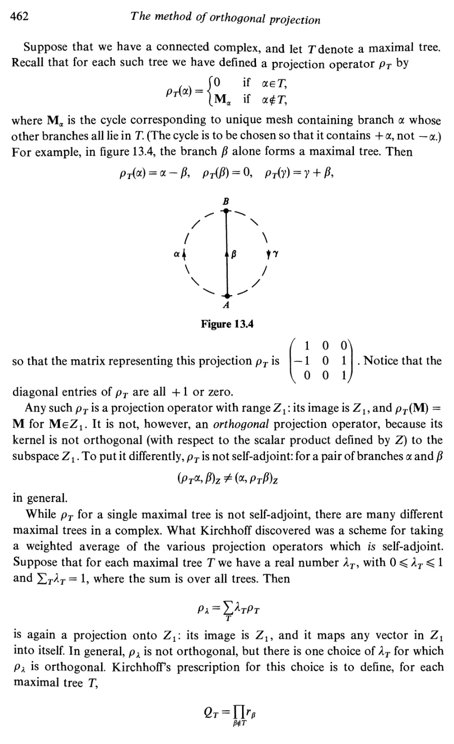
The method of orthogonal projection
Weyl's method of orthogonal projection
Kirchhoff's method
Green's reciprocity theorem
Capacitive networks
Boundary-value problems
Solution of the boundary-value problem by Weyl's
of orthogonal projection
Green's functions
The Poisson kernel and random walk
Green's reciprocity theorem in electrostatics
Summary
Exercises
Higher-dimensional complexes
Complexes and homology
Dual spaces and cohomology
Summary
Exercises
viii
xi
407
407
411
419
429
431
433
436
444
446
451
451
458
458
461
466
469
474
method
477
482
485
487
492
492
502
502
520
526
526

15 Complexes situated in U" 532
Introduction 532
15.1 Exterior algebra 535
15.2 /c-forms and the d operator 539
15.3 Integration of/c-forms 541
15.4 Stokes Theorem 553
15.5 Differential forms and cohomology 564
Summary 574
Exercises 574
16 Electrostatics in R3 583
16.1 From the discrete to the continuous 583
16.2 The boundary operator 585
16.3 Solid angle 586
16.4 Electric field strength and dielectric displacement 588
16.5 The dielectric coefficient 596
16.6 The star operator in Euclidean three-dimensional space 597
16.7 Green's formulas 600
16.8 Harmonic functions 602
16.9 The method of orthogonal projection 604
16.10 Green's functions 606
16.11 The Poisson integral formula 608
Summary 612
Exercises 612
17 Currents, flows and magnetostatics 615
17.1 Currents 615
17.2 Flows and vector fields 616
17.3 The interior product 621
17.4 Lie derivatives 626
17.5 Magnetism 628
Appendix: an alternative proof of the fundamental formula
of differential calculus 633
Summary 636
Exercises 636
18 The star operator 638
18.1 Scalar products and exterior algebra 638
18.2 The star operator 641
18.3 The Dirichlet integral and the Laplacian 646
18.4 The □ operator in spacetime 651
18.5 The Clifford algebra 653
18.6 The star operator and geometry 660
18.7 The star operator and vector calculus 662
Appendix: tensor products 664
Summary 674
Exercises 674
19 Maxwell's equations 686
19.1 The equations 686
19.2 The homogeneous wave equation in one dimension 689
19.3 The homogeneous wave equation in R3 692

19.4 The inhomogeneous wave equation in R3 695
19.5 The electromagnetic Lagrangian and the energy-
momentum tensor 697
19.6 Wave forms and Huyghens' principle 700
Summary 704
Exercises 704
20 Complex analysis 706
Introduction 706
20.1 Complex-valued functions 707
20.2 Complex-valued differential forms 709
20.3 Holomorphic functions 711
20.4 The calculus of residues 715
20.5 Applications and consequences 724
20.6 The local mapping 729
20.7 Contour integrals 735
20.8 Limits and series 740
Summary 744
Exercises 744
21 Asymptotic evaluation of integrals 750
Introduction 750
21.1 Laplace's method 750
21.2 The method of stationary phase 755
21.3 Gaussian integrals 758
21.4 Group velocity 761
21.5 The Fourier inversion formula 762
21.6 Asymptotic evaluation of Helmholtz' formula 764
Summary 766
Exercises 766
22 Thermodynamics 768
22.1 Caratheodory's theorem 769
22.2 Classical thermodynamics according to Born and
Caratheodory 775
22.3 Entropy and absolute temperature 780
22.4 Systems with one configurational variable 785
22.5 Conditions for equilibrium 796
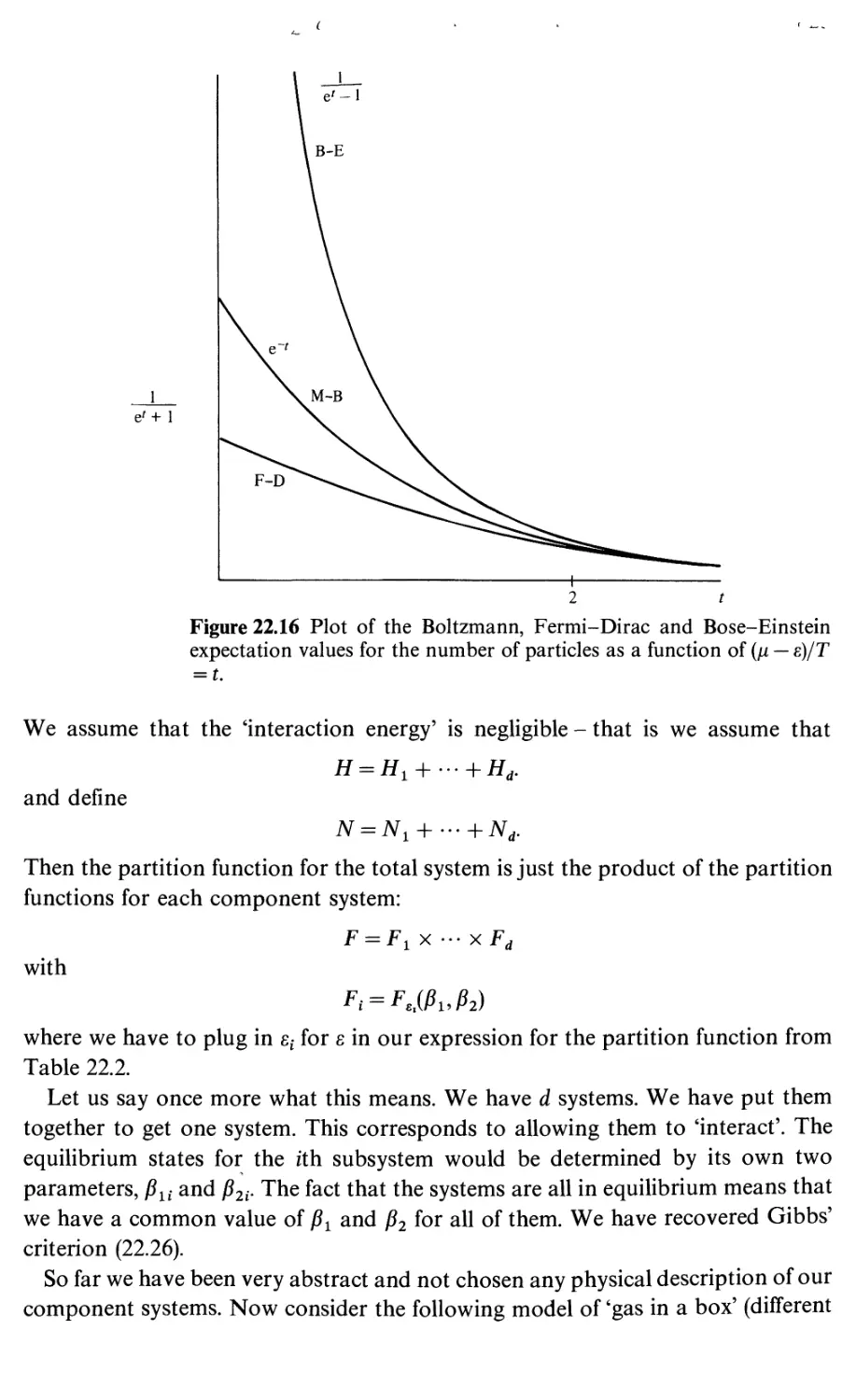
22.6 Systems and states in statistical mechanics 800
22.7 Products and images 805
22.8 Observables, expectations and internal energy 808
22.9 Entropy 814
22.10 Equilibrium statistical mechanics 816
22.11 Quantum and classical gases 823
22.12 Determinants and traces 826
22.13 Quantum states and quantum logic 831
Summary 835
Exercises 836
Appendix 838
Further reading
Index
845
848

CONTENTS OF VOLUME 1
1
1.1
1.2
1.3
1.4
1.5
1.6
1.7
1.8
1.9
1.10
1.11
1.12
2
2.1
2.2
2.3
3
3.1
3.2
3.3
3.4
3.5
4
4.1
Contents of Volume 2
Preface
Linear transformations of the plane
Affine planes and vector spaces
Vector spaces and their affine spaces
Functions and affine functions
Euclidean and affine transformations
Linear transformations
The matrix of a linear transformation
Matrix multiplication
Matrix algebra
Areas and determinants
Inverses
Singular matrices
Two-dimensional vector spaces
Appendix: the fundamental theorem of affine geometry
Summary
Exercises
Eigenvectors and eigenvalues
Conformal linear transformations
Eigenvectors and eigenvalues
Markov processes
Summary
Exercises
Linear differential equations in the plane
Functions of matrices
The exponential of a matrix
Computing the exponential of a matrix
Differential equations and phase portraits
Applications of differential equations
Summary
Exercises
Scalar products
The euclidean scalar product
viii
xi
1
1
7
13
16
18
21
22
24
26
32
36
39
43
45
46
55
55
58
66
72
73
81
81
83
89
95
103
113
113
120
120

Contents of Volume 1
4.2 The Gram-Schmidt process 124
4.3 Quadratic forms and symmetric matrices 131
4.4 Normal modes 137
4.5 Normal modes in higher dimensions 141
4.6 Special relativity 148
4.7 The Poincare group and the Galilean group 157
4.8 Momentum, energy and mass 160
4.9 Antisymmetric forms 166
Summary 167
Exercises 168
5 Calculus in the plane 175
Introduction 175
5.1 Big 'oh' and little 'oh' 178
5.2 The differential calculus 183
5.3 More examples of the chain rule 189
5.4 Partial derivatives and differential forms 197
5.5 Directional derivatives 205
5.6 The pullback notation 209
Summary 214
Exercises 215
6 Theorems of the differential calculus 219
6.1 The mean-value theorem 219
6.2 Higher derivatives and Taylor's formula 222
6.3 The inverse function theorem 230
6.4 Behavior near a critical point 240
Summary 242
Exercises 242
7 Differential forms and line integrals 247
Introduction 247
7.1 Paths and line integrals 250
7.2 Arc length 264
Summary 266
Exercises 267
8 Double integrals 272
8.1 Exterior derivative 272
8.2 Two-forms 277
8.3 Integrating two-forms 278
8.4 Orientation 285
8.5 Pullback and integration for two-forms 289
8.6 Two-forms in three-space 295
8.7 The difference between two-forms and densities 297
8.8 Green's theorem in the plane 298
Summary 305
Exercises 306
9
9.1
Gaussian optics
Theories of optics
311
311

ontents of Volume 1
9.2 Matrix methods 315
9.3 Hamilton's method in Gaussian optics 324
9.4 Fermat's principle 326
9.5 From Gaussian optics to linear optics 328
Summary 335
Exercises 335
10 Vector spaces and linear transformations 340
Introduction 340
10.1 Properties of vector spaces 341
10.2 The dual space 342
10.3 Subspaces 343
10.4 Dimension and basis 345
10.5 The dual basis 350
10.6 Quotient spaces 352
10.7 Linear transformations 358
10.8 Row reduction 360
10.9 The constant rank theorem 368
10.10 The adjoint transformation 374
Summary 377
Exercises 378
11 Determinants 388
Introduction 388
11.1 Axioms for determinants 3 89
11.2 The multiplication law and other consequences of the
axioms 396
11.3 The existence of determinants 397
Summary 399
Exercises 399
Further reading 401
Index
404

PREFACE
This book, with apologies for the pretentious title, represents the text of a course
we have been teaching at Harvard for the past eight years. The course is aimed
at students with an interest in physics who have a good grounding in one-
variable calculus. Some prior acquaintance with linear algebra is helpful but not
necessary. Most of the students simultaneously take an intensive course in physics
and so are able to integrate the material learned here with their physics education.
This also is helpful but not necessary. The main topics of the course are the theory
and physical application of linear algebra, and of the calculus of several variables,
particularly the exterior calculus. Our pedagogical approach follows the 'spiral
method' wherein we cover the same topic several times at increasing levels of
sophistication and range of application, rather than the 'rectilinear approach' of
strict logical order. There are, we hope, no vicious circles of logical error, but we
will frequently develop a special case of a subject, and then return to it for a more
general definition and setting only after a broader perspective can be achieved
through the introduction of related topics. This makes some demands of patience
and faith on the part of the student. But we hope that, at the end, the student is
rewarded by a deeper intuitive understanding of the subject as a whole.
Here is an outline of the contents of the book in some detail. The goal of the
first four chapters is to develop a familiarity with the algebra and analysis of
square matrices. Thus, by the end of these chapters, the student should be thinking
of a matrix as an object in its own right, and not as a square array of numbers.
We deal in these chapters almost exclusively with 2x2 matrices, where the most
complicated of the computations can be reduced to solving quadratic equations.
But we always formulate the results with the higher-dimensional case in mind. We
begin Chapter 1 by explaining the relation between the multiplication law of 2 x 2
matrices and the geometry of straight lines in the plane. We develop the algebra
°f 2 x 2 matrices and discuss the determinant and its relation to area and
orientation. We define the notion of an abstract vector space, in general, and
explain the concepts of basis and change of basis for one- and two-dimensional
vector spaces.

Xll
Preface
In Chapter 2 we discuss conformal linear geometry in the plane, that is, the
geometry of lines and angles, and its relation to certain kinds of 2 x 2 matrices.
We also discuss the notion of eigenvalues and eigenvectors, so important in
quantum mechanics. We use these notions to give an algorithm for computing
the powers of a matrix. As an application we study the basic properties of Markov
chains.
The principal goal of Chapter 3 is to explain that a system of homogeneous
linear differential equations with constant coefficients can be written as du/df = An
where A is a matrix and u is a vector, and that the solution can be written as
QAtu0 where u0 gives the initial conditions. This of course requires us to explain
what is meant by the exponential of a matrix. We also describe the qualitative
behavior of solutions and the inhomogeneous case, including a discussion of
resonance.
Chapter 4 is devoted to the study of scalar products and quadratic forms. It is
rich in physical applications, including a discussion of normal modes and a detailed
treatment of special relativity.
Chapters 5 and 6 present the basic facts of the differential calculus. In Chapter 5
we define the differential of a map from one vector space to another, and discuss
its basic properties, in particular the chain rule. We give some physical applications
such as Kepler motion and the Born approximation. We define the concepts of
directional and partial derivatives, and linear differential forms.
In Chapter 6 we continue the study of the differential calculus. We present the
vector versions of the mean-value theorem, of Taylor's formula and of the inverse
function theorem. We discuss critical point behavior and Lagrange multipliers.
Chapters 7 and 8 are meant as a first introduction to the integral calculus.
Chapter 7 is devoted to the study of linear differential forms and their line integrals.
Particular attention is paid to the behavior under change of variables. Other
one-dimensional integrals such as arc length are also discussed.
Chapter 8 is devoted to the study of exterior two-forms and their corresponding
two-dimensional integrals. The exterior derivative is introduced and invariance
under pullback is stressed. The two-dimensional version of Stokes' theorem, i.e.
Green's theorem, is proved. Surface integrals in three-space are studied.
Chapter 9 presents an example of how the results of the first eight chapters can
be applied to a physical theory - optics. It is all in the nature of applications, and
can be omitted without any effect on the understanding of what follows.
In Chapter 10 we go back and prove the basic facts about finite-dimensional
vector spaces and their linear transformations. The treatment here is a
straightforward generalization, in the main, of the results obtained in the first four chapters
in the two-dimensional case. The one new algorithm is that of row reduction. Two
important new concepts (somewhat hard to get used to at first) are introduced:
those of the dual space and the quotient space. These concepts will prove crucial
in what follows.
Chapter 11 is devoted to proving the central facts about determinants ofnxn

Preface
Xlll
trices. The subject is developed axiomatically, and the basic computational
algorithms are presented.
Chapters 12-14 are meant as a gentle introduction to the mathematics of shape,
that is, algebraic topology. In Chapter 12 we begin the study of electrical networks.
This involves two aspects. One is the study of the 'wiring' of the network, that is,
how the various branches are interconnected. In mathematical language this is
known as the topology of one-dimensional complexes. The other is the study of
how the network as a whole responds when we know the behavior of the individual
branches, in particular, power and energy response. We give some applications to
physically interesting networks.
In Chapter 13 we continue the study of electrical networks. We examine the
boundary-value problems associated with capacitive networks and use these
methods to solve some classical problems in electrostatics involving conductors.
In Chapter 14 we give a sketch of how the one-dimensional results of Chapters 12
and 13 generalize to higher dimensions.
Chapters 15-18 develop the exterior differential calculus as a continuous version
of the discrete theory of complexes. In Chapter 15 the basic facts of the exterior
calculus are presented: exterior algebra, /c-forms, pullback, exterior derivative and
Stokes' theorem.
Chapter 16 is devoted to electrostatics. We suggest that the dielectric properties
of the vacuum give the continuous analog of the capacitance of a network, and
that these dielectric properties are what determine Euclidean geometry in three-
dimensional space. The basic facts of potential theory are presented.
Chapter 17 continues the study of the exterior differential calculus. The main
topics are vector fields and flows, interior products and Lie derivatives. These are
applied to magnetostatics.
Chapter 18 concludes the study of the exterior calculus with an in-depth
discussion of the star operator in a general context.
Chapter 19 can be thought of as the culmination of the course. It applies the
results of the preceding chapters to the study of Maxwell's equations and the
associated wave equations.
Chapters 20 and 21 are essentially independent of Chapters 9-19 and can be
read independently of them. They are not usually included in our one-year course.
But Chapters 1-9, 20 and 21 would form a self-contained unit for a shorter course.
The material in Chapter 20 is a relatively standard treatment of the theory of
functions of a complex variable, suitable for students at the level of this book.
Chapter 21 discusses some of the more elementary aspects of asymptotics.
Chapter 22 shows how the exterior calculus can be used in classical
thermodynamics, following the ideas of Born and Caratheodory.
The book is divided into two volumes, with Chapters 1-11 in volume 1.
Most of the mathematics and all of the physics presented in this book were
eveloped by the first decade of the twentieth century. The material is thus at
east seventy-five years old. Yet much of the material is not yet standard in the

elementary courses (although most of it with the possible exception of network
theory must be learned for a grasp of modern physics, and is studied at some stage
of the physicist's career). The reasons are largely historical. It was apparent to
Hamilton that the real and complex numbers were insufficient for the deeper study
of geometrical analysis, that one wants to treat the number pairs or triplets of
the Cartesian geometry in two and three dimensions as objects in their own right
with their own algebraic properties. To this end he developed the algebra of
quaternions, a theory which had a good deal of popularity in England in the
middle of the nineteenth century. Quaternions had several drawbacks: they more
naturally pertained to four, rather than to three dimensions - the geometry of
three dimensions appeared as a piece of a larger theory rather than having a
natural existence of its own; also, they have too much algebraic structure, the
relation between quaternion multiplication, for example, and geometric
constructions in three dimensions being somewhat complicated. (The first of these objections
would, of course be regarded far less seriously today. But it would be replaced by
an objection to a theory that is limited to four dimensions.) Eventually, the three-
dimensional vector algebra with its scalar and vector products was distilled from
the theory of quaternions. It was conjoined with the necessary differential
operations, and give rise to the vector analysis as finally developed by Gibbs and
promulgated by him in a famous and very influential text.
So vector analysis, with its grad, div, curl etc. became the standard language in
which the geometric laws of physics were taught. Now while vector analysis is
well suited to the geometry of three-dimensional Euclidean space, it has a number
of serious drawbacks. First, and least serious, is that the essential unity of the
subject is obscured. Thus the fundamental theorem of the calculus, Green's theorem,
Gauss' theorem and Stokes' theorem are all aspects of the same theorem (now
called Stokes' theorem). But this is not at all clear in the vector analysis treatment.
More serious is that the fundamental operators involve the Euclidean structure
(for example grad and div) or the three-dimensional structure and orientation as
well (for example curl). Thus the theory is wedded to a three-dimensional orientated
Euclidean space. A related problem is that the operators do not behave nicely
under general changes of coordinates - their expression in non-rectangular
coordinates being unwieldy. Already Poincare, in his fundamental scientific and
philosophical writings which led to the theory of relativity, stressed the need to
distinguish between those laws of geometry and physics which are 'topological',
i.e. depend only on the differential structure of space and so are invariant under
smooth deformations, and those which depend on more geometrical structure such
as the notion of distance. One of the major impacts of the theory of relativity on
mathematics was to encourage the study of higher-dimensional spaces, a study
which had existed in the previous mathematical literature, but was not regarded
as central to the study of geometry. Another was to emphasize general coordinate
changes. The vector analysis was not up to these two tasks and so was supplemented
in the more advanced literature by tensor analysis. But tensor analysis with its

Preface
xv
ble of indices has a number of serious drawbacks, the most serious of which
h ' 2 that it is extraordinarily difficult to tell which operations have any geometric
• nificance and which are artifacts of the coordinate system. Thus, while it is
sonably well-suited for computation, it is hard to assess exactly what it is that
ne is computing. The whole purpose of the development initiated by Hamilton - to
have a calculus whose objects have a perceived geometrical significance - was
vitiated. In order to make the theory work one had to introduce a relatively
sophisticated geometrical construct, such as an affine connection. Even with such
constructs the geometric meanings of the operations are obscure. In fact tensor
analysis never displaced the intuitively clear vector analysis from the elementary
curriculum.
It is generally accepted in the mathematics community, and gradually being
accepted in the physics community, that the most suitable framework for
geometrical analysis is the exterior differential calculus of Grassmann and Cartan. This
calculus has the advantage that its computational rules are simple and concise,
that its objects have a transparent geometrical significance, that it works in all
Maxwell's equations in the course of history
The constants c,ji0, and s0 are set to 1.
The homogeneous The inhomogeneous
equation equation
Earliest form
dBx dBy dBz
dx dy dz
dEz dEy
dy dz
dEx dEz
dz dx
dEy dEx
dx dy
dEx dEy dEz
—- +—- +—- = p
dx dy dz
dBz dBy
dy dz
dBx dBz
dz dx~h+ '
SBy dBx .
dx dy
At the end of the last century
V-B = 0 V-E = p
VxE = -B VxB = j+E
At the beginning of this century
*F'«a = 0 F'%=/
Mid-twentieth-century
dF = 0 3F = J

dimensions, that it behaves well under maps and changes of coordinates, that it
has an essential unity to its principal theorems and that it clearly distinguishes
between the 'topological' and 'metrical' properties. The geometrical laws of physics
take on a simple and elegant form in terms of the exterior calculus. To emphasize
this point, it might be useful to reproduce the above table, taken from Thirring's
Course on Mathematical Physics.
Hermann Grassmann (1809-77) published his Ausdehnungslehre in 1844. It was
not appreciated by the mathematical community and was dismissed by the leading
German mathematicians of his time. In fact, Grassmann was never able to get a
university position in mathematics. He remained a high-school teacher throughout
his career. (Nevertheless, he seemed to have a happy and productive life. He raised a
large family and was recognized as an expert on Sanskrit literature.) Towards the
end of his life he tried again, with another edition of his Ausdehnungslehre, but this
fared no better than the first. Only one or two mathematicians of his time, such as
Mobius, appreciated his work. Nevertheless, the Ausdehnungslehre (or calculus of
extension) contains for the first time many of the notions central to modern
mathematics and most of the algebraic structures used in this book. Thus vector
spaces, exterior algebra, exterior and interior products and a form of the generalized
Stokes' theorem all make their appearance.
Elie Cartan (1869-1951) is now universally recognized as the leading geometer
of our century. His early work, of such overwhelming importance for modern
mathematics, on Lie groups and on systems of partial differential equations was
done in relative obscurity. But, by the 1920s, his work became known to the broad
mathematical community, due, in part, to the writings of Hermann Weyl who
presented novel expositions of his work at a time when the theory of Lie groups
began to play a central role in mathematics and in physics. Cartan's work on the
theory of principal bundles and connections is now basic to the theory of elementary
particles (where it goes under the generic name of'gauge theories'). In 1922 Cartan
published his book Lecons sur les invariants integraux in which he showed how
the exterior differential calculus, which he had invented, was a flexible tool, not
only for geometry but also for the variational calculus and a wide variety of
physical applications. It has taken a while, but, as we have mentioned above, it
is now recognized by mathematicians and physicists that this calculus is the
appropriate vehicle for the formulation of the geometrical laws of physics.
Accordingly, we feel that it should displace the 'vector calculus' in the elementary
curriculum and have proceeded accordingly.
Some explanation is in order for the time and effort devoted to the theory of
electrical networks, a subject not usually considered as part of the elementary
curriculum. First of all there is a purely pedagogical justification. The subject
always goes over well with the students. It provides a down-to-earth illustration
of such concepts as dual space and quotient space, concepts which frequently seem
overly abstract and not readily accepted by the student. Also, in the discrete,
algebraic setting of network theory, Stokes' theorem appears as essentially a

definition, and a natural one at that. This serves to motivate the d operator and
Stokes' theorem in the setting of the exterior calculus. There are deeper, more
philosophical reasons for our decision to emphasize network theory. It has been
recognized for about a century that the forces that hold macroscopic bodies
together are essentially electrical in character. Thus (in the approximation where
the notion of rigid body and Euclidean geometry makes sense, that is, in the
non-relativistic realm) the concept of a rigid body, and hence of Euclidean geometry,
derives from electrostatics. The frontiers of physics, both in the very small (the
study of elementary particles) and the very large (the study of cosmology) have
already begun to reopen fundamental questions as to the geometry of space and
time. We thought it wise to bring some of the issues relating geometry to physics
before the student even at this early stage of the curriculum. The advent of the
computer, and also some of the recent theories of physics will, no doubt, call into
question the discrete versus the continuous character of space and time (an issue
raised by Riemann in his dissertation on the foundations of geometry). It is to be
hoped that our discussion may be of some use to those who will have to deal with
this problem in the future.
Of course, we have had to omit several important topics due to the limitation
of a one-year course. We do not discuss infinite-dimensional vector spaces, in
particular Hilbert spaces, nor do we define or study abstract differentiable manifolds
and their properties. It has been our experience that these topics make too heavy
a demand on the sophistication of the student, and the effort involved in explaining
them is best expended elsewhere. Of course, at various places in the text we have
to pay the price for not having these concepts at our disposal. More serious is the
omission of a serious discussion of Fourier analysis, classical mechanics and
probability theory. These topics are touched upon but not presented as a coherent
subject of study. Our only excuse is that a thorough study of each would probably
require a semester's course, and substantive treatments from the modern viewpoint
are available elsewhere. A suggested guide to further reading is given at the end
of the book.
We would like to thank Prof. Daniel Goroff for a careful reading of the
manuscript and for making many corrections and fruitful suggestions for
improvement. We would also like to thank Jeane Morris for her excellent typing and
her devoted handling of the production of the manuscript from the inception of
the project to its final form, over a period of eight years.

12
The theory of electrical networks
Introduction
12.1 Linear resistive circuits
12.2 The topology of one-dimensional complexes
12.3 Cochains and the d operator
12.4 Bases and dual bases
12.5 The Maxwell methods
12.6 Matrix expressions for the operators
12.7 Kirchhoff's theorem
12.8 Steady-state circuits and filters
Summary
Exercises
407
411
419
429
431
433
436
444
446
451
451
Chapters 12-14 are meant as a gentle introduction to the
mathematics of shape, that is, algebraic topology. In Chapter
12 we begin the study of electrical networks. This involves two
aspects. One is the study of the 'wiring' of the network, how
the various branches are interconnected. In mathematical
language this is known as the topology of one-dimensional
complexes. The other is the study of how the network as a
whole responds, when we know the behavior of the individual
branches, in particular as regards power and energy. We give
some applications to physically interesting networks.
Introduction
Electrical circuit theory is an approximation to electromagnetic theory in which
it is assumed that the interesting phenomena can all be described in terms of
what is happening along the wires and other parts of an electrical circuit. It further
assumes that the circuit can be decomposed into various components, each with
a specified mode of behavior, and the problem is to predict how the system as
a whole will behave when the components are interconnected in various ways.
The basic variables of circuit theory are familiar from household appliances;
they are current, voltage and power. A fundamental unit in electromagnetic theory
is the charge of the electron. As of this writing (prior to the discovery of quarks)
no known particle has a charge that is a fractional part of the charge of the
electron. The practical unit of charge is the coulomb, which represents the
negative of the charge of 6.24 x 1018 electrons. In 1819 Oersted observed that a
flow of electric charge produced a force on a magnetic needle, and that the force
was proportional to the rate of flow of charge. The measurement of this effect is
much easier than the measurements of electrostatic * forces that are needed to

- <)<:
The theory of electrical networks
measure charge. For this reason, current, rather than charge, is a basic variable
of circuit theory. The unit of current is the ampere, where4 ampere = 1 coulomb/
second. We shall use I to denote current. Thus
where I is current, measured in amperes, Q is charge, measured in coulombs,
and t is time, measured in seconds. In general, we would expect that the current
flowing through a circuit would depend on position. In circuit theory it is assumed
that the current takes on a definite value at each component (but may be time-
dependent). If a denotes a branch of the circuit, then we let Ia (t) denote the current
flowing through a at time t.
An element of charge may gain or lose energy as it passes through a portion
of a circuit. The energy change (measured in joules) per unit charge (measured in
coulombs) is known as the voltage. Thus 1 volt = 1 joule/coulomb. We will denote
voltage by V. The voltage difference at time t between the two end points of the
branch a will be denoted by Va(t).
The product of current and voltage has the units of energy/time which is known
as power. The unit of power corresponding to the units that we have introduced
above is called the watt. Thus
1 watt = 1 volt x ampere = 1 joule/second.
In circuit theory, it is assumed that there are three kinds of branches: inductors,
capacitors and resistors. Each of these types has a different kind of relationship
between voltage and current. In an inductor, the voltage is proportional to the
rate of change of the current: if a is an inductor the relation is
where the constant La is known as the inductance of the inductor. The unit of
inductance corresponding to the units introduced above is the henry, defined by
1 henry = 1 volt/(l ampere/second) = 1 volt-second/ampere.
In a capacitor, the current is proportional to the rate of change of voltage:
if a is a capacitor the relation is
dV"
c dt a
where the constant Ca, known as the capacitance of the capacitor, is measured in
farads. In terms of units already introduced,
1 farad = 1 coulomb/volt.
In a resistor, there is a functional relation involving the current and the voltage
(and not their derivatives directly). In the classical theory of linear passive circuits,
the relation is given in the form V=RI where R is a constant, measured in ohms,

Introduction
409
v
"""I i
resistor only
Figure 12.1
real battery
Figure 12.2
I
ideal battery
Figure 12.3
called the resistance of the branch. Its graph in the /K-plane is a straight line
passing through the origin. More generally, we shall regard as a linear resistor
any device which can be described by an (inhomogeneous) linear equation in I
and V. For example, a real battery, with internal resistance Ra, can be described
by Va=Wa + RaIa, where the constant Wa is called the emf of the battery. An
ideal battery, which provides voltage Wa no matter how much current is drawn,
is described by V" = Wa, whose graph is a horizontal straight line, while an ideal
current source, which provides current Ka no matter what the voltage across its
terminals may be, is described by Ia = Xa, whose graph is a vertical straight line.
In analyzing circuits in which the voltages and currents change with time, we
must consider sources of voltage and current which vary with time. In this case,
the most general linear resistive branch is described by
v%t)-w%t) = RjLijtt)-KM
where Wa(t) and Ka(t) are specified functions of time. *
More generally, we might consider nonlinear resistors, inductors, or capacitors.
A device such as a diode or thermistor may be regarded as a nonlinear resistor

The theory of electrical networks
Figure 12.4
described by a nonlinear function Ia =f(Va) as suggested in figure 12.4. The most
general resistive branch is characterized by a functional relationship R(I,V,t) = 0,
where the only restriction is that no derivatives of I or V appear.
Generalizing the notion of inductor or capacitor, we might imagine an inductor
whose inductance is a function of /, so that
This would be the case, for example, if an inductor with an iron core were
used for large currents. Similarly, we might consider a nonlinear capacitor, described
by
I=C(V)
dt
which could be the result of using a dielectric with a nonlinear response.
Little more will be said about nonlinear devices, but it is important to recognize
that most of the theory which follows, which is concerned primarily with setting
up rather than solving the equations for electrical networks, applies with equal
validity to linear and nonlinear elements.
We now assume that our electrical circuit is built out of b branches of the three
types just mentioned. The branches are connected at their end points to one
another in some way. We wish to determine the currents and voltages in all the
branches, lb unknowns in all. Each branch gives one equation (either a differential
equation or a functional relation involving the current and voltage through that
branch). We need b more equations. These are given by what are now known as
Kirchhoff's laws.
Kirchhoff, as a student in Neumann's seminar, made the first comprehensive
study of the network problem. He published his results in 1845 and 1847. He
proved the existence of a solution to the network problem for a passive linear
purely resistive network; i.e., for one in which there are only passive linear resistors.
In solving this problem, he was one of the first-to study the algebraic properties
of shape. This abstract study of shape was created, as a mathematical discipline,
some fifty years later by Poincare, who called the subject analysis situs. Today the

Linear resistive circuits
411
subject is called algebraic topology. The natures of the methods of algebraic topology
make themselves apparent in the case of passive linear resistive networks, and so
we shall occupy a considerable amount of space studying these networks before
returning to the general case. In treating these networks, we shall follow a 1923
paper by Weyl, in which a proof of Kirchhoff's results is presented in a fashion
that explains more directly the relations with algebraic topology.
Kirchhoff's laws, as restated by Maxwell, have a very simple formulation.
Kirchhoff's current law asserts that since charge cannot be created or destroyed,
and since no charge can be stored at an ideal point, the algebraic sum of all the
currents entering or leaving a junction of branches must be zero. Kirchhoff's voltage
law asserts that there exists a function, 0), called the electrostatic potential,
such that the voltage across each branch is given by the difference of the values
of 0) at the end points, i.e., the two junctions of the branch. Maxwell devised two
methods of solving the resistive network problem which are known as Maxwell's
mesh-current and node-potential methods. We shall begin by working some
examples to illustrate Maxwell's methods, and, in the process, set up some of the
language of algebraic topology.
12.1. Linear resistive circuits
Resistors connected by metal wires of negligible resistance, as shown in figure 12.5,
are said to be connected in parallel Suppose that a battery supplying a constant
voltage, V, is connected across the group of resistors. The ith resistor has resistance
R( and we set Gt = Rf1- (Gt is called the conductance of the ith resistor.) We are
interested in calculating the total current delivered by the battery and the current
in each branch after the current has become steady. The connection between all
the upper terminals of the resistors ensures that in the steady state all these
terminals are at the same potential, and the same applies to the lower terminal.
Hence the voltage across each resistor is the same, and is equal to the voltage, V,
of the battery. From the point of view of circuit theory, we can imagine all of the
upper wire shrunk to a point, and similarly all of the wire connecting the lower
terminals. We may thus replace figure 12.5 by figure 12.6 in which there are two
vertices A and B, the top and the bottom, and n + 1 branches, of which one is the
Figure 12.5

412 The theory of electrical networks
B
Figure 12.6
battery and the rest are linear passive resistors. Since the same voltage, V, is applied
across all the resistors, it follows from the equation V=RI or / = GKthat the
currents through the resistors are GXK, G2K-., GnV. By Kirchhoff's current law,
the current flowing through the battery branch must be equal and opposite to the
sum of the currents flowing through the resistors, and is therefore
_(Gl + G2 + -.. + Gw)K.
(In deriving this result, we are making the sign convention that all branches
in figure 12.6 are given similar orientations, so that, for example, all currents flowing
from top to bottom are counted as positive, and from bottom to top are considered
as negative.) We have completely solved this trivial network problem in that we
now know the voltage across and the current through each branch. It follows
from the above result that the total current supplied by the battery is the same
as would be supplied if the battery were connected across a single resistor of
conductance G = G1 + G2 + •• • + G„, i.e., of resistance R where
1 _ 1 1 1
R Rt R2 Rn
This is, of course, the well-known result, taught in all elementary courses,
which states that, if a number of resistors are connected in parallel, they are
Rl R2-" Rn
C'
V
—^1
Figure 12.7

Linear resistive circuits
413
equivalent to a single resistor the reciprocal of whose resistance is equal to the
sum of the reciprocals of the resistances of the individual resistors.
A group of resistors connected by wires of negligible resistance as shown in
figure 12.7 is said to be connected in series. Suppose that a battery of voltage V is
connected as shown, and that, as a result, a steady current I flows around the
circuit. (By Kirchhoff's current law we must have the same current, /, flowing
through each branch, because the algebraic sum of the currents at each node must
be zero.) Let the resistances of the various resistors be Rl,R2,...,R„. Since the
current I flows through the ith resistor, it follows that the voltage across the ith
resistor is RtL It follows from Kirchhoff's voltage law that the voltage across the
battery must equal the sum of the voltage differences across all the resistors. Thus
V = (Rl+R2 + .- + Rn)L
Since we know V, we can solve this equation for I and thus obtain the currents and
voltages through each branch. We have completely solved this network problem.
Again we have merely reproduced the well-known elementary result which states
that if a number of resistors are connected in series they are equivalent to a single
resistor whose resistance is the sum of the resistances of the individual resistors.
Let us now consider a slightly more complicated circuit consisting of a battery of
voltage V connected to three resistors of resistances RUR2 and #3, as shown in
figure 12.8. A point in the network from which two or more wires run to different
elements is called a node or a vertex. The point A is a node from which wires run to
the battery and to one of the resistors. The point B is a node from which wires run to
all three resistors. The point C is a node from which there run three wires, one to the
battery and two to different resistors. We do not consider the lower right-hand
corner as a separate node; since it is connected by a wire of zero resistance to the
point C, it must be identified as being the same node as C. Thus the circuit has three
nodes, A, B, and C, and four branches, the battery branch joining A to C, the resistor
joining A to £, and the two resistors joining B to C. The lengths and shapes of the
wires making the interconnections are completely irrelevant. What matters are the
branches and the nodes and how the branches and nodes are interconnected. Thus
figure 12.9 describes exactly the same circuit as figure 12.8. A network as simple as
that shown in figure 12.8 or 12.9 can be analyzed into parallel and series connections,
^1
-* 'wv^
R2
Figure 12.8

The theory of electrical networks
Af
Figure 12.9
and in this way all the information about the network can be calculated. Thus the
resistors R2 and R3 are in parallel, and hence are equivalent, as far as the rest of
the circuit is concerned, to a single resistor whose resistance is the reciprocal of
R^1 + R3 \ i.e., of resistance
#2+^3'
This equivalent resistor is connected in series with the resistor Rt. Thus, as far as the
battery is concerned, it is as if there were just a single resistor of resistance
R = Rl+ ***3,
R2 + R3
Thus the current drawn from the battery is
I = V/R.
This must also be the current through Ru so that /x = V/R is the current through
Rv The voltage drop across Rt is then V1 = ItRlm The current I divides jbetween the
parallel resistors R2 and R3 in proportion to the inverse of their resistances, as we
have seen when we discussed the example of resistors in parallel. Thus the currents
through R2 and R3 are
/,=
R,I
and /3 = -
R,I
#2+ #3 ** R2 + R3
From this we see that the common voltage drop across R2 and R3 is
R2 + R3
In this case we have obtained all the relevant information about the network by
considering it as a resistor Rx in series with a pair of parallel resistors R2 and R
This procedure is frequently the most convenient way of proceeding when the
network is not too complicated. A more systematic method is needed for more

Linear resistive circuits
415
complicated networks. We will now illustrate the two methods of Maxwell for this
same simple network.
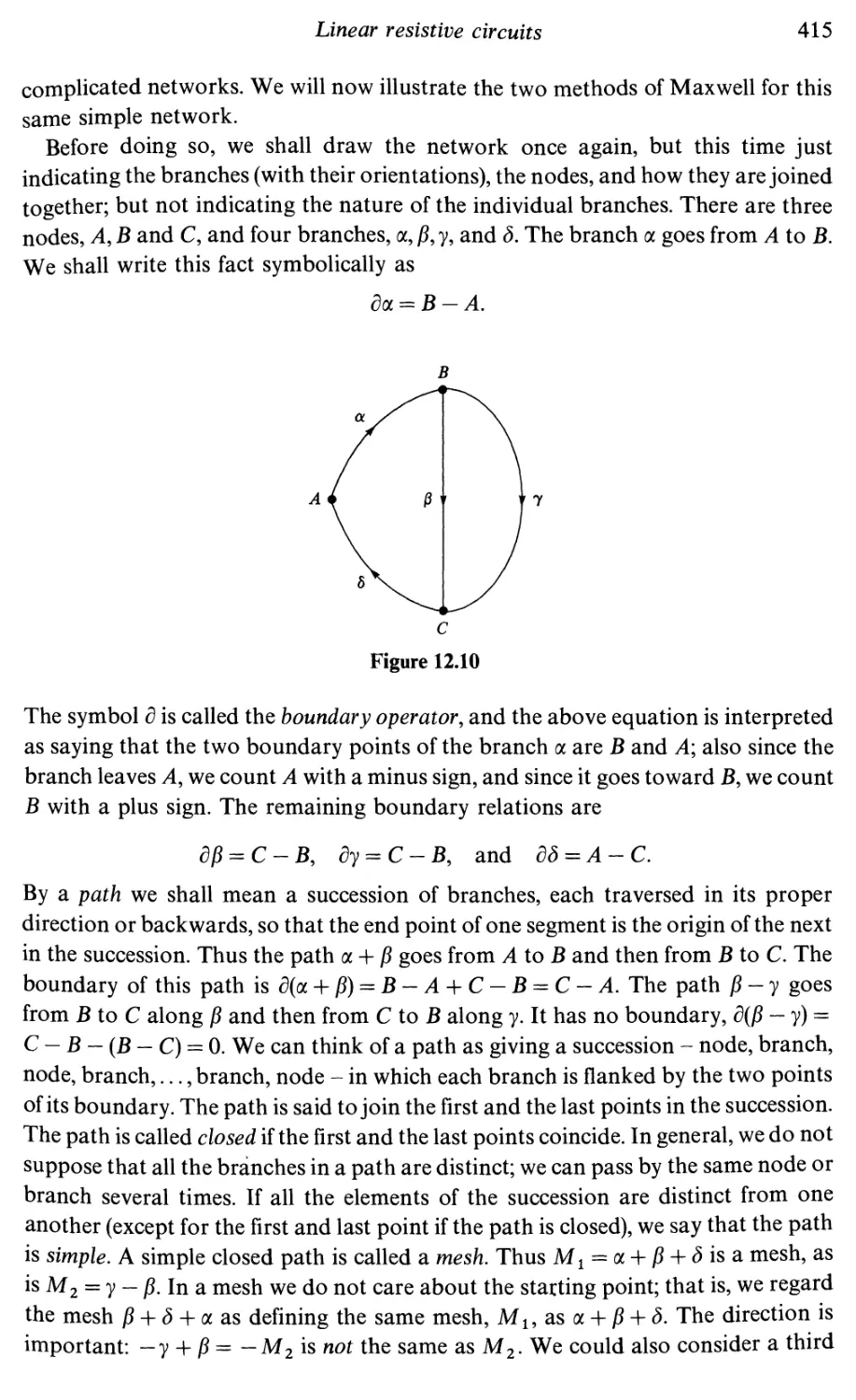
Before doing so, we shall draw the network once again, but this time just
indicating the branches (with their orientations), the nodes, and how they are joined
together; but not indicating the nature of the individual branches. There are three
nodes, A, B and C, and four branches, a, jS, y9 and 5. The branch a goes from A to B.
We shall write this fact symbolically as
doc = B - A.
c
Figure 12.10
The symbol d is called the boundary operator, and the above equation is interpreted
as saying that the two boundary points of the branch a are B and A; also since the
branch leaves A, we count A with a minus sign, and since it goes toward £, we count
B with a plus sign. The remaining boundary relations are
dj3 = C-B, dy = C-B, and d3 = A-C.
By a path we shall mean a succession of branches, each traversed in its proper
direction or backwards, so that the end point of one segment is the origin of the next
in the succession. Thus the path a + jS goes from A to B and then from B to C. The
boundary of this path is d(a + /?) = B - A + C - B = C - A. The path p-y goes
from B to C along jS and then from C to B along y. It has no boundary, d(fi -y) =
C — B — (B — C) = 0. We can think of a path as giving a succession - node, branch,
node, branch,..., branch, node - in which each branch is flanked by the two points
of its boundary. The path is said to join the first and the last points in the succession.
The path is called closed if the first and the last points coincide. In general, we do not
suppose that all the branches in a path are distinct; we can pass by the same node or
branch several times. If all the elements of the succession are distinct from one
another (except for the first and last point if the path is closed), we say that the path
is simple. A simple closed path is called a mesh. Thus M1 = a + jS + ^isa mesh, as
is M2 = y - jS. In a mesh we do not care about the starting point; that is, we regard
the mesh jS + 5 + a as defining the same mesh, Ml9 as a + jS + 3. The direction is
important: -y + /? = -M2 is not the same as M2. We could also consider a third

le theory of electrical networks
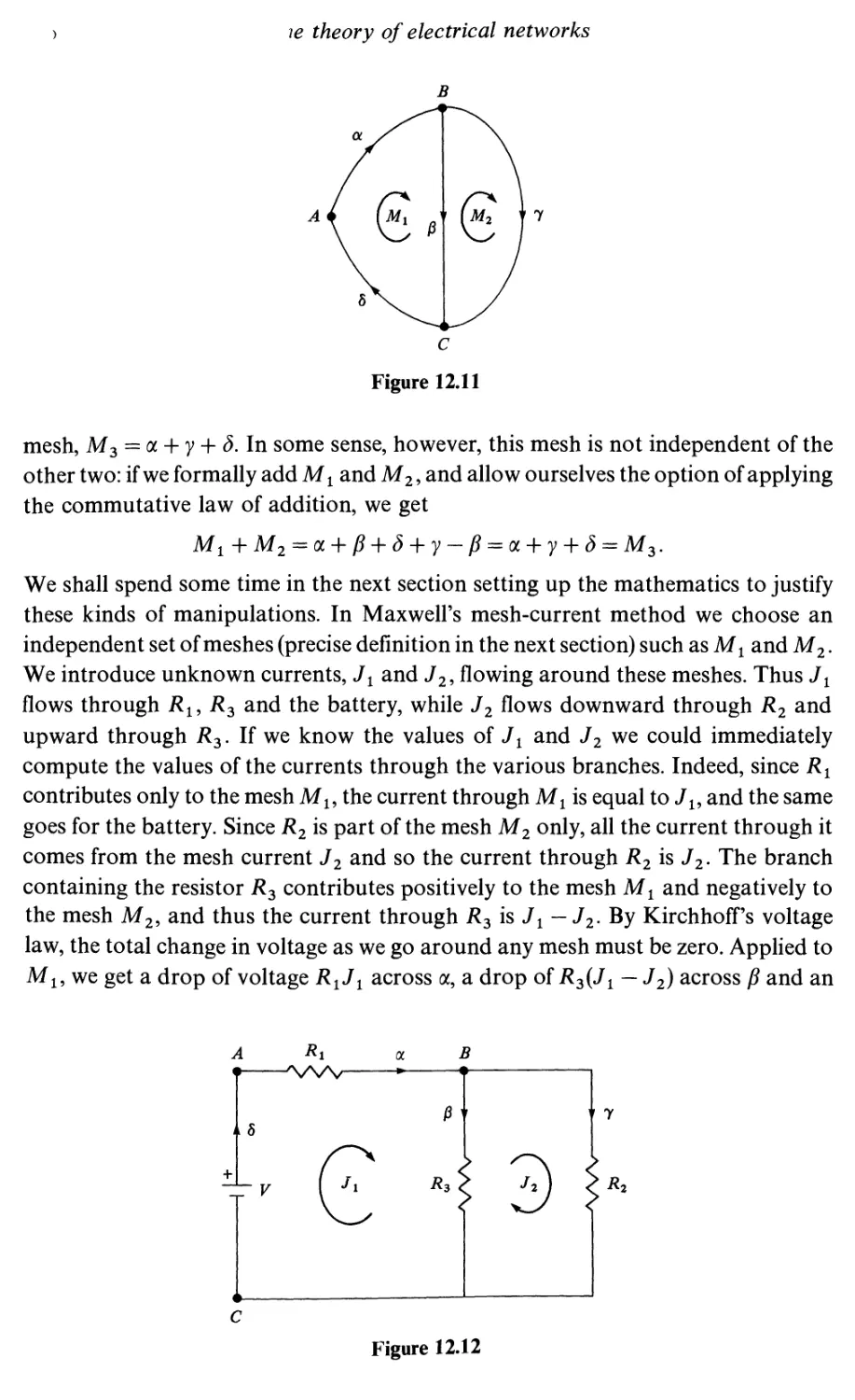
Figure 12.11
mesh, M3 = a + y + 3. In some sense, however, this mesh is not independent of the
other two: if we formally add M1 and M2, and allow ourselves the option of applying
the commutative law of addition, we get
M1+M2 = a + /? + 5 + y-/? = a + y + <5 = M3.
We shall spend some time in the next section setting up the mathematics to justify
these kinds of manipulations. In Maxwell's mesh-current method we choose an
independent set of meshes (precise definition in the next section) such as Mt and M2.
We introduce unknown currents, Jx and J2, flowing around these meshes. Thus Jl
flows through jRl9 R3 and the battery, while J2 flows downward through R2 and
upward through R3. If we know the values of Jl and J2 we could immediately
compute the values of the currents through the various branches. Indeed, since Rt
contributes only to the mesh Mu the current through Mt is equal to Jl9 and the same
goes for the battery. Since R2 is part of the mesh M2 only, all the current through it
comes from the mesh current J2 and so the current through R2 is J2. The branch
containing the resistor R3 contributes positively to the mesh Mx and negatively to
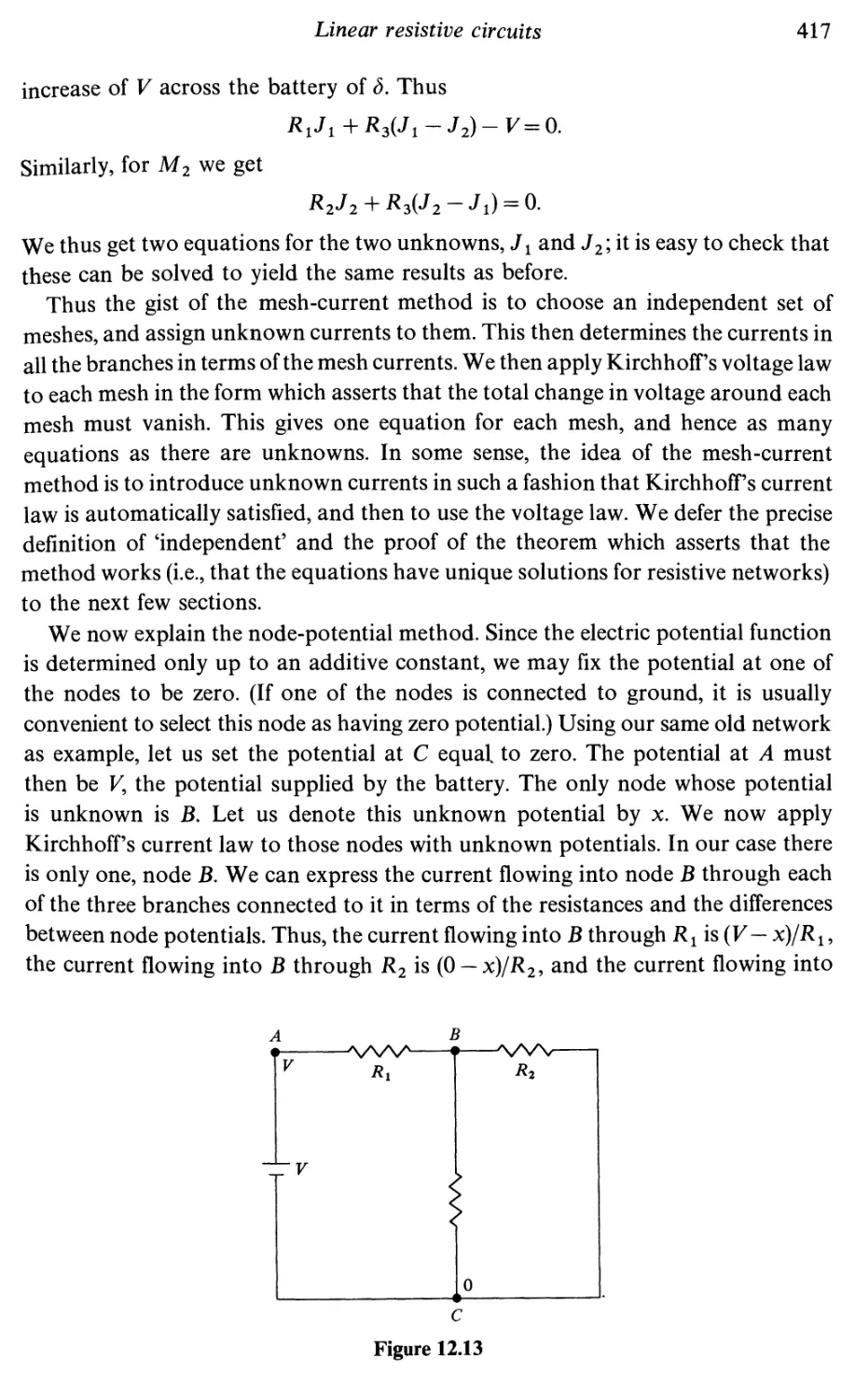
the mesh M2, and thus the current through R3 is Jx — J2. By Kirchhoff's voltage
law, the total change in voltage as we go around any mesh must be zero. Applied to
Mu we get a drop of voltage R1J1 across a, a drop of R3(Ji—J2) across /? and an
Figure 12.12

Linear resistive circuits
417
increase of V across the battery of S. Thus
R1J1+R3(J1-J2)-V=Q.
Similarly, for M2 we get
R2J2 + R3{J2-J1) = 0.
We thus get two equations for the two unknowns, Jx and J2; it is easy to check that
these can be solved to yield the same results as before.
Thus the gist of the mesh-current method is to choose an independent set of
meshes, and assign unknown currents to them. This then determines the currents in
all the branches in terms of the mesh currents. We then apply KirchhofPs voltage law
to each mesh in the form which asserts that the total change in voltage around each
mesh must vanish. This gives one equation for each mesh, and hence as many
equations as there are unknowns. In some sense, the idea of the mesh-current
method is to introduce unknown currents in such a fashion that KirchhofTs current
law is automatically satisfied, and then to use the voltage law. We defer the precise
definition of 'independent' and the proof of the theorem which asserts that the
method works (i.e., that the equations have unique solutions for resistive networks)
to the next few sections.
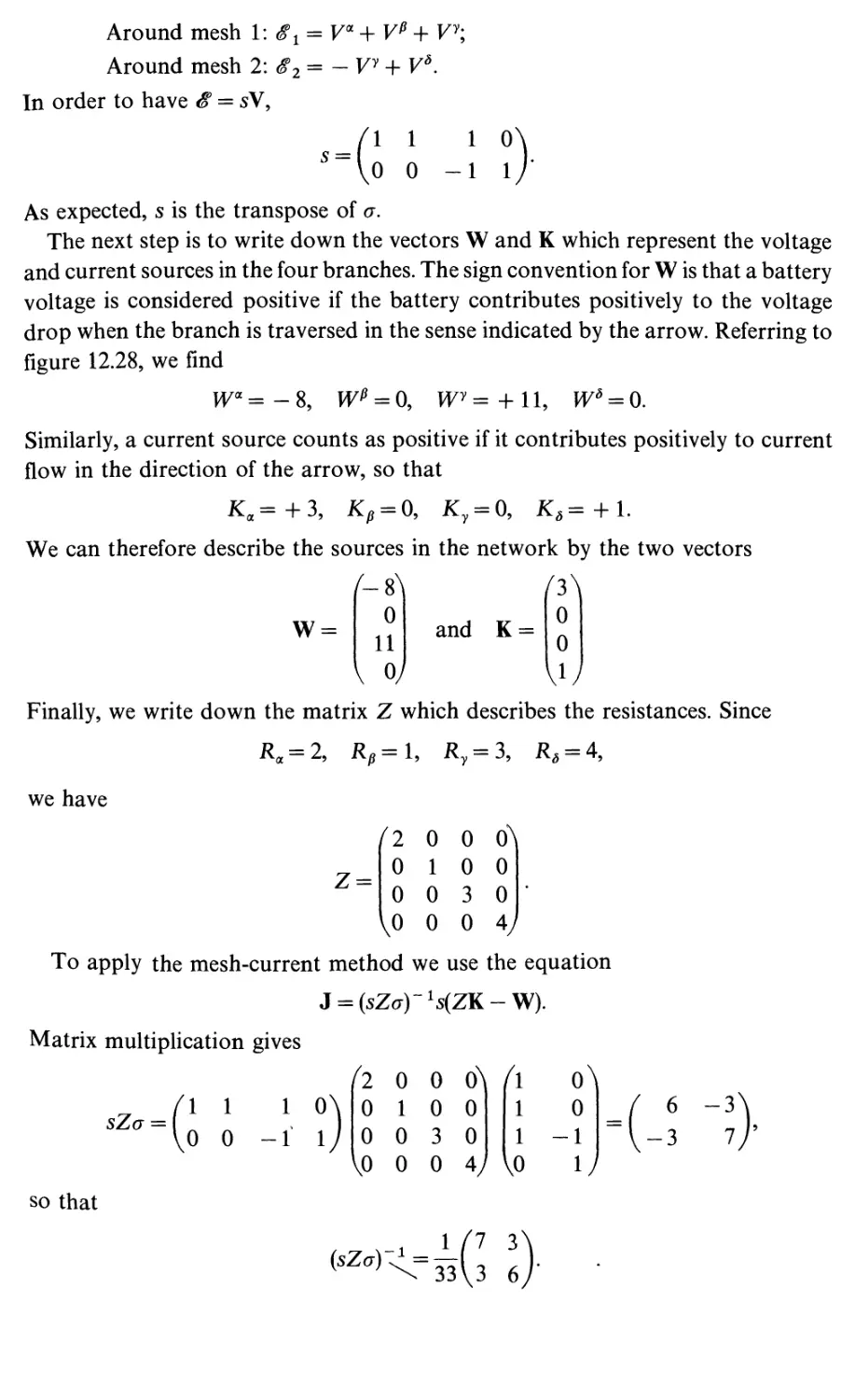
We now explain the node-potential method. Since the electric potential function
is determined only up to an additive constant, we may fix the potential at one of
the nodes to be zero. (If one of the nodes is connected to ground, it is usually
convenient to select this node as having zero potential.) Using our same old network
as example, let us set the potential at C equal to zero. The potential at A must
then be V, the potential supplied by the battery. The only node whose potential
is unknown is B. Let us denote this unknown potential by x. We now apply
KirchhofPs current law to those nodes with unknown potentials. In our case there
is only one, node B. We can express the current flowing into node B through each
of the three branches connected to it in terms of the resistances and the differences
between node potentials. Thus, the current flowing into B through R1is(V— x)/Ru
the current flowing into B through R2 is (0 - x)/R2, and the current flowing into
■AAAA-
AAV
*2
Figure 12.13

c ory ol e ectrica networks
B through R3 is (0-x)/R3. Kirchhoff's current law states that the sum of these
three currents equals zero, so that
(V- x)/R1 - x/R2 - x/R3 = 0.
We can solve this equation for x, then determine the voltages across and the currents
through all branches. The proof of why this method works in general will be deferred
to the next section.
Notice that in our example the node-potential method is superior to the mesh
method since it involves solving for one unknown rather than two. It is not clear that
the node-potential method is superior to our original analysis into parallel and
series connections.
In dealing with a general network, it is advisable first to check by inspection
whether it can easily be decomposed into parallel and series connections. If not, it is
probably not worthwhile to try to figure out such a decomposition. Then check
how many independent meshes there are and determine how many unknown mesh
currents. Similarly determine how many unknown node potentials there are.
(Frequently, symmetry considerations can cut down on the number of unknowns.)
Choose the method with the fewer unknowns and use it to solve the network.
Although it is not advisable to choose between the latter two methods by casual
inspection, a general rule of thumb is that a network with few meshes and many
nodes will yield more readily to the mesh-current method, and a network with few
nodes and many meshes will yield more readily to the node-potential method.
Another relevant factor is how the sources are specified. If the network is energized
by sources having specified voltages, this tends to reduce the number of unknown
node potentials, and hence favor the node-potential method. If currents are
specified, this tends to favour the mesh-current method. To allow for all these
considerations, it is usually best to draw two diagrams of the network and mark the
number of unknowns of the mesh-current method on one and the number of
unknowns of the node-potential method on the other in order to make an intelligent
choice between the two methods.
So far we have been considering purely resistive networks. We can also apply
these methods to determine the steady-state (oscillating) behavior of linear circuits
with inductors and capacitors. (Linear here means that all inductances and
capacitances are constant.) If all the generators are sinusoidal with the same
frequency, co/ln i.e., all voltage sources are of the form Keicot, and all current sources
of the form JeiG>r, then, as is well-known (and follows trivially from the definitions),
an inductor with inductance L acts by the law V=icoLI and a capacitor with
capacitance C acts by the law V= (l/iCco)I. We can now apply the same rules as
before with these complex resistances or impedances. In this situation, however,
solutions need not always exist, due to the phenomenon of resonance. Thus, for
example, suppose that an inductor with L = 1 is in series with a capacitor with C = 1.
If we put this series together with a generator with co = 1 the rule for adding
resistances in series gives R = i + 1/i = 0, i.e., a short circuit drawing an infinite

The topology of one-dimensional complexes
419
current. In the next section we shall discuss some conditions which avoid this
unrealistic situation.
12.2. The topology of one-dimensional complexes
The terms oriented graph and one-dimensional complex are synonymous. They both
refer to a mathematical structure that will represent for us the structure consisting of
the various interconnections of the branches of an electrical network when we ignore
the nature of the various branches; this structure will allow us to study the nature of
Kirchhoff's laws in somewhat abstract form and then see how the properties of the
individual branches affect the solution of the network problem.
A one-dimensional complex is a collection consisting of two sets: a set of zero-
dimensional objects or nodes, {A, B,...} = S0 and a set of one-dimensional objects
or branches {a, j3,...} = St, together with a rule which assigns to each branch two
distinct nodes, the initial point and the final point of the branch. Thus we are given a
map from Sx to S0 x S0 .* In what follows we shall assume that the sets S0 and St are
finite.
We define the terms path, mesh, etc., as in the preceding section. A path determines
an integer for each branch, namely the number of times the branch is traversed in the
path, with orientation taken into account, so that when the branch is traversed from
its initial point to its final point the contribution is +1 and when the branch is
traversed in the opposite direction the contribution is — 1. Thus each path
determines a vector p = (pa,Pp,.. .)T with integer coefficients, where the coordinates of
the vector p are labeled by the branches of the graph; with pa, for example, giving the
total number of times the branch a is crossed in the positive direction minus the total
number of times it is crossed in the negative direction. We can also think of a current
distribution of the network as giving a vector I = (7a, Ip,.. .)T whose coordinates are
labeled by the branches, where now /a, for example, is the real number giving the
current, in amperes, through the branch a (if our one-dimensional complex were the
complex of branches of an electrical network). This suggests that for any complex we
introduce the vector space consisting of all vectors K = (Ka,Kp,...)T whose
components are indexed by the branches. (Unless otherwise specified, we shall
assume that these components are real numbers so that we get a real vector space.)
We shall denote this vector space by Cl and call it the space of one-chains. We shall
identify each branch, *c, with the vector that has 1 in the k position and zeros
elsewhere. Thus a = (1,0,0,.. .)T, p = (0,1,0,.. .)T etc.
Similarly, we construct the real vector space, C0, consisting of vectors whose
components are indexed by the nodes and call this the space of zero-chains. Again,
we will identify a node A with the vector which is 1 in the Ath position and zero
elsewhere, so that a node is now an element of the vector space C0. In particular, an
* S0xS0 denotes the Cartesian product of the set S0 with itself. So S0 x S0 is just the collection
of all ordered pairs of nodes.

420
The theory of electrical networks
expression such as A - B makes sense as an element of the vector space C0. Notice
that dim C1 is the number of branches and dim C0 is the number of nodes.
We now define a linear map called the boundary map, d, from Cx to C0. To define
the map d it is sufficient to prescribe its values on each of the branches, since the
branches form a basis for Cv Each branch has an initial point and a terminal point
and we define d (branch) = (terminal node) - (initial node). Thus, for example, if a is
a branch going from A to B, then doc = B - A.
Let us examine the meaning of the operator d. Suppose that* K =
(Ka, Kfi, Ky,.. .)T and dK = L, where L = (LA, LB,.. .)T. In computing a term such as
LA, we see that we get a sum of certain of the coefficients of K: in fact
LA = (KSl + .- + Kdl) - (K8l + - + KJ
where 6t,..., <5f are all the branches which go to A and s1,..., sk are all the branches
which leave A. Thus, from the example in figure 12.14,
LA = Kp — K,, — Ka.
From this we see that Kirchhoff's current law has a very simple formulation:
Figure 12.14
Kirchhoff's current law: If I is the one-chain giving the current distribution
of an electric current, then
31 = 0.
Recall that a simple closed path is called a mesh. In figure 12.15, for example, the
path a + /? + S, represented by the vector px = (1,1,0,1)T, is a mesh, as is the path
— P + y, represented by the vector p2 = (0, — 1,1,0)T. The sum of these two vectors,
P3 = Pi + P2 = (1> 0,1,1)T is another mesh, a + y + 3. Clearly, each of these meshes
has no boundary: 3px = dp2 = dP3 = 0.
For any one-dimensional complex we shall denote the subspace of C1 consisting
of those one-chains satisfying dK = 0 by Zx. We express this relationship
symbolically as Zl =ker d c C1. We call the elements of Z1 cycles. Every mesh is a cycle, but
* On the preceding page and in much of what follows we write vectors in U" as (a,b,c,...)T
instead of
fl
in order to save typesetting space.
c '

The topology of one-dimensional complexes
All
c
Figure 12.15
not every cycle is a mesh. For example, the vector
2 \
!
^/
2/
satisfies dlt = 0 but does not describe a mesh since it has entries other than 1,-1,
or 0. It does represent a set of currents satisfying Kirchhoff's current laws. In fact,
one of the easiest ways to verify that It is a cycle is to write in the appropriate
current next to each branch and to check that the algebraic sum of the currents
at each node equals zero. See figure 12.16.
Alternatively we could notice that Ix =fpi -h ip2; since px and p2 are elements
of Zx, so is It. In fact, for this simple network, the two meshes pt and p2 form a basis
forZi.
Figure 12.16
Havin defined the subspace Zt c C1 as being of the kernel of the boundary map
d, we now turn our attention to the image ofd. We denote by B0 the subspace of C0
which is the image of d. Symbolically, we may write
We call B0 the space of boundaries.

The theory of electrical networks
A #
B *
C +
Figure 12.17
The significance of B0 may be made clearer by reference to figure 12.17. The
element of C0, A — B = (1, — 1,0)T which is the boundary of the branch a, lies in the
subspace B0; so does B — C = (0,1, — 1)T which is the boundary of /?. The sum of
these two vectors, A — C = (1,0, — 1)T, is again an element of C0, and it is the
boundary of the path a + /?.
Not every element of B0 can be interpreted as the boundary of a path, however.
For example, (2, — 1, — 1)T is an element of B0 that corresponds to no single path.
If we consider these elements of C0 that do not lie in the subspace B0, we find that
they do not form a subspace. For the network of figure 12.17, to take a simple
example, the vectors A = (1,0,0)T, and B = (0,1,0)T are not elements of B0, but their
difference A — B = (1, -1,0)T is an element of B0. We can, however, form the
quotient space H0 = C0/B0, whose elements are equivalence classes of elements of
C0 whose difference lies in B0. The vectors A = (1,0,0)T and £ = (0,1,0)T in C0
correspond to the same vector in H0 because their difference is the vector (1, — 1,0)T,
which lies in B0. We denote this equivalence class by A or by (1,0,0)T. Similarly, the
vectors (2,0,0)T and (0,1,1)T belong to the same equivalence class, (2,0,0)T, because
their difference (2, -1, - 1)T lies in B0. For the simple network of figure 12.17, in
fact, every vector in C0 lies in the same equivalence class as a vector of the form
(a, 0,0)T, where a is a real number. The quotient space H0 = C0/B0 is therefore
a one-dimensional vector space, isomorphic with the real numbers.
For an example of a one-complex in which H0 is two-dimensional, refer to
A •
c #
Figure 12.18

The topology of one-dimensional complexes
423
figure 12.18. The vectors (1,0,0,0)T and (0,0,1,0)T do not belong to same equivalence
class because their difference (1,0, -1,0)T is not the boundary of any element of Ct.
In that case, the equivalence class of (1,0,0,0)7 and the equivalence class of
(0,0,1,0)7 form a basis for the two-dimensional vector space H0. Notice that, if a
branch y, joining A to C, were added to the complex, then (1,0, -1,0)7 would
become an element of B0 and H0 would become one-dimensional.
The meaning of H0 and Zx
Our immediate goal is to give some geometric interpretation to the spaces H0 and
Zx; in the process we shall get some understanding of the mesh-current method. We
wish to prove the following two facts (whose precise statement we shall give in the
course of the discussion):
(i) dim H0 is the number of connected components of the complex;
(ii) We can find a basis ofZl consisting of meshes.
We begin with (i). What do we mean by connected components? We recall that a
path joins the node A to the node D if A is the initial point of the first segment of the
path and D is the final point of the last segment of the path. If P is the one-chain with
integer coefficients corresponding to this path, then it is clear that dP = D — A, since
we can compute dP by adding the boundaries of all the individual branches, and all
the intermediate nodes will vanish. A complex is called connected if every point can
be joined to every other point. In this case we can write an arbitrary zero chain
L= £ LNN = (LA,LB,...)
N = A,B,C,...
in the form
L = XM04 + (JV - A)} = ^LNA + X LN(N - A)
or, equivalently,
L = (LA + LB + . ..,0,0,... )^ + 1^(-1,1,0,0,...)7 + Lc(-l, 0,1,0,. ..)7 + ....
For a connected complex, N — A is a boundary for all N (/ A), and
\N J N*A
is an element of B0. Thus every zero-chain L is in the equivalence class of some
multiple of A, and in the quotient space H0 = C0/B0 every element is a multiple of A,
the equivalence class of A: On the other hand, A by itself is not a boundary, and so
A ^ 0. We have thus proved that dim H0 = 1 for any connected complex.
Now consider any complex, and let A be some node. Starting with A, we consider
all branches which have A as a boundary point, either an initial or a final point. Let
us adjoin to A the set of all nodes that are at the other end of these branches. We then
adjoin all new branches emanating from these nodes and then all new points at the
end of these branches. We continue this way until we have no new branches or nodes

424
The theory of electrical networks
to add. We thus obtain a collection S0(A) of nodes and a collection S^A) of branches
with the property that the boundary points of any branch in St(A) lie in S0(A). Thus
(SoiAlS^A)) forms a subcomplex of our original complex. If it is not the whole
complex, we pick some node B which does not lie in S0(A) and repeat the process.
Proceeding in this way we get a collection of disjoint sets S0(A), S0(B\ etc., and
S^AlSiiBl etc., with each of the subcomplexes SoiAXS^A^SoiBlS^B); etc,
connected and none of them connected to any other. We get corresponding vector
spaces C0(A), etc, and direct sum decompositions* C0 = C0(A)@ C0(B)... and C1 =
C1{A)®C1{B)... with dCx(A) c C0(A),dCx{B) c C0(B), etc. From this we see that
H0 = H0(A) © H0(B) H— and so dim H0 = the number of summands = the number
of connected components.
We now turn to (ii). A mesh is a simple closed path. Hence each mesh determines
an element, M, of Cl whose coordinates are either + 1, — 1 or 0, and furthermore,
dM = 0. We say that a set of meshes is independent if the corresponding elements of
Cl are linearly independent. (This is the precise formulation of the notion of
independence that we used in the preceding section.) We wish to show that we can
find a family of meshes so that the corresponding elements Mx,..., M2 form a basis
of Zv In the process of proving this result we shall give a constructive procedure for
finding such a family of meshes. Notice that in view of our discussion of (i) it is
sufficient to work with a connected complex; if the complex is not connected we
simply apply our procedure to each connected component separately. Since the
components are completely independent of one another, this will give the result for
the full complex.
A connected complex containing no meshes is called a tree. In a tree there exists at
least one node which is a boundary point of only one branch. (We are uninterested in
the trivial case of a complex with one node and no branches.) To prove this fact,
simply start at any node. If more than one branch impinges on this node choose one
of these branches and move to the other end point of this branch. If this node does
not have the desired property, move along a branch, other than the one just used to
* The direct sum of two vector spaces Vx and V2 is the Cartesian product Vx x V2 made into
a vector space in the obvious way: (vuv2) + (w1,w2) = (vt + wuv2 + w2) and r(v1,v2) =
(rv1,rv2). If U and W are subspaces of a vector space V so that every veV can be written
uniquely as v = u + w with ue V and ve W then vt-+{u, w) gives an isomorphism of V with the direct
sum of U and W. In this case we write V=U®W, and we have dim V = dim U + dim W.

The topology of one-dimensional complexes
425
still another node. Continue this procedure. Since there are no meshes, we can never
come back to an earlier node. Since there are only a finite number of nodes,
eventually we must reach a node which is the boundary of only one branch.
Suppose we have a tree and we start from a node which is at the end of only one
branch. From this node we can build up the whole tree by adding one branch at a
time. Since there are no meshes, each time we add a new branch we add a new node.
Thus, in a tree, the number of nodes is exactly one more than the number of
branches: if b denotes the number of branches and n denotes the number of nodes
than in any tree
w = b+l.
We have proved that, for any connected complex, dimif0 = l. Since H0 =
C0/B0, dim H0 = dim C0 - dim B0, and we may conclude that dim B0 =
dim C0 - dim H0 = n-l = b. Therefore B0, the image of the map d, has the same
dimension as the space Cl on which d acts. For any linear map T: V-+ Wwq know
that dim(imT) + dim(ker T) = dimK Applying this to the map d, we conclude
that dim(ker d) = dim C1 - dim B0 = b - b = 0, so that ker d = {0}; i.e. Zx = {0}.
This proves (ii) for the case of a tree: if there are no meshes there are no non-trivial
cycles.
Suppose we had any connected complex and built it up as before starting from
some arbitrary node. Each time we add a branch we may or may not add a new node.
Eventually, when we attach all the branches, we will have added all the nodes since
the complex is connected. Thus for a general connected complex we have
For a connected complex we have already proved that dim H0 = 1, and we may
conclude because dim C0 - dim B0 = dim H0 that n — dim B0 = 1 or dim B0 = n — 1.
Since B0 is the image of d and Zx is the kernel of d, we know that dim£0 +
dim Zl = dim C1 = b or (n - 1) + dim Zx = b. Therefore
dimZi = b+ 1 — n
for any connected complex.
To prove (ii) we must exhibit a family of b + 1 — n independent meshes which form
a basis for Zx. We do this by first dividing the set of branches S1 into a maximal tree T
which contains all the nodes of our complex, and a set of branches T which are not
part of this tree, by the following procedure: Choose any branch which forms part of
a mesh, and put it aside as a member of the subset T. The remaining branches still
connect all nodes. Repeat this procedure until no meshes remain. At this point the
branches which have not been placed in the subset f constitute the maximal tree T.
This procedure does not determine a unique maximal tree; figure 12.20 shows two
different ways in which a given complex can be reduced to a maximal tree (solid lines)
by removal of branches (dotted lines) which form part of meshes.
Since T forms a tree which connects all nodes, it contains n — 1 branches. There
are b — (n - 1) = b + 1 - n branches in T. Each of these branches in T has its ends

26 The theory of electrical networks
Figure 12.20. Two different maximal trees for the same
complex
connected by a set of branches in T, since T connects all nodes; and, furthermore,
since T contains no meshes, this connecting path is unique. Each branch in T,
combined with this unique path in T joining its ends, forms a mesh. Since the
number of branches in T, b + 1 — n, equals the dimension of Zx, we now have only
to prove that the meshes that we have constructed are linearly independent.
To prove linear independence, let af denote the ith branch of T, and let Mt
denote the mesh that includes branch af. Consider a linear combination of meshes:
X^Mf. Since at occurs only in mesh Mi9 with a coefficient of + 1, the coefficient
of oLi in the sum must be c{. Therefore we cannot have 2^^ = 0 unless all the
c{ = 0, and we conclude that the meshes Mt are linearly independent.
Trees and projections
Notice that a choice of maximal tree T determines a projection pT of Cl onto the
subspace Zl9 as follows:
If (XiE T, then pr(af) = 0.
If octe T, then pr(af) = Mt.
Figure 12.21

The topology of one-ciimensiona compexts
For example, if the maximal tree consisting of a and /? is chosen in the network of
figure 12.4 the projection operator pT is pr(a) = 0, pT(/J) = 0, Pt(j) = a + P + V,
w<5) = —a + <5. (Notice that each mesh Mf includes the branch a^GTwith a
coefficient of +1, not — 1.) The projection pT may be represented by the matrix
/0 0 1 -l\
0 0 1 0
0 0 1 of
\0 0 0 1/
If we are dealing with a complex which is not connected we can complete the proof
of (ii) and construct the projection pT by simply choosing a maximal tree in each
connected component.
The mesh current method
We now understand the significance of Maxwell's mesh-current method: by
choosing an independent family of meshes and assigning mesh currents J{ to each
mesh, we form an element J1M1 + ••• + JmMm of Zl5 and the most general
assignment of currents consistent which Kirchhoff's current law, i.e., the most
general element of Zl5 can be obtained in this way.
In the preceding discussion we have made use of the equation
1 - dim Z1=n-b (12.1)
for connected complexes. Applying this to each component of a general complex and
adding, we get
dim H0 — dim Zx = dim C0 — dim Cx. (12.2)
Since dim H0 = dim C0 — dim B0 and dim B0 = dim C1 — dimZx, (12.2) is an
immediate consequence of the definitions of the various spaces associated with d.
In Maxwell's mesh-current method, we think of the 'mesh currents as determining
the currents in each branch'. We can give a mathematical formulation to this way of
thinking as follows: Consider the space of mesh currents just as another copy of Zx,
call it H1. That is, Hl, the space of mesh currents, is just a copy of Zx, but thought of
as an abstract vector space, not as a subspace of C1. We shall then consider the
operation of 'finding the branch currents determined by the mesh currents' as a
linear map, a, where <j:H1-+C1 is the (identity) map which identifies H1 with the
subspace Zx of Cx. For example, in the circuit of figure 12.21, the space H1 is two-
dimensional. The map a assigns to the mesh Mx the branch currents a + jS + y9 so we
write
a(M1) = a + jS + y
and similarly
o(M2) = y-p.
Thus, if we use Mx and M2 as a basis in our abstract space, Hx, of mesh currents, and

le leory o e ectrica networks
use oc,P,y,d as a basis of Cl9 then the matrix of a relative to these basis is
(: ll
We shall see that Maxwell's mesh-current method reduces to the problem of
inverting a linear map from H1 to its dual space, which we shall denote by //1.
Returning to equation (12.2), we can now rewrite it as
dim//0 — dim//1 = dimC0 —dimCj (12.3)
Kirchhoff's voltage law states that all branch voltages can be obtained as
potential differences from a potential function defined on the nodes. Since only
differences of potential are significant, we may arbitrarily assign the potential at one
node of each connected component to be zero. The potentials at the remaining nodes
then determine all the branch voltages. For example, in figure 12.22, if we assign
®A = ®D = 0, then the branch voltages are Va = <DC, V* = <D* Vs = <DC - <D* Vy = 0>£.
Since the number of nodes is dim C0, the number of connected components dim i/0,
we see that there are only dim C0 — dim H0 independent assignments of branch
voltages compatible with Kirchhoff's voltage law. Thus, roughly speaking, the
number of conditions imposed by Kirchhoff's voltage law is
dim Cx — (dim C0 — dim i/0) = dim Hx.
c E
A 1
•V/ 1
A D
Figure 12.22
Since the number of independent assignments of branch currents compatible with
Kirchhoff's current law equals dimf/l9 the number of linearly independent meshes,
we see that Kirchhoff's current law imposes dim Cx — dimH1 conditions. Thus the
two laws together impose dim Cx = b conditions. (The laws are independent of each
other since one refers to current and the other to voltages.) The equations relating
current to voltage in each branch give b equations. Together we get 2b equations
for the lb unknows consisting of the currents and voltages. Kirchhoff's theorem
about linear resistive circuits asserts that we can indeed solve these equations. To
prove Kirchhoff's theorem we must now turn our attention to Kirchhoff's voltage
law.

12.3. Cochains and the d operator
We first observe that voltage is, in a sense, dual to current; the product of the voltage,
yy across a branch, y, with the current Iy through y gives the power dissipated by y.
Thus, if we want to introduce a voltage vector V = (Va, Vfi9...) then the vector V
should lie in the dual space of the space CY. We therefore introduce this dual space
and call it the space of one-cochains. We denote it by C1. Thus C1 is the space of
linear functions on Cx. Similarly, we introduce the space C° of linear functions on C0
and call it the space oizero-cochains. We now introduce two bits of notation that will
appear somewhat strange at first, but will prove suggestive of some far reaching
generalizations later on. Given a K = (Ka9 Kfi9... )TeC1 and a W = (W\ Wfi9... )eC1
we shall denote the value of the linear function, W, on the vector, K, by JKW; thus
K
Similarly, we shall denote the value of a zero-cochain f = (fA, fB,...)TeC° on a
zero-chain c = {cA, cB9.. .)T by Jc/; thus
f = fAcA+fBcB+-.
Our second bit of notation has to do with the map d. The boundary map, d, is a linear
map from Cx to C0. Its adjoint will be a linear map from C° to C1. We shall denote
this adjoint map by d and call it the coboundary operator. Thus, if f is a zero-
cochain and K is a one-chain, the value of d/on K is equal to /evaluated on dK. In
terms of the notation we have introduced, we can write this as
df= [ f. (12.4)
(Our notation has been chosen so as to make the preceding equation look like the
fundamental theorem of the calculus. Of course, in the above equation there are no
integrals, just the evaluation of linear functions on vectors in a vector space - i.e.,
finite sums. However, if we think of/as a differentiable function on the line and d/as
the expression /'(x)dx, and if we think of K as the interval A^ x < £, then the left-
hand side of (12.4) would be interpreted as the integral jKd/ = j^/'(x)dx =
f(B) —f(A)9 and this is what we would expect the right-hand side to mean. This said,
the reader is asked to forget this analogy for the present. We shall return to it in
section 15.2.)
If a is a branch and da = B — A9 then the above equation becomes fad/=
f(B) ~ f(A). Kirchhoff 's voltage law says that there exists a function, <D, on the nodes,
i.e., a zero-cochain, such that V* = Q)(A) — <D(2?) for any branch a with doc = B - A.
Thus Kirchhoff's voltage law can be formulated as
V= -d<D.
(To see this we observe that if the equation JKV = — J.kO holds for all branches then

The theory of electrical networks
it holds for all one-chains, since the branches form a basis of the space of one-chains.
Thus V and — d(P take on the same value for all one-chains, i.e., V= — d<I>.)
An immediate consequence of KirchhofTs current and voltage laws is the result
known as Tellegens theorem. Suppose that, for a given network, IeC1 is a
distribution of branch currents satisfying Kirchhoff 's current law, dl = 0. Suppose
also that, for the same network, there is a distribution of voltages, V, which satisfies
the voltage law V = -d<D. Then the total power dissipated in all branches is
But, by the very definition of the map d,
"v--J
d<D.
--J*--
¢ = 0,
since dl = 0. This result shows that energy is conserved in electrical networks -
batteries and generators supply energy at the same rate that it is dissipated in
resistors. It is characteristic of the power of our notation that no assumptions had
to be made about the nature of the branch elements.
In considering currents, we found it useful to introduce two subspaces related
to the kernel and image of the boundary map d: the subspace of cycles Zx =
ker d a Cx and the subspace of boundaries B0 = imd czC0. Let us now carry out
a similar program with the coboundary operator d.
Let Z° cz C° denote the kernel of the operator d. Thus Z° is the subspace of
potential functions on the nodes with the property that all branch voltages are
zero. For a connected complex, all branch voltages will be zero if and only if the
potential is the same at every node. More generally, Z° is the subspace of potentials
which are constant on each connected component. Adding an element of Z° to
an element of C° has no physical significance; it amounts simply to changing the
arbitrary reference level with respect to which any potential is defined.
Suppose that <D is an element of Z°, so that d<D = 0. Let <3K denote an arbitrary
element of the space of boundaries B°. Then
¢ =
dK
d<D = 0.
K
In other words, any element of Z°, acting on any element of B0, gives zero.
Conversely, suppose that Jai<D = 0 for all K. Then j^dO) = 0 for all K. So d<D = 0, the
zero function on C1, and $eZ°. For this reason Z° is said to be the annihilator space
of Bo-
Consider now the quotient space H0 = C0/B0, whose elements are equivalence
classes of elements of C0 whose difference lies in B0. Let cx and c2 be elements of
C0 whose difference c1-c2 lies in B0. Then, for any <DeZ°,
¢- O
<D = 0

Bases and dual bases
so that JC10) = JC20) if ct = c2 (mod B0). Thus an element of Z° has the same value
when evaluated on any member of an equivalence class, so that Z° may be regarded
as the space of linear functions on H0.
This relationship of Z° to C0, B0, and H0 is an example of a general principle
which we have encountered: the kernel of the adjoint of a linear transformation is
both the annihilator space of the image of the transformation. It is also the dual
space of the quotient by the image subspace. Here we have the transformation 3,
acting on Cu the adjoint transformation d, acting on C°, and the kernel of the
adjoint, Z°, which is the annihilator space of B0 = imd and also the dual of
ffo = C0/B0.
We now consider the quotient space P° = C°/Z°. Since Z° consists of functions
which are constant on each connected component, the elements of P° are
equivalence classes of functions which differ only by a constant on each connected
component. Thus if we modify a vector in C° by adding on a physically insignificant
constant, possibly different for each connected component, the resulting vector
still corresponds to the same element of P°. It is P° which corresponds to the
space of potentials, when we allow for the arbitrary additive constant in each
connected component. Given a voltage vector V which obeys Kirchhoffs voltage
law, the associated potential <D, for which V = — d<D, is determined uniquely only
up to the element of P° that 0) defines.
12.4. Bases and dual bases
To choose a basis for P°, it is convenient to select one node in each connected
component as ground, then choose a total of dim C° — dim Z° basis vectors for
which the potential is unity at one node which is not a ground node, zero at all
other nodes. For the network of figure 12.23, for instance, we may choose A and
D as ground nodes, whereupon the vector (0)B, <DC, <D£) represents an arbitrary
element of P°.
The mapping d.C0-^1 induces a map [d]:P°^C1, which we shall call the
restricted coboundary map. A matrix representation of [d] is obtained from that
of d by simply deleting the columns corresponding to ground nodes. For the
network of figure 12.23, we cross out columns 1 (A) and 4(D), so
-110 0 0
0-1 10 0
1 0-10 0
0 0 0 1-1
while [d] ■
Since Z° is the annihilator space of £0, any two elements of C° differing by
an element of Z° give the same result when acting on an element of B0. Thus
the quotient space P° = C°/Z° may be identified with the dual space of B0. The
adjoint of the map [d]: P° -> C1 is the restricted boundary operator [S]: Cx -> B0.
It is convenient to use a basis for B0 which is dual to that chosen for P°, so that

The theory of electrical networks
t $
A D
Figure 12.23
the matrix representing [d] is just the transpose of the matrix representing [d].
Relative to this basis, a vector in B0 is represented by simply deleting from its
expression as a vector in C0 the components corresponding to ground nodes. For
example, in figure 12.23, with ground nodes A and D, we have
doc = B - A
so that in vector notation
and [3]
and
3 =
1
1
0
0
0
0 1
-1 0
1 -1
0 0
0 0
0 x
0
1 ,
-l/
but [a] =
1 0
1 -1
0 0
[d]T.
We now denote by B1 the subspace of C1 that is the image of d. Physically, B1
is the space of branch voltage vectors that obey Kirchhoff's voltage law.
Furthermore, by Tellegen's theorem, which we proved earlier, B1 is the annihilator space
of Z{. any voltage distribution obeying Kirchhoff's voltage law, applied to any
current distribution obeying Kirchhoff's current law, gives zero. If we form the
quotient space H1 = C^jB1, then, it may be identified with the dual space of Hl
(also known as Zx). The proof is simple. Let Vx and V2 be vectors in C1 whose
difference lies in B1, so that Vx — V2 = — dO for some O. Then, given an arbitrary
current vector IeZl5 for which dl = 0,
vx- V2 =
(V!-V2) =
dO
= - O = 0
Jei
so that jjVi = j,V2. Thus Vt and V2, which correspond to the same element of if1,
are also equal as elements of the dual space of Hv
We may summarize the relationship among C°, C1, Z1, B1, and Zx as follows:
The transformation d acts on C°, and maps C0^O\
Its adjoint d acts on Cl9 mapping Cl -► C0;

The Maxwell methods
433
The kernel of d is Zu which has as its annihilator space B1 = im d and also
has as its dual space H1 = C^jB1.
12.5. The Maxwell methods
We earlier considered a procedure for constructing a basis of meshes for Zx by
choosing a maximal tree. We denote by a the map that identifies each vector in
Zx = //1 as an element of Ct. We can now choose a basis for //1 which is dual to the
basis chosen for Hl9 and denote by s the map that projects the space C1 onto the
quotient space H1 = C1 /B1. Then s and a are adjoint transformations, and their
matrix representations are transposes of one another.
Constructing the matrices of a and s is easier than it sounds. Consider the network
of figure 12.24, with a maximal tree consisting of a and y. Then a basis for Z1 is
Oj
M2 = - y + 5 =
so that the matrix of a is
Note that
so that a provides the rule for expressing branch currents in terms of mesh currents
Now s is just the transpose of a:
11 1 0N
s =
0 0-11
Figure 12.24

Note that
/M
VW
va + vp + vy
-vy + v3
so that the components of sV simply equal the sum of the branch voltages around
the various meshes we choose as a basis for H1.
We may summarize all the above relations in a single diagram:
[d]
P°—+C1
►if1
B0<— C1<r-H1
In this diagram, vector spaces in the same column are dual to one another: C1
and Cu P° and B0, H1 and H1. Furthermore, [d] and [5] are adjoint, as are 5
and a. Both [d] and a are injective (have zero kernel) while their adjoints [<3] and
5 are surjective (have the entire indicated vector space as their image). Finally,
im a = ker [5] while im [d] = ker s. With this scheme we can write both of
Kirchhoff's laws in a symmetrical form:
Kirchhoff's current law: I = a J, J e H x;
Kirchhoff's voltage law: V = - [d]<D, <DeP°.
Kirchhoff's laws
We are now in a position to discuss Kirchhoff's theorem on resistive circuits. We
shall assume that we have an electric circuit made up of resistors for which the
operating characteristic of each branch a is a straight line in the (7a, Va) plane. We
shall also make the realistic (and simplifying) assumption that this line is not
* B
Figure 12.25

parallel to either of the axes. This means that any voltage source is in series with
some resistance and any current source is in parallel with some resistance: there
is no source that can supply constant voltage no matter what the current drawn
and no source that provides constant current no matter what the voltage. We thus
assume that each branch a with doc = B — A looks like figure 12.25.
The voltage across the resistor is Va — W" and the current through the resistor
is Ia — Ka. Thus the characteristic of the system is given as
(V«-W*) = za(Ia-Ka).
Here Wa, Ka (either of which might be zero) are given, as is za #= 0. In a purely
resistive circuit za is a positive real number. We can also consider the case of the
steady state of a linear circuit containing capacitors and inductors, in which case
za is a complex number depending on the frequency. The Ia and Va are unknowns.
We let Z: Cx -> C1 be the linear transformation whose matrix (in terms of the basis
consisting of the branches) is the diagonal matrix with entries za. We can then
write the above as
V-W = Z(I-K).
Combined with Kirchhoff's laws we obtain the equations
V-W = Z(I-K), I = aJ, V=-[d]<D
for the unknowns JeHl and <DeP°, where W, K and Z are given. We can try to
solve these equations by either of the following two methods.
The mesh current method
(i) Write I = crJ to insure that Kirchhoff's current law is satisfied, then apply s
to the equation V — W = Z(crJ — K). Since, by Kirchhoff's voltage law, sV =
s(- [d]$) = 0 we obtain - sW = sZaJ - sZK or (sZa)J = s(ZK - W). The right-
hand side of this equation is given, as is the linear transformation sZa. If sZa is
invertible we obtain
J = (5Za)-15(ZK-W) (12.5)
from which all currents and voltages may be obtained by I = crJ, V = W + Z(I — K).
This is Maxwell's mesh-current method. It depends upon inverting sZa.
The node potential method
(ii) Write V = - [d]<D to insure that Kirchhoff's voltage law is satisfied. Then
invert Z, which is just a diagonal matrix, to obtain I- K = Z_1(- [d]<D- W).
Now apply [5] to both sides. Since, by Kirchhoff's current law, [d]I = 0, we
obtain
- [3]K = - [d]Z-x[d]^> - [3]Z"XW
or
([a]Z-1[d])<D = [a](K-Z-fW).

( C WOYkS
If \_d~\Z *[d] is invertible we obtain
0 = ([^]Z-1[d])-1[^](K-Z-1W)
and can obtain all voltages and currents from
(12.6)
V = - [d]0, I = K + z \y - W).
(12.7)
This is Maxwell's node-potential method. It depends upon inverting {\_d~\Z 1[d]).
12.6. Matrix expressions for the operators
Equations (12.5)-(12.7) give the essence of Maxwell's methods. To make them
work in practice we need matrix expressions for the operators. This involves
appropriate choices of bases and dual bases. In this section we review how these
choices are made and work out some examples. The proof that the methods always
work for resistive networks will be given at the beginning of Section 12.7.
For the spaces £0,iJ0,Z°, and P°, a basis follows from a choice of a ground
node in each connected component of the network. For example, in the network of
figure 12.26, we might choose node A as ground in one connected component, node
E in the other. Then a basis for B0 consists of the boundaries of paths joining ground
*d
E
Figure 12.26
nodes to each other node in the same connected component. In the example, these
basis elements are
bx
i
0
0
I!
b,=
\
-1^
0
0
1
0
o
To construct a basis for the quotient space H0 = C0/B0 we extend the basis for
B0 to a basis for C0 by choosing basis vectors which have 1 in the position of one
ground node, zero elsewhere, and we take the equivalence class of each of these. In

the example, this gives
(l)
0
0
0
0
VoJ
, h2 =
^0\
0
0
0
1
\o)
hi =
In the space Z°, the kernel of d, which is dual to H0, the basis elements are
potentials with a constant value of 1 on each connected component in turn. In
the example we have
(l)
11
; i
i
0
\o)
, *2 =
r°)
0
0
0
il
Vi)
which are clearly dual to hl and h2 above. To choose bases for the quotient space
p° = C°/Z°, we simply choose potentials which are 1 at each non-ground node
in turn, and take the equivalence class of each. In the example, this gives
Px =
(o)
1
0
0
0
\0)
, P2=
(0)
0
1
0
0
{¢)
, P3=
(o)
0
0
1
0
w
, P4=
(0\
0
0
0
0
\v
These equivalence classes are clearly dual to the basis {b1,b2,b3,b4} for B0 which
we constructed earlier. This is why the matrix representing [d]:P°->C° is the
transpose of the matrix representing [5]: C0 -> B0. The columns of [d], and the rows
of [3], correspond to the non-ground nodes which are associated with basis vectors.
We turn our attention now to the spaces Zl9Bi9 and H1 which are associated
with the kernel of d and the image of d. For the sake of completeness, we consider
A
Figure 12.27

\e t leory of e ectrica networks
also the quotient space G1 = Cl/Zl9 which is dual to B1. For all these spaces, the
choice of basis is governed by a choice of maximal tree, such as branches a, /?, s in
figure 12.27.
The basis elements for Zl9 as we have already seen, are the meshes associated
with the branches which are not in the maximal tree. In the example, these are
in, =
and m? =
associated with branches y and d respectively. For the quotient space Gx = Cl/Zl9
which represents violations of Kirchhoff's current law, we may form the
equivalence classes of vectors which have 1 in the position of each tree branch in turn. In
the example this gives
/0\
gi =
g2 =
g3 =
Since these vectors all have 0 in the position of every non-tree branch, no linear
combination can be a mesh. This shows that they are independent elements of Gl.
For the subspace B1 of coboundaries, branch voltages that obey Kirchhoff's
voltage law, we may construct a basis by assigning unit voltage to one branch in
the maximal tree, zero to the other branches in the maximal tree. This assignment
associates a potential (up to a constant) with each node, and these potentials can
be used to determine the voltages across the non-tree branches. Equivalently, since
each branch which is not in the maximal tree is associated with a unique mesh,
containing that branch plus branches that are in the tree, we can use each such mesh
in turn to determine the voltages across the non-tree branches. For the example of
figure 12.27 this procedure leads to basis vectors associated with a, jS, s respectively:
bx=(l 0 1 -1 0),
b2 = (0 1 -1 0 0),
b3=(0 0 0-1 1).
These annihilate the meshes n^ and m2, and they are dual to the basis gl9 g2, g3 for
G1. They do not coincide precisely with the columns of [d], but they span the same
subspace of C1.
Just as the basis vectors for B1 may be associated with the branches which are in
the maximal tree, those for H1 = O/B1 are associated with branches which are not

(0)
0
1
|0
\o)
, h2 =
(0\
0
0
1
w
in the tree. They are equivalence classes of voltage vectors which have + 1 in the
position of one non-tree branch, zero elsewhere. In our example, the basis vectors
for Hx are thus
hx =
which correspond to unit violations of Kirchoff's voltage law in mesh 1 and mesh 2
respectively. Clearly h1 and h2 are dual to the meshes n^ and m2.Because of this,
the matrix representing siC1-*//1 is the transpose of the matrix representing
An alternative method of choosing basis vectors for the space B1 of voltages
obeying Kirchhoff's voltage law is sometimes convenient. We simply choose the
potential to be 1 in turn at each of the non-ground nodes, zero at all other nodes,
and apply d to the resulting potentials. (Equivalently, we take the potential as — 1
in turn at each non-ground node and write down the branch voltages.) In the present
example, with node A chosen as ground, this leads to the basis vectors
a1 =(0 -1 1 0 0),
a2 = (1 10-1 0),
a3 =(0 0 0 1 -1),
associated with nodes B, C, and D respectively. As dual basis vectors mGl = Cl/Zl9
we must choose current distributions in which unit current flows from the ground
node along the tree to each non-ground node in turn. In the example, this leads to
basis vectors
l l\
-1
0
0
V <V
, k2 =
(i\
0
0
0
W
, k3 =
( °\
0
0
0
v-w
ki =
which correspond respectively to unit violations of Kirchhoffs current law at
non-ground nodes B, C, and D respectively.
Let us now apply both of Maxwell's methods to the circuit of figure 12.28, which
has the topology which we considered earlier while analyzing figure 12.24. Wemust
first make an arbitrary choice of which node will be ground: let us select node A,
so that <DA = 0. The branch voltages are now expressed in terms of the remaining
node potentials as follows:
Va= - <DB, Vp = O* - Oc, Vy = Oc, Vs = <DC.

le leory o e ec rica networks
0 C
3A
1
> "\/W *—
in
-8V ^-^
>2ft
7
<
i ».
— 11V ^-^
, y
>
S4fi
1A
Figure 12.28
Therefore, in order to have V— — [d]<D, we have
f+l 0^
[d] =
-1 +1
0 -
0 -
As a check on this calculation, we form the matrix d. Since da = B — A; d/3 = C — B;
dy = A — C; dd = A — C, we have
/-1 0+1+1
d=[ +1-10 0
\ 0 +1 -1 -1
To form [d], we simply delete the row of d which corresponds to the chosen ground
node A. With the first row thus deleted we have
[3] =
+ 1
1
0
0
0 +1 -1 -1
As expected [d] is simply the transpose of [d].
With the meshes Mt and M2 chosen as indicated in figure 12.28, we see that the
branch currents are expressed in terms of mesh currents Jx and J2 as
so that, since I = a J, we have
'i o\
1 0
1 -1
.0 1/
As a check, we construct s by expressing the voltage drop S around each mesh in
terms of the branch voltages.
(7 =

s =
Around mesh 1: &x = Va + Vfi + Vy;
Around mesh 2: S2 = - Vy + K*.
In order to have <f = sV,
'11 10
,0 0 -1 1
As expected, s is the transpose of o.
The next step is to write down the vectors W and K which represent the voltage
and current sources in the four branches. The sign convention for W is that a battery
voltage is considered positive if the battery contributes positively to the voltage
drop when the branch is traversed in the sense indicated by the arrow. Referring to
figure 12.28, we find
W"=-S, Wfi = 09 Wy =+11, W3 = 0.
Similarly, a current source counts as positive if it contributes positively to current
flow in the direction of the arrow, so that
Ka=+3, K, = 0, Ky = 0, K,= +l.
We can therefore describe the sources in the network by the two vectors
l- 8\ /3\
W =
0
11
and K =
0
0
Finally, we write down the matrix Z which describes the resistances. Since
^<x= 2, Rp= 1> Ry = 3, R3 = 4,
we have
Z =
To apply the mesh-current method we use the equation
J = (sZa)-1s(ZK-W).
2
0
0
M>
0
1
0
0
0
0
3
0
0\
0
0
V
Matrix multiplication gives
sZa =
1 1 1
0 0-1
so that
J)
(2 0 0 0\
0 10 0
0 0 3 0
VO 0 0 4/
(si
*>-<-5(l
A
l
l
\o
I)
o\
0
-1
=(-
1/
6
-3
-3
7

le t wory o electrical networks
We also find
ZK-W =
2 0 0 0\
0 10 0
0 0 3 0
0 0 0 4/\l
so that
s(ZK - W) =
1 1
0 0
J =
1 /66
331 99
I = a J = I
Then, at last,
'7 3\/ V
33V3 6A15,
so the solution is Jx = 2, J2 = 3. Finally,
1 0
1 0
0 1
If you look back at the calculation, you can confirm the following points, which in
fact hold for any network.
(1) In sZcr, each diagonal entry is the sum of all the resistances in the branches
which constitute a mesh. For example, mesh Ml9 consisting of branches
a, /?, and y9 has a total resistance of 6 ohms, the upper left entry of the matrix.
(2) In sZa, each off-diagonal entry is (up to a ± sign) the resistance common to
two meshes. In the circuit which we have been considering, meshes 1 and 2
have 3 ohms in common. The — sign arises because y occurs in M1 and M2
with opposite sign.
(3) The components of (sZa)J are the voltage drops which would exist around
each mesh if there were no sources. With Jx = 2, J3 = 3, you can check, for
example, that there would be a net drop of 3 volts around mesh 1.
(4) The components of ZK — W are the voltage rises which would exist in the
branches if all mesh currents were zero. For example, ifj1 were zero, there
would be a current of 3 amperes down through the 2 ohm resistor in branch
a and a rise of (2-3 + 8) = 14 volts across a.
(5) The components of s(ZK — W) are the net voltage rises which would occur
around the various meshes if all branch currents were zero. For example,
with J1=J2 = 0, there would be a total rise of 3 volts around mesh 1.
(6) The equation (sZa)J = s(ZK - W) therefore states that, for each mesh, the
sum of the voltage drops caused by the mesh currents flowing through the
resistances equals the sum of the voltage rises that would exist if the mesh

Matrix expressions for the operators
443
currents were all zero, so that the total voltage drop around each mesh, due
to both the mesh currents and the sources, is zero as required by Kirchhoff s
voltage law.
To apply the node-potential method, we use the equation
* = ([3]Z-1[d])-1[3](K-Z-1W).
Matrix multiplication gives
fflZ^ld^
0
-1
1
0
-1
-!)
(\ 0 o o\
0 10 0
0 0^0
lo 0 o 1/
' 2. _ 1 \
2 l \
19
(
o\
l
-l
—1 ±2
so that
{mz-l\Airl =
24 m i
33 VI
We also find
K-Z_1W =
0
0
4
0
0
Vo
0
0
1
3
o i
so that
0\
0
0
ij
/-8\
0
11
I °J
f 7^l
0
11
3
I ly
[5](K-Z"1W) =
Then
19
12
33V 1
0 0
-1 -1
= 24/W
33\ 11
A
o
ii
' 3
10
so that the unknown node potentials are <D* = 10, <DC = 8.
Look back at this calculation to confirm the following points, which again are true
in general.
(1) Each diagonal entry in [d]Z~1 [d] is the sum of the reciprocal resistances
(conductivities) of all the resistors connected to a node. For example, node
B has resistance of 1 and 2 ohms connected to it, and the upper left entry is
just i + i = |.
(2) Each off-diagonal entry in [d]Z-1[d] is (up to*a ± sign) the reciprocal of
the resistance in the branch which joins two nodes. Since nodes B and C are
joined by a 1 ohm resistor, the off-diagonal entry is — 1.

444
The theory of electrical networks
(3) The components of [^]Z_1[d]<I> represent the net current which would
flow out of each node if there were no sources. For example, with <PA = 0,
O* = 8 and no sources, there would be 5 amps flowing from B to A through
the 2 ohm resistor, and 2 amps flowing from B to C through the 1 ohm
resistor a total of 7 amps. You can check that the first component of the
vector [5]Z_1[d]Ois 7.
(4) The components of K - Z" XW are the branch currents which would exist if
all node potentials were zero. For example, if both <DA and <D* were zero,
then there would be a current of 4 amperes through the 2 ohm resistor in
branch a and a total branch current of 4 + 3 = 7 amps. The first component
current of K-Z_1W is 7.
(5) The components of [d](K — Z~ XW) are the net currents which would flow
into each node if all node potentials were equal to zero. For example, in the
case <DA = <D* = <DC, 7 amps would flow into node B through branch a, no
current would flow along branch /? to node C, and the net current into B
would be 7 amperes.
(6) The equation \_8\Z~1 [d]<D = [d](K - Z"x W) states that for each node, the
sum of the currents out of each node which flow through the branch
resistances as a result of node potential differences equals the sum of the
currents which would flow into the node if all node potentials were zero, so
that the total current entering each node, due to both the node potentials
and the sources, is zero in accordance with Kirchhoff's current law.
If you compare the six statements about the node-potential method with the
six about the mesh current, you will notice a remarkable duality. Replace node by
mesh, current by voltage, and resistance by conductance, and they are the same.
One feature of the above example that does not hold in general is that the size
of the matrix that had to be inverted was the same in both cases. That happened
because there were two independent meshes and two non-ground nodes. In general
one method may involve inverting a larger matrix than the other.
12.7. Kirchhoff's theorem
The question now arises whether the mesh-current method will work for any
network. The issue is whether the mapping sZa can be inverted. Since sZa
is a map from the space Hx (mesh currents) to its dual, H1 (voltage around meshes),
so both these spaces have the same dimension, we have only to verify that sZo is
injective; i.e., that its kernel is zero. Consider any non-zero element J in Ht. Its
image (sZa)J is an element of the dual space H1, and we wish to show that it is
not the zero element. We do this by simply evaluating it on the element J; since
s is the adjoint of a we have [(sZa)J](J) = [ZaJ] (a J). But a J is just the vector
of branch currents I, while ZaJ = Z\. Hence
l(sZa) J] J - (ZI)I = ZI = X V
-J.*-?'
*y

Kirchhoff's theorem
445
where the sum is over all branches. If the matrix Z has only positive diagonal
entries, then j,ZI>0 unless 1 = 0. But, since o is injective, I = crJ = 0
implies J = 0; that is, the branch currents are all zero only if all mesh currents are
zero. Thus, for any non-zero J, [(sZcr)J](J) > 0. We conclude that (sZa)J cannot
be the zero element of H1 if J ^ 0. Therefore (sZa) has zero kernel and is invertible.
This completes the proof that the mesh-current method will succeed for any purely
resistive network. A similar argument shows that [d]Z-1[d] is invertible in this
case, so that the node-potential method also works.
More generally, for a network whose branches are resistors, capacitors, or
inductors, the above procedure gives us some interesting information. For a
network with b branches, Z will still be given by a b x b diagonal matrix, whose
entries, the impedances of the branches, may be functions of frequency co/2k. If
each branch contains only one capacitor or inductor, each impedance will be icoL
or — i/coC. If there are m independent meshes, the matrix of sZa will be an m x m
matrix whose entries are functions of co, and its determinant will give rise to a
polynomial D(co2) whose degree is at most m. The operator sZa will fail to be
invertible if D(co2) = 0, which means that there can be at most m values of co2 for
which sZo is not invertible. The frequencies cd/2k are the resonant frequencies of
the system. For each of these resonant frequencies, the equation (sZa) J = 0 has a
non-zero solution even though there are no source terms on the right; that is,
currents can flow even though there are no voltage or current sources. The solutions
of this equation determine the normal modes of the system. A similar argument,
applied to the matrix of [d]Z~1 [d], whose size is (b — m) x (b — m), shows that there
can be at most (b — m) resonant frequencies. So to find the resonant frequencies
of a network, we simply form the matrix of sZo or [d]Z~1 [d], whichever is smaller,
and calculate for what values of co2 its determinant is zero.
As an illustration of this method, consider the network of figure 12.29. This has
the same topology as figure 12.28, so again
s =
1 1
0 0
1 0\
-11>
a =
(i
i
i
0)
0
-1
Figure 12.29

The matrix Z now involves the impedances of the various components:
za = 2icoL, zp = - i/coC, zy = kaL, zd= - i/2coC.
Then
/2coL 0 0 0
_ .. o -(wcy1 o o
^-11 0 0 cdL 0
0 0 0 -(2coC)_1
Matrix multiplication yields
.(^coL-icoC)'1 -coL
\ -cdL coL-(2coC)
-l
and we find that
Det(sZ<r) = - (3coL - (coC)" x)(coL - (2coC)"x) + co2L2
or
Det(sZa) = - 2w2L2 + 5L/2C - l/2co2C2.
Setting Det (sZa) = 0, we obtain a quadratic in co2:
D(co2) = 2L2co4 - 5Lco2/2C + (2C2)~* = 0.
This factors readily:
(Loj2-C-1)(2L(d2-(20)-^ = 0.
The resonant frequencies of the network are therefore given by
co2 - 1/LC and co2 = 1/4LC.
To find the corresponding normal modes, we solve the equation (sZa)J = 0 for each
resonant frequency. If co = ^/(1/LC), for example,
_(2J(L/Q -y/(L/Q\
SZa~ VV(L/C) W(W J
and a solution to (sZa)J = 0 is ( ), which means that the current in mesh 2 is
twice the current in mesh 1. Similarly, setting co = \/2y/(LC)9 we have
7 _Y-W(L/C) -|V(L/C)\
v-W(vq -y(L/Qj
so that a solution to (sZcr)J = 0 is ( ), which corresponds to a normal mode of
frequency co/2n where the mesh currents Jt and J2 have the same amplitude but
opposite phase.
12.8. Steady-state circuits and filters
The concept of impedance, used in the preceding section to determine the resonant
frequencies of circuits containing just inductors and capacitors, may be employed

eac y-s a c ( ( ((
also to analyze steady-state alternating-current circuits. We assume that all voltage
and current sources have the same frequency co/ln, so that branch currents are of
the form
and the branch voltages are of the form
v= lye \Qicot.
\:- J
Here the components /a, Ip,... and V", Vp9... are complex quantities, and it is the
real part of each component that represents the true current or voltage. (Recall
that Qi<ot = cos cot + i sin cot.) Voltage and current sources are represented by
W= \Wfi Uio)t and K =
respectively. Then it remains true for each branch that
V-W = za(Ia-Kj
where za is a diagonal matrix whose entries are now the complex impedances of
the various branches. The formalism we have developed for direct current circuits
thus carries over without change to steady-state alternating-current circuits, with
only a few minor changes:
(1) The true, physical voltage or current in a branch is given by the real part of
the appropriate component of the complex vector lQicot or VQio)t.
(2) The peak value of the voltage or current in a branch is given by the modulus
of the complex quantity that represents the voltage or current; i.e., if the
current in branch a is represented by /a, the peak value is
\Ix\ = J((ReQ2 + (ImQ2).
(3) The average power dissipated in branch a is determined by the average of
the product of the real parts of the complex quantities Va and Ia. To be
explicit, the average power P is given by
Pa = Average of [Re(Faeia>') Re(/aeia>')]
= iAverage of [(FV"< + 7a*e-to')(J«eifl* + /*e"iwt)l
= iAverage of (Fa/ae2i"<+ Fa/* + Ka*/a+ 7"*J*e-2ifl*)],
where we have used * to denote complex conjugate.
Since the terms involving e2ia>' and e~~2ia>' average to zero over time, we have
p.=i(va*/.+ya/:)=iRe(K-/*).
In the case where branch a consists simply of a resistor, so that Va = RIa, this

448
The theory of electrical networks
simplifies to
P„ = Wl
For a branch consisting simply of a capacitor or inductor, whose impedance za is
a purely imaginary quantity, the average power dissipated is zero.
As an elementary example of a steady-state circuit, consider the so-called low-pass
filter shown in figure 12.30. We may regard this circuit as having two branches.
A basis for Zx is the mesh a-hjS, so that a = ( J, 5 = (1 1). Since Z =
, we have immediately
R 0
0 -i/coC
sz"<> »(o -^cXri-f-***
■e
R
Figure 12.30
The voltage in branch a is Wa = — £eia>' (with polarity as shown) so that the mesh
current is simply
J = (sZay1(-sW) = -
1
R - i/coC
The peak value of this current is the real quantity
\J\ =
R - (i/coC)
V^ + ^C2)"1)
while the peak value of the voltage across branch /? is
-\S/cdC\ S
1^1 = 17,/,1 =
\J{{cdRC)2 + \)
\R-i/a>C\
This voltage decreases from $ when co = 0 to zero as co -> oo, hence the name
low-pass filter.
We may make the preceding circuit slightly more complicated by placing an
inductor in series with the capacitor. The impedance of branch /? then becomes
zL = icoL - (1/coC), and the mesh current is J = S/(R + i(coL - (coCy1)). This mesh
current clearly has its peak value if L = 1/coC or co = ^/(1/LC). This is the so-called
resonant frequency of the circuit shown in figure 12.31.

Steady-state circuits and filters
449
-WV-
0
&elujr
Figure 12.31
4 A
Figure 12.32
As a slightly less trivial example, consider the circuit in figure 12.32. A basis for
Z consists of the meshes Mx = a + jS and M2 = a + y9 so that
/1 0\
cr = 1 —1 and s =
\0 1/
0 \
1 1 0
0 -1 1
Since Z =
(R 0
0 icoL
Vo 0
0
-i/coCy
, we have
sZa =
icoL
-icoL
0\
-1
1/
# + icoL — icoL
— icoL icoL —i/coC
This matrix may be inverted by inspection, giving
1 /icoL —i/coC icoL
# + icoL
(sZa)_1=-
ft(icoL - i/coC) + LC "1 \ icoL
To determine the mesh currents, we write that
W =
and calculate that
0
i (7 \-u w\ g /icoL-i/coC\
J = (sZa) 1(-sW) = R{iojL_./ojCHLC.^ {Q)L J.

450
The theory of electrical networks
Of interest here is the solution for the resonant frequency cd/Iti, where coL = — 1/cdC
$ ( 0 \
and J = ( ) so that there is no current in mesh M, and no power
L/C\icoLj
dissipated in the resistor.
Of course our techniques permit us to analyze alternating-current circuits of
arbitrary complexity just as easily as direct-current circuits with the same topology.
Consider, for example, the following two-stage filter.
&e10Jf
Figure 12.33
Since this circuit has three meshes but only two non-ground nodes, it is easiest
to analyze it by the node-potential method. We choose node A as ground node,
so that
m =
i
0
0
1
and [d] =
Then[a]Z"1[d] =
-1
0
-1
1
0
-1
icoC — 2i/coL
i/coL
i/coL
i©C-(i/o)L)+l/jRy
Using the formula
oHraz-^dir^z-iw
it is a straightforward matter to invert this matrix and determine the potentials
at nodes B and C. We content ourselves with solving the problem for the resonant
frequency at which coC = 1/coL. Then the matrix to be inverted is simply
-icoC icoCN
icoC 1/Ry
mz-'id]-

Exercises
451
By noting that [d]Z ^ = ( |= ( ) at this frequency,
we see
immediately
or
1
1/R -\cdC\(\cdC
(j)cJ (-ia>C/R)-(D2C2\-i(DC -ia>Cj\ 0
icoC/R
(j)c) (- icoC/R) - co2C2 V co2C2 J'
Summary
A One-complexes
Given a diagram representing a one-complex, you should know how to construct
a maximal tree and the associated basis of meshes for Zx and write the matrices
representing cr, s, d9 and d.
You should know the definitions of the subspaces B0,Hq,ZuH°,P0, and B1
and be able to construct bases for them.
B Resistive networks
You should be able to write down the relation between V and I for a branch
containing a battery, current source, and resistor.
You should be able to derive and apply Maxwell's mesh-current and node-
potential formulas for solving electrical networks.
C Alternating-current networks
You should know how to use Maxwell's methods to find steady-state solutions
and normal modes for networks involving inductors, capacitors, and sinusoidal
voltage or current sources.
Exercises
12.1,2. For figures 12.34 and 12.35, do the following:
1A 4A
i
B 7
f—» 'VW--
312
.4V
>2n
[2a
A
Figure 12.34

452
The theory of electrical networks
■ in
3A 1 >2ft
2A III >2ft
a A e
Figure 12.35
(a) Find an independent set of meshes, and write down the element
of Ct corresponding to each mesh. (You may use notation like
M! = a + /? - y.) Check that the number of independent meshes, m,
satisfies m = b + 1 — n.
(b) Express the current in each branch in terms of mesh currents, then find
expressions for the branch voltages.
(c) By applying Kirchhoffs voltage law to each mesh, construct a set of
simultaneous equations in the mesh currents. Solve these equations.
(d) Choose node A as ground and express voltages and currents in terms
of the remaining unknown node potentials. By applying Kirchhoffs
current law to each node, obtain a set of simultaneous equations for
the node potentials, and solve them.
12.3,4. For figures 12.36 and 12.37, do the following:
A 8 F
Figure 12.36
(a) Determine the dimension of the spaces CUZUC0, and H0. Check that
dim H0 — dim Zx = dim C0 — dim Cv
(b) For each connected component, find a tree T which connects all the
nodes. Using these trees, construct a basis for Zl9 and write down
explicitly the projection pT in a form such as
Pr(«) = °>
Pt(P) = P + y-$, etc.
(c) Determine how many mesh equations and how many node equations
would be required to solve a circuit with the given topology.
12.5. For each of the three branches shown in figure 12.38, determine the
relation between V and L In each case, construct a branch with the same
relation by using only a suitably chosen battery and resistor (but no

Exercises
74 | «8 |
12V^|r-
2ft,
i:
Figure 12.37
|f|4A
12VJ±L
k J
7 F
4ft <
i2V-rr
3ft.
0
4A
Figure 12.38
Figure 12.39

454
The theory of electrical networks
current source) and also by using a suitable current source and resistor
(but no battery).
12.6. Consider the complex shown in figure 12.39.
(a) Write down the matrices d and d. Take the order of branches to be
a, /?, y, S, £, ¢, even though these are not the first six letters of the Greek
alphabet!
A\ AA
(b) Show that
1
0
0
w
and
0
1
1
w
form a basis for H°. Select nodes A and C as
ground nodes and show that
/o\
1
0
0
V°y
i
j
/Q)
0
0
1
w
, and
(o\
0
0
0
W
from
basis for P° = C°/Z°. Construct the matrix which represents the
operator [d]:P°->C1 relative to this basis.
(c) Select a maximal tree in each component by choosing branches a, S,
and £. The three basis elements of Zt are now the meshes formed by
combining the remaining branches /?, y, and <f> with branches in the
tree (always choosing the mesh so that /?, y, or S has coefficient + 1).
Write down the matrix which represents g:Z1->C1 relative to this
basis.
(d) Show that the columns of the matrix [d] determine a basis for B1.
Associate vectors of the quotient space H1 = Cl/Bl with the three
branches not in the maximal trees, obtaining
(°\
1
0
0
0
w
/o>
0
1
0
0
\0/
and
(°\
0
0
0
0
\1/
Show that these three elements form a basis for H1 which is dual to the
basis chosen for Zv
(e) Relative to this basis for jF/1, construct the matrix s: C1 -+H1. Check
that 5 is the transpose of o.
(f) Show that the boundaries of the paths joining ground nodes to non-
ground nodes form a basis for B0 which is dual to the basis chosen for
P°.
(g) Show that the equivalence classes of the ground nodes,
(*\
1 °
0
0
w
and
f°\
0
1
0
\o/
form a basis for H0 = C°/B° which is dual to the basis chosen for Z°.

Exercises
455
12.7- For Exercise 12.1 construct [d],[d],<7,s,Z,K, and W. Set up the mesh-
current and node-potential equations by using these matrices and vectors,
and check that the equations are the same. Let node A be ground and let /?
and S be the maximal tree.
12.8. Solve Exercise 12.2 by the same method, with A as the ground node and
a, /?, and S as the maximal tree.
12.9. Use the mesh current method to determine the branch currents Ia, Ip,Iy for
the network in figure 12.40. Use the meshes defined by choosing /? as a
maximal tree.
lft ,
Figure 12.40
2ft <
lft,
is
4A
IE
±T5V
m
2ft <
Figure 12.41
12.10. Consider the electrical network in figure 12.41. Suppose that the matrix
representation of s is
,=(-1 +1 ° +1\
V o o+i -l/
Indicate clearly what basis for Z1 is implied by this form of 5. What
maximal tree would lead to this basis? Suppose that a basis for P° has been
chosen as follows:
n
p1 is the equivalence class I 1
w

456
The theory of electrical networks
p2 is the equivalence class
0
W
Express
i
W
in terms of the basis vectors p1 and p2, and write down the
matrix representations of [d] and [d]. Using the node-potential method,
calculate 3>B and $c for the given network.
12.11. Consider the electrical network shown in figure 12.42.
a
2V
m
2£2
Figure 12.42
Write down the matrices d and d for this network. Branches a and y
constitute a maximal tree for the network. Write down the basis for Z1
which corresponds to this maximal tree, and construct the matrix a
relative to this basis. Use the mesh-current method to determine all the
branch currents for the given network.
12.12.(a) Using the mesh-current method, determine the normal mode frequencies
for the network in figure 12.43, i.e., determine the values ofco/2n for which
sZo is singular, and find the solution of (sZa)J = 0 for these frequencies,
(b) Solve the same network by the node-potential method. With A as a
ground node, you still get a 3 x 3 matrix to invert. Why are there only two
normal modes?
f e
Figure 12.43
(c) Convert the same network to a network with only two nodes by
combining a and /? in series and S and e in series, thereby eliminating nodes
C and D. Solve by the node-potential method. This time you only have to
look at a 1 x 1 matrix!

Exercises
457
Figure 12.44
12.13.(a) Use the mesh-current method to determine the normal modes of
oscillation of the network shown in figure 12.44. For each mode,
express the frequency co/2n in terms of the quantity co0 = 1 <J(L0C0),
and determine the ratio, J2/Ji, of mesh currents,
(b) Use the node-potential method to find the normal mode frequencies in the
same network.
12.14.(a) Construct the complex-valued matrix sZo for the network shown in
figure 12.45.
■Wv^
R
0
W
5 f
Figure 12.45
(b) Suppose that the generator in branch a supplies a voltage which is the real
part of S0Ql(at. Find expressions for the steady-state voltages Vp and V8.
12.15. Suppose that a current source that supplies a current K = Re(K0eiWot),
where co0 = l/^/(L0C0), is connected in series with the capacitor between
nodes A and B of the network of Exercise 12.13. Determine the resulting
mesh currents Jl and J2.

13
The method of orthogonal projection
13.1 Weyl's method of orthogonal projection 458
13.2 Kirchhoff's method 461
13.3 Green's reciprocity theorem 466
13.4 Capacitive networks 469
13.5 Boundary-value problems 474
13.6 Solution of the boundary-value problem by
Weyl's method of orthogonal projection 477
13.7 Green's functions 482
13.8 The Poisson kernel and random walk 485
13.9 Green's reciprocity theorem in electrostatics 487
Summary 492
Exercises 492
In Chapter 13 we continue the study of electrical networks.
We examine the boundary-value problems associated with
capacitive networks and use these methods to solve some
classical problems in electrostatics involving conductors.
13.1. Weyl's method of orthogonal projection
We turn now to two other methods of dealing with the network problem, Weyl's
method and Kirchhoff's original method. Both of these methods are restricted to the
purely resistive case; i.e., all the za are positive real numbers, za = ra> 0. However,
they are both interesting and worth studying. We begin with Weyl's method.
The equation relating branch voltages V and branch currents I is
V - W = Z(I - K)
which we can rewrite as
V = W + Z(I - K)
or as
V = Z(Z~1W-K + I).
We now use the matrix Z to define a positive-definite scalar product on the space
C1 of branch currents by
(I,I')z =
zr = ^/^ + ^½+ ••••
Suppose now that we have any current distribution I' satisfying Kirchhoff's

Weyl's method of orthogonal projection
459
current law dl = 0 and any voltage distribution V satisfying Kirchhoff 's voltage law,
so that V = - dO. We know then that JrV = 0. Since V = Z(Z"xW +1 - K), we may
write
Z(Z"1W + I-K) = 0.
Expressed in terms of the scalar product defined above, this equation is
(T.Z^W + I-K^O.
Thus we wish that the vector (K — Z~1W) — I be orthogonal to all cycles.
We can thus reformulate the resistive network problem as follows. We are given
the space Cl of branch currents, in which lies the subspace Zx of cycles. For a
network with specified sources W and K, we can form the vector K —Z~ XW, which
describes the branch currents which would exist if all node potentials were set equal
to zero. In general this vector is not an element of the subspace Zl. We wish to find a
vector leZl such that the vector K — Z~x W — I is orthogonal to all cycles. Thus we
have reduced the resistive network to the geometrical problem illustrated in figure
13.1: given the vector K — Z~1W in the space C1, we must compute its orthogonal
projection onto the subspace Zl9 relative to the scalar product defined by Z. Then
we will have expressed K — Z"1W in the form
K - Z"*W = I + (K - Z"*W -1)
Figure 13.1
where I is an element of Z1 and K - Z"1W -1 = - Z~"1V is orthogonal to Zv If we
let k denote the linear transformation which projects Cl orthogonally onto Zx, then
the solution to the network problem is
I = tc(K-Z"1W), ~]
[_____ V = Z(te-1)(K-Z"1W). _J
It is geometrically clear that a unique projection operator k exists, and that therefore
a unique solution to the network problem exists.
One procedure for orthogonal projection from C1 onto Zx makes use of a choice
of an orthonormal basis: Let {eue2,.^,em} denote an orthonormal basis for Zv

460
The method of orthogonal projection
Then, if u denotes an element of Cl9 its projection onto Zx is given by
nil = (et, u)ex + (e2, u)e2 + ...+ (em, u)em.
In practice the computation of the matrix which represents n is a tedious business.
We must first choose a basis for the subspace Zl9 say the basis given by an
independent family of meshes, and then use the Gram-Schmidt procedure to
convert this to a basis which is orthonormal with respect to the scalar product
defined by the matrix Z. We must finally take each basis vector of Cx in turn and
calculate its projection onto Zx by taking the sum of its projections along the
orthonormal basis elements of Zx. Each such projection determines a column of the
matrix n.
As a simple illustration of Weyl's method, we consider the circuit shown in
figure 13.2. For the circuit, Cl is two-dimensional. There is only one mesh, a + /?, so
Zx is the one-dimensional subspace spanned by the vector ( ). The matrix Z is
1 0
0 3
B
IV
4A
3a<
m
1A
Figure 13.2
To compute the projection matrix n we must project the two basis vectors (
(!)
and I I in turn onto the subspace Zt. We first normalize the basis element of Zt:
the length of | | is
1 0
0 3
i ), which has unit length. Then the projection of ( „ j is
j j = 4, so we divide ( I by J 4 = 2, obtaining
1 0\[$
0 MO 3/U
while the projection of | | is
0 3J(1

Kirchhoff's method
1 2
4 4
Therefore n = ( 2 3 ) • For the network of figure 13.2, K = ( ] and W = f J, so
that K-Z-1W = ( .)-( n) = ( , )• Applying 7r to this vector, we find
0
immediately
I = tc(K-Z"1W)
i 1
1 ^A 1
4 4^ ^1
SO
the solution is /« = /,= 2. Notice that K-Z ^-1 = ()-() = (),
which is orthogonal to I, as promised. The solution to this network problem is
displayed graphically in figure 13.3. Because the scalar product is not the ordinary
Euclidean scalar product, the subspace Zt and its orthogonal complement are not
represented by perpendicular lines.
/
/
~7t
/
/
/
/
/ Zx (currents satisfying KCL)
/
Figure 13.3
It is straightforward to find an explicit expression for Weyl's projection operator
ft by using the mesh-current solution. Recall that, according to the mesh-current
method, I = <rJ, where J=(sZ(7)_1s(ZK-W). Thus I^sZar^Zflt-Z^W).
Comparing this result with Weyl's formula I = 7r(K-Z_1W), we see that
it = g(sZg)~1sZ.
It is easy to check that n1 = 7r, as must be true for any projection operator.
13.2. Kirchhoff s method
We turn finally to Kirchhoff's method. Although this method was invented many
decades before Weyl's, we may regard it from our present point of view as providing
an explicit formula for the projection operator n in terms of the trees of the graph.

462
The method of orthogonal projection
pT(oc) =
Suppose that we have a connected complex, and let T denote a maximal tree.
Recall that for each such tree we have defined a projection operator pT by
fO if aeT,
»Ma if a^T,
where Ma is the cycle corresponding to unique mesh containing branch a whose
other branches all lie in T. (The cycle is to be chosen so that it contains + a, not —a.)
For example, in figure 13.4, the branch /? alone forms a maximal tree. Then
pr(a) = a-jS, pr(jS) = 0, pj(y) = y + P9
/
«*
\
\
n
/
Figure 13.4
so that the matrix representing this projection pT is
o\
. Notice that the
diagonal entries of pT are all +1 or zero.
Any such pT is a projection operator with range Zx: its image is Zl9 and pr(M) =
M for MeZ1. It is not, however, an orthogonal projection operator, because its
kernel is not orthogonal (with respect to the scalar product defined by Z) to the
subspace Zx. To put it differently, pT is not self-adjoint: for a pair of branches a and fi
(Pt^P)z^(^PtP)z
in general.
While pT for a single maximal tree is not self-adjoint, there are many different
maximal trees in a complex. What Kirchhoff discovered was a scheme for taking
a weighted average of the various projection operators which is self-adjoint.
Suppose that for each maximal tree T we have a real number Ar, with 0 < lT ^ 1
and Xr^r = 1> where the sum is over all trees. Then
T
is again a projection onto Zx: its image is Zl9 and it maps any vector in Zx
into itself. In general, pk is not orthogonal, but there is one choice of XT for which
Px is orthogonal. Kirchhoff's prescription for this choice is to define, for each
maximal tree T,

the product of the resistances of all the branches not in T. The weighting factors XT
are then made proportional to QT, with their sum equal to unity; i.e.,
/T = QT/R where R = Z6r-
Thus we have an explicit formula for the Weyl projection operator n, namely
T
We must show that this operator is self-adjoint, or, what amounts to the same
thing, that Rn = Y^tQtPt is self-adjoint. Since the branches form a basis for Cu it
suffices to show that for any pair of branches, a and /?, we have
Z Q t(p t<*, P)z = Z Q T& P tP)z •
T T
For fixed a and j3, as we sum over all maximal trees, three cases can arise, as shown
in figure 13.5.
v
/
Case 2
Figure 13.5
Case 1. Both a and jS are in the tree. In this case, pT(oc) = 0 and pT{p) = 0, so the tree
contributes nothing to either side of the equation.
Case 2. Neither a nor /? is in the tree. In this case pT(oc) is a mesh which does not
contain jS, so (pr(a),j?)z = o/Similarly (a,pT(j8))z = 0, and so the tree again
contributes nothing.
Case 3. Branch a is not in the tree, but /? is in the tree. In this case, if/? is in the mesh
Ma formed by a and branches of the tree, we have
(Pt<*J)z= ±rp

464
The method of orthogonal projection
where the + sign holds if a and ft occur with the same sign in Ma, the - sign if they
occur with opposite sign. For example, in figure 13.6(a), pT(oc) = a-y-/? + <5 and
{Pt{*\P)z= ~rp- There is now always a unique maximal tree, T", formed by
replacing p by a in the tree T, for which pT,(p) = ±pT(a), so that (a,pr(/?))z = ±ra.
Such a tree T is illustrated in figure 13.6(b).
(a) (Tree T) (b) (Tree T')
Figure 13.6
For the pair of trees T and T", QTrp = QTra, since deleting branch /? from T leaves
the same branches as does deleting branch a from T", and both QTrfi and Qrr<xare
the product of the resistances of these remaining branches. The relationship between
Tand T is symmetrical if we interchange the roles of a and /?. Thus
QT(pTcc, p)z = Qr,(a, prp)z;
and to each Tfor which the left-hand side is non-zero there corresponds a unique 7"
for which the equality holds, and vice versa. Thus, if we sum over all T we get the
desired result
Ler(Pr^)z = Ier(a,PriS)z
T T
since we can ignore zero summands. We have thus proved Kirchhoff s formula
T
where
and the sums extend over all maximal trees.
As an illustration of Kirchhoff s method, consider the network of figure 13.7,
which has the same topology as figure 13.4. There are three maximal trees, the
branch a (tree Tx)9 the branch p (T2), and the branch y (T3).

♦ 0
m
\2Sl
3a s
For Tl9
For T2,
For T3,
Then
Finally,
or
A
Figure 13.7
Prr
/0 -1 lN
0 10
\0 0 lj
and QTl = 2-3 = 6.
Pr2
f 1 0 0\
-10 1
I 0 0 1,
andQT2=l-3 = 3.
Pr3 =
(l 0
0 1
\i i
o\
o 1
oj
and QT = 1-2 = 2.
K = Gr, + Gr, + Qr3 = 6 + 3 + 2= 11.
71 =
,/5 -6 6\
-3 8 3
V 2 2 9j
11
his matrix projects onto the subspace Zx, spanned by the meshes
you can check that n
( 1\
1
V <v
onto the orthogonal subspace:
1-71 =
( l)
-1
V <v
andTt
/ 6
CM!)
A
l
v <v
and
/0\
1
W
. The matrix 1 — tt projects
11
3 3 -3 .
-2 -2 2/

466
T e met wt o orthogonal projection
Its image, which is also the kernel of n, is the one-dimensional subspace spanned by
( 6\ /1^
the vector
'°)
3
V-2/
Notice that
This is indeed orthogonal to both the meshes
I e\
1 3 U
W
(l 0 0^
0 2 0
[0 0 3>
( 6)
3 =
{-V
( e\
6
w
The vector
describes, as it should, branch voltages which are compatible
with Kirchhoff's voltage law.
13.3. Green's reciprocity theorem
We conclude our study of resistive networks with a powerful result called Green's
reciprocity theorem, which will appear in a similar form when we study capacitive
networks and electrostatics. To prove this theorem we imagine a network in which
all but two of the branches contain only resistors, but no voltage or current sources.
The remaining two branches, a and /?, may contain voltage or current sources in
addition to resistors. With a specific choice of sources in branches a and /? we will
obtain a solution with currents I satisfying Kirchhoff s current law and voltages V
satisfying Kirchhoff's voltage law. With a different choice of sources we obtain a
different solution, again with currents I and voltages V which satisfy both of
Kirchhoff's laws. (A typical situation to which the theorem would apply is shown in
figure 13.8). Both I and I, since they satisfy Kirchhoff's current law, lie in the space Zv
Both V and V, since they obey Kirchhoff's voltage law, lie in the space B1. We know
that any element of B1, acting on any element of Zx, gives zero, so we may conclude
3a 5a
Solution/, V
Solution/, V
Figure 13.8

that
V = 0= I V.
Thus, in terms of a sum over branches
all all
branches branches
Now we single out branches a and /?:
other other
branches branches
We assumed that all branches except a and jS were simply resistors, so that Vy = ryTy
and Vy = ryIy. Thus
1^, = 1^, = 1^
and we may cancel the sum over other branches from both sides, leaving
which is Green's reciprocity theorem.
Green's reciprocity theorem may be used to deduce a number of surprising
properties of passive resistive networks, ones which contain no sources, only
resistors. Given such a network, we can add a new branch in two different ways, as
illustrated in figure 13.9. Starting with the purely resistive network of figure 13.9(a),
we could connect a new branch a between a pair of existing nodes, as in figure 13.9(b).
Such a 'soldering entry' creates no new nodes. The branch a could be a short circuit
as shown, or it could include a voltage source, current source, or a resistor.
Alternatively, we could make a 'pliers entry' by cutting an existing wire, creating a
new node as in figure 13.9(c).
(a) (b) (c)
Figure 13.9 (a) Original network, (b) Soldering entry, (c)
Pliers entry.
Suppose that we take a linear resistive network, as shown in figure 13.10, and
attach two new branches, branch a between nodes A and B and branch /? between
nodes C and D. Whether we make a soldering entry or pliers entry is immaterial. We
can then reach the following conclusions by using the reciprocity theorem.

Figure 13.10
Va = &
ve = &
Figure 13.11
Case 1. We insert a battery of voltage & across a and measure the current I in
branch j3. We then connect the same battery across /? instead, and measure the
resulting current through a, as shown in figure 13.11. Since Vp = 0 and Va = 0 (both
are short circuits), Green's reciprocity theorem simplifies to
V*Ip=V%.
But we used the same battery, so Vp=Va = g. Therefore Slp = £!<, and Ip = fa.
What is remarkable about this result is that, even though the network itself need
have no symmetry properties whatever, the relation between applied voltage and
resulting current is symmetrical.
Case 2. We insert a current source j across a and measure the resulting voltage
across /?, which is an open circuit. We then connect the same current source into
P and measure the voltage across an open circuit at a, as shown in figure 13.12.
Since Ip = 0 and fa = 0 (both are open circuits), the reciprocity theorem simplifies
in this case to
But
so
v«h=vn,.
i*=fp=j>
V«j=V(*j
'« = / 1
Figure 13.12
h-l

and we conclude that
Va = Vp.
More generally, we can have a resistive n-port from which n pairs of wires
protrude. If current sources /a, Ip,... are connected to the various ports, the resulting
voltages Ka, Vp will depend upon the currents according to some relationship
Y = Rl
where R is an n x n matrix. The above argument shows that the matrix R must be
symmetric, because, for any two ports X and \i, the dependence of Vk on 1^ is the same
as the dependence of V11 upon Ix.
Green's reciprocity theorem can also be derived as a consequence of the mesh-
current solution. In the case where there are no current sources, so that K = 0, we
have
J = (sZ(7)"1s(-W)
so that
i = (7j= -oisZoyhvt.
Because Z is symmetric and s is the transpose of cr, the matrix
G= —g(sZg)~1s
is symmetric, so that if we write
I = GW
the matrix G which expresses the branch currents in terms of the imposed battery
voltages is symmetric. Similarly we can start from the node-potential solution
o> = ([a]z-1[d])-1[a](K-z-1w).
If there are no voltage sources, so that W = 0, then
v=-[d](D=-[d]([a]z-1[d])-1[a]K.
Again, since [d] is the transpose of [3], the matrix
/^[dMdlz-'Ed])-1^],
which expresses the branch voltages in terms of the imposed currents, is a symmetric
matrix.
Incidentally, the dependence of V upon W, or of I upon K, is not in general
described by a symmetric matrix.
13.4. Capacitive networks
A minor modification of the network problem is to have a network of capacitors
instead of a network of resistors. Each branch is now allowed to have a battery in
series with a capacitor. When the batteries are attached, charge will accumulate on
the plates on the capacitors, and eventually a steady state will be reached. In this

le met wi o orthogonal projection
A
— T
\~*** —r
f a I III
* I r^-
B
Figure 13.13
steady state no current will be flowing, since charge cannot cross between the plates
of the capacitors. We are interested in knowing the charge, <2a, on the capacitor in
branch a and the voltage Va across the branch. A typical capacitive network, and the
sign conventions for a typical branch a, are illustrated in figure 13.13. Notice that, as
before, positive V" and Wa refer to voltage drops when the branch is traversed in the
sense defined by the arrow, and that positive Qa implies that the positively charged
plate of the capacitor is encountered first as the branch is traversed. With these
conventions, if the capacitance in the branch is ca, we have the equation
y<* _ w<* = ±±
c.'
We may regard the vector Q = (Qa9Qp,.-.) as a one-chain, and the vector V =
(Ka, V^...)T as a one-cochain. However, the pairing between voltage and charge
now gives energy rather than power. In vector notation, we may write
V-W = C1Q
where C is the diagonal matrix with entries Ca. With the replacement of Z by C~1
and of power by energy the situation is formally identical to our discussion of
resistive circuits. The voltage V still may be derived from a potential, so V = — d®.
Since charge cannot flow across the capacitors, the total charge on the capacitors
connected to any node cannot change. If the capacitors were initially uncharged, this
total charge must be zero for each node, and dQ = 0, just as dl = 0 for resistive
networks.
Isolated networks of initially uncharged capacitors, for which dQ = 0, may be
treated exactly as we have treated networks of resistors. We need only replace I by Q
and Z by C~1 in all our previous results. The batteries are still represented by W, and
there is nothing which plays the role of a current source. Then, by analogy with the
mesh-current method, we may introduce mesh charges, described by a vector PeZl5
Va=$A _4>5

Capacitive networks
All
+ Qa
-Q*
ta
-¾ p
y +Q7
A
PA=-Qa-Qe+Qy
Figure 13.14
so that any charge distribution satisfying dQ = 0 may be written as Q = dP. Then
p = (sC-1(j)-1(-sW).
Alternatively, we can replace Z"1 by C in the node-potential method to obtain
0>=-([a]C[d])-1[a]CW.
More generally, if the capacitors were initially charged, there may be a fixed
total charge pA on the plates connected to each node. The vector p = (pj4,pjB,...)
may be regarded as a zero-chain. Since, according to our sign conventions, the
negative plate of a capacitor is connected to the node at the end of the branch, we
write dQ = —pin general. (Refer to figure 13.14 in order to convince yourself that
the minus sign is correct.) Since the sum of the charges on the two plates of each
capacitor is zero, we know that
all
nodes
when the sum is taken over all nodes in a network.
The equation dQ = — p is known as Gauss law. It expresses the node charges
in terms of the charges across the capacitors in the branches. Looking ahead to
our treatment of electrostatics in Chapter 16, we shall see that the analog of the
node charges will be the 'charge density' p, while the analog of Q will be the
'dielectric displacement', D. We will explain in Chapter 16 that D should be thought
of as a two-form on three dimensional space and describe how one would perform
the physical experiments to measure it. It will then turn out that Gauss' law is
nothing other than the three dimensional version of Stokes' theorem. In the 'vector
calculus' treatment of electrostatics as presented in most texts, the dielectric
displacement D is thought of as a vector field. The Gauss' law becomes the
'divergence theorem'. But in our present context of the theory of capacitive
networks, the equation
dQ = — p simply says that we assign to each node the sum of the charges on
the plates connected to it.

472
The method of orthogonal projection
Figure 13.15
For the rest of this chapter we will study capacitive networks with initial charges
but without voltage sources. So we are assuming that W = 0, and our equations
become
Q = CV, V=-d<D and 3Q=-p.
We can combine these three equations to obtain
-dCdd>= -p.
This equation is known as Poissons equation. It gives the relation between the
potential function and the node charges. The operator — dCd occurring on the
left hand side of Poisson's equation is called the Laplacian and is denoted by A.
Thus Poisson's equation may be written as
A<D = - p.
Now d maps C°-±Cl, C maps C1-+C1 and d maps C1-^C0. Therefore the
Laplacian, A, maps C°->C0. The <D occurring on the left hand side of Poisson's
equation belongs to C° while the p occurring on the right hand side of Poisson's
equation belongs to C0, as is to be expected.
It is instructive to write out explicitly the form of the Laplacian. Let u be an
element of C° and A a node. If a is a branch with A one of its boundaries, then
dw(a) = ± (u(A) - u{B)) if doc = ± {A - B).
So Cdu has coefficient
+ CJu(A) - u(B)) at a.
If we now apply d and see what its coefficient is at A, we see that (summing over
all a with dot = ±(A — B) for some B)
(Au)(A)= X CJu(B)-u{A)).
a:da=±(B-A)

In particular, u satisfies Laplace's equation
Au = 0
if and only if
u(A)=-±-ZCau(B\
where the sum extends over all nodes B which are the other ends of branches
emanating from A9 as illustrated in figure 13.15. In other words, Laplace's equation
says that the value of u at A is the weighted average of its values at nearest neighbor
nodes, the weighting being given by the capacitances.
This interpretation should be compared with the partial differential equation
82u 82u
introduced in Chapter 5. We saw there that this equation says that the value of
u at a point P is the average of u over a small circle centered at A. For the concept
of circle to be defined, we had to have the Euclidean geometry of the plane. Here to
define the nearest neighbor average, we need the matrix C of capacitances. There
is an analogy between the choice of C and the choice of Euclidean plane geometry.
We shall pursue this deep point in Chapter 16.
Let us now return to our study of Poisson's equation. Notice that the <£ occurring
on the left of Poisson's equation is only determined up to a function which is
constant on all connected components of the network. Indeed any such function
lies in the kernel of d, and hence surely lies in the kernel of A = — 8Cd. Also the
p which occurs on the right hand side of Poisson's equation lies in the subspace
B0 of C0 since, by definition, the node charges are determined by applying d to
the branch charges. Recall that we introduced the quotient space P° = C°/Z° and
the restricted coboundary operator [d]:P°->C1, and we also introduced the
restricted boundary operator ldy.C1-^B0. The situation is best summarized by
the following diagram of maps:
co ,Po_M^ci_£_Ci_ra_Bo >Co
This suggests that we introduce the restricted Laplacian [A] = — [3]C[d] and
consider the restricted Poisson equation
[A]¥=-p
for ^eP0. (In other words, *¥ is a 'potential determined up to additive constant
on each connected component'.) Now since the operator C is given by a positive
diagonal matrix in terms of the standard basis of C1 and C1 we know from the
node potential version of Kirchhoff's theorem that [d]C[d] is invertible and hence
the solution of the restricted Poisson equation is given by
y=([d]c[drv

w me iO( o on logonal projection
Illustrative example
A simple Poisson equation problem is presented in figure 13.16. Four units of
charge are at node B, one unit is at node C, and we wish to find the potential at
all nodes. (If you want to specify units, use microfarads for capacitance,
microcoulombs for charge, and volts for potential.)
[<ri =
[d]=
Figure 13.16
We choose A as the ground node. The restricted boundary operator is then
1-1 0N
,0 1-1,
(remember, the row for node A is deleted). The matrix [d] is the transpose of [3]:
( 1 o\
-1 1
0 -1
7
The matrix C is
[S]C[d] =
A o o"
0 2 0
io 0 3,
Vo l
, SO
-:)
0
.0
0
2
0
0)
0
3;
( 1
-1
1
-v
3 -2
-2 5
The solution to Poisson's equation is
(Meed])-1 =-1/5 2
11V2 3
T = -
1 /5 2
11V2 3
(K>
13.5. Boundary-value problems
The Poisson equation problem that we just solved is the analogue of the electrostatic
problem of computing the potential <D(r) resulting from a specified isolated charge
distribution p(r) in vacuum, with no boundary conditions specified. More
interesting electrostatic problems are ones in which the boundary condition of zero
potential on certain conductors is specified, or in which the potential is specified on

ounc ary-va ue pro i em.
Figure 13.17
the boundary of a region. We shall now consider the discrete analogues of such
problems.
We imagine a connected network of capacitors, with no batteries along any of the
branches, as shown in figure 13.17. We subdivide the nodes of the network into two
classes; boundary nodes and interior nodes. Boundary nodes, such as A and B, are
connected to external sources which maintain their potentials at specified
values. Since charge can flow freely along the wires connecting these nodes to the
external sources, it will not be reasonable to specify the total charge at a boundary
node. Interior nodes, such as C and D, are connected only to other nodes of the
network, not to any external sources. The total charge at one of these nodes is
constant and may be specified; it is unreasonable, though, to specify the potential at
interior nodes.
In the general problem concerning such a network, we would specify the potential
at each boundary node and the total charge at each interior node arbitrarily, then try
to determine the potential at each interior node and the charge at each boundary
node. In fact, such a general problem can be expressed as a superposition of two
more restricted problems:
(1) A Dirichlet problem, in which the total charge at each interior node is set
equal to zero and the potential at each boundary node has a specified
(generally non-zero) value.
(2) A Poisson equation problem, in which the potential at each boundary node is
set equal to zero and the total charge p at each interior node has a specified
value. The problem posed in figure 13.15 was of this type, with node A
functioning as a boundary node.
The solution to the general problem can always be expressed as the superposition
of the solution to a Dirichlet problem with the appropriate boundary conditions and
a Poisson problem with the appropriate charges at interior nodes.
Corresponding to our decomposition of nodes into two classes, we get a
decomposition of the vector spaces C0 (node charges) and C° (potentials). The space

i ( rojec
C0 is the direct sum
Co = Cbound0Cim
where C^ound consists of zero-chains having non-zero coefficients only at the
boundary nodes and C™1 consists of those zero-chains which have non-zero
coefficients only at the interior nodes. Similarly, we have
^ = ^bound ® Qnt?
where C£ound consists of those linear functions which vanish on C£\ while C°nt
consists of those functions which vanish on Co°und.
The potential <D may be decomposed in a unique way as the sum of an element of
each of Cgound and C?nt. We write
# = Abound + #inf
For the circuit of figure 13.17, with boundary nodes A and B and interior nodes C
and D, this decomposition reads simply
M
\*D)
=
M
0
\v
+
(o)
0
<bD\
Similarly, the vector representing node charges may be decomposed as
^bound
p = p
so that, in the circuit of figure 13.17
l+p,]
Pa
Pb
Pc
(o\
+
\
)
0
Pc
\PD/
In terms of these vector space decompositions, we can formulate our problems as
follows:
(1) Dirichlet problem: Since the potential is specified at each boundary node,
Abound is a known vector. Furthermore, since there is no charge at any interior node,
the vector plnt = 0. We must determine the vector <Dint so that
A(Oint + Obound) = 0
at all interior nodes. At the boundary nodes, we can calculate
A(a>int + 0)bound)=-Pbound
and will then know the potential and charge at all nodes.
(2) Poisson equation problem: Since the charge is specified at each interior node,
pmt is a known vector. Furthermore, since the potential is specified as zero on each
boundary node, <Dbound = 0. We must determine the vector <Dint so that
A(0)bound + (I>int)=-pint

at all interior nodes. Again, the charge distribution at the boundary nodes is
determined once the potential is known, by the equation
pbound=-A(Obound + Oint).
13.6. Solution of the boundary-value problem
by Weyl's method of orthogonal projection
We study a connected network with nt interior nodes and n0 boundary nodes.
We may solve both these problems by using Weyl's method of orthogonal
projection. We use the capacitance matrix C: C1 -> C1 to define a scalar product on
the space C1 of branch voltages by the formula
(V,V)C =
v = X cavava.
CV all
branches
Since C is a diagonal matrix whose entries are all positive, this is a positive-definite
scalar product. Not surprisingly, it has a physical interpretation in terms of energy:
for any V the expression
represents the total energy stored in all the capacitors.
Under this scalar product, the space C1 decomposes into the orthogonal direct sum
Indeed, we know that d(C°) is the annihilator space of the subspace Zx of C1.
But taking the scalar product of an element V of C1 on an element of the form
C"1/ is the same as evaluating V on I:
{v,c-li\
-J/-
Let us decompose the space d(C°) further: Since dC?nt is a subspace of C°, its
orthogonal complement inside dC° is a subspace of dC°; call it D1. So we have
the direct sum decomposition
dC^D'QdC^
so therefore
c
c1=D1edc?tec-lz1 (in)
!s a decomposition of C1 into three mutually orthogonal subspaces. Notice that an
element of D1 is of the form d<D since D1 a dC°. Also if VeD1 so VldCfM, then
0 = (K,d(Dint)c =
cv jdcv
-I
dOint = 4>int.

At any interior node, we can find a <J>int which does not vanish at that node, and
vanishes at all other nodes. Thus dCV must have vanishing components at all
interior nodes. I.e., dCVeCh0ound. But V= -dO so
A<D = 0 at all interior nodes.
In other words, D1 consists o/d<D where O is a solution of the Dirichlet problem. Now
dim C~1Zl =dimZ1 = m. If there is at least one boundary node d: C^^C1 is
injective, so dim dCfnt = nv Also, dimC1 = n + m— 1 = nh— 1 + ^ + m. It thus
follows from (13.1) that
dimD1 = nh— 1.
As there are nh — 1 boundary nodes left over if we exclude ground, we see that we can
arbitrarily assign the value of <D at the remaining boundary nodes. Thus we can
always soIvq the Dirichlet problem.
As an explicit example of the decomposition (13.1), consider the network of figure
13.18. Here A,B, and C are boundary nodes; D is an interior node. Since there are
four branches, dim C1 = 4. The orthogonal subspaces are as follows.
( i\
(1) C 1Zl is a one-dimensional subspace with basis
corresponds to a charge distribution, C
\ °j
( 0
1
2
1
2
\v
=
(l)
1
-1
l°J
. This basis element
, for which p = 0 at all
Figure 13.18

nodes. It violates Kirchhoff's voltage law, of course, and so is not derivable from a
potential.
( ^
(2) dC?nt is a one-dimensional subspace with basis ~
0
v-iy
describes branch voltages arising from a potential
®A = O* = <DC = o, ®D = 1.
(3) D1 is a two-dimensional subspace with basis elements
This basis element
(")
1
! 3
1 1
\o)
and
( *\
1
~~ 6
1
6
UJ
These describe branch voltages arising from
O^ = <Dc = 0, <D*=1 and 0^=0^ = 0, <DC=1
respectively, with pD = 0 in either case. (In general, it is not a straightforward matter
to write down a basis for D1 by inspection.)
Solution of Poisson's equation
We are now in a position to solve Poisson's equation by Weyl's method of
orthogonal projection. Suppose the charge p is specified at all interior nodes. We
construct any voltage distribution V for which — dC\ = p has the specified values at
all interior nodes. (V may even violate Kirchhoff's voltage law.) Then there is a
unique decomposition
v = v + w
where V is an element of dC?nt and W is orthogonal to dC^. Being an element of
dC-^V is derivable from a potential with O = 0 on the boundary. Since W is
orthogonal to V, it lies in D1 ®C~~1Z1, and it therefore satisfies dCW = 0 at all
interior nodes. Thus - dCV = - dC\ = p at interior nodes, and V is the solution to
the problem. If we denote by n the orthogonal projection of C1 onto dC?nt, we may
express the solution as
V = ttV.
Solution of Dirichlet's problem
Similarly, we may solve Dirichlet's problem by orthogonal projection. Let <D
denote a potential which has the specified values at boundary nodes and which is
zero at all interior nodes. Let V = — d<&. Then
V = ttV + (1 - 7T)V.
Since TCVedC^, we may write n\ = - d^, where ^ = 0 at all boundary nodes. If we

write
(l-7E)P=-d<D,
we know, since (1 - k)9eD\ that A<D = 0 at all interior nodes. Furthermore, since
-d$= -d^-dO
and ij/ = 0 at all boundary nodes, <D = $on the boundary. Thus <D is the desired
solution to Dirichlet's problem.
Examples
Both of these methods may be illustrated for the network of figure 13.19. For that
network, a basis for dC°nt was
( 1\
1
U =
0
v-i;
Figure 13.19
a vector whose (length)2 (relative to the scalar product defined by C), is 1 + 2 + 1:
4. Then, for any VeC1,
7iV = i(V,U)cU.
Applying % to the basis vectors
1
0
,..., we find the matrices
"=4
/1-20 -1\
12 0 1
0 0 0 0
V-l 2 0 \)
and (1 - n) =
(3 2 0 1\
1 2 0-1
0 0 4 0
Vl -2 0 3/

Suppose now that we wish to solve Poisson's equation for pD = 1. One possible
way of having one unit of charge at D is to choose Qa = Q« = Qy = 0, & = -1» so
/ <A /+l\
that ? =
0
0
. Then 7E V = -
4
1
0
V-i
gives the solution to the problem.
/
Notice that it is not necessary for V to satisfy KirchhofTs voltage law. Another
charge distribution for which pD = 1 is Qa = |, Qp = - \, Qy = 1, Q8 = -¾. Then
(
y = C-i§ =
X
"6
2
which fails to satisfy Kirchhoff's voltage law because the sum of the voltage drops
around the mesh /? + a — y is not zero. Still
7TV = -
( 1
-1
0
W
-2
2
0
2
0
0
0
0
-1\
1
0
V
_1
6
2
o
v-i;
and we again obtain the correct solution.
In constructing V, it is simplest, whenever possible, to assign all the charge on each
interior node to a single branch which connects that branch to a boundary node. In
complicated networks where there are interior nodes connected only to other
interior nodes, it is advisable to begin with such nodes and work from the inside out.
For example, in figure 13.20, where A and E are boundary nodes, it is best to begin
1/iF
2/iF
iMF
inF
+ 1
+2
Figure 13.20
1-2
D
8 |
+5
with node C. If pB = 1, pc = 2, pD = 3, choose Qy = 2, then Qd = 5, then Qx = - 1 so
that
/-A /-1 \
Q =
o
2
V 5;
and V =
0
6
V20;
Returning to figure 13.19, we solve Dirichlet's problem for <t>A = 0, <S>B = 5, Oc = 6.
We set O = O on the boundary and &D = 0, so that V = - dd> = -
Then

o( o ort logona projection
V = (1-tt)V = -
/3
1
i °
U
2
2
0
-2
0
0
4
0
l\
-1
0
3/
^
5
5
VV
1
~4
/16A
4
20
V8^
f4^
1
5
U/
which describes the correct solution to the problem, with Od = 4. The same solution
would have been obtained with any other arbitrarily chosen value for Od.
13.7. Green's functions
The map which assigns to the charge distribution p the corresponding potential u
which solves the Poisson equation is called the Green's operator. The matrix entries
of this operator G relative to the basis of C0 consisting of the nodes will be denoted
by G(A, B\ where A and B are nodes. We use the notation G(A, B) instead of the
more familiar G AB to make the notation look more like the corresponding formulas
that will appear later when we treat continuous charge distributions. Thus
G(A, B) = potential at B due to
solving the Poisson equation
with unit charge at A.
The function G that assigns to the nodes A and B the matrix element G(A, B) is
called the Green's function. So G is a function of two variables. When considered as a
function of the second variable, with the first variable fixed, it is an element of Cfnt.
We let A2 denote the operator A applied to the element G(A, •) of C°nt. Thus
-A2G(Ar) = 3A
G{A, B) = 0 for B on the boundary.
To repeat,
a- r°
c0 .
The inverse of — A is G so
— Au = p iff Gp = u.
Because A is symmetric, so is G. In terms of the basis given by the nodes, we can write
u(B) = Y,P(A)G(A, B) for all B
where the sum extends over all interior A.
We can also use the Green's function to solve the Dirichlet problem. For this
it is convenient to make use of a summation formula known as Green's formula.
Notice that, if u and v are arbitrary elements of C°, we have
X u(A)Av(A)= X u(A)dCdv(A)= | u= \ du = (du, di>),
~*nA alM Jdcdv JCdv

where (,) denotes the symmetric scalar product on C1. Thus
Z u{A)Av{A) = Z Au(A)v{A).
all A all A
If we split the sum up into two parts, one over the boundary and the other over
the interior, we get Green's formula:
F ^ M4)Ai<4) - &u{A)v{A)) = - £ (u(B)Av(B)-Au(B)v(B)). (13.2) I
interior .4 boundary 2?
Let us take two interior points Ax and A2, and set w = G04l9-) and i? = G(A2,) in
Green's formula; the right-hand side in (13.2) vanishes since G{Al9-) and
G(A2, *) vanish on the boundary. At interior points u(A) = 0 if /1^^ and
u(Ai)= 1. Similarly for i? and ,42. Thus the vanishing of the left-hand side (13.2)
says that
G(A1,A2) = G(A2iA1).
If we write u = O, Aw = - p and v = O, Av = - p, (13.2) becomes
Z (Pc*C-Pc$C)= Z UJP-pJP)- (13.3)
interior boundary
nodes C nodes 2?
We see that Green's formula is just Green's reciprocity theorem for capacitive
networks.
We now suppose that O is a solution to the Dirichlet problem with specified
values on the boundary, so p = 0 in the interior. Take <D = G(A, •) in (13.3). Then we
have
£ (-AG(A,C)$c-(>cG(A,Q)= £ (pBG(A,B) + AG(A,B)QB).
interior boundary
nodes C nodes B
Recall now that - AG(A, C) = 1 if C = A and 0 otherwise, because G(A, C) is the
solution to Poisson's equation with one unit of charge at A9 zero at other interior
nodes. Furthermore, we have assumed that pc = 0 at interior nodes. So only one
term, ¢^, survives on the left-hand side of the equation. On the right, G(A,B) = 0,
so we have finally
$A= Z &G(A,B)®B.
boundary
nodes
That is, $A, at an interior node A, is a weighted average of the values of $*
at boundary nodes, with the weighting factor AG(A, B) being the quantity of negative
charge which is induced at boundary node B when unit positive charge is placed
at A with the entire boundary held at zero potential. The matrix (AG(,4, £)), which
represents a linear transformation from C°ound to C?nt, is known as the Poisson
kernel

. w met W( o orthogonal projection
It is a simple matter to apply the Green's function approach to the network of
figure 13.18. Since there is only one interior node, D, we need only to solve Poisson's
equation for the case pD = 1. We have already done this, obtaining voltages
v = I
4
( 1\
1
0
V—l/
Therefore, with A, B, and C grounded, the potential at D is ±, and G(D, D)=±.
lne charges at the boundary nodes under the circumstances are pA= — £,
P*= -i Pc= -i; so we have AG(D,A) = i AG(D, B) = i, AG(D,C) = i Armed
with this Green's function, we can easily solve Dirichlet's problem for the network. If
pD = 0, then 0>D is given by a weighted average of the potentials on the boundary
with AG supplying the weights:
<&D = AG(D, A)®A + AG(D, B)®B + AG(D, C)<DC
or
¢^ = ^ + ^ + ^.
There is another version of Green's formula (called Green's second formula)
which is sometimes useful. Let us now look at a boundary point, A. In the formula
Au(A)= ^ CMA)-u(B))
amth±da = (B-A)
let us divide the sum on the right into two parts according to whether the branch
a joins two points on the boundary or joins the boundary point to an interior
point. Thus
Au(A) = £ Ca(u(^)-u(B))+ X Ca(u(^)-u(B)).
awith±5a = jB_A awith±5a = B-A
a an interior point B a boundary point
Let us denote the second sum by Aboundu(A). We can think of the boundary,
ogether with the branches of the network which join two boundary points, as
forming a network in its own right. Then Abound would be the Laplace operator
on this subnetwork, determined by the capacitances of these boundary-to-boundary
branches. Therefore
and so
£ (u(A)Aboundv(A) - Aboundw(^)^(^)) = 0
boundary A
A. T. (u(A)Av(A)-Au(A)v(A))
A in boundary
= X (u(A)CMA)-v(B))-CMA)-u(B))v(A)).
<* in boundary
d<*=±(B-A)

T e Poisson kernel and random walk
485
jhe terms involving u(A)v(A) on the right cancel and the right-hand side simplifies to
X cMB)v(A)-u(A)v(B)).
A in boundary
dcf=±(B-A)
B in interior
Substituting into Green's formula, we gttGreen's second formula:
£ (u(A)Av(A) - Au(A)v(A)) = £ cMA)v(B) - u(B)v(A)).
A in interior a in boundary
da=±(B-A)
B in interior
13.8. The Poisson kernel and random walk
We continue our study of the Dirichlet problem. Let Q = AG be the Poisson kernel.
Thus, if 0eCbOund gives the specified boundary potential, then w, given by
u(A)= ^ Q(A,B)cl)(B\
B on boundary
gives the solution of the Dirichlet problem with boundary values </>. In the preceding
section we saw how to find G, and hence Q, by the method of orthogonal projection.
In this section we shall give a probabilistic construction of Q. While this method
is not usually amenable to direct computation, it does give new insights into the
problem and also provides an iterative scheme for computing Q.
We first recall exactly what the Dirichlet problem says. Let A be any interior
node. Let B be a nearest neighbor node to A. That is, B is a node at the other
end of some branch /? with end point ± A. (B can be interior or boundary.) Let
\da=±(E-A) J
Then the condition
is the same as
(Au)(A) = 0
u(A) = YJu(B)PBM
summed over all nearest neighbors. Notice that by construction
Pa,b >0, IPbm=1-
B
Let us set
at all boundary nodes. Then let P denote the n x n matrix whose entries are PBtA.
0 fix the notation, let us write the boundary nodes first, so that upper left-hand
corner of P will be a k x k identity matrix, where k is the number of boundary
n°ues. The column corresponding to an interior node will have PBA at the B'th

The method of orthogonal projection
node, if B is a nearest neighbor of A, and 0 otherwise. The condition
Aw = 0 at interior A
becomes
u = uP
if we think of u = (wC^), u{B2),...) as a row vector. If the first k components of u
are given by </>, then so are the first k components of wP, since the first k columns
of P have 1 in the /cth position and 0 elsewhere. Thus, the Dirichlet problem can
be formulated as
uP — u and the first k entries of u are given by ¢.
On the other hand, the matrix P has the structure of a matrix of transition
probabilities. Indeed, suppose we had a particle which is situated at some node of
the network at each instant of discrete time t = 1,2,.... We suppose that it moves
according to the following rule. If at some time t it is located at a boundary point,
it stays put. If it is located at an interior point, then it must move to a nearest
neighbor. The probability of its moving to a nearest neighbor B is PBA.
Now the matrix PN represents the transition probability after N steps, and it is
clear what the limiting behavior of the matrix PN will be like from the probability
interpretation: Starting at any interior point, there will, after a sufficiently large
number of steps (the number being independent of the point if large enough), be
a non-zero probability of hitting the boundary, and thus a probability less than
one of remaining in the interior; and therefore, as the number of steps increases,
the probability of remaining in the interior goes to zero. Thus, in the limit, the
matrix PN tends to a matrix of the form
where I is the k x k identity matrix and Q is a matrix with k rows and n — k
columns, where n — k is the number of interior nodes. The entry Q(A, B) represents
the probability that the particle starting at the interior point A will eventually end
up at the particular boundary point B. (It must eventually end at some boundary
point.) Now PN-*H and hence PN+1=PNP-*H and thus HP = H. Therefore, if
v is any potential, \H satisfies
(\H)P = \H
and hence
u = \H
is a solution of the Dirichlet problem, whose boundary values are those given by
the first k entries in v. If we choose v to be a vector whose first k components are
given by </>, i.e., if we choose v of the form
v = (</>, w) w any n — k row vector,
then \H is a solution of the Dirichlet problem. From the form of the matrix H

Greens reciprocity theorem in electrostatics
we see that, at any interior point A, we have
u(A) = (\H)(A) = £ 4>{A)Q(A, B)
B in boundary
so that Q is indeed the Poisson kernel.
The form of H as the limit of PN can be given an interesting geometrical
interpretation. The entry PN(A2,Al) is the probability of getting from Al to A2 in N steps.
This probability is the sum of the probabilities of all N-step paths leading from
A! to A2. (If A 2 is a boundary node, then some of these paths may really be of
smaller length - that is, the last r 'steps' in the path may consist of the particle
standing still at A2.) The probability of any path is simply the product of the PB A
over all the branches a traversed in the path. If A is an interior point and B is a
boundary point, it is clear that as N increases, we are simply adding longer and
longer paths in the computation of PN(B, A). Thus
Q(B, A)= £ (probability of path).
all paths joining A to B
13.9. Green's reciprocity theorem in electrostatics
As a slight generalization of capacitive networks, we may consider a system of
charged conductors, each of which has a well-defined charge p and a well-defined
potential ¢. To describe the analogue of a branch for this sort of system requires
the introduction of the dielectric displacement field and must be deferred until
Chapter 16, where we consider electrostatics. The description in terms of charges
and potentials, however, has much in common with capacitive networks.
Figure 13.21
The total charges on each of the various conductors may be described in terms
(p\
of a vector p = I pB J in a space we may call C0, while the potentials form a
vector (j) = ((j)A,(f)B,...) in its dual space C°. As with capacitive networks, the
evaluation of an element of C° on an element of C0 gives the electrostatic energy
of the system of conductors: to be precise, the energy is JJp(t> = tZpA<t>Al-

< > or wgonal projection
(In Chapter 16 we will see that this expression will be equal to a certain integral
\(d&d(f))dxdydz
over the space between the conductors, where </> is the electrostatic potential For
now, we must content ourselves with a description of what happens at the
conductors.)
The total conductor charges p may be expressed in terms of the potentials (j> by
a Laplace operator A, so that
p= -A0.
The operator A depends upon the shapes of the various conductors, on their
distribution in space, and on fundamental constants of electrostatics. Except in
certain cases involving parallel planes or concentric spheres or cylinders, calculation
of A is extremely difficult. However, as we shall learn in Chapter 16, a Green's
reciprocity theorem holds for systems of conductors just as it does for capacitive
networks. To be specific, if p and (/> denote one possible distribution of total charges
and potentials for a system of conductors, while p' and (/>' denote another possible
distribution, then Green's reciprocity theorem states that
jp
¢ =
<f>'.
It follows immediately from this theorem that A is a self-adjoint operator,
represented by a symmetric matrix. To see this, let
p= — A0, p' = — A(j>'.
Then
i.e.,
/%
J ~
-A0
(A0',0) = (0',A0)
from which it follows that A is self-adjoint. In the physics literature, - A is usually
called the matrix of capacitance coefficients.
Figure 13.22

j i y worem in e ectros atics
The inverse of the matrix — A is called the matrix of potential coefficients. In
certain simple cases we can write this matrix down in terms of well-known formulas
of elementary electrostatics. Consider, for example, a system of two concentric
spheres, with radii rA and rB. For a sphere of radius r0 bearing unit positive charge,
the electric potential, expressed in Gaussian units, is
'l/r0 ir^r0\
[1/r (r>r0).
(See, for example, Purcell, Electricity and Magnetism, section 1.11.) For an
alternative treatment, see later in sections 16.1 and 16.2 where we derive this result from
first principles.
If pA = UpB = 0, the potentials are therefore 4>A = l/rA9 4>B = l/rB, while, if pA = 0,
pB= 1, both potentials are equal: (f)A = cj)B = l/rB. It follows that
V/rB VrB
This matrix permits us to calculate the potential of the two spheres for an arbitrary
charge distribution. Its inverse gives the Laplace operator:
\rBrA r2B) \-l/rB l/rA
or
rArB ( 1 -1 \ rB ( rA -rA
-A =
rB-rA\-l rB/rAJ rB-rA\-rA rB
This matrix determines the charges on the two spheres for specified potentials. For
the case 4>A = 1, (f)B = 0 it gives
'Pa\ rA^B ( 1'
,Pb/ rB-rA\-l,
i.e., there are equal and opposite charges of magnitude rArB/{rB — rA) on the two
spheres. This quantity rArB/{rB — rA) is called the capacitance of the pair of spheres.
Figure 13.23

The matrix — A * is equally easy to write down for any number of concentric
spheres. For example, with three spheres as shown in figure 13.23 it is
A/rA \/rB \/rc\
-A = ll/rB \/rB \/rc .
\Vrc l/rc \/rcJ
Let us now, as for capacitive networks, imagine that some of the conductors are
boundary conductors whose potential may be established by connecting them to
batteries, while others are interior conductors whose charge may be specified. In a
Poisson equation problem, we are given </>' = 0 on all boundary conductors, while p' is
specified on all interior conductors, and we are required to determine </>' for the
interior conductors, p' for the boundary conductors. In a Dirichlet problem, on the
other hand, we are given p = 0 on interior conductors, while $ is specified on all
boundary conductors, and we must determine <j> for interior conductors, p for
boundary conductors.
The two types of problems are related by Green's reciprocity theorem. In general
I P'a$A+ I p'B<t>B= I Pa4>'A+ I PbV*.
boundary interior boundary interior
But given that </>' = 0 on the boundary (Poisson) and p = 0 in the interior (Dirichlet),
we get
I P'B<t>B = I p'aV-
interior boundary
Suppose we denote by Q(C, A) the charge p'A on boundary conductor A for the
Poisson equation problem in which unit charge is placed on interior conductor
C, while the charge is zero for all other interior conductors. Then only one term
survives on the left-hand side, and we have
</>c = - Z Q(c> AWA> where 6(c> A)=- AG(C>A)
This is the Green's function solution to the Dirichlet problem.
A B c
Figure 13.24

In practice, it is frequently easy, for systems of conductors, to solve Dirichlet's
problem, by inspection, then to use Green's reciprocity theorem to solve Poisson's
eauation. Consider, for example, the system of three large parallel conducting
nlanes shown in figure 13.24. We regard A and C as boundary conductors, B as
interior conductor. Since potential is a linear function of position between the
planes for this geometry, it is apparent that
or
^ = 1^+1^
This is a solution to Dirichlet's problem.
Now consider Poisson's equation, with charge p'B on the middle plane,
(k'A = (f)'c = 0. By the reciprocity theorem,
p'b4>b= - p'A<t>A - p'c<t>c •
gut (f)B = \(f)A -f |</>c for an arbitrary Dirichlet problem, so
It follows that
Pa = ~ f Pb>
Pc= ~\Pb
so that we have learned how the induced charge is distributed between the
two boundary planes.
More generally, Green's reciprocity theorem may be applied to problems
involving both conductors and specified distributions of charge in the region bounded
by these conductors. For example, if a charge + q is placed near an infinitely large
conducting plane, the electric potential everywhere on the same side of the plane
of the charge may be determined by the method of images,
r r
see section 16.1. From this potential function it is possible to determine the
distribution of negative charge over the conducting plane. This in turn makes possible
/
-q (image)
Figure 13.25

the solution of the Dirichlet problem in which the potential is specified everywhere
on one plane and it is required to determine the potential throughout all space.
In a similar manner, one can construct the Green's function for the Poisson
equation problem of a point charge inside a grounded conducting sphere and use
it so solve the Dirichlet problem in which the potential is specified on the surface
of a sphere, and it is required to determine the potential within the charge-free
region bounded by the sphere.
Summary
A Orthogonal projection
You should be able to state the properties of the self-adjoint projection operator n
for resistive networks and to use n to solve network problems.
You should be able to construct n by using the Gram-Schmidt process or by
Kirchhoff's method.
B Capacitive networks
You should be able to solve capacitive network problems by using Maxwell's
methods or by inverting the Laplace operator.
You should be able to solve Poisson's equation or the Dirichlet problem for a
capacitive network by means of orthogonal projection and to describe the
associated decomposition of C1 into orthogonal subspaces.
C Green's functions
You should know how to construct the Green's function for a capacitive network
and to use it in solving Poisson's equation or the Dirichlet problem.
Exercises
13.1. Consider the network shown in figure 13.26.
(a) Write down a basis for Zx. Explain the meaning of the statement 'n
represents a projection from Cx onto the subspace Z/. By carrying out
»
6V '
2ft.
2A
ift
8V _
4ft <
Figure 13.26

appropriate computations verify that the matrix
'5 2 2^
4 3
1 -1
represents a projection from Cl onto Zx.
(b) Use n to determine the branch currents in the above network. Make a
sketch which shows the image and kernel of n and indicates how it
solves the problem.
(c) What linear transformation is represented by 7rT, the transpose of 7r?
Name, and characterize in physical terms, the space which is the kernel
of this transformation. Support your answer either by invoking a
general theorem or by citing appropriate properties of the matrix 7rT.
13.2.(a) Construct the 2 x 2 matrix that represents n:C1^Z9 for the network
shown in figure 13.27.
(b) Construct a sketch showing the image and kernel of n. On the sketch
display the vectors K and I = rcK.
4A
—*~
P
'7ft
2«,
5A
Figure 13.27
Figure 13.28
13.3. Consider the network in figure 13.28.
(a) Using the Gram-Schmidt process, convert the basis
1
M1 =
0
Vo
M2 =
-1
1
17

to an orthonormal basis {ElsE2} for Zt. By applying nl = (E^IJzEi
+ (E2,1)ZE2 in turn to each of the four basis vectors of Ct, construct
the matrix representing n, and use it to solve the above network.
(b) Verify the formula n = ci^ZoY^sZ for the above network.
(c) Construct the matrix Z(\ - n\ and show that its image is the space B1.
1
" % — —
50
/22
14
8
\ 8
28
36
-8
-8
24
-12
36
36
4\
-2
6
6/
13.4.(a) For the network of Exercise 13.3, construct a matrix to represent
t.C^C1
which projects C1 onto B1, orthogonally with respect to the scalar product
defined by Z~\ i.e., (V,V')z-i = Jz-ivV. To construct a basis for B1,
choose the potential to be 0 at A (ground) and — 1 in turn at B and at C.
(b) Show that V = t(W — ZK), and use this result to solve the network of
Exercise 13.3.
13.5.(a) Find an explicit expression for the matrix t of Exercise 13.4 in terms of [d],
Z ~ \ and [d]. Use it to show in general that t2 = t, that the image of t is B1,
and that t is self-adjoint with respect to the scalar product defined by Z~1
(b) Show that for any network, the matrix
Z-1[d]([d]Z-1[d])-1[d'] + (T(sZ(T)-1sZ
which represents a linear transformation from Cl to Cls is the identity
matrix.
13.6. Apply Kirchhoff's method to Exercise 13.3, as follows:
(a) There are five different maximal trees. Find the projection operator
pT(a. 4x4 matrix) for each tree. Note that each pair of branches except
{a, /?} defines a tree. (Watch the signs - all diagonal entries in pT must
be ^0.)
(b) Compute QT for each tree and find R = £gr. (We get R = 50, the same
as Det(sZo-). Is that true in general?)
(c) Use Kirchhoff's formula
to obtain the projection operator n of the Weyl method.
13.7. Invent a variation of Kirchhoff's method which constructs the self-adjoint
projection operator t: C1 -> C1, with the property that V = t(W — ZK), as
a weighted average of projections from C1 onto Z1 which are not self-
adjoint. One way to proceed is to start from Kirchhoff's method in Cl and
multiply both sides by Z.
13.8. Prove the formula n — o(sZo)~xsZ for the Weyl projection operator by
verifying that n has all the required properties:
(a) % is a projection: n2 = it.
(b) The image of % is Zx.
(c) % is self-adjoint relative to ( , )z; i.e., (7rI,I')z = (I,7rI')z.
13.9.(a) Construct the matrix % which represents the orthogonal projection of Cx
onto the subspace Zx for the network shown in figure 13.29. Use this

Figure 13.29
projection operator to calculate the branch currents I in the network.
(They are all integers.)
(b) Construct a basis for the kernel of % for the network, and use it to show
explicitly that the kernel of % is orthogonal to its image.
13.10. As an illustration of Green's reciprocity theorem, consider the network
shown in figure 13.30.
Figure 13.30
(a) If you connect a 60 volt battery across AB, what current flows in a
short circuit across CD? If, instead, you connect the same battery
across CD, what current flows in a short circuit across AB!
(b) If you connect a 25 ampere current source across AB, what voltage is
developed across CD (left open-circuited)? If, instead, you connect the
same current source across CD, what voltage is developed across AB!
13.11.(a) For the network shown in figure 13.31, construct the symmetric matrix
Zn. Use it to determine the branch voltages V if an 8 ampere current
source is inserted in branch a. Also determine V for the case of an 8 ampere
current source in branch y.
(b) For the same network, construct the symmetric matrix nZ~l. Use it to
determine the branch currents I for the case of a 16 volt battery inserted in
branch a or as in branch y.

AAAA-
U2
T7
T5
2«
2ft
2«
Figure 13.31
Figure 13.32
2. Determine the charge on each capacitor in the network in figure 13.32, by
using both the mesh-charge method and the node-potential method.
Assume that [d]Q = 0, i.e., that all the capacitors were uncharged before
the batteries were connected. (If you insist on units, V is in volts, C in
microfarads, Q in microcoulombs.)
Figure 13.33

13.13. In the network shown in figure 13.33, pB= 13 and pc= -l(sop,4 = -12).
Solve Poisson's equation A0> = - p for this network to determine <&B and
/-lA
3>c. Calculate the branch charges Q and check that dQ = - j 13 J.
13.14. Write down the matrices d and d for the capacitive network shown in
figure 13.34. Given that pB= 10, pc= — 2, solve Poisson's equation to
determine the node potentials <X>B and <X>C.
A (ground)
Figure 13.34
f A
t C
0 +
*fl
Figure 13.35
13.15. Consider the network of capacitors shown in figure 13.35. Nodes A and B
are boundary nodes; node C is an interior node.
(a) Construct the 2x2 matrix % which is the orthogonal projection
(relative to the scalar product defined by C) of C onto dC?nt.
/ 0\
(b) The vector W = I J corresponds to a situation in which there are
four units of charge at node C. Use n to determine how this charge will
distribute itself if nodes A and B are both grounded.
(c) Suppose the potential at A is Q>A = 0, the potential at B is 0>B = 4, and
there is zero charge at node C. Use n to determine the branch voltages
V* and VK
13.16. Consider the network of capacitors shown in figure 13.36. A and D are
boundary nodes; B and C are interior nodes.

1L
0f
▼ 7
Figure 13.36
(a) Write down the matrices d and d for this network.
/0\ /0\
(b) Let 0! =
0
1
vo;
and 02 =
3
1
VO/
be vectors in C°. Calculate d0x and d02
and verify that they are orthogonal with respect to the scalar product
defined by the capacitance matrix C.
(c) Let n represent the orthogonal projection from C1 onto the subspace
spanned by d(/)1 and d02- Evaluate 7rl 0 .
\0/
(d) Suppose that there is one unit of charge at node B, no charge at node
C, and nodes A and D are grounded. Use orthogonal projection to
calculate the potential at B and at C. Find the charge at A and D.
(e) Suppose that Q)A = 5, d>D = 0, and there is no charge at nodes B and C.
Use the method of orthogonal projection to determine the branch
voltages V.
(f) For the problem posed in (e) show how to determine <DB by using the
Green's function of part (d).
Figure 13.37

(°)
0
0
\l)
and i//2 =
(°\
0
2
Vl/
13.17. Consider the network of capacitors shown in figure 13.37. Nodes A and B
are boundary nodes; nodes C and D are interior nodes,
(a) Consider the vectors
*.=
both elements of the space C°. Name, and characterize in physical
terms, the subspace which they span. Determine di//l and dt/f2, and
verify that they form an orthogonal basis for a subspace of C1, relative
to the scalar product defined by C.
(b) Let n denote the orthogonal projection of C1 onto the subspace for
which you have just found a basis. Characterize in physical terms the
vectors which lie in the kernel of n. Determine n\
Vl/
(c) Suppose there is 1 unit of positive charge at D, none at C, and nodes A
and B are grounded. Using the result of part (b), find all the branch
voltages and charges.
(d) Suppose there are 2 units of charge at D, no charge at C, <bA = 4 and
®B = 1. Using the Green's function which you have just constructed,
determine the potential at D.
(Hint: The problem is a superposition of Poisson and Dirichlet.)
13.18. Consider the network in figure 13.38. Regard A, B, and C as boundary
Figure 13.38
nodes, D and E as interior nodes,
(a) Find a basis for the subspace C°nt<
dC?nt c C1. Verify that the matrix
: C° and for the subspace
/8
2
8
2
\6
1
5
1
5
-4
8
2
8
2
6
2
10
2
10
-8
3
-4
3
-4
7
projects C1 onto this subspace.
(b) Construct 1 — n9 and verify that its image is orthogonal to the image
of n.

500
The method of orthogonal projection
(c) Verify that H1 (the image of Zv under the action of C~l) is in the kernel
Of 7T.
(d) Construct the matrix (1 — 7r)d, which represents a transformation
from C° to C1. Verify explicitly that if ^ is any basis vector in C^ound
then V= — (1 — 7r)d<I> describes a set of branch voltages for which
dC\ = 0 at interior nodes D and E.
13.19. For the network of exercise 13.18 use the matrix (1 — n)d to solve
Dirichlet's problem for potentials <5>A = 3, ®B = - 5, <DC = 0, with pD = pE
= 0. Determine <bD,$>E, pA, pB and pc.
13.20. In the preceding exercise, solve the Poisson equation for the case where
Pe=U Pp = 0, (D^ = (D* = <Pc = 0,
as follows:
(a) Choose any Q compatible with the conditions pD — 0, pE = 1. Now
form y = C~1Q, the associated branch voltages.
(b) Calculate V = itf, and determine a potential such that 3> = 0 on the
boundary and — d3> = V.
(c) Repeat steps (a) and (b) with a different g. You should get the same
answer.
(d) Solve Poisson's equation for the case pD — 1, pE — 0. You have now
constructed the entire Green's function for this network. Use it to solve
Poisson's equation for pD = 10, pE — 7.
(e) Using the Green's function, construct the Poisson kernel AG(A,B).
This is a matrix with three columns and two rows which represents a
mapping of
Its transpose is the matrix which maps
( D) into - pB\
(f) Check that the Poisson kernel gives the correct solution to the
Dirichlet problem posed in Exercise 13.18(c).
13.21. A capacitor consists of three long coaxial cylinders, each of length /, whose
radii are rA — a,rB — 2a, rc — %a.
(a) Solve the Dirichlet problem in which cylinder B is uncharged and the
potential difference between cylinders A and C is d>°.
(b) Using Green's reciprocity theorem, solve the Poisson equation
problem in which cylinders A and C are grounded and charge Q is
placed on cylinder B.
13.22. Three concentric conducting spheres have radii rA = 2, rB = 3, rc — A
respectively.
(a) Write down the matrix -A-1 for this system, and invert it to
construct the Laplace operator — A.
(b) Suppose the potentials are <j)A = 0, <j)B = 1, <j)c = 0. Determine the
charge on each sphere.

Exercises
501
1
«-l—
-/-J
A B C D
Figure 13.39
13.23. Four large parallel conducting planes, each of area A0, are separated by a
distance /.
(a) Solve by inspection the Dirichlet problem in which §A and cj)D are
specified, while planes B and C are uncharged.
(b) Using Green's reciprocity theorem, solve the Poisson equation
problem in which planes A and D are grounded while charges QB and
Qc are placed on the interior planes. Determine the potentials (j)B and
0C and the charges QA and QD.

14
Higher-dimensional complexes
14.1 Complexes and homology 502
14.2 Dual spaces and cohomology 520
Summary 526
Exercises 526
In Chapter 14 we conclude our introduction to algebraic
topology by sketching how the one-dimensional results of
Chapters 12 and 13 generalize to higher dimensions
14.1. Complexes and homology
We now interrupt our study of electrical circuits in order to study some extensions of
the mathematical methods of the preceding two sections. We have defined a one-
dimensional complex as a system made of zero-dimensional objects called nodes and
one-dimensional objects called branches, with the branches joined together at the
nodes. Of particular interest in the study of such a complex are the notion of
connectivity, which reflects itself in the space //0, and the number of independent
meshes, which equals the dimension of the space H1. We now want to generalize to
higher dimensions by considering complexes which include elements of two, three,
or more dimensions. A two-dimensional complex or two-complex will include, in
addition to nodes and branches, two-dimensional elements (bits of surface), which
we shall call two-cells ox faces. As indicated in figure 14.1, these faces can attach to
Figure 14.1

one another along the branches. The boundary of a face will consist of a collection of
branches, each with a plus or minus sign. Similarly, a three-dimensional complex
will include three-dimensional elements (bits of volume), called three-cells, which
can attach to one another along faces. The boundary of a three-cell will consist of a
collection of faces, again each with a plus or minus sign.
More generally, we define an n-complex to consist of n + 1 (finite) sets
S0,Si>S2>-~>Sn> related by some conditions which we shall describe below after we
have introduced some notation. The set S0 will consist of the zero-dimensional
elements, or nodes, of the complex, the set Sx of the one-dimensional elements, or
branches, the set S2 of the two-dimensional elements, or faces, and so on. Since we do
not have enough alphabets handy to assign a different alphabet to each dimension,
we shall sometimes denote the elements of So by 0ls02,03,...,the elements of Sl
by li,I25^3» ,the elements of S2 by 2^2,23,..., and so on. Less formally, we
shall continue in examples to use Latin letters to denote elements of S0, Greek
letters to denote elements of Sl9 and names (e.g., Red, Bill, Canada) to denote
elements of S2,S3, etc.
For each set Sk we now introduce the vector space of/c-chains, Cfc, consisting of
vectors whose components are indexed by the elements of Sk. The spaces C0 and Cl
are already familiar from our study of electric networks. In general, the dimension of
the space Ck equals the number of elements of Sk. As before, we shall identify an
element of Sk with the vector which is one in the position corresponding to that
element, zero in all other positions. Thus, for example, in the complex of figure 14.1,
we have vectors in C0:0X=A = (1,0,0,.. .)T, 02 = B = (0,1,0,.. .)T, etc.; vectors in
C1:l1=a = (l,0,0,...)T, l2=j? = (0,l,0,...)T, etc.: vectors in C2:21=Red =
(1,0)T and 22 = Blue = (0,1)T.
To complete the description of a complex, we must specify the boundary operator,
actually a sequence of boundary operators, which we shall denote all by the same
symbol: d:Ck-*Ck-l for each k. We think of d as assigning to each element of Sk
some combination of elements of Sfc_ l (with appropriate signs) which constitute its
boundary: this defines d on each basis element of Ck and hence determines a linear
map of Ck into Ck _ l. (For k = 0 we take d = 0, since there are no elements of negative
dimension.)
For the two-complex of figure 14.1 we have
da = B-A,dp = C-A, etc.
This determines the boundary map from Cl to C0, which we could represent by an
8x6 matrix. To write down this operator, it was essential to have specified the
orientation of each branch by an arrow on the diagram. Similarly, in order to specify
the boundary operator from C2 to Cl9 we must have specified an orientation for
each face, either clockwise or counterclockwise as shown on the diagram. The
boundary of a face is the closed path around its perimeter, traversed in the direction
determined by the orientation of the face. In figure 14.1, for example, d (Red) =
a + 7- p while d (Blue) =y+v-e-& As a map from C2 to Cx, the boundary

operator is represented by the matrix
( l °\
-1 0
1 1
0 0
0 0
V o l;
with respect to the bases {Red,Blue} of C2 and {a, /?,y9e, A, v} of Cl.
In our study of one-complexes we found it worthwhile to consider the subspaces
that were the kernel and image of the operator d. We now generalize this idea by
defining the space of fc-cycles, Zfc, to be subspace of Ck consisting of elements with
zero boundary, i.e., the kernel of d: Ck-^Ck-l. In the complex of figure 14.1, for
example:
Z2 is the zero subspace, because no non-trivial linear combination of Red
and Blue has zero boundary;
Zx is the three-dimensional subspace spanned by the meshes, for which a
basis is
Mt = a + y — /J, M2 = y + v — e — <5, M3 = A — /i — v;
Z0 is the entire space C0, since by definition dc = 0 for any zero-chain c.
Similarly, we define the space Bk of fe-boundaries to be the subspace of Ck consisting
of elements which are boundaries of elements of Ck+ x; i.e. the image oid:Ck+1-±Ck.
For the complex of figure 14.1;
B2 is the zero subspace, because there are no three-dimensional elements in
a two-complex (similarly, in the one-complexes which we have considered,
the subspace B1 was always the zero subspace);
Bl is the two-dimensional space spanned by d (Red) = a + y — fi and
d (Blue) = y + v-s-d;
B0 is a five-dimensional subspace, exactly as if the complex were a one-
complex rather than a two-complex.
In this example, each space Bk is a subspace of the corresponding Zk\ i.e., every
boundary is a cycle. A moment's thought will convince you that this property must
hold for any two-complex defined by a diagram like figure 14.1. Since B2 is empty, it
is trivially a subspace of Z2. Since the boundary of any polygon is a closed path, Bl is
a subspace of Zl. Finally, since Z0 is the entire space C0, B0 is trivially a subspace of
Z0. The condition Bk c Zk can be stated somewhat differently. Since Bk is the image
of d'-Ck+1-+Ck and Zk is the kernel of d:Ck-+Ck_l9 BkczZk means that the
composition d°d: Ck+l -^Cfc_! is zero. To put it in words: the boundary of a
boundary is zero. In the examples which follow, it will become clearer why this is so
for any complex.

Homology
Because Bk is a subspace of Zfc, we can form the quotient space Hk = Zk/Bk. Hk,
called the /cth homology space of the complex, will turn out to be of more
fundamental significance than either Zk or Bk individually. While Zk and Bk relate to
properties of a specific complex, Hk, as we shall see, relates to properties of the space
built up from the elements of the complex.
We have already met the spaces H0 and Hl in our study of networks. Recall that
the space H0 has a dimension equal to the number of connected components, and
that its dual space H° can be interpreted as the space of potentials which are
constant on each connected component. Since the space Bl of boundaries is empty
for a one-complex (there are no two-dimensional elements), Hl = Z1/B1 =Z1. Thus,
(b)
Figure 14.2

for any one-complex, Ht is just the space Z1 of cycles which played such an
important role in Maxwell's mesh-current method.
Let us now consider the spaces Hk for the two-complex of figure 14.1. Since there
are no two-cycles, Z2 is {0}, and so is H2. Since Zx is three-dimensional, while B1 is
only two-dimensional, the quotient space H x = Z1/Bl is one-dimensional. Looking
at the figure, we see why: the path X - fi - v is not the boundary of any element of C2.
If the triangle CEF were added to the complex as a third basis element of C2,
then I — /i — v would become a boundary, and H1 would have dimension zero.
Finally, because the complex is connected, the space H0 is one-dimensional.
As an example of a three-complex, consider a solid tetrahedron with all its faces,
edges (branches), and vertices (nodes), as shown in figure 14.2(a). The surface of the
tetrahedron, unfolded, is shown in figure 14.2(b). There are four vertices, A, B, C,D,
and six edges, a, /?, y, (5, e, r\. There are four faces, labelled Red, Yellow, Green, and
Blue in the figure. Each face has been assigned an orientation, described by the
circulating arrows in the figure. These orientations have all been chosen so that
the arrows circulate counterclockwise when the tetrahedron is viewed from the
outside (see Yellow and Green in figure 14.2(a)) and clockwise when the tetrahedron
is viewed from the inside (see figure 14.2(b)).
From the figure it is easy to read off the boundary operator from C2 to Cl9 for
example:
3(Red)=-a-j8-y,
d (Green) = a + s — 5.
Since the boundary of each face is a cycle, each such boundary itself has zero
boundary, for example:
d[d(Green)] = d(oc + e - 8) = (B - A) + (D - B) - (D - A) = 0.
Finally, there is one three-dimensional element in the complex, the solid
tetrahedron itself. In order to write down the boundary operator from C3 to C2, we
must assign this element an orientation. It is no longer an easy matter, though, to
depict this orientation on a diagram: we must do it more abstractly. We will choose
the so-called right-handed orientation, which means that, when the element is viewed
from outside, all of the faces which comprise its boundary appear with a
counterclockwise orientation. The reason for the term right-handed is that if you
were to place your right hand on the surface of the tetrahedron, with the thumb
pointing outward, then the fingers of the right hand would circulate in the sense
appropriate to a face which appears with a plus signs in the boundary. Of course, this
is stated much more succinctly in algebraic terms by writing down the boundary
operator from C3 to C2:
^(Tetrahedron) = Red + Yellow + Green + Blue.
If a left-hand orientation had been chosen for the tetrahedron, then all four faces
would have appeared with negative signs in the expression for the boundary of the
tetrahedron. Likewise, reversing the orientation of any face would change its sign in
the expression for the boundary.

It is obvious that the boundary of the tetrahedron, a closed surface, has zero
boundary. This may readily be confirmed algebraically by using the expressions for
the boundary operator from C3 to C2 and from C2 to C1:
^[^(Tetrahedron)] = d [Red + Yellow + Green + Blue]
= (-a - p - y) + ()8 + rj - e) + (a + e - 3) + (y + 5 - rj) = 0.
This result in no way depended on our choice of orientation for the tetrahedron or
for any of its faces or edges. (You might try reversing the orientation of one face and a
couple of edges just to appreciate why this is so.)
So far our complexes have all been defined initially by figures, and we have
translated the figures into an algebraic specification of the boundary operator d. It is
apparent that the boundary operator determines the complex as completely as the
figure does, and it is tempting to try to specify a complex without drawing a diagram,
simply by listing the elements and writing down the boundary operator. When we do
so, we shall insist that for any element c of the complex d(dc) = 0.
Let us see why the condition d(dc) = 0 is a reasonable one to impose on any
complex, even, for example, a surface which cannot be assembled in three-
dimensional space or a complex whose elements include four-dimensional regions of
spacetime. To verify that d(dc) = 0 holds for all c9 it is sufficient to verify that it holds
for the generators, i.e., for the elements of Sk. Now for any such element, we can
construct the subcomplex consisting of this element, all the elements of Sfc_ x which
enter non-trivially into the expression for its boundary, all their boundaries, and so
on. The boundary relations between these elements are really properties of the single
component we started with. So, although the interconnections between the various
building blocks might be complicated, we expect that the individual elements out of
which we are building our complex are reasonably familiar geometrical objects. For
example, we might want to assume that every element of S3 looks like some convex
polyhedron in three-dimensional space (at least as far as its relations with its
boundary are concerned - we will allow for all kinds of continuous geometrical
distortion in the actual shape of object, much as we did not care about the shape of
the wires in studying circuit theory). Now the boundary of such a polyhedron will
consist of a finite number of polygonal faces, each of which can be oriented
counterclockwise when we look at the polyhedron from the outside. When we
compute the sum of the boundaries of these polygonal faces, each edge is shared by
exactly two faces and they induce opposite orientations, so the sum of the
boundaries is zero. Thus the boundary of every element of S3 is a cycle in this case.
Figure 14.3

nswna comp exes
Similarly, we might be willing to assume that every element of S2 looks like some
convex polygon in the plane. It is then clear that the boundary of any element of S2 is
a cycle (in fact it corresponds to a mesh).
Let us investigate the homology spaces of the complex of the tetrahedron.
As far as H0 is concerned, we can ignore C2 and C3 and consider the one-complex
determined by the vertices and edges. This is a connected one-complex and so
dim//0= 1.
To determine Hl9 we may consider the two-complex determined by the vertices,
edges, and faces. We can analyze the space Zx by the method already familiar from
our study of electric networks. Referring to figure 14.2, we see that branches £, e, and
rj form a maximal tree. Each of the remaining branches a,/?,y determines an
independent cycle and so dimZx = 3. Each of these cycles is the boundary of a
face and so dim Bl = 3. Hence dim H1 = dim Zl - dim B1 = 0, so H1 = {0} is the
trivial zero-dimensional vector space.
Turning our attention next to //2, we first consider the space Z2 of two-cycles, the
kernel of the operator d acting on C2. We have already seen that the image of d, the
space Bl c C2, is three-dimensional. Since C2 is four-dimensional, the kernel of d is
one-dimensional. A basis for the space Z2 is the element Red + Yellow + Green +
Blue, the surface of the tetrahedron, which clearly has zero boundary. Of course
this element belongs also to £2, since it is the boundary of the solid tetrahedron.
Hence dim B2 = 1, dim Z2 = 1 and dim i/2 = 0.
Turning our attention finally to i/3, we note that there are no three-cycles so that
dim Z3 = 0 and dim i/3 = 0.
Euler's Theorem
In our study of electrical networks, we proved that
dim H0 — dim H1 = dim C0 — dim C1.
The generalization of this result to w-complexes is Euler's theorem:
dim//0 —dim//x + dim//2 ±dim//„
J = dim C0 — dim Cl + dim C2 ± dim Cn.
The number given by either side of this equation is called the Euler characteristic of
the complex. We shall prove this result shortly, but let us check it immediately for the
complex of the tetrahedron. Since dim//0 = 1, while the spaces Hl9 H2 and H3 are
{0},
dim H0 — dim H1 + dim H2 — dim i/3 = 1.
On the other hand,
dim C0 — dim C1 + dim C2 — dim C3 =4 — 6 + 4—1 = 1.
Suppose, instead of the solid tetrahedron, we consider the two-complex consisting

0f the surface of the tetrahedron. The only change is that there is now no three-
dimensional element in the complex. As before, dim H0 = 1 and dim H1 = 0. It is still
true that dimZ2 = 1, since the surface of the tetrahedron has zero boundary, but
^vy dim B2 = 0, since there is no three-dimensional element to give rise to a two-
dimensional element which is a boundary. Therefore dim H2 = dim Z2 - dim B2 = 1
in this case. For this complex, then, dimH0 - dimH1 + dimH2 = 1 - 0 + 1 = 2
while dim C0 - dim Ci + dim C2 = 4-6 + 4 = 2 also.
Let us now do a similar computation for the solid cube, shown in perspective in
figure 14.4(a), with its surface shown unfolded in figure 14.4(b). As before, dim H0 = 1
(a)
E
H
H £
E A
E
F
G
\£ G
B F
F
(b)
Figure 14.4

? i
ig ier-( imensional complexes
because the complex is connected, and dim H3 = 0 because there are no three-cycles.
To determine the dimension of Z1, consider the maximal tree of seven branches
which is shown in figure 14.4 (thick lines). Each of the remaining five branches
determines a cycle. Hence dimZ1 = 5, but dim^ = 5, and so dimff x = 0.
Turning our attention to H2,we proceed as for the tetrahedron. Since dim C2 = 6
and dimBl = 5, we conclude that dimZ2 = 1. A basis for Z2 is the entire surface
of the cube. But this surface is the boundary of the cube, so dim£2 = 1 and
dim H2 = dim Z2 - dim B2 = 0.
To homology spaces of the cube have turned out to be the same as those of the
tetrahedron. Again dim//0 — dim/^ + dim#2 — dimH3 = 1, and we can check
that
dim C0 - dim C1 + dim C2 - dim C3 = 8-12+ 6-1 = 1 also.
Invariance of homology
From the point of view of topology there is a fundamental reason why the
complex of the solid cube and the solid tetrahedron have the same homology spaces.
(b)
Figure 14.5

The space consisting of the solid cube is the same as the space consisting of the solid
tetrahedron, which in turn is the same as the space consisting of the solid ball - they
can all be continuously deformed into one another. Similarly, the surface of the
tetrahedron, cube, and sphere are all the same space. Figure 14.5(a) illustrates how
the surface of the sphere may be broken up as a tetrahedron, while figure 14.5(b)
shows how it may be broken up as a cube. Of course the complex of the tetrahedron
and the complex of the cube are different, but they represent different ways of
breaking up the same space.
There is a basic theorem of topology which says roughly the following. Suppose
we can build up a space X by attaching various cells to one another along their
boundary cells of one lower dimension. For example, we could build up the surface
of the sphere by attaching four two-cells together along their edges as in
figure 14.5(a), or by attaching six two-cells as in figure 14.5(b). Alternatively, we
could build up a three-dimensional cluster of polyhedra joined along their faces, like
a cluster of soap bubbles. Then, says the theorem, the homology spaces of the resulting
complex depend only on the space of X and not upon how we built it up; if we can
decompose X into cells in some other way, to get some other complex, the spaces Hk
of the two complexes will be isomorphic for all k.
To continue with thcexample of the sphere, we can find a decomposition which is
simpler than either the tetrahedral or the cubical decomposition, as illustrated in
figure 14.7. The surface is broken into two triangles, corresponding to the north and
south hemispheres respectively, which are joined along the equator.
Figure 14.6
For this two-complex there is only one mesh, a + jS + y9 and this mesh is clearly the
boundary of either hemispherical face. Hence dimZx = dim I*! = 1 and again
dim Hi = 0. The sum of the two faces has zero boundary, since
d(North) = a + p + y
while
d(South) = -a-j8-y.

Yellow (below)
(a) A
Blue (below)
(b)
/
D i
B '
0<
i
1 e J
i Red J i
n
i Yellow J /
> * \
D
i 7
C
i5
>
X A
Green J A
M ]
Blue J 1
» 4
(c)
Green J 4 a

So again dim H2 = dim Z2 = 1 as for the surface of the cube or tetrahedron. Again
we notice, for this two-complex, that
dim C0 - dim Cx + dim C2 = 3 - 3 + 2 = 2 = dim H0 - dim Hx + dim H2.
We are not in a position to prove the theorem sketched above or even to state it
precisely. To do so we would have to define exactly what we mean by space, deform,
attach, and so on. Once these notions have been defined properly, it is not too
difficult to state the theorem precisely and to prove it, but it would take us too far
afield to set up all the necessary concepts in a mathematically correct form.
Nevertheless, let us work with the theorem in the back of our minds, no matter how
imprecisely formulated, while we do some more computations in order to gain more
familiarity with the spaces Hk.
The torus
To obtain an example of a two-complex that has different homology spaces from
those which we have been considering, we consider a decomposition of the two-
dimensional torus; i.e., the surface of a donut. (Instead of cutting up a beach ball, we
are now cutting up an inner tube!) Figure 14.7(a) shows the torus broken up into
four regions; figure 14.7(b) shows these regions flattened out, but still attached;
figure 14.7(c) shows the regions disassembled, but still labeled so that it is possible to
reassemble them. We might think of figure 14.7(c) as depicting a 'torus kit' and try to
discover in what fundamental ways it differs from the 'sphere kit' which would be
obtained by cutting apart figure 14.7(a).
Counting vertices, edges, and faces, we find that dimC0 = 4, dimCx =8, and
dim C2 = 4, so that dim C0 - dim C1 + dim C2 = 4-8 + 4 = 0. (Recall that, for a
two-complex formed from the surface of the sphere, this quantity was always 2.)
We now consider the homology spaces of the complex of the torus. Since the
complex is connected, we know that H0 is one-dimensional. Since the entire surface
of the torus has zero boundary, dimZ2= 1. (Check for yourself that, with the
orientations shown, d(Red + Yellow + Green + Blue) = 0.) Since we are considering
a two-complex, there can be no elements of C2 which are boundaries, so dim B2 = 0
and dimH2 = dimZ2 - dim£2 = 1. (More generally, it is clear that, for any two-
complex which is obtained by subdividing a smooth, connected surface which is the
boundary of a region in [R3, dimH2 = 1 for the same reasons.)
We turn finally to the space Hx. Figure 14.8 shows a maximal tree consisting of
only three edges. Take the time to convince yourself that any of the other fiwQ edges,
when added to this maximal tree, completes a cycle! For example, a + jS is a cycle, as
is e + A or fi + rj. Therefore dimZx = 5 for this complex. On the other hand,
dimC2 = 4. The kernel of d acting on C2, the space Z2, is one-dimensional, so
the image of d, the space Bu has dimension 3. Therefore
dim Hi = d\mZl —dimBl = 5 — 3 = 2.
It is instructive to proceed further and construct bases for the spaces B± and Hl. A
simple choice of basis elements for B{ consists of the meshes which are boundaries of

-(imenswnal complexes
A a
r
4—
Red J ,
. ». •
\ 1 Green) 4
C 1
Yellow J |5 Blue J A
e X
> 4 * 4
^ £) A
Figure 14.8
three of the four faces, for example:
d(Yellow) = rj - p + e + 5,
d(Green) = cc — X — y — /i,
d(Blue) = l + p + fi-5.
Since H1 is the quotient space Z1/B1, its elements are equivalence classes modulo Bl.
We must therefore find two cycles which are not boundaries, with the additional
property that no linear combination of them is a boundary. Referring to
figure 14.7(a), we can readily find two such cycles: the cycle a + /? which goes around
the torus in one direction, and the cycle e + A which goes around the torus in another
independent direction. A basis for H1 therefore consists of the equivalence classes
a + /? and e + 1. Of course, there are many other cycles which are not boundaries,
but they all fall into the equivalence class of some linear combination of a + /?
and e+1 For example, the cycle y + d lies in the equivalence class of a + /? because
y + (5 = a + £ + <?(Red) + 3( Yellow).
The cycle a + s + £ — /i may be expressed
(a+ j8) + (e +J.)-fl(Blue)
and so it lies in the same equivalence class as
a + j8 + £ + 1
The meaning of //x
We are now in a position to understand the general significance of dimHl:it is,
roughly speaking, the number of independent closed curves which do not bound any
region. For the sphere, any closed curve is necessarily the boundary of some region
and so dim//! = 0. For a torus, on the other hand, there are two distinct types of
closed curves which do not bound any region, as illustrated by figure 14.9, and so

omp exes anc \omo ogy
dim//x = 2. Notice that for the complex which we constructed for the torus we
had dimC0 — dimCx + dimC2 = 4 — 8 + 4 = dim//0— dimHl +dim//2. Let us
examine how the spaces H1 change when we modify a surface by attaching a
'handle'. By this we mean that we cut two small disks out of the surface and attach a
(curved) cylinder, open at the top and the bottom, to the surface by attaching the top
of the cylinder to the boundary of one of the disks and the bottom of the cylinder to
the boundary of the other disk. Let us choose a decomposition of our original
surface so that each of the disks is a cell in our decomposition, say a square, and we
think of the cylinder as being made up of four sides. Thus in attaching the cylinder we
add no new nodes, we add four new branches (the edges of the square cylinder),
remove two former elements of S2 (the interiors of the disks) and add four new
elements of S2 (the four sides of the cylinder). For the new surface we still have that
H0 and H2 are one-dimensional. In computing Zx for the new complex we can
clearly choose a maximal tree which does not contain any of the four new branches
(since each of them clearly lies on a mesh - recall our procedure for constructing
maximal trees in our study of electrical networks). Thus we can construct a maximal
tree consisting entirely of branches of the complex of the old surfaces. Each branch of
the cylinder then gives a new independent mesh, and we have increased the
dimension of Zx by 4. On the other hand, we have increased the dimension of C2,
and hence of B1, by 2, and so we have increased the dimension of Hx by 2. Thus we
have shown that, each time we add a handle, we increase the dimension of//x by 2. A
sphere with k handles attached has dim i/0 = 1, dim H1 = 2k and dim H2 = l. For
example, we can think of the torus as a sphere with one handle attached, giving us
another proof of our preceding results for the torus.
Figure 14.11 Figure 14.12

Figure 14.13
We can also investigate the effect of cutting a hole out of a surface. Consider, for
example, a complex in the plane in the form of a square together with its interior. For
such a complex it is clear that dim/f0=l while dim//1=0 and dimH2 = 0.
Suppose we cut out a hole from the interior of the square. If we had a decomposition
of our original square for which the hole we removed was one of the elements of S2,
we see that the process of removing the hole does not change Zl9 but does decrease
the dimension of C2, and hence of Bl9 by 1; and hence increases the dimension of H1
by 1. Thus, if we have a region in the plane with k holes cut out, dim H1 = /c, while
dim H0 = 1 and dim H2 = 0. A similar argument in three dimensions shows that if we
have a region in three-dimensional space with k (three-dimensional) holes cut out
then dim H0 = 1, dim H1 = 0, dim H2 = k and dim H3 = 0.
The Klein bottle
You may have become aware, in your study of electrical networks, that there are
networks, like the one shown in figure 14.14, which cannot be assembled in the plane
Figure 14.14
without having wires cross. Such non-planar networks can, however, always be
assembled in three-dimensional space. Similarly there exist two-complexes which
cannot be assembled in three-dimensional space. A well-known example is the so-
called Klein bottle, a surface which gives rise to the complex of figure 14.15(a). In
spite of its close resemblance to the torus of figure 14.7(b), this surface cannot be

(b)
Figure 14.15
constructed in three-dimensional space. The flattened out complex can be formed
into a cylinder as shown in figure 14.15(b), but there is then no way of fastening edges
e and X together with their correct orientations. For the complex of the Klein bottle,
the homology spaces are somewhat different than for the torus. Of course, dim H0 =
1 because the complex is connected. However, dim//2 = 0, because there is no
element of C2 which has zero boundary. (The boundary of the entire flattened out
complex of figure 14.15(a) is 2e + 2A, and you can readily convince yourself that
changing the sign of one or more two-cells will still not yield an element of C2 whose
boundary is zero.) As for the complex of figure 14.7, dim Zt = 5, but, for the Klein
bottle complex, dim Bx = 4 and dim //1 = 5 - 4 = 1. This means that there is only
one independent cycle which is not a boundary. The cycle a + jS is not a boundary in
either figure 14.7(b) or figure 14.15(a), but the cycle s + A, which was not an element
°f Bx in the case of the torus, is an element of Bx in the case of the Klein bottle: it is
half the boundary of the entire complex of figure 14.15(a).
For both the torus complex and the Klein bottle complex which we have
considered, dim C0 = 4, dim Ct = 8, and dim C2 = 4, so that
dim C0 - dim Ct + dim C2 = 4 - 8 + 4 = 0.

It is reassuring to notice that, for the Klein bottle case,
dim H0 - dim H1 + dim H2 = 1 - 1 + 0 = 0 also.
Proof of Euler's theorem
We now prove the general result
dim H0 — dim Hx + dim H2 — • • • ± dim Hn = dim C0 — dim Ct + • • • ± dim Cn
which we have checked in many special cases. The ingredients of the proof are
simple.
(1) Since Hk = Zk/Bk, dim Hk = dim Zk - dim Bk.
(2) As a consequence of the rank-nullity theorem applied to d:Cfc + 1->Cfc,
dim Ck + 1 = dim Zk +1 + dim Bk.
(3) For an n-complex, dim Bn = 0 because there are no (n + l)-dimensional
objects.
(4) dim Z0 = dim C0 because the boundary of any zero-dimensional cell is zero by
definition, there being no objects of negative dimension the complex.
Combining (1) and (2) we find
dim Hk = dim Zk — dim Ck + 1 + dim Zk +1
for 1 ^ k < n. For k = 0 we have, by virtue of (4),
dim H0 = dim C0 — dim Ct + dim Zt
while for /c = n we have, by virtue of (3),
dim Hn = dim Zn.
Thus
dim H0 — dim //1 + dim i/2 + • • • ± dim Hn
= (dim C0 — dim Ct + dim Zt) — (dim Zt — dim C2 + dim Z2)
+ (dim Z2 — dim C3 + dim Z3) — • • • + dim Z„
= dimC0 — dimCt + dimC2 ±dimC„.
As an application of this result, we consider a convex polyhedron, which we
regard as a complex formed by cutting up the surface of the sphere into cells. If we
believe the theorem quoted earlier to the effect that the dimensions of the spaces
i/o,//^ and H2 are the same for any complex formed by decomposing a given
surface, we can deduce that dim i/0 — dim H1 + dim H2 = 1 — 0 + 1 = 2 as we found
earlier for the cube and tetrahedron. It follows that, for any convex polyhedron,
dim C0 — dim Ct + dim C2 = 2
or
number of vertices — number of edges + number of faces = 2.
Orientation and the d operator
As we have said above, we have not given a precise definition of the notion of the
underlying space of a complex. But here is how we would like you to think about the

situation. Each fc-cell, that is, each element of Sk9 should be thought of as a bounded
convex polyhedron in Uk with a definite orientation. (Remember that we can choose
one of two orientations on [Rfc, and hence on any open subset, by choosing an (ordered)
basis.) Now the boundary of this convex polyhedron will be a union of finitely many
convex polyhedra of dimension k — 1, lying in some affine subspace of dimension
^ — l. By a choice of origin and basis we may identify each such subspace with Uk ~1.
We assume that, after we have made such identifications, each of the corresponding
(k — l)-dimensional polyhedra corresponds to a (k — l)-cell in our complex, that is,
to an element of Sk_ v But the elements of Sfc_ x come with orientations. So we must
see how the orientation of a /c-cell relates to the orientation of the (k — l)-cells on its
boundary. This information, of course, is coded into the d operator.
Let vl9..., vfc be abasis of Uk chosen so that v2,..., vk is tangent to a specified (k — 1)-
dimensional face of our k-cell C, and so that v t points out of the k-cell. Suppose that the
orientation of Uk determined by vl9..., \k coincides with the orientation of C. Then
v2,...,vk determines an orientation of the particular k —1 dimensional face
corresponding to, say, FcSfc_1( Now this orientation may or may not coincide with
the orientation of J7. If it does, we will assign a + sign to F, otherwise, a — sign. Thus
dC = YJ±F
where the sum is over those F corresponding to the boundary k — 1 faces of C. If the
basis vl9..., \k corresponded to the opposite orientation of C, the signs would all be
reversed, of course.
If k ^ 2 we could replace vfc by — \k if necessary to get a 'good' basis. For k = 1 the
space Mk~1 is just the zero vector space. An 'orientation' here is just a choice of + or
— sign. Then our rule says to pick the + sign if the vector vt giving the orientation
points out and the — sign otherwise:
- vt +
Of course, each (k — l)-cell might occur in the boundary of several k-cells. But since
the k-cells form a basis of C, defining as above for each k-cell determines the linear map
To check that d°d = 0 it is sufficient to check that d{dC) = 0 for each k-cell. Now
every (k — 2)-cell E that can occur in the expression for d(dC) occurs because it is the
boundary of exactly two (k — l)-dimensional faces, say Fx and F2, of C. You should
now check your understanding of the notion of orientation and our definition of d to
see that d{dC) = 0.
Having realized each element of Sk as a convex polyhedron, we can define a smooth
map of the complex as a whole into UN. This will be a rule f that assigns to each point of
each k-cell a point of MN. Whenever we have made one of our identifications of a k-cell
C as a convex polyhedron in (RN, the map /, restricted to C, can be thought of as a
map from a convex polyhedron in Uk to UN. We want this map to be smooth. In fact, we
want it to be the restriction of a map g defined in a slightly larger region (so as to include
C and all its boundary in the interior) where g is smooth. We will study this in
more detail in Chapter 15.

5
Higher-dimensional complexes
14.2. Dual spaces and cohomology
We turn our attention now to the collection of dual spaces to the spaces Ck. We
denote these spaces by Ck. Thus, an element of Cfc, which we call a fe-cochain, is
a linear function of the elements of Ck9 which we call fc-chains. If a is a fe-cochain
and c is a fe-chain, we shall denote the value of the cochain a on the chain c by J"^
just as we have already done in the cases fe = 0 and fe = 1 while considering electrical
networks.
We can now consider the transpose, d, of the boundary operator d:Ck + 1-+ Cfc,
which we shall call the coboundary operator. Thus d: Ck -> Ck +1 is defined by the
formula
dcr= a where treCk and ceCfc + 1.
Jc J 5c
It follows directly from the fact that the boundary of a boundary is zero that
d°d is zero. (Of course, this is the composition of d: Ck -> Ck + x with d: Ck+ x -> Ck + 1)
In the notation just introduced,
d(d<r)= d<r= ^=0 since 3(3c) = 0.
Jc Jdc Jd(dc)
In order to gain a feeling for the meaning of a cochain and the significance of
the coboundary operator d we consider the two-complex of figure 14.16. An element
of C°, a zero-cochain <D, is defined completely by specifying its value at each node,
for example
¢^=1, <D*=3, <DC = 2, <DD = 5.
The potential functions which figured prominently in electrical network theory
are examples of zero-cochains.
The action of the coboundary operator d on a zero-cochain yields a one-cochain
d<D. To compute the value of d<D on a branch, we use the fact that d is the adjoint
of a. For example, since doc = B - A, ja d<D = j^O = <D* - <K As is already familiar,
the operator d:C° -►C1 converts a potential function, which is a zero-cochain or
linear function defined on nodes, into a voltage rise function, a one-cochain defined
as a linear function on branches.

We can now proceed to investigate the significance of d: C1 -+C2. An example
of a one-cochain might be a linear function W with values such as
Wa =l,Wfi = 2, Wy = 1, W3 = 2, We = - 3, W = 2.
Xhe battery voltages in an electric network defined such a one-cochain.
Now the effect of d on a one-cochain W is to yield a two-cochain dW which is
a linear function on two-chains. We can compute the value of dW on the two cell
Red, for example, by using the definition
dW= W.
J Red J a(Red)
Since d(Red) = a + /? - y9 we have
dW = Wa + Wp - Wy = 1 + 2 - 1 = 2.
J Red
Similarly
/»
dW = W3 - We + W = 2 + 3 + 2 = 7.
J Blue
Now that the values of dW on a basis for C2 are known, its values on any element
of C2 may be found by linearity.
As a final example, consider the three-complex of the tetrahedron shown in
figure 14.17. Let R, Y, G, and B denote the four faces of the tetrahedron, all oriented
Figure 14.17
counterclockwise as viewed from the exterior. Then a two-cochain T is specified
by its values on the faces, e.g., TR = 1, TY = 2, TG = 4, TB = - 1. The effect of
d: C2 -» C3 on the two-cochain T is to yield a three-cochain dT defined on the
elements of C3. We need only to compute the value of dT on the solid tetrahedron.
If the tetrahedron is given a right-handed orientation, so that
e(Tetrahedron) = R + Y + B + G,
then
/»
dT = TR + TY + TG + TB = 1 + 2 + 4 - 1 = 6.
J Tetrahedron
The reader who is familiar with electromagnetic theory may already have noticed
the similarity between the coboundary operator and certain operations of signi-

<- -< imensiona comp exes
ficance in physics. For example, the two-cochain T might have specified the flux of
the electric field through the various faces of a tetrahedron, in which case the
three-cochain dT would be, by virtue of Gauss's Law, proportional to the total
electric charge within the solid tetrahedron. In the earlier example, if the one-
cochain W had represented voltages induced by a changing magnetic field, then
the two-cochain dW would be, by virtue of Faraday's Law, proportional to the
rate of change of magnetic flux through each of the various two-cells. Indeed, the
coboundary operator d is going to evolve into a differential operator that will
permit a concise statement of all of Maxwell's equations.
We can now consider the image and kernel of the coboundary operator in order
to construct subspaces of the spaces Ck. To be specific, the image of d: Ck~l ->Cfc
is called Bk, the subspace of coboundaries, while the kernel of d: Ck -► Ck + * is called
Zfc, the subspace of cocycles. Since d°d = 0, any coboundary is necessarily a cocycle,
and Bk is therefore a subspace of Zk. We form the quotient space Hk = Zk/Bk called
the kth cohomology space of the complex.
Many aspects of the construction of these spaces have appeared already in our
study of electrical networks. In the case k = 0, for example, the space Z° (zero-
cocycles) was the space of physically meaningful potentials that were constant on
each connected component of a network. The space B° was empty, since there is
no way for a zero-cochain to lie in the image of d. As a result, the quotient space
H° = Z°/B° = Z°. (We used the notation H° exclusively in discussing this space
earlier.)
For a one-complex, the space Z1 is the entire space C1, for the simple reason
that, with no two-cochains available, every one-cochain must lie in the kernel of
d. The space B1 of coboundaries contains those voltage distributions which are
derivable from a potential. The quotient space H1 = Z1/B1 is, in this case, also
the space C^B1. You will recall that the space H1 is dual to the space Hl (for a
one-complex, the same as Zt).
The simplest example in which Zfc, B*, and Hk are all non-trivial subspaces is
the case k= 1 for a two-complex. Consider the complex shown in figure 14.18.
Figure 14.18

Here, since there are six branches, the space C1 is six-dimensional. To determine
dimZ1, we must look at the image and kernel of d: C^-^C1.
Consider first the image of d: C1 -► C2, the space B2. Since C2 is two-dimensional,
B2 cannot have dimension greater than 2. To show that its dimension is 2, it is
sufficient to exhibit a basis for C2 which lies in the image of d. The one-cochain
V which assigns 1 to branch a and 0 to all other branches has the property that
dV(Red)=l,dV(Blue) = 0.
Similarly, the one-cochain W which assigns 1 to branch jS and 0 to all other
branches satisfies
dW (Red) = 0,dW (Blue) = 1.
Therefore B2, the image of d, spanned by dV and dW, has dimension 2, and by
the rank-nullity theorem the kernel of d, the space Z1, satisfies
dim Z1 = dim C1 - dim B2 = 6 - 2 = 4.
Turning our attention now to B1, we consider d:C°->C1. The kernel of this
operator, the space Z° (which is the same as //°) has dimension 1, because the
complex is connected. Therefore
dimB1 = dim C° - dimZ0 = 4 - 1 = 3.
That is, there are three independent one-cochains which are derivable from
potentials.
We see now that the space Z1 of one-cocycles has dimension 4, while the space
B1 of one-coboundaries has dimension 3. Therefore dim//1 = dimZ1 — dimB1 =
4 — 3 = 1. This means that there exist 'interesting' cocycles which lie in the kernel
of d even though they cannot be derived from a potential. The equivalence class
of one such cocycle will provide a basis for the one-dimensional quotient space
Z1. Let us choose, for example, the cocycle V for which Va = ^ Vp = ^, Vy = ^,
V3 = f,P = 0, V = 0. This is clearly not derivable from a potential, because the
sum of the voltage drops around a cycle such as a + jS or y + 3 is not zero. On
the other hand, V lies in the kernel of d:C1-^C2, since dV(Red)= Va - V3 =
i-i = OanddV(Blue)=J^-Ky = f-f = 0.
It is clear from the above analysis that the existence of an 'interesting' cocycle
is intimately related to the presence of a hole in the complex. If the disk bounded
by y and 3 were added to the complex (call it Yellow) then the only cocycles would
be the coboundaries; the cochain V considered above would have dV(Yellow) = 1,
for example, and would not be a cocycle. In this way the analysis of the cohomology
spaces of the complex reveals the presence of the hole just as the analysis of the
homology spaces would have.
In this example, the space //1 is readily seen to be dual to H1 in the sense that
the basis element V assigns 1 to any cycle which encircles the hole once in a
counterclockwise sense. Consider, for example, the cycle I = a + £ — 3 + rj. We see that
JjV = Va + VE - V3 + Vn = \ - \ = 0. But all cycles which encircle the hole once

-(imensiona comp exes
counterclockwise constitute an equivalence class which can serve as a basis for
Hv Furthermore, the specific choice of the element V as a representative of its
equivalence class did not matter. Suppose we had used W = V + d$ instead. Then
for any cycle M
W = V+|dO=|V+| $=| V
Jm Jm Jm Jm JdM Jm
since dM = 0 if M is a cycle. In this sense, the equivalence class V (a basis for if1)
determines a linear function on the equivalence class I (a basis for Ht). To evaluate
the function, we evaluate JjV, using any member of either equivalence class.
Let us now proceed to prove that Hk can be identified in general with the dual
space of Hk. We shall first establish that dim Hk = dim Hk, then show that any
element of Hk defines a linear function on the space Hk.
Everything will follow from the now-familiar result: the kernel of the adjoint
annihilates the image; the image of the adjoint annihilates the kernel. Consider
the following diagram:
Ck-iXckXck+1
d d
Ck-i^Ck^Ck + i
We look first at d: Ck+ x -> Ck and its adjoint d: Ck -+Ck+1. The kernel of the adjoint
d is the space Zk of cocyles; it annihilates the image of 3, which is the space Bk of
boundaries. We turn our attention next to d: Ck -> Cfc_ x and its adjoint d: Ck~1 -> Ck.
The image of the adjoint is the space Bk of coboundaries; it annihilates the kernel of d,
which is the space Zk of cycles.
But we know that, for any subspace of Cfc, the dimension of the subspace plus
the dimension of its annihilator space must equal the dimension of Ck. Hence
dim Bk + dim Zk = dim Ck = dim Zk + dim Bk.
It follows that
dim Zk - dim Bk = dim Zk - dim Bk,
i.e., that
since
dimHfc = dimHi
k
Hk = Zk/Bk and Hk = Zk/Bk.
A typical element of Hk is the equivalence class V consisting of cocycles of the
form V + d<D. If V is different from the zero element, then V is not a coboundary.
Similarly, a typical element of Hk is the equivalence class T consisting of cycles of
the form I + dx. If T is different from the zero element, then I is not a boundary.
We define the value of V acting on T, jTV, by letting any element of the

class V act on any element of the class I. Thus
I V= V + d<D= J V+ fdO> +
Jl Jl+dr Jl Ji
r r r r
dV + d(d<D).
Jdz J &
dd>
V +
O-f dV-f
gut 51 = 0 because I is a cycle, dV = 0 because V is a cocycle, and of course
d(d$) = 0. Hence
M*
In other words, it makes no difference which element of the equivalence classes
we choose, and so we have a well-defined action of the elements of Hk as linear
functions on Hk. This completes the identification of Hk with the dual of Hk.
It was mentioned previously that the homology spaces Hk associated with a
complex depend only upon the underlying space and not upon how it was cut up
to form the complex. It follows now that the same must hold true for the coho-
mology spaces Hk. Because the cochains which give rise to the Hk are closely
related to quantities of physical significance, these spaces will eventually reveal
the impact of topology on electromagnetic theory.
Before leaving the subject of complexes, it is worthwhile to summarize everything
which we have studied in a single diagram, figure 14.19. While drawn for a three-
complex, it suggests all the relationships among the spaces that we have considered.
Z° annihilates B0
B° is empty
H0 = Z° dual to H0 = C0/B0
Z1 annihilates B1
B1 annihilates Z1
H1 = Z'/B1 dual to U1 = ZJB1
B3 is empty
B3 annihilates Z3
H3 = C3/B2 dual to H3 = Z3
Z2 annihilates B2
B2 annihilates Z2
H2 = Z2/B2 dual to Hi = Z2/B2
Figure 14.19

-i imensiona comp exes
Summary
A Higher dimensional complexes
You should know the definitions of the spaces Zfe, Bk, and Hk for an n-complex and
be able to construct bases for these spaces.
Given diagrams that represent the cells of a two-complex, you should be able to
determine whether the complex corresponds to a sphere, a torus, or something else.
B Cohomology and the d operator
For an w-complex, you should be able to define the d operator and the spaces Zfc, £fc,
and Hk and be able to construct bases for these spaces.
You should understand how to prove and apply the duality of Hk and Hk.
Exercises
14.1. The five two-complexes in figure 14.20 represent (in some order):
(a) the curved surface of a cylinder;
(b) a Mobius strip (a cylinder with a twist in it);
(c) a sphere;
(d) a torus;
(e) a Klein bottle.
Identify them, and calculate dimHl and dimH2 in each case. Find
bases for Zl9Bl9 and Hl in each case, and check that dim C0 — dim C1 +
\C2 -
A
V
A
A
r
A
= dim H0 -
a
OL
-ia
(Sue
OL
-dimHl + dinuF/2.
A B a
o .
A j
^
'
i i
<0
A
. 0 ( Orange
1 7
3
a
\ fi (Green
4 7
Figure 14.20
A
P\
B
A
a B
14.2. For each complex of Exercise 14.1, construct bases for Z1, B1, and H1.
14.3. An inflatable rubber swimming-pool toy has been divided into three
colored regions. Figure 14.21 shows two of the regions.
(a) Determine d(Red) and d(Blue).
(b) Determine the dimension of Z2, H2, and H0.
(c) Find bases for Zl5 Bl9 and H1.

D
V
bl
7
B
&
(r*
0
C
A
a
id
e
B C
Figure 14.21
6 A (Yellow
Figure 14.22
(d) Figure 14.22 shows the third region:
After the complete toy has been assembled, what are the dimensions
of C0, Cl9 C2, Hu #2? Is the assembled toy a beach ball (dim H0 = 1,
dim/^ = 0, dimH2 = l), a life ring (dim#0 = l, dimH^2,
dim H2 = 1), or something else?
14.4. Three employees of an automobile-tire manufacturing company have
divided the surface of an inner tube into three oriented regions, and each
employee has attached his name to one region. The resulting two-complex
is shown in Figure 14.23.
Figure 14.23
(a) What is the dimension of H0?
(b) Determine the dimension of H2, and write down a basis for this space.
(The two-cells are named Al, Ben, and Clem; just form an appropriate
linear combination, but be careful with orientation.) What does your
result imply about the assembled 'kit'?
(c) Determine dim C0, dim Cu and dim C2, then calculate dim Hv
(d) Write down a basis for Zl5 a basis for B1 and a basis for the quotient
space Hl = ZJBV

Higher-dimensional complexes
(e) Here are three one-cochains, elements of C1
o(a) = 1 T(a) = 1
0(0)=1 t(£)=-1
(Hy)=2 x(y) = 2
o(8)=-2 t(S) = 2
<t(s) =-2 T(e) =-2
o(A) = 1 t(/1) = - 1
co(a) = 1
co(P)=-l
co(y) = 2
co(S) =-2
co(e) = 2
<o(k) = - 1
Identify the cochain which is not a cocycle and determine the two-
cochain which is its coboundary (e.g., dQ(Al) = 1, dQ(Ben) = 3,
dQ(Clem) = 2).
(f) Identify the cochain which is a coboundary and write down a zero-
cochain f whose coboundary it is.
(g) Show that the remaining cochain is a cocycle but not a coboundary.
Evaluate it on your two basis elements for Hv
(h) Construct a second cocycle which is not a coboundary and which will
serve as a second basis element for H1.
(i) Write down a basis for B1 and a basis for Z1.
.5. G.J. Caesar, special envoy of Galactic Rome, was sent to survey the space
station New Gaul. His report, which began 'Nova Gallia omnis est divisa
in partes tres', included the three maps shown in figure 14.24, which show
the portions of the space station controlled by the Aquitani (Aqu), Belgae
(Bel) and Celts (Cel) respectively. These warring tribes have been unable to
agree on a consistent orientation for the entire surface of the station.
Figure 14.24

Answer the following questions about the New Gaul complex:
(a) Calculate the boundary of each region; d(Aqu), etc.
(b) Find a maximal tree. Using this tree, calculate dimZl5 dimBl5 and
dimHl5 and construct a basis for Hv Express a — y + S — r\
and p + y in terms of this basis.
(c) If co is a one-coboundary (element of Bl) satisfying coa = 2, co& = 1, then
what are the values coy and a/?
(d) If t is a one-cochain whose value on each branch is 1, then what are the
values dx(Aqu) and dx(Bel)?
(e) Calculate dim Z1. If o is a one-cocycle (element of Zt) with <ra = 3,
ffP = 1, Gd = 2, an = 4, what are the values oy and <r£?
(f) Construct a basis of H1 which is dual to the basis for H1 from part (b).
Express the equivalence class a in terms of this basis.
(g) Could the surface of New Gaul be a sphere? A cylinder? A torus?
14.6. A colony on a small planet is divided into two provinces, shown as Red
and Green in figure 14.25.
Figure 14.25
(a) Calculate d(Red) and 3(Green) and use the result to determine the
dimension of H2 for this two-complex. Interpret your result to
determine whether or not the colony occupies the entire surface of the
planet.
(b) A maximal tree for the complex consists of branches a, j8, and S. Find
bases for the spaces ZuBl and Hx. Interpret your basis element for Hl
geographically.
(c) Define the space B1. Of what space is it the annihilator space? Prove it.
For the remainder of the problem, consider a one-cochain W for which
Wa = 2, Wp=-h W3=l.
(d) Find values of Wy, WE, Wn so that W is a coboundary.
(e) Suppose that Wy = 3, W£ = 2, W« = 1. Calculate dW.
(f) Find values of Wy, WE, Wn such that W is a cocycle but not a
coboundary. Evaluate this cochain on your basis for Hv

71
AT
(b)
(c)
Figure 14.26
14.7.(a) Find the dimension of the spaces Cl9C2,Zl9Bl9 and H1 for the complex
illustrated in figure 14.26(a).
(b) Find the dimension of H0 and H2 and verify
dim C0 - dim C1 + dim C2 = dim H0 - dim Hl + dim H2. (14.1)
(c) Let a new branch g and a new node C be added as shown in figure
14.27(b). Write down the matrices d: Cl -► C0, d: C2^>Cl and compute the
matrix d°d:C2->C0 explicitly.
(d) Now a cut is made along branch g separating it into g1 (on the Green side)
and g2 (on the Blue side). Write down d:C1 ->C0. Find the dimension of
H0 by constructing a basis. What does this say about the network?
Construct a basis of Hl and verify (14.1).
(e) Let t be a one-cochain with the value 1 on all branches between distinct
points, zero otherwise. What are dx(Green) and dx(Blue)?
14.8. The two pieces shown in figure 14.27 define a two-complex.
(a) Calculate d(Front) and d(Back), and use the result to determine
dim Z2.

Figure 14.27
(b) Find a maximal tree for the complex, and use it to determine dim Zl5
dimBl5 and dim//^
(c) Find a basis for Hx and express y and a + 5 + j8 in terms of the basis.
(d) Let co be a one-coboundary satisfying cop = 2. Calculate of.
(e) Let t be the one-cochain whose value on each branch is 1. Calculate di.
(f) Determine dim B2 for this complex.

15
Complexes situated in U"
Introduction 532
15.1 Exterior algebra 535
15.2 /c-forms and the d operator 539
15.3 Integration of/c-forms 541
15.4 Stokes' theorem 553
15.5 Differential forms and cohomology 564
Summary 574
Exercises 574
Chapters 15-18 develop the exterior differential calculus as a
continuous version of the discrete theory of complexes. In
Chapter 15 the basic facts of the exterior calculus are
presented: exterior algebra, /c-forms, pullback, exterior
derivative and Stokes' theorem.
Introduction
In our previous consideration of complexes we have avoided making use of the
fact that a complex might be situated in Un. We ignored the shapes of the wires in
electrical networks, and even the question of whether a given network could be
constructed in the plane. Now we turn our attention to the special case of a
complex situated in Un in order to see how cochains can arise naturally from
physical or geometrical considerations.
Think first of a one-complex, such as figure 15.1, situated in U3. The nodes are
points in [R3; the branches are differentiate curves in U3. Since a zero-cochain is
determined once we know its value on each node of the complex, we can regard
it as a function on the nodes. One obvious way of getting such a function is to
have a function defined on U3. Each such function c/)(x,y,z) determines a zero-
cochain <£> by the rule $>A = (j){xA, yA, zA) where xA,yA,zA are the coordinates of
Figure 15.1

node A. The function 0 may be regarded as an incipient zero-cochain in the sense
that it defines a zero-cochain on any complex which may be situated in the space-
In order to obtain a one-cochain in a similar manner we need a rule that assigns
a number to any branch of a complex. Such a rule can arise from a differential
one-form, co, defined on U3. Then, if each branch of the complex is a differentiable
arc, we can construct a one-cochain by integrating co along each branch. For
example, if branch a is described by the parameterized curve a(t), the one-cochain
determined by co will have the value Jaco on branch a. In this way, a one-form co can
be regarded as an incipient one-cochain; it determines a one-cochain on any complex
which may be situated in IR3.
Now suppose that 0 is a continuously differentiable function and we form its
differential, the one-form co = d0. Suppose that a is a branch with da = B — 4, so
(x(t)\
that a has a curve
with
Then
1
CO =
I
x(0)\
y(0)
=
(xA\
yA\
V(0)J \zaJ
C f1 r1
d</>=
Ja
a*d(j)= \
Jo
Jo
and
b(i)
W)7
W
d(a*0) = a*0(l) - a*0(O) = 0(B) - 0(A).
But the function 0 determines a zero-cochain <b, with O^4 = 0(4) and <bB = 0(B).
From this zero-cochain we can form the one-cochain dO, whose value on a is
d<D= 0 = 0^-0^ = 0(^)-0(4).
We have been using the notation d in two quite different ways: as a linear
operator which acts on a zero-cochain O to produce a one-cochain dO, and as a
differential operator which acts on a function 0 to produce a differential form d0.
It is now clear that this use of d is consistent in the sense that if the function 0
gives rise to the zero-cochain O, then the one-form d0 gives rise to the one-cochain
dO. If we denote the space of smooth functions on R3 by Q°(R3) and the space
of smooth one-forms by QX(R3), we can summarize the consistency of d by the
diagram
ft°(IR3)
ft^R3)
function
which is commutative in the sense that we can proceed from a
0 to a one-cochain either via C° or via Q1.
Our aim will be to do something similar for two-cochains and three-cochains.
We will introduce, in the next section, objects called differential two-forms and

Figure 15.2
three-forms, which will give rise, by suitable processes of integration, to two-
cochains and three-cochains respectively. The problem is then to define a differential
operator d that converts one-forms into two-forms and two-forms into three-forms,
in a manner consistent with the action of d on the corresponding cochains.
For the very special case of a two-complex situated in the plane we can see how
this program might work out. An incipient two-chain will have to assign a number
to each oriented region on the plane; the value assigned to each cell Q in a complex
will then define a two-cochain. Now we can proceed from a one-form (incipient
one-cochain) co to a two-cochain T in two different ways, as suggested by figure 15.2:
consider, for example, the path a + jS + y which is the boundary of the cell Q. One
approach is to form a one-cochain W from co by evaluating its path integral along
each branch of the complex, then apply the operator d: C1 -► C2. This yields
1
T =
dW =
w = wa + wfi + wy =
dQ
co +
co +
CO.
Alternatively, we could hope to apply a differential operator d to co to obtain a
two-form t, which could then be integrated over the region Q to yield the value
of the two-cochain T on the cell Q.
In this case Green's theorem in the plane tells us what form the operator d must
take. Recall that, according to Green's theorem, if an oriented region Q in the plane
has boundary dQ, then the path integral
C r /PR 7\ A \
Adx + Bdy=\ [- —--IcbcAdy.
JSQ }q\Sx dy)
Thus it seems promising, in this special case, to introduce two-forms of the form
T =f(x9 y)dx a dy. Such a two-form gives rise to a two-cochain by the process of
iterated integration, and a two-form can be obtained from a one-form by the rule
fdB dA\
d(Adx + Bdy) = i—-—JdxAdy.

15.1. Exterior algebra
The one case in which we already have a differential operator that is perfectly
consistent with the coboundary operator is the case of zero-cochains and one-
cochains. An incipient zero-cochain is a differentiable function (/>, which assigns a
real number to every point. An incipient one-chain is a one-form co, which assigns
to every point an element of the dual space K* of whatever underlying vector
space V we are using. A function </> belongs to the space Q°(K); a one-form co
belongs to the space Q1(K), and we have found an operator d:Q°(K)->Q1(K) that
is consistent with the coboundary operator.
We shall now construct new spaces Q2(K), Q3(K),...,Qfc(K), which will permit
the differential operator d to be generalized. An element co of Qfc(K), called a
differential k-form, will assign to every point in the domain of co an element of a
space called Afc(K*), usually pronounced 'wedge k of V*\ as a generalization of
the dual space V*. A /c-form is what we shall integrate to determine a /c-cochain. We
will then be able to define a differential operator d:Qfc(K)->Qfc + 1(K) that will be
consistent with d: Cfc->Cfc + 1 for any complex. As a first step in this direction, we
introduce the space Afc(K*).
Let V be a vector space of dimension n9 and let K* be its dual space.
The dual space, V*9 is the space of linear functions from V to U: £?(V\ U). Let us
now consider the space &(V9 V; U) of bilinear functions from Vx V to U. To say
that such a function, t(\19 v2), is bilinear means that, for fixed v2, z(\1, v2) is a linear
function of its first argument, i.e., x(ixyl + /to^, v2) = ccx(yl9 v2) + Pt(w1 , v2). Similarly,
for fixed vl9 t is a linear function of its second argument. The space ^(V, V\ U) is a
vector space under the usual rule for addition of functions or multiplying a function
by a constant.
Within the space of functions ^(K, V; U) is the subspace, denoted A2(K*), of
alternating bilinear functions. These satisfy the condition t(v19v2) = — t^^).
From any bilinear function cr(v1,v2) we can create an alternating function by the
construction x(yl9 v2) = g(\19 v2) — ff(v2, vx).
It is not difficult to construct elements of A2(K*) from elements of V*. Given
two elements co',coJeK* we can define a function co1 a coj by
co1' a (oi(yl9v2) = co^vj^v^-CO^CO^Vi).
Since the functions co1 and coJ are linear, co1 a coj is bilinear. Furthermore,
co1 a coj(v2, vx) = ^^2)^^1) — ^(^1)^(^2) = — co' a coj(\l9 v2) so that co1' a co-7' is
alternating.
It follows from the definition of the wedge product that it is distributive with
respect to addition:
(CO1 + CO2) A CO3 = CO1 A CO3 -h CO2 A CO3.
To prove this, let yt and v2 be arbitrary vectors. Then:
[(CO1 + CO2) A C03](V15 V2) = [(CO1 + G)2)^)]©3^) - [(CO1 + CO2)^)]©3^)
= [CO1^) + G)2^)]©3^) - [CO1^) + CO2^)]©3^)
= CO1 A C03(Vi, V2) -f CO2 A C03(vl5 V2).

Suppose that we have chosen dual bases: a basis {el5e2,...,e„} for V, and a
basis {fiSe2,...^"} for V*, such that
u . fl iff =/,
V'' [0 ifi*/.
If we express co1 and co2 in terms of a basis for V*, then co1 a a>2 = (a1s1 +
a2£2 -f • • •) a (b^1 + b2s2 -f • • •) is a sum of terms of the form e1 a £j. However,
e? a ef = — 6* a eJ. So every element of the form co1 a co2 can be expressed in terms
of the 6* a £-7 with i </. More generally, let t be any element of A2(K*). Then the
bilinearity and antisymmetry of t show that t is determined by the values x(eb e,.),
i </. Let us call x^e,-) = biy Then X&yfi' A &i takes on the same values as t on all
eft,ez. Hence, t = 1¾^ A £J- Thus ^e £' A ^ sPan A2(K*). On the other hand, it is
easy to check that they are linearly independent. Thus, from the n basis elements
of V*9 we can construct \n(n — 1) independent elements of A2(K*): the elements
£* a £J, with i </, form a basis for A2(K).
In the case where V is the space R3, it is convenient to name the basis elements
of K* as dx, dy, and dz. Then a basis for A2((R3*) consists of the three elements
dx a dy, dx a dz, and dj; a dz.
Given two elements of V*, we can use the wedge operator and the rule coJ a co1 =
— co' a coj to multiply and simplify, e.g., (dx + dy) a (dx + 2dj; — 3dz) = 2dx a dy —
3dx a dz + dy a dx — 3dy a dz = dx a dy — 3dx a dz — 3dj; a dz.
A convenient way to express the action of an element of A2(F*) is by use of
determinants:
co1Aco2v1,v2) = Det 2 2 2 .
Vco2(vx) co2(v2)/
We shall use this notation to generalize the wedge product to the case of more
than two factors.
A function f of three vectors in V is called trilinear if /(vl9 v2, v3) depends linearly
on vf (i = 1,2 or 3) when the other two vectors are kept fixed. A trilinear function f is
called antisymmetric if
/(v2,v1,v3)= -/(vl9v2,v3)
and
/(vi,v3,v2)= -/(Vi,v2,v3).
From these equations it follows, for example, that
/(^3^2.^)= -/(vl9v2,v3).
For instance, the determinant of a 3 x 3 matrix is a trilinear antisymmetric function
of the columns.
We turn now to the construction of the space A3(K*), the space of alternating
trilinear functions from V to IR. We can construct elements for this space by using the
wedge notation and an extension of the definition in terms of determinants, as
follows:

Mvi) col'(v2) col'(v3)\
col a coJ a oAvi, v2, v3) = Det coj(vx) ay'(v2) coJ'(v3) .
\coHyi) ojk(y2) (ok(y3)J
The following properties of the function co1 a co7 a cofc are immediate consequences
of the linearity of co'(v) and elementary properties of determinants.
(a) For fixed v2,v3, cd1 a co-7' a cok is a linear function of vl9 because the entries of
the first column are linear in vx, and the determinant is a linear function of
the entries in its first column.
(b) co1 a coJ a (Dk is also linear in v2 and v3; i.e. it is trilinear.
(c) col a coJ a cofc changes sign if two adjacent arguments (e.g. \l and v2, or v2
and v3) are interchanged, because a determinant changes sign if adjacent
columns are interchanged.
(d) co1' a coj a cofc changes sign if two adjacent 'factors' are interchanged (e.g.
sj a sl a sk = — 8l a sj a 8k\ because a determinant changes sign if adjacent
rows are interchanged.
(e) co1 a co1 a coJ = 0, because a determinant with two equal rows is zero.
(f) The triple wedge product is distributive with respect to addition in each
factor, because a determinant is distributive with respect to addition in each
row.
(g) If vl5v2, and v3 are linearly dependent, then co* a coj a cofc (vl9v2,v3) = 0
because a determinant is zero if its columns are linearly dependent.
(h) If co', coJ, and cofc are linearly dependent elements of V*9 then
co1' a coJ a cofc = 0, because a determinant is zero if its rows are linearly
dependent.
As above, it is straightforward to prove that the elements 8l a 8j a efc, i<j< k,
form a basis for A3(K*) where £',£J,£fc are basis elements of V*. There are n choices
for i, n — 1 for j\ n — 2 for k, because, if any two indices are equal, 8l a 8j a 8k = 0.
But now each combination of three indices has appeared in 3-2-1 = 6 permutations,
which correspond to only one element with i<j<k. Hence dimA3(K*) =
in(n-l)(n-2) = n!/(3!(n-3)!).
It is now straightforward to extend the preceding definition to the space Afc(K*).
This is the subspace of the space of multilinear functions 5£(V9 V9..., V\ R) which is
alternating in tht sense that it changes sign if any two adjacent arguments are
interchanged. An element of Afc(K*), called a k-form, can be constructed from k
elements of V* by the definition:
/CO^VJ C0^(V2) -• (Dil(vk)\
co11 a co12 a ••• a cJIk(v1,v2,...vfc) = Det . 1J
V»ik(vi) co>2) ••• co'**(vfc)/
The dimension of Afc(K*) is n\/(k\ (n - k)!) and a basis consists of all elements
e'1 a 8h a ...6ifc with il < i2 < < ik. Notice that An(V*) is one-dimensional, with
the single basis element 81 a 82 a •••£", and Afc(K*) = {0} if k > n.

There is one further algebraic operation that will be of importance to us -
'exterior' (sometimes called 'wedge') multiplication of an element of AP(K*) with an
element of Aq(V*) to obtain an element of Ap+q(V*). On basis elements it is defined
by
(S(l A 8h A ••• A Sip) A (Sjl A ••• A 8jq) = 8h A ••• A £ip A £jl • • • A £jq.
It is then extended to linear combinations of basis elements so as to be linear in each
factor separately, i.e. the distributive law for this multiplication should hold. For
example, if
co = 5c1 a e7 + 3e2 a £4 and o = 6c1 a s5 + 2e3 a s5 - 9e3 a £6
are both elements of A2(F*) then the element co a cr of A4(K*) is computed as
CO A G = 5(81 A £7) A CF -f 3(fi2 A £4) A G
= 30c1 A £7 A 81 A £5 + lOfi1 A £7 A £3 A £5 - 45fiX A £7 A £3 A £6
+ 18£2 A £4 A 81 A £5 + 6fi2 A £4 A £3 A £5 - 27fi2 A £4 A £3 A £6.
The first summand vanishes because of the repeated factor of 61. The remaining
terms need some rearranging to make them into basis elements, and this may
introduce some sign changes. For example,
fi1 A £' A £ A £° = £x A 8 A £^ A £'
since the £7 has to be moved past two factors to get it to its proper position while
£2 A £4 A £3 A £6 = — £2 A £3 A £4 A £6.
Thus
CO A G = lOfi1 A £3 A £5 A £7 — 45fiX A £3 A £6 A £7 + 18£X A £2 A £4 A £5
- 6£2 A £3 A £4 A £5 + 27fi2 A £3 A £4 A £6.
At this point we strongly urge you to write down many examples of exterior
multiplication so as to get the hang of how it works. It will be one of the basic
computational tools for the rest of the book so the effort invested now in gaining this
computational skill is very worthwhile. By working out many examples you should
convince yourself of the truth of the following rules:
The associative law: (co a cr) a t = co a (cr a t).
The distributive law: coA(cr + T) = coAcr + coAT.
Anticommutativity (nowadays called supercommutativity):
q)at = (-1)«taq) if co£Ap(K*) and T£A4(K*).
These rules, in turn, facilitate the computation of exterior multiplication.
From a logical point of view, our definition is somewhat unsatisfactory in that it
seems to depend on the choice of basis. Strictly speaking we should prove that, if we
choose a different basis of V9 and, correspondingly, different bases of AP(K*), the
actual multiplication of elements does not change. This can be done directly, but is a
bit tedious. A better way is to give a more abstract definition of multiplication which

automatically satisfies the above rules so that the formula we wrote down for
multiplication becomes a consequence of the definition. We do this in the appendix
to Chapter 18, and if you are so inclined, you can read that appendix right now. It
can be read independently of any other material. But the important point is to gain
some computational familiarity with exterior multiplication.
As an example, let the vector space V be four-dimensional. With eventual
application to spacetime in mind, we shall name the basis elements of K* as dt, dx,
dy, and dz. The complete collection of spaces Afc(K*) is then as follows:
A°(K*) is one-dimensional: if we need to name the basis element, we call it 1.
AX(K*) is four-dimensional: it is the space V*. A basis is {dt,dx> dy,dz}.
A2(K*) is six-dimensional, with basis elements dt a dx,dt a dy, dt a dz,
dx a dy, dx a dz, dj; a dz.
A3(K*) is four-dimensional, with basis elements dt a dx a dy, dt a dx a dz,
dt a dy a dz, dx a dy a dz.
A4(K*) is one-dimensional, with basis element dt a dx a dy a dz.
15.2. /c-forms and the d operator
To proceed from the space Afc(K*) to the space Qfc(K), we now make the same
extension as in going from the dual space K* (also called A1(K*)) to the space
QX(K). An element of Qfc(K) is a function which assigns an element of Afc(K*) to
each point; that is, the coefficients of the basis elements of Afc(K*) are now real-valued
functions. The general element of Q2((R3), for example, is
a(x, y, z)dx a dj; + b(x, y, z)dx a dz + c(x, y, z)dy a dz
where a, b, c are real valued functions. As far as algebraic operations involving
addition and the wedge multiplication are concerned, elements of Qfc(K) behave
exactly as elements of Afc(K*) do. These elements of Qfc(K), called differential k-forms
or more commonly just k-forms, will serve as our incipient k-cochains. We must now
learn how to differentiate and integrate them. We take V = Un with dx1,..., dx" a
basis for V*. (We also use dx, dy, etc.)
The differential operator d which assigns a one-form to a zero-form is already
familiar. If /(x, y, z) is a differentiate function (a zero-form), then
dx dy dz
Eventually, we want to consider a /c-form as an object which we integrate over a 'fe-
dimensional hypersurface' and want to prove Stokes' theorem which says that
dco =
s
CO,
dS
where S is a '/c-dimensional hypersurface' and dS its 'boundary'. In Chapter 8 we saw
that this equation, applied to infinitesimal parallelograms, forced the definition of

the d operator as applied to one forms. We saw there that
d(/dflf) = df a dg.
Since every one-form is a sum of such expressions, this determined the definition of d
on one-forms. Perhaps now is a useful time to go back and review the basic formulas
of Chapter 8 as summarized on page 305.
Let us now proceed more algebraically and follow the example provided by one-
forms. We would like to have
d(fdg Ad/iA •••) = df a dg a dh a •••. (*)
This forces us to define the operator d acting on /c-forms as follows:
If t= fdx1'1 a ••• a dxik + gdxjl a ••• a dxjk + •••
. (15 n
thendx = d/ Adx'1- a dxlk + dg a dxJ1 ••• a dxJk K >
After the operator d has been applied, some rearrangement of terms may be
necessary in order to collect the coefficients of each basis element.
As an example of the action of d on a two-form in R3, let t = Bxdy a dz —
Bydx a dz +Bzdx a dy where Bx,By, Bz are differentiable functions of x, y, z which
may be regarded as the components of a vector field. Then dx = dBx a dy a dz —
dBy a dx a dz + dBz a dx a dy. Expanding the differentials, and making use of the
fact that a wedge product is zero if any two factors are the same, we have:
J fdBx dBy aBz\ , ,
dx= -^ + -^ + --^ dx a dy Adz.
\ dx dy dz J
For those of you familiar with vector analysis, notice the similarity between
d:Q2(R3)->Q3(R3) and the operation div.
There are several properties of the operator d that are useful and worth recording.
In every case, it will be sufficient to verify the property for the case of a /c-form
Q =/dx Adj/A • • •. The general case then follows immediately by the linearity of d.
The first property concerns the result of applying d to the product of a function
and a fe-form. Let f and y be differentiable functions; let Q = gdx a dy a •••. Then
d(/Q) = d(fgdx a dy a •-.) = d(fg) a dx a dy. But we have the product rule
d(fg) = fdg + gdf for differentials. It follows that d(fQ) = fdgA
dx a dy a ... + gdf a dx a dy a ••• or d(/Q) = fd(gdx a dy a •••) + d/ a {gdx a
dy a )••-. We conclude that
d(/Q)=/dQ + d/AQ.
The second property is a more general product rule which applies to the product
of a p-form co and a <?-form Q. Let co =fdx1 a ••• a dxp and Q = gdy1 a ••• a dyq
where f and g are differentiable functions. d(co a Q) = d(/^fdxx a ■•• a dxp a
dy1 a ••• Ad/). So d(co AQ)=f(dg Adx1 a ••• a dxp a dy1 a ••• Adf) + gdfA
dx1 a • • a dxp a dy1 a • • • a dy*. In the first term, we now interchange dg with the
factor dx1 a ••• a dxp, which introduces a sign (— l)p. Then:
d(co a Q) = (- lYifdx1 a ... a dxp) a (dg a dy1 a ••• a dyp)
+ (d/A dx1 a ••* a dxp) a (gdy1 a ••• a dyp).

As every p-form is a sum of terms of the form /dx1 a ••• a dxp and every g-form
is a sum of terms of the form gdy1 a ••• a dyp, we conclude that
d(co a Q) = (- XfcD a dQ + dco a Q. (15.2)
The third property concerns the application of d twice in succession. We consider
first d(d/) where f is a twice-differentiable function /(x, y,...). In this case,
d(d/) = d(|dx+|dy+-) = |^d3;Adx+g;dxAd3;+....
From the equality of mixed partial derivatives and the relation dy a dx =
- dx a dy, it follows that d(d/) = 0. Now consider the more general case of a
/c-form co = f dx a dy a •••. In this case, dco = df a (dx a dy a •••) and d(dco) =
d/A d(dx Ad]/A •••) + d(d/) a dx a dy a •••.Butd(dx a dy a • --) = 0 and d(d/) =
0, so we conclude that, in general,
d(dco) = 0. (15.3)
This is consistent with the property
d°d = 0
of the coboundary operator.
Of course equation (*) now follows from (15.2) and (15.3)
If we think of dx as being the result of applying the operator d to the coordinate
function x, then the definition (15.1) becomes a consequence of (15.2) and (15.3). So
once you have convinced yourself that the operator d actually exists, all that you
have to remember about d are the following four properties:
(1) df = (df/dx)dx + (df/dy)dy -\ , where x, y,... are the coordinate
functions,
(2) d respects addition, i.e. d(co + a) = dco + da,
(3) how d acts on a product, i.e. (15.2), and
(4) d°d = 0.
From these four rules you can compute d of any form.
15.3. Integration of /c-forms
To complete the identification of /c-forms as incipient k-cochains we must now
explain how a /c-form Q assigns a /c-cochain to every complex with differentiable
cells situated in an w-dimensional space. Let us first review the case /c = 1. Given
a smooth curve in Un which joins point A to point £, and a one-form co, we wish
to evaluate co on the curve. To achieve this, we choose any smooth parameterization
of the curve, any smooth mapping a: R->R" which maps the interval [0,1] into
the desired curve, with a(0) = A and a(l) = £, as shown in figure 15.3. We then
Pull back the one-form co to obtain a*co, an expression of the form g(t)dt, and we
define the path integral of the form co over the curve a as jaco = JJ(a*co). The

Figure 15.3
usefulness of this definition lies in the fact that the result is independent of the
particular parameterization, a, chosen for the curve. The strategy in this case was
to reduce the integral over a curve to an integral over a much simpler region (the
interval [0,1]). The crucial construction was the pullback procedure for a one-form:
if co = /dx + gdy + • • • then a*co = (a*/)d(a*x) + (oc*g)d(oc*y) + • • •. What had to be
proved (from the chain rule) was that the result was independent of the
parameterization.
The crucial ingredient in this definition, and in the corresponding theory of two-
dimensional integration that we discussed in Chapter 8, is the notion of pullback. So
our first order of business is to generalize the notion of pullback: Let </>: IRfc -► Un be a
differentiable map. We wish to define an operation, </>*, called pullback, which
assigns to any differential form co (of any degree) on Un a differential form </>*co (of the
same degree) on Uk. We would like </>* to preserve addition and multiplication of
forms, that is, we would like to have
0*(CO! + co2) = 0*cox + </>*co2 (15.4)
and
0*(CO1 A C02) = (f)*(D1 A </>*co2. (15.5)
We would also like </>* to be our old pullback when applied to 'zero-forms', that is to
functions, and when applied to linear differential forms. More precisely, if/£Q0(R")
is a function, we want
0*/ = /°& (15.6)
and
0*d/ = d(0*/). (15.7)
The requirements (15.4)-(15.7) completely force our hand. For example, consider the
map </>: [R3 -► U3 given by
x = r sin 9 cos ^,
where y = r sin 9 sin \j/,
z = r cos 9.

Thus
</>*x = rsin0cos^
etc. by (15.6). Suppose we want to compute </>(dx a dy a dz). Then
<£*(dx Adj/A dz) = </>* dx a </>* dy a 0* dz by (15.5)
= (d</>*x) a (d(/>*y) a (d</>*z) by (15.7)
= [d(r sin 0 cos i/0] a [d(r sin 6 sin i/0] a [d(rcos 0)] by (15.6).
Within each factor of this triple product we apply the usual rule for computing the
differential of a function, so that d(r sin9cos \j/) = sindcosi/zdr — r sin0sin i/jdi// +
r cos 0 cos \// d0, etc. We then use the rules of exterior multiplication to express the
triple product in terms of dr a d0 a d\//. We find that
c/)*(dx Adj/A dz) = r2 sin 6 dr a dd a d^.
(This formula is usually called the 'expression of Euclidean volume in polar
coordinates'.)
In general, requirements (15.4)-(15.7) force us to define
</)* (fdxilAdxi2A ••• Adx*) = (/« </))d(xl° 0)a ••• a d(jc'*o 0), (15.8)
where the xl (i = 1,..., n) are coordinates on R". We must then define 0* on the most
general form, which is a sum of such expressions, by (15.4). If we take (15.8) and its
extension to sums as the definition of pullback, then we must go back and check that
(15.4)-(15.7) actually hold. This is straightforward and will be left as an exercise.
From the definition of d and the properties of pullback it follows that
0*[d(/dx* a dxj a -..)] = 0*[d/ a dx1 a •••]
= d($*f)Ad$*xi a ...
= d[0*(/dx£ a •••)]•
Applying this computation to sums of expressions of the above form we get the basic
formula
0*dco = d0*co. (15.9)
This result is of central importance. It says that first applying d and then pulling back
is the same as first pulling back and then applying d. It can be thought of as a version
of the chain rule.
There is one final formula about pullbacks that we should record. Suppose that
iA:Rp->[Rfc so that we can form the composite map 0 ° \//: Up -► Un. Then for any
function f we know that
But then it follows from our rules that
(4/°$)*ca = (j>*(il/*(o) (15.10)
for any differential form co.

Let us collect the various rules of the exterior differential calculus.
Algebraic operations: addition and multiplication of differential forms.
the differential forms (of any fixed degree) constitute a vector space under
addition and multiplication by scalars.
the product of a form of degree p by a form of degree q is a form of degree
p + q
distributive law: (cox + co2) a a = col a a + cd2 a a-
associative law: (cox a co2) a co3 = a>1 a (co2 a co3).
anticommutativity: col a co2 = (— l)pq(D2 a cox if deg co2 = p and deg co2 = qt
The operator d.
if co is a form of degree p then dco is a form of degree p + 1,
where
Also
and
Fullback
d/ = (df/dx) dx + (df/dy) dy H , in terms of coordinates (x, j;,.
d(cox + co2) = dcox + dco2,
d(co a ex) = dco a 0 + (— l)pco a da if co is of degree p,
d(dco) = 0.
0*/ = /°0 for a function /,
0*^! + C02) = 0*CO! -f 0*CO2,
0*(CO A (7) = 0*CO A </>*C7,
</>*d = d(/>*,
and
(1/^0 0)* = </>*°i/f*.
In the above discussion it was assumed that the maps 0, ^ etc. and the forms co, a etc.
were defined over the entire space. Of course this is not needed; we can define the
various operations for forms, maps and so on which are defined on various open sets.
We just must make sure that the domains of definition match. Thus, if 0 is defined
only on some open set U, it is enough that co be defined on some open set 0 which
contains </>( U) in order to be able to define the pullback </>*co. If i// is only defined on
some open set 0 then we must assume that 1(/(0) cz U if we want to define 00^.
Definition of integration over regions in IRfc. We now want to define the integral of a k-
form over an oriented region, U9 in Rk. That is, we are considering the situation
where the degree of the form equals the dimension of the space. We will assume that
U is a bounded region and is 'nice' in the following sense. Suppose we put a mesh of
size e on Uk so that Uk is a union of non-overlapping cubes of edge size £. Let lnne(U)
denote the total volume of all the cubes completely contained in U. Let Out£(l0
denote the total volume of all the cubes which have non-empty intersection with U.

1
Figure 15.4
(See Fig. 15.4.) Then we assume that we can made the difference
OutE(U)-IrmE(U)
as small as we like by choosing s sufficiently small. This means that in computing
Riemann approximating sums we don't have to worry about 'cubes along the
boundary'. For example, it is clear that any bounded polyhedron is nice in this sense.
Also, if U is nice and if \j/ is a differentiable map defined in a slightly larger region
than U, then the mean value theorem implies that ^( [/) is also nice. (You can prove
this yourself, or, if you prefer, read Chapter 8 of Loomis-Sternberg Advanced
Calculus where the basic facts about the Riemann integral in n dimensions are
explained in detail.) We will also assume that orientation on U is the standard
orientation (given by the standard basis and associated coordinates x ^..., xfc).
Now let Q be a /c-form on Uk. Then we can write
Q = fdx1 a ••• a dxfc,
where f is a differentiable function. For any s mesh we can construct the Riemann
approximating sum
I/(P;)vol(U-) = SfcI/(P;)
where p, e □ t and the □,- range over all the cubes in the mesh contained in (or having
non-empty intersection with) U. The (uniform) continuity of/ implies that this sum
approaches a limit as s -> 0 independent of the choice of the p, or of the mesh. This
limit will be denoted by
I
Q.
It is important to remember that in this definition U has the standard orientation of
Kfc. The following are obvious properties of the integral. Suppose that
U =U1kj---vUp is a finite union of nice subregions, all with the standard
orientation, then
Q= Q+ 0 + -- +
u2
Q.

Figure 15.5
Irrelevance of lower dimensional pieces. Let us say that a set S has zero content if, for
any positive number (5, we have Out£(S) < 5 if s is chosen sufficiently small. (In other
words, S has content zero if the total volume of the cubes in a mesh which intersect S
can be made as small as we like by choosing the mesh size small enough.) For
example, if S lies in a linear subspace of dimension < k (or any translate thereof) then
S clearly has zero content. Then sets of zero content are irrelevant as* far as
integration is concerned. That is, if U =U'uS where S has zero content then
j^Q = j^Q. This implies, for example, that if we divide a polyhedron up into
subpolyhedra, we don't have to worry about the lower dimensional faces in
computing the integral.
Also,
if U is the unit cube, {0 < x,- < 1, i = 1,..., fc} then
jvQ = k-fold iterated integral of f = jo • • • jo f &xi'''^xk-
The proof is the same as in two dimensions, cf. p. 279 of Chapter 8. Of course, just as
in two dimensions, any region that lends itself to iterated integration will do, not just
a cube.
The change of variables formula. We now come to a basic fact, the change of variables
formula. It says:
Suppose that <f>: IRfc -> Uk is a one-to-one differentiate orientation-preserving map
with difFerentiable inverse. Then for any k-form co defined on the image space, and
for any nice region U in the domain space, we have
co=\ (j)*(D
J0(U) )u

(As usual, 4> need only be defined on some region slightly larger than U and co need
only be defined on some region slightly larger than (/>((/).)
Proof of the change of variables formula
(i) Let ,4:(Rfc->[Rfc be a linear map. Then for any bounded nice region
(vol(i4U)/vol(U)) = |det^|.
One begins by proving that the left-hand side of the equation in (i) is independent of
U. This goes just as in the two-dimensional case, cf. section 1.9. Let us call the
quotient on the left side of the equation vol (A). So vol (A) measures the proportional
change in volume effected by A. It follows from the definition that
vol (,45) = vol (4) vol (£),
and we know from Chapter 11 that
det(AB) = det4det£.
We wish to prove that
vol(4) = |det,4| (*)
for all k by k matrices. From the preceding two equations we can conclude that if (*)
is true for A and for B then it is true for AB. If A is a diagonal matrix then (*) is true by
inspection. If the matrix A has zero entries below the diagonal, all 1 on the diagonal,
and only one nonzero entry above the diagonal, then vol (A) = 1 (this is really the
two-dimensional assertion about shear transformations). From this it follows that if
A = U is an upper triangular matrix with 1 on the diagonal (and all zeros below the
diagonal) then vol ([/) = det U= 1. Similarly for lower triangular matrices. We
conclude that (*) is true for all matrices A which can be written as
A = LDU
with L lower triangular, D diagonal, and U upper triangular. When does a matrix A
have such a decomposition? An examination of the row reduction procedure of
section 10.8 shows that this will happen if and only if the row reduction of A needs no
transpositions, and this will occur if and only if none of the principal minors vanish
(The principal minors are the determinants of the square matrices coming from
taking the first r row and columns of A) Thus the conditions are
a\\ #0> (^11^22 -^21^12) #0,...,det 4 #0.
But for any matrix A we can arrange that all these inequalities hold by making
arbitrarily small changes in the matrix entries. Since both vol (A) and det A are
continuous functions of A we conclude that (*) holds for all matrices.
Here is an alternative proof of (*) based on a different way of decomposing non-
singular matrices into products. For any matrix A, the matrix A*A is self-adjoint,
since
(A* A)* = A* A** = A* A.
Furthermore, if A is non-singular, then the eigenvalues of A* A are all positive, since
(A*Ax9x) = (Ax, Ax) > 0 for any non-zero vector x. Therefore A*A has a positive

definite square root, i.e. a matrix S which is symmetric and positive definite and
which satisfies S2 = A*A. (Indeed, we may write A*A = 0L0* where L is a diagonal
matrix with positive entries on the diagonal, and 0 is an orthogonal matrix. Then
S = 0M0* where M is the diagonal matrix whose entries are the square roots of the
entries of L.) We claim that the matrix AS'1 is orthogonal. Indeed
(AS-'XiAS-'y) = (3-^, A*AS-1y) = (S-1x,S2S-1y) = (xiy)
since S-1 is self-adjoint. Thus we may write
A = SK
where K = AS~X is orthogonal. But S = 0M0*. So
A = OMO*K
where 0 (and 0* = 0-1) and K are orthogonal and M is diagonal, with positive
entries. For M we have vol (M) = det M. Orthogonal matrices preserve length and
therefore preserve volume, so vol (0) = vol (K)= 1. On the other hand,
det 0 = ± 1 (since det 0-det 0* - det 00* = 1 and det 0 = det 0*). This gives an
alternative proof of (*).
(ii) Let 0 = A:Uk-» Uk be a linear map. Then
0*(dx1 a • • • a dxk) = (det 4) dx1 a • • • a dxfc. (**)
This follows from the definition of pullback and exterior product:
0*xx = a11x1 + a12x2 + ••• + alkxk and since the atj are constants
^dx1 = a11dx1 + —h 0lfc dxfc,
0* dxfc = 0fcl dx + h 0fcfc dxk.
Now 0*dxx a ••• a </>*dxfc will be some multiple of dx1 a ••• a dxfc, and this
multiple, call it f(A\ is some numerical function of the matrix A which satisfies the
axioms for the determinant function. Hence by the uniqueness properties of the
determinant function proved in Chapter 11, we conclude that (**) holds.
Figure 15.6

(iii) Steps (i) and (ii) imply the change of variables formula for the case that <f> is a
linear map, i.e. $ = A with det A > 0. Here is the proof: Write co = g dx1 a • • • a dxfc,
where g is a function. Then by (ii),
</>*co = h det A dx1 a • • • a dxk where /z(x) = g(Ax).
Cover the region U by a mesh of small cubes, see Fig. 15.6. This has the effect of
covering the region ¢(11) by a mesh of small parallelepipeds, and the volume of each
parallelepiped differs from the volume of the corresponding cube by a factor of det A.
Given any e > 0, we can choose the mesh size sufficiently small so that the function
g does not vary by more that e on each parallelepiped:
l0(P)-0(q)l<e,
whenever p and q lie in the same parallelepiped. This implies, that if □ denotes any
one of the internal cubes, and so </>(D) the corresponding parallelepiped,
co -g(p) vol (0(D)
0(D)
<£,
/***\
where p is any point in 0(D)- But
vol (0(D)) = det A vol (□) by (i).
So
co — g(p) det A vol (□)
0(D)
<£.
/****\
Let I/' denote the union of all the internal cube of the mesh. Then summing the
inequalities (****) over all the internal cubes implies that
0(D)
co - Y, d(A*) det A vol (□)
<e,
where r is any point in the cube D, and the sum extends over all internal cubes. As
the mesh gets finer and finer, the cubes along the boundary can be ignored and
co-
while
W)
co
¢(17)
X^r)det^vol(D)-
</>*co.
(iv) Now let us see what has to be modified in the preceeding argument when </> is no
longer assumed to be linear. First of all, </>*co = h det {d^/dx) dx1 a • • • a dxk. So the
constant det A is replaced by a function, det(d</>/dx) where (30/dx) denotes the
matrix-valued function
The Riemann approximating sum now becomes
£0Mr)det(3^/ax)(r)vol(D).

<> exes situatec in I
The inequality (***) will still hold if the mesh is fine enough, but (/>(□) is no longer a
parallelepiped, and we will not have the exact equality
vol(0(D)) - det(d(t>/dx){r) vol(□)•
But it would be enough to know that this holds approximately in the sense that
|vol(0(n)-det(a0/ax)(r)vol(n)l<evol(n).
This inequality is a consequence of the mean value theorem. The details of the proof
are not too complicated and can be found in Loomis-Sternberg Advanced Calculus
Chapter 8, pp. 343-4. The reader is referred once again to that whole chapter for a
comprehensive treatment of the theory of integration in IRfc. This completes our
discussion of the change of variables formula.
Integration of A-forms over A-chains in a complex. Now suppose that co is a k-form
on Un. Let </>:(Rfc->[R" be a smooth map. Let U be a region in Mk. Then we can
consider the integral
</>*co.
Let K be a complex. Let 0 be a map of this complex into Un. Recall what this means.
It is a map of each cell of the complex into Un with the property that
the restriction </> to each cell C of the complex is a differentiable map.
This makes sense because each cell C is a convex polyhedron in some Euclidean
space. In fact, we require that the map </> satisfies a technically slightly stronger
condition: For each k-cell C of the complex, there is a neighborhood U of C in Uk and
a differentiable map \j/: U -> Un such that </> and \jj restrict to the same map on C. Each
k-cell, C, of the complex is oriented. We can therefore consider the integral
/»
Jc
over the cell C. Let c be a k-chain. So c is a linear combination of k-cells:
where the Cj are k-cells and the r,- are real numbers. Then we define the integral of
</>*co over the chain c by the formula
</>*co = £r;
0*CO.
Cj
It is clear that this expression depends linearly on the chain c. Thus
the /c-form co together with the map (j) defines a k-cochain on the complex K.
For example, suppose that our complex K consists of the faces, edges and vertices
of a tetrahedron. For simplicity let us assume that the faces are oriented
'consistently'. By this we mean that if we take
c=C1 + C2 + C3 + C4r then dc = 0.

Integration of k-forms
551
Figure 15.7
To fix the ideas, let us imagine that the tetrahedron is drawn with its center at the
origin in U3.
Independence of cellular subdivision. Let us now consider projection from the center
of the tetrahedron onto the surface of the unit sphere, S, and call this map </>.
It is easy to see that 0 is a smooth map of the tetrahedron into U3. Each face of the
tetrahedron is mapped onto a portion of the sphere and we can think of </> as
mapping the chain c onto the surface of the sphere (with a definite choice of
orientation). If co is a two-form in U3 then we can think of jc</>*co as the integral of co
over the sphere (with a definite choice of orientation) and write this as
/»
CO.
Js
This notation implicitly assumes a number of justifications all of which are correct.
First of all, it assumes that the boundary curves of the triangular regions into which
we have divided the sphere are irrelevant. This is because in computing a two-
dimensional integral, the definition via Riemann sums implies that (smooth) curves
make no contribution. A more important assumption implicit in the notation is that
the subdivision into triangular regions - indeed the complex K and the map 4> - are
irrelevant. All that matters is the surface of the sphere (covered once) with a definite
orientation. This is a consequence of the change of variables theorem. Let us explain.
Suppose we consider a different complex, say the complex L consisting of all the
faces, edges, and vertices of a cube which we draw centered at the origin, and
consider the map /i of L onto the surface of the sphere given by projecting from the
center. We also assume that the faces of L are consistently oriented so that
e = Fl+F2 + Fi+F4 + F5+F6 satisfies de = 0

t s situatec in
Figure 15.8
where the Ft (i = 1,..., 6) are the faces of the cube.
We claim that
1
ll*(D= ±
</>*C0
(15.11)
with the + sign if the orientations of e and c are the 'same'. (We shall explain what
this means in the course of proving the above assertion.) Indeed, consider the curves
on the sphere which are the images of the edges of K (under ¢) and of L (under /i).
These curves subdivide the surface of the sphere into a large number of subregions.
Figure 15.9

Stokes' theorem
553
Each triangular region on the sphere is a union of several such subregions and so is
each 'square region' coming from the cube. Let W be one such subregion. Then we
can write
W=(j)(U) where U is a subregion of one of the faces of K
and
W = n(V) where V is a subregion of one of the faces of L.
Consider the map \I/:U-*V given by \j/ = \i ~1 ° ¢. Then
so
</>*co = \I/*(ji*cq)
and
(It is easy to check that \j/ is a differentiate map.)
The change of variables theorem says that
fi*Q) = + </>*co
with the plus sign if and only if i// is orientation preserving. It is easy to see that the
map ij/ that we have constructed for the subregion W will be orientation preserving if
and only if the corresponding maps for all the others will also be orientation
preserving. If this happens we say that c and e induce the same orientation on the
sphere. Summing over all the subregions proves (15.11) and justifies the notation.
We have sketched the proof of the justification of our notation for the case of a
sphere. Of course it works in far greater generality. For any oriented surface in three-
space (or more generally for any oriented submanifold M in M") the integral jMco
makes sense and does not depend on how we cut M up into pieces so as to write it as
the union of images of cells.
(We have defined the integral of a two-form over the oriented two-sphere by
'cutting it up into pieces' and then showing that the result is independent of how we
cut up the sphere. There is an alternative (and equivalent) definition which involves
'covering the sphere with patches' rather than cutting it up into pieces. We shall
sketch this definition at the end of the next section.)
15.4. Stokes' theorem
The general form of Stokes' theorem that we will prove in this section says the
following: Let K be a complex. Let 0 be a smooth map of K into IR". Let co be a
(k - l)-form on IR", and let c be a k-chain. Then
</>*dco =
0*©. . (15.12)
If we think of </> and co as fixed, both sides of (15.12) are linear functions of c. Since

every chain is a linear combination of cells, it is enough to prove (15.12) for the case
where c is a cell. We will now follow the proof given in Chapter 8 for the two-
dimensional case, but with a slight twist at the end.
The first step is to prove the theorem for the case that the cell is a cube. We might
as well assume that the cell C is the unit cube in Uk. Let m1, ..., uk be the coordinates
on Uk. Then we can write
cj)*a) = a1du2 a ••• a duk + a2du1 a dw3 a ••• a duk + ••• -h^dw1 a ••• a dufc~\
(15.13)
so that the left-hand side of (15.12) becomes
</>*dco= d(j)*CD =
c Jc
(dajdu1 — da2/du2 + ■•■ ± dajdu^du1 a
a duk.
(15.14)
We now recall the signs associated to the d operator applied to any cell. Our
procedure was as follows:
Recall that the orientation of a cell C determines whether a k-tuple of basis
vectors is 'correctly' or 'incorrectly' ordered. An 'incorrect' set of basis vectors is
converted to a 'correct' set either by interchanging two vectors with consecutive
numbers or by changing the sign of one vector. Correct and incorrect sets for
k= 1, 2, and 3 are illustrated in figure 15.10.
The boundary of an oriented k-cell consists of a sum of oriented (k — l)-cells, and
we gave a general prescription for determining the sign of each cell in the boundary:
At a point on the boundary of C, construct a set of vectors in which the first
vector points out of the cell C and the remaining k — 1 vectors are a correctly
oriented set for the boundary cell. If the resulting set of k vectors is a correctly
oriented set for the cell C then the boundary cell appears with a plus sign in dC;
otherwise it appears with a minus sign.
k= 1
k = 2
k = 3
Correct
Incorrect
Incorrect
Figure 15.10
Correct
VL *v2
Incorrect
v2
Incorrect
right-
handed

Figure 15.11
Correct (+ a) Correct (+j3) Incorrect (-7)
Figure 15.12
Figure 15.11 illustrates the application of this rule in the case k = 1. The vector
vx points out, and there are no other vectors. At B, the vector vx has the correct
orientation for the branch a, but at A it has the wrong orientation. Hence
da = B - A.
The case k = 2 is illustrated in figure 15.12 for a triangular cell C with
counterclockwise orientation.
For each branch, the vector v2 is chosen to lie tangent to the branch, its direction
determined by the orientation of the branch. The vector vx always points out of
the cell C. For branches a and jS, the resulting pair of vectors is correctly ordered
(according to the counterclockwise orientation of C) but for branch y it is incorrectly
ordered. Hence dC = a + jS — y.
We return to the case where C = lk is a cube. Let us consider the various terms
obtained by substituting (15.13) into J^c^*00- We consider the various faces of dC.
We begin with the two faces for which ul = constant. On the face Bl where u1 = l9
the vector vx points out and the remaining vectors v2,..., vfc are correctly oriented.
On the face At where ul = 0, the vector \l points in, and so v2,..., vfc are incorrectly
oriented. This situation is illustrated for the cases k = 2 and k = 3 in figure 15.13.
When we come to evaluate 0*co on these two faces with u1 = constant, all the
terms in t which include a factor dw1 give zero, and all that remains is
ai(ul, u2,..., uk) du2 a • • • a duk. Evaluation of this term on face Bu where v2,..., vfc
are correctly ordered, gives j/k-ia1(l,w2,...,wfc)dw2...dwfc. Evaluation on face
Au where the vectors v2,..., vfc are incorrectly ordered, gives
— §Ik-1(0, w2,..., uk) du2... duk. The two terms together yield the integral
I [^1(l,w2,...,ufc)-^1(0,w2,...,wfc)]du2...dwfc.

exes situatec in <
"2|
v2
At
v2
^Vj
k = 2
XVi
ux
Figure 15.13
But by the fundamental theorem of calculus
at(l9 w2,..., uk) - ^(0, w2,..., wfc) =
0^1
n = constant
is
and so the combined contribution of the two faces with u
J/k(3fl1/3u1)dM1 ...du\ where the integral is now over the unit cube in
In carrying through the same procedure for the faces where u2 = constant, we
note that the set of vectors v2, v1, v3,..., vfc is incorrectly ordered. On the face where
u2 = 1, v2 points out, and so remaining vectors v1, v3,..., vfc are incorrectly ordered.
On the face where u2 = 0, v2 points in, and v1,v3,...,vfc are correctly ordered. In
the evaluation of t, only the term a2(u1, w2,..., uk) dw1 a dw3 a • • • a duk contributes,
and we obtain
[ - a2(u\ 1,..., uk) + a2(u\ 0,..., wfc)] dw1 dw3... dw'
J/fe
da
dw1dw2...dwfc
J/*-1 Jikdu
A similar argument shows that the faces where uj is constant contribute
± jIk(daj/duj) du1... dwfc, with a + sign for oddy, a — sign for evenj. On summing the
contributions from all the 2k faces in dlk, we obtain (15.12).
This completes our proof of Stokes' theorem for a cube. We must now consider
more general cells. In the plane, as we pointed out in Chapter 8, every polygon can be
decomposed into triangles. Indeed, we can decompose any polygon into convex
polygons and any convex polygon can be decomposed into triangles by choosing a
point in the interior and joining it to all the vertices.
Similarly, in three dimensions, every polyhedron can be decomposed into
tetrahedra. Indeed, we may, after a preliminary decomposition, assume that C is convex.
We may also assume that the faces of C have been decomposed into triangles. Again,
just pick a point p in the interior. C will be decomposed into tetrahedra whose bases
are the facial triangles and with apex p. Thus for two-forms, it is sufficient to prove
Stokes' theorem for tetrahedra.
By induction we can do the same in k dimensions: Let SeUk be the set defined by
S = {x\Xi^0 all i and£x£<l}.

\es worem
A /c-simplex is the subset of Uk which is the image of S under an invertible affine map.
Thus a 1-simplex is an interval, a 2-simplex is a triangle and a 3-simplex is a
tetrahedron.
Now suppose that we have C decomposed into simplices[AJ. We claim that if we
know Stokes' theorem for all simplices then we know it for C. Indeed, consider the
complex whose cells are all the simplices going into the decomposition of C, together
with all their lower dimensional faces. We can then identify C with a chain in this
complex, i.e. we can write
and
Therefore
5C = £3A(.
J8 J8
CD
5A.
= 1
dco since we know Stokes' theorem for the Af.
a,
dco.
c
By the preceding argument, it is enough to prove Stokes' theorem for the case
of a simplex.
We will make use of the invariance of the integral under pullback to reduce the
proof for a simplex to that for a cube. Here is the idea for the case of a triangle.
To prove Stokes' theorem for a triangle, it is enough to prove it for an equilateral
triangle A since we can find an affine transformation which carried any triangle
into an equilateral one. We may assume that the edge length of A is 1. Suppose
the linear differential form t were identically zero outside a disk whose center is
at one of the vertices and which does not tough the opposite side.
Then dr is also identically zero outside this disk. Now as far as Stokes' theorem is
Figure 15.14

omp exes situated in Un
Figure 15.15
concerned, the only contributions to the integral come from within the circle and we
can 'close Up' this portion of the triangle by making it a parallelogram:
That is, if □ denotes the parallelogram and A the triangle, then because t and dx
vanish outside the circle
and
1
1
T =
dn
dx =
dr.
But, up to a change of variables, the parallelogram is just a square. Hence
fan T = f□ dx and therefore j5Ar = jAdr.
We will have proved Stokes' theorem for A if we can establish the following:
Every smooth linear differential form (defined in a neighborhood of A) can be
written as a sum of three terms
where each tt is identically zero outside the disk Dh where Dt is the disk centered at
the Cth vertex and of radious R, where \ < R < | (so that the three disks cover the
triangle, but each disk does not meet the opposite edge).
To prove this we first establish a fact about a function of one variable.
Lemma. The function
m=
-l/u
is infinitely differentiable at all points.
Proof. Fo j u ^ 0 it is clear that/ has derivatives of all orders and that fik)(u) = 0
for u<0. So we must prove that /(fc)(u)/u->0 as u->0 for any k. But

Figure 15.16
f(k)(u) = Pfc(l/w)e 1/M where Pk is some polynomial and hence
lim (l/uf\u) = lim sPk(s) e"s = 0
«-»■0 s-^oo
since es goes to infinity faster than any polynomial.
Notice that the function f is = 0 for u ^ 0 and is strictly positive for u > 0.
Let rt denote the distance from the ith vertex and define the function gt by
'tAR-rlx)) r£x)^R
Qi<x) =
0
rt(x)>R.
Then gt is infinitely differentiable and
> 0 rfcc) < R
Sfi<x)
= 0 rt(x)^0.
Let
0 = 01 + 02 + 03-
Since each point in A is interior to at least one of the disks Dt - that is - since
rix) < R for at least one of 1 = 1,2,3 we know that
g(x)>0

for every xeA. So we can divide by g and set
4>l = -> L= 1,2,3.
9
Then
Mx)l>° rfrXR
1=0 rf(x)>0
and
0i(x) + 02(x) + 03(x) = 1 for all xeA.
Multiplying this last equation by t gives
If we set Tj = fa we get the desired decomposition
It is also clear that the above proof works in n dimensions. Just replace 3 by n + 1
and I by ^ + ^ w. This completes the proof of Stokes' theorem.
Indeed, we don't have to be so precise. Just cover the simplex by a finite number of
balls Dt such that the intersection of Dt with the simplex looks like a bit of a cube -
break up into pieces and reduce to the cube case.
Example
As an explicit example of Stokes' theorem and the evaluation of forms on cells,
we consider a two-form in (R3, t = (x2 + y2 + z2)dx a dy, and a cell C which is the
solid hemisphere of radius R shown in figure 15.17, with a right-handed orientation.
We will evaluate \dcx and Jcdr explicitly.
The solid hemisphere is bounded by two cells: the hemispherical surface A and
the disk B in the equatorial plane. If we assign both of these cells a counterclockwise
orientation as seen from outside, then dC — A + B.
For the hemispherical surface, we use the spherical coordinates 9 and $ as
parameters. The two-dimensional parameter space is shown in figure 15.18. In
principle we could define parameters u = 20/n and v = c/)/2k so that the region of
integration is the unit square, but in practice a rectangle is just as convenient.
Figure 15.17

north pole
north pole
zero tt/2
meridian
Figure 15.18
The pullback of x, y and z under the parameterization a is a*x = R sin 0 cos </>,
a*y = R sin 0 sin 0, a*z = # cos 0. Thus
a*dx = R cos 9 cos 0 d0 — R sin 0 sin 0 d</>,
a*dy = # cos 0 sin 0 d0 -f R sin 0 cos 0 d</>,
so that
a*T = a*(x2 -f y2 -f z2)(a*dx) a (a*dy)
= R2(R2 sin 0 cos 0 cos2 $ dO a dcf) - R2 sin 0 cos 0 sin 2 0 d</> a d0)
= R*sinOcosOdOAd$.
To check that a preserves orientation, we look at the images of the ordered set
of vectors ex and e2. The images vx and v2 agree with the orientation of the
hemisphere A9 as shown in figure 15.18.
Now, to evaluate t on the hemisphere A, we just calculate the double integral
Ja*x = fS^o J^Lo^4 sin Ocos OdOdcf) = nR\
For the disk B, a convenient choice of parameters consists of r = (x2 + y2) and
the angle ¢. In order to obtain the disk B with the correct orientation we choose
the ordering </>, r, so that the parameter space is as shown in figure 15.19. Then
the images of ex and e2 have the correct ordering for the orientation of B
(counterclockwise as seen from below - clockwise as seen from above).
This parameterization ft is specified by the pullback /?*x = r cos </>, P*y = r sin </>,
P*z = 0, so that /?*t = r2(cos </> dr — r sin </> d</>) a (sin <j> dr + r cos 0 d</>) or /?*t =
r3 dr a dcj) = - r3 d</> a dr. Thus the value of t on the oriented disk B is
r = 0 J
-r3d</>dr = -^tlR4.
0 = 0
Combining the results for the two cells in the boundary, we find
= t+ x = nR*-iizR* = ±nR*.
J 3C .M J B
Now we evaluate Jcdx. Since t = (x2 + y2 + z2)dx a dy, dr = 2zdz a dx a dy =

r i
R
equator
e*L
el
2?r 4>
Figure 15.19
2z dx a dj; a dz. We parameterize the cell C by using spherical coordinates, r, ¢, 0.
The pullback under this parameterization if/ is \l/*x = rsin0cose/), \l/*y =
rsin#sin</>, \jj*z = rcos6 and, after some calculation, we find i/f*(dT) = 2r3sin0 x
cos 6 dr a d# a d^>. To determine the value of dx on C we integrate over a
rectangular solid in parameter space:
7T/2
dx =
•R /»7t/2
r = 0 Je = c
2r3 sin 0 cos 0 dr dO d<t> = ^kR4
Let us now briefly indicate how we can use the proof that we gave of Stokes' theorem
to suggest an alternative definition of integration of a k-form over a k-dimensional
submanifold. This alternative definition will coincide with the definition of
integration over a k-chain that we gave above in the case that the submanifold is
given as the image of a k-chain. This will then sketch out in more detail how to prove
the fact that the integral over a k-chain is independent of the cellular decomposition,
as we illustrated at the end of the preceding section for the case of a sphere. The
material presented from here to the end of this section can be omitted on first
reading.
Patching
In our proof of Stocke's theorem we made use of a collection of functions
{0ij • • • j </>„} with the property that each of the 0s was continuously differentiable,
non-negative, and
4>i~\ h </>„ = 1 in the region of interest (the simplex).
Furthermore each $( vanishes outside a ball Dt where we choose the ball Dt to have a

desirable property. (In our proof of Stokes' theorem this desirable property was that
the intersection of Dt with the simplex could be transformed into an open subset of
the cube by a differentiable map.)
We now recall the definition of a submanifold, M, of Un. A subset M of IR" was
called a submanifold of a dimension k if about each point, /?, of M we can find a ball D
and a diffeomorphism f of D with an open subset, U, of Un such that f(DnM) =
JJnUk where Uk is identified with the /c-dimensional subspace of Un given by
setting the last n-k coordinates equal to zero. Suppose that we can cover M by a finite
number of such balls, Dl5..., Dr (This will always be the case if M is 'compact', i.e. a
closed and bounded subset of Un.) Each Dt comes with its own ft and
fi(DinM)=UinUk.
Let us call this subset Wt so
Wi=UinRk
is an open subset of Uk. On any overlap D^nDy we can consider the restriction of
either ft or f-y So fi(Di n Dj) is an open subset of Ui and fJJ)t n D-) is an open subset
of Uj and
/,0/-1 maps fjiD^Dj) onto fHDtnDj)
and carries
WjnfjiD.nDj) onto W^f^nDj).
So our situation is as follows: We have covered M with sets Ol =DlnM. Let gx
denote the restriction of / to Ot. Then gt is a one-to-one map of Ot onto the open
Figure 15.20

subset Wt of Uk. Furthermore, the map
9tj = Gt ° 9j1 of Wj n g^ n Oj) onto Wt n &(0, n 0,)
is differentiate with differentiate inverse given by gji = gjogr1'
We can think of the manifold M as being covered with 'patches': The maps gj~1 tell
how the Wt cover the manifold, and the maps gtj tell how the Wt and Wj patch
together. Now each map gtj can be either orientation preserving or reversing.
Suppose that we are in a situation where all the gtj are orientation preserving. (This
then determines an 'orientation' on M. It is intuitively clear that if M is connected
there are then only two orientations.) Now let (j>u..., </>r be a collection of functions
as above so that
0^</>; ^1, <t>i = 0 outside of Dt and $!-{ h</>r=lonM.
Now for any k-form co we can write
Each summand on the right vanishes outside Dt. We would then define
c r
00 = Z tef1)*^-
In other words, instead of cutting M up into pieces, we write any form as a sum of
small pieces each of which lives only on one coordinate patch on M which we can
then integrate by pulling it back to a subset of IRfc. A repeated use of the change of
variables formula easily shows that this definition of integral does not depend on the
choice of the (f){ or of the patching (i.e. of the choice of Oi and gt) but only on the
choice of orientation of M. For further details on this definition we refer once again
to the book Advanced Calculus by Loomis and Sternberg, Chapter 9-12.
15.5. Differential forms and cohomology*
The k-forms which we have defined will function as incipient k-cochains for any
complex situated in Un9 and the differential operator d is consistent with the
coboundary operator d. Corresponding to the subspaces which were defined in
terms of the image and kernel of the coboundary operator, we can now construct
subspaces of the (infinite-dimensional) spaces Q(fc)([R") by using the differential
operator d.
If a k-form <o satisfies dco = 0, it is called closed. Such a k-form becomes, by
integration over cells, a k-cochain W which satisfies dW= 0 and therefore belongs
to the space Zfc of k-cocycles. In other words, a closed k-form is an incipient
k-cocycle.
If a k-form co can be expressed as co = dx, it is called exact. In this case, by
integration over the cells of a complex, t gives rise to a (k — l)-cochain T, co to a
k-cochain W9 such that W=dT. The cochain W therefore lies in the subspace Bk
* Can be omitted on first reading.

of /c-coboundaries. In other words, any exact /c-form is an incipient coboundary.
For any complex, we know that Bk is a subspace of Z\ The corresponding
statement about /c-forms is that any exact /c-form (incipient element of Bk) is also
closed (incipient element of Zfc). The proof is simple: if co is exact, co = dt and so
dco = d(dx) = 0 and co is closed.
For any complex, the quotient spaces (cohomology spaces) Hk = Zk/Bk depend
just upon the underlying space and not upon how it is cut up to form a complex.
We. might reasonably expect, therefore, to obtain the spaces Hk by considering
differential forms: we take the quotient of the infinite-dimensional space of closed
forms (dco = 0) by the space of exact forms (co = dt). The resulting spaces define
the so-called de Rham cohomology of the underlying space on which the differential
forms are defined.
As a clue in constructing a basis for the spaces Hk, we recall that, for any
complex, the space Hk is dual to the homology space Hk. It is therefore reasonable
to expect that a basis element for Hk will be determined by its values on the
k-chains which form a basis for Hk in any convenient complex in the space.
Let us consider some extremely simple examples which illustrate these rather
abstract considerations.
Example 1A. The underlying space is a single line segment. On the space we
construct zero-forms, which are differentiable functions f(t\ and one-forms, which
are all of the form co = g(t) dt.
In this case, the closed zero-forms are the constant functions, which define a
one-dimensional subspace. There can be no exact zero-forms, so the quotient space
H° of closed zero-forms by exact zero-forms is one-dimensional. This reflects the
fact that no matter how we cut up the line segment to obtain a complex, the
complex is always a connected one, with dimH0 = 1.
On considering one-forms, we discover that every one-form is exact: given co =
g(t)dt we form an antiderivative G(t) = \g{t)dt, so that co = dG. Hence H1 is zero-
dimensional in this case.
Example IB. The underlying space now consists of two disjoint line segments. In
this case the space H° = Z° is two-dimensional: it consists of functions which
have one constant value on the interval \_a,b~\ and another, possibly different,
constant value on the interval [c, d]. This reflects the fact that a complex constructed
on this space will have two connected components.
a b t
Figure 15.21
-i 1 1 1—
a be d
Figure 15.22

Figure 15.23
More generally, whatever the dimension of the underlying space, the closed
zero-forms will be functions which are constant on each connected component,
and these will form a space H° = Z° whose dimension equals the number of
connected components in the underlying space. From now on, we shall consider
only connected spaces, and we need say nothing more about H°.
Example 2A. The underlying space is a rectangle in the plane. Because the space
is connected, H° is one-dimensional. On considering one-forms, we note that any
closed one-form co is also exact, a result which we proved when considering line
integrals. The space H1 is therefore zero-dimensional.
Looking now at two-forms, we note that every two-form is exact. The most
general two-form can be expressed as t =f(x, y) dx a dy. We form a function
so that
F(x,y) = j'ftt,
£-"*»
y)dt
and then
d(Fdy) =f(x, y) dx a dj; = t.
We conclude that H2 is zero-dimensional.
Example 2B. The underlying space is again a rectangle in the plane, but with one
point, which we take to be the origin 0, deleted. Again, H° is one-dimensional
because the space is connected, and H2 is zero-dimensional because every two-form
Figure 15.24

Figure 15.25
is exact. When we turn to one-forms, however, a new phenomenon arises: there
exist one-forms which are closed but not exact, so that H1 is not empty in this case.
We can guess a basis for H1 by first considering the homology space Hx for a
two-complex situated in this space, as shown in figure 15.25. Because the origin
is not part of the space, there can be no cell in the complex which includes the
origin. As a result, a cycle like a + P + y that encircles the origin cannot be a
boundary. The equivalence class of such a cycle (modulo the space Bl of boundaries)
forms a basis for the one-dimensional space Hv For the same complex, the
cohomology space H1 is dual to Hv Its basis element will be the equivalence class of
a one-cocycle W which is not a coboundary. Because H1 is dual to Hu we expect
W to have a fixed non-zero value on any cycle such as a + /? + y which encircles
the origin once in a counterclockwise sense. To find a basis for the de Rham
cohomology space if1, we must discover an incipient cocycle for W: a closed
one-form co0 with a fixed non-zero value on any curve which encircles the origin
once. We can obtain such a one-form by considering the function 0 = arctan (y/x),
which is defined everywhere except at the origin and which can be made continuous
except on one line proceeding outward from the origin (usually the negative x-axis,
so that — k < 0 ^ k). We then form the differential
xdy — ydx
(D0 = dO = -
x2 + y2
This one-form is defined and continuous everywhere except at the origin. It is
closed: dco0 = 0, as you can verify by direct computation. On the other hand, it
is not exact: there is no continuous function /(x, y) such that co0 = d/. For any
curve a which encircles the origin n times in a counterclockwise sense,
1
co0 = 27tn.
i
A basis for H1 in this case is therefore the equivalence class
xdy — ydx
COn
x2 + y2
+ dg
where g(x9 y) is any differentiate function.

Figure 15.26
Example 3A. The underlying space is a rectangular parallelepiped region in [R3. We
state the results without proof:
//° is one-dimensional (the region is connected);
H1 is {0} (every closed one-form is exact);
H2 is {0} (every closed two-form is exact);
H3 is {0} (every three-form is exact).
The results for /J1,/J2,/J3 follow as consequences of a general theorem, known
as Poincares lemma, which states, loosely speaking, that, on any space that can
be continuously contracted to a point, every closed differential form is also exact.
The interesting cases are those in which the space has 'holes' and so cannot be
contracted to a point. Of course, these are also the cases in which there exist cycles
which cannot be boundaries, so that the dual spaces HUH2,... are non-empty.
Example 3B. The underlying space is a rectangular region in IR3 with the origin
excluded. The results for /J0,//1, and H3 are unchanged, but now H2 is one-
dimensional. The differential form
x dy a dz + y dz a dx + z dx a dj;
To= (x2 + y2 + z2)*2
is defined everywhere except at the origin. It is closed, as you can verify by a
rather tedious computation. However, |st0 = 4k for any closed surface S which
encloses the origin. Such a surface, of course, is a cycle which is not a boundary,
and so it is not surprising to find it belongs to the equivalence class which is dual
to//2.
Example 3C. The underlying space is a rectangular region in IR3 with the z-axis
excluded. In this case //1 is one-dimensional, with basis
x dy — y dx
xz + yL
but H2 is zero-dimensional.

Figure 15.27
Example 3D. The underlying space is the surface of a torus situated in IR3 as
suggested by figure 15.27. In this case H1 is two-dimensional. One basis element is
again
xdy — ydx
a)a = -
x2 + y2
+ dg
which measures how many times a closed curve encircles the z-axis. The other basis
element is
co1 =-
(R-l)dz-zdR
z2 + (R-l)2
+ dg R = J(x2 + y2).
The value of this form on any closed curve measures how many times the curve
winds around the unit circle in the xy-plane. Thus the basis elements co0 and oj1
are dual to the two 'interesting' types of cycles for any complex on a torus.
In support of some of the statements made in the above examples, we shall
now prove Poincare's lemma by giving an explicit prescription for constructing a
(k — l)-form (f> with the property that d0 = co, where co is a specified closed /c-form.
The theorem will be proved for the case where co is defined on an open set in IR"
which has the property that each point in the set can be joined to the origin by
a straight line which lies entirely within the set. Such a set is called star-shaped.
Later we can easily extend the proof to the case of a set which can be put into
one-to-one correspondence with a star-shaped set by a smooth mapping. Examples
are shown in figure 15.28.
Given a star-shaped region Q, with coordinates x1,...^", we can construct a
line segment joining the origin to an arbitrary point p. Because Q is star-shaped,
this line segment is guaranteed to lie within Q. We define a function fi which, for
each point p, maps the interval [0,1] into this line segment. Thus, if the coordinates

Star-shaped relative to 0
(though not with respect to p).
Not star-shaped with respect to
any origin, because of the hole.
Region on surface of sphere-
not star-shaped, but the image
of a star-shaped region.
Figure 15.28
The surface of the entire
torus is not the image of any
star-shaped region.
of p are \ , the line segment is specified parametrically by
v
tx
i\
O^t^l.
\unJ \txnJ
In terms of pullback, we have /^(u1) = tx1, etc.
Any function g defined on the region Q can be pulled back to the region gx[0,l].
For example, the function ^(w1,..., un) pulls back to the function fi*g = gitx1,..., txn).
This means, in effect, that fl*g is a function of p = (x1,..., xn) and t which assigns,
as t ranges from 0 to 1, the values assumed by g along the line joining the origin
to p. Of course /?*# is also a function of the coordinates of p; if p is changed, we
look at values of g on a different line segment. Study figure 15.29 until you visualize
the significance of /?*#.
.. •, xn)
f = 0
(xV-'>^
Figure 15.29

By the usual rules, we can pull back any basis one-form,
P*dui = d(txi) = xidt + tdx\
of any /c-form. Given a /c-form co defined on g, we can write it in terms of the
coordinates ul,...,un\
(°= Z ail^iJu1...un)duh a ••• Adu*\
ii<"<ik
On pulling back such a form we obtain
P*co = X ail^Ak(tx1...txn)(tdxil + xildt) a ••• a (tdxik + xikdt).
»1 <•■• <»k
This /c-form /?*co is a sum of terms of the form Tx(t) = A(t9 x1,..., x")dx£l a • • • a dx£k
or T2(t) = B(t,x1,...,xn)dt a dxfl a • • • a dx1*-1. We now define a linear operator L
which acts on these terms as follows:
B(t,x\...,xn)dt )dxil a-" Adx1"-1.
Lt1=0
Lt2 =
This operator has the remarkable property that
dLxl+Ldxl = x1(l)-z1(0)9
dLx2 + Ldx2 = 0.
This proof is a matter of straightforward computation.
We start with xv Of course dLx1 = 0. Also
dA
dx1 = — dt a dx*1 a • • • a dx£k -f terms with no dt
so that
%18A .
— dx11 A-"AdxIk
o St
Ldxl =
= (,4(1, x1,..., x") - 4(0, x1.. .x")) dx£l a • • • a dx*.
For t2 we have
Lt2 = ( B(t,x\...,xn)dt\dxil a-" Adx^"1,
which is not a function of t. In forming dLx2, we may differentiate under the
integral sign to obtain
<-A'(J»
dLx2= >. ( I —dt|dxJ Adx11 a--- Adx1*-1.
On the other hand
n dB .
dx2 = J] T~/ ^xJ A dt a dx11 a • • • a dx1*-

or
n fig
dr2= - £ —7dt Adxj' a dxfl a--- Adx1*"1
j=! ax7
so that
Ldr2=- £ ( l^dndx-^Adx'1 a-a^-»
and we conclude that dLx2 + Ldx2 = 0.
It follows that if we consider dL(/?*co) + Ld(/?*co), we can ignore all the terms
of type t2, which involve a factor of dt. As long as k> 0, we have t^O) = 0 because
of the factor of t which accompanies each dx\ Thus, setting t = 1, we obtain
dL(P*w) + Ld£*co = X **,...J*1*• • • >*")dx£l a ■ • • a dxik = co.
i'i < •••<ik
But we know that d/?*co = /?*dco, so we have
dL/?*co + L£*dco = co.
Thus the linear operator S = L/?* satisfies the identity
dSco + Sdco = co.
If co is closed, so that dco = 0, we have
dSco = co
and we have proved that co is exact.
So far we have assumed that co is defined on a star-shaped region Q. We now
extend the above result to the case where co is defined on a region ^(Q) which is
the image of a star-shaped region under a smooth one-to-one mapping *F. If co is
closed, so is *F*a), since d^co = lF*dco = 0. We therefore can write lF*co = d(S*F*a>).
Now, since *¥ is invertible, we can apply the inverse pullback (^F*)-1 to obtain
co = 0F*)d(S*F*©)
or
co = (vF*)_1S'xF*co.
Thus, for a form co defined on a region D, we have a whole family of antiderivative
operators, (x¥*)~1Sx¥*co9 corresponding to various ways of expressing D as the
image of a star-shaped region: D = *¥(()). Another way of looking at this state of
affairs is to note that we may introduce various coordinate systems on D in such
a way the region in coordinate space which gets mapped into D is star-shaped.
The operator (V*)"1^* then corresponds to integrating along straight lines in
coordinate space. If D is the surface of the Gulf of Mexico, for example, then we
form S by integrating along straight lines joining points of D to the center of the
Earth (or other origin). By introducing spherical coordinates, we construct a
different antiderivative (^fxyiSH'* which corresponds to joining each point to the
origin by a path which appears straight when drawn on a Mercator projection map-
Here is a summary of the procedure for forming an antiderivative of a differential

form
^= Z fl<i...ik(^1...x")dxl1 a--- a dx'\
ii < ••• <ik
Step 1 • Form the pullback /?*co by making the replacement x£ -> tx' in the arguments
0f all the coefficient functions, so that
a(xx,. • •, xn) -» a(txx,..., tx")
and make the replacement
dx* -» x'dt + tdx\
Step 2. Throw out all terms which do not involve dt. Move dt to the left in all other
terms, keeping track of signs carefully.
Step 3. Treat the dt as in an ordinary integral, and integrate over t from 0 to 1. The
following examples show the procedure in action:
Example 1. co = y2dx + 2xydy (a closed one-form).
Step 1. £*co = t2y2(xdt + tdx) + 2t2xy(ydt + tdy).
Step 2. £*co = (t2xy2 + 2t2xy2)dt + other terms.
Step 3. ScD = xy2$103t2dt = xy2.
Check. d(xy2) = y2dx + 2xydy.
Example 2. co = sin x dx a dy.
Step 1. /?*co = sin (tx)(xdt + tdx) a (ydt + tdy).
Step 2. /?*co = xt sin tx dt a dj; — yt sin Do dt a dx + term without dt.
Step 3. Sco = (xdy — ydx)J* t sin xt dt
. t t /sinx —x cos x
= (xdy — yax)
or
sin x — x cos x \ , f smx — x cos x . t
dy-y\ -2 )d*
. x cos x — sin x \ t sin x .
Sa>= — cos x dj; -f j; ^ dx H dy.
The answer differs from the 'obvious' antiderivative — cos x dj; by the exact one-
form
*(y • \ xcosx — sinx t sinx t
d I — sin x J = 2 y ®x H dy.
\ X I X X
Example 3. /?*co = (y2 — x2)zdx a dj; -f (x2 — z2)ydz a dx -f (z2 — y2)x dj; a dz.
Step 1. P*co = t3(y2 - x2)z(xdt + tdx) a (ydt + tdy)

+ t3(x2 - z2)y(zdt + tdz) a {xdt + tdx)
+ t\z2 - y2)x(ydt + tdy) a (zdt + tdz).
Step 2. p*a> = t4( - (y2 - x2)zy + (x2 - z2)yz) dt a dx
+ (0>2 - x2)zx - (z2 - y2)xz) dt a dy
+ (- (x2 - z2)yx + (z2 - y2)xy)dt a dz
+ terms without dt.
Step 3. Sco = J* tArdt(2x2yz - y3z - yz3) dx
+ (2y2zx — x3z — xz3)dy -f (2z2xy — xy3 — x3y)dz
or
Sco = f (x2yz dx + y2zxdy + z2xy dz).
We have just shown that the kernel of S':Qfc->Qfc~1 is a subspace of the image
of S:Qfc + 1 ->Q\ Indeed, it is the entire image. Suppose, for example, that a /c-form
satisfies Sco = 0. Then, since co = Sdco + dSco we know that w = S dco so that co is
in the image of S. To summarize: So = 0 if and only ifco = S(f) for some <j>.
Summary
A Exterior algebra and calculus
You should be able to define the spaces Afc(K*) for an w-dimensional vector space
V, and to write down a basis for each of these spaces.
You should be able to state and apply the properties of the d operator for
differential forms of arbitrary degree, including its relationship to pullback.
B Integration of differential forms
You should be able to evaluate the integral of a k-form over a k-cell which is
expressed as the image of the unit k-cube.
You should be able to state and apply Stokes' theorem and outline a proof of it.
C Differential forms and cohomology
You should know how to construct cochains by interaction of differential forms
and be able to identify forms that define basis elements of Hk for 2-complexes or
3-complexes.
Given a differential k-form 0 with d</> = 0, defined on a star-shaped region, you
should be able to construct the (k - l)-form Scf) with the property dScf) = </>.
Exercises
15.1(a) Let t(v1,v2,v3) be an alternating trilinear function (i.e., a three-form).
Without invoking properties of determinants, prove that, if v1,v2, and v3
are linearly dependent, then t(v19 v2, v3) = 0.

(b) Let co1, co2, co3 be three elements of K*. Without invoking properties of
determinants, prove that, if co^co^co3 are linearly dependent, then
CO1 A CO2 A CO3 = 0.
15.2. In four-dimensional spacetime let E be the two-form E = dt a {Exdx +
Eydy + Ezdz). Let B = Bzdx a dy - Bydx a dz + Bxdy a dz. Calculate
EaB.
15.3. Suppose we define the determinant of a linear transformation A: Un -► Un
by
Det 4 = dx1 a dx2 a ••• a dx"[ylel9Ae2,...9AeJ
where {dx\dx2,..., dx"} are dual to {el,e2,...,en}.
(a) Prove that if A is the identity matrix, Det 4 = 1.
(b) Prove that if A* denotes the adjoint of A, then
Det A^A*dxl a A*dx2 a ••• a ^*dxn(e1,e2,...,e„).
15.4. Evaluate the following determinants by using the results of Exercises
15.3(c), (b):
(a) Det
(b) Det
-1
3
2
-b
a
b
0
3\
2 = dx a dy a dz
o o\
-b 0
a -b
b a)
\(2)
-1
Lv3
5
f-A
3
l2J
,
(3Vi
2 j
v-VJ
15.5. Let A3(V) denote the space of all alternating multilinear functions from
Vx Vx VtoU. Suppose that Kis four-dimensional, and let e1, e2, e3, e4 be
a basis for the dual space V*. Using the wedge notation, write down a basis
for A3{V) and write a formula for the action of one basis element on a
triplet of vectors (v!,V2,v3).
15.6. Let (d — fdx + dy, x — gdx + dz where f and g are differentiable functions
of x, y, and z. Calculate d(co a t), expressing your answer as a multiple of
dx a dy a dz.
15.7. Let /? be a differentiable mapping from an affine space A (dimension m) to
£ (dimension n). Let i(g; w) be a one-form on B, where q is a point of B, w a
vector at that point. Then di may be defined as
dtfe wl9w2) = best linear approximation to
x(q + wl9 w2)- T(q, w2) - t(<? + w2, wx) + t(<?, wj.
The pullback of a one-form is defined by
tf*T)tev) = T(P«;d«v))
while for a two-form ¢7,
(/?*CT)ta yl, V2) = (7(/¾ d/?(Vl), d/?(v2)).
(a) Prove directly from the above definitions (and the chain rule, if you
need it)
d0*T = p*(dx).

(b) Introduce affine coordinates w1,..., wm on A and x1,.. •, xn on B. Then
P may be specified by the differentiable pullback functions
P*x1=Fl(ul,...9um),
P*x2 = F2{ul,...,ir),
p*xn = Fn(u\...,um)
while
T= £ GV,...,x")dxj
./=1
where the functions G are differentiable. Calculate dp*z and /?*(dr)
explicitly and show that they are equal.
(c) Let t and X both be one-forms. Show that if Q = t a X then /?*Q =
(0*T) A ifi*k).
15.8. Spherical coordinates r,0, (j) and Cartesian coordinates x,y,z are related
by
a*x = r sin 0 cos 0,
a*y = r sin 6 sin ¢,
a*z = rcos0
where a is the mapping which carries the point \ 9 in spherical
/XN
coordinate space into the point y whose coordinates are r, 0, and ¢.
Calculate the pullback of the following differential forms (i.e., express them
in spherical coordinates).
(a) a*(xdy — ydx);
xdx + ydy + zdz
(b) or
(c) a
(x2 + y2 + z2)3 '
xdy a dz + ydz a dx + zdx a dy
(x2 + y2 + z2)3'2
(d) a*dx a dy a dz.
15.9(a) Let /be a differentiable function on IR3. Let A be the two-form
M df df
A — — dy a dz + — dz a dx H dx a dy.
dx dy dz
Show that d/4 = A/dx a dy a dz, where A denotes the Laplacian
e2/dx2 + d2/dy2 + a2/az2.
(b) Let Fx,Fy,Fz be differentiable functions on IR3 which satisfy
dFx 3FV dFz
—^ + -^ + -^ = 0. Define
ox dy dz

\3y dz J \dz dxj y^\dx dy J
Show that dB = AFxdy a dz + AFydz a dx + AFZ dx a dy.
15.10. A solid of revolution about the z-axis is bounded below by the disk
x2 + y2 ^ 1, z = 0, on the side by the cylinder x2 + y2 = 1,0 < z < 2, and on
top by the paraboloid z = 1 + x2 + y2 described parametrically by
j8*x = rcos0,
j8*y = rsinO,
p*z = 1 + r2.
All these surfaces are oriented counterclockwise as viewed from outside,
as shown in Fig. 15.30.
(a) Evaluate the integral of the two-form t = xdy a dz — ydx a dz over
the paraboloidal top surface.
(b) Evaluate the integral of i over the cylindrical surface.
(c) Use Stokes' theorem to express the volume of the solid in terms of the
integrals which you have just calculated.
15.11. Let Q = xdy Adz.
(a) Evaluate jQ over the disk x2 + y2 ^ R2, z = 0.
(b) Consider the hemisphere x2 + y2 + z2 = R2, z ^ 0, which can be
parametrized by spherical coordinates as follows (see Fig. 15.31):
z = R cos 6,
x = Rsin6 cos ¢,
y — R sin 6 sin ¢.
Express Q in terms of the constant R and the coordinates 6 and ¢, and
thereby evaluate jQ over the hemisphere described above.
(c) Use Stokes' theorem to write down an integral of a three-form which
must equal the difference of the two surface integrals in (b) and (a).
State the geometrical significance of this integral, and thereby
evaluate it by inspection.
iz
f \
Figure 15.30

Figure 15.31
15.12(a) Consider a solid of uniform density p which occupies a region Q in IR 3.
Show that the integral of the two-form
r = |(x3dy a dz — y3dx a dz)
over the boundary of Q gives the moment of inertia Izz for the solid.
(b) Invent a two-form a whose integral over dQ gives the product of inertia
Ixy. Why is your answer not unique?
(c) Use the result of part (a) to calculate the moment of inertia of a sphere of
radius a about a diameter.
Hint: Use spherical coordinates.
15.13(a) Let Wbe the region in 0tz occupied by a solid body of uniform density p.
Show that the z-component of the center of mass of the body, z, can be
determined as a quotient of two surface integrals evaluated over the
boundary of the body, dW, as follows:
p\r2dx/\dy
-_ JdW
zdx a dy
JdW
where r2 = x2 + y2 + z2.
(b) Spherical coordinates are defined by the pullback a*x = rsin#cos0,
a*y = r sin 0 sin ¢, a*z = r cos 6. Calculate a*(dx a dy).
(c) Using the result of (b), evaluate
\r2dx a dy
jdw
for the case where W is the interior of a hemisphere of radius a, with a
right-handed orientation.
15.14. Let C be the half-cylinder bounded by the planes z = 0 (Bottom) and z = 1
(Top), the plane x ~ 0 (Flat) and the surface x2 + y2 = a2 (Curve). C has a
right-handed orientation, so that ex, e^, ez, as shown in figure 15.32, are a
correctly ordered basis. Each face in the boundary of C has been given an
ordered basis, as shown, which defines its orientation.
(a) Write down an expression, with appropriate signs, for dC.
(b) Let t be the two-form t = x2dy a dz — 2xzdx a dy. Calculate the
pullback of t under the mapping defined by /3*x = a cos w,

C^e
Flat
Figure 15.32
P*y — a sin w, [$*z = v, and thereby calculate the integral of t over the
face Curve.
Using the mapping defined by a*x = rcos 6, a*y = r sin 6, a*z = 1,
evaluate the integral of i over the face Top.
What is the integral of t over the other two faces? Explain.
Calculate di. Using Stokes' theorem, explain how this result provides
a check on your answers to parts (b), (c) and (d).
15.15. Consider the two-complex shown in figure 15.33.
(a) Let VFbe a one-cochain. Express the two-cochain dW in terms of W;
i.e., express JSldVF and js2dVF in terms of Wa,....
Consider the one-form co = ydx + xdy — d(xy). Calculate the one-
cochain VFdetermined by co by integrating co over the branches. Verify
thatdW = 0.
Do the same for the one-form co = (xdy — ydx)/r2. Show that it
determines a cochain W which is a cocycle but not a coboundary.
Would W still be a cocycle if 53, the interior of the circle bounded
by a and e, were included in the complex?
15.16. The unit cube shown in figure 15.34 determines a three-complex with six
faces:
S^x^O; CK.y,z^l
52:x = l; CKj;,z^l
S3:y = 0; 0^x,z^l
(c)
(d)
(e)
(b)
(c)

c
Figure 15.33
S5:z = 0; (Kx,);^l
S6:z = l; 0<x,.y<l.
Each face is given a counterclockwise orientation as seen from the outside,
so that the interior of the cube, R, has as its boundary dR — S1 + S2 +
(a) Let T be any two-cochain. Find an expression for dT.
(b) Let t be the two-form t = x2dy a dz + yxdz a dx + xzdx a dy.
Construct the corresponding two-cochain T by integrating i over each face.
Evaluate di and construct the corresponding three-cochain: check
that it equals dT.
Figure 15.34

7
Figure 15.35
(c) Let co be the one-form co — x2ydz. Compute dco. Evaluate the one-
cochain Wcorresponding to co on branches a, jS, y, S,s, rj. Evaluate the
two-cochain T corresponding to dco on faces S2 and 53. Check that
T, evaluated on S2 + S3, equals devaluated on the boundary of
s2 + s3.
15.17(a) Let t be a two-form on IR3: x = adx a dy + bdx a dz + cdy a dz, where
a, b, c are differentiate functions of x, y, z. Let $ be a mapping from IR2
(coordinates w, v) to IR3 (coordinates x, y, z) defined by
(j)*x — F{u, f), 0*3; = G(w, f), 0*z = H(u, v).
Verify by explicit computation that 0*(di) = d(0*i). You will of course
have to use the chain rule,
(b) Let vl5v2 be vectors in IR2. Then the pullback 0*t can be defined by
(j)H(yl, v2) = xCd^vJ, d0(v2)]
(remember, d(j) is represented at each point by a 3 x 2 Jacobian matrix).
Use this definition and the chain rule to prove that 0*di = d(0*i).
15.18. Using the 5-operator described in section 15.4:
(a) Find a function f{x, y, z) such that
df = yeyzdx + {x + xyz )eyzdy + xy2eyzdz.
(b) Find a one-form co such that
dco = xdy a dz + ydx a dz.
(c) Find a two-form 1 such that
di = xy2z3dx a dy a dz.
15.19. Let B — z2dx a dy + yzdx a dz — xzdy a dz.
(a) Let W be any region in IR3. Show that \dWB — 0.
(b) Find a one-form A such that dA = B.
15.20. Consider the two-complex shown in figure 15.35, with four nodes, five
branches, and one two-cell 5, which is shaded in the diagram. Let
xdy —ydx
co = d<9 =
x2 + y2
Determine the one-chain W which corresponds to co. (Calculate
Wa, Wfi, W\ W\ W\ Show that W is a cocycle but not a coboundary.
15.21. Let IR1,3 denote four-dimensional spacetime, with affine coordinates
ordered t,x,y,z.
(a) Write down a basis for A2(R1'3).

(b) Consider the two form
W= A(x, y, t)dt a dx + B(x, y, t)dt a dy + C(x, y, t)dx a dy.
If dW = 0, what relation among the partial derivatives of A, B, and C
must hold?

16
Electrostatics in R3
16.1
16.2
16.3
16.4
16.5
16.6
16.7
16.8
16.9
From the discrete to the continuous
The boundary operator
Solid angle
Electric field strength and dielectric
displacement
The dielectric coefficient
The star operator in Euclidean
three-dimensional space
Green's formulas
Harmonic functions
The method of orthogonal projection
16.10 Green's functions
16.11
The Poisson integral formula
Summary
Exercises
583
585
586
588
596
597
600
602
604
606
608
612
612
Chapter 16 is devoted to electrostatics. We suggest that the
dielectric properties of the vacuum give the continuous
analog of the capacitance of a network, and that these
dielectric properties are what determine Euclidean geometry
in three-dimensional space. The basic facts of potential theory
are presented.
16.1. From the discrete to the continuous
We let A0 = Q°([R3) denote the space of smooth functions on IR3 (thought of as forms
of'degree zero'); we let A1 = Q1(IR3) denote the space of smooth linear differential
forms, A2 denote the space of smooth forms of degree two and A3 the space of smooth
forms of degree three. We have been thinking of A1 as incipient cochains of degree
i; that is, if we are given a complex in IR3, each form of degree i defines a cochain of
degree i by a process of integration. We thus have been thinking of /-forms as rules
which assign numbers to chains. We can turn this picture around. If we fix a definite
chain c of degree i9 then we can think of c as defining a linear function on the space A1:
to each form co of degree i we assign the number Jcco. If co1 and co2 are two forms of
degree i and if a and "b are real numbers, then it follows from the properties of
integration that
(aco1 + boj2) = a\ col + b\ co2;
Jc Jc Jc,
in other words, the rule which assigns to each co the number jcco is a linear function.

584
Electrostatics in U3
The simplest illustration of this is when we take the chain c to be a zero-chain, say
the zero-chain which consists of the single point PeIR3 with the orientation +. In this
case, the integration reduces simply to evaluation: the chain c gives rise to the linear
function on A0 which assigns to each/e ,4° the value/(F). If we think of c as a unit
charge placed at the point P and f as a potential, then f(P) is the energy
corresponding to the charge distribution which places a unit charge at P when the
potential is given by f. This reversed viewpoint, where we consider P as a linear
function of/, has the following advantage. Suppose that we want to replace the
discrete charge distribution concentrated at P by a 'smeared-out' or 'continuous'
charge distribution, say with density p. Here p is assumed to be a smooth function of
compact support. (Compact support means that p vanishes outside some bounded
set.) We can do so as follows. Consider the three-form (of compact support)
pdx a dy a dz. For each feA° we can multiply f with pdx a dy a dz to obtain the
three-form fpdx a dy a dz which is a three-form of compact support on [R3. Having
fixed the orientation on [R3, we can integrate this three-form to obtain a number.
Thus the form pdx a dy a dz defines a linear function on A0, the linear function
which assigns to each fe A0 the number §R3fpdx a dy a dz. (Notice that if the total
integral of the function p equals 1 and if p gets more and more concentrated about
the point P - in other words, if we let the continuous charge distribution approach
the point charge concentrated at P - then the value of this integral will approach the
number /(P).) Let A3 denote the space of three-forms of compact support on IR3.
Then we have shown that every pdx a dy a dzeA^ defines a linear function on A0.
We can think of an element of A 3 as a kind of smeared-out zero-chain.
In reality, as we know, the electric charges are discrete. But we can now get a grip
on the notion of approximating the discrete by the continuous. Suppose we had some
densely packed distribution of small charges, c(P;). Then we would get a linear
function
f^cJiPd —— .'• ;' • Figure 16.1
on functions. This linear function might be well-approximated (for a broad class of
functions f) by the smeared-out charge distribution pdx a dy a dz in the sense that
fpdx a dy a dz V^^>, Figure 16.2
is close to
Ec,./(p;).
We shall now introduce continuous approximations for one-chains, two-chains, etc.
Indeed, let A2 denote the space of smooth two-forms of compact support. We claim
that we can regard an element Q of A2 as a kind of smeared-out one-chain, i.e. that Q
defines a linear function on A1. To see this let cd be any element of A1 and form the
product co a Q. This is a three-form of compact support which we can again

integrate over U3 to obtain a number. In other words, Q.eA2 defines a linear
function on A1 which assigns to each co the number JR3co a Q. Similarly, if we let ^tL
denote the space of smooth one-forms of compact support, then each element of A x
defines a linear function on A2, so can be thought of as a kind of smeared-out two-
chain, and, if A0 denotes the space of zero-forms (i.e., smooth functions) of compact
support, then each element of A0 defines a linear function on A3 and so an element of
A0 can be thought of as a kind of smeared-out three-chain. To summarize:
A0 is paired with A3,
A1 is paired with A29
A2 is paired with Al9
A3 is paired with A09
in the sense that, if cog A1' and Q,eA3_h we get the number jR3C0 a Q. For fixed Q this
is a linear function of co; also, for fixed co it is a linear function of Q. Also this pairing is
invariant under any orientation-preserving one-to-one map </> of U3 onto itself with
differentiable inverse. If (j> is such a map, then, for any three-form, t, with compact
support, the change of variables formula for integration says that Jr3<£*t = JR3T. On
the other hand, </>*(co a Q) = </>*co a </>*Q. Therefore
</>*co a </>*Q =
CO A Q.
In other words, the pairing is invariant under orientation-preserving changes of
coordinates.
16.2. The boundary operator
Since we have the map d'.A^A^1 we have the adjoint map, 3, which assigns,
to each linear function, c, on Ai + 1 the linear function dc on A1 defined by (dc)(oj) =
c(dco). This suggests that we should be able to find a map d from Ai+lto At such that
for any oeAi+1 and any coeA1 we have
co a do = dco A a.
>3 Jra3
To find out what the operator d actually is we observe that
d(co a g) = dco a g + (— lyco a dcr,
and, by Stokes' theorem (and the fact that co a g has compact support, so that we can
replace integration over IR3 by integration over some finite region on whose
boundary the form co a g vanishes), the integral {^(co a g) vanishes. Thus
(-Di+1
From this we see that
-f
(o a dc = I dco a a.
R3
5 = (-l)i+1d.

)
- ectrostatics in U3
In other words,
d=~d on A09
d = d on Al9
d=~d on Al9
d = d = 0 on A3.
We thus have the series of maps
d d d
A° -> A1 -► A2 ^^3,
a a a
^4 3 <— ^2**— ^-i <—
Nowhere 3 = (-l)' + 1don Ai+l.
The operator d is sometimes called the formal transpose of d. The reason for the
word formal is the fact that we can express d purely in terms of d and that the formula
co a do = dco a o
is only valid when the integration is over a region for which there are no boundary
contributions. We have arranged this by having the integration carried out over
all space and by insisting that o have compact support. We could equally well
arrange that the same formula hold by insisting that co have compact support
That is, we could think of d as a map from At to Ai + l and d as a map from A1
to Ai+i. That is, we might want to consider the forms of compact support as the
fundamental objects, and consider that the map d is defined on the space of linear
functions on At.
16.3. Solid angle
As an illustration of this reversed point of view, we shall do a basic computation.
Let P be some point in IR3 with coordinates xP9yP9zP. Let tp be the solid angle
form subtended from P which is defined to be the two-form
(x — xP)dy a dz — (y — yP)dx a dz + (z — zP)dx a dy
tp = 3 .
r3
Here rP denotes the distance to the point P. The form xP is not defined on all of
IR3; it is only defined on the space IR3 — {P}, i.e., on three-space with the point P
removed. Nevertheless, the form xP does define a linear function on the space Av
Indeed, let co = adx + bdy + cdz be a linear differential form with smooth
coefficients and compact support. Then
co a tp = rP 3 [a(x — xP) + b(y — yP) + c(z — zP)] dx a dy a dz.
The coefficient of dx a dy a dz is not defined at P but the singularity at P is only
of order rP 2 (since the expression inside the bracket vanishes to first order at P\

-o u ang e
Hence, the point P represents no problem in the computation of the integral. Since
co is of compact support, the integral over all space is well defined. In order to
evaluate the integral, it is convenient to pass to spherical coordinates centered at
p. If rP, 0, and </> are such coordinates, then
TP = sin0d0 a d(/>.
Figure 16.3
(Thus xP gives the solid angle subtended by a surface over which it is integrated.)
Suppose that co = FdrP + GdO + Hdcf) in terms of these spherical coordinates. Then
co a xP = F sin 0 drP a dO a d</>.
Thus
rin rn r r<x> ^
co a tp = sin0< F{rP,9,(f))drp>d0d(j).
3 Jo Jo (Jo J
Let us now consider the case where co = dw for some smooth function u of compact
support. Thus in the preceding formula F = du/drP in terms of the spherical
coordinates and the innermost integral on the right reduces to the constant value
— u(P) so that integration with respect to 0 and </> just multiplies by 4n9 the area
of the sphere, and we have proved the basic formula
dwATP= -4nu(P). (16.1)
Let dp denote the zero-chain which assigns to each function the value u(P\ i.e.,
dp represents a unit charge concentrated at P. Then the right-hand side of equation
(16.1) is the value of the zero-chain — 4ndP when evaluated on u while the left-hand
side is the value of xP when evaluated on dw. We can thus write (16.1) as
dxP=-4ndp. (16.1a)
(Notice that in the preceding equation we may not equate d with d. The form xP
is not defined at P and hence dxP is not defined there. At all points where xP is
defined, we have dxP = 0. Nevertheless (16.1a) is fine as an equality of zero-chains -
that is, as linear functions on functions.)
Suppose we have a finite number of points, PUP2,P3, etc., and we place the
charges cl at Puc2 at P2, etc. That is, we consider the zero-chain
Q = c15Pl + c25P2+-~.
Let us set
D= -{c1xPl + c2Xp2 +...).

Then D gives a well-defined linear function on Ax and we have the formula
3D = - 4nQ.
If, instead of a finite discrete charge distribution, we are given a charge distribution
with smooth charge density p of compact support, then we can replace the preceding
definition of D, which involves a sum, by a corresponding integral. That is, we
can write D = \p{P)xPdP and Q = pdx a dy a dz and again the preceding equation
holds. In this case of continuous superposition, it is not hard to show, and we
shall do so shortly, that D is a smooth two-form that is defined throughout all
space.
16.4. Electric field strength and dielectric displacement
We are now in a position to define the fundamental objects in the theory of
electrostatics. The electric field strength £ is a linear differential form, which, when
integrated along any path, gives the voltage drop across the path. Thus the units
of E will be voltage/length. (Since voltage has units energy/charge and force has
units energy/length we can also write the units of E as force/charge.) The basic
equation satisfied by E is
d£ = 0.
Locally, this is equivalent to the existence of a potential w, i.e., to the equation
E=-du. (16.2)
For most of the regions that we shall consider, this is the form of the equation
that we shall use.
We want to think of E as an incipient one-cochain and of u as an incipient
zero-cochain. We now also need an object which should give a smeared-out one-
chain. This will be a two-form, D. It is called the dielectric displacement. It is to
represent a smeared-out version of the one-chain giving the branch charges. We
also want a smeared-out version of the zero-chain representing the node charges.
It will be some three-form pdx a dy a dz. In our network model we had
^(branch charges) = — node charges.
So we expect that
dD= — pdx a dy a dz.
In fact, the standard definition of the units of D and p (in the cgs system) are
such that this is true up to a factor of 4n:
dD= — Anpdx a dy a dz. | (16.3)
This is known as Gauss's Law. By Stokes' theorem, and the fact that d = — d on
two-forms, we can rewrite this as
D = 47i pdx a dy a dz

: ec ric ,ie ( strengt i and dielectric displacement 589
relating the surface integral of D over the boundary of a region W to the total
charge inside.
Of course, D is not determined by the equation dD = — Anpdx a dy a dz. Adding
any closed form to D will not change this equation. The two-form D is part of
the data of an electrostatic system. In principle, it can be measured by the following
procedure. Write
D = Dxdy a dz + Dydz a dx + Dzdx a dy.
To measure Dz, insert small parallel metal plates, lying in the xy-plane, into a
cavity in the surrounding medium. Touch the plates together, then separate them.
They acquire charges ± Q. Then
charge on top plane (toward + z)
Dz = 4n lim
area ^0
area of plates
+(2
/C
z:
^
Figure 16.4
(The An is the fault of the cgs units.) This definition works in any dielectric, even
if we do not know e, and it makes no mention of an electric field.
In fact, the preceding definition extends to a coordinate-free definition of D:
given any pair of vectors, \l and v2, form a parallel-plate capacitor whose plates
are parallelograms determined by h\l and /zv2, then define
charge on top plate
0(vi,v2):
= An lim -
/j-0
Figure 16.5
Which is the top plane depends on orientation, since orientation reverses if \x and
v2 are interchanged.
D(y2,y1)=-D(yl,y2).

> )
Electrostatics in !R3
Since charge is additive, D is bilinear in yt and v2, so by its definition it is a two-form.
We have now generalized the topological equations for capacitive networks to
electrostatics in general.
V = — dO becomes E = — dw; |
dQ= - p becomes dD = — Anpdx a dy a dz.
If D is a smooth two-form, dD = + 4npdx a dy a dz.
We should recall that (having picked an orientation - say, the standard one) we
can regard £ as a linear function of D that assigns to D the number
E aD.
JR3
In this formula, we have, so far, regarded either D or E as having compact support.
In fact, this integral may be defined, for a particular pair E and D, so long as the
product E a D vanishes sufficiently rapidly at oo. For example, if the product goes
to zero as r~4 or faster, the integral will converge. We shall need to keep this
degree of flexibility in mind.
We now have the smeared-out versions of the topological part of our theory of
capacitive networks. We still need a version of the matrix C giving the relationship
Q = CV. So we want a map
D = C(E)
sending electric fields into dielectrics. We will study this map C in some detail in
the next section. Here we will draw some consequences from the following two
assumptions about C.
Recall that in network theory the map C was diagonal in terms of the branch
voltages. In particular, if a voltage across a particular branch vanishes, then the
corresponding branch charge vanishes. As a very mild analogue to this condition,
we will assume that
(a) C is local in the sense that, if E vanishes identically in the interior of some
region, D = C(E) also vanishes identically there.
In analogy to the network case, we will assume that
(b) The map C is symmetric. That is, if Ex and E2 are two electric fields, then
\El aC(E2)= \E2aC(E1).
In the next section we shall describe the map C as it actually occurs in nature.
We shall see that there is an intimate connection between the map C for vacuum
and Euclidean geometry. In all media, conditions (a) and (b) hold. For now, we
shall derive some consequences of (a) and (b).
Conducting material, by definition, offers no resistance to the passage of electric
charge. In other words, in a conductor the form E, which measures the work
done in moving an electric charge, must vanish. Thus, using (a), we see that

In the interior of any conductor, the forms E and D must both vanish.
Hence the function u must be constant on each connected conducting body.
As D = 0 in the interior of a conductor, p = 0 there as well. So there can be no
charges (in electrostatics) in the interior of a conductor. Or, in the words of Faraday,
All the charges of a conductor lie on its surface.
The density of this surface charge is, of course, given by D. The total charge, pt,
on a particular conductor, is given by integrating D over its surface.
Let us suppose that we have introduced charges only on the conductors. So we
are assuming that dD = 0 outside the conductors. Then for two such potentials, u
and u, with corresponding D and D, we have
d(uD) = du a D + udD
= -E aD
over the exterior of the conductors, as dD = 0 there. Thus, by Stokes' theorem
(£,£)= EaD=\ uD.
J region J all
exterior to all conductor
conductors surfaces
On the ith conductor surface, u takes on a constant value - say O^. We can thus
pull u out of the surface integral and so
(E,E) = ^ *A
conductors
This gives Green's reciprocity theorem as used in section 8 of Chapter 13.
A third property of the map C is that the scalar product ( , ) is positive-definite.
Thus if we take E = E in the preceding equation, we get
(£,£)= £ (Dp.
conductors
If all the conductor charges are zero, the right-hand side is zero. By the positive-
definiteness property, this would imply that E = 0 and hence that all the CDs are
equal. So if we consider one conductor (say an imaginary conductor at infinity)
as grounded, the charges p uniquely determine the potentials <D. Similarly, the
potentials uniquely determine the charges. We would then have a map from the
space of all conductor potentials Q> to all conductor charges p and we would be
able to use the results of Chapter 13.
All of this is under the assumption that, given an assignment, O, of potentials
to the various conductors, we can find the (unique) corresponding E and D. At
this point the mathematician and the physicist part company. From the point of
view of mathematics, an interesting and non-trivial problem has been posed: the
Dirichlet problem. It is a question of an existence theorem in the theory of partial
differential equations. It occupied the efforts of many gifted mathematicians in the
last third of the nineteenth century. It was finally resolved positively, by several

different techniques, each of which has given rise to interesting mathematical
developments - some with important consequences to physics. The corresponding
problem for more general partial differential equations is still an active area of
research. We shall say something about this mathematical problem in the next
sections, but its complete discussion is outside the scope of this book. For the
physicist, the question of existence is a peripheral issue, relating to the logical
consistency of a mathematical idealization of the physical model. The physicist
knows that the hypothesis of static charge distributions is only an approximation
to the underlying physical reality. If the model is appropriate - if the idealizations
of static charges on the surfaces of conductors at constant potentials and the
corresponding electric fields give a reasonable description of the situation - then
'of course' the existence theorem must hold - because we can 'put' whatever charges
we like on each conductor. If the existence theorem is false, it is either because
the mathematicians allow weirdly-shaped conductors which cannot be constructed
in practice (or some other 'physically unreasonable' conditions) or because there
is something fundamentally wrong with the theory. Better to deduce logical
consequences of the assumed existence of solutions and observe if their physical
predictions hold. If they do, then a failure of the existence theorem probably
represents an esoteric fine point in the theory of no great physical moment.
Let us adopt the physicist's point of view for the remainder of this section. We
assume the existence of solutions for given charge or potential distributions on
conductors. We also assume that the solution depends continuously on the given
boundary conditions.
We can now draw several important conclusions.
The principle of electrical screening. Suppose that several of our conductors - say
conductors 1 through 7 - are completely surrounded by another conductor - say
conductor number 8. Suppose that no charges are placed on the surrounded
conductors. Consider any distribution of charges on the remaining conductors.
There will be some electric field E = — dw, with corresponding D and induced
Figure 16.6

potentials on all conductors. Conductor number 8 will be at some constant
potential, Og, as a result of these charges. A priori, we may not know what the
induced charges and potentials are on the interior conductors. But suppose we
consider a new function u' = u outside and u' = Og inside the cavity of conductor
number 8. This is a solution to our problem, with E = D = 0 inside the cavity - and
zero charges on all interior conductors. By uniqueness this is our original solution -
as no charges have been introduced to any interior conductor; similarly, if we
adjusted the potentials of any of the exterior conductors. In short (up to a
meaningless, overall constant in w), the interior cavity of a conductor is electrically screened
from all electrostatic systems outside the conductor. This principle is used in the
construction of electrostatic measuring instruments where we do not want any
interference from external electrical actions other than the effect we wish to observe.
(As we want to be able to see inside the cavity, we may leave a little window
open - or replace a portion of the conductor by a wire mesh which is almost as
effective a screen as a solid conductor.) In addition to its practical importance,
the principle of electrical screening is a helpful computational device when used in
conjunction with the following principle.
Replacement of an equipotential by a conducting sheet. Suppose that we have a
solution E= —du, D = CE of some system of charges or potentials. Let S be some
surface on which u is a constant, <D. (S is called an equipotential surface.) Now
suppose we replace S by a thin conducting sheet inserted at potential ¢. The
nature of the map C is such that it is essentially unaffected by the insertion of
such a conductor. Thus the insertion of the conductor has practically no effect.
In the interior of the thin conducting sheet, E and D have become zero, and charge
has accumulated along its two surfaces, but elsewhere everything is as before the
sheet was inserted.
For example, suppose our medium is rotationally invariant. Then the potential
of a charge Q placed at the origin must be of the form
u = Af(r).
(In the next section, we shall see that, if the system is invariant under all Euclidean
motions, we must have
fir) =-
r
for some constant c) Now insert a thin spherical conducting sheet of radius a.
This does not affect the fields either inside or outside the sphere, but D vanishes
in the interior of thd sheet. If we draw a spherical surface inside the sheet, the
total charge enclosed must be zero. Thus a total charge - Q has accumulated over
the inside surface of the sphere (and a total charge Q on the outside). We can now
discharge the interior (by conducting a wire between the charge at the origin and
the interior surface of the conductor). This has no effect outside the sphere by the
principle of electrical screening, while the interior potential becomes constant. Thus

the field for the exterior of a charged spherical conductor is given by
Qf(r) r^a,
Qf (a) r^a,
where/(r) denotes the potential of unit charge at the origin. This method allows
us to compute the field and the capacitance of a spherical capacitor whose plates
are a pair of concentric spherical conductors:
Figure 16.7
Again start with a charge Q at the origin, with the conductors absent. Insert the
spherical conductors. Charges accumulate along the inner and outer surfaces.
Discharge the interior surface of the inner conductor by connecting a wire to the
origin and discharge the outer surface of the outer conductor by grounding it to
infinity. The fields inside the inner sphere and outside the outer sphere vanish.
The function u between the two spheres remains the same as before with a charge
Q on the outer surface of the inner sphere and — Q on the inner surface of the
outer surface.
Figure 16.8

Here is another illustration. Suppose we place a charge Q at the point
I- A /iN
o
of the x-axis and — Q at the point
0 . Then the potential at all points will be
given by
Q(f(r-)-f(r+))
where r+ and r_ denote the distances to these two points. Under the assumption
of Euclidean invariance, f(r) = c/r. For this situation, the equipotential surfaces
look like figure 16.8.
After we insert a conducting sheet at one of these equipotentials, we can abolish
the field on one side of the surface by discharging the charge — Q. We then get
the field of a point charge Q and one of these surfaces. For example, if we take
Figure 16.9
Figure 16.10
the surface to be the plane x = 0, at zero potential, we obtain the solution for the
problem of a point charge in the presence of grounded plane conductor. A charge
- Q is induced on the inner surface. The field on the other side of the conductor
vanishes, while the field on the side of the charge is as if a. charge — Q was placed
on the other side of the conductor. This is an example of the method of images.

Figure 16.11
Here is one final example that we shall use later. Consider a sphere of radius R
'x\
Place a charge Q at a point I 0
0
. Let x' be such that xx' = R2. By similar
triangles
or
x' _R
1 _ R
*V x'rx
for any point on the sphere of radius R.
So placing a charge — Q(R/x) at the point
fx
0 J gives potential zero on the
sphere. This allows us to compute the potential for a point charge placed anywhere
in the interior of a grounded conducting sphere.
16.5. The dielectric coefficient
We now must turn to the problem of finding the analog, in electrostatics, of the
mapping from C1 to Cx given by the capacitance matrix, of the map Q = CV.
The first property we recall of the matrix C is that it was diagonal in terms of
the basis given by the branches. In other words, the branch charge contribution
of any branch voltage is localized at that branch. We shall make a similar hypothesis
in electrostatics: we want a linear map E^D such that the value of D at any point
depends only on the value of E at that same point. In other words, if
E = Exdx + Eydy + Ezdz
and
D = Dxdy a dz + Dydz a dx + Dzdx a dj;

e wna spac
(where the coefficients EX,...,DZ are functions), then the relationship between the E
and D should be given by a matrix of functions
(*tj)
so that
Dx = ellEx + s12Ey + e13Ez,
Dy = s2lEx + e22Ey + s23Ez,
^z = ^3iEx + s32Ey + 833Ez.
Each of the entries s0- will be a function, and the matrix function £ = (8l7) gives
the dielectric properties of the medium. We can write the relationship between D
and E as
D = sE.
So now the equations of electrostatics become
E = — du, dD — — Anp dx a dy a dz
and
D = eE.
We may combine these equations by introducing the Laplace operator defined by
(Aw)dx a dy a dz = —dsdu
so we get Poisson's equation
Aw = — 4np.
To make any further progress, we must get some further information about the
matrix £.
For general media, all we can say about s is that it is a symmetric matrix, for much
the same reason that C was. Beyond that, we can say nothing. There do exist
situations - crystals under stress, for example - where £ is a variable symmetric
matrix.
The medium is called homogeneous if £ is invariant under translations, and so is
a constant. The medium is called isotropic if the relationship between E and D is
invariant under rotations. We now examine what are the possible forms of £ if the
medium is homogeneous and isotropic.
16.6. The star operator in Euclidean three-dimensional space
We begin by exhibiting a linear map
•:A1(R3*)-^A2(R3*)
which is rotation invariant. Define
• dx = dy a dz,
• dy = dz a dx,
• dz = dx a dy

and extend by linearity; that is, define • :A1(R3*)->A2(R3*) bY
•(adx + bdy + cdz) = a dy a dz + b dz a dx + c dx a dy.
Let
co = adx + bdy + cdz
and
a = Adx + Bdy + Cdz
and notice that
*a> a <j=(aA + bB + cC)dx a dy a dz.
We can write this last equation as follows. The Euclidean scalar product on U3 gives
rise to a scalar product on IR3* - on one-forms - given by
(co, cr) = a A + bB + cC.
The scalar product, together with the orientation, picks out a preferred volume
form dx a dy a dz. The last equation reads
(•co a cr) = (co, <j)dx a dy a dz. (16.5)
A moment's reflection shows that this equation determines the map • uniquely. But
the right-hand side of this equation involves (as a function of co and a) only the
scalar product and the orientation. Any rotation preserves these. Hence
The • operator is rotation invariant.
We claim that, up to a scalar factor, • is the only map of A^IR3*)-* A2([R3*) which
is rotationally invariant. That is, we claim that, if r:A1(IR3*)->A2([R3*) is some
other map which is a rotation invariant, then r = a* for some scalar a. Indeed,
we claim, first, that either r = 0 or r has zero kernel. Indeed, ker r is a subspace of
U3. If r is invariant under rotations, this subspace would have to be invariant
under rotations. But there are no rotation-invariant subspaces of U3 other than
the trivial spaces {0} and IR3. Thus either r = 0 or r is an isomorphism. If r = 0,
there is nothing to prove. If r is an isomorphism, consider the map
/ = r-1*, /:R3*-*R3*.
By hypothesis, the map / is rotation invariant, i.e.,
l(Rco) = Rl(co)
for any rotation R. Let us write
/co = aco + Leo
where Leo is perpendicular to co. In other words, decompose /co into components
along and perpendicular to co. By rotational invariance, the coefficient a given by
(/co, co) = a || co ||2
is independent of co. We claim that Leo = 0. Indeed, we must have L#co = RLco
for any rotation R. Choose some rotation R which fixes co, but rotates non-trivially
in the cox plane. Then Rco = co but #Lco ^ Leo if Leo ^ 0. Thus Leo = 0. Thus
/co = aco

or
rco = a*co
which is what was to be proved.
Thus, up to scalar multiples, • is the only rotation-invariant map from A^IR3*)
to A2(^3*)-
(The converse is also worth noting. The • operator determines the scalar product
( 9 ) occurring on the right-hand side of (16.5) - hence giving the • operator in (R3*
determines the scalar product and orientation.)
We can now let
co = adx + bdy + cdz
be a differential form. That is, we can let a,b and c be functions. Define the •
operator as before
• co = ady a dz + bdz a dx + cdx a dy.
Once again
• co a t = (co, r)dx a dy a dz
where co and t are now differential forms.
We can now use the assumption that our medium is homogeneous and isotropic.
This implies that
£ = 8*
where 8 is a constant called the dielectric constant of the medium. For instance,
it is a property of the vacuum that £ = e0 • where s0 is a constant. Conversely, since
the • operator from A^IR3) to A2(IR3) determines the scalar product, we may say
that the dielectric property of the vacuum determines the Euclidean geometry of space.
In what follows, we will assume that the units of E, D and s have been chosen
so that the s is absorbed into the • operator. Thus the equations of electrostatics
have become
E =
— du, /) = •£, dD = Anpdx a dy a dz
so
Aw = — 4np
where a direct computation shows that
. d2u d2u d2u
It is important to observe that the • operator is not invariant under differentiable
maps. We do not have
</>*(*co) = *</>*(co)
unless (f> is an orientation-preserving Euclidean transformation. Nevertheless, we
can compute the • operator in more general coordinate systems by using its

definition. For example, suppose we wish to compute the • operator in polar
coordinates given by
r = V(x2 + y2 + z2\ 9 = arctan(7(x2 + y2)/z), </> = arctan(y/x).
If we calculate the differentials of these functions and express the results in terms
of the basis dx, dy, dz with coordinates expressed for convenience in terms of r, 0
and </>, we find
dr = sin 0 cos </> dx + sin 6 sin </> dy + cos 0 dz,
dO = -(cos 0cos (j) dx + cos 0 sin </> dy — sin 0dz),
r
d</> = —:—-(— sin 6 dx + cos </> dy).
rsinfl
Direct calculation, using the orthonormality of dx,dy and dz, shows that dr,d0,
and dcj) are orthogonal elements of IR3* at each point (r,B,(f)), and that
(dr,dr) = l, (d0,d0) = 4 (d^,d^) = -ri^.
rL rL%m.Lv
The best way to summarize all of these results is to notice that {dr,rdd,rs\ndd§}
forms an orthonormal basis for A1(R3) so that we can calculate with these three
differentials just as we do with dx,dy and dz. Thus
• dr = r2sin0d0 a d</>,
•(rd0) = — r sin 0dr a d$,
-k(r sin Od(f)) = rdr a d0.
Of course, using linearity, we can then compute *d0 or *d</>.
16.7. Green's formulas
In this section we give the continuous version of the Green's formulas of
Chapter 13. Let U be a bounded region in U3 with boundary dU. Let
E = Exdx + Eydy + Ezdz and F = Fxdx + Fydy + Fzdz
be linear differential forms defined on U. We define their scalar product (E, F)v by
(E,F)V= \ Ea*F =
We define the corresponding electrostatic energy to be \ || E ||2 where
(£XFX + EyFy + EzFz)dx dy dz = (F, £)D.
11^11^ = (^,^ =
Now suppose that
(£2 + £2 + £2)dxdydz.
2
y
u
E= —du and F = — di?

Green's formulas
601
where u and v are smooth functions. Then
d(w*di;) = dw a *di? + wd*di;
= dw a *di? + uAv dx a dy a dz
or
dw a *di? = d(u*di?) — (uAv)dx a dy a dz.
Then
(du,dv)v =
J u
du a *di? =
d(u*di?) —
uAvdx a dy a dz
so
This is known as Green's first formula. Since (E,F)U = (F,E)U, we can interchange
u and v in Green's first formula and subtract. We get
(u*dv — i?*du)= (uAi? — vAu)dx a dy a dz (16.7)
which is called Green's second formula. Let P be a point of U and let us draw a
small ball, £e, of radius s centered at P and completely contained in U. Let us
Figure 16.12
apply Green's second formula to the region U with BE removed. The boundary of
this region will consist of dU and ofdBe with the reversed orientation. We will take
so
and
di> =
dr
2"'
*dv = — TP,
Av = 0 in U - BP.

On the surface dBE the function v takes on the constant value e *. We thus obtain
- (uTP + ) + uxp + e~l\ *du = — I —dx a dy a dz.
Jdu\ rP / J dBe JdBE Ju-BErP
) dU \ ' P / J dB}
Now by Stokes' theorem
• dw =
d*dw
so that integral is of order s3. Hence the third term on the left goes to zero, i
in
fact is 0(82). The function w is assumed differentiate and so u(x) = u(P) + 0(8) on
dBE so we can replace
utp by u(P)
with an error which is 0(s). But
:47T,
dBR
the total area of the unit sphere. Thus, letting 8->0, we get
^=i
• dw\ 1
utp H J —
rp /
47T
Aw
dxdydz.
(16.8)
16.8 Harmonic functions
A function u is called harmonic if Aw = 0. For harmonic functions the last term in
(16.8) vanishes, and we have
This shows that a harmonic function w in the interior of a region is determined
by its value, and the value of its derivatives, at the boundary. In fact, as we shall
prove, w is determined by its values on d U alone. To begin, let us apply the preceding
formula to a ball W centered at P (and lying inside U):
Figure 16.13

c ons
Jaw Jew rP
^0w rP is constant on dW and, by Stokes' theorem,
•dw=| d*dw = 0 since Aw = 0.
■f-
Jw
Thus
"(p)=i
(16.10)
But the expression on the right is just the average of u over the sphere dW.
We have thus proved:
If u is a function harmonic in some domain, then the value of u at any point
is equal to its average value on any sphere centered at that point, whose
interior is completely contained in the domain.
We can draw a number of startling consequences. Suppose there is a point x0
and a neighborhood, Z, of x0 such that
w(x) ^ u(x0) at all points in Z.
Let Sa be a sphere of radius a lying in Z and centered at x0. Then w(x) ^ u(x0) at
all parts of Sa. Thus the average of u over Sa is ^ u(x0). Now suppose that there
were some point y on Sa at which w(y) < u(x0). Then w(x) < u(x0) at all points x
near y, and therefore the average of u over Sa would be strictly less than u(x0).
But this is impossible. Thus
w(y) = w(x0) at all points of Sa.
Figure 16.14
Now suppose that W is an open set that is connected; that is, suppose that any
two points of W can be joined by a continuous curve lying entirely in W. Suppose
u achieves its maximum' at some x0 e W. Let y be any point of W, and let C be a
curve joining x0 to y. About each x on the curve we can find a sufficiently small
ball with center x lying entirely in W. By the compactness of C we can choose a
finite number of these balls which cover C. We can therefore formulate the
following. There are a finite number of spheres Sai,...;Saic such that each sphere
and its interior lie entirely in W,Sai has center x0, the center xt of Sai + 1 lies on

Sat, and yeSak. (See figure 16.14). But this implies that k(x0) = ufa) = ••• = u(xk) =
u(y). In other words, we have established:
Let u be harmonic in a connected open set W, and suppose that u achieves
its maximum value at some x0 e W. Then u is constant on W.
An immediate corollary of this result is:
Let U be a connected open set and let U denote its closure, so 0 = t/u dU,
where dU denotes the boundary of U. Suppose that U bounded. Then if
u is a function that is continuous U and harmonic in U9
u{x) < max w(y)
yedU
unless u is a constant.
Proof. In fact, since U is closed and bounded it is 'compact' and u is continuous.
It is a standard theorem from real analysis that u must achieve its maximum at
some point x0 of U. If we could actually choose x0 e U, then u would have to be
a constant by our preceding results. If u is not a constant, then x0edU, and we
have proved the proposition.
From this, we deduce the following:
Let U be a connected open set with U compact. Let u and v be functions that
are continuous in U and harmonic in U. Suppose that
w(y) = v(y) for all yedU.
Then
w(x) = i?(x) for all xeU.
Proof. In fact, u — vis harmonic and vanishes on dU. Thus w(x) — i?(x) ^ 0 for xe U.
Similarly i?(x) — w(x) < 0, which implies the proposition.
An alternative way of formulating the last proposition is to say that on a domain
U a harmonic function is completely determined by its boundary values. This is a
uniqueness theorem: there is at most one harmonic function with given boundary
values. It suggests the problem of deciding whether the corresponding existence
theorem is true. This problem is known as Dirichlet's problem.
Dirichlet's problem. Given a continuous function f defined on dU, does there exist
a function u that is continuous in U and harmonic in U and such that u(y) =f{y) for
all yedUl
16.9. The method of orthogonal projection
Let us give an alternative proof of the uniqueness of the solution of Dirichlet's
problem for a bounded domain, U. We will use Green's first formula (16.6)
{du,dv)v =
u*dv
du
uAvdx a dy a dz.
Let C°nt denote the space of differentiable functions which vanish on dU. Let H
denote the space of harmonic functions on U - functions v that are continuous on U
and satisfy Ai? = 0 in U. Then, if weC?t, then, since u = 0 on dU,

u*dv = 0 for any smooth function v.
If veH, then uAv = 0 for any function u. Thus
If tieC?nt and ueH, then
(du,dv)u = 0.
In other words,
The spaces dC?nt and dH are orthogonal under ( , )v.
In particular, suppose u is harmonic and vanishes at the boundary. Then
{du,du)v = 0.
But
if i du\2 (du\2 (du\2S
(du,du)u =
The only way this can happen is if all the partial derivatives of u vanish identically in
U. But then u must be a constant, and since u = 0 on dU, u = 0. Thus a harmonic
function which vanishes on dU must vanish identically. As before, this proves the
uniqueness part of Dirichlet's problem.
Now the spaces dC°, dH, etc., are infinite-dimensional vector spaces. We have not,
in this book, developed a theory of such spaces, or of projection operators n, on such
spaces. Such a theory can be developed, and it can be proved that the following
principle, due to Hermann Weyl, holds:
The space dH is the entire orthogonal complement of dC°nt inside dC°.
In other words,
If E = dv and (£,dw) = 0 for all weC°nt, then At? = 0 in U,
Therefore, given any function ij/, we can break di/^ up into its components
d\\j = du + dv where ueC°nt and veH.
In other words, du = ndi)/ where n denotes the projection onto the dCfnt component,
and di? = (l — ri)d\\j. We can now solve the Dirichlet problem, given a (smooth)
function 0 defined on dU, find a function v such that At; = 0 and v = (j) on dU.
Solution: choose any i// which agrees with </> on dU and is defined throughout U.
Decompose dij/ into its components as above. Then, since u vanishes on dU, we
know that v agrees with if/ on dU and hence is the desired solution.
Notice that since (dw, dv)v = 0, we have
l|d^ll£=l|dii||£+||di;||&
so
lld<MI^||dt>||J.
Thus, among all functions which take on the values ^ on the boundary, the
solution, v, of the Dirichlet problem can be characterized as the function with the
smallest \\dv\\y. This is known as Dirichlet's principle. If we think of il|£||£ as
the energy of the electric field, then Dirichlet's principle can be thought of as saying

that the solution, v, of the Dirichlet problem is the function v whose dv has
minimum energy compatible with the constraint that v = </> on dU.
We shall not prove that the solution of Dirichlet's problem exists for general
domains. (For a proof, see Loomis & Sternberg, Chapter 12.) However, we shall
show how to solve this problem for certain kinds of domains. We shall also derive
some general principles of electrostatics.
16.10. Green's functions
Suppose that U is a domain for which the Dirichlet problem can be solved. We
shall now develop, for I/, the analog of the Green's function that we have discussed
in Chapter 13 for the discrete case.
For each x in IR3, let us set
K(x,y): l l
An || x — y || "
As a function of y (for fixed x) we have
*dK(x9-) = — Tx.
An
We can rewrite equation (16.8) of section 16.6 in terms of K as
w(x) = (u
J eu
*dK(x9-) + K{x9-)*du)-
K(x9-)AudV.
Now for fixed xeU the function K(x,y) is a differentiate function of y as y varies
on dU. By assumption, we can therefore find a function h(x9 •) that is harmonic in
U and continuous in U and such that
h(x9 y) = - K(x9 y) for all yedU.
Furthermore, for fixed y, h(x9 y) is a continuous function of x. In fact, by the
maximum principle, the harmonic function h(xl9 y) — h(x2, y) achieves its maximum
on dU9 and hence
|/z(x1,y)-/z(x2,y)|^max|K(x1,z)-K(x2,z)|
zedU
and K(x,z) is clearly uniformly continuous in x for all zedU so long as x stays a
fixed distance away from dU. We have thus constructed a function hv such that
(i) hv(x9 y) is a continuous function of x and y for x, y e U9 and is differentiable
iny for yeU;
(ii) For each fixed x, Ayhv = 0; i.e., Ahv(x9 •) = 0;
(iii) Gv{x9y) = K(x,y) + hv{x9y) = 0 for yedU.
The function Gv is called the Green's function of the domain U. Let us suppose for a
moment that Gv exists, and let us derive some of its properties. We write G = GV
when there is no possibility of confusion. We first show that for x eU and ye I/, we
have
G(x,y) = G(y,x).

Let BXE and ByE be small balls about x and y. Let u = G(x, •) and v = G(y, •) in
Green's second formula where U is replaced by U - BXE - ByE. Since both functions
are harmonic in the domain and vanish on dU, we obtain
G(x,-)*dG(y,-) +
G(x,-)*dG(y,-)
J dByyB
G(y,-)*dG(x,-) + f G(y,-)*dG(x,-).
J dBx>E J dBy,E
We will show that the left-hand side approaches G(x, y) and the right-hand side
approaches G(y,x) as 8->0. By symmetry, it suffices to look at the left-hand side.
Now
G(x,)*dK(y,) + G(x,-)*d/z.
J dByjB J dBy>E
The first term on the right-hand side approaches G(x,y) as in section 16.6, since
4n*dK is the solid angle about y. The second term tends to zero, since G(x, •) and h
are smooth functions on Bye. On the other hand,
G(x,)*dG(y,-):
JdB*t
)*dG(y,-) =
K(x,-)*dG(y,-) +
dBx,,
\ h(x,-
)*dG(y,-).
The second term tends to zero, as above. The first term can be written
1
An,
*dG(y
dBz,e
4*Jbx,e
d*dG(y, -) = 0,
since G(y, ) is harmonic in BXE. This proves that G(x,y) = G(y,x).
Let u be any smooth function on U. Apply Green's second formula to u and
v = G(x, •) on U - BxE. We get (since G(x, •) - 0 on dU\
G(x,-)Audxl a ... Adx".
w*dG(x,-)- w*dG(x,-)+ G(x,-)*dw =
JdU JdBx>E JdBx,e JI
The third integral on the left-hand side can be written as
K(x,-)*dw+ /z(x,-)*dw = *dw+ /z(x,-)*dw
JdBxe- J dBx,e ^7lsJdBx,£ J dBK,E
4718
0(e) + 0(82)
and so tends to zero. We get
u(x)= I G(x,)Audxl
A • • • A dx" +
w*dG(x,-).
We observe that this equation shows that if we know that there exists a solution
AF = f with the boundary conditions F = 0, then it is given by
F(x) =
G(x, y)/(y) dy solution of the Poissori problem. (16.11)

Similarly, if we know that there exists a smooth solution to the problem
Aw = 0, w(x) = /(X) for xedU,
then it is given by
u(x) =
w*dG(x,-) solution of the Dirichlet problem (16.12)
du
16.11. The Poisson integral formula
It is important to observe that these formulas are consequences of the existence
of Green's function for U. Thus they are valid whenever we can find the function
h such that properties (ii) and (iii) hold. For example, we can explicitly construct
the Green's function for a ball, BR, of radius R. For simplicity, let us assume that
the ball is centered at the origin.
For x^O, let x' be its image under inversion with respect to the sphere of
radius R:
R2
x' = -—-y x. (see figure 16.11.)
IIx II
Define the function GR by
1 R
4nGR(x,y)={
V ifx^O,
|y-x|| ||x||||y-x'||
UTI-5
If xeBR, then x'e£R, and so the second terms on the right-hand side of the
equation are continuous and harmonic on BR. We must merely check that property
(iii) holds. Now for || y || = R we have, by similar triangles (or direct computation),
R Jly-xl
II ^ || || y — x || *
so that
GR(x,y) = 0 for \\y\\=R.
This is (iii), so we have verified that GR is the Green's function for the ball of
radius R.
To apply our formula for the solution of Dirichlet's problem using the Green's
function, we must compute *dGR on the sphere of radius R. Now
R y'-x£ .
11*11 lly-x'||3 y
4ni
*dGR(x,
■) = v
= 1-
R
y'-x'
ly-x||3

, a ormu a
But
R ||x||2
11*11 ||y-xT~F||y-x||3 lf llyll=*'
We thus see that for || y || = r,
1 / llvll2 R2
(47i*dGR) = ~——3 V y'-x'-H" y«_._?l^x' )*dy'
lly-x||3Z"\ * 11*11
#2- Ilxll2
Zy'*dy'
||y-x||3^
K2-Ilx||2
r*rdr.
R2\\y-x\
But on the sphere of radius R, the form *rdr is just RdSR, where dSR is the area
element on the sphere of radius R. If we now substitute into our solution of
Dirichlet's problem:
w(x) =
we get
u(y)*dG(x,y)
dU
4™(x) = u(y)*r dr.
Jsr^ ly-x||J
>Srj
But (*rdr) = #dSR, where dSR is the volume element of the sphere of radius R. If we
substitute into the last formula, we obtain
u(y)
u(x) = " " I -3 dSR (the Poisson integral formula). (16.13)
,*2-llxH2f nt
4^ jsJy-
In the proof of (16.13) we used the assumption that the function u is differentiate
in some neighborhood of the ball BR and is harmonic for || x || < R. Actually, all
that we need to assume is that u is differentiable and harmonic for || x || < R and
continuous on the closed ball || x || < R. In fact, for any || x || < R, equation (16.13)
will be valid with R replaced by #a, where ||x|| <R&<R. If we then let R&
approach R, we recover (16.13) by virtue of the assumed continuity of u.
Equation (16.13) gives the solution of Dirichlet's problem for a ball provided we
know that the solution exists. That is, if u is any function that is harmonic on the
open ball and continuous on the closed ball, it satisfies (16.13). Now let us show
that (16.13) /5 actually a solution of Dirichlet's problem for prescribed boundary
values. Thus suppose we are given a continuous function u defined on the sphere
SR. Then we are given a(y) for all yeSR. Define u(x) for ||x|| <R by (16.13). We
must show that
(a) u is harmonic for || x || < R, and
(b) u{\) -> w(y0) if x -> y0 and || y0 || = R.
To prove (a) we observe that GR(x,y) is a differentiable function of x and y in
the range \\x\\ < Ri < R,Rx < \\y\\ < R2/Rl, and is, by construction, a harmonic

- ec rostatics in
function of y. For || x || < R and || y || < R, we know that
GR(x9y) = GR(y9\).
Thus for fixed y with || y || < R, GR(-9 y) is a harmonic function on BR - {y}. Letting
||y|| ->jR, we see that G^(x,y) is a harmonic function of x for ||x|| < Rl < R f0r
each fixed yeSR. Thus SG^x, y)/5y* is a harmonic function of x for each yeSR. In
other words, all the coefficients of •dGi?(% y) are harmonic functions of x for each
yeSR, and therefore so is each coefficient of u(y)*dGR{-,y). It follows that the
function u(x) = j"s u*dGR(x,) is a harmonic function of x, since the integral
converges uniformly (as do the integrals of the various derivatives with respect to x)
for || x || < jRt < R. This proves (a).
To prove (b), we first remark that the constant one is a harmonic function
everywhere, so equation (16.13) is applicable to it. We thus have
^2 _ IIx||2 r d5
j sR ii j ii
Now let y0 be some point of SR, and let u be a continuous function on SR. For
any s > 0 we can find a 3 > 0 such that
Wy)-u(y0)\<s for ||y-y0K2(5 yeSR.
Let Zx = {yeSR: || y - y0 II > 2(5} and Z2 = {yeSR: || y - y0 II ^ 2(5}. Then by (16.13)
and (16.14) we have, for || x || < R,
*2-||x||2f u(y)-u(y0)
AnR
ii(x)-ii(y0) = -
dS
R>
SO
\u(x)-u(y0)\^Il+I2,
where
and
/i =-
R2
AnR
i
/,=-
R2
Wy)-u(y0)
lly-x||3
l"(y)-"(yo)
ds*
dS,
AnR
Now if || y0 - x || < (5, then for all yeZx, we have
so that || y - x || > 3. Thus for all x such that || x
in It is uniformly bounded. Since ||x|| -►/? as x-
x->y0.
With respect to /2, we know that |n(y) - n(y0)| < s for all yeZ2
y-x|| > ||y-y0||-||x-y0||,
y01| < 3 the integral occurring
y0, we conclude that /x ->0 as
I,
R2
AnR
sdSR
<8-
R2
4kR
dSR
ly-x|
so that
- = e
by (16.14). This proves (b).
We have thus proved:

fheorem: Let u be a continuous function defined on the sphere SR. There is a
unique continuous function defined for || x || ^ R which coincides with the given function
0n the sphere SR and is harmonic for ||x|| < R. This function is given by (16.13) for
a» IN <*•
We have exerted a substantial amount of effort in giving a detailed proof of
the existence of a solution of the Dirichlet problem for the simple case of the
sphere. We will not give the details of any of the various proofs which work for
more general regions. But here is an outline of a method of proof which can be
made to work with some effort.
Suppose we approximate Euclidean space by a network. Let us place a node at
every vector v whose coordinates are dyadic fractions with denominator 2N - that
is, at all v of the form
_ 1
V~2"
I
\mj
where fc,/,m are integers.
Here N is some large, fixed integer. Let us join every node to each of its six nearest
neighbor nodes. So our network looks like a cubic scaffolding over all space. For
this network, let us assign capacitance 2N to each branch. Let AN denote the Laplace
operator for this network. For any twice-differentiable function w, it is easy to see
that
ANu -> Aw as N -> oo.
If we are now given a bounded region U with boundary dU, we can consider the
network of all nodes in U and all branches joining these nodes. We can declare
the nodes closest to the boundary to be boundary nodes. By our results for finite
networks, we can solve the Dirichlet problem for this finite approximation. Given
any continuous function 0 on dU we can assign values, (j)N, on the boundary of
our finite approximation by taking (j)N(n) = cj)(x) where x is the nearest point to n
on the boundary. (If there are several points equally near, choose x to be one of
them.) In this way, we have approximated the continuous Dirichlet problem by a
Figure 16.15

- ectrostatics in U~
discrete, finite problem we know how to solve. We expect, as N-+co, that the
sequence of solutions UN will converge to a function u (defined on all the dyadic
vectors and extended by continuity to all) which solves the honest Dirichlet
problem. In fact, this method works, at least if the shape of the boundary is not
too weird. The proof requires careful estimates which are beyond the scope of this
book.
Summary
A Electrostatics and differential forms
You should be able to state the laws of electrostatics in terms of the differential forms
D and E.
You should know how to state, prove, and apply Green's formulas for
electrostatics in IR3.
B The star operator in IR3
Given a differential form co on IR3, expressed in terms of coordinates whose
differentials are mutually orthogonal you should be able to construct an ortho-
normal basis and use it to construct *co.
You should be able to describe the relation between electrostatics in U3 and
capacitive networks, explaining how the star operator plays the same role as the
capacitance matrix.
Exercises
16.1. Let D = t0 = (xdy a dz + ydz a dx + zdx a dy)/r3 where r2 = x2 + y2 +
z2. This represents the electric displacement for a unit positive charge at
the origin.
(a) Evaluate $RlD where Rx is the disk z = z0, x2 + y2 < a2.
(b) Evaluate §R2D where R2 is the curved surface of a cylinder:
— z0 < z < z0, x2 + y2 = a2.
(c) Using the results of (a) and (b), check that §R2D = 4n, where R3 is the
cylinder with curved surface R2 plus disks like Rx at its top and
bottom.
16.2. Let A be the one-form Axdx + Aydy + ^zdz. The quantities Ax, Ay, and Az
are all functions of x, y, and z. Using the star operator • defined to be linear
and to satisfy
• dx = d);Adz, *dy = dz a dx, *dz = dxAdj;,
•dyAdz = dx, *dzAdx = d);, *dxAdj; = dz,
• 1 = dx a dy a dz, *dx a dy a dz = 1,
compute the following:
(a) *d^;
(b) *d*,4;

Exercises
(c) *d*cL4;
(d) *d*d/ where f(x, y, z) is a scalar field;
(e) *(A a B) where A and B are one-forms;
(f) *(A a *B) where /1 and B are one-forms.
16.3. Consider spherical coordinates r,0,</> defined by x = r sin 0 cos </>, y =
r sin 0 sin </>, z = r cos 0.
(a) Express dx, dy, dz, dy a dz, dz a dx, dx a dy, and dx a dy a dz in
spherical coordinates (i.e., use the pullback equations for x, y, and z to
pull back these differential forms).
(b) The star operator defined in Exercise 16.2 is a linear transformation
specified by its action with respect to basis vectors dx,dy,dz,
dy a dz, Express this operator in spherical coordinates; i.e.,
calculate *dr, *d0, and *d</> in terms of d6 a d</>, d</> a dr, and dr a d6,
and calculate *(d0 a d</>), *(d$ a dr), and *(dr a d9) in terms of dr, d#,
and d</>.
(c) Express the two-form t0 of exercise 16.1 in spherical coordinates, and
show that it equals *d(l/r).
16.4. If w represents an electric potential function on IR3, its Laplacian Aw may
be defined by
Aw dx a dy a dz = d*dw.
(a) By regarding w as a function of x, y, and z, confirm that
d2u 32u d2u
Aw = —- H H .
dx2 dy2 6z2
(b) By regarding w as a function of r, 6, and </>, develop a formula for Aw in
terms of partial derivatives of w with respect to r, 6, and ¢.
16.5. Consider a two-form D expressed in spherical coordinates by D =
r3(l - r)sin 6dO a d0 (r < 1), D = 0 (r > 1).
(a) Verify that if E = r(l - r)dr for r ^ 1, then D = •£. (Note that dr a
•dr = dx a dy a dz.)
(b) Find a potential w such that E = — dw. Also evaluate 3D (which equals
— dD). Now check that \DE = — J^w, as required by Stokes' theorem.
(Recall that \DE = J^sE a D.)
16.6. The differential form that represents D for a unit positive charge may be
expressed in spherical coordinates as t = sin 6 dO a d</>.
(a) Evaluate Jst where S is the sphere x2 + y2 + z2 = 1.
(b) Show that di = 0.
(c) Using Stokes' theorem, explain why there cannot exist a one-form
co, defined everywhere in U3 except possibly at the origin, for which
dco = T.
(d) Find a one-form co, defined on the octant of IR3 where x > 0, y > 0,
z > 0, for which i = dco. You will probably want to use spherical
coordinates to invent a suitable co, but then express it in terms of x, y,
and z.
16.7. Let w(r, 0) be a smooth function on U2 with compact support. Evaluate
f xdy — ydx
dw a co where co = dO = — — .
J u2 x2 + y2

Electrostatics in IR3
(Because co is undefined at the origin, you should first integrate over the
region outside a disk of radius e centered at the origin, then take the limit
as s -► 0.)
16.8. Let <j> be a rotation in U3, so that </> is represented by a matrix A for which
AAT = I and Det A = + 1. Let co be a one-form co = Fxdx + Fydy + Fzdz.
Prove that in this case
*(</>*co) = </>*(*co).
16.9. Consider the five functions
v1 = r2, v2 = r2cos26( = z2), v3 = r4, v4 = r4 cos2 6( = r2z2\
v5 = r4cos40( = z4).
These span a five-dimensional vector space which we shall call C°.
(a) Calculate dt>,*di>, and Av for each of these five functions.
(b) Calculate all the scalar products of the form (d^1? d^2), letting U be the
interior of the unit sphere, r ^ 1.
(c) Find a basis for the two-dimensional subspace H of C°, which consists
of functions with Av = 0.
(d) Construct the matrix (I — n), which is the orthogonal projection of
dC° onto dH. Thereby you can also write down n.
(e) Use I — % to find a function u which satisfies Aw = 0 and which equals
cos40 + cos20 on the sphere r — 1. (This is a Dirichlet problem.)
(f) Use % to find a function 0 which vanishes on the unit sphere, for which
A(j) = 5r2 — 4r2cos20 4-1. (Now you are solving the Poisson
equation.)

17
Currents, flows and magnetostatics
17.1 Currents 615
17.2 Flows and vector fields 616
17.3 The interior product 621
17.4 Lie derivatives 626
17.5 Magnetism 628
Appendix 633
Summary 636
Exercises 636
Chapter 17 continues the study of the exterior differential
calculus. The main topics are vector fields and flows, interior
products and Lie derivatives. These are applied to
magnetostatics.
17.1. Currents
At first glance, it would seem to be a straightforward matter to give the continuous
version of resistive networks. All we need to do is make some minor changes in
the discussion of the preceding chapter. We keep the form E and the equation
E =• — dw. We replace energy by power. We replace the two-form D of electrostatics
by a two-form, J, which should represent the smeared-out version of the branch
currents. We have a pairing between the current J and an electric field E given by
EaJ
measured in units of power. Kirchhoff s current law said that dl = 0. So the
corresponding smeared-out version says
dJ = 0
or, since d = - d, that
dJ = 0.
Instead of D = s*E for an isotropic electrostatic medium, we will have
J = a*E
where a is called the conductivity. If we define r = \/c and call it the resistivity,
then we can write the preceding equation
E = r*~1 J
and this is the smeared-out version of Ohm's law
V=RL

616
Currents, flows and magnetostatics
We should now pause for a moment to see what the form J represents. Suppose
we consider some surface S. What is the meaning of Js J? Suppose we had a finite
network and the surface crossed certain branches, say a,/? and y, oriented as
indicated in figure 17.1. Then, taking orientation into account, we can think of S
as defining the one-cochain which assigns to each current I the number Ia — Ip +1 .
More generally, S defines the cochain which assigns to each current I the total
current across S, taking orientation into account. Thus, in our smeared-out version,
we should think of Js J as the current across S.
If we think of current as charge in motion, then we can think of js J as the rate
of charge transport across S. If S is a closed surface, S = dU, then
J =
dJ = 0
so the total rate of transport across S is zero, no charge can be created in the
interior. This fits with our original discussion of Kirchhoff's current law, so all
works out fine.
There is a point of geometric interpretation which does require further
explanation. We know that in reality the electric current consists of electrons in
motion. Each electron, thought of as a point particle, moves along some curve.
Thus the form J, integrated over a surface S, is really counting the number of
electrons crossing S (in either direction) per unit time. We should have some
geometric object, more directly related to the family of curves of the individual
electrons, which describes their motion, and from which we can reconstruct-the
two-form J. As we shall see, the correct notion here is that of a vector field.
17.2. Flows and vector fields
In this section, to avoid an accumulation of indices, we shall work for the most
part in IR3. But we will not make any special use of three dimensions, so our
formulations are valid in any dimension.
Let U be an open region in Uk. Let I be some interval in IR containing the
Figure 17.1

Flows and vector fields
i /
origin. Let ¢: I x U -► Uk be a differentiable map. We think of tel as representing
an instant of time. We can then regard 0 in two different ways: Suppose we fix
some pel/. Then the map
0(-,p):t~>0(t,p)
is a curve in IRfc. Of course, for each different p, we get a different curve. We can
consider the tangent vector, (/>'(*, p) = (d/dt)$(t, p). On the other hand, for each fixed
t9 we can consider the map $t:U-^Rk given by
&(P) = 0(',P).
Let us assume that
i.e., that
#>,p) = p
for all p. Then for each p, the tangent <£'(0>P)to tne curve ¢(-,p) is a tangent vector
at p. We thus have a rule which assigns to each point p of U a tangent vector at
p. Such a rule is called a vector field on U. We will denote a vector field by a
symbol such as £ Thus §(p) is a tangent vector at the point p.
Figure 17.2
For any p, the assumption 0O = id implies that d^0 = id so d(0f)p is non-
singular for small enough t. Thus by the implicit function theorem, <f>t is one-to-one
with differentiable inverse in some neighborhood of p. In order to avoid
accumulation of notation, let us assume that (j>t:U -^Rk has a differentiable inverse on all
of U. Fix some time sel. Then define
Then i//t has all the properties of (j)t, but now
<As = id.
Thus for each sell we get a vector field, call it £s. In short, we have shown that,
given (j>:I x U-^Rk, we get a one-parameter family of vector fields £s. For each
pet/ there will be some neighborhood W of p and some neighborhood k of 0
such that £s is a vector field defined on W.
Example:
(a) Suppose w is some fixed vector. Let
<M*> p) = p + tw.

C urrents, flows and magnetostatics
Then </>'(0,p) = w for all p. Also
^°0S~1(P) = 0,(P-5W)
= p + (t - s)w
= <k-,(w)
SO
£s(p) = w for all v and s.
(b) Let A be a matrix. Define
0(t,p) = e*V
Then
0'(O,p) = ^p.
Also
= e(t_sMp
= 0,-,00
SO
4(p) = ^p for all s.
The vector field in this case assigns to each point p the vector A\>.
Notice that, in both examples, the vector field £s did not depend on 5. This was
a consequence of the identity
or, replacing 5 by — 5,
A map cf) satisfying this identity whenever both sides are defined is called a
(stationary) flow. In case (j)t(U) = U and I = U, we also speak of a one-parameter
group of transformations of U.
Thus, for flows, we get a fixed vector field, £ = £s all 5.
Suppose we start with a linear vector field
where A is some given matrix. Then, by the results of Chapter 3, we know that
we can form
and then we have </> defined by
M,P) = eMp.
Thus we have an existence theorem in ordinary differential equations. Starting
with £, we have found the ¢. The corresponding theorem is true in general:
Let £s be a vector field depending smoothly on s and p defined for sel and pet/.
Then each p has a neighborhood Wofp in Uk and a neighborhood K of 0 in U such

Flows and vector fields
619
that (t>'-K x W-* Mk, cj)0 = id and is smooth and the s-dependent vector fields defined
by cf) are precisely f s. If the £s = £, (i.e., do not depend on s), then <f> satisfies the identity
<t>s + k = (l>s0<l>t
whenever both sides are defined.
The proof of this theorem is not difficult. One proceeds by a method of successive
approximations. We will not present the proof here. It is standard and can be
found in any text on ordinary differential equations. For example, a proof is given
in Loomis & Sternberg Chapter 6.
Suppose that ^ is a vector field and/ is a differentiable function. At each point
p5 we can construct the directional derivative
This gives a new function: the function which assigns to each point p the value
D„ >/. For example, suppose we are in U3 and the vector field is given by
'«p>
«P) =
where a, b and c are functions. Then
df
M,
Jf,
D«o>/ = «(P) T" (P) + b® -^ G») + C(P) T- (9)-
dx
dy
dz
Thus
.v-M+4-
dx ' " dy ' " dz'
For this reason we shall use the following notation: we shall write
ox dy dz
In this notation the symbol d/dx, for example, is thought of as the constant vector
field
/l\
0
But
D f-dJ-
so this constant vector field acts like the partial derivative. So, similarly, the vector
field
(a\
£ =
\CJ

r am magne os (>
is written as
. d 1 d d
ox dy oz
and it acts on functions by
5 dx dy dz'
Another way of putting this is as follows: the differential
Af 8fA J* A J* A
d/= — dx + — dy + — dz
dx dy dz
can be thought of as the function which assigns to each point the row vector
^dx dy oz
We can (at each point) evaluate this row vector on the column vector \b I to
get the value
\dx' dy' dz )\ J dx dy dz'
So
D4/=<«,d/>.
There is still another way of thinking about D5/ which is very instructive. Let
<f>: I x U -> Uk be as above and §s the corresponding vector fields. For each t we can
consider the function </>*/. Recall that
0*/(p) = /(Mp)) = /(M,p)).
Now
\{tff-f)
is again a perfectly good function. Evaluating this function at some point v and
letting t -»0, we see that
lim-(0*/-/)(p) = liml[/(0(t,p))-/(p)]
t-+o t t
So, as functions,
. — . . ]
Def=limUtff-f).
f-»0 f

The interior product
621
We have now seen that a natural geometric object to attach to a flow is a vector
field. But we have seen in the preceding section that the electric current (which is,
after all, a flow of electrons) is given by a two-form. So we need a mathematical
operation which allows us to pass from the vector field describing the flow of the
electrons to the two-form describing the current. The two-form will depend also
on the density of the electrons. Obviously a higher density of electrons moving
along the same flow lines will produce a larger current. So we really need a
mathematical operation which will pass from vector fields, §, and three-forms
pdx a dy a dz to two-forms. We describe this operation in the next section.
17.3. The interior product
Let V be a vector space and co an element of Ak(K*). Recall that co is a function
(multilinear and antisymmetric) of k vectors in V. For every v!,...,vk, we get a
number
co(v1,v2,...,vfc).
Now let v be a vector in V. We will define a function of k — 1 vectors of V by
simply substituting v into the first position of co. That is, we consider the function
ofw!,...^-! given by
co(v,wl5...,1^0.
This function (of the w's) is again multilinear and antisymmetric. Hence it is an
element of Ak~ 1(V*). We call this function the interior product of v and co and denote
it by
*(v)co.
Thus
^)^1,...,^-0 = ^.^,...,^-0-
Let us see what the interior product looks like in various cases. Suppose we are in
U3 and take a basis:
and dual basis element dx = (1,0,0),
(-=
dx
\
(a
K
(>
dz
\
A
0
V
o\
l
o\
0
V
and dual basis element dy = (0,1,0),
and dual basis element dz = (0,0,1).
Then if k = 1, so co is a one-form, i(v)co is just co(v), a number. Thus
(■Ly*=i- <£k=°' 'Gs)dz=°
etc.

ows anc magnetos a ics
If k = 2, then
if —- j(dx a dy)(w) = dx a dy ( —, w j
= dx(|-)d,(W)-d,(£)dx(w)
= dy(w)
since dy(d/dx) = 0. So
Similarly
and
Also
i( —- )dx a dy = dy.
i\ -z- J dx a dz = dz
<oxd
i[ — Jdy a dz = 0.
<*>
so
*( — l(dx a dy)(w) = dxf — Jdy(w) - dx(w)dy
= — dx(w)
il — Idx a dy = — dx, if —- jdx a dz = 0, if — )dy a dz = dz.
\dyj \dyj \dy
And similarly
Also
i( — j dx a dy = 0, il — j dx a dz = - dx, il — )dy a dz = - dy
i( — )(dx a dy a dz)(w1?w2) = (dx a dy a dz)f — ,w1?w2
= Det
V=W=H=X
dx(Wi) dy(wx) dz(wx)
vdx(w2) dy(w2) dz(w2)
1 0 0
= Det fdx(w1) dy(wL) dz(wx )\
^dx(w2) dy(w2) dz(w2)J
'dy(Wi) dz(Wi)
= Det
dy(w2) dz(w2)

in enor proc uc
So
Similarly
and
i[ T-](dxAdyA dz) = dy a dz.
i \ — ) (dx a dy a dz) = — dx a dz
(dx a dy a dz) = dx a dy.
Now i(v)co is clearly bilinear in v and co. So, if
£ = a— b— c —
dx dy dz
and
co = pdx a dy a dz,
then
i(%)co = pa dy a dz — pb dx a dz 4- pc dx a dy.
We have defined the interior product i{%)co for vectors, §, and for co in Ak(F*). But,
using this definition at each point, we can equally well define the interior product
i(%)co where § is a vector field, a> is a differential form of degree k. In [R3, all the
preceding formulas hold.
In particular, if we start with a vector field, §, representing the stationary flow
of the electrons, and a three-form co = pdx a dy a dz giving (a smeared-out
approximation to) the electron density, we get a two-form
J = i{$)to
giving the current. The explicit formula for J in coordinates was given by the
preceding formula. In order to understand why J represents the current, we can
use the basic definition of interior product. Let us look at a point p and a small
parallelogram spanned by vectors wx and w2 at p. The vector v = h%(p) represents
H(p)
a (linear) approximation to the motion of a particle situated near p in a small time
interval, h. In other words, the parallelepiped spanned by v, wx and w2 gives
(approximately) the region swept out by the parallelogram in time h. The total

charge in this parallelogram is given by
co(v,w1,w2) = [/(v)o;](w1,w2)
= M>X§(p))w](wi,w2)
= /zJ(p)(w1?w2).
Thus «/(p)(w1?w2) does indeed represent the rate of flow of charge across the
parallelogram spanned by wx and w2. So J, when integrated over a surface, gives
the rate of flow of charge across that surface.
Let us conclude this section by proving the following important formula
concerning the interior product:
i(S)[G>l A C02] = (/(^) A CD2 + (- l)de* »i<Ox A i($)cD2. (17.1)
(A check shows that this formula is true in all the cases in U3 that we have
computed.) In (17.1), § is a vector field and cox and co2 are differential forms.
But since (17.1) is purely algebraic, it is enough to prove it at each point, i.e., to
prove it when ^ = v is a vector in V and cox is an element of Afc(F*) and co2 an
element of AZ(F*). Both sides of the expression are linear in §, cox or co2 when
the other two are held fixed. We may write % = ax\x + —h anvn where {v1?..., v„}
is a basis. By linearity in §, it is enough to verify it for § = v;, a basis element.
With no loss of generality, we may assume
Let us first prove the formula when cd1 is a one-form. By linearity, we may
assume that
(Dl = vf i= 1,..., n,
an element of the dual basis. We may also assume that co2 is a basis element of the
form
Q)2 = vj; A- AVJJ.
We can now consider various possibilities.
(a) /=1, j\ > 1. Then vj(v1) = 0 for all j=ju...Ji and in the determinant
expression for
(^i AO)2)(yl9¥fl9...9¥fi)
all elements in the top row vanish except the upper left-hand corner. For example,
if co2 = y* A vf a vj, then
/'vi(vi) V*K) vf(Vl) yt(^i)\
Vi(Wx) v^wj vf(Wi) vJ(Wi)
v*(w2) vf(w2) v?(w2) v£(w2)
\v?(w3) vf(w3) v?(w3) vj(w3)/
(a)! Acu2)(v,w1,w2,w3) = Det
Det
/ 1 0 0 0 \
vf(wx) vKwJ V*(Wi) vJ(Wi)
v*(w2) vf(w2) vf(w2) vj(w2)
Vvf(w3) vf(w3) vf(w3) vj(w3)7

M(wx) vJ(Wl) v|(wx)\
= Det vj(w2) vj(w2) v|(w2)
\v!(w3) vS(w3) vJKwa)^
= (vj A V* AV*)(W15W2,W3).
Thus the determinant expression for (co1 a co2)(y,yv1,...,yvl) *s tne same as tne
expression for o2(wls..., w,). Thus
i{y){o)i a co2) = cd2 = [i(v)a>1]a>2 — &>i A i(v)w2
since /(v)^ = 1 and i(v)a>2 = 0 in this case.
We now turn to case (b): i = 1, jx = 1. Then cox a co2 = 0. Now i{y1)co1 — 1 so
(i(v1)o;1)Aa;2 = a;2,
while
so
(«! a /(vjja^ = vf a \f2 a ••• a v*
= C02.
Thus
ifVjJO)! a <w2 — a^ a i(v1)a>2 = 0>2 — (U2 = 0.
Now consider case (c) where i > 1 and7\ = 1. Then we can write co2 = v* a co3 and
the left hand side of (17.1) can be written as
i{y)[co1 a v* a o3] = — i(v)[v* a (co1 a co3)] (by interchanging vx with coj
= — G^ a co3
by case (a). The first term on the right hand side of (17.1) vanishes and the second
term equals — co1 a co3 by another application of case (a).
Finally, if (d) i > 1 and jx > 1, then
i{yi){coi a cd2)=z0
i(y1)co1=0
and
*(vi)co2 = 0
so both sides of our equation vanish. We have now proved formula (17.1)
for the case that degc^ = 1. But then the associative law for exterior multiplication
will allow us to prove it in general. For example, suppose that co1=a1 a g2 where
deg^! =deg<72 = 1. Then
i(y)(a1 a g2 a co2) = i{y)G1 a (g2 a co2) — g1 a i{y)((72 a cd2)
<= i{y)e1 a (g2 a cd2) — a1 a i(y)o2 a cd2 + a1 a g2 a i{y)co2
= [_i{y)(T1 A G2 — Gx A i(v)<72] A(02 + Cl AC2A i(y)a>2
= /(v)^! A G2) A C02 + (Gx A G2) A i(y)C02.
This proves the formula when co1 = cx a g2 and hence, by linearity, for all cases
with dega*! = 2. We can continue to prove the general formula by induction. For
example, if dego^ = 1 and degcr2 = 2,

i(v)(g1 a g2 a co2) = i{y)o1 a (p2 a co2) -c1a /(v)(<72 a co2)
= i(\)(71 A G2 A CD2 — (71 A *'(v)<72 A 0)2 ~ Ox A G2 A i(\)a>2
= i(\)((T1 A G2) AC02~G1 AG2 A i{\)C02
SO
i(v)C01 ACD2 = i(v)cD1 ACD2 — C01 A i(\)C02
if degco1 = 3 and so on.
17.4. Lie derivatives
Let (f>:I x U-^Uk be as in section 17.2. Thus we have, for each tel, the map
and we assume that
4>o = id.
Let £ = £0 be the vector field associated to </>t at t — 0.
Let co be a differential form of degree k. We can consider the form </>*co and hence
the form
-{$*co-co)
for 17^ 0. We claim that the limit of this expression exists as t = 0. Indeed, if co =f
is a function, this limit exists at t = 0 and is just the expression
D4/=limV/-/)
as we have seen. If co = df
4>*df=dtff
so
^*d/-d/) = d|j(#/-/)J
Interchanging the limits involved in the partial derivatives expressing d and D^ is
legitimate and so we see that
Iim-(0*d/-d/) = dD€/.
Now the most general linear differential form is a sum of expressions of the form fdg
and
<t>Hfdg) -fdg = {<t>tf)4>tdg -fdg
= 4>tf4>T*Q -f<t>rdg +A4?dg) -fdg
so
lim-W*fdg -fdg) = (D4f)dg +/d(D^).

Thus limt = oWt)($*cd - cd) exists for any one-form. Furthermore, this limit can
be expressed in terms of § and cd. We shall denote this limit by D^co. Now if
CD = CD1 A CD2
where cdx and cd2 are one-forms we have
CJ)T{CD1 A CD2) - COx A CD2 = 0*0^ A c/)*C02 - 0^ A C02
= (fficDi — CD)) A (f)fCD2 -\-CD1 A (c/>*C02 — CD2).
Dividing by t and passing to the limit, we see that
Hm-(</>*(&>! A CD2) — CD1 A CD2)
t->0 t
exists and equals
T>^CDX /\CD2-\-CDl A T>^CD2.
As every two-form can be written as a sum of terms like cdx a co2, we see that
lim-(c/>*co — co)
exists for any two-form cd. We may call this limit D^co, as the limit depends only on §
and cd. Proceeding in this way, we see that this limit exists for all cd and depends only
on § and cd. We denote it by D^co. It is called the Lie derivative of co with respect to §.
The proof shows that, for any forms cd1 and co2, we have
D^(co1 A 0>2) = T>^CD1 A CD2-\-CD1 A D^CD2.
The definition, and the fact that dc/>* = c/>*d, shows that
dD^co = D^dco.
There is a formula which relates the interior product, i(§), the exterior derivative,
d, and the Lie derivative, D. Before stating the formula, we make an observation.
Recall that d maps /-forms into (/ + l)-forms and satisfies
d(co1 a cD2) = dcD1 a co2 +(— l)kcD1 a dco2,
if degree c^ = k. also i(%) maps /-forms into (/ — l)-forms and satisfies
i(^)(CD1 A CD2) = i{^)cD1 A CD2 + ( - l)kCD1 A i{%)CD2.
Therefore, d°i(%) maps /-forms into /-forms and satisfies
OiO^lK A C02) = d{i(^)CD1 A CD2 + (- l)kCD1 A i{%)CD2)
= di(%)CD1 A CD2 +(— l)*"1^)^ A dC02
+ (- \fdcD, A i($)cD2 +(- 1)2¾ A di(§)C02.
Now (— l)2k = 1. Also we have the corresponding formula
[i(§)°d](co1 a co2) = i(%)dcD1 a co2 + (- l)k+1dcD1 a i(%)cD2
+ (— l)k*(§)&>i a dco2 -\-cd1 a i{%)dcD2.

If we add these two expressions, the middle terms cancel, and we have the derivation
or Leibnitz rule property
p(S)°d + d°/(§)]K a co2) = [/(§)d + di(S)]a>i a^+^a [/(£)d + d/(§)]co2.
We can now prove the following fundamental formula of differential calculus:
I D€ = i(5)d + dz(§). (17.2)1
Proof. Both sides of this equation are operators which satisfy the Leibnitz identity
when acting on products. Every form is a sum of products of functions f and
differentials dg. So we need only to verify the identity
D4co = i{£)dco + di(%)co
for co =f and for co = df. For the case co =f, i(%)f= 0 by convention. (There are no
(— l)-forms.) The formula reduces to
D,/=i(5)d/=d/(ft
which we know from section 17.2. For the case co = dg, we have
D^dgf = dD^gf
= m)d + di(4))dg
since d2 = 0. So the formula is true in general. We will give an alternative proof
of a generalization of this formula in the appendix to this chapter.
For example, suppose
co = p dx a dy a dz
in [R3. Then da> = 0, since there are no non-zero four-forms in three dimensions.
Thus
D^co = di(%)co.
If we set
J = i(£)co,
then the condition
dJ = 0
is equivalent to
D^co = 0.
This is the infinitesimal way of asserting that </>f co = co for all t. Thus Kirchhoff's
current law can be formulated as, say, that the flow cj)t preserves the charge density
co in the sense that D^co = 0.
17.5. Magnetism
In a very primitive form, certain manifestations of the phenomena of electricity
and magnetism were known to the ancients. It is one of the wonders of history

that the investigation of these two obscure effects, by scientists of the seventeenth
and eighteenth centuries, led in the nineteenth century to the understanding of
tke fundamental role that electromagnetic forces have in nature and to the
revolutionary change in society brought about by electrical technology.
Amber, a fossilized tree resin, was known to the ancients to have the property
that, when rubbed by cloth, it could make small bits of light material jump up
and stick to it. The Greek word for amber is 'elektron'. Gilbert, in his book On
the Magnet, published in London in 1600, introduced the term 'electricity' to mean
the property of attracting like amber. He devoted a whole long chapter to amber
'to show the nature of the attachment of bodies to it and to point out the vast
difference between this and the magnetic actions' - to distinguish between the 'pure
bond of sympathy uniting iron and lodestones from the promiscuous behavior
of amber'. The ancients had regarded the attractions of amber and of the lodestone
as similar phenomena giving a similar explanation for both. Cardano (1550) had
recognized a number of distinctions between electric and magnetic attractions. But
Gilbert discovered that the electrostatic attractive property of amber could be
reproduced in a number of other hard substances. Of course, the electrostatic
attraction of a charged body for a light neutral body involving induced
polarization and stronger attraction for the nearer opposite charge - is a difficult
phenomenon both for precise theoretical computation and for experiment. The
light bits of paper fly to the amber in a jerky irregular manner, stick to it, then
fall off after a while, certainly 'promiscuous' behavior when compared to the
steady, regular attraction between magnets and iron or magnets for one another.
In fact, it took nearly two more centuries to realize that the fundamental attraction
and repulsion to be studied in electrostatics should be between charged bodies
and to discover the correct law of force. This was done in careful experiments with
the torsion balance by Coulomb in the 1780s.
Ancient Greek writings referred to certain stones that had the property of
attracting iron. A large such stone near the city of Magnesia in Asia Minor was
reported to pull at the iron tips of shepherd's staffs and the nails in their shoes.
From this city's name, we get the term magnet. It was discovered that this stone
could impart a similar attractive quality to an iron needle. The needle would
acquire a directional quality or load' from which the term lodestone was derived.
The attractive and repulsive forces between magnetic poles were also measured
by Coulomb with his torsion balance. (He once again found the inverse square
law.) However, our true understanding of the nature of magnetic forces had to
await the work of Ampere. It turned out that the correct object of study was not
the attraction of magnets for iron or of magnets for one another. Rather it was
the force that a magnet exerts on a moving charge (or, better yet, the force that
one moving charge exerts on another).
In the spring of 1820 while delivering a lecture on electric currents, Oersted
noticed that a compass needle, accidently placed nearby, was deflected by the
current. The announcement of this result - that an electric current has magnetic
effects - astounded the scientific world. Electricity and magnetism, separated for

over two centuries, once again became related. Ampere realized that, if a current
deflects a magnet, then a magnet should exert a force on a current, and two currents
should exert a force on one another. In a few breathless weeks, from September
18 to October 9, 1820, Ampere conducted a series of brilliant experiments and
geometric deductions. In some sense, the notions of differential forms and line
integrals arose in Ampere's mathematical analysis. In any event, Ampere discovered
the basic laws of magnetostatics.
A magnetic field exerts a force on a current. We can think of a current as moving
charges. Thus a magnetic field produces a force on charges. But this force depends
on the velocity of the charge, in the following way. The magnetic induction is a
two-form, B, in U3. Suppose that the charge e moves past the point p with velocity
v. Then the force is given by
ei(y)B?.
In this expression B is a two-form, so £p, the value of B at p, is an element of A2([R3).
Thus i(v)Bp is a linear function on tangent vectors at p - and that is what we have
been calling a force field, cf. page 248 of volume 1.
Thus, if a particle with charge e moves along a curve y, then at time t it will be
subject to the force
ei(y'(t))By(ty
It follows immediately from the definition of the interior product that
i(v)i(w)(D = — i(vf)i(y)co
for any v, w and co. In particular,
i(v)i(v)co = 0,
or, if a;eA2(F*), then
[i(v)a)](v) = 0.
This shows that there is no component of force along the direction of motion.
Thus the force on a conducting wire carrying a current will be perpendicular to
the wire. (This was verified by Ampere in a clever experiment involving a movable
wire connecting two basins of mercury through which a current flowed.)
At each point, the form B, if # 0, will determine a direction in space - the line
given by the equation
i{yf)B = 0.
(You should convince yourself that this really is a pair of linearly independent
equations for w.) Iron filings placed in the magnetic field (free to rotate but not to
move) will align themselves in these directions, producing the magnetic lines of
force. (These are precisely the directions in which a current will feel no force.)
Ampere not only discovered the force that a magnetic field produces on a current;
he also deduced the quantitative formulation of the fact (first discovered by Oersted)
that a current produces a magnetic field. For this it is useful to introduce a one-form

a which, following Sommerfeld, we will call the magnetic excitation. The second
of Ampere's laws then says that, if S is any surface bounded by a curve y = dS, then
I'-'" J/
In other words, the integral of the magnetic excitation around any closed curve
bounding a surface equals the flow of current through that surface.
By Stokes' theorem, this is the same as
dH = AnJ.
In contrast to electrostatics, we can formulate the next law of magnetostatics as
B = 0 for any closed surface, S.
('There are no magnetic poles' to quote Hertz.) Finally, we need a law relating B
to H. In non-ferromagnetic materials, it is given by
B = ii*H
where \i is called the permeability. To summarize the laws of magnetostatics,
(i) the force on
(ii) \sB = 0for
(iii) JMH =
and
(iv) B = n
= 4nU
•#.
a current
a closed
J or
element 1
surface S;
= es
so
dB
dH =
at a point p is
= 0;
--An J
given by /(I)£p;
Ampere's law
Suppose that we are in a region U where H2(U) = 0. Then the condition dB = 0
implies that
B = dA
for some one-form, A. Of course
A = Axdx + Aydy + Azdz
is not determined by the equation B = dA. For any function, ij/,A + dil/ will satisfy
the same equation. Let us choose ij/ so that
d2i// d2i// d2ij/ _ fdAx dAy dAz
dx2 * dy2 dz2 \ dx dy dz
Once we have chosen some A, this amounts to solving the Poisson equation*. Then,
* The following computations take on a cleaner form once we introduce the general form of the*
operator. See the next chapter.

replacing A by A + d\jt, we have arranged that
^ + ^ + ^ = 0.
dx dy dz
Now
H = -*-1B = -*~1dA
and
dH = J.
Suppose we are in a region where fi is constant. Then
d*~1dA = ijJ.
Now
so
SAX , , dAx ,
d(^dx) = - —± dx a dy + -^ dz a dx
dAY dAY ,
• " M(^dx) = - —^ dz + —^ dy
dy dz
(d*-xd)(Axdx) = - ^7^ dx a dz - -^- dy a dz
+ -^-^ dx a dy -^- dy a dz.
and
32AX d2Ax
-r—r- dX A dZ - -j-j
d2Ax d2Ax
Doing the same computation for Aydy and ^zdz and adding gives
(d*_1d)^ = —(AAxdy a dz + A^ydz a dx + A^zdx a dy)
where
is the usual Laplace operator. Then, if we write
J = Jxdy a dz + Jydz a dx + Jzdx a dy
the equations
dA = B,
B = fi*H,
dH = An J
reduce to solving three Poisson equations
AAX= —4nJx,
AAy= -4nJy,
AAZ= -AnJz.
For example, suppose we wish to determine B and H in the exterior of a long,
thin, straight wire carrying a steady current I. We may assume that the wire is of

radius a and is along the z-axis. So Jx = Jy = 0 and
0 outside the wire,
J,=
inside the wire.
na
Then Ax = Ay = 0 and we solve to get
Az=~2fiI\og^(x2 + y2)
for points outside the wire. Thus
B = dA= —— dx a dz — — dy a dz
dx dy
(x y
— dx a dz + — dy a dz
r2 r2
= —— dr a dz
r
in terms of cylindrical coordinates
x = r cos 0, r = J(x2 + y2\
y = r sin 6.
z.
The lines of force are circles centered at the wire, and H = 1/jU*" XB is proportional
to d9. If we knew this fact in advance, i.e., that
H = /dfl,
then we could conclude from symmetry that f = f(r) and then from
we could conclude that
H = 4nl
r
Since d9/r = dr a dz we would then know that
B = ii*H = 2\xTdr a dz.
More generally, the solution of the Poisson equation shows that A is given by the
volume integral
1
Ax(y) =
with similar formulas for Av and Az
v-w
ri»d3w
Appendix: an alternative proof of the fundamental formula
of differential calculus
We give an alternative proof of the basic formula (17.2). In fact, we will prove it
in somewhat greater generality. Let Wa Um and Za Un be open sets. Suppose

that we are given a differentiate map faWx I^Z, where I is some interval in (R
containing the origin. For each fixed we W, we get a curve, t~> 0(w, ¢). We let fr(wj
denote the tangent vector to this curve at c/>(w, f). It is a tangent vector in the image
space, R", but depending on t and weW. We also let fa: W-+Z be the map given
by
&(w) = 0(w,0.
We think if $f as a one-parameter family of maps of W into Z.
Let a be a differential {k 4- l)-form on Z. For each t let us define the /c-form
4>Ti(£t)o on W by the formula
O* i{Zt)&] (^/1,...,^) = ^(^(w), d^,..., d&ifc),
where ^,..., rjk are tangent vectors at w. All /c + 1 vectors occurring inside the a
on the right of this equation are tangent vectors at fa(vr). So the right-hand side
makes sense. We take it as the definition of the left-hand side. In generalization
of (17.2) we wish to prove the following:
Let ot be a smooth one-parameter family of forms on Z. Then fafot is a
smooth family of forms on W and the basic formula of the differential
calculus of forms asserts that
jt <t>?<y,=# §+4>rm,)^t)+d#i«,)<T,. (17.3)
We first prove the formula in the special case where W = Z = M x I where M
is an open subset of IRm and fa is the map i//t:M x I-+M x I given by
fa(x,s) = (x,s + t).
The most general differential form on M x I can be written as
ds a a + b,
where a and b are forms on M that may depend on t and s. (In terms of local
coordinates, s,x^...,x", these forms are sums of terms that look like
cdx'1 a • • • a dx'k,
where c is a function of £, 5, and x.) To show the dependence on x and s we shall
rewrite the above expression as
ot = ds a a(x, s, ¢) dx + b(x, s, ¢) dx.
With this notation it is clear that
ij/?(Jt = ds a a(x, s 4- £, t) dx 4- fe(x, s + £, £) dx
and therefore
di/ft*(jt * da, ^ db.
: = ds a — (x,5 + t, t)dx 4- —(x,5 + t, t)dx
dt ds os
da db
4- ds a —(x, s + ¢, t)dx + —-(x, s 4- ¢, t) dx,
ot ot

so that
#*<** ,*(d(Tt\ A da, db
~dt— ** \di) = ds A ^(x> s + r>r) dx + ^(x>s +*> r)dx- (17-4)
It is also clear that in this case the tangent to i//t{x,s) is d/ds evaluated at (x,s + t).
In this case d/ds is a vector field and
and therefore
#*( M fo \<*t J = "^(x'5 + '>')d5 A dx + dxa(x,s + t,t)dx (17.5)
(where dx denotes the exterior derivative of the form a(x,s + t, t)dx on M, holding
s fixed). Similarly,
dct = — ds a d,fl dx + —- ds a dx + dxb dx
OS
so
and
.•(iW-d^dx+gd*
i/^/f — Wf = - dxa(x,s + t,t)dx + — (x,s + t,t)dx. (17.6)
Adding equations (17.4)-(17.6) proves (17.3) for \j/v
Now let ¢: W x 7->Z be given by 0(w,s) = 0s(w). Then the image under 0 of
the lines parallel to I through w in W x I are just the curves 0s(w) in Z. In other
words
d<//^) =Ct(w).
If we let r. VF-> VF x / be given by i(w) = (w,0), then we can write the map <j>t as
4>°il/t°i. Thus (j)fot = i*\l/f$*Gt and, since i and (/) do not vary with t,
At the point w, t of Wx /, we have
and thus
Substituting into the formula for (d/dt)[^*0*(Tj yields (17.3).

Summary
A Differential forms, vector fields and magnetism
Given a vector field § and a differential form co, you should know how to define and
compute the Lie derivative D^co.
You should be able to define and compute the interior product of a vector and
a differential form and use it to formulate the magnetic force law.
You should know the formulation of the laws of magnetostatics, and the
technique for calculating B for a given current J, in terms of differential forms.
Exercises
17.1. Let {e1,e2ie3} be a basis for U3 so that
dx[ej = dy[e2~\ = dz[e3] = 1.
Let % = xe2— yev This vector field § describes the velocity associated
with uniform rotation about the z-axis. We can also denote it by § =
x(d/dy)-y(d/dx).
(a) For uniform charge density, co = p0dx Ady a dz. Using the relation
J = i(%)co, determine the current associated with a rotating uniform
distribution of charge.
(b) Let co = zdx a dy. Confirm explicitly the identities D^co = i(%)dco +
di(%)co and dD^co = D^dco, where § = x(d/dy) — y(d/dx).
17.2. Suppose current I per unit length flows axially outward from the z-axis in
such a way that the current passing through the wall of a cylinder of radius
r centered on the z-axis is independent of r. In this case the velocity of
charge carriers is described by
xel-^ye2 ltd
%= 2 , 2 or ¢= 2U-- + j/-
xz + yz x +y \ ox dyj
Calculate the two-form J using J = i(t;)dx a dy a dz and confirm that
dJ = 0.
17.3. Suppose that B = B0dz, where B0 is a constant. Find A satisfying the
conditions
dAx dAv dAz
B = dA and —^ + —^ + —1 = 0.
dx dy dz
17.4. Suppose that within a wire of radius a there is an axially symmetric current
J whose magnitude is proportional to r2. Explicitly, jx=jy = 0 and
0 outside the wire,
r2I(x2+y2)
inside the wire,
(a) Find a function Az, depending only on r = j(x2 + y2\ such that
AA2 = - 4nj2.

(b) Calculate B and H, in both cylindrical and Cartesian coordinates.
Confirm that dH = 4nJ.
17.5. A very long cylinder of radius a, centered on the z-axis, has a uniform
charge density p0. Outside the cylinder there is no charge. The cylinder is
set into rotation about its axis with angular velocity co, so that the
magnitude of J is corp0 for r < a.
(a) Express J in cylindrical coordinates and in Cartesian coordinates. (See
Exercise 17.1.)
(b) By symmetry, B is of the form B =f(r)dx a dy, and H = l/fif(r)dz.
Determine H so that dH = 4nJ.
(c) Determine A both inside and outside the rotating cylinder. In
cylindrical coordinates, A will be of the formg(r)d6.

18
The star operator
18.1 Scalar products and exterior algebra
18.2 The star operator
18.3 The Dirichlet integral and the Laplacian
18.4 The □ operator in spacetime
18.5 The Clifford algebra
18.6 The star operator and geometry
18.7 The star operator and vector calculus
Appendix: tensor products
Summary
Exercises
638
641
646
651
653
660
662
664
674
674
In this chapter, we discuss the star operator in general. This
will allow us to formulate Maxwell's equation in the next
chapter and to understand the relation between Maxwell's
equations and the geometry of spacetime. It will also explain
the various vector calculus operators and identities.
18.1. Scalar products and exterior algebra
Let V be a finite-dimensional vector space equipped with a non-degenerate scalar
product. We do not assume that this scalar product, ( , ), is positive-definite.
However, it might be good to keep the positive-definite case in mind to have an
intuitive idea of what is going on. What we wish to explain in this section is that ( , )
induces a scalar product on each of the spaces Ak(F*). The idea is that the notion of
length of a line segment implies an area for parallelograms, a volume for
parallelepipeds, etc.
We begin by pointing out that a scalar product on V induces a scalar product on
V*. Indeed, any scalar product on V induces a map L: K-> V* given by
L(v) (w) = (v, w) v, w e V.
In this equation L(v) is an element of V*, i.e., a function on V, and so may be
evaluated on any we V. The map Lis defined so that this evaluation yields (v, w). Now
if ( , ) is non-degenerate, then (v, w) = 0 for all w implies v = 0. Hence L(v)(w) = 0 for
all w implies v = 0 so L(v) = 0 implies v = 0. Since dim F* = dim V, we conclude that
( , ) is nonsingular if and only if L is an isomorphism. Since we are assuming that
( , ) is non-degenerate, we conclude that L is an isomorphism. We can now define
a scalar product on K* by
(a,j8)v* =(L-1ot,L-1P)v* otJeV*.

For example, suppose that V=Un consists of column vectors, so V* = IR"* consists
0f row vectors. The general scalar product on IR" is given by a symmetric matrix, S.
Suppose S is diagonal, so
(v,w)v* =Ysixiyi
V =
'xl\
K»/
and w
Then
Thus, if
then
so
Lv = (5^,..., s„x„).
a = (a1?...,a„),
L_1a:
, L-'P
i/? =
Si
Notice that the st now occur in the denominator. We must assume that no s( = 0.
This is the non-degeneracy assumption on ( , ).
If ( , ) is positive-definite and {e1?...,e„} is an orthonormal basis of K, let
{e*,...,e*} be the dual basis. An examination of the definition of L will show that
L(ef) = ef
and hence that e*,..., e* form an orthonormal basis of V*. More generally, if we do
not assume that ( , ) is positive-definite (but do assume that it is non-degenerate),
then we choose {e1?...,e„} to be an orthogonal basis with (ef,ef)= +1. Then
(ei>-••>£*} is an orthogonal basis of K* and
(ef,ef)K+ = (el.,efV.
Of course, we may now define ( , ) for any two linear differential forms. For example,
in the case of Euclidean space IR", the basis one-forms dx1,..., dx" are orthonormal
with
(dxf,d^)=+L
For example, in IR3, if co = ^xdx + Aydy + Azdz and t = Bxdx + Bydy + Bzdz, then
(w,t) = AXBX + AyBy + AZBZ. Notice that (co,x) is a function.
Let us now consider the space Ak(K*). Every element of Ak(K*) is a sum of the form
a = ax a ••• a ock + p1 a ••• Apk + •••.

We claim that there is a unique scalar product defined on Ak(V*) such that
(a1 a •-• a a*,?1 a ••- Ayk) = Det((a',y)). 1
It is clear that if such a scalar product exists, it is uniquely determined by the
preceding equation, since one extends ( , ) by bilinearity to all as and ys which are
sums of decomposable elements, i.e., expressions like a1 a ••• a ak and y1 a ••• a yk
The problem is to show that the definition is consistent. That is, to show that if a
and/or y are written as sums of decomposable elements in two different ways, we
shall get the same value for (a, y). This proof becomes quite straightforward once we
use a slightly more abstract definition of the space Ak(K*) than we have been using so
far. We give this definition and proof in the appendix to this chapter, so as not to
interrupt the flow of discussion here.
We now get a (function-valued) scalar product on the space of /c-forms. For
example, for two-forms,
(CO1 A CD2, T1 A T2) = (CO1, T1)^2, T2) - (to\ T2){C02\ T1).
Thus, for example, in U3 with its Euclidean scalar product,
(dx a dy, dx a dy) = +1.
For four-dimensional spacetime, with the Lorentz scalar product, we have
(dt a dx, dt a dx) = — 1
but
(dx a dy, dx a dy) =+1.
As an illustration of how to do these calculations in more general coordinate
systems, consider spherical coordinates in [R3, which may be defined by
r = VC*2 + y2 + z2\ 6 = arctan((7(x2 +y2))/z), 0 = arctan(y/x).
If we calculate the differentials of these functions and express the results in terms of
the basis {dx, dy, dz} with coefficients expressed for convenience in terms of r, 9, and
0, we find
dr = sin 9 cos 0dx + sin 9 sin cf)dy + cos 9dz,
d9 =-(cos 9 cos cf) dx + cos#sin0dy — sin#dz),
deb = —;—-(— sin cbdx + coscbdy).
rsint?
Direct calculation, using the orthonormality of dx, dy, and dz, shows that dr, d0,
and dej) are orthogonal elements of K* at each point (r, 9, ¢), and that
(dr, dr) = 1, (d9, d0) = 1/r2, (d0, d0) = 1/r2 sin2 9.
It follows immediately that dr a d#, dr a d0, and d# a dej) constitute an orthogonal
basis for A2([R3), with scalar products such as
(dr a d0, dr a d0) = 1/r2.

Finally, we can calculate the scalar product of the basis element dr a dO a d(j> with
itself:
(dr a dO a d<£, dr a dO a dcj)) = 1/r4 sin2 0.
The best way to summarize all of these results is to notice that
dr, rdO, and r sin 6 dcj)
form an orthonormal basis for A1^3*) at each point so that we can calculate with
these three differentials just as we do with dx, dy, and dz.
18.2. The star operator
Let V be a finite-dimensional vector space. In Chapter 8 we discussed the notion of
an orientation of V. We recall that our definition there was as follows. Any two bases
{e!,..., e„} and {f x,..., f„} differ from one another by a change of basis matrix, B.
The two bases are called equivalent or determine the same orientation if Det B > 0.
Otherwise, they determine opposite orientations. The set of all bases breaks up into
two equivalence classes, and each equivalence class is called an orientation. Using
the space An{V) we can put this somewhat differently. The basis {e1,...,e„}
determines a basis - simply a non-zero vector - in the one-dimensional vector
space An(V), namely the element
ex a ... Ae„.
A second basis, f1?...,f„, determines the element fx a ••• a f„. These two elements
differ by the scalar multiple Det B. Thus a choice of orientation on Kis the same as
the choice of one of the two equivalence classes of non-zero elements of An(V), when
we regard two such elements as equivalent if they differ from one another by a
positive multiple.
Now suppose that V has a non-degenerate scalar product. Let {ex,..., e„} be an
orthogonal basis of Kwith (ef, et)= ±1. Any two such bases differ from one another
by a change of basis matrix B with Det B = ± 1. Thus a choice of orientation on V,
together with the scalar product, determines a unique element, ex a • • • a e„ of An(V).
We therefore also get a unique dual element of An(V*). We shall denote this element
by g.
Suppose we are considering differential forms. Then at each point of V we get a
unique element of An{V*) at each point, in other words an /i-form. To avoid
cumbersome notation (and at the risk of some confusion), we shall also denote this n-
form by o. Thus, \iV=Rn is Euclidean rc-space, then
g = dx1 a dx2 a • • • a dxn.
If we are considering spacetime, we adopt the convention that time is the first
coordinate, so that, in four dimensions,
g = dt a dx a dy a dz.
(Notice that in this case (<j, g) = — 1.)

We are now in a position to define a linear mapping from Ak(F*) to An~k{V*)
called the star operator. To achieve this, we shall identify both Afe(F*) and A""k(K*)
with the space of linear functions on An~k(V*), then identify elements of Ak(V*)
and A"~k(F*) which correspond to the same linear function. This identification of
Ak(F*) with An~\V*) will be called the star operator.
We first show how the wedge product, together with our choice of aeAn(V*\
assigns to each XeAk(V*) a linear function on An~k{V*). Indeed, if coeAn~k(V*)
then X a co is an element of A"(K*). Hence it must be some multiple of a. In other
words, we can write.
X A CO=f(co)(T.
Thus each X defines a linear function
cD\-+f(co).
Now there is a unique element of An~\V*\ which we shall denote *A, which
determines the same function f(co) from An~\V*) to IR via the scalar product:
(•A, 0)) =/(0)).
Thus, given any XeA\V*\ we may define *XeAn~k(V*) by the condition that
X A 0) = (*A, 0))(7
for all coeAn~k(V*). Notice that this definition of the star operator depends on the
choice of orientation; reversing orientation changes the sign of c and hence the sign
of *X.
To calculate *A, we must in general apply the above definition using each basis
element of A""k(K*) in turn as co. If, however, X is a basis element of Ak(V*% of the
form dx11 a • • • a dxIk, we need to consider only one o), the basis element of A" ~ k( V*)
which involves the n — k factors which do not occur in X. In this case X a o) is the
wedge product of dx1 through dx" in some order; so it is + c. Then *X = ± co. The
only difficulty lies in determining the sign correctly.
The general definition
X A CO = (*A, 0))(7
needs to be supplemented slightly when k = nork = 0. We denote the basis element
for A°([R") by 1, with the scalar product (1,1) = 1 and the trivial wedge product 1 a
co = co a 1 = co. Then, if X = (7, we need consider only the basis element co = 1, and
(7 a 1 =(*A, 1)(7
so that *(7 = 1. On the other hand, if X = 1, we consider co = a, so that
1 A (7 = (*A, (7)(7
and • 1 = (a, (7)(7. This means that whenever we work with a Euclidean scalar
product, for which (a, o) = 1, we have *(7 = 1, * 1 = o. However, in the important case
of two-dimensional or four-dimensional spacetime, with the Lorentz scalar product,
((7,(7)= - 1, so that
• (7=+l but ^1=-(7.
The computation of the star operator is best illustrated by a few examples.

The star operator
643
Example 1. 1R2 with the Euclidean scalar product: basis for A1 (J7*) is dx,dy, with
(dx, dx) = 1, (dy, dy) = 1 and (T = dxA dy.
•(dx a dy) = 1 (always true);
dx a dy = (*dx, dy)dx a dy so *dx = dy;
dy a dx = (*dy, dx)dx a dy so *dy = — dx;
• 1 = dx a dy because (<j, a) = + 1.
Example 2. Two-dimensional spacetime, with the Lorentz scalar product: basis for
Al(V) is {dt, dx}, with (dt, dt) =+1, (dx, dx) = -1 and c = dt a dx.
•dt a dx = 1;
dt a dx = (*dt, dx)dt a dx so *dt = — dx;
dx a dt = (*dx, dt)dt a dx so *dx = — dt;
• 1 = — dt a dx because (a, a) =-1.
Example 3. U3 with the Euclidean scalar product: basis for Al(V) is {dx,dy,dz},
with (dx, dx) = (dy, dy) = (dz, dz) = 1 and o = dx a dy a dz.
•(dx a dy a dz)= 1,
(dx a dy) a dz = (*(dx a dy), dz)<r so
(dx a dz) a dy = (*(dx a dz), dy)o so
(dy a dz) a dx = (*(dy a dz), dx)<r so
dx a (dy a dz) = (*dx, dy a dz)<r so
dy a (dx a dz) = (*dy, dx a dz)<r so
dz a (dx a dy) = (*dz, dx a dy)<r so
• 1 = dx a dy a dz.
Example 4. Four-dimensional spacetime with the Lorentz scalar product: basis for
A^V) is {dt, dx, dy, dz] with (dt,dt)= 1, (dx, dx) = (dy, dy) = (dz, dz) = - 1, and c
= dt a dx a dy a dz.
•(dt a dx a dy a dz) = 1,
•(dx a dy) = dz;
•(dx a dz) = — dy;
•(dy a dz) = dx;
•dx = dy a dz;
•dy = — dx a dz;
•dz = dx a dy;
Now
so
Similarly
Also
so
(dt a dx a dy) a dz = (*(dt a dx a dy), dz)<r,
•(dt a dx a dy) = — dz.
• (dt a dx a dz) = + dy;
• (dt a dy a dz) = — dx;
(dx a dy a dz) a dt = (*(dx a dy a dz), dt)<r;
•(dx a dy a dz) = — dt;

Now consider two-forms:
{dt a dx) a (dy a dz) = (*(df a dx), {dy a dz))a;
so
*(df a dx) = dy a dz.
Similarly
•
*(dt a dy) = — dx a dz,
*(dt a dz) = dx a dy;
(dx a dy) a (dt a dz) = (*(dx a dy), dt a dz)<r;
so
•
(dx a dy) = — dt a dz.
Similarly
• (dx a dz) = dt a dy,
• (dy a dz) = — dt a dx;
Next consider one-forms
dt a (dx a dy a dz) = (*d£, dx a dy a dz)<r;
so
Also
so
Similarly
Finally
*dt= — dx a dy a dz;
dx a (dt a dy a dz) = (*dx, dt a dy a dz)c\
•dx = — dt a dy a dz.
•dy = dt a dx a dz,
• dz= — dt a dx a dy.
• 1 = — dt a dx a dy a dz.
It is apparent that, in the above examples, *(*A)= ±X. To discover the general
rule, we choose an orthogonal basis ex,...,e„ of V with (ehef) =+1. We consider
the case where XeAk is the product of k of the ef's and co is + the product of
the remaining (n — k) e*'s. Suppose we have chosen X and co so that X a co = c (e.g.,
X = dx, co = dy a dz in (R3). Then • X = + co and *cy = + X. To determine the signs,
set *X = cxco and *cy = c2X. Now
g = X A CO = (*X,CO)(J
so
(•A, co) = cx(co, co)= 1.
Also, by the rule for interchanging factors in a wedge product,
(-1)*<b-*><t = q>aA = (*q> ,X)cj

so
(*cM) = c2(A,A) = (-l)k("-fc).
But because A and co are basis elements,
(A, A)(oo, w) = (Aaw,Aaw) = (o-, a)
so
^^((7,(7) = (-1)^-^.
Since (o-, o-) = ± 1 we can move it to the other side of the equation. Thus
• (•A) = Cx*CO = CXC2X
where
^ = (-1)^)(^).
But by linearity of the • operator, if the above equations hold for each of the
basis elements of Ak(K*) they must hold for all of Ak(K*). Thus we have proved
I " ** = (- l)k("-fc)((7,0-) on Ak(K*)
If n is odd and {0,0)= + 1, as for R3 with the Euclidean scalar product, then
•(•A) = A, but in general this is not the case.
Using the result just derived, that
we can derive a useful explicit expression for the scalar product of any two k-forms.
Notice first that, because ••&>= ±co, four successive applications of the star
operator yield the identity: i.e.,
• •••&> = CO.
By definition of the star operator,
(••••A,o;)(7 = **(*A a co) = (- l)k{n~k)(o,o)*X a co
for any two k-forms A and co, so
(A, C0)0 = (- lpn~k\o, (7)*A a co
= co a *A(o-, 0").
But
• ••(7 = **(1) = (a, 0-)1.
So by applying ••• to both sides we have
(A, co){o, 0-)1= •••(&> a *A)(o-, o-)l
or
(A, co) = •••(a* a *A) = ***(A a *a)).
A similar useful result follows from
(•A, *co)o = A a •&>.

Simply applying • to both sides, we have
(•A, *C0) = • (/£ A *CO) = *((W A */l).
Using this result and the preceding one we can express scalar products in terms of
the star operator.
18.3. The Dirichlet integral and the Laplacian
Let a> be a /c-form and X be a (k— l)-form. Then
d(^A *co) = dXA •&> + ( — \)k~xX a d(*o>).
So, for any (bounded) domain U we have
J dX a *a> + (-l)<*-i>|
J c/ J c/
A A d*a>:
d(A A •&)).
If U is unbounded and if X or a> have compact support (or if they vanish sufficiently
rapidly at infinity), then by Stokes' theorem
dX a *co +
(-l)*-1AAd(*Q)) = 0.
Now applying * to the rule (p, t) = •••(£ a *t), we see that
dX a *a) = (dA,a))*l.
On the other hand, a> is a /c-form so •&> is an {n — /c)-form so d*co is an (n — k + 1)-
form. Therefore
X a d*o) = (- l)(fc-1)("-fc+1)d*o; a A
= (_l)(*-i)(»-* + i)(*-id*Q),A)(r
= (_l)(*-i)(»-*+i)(^*-id*Q))(r.
Now *d*a; is a form of degree n — (w — fc + 1) = fc — 1. So, since •••• = id,
• -M*a; = **(*d*a;) = (-l)(k-1)("-k + 1)((7^)*d*a;,
and
Thus
g = (a, <j)* 1.
A a d*co = (A, •••d*a>)*l.
So we can write
dX a *o) + (- l)k'U a d*o> = [(cU,g)) + (-1)^-^^-^0)^1.
Thus, if A or a; vanish at 51/ (if I/ is bounded) or have compact support (or vanish
sufficiently rapidly at infinity),
{dX, €0)(7= (A,
JU Ju
(— l)k***d*a>)<j.

Let us define the operator d* by
d*co = (- l)****d*a) = (- l)fc*" 1d*o.
Thus d* maps /c-forms into (k — l)-forms. Let us also write, for any /c-forms X and t,
Then we have
DlA&k,a>) = Dv(ki&*cD)
for I or co vanishing at dU (or sufficiently rapidly at infinity).
Notice that
d*d* = 0
since
dd = 0.
Let us define the Laplace operator □ mapping /c-forms into /c-forms byf
□ = dd* + d*d.
I I
We claim that
□d =
□d* =
□ * =
= dD,
= d*n,
= *□.
To see that Dd = dD, observe that
Dd = (dd* + d*d)d = dd*d
and
dD=d(dd* + d*d) = dd*d
since dd = 0. A similar computation shows that
□d* = d*n.
The proof that □* = •□ is trickier, requiring careful attention to signs. We start
with
d*a> = (— l)fe***d*a> for a /c-form co.
On replacing the /c-form co by the (n — /c)-form *a), we have
> d**a) = (—l)"~fe***d**a).
Since d(**a>) is a (/c + l)-form,
**d(**a)) = (-l)(k + 1)("""k"1)((T,(T)d(**a}).
+ This operator □ differs by a minus sign from what we have called the Laplacian in previous
chapters.

Since a> is a /c-form,
**to = (-\)k(n-k\o,o)co.
Combining these results, and using (cr, a)2 = 1, we find
d**co = (-l)"-fc(-l)^+1^-fc-1)(-l)fc(""fc)*do;
or
d**o; = (-l)<fc + i)("-fc-i)(-lf+ 1H""fc>*do;
or
d**a> = (-l)k-l*da).
With this rule and the rule *d*a; = (— l)fcd*a>, the proof becomes easy:
• □cu = *d(d*(y) + *d*(d(y)
*Dg> = (- l)kd**dco + (- l)fc + 1d*do;
while
□*a> = dd**a> + d*d*a>
□ *cu = (- l)fc + 1d*do; + (- l)fcd*d*o;
so that
•n = n*.
The □ operator on [R3
We compute the Laplacian explicitly in [R3. For a function /,
□/=dd*/+d*d/.
But */is a three-form and dQ = 0 for any three-form on U3. Thus □/= d*d/.
Now
and
and so
and
d/ = — dx+—-dy+—-dz
ox oy oz
V A d?A A
• — dx = —dy a dz
3/. d2f
— dx = —~
ox oxz
d* — dx = —2 dx a dy a dz
d*^d*)=-*-dA*=-^.
\dx J dx * dx2
Similar computations for the remaining two terms show that
Kdx2 dy2 dz2
Now let us compute the Laplacian for one-forms: it is enough to compute □&> for
co = adx. We can rotate to interchange any of the axes and □, being defined purely
□/=-(^2+^2+^2)-

by the scalar product and orientation, will commute with all rotations. So, if we
have a formula for D(adx), a similar formula will hold for \3(bdy) and D(cdz). By
linearity, we will then get a formula for adx + My + cdz.
Now
So
Thus
d(adx) = da a dx = —dy a dx + —dz a dx.
dy dz
•(d(adx)) = - —dz + — dy.
dy dz
d2a _d2a
dxdy dy2
d2a Pa
dx dz dz2
d*d(adx) = — 3 3 dx a dz — ^-^dy a dz
+ -—— dx a dy + ^-ydz a dy.
Hence, using the fact that • = • 1 for two-forms on
d2a J 32flj 5½ J d2a
-—— dy — ^r^-dx + -——dz — —
dxdy dyA dxdz dz
d*d(adx) = *d*d(adx) = -—— dy — ^-^dx + -——dz — ^^-dx.
3-- 3-. 3-.Z 3V 3_ P\rr^
Now
d*(adx) = — *d*(fldx) = — *d(ady a dz)
= — • I — dx a dy a dz
\dx
da
dx
So
Thus
(Pa _JPa_d S2a
dx2 dx dy dx dz
dd*(adx) = - ^ dx - ^^dy - ^^dz.
n(fldx) = (n«)dx
/ d2a d2a d2as
If co = adx + bdy + cdz, we may compute □ co by applying □ to each of the
coefficients.
Any two-form on R3 can be written as *o> where co is a one-form. Since •□ = □*
we see that, for
Q = v4dx a dy + Bdz a dx + Cdy a dz,
□Q = (D^)dx a dy + (D£)dz A dx + (DC)dy a dz.
Similarly
□(pdx a dy a dz) = (Dp)dx A*dy a dz.

In short, for the standard rectangular coordinates in U3, we can compute □ of any
form by applying □ to each of the coefficients.
We can now redo the argument in the last section of Chapter 17 - reducing the
equations of magnetism to Poisson's equation. We assume that units have been
chosen so that \x = 1 and we set
j= ~ *J.
Then the equations can be written as
d£ = 0,
d*B = 4nj.
We choose some A' with
dA' = B
(possible as we are assuming Hl = 0). Solve the Poisson equation
n*A = d*v4'.
Replace A' by
A = A'- dij/.
We shall have
dA = B.
Then, since ij/ is a function,
n*A = d*d^ = d*v4'
so
d*v4 = d*v4r - d*# = 0.
Thus our equations become
d*dA = 4nj,
or, since d*A = 0,
\JA = 4nj.
In the above argument, we seemed to have used the fact that B was a two-form so A
was a one-form and ij/ a function. Actually, the argument is more general. Suppose B
is a /c-form in rc-dimensional space and we wish to solve
dB = 0,
d*B = 4nj.
We assume the region in question is such that B = dA' for some A'. Then solve the
Poisson equation
Write
A = A'-dij/.

Then
d*X = dd*iA
so
dd*,4 = 0
so
□ X = (dd* + d*d)^ = 47rj
and again we are reduced to solving the Poisson equation.
18.4. The □ operator in spacetime
Let us consider four-dimensional spacetime with the coordinates t, x, y, z and scalar
product with (dt,dt) = 1, (dx,dx) = (dy,dy) = (dz,dz) =-1. For a function,
D/ = d*d/
= -.-M.f^dr + fdx + fd, + fdz
\ot ox oy oz
- —dx a dy a dz — —dt a dy a dz
dt ox
+ —-dt a dx a dz —— dt a dx a dy
dy dz
d2f d2f d2f d2f
dt2 dx2 dy2 dz
2+^-2+^2+^2 (dtAdXAdj; Adz.
So
d2f d2f d2f d2f
For one-forms, let us first consider adt. Then
so
and
d(adt) = — dx a dt + —dy a dt + — dz a dt
ox dy dz
j/ j ^ da a j da j da A
•d(adt) = — —- dy a dz + —dx a dz — —dx a dy
dx dy dz
d2a J J J 5½
_dtAdj,Adz-^
^ ^ dt a dx a dz — —~
dy dt dy2
d*d(adf) = — ^ ^ dt a dy a dz — ^-^dx a dy a dz
+ , _ dt a dx a dz — -z-jdx a dy a dz
d2a A d2aA A A
■ -^—^rdt a dx a dy — ^^rdx a dy a dz.
dzdt J dz2

So
d*d(adt) = *~ld*d(adt)
'd2a 82a d2a\ , d2a , d2a A 82a
^2 + d7+^)dt + d^-tdx+WFtdy + e^t
On the other hand,
d*(adt)=-*-ld*(adt)
= *-1d(adx a dy a dz)
_i da
= • 1 — dt a dx a dy a dz
da
ft'
So
and thus
d2a , d2a t 5½ , d2a
-z~t dt — ^ ^ dx — ^-^- dv — ——-
dt2 dtdx dtdy y dtdz
dd*(ad£) = — -^-y dt — ^7^- dx — -^-^- dy — -^-^- dz,
, JX , XJ / 5½ d2a d2a d2a\A
D(.dO = (D.)d^^-^ + ^ + ^ + ^Jd,
A similar calculation (or rotational invariance) shows that
□ (kbc) = (Dft)dx,
n(cdy) = (\Jc)dy,
etc.
The same is true for two-forms. Consider, for example, a(dt a dx). Then
d*(adt a dx) = *_1d*(fld^ a dx)
= *~1d(ady a dz)
—- dt a dy a dz J + • "* ( —- dx a dy a dz
dt I \dx
So
da t da 1
-—dx — —-dt.
dt dx
, ,+, ,, i S2a d2a . ,
dd*(adr) = ( -^ + ^)drAdx
d2° A A d'a A A
——dy a dx — ^r-dz a dx
d£dy ^ dtdz
&a a a d2a A A
-dt a dy — d^ a dz.
dxdy dxdz
On the other hand,
d(adt a dx) = — dy a dt a dx + —- dz a dt a dx
oy dz

so
j/ j j x da 1 da ,
•d(fld£ a dx) = — — dz H dv,
dy dz
d*d(adt a dx) = -( -^ + .-- )dy a dz- ^^ dx a dz
d2a d2a\ , d2a
^-f^Jd.Adz-^^-
<92a ,, d2a , , <92a J
Tdf A dz + T^Tdt A ^ + ^-^:^ a dy.
U{adtAdx)^{Ua)dtAdx = { -_ + _ + _+ )dfAdx.
dyd£ dzd£ dxdz
Then
d*d(ad£ a dx) = — *~1d*d(adt a dx)
and
Pa Pa d*a d2a"
5?" + fe2 + 5?: + a?
We will leave to you the similar verification that
□ (bdx a dz) = (□ ft)dx a dz.
It then follows that for any two-form, expressed in terms of the dt, dx, dy, dz,
applying □ is the same as applying □ to the coefficients. Having verified this for
zero-, one-, and two-forms, it now follows for three- and four-forms from •□ = □*.
18.5. The Clifford algebra
By now you should be reasonably convinced that, in Euclidean coordinates on IR",
we can compute the operator □ applied to any /c-form by applying □ to each of
its coefficients. You might also be somewhat apprehensive that, if we try to prove
this fact by the methods we have been using in the past two sections, we will end
up in a mess. The purpose of this section is to introduce an algebraic formalism
that will allow a simple direct proof. We will not need the results of this section
again in this book - we have already proved the results for the important cases
of three and four dimensions. On the other hand, the ideas we will introduce here
have proved to be important in modern physics.
Our proof is going to make use directly of the property that
Dv(dco9 t) = Dv(co, d*r) + boundary terms,
which we can phrase by saying that d* is the formal adjoint of d. The word formal
refers to the fact that there are boundary terms: we only have
Dv(do)9T) = Dv(co9d*T)
when various hypotheses are made that guarantee that there are no contributions
from the boundary. Let us study this situation in slightly more generality.
Let E and F be vector spaces, each equipped with its own scalar product. We
may then identify E with £* and F with F*. In particular, if A\ E^F is a linear
fiiap, then we may regard ,4*:F*->£* as a linear map A*:F->E defined by
(e,A*f)E = (Ae,f)P

where ( , )E and ( , )F denote the scalar products on E and F respectively. Now
suppose that we have chosen a coordinate system, xlr..,x„,ona vector space V
and so the corresponding volume form is;
cr = dx1 a ••• A dxn.
We can then consider the space ^(V,E) of smooth functions from V to £. if u
and u2 are such functions, and U is some bounded domain, we can define
Dv{uuu2) = (uuu2)E(j.
(If U is unbounded, we can still define Dv on those pairs of functions which vanish
sufficiently rapidly at infinity.) We can consider operators, L, from ^(V,E) to
^{V,F). Thus, for each ue^(V,E\ Lu is an element of ^{V,F). The operator L
is called a first-order linear differential operator if there are linear maps AX\E-^F
A2:E^F,...,An:E^F and B.E^F such that
A du A du
Lu = Ax- 1 \- An- \-Bu.
ox1 cxn
In general, the maps A1,...,An and B can depend on the point of V. That is, the
Ai and the B are functions on V whose values are linear maps. Thus the previous
equation might be written as
du du
(Lu)(x) = Ax(x)--(x) + ••• + AH(x)—(x) + B(x)u(x).
oxx oxn
If the /Is and B are constant, we say that L is a first-order linear differential
operator with constant coefficients.
Now let ue^(V,E) and ve&(V,F). Then
'fci )F \\dxi) )E V' ' dxJE
So
A^A=i{A'u'v)'-(--A"t)Au-
dAt\*
. v
dxt
Thus, if we define
dv dv ^dv / ^,/34 A* \
we see that
(Lw, v)F = (w, L*v)E + £^-(/^, u)f-
Now the last term on the right integrates out to a boundary term multiplication

by a and an integration. Indeed, if we write
— (A1u,v)Fdx2 a ••• Adx„-~
oxi dx
then
r = j^-(A1u9v)Fdx2 a ••• a dx„-^-— (A2u,v)Fdx1 a dx3 a ••• + ■
dT==Z^~{Aiu,v)Fdx1 a ••• a dxn.
So
(LW, y)F(7 :
(u,L*v)Ea +
u
X.
Thus L* is the formal adjoint of L.
Now, strictly speaking, a /c-form a> is not a function from K to a fixed vector
space. (This is because co(x) is an element of the space of /c-antisymmetric linear
functions on the tangent space at x, and the tangent space varies from point to
point.) However, once we have chosen a coordinate system, we can regard a /c-form
Co as a function from V to Afc(K*). Thus, we may take E = Ak(V*). If we want to
take our differential operator L to be d, then we set F = Ak + X(V*). Then we can write.
d = e— 8 —
1dxx ndxn
where sk denotes the linear map of Ak(V*)^>Ak + 1(V*) consisting of exterior
multiplication by dxfc, so
skco = dxfc A CO.
Now to compute d* all we need is a formula for ejf. We claim that
To prove this, assume that k = 1 (this is only a matter of notation) and examine
what happens on basis elements
co = dxI-1 a ••• a dxjk
of Ak(V) and those of Ak + 1(V*). There are tow possibilities,
(a) ix = 1. Then exco = 0. On the other hand, for
we have
t = dx, a • • • a dx:
j i jn
.(£),_„ ory,>i)
and
In either event, we have
(8XCL»,T) = ( G),i( —- Jt ) = 0.
Kdxly

' ie star operator
(b) i\ > 1. Then
&1ca = dx1 a dxh a • • • a dxh
i(±\J° tfA>i,
and
d ,- ,
,5xly/ (dxj2 a ... Adxik+1 if Ji > 1-
Then
(fiifi),T) = 0 = f cu,i( — JtJ if j\>1.
If 7\ = 1, we still have
(8^^) = 0 = 1 co.il y- )t
unless j2 = h>J3:=i2> etc- If J2 = *i>./3 = *2>--->etc-> tnen
(81<x»,T) = (dx1,dx1)(<x»,CL»)
while
"'{^)T)=(£y'w)-
This proves that
(More generally, the proof shows the following. Let L.V-+V* denote the linear
map determined by the scalar product on V. Let 6 be any one form and 8(6) denote
exterior multiplication by 6. Then
(s(6))* = 1(1,-16).)
Let us define
We have thus shown that
pfi pdxp
Now it follows from the anticommutativity of exterior multiplication that
8p8q + 8q8p = 0 for all p and q
and hence (or directly from properties of interior multiplication) that
M<? +Vp = 0 allP and 4-
If p ^ q, then exterior multiplication by dxp and interior multiplication by i(d/dxq)
satisfy
i(^-)£(dxp) + £(dxp)i(^r) = 0 p*q.

Indeed, it is enough to check this for p = 1, q = 2, and we leave this routine
verification to you. On the other hand, for basis elements co,
while
• i 8 \ (0 ifco = dx1 a •••,
0*1/ [co if co — dx2 a •••,
,j ,./ d \ (co if a> = dxi a •••,
e(dxx)i — )co = l
\^xi/ 10 ifa> = dx2 A •••.
Thus
As there is nothing general about 1, we conclude that
ip£p + 8pip = ± id, where ± = sign(dxp, dxp).
Finally, since the operators ip and sq are all constant (in our coordinate description),
we have
-+-=-(1^)(1^)-(^)(1^)
d2
p,q UApUAq
This completes our proof of the formula for □ in Euclidean coordinates.
For the case of positive-definite scalar product, the operators ep and iq have an
important significance in quantum physics where they are known as the creation
and annihilation operators for fermions. The relations
PR R P == ' ^P^R ^R^P~ '
are known as the anticommutation relations for these operators.
In mathematics, the algebra generated by these operations - that is, the set of
all sums and products of the es and is - is a special case of a family of algebras
constructed by Clifford in the last century. These algebras - i.e., sets of objects in
which addition and multiplication are defined - were created by Clifford as a
generalization of the complex number system and of the quaternions of Hamilton.
As these algebras play an important role in modern physics, we take this space
here to describe them.
We begin by reformulating the preceding example of the anticommutation
relations of the creation and annihilation operators for fermions. Let Vbe a vector
space, and K* its dual space. Let us consider the direct sum space W= V® V*.
Thus a vector of W is a pair w = I J where ve V and ae V*. Let us define a scalar

^ '
The star operator
produc
if
Letv1?
forma
Thus
:t on W by
(w,w') = i(a(v') + a'(v))
W = 0 and W' = C'}
..., v„ be a basis of V and let a1,..., a" be the dual basis of KJ
basis of W. Let
/S\ /v\ /0\ /0\
U>-'U> Ur-vJ
us call these vectors by the names ep and \q.
(e„e,) = 0, (ip,i,) = 0,
^ : >,_ f 2 if p = ^,
18. Then the vectors
That is,
we define:
'""•' 10 ifp#?.
We can now write the anticommutation relations for the es and is in a succinct
way. Let us think of the ep as being associated to the ep and the iq as being associated
to the i^. That is, we consider the linear map y which is defined by
7{eP) = tp>
Then, for
w = vlel H f-y„e„ + a1i1 H h a"i„,
y(w) = y1e1 H hy„e„ + a1;1 H \-anin
is an element of our algebra and
y(yv)y(W) + y(w')y(w) = 2(w, w')id.
This can be generalized to any vector space W with a (possibly degenerate) scalar
product: To each such vector space W with scalar product ( , ), we associate an
associative algebra+ C(W) called the Clifford algebra of W and ( , ). There should be
a linear map y: W-^C(W) such that
(i) Every element of C(W) can be written as a sum of products of the elements
y(W) (and of multiples of H)
(ii) y(w)y(w') + y(w')y(w) = 2(w,w')1
(When we use the phrase the Clifford algebra, this tacitly assumes a theorem - that
given W and ( , ) there exists a C{W) satisfying (i) and (ii) and that C(W) is unique,
f By an associative algebra A we mean that A is a vector space with a bilinear map A x A-+A
called multiplication. One assumes that this multiplication satisfies the associative law and
that there exists an identity, H, for multiplication.

up to isomorphism. We briefly sketch the proof of this theorem in the appendix
t0 this chapter.)
Let us work out some examples:
(a) Take W to be one-dimensional with a negative-definite scalar product. So
there is a vector e with
(e,e)=-l
and every element of V is a multiple of e. Condition (ii) says that
7(e)2=-l
and condition (i) then says that every element of C(W) can be written as
all + by(e).
If we call y(e) = i, we see that C(W) is precisely the algebra of complex numbers.
(b) Take V= U2 with the negative of the usual scalar product. So
(v,v)= — x2 — y2 if v = (
\y
Set
i = y(o) and j = 7(l
Then condition (ii) says that
i2=-l
j2=-1,
and
ij+ji = 0.
Condition (i) then implies that every element of C(W) can be written as
a\ + b\ + c] + dk
where we have set
k = ij.
Then
k2 = ijij = - iijj = - H
so
i=j2=k2 = —1.
Also
ij = k,
jk=jij= -ijj = i,
and
ki = iji= -iij=j,
while
kj = ijj=-i,
and
ik = iij= -j.

le star opera or
To summarize:
i2=j2=k2=_1?
ij = k, jk = i, ki=j,
ij=-ji, jk=-kj, ik=-ki.
This algebra is known as the algebra of quaternions. It was first discovered by
Hamilton.
In general, in checking condition (ii), it is enough to check that
<y(W)2 = (w,w)1l.
Indeed,
y(w + w')2 = [y(w) + y(w')]2 = y(w)2 + y(w)y(w') + y(w')y(w) + y(w')2
and
y(w + w')2 = (w + w', w + w')H
= (w, w)H + 2(w, w')H + K, w')H
so we get condition (ii).
With this in mind, let us take W= [R1,3, that is, W is spacetime with its Lorentz
metric. Set
yv
Then
/A
u
y
W
and y(w) =
( 0 0 t + z x + i)^
0 0 x — iyt — z
t — z — x — \y 0 0
V-x + iy t + z 0 0 /
y(w)2 = (t2-x2
■z2)
/l 0 0 0\
0 10 0
0 0 10
Vo o o \)
So if we call the 4 x 4 identity matrix H, then we see that (ii) is satisfied. We can,
in fact, regard C(W) as a certain subalgebra of the algebra of 4 x 4 complex
matrices. The algebra C(W) is called the Dirac algebra. It was developed by Dirac
for his study of the electron and plays a central role in the modern theory of
elementary particles.
(c) Take W to be any vector space and ( , ) to be identically zero. Then (ii)
says that
y(w)y(w,)= -yK)y(w)
for any w and w\ In this case, C(W) is exactly the exterior algebra, A(W).
18.6. The star operator and geometry
We saw in Chapter 16 that the star operator going from AX([R3) to A2(U3)
determines the Euclidean scalar product on (R3. This is the mathematical expression of

the fact that dielectric properties of the vacuum determine the Euclidean geometry of
space.
We can thus pose the following question. Let V be a vector space with orientation
and let ( , ) and ( , )' be two non-degenerate scalar products on V. Suppose that
for some 1 ^ k < n = dim V they give rise to the same star operator from Ak(V*)
to A""k(^*). Does this imply that (,) = (,)'? The answer is 'almost'. Here are
some examples.
Take V=U2 with its usual Euclidean scalar product. We can then identify
A1^2*) with R2. The star operator •: A*(IR2*)-> A*(IR2*) is, as we have seen, in this
case just rotation through ninety degrees. Any other scalar product on U2 (or (R2*) is
given by
(u,v)' = (,4u,v)
for some symmetric matrix A. If ( , )' determines the same operator, we must have
(*u,*v)' = (u,v)'
so
R~lAR = A.
But if RAR'1 =A for some rotation R (other than through 0° or 180°), then A
must be a scalar multiple of the identity. Thus
(u,v)' = A(u,v)
for some non-zero number X.
In fact, as we shall check in a moment, any such ( , )' with X > 0 determines
the same • operator. Thus in the plane, the • operator does not determine the
Euclidean geometry, but it does determine the conformal geometry of the plane.
This fact lies at the basis of the theory of functions of a complex variable. We
shall present an introduction to this subject in Chapter 20.
Let us see, in general, what the effect of a scale transformation - replacing v by
cv for some non-zero number c - has on the • operator. Multiplying lengths by c
multiplies areas by c2, volumes by c3 etc., so we are multiplying by a factor of ck
on Ak(V*). Then, if the scale factor c is to have no effect, we must have
(ckX,cn~kco)cn(j = ckX A cn~kco
or, to get the same linear function of co, we must have
c2k-" = l.
So
For fc = n/2 a scale transformation has no effect on •: Ak{V*)->Ak(V*).
It is not hard to prove - much as the proof we gave in Chapter 16 for •: A*(IR3*) ->
A2(R3*) - that in all other cases the star operator determines the scalar product.
We now turn to another important point that we can only discuss briefly. Recall
in our discussion of the dielectric 'constant' we allowed the possibility th?t e might

be a variable symmetric matrix:
( ^xx &xy &xz \
&yx &yy Eyz
\ ^zx &zy &zzJ
where all the entries are functions on 1R3. This suggests the possibility that the
very notion of length should be allowed to vary from point to point: that is, that the
scalar product of two tangent vectors § = (x, v) and r\ = (x, w) at the point x be given
by
where the vl and wj are the coordinates of v and w. This idea - that the scalar
product might be allowed to vary from point to point - was first introduced by
Riemann and has been a basic concept in geometry ever since. In particular, it
gave rise to the theory of general relativity of Einstein. The theory of the star
operator extends without difficulty to this Riemannian geometry.
18.7. The star operator and vector calculus
The existence of a scalar product establishes, as usual, a correspondence between
the space V and its dual V* = Al(V\ which we can use to identify a differential
form with a vector field. As a notational convenience, we shall identify the vector
field associated with a differential form by writing an arrow over the symbol for
the form: thus, if A is a one-form, A is the vector field related to it by
(d[A~\ = (A,co) for all one-forms co.
Thus if
A = ,4^ + A2e2 + •••
the associated one-form is
A= ±Axdxl ±A2dx2 + --
where for each term the + sign is chosen according to whether (e,-,ef)= ± 1. In
particular, for U3 with the Euclidean scalar product, if
A = Axex + Ayey + Azez
then
A = Ax dx + Ay dy + Az dz.
For four-dimensional spacetime, with the Lorentz scalar product, if
A = Atet + Axex + Ayey + Azez,
then
A = At dt — Ax dx — Ay dy — Az dz.
We can now express the operations of vector calculus in U3 in terms of the star

operator and the d operator. Then the dot product may be written
AB = *(A a *B) = •(£ a *A)
while the cross product is
A x B = *{A a B).
The differential operators are
grad/=d/,
curl^4 = *cL4,
div^4 = *d*y4.
In coordinates other than Cartesian, the association between a vector A and a
differential form A is most conveniently made by first constructing an orthonormal
basis of one-forms at each point. For example, in cylindrical coordinates, dr, rdO,
and dz are orthonormal one-forms, dual to the (unit) basis vectors er, e0, and ez. Thus
A = Arer + Aeee + Aztz
is associated with the one-form
A = Ardr + Ae(rd6) + Azdz.
Similarly, in spherical coordinates, dr,rd0, and rsinOdcf) are orthonormal, so
A = Arer + Aeee + A^e^
is associated with
A = Ar dr + A0rd6 + ^/ sin 6 dcj).
It now becomes a simple matter to compute div, grad, and curl in cylindrical
or spherical coordinates. The rule for applying d is the same in any coordinate
system, while the star operator acts on the orthonormal basis {dr,rd0,dz} or
{dr,rd0,rsin0d(/>} exactly as it does on {dx,dy,dz}. For example, we compute
curl A in cylindrical coordinates, using curl A = *dA:
A = Arer -+- AqGq -+- Azez,
A = Ar dr + rAed6 + Azdz,
\d0 dz Jr \dz dr J \ dr 36 j r
so that, on replacing dr by lr, r d9 by e„, dz by ez,
/8AZ d(rAe)\ 1. /3/1,. 3/1, V /5(M9) 3/lr\ 1

664
The star operator
Similarly, we compute in spherical coordinates the divergence of a radial vector
field using A = *d*A:
A = Ar dr,
*A = Ar(r dO Ar sin 6 dcj)) = r2Ar sin 6 dO a d(/>,
d(r2Ar) 1 d(r2Ar)
sinfldr a d0 a d(/> = -, -
or rz or
d*A= K a_ r sinfldr a dO a dcf) = -^ v ^ r)dr a rdO a rsinOdfa
1 d(r2Ar) -
•d*y4 = -5- — = div A.
r or
In both examples, the secret is to express all differential forms in terms of ortho-
normal one-forms before applying the star operator.
Appendix: tensor products
The notion of the tensor product of two (or more) vector spaces is essential to
much of what we do in this book. It is a basic notion in the theory of vector
spaces, but, as it does not appear in many of the elementary linear algebra texts,
we give a brief introduction to the subject here.
Let V and W be vector spaces, and let U be a third vector space. A map
f: Vx W-+ U is called bilinear if
/(vi + v2, w) =/(v1? w) +/(v2, w),
/(v, wx + w2) =/(v, wj +/(v, w2),
and
/(av, w) = a/(v, w) =/(v, aw) for scalar a.
In other words, f is called bilinear if it is linear in v when w is held fixed, and is
linear in w when v is held fixed.
A familiar example, where V= W= U, is the vector product in ordinary three-
dimensional space.
Starting with V and W we wish to construct a vector space Z and a bilinear
map b: Vx W^Z which is universal in the following sense. Suppose that f: V*
W-+ U is any bilinear map. Then there exists a unique linear map //. Z-^U such that
f=lfob.
Diagrammatically,
b
vxw—►z
u
for any f there is a unique linear lf making the diagram commute i.e. lf°b = J-
Notice that ifb and Z exist, they are unique up to isomorphism. Indeed, suppose
b' and Z' were a second universal bilinear map. Then taking U = Z' and /= ^ in

Appendix 665
the above diagram, we get
vxw—*z
z'
solv:Z-+Z' with
b' = /b,°b.
Similarly we get a linear map lb:Z'^Z with
b = lbob*.
But then
But
vxw—*z
z^
then id and /b°/b/ both satisfy the equation
b = l°b.
By the uniqueness, we conclude that
lb°lb> = id;
and similarly
lb>°lb = id.
Thus ib, gives an isomorphism of Z with Z' and b' = /b,°b. So, up to isomorphism,
{b,Z) is unique.
Our problem is thus to show that such a (b,Z) actually exists. We shall give
two rather different looking constructions. Of course, we know by uniqueness that
they must give the same final answer.
Let Y denote the space of all scalar-valued bilinear functions on V x W. Thus
ae Y is a bilinear map of Vx W-+ U. It is clear that the set of all bilinear functions,
a, forms a vector space and this is Y. Now take
z=y*.
So a vector in Z is a linear function on Y. Define the map b: Vx W-+Z by
[b(v, w)] (a) = a(v, w).
That is, b(v, w) is that linear function that assigns to each bilinear function, a, the
value a(v, w). It is clear that b(v, w) is a linear function of a and that it depends
^linearly on v and w. We claim that b and Z give a solution to our universal
Problem.

w star opera or
Indeed, suppose that f:Vx W-+ U is a bilinear map, where U is some vector
space. For each veU* we get a bilinear function
v°feY,
We have thus defined a linear map, /*: U* -» 7:
Z*(v) = v°/.
Therefore, we get its adjoint, /**:Z= 7* _>£/**. By definition,
/**(b(v,w))(v) = b(v,w)(/*(v))
= ('*(v))(v,w)
= (v°/)(v,w)
= v(/(v,w)).
In other words, /**(b(v,w)) is that linear function on I/* which assigns to each v
the number v(/(v,w)). Now recall that there is a canonical isomorphism
17-* IT**
where each ueU is identified with the linear function i(u) on U* given by
i(u)(v) = v(u) ue U, ve U*.
We can thus write
/**(h(v,w)) = i(/(v,w)).
Using the identification i, we can write /** = i°/, where / is then defined as a map
of Z-» I/. Thus we have found a map l:Z-^U satisfying
Suppose there were two such maps. Then the difference, m, would imply
(m°b)(v,w) = 0 for all v,weK
So
w*(v)(b(v, w)) = 0 for all ve I/*.
Thus m*(v)e 7 is that bilinear function onVx W which assigns 0 to all pairs (v, w).
Thus m*(v) is the zero bilinear function. Thus m* sends all of I/* into 0 so is the
zero linear map. Thus m = 0. This proves the uniqueness of /.
The space Z is called the tensor product of the spaces V and W and is denoted
by V® W. We shall also use the notation
b(v, w) = v ® w.
Suppose that V and W are finite-dimensional. Let {e1?...,em} be a basis of V
and {f1?... ,f„} be a basis of W. Then a bilinear function p on F(g) W is completely
determined by its values /?(e,-, f,): we can write

ppenc ix
where ey is the bilinear function determined by
fiy(v'w) = y'w; if v = viei + •' * + ymem, w = Wi f x + • • • + w„f„.
The £*• are clearly linearly independent and span Y; they form a basis of Y. The
dual basis of Z = Y* is just b^f,) = ef ® f,. Thus,
If {e1?...,em} is a basis of V and {f1?...,f„} is a basis of W, then
{ef®fj}/=1, ,mj=i, ,„ gives a basis in V®W. In particular
dim (K® W) = (dim F) x (dim W).
Here is another construction of V® W. It is more direct - and abstract - but
has the disadvantage of invoking some infinite-dimensional spaces. For any set
M, let F(M) denote the vector space of all formal linear combination of elements
of M. Thus an element of F(M) is a finite expression of the form
amxmi + '- + ami?nk
where the m{ are elements of M and the ami are scalars. We add two such expressions
by adding the coefficients. If M were a finite set, F(M) would simply be the space
of all functions on M, and the function f corresponds to the formal expression
meM
If M is not finite, then F(M) can be thought of as the space of all functions on M
which vanish except on a finite number of points. (Here we are identifying meM
with the function Sm where dm(n) = 0 if nem and dm(m) = 1. Thus the most general
element of F(M) is a finite linear combination of the Sm. The map M -> F(M) sending
m->(5m gives M as a subspace of F(M).)
The space F(M) is universal with respect to maps of M into vector spaces:
given any map ¢: M-> I/, where U is a vector space, there is a unique linear map,
L(j)\F{M)-^U such that
Indeed, this last equation defines L0 on the elements Sm and hence L0 extends by
linearity to all of F(M).
Now let us get back to our problem. Take M = V x W. If (/) is any map of the
set Kx W-^> U, there is an L0: F(Fx W)-> l/ which is linear and satisfies L^5m =
</>(m) for all meVxW. If/: Kx jy-> L/ is bilinear, then Lf must vanish on all the
elements
%x +v2,w) ~~ fyv^w) ~~ ^(v2,w)>
^(v,Wl +w2) _ ^(v,Wl) ~~ ^(v,w2)»
^(rv,w) _ ^(v,w)>
fyv.rw) ~~ r^(v,w)-
Thus, Lf must vanish on the subspace B spanned by these elements. We can thus
define V® W to be the quotient space
V®W=F(VxW)/B *

e star operator
and the map b:Vx W-^> V® W by
b(v, w) = [5¥>w]
where [•] denotes the equivalence class modi?. It is now clear that this definition
of b and V® W fulfills the universal properties.
Let us now draw some consequences of the universal property. Let V and W
be another pair of vector spaces. Let A: V-> V and B: W^> W be linear
transformations. Consider the map sending (v, w) into Am ® By/. This is clearly bilinear
Hence there exists a unique linear map from V® W-> V ® W\ which we shall
denote by A®B, such that
(A ® B){v ® w) = v4v ® By/.
Suppose that A': V'->V" and B'\ W -* W" are a second pair of vector spaces and
linear transformations. Then the map sending (v,w) into A'Av ® B'Bw gives
A'A ® B'B: V® W-+ V" ® W".
But we also have the maps
A®B\V®W-+V'®W
and
A'®B':V'®W'-+V"®W"
so we get
(A' ® By {A ® B): V® W-+ V" ® W".
By construction (A'®B')(Av® Bw) = AA'\®BB'w. Hence we conclude (from the
uniqueness part of the universal property) that
(A'®B')iA®B) = A,A®B'B.
Here is another consequence of the defining property of tensor products. Suppose
that V and W are equipped with scalar products, ( , )v and ( , )w. Consider the
scalar valued function f defined on (V x W) x (V x W) by
f( (v, w), (v', w')) = (v, v')K(w, wV-
For fixed v' and w', f is bilinear in v and w, hence defines a linear function 1{VW) on
V® W satisfying
/Kw0(v ® w) = (v, v')K(w, w V-
For fixed v and w, this expression is bilinear in v' and w'. Since every oceV® W
is a finite sum of elements of the form v ® w, we conclude that
*,',w'(a)
is bilinear in v' and w', for any fixed a in V®W. Thus there is an linear function
/a on F®P^such that
/«(v'(g)w') = /v>,(a).
Then
is linear in a and (anti-)linear in /?. It is easy to check that

defines a scalar product on V® W. To summarize:
There is a unique scalar product ( , )v@w defined on V® W which has the
property that
(v ® w, v' ® w')F@^= (v, v')K(w, w V-
Tensor products and Horn
Here is one further identification involving tensor products which is very useful.
Let V and W be vector spaces. We define the vector space Hom(W, V) to be the
space of all linear transformations from W to V. This is a vector space (by the
addition of linear transformations) where dimension is (dim W)(dim V). For each
yeV and fieW*, consider the rank 1 linear transformation 7^: W-+ V define by
r» = <M,w>v.
Here <M,w> denotes the value of the linear function fieW* on the vector weW.
The map T% clearly depends linearly on v for fixed \i and linearly on \i for fixed
v. Thus we have a unique linear map
i:V®W*-+Horn (W,V)
determined by
i(v®ju)w = <ju,w>v.
It is easy to check that the map i is an injection. It maps V® W* onto the subspace
of Hom(W, V) consisting of those linear transformations of finite rank. If W or V
is finite-dimensional, this is all of Hom{W9V). If V and W are both infinite-
dimensional, this is a proper subspace.
Higher order tensor products
There are a number of extensions and modifications of the notion of tensor
product which we now briefly describe. Suppose that instead of just two vector
spaces V and W we had k vector spaces Vi,..., Vk. We can then define a /c-linear
(or multilinear) map f: Vx x • • • x Vk-+ U to be a map which is linear in any one
of the variables when all the others are held fixed. Then there is a universal space
Vx ® -"®Vk and multilinear map m:Vl x ••• x Vk-+Vx®V2®--®Vk)x\si as in
the other case. It follows from the universal properties that there is an isomorphism
of
[Vl®'-®Vk)®{Vk+x®'"®Vk + l)
with
since they both satisfy the universal property for (k + /)-linear maps.
As in the case k = 2, if we are given linear maps Al:Vl-> Wu A2'- Vi -+ W2, etc.,
We get a linear map
4!®"-®^:^®-"®^-^®-'-®^.
The generalization of the rule for composition holds as well. Also, under the

identification of {Vx®--®Vk)®(Vk + l®--®Vk + l) with Vl®---®Vk + h We get
an identification of [Ax ® --• ®Ak)®(Ak+l ® •••®Ak + l) with Ax®---®Ak + h
Now suppose that Vx = V2 = - - • = Vk are the same vector space. We say that a
multilinear map f'.Vx ••• x V (k times) is antisymmetric if
/(vi,..., yhyi+1,..., vk) = -/(v1,...,vi+1,vi,...,vk)
for all i = 1,2,..., k. In other words, interchanging any two adjacent entries changes
the sign of f. It then follows that for any permutation n of the indices (1,...,¾)
/(vn(i), • • •, vn(k)) = (sign 7c)/(v!,..., vk).
We can now look for a universal space and antisymmetric multilinear map. That
is, we look for a vector space Ak(V) and an antisymmetric multilinear map
mk: Vx ••• x V (k times)-> AfcF such that for any antisymmetric multilinear map
f'.Vx ••• x V-> U there is a unique linear map lf:A\V)-+ U such that hmk-f.
Diagrammatically,
& times mi.
Vx ... xK—^A^(K)
given /, there should exist a unique /y making the diagram commute.
It follows immediately that, if (mk,Ak(V)) exist, they are unique up to
isomorphism. Also, an examination of either of our two proofs of the existence of the
tensor products leads, with minor modifications, to a proof of the existence of
Ak(V) and mk. In particular, the first proof shows the following:
Let F* be the dual space of V. Then A\Vk) can be identified with the space
of all /c-linear antisymmetric functions on V x -•- x V.
Exterior algebra
Consider the map mk + l: V x • • • x V(k + I times) into Afc + \V). It is multilinear and
antisymmetric in the first k variables and also in the last I variables. Hence it defines a
map of
A\V)®A\V)-±Ak + \V)
known as exterior multiplication, and denoted by a . From the universal properties,
it is easy to check that a is associative, that is
(CO A O) A T = CO A ((7 A l)
as maps into Ak + l + p(V) where coeA\V\ geA\V) and zeAp(V). Also, by evaluating
on basis elements, it can be checked that
CO A G = (- 1)W(7 A CO COEA\V\GEA\V).
Finally, suppose that Vhas a scalar product. Then the function on (Vx ••• x V) x
(Vx •-• x V) (k times each factor) given by
/(v1,...,vk;w1,...,wk) = BQt{{yhvfj)v)

•s multilinear and antisymmetric in v1?...,vfc and is multilinear and
antisymmetric in the w1?..., wfc. Thus, just as we argued for the induced scalar product
n V® W> ^ foH°ws fr°m tne universal properties that f induces a scalar product
on Ak(*0- In otner words? we get a unique scalar product ( , )Ak{V) which is
characterized by
(Vi A .-• A Vk,W! A ". A Wk)Ak{V) = Det((vhWj)v).
We can use the idea of the 'universal construction' to build some of the algebras
we have studied in this chapter, such as the exterior algebra and the Clifford algebra.
Here are some of the details. A vector space A is called an algebra if there is
given a map m (called multiplication)
m: A® A-^ A.
We shall denote m{a®b) by a-b (or just by ab). The algebra is called associative if
a(bc) = (ab)c
for all a, b, and c. It is said to have a unit (denoted by \A or just 1 if there is no risk of
confusion) if
lAa = a
for all elements of A. Unless otherwise specified, all algebras will be assumed
associative and to have units.
The tensor algebra
Let V be a vector space. Consider the following universal problem: to find an
algebra U and a linear map i: V-^> U such that for any algebra A and any linear
map f: V-^A there exists a unique homomorphism (f>:U-^A such that
and
(f)(iv) =f{v) for all veV.
(Here the word homomorphism means that $ is a linear map satisfying (j)(ab) =
<\>{a) (j)(b).) If U and i exist, then the pair (L/, i) is unique up to a 1-1 homomorphism -
by the same arguments that apply to all universal constructs. (They are really
arguments that belong to category theory.) The problem, as usual, is to construct
°ne such algebra. Consider the (infinite) direct sum
T(V) = R@V®{V®V)@(V®V®V)®.~.
Make this into an algebra by defining the map
p factors q factors (p.+ q) factors

to be the unique map given by
w[(v1(8)---®vp)®(w1(8)...(8)w€)]=v1®---®vp®w1®--.®w9
(just remove the parentheses). Multilinearity guarantees that this is well defined
So we know how to multiply ap with bq where
def p
apeTp{V)= F®---®K
and
bq€Tq(V).
(We define ra = ra for reR). Since every element of
T(V)=Q)Tr(V)
r = 0
is a finite sum of a = a0 + ax + h ar of elements apeTp(K), the distributive law
(bilinearity) then determines multiplication in T(V). Take U=T(V) and let
i: V-> T(V) be the map which simply identifies V as the r = 1 piece, Tt(V\ of the
direct sum, T(V).
Now let f: V-^ A be any linear map. Then
f(vi)f(v2)
(multiplication in A) is bilinear in vx and v2, and hence defines a map
02:F®F-v4.
Similarly
(f>r:Tr(V)-+A
is uniquely defined by
0r(v1®"-®Vr) = /(v1)---/(vr).
Finally set
0(ao + • • • + ar) = 0o(«o) + *' • + <*r(flr)
(where <l>0(a0) = a0- 1J. It is easy to check that (/) is a homomorphism and is the
unique one which satisfies
0(jv) = /(v) for all veK
Thus T(V), i is the 'universal' algebra over V.
If A is an algebra, a subspace I a A is called a (two-sided) ideal if
aeA,beI implies abel and bael.
We can then define multiplication on the quotient space
B = A/I
by
[a//]-[ay/] = [aay/]
where we have used the notation [a//] to denote the equivalence class of a mod/.
The point is that the above rule is well defined - it is independent of the particular
choice of a or a' mod/.

The Clifford algebra
We can now use this notion of quotient algebra to solve other 'universal
construction' problems. For example, let us consider Clifford algebras. Let V be a
vector space with a quadratic form Q, and associated scalar product ( , ). Let A be
an associative algebra with unit \A. A Clifford map is a linear map
f:V^A
such that
/(v)2 = G(v)1.4 for all veV.
We can equally write this condition as
/(u)/(v)+/(v)/(u)^2(u,v)U.
The Clifford algebra over V is an algebra C(V,Q) together with a Clifford map
j. y-+ C{V, Q) which is universal in the usual sense: given any Clifford map f: V-^> A
there is a unique homomorphism (j): C(V9Q)->A such that f= (j)°j.
1 *C(V,Q)
A
f
As usual, if a C(V, Q) exists, it must be unique up to isomorphism. The problem
is to construct one. The universal property of the tensor algebra forces our hand.
If there is to be such a map j of V into the algebra C(V,Q), we must have a unique
homomorphism (j): T(V)->C(V9Q) such that
Still assuming for the moment that C(V,Q) and j exist, let J czT{V) be the set of
all b in T(V) such that
ij/(b) = 0.
Then J is an ideal, and we would get an isomorphism of algebras
T(V)/J^C(V,Q)
induced from ij/:
ij/\_a/J] = ij/(a) (independent of the choice of a in [a/7]).
Now the elements
v®v-G(v)lT(F)
would certainly have to lie in J by the defining property of Clifford maps. Hence
J would have to contain all sums of right and left multiples of these elements. So

let us start afresh. Let I be the ideal in T(V) generated by the elements
v® v - Q(v)lr(F). That is I consists of all (finite) sums of expressions of the form
a-(\®\-Q(\)lT{V))b
where a and b range over T(V) and v over V. Then I is an ideal. Define
C(V,Q) = T(V)/I
and
j:V^C(V9Q) j(v) = [i(v)/n
= [v//].
By construction j is a Clifford map and we leave it to you to check that all the
universal properties are satisfied. In the special case that Q = 0, the Clifford
condition becomes
/(n)/(v)=-/(v)/(u).
In this case (as you should check), the Clifford algebra is exactly the exterior
algebra A(V). A detailed analysis of the structure of Clifford algebra is given at
the end of the Exercises to this chapter.
Summary
A Scalar products and the star operator
Given an orthonormal basis for A^K*), you should be able to compute scalar
products on Ak(K*).
Given a vector space with a scalar product (not necessarily positive-definite)
and an orientation, you should be able to use the definition of the star operator
to compute * X for an arbitrary basis /c-form X.
You should be able to define the Laplace operator and express it in terms of
partial derivatives with respect to Cartesian coordinates.
B Vector calculus
You should be able to define div, grad and curl in terms of d and * and to use
these definitions to prove identities of vector calculus or to express differential
operators in orthogonal coordinate systems.
Exercises
18.1. Two-dimensional spacetime has affine coordinates t and x, with scalar
product (ef,ef)= + l, (^,6^)=-1, (ef,ex) = 0. The basis two-form is
dt a dx.
(a) Using the definition of the star operator,
X a co = (*X, (o)a
calculate •!, *dt, *dx, and *(dr a dx).

(b) Another pair of affine coordinate functions on this space is
u = t — x,v = t + x.
Calculate du, di>, *du, *dv.
(c) Let f be a twice-differentiable function on two-dimensional spacetime.
Calculate the Laplacian of /,
□ /=-d*d/
in terms of partial derivatives of f with respect to t and x.
(d) Calculate D / in terms of partial derivatives of/ with respect to u and v.
18.2. When polar coordinates are used in the plane, the vectors er and ed are an
orthonormal basis at every point except the origin, where 0 is not defined.
The one-forms dr and rdO are dual to these basis vectors.
(a) Using the definition of the star operator,
co a a = (*co, k)a,
calculate *dr and *d6.
(b) Let / be a twice-differentiable function on the plane. Calculate the
Laplacian of /
D/=-d*d/
in terms of partial derivatives of / with respect to r and 0.
18.3. Translate the following identities into vector calculus notation (/ denotes
a function, A a one-form, but your answers will involve a vector A).
(a) d(d/) = 0.
(b) d(dA) = 0. (In K3, •• is the identity.)
(c) d(fA) = dfAA +fdA. (Apply • to both sides.)
(d) d(AAB) = dAAB-AA d£. (Look at (*d*)*(X a B).)
(e) d{f*A) = d/a *A +fd*A. (Apply • to both sides.)
18.4. Let f{t,x,y,z) be a twice-differentiable function on four-dimensional
spacetime. Calculate the Laplacian D/in terms of partial derivatives of/.
18.5. Let B be a vector field in spherical coordinates: B = Brer + Beee + Bqeq.
By calculating •<!•£, where B is the associated one-form, develop an
expression for div B .
18.6. (a) Let A = Axex + Ayey + Azez. By evaluating (dd* + d*d) A, where A is
the one-form associated with A, find an explicit formula for the vector
Laplacian of A in terms of partial derivatives of Ax, Ay, Az.
(b) Do the same in cylindrical coordinates, where A = Arer + A^ +
Azez. Careful: The coefficient of d6 will be rAe\
18.7. Develop a complete expression for curl A in spherical coordinates; i.e.,
start with
A = Arer + Aded + A^e^,
so that the corresponding form is
A = Ardr + Adrd6 + A^r sin 0d$.
Calculate *d^, and reinterpret as a vector.
The purpose of the next discussion is to describe all (finite-dimensional)
Clifford algebras over the real numbers. Recall that the Clifford algebra C(V, W)
is completely determined by the vector space V and the quadratic form Q. This

has the following implication, as follows immediately from the 'universal' property
of the Clifford algebra:
Let/: V-> V be a linear map which 'preserves length', that is, satisfies
Q'(f(v)) = Q(v) for all i?6 K
Then/ induces a unique homomorphism, 4>f: C(V,Q) -> C(V\Q) such that
4/(v)=f(v) for veV,
when we regard Kasa subspace of C(V,Q). In particular, if/ is an isometry, that
is/ is also a linear isomorphism of V with V\ then <j)f is an isomorphism of C( V, Q)
with C(V\ Q). Thus the classification of Clifford algebras is the same as the
classification of vector spaces with quadratic forms. We know the answer to this classification
problem: the quadratic form is completely classified by its signature (p, q). More
precisely, let V1 a V denote the subspace of V consisting of all vectors u which
satisfy (u,v)Q = 0 for all veV. Then Q induces a scalar product on the quotient
space V/V1 which is non-degenerate, and we know from Gram-Schmidt that this
induced scalar product is determined up to isomorphism by the numbers p and
q of + and — signs in its orthonormal basis. If we choose a vector space complement
W to V1, so we can write V = W® V1, then W is isometric to V/V1. If dim V=n,
then V is isometric to IR" where the standard basis 81,...,8„is orthogonal with
Q{8{)=\ KUp,
Q{8{)=-\ p+l^i^q,
and
Q(8i) = 0 p + q<i^n.
Thus the Clifford algebras are completely specified by the integers (n, p, q) with
p + q^n. What we wish to do is get some insight into what each of these algebras
actually looks like. We begin with an elementary but important consequence of
our observation that an isometry /: F-> V induces an isomorphism <f>f of the
corresponding Clifford algebra. Consider the map/ of V into itself given by
f(v)=-v.
It is clearly an isometry and/2 = id. It therefore induces an isomorphism (j)f of
the Clifford algebra C = C{V,Q) with itself. We shall denote this isomorphism by
CD, so
CD = (j)f.
Notice that it follows from general principles that, if/: V->V and g: V -> V" are
isometries, then
Taking V=V'= V" and g =/, we get
(j)f2 = CD2.
But/2 = id and, by the uniqueness property of cj), 0id must be the identity isomor-

phism of C with itself. Thus
CD2 = id.
We say that co is an involution of C.
The Z2 grading
Let C0 be the subspace of C consisting of all c satisfying
cd(c) = c
and let Cx be the subspace consisting of all c satisfying
cd(c) = — c.
Then any c can be written as
c = c0 + c1 c0=$(c + co{c)) Cl=^{c-co{c))
with
c0eC0 and c1eC1.
Thus
c = c0®cx
as a vector space. Also if
co(c) = (- Yfc and a>(c') = (- \)vc'
then
w(cc') = (-l)i + I"cc'
so
CqCqgCq if c0 and c'0eC0,
c0c\eC1 if c0eC0 and c^eC!,
c1c'0eC1 if c^C! and c'0eC0,
and
cxc\eC0 if Ci^Ci and c\eC1.
We can summarize this fact by writing
and
GjCj c: C0.
We say that C is a (Z2-)graded algebra. Now V czCx and H eC0 and every element
of C can be written (perhaps in several ways) as sums of products of (H and)
elements of V. Thus C0 consists of those elements which can be written as sums
of products of elements oiV having an even number of factors, while Cx consists
of sums of products with an odd number of factors.
Twisted tensor products
Let A = A0®AX and B = B0®B1 be two Z2-graded algebras. We define their
twisted tensor product denoted by A®B as follows. As a vector space, A®B is

from the Clifford algebraic properties. Now set
k = y = ij.
Then
k2=-H
and
ki + ik=0 = kj+jk.
Thus C( — 2) is spanned by l,i,j, and k and the above relations are precisely the
defining properties of the quanternions. This algebra is frequently denoted by H
Let A and B be algebras. We define X®5asan algebra to be the vector space
A ® B with the multiplication law
(a ® by (a' ® b') = ad ® bb'.
(Notice, in contrast to the twisted tensor product, there is no sign change.)
Periodicity
We wish to prove the following basic formulas
C(p,q)®C(2)^C(q + 2,p\
and C(p,q)® C(l, 1) ^ C(p + l9q + 1),
C(p,q)®C(-2)^C(q,p + 2l
where ^ means isomorphism.
Let us prove the first of these isomorphisms. Let V be a p + g vector space (say
IR") with a quadratic form of type (p,q\ and let W=U2 with its positive-definite
inner product. Let y denote the y = e^ of C(W) = C(2). Consider the map
iA:F0^->C(p,^)®C(2)
given by
^(v) = v®y veV
and
^(w) = 1®w.
Now
(v®y)(H ®w) + (H ®w)(v®y) = v®(yw + wy) = 0
so
^(v)^f(w) + ^(w)^(v) = 0.
Also
i/,(w)2 = 1®w2 = ||w||21
and
<A(v)2 = (v ® y)(v ® y) = v2 ® y2
= v2®(-1)
Thus, change Q into - Q on K and take the direct sum of — Q on V with || II2

on \V. For this quadratic form on V® W, the map xj/ satisfies the Clifford identities.
This quadratic form has q + 2 pluses and p minuses. Thus \j/ extends to a
homomorphism
^: C(q + 2,p) = C(V® W)->C{p,q)®C{2).
We leave it as an exercise to construct the inverse map and verify that \jj is an
isomorphism. Exactly the same argument (except that ||w||2 is now negative) gives
the isomorphisms
C(p,g)®C(l,l)^C(p+l,q + l)
and
C(p,q)®C(-2)^C(q,p + 2).
Here are some applications of these isomorphisms:
H®H = C(-2)®C(-2)
= C(0,2)®C(-2)
= C(2,2)
^ U(22) = R(4)
so
H ® H ^ R(4).
Now
C(1)^U®U
under the isomorphism sending
x 1 + ye -> (x — y, x + y)
as can be easily checked (exercise). Thus
C(-3)~C(1)®C(-2)^(R©R)®H
We have already verified that C( — 1) ^ C. Hence
C(3) ^ C( - 1) ® C(2) = C ® R(2)
which is just the algebra of complex two-by-two matrices, which we denote by C(2).
Similarly
C®H^C(-1)®C(-2)^C(0,1)®C(0,2)
= C(1,2)
^C(0,1)®C(1,1)
^C®R(2) = C(2).
SoC(g)IH~C(2).
We can use these various isomorphisms to fill in, successively, a table of all the
entries of the C(p, q):

just the ordinary tensor product, A®B, of A and B. Thus, as a vector space,
A®B = (A0®A1)®(B0®B1)
= A®B0®A1®B0®A0®B1®A1®B1.
We define multiplication:
(a ® b0)-(af ® 6') = ad ® b0b,
(a ® b)'(af0 ® b') = aa'0 ® bb\
(a®b1)'(a1®b')= — aa\®blb\
where subscript denotes whether the element is even or odd. A lack of subscript
means that the equation is true regardless of whether the element is even or odd.
More succinctly
{a®bi){a)®b') = {- l)°aa}(g)^b'.
In other words, one must multiply by (— l)lJ in order to move the a) past the bt.
The utility of the concept of twisted tensor product for us lies in the following.
Let V and W be vector spaces equipped with quadratic forms Qv and Qw
respectively. On the direct sum, V® W, put the direct sum quadratic form. That
is, V and W are to be orthogonal, and the quadratic form Qv@w is to coincide
with Qv on V and with Qw on W. Then we have an isomorphism
C(V®W,Qvew)*C(V9Qv)&C(W9Qw).
More precisely: the maps f:V-^V®W,f(v) = v®0 and g:W->V®W, g(w) =
0®w 'preserve length' and so induce homomorphisms
and
<t>rC(W,Qw)-+C(V®W,Qmw).
Define the map
Q'.C(V9QV)®C(W9QW)->C(V@W9QV(BW)
by
<t>(a®b) = (f)f(ay(t)g(b).
We claim that (j> is an isomorphism. First we must show that d> is a homomorphism,
i.e., that
<t>((a ® b) • {a' ®b')) = (f)(a ® b) • $(a' ® b').
It is enough to check this for
b = w1...wi
and
a' = vx... Vj.
Now for veV and weW we have (v,w) = 0 in V®W. (We write v instead of
f(v) = v®0 and similarly for w.) So in the Clifford algebra C{V®W,QV@W)
we have
vw + wv = 0

and hence
ba'=(- l)ija'b.
This is just what is required to prove that <D is a homomorphism. To see that 0
is an isomorphism, consider the map h: V® W-> C{V, QV)®C{W9 Qw) given by
h(v®w) = lv®w + v®lw
where \v is the H of C(V,QV) and \w is the H of C(W,QW). It follows immediately
from the definition of ® that
h(v e o)h(o e w) + h(o e w)h(v e o) = o
while h(v®0)2 = Q(v)lv and /i(0 + w)2 = Q(w)lw. Thus by the universal properties
of C(V®W, Qvew) the map h induces a homomorphism
4h:C(V®W,QV(BW)->C(V9Qv)®C(W,Qw).
and
(/)°(/)h(i;©vv) = (/)(i;® V+ lF(g)w)
= y + w.
Thus (/>°(/)h = id on V+W, hence, by uniqueness,
(/)0^ = id.
Thus (f)h is a (right inverse) to (f). A similar argument shows that (j)ho(j) = id. Thus cj) is
an isomorphism.
For example, if U is a vector space with the quadratic form Q = 0, its Clifford
algebra is just A(l/) (as follows from the definitions). Now let V be any vector space
with quadratic form Q. Recall that we can write
v=v1®w
where the restriction, Qw, of Q to the subspace W is non-degenerate. Then (j)
establishes an isomorphism of C(V,Q) with &{VL)®C(W,QW). So, up to
throwing in a twisted tensor product by an exterior algebra, we may restrict
attention to quadratic forms which are non-degenerate. Let us introduce the
notation
C(p9q) = C(R"9Qp,q)
where Qpq denotes the standard quadratic form on Un(p + q = n) with p + 's and
q — 's. We wish to understand the structure of C(p, q).
The split case
For example, in the case p = q, as a possible model for C(p, p) we could take
V=U +U* where U is a p-dimensional vector space and we take (w,w') = 0,
(w*,w'*) = 0 for u,u'eU and w*, w'*el/* and
(w*,w) = <w*,w>
(the evaluation map). As discussed in the text we have a description the
corresponding Clifford algebra in terms of creation and annihilation operators on A(U).

An examination of the discussion there will show that the Clifford algebra becomes
identified with the algebras of all linear transformations on A(17). Since dirr
A(U) = 2P we can thus identify the Clifford algebra
C{p,p) with U(2P)
where we have used the notation U(n) to denote the algebra of all real n x n matrices.
For p^q observe that we can write IR" as the direct sum of Up with a positive-
definite form and Uq with a negative-definite form. Hence, by our direct sum
theorem, we have
C(p,q) = C(p,0)®C(0,q).
If we use the notation C(p) = C(p, 0) and C( - q) = C(0, q) we can write the preceding
equation as
C{p9q) = C(p)®C(-q).
We thus wish to understand C{p) and C( — q).
The nondegenerate case
For the moment, however, we study the general case of a vector space V with
a non-degenerate quadratic form Q and let
C=C(V,Q).
Let {e1?...,e„} be an orthonormal basis of V (with Q(ex)= ••• = Q(ep)=l and
Q(e,) = — 1 for i = p + 1,... ,n). Consider the element
y = er..e„ in C.
If
n
xt= X ^fr i = 1,...,n
j = i
are any elements of V, it follows from the orthogonality of the e7- that
xx • • xn = Det (al7)ex -en = Det (a^y.
In particular, if {f1?...,f„} is some other orthogonal basis, then
fr-f„= ±ei-e„.
Thus, up to a sign, the element y is independent of the choice of basis. (For the
Dirac algebra, C(l,3), the element y is usually denoted in the physics literature by
y5. The subscript 5 refers to the fact that in this four-dimensional case y is the
product of four elements.) Notice that
y2 = (- !)"("-D/2 + <77
The n(n— 1)/2 comes from moving ex past e2---ew, then e2 past e3---e„, etc.
The q comes from the fact that e^+1 = • • • = e^ = — 1 where n — p = q.
Notice that for any i with 1 ^ i' ^ n
yet = ex —enei = (- l)""Ie1--.eI-eieI-+1---e„
while

Thus
re« = (—l)"_1efr.
Since the e, form a basis of V, it follows that
yv = {— l)"_1vy for all veK
Hence
ya = co{a)n~1ay for any aeC.
Low-dimensional examples
Here are two important low-dimensional examples. Take V = U2. We claim that
C(2) ^ M(2) = the algebra of all 2 x 2 matrices,
when = means 'is isomorphic to'. To prove this, let
0:[R2->M(2)
be given by
Then
so
yjj \y ~x
<w-r/ ,:,)--4-
e(u)2 = e(v)(Q °
and M(2) thus has all the desired properties of the Clifford algebra C(2). If we
take the orthogonal basis I , I then the corresponding elements of the
Clifford algebra M(2) are
/1 0\ /0 1
ei = I 1 and e9 =
o -\) * Vi o
so
/ o 1
? = eiC2 = i-i 0,
Notice that y2 = — 1 as required. The even piece, C0, of C consists of all 2 x 2
matrices which commute with y. This is just the set of conformal matrices. The
subspace C1? the odd component of C, consists, in this special case, of the subspace
U2 itself, identified with the space of symmetric matrices of trace zero.
We have already investigated the case of C( - 2) and found that it is isomorphic
to the quaternions. We review the construction. We define i to be the element
J in C( — 2) and j to be the element ( ]. Then
i2=-H? j2=-H ij+ji = 0.

0 12 3 4...
0 U C H H0H
1 U-^-U U{2)
2 U{2) U(4)
3 C(2)
4
For example, to find C(l,2) we tensor the entry, C, for C(0,1) by R(2) ^ C(l, 1) to
find that C(l,2) ^ C(2). Similarly, to find C(3,1) we tensor the entry R(2) ^ C(2,0)
by R(2) to find that C(3,1) ^ R(2)® R(2). But, by the definition of matrix algebras,
U(R) ® (R(/) ^ R(K/). So R(2) ® R(2) ^ R(4). Similarly,
C(1,3)^H®R(2) = H(2),
the algebra of all 2 x 2 matrices with quaternionic entries. (Notice that C(l, 3) and
C(3,1) are not isomorphic.) Similarly
C(4,0) ^ C(0,2) ® C(2,0) = H ® R(2) ^ H(2)
and
C(0,4) ^ C(2,0) ® C(0,2) ^ H (2).
Thus by working back and forth you will find
q
0 12 3 4 5 6 7 8
OR C H H0H H(2) C(4) R(8) R(8) + R(8) R(16)
1 R©R
2 R(2)
3 C(2)
4 H(2)
5 H(2)0H(2)
6 H(6)
7 C(8)
8 R(16)
The rest of the table can be filled in by moving along the diagonal, tensoring by
R(2) for each step. This eight by eight block then determines all the Clifford
algebras, as C{n + 8,0) ^ C(n, 0) ® R( 16) and C(0, n + 8) ^ C(0, n) ® R( 16) as follows
from a fourfold application of our basic isomorphisms: For example
To compute C(9) we can start from C(l) and successively tensor by C( —2),

C(2), C( - 2), C(2). But this is the same as tensoring by
C(2) ® C( - 2) (x) C(2) ® C( - 2)
= C(-4)®C(2)(x)C(-2)
^C(6)®C(-2)
^C(8)^C(-8)^R(16).
This same argument shows that
C(fc + 8)sC(fc)®R(16)
and
C(-fc-8)sC(-fc)®R(16).
Thus
C(8r + k) ^ C(fc) ® R( 16r) (Bott periodicity)
and
C{-kr-k)^C{-k)® M{l6r).
This completely determines the structure of all finite-dimensional Clifford
algebras.

19
Maxwell's equations
19.1 The equations
19.2 The homogeneous wave equation in one
dimension
19.3 The homogeneous wave equation in U3
19.4 The inhomogeneous wave equation in U3
19.5 The electromagnetic Lagrangian and the
energy-momentum tensor
19.6 Wave forms and Huyghens' principle
Summary
Exercises
686
689
692
695
697
700
704
704
Chapter 19 can be thought of as the culmination of the course.
It applies the results of the preceding chapters to the study of
Maxwell's equations and the associated wave equations.
19.1. The equations
Electrostatics and magnetostatics are only approximately correct. For time-varying
fields they must be replaced by Maxwell's theory. We begin with Faraday's law
of induction which says that for any surface S spanning a curve y the time derivative
of B is related to E by
d
dt
B= -
We now rewrite this in a form suitable to four dimensions. Consider an interval
[a, b~\ in time and the three-dimensional cylinder S x [a, b~\ whose boundary is the
two-dimensional cylinder y x [a, b] together with the top and the bottom of this
two-dimensional cylinder. (See figure 19.1.) Integrating Faraday's law of induction
b 4
a *
Space
Figure 19.1

with respect to t from a to b gives the equation
B
<{b}
■f
B + £ a dt = 0.
Let us set
F = £ + E a dt
so that F is a two-form defined on four-dimensional space. Let C denote the three-
dimensional cylinder, C = S x [a, b], so that
aC = Sx{b}-Sx{a} + yx [a, b].
Now, 5 is a two-form involving just the spatial differentials and, therefore, must
vanish when restricted to the side y x [a, b] of the cylinder, while dt and hence
E a dt must vanish on the top and the bottom. Thus, we can write Faraday's law of
induction as
F = 0.
dC
We can also consider a three-dimensional region C lying entirely in space at one
fixed constant time. In this case, dC will be a surface on which dt = 0 so that
F =
dC
B
dC
and, by the absence of true magnetism, the surface integral must vanish. Thus,
J5CF = 0 for all three-dimensional cubes whose sides are parallel to any three, of the
four coordinate axes. This is enough to imply that dF = 0, where now, of course, d
stands for the exterior derivative in four-space. Since
F = Bxdy Adz- Bydx a dz + Bzdx a dy + Exdx a dt + Eydy a dt
+ Ezdz a dt,
the equation dF = 0 is equivalent to the four equations
dx dy dz ' dt dx dz
SB^_dE1 + dE1 = Q SB1_dE^ + dEl = 0
dt dz dy ' dt dy dx
We will use Faraday's law to define B so that the units of B are
voltage • time energy • time
area charge • (length)2
Ampere's law relates current to magnetism. It says that the electric current flux
through a surface S whose boundary is y equals the magnetic loop tension around y.
According to Maxwell's great discovery, we must write the electric current flux as the
sum of two terms dD/dt + 4nJ, where D is the dielectric displacement and J is the
current density of moving charges. (For slowly varying fields, the first term is

negligible in comparison to the second and did not appear in Ampere's original
formulation.) The magnetic loop tension is obtained by integrating a linear
differential form H, called the magnetic field strength, around y. Thus Maxwell's
modification of Ampere's law says
Kt+«)-J>-
Consider the three-dimensional cylinder C = Sx[a,b] as before and set
G = D - H a dt.
We integrate Ampere's law from a to b with respect to t and get
G= -An
ec
J a dt.
c
If we consider a three-dimensional region R at constant time, then dt vanishes on dR
and the integral of G over dR is the same as the integral of D. This equals An x (the
total charge in R) which is An\pdx a dy a dz. Thus, for regions which lie in constant
time, we have
Let us set
and we see that
G = An \ pdx a dy a dz.
dR JR
j = pdx a dy a dz — J a dt
G = 4n
dC
for any three-dimensional cube whose sides are parallel to the coordinate axes. Thus
dG = 4tc/,
from which it follows that d/ = 0.
We summarize:
Set then Maxwell's equations say
F = B + EAdt, dF=0,
G = D-H Adt, dG = 4nj.
Note that Maxwell's equations are invariant under smooth changes of
coordinates.
We will use Ampere's law to define H. D has units charge/area so dD/dt has units
charge/(area-time) and J has units current/area = charge/(area-time). Thus H has
units charge/(time-length). In vacuo we have the constitutive relations
D = s0*E and B = fi0*H.
s0 has units:
charge length (charge^
2
area voltage energy • length

pi0 has units
energy time time • length _ energy (time)2
charge ■ (length)2 charge ~~ (charge)2 • length'
Thus 1/^oMo has units (length)2/(time)2 = (velocity)2. Thus the theory of electromag-
netism has a fundamental velocity built into it. It was Maxwell's great discovery that
this velocity is exactly c - the velocity of light! So introduce cdt instead of dt and the
four-dimensional • operator becomes
• (dx a dy) = — cdt a dz,
• (dx a dz) = cdt a dy,
*(dy a dz) = — cdt a dx,
• (dx a cdt) = —dy a dz,
*(dy a cdt) = dx a dz,
• (dz a cdt) = — dx a dy.
Then
*F = c(Bzdz Adt-\- Bydy a dt + Bzdx a dt)
— (l/c)(Exdy a dz — Eydx a dz + £zdx a dy).
The constitutive relations can now be written as
G= *F.
Mo
Finally, in vacuum, where s0/fi0 is a constant, we can absorb all constants into a
redefinition of j and write Maxwell's equations as
dF = 0 and d*F = 4nj.
From the last chapter, we know a procedure for dealing with this system of
equations: Assuming the appropriate topological condition, we look for a one-form
A with
dA = F, d*A = 0
and
— [J A = 4n*j.
Thus the solutions of Maxwell's equations are closely related to the study of the wave
operator
_ d2 d2 d2 d2
~°~W~'dx^~dy2~^?
if we use coordinates where c = 1.
19.2. The homogeneous wave equation in one dimension
In this section, as a warm-up to the study of Maxwell's equations, and of interest in
its own right, let us study the equation
d2u d2u_
dt2 dx2~

If we make the change of variables p = x + t,q = x — t, this equation becomes
d2u
so, by integration,
dpdq
u = ux{p) + u2(q)
or
u(x, t) = ux{x + t) + u2(x - t). (19.1)
Any such function is clearly a solution. The function u2{x — t) can be thought of
dynamically. At each instant of time t, the graph of u2{x — t) is just given by the graph
of u2(x) displaced t units to the right. We say that u2{x — t) represents a wave moving
without distortion to the right. Thus, the most general solution of the homogeneous
wave equation in two dimensions is the sum of two undistorted waves, one moving
to the left and the other moving to the right.
We are usually interested in describing the wave motion corresponding to some
initial disturbance - say at time t = 0. Since the equation is of degree two, we expect
to be able to specify the initial values u0 and v0 where
u0(x) = u(x, 0)
and
du
Indeed, let us denote by A(x, t) the operation of averaging over an interval of length
It (or radius t) centered at x. Thus for any function w, by definition,
A(x,t)w = -
>x + t
w(s)ds.
We claim that
u(x, t) = A{x, t)v0 + — [>4(x, t)uo]
dt
is the unique solution of the wave equation with the given initial conditions. Indeed,
writing w(x, t) = ux(x + t) + u2{x - t), we see that
w(x, 0) = ux(x) + u2(x)
and
du
—(x,0) = u\(x) - u'2(x).
Substituting v0 = du/dt and integrating this last equation give
ux(x) — u2(x) = v0(s)ds + c

where c is some constant. So adding and subtracting the equation u0(x) =
tf1(x) + w2M, we see that
2«iC
x) = u0{x)+ v0\
(s)ds -+- c,
2u2(x) = u0(x) -
v0(s)ds — c.
So, from (19.1), we see that
"(*» 0 = 2( wo(* + 0 + w0(x - f) +
y0(s)ds
This is just another way of writing our formula.
Notice that we have proved an existence and uniqueness theorem for our initial-
value problem. We also see from the explicit formula that small changes in the initial
values cause small changes in the solution. We say that the problem is well-posed.
Notice that the value of u at (x0, t0) does not depend on all the values of u and du/dt at
t = 0
Figure 19.2. Domain of dependence
t = 0, but only on the values in the interval [x0 — t0,x0 + f0]. Put another way, the
values at (x,0) only influence those spacetime points which lie in the forward cone
l|x0l| = IUoll-
This is known as the principle of causality.
Figure 19.3. Domain of influence
t = 0

19.3. The homogeneous wave equation in U3
We wish to solve the initial-value problem
d2u d2u _d^u_d2u
dt2 dx2 ~df dz2~ '
w(x, 0) = w0(x),
du
—(x,0) = t;0(x).
Let A(t, x) denote the process of averaging over a sphere of radius \t\ centered at x.
Thus
A{t,x)f--
s
Here/(x + V) denotes the function on the unit sphere S whose value at any vector v
with || v || = 1 is given by fix + t\) and t is l/4n times the solid angle form. We
claim that the function u given by
rs
w(x, t) = tA{t, x)v0 + —\tA(t, x)w0]
ot
is the unique solution to our problem.
We first show that it is a solution and begin by showing that it satisfies the initial
conditions. For small values of t we can expect
w(x, t) = A(t, x)u0 + 0(0
and the limit of A(t, x) is clearly w0(x) as we are averaging over smaller and smaller
spheres centered at x. Thus
w(x, 0) = w0(x)-
Also
-(x,0) = lim
Ot r-,o
dA 1
A{t,x)v0 + —(t,x)u0
since all remaining terms are 0(t). But
8A<n , f V5w^
^(0'xK=Js^xKt
vxi J S
since the average of an odd function - like the coordinate xt - over the unit sphere
must vanish.
To prove that u satisfies the wave equation, it is clearly enough to prove that, for
any function co of x, the function
W{x,t) = tA(t,x)co

c ( ( neous wave equation in
satisfies the wave equation. This is because our expression for u is a sum of two
terms - one of the above form and the other of the form dW/dt. And if Wis a solution
0f the wave equation, so is dW/dt.
For any twice-differentiable function co, we have
f /32g) d2co d2co\A A A [ A A I
jM-xl\<t\dxZ dyz dzZ J Jlty-xlUr J
where Sxt denotes the sphere of radius \t\ centered at x.
Now on the surface of a sphere of radius r we can write
(•dco) a dr = — dx a dy a dz
*dco
Kt
and
so
Thus
dr
dx a dy a dz = x a dr
• dco =— A(t,x)co.
sxf dt
Ant2
8 A< x !
— v4(t,x)o> = -
dt Ant2
1
47Tt2
lly-xKkl
'dp
(Aco)(y)dy
(Aa))(y)dS.
Ily-xll=p
Differentiating with respect to t, we see that
d2A_ -1
dt2 ~2jtt\
Now set W(x,t) = t^(t,x)a). Then
'dpi*
0 Jlly
(Ao))(y)dS +
1
4nt2
Aco(y)dS.
d2W
^- = 2-^,^ + ^(^)0,
But
AW =
'Ft
1
47lt
t
1
47Tt
d2A
Aco(y)dS.
Axco(x + tv)dS
Ao)(y)dS
||y-x||=f
so Wis a solution of the wave equation.
We can turn this argument around and prove the uniqueness of our solution by
reducing the three-dimensional homogeneous wave equation to the one-

dimensional equation. We have proved the integral formula
Au(y)dy = r2 — u(x + vr)da>.
Jiiy-xKr Jiivii = i3r
So, for a function w(x, t), we have
I
Au(y, r) = 4nr2—A(r, x)u.
y-xKr Or
If u satisfies the equation
dt
.2 = A"'
then we can substitute into the above equation to obtain
Anr2 A(r,x)u =
d2u
(y,t) =
dp
lly-x||
„ ..y-x||^r 3t
Differentiation with respect to r now shows that the function
Z(r, t) = rA(r, x)w(x, v)
satisfies the one-dimensional wave equation
d2Z d2Z
d2u
dr2 dt2
- = 0.
Thus
Z(r, t) = rA(r,x)u(x,v)
Since Z(0, t) = 0, we see that
So writing w for wx
Z(r, t) = w(r + t) - w(t - r).
Differentiating this with respect to r and letting r -> 0, we get
w(x, 0 = 4(0, x)w(x, 0 = 2w'(t).
Also
_ + _ = 2w(r + r)
so
w(x, r) = 2w'(r) = lim 2w'(r +1) = lim — + lim —.
f->o f->o or t-*o dt
Substituting the expression Z into this last equation gives
r
i ^ 8f r
dr\4n
u(x + yr90)dS + -
11/11 = 1 47T
-(x + yr,0)dS

But
u(x + yr, 0) = w0(x + yr)
and
du
—(x + yr) = t?0(x + yr).
Putting r = tin the last equation gives us back our original solution. This proves
the uniqueness.
19.4. The inhomogeneous wave equation in IR3
We can solve Maxwell's equations by solving a succession of equations of the form
Let us first show how to solve this equation with the initial conditions
w(x, 0) = 0, ^(x, 0) = 0.
ot
We can solve the inhomogeneous wave equation by reducing it to solving the
homogeneous wave equation with a series of initial conditions as follows. Let
u(x, t, t) be the solution to the initial value problem
dv
□ v = 0, u(x, t) = 0, —(x, t) = /(x, t).
We set
w(x, t) =
v(x, t, r)dr.
o
Then it is obvious that w(x, 0) = 0 and
du
Tt(
But t?(x, f, f) = 0 by the initial conditions on y. So
^(x, t)=- v(x, t,t)-\ -£{x, t, T)dr.
du
a(x't)=-
—(x, f, r)dr
08t
and therefore
at(x,0) = 0.
Also, differentiating the equation for du/dt gives
d2u, x St;
-^r(x't) = ^r(x,t,0 +
Jo^(x,t,T)d,

while
Au
= - v{x, t,
x)dx
so
2~A ]U=f-
Now the function v is given by
1;(X, t, T) = (t~ T)Axt_J = —{t - T
An
irii = i
/(x + (*-T)y,T)dy
so
w(x, t) = —
1
47T
1
An
(t-T)
[ /(*
J 11/11 = 1
+ (£ — T)/,T)d/dz
T
0 J
1/11 = 1
/(x + t'z, t— T')d/dT'.
Setting y = x + yx' this last integral becomes
1
An
'4
/(y,r-T')dSdT'
47rJlly-x||=T' |
%•
This is the formula of retarded potentials:
'/(y,t-lly-x|
%
It looks like Poisson's formula for the potential, but the contribution from the
sphere of radius a about x is given by l/a times the value of f at time a units.
Once we have a solution for the inhomogeneous equation with zero initial
conditions, we can then reduce the inhomogeneous equation with arbitrary initial
conditions, by subtracting off our given solution, to solving the homogeneous
equation.
Se can now apply the preceding formula for the solution of the inhomogeneous
wave equation to each of the components of the four-potential A in Maxwell's
equations. We obtain
\j{x,t-\x-x'\)
A(x) =
-dx.
This solution is known as the Lienord-Wiechert potential for the given charge-
current density j. The general solution to Maxwell's equations is obtained by
adding to A a potential whose components satisfy the homogeneous wave
equation.

19.5. The electromagnetic Lagrangian and the
energy-momentum tensor
^et A be a one-form and 7 a three-form on Minkowski space, R1'3. Consider the
four-form
if = &(A,J) = -\&A a *(L4 -4tt,4 a *j.
We can integrate if over any bounded four-dimensional region N and so obtain a
function
LNij(A) =
if.
Here we are regarding N andj as fixed and given, so that L is considered as a function
of A. We say that A is an extremal of L if
d
ds
Wv4s)|s=0 = 0
for ajiy differentiable family of one-forms As with A0 = A and AS = A on
3JV.
Write
ds
: B: then
ds
Now
and
so
(AsJ)\s = o = - i(dfl a *dv4 + dv4 a *dfl) - 4tt£ aj.
d(B a *cL4) = d£ a *dv4 + 5 a d*d/4
d5 A*d^=dv4 A*d£
d
ds"
= B a [d*dv4 - 4tc/] = d(£ a *d4).
Now the boundary integral Jaw5 a *dv4 vanishes since B = 0 on the boundary. Thus
dLNJ(As)\
ds
fl A[d*cL4-47cj].
If this vanishes for all B vanishing at the boundary, we must have
d*dv4 = 4nj.
But, on a region where H2 = 0 this is equivalent to Maxwell's equation F = dA.
Notice that as a necessary condition to be able to solve these equations, we must
have
4/ = 0.

We have thus derived Maxwell's equations from a variational principle: Maxwell'
equations are precisely the equations for the critical one-forms A of the Lagran$ian t
There are several advantages to a Lagrangian formulation. One is that h
modifying L, we get a procedure for modifying the equations for its extremals, and
thus exploring various alternative laws of nature. A second is that the Lagrangia
formulation lends itself to one of the procedures for passing from classical mechanic
to quantum mechanics. The function L plays a key role in quantum
electrodynamics. A third advantage of a Lagrangian formulation is that every one-
parameter group of symmetries of L gives a conservation law by a method known as
Noether's theorem. We explain the method in our special case of electromagnetism
Let § be a vector field on U1,3 with the property that
D^+oj = •D^o) for all two-forms co.
As we have seen, any conformal transformation of spacetime preserves the star
operator on two-forms. So § can be the vector field associated with any one-
parameter group of conformal transformations. In particular, § can be any constant
vector field - corresponding to translations, or any infinitesimal Lorentz
transformation.
Now
D^= -^dD^A A*d^-^dv4D^*dv4-D^ a 4nj - A a 4nDJ.
Since
and
D^ *dA = *D^ dA = *dD^ A
dD^A a *dA = dA a *dD^
the first and second terms are equal, so they add up to
- dD^v4 a *dv4 = - d(D^ a *dv4) + D^A a d*dA
Thus
D^Jgf = - d(D^v4 a *cL4) + D^v4 a (d*dv4 - 4nj) -A a 4nD^j.
But d*dA = 4nj by Maxwell's equations. So
D^if = - d(D^v4 a *cL4) - A a 4nD^j
= - d((i(£)(L4 + di(%)A) a *dA) -A a 4nB^j
= - dp(QF a *F] - di($)A a d*dA -A a 4nD^j
= - dp(§)F a *f] - di(£)A a 4nj -A a 4nDJ
using dA = F and d*d>4 =j. On the other hand,
D4A = i($)dA + dA + di($)A
= i(5)F + d«M
while
D^JSf = - ^D^F a *F) = D^/l a 4tcj)
= - idi(«)(F a *F) - 0($)F + di(§M) A; - A a B4j

ince d(F a *F) = 0 because F a *F is a four-form. Setting these two expressions for
p if equal, we get
- d[i(€)F a *F] - di{%)A a Anj -A a B^j
= - %d[i{£)F a *F + F a i(£)*F] - i{%)F aj- di{%)A a Anj -A a 4nT>J
or
d\\_F a i(§)*F - i(£)F a *F] = - i{%)F a 4nj.
In the absence of currents, i.e., if j = 0, we would find that the three-form
C(§) = H^a^)*F-^)Fa*F]
would be closed. This is interpreted as a conservation law: the integral of C(£) over
two three-dimensional regions which bound some four-dimensional region will give
the same answer.
If F vanishes sufficiently rapidly as we go out to infinity in space-like directions,
then the integrals of C(§) over any two space-like three-surfaces will be equal.
For example, in some coordinate system, we take the three-surfaces to be given by
t = tx and t = t2. So the total amount of C(§) at time t = t1 equals the total amount
Figure 19.4
of C(§) at time t = t2. In this sense, the total amount of C(§) is conserved in time.
For this reason the equation dC(§) = 0 is called a conservation law.
For example, let us take § = d/dt corresponding to infinitesimal translation in
the time direction (in terms of some spacetime splitting). A straightforward but
instructive calculation which we leave to you will show that
C(^) =i(||E||2 + ||B||2)dx a dj; a dz
+ Pxdy a dz a dt — P2dx a dz a dt + P3dx a dy a dt
where
Px = EyBz — ByEz,
Pi = EXBZ - BXEZ,
BxEy,
P3 = ExBy
or more succinctly
P = ExB.

(The three-vector P is called the Poynting vector.) Thus on a surface t = constant
the integral of C(§) gives the total energy of the electric and magnetic fields. Our
conservation law thus becomes the conservation of energy. The remaining
components of C(§) in this case describe the flux of (local energy density) across any
surface.
Just as energy is associated with time translation, the x-component of momentum
is associated with infinitesimal translation in the x-direction. This is a general
principle of mechanics - see for example Loomis & Sternberg, Chapter 13, or, for a
more sophisticated version, Guillemin & Sternberg, Chapter 2. Thus C(d/dx) will be
a closed three-form whose integral over the space-like three-surface t = constant
gives the total momentum of the electromagnetic field in the x-direction. Over
surfaces of the form \_a,b~\ x 5, where S is a surface in U3 and [a,b] an interval of
time, the integral of C(d/dx) gives the flux of x-momentum across S in the time
interval [fl,b].
For each constant vector §, C(§) is a three-form. Thus *C(§) is a one-form. Thus
T(£,f/) = C(£)(iy) makes sense for some other constant vector i/. The function
T= T(%,rj) is called the energy-momentum tensor because coded into it are all
components of energy or momentum density and flux.
In the presence of a source term j, the forms C(§) are not closed, but satisfy
dC(t) = i(t)FA4nj.
This represents an exchange of energy-momentum from the electromagnetic field to
the charge-current. It is the Lorentz force.
19.6. Wave forms and Huyghens' principle
A solution of the wave equation
— - Aw = 0
dt2
of the form
u(x,t)=f(x)g(h(x)±t)
is called a progressing wave. The expression h(x) ± t is called the phase of the wave
and the level surfaces h = constant are called wave fronts.
In one dimension, we have seen that taking f= 1, h(x) = x and g arbitrary gives a
solution (and that the general solution can be written as the sum of two such
expressions, one with a + and the other with a —).
In three dimensions we can take h to be a linear function of x
h(x) = k'x
and /=1,0 again arbitrary. The only condition to solve the equation is that
II k ||2 = 1. (In fact, we have reduced the problem to a one-dimensional problem: By
rotation we may assume that k = (1,0,0). So it is really just a function of x and t and
we are reduced to the wave equation in one spatial dimension.)

ave orms am uyg \ens princip e
In particular, if we take g(0) = eie, we get the functions
eI(k-x-f),||k||2 = l.
The importance of these sinusoidal phase wave solutions is the following: It is a
theorem that every smooth function on 1R1'3 (or more generally on IR") which
vanishes sufficiently rapidly at infinity can be written as a superposition of functions
of the form eI,v. That is, we can write any such function as
1
/« =
{In)
3/2
/«)e*-*dx
for a suitable function, f. We shall give a rapid proof of this fact in Chapter 21. It
turns out that this Fourier inversion formula is true in greater generality, and that (in
our case), the most general solution of the wave equation can be represented as a
superposition of the functions e1(kx"°, ||k||2 = 1.
As a second example of a wave form, consider spherically symmetric solutions of
the wave equation (defined outside the line r = 0). In terms of polar coordinates, we
have
\ d ,du 1 d . ndu 1 d2u
r2dr dr r2sm6d6 d6 r2 sin2 6 d(f)2
so that if u is spherically symmetric, u = w(r, t), the wave equation becomes
d2u 1 d 2du _ 1[
dt2 r2 dr dr r\
du d2u
dr dr2
1 d2 /
2N).
r dr
Thus v = ru satisfies the one-dimensional wave equation
d2 d>\
The general solution of this equation is given by
v(r,t)=f(r + t) + g(r-t)
and so the general solution of the symmetric wave equation is given by
r r
Here the first term represents an incoming wave and the second term represents an
outgoing wave. In particular, if we take /=0 and g(s) = eiks then
eik(r-f)
vvk(£,r) =
r
represents an outgoing (sinusoidal) wave of frequency k. Indeed, up to normalizing
constants, it is easy to check that
Ek{r) = —
r

is the 'fundamental solution' to the reduced wave operator A + /c2, i.e.,
(A + k2)Ek = 0
for r 7^ 0 while
W-
Ek{A + /c2)0dx = ¢(0)
for any smooth function c/> . We proved this result for the case k = 0 in Chapter 15
from Green's formula. The identical proof works here.
Furthermore, if D is any bounded region in 1R3 and u satisfies the reduced wave (or
Helmholtz) equation
Aw + k2u = 0
then the argument from Green's formula shows that the following formula due to
Helmholtz is true:
where rP denotes the distance from P.
In many applications we are interested in the situation where D, instead of being
bounded, represents the exterior to some surface S. Let us first apply the formula to
the bounded region DR, consisting of the intersection of D with a ball of radius R
centered at P.
Figure 19.5
If R is taken large enough the previous integral becomes a sum of two surface
integrals, yielding
1
471
1
471
2r
where XK is the sphere of radius R. Now
u(P) if PeD,
0 P$D.
dr
eikr
r
., 1
\k-- 1
rJ
and *dr = R2da> on X#, where dco is the element of solid angle on Z#. Thus the
second integral becomes
, rl \ku ) + u
dco.
\r = R

ave forms and Huyghens' princip e
Thus the integral over the sphere will go to zero as R-> ooif
I |w|dco = o(l) and
du
~dr'
\ku
dco = o{R'1).
where the integrals are evaluated for r = R. These conditions are known as the
Sommerfeld radiation conditions. Their significance is that they represent the
condition that u consists of expanding waves radiating outward and no incoming
waves*. Let us assume that this condition is satisfied. Then the value of u outside
some surface 5 is given by
1 f reikr /eikr\~|
u{P) = —\ —*du-u*d[— . (19.2)
In this way, the solution exterior to 5 is described in terms of radiation emitted from
S. It was Huyghens who originally had the idea that propagated disturbances in the
wave theory could be represented as the superposition of secondary disturbances
along an intermediate surface such as 5; but he did not have an adequate
explanation of why there was no backwardwave, i.e. why the propagation was only in
the outward direction. The idea that the backward waves would cancel one another
out because of phase differences was due to Fresnel. Fresnel believed that if all the
sources were inside 5, the secondary radiation (i.e. the integrand in Helmholtz
formula) from each separate surface element would produce a null effect at each
interior point due to interference. The above argument, due essentially to
Helmholtz, was the first rigorous mathematical treatment of the problem, and shows
that the internal cancellation is due to the total effect of the boundary. Nevertheless,
as we shall see in Chapter 21, Fresnel was right, up to terms of order l//c. This is due
to a method for giving an asymptotic evaluation of the integrals in Helmholtz
formula.
So far, we have dealt with monochromatic radiation u, corresponding to the time-
dependent function v where v{x,y,z,t) = u(x,y,z)e~'lkt. For a fixed point, P, let vP
denote the function vP(x, y, z, t) = v(x, y,z,t — r), where r is the distance from P to
(x, y, z). The substitution into Helmholtz' formula shows that
v(P, t) = j-\ (i7P*d(l/r) - (l/r)(du/dtP)*dr - {l/r)*dvP).
For a precise mathematical explanation of the Sommerfeld radiation conditions see the book
by Lax & Phillips, pp. 120-128. The gist of what they prove is the following. Let/= {/x, f2} be
Cauchy data for the wave equation; we thus seek a solution of the wave equation
d2w
Aw = 0
dt2
with w(x, 0) =/x and (dw/dt)(x,0) =f2. We say/is eventually outgoing if there is some constant
c such that w = 0 for |x| < t - c. If we seek a solution of fixed frequency, then the appropriate
Cauchy data are {w,ikw}. Suppose that w is a solution of the reduced wave equation outside
some bounded domain. Then {w, i/cw} is eventually outgoing if and only if the Sommerfeld
radiation conditions are satisfied.

This is Kirchhoffs formula. Since it is linear in v, and does not explicitly involve the
frequency, it is true for any superposition of monochromatic waves of varying
frequencies, and hence for an arbitrary solution of the wave equation. In this form
the relation with Huygens' principle is very apparent.
Summary
A Maxwell's equations
You should be able to state Faraday's law and Ampere's law in both integral and
differential form and to show that the two-forms
F = B + E Adt and G = D-H a dt
satisfy G = *F in vacuum.
You should be able to convert Maxwell's equations to the form □ A = 4nj and to
describe the solutions to this wave equation.
You should know how to formulate energy-momentum conservation for
electromagnetism in terms of differential forms.
Exercises
19.1. In four-dimensional spacetime, if we use units where c= 1, (dt,dt) = 1,
(dx, dx) = (dy, dy) = (dz, dz) = — 1 and a = df a dx a dy a dz. A two-form
F, which represents the electromagnetic field, may be expressed in terms
of coordinates x, y,z,t as F = Bz(x, y, t)dx a dy — Ex(x, y, t)dt a dx —
Ey(x, y, t)dt a dy. Its other terms are all zero.
(a) What relation among the partial derivatives of BZ,EX, and Ey must
hold in order that dF = 0?
(b) Express *d*F in terms of partial derivatives of BZ,EX, and Ey.
19.2. A Lorentz transformation a corresponding to velocity v along the x-axis
may be described in terms of pullback as follows (for convenience, we set
c=l):
cc*t' = y(t — vx),
cc*x' = y(x — vt\
CC*y' = y (X*z' = Z,
where y = 1/^/(1 — v2). If x,y,z,t are coordinates used by platform
observers and x', /, z', t' are used by observers on board a train moving
with velocity v along the x-axis, then a* pulls back the train coordinates
x', /, z', f of an event into the coordinates of that even in the platform
frame of reference,
(a) Show explicitly that a* preserves the star operator; i.e. that a**co =
•(a*co). Using the star operator for the coordinates x, y, z, r; i.e., *dr =
dx a dy a dz, etc., check the following:
a**dx' a dy' a dz' = *a*(dx' a dy' a dz'),
a**dr' a dy' a dz' = *a*(dr' a dy' a dz'),

cc**df a dx' = *a*(df a dx'),
a**dx' a dy = *a*(dx' a dy).
(b) In terms of the train coordinates, the potential A may be expressed as
A = A'tdt' + A'xdx' + A'ydy' + A'zdz'.
Calculate a*A and equate it to Atdt + Axdx + Aydy + Azdz, thereby
obtaining expressions for At, Ax, etc., in terms of A'ti A'x, —
19.3. Carry out the same program as in Exercise 19.2 for the two-form
F = B' + E a dr',
F = B'xdy a dz' + •• • + E'zdz' a dr'.
Calculate *F, compare the result with
F = Bxdy a dz + ••• + £zdz a dr,
and thereby obtain expressions for the field components Bx,By,
BZ;EX, Ey, Ez in terms of BxiB'yiB'zi E'xi E'yiE'z.
19.4. For a point charge at rest at the origin in the train frame, we know that
x'dx' + v'dy + z'dz'
F = B' + E' A dt'=—z ~2 -pr-rpr- A dr'.
(x/2 + y2 + z/2)3/2
Calculate a*F, thereby obtaining the description of the fields of a charge in
uniform motion along the x-axis.
19.5. From the two-form F it is possible to create two different zero-forms:
/! = *(FaF), /2=*(Fa*F).
Express these Lorentz invariant quantities in terms of the components of
F; i.e., in terms of Bx,By...Ez.

20
Complex analysis
Introduction 706
20.1 Complex-valued functions 707
20.2 Complex-valued differential forms 709
20.3 Holomorphic functions 711
20.4 The calculus of residues 715
20.5 Applications and consequences 724
20.6 The local mapping 729
20.7 Contour integrals 735
20.8 Limits and series 740
Summary 744
Exercises 744
The material in Chapter 20 is a relatively standard treatment
of the theory of functions of a complex variable.
Introduction
This chapter is devoted to the study of the theory of functions of a complex
variable. This theory, in its various ramifications, represents the major achievements
of nineteenth-century mathematics. We shall touch on the key results here. Recall
from Chapters 7-8 the basic facts of the calculus of several variables, in particular
of two variables: Let x and y be the standard coordinates on U2. The basic objects
in the calculus are functions, linear differential forms, and forms of degree 2. Each
of these may only be defined on an open subset of U2. A function is a rule, /,
which assigns the number f(x, y) to the point (x,y). Unless otherwise specified, all
functions are assumed to be differentiable. A linear differential form is an expression
like
co = adx + bdy
where a and b are functions. If y is an oriented curve (which is piecewise differentiable
and lying in the domain of definition of co), then we can form the line integral \yco-
If y = 7i • • • yn where the y{ are differentiable curves and yt is parameterized by xt{t\
y&) a£ < t < pi then
co + ••• +
Jy Jy
where
J y Jyi
CO

Given any function/ its differential, d/ is the linear differential form given by
as dfa Ma
df = -fdx + -fdy.
ox oy
Stokes' theorem for functions (the fundamental theorem of the calculus) says that,
if y is any curve going from p to q, then Jyd/ = f{q) -f(p).
A two-form is an expression like
Q = cdx a dy
where c is a function. If D is a bounded region in the plane (contained in the
domain of definition of Q), then we can form the integral j^Q. If D is given the
standard orientation, then §DQ is just the double integral
co =
D
c(x,y)dxdy.
D
(If D is given the opposite orientation, then we must reverse the sign.) All regions
will be assumed to have a piecewise differentiable boundary which gets an induced
orientation. This boundary (with orientation) is denoted by 3D. If co = adx + bdy,
then dco is the two-form given by
and Stokes' theorem (for one-forms) says that
cd= dco.
We assume that the reader is familiar with the basic facts about the complex
numbers. Every complex number c can be written as c = r + is, where r and s are
real numbers and i2 = — 1. Here r is called the real part and s the imaginary part
of c. The number c = r — is is called the complex conjugate of c and cc = \c\2 =
r2 + s2. All the usual algebraic laws such as the commutative and associative laws
for addition and multiplication and the distributive law hold.
20.1. Complex-valued functions
We can now allow the functions (and differential forms) that we have been
considering to take on complex values. Thus a complex-valued function /assigns a complex-
number f(x, y) = u(x, y) + iv(x, y) to each point in the plane, where u and v are real-
valued functions. In other Words, giving a complex-valued function is the same as
giving a pair of real-valued functions, i.e., the same as giving a map of (an open
subset of) U2 into M2. We say that / is differentiable if this map is differentiable,
that is if both functions u and v are differentiable. Thus df/dx = du/dx + idv/dx
and df/dy = du/dy + idv/dy give the partial derivatives of/. We can consider various
linear combinations of these partial derivatives with real or complex coefficients.

For example, we can consider the expression x^~ + ~ s~- We can regard
this expression as the result of applying the differential operator j(d/dx + id/dv)
to the function f. This operator will be of crucial importance to us in all that
follows and we shall denote it by d/dz. Thus
d 1/d . d\
Tz-2\te+%) (20-1)
and, similarly, we define
d 1/5 . d\
The reasons for this notation will become clear in a little while. Notice that if
f = u + iv then
df du . dv
dz dz dz
1/du .du\ i /dv .dv\
= 2\fa+%) + 2\fa+l~dyf
so, collecting real and imaginary parts,
df 1 (du dv\ i Idu dv
dz 2\dx dyj ' 2\dy ' dx/'
Notice that for any pair of differentiate functions f and g we have
with a similar equation for d/dz.
We define the particular complex function z as z(x, y) = x + iy. We write this as
z = x + iy (20.5)
and similarly
z = x — \y.
Then the function z2 is given by
z2 = (x2 - y2) + i2xy
while
z2 = (x2 - y2) - i2xy
and
Zz = |z|2 = x2+3;2.
Similarly we can form polynomials in z alone such as 17z3 — 5z2 + 2z — 3 or
polynomials in z or mixed polynomials like 3z2z —2zz3+ z2 — 5z+ 1, etc. All these
are examples of complex-valued functions. If we substitute z for f in (20.3) where
now w(x, y) = x and v(x, y) = y, we see that
^ = 0 (20.6)
dz

and, similarly,
dz
3zsl-
By (20.4) and the linearity of d/dz we see that, if P = P(z) is any polynomial in z
alone, we have
£-*
jf p(z) = a0-\-a1z-\ h anzn, then
—- = ax +2a2z + \-nanzn \
dz
This is just the polynomial F{z\ the ordinary derivative of P in the sense of
polynomials. Thus
8P „ , dp «
— = 0 and -=- = F.
dz dz
20.2. Complex-valued differential forms
We can also consider complex-valued differential forms. A linear differential form
is an expression
a dx + b dy
where now a and b are complex-valued functions. The notion of line integral and
the (zero-dimensional) Stokes' theorem are as before, with complex numbers as
values. We define the linear differential forms dz and dz by
dz = dx + i dy, and dz = dx — i dy.
Notice that these differential forms are linearly independent at each point and in fact
dx = -(dz + dz), dy = — (dz — dz).
We can thus write any linear differential form as
a dx + b dy = A dz + B dz
where
A=\(a- \b) and B = \(a + \b\
In particular, for any (complex-valued) differential function f, we have
2\dx dy) 2\dx dy J
Going back to the definitions (20.1) and (10.2), we can write this as
df=^dz+^dz. (20.7)
dz dz

Let us work out some examples. If we take f= z, then (20.5) and (20.6) say that
d(z) = dz. Thus our notation is consistent (and this is the reason for the choice of
the d/dz and d/dz notations). If /= P is a polynomial in z, then
dP = P'dz
with no dz component. If we take /= |z|2 = zz, we get
d|z|2 =zdz + zdz.
Let us define the complex exponential function ez by
ez = e*(cos y + i sin y).
Then
dez = e*(cos y + i sin y) dx + e*( — sin y + i cos y) dy
= e*(cos y + i sin y) (dx + i dy)
so
dez = ezdz.
From this we can conclude that
dz
A (complex-valued) two-form is an expression like
cdx a dy
where now c is a complex-valued function. We can form the exterior product,
co1 a co2, of jtwo complex-valued linear differential forms co1 and a>2- Thus, for
example
dz a dz = (dx + i dy) a (dx — i dy)
= — 2i dx a dy
or
In particular,
dx a d v = - dz a dz.
y 2
dA
d{A dz) = 0 if and only if — = 0.
dz
Stokes' theorem remains true without change except that now a> is a complex-
valued linear differential form. Thus, for example, if A dz satisfies d(A dz) = 0, then
Stokes' theorem says that for any region D contained in the domain of definition
of v4, we have
A dz = 0.
J 3D
This important result is known as Cauchy's theorem.

20.3. Holomorphic functions
A differentiate function f (defined on some domain D of U2) is called holomorphic
if it satisfies the identity
^ = 0. (20.8)
oz
Since this definition is basic to the whole subject, the rest of this section will be
devoted to discussing equivalent formulations and elementary consequences of the
notion of holomorphicity. Since d/dz is a differential operator, we have the equations
From these we see that the sum, product and quotient of two holomorphic functions
are holomorphic (in the case of quotient only if the denominator is nowhere zero).
We have already used this remark in the preceding section to conclude that
(d/dz)P(z) = 0, i.e., that any polynomial (in z alone) is holomorphic. Similarly any
rational function, i.e., the quotient of two polynomials, P/Q, is holomorphic in
a region D, provided Q does not vanish anywhere in D.
In view of (20.7), a function f is holomorphic if and only if
df=hdz (20.9)
that is, if and only if df has no dz component. Here, of course, h = df/dz. Equi-
valently, we can write this condition as
d(/dz) = 0. (20.10)
Let us write f=u + iv where the real-valued functions u and v are the real and
imaginary parts of f Then, setting the real and imaginary parts of df/dz equal
to zero, we see by (20.3) that
du=Sv du=-d1_
dx dy dy dx
These equations are known as the Cauchy-Riemann equations. They are a system
of first-order partial differential equations for u and v. Again, f is holomorphic if
and only if the Cauchy-Riemann equations hold.
Here is another way of, writing the Cauchy-Riemann equations. Consider the
differential form
udx + v dy.
Then relative to the Euclidean metric in the plane
*(udx + vdy)= — v dx + u dy.

712
Complex analysis
Thus the Cauchy-Riemann equations are equivalent to
d(w dx + v dy) = 0
and
d*(wdx + vdy) = 0.
Notice that they are the analogues, in U2, of the Maxwell equations in
Maxwell's equation we dealt with a two-form on four-space. The Cauchy-Riemann
equations are for a one-form on two-space. As we remarked in Chapter 18, the
star operator: An/2 -> A"/2 (n even) depends only on the conformal structure.
Let us think of f as giving a map of (a subset of)
(w(x,y), v(x,y)). The Jacobian matrix of this map is
Idu du\
dx
ff*1'3. In
into [R2, sending (x, y) into
dv
dx
dy
dv
dy)
Now a matrix in
Equation (20.11) says that this matrix has the form
U2 is of this form, with a2 + b2 / 0, if and only if it is conformal (i.e., preserves
angles) and orientation-preserving. Thus we can rewrite (20.11) as
(du du\
dx
dv
\dx
dy
dv
dy)
either is zero or is conformal and orientation-preserving. (20.12)
Let f=u + iv and g = r + is be complex functions. We think of f and g as maps
of (subsets of) U2 into U2. If the image of g lies in the domain of /, then we can
form the composite function f°g. By the chain rule, the Jacobian matrix of f°g
(thought of as a map of U2 into U2) when evaluated at (x,y) is the product of the
Jacobian matrix of /, evaluated at {r(x,y% s(x,y)) with the Jacobian matrix of g,
evaluated at (x,y). Now the product of two conformal, orientation-preserving
matrices is again conformal and orientation-preserving. Also the product of the
zero matrix with any matrix is zero. Thus it follows from (20.12) that the composition
of two holomorphic functions is again holomorphic. The expression that we use
for the composition of two holomorphic functions is standard: if, for example, /
is given by f(z) = ez and g is given by g(z) = 3z2 - 2, then /°g(z) = e3z2~ 2. Also, since
d/dz is a linear combination of the operators d/dx and d/dy (with constant
coefficients), the chain rule implies that
So, in the case of the preceding example,
d
~3z2-2
dz
df
o
dz
6ze3
dg
dz'
(20.13)

In other words, for holomorphic functions, we can compute with d/dz as with the
ordinary derivative of a function of one variable. We shall presently see the reason
why this is so.
Condition (20.12) is a bit awkward in that there are two separate cases according
to whether the Jacobian matrix is or is not the zero matrix. Here is a way of
writing (20.12) as one single condition. Consider the matrix
J =
Then a matrix
0 -1
1 0
a c
b d
commutes with J, i.e., satisfies
AJ = JA
if and only if a = d and c = — b, as can be seen by multiplying out both sides.
Thus A J = J A if and only if A has the form
'a -bN
b a ^
(where now a and b can both be zero). Thus we can write (20.12) as
fdu du\ fdu du\
A =
dx dy
dy dv
\dx dy)
dx dy
dv dv
\dx dy)
(20.14)
We can give an interesting interpretation to the condition AJ = J A and thus to
(20.14). The matrix A is a 2 x 2 matrix. It gives a linear transformation of the real
two-dimensional vector space U2 into itself. Now we can identify U2 with the
one-dimensional complex vector space C by identifying the vector ( ) with the
complex number — y + ix corresponds to the vector
. Thus J is
complex number x + iy. Multiplication by i sends x + \y into — y + ix. But the
-y\ J^
XJ \y,
the matrix of multiplication by i from the real point of view. Now any linear
transformation of the one-dimensional complex vector space C is a linear
transformation of U2. But not every linear transformation A of U2 over the reals
corresponds to a linear transformation of C over the complex numbers. A complex
linear transformation must commute with multiplication by complex numbers, in
particular by i. Thus for A to correspond to a complex linear transformation, it must
satisfy A J = JA.IfA satisfies this equation, so that A = ( , ), it is immediate to
Kb . a,
check that A corresponds to multiplication by the complex number a + ib, i.e., that

The transformation
is complex linear. (20.15)
A ( ) corresponds to (a + \b)(x + \y). Multiplication by a complex number on C is
obviously complex linear. Thus we can write (20.14) as
fdu du\
dx dy
dv dv
\dy dy)
So far none of the above equivalent formulations, with the exception of the
Cauchy-Riemann equations (20.11), would be familiar to a nineteenth-century
mathematician. We now turn to the classical formulation, one which is closely
related to (20.15). Let f be a differentiate function, not necessarily holomorphic.
Let ( ) be a point in the domain of definition of F. Let ( J be a small vector.
Then we have
X + kW J(A\ Sfu , Sfi , .,,,,,.2 , ,2,,^
by the definition of differentiability. I Here the partial derivatives are evaluated at
. Let us write z = x + iv and h = k + il and write f(z) instead of f\ \
yjj \\y
So we may write the preceding equation as
f{z + h)-f{z) = ^k + ^l + o(\h\).
ox dy
By (20.7) we can write this as
f(z + h)-f(z) = ^h + %h + o(\h\).
cz cz
This is an equation involving complex numbers, so, if h ^ 0, we can divide both
sides of the equation by h so as to obtain
f{z + h)-fjz)Jf | dfh |
h dz dz h
Notice that the left-hand side looks like an ordinary difference quotient, but relative
to the complex numbers. Suppose we let |ft|->0. The value of h/h can be any
complex number of absolute value one. (For instance, if h is real, then H/h = 1,
while, if h = si is pure imaginary, then Ji/h = — 1.) So the limiting expression on
the right may depend on the angle at which h -> 0. If we want this limit to exist,
that is, to be independent of the angle of approach, we must have df/dz = 0 at
the point I J. Thus if f is holomorphic, we conclude that the limit on the
left-hand side exists at all points in the domain of definition off and this limit equals

w ca cu us o resu ues -^
gf/dz which is a continuous function. Conversely, suppose that at each point the
limit
h-*o n
exists (independently of how h approaches zero) and is a continuous function.
Then taking h real shows that df/dx exists and is continuous and taking h purely
imaginary shows that df/dy exists and is continuous. Thus f is continuously
differentiable. The preceding argument then shows that df/dz = 0 and f\z) =
df/dz. Thus we have proved that f is holomorphic if and only if
f(z + h)-f(z)
hm — =f(z) (20.16)
h->o n
exists (independently of how h approaches zero) and is a continuous function. In
short, we can formulate (20.16) as saying that f is continuously differentiable from
the complex point of view. This is the approach that was mainly taken in nineteenth-
century mathematics. It is somewhat deceptive in that the condition of complex
differentiability is so much more restrictive than the standard notion of
differentiability. Nevertheless we shall adopt f\z) as a more convenient notation that
df/dz.
We have observed that Stokes' theorem and (20.10) imply that
/(z)dz = 0, (20.17)
dD
which is Cauchy's integral theorem, for any domain D contained in the domain
of definition of a holomorphic function f Conversely, if f is any function, then
§dDf(z)dz = §Dd(fdz). This integral can vanish for all D only if the integrand
vanishes identically, i.e., if f is holomorphic.
We have thus seen that the conditions (20.8)-(20.17) are all equivalent. A function
that satisfies any one (and hence all) of them is holomorphic.
20.4. The calculus of residues
We begin by calculating the line integral \yzn dz where y is a circle centered at the
origin. If n ^ 0, the function zn is holomorphic in the entire plane and it follows
from Cauchy's theorem that the integral is zero. For negative values of n, the
function zn is not holomorphic (and not defined) at the origin and hence we must
evaluate the integral directly. If y has radius r, we can use polar coordinates to
write z = re161 and thus, along y, dz = irewd6. Thus
zndz = irn+1Qi(n + 1)ed0
and
z"dz = ir"+1
ei("+1)0d0.

omp ex ana ysis
This last integral vanishes except when n = — 1, when it equals 2n. In this case
rn + 1 = 1 and so
J,—&
if n^-1,
2m if n = — 1.
Let D be some region containing the origin and let f be a function which is
holomorphic in D — {0}. Suppose, further, that near the origin we can write
where g is holomorphic near the origin.
Figure 20.1
Let us evaluate §dDf(z)dz. Let us draw a small circle y about the origin (lying
entirely in D) and in a region where the above expansion holds. Then f is
holomorphic in that region of D which is exterior to y. Therefore, by the Cauchy
integral theorem,
fdz =
3D
fdz.
Figure 20.2

ie ca cu us o resu ues
If we now substitute the above expansion for /, and integrate term by term, all
the negative powers give zero except a _ xz~ \ while ]yg dz = 0 since g is holomorphic.
Thus
f(z)dz = 2nia-v
JdD
Now there is nothing special about the origin, which we can replace by any other
point in D, or by a finite number of points. A function f is said to have a pole at
the point a if it is holomorphic in U — {a} where U is some neighborhood of a
and if (near a) it has an expansion
f(z) = a.n{z - a)"" + • • • + a_ x(z - a)"x + g
where g is holomorphic near a. The number a_x is called the residue of f at a,
and it follows from the preceding argument that the integral of f(z) dz around a
small circle about a equals 2n\a_1 =2niresa{f). A function which is holomorphic
in a domain D except for poles is called meromorphic.
Figure 20.3
Figure 20.4
Suppose that f is meromorphic in D with a finite number of poles. Then we can
draw little circles about each of the poles, and apply the Cauchy integral theorem
to conclude that
r
f(z)dz = 2ni X resXO- '
I JdD poles a

This is known as Cauchys residue theorem. It is very useful in the computation
of definite integrals. For example, suppose we wish to evaluate the definite integral
d6
1
o a + cos0'
where a > 1. We write this as
2tt
&Q
a + cos 6'
Let us set z = eie so that, on the unit circle, dz/iz = dO. Also, 2 cos 6 = eie + e~ie -.
z + z"
Thus the preceding integral becomes
dz
Jyiz(a + i(z + z x))
where y is the unit circle. But
1
l
dz
,(z2 + 2az+l)
where
and
z2 + 2az + 1 = (z — ax)(z — a2),
ax = -a + j(a2- 1)
a2= -a-7(«2-1)
and we have the partial fraction expansion
1 1/1
1
z +2az+l ax —a2\z —ax z —a
Now, since a> 1, it follows that a2 < — 1 and so a2 lies outside the unit circle.
Since axa2 = 1, it follows that ax lies inside the unit circle and the above partial
fraction expansion shows (since l/(z — a2) is holomorphic inside the unit circle)
that the residue is
1
1
K1 — UC2
Thus, by Cauchy's residue theorem,
d0
ax-a2 2V(a2-l)'
f' dfl _lf
J0 a + cos# 2i Jy
dz
: + cos0 2iJyz2 + 2az+l j(a2-\)'
We shall soon see that any rational function R(z) = P(z)/Q(z) is meromorphic with
poles located at the zeros of q. (This follows immediately from the partial fraction
expansion for rational functions. But we will not assume this here.) We shall also
get an effective way of evaluating the residues. This will, for example, allow us to
evaluate integrals of the form j^/^cos^sin^dfl by setting z = eie, cos# =
\(z + z" % and sinz = (l/2i)(z — z"x) and proceed as above.
We begin with a lemma. Suppose that g is holomorphic in Df except for a finite
D is the closure of D: it includes all points of D plus points on the boundary.

number of points a1?..., ak. Suppose that at each one of these points the function
g satisfies
lim|z-a||0(z)|=O.
Then
gdz = 0.
Indeed, by putting little circles yt around each cch we conclude as before that
g{z)dz
^ 2nrMr
where r is the radius of y{ and Mr is the maximum of \g\ on rt. By assumption,
rMr-»0 as > ->0. Thus, by shrinking the radius of the circles, we conclude that
$dDgdz = 0.
Now let f be holomorphic in D and let a be a point of D. We apply the preceding
lemma to
0(z)="
m-m
z — a
The function g is holomorphic in D except at the single point a. Furthermore,
(z — d)g{z) = f(z) — f(a) and this tends to zero as t -> a. Thus
dz = 0.
z — a
But f(a) is a constant and
Thus
dz
= 2ni.
,z — a
f(a)dz
z — a
= 27ti/(a),
and we can write the preceding equation as
/(fl)=i
/(z)
dz.
,z —a
For convenience we shall replace a by z and z by £ and write Cauchy's integral
formula
m=
i
>M>
«-z
d£
(20.18)
This formula is the cornerstone of all the theoretical developments in the subject
of complex analysis.

We use the following lemma. Let </> be a complex-valued function which is
defined and continuous on the boundary, dD, of some domain D. Then the functions
™4
*«)
d£
IK-*)"
are all holomorphic in D and satisfy
F'n(z) = nFn+1(z).
We prove this by induction on n. First of all we prove that Fx is continuous in
D. Let z0 be some point of D and choose a so small that the neighborhoods
\z" — z0\ < 2a and \z — z0\ < a lie entirely in D. Thus, the distance of z' to all points
of dD is at least a and hence, for £edD,
|£-z'||£-z0| 2a2 a2
for all such z. Now, suppressing the prime,
1 1 1
so
\F1{z)-F1{z0)\ = \z-z0
£-z £-z0 (£-z)(£-z0)
#0 d{
(z - zo)
JaD(Z-z)G-z0)
This shows that Fx is continuous. Furthermore,
<|z-Z0|-2
a
M0|d£
F^zJ-F^o)
2-Zn
■aDK-z)K-z0)
Keeping z0 fixed, the function </>(£)/(£ — z0) is continuous on dD. Hence, the
right-hand side of the above equation is a continuous function of z, and equals
the left-hand side at all z^z0. Letting z-^z0 shows that Fx is differentiate in
the complex sense and that
F'i(*o) =
m
Now
(z — z
= F2(zo)-
(£-z)(£-zor(£-z)2(£-z0) «-z)2
so
F2(z)-F2(z0) =
<m<%
(Z-z)(Z-z0)
<m*z
(£-*„)
+ (z - z0)
#Dd£
(£-z)^-z0)'
showing by the preceding argument that F2 is continuous, and hence that Fx is
holomorphic. Also
F2(z)-F2(z0) RM-RM
z-zn
1 m
(£-z)2(£-z0;
d£

with
R1(z) =
<MQd£
IK-z)«-z0)"
Since the function </>(£)/(£ — z0) is continuous on 3D, we conclude (by the preceding
result) that Rx is differentiate and R\(z0) = j(</>(£)/(£ -z0)3)d£. Thus, passing to
the limit in the above equation, we conclude that F2 is differentiable in the complex
sense and that
F2 = 2F3.
It is now clear how to proceed in the induction argument. Suppose that we have
proved that F'n-X = (n— \)Fnfor all continuous functions <j). Using the identity
1 z — za 1
(t-zy-Hz-zo) a-znt-zo) (z-z0r
we see that
F„(z)-Fn(z0) =
<kz)
(z-
\z-
-dZ-
<t>(Z)dZ
(Z-z0
= R„..i(z)-Rn-1(z0) + (z-z0)
where the functions
**(*) =
- + (z - z0)
*(0 d{
tt-zm-z,)
0(0
(z-zns-z0y
d£
tf-z)k(t-z0)
are associated to the continuous function $(/)/(£ — z0). We see that Fn is
continuous.
By induction F'n{z0) = nRn(z0) = nFn + 1(z0), so dividing the preceding equation
for Fn(z) — Fn(z0) by z — z0 and letting z->z0 show that F'n = nFn + l9 completing
the induction.
We now apply this result to the Cauchy integral formula, (20.18). Since f is
continuous, we conclude the remarkable fact that if f is holomorphic in D, it must
be infinitely differentiable there, each of its (complex) derivatives/**0 is holomorphic,
and that
1 [Z) 2ni]dD(t-z)n+l'
(20.19)
There are many important consequences of (20.18) and (20.19) which we will
derive in the next few sections. We begin with the principle of removable singularities.
Suppose that a function f is defined and holomorphic in D — {a} where aeD\ i.e.,
in all of D except at a single point a. A necessary and sufficient condition that
there exist a holomorphic function defined throughout D which coincides with/
on D - {a} is that limz_a(z - a)f(z) = 0. The extended function (if it exists) is
uniquely determined.

Proof. Let/(a) denote the value of the extended function at a. Since the extended
function is holomorphic, it is continuous at a, and limz_a/(z) =f{a). Therefore
limz_a(z - a)f(z) = limz_a(z - a)f(a) = 0, which proves the necessity. To prove the
sufficiency, draw a circle y about a which lies entirely within D. Consider the function
1 r/(g)dg
2ni Jy £-z '
This function is holomorphic inside y. Suppose we draw a small circle yx about
a lying inside y. Then, at all points in the annulus between yx and y, Cauchy's
integral formula (20.18) says that
™'k
, £ — z 2ni
By hypothesis, if we hold z fixed and shrink yx to a, the second integral goes to
zero. So we have
™-h
for all z^a inside y. This shows that the right-hand side gives a holomorphic
function, defined throughout the interior of y, which coincides with f at z ^ a.
This extension is clearly unique since Cauchy's integral formula must hold for it.
We shall continue to denote this extended function by/.
Let f be holomorphic in a domain D and let a be a point of D. Let us apply
the principle of removable singularities to the difference quotient
z — a
The function fx is clearly defined and holomorphic in D — {a} and satisfies
limz_a(z — a)fx(z) = 0. Hence it extends to a holomorphic function defined
throughout D and
fM=M
fW-f(a) „
dc.
But
and so
,«-a)(£-2;
1
■{a-z)-
i-a i-
Thus
Of course
/,(a)=/'(a).
/w^+(^/>w - /,«)^{,«-^-.

w ca cu s
We can apply the same result to f1 so as to define the function f2 by writing
fi(z) =fi(a) + (z~ a)f2(z) and in fact take the method n steps:
f(z)=f{a) + (z-a)fx(z)9
fi(z)=fi(a) + (z-a)f2(z),
/„_'1(z)=/„_1(a) + (z-a)/„(z),
so that
f(z) =f(a) + (z - a)/^) + • • • + (z - ay-lfn. x{a) + (z - a)nfM
Differentiating k^n times, we see that/fc(a) = (l//c!)/(k)(a), so we get the Taylor
expansion with remainder
f(z) =f(a) + (z - a)f\a) + ^ZfL/"(a) + • • • + (z - affn{z\ (20.20)
where, as above,
uz)=h
•^ -d{ (20.21)
}1{£-am-z)
for all z inside y.
We can derive a useful estimate on the remainder term from (20.21). Suppose
that y is a circle of radius jR centered at # and that M is the maximum value of
|/(C)| for C on y. Substituting into (20.21) gives
'^'S^/lz-sl)- (2°-22)
Since ^(aHO/n!)/^) we obtain, from (20.21) and (20.22), the formula and
estimate
nn)(n,_- , /(OdC
/W(a) = -^- -JVW ", (20.23)
J {) 27riJy(c-zr+i l ;
and
\f{n){a)\^Mn\R~\ (20.24)
if we take y to be a circle of radius R centered at a and where M is the maximum
of/ on this circle.
Notice the remarkable logic of the situation. We started out with the assumption
that the function/ possesses a continuous derivative of the first order which satisfies
the Cauchy-Riemann partial differential equations. These equations imply that /
has derivatives of all orders and that the nth derivative of /, in the complex sense,
exists and is given by the simple expression (20.23) in terms of the values of
/ itself.
We shall draw some consequences of these facts in the next section.

20.5. Applications and consequences
As a first illustration of an application of (20.24), we prove Liouville's theorem
which asserts that
A function which is holomorphic and bounded in the whole plane must be a
constant.
Proof. Let |/(z)| ^ M for all z. In (20.24) take n = 1. We may choose jR arbitrarily
large, which shows that/'(a) = 0 for all a. Thus both partial derivatives of/ vanish
identically and so / is a constant.
An immediate consequence of Liouville's theorem is the fundamental theorem of
algebra which says that:
Any polynomial P of positive degree has at least one root.
Proof Write P(z) = anzn + a„_ 1z"~l + • • • + a0, where w > 0, and an ^ 0. Then
\P(z)\>L\an\-(\an^\\z\-l + - + \a0\ |z|--)]|z|".
For |z| large enough, the expression in square brackets is > j\an\. Thus |P(z)| -+ oo
as \z\ -> oo and hence the function \/P is holomorphic and bounded outside some
large circle. If P(z) were never zero, the function \/P would be holomorphic and
bounded in the entire plane, and hence would have to be a constant. Since P is
not a constant, this is impossible. Thus there must be at least one zero of P,
proving the theorem.
If P(a) = 0, then (z — a)[P{z)/{z — a)] ->0, and so we would apply the principle
of removable singularities to conclude that P(z)/(z — a) is again a holomorphic
function. In fact, since zj — a3 = {z — a){zj~x H h aj~x), it follows that P(z) — P(a)
is divisible by z — a, and since P(a) = 0, we see that P(z)/(z — a) is a polynomial of
degree n— 1. If n> 1, we can apply the fundamental theorem of algebra once
again. We conclude:
A polynomial of degree n has exactly n roots (counted with multiplicity).
As our next application we show that a holomorphic function, defined in some
connected region D, cannot vanish together with all its derivatives at some point
a inside D unless it is identically zero. Indeed, suppose that/(a) = 0 and/(n)(a) = 0
for all n. Let us choose R so that the disk of radius R centered at a lies entirely
within the region D. We first show that/ is identically zero in this disk. By (20.20)
Figure 20.5

and (20.22) we know that
M
f{z) = (z-ar+ifH+l(z) where l/- + iWI<^R-|z„fl|)
so
l/WK;
M
z-fl*
"(R-|z-a|) K"
Since |z — a|<jR and n can be taken as large as we like, the preceding
inequality implies that f(z) = 0. Now we can take any point in the disk as a new
center, and so enlarge the region on which we know that/(z) = 0. If b is any other
Figure 20.6
Figure 20.7
point in D, we can join a to b by a curve which lies entirely in D and hence is at
a finite distance from the boundary. We can then draw a finite number of disks
starting with one centered at a and ending with one containing b to conclude that
f(b) = 0. We have thus proved:
Suppose that/ is holomorphic in some connected region D and/ vanishes
with all its derivatives at some a inside D. Then / is identically zero.
Suppose that an is a sequence of points in D such that an^a where a is also a
point inside D. Suppose that/(a„) = 0 for all n. Then f(a) = lim/(a„) = 0 and
/'(a) = lim(/(a)-/(a„))/(a-a„) = 0. We claim that in fact all the derivatives
pk\a) =0 and hence /= 0. Indeed, suppose that k is the first positive integer with
f{k){a) # 0. Then by (20.20),/(z) = (z - affk{z) with/fc(a) #0, and hence fk(z) ^0 for
z near a. But since z - a ^ 0 for z ^ a, we conclude that /(z) ^ 0 for all z close

enough to but not equal to a. This contradicts the hypothesis that/(a„) = 0 with
an -» a. We express this by saying that the zeros of a (non-trivial) holomorphic
function must be isolated. If/ and g are two holomorphic functions, we can apply
the preceding result to the holomorphic function f — g to conclude that:
If/and g are holomorphic in a connection region D, and if/(a„) = g(an) at a
sequence of points an having a limit a = lim an lying in D, then f=q
throughout D.
This result shows how strikingly different the theory of holomorphic functions
is from the theory of C°° functions of a real variable. The function/ defined by
fe~1/x forx>0,
/(X) [0 for x ^0,
is a C°° function on U, which coincides with the identically zero function for all
negative x. Thus the behavior of a C00 function in one region of its domain of
definition has no effect on its behavior on some other region at some finite
distance. This is not the case for holomorphic functions. Once we are given its
behavior on some small portion of its domain of definition, it is completely
determined throughout.
We have already seen that a holomorphic function, g, cannot vanish to infinite
order at any point interior to its domain of definition. So, if g(cc) = 0 at some such
point a, then there is some smallest k with g(k\oL) ^ 0 and thus
g(z) = (z — cc)kgk{z) ^0 for z near a, z ^ a,
and where gk is a holomorphic function. Suppose that / is also holomorphic in
the same region and let us consider the quotient function h =f/g which is defined
for z near a, z ^ a. Let us use the expansion (20.20) of/ about a:
/(zl^ + lz-a^l + ^lz-af-^ + lz-ato
(fc-1)!
Then
h(z)-f(z)'a(z) = m l I />(a) 1 l i /('~1)(g) 1 lA^
(z-*fgk{z) (z-z?-'gk(z) (z-a) (k-1)1 gk(z) gk{z)
Since l/gk is holomorphic near a, we can expand it about a as well:
l/0*(z) = K + bx{z - a) + ... + (z - cc)kbk(z)
where
*o = V&(«) =1/0W(«) etc.
If we substitute this expansion into the preceding expression for h, we see that
Mz) = a_fc(z-a)~k + a_fc+1(z-a)"(k_1)+ ••• +a.l{z-a)~l + h0(z)
where
a-k=f(Gc)b0=f(cc)/gk{Gc\)
a-k + i=f^)hl+f'{a)b0
h0 holomorphic near a,

Applications and consequences
etc. We have thus proved that:
The quotient of two holomorphic functions is meromorphic.
The preceding formulas simplify if g has a simple zero at a, i.e., if k = 1. In that case,
we can assert that:
If g{cc) = 0 and g'(<x) ^ 0, then f/g has a simple pole at a with residue
/(a)/0'(a), i.e.,/(z)/gr(z) = fl-^z - a)-1 + fc0(z) near a with a_x =/(a)/gf'(a)
and /i0(z) holomorphic near a. (20.25)
The number k that we have been using in the preceding analysis is called the
order of the zero. Thus a holomorphic function g has a zero of first order at a if
g(a) = 0 and g'(ct) ^0. It has a zero of order/cat a if 0(a) = ••• = 0(k_1)(a) = 0, while
0(k)(a)^O.
Let the function f be holomorphic in a bounded region D and suppose that f
has a finite number of zeros in D. That is, we suppose that there are a finite number
of distinct points a1?..., ar at which f vanishes and let k] be the order of the zero
of/ at GCj. Then/(z) = (z-a1)kl^(z), where g vanishes only at a2,...,ar and has
the same order at each of these points as/. We can write g(z) = (z — a2)k2h(z) where
h vanishes only at a3,..., ar. Proceeding in this way, we conclude that we can write
/(z) = (z - 0Lx)k>(z - a2)fc2... (z - ar)*-F(z)
where F is holomorphic in Z) and does not vanish anywhere in D. Differentiating
and dividing by / shows that
f{z)_ kx kr F(z)
/(z) z-**! z-ar F{z)
where F/F is holomorphic in D. In particular, if g is some other function
holomorphic in D, then gf/f has only simple poles located at the olj with residues
kjg(oLj). Thus by Cauchy's formula we get the following result:
Suppose that/ and g are holomorphic in a bounded region D and that/ has
only finitely many zeros inD located at olu...,ar with orders ku...,kr and
/ ^ 0 on 3Z).
h [ QiO^dt; = ^(^) + - +^(0,). (20.26)
27rijaz) /(C)
In particular, taking g = 1, we get
1 f f (0
—7 —— dC = /q H h /cr = the number of zeros of/
2m J dDfiO * counted with multiplicity. (20.27)
Notice that if/ is holomorphic on a larger region, £, such that D is contained in
£, then / can only have finitely many zeros in Z), for otherwise / would vanish at
a sequence of points converging to a limit in £, which would imply that / is
identically zero. So we can readily guarantee that the hypotheses of (20.26) and
(20.27) are satisfied.

Rouche's theorem says that:
If/ and h are both holomorphic in a bounded region D and continuous on
D = DudD, and if \f(z) - h{z)\ < \f{z)\ on D, then/ and h have the same
number of zeros (counted with multiplicity) in D. (20.28)
Notice that the hypothesis implies that/ does not vanish on dD and hence does
not vanish in some small strip about dD, so / has finitely many zeros in D and
the same is true for h. In fact, the hypothesis implies that for any O^r^ 1? the
function ht defined by
ht(z)=f(z) + t(h(z)-f(z))
is holomorphic in D, does not vanish on dD, and has a finite number of zeros in
D which we can compute by (20.27). The formula (20.26) depends continuously
on t and is an integer. Hence it must be a constant. But h0=f and hx=h, so /
and h must have the same number of zeros, proving Rouche's theorem.
Suppose that a function / is holomorphic at all points z ^ /? but near /?, and
that |/(z)|-»oo as z->/?. Then l//(z)^0 for z near enough to /? and so 1// is
holomorphic for z near /?, z ^ /? and l//(z)->0 as z -►/?. This means that 1// has
a removable singularity at /? so that 1// becomes holomorphic at /? if we assign
the value zero there. Since 1// is now holomorphic near and including /?, and is
not identically zero, it must vanish to some finite order at /?, so l//(z) = (z — P)jQj{z\
where gj is holomorphic near /? and Q0) ^ 0. But then
/(z) = (z — f$)~jh(z) where /i = 1/^^- is holomorphic near /?.
If we use the Taylor expansion of h about /?, we see that / has a pole of order j
at /?. We have proved that:
If/ is holomorphic for z near /?, z ^)5 and |/(z)|->oo as z -►/?, then/has a
pole of finite order at p.
Suppose that / is meromorphic in a bounded region D and continuous (and
nowhere zero) on dD. Then/ can have only a finite number of zeros and poles in D.
Dealing with each zero or pole one at a time as above, we conclude that
m=(z-w>...(z-fiy{z)
where F is holomorphic with no zeros in D. (Here the a£ are the zeros with order
kt and the pt are the poles with order jt.) We can then proceed as in the proof of
(20.25) and (20.26). We conclude:
Suppose that/ is meromorphic in a bounded region D\ continuous in D
near dD and nowhere zero on dD. Suppose that g is holomorphic in 5, and
continuous on D. Then
2n\)dl
Here au...,ar are the zeros of/with orders hu...,hr and /?1?...,/?pare the
C^d( = *i0(ai)+-+*r0(ar) -Uig(Pi)+'~+JP9(Pp)y
]dD /(4)

poles of/ with orders jl9... Jp. In particular, taking g = 1, we get
— f ^-dr
27iiJdDf(Q ^
= number of zeros of/ — number of poles of/(counted with multiplicities).
Suppose that / is holomorphic for z # 7, z near 7. Suppose that 7 is not a
removable singularity of/ and also that 7 is not a pole of/ (so that we do not
have |/(z)|->co as z-+y). Then 7 is called an essential singularity of / Some
idea of the complicated behavior of a function near an essential singularity is
expressed by the following result:
Suppose that / is holomorphic near 7 except at 7 and has an essential
singularity at 7. Then given any complex number c whatsoever, we can find
a sequence of points a,->7 such that/(af)->c.
Indeed, suppose that this did not hold for some c. This means that we can find
some neighborhood, 17, of 7 such that/(z) stays a finite distance away from c for
all z in 17, z #7. Say \f(z) — c\ > 1/M for some M. Let g be defined by g(z) =
l/(/(z) — c). Then g is holomorphic in 17 (except at 7) and \g(z)\ < M. So g has a
removable singularity at 7. But then/= l/(g — c) is meromorphic (with at worst
a pole) at 7 contradicting the assumption. An example of a function with an
essential singularity at 0 is the function e1/z. Let us show explicitly that the
conclusion of (20.29) holds for this function. We must show that we can make e1/z
as close as we please to any complex number, with z arbitrarily close to tohe origin.
Let us set w = 1/z. We want to show that we can make ew as close as we like to
any complex number c with | w\ > R for any R. Write c = reie and w — u + it?. Then
we can arrange that |w| > R by simply choosing v > R. Now ew = e"elt;, so if r > 0,
we can choose u = logr and v = 0 + Inn, where Inn is large enough so that v>R.
So we have exactly solved the equation ew = c, and infinitely often by choosing
larger and larger values of n, which amounts to the corresponding z = 1/w getting
closer and closer to 0. The only value of c that we cannot hit exactly is c = 0. But
we can choose a sequence of ck->0, ck^0 and corresponding wk with |wk|-> go
and eWk = ck. Then zk = \/wk is the desired sequence of points approaching 0 with
e1/2k->0.
It is a somewhat deeper fact, which we will not prove here, that the above
behavior of e1/z is typical of a holomorphic function near an essential singularity.
That is, we can actually solve f{z) = c exactly, infinitely often near z = 7 for all
values of c with perhaps one possible exception. (For e1/z the exceptional value
was c = 0.)
20.6. The local mapping
In this section we study the local properties of holomorphic functions a little more
closely. Our first result is an easy consequence of Rouche's theorem:

Suppose that/is holomorphic and not constant near a and/(a) = b. Then
there is an s > 0, such that for all w satisfying | w - b\ < s there is a z near a
with/(z) = w. (20.30)
Proof. Set g(z) =/(z) - fe. Then g has a zero of some finite order at a. We can
find some small enough r such that g(z) # 0 for \z — a\ ^ r except at a. Take D to
be this disk of radius r centered at a and choose e > 0 so that |gf(z)| > s for zg^D
Suppose that \w — b\<e and define gw by
^w(^) =/W - w = g(z) + (b - w).
By Rouche's theorem, (20.28), ^^ has the same number of zeros (counted with
multiplicity) in D as does g. Since g has at least one, so does gw, so we can find
at least one value of z in D with/(z) = w.
(20.30) is sometimes expressed by saying that a holomorphic function
defines an open map; that is, if a point is in the image, then a whole neighborhood
of the point is in the image.
(20.30) shows another striking difference between the theory of holomorphic
functions of a complex variable and the theory of smooth functions of a real
variable. Consider the map of [R-> IR sending x into u = x2. Then u takes on only
Figure 20.8
Figure 20.9

non-negativevalues. So 0 is in the image of this map but no neighborhood of 0
js in the image. We can easily jack this example up to a map of the plane into the
plane by sending (x, y) into (w, v) where u = x2 and v = y. In this map the plane is
folded over along the y-axis so that no points (u, v) with u negative are in the image.
(20.30) says that this cannot happen for maps corresponding to holomorphic
functions. For instance, if we take/(z) = z2, then for w = rei0 ^ 0, we can find two
values of z, namely z = r1/2Qie'2 and z = r1/2ei(w+*/2), with z2=w. So instead of
finding no solutions of z2 = w for some range of w, we find two solutions.
This last property of the function f(z) = z2 is also typical. Suppose that f is a
holomorphic function near a with/(a) = b. Let us go back to the proof of (20.30).
The function g defined there has a zero of finite order at a. Let k be the order of
the zero. If k> 1, then g'(a) = 0. We can choose the r (possibly smaller than in the
proof of (20.30)) so that not only g, but also g\ has no other zeros in D. Thus in
all cases, k = 1 or k > 1, g has no zeros in D except at a and g' has no zeros in D
except possibly at a. Notice that gw, defined in the proof of (20.30), differs from g
by a constant. Thus g'w = g' and so g'w(z) ^ 0 in D for z ^ a. But, for w^b, the
zeros of gw are not located at a. This means that each of the zeros of gw must be
simple, and hence there must be k distinct zeros. We have thus proved:
Let/ be holomorphic near a with/(a) = b and suppose that the function g
defined by g(z) =f(z) — b has a zero of order k at a. Then we can find an
r > 0 and an s > 0 such that for any w^b with | w — b \ < s there are exactly k
distinct z values, z1?...,zk, with \zt — a\ <r and f{zt) = w. (20.31)
(20.31) shows the true meaning of a zero of order k. It is where k distinct roots
coalesce.
The case k = 1 of (20.31) is sufficiently important for us to record it separately:
Let/be holomorphic near a with/(a) - b and/'(a) ^ 0. Then we can find an
r > 0 and an e > 0 so that for each w with \w-b\<s there is a unique z with
\z — a\ < r satisfying/(z) = w. In other words, there is a unique function g
defined for \w — b\<s satisfying \g(w) — b\ < r and/(#(w)) = w. (20.32)
We claim that:
The function g defined in (20.32) is holomorphic and g'{w)= l/f'(g(w)).
(20.33)
We have chosen the r in (20.32) so that/'(z) ^0 for \z-a\>r. So to prove
(20.33), it is enough for us to prove that g is differentiate in the complex sense
at the point b and g'(b) = l//'(a). The same argument would then apply to any
z = g(w) and the formula for g' would show that it is continuous. Suppose that
f'(a) = c^0. Let rj<\\c\. By the definition of the derivative of/, we can find a
S > 0 such that
<n for|z-a|<<5. (20.34)
Taking S as a new r (if necessary) in (20.32) shows that, for all w close enough to

omp ex analysis
b, we have
nv
w — b
z — a
<ik| so \w-b\>^\c{z-a)\
\JL
z — a
(w — b)c
2
If we now multiply (20.34) by (z — a)/c(w — b), we get
1
TV)
gM-
w — b
a
<2\c\~2r
where
: 0(w),
We can make rj as small as we like by choosing S and hence s small enough. This
shows that g is differentiate in the complex sense at b with g\b) = l/f'(a\
proving (20.33).The two assertions, (20.32) and (20.33), constitute the implicit
function theorem for holomorphic functions. We must emphasize that the
implicit function theorem is a local theorem. Let us look again at the function
f(z) = z2. We know that for any w^O there are two roots of/(z) = w. Suppose
that we specify the square root of a positive number by demanding that it be
positive; for example, take a = 1 with/(a) = 1. The (20.32) implies that for w near
to one, we will have specified a unique square root by demanding that it be close
to one, and (20.33) implies this function g(w) = wl/2 will be holomorphic near
w= 1. Indeed, it is not hard to see that we can take the e in (20.33) to be any
number less than 1. Of course, we can take any point w in the disc of radius s
about w = 1 as a new choice of b, with its g(w) as a new choice of a and apply the
implicit function theorem once again. Suppose we make such a succession of
choices with |w| = 1 as indicated in figure 20.10.
As we come back full circle to the positive w-axis, we end up with the opposite
choice of the square root, which is not surprising. Thus, although (20.32) guarantees
the existence of a local inverse for a function /, a succession of applications of
(20.32) may lead to a global inconsistency. In the case of/(z) = z2 there simply is
no globally well-defined function w1/2 on the w-plane.
z-plane
Figure 20.10
w-plane

The local mapping
733
There are two ways that are used to deal with this problem of ambiguity and
we shall illustrate each of them for the special case of the square-root function.
One is simply to live with the ambiguity. We think of the z-plane as being a
two-sheeted covering of the w-plane with a ramification point at the origin where
only one z-value corresponds to the w-value. Whenever we are given a functional
expression such as cos(w3/2 + 1), we understand that this is not really a function
defined on the w-plane but is a function of z; i.e., cos(z3 + 1). The z-plane is the
Riemann surface associated to all functions of w1/2 in the sense that they are all
defined as functions of z. This was the point of view espoused by Riemann. The
detailed study of the structure of such Riemann surfaces for various other kinds
of holomorphic functions had a profound effect on the development of geometry,
topology and algebra well up to the present time. We will not go into these matters
here.
An alternative, more mundane, approach to the problem of defining w1/2 is to
specify some curve extending from the origin out to infinity along which we decide
that w1/2 is not to be defined, so as to make its specification unique everywhere
else. For example, suppose we agree to cut the w-plane along the negative w-axis.
Thus every w not on this cut line can be written as w = reie with —n<9<n. Then
choosing w1/2 = r1/2 for 6 = 0 (i.e., a positive square root for positive w), and
continuing from this choice into the first and fourth quadrants and throughout
the range of 6 indicated above, gives
wl/2=rl/2ei0/2 f()r -n<Q<n%
So, for example, with this choice of square root,
jl/2 =e«i/4-
while
(_i)l/2=e-*i/4
i (
-i<
^^^N^e^1/4
v*V*i/4
Figure 20.11
Where to draw the cut line is mostly determined by convenience to the application
one has in mind. The above choice is frequently convenient and is sometimes
known as the principal branch of the square root.
Let us illustrate an application of such a choice to the computation of some

integrals which will be of extreme importance to us later on. Consider the integral
e~Xx2/2dx.
oo
When Re X > 0, the function e " A*2/2 vanishes rapidly at ± oo and the above integral
converges absolutely. When ReA<0 the function e"A*2/2 blows up at infinity, so
the integral makes no sense. When Re X = 0, the function e " Xx2/2 has absolute value
one for all x, so the integral certainly does not converge absolutely. Nevertheless
we claim that it does converge. In fact, we claim:
The integral j^e'^^cbc converges uniformly when X satisfies Re A ^0
\X\^l and its value is therefore a continuous function of X on this range
To establish uniform convergence, we must show that for any s > 0, we can find
some RE (depending on e but not on X) so that
£
e_ix2/2dx
<e and
j:
e~A*2/2dx
< e for all S > R > RP.
Now
-Xx2/2 _
dx
Xxe
-Xx2/2
so integration by parts gives
fse-A*2/2dx=_ rj_A
Jr Jr kx d*
e ^/2 dx =
XR
-XR2/2 Le-^S2/2
XS
"x2'2dx.
Since |e A*2/2| ^ 1 for all x and X under consideration, we can estimate the integral
on the right-hand side by J|x"2dx and thus (since S> R) the whole expression by
j;
e~A*2/2dx
<
:\*\*
which will be less than eif R>4\X\~1e~1. Since \X\ ^ 1, we can take Re = 4/e, with
exactly the same argument working for J if. (Notice that, instead of \X\ ^ 1, we
could take \X\ ^ c for any fixed c> 0 and have uniformity of convergence.) Since
e-A*2/2 js a continuous function of X and x, the uniform convergence of the integral
guarantees that the value of the integral is a continuous function of X. We shall
evaluate this integral for Re X > 0, where it converges absolutely, by a trick. In
fact, we compute the square of the integral by passing to polar coordinates:
it
Q~Xx2/2dx
Thus
~]2 f*co f*co C*co f*co
= e-Xx2i2-e-Xy2l2dxdy= e-"A<*2+J,2)/2dxdy
J J — oo J — CO J — CO J — 00
r2n Too ^oo
e-Xr2i2rdrd6 = 2n\ e~Xr2i2rdr = 2n/L
Jo Jo Jo
e-**2i2 = (2n/A)
1/2
(20.35)

Which square root do we take? When A is real and positive, the integrand, e~A*2/2,
is a positive function and so the integral must be a positive number. Hence, for
positive real A, we must choose the positive square root. Since the integral is a
continuous function of A, we must take the principal branch of the square root.
This is a typical illustration of how the problem at hand tells us which determination
of the square root to use.
Formula (20.35) is valid, by continuity, for all Re X ^0. In particular, setting
Xz= —it and X = it, we obtain the important formulas
eiw2/2dx = e'ti/4(27r/t)1/2 and e^^d^e-""*^/*)1'2
J — oo J — oo
valid for all real t > 0, and where the positive square root is meant. These integrals
are known as Fresnel integrals and are of importance in optics. We shall have
much need for them later on.
All that we have said about the square root goes over with minor change for
the nth root, for any positive integer n. In fact, it also goes over for the exponential
function. The function ez maps the z-plane onto the w-plane infinitely often; each
strip of width 2n parallel to the x-axis is mapped onto the entire w-plane. Thus
the logarithm function, log w, is not well defined; it is only defined up to adding
an arbitrary integer multiple of 2n. Again there are two approaches to this
ambiguity. One is to think of the z-plane as being an infinitely sheeted covering of
the w-plane, and any functional expression involving log w is to be thought of as
a function of z. The alternative is to cut the w-plane, say along the negative real
axis and then, writing
w = reie, — n < 6 < n,
define the principal branch of the logarithm function by
logw = logr + i#.
By (20.32) and (20.33) we know that log w is a holomorphic function whose
derivative is 1/w. Having defined the logarithm, we then can define the complex power
of any complex number. For any complex number c, define
wc = eclogw.
As mentioned above, there are two possible interpretations of this definition. One
is to consider wc as a multiply valued function of w; i.e., not a function of w but a
function of z. The other is to pick a branch, say the principal branch of log w, so
then wc becomes defined at all points except for w lying on the non-positive real axis.
n 20.7. Contour integrals
One of the applications of the Cauchy residue theorem is to the calculation of
definite integrals. We have indicated a typical application in section 20.4. We have
also given, in section 5, especially formula (20.25), a convenient tool for the
evaluation of residues. In this section, we give some more illustrative examples,

some of which will be of use to us later on. In all cases, a certain amount of
ingenuity is required in the choice of contour. One is given a definite integral to
evaluate. This usually translates into an integral over a curve in the complex plane
One then adds other curves so as to get the boundary of some region and apply
Cauchy's residue theorem. One must choose the other pieces so that their
contribution to the integral either is known, or is some multiple of the desired integral
or becomes vanishingly small when an appropriate limit is taken.
(a) Let R(x) = P(x)/Q(x) be a rational function, so P and Q are polynomials
Suppose that Q has no real zeros. If the degree of Q is at least two more than the
degree of P, the integral ^aoR(x)dx converges, and is the limit of $r_rR(x)dx as
r->oo. We think of this as the integral of the complex function R(z) along the
line segment from — r to r on the real axis. Adjoin the semicircle of radius r
centered at the origin in the upper half-plane.
Figure 20.12
We now have a closed path which is the boundary of the half-disk in the upper
half-plane, and we can apply the Cauchy residue theorem. On the other hand,
\R(z)\^Kr~2 for z on the semicircle and K some suitable constant. Since the
semicircle has length nr, this means that the integral over the semicircle tends to
zero as r-> oo. Thus
R(x) dx = 2ni £ res R(z\
J-oo lmz>0
the sum being taken over all poles in the upper half-plane.
(b) Consider the integral /^ eixR(x) dx where R = P/Q is a rational function
with no poles on the real axis. If deg Q ^ deq P + 2, we can proceed exactly as
before. If deg Q ^ deg P + 1, so all we know is that R(x) vanishes like 1/x at infinity,
we still can prove that the integral is convergent. In fact, we can use an integration
by parts argument as in section 20.6. Since e1* = - i(d/dx)eix, we have $eixR(x)dx =
-ieisR{s) + ieirR(r) + $sreixR'{x)dx, and R' vanishes to order 1/x2 at infinity. To
evaluate the integral, we again take the limit of the integral from — r to r and
evaluate this integral by adjoining the integral over a semicircle in the upper
half-plane. Here we must be slightly more careful in estimating the integral over
the semicircle. If z = reie = r(cos 6 + i sin 0), then
jz p\r cos 6 p, — rsinO

ontour Integra s
and so the integral over the semicircle can be estimated as follows:
J semi eizR(z)dz = *eircosee-"ineR(reie)rd0 ^ j Vrsin0r|R(rei0)|d0.
J circ,e I I Jo I Jo
jsjow \rR{rei0)\ is bounded by some constant, say K. So our problem becomes one
of estimating the integral JSe"rsin0d^ = 2jS/2e~rsin0d& Now sin0^20/7r for
0^6 <: tt/2. (Indeed, both sides are equal at the end point and the difference has one
maximum in the interior.) So
rn/2
ied6^
're/2
- 2r9/iz
d0 = (7r/2r)(l-e-r)--O.
Thus the integral over the semicircle goes to zero and we get
eixR(x)dx = 27ri £ eizresK(z),
qo lmz>0
the sum being taken over all poles in the upper half-plane. If Q has a zero on the
real axis, the above integral makes no sense as it stands. Still, it might make sense
in some case as a special kind of limit known as the Cauchy principal value, as is
illustrated in the following example. Suppose that R has a simple pole at z = 0
with residue A, so that R(a) = A/z + R0(z) with R0 holomorphic near the origin.
Let us consider the same line integral as before, except that we make a detour
along a small semicircle of radius e in the lower half-plane to avoid the origin.
Figure 20.13
The enclosed region now contains all the poles in the upper half-plane together
with the pole at the origin. The integral of A/z around the little semicircle gives
n\A, canceling out half the residue from the origin. Thus
QixR(x)dx
)-s[J.
eixR{x)dx = mA + 2ni X res(eizR(z)).
Imz>0
where P( ) means the Cauchy principal value. For example, taking R(x) = l/x gives
Taking the real and imaginary parts of this equation gives Ptf-^cos x/x) dx) — 0,
which is obvious since cos x/x is an odd function, and P(J^Q0(sinx/x)dx) = 7r.
Now sin x/x has no singularity at the origin, so we do not have to worry about

omp ex ana ysis
taking the principal value for this last integral and sin x/x is an even function. So
we get
* " sin x
dx = 7C/2.
0 *
We shall have occasion to use this formula in the theory of Fourier series.
(c) Suppose we consider integrals of the form J" xaK(x)dx, where a is some
real number with 0 < a < 1, and where R is a rational function vanishing to second
order at infinity and with at worst a pole of first order at the origin. Here the
trick is to first make the change of variables x = t2, so the integral now becomes
2\ot2(X+ xR(t2) dt. For evaluating this integral, it is convenient to choose the branch
of z2a which is obtained by cutting the z-plane along the negative imaginary axis
so that we write z = reie with - n/2 < 6 < 3n/2, so that z2a = r2aei2a0 with
— 7ra < 2a6 < 3na. We must now choose our contour so that it does not come in
contact with the negative imaginary axis. Choose a contour to consist of two line
segments, along the negative and positive real axis, a large semicircle and a small
Figure 20.14
semicircle in the upper half-plane. Our assumptions clearly imply that the integrals
over the semicircles tend to zero as the large semicircle expands out and the small
semicircle shrinks down to zero. Thus
27ri£ residues =
lR(z2)dz =
(z2a+1+(-z)2a+1)K(z2)dz.
Jo
But our choice of branch of z2 is such that ( — z)2a = e27tiaz2a for z positive, and so
the integral on the right becomes
»i:
(l-e2™) t2a+lR{t2)dt
Since (1 — e27tia)^0, we can divide by it to give an evaluation of our original
integral. The residues to be summed are the residues of z2a+lR(z2) in the upper
half-plane. These are the same as the residues of zaR(z) in the whole plane cut
along the positive real axis. So another way of solving our problem is not to make
the initial substitution x = t2 but to cut the z-plane along the positive real axis
and use the branch of za determined by writing z = rei0 with 0 < 6 < 2. Notice that
we have cut precisely along the path of our original integral! So we cannot get

our original integral as a precise component of a closed contour. Instead, integrate
along a path parallel to the positive real axis but deformed slightly into the upper
half-plane, with the idea of then passing to the limit to get our original integral.
§0 we consider a closed contour consisting of two line segments, one just above
and the other just below the positive real axis, together with most of a small and
a large circle. The circle contributions vanish in the limit. The two line segment
Figure 20.15
contributions do not cancel each other out precisely because the determinations of
za just above and just below the positive real axis differ by a factor of e27tia. So it
is precisely the fact that za is not well defined that allows us to evaluate the integral,
(d) We can use contour integration to sum various infinite series. The idea is
to apply Cauchy's residue theorem to larger and larger domains where the boundary
integrals tend to zero. We are then left with an (infinite) sum of residues which
must vanish. Bringing one summand to the other side of the equation gives us a
sum of an infinite series. We illustrate this with some sums that are useful in the
study of trigonometric functions. For this purpose we first define the trigonometric
functions of a complex variable. We set
cos z = i(eiz + e " iz)v and sin z = - (¾ (eiz - e "iz).
These functions are clearly holomorphic in the entire complex plane and coincide
with their usual definitions for real values of z. Notice that sin z = 0 if and only if
e2iz = l, and this can only happen for the real values z = nn. Similarly the only
complex zeros of cos z are at the real points (n + ^)n. We then define
sinz cosz
tan z = and cot z = ——
cos z sin z
which are meromorphic with poles located at the zeros of their denominators. We
can use (20.25) to compute the residues at these poles since all the zeros are simple.
So, for example, cotz has its poles located at the points nn and all its residues
equal 1. Notice that
.eiz + e"iz
cot Z = 1 — —
eiz_e-,z
will be bounded in absolute value so long as z stays a finite distance away from
the points nn. In particular, |cotz| will be uniformly bounded on all circles of

radius (n + ±)n centered at the origin. Now consider the integral
cotC
over these circles, where z is some fixed complex number # nn. As we let the circles
expand out to infinity the integrals go to zero since |cot CI is bounded, and we have
a polynomial in £ of degree two in the denominator. The poles of the integrand
are located at ±z and at nn. The residues at ±z are each equal to jcot z/z and
the residue at nn is (n2n2 — z2)-1. So
rot z °°
Z 1
Bringing the first term over to the other side, multiplying by z and separating off
the summand corresponding to n = 0, give the formula
1 °° 1
COtZ = z + 2z??^v- (20.36)
The series on the right converges, and converges uniformly in z so long as z stays
a fixed distance away from all the poles. If f(z) = sin z, then f'(z)/f(z) = cot z. We
can also write f'(z)/f(z) = (d/dz)(logf(z)) anc[ so write (20.36) as
The function sin z/z does not vanish at z = 0. Let us integrate the above equation
along any path joining 0 to z and staying a finite distance away from all the points
nn. We get the equation
oo
log (sin z/z) — log 1 = Yj (log (z2 — n2n2) — log (— n2n2)).
l
This equation is somewhat ambiguous as it stands, since the values of the logarithm,
defined as log g = the integral of g'/g, depend on the path chosen. But exponentiating
both sides of the equation eliminates all these ambiguities and gives the famous
formula
representing sinz as an infinite product.
20.8. Limits and series
We begin with a straightforward application of Cauchy's integral formula.
Let /„ be a sequence of functions all holomorphic in a domain D and
suppose that fn(z) -^f{z) uniformly in D. Then f is holomorphic in D and the
f'„{z) converge uniformly to f'(z) on any subset of D which is a finite
distance from dD. (20.37)

MYll S (
proof. For any zeD choose a circle C lying with its interior inside D with z inside C.
Then
,,, 1 f fn(0 Ar
Passing to the limit gives
,=-Lf I®
m=^\ 7¾¾
and we know from the discussion immediately following (20.18) that this implies
that f is holomorphic. By formula (20.19) we have
which clearly converges to
^)=i
''«-5d
' /(0 Hr
and the uniformity of the convergence is clear. We may frequently want to apply
(20.37) to the case where D is a bounded subregion of some larger domain on
which the /ns are defined and converge. That is, the /ns are defined and holomorphic
on some large region E and converge uniformly on each of a sequence of subregions
Dk with [JDk = E. By applying (20.37) to each Dk, we conclude that the limit
function f is holomorphic in all of E.
Applying (20.37) to the partial sums of a series gives
If a series with holomorphic terms f [z) = f x(z) + f 2(z) H— converges
uniformly in Z), then the sum f is holomorphic and the series can be
differentiated term by term. (20.38)
The most important series associated with a holomorphic function is its Taylor
series. Suppose that f is holomorphic in a domain D and the disk of radius R
centered at a point a lies entirely inside D. Let z be any point interior to this disk
so that \z — a\ < R. Then we can use (20.22) to estimate the last term in (20.20) as
having absolute value at most
M\z-a\ \z-a\n~l
R-\z-a\ Rn~l
which tends uniformly to zero on any slightly smaller disk. Thus by (20.38) we get
If f is holomorphic in a domain D and a is any point of D, then the series
f"(a) f{n)(a)
f[a) +f'{a){z - a) +^ (z - a)2 + .. • +J-±± (z - af + • • •
converges to f(z) in the largest open disk centered at a lying entirely in D.
(20.39)
The series in (20.39) is known as the Taylor series of f at a. Many operations on

holomorphic functions correspond to simple operations on their Taylor series. For
ease in exposition let us take a = 0. Then if
f(z) = a0 + a1z + a2z2 + —
and
g{z) = b0 + bxz + b2z2 H
then
f'(z) = ax + 2a2z -f 3a3z2 H ,
f(z) + g(z) = (a0 + b0) + (flt + bx)z + (a2 + b2)z2 + ••-,
/(z)gf(z) = a0b0 + (fli^o + ao^i)z + (a2^o + ai^i + ^2)^2 + * * ■ •
If a0 = b0 = 0, then
f{g{z)) = ax(bxz + b2z2 + •••) + a2{bxz + b2z2 + --)2 + •••
= a^^ + (flib2 + a2b2)z2+{axb3+2a2bxb2+a3bl)z3 + •••.
From this last equation, we can recursively determine the power series of the inverse
of a function, /, if we know the power series of/. If we know the as and we want to
find the bs such that f(g(z)) = z, we get
axbx = 1 so bx=axl
(we must assume /'(0) ^0 to be able to invert the function),
axb2+a2b2=0 so b2= —axl(a2b2),
axb3 + 2a2bxb2 + a3b\ =0 so b3= — ax l(2a2bxb2 + a3b\\
and so on. In general, the coefficient of z" will be an expression of the form
axbn + (terms involving bs of order less than n) and so we can solve recursively for
each bn.
It is an elementary fact that any power series has a radius of convergence, R
(possibly zero), such that the series converges for \z\ < R, and for no z with \z\>R.
It follows from (20.38) that the series represents a holomorphic function inside its
circle of convergence. It follows from (20.39) that, conversely, the Taylor series of
a holomorphic function has, as its radius of convergence, the radius of the largest
disk contained in the true domain of definition of/
A series of the form a0 + a_xz~l + a_2z~2 + ••• can be thought of as a power
series in the variable 1/z. So it will converge outside some circle of radius R
(possibly R = go). A series of the form Z-ooa„z" is said to converge if and only
if its positive and negative parts converge. The positive part will converge for
\z\ < R2 for some R2 and the negative part will converge for \z\ > Rx for some Rx.
So there will be some non-empty region of convergence for the double series if and
only if Rx <R2, in which case, by (20.38), it represents a holomorphic function on
the annulus Rx <|z|<R2- Conversely, suppose that / is holomorphic in such an
annulus. We shall show that / has such a double series expansion. In fact, to prove
this, all we have to do is show that / can be written as the sum f=fx +f2, where
fx is holomorphic for \z\ < R2 and fx is holomorphic for |z| > -Rx and is such that
/2(l/z) has a removable singularity at 0, so that /2(VZ) is holomorphic for

Am
l/z| < 1/Ki. To do this, define
w=k
/(0
dC
;ici=rj-z
where the integration is over any circle of radius r2 with \z\ < r2 < R2 and
fiW-
■dC
27riJlcl=riC-z
where this integral is over any circle of radius rx satisfying R1<rl< \z\. It is clear
that fi is holomorphic for \z\ < R2 and /2 is holomorphic for \z\ > Rl. By Cauchy's
integral formula, /t(z) +f2{z) =f(z). If we set z' = 1/z and substitute £ = 1/( in the
integral defining /2, we get
UW) =
1
27ri
/(1/0 2'
dC
;ici=i/ri C'-z' C
which shows that /2(l/z') is holomorphic in z' for |z'| < 1/RX. We can expand /x
in a power series
oo i
fx{z) = Yjanzn with aB= —
0 Z7T1
and we can expand f2{^lz') = lL\bnz'n with
' /(1/CV- *
|C'| = l/r fc ^'"
ICI=r
/(0 Hr
p^dC
6-=i
f(0Cn~ldC
\C\ = r
where r is any value between Rx and R2. Setting a_„ = b„, we get the desired
expansion, known as the Laurent expansion
oo i
f(Z) = Z V" Where an = ^
-oo Z7T1
ICI = r
/(0 ..
prdC-
(20.40)
It will be very important for us later on to write out this formula explicitly in the
case where Rx < 1 < R2. Thus we assume that f is defined and holomorphic in
some neighborhood of the unit circle, \z\ = 1. Let us write F{6)=f{ew) and take
r = 1 in (20.40). Then we get
/(*) = I<V"
where
1
'In
F(9]eMde.
(20.41)
In particular, taking z = e'8 to be on the unit circle and substituting into the Laurent
expansion of /, we get
F{9)=Yjane"
(20.42)
with the a„s given by (20.41). The series (20.42) is known as the Fourier series for
F. If / is holomorphic on some region R<\z\<\/R where R is some number,

jR < 1, then, since the an are coefficients of convergent power series, it f0H0,
from the convergence criterion for power series that
\an\<cr~lnl for any r>R
for some suitable constant c = cr.
Summary
A Holomorphic functions
You should be able to define a holomorphic function in terms of two-forms and
show that its Jacobian matrix represents a conformal transformation.
You should be able to derive the Cauchy integral theorem and residue formula
from Stokes' Theorem.
You should be able to calculate the residue of a function at a simple or multiple
pole.
B Contour integration
You should be able to evaluate integrals by applying the residue theorem to a
specified contour, and in a few standard cases you should be able to construct the
appropriate contour.
C Power series
You should know how to expand a holomorphic function in a Taylor or Laurent
series and be able to calculate the radius of convergence of such a series.
Exercises
20.1. (a) Suppose that f(z) is a holomorphic function. Let z = x + iy,f(z) =
u + if. Show that the families of curves u(x, y) = constant and
v(x, y) = constant are orthogonal; i.e. they cross at right angles,
(b) Verify this property explicitly for the case where f(z) = z2. Sketch a
few curves. Do the same for f(z) = 1/z. What happens at the origin
in this case?
20.2. (a) Suppose that f(z) is a holomorphic function whose real part is
3x2y — y3. Determine the imaginary part of f(z).
(b) Can there be a holomorphic function whose real part is xy2l If so,
find one. If not, explain why not.
20.3. We can define holomorphic functions cos z and sin z by using the identities
cosz = ^(eiz + e~iz), sinz = (eiz - e_iz)/2i and the definition of the
complex exponential function.
(a) Express cosz and sinz in terms of trigonometric and hyperbolic
functions of x and y. Calculate d(cos z) and d(sin z) by using these
expressions.
(b) Prove that the addition formulas sin (z + w) = sin z cos w + cos z sin w,
cos (z + w) = cos z cos w — sin z sin w hold even for complex z and w.
(c) Using the addition formulas, show explicitly that the functions sin z
and cos z are continuously differentiate from the complex point of

view, and calculate the derivatives of these functions by evaluating the
appropriate limits.
20.4. Use the technique presented on pp. 736-8 to establish the following
definite integrals:
(a) sin6 OdO-
Jo
(b)
a2<L
16
cos OdO
■2acos6 + a2 I—a2'
20.5. Use technique (a) on p. 736 to establish the following definite integrals:
dx 71
(a)
r-
i technii
J-i(*-
b)2 + a2
(b)
(c)
dx
K
o (x4 + 4a4) 8a3'
%co x2dx n
o x6 + 1 ~ 6 '
«>0;
a>o;
20.6. (a) Suppose that f(z) is holomorphic in a region except at z = a, where
it has a pole of second order. Prove that the residue at the pole is given
by the formula
d
res = hm — ((z-a)2f(z)).
z^fldz
(b) Use the above result to evaluate
i:
dx
,(x2+a2)2'
(c) Generalize the above technique to evaluate
dx
i:
,(x2 + fl2r
for an arbitrary positive integer k.
20.7. (a) Here is an alternative approach to technique (b) on p. 736. Let.
R(z) = P(z)/Q(z)
where P and Q are polynomials with deg Q ^ deg P + 1 so that
\R(z)\^A/\z\
for some constant A for sufficiently large |z|. Suppose that Q has no
real zeros. The purpose of this exercise is to prove that the
nx2
exists and its value is
lim
R(x)eixdx
-Xi
R(x)eix dx = 27riJ>es (R(z)eiz)
l

ip ex ana ysis
where the sum is taken over all the poles lying in the upper half-plane.
Step 1. Choose XUX2 and Y large enough so that the rectangle in figure
20.16 contains all the poles in the upper half-plane.
Step 2. Show that
-Xj + ir<
| IV
-X,
III
lX2 + iY
II
Figure 20.16
R(z)QiZdz\^A\ — dy^ —
Jh I Jo \A xlt
0 %2
for X2 large enough.
Step 2'. Show that
j
Jrv
R(z)eizdz
"*i*
Step 3. Show that
1.
R(z)eizdz
^Ae-^X^XjyY
i:
Step 4. Let Y-> oo. Conclude that
^2 / 1 1
K(x)eix dx - 2ni £ res (K(z)eiz) < AI — + —
Complete the proof,
(b) Evaluate j"J(cosx/(x2 + a2))dx.
20.8. Suppose that g(0) = 0 while g'(0) # 0 so that R(z)eiz has a simple pole at 0.
Let B be the residue at 0. Consider the region of integration which is the
same as before except that we avoid the origin by following a small
semicircle of radius 3 in the lower half-plane.
-XX+\Y
-5 0 5
X2+iY
„ v^/ '—
Figure 20.17
(a) Show that the limit as S -» 0 of the integral around the semicircle is niB.
(b) Conclude that the Cauchy principal value
lim
.5-+0
if + | \R(x)i
L J - oo J d J
)eix dx I = 2ni £ res (R(z)eiz) + ^£.
(c) Show that
sinx
- dx = n/2.

Exercises
141
20.9. Let f(z) = (fij(z)) be a matrix-valued function. We say that f is
holomorphic in a region D if each of the matrix entries ftj is a holomorphic
function on D. If 7 is any curve, define Jy/(z) dz to be the matrix whose
i/th entry is Jy/0(z) dz. Notice that if B and C are constant matrices, then
if f is a holomorphic matrix-valued function so is BfC, and for any
curve y we have
Bf(z)Cdz = B
f(z)dz)C
Figure 20.18
/1 0 0\ /10 0\
(a) Let A =10 2 0 land set /(z) = (z/ - /4)"1, where I =1 0 1 0 1.
\0 0 3/ V° ° V
Show that / is holomorphic everywhere except at z = 1, z = 2, and
z = 3.
Let P7i = (l/27ri)Jyi/(z)dz. Evaluate Pyi for i = 0,1,2 and 3.
(b) Let D be a 3 x 3 matrix whose eigenvalues are 1, 2 and 3. Let g(z) =
(zl — D)~l. Show that g is holomorphic everywhere except at z = 1, 2
or 3. Let
.-Lf
27riL
g(z)dz.
Describe im Qn and ker Qyi. What is g^? Describe im gy2 and ker gy2.
What is gy22?
(c) Formulate a general theorem. Let i be an n x w matrix with distinct
eigenvalues ^,...,^. Let f(z) = (zI — A)~1. Where is / holomorphic?
Let y be a curve that does not pass through any of the eigenvalues and
is the boundary of a region which contains A.u...,kk but none of the
remaining eigenvalues. Set
P,>=^-\ f(z)dz = —\(zI-Ay
2ni
Ldz.
What is imPy? What is kerPy? What is P2yl
20.10. (a) Let f(z) denote the branch of the function z1/4, defined everywhere
except on the positive real axis, with the property that
lim/(x + is) = |x|1/4 (a real quantity).
Evaluate f( - x) and lim£^0 f(x - is) for real x.

748
Complex analysis
Figure 20.19
(b) By using the contour shown in figure 20.19 evaluate the definite
integral
I-
f00 t^dt
Jo {t + af
By sure to discuss the contributions from the circles.
20.11. Use technique (c) on pp. 738-9 to establish the following integrals by
integrating around the contour shown on p. 738.
(a)
(b)
o x+ 1
-dx = -
0<<x<l,
(l-a)7r
- dx = 0 < a < 2.
J0 (x + 1)2 sin an;
20.12. (a) By evaluating jf(z) logzdz around the contour on p. 739 using the
branch of log z defined by
log z = log r + i0 0 < 9 < 2n,
establish the formula
f(x)dx = - £ res (f(z) log z),
valid whenever f(z) tends to zero as \z\ -> oo fast enough so that the
contribution from the large circle vanishes,
(b) Show that
dx
7ra + 2Mog(fr/a)
0 {x + a){x2+b2) 2b(a2 + b2)
a,b>0.
(c) By considering j"/(z)(logz)2 dz, devise a similar technique for
evaluating \™ f(x)\ogxdx, and use it to establish the formula
log* rcloga
dx = -
0 x2 + a2
2a

Exercises
749
20.13. (a) Determine the Laurent expansion of
by contour integration around the unit circle. Where does this
expansion converge?
(b) Find the same expansion by doing a partial fraction decomposition
of f(z), then expanding each term in powers of z or 1/z as appropriate
so that the series converges when |z| = 1.
(c) Find the Fourier expansion of
F(0) = (f + 2cos0)_1.
20.14. Find the Fourier expansion of the function
F(6) = 6 -n<e<7i.
Can this be obtained as the Laurent expansion of a holomorphic function?

21
Asymptotic evaluation of integrals
Introduction 750
21.1 Laplace's method 750
21.2 The method of stationary phase 755
21.3 Gaussian integrals 758
21.4 Group velocity 761
21.5 The Fourier inversion formula 762
21.6. Asymptotic evaluation of Helmholtz'formula 764
Summary 766
Exercises 766
Chapter 21 discusses some of the more elementary aspects of
asymptotics.
Introduction
Many important laws of physics can be understood in terms of the asymptotic
behavior of integrals. In this chapter we give some elementary illustrations of the
mathematical techniques involved and present some important physical and
mathematical applications.
One of the earliest, and still most important, asymptotic formulas is
Stirling's formula: n\ ~ (27r)1/2n" + 1/2e""
discovered by James Stirling in the first third of the eighteenth century. Here the sign
~ may be taken to mean that the ratio of the two sides (which are both tending to go
with n) tends to 1 as n -► oo. We shall soon state and prove a more accurate version of
his formula together with an estimate of the error.
Although Stirling's formula only makes an assertion about large n, it gives a
remarkably accurate approximation (in terms of percentage error) even for small n.
Thus for n = 1 we have n\ = 1 while the right-hand side of Stirling's formula gives
0.92. For n = 10 we have 10! = 3 628 800 and the right-hand side gives 3 598 600, an
error of less than one percent. This is a recurrent phenomenon. In this chapter we
will give estimates valid for a large value of a parameter, but the formula seems to
work well for small values as well.
21.1. Laplace's method
We illustrate the method by giving a refined version of Stirling's formula.
Integration by parts shows that the T function, defined by
T(x)= Q-ltx-ldt x>0,

Laplace's metho
751
satisfies
so that
r(x + i)=xr(x), r(i)=i
r(n+l)=n!.
We can thus rewrite Stirling's formula as
/27r\1/2
r(x)-e-xxx(— j .
In fact, we shall prove a more precise result. We shall show that
T(x) ~ e xxx[ — 1 + —— h + •
V ; \x J V 12x 288x2
An asymptotic series of this form means, for example, that
r(x) — e xx*
2ttV/2
<C0(e-W^x-1
that
that
2nV'2/ 1
n»-.-v|T) >+IS
<C, e"V
2tt\1/2
rM-e-.,.|^)"Y1+Ti--^
<C2 e"*x*
*r«-
etc., where the C, are constants. In other words, whenever we break off the series, we
can estimate the error in terms of the next higher power of x"l. We begin by writing
T(x) = r(x + l)/x so
1
r(x) = :
e ttxdt
g-xLw-logd+w)]^.
w
e~*p(H°d
w
where t = (1 + w)x, so that dt = xdw and t = Oow =-1, t = coow = go, and
where
p(w) = w — log(l + w) = + ^ w2 — ^ w3 + • • •
has the above Taylor expansion at the origin. Notice that p'{w) = 0 only at w = 0 and,
in fact, p has an absolute minimum at the origin. The factor e"*x* occurs on the
right-hand side of Stirling's formula. So we need only concentrate our attention on
the asymptotic properties of the integral
I:
Q~xp{w)dw.
Our first observation is that, for large x, the only substantial contribution to the

integral comes from w near 0, the minimum of p. For example, if 8 is any fixed positive
number
e~xp(w)dw<
Q~x^w2dw<
j E e-*w2/2dv
J — oo
We can estimate this last integral very crudely by writing
q-xw2/2 _ q-xw2/4.e~xw2/4 <• e-£2x/4g-xw2/4
for — oo < w < — 8. So
e-xw2/2dw^C{x)e-£2x/*, where C(x) = e~xw2'*dw
J — oo J — oo
is a convergent integral, and, in fact C(x)->0 as x->oo. So Jz* decreases
exponentially with x. Similarly, for w > 0, p(w) is strictly increasing so that
Q-xp(w)^w<Q-p(E)x/2
-xp(w
')/2dw.
This second integral converges absolutely and uniformly in x > 0 (and more and
more rapidly as x->co). Thus we can control both Jz* and §™ and concentrate
attention on f_£e-^(w)dw for any s > 0. Nowp(O) = 0,//(0) = Oandp"(0) = 1. We can
therefore make a change of variables w = w(s) near the origin so that p goes over into
is2, i.e.,
p(w(s)) = s2/2.
For convenience, we remind the reader how this is done. Since p(0) = 0, we have
p{w)
p\r)dr = w
p'(wu)du
where we have set r = wu to get from the first integral to the second. Similarly,
p'(w) = w
p"(wu)du
so that
where
p(w) = ^w2q(w)
q(w]
<
up"(uvw)dudv.
Notice that q is a differentiable function of w and q{0)= 1. Thus q(w)>0 for w
sufficiently small. Thus we may make the differentiable change of variables
s = wjq(w)
and
p(w(s)) = ±s2.
Let us choose our 8 > 0 small enough that this change of variables is valid for

,ap ace s
-e < w < e. (Thus, so that q(w) is positive on this range.) We can then make this
change of variables in the integral J£_£e~*p(vv)dw to get
where e2 = sjq(s) and —e1= — e^Jqi — e).
Figure 21.1
In estimating the integral, the only region that matters is the neighborhood of
5 = 0. For example, suppose we choose some function p, differentiable to all orders
and such that p = 1 for \s\ < rj and p = Ofor s > 2rj and —ex < —2rj,2rj < e. Then set
dw dw
b{s) = p{s)—~ so b(s) = —(s) for \s\< rj.
as as
We can write
Figure 21.2
f*£2 f*£2
e " xs2/2 W (s)ds = e " xs2/2 b(s)ds + error
J-fii J-fii
where the error goes to zero exponentially with x, e.g., faster than some constant
times e^2*. (This is because the error will be given by integrals of the form
^Ele-xs2/2{b{s) - W{s))ds and ^2Q-xs2/2(b{s) - W(s))ds and the integrand goes to
zero faster than some constant times e-^2*.)
We may replace j£i£le"s2x/2b(s)ds by
-s2x/2
b{s)ds
since b = 0 for s< -sl and s>e2. We are thus reduced-to estimating this last
integral.

We now apply Taylor's formula with remainder to write
b(s) = b0 + bxs + b2s2 + ...+&„_ ^-1 + bN(s)sN
where bN{s) is a smooth bounded function. Then
f oo f °°
s)ds = b0 e"^2/2ds + bt e--2/2sds
J -00 J -CO
+ b2\ c-x2"2s2ds+- + RN(s)
j:
-xs2/2
b(s>
where
so
where
R^s)
e-xs2'2bN(s)sNds
e-xs2'2\s\Nds
Now, by symmetry,
\RN(s)\^D
Dw = sup|Ms)l-
'oo
Q~xs2/2skds = 0 if k is odd,
while, for even /c, make the substitution
xl/2s = y
so
and
ds =
dy_
vl/2
e-xs2/2skds = x-l/2x-k
e"y2/Vdy
_ /- -1/2 -fc/2
where
CR = e-y2l2/dy
J — co
is independent of x (with C0 = Cx =j{2n)). Notice that
J — oo
e-(2«)'-1/2id« = 2^-r(^-
so
/c-l„ /fc+1
ck = 2—-r

Similarly, the remainder term can be estimated by some constant times x~1/2x~N/2.
Thus, taking N = In even
-xs2/2
b{s)ds =
2i)
1/2
(ao + fli* H hfln-ix"
+ en(x))
where eB(x) = o(x~"). Here a0 = b0, ax = b2, a2 = bjj{2n), etc. Notice also that b and
dw/ds have the same Taylor expansion at the origin. Substituting the Taylor
expansion for p(w) = w- log(l + w) gives the refined Stirling approximation.
More generally, suppose that we are given a smooth positive function p with a
single absolute minimum at a point t0 interior to its domain of definition and such
that p"(t0) > 0. Let a(t) be some other smooth function and consider the integral
a{t)e~kp{t)dt.
We can write this as
Figure 21.3
Q-kp(to) \a(t)e-k{pv-p{t0»dt
where now p(t) — p(t0) takes the minimum value 0 at t = t0. We can thus apply the
preceding method to conclude the principle of Laplace (1820):
-kp(t0) /2n\1,2i
a{t)e~kp{t)dt'
Jp"(t0)\k
a* a7
—±—i—^ -i-
where a0 = a(t0) and the higher-order coefficients can be expressed in terms of a, p
and their derivatives at tn.
21.2. The method of stationary phase
Let us now examine what happens in Laplace's method when we replace — kp by ikp
in the exponential. We will find that a similar formula holds, but that this time all the
critical points of p enter, not just the absolute minimum. In Laplace's method, the
factor e_p(w) integrand was decaying exponentially relative to its value near the
minimum of p. For this reason all the asymptotic information was located at the
minimum. When we consider an integral of the form
$&kp{y)a(y)dy
the factor eikp{y) is not going to zero as fc->oo. But it is oscillating rapidly as a

function of y, at points where p'(y) # 0. These rapid oscillations mean that there will
be a mutual cancellation and for this reason the important contribution will come
from near the critical points. To illustrate, let us consider the case where p\y) does
not vanish at all on the region where a(y) ^ 0. More precisely, let us assume that a(y)
has derivatives of all orders and has compact support, that is, that a(y) vanishes
outside some finite interval. Let us also assume that
\p'(y)\ > C > 0 at all y where a(y) ^ 0.
We then claim that for any N there is a constant CN such that
*ikp(y)
a{y)dy
<
CN
In other words, we claim that the integral tends to zero faster than any inverse
power of k. Indeed, consider the differential operator
p'iy) dy
which (by virtue of our assumptions) is well-defined on the range where a(y) ^ 0, and
£)eifcp(y) = ite*p(y)
or
*ikp(y)
l/c
ikp(y)\
Then
*ikp(y)t
a{y)dy ■■
(Ve*p(y))a(y)dy
\k\dy
*ikp(y)
P'iy)
dy
P\kPi
c(y)dy
where
C(y) = —J~ -77T
l dy\p(y)
and we have used integration by parts and the fact that a vanishes (with its
derivatives) at the end points of integration. The function c has all the properties of a
so we can repeat the process to conclude that
for some suitable function cN(y). Letting
b{y)eikp{y)dy =
N(y)&kp{y)dy
cN--
h
(y)e*p(y)dy
proves our claim.

Let us now consider the general case. We will still suppose that a is smooth with
compact support. We will no longer assume that p'{y) has no zeros. But we will
assume that p has a finite number of critical points, yl9...,yr (points at which
V'(y) = 0) an<i that p"(y) ^ 0 at each of the critical points. We then claim that
^±7ti/4^ikp(3>j) .
a{y)&kP(y)dy >
2n
k ) crifeal \j\p"(yj)\
points, )>j
i
loj-
*U
+
where a0J = a{yj) and the higher coefficients can be expressed in terms of the
values of a, p and their derivatives at yy The + sign in e±7tl/4 is used at minima, where
p"(yj) > 0 and the - sign at maxima where p"{y3) < 0. In the above expression, p is a
real-valued, and a may be a complex-valued function of y. This is known as the
formula of stationary phase. We shall prove this formula as follows. About each
critical point, yb we can find coordinates s such that
p(y(s))=±s2/2
(the ± sign depending on the sign of p"(y-j). In making this change of variables, we
will have
Ay
1
at y.
ds Vlp"(3>,-)l
This accounts for the factor \lyj\p"(y$\ occurring in the stationary phase formula.
About each point y} choose a function <p} such that 4>j = 1 near yj and tpj = 0
outside some small neighborhood where the changes of variables are defined. Then
b = a — (a14>1 +a2<p2 -\ \-ar(j>r)
JZM
yt-
Figure 21.4
03
Figure 21.5
has the property that it has compact support and p'(y) / 0 anywhere that a(y) # 0.
Thus the preceding result applies to b, so we have
J eik"ady = ^ | eikpMy)dy + 0(k~N)

for any N. We may thus consider each summand separately. We may make the
change of variables in each summand. So the 7th summand looks like
Ms
M"£>
Let us define the function \jj by
dy
Then ij/ has compact support and we are reduced to an evaluation of
» 2
e±l/cs /2ij/(s)ds.
a
For this purpose, we pause to collect some facts about Gaussian integrals. We
already touched upon this subject in the previous chapter.
21.3. Gaussian integrals
Everything in this section stems from the basic fact that
1 f*CO
-. e_x2/2dx = l.
V(27t)J-°o
This is proved by taking the square of the left-hand side:
1
J(2n)
e~x2l2dx =
2 1
~2»c.
1
= 2*\
"00
-CO „
"2tt r
0 J
e~(x2+y2V2dxdy
e~r2/2rdrd6
Now
1
V(2tt)
Q-'2/2rdr=\.
e-x2/2-^dx
converges for all complex values of rj and uniformly in any compact region. Hence it
defines an analytic function that may be evaluated by taking rj to be real and then
using analytic continuation. For real rj, we simply complete the square and make a
change of variables:
1
V(2rc)J
exp(-x2/2-
xrj)dx=7(¾) exp [ ~(x + ^2/2 +1217*6*
= CXP(??2/2)7(L) exPC-(x + ^)2/2]dx
= e
7/2/2

Gaussian Integra s
This is true for all complex values of rj. In particular, taking n = i(, we get
X— fexp(-x2/2 - iWdx = exp(-C2/2).
V(2
In other words, the Fourier transform of exp(-x2/2) is exp(-(2/2). Now set
x = y}Xu, where ^/X > 0 is some positive real number. Then dx = jXdu and setting
£ = ^¾ we §et
1 [Q-^/2Q-^udu=_}^e-
S2/2
V(2tt)J^ ~ ~" V(2tt)x
Now this last integral converges for any X with Re X > 0 and X # 0. Indeed, for
5 > R > 0,
e-A*2/2e-tf*dx= -
1 d
(e-Ax2/2)e-i^dx
1^ Ax dx
e-AjR2/2e-i^jR e-AS2/2e-i£S
fS
In this last integral we can write
e-Ax2/2 .
xs
1 d
Xx dx
- Ax2/2
d /e**
dx\ Ax
dx.
- Ajc2/2
and integrate by parts once again. We thus see that
e-A*2/2e-i^dx
O
1
\X\R
We thus see that
1
.e-A*2/2e-i^dx
J(2n
converges uniformly (but not absolutely) for X in any region of the form
ReA>0,
\X\>S any(5>0.
By analytic continuation, its value is given by the same formula as for X real and
positive, where the square root must now be taken to be the analytic continuation of
the positive square root. In particular, if we set X = — ir, r > 0, then
and
V(2
and, similarly with X = ir,
1
V(2*).
27T)J'
eirx2/2e-i^dx _ Qni/4r-l/2Q-ir]2/2r
Q-irx2/2Q-iZx dx _ Q-ni/4r-l/2Qiri2/2r

We can now complete the proof of the formula of stationary phase. We wish to
find an asymptotic evaluation of an integral of the form
i:
, + iks2 /2
ij/(s)ds
where ij/ is a function of compact support:
*Ks) = iA(0) + sx{s).
Multiply this equation by some function p which is identically one where ij/ ^ 0 and
vanishes for large values of |s|. Then
ij/(s) = i//0(s) + sp(s)x{s)
where
il/0(s) = p{s)ij/{0) = 1//(0) near s = 0.
Thus
1
^O(s)e±,fa2/2<k = ye±^+error
where the error term vanishes to infinite order in k. But
d
fsMs)x(s)y°2'2 = -^ j [p(s)x(s)]-e
+ifcsz/2
-1
ds
[p(s)x(S)]e±lfcs2/2ds
and (d/ds) [p(s)x(s)] vanishes for large | s |. We can thus repeat the process to yield the
derived asymptotic series, completing the proof of the formula.
We can give an n-dimensional version of the Gaussian integral.
Take
fx\
v"/
to be a vector variable and let
e =
(±ri
0 \
±rn/
be an n x n matrix with all the r{ > 0 and sgn Q = number of +s minus number of
-s. Then M-'-lrJ = |Det(Q)|, and, by multiplying the formulas for the one-
dimensional integrals, we get
^rpjexpQex-xjexp(-i^x)dx = |Det
(er^-expf-sgne
n\
where now £ is also a vector and Q "x is the inverse matrix. We have proved this for

Group velocity
761
diagonal Q. But given any nonsingular symmetric matrix g, we can find an
orthogonal matrix 0 such that OQO'1 is diagonal. This proves that the above
formula is true for all such Q.
We can use the n-dimensional version of the Gaussian integral to obtain an n-
dimensional version of the stationary phase formula. Let p be a function with a finite
number of critical points. We assume that each of the critical points of p is non-
degenerate. Thus the Hessian, the matrix
is non-degenerate at each critical point, yjm Let o = oj denote the signature of thejth
critical point. Then
/^-(^^^-)
where the sum extends over all critical points. Here the terms ax{y^ a2{y^ etc., can
be expressed in terms of a, p and their derivatives of various orders at ys.
21 A. Group velocity
As an application of the method of stationary phase in one variable, let us consider
the following situation. Suppose we have a family of traveling waves
e-(l/h)(E(p)t-px)
where h is a small number so that \/h plays the role of our large parameter, k. The
wave number of the space variation is p/h at each fixed time, t. Since we allow E to
depend on p, each of these waves is traveling with a different velocity. Now suppose
we superimpose such a family of traveling waves so that we consider an integral of
the form
/»
\a{p)Q-{i'h){E{p)t-px)dp.
Let us further assume that the function a(p) is concentrated about some fixed value
p0. In other words, we assume that a vanishes except for values of p close to p0. Now
the method of stationary phase says that the only non-negligible contributions to
the integral come from values of p for which the derivative of the exponential term
with respect to p vanishes, i.e., for which
E\p)t - x = 0.
Since a(p) vanishes unless p is close to p0, this equation is really a constraint on x and
t: it says that the integral is essentially zero except for those values of x and t such that
x = E\p0)t
holds approximately. In other words, the integral looks like a little blip, when
thought of as a function of x, and this blip moves in time with velocity E'(p). (This
blip is called a wave packet and the velocity E'(p) is called the group velocity.)

mptotic evaluation of integrals
Let us examine what kind of function E can be of p if we demand that the
expression Et — pxbe invariant under Lorentz transformations. Under a Lorentz
transformation, we can move (t,x) into any other point (t\xf) so long as
c2t2-x2=c2t2-x'2.
Thus (£, p) can be transformed into any other (£', p') with
E2 - c2p2 = E'2 - c2p'2.
Thus the only invariant relation between E and p is of the form
E2 — (pc)2 = constant.
Let us call this constant m2c4 so that
E2-(pc)2=m2c+
or
Then
where
E(p) = ((pc)2+m2c+)1'2.
r« \ pc2 p
E{P)=W)=M
E(p) = Mc2 or M = (m2 + (pc)2)1/2
(so that, if p/c is small in comparison to m, then M = m). If we think of M as a mass,
then the relationship between the group velocity E\p) and p is precisely the
relationship between velocity and momentum. In this way we have associated a
wave number k = p/h to the momentum p and the associated wavelength is
1 h
X = - = - (de Broglie's formula).
k p
If we think of £ as energy, then the relation between the energy and the frequency, v,
of the time variation is given by
E = hv (Einstein's formula).
In these formulas we have been thinking of h as a small parameter which we have
been letting tend to zero. The great discovery of quantum physics is that h should not
tend to zero, but rather is a fundamental constant of nature (known as Planck's
constant). In Einstein's formula it occurs as a conversion factor from inverse time to
energy, and hence has units energy x time. It is given by
/1 = 6.626 xlO"34 J s.
21.5. The Fourier inversion formula
Let us give an important application of the stationary phase formula. Let us take
n = 2 with coordinates x and (J. Consider the function
P(x>€) = Pf,(x,€) = x(£-ri)

The Fourier inversion formula
763
where rj is a fixed number. This function has only one critical point, at
x = 0, £ = n.
This critical point is non-degenerate with signature a = 0.
Thus
1
fei^-^(x,^)dxd^ = Yfl(0^)+^+--A
This formula was proved for a(x, E) of compact support. But an expansion of the
proof shows that it works as well for functions which vanish at infinity, together
with their derivatives at any order faster than any inverse power of k. In particular,
we shall take
a{x,i)=f(x)g(Z)
where / and g are smooth functions of one variable, which vanish rapidly at
infinity with all their derivatives. So we have
1
Let us make the change of variable « = /ex in the integral. So
fixMfr-^-'Kxdt = lf(0)g(r,) + o(^
/(0)0(1,) + 0
/( i Mae-'-K-OdHdf
1
_1 1
Define $, the Fourier transform of g, by the formula
1
/I
/cJe'"\V(27T)J
dOe-'-^ dw.
#h) =
7(2«)
fltfJe-'Me.
Thus, substituting into the preceding formula, we have
Suppose we choose f with /(0) = 1, so
'(i)-°G
and
y/(2n)
Letting k -> oo we see that
/( - )g(uW"du
=7k\g{u)ei
iu"du + 0
9(1) = -
1
g(u)eiu"du.
V(2^)J
This formula is known as the Fourier inversion formula. It shows how to recover a
function from its Fourier transform.

Of course the same proof works in n dimensions to prove that
21.6. Asymptotic evaluation of Helmholtz's formula
Let u be a solution of the reduced wave equation (A + k2)u = 0 in three-space. Recall
from section 19.6 that, if u satisfies the reduced wave equation, then outside some
closed surface 5, we have Helmholtz's formula
u(P)-
1
An
'ikr /e}kr
—*dw — u*d\ —
r V r
(19.2)
for P outside 5, while the integral vanishes for P inside S. As we indicated there,
this was Helmholtz explanation of Huyghens' principle - and the absence of
backward waves. However, this vanishing inside S depends on contributions from the
whole surface. Fresnel believed that if all the waves were inside 5, the integral from
grad0O)>
Vad r(y)
S
(a)
grad 0O) = -grad r(y)
*d0O) = -*dr(y)
P = y +r grad <p(y)
case (a)
grad 0O) = 2(grad 0O), ra)ra-grad r(y)
*d0O) = *dr(y)
P = y-K2(grad 0O), n)n -grad 0(^))
case (b)
Figure 21.6
grad 0O)
grad r(y)
(b)

symptotic evaluation of Helm o tz s formu a
765
each small surface element would produce a null effect at interior points due to
interference. We shall now show, using stationary phase, that Fresnel was right, up to
terms of order l/k. In applying stationary phase, the function w, which occurs on the
right-hand side of the formula will itself be oscillatory, and we must make some
assumptions about its form before we can proceed. We shall assume that, near
S,u = ae^where a and $ are smooth, and that || grad 01| = 1. This would be the
case, for example, if u represented radiation from a single point, Q, lying inside 5,
where 4>{y) = y-Q.
We shall assume that we are sufficiently far from S so that 1/r2 is negligible in
comparison with /c, and that a and da are also negligible in comparison with /c,
Substituting into (19.2) we find that the top-order term (relative to powers of k)
is
ik
An
(a/r)eik(0+r)(*dc/)-*dr).
Now the points of stationary phase are those points y, on S where
grad <t>(y) + grad r(y) is normal to S. There are two possible situations.
Let us suppose for the moment that y is a non-degenerate critical point of type (b).
The top-order term in the stationary phase formula will vanish, and the total
contribution coming from y in Helmholtz formula will be of order l/k. (Notice that,
if S were convex and grad c/> pointed outward, then, for any P inside 5, all the critical
points would be of type (b). This, in a sense, justifies Fresnel's view that there is local
cancellation of the backward wave.) For non-degenerate critical points of type (a)
since *d4>(y) = — *dr(y\ we may, in computing the highest-order contribution to
the stationary phase formula, replace the above integral by
^-\ \{a/r)^+y)d*r.
271
This shows, that (up to order l/k) the induced secondary radiation along S behaves
as if it
(i) has an amplitude equal to \/X times the amplitude of the primary wave
where X = 2%/k is the wavelength, and
(ii) has phase one-quarter of a period ahead of the primary wave. (This is a way
of interpreting the factor i.)
Fresnel made these two assumptions directly in his formulation of Huyghens'
principle, and this led many to regard his theory as being ad hoc. As we have seen,
they are a consequence of the method of stationary phase and Helmholtz's
formula.
We still must discuss the question of when the critical points are non-degenerate.
We shall treat points of type (a); the points of type (b) can be treated in an identical
manner. Actually, the discussion is almost the same as in our treatment of emitted
radiation. Let us define the exponential map E:S x U+ -+M* by
E{y,r) = y + r grad cj){y).

Then the critical points on S associated with a point P consist precisely of those
y such that E(y,r) = P, where r = \\y - P\\. If grad 4>{y) is not tangent to S, then
E is a diffeomorphism near (y, 0).
It is not hard to show that y is a degenerate critical point for P = E(y, r) if and
only if (y, r) is a point at which the map E is singular. In this case we call P a
focal point of the map E at y. If P is not a focal point, then the index of the
Hessian of c/> + r at y is the number of focal points on the ray segment from y to
P (counted with multiplicity). We leave the details to the reader.
Summary
A Asymptotic expansion of integrals
Given a function defined by an integral of the form
you should be able to identify what range of values of co makes the major contribution
to the integral when x is large and to develop the first two terms of the asymptotic
expansion of the integral.
B Stationary phase
Given an integral of the form
a{y)eikp{y) dy,
you should be able to develop and apply a formula for the first two terms in the
asymptotic expansion for large k.
You should be able to develop the Fourier inversion formula by the method of
stationary phase.
Exercises
21.1. The modified Bessel function of the third kind may be defined by the integral
1
Determine the first two terms in the asymptotic expansion of k0(x).
21.2. The Bessel function J0(x) may be defined by the integral
1
2n
*2n
eixsintdt.
0
Use stationary phase to find the first two terms in the asymptotic
expansion of J0(x).

.xercises
21.3. The beta function B(x + 1, x + 1) may be represented by the integral
r\
I= W-t)Ydt
Jo
r\
ex[logr + log(l-r)]^^
0
(a) For very large x, where does the principal contribution to theintegral
come from?
(b) Find the leading term in the asymptotic expansion of B(x + 1, x + 1).
(c) Describe carefully, and as explicitly as you can, how you would
calculate more terms in the asymptotic expansion. Calculate one more
term.
21.4. (a) Describe the general strategy for obtaining an asymptotic expansion
of an integral of the form
Q-->xpWq(0)dO.
■r
Assume that p(0) has only one critical point on [#i,#2]> at 0 = a.
(b) Apply this strategy to obtain the leading term in the asymptotic
expansion of the Bessel function
J„(x) = ~(rq QixSin6Q-indd9
where n is an integer.

22
Thermodynamics
22.1
22.2
22.3
22.4
22.5
22.6
22.7
22.8
22.9
22.10
22.11
22.12
22.13
Caratheodory's theorem
Classical thermodynamics according to Born
and Caratheodory
Entropy and absolute temperature
Systems with one configurational variable
Conditions for equilibrium
Systems and states in statistical mechanics
Products and images
Observables, expectations and internal energy
Entropy
Equilibrium in statistical systems
Quantum and classical gases.
Determinants and traces
Quantum states and quantum logic
Summary
Exercises
Appendix
769
775
780
785
796
800
805
808
814
816
823
826
831
835
836
838
Chapter 22 shows how the exterior calculus can be used in classical thermody-
namyics, following the ideas of Born and Caratheodory.
The subject matter of this chapter is equilibrium thermodynamics. This subject has
several branches. The first of these - 'classical thermodynamics' - deals with the
notions of heat and work and gives rise to the concepts of entropy and temperature
and the celebrated 'second law'. It deals with general principles but does not attempt
to describe the behavior of substances or compute measurable quantities in terms of
a microscopic model. A second branch - 'equilibrium statistical mechanics' - whether
in its classical or quantum versions, provides very explicit formulas for all
'macroscopically observable quantities' of equilibrium states in terms of a model of
the atomic or molecular interactions. These formulas are of a general nature. That is,
they all have a common underlying form, and are associated with the names of
Maxwell, Boltzmann and especially Gibbs. A third branch deals with explaining
why these formulas work, and studies this problem from the point of view of
probability theory or dynamics or both, and also deals with the question of
approach to equilibrium. We shall have very little to say about this third branch. The
first few sections will deal with classical thermodynamics. However, we will begin
with a purely mathematical theorem due to Caratheodory which is geometrically
quite plausible - although we will postpone some of the details of the proof to the
appendix to this chapter. This theorem serves as the mathematical tool which
implies the existence of the entropy function according to the approach to

Caratheodory's theorem
)>
thermodynamics given by Born and Caratheodory. We then derive some physical
consequences of the theory and devote the remainder of the chapter to 'equilibrium
statistical mechanics'.
22.1. Caratheodory's theorem
Let a = v41dx1 H h Andxn be a linear differential form in Un. Here the At are all
functions on IR". If we look at some fixed point P then the 'value of a at P' can be
thought of as the row vector {AX(P),..., An(P)). If this row vector is not zero, its null
(xl\
space is the (n — l)-dimensional space of all X = : such that
Uv
^(P)*1 + ..-+ AJ[P)Xn = 0.
Let y = x(t) be a piecewise differentiable curve. Then
a = ilAWt))*1®-
■A(x(t))*r(t)-]dt.
In particular, if for every t the tangent vector x(t) =
fx\t)\
\xn(t)J
lies in the null space of
(v41(x(t)),..., An(x(t))\ then the integral jya = 0. A curve y is called a null curve of a if y
is continuous and piecewise differentiable and if, at every t for which x(t) is defined,
x(t) lies in the null space of (^L1(x(t)),..., An(x(t))). We want to consider the following
geometrical problem.
Suppose we start at some point P. What are the points Q which we can join to P by
null curves? For example, suppose that
a = d/
for some function /. Then if y is a null curve joining P to Q, we have
0 =
« = /(Q)-/(P)-
f- const
Figure 22.1

wrmoc ynamics
Thus we must have /(Q)=/(P). If d/VO, the set /(P) = const is an {n~~\y
dimensional surface passing through P, and the condition on Q is that it must lie on
this surface.
In particular, there will be points arbitrarily close to P which can not be joined to
P by null curves.
The same is true if a = gdf where g is some non-zero function and d/V 0. This is
because y is a null curve for a if and only if it is a null curve for g~ *a = d/. The
conditions to be a null curve are the same. So again Q must lie on the (n —1)-
dimensional surface / =/(P) if we are to be able to join Q to P by a null curve of a.
Notice that if a = gdf then da = dg a d/so
a a da = gdf a dg a df= 0.
On the other hand, consider the form
a = dz + xdy
defined on (R3. Here we have da = dx a dy so
a a da = dx a dy a dz
is nowhere zero. We wish to show that one can get from any point to any other point
by a null curve of dz + xdy. It is enough to show that we can get from the origin, 0, to
any other point Q. Let us write
Q =
fa\
\b\.
w
Let us first assume that b ^ 0. Now the x-axis is a null curve for a since both dz and
dy vanish along the line z = y = 0, More generally any line parallel to the x-axis is a
null curve for a for the same reason. So let us first move along the x-axis from 0 to the
point whose x coordinate is — c/b during time 0 ^ t ^ 1. Then go from
f-c/b\ (-c/b\ f~c/b\ ( 0 \
0
\0
to
)
Since
b
V c J
fV
along x(t) =
0
0
+
(t-l)b
(t-\)c
1 ^ t ^ 2.
4^) = 1 b |and {A1{x(t)),A2Wt)),AMt))) = [0, ~y 1
we see that this is also a null curve. Finally, go from
f-c/b\ (a\ (~clb\ ((t-2)(a-c/b)\
|alongx(t)= \ b \+ 0
Since this is a line parallel to the x-axis it is also a null curve. We have thus gotten
from 0 to Q along a continuous, broken path having three pieces, each a straight line
segment which is a differentiable null curve.
2^t^3.

Caratheodory's theorem
111
If b = 0 and c # 0 we make a slight detour. First go to the point
c
w
along a null curve. Since c # 0 we can get to this point by the above procedure.
Then from
/1\ f\\ fl\ t 0 \
top along x(f) =
c
-(t-3)c
3 < t < 4.
Since along this curve dz = cdt and dj = — cdt and x = 1, we see that dz + xdy
vanishes identically along this curve and so it is a null curve. We can then go to the
point Q along a line parallel to the x-axis. That is, keep the y and z coordinates fixed
and move the x coordinate from 1 to a.
Of course, if b = c = 0 we can go straight from 0 to Q along the x-axis. We have
thus proved that any two points of IR" can be joined by a null curve of dz + xdy.
We can thus consider three types of one-forms on U3:
Type Example
(i) a with a#0 but da = 0 a = dz
(ii) a with da ^ 0 but a a da = 0 a = xdy
(iii) a with a a da ^ 0 a = dz + xdy.
In case (i) we know that if da = 0, then, locally, we can find a function f such that
a = df. (We can do so in any star-shaped region contained in the domain of definition
of a.) If a does not vanish at some point P then the implicit function theorem implies
that we can make a change of variables so the function f becomes one of the
coordinates, say the coordinate z. In other words, up to a change of variables, in the
first row, the example represents the general case. The mathematical theorem that
we wish to quote says that the same holds in the remaining two cases. We will give a
statement and indicate the proof of this theorem later on in this section, but defer the
details to an appendix. Our statement and proof will be valid in n dimensions, not
just three. Now we have seen that in case (iii) we can join any point to any nearby
point by a null curve of a. Hence, if the form a has the property that for any point P
there are points Q arbitrarily close which can not be joined to P by a null curve of a
then we must be in case (i) or (ii). This assertion, or rather its n-dimensional
generalization, is the content of Caratheodory's theorem.
Caratheodory's theorem. Let a be a linear differential form with the property that for
any point P there are points Q arbitrarily close to P which can not be joined to P
by a null curve of a. Then (locally) there exist functions f and g such that
a= fdg.
The expression for a is not quite unique. Indeed, if if is any differentiate function
of one variable with nowhere vanishing derivative, and
G = H°q

e moc ynamics
then dG = H'(g)dg by the chain rule, so we can also write a as
a = FdG where G = Hog and F=f/H'{g).
Before continuing our purely mathematical discussion of Caratheodory's
theorem, let us sketch how it is actually used in thermodynamics. The detailed
discussion with the precise definitions and axioms will be given in the next section
The quantity of heat given off by a chemical reaction performed in a specified way
such as at constant volume or at constant pressure is readily measurable. (It can, for
example be measured in a clever device known as an ice calorimeter which makes use
of the fact that as ice melts it contracts, and it takes a specified amount of heat to melt
a certain amount of ice under standard conditions.) The amount of heat needed to
effect some small change (such as to raise the temperature of one gram of water by
one degree on a standard thermometer, or to expand its volume) when performed in
some specified way is (approximately) linearly related to these small changes. So the
'quantity of heat added' to a system in equilibrium is a linear differential form, a. For
a long period of time it was thought that this form was exact. That is, it was thought
that there was a function, C (called the caloric), representing the 'total amount of
heat in the system' such that a = dC. In other words, it was thought that the 'caloric'
in the system was changed by the quantity of heat added. It was only gradually
realized that the form a is not closed and therefore cannot represent the infinitesimal
change in any function.
On the other hand it was realized quite early that the work done on a system is
given by a linear differential form co which is not closed. Indeed, if we compress
a piston at high temperature, where the pressure is high, we do more work than
compressing it at a low temperature where the pressure is low. Therefore, we can
compress a piston at high temperature, then cool it off in its compressed state
(doing no work since the piston is stationary), expand it when cool and then heat
it up in its expanded condition. We will have gone around a 'cycle'. That is, we
will have traversed a closed curve around which the integral of co is not zero. (Of
course to check whether or not a form is closed, an effective way is to integrate
it around closed curves. This is why the 'cycles' play such an important role in
the development of the ideas of thermodynamics.)
The first law of thermodynamics asserts that although neither a nor co are closed,
the sum is closed - that d(a + co) = 0. In other words, the first law states that (locally)
01 +co = dU
where U is a well defined function on the system (determined up to an additive
constant) known as the internal energy. The existence of U is a version of the
physical principle of conservation of energy.
The second law of thermodynamics derives from the behavior of a system when no
heat exchange is allowed. If we put a system in an enclosure (known as an adiabatic
enclosure) where no heat is exchanged, this means that we are constraining the
system to change according to paths which are null curves of a. It is an observed fact
of nature that then near every state of the system there will be nearby inaccessible

Caratheodory's theorem
773
states. By Caratheodory's theorem, this implies that there are functions f and g such
that
a=fdg.
Of course this does not determine f or g completely, as we mentioned in our
discussion above. However an analysis of exchange between systems in thermal
contact shows that we can choose f to be a universal function, T, of all systems
known as the absolute temperature which is determined up to a multiplicative
constant (a scale factor). Having fixed the scale of the absolute temperature, this
means that the function g is determined up to an additive constant for each fixed
system. It is usually denoted by S and is called the entropy of the system. Thus the
second law of thermodynamics asserts that there exists a universal temperature scale
T (called the absolute temperature and determined up to a multiplicative constant)
and a function S on each system (called the entropy and determined up to an additive
constant once the temperature scale is fixed) such that
a = TdS.
The temperature function can be chosen to be always positive. With this convention,
the change of entropy has the same sign as the amount of heat added along any
tangent vector (i.e. infinitesimal change) to the system. Since the net change of S
around any closed path must be zero, this means that around any cycle, if heat is
added in one portion, heat must be extracted in some other portion. This is Kelvin's
famous formulation of the second law - that 'no cycle can exist whose net effect is a
total conversion of heat into work', work can only be produced by a heat engine by
dumping a certain amount of the heat into a cold reservoir.
We will come back to give a precise formulation of all of these laws in the next
section. For the moment let us return to a purely mathematical discussion
surrounding Caratheodory's theorem. Suppose we consider the form
a = dz + xdy
in a six-dimensional space, [R6, with coordinates x, y9 z, w, v, w. Obviously any curve
along which y and z are constant is a null curve for a. So we can move from 0 to any
point Q in U6 along a null curve of a by first moving in the three-dimensional space
u = v = w = 0 to the point whose first three coordinates are the same as those of Q
and then along the straight line from there to Q. (Along this line x, y and z are
constant.) Now consider the form
a = dz + xdy + udv.
Once again, we can move from the origin to the point whose first three
coordinates are the same as those of Q in the u = v = w = 0 space as before. Then,
holding x and y constant, we can adjust the u and v coordinates, because along any
curve with y = const the form a takes the same value as the form dz + udv, so we are
back in the three-dimensional situation. Then we can adjust w while keeping the
other five variables constant. Next consider the form
a = wdz +.xdy + udv.

Thermodynamics
Suppose the point Q has its w coordinate # 0, say
w(Q) = r ^ 0.
We can first move from 0 along the line* = y = z = u = v = Oto the point whose w
coordinate is r. We will then move entirely in the hyperplane w = r. Now on any
curve in the hyperplane w = r, the form a restricts to the same values as the form
a' = rdz' + xdy + udv.
If we make a change of coordinates replacing z by z' = rz then
a' = dz' + xdy + udv.
We can now adjust the remaining five variables using the three-dimensional case
as before. Similarly, if either the x coordinate or the u coordinate of Q does not
vanish the same argument goes through: simply interchange the role of the various
coordinates.
On the other hand, if Q lies in the three-dimensional subspace given by the
equations x = u = w = 0, then any curve in this subspace is a null curve, so once
again we can join the origin to Q. Thus in U6 we can consider six types of one-forms:
Type
(i) a ^ 0 but da = 0
(ii) da y£ 0, but a a da = 0
(iii) a a da ^ 0 but da a da = 0
(iv) da a da ^ 0 but a a da a da = 0
(v) a a da a da ^ 0 but da a da a da = 0
(vi) da a da a da ^ 0
Example
dz
xdy
dz + xdy
xdy + udv
dz + xdy + udv
wdz + xdy + udv.
Our arguments show that for examples (iii)-(vi) we can move from any point to
any other by a null curve. It is a mathematical theorem that for each of the cases on
the left, we can make a local change of coordinates so that in the new coordinates a
has the form given on the right. Granted this fact (whose proof we shall sketch in the
appendix) we can prove Caratheodory's theorem (in six dimensions) as follows. We
begin by showing that we must have
da a da a da = 0.
Indeed, suppose the contrary - that a is such that da a da a da is not identically
zero. Then at some point P (and therefore in an entire neighborhood of P) we are in
case (vi). Hence we can make a change of coordinates near P so that a has the form
indicated in the right hand column. But then we can join P to any nearby point by a
null curve of a. However our hypothesis is that every point has nearby points which
are unreachable by null curves. Contradiction. So we must have da a da a da = 0.
But now the same argument shows that we must have
a a da a da = 0
for otherwise we will be in case (v) near some point etc. So we can work our way
down to prove that a a da = 0 and thus conclude Caratheodory's theorem. A similar
argument works in n dimensions.

Classical thermodynamics according to Born and Caratheodory 775
22.2. Classical thermodynamics according to Born and
Caratheodory
In this section we present the basics of thermodynamics from the point of view of
Born and Caratheodory. This approach has the advantage that it avoids the
intricate arguments involving Carnot cycles and the non-existence of perpetual
motion machines. Rather it is based on ideas abstracted from everyday experience
and some simply stated physical laws. In this approach 'heat' is a derived concept.
The theory is formulated in terms of standard concepts of elementary mechanics.
But although the concepts of mechanics enter into the theory, the laws of elementary
mechanics must be modified. It is the modification of these laws that involves such
notions as temperature and heat. Then two simply stated physical laws together with
an application of Caratheodory's theorem lead to the concepts of absolute
temperature and entropy.
The first basic assumption, common to almost all physical theories, is that we can
isolate a portion of the universe that we are interested in studying from the rest of the
universe. This portion of the universe is called a system. The system can exist in
various states. The description of all possible states of the system might be
enormously complicated. For instance, if our system consisted of a gas in some
enclosure, the gas might be in turbulent motion in which case we would have to
specify the local velocity of each small portion of the gas as part of the description of
its state. Thus we would expect that the collection of all states might be infinite-
dimensional in an appropriate sense. In any event, we shall deal with 'system' and
'state' as undefined terms in our theory. Later on, when we develop a 'model' for
thermodynamics, such as (classical) statistical mechanics, the undefined terms of
thermodynamics will be given mathematical definitions in terms of the model.
Another term which is intuitively clear but which will be left undefined is interaction.
We assume that we can specify the various interactions of our system with the rest of
the universe or with other systems.
The next basic assumption is that among all the possible states of the system there
is a distinguished class of states called equilibrium states. If all interactions of the
system with the rest of the universe are held constant then the system will pass
through various states but tend to a definite equilibrium state (determined by the
initial state of the system at the moment the interactions are held constant).
Although the general states of the system are very complicated, the class of
equilibrium states are relatively simple to describe and can be parameterized by a
finite number of variables.* Thus the set of equilibrium states has the structure of
a submanifold* of a finite-dimensional vector space. This 'manifold of equilibrium
states' is a subset of the set of all states of the system.
The next assumptions single out certain types of interactions: There exists a
special form of interaction between two systems called diathermal contact. In this

System 2
lermoc ynam cs
Combined system
Figure 22.2
form of interaction there is no observed macroscopic motion nor any exchange of
material. The changes which do occur can be described as follows. Consider the
combined system of the two original systems as a new system. This combined system
is the direct product of the two original systems in the sense that the states of the new
system are pairs (pl9 p2) where px is a state of the first system and p2 is a state of the
second. In diathermal contact the equilibrium states of the combined system
constitute a subset of the set of pairs of equilibrium states of the original system. In
other words, if px is an equilibrium state of the first system and p2 is an equilibrium
state of the second, and the two system are brought into diathermal contact, the
combined system will not necessarily be in equilibrium but will tend to a definite
Equilibrium states of the combined system
Figure 22.3

lermoc ynam c.
equilibrium state (ql9 q2) where qt is a new equilibrium state of the first system and q2
is a new equilibrium state of the second system. We say that the first system in state
qx is in thermal equilibrium with the second system in state q2.
It is an observed law of nature (sometimes called the zeroth law of
thermodynamics) that thermal equilibrium is an equivalence relation in the sense that if we
have three systems and if p1?p2> and Pi are equilibrium states of these systems such
that px would be in thermal equilibrium with p2 if the first two systems were to be
brought into diathermal contact and p2 and p3 would be in thermal equilibrium if
the second and the third system were to be brought into diathermal contact, then the
first and third system would be in thermal equilibrium if they were brought into
equilibrium at the states px and p3.
The equivalence class of all systems at thermal equilibrium is called an abstract
temperature. Suppose that we fix one definite system and some numerical function of
the equilibrium states of this system which takes distinct values on states belonging
to differing abstract temperatures. We thus obtain a numerical function, 9, defined
on all equilibrium states of all systems called an empirical temperature. The chosen
system with its numerical function is called a thermometer.
It is part of the assertion of the 'zeroth law of thermodynamics' that we can choose
9 to be a differentiable function on the set of equilibrium states of any system.
Furthermore we can find some definite system and choose 9 so that d9 ^ 0
any where on the manifold of equilibrium states of that particular system. We shall
only use such functions 9 as empirical temperatures. Of course, if 9' is some other
empirical temperature, then 9' is a strictly monotonic differentiable function of 9.
Conversely, given any strictly monotonic differentiable function, we can apply it to 9
to obtain a new empirical temperature, 9'. In any event, two states have the same
abstract temperature if and only if they have the same value of 9, for any choice of
empirical temperature.
In the description of each system there are certain functions that play an
important role. Thus, for example, if the system consists of gas in a container, the
total volume occupied would be such a function, as would the total mass of each of
the various chemical constituents of the gas. These functions are called
configurational variables. Thus each system has n functions defined on the set of its states
called configurational variables. Here the number n of configurational variables may
depend on the system but for any system n ^ 1. The configurational variables, when
restricted to the equilibrium states, are differentiable functions. The configurational
variables together with 9 form a system of local coordinates on the manifold of
equilibrium states. Thus the manifold of equilibrium states is (n + l)-dimensional. If
x1? x2,..., x„ denote the configurational variables, then 9, x1?..., x„ will be a local
system of coordinates on the manifold of equilibrium states. In many examples, the
total volume of the system, denoted by V9 is one of the configurational variables. We
will then usually take xx = V so that 9, V, x2,..., x„ will be local coordinates, where
x2,..., x„ are the remaining configurational variables.
Since d# does not vanish anywhere, the sets 9 = const form n-dimensional

submanifolds by the implicit function theorem. These submanifolds 6 = const are
called isotherms and the configurational variables can be used as local coordinates
on the isotherms.
There exists another important class of interactions of the system with the rest of
the universe, called adiabatic interactions. These interactions have the property
that for such interactions the equilibrium is not disturbed unless there is some
change in the configurational variables. If, for a period of time, all the interactions
of the system are adiabatic, the system is said to be in an adiabatic enclosure. A
familiar, everyday (approximation to an) adiabatic enclosure is a thermos bottle.
A curve y joining two states p and p' while the system is in an adiabatic enclosure is
called an adiabatic curve. The first law of thermodynamics is a generalization from
experience which asserts that if a system in an adiabatic enclosure is brought from
one state p to another state p' by applying external work, the amount of this
work is always the same no matter how this work is applied. There is therefore a
function U on the space of states of the system called the internal energy such that
W= U(p') — U(p) represents the amount of work done on the system when the
system is moved from p to p' along any adiabatic curve.
If the system is not in an adiabatic enclosure and is brought from p to p' by some
curve of interactions, then the total external work applied need no longer equal
U(p') - U(p). The difference V{p') - U{p) - W= Q is called the heat supplied to the
system by the process. Here the work done and the heat supplied depend on the
process and not merely on the initial and final states p and p'.
(This is the formulation of the first law of thermodynamics in the Born-
Caratheodory approach. Notice that in this approach heat is defined as the
difference between the change in internal energy and the work applied to this
system. This idea, to regard heat as a derived rather than a fundamental quantity, is
both the strength and the weakness of the Born-Caratheodory approach. It is its
strength because it reflects the fundamental view in physics for more than a
century - that the basic object is energy which is conserved when all its forms are
taken into account. But its weakness is that it does not reflect the experimental or
historical realities. In fact, it is usually the heat added to a system which is easiest to
measure. Joule's experiments in the 1840s which inaugurated this whole subject were
to derive the mechanical equivalent of heat. That is if a system in an adiabatic
enclosure was changed by adding a specific amount of heat, this same change could be
effected by doing work on the system. But the total work done is a definite amount,
always the same, no matter how the work was done. So in the actual experiments it is
the heat added which is the measured quantity, along with various types of work. It
is a deduction from the existence of a unique mechanical equivalent of heat that
allows us to conclude that the total work in bringing the system from one state to
another is independent of the path if the work is done adiabatically.)
The next basic notion in the theory is that of a reversible curve. A curve y is called
(almost) reversible if for every t the state y(t) is (sufficiently close to) an equilibrium
state.

lermoi ynami \ < <
The intuitive meaning of reversibility is that the interactions are proceeding very
slowly relative to the 'relaxation time' of the system, i.e., the time it takes the system
to reach its equilibrium state. For example, suppose the interaction takes place
through some piston and rod arrangement which changes the volume of a gas. If the
gas is in an equilibrium state, and we suddenly push in the piston, the new state of the
gas will not be an equilibrium state; there will be all sorts of eddies or even shock
waves set up in the gas. Of course, if we hold the piston in its new position, the gas
will settle down to a new equilibrium state. We can reckon that the rate of return to
equilibrium is quite rapid, so that if we move the piston sufficiently slowly, the states
of the system are (approximately) equilibrium states for all time. Such a curve of
states is called reversible. For the case of volume changes, it is a familiar observation
that there exists a function, p, called the pressure, so that the work done on the
system along any reversible curve y is given by — \ypdV.
Notice that up until now we have been measuring work in terms of change
external to the system. The pressure is a function on the equilibrium states which
allows us to compute the work done by a reversible change of volume. More
generally, it is observed that there are similar functions corresponding to the other
configurational variables. That is, there exist functions v1?...,vM on the space of
equilibrium states of a system such that the work done on the system along any
(almost) reversible curve y is (approximately) equal to the integral along y of the
linear differential form
co = v1dx1 + ••• + v„dx„
so
W(y) =
Therefore the heat supplied along the path y is given by the integral
CO.
y
Q(y)= «
Jy
where a is the linear differential form
a = dU -co.
In case xx = V is the volume, it is customary to call p= —v1 the pressure so that
co = - pdV+ v2dx2 + h v„dx„
and
a = dJJ — co = dUpdV — v2dx2 — v„dx„.
In particular, by definition, an adiabatic reversible curve is a curve on the manifold of
equilibrium states which is a null curve for the linear differential form a.
We now come to the celebrated 'second law of thermodynamics'. It is an everyday
experience that certain types of work done on a system cannot be recovered. More
precisely, given a system in an adiabatic enclosure, there are certain types of work
that can be done on the system, such as violent shaking or stirring, which are such

that you cannot get your work back by any reversible adiabatic curve. The assertion
is that this can happen near any equilibrium state. Thus the second law of
thermodynamics asserts that:
Near any equilibrium state p of any system there exist arbitrarily close
equilibrium states which can not be joined to p by reversible adiabatic
curves.
This simple assertion has far-reaching consequences as we shall now see. The law
asserts that near any point of the manifold of equilibrium states there are arbitrarily
close points which cannot be reached by null curves of a. It follows from
Caratheodory's theorem that for any system there exist functions X and $ defined on
the manifold of equilibrium states such that a = XA<\>.
Of course, for any given system, neither the function X nor the function § is
determined completely by the equation a = Xd$. However, once we have fixed one
such choice of X, then 0 will be determined up to an additive constant. In the next
section we shall show that by considering how a must behave when we combine
systems, we can conclude that there is a preferred choice of temperature function, T,
(determined up to a constant factor) so that we can take X = Tfor all systems. This
function T is called the absolute temperature. In terms of some chosen empirical
temperature 6, we are asserting that there is some universal function T= T(6) such
that we may choose X = T(6) for all systems.
Once we decide to use the absolute temperature for our temperature scale, then
for any system we may write
oc=TdS
where the function S is then determined up to an additive constant. The function S is
called the entropy.
22.3. Entropy and absolute temperature
Suppose that two systems are in diathermal contact. We may assume that the energy
involved in bringing the two systems together is negligible. There are no moving
walls between the systems and no direct exchange of matter. Thus the total internal
energy U at any state of the combined system is the sum of the energies of the
component states
U(pl,p2)=U1(pl)^U2(p2)
for any state (pu p2) of the combined system. Here U denotes the internal energy
function of the combined system and Ux the internal energy function of the first
system while U2 denotes the internal energy function of the second system.
Similarly, the work forms are additive:
co = co1 + co2.
This equation is to be understood in the following sense. co1 is a linear differential

inirop ( ( i
form defined on the set of equilibrium states of the first system. It can be considered
as a linear differential form defined on the product space consisting of all pairs of
equilibrium states. It simply does not involve the equilibrium states of the second
system. Similarly co2 can be defined on the set of such pairs of equilibrium states.
Hence cox + co2 is defined on the space of all pairs of equilibrium states. The space of
equilibrium states of the combined system in thermal contact is a submanifold of the
space of all pairs (in fact the submanifold specified by the equation 6X = 62). Then the
above equation asserts that co is the restriction of co1 + co2 to this submanifold.
Equilibrium states of the combined system
given by the equation
#1 -02
Figure 22.4
It follows that (in the same sense)
a = cc1 + a2.
Writing
cc = ld(f), cc1= Xxd(j)l9 and a2 = A2d(f)2
we obtain
Ad0 = Xx<\(f)x + A2d02. (*)
For any system, we can change the temperature (for example by changing V at
constant pressure) adiabatically. This means that for system 1 the forms ol1 and d61
are linearly independent, and similarly for system 2. As cc1= ^1d(f)1 this implies that
the differential forms dc/)1 and d6x are independent. By the implicit function theorem,
this means that we can make a change of variables so that 0X and (j)x are the first two
coordinates, i.e. that the local coordinates on the manifold of equilibrium states of
system 1 are (0l9 (j>l9 yl9...) and similarly for system 2. So local coordinates on the set
of pairs of equilibrium states can be taken as
(^,02,(^,02^,...^2,...)
while the equilibrium states of the combined system (in thermal contact) are
described by the condition 0X = 62. So we can use
(0> </>i></>2;yi> ...,-¾...)

as coordinates on the set of equilibrium states of the combined system. Equation (*)
says that d$ is a linear combination of d(pt and d(/>2 in these coordinates, i.e. 0 =
F(4>i, c/>2). In other words, the function $ of the combined system depends only on
the values of the functions <f>x and cj)2 and is independent of all the other coordinates.
Now we can always add heat to any system at any state, so the form a and hence the
function X does not vanish anywhere. So we may divide (*) by X to write it as
d0 = (VWi+(VW2. (**)
This means that
^iM = /i(0i> ¢2) where fx = 3F/3$X
is a function only of (j)x and 02 and similarly
^2/^=/2(^1^2) where /2 = dF/d02.
We may divide the first of these equations by the second since none of the functions
XUX2 or X vanishes. We get
^1/^2=/1//2
or
\ogX1-logX2=\og(f1/f2)
where the right hand side depends only on (j>1 and (j>2. In particular, if we compute
the partial derivative of both sides with respect to 9 the right hand side vanishes and
we get
3\ogXx dlogX2
39 = 39 '
The left hand side of this equation is a function of the variables describing system
1, that is, it is a function of (9, cj>l9 yl9...) and the right hand side is a function of
(9,02, z2,.. .)• The only way that they can agree for all values of the variables is for
each side to depend only on 9 and to be the same function of 9. In other words, there
is some universal function g such that
3(logX)/39 = g(9)
for all systems. By examining some specific systems one verifies that this function g is
nowhere equal to zero.
Now suppose that we make a change of variables in the empirical temperature -
that is, replace 9 by T(9). Then the coordinates are now (T, 0,...) and we have
3(log X)/3T= [dQiogX)/dff](dO/dT) = [3{logX)/391{dT/d9)-\
In particular, if we choose T so that
dT/d9 = Tg(9) (***)
then
3(log X)/3T= 1/T= 3{log T)/3T.
Equation (***) determines T up to a multiplicative constant. Indeed T(9) = ceG(e)
where G is an indefinite integral of g and c is a constant. Any such choice of T is

Entropy am cnsou e emperature
783
called an absolute temperature. Let us now go back over our entire discussion in this
section but now use an absolute temperature, T, for the 6. Then for each system we
have
log^ = logT + logG,
where Gt is independent of T. Thus
X1 = TGU X2 = TG2 and X=TG
where the functions G1? G2, and G are independent of T Also we know that Xx/X2 is a
function only of <j>x and <j>2. But Xx is a function of the first system, hence independent
of 02 and similarly X2 is independent of <j>v Hence Gt is a function of (j>t alone for each
system.
Let us drop the subscripts once again. What we have shown is that for any system
we have
a = TG(0)d0,
where G is a function (depending on the system) which does not vanish anywhere.
But now we can solve the equation
dS = Gdcf)
which determines 5 up to an arbitrary additive constant. In other words, 5 is any
indefinite integral of G. Then we get
a = TdS.
To summarize, we have proved that
There exists a universal absolute temperature scale T determined up to a
multiplicative constant. Fixing this constant, and thus choosing T,
determines a function 5 on the set of equilibrium states of every system. This
function 5 is determined up to an additive constant (one for each system)
and is called the entropy. The heat form a is given by
a = TdS.
As we have already indicated, the existence of the function £ and the equation
a = TdS imply Kelvin's formulation of the second law - around any closed curve one
must have jdS = 0 and Thas a constant sign (which may be chosen to be positive). If
heat is added along one portion of the cycle, heat must be extracted along some
other portion and hence 'no cycle can exist whose net effect is a total conversion
of heat into work'. Thus 'perpetual motion machines of the second kind' cannot
exist.
A simple type of cycle, C, is a curve built up out of four portions, two of which, say
C3 and C4, are on surfaces where 5 is constant (and so no heat is exchanged) along
one of which, say C1? the system is in thermal contact with a large system (called a
heat reservoir) at a high temperature 7\, and along the fourth, C2, the system is in
thermal contact with a cold reservoir at a low temperature, T2. Let Qi = jcia ^e tne
total heat absorbed by the system along Cx and let Q2 = — jC2a be the heat emitted

T,
Figure 22.5
along C2. Then Q, = fCl TdS = Tt JCldS and Q2 = - TjC2dS. But
0 =
so
Now we have
0 =
dl/ =
dS =
co +
dS +
7\
dS
c2
a> + Qx-Q2-
Thus if W denotes the work done by the system so that
W=
(O
then
W=Q1(1-T2/T1).
This is, of course, the famous formula found in all the textbooks for the work done
by a Carnot cycle operating between the temperatures T2 and Tv The actual
statement of Carnot is that this is the most efficient way of extracting work from heat
between these two temperatures. That is, that for any machine extracting the
amount of heat Qx at 7\ and giving up heat at T2 the above formula represents the
maximum possible output of work. This stronger statement has to do with
irreversible processes, and relates to the changes in the function S in the course of
irreversible adiabatic processes. Let us formulate the general statement, and leave
the applications to work efficiency to the reader (or to the standard texts).

^ ystems wit i one c
varia ) e
the curves represent I ^--^^^^
surfaces S = const f ~~~ ~-~-^^~~1
Set of equilibrium states -^^ »^ ^\ \/
Figure 22.6
If two equilibrium states, cx and <j2, can be joined by a reversible adiabatic
curve then we know that they lie on the same 5 = const surface, i.e. S(ox) = S(a2). But
suppose that we start with the equilibrium state a1 and apply an adiabatic process
which is not necessarily reversible, and end up at an equilibrium state o2. Thus the
curve joining cx to c2 might not lie in the submanifold of equilibrium states,
although the end points do. For example, we might keep a fluid in a thermos bottle
and stir a propeller in the fluid. After the stirring ends, the fluid in the thermos bottle
comes to an equilibrium state, with a different value of 5. Experience shows that then
we cannot get back to the original state unless we extract heat from the system. Thus
(if we have chosen the multiplicative constant so that T is positive) we have S(gx) <
S(a2) for such an irreversible adiabatic curve. We can thus state this stronger version
of the second law of thermodynamics as:
if the equilibrium states ox and o2 can be joined by an adiabatic curve (that
is if a process can lead from ox to c2 while the system is in an adiabatic
enclosure) then
S(ax)^S(a2)
with 5((7^ = S(a2) if and only if a1 and a2 can be joined by a reversible
adiabatic curve.
22.4. Systems with one configurational variable
In this section we shall study the important special case where there is one
configurational variable, and hence the manifold of equilibrium states is two-
dimensional. Throughout this section we shall assume that the configurational
variable in question is volume. The corresponding function entering into the
expression for the work form is pressure and the work done on the system is given by
the differential form
cd= — pdV.
However, the considerations equally apply to many other interesting physical
systems. In many of the general theorems, all that has to be done is to replace volume
by the appropriate configurational variable and the pressure by the appropriate

Table 22.1 Systems with one configurational variable
System
Gas
Wire
Surface area
Electrical cell
Magnetic material
Configurational
variable
volume, V, in m3
length L in m
area A in m3
charge Z in coulombs
total magnetic moment
(total magnetization)
M in amp/meter
Generalized
force
pressure p in N/m2
tension T in N
surface tension S in
N/m
voltage E in volts
magnetic field H in
amp/meter2
Work from co in
joules = newton
meters
co = —pdV
co=TdL
co = SdA
co = EdZ
co = fi0HdM
'generalized force' in all the formulas of this section. Table 22.1 lists some of the
important physical systems. We will make no further mention of them in this
section.
Before embarking on our general discussion, some comments are in order about
the history and literature of our subject. Many of the most basic mathematical
concepts that we use in this book such as 'set', 'function', 'manifold', 'coordinates',
'linear differential form' were introduced (in their modern form), or became
commonly known, after the fundamental discoveries in thermodynamics.
Furthermore, most of the early heroes of our story (with the notable exceptions of
Kelvin and Helmholtz) were not mathematically trained, or (Carnot) chose not to
express themselves in mathematical language. As a result, most of the standard texts
to this very day use a mathematically obscure language reflecting the early
formulations of the subject, with a plethora of formulas involving relations between
partial derivatives. Here is an example: the notion of a linear differential form and its
line integral together with a version of Stokes' theorem (in the plane) were
introduced to the world by Ampere in the early 1920s in a breathtakingly original
series of papers combining important new mathematics with ingenious physical
experiments. The more general version of Stokes' theorem for a line integral of a one-
form in three-space first occurs in a letter from Kelvin to Stokes in 1850. (Stokes
published it as an examination question (!) some years later.) Yet in all his papers on
thermodynamics Kelvin never once uses Stokes' theorem, although it would have
greatly simplified his arguments.
Now we have expressed the heat added to a system as a linear differential form, a,
on the manifold of equilibrium states. The functions T and V have independent
differentials and so if the manifold is two-dimensional we can use T and V as local
coordinates and write
a = AvdV+CvdT, (22.1)
where Av and Cv are functions on the manifold of equilibrium states. Similarly, the

Systems with one con igurationa varia i e
8
functions p and T are independent so we can use them as coordinate? and write
a = Apdp+CpdT (22.2)
where Ap and Cp are two other functions. (Strictly speaking we should, from the
historical point of view, use an empirical temperature, 6, instead of T since we are
discussing the subject prior to the discovery of the second law of thermodynamics.
But then we would have to rewrite all of the formulas with T when we return to the
modern period. So we will let the reader make the various mental substitutions.) Of
course the four functions are related to one another by the change of variables
formula going from the V, T to the p, T coordinates, and we shall return to this point
shortly. The underlying physical law expressed by the two preceding assertions was
formulated as the 'doctrine of latent and specific heats'. The function Av was known
as the 'latent heat with respect to volume' and the function Cv was called 'the specific
heat at constant volume'. Similarly the function Ap was known as 'the latent heat
with respect to pressure' and Cp was called 'the specific heat at constant pressure'.
The meaning of the word 'latent' was as follows. For a long time there was a
confusion between the concepts of heat and temperature, and it was thought that the
temperature of a body reflects the 'total amount of heat that it contains' (a
meaningless concept, of course, once we know that a is not closed). If we add heat we
raise the temperature. But if some of the heat added goes into expanding the volume
or increasing the pressure then it becomes 'hidden' or 'latent'. Of course equations
(22.1) and (22.2) give clear mathematical formulations to rather mysterious sounding
physical 'doctrines'.
In two dimensions many computations simplify because of the fact that if Q1 and
Q2 are two-forms with Q2 j=- 0 then Qx = /Q2 where f is a function. In other words,
we can take the 'quotient' of two two-forms to obtain a function, provided that the
denominator does not vanish, and we would write /=Q1/Q2.
For example, consider the function
« a dp _
aAdF^'
What does it represent? At any point x let £ be a vector tangent to the adiabatic
curve passing through x so that a(£) = 0, and rj some tangent vector independent of £,
so that a(rj) ^ 0. Then evaluating the forms a a dp and a a dV on the parallelogram
spanned by £ and rj shows that
We can write the right hand side of this equation as
/=(dp/dF)adiabatic
where the right hand side means the ratio of the linear differential forms dp and dV
when evaluated on vectors tangent to adiabatics. Similarly, and with similar

meaning
dT a dp
dfA£V = (dP/d ^isothermal-
If we take the exterior product of (22.2) with dp we get
a a dp = CpdT a dp
and the exterior product of (22.1) with dV gives
aAdF=CVdTAdK
Dividing the first equation by the second gives the important result
(dp/d F)adiabatic = y(dp/d F)isothermal where y = Cp/Cv. (22.3)
If we introduce the density
p = m/V
we can also write (22.3) as
(dp/dp)adiabatic = y(dp/dp)isothermal, y = Cp/Cv. (22.4)
This result is important for the following physical and historical reasons. One of
Newton's famous results was to show that his laws implied that the speed of sound, c,
in a gas is given by
c2 = dp/dp (22.5)
where Newton assumed that p and p are related by the equation
p = Np where AT is a constant, (22.6)
i.e.
pV= const. (22.7)
Now the pressure, density, and speed of sound (in air for example can'be
independently measured, and Newton's assertion that c2 = p/p was repeatedly
contradicted by experiment for the next 100 years. The speed of sound was found to
be greater than that predicted by Newton's formula by a factor of about 1.4. On the
other hand, experiments by Gay-Lussac and others showed that equation (22.7)
holds at constant temperature, but that the constant on the right hand side of (22.7)
varies with the temperature. Thus, if we use the independent functions p and V as
coordinates on the manifold of equilibrium states, equation (22.7) for differing
values of the constant are the equations for isothermals, and we can write Newton's
formula as
c2 = (dp/dp)isothermal.
Laplace (in 1816) argued on physical grounds (essentially that the speed of
propagation of the disturbance is far greater than the time it takes for heat to be
transferred) that one should replace Newton's formula by
c2 = (dp/dp)adiabatic = y(dp/dp)isothermal. (22.8)
To quote Laplace: 'The true speed of sound equals the product of the speed

Systems with one configurational variable
789
according to Newton's formula with the square root of the ratio of the specific heat
of air subject to the constant pressure of the atmosphere at various temperatures to
its specific heat when its volume remains constant.' Laplace also points out that we
can use the observed value of the speed of sound to experimentally determine y. Of
course, once we know y and the equations for the isothermals, then we can regard
equation (22.3) as a differential equation for the adiabatic curves. For example, for a
large variety of gases under low pressure, y is essentially a constant. (Hydrogen is an
example of an exception to this rule.) Also, equation (22.7) holds at constant
temperatures. If we assume that equation (22.7) are the equations for isothermals
and that y is constant then we can conclude from equation (22.3) that the adiabatic
curves are given by
pVy = const. (22.9)
Notice that in our discussion so far in this section we have not used either the first or
the second law of thermodynamics. We have only used the hypothesis that the set of
equilibrium states is a two-dimensional manifold and that the heat is given by a
linear differential form - 'the doctrine of latent and specific heats'.
Let us now introduce both laws, the first law, dU = a — pdV, and the second law,
a = TdiS, and combine them as
dU = TdS-pdV. (22.10)
If we take the exterior derivative of this equation we get
dTAdS = dpAdK (22.11)
How do we determine the functions T, S and U by observations, say in terms of the
p, V coordinates? To illustrate the method, suppose that the observed isothermals
and adiabatics are given by equations (22.7) and (22.9). So if we introduce the
functions
t(p,V) = pV (22.12)
and
a(p9V) = pV* (22.13)
then
the isothermals are the level curves of t (22.14)
and
the adiabatics are the level curves of a. (22.15)
Since t and T have the * same level curves, and since both have nowhere zero
differentials, we conclude that T can be expressed as a function of t, i.e. that
T= T(t) with T'(t) nowhere zero. Similarly, S = S(a). Our problem is to determine
the functions T(t) and S(a). Now
dTA dS = T'(t)S'(a)dt a da = dp A-dF
by equation (22.11). So we must use the explicit expressions for t and a as functions of

lermodynamics
p and V to express dt a da in terms of dp a dV. We will then find that
dpAdV
dt a da
is a product of a function of t and a function of a, and this will determine T and 5'.
Explicitly
duda = (pdF+ Fdp) a (y/?Fy"MK+ KMp)
= (y - l)/?FMp a dF= (y - l)adp a dF
so
dp AdF
d£ a da
This shows that
T{t)S\a) = l{y-\)ay\
In this last equation we can multiply T by any constant k provided that we multiply
S' by fc-1. This of course reflects the fact that the absolute temperature is only
determined up to a multiplicative constant. So with no loss of generality we may
assume that T = 1 and then S'(a) = [(y — l)d] ~x and so
T=t+T0 and S = (y- l)-1log<3 + S0,
where T0 and 50 are constants. Remember that 5 is only determined up to an
additive constant. But we still must determine T0 and the function U. For this
purpose we substitute the above values into (22.10) to get, after some computation,
dU = (y- l)-l[T0d\oga + df].
We now call on an additional experiment - the Joule-Thompson experiment - which
shows that if we allow a gas to expand adiabatically into a vacuum there is
(essentially) no change in temperature. In such an expansion there is no heat added
nor is any work done, so the internal energy, U, is unchanged. But the expansion is
irreversible and so 5 definitely increases. The only way that this can happen is if the
constant T0 vanishes. Thus
To = 0
and
U = (y-iy1t. (22.16)
Of course the internal energy is proportional to the total amount of gas present, and
this has to do with the constant relating t to a choice of the universal temperature
scale. So let us write
t = nRT (22.17)
where n denotes the number of moles present, and T the universal temperature
scaled in kelvins. (This is a conventional choice of scale so that the difference between
the freezing and boiling points of water is about 100°. The precise agreement going
into this scale need not detain us.) Then R is a constant conversion factor from units
of temperature to units of energy known as the gas constant. It follows from (22.10)

Systems with one configuration^ variable
791
that
dU a dV= a a dV= CvdTa dV
and then from (22.16) and (22.17) that Cv is a constant given by
Cv = (y-iy1nR.
Of course then Cp must also be a constant and
Cp — Cv = nR.
All of the above properties were derived on the basis of three assumptions which
define an ideal gas:
(i) the law of Boyle, Gay-Lussac (equation (22.7)) which says
pV=nRT,
(ii) That U is a function of T alone (the Joule experiment), and
(iii) that y is a constant.
Let us summarize our conclusions, but state them per mole. That is, assume n = 1
and write lower case letters, v for V, cp for Cp etc. to indicate that we are dealing in
molar quantities. We then have
Ideal gas laws.
the isotherms are pv = RT,
the adiabatics are pvy = const.,
u = (y-l)-lRT,
cv = (y-iylR9
cP = Ly/(y -1)]# so cp - cv = R,
s = (y- ly^logpv7 + s0 = R\ogv + cv\og T+ s'0.
The quantities that can be directly measured for real gases are p, v, T, cv, cp and y. To
measure cv the gas is put in a thin walled steel flask with a heating coil wrapped
around it. The heat delivered is measured by the known current flowing through the
coil and the temperature change of the gas is measured. To measure cp the gas flows
at constant pressure through a similar heating coil arrangement and the difference
between inlet and outlet temperatures is measured. The results of these experiments
at low pressures, where the gas behaves approximately like an ideal gas, are as
follows:
All gases
cv and cp are functions of T only
and
cp - cv = R.
Monatomic gases such as He, Ne, A, and most metallic vapors
cv is constant over a wide range of T and is very nearly equal to f R. So cp is
very nearly equal to %R and y is constant over a wide range of T and close to
5.
3-

Permanent diatomic gases such as 02, N2, NO, CO, and air
cv is constant at ordinary temperatures and approximately equal to §R. So
cp is approximately lR and y is constant at ordinary temperatures and
approximately |, and decreases as the temperature is raised.
It is this value of j for y which gives Laplace's account of the speed of sound in air.
The true meaning of the fractions |,|, etc. will only become apparent in the
framework of statistical mechanics.
Now for real gases, we can carry out the entire discussion starting with equation
(22.14). We no longer make the assumption that the isothermals and adiabatics are
given by equations (22.12) and (22.13) or that y is constant. But one can
experimentally determine the isothermals and y and hence solve equation (22.3)
(perhaps only numerically) to get the adiabatics, and then find T'(t) and S\a) to get S
and then U by solving equation (22.10). Over the past 150 years this information has
been accumulated for various substances and is available in chart form.
Furthermore certain functions in addition to the ones we have been considering are
useful for special purposes. For example, the enthalpy H is defined as
H=U + pV.
It is important for the following reason. Equation (22.10) says that the heat added to
a system which is held at constant volume is equal to the change in the values of U.
But in a chemical laboratory, it is much more convenient to keep the pressure
constant (say everything at atmospheric pressure) and let the volume vary. Now
differentiating the above equation gives
dH = a + Vdp
so differences in H give the amount of heat added under constant pressure. Thus
heats of chemical reaction are recorded as differences in enthalpy.
A particularly useful type of emprical chart is a Mollier diagram in which p
and H are used as coordinates and the level curves of S, V, and T are then drawn
in. An example is given opposite
There are several other combinations of U, p, Fand S which give rise to functions
Figure 22.7 The submanifold <£ is Lagrangian. Projection to the /?, v
plane allows the introduction of /?, v as local coordinates. Similarly,
projection to the U, V plane allows us to use U and V as coordinates.

o £

which are each very useful for special purposes. The notation for them varies and we
need not go into their description here. However, there is one function of some
practical application but with immense theoretical significance. We will describe it
several times in increasing generality over the next several sections. What we are
about to do may look strange here, but will become convincing when we get to
statistical mechanics. First consider the Planck function Y defined as follows:
Y=S- (RT)-XU- (RT)~lpV.
To write this function in more convenient form let us introduce
P = (RTy1 (22.18)
and
v = Pp.
Notice (from equations (22.16) and (22.17) for example), that R is a conversion factor
going from temperature to energy, so P has units of inverse energy, say (joule)"x, and
v has units of inverse volume, so that pdU and vdFare dimensionless. Let us assume
that we had absorbed R into the definition of T from the very beginning, so that we
choose to measure temperature in units of energy and the gas constant disappears.
Since a = TdS has units of energy, and we are measuring Tin units of energy, we see
that S also becomes dimensionless with this choice of temperature scale. Thus both S
and the Planck function
Y=S-pU-vV (22.19)
are dimensionless. We can write the combined first and second laws, equation
(22.10), as
dS = j8d£7 + vdK (22.20)
It then follows from equation (22.19) that
dY=-Udp-Vdv. (22.21)
We wish to interpret equations such as (22.20) and (22.21) as follows: Consider a
four-dimensional space [R4 with coordinates (/?, v, U, V). On this space introduce the
exterior two-form
Q = dp a dU + dv a dV. (22.22)
Notice that on all of U4 we have
Q = d(pdU + vdV)
and also
Q = d( - Udp - Vdv).
A two-dimensional submanifold, ££, of [R4 is called Lagrangian if the two-form Q
vanishes identically when restricted to j£f. For any two-dimensional submanifold of
R we can consider p and v as functions. If their differentials are linearly independent
when restricted to the submanifold, we can use P and v as local coordinates.
Similarly we can consider the functions U and V as local coordinates if their
differentials are linearly independent. See figure 22.8. If the submanifold ££ is

Figure 22.8 Two systems with three kinds of contact. They can exchange
heat (top) material (middle) and volume (bottom).
Lagrangian then
d(j8dt/ + vdV) = 0 when restricted to if
and hence (locally) there is a function 5 defined on such that equation (22.20) holds
on 5£. Similarly, since
d(- £/dj3 - Vdv) = 0 when restricted to &
we conclude that (locally) there is a function Y such that equation (22.21) holds on .
Thus we can formulate the combined first and second laws as saying that
the manifold of equilibrium states is a Lagrangian submanifold of
(j8, v, U, V) space.
But let us carry the mathematical discussion a little further. Suppose we introduce U
and V as local coordinates as in figure 22.8, and suppose that we know the function
S. This means that we are given S as an explicit function of U and V. If we compare
the equation
dS = (dS/dU)dU + (dS/dV)dV
with equation (22.20) we see how to express /? and v in terms of U and V, namely,
P = dS/dU and v = dS/dV. (22.23)
This of course, determines the submanifold if. In other words, if we had a Mollier
type diagram with U and V as coordinates and with the level curves and values of
just the single function 5, we could reconstruct if and hence, at least in principle, all
the relevant thermodynamic functions. All the information about if is coded into S
when S is given as a function of U and V. We say that 5 is a generating function of the
Lagrangian submanifold, ^£.
Similarly if we start with fl and v as local coordinates and are given Y as a
function of jS and v, then it follows from equation (22.21) that can we recover U and
V as functions of fl and v by
U=-dY/dp and V= -dY/dv.
Thus Y is a generating function of 2. (Notice that this gives the inverse of the

map expressing /3 and v as functions of U and V.)
We can play this game with still other choices of variables as local coordinates.
For example, we can write (on all of (R4)
Q = d(-t/d£ + vdF)
and, correspondingly
dZ=-Udp + vdV onif
where the Massieu function Z is defined by
Z = S-0U. (22.24)
Thus the Massieu function is a generating function for 27in terms of the variables
p and V. Coded into (22.24) are the first and second laws of thermodynamics
together with a complete description of the equilibrium states of our system!
When we get to the subject of equilibrium statistical mechanics, we will find that
the functions £ and Z are the truly basic ones. The function 5 will be given an
interpretation in terms of probability theory whose significance extends far beyond
the domain of thermodynamics. The function Z will provide the link between the
microscopic theory and the observed macroscopic phenomena. That is, a very
general construction will show how a model of the energy at the atomic or molecular
level leads to a definite expression for Z as a function of /? and V. (Much of the
technical aspects of the subject then becomes the purely mathematical question of
how to evaluate or approximate this expression.) Of course we will develop the
theory so as to apply to systems with more than one configurational variable.
Before getting to statistical mechanics we need to develop some further ideas
about equilibrium, and will do so in the next section. But let us close this section with
an amplification on a remark we made at the beginning. We mentioned that many
physically measurable quantities are given as quotients of two-forms on the surface
of equilibrium states, and illustrated this with the two 'specific heats'. Here are two
more:
coefficient of thermal expansion
at constant pressure
coefficient of compressibility
at constant temperature
We will leave some others and manipulations with
22.5. Conditions for equilibrium
We return to the study of systems with an arbitrary number of configurational
variables. Up until now we have defined the function S only on the manifold of
equilibrium states. It is important to observe that certain functions, like temperature
or pressure, are only defined on the manifold of equilibrium states. It does not
make sense to talk of the temperature of a gas (as a whole) unless it is in equilibrium.
It was one of the great discoveries of the subject that the entropy is a function
dVAdp
VdTAdp
dVAdT
VdTAdp
them to the exercises.

Cone itions or c
which is defined on the set of all states. That is, there is a function, Ent, defined
on the set of all states of the system such that
Ent(p) = S(p)
whenever p is an equilibrium state. We shall not write down a definition of Ent
now, since this would require us to have a workable description of the general
states of a system. Once we get to statistical mechanics, where we will give such
a description, we will write down an explicit formula for Ent, due essentially to
Boltzmann. However, many of the ideas of this section were developed by Clausius
and others prior to the discovery of the statistical interpretation.
We shall make use of one property of the entropy function for two systems in
contact. (We can regard this property as an axiom at present - it will be obviously
verified in the statistical mechanical model.) By two systems in contact we mean
that we have a larger system built out of the two smaller system so that a state
p of the new system is a pair of states p = (Pi,p2) of the individual component
systems and so that
U(p)=U1(p1)+U2(p2).
In other words the 'interaction' energy is negligible in comparison with the sum
of the individual energies. We are not assuming that the contact is only thermal.
For example, there might be a movable piston between the two systems so that
they can 'exchange volume'. Or there might be a permeable wall between them
so that they can exchange gas molecules, etc. The property that we shall use is
that the entropy for systems in contact is also additive, i.e. that
Ent(p) = Ent(p1) + Ent(p2) if p = (pl9p2Y
Let us now go back to the second law of thermodynamics. Once we have an entropy
function defined on all states, then it is reasonable to formulate a strengthened
version of the second law which says
if a system is placed in an adiabatic enclosure, the entropy of any state will
not decrease as it evolves in time, and in fact, the entropy will increase unless
the system is already in an equilibrium state.
Since energy is conserved, these lead to an important characterization of the
equilibrium states, one that will be central in statistical mechanics:
Maximum entropy principle.
among all states with a given internal energy the equilibrium state has
maximum entropy.
Although this is the basic underlying principle, a variant of this principle due to
Gibbs is also very useful in practice:
Minimum energy principle of Gibbs.
If p is an equilibrium state, then if a is any other state with the same entropy
as p, i.e., Ent {c) = Ent (p), we must have U(p) ^ U(cj).

In order to derive Gibbs' rule from the maximum entropy principle we make use of the
physical observation that we can always add heat to a system and so continuously
increase both the energy and the entropy, and we can do so without changing the
configurational variables. Suppose that p is an equilibrium state, and suppose
(contrary to fact) that there were some other state o near p with Ent (a) = Ent (p) and
U(o) < U(p). By adding heat we could gradually increase both the entropy and the
internal energy until we reach a new state having the same internal energy as p but
having a larger entropy, contradicting the maximal entropy principle. This
establishes Gibbs' principle.
To apply Gibbs' principle we make a number of preliminary remarks. Suppose
that /^... Jk are functions of the configurational variables of a system. We can then
obtain a new system by fixing the values of these functions. For example, imagine
that the two systems in figure 22.9 were initially separated (and each had its own
piston). Before the systems were brought together, we had a system which was
simply the direct product of the two subsystems, and so there were four
configurational variables, Vx and V29 the volumes of each, and Mx and M2, the total
mass of the gas in each. (Let us assume for the sake of the discussion that we have one
and the same type of gas in each subsystem.) By bringing the systems into contact as
in figure 22.9 we have fixed the total volume and the total mass. In other words we
have imposed constraints of the form f = const and g = const where
f=V1 + V2 and g = Mx + M29
cutting the number of independent variables down from four to two.
Let us start with some system and obtain a new system by imposing a number of
constraints on the configurational variables. The constrained system will have its
own equilibrium states which can be characterized by maximum entropy or
minimum internal energy, but of course, relative to the more restricted class of
states - those satisfying the constraints. Suppose that we are given a subset, Ji, of
the states of the unconstrained, original system which contains all the equilibrium
states of the original system and suppose that Ji is a manifold. Furthermore assume
that the function Ent and the constraint functions j\,...,fk are differentiable
functions on Ji. Let p be an equilibrium state of the constrained system, where the /s
are held constant. The Gibbs minimum energy principle asserts that U must take a
local minimum at p subject to the constraints
Ent = const, fx = const,..., fk = const.
Then the method of Lagrange multipliers implies that there exist functions
A>o9Al9..9Ak such that
dU = X0d Ent + kxAfx + ■•• + kk&fk. (22.25)
For example, suppose we consider the case illustrated by figure 22.9, where we take
Ji to be the set of all pairs of equilibrium states of the individual systems, if they were
not in contact with one another. Each subsystem when considered separately has

two configurational variables, V and M. Thus for the two subsystems we have
dUx = T1dS1 - PldVx + MidMi and dU2 = T2dS2 -p2dV2 + fi2dM2.
(The coefficient, fi, of dM, is called the 'chemical potential'.) The manifold Ji is
six-dimensional since the set of equilibrium states of each system separately is
three-dimensional. We are assuming that
u = ux + u29
and the additive property of the entropy function asserts that
Ent = Sx + 52.
Thus
dV = T1dS1 + T2dS2 - PldVx - p2dV2 + fi1dM1 + \i2dM2,
while condition (22.25) requires that
dV = X0(dS1 + dS2) + X1{dV1 + dV2) + A2(dMx + dM2)
since the constraint functions are Vx + V2 and Mx + M2.
Since the differentials occurring on the right of these two equations are
independent on JK9 the only way that this can happen is that
Ti = T2,p1=p2 and ^1=^2-
Thus the temperatures, pressures and chemical potentials must be equal. It is clear
that this argument generalizes to the case where we have several (not just two)
systems in contact and where each system can contain a mixture of a number of
different species of substance. So if the expression for the internal energy on the
equilibrium states of each separate subsystem is
dUi = TidSi-pidVi + ^dMai+^dMbi + '-
the conditions for equilibrium become
TX = T2 = :
Pi =P2 = *••
^1=^2 =
/1=/2 =
(22.26)
etc.
These are then the general conditions for equilibrium and give us some further
feeling about the meaning of the 'intensive variables' T, p, \i, etc.
For example, let us consider a gas consisting of a single type of substance. We can
imagine each small region o£the gas as being a subsystem. If we think that each small
subsystem is in a state of equilibrium (considered separately) then we would get a
value of T, p and \i for each such region. In other words, we could think of T, p and \i
as being a function on three-dimensional space which assigns to each point the
values of temperature, pressure and \i in a small region about that point. The
condition that the gas as a whole be in equilibrium is that these functions be
constant: that the same temperature, pressure and \i persist throughout. Now the gas
as a whole, with a constant total mass, say, has only one configurational degree of

wrmoc ynamics
freedom, V. Thus we can use p and T as coordinates on the two-dimensional space of
equilibrium states of the gas as a whole. This means that the value of \i can be
expressed as a function of/? and T. Thus for a gas of a pure substance in equilibrium
with itself, [i is some definite function of p and T,j* = figas(p, T). Suppose this same
substance can exist in liquid form. For the liquid in equilibrium with itself we would
get some other function, nhq(p, T). Now consider a combined system consisting of
liquid and gas of the same substance. The gas and the liquid are separately in
equilibrium and suppose that the system as a whole is in equilibrium. Then
conditions (22.6) imply
Fliq Fgas>
T = T
x liq x gas
and
A*liq A^gas*
If we let p and T denote the common values in the first two equations, the third
equation becomes
0Hq(P> T) = Mgas(A T).
Since fihq and jugas are (usually) independent functions of p and T, this last equation
defines a curve in the p, T plane. In other words a liquid and gas of the same
substance can only coexist in equilibrium when there is a definite relation between
temperature and pressure. If there were three phases, say gas, liquid and solid, then
they could only exist at equilibrium if
A*sol(P> T) = Hliq(P> T) = Mgasfe T)
and these equations then (in general) determine a point (the so called triple point)
with a definite value of temperature and pressure. Finally one cannot have four
distinct phases of the same substance coexisiting in equilibrium. This was Gibbs'
famous derivation of his celebrated phase rule. It (and its obvious generalizations)
are all contained in equation (22.26) which is an immediate consequence of equation
(22.5) - Gibbs' principle of minimum energy.
22.6. Systems and states in statistical mechanics
We now want to examine microscopic theories that can serve as a model for
thermodynamics. We begin with a discussion of classical statistical mechanics
wherein a 'state' is defined as a 'probability measure' of a certain kind and the
entropy of a state will be 'the amount of disorder in the state'. The mathematical
foundations of the theory of probability were laid in the first third of this century,
principally by Borel, Lebesgue and Kolmogorov. Again this was long after the basic
ideas of statistical mechanics were put forth by Boltzmann and Gibbs, leading to
another communications barrier. The basic language of the theory of probability is
measure theory. We shall use this language without going into the theory. For any of
the deeper results in probability theory which involve infinite numbers of

Systems and states in statistical mechanics
801
alternatives the use of the full machinery of measure theory is essential. As we will
only be using the most elementary facts, we will only have to use the most elementary
notions which will be transparent in the examples that we develop.
A measure space is a set M together with a collection, stf of subsets of M and
measure, \i, which is a rule that assigns a non-negative number (or + oo), fi(A\ to each
set A in the collection s/. The collection s/ and the measure \i are subject to certain
axioms which need not detain us. (Essentially that &/ be closed under countable
union, intersection and under complement and that n(\jAi) = "£ln(Ai) for any
countable union of disjoint sets, At.) The reason for not considering the collection of
all subsets of M is to avoid certain contradictions which arise from the consideration
of highly pathological sets.
In most of our applications the set M will be of a very simple kind. For example, if
M is a finite set, we will take s/ to be the collection of all subsets of M. Then the sets
consisting of single points of M are in our collection, and to each such set, {m} we
have assigned a non-negative number n({m}). From the knowledge of these numbers
we can reconstruct the measure \i because
^)=I/4W)-
meA
If f is any (real or vector valued) function of M we defined its 'integral with respect
to \i as
J meM
(This is the same convention we made in our study of electrical network theory.)
We might take M to be Z, the set of all integers, or M, the set of all non-negative
integers. Again we would take st to consist of all subsets, so assigning a measure
means assigning a non-negative number to each integer (in the case of Z) or to each
non-negative integer (in the case of M). We would get the same expression for \i(A) as
above, but the sum on the right is now an infinite series which may or may not
converge. If it converges, this is the number we assign to fi(A). If the series does not
converge we assign the value \i(A) = + 00. Similarly, if f is a function we attempt to
define its integral, J//i by the above expressions. It is also an infinite series. We will
say that f is integrable if this series is absolutely convergent, and then J//z is defined
as the sum of the series. Otherwise we do not assign a meaning to \f\i.
We might take M to be the real line, U. Here the collection st should contain all
intervals [a,b] = {x\a ^ x ^ b}9 and the usual (Lebesgue) measure assigns to each
interval its length:
H([a9b']) = b-a.
If/ is any piecewise continuous function which vanishes sufficiently rapidly at
infinity we know how to compute its integral
f f°°
\ffi= \ f(x)dx.

The whole machinery of measure theory is devoted to constructing a suitably rich
class of sets, stf, on which p is defined, and a suitably broad class of functions whose
integral is well defined. In all of our applications the sets and functions will be so
simple-minded that we need not avail ourselves of the theory. As we have mentioned
it is essential to use the full theory when one wants to probe a bit deeper.
A probability measure is a measure which assigns the value 1 to the set M, i.e.
p(M) = 1. This corresponds to the convention in probability theory that 'probabilities'
take on values between 0 to 1.
The fundamental concept of a 'system' in statistical mechanics is a measure space.
The set M, the collection of subsets, stf, and the measure p are given to us by the
physics or the geometry underlying the theory. The measure p will not, in general, be
a probability measure. But it plays the role of providing the 'a priori state of
knowledge' of the system. We illustrate with a series of examples.
A. Finite sample space, equal a priori probability. This is the simplest example. M is
a finite set, srf is the collection of all subsets of M. Here p({m}) = 1 for every raeM.
This describes the situation where there are a finite number of alternatives and we
have no reason to prefer any one to any other.
B. M = the real line, IR, with its standard collection of (Lebesgue) measurable sets
and its usual measure p. Thus p([a, b~]) = b — a for any interval [a, b~\. The measure p
indicates that the 'a priori probability' of any interval is proportional to its length. Of
course p is not a probability measure since fi(U) = oo. Notice that if p is any
integrable function with
i:
p(x)dx = 1
then p determines a probability measure, pdx, on IR
P(l<*,b'])= p(x)dx.
The measure p( = dx) thus determines a distinguished class of probability measures
on IR. (In the technical language of measure theory, it is the class of those probability
measures which are absolutely continuous with respect to dx. Not all probability
measures on IR are of this form. For example, consider the probability measure, P,
which assigns P({0}) = ± P({1}) = i and P(A) = 0 if {0,1} n A = 0. Thus P
corresponds to the probability measure in the case that either 0 or 1 is achieved, each one
with equal probability. Clearly P is not of the form pdx.)
For any measure // on a measure space and any integrable non-negative function
p we obtain a new measure, which we denote by pp by setting
pp(A) --
pp.
A
This suggests the following general definition:
Definition: Let (M, j/9 p) be a measure space. A (statistical) state of (M, srf, p) is a

probability measure on M of the form p\i where p^Ois an integr able function. In other
words, a state corresponds to an integr able function p such that §Pfi= 1.
Examples, continued
C. M = U and \i = H(-)dx where H(x) = 0 for x ^ 0 and H(x) = 1 for x > 0. This
corresponds to the situation where we are sure that the real number is positive but
otherwise all positive numbers are equally probable. Of course, we could equally
take M =U+ = {x\x>0} since the measure \i is concentrated there.
D. Occupancy for classical particles. Here M= N = {0, 1, 2, 3,...} and fi({k}) =
l/k\. The measure \i assigns the weight l//c! to the possibility of k particles
occupying the box. Let us explain why this is an appropriate measure. Suppose we
had many, say n, boxes and several, say AT, particles. The number of ways of
distributing the particles so that h1 particles lie in the first box, k2 in the second, etc.,
is
*!!...*/
(Here, of course, the particles are considered as 'distinguishable': interchanging a
pair of particles between different boxes given a different way of distributing, the
particles. There are N\ different permutations of the particles, but we must divide by
/cx!.../c„!, since permuting particles within a box does not give a different way of
distributing particles.) If we are unaware of N and n, the best we can say is that the
number of ways of distributing the particles so that kx end up in box number 1 is
proportional to l/kx\. This is our a priori assignment of relative probabilities.
E. Occupancy according to Fermi-Dirac. We have a box which can contain at most
one particle. Here M = {0,1} and ju({0}) = ju({1}) = 1. This, of course, is a subcase of
A. We could also take M = N = the non-negative integers, with ju({0}) = /x({l}) = 1
and ju({/c}) = 0 for all k> 1. The scheme represents occupancy with an 'exclusion
principle'. No more than one particle can occupy the box. The existence of zero and
one particles in the box are regarded as equally likely, a priori. Of course, in actual
applications, the 'box' may be rather abstract. It may represent a single particle
quantum state, for example, for particles obeying the Pauli exclusion principle.
F. Occupancy for Bose-Einstein particles. Here M= N = {0,1,2,3,...} and
fi({k})= 1. Thus all numbers of particles in the box are equally likely. If, for
example, a particle represents a disturbance of medium (a blip on a screen, for
instance) and two particles represent a disturbance of twice the intensity, then in
distributing W units of disturbance' among n boxes the 'particles' are
'indistinguishable' in the sense that all distributions are equally likely. Thus the a priori measure
assigned to getting h1 particles in box number 1 is 1.
In quantum mechanics all particles are of either Fermi-Dirac or Bose-Einstein
type. The Fermi-Dirac type particles, for example electrons, protons, neutrons, are
called fermions. Particles of Bose-Einstein type (for example photons, pions) are
called bosons.
G. Binomial measure. Suppose that we have a large number, say N, of particles,
each of which can be in one of two possible states 'up' and 'down'. Suppose we are

affected only by the total number of particles in the 'up' position minus the total
number in the 'down' position. Then M = { - N9 - N + 2,..., N - 2, N}. Suppose,
for simplicity, that N is even. Then #(up) - #(down) = 2m means that (N/2) + m
particles are up and (N/2) — m particles are down. This can happen in
AT!
(n
\n
\
+ m
J
N
+ m !
N
different ways.
If we are interested in the relative frequency of occurrence of 2m we divide by the
, N
largest binomial coefficient which is
fi({2m})-
(
N
N
+ m
V
and thus define
[(iV/2)!]2
(iV/2 + m)!(iV/2-m)f
An application of Stirling's formula N\=N(2nN)-NNe~N shows that for large
values of N this last expression is fairly closely approximated by e~2m2/N.
This approximation suggests
H. Discrete Gaussian measure. We let M = Z = the set of all integers and
fi{m} = e-2m2/N.
Notice that when m/N = (1/2N)1/2 the value of//({m}) is reduced to e~x times fi({0}).
Suppose we are interested in the quantity m/N. (That is suppose each 'up' or 'down'
state contributes an effect of order + 1/AT to the quantity that we measure.) Then
m/N is extremely sharply peaked about the origin if N is large. Thus, for example, if
N ~ 1024 then fi({m}) will have decreased by a factor of e "x by the time that m/N has
moved from the origin by about 10"12.
To actually 'see' the distribution we have to change the scale by a factor of N1/2
rather than N. If we set xk = 2k/N1/2 then
fi{a ^xk^b}
b
4P
The sum on the right grows as approximately AT1'2. Indeed, if we divide by
(2nN)~112 then the right hand side tends to
V(2
/2dx.
This leads to example
I. M = U and fi is the (normalized) continuous Gaussian measure
Ai([o,t]) =
1
V(2*)J
2'2dx.
J. As our final example we consider the case of classical mechanics. Here the space M
is the phase space of the mechanical system. Phase space has distinguished

coordinates (canonical coordinates) q,p and a distinguished measure (Liouville
measure)
fi = dpdq.
For example, for a single classical particle moving in 1R3, the coordinates qu q2, q3
describe its position and the coordinates pup2,p3 describe its momentum. Then
M = U6 and
dpdq = dp1dp2dp3dq1dq2dq3,
that is U6 with its usual measure.
22.7. Products and images
In this section we are going to discuss various ways of constructing systems. The first
notion we wish to discuss is that of product. Suppose that we are given two systems,
(Mi,^,^) and (M 2, ji/2i fj,2). We can then form the product system (Mx x M2,
ts/1 x s/2, fix x fi2). For example, suppose (Mu s/u fix) and (M2, s/2, /z2) are as in E,
that is, they represent the possible number of particles in a box (figure 22.10). Then
M,
®
®
M2
vW)'-
k\
M((/}):
Figure 22.9.
(Mx x M2,si\ x srf 2, fix x fi2) represents the system consisting of the pair of boxes
together (figure 22.11).
MiXM2
©
©
(M1XM2) (k,l) = -^-
Figure 22.10
The measure fix x \i2 is characterized by
(Mi x /^2)(^1 x Ai) = ^1(^1)^2(^2)
for product sets A = A1xA2, A{e^b i = 1,2. A state p, on the product system need
not, of course, be of the form px x p2. If p is of the form p = Pi x p2 then the
corresponding probability measures (px x p2)(jux x /½) = plpL1 x p2ju2 on Mx x M2
is also a product measure. This corresponds to an assignment of independent
probabilities to the events of Mx and M2.

Similarly, we can form the product of any collection of systems (Mh s/h /if) where i
varies through an arbitrary index set, I.
Another way of constructing a system is via a map. Let (M, &/, fi) be a system and
let (N, @) be a measure space, that is iV is a set with a distinguished class of subsets.
Let f: M -> iV be a map. Suppose that for each B e& the subset, / "x (5), of M belongs
to the collection s/. We can then define the rule f^ which assigns to every Be& the
value
f^(B) = »(f-iB).
If the function f^ja on sets in & is a measure, then it is called the pushforward of the
measure jn under the map / Then we have a new system (N, &,f*fi) which we might
call the pushed forward system. For example, suppose we begin with the product
system M = Mx x M2 of two systems of type E that we have just been considering.
Let N consist of the large box with the partition removed (figure 22.12).
where the map f is given by
f((k,i)) = k + i.
©
©
MXXM2
N
Figure 22.11
Thus the map f has the effect of ignoring the fact that there are k particles in the
box on the left and I particles in the box on the right, and yields the less informative
assertion that there are k + I particles altogether in the larger region. Here, for
any positive integer s,
(/•*)({»})= i i4=i z s!
kpt=sk\l\ s\k + f=sk\l\
Thus
(/»({*}) = :
Both the product construction and the map construction become more intuitive
in this example if we modify example E slightly. Suppose we define Mv to be a
system corresponding to a box of volume V by setting
Yl
k\ '
MV = N, M{*}) =
Then if we have to systems corresponding to boxes of volume Vx and V2
(figure 22.13).

Products an images
807
My
My
Mk2 (W) =
Figure 22.12
then MVl x MV2 corresponds to considering the two boxes together (figure 22.14)
©
1 Kl
©
My My
Y 1 v %
VLViXVLV2«k,l)) =
v\v[
kin
Figure 22.13
Then we can remove the partition and consider the box of volume Vx + V2
(figure 22.15)
Vt + V2
M
vi + vi
Figure 22.14
Again we set N = MVl + V2 and f: MVl x MV2 -> N by f((k, 1)) = k + /. Then
V\V\
(f*M W)= I kW
k + l = s Kill
Si
y —v\V'
.4-» M7? x
s!k+%sfc!/!
s!
Let us return to general considerations. Let (M,j/,h) be a system and F:M-+N give an image
system (N,^,/». If ¢7 is any state on (N,&, F+n) then the function f*o = o°f defines a state on
(M,j#,h). Indeed f*a> 0 and, it follows from the definition of integration that
I-
/*^=
pO» = i.
Thus states on JV determines states on M.

A state p on M also determines a state f^p on N but the definition lies considerably deeper. Before
stating the result in general let us illustrate by an example. Suppose Mt = M2 with its standard choice
of j* and p (= dxdy). Let f\0l2-*gi + be given by f(x,y) = (x2 + y2)1'2. Thus /> = 2;rrdr. Let p^y)
be any continuous function on the plane with jpdxdy = 1. Thus p is a state. Define the state f^p by
1 f2*
(/*P)W =— p(r cos 0,r sin 0)d0.
In J0
Thus /#p(r) is the 'average' of p over the circle of radius r, i.e. the average of p over f~\r). Then
(/•P)dA*= (/,p)(r)2*rdr
ri
p(r cos 9, r sin 0)r dr d0
J _ go J _ a
p(x,y)dxdy = 1.
Thus /*p is a state on N. Notice that f+f*a = o but, in general, /*/*P need not equal p. In the
general situation, if p is a state on M then p// is a probability measure on M. Therefore fjjpn) is a
probability measure on N. Furthermore, if Be@ is any set such that
(/»(B) = 0
then
and hence
(fJpn)(B) = (pn)(f~HB))= f «i-C
Thus (f*p)(B) = 0 implies that f^{pp){B) = Q. A theorem in measure theory, called the Radon-
Nikodym theorem, asserts that if vt and v2 are measures such that v2(B) = 0 implies v^B) = 0 for all
5 then there exists a function o- such that v^B) = $B<rdv2. Taking vt = f#(pp) and v2 = /^// we conclude
that there is a non-negative integrable function o on N such that
iUpmB)-
pd(U)
for any 5. Since fj^pp) is a probability measure we conclude that \B°d{f^) = 1- Thus <r is a state on
(N, &, f^p) and we define
22.8. Observables, expectations and internal energy
A particular kind of map is an ordinary numerical valued function f: M -> U. Such a
map is called an observable of the system. Roughly speaking, an observable of a
system is a numerical property of the system that we can measure. We shall, when
discussing theoretical points, usually denote an observable by the letter J. Specific
observables, as they arise, will be denoted by letters connected with their physical
significance. Of course, as part of our definition of the concept of observable, we
assume that «/_1([>, b~]) belongs to the collection st for every interval {a, b] on the
real line. This is a regularity assumption about the map J.
Let J be an observable and let p be a state. For each interval [a, ft] we can consider

the subset J ^a, fr]) of M and then the integral
pp.
This is just the size of the set J " 1([a, b']) with respect to probability measure pp. In
other words, it is the probability that a point of M lies in J "1 ([a, b~\) when we assign
probabilities according to the probability measure pp. Or, which is just a different
way of saying the same thing, it is the probability that the observable J take values in
the interval [a, ft] when we assign probabilities on the set M according to the
probability measure pp. We write this as
Prob(Je[a,ft], when the system is in the state p)= pp,
or more succinctly as
J-
Prob(Je[a,ft];p)= | pp. (22.27)
Thus an observable and a state together give a probability assignment on the real
line. The probability assigned to any interval being the probability of measuring the
observable J in the interval when the system is in the state p\ it is given by the
preceding formula.
There is some useful language in probability theory that we shall adopt here. The
integral
Jpp
JM
is called the expectation, or expected value of the function J with respect to the
probability measure pp. It is an average of J where we weight subsets of M according
to the probability assignment pp. Accordingly we shall define the expected value of J
in the state p as
E(J;p) =
Jpp. (22.28)
M
Here is an example. Let M be the phase space of a classical particle, so that M = U6
with its standard measure and with coordinates ql9 q2, q^Pi.Pi.P^ We will take J to
be the energy function which we assume is the sum of a kinetic and a potential
term, so that J = H = K + 1^ where
H(<ll,<l2,<l3>Pl,P2,P3) =UpI + Vl + Pi) + ^(¢1^2,¾)
where
k=M + pI + pD
is the kinetic energy and Y is the potential energy. A state is just a non-negative
function, p, on U6 with total integral 1 and, by definition,
E(H;p)= I Hpdqidq2dq3dPldp2dp3. (22.29)
J all 0¾6

Suppose we want to consider the energy to be that associated 'free particle
constrained to lie in a box, B, of volume V\ We can do this by assuming an
appropriate form for the potential V. Let us take V to vanish when (quq2, q3) lies
inside the box B, and to have some extremely large value when (q1,q2, q3) lies outside
the box, B. The idea is that a particle has to overcome some huge potential barrier to
get out of the box. We would then plug this choice of "T into the expression for H in
(22.29). Now suppose that the state p is such that it assigns negligible probability to
extremely high values of the energy. That is, assume that Prob (H>E;p) is
essentially equal to zero for E very large. To be precise, let us assume that this
probability assignment is so small that in computing (22.29) we can ignore the
contribution to the integral coming from values of(ql9 q2, q3) lying outside the box.
Inside the box "V = 0 and the integral becomes
Wi + Pi + Pl)p(Qu ¢2, ¢3, Pi, P2, P3)^id<32d<33dp1dp2dp3. (22.30)
;bxir3
To go further we need more information about the state p. For example, suppose
that we expect that once we know that the particle is in the box, it is just as likely that
it be at one location as at another, that is, p does not depend on (qu q2, q3) but is a
function of (p1?p2,p3) alone. Then the integral (22.30) becomes
v\ M + pI
Ju3
+ P3)p(Pi,P2,P3)dPidp2dp3. (22.31)
Suppose that we are told that p is given by the so-called Maxwell velocity
distribution law with parameter /?; that is suppose that
p(Pi,P2,P3) = Ffi 1 exp [ - (p±)(pl +p\+ p\)~]
where Fp is a constant of proportionality depending on p. We must choose Fp to
make the total integral §Mpfi = 1. So we must choose Ffi = §Mpfi, or
and (22.31) becomes
0?/2tO3/2
Wi +Pl + Vl) exp [ - (#)(p? + pl + p|)]dp1dp2dp3
This is a Gaussian integral which we can evaluate to get (3/2))3 i. Thus with all these
choices we would obtain
E(H; ,)) = (3/2)0-1.
How are we supposed to think about all of this? From the point of view of
mathematics, formulas (22.29)-(22.31) represent cut and dried integrations. They are
standard procedures in the mathematical theory of probability. From the viewpoint
of the kinetic theory of gases we might think of an enormous number of gas molecules
confined to a box, but otherwise not interacting with one another. We then might
think of p(qu q2, q3,pu p2, P3)as measuring the relative frequency of gas molecules in
a small region centered about the point (ql9 q2, q3,px,p2,p3) in phase space. With this

interpretation the averaging process going into the definition of E(H; p) is an
average of the gas molecules and we would then interpret
E(H; p) as the average energy per gas molecule.
It took the genius of Gibbs to realize that we don't have to commit ourselves to this
interpretation. We might be studying a system consisting of a single gas molecule in a
box. The theory of probability applies just as well to this situation, and all the
mathematics goes through unchanged. Having chosen some state, p, we can talk of
the probability of the energy taking values in any interval, or of the particle having
its position and momentum in some region of phase space once the state p is specified.
Of course, if we want to probe any deeper we must investigate the general meaning of
the word 'probability'. Unfortunately, although the mathematical foundations of
the theory of probability were clarified over fifty years ago, the same cannot be said
for the philosophical interpretation. Writing today, in 1987, there is still a raging
controversy over what the 'true' meaning of probability is. At one extreme there are
the frequentists who restrict the range of application of probability to situations in
which the 'same' phenomenon recurs many times and probability is a form of
frequency. At the other end are the extreme 'bayesians' who regard probability as
providing rules of thought - the theory of probability expressing how every right
minded 'rational' citizen should think. Extremists of each school regard the
members of the other as being 'muddle-headed' etc. This philosophical argument
has real consequences in actual statistical practice. The different views lead to
different statistical procedures, especially when dealing with small samples.
Fortunately, as far as statistical mechanics is concerned, because the samples
involved are extremely large, these debates are irrelevant. All that matters is the
mathematical aspect of the subject, that is, computations with the definitions we
have given. However, Gibbs, writing a hundred years ago, before the mathematical
theory had been developed, felt compelled to take a stand on the philosophical issue.
He seems to have leaned toward the frequentist position. Therefore he would talk of
an 'ensemble' in describing a probability measure such as p//, signifying the
frequentist interpretation of the probability assignment. Unfortunately this
terminology and the word 'ensemble' as a synonym for probability measure have gotten
stuck in the standard texts.
Whatever the interpretation, we are now prepared to make the first link up
between the notions of statistical mechanics and thermodynamics. If the observable
we are considering is regarded as the energy, /J, then
the internal energy of the state p is defined to be E(H; p).
In other words, the internal energy is the expected value of the energy in the given
state. Of course the energy function H is a fixed function on M. There are various
different states, p, each giving a value to E(H; p). In other words we write the above
definition as
U(p) = E(H;p) (22.32)
so the internal energy is a function on the space of states.

We have said that if is a fixed function on M. But of course we will, in general,
want to allow H to depend on some additional parameters. For example, consider
the situation we described above; a gas confined to a box. But now allow the 'box' to
have various pistons and so its shape to vary according to the values QuQ2,...,Qd
which determine the position of the pistons. Then the potential energy function ir
(assumed to be 0 inside the box and essentially '+00' outside the box) depends on
the shape of the box and hence on the parameters Ql9 Q2,...,Qd-
i^ = 0 inside
if = '+00' outside
Figure 22.15 Dependence of 1f on parameters.
Thus U depends on these parameters as well,
U=U(p,Q1,Q2,...,Q<t).
So we now have the notion of state and of internal energy. What are the equilibrium
states? Once we have given the definition of entropy, we will use the maximum
entropy principle to define and determine the equilibrium states. We will do this in
general in section 22.11. But let us give a preview here for our special case of gas in a
box.
For each positive value of ft consider the function e~pH on M6. (Here fi is a
parameter which has units of inverse energy, so that pH is a numerical-valued
function which can be exponentiated. Of course f$ will soon play the role we assigned
to it in section 22.4). Since *V and hence H take on the value + 00 when (qu q2, q3) is
outside the box, the function e ~pH vanishes when (ql9 q2, q3) is outside the box, and is
non-negative everywhere. So we could use F~ 1e"/?H as a state, where the constant F
is chosen to make the total integral 1, that is
Jo*6
e fiHdq1dq2dq3dp1dp2dp3
(22.33)
We have essentially done this integration already. The q integration is only over the
region where (ql9 q2, q3) lies in the box, and there H does not depend on (ql9 q2, q3\ So
the q integral gives a factor V, the volume of the box, while the p integral is a
Gaussian integral and the final answer is
F=V(2tiP)-312. (22.34)

Observables, expectations an internal energy
813
Here F depends upon P and also upon QUQ2,--., Qd> but only since V does. The
dependence of F on the Qs is only through V. The basic definition (in this special
case) is to assert that the states defined by
Pm = F~^-w (22.35)
where F = F(fi, Qu Q2,..., Qd) is given by (22.33) are the equilibrium states.
Let us define
Z = logi^. (22.36)
We may compute dZ/dp by using (22.36) and differentiating under the integral sign
in (22.33) to obtain
dZ/dp = F~1dF/dp = F-
He pHdq1dq2dq3dp1dp2dp3
= ~ HPp,QdQid^Q3dpxdp2dp3 = - E(H;pM) (22.37)
or
dZ/dp=-U. (22.38)
Now let us return to the notion of reversible curve and work. Suppose that we
slowly move one of the pistons, to change, say, Qv The corresponding change in H at
some definite point of M, the function dH/dQx, would be the corresponding
theoretical force term. At any given state p we must compute the average value to get
the generalized force
E(dH/8Qi;p).
Reversibility means that we are restricting the ps to lie on the manifold of
equilibrium states. Hence the work form is given by
co = EidH/dQ^dQ, + E(dH/dQ2; p)dQ2 + • • • + E(dH/dQk; p)dQk.
Again, computing the derivative of Z with respect to the Qi9 we can write this as
- /to = (dZ/dQ1)dQ1 + (dZ/dQ2)dQ2 + • • • + (dZ/dQk)dQk (22.39)
or, more symbolically as
dQZ=-pco (22.39a)
where the dQ in (22.39a) means the right hand side of (22.39), i.e. that we compute the d
operator in the Q directions (holding P fixed). Notice that our derivation of
equations (22.37)-(22.39a) was quite general. It did not depend on the specific form of
H. If we now assume that we are dealing with 'free gas in a box' where the function F
and hence Z depend onnhe Qs only via the volume V, we can write dZ/dQt =
(dZ/dV)(dV/dQd and (22.39) becomes
-Pco = (dZ/dV)dV.
Of course an increase in V corresponds to a decrease in H (since points that were
outside the box where V = + oo are now inside the box where 'V =0). With the usual
convention to take pressure as positive this means that co= —pdV. Thus the last

equation becomes
dZ/dV=pp = v,
which shows that Z has all the properties we ascribed to the Massieu function.
In short we now have a rather general prescription for computing the Massieu
function. Given a system (M, j/, //) and a function HonM interpreted as the 'energy'
define the partition function F by
F= e"'V (22.40)
The function H, and hence F, may depend on some auxiliary variables Qu..., Qk.
Also the integral in (22.40) will converge only for some range in (/?, gx,..., Qfc) space.
Define the internal energy by (22.32), the equilibrium states by (22.35) (with F given
by (22.40)) and the Massieu function by (22.36). Then (22.38) holds and the work
form cd is given by (22.39a). This is the prescription for passing the 'microscopic
model' coded into the function H to the 'macroscopic equilibrium phenomena'
generated by the Massieu function. It is an explicit prescription, but we still must
justify it. This will come once we undersand the probabilistic definition of entropy, a
subject whose study we shall begin in the next section.
There is one slight generalization of what we have been doing which will prove
convenient. Suppose that instead of considering a single observable, we want to
consider several, (Ju...,Jn), at once. We can regard J = (J1?..., Jn) as a single
vector-valued observable with values in R". Thus we want to allow W-valued
observables where Wis a vector space. A W- valued observable is just a function from
M to ^(satisfying the appropriate regularity conditions with respect to subsets as in
the U valued case). The notion of an integral of a vector valued function makes good
sense so the definition (22.28) of the expectation of a vector-valued observable with
respect to a state carries through without change. Similarly we can talk of the
probability (in a given state) for J to lie in some (nice) subset of W. We need not
elaborate on these points.
22.9. Entropy
We now introduce the notion of the entropy of a state. Let (M, &/, //) be a system. We
wish to assign a number, Ent (p), to each state, p. The number Ent (p) is to be a
measure of the 'disorder' of p relative to //. Thus Ent is to be a function on the space of
all states. In order to motivate our definition, we first examine the case of a finite
sample space, case (A) of section 22.6. If M = {eu..., ek} then a state p is specified by
giving the k real numbers p( = p(^), i = 1,..., k. Thus pt is the probability of the event
{e;}. In information theory, the entropy of the state p = (pl9... ,pk) is defined as
Entk(p)=- £p£logPl. (22.41)
This function has various properties which make it very attractive as a measure of

'disorder' or lack of information. We list some of them:
(i) Entk(p!,..., pj is symmetric in the (pl9..., pk).
This corresponds to the requirement that our measure of disorder not depend on the
way we label the outcomes.
(ii) Entfc(l, 0,..., 0) = 0
(Here we define x log x = 0 for x = 0 by continuity.)
This corresponds to the assertion that a state in which we are sure of the outcome
has zero disorder.
(iii) Entk + 1{pl9... ,pk,0) = Entfc(/?1?... 9pk).
This corresponds to the idea that if we replace our system M = {el9..., ek} with the
system M' = {el9...,ek,ek + 1} but only consider states in which ek+1 is impossible,
then the entropy is unchanged. In other words, throwing in a fake alternative does
not change the lack of information.
(iv) Entk(pu...,pk)^Ent
with strict inequality if pt ^ 1/k for some i.
This says that the lack of information is a maximum when all alternatives are
equally likely. For the proof of this assertion, observe that for all x ^ 0 we have
xlogx^x— 1
with equality holding only at x = 1, as can be verified by computing the derivatives
of both sides. For x^Owe can write this as
— logx^x-1 — 1.
Thus
-PilogPi-i-PilOg-^-PtlOg^;
k~x 1 l
^~Pi 1=-T-Pr
Pi k
Summing over i the right side vanishes since X(l/k) = 1 = YjPk- Thus
1 111
-ZPflogp^ -IP;log-= - log-= -Z^log^-
Notice that we can think of Ent(p1?..., pk) as representing our ignorance before
performing the experiment which tells us which of the k alternatives actually
occurred. In this sense, Ent {pu..., pk) represents the amount of information obtained
by performing the experiment.
(v) Suppose that M = MX x M2 where Mx consists of k elements {eu...,ek} and
M2 consists of I elements, so that M consists of the kl elements {(ei9fj)}. Suppose that
1 1
k""'k

P = Pi x Pi so that \{(ei9fj)}) = ptqj. Then
Enki(p) = - Y,PAi loS M
So since 5>i = Ety=l,
Entfc^! x p2) = Ent^pO + Ent,(p2).
In other words, if we conduct two independent experiments the total amount of
information gained is the sum of the information gained in each.
It turns out that properties (i)-(iv), together with a slightly stronger version of (v),
determine the function Ent (up to a multiplicative constant). Thus, for finite sample
space, there is essentially only one way of measuring the 'disorder' of a state if this
measure of disorder is to satisfy a few reasonable axioms. This measure of disorder is
given by (22.41). We can rewrite (22.41) in such a way that it makes sense for any
system.
For any system (M, srf, jj) and any state p we define
Ent(p) =
provided that the integral converges.
plogpdfi (22.42)
22.10. Equilibrium in statistical systems
We now have a measure of 'disorder' for any state. Now suppose we are given a
system and a sequence Ju...,Jn of real valued observables. We can observe the
expected values of these observables in any state. We collect the observables into a
vector-valued observable J = (J1?..., Jn). Using the maximum entropy principle as
motivation, we consider a state of 'statistical equilibrium' to be a state which
maximizes 'disorder' subject to our knowledge of the expected value of J. We can
now pose a precise mathematical problem.
Let J:M-> V be a vector-valued observable of the system. If J is any possible
expected value of J we consider the following problem:
Among all states p for which
£(J;p):
: />Jm = <
find a state which maximizes the entropy.
We are thus looking for the solution of a maximum problem with constraints:
Maximize Ent(p) subject to the constraint that
/»
pjjj, = J.
It turns out that if the system (M, s/, ju) and the observable J satisfy certain

hypotheses which will be discussed below, this problem has a unique solution which
we now proceed to describe.
Let F* denote the dual space to V. Thus an element ye V* is a linear functional on
V. We denote the value of y at the vector v by /v. For any ye V* and meM we can
form /-J(m) which -is a number depending on y and m. Thus /J is a numerical
function on M. We can thus form the integral
F(y) =
e^'V
Thus 0 < F(y) ^ + go (the integral may diverge to + oo). Suppose that /is such that
F(y) is finite. Then
Pr=^-frl (22.43)
defines a state of the system. Indeed pyis a positive function and by the definition of
F(y) we have jprju = 1. For each value of y where F(y) < + oo we get a state py.
We thus have a collection of states, parametrized by a subset of V*. Notice that
if F(y) < + oo then Ent(py) is finite. Indeed
\py\ogprii=- \pr(-\ogF(y)-rJ)fi.
j
Now F(y) is a constant, when considered as a function of an M. Therefore
I Prlog F(y)fi = log F(y).
Furthermore,
pyJ/x = £(J;py)
isjust the expectation of the vector-valued observable J in the state py. Therefore we
can write
\pYyJli=yE(J;pY).
Thus
Ent(pr) = logF(7)+ yE{J;pr). (22.44)
Let us take into account that the function J may also depend on some
'configurational' parameters, g. If we write %,g) = Ent(pr,6) and Z{y,Q) =
log F{y,Q) then (22.44) becomes
S = Z + y-J(y,6).
In the special case that J = H this is exactly (22.24). But (22.24) is the combined
first and second law of thermodynamics and we derived.
Suppose that for a given value of Je V we can find a yeV* such that
lj
\JpYfi = E(J;pY) = J.
(In particular we are assuming that \JpYfi converges absolutely.)

i c ynam c.
We claim that the state p is then the unique solution to the maximization problem.
In other words, we have the following theorem.
Theorem: Let ye F* be such that F(y) < + oo, and (22.44) holds, where pyis defined by
(22.43). Let p be any other state with
J-
pjfi = J.
(22.45)
Then
Ent(p)^Ent(pY)
with strict inequality if p and py differ on a set of positive \x-measure.
Proof The proof is a repetition of the argument we gave to show that (l//c,..., l//c)
maximizes, the entropy for a finite system. For any state p and any meM we have
- p(m) log p(m) - (- p(m)logpY(m)) ^ py(m) - p(m). (22.46)
Indeed, if p(m) = 0 the left hand side vanishes and the right hand side is positive.
If p{m) > 0 then
- p(m) log p{m) - (- p(m) logpy(m)) = - p{m)log \_p{m)lpy{m)~]
< p(m)([pr(m)/p(m)] - 1) = pr(m) - p(m),
the inequality holding since — logx ^ x~x — 1.
Integrating over M yields
plogpji-
plogp fi^O
since
But
ans so
p\i-
PYfi=l.
log/? = -logF(/)-/-J
plogp fi = log F(y) +
p{y J) fi = log F(y)+y
pjfi
= logF(/)+7-J = Ent(py),
since£(J;py) = J.
Thus
Ent(p) ^ Ent(py).
(Notice also that inequality (20.46) shows that
- plogp ^ - p[logF(/) + rJ] + PY- P
and the right hand side of this inequality is an absolutely integrable function. Thus if
~ $ plogp p diverges, it must diverge to — oo.)

qui i mum
Notice also that inequality (20.46) is strict if p(m)/pjjn) ^ 1. Thus if p(m) ^ pftn) for
a set of positive measure we must have Ent(p) < Ent(py). This completes the proof of
the theorem.
As a consequence of the above theorem we now give the (statistical) definition of
an equilibrium state.
Definition: Let J be an observable on (M, stf, fi). If y is such that F(y) = Je~ r'Jfi < oo
then
is called an equilibrium state of the system (relative to the observable J).
We must show that (under suitable hypotheses) for any value of J there exists a
state pY such that £(J; py) = J. The proof of our theorem shows that if such a py exists
it must be unique. We defer this question to a later section. We first give various
examples of the notion of equilibrium state, using the systems introduced in those
examples of section 22.6.
Al. Let M={el9..,ek} and \i be as in example A of section 22.6. Let V= U be one-
dimensional and let J:M-> IR be given by J(et) = s{ where the s{ are real numbers
(which we may think of as 'energy levels'). With no loss of generality we may assume
the labelling of the elements of M is such that
Then V* = M and for any /?eF* we have
p=l
so that the equilibrium state, pp, is given by
Pfad=-k
This is known as the 'Maxwell-Boltzmann distribution'.
We recall the computation of the expected value of the 'energy':
Z8*e
E(J;pfi)=-k
or more succintly,
Ze"

(This last equation represents a general rule, as we have seen.) Then
= [lUII2P^-(fjp^)'
(J-J)2ppp^0
with strict inequality unless all the et are equal. (If all the e£ are equal there is only one
possible value for J, namely the common value of all the sh and all the pp are the
same: Pp(et) = 1/k. Thus, in this case, our theorem reduces to assertion (iii).) If ex ^ sk
then £(J; pp) is a strictly decreasing function of /?. It is clear that
lim £(J; pp) = ek and lim £(J; p/i) = e1.
/?-> — qo fi-* oo
Thus, any value of J such that ex < J < sk can be achieved by a unique choice of /?.
For any value of /? we have
Ent(p^) = - pfod log p^ed
p
_Zfee"
= j8-J + logF(/J).
This is of course a special case of (22.24).
A2. Let us again consider the case of a finite system M where, for purposes of
convenience, we label the elements as e0,..., ek so that there are k + 1 elements in M.
Let J = (Ju..., Jk) map M into [Rk where
Jfa) = 5i.
Thus J maps M onto the vertices ofthe simplex in Uk spanned by the basis vectors.
In this case y = (y 1?..., yk) and
F(y) = l+e"yi + •••+e"yk
clearly converges for all values of y with
1 e~71 e~7k
If we denote pfa) by pf then it is clear that any point p = (pl9..., pk) in the interior of
the simplex can be achieved by a suitable choice of the yt. In this case all states
corresponding to interior points p are equilibrium states.
The mapping y -> E(Jpy) maps all of IR" = F* onto the interior ofthe unit simplex.

Equilibrium in statistical systems
821
The reader can check that this map is one-to-one with a differentiable inverse.
B. Let (M,sf,n) be the real line with its standard measure. If we take J to be the
identity map J(x) = x then the corresponding Z(y) = \^aoQ~rxdx diverges for all
values of /. However, let us consider the map J:IR -> 1R2 given by J(x) = (x, x2). Then
for all y = (y1? y2) with y2 > 0 the function
F(y) =
converges. The corresponding equilibrium state
p = f(y\-iQ-yix-y2x2 = ^y\-ieyi/4y2e-(x + yi/2y2)/2(i/2y2)
is clearly a normal density with expectation m = yx/2y2 and variance a = (2y2)~1/2.
It is clear that for any a > 0 and any m we can find y = (y x, y2) such that
Thus among all random variables with derivatives and having a given expectation
and variance, the normal distributions maximize the entropy. To compute the
entropy we observe that by translational invariance we may as well assume that
m = 0. Then
^(P^^je-^log^ + loga
x2"
+ 2?
dx
= logcr+|log27r + 1.
Notice that the entropy tends to — oo as c -> 0. This corresponds to the fact as c -> 0
the p is more and more concentrated about a point and an 'infinite amount of
information is required to pick a point out of a continuum'.
C. Let us consider the observables Jx=x and ./2 = 1°^ on ^ + - Then
7= (yi,y2), J = (^1^2) and
'-£
F(y)= e"yi*e-y2log*dx
Q~yiXx~y2dx
I
converges for yx > 0 and y2 < — 1.
If we set k = — y2 + 1 and y = yxx the integral becomes
F(y)= Q-yiXxk~xdx
/*QO
= y;kr(k).

The corresponding distributions are called the gamma distributions. The density p
is now
We want to compute the vector valued expectation
E(J) = (E(J1\E(J2)).
We have
E(JX) =
XQ~7lX~y2logxdx
0
j;,of
E(J2)= | logx-e-yiX-y2lo*xdx.
So,
Again, we set y = yxx and k = 1 — y2 which give
E{J1) = y\-1\ e-yykdy = yk1-1T(k + l).
xl-y2e-yiMx
0
The evaluation of E(J2) is left as an exercise.
D. Let J be the identity observable given by J(/c) = k. Then for /? e U1 we have that
converges for all values of /3. We set
e-^A, then F(j8) = eA.
(The parameter A is frequently called the "activity".) Then
and so
Xk
Prob{JP/? = /c}=e-A-.
This assignment of probabilities is called the Poisson distribution. Notice that
E(J;pfi)= -dlogF(P)/dp= -de-fi/dp = e-'
or
E(J,qp) = L
In other words, the parameter X measures the expected number of particles in the
box. Let us pause in our list of examples to summarize the general theoretical results
once more. In classical statistical mechanics
a system is a measure space (M, «s/, p),

a state is a non-negative function p on M such that Jp/z = 1,
the entropy of a state is Ent(p) = - Jplogp/x,
an observable is a vector-valued function on M,
the expectation of an observable X in a state p is E(K\p) = \Kpn.
If J is a particular V- valued observable the partition function associated to J is the
function defined for /e V* by
F(y) =
Q~rJp
This is defined on the subset C of F* where this integral converges.
The Massieu function Z is defined on C by Z = log F. The equilibrium states
relative to J are the states of the form
for yeC. Whenever /lies in the interior of C we can compute the expectation of J in
the equilibrium state py from the Massieu function by the formula
J^-dZ/dy,
which we may write as
J = - dZ/dy
for short. Then
5(7) = Ent(py) = Z + rJ.
In particular, we can determine y from J by the formula
y =dS/d J.
(Here we are thinking of 5 as a function of J by considering y as a function of J by
inverting the given function J = J(/).) The observable J may depend on some
auxiliary variables, Qu..., Qd. That is J may be a function ofMxB where B is some
space with coordinates Ql9..., Qd. Then the function F and the equilibrium states py
will also depend on these auxiliary parameters.
If one of the components of J is called H - the 'energy' - then the internal energy
of a state p is defined to be E(H; p). With these definitions, and the discussion of work
that we gave in section 22.8 (cf. equation (22.40)) we now have all the ingredients to
pass from the 'microscopic' model to the 'macroscopic' observed phenomena.
22.11 Quantum and classical gases
Let us begin by comparing the partition functions for the three systems, D, E, and F
in section 22.8. For each of these systems we shall consider a two-dimensional
observable J = (N, H) as before, where N is to be thought of as the 'number of
occupancy' and H as the 'energy level', and where the functions N and H are related
by
H = Ns

Table 22.2
System
D
E
F
m
l/fc!
^(0) = ^(1)=1
H{k) = 0 if k> 1
1
Partition function
exp[e-^1+/,2£)] = exp[e(/'"'
1 1
J _ Q-(Pi+02e) i_Q(n-£)/T
^j
E(N)
e(^-£)/r
1
1
e-(M-£)/r_2
where e is thought as the 'energy of the single state occupancy'. We have already
done the computation for case D in the preceding section, but let us now do them all
at once in the form of a table: Table 22.2.
Inall three cases we compute the last column by E(N) = —dlogF/dpx. The sum
involved in the computation in case F is just a geometric series. In case E it is just the
sum of two terms. Notice that in all three cases, E(N) is small if and only if e~(Ai_£)/r is
large, in which case the + 1 occurring in the denominator of the expression for Z is
negligible. When this happens the probability assignments to the observable N are
quite close. In Table 22.3 we have set
^ = e(^-a)/r
If we think of the expected occupancy number as a measure of 'concentration' then
for a 'dilute system' the Boltzmann, Fermi-Dime, and Bose-Einstein probability
assignments will be quite close. That is, the terms in the right hand column of
Table 22.3 will all be close to one another when X is very small. But for high
'concentration' they can differ markedly. Figure 22.17 is a graph of the three
functions e~f, l/(ef + 1) and l/(ef — 1). Notice that for t > 2 the curves are practically
identical, but for small values of t (corresponding to high concentrations) they
diverge from one another considerably.
Let us now consider the situation where we have d copies of one of these systems,
each with a different value of the single occupancy energy, so that we have d values
eu..., sd. Our system now consists of the direct product
M = M1 x ••• x Md.
Table 22.3
System Name Prob (N = k)
D Boltzmann-Poisson e~kkk/k\
rProb(JV = 0) = 1/(1 + /1)
E Fermi-Dirac {Prob (N = 1) = /1/(1 + X)
tProb(AT>l) = 0
F Bose-Einstein (geometric) (1 — X)Xk

Figure 22.16 Plot of the Boltzmann, Fermi-Dirac and Bose-Einstein
expectation values for the number of particles as a function of (/i — e)/T
= t.
We assume that the 'interaction energy' is negligible - that is we assume that
H = HX + -+Hd.
and define
Then the partition function for the total system is just the product of the partition
functions for each component system:
F = FX x .. xFd
with
Ft = F.,(P1,P2)
where we have to plug in et for e in our expression for the partition function from
Table 22.2.
Let us say once more what this means. We have d systems. We have put them
together to get one system. This corresponds to allowing them to 'interact'. The
equilibrium states for the ith subsystem would be determined by its own two
parameters, pu and p2i. The fact that the systems are all in equilibrium means that
we have a common value of fix and P2 for all of them. We have recovered Gibbs'
criterion (22.26).
So far we have been very abstract and not chosen any physical description of our
component systems. Now consider the following model of 'gas in a box' (different

from the approach we took before). Consider a subregion in phase space of the form
BxD where B a 1R3 is our box and □ cz U3 is a little cube (say) centered about
some point p in momentum space. To say that a gas molecule lies in our region
means that it is in the box and that its momentum is close to p. The occupation
number for this subsystem tells us how many particles lie in the box and have
momentum close to p. The subsystems 'interact' by collisions, that is by
interchanging momenta. Let us assume that the energy of a single particle in the subregion is its
kinetic energy. Thus
is the 'single occupancy' energy for the subsystem centered at p. Thus the
Boltzmann-Poisson prescription says that 'expected number of particles in our
subsystem' is proportional to
exp[(/x-i||p||2)/r].
This is just the Maxwell-Boltzmann distribution, where the additional parameter \i
adjusts for the density of the gas. Of course we have passed over two steps of a
technical nature - allowing for an infinite number of subsystems to fill up all of phase
space and letting the size of the phase space regions shrink to zero. Neither of these
presents great difficulties.
But we could apply the same idea to the Fermi-Dirac or to the Bose-Einstein
statistics. Thus for Fermi-Dirac the Maxwell-Boltzman distribution would be
replaced by
exp[(i||p||2-/z)/r] + r
with a similar replacement for the Bose-Einstein case.
22.12. Determinants and traces
We will now express the formula
F(PiJ2) = F1(P1J2)xF2(P1J2)x-xFd(P1J2)
(for each of our three cases) in a fashion that looks weird, but has profound
consequences. Let V=Ud and let X be a diagonal matrix whose ith entry is e£.
Let us first consider the Boltzmann-Poisson case. Then since the product of
exponentials is the exponential of a sum we have
^i,W = exp[e-J^ + ^£l)+...e-(^+^£d)]
= exp(tre-(/?l/+/M))
= Det(expe-(/?l/+/M))
since, for any matrix we have Det(exp^4) = exp(tr^).
Next let us look at the Fermi-Dirac case. Then since the determinant of any

Determinants am traces
827
Table 22.4
System
Partition function
Boltzmann
Fermi-Dirac
Bose-Einstein
Det(expe-^/+*2X))
DetfJ-e-^1^^]-1
diagonal matrix is just the product of its diagonal entries,
(FAPuPi) 0
F2(PiJ2) •"
F(PiJ2) = det
0
0
0
\
(22.48)
0 Fd(PxJ2)J
The matrix on the right of (22.48) is the same as the matrix
J + e-(/M + /M)
and so
F = Det(/ + e-(/?l/+/M)).
Similarly, in the Bose-Einstein case the corresponding equation is
F^DetCZ-e-^+^r1.
In other words, we get Table 22.4.
If we compare Table 22.2 with Table 22.4 we see that the change consists of
replacing the scalar px + P2s by the matrix PJ + P2X and taking the determinant.
We will now express the process of taking the determinant in a slightly different
fashion. Before doing so we make a number of preliminary remarks about linear
algebra. Let Fbe a vector space and A a linear transformation of V. Then A induces a
linear transformation A® A of V® V determined by
(A ® A)(u® v) = Au® Av.
If A = QtY then differentiating the equation
QtY (X) QtY(u ®V) = QtYU (X) QtYV
with respect to t at t = 0 gives
(d/dO[efy(x)ery(w(x)i;)]|f = 0 = Yu (x) v + u (x) Yv
= (F(x)/ + /®y)[w(x)i;]
This shows that efy (x) efY = exp tZ where Z is the operator
r®/+ /(8) K
In other words,
e'y(8)ef]
.t[Y®i+i®n
Similarly, if we consider the induced action on V® V® V we obtain
QtY £n QtY ^ QtY _ QtiY®I®I + I® Y®I + I®I® 7]

lermoi ynamics
with a similar expression for V® V® V® V and so on. We shall use the general
expression for the matrix that occurs in the exponential on the right hand side as
Dk(Y). Thus
D2(Y)=Y®I + I®Y on V® V,
D3(Y)=Y®I®I + I®Y®I + I®I®Y on F®F®F,
and so on. Thus, for example, setting t = l, on V®V®V we would get
ey®ey® eY = eD*Y\
Taking the trace of the left-hand side of this equation gives (trey)3, since
tr(^ ®£(x)C) = (tr^)(tr£)(tr €)-traces multiply under tensor product. Thus
(tre^tre*3™
Let us also set
Do(Y) = 0
and
D1(Y)=Y
so that
(trr)" = treDfc(r>
for all k.
We can thus write the partition function for the Boltzmann composite system as
Det^xpe^'7^**) = exp(tre -<*>'+**>)
= X(tr[e-«w+<M>])7W
= £(l/fc!)tr {exp(Dt[ - {fij + /?2X)])}
by taking Y= e~(/?l/+/M). We shall write this formula in even more compact form.
Let Tk(V) denote the /c-fold tensor product of V with itself, so
T0(V)=M,
7\(7)=7,
T2(V)=V®V,
T3(V) = V® V® V, etc.
Let us now consider the full tensor algebra
T(V)=T0(V)®T1(V)®T2(V)@...
(This is an infinite-dimensional space, but not to worry.) Any matrix on this space
will have a block decomposition
A =
^00 ^01
^10 AX1
^02
^12
^22
^32
^03
^13
^23
A%%
\
where A00 is a transformation of T0(V) (i.e. a scalar), A x x is a linear transformation of

eterminan s anc races
Ti(V), A22 is a linear transformation of T2(V) and so on. Now define
tr^ = E(l/fc!)tr,V
Of course this expression need not converge. We will consider it defined only when
the infinite series converges absolutely.
For any operator Y on V we can put all the Dk(Y)s together as
D(Y) =
(D0(Y)
0
0
0
0
D1(Y)
0
0
0
0
D2(Y)
0
0
0
0
D3(Y)
0
0
0
0
...\
Here we have set D0(Y) = 0 and DX{Y) = Y. We then have
tY®QD(Y) = £(1/fc!)trexp {Dk(Y)}
so
F(Pl9P2) = tx9e-*filI+fi2X).
We now turn to an analogous construction for the Fermi-Dirac situation. Instead of
T(V), the tensor algebra, let us consider A (V), the exterior algebra. For example,
let us look at A 2(V) = V a V, the space of exterior two-vectors over V. This time
define D2(Y) as a linear transformation on A2(V) by
D2(Y)(u a v)= Yu a v + u a Yu.
It is the same formula as before with (x) replaced by a . As before we have
eyAey = el)a(y) on A2(K).
In the same way we define
D3(F)=Fa/a/ + /a Fa/ + /a/a V on A3V
and so on. Just as before we than define D(Y) to be the direct sum of all the Dt(Y) -
the single matrix on A (V) whose diagonal components are the Dt{Y\ Of course, this
is now a finite matrix (if V is a finite-dimensional vector space).
Suppose that Z is a (diagonalizable) matrix with eigenvalues zu...9zd and
corresponding eigenvectors el9...,ed. Then we know that the vectors ex a ejform a
basis of A2(V\ and
(Z a Z)(e{ a e^ = Zet a Ze^ = zizfi a ej9
so that
KJ,
are the eigenvalues of Z a Z on A 2{V). Similarly,
ztZjZk9 i<j<k,
are the eigenvalues of Z a Z a Z on A 3(V) and so on. So if we let Z A denote the
direct sum operator on A(V) = M®V®(V a V)®...;

lermoc ynamics
0 0
0 0
0 0
ZaZaZ 0
then
We apply this to Z
//0 0
0 Z 0
0 0 ZaZ
0 0 0
trZ A = 1 + J>£ + ^ztzj + J>iZ/Z* +
= Yl(l+zd = T>et(I + Z).
= ey. We use the formula
(er)'
^m
which is just the direct sum of all the formulas
We obtain
1
ey
erAer
= e°
= eD
= eD0(Y)
(Y)
= efl2(Y)
trAeD(y> =
= det(l
on
on
on
+ er)
R,
K
A-
Hn
etc.
where we have used a boldface trA on the left of this equation to emphasize that we
are computing the trace over A (V). If we take Y = e
-(fiil + fiiX)
we get
det(7 + e_0M+/?2X)) = tr A e~ Wl/+/?2*>.
Let us summarize the strange mathematical manipulations that we have been
performing so far. Suppose we start with a simple system that can exist in d states,
with 'energies' e1?...,ed. The corresponding partition function is
Z(p) =
-fiei
If we let X be the diagonal matrix with eigenvalues e1?..., ed then we can write this
formula as
Z(jB) = tre-'*
We are letting V denote the vector space Ud and the trace is the usual trace of a
matrix. We now want to consider a more complicated system where each of these
'energy levels' can be occupied by a varying number of 'occupants'. We now have
two equilibrium observables - the total number of occupants and the total energy.
The partition function now depends on two variables and the passage from the
simple system to the occupancy system is:
replace
V by T(V) and then Z(Pup2) = tr®e"Wl/+^X] (Boltzmann-Poisson),
V by A (V), then Z(0l9 j82) = tr Ae~Wii+^ (Fermi-Dirac).

Table 22.5
^uan
System
Vector space Partition function
Simple
Boltzmann-Poisson
Fermi-Dirac
Bose-Einstein
V exp(-/?X)
T(V) tr®e-D[p1i+p2x] = Det(expe-[^lJ + ^X])
A(V) ^ Ag-DWxI + ^X] = Det(7 + e-tf1I + /»2X]j
S(V) irsyme-D[p1I + p2X] = Det^ _ e-W1I + P2X]yl^
Thus the difference between Boltzmann-Poisson and Fermi-Dirac consists of using
the exterior algebra, A (V) instead of the full tensor algebra, T(V). For the Bose-
Einstein case, we replace the exterior algebra by the symmetric algebra S(V) (the
algebra of all polynomials on V*). The argument is the same as in the Fermi-Dirac
case except that now we will have
trSymZ = Det(/-Z)-1.
We summarize our results in Table 22.5.
22.13. Quantum states and quantum logic
Let us review the construction of the preceding section in the simplest case. We
consider a system which is a finite set and for which \i assigns equal weight' to all
points. In other words system A of section 22.6. 'Integration' is just summation. An
observable is a function on this finite set and a state is a non-negative function which
sums up to 1. But we decide to write functions as diagonal matrices, so that sums
become traces. Thus a state p is written as
(p{\) 0 0
0 p(2) 0
0 0 p(3)
0
0
0
\
V
/
and an observable J is written as
T-
so that
The partition function was
/J(l) 0 0
0 J(2) 0
0 0 J(3)
£(J;p) = trJp.
given as
F(fi) = tre-"*
0
0
0
(22.50)
(22.51)

where
X =
(S1
0
0
0
s2
0
0
0
£3
0
0
0
V-
and then the equilibrium states are given by
p, = W
(e~fiei
0
0
V •••
0 0
e""" 0
0 e~"£3
m-^-".
0
0
0
...\
or
(22.51)
The passage from the simple case to the occupancy case involved replacing the finite-
dimensional vector space V by one of the larger spaces T(V), A(V) or S(V)
depending on what kind of 'statistics' we wished to consider. In all of this, the only
matrices we considered were diagonal matrices, so the use of matrices altogether was
very artificial. But now let us take this matrix picture seriously.
Let V be a vector space with a scalar product. (For important physical reasons we
will want V to be a complex vector space and (,) to be a positive definite scalar
product, so that V is a Hilbert space. In actual applications one frequently will also
want V to be infinite-dimensional. But for understanding the key ideas we do not
need to get involved with the technical problems of Hilbert space theory and can
illustrate the concepts in a finite-dimensional setting.) Recall that an operator A on V
is called self-adjoint if
(An,v) = (u, Ay) for all \x,yeV
The arguments of section 4.3 (done in the complex vector space setting) show that
any self-adjoint can be diagonalized - that is, that there is an orthonormal basis
e1?...,ed of Fsuch that
Aei = Aiei, i= 1,..., d,
where the lt are real numbers. (In the infinite-dimensional setting the corresponding
theorem, suitably modified, is known as the spectral theorem.) Let us say that A is
non-negative, or A ^ 0, if all the X{ are ^ 0. What amounts to the same thing, A is
non-negative if and only if
(^u,u)^0 for all ueV
as can be seen by writing u as a linear combination of the ef. We can now make the
following definitions.
A quantum system is a complex Hilbert space, V.
A quantum (statistical) state is a non-negative self-adjoint operator, p, such that
trp = l.

uan f
The entropy of a state p is given by
Ent(p) = -trplogp.
A quantum observable is a self-adjoint operator.
The expectation of the observable A in the state p is given by
E(^;p) = tr^p.
Let J1? ,Jk be /c commuting observables. That is, assume that
JtJj = JjJt for all i and /
Let /? = (ft,..., ft) where the ft are real numbers, and define ftT to be the observable
ftJ = ftJ1 + ... + ftJk.
Then the corresponding partition function is defined by
F(fi) = txe-fiJ (22.52)
and the equilibrium states p^ are defined by
Thus the expectation of an observable A in the equilibrium state corresponding to P
is given by
E(A;pfi) = F(P)-1trAe-». (22.53)
Equations (22.52) and (22.53) represent the basic theoretical content of quantum
statistical mechanics. To quote from page 1 of Feynman's book Statistical
mechanics: 'This fundamental law is the summit of statistical mechanics, and the
entire subject is either the slide-down from this summit, as the principle is applied to
various cases, or the climb-up to where the fundamental law is derived...'.
In the case when V is infinite-dimensional, the trace of an operator becomes an
infinite series, which may not converge. So not all operators have traces.
Correspondingly, the function F(ft will only converge for a given range of ft We will
leave this question aside and concentrate on the case where V is finite-dimensional
as a model.
The basic difference between the quantum system and the classical system is that
in the classical system an observable was a function (on a finite set) which we chose to
regard as a diagonal matrix while in the quantum system we allow all (self-adjoint)
matrices. This might appear, at first glance, as a technical modification (one that has
been amply verified by experiment over the past sixty years). In fact, it represents the
most profound revolution in the history of science because it modifies the
elementary rules of logic. Let us explain.
We begin with a classical system again. Let us define a 'yes or no observable' to be
a function, /, that can take on only the values 0 and 1. This corresponds to any
experiment in which the final answer is given by a certain indicator (say a light or a
click) being on or off. To say that a function f takes only the values 0 and 1 is the
same as to say that
f(m)2 =f(m)

for all m, or, more succinctly, that,
P=f. (22.54)
Every such function corresponds to a subset, B cM, the set where f= 1. So given
any subset b we get a function, fB, where
/B(m)= 1 if meB and fB(m) = 0 if w^£.
If / and g are two 'yes or no observables' then, in a classical system,
fg is again a 'yes or no observable'. (22.55)
Indeed, if C and D are subsets then
fcfD=fcnD (22.56)
since /c(m)/z)(m) = 1 if and only if both /c(m) = 1 and fD(m) = 1. Thus multiplication
of functions corresponds to intersection of subsets, i.e. to logical conjunction - a
point belongs to Cr\D if and only if it belongs to C and it belongs to D. For example,
C and D are disjoint, i.e.,
Cr\D = 0 if and only if fcfD = 0.
If C and D are disjoint then
*c + ^ = iW (22.57)
since both sides take on the value 1 when the argument belongs either to C or to D
(and no point belongs to both). The distributive law for multiplication
fB(fc+fD)=fBfc+fBfD (22.58)
is just a translation of the distribution law in set theory
Bn(CuD) = (BnC)u(Bn D). (22.59)
This, in turn, is just a version of the distributive law in logic. If we let B denote the
assertion that meB etc., then n denotes conjunction: B n C is the assertion that both
B and C are true. Similarly u denotes the (inclusive) or: C uD means that either C or
D (or both) is true. (We will use the word 'or' inclusively, so we don't have to keep
saying 'or both'.) Thus the distributive law above just reflects the elementary
principle of logic:
To say that both B and (either C and D) are true is the same as saying that
either (B and C are both true) or (B and D are both true).
Let us now examine the corresponding situation in a quantum system. Our
observables are no longer functions but self-adjoint operators. We can not talk
about the 'values' of an observable, but we can talk about its eigenvalues. So we will
call a self-adjoint operator, n, a 'yes or no observable' if it has only 0 or 1 as
eigenvalues. This will clearly happen if and only if
7i2 = 7i (22.60)
which is the analogue of (22.54). Now condition (22.60) says that n is a projection. In
fact, if el5..., ed are the eigenvectors of n, then n is orthogonal projection onto the

subspace spanned by the eigenvectors corresponding to the eigenvalue 1. Thus each
yes or no question corresponds to a subspace (instead of a subset) and we can write
nA for orthogonal projection onto the subspace A. Notice that now the zero operator
corresponds to orthogonal projection onto the zero subspace, {0}, and
ncnD = 0 if and only if CnD = {0}, (22.61)
so the zero subspace, {0}, plays a role analogous to the empty set. Notice also that if
7ic7iD = 0 then, taking adjoints, we have
0 = (ncnD)* = %t%t = nDnc
so nDnc = 0 and
(nc + nD)2 = n2c + nl = nc + nD
since the cross terms vanish. Thus nc + nD is again a yes or no observable. It is clearly
orthogonal projection onto the direct sum, C © D, of the orthogonal spaces C and D.
Thus
™c + nD = nc®D if ncnD = ° (22.62)
in complete analogy with (22.57) where © replaces u. What fails drastically is
(22.55). Given two subspaces C and D, it is not true, in general, that ncnD = nDnc and
therefore the operator ncnD is not self-adjoint and hence is not an observable. For
example, if C and D are two non-orthogonal lines in the plane, then ncnD ^ 0. But the
image of7ic7iD is C, while the image oinDnc is D. So ncnD ^ nDnc. The problem stems
from the noncommutativity of matrix multiplication. Notice that the analogue of
the distributive law in set theory - the would-be assertion that
Bn(C©D) = (BnC)®(BnD) - is not true in general
Indeed, if we take C to be the x-axis and D to be the y-axis in the plane, then C © D is
the whole plane and therefore B n (C © D) = B for any line B in the plane. But if B is
any line other than the xorj; axis, then BnC = BnD = {0} so (BnC)©(BnD)
= {0} © {0} = {0}, and the two sides are not equal.
Thus the distributive law does not hold in quantum logic. As we mentioned above,
the validity of quantum mechanics has been experimentally demonstrated over and
over again during the past sixty years. So experiment has shown that one must
abandon one of the most cherished principles of logic when dealing with quantum
observables.
Summary
A Caratheodory's formulation of the Second Law
You should be able to explain under what circumstances there exist points near a
point P which cannot be joined to P by null curves of a one-form a.
You should be able to state and explain Caratheodory's formula of the Second
Law.
You should be able to explain the concepts of absolute temperature and entropy

in terms of differential forms and line integrals and to describe how these quantities
may be computed from empirical data.
Exercises
22.1. Let a = (y3 + y)dx 4- (xy2 + x)dy. Characterize the set of points in U2 that
can be joined to ( J by a null curve.
22.2. Let a = ydx + xdz. Find a null curve of a that joins the origin to the point
, where b > 0 and c> 0. With the exception of the origin, the curve
should not pass through any points where x, y, or z equals zero.
22.3. Let a = xdy. Show that any two points in U3 can be joined by a null curve
of a, even though a a da = 0. Show that for the form /? = (1 + x2)dy, two
points with different y coordinates cannot be joined by a null curve.
22.4. Write to form <x = 2y exdx as a =fdg and as a = FdQ. in such a way that F
is not simply a constant multiple of f.
22.5. Consider one mole of a monatomic ideal gas, for which pV= RT and
JJ = \pV. Suppose the gas in initially in the statep = 32, V= 1 and expands
to the state p = 1, V— 8. Calculate the work done by the gas and the heat
absorbed by the gas for each of the following processes:
(a) First p is reduced to 1 by cooling the gas at constant volume, then V is
increased to 8 at constant pressure.
(b) First the gas expands isothermally to V= 8, then p is reduced to 1 at
fixed volume.
(c) Throughout the process, pV5'3 = 32.
22.6. For the monatomic ideal gas of exercise 22.5, write the heat form as
a = TdS. Thereby determine S (up to an additive constant) as a function
of p and V. Confirm that dT a dS = dp a dV.
22.7. For a container of volume V filled only with electromagnetic radiation at
temperature T, the pressure is p = ^CT4, while the energy is U = 3pV.
(Here C is constant.)
(a) By expressing the heat form dU + pdVas a = TdS, find an expression
for 5 as a function of p and V.
(b) Suppose that initially the volume of the container is V0i the
temperature T0. The volume is now increased adiabatically to 64 V0.
Determine the final temperature and the work performed during the
expansion.
22.8. (a) In a Carnot engine, heat is absorbed at temperature 4T0 and
exhausted at temperature T0. What maximum fraction of the heat
absorbed can be delivered as useful work by the engine?
(b) Suppose this same engine were operated backwards as a refrigerator.
If heat Q is absorbed at the lower temperature T0, how much work
must be performed on the refrigerator?
22.9. For a system of AT protons, each of magnetic dipole moment /i, placed in an
external megnetic field i/, it is reasonable to regard H as the only
configuration variable. The magnetization M of the protons, and the
0

exercises
837
associated energy I/, are well approximated, in the limit of large T, by
Nfi2H tt N{fiH)2
kT kT
The work done by the system is given by W= jMdi/. The heat absorbed is
of course At/ + W. Find an expression for entropy 5 as a function of T and
H.
22.10. Consider a system for which the volume V is the only configurational
variable. Prove the following relationships:
(a) (^) =(^
V0 ' /adiabatic \V& /fixed volume
(b) (dJ) J*)
\Or /isothermal \^' /fixed volume
(Hint: make use of dTA dS = dp a dV.)
22.11. The 'Helmholtz free energy' F of a system is defined in terms of the internal
energy U as F=U~TS.
(a) Show that if a system interacts isothermally with its surroundings, the
increase in F equals the work done on the system.
(b) Suppose F is expressed as a function of V and T Determine its partial
derivatives with respect to these two variables.
(c) Determine the function F(V,T) for the ideal monatomic gas of exercise
22.5.
dFAdT
22.12. Let K = denote isothermal compressibility
VdTA dp
dVAdp
and a = denote coefficient of thermal expansion at constant
VdTA dp
pressure.
a2
Prove the relation Cn = C„ + VT-.
p K
22.13. For the monatomic gas of exercise 22.5, find an explicit expression for
the function Z(/?, V). Evaluate its partial derivatives and show that they
equal — U and /3p respectively.
22.14. Suppose that entropy 5 of a system is a function only of its energy U, in
accordance with the formula S = N(U/U0)1/2. Find expressions for the
heat capacities of this system as a function of temperature.
22.15. Consider a system that consists of three particles. Two of them are
indistinguishable bosons, while the third is distinguishable from the other
two. Available to each particle are three states, all of the same energy.
(a) What is the probability that all three particles occupy the same state?
(b) What is the probability that each particle occupies a different state?
22.16. For a classical magnetic dipole of moment /i in a magnetic field H, the
energy is U = — /iH cos 0, where 6 is the angle between the vectors.

By integrating over all possible orientations, evaluate the partition
function for this system.
22.17. Consider a system with three states whose energies are —6,0, and 6
respectively. Suppose the expected value of the energy is — fe. Determine
the probabilities of the three states.
22.18. Suppose that a system has one state of energy — e, two states of energy 0,
and one state of energy e. If the expected value of the energy is — ^e, what
are the probabilities of the various states?
22.19. Consider a system with just two states, of energy —e and £ respectively.
Write down its partition function and use it to determine the energy U and
entropy S as functions of temperature T.
Appendix. Proof of the normal form theorem
1. Rank of a one-form
We first define the rank of a two-form. Let Q be a two-form. For each positive
integer k we can consider the 2/c-form
Qfc = Q a Q a ••• a Q (k times).
For each point x let k be that non-negative integer such that (Qk)x^0 but
(Qk+1)x = 0. This integer k will, in general, vary with x. We define the rank of Q
at x to be the integer 2k. We will, in the main, be interested in forms of constant
rank where 2/c is independent of x. To say that 2/c = 0 means that Q = 0. Then
form Q = dx a dy has rank 2 since Q ^ 0 while Q2 = 0. The form
Q = dx a dy + du a dv
has rank 4 since
Q2 = dx a dy a du a dv ^ 0
while Q3 = 0. (Here we are assuming that x, y, u, v, etc. are independent functions.)
We now define the rank of a one-form. This definition is a little trickier, so we
begin inductively. If co = 0 at x we say that co has rank zero at x. If cox ^ 0 but
dcox = 0 we say that co has rank one at x. If cox ^ 0 and dcox ^ 0 but cox a dcox = 0
we say that co has rank two at *x. In general, look for the positive integer k such
that
^Aidcof^^O
but
cox a (dco)kx = 0.
There are then two possibilities:
If (dco)kx #0we say that co has rank 2/c at x.
If (dco)kx = 0 we say that co has rank 2/c — 1 at x.
Of course, these alternatives exist at each point x. We will only be interested in
the case where the rank is constant. So what we really want to say is that co has
rank 2/c + 1 if co a (dco)k is nowhere zero and (dco)k+1 is identically zero. We want

to say that co has rank 2/c if (dcof is nowhere zero but
co a (dcof = 0 identically.
If we apply d to this equation we see that then (dco)k +1 is identically zero, in other
words dco has rank 2/c.
Examples
The zero-form has rank zero.
dx0 has rank 1 since d(dx0) = 0 so k = 0.
x1dx2 has rank 2 in the region xx ^0 since d(xxdx2) = dxx a dx2 has k = 1 and
x1dx2 a dxt a dx2 = 0.
dx0 + x1dx2 has rank 3 since d(dx0 + x1dx2) = dxx a dx2 has /c = 1 while
(dx0 + xxdx2) a dxx a dx2 = dx0 a dxx a dx2 ^ 0.
In general it is clear that
dx0 + xxdx2 + x3dx4 + ••• + x2k-xdx2k has rank 2/c+ 1
while
xxdx2 + x3dx4+ ••• +x2fc-idx2fc ^as ran^ ^
in the region where not all the x2fc_x vanish.
We wish to prove, in this appendix, that these are the only examples: that if co is
a linear differential form of constant rank 2/c then we can always find local
coordinates xlvx2,...,x2fc so that
co = xxdx2 + x3dx4 + h x2fc_xdx2fc,
while if the rank of co is 2/c +1 then we can always find coordinates
Xo,xl9x29...9x2k, so that
co = dx0 + xxdx2 + x3dx4 + ••• + x2k-xdx2k.
It was this fact that we used to prove Caratheodory's theorem.
2. Reduction to Darboux's theorem
If we believe the above theorem, then we can always introduce coordinates so that
dco = dxx a dx2 +dx3 a dx4 + ••• +dx2fc_x a dx2fc.
Darboux's theorem, which we shall prove later on in this appendix, asserts that
if Q is any closed two-form of constant rank 2/c, then we can always introduce
coordinates so that
Q = dxx a dx2 + dx3 a dx4 + • • • + dx2fc_ 1 a dx2k.
Let us assume Darboux's theorem for the moment and derive the normal form
theorem of the preceding section. If the rank of co is odd, there is no effort at all.
Indeed, dco is a closed two-form of rank 2/c, so we can write dco as above. Then
dco = d(xxdx2 + x3dx4H hx2fc_1dx2fc)
or
d(co — x1dx2 + x3dx4H hx2fc_1dx2fc) =0.

< mo( ynamics
So
co - xxdx2 + x3dx4 +.-. + x2k-1dx2k = dx0
by the Poincare lemma, where x0 is some function. Thus
co = dx0 + x1dx2 + x3dx4H h x2fc-idx2fc.
But
co a (dco)k = dx0 a dxx a dx2 a ••• a dx2k-\ a dx2fc
is not equal to zero by assumption. Hence dx0 is independent of the remaining
dxi and so we can use x0, xl9... ,x2k as part of a coordinate system. This completes
the proof of the normal form theorem for linear differential forms of odd rank,
assuming Darboux's theorem about closed two-forms. For even rank we have to
work a little harder. What we shall prove is that if co has (constant) rank 2/c, then
we can find a positive function, f, so that
co= fa
where g has rank 2/c — 1. If we then apply the normal form theorem for forms of
odd rank, we can write
g = dx0 + w1dx2 + ••• + w2fc_3dx2fc_2
where x0,w1,x2,w3 etc. are coordinates. Now
a>= fdx0 + fwxdx2 + •••
= xxdx2 + x3dx4 + ••• + x2k-3dx2k-2 + x2k-xdx2k
if we set
*1= f™U *3= /w3,...,X2fc-3= fW2k-3> *2fc-l= f and X2k = *()•
The fact that these xs are part of a coordinate system follows from the fact that
(dcof 7^ 0, which says that the exterior product of all the dx's does not vanish, so
that the dx's are linearly independent at all points. So we must prove that co = fa
where a has rank 2/c — 1 and f is positive. For this purpose, we make use of
Darboux's theorem (still to be proved), which allows us to write
dco = dyx Ady2+dy3 a dy4 + •••+d3;2fc_1 a dy2k
where yx,..., yn are suitable local coordinates. If we use these coordinates and write
co = a1dy1 + a2dy2 + ••• + andyn
then, since co a {dcof = 0, all the at = 0 for i > 2/c. The form of dco implies that the
a(s for i^2k cannot depend on the variables yik+u-'^y^ since otherwise we
would then get non-zero coefficients of d^ a d^-, with i ^ 2/c and j > 2/c in the
expression for dco. So in proving our normal form theorem in the case of a form
of even degree 2/c, we may as well assume that we are dealing with a form on
U k. All other variables are irrelevant.
Now
CO A (dcof"1
is a nonvanishing form of degree 2/c — 1 on U2k. Hence, at every point in its domain

Appendix
841
of definition it defines a line, namely the one dimensional space of all solutions of
i(QlcDA(d(D)k-1l=0.
Thus co a (dco)k~1 defines a 'line element field' - in other words a system of ordinary
differential equations. Let us choose a (2/c — l)-dimensional surface and use points
on this surface as initial conditions. Then each point near the hypersurface lies on
a unique solution curve, and so corresponds to a definite time, t (the parameter
along the curve), and a definite point (initial condition) on the hypersurface.
If we introduce coordinates zu..., z2k- x on the hypersurface then t, zu..., z2k- x
are local coordinates on U2k. In terms of these coordinates f = d/dt. In other words,
the forms
coA{dco)k~l and dzx a dz2 a ••• a dz2fc_1
define the same line element field. Thus
co a (dco)fc_1 = gdzx a ••• a dz2k-i
where g is a nowhere vanishing function. Replacing z1 by — zx if necessary allows
us to assume that g is positive. Take f to satisfy
f = g.
If we then define a by co = fa then
dco = df a g + fdc
so
co a dco = fc a do
and, more generally,
co a (dco)k_1 = fko a (d<7)k_1 =gdzx a dz2 a ••• a dz2k-i-
Thus
a a (d<j)fc-1 =dzx a dz2 a ••• a dz2k-x.
Taking d of both sides of this equation shows that
(dcr)fc = 0.
In other words, o is a form of rank 2/c — 1. This completes the normal form theorem,
assuming Darboux's theorem.
3. Proof of Darboux's theorem
Let us make some preliminary reductions for the proof of Darboux's theorem.
We are starting with a closed two-form Q of rank 2/c on an n-dimensional space.
Suppose that n > 2/c. Then we can choose a vector field f so that i(^)Q vanishes
identically. As before, we can then introduce coordinates (by solving a system of
ordinary differential equations) 3^,...,3^^, t so that £ = d/dt. The fact that i(f)Q
vanishes identically then means that Q does not involve dt in its local expression
in these coordinates, i.e. that
Ot = Yiai}dyiAdyj

But then
d^ — E (d<iij/dt)dt a &yt a dyy
and so the equation dQ = 0 implies that all the (datj/dt) = 0. Thus the atj depend
only on the ys. In other words, Q is really a two-form defined on the (n — 1)-
dimensional space of the ys. If n — 1 > 2/c we can go through the same procedure
to cut down an additional dimension. In other words, in the proof of Darboux's
theorem we may assume that 2/c = n.
We claim that this condition implies that the form Q is non-singular at every
point in the sense that if
*(W = o
for a tangent vector £p at some point p, then £p = 0. Indeed, the above equation
clearly implies that
^[QaQa ... aQ]p = 0.
(k times)
But [Q a Q a • • • a Q]p is an n-form on an n-dimensional space, and the space of
n-forms is one-dimensional. Since, by assumption, the n-form [QaQa-a Q]p #= 0,
we must have £p = 0. (In fact, it will follow from the ensuing discussion that, on an
n-dimensional space, the condition of non-singularity of Q is equivalent to the
condition that it be of rank n.) Another way of saying that Q is non-singular is
simply to say that the n by n matrix
that occurs in the expression
Q = YjaijdyiAdyj
is a non-singular matrix at all y.
We will break the proof of Darboux's theorem into two parts:
(a) a differential geometric part which asserts that it is always possible to introduce
a local change of coordinates so that in the new coordinates the matrix
KM)
is constant, i.e. that all the ai}{y) are independent of y\
(b) an algebraic part which asserts that we can make a further linear change of
coordinates so that the constant matrix {atj) takes the form
f ^1 o - o^
no
0 - 0
0 °-1
This is a theorem about antisymmetric bilinear forms on a vector space which we shall
prove by induction on the dimension.

ppem ix
Suppose that V is a two-dimensional vector space and Q is a nondegenerate
bilinear form on V. Let u be any non-zero vector in V. Then the linear form
i(w)Q = Q(iv)
is a non-zero linear form, by the nondegeneracy of Q. Hence we can find a vector
v so that
Q(u,v)=l.
If we take u,v to be a basis of V, and dyl9dy2 the dual basis then
Q = dy± a dy2
which is our desired result. If V has dimension n where n is some even integer
> 2, choose u and t; as above, and let Vx be the two-dimensional space spanned
by u and v. Then
where V{ denotes the orthogonal complement with respect to Q. The restriction
of Q to V{ is non-degenerate, and so we can find the desired basis of V± by
induction. The direct sum decomposition together with the two-dimensional result
then establishes the theorem for V. We now turn to the geometrical result, part
a). If we freeze the coefficients a^y) at any particular value, y0, we get a
nondegenerate two-form Q0 which agrees with W at the point y0. So it is enough
to prove the following result.
Let Qx and Q0 be two closed nondegenerate two-forms which agree at a point,
say 0. Then there exists a diffeomorphism f defined in some neighborhood of 0
so that
f*ax=a0.
Once again we shall prove this result by solving some differential equations; but
first some preliminaries. Set
Qt = (l - t)Q0 + rQx = Q0 + to where c = Q1 - Q0.
Then do = 0 and c vanishes at 0. Since Q0 is non-singular, it follows that Qf(0) = Q0
is a non-singular for all t. Hence we can find a neighborhood of the origin on which
Qt is non-singular for all 0 ^ t ^ 1. By passing to a smaller neighborhood if
necessary, we may assume that our neighborhood is star shaped, and hence there
is a one-form /?, defined in this neighborhood such that
(7 = dp and )8(0) = 0.
Since the form Qt is nondegenerate, there exists a unique (t-dependent) vector field
£t witn
KQnt=-p.
We think of £t as defining a time-dependent system of ordinary differential
equations. Solving these equations gives us a one-parameter family of diffeomor-
phisms, ft, such that f0 = jd and such that the tangent vector to the curve ft(x)

at time t is £t(ft{x)). Furthermore ft(0) = 0 for all t. Now by the fundamental formula
of the differential calculus of forms (Chapter 18) we have
£/*«, = /* (jQt + i(tt)dQt + di(£t)Qt) = 0
since
and
Hence
dQ, = 0,
d
— Qf = <7,
dt
di{QQt=-dp=-a.
f tax-00 = /*^-f*a0-
0dt
(/*«,)<!* = 0.
Thus fx is our desired diffeomorphism. This completes the proof of Darboux's
theorem, and with it the normal form theorem used in the text to derive
Caratheodory's theorem.

Further reading
Once again, the list of books that we give at the end of this section is not meant as
a bibliography, but as a guide to further reading. The book by Loomis and Sternberg
has been out of print for a while. It has just been republished by Jones and Bartlett
and so is available once again. Even more than was the case for volume I, it should
be considered as a companion text. We refer to it on occasion for precise (or more
abstract) mathematical proofs. Similarly the Feynman Lectures once again provide
a general reference for the physics.
The main algebraic content of volume II is the passage from linear algebra to
multilinear algebra. The book by Greub is a clear and careful introduction to this
subject. In particular such subjects as the tensor algebra, the symmetric algebra,
and the Clifford algebras, which we touch briefly, are given a leisurely and detailed
treatment.
Chapters 12 and 13 treat electrical network theory. The classical old school circuit
theory text is Guillemin. The book by Lorrain, Corson, and Lorrain discusses the
circuit theorems in Chapter 8. Once again we recommend Doyle and Snell for a
delightful introduction to the probabilistic aspects of network theory and Kelly
for a more advanced treatment. For the subject of graph theory in its own right
and with extensive applications we recommend the book by Bondy and Murty.
In Chapter 14 we barely give the definitions of homology and cohomology, so
as to introduce some language. We don't really treat the subject at all. For an
introductory treatment at the level of this book see Giblin. For an introduction
at a higher level of mathematical sophistication see the book by Munkres. After
finishing this text, you should be able to read Bott and Tu which is a brilliant and
elegant treatment of many of the deep topics in algebraic topology from the
viewpoint of the exterior calculus. For a geometrically intuitive and mathematically
precise treatment of differential topology we recommend Guillemin and Pollack
once again. Application of the exterior calculus, which we study in Chapter 15, to
differential geometry can be found in Sternberg.
Chapters 16-19 treat electricity and magnetism. There are many excellent books
on this subject, and we have listed a selection. The one most accessible at the level

of this book is Purcell which is elegant and extremely clearly written and which
develops the subject from a point of view different from ours. The book by Misner
et al discusses electromagnetism using differential forms.
Two series of books which develop mathematical physics at level substantially
above this text are those of Reed and Simon and of Thirring.
The first is mathematical and the second is a physics text series. Both are rough
going but worth the effort. The text by Thirring uses the exterior calculus.
The classical text on complex analysis is that by Ahlfors which can be read with
profit after finishing our Chapter 20. Another good book is Polya and Latta. Of
course there are many others. A thorough book on asymptotic methods in relation
to complex analysis is Olver which comes in a big and a small version. The book
by Guillemin and Sternberg takes the discussion in Chapter 20 of the asymptotics
of radiation as a starting point to develop the modern theory of Fourier integral
operators and the geometric theory of asymptotics. It makes rather heavy
mathematical demands on the reader.
There are hundreds of books on thermodynamics and on statistical mechanics.
For an iconoclastic treatment of the history of the subject see Truesdell. By the
way, he violently opposes the point of view we adopt here towards thermodynamics.
The book by Born is a classic semipopular account of related topics. Our treatment
of statistical mechanics is rather close to the viewpoint of Tribus which is a rather
thick book. Kittel is thinner and more elementary in its outlook than our treatment.
A standard text is Reif and a good treatment of various topics from a more
mathematical angle is Thompson.
We never got to quantum mechanics in this course except for a brief mention
of quantum logic at the very end. The best introduction to the subject from the
mathematical point of view is still Mackey. A detailed scholarly treatment of
quantum logic at an advanced level is Varadarajan. A balanced well thought out
treatment with many applications is Bohm. Another user-friendly introduction is
Sudbery.
References
Ahlfors, L. Complex Analysis, McGraw-Hill, 1979
Bohm, A. Quantum Mechanics, Springer, 1986
Bondy, JA. and Murty, U.S. Graph Theory with Applications, Macmillan, 1976
Born, M. The Natural Philosophy of Cause and Chance, Oxford Univ. Press, 1964
Bott, R. and Tu, L. Differential Forms in Algebraic Topology, Springer, 1982
Doyle, P.G. and Snell, J.L. Random Walks and Electric Networks, Math. Assoc, of America,
1985
Feynman, R.P., Leighton, R.B. and Sands, M. The Feynman Lectures on Physics,
Addison-Wesley, 1963
Feynman, R. Statistical Mechanics, Benjamin, 1972
Giblin, PJ. Graphs, Surfaces and Homology, 2nd edn, Chapman & Hall, 1981
Greub, W. Multilinear Algebra, Springer, 1978

Guillemin, E.A. Introductory Circuit Theory, Wiley, 1953
Guillemin, V. and Sternberg, S. Geometric Asymptotics, Am. Math. Soc, 1978
Guillemin, V.W. and Pollack, A. Differential Topology, Prentice-Hall, 1974
Kelly, F.P. Reversibility and Stochastic Networks, Wiley, 1979
Khinchin, A. Mathematical Foundations of Information Theory, Dover, 1957
Kittel, C. Thermal Physics, Freeman, 1980
Loomis, L. and Sternberg, S. Advanced Calculus, Jones & Bartlett, 1989
Lorrain, Corson, and Lorrain Electromagnetic Fields and Waves, Freeman, 1988
Mackey, G.W. The Mathematical Foundations of Quantum Mechanics, Benjamin, 1963
Marion, J. Classical Electromagnetic Radiation, Academic Press 1980
Misner, C.W., Thorne, K.S. and Wheeler, J. Gravitation, Freeman, 1973
Munkres, J. Elements of Algebraic Topology, Addison-Wesley, 1984
Olver, F.W. Asymptotics and Special Functions, Academic Press, 1974
Polya, G. and Latta, G. Complex Variables, Wiley, 1974
Purcell, E. Electricity and Magnetism, McGraw-Hill, 1965
Reed, M. and Simon, B. Methods of Modern Mathematical Physics, Vol. I-IV, Academic
Press, 1972
Reif, F. Fundamentals of Statistical and Thermal Physics, McGraw-Hill, 1965
Ross, S.M. Introduction to Probability and Statistics, Wiley, 1987
Scott, W. Physics of Electricity and Magnetism, Wiley, 1977
Sommerfeld, A. Electrodynamics, Academic Press, 1952
Sternberg, S. Lectures on Differential Geometry, Chelsea, 1983
Sudbery, A. Quantum Mechanics and the Particles of Nature, Cambridge Univ. Press, 1986
Thirring, W. A Course in Mathematical Physics, 4 vols., Springer, 1978
Thompson, C.J. Mathematical Statistical Mechanics, Princeton Univ. Press, 1972
Tribus, M. Thermostatics and Thermodynamics, van Nostrand, 1961
Truesdell, C. The Tragicomical History of Thermodynamics, Springer, 1980
Varadarajan, V.S. Geometry of Quantum Theory, 2nd edn, Springer, 1985

INDEX
absolute temperature 773, 780, 783
abstract temperature 777
adiabatic curve 778
adiabatic enclosure 772, 778
adiabatic interaction 778
ampere 408
Ampere's law 631, 688
antisymmetric 536
bilinear function 535
alternating 535
binomial measure 803
Bose-Einstein statistics 803
bosons 803
Bott periodicity 685
boundaries 421
boundary map 420, 503
boundary operator 415, 503
boundary value problems 474
Boyle's law 791
calculus of residues 715
capacitance 408
capacitive networks 469
capacitor 408
Caratheodory's theorem 771
statement of proof of 771, 850
Carnot cycle 784
Cauchy integral formula 719, 721
Cauchy principal value 737
Cauchy's residue theorem 717
Cauchy's theorem 710
Cauchy-Riemann equations 711
causality 691
chains 419
change of variables formula 546
chemical potential 799
circuit theory 407
circuits, linear passive 408
classical phase space 804
Clifford algebras 658, 673, 675
co-chain 429
cohomology 520
commutative diagram 533
complexes, higher dimensional 502
conductance 411
conductivity 615
configurational variables 777
contour integrals 735
coulomb 407
creation and annihilation operators 657
current 407
cycle 420
d operator 539-541
de Broglie's formula 762
deRham cohomology 565
diathermal contact 775
dielectric coefficient 596
dielectric constant 599
dielectric displacement 588
diode 409
Dirac algebra 600
Dirichlet integral 646
Dirichlet problem 476, 591, 604
solution 479, 608
Dirichlet's principle 605
doctrine of latent and specific heat 787
domain of dependence 691
domain of influence 691
Einstein's formula 762
electric field strength 588
electrical screening,
principle of 592
electromagnetic Lagrangian 697
electromotive force 409
electrostatic energy 600
electrostatics, equations of 597, 599
empirical temperature 777
energy momentum tensor 697, 700
enthalpy 792
entries, to a circuit 467
entropy 773, 780, 783, 797, 814
equilibrium states 775, 816, 819
equipotential 593

essential singularity 729
Euler characteristic 508
Euler's theorem 508, 518
exterior algebra 535-9
face 502
farad 408
Faraday's law of induction 686
Fermi-Dirac statistics 803
fermions 803
filter 446
first law of thermodynamics 772, 778
flow 618
formal transpose 586
Fourier inversion formula 763
Fourier series 743
Fourier transform 763
Fresnel integrals 735
fundamental formula of differential
calculus 628, 633
fundamental theorem of algebra 724
gamma distribution 822
gamma function 750
gas constant 790
Gauss' law 471, 588
Gaussian integrals 758
Gaussian measure
discrete 804
continuous 804
graph, oriented 419
Green's formulas 483, 601
Green's functions 482, 606
Green's reciprocity theorem 466, 467, 487
group velocity 761
harmonic functions 602
heat 778
Helmholtz equation 702
henry 408
holomorphic functions 711-5
homology 505
invariance 510
Huyghen's principle 703
ideal gas 791
impedance 418
incoming wave 701
inductance 408
inductor 408
intensive variables 800
interior product 621
internal energy 772, 778, 812
isotherms 778 ,
/c-chains 503
fc-fonn 537, 539
closed 564
exact 564
integration 541
Kirchhoff's current law 411, 420, 434, 615, 628
Kirchhoff's laws 410
Kirchhoffs theorem 428, 444
Kirchhoff's tree method 461, 463
Kirchhoff's voltage law 411, 429, 434
Lagrangian formulation 698
Lagrangian submanifold 794
generating function 795
Laplace operator on /c-forms 647
Laplace's equation 473
Laplace's method 750
Laplace's principle 755
Laplacian 472, 646
latent heat 787
Laurent expansion 743
Laurent series 743
Lie derivative 626
Lie derivative of a /c-form
properties 627
formula 628
Lienard-Wiechert potential 696
Liouville's theorem 724
Lorentz force 700
magnetic excitation 631
magnetic lines of force 630
magnetism 628
magnetostatics, laws of 631
Massieu function 796, 814
maximum entropy principle 797
Maxwell-Boltzmann distribution 819
measure 801
meromorphic function 717
mesh 415
mesh current method 416, 427, 435
method of images 491
minimum energy principle 797
Mollier diagram 793
rc-complex 503
networks, electrical 407
node 413
node potential method 417, 435
Noether's theorem 698
normal modes 445
null curve 769
observables (in classical statistical
mechanics) 808, 823
occupancy 803
ohm 408
Ohm's law 408, 615
one-dimensional complex 419
one-chains 419
one-parameter group 618
orthogonal projection,
Weyl's method of 458, 604
outgoing wave 701
partition function 814, 823
partition of unity 559, 562

path 415
permeability 631
Planck function 794
Poincare's lemma 568, 569
Poisson equation problem 475
Poisson integral formula 608
Poisson kernel 483, 485
Poisson's equation 472
solution 479, 607
pole 717
power 407
Poynting vector 700
principle of removable singularities 721
probability measure 802
progressing wave 700
pushforward, of a measure 806
quantum logic 831
quantum state 831
quaternions 660
ramification 733
random walk 485
reduced wave equation 702
resistance 409
resistivity 615
resistor 408
linear 409
non-linear 409
in parallel 411
in series 413
resonance, in circuit theory 418
resonant frequencies 445
restricted coboundary map 431
retarded potentials 696
reversible curve 778
Rouche theorem 728
second law of thermodynamics 773, 780
short circuit 418
solid angle 586
specific heat 787
speed of sound 788
star operator 641
in U3 597
in spacetime 643, 644
star shaped 569
state 775
statistical 802, 823, 832
stationary phase, method of 755
Stirling's formula 750
Stokes' theorem 553
system 775, 822
Tellegen's theorem 430
tensor algebras 671
tensor products 664
thermal equilibrium 777
thermistor 409
thermometer 777
torus 513
tree 424
trees and projections 426
trilinear 536
two-cell 502
two-complex 502
vector field 617
vertex 413
volt 408
voltage 407
voltage vector 429
watt 408
wave equation
homogeneous: one-dimensional 689
three-dimensional 692
inhomogeneous 695
wave front 700
wedge product 535, 538
zeroth law of thermodynamics 777
zero-chains 419

Tnis textbook has been developed from a
course taught it Harvard over the last
decadn The course covers prmc.paNy the
theory and physical appl.cations of hnear
algebra and of the calculus of several
variables, particularly the exterior
caicuL-«
The authors adopt the 'spiral method of
teaching cover.ng the same topic several
times at increasing levels of
sophist, jat'on and range of app'ication
Thus the student develops a deep
intuiti- -e understanding of the subject as a
whr'e and an appreciation of the natural
progression of ideas
This, the second volume opens witn an
introduction to algebraic topology,
introduced by the analysis of electrica
i jtworks, or mathematically speaking
t,,et( pologyofone-dimensional
complexes
Chapters 15 18 develop the exterior
d.fferent.al calculus as a continuous
vers.on of the discrete theory of
complexes Facts of the exterior ca,cuius
are presented exterior algebra, /c-forms,
pullbacl: exterior derivative and Stokes
theorem
Chapte-16 presents another physical
theory electrostatics The authors argue
that the dielectr cpropert.es of the
vacuum determine Euclidean geometry m
three-dimensional space The basic facts
of potential theory are presented.
Chapters 17 and 18 continue and
conclude the study of the exterior
Coverdesign Ken Vail
differential calculus, developing the
notions of vector fieMs and flows, interior
products and Lie derivatives, and
applying them to magnetostatics The star
operator is discussed in a general
context
Chapter 19 can be thought of as the
culmination of the course Itappliesthe
results of the preceding chapters to the
study of Maxwell s equations and the
associated wave equations.
The last two chapters cover complex
analysis and elementary asymptotics,
and the book ends with a sophisticated
treatment of thermodynamics
tnis book will serve as afundamental
text not only for students in physics, but
also for students m mathematics
interested in the most evident
applications of mathematical definitions
results and theories.'
Padiatre and Padologie
there is to my knowledge no
comparable book, and it is hard to
imagine a more inspiring one
Times Higher Education Supplement
Not only is the mathematics clean,
elegant, and modern, but the presentation
is humane, especially for a mathematics
text Examples are provided before
generalisation, and motivation and
applications are kept firmly in view .. This
is first rate1'
American Journal of Physics
Cambridge
UNIVERSITY PRESS
ISBN 0-521-40650-1