MATHEMATICALTHEORY OF COMPUTATION

ZOHAR MANNA
Applied Mathematics Department
Weizmann Institute of Science
Rehovot, Israel
Mathematical Theory
cf Qomputfation
McGRAW-HILL BOOK COMPANY
New York St. Louis San Francisco Dusseldorf Johannesburg
Kuala Lumpur London Mexico Montreal New Delhi
Panama Paris Sao Paulo Singapore Sydney Tokyo Toronto

TO NITZA
MATHEMATICAL THEORY OF COMPUTATION
Copyright © 1974 by McGraw-Hill Inc.
All rights reserved.
Printed in the United States of America.
No part of this publication may be reproduced,
stored in a retrieval system, or transmitted,
in any form or by any means, electronic, mechanical,
photocopying, recording, or otherwise,
without the prior written permission of the publisher.
1234567890 KPKP 7987654
This book was set in Times Roman.
The editors were Richard F. Dojny and Michael Gardner;
the designer was Nicholas Krenitsky;
the production supervisor was Sam Ratkewitch.
The drawings were done by Keter, Inc.
Kingsport Press, Inc., was printer and binder.
Library of Congress Cataloging in Publication Data
Manna, Zohar.
Mathematical theory of computation.
(McGraw-Hill computer science series)
Includes bibliographical references.
1. Electronic digital computers—Programming.
2. Debugging in computer science. I. Title.
QA76.6. M356 001.6'425 73-12753
ISBN 0-07-039910-7

CONTENTS
PREFACE ix
CHAPTER 1 COMPUTABILITY 1
INTRODUCTION 1
1-1 FINITE AUTOMATA 2
1-1.1 Regular Expressions 3
1-1.2 Finite Automata 7
1-1.3 Transition Graphs 9
1 -1.4 Kleene's Theorem 11
1-1.5 The Equivalence Theorem 17
1-2 TURING MACHINES 20
1-2.1 Turing Machines 21
1-2.2 Post Machines 24
1-2.3 Finite Machines with Pushdown Stores 29
1-2.4 Nondeterminism 35
1-3 TURING MACHINES AS ACCEPTORS 37
1-3.1 Recursively Enumerable Sets 38
1-3.2 Recursive Sets 39
1-3.3 Formal Languages 41

vi CONTENTS
1-4 TURING MACHINES AS GENERATORS 43
1-4.1 Primitive Recursive Functions 45
1-4.2 Partial Recursive Functions 50
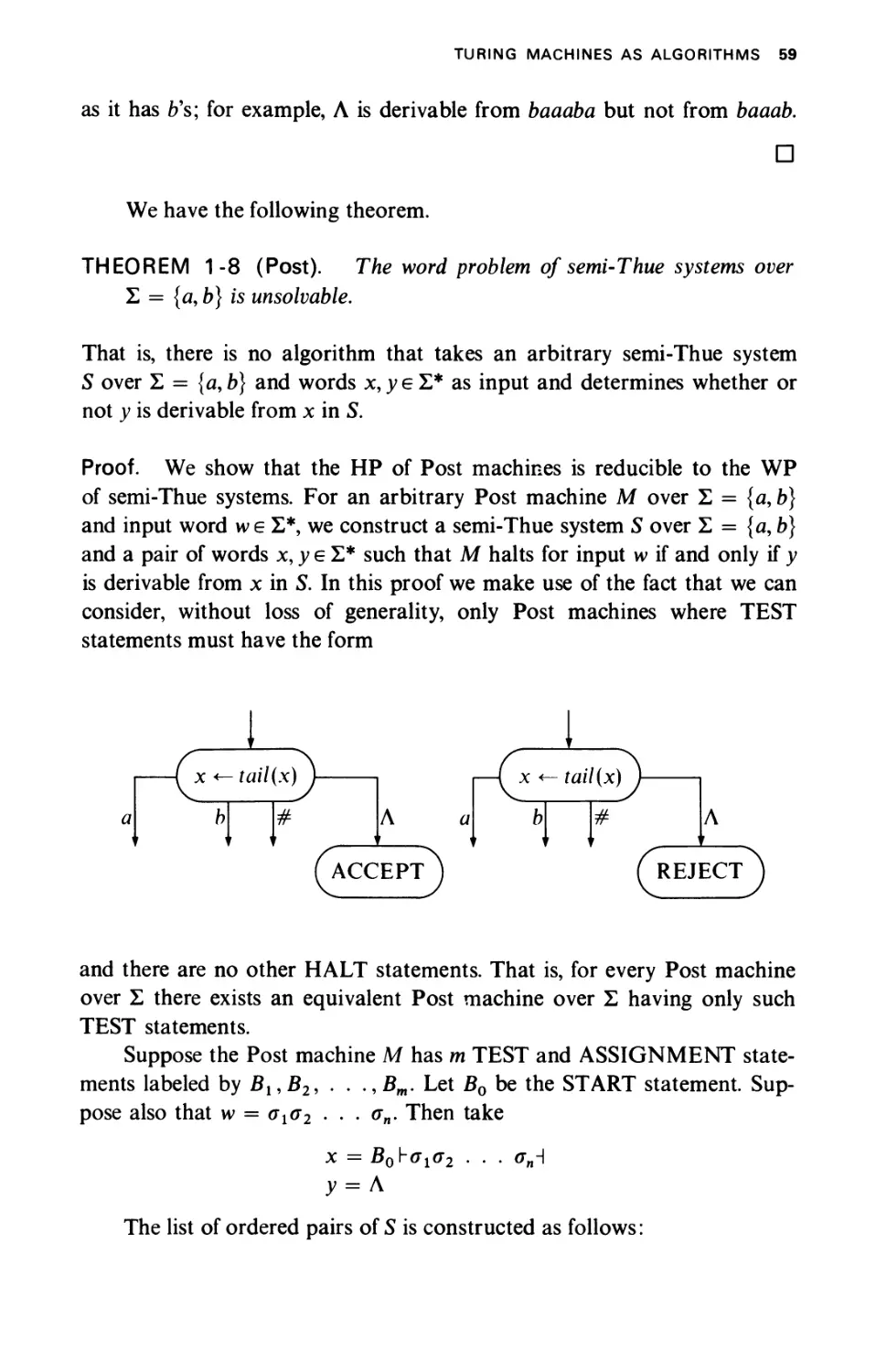
1-5 TURING MACHINES AS ALGORITHMS 53
1-5.1 Solvability of Classes of Yes/No Problems 54
1-5.2 The Halting Problem of Turing Machines 56
1-5.3 The Word Problem of Semi-Thue Systems 58
1-5.4 Post Correspondence Problem 60
1-5.5 Partial Solvability of Classes of Yes/No Problems 64
BIBLIOGRAPHIC REMARKS 67
REFERENCES 68
PROBLEMS 70
CHAPTER 2 PREDICATE CALCULUS 77
INTRODUCTION 77
81
81
85
90
95
101
105
2-2 NATURAL DEDUCTION 108
2-2.1 Rules for the Connectives 110
2-2.2 Rules for the Quantifiers 115
2-2.3 Rules for the Operators 122
2-3 THE RESOLUTION METHOD 125
2-3.1 Clause Form 125
2-3.2 Her brand's Procedures 130
2-3.3 The Unification Algorithm 136
2-3.4 The Resolution Rule 140
BIBLIOGRAPHIC REMARKS 145
REFERENCES 146
PROBLEMS 147
-1 BASIC NOTIONS
2-1.1
2-1.2
2-1.3
2-1.4
2-1.5
2-1.6
Syntax
Semantics (Interpretations)
Valid Wffs
Equivalence of Wffs
Normal Forms of Wffs
The Validity Problem

CONTENTS vii
CHAPTER 3 VERIFICATION OF PROGRAMS 161
INTRODUCTION
FLOWCHART PROGRAMS
3-1.1 Partial Correctness
3-1.2 Termination
FLOWCHART PROGRAMS WITH ARRAYS
3-2.1 Partial Correctness
3-2.2 Termination
ALGOL-LIKE PROGRAMS
3-3.1 While Programs
3-3.2 Partial Correctness
3-3.3 Total Correctness
BIBLIOGRAPHIC REMARKS
REFERENCES
PROBLEMS
161
161
170
182
189
189
195
202
203
205
211
218
220
223
CHAPTER 4 FLOWCHART SCHEMAS 241
INTRODUCTION
BASIC NOTIONS
4-1.1 Syntax
4-1.2 Semantics (Interpretations)
4-1.3 Basic Properties
4-1.4 Herbrand Interpretations
DECISION PROBLEMS
4-2.1 Unsolvability of the Basic Properties
4-2.2 Free Schemas
4-2.3 Tree Schemas
4-2.4 Ianov Schemas
FORMALIZATION IN PREDICATE CALCULUS
4-3.1 The Algorithm
4-3.2 Formalization of Properties of Flowchart Programs
4-3.3 Formalization of Properties of Flowchart Schemas
241
242
242
244
248
260
262
264
268
274
284
294
295
307
311

viii CONTENTS
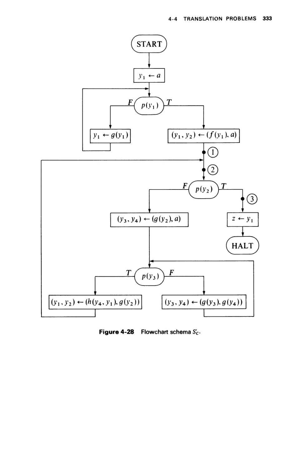
4-4 TRANSLATION PROBLEMS 317
4-4.1 Recursive Schemas 319
4-4.2 Flowchart Schemas versus Recursive Schemas 322
BIBLIOGRAPHIC REMARKS 334
REFERENCES 335
PROBLEMS 337
CHAPTER 5 THE FIXPOINT THEORY OF PROGRAMS 356
INTRODUCTION 356
5-1 FUNCTIONS AND FUNCTIONALS 357
5-1.1 Monotonic Functions 359
5-1.2 Continuous Functionals 366
5-1.3 Fixpoints of Functionals 369
5-2 RECURSIVE PROGRAMS 374
5-2.1 Computation Rules 375
5-2.2 Fixpoint Computation Rules 384
5-2.3 Systems of Recursive Definitions 389
5-3 VERIFICATION METHODS 392
5-3.1 Stepwise Computational Induction 393
5-3.2 Complete Computational Induction 400
5-3.3 Fixpoint Induction 403
5-3.4 Structural Induction 408
BIBLIOGRAPHIC REMARKS 415
REFERENCES 416
PROBLEMS 418
INDEXES 431
NAME INDEX
SUBJECT INDEX

PREFACE
What is mathematical theory of computation! I am sure that no two computer
scientists would define this concept in exactly the same way. Following
John McCarthy's pioneer paper "A Basis for a Mathematical Theory of
Computation,"! I consider it to be the theory which attempts to formalize
our understanding of computation, and in particular to make the art of
verifying computer programs (the famous debugging technique) into a
science.
In this book I attempted to treat both the practical and the theoretical
aspects of the theory. To make the book self-contained, I included selected
concepts of computability theory and mathematical logic.
My aim was to introduce these topics to a wide variety of readers:
junior-senior undergraduate students, first-year graduate students, as well
as motivated programmers. I deliberately omitted tedious details and
stated some results without proofs, using the spare space for giving extra
examples. My intention was to give an overview of the methods and the
results related to this field, rather than a standard mathematical textbook
of the style "definition-theorem-proof." I therefore ask the forgiveness of
my more theoretical-minded readers for preferring clarity over formality.
Numerous papers in mathematical theory of computation have been
published during the last few years, and activity in the area is increasing
every year. As a result, one of my main problems in writing this book was
t In P. Braffort and D. Hirschberg (eds.), "Computer Programming and Formal Systems," North-
Holland Publishing Company, Amsterdam, 1962.
ix

χ PREFACE
to decide what should be included in an introductory text in this area.
1 used two criteria for making this decision. First, I included only material
that I feel every computer scientist should know, based mainly on my
experience in teaching the mathematical theory of computation courses
at Stanford University and the Weizmann Institute for the last few years.
Second, because of the introductory nature of this text, I did not include
topics which I expect will undergo major changes and upheavals in the
near future. A few such topics are: automatic program synthesis, the logic
of partial functions, and verification techniques for large-scale computer
programs (such as compilers), as well as parallel programs.
Most of the chapters are self-contained. Neither chapter 1 nor chapter
2 requires any prerequisites with the exception that section 1-5 is necessary
to the understanding of section 2-1.6. The reader interested in the practical
aspect of the field should be aware that only sections 2-1.1 and 2-1.2 are
prerequisites for chapters 3 and 5, which contain the more applicable
techniques. Chapter 4, which is more theoretical in nature, requires both
sections 1-5 and 2-1 for its understanding.
I added to each chapter some bibliographic remarks and references.
My intention was to include in the bibliographic remarks and references
only what I consider to be the most relevant papers and books on each
topic, rather than trying to list all existing publications. I added also to
each chapter a selected set of about 20 to 30 problems (* indicates a hard
problem). I consider these problems an essential part of the text and
strongly urge the reader to attempt to solve at least some of them.
Many people contributed directly or indirectly to the completion
of this book. Thanks are due first to David Cooper, Robert Floyd, and
John McCarthy, who introduced me to this field. Thanks are also due to
my colleagues for their most helpful comments and suggestions on different
versions of the manuscript. I am most indebted in this way to Peter Andrews,
Edward Ashcroft, Jean-Marie Cadiou, Ashok Chandra, Nissim Francesz,
Shmuel Katz, Lockwood Morris, Stephen Ness, David Plaisted, Amir
Pnueli, Adi Shamir, Mark Smith, and Jean Vuillemin. Special thanks are
due to John McCarthy and Lester Earnest for their consistent
encouragement while I wrote this book. And finally, I am indebted to Phyllis Winkler
who very patiently typed the numerous drafts of the manuscript.
ZOHAR MANNA

MATHEMATICAL THEORY
OF COMPUTATION

CHAPTER 1
Qomputsbilily
Introduction
In the last few decades substantial effort has been made to define a
computing device that will be general enough to compute every
"computable" function. In 1936 Turing suggested the use of a machine, since then
called a Turing machine, which is considered to be the most general
computing device. It was hypothesized by Church [Church's thesis (1936)]
that any computable function can be computed by a Turing machine. Since
our notion of computable function is not mathematically precise, we can
never hope to prove Church's thesis formally. However, from the definition
of a Turing machine, it is apparent that any computation that can be
described by means of a Turing machine can be mechanically carried out;
and conversely, any computation that can be performed on a modern-day
digital computer can be described by means of a Turing machine. Moreover,
all other general computing devices that have been proposed [e.g., by
Church (1936), Kleene (1936), and Post (1936)]t have been shown to have
the same computing capability as Turing machines, which strengthens our
belief in Church's thesis.
In this chapter we discuss several machines, such as Post machines
and finite machines with pushdown stores, which have the same computing
capability as Turing machines. We emphasize that there are actually three
different ways to look at a Turing machine: (1) as an acceptor (accepts a
recursive or a recursively enumerable set), (2) as a generator (computes a
total recursive or a partial recursive function), and (3) as an algorithm
(solves or partially solves a class of yes/no problems).
We devote most of this chapter to discussing the class of Turing
machines (the "most general possible" computing device); however, for
purposes of comparison, in the first section we discuss the "simplest possible"
computing device, namely, the finite automaton.
t All three papers appear in the collection by Davis (1965).

2 COMPUTABILITY
1-1 FINITE AUTOMATA
Let Σ be any finite set of symbols, called an alphabet; the symbols are
called the letters of the alphabet. A word (string) over Σ is any finite sequence
of letters from Σ. The empty word, denoted by Λ, is the word consisting of no
letters. Σ* denotes the set of all words over Σ, including the empty word Λ.
Thus, if Σ = {a, b}, then Σ* = {A,a,b,aa,ab,ba,bb,aaa, . . .}. φ denotes
the empty set { }, that is, the set consisting of no words.f
We define the product (concatenation) UV of two subsets U, V of Σ* by
UV = {x\x = uv, и is in Uand ν is in V]
That is, each word in the set U V is formed by concatenating a word in
U with a word in V. As an example, if U = {a,ab,aab} and V = {b, bb},
then the set UV is {ab,abb,abbb,aabb,aabbb}. Note that the word abb
is obtained in two ways: (1) as α concatenated with bb, and (2) as ab
concatenated with b. The set VU is {ba,bab,baab,bba,bbab,bbaab}.
Note that UV Φ VU, which shows that the product operation is not
commutative. However, the product operation is associative, i.e., for any
subsets U, V, and W of Σ*, (UV)W = U(VW).
The closure (star) of a set S, denoted by 5*, is the set consisting of the
empty word and all words formed by concatenating a finite number of
words in 5. Thus if S = {ab,bb}, then
5* = {Λ, ab, bb, abab, abbb, bbab, bbbb, ababab, . . . j.
An alternative definition is
S* = 5° u S1 u S2 u S3 u . . .,
where 5° = {A}, and ^ = 5|_15, for / > 0.
We shall now discuss a special class of sets of words over Σ, called
regular sets. The class of regular sets over Σ is defined recursively as follows:
1. Every finite set of words over Σ (including φ, the empty set) is a
regular set.
2. If U and V are regular sets over Σ, so are their union [/uF and
product U V.
3. If 5 is a regular set over Σ, so is its closure 5*.
This means that no set is regular unless it can be obtained by a finite number
t Note the difference between Л, { }, and {Л};Л is a word (the empty word); { } is a set of words
(the set consisting of no words); and {Л} is a set of words (the set consisting of a single word, the
empty word Л).

FINITE AUTOMATA 3
of applications of 1 to 3. In other words, the class of regular sets over Σ
is the smallest class containing all finite sets of words over Σ and closed
under union, product, and star.
Let Σ = {α, b}. For example, we shall show that the set of all words
over Σ containing either two consecutive a's or two consecutive b's, and the
set of all words over Σ containing an even number of a's and an even
number of b's, are regular sets over Σ. On the other hand, we shall show that
the set {anbn\n ^ 0} (that is, the set of all words which consists of η a's
followed by η b's for any η ^ 0) is not a regular set over Σ. Similarly, it
can be shown that the sets {anbcf\n g: 0} and {cf2\n ^ 0} are not regular
sets over Σ.|
In this section we describe three different ways of expressing regular
sets. A subset of Σ* is regular if and only if: (1) it can be expressed by some
regular expression, (2) it is accepted by some finite automaton, or (3) it is
accepted by some transition graph. Finally we prove that there is an
algorithm to determine whether or not two given regular sets over Σ
(expressed by any one of the above forms) are equal, which is one of the
most important results concerning regular sets.
1 -1.1 Regular Expressions
We consider first the representation of regular sets by regular expressions.
This representation is of special interest since it allows algebraic
manipulations with regular sets. The class of regular expressions over Σ is defined
recursively as follows:
1. Λ and φ are regular expressions over Σ.
2. Every letter σ e Σ is a regular expression over Σ.
3. U Rx and R2 are regular expressions over Σ, so are (R{ + Я2),
(/*! Я2), and (/*!)*.
For example, if Σ = {α, b}, then (((a + (b · a)))* · a) is a regular expression
over Σ.
Every regular expression R over Σ describes a set R of words over Σ,
that is, R с Σ*, defined recursively as follows:
1. If R = Λ, then R = {Λ}, that is, the set consisting of the empty
word Λ; if R = φ, then R = φ, that is the empty set.
t Note the difference between a word, for example, bbaba, a set of words, for example, {a"bn\n ^ 0),
and a class of sets of words, for example, {{a"\n ^ 0}, {a"b"\n ^ 0}, \anbna"\n Ζ 0}, \anbna"b"\n ^ 0},.. .J.

4 COMPUTABILITY
2. If R = σ, then R = {σ}, that is, the set consisting of the letter a.
3. Let Rx and R2 be regular expressions over Σ which describe the
set of words Rx and R2, respectively:
If Я = (Ях + K2),then£ = Rx u Д2 = {x|xe Лхог xe Д2}, that is,
set union.
If R = (Rr R2), then R = R^ = {xy|xe^ and уеЯ2}, that is
set product.
If R = (Ri)*, then Л = Л? = {Л} u {x|x obtained by concatenating
a finite number of words in Rx}, that is, set closure.
Parentheses may be omitted from a regular expression when their omission
can cause no confusion. There are several rules for the restoration of
omitted parentheses: V is more binding than '·' or ' + ', that is, V is always
attached to the smallest possible scope (Λ, φ, a letter, or a parenthesized
expression), and '·' is more binding than ' + '. The '·' is always omitted. For
example, a + ba* stands for (a + (b-(a)*)\ and (a + ba)*a stands for
(((a + (b-a)))*-a). Whenever there are two or more consecutive '·', the
parentheses are associated to the left, and the same is true for ' + '.
For example, aba stands for ((ab)a), and a*(aa -f bb)*b stands for
(№*-(((а'а) + (Ь-Ь)))*)'Ь).
EXAMPLE 1-1
Consider the following regular expressions over Σ = {a, b).
R R
ba* All words over Σ
beginning with a b
followed only by a's.
a*ba*ba* All words over Σ
containing exactly
two b's.
(a + b)* All words over Σ.
(a + b)* (aa + bb) {a + b)* All words over Σ
containing two
consecutive tf's or two
consecutive b's.

FINITE AUTOMATA 5
[aa + bb + (ab + ba)(aa + bb)* (ab + ba)~\* All words over Σ
containing an even number
of a's and an even
number of b's.
(b + abb)* All words over Σ in
which every a is
immediately followed by
at least two b's.
D
From the definition of regular expressions, it is straightforward that
a set is regular over Σ if and only if it can be expressed by a regular expression
over Σ. Note that a regular set may be described by more than one regular
expression. For example, the set of all words over Σ = {a, b] with alternating
as and b's (starting and ending with b) can be described by the expression
b(ab)* as well as by (ba)*b. Two regular expressions Rx and R2 over Σ are
said to be equivalent (notation: Rx = R2) if and only ifRx = R2; thus, b(ab)*
and (ba)*b are equivalent. Later in this section we shall describe an algorithm
to determine whether or not two given regular expressions are equivalent.
In certain cases, the equivalence of two regular expressions can be shown
by the use of known identities. Some of the more interesting identities are
listed below. For simplicity, we let Rx я R2 stand for Rx я R2 and weR
stand for we R.
For any regular expressions R, S, and Τ over Σ:
1. R + S = S + R, R + φ = φ + R, R + R = Я,
(R + S)+ T= R + (S+ T).
2. ЯА = АЯ = Я, R<t) = <t>R = φ, (RS) T= R(ST)
Note that generally RS φ SR.
3. R(S + T) = RS + RT, (S + T)R = SR + TR.
4. R* = R*R* = (R*)* = (A + Я)*, φ* = A* = A.
5. Я* = A + R + R2 + . . . + Rk + Rk + lR* (к ^ 0)
special case: R* = A + RR*.
6. (R + S)* = (R* + S*)* = (K*S*)* = (R*S)*R* = Я*(5Я*)*
Note that generally (R + S)* φ Я* + S*.
7. R*R = RR*, R(SR)* = (RS)*R.
8. (R*S)* = A + (R + S)*S, (RS*)* = A + R(R + S)*.

6 COMPUTABILITY
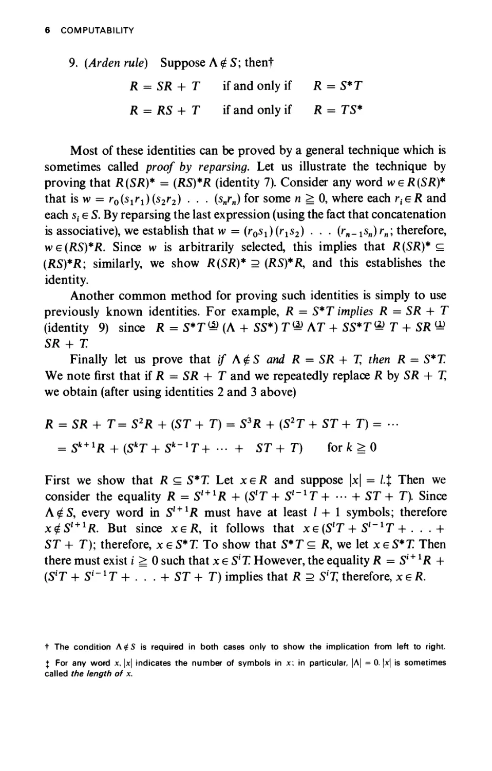
9. {Ayden rule) Suppose Λ φ 5; thenf
R = SR + 7 if and only if R = S*T
R = RS + Τ if and only if R = 75*
Most of these identities can be proved by a general technique which is
sometimes called proof by reparsing. Let us illustrate the technique by
proving that R(SR)* = (RS)*R (identity 7). Consider any word weR(SR)*
that is w = r0(s1rl)(s2r2) · . . (snrn) for some η g: 0, where each rteR and
each st e 5. By reparsing the last expression (using the fact that concatenation
is associative), we establish that w = (г^Нг^) · · · (rn-isn)rn> therefore,
we(RS)*R. Since w is arbitrarily selected, this implies that R(SR)* с
(RS)*R; similarly, we show R(SR)* 2 (RS)*R, and this establishes the
identity.
Another common method for proving such identities is simply to use
previously known identities. For example, R = S*7 implies R = SR + Τ
(identity 9) since R = 5*7^ (Λ + 55*) Τ® ΛΤ + 55*7^ Τ + SR Ш
5Я + X
Finally let us prove that if Λ£5 and R = SR + % then R = S*T.
We note first that if R = SR + Τ and we repeatedly replace R by SR + %
we obtain (after using identities 2 and 3 above)
R = SR+ T=S2R + (5T+ T) = S3R + (S2T+ ST+ T) = ...
= 5*+1Я + (5*T+5fc-1T+ ·.. + 57+ T) for к ^ 0
First we show that R с 5*7 Let хеЯ and suppose |x| = l.% Then we
consider the equality R = Sl+1R + (SlT + Sl~xT + ··· + 57+ 7). Since
Λ φΞ, every word in Sl + 1R must have at least / + 1 symbols; therefore
х<£5| + 1Я. But since хеЯ, it follows that xe(SlT + 5I_17 + . . .+
57 + 7); therefore, χ e 5*7 To show that 5*7 с Я, we let χ e 5*7 Then
there must exist i ^ 0 such that χ e 5f7 However, the equality Я = 5i+ *R +
(5T + 51'"x Τ + . . . + 57 + 7) implies that R 2 S*T, therefore, xeR.
t The condition A$S is required in both cases only to show the implication from left to right.
{ For any word x, |x| indicates the number of symbols in x; in particular, |Λ| = 0. |x| is sometimes
called the length of x.

FINITE AUTOMATA 7
We shall now demonstrate the use of the above identities for proving
equivalence of regular expressions.
EXAMPLE 1-2
We prove the following:
(b + aa*b) + (b + aa*b)(a + ba*b)* (a + ba*b) = a*b{a + ba*b)*
(b + aa*b) + (b + дд*Ь)(д + Ьд*Ь)* (а + Ьд*Ь)
^ (b + <ю*Ь) [Л + (a + ba*b)* (я + Ьд*Ь)]
^(Ь + аа*Ь)(я + Ьа*Ь)*
^(Л + аа*)Ь(а + Ьа*Ь)*
& a*b(a + ba*b)*
D
1 -1.2 Finite Automata
A finite automaton A over Σ, where Σ = {σΐ5σ2, . . .,σ„}, is a finite directed
grapht in which every vertex has /1 arrows leading out from it, with each
arrow labeled by a distinct σ{ (1 ^ i ^ /1). There is one vertex, labeled by a
'—' sign, called the initial vertex, and a (possibly empty) set of vertices,
labeled by a ' + ' sign, called the final vertices (the initial vertex may also
be a final vertex). The vertices are sometimes called states.
For a word w e Σ*, a w ραί/j from vertex ι to vertex j in Л is a path
from ι to ; such that the concatenation of the labels along this path form
the word w. (Note that the path may intersect the same vertex more than
once.) A word w e Σ* is said to be accepted by the finite automaton A if
the w path from the initial vertex leads to a final one. The empty word Λ is
accepted by A if and only if the initial vertex is also final. The set of words
accepted by a finite automaton A is denoted by A. Kleene's theorem
(introduced in Sec. 1-1.4) implies that a set is regular over Σ if and only if
it is accepted by some finite automaton over Σ.
t A finite directed graph consists of a finite set of elements (called vertices) and a finite set of
ordered pairs (v,v') of vertices (called arrows). An arrow (v, v') is expressed as@-»@. A finite
sequence of (not necessarily distinct) vertices vitv2,. . · , vk is said to be a path from vt to vk if
each ordered pair (vitvt + i)t 1 ^ / < /c, is an arrow of the graph.

8 COMPUTABILITY
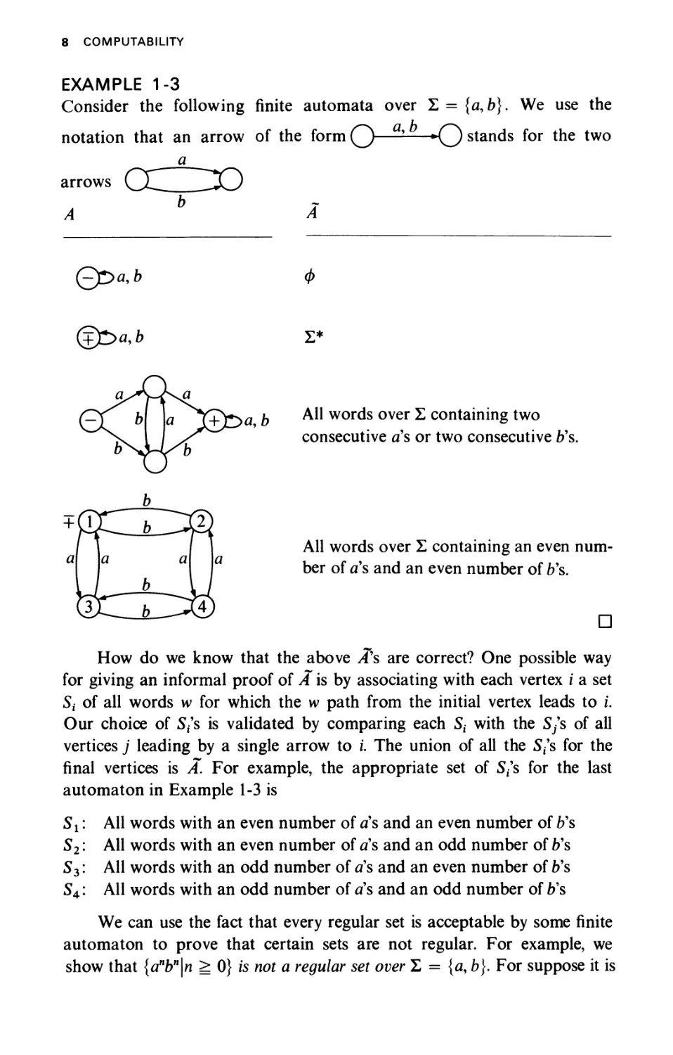
EXAMPLE 1-3
Consider the following finite automata over Σ = {α, b}. We use the
notation that an arrow of the form Q—— *0 stands for the two
a
arrows СС__ЛХ)
£ра,Ь ф
©Sa,b Σ*
All words over Σ containing two
consecutive as or two consecutive b's.
2}
J All words over Σ containing an even num-
I ber of a's and an even number of b's.
^ D
How do we know that the above /f s are correct? One possible way
for giving an informal proof of A is by associating with each vertex i a set
St of all words w for which the w path from the initial vertex leads to i.
Our choice of 5/s is validated by comparing each St with the S/s of all
vertices j leading by a single arrow to i. The union of all the Sf's for the
final vertices is A. For example, the appropriate set of Sf's for the last
automaton in Example 1-3 is
Sx: All words with an even number of a's and an even number of b's
52: All words with an even number of as and an odd number of b's
53: All words with an odd number of a's and an even number of b's
54: All words with an odd number of a's and an odd number of b's
We can use the fact that every regular set is acceptable by some finite
automaton to prove that certain sets are not regular. For example, we
show that {anbn\n ^ 0} is not a regular set over Σ = {a, b). For suppose it is

FINITE AUTOMATA 9
a regular set; then there must exist a finite automaton A such that A =
{anbn\n g: 0}. Let us assume that A has N states, N > 0. Consider the word
aNbN. Since the word is accepted by A and its length is greater than the
number of vertices in A, it follows that there must exist in Л at least one
loop of as or at least one loop of b'sf, which enables A to accept the word
aNbN. Suppose it is a loop of as of length fc, where к > 0. Then since we can
go through the loop i times for any i ^ 0, it follows that A must also accept
all words of the form aN+ikbN (for i g: 0), which contradicts the fact that
A = {anbn\n ^0}.
1-1.3 Transition Graphs
We shall now introduce a generalization of the notion of finite automata,
called transition graphs, by which it is much more convenient to express
regular sets. We show, however, that although the class of finite automata
is a proper subclass of the class of transition graphs, every regular set
that is accepted by a transition graph is also accepted by some finite
automaton.
A transition graph Τ over Σ is a finite directed graph in which every
arrow is labeled by some word we Σ* (possibly the empty word Λ). There
is at least one vertex, labeled by a ' —' sign (such vertices are called initial
vertices), and a (possibly empty) set of vertices, labeled by a ' +' sign (called
the final vertices). A vertex can be both initial and final.
For a word we Σ*, a w path from vertex i to vertex j in Τ is a finite
path from i to j such that the concatenation of the labels on the arrows
along this path form the word w (ignoring the A's, if any). A word w e Σ*
is said to be accepted by a transition graph Τ if there exists a w path from
an initial vertex to a final one. The empty word Λ is accepted by Τ if there
is a vertex in Τ which is both initial and final or if a A path leads from an
initial vertex to a final one. The set of words accepted by a transition graph
Τ is denoted by T. Kleene's theorem (introduced in Sec. 1-1.4) implies that
a set is regular over Σ if and only if it is accepted by some transition graph
over Σ.
Note that every finite automaton is a transition graph, but not vice
versa. One of the key differences between the two is that a finite automaton
is deterministic in the sense that for every word w e Σ* and vertex i there
is a unique w path leading from i. On the other hand, a transition graph
is nondeterministic because it may have more than one w path leading
from i (or none at all).
t A loop of a's, where <reZ,.is a path in which the first vertex is identical to the last one and such
that all its arrows are labeled by σ.

10 COMPUTABILITY
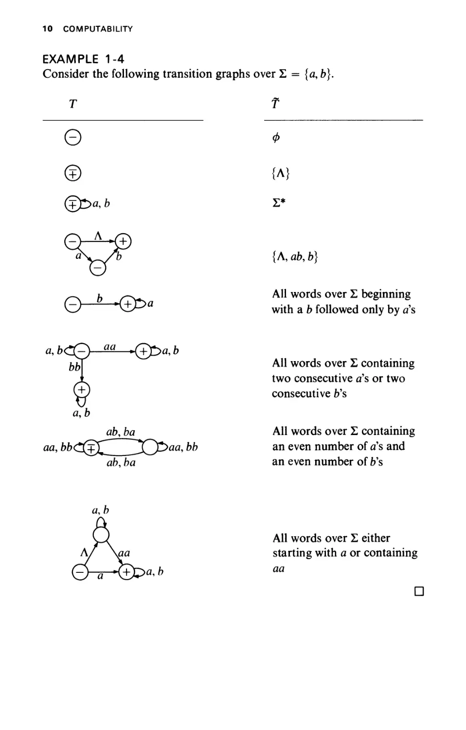
EXAMPLE 1-4
Consider the following transition
Τ
a, b
ab,ba
aa, ЬЬС(^^_^У^р>аа, bb
ab,ba
s over Σ = {α, b).
Τ
Φ
{Λ}
Σ*
{Λ, ab9 b)
All words over Σ beginning
with a b followed only by a's
All words over Σ containing
two consecutive a's or two
consecutive b's
All words over Σ containing
an even number of a's and
an even number of b's
All words over Σ either
starting with a or containing
aa
D

FINITE AUTOMATA 11
1 -1.4 Kleene's Theorem
THEOREM 1-1 (Kleene). (1) For every transition graph Τ over Σ there
exists a regular expression R over Σ such that R = Τ; (2) for every
regular expression R over Σ there exists a finite automaton A over Σ
such that A = /?.
Because every finite automaton is a transition graph, it follows from the
theorem that: (1) a set is regular over Σ if and only if it is accepted by
some finite automaton over Σ, and (2) a set is regular over Σ if and only if
it is accepted by some transition graph over Σ.
Proof (part 1). We describe briefly an algorithm for constructing for a
given transition graph Τ a regular expression R such that R = T. For
the purpose of this proof, we introduce the notion of a generalized transition
graph, which is a transition graph in which the arrows may be labeled by
regular expressions rather than just by words.
First, add to the given transition graph Τ a new vertex, called x, and
Λ arrows leading from χ to all the initial vertices of T. Similarly, add
another new vertex, called y, and Λ arrows leading from all the final
vertices of Τ to y. Let χ be the only initial vertex in the modified transition
graph, and у the only final vertex.
We now proceed step by step and eliminate all vertices of Τ until
only the new vertices χ and у are left. During the elimination process, the
arrows and their labels are modified. The arrows may be labeled by regular
expressions, i.e., we construct generalized transition graphs. The generalized
transition graph which is constructed after each step still accepts the
same set of words as the original T. The process terminates when we obtain
a generalized transition graph with only two vertices, χ and y, of the form:
αϊ
Then ax + a2 + · · · + a„ is the desired regular expression R.
The elimination process is straightforward. Suppose, for example, we
want to eliminate vertex 3 in a generalized transition graph, where the
—Φ

12 COMPUTABILITY
arrows leading to and from vertex 3 are of the form
(αΐ5α2,/?ι,/?2>Уь and y2 are regular expressions.) To eliminate vertex 3
from the generalized transition graph, we replace that part by
«ι(/*ι +βι)*7
Μ/*ι +β2)*γ2
In the special case that vertices 1 and 4 are identical, we shall actually get
(?Ρ*Λβι+β2)*7ι
«l(j»l +βΐ)*72
I
—U\
Let us illustrate the process before proceeding with the proof of part 2 of
theorem 1-1.

FINITE AUTOMATA 13
EXAMPLE 1-5
Consider the following transition graph T0, which accepts the set of all
words over Σ = {α, b} with an even number of a's and an even number
of b's.
aa,bb
aa,bb
First we add the new vertices χ and y. Since vertex 1 is both an initial and
a final vertex of T0, we add an Λ arrow leading from χ to 1 and an Λ arrow
leading from 1 to y. The corresponding generalized transition graph is
aa + bb
Eliminating vertex 2, we obtain
aa + bb
(ab + ba)(aa + bb)*(ab + ha)
Finally, eliminating vertex 1, we obtain
\aa + bb + (ab + ba)(aa + bb)*(ab + ba)]*
Thus the desired regular expression R0 (that is, R0 = f0) is
[aa + bb + (ab + ba)(aa + bb)* (ab + ba)]*.
D

14 COMPUTABILITY
Proof (part 2) We now describe briefly an algorithm (known as the
subset method) for constructing for a given regular expression R a finite
automaton A such that A = R. We proceed in three steps.
Step 1. First we construct a transition graph Τ such that Τ = R. We
start with a generalized transition graph of the form
We successively split R by adding new vertices and arrows, until all arrows
are labeled just by letters or Λ. The following rules are used:
© AB ·© is replaced by Qy^^y_B_Q
(DA + B*Q) isrePlacedьу QXZ^XD
В
©—^—*© is replaced by © Л >© Л '©
A
Note that in the final transition graph, χ is still the only initial vertex and
у is the only final vertex. In practice, often an appropriate simple transition
graph can be constructed in a straightforward way without using the above
inductive steps.
Step 2. Let Τ be the transition graph generated in Step 1. Now we
construct the transition table of T; for simplicity we assume that Σ = {a, b).

FINITE AUTOMATA 15
Let Μ be any subset of vertices of T. For any word w e Σ* we define Mw
to be the subset of all vertices of Τ reachable by a w path from some vertex
of M. For example, M^ consists of all vertices of Τ reachable by an ab path
from some vertex of M, or, equivalently, all vertices of Τ reachable by a
b path from some vertex of Ma.
The transition table of Τ consists of three columns. The elements of
the table are subsets of vertices of Τ (possibly the empty set). The subset
in the upper-left-hand corner of the table (first row, column 1) is {х}л,
that is, the subset which consists of the initial vertex χ and all vertices of
Τ reachable by а Л path from x. In general, for any row of the table, if the
subset Μ is in column 1, then we add Ma (that is, the set of vertices of Τ
reachable by an a path from some vertex of M) in column 2 and Mb (that is,
the set of vertices of Τ reachable by a b path from some vertex of M) in
column 3. If Ma does not occur previously in column 1, we place it in
column 1 of the next row and repeat the process. We treat Mb similarly.
The process is terminated when there are no new subsets in columns
2 and 3 of the table that do not occur in column 1. The process must always
terminate because all subsets in column 1 are distinct and there are only
finitely many distinct subsets of the finite set of vertices of T.
Step 3. Finally we use the transition table to construct the desired finite
automaton A. The finite automaton A is constructed as follows. For every
subset Μ in column 1 of the table there corresponds a vertex Μ in A. From
every vertex Μ in A there is an a arrow leading to vertex Ma and a b
arrow leading to vertex Mb. The vertex {х}л (that is, the vertex
corresponding to the subset in the upper-left-hand corner of the table) is
the only initial vertex of A. A vertex Μ of Л is final if and only if Μ contains
a final vertex of T.
We leave it to the reader to verify that a word w e Σ* is accepted by
Τ if and only if it is accepted by A. The following example illustrates the
method.

16 COMPUTABILITY
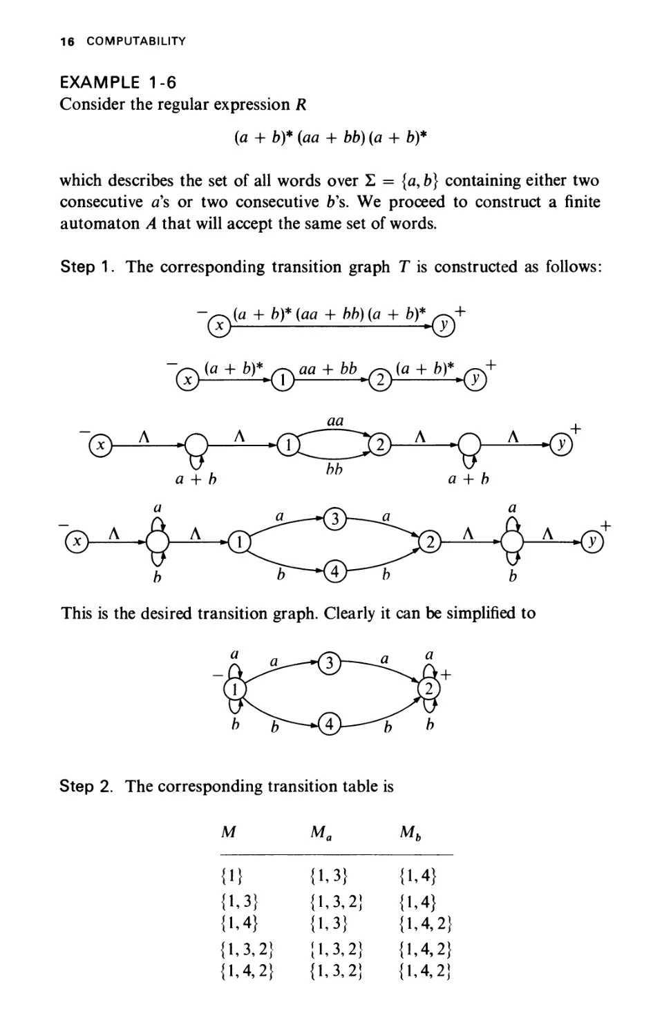
EXAMPLE 1-6
Consider the regular expression R
(а + Ь)*(аа + ЬЬ)(а + Ь)*
which describes the set of all words over Σ = {α, b) containing either two
consecutive a's or two consecutive b's. We proceed to construct a finite
automaton A that will accept the same set of words.
Step 1. The corresponding transition graph Τ is constructed as follows:
-^(a + b)*(aa + bb)(a + fo)* w+
This is the desired transition graph. Clearly it can be simplified to
Step 2. The corresponding transition table is
Μ
{Π
{1,3}
{1,4}
{1,3,2}
{1,4,2}
Ma
{1,3}
{1,3,2}
{1,3}
{1,3,2}
{1,3,2}
Mb
{1,4}
{1,4}
{1,4,2}
{1,4,2}
{1,4,2}

FINITE AUTOMATA 17
Step 3. The desired finite automaton A is
+
jTuT) a *( 1,3,2 У^а
OX b\ г b\ r
\''4>-гЧ ^2 X>
+
Note that it is possible to simplify the finite automaton to obtain
0С^Г b( )a J^QOa^h
D
1-1.5 The Equivalence Theorem
We shall conclude this section with an important theorem.
THEOREM 1-2 (Moore). There is an algorithm to determine whether
or not two finite automata A and A' over Σ are equivalent (that is, A = A').
Proof. Given two finite automata A and A' over Σ. Suppose for simplicity
that Σ = {a, b}. First we rename the vertices of Л and A' so that all vertices
are distinct. Let χ and x' be the initial vertices of A and A', respectively.
To decide whether or not A and A' are equivalent, we construct a
comparison table which consists of three columns. The elements of the
table are pairs of vertices (v, v'\ where ν is a vertex of A and v' is a vertex
of A'. The pair in the upper-left-hand corner of the table (first row, column
1) is (x, x'). In general, for any row of the table, if the pair (v, v') is in column
1, then we add in column 2 the pair of vertices (va, v'a\ where the a arrow
from ν leads to va in A and the a arrow from v' leads to v'a in A'. Similarly,
in column 3 we add the pair of vertices (vb,v'b\ where the b arrow from
ν leads to vb in A and the b arrow from t/ leads to v'b in A'. If (va, v'a) does
not occur previously in column 1, we place it in column 1 of the next row
and repeat the process; we treat (vb, v'b) similarly.
If we reach a pair (v, v') in the table for which ν is a final vertex of A
and t/ is a nonfinal vertex of A or vice versa, we stop the process: A and
A are not equivalent. Otherwise, the process is terminated when there are
no new pairs in columns 2 and 3 of the table that do not occur in column 1.

18 COMPUTABILITY
In this case A and A' are equivalent. We leave it to the reader to verify these
claims. The process must always terminate because all pairs in column 1
are distinct pairs and there are only finitely many distinct pairs of the
vertices of A and A'.
Q.E.D.
EXAMPLE 1-7
1. Consider the following two finite automata A and A' over Σ = {a, b]
described in Fig. 1-1.
A A'
Figure 1-1 The finite automata A and A.
They are equivalent because the corresponding comparison table is
(v,v') (va,v'a) (vb,v'b)
(1,4)
(2,5)
(3,6)
(2,7)
(1,4)
(3,6)
(2,7)
(3,6)
(2,5)
(1,4)
(3,6)
(1,4)
There are no pairs in columns 2 and 3 that do not occur in column 1.
2. Consider the two finite automata В and B' described in Fig. 1-2.
(ьрь
В'
Figure 1-2 The finite automata В and B'.

FINITE AUTOMATA 19
They are equivalent because the corresponding comparison table is
(ν, ν')
(1,4)
(2,5)
(3,7)
(2,6)
("a, f'J
(1,4)
(3,7)
(1,4)
(3,7)
(vb,v'b)
(2,5)
(2,6)
(2,5)
(2,6)
Again, there are no pairs in columns 2 and 3 that do not occur in column 1.
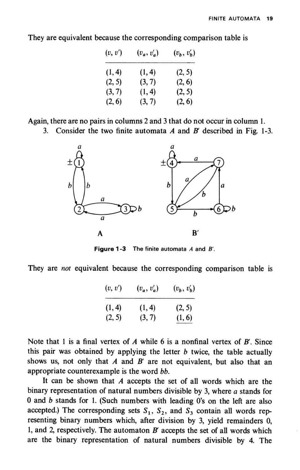
3. Consider the two finite automata A and В described in Fig. 1-3.
a a
A B'
Figure 1 -3 The finite automata A and B'.
They are not equivalent because the corresponding comparison table is
(v, V) (va, υ'α) (vb, v'b)
(1.4) (1,4) (2,5)
(2.5) (3,7) (1,6)
Note that 1 is a final vertex of A while 6 is a nonfinal vertex of B. Since
this pair was obtained by applying the letter b twice, the table actually
shows us, not only that A and В are not equivalent, but also that an
appropriate counterexample is the word bb.
It can be shown that A accepts the set of all words which are the
binary representation of natural numbers divisible by 3, where a stands for
0 and b stands for 1. (Such numbers with leading O's on the left are also
accepted.) The corresponding sets Sl9 S29 and 53 contain all words
representing binary numbers which, after division by 3, yield remainders 0,
1, and 2, respectively. The automaton В accepts the set of all words which
are the binary representation of natural numbers divisible by 4. The

20 COMPUTABILITY
corresponding sets S4, S5, S6, and 57 contain all words representing binary
numbers which, after division by 4, yield remainders 0, 1, 3, and 2,
respectively.
D
1-2 TURING MACHINES
In this section we define three classes of machines over a given alphabet Σ:
Turing machines, Post machines, and finite machines with pushdown stores.
Each of these machines can be applied to any word w e Σ* as input. It
can stop in two different ways—by accepting w or rejecting w—or it can
loop forever. For such a machine Μ over Σ, we denote the set of all
words over Σ accepted by Μ by accept (M), the set of all words over Σ
rejected by Μ by reject(M), and the set of all words over Σ for which Μ
loops by loop(M). It is clear that for any given machine Μ over Σ, the
three sets of words accept(M), reject(M), and loop(M) are disjoint and
that accept(M) u reject(M) u loop(M) = Σ*.
Two such machines Mx and M2 over Σ are said to be
equivalent if accept(Mx) = accept(M2) and, clearly, reject(Mx) kj loop(Mx) =
reject(M2) u loop(M2). A class Μχ of machines is said to have the same
power as a class J(2 of machines, Л x = J(2, if for every machine in Mx
there is an equivalent machine in Μ 2, and vice versa. We also say that a
class Μx of machines is more powerful than a class Jt' 2, Jix > Ji2, if for
every machine in M2 there is an equivalent machine in Jix, but not vice
versa.
We shall show that the three classes of machines—Turing, Post and
finite machines with two pushdown stores—have the same power. We
finally emphasize that the introduction of a nondeterministic mechanism
to these machines does not add anything to their power.
We make use of three basic functions defined over Σ*:
head(x): gives the head (leftmost letter) of the word χ
tail (χ): gives the tail of the word χ (that is, χ with the leftmost
letter removed)
σ - χ: concatenates the letter σ and the word x.
For example, if Σ = {α, b}9 then head (abb) = a, tail (abb) = bb, and
a- bb = abb. We agree that head(A) = tail(A) = Λ. Note that by definition
head(a) = a, tail(a) = Λ, and σΛ = a for all a e Σ.
For simplicity, we present most of the results for the alphabet Σ = {a, b};
however, all the results hold as well for any alphabet with two or more letters.'f
t In this chapter we never discuss the special case of an alphabet consisting of a single letter.

TURING MACHINES 21
1-2.1 Turing Machines
Specifications for Turing machines have been given in various ways in
the literature. In our model, a Turing machine Μ over an alphabet Σ consists
of three parts:
1. A tape which is divided into cells. The tape has a leftmost cell
but is infinite to the right. Each cell of the tape holds exactly one tape
symbol. The tape symbols include the letters of the given alphabet Σ, the
letters of a finite auxiliary alphabet K, and the special blank symbol Δ.
All symbols are distinct.
2. A tape head which scans one cell of the tape at a time. It can move;
in each move the head prints a symbol on the tape cell scanned, replacing
what was written there, and moves one cell left or right.
b
a
a
b
b
a
A
Δ
Δ
Δ
Tape
head
3. A program which is a finite directed graph (the vertices are called
states). There is always one start state, denoted by START, and a (possibly
empty) subset of halt states, denoted by HALT. Each arrow is of the
form
where aeZuKu{A}, /ieZuKu{A}, and ye{L,R}. This indicates
that, if during a computation we are in vertex (state) i and the tape head
scans the symbol a, then we proceed to vertex (state) j while the tape head
prints the symbol β in the scanned cell and then moves one cell left or
right, depending whether γ is L or R. All arrows leading from the same vertex
i must have distinct a's.
Initially, the given input word w over Σ is on the left-hand side of
the tape, where the remaining infinity of cells hold the blank symbol Δ,
and the tape head is scanning the leftmost cell. The execution proceeds as
instructed by the program, beginning with the START state. If we
eventually reach a HALT state, the computation is halted and we say that the

22 COMPUTABILITY
input word w is accepted by the Turing machine. If we reach a state i of the
form
where the symbol scanned by the tape head is different from al5 a2, . . .,
and a„, there is no way to proceed with the computation. In this case
therefore, the computation is halted and we say that the input word w is
rejected by the Turing machine. The other case where the computation is
halted and the input word is said to be rejected by the Turing machine
is when the tape head scans the leftmost cell and is instructed to do a left
move.
EXAMPLE 1-8
The Turing machine Ml over Σ = {α, b) (shown in Fig. 1-4) accepts every
word of the form anbn9 n^O, and rejects all other words over Σ; that is,
acceptWi) = {anbn\n §: 0}, rejec^M^ = Σ* — accept(M^), and Ιοορ(Μχ) =
φ. Here V = {A, B}. [Note that the specification of β and γ in (Δ, Δ, R) are
irrelevant for the performance of this program.]
(Δ, Δ, R)
(β, β, R) (Б, В, L) (Б, Б, R)
START ^(^K) A (b,frL) Α^/Ι,^^ΙΔ,Δ^)^
HALT
V(a, a, R)
(Λ,Λ,ΚΓ
(a, a, L)
> (a, a, L)
Figure 1 -4 The Turing machine M, that accepts {a"b"\n s 0}.

TURING MACHINES 23
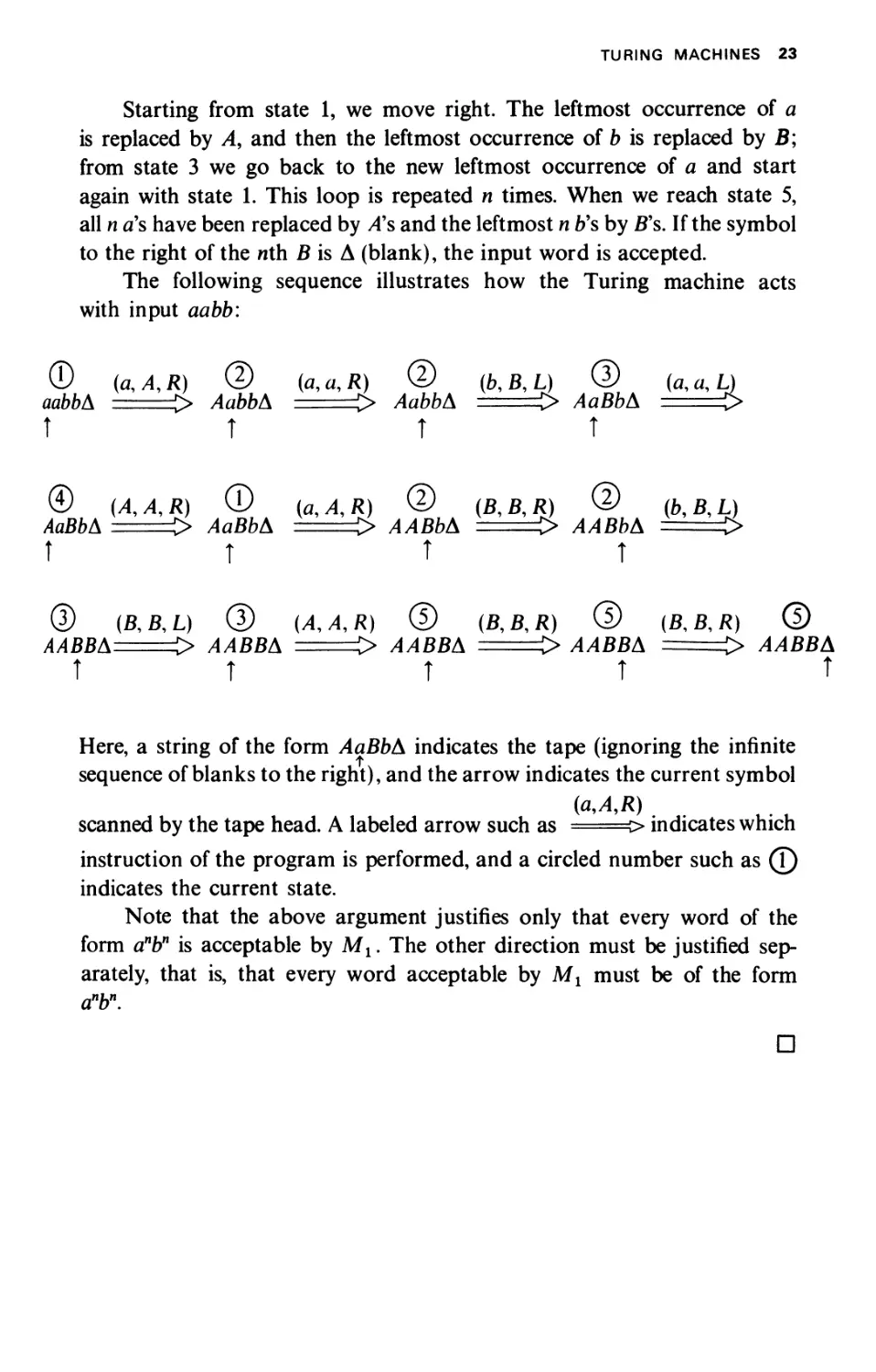
Starting from state 1, we move right. The leftmost occurrence of a
is replaced by A, and then the leftmost occurrence of b is replaced by B;
from state 3 we go back to the new leftmost occurrence of a and start
again with state 1. This loop is repeated η times. When we reach state 5,
all η a's have been replaced by A's and the leftmost η b's by B's. If the symbol
to the right of the nth β is Δ (blank), the input word is accepted.
The following sequence illustrates how the Turing machine acts
with input aabb:
Θ (α, Λ, R) © (я, α, Я) © (b,B,L) @ (fl,«,L)
aabbA > AabbA > AabbA > AaBbA ==>
Τ Τ Τ Τ
© (A,A,R) © (a,A,R) © (В, В, Я) © (&,β,^)
АоВЬА > ЛдВЬА > ААВЬА > ААВЬА >
τ τ τ τ
® (B,B,L) © (Л, Л, К) ® (В, В, R) © (Б, Б, Я) ©
ΛΛΒΒΔ -> ААВВА > ААВВА > ААВВА > ЛЛББД
Τ Τ Τ Τ Τ
Here, a string of the form AaBbA indicates the tape (ignoring the infinite
sequence of blanks to the right), and the arrow indicates the current symbol
(М,Д)
scanned by the tape head. A labeled arrow such as ===> indicates which
instruction of the program is performed, and a circled number such as (\)
indicates the current state.
Note that the above argument justifies only that every word of the
form anbn is acceptable by Mx. The other direction must be justified
separately, that is, that every word acceptable by Mx must be of the form
anb\
D

24 C0MPUTABIL1TY
1-2.2 Post Machines
A Post machine Μ over Σ = {α, b] is a flow-diagram^ with one variable x,
which may have as a value any word over {a, b, #}, where # is a special
auxiliary symbol. Each statement in the flow-diagram has one of the
following forms:
1. START statement (exactly one)
С START Л
2. HALT statements
ι
ι
(^ACCEPT·) С REJECT J
3. TEST statements
I
or in shorti
i
ΚΞΞΗ1-
ζ head (x) \-
x <- tai/ (x)
χ *-tail (x)
χ <-fai/(x)
F^q=^=F
ι
\x*- tail(x) V
4. ASSIGNMENT statements
χ <-xa
χ <- xb
X#
t A flow-diagram is a finite directed graph in which each vertex consists of a statement. We
always allow the JOfNT statement for combining two or more arrows into a single one.
JNote that for a general л-letter alphabet Σ = {σ,,σ2 σ„], a TEST statement would have
η + 2 exits labeled bya,,ff2, · . ·. σ„, # , Λ.

TURING MACHINES 25
Thus the TEST statements checks the leftmost letter of x, head{x), and delete
it after making the decision. The only ASSIGNMENT statements allowed
are to concatenate a letter (a, b, or #) to the right of x.
A word w over Σ is said to be accepted/rejected by a Post machine Μ
if the computation of Μ starting with input χ = w eventually reaches an
ACCEPT/REJECT halt.
EXAMPLE 1-9
The Post machine M2 over Σ = {я, b} described in Fig. 1-5 accepts every
word over Σ of the form anbn, η ^ 0, and rejects all other words over Σ;
that is, accept{M2) = {anbn\n ^ 0}, reject(M2) = Σ* - accept{M2), and
loop{M2) = 0.
(^START J
χ <-x#
m
®
л ίχ *- tail(x)\
-ίχ <- tail(x) ) 1 ^REJECT) (ACCEPT^
χ *—χα
®
ζ
I—/reject)
χ *- tail(x)
(reject)
>
#
(rejectJ
χ *-x#
χ +-xb
Figure 1-5 The Post Machine M2 that accepts {anbn\n ^ 0}.

26 COMPUTABILITY
Suppose χ = <fbn for some η §: 0. The key point is that whenever we reach
point 1, we have the word а'Ь'# in x, 0 ^ i ^ n. Now if we find an a
on the left of x, we go i — 1 times around loop 2 until we obtain bl#al~l;
then we go i - 1 times around loop 3 until we obtain #ai~1bi~1; finally
we move the # symbol to obtain ai_1bi_1# and repeat the process from
point 1. Note that there is only one ACCEPT statement, which corresponds
to the case that we reach point 1 with only # in χ (that is, i = 0).
D
EXAMPLE 1-10
Consider the Post machine M3 over Σ = {a,b} shown in Fig. 1-6. Here
accept(M3) = {all words over Σ with the same number of ds and b's}
reject(M3) = {all words over Σ where the difference between the number
of a's and b's is 1}
loop(M3) = {all words over Σ where the difference between the number
of as and b's is more than 1}
For example, ab e accept(M3\ aba e reject(M3\ while aaba ε loop(M3).
С START
■ »
a
X
a
j
—( χ <-tail(x) J—
>
<— xa
I ι
b
л
(^reject)
b
X
<
©
f i/ чЛ_
( χ <— tail (χ) )
b
r
-ix <— tail(x) j—
:
<-xb
j
a
'
л
t
CaccefF)
л
(reject)
Figure 1-6 The Post machine Μ3 that accepts all words with the same number of
a's and b's.
Note that we have not used the special symbol #, and therefore we ignored
the # exit from the tests. The main test is at point 1: if head(x) = a, then
we keep searching for a letter b to be eliminated, while if head(x) = b, then
we keep searching for a letter a.
D

TURING MACHINES 27
THEOREM 1 -3 (Post) The class of Post machines over Σ has the same
power as the class of Turing machines over Σ.
That is, for every Post machine over Σ there is an equivalent Turing
machine over Σ and vice versa.
Proof. First we show that every Turing machine over Σ = {α, b) can be
simulated by an equivalent Post machine over Σ = {α, b}. The main idea
behind this simulation is that the contents of the tape and the position of
the tape head at any stage of the computation of the Turing machine are
expressed as values of the variable χ in the Post machine.
For example, if at some stage of the computation of the Turing machine
the tape is of the form
dx d
d* d5
di
ύ
where each dte Σ υ Vkj {Δ} and the tape head scans the symbol d4, then
this situation is expressed in the Post machine by
χ = d4rd5d6d1#d1d2d3
In other words, the infinite string ofA's is ignored and the string dxd2 . . . d7
is rotated in such a way that the leftmost symbol of χ is the one scanned
by the tape head of the Turing machine. The special symbol # is used
to indicate the breakpoint of the string. Now, suppose we have χ =
d4rd5d6d1#d1d2d3 and the next move of the Turing machine is (d4,/i,R);
then the contents of χ are changed by the Post machine to
x = d5d6d1#d1d2d3fi
If χ = rf4rf5rf6d7#d1d2^3 and the next move of the Turing machine is
(d4, β, L) then the contents of χ are changed to
χ = d3j?d5d6d7#d1d2
However, there are two important special cases: The first case occurs
when we have χ = d1#dld2 . . . d6 and the next move of the Turing ma-

28 COMPUTABILITY
chine is (dn, β, R)', then we had to change χ by the Post machine to χ =
#dxd2 . . . ά6β (# is the leftmost symbol of x). This means that the next
symbol to be scanned by the tape head of the Turing machine is the first Δ
(blank) to the right of d7. Therefore in this case we change the value of χ
to χ = Δ # dxd2 . . . ά6β. The second case occurs when we reach a
situation where χ = dxd2 . . . d7 # (# is the rightmost symbol' of x) and the
next move of the Turing machine is (dx, β, L). This case happens when the
tape head of the Turing machine scans the leftmost symbol of the tape
and we are instructed to make a left move. Therefore, in this case we shall
go to a REJECThalt in the Post machine.
Note that the Post machine obtained is over ΣυΚυ {Δ} rather than
just over Σ. We can overcome this difficulty by using a standard encoding
technique: If there are / symbols in Σ u V υ {Δ}, where 2""1 <ί^2", then
each one of these symbols is encoded as a word of length η over Σ = {a, b).
For example, if Σ u V υ {Δ} = {a', b', А, В, С, D, Δ}, then each one of these
symbols is encoded as a word of three as and b's: a' = aaa, b' = aab, A =
aba, В = abb, С = baa, D = bab, and Δ = bba. Now, rather than looking,
for example, for A as the leftmost letter of x, we shall look for the string
aba on the left of x; similarly, rather than adding the letter A to the right
of x, we shall add the string aba; and so forth.
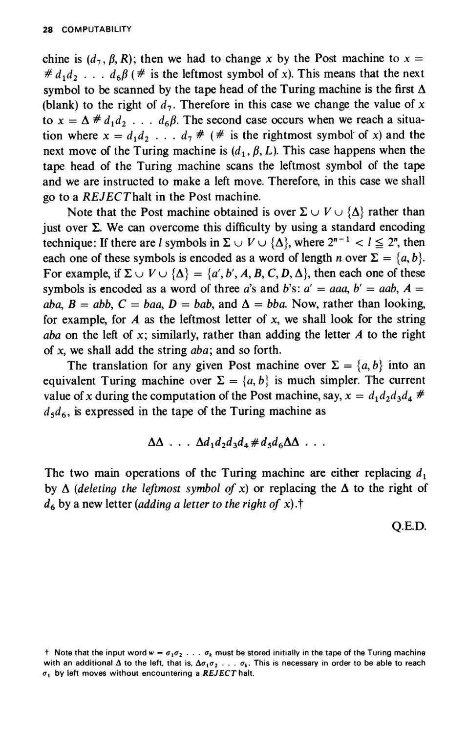
The translation for any given Post machine over Σ = {a, b) into an
equivalent Turing machine over Σ = {a, b) is much simpler. The current
value of χ during the computation of the Post machine, say, χ = ά^ά-^ά^ #
d5d6, is expressed in the tape of the Turing machine as
ΔΔ . . . ^а2аъа^фаъаьЬА . . .
The two main operations of the Turing machine are either replacing dx
by Δ (deleting the leftmost symbol of x) or replacing the Δ to the right of
d6 by a new letter (adding a letter to the right of x).t
Q.ED.
t Note that the input word w = σχσ2 . . . ak must be stored initially in the tape of the Turing machine
with an additional Δ to the left, that is, Δσγσ2 . . . ak. This is necessary in order to be able to reach
σγ by left moves without encountering a REJECT* halt.

TURING MACHINES 29
1-2.3 Finite Machines with Pushdown Stores
A finite machine Μ over Σ = {a, b) is a flow-diagram with one variable χ
in which each statement is of one of the following forms. (The variable χ
may have as value any word over {a, b})
1. START statement (exactly one)
С START ^
2. HALT statements
L
С ACCEPT^) ί REJECT )
3. TEST statement
G^5
χ <-tail(x)
τ
-i head(x) j-
x <-tail(x)
T"
or for short
-f χ <-tail(x) V

30 COMPUTABILITY
A variable yt is said to be a pushdown store over Σ = {α, b) if all the
operations applied to yt are of the form
1. TEST yt
I
■k
a
1
(?- = * ^
V J' У T
1—Сhead{yi) )—ι
r
r
| yt*-tail fa) 1 J yt^ tail fa) |
1
r
' '
'
or for short
yt <- tail {yd
τ
2. ASSIGN TO yt
Уг*-ЯУг
Уг +- ЪУг
Although the Post machines seem to be very "similar" to the finite
machines with one pushdown store, there is a vast difference between the
two. In a Post machine, not only may we read and erase letters on the
left of x, but also we may write new letters on the right of x. Thus, in a Post
machine, as the ends of χ undergo modification, the information in χ
circulates slowly from right to left. In a pushdown store we may write
only on the left of yt. Thus, while a pushdown store manipulates the
string in yt in a "last-in-first-out" manner, a Post machine manipulates
the string in χ in a "first-in-first-out" manner.

TURING MACHINES 31
A word w over Σ is said to be accepted/rejected by a finite machine Μ
(with or without pushdown stores) over Σ if the computation of Μ starting
with input χ = w eventually reaches an ACCEPT/REJECT halt. All the
pushdown stores are assumed to contain the empty word Λ initially.
EXAMPLE 1-11
The finite machine M4 with one pushdown store y, described in Fig. 1-7,
accepts every word over Σ of the form anbn9 η ^ 0, and rejects all other
words over Σ; that is, accept(M^) = {anbn\n ^ 0}, and rejectiM^) = Σ * -
accept (Μ4.).
С START ^
ω
45
x <— tax
У *~ay
®
® a
rC
m)-
©
у <—tai
Ь-fxt-tailixi) L/rEJECTJ
«ω)η
^-Qy <- tail{y)J-^
(^REJECT\J ^ACCEPT)
(reject)
Figure 1-7 The finite machine M4 with one pushdown store that accepts \anbn\n ^ 0}.
Suppose that χ = anbn. First we move the a's from χ to у so that at point
2, a" is stored in у while bn_1 is still in x. Then in loop 3 we eliminate the
a's from у and the b's from x, comparing their numbers, until both χ and у
are empty at point 4.

32 COMPUTABILITY
EXAMPLE 1-12
The finite machine M5 with two pushdown stores yx and y2, described in
Fig. 1-8, accepts every word of Σ of the form апЪп(Г, η ^ 0, and rejects all
other words over Σ; that is, accept(M5) = {a"bn<f\ η ^ 0}, and reject(M5) =
Σ* — accept (M5).
TstartJ
G>
(x <~tail(x)jr
Μ
L)'l <-«)':
y, *-fai
(rejectY
ί/ΟΜ)-^
(D
)'2 «~ b)>2
«
Δ (x <- tail (χ)]
4,-i#.F
(rejectV—' (accept)
©f
ΠΙ EJECT J pOi «-ifl«'(y^
(rejectV-'
©
€
(y2 <- iflfi7(>-2n
/ш/(х
/rejectJ
(^ -l^T^a
(rejectV—' (accept)
Figure 1 -8 The finite machine M5with two pushdown stores that accepts)a"f>"o"|n έ 0}.

TURING MACHINES 33
Suppose that χ = anbnan. First, in loop 1 we move the left a's from χ to
уγ so that at point 2 we have a" in уг and bn~ V in x. Then, in loop 3 we
move the b's from χ to y2, comparing at the same time the number of as
in yx and the number of b's in x, so that at point 4 we have bn in y2 and
a" ~1 in χ (yx is empty). Finally, in loop 5 we remove the b's from y2 and
the as from x, comparing their numbers, until both χ and y2 are empty.
D
We are now interested in investigating whether or not the addition of
pushdown stores really increases the power of the class of finite machines.
We note that for a fixed alphabet Σ:
1. The class of finite machines (with no pushdown stores) has the
same power as the class of finite automata introduced in Sec. 1-1.2. In
other words, a set S over Σ is regular if and only if S = accept (M) for some
finite machine Μ over Σ with no pushdown stores.
2. The class of finite machines with one pushdown store is more
powerful than the class of finite machines with no pushdown stores. For
example, there is no finite machine over Σ = {α, b] with no pushdown
stores that is equivalent to the finite machine M4 with one pushdown store
described in Example 1-11.
3. The class of finite machines with two pushdown stores is more
powerful than the class of finite machines with only one pushdown store.
For example, there is no finite machine over Σ = {α, b] with one pushdown
store that is equivalent to the finite machine M5 with two pushdown stores
described in Example 1-12.
4. For /i^2, the class of finite machines with η pushdown stores has
exactly the same power as the class of finite machines with two pushdown
stores.
It can be shown that the class of finite machines with two pushdown
stores has exactly the same power as the class of Post machines, or
equivalent^, the class of Turing machines.
THEOREM 1 -4 (Minsky). The class of finite machines over Σ with two
pushdown stores has the same power as the class of Turing machines
over Σ.
That is, for every finite machine over Σ with two pushdown stores, there is
an equivalent Turing machine over Σ and vice versa.

34 COMPUTABILITY
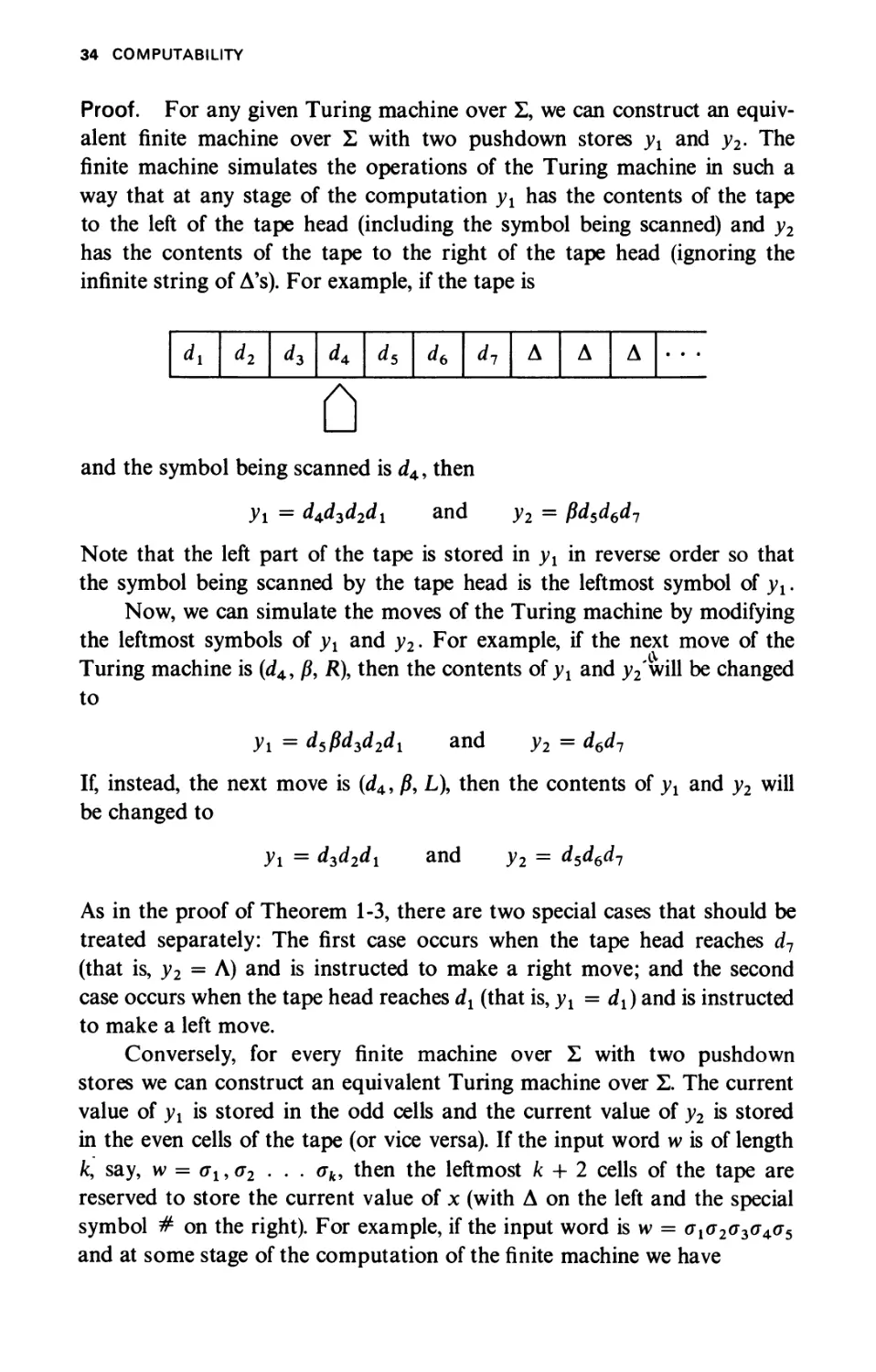
Proof. For any given Turing machine over Σ, we can construct an
equivalent finite machine over Σ with two pushdown stores yx and y2. The
finite machine simulates the operations of the Turing machine in such a
way that at any stage of the computation yx has the contents of the tape
to the left of the tape head (including the symbol being scanned) and y2
has the contents of the tape to the right of the tape head (ignoring the
infinite string of A's). For example, if the tape is
dt
d2
d3
d*
ds
db
d7
A
A
A
0
and the symbol being scanned is d4, then
У\ = d^d3d2dx and y2 = βά5ά6άΊ
Note that the left part of the tape is stored in yx in reverse order so that
the symbol being scanned by the tape head is the leftmost symbol of yx.
Now, we can simulate the moves of the Turing machine by modifying
the leftmost symbols of yx and y2. For example, if the next move of the
Turing machine is (d4, β, R\ then the contents of yx and y2 will be changed
to
yx = d5fid3d2d1 and y2 = d6d7
If, instead, the next move is (d4, β, L), then the contents of yx and y2 will
be changed to
yx = d3d2dx and y2 = d5d6d7
As in the proof of Theorem 1-3, there are two special cases that should be
treated separately: The first case occurs when the tape head reaches d7
(that is, y2 = Λ) and is instructed to make a right move; and the second
case occurs when the tape head reaches dx (that is, yx = dx) and is instructed
to make a left move.
Conversely, for every finite machine over Σ with two pushdown
stores we can construct an equivalent Turing machine over Σ. The current
value of yx is stored in the odd cells and the current value of y2 is stored
in the even cells of the tape (or vice versa). If the input word w is of length
fc, say, w = σΐ9σ2 . . . σΛ, then the leftmost к + 2 cells of the tape are
reserved to store the current value of χ (with Δ on the left and the special
symbol # on the right). For example, if the input word is w = σισ2σ2>σ^σ5
and at some stage of the computation of the finite machine we have

TURING MACHINES 35
χ = σ3σ4σ5
yx = dld2d2dAr
Уг = exe2
then the corresponding tape in the Turing machine is
Δ
Δ
Δ
<*з
σ4
σ5
#
dx
£\
d2
<?2
d3
A
dA
Δ
Δ
Δ
Now, the operations on yx and y2 of the finite machine are simulated by
applying the corresponding operations on the even and odd cells of the
tape to the right of #.
Q.E.D.
1 -2.4 Nondeterminism
An important generalization of the notion of machines discussed above is
obtained by considering nondeterministic machines. A nondeterministic
machine is a machine which may have in its flow-diagram choice branches
of the form
A
That is, whenever we reach upon computation such a choice branch, we
may choose arbitrarily any one of the possible exits and proceed with the
computation as usual. For Turing machines we introduce nondeterminism,
not by using choice branches, but just by removing the restriction that
"all arrows leading from the same state / must have distinct a's."
A word ννβΣ* is said to be accepted by a nondeterministic Turing
machine, Post machine, or finite machine Μ (with or without pushdown
stores) over Σ if there exists a computation of Μ starting with input χ = w
which eventually reaches an ACCEPT halt. If w is not accepted but there is
a computation leading to a REJECT halt, then w is said to be rejected;
otherwise, we loop(M).
EXAMPLE 1-13
The nondeterministic finite machine M6 with one pushdown store y,
described in Fig. 1-9, accepts every word over Σ = {a9b} of the form wvH,

36 COMPUTABILITY
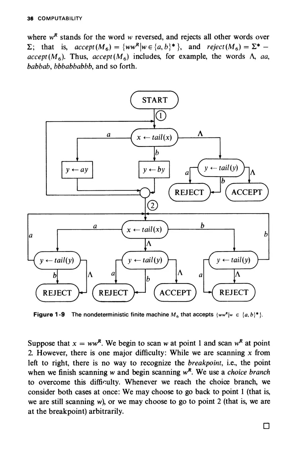
where w* stands for the word w reversed, and rejects all other words over
Σ; that is, accept(M6) = {ww*|we {a, b}* }, and reject(M6) = Σ* —
accept(M6). Thus, accept(M6) includes, for example, the words Λ, aa,
babbab, bbbabbabbb, and so forth.
С START J
ω
( χ <— tail (χ) V
y+-ay
y<-by
r-(y<~tail(y)\
©
REJECT
•V-l ^accept)
-Γ χ «-iai/(x) J·
у <- гш'/(у)
(rEJECt\-I (^REJEcT)—' ГаССЕРТЧ
г-Гу «- tai/(y)Vi г-Г у «- rai/(y) J—'
REJECT
)
Figure 1-9 The nondeterministic finite machine M6 that accepts {wwR\w e {a, b]
Suppose that χ = ww*. We begin to scan w at point 1 and scan w* at point
2. However, there is one major difficulty: While we are scanning χ from
left to right, there is no way to recognize the breakpoint, i.e., the point
when we finish scanning w and begin scanning wR. We use a choice branch
to overcome this difficulty. Whenever we reach the choice branch, we
consider both cases at once: We may choose to go back to point 1 (that is,
we are still scanning w), or we may choose to go to point 2 (that is, we are
at the breakpoint) arbitrarily.
D

TURING MACHINES AS ACCEPTORS 37
A natural question that may be asked is "Does the use of nondeterminism
really increase the power of the class of machines?" It can be shown that
the classes of nondeterministic Turing machines, nondeterministic Post
machines, and nondeterministic finite machines with two or more pushdown
stores have the same power as the class of Turing machines. The relation
between the different classes of finite machines over the same alphabet Σ
can be summarized as follows:
{Finite automata}
II
{Finite machines with no pushdown stores}
II
{Nondeterministic finite machines with no pushdown stores}
л
{Finite machines with one pushdown store}
л
{Nondeterministic finite machines with one pushdown store}
л
{Finite machines with two pushdown stores}
II
{Nondeterministic finite machines with two pushdown stores}
II
{Turing machines}
Note the following:
1. There is no nondeterministic finite machine with no pushdown
stores that is equivalent to the finite machine M4 with one pushdown store
(Example 1-11).
2. There is no finite machine with one pushdown store that is equivalent
to the nondeterministic finite machine M6 with one pushdown store
(Example 1-13).
3. There is no nondeterministic finite machine with one pushdown
store that is equivalent to the finite machine M5 with two pushdown
stores (Example 1-12).
1-3. TURING MACHINES AS ACCEPTORS
In this section we introduce two new classes of sets of words over an alphabet
Σ: recursively enumerable sets and recursive sets. These are very rich classes

38 COMPUTABILITY
of sets; actually, the intention is to have these classes rich enough to include
exactly those sets of words over Σ which are partially acceptable or
acceptable by any computing device. Since by Church's thesis, a Turing
machine is the most general computing device, it is quite natural that we
define the two classes by means of Turing machines.
We define a set S of words over Σ to be recursively enumerable if there is
a Turing machine Μ over Σ which accepts every word in S and either rejects
or loops for every word in Σ* — 5; that is, accept (M) = 5, and reject (Μ) υ
loop (Μ) = Σ* — 5. However, the main drawback is that if we apply the
machine to some word w in Σ* — 5, there is no guarantee as to how the
machine will behave: It may reject w or loop forever. Therefore we also
introduce the class of recursive sets, wfrich is a proper subclass of the
class of recursively enumerable sets.
We define a set S of words over Σ to be recursive if there is a Turing
machine Μ over Σ which accepts every word in S and rejects every word in
Σ* - 5; that is, accept (M) = 5, reject (Μ) = Σ* - 5, and loop(M) = φ.
There is a very important relation between the class of recursively
enumerable sets and the class of recursive sets: a set S over Σ is recursive if and
only if both S and Σ* — S are recursively enumerable.
1-3.1 Recursively Enumerable Sets
Alternative definitions for a set S of words over Σ to be recursively
enumerable are:
1. There is a Turing machine which accepts every word in S and
either rejects or loops for every word in Σ* — 5.
2. There is a Post machine which accepts every word in S and either
rejects or loops for every word in Σ* — 5.
3. There is a finite machine with two pushdown stores which accepts
every word in S and either rejects or loops for every word in Σ* — S.
EXAMPLE 1-14
Examples 1-8, 1-10, and 1-12 imply that the following sets of words over
Σ = {a9b} are recursively enumerable: {a"bn\n §: 0}, {all words over Σ
with the same number of a's and b's}, and {anbnan\n ^ 0}.
D

TURING MACHINES AS ACCEPTORS 39
Although the class of recursively enumerable sets is very rich, there
exist sets of words over Σ = {a, b] that are not recursively enumerable. We
now demonstrate such a set of words. All words in {a, b}* can be ordered
by the natural lexicographic order
A, a, b, aa, ab, ba, bb, aaa, aab, aba, abb, baa, bab, bba, bbb, aaaa, aaab,. . .
that is, the words are ordered by length and lexicographically within each
length. Thus it makes sense to talk about the ith string xt in {a, b}*. Every
Turing machine over Σ = {a, b} can be encoded (see Prob. 1-13) as a string
in {a, b}* in such a way that each string in {a, b}* represents a Turing
machine and vice versa. Therefore we can talk about the 7th Turing machine
Tj over Σ = {a, b), that is, the one represented by the 7th string in {a, b}*,
Consider now the set
Lt = {x^Xi is not accepted by 7]}
Clearly, Lt could not be accepted by any Turing machine. If it were, let
TJ be a Turing machine accepting Lt. Then, by definition of Ll9 xjeL1
if and only if Xj is not accepted by 7}. But since 7} accepts Ll5 we obtain
the contradiction that Xj is accepted by 7} if and only if χ,- is not accepted
by Tj. Thus, there is no Turing machine accepting Lx; that is, Lx is not a
recursively enumerable set.
1-3.2 Recursive Sets
Alternative definitions for a set S of words over Σ to be recursive are:
1. There is a Turing machine which accepts every word in S and
rejects every word in Σ* — S.
2. There is a Post machine which accepts every word in S and rejects
every word in Σ* — S.
3. There is a finite machine with two pushdown stores which accepts
every word in S and rejects every word in Σ* — S.
EXAMPLE 1-15
Examples 1-8 and 1-12 imply that the following sets of words over Σ =
{a,b} are recursive: {anbn\n ^ 0} and {апЪпсГ\п ^ 0}.
D

40 COMPUTABILITY
The most important results regarding recursive sets are:
1. If a set over Σ is recursive, then its complement Σ* — S is also
recursive^ If 5 is a recursive set over Σ, then there is a Post machine Μ
which always halts and accepts all words in S and rejects all words in
Σ* — S. Construct a Post machine M' from Μ by interchanging the
ACCEPT and REJECT halts. Clearly Μ accepts all words in Σ* - S and
rejects all words in S.
2. A set S over Σ is recursive if and only if both S and Σ* — S are
recursively enumerable, (a) If S is recursive, then (by result 1 above) Σ* — S
is recursive; and clearly if 5 and Σ* — S are recursive, then S and Σ* — S are
recursively enumerable, (b) If S and Σ* — S are recursively enumerable,
there must exist Turing machines Mx and M2 over Σ which accept S and
Σ* — 5, respectively. Mx and M2 can be used to construct a new Turing
machine Μ which simulates the computations of Mx and M2% in such a way
that Μ accepts all words in S and rejects all words in Σ* — S; that is, 5 is a
recursive set. Note that the contents of the tape of Μ must be organized
in such a way that at any given time it contains six pieces of information:
the contents of the tapes of Mx and M2, the location of the tape heads of
Μγ and M2, and the current states of Mx and M2.
3. The class of recursively enumerable sets over Σ properly includes the
class of all recursive sets over Σ. It is clear that every recursive set is
recursively enumerable. We shall show that there exists a recursively
enumerable set over Σ that is not recursive. For this purpose, let xf denote
the ith word in {a, b}* and 7] the ith Turing machine over Σ = {a, b},
and consider the set L2 = {x^x,- is accepted by 7^}. (a) L2 is a recursively
enumerable set because a Turing machine Τ can be constructed that will
accept all words in L2. For any given word w e Σ*, Τ will start to generate
the words x1?x2»x3» · · · » an^ test each word generated until it finds
the word xt = w, thereby determining that w is the ith word in the
enumeration. Then Τ generates Th the ith Turing machine, and simulates its
operation. Therefore w is accepted by Τ if and only if xt = w is accepted by Tt.
(b) L2 is not a recursive set since Σ* — L2 = Lx and Lx is not recursively
enumerable, as has been shown.
t However, there are recursively enumerable sets of words over Σ such that their complement is
not recursively enumerable.
X The simulations of Mt and M2 are done "in parallel" (by applying alternately one move from
each machine) so that neither requires the termination of the other in order to have its behavior
completely simulated.

TURING MACHINES AS ACCEPTORS 41
1-3.3 Formal Languages
A type-0 grammar G over Σ consists of the following:
1. A finite (nonempty) set V of distinct symbols (not in Σ ), called
variables, containing one distinguished symbol 5, called the start variable.
2. A finite set Ρ of productions in which each production is of the
f°rm α - β where <xe{V υ Σ)+ and |5e(FuI )*t
A word w e Σ* is said to be generated by G if there is a finite sequence
of words over V υ Σ
w0 => ννχ => w2 =>···=> w„ и ^ 1
such that w0 is the start variable 5, w„ = w, and wi+1 is obtained from
wh 0 ^ i < и, by replacing some occurrence of a substring α (which is the
left-hand side of some production of P) in wf by the corresponding β (which
is the right-hand side of that production).} The set of all words generated
by G is called the language generated by G.
EXAMPLE 1-16
Let Σ = {a, b}. Consider the grammar Gx where V= {S} and Ρ = {S -►
aSb, S -► ab). By applying the first production η — 1 times followed by an
application of the second production, we have
S => aSb => a2Sb2 => a3Sb3 => ··· => α"-^"'1 => anbn
It is clear that these are the only words generated by the grammar. Thus
the language generated by the grammar Gt is
{anbn\n^ 1}
D
EXAMPLE 1-17
Let Σ = {a, b}. Consider the grammar G2, where V = {A, B, S} and Ρ
consists of six productions:
1 S - aSBA
2 S -+ abA
3 AB^BA
4 bB^bb
5 bA^ba
6 aA -* aa
t (К uZ)+stands for all words over V u Σ except Λ (the empty word); that \s,(V uZ)+ = (l^uZ)* {Λ}.
t α is a substring in w, if and only if there exists words w, ν (possibly empty) such that uav = w,; wi + 1
is then the word ufiv.

42 COMPUTABILITY
The language generated by the grammar G2 is
{anbnan\n^ 1}
To obtain anbna", for some η ^ 1, first we apply η — 1 times production
1 to obtain a"~iS(BA)n~1; then we use production 2 once to obtain
anbA(BAf~1. Production 3 enables us to rearrange the ZTs and As to
obtain a"bBn~1An. Next we use η — 1 times production 4 to obtain anbnAn\
then we use production 5 once to obtain anbnaAn~l. Finally, we use η — 1
times production 6 to obtain a"bnan.
Now, let us show that no other words over Σ can be generated by
the grammar G2. At the beginning we can apply only production 1 (and
possibly production 3) until production 2 is applied the first time. At this
point we have anb followed by some string of η A's and « - 1 B's (in any
order). (Now we can apply productions 3 to 6, but in each step it is always
true that the left part of the word consists of a's and b's while the right
part consists of A's and B's.) Next we must apply η — 1 times production 4
(and possibly production 3) to obtain the word anbnAn. The only other
production we could possibly apply is production 5. However, in this case
sooner or later we would have to eliminate aB in the word; but there is no
such production in P, and so we must obtain the word anbnAn. The only
way we can proceed now is by applying production 5 once and then
applying η — 1 times production 6 to obtain the word anbnan.
D
A set of words over Σ is called type-0 language if it can be generated
by some type-0 grammar over Σ. We have the following theorem.
THEOREM 1 -5 (Chomsky). A set of words over Σ is recursively
enumerable if and only if it is a type-0 language.
Certain restrictions can be made on the nature of the productions of a
type-0 grammar to give three other types of grammars. A grammar is said
to be of
1. Type-1 (context-sensitive) if for every production α -► β in Ρ
2. Type- 2(context-free) if for every production α -► β in Ρ
oceV and ]5g(FuI)+
3. Type-3 (regular) if every production in Ρ is of the form
A -► σΒ or A -► σ
where A,BeVand σeΣ.
t Recall that |x| stands for the length of the string (i.e., the number of letters in x); in particular,
|A| = 0.

TURING MACHINES AS GENERATORS 43
In any one of the above grammars we allow also the use of a special
production, S -► Λ, but only if S (the start symbol) does not occur in the right-
hand side of any production in P.
Correspondingly we define a set of words over Σ to be a language of
type-i, 1 ύ i ύ 3 (or context-sensitive, context-free, and regular language,
respectively), if it can be generated by some type-i grammar. The following
table summarizes the inclusion relations between the classes of sets over Σ
discussed so far.
{Type-0 languages} = {recursively enumerable sets}
= {all sets accepted by some finite machine
with two pushdown stores}
и
{Recursive sets}
и
{Type-1 languages}
и
{Type-2 languages} = {all sets accepted by some nondeterministic
finite machine with one pushdown store}
и
{Type-3 languages} = {regular sets}
= {all sets accepted by some finite machine
with no pushdown stores}
All the above inclusions are actually proper since for Σ = {a,b} [see, for
example, Hopcroft and Ullman (1969)].
1. L2 = {xi\xi is accepted by 7]} is a type-0 language but not a recursive
set.
2. {Xi\xi is not generated by the ith type-1 grammar}! is a recursive
set but not a type-1 language.
3. {anbnan\n ^ 1} is a type-1 but not a type-2 language.
4. {anbn\n ^ 1} is a type-2 but not a type-3 language.
1-4 TURING MACHINES AS GENERATORS
In this section we introduce a class of n-ary partial functions (n g: 1),
called Turing computable functions, mapping /ι-tuples of words over Σ into
f Note that in order to carry out the enumeration of type-1 grammars over Σ = {a, b), we must
consider only type-1 grammars with variables from V = {y,, t>2, t>3,. . .};that is, if the grammar has
η variables, they must be υι,υ2 v„.

44 COMPUTABILITY
words over Σ. This is a very rich class of functions; actually, the intention
is to have this class rich enough to include exactly all computable /ι-ary
partial functions mapping /ι-tuples of words over Σ into words over Σ.
Again, since, by Church's thesis, a Turing machine is the most general
computing device, it is quite natural that we define the class by means of
Turing machines.
A partial functiont /(*i, · . . ,x„), η ^ 1, mapping и-tuples of words
over Σ = {a, b] into words over Σ, is said to be Turing computable if there is
a Turing machine Μ over {a, b, *} which behaves as follows: For every n-
tuple (wl, . . . , w„) of words over Σ, Μ takes the string wx * . . . * w„ as
input and
1. If/(wl5 . . . , w„) is undefined, then Μ will loop forever.
2. If/(wl5 . . . ,w„) is defined, then Μ will eventually halt (either
rejecting or accepting the input) with a tape containing the value of
/(wj, . . . , w„) followed only by A's.
EXAMPLE 1-18
The Turing machine M7 over {a,b, *}, described in Fig. 1-10, computes
the concatenation function over Σ = {a, b): It takes a pair of words (wx, w2)
as input and yields the word ννχνν2 as output. For example, if wx = abaa
(·.*■*> START J^ / \ ^\ HALT
(я,я,Я)С0 (Δ'Δ^>.(
(Ь, Ь, R)
К Δ, ^
Figure 1-10 The Turing machine M7 that computes the concatenation function.
t The words partial function indicate that/^,..., w„) may be undefined for some η-tuple of words
(w, wjover Σ, in contrast with a total function for which /(w, w„) is defined (and yields
a word in Σ) for all possible η-tuples of words over Σ.

a
b
a
a
*
b
b
a
b
Δ
Δ
Δ ···
a
b
a
a
b
b
a
b
Δ
Δ
Δ
Δ ···
TURING MACHINES AS GENERATORS 45
and w2 = bbab, then the input and output tapes look like this:
Input tape
Output tape
We start with state 1 and scan the input tape moving right until we reach
the first Δ symbol (state 2). Now we move left until we reach the * symbol
(state 5). While we are moving to the left, we read each symbol on the tape
cell, remember it, move one cell to the left, and print it on the new cell. We
are at state 3 whenever we have to remember the symbol a, and at state 4
whenever we have to remember the symbol b.
D
In this section we give an alternative definition of the class of Turing
computable functions; that is, we show that a function is Turing computable
if and only if it is a partial recursive function. First we shall discuss the
class of primitive recursive functions, which is a proper subclass of the
class of partial recursive functions. Virtually all functions of practical value
are primitive recursive.
1-4.1 Primitive Recursive Functions
Every w-ary (n ^ 1) primitive recursive function is a total function mapping
«-tuples of words over Σ into words over Σ, but not every such total function
is a primitive recursive function. The class of all primitive recursive functions
over an alphabet Σ = {a, b] is defined as follows:
1. Base functions:
nil(x) = A (that is, for every argument χ g Σ*, the value of
nil(x) is Λ, the empty word)
consa(x) = ax
consb(x) = bx
These are primitive recursive functions over Σ.
2. Composition:
If h, gl9 . . . ,gm are primitive recursive functions over Σ, then so
is the n-ary function/defined by
/(*!,. . ., x„) = h(g1(xl9. . . ,x„),. . . ,0m(xi,. . .,*„))

46 COMPUTABILITY
(In each gt some of the arguments may be absent.)
3. Primitive recursion:
If g, ht, and h2 are primitive recursive functions over Σ, then so is
the и-агу function/defined by
(a) Ifw = 1,
/(Л) = w (any word w of Σ*)
f{ax) = hx (x,/(x))
f(bx) = h2(x,f(x))
(In /i! and h2 some of the arguments may be absent.)
(b) If η £2,
/(Λ,χ2,. . . ,x„) = #(x2,. · · ,*„)
/(flXi,x2,. . . ,x„) = hi (xl5x2,. . . ,x„, J(X\,x2) · · · >Xn)j
/(bxl5X2,. . . , X„) = П2 (Xi , X2> · · · > Xn> /(xl > *2> · · · »хи))
(In hx and /i2 some of the arguments may be absent.)
EXAMPLE 1-19
The following are primitive recursive functions over Σ = {a,b}.
1. The constant functions a and b, where a(x) = a and b(x) = b for
all x, are primitive recursive because, by composition,
a(x) = consa(nil{x))
b(x) = consb(nil(x))
2. The identity function iden, where iden(x) = χ for all x, is primitive
recursive because by primitive recursion (case η = 1),
iden(A) = Λ
iden(ax) = consa(x)
iden(bx) = consb(x)
3. The concatenation function append, where append(xl9x2) = ΧχΧ2
for all Xi and x2 [that is, append(xl9x2) concatenates the words x1 and
x2 into one word xxx2] is primitive recursive because, by primitive
recursion (case η = 2),
append(A,x2) = iden(x2)
append (ax l9 x2) = consa(append(x1,x2))
append(bxl9x2) = consb(append(xl, x2))
4. The /lead and ίαι/ functions, where head(x) = "the leftmost letter
ofx"andiai/(x) = "the word χ after removing the leftmost letter" \_head{A) =

TURING MACHINES AS GENERATORS 47
Λ and tail (A) = Λ], are primitive recursive because, by primitive recursion
(case /i = l),
head(A) = A tail(A) = A
head {ax) = a(x) tail (ax) = iden(x)
head(bx) = b(x) tail{bx) = iden(x)
5. The reverse function, where reverse (x) = "the letters of χ in reversed
order," is a primitive recursive because, by primitive recursion (case η = 1),
reverse (A) = A
reverse (ax) = append(reverse(x\ a(x))
reverse (bx) = append (reverse (x), b(x))
6. The right and /β/ί functions, where right (x) = "the rightmost letter
of x" and left(x) = "the word χ after removing the rightmost letter"
[right (A) = left (A) = Λ], are primitive recursive because, by composition,
right (x) = head (reverse (x))
left(x) = reverse (tail (reverse (x)))
7. The next-string function next(x) = "the next word in the natural
lexicographic order" is primitive recursive because
next(x) = reverse(nextl(reverse(x)))
where
nextl(A) = a
nextl(ax) = consb(x)
nextl(bx) = consa(nextl(x))
8. The conditional function сопа(х19х2,Хз) = "if xx =^ Л then x2 else
х3" is primitive recursive because, by primitive recursion (case η = 3),
cond(A, х2,*з) = iden(x3)
сопа(ах1,х2,Хз) = iden(x2)
condfixi, x2, x3) = iden(x2)
9. The predecessor function pred(x) = "the predecessor of χ in the
natural lexicographic ordering" \_pred(A) = Λ] is primitive recursive
because
pred(x) = reverse (predl (r ever se(x)))
predl(A) = A
where predl (ax) = cond (x, consb (predl (x)), nil (x))
predl (bx) = consa(x)
D

48 COMPUTABILITY
For abbreviation, from now on we shall write Λ, x, a, and b where ш7(х),
iden(x), a(x), and b(x), respectively, are required.
So far we have defined the class of primitive recursive functions over
Σ; we proceed to define the class of primitive recursive predicates. A
total predicate! p(xi,. . . 9x„\ η ^ 1, mapping и-tuples of words over Σ
into {true, false} is said to be a primitive recursive predicate if the function
defined by
Λ if p(xl5. . . ,x„) = false
a if p(xi,. . . ,x„) = true
is primitive recursive. This function is called the characteristic function of ρ
and is denoted by fp(xx,. . . , x„).
EXAMPLE 1-20
1. The predicates true and false, where true(x) = true and false (x) =
false for all x, are primitive recursive predicates because their characteristic
functions a(x) and nil(x) are primitive recursive functions.
2. The predicate null, where null(x) = "is χ = Λ?" is a primitive
recursive predicate because its characteristic function / is primitive recursive:
/(A) = a and f(ax) = f(bx) = A
3. The predicate eqa(x) = "is χ = α?" is a primitive recursive predicate
because its characteristic function is
f(x) = cond(x, cond(pred(x), A, a), A)
The predicate eqb(x) = "is χ = Ь?" is also a primitive recursive predicate
because
eqb(x) = eqa(pred(x))
D
We shall now introduce several interesting results related to primitive
recursive functions and primitive recursive predicates. We let χ stand for
(Xl>· · · » Xnl·
1. If-then-else:
If p(x) is a primitive recursive predicate and/(x) and g(x) are primitive
recursive functions, then the function
t A predicate is actually a function but one which yields for every n- tuple of words over Σ not a
word over Σ, but true or false.

TURING MACHINES AS GENERATORS 49
ifp(x) thenf{x) else g(x) that is,
is primitive recursive.
In general, if px(x),p2(x),. . . , p„,-i(x) are primitive recursive
predicates, and g\(x\g2(x\ . . . ,gm{x) are primitive recursive functions, then
the function
ifPiffitheng^x)
else if p2 (x) then g2 (x)
else . . . ifPm-A^theng^^x)
elsegm{x)
is primitive recursive. Note that the function is identical to
cond(fPm_i (x),gm-i(x),gm(x)) . . . ))
where fPi(x) is the characteristic function of pt for 1 ^ i ^ m — 1.
2. Propositional connectives:
If p(x), g(x), and r(x) are primitive recursive predicates, then so are the
following predicates
- p(x)
p(x) ν q(x)
p(x) л q(x)
p(x) = <?(x)
The characteristic functions of the first two predicates are
f~p(x) ifnull(fp(x)) then a else A
fPvq(x) ifnull{append(fp(x\fq{x))) then A else a
Therefore ^ ρ and ρ ν q are primitive recursive predicates. The other
two predicates are also primitive recursive since
p(x) л q(x) is ~((~p(x)) ν (~ «(*)))
p(x) = q(x) is (p(x) ν ~ q(x)) л (q(x) ν ~ ρ(χ))
/(χ) if ρ (χ) = irwe
g{x) if p(x)= false
[ true if p(x) = /a/se
\/tf/se otherwise
J rrwe if p(x) = true, or g(x) = rrw^, or both
[false otherwise
true if p(x) = q{x) = irwe
/я/se otherwise
irwe if p(x) = q(x) = true or p(x) = q(x) = false
false otherwise
{

50 COMPUTABILITY
Three very useful primitive recursive functions are code, decode,
and sub, where code(x) = a1 and decode {a1) = χ iff χ is the ith word
in the natural lexicographic ordering (i g: 0) and sub(a\aj) = al~j
(if i g: j). In all other cases decode and sub are defined (arbitrarily)
to be Λ. In Prob. 1-17 the reader is asked to prove that these functions
are indeed primitive recursive. We shall now illustrate two
applications of these functions.
3. Bounded minimization:
If ρ is a primitive recursive predicate, then so is the function f(x,z) defined
as follows:
The value of/(x, z) is the first word у of Σ* in the natural lexicographic
order (that is, Л, a, b, aa, ab, ba, bb, aaa, . . .) such that p(x, y) =
true or у = ζ. For all y' preceding у (у Φ Λ) in this order, ρ (χ, у) =
false and y' Φ ζ.
Note that the test у = ζ ensures that the function obtained is always
defined; that is, / is a total function. For brevity, we shall denote this
definition by
f(x, z) = h(A, x, z) where
h(y, x, z) <= ifp(x, y) ν у = ζ then у else h(next(y), x, z)
/(x, z) is primitive recursive because
/(x, z) = g(code{z), x, code(z))
where
g(A, χ, ί) = decode (t)
g(as, x, t) = ifpix, decode (sub (i, as)))
then decode (sub (t, as)) else g(s, x, t)
g (bs, x, t) can be defined arbitrarily.
4. Equality predicate:
The equality predicate equal (x,y) = "is χ = yT is a primitive recursive
predicate because it can be expressed as
equal (x,y) = null (append (sub (code (x), code(y)), sub (code (y), code(x))))
1-4.2 Partial Recursive Functions
The class of all partial recursive functions over an alphabet Σ = {a, b} is
defined as follows:
1. Base functions:
nil(x), consa(x) and consb(x) are partial recursive functions over Σ.

TURING MACHINES AS GENERATORS 51
2. Composition:
If h,gl9. . . 9gm are partial recursive functions over Σ, then so is
the и-агу function / defined by composition.!
3. Primitive recursion:
If g, hl9 and h2 are partial recursive functions over Σ, then so is the
и-агу function /defined by primitive recursion. For η = 1 we allow
/ to be defined also as
/(Λ) = undefined
f(ax) = h1(xj(x))
f(bx) = h2(xj(x))
(In hx and h2 some of the arguments may be absent.)
4. (Unbounded) minimization:
If ρ is a partial recursive predicate^ then the function / defined by
f(x) — ft(x, Λ) where
h(x, y) <= ifp(x, y) then у else h(x, next(y))
is partial recursive. In other words, the value of f(x) is the first
word у of Σ* in the natural lexicographic order (that is, Л, я, b, aa9
ab, ba, bb, aaa9 aab,. . .) such that p(x, y) = true; for all yf preceding
у in this order p(x, /) = false. In all other cases, that is, if p(x,y) =
false for all ye Σ*, or p(x,y) is undefined for some у and for all /
preceding у in this order p(x,/) = false, then the value of/(x) is
undefined.
EXAMPLE 1-21
1. The uhead and utail functions, where uhead(x) = "the leftmost
letter of a nonempty word x" and utail (x) = "the tail of a nonempty word
χ obtained by removing the leftmost letter" [uhead(A) = atail(A) =
undefined], are partial recursive functions because they can be defined by
primitive recursion:
uhead (A) = undefined utail(A) = undefined
uhead (ax) = a utail (ax) = χ
uhead (bx) = b utail (bx) = χ
+ Since a partial recursive function may be undefined for some arguments, a composition of partial
recursive functions may require the value of such a function for undefined arguments. We agree
that any partial function is undefined whenever at least one of its arguments is undefined.
ί That is the characteristic function fp(x) is a partial recursive function, where fp(x) is defined as
Λ if p(x) = false
a if p(x) = true
undefined if pix) is undefined

52 COMPUTABILITY
2. The function undef(x) which is undefined for every string χ is a
partial recursive function because it can be defined by minimization with
ρ being/a/se(x) or alternatively using primitive recursion:
undef(A) = undefined
undef(ax) = undef(bx) = undef(x)
3. The function half, where half(x) = у iff append(y9y) = χ [half (x)
is undefined if no such у exists], is a partial recursive function because,
by minimization,
half(x) = й(х, Л) where
ft(x, y) <= if equal(append(y, y\ x) ifte/i у else ft(x, next(y))
D
One very surprising result related to partial recursive functions is that
every partial recursive function can be obtained by applying the
minimization rule at most once, and even in this case it suffices to use a predicate ρ
which is primitive recursive (not necessarily partial recursive). Our interest
in the class of partial recursive functions is due to the following important
result (which we shall present without proof).
THEOREM 1-6 (Kleene). An n-ary partial function mapping n-tuples
of words over Σ into words over Σ is partial recursive if and only if it is
Turing computable.
A partial recursive function that is total (defined for all arguments) is
called a total recursive function. The relation between the various classes
of functions over Σ (that is, mapping η-tuples of words over Σ into words
over Σ) can be summarized as follows:
{All functions over Σ}
и
{Partial recursive functions} = {Turing computable functions}
и
{Total recursive functions}
и
{Primitive recursive functions}
All the above inclusions are proper inclusions. To show that the top inclusion
is proper we consider the set Lx = {χ,Ιχ, is not accepted by 7]}. Since this
set is not recursively enumerable (see Sec. 1-3.1), it follows that any
function, which is defined for every xeLx and undefined for every x£Ll9

TURING MACHINES AS ALGORITHMS 53
is not Turing computable; therefore, by Theorem 1-6, this function is not
partially recursive.
It is also straightforward that the class of partial recursive functions
properly includes the class of all total recursive functions (see Example 1-21).
Ackermann's function A(x) over Σ is the classic example of a total
recursive function that is not primitive recursive. A(x) is equal to/(x, x),
where/is defined recursively as follows [see, for example, Hermes (1967)]:
/(*1,*2)
ax2 ifx! = Λ
/{tailix^a) if χχ φ Λ and x2 = Λ
f(tail(xi\f(xi, tail(x2))) if Χχ Φ Λ and x2 φ Λ
The main point in the proof that A(x) is not a primitive recursive
function is that for every unary primitive recursive function g there exists a
word weΣ* such that A(w) yields a longer word than that of g(w\ which
implies that A(x) cannot be a primitive recursive function.
1-5 TURING MACHINES AS ALGORITHMS
In mathematics we often consider classes of yes/no problems, i.e., problems
for which the answer is always either "yes" or "no," and investigate whether
or not there is any algorithm (computing device) for solving (or at least
partially solving) all the problems in the class. By Church's thesis, a Turing
machine can be considered to be the most general possible computing
device, and this suggests formalizing the common vague notion of
"solvability" of classes of yes/no problems by means of Turing machines.
We say that a class of yes/no problems is solvable (decidable) if there is
some fixed algorithm (Turing machine) which for any problem in the class
as input will determine the solution to the problem; i.e., the algorithm
always halts with a correct "yes" or "no" answer. (A "yes" answer is obtained
by reaching an ACCEPT halt, while a "no" answer is obtained by reaching
a REJECT halt.) If no such algorithm (Turing machine) exists, we say that
the class of problems is unsolvable (undecidable). Note, however, that the
unsolvability of a class of problems does not mean that we cannot
determine the answer to a specific problem in the class by a Turing machine.
An important task of theoreticians in computer science is to
indicate unsolvable classes of yes/no problems to prevent computer scientists
from looking for nonexisting algorithms. One of the most famous unsolvable
classes of yes/no problems is Hilberfs tenth problem. In 1901 Hilbertf
t David Hubert, "Mathematical Problems/' Buff. Am. Math. Soc.S: 437-479 (1901).

54 COMPUTABILITY
listed a group of problems which were to stand as a challenge to future
generations of mathematicians. The tenth problem in this group is to find
an algorithm that takes an arbitrary polynomial equation Ρ(xl9 . . ., x„) =
0 with integer coefficients as input and determines whether or not the
equation has a solution in integers. This was an open problem for about
seventy years. In 1970, Matijasevict showed that there cannot exist such an
algorithm, in other words, that Hilberfs tenth problem is unsolvable.
Unfortunately many interesting classes of yes/no problems are
unsolvable. This suggests introducing a weaker notion of algorithms which
will only partially solve the problems in the class in the sense that for any
problem in the class as input: if the answer to the problem is "yes," the
algorithm will eventually halt with a "yes" answer, but if the answer is
"no," the algorithm may supply no answer at all! More precisely, a class
of yes/no problems is said to be partially solvable (partially decidable) if
there is an algorithm (Turing machine) that will take any problem in the
class as input and (1) if the answer to the problem is "yes," the algorithm
will eventually reach an ACCEPT halt, but (2) if the answer to the problem
is "no," the algorithm either reaches a REJECT halt or never halts. This
definition of solvability is clearly weaker than the original one in the sense
that if a class of yes/no problems is solvable, then it is also partially solvable.
However, this weaker notion of solvability is very important because
many unsolvable classes of problems can be shown to be partially solvable.
At this point the reader will probably wonder how we can give a
yes/no problem as input to an algorithm (Turing machine). This is purely
an encoding problem. We shall be very vague regarding this problem and
comment only that we restrict our yes/no problems to those that can be
represented by some suitable encoding as words over Σ = {a, b].
1 -5.1 Solvability of Classes of Yes/No Problems
There are several interesting classes of yes/no problems related to the
material discussed previously in this chapter which are solvable. For example:
1. The equivalence problem of finite automata is solvable', that is,
there is an algorithm that takes any pair of finite automata A and A over
Σ = {a, b] as input and determines whether or not A is equivalent to A.
2. The word problem of context-sensitive grammars is solvable; that is,
there is an algorithm that takes any context-sensitive grammar G over
t Ju. V. Matijasevic, "Enumerable Sets are Diophantine," Sov. Math. Doki, 11 (2):354-358 (1970).

TURING MACHINES AS ALGORITHMS 55
Σ = {я, b) and any word weT* as input and determines whether or not
w is in the language generated by G.
In the following sections we present several classes of yes/no problems
which are unsolvable. The first and most important unsolvable class of
problems is known as the halting problem of Turing machines. It can be
shown that there is no algorithm that takes an arbitrary Turing machine
Μ over Σ = {a, b] and an arbitrary word ννβΣ* as input and always
determines whether or not Μ would halt if it were given input w. This
result is proved later by contradiction showing that if there did exist such
an algorithm, then we could conclude that there exists a Turing machine
В over Σ = {α, b} such that В halts for input d(B) if and only if В does
not halt for input d(B\ where ά(Β)εΣ* is the encoded description of В
as a word over Σ.
Using the unsolvability of the halting problem of Turing machines,
we can prove many other classes of problems to be unsolvable by reducing
the halting problem of Turing machines to those classes. More precisely,
we say that a class 0 of yes/no problems is reducible to another class 9?
of yes/no problems if there is a Turing machine that takes any problem
Pe0 as input and yields some problem Fe0' as output such that the
answer to problem Ρ is "yes" if and only if the answer to problem F is
"yes." We call such a Turing machine a reduction Turing machine from
0 to 0".
Now, suppose we show that 0 is reducible to 0'. Then, if 0* is solvable,
we can combine the reduction Turing machine from 0 to 0* and the
algorithm for solving 0' to form an algorithm for solving 0. Thus, if 0
is reducible to 0* and 0* is solvable, so is 0\ in other words, if 0 is reducible
to 0* and 0 is unsolvable, so is 0'. In particular, since we already know that
the halting problem (HP) of Turing machines is unsolvable, it follows that
for every class 2P of yes/no problems, if HP is reducible to 0\ then 3P is
unsolvable.
Using this reduction technique, we show two classes of yes/no problems
to be unsolvable:
1. The word problem ofsemi-Thue systems is unsolvable.
2. The Post correspondence problem is unsolvable.
Note that if 0 is a class of yes/no problems and 0' is a subclass of 0 (that
is, every problem in 0' is a problem in 0\ then it is clear that if 0 is solvable,
so is 0', and if 2P is unsolvable, so is 0.

56 COMPUTABILITY
1-5.2 The Halting Problem of Turing Machines
The HP of Turing machines over Σ = {a, b) is actually a class of yes/no
problems and can be stated as follows: Given an arbitrary Turing machine
Μ over Σ = {α, b] and an arbitrary word w e Σ*, does Μ halt for input w?
We have the following theorem.
THEOREM 1-7
unsolvable.
(Turing). The halting problem of Turing machines is
That is, there is no algorithm that takes an arbitrary Turing machine Μ
over Σ = {a, b} and word w e Σ* as input and determines whether or not
Μ halts for input w.
Proof (Minsky). Again we shall be vague regarding the encoding
problem. We denote simply by d(M) and d(M) * w the encoded description
of Μ and (M, w), respectively, as strings over Σ = {a, b).
The proof is by contradiction. Suppose there exists such an algorithm
(Turing machine), say, A. Then for every input d(M)*w to /4, we have:
If Μ halts for input w, then A reaches an ACCEPT halt; if Μ does not halt
for input w, then A reaches a REJECT halt. That is,
Μ halts for input vv
Input d(M)*w
Turing machine A
ACCEPT halt
• REJECT halt
Μ does not halt for input w
Now we can construct the Turing machine В which takes d(M) as input
and proceeds as follows: First, it copies the input to obtain d(M)* d(M\
and then it applies the Turing machine A on d(M)*d(M) as input, with
one modification—whenever A is supposed to reach an ACCEPT halt,
instead В wilUoop forever. Considering the original behavior of A, we obtain
Input d{M)-
M halts for input w = d(M)
I
I
-*·
I
L
Copy Μ
-+d{M)*d{M)-+
Modified А Г
T^LOOP
T-*HALT
Μ does not halt for input w = d(M)

TURING MACHINES AS ALGORITHMS 57
The above discussion holds true for an arbitrary Turing machine Μ
over Σ = {я, b}. Since В itself is such a Turing machine, we let Μ = B\
then, replacing В for Μ in the above figure, we obtain
В halts for input d(B)
Input d(B) —
Turing machine В
LOOP
-HALT
В does not halt for input d(B)
Thus, В halts for input d(B) if and only if В does not halt for input d{B).
Contradiction.
Q.E.D.
There are two interesting variations of the halting problem of Turing
machines:
1. The empty-word halting problem of Turing machines is unsolvable.
That is, there is no algorithm that takes an arbitrary Turing machinge Μ
over Σ = {a, b] as input and determines whether or not Μ halts for input
Λ (the empty word).
2. The uniform halting problem of Turing machines is unsolvable.
That is, there is no algorithm that takes an arbitrary Turing machine Μ
over Σ = {я, b] as input and determines whether or not Μ halts for every
input.
Both results can be proved easily by the reduction technique.
1. We show that the halting problem of Turing machines is reducible
to the empty-word halting problem of Turing machines. In this case the
reduction algorithm takes any Turing machine Μ over Σ = {α, b] and
any word w e Σ* as input and yields a Turing machine Μ over Σ = {α, b]
which first generates the word w onto the tape and then applies Μ to it.
Thus, Μ halts for input w if and only if M' halts for input Λ (the empty word).
2. We show that the halting problem of Turing machines is reducible
to the uniform halting problem of Turing machines. In this case the reduction
algorithm takes any Turing machine Μ over Σ = {α, b] and any word
w e Σ* as input and yields a Turing machine M' over Σ = {a, b} which
first clears the input tape to A's, then generates the word w onto the tape,
and finally applies M. Thus, Μ halts for input w if and only if M' halts for
every input.

58 COMPUTABILITY
From the discussions in previous sections it is clear that one can show
the following (by using either the proof of Theorem 1-7 or the reduction
technique).
1. The halting problem of Post machines is unsolvable. That is, there
is no algorithm that takes an arbitrary Post machine Μ over Σ = {a, b}
and word w e Σ* as input and determines whether or not Μ halts for input w.
2. The halting problem of finite machines with two pushdown stores is
unsolvable. That is, there is no algorithm that takes an arbitrary finite
machine Μ over Σ = {a, b) with two pushdown stores and word w e Σ*
as input and determines whether or not Μ halts for input w.
3. The totality problem of partial recursive functions is unsolvable.
That is, there is no algorithm that takes a definition of a partial recursive
function/over Σ = {α, b} as input and determines whether or not/ is total.
4. The recursiveness problem of type-0 grammars is unsolvable. That
is, there is no algorithm that takes an arbitrary type-0 grammar G over
Σ = {a, b) as input and determines whether or not the language generated
by G is recursive.
1-5.3 The Word Problem of Semi-Thue Systems
A semi-Thue system S over Σ = {α, b} consists of a set of fc, к g: 1, ordered
pairs (α,, β() of words over Σ; that is,
S={(a1,jS1),(«2.i»2). · · ·,(«*,&)}
For two words x, у e Σ*, we say that у is derivable from χ in S if there exists a
sequence of words over Σ
ννο,νν!,νν2, . . . ,w„ и ^ 0
such that w0 is x, wn is у and wI+1 is obtained from wt, 0 ^ i < n, by
replacing some occurrence of a substring a, (which is the left-hand side of
some pair in 5) in w( by the corresponding β] (which is the right-hand side
of that pair).
The word problem (WP) of semi-Thue systems over Σ = {α, b) is a
class of yes/no problems which can be stated as follows: Given an arbitrary
semi-Thue system S over Σ = {α, b} and two arbitrary words x,yel*,
is у derivable from χ in 5?
EXAMPLE 1-22
Consider the semi-Thue system S = {(ba9 ab\ (aab, Λ)} over Σ = {α, b).
Then Λ is derivable from χ e Σ* in S if and only if χ has twice as many a's

TURING MACHINES AS ALGORITHMS 59
as it has b's; for example, Λ is derivable from baaaba but not from baaab.
We have the following theorem.
THEOREM 1-8 (Post). The word problem of semi-Thue systems over
Σ = {я, b} is unsolvable.
That is, there is no algorithm that takes an arbitrary semi-Thue system
S over Σ = {a, b] and words xjel* as input and determines whether or
not у is derivable from χ in 5.
Proof. We show that the HP of Post machines is reducible to the WP
of semi-Thue systems. For an arbitrary Post machine Μ over Σ = {α, b]
and input word we Σ*, we construct a semi-Thue system S over Σ = {α, b]
and a pair of words x, у е Σ* such that Μ halts for input w if and only if у
is derivable from χ in 5. In this proof we make use of the fact that we can
consider, without loss of generality, only Post machines where TEST
statements must have the form
tail(.
π
4
(ассертЛ
tail(x) )-
#
(Reject)
and there are no other HALT statements. That is, for every Post machine
over Σ there exists an equivalent Post machine over Σ having only such
TEST statements.
Suppose the Post machine Μ has m TEST and ASSIGNMENT
statements labeled by Bx, B2, . . ., Bm. Let B0 be the START statement.
Suppose also that w = σίσ2 . . . on. Then take
χ = В0Уаха2 . . . ση-\
y = A
The list of ordered pairs of S is constructed as follows:

60 COMPUTABILITY
ι. в0
yield (Β0»βι)
ί START J
2.
В,
-С χ <— tail(x) Υ
41*
вк в,
yields
С АССЕРТЛ
V REJECT J
{B,\-a,Bjl·)
(Bi\-b,Bkl·)
(В,Ь#,В,Ь)
(В, I-Η, Λ)
i
χσ
yields (-\Bha-\Bj)
where (jg {a, b, #}.
4. ^ Γ ((σβ,,Β,σ)
for all σ e {a, b, #, I-, -I} and 1 ^ i ^ m.
It is straightforward to see that Μ halts for input w if and only if у is derivable
from χ in S.
Note that the alphabet of the semi-Thue system S that we have
constructed is actually {a,b, #,Ы} и {Β0,Βΐ9 . . .,#„,}. However, with
"suitable" encoding one can construct a semi-Thue system S' over Σ = {α, b}
and words x', y' e Σ* such that Μ halts for input w if and only if/ is derivable
from x' in 5'.
Q.E.D.
1-5.4 Post Correspondence Problem
A Post system S over Σ = {α, b} consists of a set of fc, fc g: 1, ordered pairs
(a,, ft) of words over Σ; that is,
S = {(a1,jS1),(«2,J»2), · · ·,(«*,&)}
A solution to a Post system is a nonempty sequence of integers ix, i2, . . ., /„,

TURING MACHINES AS ALGORITHMS 61
(1 g ij ^ k) such that
αΜαί2 · · · ai„. = βίβίι · · · A,.,
The Posi correspondence problem (PCP) over Σ = {a, b} is a class of yes/no
problems which can be stated as follows: Given an arbitrary Post system
over Σ = {α, b}, does it have a solution?
EXAMPLE 1-23
1. Let Σ = {a,b}. The Post system
S={(b, bbb)9 (babbb, ba\ (ba9 a)}
has a solution ix = 2, i2 = 1, /3 = 1, and i4 = 3 (that is, m = 4) since
babbbbbba=babbbbbba
I IUUI I I II II ILJ
a2 (Xiccla3 β2 βχ βχ β3
2. Let Σ = {a, b]. The Post system
S = {(ab9abb)9(b,ba)9(b9bb)}
has no solution. In each pair a; is shorter than &; therefore, for any
nonempty sequence of integers the string of α/s will be shorter than the
corresponding string of /Vs. PI
We have the following theorem.
THEOREM 1-9 (Post). The Post correspondence problem over Σ =
{α, b) is unsolvable.
That is, there is no algorithm that takes arbitrary Post system over Σ = {a, b]
as input and determines whether or not it has a solution.
Proof (Scott). We show that the HP of Post machines is reducible to
the PCP. For an arbitrary Post machine Μ over Σ = {α, b] and input word
weΣ*, we construct a Post system S over Σ = {α, b) such that Μ halts for
input w if and only'if 5 has a solution.
Suppose the Post machine Μ has m TEST and ASSIGNMENT
statements labeled by BX,B2, . . ,Bm (see the proof of Theorem 1-8). Let
B0 be the START statement, and let Bm + 1 stand for any ACCEPT or
REJECT halt. Suppose also that w = σχσ2 . . . ση. Then the corresponding
Post system S over the alphabet {a, b, #, *, β0, . . ., Bm+ x} is

62 COMPUTABILITY
2.
Во
С STARTj yields (Β0,Β0*σ1*σ2* . . . *σ„*Βι*)
В,
Β,
1
-ί χ +- tail(x)\
1 Bm+l yields
Bj Bk В, /^ACCEPT/ Л
V REJECT J
(*Bi*a, Bj*)
(*Bi*b, Bk*)
(*В,*#,В,*)
3. Β,·|
yields (*Bi,a*Bj*)
χ <— χσ
В
j
where ae {a, b, #}.
4. Cycling: (*σ,σ*) for all ae {a,b9 #}.
It should now be verified that a concatenation of words from the
first members of these pairs can equal a corresponding concatenation from
the second members if and only if it transcribes word by word a terminating
computation of the Post machine with input w. The terminating
computation is described as a sequence of Β,-'s. Between two successive B/s and
B/s, we have a string over {a,b, #} that represents the current value of χ
after the execution of Bt and before the execution of Bj. All letters are
separated by *; the role of the *'s is to ensure that the current value of χ will be
copied between the B/s.
Q.E.D.
The unsolvability of the Post correspondence problem is very often
used to prove the unsolvability of other classes of yes/no problems. In
particular, the Post correspondence problem can be reduced to · many
classes of yes/no problems in formal language theory, concluding,
therefore, that they are unsolvable. For example, the following can be shown.

TURING MACHINES AS ALGORITHMS 63
1. The equivalence problem of context-free {type-2) grammars is un-
solvable. That is, there is no algorithm that takes any two context-free
grammars over Σ = {α, b} as input and determines whether or not they
generate the same language. Note that the equivalence problem of regular
(type-3) grammars is solvable.
2. The emptiness problem of context-sensitive (type-1) grammars is
unsolvable. That is, there is no algorithm that takes any context-sensitive
grammar G over Σ = {α, b] as input and determines whether or not the
language generated by G is empty. Note that the emptiness problem of
context-free (type-2) grammars is solvable.
3. The word problem of type-0 grammars is unsolvable. That is, there
is no algorithm that takes any type-0 grammar G over Σ = {α, b} and word
w e Σ* as input and determines whether or not w is in the language of G.
Note that the word problem of context-sensitive (type-1) grammars is
solvable.
EXAMPLE 1-24 (Floyd)
A finite (nonempty) set of 3 χ 3 matrices {Mj over the integers is said to
be mortal with respect to Oi,y2X 1 = J1J2 = 3, if there is a finite product
of members of the set Μ = MhMi2 . . . Mik such that the 0'i,y2> element
of Μ is 0. We shall show that the mortality problem of matrices is unsolvable;
that is, there is no algorithm that takes a finite set of 3 χ 3 integer matrices
{MJ and a pair (jx J2 >, 1 й J1J2 = 3, as input and decides whether or not
{Mt} is mortal with respect to < уx, y2 >.
We prove the unsolvability of the mortality problem by reducing the
Post correspondence problem to the mortality problem; i.e., for an arbitrary
Post system S over Σ we construct a set of 3 χ 3 integer matrices {Mf}
in such a way that S has a solution if and only if {MJ is mortal with respect
to <3,2>. The idea is to construct for a given pair of words (μ, ν) over Σ a
3x3 integer matrix M(u, v) in such a way that
1. The <3,2> element of M(w, v) is 0 if and only if и = v.
2. For all words u1,u2,v1,v2eΣ*
M{ul9vx)· M(u2,v2) = M(u1u2,vlv2)
Now, for a given Post system S = {(α,·,β()} over Σ, we construct a set of
3x3 integer matrices {MJ where each Mt = Μ(αί9 /?,·). Then from
properties 1 and 2 above, it is clear that S has a solution i\, i2, . . ., ik if and only
if the <3,2> element of Mix-Mi2- . . . Mikis0.

64 COMPUTABILITY
To define the matrix M(w, v) we use two functions с (code) and el
(exponent of length) mapping words over Σ into integers:
c(x) = i iff χ is the ith word in the natural lexicographic ordering
el(x) = и1*1 where |x| is the length of χ and η is the number of letters in Σ
It is easy to prove that
c(xy) = c(x)el(y) + c(y)
el(xy) = el(x)el(y)
Now, for a pair (w, v) of words over Σ, we define
M(w, t;)
el(u) el(v) — el(u) 0
0 el(v) 0
^(w) c(v) — c(u) lj
M(w, v) has the desired properties:
1. The <3,2> element of M(u9 v) is 0 iff и = ν since c(v) - c(u) = 0
iff и = v.
2. For all words u1,u2,v1,v2eZ*,M(ul9vl)' M(u2,v2) = Miu^,
vxv2) since
Μ^,ι^-Μ^,ι^)
el(ux) el(vx) - el(ux) 0
0 elfa) 0
_c(ux) c{vx)- c(ux) 1_
el(u2) el(v2) - el(u2) 0
0 el(v2) 0
_c(u2) c(v2) - c{u2) 1_
el{ul)el{u1) βΙ(νγ)βΙ(ν2) — el{ux)el{u2) 0
0 el{vx)el{v2) 0
_c(ui)el{u2) + с(и2) КуО^Ы + c(v2)] - [c{Ul)el(u2) + c(u2)] 1_
= Afiiiiiij,!;!^)
D
1-5.5 Partial Solvability of Classes of Yes/No Problems
It is quite interesting to note that although the classes of yes/no problems
discussed in the previous sections are unsolvable, many of them are partially
solvable. For example, the halting problem of Turing machines is partially
solvable. That is, there is an algorithm (Turing machine) that takes any
Turing machine Μ over Σ = {α, b) and any word w e Σ* as input and

TURING MACHINES AS ALGORITHMS 65
(1) if Μ halts for w, the algorithm will eventually reach an ACCEPT halt,
but (2) if Μ does not halt for w, the algorithm either reaches a REJECT
halt or never halts. The standard proof of this result proceeds by
constructing an algorithm (Turing machine) that takes an arbitrary Turing
machine Μ over Σ = {я, b] and a word w e Σ* as input and simulates the
behavior of Μ for input w. We call such a Turing machine a universal
Turing machine. We can think of a universal Turing machine as a general-
purpose computer which is powerful enough to simulate any computer,
including itself.
The relationship between the solvability and partial solvability of a
class 9 of yes/no problems is best described by means of the complement
class ^, that is, the class of yes/no problems obtained from 0> just by taking
the negation of each problem in the class. Then the key result can be stated
as follows: 9 is solvable if and only if both 0* and & are partially solvable.
It is clear that if & is solvable, then so is # (interchange all the ACCEPT
and REJECT halts in the given algorithm), and therefore if 9 is solvable,
both 9 and 9 are partially solvable. To show the result in the other
direction, let us assume that algorithms A and A partially solve 9 and ^,
respectively. Then construct an algorithm В which simulates the operations of
both A and At Whenever A reaches an ACCEPT halt, so will B\ but
whenever A reaches an ACCEPT halt, В is modified to reach a REJECT
halt. Thus, for every problem of 9 as input, if the answer to the problem
is "yes," В will reach an ACCEPT halt and if the answer to the problem is
"no," В will reach a REJECT halt; in other words, В solves the problems
in^.
Since the halting problem of Turing machines is unsolvable but is
partially solvable, an important consequence of the above result is that
its complement is not partially solvable; i.e., the nonhalting problem of
Turing machines is not partially solvable. That is, there is no algorithm
(Turing machine) that will take any Turing machine Μ over Σ = {α, b]
and word we Σ* as input and (1) if Μ does not halt for w, the algorithm
will reach an ACCEPT halt, but (2) if Μ halts for w, the algorithm either
reaches a REJECT halt or never halts.
The reduction technique for solvability can be used for partial
solvability as well because we have that if a class 0* of yes/no problems is reducible
to 3F and Θ* is partially solvable, then so is βΡ\ in other words, if a class 0> of
yes/no problems is reducible to 3P and 0> is not partially solvable, then neither
is &'. We shall illustrate this technique with one example. (An important
t The simulations of A and A are done "in parallel" so that neither requires the termination of
the other in order to have its behavior completely simulated.

66 COMPUTABILITY
application of the results presented in this example is discussed in Chap. 4,
Sec. 4-2.1.)
EXAMPLE 1-25 (Paterson)
Let Σ = {α, b). A two-registered finite automaton A over Σ is a machine
with domain Σ00 (the set of all infinite tapes of letters from Σ) and is described
by a flow-diagram such that each statement in it is of one of the following
forms:
С START J
'
>
(УпУг) «-(*,*)
^
I
yi*-tail(yi)
'
'
1
1
(accept^) (^rjejectJ
f head(yi) \
Forf = 1,2
where, for every σεΣ and νν£Σ°°, tail {aw) = w and head {aw) = a. Note
that the first letter of χ is removed by the first application of tail.
For each input tape ξ e Σ00 for x, we distinguish between three possible
computations: (1) If ACCEPT is reached, the tape is said to be accepted;
(2) if REJECT is reached, the tape is said to be rejected; (3) otherwise, the
automaton A is said to loop on the tape. Thus, a two-registered finite
automaton A determines a threefold partition of Σ00 into accept {A), reject {A),
and loop{A\ the classes of tapes of Σ00 which A accepts, rejects, and on which
it loops, respectively.
We show the following results to be true.
1. The nonacceptance problem of two-registered finite automata over
Σ = {a, b) is not partially solvable. That is, there is no algorithm that takes
any two-registered finite automaton A over Σ = {a, b} as input and (1) if
accept {A) = φ, the algorithm will reach an ACCEPT halt, but (2) if
accept {Α) Φ Φ> the algorithm either reaches a REJECT halt or never halts.
2. The looping problem of two-registered finite automata over Σ =
{a, b} is not partially solvable. That is, there is no algorithm that takes any two-
registered finite automaton A over Σ = {я, b} as input and (1) if loop{A) Φ φ,

BIBLIOGRAPHIC REMARKS 67
the algorithm will reach an ACCEPT halt, but (2) if loop (A) = φ, the
algorithm either reaches a REJECT halt or never halts.
Both results are proved by reducing the nonhalting problem of Turing
machines to the nonacceptance and the looping problems of two-registered
finite automata.
Given a Turing machine Μ and an input word w over Σ = {α, b},
there is an effective method [see Paterson (1968) and Luckham, Park, and
Paterson (1970)] for constructing a two-registered finite automaton A (M, w)
over Σ which checks whether or not its input tape ξ e Σ00 describes a
computation of Μ starting with input w. In other words, A accepts a tape
ξ £ Σ00 if and only if ξ has a finite initial segment which describes a complete
computation of Μ starting with w; A loops on the tape if and only if ξ
describes a nonterminating computation of Μ starting with w; otherwise,
A rejects the tape ξ. Roughly speaking, this is done by assuming ξ to be of
the form (XqOl^oii . . ., where each α^Σ* indicates the configuration of
Μ (contents of tape, position of reading head, and current state) after the
ith step of the computation. The checking is done by letting y2 "read"
along the string a, while yx "verifies" that the following string ai+1 is indeed
the next configuration of the computation of Μ starting with w.
Then, the automaton A(M,w) has the following property: Μ fails
to halt starting with input w if and only if accept (A) = 0, or, equivalently,
if and only if loop(A) φ φ. Now, since the nonhalting problem of Turing
machines is not partially solvable, neither are the nonacceptance and
looping problems of two-registered finite automata.
D
Bibliographic Remarks
Three excellent books on computability are those of Minsky (1967), Hop-
croft and Ullman (1969), and Kain (1972). There are several more advanced
books such as those of Davis (1958), Hermes (1965), and Rogers (1967).
Our presentation benefitted from the excellent papers of Shepherdson and
Sturgis (1963) and Scott (1967).
The notion of finite state devices is attributed to McCulloch and
Pitts (1943). An important paper discussing this topic is the one by Rabin
and Scott (1959). The notion of regular expressions and their relation to
regular sets (Theorem 1-1) is due to Kleene (1956). The equivalence of
regular sets (Theorem 1-2) was first discussed by Moore (1956). An excellent
exposition of regular sets is given by Ginzburg (1968) and Salomaa (1969)
[see also the selected papers in Moore (1964)].
The basic notion of computability by Turing machines appears in

68 COMPUTABILITY
Turing's pioneer paper (1936). Our Post machine (Theorem 1-3) is very
similar to Post's normal system (1936). However, it was not defined by
Post, but by Arbib (1963) and independently by Shepherdson and Sturgis
(1963). The power of finite machines with two pushdown stores (Theorem
1-4) was first discovered by Minsky (1961) [see also Evey (1963)]. Formal
languages are discussed in detail by Hopcroft and Ullman (1969). The
relation between recursively enumerable sets and type-0 languages (Theorem
1-5) was first given by Chomsky (1959). The notion of partial recursive
functions (Theorem 1-6) was first introduced by Kleene (1936).
The unsolvability of the halting problem of Turing machines (Theorem
1-7) is given in Turing (1936); our proof is based on the exposition of Minsky
(1967). The unsolvability of the semi-Thue system (Theorem 1-8) is due to
Post (1947). Post's correspondence problem (Theorem 1-9) was first
formulated and shown to be unsolvable by Post (1946); our proof is due to Scott
(1967).
REFERENCES
Arbib, M. A. (1963): "Monogenic Normal Systems are Universal,"
J. Aust. Math. Soc, 3:301-306.
Chomsky, N. (1959): "On Certain Formal Properties of Grammars,"
Inf. & Control, 2(2): 137-167.
Church, A. (1936): "An Unsolvable Problem of Elementary Number
Theory," Am. J. Math., 58:345-363.
Davis, M. (1958): Computability and Unsolvability, McGraw-Hill Book
Company, New York.
(1965): The Undecidable, Raven Press, Hewlett, N.Y.
Evey, R. J. (1963): "The Theory and Applications of Pushdown Store
Machines," Ph.D. thesis, Harvard University, Cambridge, Mass.
Ginzburg, A. (1968): Algebraic Theory of Automata, Academic Press, Inc.,
N.Y.
Hermes, H. (1965): Enumerability, Decidability, Computability, Academic
Press, Inc., New York.
Hopcroft, J. E., and J. D. Ullman (1969): Formal Languages and their
Relation to Autor^ata, Addison-Wesley Publishing Company, Inc.,
Reading, Mass.
Kain, R. Y. (1972): Automata Theory, Machines and Languages, McGraw-
Hill Book Company, New York.

REFERENCES 69
Kleene, S. С (1936): "General Recursive Functions of Natural Numbers,"
Mathematisch Ann., 112: 727-742.
(1956): "Representation of Events in Nerve Nets and Finite
Automata," in С E. Shannon and J. McCarthy (eds.), Automata Studies,
pp. 3-42, Princeton University Press, Princeton, N.J.
Luckham, D. C, D. M. R. Park, and M. S. Paterson (1970): "On
Formalized Computer Programs," J. CSS, 4(3): 220-249.
McCulloch, W. S. and W. Pitts (1943): "A Logical Calculus of the Ideas
Immanent in Nervous Activity," Bull. Math. Biophys., 5: 115-133.
Minsky, M. L. (1961): "Recursive Unsolvability of Post's Problem of
Tag' and Other Topics in Theory of Turing Machines," Ann. Math.,
74(3): 437-454.
(1967): Computation: Finite and Infinite Machines, Prentice-Hall,
Inc., Englewood Cliffs, N.J.
Moore, E. F. (1956): "Gedanken Experiments on Sequential Machines," in
С Ε. Shannon and J. McCarthy (eds.), Automata Studies, pp. 129-
153, Princeton University Press, Princeton, N.J.
(1964): Sequential Machines: Selected Papers, Addison-Wesley
Publishing Company, Inc., Reading, Mass.
Paterson, M. S. (1968): "Program Schemata," in D. Michie (ed.), Machine
Intelligence 3, pp. 19-31, Edinburgh University Press, Edinburgh.
Post, E. L. (1936): "Finite Combinatory Processes—Formulation, I,"
Symb. Logic, 1:103-105.
(1946): "A Variant of a Recursively Unsolvable Problem," Bull.
Am. Math. Soc, 52(4): 264-268.
(1947): "Recursive Unsolvability of a Problem of Thue," Symb.
Logic, 12:1-11.
Rabin, M. and D. Scott (1959): "Finite Automata and Their Decision
Problems," IBM J. Res. ά Dev., 3(2): 114-125. [Reprinted in Moore
(1964).]
Rogers, H. (1967): Theory of Recursive Functions and Effective Computa-
bility, McGraw-Hill Book Company, New York.
Salomaa, A. (1969): Theory of Automata, Pergamon Press, New York.
Scott, D. (1967): "Some Definitional Suggestions for Automata Theory,"
J. CSS, 1(2): 187-212.
Shepherdson, J. С and Η. Ε. Sturgis (1963): "Computability of Recursive
Functions," J. ACM, 10:217-255.
Turing, A. M. (1936): "On Computable Numbers, With an Application
to the Entscheidungsproblem," Proc. Lond. Math. Soc, Ser. 2,42:230-
265; correction, ibid., 43:544-546 (1937).

70 COMPUTABILITY
PROBLEMS
Prob. 1 -1 Prove the following identities for any regular expressions R
and Sover Σ:
(a) R* = R*R* = {R*)* = (Λ + R)* = Λ + RR*
(b) (R + S)* = (R* + S*)* = (R*S*)* = (R*S)* R* = R*(SR*)*
(c) R*R = RR*
(d) (R*S)* = A + (R + S)*S
Prob. 1 -2 Let E(Ri, . . ., R„) stand for any regular expression over Σ
containing regular expressions Rlt . . . ,R„ in addition to '*', '·' and
'+'. Prove the following:
(a) E(RU . . . ,Rn) + (R1 + · · + Ю* = («!+···+ Rn)*
(b) (R,+ ■ ■ ■ +Rn + E(Rlf . . . , Rn))* = (R1+ ■ ■ ■ + Rn)*
Prob. 1-3 Use the identities given in Sec. 1-1.1 to prove the following:
(α) Λ + b*(abb)* [b*(abbf\* = (b + abb)*
φ) φα)*b + (ba)*(bb + a)[a + b(ba)*(bb + a)]*b(ba)*b =
[ba + (bb + a)a*b]*b
Hint: Show [a + b(ba)*(bb + a)]*b = a*b[(ba)*(bb + a)a*b~]*
(c) (a + b + aa)* = (a + b)*
Hint: Show (a + b + aa)* = [(a + b)* + aa}* = (a + b)*.
(d) i(b*a)*ab*]* = A + a(a + b)* + (a + b)* aa(a + b)*
Hint: Show [a + b + (a + b)* aa]* = (a + b)*.
*Prob. 1-4 [One-dimensional checkers (Reynolds)]. Consider a one-
dimensional (infinite) checkerboard where each square contains the
letter a or b, for example,
■■■\a
a
b
a
a | b
b
b
a
a
b
a
a
a
There is always some word, starting and ending with b, (baabbbaab in
the example above) with an infinite string of a's in both directions.
A move in the game consists of jumping a b over a neighbor b to an a
square, as follows:
Before move After move
b b a a a b
or ^
abb baa

PROBLEMS 71
In the board a game starts with a word w (starting and ending with b).
w is said to be a winning word if there is a finite sequence of moves
that will lead to the final board with one b (and the rest are a's).
(a) Express the set of all winning words as a regular expression
over {a, b}.
Hint: Consider the final board and play backwards.
(b) Prove your result.
*Prob. 1-5 [Regular equations (Ardent)].
(a) Let r be a variable, and let S and Τ denote regular expressions
over Σ. Consider the equation
r = Sr + Τ
A set X с Σ* is said to be a fixpoint {solution) of the equation
if X = SX u Τ In general, an equation may have several fixpoints.
A fixpoint X of the equation is said to be a least fixpoint if for
every fixpoint Υ of the equation, X я Υ Clearly, there can be at
most one least fixpoint. ^^
(i) Show that if A^S there is a unique fixpoint given by 5*T.
(ii) Show that every equation has a (unique) least fixpoint given
by 5*7:
(iii) Find the fixpoints of the equation r = (baf r + b over Σ =
{a,b}.
(b) The above definition can be extended to systems of equations
fi = Silrl + Si2r2 + · · · + Sinrn + Tt
where 1 g i ^ n. An η tuple of sets X = (Xx, . . . , Xn) is said to
be a fixpoint of the system if
Xt = SilXl u Si2X2 u . . . и SinXn u %
for 1 ^ i: ^ n. A fixpoint X = (Xx, . . . , Xn) is said to be a /e^si
fixpoint of the system if for every fixpoint Υ = (Yl4 . . . , YJ,
Xt с ^ for 1 g i g и.
(i) Show that if A^SnuS12u . . . u Snn, then there is a
unique fixpoint which is regular,
(ii) Use this result to prove that for every finite automaton A over
Σ there exists a regular expression R such that R = A.
t D. N Arden, "Delayed logic and finite state machines/' in Theory of Computing Machine
Design, pp. 1—35, University of Michigan Press, Ann Arbor, 1960.

72 COMPUTABILITY
(iii) Show that every system of equations has a (unique) least fix-
point X = (ATl9 . . . , Xn) such that each Xi9 1 <; i <; и, is
regular.
(iv) Find the least fixpoint of the system
rx = (a + b) rx + (bb) *r2 + b
r2 = (aa) *rx + (a + b)r2 + a
Prob. 1 -6 Write finite automata that accept the following regular
expressions:
(a) Л + a(a + b)* + (a + b)* αα(α + b)*
(b) [Ьа + (а + ЬЬ)я*Ь]*
(c) (ba)* (ab)* (aa + bb)*
Prob. 1 -7 Suppose that Lis a regular set over Σ. Prove that the following
are also regular sets:
(a) rev(L) = {w\w reversed is in L}
(b) init{L) = {wilwjM^ gLfor some w2eZ*}
(c) comp(L) = {w\w g Σ* and \νφ L)
(d) lefthalf(L) = {w1|w1w2 e Lfor some w2 e Σ* where |vvx| = |w2|}
(β) righthalf(L) = {w2\wlw2e L for some νν^Σ* where |ννχ| = |w2|}
Suppose Ll9L2 are regular sets over Σ. Prove that the following is also
a regular set.
(/) and(Ll9 L2) = {wlweLi and we L2}
Prob. 1 -8 Find regular expressions, finite automata, and. simple
transition graphs representing the following regular sets over Σ = {a, b}:
{a) All words in Σ* such that every a has a b immediately to its right
(b) All words in Σ* that do not contain two consecutive b's
Prob. 1-9
(a) Describe an algorithm to determine whether or not an arbitrary
transition graph accepts every word we Σ*, that is, T= Σ*.
(b) Does the following transition graph over Σ = {я,Ь} accept Σ*?
Prob. 1-10
(a) Consider the set L of words over Σ = {α, b}
L= {anban\n ^ 0}

PROBLEMS 73
(i) Construct a Turing machine Ml9 Post machine M2, and finite
machine M3 (with one pushdown store) such that accept (Mt) =
L and reject {M^ = Σ* - L for 1 g ι^ 3.
(ii) Prove that there is no finite machine Μ with no pushdown
stores such that accept (M) = Land reject (Μ) = Σ* — L.
(b) Do the same for L = {w|w consists of twice as many a's as b's}.
Prob. 1-11 We define two different classes of boolean expressions.
(a) A boolean expression (be) is defined recursively as follows:
(i) Τ and F are be's.
(ii) If A and В are be's, so are Л ν β and А л В (по parentheses!).
The computation rules of be's are
Τ a T=T TaF = FaT=FaF = F
F ν F = F FVT=TVF=TVT=T
We assume that л is more binding than v. Construct a Turing
machine Ml5 Post machine M2, and finite machine M3 (with no
pushdown stores) over Σ = {T,F, л, ν} such that
accept (M^ = all be's with value Τ
reject (M^ = all be's with value F
loop(Mi) = all words over Σ which are not be's
for 1 й i й 3.
(b) Similarly construct a Turing machine Ml5 Post machine M2, and
finite machine M3 (with one pushdown store) over Σ = {Τ, F, л, ν,
(,)} for the following class of boolean expressions (be's):
(i) Tand F are be's.
(ii) If A and В are be's, so are Л ν β and А л В.
(iii)If Л is a be, so is (A).
*Prob. 1-12 (Finite machines with counters). A variable yt is said-to
be a counter over Σ = {α, b] if all the operations applied to yt are of the
form ,
and
GE>
yt <- ayt
y( 4- гш7(у£)

74 COMPUTABILITY
All counters are assumed to contain the empty word Λ initially. Thus
a counter is actually a pushdown store which may contain only a's.
(a) Prove the following relations between the different classes of
finite machines with counters over the same alphabet Σ
(Finite automata)
II
(Finite machines with no pushdown stores or counters)
л
(Finite machines with one counter)
л
(Finite machines with one pushdown store)
л
(Finite machines with two counters)
II
(Turing machines)
(b) How will the class of nondeterministic finite machines with one
counter fit into this diagram?
Prob. 1-13 Describe a way for encoding every Turing machine over
Σ = {я, b} as a word over Σ = {α, b} such that each word represents
a unique Turing machine and vice versa.
Hint: Let every arrow of the form Q) (g,/*'Y) >Q) be denoted by a
5-tuple (ι, α, β9 yj). Then express each Turing machine as a sequence
of such 5-tuples followed by some indication as to what are the start
and final states.
Prob. 1-14 Prove that a set of words over Σ is regular if and only if it
is a type-3 language over Σ.
Prob. 1-15 Give grammars over Σ = {α, b, c] that generate the
following languages. In each case try to find a grammar of the highest possible
type (i.e., a grammar of type-3 if possible; if not, then a grammar of
type-2; and so on)
(a) {а1Ь1с1\1 ^ 1}
(b) {а(Ь1с%к^ 1}
(c) {а1Ъкс% к ^ 1}
(d){aVc%j9k^ 1}
(е) {w e Σ*|ηυπ^Γ of as, number of b's, and number of c's in w are all
equal}
{f){wyvft\we{a9b9c}*}.

PROBLEMS 75
Prob. 1-16 (Prefix-free language). A set L of words over Σ is called
prefix-free language if there exists a set of words S over Σ such that
L= Σ*5 = {w|w = w^ where wx e Σ* and w2 e 5}
Denote by У the class of all prefix-free languages over Σ.
(a) Give an example of a prefix-free language L over Σ = {a, b}.
(b) Show that a necessary and sufficient condition for a language L
to be in if is L= Σ*^. What can you conclude about a prefix-
free language containing Λ (the empty word)?
(c) Is if closed under complementation (that is, if Leif, then
Σ* - Le if)?
(d) Show that for any Le !£, L* = {Λ} + L. Is if closed under closure
(that is, if Le <£, then L* e if)?
Prob. 1-17
(«) Prove that the following functions are primitive recursive:
(i) length(x) = "the binary representation (no leading O's) of the
number of letters in x, where a stands for 0 and b stands for 1."
(ii) code, decode, and sub, where code(x) = a1 and decode {a1) = χ
iff χ is the ith word in the natural lexicographic ordering
(i g: 0) and sub(a\ aj) = al~j (if i g: j). In all other cases decode
and sub are defined arbitrarily to be Λ.
(b) Prove that the following predicates are primitive recursive:
(i) substring (x, y) = "is χ a substring of yV
(ii) palindrom(x, y) = "does χ = append(y, reverse(y))T
(iii) after (x,y) = "does χ follow у (not necessarily the next one)
in the natural lexicographic ordering?"
Prob. 1-18 The class of partial recursive functions was defined in terms
of the minimization operation:
(1) f{x) = h(x,A)where
h(x, y) <= ifp{x, y) then у else h(x, next(y))
Prove that if we replace in this definition next(y) by consa(y\ that is,
(2) /(χ) = /ι(χ,Λ) where
h{x, y) <= ifp(x, y) then у else h(x, consa(y))
we still obtain exactly the class of all partial recursive functions. In
other words, every partial recursive function which is expressed by
definition 1 can be expressed by definition 2 and vice versa.

76 COMPUTABILITY
Prob. 1-19 (The word problem of Thue systems). A Thue system over
Σ = {a, b) is a semi-Thue system S over Σ with the property that if
(aiJi)e5, then (fii90Lt)eS. (Thus, in a Thue system, if у is derivable
from x, then χ is derivable from y.) Prove that the word problem of
Thue systems is unsolvable.
Hint: A semi-Thue system S = {(och&)} is said to be monogenic with
respect to an initial word x0 e Σ*, if for every χ e Σ* which is derivable
from x0, у = у' whenever у and / are both immediately derivable
(in one step) from x. Given such a monogenic semi-Thue system S,
consider the Thue system S+ = {(ochβϊ)9(βί9<*ι)} and show that every
terminal word j; e Σ* (that is, no word over Σ is derivable from у in S)
is derivable from x0 in S if and only if it is derivable from x0 in S+.
Prob. 1 -20 (Post correspondence problem). Let Σ = {a, b}.
{a) Prove that the Post system
S = {(ba, bab\ (abb, bb\ {bab, abb)}
has no solution.
(b) Find a solution for the Post system
S = {(aab, a\ (ab, abb), (ab, bab\ (ba, aab)}
Warning: The shortest solution is a sequence of 66 integers.
*Prob. 1-21 [Unsolvability in 3 χ 3 matrices (Patersont)]. A finite
(nonempty) set of 3 χ 3 matrices over the integers is said to be mortal
if the zero matrix can be expressed as a finite (nonempty) product of
members of the set. Prove that the problem of deciding whether a
given finite set of 3 χ 3 matrices is mortal is unsolvable.
Prob. 1 -22 (Partial solvability). Consider all the unsolvable problems
mentioned in Sec. 1-5.2 to 1-5.4. Indicate those problems among them
that are not partially solvable.
t See M. S. Paterson, "Unsolvability in 3 X 3 matrices/' Stud. Appl. Math., 49(1): 105-107
(March 1970).

CHAPTER 2
Predicate Calculus
Introduction
The predicate calculus is a formal language whose essential purpose is to
symbolize logical arguments in mathematics. The sentences in this language
are called well-formed formulas (wffs). By "interpreting" the symbols in a
wff we obtain a statement which is either true or false. We can associate
many different interpretations with the same wff and therefore obtain a
class of statements where each statement is either true or false. Our interest
is mainly in a very restricted subclass of the wffs, those that yield a true
statement for every possible interpretation.
The following is a typical wff of the predicate calculus
(3F){(F(a) = b) л (Vx)[p(x) => (F(x) = #(x, F(/(x))))]}
Five of the symbols in this wff have fixed meaning:
1. (3F) . . . stands for "there exists a function F such that ... is
true," or, in other words, "for some function F, ... is
true."
2. · · · = · · · stands for ". . . equals ... is true."
3. ... л ··· stands for". . .and. . . are true."
4. (Vx) . . . stands for "for every element χ ... is true."
5. · · · 3 · · · stands for "if... is true, then ... is true."
The wif can therefore be considered as representing the following English
sentence:
There exists a function F such that F(a) equals b is true and for every
x, if p(x) is true, then F(x) equals #(x, F(/(x))) is true.

78 PREDICATE CALCULUS
or in short
There exists a function F such that F(a) = b and for every x, if p(x),
XhmF(x) = g{x,F(f{x))).
An interpretation of this wff is given by specifying a nonempty set
D and then assigning an element of D to a, an element of D to b, a
unary function (mapping D into D) to/, a binary function (mapping D χ D
into D) to 0, and a unary predicate (mapping D into {irwe,/a/se}) to p. For
example, if we choose D to be the set N of all natural numbers and we let
a be 0, b be 1, /(x) be the predecessor function χ - 1 (where 0-1=0),
g(x, y) be the product function xy, and p(x) be the predicate χ > 0, then
the interpreted wff yields the following statement:
There exists a function F over N such that F(0) = 1 and for every
χ e JV, if χ > 0, then F(x) = xF(x - 1).
This is clearly a true statement. The factorial function x! is an appropriate
choice for F since 0! = 1 and, for every χ > 0, x! = x(x — 1)!.
Let us consider now another interpretation of the same wff. We choose
D as the set of all words over the alphabet {α, β} and we let a and b be Λ
(the empty word),/(x) be tail(x\ g(x,y) be у*кеаа(х)Я and p(x) be the
predicate χ Φ A. Then the interpreted wff yields the following statement:
There exists a function F over Σ* such that F(A) = A and for every
word xeZ*, if χ φ Λ, then F(x) = F(tail(x))*head(x).
Again this is a true statement because if we take F to be the reverse function,
reverse (x), which reverses the order of the letters in any given word x, all
the above requirements are satisfied; i.e., reverse (A) = A and, for every
χ Φ A, reverse (x) = reverse (tail (x))*head{x).
However, the wff yields false statements for some other interpretations.
For example, if we consider the interpretation in which D is the set N of
all natural numbers, a is 0, b is l,/(x) is χ (the identity function), g(x, y)
is у + 1, and p(x) is χ > 0, then we obtain the statement
There exists a function F over N such that F(0) = 1 and for every
χ g JV, if χ > 0, then F(x) = F(x) + 1.
•j. w, * w2stands for appending w2),that is, it concatenates the words w, and w2 into one word w,w2.

INTRODUCTION 79
This is a false statement because there is no (total) function over N such
that F(x) = F(x) + 1 for χ > 0.
Note that F and χ are quantified in the wff; i.e., they are preceded by
the words "there exists . . ." or "for all . . .," and therefore there is no
need to specify them in any interpretation of the wff. On the other hand,
it is essential to specify all the nonquantified symbols a, b,/ g, and ρ in any
interpretation. To distinguish between the two types of symbols, the
quantified symbols F and χ are called variables (F is a unary function
variable and χ is an individual variable), while the nonquantified symbols
a, b,f> #, and ρ are called constants (a and b are individual constants,/is a
unary function constant, g is a binary function constant, and ρ is a unary
predicate constant).
As a second example, let us consider the following wff:
(VP){[P(a) л (Vx)[|> (x = a) л P(/(x))] => P(x)]] => (Vx)P(x)}
Here we use one additional symbol which has a fixed meaning:
6. ~ . . . stands for "not ... is true," or, in other words, "...
is false."
Therefore the wff can be read as follows:
For every (unary) predicate Ρ over Д if Ρ (a) is true, and for every
xeN, ifx ψ a and P(/(x)) are true then P(x) is true, then for every
χ £ N, P(x) is true.
Let us examine the meaning of this wff under two interpretations which
are similar to those discussed earlier. First, if we consider the interpretation
where DisN.a is 0, and/(x) is χ — 1, then we obtain the following statement:
For every (unary) predicate Ρ over JV, if P(0) is true, and for every
χ £ N, if χ Φ 0 and P(x — 1) are true then P(x) is true, then for every
χ £ N, P(x) is true.
This is a true statement because it is simply a version of the well-known
induction principle over natural numbers.
Second, if we consider the interpretation in which D = Σ*, where
Σ = {α, β}, a is Λ, and/(x) is tail(x), we obtain the statement
For every (unary) predicate Ρ over Σ*, if Ρ(Λ) is true, and for every
χ £ Σ*, if χ Φ A and P(tail(x)) is true then P(x) is true, then for every
χ£Σ*, P(x)is true.

80 PREDICATE CALCULUS
Again this is a true statement because it is a version of the induction
principle over strings.
One can easily find interpretations of this wff which yield false
statements.
As a last example, let us consider the following wff:
~ (Xl = a) л (Vx2)[(3x3)(x1 = /(x2,x3)) => [(*2 = *i) v (*2 = я)]]
Here we use one additional symbol which has a fixed meaning:
7. · · ν ... stands for". . . or . . . is true."
Let us examine the meaning of this wff under the interpretation where D
is the set of all positive integers, a is 1, and/(x2, X3) is х2Хз; then we obtain
the following statement:
xx Φ 1 and for every positive integer x2, if there exists a positive integer
x3 such that xx = x2x3, then x2 = xx or x2 = 1.
or in short
xx is a prime number.
In order to decide whether this statement is true or false, we have to extend
the notion of interpretation and assign some positive integer to xx. The
reason is that although xx is a variable, it is not quantified (by "for all . . ."
or by "for some . . ."); such unqualified variables are called free variables.
Thus, for example, if we let χt be 17 in our interpretation, we obtain "17
is a prime number," which is a true statement.!
In Sec. 2-1 we introduce formally the notions of wffs and interpretations.
The class of wffs we discuss is the so-called second-order predicate calculus
(with equality). In our discussion we emphasize two subclasses of the wffs
which are of special interest: the wffs of the propositional calculus and
those of the first-order predicate calculus (with equality). A wff is said to
be valid if it yields a true statement for all possible interpretations. This is
a very strong requirement, and actually the three wffs discussed above
are nonvalid. We are mainly concerned with the validity problem in predicate
calculus, i.e., the existence of an algorithm (Turing machine) to determine
whether or not a given wff is valid. We show that the validity problem of
the propositional calculus is solvable, the validity problem of the first-
order predicate calculus is unsolvable but partially solvable, while the
t Note that the role of free variables is actually identical to the role of constants. The need to
distinguish between the two notions arises when we consider parts of wffs, as will be clarified later
in Sec. 2-1.2.

BASIC NOTATIONS 81
validity problem of the second-order predicate calculus is not even partially
solvable.
In Sees. 2-2 and 2-3 we describe two algorithms for partially solving
the validity problem of the first-order predicate calculus. That is, each
algorithm takes any first-order wffas input: If the wffis valid, the algorithm
will eventually reach an ACCEPT halt; if the wffis not valid, the algorithm
either reaches a REJECT halt or loops forever. The first algorithm is
based on a common natural deduction system, while the second is based
on the resolution rule.
2-1 BASIC NOTATIONS
2-1.1 Syntax
The symbols from which our sentences are constructed are listed below, t
1. Truth symbols: Τ and F
2. Connectives: ~ {not), =э (implication), л (and), ν (or), = (equivalence),
and IF-THEN-ELSE (conditional connective)
3. Operators: = (equality) and if then-else (conditional operator)
4. Quantifiers: V (universal quantifier) and 3 (existential quantifier)
5. Constants:
(a) n-ary function constants/" (i §: 1, η g: 0);f° is called an individual
constant and is also denoted by at
(b) /ι-ary predicate constants p" (i §: 1, η §: 0); pf is called a proposi-
tional constant
6. Variables:
(a) n-ary function variables F" (i ^ 1, η ^ 0); Ff is called an individual
variable and is also denoted by xt
(b) /ι-ary predicate variables P" (i ^ 1, η ^ 0); Pf is called a proposi-
tional variable
Using these symbols we define recursively three classes of expressions:
terms, atomic formulas (atfs), and well-formed formulas (wffs).
1. Terms:
(a) Each individual constant at and each individual variable xt is a
term.
(b) Iftl5 i2, . . · , tn(n ^ 1) are terms, then soared" (tut 2, . . . , tn)
anaFni(tl,t2, . . . , tn).
(c) If Л is a wff (see below) and tl and t2 are terms, then (if A then
tx else t2) is a term.
t In addition, we use punctuation marks ( ) and ,.

82 PREDICATE CALCULUS
2. Atomic formulas (atfs)
(a) T and F are atfs.
(b) Each propositional constant pf and each propositional variable
P? are atfs.
(c) If rl9r2, . . . , tn(n ^ 1) are terms, then p?(il9i2, . . . , ij and
Fi(h9t2> . · · , tn) are atfs.
(d) If rl5 i2 are terms, then (tt = r2) is an atf.
3. Well-formed formulas (wffs)
(a) Each atf is a wff.
(b) If А Б, and С are wffs, then so are (~Л), (Л z> Б), (Л л Б),
(Л ν Я), (Л = Б), and (IF A THEN β ELSE С).
(c) If uf is a variable (that is, Ft or Pt) and Л is a wff, then ((Vt;,) Л)
and ((3^·) Л) are wffs. For simplicity we assume that this step
can be applied only if neither (Vt;,·) nor (3u,·) occurs already in At
The reader should be aware that there is an essential difference in the
use of the connective = (equivalence) and the operator = (equality). The
equivalence connective is used in expressions of the form
<wff> = <wff>
yielding a wff, while the equality operator is used in expressions of the form
<term> = <term>
yielding an atf. Similarly, there is an essential difference in the use of the
connective IF-THEN-ELSE (conditional connective) and the use of the
operator if then-else (conditional operator). The conditional connective is
used in expressions of the form
IF <wfT> THEN <wff> ELSE <wfT>
yielding a wff, while the conditional operator is used in expressions of the
form
if <wff> then <term> else <term>
yielding a term.
In the following examples we use several straightforward
abbreviations. Since the superscripts /", F"9 p", and F· are used only to indicate the
number of arguments, they are always omitted. The subscripts are used
for enumerating the symbols and are omitted whenever their omission
can cause no confusion. For simplicity we usually use additional symbols:
a, b, and с for individual constants;/ g, and h for function constants; p,
q, r, and s for predicate constants; x, y, and ζ for individual variables;
tThis assumption is not essential and is added in order to simplify our discussion.

BASIC NOTATIONS 83
F, G, and Η for function variables; and P, Q, R, and S for predicate variables.
Also we usually omit parentheses whenever their omission can cause
no confusion; in particular, we usually write (3t;f) and (Vt>£) as 3vt and Vvt
without parentheses. Sometimes we use brackets [ ] or braces {} rather
than parentheses () to gain clarity. A wffof the form ~ (ix = t2) will usually
be written as гхф t2. We assume that (3^·), (Vty), and ~ bind tighter than
any other connective, i.e., they are always applied to the smallest possible
scope (atf or a parenthesized expression). Thus — ρ л ~ q stands for the
wff ((~p) л (~g)) , ~(p zd q)zD q stands for ((~(p з <?)) =э g), and
- Vxp(x) ξ Зх - /?(х) stands for ((~ ((Vx)p(x))) ξ ((3χ)(- ρ (χ)))).
EXAMPLE 2-1
The following are wffs:
El:(^F){(Fia) = b) л (Vx) [p(x) => (F(x) = fif(x, F(/(x))))] j
I I l_l I I I I I I
term term term term term
I I I I I I
atf (wff) atf (wff) atf (wff)
I
wff
wff
vfT
wff
E2:(VP){[P(a) л (Vx)[|>(x - а) л P(f(x))] => P(x)]] ^(Vx)P(x)}
LJ I I I I LJ l_l
term atf (wff) term term term
I I I I I I I I I I
atf(wflf) wfT atf(wflf) atf (wff) atf(wflf)
l I I I
wff wff
wff
wff
wff
wff
L
wff
D
A wff which is a part of a wff A is said to be a well-formed part (wfp)
of A. For example, there are seven wfps of the wff Ex above:

84 PREDICATE CALCULUS
F(a) = b
P(x)
F{x) = g(x,F{f(x)))
p(x)=>(F(x) = g(x9F{f{x))))
(Vx)[p(x)=d(F(x) = 0(x,F(/(x))))]
(F(a) = b) л (Vx)[p(x) z> (F(x) = flf(x,F(/(x))))]
and £x itself.
The capital letters A9 B9 C9 . . . 9 and so forth, usually indicate wffs or wfps.
Thus an expression of the form (А =э В) =э VxA stands for the class of all
wffs having that form, for example, (p(x) =э q(x)) =э Vxp(x), ((χ = у) =э
q) :э Vx(x = y), (Зур(х, у) =э χ = у) =э Vx3yp(x, y), and so forth.
For a wfp of the form (Vuf) A, we say that the occurrence of the variable
vt in (V^) is universally quantified, A is the scope qf (Vt;,·)» and every occurrence
of vt in Л is bowm/ by (Vi^). Similarly, for (3i^)A we say that the occurrence
of the variable vt in (3vt) is existentially quantified, A is the scope of (3uf),
and every occurrence of t;f in A is bownrf by (Эиг). Every occurrence of a
variable t;t in a wff which is not quantified or bound is said to be a free
occurrence. A variable vt is said to be a free variable of a wff if there are
free occurrences of vt in the wff. A wff with no free variables is said to be
closed. For example, the wffs Ex and E2 discussed above are closed wffs,
while the following wff is not closed because χ is a free variable of it:
(VP){[P(a) л ЧхЦхфалР(Ах))] => P(x)]] => P(x)}
it τ τ τ τ
bound bound bound
Τ ΐ Τ
quantified quantified
bound bound bound bound free
The class of wffs described here is usually called second-order predicate
calculus (with equality). There are several subclasses of the wffs which are
of special interest; these subclasses are obtained by restricting the set of
constant and variable symbols that may occur in the wffs. We now describe
four such subclasses. Each subclass is indicated by stating the admissible
set of constant and variable symbols.
1. Propositional calculus:
(a) Propositional constants pf
2. Quantified propositional calculus:
(a) Propositional constants p°
(b) Propositional variables Pf
3. Equality calculus:
(a) Individual constants a{
(b) Individual variables xf

BASIC NOTATIONS 85
4. First-order predicate calculus {with equality):
(a) и-агу (η = 0) function constants fn
(b) и-агу (η ^ 0) predicate constants p?
(c) Individual variables xf
EXAMPLE 2-2
Consider the following wffs:
A: (IF p! THEN p2 ELSE p3) = (IF - Pl THEN p3 ELSE p2)
В: УРХ(Л eP)d3P2(P2e ~p)
C: Vx1Vx2Vx3[(x1 = x2 л x2 = x3) =э хх = x3]
Z): (xx ^ а) л Vx2[3x3p(x1,/(x2,x3)) з [p(x2,X!) ν ρ(χ2,α)]]
The wffs Л to D belong to subclasses 1 to 4, respectively. The two wffs
Ex and E2 discussed previously are of the second-order predicate calculus
but belong to none of the four subclasses.
D
Note that no function symbol (constant or variable) may occur in
the propositional calculus. This implies that there are no terms in the
propositional calculus, and therefore the operators = (equality) and if-
then-else (conditional operator) can never be used. The same applies to the
quantified propositional calculus. The most important subclass is the first-
order predicate calculus. Note that it includes properly all the wffs of the
propositional and equality calculus.
2-1.2 Semantics (Interpretations)
We can assign a meaning to each wfif by "interpreting" the constant symbols
and free variables in it. By associating different interpretations with a
given wff, we obtain different statements, where each statement is either
true or false. In this section we shall discuss the notion of an interpretation
of a wff and the statement generated by it.
Let D be any nonempty set; then Dn (n g: 1) stands for the set of all
ordered «-tuples of elements of D. An n-ary function over D (n g: 1) is a
total function mapping Dn into D. An n-ary predicate over D (n §: 1) is a
total function mapping D" into {true, false}. In general, we also allow the
case /i = 0 where a 0-ary function over D denotes a fixed element of Д while
a 0-ary predicate over D denotes a fixed truth value (true от false).

86 PREDICATE CALCULUS
EXAMPLE 2-3
Let D = / (the integers); then D1 is the set of all ordered pairs of integers,
and D3 is the set of all ordered triples of integers. x2 + 1, Xi + x2, and
(xx + x2)x3 are unary, binary, and ternary functions over /, respectively;
xx = 0, xt > x2,andxt + x2 = x3 are unary, binary, and ternary predicates
over /, respectively. π
An interpretation J of a wff Л is a triple (D,JC9J0) where we have
the following.
1. D is a nonempty set, which is called the domain of the interpretation.
2. J'c indicates the assignments to the constants of A:
(a) To each function constant^" (n §: 0) which occurs in Л, we assign
an w-ary function over D. In particular (case η = 0), each
individual constant at is assigned some element of D.
(b) To each predicate constant p" (n g: 0) which occurs in A, we assign
an n-ary predicate over D. In particular (case η = 0), each
propositional constant is assigned the truth value true or false.
3. J\ indicates assignments to the/ree variables of A:
(a) To each free function variable F" (n g: 0) of A, we assign an /ι-ary
function over D. In particular (case η = 0), each free individual
variable xt in A is assigned some element of D.
(b) To each free predicate variable Ρ? (η ^ 0) of A, we assign an
/ι-ary predicate over D. In particular (case η = 0), each free
propositional variable in Л is assigned the truth value true or
false.
For a given interpretation J of a wff Л, the pair <Л, J} indicates a
statement (sometimes called an interpreted wff) which has a truth value
true or false. This truth value is obtained by first applying the assignments
of Jc to all the constant symbols in A and the assignments of JO to all free
occurrences of variable symbols in Л, and then using the meaning (semantics)
of the truth symbols, connectives, operators, and quantifiers as explained
below.
1. The meaning of the truth symbols:
The meaning of Τ is true and of F is false.
2. The meaning of the connectives:
(a) The connective ~ (not) stands for a unary function mapping
{true, false} into {true, false} as follows:
~ true is false
~ false is true

BASIC NOTATIONS 87
(b) The connectives z> (implication), л (and), ν (or), and =
(equivalence) stand for binary functions, mapping {true, false}2 into
{true, false} as follows:
true 3 false is false
true =э true, false =э true, and/a/se z^ false are true
true л rrwe is true
true a false, false л true, and false л false are false
false ν false is false
true ν true, true ν false, and false ν true are irwet
rrwe = true and false = false are irwe
true = false and false = true are false.
(c) The connective IF-THEN-ELSE (conditional connective) stands
for a ternary function mapping {true, false}3 into {true, false}
as follows:
(IF trwe THEN α ELSE 0) is α
(IF /eke THEN α ELSE β) is 0
where α and β are either true от false.
Actually, the unary connective ~ and all the binary connectives
з, л, v, and = are redundant because each one of them can be
expressed in terms of the IF-THEN-ELSE connective and the
truth symbols Τ and F:
~ A
А л В
Α ν Β
A^B
A = B
by
by
by
by
by
IF A THEN F ELSE Τ
IF A THEN В ELSE F
IF A THEN Τ ELSE В
IF A THEN В ELSE Τ
IF /4 THEN В ELSE ~ В that is,
IF A THEN В ELSE (IF В
THEN F ELSE
T)
3. Tfte meaning of the quantifiers
We consider wfps of the form (VF?) Л (VP?) 4, (3F?) Л, and (3Pf) A.
Since such a wfp might have some free occurrences of variables, we
have to consider its value for some fixed assignment of values to those
free occurrences.
(a) The quantifier V (universal quantifier) stands for the words
"for all . . . is true". The value of (VF?)A is true, iff for all
t Note that by our definition true ν true is true. Therefore the ν connective is sometimes called
the inclusive or to distinguish it from the exclusive or for which true ν true is false.

88 PREDICATE CALCULUS
и-агу functions Φ over Д the value of A (with Φ assigned to
all occurrences of F") is true; otherwise, the value of (4F1)A
is false. Similarly, the value of (VP")A is true if for all /l-ary
predicates φ over Д the value of A (with φ assigned to all
occurrences of P") is true; otherwise, the value of (VP")A is
false,
(b) The quantifier 3 (existential quantifier) stands for the words
"there exists . . . such that . . . is true." The value of (3F?) A is
true if there exists an /ι-ary function Φ over Д such that the
value of A (with Φ assigned to all occurrences of F") is true;
otherwise, the value of (3Fni)A is false. Similarly, the value of
(3P") A is true if there exists an /ι-ary predicate ψ over Д such
that the value of A (with φ assigned to all occurrences of P")
is true; otherwise, the value of (3P")A is false.
Note that one of the two quantifiers is actually redundant because
each one of them can be expressed in terms of the other:
(Vu,) A by - (3vt) ~ A
(3vt) A by - (Vuj) - A
4. The meaning of the operators:
(a) The operator = (equality) stands for a binary function mapping
D χ D into {true,false} as follows:
For dl9d2e A dx = d2 is true if and only if d1 and d2 are
the same element of D.
(b) The operator if-then-else (conditional operator) stands for a
ternary function mapping {true, false} χ D χ D into D as
follows:
(if true then dx else d2) is dx
(iffalse then dx else d2) is d2,
where dl,d2eD.
Actually both operators are redundant because every atf of the
form ix = t2 can be replaced by VP[P(ii) = P(t2)] while every
atf of the form p(tl9 . . . , Г,_ x, if A then t\ else ij',ii+1, . . . , tn)
can be replaced by
IF A THEN p(tl9 . . . , t^l9fi9ti+u . . . , tn)
ELSE p(i1? . . . , ii-i.^ii+i, . . . , Ο

BASIC NOTATIONS 89
EXAMPLE 2-4
1. Thewff
3xVy[p(y) =э χ = у]
means "there exists χ such that for all y, if p(y) is true then χ = y\ or in
short, "there is at most one χ such that p(x) is true." This wff yields the
value true for any interpretation with an arbitrary domain D and an
assignment of a unary predicate over D to ρ as long as p{d) is true for at most one
element d of D.
2. The wfT
Зх[р(х) л Vy[p(y)=> χ = y]]
means "there exists χ such that p(x) is true, and for all y, if p(y) is true then
χ = /', or in short "there is a unique χ such that p(x) is true." This wff
yields the value true for any interpretation with an arbitrary domain D
and an assignment of a unary predicate over D to ρ as long as p(d) is true
for exactly one element d of D.
D
EXAMPLE 2-5
Consider the wff
Vz3w3t;[(z = uvz = v)au=^v]
л VxVyVPfx φ у ν (Ρ(χ,χ) ν - Р(у,у))]
Since there are neither constant symbols nor free variables in this wff,
each interpretation of the wff consists only of the specification of some
nonempty set D (the domain of the interpretation). We show that this wff
yields the truth value false for any domain with one element but yields
the value true for any domain with two elements. (It can also be shown
that it yields the value true for any domain with n, п g: 3, elements.)
1. Suppose the domain D consists of one element, say, d. In this case,
in the process of interpreting the meaning of the quantifiers, only
d can be assigned to any individual variable. Thus, (z = и ν ζ = ν) л
и φ ν becomes (true v true) л false, which is false. It is clear also
that Vz3w3t;[(z = и ν ζ = ν) л и Φ ν], which stands for "for all
zeD, there exists ueD and veD such that . . ." also yields the
value false. Therefore because of the meaning of the л (and)
connective, it follows that the entire wff yields the value false.
2. Now suppose D is composed of two elements dx and d2. We treat
the two parts of the wff separately.

90 PREDICATE CALCULUS
(a) First notice that (z = uvz = v)au±v obtains the value
true if and only if the elements of D assigned to и and ν are
different; for as there are only the elements dx and d2, the element
assigned to ζ is the same as one of the elements assigned to и
or v. Then ζ = и ν ζ = ν obtains always the value true, and
therefore the truth value of this expression depends only on the
truth value oiu Φ υ. Thus the value of Vz3w3t;[(z = и ν ζ = ν)
л и Φ ν] must be true because, for any choice (dx or d2) for z,
let и bedx and ν be d2.
(b) We show now that VP[x φ у ν (Ρ(χ,χ) ν ~ Р(у,}>))] obtains
the value true for any assignment of a pair of elements of D
to χ and y. If we assign two different elements to χ and y, then
χ Φ у is true and therefore, because of the meaning of the ν
{or) connective, the entire expression is true. If we assign the
same element to χ and y, say, dx, then P(x, x) and P(y, y) obtain
the same value by any assignment of a binary predicate over
D to P. Therefore, P(x, χ) ν ~ P(y,y) is true; and because of
the meaning of the ν (or) connective, хфу ν (Ρ (χ, χ) ν
~ Ρ {у, у)) obtains also the value true. Since the above discussion
was independent of the assignment for P, it follows that
VP[x Φ у ν (Ρ (χ, χ) ν ~ Ρ (у, у))] obtains the value true. Thus,
\/P[x φ у ν (Ρ(χ, χ) ν ~ P(y,y))] obtains the value true for
any assignment of χ and y; that is, VxVyVPfx Φ у ν (Ρ(χ, χ) ν
~ ^(^У))] obtains the value irwe.
D
2-1.3 Valid wffs
The examples just presented show that a wff may yield the value true for
some interpretations and the value false for some other, interpretations.
We are interested mainly in two types of wffs: those that yield the value
true for every possible interpretation, called valid wffs, and those that yield
the value false for every possible interpretation, called unsatisfiable wffs.
In other words:
1. A wff Л is said to be valid if it yields the value true for every
interpretation. Thus, a wff is nonvalid if and only if there exists some interpretation
for which A yields the value false; such an interpretation is called a counter-
model for A.
2. A wff Л is said to be unsatisfiable if it yields the value false for every
interpretation. Thus, a wff is satisfiabie if and only if there exists some

BASIC NOTATIONS 91
interpretation for which A yields the value true\ such an interpretation is
called a model for A.
There is one important relation between the two notions: A wff A is valid
if and only if ' ~ A is unsatisfiable.
EXAMPLE 2-6
1. The wff VxVyVPfx φ у ν (Ρ (χ, χ) ν ~ Ρ (у, у))] is valid. For if
we assign two different elements dx and d2 to χ and y, χ Φ У is true and
therefore VP[x φ у ν (Ρ(χ, χ) ν ~ P(y,y))~\ is true. If we assign the same
element d to χ and y, then P(x, x) and P(y9 y) obtains the same value by any
assignment of a binary predicate over D to P; that is, P(x, χ) ν ~ P(y, y) is
true. Therefore VP[x Φ у ν (Ρ (χ, χ) ν ~ Ρ (у, у))] is trwe.
2. Tfte w/f 3PVx3y[P(x, χ) л ~ Р(х,у)] is neither valid nor
unsatisfiable. Actually, the wff obtains the value false for every interpretation with
a domain of only one element and the value true for every interpretation
with a domain of at least two elements. If there is only one element in D,
P(x, x) л ~ P(x,y) obtains the value false by any assignment of a binary
predicate over D to Ρ because the elements assigned to χ and у are the same.
If there are at least two elements in Д we assign to Ρ a binary predicate
over Д the value of which is true only for ordered pairs of elements of the
form (d,d\ where deD (that is, both members are the same). Then, given
any assignment for x, an assignment for у can be found, namely, an element
of D different from the element assigned to x, so that P(x, x) л ~ Р(х, у)
obtains the value true, which means that 3PVx3;y[P(x, x) л ~ Р(х, y)~\
obtains the value true.
3. The wff 3P3x3y[(P(x, x) л ~ Р(х,у)) л χ = у] is unsatisfiable.
If we assign to Ρ an arbitrary binary predicate over D and the elements
dx and d2 of D to χ and y, there are two cases: either dx and d2 are not the
same element, then χ = у obtains the value false, or dx and d2 are the
same element, then P(x, x) and P(x, y) obtain the same value, so that either
P(x, x) or ~ P(x, y) obtains the value false. Thus, in both cases (P(x, x) л
~ P(x,y)) лх = у obtains the value false.
D
EXAMPLE 2-7
We shall now list 11 valid first-order wffs; for each wff we shall give a
"similar" nonvalid first-order wff.
VALID wffs NONVALID wffs
A!: Vxpx (x) =э 3xpx (x) Bx: Зхрх (х) з Vxpx (x)
A2: px (x) 3 Pl (χ) Я2; Pl (x) z> px (a)

92 PREDICATE CALCULUS
Л3: Vxg^x) з qi(a) B3:
Л4: /?!(α) з Зхр^х) Я4:
Л5: УхУ};(р2(х,з;)зр2(х,з;)) B5:
A6: ЗзЛ/хр2 (x, у) з Vx3};p2 (x, 3;) B6:
A7: Зхр2 (х, х) з ЗхЗур2 (х, y) ΒΊ:
Л 8: VxV^2 (χ, у) з Vxg2 (χ, χ) Β8:
Л9: [Vxpi(x) v Vxg^x)] з Я9:
Vx(Pi(x) v^(x))
^10· Зх(рх(х) л qx(x)) з Я10:
[Зхрх(х) л Зхд^х)]
4ц: [Зхр^х) з Vxg^x)] з βη:
Vx(px(x) з ^(χ))
qx(a) з Vxg^x)
Зхр^х) з рх (α)
УхУ};(р2(х,з;)з р2(з;,х))
Vx3};p2 (χ, у) з 3yVxp2 (χ,3;)
ЗхЗур2 (х, у) з Зхр2 (χ, χ)
Vxg2(x,x) з \/xVyq2 (x, y)
Vx(Pi(x) ν ^!(х))з
[Vxp^x) ν Vx^iW]
[Зхрх(х) л Зх^х(х)] з
3x(Pi(x) л ^(x))
Ух(р1(х)зр1(х))з
[Зхрх(х) з Ухрх(х)]
We can show the nonvalidity of wffs Βγ to Bn by stating appropriate
countermodels. For this purpose, let D = {all integers}, px (x) be χ > 0, qx (x)
be χ < 0, p2 (x, y) be χ > у, q2 (x, y) be χ = у, a be 0, and the free χ be 1.
The interpretation is a countermodel for βχ to Bn because (note that
true з false is false)
Bl: 3x(x > 0) з Vx(x > 0) is false.
B2: (1 > 0)з(0 >0)is/a/se.
B3: (0 ^ 0) з Vx(x ^ 0) is false.
B4: 3x(x > 0) 3 (0 > 0) is false.
B5: Ух\Лу(х > 3; з 3; > x) is false.
B6: Vx3y(x > у) з 3yVx(x > 3;) is false because for every integer χ there
is a y, say, χ — 1, for which χ > у, but there does not exist а у for
which every integer χ has the property χ > у.
ΒΊ: ЗхЗз>(х > у) з Зх(х > х) is false.
В8: Vx(x = χ) з VxVy(x = у) is false.
В9: Vx(x > 0 ν χ ^ 0) з [Vx(x > 0) ν Vx(x ^ 0)] is/a/se because
Vx(x > 0 ν χ <; 0) is true, but both Vx(x > 0) and Vx(x ^ 0) are
false.
B10: [3x(x > 0) л 3x(x :§ 0)] з 3x(x > 0 л х g 0) is/α/se because both
3x(x > 0) and 3x(x g 0) are true, but 3x(x > 0 л χ g 0) is false.
Bn: Vx(x > 0 3 χ > 0) 3 [3x(x > 0) з Vx(x > 0)] is false because both
Vx(x > 0 3 χ > 0) and 3x(x > 0) are true, but Vx(x > 0) is false.
[Note that true з (true з /я/se) is /я/se.]
The validity of wffs AltoAnis best proved using the natural deduction
technique or the resolution method (introduced later in this chapter).
However, we can prove the validity of these wffs by contradiction. Let us

BASIC NOTATIONS 93
prove, for example, that the wff
A6: 3yVxp2 (x,y)=> Vx3yp2 (x, y)
is valid. For suppose A6 is not valid; then there must exist a countermodel
J of A6. In other words, A6 is false under J, and therefore 3yVxp2(x,y) is
true while Vx3yp2 (*> У) is /я/se. Since 3yMxp2 (*, y) is Ггме, there must exist
an element of D (the domain of J\ say, dx, such that Vxp2(*>^i)t is true.
Since Vx3yp2 (x, y) is false, there must exist an element of Д say, d2, such
that Зур2(^2,з;) is false. Now, since Vxp2(x,dx) is irwe, then p2(d2, dx)
must be true, which contradicts the fact that 3yp2 (d2, y) is /a/se.
D
EXAMPLE 2-8
The following wffs of the propositional calculus are valid:
P=> Ρ
pv(~p)
(P a 4) з ρ
((ρ з^)эр)эр
[((ρ л 4) з г) л (ρ з <?)] з (ρ :э г)
IF ρ THEN ρ ELSE ~ ρ
IF F THEN ρ ELSE Τ
D
It is always possible and actually very easy to check the validity of
wffs of the propositional calculus.
THEOREM 2-1 (Validity in the propositional calculus). There are
algorithms to decide the validity of wffs of the propositional calculus.
Proof. We illustrate one algorithm (due to Quine, 1950) using the wff
[((p л q) id r) л (p id q)] id (p id r)
By substituting Τ for ρ (left branch) and F for ρ (right branch), we obtain
[((p л q) 3 г) л (р з <?)] id (p id r)
p=T /\ p = F
[((Та 9) 3 г) л (Tid q)] id (T=> r) [((F л 9) id г) л (F id 9)] э (F => г)
t Note that this is not a wff because dx is an element of D and not a symbol of the predicate
calculus. We shall sometimes use such expressions as part of the metalanguage as long as no confusion
is caused.

94 PREDICATE CALCULUS
Each such wff can be simplified by replacing
~F by Τ
T=> A by A
F => A by Τ
ΓνΑοΓ^νΓ by Τ
Г л Л or Л л Т by А
Г= A or A = Τ by Л
(IF Τ THEN /4 ELSE B)
(IF Л THEN Τ ELSE T)
(IF Л THEN 7 ELSE F)
by
by
by
A
Τ
A
~ Τ by F
A з Τ by Τ
Л з F by - Л
F ν Л or Л ν F by Л
F л Л or Л л F by F
F = Л or Л = F by ~ Л
(IF F THEN Л ELSE B) by
(IF Л THEN F ELSE F) by
(IF Л THEN F ELSE T) by
В
F
Thus for our example we obtain, after applying all possible simplifications,
[((P a q) 3 г) л (р з д)] 3 (ρ 3 r)
Ρ =^/\J = f
(И => г) л Я) => r ^^T
We say that a wff is terminal if it consists of just Tor F. Thus on the right
branch we have reached a terminal wff T, while on the left we have reached
a nonterminal wff. We continue the branching process of substituting Τ
for q and F for q in the nonterminal wff((g з г) л д) з г and then applying
all possible simplifications.
In general, we construct a binary tree of wffs, with the given wff as the
root, substituting in each level Tor F for one propositional letter and then
applying all possible simplifications. The process terminates if either some
terminal wff F is reached (which implies that the given wff is not valid) or
all terminal wffs are Τ (which implies that the given wff is valid).
The complete binary tree obtained for the given wff A is
[((P a q) 3 г) л (р з q)] з (р з г)
All terminal wffs are T; therefore A is valid.
Q.E.D.

BASIC NOTATIONS 95
Actually, one can use the idea behind the proof of Theorem 2-1 to
show a stronger result:
There are algorithms to decide the validity of wffs of the quantified
propositional calculus.
Proof. Given any wff of the quantified propositional calculus, we first
transform it into an equivalent wff containing no propositional variables.
This is done simply by replacing every part in the wff of the form
(VP?)B(P?) by B(T) a B(F)t and every part of the form (ЭР?)Я(Р?)
by Β (Τ) ν B(F). As the next step, each propositional constant p° occurring
in the resulting wff A is eliminated by replacing the wif A (p?) by A (T) л A (F).
This process is repeated now for the propositional constants in A (T) л A (F)
until all the propositional constants are eliminated. If one keeps simplifying
the resulting wff using the meaning of the connectives, the wff must reduce
finally to Τ or F. The given wff is valid if and only if it reduces to T.
Q.E.D.
At this point it is worthwhile to introduce a theorem which enables
us to reduce in certain cases the validity of wffs in predicate calculus to
the validity of wffs in propositional calculus. The theorem can be stated
as follows:J
THEOREM 2-2 (The tautology theorem). Let A be a wff in the
propositional calculus with propositional constants Pi,p2, · · · , p„- Let A'
be the result of replacing each occurrence of pf (1 ^ i ^ n) in A by some
wff Bt of the predicate calculus. If A is valid, then so is A'.
For example, since ρ ^> ρ is a valid wff of the propositional calculus, it
implies thai any wff of the predicate calculus of the form А =э A is valid.
This is the reason why from now on we say that А =э A is valid (i.e., every
wff of the predicate calculus having this form is valid) rather than saying
that ρ 3 ρ is valid.
2-1.4 Equivalence of wffs
We say that two wffs A and В are equivalent if both of them yield the same
truth value for any interpretation which includes assignments to all the
constants and free variables occurring in A and B. From the definition of
t We denote the wfp В by B(Pf) so that B(T) stands for the wfp obtained by replacing all free
occurrences of V? in β by Τ and similarly B(F) stands for the result of replacing all free occurrences
of Pf in В by F.
X The theorem is called the tautology theorem because valid wffs of the propositional calculus
are usually called tautologies. (The unsatisfiable wffs of the propositional calculus are usually
called contradictions.)

96 PREDICATE CALCULUS
validity and the meaning of the equivalence connective =, it follows that
two wffs A and В are equivalent if and only if the wff (A = B) is valid.
The following theorem is one of the most important results concerning
equivalence of wffs.
THEOREM 2-3 (The replacement theorem). If A' is a wff containing a
wfp A, and Ε is the result of replacing one or more occurrences of A
in A' by B, then if A and В are equivalent, so are A' and B!.
Another important property is the transitivity of the equivalence relation,
that is:
if A and В are equivalent wffs and В and С are equivalent wffs, so are A and C.
It follows therefore that, in general, wffs can be transformed into simpler
(shorter) equivalent wffs by successively replacing wfps of the wffs by
equivalent wfps. Some of the standard simplification rules follow directly
from the meaning of the connectives, operators, and quantifiers; for example,
we can replace:
1.
(a) Tzd В by В
(b) F 3 В by Τ
(с) Bz> В by Τ
(d) В з ~ В by - В
(e) ~ ~ В by В
(a) Tv В or В у Т
(b) Β ν Β by В
(с) Τ а В or Β α Τ
(d) В а В by В
by
by
Τ
в
В ζ> Τ by T
В z> F by - В
~ В з В by В
F ν В or В у F by В
В ν ~ В or - В ν В by
F а В or В a F by F
В А ~ В ОГ ~ В А В
by F
Τ
(е) В ν (В а С) or В а
(В ν С) by В
(f)(Bv С) a(~BvC) or
(В а С) ν (- В л С) by С
3. (а) Т= В or В=ТЪу В F = B or B = F by -Б
(b) В = В by Τ Β = - Β or - В = β by F
4. (a) (IF Τ THEN В ELSE C) (IF F THEN β ELSE C)
Ъу В by С
(b) (IF β THEN Τ ELSE F) (IF В THEN F ELSE T)
by Б Ъу ^ В
(c) (IF Б THEN С ELSE С) (ι/В then t else t) by t
by С
(d)(ifTthentxelset2) by ix (if F then tx else t2) by i2

BASIC NOTATIONS 97
5. (a) ~ Vx - A by 3xA
(b) ЭРУх[(Л ν Ρ(χ)) л
(Β ν ~ Ρ(χ))]
by Ух[Л ν β]
(с) УРЭх[(Л л P(x)) ν
(β л ~ Ρ(χ))]
by Эх [Л л β] ,
6. (α) t = t by Τ
(b) VP[P(x) = P(y)]
by χ = у
(c) Ух[хф у ν A] by Л'1
(d) 3x\_x = у л Л] by Л'J
~ Зх ~ A by УхЛ
where A and Б are assumed not
to contain the predicate variable
Ρ
t φ t by F
3P[P(x) л ~ P(y)]
by χ φ у
where Л' is the result of
replacing all free occurrences of
χ in A by у
Several additional interesting equivalent pairs of wffs which follow
from the meaning of the connectives are:
7. (a)
(b)
(c)
8. (a)
(b)
(c)
9. (a)
A => В and ~ Α ν β
A = В and И => В) л (В з Λ)
(IF A THEN В ELSE C)
and (A => В) л(~ A = C)
~ β
(*>)
~β|
~ β)
10.
11
(α)
(Ь)
(с)
(α)
Φ)
(с)
12. (α)
(Ь)
(с)
(d)
~ (Л =э #) and Л л
- {Α ν Б) and - Л
- (Л л В) and - Л
Л л (β ν С) and
(Л л β) ν (Л л С)
Л ν (β л С) and
(Л ν β) л (Л ν С)
Л ν β and β ν Л
Л л Б and В а А
А = В and В = А
(Л ν β) ν С and Л ν (β ν С)
(Л л Б) л С and Л л (Б л С)
(Л ξ Б) = С and Л = (В = С)
А з (В з С) and
(Л л β) з С
Л = Band (~ Л ν В) л
(Л ν - β)
Л = Яand~Л = ~Я
(IF - Л THEN Б ELSE С)
and
(IF Л THEN С ELSE Б)
Л з Б and - (Л л - В)
~ (Л = В) and Л ξ - Б
de Morgan's laws
Distributive laws
Commutative laws t
Associative laws
A^(Bzd C) and
B^(A^ C)
A = В and (Л л В) ν
(~ Л л ~ Я)
ЛзВапё-Вз -Л
t Note that /4 з В is not equivalent to β з /4.

98 PREDICATE CALCULUS
The associative laws imply that we can write Α ν Β ν С (called the
disjunction of A, B, and С), А л В л С (called the conjunction of A, B, and C),
and A = Β ξ С without any parentheses. Note, however, that (A => В) =э С
is not equivalent to Л з (β d С).
EXAMPLE 2-9
Consider the following wffof the propositional calculus:
A: [((p л q) z> г) л (ρ => 4)] => (ρ => г)
Show that Л is equivalent to the wff
Β: Τ
We first use la to eliminate з in A, and get
- [( ~ (p л 9) ν г) л ( - ρ ν q)~\ ν ( ~ ρ ν г)
Then by de Morgan's laws (8b and 8c), we have
[(^ ~ (p л д) л ~ r) ν (~ ~ ρ л ~ #)] ν (~ ρ ν г)
Then by le and the associative laws (11a and lib) we get
(p л q л ~ r) v(pA~g)v~pvr
Applying repeatedly the distributive law 9b and the commutative law 10a
we obtain
(ρ ν ρ ν ~ ρ ν r)
Λ(ρν ~ q ν ~ ρ ν r)
A(<?VpV~pVr)
A(gV~gV~pVr)
A(~rvpv~pvr)
a (~ r ν ~ g ν ~ ρ ν r)
Then finally by the commutative law 10a and equivalences 2a to 2c we
obtain the simple wff
Β: Τ
Any single step in the transformation is obtained by replacing some
wfp by an equivalent wfp. Therefore, by the replacement theorem, any two
successive wffs in the above transformation are equivalent. This implies,
by the transitivity of the equivalence relation, that the given wff A and the
wff Б are equivalent. In other words, Л is a valid wff. D

BASIC NOTATIONS 99
From the meaning of the quantifiers and connectives we obtain the
result that the following pairs of wffs are equivalent. We distinguish between
B(Vi) and В to indicate that in the first case В may contain occurrences
oft;,· while in the second case no occurrences oft;,· in В are allowed. Similarly,
we distinguish between A (t;,·) and Aj
(a) (Vt>()B
(b)(3»,)B
(а) ~Уь,)АЫ
(ft) ~(3Ot)A{vt)
(a) (3Vi) A(Vi) ν (3v,
(ft) (3»,M(»,) ν В
(с) Β ν 0»,M(»i)
(d) (Щ) Α(ν() ν Β
(е) В ν p/Vi) A(Vi)
(α) (У»,М(»,) л (V»
(ft) (3»,М(»,) Л В
(c) BA$vt)A(vt)
(d)^vt)A(vt)AB
(e) ΒΛφν,)Α{υ,)
(ο)(ν»,)^(»,) = (3»
(ft) (3»,Μ(ι>,) =» В
(c)B=>(3»,M(»,)
(<0(V»,M(»,)=>B
(e) В => (V»,M(t>,)
(а)(*»,)ГУ»,М0;„1
(*)(3»,)(З^М(»„с
,)β(^)
ι)Β(θ|)
i)B(»()
'i)
;)
and
and
and
and
and
and
and
and
and
and
and
and
and
and
and
and
and
and
and
and
and
В
В
(3Vi)^A(Vi)
QtOj-AiVt)
(3vi)[A(vi)vB(vi)]t
0»i)W»i)vB]
(3Vi)[B ν A(Vi)]
фщ)1А{щ) ν Β]
N[Bv^)]
№|)[/К»,)лВ(1;,т
WW»l)Ai]
W[UA^fe)]
№)[А(»,)лВ]
NtBAAfe)]
м[^ы = ад]
NW»i) = b]
М[в^ы]
(ЭДЛ(^Я]
№)[^АЫ]
(Vt^OtyMfa,!;,)
(3^)(Эи£М(и„^)
EXAMPLE 2-10
Consider the wff
A: Vx3P{3y[x фу a P(y)] л 3zVw[x φ ζ λ {ζ φ и ν ~ P(u))]}
We would like to find a simpler wff, with no predicate variables, which is
equivalent to it. First we use the equivalences 16b and с to place 3y and
3z at the beginning of the wff and then use 18b to change the succession of
3P, 3y, and 3z and get
Vx3y3z3P{[x φ у a P{у)] л Vw[x φ ζ л (ζ φ и ν ~ Ρ (и))]}
t We use this convention in a few other places in this chapter; however, whenever it is used, we
state this fact explicitly.
t Note that (Vi;,) Α{υ{) ν (Vu.) β(υ,) and (νι;{) [/4(ι>,) ν β(υ,.)] are not equivalent.
| Note that (3υ,Μ(υ,) л (3υ.) β(υ,) and (3vt)[A(vt) л β(υ,)] are not equivalent.

100 PREDICATE CALCULUS
We now use 16e to push Vw to the right and get the wff
Vx3y3z3P[x φ у л Р(у) л χφ ζ л Vw[z фи ν ~ Ρ (и)]]
Now we can use be to replace the part Vw [ζ Φ и ν ~ P(w)] by ~ P(z) and
obtain
Vx3y3z3P[x φ у л Р(у) л χ φ ζ л - Ρ(ζ)]
By 10b we get
Vx3y3z3P[x фулхфглР(у)л~ P(z)]
Then by 16c we obtain
4x3y3z[x φ у лхф ζ л ЗР[Р(у) л - Ρ(ζ)]]
By 6b the part 3P[P(y) л ~ Ρ (ζ)] can be replaced by у ^ z, and therefore
we obtain the wff
B: Vx3y3z[x фулхфглуфг]
Again, by the replacement theorem, and the transitivity of the equivalence
relation, it follows that the given wff A and the wff Б obtained are equivalent.
D
Let A (x) be any wff and A (y) the result of substituting у for all free
occurrences of χ in A. We say that A(x) and A(y) are similar if A(y) has free
occurrences of у in exactly those places where A (x) has free occurrences
of x. For example, the wffs A(x): 3z[x φ ζ л P(z,χ)] and A(y):
3z[y φ ζ л Ρ (ζ, у)] are similar while the following wffs are not similar:
B(x): 3z(x φ ζ) л VyP(x, у) and B(y): 3z(y φ ζ) a VyP(y,y)
Τ Τ
free bound
The following rule, called alphabetic change of bound variables, is often used:
If A(x) and A(y) are similar, then VxA(x) and VyA(y) are equivalent
and 3xA(x) and 3yA(y) are equivalent.
It is important to introduce two new notions at this point. Let A be
a wff and let yh v2, . . . , vn be all the distinct free variables of A. The
universal closure of A is the wff \/vl\/v2 . . . 4vnA, and the existential
closure of A is the wff Ξι^Ξι^ . . . 3vnA. There is, however, one difficulty
involved in obtaining the closure, because we do not allow our wffs to
contain nested quantifiers having the same variable. Thus, to obtain the

BASIC NOTATIONS 101
appropriate closure of Л, we may have sometimes to do alphabetic change
of bound variables.
For example, the universal closure of the wff p(x) з q(y) is VxVy
[p(x) =э q(y)~\. However, to obtain the universal closure of the wffp(x) =э
Vxg(x), we first replace Vxg(x) by Vyq{y) (alphabetic change of the bound
variable x) and then, taking the universal closure of p(x) =э Vyq(y\ we
obtain Vx[p(x) =э 4yq(y)~\.
It is straightforward to show that: (1) a wff is valid if and only if its
universal closure is valid, and (2) a wff is unsatisfiable if and only if its
existential closure is unsatisfiable.
Since an interpretation of a wff consists in general of a triple, (D, JC,JO\
while an interpretation of a closed wff consists only of a pair, (D, Jc), it is
clear that we prefer whenever possible to consider closed wffs. Thus,
whenever we discuss the validity of a wff, we prefer to consider its universal
closure. Similarly, whenever we discuss the unsatisfiability of a wff, we
prefer to consider its existential closure.
2-1.5 Normal Forms of wffs
In this section we describe two special forms of wffs: prenex-conjunctive
normal form and prenex-disjunctive normal form. Both forms are called
normal because they have the common property that every wff can be
transformed into an equivalent wff having any one of these forms.
(A) Prenex-conjunctive normal form A wff is said to be in prenex-
conjunctive normal form if it is of the form
(Dvl)(Dv2) · · · (DO{[i4n ν Al2 ν · · · ν Alh]
л [a21 ν Α22 ν · · · ν A2/2]
a [Amlv Am2v . . . ν AmlJ}
where (1) each Π is either a universal V quantifier or an existential 3
quantifier; (2) the t^'s are all distinct function or predicate variables occurring
among the A^s; and (3) each Ai} is either an atomic formula or a negation
of an atomic formula (with no occurrences of the if then-else operator).
For example, the following wff is in prenex-conjunctive normal form
VxBQVyl [~ pvx±avx = b]A [Q{y) ν a = b]}
The first part of the wff, the succession of the quantifiers (Dt^)
{Ών2) . . . (D^„), is called the prefix of the wff, while the rest of the wff
is called the matrix of the wff. Note that it is not required that all the variables

102 PREDICATE CALCULUS
occurring in the matrix will appear in the prefix; in other words, a wff
in prenex-conjunctive normal form is not necessarily closed.
We now prove the following theorem.
TH EOREM 2-4A Every wff can be transformed into an equivalent wff in
prenex-conjunctive normal form.
Proof. Suppose the wff is D. We construct a wff D' in prenex-conjunctive
normal form by successively replacing wfps of D by equivalent wfps. Thus,
by the replacement theorem and the transitivity of the equivalence relation it
follows that D is equivalent to D'. We proceed in steps:
Step 1: Eliminate in D all redundant quantifiers. That is, eliminate any
quantifier Vt>£ or 3vt whose scope does not contain vt.
Step 2: Rename variables. Pick out the leftmost wfp of D of the form
VvB(v) or 3vB(v), such that ν occurs (free or bound) in some other part
of D. Replace it by WB(v') or 3v'B(v')9 respectively, where v' is a new
variable. The new variable v' may be any variable of the same type as ν
(F" or P") that does not already occur in the wff. This renaming process
(alphabetic change of bound variables) is repeated until all quantifiers in
the wff have different variables and no variable is both bound and free.
Step 3a: Eliminate the if then-else operator. Replace any wfp A
containing one or more occurrences of a term if В then t' else t" by
IF В THEN A' ELSE A"
where A' (respectively, A") results from A by replacing all occurrences of
if В then t' else t" by f (respectively, t").
Step 3b: Eliminate all occurrences of connectives other than л, ν, and ~.
Replace
{A 3 B) by (-Л ν Β)
(A = B) by (- A v В) л (- Β ν Α)
(IF A THEN В ELSE C) by (~ A v В) л (A v С)
Step 4. Move ~ all the way inward. Replace
~(Щ)АМ by (3vi)^A(vi)
~(Зщ)А(щ) by (Чщ)~А(ч)
- (A v B) by - А л - В
- (A a B) by - A v - В
~ ~ A by A
until each occurrence of ~ immediately precedes an atomic formula.

BASIC NOTATIONS 103
Step 5. Push quantifiers to the left. Replace
(3»,М(0,) ν Β by (3»,)[A(o() ν Β]
Β v(3»£M(»£) by (3»,)[B vA(»,)]
(V»£M(»£) νί by (V»,)[A(»,) vfl]
В v(V»£)A(»,) by (Vp£)[B νΛ(ρ,)]
(3»£М(»,)лВ by (3»,)[^(»,)лВ]
Вл(3»£М(»£) by (3»,)[ВлЛ(0,)]
(У»£М(»£)лВ by (V^L^aB]
В л ГУ»£М(»,) by (V»,)[B л A(t>,)]
Note that, by Step 2, β cannot have any occurrences of «,. Very often
the number of quantifiers can be reduced by replacing
(3»£M(t>,) ν (3»,)B(»£) by (3»,) [>(«;,) ν Β(ι>,)]
WilWAlVrJBW by (Ур,)[Х(»,)лВ(»£)]
Step 6. Distribute, whenever possible, л orer ν. Replace
И л В) ν С by (/4 ν С) л (В ν С)
Α ν (В л С) by (/4 ν В) л (Α ν С)
The wff obtained is the desired wff £>'. Q.E.D.
EXAMPLE 2-11
Consider the wff
D: Vx[(Vyp(x) ν 4zq(z,y)) => ~ Vyr(x,y)]
1. Eliminate the redundant quantifier Vy:
/V Vx|>(x) ν 4zq{z,y)) => ~ Vyr(x,y)]
2. Rename у because it occurs both free and bound:
D2: Vx[(p(x) ν 4zq(z,y)) = ~ Vy^x,^)]
3. Eliminate the occurrence of =>:
D3: Vx[~ (ρ(χ) ν Vzq(z,y)) ν ~ Vy,r(x,j/,)]
4. Move ~ all the way inward:
CV Vx[(~ p(x) л 3z ~ i(z,y)) ν 3^ ~ γ(χ^)]
5. Push quantifiers 3 to the left:
D5: νχ3ζ3^[(~ p(x) л ~ q(z,y)) ν ~ r(x,yi)]
6. Distribute л over ν :
D': Vx3z3y![(~ ρ(χ) ν ~ г(х,У1)) λ (~ q(z,y) ν ~ r(x,yt))]
Thus, D' is in prenex-conjunctive normal form, and is equivalent to D.
D

104 PREDICATE CALCULUS
(В) Prenex-disjunctive normal form A wffis said to be in prenex-
disjunctive normal form if it is of the form
(Dv1)(Dv2) . . . (DrJ{[i4n л А12 л · · · л AUi]
ν [A21 л А22 л · · · л A2l2]
v Ki а Лт2 л · · · л Лт/т]}
where the meaning of the D's and the 4t/s is exactly as in prenex-conjunctive
normal form.
We have again the following theorem:
THEOREM 2-45. Every wff can be transformed into an equivalent wff
in prenex-disjunctive normal form.
We can simply follow the previous algorithm, but with one change:
In Step 6 replace , . _4 _ , , . _ч /п _ч
F F (A v В) л С by (А л С) ν (В л С)
Л л (Б ν С) by (Л л β) ν (Л л С)
There is a very important relation between wffs in both forms. Let Б be a
wff in prenex-conjunctive normal form
{Πινι){Π2ν2) · · · (Πλ){[^ιι ν Al2 ν · · · ν AUl]
л [Л21 ν Α22 ν · · · ν Л2/2]
а [Лт1 ν Лт2 ν · · · ν Ат1ш]}
and let С be a wff in prenex-disjunctive normal form
(Di^XDi^) · · · (□>И){[Л'11 л Л'12 л · · · л Α\1λ]
ν [Л21 л Л'22 л · · · л Л'2/2]
V Wml А А'т2 Λ · · · A4J}
where Πί is the complement quantifier to Di (that is, V and 3 are
interchanged) and А'и is the complement atomic formula to Ai} (that is, non-
negated atomic formulas are now negated and vice versa). Then it is
straightforward (using equivalences 14я and b, 8b and c, and \e) to show that В
and ~ С are equivalent.
A wff is said to be in prenex normal form if it is of the form (D vx) (D v2)
. . . (Ώνη)Α where (1) each D is either a universal V quantifier or an
existential 3 quantifier; (2) the t^'s are all distinct function or predicate
variables occurring in A; and (3) there are no quantifiers in A.
As before, the succession of the quantifiers is called the prefix of the
wff, while A is called the matrix of the wff. Note that both prenex-conjunctive
and prenex-disjunctive normal forms are special cases of the prenex normal
form.

BASIC NOTATIONS 105
2-1.6 The Validity Problem
Considering our interest in the class of valid wffs, it is quite natural to look
for an algorithm (Turing machine) that will take any wff of the predicate
calculus as input and determine whether or not the wff is valid. This is
called the validity problem of the predicate calculus.
The following theorem is presented without proof.
THEOREM 2-Γ· (Godel). The validity problem of the (second-order)
predicate calculus is not partially solvable.
That is, there is no algorithm (Turing machine) that takes any second-
order wff as input and reaches an ACCEPT halt if the wff is valid but may
reach a REJECT halt or loop forever if the wff is nonvalid.
However, we still can obtain positive results if we consider appropriate
subclasses of wffs. For example, the validity problem for the first-order
predicate calculus is partially solvable although still unsolvable.
THEOREM 2-6 (Church). The validity problem of the first-order
predicate calculus is unsolvable, but partially solvable.
That is, there is no algorithm (Turing machine) that takes any first-order
wff as input and always halts, reaching an ACCEPT halt if the wff is valid
and a REJECT halt if the wff is nonvalid. However, there exists an algorithm
that takes an arbitrary first-order wif as input and always reaches an
ACCEPT halt if the wff is valid but may reach a REJECT halt or loop
forever if the wff is nonvalid. In the following sections we present two such
algorithms.
PROOF (Floyd). The unsolvability is best proved by showing that the
Post correspondence problem is reducible to the validity problem in first-
order predicate calculus. That is, there exists a Turing machine that takes
as input any Post system S over Σ = {0,1} and yields as output a first-
order wff Ws such that S has a solution if and only if the wff Ws is valid.
Thus, since the Post correspondence problem is unsolvable, so is the
validity problem of the first-order predicate calculus (see Chap. 1, Sec.
1-5.4).
In the construction of the wff Ws the only constant symbols we use
are: one individual constant a, two unary function constants/0 and/i,
and one binary predicate constant p. This implies that we actually show
that the validity problem is unsolvable for a very restricted subclass of the

106 PREDICATE CALCULUS
first-order wffs. In the description of the wff Ws we make use of one
abbreviation: we denote a term of the form fam(. . . (fa2(fai(x))) . . .)> where
a|e{0,l},by/.1<r2 . . . ,m(x).
Let S = {(<*ι,βι)Λ<*2>β2\ · · · » («и» Αι)}» η ^ 1» be any Post system
over Σ = {0,1}; then the wff Ws is
a P(fja)jfii(a)) (2-1)
i= i
л УхУЯр(х,У) => .а, р(/в|(х),/л(у))] (2-2)
3 3zp(z,z) (2-3)
We proceed to show that the given Post system S has a solution if and only if
Ws is valid.
Part 1. Assume Ws is valid. Let J be the interpretation with domain
{0, 1}* for which a is Л (the empty word),/0(x) is the unary function xO
(the concatenation of the word xe {0, 1}* with the letter 0), /i(x) is the -
unary function xl (the concatenation of the word xe{0,1}* with the
letter 1), and p(x,y) is true iff χ = aflai2 . . . aim and у = AiA2 · · · Aw
for some nonempty sequence of integers il9 i2, . . . , im (where 1 ^ ij ^ n).
Since Ws is valid, in particular, it must be true for this interpretation.
The antecedents of Ws [Eqs. (2-1) and (2-2)] are clearly true under this
interpretation; therefore, the consequent of Ws [Eqs. (2-3)] must also be
true. This means that there exists a word ze {0,1}* such that p(z, z) is true
under J\ that is, there is some nonempty sequence of integers il9 i2, . . . ,
im such that _7_яя . . . л
αίΐαί2 0tim = Z = PilPil Pin,
In other words, the given Post system S has a solution.
Part 2. Assume 5 has a solution ι\, i2, . . . , im; that is,
aiiai2 · · · *im = AiA2 · · · Am
We show that for every interpretation У of W^ if the antecedents of Ws
[Eqs. (2-1) and (2-2)] are true, then so is the consequent of Ws [Eq. (2-3)].
This implies that Ws is true for every interpretation; that is, Ws is valid.
Thus, let J be an arbitrary interpretation for which the antecedents of Ws
[Eqs. (2-1) and (2-2)] are true. We can deduce then from Eq. (2-1) and
repeated applications of Eq. (2-2) that ρ(/α.α.2.α. (β\ίβίχβίΓβ{ (я)) is irwe
under J. But since by our assumption aflal2 . . . aim = AiA2 · · · Am'
it implies that the consequent of Ws [Eq. (2-3)] is true under J.
Q.E.D.

BASIC NOTATIONS 107
Although the validity problem of the second-order predicate calculus
in general is unsolvable (not even partially solvable), there are still several
interesting restricted subclasses of wffs for which the validity problem is
solvable, in addition to the propositional calculus (see Theorem 2-1). In
the remainder of this section we discuss several such subclasses.
1. The most important class of wffs for which the validity problem is
known to be solvable is the unary (monadic) predicate calculus. All wffs of
the unary predicate calculus, called unary wffs, contain no constant or
variable symbols other than individual constants and variables,
propositional constants and variables, and unary predicate constants and variables.
Note that the class of unary wffs contains all the wffs of the equality calculus
and all the wffs of the quantified propositional calculus. We have the
following result:
The validity problem of the unary predicate calculus is solvable.
That is, there exists an algorithm that takes any unary wff as input and
determines whether or not it is valid.
2. We have shown before that the validity problem of the first-order
predicate calculus is unsolvable. We present now several subclasses of the
restricted first-order predicate calculus for which the validity problem is
solvable. The restricted first-order predicate calculus consists of all wffs,
called restricted first-order wffs, with no constant or variable symbols other
than individual variables and predicate constants. We have the following
theorem.
The validity problem is solvable for the classes of the restricted first-
order wffs which are in prenex normal form and which have a prefix of
one of the following forms (m, η g: 0):
(a) Vxx . . . Vxm3yx . . . 3yn
(b) Vxx . . . Vxm3yVzl . . . Vz„
(c) Vxx . . . >/xM3yl3y2y/zl . . . Vz„
It is quite interesting that the validity problem is unsolvable for the
classes of restricted first-order wffs which are in prenex normal form and
which have a prefix of one of the following forms (m, η ^ 0):
(d) 3Xi . . . ЗхтУуг . . . Vyn
(е)Ухх . . . Vxm3y13y23y3\/z1 . . . Vz„

108 PREDICATE CALCULUS
2-2 NATURAL DEDUCTION
A deduction system for the predicate calculus consists of a (possibly infinite)
recursive setf of valid wffs, called axioms, and a finite set of mappings,
called rules of inference; each rule of inference maps one or more valid
wffs into a valid wff A wff В is said to be deducible (provable) in such a
system if there exists a finite sequence of wffs such that В is the last wff
in the sequence and each wff in the sequence is either an axiom or derived
from previous wffs in the sequence by one of the rules of inference. (Such a
sequence of wffs is called a proof of B.) Thus, since each axiom is a valid
wff and each rule of inference maps valid wffs into a valid wff, it follows
that every deducible wff is valid.
The converse, however, is not always true; there may exist a deduction
system in which some valid wffs cannot be deduced. We are interested
mainly in complete deduction systems, i.e., deduction systems in which
every valid wff can be deduced. Our interest arises from the fact that if
we have a complete deduction system, then every valid wff can be proved
to be valid by showing that it is deducible in the system. This suggests a
very important and useful tool for proving the validity of wffs.
Unfortunately, we have the following theorem.
THEOREM 2-7 (Godel) (a) There is no complete deduction system for
the second-order predicate calculus, (b) There are complete deduction
systems for the first-order predicate calculus.
In the remainder of this section we shall describe a complete deduction
system for the first-order predicate calculus adapted from Gentzen's work.
Such a deduction system is usually called a natural deduction system because
its set of axioms and rules of inference is rich enough to enable valid
wffs to be deduced in a very "natural" way. In order to discuss the
natural deduction system, we must introduce some notation. We use
expressions of the form Al9A2, - . . , An=> B, where each A{ and В are
wffs, as abbreviated notation for the wff Al л А2 л ... л Ап =э В\ such
expressions are called assumption formulas. Since in our discussion we are
interested only in the validity or nonvalidity of the wff indicated by
Al9 A2, . . . , An=> Б, it makes no difference if we reorder the At's or
eliminate duplicate occurrences of them. It is therefore most convenient
to consider the sequence AX,A2, . . . , An as a set of wffs, allowing the
special case of the empty set; in this special case, the assumption formula
t That is, there is an algorithm (Turing machine) that takes an arbitrary wff as input and determines
whether or not it is an axiom.

NATURAL DEDUCTION 109
=> В stands for the wff В itself. We often use the Greek letter Г to indicate
any finite set of zero or more wffs.
We shall now list the axioms and rules of inference of our natural
deduction system. These are divided into four parts: (1) the axioms and
basic rules, (2) rules for the connectives, (3) rules for the quantifiers, and
(4) rules for the operators. All the axioms and rules of inference are expressed
in terms of the assumption formulas. Each rule of inference is of the form
(assumption formula) and . . . and (assumption formula)
(assumption formula)
which indicates that from the assumption formulas given above the line
we can infer the one given below the line. We leave it to the reader to verify
that each axiom is a valid wff and each rule of inference indeed maps valid
wffs into a valid wff.
The most important point to note is that:
our deduction system is a complete deduction system for the first-order
predicate calculus.
That is, for every given valid first-order wff В it is possible to construct a
finite sequence of assumption formulas of the form
Гг => Bl Г2=>В2 K=>Bn
where (1) each assumption formula Г£ => Bt is either one of the given axioms
or can be derived from previous assumption formulas in the sequence
by one of the rules of inference, and (2) the final assumption formula in
the sequence, Г„ => Bn, is of the form => B, which stands for the given wff B.
1.
(a)
(b)
The axioms and basic rules
Assumptions
Г,А=>А
Г=>В
Г,А=>В
Г, A => В and Г, - A => В
Г=>В
Truth-symbols axioms
Г=>Т
Г=> ~ F
Assumption axiom
Introduction of assumption
Elimination of assumption
Τ axiom
F axiom
Note that there are infinitely many axioms, since every assumption
formula of the form Γ, A => А, Г => Τ or Γ => ~ F is an axiom.

110 PREDICATE CALCULUS
2-2.1 Rules for the Connectives
II. Rules for the connectives
(a) v rules
Γ=>Α Γ=>Β
Γ=>Α ν Β Γ=>Α νβ
Г, А => С and Г, В => С and Г
г=>с
(Ь) л rules
Г=>А and Г=>В
Г=>А л В
Г=> А л В Г=> А л В
Г=>А Г=>В
(с) =э rules
Г, А => В
Г=>Л id В
Γ=>ΑζηάΓ=>Αζ>Β
г=>в
(d) ~ rules
Γ,/1=>β and ΓΜ=>-β
Γ=> ~ А
Г => A and Г => ~ А
Г=>В
(е) ~ ~~ rules
Г=>А
Г=> А
Г=> ~ - А
Г=>А
(/) = rules
Г =>Л з В and Г=>Бз/1
Г=>Л = В
Г=>А = В Г=>А = В
Г=>А dB Г=>Вз Л
v introduction
=> Α ν Β
ν elimination
л introduction
л elimination
=э introduction
(discharge rule)
=э elimination
(modus ponens)
~~ introduction (reductio ad\
absurdum)
~~ elimination
~ ~ introduction
~ ~ elimination
= introduction
= elimination

NATURAL DEDUCTION 111
(g) IF-THEN-ELSE rules
Γ => Λ => В and Г => ~ Л => С
Г => IF A THEN В ELSE С IF-THEN-ELSE
introduction
Г => IF Л THEN В ELSE С |
г=>ьв
Г => IF A THEN В ELSE С
Г=> ~/4 з С I
■ IF-THEN-ELSE elimination
It can be shown that the set of axioms and rules of inference stated
so far form a complete deduction system for the propositional calculus;
that is, every valid wff of the propositional calculus can be deduced in this
system (see Prob. 2-15).
At this point let us illustrate the deduction mechanism for a few valid
wffs of the propositional calculus.
EXAMPLE 2-12
Deduce the wff
ν ~
1. p=>p
2. ρ => ρ ν ~ ρ
3. ~ p=> ~ ρ
4. ~ p=> ρ ν ~ ρ
5. => ρ ν ~ ρ
Assumption axiom
ν introduction (line 1)
Assumption axiom
ν introduction (line 3)
Elimination of assumption
(lines 2 and 4)
EXAMPLE 2-13
Deduce the wff
(P => q) = (~ q =5 ~ P)
We deduce both wffs (p з g) з (~ g з ~ ρ) and (~ g з ~ ρ) з (р з g);
and therefore, using the = introduction rule, we deduce (p з q) =
(~ g з ~ p). For example, to deduce the wff (p з g) з (~ g з ~ ρ), we
first deduce (ρ з д), ~ q=> ~ ρ and then apply the з introduction
(discharge) rule twice. We observe that the ~ introduction rule is the only rule
we can use to introduce ~ p. In order to apply this rule, we must find some

112 PREDICATE CALCULUS
wff В such that ρ =э q, ~» q, ρ => В and ρ =э q, ~~ q, ρ => ^ B. An appropriate
В is g; therefore we deduce first ρ =э q, ~ q,p=>q and ρ => q, ~ q,p=> ^ q.
The wff (~ g 3 ~ p) z> (p z> g) is deduced similarly.
1.
2.
3.
4.
5.
6.
7.
8.
9.
10.
11.
12.
13.
14.
15.
16.
Р=>Я,~Я>Р=>Р
p^q,~q,p=>p^q
p=> q,~ q,p^q
p=>q,~q,p=>~q
p=> q,~ q=> ~ ρ
ρ => q=> ~ д =5 ~ ρ
=>(p =>g) => (~ q => ~
~ q э ~ p, p, ~ ij => ~
~ q => ~ ρ-,ρ, ~ g => ~
~ g => ~ p, p, ~ <? => ~
~<? = ~ p,p,~ q^>p
~<j=> ~ p,p=> ~ ~<?
~ <j э ~ p,p=>q
~ g => ~ ρ=> ρ => q
=>(~ <j 3 ~p) = (p 3
=>(P => <?) Ξ (~ € => ~
EXAMPLE 2-14
Deduce the wff
1.
2.
3.
4.
5.
6.
7.
8.
9.
10.
(P
F=>F
^ => /X/ ^
F=>pA ^p
=> F 3 (p л - ρ)
рл ^ ρ => ρ л ~ ρ
ρ л ъ ρ=> ρ
ρ л ^ ρ => ~ ρ
ρ л ^ ρ=> F
=> (ρ л — ρ) ^ F
=>(ρ л - ρ) = F
Ρ)
4
q zd ~ ρ
Ρ
4)
Ρ)
л ~ ρ) =
Assumption axiom
Assumption axiom
=э elimination (lines 1 and 2)
Assumption axiom
— introduction (lines 3 and 4)
=э introduction (line 5)
=э introduction (line 6)
Assumption axiom
Assumption axiom
=э elimination (lines 8 and 9)
Assumption axiom
~ introduction (lines 10 and 11)
~ ~ elimination (line 12)
=э introduction (line 13)
=э introduction (line 14)
= introduction (lines 7 and 15)
D
F
Assumption axiom
F axiom
~ elimination (lines 1 and 2)
3 introduction (line 3)
Assumption axiom
л elimination (line 5)
л elimination (line 5)
~ elimination (lines 6 and 7)
id introduction (line 8)
ξ introduction (lines 4 and 9)
D
EXAMPLE 2-15
Deduce the wff
(IF ~ ρ THEN q ELSE r)
1. IF ~ ρ THEN q ELSE r =
IF ~ ρ THEN q ELSE r
(IF ρ THEN r ELSE g)
Assumption axiom

NATURAL DEDUCTION 113
2. IF ~ ρ THEN q ELSE r =>
~ p^q
3. IF ~ ρ THEN q ELSE r =>
~ ~ ρ 3 r
4. IF ~ ρ THEN 4 ELSE r, ρ =>
~ ~ ρ 3 r
5. IF ~p THEN g ELSE r,p=>p
6. IF ~ ρ THEN g ELSE r, ρ =>
/-w "w ρ
7. IF - p THEN 9 ELSE r,p=>r
8. IF - ρ THEN q ELSE r =>
ρ =э r
9. IF - ρ THEN ^ ELSE г =>
IF ρ THEN г ELSE q
10. => (IF ~ ρ THEN q ELSE r z>
IF ρ THEN r ELSE 4)
IF-THEN-ELSE
elimination (line 1)
IF-THEN-ELSE
elimination (line 1)
Introduction of assumption
(line 3)
Assumption axiom
~ ~ introduction (line 5)
=> elimination (lines 4 and 6)
3 introduction (line 7)
IF-THEN-ELSE
introduction (lines 2 and 8)
=> introduction (line 9)
Derived rules of inference
In order to be able to write shorter deductions for wffs in practice,
it is most convenient to have a library of derived rules of inference. We list
below a few useful derived rules of inference. Each such rule can be given
an effective proof in the sense that we can show effectively how to replace
any derived rule of inference whenever it is used in a deduction by an
appropriate sequence of wffs using only the "primitive" rules of inference.
1. (a)
r=>Az>(Bz>C)
Г => (А л В) э С
Proof.
1. Г=>Ь(ВзС)
2. Г, А л В => А => (В
3. Г,А л В=>А л В
4. Г, А л В => А
5. Г,А л В=>В^ С
6. Г, А л В => В
7. Г, А л В => С
8. Г => (А л В) з С
Ф)
Given
С) Introduction of assumption
Assumption axiom
л elimination
=э elimination (lines 2 and 4)
л elimination (line 3)
3 elimination (lines 5 and 6)
3 introduction
Г => (А л В) =5 С
Г=>Ь(ВзС)
Яшг: Show Г, А, В=>С; then use the => introduction rule.

114 PREDICATE CALCULUS
2. (a) —*' " Generalized => introduction
Г=>(Л,л··· лЛл)эВ
Φ)
Г
г
=>Λ
=>/4
ν В and Г =>
г=>в
ν β and Г =>
~Λ
~В
//mi: Use the derived rule \a above.
Г => Ax and . . . and Г => An and Г => Ax л · · · л Ап =э В
___
Generalized =э elimination
Hint: Show Г => Ax л · · · л Л„; then use the =э elimination
rule.
3. (a)
ι => a
modus tollendo ponens
Г=> ~ В
Г=>А
Hint: Show Г,Л=>Я and Γ,β=>Β for the first rule, and
Г, A => A and Г, В => A for the second rule; then use the ν
elimination rule.
Γ => A 3 В and Г => - В
(b) modus tollens
Г => ~ Л
Hmi: Show that Г, Л => В and Г, Л => - Б; then use the ~
introduction rule.
Г, А => С and Г, В => С Proof by cases
(c)
Γ, Α ν В => С
Hint: Show that Γ, Α ν Β=> Α ν Β and Γ, Α ν Я, Л => С and
Г, Л ν В, В => С; then use the v elimination rule.
A , ч Г=>Л з BandT^^D С _, ... ,. ,. .
4. (α) Transitivity ο] implication
Г => А з С
(h\ ^ = Z! Ζ Transitivity of equivalence
1; г=>л = с
EXAMPLE 2-16
Deduce the wff
[(рл^зг)л(рз <?)] id (p 3 r)
First we deduce that (p л g =э г), (р =э g), p => r, and then, by applying the
=э introduction and the generalized =э introduction rule, we obtain the
given wff.

NATURAL DEDUCTION 115
1. (ρ л q z> r\{p 3 q\p=>p
2. (p л q id r\{p id q\p=>p id q
3. (p л 4 3 r),(p ^q\p=>q
4. (p л g 3 r),(p 3 q\p=>p л g
5. (p л g 3 r),(p =5 <?),p=>
ρ л^эг
6. (ρ л q з г), (ρ з q\p=>r
Ί. (ρ л q => r)9(p => q)=> ρ ^ г
8. => [(Ρ л q id г) л (р id 4)] id
(P=>r)
Assumption axiom
Assumption axiom
id elimination (lines 1 and 2)
л introduction (lines 1 and 3)
Assumption axiom
id elimination (lines 4 and 5)
=э introduction (line 6)
Generalized id introduction
(line 7)
D
2-2.2 Rules for the Quantifiers
We shall now describe the third group of rules of inference in our natural
deduction system: the rules for handling the quantifiers. The reader should
be aware that in an assumption formula of the form Al9 . . . , A„=>B
both the A^s and В may contain free occurrences of individual variables.
Therefore, the rules of inference given below for introducing or eliminating
quantifiers may be applied only if certain conditions regarding the free
occurrences of individual variables in the Л/s and В are satisfied.
In order to state the rules of inference in the third group, we need to
establish a substitution notation. To indicate that a term t is substituted
for all free occurrences (if any) of χ in a wff A, we denote АЪу A (x) and then
use A (t) to stand for the result of the substitution. For example,
If A(x) isp(x) 3 Vyq(x9y)
t ί
free free
then A(f(y)) is p(f(y))^Vyq(f(y\y)
free bound
Here, both free occurrences of χ were replaced by f(y). In the new wff
A(f(y)\ the occurrence of у in the first f{y) is free while the second is bound.
In general, we would like to exclude substitutions which introduce new
bound occurrences, and therefore we make use of the following definition.
We say that a term t is free for χ in a wff A if, by substituting t for all
free occurrences (if any) of χ in A, we do not introduce new bound
occurrences of variables.
Note that the condition is trivially satisfied whenever ί is χ itself, or
t does not contain individual variables, or there are no free occurrences
of χ in A.

116 PREDICATE CALCULUS
III.
(a)
Φ)
Rules for the quantifiers
V rules
— ——■ V introduction (generalization)
Г => УхЛ(х)
where χ is not free in any member of Γ.
Γ => VxA{x)
— 77— V elimination
Γ => A (t)
where t is free for χ in A(x).
Special cases:
Г=>УхА(х) Г=>УхА(х)
and
Γ=>Α(χ) Γ=>Α(α)
3 rules
Γ=>Α(ή
— 3 introduction
Γ=>3χΑ(χ)
where t is free for χ in A(x).
Special cases:
Γ=>Α(χ) t Γ=>Α(α)
and
Г => ЗхА (χ) Γ => ЗхА (х)
Γ => 3χΑ{χ) and Г9А(Ь) => С
f; -μ 3 elimination
Γ => С
where b is an individual constant not occurring in any member
of Г, in 3xA (x), or in C.
Note that in the 3 introduction rule A(t) stands for the result of
substituting t for all free occurrences of χ in Л (х). Thus, as a special case, from
Γ => ρ (a, a), we can deduce Γ => Зхр(х, я), or Г => 3χρ(α, χ), or Γ => 3xp(x, χ).

NATURAL DEDUCTION 117
EXAMPLE 2-17
Deduce the wff
1. VxA (χ) => VxA (x)
2. VxA(x)=>A(x)
3. VxA(x)=> 3xA(x)
4. => VxA(x) zd 3xA(x)
VxA(x) =э ЗхА (х)
Assumption axiom
V elimination
3 introduction
=э introduction
Note again that У χ Α (χ) =э ЗхА (х) is not really a wff but represents an
infinite class of wffs each having this form, for example, Vxp(x) =э 3xp(x)
and Vx3yp(x,y) =э ЗхЗур(х,у). Every one of the wffs in the class can be
deduced by following the deduction above with A{x) being replaced by
the appropriate wfp. We shall use this notation throughout the remaining
sections of this chapter.
EXAMPLE 2-18
Deduce the wff
3xVyA(x, у) =э Vy3xA(x, у)
The basic step is to deduce ЗхУуА (х, у) => ЗхА (х, у). For this purpose, we
use the 3 elimination rule, where Г is {Зх\ЛуЛ(х,у)}, ЗхЛ(х) is ЗхУуА(χ,у\
A (b) is \/yA (b, у), and С is ЗхА (х, у).
1. ЗхУуА (χ, у) => ЗхУуА (χ, у) Assumption axiom
2. ЗхМуА (χ, у\ VyA (b, у) => VyA (b, у) Assumption axiom
3. 3x\/yA (x, y), VyA (b, y) => A (b, y) V elimination
4. ЗхУуА (х, у\ УуА (b, у) => ЗхА (х, у) 3 introduction
5. ЗхМуА(х, у) => ЗхА (χ, у) 3 elimination (lines 1 and 4)
6. ЗхУуА (х, у) => УуЗхА (х, у) V introduction
7. => 3xVyA(x,y) z> Vy3xA(x, 3;) =э introduction
EXAMPLE 2-19 D
Deduce the wff
(VxA(x) ν VxB(x)) э Vx(A(x) ν Β {χ))
1. VxA (χ) => A (x) Assumption rule and V elimination
2. VxA(x)=> Л(х) ν β (χ) ν introduction
3. VxA(x) => Vx(i4(x) v Я (χ)) V introduction
4. VxB(x) => Б (х) Assumption rule and V elimination

118 PREDICATE CALCULUS
5. УхЯ(х) => Л(х) ν Β(χ) ν introduction
6. УхЯ(х) => Ух(Л(х) ν Я (χ)) V introduction
7. УхЛ(х) ν УхЯ(х)=> Proof by cases (a derived rule of
Ух(Л(х) ν B{x)) inference), lines 3 and 6
8. =>(УхЛ(х) ν УхБ(х)) =5 з introduction
Ух(Л(х) ν Β(χ))
EXAMPLE 2-20
Deduce the wff
Ух(Л з B(x)) = (Л з УхЯ(х))
where χ is not free in A.
1. А з УхБ(х), Л => VxB(x) Assumption axiom and з
elimination
2. Л 3 УхЯ(х), Л => Β {χ) У elimination
3. A з УхБ(х) => Л з £(x) з introduction
4. Л з УхБ(х) => Ух(Л з £(x)) V introduction (since χ is not
free in Л)
5. => (Л =э УхБ(х)) =э =э introduction
Ух(Л з B(x))
6. Ух (Л з Б (χ)), Л => Л з Β (χ) Assumption axiom and V
elimination
7. Ух(Л з Б (χ)), Л => Б (χ) Assumption axiom and з
elimination
8. Ух (Л з Б(х)), Л => УхБ(х) У introduction (since x is not
free in Л)
9. Ух(Л 3 Б (χ)) => Л з УхБ(х) з introduction
Ю. =>Ух(Л з В(х)) з з introduction
(Л з УхЯ(х))
11. => Ух(Л з Б(х)) = (Л з УхБ(х)) ξ introduction (lines 5 and 10)
D
EXAMPLE 2-21
Deduce the wff
- ЗхЛ(х) = Ух -Л (х)
1. ~ ЗхЛ (х), Л (χ) => ЗхЛ (χ) Assumption axiom and 3
introduction
2. ~ ЗхЛ(х), Л(х)=> ~ ЗхЛ (х) Assumption axiom
3. ~ ЗхЛ (χ) => ~ Л (χ) ~ introduction (lines 1 and 2)

NATURAL DEDUCTION 119
4. ~ ЗхЛ (x) => Vx ~ A (x) V introduction
5. => (~ ЗхЛ(х)) =э Vx ~ Л(х) z> introduction
6. Vx ~ Л (х), ЗхЛ (х), Л (b) => A (b) Assumption axiom
7. Vx ~ Л (х), ЗхА (х), Л (b) => Assumption axiom and V elim-
~ A(b) ination
8. Vx ~ Л(х), ЗхЛ (х), Л(Ь)=> F ~ elimination (lines 6 and 7)
9. Vx ~ Л (х), ЗхЛ (х) => ЗхЛ (х) Assumption axiom
10. Vx - Л(х),ЗхЛ(х)=> F 3 elimination (lines 8 and 9)
11. Vx ~ Л(х), ЗхЛ (х) => ~ F F axiom
12. Vx ~ A(x)=> ~ ЗхЛ(х) ^ introduction (lines 10 and 11)
13. => Vx ~ Л(х) =э ~ ЗхЛ(х) =э introduction
14. => ~ 3χΑ (χ) = Vx ~ Л (х) = introduction (lines 5 and 13)
D
The reader should be aware of the importance of the special restrictions
attached to the rules. The rules, without the special restrictions, may map
valid wffs into nonvalid wffs; thus, one may deduce nonvalid wfifs just by
applying one of these rules, ignoring the special restriction induced on its
use. We shall illustrate this point with two examples.
EXAMPLE 2-22
1. Vx3yp(x, y) => Vx3yp(x, y) Assumption axiom
2. Vx3yp(x, y) => 3yp(y, y) V elimination (line 1)
3. => Vx3yp(x, у) =э Зур(у,у) =э introduction (line 2)
Thus, we have deduced the wff Vx3yp(x, y) z> 3yp(y,y\ which is clearly
nonvalid. Countermodel: Let D be the set of all integers and p(x,y) be
χ φ y. Then, since Vx3y(x Φ у) is true but Зу(у Ф у) is false, it follows that
Vx3y(x φ у) =э Зу(у ф у) is false.
The reason that we have managed to deduce a nonvalid wff is that
line 2 of our deduction is illegal. The V elimination may not be applied
in this case because у (which stands for the term i) is not free for χ in 3yp(x, y)
(which stands for the wff Л (х)).
D
EXAMPLE 2-23
1. Vx3yp(x, y) => Vx3yp(x, y) Assumption axiom
2. Vx3yp(x, y) => 3yp(x9 y) V elimination (line 1)
3. Vx3yp(x,);),p(x, b)=>p(x, b) Assumption axiom (line 2)
4. Vx3yp(x, y\ p(x, b) => Vxp(x, b) V introduction (line 3)
5. Vx3yp(x, y),p(x, b) => 3yVxp(x, y) 3 introduction (line 4)
6. Vx3yp(x,y)=> 3yVxp(x, y) 3 elimination (lines 2 and 5)
7. => Vx3yp(x, y) z> 3yVxp(x, у) z> introduction (line 6)

120 PREDICATE CALCULUS
Thus we have deduced the wff УхЗур(х, y) z> 3yixp(x,y\ which is also
nonvalid. Countermodel: Let D be the set of all integers and p(x,y) be
χ > y. Then Vx3y(x > y) is true (for every given integer χ there is a y,
say, χ — 1, for which χ > у), but 3y\/x(x > y) is false (there does not exist
а у for which every integer χ has the property χ > у); thus, Vx3y(x > у) =э
3yVx(x > y) is false.
The reason that we have managed to deduce a nonvalid wff in this
case is that line 4 of our deduction sequence is illegal. Since Г contains the
wff p(x, b) and χ is free in p(x,b), it is forbidden to apply the V introduction
rule on x.
D
Derived rules of inference
The following are several useful derived rules of inference for handling
quantifiers. We leave it to the reader to verify that they can indeed be derived
from the basic rules of inference.
Г,А(х)=>В(х)
W Г, УхЛ (x) => B(x) Lefi V ^induction
Proof:
1.Г,Л(х)=>Я(х) Given
2. Г => А (х) =э В(х) =э introduction
3. Г, УхЛ(х) => Α (χ) Ζ5 Б(х) Introduction of assumption
4. Г, VxA (x) => УхЛ (х) Assumption axiom
5. Г, УхЛ (χ) => A(x) У elimination
6. Г, Ух Л (χ) => В(х) Z5 elimination (lines 3 and 5)
Г,Л(х)=>Я(х)
{Ь) Г,УхЛ(х)=>УхБ(х) Winlr^ito.
where χ is not free in any member of Γ.
Hint: Deduce Г, УхЛ(х) => Б(х) and then use the У introduction
rule (x is not free in any member of Г).
_ . . Г,Л(х)=>Б
2. (a) ————— Left 3 introduction
Г, 3xA(x)=> В
where χ is not free in any member of Γ or in B.
Hint: Deduce Г, ЗхА(х), Л (b) => В and then use the 3 elimination
rule.

NATURAL DEDUCTION 121
ГМ(х)=>В(х) м. _ .
(Ь) 3d introduction
Γ,ЗxЛ(x)=>Зχβ(x)
where x is not free in any member of Γ.
Hint: Deduce Γ, ЗхЛ(х), Л(b)=>3χβ(x) and then use the 3
elimination rule.
EXAMPLE 2-24
Deduce the wff
Зх(А{х) л B(x)) d (ЗхА(х) л ЗхВ(х)).
1. A(x) a B(x)=> A(x) Assumption rule and л elimination
2. Зх(А(х) л В(х))=> ЗхА(x) 33 introduction
3. Л(х) л В(х)=> В(х) Assumption rule and л elimination
4. Зх{А{х) л В(х))=> 3χβ(χ) 33 introduction
5. Зх(Л(х) л β(χ))=> a introduction (lines 2 and 4)
ЗхЛ(х) л 3χβ(χ)
6. => Зх(Л(х) л В (х)) =э з introduction
(ЗхЛ(х) л 3χβ(χ))
EXAMPLE 2-25
Deduce the wff
Ух(Л(х) = B(x)) z> (УхЛ(х) ξ УхБ(х))
1. Ух (Л (χ) = Б (χ)), Л (χ) => Assumption axiom and У elim-
A(x) = β (χ) ination
2. Ух (Л (χ) = β(χ)), Л(х)=> = elimination
А {х) => β (χ)
3. Ух (Л (χ) = β (χ)), Л (χ) => Л (χ) Assumption axiom
4. Ух (Л (χ) = Я (χ)), Л(х)=> β (χ) з elimination (lines 2 and 3)
5. Ух (Л (χ) = Β (χ)), Ух Л (х) => УУ introduction
УхЯ(х)
6. Ух (Л (χ) = В(х))=> УхЛ(х) з з introduction
УхЯ(х)
7. Ух (Л (χ) ξ β (χ)), β (χ) => Assumption axiom and У elim-
Л(х) ξ Β {χ) ination
8. Ух (Л (χ) = В(х)),В(х)=> = elimination
β (χ) =э Л (χ)
9. Ух (Л (χ) = В (χ)), β (χ) => β (χ) Assumption axiom
10. Ух (Л (χ) = β(χ)),β(χ)=> Л (х) => elimination (lines 8 and 9)

122 PREDICATE CALCULUS
11. Vx(A(x) = B(x)),VxB(x)=>
Vx4(x)
12. Ух(Л(х) = B{x)) => VxB(x) э
VxA(x)
13. \/x(A(x) = B{x)) => VxA(x) =
VxB(x)
14. =>Ух(А(х) = В(х))^
(VxA(x) = VxB(x))
VV introduction
z> introduction
= introduction (lines 6 and 12)
=э introduction
2-2.3 Rules for the Operators
Finally we shall proceed to describe the last group of rules of inference:
the rules for handling the operators. Recall that for a wff B(x) and term i, the
expression B(t) stands for the result of replacing all free occurrences (if
any) of χ in B(x) by t. Similarly, for a term τ(χ), the expression τ(ή stands
for the result of replacing all free occurrences (if any) of χ in τ(χ) by t.
IV.
(a)
Φ)
Rules for the operators
If-then-else rules
Г=> А 3 B(t^ and Г=> ~ А =>
Γ => B(if A then tx else t2)
Γ => В (if A then tx else t2)
Г=>А э B(tx)
Г => В (if A then tx else t2)
Γ=>~Αζ>Β(ί2)
►
= rules
T=>t = t
r=>fi = h
r=>A(tl)=A(t2)
where t1 and t2 are free for χ in
B(t2)
A(x).
If-then-else
introduction
If-then-else
elimination
= axiom
= rule

NATURAL DEDUCTION 123
1.
2.
3.
4.
5.
A{t),x =
A{t),x =
A{t),x =
A(t),x =
A(t),x =
= I=>x = ί
= ί=>Λ(χ) ξ
= t=> A(t) =>
= t=>y4(t)
= t=>A(x)
= A(t)
A(x)
EXAMPLE 2-26
Deduce the wff
A(t) = Vx(x = t id A{x))
where t is free for χ in A(x) and χ is not free in t.
Assumption axiom
= rule (t is free for χ in A (x))
= elimination
Assumption axiom
id elimination (lines 3 and 4)
6. A(t) => χ = t id A(x) id introduction
7. A(i) => Vx(x = t id A(x)) V introduction (x is not free in A(t))
8. => A(t) id Vx(x = t id A(x)) =5 introduction
9. Vx(x = t id A(x)) => Assumption axiom
Vx(x = iiD A(x))
10. Vx(x = t id A(x)) => V elimination (i is free for χ in
t = t ID ^(ί) X = t ID A(X))
11. Vx(x = ί id A(x)) => t = t = axiom
12. Vx(x = t id A(x)) => A (t) id elimination (lines 10 and 11)
13. => Vx(x = t id A(x)) id A(i) id introduction
14. => A(i) = Vx(x = t id Л (х)) = introduction (lines 8 and 13)
D
EXAMPLE 2-27
Deduce the wff
A(t) = 3x{x = t л А{х))
where t is free for χ in Л (х).
1. Α (ί) => Α (ί) Assumption axiom
2. A (t) => t = t = axiom
3. A(t)=> t = t a A(t) a introduction (lines 1 and 2)
4. A (t) => 3x(x = t a A (x)) 3 introduction (i is free for χ in
X = t A A(x))
5. => A(t) id 3x(x = t a A(x)) =э introduction
6. 3x(x = t a A (x)) => Assumption axiom
3x(x = t a A(x))
7. 3x(x = t a A(x)\ Assumption axiom
b = t a A{b)=>b = t a A(b)
8. 3x(x = t a A(x)), a elimination (line 7)
b = t a A{b)=>b = t

124 PREDICATE CALCULUS
9. 3x(x = t a A{x)\ a elimination (line 7)
b = t a A(b)=>A(b)
10. 3x(x = t a A(x)\ = rule (line 8, t is free for χ in A(x)
b = t a A(b)=>A(b) = A(t)
11. 3x(x = t a A(x)), = elimination
b = t a A{b)=>A(b)^ A{t)
12. 3x(x = t a A{x)\ =э elimination (lines 9 and 11)
b = t a A(b)=>A(t)
13. 3x(x = t a A(x))=> A(t) 3 elimination (lines 6 and 12)
14. => 3x(x = t a A(x)) =э A(t) =э introduction
15. => A (t) = 3x(x = t a A (x)) = introduction (lines 5 and 14)
Derived rules of inference:
1.
Proof:
(a) Г => tx = t2 Given
(b) r=>(it = ix) = (t2 = ίι) = rule (where A(x) is χ = гх)
(c) Г => {tx = tx) =э (t2 = tx) = elimination
{d) Г=> tx = tx = axiom
(e)r=>t2 = tx =э elimination (lines 3 and 4)
Г => tx = t2 and Г => t2 = t3
Proof:
(α)Γ^
(ί>)Γ=>
(с)Г^
(<*)Г=>
(e) Г^
Proof:
(α)Γ^
(Ь)Г^
ti = t2
(ti = h)
(t2 = t3)
ti = h
ti =t3
ti = t2
(t(t!) =
(τ(ί2) =
= (t2
^(ti
F
t(t2))
τ(ί2))
Γ=>ί!
= t3)
= t3)
Γ=>ί!
=>τ('ι)
=
= h
Given
= rule (where A (x) is χ =
ξ elimination
Given
=> elimination (lines 3
= f2
= t(t2)
Given
= rule (where A (jc) is τ (χ)
t3)
and 4)
= t(t2))

THE RESOLUTION METHOD 125
(c) Γ=> (τ(ί2) = τ(ί2)) => = elimination
(τ(ί1) = τ(ί2))
(d) Γ => τ(ί2) = τ(ί2) = axiom
(e) Γ=>τ(ί!) = τ(ί2) =5 elimination (lines 3 and 4)
2-3 THE RESOLUTION METHOD
The resolution method is a partial decision procedure (algorithm) for
deciding whether a given wff of the first-order predicate calculus is unsatis-
fiable. That is, it takes a wff Б of the first-order predicate calculus as input
and if Б is unsatisfiable it will eventually detect it and stop; otherwise, if
В is satisfiable, the procedure may run forever.f Thus, to decide whether or
not a given wff A is valid, we apply the resolution method to ~ A and
check whether or not ~ A is unsatisfiable} If ~ A is unsatisfiable (that is,
A is valid), the procedure will eventually detect it and stop; otherwise,
if ~ A is satisfiable (that is, A is not valid), the procedure may run forever.
The resolution method can be applied only to wffs of a special form
called the clause form. In this section, therefore, our first task is to show
that every wff can be transformed effectively to a wff in clause form
preserving the property of being or not being satisfiable. We then introduce
Herbrand's theorem, which was the basis for most earlier decision procedures
for proving the unsatisfiability of wffs of first-order predicate calculus. We
describe two such Herbrand procedures: Davis and Putnam's method and
the ground resolution method. Both methods are very inefficient; however,
the ground resolution method can be generalized to a much more efficient
method: the resolution method. The main part of the generalization is the
application of the unification algorithm. For simplicity we introduce the
resolution method for first-order predicate calculus without equality;
however, the method can be extended to the first-order predicate calculus with
equality as well.
2-3.1 Clause Form
A literal is an atomic formula or the negation of an atomic formula (with
no occurrences of the if-then-else operator); for example, p(/(x), a) and
^ q(y) are literals. A clause is a disjunction of one or more literals; for
t Formally, the procedure can be simulated by a Turing machine that takes an arbitrary wff В of
the first-order predicate calculus as input and if В is unsatisfiable, it will eventually reach an ACCEPT
halt; otherwise, if В is satisfiable, it either reaches a REJECT halt or loops forever.
X In particular, rather than showing that a wff of the form At л А2 л . . . л Ан э Лв+1 is valid, we
show that Ax л Аг л ... л Ан л ~ AH+i is unsatisfiable.

126 PREDICATE CALCULUS
example, p(/(x), a) v ~ q(y) ν ~ ρ (α, у) is a clause. A wff is said to be in
clause form if it is of the form
VxitVxi2 . . . Vxiw[Ct л С2 л . . . л Ск]
where each Q(l ^ i' ^ /c) is a clause and xil5xi2, . . . , x^ are all the
distinct individual variables occurring in the Cj's. The succession of
quantifiers \fxtyxi2 . . . Vxiw is called the prefix of the wff, and the conjunction
of clauses Cl л С2 л ... л Ск is called the matrix of the wff. Note that
a wff is in clause form if and only if it is closed and in prenex-conjunctive
normal form (see Sec. 2-1.5) with the prefix consisting only of universal
quantifiers.
We now prove the following theorem.
THEOREM 2-8 (Skolem). Every wff D can be transformed into a wff
Π in clause form such that D is satisfiable if and only ifD' is satisfiable.
Proof. The transformation is done by constructing a sequence of wfifs
Dl9D2, . . . , Dn such that Dx = Д Dn = D' and for each ι, 1 g ί < и,
Dt is satisfiable if and only if Di+i is satisfiable. The main step during the
process is the elimination of existential quantifiers. This is done by
repeatedly eliminating an existential quantifier 3y and replacing all free occurrences
of у in its scope by a new constant function / that does not already occur
in the wff. These functions are called Skolemfunctions. For practical purposes
it is important to minimize the number of arguments in the Skolem
functions introduced during the process, which is the reason for Step 5 below.
The main step, step 6, is justified later.
Given a wff D:
Step 1 a. Take the existential closure ofD.
Step 1 b. Eliminate in D all redundant quantifiers. That is, eliminate any
quantifier Vxf or 3xf whose scope does not contain xt.
Step 2. Rename any variable that is quantified in D more than once. That
is, choose one such quantifier and replace the quantified variable xi5
together with all free occurrences of x( in the scope of the chosen quantifier,
by a new variable x, that does not already occur in the wff (alphabetic
change of bound variables). This renaming process is repeated until all
quantifiers in the wff have different variables.

THE RESOLUTION METHOD 127
Step 3a. Eliminate the if-then-else operator. Replace any atf A containing
one or more occurrences of a term if В then t' else f by
IF В THEN A ELSE A
where A (A, respectively) results from A by replacing all occurrences of
if В then t else t" with t' (i", respectively).
Step 3b. Eliminate all occurrences of connectives other than л, ν, and ~.
Replace
(A => B) by (~ Α ν Β)
(A = B) by (~ Α ν Β) λ(~Β ν A)
(IF A THEN В ELSE C) by (~ Α ν β) л (A v С)
Step 4. Moue ~ α// ifte way inward. Replace
~ УхЛ by Зх ~ А
~ 3xA by Vx ~ A
- (Α ν β) by - Л л ^ Б
^ (Л л Б) by ^ Л ν ~ В
~ ~ A by A
until each occurrence of ~ immediately precedes an atomic formula.
Step 5. Push quantifiers to the right. Replace
A v 3xB if χ is not free in A
3xA ν В if χ is not free in В
VxB if χ is not free in A
ν В if χ is not free in В
A a 3xB if χ is not free in A
ЗхА л В if χ is not free in В
A a VxB if χ is not free in A
VxA а В if χ is not free in В
3x{A ν β) by
Vx(A ν β) by
Зх(А а В)Ъу
Ух (А а В) by
(A v
[VxA
Step 6. Eliminate existential quantifiers. Pick out the leftmost wfp 3yB(y)
and replace it by B{f(xh,xi2, . . . , xj), where
{a) xil9xi2, . . . , xin are all the distinct free variables of ЗуЩу) which are
universally quantified to the left of 3yB(y\ and
(b) /is any n-ary function constant which does not already occur in the wff.
Repeat the process until there are no more existential quantifiers.
Special case: If η = 0, that is, there are no variables universally quantified

128 PREDICATE CALCULUS
to the left of 3yB{y) which have free occurrence in 3yB(y), 3yB(y) is replaced
by В (a), where a is any individual constant (0-ary function constant) which
does not already occur in the wff.
Step 7. Advance universal quantifiers. Move all universal quantifiers to the
left.
Step 8. Distribute, whenever possible, л over ν. Replace
(Α α Β) ν С by (A v С) л {В ν С)
Α ν {В л С) by (Α ν β) л (Α ν С)
Step 9. Use simplification rules which preserve satisfiability. (This step is
optional.) Simplify the resulting wff/ without affecting its property of being
or not being satisfiable. For example:
(a) Factoring. Eliminate all duplicate occurrences of the same literal in a
clause; e.g., the clause p(x, a) v q(y) ν ρ (χ, a) may be replaced by
ρ(χ,α) ν q(y).
(b) Elimination of tautologies. Eliminate any clause containing an atomic
formula and its negation as literals; e.g., a clause such as ρ(χ,α) ν
q(y) ν ~ ρ(χ, a) may be eliminated.
The final wff is the desired D'.
EXAMPLE 2-28
Transform the following wff D into a wff D' in clause form such that D
is satisfiable if and only if D' is satisfiable:
D: Vx{p(x) =э 3z{~ Vy[e(x,y) => P(/(*i))] a Vy[9(x,y) => p(x)] }}
1. Take the existential closure of D and eliminate the redundant
quantifier 3z:
3xtVx{p(x) => {~ Vylq(x,y) => p(/(xi))] л Vy[i(x,y) = p(x)]}}
2. Rename у because it is quantified twice:
3xtVx{p(x) z> {- Vy[«(x,y) => P(/(*i))] a Vz[9(x,z) => p(x)]}}
3. Eliminate all occurrences of z>;
3χλνχ{~ p(x) ν {- Vy[~ 9(x,y) ν p(f(Xl))] л Vz[~ 9(x,z) ν ρ(χ)]}}
4. Move ~ all the way inward:
3xtVx{~ p(x) ν {3y[q(x,y) л - p(/(xt))] л Vz[~ <?(x,z) ν ρ(χ)]}}

THE RESOLUTION METHOD 129
5. Push the quantifiers 3y and Vz to the right:
3xxVx{~ p(x) ν {[3yq(x9y) л ~ p(/(xt))] л [Vz - 9(χ,ζ) ν ρ(χ)]}}
6. Eliminate the existential quantifiers 3xx and 3y:
Vx{~p(x) ν {[9(x,flr(x)) л ~ρ(/(α))] л [Vz - 9(x,z) ν p(x)]}}
7. Advance the universal quantifier Vz to the left:
VxVz{~ p(x) ν {[9(x,ff(x)) л - p(/(fl))] л [~ 9(χ,ζ) ν ρ(χ)]}}
8. Distribute л over ν :
VxVz{[~ p(x) ν [9(x,flf(x)) л ~ ρ(/(α))]] л [~ p(x) ν ~ 9(χ,ζ) ν P(x)]}
VxVz{[~ p(x) ν q{x,g(x))] a [~ p(x) ν ~ ρ (/(*))]
a [~p(x) ν ~9(x,z) vp(x)]}
9. Simplify:
(a) Eliminate the third clause (a tautology).
(b) Remove the now redundant quantifier Vz.
(c) In the second clause eliminate the literal ~ p(x) because the
wff is satisfiable before the elimination if and only if the wff
is satisfiable after the elimination.
Thus
/)': Vx{[~ p(x) ν q(x9g(x))] a ~ ρ (/(*))}
D
Step 6. (elimination of existential quantifiers) may need some
justification. Let Dt be a wff and Di+l be the result of replacing the leftmost
wfp ЗуБ();) by B(f(xh,. . . , xin)). If Df is satisfiable, it must have a model
J such that for each assignment of values to xh,. . . , xin there would be
one or more values of у making Dt true. Hence, consider the interpretation
J\ which is identical to J but, in addition, assigns to / a function such
that for each assignment of values to xh,. . . , χ^,/ίχ^,. . . , xin) has one
of those values of у which make Dt true. Then J' is a model for Di+1; that
is, Di+1 is satisfiable. A similar argument holds also in the other direction,
showing that if Di+ x is satisfiable, then so is Dt.
It was mentioned previously that for practical purposes it is important
to minimize the number of arguments in the Skolem functions introduced
in Step 6, which is the reason for Step 5 of our algorithm. Let us consider,
for example, the following wff:
D: Vx23y1Vx13);2[p(x1,);1) л q(x2,y2)']

130 PREDICATE CALCULUS
Applying the algorithm without Step 5, we obtain the wff
D': Vx2Vx1[>(x1,/(x2)) л <?(x2,0(x2,Xi))]
where/and g are the Skolem functions introduced in the process. However,
if we apply the algorithm with Step 5, we obtain first, by pushing quantifiers
to the right,
3yiVxiP(xi,yi) а Vx23y2g(x2,);2)
and then, by eliminating the existential quantifiers,
VxiP{xi,a) л Vx2g(x2,0(x2))
Finally, moving the universal quantifiers to the left, we obtain
D': Vx1Vx2[p(x1,a) л q{x2,g(x2))]
where a and g are the Skolem functions introduced in the process.
2-3.2 Herbrand's Procedures
By definition, a wff A is unsatisfiable if and only if its value is false for all
interpretations over all domains. Clearly it would be of great help in
proving that A is unsatisfiable if we could fix on one special domain D
such that A is unsatisfiable if and only if A obtains the value false for all
the interpretations with this domain D. And, indeed, for any wff A, there
does exist such a domain, which is called the Herbrand universe of A, denoted
by HA. HA is the set of all terms that can be constructed from the individual
constants a{ and the function constants f occurring in Л (if no individual
constant occurs in A, we use an arbitrary individual constant, say, a). For
clarity in the following discussion, we enclose every term in this set within
quotation marks; for example, we write "gf(a,/(b))" rather than g(a,f(b)).
For simplicity we consider from now on only closed wffs.
EXAMPLE 2-29
If Л is the wffVx[p(a) ν q{b) z> p(/(x))], then
HA = {^\^\J(aY\J(bY\J(f(a)Y\J(f(b)Y\ . . .}
If A is the wflFVxVy[p(/(x),y,ff(x,y))l then
ΗA = {^\J(aY\-g(a,aY\J(f(a)Y\ίίg(aJШ\iig(f(aYaY\ . . .}

THE RESOLUTION METHOD 131
Now, for any given closed wff A, an interpretation over the Herbrand
universe HA of A consists of assignments to the constants of A as follows:
(1) to each function constant f" which occurs in A, we assign an и-агу
function over HA (in particular, each individual constant a{ is assigned
some element of HA); and (2) to each predicate constant p\ which occurs
in A, we assign an n-ary predicate over HA (in particular, each propositional
constant is assigned the truth value true or false).
Among all those interpretations over HA, we are interested in a special
subclass of interpretations, called Herbrand interpretations of A, which
satisfy the following conditions: (1) each individual constant at in A is
assigned the term %" of HA; and (2) each constant function fn occurring
in A is assigned the и-агу function over HA which maps the terms %",
'V, · · · ,"*„" of HA into the term "/"(*i»*2,· · · ,ij" of Ял. Note that
there is no restriction on the assignments to the predicate constants of A.
The most important property of Herbrand interpretations is that for
any interpretation /ofa wff A in clause form, there exists a Herbrand
interpretation J* such that if (A, J} is true—so is <Л,У*>. The
appropriate Herbrand interpretation J* of A is obtained by defining the
truth value of pJT'ii", "ί2", · · · >'Ό as follows: If under interpretation
J (with domain D), (il5. . . ,tn) = (dl9. . . ,dn) where djsD and
p?(dl9. . . ,dn) = true, then we let p"("ii", . . . ,"С) = true under
interpretation У*; and if p?(dl9 ...,</„) = false, then #(%", . . . ,"i„") =
/α/se. This property implies an important result which indicates that to
show unsatisfiability of a wff A, it suffices to consider only Herbrand
interpretations over HA:
A wff A in clause form is unsatisfiable if and only if it yields the value
false under all Herbrand interpretations of A.
Now we arrive at a very important theorem, Herbrand's theorem, which
is the basis for the resolution method. Let A be a wff in clause form
Vx^Vx^ . . . Vxin[Cj_ л С2 л ... л Ск]. A ground instance of a clause
Q (1 g i g fc) of A is a clause obtained by replacing all individual variables
in Ct by some terms of HA (ignoring the quotation marks). Such clauses
with no individual variables are called ground clauses.
THEOREM 2-9. A wff A in clause form is unsatisfiable if and only if
there is a finite conjunction of ground instances of its clauses which is
unsatisfiable.
Herbrand's theorem suggests a procedure, called Herbrand9s procedure,
for proving the unsatisfiability of wife in clause form. For a given wff A
in clause form, we can generate successively the ground instances Gf of
the clauses of A and test successively whether their conjunction is unsatis-

132 PREDICATE CALCULUS
fiable. By Herbrand's theorem, if A is unsatisfiable, the^ocedure will
detect it after a finite number of steps; otherwise, if Л is satisfiable, the
procedure may never terminate (it could keep generating new ground
instances and testing their conjunction). One of the problems in
implementing this procedure is how to test the unsatisfiability of a finite conjunction
S = Gx л G2 л · · · л GN of ground clauses G,. We show two methods for
testing the unsatisfiability of S: Davis and Putnam's method and the ground
resolution method.
(A) Davis and Putnam's method Davis and Putnam's method for
deciding whether a finite conjunction 5 = Gx л G2 /\ · ' · л GN of ground
clauses Gf is unsatisfiable consists essentially of applying repeatedly the
rules listed below. In each step the conjunction S is transferred to a new
conjunction S' such that S is unsatisfiable if and only if S' is unsatisfiable,
or to a new pair of conjunctions S' and S" such that S is unsatisfiable if and
only if both S' and S" are unsatisfiable. The process must terminate
because the number of distinct literals occurring in S is reduced in each
step.
1. One-literal rules:
(a) If both the one-literal ground clauses G, = / and G, = ~ /|
occur in S, S is unsatisfiable.
(b) If rule a does not apply and S contains a one-literal ground clause
Gf = /, obtain S' from S by deleting all ground clauses in S containing
/ (including Gt) and then deleting all occurrences of the complement
literal ~ / from the remaining ground clauses. If S' is empty, S is
satisfiable.
2. Purity rule:
If rule 1 does not apply and a literal / occurs in S while its
complement ~ / does not occur in 5, then delete all the ground clauses Gt
containing /. The remaining conjunction S' is unsatisfiable if and
only if 5 is unsatisfiable. If no clauses remain, S is satisfiable.
3. Splitting rule:
Suppose that rules 1 and 2 do not apply. Then there must be a
literal, say, /, such that both / and its complement ~ / occur in S.
Thus, S may be put into the form
(Ax ν /) л · · · л (ANl ν /) л
(B1 ν ~ /) л · · · л (ΒΝ2 ν ~ Ζ) л
Rx л · · л R„3
t By ~ / (the complement literal of/) we understand ~ p(. . .) if / is the literal p(. . .), and p(. . .)
if / is the literal ~ p(. . .).

THE RESOLUTION METHOD 133
where Ai9 Bb and Rt are ground clauses free of / and ~ /. Then
the conjunctions S' = Ax л · · · л ANl л Rt л · · · л RN3 and
S" = Bx л · · · л βΛ2 л Ях л · · · л RN3 are obtained. S is
unsatisfiable if and only if {S' ν S") is unsatisfiable; that is, both
S' and S" are unsatisfiable.
EXAMPLE 2-30
Let S be
[Pi(<0 v Рг(Ь)] л [Pi(<0 v ~ Рз(я)] a |> px(a) ν ρ3(α)]
л |> Pl(a) ν - p2(b)] л [ръ(а) ν - р2(Ь)] л [~ ρ3(α) ν Р2(Ь)]
The following tree describes a proof that S is unsatisfiable:
p2(b) л - ρ3(α) л [p3(fl) ν - p2(fc)] p3(fl) л - p2(b) л [p3(fl) ν ~ p2(b)]
a [~ ръ(а) ν p2(b)] л [~ ρ3(α) ν p2(b)]
One-literal
rule lb on
Pi(b)
~Рз(я) л РзИ
Unsatisfiable by rule 1 α
One-literal
rule lb on
Рз(а)
~ Р2Ф) л p2(b)
Unsatisfiable by rule la
Hence S is unsatisfiable.
EXAMPLE 2-31
Let S be
[Pi(a) v Р2Ф)] a - p2(b) л [~ Pl(fl) ν p2(b) ν - ρ3(α)]
Then, by applying rule lb on ~ p2(b\ we obtain
Pi (я) a |>Pi(fl) ν ~p3(a)]
Applying rule lb on ργ (a), we obtain
~ Рз(а)
Finally, applying rule lb on ~ p3(a), no clauses remain, which implies that
S is satisfiable.
D

134 PREDICATE CALCULUS
EXAMPLE 2-32
Let S be
[~ Pi(a) v ~ Ρ2Φ) ν Рз(а)] л [~ ργ(α) ν p2(b)] л р^а) л - ρ3(α)
Then, by applying rule \b on px (a\ we obtain
[~ ΡιΦ) ν ρ3(α)] л p2(b) л - ρ3(α)
Again applying rule lb on p2(b), we have
ρ3(ά) ν ~p3(a)
which implies by rule la that S is unsatisfiable.
D
(B) The ground resolution method The ground resolution
method consists of a single inference rule, called the ground resolution rule, which is
essentially an extension of the one-literal rule of Davis and Putnam. The
ground resolution rule can be stated as follows:
For any two ground clauses Gx and G2 containing a literal / and its
complement ~ /, respectively, construct a new clause G3, called the
resolvent of Gt and G2, obtained by first deleting all occurrences of /
and ~ / in Gt and G2, respectively, and then letting G3 be the disjunction
of the resulting clauses G\ and G2. Eliminate duplicate occurrences of
literals in G3.
Special case: If there are two one-literal clauses, a literal / and its
complement ~ /, then their resolvent is the empty clause, denoted by □.
The key result is that a finite conjunction S of ground clauses is
unsatisfiable if and only if О (the empty clause) can be derived from S by repeated
application of the ground resolution rule. Clearly the process must always
terminate because there are only finitely many distinct clauses (with no
duplicate literals) that can be constructed from the literals of S. If the
process terminates and D (the empty clause) has not been derived, S is
satisfiable. The idea behind the method is that S = Gj л G2 л · · · л GN
is unsatisfiable if and only if 5' = Gx a G2 a · · · л GN + l is unsatisfiable,
where GN + l is the resolvent of some Gt and Gj. Any satisfiability-preserving
simplification rule may be applied during the process.
EXAMPLE 2-33
Let 5 be
[px(a) ν p2{b)] a [p^a) ν - p3{a)] л [~ Pl(a) ν ρ3{α)]
a [~ Pl(a) ν ~ P2(b)] a [p3{a) ν - p2{b)] л [~ p3{a) ν p2{b)]

THE RESOLUTION METHOD 135
We want to prove that S is unsatisfiable by the ground resolution method.
First let us enumerate the clauses of S:
1.
2.
3.
4.
5.
6.
ngl
7.
8.
9.
10.
11.
Ρι(α) νρ2(ί>)
Pi (α) ν ~Рз(а)
~ Pi(a) v Pi(")
~ Pi(a) ν ~ p2(b)
p3(a) ν ~ p2(b)
~Рз(а) v РгФ)
the ground resolutior
p2(ft) ν ρ3(ά)
Рг(Ь)
~Ръ(а) v ~ РгФ)
~Рг(Ъ)
D
from 1 and 3 onpja)
from 6 and 7 on p3 (a)
from 2 and 4 on pt (a)
from 5 and 9 on p3 (a)
from 8 and 10 on p2{b)
Thus S is unsatisfiable.
EXAMPLE 2-34
Let S be
[Pi(<0 V Рг(Ь)] л ~ Рг(Ь) л l> Ρ ι (α) ν Рг(Ь) ν ~ РзШ
The ground clauses of S are
1. Pl (a) vp2(b)
2. ~p2(b)
3. -Pi(a) v p2(b) ν ~p3(a)
Using the ground resolution rule repeatedly, we obtain
4. px (a) from 1 and 2 on p2 (b)
5. p2(b) ν ~ p3(a) from 1 and 3 on pi{a)
6. ~ Pi (a) v ~ p3 (α) from 2 and 3 on p2(b)
7. ~ p3 (α) from 2 and 5 on p2 (b)
Since no new clause can be produced, it follows that S is satisfiable.
D
EXAMPLE 2-35
Let S be
[~ px(a) ν - p2(b) ν p3(a)] л [~ Pl(a) ν p2(b)] л ρχ(α) л - ρ3(α)
The ground clauses of S are
1. -Pi(α) ν ~p2(b) vp3(a)
2. ~px(a) vp2(b)

136 PREDICATE CALCULUS
3. ρχ{ά)
4. ~ρ3(α)
Applying the ground resolution rule repeatedly, we obtain
5. ~ Pi (a) v p3(a) from 1 and 2 on p2(b)
6. p3 (α) from 3 and 5 on px (a)
7. Π from 4 and 6 on p3 (a)
Thus S is unsatisfiable.
D
2-3.3 The Unification Algorithm
Testing the unsatisfiability of a finite conjunction of ground clauses was
only one of the problems in implementing Herbrand's procedure. The
major drawback with this procedure is that it needs to generate the ground
instances of the given clauses. For most wffs, the number of ground instances
that must be generated before an unsatisfiable conjunction is encountered
is so large that it is impossible even to store all the ground instances in a
computer, not to mention the time required for testing for unsatisfiability.
In order to avoid the generation of ground instances as required in
Herbrand's procedure, Robinson (1965) introduced the resolution rule, which is
a generalization of the ground resolution rule. The main difference is that
it can be applied directly to any conjunction S of clauses (not necessarily
ground clauses) to test the unsatisfiability of 5.
EXAMPLE 2-36
Suppose we want to use the ground resolution method to prove that the
following wff A is valid:
A: [Vx3yp(x,y) a Vy3zq{y,z)~\ z> \/x3y3z(p(x,y) л q(y,z))
For this purpose we show that ~ A is unsatisfiable. First, we transform
~ A to clause form and obtain the wff (check!)
B: VxVyVyiVz[p(x,/(x)) л q{y9g{y)) л (~ ρ(α,^ι) ν ~ q{yl9z))]
To prove that В is unsatisfiable using the ground resolution method, we
generate successively the ground instances of the clauses of В and test
successively whether their conjunction is unsatisfiable. We must keep
repeating this procedure until we first encounter the following conjunction:
[ρ(α,/(α)) л q{a,g{a)) л [~ p{a,a) ν ~ q(a,a)\\
a [p(**f(a)) л q(f(a),g(M)) a [> p(aj(a)) ν ~ q(f(a\g(f(a)))]]

THE RESOLUTION METHOD 137
where the last conjunction is obtained by replacing χ by а, у and уг by
f{a), and ζ by g{f{a)). The empty clause Π is then derived from the above
conjunction as follows:
1. p(a,f(a))
2. q(f(a\g(f(a)))
3. ~p(a,f(a)) ν ~ q(f(a),g(f(a)))
By resolving clauses 1 and 3 we obtain
4. ~q(f(a),g(f(a)))
and then by resolving clauses 2 and 4 we obtain
5. D
The general resolution method suggests resolving the given clauses
directly without actually looking at their ground instances. This method
will be described in detail in the remainder of this section, but now let us
illustrate how the method will be applied to prove the unsatisfiability of
the wff B. The clauses of В are
1. p(x,/(x))
2. q(y,g(y))
3. ~ρ(α,)>ι) ν ~ q{y^z)
Consider the clauses 1 and 3. The literal in 1 is not complementary to any
literal of 3. However, complementary literals can be obtained if we replace
χ by α and yx by f(a) to obtain
1'. p(aj(a))
3'. ~ρ(α,/(<ι)) ν ~9(/(<i),z)
We denote such a substitution by {<x, a>, <)>1,/(я)>}; however, this is а
very special substitution called a unifier because it unifies both p(x,/(x))
and ρ (а, уг) to yield the atomic formula ρ (a, f(a)). Note that i£ in addition,
we replace ζ by a, or ζ by f(a), and so forth, we obtain a class of unifiers
{<χ,α}Χγι^(α)},<ζ,α}}, {{χ,α}^γι,/(α)}Χζ,/(α)}}, The one
we chose, {<x, a}, {yx, f(a)}}, is the most general unifier among them, and
it is best suited for our purpose.
If we resolve clauses Г and 3', we obtain
4. ~q{f{alz)
Now let us consider clauses 2 and 4. In order to unify q(y,g(y)) and
~ q(f(a\ z\ we need only replace у by f{a) and ζ by g{f(a))\ that is, we
apply the substitution {(y,/(a)>, (z,g(f(a))}} and obtain the clauses

138 PREDICATE CALCULUS
2'. q(f(a),g(f(a)))
4'· ~ q(f(a),g(f(a)))
Clauses 2 and 4' can now be resolved to obtain the desired empty clause
5. D
D
In order to describe the (general) resolution method, we must first
introduce a few definitions. We denote a substitution by a finite set (possibly
empty) of pairs of the form α = {(ι?!, it>, <y2, t2>, . . . , <!>„, i„>}, where
the ViS are distinct individual variables and each if is a term different from
vt. For any literal L, £ = Lot is the literal obtained from L by replacing
simultaneously each occurrence of the variable vb 1 ^ i ^ n, in Lby the
term if. £ is called an instance of L. For example, if α = {(x,f(y)}Xy,g{b)}}
and L is p(x,yj{y)\ then La is ρ(Яу)>0(&),/(#(&))).
The disagreement set of a disjunction of atomic formulas p(t(i\ . . . ,
#>) ν р(42), . . . ,ί<2)) ν ... ν p(if), . . . ,tf>), or for short Α, ν
Л2 ν . . . ν AN, is a set of subterms {τ(1), τ(2), . . . ,τ(Λ)} obtained as
follows: We regard each of the atomic formulas A-x as a string of symbols
and detect the first symbol position in which not all the A?s have the same
symbol. Then, for each i (1 ^ i: ^ JV), we let τ(0 be the subterm of 4,- that
begins with this symbol position. For example, the disagreement set of the
disjunction
ρ (χ, g (/(у, ζ), χ), y)vp (χ, 0 (a, b\ b) ν ρ (χ, # (g{h(x\a\ y\ h (χ))
is the set of subterms {f(y,z),a,g(h(x),a)}. Note that the disagreement
set can have less than N elements because not all the t(0's need be distinct.
A substitution α is called a unifier for a disjunction of atomic formulas
Ax ν Α2 ν · · · ν ANif Ахос = A2oc = · · · = Л^а. If there exists a unifier
for a disjunction, the disjunction is said to be unifiable. A unifier β for a
disjunction of atomic formulas Ax ν Α2 ν ··· ν Л N is a most general
unifier if for each unifier α for the disjunction, 4fa is an instance of Αφ (for all
U l^i^ АО· The atomic formula В where В = Αχβ = Α2β = · · · = Лл0
obtained by any most general unifier β, called a,factor οϊΑχ ν Α2 ν · · · ν
AN, is unique except for alphabetic variants. For example, the disjunctions
ρ(α,χ) ν p(b,y) and ρ(α,/(χ)) ν p(x,/(b)) are not unifiable. A unifier of
the disjunction р(я,/(х)) vp(y,z) is {<у,я>, <х,Ь>, <z,/(b)>}. A most
general unifier of the disjunction is {(у,а>, <z,/(x)>}. A most general
unifier of the disjunction p(a,x,f(g(y))) ν p(z,/i(z, w),/(w)) is {<z, a>,
<x,ft(a,0W)>><w,0(y)>}-

THE RESOLUTION METHOD 139
The bask part of the (general) resolution method is the application
of the unification algorithm, which finds a most general unifier β for a given
unifiable disjunction of atomic formulas p(t{i\ . . . ,ί£υ) ν p(tf\ . . . ,
t(2)) v ... γ p(t(?\ . . . , iJ,N)), denoted by Αγ ν Α2 ν · · · ν ΑΝ, and
reports a failure when the disjunction is not unifiable.
THE UNIFICATION ALGORITHM
Step 0. The algorithm starts with the empty substitution Oq (the
substitution that consists of no pairs) and constructs, in a step-by-step process, a
most general unifier β if one exists.
Step к + 1 (fc ^ 0). Suppose that at the feth step (к ^ 0) the substitution
produced so far is ak. If all the atomic formulas Арк are identical, then
β = ock is a most general unifier of Ax ν Α2 ν · · ν ΑΝ and the process
is terminated. Otherwise, first we determine the disagreement set, say, Dk,
of Ахак ν A2oik ν · · · ν ANock. Now the algorithm attempts to modify
the substitution ock (to obtain ak+1) in such a way as to make two elements
of the disagreement set equal. This can be done only if the disagreement
set contains as members some variable, say, vk, and some term, say, tk9
such that tk does not contain vk. (If no such members exist in Dk, we report
a failure: the disjunct Ax ν Α2 ν · · · ν ΑΝ is not unifiable.) Next we
create the modified substitution ak+1, which consists of all pairs of ock
obtained after replacing all occurrences of vk in the terms of ak by ik, and
add to ak+1 the pair <i;k, ik>. We then increment к and perform another
step of the algorithm. D
Note that the process must always terminate because each ak, к ^ 0,
contains substitutions for к distinct individual variables vl9v2, · . . ,vk
and there are only finitely many distinct individual variables in the given
disjunction Αγ v A2 v · · · v AN.
EXAMPLE 2-37
To find a most general unifier of the disjunction
p{a9x,f(g(y))) ν p(z,h(z,wlf(w))9
or for short, Αγ ν Л2, we start with
a0 = { } the empty substitution
The disagreement set D0 of A t ν Α2 is {a, z}. Therefore we have
at = {<z,a>}

140 PREDICATE CALCULUS
Since the new disjunction A1ol1 v A2ol\ is p{a,x,f{g(y))) ν p(a,h(a,w\
/(w)), the disagreement set Dx is {x, h(a, w)}. We now have
a2 = {<z,a>, <x,/i(a,w)>}
The new disjunction Αγν.2 ν A2a2 is p(a,h(a,w),f(g(y))) ν p(a,h{a,w\
/(w)), and the disagreement set D2 is {giy\ w}. Therefore we have
a3 = {<z,a>,<x,M^0(y))X<w,0(y)>}
Since i4xa3 = A2ol3 = p{a,h(a,g(y)\f(g(y))\ β = a3 is a most general
unifier.
D
2-3.4 The Resolution Rule
The general resolution method for proving the unsatisfiability of a wif S
in clause form is based on repeated application of the resolution rule, which
is a very powerful inference rule. We start by applying the resolution rule
to a pair of clauses Ct and C2 from S to obtain a (general) resolvent C3
of Сγ and С2 · We then add the new clause C3 to S and apply the resolution
rule again until Π (the empty clause) is derived. The essential result is the
following theorem.
THEOREM 2-10 (Robinson). A given wffS in clause form is unsatis-
fiable if and only if Π (the empty clause) can be derived eventually by
repeated application of the resolution rule.
THE RESOLUTION RULE
Let Q and C2 be two clauses such that no individual variable is common
to both Cx and C2. Suppose that
is a subdisjunctiorf of Cx and
~p№ τί»)ν ~ρ(τ?>,
is a subdisjunction of C2 such that a most general unifier β exists for the
disjunction
МЧ · · · ,Ο ν p(t?>, . . . ,ί<2)) ν · · · ν PW\ . . . ,,<">)
ν ρ(χγ\ . . . ,τί,1») ν Ρ(τγ\ . . . ,·#>) ν · · · ν ρ(^\ . . . ,τ™)
t A subdisjunction of Ct is a disjunction of some (or possibly all) of the atomic formulas of C,.
.. ,tf>)v ... vp(tfV..,(W)
. ..,τ<2>)ν ··· v~p(tf> tS»>)

THE RESOLUTION METHOD 141
Let us denote by p(rl9 . . . ,rn) the factor of this disjunction. Then
we can construct a new clause C3, called a resolvent of Cx and C2, by
taking the disjunction of Сф and C2/J after eliminating all occurrences of
P(ri ·> · · · ·> rn) m C\fi and all occurrences of ~ p(rt,. . . , rn) in C20.
D
The requirement that there are no common variables to Cx and C2
is not a real restriction because any set of clauses
C\(x), C2(x),. . . , Q(x)
can be replaced by an equivalent set of clauses
Ci(xi),C2(x2),. . . ,Ck(xk)
since the wffs
Л: Ух[С\(х) л С2(х) л · · ■ л Cfc(x)]
Б: УххУх2 . . . Ух^СЛх!) л С2(х2) л · · · л Q(xk)]
are equivalent. [Note that the wff A is equivalent to A': VxC\(x) л
VxC2(x) л · · · л VxQ(x), and the wO is equivalent to В: Vx^^) л
Vx2C2(x2) л · · л VxkCfc(xk).] A similar argument holds when the
clauses contain more than one variable.
EXAMPLE 2-38
Show that the following wff is valid:
A: ~ 3yVz[p(z,y) = ~ 3x[p(z,x) л p(x,z)]]
We shall prove that ~ A, that is,
3yVz[p(z,y) = ~ 3x[p(z,x) л p(x,z)]]
is unsatisfiable using the resolution method. First we transform the wff to
clause form.
(a.) Eliminate the = connective:
3yVz{[p(z,y) => ~ 3x[p(z,x) л p(x,z)]]
л [~ 3x[p(z,x) л p(x,z)] .=> p(z,y)]}
(b.)Eliminate the =э connective:
3yVz{|> p(z,y) ν - 3x[p(z,x) л p(x,z)]]
л [3x[p(z,x) л ρ(χ,ζ)] ν p(z,y)]}

142 PREDICATE CALCULUS
(с.) Push ~ all the way inward:
3yVz{[~ p(z,y) ν Vx|> p(z,x) ν ~ p(x,z)]]
л [3x[p(z,x) a p{x,z)] ν p(z,y)]}
(d.) Eliminate existential quantifiers:
Vz{[~p(z,e) ν Vx[~p(z,x) ν ~p(x,z)]]
Λ[[ρ(ζ,/(ζ))Λρ(/(ζ),ζ)] ν,(ζ,α)])
(e.) Advance universal quantifiers:
VzVx{[~ ρ(ζ,α) ν ~ρ(ζ,χ) ν ^ρ(χ,ζ)]
A[[pfe/(2))A/)(/(z),z)] νρ(ζ,α)])
(/) Distribute л over ν :
VzVx{[~ ρ(ζ,α) ν - ρ(ζ,χ) ν - ρ(χ,ζ)] л |>(ζ,/(ζ)) ν ρ(ζ,α)]
л |>(/(ζ),ζ) νρ(ζ,α)]}
The clauses are
1. ~ρ(ζΐ5α) ν -piz^xj v -pix^Zi)
2. p{z2,f{z2)) ν ρ(ζ2,α)
3. ρ(/(ζ3),ζ3) ν ρ(ζ3,α)
Note that we renamed the variables in each clause by adding appropriate
subscripts. First we try to resolve clauses 1 and 2, taking the subdisjunctions
~ ρ(ζγ, α) ν ~ ρ(ζγ,xt) ν ~ p(xx, zt) in clause 1 and p(z2, л) in clause 2.
Since the most general unifier of ρ(ζΐ5α) ν ρ(ζί,χι) ν p(xl,zl) ν p(z29a)
is {<xx, a>, <z2, α>, <zt, a>}, we obtain the resolvent
4. P(a,f(a))
Similarly, by resolving clauses 1 and 3 taking the subdisj unctions ~ p(zl9 a)
ν ~ p(Zi,Xi) ν ~ p(xi,zt) in clause 1 and p(z39a) in clause 3, we find
that the most general unifier is {<xx, a}, <zx, a}, <z3, я >} and the resolvent
is, therefore,
5. p(fifiU)
Now resolving clauses 1 and 4 looking for the most general unifier of
Ρ(*ι>*ι) ν p(aj(a)\ we find that it is {<xl9a>, <zl5/(a)>}, and the
resolvent is therefore
6. ~ρ(/(α),α)

THE RESOLUTION METHOD 143
From clauses 5 and 6 we obtain finally the empty clause
7. D
It follows therefore that ~ A is unsatisfiable; i.e., the given wff A is valid.
EXAMPLE 2-39 D
Show that the following wff is valid;
A: 3x3yVz{[p(x, y) => [p(y, z) л p(z, z)]]
a [[>(*>)>) л Ф>у)] => 1я(х,г) л q(z,z)]]}
We shall prove that ~ A is unsatisfiable using the resolution method.
First we transform ~ A to clause form.
(a)Eliminate the z> connective:
~ 3x3)A/z{|> p(x,};) ν \_p{y,z) л ρ(ζ,ζ)]]
л |> [>(*>)>) а 9(х,у)] v [q(x,z) a 9(z,z)]]}
(fe) Push ~ all the way inward:
\/xVy3z{[p(x,y) л [~ p(y,z) ν ~ p(z,z)]]
ν 0(х,з;) л q(x,y) л [~ <?(x,z) ν ~ ςί(ζ,ζ)]]}
(c) Eliminate existential quantifiers:
VxVy{[p(x,y) a [~ p(y,/(x,y)) v - P(f(x,y),f(x,y№
ν [p(x,y) л q(x,y) a [~ ^f(x,/(x,y)) v ~ 4(/(x,)>),/(x, )>))]]}
(d) Distribute л over ν : f
VxVy{[p(x,3;) vp(x,y)]
a |>(x,)>) v 4(x>)>)]
a [p(x,y) ν - q(x,f(x,y)) ν - 9(/(х,Л/(х,у))]
a [ ~ p(y,/(x,y)) v ~ p(f(x>y)>f(x,y)) v />(*>)>)]
a [~р(у,/(х,з0) v ~p(f(x,y\f(x,y)) v 9(*>y)]
A [~p(y,f(x,y)) v ~P(/(*> Л/(*,)>)) v ~ «(*./(*> У))
ν ~«(/(х,Л/(*,у))]}
t Note that the matrix is of the form [A * (Β ν Q] ν [А л D л (E ν F)]
which is equivalent to
(/4vyl)A(y4vD)A(y4v£vF)A(BvCvi4) л (BvCvD)a(£vCv£vF)

144 PREDICATE CALCULUS
{e) Simplify: Eliminate one occurrence of p(x,y) from the first clause.
Eliminate clauses 2 to 4 since the first clause p(x,y) occurs as a
subdisjunction in these clauses.!
Then, after renaming the variables in the remaining clauses, we have
1· P(*i>)>i)
2. ~ р{у2,/(х2>У2)) v ~ Р(/(Х2>У2)>/(Х2>У2)) ν q(x2,y2)
3. ~ р(Уъ>/(хъ>Уъ)) v ~ Р(/(хз>Уъ)>Яхъ>Уз))
v ~Я(Хз>/(хз>Уъ)) v ~Я(/(хз>Уз)>/(Хз,Уз))
Applying the resolution rule, we obtain the following clauses. By clauses
1 and 2 with {<Xi,y2>> Оч»/(*2».У2)>Ь we obtain
4. ~ Р(/(Х2>У2),/(Х2>У2)) V tffo,^)
By clauses 1 and 4 with {<xx, /(x2,Уг))» <)Ί»/(*2> Уг))}» we obtain
By clauses 3 and 5 with {<х2»/(*з».Уз)Х <.У2»/(*з».Уз)>Ь we obtain
6. ~ р(Уз>/(хз>Уз)) v ^P(/fe^3),/(^3^3))v ~4(хз>/(Хз,.Уз))
By clauses 5 and 6 with {<x2, x3>, <y2, /(x3, y3) >} we obtain
7. ~ р(Уз>Яхз,Уз)) v ~Р(/(*з>)>з),/(хз,)>з))
By clauses 1 and 7 with {<xt, /(x3,3>3)X <yx,/(x3»ЗЪ)>}>we obtain
8. ~Р0>з,/(*з,)>з))
Finally, by clauses 1 and 8 with {<xx, y3 >, <y x, /(x3, y3) >}, we obtain
9. D
This implies that ~ A is unsatisfiable; that is, Л is valid.
Note that there was no need to rename the variables in clauses 4 to 8,
because every pair of clauses Cx and C2 which were resolved did not have
any variable in common.
D
tNote that, for example, VxVy[p(x,y) л [p(x,y) ν g(x,y)]] is satisfiable if and only if VxVy[p(x,>/)]
is satisfiable.

BIBLIOGRAPHICAL REMARKS 145
Bibliographical Remarks
There exists quite a variety of textbooks on mathematical logic: elementary
books like Hubert and Ackermann (1950) and Rogers (1971), intermediate
books like Mendelson (1964) and Kleene (1968), and advanced books like
Church (1956) and Schoenfield (1967). We have tried to maintain an
intermediate level in our own exposition.
Godel (1931) was the first person to show that the second-order
predicate calculus is incomplete and not partially solvable. The unsolvabil-
ity of the first-order predicate calculus was discovered by Church (1936)
and independently by Turing (1936-1937). Subclasses of wffs for which the
decision problem is solvable are discussed in Church (1956) and Ackermann
(1962).
Our natural deduction system for the first-order predicate calculus
was adapted from Gentzen's work (1934-1935). Similar systems are
discussed also in Kalish and Montague (1964), Smullyan (1968), and Kleene
(1968). An early computer implementation is due to Wang (1960).
The resolution method, introduced in Sec. 2-3, is based on Herbrand's
theorem (1930)t [see also Quine (1955)]. There were several efforts [Davis
and Putnam (1960) and Gilmore (I960)] at direct implementation of
Herbrand's procedure, but all of them turned out to be grossly inefficient.
Improvements due to Prawitz (1960), Davis (1963), and others led to the
resolution method of Robinson (1965). Excellent expositions of the
resolution method are given in the books by Nilsson (1971) and Chang and Lee
(1973).
Extension of the resolution method to first-order predicate calculus
with equality is discussed by Robinson and Wos (1969), and Morris (1969).
The possibility of extending the method to higher-order logic is discussed
by Andrews (1971), Pietrzykowski (1973), and Huet (1973).
One part of the resolution method has remained unspecified: How to
choose pairs of clauses and the subdisjunctions of these clauses to be
resolved. An appropriate choice may significantly improve the efficiency
of the method. Substantial effort has been devoted toward developing
strategies for making this choice. The most important strategies are
described in Nilsson (1971) and Chang and Lee (1973).
t This theorem is sometimes called the Skolem-Herbrand-Godel Theorem. See their papers in:
"From Frege to Godel: A Survey Book in Mathematical Logic, 1879-1931," J. Van Heijenoort,
ed., Harvard University Press, Cambridge, 1967.

146 PREDICATE CALCULUS
REFERENCES
Ackermann, W. (1962): Solvable Cases of the Decision Problem, North-
Holland Publishing Company, Amsterdam.
Andrews, P. (1972): "Resolution in Type Theory," /. Symb. Logic, 36:
414-432.
Chang, С L., and R. С. Т. Lee (1973): Symbolic Logic and Mechanical
Theorem Proving, Academic Press, New York.
Church, A. (1936): "An Unsolvable Problem with Elementary Number
Theory," Am, J. Math., 58: 345-363.
(1956): Introduction to Mathematical Logic, vol. 1, Princeton
University Press, Princeton, N.J.
Davis, M. (1963): "Eliminating the Irrelevant from Mechanical Proofs,"
Proc. Symp. Appl. Math., 18: 15-30, American Mathematical Society,
Providence, R.I.
and H. Putnam (1960): "A Computing Procedure for
Quantification Theory," J.ACM, 7(3): 201-215.
Gentzen, G. (1934-1935): "Untersuchungen uber das Logische Schliessen,"
in Μ. Ε. Szabo (ed.), The Collected Papers of Gerhard Gentzen, pp. 68-
132, North-Holland Publishing Company, Amsterdam.
Gilmore, P. С (1960): "A Proof Method for Quantification Theory,"
IBM J. Res. & Dev., 4: 28-35 (January).
Godel, K. (1931): "On Formally Undecidable Propositions of Principia
Mathematica and Related Systems I," in J. Heijenoort (ed.), From
Frege to Godel PP· 592-617, Harvard University Press, Cambridge,
Mass. (1967).
Herbrand, J. (1930): "Investigations in Proof Theory," in J. Heijenoort (ed.),
From Frege to Godel, pp. 525-581, Harvard University Press,
Cambridge, Mass. (1967).
Hubert, D., and W. Ackermann (1950): Principles of Mathematical Logic,
Chelsea Publishing Company, New York.
Huet, G. P. (1973): "A Mechanization of Type Theory," Third
International Joint Conference on Artificial Intelligence, Stanford,
California (August 1973), pp. 139-146.
Kalish, D., and R. Montague (1964): Techniques of Formal Reasoning,
Harcourt, Brace and World.
Kleene, S. C. (1968): Mathematical Logic, John Wiley & Sons, Inc., New
York.
Mendelson, E. (1964): Introduction to Mathematical Logic, D. Van Nostrand
Company, Inc., Princeton, N.J.

PROBLEMS 147
Morris, J. B. (1969): "E-resolution: Extension of Resolution to Include
the Equality Relation," Proc. Int. J. Conf. Artif. Intell.
Nilsson, N. J. (1971): Problem-Solving Methods in Artificial Intelligence,
McGraw-Hill Book Company, New York.
Pietrzykowski, T. (1973): "A Complete Mechanization of Second Order
Type Theory," J. ACM, 20(2): 333-364 (April).
Prawitz, D. (1960): "An Improved Proof Procedure," Theoria, 26:102-139.
Quine, W. V. (1950): Methods of Logic, Henry Holt and Company, Inc.,
New York.
(1955): "A Proof Procedure for Quantification Theory," /. Symb.
Logic, 20: 141-149.
Robinson G. Α., and L. Wos (1969): "Paramodulation and Theorem-
proving in First-order Theories with Equality," in B. Meltzer and
D. Michie (eds.), Machine Intelligence 4, pp. 135-150, American
Elsevier Publishing Company, Inc., New York.
Robinson, J. A. (1965a): "A Machine-oriented Logic Based on the
Resolution Principle," /. ACM, 12(1): 23-41 (January).
Rogers, R. (1971): Mathematical Logic and Formalized Theories, North-
Holland Publishing Company, Amsterdam.
Schoenfield, J. R. (1967): Mathematical Logic, Addison-Wesley Publishing
Company, Inc., Reading, Mass.
Smullyan, R. M. (1968): First-order Logic, Springer-Verlag.
Turing, A. M. (1936-1937): "On Computable Numbers, with an
Application to the Entscheidungsproblem," Proc. Lond. Math. Soc, 42:
230-265; correction, ibid., 43: 544-546 (1937).
Wang, H. (1960): "Toward Mechanical Mathematics," IBM J. Res. &
Dev., 4: 2-22 (January).
PROBLEMS
Prob. 2-1
(a) In Sec. 2-1.2 we showed that any given n-ary (n g: 0) function
mapping {true, false}" into {true, false} can be expressed by the
conditional connective (IF-THEN-ELSE) and the truth symbols
(T or F) alone. Show that similarly any n-ary (n ^ 1) function
mapping {true, false}" into {true, false} can be expressed using
only the connectives л and ~, or ν and ~, or =э and ~ (what
about = and ~?)
(b) There exist two binary connectives which are used only occasionally,
but which are interesting because each alone suffices, by compound

148 PREDICATE CALCULUS
use, to yield any given w-ary (n ^ 1) function mapping {true,
false}" into {true, false}. These are:
(i) | (Sheffer stroke)
true\ true is false, while
false\true, true] false and false\ false is true
[Note that A\B is equivalent to ~ (А л В) and therefore reads
"not both A and £."]
(ii) i (Joint denial)
false I false is true, while
trueltrue, true [false and false [true is /я/se
[Note that /ЦБ is equivalent to ~(Л ν Β) and therefore reads
"neither A nor &"]
Prove that any given n-ary (n g: 1) function mapping {true, false}"
into {true, false} can be expressed by the Sheffer stroke alone and
also by the joint denial alone (without using any other connective
or the truth symbols Τ and F). Show that no other binary
connective has this property, [see Mendelson (1964).]
Ρ rob. 2-2 (Conditional form). The class of all wfifs of the propositional
calculus which are in conditional form is defined recursively as follows:
{a) The truth symbols Τ and F are in conditional form,
(b) If A and В are in conditional form and neither A nor В contains
any occurrences of the propositional letter p, then
IF ρ THEN A ELSE В
is in conditional form.
For example, the following wff is in conditional form.t
IF ρ THEN IF q THEN Τ
ELSEF
ELSE IF q THEN F
ELSE Τ
Describe an algorithm to transform every wff of the propositional
calculus into an equivalent wff in conditional form.
t Note that instead of using parentheses we write each ELSE under the corresponding THEN.

PROBLEMS 149
Prob. 2-3 (Truth tables). For any given wff A of the propositional
calculus, we are usually interested in the final values of Л for all possible
interpretations. This information is best described by a table, called
the truth table of A. For example, the truth table of the wff( ρ ν q) л ~ г
is
Ρ
true
true
true
true
false
false
false
false
1
true
true
false
false
true
true
false
false
r
true
false
true
false
true
false
true
false
(ρ ν q
false
true
false
true
false
true
false
false
) л ~ r
Note that the wff contains three distinct propositional constants, and
therefore its truth table has 23 = 8 rows and 3 + 1 columns. In general,
each wff of the propositional calculus with ή distinct propositional
constants can be described by a truth table of 2" rows and η + 1
columns. (The left η columns must clearly be of fixed form, while the
right column is arbitrary.)
(a) Given any truth table of order η, η ^ 1 (that is, of 2" rows and
η + 1 columns), give three algorithms for constructing three wffs
(containing at most η distinct propositional constants) that yield
this truth table such that
(i) The wff is in conditional form (see Prob. 2-2), or
(ii) The wff is in conjunctive normal form (i.e., a conjunction of
disjunctions of literals), or
(Hi)The wff is in disjunctive normal form (i.e., a disjunction of
conjunctions of literals).
For example, for the truth table
Ρ
true
true
true
true
false
false
false
false
Я
true
true
false
false
true
true
false
false
r
true
false
true
false
true
false
true
false
?
true
true
false
false
false
true
false
false

150 PREDICATE CALCULUS
the wffs will be
A: IF ρ THEN IF q THEN Τ
ELSE F
ELSE IF q THEN IF r THEN F
ELSE Τ
ELSE F
В: (р л q) ν (~ ρ л q л ~ r)
C: (~ ρ ν q) л (ρ ν ~ g ν ~ г) л (ρ ν q)
(b) Apply your algorithms to the following truth table:
Ρ
true
true
true
true
false
false
false
false
q
true
true
false
false
true
true
false
false
r
true
false
true
false
true
false
true
false
?
false
true
true
false
false
true
true
true
Prob. 2-4 Prove that a wff of the propositional calculus containing only
the connective = is valid if and only if each propositional constant
occurs an even number of times. [For example, (p = q) = (p = (q = p))
is not valid because ρ occurs an odd number of times.]
Prob. 2-5 Determine whether each of the following wffs of the
propositional calculus is valid, unsatisfiable, or neither valid nor unsatisfiable.
(a) (i)
(ϋ)
(Hi)
Φ) (i)
(")
(iii)
(c) (i)
(ϋ)
(iii)
(d) (i)
(ϋ)
(iii)
F ρ 3 q THEN ρ л ~ q ELSE q
F ρ => q THEN ~ ρ ν q ELSE ρ
Fp = « THEN ρ ELSE q
F ρ л q THEN q ELSE ρ => ~ q
F ρ л qTHEN q ELSE ~p
F ρ л q THEN ~ ρ ELSE (IF ρ THEN ~ ρ ELSE p)
¥ ρ у q THEN ~ ρ ELSE ρ = q
¥ ρ у q THEN ρ => ρ ELSE ~ q
Fpv? THEN ~ ρ л ~ q ELSE ρ
F ~ ρ THEN ρ ELSE (IF ρ THEN F ELSE Γ)
F ~ ρ THEN (IF ρ THEN F ELSE T) ELSE ρ ν q
¥ ~p THEN ρ ELSE ρ

PROBLEMS 151
(e) (i) IF ρ z> q THEN q z> r ELSE ρ z> r
(ii) (pd^)d [(4 => г) =э (р :э r)]
(iii)[(p 3 9) 3 (9 id r)] =5 (p =5 r)
(iv)te => ',)=5 [(Ρ => 4)=> (P=> *")]
(/)(i) -(p3«) = (-pvi)
(ii) (рэ^)Е-(рл-й
(iii)(p z> g) = fa z> p)
(iv)(~p 3 4) = (~ 4 id ρ)
Prob. 2-6 Given the following three statements as premises:
1. If Bill takes the bus and the bus is late, then Bill misses his
appointment.
2. Bill should not go home if (i) Bill misses his appointment and (ii)
Bill feels downcast.
3. If Bill does not get the job, then (i) Bill feels downcast and (ii) Bill
should go home.
Is it valid to conclude the following?
(a) If Bill takes the bus and the bus is late, then Bill does get the job.
(b) Bill does get the job if (i) Bill misses his appointment and (ii) Bill
should go home.
(c) If the bus is late, then either (i) Bill does not take the bus or (ii) Bill
does not miss his appointment.
(d) Bill feels downcast if (i) the bus is late or if (ii) Bill misses his
appointment.
(e) If (i) Bill should go home and Bill takes the bus, then (ii) Bill does
not feel downcast if the bus is late.
Hint: Let px stand for "Bill takes the bus," p2 for "the bus is late,"
p3 for "Bill misses his appointment," p4 for "Bill feels downcast," p5
for "Bill gets the job," and p6 for "Bill should go home." Thus, to
show statement (a) you have to prove that assumptions (1) to (3) imply
(Pi л Pi) ^ Ρ5 f°r aH possible interpretations. Note the difference
between "either . . . or . . ." (exclusive or) and "... or . . ."
(inclusive or).
Prob. 2-7 Use wffs of the propositional calculus to solve the following
problems.
(a) A certain country is inhabited only by people who either always
tell the truth or always tell lies, and who will respond to questions
only with a "yes" or a "no." A tourist comes to a fork in the road,
where one branch leads to the capital and the other does not.
There is no sign indicating which branch to take, but there is an
inhabitant, Mr. Z, standing at the fork. What single yes/no question

152 PREDICATE CALCULUS
should the tourist ask him to determine which branch to take?
Hint: Let ρ stand for "Mr. Ζ always tells the truth," and let q
stand for "the left-hand branch leads to the capital." By examining
a suitable truth table, construct a wff A involving ρ and q such
that Mr. Z's answer to the question "Is A true?" will be "yes"
when and only when q is true (i.e., the left-hand branch leads to
the capital).
*(b) A tourist is enjoying an afternoon refreshment in a local pub in
England when the bartender says to him: "Do you see those three
men over there? One is Mr. X, who always tells the truth, another
is Mr. Y, who always lies, and the third is Mr. Z, who sometimes
tells the truth and sometimes lies (that is, Mr. Ζ answers "yes"
or "no" at random without regard to the question). You may ask
them three yes/no questions, always indicating which man should
answer. If, after asking these three questions, you correctly identify
Mr. X, Mr. Y, and Mr. Z, they will buy you a drink." What yes/no
questions should the thirsty tourist ask?
Hint: Use the first question to find some person of the three who
is not Mr. Z. Ask him the other two questions.
Prob. 2-8
(a) A wff A is said to be η valid if it yields the value true for every
interpretation with a domain of η elements.
(i) Find a wff which is 1 valid but not 2 valid.
(ii) Find a wff which is 1 valid and 2 valid but not 3 valid.
(iii) Find a wff which is 1, 2, and 3 valid but not 4 valid.
(b) Consider the wff A:
{Vxp(x,x) л VxVyVz[(p(x,y) л p(y,z)) z> p(x9z)~\
л VxVy[p(x,y) ν p(y,x)]} z> 3yVxp(y,x)
(i) Show that A yields the value true for any interpretation with
finite domain.
Hint: Use induction on the number of elements in the domain,
(ii) Find an interpretation with the set of natural numbers as domain
for which the value of A is false.
(c) Consider the wff В;
3P[Vx3yP(x9y) л Vx - P(x,x)
л VxVyVz[(P(x,;y) л P(y,z)) => P(x9z)]]
Show that В yields the value true for any interpretation with infinite
domain and the value false for any interpretation with finite domain.

PROBLEMS 153
Prob. 2-9 Give countermodels to show that the following wffs are not
valid:
(a) 3xVy[(p(x9y) л - p(y9x)) => (p(x,x) = p(y,y))]
(b) [УхУзЛ/2[(р(х,з;) л p(y,z)) z> p(x,z)] л Vx - Л(х,х)]
3 3xVy - p(x,}>)
(c) VxVyVz[p(x,x) л [p(x,z) z> (p(x,y) ν p(y,z))J] э 3yVzp{y9z)
Prob. 2-10 Which of the following wffs are valid? Construct counter-
models for those which are not valid and give informal proofs for
the valid wffs.
(a) p(x) =э 3xp(x) (b) 3xp(x) =5 p(x)
(c) p(x) 3 Vxp(x) (d) Vxp(x) 3 p(x)
(в) VxV);p(x, y) z> VyVxp(x, y) (/) VxVyp(x,y) => VxVW(y, x)
(g) Vx[p(y) 3 q(x)] 3 \_p(y) => (ft) Vx[p(x) => q(x)] =>
Vx^(x)] [p(x) 3 Vx9(x)]
(О УхЗур(х,зО z> 3yp(z,);) (j) Vx3yp{x,y) => 3yp{y9y)
(k) Vx[p(x) z> p(x)] (0 Vx[p(x) :э ρ (α)]
(m)VP[VxP(x) 3 ЗхР(х)] (и) 3P[3xP(x) э VxP(x)]
(o) VP[3xP(x) z> VxP(x)] (p) VPVxVy[P(x,y) z> P(x,y)]
(9) VPVxVy[P(x,y) z> P(j;,x)] (r) 3PVxVy[P(x,y) э Ρ (у, х)]
(s) VP3QVxVy[P(x,30=>Q(y,x)]
Prob. 2-11 Use the replacement theorem, the transitivity of the
equivalence relation, and the equivalences given in Sec. 2-1.4 to show that
the following pairs of wffs are equivalent:
(a) (p a q) ν ~ (p л r) ν (q л г л s) and (p л q) ν ~ (p л r)
(b) (pd^)d [(г зд)з ((ρ ν r) 3 ^)] and Τ
Prob. 2-12 (The duality theorem). Let A and В be wffs which contain
no operators and no connectives other than л, ν, and ~. Let A+
and B+ result from A and B, respectively, by interchanging in each the
connectives л and ν, the truth symbols Τ and F, and the quantifiers
V and 3. Show the following:
(a) A is valid if and only if ~ A+ is valid.
(b) If A 3 В is valid, so is B+ z> Л + .
(c) If A = В is valid, so is Л+ ξ B+.
Prob. 2-13 (Prenex-conjunctive/disjunctive normal form). Find wffs in
prenex-conjunctive normal form and in prenex-disjunctive normal
form which are equivalent to
(a) [3xp(x) ν 3xq(x)] з 3x[p(x) ν q(x)]
(b) Vx[p(x) z> V3;[Vz<z(x,3;) => - Vzr(y,x)]]
(c) Vxp(x) =э 3x[Vzg(x, ζ) ν Vzr(x, y, z)]

164 PREDICATE CALCULUS
id) Vx[p(x) => q(x,y)] => [lyp(y) л 3zq{y,z)]
(e) 3xp(x,z) => Vz[3yp(x,z)=3 ~ Vx3yp(x,.y)]
Prob. 2-14 Use our natural deduction system to deduce the following
valid wffs of the propositional calculus:
(a) (i) (~ ~ A) = Л /1 = /I
(ii) (/4 z> (B => Q) ξ (В =з (Л => С))
(ш)(Л л Л) ξ Л μ л В) = (В л А)
((А л В) л С) = (/4 л (В л Q)
(iv)(/4 ν /4) ξ /4 μ ν Β) ξ (β ν А)
((Α ν Β) ν С) ξ (Л ν (β ν С))
(ν) (А = В) = (В = Л)
((Л г В) г С)(Л г (В = Q) (А = В) ее (~ В = ~ Л)
(vi) (IF /4 THEN В ELSE В) = В
(b) (i) (Л => В) ее (~ Л ν В) (Л з В) ее ~ {А л ~ В)
(И) (/4 Ξ В) ЕЕ ((/4 => В) Λ (А => (В 3 Q) ЕЕ
(В з /4)) (И л В)^ С)
(Hi) (IF Л THEN В ELSE С) =
((/4 z> В) л (~ А => С))
(iv) ~ (Α ν В) ее ~ μ л В) ее (~ Л ν ~ В)
(~/4 л ~ В)
(ν) μ л (в ν Q) εξ μ ν (в л С)) ее
(μ л В) ν μ л С)) (μ ν в) л μ ν с»
(vi) μ ν μ л Β)) ξ /4 μ л μ ν в)) ее л
(νϋ) ((Α ν β) л (~ Α ν Β)) ξξΒ (μ л В) ν (~ Л л Β)) ξ Β
(c) (i) /4 = (В => /4) ~ /4 = μ =з В)
(ϋ) μ => Β) ν (в з л) μ л μ = в)) => в
(Ш)((/4 ν β) л ~ Α) => В (μ 3 В) л ~ В) =з ~ А
(ΐν)(μ ζ> В) л (Β => Q) =3 (μ =з в) =з χ) =з а
(A=>Q
(d) (i) (IF A THEN (IF A THEN Bt ELSE B2) ELSE B3) =
(IF A THEN Bj ELSE B3)
(ii) (IF /4 THEN Bt ELSE (IF /4 THEN B2 ELSE B3)) ее
(IF A THEN B! ELSE B3)
(iii)(IF (IF A! THEN A2 ELSE Λ3) THEN B! ELSE B2) ее
(IF At THEN (IF A2 THEN Bt ELSE B2) ELSE (IF /43
THEN Bl ELSE B2))
(iv)(IF Ax THEN (IF /42 THEN Bx ELSE B2) ELSE (IF A2
THEN B3 ELSE B4)) ξ (IF /42 THEN (IF Ax THEN B!
ELSE B3) ELSE (IF At THEN B2 ELSE B4))

PROBLEMS 155
Prob. 2-15 (Completeness [Mendelson (1964)]). Prove the
completeness of the natural deduction system for the propositional calculus;
i.e., every valid wff of the propositional calculus can be deduced from
the axioms, basic rules, and the rules for the connectives.
Hint: Consider, for example, the wff
A: [((p л q) z> г) л (ρ id q)] =э (ρ ζ> г)
Since there are three distinct propositional constants in A, there are
eight possible combinations of literals to consider:
(p, q, r),{p, q, ~ r),(p, - 4, r), . . . , (~ p, - 4, - r)
Therefore deduce by our rules the following eight implications:
p, q, r => A
p,q, - r=> A
~ p, ~ q, ~ r=> A
Then, by applying repeatedly the elimination of assumption rule,
finally deduce => A. [To show, for example, p, ~ q, ~~ r => A, consider
the way the truth value of A is computed by assigning true to p, /я/se
to q, and false to г.]
"Prob. 2-16 (System L [Mendelsohn (1964)]). The following is a
complete deduction system for the wffs of the propositional calculus
with no connectives other than з and ~ :
Al. A 3 (B 3 A)
A2. {A 3 (B 3 Q) 3 ((A 3 β) ζ> (A => Q)
A3. (- Я id - /t)=>((~ Яз А)=э В)
A and A zd В
\4P
Axiom Al
Axiom A2
Axiom A3
AAs\/1iie r\r\v
В
Deduce in this system the following valid wffs:
{a) (<? => r) id ((p 3 q) id (р з г))
(b) (ρ 3<7)ζ5 ((<? з г)з (р з г))
(c) ((Ρ з <7) з ρ) з (-ρ з ρ)
(d) ((ρ 3 ^f) 3 ρ) 3 ρ
Example: The wff ρ =э ρ is deduced in this system as follows:
1. (p =э ((p id p) id p)) id Instance of axiom A2
((P ID (p ID p)) ID (p ID p))
2. ρ id ((p id p) id p) Instance of axiom Al

156 PREDICATE CALCULUS
3. (p=>(p=> p)) ^{p^p) MP (by 1 and 2)
4. ρ Ζ5 (p =э p) Instance of axiom A\
5. ρ 3 ρ MP (by 3 and 4)
Hint: Prove first the following derived rules of inference:
A A z> В and β 3 С Л з (Я :э С)
and
лл.
ΑΙ.
/42.
A3.
MP
1V1.T *
OR
Г,Л=>Л
Γ => А ζ> (β з Л)
Г=>(Ь(Ь С))=э((Л з β) ζ:
(А =э Q)
Г=>(~ Я=э - А) з((~ Б з Л)
Г=>АьпаГ=>А=>В
Г=>В
Г,А=> В
Bid А Л з С В =э (Л =э С)
Prob. 2-17 (System Lwith deduction [Mendelson (1964)]). The
following is a complete deduction system for the wffs of the propositional
calculus with no connectives other than =э and ~:
Assumption axiom
Axiom A1
Axiom A2
B) Axiom ЛЗ
Modus ponens
Deduction rule
Г=>А 3 В
Deduce in this system the following valid wffs:
(a) pz>({qz>r)z> ((p 3 q) id r)) (ft) (pi)D ((<? з г) з (p zd r))
(c) (p Z5 й Z5 r)) 3 (q 3 (p о г)) (d) p^p
(e) ρ 3 - - ρ (/) - ρ з (р з q)
(g) (~qz> ~ p)z>(pz>q) (ft) (p z> g) z> (~ g z> ~ p)
(0 ρ 3 (~ g z> ~ (p z> g)) (y) (p 3 4) 3 ((- ρ 3 4) :э q)
Prob. 2-18 (Wang's method (1960) for proving validity in the
propositional calculus). We denote a wff of the form (Ax л А2 л · · · л
AM)z>{Bx ν Β2 ν · · · ν BJbyЛ19Л2, . . . , Am=>BuB2, . . . ,
#„. Note that for η = 1 we have Al,A2,..,Am=>B, which is
the form of the assumption formulas used in the text.
(a) Show that for any (finite) sets Γ χ and Г2 of zero or more wffs and
any wffs Л, By and C:
(i) Г19Л=>Г2,Л is valid,
(ii) Γι=>Γ2,Τ is valid.
Г15 Т=> Г2 is valid if and only if Гх => Г2 is valid,
(iii) Гх, F => Г2 is valid.
Гх => Г2, F is valid if and only if Гх => Г2 is valid,
(iv) rt => T2,(IF A THEN Б ELSE C) is valid if and only if
Tj, A => Γ2, Β and Г\ => Г2, Л, С are valid.

PROBLEMS 157
(v) rl9(IF Л THEN В ELSE С)=>Г2 is valid if and only if
Г1, Л, В => Г2 and Г\, С => Г2, Л are valid.
(b) Show also that a wff of the form At л · · · л Am z> Βγ ν · · ν
Ви, where each Ax and Bf is a propositional constant or a truth
symbol, is valid if and only if either one of the Л/s is F, or one of
the Bi's is T, or some propositional constant occurs in both sides
of the implication.
(c) Use the above results to describe an algorithm for proving validity
of wffs in propositional calculus. Apply the method to show the
validity of the wff [(p л q z> г) л (ρ =э q)] =э (ρ з г).
(d) Give similar pairs of rules to eliminate the connectives ~, л, ν,
з, and = from the left- and right-hand sides of =>.
Prob. 2-19 Let Л(х) and B(x) be any wffs, and let А,Б be any wffs not
containing free occurrences of x. Use the natural deduction system to
deduce the following wffs:
(a) (i) Ух(Л э B(x)) = (A z> УхВ(х))
(ii) Ух(Л(х) 3 B) = (ЗхЛ(х) z> B)
*(iii) Зх(Л(х) 3 B(x)) = (УхЛ(х) э ЗхВ(х))
(iv) Зх(Л з В(х)) = (Л з ЗхВ(х))
(ν) Зх(Л(х) dB) = (УхЛ(х) з Б)
(b) (i) Ух(Л ν В(х)) = (Л v УхВ(х))
(ii) Ух (Л (χ) ν В) = (УхЛ(х) ν В)
(iii) Зх(Л(х) ν В(х)) = (ЗхЛ(х) ν ЗхВ(х))
(iv) Зх(Л ν В(х)) = (Л ν ЗхВ(х))
(ν) Зх(Л(х) ν В) = (ЗхЛ(х) ν В)
(c) (i) Зх(Л л В(х)) = (А л ЗхВ(х))
(ii) Зх(Л(х) л5) = (ЗхЛ(х) л В)
(iii) Ух (Л (χ) л В{х)) = (УхЛ(х) л УхВ(х))
(iv) Ух (Л л В{х)) = (А л УхВ(х))
(ν) Ух (Л (χ) л В) = (УхЛ(х) л В)
Prob. 2-20 Let Л (χ) and B(x) be any wffs. Use the natural deduction
system to deduce the following wffs:
(a) (i) Ух(Л(х) = B{x)) э (УхЛ(х) = УхВ(х))
(ii) Ух (Л (χ) = Β {χ)) з (ЗхЛ(х) = ЗхВ(х))
(b) (i) (ЗхЛ(х) з УхВ(х)) з Ух(Л(х) з В(х))
(ii) Зх(Л(х) л В(х)) з (ЗхЛ(х) л ЗхВ(х))
(iii) (УхЛ(х) ν УхВ(х)) э Ух(Л(х) ν В(х))
(c) (i) Ух (Л (χ) з Б (χ)) з (Ух Л (χ) з ЗхВ(х))
(ii) Ух (Л (χ) з β (χ)) id (Ух Л (х) =э УхВ(х))
(iii) Ух(Л(х) э В(х)) з (ЗхЛ(х) э ЗхВ(х))

158 PREDICATE CALCULUS
(d) (i) УхА(х)з A(t) . . , , . Ai ч
v ' ,' , ч ' ,, ' where ί is free for χ in A(x)
(и) Л(0 =5 ЗхЛ(х)
Give countermodels to show that the 10 wffs obtained from the above
wffs by changing the direction of the main implication are nonvalid.
Prob. 2-21 Let A(x) be any wff. Use the natural deduction system to
deduce the following wffs:
(a) ~ 3xA(x) = Vx - A(x)
(b) - VxA(x) = 3x~A(x)
(c) ~ Vx- A(x) = 3xA{x)
(d) ~ Эх~ Л(х) = УхЛ(х)
Prob. 2-22 Given the following statements:
(a) Anyone who likes George will choose Nick for his team.
(b) Nick is not a friend of anyone who is a friend of Mike.
(c) Jay will choose no one but a friend of Ken for his team.
Prove that if Ken is a friend of Mike, then Jay does not like George.
[Let g stand for George, η for Nick, j for Jay, к for Ken, m for Mike,
L(x,y) for "x likes y," C(x,y) for "x will choose у for his team," and
F(x, y) for "x is a friend of y."]
Prob. 2-23 (Herbrand's theorem)
(a) Let 5 be a (possibly infinite) set of wffs of the propositional calculus.
An interpretation J of S consists of an assignment of truth values
to the propositional constants occurring in the wffs of 5. S is said
to be satisfiable if there exists an interpretation J of S under which
every wff in 5 is true; otherwise, S is said to be unsatisfiable. For
an infinite set 50 of wffs, show that if every finite subset of 50 is
satisfiable, then 50 is satisfiable; or, equivalently, if 50 is
unsatisfiable, then there exists a finite subset of 50 which is unsatisfiable.
Hint: Suppose pil9 pi2, pi3, . . . , are all the propositional constants
occurring in the wffs of 50. Describe all possible truth-value
assignments to these propositional constants by the following tree:
ph = true^ ^^^^Pii = false
ph = true^\^ Ph = false Ph = tr™/*^^i2 = false
ph = true/\ Ph = false

PROBLEMS 159
Then make use of Konig's infinity lemma; that is, a binary tree
with no infinite paths must have only finitely many vertices.
(b) Use the above result to prove Herbrand's theorem (Theorem 2-9).
Prob. 2-24 (Davis and Putnam's method and the ground resolution
method)
(a) Prove the correctness of Davis and Putnam's method; i.e., show
that in each step of the process the conjunction S of ground clauses
is transformed into a new conjunction S' such that S is un-
satisfiable if and only if S' is unsatisfiable, or to a new pair of
conjunctions S' and S" such that S is unsatisfiable if and only if both
S' and S" are unsatisfiable.
(b) Prove the correctness of the ground resolution method; i.e., show
that a conjunction S of ground clauses is unsatisfiable if and only
if Π (the empty clause) can be derived from S by repeated
applications of the ground resolution rule.
Hint: Show that S = Gx л G2 л · · · л GN is unsatisfiable if
and only if 5 = Gj л G2 л · · · л GN л GN+l is unsatisfiable,
where GN + 1 is the resolvent of some Gt and G,.
Prob. 2-25 Use Quine's method, Davis-Putnam's method, and the
ground resolution method to prove that each of the following wffs
of the propositional calculus is valid:
(α) [(p 3 q) л (ρ => r)] id [p id (q л г)]
(b) [(p z> q) л (ρ ν r)] Df^vr)
(c) |>(р ν q)] = [~р л - q]
id) Цр э (q л (г ν s))] л (~ q v ~ r)] z> (p id s)
Prob. 2-26 Use the resolution method to prove that the following wffs
are valid:
{a) Vx1Vx23};{[p(x1) з q(x2, у)] => Vz[[g(x2,y) => Ф)] => [p(*i) =>
Ф)]]}
(b) ЗхЗу[р(х,у) лУг- g(x, r)] ν VsVi3z[~ p(s,i) ν ς[(ί,ζ) ν
[q{s,z) л -ρ(ί,ζ)]]
Prob. 2-27
(a) Prove by resolution that every predicate ρ that has the following
properties:
Η1. VxVy [ ρ (χ, у) =5 ρ (j;, x) ] Symmetry
Η2. VxV^Vz[(p(x,^) л p(y,z)) =э p(x,z)] Transitivity
ЯЗ. Vx3yp{x,y)
must be reflexive; that is,
C. Vxp(x, x)
In other words, prove that (HI л HI л ЯЗ) =э С is a valid wff.

160 PREDICATE CALCULUS
(b) Prove by resolution that for any ordered set, χ ^ у and у < ζ
imply χ < ζ for all x, y, and z. For this purpose show that for
any predicates Ε (stands for =) and L (stands for <) which have
the following properties
HI. Vx£(x,x)
HI. VxVyVz[(E(x9y) л Ε (у, ζ)) => Ε (χ, ζ)]
ЯЗ. VxVy[£(*,)>)=> E{y,x)]
HA. VxVyVz[(L(x9y) л L{y9z)) => L(x,z)]
HS. VxVy[L(x9y) ν £(x,y) ν L(y,x)]
H6. УхУз;[£(х,з;)з - L(x,y)]
H7. УхУз;[Цх,з;)з - L(y,x)]
must satisfy
С VxVyVz{[(L(x,30 ν £(x,y)) л L(y9 z)] z> L(x,z)}
In other words, prove that (HI л Н2 л · · · л HI) з С is a valid
wff.
(c) Formulate as predicate-calculus expressions the facts given and
the question asked in the following puzzle. Use the resolution
method to determine the answer to the question.
Tony, Mike, and John belong to the Alpine Club. Every
member of the Alpine Club is either a skier or a mountain
climber or both. No mountain climber likes rain, and all
skiers like snow. Mike dislikes whatever Tony likes and
likes whatever Tony dislikes. Tony likes rain and snow. Is
there a member of the Alpine Club who is a mountain
climber but not a skier?
Use the following predicates: AC(x) for "x belongs to the Alpine
Club," SK (x) for "x is a skier," MC(x) for "x is a mountain climber,"
and L(x, y) for "x likes y"

CHAPTER 3
Verification
of Programs
Introduction
The purpose of this chapter is to describe methods for verifying computer
programs. Suppose we are given a computer program with a description
of its behavior, that is, a characteristic predicate (later called an output
predicate), which describes the relationships among the program variables
that must be satisfied at the completion of the program execution. Sometimes
we are also given an input predicate, which defines the input restrictions
that must be satisfied to make execution of the program meaningful. Our
task is to prove that the program is correct with respect to such input and
output predicates; that is, for all program executions with inputs satisfying
the input predicate, we must guarantee that the program is terminated and
that at the completion of execution the output predicate is satisfied. In
this chapter we shall describe the construction of such proofs of correctness.
In order to discuss programs and their correctness we must specify
a programming language. We shall consider flowchart programs without
arrays (Sec. 3-1) and with arrays (Sec. 3-2), as well as simple Algol-like
programs (Sec. 3-3). Methods for proving correctness of recursive programs
are discussed in detail in Chap. 5.
3-1 FLOWCHART PROGRAMS
First let us consider a very simple class of flowchart programs. We
distinguish among three types of variables (grouped as three vectors): (1) an input
vector χ = (xl9x2,. . . ,xa), which consists of the given input values and
therefore never changes during computation; (2) a program vector у =
161

162 VERIFICATION OF PROGRAMS
{У\>Уг>- · · >Уъ\ which is used as temporary storage during computation;
and (3) an output vector ζ = (ζί9ζ29. . . , zc), which yields the output values
when computation terminates. Correspondingly, we also distinguish among
three types of (nonempty) domains: (1) an input domain Dx, (2) a program
domain Dy, and (3) an output domain D2. Each domain is actually a cartesian
product of subdomains:
Dx = DXl χ DX2 χ .. χ DXa
Df = Dyi χ Dy2 χ · · · χ Dyb
D-2 = DZlx D22x ·· χ DZc
We also distinguish among four types of statements :f
1. START statement
С START J
ι
I y<-№ I
where/(x) is a total function mapping Dx into Dy.
2. ASSIGNMENT statement
ι ,
y^g(x,y)
where g(x, y) is a total function mapping Dx χ Dy into Dy
3. TEST statement
ι
where i(x,))) is a total predicate over D* χ Dy
t In addition, we clearly allow the JOINT statement for combining two or more arcs (arrows) into
a single one.

FLOWCHART PROGRAMS 163
4. HALT statement
ι
z<r-h(x,y)
С HALT Л
where й(х, у) is a total function mapping D* χ Dy into Df
A flowchart program is simply any flow-diagram constructed from these
statements (with exactly one START statement) such that every
ASSIGNMENT or TEST statement is on a path from the START statement to
some HALT statement. In other words, flowchart programs are not
allowed to include "dead-end" TEST statements such as
Given such a flowchart program Ρ and an input value | e D^ for the
input vector x, the program can be executed. Execution always begins at
the START statement by initializing the value of у to/(|) and then proceeds
in the normal way, following the arcs from statement to statement.
Whenever an ASSIGNMENT statement is reached, the value of у is replaced
by the value of #(x, y) for the current values χ and y. Whenever a TEST
statement is reached, execution follows the Τ or F branch, depending
on whether the current value of i(x, y) is true or false; the value of у is
unchanged by a TEST statement. If the execution terminates (i.e., reaches a
HALT statement), ζ is assigned the current value, say, £ of й(х, у) and we
say that Ρ (ξ) is defined and Ρ (ξ) = ζ; otherwise, i.e., if the execution never
terminates, we say that Ρ (ξ) is undefined. In other words, the program Ρ
should be considered as representing a partial function z = P(x) mapping
Ωχ into ΩΈ.
For example, the flowchart program in Fig. 3-1 performs the integer
division of xx by x2, where xx g: 0 and x2 > 0, yielding a quotient zt and
a remainder z2; that is, zx = div(xux2), and z2 = rem(x1,x2). Here χ =
(xl9x2), у = (y\,yi\ z = [zl,z2\ and D* = Dy = D^ = {all pairs of
integers}.

164 VERIFICATION OF PROGRAMS
С STARTЛ
(3^i^2)<-(0,Xi)
-iy2 ^x2\
{У1>У2)<^(У1 + 1>У2 - *2)
(zl,z2)*-(yl9y2)
(^HALT J
Figure 3-1 Flowchart program for performing integer division.
Note that {yx, y2) <- (0, xx) means that yx is replaced by 0 and y2 is replaced
by xx; similarly (yi9y2) <- {yi + l,y2 — Χι) means that yx is replaced by
yx + 1 and y2 is replaced by y2 — x2. In general, we shall use the notation
{УиУг* · · · >Уп)+-(9Лх>%9г(*1У\ · · · »0И(*»Й) to indicate that the
variables yh 1 ^ i ^ и, are replaced by 0f(x, 3;) simultaneously; that is, я//
the g/s are evaluated before any yt is changed. For example, if yx = 1 and
У2 = 2, the assignment (yx, y2) <- (3^ + 1, зч + ЗЪ) yields з;2 = 3, not y2 =
4. The assignment (3^, з;2) <- (y2, у ι) has the effect of exchanging the
contents of yx and y2.
The verification of a flowchart program depends on two given
predicates :
1. A total predicate φ(χ) over Z)^, called an input predicate, which
describes those elements of D* that may be used as inputs. In other words,
we are interested in the program's performance only for those elements of
Df satisfying the predicate φ(χ). In the special case where we are interested
in the program's performance for all elements of D*, we shall let φ(χ)
be T; that is, φ(χ) is true for all elements of D^.
2. A total predicate φ(χ,ζ) over D^ χ D^, called an output predicate,
which describes the relationships that must be satisfied between the input
variables and the output variables at the completion of program execution.
We may then define the following:
1. Ρ terminates over φ if for every input ξ, such that φ (ξ) is true, the
computation of the program terminates.

FLOWCHART PROGRAMS 165
2. Ρ is partially correct with respect to (wrt) φ and ψ if for every ξ
such that φ (ξ) is true and the computation of the program terminates,
φ(ξ9Ρ(ξ)) is true.
3. Ρ is totally correct with respect to (wrt) φ and ф if for every ξ such
that φ(ξ) is true, the computation of the program terminates and ψ (ξ, Ρ(ξ))
is true.
Thus, in partial correctness we "don't care" about termination, but
in total correctness termination is essential. Verifying a program for a
given input predicate φ(χ) and an output predicate φ(χ9ζ) means showing
that it is totally correct wrt φ and ψ. However, usually it is most convenient
to prove the program in two separate steps: first prove partial correctness
wrt φ and ψ, and then prove termination over φ.
We shall now introduce methods for proving both partial correctness
and termination of flowchart programs. Let us demonstrate the correctness
of the division program introduced previously. First we show that the
program is partially correct wrt the input predicate
φ(Χ\,Χι)'> Χι ^ 0 л x2 ^ 0
(which asserts that we are interested in the program's performance when
both xx and x2 are nonnegative) and the output predicate
ψ{χι,χ2,ζ1,ζ2): xx = zxx2 + z2 л 0 :g z2 < x2
(which is essentially a definition of integer division). Then we show that the
program terminates over
q>'(xl9x2): Xj ^ 0 л x2 > 0
Thus, since the program is partially correct wrt φ and ψ and terminates
over φ\ it follows that the program is totally correct wrt φ' and ψ. Note
the difference between φ and φ'; it is essential to exclude the case x2 = 0
when termination is discussed because the program does not terminate for
x2 = 0.
Partial correctness To prove the partial correctness of the division
program wrt φ and ф (see Fig. 3-2), we attach the input predicate φ to
point A and the output predicate ψ to point C. The main problem in verifying
programs is how to handle loops. The loop of this program becomes
manageable by "cutting" the program at point B, which decomposes the
program flow into three paths: the first path is from Л to Б (arcs 1 and 2);
the second is from В around the loop and back to В (arcs 3, 4, and 5); and
the third is from Б to С (arcs 3, 6, and 7). We identify these three paths as

166 VERIFICATION OF PROGRAMS
α (START), β (LOOP), and у (HALT), respectively. All terminating
executions of the program must first follow path a, then pass some number of
times (possibly zero) around the loop β, and finally finish with path y;
thus all executions are "covered" by these three paths.
5
1
f STAR-ΐΛ
| (yi,.V2)«-(0,Xi)|
2
3
1
>£ Cut
1
Τ Л.>ГЛ F
ν-- -J
4 6
x2): x, S
'
(>'1,У2)<-(У1 + 1,У2 - *г) (zi,z2)*-(yl,y2)
7
Гл
1
)
r
Γ HALT Л
Xt = ZiX2 + Z2
л 0 ί z2 < x2
Figure 3-2 Flowchart program for performing integer division (with the input and
output predicates).
In order to prove the partial correctness of the program, first we must
find a predicate ρ(χι,χ2^ι^2) describing the relationships among the
program variables at cutpoint Я An appropriate predicate for this purpose
is obtained by taking ρ (χ χ, x2, у χ, y2) to be
*i = )>i*2 + Уг лу2^0
Having obtained this predicate, we have covered the program by three
paths, each of which begins and ends with a predicate. The partial
correctness of the program is proved by verifying each one of the three paths
a, /?, and у by showing that if its initial predicate is true for some values of
χ and y9 and the path is executed then its final predicate will be true for the
new values of χ and y.
In the integer division program, verification of path α establishes that
Р(х\>Х2>У\>Уг) ls tme on ^e first entrance to the loop of the program
(assuming the input predicate of the program is satisfied). Verification of

FLOWCHART PROGRAMS 167
path β shows that if p(xx, x2, yx, y2) is true at the entrance of the loop the
first time, it will be true the second time; if it is true the second time, it will
be true the third time; etc. Verification of path у shows that when the loop
is left with predicate p(xx, x2, у χ, y2) true, then the output predicate of the
program is true. In other words, verification of paths α and β guarantees
that р(Х\>Хг>У\>Уг) has the property that whenever the computation of
the program reaches the cutpoint Б, p(xx, x2, у ι, y2) is true for the current
values of xl9 x2, yi9 and y2. Therefore, verification of path у implies that
whenever the computation of the program reaches point C, the output
predicate of the program is true.
In order to complete the proof of the partial correctness of the division
program, we must verify the paths a, 0, and y. The verification of a path
is performed in two steps: First we construct a verification condition for
each path in terms of the given predicates, and then we prove it.
Constructing a verification condition of a path is usually done by
moving backward through the path, considering each statement in turn.
Path α: Let's consider first path α of Fig. 3-2.
i
1
►
(У\.Уг)< (0,*i) I
2
<
|
в
(p{xux2)
Р(Х\*Х2*УиУ2)
What must be true at point Л, that is, before the execution of the statement
(^l>Уг) <-(0,X\\ to ensure that p(xx,x2,yi,У2) is irM^ after its execution?
The answer is ρ(χΐ9χ2,0,xt), which is formed by substituting 0 for all
occurrences of yx in the predicate and xx for all occurrences of y2. Thus,
the verification condition of this path is
that is,
<P(*i,x2) => P(*i,*2»0»*i)
[xx ^ 0 Λ x2 ^ 0] 3 [Xl = 0·x2 + xx Лх^ О]
Path β: To construct the verification condition of path β, the TEST
statement must be handled. As we follow path β, the TEST statement finds
У2 ^ x2> which can be shown as an annotated piece of flowchart:

168 VERIFICATION OF PROGRAMS
В
— р(Х1,Х2>У1,У2)
-СУ2 ^XiJ
(У1>У2)<-(У1 + Uy2~ χι)
В
-Р(Х1,Х2>У1>У2)
Deriving the predicate p{xx, x2, у ι, y2) backward past the ASSIGNMENT
statement yields p(xi,x2,yi + 1»У2 — хг) at arc 4. Although the TEST
statement does not change the value of any program variable, it does
supply additional useful information because, after the test, it is clear that
У2 ^ x2 · To handle this case, the same question used on ASSIGNMENT
statements is asked: What must be true at arc 3 so that when control takes
the Τ branch of the TEST statement, that is, when y2 ^ x2 is true, the
predicate p(xi,x2,yi + 1,y2 — x2) wiH be true at arc 4? In this case, the
answer is simply y2 ^ x2 => Р(х\,х2,У\ + 1^2 — X2)· Thus, the complete
analysis of path β is
В
·-
-Р(Х1,Х2>У1,У2)
-У2 ^ х2 => Р(х1,х2>У2 + ^У2 -х2)
(У2 ^x2J
-Р(Х1,Х2,У1 + 1^2 - X2)
(У1,У2)<~(У1 + 1,}>2 - *2)
В
■p(x1,x2,y1,y2)
In this case the verification condition to be proved is
Р(Х\,Х2>УиУ2) => [.У2 ^ *2 => P(Xi,X2>yi + Ь-Уг - *г)]

FLOWCHART PROGRAMS 169
or, equivalently,
Р(х1>Х2>Уг>У2) λ^^ι15 Ρ(*ι»*2»3Ί + ^Уг ~ *2>t
Path у: The analysis of path у results in
p(xl,x2,yl,y2)
y2 < χ2 3 ф(х1,х2,у1,у2)
fy2^x2\
*1*(Х1>Х2*У1,У2)
(zl,Z2)^(yl4y2)
Xx1,x2,z1,z2)
7
<
С
The verification condition to be proved is
Р(Х1,Х2,УиУ2) => 1У2 <*2
or equivalently,
P(*i>*2,)>i>)>2) лу2< x2=> ф{х1,х2>УпУ2)
Ф(Х19Х29УиУ2)~\
Thus, we have formed the three verification conditions:
φ(Χι,χ2)=> p(Xi,x2,0,Xi)
P(Xi,*2>)>i,)>2) лу2^х2з ρ(Χι,Χ2»3Ί + 1.У2 - X2)
Р(х1>Х2>Уг>У2) л у2 < x2 =э ιΑ(*ι >*2,)>ι,)>2)
where
φ(χι,χ2
is
χ^0λχ2^0
(α)
(β)
(?)
Р(Х1>Х2>У1*У2) is *1 = У1Х2 + )>2 Α )>2 ^0
^(χ1,χ2,ζ1,ζ2) is χχ = ztx2 + ζ2 л 0 ^ ζ2 < χ2
The reader can check for himself that for all integers xl9 x2, yl9 and y2,
the three verification conditions are true; thus, the program is partially
correct wrt φ and ψ.
■^Throughout this chapter it should be understood that an expression of the form Ax л A2 => В
stands for Μ, л А2) => β and, in general, Ax л А2 л . . . л A„ => Bstandsfor (/4t л /42 л ... л А„)
=> B.

170 VERIFICATION OF PROGRAMS
Termination Actually, so far we have only partially verified our program:
We have proved that whenever a computation of the program terminates
(that is, reaches a HALT statement), the output predicate is true; however,
we have not proved at all that the computation of the program indeed
terminates. Thus, in order to complete the verification of the division
program, we must prove termination as well.
We shall now prove that the program terminates for every input xx
and x2 where
<Р'{х\>ХгУ- xi = 0 л x2 > 0
(Note, again, that the program does not terminate for x2 = 0.) First we
show that the predicate
Я(Х1,Х2,У1,У2)- У2 ^ 0 Л X2 > 0
has the property that whenever we reach point В during the computation,
Q(xi>X2>yi>yi) is true f°r the current values of the variables. For this
purpose, we must prove the following two verification conditions:
<p'(xi,x2)=> q(xi,X2>Q>Xi) («)
Я(Х1,Х2,У1>У2) л У2 ^ *2 => q(xi,X2>yi + 1,ЗЪ -*г) (β)
that is,
(х1^0лх2>0)з(х1Нлх2> О)
(y2 ^ 0 л x2 > 0 л y2 ^ x2) 3 (y2 - χ2 ^ 0 л х2 > 0)
which are clearly true.
We observe now that since we always have x2 > 0 at point B, whenever
we go around the loop (from В back to B\ the value of y2 decreases. Also,
we know that y2 ^ 0 whenever we reach point B. Thus, since there is no
infinite decreasing sequence of natural numbers, we cannot go infinitely
many times around the loop; in other words, the computation must
terminate. Using this approach, we present a general technique for proving
termination of programs in Sec. 3-1.2.
3-1.1 Partial Correctness
Let us generalize the technique demonstrated in verifying the division
program. Suppose we are given a flowchart program P, an input predicate
φ, and an output predicate ф; to prove that Ρ is partially correct wrt φ
and ф we proceed as follows.

FLOWCHART PROGRAMS 171
Step 1. Cutpoints. The first step is to cut the loops of the program by
choosing on the arcs of the flowchart a finite set of points, called cutpoints,
in such a way that every loop includes at least one such cutpoint. To this
set of cutpoints we add a point on the arc leading from the START box,
called the START point, and, for each HALT statement, a point on the
arc leading to the HALT box, called a HALT point.
(start)
---START point
ζ <— h(x, y)
У <-/(*)
-HALT point
СHALT^
We consider only paths which start and end at cutpoints and which
have no intermediate cutpoints. Each such path is finite because of the
restriction that every loop includes a cutpoint, and there can be only a finite
number of paths. Let α be a path leading from cutpoint i to y.f In the
following discussion, we shall make use of the predicate Ra{x, у), which indicates
the condition for this path to be traversed, and га(х, у), which describes
the transformation of the values of у effected while the path is traversed.
Thus, Яа(х, у) is a predicate over D^ χ Dy, and га(х, у) is a function mapping
DR χ Dy into Dy. Both Ra and ra are expressed in terms of the functions
and tests used in a; a simple method for deriving them is to use the
backward-substitution technique.
Initially, R(x, y) is set to Τ and r(x, y) is set to j>, and both are attached
to cutpoint у; then, in each step, the old R and r are used to construct the
new R and r, moving backward toward cutpoint l The final R and r obtained
at cutpoint i are the desired Ra and ra. The rules for constructing the new
R and r in each step are:
tNote that / = / is possible, as in the division example.

172 VERIFICATION OF PROGRAMS
New
у <-№
-Old
R(xJ(x))
HxJ(x))
R(x,y)
r(x. У)
-New
y<-y(x,y)
-Old
С
R(x,g(x,y))
r(x,g(x,y))
R(x,y)
r(3c,y)
t(x,y) a R(x,y)
-New
*(*,y)
Old
r(x, y)
R(x,y)
r(x,y)
t(x.
^T)
New
Old
- t(x,y) л R(x,y)
r(x,y)
χι iR^^
lr(x,y)
R(x,y)
Old
r(x,y)
Consider, for example, the backward-substitution technique for path
α described in Fig. 3-3. Starting with Τ for R and у for r at cutpoint y, we
proceed backward and at cutpoint i finally obtain
Ra(x>y)'· h(x,9i(x>y)) л ~h%9i{x>9i(x>y)))
га(х>У)· 9*(x,92(x,9i(x,y)))

FLOWCHART PROGRAMS 173
In the special case that j is a HALT point, r is initialized to ζ and R
to T; then in the first step of moving backward we obtain
R(x9y) : Τ
г (х, у) : h(x,y)
ζ <— /ι (χ, у)
ΓHALT J
The process then continues by moving backward, as described previously.
In the special case that ί is the START point,both Ra(x, y) and ra(x, y) contain
no j;'s; Ra is a predicate over D& and ra is a function mapping D^ into Dp.
Step 6 I R: t^x.g^x.y)) л - t2(x,g2(x,gi(x,y)))
г: дз(х>92(х,9Лх>У)))
y*-9i(x,y)
Step 5__\R: tx(x,y) л - t2(x9g2(x,y))
г'· дъ(х,д2(х,У))
Си(х9у)Л
г
'
Step
'
?<-02(*»Й
<
Step
4
3
*
Л: ~t2{x9g2(x,y))
r' дз(х,д2(х>у))
R'· ~h(x9yyr
r· g*(x,y)
-ftifry)^)
Step 2
R: Τ
г: дъ(х>У)
у<-дз(*,у)
• J Stepl Ir: Τ
\r: у
Figure 3-3 Backward-substitution technique.
fNote that we have used the fact that - t2(x<y) л Г is logically equivalent to - /2 (*'>")■

174 VERIFICATION OF PROGRAMS
Step 2. Inductive assertions. The second step is to associate with each
cutpoint i of the program a predicate p^x, y) (often called inductive assertion),
which purports to characterize the relation among the variables at this
point; that is, pf(x, y) will have the property that whenever control reaches
point i, then р((х, у) must be true for the current values of χ and у at this
point. The input predicate φ(χ) is attached to the START point, and the
output predicate ψ(χ,ζ) is attached to the HALT points.
Step 3. Verification conditions. The third step is to construct for every
path α leading from cutpoint i to j the verification condition:
VxVy|>(x,У) a Ra(x,y) 3 p,.(x,ra(x, j)))]
This condition states simply that if pt is true for some values of χ and j),
and χ and у are such that starting with them at point i the path α will
indeed be selected, then pj is true for the new values of χ and у after the
path α is traversed.
In the special case that j is a HALT point, the verification condition
is
VxVy|>(x>У) a Ra(x,у) => iA(x,ra(x,У))1
and in the case that i is the START point, the verification condition is
Vx|>(x) л Ra{x) id p;(x,ra(x))]
The final step is to prove that all these verification conditions for our
choice of inductive assertions are true. Proving the verification conditions
implies that each predicate attached to a cutpoint has the property that
whenever control reaches the point, the predicate is true for the current
values of the variables; in particular, whenever control reaches a HALT
point, φ(χ,ζ) is true for the current values of χ and z. In other words,
proving the verification conditions implies that the given program Ρ is
partially correct wrt φ and ψ.
To summarize, we have the following theorem.
THEOREM 3-1 [INDUCTIVE-ASSERTATIONS METHOD (Floyd)]
For a given flowchart program P, an input predicate φ{χ), and an output
predicate ^(x, z), apply the following steps: (7) Cut the loops; (2) find
an appropriate set of inductive assertions; and {3) construct the
verification conditions. If all the verification conditions are true, then Ρ is partially
correct wrt φ and ψ.

FLOWCHART PROGRAMS 175
In general, all the steps are quite mechanical, except for step 2;
discovering the proper inductive assertion requires a deep understanding of
the program's performance. Let us illustrate the inductive-assertions
method with a few examples.
EXAMPLE 3-1
The program Px over the integers (Fig. 3-4) computes ζ = 1фс\ for
every natural number x; that is, the final value of ζ is the largest integer к
such that к ^ y/x. The computation method is based on the fact that
1 + 3 + 5 + · · · + (2n + 1) = (n + l)2 for every η ^ 0; η is computed
in yx, the odd number In + 1 in y3, and the sum 1 + 3 + 5 + · · · +
(In + l)iny2.
(start)
(У1,У2, Уз)-(0,0,1)
У2<^У2+ Уз
в
<jEDji
(У1,Уз)*-(У1 + 1Уз +2)
z+~yi
С HALT^
Figure 3-4 Program ?! for computing z = [V*J
We shall prove that the program is partially correct wit the input
predicate φ(χ): x^O and the output predicate ψ{χ,ζ)\ ζ2 ^ χ <
(ζ + I)2. For this purpose first we cut the only loop of the program at

176 VERIFICATION OF PROGRAMS
point В and therefore have three control paths to consider. Using the
backward-substitution technique, we obtain the predicate R and term r
for each path as follows.
Path oc (from A to B):
A Step 3 I r : γ
Τ [г: (0,0 + I, I)
(>'1,>'2*Уз)-(0,0,1)
Step 2
R: Τ
r'· 0Ί<>'2 + Уз* Уз)
У 2*-У 2 + У 2
Step 1
-|*:
τ
1У\*У2*Уз)
Thus, Ra is 7^ and ra is (0, 1,1).
Pai/ι β (from BtoB):
B<
Step 4 I R: y2 й х
г'· (Ух + hy2 + )>з + 2,y3 + 2)
Г ЗЪ > x J
Step3 |Я: Т
г: (Ух +'1у2 +Уз + 2,.у3 + 2)
(Ух.^з) ^-(^i + 1,Уз + 2)
Step 2 J Я: Τ
г: (Ух, У2 + )>з,)>з)
У2<~У2 + УЪ
в
Stepl__|Я: Τ
Thus, Rp is у2 ^ χ, and г, is (3>ι + 1, ЗЪ + Уз + 2, Уз + 2).

FLOWCHART PROGRAMS 177
Path γ (from В to C):
В
Step_3_ _ J R: y2 > x
r: yx
Cy2 > χ Л
Step 2
R: Τ
r: yx
z<-yl
i Step 1 j R. τ
r: ζ
Thus, Ry is у2 > χ, and ry is yx.
Now we are ready to verify the given program. For this purpose we
attach the inductive assertion
Р(*>УиУг,Уъ)'· У\ ^ x л Уг = (3Ί + l)2 л уъ = 2ух + 1
to cutpoint β, in addition to attaching the input predicate φ(χ): x ^ 0
to cutpoint A and the output predicate ψ(χ,ζ): ζ2 ^ χ < (ζ + l)2 to
cutpoint C (see Fig. 3-5).
The three verification conditions to be proved (for all integers x, yx,
у2, and y3) are:
1. For path α
[φ(χ) л Г]зр(х,0, 1,1)
that is,
х = 0=э [О2 = х л 1 =(0+ l)2 л 1 =20+ 1]
2. For path β
[р(х,У1,У2>Уъ) л ^2 = *] => Ρ(*>)Ί + U)>2 + Уз + 2,уз + 2)
that is,
[у? ^ х л у2 = (уг + I)2 л уъ = 2ух + 1 л у2 ^ х]
з [(^ + Ι)2 ^ χ л у2 + уз + 2 = (у! + 2)2
л у3 + 2 = 20ч + 0+1]

178 VERIFICATION OF PROGRAMS
(start")
A,
φ(χ)
{У1,У2>Уз)<-(0,0, 1)
<
г
\y2 <- У 2 + У г
1
гЧ>а>0
г
(У1,Уз)*~(У1 + l Уз +2)
(
: χ ^ 0
Р(х>У1>У2*УзУ- У\ й х а у2 = (у{ + I)2
л у,* = 2у, + 1
г
г*~ У ι
С'
>
г
HALT
ψ(χ,ζ): ζ2 < χ <(ζ + I)2
)
Figure 3-5 Program Px for computing z= \_^β\ (partial correctness).
3. For path γ
|>(^У1.У2.Уз) л у2 > χ] з ^(х,^)
that is,
[^хлу2 = (^! + l)2 л уъ = 2ух + 1 л у2 > х]
з у2 ^ х < (Уг + I)2
Since the three verification conditions are true, it follows that the given
program Px is partially correct wrt the input predicate χ ^ 0 and the
output predicate z2 :g χ < (z + l)2.
EXAMPLE 3-2
The program P2 over the integers (Fig. 3-6) computes ζ = x^2 for any
integer xx and any natural number x2 (we define 0° as equal to 1). The

FLOWCHART PROGRAMS 179
computation is based on the binary expansion of x2, i.e., that for every
У г ^0
У1У2 = У1'У1У2~1 if^isodd
У\У2 = {У1'У1)У2/2 ify2iseven
rSTART^)
A*
φ(χ): x2^0
(У1,У2>Уъ)+-(хцХ2*Ц
В-
G3
Τ
*Уз'У1У2 = Х1Х2
Τ Γ λ F
odd(y2)
2<-Уз
(^2^3)^(3^2-1^1^3)
Σ
— ψ(χ,ζ):
Chautj
ζ = χ.
(УΙ ,У2) ^-(3^1^1^2/2)
I
Figure 3-6 Program P2 for computing ζ = χλΧ2 (partial correctness).
We shall prove that the program is partially correct wrt the input
predicate φ(χ): x2 ^ 0 and the output predicate φ(χ9 ζ): ζ = хгХ2. For
this purpose we cut both loops of the program at point В and attach to it
the inductive assertion
p(x, у): х2Нлу2^0лу3· yxyi = xxX2
The verification conditions to be proved (for all integers xl9 x2, yi9 y2,
and y3) are:
1. For path α (from A to B)
φ(χ) zd p(x, xl9x2,1)

180 VERIFICATION OF PROGRAMS
that is,
x2Hd[x2Hax2^0a1· x^2 = x^2]
2. For path βι (from Б to Б via statement 1)
[p(x,y) л y2 φ О л odd(y2)~\ z> ρ(χ,}Ί,}>2 - U-Vib)
that is,
[х2^0л]/2^0лу3· у/2 = ххХ2 лу2ф0 л odd{y2)~\
^[х2^лу2-Ц0 А^уз)·^2"1 = V2]
3. For path β2 (from β to Б via statement 2)
[р(х,Я л);2^0л е^и();2)] z> ρίχ,^^,^Α^)
that is,
[x2 ^ 0 л y2 ^ 0 л уъ · yxyi = χ/2 л y2 Φ О л even(y2)~\
=э[х2^0 лу2/2^0 луз^1У1)У2/2=Х1Х2]
4. For path γ (from β to С)
0(x,j>) л y2 =0] :э ф(х9уъ)
that is,
[x2 ^ 0 л y2 ^ 0 л jv 3Ί,2= *ι*2 лу2 = 0]зу3 = х^2
Since the four verification conditions are true, it follows that the program
is partially correct wrt the input predicate x2 g: 0 and the output predicate
D
EXAMPLE 3-3
The program P3 over the integers (Fig. 3-7) computes ζ = gcd(xl9x2) for
every pair of positive integers xx and x2; that is, ζ is the greatest common
divisor of xt and x2 [for example, go/(14, 21) = 7, and go/(13,21) = 1]. The
computation method is based on the fact that
If Ух > y2,ihmgcd{yl9y2) = gcdiyx - y2,y2)
И>1 < у2, then gcd(yl9y2) = gcd{yl9y2 - уг)
If ^i =y2,thengcd(yl9y2) = yl = y2

FLOWCHART PROGRAMS 181
We shall prove that the program is partially correct wrt the input
predicate φ(χ): xx > 0 л x2 > 0 and the output predicate φ(χ,ζ): ζ =
дса(хг, χ2). For this purpose we cut the two loops of the program at point
В and attach to the cutpoint В the assertion
p(x,y): xx > О л.х2 > 0 л }Ί > 0 л y2 > 0 л gcd(yl,y2) = gcd{xl,x2)
(sTARTj
■φ(χ): Xj > 0 л х2 > О
(УпУг) <-(*!, *2)
-*■♦
В
-р(х,у): хх > О л х2 > О
л ух > О л у2 > О
a gfcd^!,^) = ^(х19х2)
С^У
z<-yx
С HALT ^
■*—Η HALT
-^(х,^): ζ = gcd(xl,x2)
Τ Г Λ F
' Ух > Уг Ν
3Ί <-)>ι " ЗЪ
3>2«-3>2 ~ У ι
Figure 3-7 Program P3 for computing ζ = £o/(xi,x2) (partial correctness).
The verification conditions to be proved (for all integers xl9 x2, yl9
and y2) are:
1. For path α (from A to B)
φ{χ) 3 p(x,xl9x2)
that is,
[x1>0ax2>0]d[xi>0ax2>0
лх1>0лх2>0л gcd{xl9x2) = ^(χΐ9χ2)]

182 VERIFICATION OF PROGRAMS
2. For path βχ (from В to В via statement 1)
!>(*,у) л уг ф y2 л yx > y2~\ => p(x,yi - y29y2)
that is,
[xx > 0 л x2 > 0 л yx > О л y2 > 0
л яЫО^,у2) = gfcd(xl9x2) aj/^^aj;^ y2]
э [xt > 0 л x2 > 0 л )Ί - y2 > 0 л j/2 > 0
л gcd{yl - yl9y2) = gcd{xl,x2)']
3. For path β2 (from Б to Б via statement 2)
[р(х>У) Λ 3Ί ^ Уг Λ 3Ί ^ 3b] => Р(^У1,У2 - 3Ί)
that is,
[xt > 0 л x2 > 0 л )Ί > 0 л j/2 > 0
л gcd(yl9y2) = gcd(xl9x2) а уг ф у2 л ух ^ y2]
d [xt > 0 л x2 > О л y! > 0 л y2 - ]/! > 0
a gcd(yuy2 -уг) = gcd(xl9x2)~\
4. For path у (from Б to C)
[р(х,У) л 3Ί = 3b] => ф(х9уг)
that is,
[xx > 0 л x2 > 0 л yx > О л y2 > 0
a 00/(3^, y2) = gcd{xl9x2) лу1= y2]
=>3Ί= gcd{xl9x2)
Since the four verification conditions are true, it follows that the program
is partially correct wrt the input predicate xx > 0 л x2 > 0 and the output
predicate ζ = gcd(xx, x2).
D
3-1.2 Termination
Next we shall describe a method for proving the termination of flowchart
programs. We simply use an ordered set with no infinite decreasing
sequences to establish that the program cannot go through a loop indefinitely.
The most common ordered set used for this purpose is the set of natural
numbers ordered with the usual > (greater than) relation. Since, for any

FLOWCHART PROGRAMS 183
и, we have η > · · · > 2 > 1 > 0, there are no infinite decreasing sequences
of natural numbers. Note that we may not use the set of all integers with
the same ordering because it has infinite decreasing sequences such as
η > ··· >2>1>0>— 1>— 2 > · · · .In general, every
well-founded set can be used for the purpose of proving the termination of flowchart
programs as we shall demonstrate.
A partially ordered set (W, -<) consists of a nonempty set W and any
binary relation -< on elements of W which satisfies the following properties:
1. For all a,b,се Щ if a -< b and b -< c, then a <c {transitivity).
2. For all a, b e W9 if a -< b, then b -£ a (asymmetry).
3. For all a e W9 a -£ a (irreflexivity).
As usual, we write a <b or b >a\ a -£b means "a does not precede b."
Note that the ordering need not be total, i.e., it is possible that for some
a,beW9 neither a -< b nor b <a holds.
A partially ordered set (W9 -<) which contains no infinite decreasing
sequences, a0 >■ ax >■ a2 > * * * , of elements of W is called a well-founded
set. For example:
(a) The set of all real numbers between 0 and 1, with the usual ordering
<, is partially ordered but not well-founded (consider the infinite decreasing
sequence^ > i > i > * * · ).
(b) The set / of integers, with the usual ordering <, is partially
ordered but not well-founded (consider the infinite decreasing sequence
0 > -1 > -2 > · · · ).
(c) The set N of natural numbers, with the usual ordering <, is well-
founded.
(d) If Σ is any alphabet, then the set Σ* of all words over Σ with the
substring relation -< (that is, wx -< w2 iff wx is a proper substring of w2),
is well-founded.
Now, suppose we are given a flowchart program Ρ and an input
predicate φ. To show that Ρ terminates over φ9 we propose the following
procedure:
1. Choose a well-founded set (W, -<).
2. Select a set of cutpoints to cut the loops of the program.
3. With every cutpoint i, associate a function wf(x, y) mapping D^ χ Ds
into W\ that is,
(*) ЧхЧу[щ(х,у)е\У]
If for every path α from cutpoint i to j with no intermediate cutpoints
which is a part of some loop (i.e., there is also some path fromj to /), we

184 VERIFICATION OF PROGRAMS
have
(**) VxVj){φ(χ) л Ra(x, у) => [ц(х, у) > uj(x9 га(х, у))]}
then Ρ terminates over φ.
In other words, for any computation, when we move from one cutpoint
to another, there is associated a smaller and smaller element щ(х,у) of W.
Since W is a well-founded set, there is no infinite decreasing sequence of
elements of W, which, in turn, implies that any computation of Ρ must be
finite.
The main drawback of the procedure just described is that conditions
(*) and (**) are too restrictive, and it is possible only rarely to find an
appropriate set of functions щ(х,у) that will satisfy both conditions. The
problem is that we require that the conditions will be true for all χ and y,
while, in general, it suffices to show (*) and (**) only for those values of χ
and у which can indeed be reached at point i at some stage of the
computation. This problem suggests attaching an inductive assertion ft(x, j;) to
each cutpoint i in such a way that ft(x, j>) has the property that whenever
the computation of the program reaches cutpoint i, qt(x, y) is true for the
current values of χ and y. Then we can state a more powerful method for
proving termination, as follows.
Step 1. Select a set of cutpoints to cut the loops of the program and with
every cutpoint i associate an assertion ft(x, y) such that ft(x, y) are good
assertions. That is, for every path α from the START point to cutpoint j
(with no intermediate cutpoints), we have
Vx|>(x) л Ra{x) 3 <?;(x,ra(x))]
and for every path α from cutpoint i to j (with no intermediate cutpoints),
we have
VxVj?[fc(x,jO л Ra(x,y) => qj(x,ra(x,y))~\
Step 2. Choose a well-founded set (W, <) and with every cutpoint i
associate a partial function ыДх, у) mapping D^ χ Dy into W such that
wf(x, y) are good functions. That is, for every cutpoint i, we have
Vx Vy [ft (x, y) 3 щ (x, y) ε W]
Step 3. Show that the termination conditions hold. That is, for every path
α from cutpoint / to j (with no intermediate cutpoints) which is a part of
some loop, we have
Vx У У {qt(x, у) л Λα(χ, j;) => [Μί(χ, у) > Uj(x, ra(x, J)))]}
The method just described is summarized in the following theorem.

FLOWCHART PROGRAMS 185
THEOREM 3-2 [WELL-FOUNDED-SETS METHOD (Floyd)]. For α
given flowchart program Ρ and an input predicate φ{χ), apply the
following steps: (1) Cut the loops and find "good" inductive assertions;
and (2) choose a well-founded set and find "good" partial functions. If
all the termination conditions are true, then Ρ terminates over φ.
EXAMPLE 3-4
First we prove that the program Px of Example 3-1 terminates for every
natural number x. To show that the program terminates over φ(χ): χ g: 0,
we use the well-founded set (JV, <), that is, the set of natural numbers with
the usual ordering <. We cut the single loop at point В and attach to it
the assertion q(x, y): y2 ^ χ л у3 > 0 and the function w(x, y): χ — y2
(see Fig. 3-8).
TsTARTJ
(У1,У2>Уъ)*-(0Л\)
В
φ(χ): x^O
q{*,yY Уг^х a y3>0
u(x,y): x-y2
У2<-У2 + УЗ
-Гу2 > хЛ
{УиУъ)^{У\ + l Уз + 2)
1
(halt)
Figure 3-8 Program ?! for computing z= [Jx] (termination).
Note that there are two paths of interest here:
Path at (from A to B): Rai is T9 and rai is (0,0,1).
Path a2 (from В to B): Ra2 is y2 + уъ ^ x, and
ra2 is [yx + 1, y2 + Уз.Уз + 2).
Our proof consists of three steps. For all integers x, yl9 y2, and уъ:

186 VERIFICATION OF PROGRAMS
Step 1. q(x,y) is a good assertion.
For path
φ(χ) z> g(x,0,0,1)
that is,
x ^ 0 => [0 ^ χ Л1>0]
For path a2
1Ф>У1>У2>Уз) лу2 + Уз^]3 Ф,У1 + 1У2 + Уз,Уз + 2)
that is,
[h ^ ^ л ]/3 > 0 л j;2 + ]/3 ^ χ] э [j/2 + ]/3 ^ χ л ]/3 + 2 > 0]
Step 2. м(х, у) is a good function.
q(x,y)z> u{x,y)eN
that is,
|>2 ^ ^ л у3 > 0] =э χ - y2 ^ 0
Step 3. 77ie termination condition holds.
For path a2
[<?(x,y) л у2 + y3 gx]
=5 ["(я.З'пЗЪ.З'з) > "Uh + 1.У2 + Уз, Уз + 2)]
that is,
[y2 й x л уз > 0 л у2 + уз й х] =э [х - 3>2 > х - (у2 + Уз)]
(Note that path αχ is not considered because it is not part of any loop.)
Since all three conditions are true, it follows that the program terminates
for every natural number x.
D
It is straightforward to prove that the program P2 of Example 3-2
terminates over φ(χ): x2 ^ 0 [let qB(x, y) be y2 ^ 0 and uB(x, y) be y2]
and that the program P3 of Example 3-3 terminates over φ(χ): xx > 0 Λ
x2 > 0 [let qB(x,y) be yt > 0 Λ y2 > 0 and wB(x,y) be wax(yl5y2)]. We
proceed with a less trivial example.

FLOWCHART PROGRAMS 187
EXAMPLE 3-5 (Knuth)
The program P4 over the integers (Fig. 3-9) also computes ζ = gcd(xl9x2)
for every pair of positive integers xx and x2; that is, ζ is the greatest common
divisor of xx and x2. We leave it as an exercise for the reader to prove that
the program is partially correct wrt the input predicate φ(χ): χ ι > О л
х2>0 and the output predicate ψ {χ, ζ): ζ = gcd(xi9x2)j We would
like to prove that P4 terminates over φ.
(start)
f_
(}Ί ,Уг >Уз)+- (*ι,*2.1)
φ{χ): Χι > О л х2 > О
±
I (eveniy^J-
Τί \F
1 even(y2
(У2.Уз)^-(У2/2,2у3)
1в(х>У)· Ух> 0 а у2>0
ив(х>У)'. 3Ί
qc(x,y)'· yi>o
л у2 > О
Uc(x,y)'> Уг + 2у2
even(у2)
13 Xi У\
■Л/2
= Уг\
-УгУъ
у2+-у2/2
\(У1,У2)<-(У2,\У1 ~ Уг\)
τ
С HALT Л
Figure 3-9 Program P4 for computing z = gcd(xl, χ2) (termination).
Again we use the well-founded set (JV, <). We cut the loops of the
program at points В and С and then attach to cutpoint В
Яв(х>У)' Уг > 0 л у2 > О and ив(х,у): ух
t Let Рв(**у) be χ, > 0 л х2 > 0 л у, > 0 л у2 > 0 л у3 gcd(yx,y2) = 0а/(хьх2) and let pc(x,y)
be Χχ > 0 л х2 > 0 л у, >0 лу2 > 0 л odd{yx) л у3-0а*(У1,у2) = 0cd(x1}x2).

188 VERIFICATION OF PROGRAMS
and to cutpoint С
Чс&уУ- У\ > 0 л у2 > О and ис(х,у): ух + 2у2
Note that there are six paths of interest in this program:
olx (from A to B): Rai is T, and rai is (xx, x2,1).
oc2 (from Б to Б via statement 2): Ra2 is eveniy^ л even(y2\ and
г^вО^Азъдгуз).
α3 (from Б to Б via arc 3): Ra3 is euewCyJ-A odd(y2), and
'■«з is(yι/2,3^2» Уз)·
α4 (from Б to С): Яа4 is odd^), and ra4 is (yl9y2,Уз)·"
α5 (from С to С via arc 5): Ra5 is even(y2\ and ra5 is {у\,у21ХУъ\
a6 (from С to С via statement 6): Ra6 is odd(y2) л ух Ф y2, and
^isO^bi -л|/2,Уз)·
Again our proof consists of three steps. For all integers x, yl9 y2, and
Уз-
Step 1. qB and qc are good assertions.
For path
<p(x)=> <7b(x,Xi,x2>1)
For path oc2
qB(x,y) /\even{yx) л even(y2) => qB(x,yJ2,y2/2,2y3)
For path a3
qB{x9y) л even(yx) л οώί();2) => qB(x,yi/2,УпУъ)
For path a4
4в(х, j>) a oddO^) =5 Чс(х>У\>Уг>Уъ)
For path a5
4с(*>.У) л even(y2) z> ^у^УгДУз)
For path a6
gc(x,.y) л odd(};2) лух± у2=> Яс(х,Уг,\У1 ~ Уг\1ЪУъ)
Step 2. wB a/id wc are good functions.
Чв&У)^ uB(x,y)eN
Icfcy)^ uc(x,y)eN

FLOWCHART PROGRAMS WITH ARRAYS 189
Step 3. The termination conditions hold.
For path a2
1<1в(х>У) л evenly a even(y2)]
=> iuB(x9yl9y29y3) > uB(x,yl/2,y2/2,2y3)']
For path a3
[Яв&У) a even(yx) л <wUtv2)]
=> [М*>)>1,)>2,)>з) > M^iA^Jb)]
For path a5
Ьс(^»Й л ^"Ы] => [М^З^.УгэУз) > "c(^ 3^1^2/2,^)]
For path a6
[4c(*,)>) л «М(У2) л У ι +У2~\
=> [Μ*>)Ί>)>2>)>3) > М*> У2, bi " Уг\1ХУъУ\
Substituting the given assertions qB and qc and the given functions uB and
uc, all the above statements can easily be verified; therefore it follows
that the program terminates for every pair of positive integers x1 and x2.
3-2 FLOWCHART PROGRAMS WITH ARRAYS
An array is a programming feature used for describing a large family of
related program variables. For example, to describe a group of 21 integer
variables, instead of using letters A, B, C,. . . , T9 U, we prefer to identify
the variables as 5[0], 5[1],. . . ,5[20], where 5 is a 21-element array;
this notation corresponds to the mathematical subscript notation S0,
Sl9 . . . ,S20. An expression like S[i + j~\ indicates the (i + j)th element
(0 ^ i + j' ^ 20) in this family, depending on the current value of i + j.
3-2.1 Partial Correctness
In this section we shall prove the partial correctness of several flowchart
programs which use arrays and discuss some of the difficulties involved in
treating arrays. However, in our examples we shall ignore one problem
concerning the correctness of flowchart programs with arrays: We shall
not verify that the array subscript actually lies within the boundaries of
the array. For instance, suppose that a program uses an array 5 of 21

190 VERIFICATION OF PROGRAMS
elements S[0],S[1], . . . ,5[20] and a statement in the program is
у <- S[i + j~\. Then we must prove that whenever we reach this statement,
O^i+j^ 20, that is, the current value of i + j is within the boundaries
of the array. We may perform this proof simply by attaching the assertion
0 ^ i + j ^ 20 to the arc leading to this statement and verifying it using
the inductive-assertions approach.
EXAMPLE 3-6
Consider the program P5 described in Fig. 3-10 (for a moment ignore the
attached assertions) for bubble-sorting into increasing order an array X of
η + 1 (η ^ 0) real numbers X[0], AT[1],. . . , AT[n]. First we transfer the
elements of X to an array S and then rearrange the order of the elements
of S. Note that the operation
(5[Д5[;Ч1])-(5[]Ч1],5[)])
has the effect of exchanging the contents of S[j] and S\_j +1]. Finally
we transfer the elements of S to the output array Z.
We wish to prove that whenever this program terminates:
1. The η + 1 elements of the array Ζ are a permutation of the elements
of the original array X. We denote this property by perm(X, Z, 0, w), where
the predicate perm(X,Z,k,l) is taken to mean that the elements Z[fc],
Z[/c + 1],. . . ,Z[/] are a permutation of the elements X\k\X[k + 1],
. . . , X [/]. (This is considered to be vacuously true if к ^ I)
2. The elements of the array Ζ are in increasing order. We denote
this property by ordered(Z9 0, w), where the predicate ordered(Z,k,l) is
taken to mean that the elements Ζ [fc], Ζ [fc + 1],. . . , Ζ [Γ] are in
increasing order; that is, Z[/c] ^ Z[k + 1] ^ · · · ^ Z[/]. (This is considered to
be vacuously true if к ^ /.)
Thus, we must prove that the program is partially correct wrt the input
predicate
φ(η9Χ): η^Ο
and the output predicate
φ(η, Χ, Ζ): perm(X, Ζ, 0, η) л ordered (Ζ, 0, η)
Note that it is quite straightforward that perm(X,Z,0,n) holds because
(5[j], S[j + 1]) <- (S[j + 1], S[;]) is the only operation applied to S and
it leaves the contents of the array S unchanged except for order.
To show that ordered(Z90,ri) holds, we cut the three loops of the

FLOWCHART PROGRAMS WITH ARRAYS 191
(startJ
ψ(η,Χ): и = 0-
*A
S[k]<-X[k]
for all к (0 = к = n)
ι <—n
ρ^η,Χ,Ξ,ί): O^i = w
a ordered (5, i, n)
л {S[0], · · · ,S[i]} ^ {S[i + 1], . . · ,SM}—B
Γ HALT \—f
Z[fc]«-S[Jfc]
for all fc (0 = к = η)
ι = 0
φ (η, Χ, Ζ): perm(X, Ζ, 0, η) л ordered(Z, 0, η)
)
7-0
p2(n,X,SJJ): 1 = ί = я л 0 = 7 g; ί.^^
л ordered (S, i, w) *" ^ ^
л {S[0], . . . ,S[i]} ^ {S[/ + 1], . . . ,ВДГ\
a{s[0], ... ,srj-i]}g{s[/]}
= 1 u
ι <- i - 1M
(5[У]>Др-+1])п
^[7],S[;+1])-
(S[y+l],S[;])
u'W+4
Figure 3-10 Program P5 for bubble-sorting an array of real numbers (partial
correctness) .

192 VERIFICATION OF PROGRAMS
program at points В and С and attach to them appropriate inductive
assertions. To express the inductive assertions, we use {5[/c], . . . ,S[/]}
to represent the set of all elements S [m], к ^ m ^ / (note that this set is
empty if к > I). Furthermore, for any two sets of real numbers Tt and T2,
Ti ^ T2 means that every element of Тг is less than or equal to any element
of T2 (which is vacuously true if either Tx or T2 is empty).
Now the inductive assertions can be expressed as follows:
pt (n, X, S, ι) at cutpoint B:
0 ^ i: ^ η a ordered(S, i, ri)
л{5[0], . . . ,S[i]}g{S[i+l], . . . ,S|>]}
p2(n, X, 5, ij) at cutpoint C:
lii^nAU^j^iA ordered(S, i, n)
a {5[0], . . . ,S[i]}^{S[i + l], . · · ,S[n]}
л{5[0], ...,5D-1]}^{5D]}
Six verification conditions must be proved:
1. For path α (from A to B)
φ(η,Χ)^ Ρί(η,Χ,Χ,ή)
2. For path γ (from Б to D)
[Pl(n,X,S,i) ai' = 0]d il/(n,X,S)
3. For path βχ (from В to C)
[P! (и, X, S, 0 m^0]d р2(и, X, 5, /, 0)
4. For path β2 (from С to С via arc 1)
[p2(n, X, S, У) л (5[7] ^ S[j +1])aj^]d
p2{n9X,S9lJ+ 1)
5. For path j?3 (from С to С via statement 2)
[p2(n, X, 5, i,7) л (5[7] > S[j +1])aj^]d
p2(n,X,S*,i,7 + 1)
where S* represents the array S after exchanging the values of S [7]
andS[y* + 1].
6. For path 04 (from С to Я)
[p2 (n, X, 5,1,7) л 7 = i] =э Pl («, AT, 5, i - 1)
It is straightforward to prove the six verification conditions. For example,

FLOWCHART PROGRAMS WITH ARRAYS 193
to prove verification condition 6, we must show
[p2(n, AT, S, Uj) aj = i] =5 px (w, AT, S, ι - 1)
that is,
[1 S * ^ и л 0 ^ у ^ i л ordered(S, i, ri)
л{5[0], . . . ,5[ι]}^{5[/+1], . . . ,S[>]}
a{S[0], . . .,5[7-l]}^{5[7]} AJ = Q
з[0^'-и«л ordered(S, i - 1, n)
a{S[0], .. .,S[i-l]}^{SH,. ...S[«]}]
First, it is clear that 1 ^ i ^ η implies 0 ^ i — 1 ^ n; in addition,
ordered (5, i, w) and 5[i - 1] ^ 5[i] (we have S [j - 1] ^ S [y] and у = i)
imply ordered{SJ - 1, л); finally, {5[0], . . . ,5[f]} ^ {5[i + 1], . . . ,
S|>]}and{S[0], . . . ,S[i- 1]} fg {5[/]}imply{5[0], . . . ,S[i - 1]}
^{5H, .· . ,S[n]}.
D
In Example 3-6 the inductive assertions were expressed in a very
informal manner. For a more formal treatment of such assertions,
quantifiers might be used; e.g., the part of assertion p2
{S[0], ...,S[y-l]}^{S[y]}
should be expressed formally as
Vfc[0^fc<7=.5[fc]^5[j]]
The verification conditions of the example were also constructed in quite
an informal manner. In general, special care should be taken in the
construction of the verification conditions for programs with ASSIGNMENT
statements which change the value of some element of an array.
As an illustration, consider the ASSIGNMENT statement which
exchanges the values of S[у] and S[j + 1]
3
r
|(S[y].S[y+l])-(S[;+l],S[/])|
4
'

194 VERIFICATION OF PROGRAMS
where the assertion
V/c[0 ^k^jzi 5[/c] ^ S[j + 1]]
is assumed to be true at arc 4. (Note that this would actually be a part of
the construction of verification condition 5 of Example 3-6.) The
construction of the appropriate assertion at arc 3 requires the substitution of S\_j]
for S[j + 1] and of S[j + 1] for S[7*] simultaneously. There are two
possible places for the substitution to occur, namely, 5[/c] and S [j + 1]:
5[/c] is replaced by the expression "if к =j then S\_j + 1] else (if к =
j + 1 then S[j] else 5[fc])," while S[j + 1] is replaced simply by S[y]
because it appears explicitly in the assertion. Thus, we obtain
Э (if к = j then S[j + 1] else (if к =7 + 1 then S[fl else 5[/c])) <: 5[j]]
which, by considering the two cases к = j and 0 ^ fc < j (note that
0 ^ fc ^ j implies that к φ j + 1), can be simplified to
«[У + 1] = ВД a Vfc[0 = fc <j => S[fc] = 5[7]]
Another approach for handling arrays is the use of the special functions
с (contents) and a (assign), which were introduced by McCarthy (1962).
An array, say, 5[0], 5[1],. . . , is described as a single variable S whose
value represents some coding of all the information contained in the array
in such a way that
1. The function c(S, i) extracts the value (contents) of 5[i].
2. The function a(S,i1,xi,i2,x2, · · · Jn>xn\ n^h yields a new
coded value representing the array S after applying the assignments
S [}i ] «- *i IS [i2] «- x2; · · · ; S [*'„] <- x„ simultaneously.!
Thus, in this notation, the statement
would be written as
S<-a(S9i,c(S9j) + 2)
A new problem arises, however: How does one deal with с and dl
The following axioms allow us to work with these functions:
1. If/χ ±j,i2 ΦΙ- . . , and in φ j9iheiic(a(S,il9xl9 . . . 9in9xn)9j) =
c(SJ).
2. If ik = j9 where 1 ^ к ^ n9 then c(a(S9il9xl9 . . . ,in,xn\j) = xk.
Kaplan (1968) actually showed that these two axioms are sufficient to
handle all necessary operations with с and a.
Let us redo the previous example using the McCarthy notation. The
ASSIGNMENT statement which exchanges the values of S[y'] and
S[j + 1] will be expressed as
fWe assume that the values of ι,, i2 /„ are always distinct.

FLOWCHART PROGRAMS WITH ARRAYS 195
'
3
S<-a(SJ,c(S,j + l)J + Uc(SJ))
'
4
and the given assertion at arc 4 will be written as
Vfc[0 Uk^j^ c{S,k) ^ c(SJ + 1)]
Performing the substitution indicated by the statement, we obtain the
following assertion at arc 3:
Vfc[0 ^k^jz> c(a(SJ,c(SJ + l),7 + U(SJ)),*)
^ c(a(SJ,c(SJ + l)J + lc(Sj))J + 1)]
By case analysis (k = j and 0 ^ /c < j\ using axioms 1 and 2, this assertion
can be simplified to
c(SJ + 1) ^ c(5,7) л Vfc[0 ^ ft < ; => c(S, fc) ^ c(5,y)]
3-2.2 Termination
In Sec. 3-1.2 we introduced a method for proving the termination of
flowchart programs which was based on the use of well-founded sets. In practice,
it is very convenient to use the following known result regarding well-
founded sets:
lf(W,<) is a well-founded set, then so is (Wn,„-<), where Wn is the set
of all η-tuples of elements of W andn< is the regular lexicographic
ordering on Wn\ that is, <al9 . . . ,an}n<(bu . . . ,b„> iff ax = bu
a2 = b2, . · · , я,·-1 =bi-uandai< b{ for some i (l^i^n).
For example,
1. Since the set (JV, <) of natural numbers with the usual ordering <
is well-founded, so is the set (N2,2<) of all pairs of natural numbers. Note
that <Hi,rc2>2< <w1,m2>ifTn1 < mx or (пг = mx) л(п2 < m2); for
example, <1,100>2^ <2,1>.
2. Since the alphabet Σ = {Л, Я, . . . , Ζ} with the usual ordering
A<B <C < · · · -< Ζ is well-founded, so is the set (Σ3)3-<) of words
of length 3. Note that 3^ gives the usual alphabetic order; for example,
ANT3-< BAT3< BEE.
We shall now illustrate the use of well-founded sets of the form
(Wn, ^) for proving the termination of three flowchart programs with
arrays.

196 VERIFICATION OF PROGRAMS
EXAMPLE 3-7
Let us prove the termination of the bubble-sorting program P5 introduced
in Example 3-6.
(STARTJ
φ(η): w^O
S[k]<-X[k]
for all fc (0 ^ к й п)
ι <—η
С
HALT
Z[/c]-S[fc]
for all к (О й к й п)
<ZD
у-о
q(n,i,j): O^y'^i л l gi^n
u(i,j): (ij-j)
«+£
(2Ξ>
/«- / - 1
(s[y] > S[j + 1])-^
(S[/],S[/+1])-
(S[/+1],S[/])
-У+Ч
Figure 3-11 Program P5 for bubble-sorting an array of real numbers (termination).
For this purpose we use the well-founded set (N2,2<)- We cut the three
loops of the program at point В and attach to it the assertion
q(nj,j): 0 uju i л 1 ^ i< <>n
and the function
u(Uj): (Ui-j)

FLOWCHART PROGRAMS WITH ARRAYS 197
(see Fig. 3-11). We proceed in the three steps. We must prove the following
conditions for all integers ij, and n:
Step 1. q is a good assertion.
For path Л to Б
[φ(η) л п ф 0] 3 q(n,n90)
For path В to В (via arc 1)
[q(n, i,j) л j = i a i - 1 ф 0] z> д(и, i - 1,0)
For path Б to В (via arc 2 or statement 3)
1я(п, UJ) a j' ф i] => <?(и, ij + 1)
Step 2. и is a good function.
q(n,ij)z> u(iJ)eN2
that is,
[0 ^ ; ^ ι л 1 g ι ^ w] 3 [0 ^ ι л 0 ^ ι - ;]
Step 3. 77ie termination conditions hold.
For path Б to Б (via arc 1)
[q(n, Uj) л 7 = i л i - 1 ф 0] 3 [M(i,7) ^ u(i - 1,0)]
that is,
[O^j^i Al^i^n Aj = i Ai-ΙφΟ']^ \_(Ц -j)>2 (i - l,i - 1)]
For path β to β (via arc 2 or statement 3)
|>(л, U) л у* ^ f] 3 [u(i,;) ^ u(ij + 1)]
that is,
[O^j^i Al^i^n Л7^/]э[Й!-Л >2(i,i-0+ 1))]
The reader can verify easily that all these conditions are true for all
integers i, y', and n. The first termination condition holds because the left
component of и decreases from i to i — 1 and therefore we do not care
what happens to the right component; the second termination condition
holds because the right component of и decreases from i — j to i — (j + 1)
while the left component remains unchanged. Therefore, it follows that the
program terminates for every given real array X [0], . . . , X [n], where
η ^ 0. (Note that the proof that the program terminates depends only on
the values of i, j, and η and has nothing to do with the given array X.)
D

198 VERIFICATION OF PROGRAMS
EXAMPLE 3-8
Consider the program P6 for evaluating the determinant ζ = |ΛΓ| of a two-
dimensional real array X of order η (η ^ 1) by gaussian elimination (Fig.
3-12).| For simplicity, we use X both as an input array and as a program
array. We want to show that the program terminates for every positive
integer η (η ^ 1) and two-dimensional real array X of n2 elements (X [i, J]
for 1 ^ ij ^ ή). The program makes use of a real variable у and integer
variables ij, and k.
For this purpose we use the well-founded set (JV3, ^c). We cut the
loops of the program at points В and С and attach to them the assertion
qB and qc and the functions uB and wc, as indicated in Fig. 3-12. Again, we
proceed in three steps. We must prove the following conditions for all
integers ij, fc, and n:
Step 1. qB and qc are good assertions.
For path Л to Б
[φ{η) л 1 ф ή] => qB(n929l)
For path Б to Б
[qB(n, ι, к) л к + 1 ф п л i = η + 1] =5 дв(и, k + 2, fc + 1)
For path Б to С
[Яв(п, U к) л ίφ η + 1] =э дс(и, f, w, fc)
For path С to Б
[0c(и, U» fc) л ; = fc] =5 qB(n, i + 1, fc)
For path С to С
[Яс(н> U» Ό л у ^ fc] з дс(и, U - 1, k)
Step 2. wB α/id uc are good functions.
For cutpoint В
qB{n9i9k) => uB(nJ,k)eN3
For cutpoint С
4c(", U, *) => Μ", U, fc) e N3
tWe consider the division operator over the real domain as a total function. (For example, interpret
r/0 as r/10",0 for every real r.)

FLOWCHART PROGRAMS WITH ARRAYS 199
(start)
Af <p(n): n^. 1
У«-*[U]
I
/c<-l
y<-yxik,k]
k<^k+ 1
£QT7\
i <- к + 1
β^
Τ
Γ HALT ^
<Wj)
F I
J*-n
li<-j- ii
(2
i «- i + 1
fe^
л (2 g i g и + 1)
uB(n,i,k): (n — l — k,n + l — i,n+l)
qc(n,i,j,k): (1 £*£«- 1)
л (2 й i й и)
л (fc g ; g и)
uc(n,i,j,k): (n-l-k,n+l-i,j)
'
^[U]-x[U]-^|]x[M
Figure 3-12 Program P6 for evaluating the determinant ζ = \X\ (termination).
Step 3. The termination conditions hold.
For path Б to Б
[qB(n, i,k) л к + 1 Φ η л i = η + 1] =э
[мв(и, f, fc) :> wB(n, /с + 2, fc + 1)]
For path Б to С
[qB(n> U к) a i φ η + 1] z> [wB(w, ι, fc) :> wc(/i, f, w, /c)]

200 VERIFICATION OF PROGRAMS
For path С to Б
[qc(n> U> fc) л 7 = fc] 3 [uc(n, i,j9 к) >ъ uB(n, i + 1, fc)]
For path С to С
[0с(л» U, fc) л j'φ к] ζ> [цс(п, i,7, fc) ^ uc(w, 1,7 - 1, fc)]
The reader can show easily that all these conditions are true for all
integers i, 7, fc, and w; therefore, it follows that the program terminates for
every positive integer η and two-dimensional real array X.
EXAMPLE 3-9
The program P7 (Fig. 3-13)t computes (without recursion) Ackermann's
function ζ = A(m, n) for a given pair of nonnegative integers (m, n); it uses
the two integer arrays place and value to perform the computation. For a
moment, ignore the initial ASSIGNMENT statement enclosed within
dashed lines. A different version of Ackermann's function (mapping Σ*
into Σ*) was discussed in Chap. 1, Sec. 1-4.2. Let us indicate again that this
function is of special interest in recursive function theory because it grows
faster than any primitive recursive function; for example, 4(0,0) = 1,
,2
16
4(1, 1) = 3, 4(2,2) = 7, 4(3,3) = 61, and 4(4,4) = 22 - 3.
We would like to prove that the program terminates lor any pair
(m, n) of nonnegative integers. For this purpose we use the well-founded
set {Nm + 1, > ), that is, the set of all (m + l)-tuples of nonnegative integers
m + 1
ordered by the regular lexicographic ordering. (Note that the well-founded
set used may differ from one computation to another, depending on the
input value of m.) To simplify our proof, we assign the initial values
placelj^-n {ovMj(lujum+1)
valueij] <- 1 j
It can be verified easily that this assignment of values does not affect the
performance of the program because the program does not make use of
any initial values in place[j~\ or value[j~\.
There are five loops in the program, denoted by α, β, γ, <5, and ε. Since
all the loops pass through point Б, we choose Б to be our cutpoint, and
we attach to cutpoint В the predicate q and the function w, as indicated in
tThis program is taken from H. G. Rice, "Recursion and Iteration," С ACM. 8(2): 114-115
(^February 1965).

FLOWCHART PROGRAMS WITH ARRAYS 201
Fig. 3-13. Note that, according to the special initial values that were
introduced, the value of the (m + l)-tuple at the beginning of the program
is (n + 1,2,2, . . . , 2). Note, also, that it can be shown easily that the
values of all the variables in the program during computation are non-
negative except for the initial value of place [y], which is — 1.
The proof proceeds in three steps:
1 value[j] <— 1
1 place [j] < 1
for all j
i(l ujum+ l)i
q: n> place[m + 1]
л [value [j + 1] ^ place [j]
for all; (1 ujum)]
л 1 ^ i ^ m
л [ptace[i] = 1
=> place\_j + 1] = — 1
foralljO' uj й m)~\
u: (n — place\m + 1],
value[m + 1] — place [m],
value [3] — place [2],
value [2] — place\_\])
(^STARTj
. φ: n ^ 0 л m ^ 0
©
z<-n + 1
*( HALT Л
ид/ие[1] <— 1
place[\]<-0\
value[\] <— value[\] + 1
place\_\] <— place[Y] + 1
i«-l
£+
Θ
i «- / + 1
fp/ace[i] = l\_
f
taa/ue[i + 1
IT ©
Qk£>
value [\~\
blace[i + 1] <-0
§KH)
©
fplace\i\ =\
ωΐ®
value [/ + 1] «- value [1]
\place[i + 1] <-p/ace[i + 1] + ll
n.
®
/place [m + 1] = w
ζ <—ид/ие[1]
/haltj
Figure 3-13 Program P7 for computing Ackermann's function (termination).

202 VERIFICATION OF PROGRAMS
Step 1. q is a good predicate. For this purpose six paths must be
considered—A to B, and five paths from В to В (ос, β, γ, <5, and ε)—and the
corresponding six verification conditions must be verified. The details are
left to the ambitious reader.
Step 2. и is a good function. This follows immediately because
[(n ^ place[m + 1]) л (value\_j + 1] ^ place[j~\ for allj, 1^7^ m)]
=5 [(n - place[m + 1] ^ 0) л {value[j + 1] - place[fl ^ 0
for ally, 1^7^ m)]
Step 3. Tte termination conditions hold. The five paths from Б to Б
(α, β9 γ, <5, and ε) must be considered, and for each path we must show that
the value of и decreases after going along that path.
(a) Paths α and β: Since place [i] = 1, it follows by q that place [i + 1] =
— 1; thus, by place[i + 1] <- 0, we have increased the value of place [i + 1].
It is also given by q that 1 ^ i: ^ m. We distinguish between two cases.
Ifi = m, then since place\m + 1] has been increased, η — place[m + 1] is
decreased and the value of w is decreased in the lexicographic ordering,
independent of how the other components are changed. If 1 ^ i < m,
then since place[i + 1] has been increased while value\i + 2] is unchanged,
ш/we [i + 2] — p/ace [i + 1] is decreased. Thus, since all the components
to the left of value[i + 2] — place[i + 1] are unchanged, the value of w
is decreased in the lexicographic ordering.
(b) Paths γ and δ: We use the same argument as in the previous paths
because the value of place [i + 1] is increased by place[i + 1] <- place[i +
1] + 1.
(c) Ραί/ι ε: The value of place[\~\ is increased by p/ace[l] <-p/ace[l] +
1 while value[2~\ is unchanged; hence, the value of value[2] — place\_1~\
is decreased. Thus, since all the other components are unchanged, the value
of и is decreased in the lexicographic ordering.
D
3-3 ALGOL-LIKE PROGRAMS
So far we have discussed the class of flowchart programs (with or without
arrays), and it is clear that the essential aspect in verifying such programs
is the way loops are handled. In practice, programs are written in "linear
forms," and loops are expressed in quite a variety of ways. In this section
we shall discuss verification techniques for the class of while programs
in which loops are expressed in terms of WHILE statements and no GO TO
statements are allowed.

ALGOL-LIKE PROGRAMS 203
3-3.1 While Programs
First we introduce the class of while programs. A while program consists of
a finite sequence of statements Bt separated by semicolons:
B0\ Bl; B2\. . . ; Bn
BQ is the unique START statement
START
and each Bt (1 ^ ι ^ n) is one of the following statements.
1. ASSIGN MEN Τ statement:
2. CONDITIONAL statement:
if i(x, y) then В else B'
or
ifi(x, y) do В
where В and B' are any statements
3. WHILE statement:
while i(x, j;) do Б
where Б is any statement
4. Η ALT statement:
ζ <^h{x,y)
HALT
5. COMPOUND statement:
begin ΒΊ; #'2 i · · · I B'k en<*
where B) (1 ^ j' ^ fc) are any statements
Given such a while program Ρ and an input value leD^ for the
input vector x, the program can be executed. Execution always begins at
the START statement, initializing the value of у to be /(|), and it then
proceeds in the normal way following the sequence of statements. Whenever
an ASSIGNMENT statement is reached, у is replaced by the current

204 VERIFICATION OF PROGRAMS
value of g{x,y). The execution of CONDITIONAL and WHILE
statements can be described by the following pieces of flowcharts:
if*(x,j;)theii£else#'
if t(x,y) do В
£-£(*
»1
I>
1^
F
Пвч
ι
Ε
Τ ,
(
^t(x,y)
'
F
1
while t(x9 у) do В
С t(x,y) ^
If execution terminates (i.e., reaches a HALT statement), ζ is assigned the
current value ζ of h(x, y) and we say that Ρ {ξ) is defined and Ρ(ξ) = ζ;
otherwise, i.e., if the execution never terminates, we say that Ρ{ξ) is undefined.
EXAMPLE 3-10
1. The square-root program Px of Example 3-1 can be expressed by
START
0>1,)>2,)>з)*-(Ο,ι,ΐ);
while y2 g χ do (yx, у2,Уз) <- (у ι + 1, У ι + Уъ + 2, у3 + 2);
z+-yi
HALT

ALGOL-LIKE PROGRAMS 205
2. The gcd program Ръ of Example 3-3 can be expressed by
START
while yx φ y2 do if yx > y2 then yx <- yx - y2 else y2 <- y2 - yx;
HALT
3. The gcd program F4 of Example 3-5 can be expressed by
START
Οί »зъ »зъ) <-(χι,χ2,ΐ);
while euewtyjdo
begin
if even(y2) do (y2, y3) 4- (y2/2,2y3);
3Ί ^-У1/2
end;
while even(y2) ν yx φ y2to
begin
if«W(y2)do (У1,л)^-(У2эЬ1 ~ Уг\)\
У2^У2/2
end;
HALT D
3-3.2 Partial Correctness
In order to prove partial correctness of while programs, Hoare (1969)
introduced the notation (called inductive expression)
{p(x,y)}B{q{x,y)}
where p,q are predicates and Б is a program segment, meaning that if
p(x9y) holds for the values of χ and у immediately prior to execution of
В and if execution of В terminates, then q(x, y) will hold for the values of
χ and у after execution of B.
Now, suppose we wish to prove the partial correctness of a given
while program Ρ with respect to an input predicate φ and an output
predicate ψ; in other words, we would like to deduce
{φ(χ)}Ρ{φ(χ9ζ)}

206 VERIFICATION OF PROGRAMS
For this purpose we have verification rules, which consist of an assignment
axiom, describing the transformation on program variables effected by
ASSIGNMENT statements, and inference rules, by which expressions for
small segments can be combined into one expression for a larger segment.
To apply the rules, first we deduce inductive expressions of the form
{p} B{q} for each ASSIGNMENT statement В of the program, using the
assignment axiom. Then we compose segments of the program, using the
conditional rules, the while rule, the concatenation rule, and the consequence
rules until we obtain the desired expression {φ} Ρ {ψ}.
The inference rules will be described as
αϊ (x1 and a2
— or
β β
where at and a2 are the antecedents (the conditions under which the rule is
applicable) and β is the consequent (the inductive expression to be deduced).
Each of the antecedents is either an inductive expression, which should
have been previously established, or a logical expression, which should
be proved separately as a lemma.
The verification rules are
1. Assignment axiom:
{p(x,g(x, y)) }y^g(x,y) {p{x, y)}
2. Conditional rules:
{p At}Bx{q} and {p л ~t}B2{q}
{p} if t then Bx else B2{q}
and
{p л ί} B{q} and (p л ~ i) =э q
{p}if t doB{q}
Note that (p л ~ί) =э q is a logical expression. It should be considered
as a closed wff with all free variables universally quantified. That is,
VxVy[(p(x,y) л ~i(x,y)) =э q(x,y)~\
3. While rule: The rule for WHILE statement is based on the simple
fact that if the execution of the body В of the WHILE statement leaves
the assertion ρ invariant (that is, ρ is always true on completion of В
provided it is also true on initiation), ρ is true after any number of iterations

ALGOL-LIKE PROGRAMS 207
Of β.
{Ρ Λί}Β{ρ}
{ρ} while t do B{p л ~ i}
4. Concatenation rule:
{р}Вг{д} and {<?}B2{r}
{p}B1;B2{r}
5. Consequence rules:
ρ =5 g and {g}B{r} {p}£{g} and pr
WBW an ИЩ
Note again that ρ ^> q and q z> г are logical expressions and should be
proved separately as lemmas.
To summarize, we have the following theorem.
THEOREM 3-3 [VERIFICATION-RULESMETHOD(Hoare)].Gitwi
a while program P, an input predicate φ(χ), and an output predicate
φ(χ,ζ). If, by applying successively the verification rules just described,
we can deduce
{φ(χ)}Ρ{ψ(χ,ζ)}
then Ρ is partially correct wrt φ and \j/.
Some of the verification rules can be combined to form new rules that
are more convenient to use; such rules are usually called derived verification
rules, four of which are the following.
1. Assignment rule: From the assignment axiom and the consequence
rule, we obtain pfe^ 3 q%g%$)
{p(*> y)}y <-#(*, y) {q(x, y)}
2. Repeated assignment rule: From the assignment and concatenation
rules we obtain
р{х>У)=> <?(x,gn(x,0n-i(x> · · · ,02(s»gi(*>y)) ···)))
{р(х,у)}у<-дЛх,у)'>у+-д2(х>у)'>- · · \y «-flbfoy){?(*>$}
3. Modified while rule: From the while and consequence rules we
obtain
{p л t] B{p] and (p л ~ t) => q
[p] while t doB{q}

208 VERIFICATION OF PROGRAMS
4. Modified concatenation rule: From the concatenation and
consequence rules we obtain
{p}Bi{<l} and {r}B2{s} and q z> r
{p}Bx;B2{s}
Note that for the START statement
START
by the assignment axiom we obtain
(P(x,/(x))}j>-/(x){p(x,j>)}
and for the HALT statement
ζ +-1г(х,у)
HALT
we obtain
{p(x, h{x,y))}z<- h{x, y) (p(x,z)}
EXAMPLE 3-11
Let us prove again the partial correctness of program Px of Example 3-1
wit the input predicate χ g: 0 and the output predicate z2 ^ χ < (ζ 4- Ι)2.
The program is
START
Оч.зъ, Уз) <-«U,i);
while y2 ux&o(yl9y29y3)<-{yi + l,y2 + Уъ + 2,з;3 + 2);
HALT
In our proof we shall use the following assertion:
Д(*,У1,У2,Уз): (У? ^)a(j2 = (У1 + I)2) a (y3 = 2^ + 1)
The proof can be stated formally as follows:
I.x^Od Я(х, 0,1,1) Lemma 1
2. {χ ^ 0}
(УпУнУз) -(0,1,1)
{Я(χ, )Ί, У2, Уз)} Assignment rule (line 1)
3. Я(х,У1,у2>Уз) a y2 ^ χ =d Kfo^ + l,y2 + уъ + 2,з;3 + 2)
Lemma 2

ALGOL-LIKE PROGRAMS 209
4. {K(x,yi,y2,y3) лу2^х}
(У1,У2,Уз)*-(У1 + 1,Уг + Уз + 2, уъ + 2)
{R (χ, у ι, у2, Уз)} Assignment rule (line 3)
5. (Я(х,У1,у2,Уз)}
while y2 ^ χ do (yx,y2, Уз) «- (3Ί + Uy2 + Уъ + 2,Уъ + 2)
{R (χ, yx, у2 ·> Уъ) л У 2 > A While rule (line 4)
6. {χ ^ 0}
Οί, л, л)-(Ο,ι,ΐ);
while v2 ^ * do (з^З^ЗЪ)4-^ + 1»У2 + Уз + 2,у3 + 2)
{К (χ, 3^1, у2, Уз) л У 2 > *} Concatenation rule (lines 2 and 5)
7. Я(х,У1,у2,Уз) лу2>хэ^х<(};1 + 1)2 Lemma 3
8. (Я(х,)>1,У2,Уз) А У2 > Х}
{ζ2 ^ χ < (ζ + I)2} Assignment rule (line 7)
9. {χ ^ 0}
(У1,у2,Уз)*-(0, ι, i);
while y2 й x do (3^, y2, Уз) «- Οί + 1, Уг + Уз + 2, у3 + 2);
{ζ2 ^ χ < (ζ + Ι)2} Concatenation rule (lines 6 and 8).
Thus, since Lemmas 1,2, and 3 are true, the proof implies that Px is partially
correct wrt χ g: 0 and ζ2 ^ χ < (z + l)2.
As in the inductive-assertion method (described in Sec. 3-1.2), the
choice of the assertion R(x, yx, y2, y3) is the most crucial part of the proof.
In general, the process of finding such assertions requires a deep
understanding of the program's performance. It is our hope that these assertions
will be supplied by the programmer as comments in every program he
writes; for example, if we enclose comments within braces, an appropriate
way to express the square-root program would be
START
{x ;> 0} ^
(У1,У2,Уз)- (0,1,1);
while y2 й x do {(y2 ^ x) л (y2 = (yx + l)2) л (y3 = 2yx + 1)}
(У1,У2>Уз)*-(У1 + ty2 +Уз + 2, Уз + 2);
z<-yx
{z2^x<(z+ l)2}
HALT

210 VERIFICATION OF PROGRAMS
EXAMPLE 3-12 [Hoare (1961), (1971)]
The purpose of the program P8 in this example is to rearrange the elements
of an array S of η + 1 {η > 0) real numbers S[0], . . . ,S[n] and to find
two integers i and j such that
О й j < i й п
and
VaVb[(0 ^<i'aj<Hw)d S[a] ^ 5[b]]
In other words, we would like to rearrange the elements of S into two
nonempty partitions such that those in the lower partition 5[0], . . . ,
S[i — 1] are less than or equal to those in the upper partition 5[j + 1],
. . . ,S[w], where 0^j<ign. In the program, n is an input variable,
r is a program variable, and i and j are output variables. For simplicity,
S is used as an input and program array as well as an output array:
START
{n>0}
r^S[div(n,2)lAiJ)^(0,n);
while i ^ j do
begin while S [i] < r do i <- i + 1;
whiler < S[j~\ doy <-y - 1;
ttiuj then begin(S[i],S[;]) -(S[;],S[g);
end (U>«-<i+U-D
end
{0<:j <i^n л VaVb [(0^fl<iAJ<Hn)D5H^S[f)]]}
HALT
The division into smaller and larger elements is done by selecting the
element r = S[div(n, 2)]| and placing elements smaller than it in the lower
partition and elements larger than it in the upper partition. Initially / is
set to 0 and j to n, and i is stepped up for as long as S [/] < r since these
elements belong to the lower partition and may be left in position. When
an S [/] is encountered which is not less than r (and hence out of place),
the stepping up of i is interrupted. The value of j is then stepped down
while r < 5[y], and this stepping down is interrupted when an S [j] not
greater than r is met. The current S[i] and S[j] are now both in the wrong
positions; the situation is corrected by exchanging them. If i ^ j, i is stepped
up by one and j is stepped down by one and the "i search" and "j search"
tNote that div{n,2) denotes the quotient of the integer division of η by 2.

ALGOL-LIKE PROGRAMS 211
are continued until the next out-of-place pair is found. If j < i, the lower
and upper parts meet and the partition is complete.
We wish to prove that this program is partially correct; that is, when
it terminates (if at all), (1) the elements of the array S are a permutation of
the elements of the initial arrayt and (2) the following relation holds
(j < i) л Va, V/> [(0 й a < i л j < b ^ n) =э S[a] ^ 5[b]]
We leave it as an exercise to the reader (Prob. 3-13) to prove that the stronger
relation 0 ^ j < i: ^ η holds. It is clear that relation 1 holds because
(S [i], S [j ]) <- {S [j ], S [i]) is the only operation applied to S and it leaves
the elements of the array S unchanged except for order.
Relation 2 can be verified in steps using the verification rules. Instead
of giving a complete proof, we shall just describe the assertions that should
be used in such a proof. The annotated program is
START
{n>0}
r^S[div(n,2)lAiJ)^(0,n);
{0 ^ i л Va(0 ^ a < i =э S[a] ^ г) л (i invariant)
j ^ η л \/b{j <Ь^«эг^5[Ь])} {j invariant)
while i ^ j do
begin {i invariant л j invariant}
while S[f\ < r do / <- i + 1;
{i invariant л j invariant л г ^ S[i\}
while r < S[fldoj<^j- 1;
{i invariant л j invariant aS[j]^t^ 5[i]}
if/ £j then begin (5[i], S[/]) ^ (S[j], 5[/]);
(U) Mi+1J-1)
end
end {i invariant л j invariant}
{; < i л VaVb[(0 ^ a < i a j < b ^ n) ^ S[a] ^ 5[b]]}
3-3.3 Total Correctness
The verification-rules method (Theorem 3-3) enables us to prove only the
partial correctness of while programs. In order to extend the method
to prove the total correctness (including termination), Manna and Pnueli
tThat is, perm(Sinput, Soutpu„ 0, n) holds, where Sinput indicates the value of 5 at the START statement
and 50ulpu, indicates the value of 5 at the HALT statement.

212 VERIFICATION OF PROGRAMS
(1973) have introduced the notation
{p(x,y)}B{q(x9y,y')}
meaning that for every x,y if p(x9y) holds prior to execution of B, the
execution of В terminates and (denoting the set of resulting values of у
by y') q(x,y,y') holds. A new system of inference rules (called termination
rules) can then be developed; they ensure that termination is hereditary
from constituents to larger program segments. Using the termination rules,
if we are able to deduce
{φ(χ)}Ρ{ψ(χ,ζ)}
then, in fact, we have shown that Ρ is totally correct wrt φ and ψ.
First we present the straightforward termination rules dealing with
assignments, conditionals, and concatenations, leaving the while rule (which
is more complicated) to the end. For brevity, since χ is never changed
during the execution of the program, we express our predicates p(x, y) and
<?(*> У> У') as P(y) and <1& У'\ respectively. The termination rules are
1. Assignment rule:
W[p(fl Ау'=/(у)=><?(у,Л]
Ш} у <-№№>?)}
This rule is essentially an axiom because it uses only logical expressions
to create an inductive expression.
2. Conditional rules:
{pWbtiyftB^q&y)}
Ш A~t(y)}B2{q(y,y')}
{p(y)} if t(y) then Bt else B2{q(y, y')}
and {p(y) At(y)}B{q(y,y')}
WCpOO а ~*(у)д9(у,Л]
{ p(y)} if t(y) do В {«(у, ?)}
3. Concatenation rule:
{piG0}Mii(F,jO} (3-D
{Р2®}В2Ш,?)} (3-2)
W[ii(u7)=>P2(J0] (3-3)
VyVy'Vy" [gl g, Л a q2 (Л У") => qiy, Л ] ««
{р1(Я}В1;В2{9(у,Я}

ALGOL-LIKE PROGRAMS 213
Condition (3-3) ensures that y' (the value of у after execution of Bx) satisfies
p2, the needed predicate for correct execution of B2. Condition (3-4)
characterizes q(y,y") as a transfer relation between у before execution and
y" after execution of Bx; B2. It requires an intermediate y\ which appears
temporarily after execution of Bx and before execution of B2.
4. Consequence rules:
{r(y)}B{q(y,y')}
vy[p(y) => nm
{p(y)}B{q(y,y')}
and
{p(y)}B{s(y,y')}
4yVy'[s(y,y')^q(y,y')-\
{р(У)}В{Ч(у,у')}
5. Or rule:
{Pi(y)}B{q(y,y')}
{P2(y)}B{q(y,y')}
{Pi(y) v P2(y)}B{q{y,y')}
This rule creates the possibility for proof by case analysis.
6. And rule:
Ыу)}вШу,у')}
{p(y)}B{q2{y,y')}
{p§)}B{qi(y,y') лд2(У.Л}
This rule enables us to generate incremental proofs.
7. While rule:
{Р(У) a t(y)} B{q(y,y') л \и(у)>и{у')~]}
VWbtiy,?)* t(¥) => p{y')~]
VWWiq(y,y") a q(y',y") => q(y,y")l
Vy[p(y) л ~ t(y)=>q(y,y)~\
{p(y)} while t(y) do B{q(y,y') л ~ t(/)}
where (№!«() is a well-founded set and м is a partial function mapping
Di χ Dy into Ж
(3-5)
(3-6)
(3-7)
(3-8)

214 VERIFICATION OF PROGRAMS
Rule 7 (the while rule), which is seemingly complicated, is devised to
overcome several difficulties caused by the need to prove termination.
Termination of a looping WHILE statement is essentially ensured here by
the well-founded-sets method (Theorem 3-2). Condition (3-5) requires
establishing a well-founded set (W, -<) and a partial function и mapping
Ωχ χ Dy into W. If we were able to prove that after each execution of B,
u(y) > u(y') [where by writing this inequality we also mean that u(y) and
u(y') are both defined], then clearly В cannot be repeatedly executed an
infinite number of times.
Let us review conditions (3-5) to (3-8) of the while rule:
1. Condition (3-5) ensures that if t(y) holds, then the execution of В
will establish q(y, y') and a decrease in the value of u(y), knowing that В
will be executed at least once.
2. Condition (3-6) requires that having executed В at least once and
having t(y') correct at this instance logically establishes p(y'). p(y) is exactly
the predicate needed to use (3-5) once more and thus propagate the validity
of q for all subsequent executions.
3. Condition (3-7) ensures that q{y,yf) bridges across, not only one
execution of B, but any number of executions of В greater than one.
4. Condition (3-8) deals with the case of the initially vacant WHILE
statement, where В was not executed even once. Here, also, we wish to
establish the final outcome q(y, y'). [Note that у' = у in this case.]
To summarize, we have the following theorem.
THEOREM 3-4 [TERMINATION-RULES METHOD (Manna and
Pnueli)]. Given a while program P, an input predicate φ(χ), and an
output predicate φ(χ, ζ). If, by applying successively the termination rules,
we can deduce
{φ(χ)}Ρ{φ(χ,ζ)}
then Ρ is totally correct wrt φ and ψ.
Since a program Ρ terminates over φ if and only if it is totally correct wrt
φ and Τ [that is, ^(x, z) is always true\ we obtain the following corollary.
COROLLARY. Given a while program Ρ and an input predicate φ(χ).
If, by applying successively the termination rules, we can deduce
{φ(χ)}Ρ{Τ}
then Ρ terminates over φ.

ALGOL-LIKE PROGRAMS 215
EXAMPLE 3-13
The following while program P9 over the integers computes ζ = gcd(xl,x2)
for every pair of positive integers xt and x2; that is, ζ is the greatest
common divisor of Xj and x2 (see Example 3-3). In order to be able to refer
to the program segments, we have labeled them with letters on the right.
START
while у γ φ у 2 do
begin
while yx > у г do
)
while y2 > У\ do
HALT
3Ί
У2;] a_
Уг^Уг -3Ί;] c J
end
and
We would like to prove that the program P9 is totally correct wrt
φ(χΐ9χ2): Xi > 0 л x2 > 0
Ψ(χι,χ2^): ^ = 0α*(χΐ5χ2)
Because of the amount of detail involved, we shall concentrate on proving
termination, with only general indication of the modifications required to
add correctness. The well-founded set we shall use for proving termination
is the domain of nonnegative integers with the ordinary < relation. We
shall use the same termination function u(yl,y2): у γ + y2 for both the
two inner WHILE loops and the outer WHILE loop. Our proof of
termination distinguishes between two cases, according to whether yx > y2 or yx <
у2 upon entrance to the compound statement e: In the first case, statement a
is executed at least once {уг + y2 decreasing) while statement с is executed
zero or more times (^ + y2 remaining the same or decreasing); in the
second case, statement a is never executed (yx + y2 remaining the same)
while statement с is executed at least once (yx + y2 decreasing). Therefore
in our proof we shall analyze these two cases separately: Steps a\ to el for
the case yx > y2 and Steps al to el for the case yx < y2. Their results will
then be combined using the or rule (Step e).
In all the predicates of the following inductive expressions, the
conjunction yi > 0 л у2 > 0 is omitted. We also use the consequence rules
within while rule derivations without explicit indication.

216 VERIFICATION OF PROGRAMS
αϊ. Assignment rule: Since [yx > y2 л y\ = yx — y2 л y'2 = y2~\ =э
У ι + У ι > У\ + Уг» by the assignment rule, we obtain
{Ух > У2}а{У1 + У2 > Уг + y'i}
Ы. While rule: We use the while rule with the following predicates:
p(y) and t(y) are yx > y2 ; u(y) > u(f) and q(y, f) are ^ + y2 > y\ + y2.
Condition (3-5) of the while rule is justified by αϊ. We obtain
{)>i >У2}Ь{з^1 +}>2 >/i +/2}
cl. Assignment rule: Since [y2 > У1 Λ /ι = У\ л /2 = У ι — У Л 3
.У ι + У 2 > /ι + /г* by the assignment rule, we obtain
{y2 > y1}c{y1 + y2 > y\ + y'2}
dl. While rule: Assume the following substitution: p(y) is T\ t(y) is
У 2 >У\'Му)>и(у')\ьу1 + y2 >y\ + y'2;andq(y,y')isyi + y2 ^ y\ -l· y'2.
Condition (3-5) of the while rule is justified by cl. We obtain
{T}d{yl+y2^y'l+y2}
el. Concatenation rule: Combining Ы and dl and using \_yl + y2 >
Уг + У2 л У\ + /2 ^ Ух + /2] => 3Ί + У2 > У1 + /2» we obtain
{^i > У2}е{У1 + У2 >/i +У2}
a2. Assignment rule: Since [F л y\ = yx — y2 л y'2 = y2] ^ ^ we have
{F}e{f}
Ь2. While rule: Let r(y) be yx > y29p(y) be 3^ < y2,u(y)>u(y')
be }>! + y2 > y\ + y2 and q(y9y') be У < y'2 a y{ + y2 = y\ + /2. By
using a2, we obtain
{yl < y2} b{y\ < yf2 л yx + y2 = y\ + y'2}
c2. Assignment rule: By the assignment rule, we obtain
{У1 < У2}с{у1 + y2 > y\ + /2}
dl. While rule: Let/?(>>) and t(y)bcy2 > y{ \u(y) > и{у')апа q{y,y')
beyi + у2 > У\ + /2· By using c2 we obtain
{^i < y2}d{yl + y2> y\ + /2}
el. Concatenation rule: By combining Ы and d2, we obtain
{yx < y2}e{yl + y2> y\ + y'2}

ALGOL-LIKE PROGRAMS 217
e. Or rule: Combining el and el, we obtain
{Ух Ф У2}е{у1 + у2 >У\ +/2}
/ While rule: Let t(y) be yl Φ Уг, Ρ (у) be Τ, u(y) > u(y') Ъе уг + y2 >
У\ + /2» and fl(U j>') be y\ = y'2. By using e for condition (3-5), we obtain
[introducing the omitted conjunction yx > О л у2 > 0]
{уг >0 лу2 >0}/{yi =y2}
#. Assignment and concatenation rules: From/we obtain
{*! >0 лх2 >0}Р9{/1 =у2}
Thus we have shown termination with the additional information that on
exit y\ = у2.
Trying to extend this result to prove correctness, we encounter the
notion of incremental proofs: That is, having proved some properties of the
program, including termination, how do we prove additional properties
without repeating the whole proof process? For this particular example,
we can use the following argument: Assume that instead of using the
predicate q(y, y') in any of the expressions, we used the predicate
Я(У,У') a gcd(yl9y2) = gcd{y\,y'2)
It is not difficult to ascertain that all the steps remain valid, and consequently
for the segment/we are able to prove
{Уг>0 л y2> 0}f{y\ = у'2 л gcd(yl9y2) = gcd(y\,y'2)}
that is,
{У1>0лу2> 0}f{y\ = gcd{yl9y2)}
Thus, for the complete program, we obtain
{xx > 0 л x2 > 0}P9{z = gcd{xl9x2)} ^
Generalizing the previous argument, we obtain the following meta-
theorem.
METATHEOREM. Suppose that the inductive expression
α: {φ(χ)}Ρ{φ(χ,ζ)}
had been deduced. Let S(y,y') be a reflexive and transitive relation',
that is,
Vy [S(y, y)] and Vyiy'Vy" [S(y, у') л S(y\ y") => S(y9 Я]

218 VERIFICATION OF PROGRAMS
Suppose, also, that for any inductive expression of the form
{p(y)}y^efry){<i&y')}
used in the deduction ofcc, it is possible to deduce
{p(y)}y ^gfry){q(y,y') *S{y,y')}
Then the inductive expression
α+: {φ(χ)}Ρ{φ(χ,ζ) л 5(x,z)}
is also true for the complete program.
Thus, it is sufficient to treat ASSIGNMENT statements in order to
extend the inductive expressions. In Example 3-13 above, the only
ASSIGNMENT statements to be considered are
У1^У1-У2 and у2<-У2-У1
which obviously preserve the gcd function. In order to prove the meta-
theorem, all the nonassignment termination rules must be inspected and
it must be verified that if S was preserved in the constituents, it will be
preserved in the bigger segment.
Bibliographic Remarks
The motivation for developing verification methods has existed since
shortly after people began to write programs for computers. Some indication
of the inductive-assertions method was mentioned as early as 1947 by
Goldstine and von Neumann (1947) and later by Turing (1950) and Naur
(1966). However, Floyd (1967) was the first to suggest explicitly the
inductive-assertions method (Theorem 3-1) as a powerful verification
technique. The method was formalized by Manna (1969), and it is briefly
described also in Knuth (1968 pp. 14-20). Our exposition of the integer
division example in Sec. 3-1 is based on King's IFIP paper (1971). Manna
and Pnueli (1970), Ashcroft (1970), Burstall (1970), and others extended
the method to higher-level programs.
The idea of using properties of well-founded sets for proving
termination of programs (Theorem 3-2) was suggested by Floyd (1967) and was
investigated further by Manna (1970).
The verification-rules method for proving the partial correctness of
while programs (Theorem 3-3) is due to Hoare (1969), (1970). [See also
Clint and Hoare (1972).] The termination-rules method for proving the

BIBLIOGRAPHIC REMARKS 219
total correctness of while programs (Theorem 3-4) was suggested by Manna
and Pnueli (1974).
The practical aspects of the inductive-assertions method have been
substantially pursued in three main directions:
1. Machine implementation: King (1969) was the first to use the
technique for constructing an automatic verification system; other attempts
in this direction include those of Good (1970), Gerhard (1972), Deutsch
(1973), Waldinger and Levitt (1973). and Igarashi, London, and Luckham
(1973). Some implementation techniques are discussed in Cooper (1971).
2. Hand simulation: Substantial effort has been devoted toward
applying the inductive-assertions method to prove manually the correctness
of "real" programs [see London (1970a)]. A typical example is the proof
by London (1970b) of the correctness of Floyd's TREESORT3 algorithm.
3. Heuristic approach: Various heuristic techniques have been
developed [Wegbreit (1973), Katz and Manna (1973), and others] to obtain
automatically an appropriate set of inductive assertions.
One important topic has not been discussed in this chapter: program
synthesis. This is the theory for constructing programs that are guaranteed
to be correct and therefore do not require debugging or verification. There
are three major approaches to the problem:
1. Constructive approach: The desired program is constructed step by
step in such a way that it is guaranteed that each step preserves the desired
properties of the program and therefore the final program must be correct.
Several works along this line are those of Dijkstra (1968), Naur (1969),
Wirth (1971), and Floyd (1971). This approach is also discussed in
the excellent books by Dahl, Dijkstra, and Hoare (1972), and Wirth
(1973).
2. Theorem-proving approach: To construct a program satisfying certain
specifications, a theorem induced by those specifications is proved and the
desired program is extracted from the proof. Early work in this direction
by Green (1969) and Waldinger (1969) [see also Waldinger and Lee (1969)]
considered essentially only loopfree programs. The possibility of
constructing programs with loops and recursion is discussed by Manna and
Waldinger (1971).
3. Evolutionary approach: A program is initially written which
satisfies only part of the given specifications. The program is then debugged
and modified in steps to satisfy more and more specifications, until we finally
get the desired program which satisfies all the given specifications. The
first attempt in this direction is due to Sussman (1973).

220 VERIFICATION OF PROGRAMS
REFERENCES
Ashcroft, E. A. (1970): "Mathematical Logic Applied to the Semantics of
Computer Programs," Ph.D. thesis, Imperial College, London.
Burstall, R. M. (1970): "Formal Description of Program Structure and
Semantics of First-order Logic," in B. Meltzer and D. Michie (eds.),
Machine Intelligence 5, pp. 79-98, Edinburgh University Press,
Edinburgh.
Clint, M., and C. A. Hoare (1972): "Program Proving: Jumps and
Functions," Acta Inf., 1 (3): 214-224.
Cooper, D. С (1971): "Programs for Mechanical Program Verification,"
in B. Meltzer and D. Michie (eds.), Machine Intelligence 6, pp. 43-59,
Edinburgh University Press, Edinburgh.
Dahl, O. J., E. W. Dijkstra, and C. A. R. Hoare (1972): Structured
Programming, Academic Press, New York.
Deutsch, L. P. (1973): "An Interactive Program Verifier," Ph.D. thesis,
University of California, Berkeley, Cal. (May).
Dijkstra, E. W. (1968): "A Constructive Approach to the Problem of
Program Correctness," BIT, 8: 174-186.
Floyd, R. W. (1967): "Assigning Meanings to Programs," Proc. Symp.
Appl. Math., 19; in J. T. Schwartz (ed.), Mathematical Aspects of
Computer Science, pp. 19-32, American Mathematical Society,
Providence, R.I.
(1971): "Toward Interactive Design of Correct Programs," Proc.
IFIP, pp. 7-10.
Gerhard, S. (1972): "Verification of APL Programs," Ph.D. Thesis,
Carnegie-Mellon University, Pittsburgh, Pa. (November).
Goldstine, H. H., and J. von Neumann (1947): "Planning and Coding
Problems for an Electronic Computer Instrument," in A. H. Traub
(ed.), Collected Works of John Von Neumann, vol. 5, pp. 80-235,
Pergamon Press, New York (1963).
Good, D. I. (1970): "Toward a Man-Machine System for Proving Program
Correctness," Ph.D. thesis, Computer Sciences Department, University
of Wisconsin, Madison (June).
Green, С (1969): "The Application of Theorem Proving to Question-
Answering Systems," Ph.D. thesis, Computer Science Department,
Stanford University, Stanford, Cal.
Hoare, С A. R. (1961): "Algorithm 65, Find," С ACM, 4 (7): 321 (July).
(1969): "An Axiomatic Basis of Computer Programming,"
C.ACM, 12 (10): 576-580, 583 (October).
(1970): "Procedures and Parameters: An Axiomatic Approach,"

REFERENCES 221
in Ε. Engeler (ed.), Lecture Notes in Mathematics 188, pp. 102-116,
Springer-Verlag, Berlin.
(1971): "Proof of a Program: FIND," С ACM, 14 (1): 39-45
(January)
Igarashi, S., R. L. London, and D. C. Luckham (1973): "Automatic
Program Verification I: Logical Basis and its Implementation,"
Computer Science Report 365, Stanford University, Stanford, California
(May).
Kaplan, D. (1968): "Some Completeness Results in the Mathematical
Theory of Computation," /. ACM, 15(1): 124-134 (January).
Katz, S. M., and Z. Manna (1973): "A Heuristic Approach to Program
Verification," Third International Joint Conference on Artificial
Intelligence, Stanford, Cal., pp. 500-512 (August).
King, J. С (1969): "A Program Verifier," Ph.D. thesis, Carnegie-Mellon
University, Pittsburgh, Pa.
(1971): "A Program Verifier," Proc. IFIP, pp. 234-249.
Knuth, D. E. (1968): The Art of Computer Programming, vol. 1, Addison-
Wesley Publishing Company, Inc., Reading, Mass.
London, R. L. (1970a): "Proving Programs Correct: Some Techniques and
Examples," BIT, 10: 168-182.
(1970b): "Proof of Algorithms: A New Kind of Certification,"
С ACM, 13(6): 371-373 (June).
Manna, Z. (1969): "The Correctness of Programs," /. CSS, 3(2): 119-127
(May).
(1970): "Termination of Programs Represented as Interpreted
Graphs," Proc. Spring J. Comput. Conf., pp. 83-89.
and Pnueli, A. (1970): "Formalization of Properties of Functional
Programs," /. ACM, 17(3): 555-569 (July).
and (1974): "Axiomatic Approach to Total Correctness,"
Acta Informatica (to appear).
and Waldinger, R. J. (1971): "Towards Automatic Program
Synthesis," С ACM, 14(3): 151-165 (March).
McCarthy, J. (1962): "Towards a Mathematical Science of Computation,"
in С. М. Popplewell (ed.), Information Processing, Proceedings of
IFIP Congress 62, pp. 21-28, North-Holland Publishing Company,
Amsterdam.
Naur, P. (1966): "Proof of Algorithms by General Snapshots," BIT, 6:
310-316.
(1969): "Programming by Action Clusters," BIT, 9: 250-258.
Sussman, G. J. (1973): "A Computational Model of Skill Acquisition,"
Ph.D. Thesis, M.I.T., Cambridge, Mass. (August).

222 VERIFICATION OF PROGRAMS
Turing, A. (1950): "Checking a Large Routine," in Rep. Conf. High Speed
Automatic Calculating Machines, Institute of Computer Science,
McLennan Lab., University of Toronto, Toronto, Ont., Can. (January)
Waldinger, R. J. (1969): "Constructing Programs Automatically Using
Theorem Proving," Ph.D. thesis, Carnegie-Mellon University,
Pittsburgh, Pa. (May).
and Lee, R. С. Т. (1969): "PROW: A Step Toward Automatic
Program Writing," Proc. Int. J. Conf. Artif. IntelL, Washington, D.C.
(May).
and Levitt, K. N. (1973): "Reasoning About Programs,"
Proceedings of the Symposium on Principles of Programming
Languages, Boston (October).
Wegbreit, B. (1973): "Heuristic Methods for Mechanically Deriving
Inductive Assertions," Third International Joint Conference on
Artificial Intelligence, Stanford, Cal., pp. 524-536 (August).
Wirth, N. (1971): "Program Development by Stepwise Refinement,"
С ACM, 14(4): 221-227 (April).
(1973): Systematic Programming: An Introduction, Prentice Hall.

PROBLEMS 223
PROBLEMS
Prob. 3-1 Consider the flowchart program (Fig. 3-14) over the integers
for computing ζ = x!. Prove that it is totally correct wrt φ{χ): χ §: 0
and φ(χ,ζ): ζ = χ!.
(^ START J
(У1,У2) -(0,1)
(T=7>
(У1.3Ъ)«-(У1 + Ι.ϋΊ + 1)ЗЪ)
z«-y2
(^HALTJ
Figure 3-14 Flowchart program for computing ζ = x\
Prob. 3-2 Consider the flowchart program (Fig. 3-15) over the natural
numbers which computes zx = div(xi, x2) and z2 = rem(xl, x2\ Prove
that it is totally correct wrt φ(χ): x{ > 0 л x2 > 0 and ф(хЛ)'.
0 ^ z2 < x2 л хх = ztx2 + z2.
' START J
0'иЗ'2.3'з)«-(О,0,х1)
<S>
У\ *- (fab + 1 = X2 ίΊβΛ yx + 1 e/se yx
У ι <~ 'УУг + 1 = X2 *Леи 0 else y2 + 1
Уз—Уз - 1
(z1,z2)*-(y1,y2)
(^HALT J
Figure 3-15 Flowchart program for performing integer division.

224 VERIFICATION OF PROGRAMS
Prob. 3-3 Consider the flowchart program (Fig. 3-16) over the natural
numbers for computing the greatest common divisor of xx and x2.
Prove that it is totally correct wrt φ(χΐ9χ2): xx > 0 л x2 > 0 and
ψ(χΐ9χ2,ζ): ζ = gcd{xl9x2).
(start)
'
'
ϋΊ.^)*-^^)
F S
[
τ
1
U
1
(УиУ2)<-(гет(у2,у1\у1)
V
У\ -
" /2
J
-о Л
Τ
1
Ί
'
>
{У1>Уг)+-{Уг>У1)
r
z^-y2
'
1
С HALT ")
Figure 3-16 Flowchart program for computing ζ = gcd(xx, x2).
Prob. 3-4 [Knuth (1968)]. Consider the flowchart program (Fig 3-17)
over the integers for computing the greatest common divisor of xx
and x2 and the appropriate multipliers. Prove that it is totally correct wrt
φ(χ): xx > 0 л x2 > 0 and φ(χ,ζ): z3 = дса(хг, х2) л zlxl +
Z2*2 = Z3'

PROBLEMS 225
С START J
СУ1..У2) <-(*!, X2)
τ
'
f
(У1,У2)^(У2,У1)
1
r
V
(Уз>У4>У5,Уб)^- (0,1,1,0)
fyi >Уг\
(Уз,.У4>;У5>:Уб)«-(1,о,о,1)
>-7 «-<ft»Cy2,.yi)
0'i>)'2)«-("»»(>'2>)'i),)'i)
CED-
(z1,z2,z3)<-(y3,y5,y2)
•{"halt J
^з. У*> Уъ> Ув) «- iy* ~ УпУъ* Уъ> Уб ~ УпУъ, Уз)
Figure 3-17 Flowchart program for computing z3 = gcd(xl,x2) and the appropriate
multipliers.

226 VERIFICATION OF PROGRAMS
*Prob. 3-5 Consider the flowchart program (Fig. 3-18) over the integers
for computing McCarthy's 91 function. Prove that it is totally correct
wit φ{χ): Τ and φ{χ, z):z = if χ > 100 then χ - 10 else 91.
ΓSTART J
'
'
(У1.У2) <-(*Л)
■
r
/yt > ΙΟοΎ
'
[У1,У2)*-(У1
г^
ι —
'
-10,^-
-ij
(3Ί.Λ)«-θΊ + П. У2 + 1)
z«-yi- 10
t
Г HALT J
Figure 3-18 Flowchart program for computing McCarthy's 91 function.

PROBLEMS 227
Prob. 3-6 Consider the flowchart program (Fig. 3-19) over the integers
for deciding whether or not a given integer χ is a prime number.
Prove that it is totally correct wrt φ(χ): χ g: 2 and ψ (χ, ζ): ζ =
prime (χ), where prime (χ) is true if and only if χ is a prime number;
that is Vfc [2 ^ к < χ з rem(x9 к) ф 0].
TsTARTJ
<ΞΞΞ>
ζ <— true
rem (χ, у)
>1
С* ♦
HALT ^ | ζ <-false \
f
(halt)
У+-У+ 1
Figure 3-19 Flowchart program for deciding whether or not χ is a prime number.

228 VERIFICATION OF PROGRAMS
Prob. 3-7 Consider the flowchart program (Fig. 3-20) over the natural
numbers for deciding whether or not a given positive integer χ is a
perfect number; that is, χ is the sum of all i's such that 1 ^ t < χ and t
divides x. For example, 6 and 28 are perfect numbers because 6 =
1 + 2 + 3 and 28 = 1 + 2 + 4 + 7 + 14. Prove that the program is
totally correct wrt φ{χ): χ > 0 and φ(χ, ζ): ζ is true if and only if
χ is a perfect number.
fSTART J
(3Ί>Уг>Уъ) <-(х,х,х)
Ух «-3Ί - 1
<ΣΞ)
ι—С У2^У1 Vi
ЧУ2*-У2 -У1
(у2 = 0
Уз<-Уъ ~У\
и
τ
1
-С Уъ =
'
->ι
г
ζ <— true
■
F
*
ζ <-false
'
С HALT J
'
С HALT J
y2<-x
Figure 3-20 Flowchart program for deciding whether or not χ is a perfect number.

PROBLEMS 229
Prob. 3-8 Consider the flowchart program (Fig. 3-21) over the integers for
computing the quotient and the remainder of positive integers xx and
x2 using hardware integer division. Prove that it is totally correct wrt
φ{χ): х^0лх2>0 and ψ(χ, ζ): 0^ζχ < x2 лхх = ζ2χ2 + Ζι·
TsTART J
(Ух>Уг>Уъ,Уа) «-(*ι,*гЛ,0)
-С У ι ^ Уг \
(У2>Уъ)^(2у2ЛУъ)
-Г Ух ^ У ι J
(У1,У4)<-(У1 ~Уг,Уь + Уз)
С
(Уг> Уз) *- (div(y2,2), div(y3,2))
Уз = 1
>
(zi,z2)<-(y1,y4)
С HALT J
Figure 3-21 Flowchart program for performing hardware integer division.

230 VERIFICATION OF PROGRAMS
Prob. 3-9 The flowchart program (Fig. 3-22) finds all the prime numbers
between 2 and w, where η ^ 2. It is based on the sieve of Eratosthenes'
method. The program uses a boolean array S of η — 1 elements
5[2], 5[3],. . . ,S[n]; that is, each element in the array can take
only two possible values: true or false. Prove that the program is
totally correct wrt φ(η): η ^ 2 and ф(п9 S): Vfc {2 g к g п =э S[fc] =
prime {к)}.
i «- i + 1
(startj
5[fc] <-irwe
forallfc(2 g /eg n)
I
7 «- ι· i
~(s[i] =fals?)
S[j]+-false
<2E>
С j> η J— *f HALT J
Figure 3-22 Flowchart program for finding all the prime numbers between 2 and n.

PROBLEMS 231
Prob. 3-10 The flowchart program (Fig. 3-23) sorts a given array AT[1],
. . . , AT[w] of real numbers, where η §: 1. Prove that it is totally
correct wit φ(η, Χ): η §: 1 and ψ (η, AT, Ζ): perm(X, Ζ, 1, η) л
ordered{Z, 1, ή) [see Example 3-6 (Sec. 3-2.1)].
S[loc\*-SlJ]
SO]*-big
y'W-i
,
I
(ΊδΤΑΙπΛ
f
S[fc]<-AT[fc]
forallfc(l ^ fc ^ w)
-
'
1 j<~n 1
'
'
(y<2)^
'
zw-s[fe] I
forallfe(l ^k^n) f
(%,/oc,i)^(S[l],l,2)
Τ f ·
big*-S\_i]
loc *— i
1
V "
j[
Г HALT
«* 1
7 у
If
| f
P^sp] > %)
'
|i«-i+ 1|
Figure 3-23 Flowchart program for sorting an array.

232 VERIFICATION OF PROGRAMS
Prob. 3-11 The flowchart program (Fig. 3-24) takes an array X of η + Ι,
η ^ 0, elements Χ [0], Χ [1],. . . , Χ [η] as input and yields as output
an array Ζ of η -f 1 elements Z[0], Z[l],. . . , Z[n] in such a way
that the elements of Ζ are the elements of X in reverse order; that is,
Z[0] = AT|>],Z[1] = X[n - 1],. . . , and Ζ[w] = AT[0]. Prove that
the program is totally correct wrt φ(η, Χ): w g: 0 and φ(η,Χ9Ζ):
v/e{o ^ к <: η =э z[/c] = *[и - fc]}.
S[i]<-r
i: «- i - 1
Г START
)
S[fe]«-A-[/c]
for 0 < к < η
ΟΞ>
Z[k]<-S[k]
for 0 < к < η
/ HALT Λ
t+- S[0]
У-0
GE>H
S[;]-S[;+l]
у «-; + ι
Figure 3-24 Flowchart program for reversing the order of the elements in an array.
Prob. 3-12 The flowchart program (Fig. 3-25) computes the minimum of
a given real array Χ[ϊ]9. . . 9X[n + ϊ]9 η ^ 0. Prove that it is
partially correct wrt φ(η,X): и §: 0 and φ(η,AT, ζ): ζ = min(X\\\
. . . ,Х[и+1]).

PROBLEMS 233
ίSTART ^
I <r-n
S\n + k]+-X[k]
for 1 ^ к < η + 1
<ΞΞ>
6[2i] й S[2i + lV, |z^5[l]
Sp]^-S[2i]| |s[i]<-S[2i + 1]| С HALTJ
i<—i— 1
Figure 3-25 Flowchart program for computing the minimum of an array.
*Prob. 3-13 Consider the flowchart program P8 for partitioning an array
which was introduced in Example 3-12 (Sec. 3-3.2).
{a) Use the inductive-assertions method (Theorem 3-1) to prove that
the following relation holds
(О й j < i ^ n) a VaVb[(0 ^a<i Aj <b<:n)^ S[d]<: 5[b]]
(b) Use the verification-rules method (Theorem 3-3) to prove that the
following relation holds
(j < i) a VaVb[(0 ^a<iAj'<Hn)D S[a] ^ 5[b]]
(c) Use the termination-rules method (Theorem 3-4) to prove that the
program terminates over η ^ 0.
*Prob. 3-14 [Hoare (1971)]. The following program (called FIND) finds
for a given array S [ 1 ],..., S [ΛΓ] of integers and integer f(l^f^N)
that element of the array whose value is the fth in order of magnitude.

234 VERIFICATION OF PROGRAMS
It rearranges the elements of the array in such a way that
VaVb(l ^ a ^/^ b ^ N z> S[a] ^ 5[/] ^ S[b})
Thus 5[/] contains the desired final result [See also Example 3-12
(Sec. 3-3.2.)]
(a) Use the inductive-assertions method to prove partial correctness
of the program.
(b) Use the verification-rules method to prove partial correctness of
the program.
(c) Use the termination-rules method to prove termination of the
program.
START
(т,л)«-(1,Л0;
while m < η do
begin (ij) <- (m, и); r <- 5[/];
while i ^ 7' do
begin while 5 [i] < r do f <- / + 1;
while r < S[j] do j <^j — 1;
if i ^ j do begin (5[i], 5[j]) 4- (5[Д 5[i]);
end <U>-<'+U-l>
end;
if/^7 then η <-j
else if 1 ^ / then m <- 1
else HALT
end
*Prob. 3-15 Consider the program P7 (Fig. 3-13) in Sec. 3-2.2 for computing
Ackermann's function ζ = A(m, ή). Prove that the function A(m, n)
computed by this program has the property that for every m, η g: 0:
A{m, n) = (ifm = 0 then η + Ι
else if η = 0 then A(m — 1,1)
else A{m — 1, A(m, η — 1)))
Prob. 3-16 Consider the flowchart program (Fig. 3-26) over the integers
for computing Ackermann's function ζ = A(m, ή).
(a) Prove that the program terminates over <p(m, ή): wiHah^O.
(b) Prove that the function A(m, n) computed by this program has the
property that for every m, η g: 0:
A(m, ri) = (ifm = 0 then η + 1
else if η = 0 then A(m — 1,1)
else A{m — \,A(m,n — 1)))

PROBLEMS 235
С START4)
S[l]<-m
S[2]*-n
i«-2
( ί=ί^Σ »|z«-S[l]| »( HALT )
(fo-i]=j)
S[i- 1]-S[i] + 1
i *- i - 1
0?Н = о)
S[j- 1]—S[i- 1] - 1
sH<-i
S[i+ 1] —SCO — 1
SW — S[i - 1]
S[i- 1]«-S[i- 1] - 1
i«- i + 1
Figure 3-26 Flowchart program for computing Ackermann's function.
*Prob. 3-17 [London (1970b)]. The following is the Algol-60 program of
TREESORT3.f Prove its total correctness (see the first comment in
the program).
procedure TREESORT3 (M, n);
value η; array M; integer η;
comment The algorithm sorts the array M[l:n], η Ξ> 1. It is most easily
followed if Μ is thought of as a tree, with M[j ч- 2] the father of
M[f\ for 1 <j^n;
t R. W. Floyd, "Algorithm 245: Treesort 3," С ACM. 7 (12): 701 (December 1964).

236 VERIFICATION OF PROBLEMS
begin
procedure exchange (x, y)\ real x,y;
begin real t;t: = x;x: = y\y: = t
end exchange;
procedure siftup (z, w); value i, n; integer ι, n;
Μ [i] is moved upward in the subtree of Μ [1: ή\ of
which it is the root;
begin real copy; integer j;
copy: = M[i];
loop:; : = 2 χ i;
if j ^ η then
begin if j < η then
begin if M[j + 1] > Μ [у] then 7: =7 + 1 end;
if M[j] > copy then
begin Μ [i]: = Μ [j]; i: = j; go to loop end
end;
Μ [i]: = copy
end siftup;
integer i\
for i: = η -е- 2 step — 1 until 2 do siftup(1, w);
for /: = η step — 1 until 2 do
begin siftup(l,i);
comment M[) -r- 2] ^ M[j~\ for 1 <y'^ f;
exchange (M [1], Μ [/]);
. comment M[i:n] is fully sorted;
end TREESORT3.
Prob. 3-18
(a) Find several distinct orderings to make the following sets well-founded:
(i) The set of all integers. [Note that the regular < (greater than)
relation is not an appropriate ordering.]
(ii) The set of all rational numbers a/b, where both a and b are positive
integers.
(b) Prove the following:
(i) If (W, О is a well-founded set, so is {W\ -<), that is, the set of all
и-tuples of elements of W with the lexicographic ordering,, <.
(ii) If (Wl9 !^) and (W2,2-<) are well-founded sets, so is (W, <) where
(1) w= Wt и Wl9 that is, the union of all elements of Wx and W2
(2) a < b iff a, b e Wx and я х-< b
or a, be W2 and a2^b
or aeWl and beW2.

PROBLEMS 237
Prob· 3-19 (a) Prove that Theorem 3-1 holds also in the other direction;
that is, if Ρ is partially correct wrt φ and ψ, then there exist cutpoints
and inductive assertions such that the verification conditions are true.
(b) Prove that Theorem 3-2 holds also in the other direction; that is,
if Ρ terminates over φ, then there exist cutpoints, "good" inductive
assertions, and "good" partial functions such that the termination
conditions are true.
Prob. 3-20 [Dijkstra]. Use the verification-rules method to prove the
partial correctness of the following while programs over the integers:
{a) START
{xx ^ 0 л x2 > 0}
(У1»3>2)<-(*1»0);
while x2 ^ yx do (yi,y2)<-{yi ~ *2>У2 + 1);
(zuz2)^{yuy2)
{0 ^ zt < x2 л xx = z2x2 + zx}
HALT
(b) START
{xx ^ 0 л х2 ^ 0}
{У1,У2>Уз)<-(х1>х2Л);
while у2 ф 0 do
begin if odd (у2) do (у29уъ)<- Ob ~ lMi)i
евй. (У1>У2)<-{У1У1>У2Р)
2<^Уз
HALT
(c) START
{xx > 0 л х2 > 0}
Оч.ЗЪ) <-(*i>*2);
while з;х ^ y2 do
if yx > y2 then у!<-уг- y2 else y2 «- y2 - ^;
z^yx
{z^gcd(xl,x2)}
HALT
(<Q START
{xx > 0 л х2 > 0}

238 VERIFICATION OF PROGRAMS
while у ι φ y2do
begin while y1 > y2 do yx <- y1 - y2;
while у 2 > У\ do y2 «- y2 - У\
end;
z^yx
{z = gcd(xl9x2)}
HALT
(e) START
{х^0лх2> 0}
(У1>У2>Уз)<-(*1,0,х2);
while y3 ^ yt do y3 «- 2y3;
while y3 =/= x2 do
begin (y2,y3)<-(2y2,y3/2);
if Уз ^yido (yi,y2)^-(yi - Уз»У2 + 1)
end;
(zl9z2)^{yl9y2)
{0 ^ z1 < x2 л xt = z2x2 + zx)
HALT
(/) START
{xx > 0 л х2 > 0}
(У1>У2>Уз>У4)«-(*1>*2»*2>0)'»
while yt φ y2 do
begin whUe yx > y2 do (yt, y4) <- 0>i - y2, y4 + Уз);
while y2 > yx do (y2. Уз)«~ (У2 ~ У1 > Уз + У4)
end;
(z1,z2)^-(y1,y3 + yj
{zt = gcd{xl9x2) л z2 = scm{xl9x2)}
HALT
where scm(xl,x2) is the smallest common multiple of xx and
x2; that is, it is their product divided by the greatest common
divisor.
(g) The following program locates an integer χ in a sorted array
A\\\ . . . ,Λ[η], where η ^ 1.
START
{n^ 1 лЛ[1]^[2]^"^[п] λ3ϊ,1 uiun, such that x = A[i]}
(У1,У2) <"(!,");
while yt =£ y2 do
begin y3 «-ΛΥ;^ + y2,2);
if χ ^ 4[y3] then y2 «- y3 else yt <- y3 + 1

PROBLEMS 239
end;
z<-yx
{l^z^n л χ = A[z]}
HALT
*Prob. 3-21 Prove that the flowchart program (Fig. 3-27) computes the
greatest common divisor of any array AT[1], . . . , AT[w], η ^ 1, of
nonnegative integers; that is, ζ = gcd(X[\~\, . . . , AT[w]). [It is
assumed that O's can be ignored; e.g., gcd(5,0,0,15,0,7) = gcd(5,15, 7)
andgcd(0,5,0) = gcd(5).~\ For every non-negative integer a, gcd{a) = a.
second = 0
S\j~\ <^ first — second
ι
(jSTARTj
for 1 < ί < π
first <-S[l]
second <— 0
i«-2
У-1
CUD-
i^i+ 1
ζ *-first
(SW
S[i] >./ΐ>·5ί
> seconi
(^ HALT J
7Ί
kecowd <— S
§i
second <^ first]
first+-S[i]
Figure 3-27 Flowchart program for computing the greatest common divisor of an
array.

240 VERIFICATION OF PROGRAMS
*Prob. 3-22t The following program (in-place permutation) rearranges
the elements of an array 5[1], 5 [2], . . . , S[ri], η ^ 1, using a given
permutation function /(/) over the integers 1,2, ... , w; that is, the
program rearranges the elements of S without using extra storage in
such a way that 5output[i] = Sinput[/(i)] for 1 ^ i: ^ n. Prove that the
program is totally correct wrt
φ{η, f, Sinput):n ^ 1 л (/is a permutation function over 1,2, ... ,n)
and
Ф(п, /, Sinput, Soutput): Vi(l й i й w э 5output[i] = 5input[/(i)]).
START
for к <- 1 step 1 until η do
begin/<-/(fc);
while / < к do / <- /(0;
end (S[/c],5[/])-(5[/],5[fc])
HALT
fSee A. J. W. Duijvestijn, "Correctness Proof of an In-place Permutation," BIT, 12(3): 318-324
(1972).

CHAPTER 4
Flowchart gchemss
Introduction
A flowchart schema is a flowchart program in which the domain of the
variables is not specified (it is indicated by the symbol D) and the functions
and predicates are left unspecified (they are denoted by the'function symbols
/ь/2» · · · » and the predicate symbols Pi,p2> · · · )· Thus a flowchart
schema may be thought of as representing a family of flowchart programs. A
program of the family is obtained by providing an interpretation for the
symbols of the schema, i.e., a specific domain for D and specific functions and
predicates for the symbols f{ and pt. In Section 4-1 we introduce the basic
notions and results regarding flowchart schemas.
In Sec. 4-2 we discuss the application of the theory of flowchart schemas
for proving properties of programs. It often turns out that properties of
a given program can be proved independent of the exact meaning of its
functions and predicates; only the control structure of the program is really
important in this case. Once the properties are proved for a schema, they
apply immediately to all programs that can be obtained by specifying
interpretations to the schema.
Flowchart programs are obtained from a given flowchart schema by
specifying an interpretation in much the same way as interpreted wffs
are obtained from a wff in the predicate calculus. In Sec. 4-3 we discuss
first the relation between interpreted wffs of the predicate calculus and
241

242 FLOWCHART SCHEMAS
flowchart programs, and then the relation between (uninterpreted) wffs
and flowchart schemas.
Essentially, a flowchart schema depicts the control structure of |he
program, leaving much of the details to be specified in an interpretation.
This leads to a better understanding of program features because it allows
for the separation of the effect of the specific properties of a given domain
and the control mechanism used in the program. In Sec. 4-4 this idea is
used to show that recursion is more powerful than iteration. For this purpose
we define a class of recursive schemas and prove that every flowchart schema
can be translated into an equivalent recursive schema but not vice versa.
4-1 BASIC NOTIONS
4-1.1 Syntax
An alphabet Σ8 of a flowchart schema 5 is a finite subset of the following
set of symbols.
1. Constants:
w-ary functions constants f" (ι g: 1, η g: 0); /? is called an
individual constant and is denoted by a{.
n-ary predicate constants p" (i ^ 1, w ^ 0); p® is called a proposi-
tional constant.
2. Individual variables:
Input variables xt (i ^ 1)
Program variables yt (i ^ 1)
Output variables z{ (i ^ 1)
The number of input variables x, program variables y, and output variables
7, in Σ5 is denoted by a, b, and c, respectively, where a, b, с ^ 0. The
subscripts of the symbols are used for enumerating the symbols and will be
omitted whenever their omission causes no confusion. The superscripts of
/" and p" are used only to indicate the number of arguments and therefore
will always be omitted.
A term τ over Σ8 is constructed in the normal sense by composing
individual variables, individual constants, and function constants of Σ5. An
atomic formula A over Σ8 is a propositional constant pf or an expression
of the form p?^, . . . ,i„),n^ 1, where ii, . . . , t„ are terms over Zs. We
shall write τ(χ) and A{x) to indicate that the term τ and the atomic formula
A contain no individual variables other than members of x; similarly, we
shall write τ(χ, у) and A (x, y) to indicate that the term τ and the atomic
formula A contain no individual variables other than members of χ and y.

4-1 BASIC NOTIONS 243
A statement over Σ8 is of one of the following five forms.
1. START statement:
(start)
(У1э...,Л)«-Мх)>...,ть(х))
I
2. ASSIGNMENT statement:
1
(3Ί>...> Л)«- (τι(*> У)> ···> ть(*>У))
I
3. TEST statement:
j_
4. HALT statement:
р^А(х,яул
1
(zx,..., zc) <- (τχ(x, y),..., тс(х, y))
5. LOOP statement:
(jHALT^)
(loop)
where all the terms and atomic formulas are over Σ5.
A flowchart schema S over alphabet Σ8 (called schema, for short) is
a finite flow-diagram constructed from statements over Σ5, with one START
statement, such that every ASSIGNMENT or TEST statement is on a path
from the START statement to some HALT or LOOP statement.

244 FLOWCHART SCHEMAS
EXAMPLE 4-1
In the sequel we shall discuss the schema Sx described in Fig. 4-1. Σ5ι
consists of the individual constant a, the unary function constant /l5 the
binary function constant /2, the unary predicate constant p, the input
variable x, the program variables yx and y2, and the output variable z.
D
(start)
(УнУ2) <-(*»<*)
<
p(y
z>
(УпУ2) *-(/i(yi). fiiyuyi))
•Уг
(halt)
Figure 4-1 Schema 5^
4-1.2 Semantics (Interpretations)
An interpretation J of a flowchart schema S consists of
1. A nonempty set of elements D (called the domain of the
interpretation).
2. Assignments to the constants of Σ5:
(a) To each function constant /J in Σ8 we assign a total function
mapping Dn into D (if /1 = 0, the individual constant /? is
assigned some fixed element of D).
(b) To each predicate constant p" in Σ5 we assign a total predicate
mapping Dn into {irwe, /α/se} (if η = 0, the propositional
constant p° is assigned the truth value true or false).
The pair Ρ = <5, J\ where 5 is a flowchart schema and J is an
interpretation of S, is called a flowchart program (or program, for short). Given
initial values ξ e D* for the input variables χ of S, the program can be
executed.

4-1 BASIC NOTIONS 245
The computation o/<5, /, <f> proceeds in the normal sense, starting
from the START statement, with χ = ξ. The values of (yl9 . . .,yb) are
initialized in the START statement to (τ^ξ), . . ., tb(£)).t Note that if an
ASSIGNMENT statement of the form (yu . . .,3>b) <-(*ifc.y)> · · >ть(*>.У))
is reached with у = ή for some j/ e Db, the execution of the statement results
in(yb · · · ,3Ί>) = (τι (£*/)> · · · , ть(I, ^)); in other words, the new values
of >'b . . . ,уь are computed simultaneously. Thus, for example, to
interchange, the values of yx and yl9 we can write simply (yuy2) +-&2>)?ι)·
The computation terminates as soon as a HALT statement is executed
or a LOOP statement is reached: In the first case, if the execution of the
HALT statement results in ζ = ζ e Dc, we say that val <5, f, ξ} is defined
and val(S9f9 ξ} = ζ; in the second case (i.e., if the computation reaches
a LOOP statement) or if the computation never terminates, we say that
val <5, J, ξ} is undefined. Thus a program Ρ represents a partial function
mapping Da into Dc.
EXAMPLE 4-2
Consider the schema 5X (Figure 4-1) with the following interpretations.
1. Interpretation JA: D = {the natural numbers}; α is 1; /i(yi) is
3Ί - 1; fiiy^yi) is У1У2', and р(ух) is yx = 0. The program PA =
(Sl9JAy, represented in Figure 4-2a clearly computes the factorial function;
i.e., z = factorial (x).
Q
START )
Οί.^ )<-(*>!)
В1
(У ι, У г) "-(У ι ~ ЪУхУг)
'Уг
MEIALTJ
Figure 4-2a Program PA = (SuJAy for computing 2 = factorial (χ).
t In some of the examples and problems in this chapter we do not initialize all the program
variables in the START statement; however, the program variables are always assigned initial
values before they are first needed.

246 FLOWCHART SCHEMAS
2. Interpretation J>B: This uses as domain the set Σ* of all finite strings
over the finite alphabet Σ = {Λ, Β, . . . , Ζ}, including the empty string
Λ, thus D = {A,B, . . . , Ζ}*; α is Λ (the empty string); fi(yx) is tail(yx);
&{УиУг) is headiy^' У2I and p(yx) is yt = Л. The program PB = <Sl9 >B>
represented in Figure 4-2b clearly reverses the order of letters in a given
string; i.e., ζ = reverse (χ). p.
(start)
{У\>Уг) <-(*>Л)
<*Ξ}η
(}Ί > ЗЪ) «- (ί<"%ι), ^<*()>i)* У 2)
2^У2
mhalt)
Figure 4-Zb Program Рв = {SUJB} for computing ζ = reverse{x).
EXAMPLE 4-3
Consider the schema S3 (Fig. 4-3), where yx <-/0ί) abbreviates (yx, y2) <-
(/(^1)^2)· Note that S3 does not contain any input variable; thus, for
a given interpretation J of S3, the program <S3, J} can be executed without
indicating any input value. Therefore, in this case we shall discuss the value
of val(S3,J} rather than ш/<53,У, ξ}. S3 contains a dummy output
variable (it is always assigned the individual constant a) because in this
example we would like to know just whether or not val <53, У> is defined
rather than the value of val < S3, J >.
Let us consider the following interpretation У* of 53:
1. The domain D consists of all strings of the form: a,f{a),f(f{a)),
f(f(f(a))), . . .. For clarity we enclose the strings within quotation marks
and write
"f(aY\ J(f(a))", "/(/(/(я)))",
t Here, /(0)(a) stands for a; /(1>(a) for f(a)· /(2)(a) for f(f{a))\ /(3>(a) for /(/(/(β))); and so forth.

4-1 BASIC NOTIONS 247
2. The individual constant a of Σ$3 is assigned the element V of D.
3. The unary function constant / of Σ53 is assigned a unary function
mapping D into D as follows:! Any element "/(n)(a)" of D (η ^ 0) is mapped
into "f{n+l)(a)'\ which is also an element of D.
4. The unary predicate constant ρ of Σ$3 is assigned a unary predicate
mapping D into {true, false] as follows: р("/(и)(я)")> и ^ 0, takes the values
(where t stands for true and / for false)
n: 0 1 2 3 4 5 6 7 8 9 10 11 12 13 14 15
P(T>)"): / / t f t t f J t t, f t t t t f . . .
(start)
{У\> У г) <-{<*><*)
(рЫ^Н
Ух <-/0ί)
( Р(Уг)У
(yi,y2)^(f(yi)J(y2))
у
[г
^ рЫ )
ζ <-α
-/halt J
Figure 4-3 Schema S3.

248 FLOWCHART SCHEMAS
The computation of <S3, У*> is best described by the following sequence of
elements of D χ D indicating the successive values of (yuy2)'
("a", V) -> {"/(a)", V) -> (ψ2)(αΥ\ Ύ«) - ('7(3)(*)'\ 7»")
- (Τ4)(αΥ\ Υ2)(αΤ) -> ("/(5)(*)'\ Τ3)(βΓ)
-("/(6)«5"/(3)(«Γ)-
It can be proved (by induction) that val <53,У*> is undefined.
Interpretations similar to </* are of special interest and will be discussed in Sec. 4-1.4.
Furthermore, it can be shown (see Prob. 4-1) that ш/<53,У> is
defined for every interpretation J with finite domain, and that it is also
defined for every interpretation J with infinite domain unless p(fin){a)),
η g: 0, takes the following values under J:
/, /, t^ f t, t, f U U t, f t, t, t, U f . . ·
D
4-1.3 Basic Properties
After defining the syntax and the semantics of schemas, we shall now
introduce a few basic properties of schemas which will be discussed in the
rest of this chapter.
(A) Halting and divergence For a given program <5, J> we say that
1. <5,У> halts if for every input |eDa, ш/<5,У,1> is defined.
2. <5, </> diverges if for every input ξ e Da, val <5, J, ξ} is undefined.
Note that a program <5,У> may neither halt nor diverge if for some
<*! eDa, val(S, J, ξι > is defined and for some other ξ2 eDa, val <S, J, ξ2}
is undefined. For a given schema S we say that
1. S halts if for every interpretation J of 5, < 5, У > halts.
2. 5 diverges if for every interpretation У of 5, < 5, У > diverges.
EXAMPLE 4-4
The schema 54 in Fig. 4-4 halts (for every interpretation). It can be
observed that (1) the LOOP statement can never be reached because whenever
we reach TEST statement I, p(a) is false; and (2) we can never go through
the loop more than once because whenever we reach TEST statement 2,
either ρ {a) is true, or p{a) is false and p(f(a)) is true.
D

4-1 BASIC NOTIONS 249
(start)
y^a
^ Р(У) У
EI p(y) ML
У
У -/(У)
ГLOOPJ
-( Piy) У
y^a
ThaltJ
Γ-^Τω)^-
У «-/()0
ГнАЬТМ
Figure 4-4 Schema S4 that halts for every interpretation.

260 FLOWCHART SCHEMAS
(start)
(УиУ2,Уз)^(а,№,Р2)(а))
Уз «-/(Уз)
^ р(Уз) }
Уз <~ЯУз)
^ Р(Уз) ^
У ι <-/(У1)
( Р(У1) )—£-
Уг <-/(Уг)
^-(~р^)Л
ГнаыЛ
mhaltJ
У ι ^f(yi)
(р(У1)}-
ГнАЫМ
Figure 4-5 Schema S, that halts for every interpretation.

4-1 BASIC NOTIONS 251
EXAMPLE 4-5 (Paterson)
The schema S5 in Fig. 4-5 also halts (for every interpretation); however, it
is very hard to prove it because there are some interpretations for which
we must test p(f{l40)(a)) [but we shall never test p(fil)(a)) where i > 140].
D
(B) Equivalence The next property of schemas we shall discuss is the
equivalence of two schemas, which is certainly the most important relation
between schemas. Two schemas S and S' are said to be compatible if they
have the same vector of input variables χ and the same vector of output
variables z. Two programs <S, У> and <S', У> are said to be compatible
if the schemas S and S' are compatible and the interpretations J and J9
have the same domain.
For two given compatible programs <5,У> and (S\J'}, we say
that <5,У> and <S',У> are equivalent [notation: <S,./> « <S',./'>],
if for every input ζεϋΛ, val(S,*f, ξ} = w/<S',./', |>t, i.e., either both
val(S, J,ξ} and t;a/<S\ «/',£> are undefined, or both val(S,</,ξ} and
val(S\ J\ Ь are defined and val <5, У, ξ} = val <S', J\ ξ}.
For two given compatible schemas S and S\ we say that S and S' are
equivalent [notation: S « S'] if for every interpretation} J of S and S',
<S, jy and <S', У> are equivalent.
Note that the notion of equivalence is not only reflexive and symmetric
but also transitive; i.e., it is really an equivalence relation. Thus one way to
prove the equivalence of two schemas is by passing from one to the other
by a chain of simple transformations, each of which obviously preserves
equivalence. Some examples of such transformations are shown below.
In each case it should be clear that equivalence is preserved.
1
I У2«-/(У1> J
1 *
t ξ is the extension of the = relation for handling undefined values: It is true if either both
arguments are undefined or both are defined and equal; otherwise it is false. (Thus, the value is false
if only one of the arguments is undefined.)
% That is,.X includes assignments to all constant symbols occurring in Σ5^ Σ5<.
у ι ^д{у^Уъ)

252 FLOWCHART SCHEMAS
1
У2*-/(У\)
1
}>2«-/ϋΊ)
Σ/ р(У2) \£.
г<
У1 <~0(У1,Уз)
Р(Уг)
Гшсйм
1
Уг^/Ы
ь^/Οί)
Р(Уг)
^Р(У2)^
β
Ух *-f(yi)\
[HS^i
У1 *-/0Ί)
i
У -/(У)
у*-/(у)
±{м}
у
-( рСу) ^
У -/(У)
-( р(у) у

4-1 BASIC NOTIONS 253
EXAMPLE 4-6 (Paterson)
We shall apply some of these transformations to the schema S6A (Fig. 4-6a)
to show that it is equivalent to the schema S6E (Fig. 4-6e). We proceed in
4 steps (see Figs 4-6b to e).
Step 1: S6A « S6B. Consider the schema S6A. Note first that if at some
stage we take the F branch of statement 7 (that is, p(y4) = false), the schema
gets into an infinite loop because the value of y4 is not changed in statements
3, 4, and 6; note also that after execution of statements 2 and 3, we have
У ι = Уаг- Thus, the first time we take the F branch of statement 5, either we
get into an infinite loop through statements 3 and 4 or, if we get out of the
loop, we get into an infinite loop when p(y4) is tested. Hence, let us replace
the F branch of statement 5 by a LOOP statement; now, whenever we reach
statement 5, we have yx = y4. Thus whenever we reach statement 7, we
must take its Τ branch; therefore statement 7 can be removed. Since at
statement 4 we always have yx = y4, we can replace y4 by yl in this
statement. Now, since y4 is not used any longer, we can remove statement 2.
Finally, we introduce the extra test statement 8' just by unwinding once
the loop through statements 8 and 9.
Step 2: S6B % S6C. Consider the schema S6B. Since y2 and y3 are assigned
the same values at statement 4, we have y2 = y3 when we first test p(y2)
in statement 8. Therefore, if we take the Τ branch of p(y2), we can go directly
to statement 11; however, if we take the F branch of p(y2) and later take
the Τ branch of statement 8' we return to statement 3 [since p(y3) is false
(j>3 has not been modified)]. Thus, statement 10 can be removed (as shown
in Fig. 4-6c), and y3 can be replaced by y2 in statement 6. Finally, since y3
is now redundant, it can be eliminated.
Step 3: S6C « S6D. Consider the schema 56C. Leaving the inner loop
(8'-9), the value of y2 is not used in statement 3 while we reset y2 in
statement 4; thus, the value of y2 created in statement 9 serves no purpose. This
suggests that we can remove the inner loop; however, there is the chance
that we could loop indefinitely through statements 9 and 8'. In this case, if
we reach^ statement 8 with some value γ2 = η, then p{f(i){η)) = false
for all i and especially p(/(2)(>/)) = false. Now, if we remove the inner loop,
in statement 6 we set yx =/(τ/) and then in statement 3 we set yx =/(2)(τ/).
Thus p(yi) in statement 5 will be false leading to the LOOP statement.
Thus, since the only possible use of statements 9 and 8' is covered by
the LOOP statement, the inner loop can be removed. Finally, since the value

254 FLOWCHART SCHEMAS
of у2 is not used in statement 5, we can execute statement 4 after testing
ρΟί); similarly, since the value of yx is not used in statement 8, we can
execute statement 6 after testing ρ(y2).
(start)
li *
У1*-х
y**-f(yi)
У ι *-/0Ί)
(Уг>Уз) <-(в(У1,УЛд{У»У1))
-( Ρ(>Ί))
У ι <-/(Уз)
-^ ры)
-(рЫ^
У2 *-/(У2>
(р(Уз)J-
11
Z4-y2
Thaltj
Figure 4-6e Schema S6A.

4-1 BASIC NOTIONS 255
(start)
У1 «-*
У1 *-/0Ί)
Оъ. Уз) - (gtoi. У11 giyi. 3Ί))
-Q р{Ух)У
&)
3Ί «-/"(Уз)
-( р(у2) У*-
Уг *-/(Уг)
10, 1
( р(Уз))-
11
ζ*-Л
(halt)
Figure 4-66 Schema S6B.

256 FLOWCHART SCHEMAS
(start)
У ι <-x
У ι «-/Οί)
У2+-в(УиУ1)
(j^y
(lOOPJ 1 У ι «-/(у2)
-( р(Уг) )
ЗЪ «-/Ob)
t
Ρ (Уг)
11г
z^y2
(halt)
Figure 4-6c Schema S6C-

4-1 BASIC NOTIONS 267
(start)
У ι <-x
У1 *-/(3Ί)
НуУ)1^
mloopj
^2*-αΌί,3ί)
ι
3Ί «-/(Ы
PWl)
11
'
z<-y2
'
г
(halt")
Figure 4-6</ Schema S6D.

258 FLOWCHART SCHEMAS
(start)
Ί у «-/(*) |
F5r~
Γ ( rsi
'
r
(loop^)
/:
ι
νΓΛτ
J
'
\ y^g(y,y) \
F f п/,л λ Τ
'LJ
г
"\y^f(f(y))\ "| г^У |
_l
uhalt^
Figure 4-6e Schema S6£
Step 4: S6D « S6£. Considering statements 4 and 6 in S6D, we realize
that у2 is merely a dummy variable and can be replaced by yx. Therefore,
dropping the subscript and modifying statements 1, 3, and 6, we obtain
s6E. π
(С) Isomorphism Sometimes we would like to know, not only whether
or not two schemas S and S' yield the same final value for the same
interpretation, but also whether or not both schemas compute this value in
the same manner. Therefore we introduce the stronger notion of
equivalence called isomorphism. Two compatible schemas S and S' are said to
be isomorphic (notation: S S S') if for every interpretation J of S and S'
and for every input ξ e Da, the (finite or infinite) sequence of statements
executed in the computation of <5,У, ξ} is identical to the sequence of
statements executed in the computationof <S', J, ξ}.
EXAMPLE 4-7
The three schemas S1A, S7B, and S1C (Fig. 4-7) are compatible. It is clear
that S1A « S1B « 57C, but S1A S S1B φ 57C.
D

4-1 BASIC NOTIONS 259
F
(start)
I y<^x I
f
|-( Р(У) )η
Γ
| у <-/(y) | | ζ <- у I
Ι ι
'
f
f
(halt)
Schema S7
(start)
y<-x
HSh,
У -/(У)
z^-y
К p(y) )ητ (halt)
у «-/(у)
ID
z«-y
Thalt)
Schema S1B
(start)
у *- χ
( p(y) )-
p^p(/(y)))^
У -/(2)(У)
ζ «-у
ζ -/(У)
(halt J
(halt)
Schema S7C
Figure 4-7

260 FLOWCHART SCHEMAS
4-1.4 Herbrand Interpretations
The basic properties of schemas, such as halting, divergence, equivalence,
or isomorphism, depend by definition on their behavior for all
interpretations (over all domains). Clearly it would be of great help in proving
properties of schemas if we could fix on one special domain such that the
behavior of the schemas for all interpretations over this domain characterize
their behavior for all interpretations over any domain. Fortunately, for
any schema 5, there does exist such a domain: It is called the Herbrand
universe ofS and is denoted by Hs. Hs consists of all strings of the following
form: If X; is an input variable and a-x is an individual constant occurring
in 5, then "xf" and "a," are in Hs; iff" is an n-ary function constant occurring
in S and "i!",%", · · · , "Care elements of Hs, then so is "f"(tl9 . . . ,*„)".
EXAMPLE 4-8
For the schema 5X (Fig. 4-1), HSl consists of the strings
V, "x", % (α)", "Λ (χ)", "/2 (α, af\ "f2 (α, χ)", "/2 (χ, α)", "/2 (χ, χ)",
"/ι (/ι (*))", · · ·
For the schema S3 (Fig. 4-3), Н8з consists of the strings
ν,"/(αΓ,"/(/(α))","/(/(/(α))Γ, ... D
Now, for any given schema 5, an interpretation over the Herbrand
universe Hs of S consists of assignments to the constants of S as follows:
To each function constant /" which occurs in 5, we assign an /ι-ary function
over Hs (in particular, each individual constant at is assigned some
element of Hs); and to each predicate constant p" which occurs in 5, we assign
an n-ary predicate over Hs (in particular, each propositional constant is
assigned the truth value true or false). Among all these interpretations
over HS9 we are interested in a special subclass of interpretations called
Herbrand interpretations of S which satisfy the following conditions: Each
individual constant at in S is assigned the string "a^" of Hs; and each
constant function /" occurring in S is assigned the /ι-ary function over Hs
which maps the strings "ti\"t2"9 . · . , and "tn" of Hs into the string
77(*1> *2> · · · > O" of Hs. (Note that there is no restriction on the
assignments to the predicate constants of S.)
EXAMPLE 4-9
The interpretation J* described in Example 4-3 is a Herbrand
interpretation of the schema 53.
D

4-1 BASIC NOTIONS 261
Note that Hs contains the strings "xt" for all input variables xt occurring
in S. We let "x" denote the vector of strings ("хГ,"х2"> · · · >"*·")· In
general, among all possible computations of a schema S with Herbrand
interpretation ./*, the most interesting computation is <S, «/*,"*" >> that
is, the one in which the strings "xt" of Hs are assigned to the input variables
Xj. The reason is that for any interpretation J of a schema S and input
ξ e Da, there exists a Herbrand interpretation J* such that the (finite or
infinite) sequence of statements executed in the computation of <5, ./*, "x" >
is identical to the sequence of statements executed in the computation of
<S, ./,?>.
The appropriate Herbrand interpretation J* of S is obtained by
defining the truth value of ρ"("τι\ · · · » "Ό as follows: Suppose that under
interpretation J and input £ (τΐ5 . . . ,τ„) = (dl9 . . . ,dj where dteD.
Then, if p(<2l9 . . . ,dn) = true, we let ρ{"τχ\ . . . , "Ό = true under
interpretation J*\ and if ρ (dl9 . . . ,dn) = false, we let ρ ("τ i", . . . ,"τ„") =
,/α/se. This implies that many properties of schemas can be described and
proved by considering just Herbrand interpretations rather than all
interpretations, as suggested by the following theorem.
THEOREM 4-1 (Luckham-Park-Paterson).
(1) For every schema S, S halts/diverges if and only if val <5, ./*, "x">
is defined/undefined for every Herbrand interpretation У* of S.
(2) For every pair of compatible schemas S and S\ S and S' are
equivalent if and only if ш/<5, У*,"х"> = val(S\J*, "x"> for every
Herbrand interpretation J* of S and S'.
(3) For every pair of compatible schemas S and S\ S and S' are isomorphic
if and only if for every Herbrand interpretation J* of S and S' the
sequence of statements executed in the computation of <5, J*, "x"> is
identical to the sequence of statements executed in the computation of
<s\./v4jr>.
Proof. Let us sketch the proof of part (2). (Parts 1 and 3 can be proved
similarly.) It is clear that if S and S' are equivalent, then val <5, J*, "x" > =
val(S\ J*,"x"> for every Herbrand interpretation J*. To prove the
other direction, we assume that S and S' are not equivalent and show the
existence of a Herbrand interpretation J* such that val(S9 J*, "x"> φ
val <S', J*, "x">. If S and S' are not equivalent, there must exist an
interpretation J of S and S' and an input £eDa such that val<5, J, ξ} φ
val <5', с/, О. For this interpretation J and input ξ, there exists a Herbrand
interpretation J* of S and S' such that the computations of <S, J*, "x">
and <S', ,/*, "x"> follow the same traces as the computations of <5, J, ξ}
and <S',c/, <f>, respectively. Now, suppose ua/<S, «/*,"*"> =

262 FLOWCHART SCHEMAS
ш/<5', У*, "х">, this means that both final values are either undefined
or are an identical string over Hs и Hs,. This string is actually the term
obtained by combining all the assignments along the computations of
<S, ./*, "x"> or <S', ./*, "x">· Because of the correspondence between
these computations and those of <S, J, ξ} and <S', J, |>, it follows thatf
val <S, f, О = val <S', J, ξ} : a contradiction.
Q.E.D.
4-2 DECISION PROBLEMS
The notions of solvable and partially solvable were introduced in Chap. 1.
Sec. 1-5. We say that a class of yes/no problems (that is, a class of problems,
the answer to each one of which is either "yes" or "no") is solvable, if
there exists an algorithm (Turing machine) that takes any problem in the
class as input and always halts with the correct yes or no answer. We say
that a class of yes/no problems is partially solvable if there exists an algorithm
(Turing machine) that takes any problem in the class as input and: if it is
a yes problem, the algorithm will eventually stop with a yes answer;
otherwise, that is, if it is a no problem, the algorithm either stops with a no answer
or loops forever. It is clear that if a class of yes/no problems is solvable
then it is also partially solvable.
In this section we shall discuss four classes of yes/no problems.
1. The halting problem for schemas: Does there exist an algorithm
that takes any schema S as input and always halts with a correct yes (S
halts for every interpretation) or no (5 does not halt for every
interpretation) answer?
2. The divergence problem for schemas: Does there exist an algorithm
that takes any schema S as input and always halts with a correct yes (S
diverges for every interpretation) or no (5 does not diverge for every
interpretation) answer?
3. The equivalence problem for schemas: Does there exist an algorithm
that takes any two compatible schemas S and S' as input and always halts
with a correct yes (S and S' are equivalent) or no (5 and S' are not equivalent)
answer?
4. The isomorphism problem for schemas: Does there exist an algorithm
that takes any two compatible schemas S and S' as input and always halts
with a correct yes (S and S' are isomorphic) or no (S and S' are not isomorphic)
answer?
t Note that val <S, f*t "3c"> = val <S, f*, "3c"> implies val <S, J, ξ} = val <S\ J, ξ} but not necessarily
vice versa I

4-2 DECISION PROBLEMS 263
We shall show that the halting problem for schemas is unsolvable
but partially solvable while the divergence, equivalence, and isomorphism
problems for schemas are not even partially solvable. It is quite surprising
that all these unsolvability results can actually be shown for a very restricted
class of schemas. For this purpose let us consider the class of schemas ¥ v
We say that a schema S is in the class ¥ x if
1. Σ5 consists of a single individual constant a, a single unary function
/, a single unary predicate p, two program variables yx and y2, a single
output variable z, but no input variables.
2. All statements in S are of one of the following forms:
(start)
()>1,3>2)^(Д>Д)
л «-/(л)
i = 1,2
Zbfl
(loop)
uhalt)
In Section 4-2.1 we shall show that
1. The halting problem for schemas in &Ί is unsolvable.
2. The divergence problem for schemas in Sf 1 is not partially solvable.
3. The equivalence problem for schemas in 5^ is not partially solvable.
4. The isomorphism problem for schemas in ¥ x is not partially
solvable.
In the rest of this chapter (Sec. 4-2.2 to 4-2.4) we shall discuss subclasses
of schemas for which these problems are solvable. For example, it is very
interesting to compare the four decision problems for 9*x with those of a
very "similar" class of schemas, namely, Sf2. Classes $fx and Sf2 differ
only in that every schema in if2 contains two individual constants a and
b and the START statement is of the form
TsTARTJ
J_
(УиУг)^(^Ь)

264 FLOWCHART SCHEMAS
However, from our discussion in Sec. 4-2.3 it will follow that since every
schema in У2 is "free", Sf2 has entirely different decision properties:
1. The halting problem for schemas in У2 ls solvable.
2. The divergence problem for schemas in У2 is solvable.
3. The equivalence problem for schemas in У2 is solvable.!
4. The isomorphism problem for schemas in У2 is solvable.
4-2.1 Unsolvability of the Basic Properties
The main result is the following theorem.
THEOREM 4-2 (Luckham-Park-Paterson). The following properties of
schemas in Sf x are not partially solvable:
(1) <S,y> diverges for every interpretation J; and
(2) <S,y> diverges for some interpretation J.
Proof. The theorem is proved by showing that the nonacceptance/looping
problem of two-registered finite automata (see Chap. 1, Example 1-25)
is reducible to the divergence problem for every/some interpretation of
schemas in 5^. In Chap. 1, Example 1-25, we showed the following:
1. The nonacceptance problem of two-registered finite automata over
Σ = {ί, /} is not partially solvable. That is, there is no algorithm that takes
any two-registered finite automaton A over Σ = {ί, /} as input and if
accept {A) = φ, the algorithm will reach an ACCEPT halt; if accept (Α) Φ φ,
the algorithm either reaches a REJECT halt or never halts.
2. The looping problem of two-registered finite automata over Σ =
{ί,/} is not partially solvable. That is, there is no algorithm that takes any
two-registered finite automaton A over Σ = {ί, /} as input and if loop (Α) Φ
φ, the algorithm will reach an ACCEPT halt; if loop {A) = φ, the
algorithm either reaches a REJECT halt or never halts.
Now, for any given two-registered finite automaton A over {r, /} we
construct its corresponding schemas S'A and S'A, both in ¥x, as follows:
t This property follows from the recent work of Bird (1972).

4-2 DECISION PROBLEMS 265
(start)
(start)
Оч.Уг )<-(*»*)
is replaced by
ϋΊ»?2)«-(«.«)
3>f <- Гш7(у,)
/
I
'head{yt)y-^
is replaced by
у, -/to)
I
r^^Jn
1
(accept)
is replaced by
TrejectJ
is replaced in S"A by
1
ζ «- α
Thaltj
1
is replaced in s'A by ("loopJ
1
Ζ 4- β
Γhaltj
The desired result then follows from the fact that accept (A) = φ ΰ and only
if (S'A,jy diverges for every interpretation J and loop (Α) Φ φ if and only
if <S^,c/> diverges for some interpretation ./. The main idea in the proof
is that every Herbrand interpretation J* of a schema 5 in У х can actually
be described by an infinite string over {*,/}, where the /th (i ^ 0) letter in
the string indicates the truth value, true ox false, of p("/(i)(a)") under «/*.
Q.E.D.

266 FLOWCHART SCHEMAS
EXAMPLE 4-10
Consider the simple two-registered finite automaton A described in Fig. 4-8.
It diverges only on the tapes
a: tftfttftttfttttf...
a': / fj^f tjf\Ц±/UJ_lf · · ·
and it accepts/rejects all those tapes which first deviate from α or a' with
an extra f/t. For example, any tape with prefix of the form tftff. . .
will be accepted, while any tape with prefix of the form tftt... will be
rejected. When A is operating on such a tape, y2 "reads·' along a block of
i's while yi verifies that the following block of i's contains precisely one
more t. After this, y2 is positioned to read the latter block and yx is
positioned for the next block of i's. An extra t causes A to reject; the Л ape,
but an extra / causes A to accept the tape. The schemas S'A and S"A
corresponding to A are described in Fig. 4-9. Note that they differ only in the
LOOP/HALT statements. rj
start)
(y^y2) <-(χ,χ)
yx ^tailiyt)
(headjy^y1-
yx ^tail(yx)
(headjy^y-1-
(accept)
у2 <-tail{y2)
±
(headjy^
TrejectJ
Figure 4-8 Two-registered finite automaton A.

4-2 DECISION PROBLEMS 267
(start4)
(У ι, У 2)*-(a, a)
У1«-/Ы
γ-^ ΡθΊ))
I
ι
1
Γ__ι.
—1
a_J
\ ( HALT )
\ \,
1
for S'A
for S"A
MHALTj С Р(Уг)V^
Figure 4-9 Schemas S'A and 5^
From Theorem 4-2 we obtain the following important corollary.
COROLLARY. (1) The halting problem for schemas in 9\ is unsolvabletf
(2) the divergence problem for schemas in &\ is not partially solvable;
(3) the equivalence problem for schemas in 5^ is not partially solvable;
(4) the isomorphism problem for schemas in ¥γ is not partially solvable.
Part 1 of the corollary follows from part 2 of Theorem 4-2
because if the halting problem is solvable, its complement (the divergence
problem for some interpretation) should be solvable also. Part 2 of the
corollary is actually part 1 of Theorem 4-2. Part 3 of the corollary follows
from Part 2 of the corollary because a schema S of Sf x diverges if and only
if it is equivalent to the following schema of 5^:
t From our discussion in Sec. 4-2.3, it will actually follow that the halting problem of the class
of all flowchart schemas is partially solvable.

268 FLOWCHART SCHEMAS
START
1У\>Уг) «-(я, я)
(loop
Thus, if the equivalence problem were partially solvable, the divergence
problem would be partially solvable also. Part 4 of the corollary also follows
from Part 2 of the corollary. For any schema S of «9V let S be the schema
of Sfx obtained by replacing all HALT statements in S by LOOP statements;
then, S is isomorphic to S if and only if S diverges.
Q.E.D.
In the following sections we shall discuss subclasses of schemas for
which the four problems are solvable.
4-2.2 Free Schemas
Freedom is an important notion because it is usually substantially simpler
to prove the properties of free schemas rather than those of nonfree schemas.
First let us consider the following example.
EXAMPLE 4-11
Consider the schema SllA described in Fig. 4-10a. Note that no computation
of Sx lA includes a sequence of statements of the form · · — 1 — 2 — 4 —
7 — · ·, or a sequence of statements of the form · · · — 1 — 2 — 5 —
8— · ·, or a sequence of statements of the form· ··—5 —1—3— ···;
in addition, no finite computation of SllA includes the sequence of
statements 1—2 — 5 — 1. Therefore it follows that the schema S11B (Figure
4-10b) is equivalent to SllA. q
The schema S11A had impossible sequences of statements in the sense
that no computation could follow those sequences; schemas with such
impossible sequences are said to be nonfree. The schema 511B has no such
impossible sequences and therefore is said to be free. Formally, a schema
S is said to be free if every finite path through its flow-diagram, from the
START statement, is an initial segment of some computation. This definition
implies that for a free schema every infinite path through its flow-diagram,
from the START statement, describes some computation [see Prob. 4-6(b)].
)

4-2 DECISION PROBLEMS 269
(starts
у <- χ
-(ρ,ω у
муР)
>--/i(y)
^ ρ. ω γζ-
У <~fi(y)
У <-/з(У)
5, 1
Pi(y)
у «-AC)
z«-y
(halt)
Figure 4-1 Оэ Schema S„A.
(start)
2.
6
I у *-χ
Τ ( η (v\
l рЛу) >
'
гл р^ УЧ
] ^«-ΛϋΟ |
Ι, ι
у
Tloopj
"\f
J
з
г
"| У <-fi(y) |
ь.—
'
^нГ^(у)>
ζ <-/4(у)
ThaltJ
Figure 4-10/7 Schema SnB.

270 FLOWCHART SCHEMAS
EXAMPLE 4-12
The schema 512 (Fig. 4-11) is not free. Note that among all possible finite
paths from the START to the HALT statements, only those that go through
loop α the same number of times as through loop β describe possible
computations of512. q
(startJ
(УиУ2)^{ъ<>)
©
-( р(у,))-
У1 <-/ιθΊ)
-( р(у2) У
z^yx
(УиУ2)^(/2(У1),/ЛУ2))
to
(haltJ
Figure 4-11 Nonfree schema Sl2.
The following are several interesting properties of the class of free
schemas:
1. The halting problem for free schemas is solvable. This follows from
the fact that a free schema does not halt if and only if it contains a LOOP
statement or its flow-diagram contains a loop in its structure.
2. The divergence problem for free schemas is solvable. This follows
from the fact that a free schema does not diverge if and only if it contains
a HALT statement.
3. It is not partially solvable whether or not a schema is free [Paterson
(1967)].
We shall show that for every Post correspondence problem (PCP)
С over Σ it is possible to construct a schema 5(C) such that 5(C) is free if
and only if С has no solution. Since the PCP over Σ is unsolvable but
partially solvable, it follows that its complement is not partially solvable (see

4-2 DECISION PROBLEMS 271
Chap. 1, Sec. 1-5.4). Then, since it is not partially solvable whether or not
an arbitrary PCP does not have a solution, it is also not partially solvable
whether or not an arbitrary schema is free.
Let С be a PCP which consists of a set of η pairs of strings {(ui,vi)}1^iu„
over an alphabet Σ. Then the corresponding schema 5(C) is constructed
as follows: The function constants used in 5(C) are / and fa for every σ e Σ.
For any word w = σχσ2 . . . 0*eZ*, let
«(1)
denote
У\ 4-/σ1(/σ2(/σ3(···(/σ,(3^ΐ))..·)))
and
Λ2)
denote
y2^fM2(f.,(-(fM)...)))

272 FLOWCHART SCHEMAS
(start)
-(p(y3))
.(1)
„(2)
Уз *~/(Уз)
Г
-( Р(Уз) У
itf»
Уз <-/(Уз)
„(2)
I
Уз *~/(Уз)
р^ТсУзТ)^
,/!>
„(1)
п(2) .
„(2)
Τ
Уз <-/(ЗЪ)
1
7 ^ ρϋ^Λ^
# '"■» ^
(hALTJ (halt)
Уз*-/(Уз)
Figure 4-12 Schema S(C) corresponding to the Post correspondence problem C.

4-2 DECISION PROBLEMS 273
The schema 5(C) (see Fig. 4-12) is constructed in such a way that the
program variable yx simulates the composition of the wf's while the program
variable y2 simulates the composition of the t^'s. Nonfreedom can only
result from reaching α with yx = y2, in which case the path . . . α/fy is
impossible. Thus, 5(C) is not free if and only if the PCP С has a solution;
or, equivalently, 5(C) is free if and only if С has no solution.
4. It is unknown yet whether or not the equivalence problem for free
schemas is solvable.
5. The isomorphism problem for free schemas is solvable. To show this
it is very convenient to express a schema by a regular expression which
consists of statements rather than letters, as illustrated below.
EXAMPLE 4-13
The regular expression @{S13A) representing the schema S13A (Figure 4-13)
is
START [y «- x] ([p(y) = F] [у <-/(y)])· [p(y) = Г] [z «- y] HALT
and the regular expression ^(513B) representing the schema 513B is
START [y «- x] (Ш = T] [z «- y] HALT
+ Ш = F] [у «-/(у)] ([p(y) = f] [y -/(3^)])*
|>(у)=Г][^^У]НАЬТ) D
For any free schema 5, every "word" in 0t(S) represents the sequence of
statements of some finite computation <5,У*, "x"> and vice versa. We
leave to the reader to conclude that two compatible free schemas 5 and 5'
are isomorphic if and only if $(S) = $(S'). Since it is solvable whether or
not two regular expressions define the same set of words (Chap. 1, Theorem
1-2), it follows that it is solvable whether or not two free schemas are
isomorphic. For example, $(Sl3A) in Example 4-13 has the form ab{cd)* efg
while ^(513B) has the form ab(efg + cd(cd)* efg). Since
ab(efg + cd(cd)* efg) = ab(A + cd(cd)*) efg = ab(cd)* efg,
and since Sl3A and 513B are free schemas, it is implied that S13A £ 513B.

274 FLOWCHART SCHEMAS
(start)
1 y*~x 1
A( р(у) у.
1 у "-/(у) I 1z <- у 1
. 1 1
1 1
f
(hALt)
Schema д13д
(startJ
1 y*~x 1
1 у <-f(y) I | ζ <- 3; 1
1 f
r^f р(у) \^ (halt
1 J
I у <-/(y) Ι Ι ζ ·<- y\
I I I
Chaltj
Schema S13B
Figure 4-13 Isomorphic schemas Sl3A and 513B.
6. The nonfree schema S12 {Fig. 4-11) has no equivalent free schema
[Chandra (1973)]. We shall sketch the proof of this result: Suppose there
exists a free schema, say, S\ which is equivalent to S12. It can be proved
that there must exist a free schema 5" which is equivalent to S' and contains
no function constants other than the unary functions /i and /2 (and the
individual constant a). Then, since S" is free and contains only unary
function constants, it can be shown (see Prob. 4-7) that the set of all final terms
(without parentheses) generated by 5" under all possible Herbrand
interpretations can be expressed by a regular expression. But the set of all
final terms generated by 512 is /Ψ/ψα, i ^ 0, which cannot be expressed
by any regular expression: contradiction.
The last result clearly implies that in general there cannot exist an
algorithm for transforming a given schema into an equivalent free schema.
The best we can do is to construct for any given schema an equivalent free
tree schema. In Sec. 4-2.3 we shall discuss the class of tree schemas.
4-2.3 Tree Schemas
A tree schema Τ over a finite alphabet ΣΓ is a (possibly infinite) treelike
flow-diagram constructed from statements over ΣΓ such that

4-2 DECISION PROBLEMS 275
1. There is exactly one START statement.
2. For each statement, there is exactly one way it can be reached
from the START statement.
3. Each terminal statement is either a HALT or LOOP statement.
Note that every finite tree schema (that is, a tree schema with finitely many
statements) is a flowchart schema. It is straightforward to show that the
halting problem, the divergence problem, the equivalence problem, and the
isomorphism problem for finite tree schemas are solvable.
We shall now illustrate the method for deciding whether or not two
compatible finite tree schemas are equivalent.
EXAMPLE 4-14
Consider the finite tree schema S14i4 (Fig. 4-14a) and S14B (Fig. 4-14b). Here,
*i is "/(χι,χ2Γ. e2 is "g(x2T> and еъ is "/(/(χι,χ2).0(*2)Γ· The final
value of ζ obtained by S14i4 for all Herbrand interpretations can be
described by
if P(e2) = P(e3)= false then "a" else "ft"
(start)
(ЗЧ.ЗЪ) H/(*b *2).0(*2))
p(e2) = F^
-Грш\
У ι «-/(УмУг)
Р(*з) = И
-Р(*2
z^b
Р{У\\
ζ 4- а
(нк\л\---р{е2)=Т
V У =* 7 = "Ь"
■Р(ез) = Т
z<-b
MHALtJ UHALTJ—p(e2) = F * р(еъ) =T^>z = "ft"
p(e2) = p(e3) = F ^ ζ = "a"
Figure 4-14a Finite tree schema 514i4

276 FLOWCHART SCHEMAS
(start)
0Ί.^2.^3)«-(*Ι**2./(*1.*2))
p(ex) = F-
"( Р(Уз) У
y2 <-д(У2)\
-P(ei)=T
\У\ *-ЯУ|.у2)
p(e2) = F-
^-Tp^TV1-
p(e2) = T-
Цр(П/(х1,х2\У2))У1
-p(e3) = F
p{ex) = F —
(impossible path)
P(yi)
— р(е3) = Т
-p(e,) = T
У1 <-/(Уз,У2)\ Г LOOPJ\ух ^fiyyQiyil)
*«-*
p(e,) = F-
(haltJ (jmltj
P(ei) = P(e2) = p(e3) = F
Piyi)
У\
— р(ел)=Т
p(e3) = F-
K^D2]
р(е,) = Т-
z*-b\ |z<-b| \Уг<-9(Уг)\ \z+-b
?£,'!·?::.■,& (S> ί(*ΐ>ι
/
P(ei) = p(e3) = F л p(e2) = T=> ζ = "b"
P(^2) = ^-
pfci) = F л p(<?2) = p(e3) = T=>z = "fc"
p(e2)=T—
ГнлиГ)
?2 «"flub)
D
Р(ех) = р(еъ)= Т
=> ζ = "Ь"
HALT J z<-*>
p(e,) = Τ л p(e2) = p(e3) = F => ζ = V
HALT
)
p(ex) = p(e2) = Τ л p(e3) = F => ζ = "Ь"
Figure 4-146 Finite tree schema S14B

4-2 DECISION PROBLEMS 277
The final value of ζ obtained by S14B can be summarized by the following
table:
P(*i)
true
true
true
true
false
false
false
false
Pie 2)
true
true
false
false
true
true
false
false
Р(*ъ)
true
false
true
false
true
false
true
false
ζ
"b"
"b"
"b"
V
"b"
"b"
"b"
V
if p(e2) = p(e3) = false then V e/se "b"
This implies that ш/(514Л,У*,"х") ξ ш/(514В,У*,"х") for every Her-
brand interpretation J*. Thus, S14/1 and S14B are equivalent.
D
Tree schemas and flowchart schemas are computed in the same manner,
and therefore we can naturally define the freedom of tree schemas and
discuss equivalence between compatible tree schemas and flowchart schemas.
Furthermore, Theorem 4-1 (see Sec. 4-1.4) holds for tree schemas as well
as for flowchart schemas. The main point concerning tree schemas is that
for any given flowchart schema S we can construct an equivalent free tree
schema T(S), called the tree schema of S. Rather than giving a detailed
algorithm, we shall illustrate the construction of Τ (S) in the next example.
(Note that by Theorem 4-1 it suffices to consider only Herbrand
interpretations.)
EXAMPLE 4-15
Consider again the flowchart schema 53 (Fig. 4-3). We can "unwind"
the loops of S3 to produce an equivalent infinite tree. While unwinding,
we systematically look for impossible paths, which can be pruned. In this
way for S3 we construct the infinite tree schema described in Fig. 4-15a.
The FAILURE statements indicate impossible computations; that is, no
computation can reach these points. In the part of the tree that is shown in
Fig. 4-15a there are two FAILURE statements because

278 FLOWCHART SCHEMAS
P("a") = F-
(start)
3Ί«-/()Ί)
ζ <-α
ρ("/(α)") = F-
ΛρΟί)^! ("halt J
(У.^-ШЫДУг))
p(T2\aT) = Τ,
ζ <-α
,' ®,
---ΐίΚ^Οπ (HALT)
/ r.
ι \
P(b
ζ *- a
(FAILURE)/ J3Ί *-/(3Ί)| (HALT)
P(T3)(aT) = F-
-(To^T)
(Уь-ЫМЯМ/Оъ))
τ
ζ <- α
р(Т4ЧаП=Т^тГр~^\
/®7U —
^Γ>-^
(halt)
ЦУиУг)
^TVzly—FIN II
(/(уД/Оъ))! Yfailure) i(1halt)
—j '^ ^/4 У
; p(V(S)(«)") = Τ
ζ <r- a
(halt)
Figure 4-15a Intermediate step in the construction of T(S3).

4-2 DECISION PROBLEMS 279
1. Whenever we reach the TEST statement a, iyuy2) = ("/(2)W","/(«)")
and р("/(я)") = false; therefore it is impossible to take the 7 branch.
2. Whenever we reach the TEST statement 0, (yuy2) = ("/(4)(я)",
У(2)(я)") and р("/(2)(д)") = irwe; therefore it is impossible to take the F
branch.
The tree is pruned further (by removing those parts enclosed within broken
lines) to obtain the free tree schema 7(53) (Fig. 4-15b). Thus, 7(53) is clearly
equivalent to 53.
Suppose that we translate in the same way a flowchart schema 5 which
halts (for every interpretation) to obtain its equivalent free tree schema 7(5).
Since every path in 7(5) corresponds to the trace of some computation of
5, and since 5 halts for every interpretation, it follows that there are no
infinite paths in T(S). Moreover, every node (statement) in 7(5) has at
most two branches leading from it. Thus by Konig's "infinity lemma,"t
it follows that 7(5) has only finitely many statements; that is, 7(5) is finite.
Therefore we can conclude that for every flowchart schema which halts
for every interpretation we can effectively construct an equivalent finite
free tree schema.t
t See, for example, D. E. Knuth, The Art of Computer Programming, Vol. 1, Addison-Wesley
Publishing Com., Reading, Mass. (1967), pp. 381-383.
t In Section 4-2.1 it was shown that the halting problem for flowchart schemas is unsolvable;
however, this discussion implies that the halting problem for flowchart schemas is partially solvable.

280 FLOWCHART SCHEMAS
(start)
yi*-f(yi)\ к "-a
ΓρΟίΛ^π (jUALTj
(У1,У2)^(/(УЛ/(У2))
ζ *- a
T^P(yi)VL. (halt)
3Ί«-/0ί)
ζ <- α
F^(y.P r
(УьЗ^Ч/ОчЬ/Ы)
I
(halt)
ζ <- a
'
'
ΟΊ,ΛΪ^-ί/ϋΊί,/Μΐ |*«-«|
HALT
7 'р(у,Л F
HALT
ζ «- a
HALT
Figure 4-156 Tree schema T(S3).

4-2 DECISION PROBLEMS 281
This result is actually quite strong: It implies that for every flowchart
schema S that halts for every interpretation, there exists a bound b > 0
such that no computation of S executes more than b statements. In other
words, any flowchart schema S which has the property that for every
positive integer i there is a computation of S that executes more than i
statements, must have at least one infinite computation.
EXAMPLE 4-16
Consider the flowchart schema Sl6A (Fig. 4-16a), which halts for every
interpretation. First we construct the flowchart schema described in Fig.
4-16b. We have three FAILURE statements because
1. Whenever we reach the TEST statement a, (yl9y2) = ("/WY'/(2)M")
and p("/(x)") = true; therefore it is impossible to take the F branch.
2. Whenever we reach the TEST statement β, (yuy2) = ("/(2)to",
"/(3)M") and p("/(2)M") = false; therefore it is impossible to take the Τ
branch.
3. Whenever we reach the TEST statement γ, (yi,y2) = ("/(2)W\
"/(3)(x)") and p("/(3)W") = false; therefore it is impossible to take the Τ
branch.
The tree is pruned further (by removing those parts enclosed within broken
lines) to obtain the finite free tree schema S16B (Fig. 4-16c).
D
The results achieved in this section can be used to show the following:
1. The equivalence problem for flowchart schemas which halt for every
interpretation is solvable.
2. The isomorphism problem for flowchart schemas which halt for every
interpretation is solvable.
Recall, however, that the halting problem for schemas is unsolvable;
that is, there does not exist an algorithm that decides whether a given schema
is a member of our class (halts for every interpretation) or not.

282 FLOWCHART SCHEMAS
("start)
КУ1..У2 )«-(*>/(*) л
^ Р<Уг) У
Уг <-f(y2)
z^b
-^ Pfo) }-
(halt)
ζ <- α
3>2«-/ϋΊ)
)Ί «-/(ίΊ)
Гн alt j ip(yi)j
Figure 4-16a Flowchart schema Sl6

4-2 DECISION PROBLEMS 283
(start)
iyi>y2)<-(x>f(x))\
(p(y2))-
Уг *-fb>2)
z<-b
-Q Р{Уг) У
ζ <-α
I
(halt)
yt <-/Ы
(halt) rx^7^7).
IF \
Уг «-/(y2)
I
4 χ (failure) j
r^{W)A
z <r- a
Ух <-/()Ί)
(HALT) ,4^ы^
('(failure) /' 1 y2*-f{yi)
{ (failure) /
V4 У/
z<^b
(halt)
Figure 4-166 The intermediate step in the construction of Sl6

284 FLOWCHART SCHEMAS
START
(yi,;v2)«-(x./(*))
p(y2)
У 2 *~/(У2)
ζ *-α
HALT
z^b
T f Р(Уг) VJL
HALT
(УиУг)^(/(У1\/(У2))
Р(У2
ζ *- a
(УиУ2)+-(/(У11Р2)(У1))
HALT
ζ <- b
mhaltJ
Figure 4-16c Finite free tree schema S16B.
4-2.4 lanov Schemas
In Sec. 4-2.3 it was stated that the equivalence and isomorphism problems
are solvable for the class of all flowchart schemas which always halt. In
this section we shall discuss another class of flowchart schemas, known as
lanov schemas, for which the four decision problems are solvable. The most
important feature characterizing lanov schemas is that they have a single
program variable y. We say that a flowchart schema S is an lanov schema if
1. Σ8 consists of a finite set of unary function constants {£}, a finite
set of unary predicate constants {pj, a single input variable x, a single

4-2 DECISION PROBLEMS 285
program variable y, and a single output variable z. (Note that individual
constants are not allowed.)
2. All statements in S are of one of the following forms:
(start)
1 y<-x
'
ΊΥ
'
'
ftuo¥j
<
'
'
ι
у <-т
\
t
1
;
Гьоор^)
(
1
Ζ <-у Ι
1
HALT J
The following are several interesting properties of the class of Ianov
schemas.
1. It is solvable whether or not an Ianov schema is free. This follows
from the fact that an Ianov schema is nonfree if and only if it has a path
with two identical tests and no ASSIGNMENT statement between the
tests.
EXAMPLE 4-17
The schema S11A (Fig. 4-17a) is an Ianov schema. It is not free because of
the path from 1 to 2, the loop around 2, and the path from 1 to 3. The schema
Si7B (Fig· 4-17b) is a free Ianov schema.
D

286 FLOWCHART SCHEMAS
(start)
у *-*x
CD,
(Tiufy-
®A
Рг(У)
Tf p2(y)\E
y^fiiy)
LOOP
Ti рЛу)^
у*-AM
z<-y
(haltJ
-(pTw)-
dli
У «-/зО
7/Pl(y)\£
у-«-Л (у) у*-Л(у)
z<-y
ζ «-.у
Γ HALTJ ("HALT J
У-/з(У)
L^{7^y))-|
z<-y
Pi(y)
у<-Му)\ U*-y
(haltJ (haltj
Figure 4-17a lanov schema SllA.

4-2 DECISION PROBLEMS 287
αό f startJ
y<-x
^L-(p2^y
ГьоорЛ
A\
-(J^y
у^Ш
A\
A\
У «-/sW
y^hiy)
z<-y
'—TfpzMj-^-y A'XhALTJ
z<-y
A'XuALTJ
Figure 4-176 lanov schema Si 7B.
2. Every nonfree lanov schema S can be transformed effectively into
an equivalent free lanov schema S'. We leave the formal proof of this property
as an exercise to the reader [Prob. 4-9(a)]. However, let us sketch here one
possible algorithm: Suppose the schema S consists of two predicate
symbols pj and p2. The idea is first to construct a free schema which consists
of tests of the form
-(ρ,ω)-
βχ
г&Уп
F Τ
ψ2 03
гС^Уп
β*

288 FLOWCHART SCHEMAS
where the statement leading to arc α is the START statement or an
ASSIGNMENT statement, and the first statement reachable from each ft
is a HALT, a LOOP, or an ASSIGNMENT statement.
The next step (recommended, but not required) is to simplify the free
schema obtained by looking for two /Ts in the same test such that both
/Ts lead to identical subschemas. For example, if ft and β2 lead to identical
subschemas, we can replace the test by
fil
pi ω
Pi(y)
and if β ι and /?3 lead to identical subschemas, we can replace the test by
βι
T f рЛу) ^ F
T f Pxiy) л F
04
For the nonfree Ianov schema SllA (Fig. 4-17a), the algorithm will yield the
free schema S17c (Fig. 4-17c), which is clearly equivalent to Sl7A.

4-2 DECISION PROBLEMS 289
(start)
\y<-x
X/pa(y)VE.
LOOP ) ^2
Γ
РгСЙГ}^
у «-/2 ω
LOOP
У«-/5(У)
pi ω
у<-/зО0
^1
z<-y
Л«|у«-/з(у)| ('нАшЛл
z*-y
г^ч^уч
y^hiy)
z*-y
АЬ(ШЛЛ\
(halt^6
Figure 4-17c lanov schema 517C.
3. The halting J divergence problems for lanov schemas are solvable.
By property 2 every nonfree lanov schema can be transformed effectively
to an equivalent free lanov schema, and the result then follows from the
fact that these problems are solvable for free flowchart schemas.
4. The equivalence problem for lanov schemas is solvable [lanov (1960)
and Kaplan (1969)]. Suppose that we are given a free lanov schema S with
a START statement labeled A0 and ASSIGNMENT statements
A!,..., Ak. Since every lanov schema can be translated easily to an
equivalent lanov schema which has only one HALT statement, we can assume

290 FLOWCHART SCHEMAS
that S has only one HALT statement, say, Ak+l. Suppose, also, that Σ5
consists of η function constants fx, . . . , fn and m predicate constants
pl9 . . . ,pw. We shall construct for S a transition graph Gs (see Chap. 1,
Sec. 1-1.3) in such a way that Gs simulates the computations of 5.
(a) The vertices (states) are
b0 (representing the START statement)
Ъ and bt 1 ^ i ^ к (representing the ASSIGNMENT statements)
ak+1 (representing the HALT statement)
The vertex b0 is the only initial vertex (labeled by —), and the vertex
ak + l is the only final vertex (labeled by + ). Note that we ignore
the LOOP statements in S.
(b) The alphabet of Gs consists of the function constants fu . . . , fn
and the 2m words of {T,F}m. Intuitively, each such word (of length
m) indicates the possible truth values true or false of the m predicate
constants pt, . . . , pm for a given y.
(c) The arrows in Gs are constructed as follows:
0 fk »(bj) if A, is у +-fk(y)
where we {T, F}m
if there is in S a path from At to
Aj with no ASSIGNMENT
statement such that the predicate values
indicated by w do not contradict
the tests along the path.
Now, for two given Ianov schemas S and S\ we first translate them
into equivalent free Ianov schemas and then construct the corresponding
transition graphs Gs and Gs>. It is clear that S is equivalent to S' if and only
if Gs is equivalent to Gs.. Since the equivalence problem for transition
graphs is solvable (see Chap. 1, Theorem 1-2), the equivalence problem
of Ianov schemas is solvable also.
EXAMPLE 4-18
Consider again the Ianov schemas SllA (Fig. 4-17a) and 517B (Fig. 4-17b).
We would like to prove that SllA is equivalent to SllB. Informally it is
easy to see this because:

4-2 DECISION PROBLEMS 291
У<-/з(У)
у «-ЛО0
r-(jh(y)
and therefore
Г\^У^1
у ~ш
-zTpiwY
у^Му)
у «-ЛО0
-
l24-^
1
■
ι
Ι^-Λοοΐ \z*-y\
ι
fHALTJ fHALTJ
у-ЛОО
L^MyT)
F
τ
*
ThaltJ
PiOO
Pi(y)
У^МУ)
If Pl(y)\L·
(i
ТГРг(У)^
LOOP
\z^y\

292 FLOWCHART SCHEMAS
and therefore
4
Τ
r
ω)
F
VF
f 1
(loop)
r
%
1
^Й(У)^
LOOP
pi ω
у +-Му)
ζ <-у
HALT)
Let us show now the equivalence of SllA and S11B using the algorithm
described previously. First we shall translate S11A into the equivalent free
Ianov schema 517C. The transition graph GllA for S17C is described in
Fig. 4-lSa while the transition graph GllB for SllB is described in Fig.
4-18b. It is straightforward to show that GllA is equivalent to G17B following
any one of the known algorithms for proving equivalence of transition
graphs. n
TF^^ ^^FF
TT FT
TT, TF, FT, FF
Figttr»4-18& Transition graph GilA.

4-2 DECISION PROBLEMS 293
TT, 7T, FT, FF\ [TT9 TF, FT, FF
TT,FT( Tfz
φ
VTF,FF
Figure 4-186 Transition graph G17B-
5. The isomorphism problem for Ianov schemas is solvable. The proof
is based again on the fact that the equivalence problem for transition graphs
is solvable. For two given Ianov schemas S and S\ we construct
corresponding transition graphs Gs and Gs> in such a way that the transition
graphs are equivalent if and only if 5 is isomorphic to S'. In Fig. 4-18c
we illustrate the transition graph GilA for Ianov schema S11A (Fig. 4-17a).
Note that we have not transformed SllA to an equivalent free schema as
before. All the HALT and LOOP vertices are final vertices (denoted by
+). Impossible paths in S11A are eliminated, but the redundant tests (see
vertices 1 and 2) remain.

294 FLOWCHART SCHEMAS
Figure 4-18c Transition graph GllA.
4-3 FORMALIZATION IN PREDICATE CALCULUS
In this section we shall formalize the properties of both programs and
schemas in the framework of predicate calculus. In addition to the properties
of halting, divergence, and equivalence, discussed previously, we shall
introduce and formalize two additional properties: partial correctness and
total correctness.
The properties of schemas are formalized in terms of the validity of
wffs, and, similarly, the properties of programs are formalized in terms of
the truth of interpreted wffs. This formalization enables us to prove
properties of schemas and programs by using the proof techniques of predicate
calculus (for example, natural deduction or the resolution method).

4-3 FORMALIZATION IN PREDICATE CALCULUS 295
First we shall describe an algorithm for constructing a wff Ws for any
given schema S in such a way that for every program Ρ = <S, ./>, Ρ is
partially correct (that is, the input value of χ and the output value of ζ
satisfy some given relation, assuming that the program halts) if and only
if the interpreted wff WP = < Ws, J У is true; then we shall use WP to construct
interpreted wffs which characterize the other properties of programs.
Similarly, we shall use Ws to construct wffs which characterize the properties
of schemas. The basic result—that Ρ is partially correct if and only if WP
is true—is actually a formalization of the inductive-assertions method
introduced in Chap. 3 (Theorem 3-1).
4-3.1 The Algorithm
In this section we shall describe an algorithm for constructing a wff Ws
for any given schema S in such a way that for every program Ρ = <5,У>
the interpreted wff WP = (WS,J} characterizes the partial correctness of
P. Given a schema S we can construct the wff Ws as follows.
Step 1. Choose a finite set of cutpoints on the arcs of S in such a way
that every loop in the flow-diagram includes at least one such cutpoint.
Associate a predicate variable Qt(x, y) with each cutpoint. In addition,
associate with each HALT box in S the predicate variable Я(х, z).t
EXAMPLE 4-19
Consider again the schema 53 (Fig. 4-19a). Note that 53 has no input variables
and that its output variable ζ is actually a "dummy variable": Whenever
we halt, ζ = a. We associate the predicate variables Qt (yi9y2), бгСУьУг)»
and 63(3^1,3^2) with the cutpoints A9 B9 and C, respectively. Note that 53
contains two loops: The outer loop 1 includes the cutpoints В and C,
and the inner loop 2 includes the cutpoint C. The predicate variable H(z)
is associated with the HALT box.
D
Step 2. Decompose the given schema into a set of subtrees such that
{a) The root of each subtree is either the START statement or a cut-
point.
t Note that Qi{x,y) andH(x,z) are actually atomic formulas, while β, and Η are predicate variables.

296 FLOWCHART SCHEMAS
(start)
(У1,У2)*-(а,а)
βιϋΊ,Λ)-
(Точ))-
3Ί «-/(*)
(ЫУнУгЬ
B
(Ты)-'
ω
(2) J (3>1,У2)«-(/(У1),/(У2))
63СУ1.У2)-
(Το^?Η
-(Ты)
ζ <-α
►(haltJ
Η(ζ)
Figure 4-19a Schema 53.
(b) Each terminal of a subtree is either a HALT statement, a LOOP
statement, or a cutpoint.
(c) No other outpoints are included in any subtree.
Since there are only finitely many cutpoints, there is always only
a finite number of such subtrees. Each subtree must be finite because the
set of cutpoints was chosen in such a way that every loop includes at least
one cutpoint. Intuitively, the decomposition process is equivalent to cutting
the flowchart at each cutpoint and converting the result to a set of
subtrees.
EXAMPLE 4-19 (continued)
The four subtrees of the decomposition of schema 53 are shown in Fig.
4-19b.
D

4-3 FORMALIZATION IN PREDICATE CALCULUS 297
йЛУ^УгУ
(startJ
(У1,У2)^(а>а)
61(3^1^2)---*^
Subtree oc0
У ι <~f(yi)
ζ <-α
-H(z)
й2(У1>Уг)—*В (HALTJ
Subtree oti
йг^УиУг)
'
{
1
>B
1
>
{.УиУг) ^U(yx\f(yi))\\z ^a\
(ha
!
at)
-H(z)
бзО^ЗЪ) fC
ΓΣ(^))ζη
:{7o^)
(УьЗ^МЯуД/ОЪ)) 3Ί«-/(ίΊ)
ζ *- α\
Η(ζ)-
Ct— йг(Ух,Уг)
Q3(yi,y2)—lc Q2(yi,y2)—lB
Subtree a2 Subtree a3
Figure 4-19Л Decomposition of the schema S3.
HALT
)
Step 3. To each subtree α of 5 there corresponds a wff Wa which will be
used in the final construction of Ws. Wa is constructed in steps: First,
initial ^ constructed, starting with the terminals of a; then, in each step
W0id is used to construct Wnevf by moving backward toward the root;
finally, Wfmab which is the desired Wa, is constructed.

298 FLOWCHART SCHEMAS
The construction proceeds as follows:
(a) The construction of Wini,iai:
Qi(x,y)-
'Иьшы(*»У) is Qi(x,y)
Щппш(х>У) is H(x,z(x,y))
z*-i(x,y)
H(x,z)-
(hALTJ
Г ' »Utoi(*.# is Τ
Cloopj
{b) The construction of W^,ew (using Wold):
WMJx,y) is Wola(x,x(x,y))
у <- τ (χ, у)
wM(x>y)
"Wiew^y) is
Л{т^р
IF A(x,y) THEN W0'ld(x,y) ELSE KU(x,y)
■ΚΙΑχ,ϊ)
Ж,Лх,У)

4-3 FORMALIZATION IN PREDICATE CALCULUS 299
(c) The construction of W6b11\ (that is, Wa):
QAxJ)-
Wn„ai(*) is 4y[Qj(x,y)^ WM(x,y)-\
-wM(x,y)
ЩчпАх) is WM(x,x{x))
^oid(^y)
EXAMPLE 4-19 (continued)
The wffs for the four subtrees in Figure 4-19b are
Wai is Vy,Vy2 [Q, (yuy2) => IF p(yi) THEN Я (a) ELSE Q2{f{yx), y2)]
Waii^y^y2{Q2{yuy2) => IF р(уг) THEN Η (β) ELSE бэС/Ы./Ы)]
W«3 is VyxVy2 [ρ3θΊ, л) => IF p(y,) THEN IF p(y2) THEN Q3(/(yiX/(y2))
ELSEQ2(/(yi),y2)
ELSE H(a)~\

300 FLOWCHART SCHEMAS
The construction of Wai, for example, proceeds backward as follows:
j^Pl TFp{yi)THENH(a)ElSEQ2{f{y1),y2)
Step 4 Wai: V^V^e^,^) => №p(yi)
THEN Η (a) ELSE Q2(f(y1),y2)']
ОгШУЛУгУ
Step 2 a
r-^{W^-
3Ί«-/0ί)
Q2(yi,y2)
Step 1
Step 2 b
■H(a)
ζ <- a
-H(z)
в\-йг(У1,Уг) С НМЛ J
Step 4. Define W£ as 3β[Λα W£], where 3Q means that all the predicate
variables Q,(x, y) associated with the cutpoints of S are existentially
quantified; and ла W„ stands for the conjunction of the Wa for all subtrees α in
the decomposition of the schema S.
Usually, we write Ws(x, H) to emphasize that the input variables χ
and the predicate variable Я are free (that is, unqualified) in Ws. Note that
in general Ws is not unique because it depends on the choice of cutpoints
made in Step 1.
EXAMPLE 4-19 (continued)
The wff WS3 for the schema S3 (Fig. 4-19a) is
3βι3β23ρ3{β1(α,β)
a Чу^УгШУпУг) => IFp(y1)THENH(a)ELSEfl2(/(yi),3'2)]
л Чу1Чу2ШУиУ2) => IF p(yi) THEN Я (о) ELSE Q3(f(y1),f(y2))}
л ^У^УгЫъЬиУг) => IF p(yt) THEKW p{y2)THENQ3{ f (у ^ f(y2))
ELSEQ2(/(yi),y2)
ELSE Я (a)]}

4-3 FORMALIZATION IN PREDICATE CALCULUS 301
or, equivalently,f
3βι3β23ρ3{ρ1(α,α)
л VyiVyiiQitouyi) Λ Ρ(>Ί) 3 #(α)]
a VyiVyiiQityuyi) А ~ рЫ => Qi{f (У 1)^2)]
л VytVyjiQaiyt.^) а рЫ => Η (в)]
л νΛνΛ[β2θΊ,Λ) α ~ Ρ(3Ί) => бз(/(У1)./Ы)]
A V^V^CQaCi.yi) л РЫ л йЫ => бз^Ы./Ы)]
A VyiVyjCfiaiyi»Уг) α рЫ л ~ р(у2) => б2(/(У1),у2)]
Α ν^ν^^ΟΊ» Л) а ~ pCi) => Я(о)]}
EXAMPLE 4-20
Since both loops in the schema S3 include point C, it suffices to choose
С as the only cutpoint (see Fig. 4-20a). In this case there are only two
subtrees in the decomposition of S3 (Fig. 4-20b), and the wff W£3 obtained is
36{[IFp(a)THENH(a)
ELSE IF p(f(a)) THEN H(a)
ELSEQ(/<2>(a),/(a))]
a VyiVyiiQiy^yz)^
IFp(y1)THENIFp(y2)THENe(/(y1),/0'2))
ELSE IF ρ(/0ί)) THEN H(a)
ELSEH(a)]} ELSE β^Ο,,),/(b))
D
t Note that A => IF £ THEN С ELSE D is logically equivalent to (А л В з С) л (А л ~ В з D)

302 FLOWCHART SCHEMAS
(STARTM
(У1,У2)*-(а,а)
ЫулУ-
3Ί *-№ι)
ш)1
(У1,У2)*-(ЯУ1),/(Уг))
<2(У1>Уг)
:{7ы)
ζ *-α
►Thaltj
H(z)
Figure 4-20a schema 53.

4-3 FORMALIZATION IN PREDICATE CALCULUS 303
M5TARTM
(У1..У2)«-(«»л)
Piyi)
У ι «-/(Vi)
ζ *- a
—Η(ζ)
ι
V
\(УиУ2)^(ПуЛ/(У2))\
с<
>-—бОч.зъ
(7ы)^-| (halt)
ζ <-λ
1—Η(ζ)
Subtree α0
COWa)—+C
-^рЫ^
{iw)
^.ΛΪ-ί/ΟΊλ/ϋΊ))
βΟΊ.Λ)—
ζ <-й
-Я(г)
3ί<-/0ί)
ThaltJ
^π-
(У|.Л)*-а(УД/(Уа))
б(У|. Уа)—*С
ζ *-α
\—Hjz)
Thaltj
Subtree at
Figure 4-20b Another decomposition of schema S3.

304 FLOWCHART SCHEMAS
For a given program Ρ = <S, </>, we denote by WP the pair < Ws, J},
that is, the interpreted wff obtained from Ws under the interpretation J,
To emphasize that the input variables 3c and the predicate variable Η are
still free in WP (that is, unqualified), we write WP(x, H).
EXAMPLE 4-21
Consider the schema S21 (Fig. 4-2la). Since S21 has only one loop, it suffices
to choose point A as the cutpoint. The wff WS2i(x, H) obtained is
(*) 3Q{Q(x,x,a)
л Чу^УгШ^УиУг) => IFp{yx)THENH(x,y2)
ELSEQ(x, Л Ы, /2(У1,Л))]}
Consider, now, the program Ρ2ι == ^^и^^У (described in Fig. 4-2lb)
which computes ζ == factorial (x) over the natural numbers (see Sec. 4-1.2).
The corresponding interpreted wff WPll{x, H) can be expressed as
(**)3Q{Q(x,x,l)
л Чу^УгШъУиУг) => IF Л = 0 THEN H(x,y2)
ELSEQ(x,^i - 1,3ΊΛ)]}
D
For a given program P, input value <feDa, and output predicate
φ(χ, z) mapping Da χ Dc into {irwe, /α/se} we say that <P, <f> is partially
correct wrt φ if either val <P, <f> is undefined or val <P, £> is defined and
\Ι/(ξ,ναΙ(Ρ,ξ}) = irue. All the results presented in the rest of this section
are based on the following lemma.

4-3 FORMALIZATION IN PREDICATE CALCULUS 306
(start)
СУ1.У2 )«-(*. β)
-4/1 <2(х,У1,Уг)
F f niv.\\T
0Ί. Уг) *- (ΛθΊ). /г ΟΊ. Уг))
J
z<-y2
—H(x,z)
(halt J
Figure 4-21 a Schema S21.
(start)
()Ί. Λ )«-(*.!)
Θ
>A Q(x,yi,yi)
Σ
ϋΊ.Λ)«-()Ί - 1.У1У2)
τ
И*-^2
Η(χ,ζ)
Chaltj
Figure 4-21 b Program P21 = <S21)^> for computing ζ = factorial (χ).

306 FLOWCHART SCHEMAS
LEMMA (Manna). For every program P, input value ξ, and output
predicate φ(χ,ζ), (Ρ, ξ} is partially correct wrt φ if and only if WP(l, φ) is
true.
Proof. The lemma is proved by the use of the following definitions:
1. A predicate q^y) over Db is said to be a valid predicate of cut point i
if for every ή e Db, such that during the execution of < Ρ, ξ > we reach cut-
point i with у = ή, q^fj) = true.
2. A predicate q^y) over Db is said to be the minimal predicate of
cut point i if for every J/eDb, such that during the execution of <P, ξ} we
reach cutpoint i with у = J/, and for no other fj, q^fj) = true.
We shall now sketch the proof of the lemma.
=> For each predicate variable Q{ in WP(l, φ), let Q£(|, y) be the minimal
predicate of cutpoint i. Since <P, ξ} is partially correct wrt φ, by the
construction of WP it follows that \νΡ(ξ, φ) is true.
<= If \νΡ(ξ9φ) is true, it means that there exist predicates qt(y) over Db
for the predicate variables Qt for which the formula is true. By construction
of WP, this implies that each qt is a valid predicate of cutpoint i and therefore
that < P, |> is partially correct wrt φ. Q.E.D.
Thus, to prove that <P, ξ} is partially correct wrt a given output
predicate φ, it suffices to find an appropriate set of predicates (assertions)
for the Qt's to make the corresponding interpreted wff WP{1, φ) true. This
is exactly the inductive-assertions method introduced in Chap. 3 (Theorem
3-1).
EXAMPLE 4-21 (continued)
Consider again the program P21 = <52ι,^> (Fig. 4-21b) which computes
ζ = factorial(x) over the natural numbers. We want to show that for every
natural number ξ, <Ρ2ι,£> is partially correct wrt the output predicate
ζ = xl For this purpose, in the interpreted wff (**) above we replace the
predicate variable Q(x, yb y2) by y2' yi! = x! and H(x, z) by ζ = χ!; thus,
we obtain
1-х! = x!
а ^У^У2[у2'У1\ = x! => IF3^1 =0THEN};2 = x!
ELSEyiy2-(yi-l)! = x!]
which is clearly true. Therefore, from the previous lemma, it follows that
for every natural number ξ, <P2i,0 is partially correct wrt the output
predicate ζ = χ!.
D

4-3 FORMALIZATION IN PREDICATE CALCULUS 307
4-3.2 Formalization of Properties of Flowchart Programs
Thus far we have formalized in predicate calculus only the partial
correctness of programs. In this section first we shall define other properties of
programs which are of interest (most of these properties have been introduced
previously in this chapter); then we shall show how these properties can
be formalized in predicate calculus just by using the lemma presented
in Sec. 4-3.1,
For a given program P, input value ξ, and output predicate φ(χ,ζ),
we say that
1. <P, ξ} is partially correct wrt φ if either ш/<Р, ξ} is undefined,
or val <P, ξ} is defined and φ (ξ, ναΙζΡ,ξ}) = true.
2. <P, ξ} is totally correct wrt φ if ναΙ(Ρ,ξ} is defined and
^(ί,ΜΖ<Ρ,ξ>) = ίπι*.
For a given program Ρ and input value ξ, we say that
1. <P, ξ} diverges iival <P, ξ} is undefined.
2. <Ρ, ξ> halts if ναΙ(Ρ,ξ> is defined.
For two given compatible programs Ρ and Ρ and input value ξ, we say
that
1. <P, ξ} is an extension o/<P', <f> if whenever ναΙ(Ρ9ξ} is defined,
then ναΙ(Ρ9ξ} is also defined and ναΙ(Ρ,ξ} = ш/<Р',|>.
2. <P, ξ} and <P', ξ} are equivalent if either both ναΙ(Ρ,ξ} and
ναΙ(Ρ\ξ} are undefined, or both ναΙ(Ρ,ξ} and ναΙ(Ρ\ξ} are defined
and ш/<Р,0 = ш/<Р',0.
Before introducing our main theorem, we shall mention a few relations
among these properties (some of them are used in the proof of the theorem):
<P, ξ} diverges if and only if <P, ξ} is partially correct wrt the output
predicate Ρ; <Ρ, ξ} halts if and only if <P, ξ} is totally correct wrt the output
predicate T; <P, <*> is totally correct wrt φ if and only if <P, ξ} is not
partially correct wrt ~φ; <P, <f> and <P', О are equivalent if and only if
<P, ξ} is an extension of <P', <*> and <P', |> is an extension of <P, ξ}.
THEOREM 4-3 (Manna/Cooper)
For every program P, input value ξ and output predicate φ: (Ια) <Ρ, ξ}
is partially correct wrt φ if and only if \¥Ρ(ξ, φ) is true; and (lb) <P, ξ}
is totally correct wrt φ if and only if ~\¥Ρ(ζ, ~φ) is true [or,
equivalent^, \νΡ(ξ, ~ φ) is false~\.
For every program Ρ and input value ζ: (2α) <Ρ, ξ} diverges if and only

308 FLOWCHART SCHEMAS
if WP&F) is true; and (2b) <P,f> halts if and only if ~ WP&F) is
true [or, equivalently, WP(%,F) is false~\.
For every pair of compatible programs Ρ and Ρ and for every input value ξ:
(За) (Ρ, ξ} is an extension of <P',|> if and only if VH[WF(& Я) =>
\νΡ>{ξ,Η)~\ is true; and (3b) <P, ξ} and <P', |> are equivalent if and
only if VH[WP&H) = ИЯ&Я)] is true.
Proof.
la. This is exactly the result of the lemma.
Lb \¥Ρ(ξ, ~φ) is false
if and only if (by la)
<P, ξ > is not partially correct wrt ~ φ
if and only if
< Ρ, ξ > is totally correct wrt φ.
2a. This follows from (la), taking φ to be F.
2b. This follows from (lb), taking φ to be T.
За. У Η [WP(l, Η) => Wr(l, Я)] is false
if and only if
3Η[\ΥΡ(ξ,Η) л - \νΡ,(ξ,Η)] is true
if and only if (by la and lb)
There exists an output predicate φ such that <P, ξ} is partially
correct wrt φ and <F, ξ} is totally correct wrt ~φ
if and only if
<P', ξ} halts and if <P, ξ} also halts then ναΙζΡ,ξ} Φ val(F, ξ}
if and only if
< Ρ, ξ > is not an extension of < Ρ', ξ >.
3b. УЯ [WP(£ H) = WP, ({, Я)] is true
if and only if
\/H[Wptf9H) => Wp'(!,#)] а VH[WP,&H) =5 ИИ&Я)] ^ *"<*
if and only if (by 3a)
<P, ξ} is an extension of <P', ξ}, and <P', |> is an extension of
<Р,Ь if and only if
< P, I > and < F, ξ > are equivalent.
Q.E.D.
Note that the properties were defined and formalized for fixed input
value ξ. All the definitions and corresponding formulas can be extended to
hold over some total input predicate φ(χ); that is, we are interested in the
program's performance for those ξεϋ* such that φ (ξ) = true. Thus,
if some property is formalized for leD*hy \Υ(ξ), then the property holds
over input predicate φ(χ) if and only if Vx[0(x) =5 W(x)~\ is true.

4-3 FORMALIZATION IN PREDICATE CALCULUS 309
EXAMPLE 4-22
Consider the program P22 (Fig. 4-22) over the integers for multiplying an
integer xt by a natural number x2 by successive additions. We want to use
part lb of Theorem 4-3 to show directly that for every pair of integers
(ζι^ζι) where ξ2 ^ 0, <P22>(£i> £г)> is totally correct wrt the output
predicate ζ = χίχ2. By Theorem 4-3, <P22,(£i, £г)> is totally correct wrt
the output predicate ζ = xxx2 if and only if the interpreted wff
Μρ22(£ι> £г>χ Φ *ι*2) is false. This interpreted wff is
(*) 3ρ{β(ξΐ5ξ2,ο,ξ2)Λ
VyiV^teKi.b. 3Ί.Λ) = IFy2 = OTHEN^ ^ ξ,ξ2
We shall discuss two methods for showing that the interpreted wff (*) is
false; In Method 1 we assume the existence of a predicate Q for which
the interpreted wff (*) is true and then derive a contradiction; In Method 2
we show directly that the negation of (*) is true.
(start)
ϋΊ>3>2)^(0,χ2)
-й(Х1,Х2>У1>У2)
■&
I
z—yj
Ζ — ΧγΧ2
(haltj
Figure 4-22 Program P22.
Method 1. Suppose there exists a predicate Q, say, Q*, for which the
interpreted wff is true. We shall derive a contradiction from the following
four clauses:
ξ2 * 0 (4-1)
VyiV^Cfi'K,,^,^,^) л y2 ^ 0 ο β*Κ„<;2,3Ί + ίι,;ν2-1)] (4-3)

310 FLOWCHART SCHEMAS
Vy1Vy2[e*(£1,£2,y1,y2) лу2=0^У1ф ζ,ξ2-\ (4-4)
We shall make use of a special case of (4-3):
VyiV^Ce*^,^!,^) лу2>0э ρ*(ξι,ξ2^ι + ίι,Λ " 1)] (4-3')
By substituting ξ1(ξ2 — Уг) for yt in (4-3'), we obtain as a special case
VMfi'tfi.fc.fifo - Jbbib) а у2 > 0 о
β*(«ι,«2.«ι«2 - Λ) + fi.Jb - 1)] (4-3")
Using the induction principle in the form
{[_ξ2 Нл Α(ξ2)-\ л Vy2[,4(y2) л у2 > О => Л(у2 - 1)]}= /1(0)
with A(t) being β*^,^,^ - 0,0, we obtain by (4-1), (4-2) and
(4-3") that A(0) is true; that is, Q*^, ξ2, £i£2.0), which contradicts (4-4).
Method 2. We shall show that the negation of the interpreted wff (*)
is true. Note that the negation of (*) can be expressed as
Зу^УгШгЛг^УиУг) AlFy2 = 0THENy1 = ^1|2
ELSE-Q^^ + ^y,-!)]}
If 6(^i^2>0>^2) is /a'se, there is nothing to prove; otherwise we assume
that Q^i, ξ2,0, ξ2) is true and show the existence of yx and y2 for which
the consequent of the interpreted wff is true. Define
yf = min{y2\y2 >0 л 3γ1^(ζ11ζ2,γι,γ2) л^ = ξι(ξ2 - Уг)]}
There is always such y% because Q£lt ξ2,0, ξ2) is true by assumption and
0 = £i«2-£2).
Clearly Зу^О^, £2,У!,у?) л ^ = ^(ξ2 - у?)] is irue. Let у? be
one of these values of yt; then, we have
Now, since y* + ξι = ξι(ξ2 — (У* ~ !))> it follows from the minimality
condition in the definition of yf that if yf > 0,
must be /α/se. Thus, we have
Q(Ui,U2,yi,yt) a [IFy? = 0THENy? = ξ,ξ2
ELSE~e(^,^2,y* + ^,yf-l)]

4-3 FORMALIZATION IN PREDICATE CALCULUS 311
which is the desired consequence.
The reader should realize that in both methods we have used the
predicate yx = xx (x2 — y2)· In Method 1, one of the key steps was to substitute
ξι(ξ2 — Уг) for yx in the interpreted wff (4-3'), while in Method 2 the
predicate yx = ξ1(ξ2 — У г) appears in the definition of y%. This is quite
interesting because the predicate^! = xx(x2 — y2) is actually an appropriate
assertion for proving the partial correctness of <P22Λ£ι» £2) > wrt the output
predicate ζ — XjX2· In this case we obtain the interpreted wff
0 = £i(i2-fc)
a VyiVy2|>i = £i«2 - Уг) => IFy2 = OTHEN^ = ξ,ξ2
ELSE^ + i^i^-^-l))]
which is clearly true.
D
4-3.3 Formalization of Properties of Flowchart Schemas
Thus far we have formalized properties of programs in predicate calculus;
however, using Theorem 4-3, it is straightforward to extend the results
to formalize properties of schemas. First we shall introduce several properties
of schemas (most of them have been introduced previously).
For a given schema S and any wff φ (χ, z),t we say that
1. S is partially correct wrt φ if for every interpretation J of S and
φ% and for every input value ξ, <S, J, ξ} is partially correct wrt (ψ,*/}.
2. S is totally correct wrt φ if for every interpretation J of S and φ
and for every input value ξ, <S,./, ξ} is totally correct wrt (φ, J}.
For a given schema S, we say that
1. S diverges if for every interpretation J of S and for every input
value I, <S,./, ξ} diverges.
2. S Λα/is if for every interpretation J of S and for every input value
£<S,./,i> halts.
For two compatible program schemas S and S\ we say that
1. 5 is an extension of S' if for every interpretation J of S and S' and
for every input value ξ, <5, J, ξ} is an extension of <S', У, |>.
f That is, $ contains no free individual variables other than χ and z.
X That is, J includes assignments to all constant symbols occuring in S or φ.

312 FLOWCHART SCHEMAS
2. S and S' are equivalent if for every interpretation J of S and S'
and for every input value ξ, <5, J, ξ} and <S', J, ξ> are equivalent.
From Theorem 4-3, we have the following theorem.
THEOREM 4-4 (Manna/Cooper).
For every schema S and wff \j/: (la) S is partially correct wrt φ if and
only if VxW£(x, \j/) is valid; (lb) S is totally correct wrt \j/ if and only
if Vx ~ Ws{x, ~φ) is valid [or, equivalently, 3xWs(x, ~ψ) is unsatisfi-
able].
For every schema S: (la) S diverges if and only if VxW£(x, F) is valid;
and (2b) S halts if and only if Vx ~ Ws(x, F) is valid [or, equivalently,
3xWs(x, F) is unsatisfiable~\.
For every pair of compatible schemas S and S': (3a) S is an extension
of S' if and only if VxVH[Ws(x, H) z> Ws.(x, H)] is valid; and (3b) S
and S' are equivalent if and only if \/x\/H[Ws{x,H) = Ws(x,H)~\ is
valid.
We shall now illustrate two applications of Theorem 4-4: In Example
4-23 we shall use part 2b of the theorem to prove that a given schema halts,
while in Example 4-24 we shall use part 3b to prove the equivalence of two
given schemas.
EXAMPLE 4-23
Consider the schema 523 (Fig. 4-23). WS23(x,H) is
3Q{Qi(x,x)
л ЫйЛъУ) => IFp(y)THENQ4(^y)ELSEQ2(x,fl)]
л ЧуШ*,У) => IFp(y)THEN β4(χ,3θ ELSE Q3{x,f(y)ft
a Vy[Q3(x,y) => IFp(};)THENQ4(x,a)ELSEH(x,c)]
л ЧуШ*,у) => IFp(y)THEN H(x,b) ELSEQ4(*,/(y))]}
By Theorem 4-4 (part 2b), S23 halts if and only if ЗхИ^23(х, F) is unsatis-
fiable. We shall prove that 3xWSl3(x, F) is unsatisfiable using the resolution
principle (see Chap. 2, Sec. 2-3.4). Since we consider the unsatisfiability
of the wff, we can eliminate the existential quantifier 3Q from the wff and
consider the β,-'s as predicate constant, thus obtaining a first-order wff.

4-3 FORMALIZATION IN PREDICATE CALCULUS 313
(start)
■Qi(x,y)
e*(*,y)--.
p(y)
у <-f(y)
J
Q2(x,y)
ζ *-b
(halt)
Q3(x,y)
—H(x,z)
ChALTJ
Figure 4-23 Schema S2

314 FLOWCHART SCHEMAS
3xWS23(x, F) can be written as
3xVy {Qx (x, x)
a IQi (x, У) л p(y) => Q4(x, у)]
a [Qi(x,y) a ~ p(y) => Q2 (*,<»)]
л [β2(*>у) л pCv) => ρ4(χ,у)]
л [fi2(x, J>) a ~ р(у) => бз(х,/0'))]
α [β3 (х, У) л рСу) => β4(χ, α)]
л [вз(*,.У) л ~р(у)=э F]
А[е4(^У)А p(y)=>F~\
А Ш*,У) Л ~ Р(У) => б4(*,/(У))]}
which is equivalent in clause form to
0. б,(4<0
ι. '-fiitf.j'K-pM.e^.y)
2. ~6i(d,j* рЫ.бгйа)
3. ~б2(4з>), ~piy),Q*(d,y)
4. -&(</,*), ρω.β3(*/ω)
5· ~Q3{d,y),~p{y),QA{d,a)
7· ~QAd,y), ~p(j>)
8. ~fi4(a\y), ρΟ.β^/ω)
Then, by resolving, we obtain
la.
2a.
9.
10.
11.
12.
13.
14.
15.
16.
17.
18.
19.
~p(d),Q4(d,<0
ρ(<0,β2(</,α)
~p(d)
Q2(d,a)
~ρ(α),β4(α\α)
~p(a)
P(a),Q3{d,f(a))
P(«),p(/(«))
ρ(α),~ρ(/(α)),ρ4(α\α)
ρ(α),~ρ(/(α)),β4(<ί,/(α))
p(e), ~p(/(a))
P(«)
D
by 0 and 1 (with у = а")
by 0 and 2 (with у = d)
by la and 7 (with у = d)
by 2a and 9
by 3 (with у = a) and 10
by 7 (with у = α) and 11
by 4 (with у = α) and 10
by 6 (with у = /(a)) and 13
by5(withy=/(a))andl3
by 8 (with у = α) and 15
by 7 (with у = /(a)) and 16
by Hand 17
by 12 and 18

4-3 FORMALIZATION IN PREDICATE CALCULUS 315
Thus, by resolving, we have inferred the empty clause □· Therefore
3xWSli(x, F) is unsatisfiable, which implies by Theorem 4-4 (part 2b) that
S23 halts.
EXAMPLE 4-24 (Cooper)
Consider the schemas S24.A and S24B (Fig. 4-24a and b).
WSl4Jx,H)is
3βι{βι(χ,χ)
л ЧуШЛъУ) => IFPl(y)THENIFp2(/(y))THENH(x,/W)
ELSE βχ(χ,/ДО)
WS2tB(x,H)iS ELSET]}
3Q23Q3{Q2(x,x)
a Vy[Q2(x,y) => IFPl(j/)THENIFp2(/0>))THENH(x,/(y))
ELSEe3(x,/(y))
ELSE Г]
л Vy[e3(x,y)^ IFPl(j;)THENIFp2(/0;))THENH(x,/0;))
ELSEfl3(x,/(y))
ELSE T] }
By Theorem 4-4 (part 3b) S24.A and S24B are equivalent if and only if the
following wff is valid:
VxVH[WS24„(x, H) = WS24B(x, Я)]
or, equivalently,
WH[WS24Jx,H)=>WS24B(x,H)-\ a 4x4HlWS2tB(x,H)^WS2iA(x,H)-\

316 FLOWCHART SCHEMAS
'
(start)
I y+-x |
■—t——QAx,y)
_—I—."
|з"-Ау)| (loop)
k^ ~
Figu
\ z *~ у
|-----Н(х,г)
(jIALTj
re 4-24з Schema SM/1.
(start)
y^x
-Qiix^y)
гЧ^у-л
у "-Усу)| (loop)
PiOO
ζ <-y
Γ |-----H(x,z)
y*-/(y)| (loop) (halt)
"^Му)лг
ζ *-y
-Я(х,г)
ГнАЬт)
Figure 4-246 Schema S21B.

4-4 TRANSLATION PROBLEMS 317
The wff VxVH[WS24A(x, H) э WSl4B(x9 Я)] is of the form
yXyH[3Q1Az,3Q23Q3B]
or, equivalently,
УхУНУб^бгЗбз^эВ]
If we guess the predicate variables Q2 and бз 0n terms of x, Я, Ql9 and the
constant symbols of the schemas), we can eliminate the existential
quantifiers on the predicate variables Q2 and Q3. Then, if we eliminate VQt and
УЯ and consider them to be predicate constants, we have a first-order wff.
In this case, the guessing is trivial: Take both Q2 and Q3 to be Qt; each of
the conjuncts of WSl4B is then a conjunct of WSl4A, and so WSl4B follows
from WSl4A.
Similarly, the wff VxVH[Wj24B(x, H) z> WSl4A(x, H)] is of the form
\/x\/H[3Q23Q3B^3Q1A]
or, equivalently,
VxVHVQ2VQ336i[B=>i4]
Take Qx to be the disjunct Q2 v Q3; each of the conjuncts of WSl4A may then
be proved true by using the conjuncts of WSl4B.
D
4-4 TRANSLATION PROBLEMS
Ackermann's function ζ = A(x) mapping natural numbers into natural
numbers, is normally defined as follows: ζ = F(x,χ) where for every pair
of natural numbers (yi9y2)9 F(yl9y2) is defined recursively as:
if Ух =0thenF{yl9y2) = y2 + l
else if у2 = Othen F(yuy2) = F(yx - 1,1)
elseF(yl9y2) = F(yl - l9F(yl9y2 - 1))
or, in short,
ζ = F(x, x) where
F(yi' Уг) <= (f У\ = 0 then y2 + 1
else if y2 = 0 then F(yx — 1,1)
elseF(y1 - \9F{yl9y2 - 1))

318 FLOWCHART SCHEMAS
Such a definition is called a recursive program: χ is an input variable, yx
and у 2 are program variables, and ζ is an output variable.
Given a natural number ξ, the computation of the recursive program
for χ = ξ is best described by a sequence of terms a0, al5 a2, . . . , where
a0 is F(£, ξ) and αί+1 (i > 0) is constructed from af by applying a
substitution rule and then all possible simplifications as illustrated below.
For χ = 1, for example, first we have that
a0 is F(l, 1)
To obtain at we replace F(l, 1) by its definition
if 1 = 0 then 1 + 1
else if 1 = 0thenF(\ - 1,1)
elseF(\ - 1,F(1,1 - 1))
which can be simplified to F(0, f (1,0)); therefore
αι is F(0,F(1,0))
Now we replace F(l, 0) by its definition
if 1 = 0 then 0 + 1
e/seif 0 = 0thenF{\ - 1,1)
e/seF(l - 1,F(1,0- 1))
which can be simplified to F(0,1); therefore
a2 is F(0,F(0,1))
Now we replace F(0,1) by its definition
if 0 = 0 then 1 + 1
else if 1 =0thenF{0- 1,1)
elseF(0- 1,F(0,1 - 1))
which can be simplified to 2; therefore
a3 is F(0,2)
Finally we replace F(0,2) by its definition
if 0 = 0 then 2 + 1
elseif2 = 0thenF(0- 1,1)
elseF(0- l,F(0,2- 1))

4-4 TRANSLATION PROBLEMS 319
which can be simplified to 3. Therefore we say that A(\) is defined and
Л(1) = 3.
The recursive program Ρ for computing Ackermann's function can
formally be described as a pair Ρ = <5, У>, where
1. 5 is the recursive schema
ζ = F(x, x) where
Р^УиУг) <= VΡΨι) then fx(y2)
else if p(y2) then F(f2{yl),al)
elseF(f2(yi)9F{yuf2(y2)))
2. J is an interpretation of S for which D = {the natural numbers},
ax is 1, p{y) is у = 0, /i(y) is у + 1, and f2(y) is у — 1.
In this section we shall define the class of recursive schemas and discuss
its relation to the class of flowchart schemas.
4-4.1 Recursive Schemas
An alphabet Σ8 of a recursive schema 5 is a finite subset of the following
set of symbols:
1. Constants:
n-ary function constants f" (i > 1, η > 0); /° is called individual
constant and is also denoted by a{.
n-ary predicate constants p" {i > 1, w > 0); pf is called propositional
constant
■ }
A quantifier-free wff π over Σ8 is a quantifier-free wff in the normal
sense constructed from function constants f", predicate constants pnb and
individual variables xf, yi9 and ζ of Σ5. (Note that π may not contain function
tFor simplicity, we consider only recursive schemas with a single output variable z. The definition
can be extended to recursive schemas with an arbitrary number of output variables.
2. Variables:
Input variables
Program variables
A single output variable
Function variables
{X\, X2,
{У1>У2>
*t
{^1^2,

320 FLOWCHART SCHEMAS
variables). A term t over Σ8 is a term in the normal sense constructed from
the function constants /", individual variables xh yb and ζ and the function
variables Ft of Σ5. A term with no occurrences of function variables is
called a constant term.
A conditional term τ over Σ8 is defined recursively as follows:
1. Each term over Σ8 is a conditional term.
2. The special symbol ω, called the undefined symbol, is a conditional
term overZs.
3. If π is a quantifier-free wff over Σ8, and τχ and τ2 are conditional
terms over Σ5, then (if π then τ ι else τ2) is a conditional term over Σ8.
The conditional terms over Σ8 consists exactly of all finite expressions
generated by repeated applications of rules 1 to 3. (Parentheses, subscripts,
and superscripts are omitted whenever their omission causes no
confusion.)
A recursive schema S over Σ8 is of the form
ζ = τ0 (χ, F) where
^i(*,y)<=*i(x,y,F)
Fn(*> У) <= *n(x> У>F)
Here, t0(x,F) is a conditional term that contains no variables other than
the input variables χ and the function variables F. Similarly, тДх,у, f),
1 < ι < N, is a conditional term that contains no variables other than the
input variables x, the program variables y, and the function variables F.
An interpretation J of a recursive schema S consists of the following.
1. A nonempty set of elements D (called the domain of the
interpretation).
2. Assignments to the constants of τ^,Ο < i < N:
(a) To each function constant /" we assign a total function mapping
D" into D. (If η = 0, the individual constant is assigned some
fixed element of D.)
(b) To each predicate constant p" we assign a total predicate over
D, that is, a total function mapping Dn into {true, false]. (If
η = 0, the propositional constant is assigned the truth value
true or false)
Note that J does not include assignments to the variables of τ,.
The pair Ρ = <5, </>, where 5 is a recursive schema and J is an
interpretation of 5, is called a recursive program. Given values ξ for the input

4-4 TRANSLATION PROBLEMS 321
variables x, the recursive program Ρ = <S, J У is executed by constructing
a (finite or infinite) sequence of terms
α0>άι>α2'α3> . · ·
called the computation sequence of < Ρ, ξ}, as follows:
1. a0 is τ0(χ, F) after a// possible simplifications (see below).
2. ai+1 (i >0) is obtained from сс( by replacing in a, the leftmost-
innermost occurrence of F, (x, f) by τ,- (χ, f, F) and then applying all possible
simplifications (see below). In other words, we replace in at the leftmost
occurrence of F,(x, i) in which all terms of t are free of F's and then apply
the simplification rules until no more simplifications can be made.
The simplification rules are (using the assignment of ξ to χ and the
interpretation J):
1. Replace any quantifier-free wff by its value (true or false).
2. Replace (if true then A else B) by A
(if false then A else B) by В
(Note that В is not computed in the first case and A is not computed in
the second case.)
3. Replace each occurrence of fKh, · · · > O» where each tt is an
element of the domain D, by its value.t
The computation sequence is finite and ak is the final term in the sequence
if and only if ak is an element ζ of the domain Д or cck contains the undefined
symbol ω. In the first case we say that val(P, ξ} is defined and val <P, ξ} =
ζ; otherwise, that is, if ock contains ω or if the sequence is infinite, we say
that val <P, ξ} is undefined. Thus, the recursive program Ρ defines a partial
function mapping Da into D denoted by z = P(x).
EXAMPLE 4-25
Consider again the recursive program Ρ = <5,У> for computing Acker-
mann's function z = A(x), where
1. The recursive schema S is
z = F(x, x) where
Р{УиУг) *= if P(yi)then&(у2)
else if p(y2) then F(f2(yl),ax)
elseF(f2(yi)9F(yiJ2(y2)))
t For a more formal treatment, see Manna and Pnueli (1970).

322 FLOWCHART SCHEMAS
2. The interpretation J of S is D = {the natural numbers}, αγ is 1,
p(y) is у = 0, /i(у) is у + 1, and f2(y) is у — 1.
Informally,
ζ = F(x, χ) w/iere
^(Уи Уг)^ if Уг = 0theny2 + 1
else if y2 = 0 ifte/i F^ — 1,1)
elseF(yx - l,F(yl9y2 - 1))
The computation sequence of <P, 1 > is (see the introduction to this section)
a0
αϊ
α2
аз
а4
F(l,l)
F(0,F(1,0))
F(0,F(0,1))
F(0,2)
3
Thus ш/<Р, 1> is defined and val(P, 1> = 3. Usually we describe such
a computation sequence informally as
F(l, 1) -> F(0, F(l, 0)) -> F(0, F(0, 1)) -> F(0, 2) -> 3
4-4.2 Flowchart Schemas versus Recursive Schemas
Consider the flowchart program P25 (Fig. 4-25a) over the natural numbers
for computing ζ = factorial (x). Let us associate the function variable
F(x,yi9y2) with point A. If we define F(x,yl9y2) recursively as
F(x,yi,y2)^if У\ = 0theny2elseF(x,y1 - l,yxy2)
then clearly Ρ{ξ,ηΐ9η2) represents the effect (that is, the final value of z)
of the subprogram starting at A with (x, yu y2) = (£, η ι, η2).
Thus, the flowchart program P25 is equivalent to the following
recursive program over the natural numbers:
ζ = F(x,x, 1) where
F(x, У и Уг) <= if У ι = 0 then y2 else F(x, yx - 1, угу2)

4-4 TRANSLATION PROBLEMS 323
(start)
(У1,Уг)<-(х,1)
<s>
(У1>У2)<-(У1 ~ ЪУгУг)
z^y2
ThaltJ
Figure 4-25a Flowchart program P2S.
In general, the flowchart schema S25 (Fig. 4-25b) is equivalent to the
recursive schema
ζ = F(x, x, a) where
F{x> УиУг) <= if Ρ (У ι) then y2 else F(x9 fx (ух), /2{УиУ2))
We shall now describe a detailed algorithm to perform such
transformations.
'
(st/
^rt)
| ϋΊ.Λ)«-(*.«) |
ι Kzi
'
| ΟΊ,Λί^-ί/ιϋΊλΛΟΊ.Λ)) | | z*-y2\
1.
(нА
[
LT
Figure 4-25 b Flowchart schema S2S.

324 FLOWCHART SCHEMAS
THEOREM 4-5 (McCarthy). Every flowchart schema can be translated
into an equivalent recursive schema.
Proof. Given a flowchart schema S, an equivalent recursive schema S'
can be constructed as follows.t Note the similarities between this algorithm
and the one given in Sec. 4-3.1 for constructing the wff Ws.
Step 1. Choose a finite set of cutpoints on the arcs of 5 in such a way that
every loop in the flow-diagram includes at least one such point. Associate
a distinct function variable Ff(x, y) with each cut point.
Step 2. Decompose S into a finite set of finite subtrees such that (a) The
root of each subtree is either the START statement or a cutpoint; (b) Each
terminal of a subtree is either a HALT statement, a LOOP statement, or
a cutpoint; and (c) no other cutpoints are included in any subtree.
Step 3. To each subtree a, an appropriate recursive equation Ел is
constructed. The recursive equations are then combined to perform the desired
recursive schema S'. To obtain Ea, a term τ is constructed in steps by
backward substitution. First, the term Tinitiai is constructed using the terminals
of a. Then, in each step r0id is used to construct Tnew by moving backward
toward the root of a. Upon reaching the root, the recursive equation Ea
is constructed.
t Since we have defined recursive schemas with only one output variable z, clearly we can
transform only flowchart schemas with one output variable z. However, it is straightforward to define
recursive schemas with an arbitrary output vector z, and then describe the transformation for any
flowchart schema.

4-4 TRANSLATION PROBLEMS 325
1. Initial step. The construction of tinitial:
■Т,пта1(х,Й18^(х,й
.*ininM,y)is?(x,y)
ζ+-τ(χ,>>)
HALT J
-ЪпшА^У)™™
Л-ООР^
2. 77ie construction of τnew /rom T0id ·
*■ "new
(x, y) is Told (χ, τ(χ, у))
>; <-τ(χ,)0
-toid (x, У)
Л (х, у)
ι/Χ(χ, j?)f^wT;ld(x, j?)
I else To,d(x,y)
ToldU. У)
<»ld (*»>')
'■new
(x,)0 isTold(x,y)
^oid(^y)

326 FLOWCHART SCHEMAS
3. Final step. The construction of the recursive equation Ea:
i—Ea is Fj (x, y) <= το1ά (x, y)
Fj(x9y)-
-toidfay)
(startJ
- Ea is ζ = τοΜ (χ, τ (χ)) where
у <-τ(χ)
-Told(x,y)
The set of all recursive equations together represent the desired recursive
schema S'. Note that intuitively each Ff(x, y) represents the final value of
ζ when the computation of S starts at cutpoint i with initial values (x, y).
Q.E.D.
EXAMPLE 4-26
Consider the flowchart schema S26 (Fig· 4-26). We would like to find a
recursive schema S26 which is equivalent to S26. Let us associate with the
cutpoints Л, В9 С, and D the function variables Fb F2, F3, and F4, as
indicated in Fig. 4-26.
Applying the algorithm, we obtain in this case the recursive schema
S26 · ζ = Fx (x, x, x) where
F\ (x> Уи Уг) <= if p(yi)then yx else F2(x, f{yl),y2)
F2(x, У и Уг) <=«/ Ρ (У ι) then уг else F3(x, f(yx\ f(y2))
Ръ(х> У ι> У ι) *= if Ρ (У ι)then РЛх, У ι> Уг) е/se У ι
*Ч(*» УиУг) *= if Piyi) then F3(x, f{yx\ f(y2)) else F2(x, /(yj, y2)

4-4 TRANSLATION PROBLEMS 327
(start)
(У1,У2)<-(х,х)
■--F1(x,yl,y2)
(jiy^y1
?ι«-/(3Ί)
B<f---F2(x,yl,y2)
(JjyTiy
{У1,У2)<-(/{уЛ/Ш)
Cf----F3(x,yi,y2)
vF
(To^y
D*-—Ft(x,yl,y2)
Р(У2)
z<-y1
-{"halt j
Figure 4-26 Flowchart schema S26.

328 FLOWCHART SCHEMAS
Note that since both loops in S26 include point C, it suffices to have
only С as a cutpoint. Therefore, if we associate the function variable
F{x, У1, У2) with С and apply the algorithm we obtain the recursive schema
^26 : z = if P(x) then χ
else if p(f{x)) then f(x)
else F(x, /(2)(x), f(x)) where
F(x,yi,y2)<=ifp{yi)
then if p{y2) then F(x, f{yx), f(y2))
elseif p{f(yl))thenf(yl)
elseF(x,f2\yi),f(y2))
else у!
D
Thus every flowchart schema can be translated into an equivalent recursive
schema; however, on the other hand, we have the following theorem.
THEOREM 4-6 (Paterson and Hewitt). There is no flowchart
schema {with any number of program variables) which is equivalent to the
recursive schema
SA: ζ = F(a) where
F(y) <= if P(y) then f{y)elseh(F(gi(y))> F(g2(y)))
Proof. We shall describe a very restricted subclass of Herbrand
interpretations {J* }n^0 of SA such that for each η (η > 0) J* has the property that
in order to compute the term val (SA,J*} with a flowchart schema, at
least /l + l program variables are required. Thus, there is no flowchart
schema (with any number of program variables) which is equivalent to
sA.
Without loss of generality we may restrict ourselves to flowchart
schemas with only "primitive" ASSIGNMENT statements, that is,
ASSIGNMENT statements in which the term contains at most one function
constant. This follows from the fact that every "nonprimitive"
ASSIGNMENT statement can always be replaced by a sequence of primitive
ASSIGNMENT statements using extra program variables; for example,
the ASSIGNMENT statement у <- h(gl(y)9g2(y)) may be replaced by
the sequence у г <-дх(у)\у2 <- д2(у)\У <-h(yl9y2).

4-4 TRANSLATION PROBLEMS 329
The Herbrand universe HSa is the set of all constant terms constructed
from a and the constant functions /, gl9 g2, and h. The desired class of
Herbrand interpretations {^*}„^0 ls defined as follows: For every η
(η > 0) and for every constant term i, the value of p(t) under J* is true
if and only if the number of occurrences of g?s in t is n.
We shall now describe the final term val <5, J* > for η = 0,1,2, and
3 (some of the parentheses are omitted for simplicity). We shall also
illustrate how these expressions can be represented as binary trees, denoted
ЬуТп.
n = 0: z=f(a)
To is /
n= 1: z = h(fgl(a),fg2(a))
Τγ is h
k\
fg2
η = 2: z = h(h(fg1g1(a),fg2gi(a))9h(fgig2(a),fg2g2(a)))
T2 is h
/0202
MM/010102 (Я), /020102 (<0), Ц/010202 (4 /020202 («))))
Т3 is fc
/010101 /020101 /010201 /020201 /010102 /020102 /010202 /020202

330 FLOWCHART SCHEMAS
In their original proof Paterson and Hewitt (1970) showed why a
flowchart schema is needed with at least η + 1 program variables. They
did this by playing a game of placing movable tokens on Tn:
The rules of the game are that any token may be put on a bottom
node at any time. If the two nodes below a given node are covered,
then the two tokens are removed and a token is put at the given node.
How many tokens are needed to be able to reach the top node? It is
easy to see that η + 1 are sufficient in general for Tn, and the following
argument establishes their necessity.
A tree will be said to be closed at a given stage of the game if there
is at least one token on each path from top to bottom. Initially, the
tree is devoid of tokens and so is not closed. Finally, there is a token
at the top node and so it is closed. We concentrate our attention on
the time at which the tree first becomes closed. This can only happen
as a result of placing a token at a bottom node, closing off the last
path. Now this path is otherwise empty of tokens and so each of the
η subtrees sprouting immediately off this path must be independently
closed. Since at least one token is needed to close any tree, there are
at least η + 1 tokens on the tree at this time.
We assume that the relation between the assignments in a computation
of a flowchart schema (with primitive ASSIGNMENT statements) and
the moves in the game just described is self-evident. Note that one of the
key points in the proof is that for any η (η > 0) there is no subtree which
occurs more than once in Tn.
Q.E.D.
It is quite essential that both F's occur as arguments of h in the
definitions of SA. For example, there are flowchart schemas which are equivalent
to the recursive schemas:
SB: ζ = F (a) where
F(y) <= if Р(У) then f(y) else h{F(g(y)))
and
Sc: ζ = F(a) where
F(y) <= ifp(y) then f(y) else h(y, F{g(y)))
1. Flowchart schema SB (Fig. 4-27) is equivalent to the recursive schema

4-4 TRANSLATION PROBLEMS 331
SB. For a given Herbrand interpretation J*, the computation of S'B proceeds
as follows: Suppose m (m > 0) is the least integer for which p("gm(a)") =
true under J*; then val(SB, ./*> is "fc(m)(/(g(m)(a)))". This term is
accumulated in уγ as follows:
y1="g(m)(a)" at point 1
Ух = J{9(m){a)f at point 2
yi = "й(т)(/(з(т)(а)))" at point 3
у2 is used as a counter to obtain m iterations in the second loop.
Ух ^9(Ух)
START
^р(Ух)^-
®<
(У1,У2)-(/(У.Ха)
^®
^Р(У^
®
(У1.У2) <-(Μ>Ί),0()>2))
Ζ <-)>,
HALT
Figure 4-27 Flowchart schema S'B.
2. Flowchart schema S'c (Fig. 4-28) is equivalent to the recursive schema
Sc. For a given Herbrand interpretation J*, if m (m > 0) is the least integer
for which р("0т(д)") = true under ./*, then val(Sc, У*> is
"%,%(*),%<>), . . . ,Μ^-^Μ,/^Η) · . · )))"

332 FLOWCHART SCHEMAS
[In the special case when m = О, val(Sc,J*} is f{a).~\ This term is
accumulated in уγ as follows:
at point 1 (i = 0):
3Ί =W»)"
У 2 = V0)(fl)" =
"flat point 2(0 < i < m):
3Ί = "fc(flf("-°(fl),fc(flf("-£+1)(fl), · · · ^(flf0"""^),/^^)) · · · ))"
Vi = V'V)"
at point 3 (i = m):
Л ="h(°>b(e(a)MJ2)(")> - · · .^""WJ^W) · · · )))"
У2 = W
The value for y4 which is used in the assignment yx <- /i(j>4, уг) is obtained
in the inner loop, since
Λ:ν,+ 1)(βΓ,νι+2)(βΓ. · · · ,W
and at the same time

4-4 TRANSLATION PROBLEMS 333
(start)
\
\ >'i --« |
F( „/„ \ λ
'
\У\ *-9\У\)\
I
Ινι,>·2)^(/(.ν.).α)
Θ
τϋΫΓ^
-Ζ/ ρ(>, > \Τ_
Θ
()'3J4)^to()'2M)
ζ^->ί
ThaltJ
-(Το^
(У\>У2) +-{Ь(У4>УЛ9(У2))
(Уз>У4)^(9(Уз)*9(У4))
Figure 4-28 Flowchart schema S'c-

334 FLOWCHART SCHEMAS
Bibliographic Remarks
The pioneer work on flowchart schemas was done by Ianov (1960), who
proved that the equivalence problem of Ianov schemas is solvable. This
specific problem has been discussed further by Rutledge (1964) and Kaplan
(1969). We shall distinguish here among several topics regarding schemas.
1. Decision problems. The most important works in this area are
those of Paterson (1967, 1968) and Luckham, Park, and Paterson (1970);
they introduced most of the basic results in this area, such as Herbrand's
theorem (Theorem 4-1) and the unsolvability of the basic properties
(Theorem 4-2). Similar work has been done for other types of schemas, such
as parallel schemas [Karp and Miller (1969)] and recursive schemas [Ash-
croft, Manna, and Pnueli (1973)]. Milner (1970) discussed the decision
problems for schemas with partial interpretations, that is, interpretations in
which functions and predicates may be partial rather than total. An excellent
survey on the Russians' work in this area is presented by Ershov in IFIP
(1971).
2. Relation to predicate calculus. Following Floyd's (1967) inductive-
assertion method for proving partial correctness of programs, Manna
(1969a, b) formalized the basic properties of flowchart programs (Theorem
4-3) and flowchart schemas (Theorem 4-4) in first-order predicate
calculus. Cooper (1969, 1970) formalized the equivalence of flowchart schemas
in second-order predicate calculus. Manna and Pnueli (1970) formalized
similarly properties of recursive schemas. [See also Manna (1970).]
3. Translation problems. Recent work has considered more powerful
types of flowchart schemas than those discussed in this text, that is,
flowchart schemas with additional programming features like arrays [Constable
and Gries (1972)], pushdown stacks [Brown, Gries and Szymanski (1972)],
counters [Garland and Luckham (1973), Plaisted (1972)], and equality
tests [Chandra and Manna (1972)]. These researchers were concerned
mainly with the problem of translating program schemas from one class to
another in an attempt to compare the "power" of those programming
features. For this purpose, we introduced the class of recursive schemas.
Since every flowchart schema can be translated to an equivalent recursive
schema [Theorem 4-5, McCarthy (1962)], but not vice versa [Theorem 4-6,
Paterson and Hewitt (1970)], it follows that recursion is more powerful
than iteration. [See also Strong (1971).] An excellent survey of the above
works together with many new results can be found in Chandra's thesis
(1973).

REFERENCES 335
REFERENCES
Ashcroft, E., and Z. Manna (1971): "The Translation of 'GOTO'
Programs to 'WHILE' programs," Proc. IFIP Cong., North-Holland
pub. com., Amsterdam, pp. 250-255.
, , and A. Pnueli (1973): "Decidable Properties of Monadic
Functional Schemas," J. ACM, 20(3): 489-499 (July).
Bird, M. (1972): "The Equivalence Problem for Deterministic Two-tape
Automata," unpublished memo., Swansea, Glamorgan, U.K.
Brown, S., D. Gries, and T. Szymanski (1972): "Program Schemes with
Pushdown Stores," SIAM J. Computing, 1(4): 242-268 (December).
Chandra, A.K. (1973): "On the Properties and Applications of Program
Schemas," Ph.D. thesis, Computer Science Department, Stanford
University, Stanford, Calif.
and Z. Manna (1972): "Program Schemas with Equality," Proc.
4th Ann. ACMSymp. Theory Compute Denver, Colo. pp. 52-64 (May).
Cooper, D.C. (1969): "Program Scheme Equivalences and Second-order
Logic," in B. Meltzer and D. Michie (eds.), Machine Intelligence, Vol.
4, pp. 3-15, Edinburgh University Press, Edinburgh.
(1970): "Program Schemes, Programs and Logic," in E. Engeler,
(ed.), Symposium on Semantics of Algorithmic Languages, pp. 62-70,
Springer-Verlag, Berlin.
(1971): "Programs for Mechanical Program Verification," in
B. Meltzer and D. Michie (eds.), Machine Intelligence, Vol. 6, pp. 43-
59, Edinburgh University Press, Edinburgh.
Constable, R.L., and D. Gries (1972): "On Classes of Program Schemata,"
SIAM. Compute 1(1): 66-118 (March).
Engeler, E. (1971): "Structure and Meanings of Elementary Programs,"
in E. Engeler (ed.), Symposium on Semantics of Algorithmic Languages,
pp. 89-101, Springer-Verlag, Berlin.
Ershov A. P. (1971): "Theory of Program Schemata," Proc. IFIP Congr.,
North-Holland pub. com., Amsterdam, pp. 28-45.
Floyd, R.W. (1967): "Assigning meanings to programs," in J.T. Schwartz
(ed.), Proceedings of a Symposium in Applied Mathematics, Vol. 19,
Mathematical Aspects of Computer Science, pp. 19-32, American
Mathematical Society, New York.
Garland, S.J. and D.C. Luckham (1973): "Program Schemes, Recursion
Schemes, and Formal Languages," J. CSS, 7 (1): 119-160 (January).
Ianov, Y.I. (1960): "The Logical Schemes of Algorithms," in Problems
of Cybernetics, vol. 1, pp. 82-140, Pergamon Press, New York (English
translation).

336 FLOWCHART SCHEMAS
Kaplan, D.M. (1969): "Regular expressions and the equivalence of
programs," J.CSS, 3(4): 361-385 (November).
Karp, R.M., and R.E. Miller (1969): "Parallel Program Schemata,"
/.CSS, 3(2): 147-195 (May).
Knuth, D.E., and R.W. Floyd (1971): "Notes on Avoiding GOTO
Statements," Inf. Process. Lett., 1(1): 23-31 (January).
Luckham, D.C., D.M.R. Park, and M.S. Paterson (1970): "On
Formalized Computer Programs," J.CSS, 4(3): 220-249 (June).
Manna, Z. (1969a): "Properties of Programs and First-order Predicate
Calculus," J.ACM, 16(2): 244-255 (April).
(1969b): "The Correctness of Programs," J.CSS, 3(2): 119-127
(May).
(1970): "Second-order Mathematical Theory of Computation,"
Proc. 2d. Ann. ACM Symp. Theory Comput., pp. 158-168 (May).
and A. Pnueli (1970): "Formalization of Properties of Functional
Programs," J.ACM, 17(3): 555-569 (July).
McCarthy, J. (1962): "Towards a Mathematical Science of Computation,"
in CM. Popplewell (ed.), Information Processing, Proceedings of IFIP
Congress 1962, pp. 21-28, North-Holland Publishing Company,
Amsterdam.
Milner, R. (1970): "Equivalences on Program Schemes," J.CSS. 4(3):
205-219 (June).
Paterson, M.S. (1967): "Equivalence Problems in a Model of
Computation," Ph.D. thesis, University of Cambridge, Cambridge, Eng.
(August). [Also: Artificial Intelligence Memo No. 1, M.I.T.,
Cambridge, Mass. (1970)].
(1968): "Program Schemata," in D. Michie (ed.), Machine
Intelligence, Vol. 3, pp. 19-31, Edinburgh University Press, Edinburgh.
and C.E. Hewitt (1970): "Comparative Schematology," in Record
of Project MAC Conference on Concurrent Systems and Parallel
Computation, Association for Computer Machinery, New York, pp.
119-128 (December).
Plaisted, D.A. (1972): "Flowchart Schemes with Counters," Proc. 4th
Ann. Symp. Theory Comput., Denver, Colo. (May).
Rutledge, J.D. (1964): "On Ianov's Program Schemata," J.ACM, 11(1):
1-9 (January).
Strong, H.R. (1971): "Translating Recursion Equations into Flowcharts."
J.CSS, 5(3): 254-285 (June).

PROBLEMS 337
PROBLEMS
Prob. 4-1 (Finite/infinite interpretation). An interpretation is said to be
finite/infinite if it has a finite/infinite domain.
(a) Prove that the flowchart schema S3 (Fig. 4-3) halts for every finite
interpretation and also halts for every infinite interpretation J
unless p(fw{a)), и ^ 0, takes the following values under J:
n: 0 1 2 3 4 5 6 7 8 9 10 11 12 13 14 15
p(fln)(a)): ff^f и f t^_tj f t t t t f . . .
(b) Consider the flowchart schema S29 (Fig. 4-29).
(i) Prove that for every finite interpretation J, (S29,jy does not
halt, that is, <S29, <?,ξ} diverges.for some ξ.
(ii) Does there exist an infinite interpretation J for which <S29, J}
halts?
(^start)
tVi,У2>Уз) «-(*!.*2>*э)
T ^Piy^yi))1-
LOOP
^(/(УЛУ^
7yi)\
■Zfpiyi," "X1-
ГьоорЛ
^-Гр(У1.У2П^ 1 fHALT J
LOOP
ί.ΛΠ-
-^рСз,»-*^
ТГР(У3,У1)Х^~
Thaltj
MHALT J
(loop)
Figure 4-29 Flowchart schema S„.

338 FLOWCHART SCHEMAS
Prob. 4-2 (Equivalence under constraints). Consider the two structures
of compatible flowchart schemas in Fig. 4-30
® ®
в
α ?
τ\
<77>
•®
and
В
В
Figure 4-30
where S stands for a START statement, Η stands for a HALT
statement, A and В stand for ASSIGNMENT statements, and α and β
stand for TEST statements. Note that for
А'· (УиУ2)<-{а>/(х>УиУ2)) «: 3Ί = я
^: (ЗЧэЗ^МЯя.З'ьЗ'гКЗ'г) 0: Pub)
the two flowchart schemas obtained are equivalent. Give a general
condition on Л, Б, a, and 0 so that any two flowchart schemas with
Л, Б, a, and 0 satisfying this condition will be equivalent.
Prob. 4-3 (Herbrand property, Chandra and Manna (1972)). All the
flowchart schemas discussed in this chapter have one important
common property (Theorem 4-1): For every interpretation there
corresponds an Herbrand interpretation such that under both interpretations
exactly the same path of computation is followed. Let us call this the
Herbrand property. If we augment the class of our flowchart schemas
and allow flowchart schemas with equality tests (that is, tests of the
form τχ(χ, у) = τ2(χ, у), where τχ and τ2 are terms), we may obtain
flowchart schemas which do not have the Herbrand property.
(a) Prove that it is not partially solvable whether or not a given
flowchart schema (with equality tests) has the Herbrand property.
(b) The flowchart schema S31 (Fig. 4-31) does not have the Herbrand
property. Find an equivalent flowchart schema that has the Herbrand
property.

PROBLEMS 339
(start)
у <- a
-(7w)-
z<-y
γ
Υ y f
Γ haltJ 1 у *-fiy) 1 (loopJ
Figure 4-31 Flowchart schema S31.
Prob. 4-4 (Decision problems).
{a) Show that the decision problem for the following properties is
partially solvable: (i) nonfreedom,t (ii) nondivergence, and (iii) non-
isomorphism.
(b) Show that the decision problem for the following properties is not
partially solvable: (i) nonhalting, and (ii) nonequivalence.
(c) Discuss the decision problem for the following properties (and
their complements):} (i) partial correctness, (ii) total correctness,
and (iii) extension.
Prob. 4-5 (Finite interpretations—decision problems). Consider the
class У\ of flowchart schemas introduced in Sec. 4-2. Show the
following.
*(a) The following properties of flowchart schemas S in Sfx are not
partially solvable:
(i) S diverges for every finite interpretation.
(ii) S halts for every finite interpretation.
(b) The following properties of flowchart schemas S in Sfx are un-
solvable (but partially solvable for all flowchart schemas):
(i) S halts for some finite interpretation.
(ii) S diverges for some finite interpretation.
t That is, there exists an algorithm that takes any flowchart schema 5 as input and if S is not free,
the algorithm will eventually halt with a yes answer; otherwise, that is, if S is free, the algorithm
either halts with a no answer or loops forever.
% Note that the properties are defined in Section 4-3.2.

340 FLOWCHART SCHEMAS
Prob. 4-6 (Freeschemas).
{a) Find a free schema which is equivalent to the flowchart schema
S32 (Fig. 4-32).
(b) Prove that for a free flowchart schema S every infinite path through
its flow-diagram, from the START statement, describes some
computation.
'
'
(start)
1 ОЧ.Уг) «-(*>/(*)) 1
Τ
г
| У2 *-f(y2) |
^η
1
I, \ \
i Pud j
ι
1 z<-a 1 | 3Ί <-/(3Ί) J
'
'
(halt )
\.
1
'
F
'
'
1 z^b 1
ГнА
ι
ltJ
Hv^rn
'
1 У2 ^—У(У1 ) |
1
1
Figure 4-32 Flowchart schema 532.
Prob. 4-7 (Outputs of free schemas are regular sets, Chandra (1973)).
Let S be a free flowchart schema with one output variable ζ and with
no function constants other than unary function constants and
individual constants. Prove that the set of all final terms generated by
S under all possible Herbrand interpretations is regular (consider
terms as strings without parentheses).
Hint: Associate with each ASSIGNMENT or HALT statement i and
program variable y} a variable r0. Construct a system of regular
equations (see Chap. 1, Prob. 1-5) in such a way that the corresponding
least fixpoint Rtj represents the set of all possible values of yj at
statement i.

PROBLEMS 341
Prob. 4-8 (Tree schemas, Paterson (1967)).
(a) Prove that the flowchart schema 533 (Fig. 4-33) halts for every
interpretation.
(b) Prove that the flowchart schema Sl4.A (Fig. 4-14a) is equivalent
to the flowchart schema S34 (Fig. 4-34).
(start)
(У1,У2,Уъ)^(х,/Ш{2)(х))
У2 ^/(У2)
-Q^y-
Уз «-/(Уз)
ζ <- a
У2 ^/(У2)
^-(Jb^y
ζ *- a
У1 *-/(3Ί)
HALT
Τ ίρ^Λ F
HALT
Уз «-/(Уз)
^—(нУзТу
z <- α
ThaltJ
Figure 4-33 Flowchart schema S3

342 FLOWCHART SCHEMAS
TsTARTj
(У\,Уг,Уз) <-(/(Χι,ΧιΙΧι,βίΧι))
-(7ы)-
Уз *~/{УиУз)
(р(Уз7)
^-(р^У
z^b
Уз *-/(У1,Уз)
Уг*-9(Уг)
Г^^УЧ
(hALTJ г-^-ГрОъП
Уг*-9(Уг)
z+-b
1
z<-b
Уз+-ЯУиУ2)
HALT
HALT
Ρ (Уз)
ζ <— а
z<-b
fHALTJ ThALTJ
Figure 4-34 Flowchart schema 534.
Prob. 4-9 (Ianov schemas—freeschemas).
{a) Prove that every Ianov schema can be transformed to an equivalent
free Ianov schema.
*(b) Prove that every one-variable flowchart schema (that is, any
flowchart schema with only one program variable) can be
transformed to an equivalent free flowchart schema.

PROBLEMS 343
Prob. 4-10 (Extended Ianov schemas, Chandra (1973)). Show that the
halting, divergence, equivalence, and isomorphism problems for the
following classes of flowchart schemas are solvable.
*(a) Ianov schemas with resets, that is, Ianov schemas with
ASSIGNMENT statements of the form у <- a{
Hint: Simulate the computations of the schemas from all resets
simultaneously.
*(b) One-variable flowchart schemas, that is, flowchart schemas with
one program variable (including individual constants, non-
monadic functions, and nonmonadic predicates).
*(c) Ianov schemas which may have equality tests of the form у = av
Prob. 4-11 (Proving properties of programs). Consider the program
P35 (Fig. 4-35) over the natural numbers. Use the two methods of
Example 4-22 to prove that for every natural number ξ, <Ρ35,ξ> is
totally correct wrt ζ = x\.
START
'
1
{yi,y2)*-m
F (7~-
(У1,У2)^(У1 + 1,(3Ί + 1)Уг)
^7\T
Chaltj
Figure 4-35 The program P35.
Prob. 4-12 (Partial equivalence and total equivalence). For two
compatible programs Ρ and Ρ and input value £, we say that
1. <P, ξ} and {Ρ,ξ} are partially equivalent if either at least one of
ναΙ(Ρ,ξ) or υαΙ(Ρ,ξ} is undefined, or both ναΙ(Ρ,ξ} and
val <P', ξ> are defined and val <P, ξ} = val <P', ξ} ;

344 FLOWCHART SCHEMAS
2. <P, ξ} and <F, ξ} are totally equivalent if both ναΙ(Ρ,ξ} and
val(F, ξ} are defined and val <P, ξ} = val(F, ξ}.
For two compatible schemas S and S', we say that S and S' are
partially I totally equivalent if for every interpretation J of S and S'
and for every input value ξ, <S, J, ξ} and <S',,/,£> are partially/
totally equivalent.
(a) Give interpreted wffs which formalize partial and total equivalence
of programs as was done in Theorem 4-3 for the other properties.
(b) Give wffs which formalize partial and total equivalence of schemas
as was done in Theorem 4-4 for the other properties.
(c) Show that partial equivalence is not a transitive relation and that
total equivalence is not a reflexive relation.
(d) Show that
(i) The decision problem for partial equivalence is not partially
solvable,
(ii) The decision problem for total equivalence is unsolvable but
partially solvable.
Prob. 4-13 (Application of Theorem 4-4, Manna (1969a)). Considering
the result of Theorem 4-4 (and Prob. 4-12), it follows that halting,
total correctness, and total equivalence can be formalized by first-order
wffs (since all quantifiers are universally quantified after being pushed
to the left). Note that all the other properties are formalized in general
by second-order wffs. Use this fact and the results of Sec. 2-1.6 (Chap. 2)
to find subclasses of flowchart schemas for which halting, total
correctness, and total equivalence are solvable.
Prob. 4-14 (Equivalence and predicate calculus, Cooper (1969)).
Consider the flowchart schemas S36A (Fig. 4-36я), S36B (Fig. 4-36b) and
S36C (Fig. 4-36c). Prove that these flowchart schemas are equivalent
by using
(a) Equivalence preserving transformations, and
*(b) the predicate calculus approach (Theorem 4-4).

PROBLEMS 345
(jstartj
(УиУг)*-^!*!)
'-(рЛу^У
Р2(У2)
Ά
Ы^/гШ
ρ^ϋ^η
(Z!j2) <-(У!Уг)
fHALTJ
Ρι()Ί)
3Ί«-/ι()Ί)
{УиУг)<-&1{У1Мг(У2))
Vi,z2)^(yi,y2)\
Гнaltj
Figure 4-36a Flowchart schema S36A.

346 FLOWCHART SCHEMAS
(start)
(3Ί^2)*-(^ι^2)
-(pm)-
3Ί«-/ιϋΊ)
-(pmX
(Zi,z2)<-(yi,y2)
Уг «-ЛСг)
(hALTJ
Figure 4-36 Ь Flowchart schema S36B.
START
(УиУ2)*~(ХиХ2)
Рг^УгП-
(ρΜγ~
3Ί *-/ι(3Ί)
У2 «-/2(У2)
(Zl^)*-^!,^)
ThaltJ
Figure 4-36c Flowchart schema S3

PROBLEMS 347
Prob. 4-15 (Recursive schemas vs. flowchart schemas).
(a) Consider the recursive schema
SA : ζ = F(a) where
F{y)<=ifp{y) thenfiy) else h(F(g(y)))
Show that there is no flowchart schema with one program variable
which is equivalent to SA.
(b) Consider the flowchart schema S'c (Fig. 4-28) with four program
variables which is equivalent to the recursive schema
Sc: ζ = F(a) where
F(y) <= if piy) then f(y) else h(y, F(g{y)))
Give a flowchart schema with only three program variables which
is equivalent to S'c.
Hint: Use the variable y2 to do also the job of y3. To reset the value
of у2 to g{i+1){a) at the end of the inner loop, use the fact that
y4 = flf<"-(i+1»(fl).
Prob. 4-16 (Noncompactness of flowchart schemas, Francez/Slutzky).
Find an infinite class of schemas if such that for every finite subclass
Sf' of У, there is an interpretation for which all members of Sf' halt
but there is no interpretation for which all members of 9* halt.
Prob. 4-17 (Flowchart schemas with additional programming features,
Chandra (1973)). Consider the following problem: Given two unary
function constants / and g and a unary predicate constant p, write
a flowchart schema S (with one input variable and one output variable)
that for every interpretation J and input ξ yields the output £ where
ζ =y(0(gr(-/)(i)) for some i,j ^ 0 and ρ (ζ) is false. If no such ζ exists,
the computation of <S,./, ξ} will loop forever.
{a) Show that no flowchart schema can solve the problem.
(b) Construct a flowchart schema with counters that solves the
problem. [Counters are special variables. The values of counters are
always nonnegative integers. The following operations can be
applied to a counter c:c <-с + 1 (incrementing a counter),
с <- с — 1 (decrementing a counter)!, с <- 0 (set a counter to 0) and
с = 01 (test a counter for 0).]
(c) Construct a flowchart schema with equality tests (that is, tests of
the form Tj(x, y) = τ2(χ, у) where τχ and τ2 are terms) that solves
the problem.
t Where 0 - 1 is 0.

348 FLOWCHART SCHEMAS
Prob. 4-18 (Normal form, Cooper (1971) and Engeler (1971)). A
flowchart schema is said to be in normal form if it is a finite tree-like schema
in which branches may bend back only to ancestors. For example,
the flowchart schema S31A (Fig. 4-37a) is not in normal form because arc
α bends back from a statement on the right branch to a statement
on the left branch. The flowchart schema S31B (Fig. 4-37b) is
isomorphic to S31A and it is in normal form.
(a) Prove that every flowchart schema can be transformed into an
isomorphic flowchart schema which is in normal form.
(b) Prdve that a flowchart schema is in normal form if and only if it
is of the form
START statement
Block
i ЛП·. I
HALT or LOOP statements
where a block is defined recursively as follows:
(i) Basic blocks: Any TEST or ASSIGNMENT statement is a
block. The empty block (with no statements at all) is also
considered to be a basic block.
(ii) Composition:
If
and
Η В
J.TT
Η в'
τ-i
are blocks, then so is
В \-,
Η в h-,

(start)
— Η
f
®
у<-Ш
(loop)
У-Л(У)
7~Ί
'
Г*-/э(У) 1
'
'
(halt)
Figure 4-37a Flowchart schema S37/l (not in normal form).
(start)
y<-x
-^м5\
Γ^^ΓΡη
у «-л ω
y-/2W
(loop) p^^D~n
у -л ω
(ΤΓοο^ι
(ί
г«-/з(У)
LOOP HALT
0
Figure 4-376 Flowchart schema S37B (in normal form).

350 FLOWCHART SCHEMAS
(iii) Looping:
If
J ·
'
'
в
-
r ··
• 1
is a block, then so is
'
' ·
1
в
ι
'
• ι
(с) Indicate the block structure of the flowchart schema S37B (Fig.
4-37b).
Prob. 4-19 (While schemas—Knuth and Floyd (1971), Ashcroft and
Manna (1971)). The class of while schemas is defined recursively
as follows:
< while schemas) : : = START statement
I
<Body>
I
HALT statement

PROBLEMS 351
<Body>:: =
or
(Basic statement)
I
<Body>
<Basic statement) :: =
or
ASSIGNMENT
statement
or
(Conditional
statement)
(Iterative
statement)
(Conditional statement) : : =
or
TEST statement
V \c
(Body) (Body)
\/
I
TEST statement
У \
<Body> <Bo
φ
1
(Iterative statement) :: =
1-
<Body>
1
TEST statement
f/ \t
<Body>
or
<Body>
1
TEST statement
τ/ \f
<Body>

352 FLOWCHART SCHEMAS
Note that each such while schema can be expressed an an
Algollike schema with ASSIGNMENT statements, IF-THEN-ELSE
statements, WHILE statements and BEGIN-END blocks. (See Chap. 3,
Sec. 3-3.1.) For example, the while schema S38 (Fig. 4-38) can be
expressed as
while Pi (y) do begin y<-fiiy)\
while p2 (y) do begin у <-f3 (у); у <-/i (y)end;
У ^hiy)
end;
y^fiiy);
if p3 (у) then begin у <-/5 (у);
while ~p*(y) do у <-f5(y)
end
else y^f6(y);
z^y.
(a) Consider the flowchart schema 539 (Fig. 4-39). It is not a while
schema.
(i) Find a while schema which is equivalent to 539.
(ii) Prove that there is no while schema which is isomorphic
to 539.
Hint: Express the class of while schemas as a class R of regular
expressions. Show that 539 is not in R.
(b) Consider the flowchart schema S40 (Fig. 4-40). It is not a while
schema. Find a while schema which is equivalent to S40. (You
may add extra program variables during the transformation.)
*(c) Prove that any flowchart schema can be transformed into an
equivalent while schema. (You may add extra program variables
during the transformation.)

PROBLEMS 353
(start)
y+-x
τ ^ρ,Ο-Λ F
у^Л(у)
у <-Ш
у+-Ш
F ^рАу)л т
y<-f2(y)
11 Рз(У)ЛТ
у^Ш
У<~Ш
рЛу)
HALT
Figure 4-38 While schema S38.

354 FLOWCHART SCHEMAS
(start)
y<-x
у^Ш
z<-y
(jiALTj
У^/iiy)
(S}
У+-Ш
Figure 4-39 Flowchart schema 539.

PROBLEMS 355
(start)
у
'
ι—H^r—
ω)-1 1
i
| У*-Л(У) |
1
r
У*-Л(У) 1 1 y*-fiiy) 1
гЧЕ
у
'
| у^Му) 1
1 »>
f
1 у^-Ш I 1 у«-Л(у) I
z <-
ГнА
;
-7~j
r
ltJ
»·
Figure 4-40 Flowchart schema S,

CHAPTER 5
The Fixpokit Thecpy
of Programs
Introduction
In this chapter we shall present and discuss methods for proving properties
of recursive programs. We shall consider a very restricted class of recursive
programs, chosen because of its similarities to familiar programming
languages such as Algol or Lisp. For example, the following is a recursive
program over the integers:
Ρ: F(x, y) <= if χ = у then у + 1
elseF(x,F(x - l9y + 1))
The essential difference between the class of recursive programs we
shall discuss in this chapter and those introduced in Chap. 4, Sec. 4-4.1,
is that here we shall allow our base functions and predicates to be partial;
that is, they may be undefined for some arguments. This is quite natural
because they represent the result of some computation which, in general,
may give results for some inputs and run indefinitely for others. We include
as limiting cases the partial functions defined for all arguments (that is,
the total functions), as well as the partial function undefined for all
arguments.
Let us consider now the following functions:
f\ (*> y): if x — У tnen У + 1 else x + 1
/2 (x> У): if x — У then χ + 1 else у — 1
/з (x> У): if (χ — У) л (х — У even) then x + 1 else undefined
These functions have an interesting common property: For each i (1 < i < 3),
if we replace all occurrences of F in the program Ρ by fh the left- and right-
356

FUNCTIONS AND FUNCTIONALS 357
hand sides of the symbol <= yield identical partial functions; that is,t
fi(x9 y) = if χ = у then у + 1 else /Дх, ft{x - l, у + 1))
We say that the functions /l5 /2, and /3 are fixpoints of the recursive
program P.
Among the three functions, /3 has one important special property:
For any pair <x,y> of integers such that /3(x, y) is defined, that is, χ > у
and χ — у is even, both fx (x, y) and /2 (x, y) are also defined and have the
same value as /3(x, y). We say that /3 is less defined than or equal to fx and
f2 and denote this by /3 ΕΞ/i and /3 cz/2. It can be shown that /3 has this
property, not only with respect to /i and /2, but also with respect to all fix-
points of the recursive program P. Moreover, /3(x, y) is the only function
having this property, and therefore /3 is said to be the least (defined) fixpoint
of P. One of the most important results related to this topic is due to Kleene,
who showed that every recursive program Ρ has a^unique least fixpoint,
denoted by fP.
In discussing recursive programs, the key problem is: What is the
partial function / defined by a recursive program P? There are two
viewpoints:
1. Fixpoint approach: Let it be the unique least fixpoint fP.
2. Computational approach: Let it be the computed function CP for
some given computation rule C.
In this chapter we shall discuss the theory of proving properties of recursive
programs assuming that the function defined by a recursive program is
exactly the least fixpoint fP; that is, we shall adopt the fixpoint approach.
This is a reasonable approach because in practice many implementations
of recursive programs indeed lead to the least fixpoint.
5-1 FUNCTIONS AND FUNCTIONALS
We shall consider /t-ary partial functions (n > 0) from a domain D\ =
Dx χ Dx χ · · χ />! into a range D2; that is, for every «-tuple of
elements <я19я2, . . . ,α„>€Ζ)Ί, f(aua2, . . . ,я„) either yields some
element b in D2 or is undefined. For example, the quotient function x/y
mapping R χ R (pairs of real numbers) into R (real numbers) is usually
considered to be undefined for у = 0. A 0-ary partial function (the case
t There are two different ways to extend the regular equality relation: The natural extension,
denoted by = , is undefined whenever at least one of its arguments is undefined; the other extension,
denoted by = , is true if both arguments are undefined and false if exactly one of them is undefined.

358 THE FIXPOINT THEORY OF PROGRAMS
η = 0) is a function with no arguments yielding a constant value or
undefined. We shall consider w-ary partial predicates as a special case because
an и-агу partial predicate is actually an /t-ary partial function mapping
D\ into {true, false).-\
In developing a theory for handling partial functions it is convenient to
introduce the special element ω to represent the value undefined. We let
D2 denote D2 υ {ω}, assuming ω φ D2 by convention. Any /t-ary partial
function / mapping D\ into D2 may then be considered as a total function
mapping D\ into D2 : If f is undefined for <al5 . . . ,аи>е/)и1, we let
f(ai9 . . . ,an) be ω. For example, we consider the quotient function x/y
as mapping R χ R into R+ by letting x/0 be ω for any χ in R.
However, there is still one essential difficulty: Since we shall consider
composition of functions, we may need to compute functions with some
arguments being ω. For example, to compute y/(x/0) we need the value
of у/ω; thus we must extend every /t-ary function mapping Щ into D2 to
a /t-ary function mapping (Df)n = D^ χ · · · χ Df into D2, where Df
denotesDx υ {ω}.
There are many ways of performing the above extension. It turns out
that the extensions which are satisfactory for our purposes always lead
to monotonic functions. In Sec. 5-1.1, therefore, we define and discuss the
class of /t-ary monotonic functions mapping (D^)" into D2. We denote the
class of all monotonic functions mapping (D^ f into D2 by [(D^)" -► D2 ].
In Sec. 5-1.2 we introduce and discuss functionals mapping [(Z)^)" -► D2 ]
into [(Dj")11 ~> ^2 ]; that is, a functional τ maps every function from
[(Dt)n -^ D2~\ into a function in [(D^)" -► Dj]. In that section we also
introduce the notions of monotonic functionals and continuous functionals.
In Sec. 5-1.3 we introduce the notions of fixpoints and least fixpoints
of functionals. We conclude this section with a presentation of Kleene's
theorem, which states that every continuous functional has a (unique) least
fixpoint, and this result provides the key to our discussion throughout the
rest of this chapter.
t For simplicity in our exposition, we consider only functions mapping D\ into D2, and not the
general case of functions mapping Ai χ A2 χ ... χ A„ into Bi χ B2 χ ... χ Bm(m > 1). All
the results presented in this chapter hold for the general case, but some of the proofs must be
modified. The if-then-else function that will be introduced in Example 5-3 is the only function used in
this chapter which is of the general form.

FUNCTIONS AND FUNCTIONALS 359
5-1.1 Monotonic Functions
Partial ordering on D+ To define monotonicity, we must first introduce
the partial orderingt ΕΞ on every extended domain D+ = D υ {ω}. The
partial ordering !Ξ is intended to correspond to the notion is less defined
than or equal to, and accordingly we let
ω Ed andd^d for all deD+
Note that distinct elements of D are unrelated by Ε; that is, for distinct
a and b in Д neither a^b nor b Ε α hold. For (D+)", we define
<al9 . . . ,Ο Ε <ftl9 . . . ,ЬИ> ЙГ Д»^^ for each U 1 <i<n
EXAMPLE 5-1
1. If Ζ) = {α, b}, then Z)+ = {a, b, ω} and the partial ordering on D+
is
ω Ε ω ω Ε α wEfc α Ε α and fcEft
2. If D = {a,b} then Ζ) χ D = {<a,a>, <a,b>, <b,a>, <b,b>} and
D+ χ D+ = {<ω,ω>,<ω,α>,<α,ω>, . . . ,<a,ft>,<M>, <ft,ft>}. The
partial ordering on D+ χ D+ is
<ω,ω> Ε <ω,ω>,<ω,α>,<α,ω>, . . . , <a,b>, <Ь,а>, <Ь,Ь>
<α,ω> Ε <а,ш>,<а,я>,<а,Ь>
<ω,α> Ε <ω,α>,<α,α>,<Μ>
<ш,Ь>Е<ш,Ь>,<я,Ь>,<Ь,Ь>
<Ь,с»>Е<Ь,а>>,<М>,<Ь,Ь>
<Μ>Ε<Μ> <b,b>E<b,b>
An alternative way to describe the partial ordering is by the following
t Recall that a partial ordering is a binary relation which is
Reflexive (Va) [a E a]
Antisymmetric (Va, b) [a E b л b Ε a => a is identical to b]
Transitive (Va,Ь,с)[аЕб л(>Ес=>аЕс]
As usual, we write α с: b if α Ε b and α is not identical to b, and α £ b if α Ε Ь does not hold.

360 THE FIXPOINT THEORY OF PROGRAMS
diagram (here A
С <ω'α
β stands for Я с А):
<м>> ^
Monotonic functions We are ready now to define monotonicity:
An n-ary function f from (D^ )n into D\ is said to be monotonic if χ !Ξ у
implies /(χ) Ε f(y) for all x9ye(Dt)n.
Intuitively, we require that whenever the "input" χ is less defined than or
equal to the input y, the "output" /(x) is less defined than or equal to the
output f(y). The class of all monotonic functions mapping (D^f into D^
is denoted by [(Df )n -► D\ ].
EXAMPLE 5-2
1. The identity /ι-ary function / mapping any χ in {D^f into itself is
monotonic.
2. The totally undefined /ι-ary function Ω mapping any χ in (D J" f into
ω is monotonic.
3. Every 0-ary function is monotonic.
4. Every /ι-ary constant function mapping any χ in (Df f into a fixed
element с of Dt is monotonic.
Properties of monotonic functions We shall now describe several
properties of monotonic functions, which will help us in deciding whether or
not a given function mapping (D^)" into D\ is monotonic. (The proofs are
straightforward and are left as an exercise to the reader.)
1. If / is a unary function mapping D\ into D\ (that is, if/ has only
one argument), then / is monotonic if and only if
either /(ω) is ω
or f(a) is с for all a e D^

FUNCTIONS AND FUNCTIONALS 361
Thus, any unary constant function /, where f(a) is с for all a e Dl9 can be
extended to a monotonic function in two different ways: by letting /(ω)
be either ω or c.
2. For η > 2, if an и-агу function / mapping (D^f into Dj is mono-
tonic, then
either /(ω, . . . , ω) is ω
or f(au . . . ,яп) is с forall<al9 . . . 9an>e(Dt)n
However, although every function satisfying the second condition is a
constant function and therefore monotonic, there are functions which
satisfy the first condition that are not monotonic. For example, the quotient
function x/y over the real numbers extended as follows—χ/ω is 0 for all
xeR, and ω/у is ω for all у e R+ —is not monotonic; for although < 1, ω> Ε
<1,1>, l/ω is 0 and 1/1 is 1, and thus 1/ω φ 1/1.
Natural extension An и-агу (n > 1) function / mapping (D^f into
Z>2 is said to be naturally extended if it has the following property:
/(αϊ, . . . , an) is ω whenever at least one of the at's is ω. The importance of
natural extension can be seen in the following result.
LEMMA (The natural extension lemma). Every naturally extended
function is monotonic.
Proof. (Proof by contradiction). Suppose the function/(xl9 . . . , xjis
naturally extended but not monotonic. Since/is not monotonic, there must
exist/i-tuples<i71, . . . ,i7n>and<b1, . . . , b„> such that <я19 . . . ,аи> Е
<bl9 . . . , bn}; that is, a{ Ε ft. for all i (1 < i < и), and f(au . . . , αη) φ
f(bl9 . . . ,bn). This implies that <я19 . . . ,α„> ιζ <bl9 . . . ,b„>, and
therefore there must exist some i0 (1 < i0 < n) such that aio с bio. Thus,
aio must be ω. Since / is naturally extended, f(au . . . ,a„) is ω. Thus,
/(fll9 . . . ,aJE/(bl9 . . . ,b„) independent of the value of/(bl9 . . . ,bj,
which contradicts our previous conclusion that
f(al9 . . . ,an)^f(bu . . . 9bn).
Q.E.D.
EXAMPLE 5-3
1. The quotient function mapping <x,y>eR χ R into x/yeR9
extended to a total function by letting x/0 be ω for any χ in R, becomes
monotonic by the natural extension: Let χ/ω and ω/у be ω for any χ and у in
R+.

362 THE FIXPOINT THEORY OF PROGRAMS
2. The equality predicate mapping D χ D into {true, false} can be
extended in the following particularly interesting ways:
{a) Weak equality = mapping D+ χ D+ into {true, false}+, which
yields the value ω whenever at least one of its arguments is ω.
This is a natural extension, and therefore the weak equality
predicate is monotonic.
(b) Strong equality = mapping D+ χ D+ into {true, false}+, which
yields the value true when both arguments are ω and false when
exactly one argument is ω. The reader should be aware that the
strong equality predicate is not a monotonic function; for example,
<cM> Ε (d,d} while (ω = d) ψ {d = d) (that is, false φ true) for
deD.
3. The is-defined function def mapping D+ into {true, false}+, defined
by
def (d) is true for any deD
def (ω) is false
is not monotonic; for we have ω Ed while def (ω) ψ def (d) (that is,
false φ true) for deD.
4. The if-then-else function mapping {true, false} χ D χ D into D
is defined for any a,be/)as follows:
(if true then a else b) is a
(if false then a else b) is b
This function can be extended to a monotonic function mapping
{true, false}+ χ D+ χ D+ into D+ by letting, for any a, beD+,
(if true then a else ω) be a
(if false then ω else b) be b
(if ω then a else b) be ω
Note that this is a monotonic function although it is not the natural extension
of if-then-else. To prove that the extended if-then-else function is monotonic,
one must show that (if ν then a else b) Ε (if v' then a' else b') whenever
(v,a,b} Ε (v',a',b'y, which is best done by considering the three cases
where ν is true, false, or ω.
D
From this point on we shall assume that all the base functions of our
examples (other than constant functions and the if-then-else function) are
naturally extended unless noted otherwise.

FUNCTIONS AND FUNCTIONALS 363
Composition of monotonic functions An important operation on
functions is composition, which allows functions to be defined in terms of
simpler functions. If / is a function from (D^f into D2 and g is a function
from D2 into D3, then the composition off and g is the function from (Ptf
into Dj defined by g(f(x)) for every χ in (Df)n. Iff and g are monotonic
functions, then so is their composition. The proof is straightforward because
if/ and g are monotonic, we have aE5 implies f(a) Е/(Б), which implies
g(f{a)) ΕΞ g(f(B)) for all a9 Be(Df)n\ thus the composition of/ and g is
also a monotonic function.
EXAMPLE 5-4
1. The function / mapping N+ into N+ given by
/(x): if χ = 0 iften 1 else χ
is defined by composition of the 0-ary functions 0 and 1, the identity
function /, the weak equality predicate =, and the if then-else function. Since
all these functions are monotonic, then so is /.
2. The function / mapping N+ into N+ given by
/ (x): if χ = ω then 0 else 1
(note that we are using the nonmonotonic predicate =) is not monotonic
because ω Ε 0 but /(ω) φ f (0) (that is, 0 φ Ι).
3. The function / mapping N+ into N+ given by
/(x): if χ = ω then 0 else 1
is defined by composition of monotonic functions (ω here is a 0-ary function),
and therefore it is a monotonic function. Note that we are using the weak
equality =, not the strong equality =; therefore the value of/(ω) is ω,
not 0, as before; in fact, /(x) is ω for all χ e N+.
D
Distribution of monotonic functions over conditionals
Finally, we shall discuss an important corollary which follows from the
properties of monotonic functions. Let us consider two functions fx and
/2 given by
/ι (*): g(if P(x) then hx (x) else h2(x))
and
/2 (*) · tf Ρ (*) then g (h г (χ)) else g (h2 (x))
where p, g,hu and h2 are monotonic functions. Both /t and /2 are monotonic

364 THE FIXPOINT THEORY OF PROGRAMS
because each is defined by a composition of monotonic functions. There
is a very interesting relation befween these two functions:
1. /2 (3c) E/^JcJforanyjceiDi)".
2. If g (ω) is ω, then /2 (x) = /i (x) for any xe{Dif.
Both of these properties are proved by considering the three cases
where p(x) is true, p(x) is false, and p(x) is ω. In the first two cases, f2(x) =
/i (x); and in the third case, [since ω Ε #(ω)] /2 (χ) Ε/χ (χ). Thus, in general,
/2(x) E/i(x) for any xe(Dif; however, if #(ω) is ω> /2(x) =/i(x) in the
third case too and therefore /2(x) =/Ί(χ) for any xG(Dj")n.
The preceding properties generalize to any /ι-ary (n > 1) monotonic
function g. The functions /i and /2 are given by
/ι(*): ^(Λι(χ), . . . ,Λί-ι(χ),
i/p(x)itewfci(3c)e/sefcj'(x),fci + 1(x), . . . ,hn(x))
and
/г(*): if p(x)theng(hx(x), . . . Λ'-ιί^ΜΚ^Λ+ιί*)» · · · A(*))
e/se^M*)» . . . Λ·_ι(*Μί'(*)Λ+ι(χ), · · · A(x))
Then the following relations still hold:
1. f2(x) ^Mx) for any xe(DtT.
2. If g(al9 . . . , α^,ω, ai+l9 . . . ,aj is ω for all values (including
c^of^, . . . 9at-l9ai+l9 . . . ,an, then/2(x) =Λ(x) for any xg(Z)J")"·
We shall often use this property in later proofs.
Least upper bound In order to introduce and discuss functionals, we
must first define a few additional notions regarding monotonic functions.
Note, again, that [(D^)" -> Z)2 ] indicates the set of all monotonic functions
mapping (D^ )n into D2,
1. Let fg e [(Z)^)" -► D2 ]. Wfc say г/шг /Ε # (read 'У is less defined
than or equal to g") if f{x) Ε g(x) for all χ in {D^)n\ this relation is actually
a partial ordering on [(Dff^Dj]. (Note that ΩΕ/ for any fe
[(Dtr^D+l)
2. Let fge [{Df )n -► Щ ]. Wfe say t/iaf / ξ g {read J is equal to g")
if f(x) = 9 (x) for all x in Φί" У1 i *n other words, / = # if and only if / Ε #
and# E/.
3. Let/0,/i,/2, . . . , be a sequence of functions in [(Z)^ )"-► Z)2],
denoted, for short, by {/J ; {/J is called а сЛши if/0 Ε/Ί Ε/2 Ε/3 Ε . . ..

FUNCTIONS AND FUNCTIONALS 365
4. Let {f} be a sequence of functions in [(DjT -* &2 ]» and let /G
[(Dj")" -► Dj]. We say that / is an upper bound of {/J if f E/ for every
i > 0. If, in addition, / is such that / Ε g for every upper bound g of {/J,
then / is called the least upper bound of {f}, denoted by lub {f}. Note that
by definition the lub of {f} is unique (if it exists at all) because if both /
and g are least upper bounds of {/J, then /Eg and # E/; therefore
f=g-
LEMMA (The lub lemma) Every chain {f} has a least upper bound.
Proof. Let a be any element in (Df)", and consider the sequence of elements
/o(o),/i(a),/2(a), . . .
Since {fi} is a chain, there are only two possibilities: Either /(я) is ω for
all i > 0, or there exists some i0 > 0 and some element beD2 such that
f(a) is ω for all i < i0 and f{a) is b for all i > i0. Therefore we can define
unambiguously a function /as follows: For every ae{Df)n,f(a) is ω in the
first case, and f(a) is b in the second case.
One can verify that / is monotonic, that is, that / is in [(Df)" -► D\ ].
We shall show now that / is the lub of {f}.
Step 1. f is an upper bound of {f}. Consider any a e (D^)" and i > 0.
We distinguish between two possibilities: If f(a) is ω, then clearly
f(a) Εf(a)\ otherwise f(a) is b (for some beD2), and therefore f(a) =
f{a) by definition of/ It follows that f E/ for all i > 0.
Step 2. / is the lub of {f}. Assume that g is any upper bound of {/·},
that is, that fIE g for all i > 0. Consider, now, any ae(Df)n. We
distinguish between two possibilities: If f{a) is ω, then clearly f(a) Ε g{a)\
otherwise f(a) is not ω and f(a) =fio(a), then since /io Ε # it follows that
/(δ) Ε 0(δ). Therefore /Ε д.
Q.E.D.
EXAMPLE 5-5
Consider the sequence of functions /0, /i,/2, . . . in [N+ ->iV+]
defined by
f(x): if χ < i then χ! else ω
This sequence is clearly a chain because f Ε /ί+1 for every i. (Note that
/0 is Ω.) By the lub lemma it follows that the sequence has an lub; it is the
factorial function χ!.

366 THE FIXPOINT THEORY OF PROGRAMS
5-1.2 Continuous Functionals
We are now ready to introduce the notion of functionals. A functional τ
over [(DJT -► I>2 ] maps the set of functions [Φί")" -► Dj ] int0 itself; that
is, τ takes any monotonic function /(mapping (D^f into Dj) as its
argument and yields a monotonic function τ[/] (mapping (Dj")n into D\) as its
value.
Two interesting properties of functionals are monotonicity and
continuity :
1. A functional τ over [(Ζ)^)η -► Z)^] is saW ίο be monotonic if /Έ #
imp/to τ [/] Ε τ |>] for all /, 0 6 [ (Df Г -> Dj ].
2. Л monotonic functional τ over [(Dj")n -► I>2 ] IS sa^ t0 be continuous
if for any chain of functions {/J, we have
т[/иЬШ]=ЬЛ {τ[/,]}·
Note that {/} is a chain; that is,/0 ΕΞ/t Ε/2 Ε . . . . Since τ is monotonic,
we have τ [/0] Etf/J ΕΞ τ[/2] Ε · · · ; that is, {τ[./;·]} is also a chain.
Therefore, by the lub lemma, both lub {f} and lub {τ [У]·]} must exist.
EXAMPLE 5-6
1. The identity functional defined by
t[F]: F
mapping any / in [(Dj")'1 -► D\ ] into itself is clearly monotonic because
/ !Ξ g implies τ [/] = / ΕΞ g = τ \g]. It is also continuous because
т[1иЬШ] = 1иЬШ=1иЬ{тШ}.
2. The constant functional defined by
t[F]: h
mapping any / in [(1>ί")η -► D2 ] into the function h is monotonic because
/ !Ξ 0 implies τ [/] = ft = τ [g]. It is also continuous because τ [lub {/J ] =
^lub{fc}=lub{T[y;]}.
D
Usually we specify a functional τ by the composition of known monotonic
functions and the function variable F; when F is replaced by any known
monotonic function / the composition rules determine the function τ[/],
which clearly is always monotonic. In all our examples we shall use the
following important result.

FUNCTIONS AND FUNCTIONALS 367
THEOREM 5-1 (Continuous functionals). Any functional τ defined by
composition of monotonic functions and the function variable F, is
continuous.
Proof. We prove that τ is continuous by induction on the structure of τ.
If τ consists of just F or ft, where ft is a monotonic function, then τ is clearly
continuous, as shown in Example 5-6. To show the inductive step we
distinguish between two cases:
1. t[F] is /(Ti[F], . . . ,t„[F]), where / is a monotonic function.
We must show that if τΐ5 . . . , τ„ are continuous, then so is τ. First, if
# Ε ft, then, by the monotonicity of the functionals τΐ5 . . . , τ„, it follows
that Tj[g] ΕΞ τ} [ft] for 1 <j<n. Then, by the monotonicity of/ it follows
that/(τ^], . . . ,a0])E/(Tl|>], . . . , τ,[ft]); that is, φ] Ε τ [Λ].
Thus, τ is a monotonic functional.
Now, we shall show that τ [lub {/J ] = 1иЬ{т[/^} for any chain
{/J. Since f !Ξ lub {f} for every i > 0, by the monotonicity of the
functionals τΐ5 . . . , τ„ and the function f it follows that r\_f{] (Ξ τ [lub {/J]
for every i > 0. Therefore, lub {τ [/·]} Ε τ [lub {/J ].
To show the inequality in the other direction, let x0 e(Df)n. Then by
the definition of τ and the inductive hypothesis, we have:
т[1иЬШ](х0)
s/(τ, Dub {/,} ](*„), . . . ,тв[1иЬЦ.}](х0))
s/flubfoLflHJCo), · . . ,lub{zB[y;.]}(xo)).
From the construction of the lub in the proof of the lub lemma (Sec. 5-1.1),
it follows that for every j, 1 <j<n, there exists a natural number ij such
that for every к > ij:
1иЬ{т,[Шх0) = т,[Л](хо).
Let i0 be the maximum of il9 i2, . . . , i„. Then for every j, 1 <j < n, we
have
1иЬ{т;Ш}(х0) = тД4](х0),
and therefore
/"(lub^ [/,]}(*>). · · · ЛиЬ{т„Ш}(х0))
= /(*iU,](*o), · ·· .τ.[Λ,](*ο))
= /(Ti[/J. •••.Tn[/i0])(x0)

368 THE FIXPOINT THEORY OF PROGRAMS
= τ[Λ,](*ο)
ElubM/JHxo).
Thus, since x0 was an arbitrary element of (D^)", we obtain
tPubi/J] Ε lub {![/,]}.
2. t[F] is F(Ti[F], . . . ,t„[F]). We must prove that if τϊ9 . . . ,τ„
are continuous functional^ then so is τ. The proof is very similar to the proof
of case 1, but here we must use the monotonicity of f and lub {fy rather
than /.
Q.E.D.
EXAMPLE 5-7
1. The functional τ over [N+ -► N + ~\ defined by
τ [F] (x): if χ = 0 then 1 e/se F(x + 1)
is constructed by the composition of monotonic functions (if then-else,
identity, addition, weak equality, and the 0-ary functions 0 and 1) and the
function variable F; therefore it is continuous.
2. The functional τ over [N+ -► N+] defined by
τ [F] (x): if (Vy e JV) [F(y) = y] ifcew F(x) β/se ω
is monotonic but not continuous; if we consider the chain /0 Ε /χ Ε /2 Ε . . . ,
where
/•(x): i/x < i ί/ιβ/ι χ else ω
then τ [/·] is Ω for any i so that lub {τ [f~\} is Ω, whereas lub {f} and
therefore also τ [lub {f} ] are the identity function.
3. The functional τ over [N+ -► N+] defined by
τ [F] (x): if F(x) = ω then 0 e/se ω
is not even monotonic. For let Ζ denote the zero function; that is, Z(x) = 0
for all xg N + . Then τ[Ζ] is Ω and τ[Ω] is Z; thus while Ω Ε Ζ, we have
τ [Ω] φ τ [Ζ] (since Ζ £ Ω). Note that the functional τ' over [N+ -► N+]
defined by
τ7 [F] (x): if F(x) = ω then 0 e/se ω
is continuous (and monotonic) because it is constructed by composition
of monotonic functions and the function variable F.
D

FUNCTIONS AND FUNCTIONALS 369
Let us consider a functional τ which is defined by composition of
monotonic functions and the function variable F. Suppose there are two
occurrences of F in τ; we denote τ by t[F, F] to distinguish between the
two occurrences of F. It can be shown [see Prob. 5-2(c)] that τ must be
monotonic with respect to any occurrence of F; that is, f^g implies
τ If, h~\ Ε τ [g, h] and τ [h, /] Ε τ [й, #] for any ft, in addition to τ [/, /] Ε
τ[0»#]> which is the regular monotonicity condition. The result holds
also in the general case when τ contains any number of occurrences of F.
5-1.3 Fixpoints of Functionals
We are now ready to introduce the notions of fixpoints and least fixpoints
for continuous functionals. Let τ be a functional over [(D^)" -► D\ ]. We say
that a function /e [(D^)" -► D J ] is a fixpoint of τ if τ [/] = / that is, if τ
maps the function / into itself. If / is a fixpoint of τ and / Ε g for any other
fixpoint 0 of τ, then / is called the least fixpoint of τ. A functional may
have either no fixpoints at all, a finite number of fixpoints, or an infinite
number of fixpoints; but a functional may have at most one least fixpoint
because if both fx and /2 are least fixpoints of τ, then /i Ε /2 and /2 Ε fx
and therefore/x =/2.
Let τ be any monotonic functional over [(D^)" -► D\ ]. Let us consider
the sequence of functions τ° [Ω], τ1 [Ω], τ2 [Ω], . . . , where τ° [Ω] stands
for Ω (the totally undefined function) and τί+1[Ω] is τ[Υ[Ω]] for i > 0.
Each function τ'[Ω] is in [(Df)n -► Щ]; moreover, since Ω Ε τ [Ω], and
since τ is monotonic, {τ'[Ω] } must be a chain; that is,
ΩΕτ[Ω] Ετ2[Ω]Ε···
Therefore, by the lub lemma, lub {τ1 [Ω]} must exist. In other words,
for every monotonic functional τ over [(D^ ]" -► D\ ], the sequence {τ'[Ω]} is
a chain and has an lub.
EXAMPLE 5-8
1. For the functional τ over [N + -> Ν + ]
τ [F] (x): if χ = 0 then 1 else χ · F(x — 1)
we have, for i > 0,
τ1 [Ω] (χ): if χ < i then χ! else ω
and
lub {τ1 [Ω]} (χ): χ!

370 THE FIXPOINT THEORY OF PROGRAMS
To justify τ'[Ω], we must show that τ[τι[Ω]] = τί+1[Ω] for i >0 (note
thatT°[Q] = Ω):
τ [τ* [Ω] ] (χ) = if χ = 0 then 1 else χ-(if χ — 1 < i then (χ — 1) ! else ω)
= if χ = 0 then 1 else (if χ < i + 1 then x! else ω)
= if χ < i + 1 then χ! else ω
= τί+1[Ω](χ)
2. Let τ be the following functional over [N+ -► N+] :
τ [F] (χ): ι/ χ > 100 then χ - 10 e/se F(F(x + 11))
For 1 < ι < 11 we have
τ1' [Ω] (χ): if χ > 100 then χ - 10
e/se ι/ χ > 101 - i then 91 else ω
while for i > 11 we have
τί [Ω] (χ): if χ > 100 tften χ - 10
else if χ > 90 - 11(ΐ - \\)then9\ elseco
Note that for / = 11 both definitions of τ1 are identical. It can be verified
that τί+1 [Ω] = τ[Υ[Ω]] for all i > 0. Clearly the lub of the sequence is
lub {τ1' [Ω]} (χ): if χ > 100 then χ - 10 else 91
D
The last property leads us to Kleene's theorem.
THEOREM 5-2 (First recursion theorem, Kleene). Every continuous
functional τ has a least fixpoint denoted by /t. Actually, f is lub {τ* [Ω]}.
Proof. Since τ is continuous, it is monotonic and therefore we know that
{τ1 [Ω]} is a chain and has an lub which we denote by /t. We shall show that
/t is the least fixpoint οϊ τ in two steps.
Step 1. /t is a fixpoint of τ. Since τ is continuous, we have
τ Ш ш τ [lub {τ" [Ω]} ] ш lub {τί+1 [Ω]} ш lub {τ' [Ω]} ш ft
Thusт[/t] Ξ/,.

FUNCTIONS AND FUNCTIONALS 371
Step 2. /t Ε g for any fixpoint g of τ. First we show that τ'[Ω] Ε g for
all i > 0 by induction on i. It is clear that τ° [Ω]=ΩΕ д. Now, if τί_ * [Ω] Ε
# for some i ^ 1, then since τ is monotonic and g is a fixpoint of τ, we
obtain
т'[0]ет[тиИ]ЕФ)е^
Thus, τ' [Ω] Ε # for all i > 0. This implies that g is an upper bound of
{τ'[Ω]}; but since /t is the lub of {τ1' [Ω]}, it follows that f Ε д.
Q.E.D.
It is possible to show that the result of Theorem 5-2 holds for every
monotonic (not necessarily continuous) functional. However, it is easy
to see that monotonicity is an essential requirement in the proof just
presented, as described in the following example.
EXAMPLE 5-9
1. The following nonmonotonic functional over [7+ -► /+]
τ [F] (x): if F(x) = 0 then 1 else 0
has no fixpoints at all. For suppose/(x) is a fixpoint oft. Then if /(0) = 0,
we have τ[/] (0) = 1; and if /(0) φ 0, we have τ[/] (0) = 0.
2. The following nonmonotonic functional over [I+ -► /+]
τ [F] (x): if F (x) = 0 then 0 else 1
has two fixpoints, the constant functions 0 and 1, but it has no least fix-
point.
D
In Examples 5-10 to 5-12 we shall introduce functionals, all of which
are defined by the composition of monotonic functions and the function
variable F; therefore, all of these functionals are continuous. For each such
functional we shall indicate its unique least fixpoint. The general technique
that can be used to verify that a function/ is the least fixpoint of a given
continuous functional τ is to find τ1 [Ω] for i > 0 and show that / = lub {τ1 [Ω]}.
(Additional methods will be described in Sec. 5-3.)
EXAMPLE 5-10
1. The functional τ over [(Df f -► Щ ] given by
t[F](x): F(x)
has every function in [(D^)" -► D\ ] as fixpoint. Clearly, Ω, the totally unde-

'372 THE FIXPOINT THEORY OF PROGRAMS
fined function, is the least fixpoint oft.
2. The functional τ over [{Df)" -► D\ ] given by
τ [F] (x): if p(x) then F (x) e/se й (х)
where ρ and й are any fixed (naturally extended) functions, has as its fix-
points the functions
if p(x) theng(x) else h(x)
for any function g in [(D^)" -► D^ ]. The function
if p(x) then Ω(χ) e/se h(x)
is the least fixpoint oft.
D
EXAMPLE 5-11
1. Consider the functional τ over [N+ -► N+~\
τ [F] (x): if χ = 0 fften 1 β/se F(x + 1)
The following functions are fixpoints oft:
/o W: if x = 0 then 1 e/se 0
/ι Μ : if x = 0 ifte/i 1 e/se l
/2 W : ι/ χ = 0 гйеи l e/se 2
and so forth. In general, all the fixpoints oft are of the form (for all η e Ν+)
fn(x): ι/ χ = 0 гйеи 1 else η
because for all ne N+ and χ e N+,
τ [/„] (χ) = ι/ χ = 0 гйеи 1 else (if χ + 1 = 0 гйеи 1 e/se η)
= if χ = 0 then 1 e/se η
= Ш
Therefore the least fixpoint is
/t(x): if χ = 0 ί/ie/i l else ω
2. The functional τ over [7+ -► / + ] given by
τ [F] (x): ifx > 100 then χ - 10 e/se F(F(x + 11))

FUNCTIONS AND FUNCTIONALS 373
has only one fixpoint
if x> 100 then χ - 10 else 91
which is therefore the least fixpoint /t, known as McCarthy's 91 function.
(See Example 5-8, part 2.)
D
EXAMPLE 5-12
Some of the fixpoints of the functional τ over \_I+ -► /+] defined by
τ [F] (x, y): if χ = у then у + 1 e/se F(x, F(x — 1, у + 1))
are
f(x,y)\ if χ = у then у + 1 e/se χ + 1
g(x, y): if χ > у then χ + 1 e/se у — 1
й(х, у): ι/ (χ > у) л (χ — у even) ί/ie/i χ + 1 else ω
The function /(χ, у), for example, is a fixpoint of τ because
τ[/](*>3θ Ξ *У* = у then у + 1 e/se/(x,/(χ - 1,}' + 1))
= if χ = у then у + 1 else
(if χ = [if χ — 1 = у + 1 tften у + 2 e/se x]
Гйеи [ι/ χ - 1 = у + 1 ί/ie/i у + 2 e/se x] + 1
elsex + 1)
= if χ = у then у + 1 else (if χ = у + 2 then у + 3 e/se χ + 1)
= if x = у then у + 1 else χ + 1
Note that in performing such simplifications we must consider carefully
the cases where χ от у are ω. At this point the reader may wonder why
we chose the strange /(x, y) rather than f'(x,y): χ + 1. The reason is
that /'(x, y): χ + 1 is not a fixpoint of τ because τ[/'] (χ, ω) is ω while
/'(χ, ω) is χ + 1.
The function g (χ, у) is also a fixpoint of τ because
τ[#] (*> У) = if x = Уthen У + 1
e/se #(x, ι/ χ — 1 > у + 1 then (x — 1) + 1
else(y + 1) - 1)

374 THE FIXPOINT THEORY OF PROGRAMS
= if χ = у then у + 1
else (if χ - 1 > у + 1 then g(x, x) else g(x, y))
= if χ = у then у + 1
else (if χ — 1 > у + 1 Гйеих + 1 elseg(x,y))
= ifx=yvx>y + 2 then χ + 1 e/se # (x, y)
Similarly, it can be verified that h(x, y) is also a fixpoint of τ and, in fact,
that it is the least fixpoint oft.
D
5-2 RECURSIVE PROGRAMS
We are ready now to define our class of recursive programs. In our class,
a program called a recursive definition, or recursive program, over D is
oftheformf
F(x)<=t[F](x)
where τ [F] (x) is a functional over [(Z)+)n -► Z)+] expressed by composition
of known monotonic functions and predicates (called base functions and
predicates) and the function variable F, applied to the individual variables
X = \X1? X2, · . · , X„/.
Of course, our programs are meaningless until we describe the semantics
of our language, that is, indicate the function defined by a program. We agree
that the function defined by a recursive program Ρ
Ρ: F(x)^t[F](x)
is f (the least fixpoint of τ) and denote it by fP.% For example, the following
recursive program over the natural numbers
Ρ: F(x) <= if χ = 0 then 1 else χ · F(x — 1)
defines the factorial function (that is,/P(x) is x!) because this is the least
fixpoint of the functional
t[F] (x): if χ = 0 then 1 else χ · F(x - 1)
t A more general notion of recursive programs which consist of systems of recursive definitions
will be introduced in Sec. 5-2.3.
X Note that the existence of fx is assured by the results of Theorems 5-1 and 5-2.

RECURSIVE PROGRAMS 375
In order for our programming language to have any practical use,
we must describe how to compute the function defined by a recursive
program. Therefore our next step is to give computation rules for executing
recursive programs. However, we must remember that the computation
rules should have one important characteristic: For every program P,
the computed function should be identical to /P. We call such computation
rules fixpoint computation rules.
5-2.1 Computation Rules
Let F(x)<=t[F](x) be a recursive program over some domain D. For a
given input value Re{D+)n for x, the program is executed by constructing
a sequence of terms *0»*ь*2> · · · » called the computation sequence for
3, or the computation of F(3), as follows:
1. The first term t0 is F(d).
2. For each i (i > 0), the term ti+l is obtained from tt in two steps.
(a) Substitution: Some occurrences (see below) of F in it are replaced
by τ [F] simultaneously:
(b) Simplification: Base functions and predicates are replaced by
their values whenever possible until no further simplifications
can be made.
The sequence is finite, and tk is the final term in the sequence if and only
if tk contains no occurrences of the symbol F, that is, when tk is an element
of£>+.
A computation rule С tells us which occurrences of F(e) should be
replaced by τ [F] (e) in each substitution step. We are interested only in
"reasonable" computation rules, which, for any term it arising in a
computation and containing occurrences of F, will determine a nonempty
substitution to be carried out. For a given computation rule C, the program
defines a partial function CP mapping (D + f into D+ as follows: If for input
de(D+f the computation sequence for 3 is finite, we say that CP(d) is tk;
if the computation sequence for d is infinite, we say that CP(d) is ω.
The following are several computation rules which will be discussed
later.
1 Leftmost-innermost ("call-by-value") rule: Replace only the leftmost-
innermost occurrences of F (that is, the leftmost occurrence of F which
has all its arguments free of F's). We denote the computed function by
Up.

376 THE FIXPOINT THEORY OF PROGRAMS
2. Parallel-innermost rule: Replace all the innermost occurrences of
F (that is, all occurrences of F with all arguments free of Fs) simultaneously.
We denote the computed function by PIP.
3. leftmost ("call-by-name") rule: Replace only the leftmost occurrence
of F. We denote the computed function by LP.
4. Parallel-outermost rule: Replace all the outermost occurrences of
F (that is, all occurrences of F which do not occur as arguments of other
Fs) simultaneously. We denote the computed function by POP.
5. Free-argument rule: Replace all occurrences of F which have at
least one argument free of Fs simultaneously. We denote the computed
function by FAP.
6. Full-substitution rule: Replace all occurrences of F simultaneously.
We denote the computed function by FSP.
EXAMPLE 5-13
Consider the term
F(0,F(1)) + F(F(2),F(3))
We shall indicate by arrows those occurrences of F that will be replaced
under each one of the computation rules given previously:
Leftmost-innermost F (0, F (1)) + F (F (2), F (3))
Τ
Parallel-innermost F(0, F(l)) + F(F(2), F(3))
Τ Τ Τ
Leftmost ^(0^(1)) + F(F(2),F(3))
Τ
Parallel-outermost F(0, F(l)) + F(F(2), F(3))
Τ Τ
Free-argument F(0, F(l)) + F(F(2), F(3))
t Τ Τ Τ
Full-substitution F(0, F(l)) + F(F(2), F(3))
Τ Τ ΐ ΐ ΐ
D
EXAMPLE 5-14
Let us consider the recursive program Ρ over the integers:
F(x) <=if x> 100 then χ - 10 else F(F{x + 11))

RECURSIVE PROGRAMS 377
The least-fixpoint function is
fP(x): if χ > 100 then χ - 10 else 91
We shall illustrate the computation sequences for χ = 99 using three of the
computation rules. (We shall indicate by arrows the occurrences of F used
for substitution.)
1. Using the full-substitution rule,
ίο is F(99)
Τ
i/99 > I00then99 - 10elseF(F(99 + 11))
tt is F(F(110))
t Τ
if [if 110 > 100 then 110 - 10 else F(F(l 10 + 11))] > 100
then[if\\0> № then 110- 10 else F(F(U0 + 11))] - 10
elseF(F([if 110 > 100i^n 110 - 10e/seF(F(110 + 11))] + 11))
t2 is F(F(111))
Τ Τ
if [if 111 > 100 then 111 - 10e/seF(F(111 + 11))] > 100
then[if Ш > lOOifcenlll - 10e/seF(F(lll + 11))] - 10
c/seF(F([i/lll > lOOt/ienlll - 10c/seF(F(lll + 11))] + 11))
t3 is 91
In short, the computation sequence is
F(99) - F(F(110)) -► F(F(111)) -► 91
τ τ r τ τ
Thus,FSP(99)is91.
2. Using the leftmost-innermost rule,
ίο is F(99)
r
if 99 > №then99 - 10elseF(F(99 + 11))
ft is F(F(110))
Τ
F(i/110> ΙΟΟί/ienllO- 10e/seF(F(110 + 11)))

378 THE FIXP0INT THEORY OF PROGRAMS
t2 is F(100)
Τ
if 100 > 100 then 100 - 10 e/seF(F (100 + 11))
t3 is F(F(111))
Τ
F(i/111 > 100 then 111 - 10e/seF(F(lll + 11)))
U is F(101)
ί
if 101 > №then 101 - 10e/seF(F(101 + 11))
i5 is 91
In short,
F(99) -» F(F(110)) -» F(100) -» F(F(111)) -» F(101) -» 91
Τ Τ Τ Τ Τ
Thus, L/P(99) is 91. Note that in this case the same computation sequence
is obtained by using either the parallel-innermost or the free-argument
rule; thus, both P/P(99) and F4P(99) are 91.
3. Using the leftmost rule,
ί
ίο is F(99)
Τ
ί, is F(F(110))
Τ
t2 is if F(l 10) > 100 then F(l 10) - 10 else F(F(F(110) + 11))
Τ
t3 is F(F(F(110)+11))
ί
U is j/F(F(110) + 11) > 100ifcenF(F(110) + 11) - 10
ί
elseF(F(F(F( 110)+ 11)+ 11))
i5 is if [i/F(110) > 89i/jenF(110) + 1 elseF(F(F(110) + 22))] > 100
ί
ifcenF(F(110) + 11) - 10e/seF(F(F(F(110) + 11) + 11))
t6 is i/F(110) > 99 thenF(F(110) + 11) - 10
ί
e/seF(F(F(F(110)+ll)+ 11))

RECURSIVE PROGRAMS 379
t7 is F(F(110) + 11)- 10
Τ
ί8 is [if F {110) > S9 then F{110) + 1 else F(F(F(110) + 22))] - 10
Τ
t9 is F(110)-9
ί
ί10 is 91
Thus,LP(99)is91.
D
Computation diagram Before discussing the relation between CP
(the computed functions for some computation rule C) and fP (the least fix-
point of P), we shall introduce a few notations that will be used in the proofs
of Sec. 5-2.2 Let us consider a recursive program Ρ of the form F(x)<=
t[F](x). For simplicity, let us assume that the functional τ has only two
occurrences of F, denoted by τ [F, F] to distinguish between them. Since
τ is defined by the composition of monotonic base functions and predicates
and the function variable F, it must be monotonic with respect to any occurrence
of F; that is, / Ε g implies τ [/, Κ] Ε τ [g, hi] and τ [fc, /]Ет [ft, #] for any
ft, and clearly τ [/, /] Ε τ |>, #].
Consider, now, the following diagram, called the computation diagram
of τ:

380 THE FIXPOINT THEORY OF PROGRAMS
t[t[F,F],F]
x[z[x[F,FIFIF-\
t[t[F,t[F,F]],F]
t[t[F,F],t[F,F]]
t[t[t[F,F],t[F,F]],F]
t[t[t[F,F],F],t[F,F]]
t[t[F,t[F,F]](t[F,F]]
t[t[t[F,F],t[F,F]],t[F,F]]
F - r[F,F~\
<F,x[F,F-\-\
t[t[F,F],t[F,F]]
t[F,t[t[F,F],F]]
t[F,t[F,t[F,F]]]
t[t[F,F],t[t[F,F],F]]
t[t[F,F],t[F,t[F,F]]]
t[F,t[t[F,F],t[F,F]]]
t[t[F,F],t[t[F,F],t[F,F]]]
t[t[F,F],t[^]]
t[t[t[F,F],t[F,F]],
t[t[F,F],t[F,F]]]

RECURSIVE PROGRAMS 381
This diagram is an infinite tree. Every element in it is obtained from its
predecessor by replacing one or more occurrences of F by τ [F, F].
Corresponding to each term in the computation diagram, we can obtain a
function by substituting Ω for each F. A path of the diagram such that all F's
in its terms are replaced by Q's is called an Ω path. Since τ is monotonic
with respect to any occurrence of F, and since Ω Ε τ [Ω, Ω], clearly we
have
τ[Ω,Ω] Ε τ [τ [Ω, Ω], Ω]
τ[Ω,Ω] Ετ[Ω,τ[Ω,Ω]]
τ[Ω,Ω] Ε τ [τ [Ω, Ω], τ [Ω, Ω]]
and so forth, which implies that every Ω path in the computation diagram
determines a chain of functions. For example,
ΩΕτ[Ω,Ω] Ετ[Ω,τ[Ω,Ω]] Ε τ[Ω,τ[τ[Ω,Ω],Ω]] Ε · · ·
Note that for the bottom path of the computation diagram
F^t[F,F]^t[t[F,F],t[F,F]]^ · · .
obtained by replacing in each step all occurrences of F by τ [F, F], the
corresponding Ω path is identical to the chain
Ω Ε τ [Ω] Ετ2[Ω] Ετ3[Ω] Ε · · ·
which was introduced in the proof of Theorem 5-2.
There exists an important relation between the computation sequence
r0, tu t2, . . . of a recursive program F(x) <= t[F] (x) and the Ω paths of
the computation diagram oft: For any recursive program Ρ: F(x) <= τ [F] (x),
element d and a computation rule C, there corresponds a (finite or infinite)
path C? [F], С ρ [F], Cj> [F], . . . , in the computation diagram of τ such
that
CP[F](d) = ti
andt
lub{C{,pq}(2)s CP(R)
To construct the path C},[F] we start from F and replace in each step
some occurrences of F by τ [F, F]. The choice of occurrences of F's which
are substituted by τ [F, F] is determined by considering the computation
sequence for R. In each step we obtain Q>+1{F] from Q>[F] by replacing
exactly those occurrences of F which are chosen to obtain ti + l from r,
t The lub of a finite chain is always the last element of the chain.

382 THE FIXPOINT THEORY OF PROGRAMS
in the computation sequence for R. t The path obtained, taken to be of the
same length (finite or infinite) as the computation sequence for 3, is the
desired path C?[f],C^[F], . . .
EXAMPLE 5-15
Consider the following recursive program over the natural numbers (the
Fibonacci program):
F(x) <= if χ < 2 then 1 else [F(x - 1) 4- F(x - 2)]
We denote it by F(x) <= t[F, F] (x) to distinguish between the two
occurrences of Fin τ.
In the following table, on the left we describe the computation of
F(3) by the leftmost computation rule while on the right we describe the
corresponding path in the computation diagram of τ. (As before, we use
arrows t to indicate those occurrences of F which are being replaced.)
F(3) C°[F]: F
-+F(2) + F(1) C]>[F]: t[F,F]
ί t
-> [F(l) + F(0)] + F(l) CJ[F|: t[t[F,F],F]
ί ί
-> [1 + F(0)] + F(l) CftF]: t[t[t[F,F],F],F]
ί ί
->2 + F(l) CftF]: t[t[t[F,F],t[F,F]],F]
Τ ί
-3 С?[Г|: t[t[t[F,F],t[F,F]],t[F,F]]
Thus, the elements Cp[F] (x) of the path are
C?[F](x): F{x)
QIF] (x): if χ < 2 then 1 else [F(x - 1) + F(x - 2)]
Τ
Cj[F](x): ifx<2thenl
else {if χ — 1 < 2 then 1
else [F(x - 2) + F(x - 3)]
Τ
+ F(x-2)}
t Note that not all the occurrences of F in CP[F] will appear in the term i, because some of them
could have been eliminated by simplification during the computation.

RECURSIVE PROGRAMS 383
CHF](x):
if χ < 2 then 1
else {if χ — 1 < 2 then 1
else {if χ — 2 < 2 then 1
else [F(x - 3) + F(x - 4)]
+ F(x - 3)}
+ F(x-2)} T
C*[F](x):
if χ < 2 then 1
c/se {ί/ χ - 1 < 2 t/ien 1
c/se {ι/ χ - 2 < 2 then 1
else[F(x- 3) + F(x - 4)]
+ ι/ χ - 3 < 2 f/i<?n 1
<?/se[F(x-4) + F(x-5)]}
+ F(x - 2)}
if x < 2 then 1
e/se {ι/ χ — 1 < 2 i/ien 1
e/se {ι/ χ - 2 < 2 ί/κ?η 1
else[F{x-3) + F(x-4)-\
+ if χ - 3 < 2 ifcen 1
<?fe<?[F(x-4) + F(x-5)]}
+ ι/χ - 2 < 2tte»i le/s<?[F(x - 3) 4- F(x - 4)]}
ThevalueofC|[Q](3)is
if 3 < 2 ί/ien l
e/se {if 2 < 2 i/ien 1
else {[if 1 < 2 then 1 else со]
+ [(f 0 < 2 then 1 e/se ω]}
+ [if 1 < 2 i/ien 1 e/se ω]}
which is indeed 3.
D

384 THE FIXPOINT THEORY OF PROGRAMS
5-2.2 Fixpoint Computation Rules
A computation rule С is said to be a fixpoint computation rule if for every
recursive program Ρ over D
CP{d) = /P(3) for all I e (D +)n
The first three computation rules introduced in Sec. 5-2.1—the leftmost-
innermost {"call-by-value"), the parallel-innermost, and the leftmost
("call-byname") rules—are not fixpoint rules. The following example illustrates a
recursive program Ρ for which LIP φ /P, ΡΙΡ φ /P, and LP φ fP.
EXAMPLE 5-16
Consider the recursive program Ρ over the integers
F(x, y)<=ifx = 0 then 0 else [F(x + 1, F(x, y)) * F(x - 1, F(x, y))\
where the multiplication function * is extended as follows:
0*ω and ω*0 are 0
α*ω and ω*α are ω (for any nonzero integer a)
ω* ω is ω
Extended in this way, the multiplication function is a monotonic function
and therefore can be used as a base function in our recursive definition.
The least fixpoint /P(x, y) is the binary zero function Z(x,y); that is,
Z(x,y) is 0 for all x, yel+ ; thus, /P(l,0) is 0. However, the computation
of F(1,0) under the parallel-innermost rule yields the following infinite
sequence:
F(1,0)^F(2,F(1,0))*F(0,F(1,0))
Τ Τ
^F(2,F(2,F(1,0))*F(0,F(1,0)))*F(0,F(2,F(1,0))*F(0,F(1,0)))
τ τ · τ τ
Similarly, we obtain infinite computation sequences for F(1,0) under the
leftmost-innermost and the leftmost rules. Thus, the value of L/P(1,0),
P/P(l,0),andLP(l,0)isca
Note that the computation of F(1,0) under the parallel-outermost
rule yields the following sequence:
F(1,0)^F(2,F(1,0))*F(0,F(1,0))
Τ Τ
^[F(3,F(2,F(1,0)))*F(1,F(2,F(1,0)))]*0
= 0

RECURSIVE PROGRAMS 385
Similarly, we obtain that the value of F(l, 0) for the free-argument and full-
substitution rules yield the value 0, not ω. The crucial point in these
computations is that we are required to do simplifications whenever possible.
Therefore, if we can determine the value of a function by having the value of
some of its arguments, we must replace the function by its value without
waiting for the other arguments to be calculated. Thus, the term
[F(3,F(2,F(1,0))>F(1,F(2,F(1,0)))]*0
must be replaced by 0.
D
There is one important property of CP that holds for any computation
rule C.
THEOREM 5-3 (Cadiou) For any computation rule C, the computed
function С ρ is less defined than or equal to the least fixpoint fP; that is,
CP^fP.
Proof. Let Ρ be any recursive program F(x)<= t[F, F] (x) over D; let R
be any element of (D+)"; and let С be any computation rule. Then we denote
by С ρ [F], Clp [F], C\ [F], . . . , the corresponding path in the computation
diagram of τ. Consider, in addition, the bottom path in the diagram:
τ° [F], τ1 [F], τ2 [F], . . . . Since for each i, τ1 [Ω] can always be obtained
from Cp[Q] by replacing some occurrences of Ω by τ[Ω,Ω], it follows
that
0>[Ω]Ετ'[Ω] for all i>0
Since τ'[Ω] Ε lub {τ*[Ω]}, it follows that 0>[Ω] Ε lub {τ1 [Ω]} for
i > 0. Thus lub {τ^Ω]} is an upper bound of {0>[Ω]}, and
lub{q>pV|} Ε lub {τ1 [Ω]}
Now, since CP(3) = lub {0>[Ω]} (3), and since /P = lub {τ1 [Ω]} (by
Theorem 5-2), it follows that
Cp(d)^fp(S)
Q.E.D.
We shall now describe a sufficient condition for a computation rule
to be a fixpoint computation rule, which will imply that the parallel outer
most, free-argument, and full-substitution rules are fixpoint computation
rules. For this purpose, we shall need a few additional notations: Let

386 THE FIXPOINT THEORY OF PROGRAMS
a[F*, . . . , F, Fi+1, . . . , Fk](3) denote any term in the computation
sequence for 3, where we use superscripts to distinguish the individual
occurrences of F in α (however, the superscripts do not necessarily indicate
the order of the occurrences). Suppose that, for substitution, we choose
the occurrences F1, . . . , F' of F in a. We say that this is a safe substitution
if
α[Ω, . . . ,Ω,/ρ, . . . ,/Ρ](3) = ω
A computation rule is said to be safe if it always uses only safe substitutions.
THEOREM 5-4 (Vuillemin) Any safe computation rule is a fixpoint
computation rule.
Proof. We assume that С is a safe computation rule but not a fixpoint
computation rule and derive a contradiction. Let Ρ be a recursive program
F(x) <= τ [F, F] (x) over D for which CP φ fP. From Theorem 5-3 we know
that С ρ ΕΞ fP for any computation rule C; therefore if С is not a fixpoint
computation rule, we must have CP(d) = ω and /P(3) φ ω for some cle(D+)".
Since, by Theorem 5-2, we have fP(3) = lub {τ'[Ω] }(3), the assumption
fp(R) φ ω implies that τ" [Ω] (3) φ ω for some η > 0.
For the purpose of this proof it is convenient to express the elements
of the computation diagram of τ as a binary tree in which every nonterminal
vertex is labeled by τ and every terminal vertex is labeled by Ω. This method
enables us to associate a depth with each occurrence of Ω in the term;
for example, the term τ [Ω, τ [τ [Ω, Ω] ,Qj]will be expressed as follows
Let C°p[F]Xp[F],C2p[F], . . . , be the path in the computation
diagram of τ which corresponds to the computation rule С and the input
value d. Since by our assumption CP(ct) = ω, it follows that there are two
possibilities: Either the computation sequence for 3 is finite and the last
term is ω, or the computation sequence is infinite. In the first case, we
derive the contradiction easily. Let us replace fP for all occurrences of
F in the terms of the computation sequence. Each term is now equivalent

RECURSIVE PROGRAMS 387
to its predecessor, while the first term is fP(d) and the last one is ω. Thus,
/P(3) = ω, which contradicts our assumption that fP(R) φ ω.
In the second case, the path C°P [F], Cp [F], Cp [F], . . . , must
be infinite. Since each term CP [F] contains only finitely many F with depth
< n, it follows that there must exist some N {N > 0) such that С$+1[Р~\
is derived from Cp [F] by substituting only Fs of depth > n. Let us denote
CNP by a[F\ . . . ,F'',Fi+1, . . . ,F*], where F\ . . . ,Fl are the
occurrences of F which are replaced in the process of obtaining Cp + l[F]. Now,
consider the term
α[Ω, . . . ,Ω,τ"[Ω], . . . ,τ"[Ω]]
All the first i occurrences of F are of a depth greater than η and are replaced
by Ω; the remaining occurrences of F are replaced by τ"[Ω], which makes
all occurrences of Ω in α to be of depth > n. Therefore
τ"[Ω] Εα[Ω, . . . ,Ω,τ"[Ω], . . . ,τ"[Ω]]
However, since τ" [Ω] Ε/Ρ and α is monotonic with respect to any
occurrence of F, it follows that
α[Ω, . . . ,Ω,τ"[Ω], . . . ,τ"[Ω]] Εα[Ω, . . . ,Ω,/Ρ, . . . ,/Ρ]
Thus τη[Ω] Ε α[Ω, . . . , Ω, /ρ, . . . , /ρ]. Since τ"[Ω] (3) φ ω, we obtain
α [Ω, . . . ,Ω, /ρ, . . . ,/ρ](3)#ω, which contradicts our assumption
that С is a safe computation rule.
Q.E.D.
COROLLARY. The parallel-outermost, the free-argument^ and the full-
substitution rules are safe rules and therefore are fixpoint computation
rules.
Proof. Instead of introducing a formal proof showing that the three rules
are safe, we shall discuss a few problematic cases. To show that the parallel-
outermost rule is a safe rule, let us consider a term of the form
g(au . . . ,ak, F{tx)9 . . . ,F(iJ)
Τ Τ
where g is a base monotonic function, а(еО+, and each tt might contain
further occurrences of F. If we reach such a term in a computation sequence,
the next substitution will choose exactly those occurrences of F displayed
above. Since we are required to do simplifications in the terms of the
t To show that the free-argument rule is safe, we need the restriction that fP is not a constant
function.

388 THE FIXPOINT THEORY OF PROGRAMS
computation sequence whenever possible, it follows that
g(al9 . . . 9ak9(o9 . . . 9ω) = ω.
For suppose g(al9 . . . ,α*,ω, . . . , ω) ^ ω; then
g(al9 . . . 9ak9o9 . . . ,ω) = d
for some deD. Therefore, by the monotonicity of g9
g(al9 . . . 9ak9bl9 . . . 9bn) = d
for all bieD+. Since the simplification rules require doing simplifications
whenever possible, we had to replace the term
g(al9 . . . ,ak9F(tx)9 . . . 9F(tn))
by d in some previous step of the computation, and therefore it cannot be
a term of a computation sequence. Thus, g(al9 . . . ,ak9co9 . . . ,ω) = ω,
which is exactly the condition needed for safe substitution. Note that for
any term of the form F( . . . ) the substitution is clearly safe.
The fact that the parallel-outermost rule is safe implies immediately
that the full-substitution rule is safe. The reason is that all occurrences of
F replaced by the parallel-outermost rule are always included in the set
of occurrences of F's replaced by the full-substitution rule.
To show that the free-argument rule is safe, consider a term of the
form
F(F(t1)9F(t2)9 . . . ,F(iJ)
Τ Τ ΐ
where each it is free of Fs. Since by the free-argument rule we replace only
the inner occurrences of i\ we have to check the value of
/ρίΩίίΟ,Ω^), . . . ,Ω(ί„))
Since fP is monotonic and not a constant function (by our assumption),
it follows that /Ρ(ω, ω, . . . , ω) = ω, which is the condition needed for
safe substitution. (See Prob. 5-5 (b).) OFF)
We have shown previously that the three computation
rules—leftmost-innermost, parallel-innermost, and leftmost—are not fixpoint
computation rules. Our counterexample (Example 5-16) made use of a base
function (the multiplication function) which is not naturally extended.
Since the base functions in most recursive programs are naturally extended,
it is quite interesting to check to see what happens in this case:
For the restricted class of recursive programs, which use only naturally
extended base functions (except for the if-then-else function), the leftmost-

RECURSIVE PROGRAMS 389
innermost ("call-by-value") and the parallel-innermost rules are still not
fixpoint rules, while the leftmost ("call-by-name") rule is safe and is therefore
a fixpoint rule.
Consider any term in a computation sequence which is of the form
0(F(tl),F(t2))
Τ
where g is a naturally extended base function and each t{ may contain other
occurrences of F. The leftmost rule will substitute the leftmost occurrence
of F. Since g is naturally extended, #(ω, fP(t2)) = ω and the substitution
is therefore safe. However, without this restriction (as was the case
previously), we could have obtained g(co, fP(t2)) Φ со, which makes our
substitution unsafe. The only function allowed which is not naturally extended
is the if-then-else function for which if ω then a else b is ω for all a, be D + .
This is the reason why the leftmost rule is the only rule that becomes now
safe: It ensures that within if χ then у else ζ we substitute first for χ before
trying to compute у or z.
The following example illustrates a recursive program Ρ of the
restricted class for which both LIP φ fP and PIP φ fP.
EXAMPLE 5-17 (Morris)
Consider the recursive program Ρ over the integers
F(x, y)<=ifx = 0 then 1 else F(x - 1, F(x, y))
where the least fixpoint fP is
/P(x, y): if χ > 0 then 1 else ω
We compute F(1,0) using the leftmost-innermost computation rule:
F(1,0)^F(0,F(1,0))^F(0,F(0,F(1,0)))^ · · ·
Τ Τ Τ
and so on. The sequence is infinite, and therefore L/P(1,0) is ω. In fact,
L/P(x, y): if χ = 0 then 1 else ω
which is strictly less defined than fP. The function PIP for this program is
identical to LIP.
D
5-2.3 Systems of Recursive Definitions
The programming language discussed so far is very restrictive, mainly
because we allow the use of only one function variable F and one recursive

390 THE FIXPOINT THEORY OF PROGRAMS
definition in every recursive program. In general, we would like a recursive
program over D to consist of a system of recursive definitions of the form
fi(*)<=ti[fi> · · · >**](*)
F2(x)^t2[Fu . . . ,Fj(x)
Fm(x)^xm[Fu . . . ,Fm](x)
where each τ,- is a functional over \_(D+)n -► D+] expressed by composition
of known monotonic base functions and predicates and the function
variables FX,F2, . . . , Fm applied to the individual variables x =
<xt, x2, . . . , x„>. In order to discuss such a system of recursive definitions
we must first extend some of the notions that were introduced in the first
part of the chapter.
Form-tuples of functions/= </l5 . . . , fm}9 we say that/ is monotonic
if each ft is monotonic. For /= </l9 . . . , /m> and g = <gl9 . . . ,gm}
we define / Ε g ifff Ε 0f for all i (1 < i < m). Now we consider a functional
t[F15 . . . , Fm] over [(DJT -► D^ ]m; that is, it maps an m-tuple of
functions </i, . . . ,/m> into an m-tuple of functions <0l9 . . . ,gm}, where
each fi and ^r£ are in [ (D J" f -► D J ]. The best way to express such a functional
is by coordinate functionals τί9 . . . , тт so that t[F19 . . . ,Fm~\ is
(^[Fi, . . . ,Fm\,x2[Fl, . . . ,Fm], . . . ^„[F^ . . . ,FJ>
An m-tuple of functions /= </b . . . , /m> is said to be a fixpoint of τ
if f = Tff/, . . . , /„,] for all i (1 < i < m). If / is a fixpoint of τ and
/Έ g for all other fixpoints g = <0l9 . . . ,^m> of τ, then / is said to be
the least fixpoint of τ.
A functional τ = <τΐ9 . . . , тт> over [(Df)n -► D2 ~\m is said to be
continuous if each τ,- is continuous. The results of Theorems 5-1 and 5-2 still
hold: (1) any functional τ defined by composition of monotonic functions
and the function variables Fl5 . . . ,Fm is continuous, and (2) every con-
tinous functional τ has a unique least fixpoint, denoted by
Jx \Λρ · · · 5 Jrm/'·
EXAMPLE 5-18
Consider the functional over \_N+ -► N+~\2
t[F1,F2] = <t1[F1,F2],t2[^i,^]>
where
τι [^1,^2] Μ * ifx = Ъ then \ else [F^x - 1) + F2(x - 1)]

RECURSIVE PROGRAMS 391
and
τ2 [^i^2] (*) · if x = 0 then0 else F2{x + 1)
For any и e JV, the pair (gn,hn} where
gn(x): if χ = 0 ν χ = 1 then 1 e/se [n(x — 1) + 1]
and
^л (x): ι/ χ = 0 iftew 0 else η
is a fixpoint oft since gn = τχ [gn, hn~\ and hn = τ2 [gn, hn~\. The pair
<i/x = 0 νχ= 1 then 1 else ω, if χ = 0 i/iew 0 else ω>
is the least fixpoint of τ. π
EXAMPLE 5-19
Consider the functional over [N+ -► N+]2
t[F1,F2] = <t1[F1,F2],t2[F1,F2]>
where
^1[^1,^2](х): ι/χ > lOOi/iewx - 10 else Ft(F2(x + 11))
and
τ2[^ι^2]Μ· */*> lOOiftewx- \0elseF2(Fi{x + 11))
The only (and therefore also the least) fixpoint of τ is the pair
{if χ > 100 then χ - 10 else 91 if χ > 100 then χ - 10 else 91 >
D
Similarly, we can generalize the computation rules to systems of
recursive definitions. All the results relating the least fixpoint to the
computed functions mentioned previously hold for systems of recursive
definitions.
EXAMPLE 5-20
Let us consider again the recursive program over the natural numbers
Fx(x) <= if χ = 0 then 1 else [Fx{x - 1) + F2(x - 1)]
F2 (x) <= if χ = 0 then 0 else F2 (x + 1)
The least fixpoint is the pair
<i/x = 0 νχ= 1 then 1 else ω, if x = 0 then 0 else ω>
If we compute Fx (2) using the leftmost rule we obtain

392 THE FIXPOINT THEORY OF PROGRAMS
t0 is Fi(2)
τ
if 2 = 0 then 1 else [Fl(2 - 1) + F2(2 - 1)]
h is Fl{l) + F2(l)
t
[i/l «OtAenlebeCF^l - 1) + F2(l - 1)]] + F2(l)
t2 is F1(0) + F2(0) + F2(1)
Τ
[ι/ 0 = 0 rften 1 else [Ft(0 - 1) + F2(0 - 1)]] + F2(0) + F2(l)
t3 is 1+F2(0) + F2(1)
Τ
1 + [i/0 = 0tfcen0e/seF2(0 + 1)] + F2(l)
t4 is 1 + F2(l)
Τ
1 + [,/ 1 =0 then0 else F2(l + 1)]
t5 is 1+ F2(2)
Τ
and so on. The computation never terminates, and therefore the value of
Fj (2) is ω, agreeing with the value of ftl (2).
D
5-3 VERIFICATION METHODS
In this section we shall describe a few inductive methods for proving
properties of the least fixpoint of recursive programs. The two main methods
are the computational induction method, which is an induction on the level
of recursion, and the structural induction method, which is essentially an
induction on the depth of the data structure.
We shall concentrate on the computational induction and structural
induction methods because they form a natural basis for future automatic
program verifiers. In particular, most other known verification techniques
can be justified directly by application of these methods.

VERIFICATION METHODS 393
5-3.1 Stepwise Computational Induction
The first method we shall describe for proving properties of recursive
programs is the stepwise computational induction method. The idea of the method
is essentially to prove properties of the least fixpoint fP of a given recursive
program Ρ by induction on the level of recursion. For simplicity, first we
shall explain the method for simple recursive programs, consisting of a
single recursive definition; then we shall generalize to more complex
programs.
Let Ρ be a recursive program of the form F(x) <= t[F] (x). We shall
consider the chain of functions {τ'[Ω]}. By Kleene's theorem (Theorem
5-2) we know that
lub {τ4 [Ω] }=/,=/„
which suggests an induction rule for proving properties of/P. To show that
some property φ holds for fP (that is, (p{fP) is true), we show that (ρ(τ'[Ω])
holds for all i > 0, and that φ remains true for the lub. Therefore, we may
conclude that (p(lub {τ'[Ω]}), that is, q>(fP), holds. Unfortunately, in
general it is not true that if ςο(τ'[Ω]) holds for all i, then (p(lub {τ'[Ω]}) must
hold, as illustrated in the following example.
EXAMPLE 5-21
Consider the recursive program over the natural numbers
Ρ: F{x) <= if χ = 0 then 1 else χ · F(x - 1)
As indicated in Example 5-8, part 1, we have for i §: 0
τ1 [Ω] (χ): if χ < i then χ! else ω
and
lub {τ*[Ω]} (χ): χ!
Let us consider the predicate
p(F): (3x6iV)[F(jc) = u)]
Then ^(τ'[Ω]) holds for all i > 0; but since for all xeN, χ! φ ω,
(ρ (lub {τ1 [Ω]}) does not hold.
D
A predicate (p(F) is said to be admissible if it has the property that for
every continuous functional τ, if φ(τι[ίϊ]) holds for i ^ 0, then (p(/wb {τ'[Ω]})
holds. The following lemma indicates one class of admissible predicates
which will be used in all our examples. (In Problem 5-11 the reader is asked
to prove the admissibility of a much wider class of predicates.)

394 THE FIXPOINT THEORY OF PROGRAMS
LEMMA (The admissible predicates lemma). Every predicate which
is of the form л ?=1 (a,[F] ίΞ &[F]), that is, a finite conjunction of
inequalities ΕΞ, where a, and β( are continuous functional, is admissible.
Proof. Suppose φ{¥) is of the form a[F] Ε j?[F]. We assume that a|V [Ω]] Ε
0[τ'[Ω]] holds for all i > 0. Since τ'[Ω] Ε lub {τ* [Ω]}, it follows by the
monotonicity of β that 0[τ''[Ω]] Ε 0[lub {τ*[Ω]}] and therefore that
α[τ'[Ω]] Ε 0[lub {τ'[Ω]}] for all i > 0. Thus j?[lub {τ'[Ω]}] is an upper
bound of {α[τ'[Ω]]}, and therefore lub {α [τ1 [Ω]]} Ε β [lub {τ* [Ω]}].
Since a is continuous, a [lub {τ* [Ω]} ] = lub {α [Υ [Ω] ]}. Thus,
а[1иЬ{^И}]^)8[1иЬ{^И}];
that is, φ (lub {τι[Ω]}) holds. (The extension of the proof for the case where
φ is a finite conjunction of inequalities is straightforward.)
Q.E.D.
Note that the predicate a[F] = fi[F\9 where a and β are continuous
functionals, is an admissible predicate by the lemma because it can be
expressed as (a[F] Ε 0[F]) л (0[F] Ε a[F]).
From the definition of admissible predicates we obtain immediately
the following important result.
THEOREM 5-5 (Stepwise computational induction, de Bakker and
Scott). For a recursive program P:F(x)<= t[F] (x) and an admissible
predicate φ(Έ), if φ {CI) and V/[<?(/) =5 φ(τ[/])] hold, then q>(fP)
holds.
Note that the quantification V/ is V/e [(D+)" -► D+], where D is the
domain of P.
EXAMPLE 5-22
Consider the recursive program over D
Ρ: F(x) <= if p(x) then χ else F(F(h(x)))
For our purpose there is no need to specify the domain D of the program or
the meaning of ρ and h. However, as in all our examples, we shall assume
that ρ and h are naturally extended; that is, ρ (ω) and h(co) are ω. We wish
to show that
fpfp —fp
thati8t Vx[/,(/,(x))S/P(x)]
t Note that Vx stands for for all xeD+ (and not just xeD). This is the way all the universal
quantifiers should be interpreted in the rest of this chapter.

VERIFICATION METHODS 395
Using computational induction, we prove that (p(fP) holds, wheref
φ (JO: Vx[/p(F(x))eF(x)]
Note that /Ρ(ω) is ω because
fP(co) = if ρ(ω) then ω else fP(fP(h(w))) Since fP is a fixpoint
= if ω then ω else fP(fp{co)) Since ρ (ω) is ω and h(co) in ω
= ω Definition of (if ω then a else b)
Step 1. φ(Ω): Prove νχ[/Ρ(Ω(χ)) = Ω(χ)]. For any x,
/ρ(Ω(χ))Ξ/Ρ(ω)Ξω = Ω(χ)
Step 2. V/|>(/) z> <ρ(τ[/])] : Assume Vx[/P(/(x)) =/(x)] and prove
Vx [/p(t [/] (χ)) = τ [/] (χ)]. For any x,
/ρ(τ[/](χ))
= fp(if P(x) *йел x eke f(f(h(x)))) Definition oft
ξ ι/ ρ(χ) ίΛβ/1 /ρ(χ) elsefP(f(f (h(x)))) Distributing fP over
conditional (fP (ω) = ω)
ξ if ρ(χ) then (if ρ {χ) then χ else fp(fp(h(x))))
else fP(f(f(h(x)))) Definition of fP
= if p(x) then χ else fP(f(f(h{x)))) Simplification
= if p(x) then χ else f{f(h{x))) Induction hypothesis
=τ [/] (x) Definition of τ
D
EXAMPLE 5-23
Consider the recursive program
Ρ: F(x, y) <= if p(x) then у else h(F(k(x), y))
We would like to prove that
УхУз;[й(/р(х^))=/р(х,М^))]
For this purpose we let
q>(F) be VxVy[h(F(x,y)) = F{x,h(y))]
Note that since h(F(x,y)) and F(x, h{y)) are continuous functional, cp(F)
is an admissible predicate. We proceed in two steps.
t Note that it is essential to use this form of φ', not<p'(F): Vx[F(F(x)) = F(x)], since the proof does
not work for φ'.

396 THE FIXPOINT THEORY OF PROGRAMS
Step 1. φ(Ω): Prove \/x\/y[h(Q{x9y)) = П(х,Л(у))]. Clearly it holds
because ft (ω) is ω.
Step 2. V/|>(/) =э (?(τ[/])] : Assume VxVyfM/i*^)) ^/(χ,/^))] and
prove VxVy[fc(T[/](x,3>)) = т[/](х,Л(у))] .
hW\(x9y)) = h{if p(x)thenyelseh{f{k(x)9y)))
ξ= ι/ ρ(χ) then h(y)elseh{h{f(k(x),y)))
= if p{x) then h(y) else h(f(k(x), h(y))) Induction
hypothesis
= т[/](х,Л(у))
D
The next example uses as domain the set Σ* of all words over a given
finite alphabet Σ, including the empty word Λ. There are three basic
functions (see Chap. 1, Sec. 1-2):
head(x) gives the head (first letter) of the nonempty word χ
tail{x) gives the tail of the nonempty word χ (that is, χ with its first
letter removed)
σ - χ concatenates the letter σ to the word χ
EXAMPLE 5-24
The recursive program over Σ*
Ρ: F(x, y) <= if χ = Λ then у else head(x) · F(tail(x), y)
defines the append function /P(x, y), denoted by x*y. For example AB*CD
is ABCD. We would like to show that append is associative, that is, that
VxVyVz[(x*y)*z = x*(y*z)]
For this purpose we prove (p(fP), where
φ (F): VxVyVz [F (x, у)*z = F (x, y* z) ]
Note that both F(x, y)*z and F(x, y*z) are continuous functionals because
they are expressed as a composition of the function variable F and the mono-
tonic function *; therefore, (p(F) is an admissible predicate.
In our proof we shall use the face that ω*ζ = ω for all ζ because
ω*ζ = if ω = Λ then ζ else head (ω) · (tail (ω)* ζ)
= if ω then ζ else head (ω) · (tail (ω)* ζ)
= ω

VERIFICATION METHODS 397
Step 1. φ(Ω): Prove VxVyVz[Ω(χ, y)*z = Ω(χ, y*z)~\.
Ω(χ, y)*z = ω*ζ = ω = Ω(χ, y*z)
Step 2. V/|>(/) 3 (?(*[/])] : Assume Vx\/y\/z[f(x,y)*z =f(x,y*z)]
and prove VxVyVz [τ [/] (χ, y)*z ξ τ [/] (χ, y*z)].
= (ι/ χ = Λ гйеи у e/se head(x) f(tail(x),y))*z Definition of τ
= if χ = A then y*z else(head(x) /(гш/(х), y))*z Distribution of *z over
conditional (ω* ζ is ω)
= if χ = Λ then y*z else head(x) · (f(tail(x), y)*z) Definition of *
= if χ = Λ then y*z else head(x) -f(tail(x)9 y*z) Induction hypothesis
— τ [/] (*> У*2) Definition of τ
D
The examples introduced so far demonstrate that computational
induction is convenient and natural for proving many kinds of properties
of recursive programs; however, certain difficulties are involved in proving
termination and total correctness. To show that g \^fP for some fixed
function q (which is not Ω), we cannot simply choose q>(F) to be g ΕΞ F
because then φ(Ω) will always be false.
It is straightforward to extend the rules for proving some relation
between two recursive programs. Suppose we are given the two recursive
programs
and Λ: FiW^t^Fjfx)
Pi' F2(x)^t2[F2](x)
Let (^(F1,F2) be an admissible predicate, for example, a conjunction of
inequalities <xi\_Fl,F2'] Ε fii[Fi>F2~\, where α, and βί are continuous
functional^ To prove q>(fPi, /p2), we use the following rule.
ΙΜΩ,Ω)α^ν/Λ//2[<^
holds.
EXAMPLE 5-25
Consider the recursive programs over the natural numbers
Px: Ft (x, y, z) <= if χ = 0 then у else Fx (x — 1, у + ζ, ζ)
and

398 THE FIXPOINT THEORY OF PROGRAMS
P2 : F2 (x, y) <= if x = 0 then у else F2 (x — 1, у 4- 2x — 1)
We want to show that
Vx[/Pl(x,0,x)=/P2(x,0)]
Both functions are actually identical to x2, but we shall not show this.
We shall use computational induction on
<p(Fl9F2): VxVj^i ()>>*(* " У)>*) Ξ Ρ2&*2 - )>2)]
to prove (p (/Pl, /p2), which, for у = χ, simplifies to Vx [/Pl (x, 0, x) = /p2(x,0)].
Step 1. (ρ(Ω,Ω): Prove VxVypl(y,x(x - у),χ) = Ω(γ,χ2 - у2)]. Clearly
it holds because ω = ω.
Step 2. νΛνΛΕφίΛ,Λϊ^φίτ^Λ],^^])]:
Assume VxVy [/t(3;,x(x - y),x) = f2(y,x2 - y2)']
and show VxV^fr^/iJi^xix - y),x) = τ2[/2]();,χ2 - у2)]:
*i[/i]()>>x(x -У),х)
— if У = 0 ί/ien x(x — y) e/se /j(3; — 1, x(x — y) 4- x, x)
= if У = 0 then x2 else fx (y — 1, x(x — (y — 1)), x)
= if у = 0 ί/ien x2 else f2(y - 1, x2 - (y - l)2) Induction hypothesis
ξ 1/ 3; = 0 ifcen x2 - y2 else f2(y - 1, (x2 - y2) + 2y - 1)
= т2[/2](з;,х2-^2).
D
The computational induction method can be generalized and be
applied to any recursive program consisting of a system of recursive
definitions of the form
F1№<=TllFl9F2, . . . ,Fw](x)
F2(x)<=t2[F15F2, . . . ,Fw](x)
Fm{x)<=Tm[FuF2, . . . ,Fj(x)
For example, to prove <p(fXl, fX2, . . . ,/tm), where (p(Fl5F2, . . . ,FJ is
an admissible predicate, we can use the following stepwise computational

VERIFICATION METHODS 399
induction rule:
If φ(Ω,Ω, . . . ,Ω) and V/iV/2 . . . V/„|>(/i,/2. · · · ,/J =>
Φ(τι[/]» тг[Л> · · · . тт[/]) ЛоИ, ifcen <j?(/tl, /t2, . . . ,/tJ ftoWs.
EXAMPLE 5-26
Consider the recursive program
fi W <= '/ PW t^n F1(F2(/j(x))) elseF2(g (x))
^2 W <== '/ «(*) »Леи /c(F2(F!(x))) e/sc /с(й(х))
F3(x) <= ι/ p(x) ίΛβη F3(/c(F4(Mx)))) c/sc *(F4(e(x)))
F4(x) <= if q(x) then /c(F4(F3(x))) elseh(x)
We want to prove that Vx[/tl(x) =/t3(x)]. We let
<p(FuF2,F3,F4) be Ух{^(х) = F3(x)] л [F2(x) = fc(F4(x))]}
and show that <p(/tl, /t2, /tJ, /t4) holds, as follows.
Step 1. <ρ(Ω,Ω,Ω,Ω): Prove that Υχ{[Ω(χ) = Ω(χ)] л [Ω(χ) = *(Ω(χ))]}.
Clearly it holds because fc(a>) = ω.
Step 2. WWmtfoVufbh.U) => ^[Л^СЛ^эГЛ^СЛ)] :
Assume Vx^/l (χ) ξ/3(χ)] λ [/2(x) ξ /c(/4(x))]} and prove
Vx{[>! [Л (*) = τ3 [/] (x)] λ [τ2 [/] (χ) ш k{4 [/] (χ))]}.
Tl[/]W
= if p(x) then /, (/2(/i(x))) e/se /2(ff(x))
ξ ι/ p(x) then /3Сс(/4(й(х)))) else k(f4(g(x))) Induction hypothesis
= т3[Л(*)
t2[/]W
= i/ q(x) then k{f2{f, (x))) e/se k{h(x))
ξ /c(i/q(x)i/ien/2(/1(x))e/scft(x))
= fc(j/q(x)t/icnfc(/4(/3(x)))e/se/i(x)) Induction hypothesis
= к(х4[Л(х))
D

400 THE FIXPOINT THEORY OF PROGRAMS
5-3.2 Complete Computational Induction
We would like to express the stepwise computational induction rule (Theorem
5-5) using the usual mathematical induction over the natural numbers.
For this purpose we denote τ' [Ω] by /'; thus
/° = Ω
and /' = т[/1-1] fori>l
We obtain the following theorem.
THEOREM 5-6 (Complete computational induction, Morris).
For a recursive program Ρ and an admissible predicate q>(F)
if V/{[(V/ such thatj < i) (p(fJ)~\ => φ(Γ)} holds, then q>(fP) holds.
That is, to prove φ{/Ρ) it is sufficient to prove that for any i > 0, if (p(fj)
holds for all j < i, then φ(/ί) holds also. Note that the rule indicates
implicitly the need to prove φ (Ω) unconditionally because for i = 0 there is
no j such that j < i.
Theoretically, this result is stronger than the result of Theorem 5-5,
because Theorem 5-5 requires cp(f) =э φ(τ[/~\) to hold for all monotonic
functions (over the domain of the program) rather than for just all functions
of the form τ'[Ω]; however, in practice both results have the same power.
The rule can be extended for proving some relation between two
programs. For two recursive programs
and
P2: F2(x)<=x2[F2](x)
and an admissible predicate (p{F1,F2), we have the following rule:
If ЩШ such that j < i)q>(fi,fi)'] => q>(fi fl)} holds then φ (/Pl, fPl)
holds.
EXAMPLE 5-27 (Morris)
Consider the two recursive programs (see Example 5-23)
Pi : Jri(*».y)<= if p(x) then у else h(Fl(k(x)9 y))
P2 : F2(x, y) <= if p(x) then у else F2(fc(x), h(y))
Using the two forms of computational induction, we would like to prove
that
VxVy[/Pl(x,y)=/p2(^y)]

VERIFICATION METHODS 401
(A) Proof by stepwise computational induction If we restrict
ourselves to the computational induction of Theorem 5-5, we must prove
a stronger result than the desired one. (This happens very often in proofs
by induction because we may use a stronger induction assumption). Thus,
we actually show that
VxVy{[/Pl(x,y) =/pa(*30] a [/Pa(x,fc(y)) = 4/p2(x,)>))]}
holds by computational induction on
<p(Fl9F2): VxVHCiMx.y) = F2(x,y)] л [F2(x,fc(y)) = h{F2(x,y))]}
We proceed in two steps.
Stepl. <ρ(Ω,Ω): Prove
Vx\/y{[Q(x9y) = a(x9y)~\ л [Ω(χ,ΛΜ) = Λ(Ω(χ,^))]}.
Clearly it holds because h(co) = ω.
Step 2. νΛν/^φίΛ,/^ζ.^ίτ^Λ],^^])]. Assume
VxVy{[/i(x,y) =/2(х,У)] α [/2(χ,Λ(3θ) = M/2(x^))]}
and prove
ЧхЫЬгШ^^ъШ^У)] а [т2[/2](х,Л(у))^Л(т2[/2](х,у))]}.
*i[/i](x»30
= if p(x) then у else ft(/i(fc(x), y))
= i/ p(x) tftew у else h(f2(k(x), y)) Induction hypothesis
= if ρ (χ) then у else f2 (k (x), h (y)) Induction hypothesis
= τ2[/2](χ,)>)
т2[/2](х,Му))
= if ρ (χ) then h {у) else f2 (k (x), h (h (y)))
= if p(x) then h(y) else h(f2(k(x)9 h(y))) Induction hypothesis
= h(if p(x) then у else f2(k{x),h{y)))
= *(^[/2](х,У))
(B) Proof by complete computational induction Using
complete computational induction we can prove the desired result directly;

402 THE FIXPOINT THEORY OF PROGRAMS
that is, we prove that
VxVy [/Pl (x, y) = fPl (x, y) ]
holds by complete computational induction on
<p(Fi,F2): VxVy^ix.^sF^x.y)]
This is done by showing first that ^(/?, /2) and φ(/\, f\) hold and then
that q: (ftJl) holds for all i > 2. [We treat the cases for i = 0 and i = 1
separately because to prove φ (β, β) we use the induction hypotheses for
both i - 1 and i - 2.]
Step 1. (?(/?, f°2): Prove VxVy [/?(x, y) s/$(x, 3;)]. Clearly it holds.
Step 2. φ {f I /J):ProveVxVy[/i(x,y) = /2 (*,)>)].
/1 (x, 30 = ι/ Ρ W '**" У *b* ft(/?(fc (x), y))
= if p(x) then у else ω since h(co) = ω
= i/p(x)ifteHydse/§(fc(x),ft(y))
=/i(*,y)
Step 3. [(V/ sue* ί/ιαί j < i) <p(fi, fl)~\ => φ(β, β) for all i > 2:
Assume VxVy [/Г2(х, у) = Л'~2(*, )>)]
and VxV^/rW)= Л"1 (*,)>)]
and prove VxVy [// (χ, у) ξ β (χ, у) ] :
fi(x, У) = if P(x) ^en у else h{f{~1 (k(x),y)) Definition of/\
= if p(x) then у else h(fl~l (fc(x), y)) Induction hypothesis (i-1)
= if p(x) then у else h {if p(k{x)) then у
else Ji'2{k{k(x))9h(y)))
Definition of β "l
= if p(x) then у else h (if p(k{x)) then у
else f}'2{k(k(x))9h(y)))
Induction hypothesis (i—2)
= if Ρ(χ) ^en у else (if p(k(x)) then h(y)
elseh(fr2(k(k(x)),h(y))))

VERIFICATION METHODS 403
= if p(x) then у else ft'1 (k(x)9h(y)) Definition of ft~l
= if ρ (χ) then у else ft ~x(k{x),h {y)) Induction hypothesis (f — 1)
= ft (x, y) Definition of ft
D
Similarly, we can generalize the complete computational induction
rule for systems of recursive definitions. To prove (p(/tl,/t2, · · · >./tw)>
where φ{¥χ,¥2, . . . , Fw) is an admissible predicate, let
<f°ufl . · · ,/£> = <Ω,Ω, . . . ,Ω>
</r\ft+\... ,/г1> = <т1[л,т2[л,... ,ал>
The complete computational induction rule can be stated as follows:
IfVi{[(Vjsuchthatj<i)cp(Ufl . . . ,/^] =>?(//,/;{, . . . ,U)}
holds, then <p{fti9ft29 . . . ,/tJ holds.
5-3.3 Fixpoint Induction
The following result is very useful for proving properties of recursive
programs.
THEOREM 5-7 (Fixpoint invariant transformations, Vuillemin).
-Given two recursive programs P: F(x) <= t[F] (x) and P':F(x)<=
t'[F](x), where t'[F] is obtained from t[F] by replacing some
occurrences of F by either f or t[F]. Then Vx[/P(x) =/r(x)].
Proof. Let us write t[F] as t[F, F] where we use the second argument
in τ [F, F~\ to distinguish the occurrences of F in τ which we wish to replace.
We define
t1[F]=t[F,t[F,F]]
and t2[F]=t[F,/t]
Our goal is to prove that /t = /tl = /t2, and we shall show this in two steps.
Step 1. /ti Ε /t and /t2 ΕΞ /t: This part is easy because by definition of τ1
and τ2, /τ = τχ[/τ] = τ2[/τ]; that is, /t is a fixpoint of both τχ and τ2,
and therefore it is more defined than both /tl and /t2.
Step 2. /t ΕΞ /tl am/ /t Ε /t2: This is proved by stepwise computational
induction using
<p(F,Fl9F2): (F С Fx) л (F Ε F2) л (F E/t) л (F Ε t[F,F])

404 THE FIXPOINT THEORY OF PROGRAMS
Clearly φ(Ω,Ω,Ω) holds. Let us assume that cp(f, /l5/2) holds and show
that φ (τ [/], τ χ [/χ ], τ2 [/2 ]) must hold
Since / Ε τ [/, /], by the monotonicity of τ with respect to the second
argument, we have τ [/, /] !Ξ τ [/, τ [/, /] ]. Since by the induction
hypothesis /£/i, it follows by the monotonicity of τ that τ[/, τ [/,/]] ΕΞ
*[/i,*[/i,/i]];thatis,
and thus τ [/] Ε τχ [/i]. Similarly, since f ^ ft and / Ε /2, we obtain
*[/] Ξ *[/,/] Ε τ[/,/τ] Ε τ[/2,/τ] ее τ2[/2]
and thus τ[/] Ε τ2[/2]. Since /E/t, we obtain
*m = *[/,/] с T[/t,/t]=/;
and thus τ[/] E/t. Finally, since /Et[/J], we obtain
τ[/,/]Ετ[τ[/,/],τ[/,Λ].
Q.ED.
EXAMPLE 5-28
Consider the two recursive programs over the natural numbers
Px: F(x)<=i/x> 10 then x- 10 else F(F(x + 13))
and P2: F{x) <= if χ > 10 then χ - 10 e/se F(x + 3)
We want to prove that
/pt (*) = /p2 (*) for all xeN
If we replace F(x + 13) in Px by t[F] (x + 13), we obtain
P[ : F(x)<= i/x > lOifcercx - 10dseF(i/x + 13 > 10
thenx + 13 - 10 e/seF(F(x + 13 + 13)))
By Theorem 5-7, (VxeN)[/Pl(x) =/p, (x)]. Since χ > 0, we always have χ +
13 > 10; therefore F(if χ + 13 > 10 then χ + 13 - 10 elseF(F(x+13 + 13))
can be simplified to F(x + 3). Thus (VxeN) [/Pl(x) = /P2(x)], and
(Vx e JV) [/Pl (χ) εξ /ρ2(χ)] as desired.
D

VERIFICATION METHODS 405
EXAMPLE 5-29
Consider the recursive program
Fl(x)<=Vp(x)thenF3(F2(F2(f(x))))elseg(x)
^2 Μ *= if <l(x) then F3(h(x)) else k(x)
^W <= if P(x) then Fi(F4(/W)) else g{x)
F4(x) <= if q(x) then F2(F3(h(x))) else F2(k(x))
We wish to prove that
vx[/tl(x) =/;,(*)]
For this purpose first we change the definitions of Fj and F4 to
Ft(x) <= if p(x) then F3(/t2(F2(/(x)))) elseg(x)
and F4(x) <= i/ q(x) then ft2(F3(h(x))) else /t2(/c(x))
respectively. By Theorem 5-7, the least fixpoints of the functionals have
not been affected at all by this transformation. We are ready now to prove
by computational induction that
Vx{[/tl(x) =/„(*)] А [Ш2М) =fu(x)l}
using (p(FuF2, F3, F4): (Ft = F3) л (/t2F2 = F4)
Step 1. <ρ(Ω,Ω,Ω,Ω): Prove νχ{[Ω(χ) = Ω(χ)] л [/Ι2(Ω(χ)) = Ω(χ)]}.
Clearly it holds because fT2(co) = ω.
Step 2. У/^Л.Л./з./^^^^СЛ.ТгСЛ.ТзСЛ.^СЛ)]:
Assume Vx{[/t(x) = /,(*)] л [/t2(/2(x)) = AW]}
and prove Vx {[τ\ [/] (χ) = τ3 [/] (χ)] л [/t2(t2 [/] (χ)) = τ4 [/] (χ)]}.
τ'ι [/] W 3 ί/ ρ(χ) rfe» /3(/t2(/2(/(x)))) ebe <?(x)
ξ ι/ ρ(χ) iften Λ(/4(/(χ))) elseg{x) Induction hypothesis
= τ3[/](χ)
иЫ [/] (*)) = /t,(«/ 4(x) ίλβη /з(Л(*)) «be *(*))
= г/ ?(х) tAen /Т2(/3(Л(х))) e/se /t2(fe(x))
= τ; [/](*)
(The reader should be aware of the difficulties involved in proving directly
that Vx[/tl(x) s/tj(x)] without the previous transformations.)
D

406 THE FIXPOINT THEORY OF PROGRAMS
Another very useful result that can be proved using the computational
induction rule is the fixpoint induction theorem:
THEOREM 5-8 (Fixpoint induction, Park). Consider the recursive
program Ρ: F(x) <= τ [F] (x) over D. Then τ [g] Ε g implies fP^g for
everyge[(Dt)n^
Disproof. We use stepwise computational induction with
(p(F): F^g
First clearly φ(Ω) holds, and so we must prove that V/[^(/) =э φ (τ [/])].
We assume / !Ξ g and show τ [/] !Ξ д. If/ !Ξ g, then because τ is monotonic,
we obtain τ [/] !Ξ τ [g~\; and because it is given that τ [g~\ !Ξ #, we have
τ[/]Ε0.
Q.E.D.
EXAMPLE 5-30
Let us consider the recursive program over the integers
Ρ: F(x) <= ι/ χ > 100 rten χ - 10 else F(F(x + 11))
We would like to prove that
/p(x) Ε 0 (χ) for every integer χ
where
g(x): ifx> 100 then χ - 10else91.
By the fixpoint induction rule it is sufficient to show that x[g] !Ξ g;
that is,
ifx > 100 then χ — 10 else
[if [if χ + 11 > lOOthenx + 11 - \Qelse9Y] > 100
then [if χ + 11 > lOOthenx + 11 - 10e/se91] - 10
else 91]
Ei/x> 100 ifcerc χ - 10 else 91
The proof is straightforward by case analysis: χ > 100, 89 < χ < 100, and
χ < 89.
D

VERIFICATION METHODS 407
We shall now introduce another method, the recursion induction method,
which actually was the first method proposed for proving properties of
recursive programs.
THEOREM 5-9 (Recursion induction, McCarthy). Given two
functions fu f2 ε [(£> + )" - £> + ] and subset S Я (Di)". To prove Mx) =f2{x)
for all xeS, find a continuous functional τ so that (1) fx = T[/i],
(2) /2 = τ[/2], and (3) f(x) Φ ω for all xeS.
That is, we must show that both /i and /2 are fixpoints of τ and that /t(x)
is "defined" for all xeS.
Proof. Since f is the least fixpoint of τ while f and /2 are fixpoints of τ,
we know that /t(x) E/i(x) and /t(x) E/2(x) for any χ in (D^)". Therefore,
since fix) φ ω for all χ in 5, we have
/t (*) = /1 (*) = /2 (*) for all χ in S
Q.E.D.
Note that we can actually prove a stronger result: It is sufficient to
find a monotonic τ satisfying the conditions (1)/t 3 τ[/i], (2) /2 Эт[/2],
and (3) ,£(x) φ ω for all χ e S. A major drawback of the recursion induction
method is in condition (3): To prove the equivalence of two functions,
an argument of termination is needed. This implies that recursion induction
cannot be used to prove the equivalence of recursive programs for which
the domain, predicates, and functions are not specified.
EXAMPLE 5-31
The function reverse (x) over Σ* is defined as /P(x, Λ) where
Ρ: F(x, y) <= if χ = Λ then у else F(tail(x), head{x) · y)
We wish to prove by recursion induction that
reverse(x*y) = reverse(y)*reverse(x) for all x, у е Σ*
where * is the append function, that is, the least fixpoint of the recursive
program
G(x, y) <= if χ = Л then у else head(x) · G(iai7(x), y)
For this purpose we choose the functional τ defined by
τ [F] (x, y): if χ = Λ then reverse(y) else F(tail(x), y) *head(x)
Then, using the known property of * and reverse that reverse{a-w) =
reverse{w)*a for all σβΣ and weL*, we obtain the following.

408 THE FIXPOINT THEORY OF PROGRAMS
Step 1. reverse (x*y) is a fixpoint of τ because
reverse {x*y) = reverse (if χ = Λ then у else head (χ) · (tail (χ)*у))
= if χ = Л then reversely) else reverse (head (x) · (tail(x)*y))
= if χ = A then reverse (y) else reverse (tail (x)*y)*head(x)
Step 2. reverse(y) *reverse{x) is a fixpoint oft because
reverse (y) *reverse(x)
= if χ = A then reverse{y)*A else reverse(y)*reverse(x)
= if χ = Л iften reverse {y)
else reverse(y)* (reverse(tail(x))*head(x))
= if χ = A then reverse (y)
else (reverse (y)* reverse (tail (x))) * head (x)
by associativity of*.
Step 3. /t(x, y) φ ω for every x, у е Σ*, as can be shown by a straightforward
induction on x.
5-3.4 Structural Induction
The complete induction method for proving assertions on the domain N
of natural numbers can be stated as follows: In order to prove that the
statement ψ(η) is true for every natural number и, we show that for any natural
number f, the truth of \l/(j) for all j < i implies the truth of ι/φ). That is,
if (Vie JV){[(Y/eJV such that j < 0</Ό')] => <A(0} holds, then (УпеМ)ф(п)
holds. However, this induction rule is not necessarily valid for every ordered
domain; for example, it is valid for the natural numbers with ordering <
but fails for the integers with the ordering < [consider φ, which is always
false \~\.
In this section first we shall characterize the ordered domains on which
such an induction is valid. Then we shall present a general rule, called
structural induction, for proving assertions over these domains; complete
induction, as well as stepwise induction, over natural numbers are just
special cases of structural induction. Finally, we shall give several examples
using structural induction to prove properties of recursive programs.
Every partially ordered set (5, -<) which is well-founded; that is,
contains no infinite decreasing sequence a0 > ax > a2 > . . . of elements
of S (see Chap. 3, Sec. 3-1.2), is suitable for our purpose. Therefore we shall
state and prove the rule of structural induction on well-founded sets.

VERIFICATION METHODS 409
THEOREM 5-10 (Structural induction, Burstall). Let(S,<) be a well-
founded set, and let φ be a total predicate over S:
if{VaeS){[(VbeS such that b < a)q>(b)~\ э φ{α)}9 then WceS)<p(c).
That is, if for any a in S, we can prove that the truth of φ (a) is implied by
the truth of φφ) for all b-< a, then φ(ό) is true for every с in S.f
Proof. To prove the validity of this rule, we shall show that if the assumption
is satisfied, there can be no element in S for which φ is false. Consider the
set Л
A = {a\aeS and φ(α) is false}
Let us assume that A is nonempty. Then there is a least element a0 in A
such that a-K a0 for any ae A; otherwise there would be an infinite
descending sequence in S. Then, for any element b in S such that b -< a0, (p(b) is
true; that is, (VbeS such that b< α0)φφ) holds. But the assumption then
implies that φ(α0) is true, which contradicts the fact that a0 e A. Therefore
A must be empty; that is, q>(c) is true for all elements с in S.
Q.E.D.
Note that if there is no b in S such that b-fc a, the statement (Vb e S such
that b< α) φφ) holds vacuously. Therefore for such a's we must show
φ (a) unconditionally to establish the hypothesis needed for the structural
induction.
We shall now give several examples using structural induction to
prove properties of recursive programs. In many cases it is useful to use
the lexicographic ordering property of well-founded sets (see Chap. 3,
Sec 3-2.2). That is, if (5,<) is a well-founded set, then so is (Sn,-^), where
Sn is the set of all и-tuples of elements of 5, and ^C is the lexicographic
ordering defined as follows
<д1? . . . 9any^{bu . . . A>#F
ax = bl9 . . . , fl,·-! = bj_i and at < bt for some i, 1 < i < η
In all the examples we use only the fixpoint property of /P; that is, that
τ [/ρ] = /p. Therefore, the results actually hold for all the fixpoints of τ
and not only for the least fixpoint /P.
t This is actually a version of the known Noetherian induction. See, for example, Cohn, P. M.,
Universal Algebra. Harper and Row, New York (1965).

410 THE FIXPOINT THEORY OF PROGRAMS
EXAMPLE 5-32
Consider the recursive program over the natural numbers
Ρ : F(x, y) <= if χ = 0 then у + 1
else if у = 0thenF{x - 1,1)
elseF(x - l,F(x,y - 1))
fP(x,y) is known as Ackermanrfs function (see Chap. 3, Example 3-9). We
wish to show that fP(x,y) is defined, that is, that /P(x, y) φ ω, for any
x,yeN. We shall use the structural induction rule applied on (N2, <:), where
<c is the lexicographic ordering on pairs of natural numbers.
Assuming that /P(x', y') is defined for any <x', /> such that <x', y' > <£
<x, y>, we shall show that /P(x, y) must be defined also.
Step 1. If χ = 0, obviously /P(x, y) is defined.
Step 2. If χ Φ 0 and у = 0, we note that <x - 1,1> <: <x,y>, and so by
the induction hypothesis, fP(x — 1,1) is defined; thus /P(x, y) is defined
also.
Step 3. Finally, if χ φ 0 and у φ 0, {χ, у - 1> f {χ, у} and fP{x,y - 1)
is therefore defined by the induction hypothesis. Now, regardless of the
value of /P(x,y - 1), we have <x - 1,/P(x,); - 1)> <f <x,);>, and the
desired result follows by another application of the induction hypothesis.
D
In the following example we shall use structural induction on the natural
numbers N with the usual ordering <; that is, we shall use the regular
complete induction on N.
EXAMPLE 5-33 (Cadiou)
Consider the two recursive programs over the natural numbers
Px: Ft (x) <= if χ = 0 then 1 else χ · Ft (x — 1)
and Ρ2 : F2 (x, y) <= if x = у then 1 else F2 (x, у + 1) * (у + 1)
/Pl(x) and /P2(x,0) compute x! = 1 · 2 · . . . χ for every xeN in two
different ways: /Pl(x) by "going down" from χ to 0, and /P2(x,0) by "going
up" from 0 to x. We wish to show that
/P2(x,0)=/Pl(x) for all xeN
The proof uses the predicate
cp(x): (Vy € N) [/P2(x + y9 У) -fPl(У) ξξ /Pl(x + y)]
and the usual ordering on natural numbers.

VERIFICATION METHODS 411
Step 1. Ifx = av(0)is(Vy6JV)[/Pa(y,y)-/Pl(y) = /Pl(y)], which is clearly
true by definition of fPl.
Step 2. If χ > 0, we assume φ(χ') for all χ' < χ and show φ{χ). For any
fp2(x + y>y)'fpi(y)
= fp2(* + У, У + 1) * (У + !) */р!Cv) Definition of fP2 (since
χ -l· у > у)
= fp2(x + У» У + 1) '/рДу + 1) Definition of /Pl (since
у + 1 > 0)
= /pa((* - 1) + (У + 1),У + 1)'/р,(У + 1) since χ > 0
— /pMx — 1) + (У + 1)) Induction hypothesis (since
χ — 1 < x)
= /*(* +30
By complete induction we then obtain that ^(x) holds for all xeN. In
particular, for у = 0, /P2(x + 0,0) /Pl (0) = /Pl (x + 0). Since /Pl (0) = 1, we
have /P2(x,0) =/Pl(x) for all xeN, as desired.
D
In Examples 5-32 and 5-33 we used the most natural ordering on the
domain to perform structural induction. In Example 5-34 it is convenient
to use somewhat surprising ordering.
EXAMPLE 5-34 (Burstall)
The 91 function is defined as the least fixpoint fP of the following recursive
program over the integers /:
P: F(x)<=ifx > 100 then χ - 10 else F(F(x + 11))
We wish to show that
fp (x) = g (x) for every integer χ
where
g(x) is if χ > \Qtithenx — \0else9\.
The proof is by structural induction on the well-founded set (I,<), where
-< is defined as follows:
x<y iff у < χ < 101

412 THE FIXPOINT THEORY OF PROGRAMS
(here < is the usual ordering on the integers); thus 101 -< 100 -< 99^ . . . ,
but, for example, 102 -£ 101. We can easily check that (I,<) is a well-
founded set.
Suppose fP(y) = g(y) for all ye I such that y< x. We must show that
/pM = g(x)-
Step 1. If χ > 100,/p(x) = χ - 10 = g(x) directly.
Step 2. If 100 > χ > 90, /P(x) = fP{fP{x + 11)) =fP(x + 1) by definition
of /P; and since χ + 1 < χ, we have /P(x) = fP{x + 1) = g{x + 1) by the
induction assumption. But since χ + 1 < 101, g(x + 1) = 91 = g(x) by
definition of g; therefore /P(x) = g(x).
Step 3. Finally, if χ < 90, /P(x) = fP(fP(x + 11)) by definition of fP\ and
since χ + IK x, we have /P(x) =fP(fP{x + 11)) =fP(g(x + 11)) by
induction. But since χ + 11 < 100, g(x + 11) = 91 by definition of g and we
have /P(x) =/P(91). By induction we know that /P(91) = #(91), and by the
definition of g we know that g{91) = 91 = g{x). Thus /P(x) =/P(91) =
#(91) = 91 = g(x), as desired.
We could prove the previous property alternatively by structural induction
on the natural numbers with the usual ordering <, using the more
complicated predicate
φ(η): (Vx e I) [x > 100 - η ζ> /P(x) = g(x)~\
The details of this proof and those of the previous one are precisely the
same. p.
Since the set (Σ*,^) of finite strings over Σ with the substring relation
-< is well-founded, we may use it for structural induction. In the following
example we shall use an induction rule that can easily be derived from
structural induction, namely: // (ρ(Λ) and (Υχ€Σ*)[χ Φ А л φ(ίωΙ(χ)) =э ^(х)],
ώβη(^χΕΣ*)φ(χ).
EXAMPLE 5-35 (NESS)
Let us consider again the reverse (x) function which is /P(x, Λ) where
Ρ: F(x, y) <= if χ = Λ then у else F(tail(x), head{x) · y)
We wish to prove that reverse (x) is defined, that is, reverse (χ) φ ω, and
reverse(reverse(x)) = χ for all χεΣ*. Of course, proving that reverse{x)
has this property does not show that it actually reverses all words: Many
other functions, for example, the identity function, also satisfy this property.

VERIFICATION METHODS 413
Step 1. To prove that reverse (x) is always defined, we let
φ(χ) be (\/y g Σ*) [/P(x, y) is defined].
(a) If χ = Λ, then fP(x,y) = y9 and thus fP(x,y) is defined for all
yeΣ*.
{b) If χ Φ A, since tail(x)^ x, we may assume that fP(tail(x),z) is
defined for any zeZ*; therefore, /P(iai7(x),/iead(x);y) is defined
for all yeZ*. Thus /P(x, y) is defined for all yeZ*.
By structural induction it follows that /P(x, y) is defined for all x, yeZ*;
in particular, since reverse(x) = /P(x, Λ), reverse(x) is defined for all χ g Σ*.
Step 2. To prove (Vx g Σ*) [ra;erse(rei;erse(x)) ξ χ] we let
φ(χ) be (Vy g Σ*) [m;erse(/P(x, 3;)) = /P();, x)].
(a) If χ = Λ, then for any у g Σ* we have
reverse (fP(A, y)) = reverse(y) = fP(y,A)
(b) If χ Φ A, then for any у е Σ* we have
reverse(fP(x9 y))
= ret;erse(/P(tai7(x),/iefld(x)-y)) Definition of fP (since χ Φ Α)
= fP(head{x) · y, tail{x)) Induction hypothesis [since tail(x) <x]
= fP{y, head{x) · tail{x)) Definition of /P [since head{x) · у ф Л]
Therefore, reverse(fP(x,у)) = fP{y9χ) for all x,yeX*; in particular, for
у = Л, reverse(fP(x, A)) = /Ρ(Λ, χ). Thus,
reverse(reverse(x)) = reverse(fP(x, Α)) =/Ρ(Λ, χ) ξ χ
for all χ g Σ*, as desired.
D
Other properties of reverse may easily be proved by structural
induction. In particular, Example 5-36 uses the properties that for any a, b e Σ
and \νβΣ*
1. reverse(w*a) = a- reverse(w)
2. reverse (a · w) ξ reverse (w)*a
3. reverse(a · (w*b)) = b · (reverse(w)*a)
where * is the append function (defined in Example 5-24.)

414 THE FIXPOINT THEORY OF PROGRAMS
EXAMPLE 5-36 (Ashcroft)
Let us consider the recursive program over Σ*
P: F(x)<=i/x = A
then A
else if tail(x) = Λ
thenx
else head(F(tail{x))) · F(head{x) · F(tail(F(tail(x)))))
We wish to show that the least fixpoint fP also defines a reversing function
on Σ*, that is, that
fP(x) = reverse(x) for all χεΣ*
Note that this definition does not use any auxiliary functions.
The intuitive idea behind the program is very simple: The expression
a: reverse(tail(reverse(tail(x))))
is the word χ without its first and last letters; therefore
β: head(x)-oc
is the word χ without its last letter. This last letter is
у : head (reverse (tail (x)))
Thus, if χ φ Λ and tail (χ) Φ A, we have reverse (χ) = γ- reverse^).
In the proof we shall use the following lemma, which characterizes
the elements of Σ*: For any χ e Σ*, either χ = Λ, or χ e Σ [that is, χ Φ A
and tail(x) = Λ], or χ = a · (w*b) for some a, b e Σ and w e Σ*. (The lemma
is easy to prove by a straightforward structural induction.) We shall prove
that (VxgI*)[/p(x) = reverse(x)~\ by structural induction on (Σ*, <)
where -< is the following partial ordering: ·(·
x< у if and only if |x| < \y\.
(Σ*,^) is clearly a well-founded set.
Using the lemma previously given, the proof may be performed in
three steps:
Step 1. If x = Λ, /p(x) = Λ = reverseix).
Step 2. If χ g Σ, /p(x) = χ = reverse(x).
t Recall that for a string w e Σ*, |w| indicates the length of w, that is, the number of letters in м>. In
particular, |Л| = 0.

BIBLIOGRAPHIC REMARKS 415
Step 3. If χ = a · (w*b) for some a, b e Σ, w g Σ*:
/p(x)
= head(fP(tail(x))) -fP(head(x) · fP(tail(fP(tail{x))))) Definition of fP
Ξ head{fP(wb)) -fP{a ·fP(tatt(fP(w*b))))
= head(reverse{w*b))'fP(a-fP(tail(reverse(w*b))))
= head(b · rei;erse(w)) */P(a -fP(tail(b · reverse(w))))
= Ь -/P(a -fP(reverse{w)))
= b */P(a · reverse (reverse (w)))
= b -/P(a · w)
= b-reverse (a- w)
ξ b· (reverse (w)*a)
= reverse (x)
Since /lead (x) is a and
tail{x) is w*b
Induction hypothesis
(since w*b -< x)
Property 1 ofreverse
Properties of head and
tail
Induction hypothesis
[since reverse (w) -< x]
Property of reverse
proven in Example 5-35
Induction hypothesis
(since a · w -< x)
Property 2 of reverse
Property 3 of reverse
We conclude that /P(x) = reverse{x) for all xel*, as desired.
Bibliographic Remarks
The discussion in Sec. 5-1 is based on the expository paper by Manna,
Ness, and Vuillemin (1973). This topic is also discussed in the works by
Kleene (1952), Scott (1970), and deBakker (1971) and in several unpublished
works by Scott. Theorem 5-2 is due to Kleene (1952), and the extension of
its result for monotonic functionals was suggested by Hitchcock and Park
(1972).
The notion of recursive programs was introduced by McCarthy (1963a).
Fixpoint computation rules were investigated in the Ph.D. dissertations
of Morris (1968) (who showed that "call by value" is not a fixpoint
computation rule), Cadiou (1972) (Theorem 5-3), and Vuillemin (1973) (Theorem
5-4). The relation of this topic to the semantics of programming languages
is discussed in the works of Landin (1964), Strachey (1964), Scott and

416 THE FIXPOINT THEORY OF PROGRAMS
Strachey (1971), Weyhrauch and Milner (1972), and Manna and Vuillemin
(1972).
Most of the examples presented in Sec. 5-3 are from Manna, Ness,
and Vuillemin (1973). The stepwise computational induction rule (Theorem
5-5) is essentially the μ rule suggested by deBakker and Scott (1969); and
the complete computational induction rule (Theorem 5-6) is the truncation
induction rule originated by Morris (1971). A machine implementation of
proofs by computational induction is described by Milner (1972).
The fixpoint invariant transformations (Theorem 5-7) were suggested
by Vuillemin (1973), and the fixpoint induction method (Theorem 5-8)
was suggested by Park (1969). McCarthy's (1963b) recursion induction
(Theorem 5-9) was the first method proposed for proving properties of
recursive programs. It was Burstall (1969) who first suggested the
structural induction method explicitly (Theorem 5-10), although it was often
used previously [for example, by McCarthy and Painter (1967) for proving
the correctness of a compiler and by Floyd (1967) for proving the
termination of flowchart programs (see Chap. 3)]. A machine implementation of
proofs by structural induction is described by Boyer and Moore (1973).
Greif (1972), Milner (1972), and Vuillemin (1973) have discussed and
compared the "power" of the different induction methods.
REFERENCES
Boyer, R. S. and J. S. Moore (1973): "Proving Theorems about Lisp
Programs," in Proceedings of the Third international Joint Conference
on Artificial Intelligence, Stanford, Cal., pp. 486-493 (August).
Burstall, R. M. (1969): "Proving Properties of Programs by Structural
Induction," Comput. J., 12 (1): 41-48 (February).
Cadiou, J. M. (1972): "Recursive Definitions of partial Functions and
Their Computations," Ph.D. thesis, Computer Science Deparment,
Stanford University, Stanford, Calif. (March).
DeBakker, J. W. (1971): Recursive Procedures, Mathematical Center,
Amsterdam, Holland.
and D. Scott (1969): "A Theory of Programs," IBM Seminar,
Vienna, Austria (August), unpublished notes.
Floyd, R. W. (1967): "Assigning Meanings to Programs," in J. T. Schwartz
(ed.), Proceedings of a Symposium in Applied Mathematics, vol. 19,
Mathematical Aspects of Computer Science, pp. 19-32, American
Mathematical Society, New York.
Greif, I. G. (1972): "Induction in Proofs about Programs," M.Sc. thesis,
M.I.Т., Cambridge, Mass.

REFERENCES 417
Hitchcock, P. and D. Park (1972): "Induction Rules and Proofs of
Termination," IRIA Conf. Autom. Lang. & Program. Theory, France
(July).
Kleene, S. C. (1952): Introduction to Μ eta-mathematics, D. Van Nostrand,
Inc, Princeton, N.J.
Knaster, B. (1928): "Un theoreme sur les functions d'ensembles," Ann.
Soc. Pol. Math., 6:133-134.
Landin, J. P. (1964): "The Mechanical Evaluation of Expressions,"
Comput. J. 6(4):308-320 (January).
Manna, Z., S. Ness, and J. Vuillemin (1973): "Inductive Methods for
Proving Properties of Programs," С ACM, 16 (8): 491-502 (August).
and J. Vuillemin (1972): "Fixpoint Approach to the Theory of
Computation," С ACM, 15(7): 528-536 (July).
McCarthy, J. (1963a): "A basis for a mathematical theory of computation,"
in P. Braffort and D. Hirschberg (eds.), Computer Programming and
Formal Systems, pp. 33-70. North-Holland Publishing Company,
Amsterdam.
(1963b): "Towards a Mathematical Science of Computation,"
in С. М. Popplewell (ed.), Information Processing: Proceedings of
IFIP 1962, pp. 21-28, North Holland Publishing Company,
Amsterdam.
and J. A. Painter (1967): "Correctness of a Compiler for
Arithmetic Expressions," in J. T. Schwartz (ed.), Proceedings of a
Symposium in Applied Mathematics, vol. 19, Mathematical Aspects of
Computer Science, pp. 33-41, American Mathematical Society, New York.
Milner, R. (1972): "Implementation and Applications of Scott's Logic
for Computable Functions," in Proc. ACM Conf Proving Assertions
about Programs, Las Cruces, New Mexico (January).
Morris, J. H. (1968): "Lambda-Calculus Models of Programming
Languages," Ph.D. thesis, Project MAC, MAC-TR-57, M.I.T.,
Cambridge, Mass. (December).
(1971): "Another Recursion Induction Principle," С ACM,
14(5): 351-354 (May).
Park, D. (1969): "Fixpoint Induction and Proofs of Program Properties,"
in B. Meltzer and D. Michie (eds.), Machine Intelligence, Vol. 5,
pp. 59-78, Edinburgh University Press, Edinburgh.
Scott, D. (1970): "Outline of a Mathematical Theory of Computation,"
4th Annu. Princeton Conf. Inform. Sciences & Syst., pp. 169-176.
and С Strachey (1971): "Towards a Mathematical Semantics
for Computer Languages," Tech. Mono. PRC-6, Oxford University,
Oxford, Eng. (August).

418 THE FIXPOINT THEORY OF PROGRAMS
Strachey, С (1964): "Towards a Formal Semantics," in Т. В. Steel (ed.),
Formal Description Languages for Computer Programming, pp. 198—
200, North-Holland Publishing Company, Amsterdam (Proc. IFIP
Working Conf. 1964).
Tarski, A. (1955): "A Lattice-Theoretical Fixpoint Theorem and its
Applications," Pacific J. Math., 5: 285-309.
Vuillemin, J. (1973): "Proof Techniques for Recursive Programs," Ph.D.
thesis, Computer Science Department, Stanford University, Stanford,
Calif.
Weyhrauch, R., and R. Milner (1972): "Program Semantics and
Correctness in a Mechanized Logic," paper presented at U.S.A.-Japan
Computer Conference, Tokyo, Japan (October).
PROBLEMS
Prob. 5-1 (Monotonic functions). Show that the following functions are
monotonic:
(a) Sequential if-then-else (see Example 5-3)
(b) Parallel if-then-else, which is defined like the sequential if-then-else
but with one exception: (if ω then d else d) = d for alld e D+
(c) Parallel multiplication over the integers, where
(0*ω) = (ω*0) = 0
(α* ω) = (ω* α) = ω for any nonzero integer a
{ω* ω) = ω
(d) Symmetric or and and predicates, where
(true or ω) = (ω or true) = true (true and ω) = (ω and true) = ω
(false or ω) = (ω or false) = ω (false and ω) = (ω and false) = false
(ω or ω) = ω (ω and ω) = ω
Prob. 5-2 (functionals).
(a) Are the following functionals over [7+ ->/+] monotonic? con-
tinous?
(i) if (F is total) then ω else 0
(ii) if (F is total) then 0 else ω
(iii) if(F is total) then 0 else 0
where F is total means F(x) φ ω for every xe I+.
(b) Consider the functional τ [F] (x): F(F(x)). Let
f(x): if χ = ω then 0 else ω
д(х): if χ = ω then 0 else 1

PROBLEMS 419
Clearly /Eg. But
τ[/](1)=/(/(1))=/(ω) = 0
тИ(1) =β(β(1)) =β(1) =1
and thus τ [/] !£ τ [#]. In other words, although τ is defined by
composition of the function variable F, it is not monotonic (and
therefore not continuous) in contrast with Theorem 5-1. What is
wrong?
(c) Prove that every functional τ defined by composition of monotonic
functions and the function variable F is monotonic with respect
to any occurrence of F.
Prob. 5-3 (Least fixpoints).
(a) Find the least fixpoints of the following functional over [7+ -► /+].
Prove your results.
(i) // χ = 0 then 0 else [1 + F(x - 1, F(y - 2, x))]
(ii) if χ = 0 then 1 else F(x - 1, F(x - y9 y))
(b) Do the following two functionals have the same least fixpoint?
(i) ifx = 0 then у else if χ > 0 then Fx (x — 1, у + 1)
e/seF^x + l, у — 1)
(ii) ι/ χ = 0 then у else if χ > 0 then F2 (x — 2, у + 2)
elseF2{x + 2,у -2)
Prob. 5-4 (Relation between the computation rules). Consider the
following program over the integers
Ρ: F(x, y) <= if χ = 0 ifte/i 1 else F(x — 1, F(x — у, у))
{a) Compute F(2,1) and F(3, 2) using the six different computation
rules introduced in Sec. 5-2.1.
(b) Find the computed function for each one of the six computation
rules.
Prob. 5-5 (Safe computation rules, Vuillemin (1972))
(a) Describe a fixpoint computation rule which is not sale.
(b) Prove that the parallel-outermost, free-argument, and
full-substitution rules are safe.
Prob. 5-6 Prove that the following functions are the least fixpoints of the
corresponding recursive programs over the natural numbers:
(a) (i) P:F(x, y) <= if xy = 0 then χ + у else F(x - 1, F(x, у - 1))
/p(x, y): if xy = 0 then χ + у else 1

420 THE FIXPOINT THEORY OF PROGRAMS
(ii) Ρ: F(x, y) <= ifxy = 0 then χ + у + 1 else F(F(x - 1,1), у - 1)
/Р(х,3;):х + у + 1
(iii) Ρ: F(x, 3;) <= ι/xy = 0 then χ + у + 1 e/se F(x - 1, F(x,y -1))
/p(0,y) = 1 + у, /р(1,У) = 2 + л /р(2,у) =2y -h 3,
/р(3,з0 = 7-2'-3.
(b) (i) Ρ: F(x, 3;) <= if χ = 0 then у
else if у = 0 ifte/i F(x — 1,1)
elseF(x — l,F(x, у — 1))
/p(x, 3;): if χ = 0 ί/ie/i у e/se 1
(ii) Ρ: F(x, y) <= ι/ χ = 0 ί/ши у + 1
else if у = 0 ί/ie/i F(x — 1,1)
elseF(x-lF(x,y-l))
fp(09y) = y+l, fP(l9y) = y + 2, fP(Xy) = 2y + 3
/p(3,j;) = 2>+3-3
Prob. 5-7
(a) Given the following program Ρ over the integers
P: F{x)<=ifx > athenx -belseF(F(x + b + c))
where a, b, and с are integers (b, с > 0), show thatf
/p(x) is if χ > a then χ — b else [a — b + с — rem(a — x, c)]
(b) Given the recursive program Ρ over the natural numbers
Ρ : F(x) <= ι/ χ > 10 rten χ - 10 <?/s<? F(F(x + 13))
show that
/p(x) is ι/ χ > 10 then χ - 10 e/se [rem(x +1,3)+ 1]
(c) Given the recursive program Ρ over the integers
Ρ: F(x) <= ι/ χ < 0 then χ + 1 else F(F(x - 2))
show that
/p(x) is ι/ χ < 0 ί/геи χ + 1 else 0
Prob. 5-8 Consider the following class of recursive programs Pk over the
integers:
ifx> lOOthenx - 10elseF(F( . . . (F{x + 10(fc - 1) + 1)) . . . ))
к times
t Note that the meaning of rem{a -x, c)over the integers is a - χ = cdiv{a - x, c) + rew(a - x,c),
where 0 < rem(a - x, c) < с

PROBLEMS 421
where к > 2. Prove that the least fixpoint of each program in this class
is the 91 function: if χ > 100 then χ — 10 else 91.
Prob. 5-9
{a) Given the recursive programs Px and P2 over the natural numbers
Px: F1(x)<=i/x = 0 vx=l then \ else [F^x- \) + Fl(x-2)]
P2 : F2(x)<= if χ = 0 ν χ = 1 then 1 else 2F2(x - 2)
show that ifxx > x2,then /Pl(xi) ^/р2(хг) — 1·
(b) Given the recursive program Ρ over the natural numbers
Ρ: F(x, y) <= if χ = 0 then у + 1
e/se if у = 0 ί/ши F(x — 1, 1)
elseF(x — l,F(x, у — 1))
showthatifx! > x2,then/P(x1,x1) > fP(x2,X2)·
(c) [Morris (1971).] Given the recursive program Ρ over the integers
P: F(x)<=ifx < 1 then 1
else if even(x) then x/2
elseF(F{l'div(x,2) + 2))
show that for every χ > 1, if /P(x) is defined, then /P(x) < x/2.
Prob. 5-10 (Manna and Vuillemin (1972)). Consider the two recursive
programs over the natural numbers
Px: Fx(x) <= if χ = 0 then 1 else x- Fx{x — 1)
P2 : F2(x, y, ζ) <= ι/ χ = у then ζ else F2(x, у + 1, {у + 1) ζ)
Note that both /Pl(x) and /P2(x, 0,1) computes x!. Use the stepwise
computational induction to prove that
Vx[/Pi(x)=/p2(x,0,1)]
Hint: Consider the predicate χ > у over the natural numbers to be
characterized by the least fixpoint ge(x, y) of the recursive program
G(x9y) <=if χ = у then true else G(x,y + 1), then by computational
induction show that VxVy[ge(x,y) Ε [/Pl(x) = fP2{x,y,fPl(y))~\].
Prob. 5-11 (Admissible predicates). In Sec. 5-3.1 we showed (the
admissible predicates lemma) that any predicate (p(F) which is a finite
conjunction of inequalities α [F] Ε β [F], where α and β are con-

422 THE FIXPOINT THEORY OF PROGRAMS
tinuous functional, is admissible. Show that the result holds for a
more general class of predicates < АРУ, defined as follows
(AP} is (АР} л (АРУ or Vx<£P>
(ЕРУ is <EP> ν (ЕРУ or Q(x) or α[F] (χ) Ε β[F] (χ)
where Q(x) is any total predicate (mapping {D^f into {true, false})
which is free of Fs, and α and β are continuous functional.
Prob. 5-12 Use several different methods (such as computational
induction, structural induction, and recursion induction) to prove the
following results.
(a) Consider the system over the natural numbers in which the
primitives are the predicate zero(x) [true only when χ is 0], the
predecessor function pred(x) [where pred(0) is 0], and the successor
function succ(x). In this system we define the addition function
add(x,y) to be the least fixpoint of the following recursive
program:
F(x, y) <= if zero(x) then у else F(pred(x), succ(y))
Prove that
(i) Vx, ye N, succ(add(x,y)) = add(x, succ(y))
(ii) Vx, yeN, add(add(x, y), z) = add(add(x, z),y)
(b) Consider the set of all words over an alphabet Σ with the primitive
operations head, tail, and · (concatenate). The only properties of
these functions you may use are
head(a· w) = σ tail(a- w) = w σ-w φ A
w Φ Λ =5 head(w) · tail(w) = w where σ e Σ and w e Σ*
The append function x*y for concatenating two words χ and
у is defined as the least fixpoint of the following recursive program:
F(x, y) <= if χ = Л then у else head(x) · F(tail(x), y)
The reverse function reverse (x) for reversing the order of letters
in a word χ is defined as /P(x, Λ) where
Ρ: G(x, y) <= if χ = Λ then у else G{tail(x), head(x) · y)
Prove that
(i) Vx, у e Σ*, x* (y*z) = (x*y)*z (see Example 5-24).
(ii) Vx, };€Σ*, reverse(x*y) = reverse(y)*reverse(x) (see Example
5-31).
(Hi) Vx e Σ*, reverse(reverse(x))= χ (see Example 5-35).

PROBLEMS 423
Prob. 5-13 (The3x + 1 problem).
(a) Given the following recursive program Ρ over the natural numbers
Ρ: F(x) <= if even(x) then x/2 else F(F{3x + 1))
prove that fP is defined for all natural numbers.
Hint: Look at the binary representation of the numbers.
**(b) Open problem. Given the following recursive program Ρ over the
natural numbers
P: F(x)<=if χ = IthenO
else if even(x) then F(x/2)
elseF(3x + 1)
Is fP defined for all positive integers?
Warning: This is a "famous" open problem. A computer program
has checked that it is defined for all positive integers up to χ = 3*108.
Prob. 5-14 [The fixpoint theorem, Knaster (1928), Tarski (1955), and
Park (1969)]. Let Μ be any subset of functions from [(Df )" -► £>J ] ·
A function fe [(Df)n -► D^"] is said to be α lower bound of Μ if / Ε m
for every function m in M. If, in addition, every lower bound g of
Μ is such that g !Ξ f then / is called the greatest lower bound of M,
denoted by glb(M). Note that by definition, the gib of Μ is unique
(if it exists at all). Prove the following results:
(a) The gib lemma: Every nonempty subset Μ of [(Z)^)" -► D\] has
a greatest lower bound.
(b) The fixpoint theorem: If τ is a monotonic functional over
[(Di )"-►/)?] and f exists,t then
/t = gib {/e [(Dtr - Z)+] |τ[/] Ε/}
(c) The fixpoint induction rule: If τ is a monotonic functional over
[(/)ГГ-/)2+],1Ьеп
τ [g] Ε g implies /t Ε g for every g e [ (D t )n -> D\ ]
Prob. 5-15
(a) Consider the recursive schema
Ρ: F(x, y) <= i/ p(x) then у else F(fc(x), /1(3;))
t Note that this is not a real requirement because ft exists for every monotonic functional (as
indicated in the text).

424 THE FIXPOINT THEORY OF PROGRAMS
Show that
VxVy[/P(x,fc(y)) = *(/pfey))]
(b) Consider the recursive schema
Fi (x, У) <= if P(x) then F2(y) else F^hix), y)
F2(x) <= if P(x) then χ else F2{h(x))
Show that
Vx[/tl(x,x)=/t2(x)]
Prob. 5-16
(a) Consider the following recursive schema:
Fi (x) <= if Φ) theng{x) else F3(F4(/(x)))
F2(x) <= if p(x) then χ else F2(f (x))
F3(x) <= if P(x) then g(x) else Fl(F2(f(x)))
F4(x) <= if q(x) then χ else ^4(/(х))
Show that
Vx[/tl(/t2W)=/.,(/.4W)]
(b) Consider the following recursive schema:
FAx) <= if p(x) then if q(x) then F3(F2(g(x))) else F2(F3(g(x)))
elseh(x)
F2(x) <= if q(x) then ^(/(x)) else k(x)
F3(x) <= if q(x) then F4(/(x)) else k(x)
F^x) <= if p(x) then F5(g(x)) elseh(x)
F5(x) <= if q(x) then F2(F4(/(x))) else F3{k(x))
Show that
Vx[/tl(x)=/t4(x)]
Hint: Note that Vx[/t5(x) =/t3(/t2(x)) =/t2(/t3(x))] and that
Vx[/t3(x)^/t2W]·
Quite often we define a recursive program Ρ in terms of a system of
recursive definitions, but actually we are interested, not in the m-tuple of

PROBLEMS 425
least fixpoints </tl, . . . , /tw>, but only in one of them, say, /tl; that is,
fP is /tl. To indicate such a case we shall write the recursive program Ρ
as
Ρ: Fx (x) where
F2(x)<=t2[F1,
Fm(x)<=xJiFl9 . . . ,Fw](x)
This notation will be used in the following problems.
Prob. 5-17 (Morris (1971)). Consider the following two recursive
programs over the natural numbers:
px: F{x)<=if χ = IthenO
else if even(x) then F(x/2)
elseF{bx + 1)
Ρ 2- Fx (x) where
Fx(x)<= if χ = 1 then 0 else FX(F2{x))
F2 (x) <= if x = 1 then 1
else if even(x) then x/2
e/seF2(F2((3x + l)/2))
Prove that fPl (x) = fPl(x) for all χ > 0.
Prob. 5-18 Consider the following pairs (Pl9P2) of recursive programs
over the natural numbers and prove that for each pair fPi = fPl:
(a) Px: F(x) <= if χ = 0 then 0 else F(h{x))
P2: Fx (x) where
Fx (x) <= if χ = 0 then 0 else Ft (F2 (x))
F2 (χ) <= ι/ χ = 0 ifcen 0 else F2 (F2 (h (x)))
(b) Px: F(x)<=i/x = 0i^n0
e/se ι/ ρ(χ) ί/iew F(#(x)) else F(h(x))
. · · ,Fm-](x)
• · · ,Fm-](x)

426 THE FIXPOINT THEORY OF PROGRAMS
Ρ2 : Fx (x) where
Fj (x) <= if χ = 0 tften 0 else Ft (F2 (x))
F2(x)<=i/x = OthenO
else if p(x) theng(x) else F2(F2(h(x)))
Prob. 5-19 Show that the following pairs of recursive schemas are
equivalent; that is, for each pair fPi = fPl:
(a) Px : F(x) <= if p(x) then F(F(f(x))) else χ
Ρ2 : F(x) <= if p(x) then F(f(x)) else χ
(b) Px: F^x) where
F\ (x) <= V Ρ(x) then F2(Fl(/(x))) else χ
F2 (x) <= if p(x) then χ else Fx (g(x))
P2 : F(x) <= if p(x) then F(g{F(f(x)))) else χ
(c) Pl: Fl(x) where
F\ (x) <= if P(x) then Fx(F2(f(x))) elseg(x)
F2(x) <= if p(x) then F2(h(x)) else χ
P2: Fx(x) where
Fx (x) <= if p{x) then F2(f{x)) elseg{x)
Fi(x) <= if P(x) then F2(h(x)) elseg(x)
(d) Px: F^x) where
F\ (x) <= ifp(x) then Fx (F2(h(x))) else F3(x)
F2(x) <= if q(x) then f(F2{F1 (x))) else f(h(x))
F3(x) <= if <l(g(x)) then F3(x) else l(g(g(x)))
P2: Fx (x) where
Fx (x) <= if p(x) then Fx(f(F2{h(x)))) else l{F3(g(x)))
F2(x) <= if q(x) then f(F2(Fl(x))) else h(x)
F3 (x) <= if q (x) then F3 (x) else g (x)
(e) Px : Ft (x) where
f 1 (x) <= *У> (x) then F2(F3(f(x))) else F2(f(F4(g(x))))

PROBLEMS 427
F2(x) <= if q(x) then F2(f(x)) else h(x)
F3(x) <= if r(x) then f{FA(g(F5{f(x))))) elseF5(g(k(x)))
F^x) <= if s(x) then F4(fc(x)) elseg(x)
F5(x) <= if s(x) then F5{k(x)) else f(g(x))
Ρ2 : Fx (x) where
F1(x)^ifp(x)thenF2(g(F3(f(x))))elseF2{g(x))
F2(x) <= if s(x) then F2{k(x)) else F4(f(g{x)))
F3(x) <= if r(x) then F5(f(x)) else k(x)
^4(χ) <= if q(x) then ^4(/(х)) elseh(x)
F5(x) <= if s(x) then F5(k(x)) else f(g(x))
if) Pi: F^x) where
Fi (x) <= if p(x) then if q(x) then F3(F2(g(x))) else F2(F3(g(x)))
elseh(x)
Fi(x) <=if q(x) then Fx(f(x)) else к(х)
F3(x) <= if q(x) then ^4(/(χ)) else k(x)
^4(χ) <= if p(x) then F5(g(x)) else h(x)
F5(x) <= if q(x) then F2(F4(/(x))) else F3{k(x))
P2: Fx (x) where
Fx (x) <= if p(x) then F2(F2(g(x))) elseh(x)
Fi(x) <= ifq(x) then F\ (/(x)) else fc(x)
Now we must introduce a new notation. Consider, for example, the
reverse (x) function over Σ*, which was defined as /P(x, Λ) where
Ρ: F(x, y) <= if χ = Λ ί/ie/i у else F(tail(x), head{x) · y)
Another way to say this is that reverse(x) is the least fixpoint of the
following modified recursive program:
P: F(x, A) where
F(x, y) <= if χ = Л гйеи у e/se F(tail(x)9 head(x) · y)
This notation will be used in the next problem.

428 THE FIXPOINT THEORY OF PROGRAMS
Prob. 5-20 Consider the following groups of recursive programs, and
show that in each group the recursive programs are equivalent; that
is, that fPl =fP2 = . . . .
(a) Compute 2X over the natural numbers:
Px: F{x) <= if χ = 0 then 1 else 2 · F(x - 1)
p2: F(x)<=i/ x = 0then\
else if odd(x) then 2 · [F((x - l)/2)]2
else\_F{x/2)f
(b) Compute x3 over the natural numbers:
Px: F(x, 0,0) where
F{x,yi,y2)<=ifyi = x then у 2
elseF{x,yx + l,y2 + ЬЛУх + 1) + 1)
P2: F(x, 0) where
F(x, y) <= if χ = 0 then у
elseF(x -l,y + 3x(x - 1) + 1)
(c) Compute (x2 + x)/2 over the natural numbers:
Pl: F(x) <= if χ = 0 then 0 else χ + F(x — 1)
P2: F(x,0) where
F(x, y) <= if χ = 0 then у else F(x — 1, χ + у)
P3: F (χ, 1,0) where
^(х,У\,У2) <= if У\ — x + 1 theny2
elseF{x,yx + 1,^ + y2)
(d) Compute rem(x1,x2), the remainder of xx/x2, for positive integers
xx andx2:
Px: F(xl5x2)<= if xx = 0i/ie/i0
e/se if F{xx — 1, x2) + 1 = x2 ί/ιβη 0
elseFix^ — l,x2) + 1
P2 : F(x1?x2) <= if xx < x2 thenxx elseF(xx — x2,x2)
(e) Compute χ! over the natural numbers:
Pt: F(x) <= if χ = 0 tften 1 else χ · F(x - 1)

PROBLEMS 429
Ρ2 : F(x, 1) where
F(x, y) <= if χ = 0 then у else F(x — 1, xy)
P3: F(x,0) where
F(x, 3;) <= if у = χ then 1 else {y + 1) · F(x, у + 1)
P4: F(x,0, l)w/im?
*"(*» УьЗЪ) <=if У\ = x then у2 else F(χ, уl + 1,(^χ + \)y2)
(/) Reverse the order of the letters in a given string χ e Σ* :
Px: F(x,A)wftere
F(x, y) <= ι/ χ = Λ iften 3; else F(tail{x), head(x) · y)
Ρ2 : Ft (x) w/iere
Fi(x)<=if χ = Лгйеихе/хеРз^еаЛМ^^ш'Цх)))
F2 (x, y)<=if у = A then χ else head{y) · F2 (x, *ш7 (у))
(g) "Flatten" a given Lisp list x;t for example, the list (a(b c) (d e)) is
transferred to the "flat" list {abcde):
Px: F(x) <= if atom(x) then cons(x, NIL)
else append (F (car (x)), F(cdr (x)))
P2: F(x, NIL) where
F(x, y) <= if atom(x) then cons(x, y)
else F(car(x), F(cdr(x), y))
t This problem requires knowledge of Lisplike languages.

INDEXES

NAME INDEX
Ackermann, W., 145
Andrews, P., 145
Arbib, Μ. Α., 68
Arden, D. N.. 71
Ashcroft, Ε. Α., 218, 334, 350, 414
Bird, Μ., 264η.
Boyer, R. S., 416
Brown, S., 334
Burstall, R. M., 218, 409, 411, 416
Cadiou, J. M., 385, 410, 415
Chandra, A. K., 274, 334, 338,
343, 347
Chang, С L., 145
Chomsky, N., 42, 68
Church, Α., 1, 105, 145
Clint, M., 218
Cohn, P. M., 409
Constable, R. L., 334
Cooper, D. C, 219, 307, 312, 315,
334, 344, 348
Dahl, O. J., 219
Davis, M., 1, 67, 145
deBakker, J. W., 394, 415, 416
Deutsch, L. P., 219
Dijkstra, E. W., 219, 237
Duijvestijn, A. J. W., 240n.
Engeler, E., 348
Ershov, A. P., 334
Evey, R. J., 68
Floyd, R. W., 63, 105, 174, 185,
218, 219, 235и., 334, 350,
416
Francez, N., 347
Garland, S. J., 334
Gentzen, G., 108, 145
Gerhard, S., 219
Gilmore, P. C, 145
Ginzburg, Α., 67

434 NAME INDEX
Godel, K., 105, 108, 145
Goldstine, Η. Η., 218
Good, D. I., 219
Green, C, 219
Greif, I. G., 416
Gries, D., 334
Herbrand, J., 145
Hermes, H., 53, 67
Hewitt, С. Е., 328, 330, 334
Hubert, D., 53, 145
Hitchcock, P., 415
Hoare, С A. R., 205, 207, 210,
218, 219
Hopcroft, J. E., 43, 67, 68
Huet, G. P., 145
Ianov, Y. I., 289, 334
Igarashi, S., 219
Kain, R. Y., 67
Kalish, D., 145
Kaplan, D. M., 194, 289, 334
Karp, R. M., 334
Katz, S. M., 219
King, J. C, 218, 219
Kleene, S. C, 1, 11,52,67,68,
145,357,370,415
Knaster, В., 423
Knuth, D. E., 187, 218, 224, 279n.,
350
Landin, J. P., 415
Lee, R. С. Т., 145, 219
Levitt, Κ. Ν., 219
London, R. L., 219, 235
Luckham, D. C, 67, 219, 261, 264,
334
McCarthy, J., 194, 324, 334, 407,
415, 416
McCulloch, W. S., 67
Manna, Z., 211, 214, 306, 307,
312, 32ln., 338, 344, 350,
421
Matijasevic, Ju. V., 54
Mendelson, E., 145, 148, 155, 156
Miller, R. E., 334
Milner, R., 334, 416
Minsky, M. L., 33, 56, 67, 68
Montague, R., 145
Moore, E. F., 17, 67
Moore, J. S., 416
Morris, J. В., 145
Morris, J. H., 389, 400, 415, 416,
421, 425
Naur, P., 218, 219
Ness, S., 412, 415, 416
Nilsson, N. J., 145
Painter, J. Α., 416
Park, D. M. R., 67, 261, 264, 334,
406,415,416,423
Paterson, M. S., 66, 67, 76, 253,
261, 264, 270, 328, 330, 334,
341
Pietrzykowski, Т., 145
Pitts, W., 67
Plaisted, D. Α., 334
Pnueli, Α., 211,214, 218, 219,
32ln., 334
Post, E. L., 1,27,59,61,68
Prawitz, D., 145
Putnam, H., 145
Quine, W. V., 93, 145

NAME INDEX 435
Rabin, M, 67
Regers, H., 67
Reynolds, J. C, 70
Rice, H. G., 200
Robinson, G. Α., 145
Robinson, J. Α., 136, 140, 145
Rogers, R., 145
Rutledge, J. D., 334
Salomaa, Α., 67
Schoenfield, J. R., 145
Scott, D, 61,67, 68, 394,415,
416
Shepherdson, J. C, 67, 68
Skolem, 126, 145 л.
Slutzky, G., 347
Smullyan, R. M., 145
Strachey, C, 415, 416
Strong, H. R., 334
Sturgis, H. R, 67, 68
Sussman, G. J., 219
Szymanski, Т., 334
Tarski, Α., 423
Turing, A. M., 1, 56, 68, 145, 218
Ullman, J. D., 43, 67, 68
Von Neumann, J., 218
Vuillemin, J., 386, 403, 415, 416,
419, 421
Waldinger, R. J., 219
Wang, H., 145, 156
Wegbreit, В., 219
Weyhrauch, R., 416
Wirth, N., 219
Wos, L, 145

SUBJECT INDEX
Ackerman's function (program),
53, 200-202, 234-235,
317-319, 321-322, 410
Admissible predicate (for
computational induction), 393-403,
421-422
Algol-like programs {see While
programs)
Algol-like schemas {see While
schemas)
Algorithms {see Turing machines)
Alphabet, 2, 20, 396
Alphabetic change of bound
variables, 100-102, 126
And connective (Λ), 49, 77, 81,
87, 110
And rule, 213
append function (program), 46,
78л., 396-397, 407-408, 413,
422
Arden rule, 6
Array manipulation programs:
minimum, 232-233
partition, 210-211, 233
Array manipulation programs:
permutation, 240
reversing, 232
sorting, 231
{See also Bubble sorting
program; FIND program;
TREESORT3 program)
Arrays:
in flowchart programs, 189
in flowchart schemas, 334
Assertions {see Inductive
assertions)
assign function, 194-195
Assignment axiom, 206
Assignment rule, 207-209, 212,
216-217
Associative laws, 97-98
Assumption:
axiom, 109
formulas, 108-109, 156
rules, 109
Atomic formulas (atfs), 81-83,
125, 138-141
complement, 104

438 SUBJECT INDEX
Atomic formulas (atfs):
in flowchart schemas, 242-243,
295n.
Automata (see Finite automata)
Backward substitution:
in flowchart programs, 167-169,
171-173, 176-177
in flowchart schemas, 297-300,
324-328
Base functions (of recursive
programs), 356-358, 374
(See also Monotonic functions;
Natural extension)
Blocks (of flowchart schemas),
348-350
Boolean expressions, 73
Bound occurrences of variables (in
wffs), 84, 100-102, 115, 126
Bubble-sorting program, 190-197
Call-by-name (see Leftmost
computation rule)
Call-by-value (see Leftmost-
innermost computation rule)
Chain (of monotonic functions),
364-366, 369-371, 381
Characteristic function (of
primitive recursive predicates),
48-49
Choice branches (of nondetermin-
istic machines), 35
Church's thesis, 1, 38, 44, 53
Clause form (of wffs), 125-131,
140-143
Clauses, 125-126, 136-137,
140-144
empty, 134-136, 140, 143-144
ground, 131-138
Closed wff, 84, 101, 126, 131
Commutative laws, 97-98
Compatibility:
of flowchart programs, 251,
307-308
of flowchart schemas, 251,
258-259, 261-262, 277,
311-312
Completeness, 108
of first-order predicate calculus,
108-109
of propositional calculus, 111,
155
of second-order predicate
calculus, 108, 145
Computable functions, 1, 44, 67
Computation diagram (of recursive
programs), 379-38"
386-387
Computation rules (of receive
programs), 375-389,
391-392, 415, 419
(See also Fixpoint computation
rules; Safe computation
rules)
Computation sequence (of
recursive programs), 318-319,
321-322
Computational induction method,
392, 422
complete, 400-403, 416
stepwise, 393-401, 416, 421
Concatenation function, 20, 44-46
Concatenation rule, 207-209,
212-213,216,217
Conditional connective (IF-THEN-
ELSE), 81, 82, 87, 111
Conditional form (of wffs),
148-149
Conditional operator (if-then-else),
81,82,85,88, 122
Conditional rules, 206, 212
Conjunction:
of ground instances, 131
of wffs, 98

SUBJECT INDEX 439
Connectives, 49, 81-83, 147-148
derived rules for, 113-115
meaning of, 86-87
rules for, 110-113
Consequence rules, 207, 213
Constant function, 360, 362
Constant functional, 366
Constants:
of flowchart schemas, 242, 31 In.
of recursive schemas, 319-320
of well-formed formulas, 79,
80л., 81, 85-86
contents function, 194-195
Context-free grammars, 42, 63
Context-free languages, 43
Context-sensitive grammars, 42,
54-55, 63
Context-sensitive languages, 43
Continuous functionals, 358,
366-371, 390, 407-408, 418
inequalities of, 394-403,
421-422
Contradiction, 95n.
Correctness (see Partial
correctness; Termination; Total
correctness; Verification)
Countermodel (for wffs), 90, 92,
119-120, 153, 158
Cutpoints, 165-166, 171-174,
183-185, 295-304, 324-328
Davis and Putnam's method, 125,
132-134, 159
Decidable problems (see Solvable
problems)
Decision problems (see Partially
solvable problems; Solvable
problems; Unsolvable
problems)
Decomposition of schemas (into
subtrees), 295-303, 324-328
Deducible (provable) wff, 108
Deduction systems, 108
complete, 108-109, 111
natural (see Natural deduction)
De Morgan's laws, 97-98
Determinant evaluation program,
198-200
Determinism, 9
Disagreement set, 138-140
Discharge rule, 110
Disjunction:
of atomic formulas, 138-141
of wffs, 98
Distributive laws, 97-98
div function, 21 On.
Divergence:
of finite-tree schemas, 275
of flowchart programs, 248,
307-308
of flowchart schemas, 248,
261-268, 311-312, 33 ,
339
of free flowchart schemas, 270
of Ianov schemas, 289, 343
Domain of interpretation (see
Interpretation)
Duality theorem, 153
Emptiness problem (of context-
sensitive grammars), 63
Empty-word halting problem (of
Turing machines), 57
Equality calculus, 84-85, 107
Equality operator ( = ), 50, 77,
81-82, 85, 88, 122
(See also Weak equality; Strong
equality)
Equality tests (in flowchart
schemas), 334,338,343, 347
Equivalence:
of context-free grammars, 63
of finite automata, 17-20, 54
of finite tree schemas, 275-277

440 SUBJECT INDEX
Equivalence:
of flowchart and free tree
schemas, 277-281
of flowchart programs, 251,
307-308
of flowchart schemas, 251-259,
261-268, 281, 312,
315-317, 334,338-339,
341, 344
of free flowchart schemas, 273
of Ianov schemas, 289-293, 334,
343
of recursive programs, 428-429
of recursive schemas, 426-427
of well-formed formulas,
95-101, 153
Equivalence connective (=), 49,
81,82,87,96, 110, 150
Existential closure (of wffs),
100-101
Existential quantifier (3), 77, 81,
84,88, 116, 120-121, 394л.
elimination of, 127-130
Exponent program, 178-180, 186
Extension:
of flowchart programs, 307-308
of flowchart schemas, 311-312,
339
Factor (of disjunction), 138, 141
Factorial function (program), 223,
245, 304-306, 322-323, 343,
365, 369,374,393,410-411,
421, 428-429
FAILURE statement, 281
false value, 85-88
Fibonacci function (program),
382-383
FIND program, 233-234
(See also Partition program)
Finite automata, 1, 7-9, 14-17
acceptance by, 3, 7, 71-72
Finite automata:
equivalence of, 17-20, 54
power of, 33, 37, 74
two-registered, 66-67, 264-267
Finite directed graph, In.
Finite machines (with/without
pushdown stores), 1, 20,
29-35
with counters, 73-74
halting problem of, 58
nondeterministic, 35-37, 43
power of, 33-35, 37, 68, 74
words accepted/rejected by, 31,
38-39, 43
First-order predicate calculus,
80-81,85, 105-125, 145,
153, 157-158
(See also Completeness; Natural
deduction; Resolution
method; Validity)
Fixpoint:
of functionals, 356-357,
369-374, 390-391
of recursive programs, 374,
391-392, 409
of regular equations, 71-72
Fixpoint computation rules (of
recursive programs),
384-389, 415, 419
Fixpoint induction method, 406,
416, 423
Fixpoint invariant transformations
(of recursive programs),
403-405, 416
Flowchart programs, 161-202,
241-248, 294-311, 334
Flowchart schemas, 241-248, 334,
347-350
basic properties, 248-262
with counters, 334, 347
decision problems of, 262-294
with equality tests, 334, 338,
343, 347

SUBJECT INDEX 441
Flowchart schemas:
formalization in predicate
calculus of, 294-317, 334
versus recursive schemas, 242,
322-334, 347
versus while schemas, 352
Flow-diagram, 24n.
Formal languages, 41-43, 62, 68
Free-argument computation rule,
376-378, 384-388, 419
Free occurrences of variables (in
wffs),84, 100, 115
Free schemas {see Freedom)
Free variables (of wffs), 80,
84-86, 116, 120
Freedom:
of flowchart schemas, 264,
268-274, 339-340, 342
of Ianov schemas, 285-289,
342
of tree schemas, 274-284
Full-substitution computation rule,
376-377, 384-388, 419
Function constants:
of flowchart schemas, 242, 244
in predicate calculus, 79, 81-82,
85-86, 130
of recursive schemas, 319-320
Function variables:
in predicate calculus, 79, 81, 83,
86
of recursive schemas, 319,
322-328
Functionals, 358, 366-374, 390,
418-419
{See also Continuous functionals;
Fixpoint of functionals;
Least fixpoint of
functionals; Monotonic functionals)
gcd {see Greatest common divisor
program)
Generalization rule, 116
Grammars, 41, 63
type-0, 41-43, 58, 63
type-i, 42-43, 63, 74
Graph {see Finite directed graph)
Greatest common divisor {gcd)
program, 180-182, 186-189,
205, 215-217, 224-225, 239
Greatest lower bound {gib) (of
monotonic functions), 423
Ground instance, 131, 136
Ground resolution method (rule),
125, 132, 134-136, 159
Halt point, 171, 174
Halting problem (HP):
of finite machines (with
pushdown stores), 58
of finite tree schemas, 275
of flowchart programs, 248,
307-308
{See also Termination)
of flowchart schemas, 248-251,
261-268, 279-284,
311-315,337,339,341,
344
of free flowchart schemas, 270
of Ianov schemas, 289, 343
of Post machines, 58-62
of Turing machines, 55-58, 64,
68
head function, 20, 46-47, 66, 78
Herbrand interpretation:
of flowchart schemas, 246-248,
260-262, 265, 275-277,
338
in predicate calculus, 131
of recursive schemas, 328-333
Herbrand procedure, 125, 130-132,
136, 145
Herbrand property, 338
Herbrand theorem, 125, 131-132,
145, 158-159

442 SUBJECT INDEX
Herbrand universe, 130-131,
260-261
Hubert's tenth problem, 53-54
Ianov schemas, 284-294, 334,
342-343
if-then-else function, 48-49, 358,
362-363, 418
Implication connective (ID), 77, 81,
87, 110, 114
Incremental proof, 213, 217-218
Individual constants:
of flowchart schemas, 242, 244
in predicate calculus, 79,
81-82, 84, 86, 130
of recursive schemas, 319-320
Individual variables:
of flowchart schemas, 242, 31 In.
in predicate calculus, 79, 81-82,
84-86
of recursive schemas, 319
Induction principle:
over the natural numbers, 79,
310
over strings, 80
Inductive assertions:
for partial correctness, 166-169,
174, 177, 179, 181,
192-195, 208-209, 219,
311
for termination, 184-186, 188,
197-198, 202
Inductive-assertions method,
174-182,218,219,295,
306, 334
Inductive expressions, 205-206,
217-218
Input predicate, 161, 164-165,
174, 205, 308
Input variables (x):
of flowchart programs, 161-162
Input variables (jc) :
of flowchart schemas, 242, 244,
261, 284, 300, 304
of recursive schemas, 319
Integer division program, 163-170,
223, 229
Integer square-root program,
175-178, 185-186, 204,
208-209
Interpretation:
of flowchart schemas, 241-242,
244-248
finite/infinite, 337, 339
in predicate calculus, 77-80,
85-91, 101, 152
of recursive schemas, 319-322
(See also Herband
interpretation; Partial interpretation)
Interpreted wffs, 85-90, 294-295,
304-311
Invariant assertions, 206-207
(See also Inductive assertions)
Isomorphism:
of finite tree schemas, 275
of flowchart schemas, 258-259,
261-268, 281, 339, 348
of free flowchart schemas,
273-274
of Ianov schemas, 293-294, 343
Joint denial connective (|), 148
Joint statement, 162n., 172
Kleene's theorem:
equivalence of regular sets, 7, 9,
11-17
least fixpoint of functional, 358,
370-371, 393, 415
Konig's infinity lemma, 159, 279

SUBJECT INDEX 443
Languages, 41
prefix-free, 75
type-O, 42, 58, 68
type-i, 43, 74
Least fixpoint:
of functionals, 356-357,
369-374, 390-391,
407-408, 419
of recursive programs, 357,
374-375, 379-385, 391,
409, 419-429
of regular equations, 71-72, 340
Least upper bound-lub (of mono-
tonic functions), 364-365,
369-371, 381л.
Leftmost ("call-by-name")
computation rule, 376-379,
382-384, 388-389, 391-392
Leftmost-innermost ("call-by-
value") computation rule,
321, 375-378, 384, 388-389,
415
Lexicographic ordering (of well-
founded sets), 195-196, 200*
409-410
Literals, 125
complement, 132и.
instance of, 138
LOOP statement (of flowchart
schemas), 243
Looping problem (of two-registered
finite automata), 66-67,
264-265
lub lemma, 365
{See also Least upper bound)
McCarthy's 91 function, 226, 370,
372-373, 376-379, 391, 406,
411-412, 421
Machines:
equivalence of, 20
nondeterministic, 20, 35-37
Machines:
power of, 20, 37
{See also Finite machines; Post
machines; Turing
machines)
Matrix (of wffs), 101-102, 104,
126
Minimization:
bounded, 50
unbounded, 51-52, 75
Model (for wffs), 91
Modus Ponens, 110, 155-156
Monotonic functionals, 358,
366-371, 390, 418-419
with respect to an occurrence of
F, 369, 379, 419
Monotonic functions, 357-366,
390, 418
chain of, 364-366, 369-371,
381
equality of, 364, 394
inequality (less defined than) of,
359-360, 364, 385, 394
Mortality problem (of matrices),
63, 76
Multiplication program, 309-311
Natural deduction, 108
for first-order predicate calculus,
108-125, 145, 157-158
for propositional calculus,
109-115, 154-157
Natural extension (of functions),
361-362, 388-389, 394
Natural lexicographic ordering, 39
Noetherian induction, 409n.
Nonacceptance problem (of two-
registered finite automata),
66-67, 264-265
Nondeterminism, 9, 20, 35-37
Nonhalting problem (of Turing
machines), 65

444 SUBJECT INDEX
Nonvalidity (of wffs), 90-93,
119-120, 158
Normal form:
of flowchart programs, 348-350
of wffs, 101-104, 107, 148-149,
153
Not connective (~), 49, 77, 81,
86, 110
Of connective (v), 49, 77, 81, 87,
110
inclusive/exclusive, Sin.
Operators (of wffs), 81, 88,
122-125
Or rule, 213, 217
ordered predicate, 190-193
Output predicate, 161, 164-165,
174, 205, 304-306
Output variables (z):
of flowchart programs, 162
of flowchart schemas, 242, 244,
285
of recursive schemas, 319, 324
Parallel-innermost computation
rule, 376-378, 384, 388-389
Parallel-outermost computation
rule, 376, 384-388, 419
Parallel schemas, 334
Parallel simulation, 40n., 65n.
Partial correctness:
of flowchart programs, 165-169,
171-182, 189-195,
294-295, 304-308
of flowchart schemas, 311-312,
339
of while (Algol-like) programs,
205-211, 237-239
{See also Verification)
Partial equivalence, 343-344
Partial functions, 44n.
"good" for termination,
183-186, 188, 197, 198,
202, 213-214
Partial interpretation, 334
Partial recursive:
functions, 1, 45, 50-53, 58, 68,
75
predicates, 51
Partially ordered sets, 182-183,
359-360, 364
{See also Well-founded sets)
Partially solvable problems, 54,
64-67, 76
of flowchart schemas, 262-273,
279л., 338-339, 344
in predicate calculus, 105, 125,
145
Partition program, 210-211, 233
Path (of flowchart programs),
165-174
Perfect number program, 228
perm predicate, 190-191, 21 In.
Post correspondence problem
(PCP), 55, 60-64, 68, 76,
105, 270-273
Post machines, 1, 20, 24-28, 30,
68
halting problem of, 58-62
nondeterministic, 37
power of, 27-28, 33, 37
words accepted/rejected by, 25,
38, 39, 73
Post systems, 60-61, 68, 76,
105-106
Predicate calculus, 77-160
{See also First-order predicate
calculus; Propositional
calculus; Second-order
predicate calculus; Unary
predicate calculus)

SUBJECT INDEX 445
Predicate constants:
of flowchart schemas, 242, 244,
312, 317
in predicate calculus, 79, 81, 82,
85, 86
of recursive schemas, 319-320
Predicate variables (in predicate
calculus), 81, 83, 86, 295л.
Prefix (of wffs), 101-102, 104,
107, 126
Prenex-conjunctive normal form,
101-104, 126, 149, 153
Prenex-disjunctive normal form,
101, 104, 149, 153
Prenex normal form, 104, 107
Prime number program, 227, 230
Primitive recursion, 46, 51
Primitive recursive:
functions, 45-50, 52-53, 75
predicates, 48-50, 75
Program synthesis, 219
Program variables (y):
of flowchart programs, 161-162
of flowchart schemas, 242, 244,
284-285
of recursive schemas, 319,
328-333
Programs (see Flowchart programs;
Recursive programs; While
programs)
Propositional calculus, 80, 84, 85,
93-95, 109-115, 149-150,
154-157
(See also Completeness; Natural
deduction; Validity)
Propositional constants:
of flowchart schemas, 242, 244
in predicate calculus, 81, 84, 86,
95
of recursive schemas, 319-320
Propositional variables (in
predicate calculus), 81, 84, 86
Pushdown stores (see Finite
machines)
Quantified propositional calculus,
84, 85, 95, 107
Quantifier-free wffs, 319-320
Quantifiers, 79-84, 87-90,
115-122
complement, 104
elimination of, 312, 317
scope of, 84
Recursion induction method,
407-408, 416, 422
Recursive definitions (see
Recursive programs)
Recursive equations, 324-328
Recursive functions (see Partial
recursive; Primitive recursive;
Total recursive functions)
Recursive predicates (see Partial
recursive; Primitive recursive)
Recursive programs, 317-322,
356-357, 374, 388-389, 415
defined by system of recursive
definitions, 374л., 389-392,
398-399, 403, 424-429
(See also Computation rules;
Equivalence; Least fixpoint;
Verification)
Recursive schemas, 242, 319-334,
394, 423-427
versus flowchart schemas, 242,
322-334, 347
Recursive sets, 1, 37-40, 43, 58,
108
Recursively enumerable sets, 1,
37-40, 42-43, 68

446 SUBJECT INDEX
Recursiveness problem (of type-0
grammars), 58
Reductio ad absurdum, 110
Reduction (of yes/no problems),
55, 57-67, 105-106,
264-265, 270-273
Regular equations, 71-72, 340
Regular expressions, 3-7, 11-13,
16, 67, 70-72, 273-274, 352
Regular grammars, 42, 63
Regular languages, 43
Regular sets, 2-3, 5, 7-9, 11, 43y
67, 72, 74, 340
rem function, 420n., 428
Replacement theorem, 96-98, 100,
102, 153
Resolution method (rule), 81, 92
for first-order predicate calculus,
125, 136, 139-145,
159-160, 312-315
for higher-order logic, 145
{See also Ground resolution
method)
Resolvent:
of clauses, 140-145
of ground clauses, 134-136
reverse function (program), 47, 78,
246, 407-408, 412-415, 422,
427, 429
Safe computation rules (of
recursive programs), 386-389, 419
Satisfiability:
of sets of wffs, 15.8-159
of wffs, 90-91, 125-130, 132,
134, 144
Schemas {see Flowchart schemas;
Recursive schemas; While
schemas)
Second-order predicate calculus,
80-81,84-85,95, 105, 107,
108, 145
Second-order predicate calculus:
{See also Completeness;
Validity)
Semi-Thue systems, 55, 58-60, 68,
76
{See also Recursive sets;
Recursively enumerable sets;
Regular sets)
Sheffer stroke connective (|), 148
Similar wffs, 100
Skolem functions, 126, 129-130
Skolem-Herbrand-Godel Theorem,
145л.
Solvable problems, 53-55, 63, 65
of flowchart schemas, 262-264,
270,273,275,281,285,
289, 293, 334
in predicate calculus, 93-95,
107, 145
Start point, 171, 173
Strong equality (=), 25In., 357л.,
362, 363
Structural induction method, 392,
408-416, 422
Subdisjunction (of atomic
formulas), 140л.
Subtrees (of flowchart schemas),
295-303, 324-328
Synthesis of programs, 219
System L, 155-156
tail function, 20, 46-47, 66, 78-79
Tautology, 95n.
elimination of, 128
theorem, 95
Termination:
of flowchart programs, 164, 165,
170, 182-189, 195-202,
218, 416
of recursive programs, 397
of while (Algol-like) programs,
212-217

SUBJECT INDEX 447
Termination conditions, 183-186,
189, 197, 199-200, 202
Termination rules (for while
programs), 212-214
Termination-rules method,
214-219
Terms, 81-83, 242-243, 320
conditional, 320
constant, 320
free, 115-116, 119, 122
Thue systems, 76
Total correctness:
of flowchart programs, 165,
307-311, 343
of flowchart schemas, 311-312,
339, 344
of while (Algol-like) programs,
211-218
Total equivalence, 343-344
Total functions, 44n.
Total recursive functions, 1, 52-53,
58
Totality problem (of partial
recursive functions), 58
Transition graph, 3, 9-16, 72,
290-294
generalized, 11-16
Transition table, 14-15
Tree schemas, 274-284, 341-342
finite, 275-277
TREESORT3 program, 235-236
true value, 85-88
Truncation induction, 416
Truth symbols (T and F), 81, 86,
109
Truth tables, 149
Truth values (true and false),
85-88, 90-91
Turing computable functions,
43-45, 52-53, 67
Turing machines, 1, 20-23, 67-68
as acceptors, 37-43
as algorithms, 53-67
Turing machines:
encoding of, 39, 55-56, 74
as generators, 43-53
nondeterministic, 35, 37
power of, 27-28, 33-35, 37, 74
reduction, 55
universal, 65
(See also Halting problem; Non-
halting problem)
Two-registered finite automata,
66-67, 264-267
Unary (monadic) predicate
calculus, 107
Undecidable problems (see Un-
solvable problems)
Undefined function (Ω), 360
Undefined symbol (ω), 320, 358
Unifiable disjunction (of atomic
formulas), 138-140
Unification algorithm, 125,
139-140
Unifier, 138
most general, 138-140, 142
Uniform halting problem (of Turing
machines), 57
Universal closure (of wffs),
100-101
Universal quantifier (V)> 77, 81,
84,87-88, 116, 119-120,
126, 394л.
Unsatisfiability:
of sets of wffs, 158-159
of wffs, 90-91, 101, 125,
130-138, 140-144, 150,
312-315
Unsolvable problems, 53-64, 68,
76
of flowchart schemas, 263, 267,
270, 279л., 281, 334,339,
344
in predicate calculus, 105-107,
145

448 SUBJECT INDEX
vol of computation:
of flowchart programs, 245-248,
261-262
of recursive programs, 321-322,
328-332
Validity, 80-81,90-95, 101,
105-107, 145, 152
of first-order predicate calculus,
105-109, 125, 153
of propositional calculus, 93-95,
111-115, 150
of quantified propositional
calculus, 95
of second-order predicate
calculus, 95, 105, 107, 108
of unary (monadic) predicate
calculus, 107
Variables:
of flowchart schemas, 242
of recursive schemas, 319-320
of wffs, 79, 81
{See also Bound occurrences of
variables; Free occurrences
of variables; Free variables)
Verification, 161, 218
of flowchart programs, 164-169
of recursive programs, 392-416,
419-429
of while (Algol-like) programs,
202-218
{See also Partial correctness;
Termination; Total
correctness)
Verification conditions, 167-170,
174, 177-182, 192-195
Verification rules (for while
programs), 206-208
Verification-rules method,
207-211, 218
Weak equality ( = ), 357л., 362,
363
Well-formed formulas (wffs), 77,
81-90, 100-101, 294-301,
312-317
{See also Equivalence;
Interpreted wffs; Nonvalidity;
Normal form; Satisfiability;
Unsatisfiability; Validity)
Well-formed parts (wfps), 83-84
Well-founded sets, 183-185, 187,
213-214, 236, 408-415
{See also Lexicographic
ordering)
Well-founded-sets method,
185-189, 218
Wffs {see Well-formed formulas)
While programs, 202-218,
237-239
While rule, 206-207, 209,
213-214, 216, 217
While schemas, 350-355
Word problem (WP):
of context-sensitive grammars,
54-55, 63
of semi-Thue systems, 55,
58-60
of Thue systems, 76
of type-0 grammars, 63
Words, 2, 3n., 20
length of, 6n., 42n., 414n.
Yes/no problems, 1, 53-67, 262
complement of, 65
{See also Partially solvable
problems; Reduction; Solvable
problems; Unsolvable
problems)